Stata version 13 Also works for version 12people.umass.edu/biep640w/pdf/stata v 13 lab sessio… · · 2014-03-02Teaching\stata\stata version 13\stata v 13 lab session 1.docx revised

$Page 1: Stata version 13 Also works for version 12people.umass.edu/biep640w/pdf/stata v 13 lab sessio… · · 2014-03-02Teaching\stata\stata version 13\stata v 13 lab session 1.docx revised$
Stata version 13 Lab Session 1 February 2014

(mac) 1. Teaching\stata\stata version 13\stata v 13 lab session 1.docx revised 3/2/2014 Page 1 of 20

Stata version 13 Also works for version 12

Lab Session 1 February 2014

1. Preliminary: How to Screen Capture …………………………….. 2. Preliminary: How to Keep a Log of Your Stata Session ……….. 3. Preliminary: How to Save a Stata Graph …………………..……. 4. Enter Data: Create a New Data Set in Stata …………….…….… 5. Enter Data: How to Import an Excel Data Set …………..……….. 6. Import a Stata Data Set Directly from the Internet ……………..… 7. Describe Your Data – Numerical Descriptions …………………… 8. Describe Your Data – Graphical Descriptions ……………………. 9. One and Two Sample Inference ……………………………………. 10. Simple and Multiple Linear Regression ……………………………

2

4

6

8

10

15

16

17

19

20



1. Preliminary: How to Screen Capture

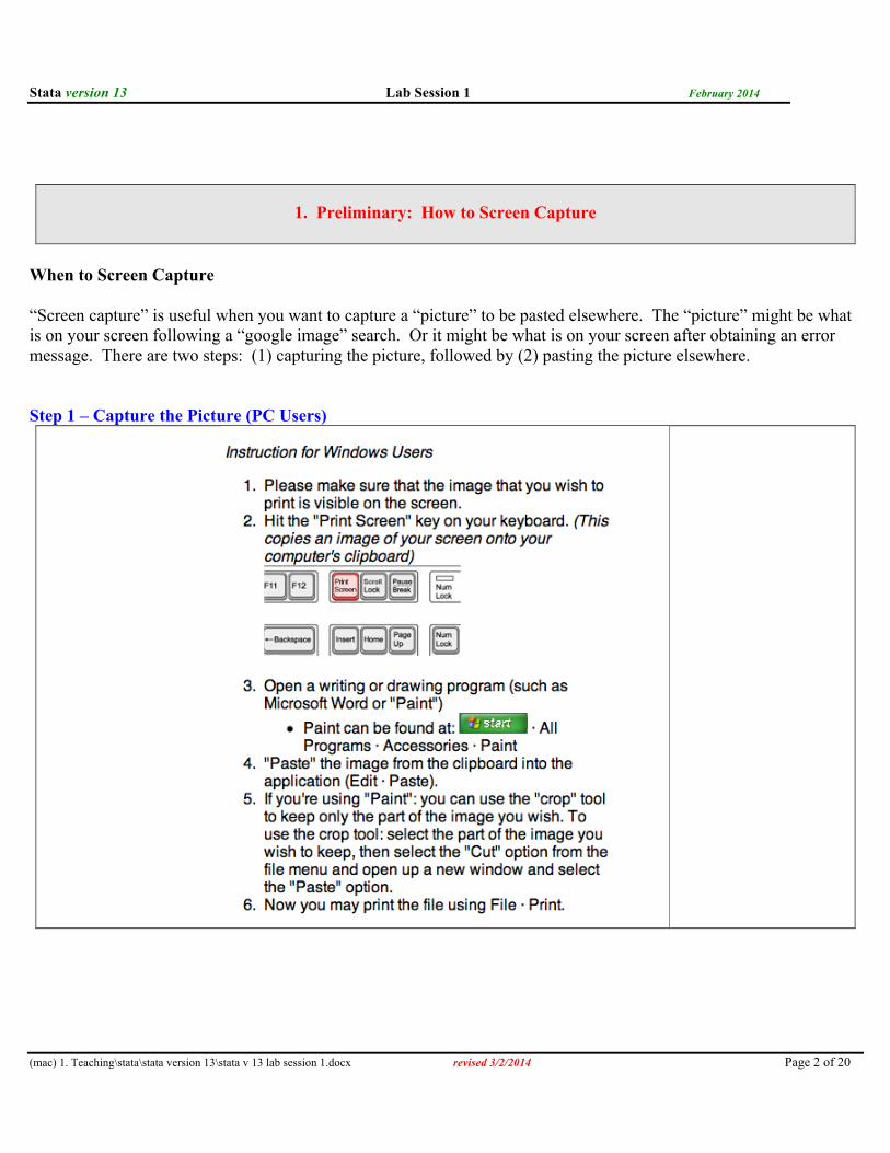
When to Screen Capture “Screen capture” is useful when you want to capture a “picture” to be pasted elsewhere. The “picture” might be what is on your screen following a “google image” search. Or it might be what is on your screen after obtaining an error message. There are two steps: (1) capturing the picture, followed by (2) pasting the picture elsewhere. Step 1 – Capture the Picture (PC Users)



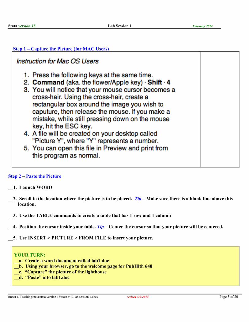
Step 1 – Capture the Picture (for MAC Users)

Step 2 – Paste the Picture __1. Launch WORD __2. Scroll to the location where the picture is to be placed. Tip – Make sure there is a blank line above this location. __3. Use the TABLE commands to create a table that has 1 row and 1 column __4. Position the cursor inside your table. Tip – Center the cursor so that your picture will be centered. __5. Use INSERT > PICTURE > FROM FILE to insert your picture.

YOUR TURN: __a. Create a word document called lab1.doc __b. Using your browser, go to the welcome page for PubHlth 640 __c. “Capture” the picture of the lighthouse __d. “Paste” into lab1.doc



2. Preliminary: How to Keep a Log of Your Stata Session

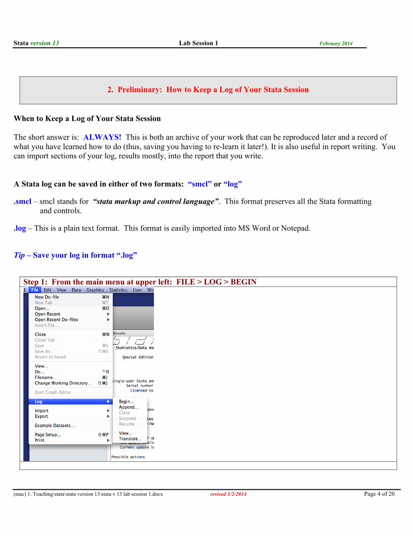
When to Keep a Log of Your Stata Session The short answer is: ALWAYS! This is both an archive of your work that can be reproduced later and a record of what you have learned how to do (thus, saving you having to re-learn it later!). It is also useful in report writing. You can import sections of your log, results mostly, into the report that you write. A Stata log can be saved in either of two formats: “smcl” or “log”

.smcl – smcl stands for “stata markup and control language”. This format preserves all the Stata formatting and controls.

.log – This is a plain text format. This format is easily imported into MS Word or Notepad. Tip – Save your log in format “.log”

Step 1: From the main menu at upper left: FILE > LOG > BEGIN



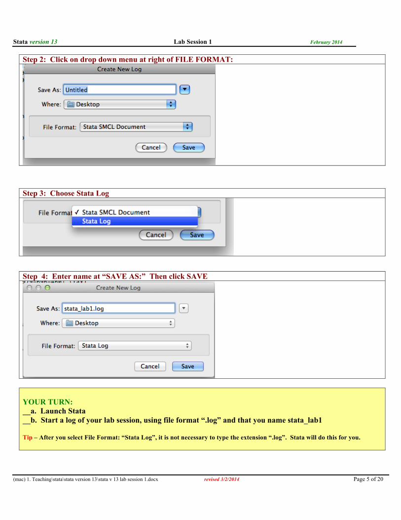
Step 2: Click on drop down menu at right of FILE FORMAT:

Step 3: Choose Stata Log

Step 4: Enter name at “SAVE AS:” Then click SAVE

YOUR TURN: __a. Launch Stata __b. Start a log of your lab session, using file format “.log” and that you name stata_lab1 Tip – After you select File Format: “Stata Log”, it is not necessary to type the extension “.log”. Stata will do this for you.



3. Preliminary: How to Save a Stata Graph

When to Save a Stata Graph Again, the short answer is: ALWAYS! Surely you will want to display your graph somewhere, yes?

Step 1: Create your graph (for now – just follow along by typing the following in the command window) use “http://people.umass.edu/biep640w/datasets/week02.dta”, clear graph twoway (scatter boiling temp) (lfit boiling temp), title(“Simple Linear Regression”)



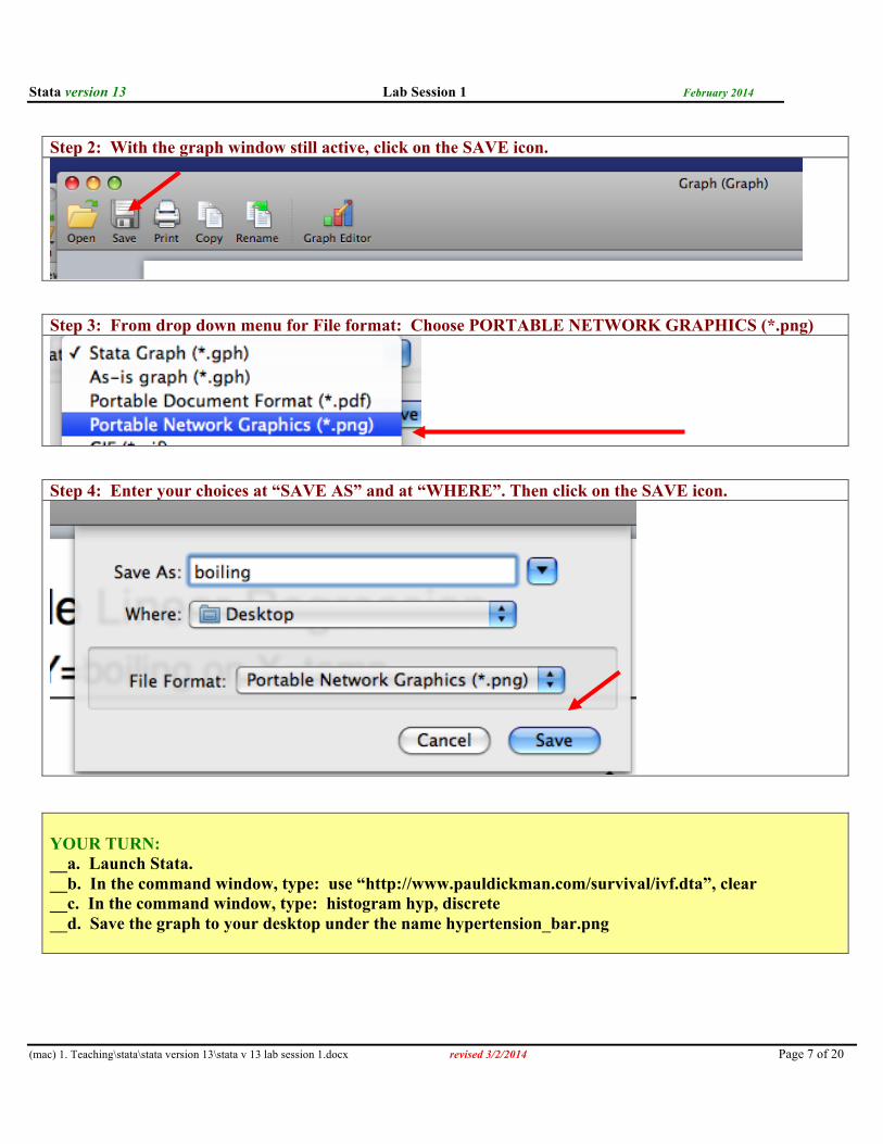
Step 2: With the graph window still active, click on the SAVE icon.

Step 3: From drop down menu for File format: Choose PORTABLE NETWORK GRAPHICS (*.png)

Step 4: Enter your choices at “SAVE AS” and at “WHERE”. Then click on the SAVE icon.

YOUR TURN: __a. Launch Stata. __b. In the command window, type: use “http://www.pauldickman.com/survival/ivf.dta”, clear __c. In the command window, type: histogram hyp, discrete __d. Save the graph to your desktop under the name hypertension_bar.png



4. Enter Data – Create a New Data Set in Stata

Most of the time, you will import data into Stata for analysis from an Excel file or from a Stata data set available on the internent. Once in a while, however, you may want to create a new data set by launching Data Editor in Stata. Tip – The Data Editor icon is located on the top, horizontal, navigation bar

YOUR TURN – Create a Stata Data Set Containing the Following Data Follow the commands below to create a data set containing the n=4 observations on the variables id, dob, gender, and weight that are shown below.

id type: numeric

dob

type: date

gender

type: string/character

weight

type: numeric 1 3/26/1926 male 161.3 2 6/9/1956 female 120.1 3 4/1/1954 male 223.2 4 11/4/1951 female 124.0

Tip – In this illustration, you will be creating three different types of variables; numeric, string, and date.

Launch Stata Then type the following two commands into the command window clear set more off



Then follow along, issuing the following commands, to create your Stata data set

. * STEP 1: Define your variables (lower case recommended), set type, and intialize . generate id=. . generate str8 dob_string="" . generate str8 gender="" . generate weight=. . * STEP 2: Click on DATA EDITOR icon. This will bring you to an empty spreadsheet . * ---- See picture on page 8. Enter the data. Then close the data editor window ---* . * STEP 3: Create dob (date of birth) that is a Stata date variable . * For date variables with year in 4 digits, use function date with option “MDY” . generate dob=date(dob_string, "MDY") . format dob %tdNN/DD/CCYY . drop dob_string . list . * STEP 4: Create 0/1 indicator of female gender . generate female=(gender=="female") . list . * STEP 5: Attach labels to variable names . label variable id "Subject id" . label variable weight "weight (lbs)" . label variable dob "Date of birth" . label variable female "0/1 female" . * STEP 6: Define dictionary of discrete variable values . label define femalef 0 "male" 1 "female" . * STEP 7: Attach coding labels to discrete variable values . label values female femalef . list . * To see data with numeric labels provided . numlabel, add . list . * To drop display of numeric labels . numlabel, remove . list . * STEP 8 - Save data set using FILE > SAVE AS



5. Enter Data – How to Import an Excel Data Set Beware - Take care that the data types are correct, especially for date variables!

There are multiple methods for importing an excel data set: (1) Copy and paste; (2) Importing the excel spreadsheet; and (3) using StatTransfer (The simplest but requires purchase of StatTransfer). METHOD 1 – Copy (from Excel) and Paste (into Stata)

Step 1 – Launch Excel. Open the file stata_lab1.xls You should see:

Step 2 – In Excel, use FORMAT > CELLS to format each column of data (numeric, text, custom, etc) Tips – (1) For each variable, position cursor over the letter of the column (eg column A for formatting the variable ID) (2) If you format a column in Excel as a date variable, it will NOT import correctly into Stata. You must format it as type = custom. Variable Format Cells as id numeric – then choose 0 places after the decimal point dob custom – then choose the type: m/d/yy gender text weight numeric - then choose 2 places after the decimal point

Step 3 – In Excel, select the data to be copied, including row headings with variable names. Use EDIT > COPY to complete selection.



Step 4 – Launch Stata. From tool bar, click on the icon DATA EDITOR

Step 5 – (a) Position cursor in cell Var1[1]. From the menu bar, use EDIT > PASTE SPECIAL to paste data here. (b) Important - be sure to check the box next to: Treat first row as variable names

You should now see the following



Step 6 – Close the DATA EDITOR window Tip – Don’t worry; data is not lost. You will save it later

Step 7 – In the command window, issue the following commands to convert the Excel date variable (that fails to import as a date variable) into a Stata date variable that is a bona fide date variable. Eg; - * For dates with year recorded in 2 digits, all in the 1900’s: * Use the function date(stringvariable, “MD19Y”) with option “MD19Y” in quotes. generate dob2 = date(dob, “MD19Y”) format dob2 %tdNN/DD/CCYY drop dob rename dob2 dob describe

Step 8 – From the menu bar, save your Stata data set using FILE > SAVE AS …



METHOD 2 – Importing the Excel spreadsheet. Tip – Before you do this, make sure that you have previously formatted (and saved) your data types in Excel! See METHOD 1.

Step 1 – Launch Stata. Click on FILE > IMPORT > EXCEL SPREADSHEET (*.xls, *.xlsx)

Step 2 – (a) Click BROWSE to locate file, (b) Check the box IMPORT 1st row as variable names (c) Click OK



You should see the following (but with your path and name, not mine) in your results window

Step 3 – In the command window, issue the following commands to convert the Excel date variable (that fails to import as a date variable) into a Stata date variable that is a bona fide date variable. Eg; - * For dates with year recorded in 2 digits, all in the 1900’s: * Use the function date(stringvariable, “MD19Y”) with option “MD19Y” in quotes. generate dob2 = date(dob, “MD19Y”) format dob2 %tdNN/DD/CCYY drop dob rename dob2 dob describe

Step 4 – From the menu bar, save your Stata data set using FILE > SAVE AS …

YOUR TURN – Create an Excel Data set. Bring it into Stata by method 1 or 2. Save. __1. Launch Excel. __2. Create an Excel data set called stata_lab1.xls __3. Create a Stata data set stata_lab1.dta using your excel data. __4. Save your Stata data set.

Here is the excel data for you. Note that the dob variable has year in 2 digits, not 4 digits.

id

type: numeric

dob

type: date

gender

type: string/character

weight

type: numeric 1 3/26/26 male 161.3 2 6/9/56 female 120.1 3 4/1/54 male 223.2 4 11/4/51 female 124.0



6. Import a Stata Data Set Directly from the Internet

When to Import a Stata Data Set You will do this often for class and perhaps not so often in your work. Tips – (1) Be sure to enclose the url in quotes, (2) Be sure to use the option clear after the comma; and (3) Be sure to save the data onto your computer so that you have it for your use later.

Use the command use to import a stata data set. Be sure to enclose the full url path in quotes. The basic command is of the following form and is issued in the command window use “http://fullurlpath”, clear To save the data onto your computer, from the top menu bar issue: FILE > SAVE AS .. Tip!! Be sure to include the extension “.dta’ in the name of the data set; see examples below.

Examples - use “http://www.pauldickman.com/survival/ivf.dta”, clear use “http://people.umass.edu/biep640w/datasets/week02.dta”, clear use “http://people.umass.edu/biep640w/datasets/larvae.dta”, clear

YOUR TURN – Import ivf.dta from the internet __1. Launch Stata (if you have not already done so) __2. In the command window, type: set more off __3. In the command window, type: use “http://www.pauldickman.com/survival/ivf.dta”, clear __4. Use FILE > SAVE AS… to save it to your computer



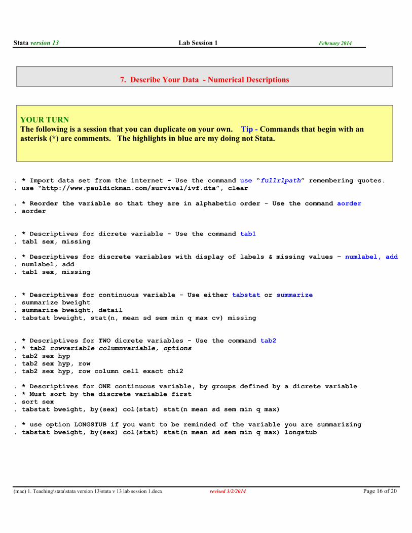
7. Describe Your Data - Numerical Descriptions

YOUR TURN The following is a session that you can duplicate on your own. Tip - Commands that begin with an asterisk (*) are comments. The highlights in blue are my doing not Stata.

. * Import data set from the internet - Use the command use “fullrlpath” remembering quotes. . use “http://www.pauldickman.com/survival/ivf.dta”, clear . * Reorder the variable so that they are in alphabetic order - Use the command aorder . aorder . * Descriptives for dicrete variable - Use the command tab1 . tab1 sex, missing . * Descriptives for discrete variables with display of labels & missing values – numlabel, add . numlabel, add . tab1 sex, missing . * Descriptives for continuous variable - Use either tabstat or summarize . summarize bweight . summarize bweight, detail . tabstat bweight, stat(n, mean sd sem min q max cv) missing . * Descriptives for TWO dicrete variables - Use the command tab2 . * tab2 rowvariable columnvariable, options . tab2 sex hyp . tab2 sex hyp, row . tab2 sex hyp, row column cell exact chi2 . * Descriptives for ONE continuous variable, by groups defined by a dicrete variable . * Must sort by the discrete variable first . sort sex . tabstat bweight, by(sex) col(stat) stat(n mean sd sem min q max) . * use option LONGSTUB if you want to be reminded of the variable you are summarizing . tabstat bweight, by(sex) col(stat) stat(n mean sd sem min q max) longstub



8. Describe Your Data – Graphical Descriptions

. * Tell Stata what graph scheme you want to use. I like the scheme s1color . set scheme s1color . * BAR GRAPH, simple - Use the command histogram with the option discrete . histogram hyp, discrete . * BAR GRAPH, fancy - Use the command histogram with the option discrete . histogram hyp, discrete percent addlabels ylabel(0(20)100) xlabel(0 "Normotensive" 1 "Hypertensive") gap(50) title("Bar Graph -Hyp") subtitle("n=639") caption("hyp_barchart.png") . * DOT PLOT, simple - Use the command dotplot . dotplot matage . * DOT PLOT, fancy – Use the command dotplot . dotplot matage, center msize(vsmall) xlabel(1 "All") title("Distribution of Maternal Age") subtitle("n=641") caption("dot_matage.png", size(vsmall)) . * DOT PLOT for more than 1 group, simple – Use the command dot plot with option over( ). . * Must sort first. . sort sex . dotplot matage, over(sex) . * DOT PLOT for more than 1 group, fancy. . sort sex . dotplot matage, over(sex) title("Distribution of Maternal Age") subtitle("by infant sex") caption("dot2_matage.png", size(vsmall)) . * BOX PLOT for more than 1 group, simple – Use the command graph box with option over( ). . sort sex . graph box matage, over(sex) . * BOX PLOT for more than 1 group, fancy. . sort sex . graph box matage, over(sex) title("Distribution of Maternal Age") subtitle("by infant sex") caption("box2_matage.png", size(vsmall)) .* HORIZONTAL BOX PLOT for more than 1 group, simple – Use the command graph hbox . graph hbox matage, over(sex) .* HORIZONTAL BOX PLOT for more than 1 group, fancy . graph hbox matage, over(sex) title("Distribution of Maternal Age") subtitle("by infant sex") caption("hbox2_matage.png", size(vsmall))



. * HISTOGRAM – Preliminary: It’s a good idea to obtain min and max . tabstat matage, stat(min max) . * HISTOGRAM, simple – Use the command histogram . histogram matage . * HISTOGRAM, fancy – Use the command histogram . histogram matage, width(5) start(20) percent ylabel(0(10)50) addlabels title("Distribution of Maternal Age") subtitle("n=641") caption("histogram_matage.png", size(vsmall)) . * X-Y SCATTERPLOT - Preliminary: Obtain min and max of the X and Y variables . tabstat matage gestwks, stat(min max) .* X-Y SCATTERPLOT, simple - Use the command graph twoway (scatter yvariable xvariable) . graph twoway (scatter gestwks matage) .* X-Y SCATTERPLOT, fancy . graph twoway (scatter gestwks matage, msymbol(d) msize(vsmall)), xlabel(20(5)45) ylabel(20(5)45) title("Scatterplot") ytitle("Weeks Gestation",size(small)) caption("scatter.png", size(vsmall)) .* X-Y SCATTERPLOT WITH OVERLAY LINEAR FIT, simple: graph twoway (lfit yvariable xvariable) . graph twoway (scatter gestwks matage) lfit gestwks matage) .* X-Y SCATTERPLOT WITH OVERLAY LINEAR FIT, fancy . graph twoway (scatter gestwks matage, msymbol(d) msize(vsmall)) (lfit gestwks matage), xlabel(20(5)45) ylabel(20(5)45) legend(off) title("Scatterplot") subtitle("with overlay linear fit") ytitle("Weeks Gestation",size(small)) caption("lfit.png", size(vsmall)) . * X_Y SCATTERPLOT W OVERLAY FIT & 95% CI, simple: graph twoway (lfitci yvariable xvariable) . graph twoway (scatter gestwks matage) (lfitci gestwks matage) . * X_Y SCATTERPLOT WITH OVERLAY FIT AND 95% CI, fancy . graph twoway (scatter gestwks matage, msymbol(d) msize(vsmall)) (lfitci gestwks matage), xlabel(20(5)45) ylabel(20(5)45) legend(off) title("Scatterplot") subtitle("with overlay linear fit and 95% CI") ytitle("Weeks Gestation",size(small)) caption("lfitci.png", size(vsmall))



9. One and Two Sample Inference

YOUR TURN Again, follow along!

. ** ONE CONTINUOUS VARIABLE - 99% CI for mean using command ci with option level(99) . ci gestwks, level(99) . ** ONE CONTINUOUS VARIABLE - Test of null: mean = 40 using command ttest . ttest gestwks=40 . ** ONE CONTINUOUS VARIABLE - Test of null: standard deviation = 1 using command sdtest . sdtest gestwks=1 . ** TWO CONTINUOUS VARIABLES - Test of null: Equality of 2 INDEPENDENT means using ttest . sort sex . ttest gestwks, by(sex) . ttest gestwks, by(sex) unequal . ** TWO CONTINUOUS VARIABLES - Test of equality of 2 independent variances using sdtest . sdtest gestwks, by(sex) . ** 1 DISCRETE (0/1)VARIABLE - Test of binomial proportion using command bitest and prtest . ** Test of null: proportion of female births = .50 . generate female=(sex==2) . bitest female=.50 . prtest female=.50 . ** 1 DISCRETE (0/1)VARIABLE - 95% CI for event probability using ci with option binomial . ci female, binomial level(95) . ** 2 DISCRETE (0/1)VARIABLES - Test of equality of probabilities prtest with option by( ) . sort sex . prtest hyp, by(sex) . ** 2 DISCRETE VARIABLES (any # rows and # columns) - chi square test: tab2 with option chi2 . tab2 sex hyp, row column chi2 . ** 2 DISCRETE VARIABLES (any # rows and # columns) -fisher exact test: tab2 with option exact . tab2 sex hyp, row column exact



10. Simple and Multiple Linear Regression

. clear . * Data are from Vittinghoff et al. Regression Methods in Biostatistics . * Y=glucose X=physact (5 levels), BMI . use “http://people.umass.edu/biep640w/datasets/hersdata1000.dta”, clear . ** descriptives of glucose, by levels of physical activity . sort physact . tabstat glucose, by(physact) col(stat) stat(n mean sd min p50 max) .** descriptive graphs . dotplot glucose, over(physact) center msymbol(d) msize(tiny) xlabel(1 "1" 2 "2" 3 "3" 4 "4" 5 "5") . graph matrix glucose age BMI, half msize(tiny) . ** Assessment of normality of Y=glucose . swilk glucose . sfrancia glucose . tabstat glucose, stat(min max) . histogram glucose, start(0) width(25) percent addlabels normal . ** One predictor - continuous . regress glucose BMI . ** One predictor - nominal physical activity with design variables . xi: regress glucose i.physact . ** multiple predictor model with both BMI and physact (with design variables) . xi: regress glucose BMI i.physact . ** Partial F test of BMI controlling for physact: 1 df Partial F . testparm BMI . ** Partial F test of physical activity controlling for BMI: 4 df Partial F . testparm _Iphysact*

Stata version 13 Also works for version 12people.umass.edu/biep640w/pdf/stata v 13 lab sessio… · · 2014-03-02Teaching\stata\stata version 13\stata v 13 lab session 1.docx revised

Documents