Welcome message from author
This document is posted to help you gain knowledge. Please leave a comment to let me know what you think about it! Share it to your friends and learn new things together.
Transcript

Table of contents
Introduction
Install the software
1 Meta-analsis in Stata: metan, metacum, and metap
1.1 metan: a command for meta-analysis in Stata
M. J. Bradburn, J. J. Deeks, and D. G. Altman, STB 1999 44 “metan: an alternative
meta-analysis command”
1.2 metan: fixed- and random-effects meta-analysis
R. J. Harris, M. J. Bradburn, J. J. Deeks, R. M. Harbord, D. G. Altman, and J. A. C. Sterne, SJ8-1
1.3 Cumulative meta-analysis
J. A. C. Sterne, STB 1998 42
1.4 Meta-analysis of p-values
A. Tobias, STB 2000 49
2 Meta-regression: metareg
2.1 Meta-regression in Stata
R. M. Harbord and J. P. T. Higgins, SJ8-4
2.2 Meta-analysis regression
S. Sharp, STB 1998 42
3 Investigating bias in meta-analysis: metafunnel, confunnel, metabias, and metatrim
3.1 Funnel plots in meta-analysis
J. A. C. Sterne and R. M. Harbord, SJ4-2
3.2 Contour-enhanced funnel plots for meta-analysis
T. M. Palmer, J. L. Peters, A. J. Sutton, and S. G. Moreno, SJ8-2
3.3 Updated tests for small-study effects in meta-analyses
R. M. Harbord, R. J. Harris, and J. A. C. Sterne, SJ9-2
3.4 Tests for publication bias in meta-analysis
T. J. Steichen, STB 1998 41
3.5 Tests for publication bias in meta-analysis
T. J. Steichen, M. Egger, and J. A. C. Sterne, STB 1999 44
3.6 Nonparametric trim and fill analysis of publication bias in meta-analysis
T. J. Steichen, STB 2001 57
4 Advanced methods: metandi, glst, metamiss, and mvmeta
4.1 metandi: Meta-analysis of diagnostic accuracy using hierarchical logistic
regression
R. M. Harbord and P. Whiting, SJ9-2
4.2 Generalized least squares for trend estimation of summarized dose–response
data
N. Orsini, R. Bellocco, and S. Greenland, SJ6-1
4.3 Meta-analysis with missing data
I. R. White and J. P. T. Higgins, SJ9-1
I. R. White, SJ9-1
5 Appendixes
Author index
Command index
4.4 Multivariate random-effects meta-analysis
5.1 What meta-analysis features are available in Stata?
5.2 Further Stata meta-analysis commands
5.3 Submenu and dialogs for meta-analysis

Introduction
This first collection of articles from the Stata Technical Bulletin and the Stata Jour-nal brings together updated user-written commands for meta-analysis, which has beendefined as a statistical analysis that combines or integrates the results of several indepen-dent studies considered by the analyst to be combinable (Huque 1988). The statisticianKarl Pearson is commonly credited with performing the first meta-analysis more than acentury ago (Pearson 1904)—the term “meta-analysis” was first used by Glass (1976).The rapid increase over the last three decades in the number of meta-analyses reported inthe social and medical literature has been accompanied by extensive research on the un-derlying statistical methods. It is therefore surprising that the major statistical softwarepackages have been slow to provide meta-analytic routines (Sterne, Egger, and Sutton2001).
During the mid-1990s, Stata users recognized that the ease with which new com-mands could be written and distributed, and the availability of improved graphics pro-gramming facilities, provided an opportunity to make meta-analysis software widelyavailable. The first command, meta, was published in 1997 (Sharp and Sterne 1997),while the metan command—now the main Stata meta-analysis command—was pub-lished shortly afterward (Bradburn, Deeks, and Altman 1998). A major motivation forwriting metan was to provide independent validation of the routines programmed intothe specialist software written for the Cochrane Collaboration, an international organi-zation dedicated to improving health care decision-making globally, through systematicreviews of the effects of health care interventions, published in The Cochrane Library(see www.cochrane.org). The groups responsible for the meta and metan commandscombined to produce a major update to metan that was published in 2008 (Harris et al.2008). This update uses the most recent Stata graphics routines to provide flexibledisplays combining text and figures. Further articles describe commands for cumula-tive meta-analysis (Sterne 1998) and for meta-analysis of p-values (Tobias 1999), whichcan be traced back to Fisher (1932). Between-study heterogeneity in results, whichcan cause major difficulties in interpretation, can be investigated using meta-regression(Berkey et al. 1995). The metareg command (Sharp 1998) remains one of the fewimplementations of meta-regression and has been updated to take account of improve-ments in Stata estimation facilities and recent methodological developments (Harbordand Higgins 2008).
viii Introduction
Enthusiasm for meta-analysis has been tempered by a realization that flaws in theconduct of studies (Schulz et al. 1995), and the tendency for the publication processto favor studies with statistically significant results (Begg and Berlin 1988; Dickersin,Min, and Meinert 1992), can lead to the results of meta-analyses mirroring overopti-mistic results from the original studies (Egger et al. 1997). A set of Stata commands—metafunnel, confunnel, metabias, and metatrim—address these issues both graphi-cally (via routines to draw standard funnel plots and “contour-enhanced” funnel plots)and statistically, by providing tests for funnel plot asymmetry, which can be used todiagnose publication bias and other small-study effects (Sterne, Gavaghan, and Egger2000; Sterne, Egger, and Moher 2008).
This collection also contains advanced routines that exploit Stata’s range of esti-mation procedures. Meta-analysis of studies that estimate the accuracy of diagnostictests, implemented in the metandi command, is inherently bivariate, because of thetrade-off between sensitivity and specificity (Rutter and Gatsonis 2001; Reitsma et al.2005). Meta-analyses of observational studies will often need to combine dose–responserelationships, but reports of such studies often report comparisons between three ormore categories. The method of Greenland and Longnecker (1992), implemented in theglst command, converts categorical to dose–response comparisons and can thus beused to derive the data needed for dose–response meta-analyses. White and colleagues(White and Higgins 2009; White 2009) have recently provided general routines to dealwith missing data in meta-analysis, and for multivariate random-effects meta-analysis.
Finally, the appendix lists user-written meta-analysis commands that have not, sofar, been accepted for publication in the Stata Journal. For the most up-to-date infor-mation on meta-analysis commands in Stata, readers are encouraged to check the Statafrequently asked question on meta-analysis:
http://www.stata.com/support/faqs/stat/meta.html
Those involved in developing Stata meta-analysis commands have been delightedby their widespread worldwide use. However, a by-product of the large number ofcommands and updates to these commands now available has been that users find itincreasingly difficult to identify the most recent version of commands, the commandsmost relevant to a particular purpose, and the related documentation. This collectionaims to provide a comprehensive description of the facilities for meta-analysis now avail-able in Stata and has also stimulated the production and documentation of a number ofupdates to existing commands, some of which were long overdue. I hope that this collec-tion will be useful to the large number of Stata users already conducting meta-analyses,as well as facilitate interest in and use of the commands by new users.
Jonathan A. C. SterneFebruary 2009
Introduction ix
1 ReferencesBegg, C. B., and J. A. Berlin. 1988. Publication bias: A problem in interpreting medical
data. Journal of the Royal Statistical Society, Series A 151: 419–463.
Berkey, C. S., D. C. Hoaglin, F. Mosteller, and G. A. Colditz. 1995. A random-effectsregression model for meta-analysis. Statistics in Medicine 14: 395–411.
Bradburn, M. J., J. J. Deeks, and D. G. Altman. 1998. sbe24: metan—an alternativemeta-analysis command. Stata Technical Bulletin 44: 4–15. Reprinted in Stata Tech-nical Bulletin Reprints, vol. 8, pp. 86–100. College Station, TX: Stata Press. (Updatedarticle is reprinted in this collection on pp. 3–28.).
Dickersin, K., Y. I. Min, and C. L. Meinert. 1992. Factors influencing publicationof research results: Follow-up of applications submitted to two institutional reviewboards. Journal of the American Medical Association 267: 374–378.
Egger, M., G. Davey Smith, M. Schneider, and C. Minder. 1997. Bias in meta-analysisdetected by a simple, graphical test. British Medical Journal 315: 629–634.
Fisher, R. A. 1932. Statistical Methods for Research Workers. 4th ed. London: Oliver& Boyd.
Glass, G. V. 1976. Primary, secondary, and meta-analysis of research. EducationalResearcher 10: 3–8.
Greenland, S., and M. P. Longnecker. 1992. Methods for trend estimation from sum-marized dose–reponse data, with applications to meta-analysis. American Journal ofEpidemiology 135: 1301–1309.
Harbord, R. M., and J. P. T. Higgins. 2008. Meta-regression in Stata. Stata Journal 8:493–519. (Reprinted in this collection on pp. 70–96.).
Harris, R. J., M. J. Bradburn, J. J. Deeks, R. M. Harbord, D. G. Altman, and J. A. C.Sterne. 2008. metan: fixed- and random-effects meta-analysis. Stata Journal 8: 3–28.(Reprinted in this collection on pp. 29–54.).
Huque, M. F. 1988. Experiences with meta-analysis in NDA submissions. Proceedingsof the Biopharmaceutical Section of the American Statistical Association 2: 28–33.
Pearson, K. 1904. Report on certain enteric fever inoculation statistics. British MedicalJournal 2: 1243–1246.
Reitsma, J. B., A. S. Glas, A. W. S. Rutjes, R. J. P. M. Scholten, P. M. Bossuyt, andA. H. Zwinderman. 2005. Bivariate analysis of sensitivity and specificity produces in-formative summary measures in diagnostic reviews. Journal of Clinical Epidemiology58: 982–990.
Rutter, C. M., and C. A. Gatsonis. 2001. A hierarchical regression approach to meta-analysis of diagnostic test accuracy evaluations. Statistics in Medicine 20: 2865–2884.
x Introduction
Schulz, K. F., I. Chalmers, R. J. Hayes, and D. G. Altman. 1995. Empirical evidenceof bias. Dimensions of methodological quality associated with estimates of treatmenteffects in controlled trials. Journal of the American Medical Association 273: 408–412.
Sharp, S. 1998. sbe23: Meta-analysis regression. Stata Technical Bulletin 42: 16–22.Reprinted in Stata Technical Bulletin Reprints, vol. 7, pp. 148–155. College Station,TX: Stata Press. (Reprinted in this collection on pp. 97–106.).
Sharp, S., and J. A. C. Sterne. 1997. sbe16: Meta-analysis. Stata Technical Bulletin38: 9–14. Reprinted in Stata Technical Bulletin Reprints, vol. 7, pp. 100–106. CollegeStation, TX: Stata Press.1
Sterne, J. 1998. sbe22: Cumulative meta analysis. Stata Technical Bulletin 42: 13–16.Reprinted in Stata Technical Bulletin Reprints, vol. 7, pp. 143–147. College Station,TX: Stata Press. (Updated article is reprinted in this collection on pp. 55–64.).
Sterne, J. A. C., M. Egger, and D. Moher. 2008. Addressing reporting biases. InCochrane Handbook for Systematic Reviews of Interventions, ed. J. P. T. Higginsand S. Green, 297–334. Chichester, UK: Wiley.
Sterne, J. A. C., M. Egger, and A. J. Sutton. 2001. Meta-analysis software. In System-atic Reviews in Health Care: Meta-Analysis in Context, 2nd edition, ed. M. Egger,G. Davey Smith, and D. G. Altman, 336–346. London: BMJ Books.
Sterne, J. A. C., D. Gavaghan, and M. Egger. 2000. Publication and related bias inmeta-analysis: Power of statistical tests and prevalence in the literature. Journal ofClinical Epidemiology 53: 1119–1129.
Tobias, A. 1999. sbe28: Meta-analysis of p-values. Stata Technical Bulletin 49: 15–17.Reprinted in Stata Technical Bulletin Reprints, vol. 9, pp. 138–140. College Station,TX: Stata Press. (Updated article is reprinted in this collection on pp. 65–68.).
White, I. R. 2009. Multivariate random-effects meta-analysis. Stata Journal. Forth-coming. (Preprinted in this collection on pp. 231–247.).
White, I. R., and J. P. T. Higgins. 2009. Meta-analysis with missing data. StataJournal. Forthcoming. (Preprinted in this collection on pp. 218–230.).
1. The original command to perform meta-analysis was meta, documented in the sbe16 articles; metais now metan. metan is described in an updated article, sbe24, on pages 3–28 of this collection.—Ed.

Install the software
You can download all the user-written commands described in the Meta-Analysis in
Stata: An Updated Collection from the Stata Journal from within Stata. Download the
installation command by using the net command. At the Stata prompt, type
. net from http://www.stata-press.com/data/mais
. net install mais
After installing this file, type spinst_mais to obtain all the user-written commands
discussed in this collection, except for those commands listed in the appendix.
Instructions on how to obtain those commands are given in the appendix. If there are
any error messages after typing spinst_mais, follow the instructions at the bottom of
the output to complete the download.
1 Meta-analysis in Stata:
metan, metacum, and metap
4 Stata Technical Bulletin STB-44
The second change to metabias is straightforward. A square root was inadvertently left out of the formula for the p
value of the asymmetry test that is calculated for an individual stratum when option by�� is specified. This formula has beencorrected. Users of this program should repeat any stratified analyses they performed with the original program. Please note thatunstratified analyses were not affected by this error.
The third change to metabias extends the error-trapping capability and reports previously trapped errors more accuratelyand completely. A noteworthy aspect of this change is the addition of an error trap for the ci option. This trap addresses thesituation where epidemiological effect estimates and associated error measures are provided to metabias as risk (or odds) ratiosand corresponding confidence intervals. Unfortunately, if the user failed to specify option ci in the previous release, metabiasassumed that the input was in the default (theta, se theta) format and calculated incorrect results. The current release checks forthis situation by counting the number of variables on the command line. If more than two variables are specified, metabiaschecks for the presence of option ci. If ci is not present, metabias assumes it was accidentally omitted, displays an appropriatewarning message, and proceeds to carry out the analysis as if ci had been specified.
Warning: The user should be aware that it remains possible to provide theta and its variance, var theta, on the commandline without specifying option var. This error, unfortunately, cannot be trapped and will result in an incorrect analysis. Thoughonly a limited safeguard, the program now explicitly indicates the data input option specified by the user, or alternatively, warnsthat the default data input form was assumed.
The fourth change to metabias has effect only when options graph�begg� and ci are specified together. graph�begg�requests a funnel graph. Option ci indicates that the user provided the effect estimates in their exponentiated form, exp(theta)—usually a risk or odds ratio, and provided the variability measures as confidence intervals, (ll, ul). Since the funnel graph alwaysplots theta against its standard error, metabias correctly generated theta by taking the log of the effect estimate and correctlycalculated se theta from the confidence interval. The error was that the axes of the graph were titled using the variable name (orvariable label, if available) and did not acknowledge the log transform. This was both confusing and wrong and is corrected inthis release. Now when both graph�begg� and ci are specified, if the variable name for the effect estimate is RR, the y-axis istitled “log[RR]” and the x-axis is titled “s.e. of: log[RR]”. If a variable label is provided, it replaces the variable name in theseaxis titles.
ReferencesEgger, M., G. D. Smith, M. Schneider, and C. Minder. 1997. Bias in meta-analysis detected by a simple, graphical test. British Medical Journal 315:
629–634.
Steichen, T. J. 1998. sbe19: Tests for publication bias in meta-analysis. Stata Technical Bulletin 41: 9–15. Reprinted in The Stata Technical BulletinReprints vol. 7, pp. 125–133.
sbe24 metan—an alternative meta-analysis command
Michael J. Bradburn, Institute of Health Sciences, Oxford, UK, [email protected] J. Deeks, Institute of Health Sciences, Oxford, UK, [email protected]
Douglas G. Altman, Institute of Health Sciences, Oxford, UK, [email protected]
Background
When several studies are of a similar design, it often makes sense to try to combine the information from them all to gainprecision and to investigate consistencies and discrepancies between their results. In recent years there has been a considerablegrowth of this type of analysis in several fields, and in medical research in particular. In medicine such studies usually relateto controlled trials of therapy, but the same principles apply in any scientific area; for example in epidemiology, psychology,and educational research. The essence of meta-analysis is to obtain a single estimate of the effect of interest (effect size) fromsome statistic observed in each of several similar studies. All methods of meta-analysis estimate the overall effect by computinga weighted average of the studies’ individual estimates of effect.
metan provides methods for the meta-analysis of studies with two groups. With binary data, the effect measure can be thedifference between proportions (sometimes called the risk difference or absolute risk reduction), the ratio of two proportions (riskratio or relative risk), or the odds ratio. With continuous data, both observed differences in means or standardized differences inmeans (effect sizes) can be used. For both binary and continuous data, either fixed effects or random effects models can be fitted(Fleiss 1993). There are also other approaches, including empirical and fully Bayesian methods. Meta-analysis can be extendedto other types of data and study designs, but these are not considered here.
As well as the primary pooling analysis, there are secondary analyses that are often performed. One common additionalanalysis is to test whether there is excess heterogeneity in effects across the studies. There are also several graphs that can beused to supplement the main analysis.
Stata Technical Bulletin 5
Recently Sharp and Sterne (1997) presented a program to carry out some of the above analyses, and further programs havebeen submitted to perform various diagnostics and further analyses. The differences between metan and these other programsare discussed below.
Data structure
Consider a meta-analysis of k studies. When the studies have a binary outcome, the results of each study can be presentedin a 2� 2 table (Table 1) giving the numbers of subjects who do or do not experience the event in each of the two groups (herecalled intervention and control).
Table 1. Binary dataStudy i; 1� i � k Event No eventIntervention ai bi
Control ci di
If the outcome is a continuous measure, the number of subjects in each of the two groups, their mean response, and thestandard deviation of their responses are required to perform meta-analysis (Table 2).
Table 2. Continuous dataStudy i; (1� i � k) Group size Mean response Standard deviationIntervention n�i m�i sd�i
Control n�i m�i sd�i
Analysis of binary data using fixed effect models
There are two alternative fixed effect analyses. The inverse variance method (sometimes referred to as Woolf’s method)computes an average effect by weighting each study’s log odds ratio, log relative risk, or risk difference according to the inverseof their sampling variance, such that studies with higher precision (lower variance) are given higher weights. This method useslarge sample asymptotic sampling variances, so it may perform poorly for studies with very low or very high event rates orsmall sample sizes. In other situations, the inverse variance method gives a minimum variance unbiased estimate.
The Mantel–Haenszel method uses an alternative weighting scheme originally derived for analyzing stratified case–controlstudies. The method was first described for the odds ratio by Mantel and Haenszel (1959) and extended to the relative risk andrisk difference by Greenland and Robins (1985). The estimate of the variance of the overall odds ratio was described by Robins,Greenland, and Breslow (1986). These methods are preferable to the inverse variance method as they have been shown to berobust when data are sparse, and give similar estimates to the inverse variance method in other situations. They are the default inthe metan command. Alternative formulations of the Mantel–Haenszel methods more suited to analyzing stratified case–controlstudies are available in the epitab commands.
Peto proposed an assumption free method for estimating an overall odds ratio from the results of several large clinicaltrials (Yusuf, Peto, et al. 1985). The method sums across all studies the difference between the observed (O[ai]) and expected(E[ai]) numbers of events in the intervention group (the expected number of events being estimated under the null hypothesisof no treatment effect). The expected value of the sum of O� E under the null hypothesis is zero. The overall log odds ratiois estimated from the ratio of the sum of the O � E and the sum of the hypergeometric variances from individual trials. Thismethod gives valid estimates when combining large balanced trials with small treatment effects, but has been shown to givebiased estimates in other situations (Greenland and Salvan 1990).
If a study’s 2 � 2 table contains one or more zero cells, then computational difficulties may be encountered in both theinverse variance and the Mantel–Haenszel methods. These can be overcome by adding a standard correction of 0.5 to all cellsin the 2� 2 table, and this is the approach adopted here. However, when there are no events in one whole column of the 2� 2table (i.e., all subjects have the same outcome regardless of group), the odds ratio and the relative risk cannot be estimated, andthe study is given zero weight in the meta-analysis. Such trials are included in the risk difference methods as they are informativethat the difference in risk is small.
Analysis of continuous data using fixed effect models
The weighted mean difference meta-analysis combines the differences between the means of intervention and control groups(m�i � m�i) to estimate the overall mean difference (Sinclair and Bracken 1992). A prerequisite of this method is that theresponse is measured in the same units using comparable devices in all studies. Studies are weighted using the inverse of thevariance of the differences in means. Normality within trial arms is assumed, and between trial variations in standard deviationsare attributed to differences in precision, and are assumed equal in both study arms.
An alternative approach is to pool standardized differences in means, calculated as the ratio of the observed difference inmeans to an estimate of the standard deviation of the response. This approach is especially appropriate when studies measure

6 Stata Technical Bulletin STB-44
the same concept (e.g., pain or depression) but use a variety of continuous scales. By standardization, the study results aretransformed to a common scale (standard deviation units) that facilitates pooling. There are various methods for computing thestandardized study results: Glass’s method (Glass, et al. 1981) divides the differences in means by the control group standarddeviation, whereas Cohen’s and Hedges’ methods use the same basic approach, but divide by an estimate of the standard deviationobtained from pooling the standard deviations from both experimental and control groups (Rosenthal 1994). Hedges’ methodincorporates a small sample bias correction factor (Hedges and Olkin 1985). An inverse variance weighting method is used in allthe formulations. Normality within trial arms is assumed, and all differences in standard deviations between trials are attributedto variations in the scale of measurement.
Test for heterogeneity
For all the above methods, the consistency or homogeneity of the study results can be assessed by considering an appropriatelyweighted sum of the differences between the k individual study results and the overall estimate. The test statistic has a ��
distribution with k � 1 degrees of freedom (DerSimonian and Laird 1986).
Analysis of binary or continuous data using random effect models
An approach developed by DerSimonian and Laird (1986) can be used to perform random effect meta-analysis for all theeffect measures discussed above (except the Peto method). Such models assume that the treatment effects observed in the trialsare a random sample from a distribution of treatment effects with a variance ��. This is in contrast to the fixed effect modelswhich assume that the observed treatment effects are all estimates of a single treatment effect. The DerSimonian and Lairdmethods incorporate an estimate of the between-study variation �� into both the study weights (which are the inverse of the sumof the individual sampling variance and the between studies variance ��) and the standard error of the estimate of the commoneffect. Where there are computational problems for binary data due to zero cells the same approach is used as for fixed effectmodels.
Where there is excess variability (heterogeneity) between study results, random effect models typically produce moreconservative estimates of the significance of the treatment effect (i.e., a wider confidence interval) than fixed effect models. Asthey give proportionately higher weights to smaller studies and lower weights to larger studies than fixed effect analyses, theremay also be differences between fixed and random models in the estimate of the treatment effect.
Tests of overall effect
For all analyses, the significance of the overall effect is calculated by computing a z score as the ratio of the overall effectto its standard error and comparing it with the standard normal distribution. Alternatively, for the Mantel–Haenszel odds ratioand Peto odds ratio method, �� tests of overall effect are available (Breslow and Day 1980).
Graphical analyses
Three plots are available in these programs. The most common graphical display to accompany a meta-analysis showshorizontal lines for each study, depicting estimates and confidence intervals, commonly called a forest plot. The size of theplotting symbol for the point estimate in each study is proportional to the weight that each trial contributes in the meta-analysis.The overall estimate and confidence interval are marked by a diamond. For binary data, a L’Abbe plot (L’Abbe et al. 1987)plots the event rates in control and experimental groups by study. For all data types a funnel plot shows the relation between theeffect size and precision of the estimate. It can be used to examine whether there is asymmetry suggesting possible publicationbias (Egger et al. 1997), which usually occurs where studies with negative results are less likely to be published than studieswith positive results.
Each trial i should be allocated one row in the dataset. There are three commands for invoking the routines; metan, funnel,and labbe, which are detailed below.
Syntax for metan
metan varlist�if exp
� �in range
� �� options
�
This main meta-analysis routine requires either four or six variables to be declared. When four variables are specified,analysis of binary data is performed. When six, the data are assumed continuous. Following the syntax of Tables 1 and 2, thevarlist should be either
a b c d
or
n1 m1 sd1 n2 m2 sd2

Stata Technical Bulletin 7
Scaling and pooling options for metan
Options for binary data
rr pool risk ratios (the default).
or pool odds ratios.
rd pool risk differences.
fixed specifies a fixed effect model using the method of Mantel and Haenszel (the default).
fixedi specifies a fixed effect model using the inverse variance method.
peto specifies that Peto’s assumption free method is used to pool odds ratios.
random specifies a random effect model using the method of DerSimonian and Laird, with the estimate of heterogeneity beingtaken from the Mantel–Haenszel model.
randomi specifies a random effect model using the method of DerSimonian and Laird, with the estimate of heterogeneity beingtaken from the inverse variance fixed effect model.
cornfield computes confidence intervals for odds ratios by the Cornfield method, rather than the (default) Woolf method.
chi� displays the chi-squared statistic (instead of z) for the test of significance of the pooled effect size. This is available onlyfor odds ratios pooled using Peto or Mantel–Haenszel methods.
Options for continuous data
cohen pools standardized mean differences by the method of Cohen (the default).
hedges pools standardized mean differences by the method of Hedges.
glass pools standardized mean differences by the method of Glass.
nostandard pools unstandardized mean differences.
fixed specifies a fixed effect model using the inverse variance method (the default).
random specifies a random effect model using the DerSimonian and Laird method.
General output options for metan
ilevel�� specifies the significance level (e.g., 90, 95, 99) for the individual trial confidence intervals.
olevel�� specifies the significance level (e.g., 90, 95, 99) for the overall (pooled) confidence intervals.
ilevel and olevel need not be the same, and by default are equal to the significance level specified using set level.
sortby�� sorts by given variable(s).
label��namevar=variable containing name string� ��yearvar=variable containing year string�� labels the data by its name,year, or both. However, neither variable is required. For the table display, the overall length of the label is restricted to 16characters.
nokeep denotes that Stata is not to retain the study parameters in permanent variables (see Saved results from metan below).
notable prevents the display of the table of results.
nograph prevents the display of the graph.
Graphical display options for forest plot in metan
xlabel�� defines x-axis labels.
force�� forces the x-axis scale to be in the range specified in xlabel��.
boxsha�� controls box shading intensity, between 0 and 4. The default is 4, which produces a filled box.
boxsca�� controls box size, which by default is 1.
texts�� specifies font size for text display on graph. The default size is 1.
saving�filename� saves the forest plot to the specified file.
nowt prevents the display of study weight on the graph.
nostats prevents the display of study statistics on the graph.
8 Stata Technical Bulletin STB-44
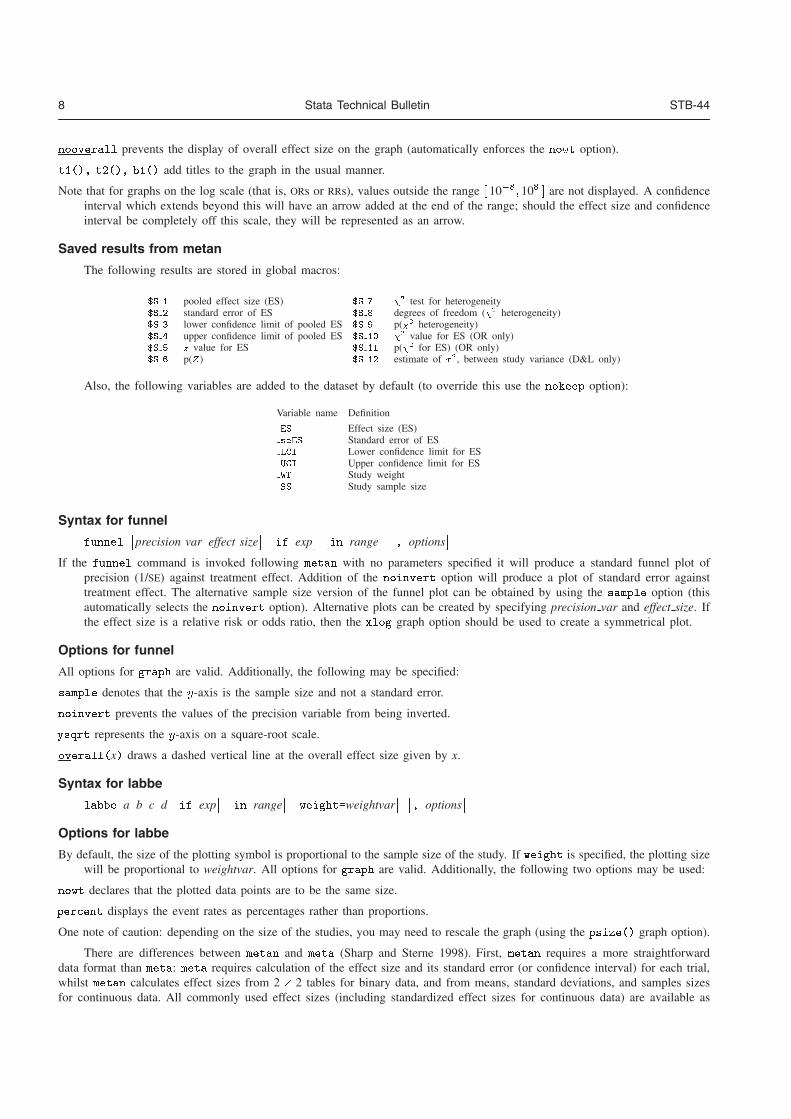
nooverall prevents the display of overall effect size on the graph (automatically enforces the nowt option).
t���� t���� b��� add titles to the graph in the usual manner.
Note that for graphs on the log scale (that is, ORs or RRs), values outside the range � 10��� 10� � are not displayed. A confidenceinterval which extends beyond this will have an arrow added at the end of the range; should the effect size and confidenceinterval be completely off this scale, they will be represented as an arrow.
Saved results from metan
The following results are stored in global macros:
�S � pooled effect size (ES) �S � �� test for heterogeneity�S � standard error of ES �S � degrees of freedom (�� heterogeneity)�S � lower confidence limit of pooled ES �S � p(�� heterogeneity)�S � upper confidence limit of pooled ES �S � �� value for ES (OR only)�S z value for ES �S �� p(�� for ES) (OR only)�S � p(Z) �S �� estimate of ��, between study variance (D&L only)
Also, the following variables are added to the dataset by default (to override this use the nokeep option):
Variable name Definition
ES Effect size (ES)seES Standard error of ESLCI Lower confidence limit for ESUCI Upper confidence limit for ESWT Study weightSS Study sample size
Syntax for funnel
funnel�precision var effect size
� �if exp
� �in range
� �� options
�
If the funnel command is invoked following metan with no parameters specified it will produce a standard funnel plot ofprecision (1/SE) against treatment effect. Addition of the noinvert option will produce a plot of standard error againsttreatment effect. The alternative sample size version of the funnel plot can be obtained by using the sample option (thisautomatically selects the noinvert option). Alternative plots can be created by specifying precision var and effect size. Ifthe effect size is a relative risk or odds ratio, then the xlog graph option should be used to create a symmetrical plot.
Options for funnel
All options for graph are valid. Additionally, the following may be specified:
sample denotes that the y-axis is the sample size and not a standard error.
noinvert prevents the values of the precision variable from being inverted.
ysqrt represents the y-axis on a square-root scale.
overall�x� draws a dashed vertical line at the overall effect size given by x.
Syntax for labbe
labbe a b c d�if exp
� �in range
� �weight�weightvar
� �� options
�
Options for labbe
By default, the size of the plotting symbol is proportional to the sample size of the study. If weight is specified, the plotting sizewill be proportional to weightvar. All options for graph are valid. Additionally, the following two options may be used:
nowt declares that the plotted data points are to be the same size.
percent displays the event rates as percentages rather than proportions.
One note of caution: depending on the size of the studies, you may need to rescale the graph (using the psize�� graph option).
There are differences between metan and meta (Sharp and Sterne 1998). First, metan requires a more straightforwarddata format than meta: meta requires calculation of the effect size and its standard error (or confidence interval) for each trial,whilst metan calculates effect sizes from 2� 2 tables for binary data, and from means, standard deviations, and samples sizesfor continuous data. All commonly used effect sizes (including standardized effect sizes for continuous data) are available as
Stata Technical Bulletin 9
options in metan. Secondly, where meta provides inverse variance, empirical Bayes and DerSimonian and Laird methods forpooling individual studies, metan additionally provides the commonly used Mantel–Haenszel and Peto methods (but does notprovide an empirical Bayes method). There are also differences in the format and options for the forest plot.
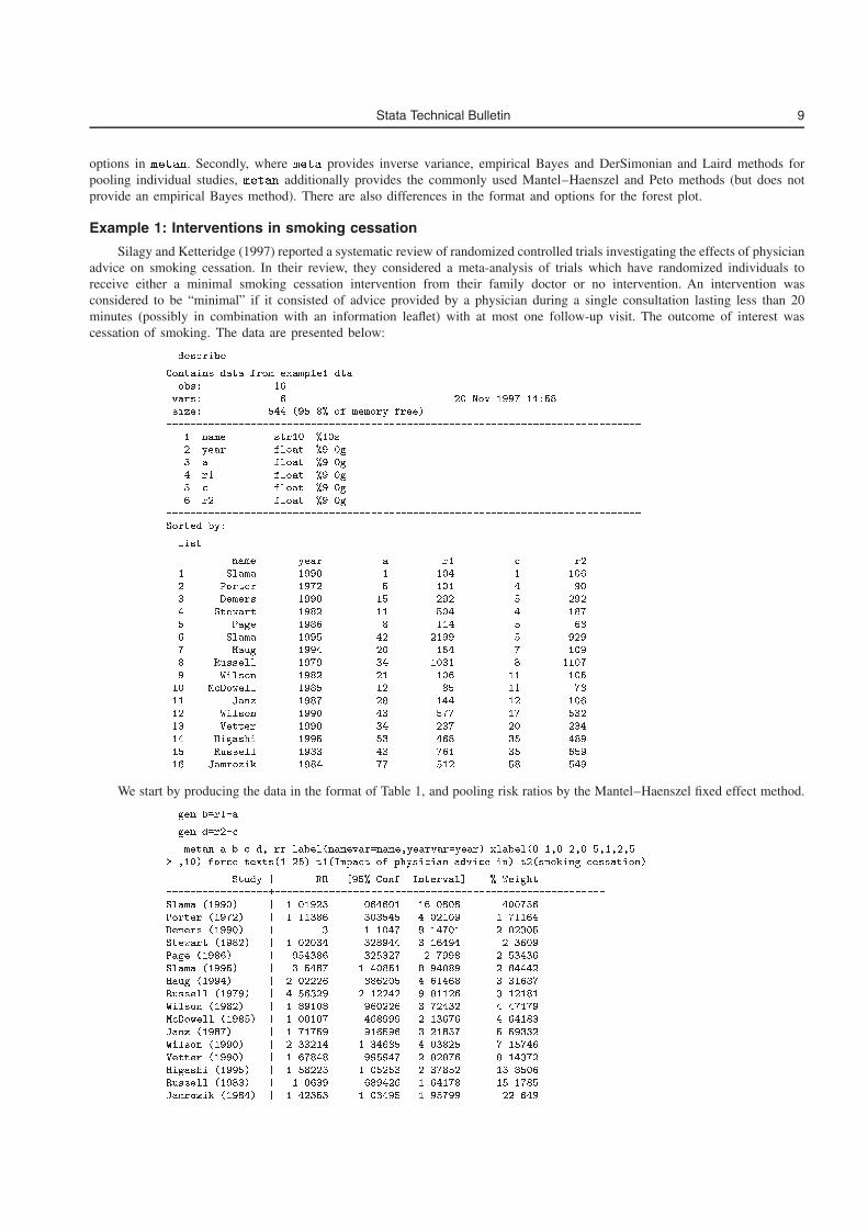
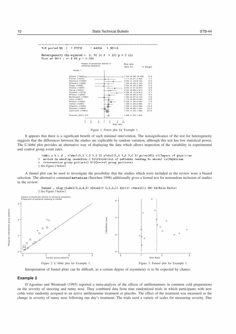
Example 1: Interventions in smoking cessation
Silagy and Ketteridge (1997) reported a systematic review of randomized controlled trials investigating the effects of physicianadvice on smoking cessation. In their review, they considered a meta-analysis of trials which have randomized individuals toreceive either a minimal smoking cessation intervention from their family doctor or no intervention. An intervention wasconsidered to be “minimal” if it consisted of advice provided by a physician during a single consultation lasting less than 20minutes (possibly in combination with an information leaflet) with at most one follow-up visit. The outcome of interest wascessation of smoking. The data are presented below:
� describe
Contains data from example��dtaobs� ��vars� � �� Nov ���� ���size� ���� of memory free�
��������������������������������������������������������������������������������� name str�� ��s�� year float ���g�� a float ���g� r� float ���g� c float ���g�� r� float ���g
�������������������������������������������������������������������������������Sorted by�
� list
name year a r� c r��� Slama ���� � �� � ����� Porter ���� ��� ���� Demers ���� � ��� ���� Stewart ���� �� � ���� Page ���� � �� ���� Slama ��� � ���� ����� Haug ��� �� � � ����� Russell ���� � ���� � ������ Wilson ���� �� ��� �� ����� McDowell ��� �� � �� ����� Janz ���� �� � �� ������ Wilson ���� � �� �� ����� Vetter ���� � ��� �� ���� Higashi ��� � �� � ���� Russell ���� � ��� � ����� Jamrozik ��� �� �� � �
We start by producing the data in the format of Table 1, and pooling risk ratios by the Mantel–Haenszel fixed effect method.
� gen b�r��a
� gen d�r��c
� metan a b c d� rr label�namevar�name�yearvar�year� xlabel����������������� ���� force texts����� t��Impact of physician advice in� t��smoking cessation�
Study � RR �� Conf� Interval� Weight�������������������������������������������������������������������������Slama ������ � ������� ������ ������� �����Porter ������ � ������� ���� ������ ������Demers ������ � � ����� ������ ������Stewart ������ � ������ ����� ����� ������Page ������ � ����� ������ ������ �����Slama ����� � ���� ����� ������ ����Haug ����� � ������� ������ ����� �������Russell ������ � ����� ������ ������� �������Wilson ������ � ������� ������� ������ �����McDowell ����� � ������� ������ ������� �����Janz ������ � ������ ������ ������ �����Wilson ������ � ������ ����� ����� �����Vetter ������ � ������ ����� ������� ������Higashi ����� � ������ ����� ������ ������Russell ������ � ������ ������ ������ �����Jamrozik ����� � ����� ����� ������ �����
10 Stata Technical Bulletin STB-44
�������������������������������������������������������������������������M�H pooled RR � ������ ���� ����
�������������������������������������������������������������������������Heterogeneity chi�squared ���� �d�f� �� p �����Test of RR � � z ���� p �����
Impact of physician advice insmoking cessat ion
Risk ratio.1 .2 .5 1 2 5 10
Study
% Weight
Risk ratio
(95% CI)
1.02 (0.06,16.08) Slama (1990) 0.4 1.11 (0.31,4.02) Porter (1972) 1.7 3.00 (1.10,8.15) Demers (1990) 2.0 1.02 (0.33,3.16) Stewart (1982) 2.4 0.95 (0.33,2.80) Page (1986) 2.5 3.55 (1.41,8.94) Slama (1995) 2.8 2.02 (0.89,4.61) Haug (1994) 3.3 4.56 (2.12,9.81) Russel l (1979) 3.1 1.89 (0.96,3.72) Wi lson (1982) 4.5 1.00 (0.47,2.14) McDowel l (1985) 4.6 1.72 (0.92,3.22) Janz (1987) 5.6 2.33 (1.35,4.04) Wi lson (1990) 7.2 1.68 (1.00,2.83) Vetter (1990) 8.1 1.58 (1.05,2.38) Higashi (1995) 13.9 1.06 (0.69,1.64) Russel l (1983) 15.2 1.42 (1.03,1.96) Jamrozik (1984) 22.6
1.68 (1.44,1.95) Overal l (95% CI)
Figure 1. Forest plot for Example 1.
It appears that there is a significant benefit of such minimal intervention. The nonsignificance of the test for heterogeneitysuggests that the differences between the studies are explicable by random variation, although this test has low statistical power.The L’Abbe plot provides an alternative way of displaying the data which allows inspection of the variability in experimentaland control group event rates.
� labbe a b c d � xlabel��������������� ylabel��������������� psize��� t��Impact of physician� advice in smoking cessation�� t��Proportion of patients ceasing to smoke� l��Physician� intervention group patients� b��Control group patients�� See Figure 2 below�
A funnel plot can be used to investigate the possibility that the studies which were included in the review were a biasedselection. The alternative command metabias (Steichen 1998) additionally gives a formal test for nonrandom inclusion of studiesin the review.
� funnel � xlog ylabel�������� xlabel��������� xli��� overall������ b��Risk Ratio�� See Figure 3 below�
Impact of physician advice in smoking cessation:Proport ion of patients ceasing to smoke
Ph
ys
icia
n i
nte
rve
nti
on
gro
up
pa
tie
nts
Control group patients0 .1 .2 .3
0
.1
.2
.3
1/S
E(E
ffe
ct
siz
e)
Risk Ratio.5 1 2 5
0
2
4
6
Figure 2. L’Abbe plot for Example 1. Figure 3. Funnel plot for Example 1.
Interpretation of funnel plots can be difficult, as a certain degree of asymmetry is to be expected by chance.
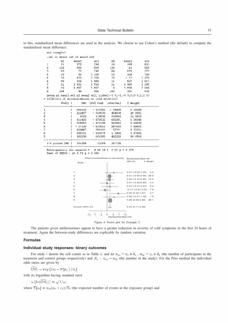
Example 2
D’Agostino and Weintraub (1995) reported a meta-analysis of the effects of antihistamines in common cold preparationson the severity of sneezing and runny nose. They combined data from nine randomized trials in which participants with newcolds were randomly assigned to an active antihistamine treatment or placebo. The effect of the treatment was measured as thechange in severity of runny nose following one day’s treatment. The trials used a variety of scales for measuring severity. Due
Stata Technical Bulletin 11
to this, standardized mean differences are used in the analysis. We choose to use Cohen’s method (the default) to compute thestandardized mean difference.
� use example�
� list n� mean� sd� n� mean� sd�
n� mean� sd� n� mean� sd��� �� ���� ���� �� ����� ����� ��� ��� ��� ��� ��� ������ �� ��� ��� � ���� ����� �� ��� ���� �� ��� ���� �� ��� ���� �� ���� ������ � ���� ����� � ���� ������ �� ����� ����� �� ���� ������� �� ����� ����� � ����� ����� � � ��� �� ��� ����
� metan n� mean� sd� n� mean� sd� xlabel����� �� ���� � ��� � ����� t��Effect of antihistamines on cold severity�
Study � SMD ��� Conf� Interval� � Weight�������������������������������������������������������������������������� � ������ ������� ����� ������ � ������ ������ ����� ������ � ����� ������� ����� ������� � ������ ������� ������ ������ � ������� ������� ���� ������� � ������ �������� ������� ������ � ������ ������ ������� ������� � ������ ������� ���� ������ � ������ ����� ����� ��������������������������������������������������������������������������������
I�V pooled SMD � ����� ����� ��������������������������������������������������������������������������������Heterogeneity chi�squared � ��� �d�f� � �� p � �����Test of SMD�� � z� ���� p � �����
Effect of antihistimines on cold severity
Standardised Mean dif f .-1.5 -1 -.5 0 .5 1 1.5
Study % Weight
Standardised Mean dif f .
(95% CI)
0.57 (-0.22,1.35) 1 2.5
0.21 (-0.03,0.45) 2 26.0
0.20 (-0.15,0.55) 3 12.5
0.01 (-0.58,0.60) 4 4.4
0.24 (-0.47,0.94) 5 3.0
-0.17 (-0.61,0.27) 6 7.9
0.93 (0.30,1.57) 7 3.7
0.59 (-0.31,1.49) 8 1.9
0.26 (0.06,0.46) 9 38.1
0.23 (0.11,0.36) Overal l (95% CI)
Figure 4. Forest plot for Example 2.
The patients given antihistamines appear to have a greater reduction in severity of cold symptoms in the first 24 hours oftreatment. Again the between-study differences are explicable by random variation.
Formulas
Individual study responses: binary outcomes
For study i denote the cell counts as in Table 1, and let n�i � ai � bi , n�i � ci � di (the number of participants in thetreatment and control groups respectively) and Ni � n�i � n�i (the number in the study). For the Peto method the individualodds ratios are given by
dORi � exp f�ai � E �ai�� �vig
with its logarithm having standard error
sefln�dORi�g �p
��vi
where E�ai� � n�i�ai � ci��Ni (the expected number of events in the exposure group) and

12 Stata Technical Bulletin STB-44
vi � �n�in�i�ai � ci��bi � di����N�
i�Ni � ��� (the hypergeometric variance of ai).
For other methods of combining trials, the odds ratio for each study is given by
dORi � aidi�bici
the standard error of the log odds ratio being
sefln�dORi�g �p
��ai � ��bi � ��ci � ��di
The risk ratio for each study is given by
dRRi � �ai�n�i���ci�n�i�
the standard error of the log risk ratio being
sefln�dRRi�g �p
��ai � ��ci � ��n�i � ��n�i
The risk difference for each study is given by
dRDi � �ai�n�i�� �ci�n�i� with standard error se�dRDi� �paibi�n��i � cidi�n��i
where zero cells cause problems with computation of the standard errors, 0.5 is added to all cells (ai,bi,ci,di) for that study.
Individual study responses: continuous outcomes
Denote the number of subjects, mean and standard deviation as in Table 1, and let
Ni � n�i � n�i
and
si �p
��n�i � ��sd��i� �n�i � ��sd�
�i���Ni � ��
be the pooled standard deviation of the two groups. The weighted mean difference is given by
dWMDi � m�i �m�i with standard error se� dWMDi� �psd�
�i�n�i � sd�
�i�n�i
There are three formulations of the standardized mean difference. The default is the measure suggested by Cohen (Cohen’sd) which is the ratio of the mean difference to the pooled standard deviation si; i.e.,
bdi � �m�i �m�i��si with standard error se�bdi� �
qNi��n�in�i� � bd�i ���Ni � ��
Hedges suggested a small-sample adjustment to the mean difference (Hedges adjusted g), to give
bgi � ��m�i �m�i��si���� ��Ni � ��� with standard error se�bgi� �pNi��n�in�i� � bg�i ���Ni � ���
Glass suggested using the control group standard deviation as the best estimate of the scaling factor to give the summary measure(Glass’s b�), where
b�i � �m�i �m�i��sd�i� with standard error se��i� �qNi��n�in�i� � b��
i���n�i � ��
Mantel–Haenszel methods for combining trials
For each study, the effect size from each trial b�i is given weight wi in the analysis. The overall estimate of the pooledeffect, b�MH is given by
b�MH=�Pwib�i���Pwi�
For combining odds ratios, each study’s OR is given weight
wi � bici�Ni,
and the logarithm of dORMH has standard error given by
sefln�dORMH�g �p
�PR���R� � ��PS �QR����R� S�� � �QS���S�
where
R �Paidi�Ni S �
Pbici�Ni
PR �P
�ai � di�aidi�N�
iPS �
P�ai � di�bici�N
�
i
QR �P
�bi � ci�aidi�N�
iQS �
P�bi � ci�bici�N
�
i

Stata Technical Bulletin 13
For combining risk ratios, each study’s RR is given weight
wi � �n�ici��Ni
and the logarithm of dRRMH has standard error given by
sefln�dRRMH�g �pP��R� S�
where
P �P
�n�in�i�ai � ci�� aiciNi��N�
iR �
Pain�i�Ni S �
Pcin�i�Ni
For risk differences, each study’s RD has the weight
wi � n�in�i�Ni
and dRDMH has standard error given by
sefdRDMHg �p
�P�Q��
where
P �P
�aibin�
�i� cidin
�
�i��n�in�iN
�
i� Q �
Pn�in�i�Ni
The heterogeneity statistic is given by
Q �Pwi�b�i � b�MH��
where � is the log odds ratio, log relative risk or risk difference. Under the null hypothesis that there are no differences intreatment effect between trials, this follows a �� distribution on k � 1 degrees of freedom.
Inverse variance methods for combining trials
Here, when considering odds ratios or risk ratios, we define the effect size �i to be the natural logarithm of the trial’s ORor RR; otherwise, we consider the summary statistic (RD, SMD or WMD) itself. The individual effect sizes are weightedaccording to the reciprocal of their variance (calculated as the square of the standard errors given in the individual study sectionabove) giving
wi � ��se�b�i��These are combined to give a pooled estimate
b�IV � �Pwib�i���Pwi�
with
sefb�IV g � ��pP
wi
The heterogeneity statistic is given by a similar formula as for the Mantel–Haenszel method, using the inverse varianceform of the weights, wi
Q �Pwi�b�i � b�IV ��
Peto’s assumption free method for combining trials
Here, the overall odds ratio is given by
dORPeto � expfPwi ln�dORi��
Pwig
where the odds ratio dORi is calculated using the approximate method described in the individual trial section, and the weights,wi are equal to the hypergeometric variances, vi.
The logarithm of the odds ratio has standard error
sefln�dORPeto�g � ��pP
wi
The heterogeneity statistic is given by
Q �Pwif�lndORi�
� � �lndORPeto��g
DerSimonian and Laird random effect models
Under the random effect model, the assumption of a common treatment effect is relaxed, and the effect sizes are assumedto have a distribution

14 Stata Technical Bulletin STB-44
�i � N��� ���
The estimate of �� is given by
b�� � maxf�Q� �k � �����P
wi � �P�w�
i��P
wi��� �g
The estimate of the combined effect for heterogeneity may be taken as either the Mantel–Haenszel or the inverse varianceestimate. Again, for odds ratios and risk ratios, the effect size is taken as the natural logarithm of the OR and RR. Each study’seffect size is given weight
wi � ���se�b�i�� � b���The pooled effect size is given by
b�DL � �P
wib�i���Pwi�
and
sefb�DLg � ��pP
wi
Note that in the case where the heterogeneity statistic Q is less than or equal to its degrees of freedom �k� 1�, the estimateof the between trial variation, b��� is zero, and the weights reduce to those given by the inverse variance method.
Confidence intervals
The 1���1� �� confidence interval for b� is given by
b� � se�b���1� ��2�� to b� � se�b���1� ��2�
where b� is the log odds ratio, log relative risk, risk difference, mean difference or standardized mean difference, and is thestandard normal distribution function. The Cornfield confidence intervals for odds ratios are calculated as explained in the Statamanual for the epitab command.
Test statistics
In all cases, the test statistic is given by
z � b��se�b��where the odds ratio or risk ratio is again considered on the log scale.
For odds ratios pooled by method of Mantel and Haenszel or Peto, an alternative test statistic is available, which is the ��
test of the observed and expected events rate in the exposure group. The expectation and the variance of ai are as given earlierin the Peto odds ratio section. The test statistic is
�� � fP�ai � E�ai��g
��P
var�ai�
on one degree of freedom. Note that in the case of odds ratios pooled by method of Peto, the two test statistics are identical;the �� test statistic is simply the square of the z score.
Acknowledgments
The statistical methods programmed in metan utilize several of the algorithms used by the MetaView software (part of theCochrane Library), which was developed by Gordon Dooley of Update Software, Oxford and Jonathan Deeks of the StatisticalMethods Working Group of the Cochrane Collaboration. We have also used a subroutine written by Patrick Royston of the RoyalPostgraduate Medical School, London.
ReferencesBreslow, N. E. and N. E. Day. 1980. Combination of results from a series of 2x2 tables; control of confounding. In Statistical Methods in Cancer
Research, vol. 1, Lyon: International Agency for Health Research on Cancer.
D’Agostino, R. B. and M. Weintraub. 1995. Meta-analysis: A method for synthesizing research. Clinical Pharmacology and Therapeutics 58: 605–616.
DerSimonian, R. and N. Laird. 1986. Meta-analysis in clinical trials. Controlled Clinical Trials 7: 177–188.
Egger, M., G. D. Smith, M. Schneider, and C. Minder. 1997. Bias in meta-analysis detected by a simple, graphical test. British Medical Journal 315:629–635.
Fleiss, J. L. 1993. The statistical basis of meta-analysis. Statistical Methods in Medical Research 2: 121–145.
Glass, G. V., B. McGaw, and M. L. Smith. 1981. Meta-Analysis in Social Research. Beverly Hills, CA: Sage Publications.
Greenland, S. and J. Robins. 1985. Estimation of a common effect parameter from sparse follow-up data. Biometrics 41: 55–68.
Greenland, S. and A. Salvan. 1990. Bias in the one-step method for pooling study results. Statistics in Medicine 9: 247–252.

Stata Technical Bulletin 15
Hedges, L. V. and I. Olkin. 1985. Statistical Methods for Meta-analysis. San Diego: Academic Press. Chapter 5.
L’Abbe, K. A., A. S. Detsky, and K. O’Rourke. 1987. Meta-analysis in clinical research. Annals of Internal Medicine 107: 224–233.
Mantel, N. and W. Haenszel. 1959. Statistical aspects of the analysis of data from retrospective studies of disease. Journal of the National CancerInstitute 22: 719–748.
Robins, J., S. Greenland, and N. E. Breslow. 1986. A general estimator for the variance of the Mantel–Haenszel odds ratio. American Journal ofEpidemiology 124: 719–723.
Rosenthal, R. 1994. Parametric measures of effect size. In The Handbook of Research Synthesis, ed. H. Cooper and L. V. Hedges. New York: RussellSage Foundation.
Sharp, S. and J. Sterne. 1997. sbe16: Meta-analysis. Stata Technical Bulletin 38: 9–14. Reprinted in The Stata Technical Bulletin Reprints vol. 7,pp. 100–106.
Silagy, C. and S. Ketteridge. 1997. Physician advice for smoking cessation. In Tobacco Addiction Module of The Cochrane Database of SystematicReviews, ed. T. Lancaster, C. Silagy, and D. Fullerton. [updated 01 September 1997]. Available in The Cochrane Library [database on disk andCDROM]. The Cochrane Collaboration; Issue 4. Oxford: Update Software. Updated quarterly.
Sinclair, J. C. and M. B. Bracken. 1992. Effective Care of the Newborn Infant . Oxford: Oxford University Press. Chapter 2.
Steichen, T. J. 1998. sbe19: Tests for publication bias in meta-analysis. Stata Technical Bulletin 41: 9–15. Reprinted in The Stata Technical BulletinReprints vol. 7, pp. 125–133.
Yusuf, S., R. Peto, J. Lewis, R. Collins, and P. Sleight. 1985. Beta blockade during and after myocardial infarction: an overview of the randomizedtrials. Progress in Cardiovascular Diseases 27: 335–371.
sg85 Moving summaries
Nicholas J. Cox, University of Durham, UK, FAX (011) 44-91-374-2456, [email protected]
Syntax
movsumm varname�if exp
� �in range
� �weight
�� gen�newvar� result�#��
window�#� end mid f binomial j oweight�string� g wrap�
fweights and aweights are allowed.
Description
movsumm produces a new variable containing moving summaries of varname for overlapping windows of specified length.varname will usually (but not necessarily) be a time series with regularly spaced values. Possible summaries are those producedby summarize and saved in result��.
It is the user’s responsibility to place observations in the appropriate sort order first.
Options
gen�newvar� specifies newvar as the name for the new variable. It is in fact a required option.
result�#� specifies which result�� from summarize is to be used. It is in fact a required option. See the table below. Notethe typographical error in the Stata 5.0 manual entry [R] summarize: result���� contains the 50th percentile (median).
# meaning # meaning
1 number of observations 10 50th percentile (median)2 sum of weight 11 75th percentile3 mean 12 90th percentile4 variance 13 95th percentile5 minimum 14 skewness6 maximum 15 kurtosis7 5th percentile 16 1st percentile8 10th percentile 17 99th percentile9 25th percentile 18 sum of variable
window�#� specifies the length of the window, which should be an integer at least 2. The default is 3. By default, results forodd-length windows are placed in the middle of the window and results for even-length windows are placed at the end ofthe window. The defaults can be overridden by end or mid.
end forces results to be placed at the end of the window.
mid forces results to be placed in the middle of the window, or in the case of windows of even length just after it: in the 2ndof 2, the 3rd of 4, the 4th of 6, and so on.
The Stata Journal (2008)8, Number 1, pp. 3–28
metan: fixed- and random-effects meta-analysis
Ross J. HarrisDepartment of Social Medicine
University of BristolBristol, UK
Michael J. BradburnHealth Services Research Center
University of SheffeldSheffield, UK
Jonathan J. DeeksDepartment of Primary Care Medicine
University of BirminghamBirmingham, UK
Roger M. HarbordDepartment of Social Medicine
University of BristolBristol, UK
Douglas G. AltmanCentre for Statistics in Medicine
University of OxfordOxford, UK
Jonathan A. C. SterneDepartment of Social Medicine
University of BristolBristol, UK
Abstract. This article describes updates of the meta-analysis command metan
and options that have been added since the command’s original publication (Brad-burn, Deeks, and Altman, metan – an alternative meta-analysis command, StataTechnical Bulletin Reprints, vol. 8, pp. 86–100). These include version 9 graphicswith flexible display options, the ability to meta-analyze precalculated effect esti-mates, and the ability to analyze subgroups by using the by() option. Changes tothe output, saved variables, and saved results are also described.
Keywords: sbe24 2, metan, meta-analysis, forest plot
1 Introduction
Meta-analysis is a two-stage process involving the estimation of an appropriate summarystatistic for each of a set of studies followed by the calculation of a weighted average ofthese statistics across the studies (Deeks, Altman, and Bradburn 2001). Odds ratios,risk ratios, and risk differences may be calculated from binary data, or a differencein means obtained from continuous data. Alternatively, precalculated effect estimatesand their standard errors from each study may be pooled, for example, adjusted log-odds ratios from observational studies. The summary statistics from each study canbe combined by using a variety of meta-analytic methods, which are classified as fixed-effect models in which studies are weighted according to the amount of informationthey contain; or random-effects models, which incorporate an estimate of between-studyvariation (heterogeneity) in the weighting. A meta-analysis will customarily include aforest plot, in which results from each study are displayed as a square and a horizontalline, representing the intervention effect estimate together with its confidence interval.The area of the square reflects the weight that the study contributes to the meta-
c© 2008 StataCorp LP sbe24 2
4 metan: meta-analysis
analysis. The combined-effect estimate and its confidence interval are represented by adiamond.
Here we present updates to the metan command and other previously undocumentedadditions that have been made since its original publication (Bradburn, Deeks, andAltman 1998). New features include
• Version 9 graphics
• Flexible display of tabular data in the forest plot
• Results from a second type of meta-analysis displayed in the same forest plot
• by() group processing
• Analysis of precalculated effect estimates
• Prediction intervals for the intervention effect in a new study from random-effectsanalyses
There are a substantial number of options for the metan command because of thevariety of meta-analytic techniques and the need for flexible graphical displays. Werecommend that new users not try to learn everything at once but to learn the basicsand build from there as required. Clickable examples of metan are available in the helpfile, and the dialog box may also be a good way to start using metan.
2 Example data
The dataset used in subsequent examples is taken from the meta-analysis published astable 1 in Colditz et al. (1994, 699). The aim of the analysis was to quantify the efficacyof BCG vaccine against tuberculosis, and data from 11 trials are included here. Therewas considerable between-trial heterogeneity in the effect of the vaccine; it has beensuggested that this might be explained by the latitude of the region in which the trialwas conducted (Fine 1995).
Example
Details of the dataset are shown below by using describe and list commands.
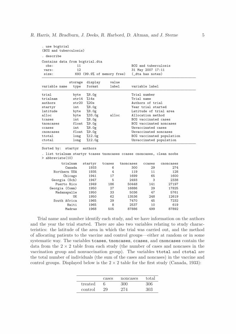
R. Harris, M. Bradburn, J. Deeks, R. Harbord, D. Altman, and J. Sterne 5
. use bcgtrial(BCG and tuberculosis)
. describe
Contains data from bcgtrial.dtaobs: 11 BCG and tuberculosis
vars: 12 31 May 2007 17:11size: 693 (99.9% of memory free) (_dta has notes)
storage display valuevariable name type format label variable label
trial byte %8.0g Trial numbertrialnam str14 %14s Trial nameauthors str20 %20s Authors of trialstartyr int %8.0g Year trial startedlatitude byte %8.0g Latitude of trial areaalloc byte %33.0g alloc Allocation methodtcases int %8.0g BCG vaccinated casestnoncases float %9.0g BCG vaccinated noncasesccases int %8.0g Unvaccinated casescnoncases float %9.0g Unvaccinated noncasesttotal long %12.0g BCG vaccinated populationctotal long %12.0g Unvaccinated population
Sorted by: startyr authors
. list trialnam startyr tcases tnoncases ccases cnoncases, clean noobs> abbreviate(10)
trialnam startyr tcases tnoncases ccases cnoncasesCanada 1933 6 300 29 274
Northern USA 1935 4 119 11 128Chicago 1941 17 1699 65 1600
Georgia (Sch) 1947 5 2493 3 2338Puerto Rico 1949 186 50448 141 27197
Georgia (Comm) 1950 27 16886 29 17825Madanapalle 1950 33 5036 47 5761
UK 1950 62 13536 248 12619South Africa 1965 29 7470 45 7232
Haiti 1965 8 2537 10 619Madras 1968 505 87886 499 87892
Trial name and number identify each study, and we have information on the authorsand the year the trial started. There are also two variables relating to study charac-teristics: the latitude of the area in which the trial was carried out, and the methodof allocating patients to the vaccine and control groups—either at random or in somesystematic way. The variables tcases, tnoncases, ccases, and cnoncases contain thedata from the 2 × 2 table from each study (the number of cases and noncases in thevaccination group and nonvaccination group). The variables ttotal and ctotal arethe total number of individuals (the sum of the cases and noncases) in the vaccine andcontrol groups. Displayed below is the 2 × 2 table for the first study (Canada, 1933):
cases noncases totaltreated 6 300 306control 29 274 303
6 metan: meta-analysis
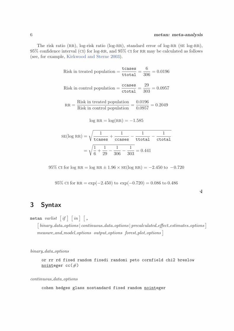
The risk ratio (RR), log-risk ratio (log-RR), standard error of log-RR (SE log-RR),95% confidence interval (CI) for log-RR, and 95% CI for RR may be calculated as follows(see, for example, Kirkwood and Sterne 2003).
Risk in treated population =tcases
ttotal=
6306
= 0.0196
Risk in control population =ccases
ctotal=
29303
= 0.0957
RR =Risk in treated populationRisk in control population
=0.01960.0957
= 0.2049
log RR = log(RR) = −1.585
SE(log RR) =
√1
tcases+
1ccases
− 1ttotal
− 1ctotal
=
√16
+129
− 1306
− 1303
= 0.441
95% CI for log RR = log RR ± 1.96 × SE(log RR) = −2.450 to −0.720
95% CI for RR = exp(−2.450) to exp(−0.720) = 0.086 to 0.486
3 Syntax
metan varlist[if] [
in] [
,[binary data options | continuous data options | precalculated effect estimates options
]measure and model options output options forest plot options
]
binary data options
or rr rd fixed random fixedi randomi peto cornfield chi2 breslownointeger cc(#)
continuous data options
cohen hedges glass nostandard fixed random nointeger
R. Harris, M. Bradburn, J. Deeks, R. Harbord, D. Altman, and J. Sterne 7
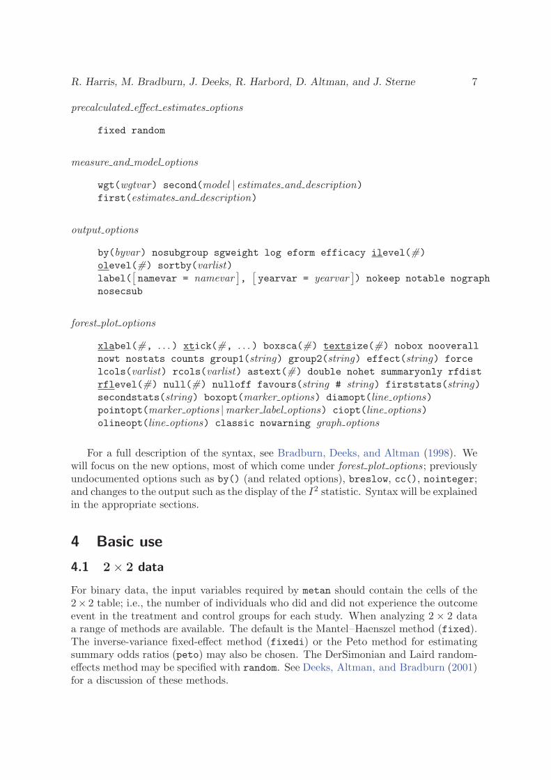
precalculated effect estimates options
fixed random
measure and model options
wgt(wgtvar) second(model | estimates and description)first(estimates and description)
output options
by(byvar) nosubgroup sgweight log eform efficacy ilevel(#)olevel(#) sortby(varlist)label(
[namevar = namevar
],[yearvar = yearvar
]) nokeep notable nograph
nosecsub
forest plot options
xlabel(#, . . . ) xtick(#, . . . ) boxsca(#) textsize(#) nobox nooverallnowt nostats counts group1(string) group2(string) effect(string) forcelcols(varlist) rcols(varlist) astext(#) double nohet summaryonly rfdistrflevel(#) null(#) nulloff favours(string # string) firststats(string)secondstats(string) boxopt(marker options) diamopt(line options)pointopt(marker options |marker label options) ciopt(line options)olineopt(line options) classic nowarning graph options
For a full description of the syntax, see Bradburn, Deeks, and Altman (1998). Wewill focus on the new options, most of which come under forest plot options ; previouslyundocumented options such as by() (and related options), breslow, cc(), nointeger;and changes to the output such as the display of the I2 statistic. Syntax will be explainedin the appropriate sections.
4 Basic use
4.1 2 × 2 data
For binary data, the input variables required by metan should contain the cells of the2× 2 table; i.e., the number of individuals who did and did not experience the outcomeevent in the treatment and control groups for each study. When analyzing 2 × 2 dataa range of methods are available. The default is the Mantel–Haenszel method (fixed).The inverse-variance fixed-effect method (fixedi) or the Peto method for estimatingsummary odds ratios (peto) may also be chosen. The DerSimonian and Laird random-effects method may be specified with random. See Deeks, Altman, and Bradburn (2001)for a discussion of these methods.
8 metan: meta-analysis
4.2 Display options
Previous versions of the metan command used the syntax label(namevar = namevar,yearvar = yearvar) to specify study information in the table and forest plot. Thissyntax still functions but has been superseded by the more flexible lcols(varlist) andrcols(varlist) options. The use of these options is described in more detail in section 5.The option favours(string # string) allows the user to display text information aboutthe direction of the treatment effect, which appears under the graph (e.g., exposuregood, exposure bad). favours() replaces the option b2title(). The # is required tosplit the two strings, which appear to either side of the null line.
Example
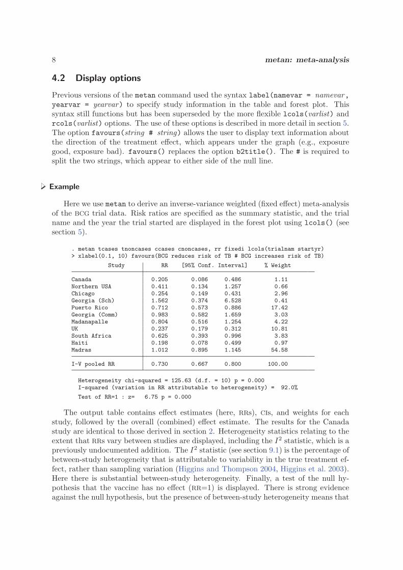
Here we use metan to derive an inverse-variance weighted (fixed effect) meta-analysisof the BCG trial data. Risk ratios are specified as the summary statistic, and the trialname and the year the trial started are displayed in the forest plot using lcols() (seesection 5).
. metan tcases tnoncases ccases cnoncases, rr fixedi lcols(trialnam startyr)> xlabel(0.1, 10) favours(BCG reduces risk of TB # BCG increases risk of TB)
Study RR [95% Conf. Interval] % Weight
Canada 0.205 0.086 0.486 1.11Northern USA 0.411 0.134 1.257 0.66Chicago 0.254 0.149 0.431 2.96Georgia (Sch) 1.562 0.374 6.528 0.41Puerto Rico 0.712 0.573 0.886 17.42Georgia (Comm) 0.983 0.582 1.659 3.03Madanapalle 0.804 0.516 1.254 4.22UK 0.237 0.179 0.312 10.81South Africa 0.625 0.393 0.996 3.83Haiti 0.198 0.078 0.499 0.97Madras 1.012 0.895 1.145 54.58
I-V pooled RR 0.730 0.667 0.800 100.00
Heterogeneity chi-squared = 125.63 (d.f. = 10) p = 0.000I-squared (variation in RR attributable to heterogeneity) = 92.0%
Test of RR=1 : z= 6.75 p = 0.000
The output table contains effect estimates (here, RRs), CIs, and weights for eachstudy, followed by the overall (combined) effect estimate. The results for the Canadastudy are identical to those derived in section 2. Heterogeneity statistics relating to theextent that RRs vary between studies are displayed, including the I2 statistic, which is apreviously undocumented addition. The I2 statistic (see section 9.1) is the percentage ofbetween-study heterogeneity that is attributable to variability in the true treatment ef-fect, rather than sampling variation (Higgins and Thompson 2004, Higgins et al. 2003).Here there is substantial between-study heterogeneity. Finally, a test of the null hy-pothesis that the vaccine has no effect (RR=1) is displayed. There is strong evidenceagainst the null hypothesis, but the presence of between-study heterogeneity means that

R. Harris, M. Bradburn, J. Deeks, R. Harbord, D. Altman, and J. Sterne 9
the fixed-effect assumption (that the true treatment effect is the same in each study) isincorrect. The forest plot displayed by the command is shown in figure 1.
Overall (I�squared = 92.0%, p = 0.000)
Madras
Haiti
Madanapalle
Trial
Georgia (Comm)
South Africa
UK
Puerto Rico
Chicago
Northern USA
name
Georgia (Sch)
Canada
1968
1965
1950
trial
1950
1965
1950
1949
1941
1935
started
1947
1933
Year
0.73 (0.67, 0.80)
1.01 (0.89, 1.14)
0.20 (0.08, 0.50)
0.80 (0.52, 1.25)
0.98 (0.58, 1.66)
0.63 (0.39, 1.00)
0.24 (0.18, 0.31)
0.71 (0.57, 0.89)
0.25 (0.15, 0.43)
0.41 (0.13, 1.26)
RR (95% CI)
1.56 (0.37, 6.53)
0.20 (0.09, 0.49)
100.00
54.58
0.97
4.22
%
3.03
3.83
10.81
17.42
2.96
0.66
Weight
0.41
1.11
BCG reduces risk of TB BCG increases risk of TB
1.1 10
Figure 1. Forest plot displaying an inverse-variance weighted fixed-effect meta-analysisof the effect of BCG vaccine on incidence of tuberculosis.
4.3 Precalculated effect estimates
The metan command may also be used to meta-analyze precalculated effect estimates,such as log-odds ratios and their standard errors or 95% CI, using syntax similar tothe alternative Stata meta-analysis command meta (Sharp and Sterne 1997). Here onlythe inverse-variance fixed-effect and DerSimonian and Laird random-effects methodsare available, because other methods require the 2 × 2 cell counts or the means andstandard deviations in each group. The fixed option produces an inverse-varianceweighted analysis when precalculated effect estimates are analyzed.
When analyzing ratio measures (RRs or odds ratios), the log ratio with its standarderror or 95% CI should be used as inputs to the command. The eform option can thenbe used to display the output on the ratio scale (as for the meta command).
10 metan: meta-analysis
Example
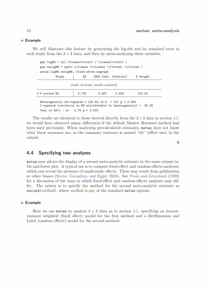
We will illustrate this feature by generating the log-RR and its standard error ineach study from the 2 × 2 data, and then by meta-analyzing these variables.
. gen logRR = ln( (tcases/ttotal) / (ccases/ctotal) )
. gen selogRR = sqrt( 1/tcases +1/ccases -1/ttotal -1/ctotal )
. metan logRR selogRR, fixed eform nograph
Study ES [95% Conf. Interval] % Weight
(table of study results omitted)
I-V pooled ES 0.730 0.667 0.800 100.00
Heterogeneity chi-squared = 125.63 (d.f. = 10) p = 0.000I-squared (variation in ES attributable to heterogeneity) = 92.0%
Test of ES=1 : z= 6.75 p = 0.000
The results are identical to those derived directly from the 2× 2 data in section 4.1;we would have observed minor differences if the default Mantel–Haenszel method hadbeen used previously. When analyzing precalculated estimates, metan does not knowwhat these measures are, so the summary estimate is named “ES” (effect size) in theoutput.
4.4 Specifying two analyses
metan now allows the display of a second meta-analytic estimate in the same output ta-ble and forest plot. A typical use is to compare fixed-effect and random-effects analyses,which can reveal the presence of small-study effects. These may result from publicationor other biases (Sterne, Gavaghan, and Egger 2000). See Poole and Greenland (1999)for a discussion of the ways in which fixed-effect and random-effects analyses may dif-fer. The syntax is to specify the method for the second meta-analytic estimate assecond(method), where method is any of the standard metan options.
Example
Here we use metan to analyze 2 × 2 data as in section 4.1, specifying an inverse-variance weighted (fixed effect) model for the first method and a DerSimonian andLaird (random effects) model for the second method:
R. Harris, M. Bradburn, J. Deeks, R. Harbord, D. Altman, and J. Sterne 11
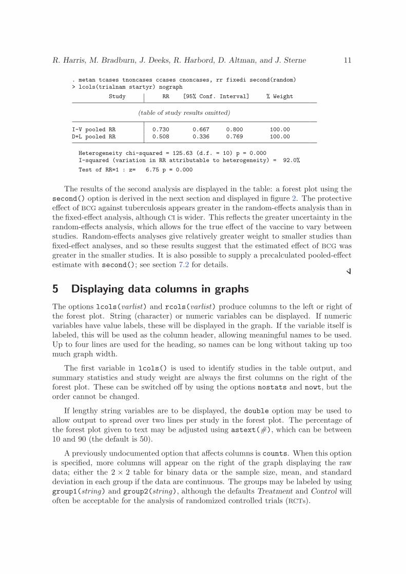
. metan tcases tnoncases ccases cnoncases, rr fixedi second(random)> lcols(trialnam startyr) nograph
Study RR [95% Conf. Interval] % Weight
(table of study results omitted)
I-V pooled RR 0.730 0.667 0.800 100.00D+L pooled RR 0.508 0.336 0.769 100.00
Heterogeneity chi-squared = 125.63 (d.f. = 10) p = 0.000I-squared (variation in RR attributable to heterogeneity) = 92.0%
Test of RR=1 : z= 6.75 p = 0.000
The results of the second analysis are displayed in the table: a forest plot using thesecond() option is derived in the next section and displayed in figure 2. The protectiveeffect of BCG against tuberculosis appears greater in the random-effects analysis than inthe fixed-effect analysis, although CI is wider. This reflects the greater uncertainty in therandom-effects analysis, which allows for the true effect of the vaccine to vary betweenstudies. Random-effects analyses give relatively greater weight to smaller studies thanfixed-effect analyses, and so these results suggest that the estimated effect of BCG wasgreater in the smaller studies. It is also possible to supply a precalculated pooled-effectestimate with second(); see section 7.2 for details.
5 Displaying data columns in graphs
The options lcols(varlist) and rcols(varlist) produce columns to the left or right ofthe forest plot. String (character) or numeric variables can be displayed. If numericvariables have value labels, these will be displayed in the graph. If the variable itself islabeled, this will be used as the column header, allowing meaningful names to be used.Up to four lines are used for the heading, so names can be long without taking up toomuch graph width.
The first variable in lcols() is used to identify studies in the table output, andsummary statistics and study weight are always the first columns on the right of theforest plot. These can be switched off by using the options nostats and nowt, but theorder cannot be changed.
If lengthy string variables are to be displayed, the double option may be used toallow output to spread over two lines per study in the forest plot. The percentage ofthe forest plot given to text may be adjusted using astext(#), which can be between10 and 90 (the default is 50).
A previously undocumented option that affects columns is counts. When this optionis specified, more columns will appear on the right of the graph displaying the rawdata; either the 2 × 2 table for binary data or the sample size, mean, and standarddeviation in each group if the data are continuous. The groups may be labeled by usinggroup1(string) and group2(string), although the defaults Treatment and Control willoften be acceptable for the analysis of randomized controlled trials (RCTs).
12 metan: meta-analysis
Example
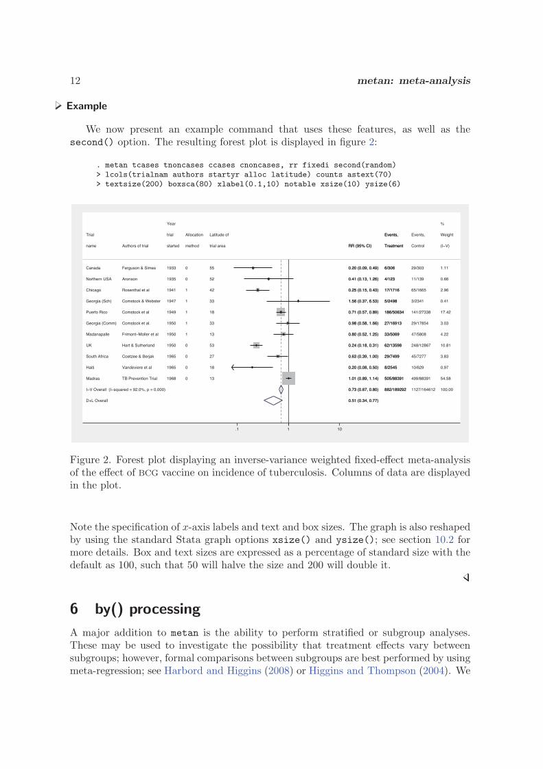
We now present an example command that uses these features, as well as thesecond() option. The resulting forest plot is displayed in figure 2:
. metan tcases tnoncases ccases cnoncases, rr fixedi second(random)> lcols(trialnam authors startyr alloc latitude) counts astext(70)> textsize(200) boxsca(80) xlabel(0.1,10) notable xsize(10) ysize(6)
I�V Overall (I�squared = 92.0%, p = 0.000)
UK
Trial
Haiti
Madras
Chicago
Georgia (Comm)
Canada
Puerto Rico
South Africa
Madanapalle
name
Georgia (Sch)
Northern USA
D+L Overall
Hart & Sutherland
Vandeviere et al
TB Prevention Trial
Rosenthal et al
Comstock et al.
Ferguson & Simes
Comstock et al
Coetzee & Berjak
Frimont�Moller et al
Authors of trial
Comstock & Webster
Aronson
Year
1950
trial
1965
1968
1941
1950
1933
1949
1965
1950
started
1947
1935
0
Allocation
0
0
1
1
0
1
0
1
method
1
0
53
Latitude of
18
13
42
33
55
18
27
13
trial area
33
52
0.73 (0.67, 0.80)
0.24 (0.18, 0.31)
0.20 (0.08, 0.50)
1.01 (0.89, 1.14)
0.25 (0.15, 0.43)
0.98 (0.58, 1.66)
0.20 (0.09, 0.49)
0.71 (0.57, 0.89)
0.63 (0.39, 1.00)
0.80 (0.52, 1.25)
RR (95% CI)
1.56 (0.37, 6.53)
0.41 (0.13, 1.26)
0.51 (0.34, 0.77)
882/189292
62/13598
Events,
8/2545
505/88391
17/1716
27/16913
6/306
186/50634
29/7499
33/5069
Treatment
5/2498
4/123
1127/164612
248/12867
Events,
10/629
499/88391
65/1665
29/17854
29/303
141/27338
45/7277
47/5808
Control
3/2341
11/139
100.00
%
10.81
Weight
0.97
54.58
2.96
3.03
1.11
17.42
3.83
4.22
(I�V)
0.41
0.66
0.73 (0.67, 0.80)
0.24 (0.18, 0.31)
0.20 (0.08, 0.50)
1.01 (0.89, 1.14)
0.25 (0.15, 0.43)
0.98 (0.58, 1.66)
0.20 (0.09, 0.49)
0.71 (0.57, 0.89)
0.63 (0.39, 1.00)
0.80 (0.52, 1.25)
RR (95% CI)
1.56 (0.37, 6.53)
0.41 (0.13, 1.26)
0.51 (0.34, 0.77)
882/189292
62/13598
Events,
8/2545
505/88391
17/1716
27/16913
6/306
186/50634
29/7499
33/5069
Treatment
5/2498
4/123
1.1 10
Figure 2. Forest plot displaying an inverse-variance weighted fixed-effect meta-analysisof the effect of BCG vaccine on incidence of tuberculosis. Columns of data are displayedin the plot.
Note the specification of x-axis labels and text and box sizes. The graph is also reshapedby using the standard Stata graph options xsize() and ysize(); see section 10.2 formore details. Box and text sizes are expressed as a percentage of standard size with thedefault as 100, such that 50 will halve the size and 200 will double it.
6 by() processing
A major addition to metan is the ability to perform stratified or subgroup analyses.These may be used to investigate the possibility that treatment effects vary betweensubgroups; however, formal comparisons between subgroups are best performed by usingmeta-regression; see Harbord and Higgins (2008) or Higgins and Thompson (2004). We
R. Harris, M. Bradburn, J. Deeks, R. Harbord, D. Altman, and J. Sterne 13
may also want to display results for different groups of studies in the same plot, eventhough it is inappropriate to meta-analyze across these groups.
6.1 Syntax and options for by()
nooverall specifies that the overall estimate not be displayed, for example, when it isinappropriate to meta-analyze across groups.
sgweight requests that weights be displayed such that they sum to 100% within eachsubgroup. This option is invoked automatically with nooverall.
nosubgroup specifies that studies be arranged by the subgroup specified, but estimatesfor each subgroup not be displayed.
nosecsub specifies that subestimates using the method defined by second() not bedisplayed.
summaryonly specifies that individual study estimates not be displayed, for example, toproduce a summary of different groups in a compact graph.
Example
Fine (1995) suggested that there is a relationship between the effect of BCG andthe latitude of the area in which the trial was conducted. Here we may want to usemeta-regression to further investigate this tendency (see Harbord and Higgins 2008).To illustrate the by() option, we will classify the studies into three groups defined bylatitude. We define these groups as tropical (≤23.5 degrees), midlatitude (between 23.5and 40 degrees) and northern (≥40 degrees).
. gen lat_cat = ""(11 missing values generated)
. replace lat_cat = "Tropical, < 23.5 latitude" if latitude <= 23.5lat_cat was str1 now str27(4 real changes made)
. replace lat_cat = "23.5-40 latitude" if latitude > 23.5 & latitude < 40(3 real changes made)
. replace lat_cat = "Northern, > 40 latitude" if latitude >= 40 & latitude < .(4 real changes made)
. assert lat_cat != ""
. label var lat_cat "Latitude region"
(Continued on next page)
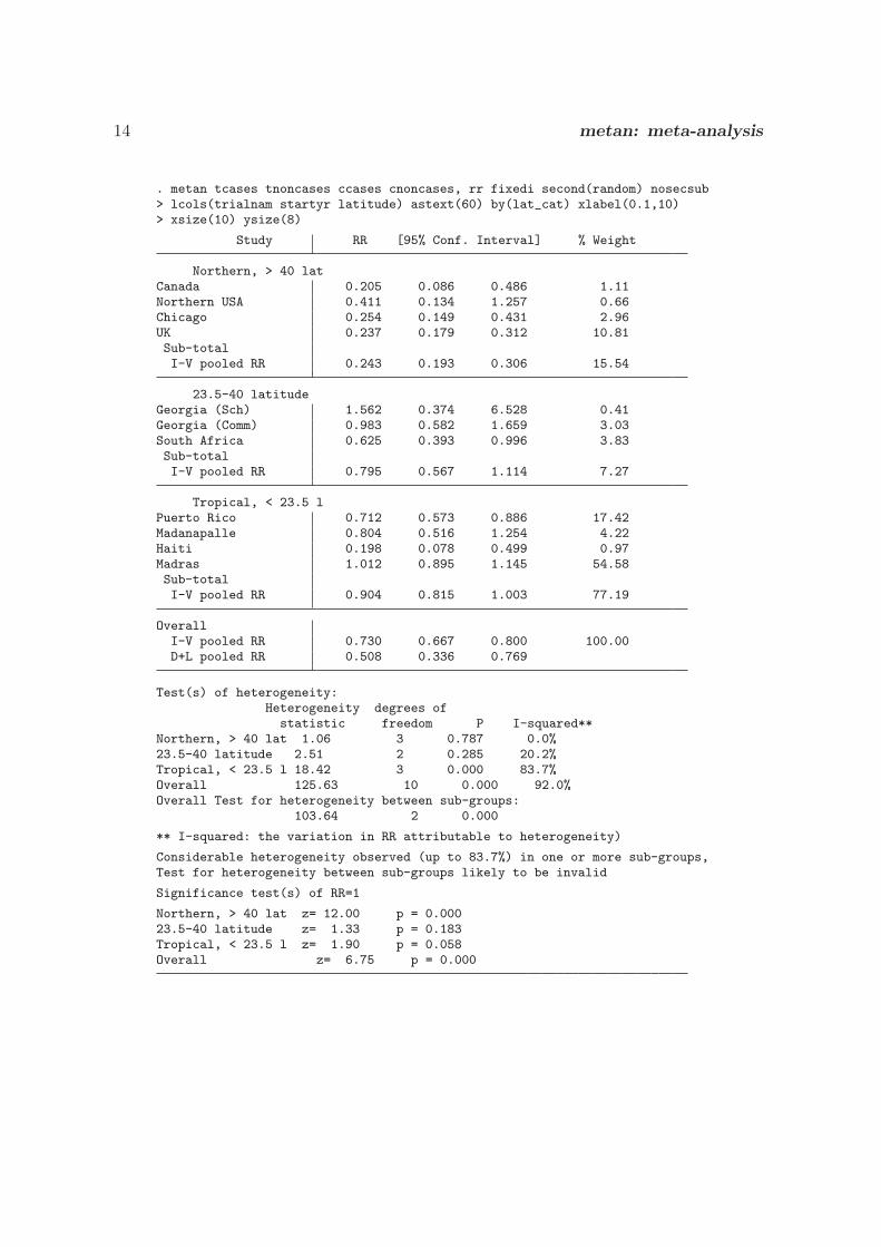
14 metan: meta-analysis
. metan tcases tnoncases ccases cnoncases, rr fixedi second(random) nosecsub> lcols(trialnam startyr latitude) astext(60) by(lat_cat) xlabel(0.1,10)> xsize(10) ysize(8)
Study RR [95% Conf. Interval] % Weight
Northern, > 40 latCanada 0.205 0.086 0.486 1.11Northern USA 0.411 0.134 1.257 0.66Chicago 0.254 0.149 0.431 2.96UK 0.237 0.179 0.312 10.81Sub-totalI-V pooled RR 0.243 0.193 0.306 15.54
23.5-40 latitudeGeorgia (Sch) 1.562 0.374 6.528 0.41Georgia (Comm) 0.983 0.582 1.659 3.03South Africa 0.625 0.393 0.996 3.83Sub-totalI-V pooled RR 0.795 0.567 1.114 7.27
Tropical, < 23.5 lPuerto Rico 0.712 0.573 0.886 17.42Madanapalle 0.804 0.516 1.254 4.22Haiti 0.198 0.078 0.499 0.97Madras 1.012 0.895 1.145 54.58Sub-totalI-V pooled RR 0.904 0.815 1.003 77.19
OverallI-V pooled RR 0.730 0.667 0.800 100.00D+L pooled RR 0.508 0.336 0.769
Test(s) of heterogeneity:Heterogeneity degrees of
statistic freedom P I-squared**Northern, > 40 lat 1.06 3 0.787 0.0%23.5-40 latitude 2.51 2 0.285 20.2%Tropical, < 23.5 l 18.42 3 0.000 83.7%Overall 125.63 10 0.000 92.0%Overall Test for heterogeneity between sub-groups:
103.64 2 0.000
** I-squared: the variation in RR attributable to heterogeneity)
Considerable heterogeneity observed (up to 83.7%) in one or more sub-groups,Test for heterogeneity between sub-groups likely to be invalid
Significance test(s) of RR=1
Northern, > 40 lat z= 12.00 p = 0.00023.5-40 latitude z= 1.33 p = 0.183Tropical, < 23.5 l z= 1.90 p = 0.058Overall z= 6.75 p = 0.000
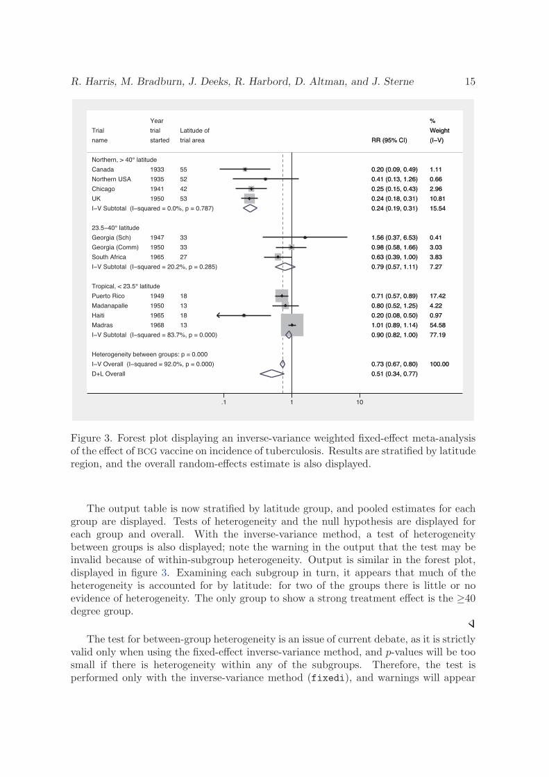
R. Harris, M. Bradburn, J. Deeks, R. Harbord, D. Altman, and J. Sterne 15
Heterogeneity between groups: p = 0.000
I�V Overall (I�squared = 92.0%, p = 0.000)
South Africa
Canada
23.5�40° latitude
I�V Subtotal (I�squared = 83.7%, p = 0.000)
I�V Subtotal (I�squared = 0.0%, p = 0.787)
Georgia (Sch)
Haiti
Northern, > 40° latitude
Madras
Madanapalle
I�V Subtotal (I�squared = 20.2%, p = 0.285)
Puerto Rico
Trial
Tropical, < 23.5° latitude
Georgia (Comm)
D+L Overall
Chicago
Northern USA
name
UK
1965
1933
Year
1947
1965
1968
1950
1949
trial
1950
1941
1935
started
1950
27
55
33
18
13
13
18
Latitude of
33
42
52
trial area
53
0.73 (0.67, 0.80)
0.63 (0.39, 1.00)
0.20 (0.09, 0.49)
0.90 (0.82, 1.00)
0.24 (0.19, 0.31)
1.56 (0.37, 6.53)
0.20 (0.08, 0.50)
1.01 (0.89, 1.14)
0.80 (0.52, 1.25)
0.79 (0.57, 1.11)
0.71 (0.57, 0.89)
0.98 (0.58, 1.66)
0.51 (0.34, 0.77)
0.25 (0.15, 0.43)
0.41 (0.13, 1.26)
RR (95% CI)
0.24 (0.18, 0.31)
100.00
3.83
1.11
%
77.19
15.54
0.41
0.97
54.58
4.22
7.27
17.42
Weight
3.03
2.96
0.66
(I�V)
10.81
1.1 10
Figure 3. Forest plot displaying an inverse-variance weighted fixed-effect meta-analysisof the effect of BCG vaccine on incidence of tuberculosis. Results are stratified by latituderegion, and the overall random-effects estimate is also displayed.
The output table is now stratified by latitude group, and pooled estimates for eachgroup are displayed. Tests of heterogeneity and the null hypothesis are displayed foreach group and overall. With the inverse-variance method, a test of heterogeneitybetween groups is also displayed; note the warning in the output that the test may beinvalid because of within-subgroup heterogeneity. Output is similar in the forest plot,displayed in figure 3. Examining each subgroup in turn, it appears that much of theheterogeneity is accounted for by latitude: for two of the groups there is little or noevidence of heterogeneity. The only group to show a strong treatment effect is the ≥40degree group.
The test for between-group heterogeneity is an issue of current debate, as it is strictlyvalid only when using the fixed-effect inverse-variance method, and p-values will be toosmall if there is heterogeneity within any of the subgroups. Therefore, the test isperformed only with the inverse-variance method (fixedi), and warnings will appear
16 metan: meta-analysis
if there is evidence of within-group heterogeneity. Despite these caveats, this methodis better than other, seriously flawed, methods such as testing the significance of atreatment effect in each group rather than testing for differences between the groups.As explained at the start of this section, meta-regression is the best way to examineand test for between-group differences.
7 User-defined analyses
7.1 Study weights
The wgt(wgtvar) option allows the studies to be combined by using specific weights thatare defined by the variable wgtvar . The user must ensure that the weights chosen aremeaningful. Typical uses are when analyzing precalculated effect estimates that requireweights that are not based on standard error or to assess the robustness of conclusionsby assigning alternative weights.
7.2 Pooled estimates
Pooled estimates may be derived by using another package and presented in a forest plotby using the first() option to supply these to the metan command. Here wgt(wgtvar)is used merely to specify box sizes in the forest plot, no heterogeneity statistics areproduced, and no values are returned. When using this feature, stratified analyses arenot allowed.
An alternative method is to provide the user-supplied meta-analytic estimate byusing the second() option. Data are analyzed by using standard methods, and theresulting pooled estimate is displayed together with the user-defined estimate (whichneed not be derived by using metan), allowing a comparison. When using this feature,the option nosecsub is invoked, as stratification using the user-defined method is notpossible.
When these options are specified, the user must supply the pooled estimate with itsstandard error or CI and a method label. The user may also supply text to be displayedat the bottom of the forest plot, in the position normally given to heterogeneity statistics,using firststats(string) and secondstats(string).
Example
The BCG data were analyzed by using a fully Bayesian random-effects model withWinBUGS software (Lunn et al. 2000). This analysis used the methods described byWarn, Thompson, and Spiegelhalter (2002) to deal with RRs. The chosen model incor-porated a noninformative prior (mean 0, precision 0.001). The resulting RR of 0.518(95% CI: 0.300, 0.824) is similar to that derived from a DerSimonian and Laird random-effects analysis. However, the CI from the Bayesian analysis is wider, because it allowsfor the uncertainty in estimating the between-study variance. The following syntax sup-
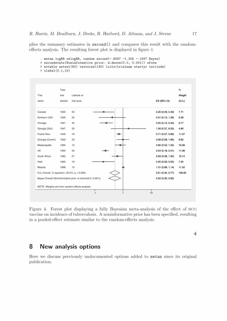
R. Harris, M. Bradburn, J. Deeks, R. Harbord, D. Altman, and J. Sterne 17
plies the summary estimates in second() and compares this result with the random-effects analysis. The resulting forest plot is displayed in figure 4.
. metan logRR selogRR, random second(-.6587 -1.205 -.1937 Bayes)> secondstats(Noninformative prior: d~dnorm(0.0, 0.001)) eform> notable astext(60) textsize(130) lcols(trialnam startyr latitude)> xlabel(0.1,10)
NOTE: Weights are from random effects analysis
D+L Overall (I�squared = 92.0%, p = 0.000)
Madanapalle
Georgia (Sch)
Canada
Bayes Overall (Noninformative prior: d~dnorm(0.0, 0.001))
Haiti
Trial
UK
South Africa
name
Northern USA
Puerto Rico
Chicago
Madras
Georgia (Comm)
1950
1947
1933
1965
trial
1950
1965
started
1935
1949
1941
1968
1950
Year
13
33
55
18
Latitude of
53
27
trial area
52
18
42
13
33
0.51 (0.34, 0.77)
0.80 (0.52, 1.25)
1.56 (0.37, 6.53)
0.20 (0.09, 0.49)
0.52 (0.30, 0.82)
0.20 (0.08, 0.50)
0.24 (0.18, 0.31)
0.63 (0.39, 1.00)
ES (95% CI)
0.41 (0.13, 1.26)
0.71 (0.57, 0.89)
0.25 (0.15, 0.43)
1.01 (0.89, 1.14)
0.98 (0.58, 1.66)
100.00
10.26
4.86
7.71
7.35
Weight
11.06
10.14
(D+L)
6.28
11.27
9.77
11.52
9.80
%
1.1 10
Figure 4. Forest plot displaying a fully Bayesian meta-analysis of the effect of BCG
vaccine on incidence of tuberculosis. A noninformative prior has been specified, resultingin a pooled-effect estimate similar to the random-effects analysis.
8 New analysis options
Here we discuss previously undocumented options added to metan since its originalpublication.

18 metan: meta-analysis
8.1 Dealing with zero cells
The cc(#) option allows the user to choose what value (if any) is to be added to thecells of the 2 × 2 table for a study in which one or more of the cell counts equals zero.Here the default is to add 0.5 to all cells of the 2× 2 table for the study (except for thePeto method, which does not require a correction). This approach has been criticized,and other approaches (including making no correction) may be preferable (see Sweeting,Sutton, and Lambert [2004] for a discussion). The number declared in cc(#) must bebetween zero and one and will be added to each cell. When no events are recorded andRRs or odds ratios are to be combined the study is omitted, although for risk differencesthe effect is still calculable and the study is included. If no adjustment is made in thepresence of zero cells, odds ratios and their standard errors cannot be calculated. Riskratios and their standard errors cannot be calculated when the number of events ineither the treatment or control group is zero.
8.2 Noninteger sample size
The nointeger option allows the number of observations in each arm (cell counts forbinary data or the number of observations for continuous data) to be noninteger. Bydefault, the sample size is assumed to be a whole number for both binary and continuousdata. However, it may make sense for this not to be so, for example, to use a moreflexible continuity correction with a different number added to each cell or when themeta-analysis incorporates cluster randomized trials and the effective-sample size is lessthan the total number of observations.
8.3 Breslow and Day test for heterogeneity
The breslow option can be used to perform the Breslow–Day test for heterogeneity ofthe odds ratio (Breslow and Day 1980). A review article by Reis, Hirji, and Afifi (1999)compared several different tests of heterogeneity and found this test to perform well incomparison to other asymptotic tests.
9 New output
9.1 The I2 statistic
metan now displays the I2 statistic as well as Cochran’s Q to quantify heterogeneity,based on the work by Higgins and Thompson (2004) and Higgins et al. (2003). Briefly,I2 is the percentage of variation attributable to heterogeneity and is easily interpretable.Cochran’s Q can suffer from low power when the number of studies is low or excessivepower when the number of studies is large. I2 is calculated from the results of themeta-analysis by
I2 = 100% × (Q − df)Q
R. Harris, M. Bradburn, J. Deeks, R. Harbord, D. Altman, and J. Sterne 19
where Q is Cochran’s heterogeneity statistic and df is the degrees of freedom. Negativevalues of I2 are set to zero so that I2 lies between 0% and 100%. A value of 0% indicatesno observed heterogeneity, and larger values show increasing heterogeneity. Althoughthere can be no absolute rule for when heterogeneity becomes important, Higgins et al.(2003) tentatively suggest adjectives of low for I2 values between 25%–50%, moderatefor 50%–75%, and high for ≥75%.
9.2 Prediction interval for the random-effects distribution
The presentation of summary random-effects estimates may sometimes be misleading,as the CI refers to the average true treatment effect, but this is assumed under therandom-effects model to vary between studies. A CI derived from a larger number ofstudies exhibiting a high degree of heterogeneity could be of similar width to a CI derivedfrom a smaller number of more homogeneous studies, but in the first situation, we willbe much less sure of the range within which the treatment effect in a new study willlie (Higgins and Thompson 2001). The prediction interval for the treatment effect in anew trial may be approximated by using the formula
mean ± tdf ×√
(se2 + τ2)
where t is the appropriate centile point (e.g., 95%) of the t distribution with k−2 degreesof freedom, se2 is the squared standard error, and τ2 the between-study variance. Thisincorporates uncertainty in the location and spread of the random-effects distribution.The approximate prediction interval can be displayed in the forest plot, with linesextending from the summary diamond, by using the option rfdist. With ≤2 studies,the distribution is inestimable and effectively infinite; thus the interval is displayed withdotted lines. When heterogeneity is estimated to be zero, the prediction interval is stillslightly wider than the summary diamond as the t statistic is always greater than thecorresponding normal deviate. The coverage (e.g., 90%, 95%, or 99%) for the intervalmay be set by using the command rflevel(#).
Example
Here we display the prediction intervals corresponding to the stratified analysesderived in section 6.1. The resulting forest plot is displayed in figure 5.
. metan tcases tnoncases ccases cnoncases, rr random rfdist> lcols(trialnam startyr latitude) astext(60) by(lat_cat) xlabel(0.1,10)> xsize(10) ysize(8) notable
(Continued on next page)
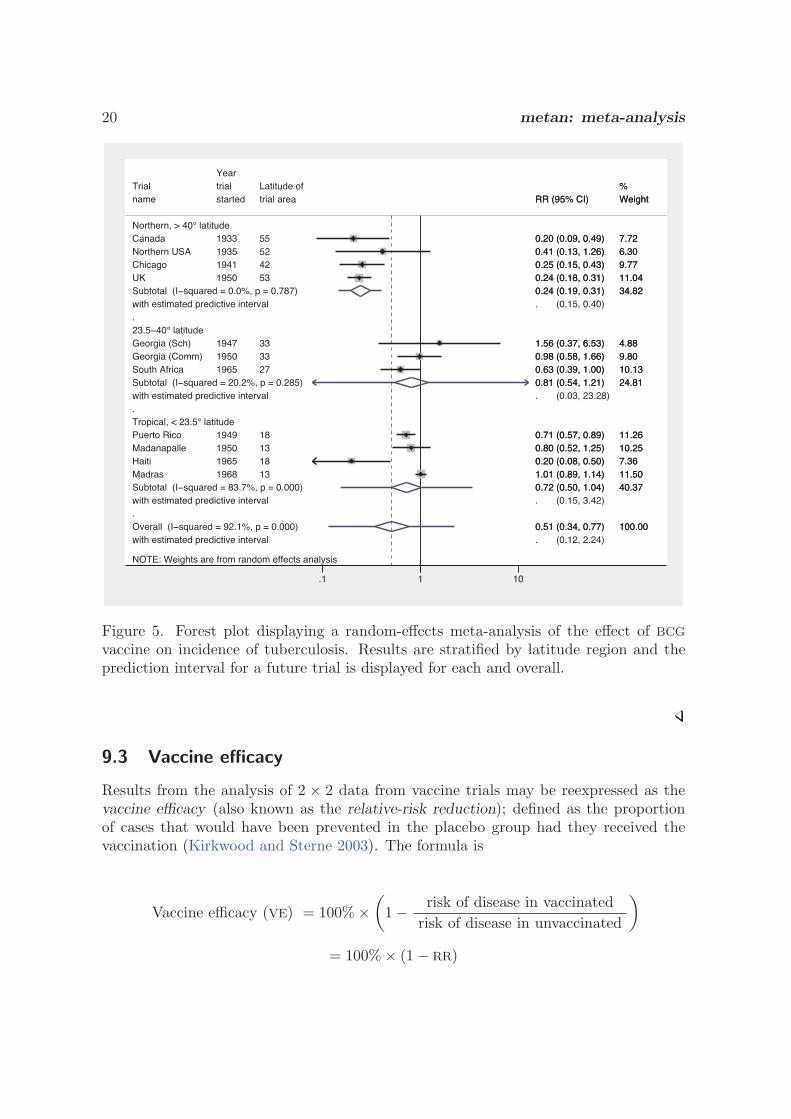
20 metan: meta-analysis
NOTE: Weights are from random effects analysis
. (0.03, 23.28)
. (0.12, 2.24)
. (0.15, 0.40)
. (0.15, 3.42)
with estimated predictive interval
with estimated predictive interval
with estimated predictive interval
with estimated predictive interval
.
.
.
.
.
.
.
Overall (I�squared = 92.1%, p = 0.000)
Subtotal (I�squared = 20.2%, p = 0.285)
Subtotal (I�squared = 83.7%, p = 0.000)
name
UK
23.5�40° latitude
Northern USA
Madanapalle
Tropical, < 23.5° latitude
Madras
Georgia (Sch)
South Africa
Subtotal (I�squared = 0.0%, p = 0.787)
Georgia (Comm)
Chicago
Canada
Haiti
Northern, > 40° latitude
Trial
Puerto Rico
started
1950
1935
1950
1968
1947
19651950
1941
1933
Year
1965
trial
1949
trial area
53
52
13
13
33
2733
42
55
18
Latitude of
18
0.51 (0.34, 0.77)
0.81 (0.54, 1.21)
0.72 (0.50, 1.04)
RR (95% CI)
0.24 (0.18, 0.31)
0.41 (0.13, 1.26)
0.80 (0.52, 1.25)
1.01 (0.89, 1.14)
1.56 (0.37, 6.53)
0.63 (0.39, 1.00)
0.24 (0.19, 0.31)
0.98 (0.58, 1.66)
0.25 (0.15, 0.43)
0.20 (0.09, 0.49)
0.20 (0.08, 0.50)
0.71 (0.57, 0.89)
100.00
24.81
40.37
Weight
11.04
6.30
10.25
11.50
4.88
10.13
34.82
9.80
9.77
7.72
7.36
%
11.26
1.1 10
Figure 5. Forest plot displaying a random-effects meta-analysis of the effect of BCG
vaccine on incidence of tuberculosis. Results are stratified by latitude region and theprediction interval for a future trial is displayed for each and overall.
9.3 Vaccine efficacy
Results from the analysis of 2 × 2 data from vaccine trials may be reexpressed as thevaccine efficacy (also known as the relative-risk reduction); defined as the proportionof cases that would have been prevented in the placebo group had they received thevaccination (Kirkwood and Sterne 2003). The formula is
Vaccine efficacy (VE) = 100% ×(
1 − risk of disease in vaccinatedrisk of disease in unvaccinated
)
= 100% × (1 − RR)
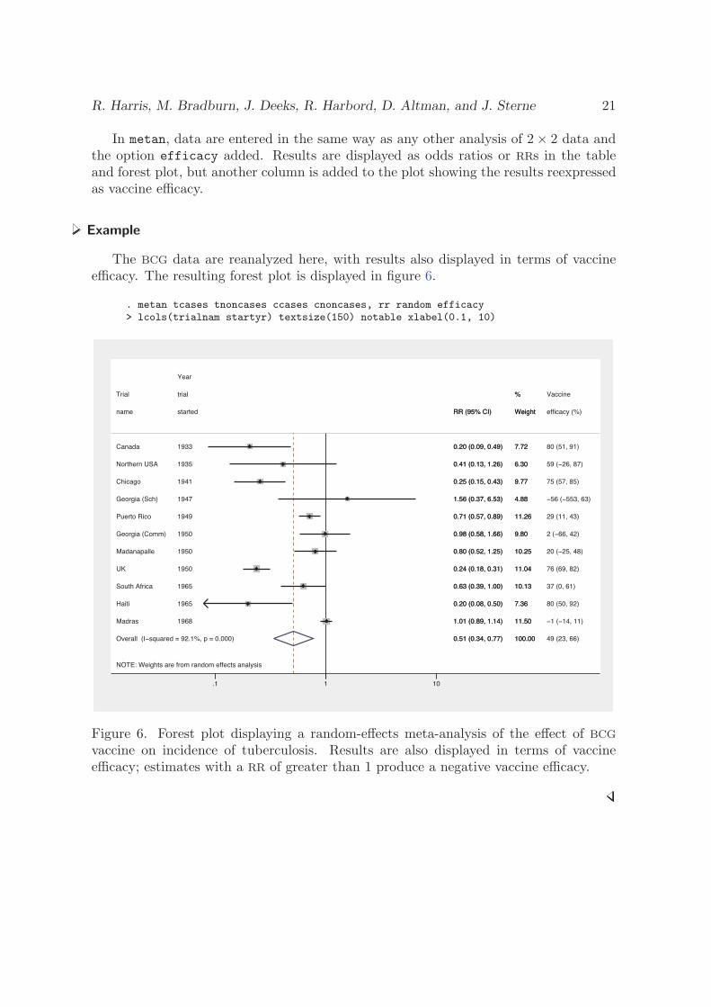
R. Harris, M. Bradburn, J. Deeks, R. Harbord, D. Altman, and J. Sterne 21
In metan, data are entered in the same way as any other analysis of 2 × 2 data andthe option efficacy added. Results are displayed as odds ratios or RRs in the tableand forest plot, but another column is added to the plot showing the results reexpressedas vaccine efficacy.
Example
The BCG data are reanalyzed here, with results also displayed in terms of vaccineefficacy. The resulting forest plot is displayed in figure 6.
. metan tcases tnoncases ccases cnoncases, rr random efficacy> lcols(trialnam startyr) textsize(150) notable xlabel(0.1, 10)
NOTE: Weights are from random effects analysis
Overall (I�squared = 92.1%, p = 0.000)
Trial
South Africa
Madras
Madanapalle
Chicago
Georgia (Comm)
Northern USA
UK
Georgia (Sch)
name
Haiti
Canada
Puerto Rico
trial
Year
1965
1968
1950
1941
1950
1935
1950
1947
started
1965
1933
1949
0.51 (0.34, 0.77)
0.63 (0.39, 1.00)
1.01 (0.89, 1.14)
0.80 (0.52, 1.25)
0.25 (0.15, 0.43)
0.98 (0.58, 1.66)
0.41 (0.13, 1.26)
0.24 (0.18, 0.31)
1.56 (0.37, 6.53)
RR (95% CI)
0.20 (0.08, 0.50)
0.20 (0.09, 0.49)
0.71 (0.57, 0.89)
100.00
%
10.13
11.50
10.25
9.77
9.80
6.30
11.04
4.88
Weight
7.36
7.72
11.26
49 (23, 66)
Vaccine
37 (0, 61)
�1 (�14, 11)
20 (�25, 48)
75 (57, 85)
2 (�66, 42)
59 (�26, 87)
76 (69, 82)
�56 (�553, 63)
efficacy (%)
80 (50, 92)
80 (51, 91)
29 (11, 43)
0.51 (0.34, 0.77)
0.63 (0.39, 1.00)
1.01 (0.89, 1.14)
0.80 (0.52, 1.25)
0.25 (0.15, 0.43)
0.98 (0.58, 1.66)
0.41 (0.13, 1.26)
0.24 (0.18, 0.31)
1.56 (0.37, 6.53)
RR (95% CI)
0.20 (0.08, 0.50)
0.20 (0.09, 0.49)
0.71 (0.57, 0.89)
100.00
%
10.13
11.50
10.25
9.77
9.80
6.30
11.04
4.88
Weight
7.36
7.72
11.26
1.1 10
Figure 6. Forest plot displaying a random-effects meta-analysis of the effect of BCG
vaccine on incidence of tuberculosis. Results are also displayed in terms of vaccineefficacy; estimates with a RR of greater than 1 produce a negative vaccine efficacy.
22 metan: meta-analysis
10 More graph options
10.1 metan graph options
Previous users of metan may find that they do not like the new box style and prefera solid black box without the point estimate marker. The option classic changesback to this style. There are also options available to change the boxes, diamonds,and other lines. This is achieved by using options that change the standard graphcommands that metan uses. For instance, the vertical line representing the overall effectmay be changed using olineopt(), which can take standard Stata line options suchas lwidth(), lcolor(), and lpattern(). Boxes are weighted markers and not muchcan be changed, although shape and color may be modified by using marker optionsin the boxopt() option, such as msymbol() and mcolor(), or we can dispense withthe boxes entirely by using the option nobox. The point estimate markers have moreflexibility and may also be modified by using marker options in the pointopt() option;for instance, labels may by attached to them by using mlabel(). The CIs and diamondsmay be changed by using line options in the options ciopt() and diamopt(). For moredetails, see the metan help file and the Stata Graphics Reference Manual ([G] graph).
Example
Here many aspects of the graph are changed and a raw data variable is defined (asin counts) and attached to the point estimates in the graph. The resulting graph is notshown here, but a similar application is shown in section 10.3.
. gen counts = string(tcases) + "/" + string(tcases+tnoncases) + "," +> string(ccases) + "/" + string(ccases+cnoncases)
. metan tcases tnoncases ccases cnoncases, rr fixedi second(random) nosecsub> notable olineopt(lwidth(thick) lcolor(navy) lpattern(dot))> boxopt(msymbol(triangle) mcolor(dkgreen))> pointopt(mlabel(counts) mlabsize(tiny) mlabposition(5))
10.2 Overall graph options
Any graph options that come under the overall , note, and caption sections of Stata’sgraph twoway command may be added to a metan command, and the x axis (and y axisif required) may have a title added. The options aspect() or xsize() and ysize()may be used to specify different aspect ratios (e.g., portrait). The default aspect ratioof a Stata graph is around 0.7 (height/width), and metan tries to stick to this shape;although graphs that are more naturally displayed as long or wide will be reshaped tosome degree. Use of the above options will control this more precisely.
Finally, the use of schemes is also supported. As colors of boxes and so on aredefined within metan, these will not always give the desired result but may producesome interesting effects. Try, for example, using the scheme economist. More onschemes can be found in [G] schemes intro.

R. Harris, M. Bradburn, J. Deeks, R. Harbord, D. Altman, and J. Sterne 23
10.3 Notes on graph building
It can be useful to declare local or global macros that contain portions of code that arefrequently used. For example, if the forest plot always has triangular “boxes” in forestgreen, contains the same columns of data, and so on, global macros may be declaredfor these bits of code. These can then be reused for a series of meta-analyses to specifythe look and contents of the graphs. These could also be declared in an ado-file so thatthey are ready to use in every Stata session. This idea is similar to using Stata graphschemes.
Example
Macros are defined to control various aspects of the graph and then used in themetan command. The resulting forest plot is displayed in figure 7.
. global metamethod rr fixedi second(random) nosecsub
. global metacolumns lcols(trialnam startyr latitude) astext(60)
. global metastyle boxopt(mcolor(forest_green) msymbol(triangle))> pointopt(msymbol(smtriangle) mcolor(gold) msize(tiny)> mlabel(counts) mlabsize(tiny) mlabposition(2) mlabcolor(brown))> diamopt(lcolor(black) lwidth(medthick)) graphregion(fcolor(gs10)) boxsca(80)
. global metaopts favours(decreases TB # increases TB)> xlabel(0.1, 0.2, 0.5, 2, 5, 10) notable
. metan tcases tnoncases ccases cnoncases,> $metamethod $metacolumns $metastyle $metaopts by(lat_cat) xsize(10) ysize(8)
(Continued on next page)
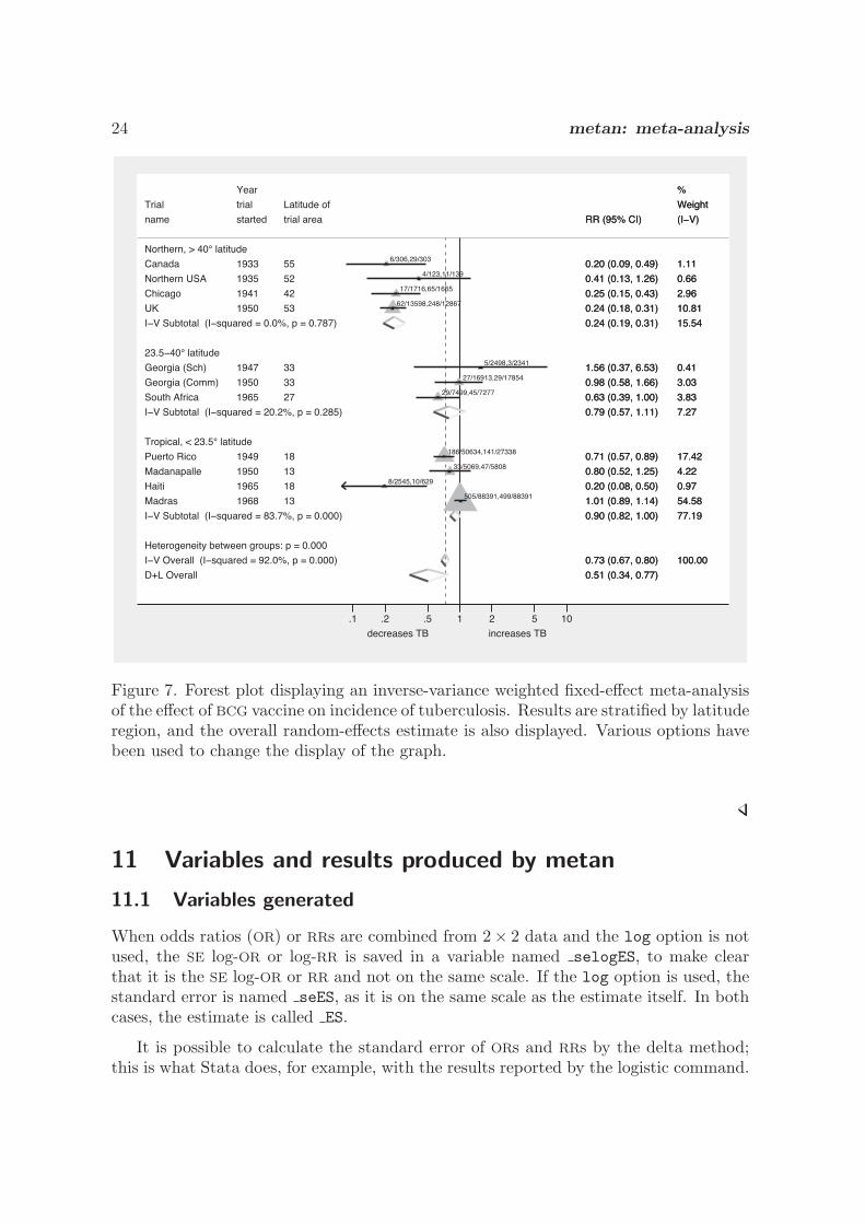
24 metan: meta-analysis
Heterogeneity between groups: p = 0.000
I�V Overall (I�squared = 92.0%, p = 0.000)
Trial
Madras
Northern USA
name
D+L Overall
South Africa
I�V Subtotal (I�squared = 20.2%, p = 0.285)
Georgia (Comm)
Haiti
23.5�40° latitude
I�V Subtotal (I�squared = 0.0%, p = 0.787)
Tropical, < 23.5° latitude
Madanapalle
Georgia (Sch)
I�V Subtotal (I�squared = 83.7%, p = 0.000)
Chicago
Northern, > 40° latitude
Puerto Rico
Canada
UK
trial
1968
1935
started
1965
1950
Year
1965
1950
1947
1941
1949
1933
1950
Latitude of
13
52
trial area
27
33
18
13
33
42
18
55
53
0.73 (0.67, 0.80)
1.01 (0.89, 1.14)
0.41 (0.13, 1.26)
RR (95% CI)
0.51 (0.34, 0.77)
0.63 (0.39, 1.00)
0.79 (0.57, 1.11)
0.98 (0.58, 1.66)
0.20 (0.08, 0.50)
0.24 (0.19, 0.31)
0.80 (0.52, 1.25)
1.56 (0.37, 6.53)
0.90 (0.82, 1.00)
0.25 (0.15, 0.43)
0.71 (0.57, 0.89)
0.20 (0.09, 0.49)
0.24 (0.18, 0.31)
100.00
Weight
54.58
0.66
(I�V)
3.83
7.27
3.03
%
0.97
15.54
4.22
0.41
77.19
2.96
17.42
1.11
10.81
505/88391,499/88391
4/123,11/139
29/7499,45/7277
27/16913,29/17854
8/2545,10/629
33/5069,47/5808
5/2498,3/2341
17/1716,65/1665
186/50634,141/27338
6/306,29/303
62/13598,248/12867
decreases TB increases TB
1.1 .2 .5 2 5 10
Figure 7. Forest plot displaying an inverse-variance weighted fixed-effect meta-analysisof the effect of BCG vaccine on incidence of tuberculosis. Results are stratified by latituderegion, and the overall random-effects estimate is also displayed. Various options havebeen used to change the display of the graph.
11 Variables and results produced by metan
11.1 Variables generated
When odds ratios (OR) or RRs are combined from 2× 2 data and the log option is notused, the SE log-OR or log-RR is saved in a variable named selogES, to make clearthat it is the SE log-OR or RR and not on the same scale. If the log option is used, thestandard error is named seES, as it is on the same scale as the estimate itself. In bothcases, the estimate is called ES.
It is possible to calculate the standard error of ORs and RRs by the delta method;this is what Stata does, for example, with the results reported by the logistic command.
R. Harris, M. Bradburn, J. Deeks, R. Harbord, D. Altman, and J. Sterne 25
However, the distribution of ratios is in general highly skewed, and for this reason,metan does not attempt to record the standard error of either the OR or RR.
Absolute measures (risk differences or mean differences) are symmetric and may beassumed to be normally distributed via the central limit theorem. Here metan storesthese quantities in ES and their standard errors in seES. The derived variables incor-porate the correction for zero cells (see section 8.1).
ES Effect size (ES)seES Standard error of ES
selogES Standard error of log ES
LCI Lower confidence limit for ES
UCI Upper confidence limit for ES
WT Study percentage weightSS Study sample size
11.2 Saved results (macros)
As with many Stata commands, macros are left behind containing the results of theanalysis. If two methods are specified by using the option second(), some of theseare repeated; for example, r(ES) and r(ES 2) give the pooled-effects estimates foreach method. Subgroup statistics when using the by() option are not saved; if theseare required for storage, it is recommended that a program be written that analyzessubgroups separately (perhaps using the nograph and notable options).
(Continued on next page)
26 metan: meta-analysis
Name Second Description
r(ES) r(ES 2) pooled-effect size (if the log option isspecified with or or rr, this is the pooledlog-OR or log-RR)
r(seES) r(seES 2) standard error of pooled-effect size withsymmetrical CI, i.e., meandifferences, risk difference, log-OR, andlog-RR using log option
r(selogES) r(selogES 2) standard error of log-OR or log-RR
when ORs or RRs arecombined without the log option
r(ci low) r(ci low 2) lower CI of pooled-effect sizer(ci upp) r(ci upp 2) upper CI of pooled-effect sizer(z) Z-value of effect sizer(p z) p-value for significance of effect sizer(het) chi-squared test for heterogeneityr(df) degrees of freedom (number
of informative studies minus 1)r(p het) p-value for significance of
test for heterogeneityr(i sq) the I2 statisticr(tau2) estimated between-study variance
(random-effects analyses only)r(chi2) chi-squared test for significance of odds
ratio (fixed-effect OR only)r(p chi2) p-value for the above testr(rger) overall event rate, group 1
(if binary data are combined)r(cger) overall event rate, group 2 (see above)r(measure) effect measure (e.g., RR, SMD)r(method 1) r(method 2) analysis method (e.g., M-H, D+L)
12 ReferencesBradburn, M. J., J. J. Deeks, and D. G. Altman. 1998. sbe24: metan – an alterna-
tive meta-analysis command. Stata Technical Bulletin 44: 4–15. Reprinted in StataTechnical Bulletin Reprints, vol. 8, pp. 86–100. College Station, TX: Stata Press.
Breslow, N. E., and N. E. Day. 1980. Statistical Methods in Cancer Research: Vol-ume I—The Analysis of Case-Control Studies. Lyon, UK: International Agency forResearch on Cancer.
Colditz, G. A., T. F. Brewer, C. S. Berkey, M. E. Wilson, E. Burdick, H. V. Fineberg,and F. Mosteller. 1994. Efficacy of BCG vaccine in the prevention of tuberculosis.
R. Harris, M. Bradburn, J. Deeks, R. Harbord, D. Altman, and J. Sterne 27
Meta-analysis of the published literature. Journal of the American Medical Associa-tion 271: 698–702.
Deeks, J. J., D. G. Altman, and M. J. Bradburn. 2001. Statistical methods for exam-ining heterogeneity and combining results from several studies in meta-analysis. InSystematic Reviews in Health Care: Meta-analysis in context, ed. M. Egger, G. D.Smith, and D. G. Altman, 285–321.
Fine, P. E. 1995. Variation in protection by BCG: implications of and for heterologousimmunity. Lancet 346: 1339–1345.
Harbord, R. M., and J. P. T. Higgins. 2008. Meta-regression in Stata. Stata Journal.Forthcoming.
Higgins, J. P. T., and S. G. Thompson. 2001. Presenting random effects meta-analyses:where are we going wrong? In 9th International Cochrane Colloquium. Lyon, France.
———. 2004. Controlling the risk of spurious findings from meta-regression. Statisticsin Medicine 23: 1663–1682.
Higgins, J. P. T., S. G. Thompson, J. J. Deeks, and D. G. Altman. 2003. Measuringinconsistency in meta-analyses. British Medical Journal 327: 557–560.
Kirkwood, B. R., and J. A. C. Sterne. 2003. Essential Medical Statistics. 2nd ed.Oxford: Blackwell Science.
Lunn, D. J., A. Thomas, N. Best, and D. Spiegelhalter. 2000. WinBUGS – A Bayesianmodelling framework: concepts, structure and extensibility. Statistics and Computing10: 325–337.
Poole, C., and S. Greenland. 1999. Random-effects meta-analyses are not always con-servative. American Journal of Epidemiology 150: 469–475.
Reis, I., K. F. Hirji, and A. Afifi. 1999. Exact and asymptotic tests for homogeneity inseveral 2 × 2 tables. Statistics in Medicine 18: 893–906.
Sharp, S., and J. Sterne. 1997. sbe16: Meta-analysis. Stata Technical Bulletin 38: 9–14.Reprinted in Stata Technical Bulletin Reprints, vol. 7, pp. 100–106. College Station,TX: Stata Press.
Sterne, J. A. C., D. Gavaghan, and M. Egger. 2000. Publication and related bias inmeta-analysis: power of statistical tests and prevalence in the literature. Journal ofClinical Epidemiology 53: 1119–1129.
Sweeting, M. J., A. J. Sutton, and P. C. Lambert. 2004. What to add to nothing? Useand avoidance of continuity corrections in meta-analysis of rare events. Statistics inMedicine 23: 1351–1375.
Warn, D. E., S. G. Thompson, and D. J. Spiegelhalter. 2002. Bayesian random effectsmeta-analysis of trials with binary outcomes: methods for absolute risk difference andrelative risk scales. Statistics in Medicine 21: 1601–1623.
28 metan: meta-analysis
About the authors
Ross Harris is a research associate in medical statistics at the Department of Social Medicine,University of Bristol, Bristol, UK. His research interests include meta-analysis, particularlysummarizing dose–response relationships from published data and examining sources of biasin randomized trials; epidemiology of HIV and AIDS and methods for dealing with missingdata.
Michael Bradburn is a medical statistician in the Health Services Research Unit, Universityof Sheffield, Sheffield, UK, and wrote most of the original metan code. His current research isfocused on randomized trials.
Jonathan Deeks is professor of health statistics at the University of Birmingham, Birmingham,UK, and head of the Medical Statistics Group and Diagnostic Evaluation Support Unit in theDepartment of Public Health. His work has focused on issues related to meta-analysis and morerecently diagnostic test evaluations, including both clinical applications and methodologicaldevelopments. Currently, Jon Deeks is the elected representative for Methods Groups on theSteering Group of the Cochrane Collaboration and is leading the implementation of Reviewsof Diagnostic Test Accuracy in the Cochrane Collaboration.
Roger Harbord is a research associate in medical statistics in the Department of Social Medicine,University of Bristol, Bristol, UK. He is a coconvenor of the Cochrane Collaborations Screeningand Diagnostic Tests Methods Group.
Douglas Altman is professor of statistics in medicine at the University of Oxford, Oxford, UK,and founding director of the Centre for Statistics in Medicine. His research interests includethe use and abuse of statistics in medical research, studies of prognosis, regression modeling,systematic reviews and meta-analysis, randomized trials, reporting guidelines, and studies ofmedical measurement.
Jonathan Sterne is professor of medical statistics and epidemiology in the Department of SocialMedicine, University of Bristol, Bristol, UK. His research interests include statistical methodsfor epidemiology and health services research, meta-analysis and systematic reviews, clinicalepidemiology of HIV and AIDS in the era of antiretroviral therapy, and the epidemiology ofasthma and allergic diseases.

Stata Technical Bulletin 13
sbe22 Cumulative meta-analysis
Jonathan Sterne, United Medical and Dental Schools, UK, [email protected]
Meta-analysis is used to combine the results of several studies, and the Stata command meta (Sharp and Sterne 1997 andsbe16.1 in this issue) can be used to perform meta-analyses and graph the results. In cumulative meta-analysis (Lau et al. 1992),the pooled estimate of the treatment effect is updated each time the results of a new study are published. This makes it possibleto track the accumulation of evidence on the effect of a particular treatment.
The command metacum performs cumulative meta-analysis (using fixed- or random-effects models) and, optionally, graphsthe results.
Syntax
metacum�
theta j exp(theta)� �
se theta j var theta j ll ul�cl�� �
if exp� �
in range�
�� var ci effect�fjr� eform level�#� id�strvar� graph
cline fmult�#� csize�#� ltrunc�#� rtrunc�#� graph options�
In common with the commands meta (Sharp and Sterne 1998) and metabias (Steichen 1988), the user provides the effectestimate as theta (i.e., a log risk ratio, log odds ratio, or other measure of effect). Likewise, the user supplies a measure oftheta’s variability (i.e., its standard error, se theta, or its variance, var theta). Alternatively, the user provides exp(theta) (e.g. arisk ratio or odds ratio) and its confidence interval, (ll, ul).
Required input variables
These are the same as for the new version of meta described in sbe16.1 in this issue.
Options for displaying results
var means the user has specified a variable containing the variance of the effect estimate. If this option is not included, thecommand assumes the standard error has been specified.
ci means the user has specified the lower and upper confidence limits of the effect estimate, which is assumed to be on theratio scale (e.g. odds ratio or risk ratio).
effect�f jr� must be included. This specifies whether fixed (f ) or random (r) effects estimates are to be used in the output andgraph.
eform requests that the output be exponentiated. This is useful for effect measures such as log odds ratios which are derivedfrom generalized linear models. If the eform and graph options are used, then the graph output is exponentiated, with alog scale for the x-axis.
level�#� specifies the confidence level, in percent, for confidence intervals. The default is level���� or as set by set level.
id�strvar� is a character variable which is used to label the studies. If the data contains a labeled numeric variable, then thedecode command can be used to create a character variable.
Options for graphing results
graph requests a graph.
cline asks that a vertical dotted line be drawn through the combined estimate.
fmult�#� is a number greater than zero which can be used to scale the font size for the study labels. The font size is automaticallyreduced if the maximum label length is greater than 8, or the number of studies is greater than 20. However it may bepossible to increase it somewhat over the default size.
csize�#� gives the size of the circles used in the graph (default 180).
ltrunc�#� truncates the left side of the graph at the number #. This is used to truncate very wide confidence intervals. However# must be less than each of the individual study estimates.
rtrunc�#� truncates the right side of the graph at #, and must be greater than each of the individual study estimates.
graph options are any options allowed with graph, twoway other than ylabel��, symbol��, xlog, ytick, and gap.
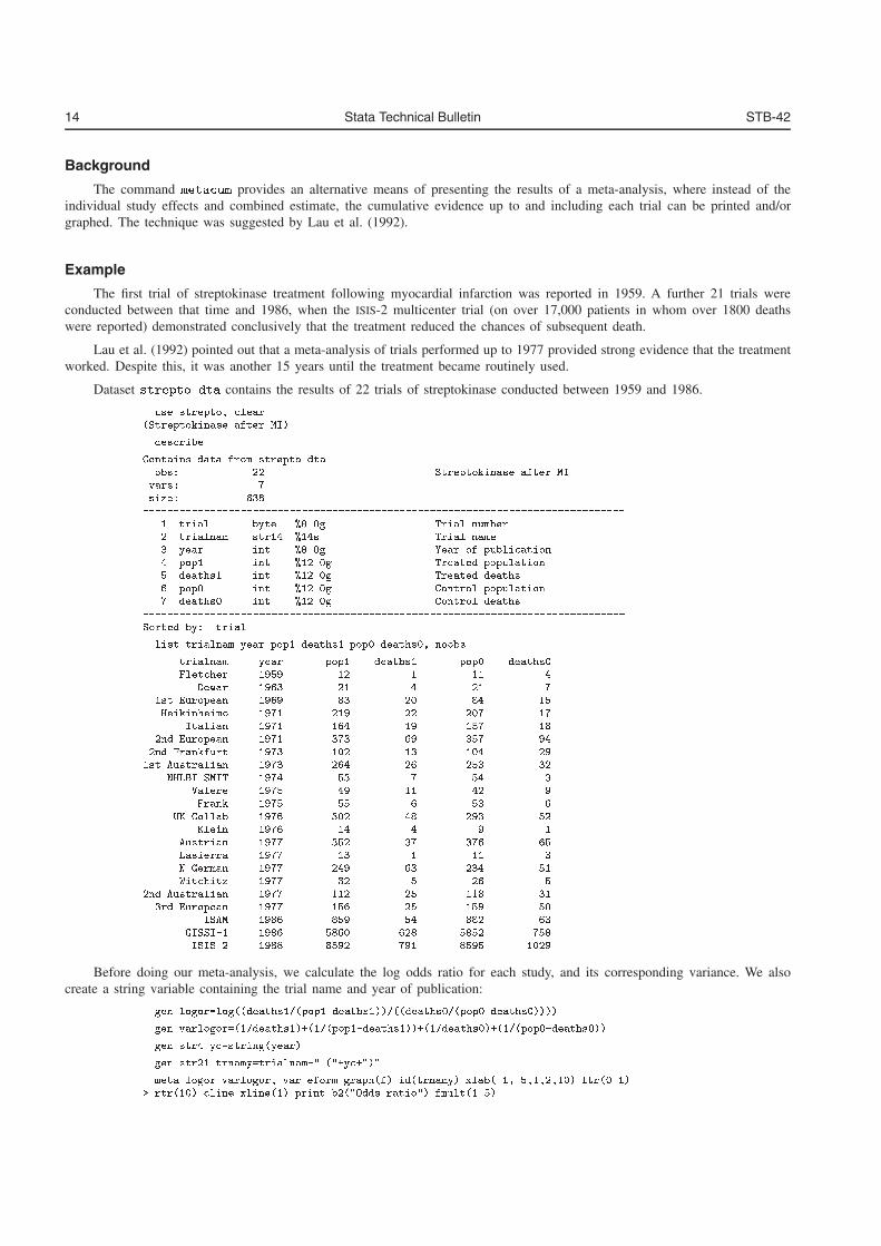
14 Stata Technical Bulletin STB-42
Background
The command metacum provides an alternative means of presenting the results of a meta-analysis, where instead of theindividual study effects and combined estimate, the cumulative evidence up to and including each trial can be printed and/orgraphed. The technique was suggested by Lau et al. (1992).
Example
The first trial of streptokinase treatment following myocardial infarction was reported in 1959. A further 21 trials wereconducted between that time and 1986, when the ISIS-2 multicenter trial (on over 17,000 patients in whom over 1800 deathswere reported) demonstrated conclusively that the treatment reduced the chances of subsequent death.
Lau et al. (1992) pointed out that a meta-analysis of trials performed up to 1977 provided strong evidence that the treatmentworked. Despite this, it was another 15 years until the treatment became routinely used.
Dataset strepto�dta contains the results of 22 trials of streptokinase conducted between 1959 and 1986.
� use strepto� clear�Streptokinase after MI�
� describe
Contains data from strepto�dtaobs� �� Streptokinase after MIvars� �size� �
��������������������������������������������������������������������������������� trial byte ��g Trial number�� trialnam str�� ��s Trial name� year int ��g Year of publication�� pop� int ����g Treated population�� deaths� int ����g Treated deaths�� pop� int ����g Control population�� deaths� int ����g Control deaths
�������������������������������������������������������������������������������Sorted by� trial
� list trialnam year pop� deaths� pop� deaths�� noobs
trialnam year pop� deaths� pop� deaths�Fletcher ���� �� � �� �
Dewar ��� �� � �� ��st European ���� �� � ��Heikinheimo ���� ��� �� ��� ��
Italian ���� ��� �� ��� ��nd European ���� � �� �� ���nd Frankfurt ��� ��� � ��� ��
�st Australian ��� ��� �� �� �NHLBI SMIT ���� � � ��
Valere ���� �� �� �� �Frank ���� �� � � �
UK Collab ���� �� � �� ��Klein ���� �� � � �
Austrian ���� �� � �� ��Lasierra ���� � � �� N German ���� ��� � �� ��Witchitz ���� � � �� �
�nd Australian ���� ��� �� �� �rd European ���� ��� �� ��� ��
ISAM ��� �� �� � �GISSI�� ��� ��� �� ��� ��ISIS�� �� ��� ��� ��� ����
Before doing our meta-analysis, we calculate the log odds ratio for each study, and its corresponding variance. We alsocreate a string variable containing the trial name and year of publication:
� gen logor�log��deaths���pop��deaths������deaths���pop��deaths�����
� gen varlogor����deaths�������pop��deaths�������deaths�������pop��deaths���
� gen str� yc�string�year�
� gen str�� trnamy�trialnam�� ���yc����
� meta logor varlogor� var eform graph�f� id�trnamy� xlab�������������� ltr������ rtr���� cline xline��� print b���Odds ratio�� fmult�����
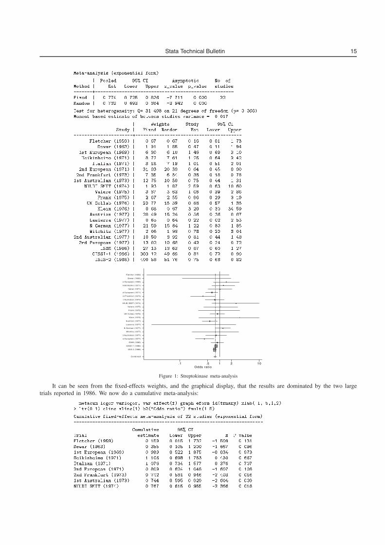
Stata Technical Bulletin 15
Meta�analysis �exponential form�
� Pooled ��� CI Asymptotic No ofMethod � Est Lower Upper zvalue pvalue studies������������������������������������������������������������Fixed � � � � �� ���� � �� ���� ��Random � � �� ���� ���� ����� ����
Test for heterogeneity� Q� ����� on �� degrees of freedom �p� �����Moment�based estimate of between studies variance � ���
� Weights Study ��� CIStudy � Fixed Random Est Lower Upper
���������������������������������������������������������������Fletcher ������ � �� �� ��� ��� � �
Dewar ������ � ��� ��� �� ��� ����st European ������ � ��� ��� ��� ��� ���Heikinheimo ��� �� � � � �� ��� ��� ���
Italian ��� �� � ��� �� ��� ��� ����nd European ��� �� � ���� ���� ��� ��� ����nd Frankfurt ��� �� � �� ��� ��� ��� � �
�st Australian ��� �� � �� � ���� � � ��� ���NHLBI SMIT ��� �� � ��� �� ��� ��� ����
Valere ��� �� � �� ��� ��� ��� ���Frank ��� �� � �� ��� ��� ��� ���
UK Collab ��� �� � �� ���� ��� �� ���Klein ��� �� � ��� �� ��� ��� ����
Austrian ��� � � ���� ���� ��� ��� �� Lasierra ��� � � ��� ��� ��� ��� ���N German ��� � � ���� ���� ��� ��� ���Witchitz ��� � � ��� ��� � � ��� ���
�nd Australian ��� � � ���� ��� ��� ��� ����rd European ��� � � ���� ���� ��� ��� � �
ISAM ������ � � �� ���� �� ��� �� GISSI�� ������ � ����� ���� ��� � � ���ISIS�� ������ � ����� �� � � � ��� ���
Odds rat io.1 .5 1 2 10
Combined
ISIS-2 (1988)
GISSI-1 (1986)
ISAM (1986)
d European (1977)
d Austral ian (1977)
Witchitz (1977)
N German (1977)
Lasierra (1977)
Austr ian (1977)
Klein (1976)
UK Col lab (1976)
Frank (1975)
Valere (1975)
NHLBI SMIT (1974)
st Austral ian (1973)
nd Frankfurt (1973)
d European (1971)
Italian (1971)
Heikinheimo (1971)
st European (1969)
Dewar (1963)
Fletcher (1959)
Figure 1: Streptokinase meta-analysis
It can be seen from the fixed-effects weights, and the graphical display, that the results are dominated by the two largetrials reported in 1986. We now do a cumulative meta-analysis:
metacum logor varlogor� var effect�f� graph eform id�trnamy� xlab���������� ltr���� cline xline��� b���Odds ratio�� fmult����
Cumulative fixed�effects meta�analysis of �� studies �exponential form������������������������������������������������������������������������
Cumulative ��� CITrial estimate Lower Upper z P valueFletcher ������ ���� ���� � �� ����� ����Dewar ������ ���� ���� ���� ���� �����st European ������ ���� ���� �� � ����� �� �Heikinheimo ��� �� ���� ���� � �� ���� ��� Italian ��� �� �� � � �� �� �� � � � �nd European ��� �� ���� ���� ���� ���� �����nd Frankfurt ��� �� � �� ���� ���� ����� �����st Australian ��� �� � �� ���� ���� ����� ����NHLBI SMIT ��� �� � � ���� ���� ����� ����
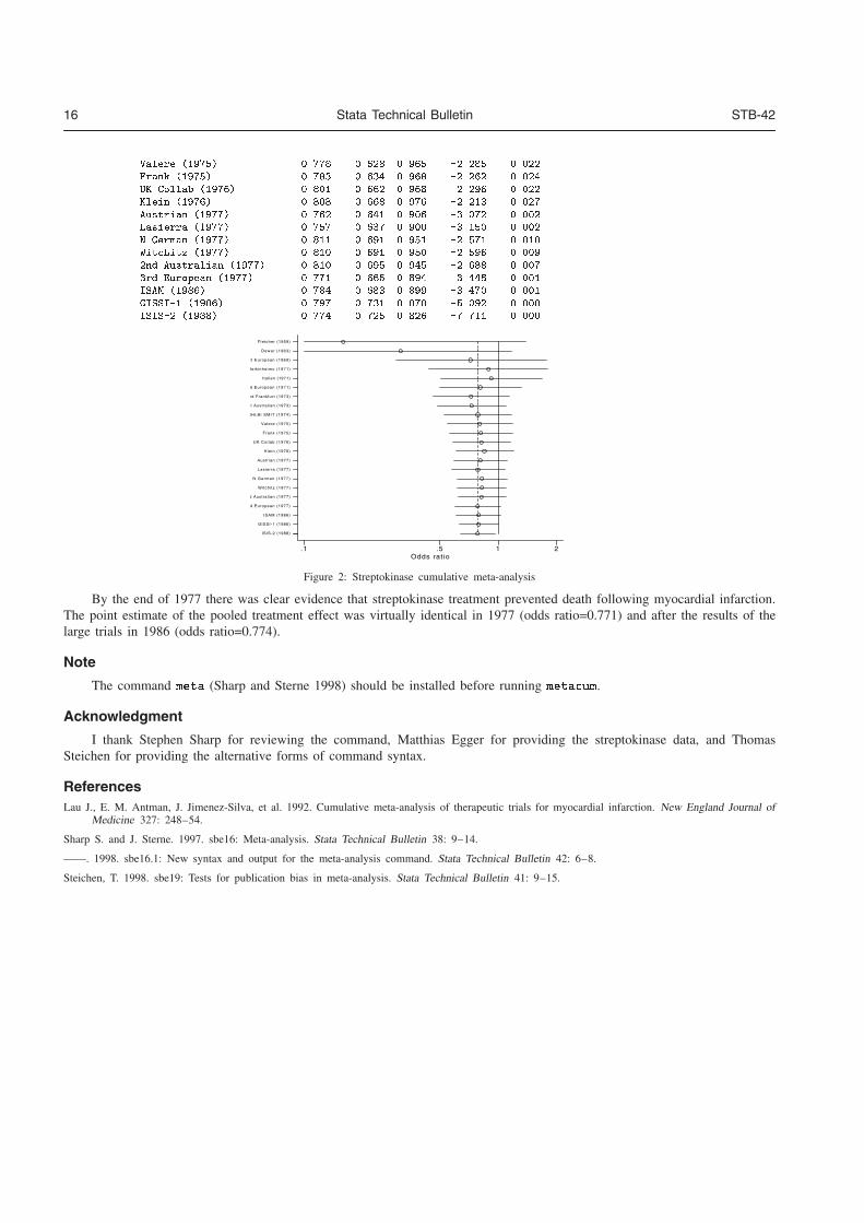
16 Stata Technical Bulletin STB-42
Valere ������ ��� ��� ���� ��� ����Frank ������ ��� ���� ��� ���� ����UK Collab ������ ��� ���� ��� ���� ����Klein ������ �� ��� ���� ���� ����Austrian ������ ���� ���� ���� ���� ����Lasierra ������ ���� ���� ���� ���� ����N German ������ ��� ���� ���� ���� ����Witchitz ������ ��� ���� ���� ���� �����nd Australian ������ ��� ���� ���� �� �����rd European ������ ���� ���� ��� ��� ����ISAM ����� ��� ��� ��� ���� ����GISSI � ����� ���� ���� ��� ���� ����ISIS � ���� ���� ���� ��� ���� ����
Odds rat io.1 .5 1 2
ISIS-2 (1988)
GISSI-1 (1986)
ISAM (1986)
d European (1977)
d Austral ian (1977)
Witchitz (1977)
N German (1977)
Lasierra (1977)
Austr ian (1977)
Klein (1976)
UK Col lab (1976)
Frank (1975)
Valere (1975)
NHLBI SMIT (1974)
st Austral ian (1973)
nd Frankfurt (1973)
d European (1971)
Italian (1971)
Heikinheimo (1971)
st European (1969)
Dewar (1963)
Fletcher (1959)
Figure 2: Streptokinase cumulative meta-analysis
By the end of 1977 there was clear evidence that streptokinase treatment prevented death following myocardial infarction.The point estimate of the pooled treatment effect was virtually identical in 1977 (odds ratio=0.771) and after the results of thelarge trials in 1986 (odds ratio=0.774).
Note
The command meta (Sharp and Sterne 1998) should be installed before running metacum.
Acknowledgment
I thank Stephen Sharp for reviewing the command, Matthias Egger for providing the streptokinase data, and ThomasSteichen for providing the alternative forms of command syntax.
ReferencesLau J., E. M. Antman, J. Jimenez-Silva, et al. 1992. Cumulative meta-analysis of therapeutic trials for myocardial infarction. New England Journal of
Medicine 327: 248–54.
Sharp S. and J. Sterne. 1997. sbe16: Meta-analysis. Stata Technical Bulletin 38: 9–14.
——. 1998. sbe16.1: New syntax and output for the meta-analysis command. Stata Technical Bulletin 42: 6–8.
Steichen, T. 1998. sbe19: Tests for publication bias in meta-analysis. Stata Technical Bulletin 41: 9–15.
sbe23 Meta-analysis regression
Stephen Sharp, London School of Hygiene and Tropical Medicine, [email protected]
The command metareg extends a random effects meta-analysis to estimate the extent to which one or more covariates,with values defined for each study in the analysis, explain heterogeneity in the treatment effects. Such analysis is sometimestermed “meta-regression” (Lau et al. 1998). Examples of such study-level covariates might be average duration of follow-up,some measure of study quality, or, as described in this article, a measure of the geographical location of each study. metaregfits models with two additive components of variance, one representing the variance within units, the other the variance betweenunits, and therefore is applicable both to the meta-analysis situation, where each unit is one study, and to other situations suchas multi-center trials, where each unit is one center. Here metareg is explained in the meta-analysis context.
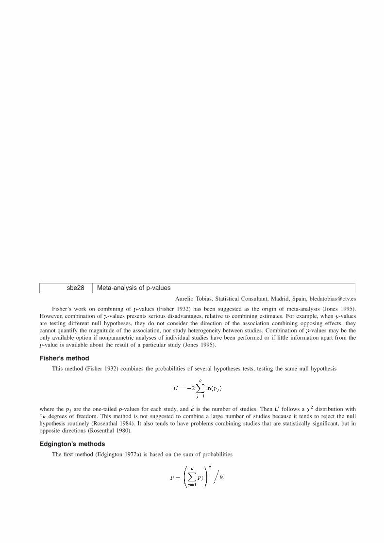
Stata Technical Bulletin 15
Potential confounders were removed one at a t ime sequential ly
Ra
te R
ati
o a
nd
95
% C
I
*CrudeAdj. all -i.sex -i.hyper -weight - i .smoke -age*
0
2
4
6
Figure 2. The result of using backward deletion.
With a backward deletion method, the rate ratio adjusted for all variables (Adj� all) is presented first. Then, epiconf deletesthe nominal variable sex first because deleting it makes the least change-in-estimate (0.9%). The most important confounder(age) in terms of change in estimate is the last covariate to be deleted. If we take 10% as a cut-point of importance, we needadjust for age and smoking. The adjusted rate ratio is 1.78 with 95% confidence interval (1.08, 2.93), while if we take 20% as acut-point of importance, we need only adjust for age. The adjusted rate ratio is 1.98 with a 95% confidence interval (1.21, 3.23).
Acknowledgment
I thank Nicholas Cox for providing a subroutine vallist and Jean Bouyer for useful suggestions.
ReferencesMaldonado, G. and S. Greenland. 1993. Simulation study of confounder-selection strategies. American Journal of Epidemiology 138: 923–936.
Rothman, K. J. and S. Greenland. 1998. Modern Epidemiology. Philadelphia: Lippincott–Raven.
sbe28 Meta-analysis of p-values
Aurelio Tobias, Statistical Consultant, Madrid, Spain, [email protected]
Fisher’s work on combining of p-values (Fisher 1932) has been suggested as the origin of meta-analysis (Jones 1995).However, combination of p-values presents serious disadvantages, relative to combining estimates. For example, when p-valuesare testing different null hypotheses, they do not consider the direction of the association combining opposing effects, theycannot quantify the magnitude of the association, nor study heterogeneity between studies. Combination of p-values may be theonly available option if nonparametric analyses of individual studies have been performed or if little information apart from thep-value is available about the result of a particular study (Jones 1995).
Fisher’s method
This method (Fisher 1932) combines the probabilities of several hypotheses tests, testing the same null hypothesis
U � �2kXj��
ln�pj�
where the pj are the one-tailed p-values for each study, and k is the number of studies. Then U follows a �� distribution with�k degrees of freedom. This method is not suggested to combine a large number of studies because it tends to reject the nullhypothesis routinely (Rosenthal 1984). It also tends to have problems combining studies that are statistically significant, but inopposite directions (Rosenthal 1980).
Edgington’s methods
The first method (Edgington 1972a) is based on the sum of probabilities
p �
�� KXj��
pj
�Ak�
k�

16 Stata Technical Bulletin STB-49
The results obtained are similar to Fisher’s method, but it is also restricted for a small number of studies. This method presentsproblems when the sum of probabilities is higher than one; in this situation the combined probability tends to be conservative(Rosenthal 1980).
An alternative method was also suggested by Edgington (1972b), to combine more than four studies, based on the contrastof the p-value average
p �kX
j��
pj
�k
in which case U � �0.5� p�p
12 follows a normal distribution.
Syntax
The command metap works on a dataset containing the p-values for each study. The syntax is as follows:
metap pvar�if exp
� �in range
� �� e�#�
�
Options
e�#� combines the p-values using Edgington’s methods. Here, two alternatives are available; specifying a means that the additivemethod based on the sum of probabilities is used, while n specifies that the normal curve method based on the contrast ofthe p-value average is used. By default, Fisher’s method is used.
Example
We consider data from seven placebo-controlled studies on the effect of aspirin in preventing death after myocardialinfarction. Fleiss (1993) published an overview of these data. Let us assume that each study included in the meta-analysis istesting the same null hypothesis H� � � � � versus the alternative H� � � � �. If the estimate of the log odds ratio and itsstandard error is available, then one-tailed p-values can easily be generated using the normprob function:
� generate pvar�normprob��logrr�logse�� list studyid logrr logse pvar� noobsstudyid logrr logse pvarMCR�� ��� �� �� �������CDP ��� ��� �������
MRC�� ��� � ���� ��� ���GASP ���� ����� �� �� PARIS ����� ����� �������AMIS ����� � �� �� �����
ISIS�� ����� ��� �����
In this situation, all methods to combine p-values produce similar results:
� metap pvar
Meta�analysis of p�values������������������������������������������������������������Method � chi� p�value studies
������������������������������������������������������������Fisher � �� ��� ���� �
������������������������������������������������������������
� metap pvar� e�a�
Meta�analysis of p�values������������������������������������������������������������Method � � p�value studies
������������������������������������������������������������Edgington� additive� � ������� �
������������������������������������������������������������
� metap pvar� e�n�
Meta�analysis of p�values������������������������������������������������������������Method � Z p�value studies������������������������������������������������������������Edgington� Normal � �������� ����� �������������������������������������������������������������
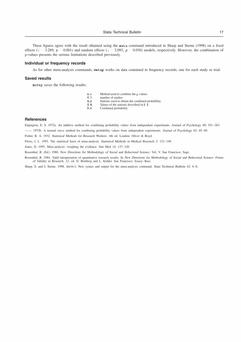
Stata Technical Bulletin 17
These figures agree with the result obtained using the meta command introduced in Sharp and Sterne (1998) on a fixedeffects (z � 3.289, p � 0.001) and random effects (z � 2.093, p � 0.036) models, respectively. However, the combination ofp-values presents the serious limitations described previously.
Individual or frequency records
As for other meta-analysis commands, metap works on data contained in frequency records, one for each study or trial.
Saved results
metap saves the following results:
S � Method used to combine the p-valuesS � number of studiesS � Statistic used to obtain the combined probabilityS � Values of the statistic described in S �
S � Combined probability
ReferencesEdgington, E. S. 1972a. An additive method for combining probability values from independent experiments. Journal of Psychology 80: 351–363.
——. 1972b. A normal curve method for combining probability values from independent experiments. Journal of Psychology 82: 85–89.
Fisher, R. A. 1932. Statistical Methods for Research Workers. 4th ed. London: Oliver & Boyd.
Fleiss, J. L. 1993. The statistical basis of meta-analysis. Statistical Methods in Medical Research 2: 121–149.
Jones, D. 1995. Meta-analysis: weighing the evidence. Stat Med 14: 137–149.
Rosenthal, R. (Ed.) 1980. New Directions for Methodology of Social and Behavioral Science. Vol. V. San Francisco: Sage.
Rosenthal, R. 1984. Valid interpretation of quantitative research results. In New Directions for Methodology of Social and Behavioral Science: Formsof Validity in Research, 12 , ed. D. Brinberg and L. Kidder. San Francisco: Jossey–Bass.
Sharp, S. and J. Sterne. 1998. sbe16.1: New syntax and output for the meta-analysis command. Stata Technical Bulletin 42: 6–8.
sg64.1 Update to pwcorrs
Fred Wolfe, Arthritis Research Center, Wichita, KS, [email protected]
This update corrects a problem in pwcorrs, see Wolfe (1997). When the option vars�� was not specified and bonferroni
or sidak was specified, the program reported p-values of 0.0000 instead of the correct values.
ReferenceWolfe, F. 1997. sg64: pwcorrs: An enhanced correlation display. Stata Technical Bulletin 35: 22–25. Reprinted in Stata Technical Bulletin Reprints,
vol. 6, pp. 163–167.
sg81.1 Multivariable fractional polynomials: update
Patrick Royston, Imperial College School of Medicine, UK, [email protected] Ambler, Imperial College School of Medicine, UK, [email protected]
Introduction
Multivariable fractional polynomials (FPs) were introduced by Royston & Altman (1994) and implemented in a commandmfracpol for Stata 5 by Royston and Ambler (1998). The model selection procedure in the Stata 5 version was essentiallythe backward elimination algorithm described by Royston and Altman (1994) with modifications described by Sauerbrei andRoyston (1999) (see the technical note below). An application of multivariable FPs in modeling prognostic and diagnostic factorsin breast cancer is given by Sauerbrei and Royston (1999) (see our example below).
Briefly, fractional polynomial models are especially useful when one wishes to preserve the continuous nature of the predictorvariables in a regression model, but suspects that some or all the relationships may be nonlinear. Using a backfitting algorithm,mfracpol finds a fractional polynomial transformation for each continuous predictor, fixing the current functional forms of theother predictor variables. The algorithm terminates when the functional forms of the predictors do not change.
Commands stfracp and stmfracp implementing respectively univariate and multivariable FPs for the survival (st) dataformat were presented by Royston (1998).
2 Meta-regression: metareg
The Stata Journal (2008)8, Number 4, pp. 493–519
Meta-regression in Stata
Roger M. HarbordDepartment of Social Medicine
University of Bristol, UK
Julian P. T. HigginsMRC Biostatistics Unit
Cambridge, UK
Abstract. We present a revised version of the metareg command, which performsmeta-analysis regression (meta-regression) on study-level summary data. The ma-jor revisions involve improvements to the estimation methods and the addition ofan option to use a permutation test to estimate p-values, including an adjustmentfor multiple testing. We have also made additions to the output, added an optionto produce a graph, and included support for the predict command. Stata 8.0 orabove is required.
Keywords: sbe23 1, metareg, meta-regression, meta-analysis, permutation test,multiple testing
1 Introduction
Meta-analysis regression, or meta-regression, is an extension to standard meta-analysisthat investigates the extent to which statistical heterogeneity between results of multiplestudies can be related to one or more characteristics of the studies (Thompson andHiggins 2002). Like meta-analysis, meta-regression is usually conducted on study-levelsummary data, because individual observations from all studies (often referred to asindividual patient data in medical applications) are frequently not available.
Sharp (1998) introduced the metareg command to perform meta-regression on study-level summary data. In this article, we present a substantially updated and largelyrewritten version of metareg. The planning and interpretation of meta-regression stud-ies raises substantial statistical issues discussed at length elsewhere (Davey Smith, Eg-ger, and Phillips 1997; Higgins et al. 2002; Thompson and Higgins 2002, 2005). In thisarticle, we will concentrate on the rationale for and the implementation and interpreta-tion of the following new features of metareg:
• An improved algorithm for the estimation of the between-study variance, τ2, byresidual (restricted) maximum likelihood (REML)
• A modification to the calculation of standard errors, p-values, and confidenceintervals for coefficients suggested by Knapp and Hartung (2003)
• Various enhancements to the output
• An option to produce a graph of the fitted model with a single covariate
c© 2008 StataCorp LP sbe23 1
494 Meta-regression in Stata
• An option to calculate permutation-based p-values, including an adjustment formultiple testing based on the work of Higgins and Thompson (2004)
• Support for many of Stata’s postestimation commands, including predict
We begin with a brief outline in section 2 of the statistical basis of meta-analysisand meta-regression, and we continue with a summary in section 3 of the relationship ofmetareg to other Stata commands. Section 4 introduces two example datasets that weuse to illustrate the discussion of new features in section 5, which constitutes the mainbody of the article and has subsections corresponding to each of the new features listedabove. The final two sections are reference material: Section 6 gives the Stata syntaxand full list of options for metareg and predict after metareg, and lists the resultssaved by the command. Finally, section 7 gives details of the methods and formulasused.
2 Basis of meta-regression
In this section, we outline the statistical basis of random- and fixed-effects meta-regression and their relation to random- and fixed-effects meta-analysis. We will usemathematical formulas for brevity and precision. Less mathematically inclined read-ers or those who are already familiar with the principles of meta-analysis and meta-regression can skip this section.
We assume that study i of a total of n studies provides an estimate, yi, of the effectof interest, such as a log odds-ratio, log risk-ratio, or difference in means. Each studyalso provides a standard error for this estimate, σi, which we assume is known, as iscommon in meta-analysis (although in practice, it will have been estimated from thedata in that study). Let us start from the simplest model:
• Fixed-effects meta-analysis assumes that there is a single true effect size, θ, sothat
yi ∼ N(θ, σ2i )
or equivalently,yi = θ + εi, where εi ∼ N(0, σ2
i )
• Random-effects meta-analysis allows the true effects, θi, to vary between studiesby assuming that they have a normal distribution around a mean effect, θ:
yi | θi ∼ N(θi, σ2i ), where θi ∼ N(θ, τ2)
Soyi ∼ N(θ, σ2
i + τ2)
or equivalently,
yi = θ + ui + εi, where ui ∼ N(0, τ2) and εi ∼ N(0, σ2i )
Here τ2 is the between-study variance and must be estimated from the data.
R. M. Harbord and J. P. T. Higgins 495
• Fixed-effects meta-regression extends fixed-effects meta-analysis by replacing themean, θ, with a linear predictor, xiβ:
yi ∼ N(θi, σ2i ), where θi = xiβ
or equivalently,yi = xiβ + εi, where εi ∼ N(0, σ2
i )
Here β is a k × 1 vector of coefficients (including a constant if fitted), and xi is a1 × k vector of covariate values in study i (including a 1 if a constant is fit).
• Random-effects meta-regression allows for such residual heterogeneity (between-study variance not explained by the covariates) by assuming that the true effectsfollow a normal distribution around the linear predictor:
yi | θi ∼ N(θi, σ2i ), where θi ∼ N(xiβ, τ2)
soyi ∼ N(xiβ, σ2
i + τ2)
or equivalently,
yi = xiβ + ui + εi, where ui ∼ N(0, τ2) and εi ∼ N(0, σ2i )
Random-effects meta-regression can be considered either an extension to fixed-effects meta-regression that allows for residual heterogeneity or an extension torandom-effects meta-analysis that includes study-level covariates.
Table 1 summarizes the relationships between these models and gives the correspondingStata commands, which are summarized in the next section.
(Continued on next page)
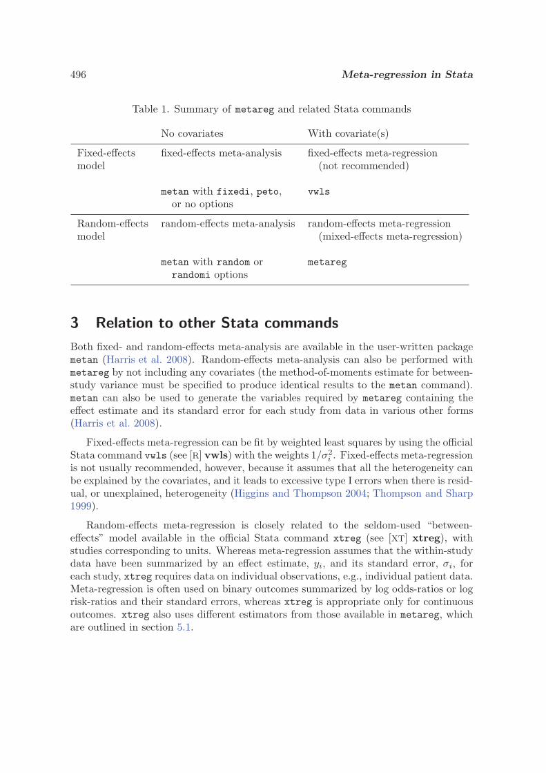
496 Meta-regression in Stata
Table 1. Summary of metareg and related Stata commands
No covariates With covariate(s)
Fixed-effects fixed-effects meta-analysis fixed-effects meta-regressionmodel (not recommended)
metan with fixedi, peto, vwlsor no options
Random-effects random-effects meta-analysis random-effects meta-regressionmodel (mixed-effects meta-regression)
metan with random or metaregrandomi options
3 Relation to other Stata commands
Both fixed- and random-effects meta-analysis are available in the user-written packagemetan (Harris et al. 2008). Random-effects meta-analysis can also be performed withmetareg by not including any covariates (the method-of-moments estimate for between-study variance must be specified to produce identical results to the metan command).metan can also be used to generate the variables required by metareg containing theeffect estimate and its standard error for each study from data in various other forms(Harris et al. 2008).
Fixed-effects meta-regression can be fit by weighted least squares by using the officialStata command vwls (see [R] vwls) with the weights 1/σ2
i . Fixed-effects meta-regressionis not usually recommended, however, because it assumes that all the heterogeneity canbe explained by the covariates, and it leads to excessive type I errors when there is resid-ual, or unexplained, heterogeneity (Higgins and Thompson 2004; Thompson and Sharp1999).
Random-effects meta-regression is closely related to the seldom-used “between-effects” model available in the official Stata command xtreg (see [XT] xtreg), withstudies corresponding to units. Whereas meta-regression assumes that the within-studydata have been summarized by an effect estimate, yi, and its standard error, σi, foreach study, xtreg requires data on individual observations, e.g., individual patient data.Meta-regression is often used on binary outcomes summarized by log odds-ratios or logrisk-ratios and their standard errors, whereas xtreg is appropriate only for continuousoutcomes. xtreg also uses different estimators from those available in metareg, whichare outlined in section 5.1.
R. M. Harbord and J. P. T. Higgins 497
4 Background to examples
Our first example is from a meta-analysis of 28 randomized controlled trials of cholester-ol-lowering interventions for reducing risk of ischemic heart disease (IHD). The outcomeevent was death from IHD or nonfatal myocardial infarction. These data are taken fromtable 1 of Thompson and Sharp (1999). Data from 25 of these trials were also publishedin Thompson (1993). The measure of effect size is the odds ratio, but statistical analysisis conducted on its natural logarithm, the log odds-ratio, because this has a samplingdistribution more closely approximated by a normal distribution. The interventions arevaried, with 18 trials of several different drugs, 9 trials of dietary interventions, and 1trial of a surgical intervention. The eligibility criteria also differed—19 studies recruitedonly participants without known IHD on entry, 6 recruited only those with IHD, and 3included those with or without IHD. The reduction in cholesterol varied among trials,as quantified by the difference in mean serum cholesterol concentrations between thetreated and control subjects at the end of each trial. Interest focuses on estimating theodds ratio for any given degree of cholesterol reduction (e.g., 1 mmol/L), assuming thatany effect on IHD is mediated through the reduction in serum cholesterol. The Statadataset is named cholesterol.dta.
The second example is drawn from a systematic review of 10 randomized controlledtrials of exercise as an intervention in the management of depression (Lawlor and Hopker2001). Here the outcome, severity of depression, was measured on one of two numericalscales, and the measure of effect size was the standardized mean difference. There wasconsiderable between-study heterogeneity in the results of the trials, and the authorsconsidered eight study-level covariates that might explain this heterogeneity. We will fo-cus on the five covariates selected by Higgins and Thompson (2004). The Stata datasetis named xrcise4deprsn.dta.
5 New and enhanced features
We now give details of each of the new and enhanced features available in this revisionof metareg, as listed in section 1. Sections 5.1–5.3 are relevant to all uses of metareg.When there is a single continuous covariate, the fitted model can be presented graph-ically, as shown in section 5.4. Section 5.5 explores a permutation-based approach tocalculating p-values, suggested by Higgins and Thompson (2004), who recommended itsuse when there are few studies and as a way of adjusting for multiple testing when thereis more than one covariate of interest. Section 5.6 is intended for more advanced usersonly; it describes the postestimation facilities available after a metareg model has beenfit, and it assumes some familiarity with random-effects models, as well as with Stata’sgraphics commands and postestimation tools.
5.1 Algorithm for REML estimation of τ 2
All algorithms for random-effects meta-regression first estimate the between-study vari-ance, τ2, and then estimate the coefficients, β, by weighted least squares by using the
498 Meta-regression in Stata
weights 1/(σ2i + τ2), where σ2
i is the standard error of the estimated effect in studyi. The default algorithm in metareg is REML, as advocated by Thompson and Sharp(1999).
The algorithm for REML estimation has been improved in this update of metareg.The original version used an iterative algorithm (Morris 1983) that was not guaranteedto converge and was only an approximation when the within-study standard errors var-ied. The original version of metareg sometimes misleadingly reported an estimate ofτ2 = 0 when the algorithm was in fact diverging (for example, with the cholesteroldata). This revised version of metareg instead directly maximizes the residual (re-stricted) log likelihood by using Stata’s robust and well-tested ml command, avoidingthe approximations and convergence problems of the previous method.
We decided not to implement the standard maximum likelihood (ML) estimator inthis updated version of metareg. (To ensure all do-files written for the original versionof metareg continue to work, however, the code of the original program is included inthis package so that a request for the ML estimator can be handled by calling the originalcode.) Both REML and ML are iterative methods. Unlike REML, however, ML does notaccount for the degrees of freedom used in estimating the fixed effects. This can makea particular difference in meta-regression because the number of observations (studies)is often small. As a result, the ML estimate of τ2 is often biased downward, leading tounderestimated standard errors and anticonservative inference (Thompson and Sharp1999; Sidik and Jonkman 2007).
Further details of the methods for the estimation of τ2 are given in section 7.1.
5.2 Knapp–Hartung variance estimator and associated t test
Knapp and Hartung (2003) introduced a novel estimator for the variances of the ef-fect estimates in meta-regression. Their variance estimator amounts to calculating aquadratic form, q, and multiplying the usual variance estimates by q if q > 1. Thisestimator should be used with a t distribution when calculating p-values and confidenceintervals. They found this procedure to have much more appropriate false-positive ratesthan the standard approach, a finding confirmed by Higgins and Thompson (2004) inmore extensive simulations.
We therefore recommend this variance estimator and have made it the default inmetareg. It is particularly suitable for estimation of standard errors and confidenceintervals. However, it can be unreasonably conservative (false-positive rates below thenominal level) when the number of studies is particularly small, further reducing thealready limited power. When there are few studies, the permutation test detailed insection 5.5 below has the potential to provide a better, though more computationallyintensive, method for calculating p-values.
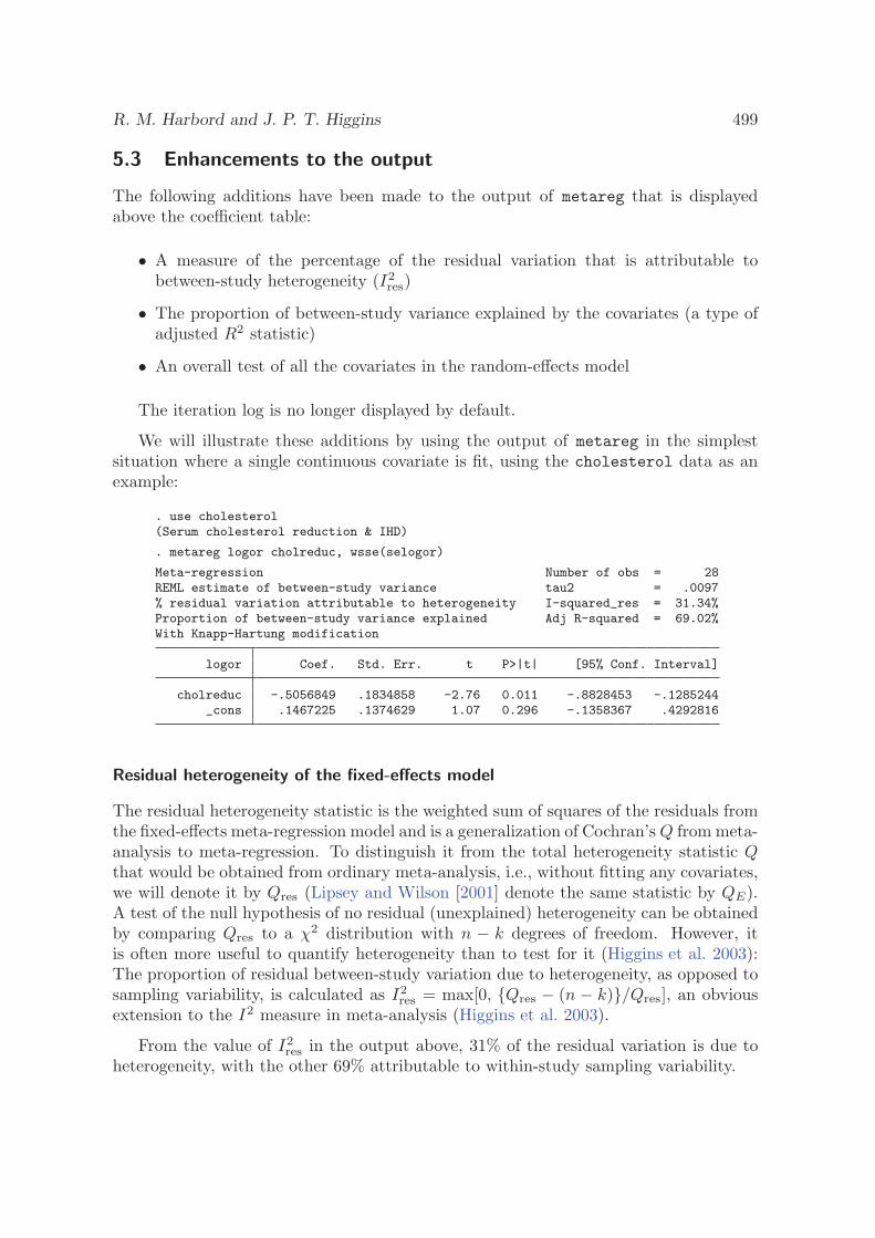
R. M. Harbord and J. P. T. Higgins 499
5.3 Enhancements to the output
The following additions have been made to the output of metareg that is displayedabove the coefficient table:
• A measure of the percentage of the residual variation that is attributable tobetween-study heterogeneity (I2
res)
• The proportion of between-study variance explained by the covariates (a type ofadjusted R2 statistic)
• An overall test of all the covariates in the random-effects model
The iteration log is no longer displayed by default.
We will illustrate these additions by using the output of metareg in the simplestsituation where a single continuous covariate is fit, using the cholesterol data as anexample:
. use cholesterol(Serum cholesterol reduction & IHD)
. metareg logor cholreduc, wsse(selogor)
Meta-regression Number of obs = 28REML estimate of between-study variance tau2 = .0097% residual variation attributable to heterogeneity I-squared_res = 31.34%Proportion of between-study variance explained Adj R-squared = 69.02%With Knapp-Hartung modification
logor Coef. Std. Err. t P>|t| [95% Conf. Interval]
cholreduc -.5056849 .1834858 -2.76 0.011 -.8828453 -.1285244_cons .1467225 .1374629 1.07 0.296 -.1358367 .4292816
Residual heterogeneity of the fixed-effects model
The residual heterogeneity statistic is the weighted sum of squares of the residuals fromthe fixed-effects meta-regression model and is a generalization of Cochran’s Q from meta-analysis to meta-regression. To distinguish it from the total heterogeneity statistic Qthat would be obtained from ordinary meta-analysis, i.e., without fitting any covariates,we will denote it by Qres (Lipsey and Wilson [2001] denote the same statistic by QE).A test of the null hypothesis of no residual (unexplained) heterogeneity can be obtainedby comparing Qres to a χ2 distribution with n − k degrees of freedom. However, itis often more useful to quantify heterogeneity than to test for it (Higgins et al. 2003):The proportion of residual between-study variation due to heterogeneity, as opposed tosampling variability, is calculated as I2
res = max[0, {Qres − (n − k)}/Qres], an obviousextension to the I2 measure in meta-analysis (Higgins et al. 2003).
From the value of I2res in the output above, 31% of the residual variation is due to
heterogeneity, with the other 69% attributable to within-study sampling variability.
500 Meta-regression in Stata
Adjusted R2
The proportion of between-study variance explained by the covariates can be calculatedby comparing the estimated between-study variance, τ2, with its value when no covari-ates are fit, τ2
0 . Adjusted R2 is the relative reduction in the between-study variance,R2
adj = (τ20 − τ2)/τ2
0 . It is possible for this to be negative if the covariates explain less ofthe heterogeneity than would be expected by chance, but the same is true for adjustedR2 in ordinary linear regression. It may be more common in meta-regression becausethe number of studies is often small.
In the above example, 69% of the between-study variance is explained by the covari-ate cholreduc, and the remaining between-study variance appears small at 0.0097. (Itis coincidence that the figure of 69% also appears in the preceding subsection.)
Joint test for all covariates
When more than one covariate is fit, metareg reports a test of the null hypothesis thatthe coefficients of the covariates are all zero, obtained from a multiparameter Waldtest by using Stata’s test command (see [R] test). The test statistic is compared tothe appropriate F distribution if the default Knapp–Hartung adjustment is used. Ifmetareg’s z option is used to specify the use of conventional variance estimates andtests for the effect estimates, a χ2 distribution is used for the joint test. To simplifythe output, this test is not displayed when only a single covariate is fit because it wouldgive an identical p-value to the one displayed for the covariate in the regression table.
This gives one way of controlling the risk of false-positive findings when performingmeta-regression with multiple covariates: we can use the overall model p-value to assessif there is evidence for an association of any of the covariates with the outcome. However,when a small p-value indicates that there is such evidence, it becomes harder to decidewhich, and how many, of the covariates there is good evidence for. Another method ofdealing with this multiplicity issue that may help overcome this problem, though at theexpense of longer computation time, is given in section 5.5 below.
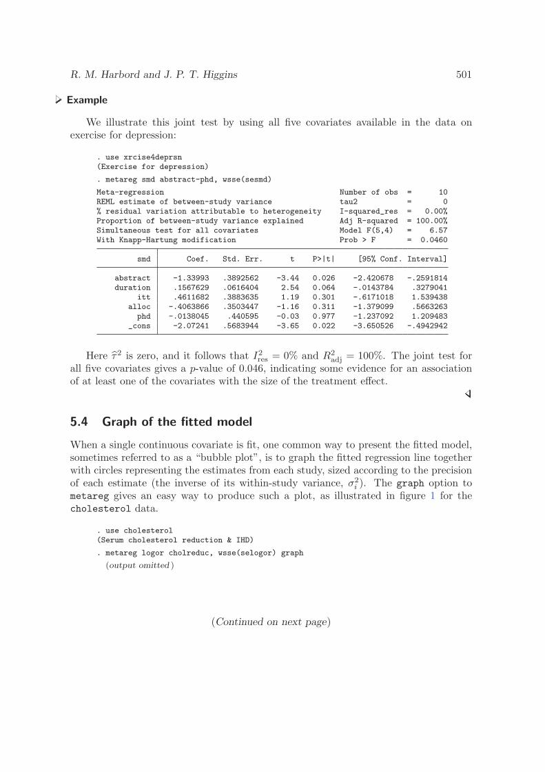
R. M. Harbord and J. P. T. Higgins 501
Example
We illustrate this joint test by using all five covariates available in the data onexercise for depression:
. use xrcise4deprsn(Exercise for depression)
. metareg smd abstract-phd, wsse(sesmd)
Meta-regression Number of obs = 10REML estimate of between-study variance tau2 = 0% residual variation attributable to heterogeneity I-squared_res = 0.00%Proportion of between-study variance explained Adj R-squared = 100.00%Simultaneous test for all covariates Model F(5,4) = 6.57With Knapp-Hartung modification Prob > F = 0.0460
smd Coef. Std. Err. t P>|t| [95% Conf. Interval]
abstract -1.33993 .3892562 -3.44 0.026 -2.420678 -.2591814duration .1567629 .0616404 2.54 0.064 -.0143784 .3279041
itt .4611682 .3883635 1.19 0.301 -.6171018 1.539438alloc -.4063866 .3503447 -1.16 0.311 -1.379099 .5663263
phd -.0138045 .440595 -0.03 0.977 -1.237092 1.209483_cons -2.07241 .5683944 -3.65 0.022 -3.650526 -.4942942
Here τ2 is zero, and it follows that I2res = 0% and R2
adj = 100%. The joint test forall five covariates gives a p-value of 0.046, indicating some evidence for an associationof at least one of the covariates with the size of the treatment effect.
5.4 Graph of the fitted model
When a single continuous covariate is fit, one common way to present the fitted model,sometimes referred to as a “bubble plot”, is to graph the fitted regression line togetherwith circles representing the estimates from each study, sized according to the precisionof each estimate (the inverse of its within-study variance, σ2
i ). The graph option tometareg gives an easy way to produce such a plot, as illustrated in figure 1 for thecholesterol data.
. use cholesterol(Serum cholesterol reduction & IHD)
. metareg logor cholreduc, wsse(selogor) graph
(output omitted )
(Continued on next page)
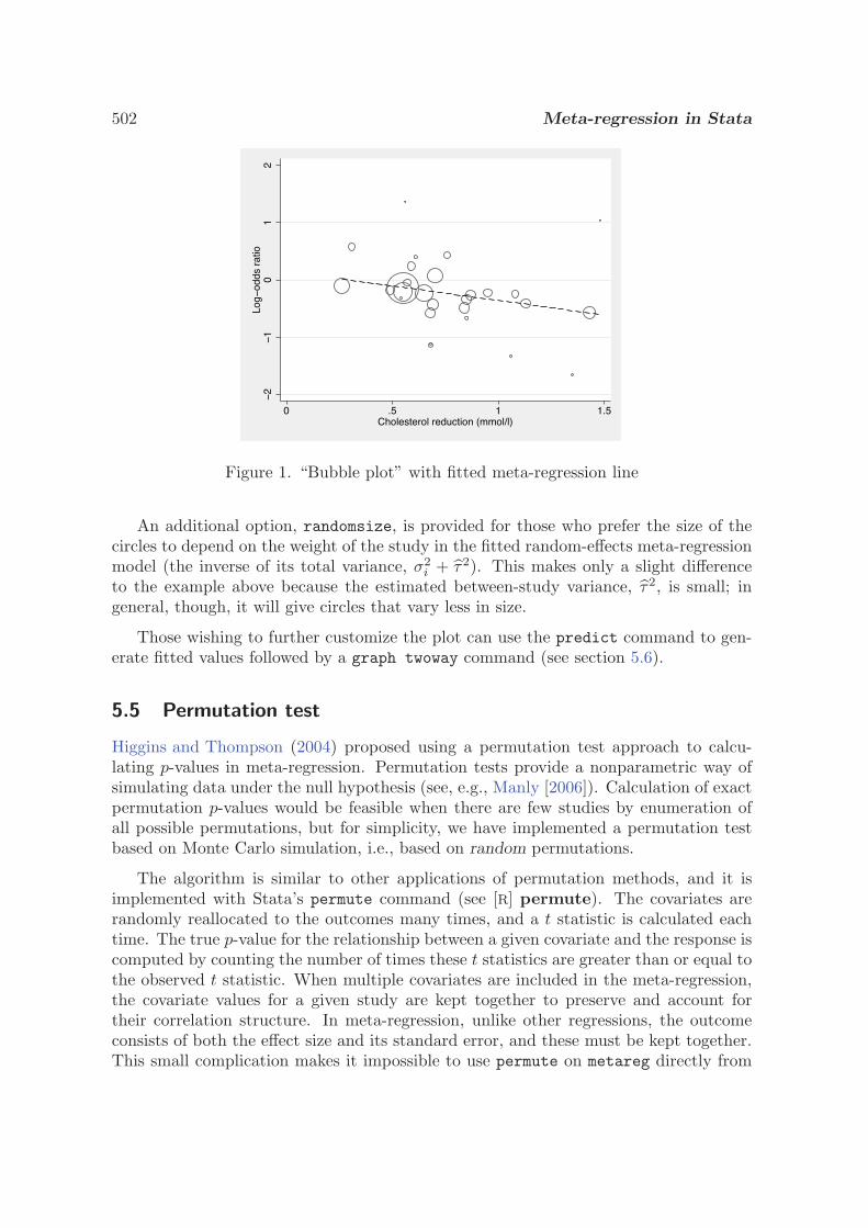
502 Meta-regression in Stata
�2
�1
01
2Lo
g�od
ds r
atio
0 .5 1 1.5Cholesterol reduction (mmol/l)
Figure 1. “Bubble plot” with fitted meta-regression line
An additional option, randomsize, is provided for those who prefer the size of thecircles to depend on the weight of the study in the fitted random-effects meta-regressionmodel (the inverse of its total variance, σ2
i + τ2). This makes only a slight differenceto the example above because the estimated between-study variance, τ2, is small; ingeneral, though, it will give circles that vary less in size.
Those wishing to further customize the plot can use the predict command to gen-erate fitted values followed by a graph twoway command (see section 5.6).
5.5 Permutation test
Higgins and Thompson (2004) proposed using a permutation test approach to calcu-lating p-values in meta-regression. Permutation tests provide a nonparametric way ofsimulating data under the null hypothesis (see, e.g., Manly [2006]). Calculation of exactpermutation p-values would be feasible when there are few studies by enumeration ofall possible permutations, but for simplicity, we have implemented a permutation testbased on Monte Carlo simulation, i.e., based on random permutations.
The algorithm is similar to other applications of permutation methods, and it isimplemented with Stata’s permute command (see [R] permute). The covariates arerandomly reallocated to the outcomes many times, and a t statistic is calculated eachtime. The true p-value for the relationship between a given covariate and the response iscomputed by counting the number of times these t statistics are greater than or equal tothe observed t statistic. When multiple covariates are included in the meta-regression,the covariate values for a given study are kept together to preserve and account fortheir correlation structure. In meta-regression, unlike other regressions, the outcomeconsists of both the effect size and its standard error, and these must be kept together.This small complication makes it impossible to use permute on metareg directly from
R. M. Harbord and J. P. T. Higgins 503
the command line when there are multiple covariates, so we have written a permute()option for metareg. This option also implements the following extension, which adjustsp-values for multiple tests when there are several covariates.
Multiplicity adjustment
When several covariates are used in meta-regression, either in several separate univari-able meta-regressions or in one multiple meta-regression, there is an increased chanceof at least one false-positive finding (type I error). The statistics obtained from therandom permutations can be used to adjust for such multiple testing by comparing theobserved t statistic for every covariate with the largest t statistic for any covariate ineach random permutation. The proportion of times that the former equals or exceedsthe latter gives the probability of observing a t statistic for any covariate as extremeor more extreme than that observed for a particular covariate, under the complete nullhypothesis that all the regression coefficients are zero.
The number of random permutations must be specified—there is deliberately nodefault. We suggest that a small number (e.g., 100) be specified initially to check thatthe command is working as expected. The number should then be increased to at least1,000, but 5,000 or 20,000 permutations may be necessary for sufficient precision (Manly2006; Westfall and Young 1993). Because the permute() option uses Stata’s random-number generator, the set seed command should be used first if replicability of resultsis desired. When the permute() option is specified, the defaults are to use the method-of-moments estimate of τ2 for reasons of speed and to not use the Knapp–Hartungmodification to the standard errors.
By default, permute() performs multivariable meta-regression; i.e., all the covariatesare entered into a single model in each permutation.
Example
We illustrate the use of the permute() option by using the data on exercise fordepression.
(Continued on next page)
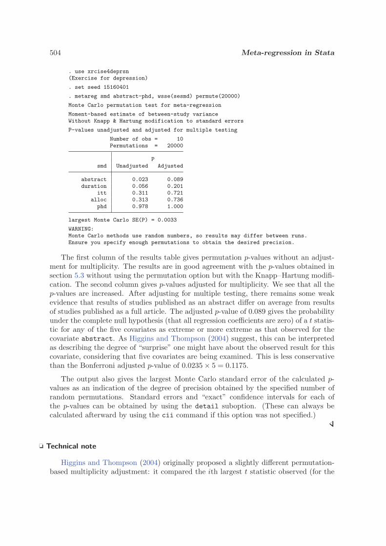
504 Meta-regression in Stata
. use xrcise4deprsn(Exercise for depression)
. set seed 15160401
. metareg smd abstract-phd, wsse(sesmd) permute(20000)
Monte Carlo permutation test for meta-regression
Moment-based estimate of between-study varianceWithout Knapp & Hartung modification to standard errors
P-values unadjusted and adjusted for multiple testing
Number of obs = 10Permutations = 20000
Psmd Unadjusted Adjusted
abstract 0.023 0.089duration 0.056 0.201
itt 0.311 0.721alloc 0.313 0.736phd 0.978 1.000
largest Monte Carlo SE(P) = 0.0033
WARNING:Monte Carlo methods use random numbers, so results may differ between runs.Ensure you specify enough permutations to obtain the desired precision.
The first column of the results table gives permutation p-values without an adjust-ment for multiplicity. The results are in good agreement with the p-values obtained insection 5.3 without using the permutation option but with the Knapp–Hartung modifi-cation. The second column gives p-values adjusted for multiplicity. We see that all thep-values are increased. After adjusting for multiple testing, there remains some weakevidence that results of studies published as an abstract differ on average from resultsof studies published as a full article. The adjusted p-value of 0.089 gives the probabilityunder the complete null hypothesis (that all regression coefficients are zero) of a t statis-tic for any of the five covariates as extreme or more extreme as that observed for thecovariate abstract. As Higgins and Thompson (2004) suggest, this can be interpretedas describing the degree of “surprise” one might have about the observed result for thiscovariate, considering that five covariates are being examined. This is less conservativethan the Bonferroni adjusted p-value of 0.0235 × 5 = 0.1175.
The output also gives the largest Monte Carlo standard error of the calculated p-values as an indication of the degree of precision obtained by the specified number ofrandom permutations. Standard errors and “exact” confidence intervals for each ofthe p-values can be obtained by using the detail suboption. (These can always becalculated afterward by using the cii command if this option was not specified.)
Technical note
Higgins and Thompson (2004) originally proposed a slightly different permutation-based multiplicity adjustment: it compared the ith largest t statistic observed (for the
R. M. Harbord and J. P. T. Higgins 505
“ith most significant” covariate) with the ith largest t statistic in each random per-mutation. This adjustment was implemented in a revised version of metareg releasedpreviously on the Statistical Software Components archive. This adjustment has beenfound to be hard to interpret in practice, however, because for the second most signifi-cant covariate it effectively gives a joint test of the two covariates with the largest twoobserved t statistics (and similarly for third and subsequent covariates if more than twocovariates are supplied). The resulting multiplicity-adjusted p-value can turn out to beeither larger or smaller than the unadjusted p-value, which can appear counter-intuitive.
For this release of metareg, we have therefore chosen to implement a differentpermutation-based algorithm for multiplicity adjustment based on the one-step“maxT” method of Westfall and Young (1993). This adjustment compares the t statis-tic for every covariate with the largest t statistic in each random permutation. Theresulting multiplicity-adjusted p-values are always as large as or (usually) larger thanthe unadjusted p-values. This procedure ensures weak control of the familywise errorrate, defined as the probability that at least one null hypothesis is rejected when allthe null hypotheses are true (Shaffer 1995). It does not guarantee strong control of thefamilywise error rate, however; i.e., when one or more null hypotheses are false, it doesnot guarantee control of the proportion of the remaining true null hypotheses that areincorrectly rejected, though such strong control should be achieved asymptotically asthe number of studies increases (Westfall and Young 1993; Shaffer 1995).
The false discovery rate (Benjamini and Hochberg 1995) and related procedures(Newson and the ALSPAC Study Team 2003; Storey, Taylor, and Siegmund 2004; Wa-cholder et al. 2004) have been suggested as an alternative method of multiplicity ad-justment, but we have chosen not to implement such procedures in metareg. Suchprocedures are always either step-up or (more rarely) step-down algorithms. Althoughstepwise algorithms are suitable for hypothesis testing and often give greater power,the resulting adjusted p-values cannot be interpreted as giving the strength of evidenceagainst the null hypothesis, the interpretation increasingly advocated in medicine andepidemiology (Sterne and Davey Smith 2001). In particular, stepwise methods may as-sign equal adjusted p-values to covariates with different unadjusted p-values.
Suboptions to permute()
The permute() option can also be used to perform a set of single-variable meta-regressions at each permutation by adding the univariable suboption. This suboptionreports permutation-based p-values for fitting a separate model for each covariate ratherthan including all the covariates in a multiple regression model. With several covariates,the execution time may be considerably longer than for multivariable meta-regression.
Example
We add the univariable suboption to the previous example but reduce the numberof permutations to cut down the computation time:
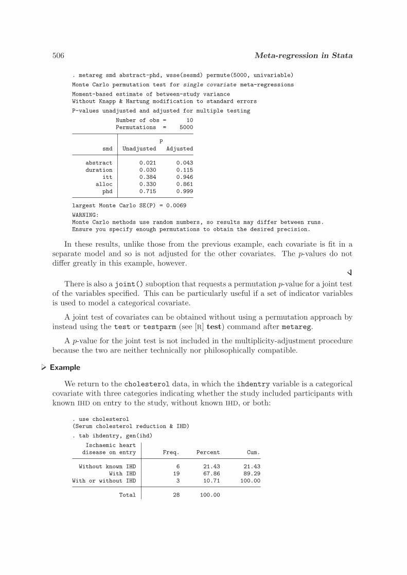
506 Meta-regression in Stata
. metareg smd abstract-phd, wsse(sesmd) permute(5000, univariable)
Monte Carlo permutation test for single covariate meta-regressions
Moment-based estimate of between-study varianceWithout Knapp & Hartung modification to standard errors
P-values unadjusted and adjusted for multiple testing
Number of obs = 10Permutations = 5000
Psmd Unadjusted Adjusted
abstract 0.021 0.043duration 0.030 0.115
itt 0.384 0.946alloc 0.330 0.861phd 0.715 0.999
largest Monte Carlo SE(P) = 0.0069
WARNING:Monte Carlo methods use random numbers, so results may differ between runs.Ensure you specify enough permutations to obtain the desired precision.
In these results, unlike those from the previous example, each covariate is fit in aseparate model and so is not adjusted for the other covariates. The p-values do notdiffer greatly in this example, however.
There is also a joint() suboption that requests a permutation p-value for a joint testof the variables specified. This can be particularly useful if a set of indicator variablesis used to model a categorical covariate.
A joint test of covariates can be obtained without using a permutation approach byinstead using the test or testparm (see [R] test) command after metareg.
A p-value for the joint test is not included in the multiplicity-adjustment procedurebecause the two are neither technically nor philosophically compatible.
Example
We return to the cholesterol data, in which the ihdentry variable is a categoricalcovariate with three categories indicating whether the study included participants withknown IHD on entry to the study, without known IHD, or both:
. use cholesterol(Serum cholesterol reduction & IHD)
. tab ihdentry, gen(ihd)
Ischaemic heartdisease on entry Freq. Percent Cum.
Without known IHD 6 21.43 21.43With IHD 19 67.86 89.29
With or without IHD 3 10.71 100.00
Total 28 100.00
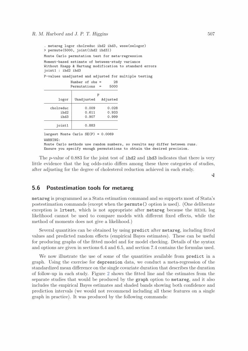
R. M. Harbord and J. P. T. Higgins 507
. metareg logor cholreduc ihd2 ihd3, wsse(selogor)> permute(5000, joint(ihd2 ihd3))
Monte Carlo permutation test for meta-regression
Moment-based estimate of between-study varianceWithout Knapp & Hartung modification to standard errorsjoint1 : ihd2 ihd3
P-values unadjusted and adjusted for multiple testing
Number of obs = 28Permutations = 5000
Plogor Unadjusted Adjusted
cholreduc 0.009 0.028ihd2 0.611 0.933ihd3 0.907 0.999
joint1 0.883
largest Monte Carlo SE(P) = 0.0069
WARNING:Monte Carlo methods use random numbers, so results may differ between runs.Ensure you specify enough permutations to obtain the desired precision.
The p-value of 0.883 for the joint test of ihd2 and ihd3 indicates that there is verylittle evidence that the log odds-ratio differs among these three categories of studies,after adjusting for the degree of cholesterol reduction achieved in each study.
5.6 Postestimation tools for metareg
metareg is programmed as a Stata estimation command and so supports most of Stata’spostestimation commands (except when the permute() option is used). (One deliberateexception is lrtest, which is not appropriate after metareg because the REML loglikelihood cannot be used to compare models with different fixed effects, while themethod of moments does not give a likelihood.)
Several quantities can be obtained by using predict after metareg, including fittedvalues and predicted random effects (empirical Bayes estimates). These can be usefulfor producing graphs of the fitted model and for model checking. Details of the syntaxand options are given in sections 6.4 and 6.5, and section 7.4 contains the formulas used.
We now illustrate the use of some of the quantities available from predict in agraph. Using the exercise for depression data, we conduct a meta-regression of thestandardized mean difference on the single covariate duration that describes the durationof follow-up in each study. Figure 2 shows the fitted line and the estimates from theseparate studies that would be produced by the graph option to metareg, and it alsoincludes the empirical Bayes estimates and shaded bands showing both confidence andprediction intervals (we would not recommend including all these features on a singlegraph in practice). It was produced by the following commands:
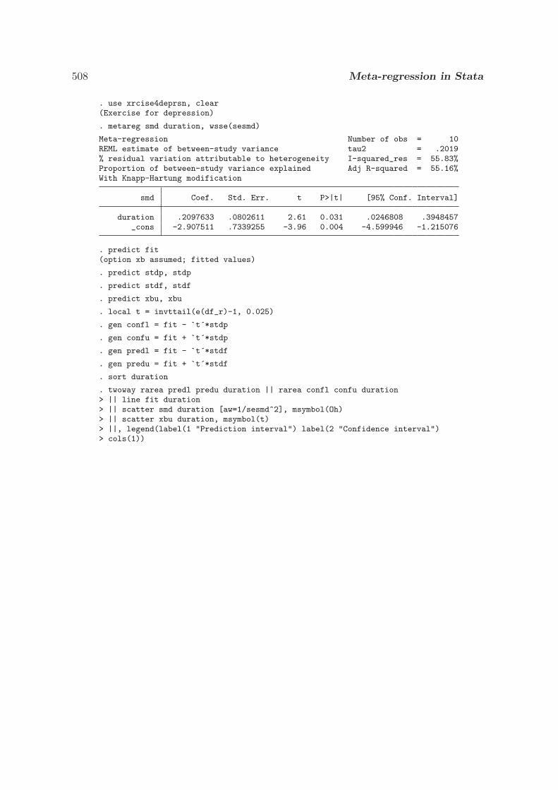
508 Meta-regression in Stata
. use xrcise4deprsn, clear(Exercise for depression)
. metareg smd duration, wsse(sesmd)
Meta-regression Number of obs = 10REML estimate of between-study variance tau2 = .2019% residual variation attributable to heterogeneity I-squared_res = 55.83%Proportion of between-study variance explained Adj R-squared = 55.16%With Knapp-Hartung modification
smd Coef. Std. Err. t P>|t| [95% Conf. Interval]
duration .2097633 .0802611 2.61 0.031 .0246808 .3948457_cons -2.907511 .7339255 -3.96 0.004 -4.599946 -1.215076
. predict fit(option xb assumed; fitted values)
. predict stdp, stdp
. predict stdf, stdf
. predict xbu, xbu
. local t = invttail(e(df_r)-1, 0.025)
. gen confl = fit - `t´*stdp
. gen confu = fit + `t´*stdp
. gen predl = fit - `t´*stdf
. gen predu = fit + `t´*stdf
. sort duration
. twoway rarea predl predu duration || rarea confl confu duration> || line fit duration> || scatter smd duration [aw=1/sesmd^2], msymbol(Oh)> || scatter xbu duration, msymbol(t)> ||, legend(label(1 "Prediction interval") label(2 "Confidence interval")> cols(1))
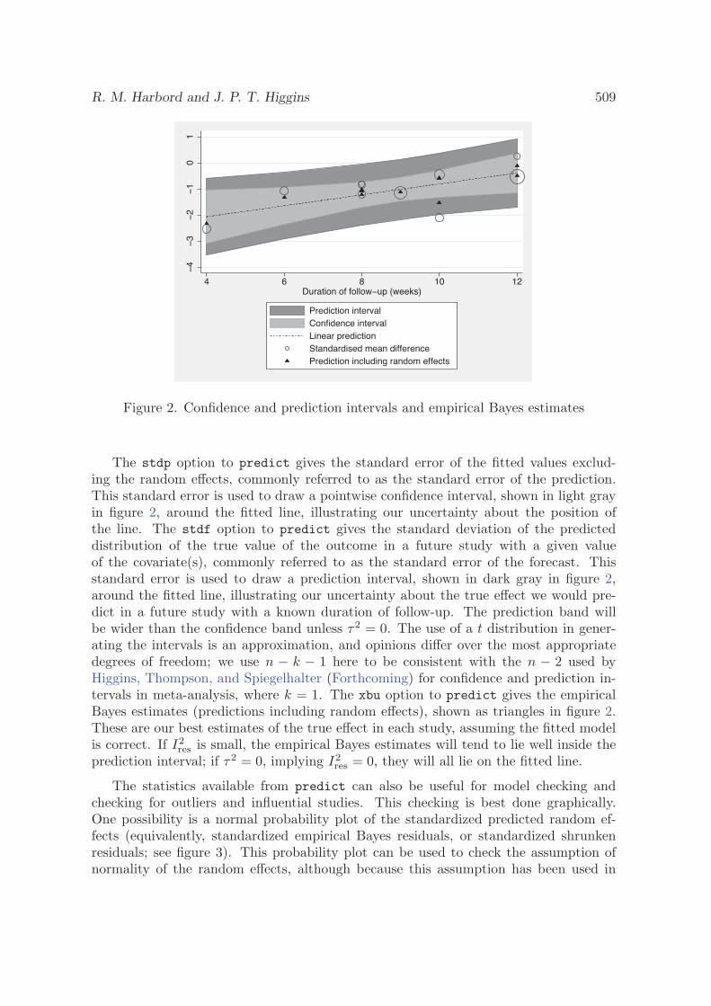
R. M. Harbord and J. P. T. Higgins 509
�4
�3
�2
�1
01
4 6 8 10 12Duration of follow�up (weeks)
Prediction intervalConfidence intervalLinear predictionStandardised mean differencePrediction including random effects
Figure 2. Confidence and prediction intervals and empirical Bayes estimates
The stdp option to predict gives the standard error of the fitted values exclud-ing the random effects, commonly referred to as the standard error of the prediction.This standard error is used to draw a pointwise confidence interval, shown in light grayin figure 2, around the fitted line, illustrating our uncertainty about the position ofthe line. The stdf option to predict gives the standard deviation of the predicteddistribution of the true value of the outcome in a future study with a given valueof the covariate(s), commonly referred to as the standard error of the forecast. Thisstandard error is used to draw a prediction interval, shown in dark gray in figure 2,around the fitted line, illustrating our uncertainty about the true effect we would pre-dict in a future study with a known duration of follow-up. The prediction band willbe wider than the confidence band unless τ2 = 0. The use of a t distribution in gener-ating the intervals is an approximation, and opinions differ over the most appropriatedegrees of freedom; we use n − k − 1 here to be consistent with the n − 2 used byHiggins, Thompson, and Spiegelhalter (Forthcoming) for confidence and prediction in-tervals in meta-analysis, where k = 1. The xbu option to predict gives the empiricalBayes estimates (predictions including random effects), shown as triangles in figure 2.These are our best estimates of the true effect in each study, assuming the fitted modelis correct. If I2
res is small, the empirical Bayes estimates will tend to lie well inside theprediction interval; if τ2 = 0, implying I2
res = 0, they will all lie on the fitted line.
The statistics available from predict can also be useful for model checking andchecking for outliers and influential studies. This checking is best done graphically.One possibility is a normal probability plot of the standardized predicted random ef-fects (equivalently, standardized empirical Bayes residuals, or standardized shrunkenresiduals; see figure 3). This probability plot can be used to check the assumption ofnormality of the random effects, although because this assumption has been used in
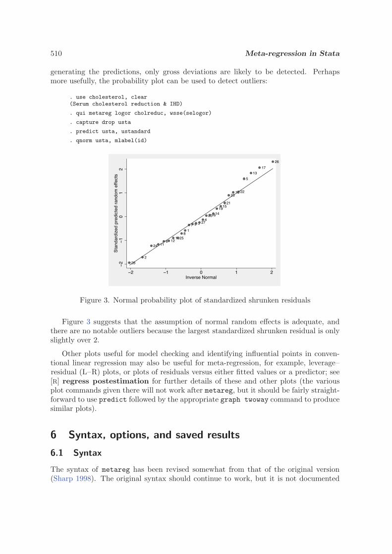
510 Meta-regression in Stata
generating the predictions, only gross deviations are likely to be detected. Perhapsmore usefully, the probability plot can be used to detect outliers:
. use cholesterol, clear(Serum cholesterol reduction & IHD)
. qui metareg logor cholreduc, wsse(selogor)
. capture drop usta
. predict usta, ustandard
. qnorm usta, mlabel(id)
28
2
24 116 12
10258
1
7 9 3 274
20161419
1521
2318 22
5
13
17
26
�2
�1
01
2S
tand
ardi
zed
pred
icte
d ra
ndom
effe
cts
�2 �1 0 1 2Inverse Normal
Figure 3. Normal probability plot of standardized shrunken residuals
Figure 3 suggests that the assumption of normal random effects is adequate, andthere are no notable outliers because the largest standardized shrunken residual is onlyslightly over 2.
Other plots useful for model checking and identifying influential points in conven-tional linear regression may also be useful for meta-regression, for example, leverage–residual (L–R) plots, or plots of residuals versus either fitted values or a predictor; see[R] regress postestimation for further details of these and other plots (the variousplot commands given there will not work after metareg, but it should be fairly straight-forward to use predict followed by the appropriate graph twoway command to producesimilar plots).
6 Syntax, options, and saved results
6.1 Syntax
The syntax of metareg has been revised somewhat from that of the original version(Sharp 1998). The original syntax should continue to work, but it is not documented
R. M. Harbord and J. P. T. Higgins 511
here. ML estimation of τ2 is not supported by the updated metareg program, but if theold bsest(ml) option is used, the new program simply calls the original version, whichis incorporated within the updated metareg.ado file.
metareg depvar[indepvars
] [if] [
in]wsse(varname)
[, eform graph
randomsize noconstant mm reml eb knapphartung z tau2test level(#)
permute(#[, univariable detail joint(varlist1
[| varlist2 . . .
])]) log
maximize options]
by can be used with metareg; see [D] by.
6.2 Options
wsse(varname) specifies the variable containing σi, the standard error of depvar, withineach study. All values of varname must be greater than zero. wsse() is required.
eform indicates to output the exponentiated form of the coefficients and to suppressreporting of the constant. This option may be useful when depvar is the logarithmof a ratio measure, such as a log odds-ratio or a log risk-ratio.
graph requests a line graph of fitted values plotted against the first covariate in in-depvars, together with the estimates from each study represented by circles. Bydefault, the circle sizes depend on the precision of each estimate (the inverse of itswithin-study variance), which is the weight given to each study in the fixed-effectsmodel.
randomsize is for use with the graph option. It specifies that the size of the circles willdepend on the weights in the random-effects model rather than the precision of eachestimate. These random-effects weights depend on the estimate of τ2.
The remaining options will mainly be of interest to more advanced users:
noconstant suppresses the constant term (intercept). This is rarely appropriate inmeta-regression. Note: It might seem tempting to use the noconstant option in thecholesterol example to force the regression line through the origin, on the reasoningthat an intervention that has no effect on cholesterol should have no effect on theodds of IHD. We would advise against using this option, however, both here and inmost other circumstances. Using it here involves the assumption that the effect ofthe intervention on IHD is mediated entirely by cholesterol reduction. It also wouldnot allow for measurement error in cholesterol reduction, which, through attenuationby errors (regression dilution bias), could lead to a nonzero intercept even when azero intercept would be expected.
The mm, reml, and eb options are alternatives that specify the method of estimation ofthe additive (between-study) component of variance τ2:
512 Meta-regression in Stata
mm specifies the use of method of moments to estimate the additive (between-study)component of variance τ2; this is a generalization of the DerSimonian and Laird(1986) method commonly used for random-effects meta-analysis. For speed, this isthe default when the permute() option is specified, because it is the only noniterativemethod.
reml specifies the use of REML to estimate the additive (between-study) componentof variance τ2. This is the default unless the permute() option is specified. Thisrevised version uses Stata’s ML facilities to maximize the REML log likelihood. Itwill therefore not give identical results to the previous version of metareg, whichused an approximate iterative method.
eb specifies the use of the “empirical Bayes” method to estimate τ2 (Morris 1983).
knapphartung makes a modification to the variance of the estimated coefficients sug-gested by Knapp and Hartung (2003) and supported by Higgins and Thompson(2004), accompanied by the use of a t distribution in place of the standard normaldistribution when calculating p-values and confidence intervals. This is the defaultunless the permute() option is specified.
z requests that the knapphartung modification not be applied and that the standardnormal distribution be used to calculate p-values and confidence intervals. This isthe default when the permute() option is specified with a fixed-effects model.
tau2test adds to the output two tests of τ2 = 0. The first is based on the residualheterogeneity statistic, Qres. The second (not available if the mm option is alsospecified) is a likelihood-ratio test based on the REML log likelihood. These aretwo tests of the same null hypothesis (the fixed-effects model with τ2 = 0), butthe alternative hypotheses are different, as are the distributions of the test statisticsunder the null, so close agreement of the two tests is not guaranteed. Both tests aretypically of little interest because it is more helpful to quantify heterogeneity thanto test for it (see section 5.3).
level(#) specifies the confidence level, as a percentage, for confidence intervals. Thedefault is level(95) or as set by set level; see [U] 20.7 Specifying the widthof confidence intervals.
permute(. . .) calculates p-values by using a Monte Carlo permutation test. See sec-tion 6.3 below for more information about this option.
log requests the display of the iteration log during estimation of τ2. This is ignored ifthe mm option is specified, because this uses a noniterative method.
maximize options are ignored unless estimation of τ2 is by REML. These options controlthe maximization process; see [R] maximize. They are ignored if the mm option isspecified. You should never need to specify them; they are supported only in caseproblems in the REML estimation of τ2 are ever reported or suspected.

R. M. Harbord and J. P. T. Higgins 513
6.3 Option for permutation test
The permute() option calculates p-values by using a Monte Carlo permutation test, asrecommended by Higgins and Thompson (2004). To address multiple testing, permute()also calculates p-values for the most- to least-significant covariates, as the same authorsalso recommend.
The syntax of permute() is
permute(#[, univariable detail joint(varlist1
[| varlist2 . . .
])])
where # is required and specifies the number of random permutations to perform.Larger values give more precise p-values but take longer.
There are three suboptions:
univariable indicates that p-values should be calculated for a series of single covariatemeta-regressions of each covariate in varlist separately, instead of a multiple meta-regression of all covariates in varlist simultaneously.
detail requests lengthier output in the format given by [R] permute.
joint(varlist1[| varlist2 . . .
]) specifies that a permutation p-value should also be
computed for a joint test of the variables in each varlist.
The eform, level(), and z options have no effect when the permute() option isspecified.
6.4 Syntax of predict
The syntax of predict (see [R] predict) following metareg is
predict[type
]newvar
[if] [
in] [
, statistic]
statistic description
xb fitted values; the defaultstdp standard error of the predictionstdf standard error of the forecastu predicted random effectsustandard standardized predicted random effectsxbu prediction including random effectsstdxbu standard error of xbuhat leverage (diagonal elements of hat matrix)
These statistics are available both in and out of sample; type predict . . . ife(sample) . . . if wanted only for the estimation sample.

514 Meta-regression in Stata
6.5 Options for predict
xb, the default, calculates the linear prediction, xib, that is, the fitted values excludingthe random effects.
stdp calculates the standard error of the prediction (the standard error of the fittedvalues excluding the random effects).
stdf calculates the standard error of the forecast. This gives the standard deviationof the predicted distribution of the true value of depvar in a future study, with thecovariates given by varlist. stdf2 = stdp2 + τ2.
u calculates the predicted random effects, ui. These are the best linear unbiased predic-tions of the random effects, also known as the empirical Bayes (or posterior mean)estimates of the random effects, or as shrunken residuals.
ustandard calculates the standardized predicted random effects, i.e., the predicted ran-dom effects, ui, divided by their (unconditional) standard errors. These may beuseful for diagnostics and model checking.
xbu calculates the prediction including the random effects, xib + ui, also known as theempirical Bayes estimates of the effects for each study.
stdxbu calculates the standard error of the prediction including random effects.
hat calculates the leverages (the diagonal elements of the projection hat matrix).
6.6 Saved results
When the permute() option is not specified, metareg saves the following in e():
Scalarse(N) number of observations e(tau2) estimate of τ2
e(df m) model degrees of freedom e(Q) Cochran’s Qe(df Q) degrees of freedom for test e(I2) I-squared
of Q = 0 e(q KH) Knapp–Hartung variancee(df r) residual degrees of freedom modification factor
(if t tests used) e(remll c) REML log likelihood,e(remll) REML log likelihood comparison modele(chi2 c) χ2 for comparison test e(tau2 0) τ2, constant-only modele(F) model F statistic e(chi2) model χ2
Macrose(cmd) metareg e(depvar) name of dependent variablee(predict) program used to implement
predicte(method) REML, Method of moments, or
Empirical Bayese(wsse) name of wsse() variable e(properties) b V
Matricese(b) coefficient vector e(V) variance–covariance matrix of
estimators
Functionse(sample) marks estimation sample
R. M. Harbord and J. P. T. Higgins 515
metareg, permute() saves the following in r():
Scalarsr(N) number of observations
Matricesr(b) observed t statistics, Tobs r(p) observed proportionsr(c) count when |T | ≥ |Tobs | r(reps) number of nonmissing results
7 Methods and formulas
The residual heterogeneity statistic, Qres, is the residual weighted sum of squares fromthe fixed-effects model and is the same as the goodness-of-fit statistic computed byvwls:
Qres =∑
i
(yi − xiβ
σi
)2
The proportion of residual variation due to heterogeneity is
I2 = max{
Qres − (n − k)Qres
, 0}
The proportion of the between-study variance explained by the covariates (adjustedR-squared) is R2
a = (τ20 −τ2)/τ2
0 , where τ2 and τ20 are the estimates of the between-study
variance in models with and without the covariates, respectively.
7.1 Estimation of τ 2
Several different algorithms have been proposed for estimation of the between-studyvariance, τ2, in meta-analysis (Sidik and Jonkman 2007) and meta-regression (Thomp-son and Sharp 1999). Three algorithms are available in this version of metareg. In eachcase, if the estimated value of τ2 is negative, it is set to zero.
Method of moments is the only noniterative method, so it has the advantages ofspeed and robustness. It is the natural extension of the DerSimonian and Laird (1986)estimate commonly used in random-effects meta-analysis. The method-of-moments es-timate of τ2 is obtained by equating the observed value of Qres to its expected valueunder the random-effects model, giving (DuMouchel and Harris 1983, eq. 3.12)
τ2MM =
Qres − (n + k)∑i{1/σ2
i (1 − hi)}
Here hi is the ith diagonal element of the hat matrix X(X′V−10 X)−1XV−1
0 , whereV0 = diag(σ2
1 , σ22 , . . . , σ2
n).
The iterative methods below use τ2MM as a starting value (this is a change from the
original version of metareg (Sharp 1998), which used zero as a starting value).
516 Meta-regression in Stata
REML estimation of τ2 is based on maximization of the residual (or restricted) loglikelihood,
LR(τ2) = −12
∑i
{log(σ2
i + τ2) +(yi − xiβ)2
σ2i + τ2
}− 1
2log |X′V−1X |
where V = diag(σ21 + τ2, σ2
2 + τ2, . . . , σ2n + τ2) and β = (X′V−1X)−1X′V−1y (Harville
1977). This log likelihood is maximized by Stata’s ml command, using the d0 method,which calculates all derivatives numerically.
The “empirical Bayes” estimator of τ2 is so named because of its introduction in anarticle on empirical Bayes inference by Morris (1983), although as he states, any approx-imately unbiased estimate of τ2 could be used in such a setting. Thompson and Sharp(1999) found it to give substantially larger estimates of τ2 than other methods. Oth-ers suggest it performs well in simulations based on 2 × 2 tables (Berkey et al. 1995;Sidik and Jonkman 2007), although this may be due to overestimation of the within-study standard errors in small studies by the conventional (Woolf) estimate ratherthan the properties of the empirical Bayes method itself (Sutton and Higgins 2008). Itcan also be considered to be a method-of-moments estimator, formed by equating theweighted sum of squares of the residuals from the random-effects model to its expectedvalue (Knapp and Hartung 2003). It is found by iterating the following equation (Morris1983; Berkey et al. 1995):
τ2EB =
n/(n − k)∑
i
{(yi − xiβ)2/(σ2
i + τ2EB) − σ2
i
}∑
i(σ2i + τ2
EB)−1
At each iteration, β must be reestimated using a weighted least-squares regression of yon X with the weights 1/(σ2
i + τ2EB).
7.2 Estimation of β
Once τ2 has been estimated by one of the methods above, the estimated coefficients, β,are obtained by a weighted least-squares regression of y on X with the weights 1/(σ2
i +τ2). The conventional estimate of the variance–covariance matrix of the coefficients is(X′V−1X)−1, where V = diag(σ2
1 + τ2, σ22 + τ2, . . . , σ2
n + τ2).
7.3 Knapp–Hartung variance modification
Knapp and Hartung (2003) proposed multiplying the conventional estimate of the vari-ance of the coefficients given above by max(q, 1), where the Knapp–Hartung variancemodification factor is
q =1
n − k
∑i
(yi − xiβ)2
σ2i + τ2
With the “empirical Bayes” estimator of τ2, q = 1, so this modification has no effect(Knapp and Hartung 2003).
R. M. Harbord and J. P. T. Higgins 517
7.4 Methods and formulas for predict
The standard error of the prediction (stdp) is spi=√
xi(X′V−1X)−1x′i.
The leverages, or diagonal elements of the projection matrix (hat), are
hi = s2pi
/(σ2i + τ2)
The standard error of the forecast (stdf) is sfi=√
s2pi
+ τ2.
Denote the previously estimated coefficient vector by b, and let λi = τ2/(σ2i + τ2)
denote the empirical Bayes shrinkage factor for the ith observation.
The predicted random effects (u) are ui = λi(yi − xib).
The standardized predicted random effects (ustandard) are
usj= (yi − xib)
/√σ2
i + τ2 − s2pi
The prediction including random effects (xbu), or empirical Bayes estimate, is
xib + ui = λiyi + (1 − λi)xib
The standard error of the prediction including random effects (stdxbu) is√λ2
i (σ2i + τ2) + (1 − λ2
i )s2pi
8 Acknowledgments
Stephen Sharp gave permission to release this package under the same name as hisoriginal Stata package for meta-regression and to incorporate his code. Debbie Lawlorgave permission to use the example dataset on exercise for depression and providedadditional unpublished data. We thank Simon Thompson for his helpful comments onthe manuscript, and we thank the organizers of and participants at a meeting in ParkCity, Utah, in 2005 for discussions that influenced the output displayed by metareg.Finally, we wish to thank the referee for helpful comments, which led to improvementsin the program and the article.
9 ReferencesBenjamini, Y., and Y. Hochberg. 1995. Controlling the false discovery rate: A practical
and powerful approach to multiple testing. Journal of the Royal Statistical Society,Series B (Methodological) 57: 289–300.
Berkey, C. S., D. C. Hoaglin, F. Mosteller, and G. A. Colditz. 1995. A random-effectsregression model for meta-analysis. Statistics in Medicine 14: 395–411.
518 Meta-regression in Stata
Davey Smith, G., M. Egger, and A. N. Phillips. 1997. Meta-analysis: Beyond the grandmean? British Medical Journal 315: 1610–1614.
DerSimonian, R., and N. Laird. 1986. Meta-analysis in clinical trials. Controlled ClinicalTrials 7: 177–188.
DuMouchel, W. H., and J. E. Harris. 1983. Bayes methods for combining the resultsof cancer studies in humans and other species. Journal of the American StatisticalAssociation 78: 293–308.
Harris, R. J., M. J. Bradburn, J. J. Deeks, R. M. Harbord, D. G. Altman, and J. A. C.Sterne. 2008. metan: fixed- and random-effects meta-analysis. Stata Journal 8: 3–28.
Harville, D. A. 1977. Maximum likelihood approaches to variance component estimationand to related problems. Journal of the American Statistical Association 72: 320–338.
Higgins, J. P. T., and S. G. Thompson. 2004. Controlling the risk of spurious findingsfrom meta-regression. Statistics in Medicine 23: 1663–1682.
Higgins, J. P. T., S. G. Thompson, J. J. Deeks, and D. G. Altman. 2002. Statisticalheterogeneity in systematic reviews of clinical trials: A critical appraisal of guidelinesand practice. Journal of Health Services Research and Policy 7: 51–61.
———. 2003. Measuring inconsistency in meta-analyses. British Medical Journal 327:557–560.
Higgins, J. P. T., S. G. Thompson, and D. J. Spiegelhalter. Forthcoming. A reevaluationof random-effects meta-analysis. Journal of the Royal Statistics Society, Series A(Statistics in Society) .
Knapp, G., and J. Hartung. 2003. Improved tests for a random-effects meta-regressionwith a single covariate. Statistics in Medicine 22: 2693–2710.
Lawlor, D. A., and S. W. Hopker. 2001. The effectiveness of exercise as an interventionin the management of depression: Systematic review and meta-regression analysis ofrandomised controlled trials. British Medical Journal 322: 763.
Lipsey, M. W., and D. B. Wilson. 2001. Practical Meta-Analysis. Thousand Oaks, CA:Sage.
Manly, B. F. J. 2006. Randomization, Bootstrap and Monte Carlo Methods in Biology.3rd ed. Boca Raton, FL: Chapman & Hall/CRC.
Morris, C. N. 1983. Parametric empirical Bayes inference: Theory and applications.Journal of the American Statistical Association 78: 47–55.
Newson, R., and the ALSPAC Study Team. 2003. Multiple-test procedures and smileplots. Stata Journal 3: 109–132.
Shaffer, J. P. 1995. Multiple hypothesis testing. Annual Review of Psychology 46:561–584.
R. M. Harbord and J. P. T. Higgins 519
Sharp, S. 1998. sbe23: Meta-analysis regression. Stata Technical Bulletin 42: 16–22.Reprinted in Stata Technical Bulletin Reprints, vol. 7, pp. 148–155. College Station,TX: Stata Press.
Sidik, K., and J. N. Jonkman. 2007. A comparison of heterogeneity variance estimatorsin combining results of studies. Statistics in Medicine 26: 1964–1981.
Sterne, J. A. C., and G. Davey Smith. 2001. Sifting the evidence—what’s wrong withsignificance tests? British Medical Journal 322: 226–231.
Storey, J. D., J. E. Taylor, and D. Siegmund. 2004. Strong control, conservative point es-timation and simultaneous conservative consistency of false discovery rates: a unifiedapproach. Journal of the Royal Statistical Society, Series B (Statistical Methodology)66: 187–205.
Sutton, A. J., and J. P. T. Higgins. 2008. Recent developments in meta-analysis. Statis-tics in Medicine 27: 625–650.
Thompson, S. G. 1993. Controversies in meta-analysis: The case of the trials of serumcholesterol reduction. Statistical Methods in Medical Research 2: 173–192.
Thompson, S. G., and J. P. T. Higgins. 2002. How should meta-regression analyses beundertaken and interpreted? Statistics in Medicine 21: 1559–1573.
———. 2005. Can meta-analysis help target interventions at individuals most likely tobenefit? Lancet 365: 341–346.
Thompson, S. G., and S. J. Sharp. 1999. Explaining heterogeneity in meta-analysis: Acomparison of methods. Statistics in Medicine 18: 2693–2708.
Wacholder, S., S. Chanock, M. Garcia-Closas, L. El ghormli, and N. Rothman. 2004.Assessing the probability that a positive report is false: an approach for molecularepidemiology studies. JNCI Cancer Spectrum 96: 434–442.
Westfall, P. H., and S. S. Young. 1993. Resampling-Based Multiple Testing: Examplesand Methods for p-Value Adjustment. New York: Wiley.
About the authors
Roger Harbord is a research associate in medical statistics in the Department of Social Medicineat the University of Bristol, UK. He is a co-convenor of the Cochrane Collaboration’s Screeningand Diagnostic Tests Methods Group.
Julian Higgins is a senior statistician in the MRC Biostatistics Unit at the University of Cam-bridge, UK. He is an honorary visiting fellow of the UK Cochrane Centre in Oxford; an editorof the Cochrane Handbook for Systematic Reviews of Interventions, published by Wiley; anda coauthor of the book Introduction to Meta-Analysis, published by Wiley.

16 Stata Technical Bulletin STB-42
Valere ������ ��� ��� ���� ��� ����Frank ������ ��� ���� ��� ���� ����UK Collab ������ ��� ���� ��� ���� ����Klein ������ �� ��� ���� ���� ����Austrian ������ ���� ���� ���� ���� ����Lasierra ������ ���� ���� ���� ���� ����N German ������ ��� ���� ���� ���� ����Witchitz ������ ��� ���� ���� ���� �����nd Australian ������ ��� ���� ���� �� �����rd European ������ ���� ���� ��� ��� ����ISAM ����� ��� ��� ��� ���� ����GISSI � ����� ���� ���� ��� ���� ����ISIS � ���� ���� ���� ��� ���� ����
Odds rat io.1 .5 1 2
ISIS-2 (1988)
GISSI-1 (1986)
ISAM (1986)
d European (1977)
d Austral ian (1977)
Witchitz (1977)
N German (1977)
Lasierra (1977)
Austr ian (1977)
Klein (1976)
UK Col lab (1976)
Frank (1975)
Valere (1975)
NHLBI SMIT (1974)
st Austral ian (1973)
nd Frankfurt (1973)
d European (1971)
Italian (1971)
Heikinheimo (1971)
st European (1969)
Dewar (1963)
Fletcher (1959)
Figure 2: Streptokinase cumulative meta-analysis
By the end of 1977 there was clear evidence that streptokinase treatment prevented death following myocardial infarction.The point estimate of the pooled treatment effect was virtually identical in 1977 (odds ratio=0.771) and after the results of thelarge trials in 1986 (odds ratio=0.774).
Note
The command meta (Sharp and Sterne 1998) should be installed before running metacum.
Acknowledgment
I thank Stephen Sharp for reviewing the command, Matthias Egger for providing the streptokinase data, and ThomasSteichen for providing the alternative forms of command syntax.
ReferencesLau J., E. M. Antman, J. Jimenez-Silva, et al. 1992. Cumulative meta-analysis of therapeutic trials for myocardial infarction. New England Journal of
Medicine 327: 248–54.
Sharp S. and J. Sterne. 1997. sbe16: Meta-analysis. Stata Technical Bulletin 38: 9–14.
——. 1998. sbe16.1: New syntax and output for the meta-analysis command. Stata Technical Bulletin 42: 6–8.
Steichen, T. 1998. sbe19: Tests for publication bias in meta-analysis. Stata Technical Bulletin 41: 9–15.
sbe23 Meta-analysis regression
Stephen Sharp, London School of Hygiene and Tropical Medicine, [email protected]
The command metareg extends a random effects meta-analysis to estimate the extent to which one or more covariates,with values defined for each study in the analysis, explain heterogeneity in the treatment effects. Such analysis is sometimestermed “meta-regression” (Lau et al. 1998). Examples of such study-level covariates might be average duration of follow-up,some measure of study quality, or, as described in this article, a measure of the geographical location of each study. metaregfits models with two additive components of variance, one representing the variance within units, the other the variance betweenunits, and therefore is applicable both to the meta-analysis situation, where each unit is one study, and to other situations suchas multi-center trials, where each unit is one center. Here metareg is explained in the meta-analysis context.

Stata Technical Bulletin 17
Background
Suppose yi represents the treatment effect measured in study i (k independent studies, i � 1� � � � � k), such as a log oddsratio or a difference in means, vi is the (within-study) variance of yi, and xi�� � � � � xip are measured study-level covariates. Aweighted normal errors regression model is
Y � N�X�� V �
where Y � �y�� � � � � yk�T is the k � 1 vector of treatment effects, with ith element yi, X is a k � �p� 1� design matrix with
ith row �1� xi�� � � � � xip�, � � ���� � � � � �p�T is a �p� 1�� 1 vector of parameters, and V is a k� k diagonal variance matrix,
with ith diagonal element vi.
The parameters of this model can be estimated in Stata using regress with analytic weights wi � 1�vi. However, virepresents the variance of the treatment effect within study i, so this model does not take into account any possible residualheterogeneity in the treatment effects between studies. One approach to incorporating residual heterogeneity is to include anadditive between-study variance component ��, so the ith diagonal element of the variance matrix V becomes vi � ��.
The parameters of the model can then be estimated using a weighted regression with weights equal to 1�vi � ��, but ��
must be explicitly estimated in order to carry out the regression. metareg allows four alternative methods for estimation of ��,three of them are iterative, while one is noniterative and an extension of the moment estimator proposed for random effectsmeta-analysis without covariates (DerSimonian and Laird 1986).
Method-of-moments estimator
Maximum-likelihood estimates of the � parameters are first obtained by weighted regression assuming b�� � �, and then amoment estimator of �� is calculated using the residual sum of squares from the model,
RSS �kX
i��
wi�yi � byi��as follows:
b��mm �RSS � �k � �p� 1��Pk
i�� wi � tr�V ��X�X �V ��X���X �V ���
where b��mm � � if RSS � k � �p� �� (DuMouchel and Harris 1983).
A weighted regression is then carried out with new weights w�i � 1�b�� � vi to provide a new estimate of �. The formulafor b��mm in the case of no covariate reduces to the standard moment estimator (DerSimonian and Laird 1986).
Iterative procedures
Three other methods for estimating �� have been proposed, and require an iterative procedure.
Starting with b�� � �, a regression using weights w�i � 1�vi gives initial estimates of �. The fitted values byi from thismodel can then be used in one of three formulas for estimation of ��, given below:
b��ml �
Pk
i�� w��
i ��yi � byi�� � vi�Pk
i�� w��
i
maximum likelihood (Pocock et al. 1981)
b��reml �
Pk
i�� w��
i
�k
k � �p� ���yi � byi�� � vi
�Pk
i�� w��
i
restricted maximum likelihood (Berkey et al. 1995)
b��eb �Pk
i�� w�
i
�k
k � �p� ���yi � byi�� � vi
�Pk
i�� w�
i
empirical Bayes (Berkey et al. 1995)
In each case, if the estimated value b�� is negative, it is set to zero.
Using the estimate b��, new weights w�i � 1�b�� � vi (or 1�vi if b� is zero) are then calculated, and hence new estimates of�, fitted values byi, and thence b��. The procedure continues until the difference between successive estimates of �� is less than
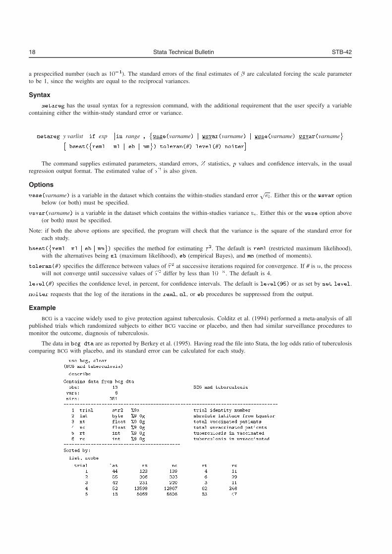
18 Stata Technical Bulletin STB-42
a prespecified number (such as 1���). The standard errors of the final estimates of � are calculated forcing the scale parameterto be 1, since the weights are equal to the reciprocal variances.
Syntax
metareg has the usual syntax for a regression command, with the additional requirement that the user specify a variablecontaining either the within-study standard error or variance.
metareg y varlist�if exp
� �in range
���wsse�varname� j wsvar�varname� j wsse�varname� wsvar�varname
��bsest�
�reml j ml j eb j mm
�� toleran�#� level�#� noiter
�
The command supplies estimated parameters, standard errors, Z statistics, p values and confidence intervals, in the usualregression output format. The estimated value of �� is also given.
Options
wsse�varname� is a variable in the dataset which contains the within-studies standard errorpvi. Either this or the wsvar option
below (or both) must be specified.
wsvar�varname� is a variable in the dataset which contains the within-studies variance vi. Either this or the wsse option above(or both) must be specified.
Note: if both the above options are specified, the program will check that the variance is the square of the standard error foreach study.
bsest��reml j ml j eb j mm�� specifies the method for estimating ��. The default is reml (restricted maximum likelihood),
with the alternatives being ml (maximum likelihood), eb (empirical Bayes), and mm (method of moments).
toleran�#� specifies the difference between values of b�� at successive iterations required for convergence. If # is n, the processwill not converge until successive values of b�� differ by less than ��
�n. The default is 4.
level�#� specifies the confidence level, in percent, for confidence intervals. The default is level���� or as set by set level.
noiter requests that the log of the iterations in the reml, ml, or eb procedures be suppressed from the output.
Example
BCG is a vaccine widely used to give protection against tuberculosis. Colditz et al. (1994) performed a meta-analysis of allpublished trials which randomized subjects to either BCG vaccine or placebo, and then had similar surveillance procedures tomonitor the outcome, diagnosis of tuberculosis.
The data in bcg�dta are as reported by Berkey et al. (1995). Having read the file into Stata, the log odds ratio of tuberculosiscomparing BCG with placebo, and its standard error can be calculated for each study.
� use bcg� clear�BCG and tuberculosis�
� describe
Contains data from bcg�dtaobs� �� BCG and tuberculosisvars� �size� ��
�� trial str� � s trial identity number�� lat byte � ��g absolute latitude from Equator�� nt float � ��g total vaccinated patients�� nc float � ��g total unvaccinated patients� rt int � ��g tuberculosis in vaccinated�� rc int � ��g tuberculosis in unvaccinated
Sorted by�
� list� noobs
trial lat nt nc rt rc� �� ��� �� � ��� ��� ��� � � � �� ��� ��� � ��� � �� � ����� �� ��� �� �� ��� �� ��
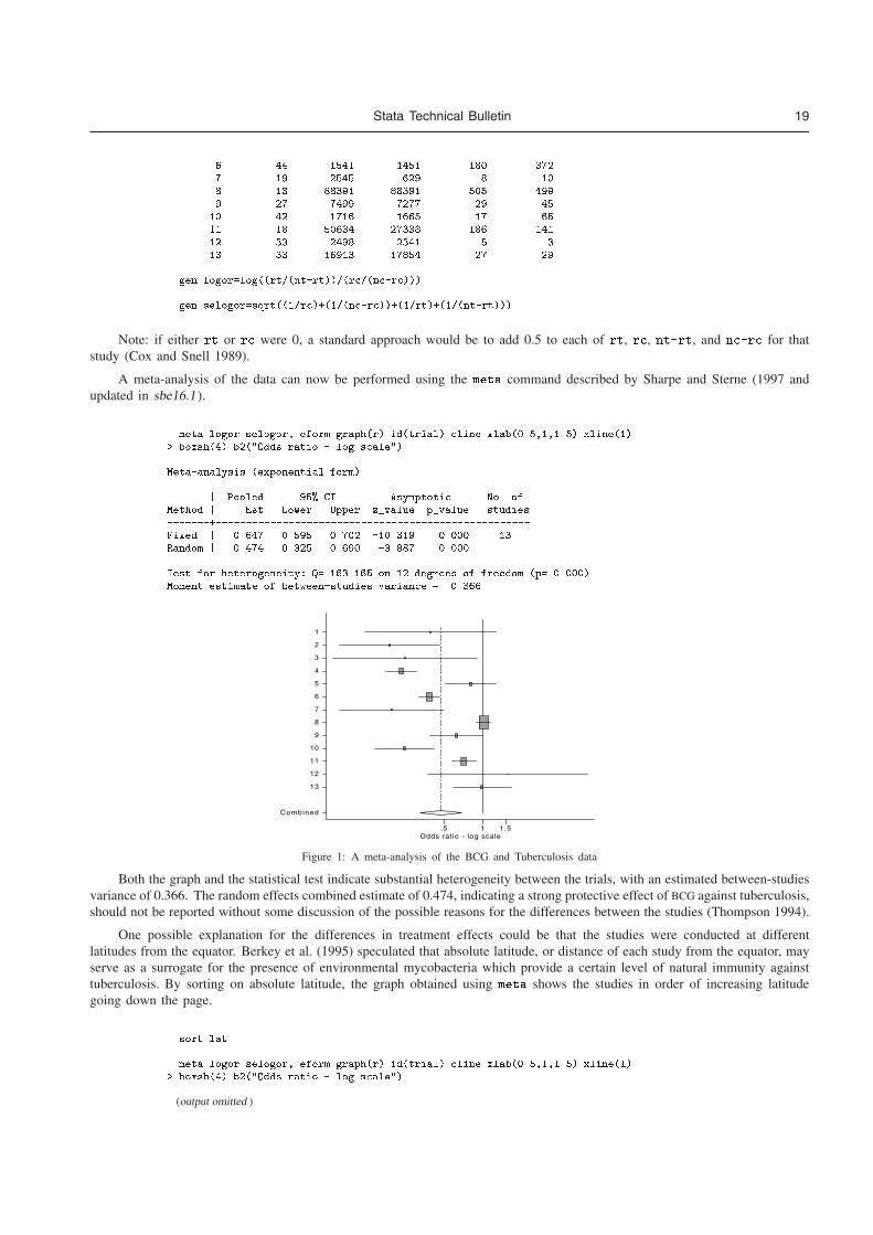
Stata Technical Bulletin 19
� �� ���� ���� ��� ��� � ��� � � ��� �� ���� ���� ��� � � �� ��� ��
�� � ���� ���� �� ���� �� ����� ���� ��� ���� �� �� ��� � ��� �� ���� ����� �
� gen logor�log rt� nt�rt��� rc� nc�rc���
� gen selogor�sqrt ��rc�� �� nc�rc��� ��rt�� �� nt�rt���
Note: if either rt or rc were 0, a standard approach would be to add 0.5 to each of rt, rc, nt�rt, and nc�rc for thatstudy (Cox and Snell 1989).
A meta-analysis of the data can now be performed using the meta command described by Sharpe and Sterne (1997 andupdated in sbe16.1).
� meta logor selogor� eform graph r� id trial� cline xlab ���������� xline ��� boxsh �� b �Odds ratio � log scale��
Meta�analysis exponential form�
� Pooled �� CI Asymptotic No� ofMethod � Est Lower Upper z�value p�value studies������������������������������������������������������������Fixed � ����� ���� ���� ������ ����� ��Random � ����� ���� ���� ������ �����
Test for heterogeneity� Q� ������� on � degrees of freedom p� ������Moment estimate of between�studies variance � �����
Odds ratio - log scale.5 1 1.5
Combined
13
12
11
10
9
8
7
6
5
4
3
2
1
Figure 1: A meta-analysis of the BCG and Tuberculosis data
Both the graph and the statistical test indicate substantial heterogeneity between the trials, with an estimated between-studiesvariance of 0.366. The random effects combined estimate of 0.474, indicating a strong protective effect of BCG against tuberculosis,should not be reported without some discussion of the possible reasons for the differences between the studies (Thompson 1994).
One possible explanation for the differences in treatment effects could be that the studies were conducted at differentlatitudes from the equator. Berkey et al. (1995) speculated that absolute latitude, or distance of each study from the equator, mayserve as a surrogate for the presence of environmental mycobacteria which provide a certain level of natural immunity againsttuberculosis. By sorting on absolute latitude, the graph obtained using meta shows the studies in order of increasing latitudegoing down the page.
� sort lat
� meta logor selogor� eform graph r� id trial� cline xlab ���������� xline ��� boxsh �� b �Odds ratio � log scale��
(output omitted )
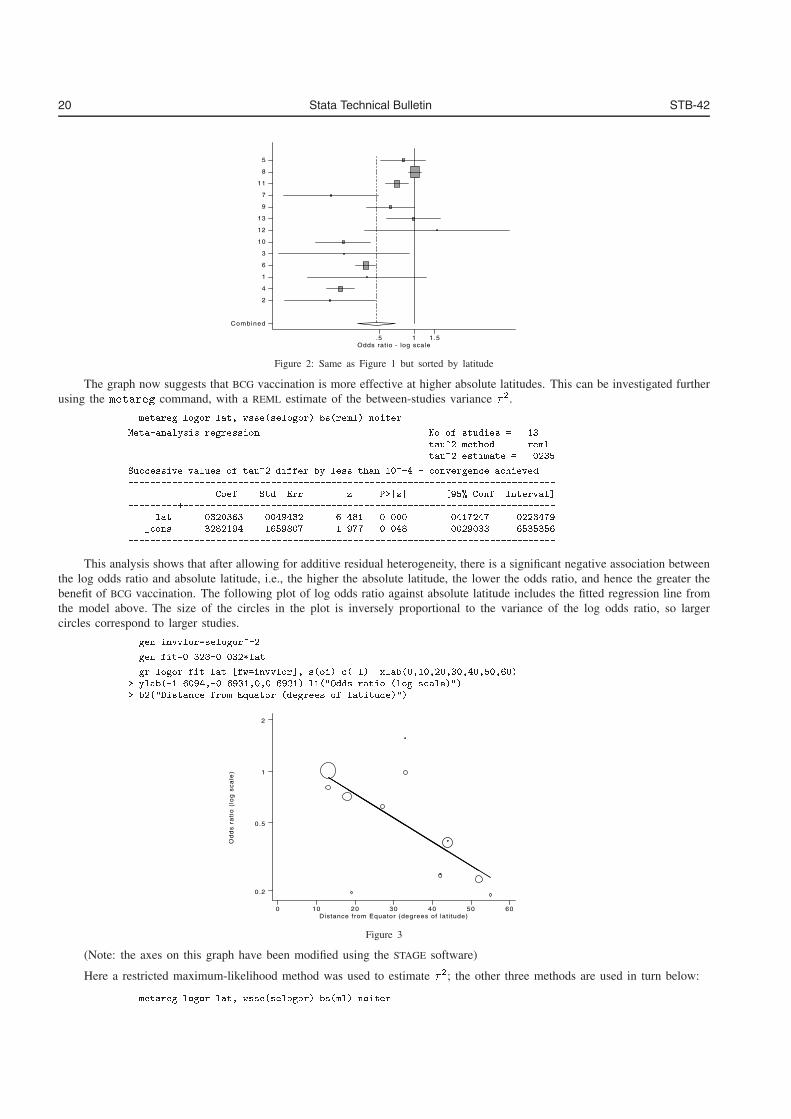
20 Stata Technical Bulletin STB-42
Odds ratio - log scale.5 1 1.5
Combined
2
4
1
6
3
10
12
13
9
7
11
8
5
Figure 2: Same as Figure 1 but sorted by latitude
The graph now suggests that BCG vaccination is more effective at higher absolute latitudes. This can be investigated furtherusing the metareg command, with a REML estimate of the between-studies variance �
�.
� metareg logor lat� wsse�selogor� bs�reml� noiter
Meta�analysis regression No of studies � ��tau method remltau estimate � ����
Successive values of tau differ by less than ��� � convergence achieved������������������������������������������������������������������������������
� Coef� Std� Err� z P��z� ���� Conf� Interval�������������������������������������������������������������������������������
lat � �������� ��� � � ��� �� ����� ��� �� � ���� ���cons � ����� �������� ����� ��� � ������� ��������
������������������������������������������������������������������������������
This analysis shows that after allowing for additive residual heterogeneity, there is a significant negative association betweenthe log odds ratio and absolute latitude, i.e., the higher the absolute latitude, the lower the odds ratio, and hence the greater thebenefit of BCG vaccination. The following plot of log odds ratio against absolute latitude includes the fitted regression line fromthe model above. The size of the circles in the plot is inversely proportional to the variance of the log odds ratio, so largercircles correspond to larger studies.
� gen invvlor�selogor�
� gen fit�����������lat
� gr logor fit lat �fw�invvlor�� s�oi� c��l� xlab����������� ��������� ylab������� ������������������ l���Odds ratio �log scale���� b��Distance from Equator �degrees of latitude���
Od
ds
ra
tio
(lo
g s
ca
le)
Distance from Equator (degrees of lat i tude)0 10 20 30 40 50 60
0.2
0.5
1
2
Figure 3
(Note: the axes on this graph have been modified using the STAGE software)
Here a restricted maximum-likelihood method was used to estimate ��; the other three methods are used in turn below:
� metareg logor lat� wsse�selogor� bs�ml� noiter
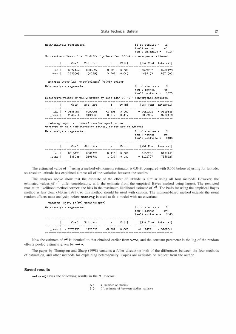
Stata Technical Bulletin 21
Meta�analysis regression No of studies � ��tau�� method mltau�� estimate � ��
Successive values of tau�� differ by less than ���� � convergence achieved������������������������������������������������������������������������������
� Coef� Std� Err� z P �z� ���� Conf� Interval�������������������������������������������������������������������������������
lat � ������ ����� ������ � ������ ���������cons � ������ ������� ����� � ������ �����
������������������������������������������������������������������������������
� metareg logor lat� wsse�selogor� bs�eb� noiter
Meta�analysis regression No of studies � ��tau�� method ebtau�� estimate � ����
Successive values of tau�� differ by less than ���� � convergence achieved������������������������������������������������������������������������������
� Coef� Std� Err� z P �z� ���� Conf� Interval�������������������������������������������������������������������������������
lat � ������ ��� ������ �� ������� ���������cons � �������� �������� ���� ��� �������� �����
������������������������������������������������������������������������������
� metareg logor lat� bs�mm� wsse�selogor� noiterWarning� mm is a non�iterative method� noiter option ignored
Meta�analysis regression No of studies � ��tau�� method mmtau�� estimate � ���
������������������������������������������������������������������������������� Coef� Std� Err� z P �z� ���� Conf� Interval�
������������������������������������������������������������������������������lat � ������� ����� ������ � ������ �������
�cons � ����� ������ ���� ���� ������ ������������������������������������������������������������������������������������
The estimated value of �� using a method-of-moments estimator is 0.048, compared with 0.366 before adjusting for latitude,so absolute latitude has explained almost all of the variation between the studies.
The analyses above show that the estimate of the effect of latitude is similar using all four methods. However, theestimated values of �
� differ considerably, with the estimate from the empirical Bayes method being largest. The restrictedmaximum-likelihood method corrects the bias in the maximum-likelihood estimate of ��. The basis for using the empirical Bayesmethod is less clear (Morris 1983), so this method should be used with caution. The moment-based method extends the usualrandom-effects meta-analysis; below metareg is used to fit a model with no covariate:
� metareg logor� bs�mm� wsse�selogor�
Meta�analysis regression No of studies � ��tau�� method mmtau�� estimate � �����
������������������������������������������������������������������������������� Coef� Std� Err� z P �z� ���� Conf� Interval�
�������������������������������������������������������������������������������cons � ������� �������� ����� � ��������� �������
������������������������������������������������������������������������������
Now the estimate of �� is identical to that obtained earlier from meta, and the constant parameter is the log of the random
effects pooled estimate given by meta.
The paper by Thompson and Sharp (1998) contains a fuller discussion both of the differences between the four methodsof estimation, and other methods for explaining heterogeneity. Copies are available on request from the author.
Saved results
metareg saves the following results in the S macros:
S � k, number of studiesS � ��
�, estimate of between-studies variance
22 Stata Technical Bulletin STB-42
Acknowledgment
I am grateful to Simon Thompson, Ian White, and Jonathan Sterne for their helpful comments on earlier versions of thiscommand.
ReferencesBerkey, C. S., D. C. Hoaglin, F. Mosteller, and G. A. Colditz. 1995. A random-effects regression model for meta-analysis. Statistics in Medicine 14:
395–411.
Colditz, G. A., T. F. Brewer, C. S. Berkey, M. E. Wilson, E. Burdick, H. V. Fineberg, et al. 1994. Efficacy of BCG vaccine in the prevention oftuberculosis. Meta-analysis of the published literature. Journal of the American Medical Association 271: 698–702.
Cox, D. R. and E. J. Snell. 1989. Analysis of Binary Data. 2d ed. London: Chapman and Hall.
DerSimonian, R. and N. M. Laird. 1986. Meta-analysis in clinical trials. Controlled Clinical Trials 7: 177–188.
DuMouchel, W. and J. Harris. 1983. Bayes methods for combining the results of cancer studies in humans and other species. Journal of the AmericanStatistical Association 78: 291–308.
Lau, J., J. P. A. Ioannidis, and C. H. Schmid. 1998. Summing up evidence: one answer is not always enough. Lancet 351: 123–127.
Morris, C. N. 1983. Parametric empirical Bayes inference: theory and applications. Journal of the American Statistical Association 78: 47–55.
Pocock, S. J., D. G. Cook, and S. A. A. Beresford. 1981. Regression of area mortality rates on explanatory variables: what weighting is appropriate?Applied Statistics 30: 286–295.
Sharp, S. and J. Sterne. 1997. sbe16: Meta-analysis. Stata Technical Bulletin 38: 9–14.
——. 1998. sbe16.1: New syntax and output for the meta-analysis command. Stata Technical Bulletin 42: 6–8.
Thompson, S. G. 1994. Why sources of heterogeneity in meta-analysis should be investigated. British Medical Journal 309: 1351–1355.
Thompson, S. G. and S. J. Sharp. 1998. Explaining heterogeneity in meta-analysis: a comparison of methods. submitted
sg42.2 Displaying predicted probabilities from probit or logit regression
Mead Over, World Bank, FAX: 202-522-3230
Syntax
probpred yvar xvar�if exp
�� from�#� to�#�
�inc�#�
adjust�covlist� one�varlist� zero�varlist� logit
level�#� poly�#� nomodel nolist noplot graph options�
Description
probpred is an extension of the logpred program of Garrett (1995). It first estimates a probit or logit regression of adichotomous (or binary) dependent variable on a set of independent variables. The purpose of probpred is to compute and graphthe estimated relationship between the predicted probability from this regression and one of the independent variables, holdingthe others constant. By default, both probpred and logpred display the regression estimates and a graph and listing of therequested predictions and the forecast interval. probpred contains four additional options not included in the original logpredprogram: logit, one, zero, and level. The default is to estimate a probit regression using the Stata command dprobit, butthe logit option instead estimates a logit model using the logistic command. The one and zero options allow the user tospecify that some of the covariates listed in option adjust are to be set equal to one or zero instead of to their means. Thelevel option allows forecast intervals to be set to confidence levels determined by the user rather than only to 95% confidencelevels.
Options
from�#� specifies the lowest value of xvar for which a prediction is to be calculated. This option is required.
to�#� specifies the highest value of xvar for which a prediction is to be calculated. This option is required.
inc�#� specifies the increment between adjacent values of xvar. The default increment is 1.
adjust�covlist� specifies the other covariates in the model all of which are set to their sample means in computing the predictedvalues unless the one or zero options are specified as described below.
one�varlist� specifies a subset of covlist to be set to one instead of to their mean values in the data.
zero�varlist� specifies a subset of covlist to be set to zero instead of to their mean values in the data.
logit specifies that a logit model will be used. The default is probit.
3 Investigating bias in meta-analysis:
metafunnel, confunnel, metabias, and metatrim
The Stata Journal (2004)4, Number 2, pp. 127–141
Funnel plots in meta-analysis
Jonathan A. C. Sterne and Roger M. HarbordDepartment of Social Medicine, University of BristolCanynge Hall, Whiteladies Road, Bristol BS8 2PR UK
Abstract. Funnel plots are a visual tool for investigating publication and otherbias in meta-analysis. They are simple scatterplots of the treatment effects esti-mated from individual studies (horizontal axis) against a measure of study size(vertical axis). The name “funnel plot” is based on the precision in the estima-tion of the underlying treatment effect increasing as the sample size of componentstudies increases. Therefore, in the absence of bias, results from small studieswill scatter widely at the bottom of the graph, with the spread narrowing amonglarger studies. Publication bias (the association of publication probability withthe statistical significance of study results) may lead to asymmetrical funnel plots.It is, however, important to realize that publication bias is only one of a number ofpossible causes of funnel-plot asymmetry—funnel plots should be seen as a genericmeans of examining small study effects (the tendency for the smaller studies ina meta-analysis to show larger treatment effects) rather than a tool to diagnosespecific types of bias. This article introduces the metafunnel command, whichproduces funnel plots in Stata. In accordance with published recommendations,standard error is used as the measure of study size. Treatment effects expressedas ratio measures (for example risk ratios or odds ratios) may be plotted on a logscale.
Keywords: st0061, metafunnel, funnel plots, meta-analysis, publication bias, small-study effects
1 IntroductionThe substantial recent interest in meta-analysis (the statistical methods that are usedto combine results from a number of different studies) is reflected in a number of user-written commands that do meta-analysis in Stata. Meta-analyses should be based onsystematic reviews of relevant literature. A systematic review is a systematic assembly,critical appraisal, and synthesis of all relevant studies on a specific topic. The mainfeature that distinguishes systematic from narrative reviews is a methods section thatclearly states the question to be addressed and the methods and criteria to be employedfor identifying and selecting relevant studies and extracting and analyzing information(Egger, Davey Smith, and Altman 2001).
While systematic reviews and meta-analyses have the potential to produce preciseestimates of treatment effects that reflect all of the relevant literature, they are notimmune to bias. Publication bias—the association of publication probability with thestatistical significance of study results—is well documented as a problem in the medicalresearch literature (Stern and Simes 1997). Further, it has been demonstrated that ran-domized controlled trials for which concealment of treatment allocation is not adequate,
c© 2004 StataCorp LP st0061
128 Funnel plots in meta-analysis
or which are not double blind, produce estimated treatment effects that appear morebeneficial (Schulz et al. 1995).
2 Funnel plots
Funnel plots are simple scatterplots of the treatment effects estimated from individualstudies against a measure of study size. The name “funnel plot” is based on the precisionin the estimation of the underlying treatment effect increasing as the sample size ofcomponent studies increases. Results from small studies will therefore scatter widelyat the bottom of the graph, with the spread narrowing among larger studies. In theabsence of bias, the plot will resemble a symmetrical, inverted funnel, as shown in thetop graph of figure 1.
If there is bias, for example, because smaller studies showing no statistically signif-icant effects (open circles in figure 1) remain unpublished, then such publication biaswill lead to an asymmetrical appearance of the funnel plot with a gap in the right bot-tom side of the graph (middle graph of figure 1). In this situation, the combined effectfrom meta-analysis will overestimate the treatment’s effect. The more pronounced theasymmetry, the more likely it is that the amount of bias will be substantial.
It is important to realize that publication bias is only one of a number of possible ex-planations for funnel-plot asymmetry; these are discussed in more detail in section 2.3.For example, trials of lower quality yield exaggerated estimates of treatment effects(Schulz et al. 1995). Smaller studies are, on average, conducted and analyzed with lessmethodological rigor than larger studies (Egger et al. 2003), so asymmetry may alsoresult from the overestimation of treatment effects in smaller studies of lower method-ological quality (bottom graph of figure 1). Unfortunately, funnel-plot asymmetry hasoften been equated with publication bias without consideration of its other possibleexplanations; for example, the help file for the metabias command in Stata (written in1998) refers only to publication bias.
(Continued on next page)
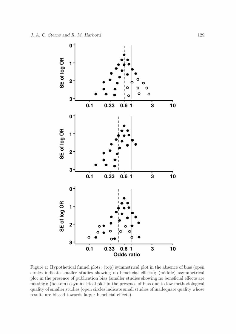
J. A. C. Sterne and R. M. Harbord 129
SE
of l
og O
R
0.1 0.33 1 33
2
1
0
100.6
SE
of l
og O
R
0.1 0.33 1 33
2
1
0
100.6
SE
of l
og O
R
Odds ratio0.1 0.33 1 3
3
2
1
0
100.6
Figure 1: Hypothetical funnel plots: (top) symmetrical plot in the absence of bias (opencircles indicate smaller studies showing no beneficial effects); (middle) asymmetricalplot in the presence of publication bias (smaller studies showing no beneficial effects aremissing); (bottom) asymmetrical plot in the presence of bias due to low methodologicalquality of smaller studies (open circles indicate small studies of inadequate quality whoseresults are biased towards larger beneficial effects).
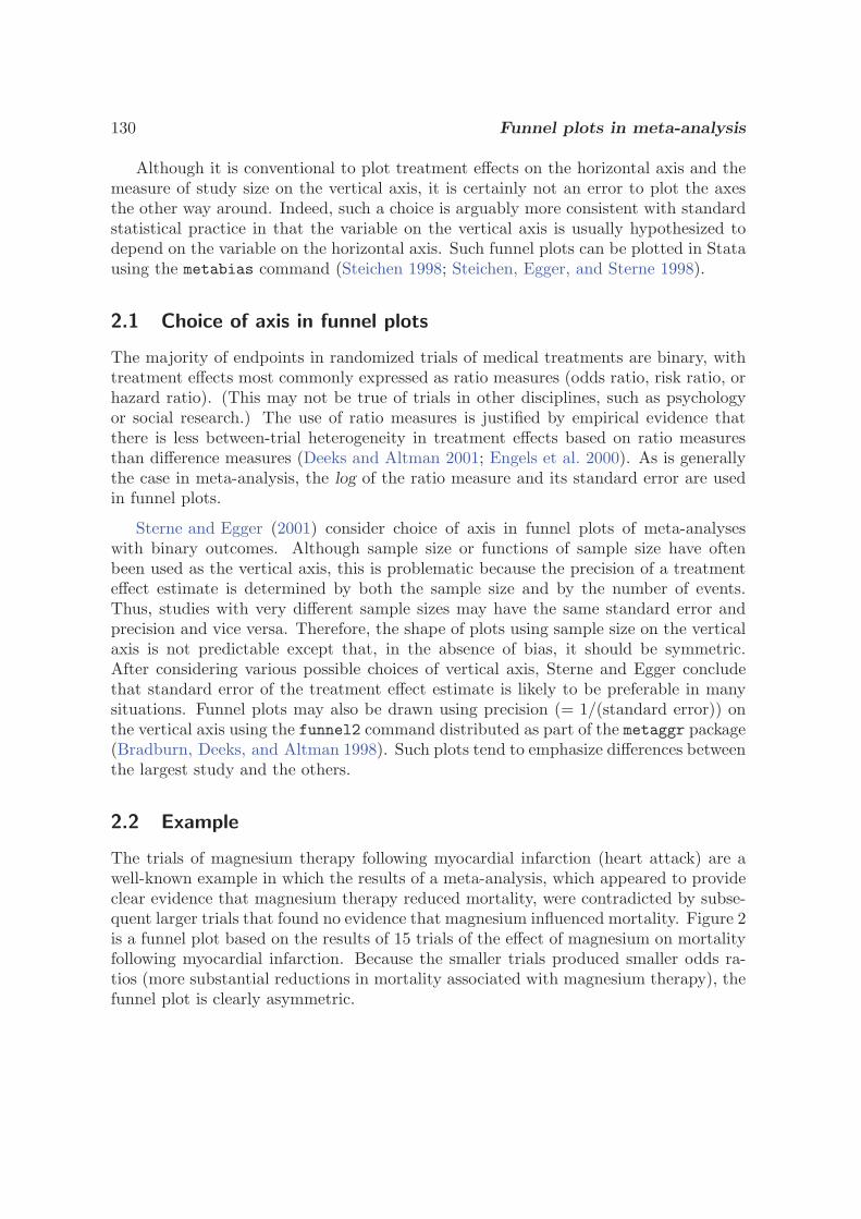
130 Funnel plots in meta-analysis
Although it is conventional to plot treatment effects on the horizontal axis and themeasure of study size on the vertical axis, it is certainly not an error to plot the axesthe other way around. Indeed, such a choice is arguably more consistent with standardstatistical practice in that the variable on the vertical axis is usually hypothesized todepend on the variable on the horizontal axis. Such funnel plots can be plotted in Statausing the metabias command (Steichen 1998; Steichen, Egger, and Sterne 1998).
2.1 Choice of axis in funnel plots
The majority of endpoints in randomized trials of medical treatments are binary, withtreatment effects most commonly expressed as ratio measures (odds ratio, risk ratio, orhazard ratio). (This may not be true of trials in other disciplines, such as psychologyor social research.) The use of ratio measures is justified by empirical evidence thatthere is less between-trial heterogeneity in treatment effects based on ratio measuresthan difference measures (Deeks and Altman 2001; Engels et al. 2000). As is generallythe case in meta-analysis, the log of the ratio measure and its standard error are usedin funnel plots.
Sterne and Egger (2001) consider choice of axis in funnel plots of meta-analyseswith binary outcomes. Although sample size or functions of sample size have oftenbeen used as the vertical axis, this is problematic because the precision of a treatmenteffect estimate is determined by both the sample size and by the number of events.Thus, studies with very different sample sizes may have the same standard error andprecision and vice versa. Therefore, the shape of plots using sample size on the verticalaxis is not predictable except that, in the absence of bias, it should be symmetric.After considering various possible choices of vertical axis, Sterne and Egger concludethat standard error of the treatment effect estimate is likely to be preferable in manysituations. Funnel plots may also be drawn using precision (= 1/(standard error)) onthe vertical axis using the funnel2 command distributed as part of the metaggr package(Bradburn, Deeks, and Altman 1998). Such plots tend to emphasize differences betweenthe largest study and the others.
2.2 Example
The trials of magnesium therapy following myocardial infarction (heart attack) are awell-known example in which the results of a meta-analysis, which appeared to provideclear evidence that magnesium therapy reduced mortality, were contradicted by subse-quent larger trials that found no evidence that magnesium influenced mortality. Figure 2is a funnel plot based on the results of 15 trials of the effect of magnesium on mortalityfollowing myocardial infarction. Because the smaller trials produced smaller odds ra-tios (more substantial reductions in mortality associated with magnesium therapy), thefunnel plot is clearly asymmetric.
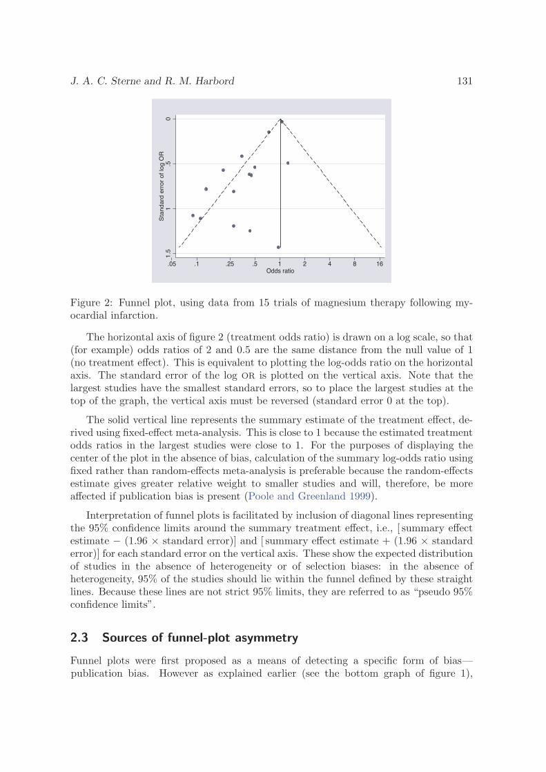
J. A. C. Sterne and R. M. Harbord 131
0.5
11
.5S
tan
da
rd e
rro
r o
f lo
g O
R
.05 .1 .25 .5 1 2 4 8 16Odds ratio
Figure 2: Funnel plot, using data from 15 trials of magnesium therapy following my-ocardial infarction.
The horizontal axis of figure 2 (treatment odds ratio) is drawn on a log scale, so that(for example) odds ratios of 2 and 0.5 are the same distance from the null value of 1(no treatment effect). This is equivalent to plotting the log-odds ratio on the horizontalaxis. The standard error of the log OR is plotted on the vertical axis. Note that thelargest studies have the smallest standard errors, so to place the largest studies at thetop of the graph, the vertical axis must be reversed (standard error 0 at the top).
The solid vertical line represents the summary estimate of the treatment effect, de-rived using fixed-effect meta-analysis. This is close to 1 because the estimated treatmentodds ratios in the largest studies were close to 1. For the purposes of displaying thecenter of the plot in the absence of bias, calculation of the summary log-odds ratio usingfixed rather than random-effects meta-analysis is preferable because the random-effectsestimate gives greater relative weight to smaller studies and will, therefore, be moreaffected if publication bias is present (Poole and Greenland 1999).
Interpretation of funnel plots is facilitated by inclusion of diagonal lines representingthe 95% confidence limits around the summary treatment effect, i.e., [ summary effectestimate − (1.96 × standard error)] and [ summary effect estimate + (1.96 × standarderror)] for each standard error on the vertical axis. These show the expected distributionof studies in the absence of heterogeneity or of selection biases: in the absence ofheterogeneity, 95% of the studies should lie within the funnel defined by these straightlines. Because these lines are not strict 95% limits, they are referred to as “pseudo 95%confidence limits”.
2.3 Sources of funnel-plot asymmetry
Funnel plots were first proposed as a means of detecting a specific form of bias—publication bias. However as explained earlier (see the bottom graph of figure 1),
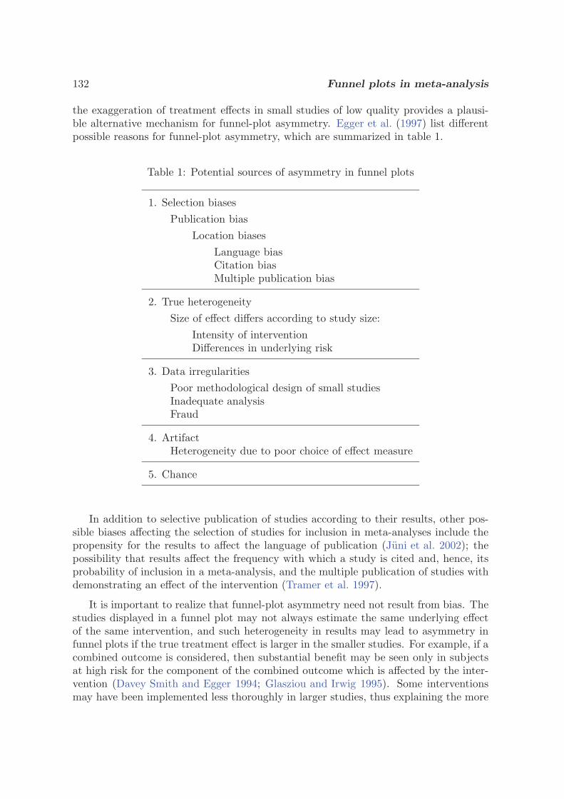
132 Funnel plots in meta-analysis
the exaggeration of treatment effects in small studies of low quality provides a plausi-ble alternative mechanism for funnel-plot asymmetry. Egger et al. (1997) list differentpossible reasons for funnel-plot asymmetry, which are summarized in table 1.
Table 1: Potential sources of asymmetry in funnel plots
1. Selection biasesPublication bias
Location biasesLanguage biasCitation biasMultiple publication bias
2. True heterogeneitySize of effect differs according to study size:
Intensity of interventionDifferences in underlying risk
3. Data irregularitiesPoor methodological design of small studiesInadequate analysisFraud
4. ArtifactHeterogeneity due to poor choice of effect measure
5. Chance
In addition to selective publication of studies according to their results, other pos-sible biases affecting the selection of studies for inclusion in meta-analyses include thepropensity for the results to affect the language of publication (Juni et al. 2002); thepossibility that results affect the frequency with which a study is cited and, hence, itsprobability of inclusion in a meta-analysis, and the multiple publication of studies withdemonstrating an effect of the intervention (Tramer et al. 1997).
It is important to realize that funnel-plot asymmetry need not result from bias. Thestudies displayed in a funnel plot may not always estimate the same underlying effectof the same intervention, and such heterogeneity in results may lead to asymmetry infunnel plots if the true treatment effect is larger in the smaller studies. For example, if acombined outcome is considered, then substantial benefit may be seen only in subjectsat high risk for the component of the combined outcome which is affected by the inter-vention (Davey Smith and Egger 1994; Glasziou and Irwig 1995). Some interventionsmay have been implemented less thoroughly in larger studies, thus explaining the more
J. A. C. Sterne and R. M. Harbord 133
positive results in smaller studies. For example, an asymmetrical funnel plot was foundin a meta-analysis of trials examining the effect of inpatient comprehensive geriatric as-sessment programs on mortality. An experienced consultant geriatrician was more likelyto be actively involved in the smaller trials and this may explain the larger treatmenteffects observed in these trials (Egger et al. 1997; Stuck et al. 1993).
The way in which data irregularities such as low methodological quality of smallerstudies may result in funnel-plot asymmetry was described earlier. Poor choice of effectmeasure may also result in funnel-plot asymmetry; for example, it has been shown thatmeta-analyses in which intervention effects are measured as risk differences are moreheterogeneous than those in which intervention effects are measured as risk ratios orodds ratios (Deeks and Altman 2001; Engels et al. 2000). The inappropriate use of riskdifferences may also result in funnel-plot asymmetry—if the effect of intervention ishomogeneous on the risk ratio scale, then the risk difference will be smaller in studiesthat have low event rates.
2.4 Tests for funnel-plot asymmetry
It is, of course, possible that an asymmetrical funnel plot arises merely by the play ofchance. Statistical tests for funnel-plot asymmetry have been proposed by Begg andMazumdar (1994) and by Egger et al. (1997). These are available in the Stata commandmetabias (Steichen 1998; Steichen, Egger, and Sterne 1998). The test proposed byEgger et al. (1997) is algebraically identical to a test that there is no linear associationbetween the treatment effect and its standard error and, hence, that there is no straight-line association in the funnel plot of treatment effect against its standard error (seeSterne, Gavaghan, and Egger [2000] for details). The corresponding fitted line maybe added to the funnel plot using the egger option of the metafunnel command—seesection 5 below.
2.5 Small-study effects
Funnel-plot asymmetry thus raises the possibility of bias, but it is not proof of bias. Itis important to note, however, that asymmetry (unless produced by chance alone) willalways lead us to question the interpretation of the overall estimate of effect when studiesare combined in a meta-analysis; for example, if the study size predicts the treatmenteffect, what treatment effect will apply if the treatment is adopted in routine practice?Sterne, Egger, and Davey Smith (2001) and Sterne, Gavaghan, and Egger (2000) havesuggested that the funnel plot should be seen as a generic means of examining “small-study effects” (the tendency for the smaller studies in a meta-analysis to show largertreatment effects) rather than as a tool to diagnose specific types of bias.
When funnel-plot asymmetry is found, its possible causes should be carefully consid-ered. For example, how comprehensive was the literature search that located the trialsincluded in the meta-analysis? Does reported trial quality differ between larger andsmaller studies? Is there a plausible reason for the effect of intervention to be greater
134 Funnel plots in meta-analysis
in smaller trials? It is possible that differences between smaller and larger trials areaccounted for by a trial characteristic; this may be investigated using the by() optionof the metafunnel command, as described in section 6 below. Explanations for hetero-geneity may be investigated more formally using meta-regression (Thompson and Sharp1999) to investigate associations between study characteristics and intervention effectestimates. For example, we might investigate evidence that studies in which reportedallocation concealment is unclear or inadequate tend to result in more beneficial treat-ment effect estimates. Meta-regression analyses may be done using the Stata commandmetareg (Sharp 1998); however, it will not necessarily be possible to provide a defini-tive explanation for funnel-plot asymmetry. In medical research, meta-analyses typicallycontain 10 or fewer trials (Sterne, Gavaghan, and Egger 2000). Power to detect associa-tions between study characteristics and intervention effect estimates will therefore oftenbe low, in which case it may not be possible to identify a particular study characteristicas the cause of the heterogeneity.
3 Syntax
metafunnel{
theta{
se | var} | exp(theta) { ll ul[cl] } } [
if exp] [
in range]
[, by(by var)
[var | ci ] nolines forcenull reverse eform egger
graph options]
4 Description
metafunnel plots funnel plots. The syntax for metafunnel is based on the same frame-work as for the meta, metabias, metacum, and metatrim commands. The user providesthe effect estimate as theta (e.g., the log-odds ratio) and a measure of theta’s variability(i.e., its standard error or its variance). Alternatively, the user provides exp(theta) (e.g.,an odds ratio), its confidence interval, and, optionally, the confidence level.
5 Options
by(by var) displays subgroups according to the value of by var. The legend displaysthe value labels for the levels of by var if these are present; otherwise, it displays thevalue of each level of by var.
var and ci indicate the meaning of the input variables in the same way as for the othermeta-analysis commands listed above. The help file for meta gives a full explanation.
nolines specifies that pseudo 95% confidence interval lines not be included in the plot.The default is to include them.
forcenull forces the vertical line at the center of the funnel to be plotted at the nulltreatment effect of zero (1 when the treatment effect is exponentiated). The defaultis for the line to be plotted at the value of the fixed-effect summary estimate.
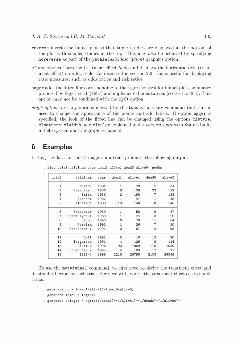
J. A. C. Sterne and R. M. Harbord 135
reverse inverts the funnel plot so that larger studies are displayed at the bottom ofthe plot with smaller studies at the top. This may also be achieved by specifyingnoreverse as part of the yscale(axis description) graphics option.
eform exponentiates the treatment effect theta and displays the horizontal axis (treat-ment effect) on a log scale. As discussed in section 2.2, this is useful for displayingratio measures, such as odds ratios and risk ratios.
egger adds the fitted line corresponding to the regression test for funnel-plot asymmetryproposed by Egger et al. (1997) and implemented in metabias (see section 2.4). Thisoption may not be combined with the by() option.
graph options are any options allowed by the twoway scatter command that can beused to change the appearance of the points and add labels. If option egger isspecified, the look of the fitted line can be changed using the options clstyle,clpattern, clwidth, and clcolor explained under connect options in Stata’s built-in help system and the graphics manual.
6 Examples
Listing the data for the 15 magnesium trials produces the following output:
. list trial trialnam year dead1 alive1 dead0 alive0, noobs
trial trialnam year dead1 alive1 dead0 alive0
1 Morton 1984 1 39 2 342 Rasmussen 1986 9 126 23 1123 Smith 1986 2 198 7 1934 Abraham 1987 1 47 1 455 Feldstedt 1988 10 140 8 140
6 Schechter 1989 1 58 9 477 Ceremuzynski 1989 1 24 3 208 Singh 1990 6 70 11 649 Pereira 1990 1 26 7 2010 Schechter 1 1991 2 87 12 68
11 Golf 1991 5 18 13 2012 Thogersen 1991 4 126 8 11413 LIMIT-2 1992 90 1069 118 103914 Schechter 2 1995 4 103 17 9115 ISIS-4 1995 2216 26795 2103 26936
To use the metafunnel command, we first need to derive the treatment effect andits standard error for each trial. Here, we will express the treatment effects as log-oddsratios.
. generate or = (dead1/alive1)/(dead0/alive0)
. generate logor = log(or)
. generate selogor = sqrt((1/dead1)+(1/alive1)+(1/dead0)+(1/alive0))
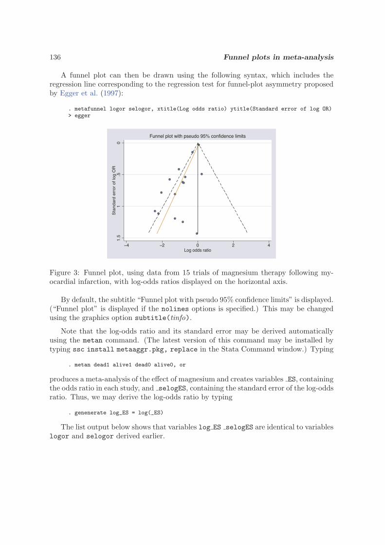
136 Funnel plots in meta-analysis
A funnel plot can then be drawn using the following syntax, which includes theregression line corresponding to the regression test for funnel-plot asymmetry proposedby Egger et al. (1997):
. metafunnel logor selogor, xtitle(Log odds ratio) ytitle(Standard error of log OR)> egger
0.5
11
.5S
tan
da
rd e
rro
r o
f lo
g O
R
�4 �2 0 2 4Log odds ratio
Funnel plot with pseudo 95% confidence limits
Figure 3: Funnel plot, using data from 15 trials of magnesium therapy following my-ocardial infarction, with log-odds ratios displayed on the horizontal axis.
By default, the subtitle “Funnel plot with pseudo 95% confidence limits” is displayed.(“Funnel plot” is displayed if the nolines options is specified.) This may be changedusing the graphics option subtitle(tinfo).
Note that the log-odds ratio and its standard error may be derived automaticallyusing the metan command. (The latest version of this command may be installed bytyping ssc install metaaggr.pkg, replace in the Stata Command window.) Typing
. metan dead1 alive1 dead0 alive0, or
produces a meta-analysis of the effect of magnesium and creates variables ES, containingthe odds ratio in each study, and selogES, containing the standard error of the log-oddsratio. Thus, we may derive the log-odds ratio by typing
. genenerate log_ES = log(_ES)
The list output below shows that variables log ES selogES are identical to variableslogor and selogor derived earlier.

J. A. C. Sterne and R. M. Harbord 137
. list trial trialnam year logor selogor _ES log_ES _selogES, noobs
trial trialnam year logor selogor _ES log_ES _selogES
1 Morton 1984 -.8303483 1.247018 .4358974 -.8303483 1.2470182 Rasmussen 1986 -1.056053 .4140706 .3478261 -1.056053 .41407063 Smith 1986 -1.27834 .8081392 .2784993 -1.27834 .80813924 Abraham 1987 -.0434851 1.42951 .9574468 -.0434851 1.429515 Feldstedt 1988 .2231435 .4891684 1.25 .2231435 .4891684
6 Schechter 1989 -2.40752 1.072208 .0900383 -2.40752 1.0722087 Ceremuzynski 1989 -1.280934 1.193734 .2777778 -1.280934 1.1937348 Singh 1990 -.695748 .5361776 .4987013 -.695748 .53617769 Pereira 1990 -2.208274 1.109648 .1098901 -2.208274 1.10964810 Schechter 1 1991 -2.03816 .7807263 .1302682 -2.03816 .7807263
11 Golf 1991 -.8501509 .6184486 .4273504 -.8501509 .618448612 Thogersen 1991 -.7932307 .6258662 .452381 -.7932307 .625866213 LIMIT-2 1992 -.2993398 .1465729 .7413074 -.2993398 .146572914 Schechter 2 1995 -1.570789 .5740395 .2078812 -1.570789 .574039515 ISIS-4 1995 .0575872 .0316421 1.059278 .0575872 .0316421
The following command was used to produce figure 2 (see section 2.2), in which thehorizontal axis is the treatment odds ratio, displayed on a log scale:
. metafunnel logor selogor, xlab(.05 .1 .25 .5 1 2 4 8 16)> xscale(log) xtitle(Odds ratio) eform subtitle( )> ytitle(Standard error of log OR)
When the eform option is used, the label of the horizontal axis (treatment ef-fect, theta) is changed accordingly, unless there is a variable label for theta or thextitle(axis title) graphics option is used.
Finally, we will illustrate the use of the by() option by grouping the studies accordingto whether they were published during the 1980s or the 1990s:
. generate period = year
. recode period 1980/1989=1 1990/1999=2(period: 15 changes made)
. label define periodlab 1 "1980s" 2 "1990s"
. label values period periodlab
. tab period
period Freq. Percent Cum.
1980s 7 46.67 46.671990s 8 53.33 100.00
Total 15 100.00
Using the latest version of the metan command (Bradburn, Deeks, and Altman1998), we can examine the effect of magnesium separately, according to time period.
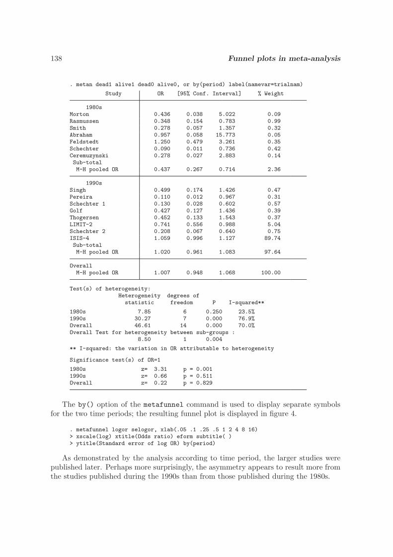
138 Funnel plots in meta-analysis
. metan dead1 alive1 dead0 alive0, or by(period) label(namevar=trialnam)
Study OR [95% Conf. Interval] % Weight
1980sMorton 0.436 0.038 5.022 0.09Rasmussen 0.348 0.154 0.783 0.99Smith 0.278 0.057 1.357 0.32Abraham 0.957 0.058 15.773 0.05Feldstedt 1.250 0.479 3.261 0.35Schechter 0.090 0.011 0.736 0.42Ceremuzynski 0.278 0.027 2.883 0.14Sub-totalM-H pooled OR 0.437 0.267 0.714 2.36
1990sSingh 0.499 0.174 1.426 0.47Pereira 0.110 0.012 0.967 0.31Schechter 1 0.130 0.028 0.602 0.57Golf 0.427 0.127 1.436 0.39Thogersen 0.452 0.133 1.543 0.37LIMIT-2 0.741 0.556 0.988 5.04Schechter 2 0.208 0.067 0.640 0.75ISIS-4 1.059 0.996 1.127 89.74Sub-totalM-H pooled OR 1.020 0.961 1.083 97.64
OverallM-H pooled OR 1.007 0.948 1.068 100.00
Test(s) of heterogeneity:Heterogeneity degrees of
statistic freedom P I-squared**
1980s 7.85 6 0.250 23.5%1990s 30.27 7 0.000 76.9%Overall 46.61 14 0.000 70.0%Overall Test for heterogeneity between sub-groups :
8.50 1 0.004
** I-squared: the variation in OR attributable to heterogeneity
Significance test(s) of OR=1
1980s z= 3.31 p = 0.0011990s z= 0.66 p = 0.511Overall z= 0.22 p = 0.829
The by() option of the metafunnel command is used to display separate symbolsfor the two time periods; the resulting funnel plot is displayed in figure 4.
. metafunnel logor selogor, xlab(.05 .1 .25 .5 1 2 4 8 16)> xscale(log) xtitle(Odds ratio) eform subtitle( )> ytitle(Standard error of log OR) by(period)
As demonstrated by the analysis according to time period, the larger studies werepublished later. Perhaps more surprisingly, the asymmetry appears to result more fromthe studies published during the 1990s than from those published during the 1980s.
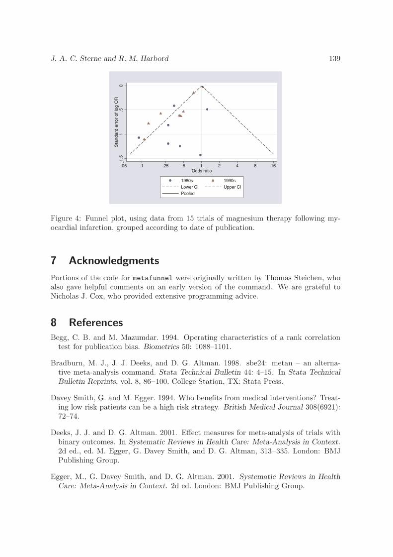
J. A. C. Sterne and R. M. Harbord 139
0.5
11
.5S
tan
da
rd e
rro
r o
f lo
g O
R
.05 .1 .25 .5 1 2 4 8 16Odds ratio
1980s 1990sLower CI Upper CIPooled
Figure 4: Funnel plot, using data from 15 trials of magnesium therapy following my-ocardial infarction, grouped according to date of publication.
7 Acknowledgments
Portions of the code for metafunnel were originally written by Thomas Steichen, whoalso gave helpful comments on an early version of the command. We are grateful toNicholas J. Cox, who provided extensive programming advice.
8 ReferencesBegg, C. B. and M. Mazumdar. 1994. Operating characteristics of a rank correlation
test for publication bias. Biometrics 50: 1088–1101.
Bradburn, M. J., J. J. Deeks, and D. G. Altman. 1998. sbe24: metan – an alterna-tive meta-analysis command. Stata Technical Bulletin 44: 4–15. In Stata TechnicalBulletin Reprints, vol. 8, 86–100. College Station, TX: Stata Press.
Davey Smith, G. and M. Egger. 1994. Who benefits from medical interventions? Treat-ing low risk patients can be a high risk strategy. British Medical Journal 308(6921):72–74.
Deeks, J. J. and D. G. Altman. 2001. Effect measures for meta-analysis of trials withbinary outcomes. In Systematic Reviews in Health Care: Meta-Analysis in Context.2d ed., ed. M. Egger, G. Davey Smith, and D. G. Altman, 313–335. London: BMJPublishing Group.
Egger, M., G. Davey Smith, and D. G. Altman. 2001. Systematic Reviews in HealthCare: Meta-Analysis in Context. 2d ed. London: BMJ Publishing Group.
140 Funnel plots in meta-analysis
Egger, M., G. Davey Smith, M. Schneider, and C. Minder. 1997. Bias in meta-analysisdetected by a simple, graphical test. British Medical Journal 315(7109): 629–634.
Egger, M., P. Juni, C. Bartlett, F. Holenstein, and J. Sterne. 2003. How important arecomprehensive literature searches and the assessment of trial quality in systematicreviews? Empirical study. Health Technology Assessment 7: 1–68.
Engels, E. A., C. H. Schmid, N. T. Terrin, I. Olkin, and J. Lau. 2000. Heterogeneityand statistical significance in meta-analysis: an empirical study of 125 meta-analyses.Statistics in Medicine 19: 1707–1728.
Glasziou, P. P. and L. M. Irwig. 1995. An evidence based approach to individualizingtreatment. British Medical Journal 311(7016): 1356–1359.
Juni, P., F. Holenstein, J. A. C. Sterne, C. Bartlett, and M. Egger. 2002. Directionand impact of language bias in meta-analysis of controlled trials: empirical study.International Journal of Epidemiology 31: 115–123.
Poole, C. and S. Greenland. 1999. Random-effects meta-analyses are not always con-servative. American Journal of Epidemiology 150(5): 469–475.
Schulz, K. F., I. Chalmers, R. J. Hayes, and D. G. Altman. 1995. Empirical evidenceof bias. Dimensions of methodological quality associated with estimates of treatmenteffects in controlled trials. Journal of the American Medical Association 273(5): 408–412.
Sharp, S. 1998. sbe23: Meta-analysis regression. Stata Technical Bulletin 42: 16–22. InStata Technical Bulletin Reprints, vol. 7, 148–155. College Station, TX: Stata Press.
Steichen, T. J. 1998. sbe19: Tests for publication bias in meta-analysis. Stata TechnicalBulletin 41: 9–15. In Stata Technical Bulletin Reprints, vol. 7, 125–133. CollegeStation, TX: Stata Press.
Steichen, T. J., M. Egger, and J. A. C. Sterne. 1998. sbe19.1: Tests for publicationbias in meta-analysis. Stata Technical Bulletin 44: 3–4. In Stata Technical BulletinReprints, vol. 8, 84–85. College Station, TX: Stata Press.
Stern, J. M. and R. J. Simes. 1997. Publication bias: evidence of delayed publicationin a cohort study of clinical research projects. British Medical Journal 315(7109):640–645.
Sterne, J. A. C. and M. Egger. 2001. Funnel plots for detecting bias in meta-analysis:guidelines on choice of axis. Journal of Clinical Epidemiology 54(10): 1046–1055.
Sterne, J. A. C., M. Egger, and G. Davey Smith. 2001. Investigating and dealing withpublication and other bias. In Systematic Reviews in Health Care: Meta-Analysis inContext. 2d ed., ed. M. Egger, D. G. Altman, and G. Davey Smith, 189–208. London:BMJ Publishing Group.
J. A. C. Sterne and R. M. Harbord 141
Sterne, J. A. C., D. Gavaghan, and M. Egger. 2000. Publication and related bias inmeta-analysis: power of statistical tests and prevalence in the literature. Journal ofClinical Epidemiology 53(11): 1119–1129.
Stuck, A. E., A. L. Siu, G. D. Wieland, J. Adams, and L. Z. Rubenstein. 1993. Com-prehensive geriatric assessment: a meta-analysis of controlled trials. Lancet 342:1032–1036.
Thompson, S. G. and S. J. Sharp. 1999. Explaining heterogeneity in meta-analysis: acomparison of methods. Statistics in Medicine 18: 2693–2708.
Tramer, M. R., D. J. Reynolds, R. A. Moore, and H. J. McQuay. 1997. Impact ofcovert duplicate publication on meta-analysis: a case study. British Medical Journal315(7109): 635–640.
About the Authors
Jonathan Sterne is a Reader in Medical Statistics and Epidemiology in the Department ofSocial Medicine, University of Bristol, UK. His research interests include statistical methodsfor epidemiology and health services research, causal models, meta-analysis and systematicreviews, the epidemiology of sexually transmitted infections, and the epidemiology of asthmaand allergic diseases.
Roger Harbord is a Research Associate in Medical Statistics in the Department of SocialMedicine, University of Bristol, UK. His research interests include statistical methods for epi-demiology and health services research, meta-analysis and systematic reviews, and geneticepidemiology.
The Stata Journal (2008)8, Number 2, pp. 242–254
Contour-enhanced funnel plots formeta-analysis
Tom M. PalmerDepartment of Health Sciences
University of Leicester, UK
Jaime L. PetersSchool of Mathematical Sciences
Queensland University of TechnologyBrisbane, Australia
Alex J. SuttonDepartment of Health Sciences
University of Leicester, UK
Santiago G. MorenoDepartment of Health Sciences
University of Leicester, UK
Abstract. Funnel plots are commonly used to investigate publication and relatedbiases in meta-analysis. Although asymmetry in the appearance of a funnel plotis often interpreted as being caused by publication bias, in reality the asymmetrycould be due to other factors that cause systematic differences in the results oflarge and small studies, for example, confounding factors such as differential studyquality. Funnel plots can be enhanced by adding contours of statistical significanceto aid in interpreting the funnel plot. If studies appear to be missing in areas of lowstatistical significance, then it is possible that the asymmetry is due to publicationbias. If studies appear to be missing in areas of high statistical significance, thenpublication bias is a less likely cause of the funnel asymmetry. It is proposedthat this enhancement to funnel plots should be used routinely for meta-analyseswhere it is possible that results could be suppressed on the basis of their statisticalsignificance.
Keywords: gr0033, confunnel, funnel plots, meta-analysis, publication bias, small-study effects
1 Introduction
Publication bias is the phenomenon where studies with uninteresting or unfavorableresults are less likely to be published than those with more favorable results (Rothstein,Sutton, and Borenstein 2005). If publication bias exists, then the published literatureis a biased sample of all studies, and any meta-analysis based on it will be similarlybiased.
Funnel plots are commonly used to investigate publication and related biases inmeta-analysis (Sterne, Becker, and Egger 2005). They consist of a simple scatterplot ofeach study’s estimate of effect against some measure of its variability, commonly plottedon the x and y axes, respectively (although this goes against the usual convention ofplotting the response variable on the y axis). In this way, the studies with the leastvariable effect sizes appear at the top of the funnel, and the smaller, less precise studiesappear at the bottom. In the absence of publication bias, the studies will fan out in
c© 2008 StataCorp LP gr0033
T. M. Palmer, J. L. Peters, A. J. Sutton, and S. G. Moreno 243
a symmetrical funnel shape around the pooled estimate, as variability due to samplingerror increases down the y axis. If publication bias is present, then the funnel willappear asymmetric because of the systematic suppression of studies.
A complication in interpreting funnel plots is that funnel asymmetry could be dueto factors other than publication bias, such as systematic differences in the results oflarge and small studies caused by confounding factors such as differential study quality;these differences are sometimes called small-study effects (Sterne and Egger 2001). Theaim of the contour-enhanced funnel plot is to aid in disentangling these different causesof funnel asymmetry (Peters et al. 2008).
Funnel plots in Stata were previously described by Sterne and Harbord (2004),and there are several commands available in Stata for drawing funnel plots includ-ing metafunnel, funnel (available with metan), and metabias. These commands aredescribed in more detail in a frequently asked question about the Stata commands avail-able for meta-analysis; the frequently asked question can be found on Stata’s web siteat http://www.stata.com/support/faqs/stat/meta.html. In Stata 10, typing help metadisplays a help file with information about the user-written commands for meta-analysisand tells which are the latest versions.
This article introduces another command for meta-analysis called confunnel, whichproduces contour-enhanced funnel plots. The concept of the contour-enhanced funnelplot is explained in the next section, followed by a description of the command syntaxand options. The use of confunnel is demonstrated on a well-known meta-analysisexample, and the use of the command is also explained in conjunction with some of theother user-written meta-analysis commands.
2 Contour-enhanced funnel plots
There is evidence that, generally, the primary driver for the suppression of studies isthe level of statistical significance of study results, with studies that do not attainperceived milestones of statistical significance (i.e., p < 0.05 or 0.01) being less likelyto be published (Easterbrook et al. 1991; Dickersin 1997; Ioannidis 1998). Despite this,no method has been previously considered to identify the areas of the funnel plot thatcorrespond to different levels of statistical significance, to assess whether any observedasymmetry is likely caused by publication bias.
On a contour-enhanced funnel plot, contours of statistical significance are overlaidon the funnel plot (Peters et al. 2008). Adding contours of statistical significance inthis way facilitates the assessment of whether the areas where studies exist are areasof statistical significance and whether the areas where studies are potentially missingcorrespond to areas of low statistical significance. If studies appear to be missing inareas of low statistical significance, then it is possible that the asymmetry is due topublication bias. Conversely, if the area where studies are perceived to be missing areareas of high statistical significance, then publication bias is a less likely cause of thefunnel asymmetry.
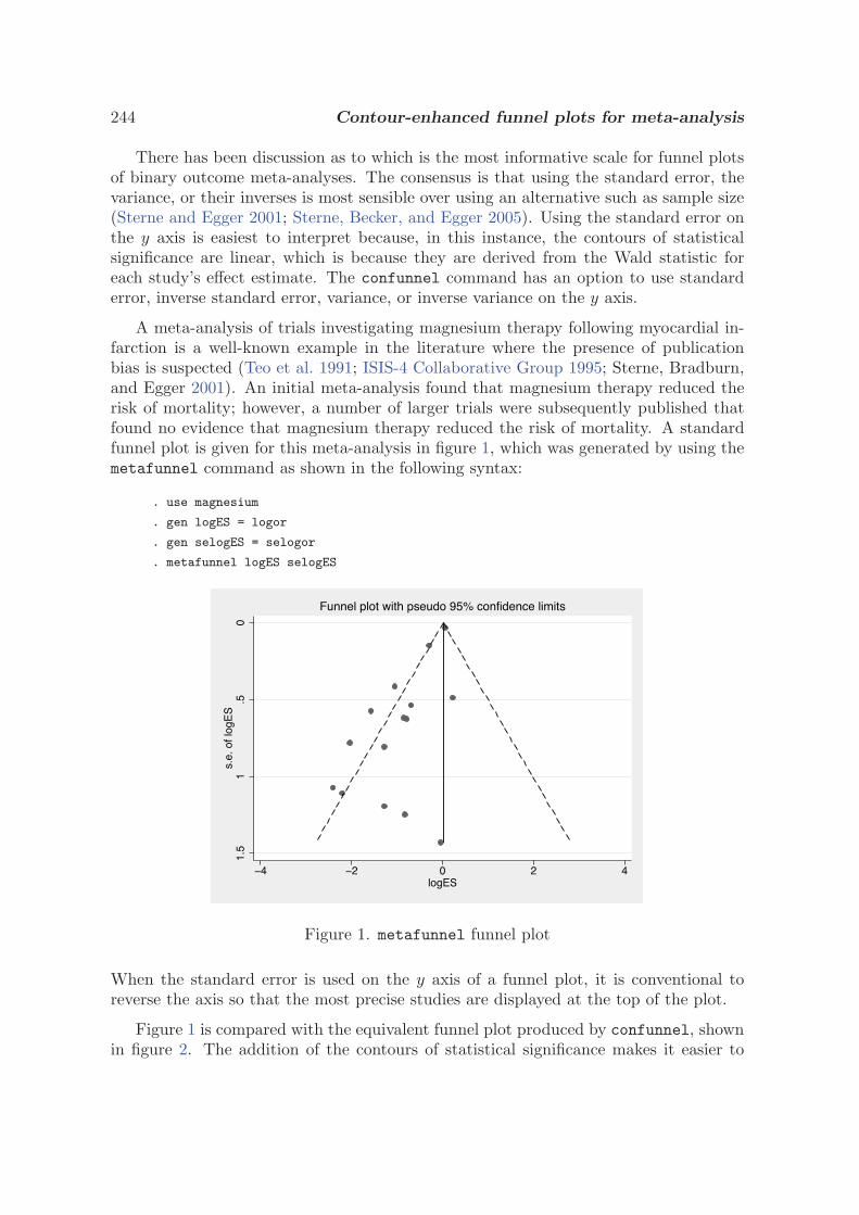
244 Contour-enhanced funnel plots for meta-analysis
There has been discussion as to which is the most informative scale for funnel plotsof binary outcome meta-analyses. The consensus is that using the standard error, thevariance, or their inverses is most sensible over using an alternative such as sample size(Sterne and Egger 2001; Sterne, Becker, and Egger 2005). Using the standard error onthe y axis is easiest to interpret because, in this instance, the contours of statisticalsignificance are linear, which is because they are derived from the Wald statistic foreach study’s effect estimate. The confunnel command has an option to use standarderror, inverse standard error, variance, or inverse variance on the y axis.
A meta-analysis of trials investigating magnesium therapy following myocardial in-farction is a well-known example in the literature where the presence of publicationbias is suspected (Teo et al. 1991; ISIS-4 Collaborative Group 1995; Sterne, Bradburn,and Egger 2001). An initial meta-analysis found that magnesium therapy reduced therisk of mortality; however, a number of larger trials were subsequently published thatfound no evidence that magnesium therapy reduced the risk of mortality. A standardfunnel plot is given for this meta-analysis in figure 1, which was generated by using themetafunnel command as shown in the following syntax:
. use magnesium
. gen logES = logor
. gen selogES = selogor
. metafunnel logES selogES
0.5
11.
5s.
e. o
f log
ES
�4 �2 0 2 4logES
Funnel plot with pseudo 95% confidence limits
Figure 1. metafunnel funnel plot
When the standard error is used on the y axis of a funnel plot, it is conventional toreverse the axis so that the most precise studies are displayed at the top of the plot.
Figure 1 is compared with the equivalent funnel plot produced by confunnel, shownin figure 2. The addition of the contours of statistical significance makes it easier to
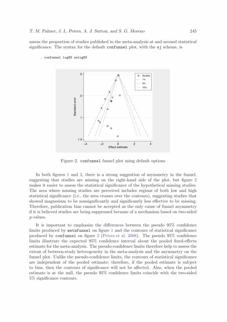
T. M. Palmer, J. L. Peters, A. J. Sutton, and S. G. Moreno 245
assess the proportion of studies published in the meta-analysis at and around statisticalsignificance. The syntax for the default confunnel plot, with the sj scheme, is
. confunnel logES selogES
0
.5
1
1.5
Sta
ndar
d er
ror
�4 �2 0 2 4Effect estimate
Studies
1%
5%
10%
Figure 2. confunnel funnel plot using default options
In both figures 1 and 2, there is a strong suggestion of asymmetry in the funnel,suggesting that studies are missing on the right-hand side of the plot, but figure 2makes it easier to assess the statistical significance of the hypothetical missing studies.The area where missing studies are perceived includes regions of both low and highstatistical significance (i.e., the area crosses over the contours), suggesting studies thatshowed magnesium to be nonsignificantly and significantly less effective to be missing.Therefore, publication bias cannot be accepted as the only cause of funnel asymmetryif it is believed studies are being suppressed because of a mechanism based on two-sidedp-values.
It is important to emphasize the differences between the pseudo 95% confidencelimits produced by metafunnel on figure 1 and the contours of statistical significanceproduced by confunnel on figure 2 (Peters et al. 2008). The pseudo 95% confidencelimits illustrate the expected 95% confidence interval about the pooled fixed-effectsestimate for the meta-analysis. The pseudo-confidence limits therefore help to assess theextent of between-study heterogeneity in the meta-analysis and the asymmetry on thefunnel plot. Unlike the pseudo-confidence limits, the contours of statistical significanceare independent of the pooled estimate; therefore, if the pooled estimate is subjectto bias, then the contours of significance will not be affected. Also, when the pooledestimate is at the null, the pseudo 95% confidence limits coincide with the two-sided5% significance contours.

246 Contour-enhanced funnel plots for meta-analysis
3 The confunnel command
The confunnel command plots contour-enhanced funnel plots for study outcome mea-sures in a meta-analysis. Contours of statistical significance from one- or two-sidedWald tests can be plotted using shaded or dashed contour lines. Contours can be plot-ted along any number of chosen levels of statistical significance; by default, 1%, 5%,and 10% significance contours are plotted. As previously mentioned, confunnel hasthe choice of four y axes. The command also has been designed to be flexible, allowingthe user to add extra features to the funnel plot.
3.1 Syntax
confunnel varname1 varname2[if] [
in] [
, aspectratio(string)
contours(numlist) contcolor(color) extraplot(plots)
functionlowopts(options) functionuppopts(options) legendlabels(labels)
legendopts(options) metric(se | invse | var | invvar) onesided(lower | upper)scatteropts(options) shadedcontours solidcontours twowayopts(options)
]
The first variable, varname1 is the variable corresponding to the effect estimates, oftenlog odds ratios, and the second variable, varname2, is the variable corresponding to thestandard errors of the effect estimates.
3.2 Options
aspectratio(string) specifies the aspect ratio for the plot; the default is 1.
contours(numlist) specifies the significance levels of the contours to be plotted; thedefault is set to 1%, 5%, and 10% significance levels.
contcolor(color) specifies the color of the contour lines if shadedcontours is notspecified.
extraplot(plots) specifies one or multiple additional plots to be overlaid on the funnelplot.
functionlowopts(options) and functionuppopts(options) pass options to the twowayfunction commands used to draw the significance contours; for example, the linewidths can be changed.
legendlabels(labels) specifies labels to appear in the legend for extra elements addedto the funnel plot.
legendopts(options) passes options to the plot legend.
metric(se | invse | var | invvar) specifies the metric of the y axis of the plot. se,invse, var, and invvar stand for standard error, inverse standard error, variance,and inverse variance, respectively; the default is se.
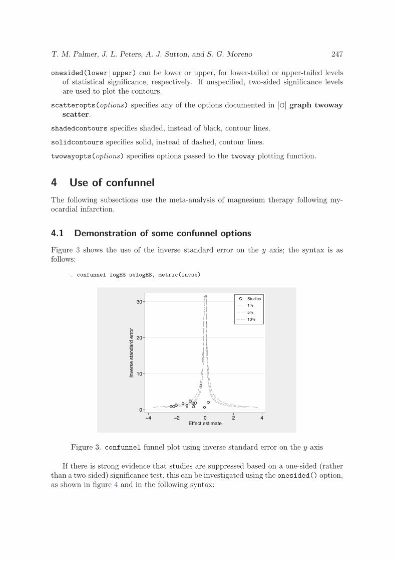
T. M. Palmer, J. L. Peters, A. J. Sutton, and S. G. Moreno 247
onesided(lower | upper) can be lower or upper, for lower-tailed or upper-tailed levelsof statistical significance, respectively. If unspecified, two-sided significance levelsare used to plot the contours.
scatteropts(options) specifies any of the options documented in [G] graph twowayscatter.
shadedcontours specifies shaded, instead of black, contour lines.
solidcontours specifies solid, instead of dashed, contour lines.
twowayopts(options) specifies options passed to the twoway plotting function.
4 Use of confunnel
The following subsections use the meta-analysis of magnesium therapy following my-ocardial infarction.
4.1 Demonstration of some confunnel options
Figure 3 shows the use of the inverse standard error on the y axis; the syntax is asfollows:
. confunnel logES selogES, metric(invse)
0
10
20
30
Inve
rse
stan
dard
err
or
�4 �2 0 2 4Effect estimate
Studies
1%
5%
10%
Figure 3. confunnel funnel plot using inverse standard error on the y axis
If there is strong evidence that studies are suppressed based on a one-sided (ratherthan a two-sided) significance test, this can be investigated using the onesided() option,as shown in figure 4 and in the following syntax:
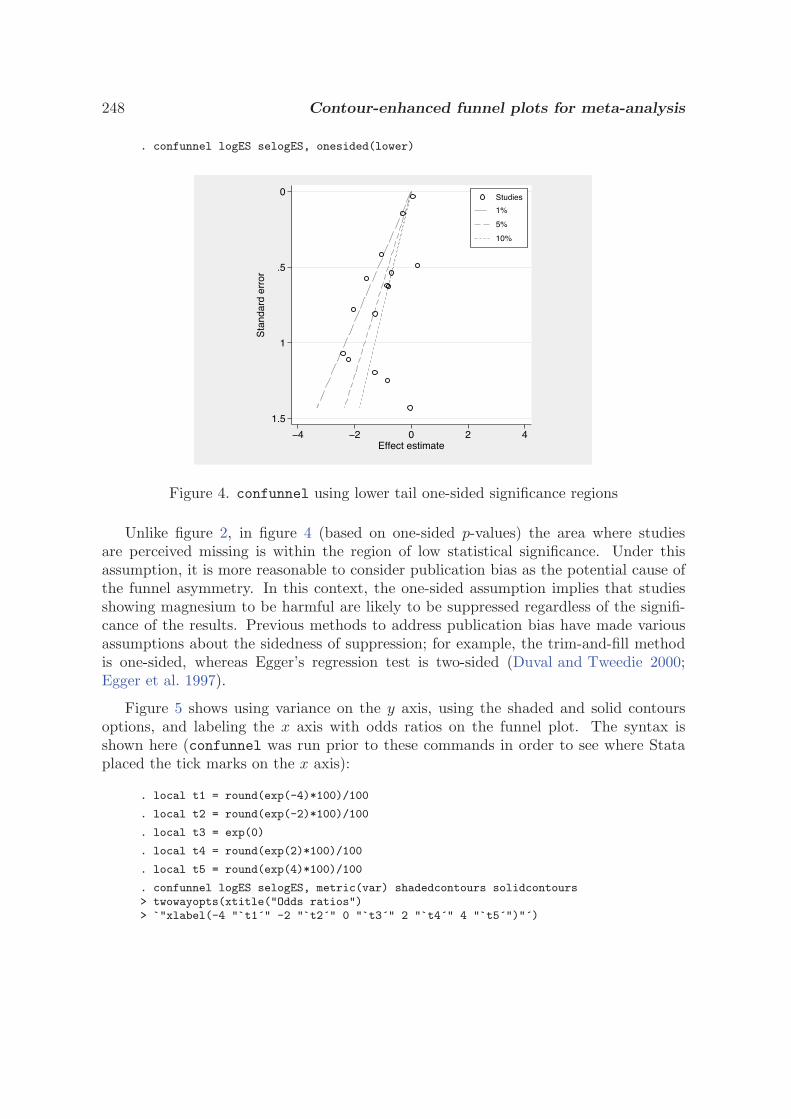
248 Contour-enhanced funnel plots for meta-analysis
. confunnel logES selogES, onesided(lower)
0
.5
1
1.5
Sta
ndar
d er
ror
�4 �2 0 2 4Effect estimate
Studies
1%
5%
10%
Figure 4. confunnel using lower tail one-sided significance regions
Unlike figure 2, in figure 4 (based on one-sided p-values) the area where studiesare perceived missing is within the region of low statistical significance. Under thisassumption, it is more reasonable to consider publication bias as the potential cause ofthe funnel asymmetry. In this context, the one-sided assumption implies that studiesshowing magnesium to be harmful are likely to be suppressed regardless of the signifi-cance of the results. Previous methods to address publication bias have made variousassumptions about the sidedness of suppression; for example, the trim-and-fill methodis one-sided, whereas Egger’s regression test is two-sided (Duval and Tweedie 2000;Egger et al. 1997).
Figure 5 shows using variance on the y axis, using the shaded and solid contoursoptions, and labeling the x axis with odds ratios on the funnel plot. The syntax isshown here (confunnel was run prior to these commands in order to see where Stataplaced the tick marks on the x axis):
. local t1 = round(exp(-4)*100)/100
. local t2 = round(exp(-2)*100)/100
. local t3 = exp(0)
. local t4 = round(exp(2)*100)/100
. local t5 = round(exp(4)*100)/100
. confunnel logES selogES, metric(var) shadedcontours solidcontours> twowayopts(xtitle("Odds ratios")> `"xlabel(-4 "`t1´" -2 "`t2´" 0 "`t3´" 2 "`t4´" 4 "`t5´")"´)
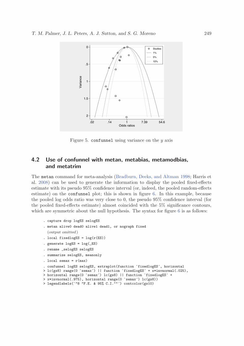
T. M. Palmer, J. L. Peters, A. J. Sutton, and S. G. Moreno 249
0
.5
1
1.5
2
Var
ianc
e
.02 .14 1 7.39 54.6Odds ratios
Studies
1%
5%
10%
Figure 5. confunnel using variance on the y axis
4.2 Use of confunnel with metan, metabias, metamodbias,and metatrim
The metan command for meta-analysis (Bradburn, Deeks, and Altman 1998; Harris etal. 2008) can be used to generate the information to display the pooled fixed-effectsestimate with its pseudo 95% confidence interval (or, indeed, the pooled random-effectsestimate) on the confunnel plot; this is shown in figure 6. In this example, becausethe pooled log odds ratio was very close to 0, the pseudo 95% confidence interval (forthe pooled fixed-effects estimate) almost coincided with the 5% significance contours,which are symmetric about the null hypothesis. The syntax for figure 6 is as follows:
. capture drop logES selogES
. metan alive0 dead0 alive1 dead1, or nograph fixed
(output omitted )
. local fixedlogES = log(r(ES))
. generate logES = log(_ES)
. rename _selogES selogES
. summarize selogES, meanonly
. local semax = r(max)
. confunnel logES selogES, extraplot(function `fixedlogES´, horizontal> lc(gs8) range(0 `semax´) || function `fixedlogES´ + x*invnormal(.025),> horizontal range(0 `semax´) lc(gs8) || function `fixedlogES´ +> x*invnormal(.975), horizontal range(0 `semax´) lc(gs8))> legendlabels(`"8 "F.E. & 95% C.I.""´) contcolor(gs10)

250 Contour-enhanced funnel plots for meta-analysis
0
.5
1
1.5
Sta
ndar
d er
ror
�4 �2 0 2 4Effect estimate
Studies
1%
5%
10%
F.E. & 95% C.I.
Figure 6. confunnel with metafunnel features using metan
Egger’s test investigating possible small-study reporting bias can be represented onthe funnel plot by using the information from the metabias command (Egger et al.1997; Steichen 1998); this is shown in figure 7 and in the following syntax:
. metabias logES selogES, graph(egger)
(output omitted )
. matrix b = e(b)
. local bias = b[1,2]
. local slope = b[1,1]
. summarize selogES, meanonly
. local semax = r(max)
. metamodbias alive0 dead0 alive1 dead1, graph
(output omitted )
. matrix c = e(b)
. local modbias = c[1,2]
. local modslope = c[1,1]
. confunnel logES selogES, contours(5 10) extraplot(function (`bias´*x + `slope´),> horizontal range(0 `semax´) lc(gs8) || function (`modbias´*x + `modslope´),> horizontal range(0 `semax´) lc(gs4)) legendlabels(`"6 "Egger" 7 "Harbord""´)
Also shown on the figure is the modified Egger test using the metamodbias command(Harbord 2003) because Egger’s test has been shown to be biased for binary outcomemeta-analyses (Harbord, Egger, and Sterne 2006). To download the metamodbias com-mand from within Stata, type net from http://www.epi.bris.ac.uk/user/rogerh/.
The modified Egger’s test is performed on different scales from those of the axesof the funnel plot, but when all trials have a reasonable sample size with small effectestimates, it is not unreasonable to view it on a funnel plot.
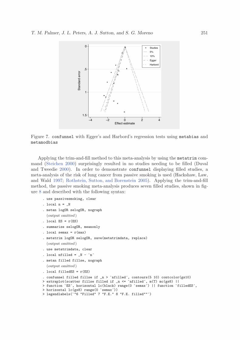
T. M. Palmer, J. L. Peters, A. J. Sutton, and S. G. Moreno 251
0
.5
1
1.5
Sta
ndar
d er
ror
�4 �2 0 2 4Effect estimate
Studies
5%
10%
Egger
Harbord
Figure 7. confunnel with Egger’s and Harbord’s regression tests using metabias andmetamodbias
Applying the trim-and-fill method to this meta-analysis by using the metatrim com-mand (Steichen 2000) surprisingly resulted in no studies needing to be filled (Duvaland Tweedie 2000). In order to demonstrate confunnel displaying filled studies, ameta-analysis of the risk of lung cancer from passive smoking is used (Hackshaw, Law,and Wald 1997; Rothstein, Sutton, and Borenstein 2005). Applying the trim-and-fillmethod, the passive smoking meta-analysis produces seven filled studies, shown in fig-ure 8 and described with the following syntax:
. use passivesmoking, clear
. local n = _N
. metan logOR selogOR, nograph
(output omitted )
. local ES = r(ES)
. summarize selogOR, meanonly
. local semax = r(max)
. metatrim logOR selogOR, save(metatrimdata, replace)
(output omitted )
. use metatrimdata, clear
. local nfilled = _N - `n´
. metan filled fillse, nograph
(output omitted )
. local filledES = r(ES)
. confunnel filled fillse if _n > `nfilled´, contours(5 10) contcolor(gs10)> extraplot(scatter fillse filled if _n <= `nfilled´, m(T) mc(gs8) ||> function `ES´, horizontal lc(black) range(0 `semax´) || function `filledES´,> horizontal lc(gs8) range(0 `semax´))> legendlabels(`"6 "Filled" 7 "F.E." 8 "F.E. filled""´)
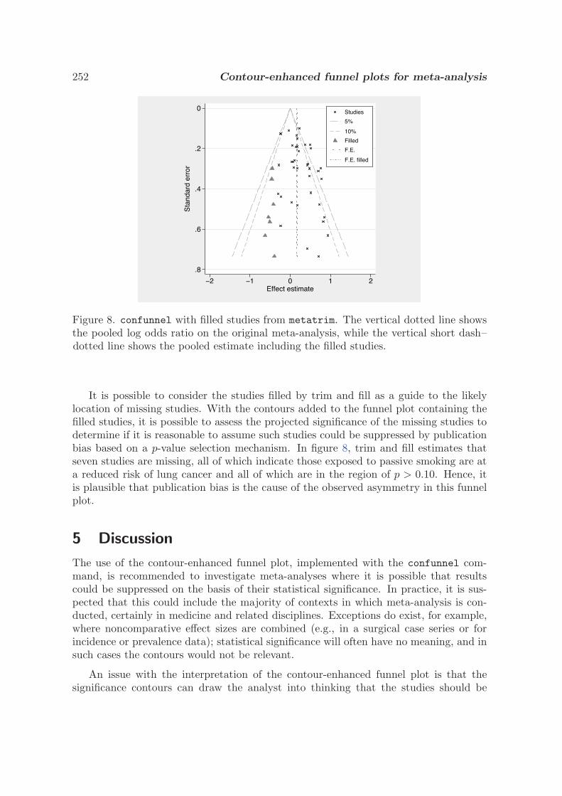
252 Contour-enhanced funnel plots for meta-analysis
0
.2
.4
.6
.8
Sta
ndar
d er
ror
�2 �1 0 1 2Effect estimate
Studies
5%
10%
Filled
F.E.
F.E. filled
Figure 8. confunnel with filled studies from metatrim. The vertical dotted line showsthe pooled log odds ratio on the original meta-analysis, while the vertical short dash–dotted line shows the pooled estimate including the filled studies.
It is possible to consider the studies filled by trim and fill as a guide to the likelylocation of missing studies. With the contours added to the funnel plot containing thefilled studies, it is possible to assess the projected significance of the missing studies todetermine if it is reasonable to assume such studies could be suppressed by publicationbias based on a p-value selection mechanism. In figure 8, trim and fill estimates thatseven studies are missing, all of which indicate those exposed to passive smoking are ata reduced risk of lung cancer and all of which are in the region of p > 0.10. Hence, itis plausible that publication bias is the cause of the observed asymmetry in this funnelplot.
5 Discussion
The use of the contour-enhanced funnel plot, implemented with the confunnel com-mand, is recommended to investigate meta-analyses where it is possible that resultscould be suppressed on the basis of their statistical significance. In practice, it is sus-pected that this could include the majority of contexts in which meta-analysis is con-ducted, certainly in medicine and related disciplines. Exceptions do exist, for example,where noncomparative effect sizes are combined (e.g., in a surgical case series or forincidence or prevalence data); statistical significance will often have no meaning, and insuch cases the contours would not be relevant.
An issue with the interpretation of the contour-enhanced funnel plot is that thesignificance contours can draw the analyst into thinking that the studies should be
T. M. Palmer, J. L. Peters, A. J. Sutton, and S. G. Moreno 253
symmetric about the null hypothesis of the Wald test, because this is the point atwhich the contours meet when standard error or variance is used on the y axis. But thisshould be avoided because the studies should form a symmetric funnel shape centeredaround the true underlying effect size and not the null. Because of this, it can behelpful to plot the meta-analysis pooled estimate for the data on the funnel, althoughthe analyst should be aware that this too may be biased if publication bias is present.
In conclusion, funnel plots are a useful tool in the assessment of systematic differencesbetween the effects in smaller and larger studies in a meta-analysis, regardless of theunderlying reason for the differences. Funnel plots can be enhanced by the inclusionof contours of statistical significance, which aid in the interpretation of whether suchdifferences in study estimates in a meta-analysis are most likely to be due to publicationbias or other factors.
6 ReferencesBradburn, M. J., J. J. Deeks, and D. G. Altman. 1998. sbe24: metan—an alterna-
tive meta-analysis command. Stata Technical Bulletin 44: 4–15. Reprinted in StataTechnical Bulletin Reprints, vol. 8, pp. 86–100. College Station, TX: Stata Press.
Dickersin, K. 1997. How important is publication bias? A synthesis of available data.AIDS Education and Prevention 9: S15–S21.
Duval, S., and R. Tweedie. 2000. Trim and fill: A simple funnel-plot-based method oftesting and adjusting for publication bias in meta-analysis. Biometrics 56: 455–463.
Easterbrook, P. J., J. A. Berlin, R. Gopalan, and D. R. Matthews. 1991. Publicationbias in clinical research. Lancet 337: 867–872.
Egger, M., G. Davey-Smith, M. Schneider, and C. Minder. 1997. Bias in meta-analysisdetected by a simple, graphical test. British Medical Journal 315: 629–634.
Hackshaw, A. K., M. R. Law, and N. J. Wald. 1997. The accumulated evidence on lungcancer and environmental tobacco smoke. British Medical Journal 315: 980–988.
Harbord, R. M. 2003. A modified test for bias in meta-analysis. Working paper, De-partment of Social Medicine, University of Bristol, UK.http://www.epi.bris.ac.uk/user/rogerh/.
Harbord, R. M., M. Egger, and J. A. C. Sterne. 2006. A modified test for small-study effects in meta-analyses of controlled trials with binary endpoints. Statistics inMedicine 25: 3443–3457.
Harris, R. J., M. J. Bradburn, J. J. Deeks, R. M. Harbord, D. G. Altman, and J. A. C.Sterne. 2008. metan: fixed- and random-effects meta-analysis. Stata Journal 8: 1–28.
Ioannidis, J. P. 1998. Effect of the statistical significance of results on the time tocompletion and publication of randomized efficacy trials. Journal of the AmericanMedical Association 279: 281–286.
254 Contour-enhanced funnel plots for meta-analysis
ISIS-4 Collaborative Group. 1995. ISIS-4: A randomised factorial trial assessing earlyoral captopril, oral mononitrate, and intravenous magnesium sulphate in 58,050 pa-tients with suspected acute myocardial infarction. Lancet 345: 669–685.
Peters, J. L., A. J. Sutton, D. R. Jones, K. R. Abrams, and L. Rushton. 2008. Contour-enhanced meta-analysis funnel plots help distinguish publication bias from othercauses of asymmetry. Journal of Clinical Epidemiology. Forthcoming.
Rothstein, H. R., A. J. Sutton, and M. Borenstein, ed. 2005. Publication Bias in Meta-Analysis: Prevention, Assessment and Adjustments. Chichester, UK: Wiley.
Steichen, T. J. 1998. sbe19: Tests for publication bias in meta-analysis. Stata TechnicalBulletin 41: 9–15. Reprinted in Stata Technical Bulletin Reprints, vol. 7, pp. 125–133.College Station, TX: Stata Press.
———. 2000. sbe39: Nonparametric trim and fill analysis of publication bias in meta-analysis. Stata Technical Bulletin 57: 8–14. Reprinted in Stata Technical BulletinReprints, vol. 10, pp. 108–118. College Station, TX: Stata Press.
Sterne, J. A. C., B. J. Becker, and M. Egger. 2005. The Funnel Plot. In Publica-tion Bias in Meta-Analysis: Prevention, Assessment and Adjustments, ed. H. R.Rothstein, A. J. Sutton, and M. Borenstein, 75–98. Chichester, UK: Wiley. DOI:10.1002/0470870168.ch5.
Sterne, J. A. C., M. J. Bradburn, and M. Egger. 2001. Meta-analysis in Stata. In Sys-tematic Reviews in Health Care: Meta-Analysis in Context, 2nd edition, ed. M. Egger,G. Davey Smith, and D. G. Altman, 347–369. London: BMJ Books.
Sterne, J. A. C., and M. Egger. 2001. Funnel plots for detecting bias in meta-analysis:Guidelines on choice of axis. Journal of Clinical Epidemiology 54: 1046–1055.
Sterne, J. A. C., and R. M. Harbord. 2004. Funnel plots in meta-analysis. Stata Journal4: 127–141.
Teo, K. K., S. Yusuf, R. Collins, P. H. Held, and R. Peto. 1991. Effects of intravenousmagnesium in suspected acute myocardial infarction: Overview of randomised trials.British Medical Journal 303: 1499–1503.
About the authors
Tom Palmer is studying for a PhD in genetic epidemiology. Jaime Peters is a research assistant
with a research interest in meta-analysis. Alex Sutton is a reader in medical statistics with
a research interest in meta-analysis; he teaches graduate-level medical statistics. Santiago
Moreno is studying for a PhD in medical statistics.
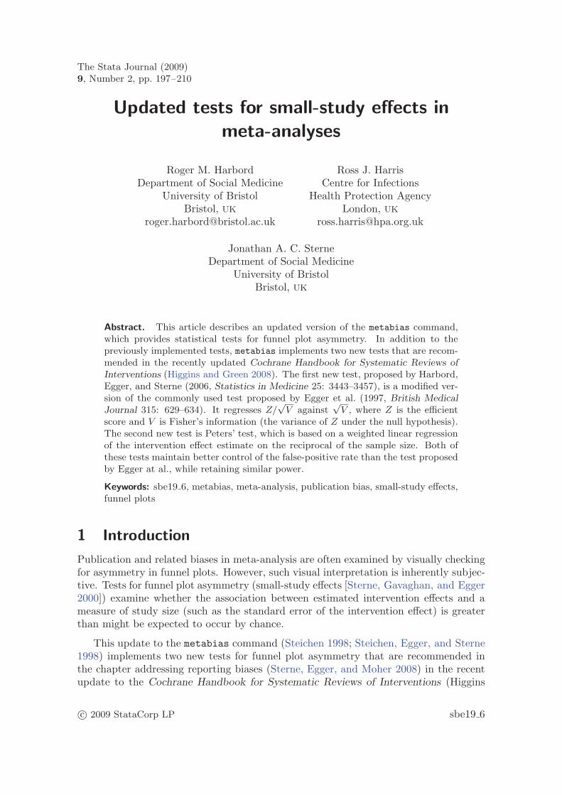
The Stata Journal (2009)9, Number 2, pp. 197–210
Updated tests for small-study effects inmeta-analyses
Roger M. HarbordDepartment of Social Medicine
University of BristolBristol, UK
Ross J. HarrisCentre for Infections
Health Protection AgencyLondon, UK
Jonathan A. C. SterneDepartment of Social Medicine
University of BristolBristol, UK
Abstract. This article describes an updated version of the metabias command,which provides statistical tests for funnel plot asymmetry. In addition to thepreviously implemented tests, metabias implements two new tests that are recom-mended in the recently updated Cochrane Handbook for Systematic Reviews ofInterventions (Higgins and Green 2008). The first new test, proposed by Harbord,Egger, and Sterne (2006, Statistics in Medicine 25: 3443–3457), is a modified ver-sion of the commonly used test proposed by Egger et al. (1997, British MedicalJournal 315: 629–634). It regresses Z/
√V against
√V , where Z is the efficient
score and V is Fisher’s information (the variance of Z under the null hypothesis).The second new test is Peters’ test, which is based on a weighted linear regressionof the intervention effect estimate on the reciprocal of the sample size. Both ofthese tests maintain better control of the false-positive rate than the test proposedby Egger at al., while retaining similar power.
Keywords: sbe19 6, metabias, meta-analysis, publication bias, small-study effects,funnel plots
1 Introduction
Publication and related biases in meta-analysis are often examined by visually checkingfor asymmetry in funnel plots. However, such visual interpretation is inherently subjec-tive. Tests for funnel plot asymmetry (small-study effects [Sterne, Gavaghan, and Egger2000]) examine whether the association between estimated intervention effects and ameasure of study size (such as the standard error of the intervention effect) is greaterthan might be expected to occur by chance.
This update to the metabias command (Steichen 1998; Steichen, Egger, and Sterne1998) implements two new tests for funnel plot asymmetry that are recommended inthe chapter addressing reporting biases (Sterne, Egger, and Moher 2008) in the recentupdate to the Cochrane Handbook for Systematic Reviews of Interventions (Higgins
c© 2009 StataCorp LP sbe19 6

198 Updated tests for small-study effects in meta-analyses
and Green 2008). The modified version of Egger’s test (Egger et al. 1997) proposedby Harbord, Egger, and Sterne (2006) still uses linear regression but is based on theefficient score and its variance, Fisher’s information. The test proposed by Peters et al.(2006) is based on a weighted linear regression of the intervention effect estimate onthe reciprocal of the sample size. These tests address mathematical problems thatcan occur with the commonly used Egger test and the rank correlation test proposedby Begg and Mazumdar (1994), which was also available in the original version ofmetabias. As with other recently updated meta-analysis commands, the syntax formetabias now corresponds to that for the main meta-analysis command, metan.
2 Syntax
metabias varlist[if] [
in], egger harbord peters begg
[graph nofit or rr
level(#) graph options]
As in the metan command, varlist corresponds to either binary data—in this order:cases and noncases for the experimental group, then cases and noncases for the controlgroup (d1 h1 d0 h0)—or the intervention effect and its standard error (theta se theta).
The Harbord and Peters tests require binary data. Although the Egger test can beused with binary data, it is recommended only for studies with continuous (numerical)outcome variables and intervention effects measured as mean differences with the formattheta se theta.
by is allowed with metabias; see [D] by.
3 Options
egger, harbord, peters, and begg specify that the original Egger test, Harbord’s mod-ified test, Peters’ test, or the rank correlation test proposed by Begg and Mazumdar(1994) be reported, respectively. There is no default; one test must be chosen.
graph displays a Galbraith plot (the standard normal deviate of intervention effectestimate against its precision) for the original Egger test or a modified Galbraithplot of Z/
√V versus
√V for Harbord’s modified test. There is no corresponding
plot for the Peters or Begg tests.
nofit suppresses the fitted regression line and confidence interval around the interceptin the Galbraith plot.
or (the default for binary data) uses odds ratios as the effect estimate of interest.
rr specifies that risk ratios rather than odds ratios be used. This option is not availablefor the Peters test.

R. M. Harbord, R. J. Harris, and J. A. C. Sterne 199
level(#) specifies the confidence level, as a percentage, for confidence intervals. Thedefault is level(95) or as set by set level; see [U] 20.7 Specifying the widthof confidence intervals.
graph options are any of the options documented in [G] graph twoway scatter. Inparticular, the options for specifying marker labels are useful.
4 Background
A funnel plot is a simple scatterplot of intervention effect estimates from individualstudies against some measure of each study’s size or precision (Light and Pillemer 1984;Begg and Berlin 1988; Sterne and Egger 2001). It is common to plot effect estimateson the horizontal axis and the measure of study size on the vertical axis. This isthe opposite of the usual convention for twoway plots, in which the outcome (e.g.,intervention effect) is plotted on the vertical axis and the covariate (e.g., study size)is plotted on the horizontal axis. The name “funnel plot” arises from the fact thatprecision of the estimated intervention effect increases as the size of the study increases.Effect estimates from small studies will therefore scatter more widely at the bottom ofthe graph, with the spread narrowing among larger studies. In the absence of bias, theplot should approximately resemble a symmetrical (inverted) funnel. The metafunnelcommand (Sterne and Harbord 2004) can be used to display funnel plots, while theconfunnel command (Palmer et al. 2008) can be used to display “contour-enhanced”funnel plots.
Funnel plots are commonly used to assess evidence that the studies included in ameta-analysis are affected by publication bias. If smaller studies without statisticallysignificant effects remain unpublished, this can lead to an asymmetrical appearance ofthe funnel plot. However, the funnel plot is better seen as a generic means of display-ing small-study effects—a tendency for the intervention effects estimated in smallerstudies to differ from those estimated in larger studies (Sterne, Gavaghan, and Egger2000). Small-study effects may be due to reporting biases, including publication biasand selective reporting of outcomes (Chan et al. 2004), poor methodological qualityleading to spuriously inflated effects in smaller studies, or true heterogeneity (whenthe size of the intervention effect differs according to study size) (Egger et al. 1997;Sterne, Gavaghan, and Egger 2000). Apparent small-study effects can also be artifac-tual, because, in some circumstances, sampling variation can lead to an associationbetween the intervention effect and its standard error (Irwig et al. 1998). Finally, small-study effects may be due to chance; this is addressed by statistical tests for funnel plotasymmetry.
For outcomes measured on a continuous (numerical) scale, tests for funnel plot asym-metry are reasonably straightforward. Using an approach proposed by Egger et al.(1997), we can perform a linear regression of the intervention effect estimates on theirstandard errors, weighting by 1/(variance of the intervention effect estimate). Thislooks for a straight-line relationship between the intervention effect and its standarderror. Under the null hypothesis of no small-study effects, such a line would be vertical
200 Updated tests for small-study effects in meta-analyses
on a funnel plot. The greater the association between intervention effect and standarderror, the more the slope would move away from vertical. The weighting is importantto ensure that the regression estimates are not dominated by the smaller studies. It ismathematically equivalent, however, to a test of zero intercept in an unweighted regres-sion on Galbraith’s radial plot (Galbraith 1988) of the standard normal deviate, definedas the effect estimate divided by its standard error, against the precision, defined as thereciprocal of the standard error; and in fact, this method is used in metabias. If theregression line on a Galbraith plot is constrained to pass through the origin, its slopegives the summary estimate of fixed-effects meta-analysis as suggested by Galbraith.But if the intercept is estimated, a test of the null hypothesis of zero intercept tests forno association between the effect size and its standard error.
The Egger test has been by far the most widely used and cited approach to test-ing for funnel plot asymmetry. Unfortunately, there are statistical problems with thisapproach because the standard error of the log odds-ratio is correlated with the sizeof the odds ratio due to sampling variability alone, even in the absence of small-studyeffects (Irwig et al. 1998); see Deeks, Macaskill, and Irwig (2005) for an algebraic ex-planation of this phenomenon. This can cause funnel plots that were plotted usinglog odds-ratios (or odds ratios on a log scale) to appear asymmetric and can meanthat p-values from the Egger test are too small, leading to false-positive test results.These problems are especially prone to occur when the intervention has a large effect,when there is substantial between-study heterogeneity, when there are few events perstudy, or when all studies are of similar sizes. Therefore, a number of authors haveproposed alternative tests for funnel plot asymmetry. These are reviewed in a newchapter in the recently updated Cochrane Handbook for Systematic Reviews of Inter-ventions (Higgins and Green 2008), which also gives guidance on testing for funnel plotasymmetry (Sterne, Egger, and Moher 2008).
4.1 Notation
We shall be primarily concerned with meta-analysis of 2 × 2 tables, where each studycontains an intervention group and a control group, and the outcome is binary. Weshall use the notation shown in table 1 for a single 2 × 2 table, using the letter dto denote those who experience the event of interest and h for those who do not, withsubscripts 0 and 1 to indicate the control and intervention groups, respectively. We shallconcentrate on the log odds-ratio, φ, as the measure of intervention effect, estimatedby φ = log(d1h0/d0h1). The usual estimate of the variance of the log odds-ratio is theWoolf formula (Woolf 1955), Var(φ) = 1/d0 + 1/h0 + 1/d1 + 1/h1, the square root ofwhich gives the estimated standard error, SE(φ).
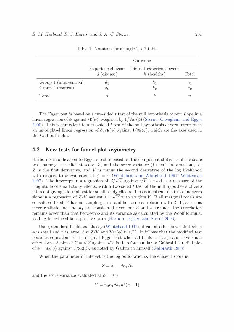
R. M. Harbord, R. J. Harris, and J. A. C. Sterne 201
Table 1. Notation for a single 2 × 2 table
Outcome
Experienced event Did not experience eventd (disease) h (healthy) Total
Group 1 (intervention) d1 h1 n1
Group 2 (control) d0 h0 n0
Total d h n
The Egger test is based on a two-sided t test of the null hypothesis of zero slope in alinear regression of φ against SE(φ), weighted by 1/Var(φ) (Sterne, Gavaghan, and Egger2000). This is equivalent to a two-sided t test of the null hypothesis of zero intercept inan unweighted linear regression of φ/SE(φ) against 1/SE(φ), which are the axes used inthe Galbraith plot.
4.2 New tests for funnel plot asymmetry
Harbord’s modification to Egger’s test is based on the component statistics of the scoretest, namely, the efficient score, Z, and the score variance (Fisher’s information), V .Z is the first derivative, and V is minus the second derivative of the log likelihoodwith respect to φ evaluated at φ = 0 (Whitehead and Whitehead 1991; Whitehead1997). The intercept in a regression of Z/
√V against
√V is used as a measure of the
magnitude of small-study effects, with a two-sided t test of the null hypothesis of zerointercept giving a formal test for small-study effects. This is identical to a test of nonzeroslope in a regression of Z/V against 1 =
√V with weights V . If all marginal totals are
considered fixed, V has no sampling error and hence no correlation with Z. If, as seemsmore realistic, n0 and n1 are considered fixed but d and h are not, the correlationremains lower than that between φ and its variance as calculated by the Woolf formula,leading to reduced false-positive rates (Harbord, Egger, and Sterne 2006).
Using standard likelihood theory (Whitehead 1997), it can also be shown that whenφ is small and n is large, φ ≈ Z/V and Var(φ) ≈ 1/V . It follows that the modified testbecomes equivalent to the original Egger test when all trials are large and have smalleffect sizes. A plot of Z =
√V against
√V is therefore similar to Galbraith’s radial plot
of φ = SE(φ) against 1/SE(φ), as noted by Galbraith himself (Galbraith 1988).
When the parameter of interest is the log odds-ratio, φ, the efficient score is
Z = d1 − dn1/n
and the score variance evaluated at φ = 0 is
V = n0n1dh/n2(n − 1)
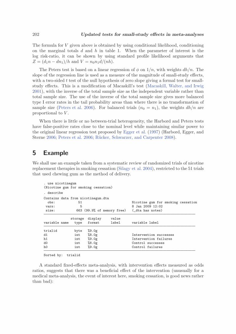
202 Updated tests for small-study effects in meta-analyses
The formula for V given above is obtained by using conditional likelihood, conditioningon the marginal totals d and h in table 1. When the parameter of interest is thelog risk-ratio, it can be shown by using standard profile likelihood arguments thatZ = (d1n − dn1)/h and V = n0n1d/(nh).
The Peters test is based on a linear regression of φ on 1/n, with weights dh/n. Theslope of the regression line is used as a measure of the magnitude of small-study effects,with a two-sided t test of the null hypothesis of zero slope giving a formal test for small-study effects. This is a modification of Macaskill’s test (Macaskill, Walter, and Irwig2001), with the inverse of the total sample size as the independent variable rather thantotal sample size. The use of the inverse of the total sample size gives more balancedtype I error rates in the tail probability areas than where there is no transformation ofsample size (Peters et al. 2006). For balanced trials (n0 = n1), the weights dh/n areproportional to V .
When there is little or no between-trial heterogeneity, the Harbord and Peters testshave false-positive rates close to the nominal level while maintaining similar power tothe original linear regression test proposed by Egger et al. (1997) (Harbord, Egger, andSterne 2006; Peters et al. 2006; Rucker, Schwarzer, and Carpenter 2008).
5 Example
We shall use an example taken from a systematic review of randomized trials of nicotinereplacement therapies in smoking cessation (Silagy et al. 2004), restricted to the 51 trialsthat used chewing gum as the method of delivery.
. use nicotinegum(Nicotine gum for smoking cessation)
. describe
Contains data from nicotinegum.dtaobs: 51 Nicotine gum for smoking cessationvars: 5 8 Jan 2009 12:02size: 663 (99.9% of memory free) (_dta has notes)
storage display valuevariable name type format label variable label
trialid byte %9.0gd1 int %8.0g Intervention successesh1 int %9.0g Intervention failuresd0 int %8.0g Control successesh0 int %9.0g Control failures
Sorted by: trialid
A standard fixed-effects meta-analysis, with intervention effects measured as oddsratios, suggests that there was a beneficial effect of the intervention (unusually for amedical meta-analysis, the event of interest here, smoking cessation, is good news ratherthan bad):
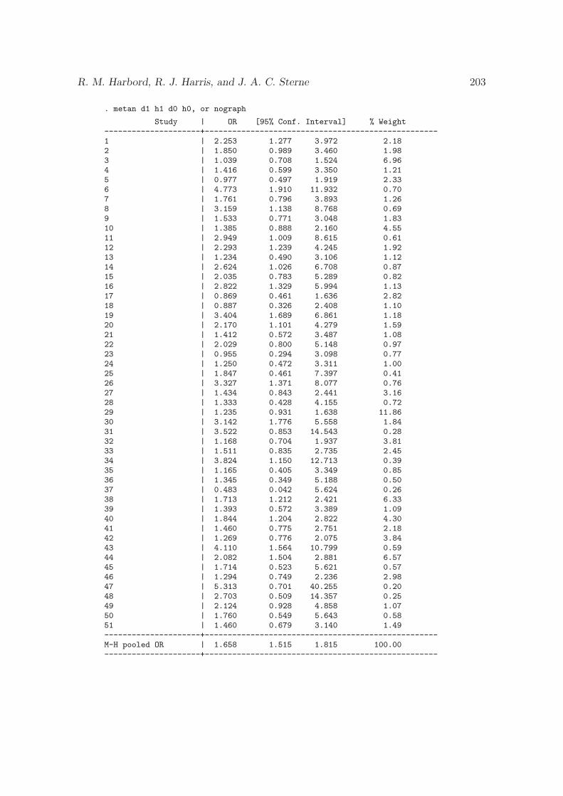
R. M. Harbord, R. J. Harris, and J. A. C. Sterne 203
. metan d1 h1 d0 h0, or nograph
Study | OR [95% Conf. Interval] % Weight---------------------+---------------------------------------------------1 | 2.253 1.277 3.972 2.182 | 1.850 0.989 3.460 1.983 | 1.039 0.708 1.524 6.964 | 1.416 0.599 3.350 1.215 | 0.977 0.497 1.919 2.336 | 4.773 1.910 11.932 0.707 | 1.761 0.796 3.893 1.268 | 3.159 1.138 8.768 0.699 | 1.533 0.771 3.048 1.8310 | 1.385 0.888 2.160 4.5511 | 2.949 1.009 8.615 0.6112 | 2.293 1.239 4.245 1.9213 | 1.234 0.490 3.106 1.1214 | 2.624 1.026 6.708 0.8715 | 2.035 0.783 5.289 0.8216 | 2.822 1.329 5.994 1.1317 | 0.869 0.461 1.636 2.8218 | 0.887 0.326 2.408 1.1019 | 3.404 1.689 6.861 1.1820 | 2.170 1.101 4.279 1.5921 | 1.412 0.572 3.487 1.0822 | 2.029 0.800 5.148 0.9723 | 0.955 0.294 3.098 0.7724 | 1.250 0.472 3.311 1.0025 | 1.847 0.461 7.397 0.4126 | 3.327 1.371 8.077 0.7627 | 1.434 0.843 2.441 3.1628 | 1.333 0.428 4.155 0.7229 | 1.235 0.931 1.638 11.8630 | 3.142 1.776 5.558 1.8431 | 3.522 0.853 14.543 0.2832 | 1.168 0.704 1.937 3.8133 | 1.511 0.835 2.735 2.4534 | 3.824 1.150 12.713 0.3935 | 1.165 0.405 3.349 0.8536 | 1.345 0.349 5.188 0.5037 | 0.483 0.042 5.624 0.2638 | 1.713 1.212 2.421 6.3339 | 1.393 0.572 3.389 1.0940 | 1.844 1.204 2.822 4.3041 | 1.460 0.775 2.751 2.1842 | 1.269 0.776 2.075 3.8443 | 4.110 1.564 10.799 0.5944 | 2.082 1.504 2.881 6.5745 | 1.714 0.523 5.621 0.5746 | 1.294 0.749 2.236 2.9847 | 5.313 0.701 40.255 0.2048 | 2.703 0.509 14.357 0.2549 | 2.124 0.928 4.858 1.0750 | 1.760 0.549 5.643 0.5851 | 1.460 0.679 3.140 1.49---------------------+---------------------------------------------------M-H pooled OR | 1.658 1.515 1.815 100.00---------------------+---------------------------------------------------
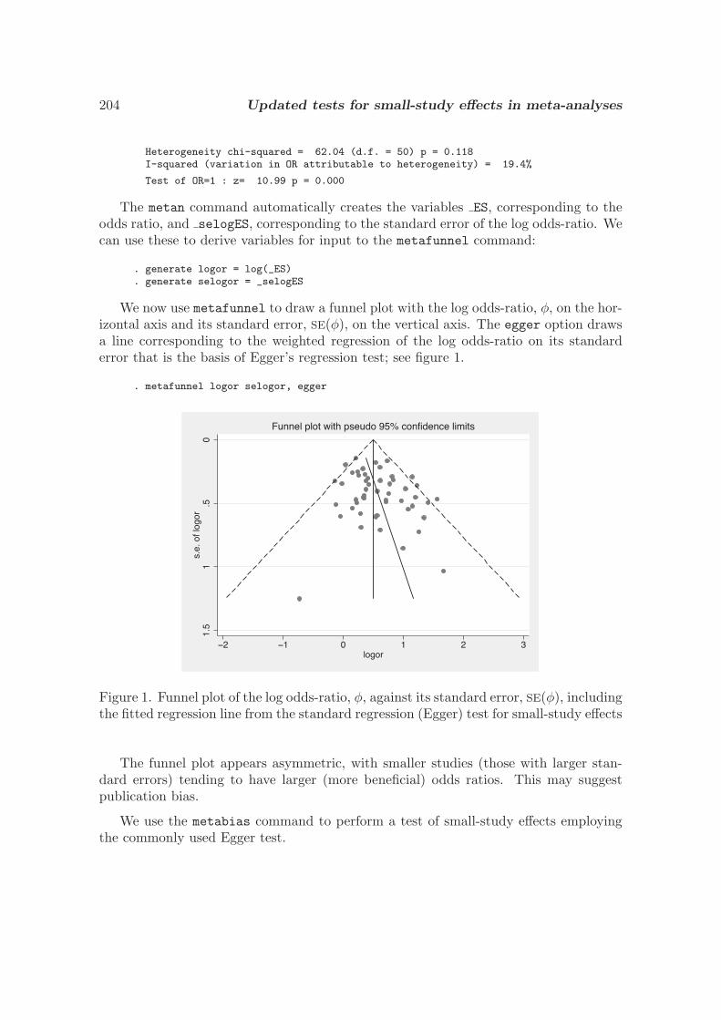
204 Updated tests for small-study effects in meta-analyses
Heterogeneity chi-squared = 62.04 (d.f. = 50) p = 0.118I-squared (variation in OR attributable to heterogeneity) = 19.4%
Test of OR=1 : z= 10.99 p = 0.000
The metan command automatically creates the variables ES, corresponding to theodds ratio, and selogES, corresponding to the standard error of the log odds-ratio. Wecan use these to derive variables for input to the metafunnel command:
. generate logor = log(_ES)
. generate selogor = _selogES
We now use metafunnel to draw a funnel plot with the log odds-ratio, φ, on the hor-izontal axis and its standard error, SE(φ), on the vertical axis. The egger option drawsa line corresponding to the weighted regression of the log odds-ratio on its standarderror that is the basis of Egger’s regression test; see figure 1.
. metafunnel logor selogor, egger
0.5
11.
5s.
e. o
f log
or
�2 �1 0 1 2 3logor
Funnel plot with pseudo 95% confidence limits
Figure 1. Funnel plot of the log odds-ratio, φ, against its standard error, SE(φ), includingthe fitted regression line from the standard regression (Egger) test for small-study effects
The funnel plot appears asymmetric, with smaller studies (those with larger stan-dard errors) tending to have larger (more beneficial) odds ratios. This may suggestpublication bias.
We use the metabias command to perform a test of small-study effects employingthe commonly used Egger test.
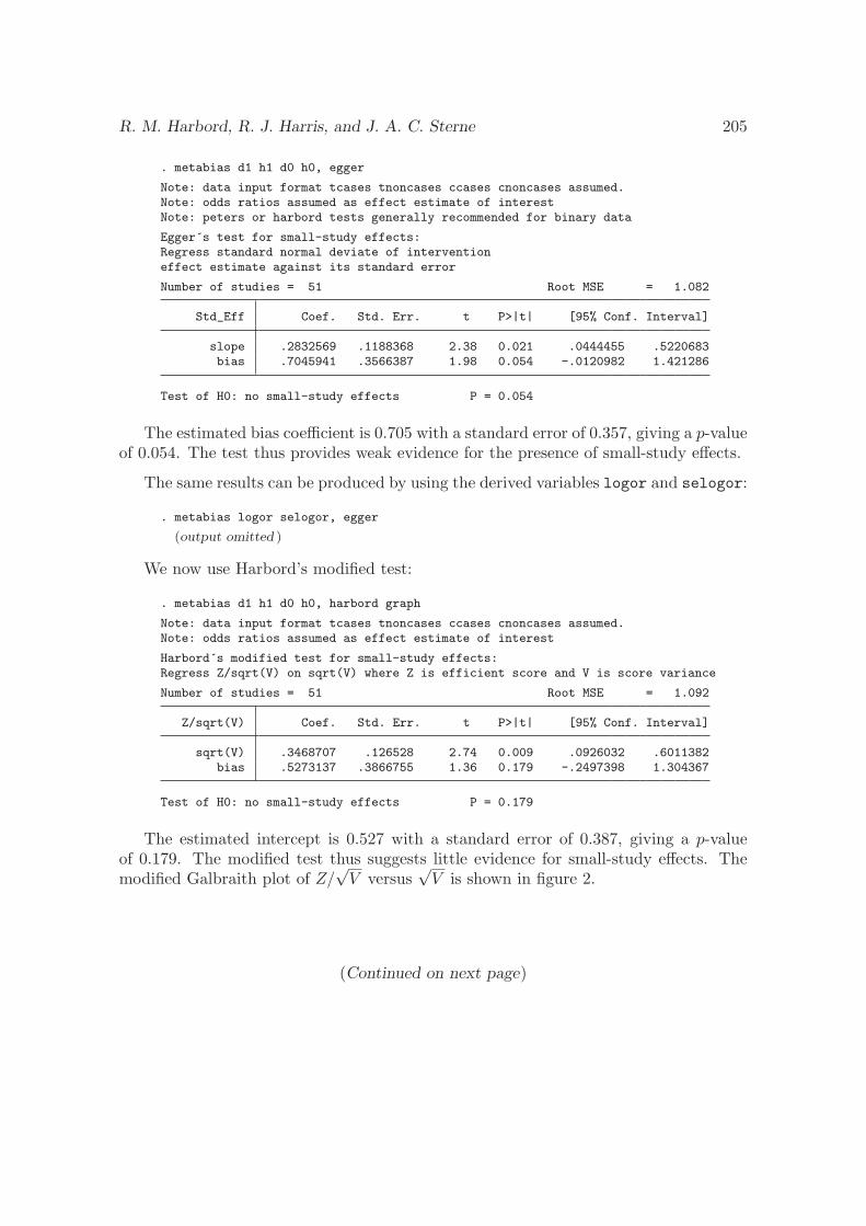
R. M. Harbord, R. J. Harris, and J. A. C. Sterne 205
. metabias d1 h1 d0 h0, egger
Note: data input format tcases tnoncases ccases cnoncases assumed.Note: odds ratios assumed as effect estimate of interestNote: peters or harbord tests generally recommended for binary data
Egger´s test for small-study effects:Regress standard normal deviate of interventioneffect estimate against its standard error
Number of studies = 51 Root MSE = 1.082
Std_Eff Coef. Std. Err. t P>|t| [95% Conf. Interval]
slope .2832569 .1188368 2.38 0.021 .0444455 .5220683bias .7045941 .3566387 1.98 0.054 -.0120982 1.421286
Test of H0: no small-study effects P = 0.054
The estimated bias coefficient is 0.705 with a standard error of 0.357, giving a p-valueof 0.054. The test thus provides weak evidence for the presence of small-study effects.
The same results can be produced by using the derived variables logor and selogor:
. metabias logor selogor, egger
(output omitted )
We now use Harbord’s modified test:
. metabias d1 h1 d0 h0, harbord graph
Note: data input format tcases tnoncases ccases cnoncases assumed.Note: odds ratios assumed as effect estimate of interest
Harbord´s modified test for small-study effects:Regress Z/sqrt(V) on sqrt(V) where Z is efficient score and V is score variance
Number of studies = 51 Root MSE = 1.092
Z/sqrt(V) Coef. Std. Err. t P>|t| [95% Conf. Interval]
sqrt(V) .3468707 .126528 2.74 0.009 .0926032 .6011382bias .5273137 .3866755 1.36 0.179 -.2497398 1.304367
Test of H0: no small-study effects P = 0.179
The estimated intercept is 0.527 with a standard error of 0.387, giving a p-valueof 0.179. The modified test thus suggests little evidence for small-study effects. Themodified Galbraith plot of Z/
√V versus
√V is shown in figure 2.
(Continued on next page)

206 Updated tests for small-study effects in meta-analyses
�2
02
Z /
sqrt
(V)
0 2 4 6 8sqrt(V)
Study regression line 95% CI for intercept
Figure 2. Modified Galbraith plot of Z/√
V versus√
V
Finally, we will use Peters’ test for small-study effects:
. metabias d1 h1 d0 h0, peters
Note: data input format tcases tnoncases ccases cnoncases assumed.Note: odds ratios assumed as effect estimate of interest
Peter´s test for small-study effects:Regress intervention effect estimate on 1/Ntot, with weights SF/Ntot
Number of studies = 51 Root MSE = .3897
Std_Eff Coef. Std. Err. t P>|t| [95% Conf. Interval]
bias 26.20225 14.58572 1.80 0.079 -3.108842 55.51334constant .4197904 .0776552 5.41 0.000 .2637364 .5758443
Test of H0: no small-study effects P = 0.079
In this example, the p-value from Peters’ test is closer to that from Egger’s testthan it is to the p-value from Harbord’s test. These differing results emphasize theimportance of selecting a test in advance; picking a test result from among several isstrongly discouraged.
R. M. Harbord, R. J. Harris, and J. A. C. Sterne 207
6 Saved results
For all tests, the following scalars are returned:
r(N) number of studiesr(p bias) p-value of the bias estimate
For the regression-based tests (Harbord, Peters, and Egger), the following scalarsare returned:
r(df r) degrees of freedomr(bias) estimate of bias (the constant in the regression equation for the
Egger and Harbord tests, and the slope for the Peters test)r(se bias) standard error of bias estimater(rmse) root mean squared error of fitted regression model
For Begg’s test, the following scalars are returned:
r(score) Kendall’s score (P –Q)r(score sd) standard deviation of Kendall’s scorer(p bias ncc) p-value for Begg’s test (not continuity-corrected)
7 Discussion
We have described how to use the metabias command to perform two tests for funnelplot asymmetry. These tests are among those recommended in the Cochrane Hand-book for Systematic Reviews of Interventions (Higgins and Green 2008) because theyreduce the inflation of the false-positive rate (type I error) that can occur for the Eggertest, while retaining power compared with alternative tests. metabias allows only onetest to be specified. Systematic reviewers should ideally specify their chosen test inadvance of the analysis and should avoid choosing from among the results of severaltests. Although simulation studies comparing the different tests have been reported(Harbord, Egger, and Sterne 2006; Peters et al. 2006; Rucker, Schwarzer, and Carpen-ter 2008), no test currently has been shown to be superior in all circumstances. A fullerdiscussion of these issues is available in chapter 10 (Sterne, Egger, and Moher 2008) ofthe Cochrane Handbook.
Tests for funnel plot asymmetry should not be seen as a foolproof method of detectingpublication bias or other small-study effects. We recommend that tests for funnel plotasymmetry be used only when there are at least 10 studies included in the meta-analysis.Even then, power may be low. False-positive results may occur in the presence ofsubstantial between-study heterogeneity, and no test performs well when all studies areof a similar size. Although funnel plots, and tests for funnel plot asymmetry, may alertus to a problem that needs considering when interpreting the results of a meta-analysis,they do not provide a solution to this problem.
(Continued on next page)
208 Updated tests for small-study effects in meta-analyses
8 Acknowledgment
We are grateful to Thomas Steichen, who wrote the original version of the metabiascommand and gave us permission to update it.
Some of the guidance in this article is based on the chapter “Addressing reportingbiases” (Sterne, Egger, and Moher 2008), published in the new Cochrane Handbook forSystematic Reviews of Interventions (Higgins and Green 2008).
9 ReferencesBegg, C. B., and J. A. Berlin. 1988. Publication bias: A problem in interpreting medical
data. Journal of the Royal Statistical Society, Series A 151: 419–463.
Begg, C. B., and M. Mazumdar. 1994. Operating characteristics of a rank correlationtest for publication bias. Biometrics 50: 1088–1101.
Chan, A.-W., A. Hrobjartsson, M. T. Haahr, P. C. Gøtzche, and D. G. Altman. 2004.Empirical evidence for selective reporting of outcomes in randomized trials: Compar-ison of protocols to published articles. Journal of the American Medical Association291: 2457–2465.
Deeks, J. J., P. Macaskill, and L. Irwig. 2005. The performance of tests of publicationbias and other sample size effects in systematic reviews of diagnostic test accuracywas assessed. Journal of Clinical Epidemiology 58: 882–893.
Egger, M., G. Davey Smith, M. Schneider, and C. Minder. 1997. Bias in meta-analysisdetected by a simple, graphical test. British Medical Journal 315: 629–634.
Galbraith, R. F. 1988. A note on graphical presentation of estimated odds ratios fromseveral clinical trials. Statistics in Medicine 7: 889–894.
Harbord, R. M., M. Egger, and J. A. C. Sterne. 2006. A modified test for small-study effects in meta-analyses of controlled trials with binary endpoints. Statistics inMedicine 25: 3443–3457.
Higgins, J. P. T., and S. Green, ed. 2008. Cochrane Handbook for Systematic Reviewsof Interventions. Chichester, UK: Wiley.
Irwig, L., P. Macaskill, G. Berry, and P. Glasziou. 1998. Bias in meta-analysis detectedby a simple, graphical test. Graphical test is itself biased. British Medical Journal316: 470.
Light, R. J., and D. B. Pillemer. 1984. Summing Up: The Science of Reviewing Research.Cambridge, MA: Harvard University Press.
Macaskill, P., S. D. Walter, and L. Irwig. 2001. A comparison of methods to detectpublication bias in meta-analysis. Statistics in Medicine 20: 641–654.
R. M. Harbord, R. J. Harris, and J. A. C. Sterne 209
Palmer, T. M., J. L. Peters, A. J. Sutton, and S. G. Moreno. 2008. Contour-enhancedfunnel plots for meta-analysis. Stata Journal 8: 242–254.
Peters, J. L., A. J. Sutton, D. R. Jones, K. R. Abrams, and L. Rushton. 2006. Com-parison of two methods to detect publication bias in meta-analysis. Journal of theAmerican Medical Association 295: 676–680.
Rucker, G., G. Schwarzer, and J. Carpenter. 2008. Arcsine test for publication bias inmeta-analyses with binary outcomes. Statistics in Medicine 27: 746–763.
Silagy, C., T. Lancaster, L. Stead, D. Mant, and G. Fowler. 2004. Nicotine replace-ment therapy for smoking cessation. Cochrane Database of Systematic Reviews 3:CD000146.
Steichen, T. J. 1998. sbe19: Tests for publication bias in meta-analysis. Stata TechnicalBulletin 41: 9–15. Reprinted in Stata Technical Bulletin Reprints, vol. 7, pp. 125–133.College Station, TX: Stata Press.
Steichen, T. J., M. Egger, and J. A. C. Sterne. 1998. sbe19.1: Tests for publicationbias in meta-analysis. Stata Technical Bulletin 44: 3–4. Reprinted in Stata TechnicalBulletin Reprints, vol. 8, pp. 84–85. College Station, TX: Stata Press.
Sterne, J. A. C., and M. Egger. 2001. Funnel plots for detecting bias in meta-analysis:Guidelines on choice of axis. Journal of Clinical Epidemiology 54: 1046–1055.
Sterne, J. A. C., M. Egger, and D. Moher. 2008. Addressing reporting biases. InCochrane Handbook for Systematic Reviews of Interventions, ed. J. P. T. Higginsand S. Green, 297–334. Chichester, UK: Wiley.
Sterne, J. A. C., D. Gavaghan, and M. Egger. 2000. Publication and related bias inmeta-analysis: Power of statistical tests and prevalence in the literature. Journal ofClinical Epidemiology 53: 1119–1129.
Sterne, J. A. C., and R. M. Harbord. 2004. Funnel plots in meta-analysis. Stata Journal4: 127–141.
Whitehead, A., and J. Whitehead. 1991. A general parametric approach to the meta-analysis of randomized clinical trials. Statistics in Medicine 10: 1665–1677.
Whitehead, J. 1997. The Design and Analysis of Sequential Clinical Trials. Rev. 2nded. Chichester, UK: Wiley.
Woolf, B. 1955. On estimating the relation between blood group and disease. Annalsof Human Genetics 19: 251–253.
About the authors
Roger Harbord is a research associate in medical statistics in the Department of Social Medicineat the University of Bristol, UK. He is a co-convenor of the Cochrane Collaboration’s Screeningand Diagnostic Tests Methods Group.

210 Updated tests for small-study effects in meta-analyses
Ross Harris is a statistician for the Health Protection Agency. His research interests includeevidence synthesis and the epidemiology of sexually transmitted diseases.
Jonathan Sterne is Professor of Medical Statistics and Epidemiology in the Department of So-cial Medicine at the University of Bristol, UK. His research interests include statistical methodsfor epidemiology and health services research, causal models, meta-analysis and systematic re-views, the epidemiology of sexually transmitted infections, and the epidemiology of asthmaand allergic diseases.
Stata Technical Bulletin 9
elapse displays a string with the result. It also creates a global S elap, which is a numerical macro of the form hhmmss,where hh is the number of hours, mm the number of minutes, and ss the number of seconds.
Exampleslocal st � ��S�TIME����elapse ��st�� �Bob�s your uncle� Bob�s your uncle took minute� seconds�
local oper �Maximum likelihood estimation�elapse ��st�� ��oper�� Maximum likelihood estimation took � minutes� seconds�
elapse �st� Elapsed time was hour� � minutes� �� seconds�
quietly elapse �st�if �S�elap � � �� �mat xx � startxx�
sbe19 Tests for publication bias in meta-analysis
Thomas J. Steichen, RJRT, FAX 910-741-1430, [email protected]
Syntax
The syntax of metabias is
metabiasftheta fse theta j var thetag j exp�theta� ll ul�cl�g
�if exp
� �in range
�
�� by�by var� graph�fbegg j eggerg� level�#� fvar j cig graph options
�
where the syntax construct fa j b j � � �g means choose one and only one of fa� b� � � �g.
Description
metabias performs the Begg and Mazumdar (1994) adjusted rank correlation test for publication bias and performs theEgger et al. (1997) regression asymmetry test for publication bias. As options, it provides a funnel graph of the data or theregression asymmetry plot.
The Begg adjusted rank correlation test is a direct statistical analogue of the visual funnel graph. Note that both the testand the funnel graph have low power for detecting publication bias. The Begg and Mazumdar procedure tests for publicationbias by determining if there is a significant correlation between the effect estimates and their variances. metabias carries outthis test by, first, standardizing the effect estimates to stabilize the variances and, second, performing an adjusted rank correlationtest based on Kendall’s � .
The Egger et al. regression asymmetry test and the regression asymmetry plot tend to suggest the presence of publicationbias more frequently than the Begg approach. The Egger test detects funnel plot asymmetry by determining whether the interceptdeviates significantly from zero in a regression of standardized effect estimates against their precision.
The user provides the effect estimate, theta, to metabias as a log risk ratio, log odds ratio, or other direct measure of effect.Along with theta, the user supplies a measure of theta’s variability (i.e., its standard error, se theta, or its variance, var theta).Alternatively, the user may provide the exponentiated form, exp(theta), (i.e., a risk ratio or odds ratio) and its confidence interval,(ll, ul).
The funnel graph plots theta versus se theta. Guide lines to assist in visualizing the funnel are plotted at the variance-weighted (fixed effects) meta-analytic effect estimate and at pseudo confidence interval limits about that effect estimate (i.e., attheta � z� se theta , where z is the standard normal variate for the confidence level specified by option level��). Asymmetryon the right of the graph (where studies with high standard error are plotted) may give evidence of publication bias.
The regression asymmetry graph plots the standardized effect estimates, theta�se theta, versus precision, 1�se theta, alongwith the variance-weighted regression line and the confidence interval about the intercept. Failure of this confidence interval toinclude zero indicates asymmetry in the funnel plot and may give evidence of publication bias. Guide lines at x � 0 and y � 0are plotted to assist in visually determining if zero is in the confidence interval.
metabias will perform stratified versions of both the Begg and Mazumdar test and the Egger regression asymmetry testwhen option by�by var� is specified. Variable by var indicates the categorical variable that defines the strata. The procedurereports results for each strata and for the stratified tests. The graphs, if selected, plot only the combined unstratified data.

10 Stata Technical Bulletin STB-41
Options
by�by var� requests that the stratified tests be carried out with strata defined by by var.
graph�begg� requests the Begg funnel graph showing the data, the fixed-effects (variance-weighted) meta-analytic effect, andthe pseudo confidence interval limits about the meta-analytic effect.
graph�egger� requests the Egger regression asymmetry plot showing the standardized effect estimates versus precision, thevariance-weighted regression line, and the confidence interval about the intercept.
level�� sets the confidence level, in percent, for the pseudo confidence intervals; the default is 95%.
var indicates that var theta was supplied on the command line instead of se theta. Option ci should not be specified whenoption var is specified.
ci indicates that exp(theta) and its confidence interval, (ll, ul), were supplied on the command line instead of theta and se theta.Option var should not be specified when option ci is specified.
graph options are those allowed with graph� twoway. For graph�begg�, the default graph options include connect�lll��,symbol�iiio�, and pen������ for displaying the meta-analytic effect, the pseudo confidence interval limits (two lines),and the data points, respectively. For graph�egger�, the default graph options include connect��ll�, symbol�oid�,and pen����� for displaying the data points, regression line, and the confidence interval about the intercept, respectively.Setting t�title��� blanks out the default t�title.
Input variables
The effect estimates (and a measure of their variability) can be provided to metabias in any of three ways:
1. The effect estimate and its corresponding standard error (the default method):
� metabias theta se theta ���
2. the effect estimate and its corresponding variance (note that option var must be specified):
� metabias theta var theta� var ���
3. the risk (or odds) ratio and its confidence interval (note that option ci must be specified):
� metabias exp(theta) ll ul� ci ���
where exp(theta) is the risk (or odds) ratio, ll is the lower limit and ul is the upper limit of the risk ratio’s confidenceinterval.
When input method 3) is used, cl is an optional input variable that contains the confidence level of the confidence intervaldefined by ll and ul:
� metabias exp(theta) ll ul cl� ci ���
If cl is not provided, metabias assumes that each confidence interval is at the 95% confidence level. cl allows the user toprovide the confidence level, by study, when the confidence intervals are not at the default level or are not all at the same level.Values of cl can be provided with or without a decimal point. For example, 90 and .90 are equivalent and may be mixed (e.g.,90, .95, 80, .90 etc.).
Explanation
Meta-analysis has become a popular technique for numerically synthesizing information from published studies. One of themany concerns that must be addressed when performing a meta-analysis is whether selective publication of studies could leadto bias in the meta-analytic conclusions. In particular, if the probability of publication depends on the results of the study—forexample, if reporting large or statistically significant findings increase the chance of publication—then the possibility of biasexists.
An initial approach used to assess the likelihood of publication bias was the funnel graph (Light and Pillemer 1984). Thefunnel graph plotted the outcome measure (effect size) of the component studies against the sample size (a measure of variability).The approach assumed that all studies in the analysis were estimating the same effect, therefore the estimated effects should bedistributed about the unknown true effect level and their spread should be proportional to their variances. This suggested that,when plotted, small studies should be widely spread about the average effect and the spread should narrow as sample sizesincrease. If the graph suggested a lack of symmetry about the average effect, especially if small, negative studies were absent,then publication bias was assumed to exist.
Evaluation of a funnel graph was a very subjective process, with bias—or lack of bias—being in the eye of the beholder.Begg and Mazumdar (1994) noted this and observed that the presence of publication bias induced a skewness in the plot
Stata Technical Bulletin 11
and a correlation between the effect sizes and their variances. They proposed that a formal test for publication bias, which isimplemented in this insert, could be constructed by examining this correlation. The proposed test evaluates the significance ofthe Kendall’s rank correlation between the standardized effect sizes and their variances.
Recently, Egger et al. (1997) proposed an alternative, regression-based test for detecting skewness in the funnel plot and, byextension, for detecting publication bias in the data. This numerical measure of funnel plot asymmetry also constitutes a formaltest for publication bias and is implemented in this insert. The proposed test evaluates whether the intercept deviates significantlyfrom zero in a regression of standardized effect estimates against their precision. The test is motivated by the observation that,under assumptions of a nonzero underlying effect and a lack of publication bias, 1) small studies would have both a near-zeroprecision (since precision is predominantly a function of sample size) and a near-zero standardized effect (because of divisionby a correspondingly large standard error), while 2) large studies would have both a large precision and a large standardizedeffect (because of division by a small standard error). Therefore the standardized effects would scatter about a regression line(approximately) through the origin that has a slope which estimates both the size and direction of the underlying effect. Underconditions of publication bias and asymmetry in the funnel plot, the sub-sample of small studies will differ systematically fromthe sub-sample of larger studies and the regression line will fail to go through the origin. The size of the intercept provides ameasure of asymmetry—the larger the deviation from zero the greater the asymmetry. The direction of the intercept providesinformation on the form of the bias—a positive intercept indicates that the effect estimated from the smaller studies is greaterthan the effect estimated from the larger studies. Conversely, a negative intercept indicates that the effect estimated from thesmaller studies is less than the effect estimated from the larger studies.
Begg’s test
This section paraphrases the mathematical development and discussion in the Begg and Mazumdar paper (the paper alsoincludes a detailed examination of the operating characteristics of this test and examples based on medical data).
Let �ti� vi�� i � 1� � � � � k� be the estimated effect sizes and sample variances from k studies in a meta-analysis. To constructthe adjusted rank correlation test, calculate the standardized effect sizes
t�i ��ti � t�
�v�i ����
where
t �
Pkj�� tjv
��
jPkj�� v
��
j
is the variance-weighted average effect size, and
v�i � vi �
�kX
j��
v��j
���
is the variance of ti � t.
Correlate the standardized effect sizes, t�i , with the sample variances, vi, using Kendall’s rank correlation procedure andexamine the p value. A significant correlation is interpreted as providing strong evidence of publication bias.
In their examples, Begg and Mazumdar use the normalized Kendall rank correlation test statistic for data that have no ties,z � �P �Q���k�k� 1��2k� 5��18����, where P is the number of pairs of studies ranked in the same order with respect to t�
and v and Q is the number of pairs ranked in the opposite order. This statistic does not apply a continuity correction. The authorsremark that the denominator should be modified if there are tied observations in either t�i or vi but, instead, apparently breakties in their sample data by adding a small constant. The metabias procedure implemented in this insert invokes a modificationof Stata’s ktau procedure to calculate the correct statistic, whether ties exist or not, and presents the z and p values with andwithout the continuity correction.
Begg and Mazumdar report that the principal determinant of the power of this test is the number of component studies inthe meta-analysis (as opposed to the sample sizes of the individual studies). Additionally, the power will increase with a widerrange in variance (sample size) and with a smaller underlying effect size. The authors state that the test is fairly powerful fora meta-analysis of 75 component studies, only moderately powerful for one of 25 component studies, and weak when thereare few component studies. They advise that “the test must be interpreted with caution in small meta-analyses. In particular,[publication] bias cannot be ruled out if the test is not significant.”
12 Stata Technical Bulletin STB-41
A stratified test can also be constructed. Let Pl �Ql be the numerator of the unstratified test statistic for the lth subgroupand dl be the square of the corresponding denominator (i.e., the variance of Pl � Ql). The stratified test statistic, withoutcontinuity correction, is defined as
zs �
Pl�Pl �Ql��P
l dl
����
The metabias procedure implemented in this insert calculates the correct stratified statistic, whether ties exist or not, andpresents the zs and ps values with and without the continuity correction.
Begg and Mazumdar assume that the sampling distribution of t is normal, i.e., t � N��� vi�, where � is the common effectsize to be estimated and the vi are the variances, which depend on the sample sizes of the individual component studies. Theyargue that the normality assumption is reasonable because t is “invariably a summary estimate of some parameter, and as suchwill possess an asymptotic normal distribution in most circumstances.” The subsequent asymptotic-normality assumption for zsinherently follows from this argument.
Egger’s test
This section paraphrases the method development and discussion in the Egger et al. paper. (The paper also provides anempirical evaluation, based on only eight examples from the medical literature, of the ability of the regression asymmetry testto correctly predict whether a meta-analysis of smaller studies will be concordant with the results of a subsequent large trial.)
Let �ti� vi�� i � 1� � � � � k� be the estimated effect sizes and sample variances from k studies in a meta-analysis. Definethe standardized effect size as t�i � ti�vi
���, the precision as s�� � 1�vi���, and the weight as wi � 1�vi. (In this form ofstandardization, t� is a standard normal deviate and is designated as such in the Egger paper.) Fit t� to s�� using standardweighted linear regression with weights w and linear equation: t� � ���s��. A significant deviation from zero of the estimatedintercept, b�, is interpreted as providing evidence of asymmetry in the funnel plot and of publication bias in the sampled data.
Egger et al. fit both weighted and unweighted regression lines and select the results of the analysis yielding the interceptwith the larger deviation from zero. This insert implements only the weighted analysis.
Egger et al. do not provide a formal analysis of coverage (i.e., nominal significance level) or power for this test, thoughthey do provide a number of assertions about power. First, they state that “[i]n contrast to the overall test of heterogeneity, thetest for funnel plot asymmetry assesses a specific type of heterogeneity and provides a more powerful test in this situation.”Second, they state that “[i]n some situations� � � power is gained by weighting the analysis.” Lastly, in a comparison to the Beggand Mazumdar test, they state that “the linear regression approach may be more powerful than the rank correlation test.” Eggeret al. note, though, that “any analysis of heterogeneity depends on the number of trials included in a meta-analysis, which isgenerally small, and this limits the statistical power of the test.”
Although the paper provides no formal analysis in support of these assertions, an empirical evaluation based on eightexamples from the medical literature is reported. This evaluation assessed the ability of the regression asymmetry test to correctlypredict whether a meta-analysis of smaller studies will be concordant with the results of a subsequent large trial. For these eightexamples, the test detected bias in 3 of 4 cases where a meta-analysis disagreed with a subsequent large trial and indicatedno bias in all 4 cases where the meta-analysis agreed with the subsequent large trial. In contrast, the Begg and Mazumdar testwas significant for only 1 of the 4 discordant cases (but like Egger’s test, for none of the concordant cases). Nonetheless, eightexample cases are too few to be statistically convincing and the test remains unvalidated. Further, the lack of coverage analysisleaves open the question of false-positive claims of asymmetry and publication bias. Interestingly, if the Egger’s publication biastest is too liberal (a concern that the author of this insert holds), that translates into conservativeness at the meta-analysis levelsince the bias test will suggest too frequently that caution is needed in interpreting the results of the meta-analysis.
An approximate stratified test can be constructed using logic similar to that of Begg and Mazumdar (although Egger etal. did not do so). Let al be the intercept from the regression equation for the lth subgroup and val be the variance of al. Thestratified test statistic is defined as
zs �
Pl al�v
al�P
l ��val
����
and is assumed to be distributed asymptotically normal. In this form, the stratified estimate is simply the variance-weighted,fixed effect meta-analysis of the intercepts. This stratified test is implemented in this insert.
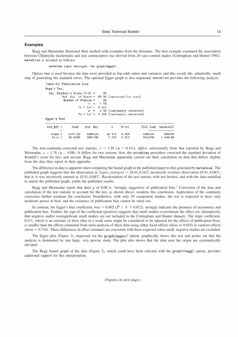
Stata Technical Bulletin 13
Examples
Begg and Mazumdar illustrated their method with examples from the literature. The first example examined the associationbetween Chlamydia trachomatis and oral contraceptive use derived from 29 case-control studies (Cottingham and Hunter 1992).metabias is invoked as follows:
� metabias logor varlogor� var graph�egger�
Option var is used because the data were provided as log-odds ratios and variances and this avoids the, admittedly, smallstep of generating the standard errors. The optional Egger graph is also requested. metabias provides the following analysis:
Tests for Publication Bias
Begg�s Test
adj� Kendall�s Score �P�Q� � �Std� Dev� of Score � �� �corrected for ties�Number of Studies � �
z � �� Pr � �z� � �����
z � ��� �continuity corrected�Pr � �z� � ���� �continuity corrected�
Egger�s Test
������������������������������������������������������������������������������Std�Eff � Coef� Std� Err� t P��t� � � Conf� Interval�
������������������������������������������������������������������������������slope � ������� ������� � ���� ����� ������� ����bias � ������ �� ��� ����� ����� �� ����� ���� � �
������������������������������������������������������������������������������
The non-continuity-corrected test statistic, z � 1.59 ( p � 0.111), differs substantially from that reported by Begg andMazumdar, z � 1.76 ( p � 0.08). It differs for two reasons: first, the metabias procedure corrected the standard deviation ofKendall’s score for ties; and second, Begg and Mazumdar apparently carried out their calculation on data that differs slightlyfrom the data they report in their appendix.
The difference in data is apparent when comparing the funnel graph in the published paper to that generated by metabias. Thepublished graph suggests that the observation at �logor� varlogor� � �0.41� 0.162� incorrectly overlays observation �0.41� 0.083�;that it, it was incorrectly entered as �0.41� 0.083�. Recalculation of the test statistic with ties broken, and with the data modifiedto match the published graph, yields the published results.
Begg and Mazumdar report that their p of 0.08 is “strongly suggestive of publication bias.” Correction of the data andcalculation of the test statistic to account for the ties, as shown above, weakens this conclusion. Application of the continuitycorrection further weakens the conclusion. Nonetheless, with only 29 component studies, the test is expected to have onlymoderate power at best, and the existence of publication bias cannot be ruled out.
In contrast, the Egger’s bias coefficient, bias � 0.802 (P � jtj � 0.012), strongly indicates the presence of asymmetry andpublication bias. Further, the sign of the coefficient (positive) suggests that small studies overestimate the effect (or, alternatively,that negative and/or nonsignificant small studies are not included in the Cottingham and Hunter dataset). The slope coefficient,0.511, which is an estimate of theta (that in a weak sense might be considered to be adjusted for the effects of publication bias),is smaller than the effects estimated from meta-analysis of these data using either fixed-effects (theta � 0.655) or random-effects(theta � 0.716). These differences in effect estimates are consistent with those expected when small, negative studies are excluded.
The Egger plot (Figure 1), requested via the graph�egger� option, graphically shows this test and points out that theanalysis is dominated by one large, very precise study. The plot also shows that the data near the origin are systematicallyelevated.
The Begg funnel graph of the data (Figure 2), which could have been selected with the graph�begg� option, providesadditional support for this interpretation.
(Figures on next page.)
14 Stata Technical Bulletin STB-41
Figure 1 Figure 2
Most of the data points in the Begg plot fall above the meta-analytic effect estimate and there is a visible void in thelower right of the funnel, that is, in the region of low effect and high variance. This is the region where studies most likely tobe subject to publication bias would appear. It is notable, though, that since the meta-analytic effect estimate and most of theindividual component effect estimates are substantially above zero, the effect of publication bias, if any, would be to inflate theestimate rather than to lead to an incorrect conclusion about the existence of an effect.
Begg and Mazumdar’s third example called for the use of the stratified test. These data examined the association betweenchlorination by-products in drinking water and cancer occurrence, with studies stratified by the site of the cancer (Morris etal. 1992). metabias is invoked as follows:
� metabias effect variance� var by�site�
Use of option by�site� informs metabias that the stratified tests are to be carried out and that variable site is to beused to define the strata. Results are provided in table format, presenting the statistics for each strata and then for the overallstratified tests:
Tests for Publication Bias
�������������������������������������������������������������������������������� � Begg�s Begg�s cont� corr� � Egger�s
site � n � score s�d� z p z p � bias p�������������������������������������������������������������������������������Bladder � � ��� ��� ����� ���� ���� � ��� �����Brain � � � ���� ��� ��� ���� ���� � �� �Breast � � � � ����� ��� ���� ���� ���� � �� � �����Colon � � � ��� ��� � ���� ���� ���� � ��� �����
ColoRect � � � � ����� ���� ���� ��� � ���� � ���� ����Esophagu � � � � ����� ���� ���� ��� ���� � ��� ����Kidney � � � � ����� ��� ���� ���� ���� � ��� ����Liver � � � � ����� ��� ���� ���� ���� � ���� ���Lung � � � ����� �� �� �� ��� ���� � �� �����
Pancreas � � � ����� ���� ����� ��� ����� � ��� ���� Rectum � � ����� �� � ���� ���� ���� � ���� �� ��Stomach � � � ����� ���� ����� ��� ����� � ���� �����
�������������������������������������������������������������������������������overall � � � �� ��� �� ����� �� ���� � ��� �����
�������������������������������������������������������������������������������
The Begg and Mazumdar results provide no evidence of publication bias in any of the small site-specific strata, yet thestratified test statistic, zs � 1.97 ( p � 0.049) provides strong evidence that publication bias exists in the chlorinated drinkingwater and cancer literature. (These results also differ slightly from those published by Begg and Mazumdar in that the publishedscore for the Pancreas strata is 6, leading to an overall score of 35 and slightly different test statistics for this strata and theoverall statistic. Results for all other strata agree.) Again, the Egger test provides a stronger indication of the possible presenceof publication bias in this literature. Four site-specific strata (Breast, Colon, Pancreas and Stomach) reach statistical significanceand the p value for the overall test is more significant than that of Begg’s test, 0.000 versus 0.049. All but one of the individualbias coefficients are positive, as is the overall bias coefficient, suggesting that the small studies in this Morris et al. dataset areoverestimating the effect (or that the negative and/or nonsignificant small studies are not included).

Stata Technical Bulletin 15
Saved Results
metabias saves
S � number of studies S � Begg’s p value, continuity correctedS � Begg’s score S � Egger’s bias coefficientS � s.d. of Begg’s score S � Egger’s p valueS � Begg’s p value S overall effect (log scale)
ReferencesBegg, C. B. and M. Mazumdar. 1994. Operating characteristics of a rank correlation test for publication bias. Biometrics 50: 1088–1101.
Cottingham, J. and D. Hunter. 1992. Chlamydia trachomatis and oral contraceptive use: A quantitative review. Genitourinary Medicine 68: 209–216.
Egger, M., G. D. Smith, M. Schneider, and C. Minder. 1997. Bias in meta-analysis detected by a simple, graphical test. British Medical Journal 315:629–634.
Light, R. J. and D. B. Pillemer. 1984. Summing up: The science of reviewing research. Cambridge, MA: Harvard University Press.
Morris, R. D., A. M. Audet, I. F. Angelillo, T. C. Chalmers, and F. Mosteller. 1992. Chlorination, chlorination by-products, and cancer: A meta-analysis.American Journal of Public Health 82: 955–963.
sbe20 Assessing heterogeneity in meta-analysis: the Galbraith plot
Aurelio Tobias, Institut Municipal d’Investigacio Medica (IMIM), Spain, [email protected]
Graphical methods are frequently used in meta-analysis to complement the statistical analysis of clinical and epidemiologicaldata. If the number of studies evaluated in a meta-analysis is small the assessment of heterogeneity is complicated. A rangeof tests to assess heterogeneity are available (Fleiss 1981), but they tend to have low power against the alternative (Laird andMosteller 1990). Moreover, it is difficult to have a visual impression of the amount of heterogeneity from common meta-analysisdiagrams (Gladen and Rogan 1983, Galbraith 1988). Hence, graphical methods are particularly important to check and to explorepotential sources of heterogeneity.
The command galbr performs the Galbraith plot (Galbraith 1988), which has been more recommended (Thompson 1993)than other graphical methods to investigate heterogeneity in meta-analysis. This command can be useful to complement theresults and graphical displays produced by the meta command (Sharp and Sterne 1997).
The Galbraith plot
Following the notation by Sharp and Sterne, let us assume that ��i is the estimated treatment effect �i in a trial i, and vi thevariance of the estimated treatment effect. Then, for each trial i the z statistic ��i�
pvi is plotted against the reciprocal standard
error 1�pvi. Different log rate ratios, log odds ratios or log hazard ratios are therefore represented on the diagram by straight
lines to the origin for different gradients. In particular, it could be verified that the (unweighted) regression line constrainedthrough the origin has a slope equal to the overall log odds ratio in a fixed effects meta-analysis. Heterogeneity may be assessedby the contribution of each trial i to the overall Q statistic (DerSimonian and Laird 1986) for heterogeneity. This investigationcan also be performed visually from a Galbraith plot. The position of each trial on the horizontal axis gives an indication of theweight allocated in the meta-analysis. The vertical axis gives the contribution of each trial to the Q statistic, that is, to say thedistance between each trial point and the regression line is equal to q�i , where q�i � wi���i � ���� and Q �
Pq�i . Points outside
the confidence bounds (positioned 2 units above and below the regression line) are these trials which have a major contributionto heterogeneity. In the absence of heterogeneity we could expect all points within the confidence limits. The Galbraith plotcan also be used to investigate possible sources of heterogeneity by labeling the points in the graph by different covariates,for example type of trial, duration of treatment, or drug differences. We should note that this is a post-hoc investigation andinterpretation should be made with caution (Thompson 1993).
Syntax
As for the command meta, the command galbr works on a dataset containing the estimate effect, theta, and its standarderror, setheta, for each trial. The syntax is as follows:
galbr theta setheta�if exp
� �in range
� �� id�labelvar� graph options
�
Options
id�labelvar� supplies a variable which is used to label the studies. If the data contains a labeled numeric variable, it can alsobe used.
Stata Technical Bulletin 3
� fillin rep�� foreign
� drop �fillin
� replace freq � � if freq �� ��� real changes made� list
rep�� foreign freq� Domestic ��� Foreign ��� � Domestic ��� � Foreign � � � Domestic ���� � Foreign ��� � Domestic ��� � Foreign ��� Domestic ��� Foreign �� � Domestic ��� � Foreign
Once again, however, collfreq with the zero option is more direct:� collfreq rep�� foreign� zero
The final advantage of collfreq is that it is easier to ignore observations with missing values. This can be done by usingthe nomiss option. In contrast, with the collapse approach, some preparatory action is needed. In the current example, itwould be easy to drop the observations with missing values:
� drop if rep�� �� � � foreign �� �
With a larger set of variables, a more efficient approach would be to flag such observations using mark and markout beforedropping them. But mark and markout are likely to be unfamiliar to Stata users who are not Stata programmers, and collfreq
with the nomiss option is a simpler alternative.
collfreq destroys the data in memory, as does collapse.
sbe19.1 Tests for publication bias in meta-analysis
Thomas J. Steichen, RJRT, FAX 910-741-1430, [email protected] Egger, University of Bristol, FAX (011) 44-117-928-7325, [email protected]
Jonathan Sterne, UMDS, London, FAX (011) 44-171-955-4877, [email protected]
Modification of the metabias program
This insert documents four changes to the metabias program (Steichen 1998). First, the weighted form of the Egger etal. (1997) regression asymmetry test for publication bias has been replaced by the unweighted form. Second, an error has beencorrected in the calculation of the asymmetry test p values for individual strata in a stratified analysis. Third, error trapping hasbeen modified to capture or report problem situations more completely and accurately. Fourth, the labeling of the Begg funnelgraph has been changed to properly title the axes when the ci option is specified. None of these changes affects the programsyntax or operation.
The first change was made because, while there is little theoretical justification for the weighted analysis, justificationfor the unweighted analysis is straightforward. As before, let �ti� vi�� i � 1� � � � � k� be the estimated effect sizes and samplevariances from k studies in a meta-analysis. Egger et al. defined the standardized effect size as t�i � ti�vi
���, and the precision
as s�1 � 1�vi���. For the unweighted form of the asymmetry test, they fit t� to s�1 using standard linear regression and
the equation t� � � � �s�1. A significant deviation from zero of the estimated intercept, b�, is then interpreted as providingevidence of asymmetry in the funnel plot and of publication bias in the sampled data.
Jonathan Sterne (private communication to Matthias Egger) noted that this “unweighted” asymmetry test is merely areformulation of a standard weighted regression of the original effect sizes, ti, against their standard errors, vi
���, where theweights are the usual 1�vi. It follows then that the “weighted” asymmetry test is merely a weighted regression of the originaleffect sizes against their standard errors, but with weights 1�vi�. This form has no obvious theoretical justification.
We note further that the “unweighted” asymmetry test weights the data in a manner consistent with the weighting of theeffect sizes in a typical meta-analysis (i.e., both use the inverse variances). Thus, bias is detected using the same weightingmetric as in the meta-analysis.
For these reasons, this insert restricts metabias to the unweighted form of the Egger et al. regression asymmetry test forpublication bias.
4 Stata Technical Bulletin STB-44
The second change to metabias is straightforward. A square root was inadvertently left out of the formula for the p
value of the asymmetry test that is calculated for an individual stratum when option by�� is specified. This formula has beencorrected. Users of this program should repeat any stratified analyses they performed with the original program. Please note thatunstratified analyses were not affected by this error.
The third change to metabias extends the error-trapping capability and reports previously trapped errors more accuratelyand completely. A noteworthy aspect of this change is the addition of an error trap for the ci option. This trap addresses thesituation where epidemiological effect estimates and associated error measures are provided to metabias as risk (or odds) ratiosand corresponding confidence intervals. Unfortunately, if the user failed to specify option ci in the previous release, metabiasassumed that the input was in the default (theta, se theta) format and calculated incorrect results. The current release checks forthis situation by counting the number of variables on the command line. If more than two variables are specified, metabiaschecks for the presence of option ci. If ci is not present, metabias assumes it was accidentally omitted, displays an appropriatewarning message, and proceeds to carry out the analysis as if ci had been specified.
Warning: The user should be aware that it remains possible to provide theta and its variance, var theta, on the commandline without specifying option var. This error, unfortunately, cannot be trapped and will result in an incorrect analysis. Thoughonly a limited safeguard, the program now explicitly indicates the data input option specified by the user, or alternatively, warnsthat the default data input form was assumed.
The fourth change to metabias has effect only when options graph�begg� and ci are specified together. graph�begg�requests a funnel graph. Option ci indicates that the user provided the effect estimates in their exponentiated form, exp(theta)—usually a risk or odds ratio, and provided the variability measures as confidence intervals, (ll, ul). Since the funnel graph alwaysplots theta against its standard error, metabias correctly generated theta by taking the log of the effect estimate and correctlycalculated se theta from the confidence interval. The error was that the axes of the graph were titled using the variable name (orvariable label, if available) and did not acknowledge the log transform. This was both confusing and wrong and is corrected inthis release. Now when both graph�begg� and ci are specified, if the variable name for the effect estimate is RR, the y-axis istitled “log[RR]” and the x-axis is titled “s.e. of: log[RR]”. If a variable label is provided, it replaces the variable name in theseaxis titles.
ReferencesEgger, M., G. D. Smith, M. Schneider, and C. Minder. 1997. Bias in meta-analysis detected by a simple, graphical test. British Medical Journal 315:
629–634.
Steichen, T. J. 1998. sbe19: Tests for publication bias in meta-analysis. Stata Technical Bulletin 41: 9–15. Reprinted in The Stata Technical BulletinReprints vol. 7, pp. 125–133.
sbe24 metan—an alternative meta-analysis command
Michael J. Bradburn, Institute of Health Sciences, Oxford, UK, [email protected] J. Deeks, Institute of Health Sciences, Oxford, UK, [email protected]
Douglas G. Altman, Institute of Health Sciences, Oxford, UK, [email protected]
Background
When several studies are of a similar design, it often makes sense to try to combine the information from them all to gainprecision and to investigate consistencies and discrepancies between their results. In recent years there has been a considerablegrowth of this type of analysis in several fields, and in medical research in particular. In medicine such studies usually relateto controlled trials of therapy, but the same principles apply in any scientific area; for example in epidemiology, psychology,and educational research. The essence of meta-analysis is to obtain a single estimate of the effect of interest (effect size) fromsome statistic observed in each of several similar studies. All methods of meta-analysis estimate the overall effect by computinga weighted average of the studies’ individual estimates of effect.
metan provides methods for the meta-analysis of studies with two groups. With binary data, the effect measure can be thedifference between proportions (sometimes called the risk difference or absolute risk reduction), the ratio of two proportions (riskratio or relative risk), or the odds ratio. With continuous data, both observed differences in means or standardized differences inmeans (effect sizes) can be used. For both binary and continuous data, either fixed effects or random effects models can be fitted(Fleiss 1993). There are also other approaches, including empirical and fully Bayesian methods. Meta-analysis can be extendedto other types of data and study designs, but these are not considered here.
As well as the primary pooling analysis, there are secondary analyses that are often performed. One common additionalanalysis is to test whether there is excess heterogeneity in effects across the studies. There are also several graphs that can beused to supplement the main analysis.
8 Stata Technical Bulletin STB-57
sbe39 Nonparametric trim and fill analysis of publication bias in meta-analysis
Thomas J. Steichen, RJRT, [email protected]
Abstract: This insert describes metatrim, a command implementing the Duval and Tweedie nonparametric “trim and fill”method of accounting for publication bias in meta-analysis. Selective publication of studies, which may lead to bias inestimating the overall meta-analytic effect and in the inferences derived, is of concern when performing a meta-analysis.If publication bias appears to exist, then it is desirable to consider what the unbiased dataset might look like and thento reestimate the overall meta-analytic effect after any apparently “missing” studies are included. Duval and Tweedie’s“nonparametric ‘trim and fill’ method” is an approach designed to meet these objectives.
Keywords: meta-analysis, publication bias, nonparametric, data augmentation.
Syntax
metatrim ftheta f se theta j var theta g j exp(theta) ll ul�cl�g
�if exp
� �in range
�
�� fvar j cig reffect print estimat�frun j linear j quadraticg� eform graph
funnel level�#� idvar�varname� save�filename�� replace
�� graph options
�
where fa j b j ���g means choose one and only one of fa� b� ���g.
Description
metatrim performs the Duval and Tweedie (2000) nonparametric “trim and fill” method of accounting for publication biasin meta-analysis. The method, a rank-based data-imputation technique, formalizes the use of funnel plots, estimates the numberand outcomes of missing studies, and adjusts the meta-analysis to incorporate the imputed missing data. The authors claim thatthe method is effective and consistent with other adjustment techniques. As an option, metatrim provides a funnel plot of thefilled data.
The user provides the effect estimate, theta, to metatrim as a log risk-ratio, log odds-ratio, or other direct measure ofeffect. Along with theta, the user supplies a measure of theta’s variability (that is, its standard error, se theta, or its variance,var theta). Alternatively, the user may provide the exponentiated form, exp(theta), (that is, a risk ratio or odds ratio) and itsconfidence interval, (ll, ul).
The funnel plot graphs theta versus se theta for the filled data. Imputed observations are indicated by a square around thedata symbol. Guide lines to assist in visualizing the center and width of the funnel are plotted at the meta-analytic effect estimateand at pseudo-confidence-interval limits about that effect estimate (that is, at theta� z� se theta, where z is the standard normalvariate for the confidence level specified by option level��).
Options
var indicates that var theta was supplied on the command line instead of se theta. Option ci should not be specified whenoption var is specified.
ci indicates that exp(theta) and its confidence interval, (ll, ul), were supplied on the command line instead of theta and se theta.Option var should not be specified when option ci is specified.
reffect specifies an analysis based on random-effects meta-analytic estimates. The default is to base calculations on fixed-effectsmeta-analytic estimates.
print requests that the weights used in the filled meta-analysis be listed for each study, together with the individual studyestimates and confidence intervals. The studies are labeled by name if the idvar�� option is specified, or by numberotherwise.
estimat�frun j linear j quadraticg� specifies the estimator used to determine the number of points to be trimmed ineach iteration. The user is cautioned that the run estimator, R�, is nonrobust to an isolated negative point, and that thequadratic estimator, Q�, may not be defined when the number of points in the data set is small. The linear estimator,L�, is stable in most situations and is the default.
eform requests that the results in the final meta-analysis, and in the print option, be reported in exponentiated form. This isuseful when the data represent odds ratios or relative risks.
graph requests that point estimates and confidence intervals be plotted. The estimate and confidence interval in the graph arederived using fixed- or random-effects meta-analysis, as specified by option reffect.

Stata Technical Bulletin 9
funnel requests a filled funnel graph be displayed showing the data, the meta-analytic estimate, and pseudo confidence-intervallimits about the meta-analytic estimate. The estimate and confidence interval in the graph are derived using fixed orrandom-effects meta-analysis, as specified by option reffect.
level�#� specifies the confidence level percent for the pseudo confidence intervals; the default is 95%.
idvar�varname� indicates the character variable used to label the studies.
save�filename�� replace�� saves the filled data in a separate Stata data file. The filename is assumed to have extension �dta
(an extension should not be provided by the user). If filename does not exist, it is created. If filename exists, an error willoccur unless replace is also specified. Only three variables are saved: a study id variable and two variables containingthe filled theta and se theta values. The study id variable, named id in the saved file, is created by metatrim; but whenoption idvar�� is specified, it is based on that id variable. The filled theta and se theta variables are named filled andsefill in the saved file.
graph options are those allowed with graph� twoway, except ylabel��, symbol��, xlog, ytick and gap are not recognized bygraph. For funnel, the default graph options include connect�lll���, symbol�iiioS�, and pen������� for displayingthe meta-analytic effect, the pseudo confidence interval limits (two lines), and the data points, respectively.
Specifying input variables
The individual effect estimates (and a measure of their variability) can be provided to metatrim in any of three ways:
1. The effect estimate and its corresponding standard error (the default method):
� metatrim theta se theta ���
2. The effect estimate and its corresponding variance (note that option var must be specified):
� metatrim theta var theta� var ���
3. The risk (or odds) ratio and its confidence interval (note that option ci must be specified):
� metatrim exp(theta) ll ul� ci ���
where exp(theta) is the risk (or odds) ratio, ll is the lower limit and ul is the upper limit of the risk ratio’s confidenceinterval.
When input method 3 is used, cl is an optional input variable that contains the confidence level of the confidence intervaldefined by ll and ul:
� metatrim exp(theta) ll ul cl� ci ���
If cl is not provided, metatrim assumes that a 95% confidence level was reported for each study. cl allows the user tocombine studies with diverse or non-95% confidence levels by specifying the confidence level for each study not reportedat the 95% level. Note that option level�� does not affect the default confidence level assumed for the individual studies.Values of cl can be provided with or without a decimal point. For example, 90 and .90 are equivalent and may be mixed(i.e., 90, .95, 80, .90, etc.). Missing values within cl are assumed to indicate a 95% confidence level.
Note that data in binary count format can be converted to the effect format used in metatrim by use of program metan
(Bradburn et al. 1998). metan automatically creates and adds variables for theta and se theta to the raw dataset, naming themES and seES. These variables can be provided to metatrim using the default input method.
Explanation
Meta-analysis is a popular technique for numerically synthesizing information from published studies. One of the manyconcerns that must be addressed when performing a meta-analysis is whether selective publication of studies could lead to biasin estimating the overall meta-analytic effect and in the inferences derived from the analysis. If publication bias appears to exist,then it is desirable to consider what the unbiased dataset might look like and then to reestimate the overall meta-analytic effectafter any apparently “missing” studies are included. Duval and Tweedie’s “nonparametric ‘trim and fill’ method” is designed tomeet these objectives and is implemented in this insert.
An early, visual approach used to assess the likelihood of publication bias and to provide a hint of what the unbiased datamight look like was the funnel graph (Light and Pillemer 1984). The funnel graph plotted the outcome measure (effect size) ofthe component studies against the sample size (a measure of variability). The approach assumed that all studies in the analysiswere estimating the same effect. Therefore, the effect estimates should be distributed about the unknown true effect level and
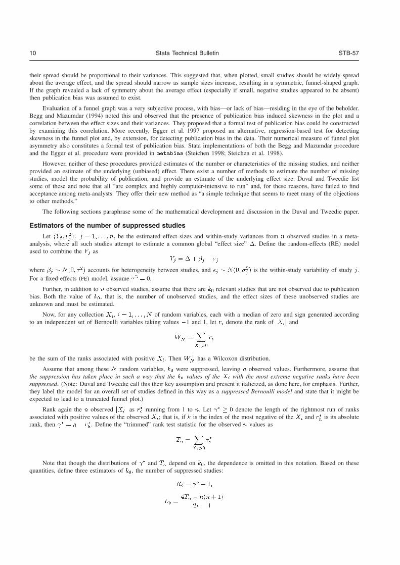
10 Stata Technical Bulletin STB-57
their spread should be proportional to their variances. This suggested that, when plotted, small studies should be widely spreadabout the average effect, and the spread should narrow as sample sizes increase, resulting in a symmetric, funnel-shaped graph.If the graph revealed a lack of symmetry about the average effect (especially if small, negative studies appeared to be absent)then publication bias was assumed to exist.
Evaluation of a funnel graph was a very subjective process, with bias—or lack of bias—residing in the eye of the beholder.Begg and Mazumdar (1994) noted this and observed that the presence of publication bias induced skewness in the plot and acorrelation between the effect sizes and their variances. They proposed that a formal test of publication bias could be constructedby examining this correlation. More recently, Egger et al. 1997 proposed an alternative, regression-based test for detectingskewness in the funnel plot and, by extension, for detecting publication bias in the data. Their numerical measure of funnel plotasymmetry also constitutes a formal test of publication bias. Stata implementations of both the Begg and Mazumdar procedureand the Egger et al. procedure were provided in metabias (Steichen 1998; Steichen et al. 1998).
However, neither of these procedures provided estimates of the number or characteristics of the missing studies, and neitherprovided an estimate of the underlying (unbiased) effect. There exist a number of methods to estimate the number of missingstudies, model the probability of publication, and provide an estimate of the underlying effect size. Duval and Tweedie listsome of these and note that all “are complex and highly computer-intensive to run” and, for these reasons, have failed to findacceptance among meta-analysts. They offer their new method as “a simple technique that seems to meet many of the objectionsto other methods.”
The following sections paraphrase some of the mathematical development and discussion in the Duval and Tweedie paper.
Estimators of the number of suppressed studies
Let �Yj � v�j �� j � �� � � � � n� be the estimated effect sizes and within-study variances from n observed studies in a meta-analysis, where all such studies attempt to estimate a common global “effect size” �. Define the random-effects (RE) modelused to combine the Yj as
Yj � �� �j � �j
where �j � N��� ��� accounts for heterogeneity between studies, and �j � N��� ��j � is the within-study variability of study j.For a fixed-effects (FE) model, assume �� � 0.
Further, in addition to n observed studies, assume that there are k� relevant studies that are not observed due to publicationbias. Both the value of k�, that is, the number of unobserved studies, and the effect sizes of these unobserved studies areunknown and must be estimated.
Now, for any collection Xi, i � �� � � � � N of random variables, each with a median of zero and sign generated accordingto an independent set of Bernoulli variables taking values �1 and 1, let ri denote the rank of jXij and
W�
N �X
Xi��
ri
be the sum of the ranks associated with positive Xi. Then W�
N has a Wilcoxon distribution.
Assume that among these N random variables, k� were suppressed, leaving n observed values. Furthermore, assume thatthe suppression has taken place in such a way that the k� values of the Xi with the most extreme negative ranks have beensuppressed. (Note: Duval and Tweedie call this their key assumption and present it italicized, as done here, for emphasis. Further,they label the model for an overall set of studies defined in this way as a suppressed Bernoulli model and state that it might beexpected to lead to a truncated funnel plot.)
Rank again the n observed jXij as r�i running from 1 to n. Let �� � � denote the length of the rightmost run of ranksassociated with positive values of the observed Xi; that is, if h is the index of the most negative of the Xi and r�h is its absoluterank, then �� � n� r�h. Define the “trimmed” rank test statistic for the observed n values as
Tn �X
Xi��
r�i
Note that though the distributions of �� and Tn depend on k�, the dependence is omitted in this notation. Based on thesequantities, define three estimators of k�, the number of suppressed studies:
R� � �� � ��
L� ��Tn � n�n� ��
n� �
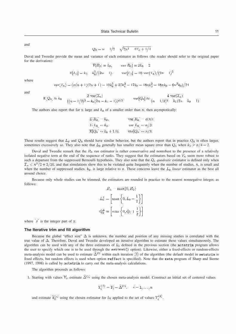
Stata Technical Bulletin 11
andQ� � n� ����
p�n� � �Tn � ���
Duval and Tweedie provide the mean and variance of each estimator as follows (the reader should refer to the original paperfor the derivation):
E�R�� � k�� var�R�� � �k� � �
E�L�� � k� � k�����n� �� var�L�� � � var�Tn���n� ��
wherevar�Tn � �n�n� ���n� � � ��k�� � ��k�� � ��k� � � nk�� � � nk� � n�k����
and
E�Q�� � k� �� var�Tn
��n� ���� � k���n� k� � ����� var�Q�� �
� var�Tn
�n� ���� � k���n� k� � �
The authors also report that for n large and k� of a smaller order than n, then asymptotically:
E�R�� � k��
E�L�� � k��
E�Q�� � k� � ���
var�R�� � o�n�
var�L�� � n���
var�Q�� � n���
These results suggest that L� and Q� should have similar behavior, but the authors report that in practice Q� is often larger,sometimes excessively so. They also note that L� generally has smaller mean square error than Q� when k� � n�4� 2.
Duval and Tweedie remark that the R� run estimator is rather conservative and nonrobust to the presence of a relativelyisolated negative term at the end of the sequence of ranks. They suggest that the estimators based on Tn seem more robust tosuch a departure from the suppressed Bernoulli hypothesis. They also note that the Q� quadratic estimator is defined only whenTn � n��� � ���, and that simulations show this to be violated quite frequently when the number of studies, n, is small andwhen the number of suppressed studies, k�, is large relative to n. These concerns leave the L� linear estimator as the best allaround choice.
Because only whole studies can be trimmed, the estimators are rounded in practice to the nearest nonnegative integer, asfollows:
R�� � maxf�� R�g
L�� �
�max
��� L� �
�
�
��
Q�� �
�max
��� Q� �
�
�
��
where �x� is the integer part of x.
The Iterative trim and fill algorithm
Because the global “effect size” � is unknown, the number and position of any missing studies is correlated with thetrue value of �. Therefore, Duval and Tweedie developed an iterative algorithm to estimate these values simultaneously. Thealgorithm can be used with any of the three estimators of k� defined in the previous section (the metatrim program allowsthe user to specify which one is to be used through the estimat�� option). Likewise, either a fixed-effects or random-effectsmeta-analysis model can be used to estimate b��l� within each iteration �l of the algorithm (the default model in metatrim isfixed effects, but random effects is used when option reffect is specified). Note that the meta program of Sharp and Sterne(1997, 1998) is called by metatrim to carry out the meta-analysis calculations.
The algorithm proceeds as follows:
1. Starting with values Yi, estimate b���� using the chosen meta-analysis model. Construct an initial set of centered values
Y���i � Yi � b����� i � �� � � � � n
and estimate bk���� using the chosen estimator for k� applied to the set of values Y ���i .
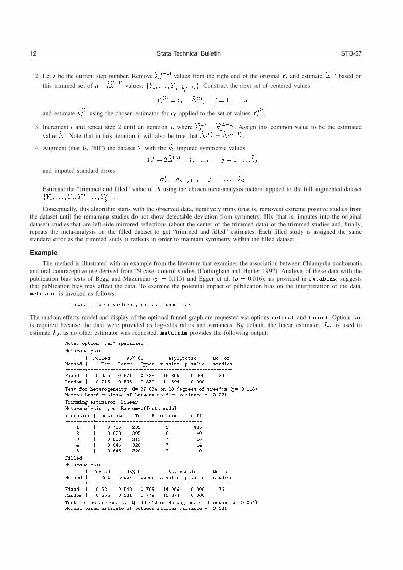
12 Stata Technical Bulletin STB-57
2. Let l be the current step number. Remove bk�l���� values from the right end of the original Yi and estimate b�
�l� based on
this trimmed set of n� bk�l���� values: fY�� � � � � Yn�bk�l���
�
g� Construct the next set of centered values
Y�l�i � Yi � b�
�l�� i � �� � � � � n
and estimate bk�l�� using the chosen estimator for k� applied to the set of values Y
�l�i .
3. Increment l and repeat step 2 until an iteration L where bk�L�� � bk
�L���� . Assign this common value to be the estimated
value bk�. Note that in this iteration it will also be true that b��L�
� b��L���.
4. Augment (that is, “fill”) the dataset Y with the bk� imputed symmetric values
Y �
j � �b��L� � Yn�j��� j � �� � � � �bk�
and imputed standard errors��j � �n�j��� j � �� � � � �bk�
Estimate the “trimmed and filled” value of � using the chosen meta-analysis method applied to the full augmented datasetfY�� � � � � Yn� Y
�
� � � � � � Y �
bk�g.
Conceptually, this algorithm starts with the observed data, iteratively trims (that is, removes) extreme positive studies fromthe dataset until the remaining studies do not show detectable deviation from symmetry, fills (that is, imputes into the originaldataset) studies that are left-side mirrored reflections (about the center of the trimmed data) of the trimmed studies and, finally,repeats the meta-analysis on the filled dataset to get “trimmed and filled” estimates. Each filled study is assigned the samestandard error as the trimmed study it reflects in order to maintain symmetry within the filled dataset.
Example
The method is illustrated with an example from the literature that examines the association between Chlamydia trachomatisand oral contraceptive use derived from 29 case–control studies (Cottingham and Hunter 1992). Analysis of these data with thepublication bias tests of Begg and Mazumdar (p � 0.115) and Egger et al. (p � 0.016), as provided in metabias, suggeststhat publication bias may affect the data. To examine the potential impact of publication bias on the interpretation of the data,metatrim is invoked as follows:
� metatrim logor varlogor� reffect funnel var
The random-effects model and display of the optional funnel graph are requested via options reffect and funnel. Option var
is required because the data were provided as log-odds ratios and variances. By default, the linear estimator, L�, is used toestimate k�, as no other estimator was requested. metatrim provides the following output:
Note� option �var� specified�
Meta�analysis
� Pooled �� CI Asymptotic No� ofMethod � Est Lower Upper zvalue pvalue studies������������������������������������������������������������Fixed � �� �� ����� ����� ������ ����� ��Random � ���� ����� ����� ������ �����
Test for heterogeneity� Q� ������ on �� degrees of freedom �p� ������Moment�based estimate of between studies variance � �����
Trimming estimator� LinearMeta�analysis type� Random�effects model
iteration � estimate Tn � to trim diff�������������������������������������������������
� � ���� ��� � ���� � �� �� ��� ��� � �� � ��� � � � � �� � ��� � ��� � �� � ��� � �
FilledMeta�analysis
� Pooled �� CI Asymptotic No� ofMethod � Est Lower Upper zvalue pvalue studies������������������������������������������������������������Fixed � �� �� ����� ����� ���� � ����� � Random � �� �� ����� ����� ������ �����
Test for heterogeneity� Q� ������ on �� degrees of freedom �p� ������Moment�based estimate of between studies variance � �����
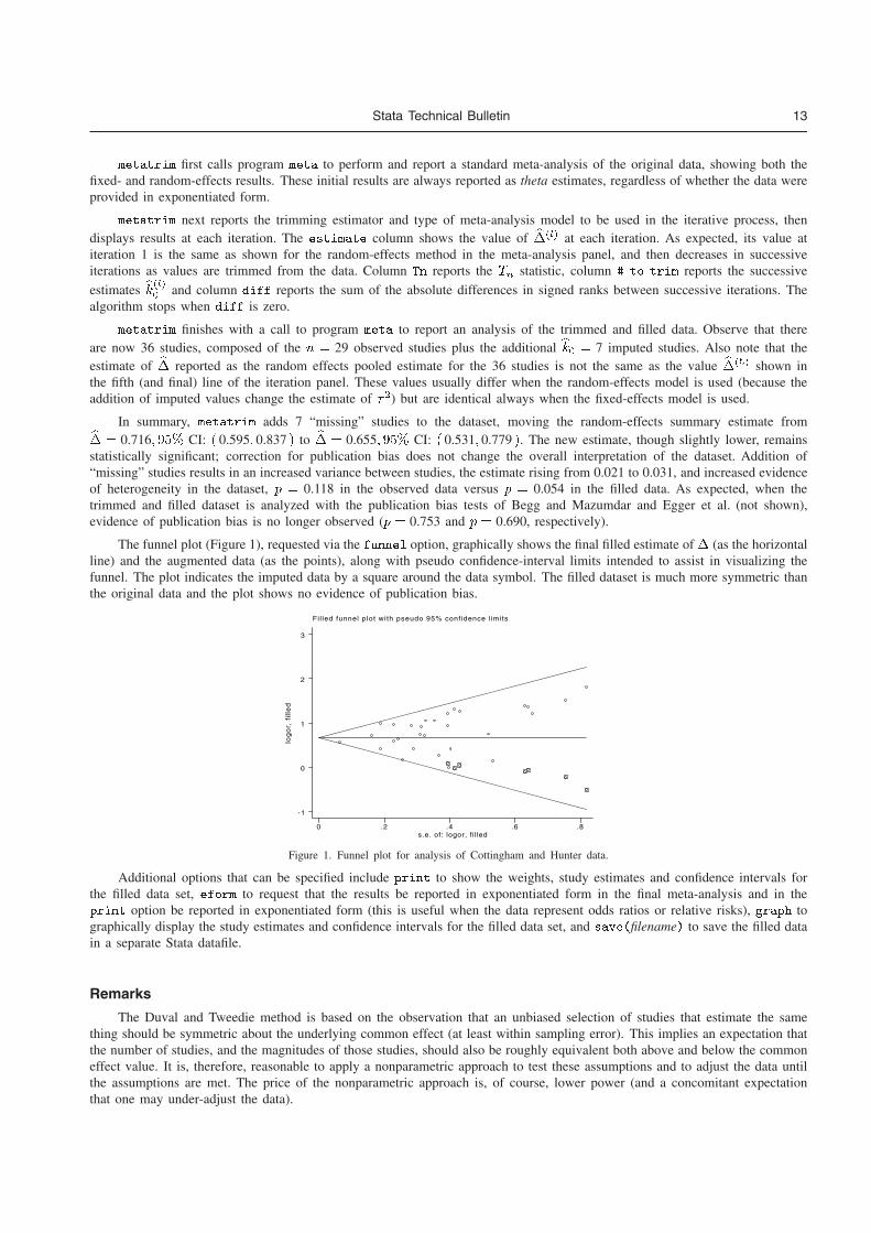
Stata Technical Bulletin 13
metatrim first calls program meta to perform and report a standard meta-analysis of the original data, showing both thefixed- and random-effects results. These initial results are always reported as theta estimates, regardless of whether the data wereprovided in exponentiated form.
metatrim next reports the trimming estimator and type of meta-analysis model to be used in the iterative process, thendisplays results at each iteration. The estimate column shows the value of b��l� at each iteration. As expected, its value atiteration 1 is the same as shown for the random-effects method in the meta-analysis panel, and then decreases in successiveiterations as values are trimmed from the data. Column Tn reports the Tn statistic, column � to trim reports the successive
estimates bk�l�� and column diff reports the sum of the absolute differences in signed ranks between successive iterations. Thealgorithm stops when diff is zero.
metatrim finishes with a call to program meta to report an analysis of the trimmed and filled data. Observe that thereare now 36 studies, composed of the n � 29 observed studies plus the additional bk� � 7 imputed studies. Also note that theestimate of b� reported as the random effects pooled estimate for the 36 studies is not the same as the value b���� shown inthe fifth (and final) line of the iteration panel. These values usually differ when the random-effects model is used (because theaddition of imputed values change the estimate of ��) but are identical always when the fixed-effects model is used.
In summary, metatrim adds 7 “missing” studies to the dataset, moving the random-effects summary estimate fromb� � 0.716� ��� CI: � 0.595� 0.837 � to b� � 0.655� ��� CI: � 0.531� 0.779 �. The new estimate, though slightly lower, remainsstatistically significant; correction for publication bias does not change the overall interpretation of the dataset. Addition of“missing” studies results in an increased variance between studies, the estimate rising from 0.021 to 0.031, and increased evidenceof heterogeneity in the dataset, p � 0.118 in the observed data versus p � 0.054 in the filled data. As expected, when thetrimmed and filled dataset is analyzed with the publication bias tests of Begg and Mazumdar and Egger et al. (not shown),evidence of publication bias is no longer observed (p � 0.753 and p � 0.690, respectively).
The funnel plot (Figure 1), requested via the funnel option, graphically shows the final filled estimate of � (as the horizontalline) and the augmented data (as the points), along with pseudo confidence-interval limits intended to assist in visualizing thefunnel. The plot indicates the imputed data by a square around the data symbol. The filled dataset is much more symmetric thanthe original data and the plot shows no evidence of publication bias.
Fil led funnel plot with pseudo 95% confidence l imits
lo
go
r, f
ille
d
s.e. of: logor, fi l led0 .2 .4 .6 .8
-1
0
1
2
3
Figure 1. Funnel plot for analysis of Cottingham and Hunter data.
Additional options that can be specified include print to show the weights, study estimates and confidence intervals forthe filled data set, eform to request that the results be reported in exponentiated form in the final meta-analysis and in theprint option be reported in exponentiated form (this is useful when the data represent odds ratios or relative risks), graph tographically display the study estimates and confidence intervals for the filled data set, and save�filename� to save the filled datain a separate Stata datafile.
Remarks
The Duval and Tweedie method is based on the observation that an unbiased selection of studies that estimate the samething should be symmetric about the underlying common effect (at least within sampling error). This implies an expectation thatthe number of studies, and the magnitudes of those studies, should also be roughly equivalent both above and below the commoneffect value. It is, therefore, reasonable to apply a nonparametric approach to test these assumptions and to adjust the data untilthe assumptions are met. The price of the nonparametric approach is, of course, lower power (and a concomitant expectationthat one may under-adjust the data).
14 Stata Technical Bulletin STB-57
Duval and Tweedie use the symmetry argument in a somewhat roundabout way, choosing to first trim extreme positivestudies until the remaining studies meet symmetry requirements. This makes sense when the studies are subject only to publicationbias, since trimming should preferably toss out the low-weight, but extreme studies. Nonetheless, if other biases affect the data,in particular if there is a study that is high-weight and extremely positive relative to the remainder of the studies, then the methodcould fail to function properly. The user must remain alert to such possibilities.
Duval and Tweedie’s final step—filling in imputed reflections of the trimmed studies—has no effect on the final trimmedpoint estimate in a fixed effects analysis but does cause the confidence interval of the estimate to be smaller than that from thetrimmed or original data. One could question whether this “increased” confidence is warranted.
The random-effects situation is more complex, as both the trimmed point estimate and confidence interval width are affectedby filling, with a tendency for the filled data to yield a point estimate between the values from the original and trimmed data.When the random-effects model is used, the confidence interval of the filled data is typically smaller than that of either thetrimmed or original data.
Experimentation suggests that the Duval and Tweedie method trims more studies than may be expected; but because ofthe increase in precision induced by the imputation of studies during filling, changes in the “significance” of the results occurless often than expected. Thus the two operations (trimming, which reduces the point estimate, and filling, which increases theprecision) seem to counter each other.
Another phenomenon noted is a tendency for the heterogeneity of the filled data to be greater than that of the original data.This suggests that the most likely studies to be trimmed and filled are those that are most responsible for heterogeneity. Thegenerality of this phenomenon and its impact on the analysis have not been investigated.
Duval and Tweedie provide a reasonable development based on accepted statistics; nonetheless, the number and themagnitude of the assumptions required by the method are substantial. If the underlying assumptions hold in a given dataset,then, as with many methods, it will tend to under- rather than over-correct. This is an acceptable situation in my view (whereas“over-correction” of publication bias would be a critical flaw).
This author presents the program as an experimental tool only. Users must assess for themselves both the amount ofcorrection provided and the reasonableness of that correction. Other tools to assess publication bias issues should be used intandem. metatrim should be treated as merely one of an arsenal of methods needed to fully assess a meta-analysis.
Saved Results
metatrim does not save values in the system S # macros, nor does it return results in r��.
Note
The command meta (Sharp and Sterne 1997, 1998) should be installed before running metatrim.
ReferencesBegg, C. B. and M. Mazumdar. 1994. Operating characteristics of a rank correlation test for publication bias. Biometrics 50: 1088–1101.
Bradburn, M. J., J. J. Deeks, and D. G. Altman. 1998. sbe24: metan—an alternative meta-analysis command. Stata Technical Bulletin 44: 4–15.Reprinted in The Stata Technical Bulletin Reprints vol. 8, pp. 86–100.
Cottingham, J. and D. Hunter. 1992. Chlamydia trachomatis and oral contraceptive use: A quantitative review. Genitourinary Medicine 68: 209–216.
Duval, S. and R. Tweedie. 2000. A nonparametric “trim and fill” method of accounting for publication bias in meta-analysis. Journal of the AmericanStatistical Association 95: 89–98.
Egger, M., G. D. Smith, M. Schneider, and C. Minder. 1997. Bias in meta-analysis detected by a simple, graphical test. British Medical Journal 315:629–634.
Light, R. J. and D. B. Pillemer. 1984. Summing up: The science of reviewing research. Cambridge, MA: Harvard University Press.
Sharp, S. and J. Sterne. 1997. sbe16: Meta-analysis. Stata Technical Bulletin 38: 9–14. Reprinted in The Stata Technical Bulletin Reprints vol. 7,pp. 100–106.
——. 1998. sbe16.1: New syntax and output for the meta-analysis command. Stata Technical Bulletin 42: 6–8. Reprinted in The Stata TechnicalBulletin Reprints vol. 7, pp. 106–108.
Steichen, T. J. 1998. sbe19: Tests for publication bias in meta-analysis. Stata Technical Bulletin 41: 9–15. Reprinted in The Stata Technical BulletinReprints vol. 7, pp. 125–133.
Steichen, T. J., M. Egger, and J. Sterne. 1998. sbe19.1: Tests for publication bias in meta-analysis. Stata Technical Bulletin 44: 3–4. Reprinted in TheStata Technical Bulletin Reprints vol. 8, pp. 84–85.
4 Advanced methods:
metandi, glst, metamiss, and mvmeta
The Stata Journal (2009)9, Number 2, pp. 211–229
metandi: Meta-analysis of diagnostic accuracyusing hierarchical logistic regression
Roger M. HarbordDepartment of Social Medicine
University of BristolBristol, UK
Penny WhitingDepartment of Social Medicine
University of BristolBristol, UK
Abstract. Meta-analysis of diagnostic test accuracy presents many challenges.Even in the simplest case, when the data are summarized by a 2 × 2 table fromeach study, a statistically rigorous analysis requires hierarchical (multilevel) modelsthat respect the binomial data structure, such as hierarchical logistic regression.We present a Stata package, metandi, to facilitate the fitting of such models inStata. The commands display the results in two alternative parameterizations andproduce a customizable plot. metandi requires either Stata 10 or above (which hasthe new command xtmelogit), or Stata 8.2 or above with gllamm installed.
Keywords: st0163, metandi, metandiplot, diagnosis, meta-analysis, sensitivity andspecificity, hierarchical models, generalized mixed models, gllamm, xtmelogit, re-ceiver operating characteristic (ROC), summary ROC, hierarchical summary ROC
1 Introduction
There are several existing user-written commands in Stata that are intended primarilyfor meta-analysis (see Sterne et al. [2007] for an overview). There is increasing interest insystematic reviews and meta-analyses of data from diagnostic accuracy studies (Deeks2001b; Deville et al. 2002; Tatsioni et al. 2005; Gluud and Gluud 2005; Mallett et al.2006; Gatsonis and Paliwal 2006), which presents many additional challenges comparedto more traditional meta-analysis applications, such as controlled trials. In particu-lar, diagnostic accuracy cannot be adequately summarized by one measure; two mea-sures are typically used, most often sensitivity and specificity or, alternatively, posi-tive and negative likelihood ratios, and the two are correlated (Deeks 2001a). Meta-analysis of diagnostic accuracy therefore requires different and more complex methodsthan traditional meta-analysis applications, even in the simplest situation where thedata from each primary study are summarized as a 2 × 2 table of test results againsttrue disease status, both of which have been dichotomized. In addition, substantialbetween-study heterogeneity is commonplace, and the models must account for this(Lijmer, Bossuyt, and Heisterkamp 2002).
Several methods of meta-analyzing diagnostic accuracy data have been proposed, ofwhich two are statistically rigorous: the hierarchical summary receiver operating charac-teristic (HSROC) model (Rutter and Gatsonis 2001) and the bivariate model (Reitsma etal. 2005). In the absence of covariates, these turn out to be different parameterizationsof the same model (Harbord et al. 2007; Arends et al. 2008).
c© 2009 StataCorp LP st0163
212 Meta-analysis of diagnostic accuracy
The bivariate model can be fit in Stata by using the user-written gllamm command,as pointed out by Coveney (2004). In Stata 10, the same model can be fit considerablyfaster by using the new xtmelogit command. In either case, however, some datapreparation is required, the syntax is complex (particularly for gllamm), and the outputis not easy to interpret.
In this article, we present a new Stata command, metandi, to facilitate the fitting ofthese hierarchical logistic regression models for meta-analysis of diagnostic test accuracy.The metandi command fits the model and displays the estimates in both the HSROC andbivariate parameterizations. metandi also displays some familiar summary measures(sensitivity and specificity, positive and negative likelihood ratios, and the diagnosticodds ratio). However, these simple summary measures fail to describe the expectedtrade-off between sensitivity and specificity, which is best illustrated graphically. Wehave therefore included a command, metandiplot, to simplify the plotting of graphicalsummaries of the fitted model, namely, the summary receiver operating characteristic(SROC) curve and the prediction region, and also to plot the summary point and itsconfidence region.
The name metandi was chosen to indicate that, like metan (Bradburn, Deeks, andAltman 1998), metandi takes the cell counts of 2× 2 tables as input but is designed formeta-analysis of diagnostic accuracy.
metandi is not intended to provide a comprehensive package for diagnostic meta-analysis by itself; other plots are also useful, such as forest plots showing within-study es-timates and confidence intervals for sensitivity and specificity separately (Deeks 2001b).
Section 2 of this article introduces an example dataset, which we will use to illustratethe commands. Section 3 then gives some background on methods and models that havebeen proposed for meta-analysis of diagnostic accuracy. Sections 4 and 5 illustrate theoutput of metandi and metandiplot on the example dataset. Section 6, which assumessomewhat greater knowledge of both statistics and Stata, gives examples of the useof predict after metandi for model checking and identification of influential studies.Finally, sections 7 and 2, which are intended mainly as reference material, detail theformal syntax of the commands, and the methods and formulas used.
2 Example: Lymphangiography for diagnosis of lymphnode metastasis
We shall illustrate the use of the metandi package on data from 17 studies of lym-phangiography for the diagnosis of lymph node metastasis in women with cervical can-cer. Lymphangiography is one of three imaging techniques in the meta-analysis ofScheidler et al. (1997), and these data have been frequently used as an example formethodological papers on meta-analysis of diagnostic accuracy (Rutter and Gatsonis2001; Macaskill 2004; Reitsma et al. 2005; Harbord et al. 2007). These data are pro-vided in the auxiliary file scheidler LAG.dta. The total number of patients in eachstudy ranges from 21 to 300. There is one observation in the dataset for each study.
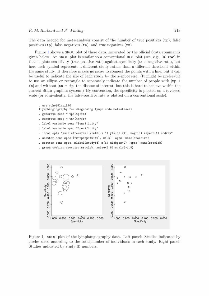
R. M. Harbord and P. Whiting 213
The data needed for meta-analysis consist of the number of true positives (tp), falsepositives (fp), false negatives (fn), and true negatives (tn).
Figure 1 shows a SROC plot of these data, generated by the official Stata commandsgiven below. An SROC plot is similar to a conventional ROC plot (see, e.g., [R] roc) inthat it plots sensitivity (true-positive rate) against specificity (true-negative rate), buthere each symbol represents a different study rather than a different threshold withinthe same study. It therefore makes no sense to connect the points with a line, but it canbe useful to indicate the size of each study by the symbol size. (It might be preferableto use an ellipse or rectangle to separately indicate the number of people with [tp +fn] and without [tn + fp] the disease of interest, but this is hard to achieve within thecurrent Stata graphics system.) By convention, the specificity is plotted on a reversedscale (or equivalently, the false-positive rate is plotted on a conventional scale).
. use scheidler_LAG(Lymphangiography for diagnosing lymph node metastases)
. generate sens = tp/(tp+fn)
. generate spec = tn/(tn+fp)
. label variable sens "Sensitivity"
. label variable spec "Specificity"
. local opts "xscale(reverse) xla(0(.2)1) yla(0(.2)1, nogrid) aspect(1) nodraw"
. scatter sens spec [fw=tp+fp+fn+tn], m(Oh) `opts´ name(sroccirc)
. scatter sens spec, mlabel(studyid) m(i) mlabpos(0) `opts´ name(sroclab)
. graph combine sroccirc sroclab, xsize(4.5) scale(*1.5)
0.00
00.
200
0.40
00.
600
0.80
01.
000
Sen
sitiv
ity
0.0000.2000.4000.6000.8001.000Specificity
1
234
5
67
8
910
11
12
13
14
15
16
17
0.00
00.
200
0.40
00.
600
0.80
01.
000
Sen
sitiv
ity
0.0000.2000.4000.6000.8001.000Specificity
Figure 1. SROC plot of the lymphangiography data. Left panel: Studies indicated bycircles sized according to the total number of individuals in each study. Right panel:Studies indicated by study ID numbers.
214 Meta-analysis of diagnostic accuracy
3 Models for meta-analysis of diagnostic accuracy
Several statistical methods for meta-analysis of data from diagnostic test accuracy stud-ies have been proposed that account for the correlation between sensitivity and speci-ficity (Moses, Shapiro, and Littenberg 1993; Rutter and Gatsonis 2001; Reitsma et al.2005).
Moses, Shapiro, and Littenberg (1993) proposed a method of generating an SROC
curve by using simple linear regression. This method has frequently been used, butthe assumptions of simple linear regression are not met, and the method is thereforeapproximate. There is also uncertainty as to the most appropriate weighting of theregression (Walter 2002; Rutter and Gatsonis 2001).
Two more-complex but statistically rigorous approaches have been proposed thatovercome the limitations of the linear regression method: the HSROC model (Rutterand Gatsonia 2001) and the bivariate model (Reitsma et al. 2005). Both approachesare based on hierarchical models, i.e., both approaches involve statistical distributionsat two levels. At the lower level, they model the cell counts in the 2× 2 tables by usingbinomial distributions and logistic (log-odds) transformations of proportions. Althoughtheir motivation is distinct and they allow covariates to be added to the models in differ-ent ways, it has been shown that the two models are equivalent when no covariates arefit, as well as in certain models including covariates (Harbord et al. 2007; Arends et al.2008).
3.1 HSROC model
The HSROC model (Rutter and Gatsonis 2001) assumes that there is an underlyingROC curve in each study with parameters α and β that characterize the accuracy andasymmetry of the curve. The 2×2 table for each study then arises from dichotomizing ata positivity threshold, θ. The parameters α and θ are assumed to vary between studies;both are assumed to have normal distributions as in conventional random-effects meta-analysis. The accuracy parameter has a mean of Λ (capital lambda) and a variance ofσ2
α, while the positivity parameter θ has a mean of Θ (capital theta) and a variance ofσ2
θ . Because estimation of the shape parameter, β, requires information from more thanone study, it is assumed constant across studies. When no covariates are included in anHSROC model, there are therefore five parameters: Λ, Θ, β, σ2
α, and σ2θ .
3.2 Bivariate model
The bivariate model (Reitsma et al. 2005) models the sensitivity and specificity moredirectly. It assumes that their logit (log-odds) transforms have a bivariate normaldistribution between studies. The logit-transformed sensitivities are assumed to have amean of μA and a variance of σ2
A, while the logit-transformed specificities have a meanof μB and a variance of σ2
B . The trade-off between sensitivity and specificity is allowedfor by also including a correlation, ρAB , that is expected to be negative. The bivariate
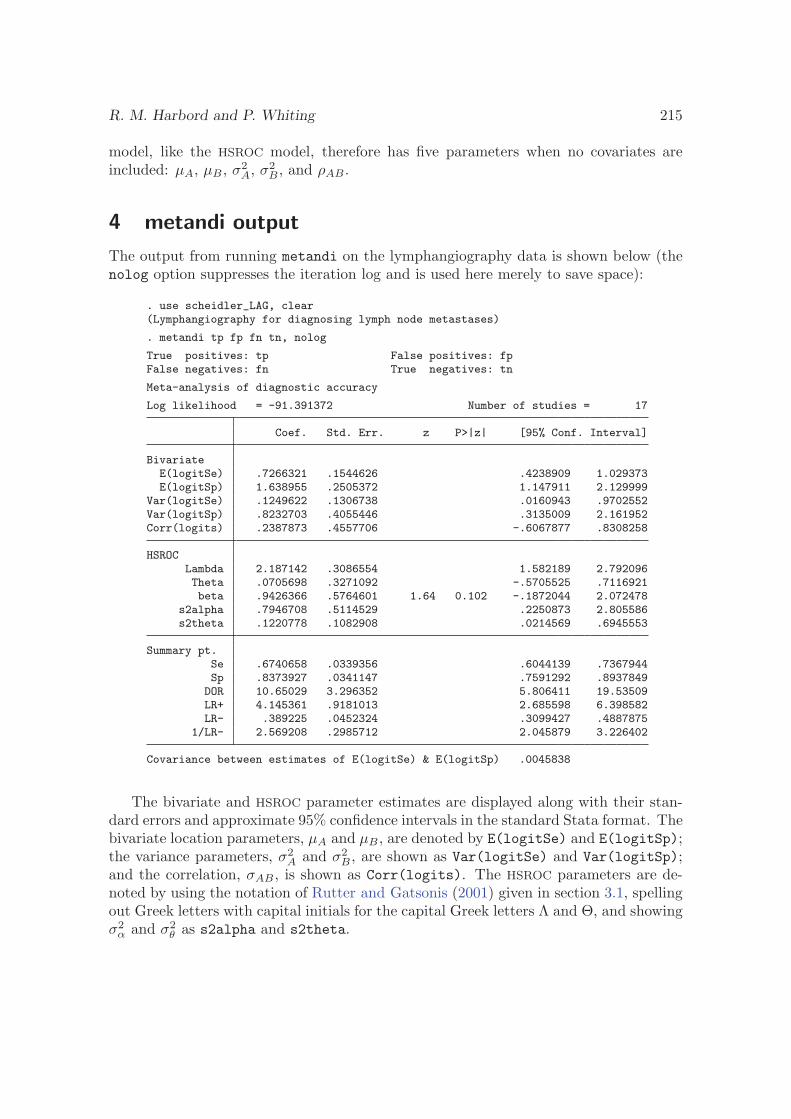
R. M. Harbord and P. Whiting 215
model, like the HSROC model, therefore has five parameters when no covariates areincluded: μA, μB , σ2
A, σ2B , and ρAB .
4 metandi output
The output from running metandi on the lymphangiography data is shown below (thenolog option suppresses the iteration log and is used here merely to save space):
. use scheidler_LAG, clear(Lymphangiography for diagnosing lymph node metastases)
. metandi tp fp fn tn, nolog
True positives: tp False positives: fpFalse negatives: fn True negatives: tn
Meta-analysis of diagnostic accuracy
Log likelihood = -91.391372 Number of studies = 17
Coef. Std. Err. z P>|z| [95% Conf. Interval]
BivariateE(logitSe) .7266321 .1544626 .4238909 1.029373E(logitSp) 1.638955 .2505372 1.147911 2.129999
Var(logitSe) .1249622 .1306738 .0160943 .9702552Var(logitSp) .8232703 .4055446 .3135009 2.161952Corr(logits) .2387873 .4557706 -.6067877 .8308258
HSROCLambda 2.187142 .3086554 1.582189 2.792096Theta .0705698 .3271092 -.5705525 .7116921beta .9426366 .5764601 1.64 0.102 -.1872044 2.072478
s2alpha .7946708 .5114529 .2250873 2.805586s2theta .1220778 .1082908 .0214569 .6945553
Summary pt.Se .6740658 .0339356 .6044139 .7367944Sp .8373927 .0341147 .7591292 .8937849DOR 10.65029 3.296352 5.806411 19.53509LR+ 4.145361 .9181013 2.685598 6.398582LR- .389225 .0452324 .3099427 .4887875
1/LR- 2.569208 .2985712 2.045879 3.226402
Covariance between estimates of E(logitSe) & E(logitSp) .0045838
The bivariate and HSROC parameter estimates are displayed along with their stan-dard errors and approximate 95% confidence intervals in the standard Stata format. Thebivariate location parameters, μA and μB , are denoted by E(logitSe) and E(logitSp);the variance parameters, σ2
A and σ2B , are shown as Var(logitSe) and Var(logitSp);
and the correlation, σAB , is shown as Corr(logits). The HSROC parameters are de-noted by using the notation of Rutter and Gatsonis (2001) given in section 3.1, spellingout Greek letters with capital initials for the capital Greek letters Λ and Θ, and showingσ2
α and σ2θ as s2alpha and s2theta.
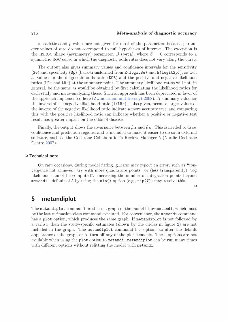
216 Meta-analysis of diagnostic accuracy
z statistics and p-values are not given for most of the parameters because param-eter values of zero do not correspond to null hypotheses of interest. The exception isthe HSROC shape (asymmetry) parameter, β (beta), where β = 0 corresponds to asymmetric ROC curve in which the diagnostic odds ratio does not vary along the curve.
The output also gives summary values and confidence intervals for the sensitivity(Se) and specificity (Sp) (back-transformed from E(logitSe) and E(logitSp)), as wellas values for the diagnostic odds ratio (DOR) and the positive and negative likelihoodratios (LR+ and LR-) at the summary point. The summary likelihood ratios will not, ingeneral, be the same as would be obtained by first calculating the likelihood ratios foreach study and meta-analyzing these. Such an approach has been deprecated in favor ofthe approach implemented here (Zwinderman and Bossuyt 2008). A summary value forthe inverse of the negative likelihood ratio (1/LR-) is also given, because larger values ofthe inverse of the negative likelihood ratio indicate a more accurate test, and comparingthis with the positive likelihood ratio can indicate whether a positive or negative testresult has greater impact on the odds of disease.
Finally, the output shows the covariance between μA and μB . This is needed to drawconfidence and prediction regions, and is included to make it easier to do so in externalsoftware, such as the Cochrane Collaboration’s Review Manager 5 (Nordic CochraneCentre 2007).
Technical note
On rare occasions, during model fitting, gllamm may report an error, such as “con-vergence not achieved: try with more quadrature points” or (less transparently) “loglikelihood cannot be computed”. Increasing the number of integration points beyondmetandi’s default of 5 by using the nip() option (e.g., nip(7)) may resolve this.
5 metandiplot
The metandiplot command produces a graph of the model fit by metandi, which mustbe the last estimation-class command executed. For convenience, the metandi commandhas a plot option, which produces the same graph. If metandiplot is not followed bya varlist, then the study-specific estimates (shown by the circles in figure 2) are notincluded in the graph. The metandiplot command has options to alter the defaultappearance of the graph or to turn off any of the plot elements. These options are notavailable when using the plot option to metandi. metandiplot can be run many timeswith different options without refitting the model with metandi.
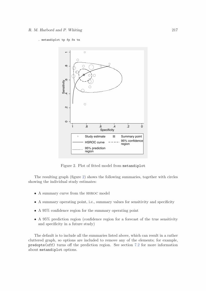
R. M. Harbord and P. Whiting 217
. metandiplot tp fp fn tn
0.2
.4.6
.81
Sen
sitiv
ity
0.2.4.6.81Specificity
Study estimate Summary point
HSROC curve 95% confidenceregion
95% predictionregion
Figure 2. Plot of fitted model from metandiplot
The resulting graph (figure 2) shows the following summaries, together with circlesshowing the individual study estimates:
• A summary curve from the HSROC model
• A summary operating point, i.e., summary values for sensitivity and specificity
• A 95% confidence region for the summary operating point
• A 95% prediction region (confidence region for a forecast of the true sensitivityand specificity in a future study)
The default is to include all the summaries listed above, which can result in a rathercluttered graph, so options are included to remove any of the elements; for example,predopts(off) turns off the prediction region. See section 7.2 for more informationabout metandiplot options.

218 Meta-analysis of diagnostic accuracy
By default, the summary HSROC curve is displayed only for sensitivities and speci-ficities at least as large as the smallest study-specific estimates if a varlist is included.
The shape of the prediction region is dependent on the assumption of a bivariatenormal distribution for the random effects and should therefore not be overinterpreted; itis intended to give a visual representation of the extent of between-study heterogeneity,which is often considerable.
6 predict after metandi
Many of Stata’s standard postestimation tools will not work after metandi or will notwork as expected, because metandi temporarily reshapes the data before fitting themodel.
The notable exception is predict, which can be used to obtain posterior predictions(empirical Bayes estimates) of the sensitivity and specificity in each study (mu), as wellas various statistics that can be useful for detecting outliers (e.g., ustd) and influentialobservations (cooksd).
The help file provides basic commands for examining diagnostics. We take theopportunity here to provide slightly more customized displays.
Empirical Bayes estimates give the best estimate of the true sensitivity and specificityin each study, and these estimates will be “shrunk” toward the summary point comparedwith the study-specific estimates shown in figure 1.
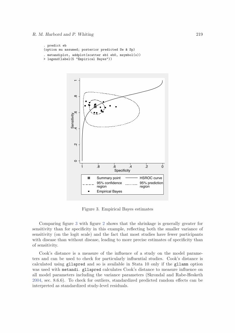
R. M. Harbord and P. Whiting 219
. predict eb(option mu assumed; posterior predicted Se & Sp)
. metandiplot, addplot(scatter eb1 eb0, msymbol(o))> legend(label(5 "Empirical Bayes"))
0.2
.4.6
.81
Sen
sitiv
ity
0.2.4.6.81Specificity
Summary point HSROC curve95% confidenceregion
95% predictionregion
Empirical Bayes
Figure 3. Empirical Bayes estimates
Comparing figure 3 with figure 2 shows that the shrinkage is generally greater forsensitivity than for specificity in this example, reflecting both the smaller variance ofsensitivity (on the logit scale) and the fact that most studies have fewer participantswith disease than without disease, leading to more precise estimates of specificity thanof sensitivity.
Cook’s distance is a measure of the influence of a study on the model parame-ters and can be used to check for particularly influential studies. Cook’s distance iscalculated using gllapred and so is available in Stata 10 only if the gllamm optionwas used with metandi. gllapred calculates Cook’s distance to measure influence onall model parameters including the variance parameters (Skrondal and Rabe-Hesketh2004, sec. 8.6.6). To check for outliers, standardized predicted random effects can beinterpreted as standardized study-level residuals.
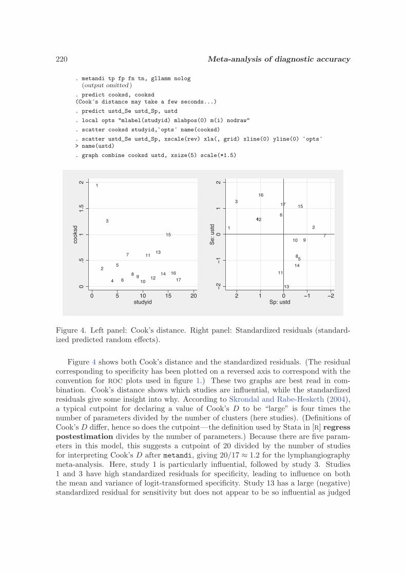
220 Meta-analysis of diagnostic accuracy
. metandi tp fp fn tn, gllamm nolog(output omitted )
. predict cooksd, cooksd(Cook´s distance may take a few seconds...)
. predict ustd_Se ustd_Sp, ustd
. local opts "mlabel(studyid) mlabpos(0) m(i) nodraw"
. scatter cooksd studyid,`opts´ name(cooksd)
. scatter ustd_Se ustd_Sp, xscale(rev) xla(, grid) xline(0) yline(0) `opts´> name(ustd)
. graph combine cooksd ustd, xsize(5) scale(*1.5)
1
2
3
4
5
6
7
8 910
11
12
13
14
15
16
17
0.5
11.
52
cook
sd
0 5 10 15 20studyid
1 2
3
4
5
6
7
8
910
11
12
13
14
15
16
17
�2
�1
01
2S
e: u
std
�2�1012Sp: ustd
Figure 4. Left panel: Cook’s distance. Right panel: Standardized residuals (standard-ized predicted random effects).
Figure 4 shows both Cook’s distance and the standardized residuals. (The residualcorresponding to specificity has been plotted on a reversed axis to correspond with theconvention for ROC plots used in figure 1.) These two graphs are best read in com-bination. Cook’s distance shows which studies are influential, while the standardizedresiduals give some insight into why. According to Skrondal and Rabe-Hesketh (2004),a typical cutpoint for declaring a value of Cook’s D to be “large” is four times thenumber of parameters divided by the number of clusters (here studies). (Definitions ofCook’s D differ, hence so does the cutpoint—the definition used by Stata in [R] regresspostestimation divides by the number of parameters.) Because there are five param-eters in this model, this suggests a cutpoint of 20 divided by the number of studiesfor interpreting Cook’s D after metandi, giving 20/17 ≈ 1.2 for the lymphangiographymeta-analysis. Here, study 1 is particularly influential, followed by study 3. Studies1 and 3 have high standardized residuals for specificity, leading to influence on boththe mean and variance of logit-transformed specificity. Study 13 has a large (negative)standardized residual for sensitivity but does not appear to be so influential as judged
R. M. Harbord and P. Whiting 221
by its Cook’s distance. Further investigation of the effect of individual studies on themodel could be undertaken by refitting the model and leaving out each study in turn.
7 Syntax and options for commands
7.1 The metandi command
Syntax
metandi tp fp fn tn[if] [
in] [
, plot gllamm force ip(g | m) nip(#)
nobivariate nohsroc nosummarypt detail level(#) trace nolog]
by is allowed with metandi; see [D] by.
Options
plot requests a plot of the results on an SROC plot. This is a convenience optionequivalent to executing the metandiplot command after metandi with the same listof variables, tp, fp, fn, and tn (and the same if and in qualifiers, if specified). Greatercontrol of the plot is available through the options of the metandiplot commandwhen issued as a separate command after metandi.
gllamm specifies that the model be fit using gllamm. This is the default in Stata 8 and9, so the option is of use only in Stata 10, in which the model is fit using xtmelogitby default.
force forces metandi to attempt to fit data where one or more studies have tp+fn = 0(or tn + fp = 0), i.e., where there are no individuals that are positive (negative) forthe reference standard. Without this option, metandi exits with an error when suchdata exist. Problems may be encountered in fitting such data, particularly when themodel is fit using xtmelogit. Sensitivity (specificity) cannot be estimated withinsuch studies, so they are not included in the plot produced by metandiplot.
ip(g | m) specifies the quadrature (numerical integration) method used to integrate outthe random effects: ip(g), the default, gives Cartesian product quadrature, whileip(m) gives spherical quadrature, which is available in gllamm but not in xtmelogit.Spherical quadrature can be more efficient, though its properties are less well knownand it can sometimes cause the adaptive quadrature step to take longer to converge.See Rabe-Hesketh, Skrondal, and Pickles (2005).
nip(#) specifies the number of integration points used for quadrature. Higher valuesshould result in greater accuracy but typically at the expense of longer executiontimes. Specifying too small a value can lead to convergence problems or even failureof adaptive quadrature; if you receive the error “log likelihood cannot be computed”,try increasing nip(). For Cartesian product quadrature, nip() specifies the num-ber of points for each of the two random effects; the default is nip(5). For spher-

222 Meta-analysis of diagnostic accuracy
ical quadrature, nip() specifies the degree, d, of the approximation; the default isnip(9), and the only values currently supported by gllamm are 5, 7, 9, 11, and 15.These defaults give approximately the same accuracy, because degree d for sphericalquadrature approximately corresponds in accuracy to (d + 1)/2 points per randomeffect for Cartesian product quadrature (Rabe-Hesketh, Skrondal, and Pickles 2005,app. B).
nobivariate, nohsroc, and nosummarypt suppress reporting of the bivariate param-eter estimates, the HSROC parameter estimates, or the summary point estimates,respectively.
detail displays the output of all gllamm or xtmelogit commands issued.
level(#) specifies the confidence level, as a percentage, for confidence intervals. Thedefault is level(95) or as set by set level; see [U] 20.7 Specifying the widthof confidence intervals.
trace adds a display of the current parameter vector to the iteration log.
nolog suppresses display of the iteration log.
7.2 The metandiplot command
Syntax
metandiplot[tp fp fn tn
] [if] [
in] [
weight] [
, notruncate level(#)
predlevel(numlist) npoints(#) subplot options addplot(plot)
twoway options]
Options
notruncate specifies that the HSROC curve will not be truncated outside the regionof the data. By default, the HSROC curve is not shown when the sensitivity orspecificity is less than its smallest study estimate.
level(#) specifies the confidence level, as a percentage, for the confidence contour.The default is level(95) or as set by set level; see [U] 20.7 Specifying thewidth of confidence intervals.
predlevel(numlist) specifies the levels, as a percentage, for the prediction contour(s).The default is one contour at the same probability level as the confidence region.Up to five prediction contours are allowed.
npoints(#) specifies the number of points to use in drawing the outlines of the confi-dence and prediction regions. The default is npoints(500).
subplot options, which are summopts(), confopts(), predopts(), curveopts(), andstudyopts(), control the display of the summary point, confidence contour, predic-tion contour(s), HSROC curve, and study symbols, respectively. The options within

R. M. Harbord and P. Whiting 223
each set of parentheses are simply passed through to the appropriate twoway plot.Any of the plots can be turned off by specifying, for example, summopts(off).
addplot(plot) allows adding additional graph twoway plots to the graph; see [G] ad-dplot option. For example, empirical Bayes predictions could be generated by usingpredict after metandi and then added to the graph. See section 6.
twoway options are most of the options documented in [G] twoway options, includingoptions for titles, axes, labels, schemes, and saving the graph to disk. However, theby() option is not allowed.
7.3 The predict command after metandi
Syntax
predict[type
]newvarlist
[if] [
in] [
, statistic]
statistic description
mu posterior predicted (empirical Bayes) sensitivity and specificity;the default
u posterior means (empirical Bayes predictions, BLUPs) ofrandom effects
sdu posterior standard deviations of random effectsustd standardized posterior means of random effectslinpred linear predictor with empirical Bayes predictions plugged in:
linpred = xb + ucooksd Cook’s distance for each study; available only when model was
fit using gllamm
Most of the above statistics require newvarlist to consist of two new variables to storethem: one for the statistic associated with sensitivity and one for the statistic associatedwith specificity. If newvarlist contains only one newvar, the statistics associated withsensitivity and specificity will be stored in newvar1 and newvar0, respectively. cooksd,however, is computed once for each study and therefore requires only one newvar. Seesection 6 for examples.
(Continued on next page)
224 Meta-analysis of diagnostic accuracy
7.4 Saved results
metandi saves the following results in e():
Scalarse(N) number of studies e(ll) log likelihood
Macrose(cmd) metandi e(predict) program used to implemente(tpfpfntn) names of tp fp fn tn predict
variables e(properties) b Ve(cmd) metareg
Matricese(b) bivariate coefficient vector e(V) variance–covariance matrix ofe(b hsroc) HSROC coefficient vector the bivariate estimators
e(V hsroc) variance–covariance matrix ofthe HSROC estimators
Functionse(sample) marks estimation sample
8 Methods and formulas
It is possible to use routines for linear mixed models to fit an approximate versionof the bivariate model obtained by using empirical logit transforms of the estimatedsensitivity and specificity in each study together with their estimated standard errors(Reitsma et al. 2005). However, the small cell counts common in diagnostic accuracystudies can lead to poor performance of such approximations. Generalized mixed mod-els, in particular, hierarchical (mixed-effects) logistic regression, can handle the binomialnature of the data directly and are therefore preferable (Chu and Cole 2006; Riley et al.2007).
Such models are complex to fit, however, because they require numerical integration(quadrature) to integrate out the random effects. metandi uses gllamm or xtmelogitto fit the bivariate model by using adaptive quadrature, then transforms the parameterestimates to those of the HSROC model by using the delta method (Cox 1998).
Because the bivariate model can sometimes prove difficult to fit, some care has beentaken to provide good starting values. First, two separate univariate models are fitto sensitivity and specificity. These provide excellent starting values for the two meanand two variance parameters of the bivariate model. A reasonable starting value forthe correlation parameter is obtained from the correlation between the posterior means(empirical Bayes predictions) of the two univariate models.
We now give the mathematical forms of the bivariate and HSROC models in theabsence of covariates. See Rutter and Gatsonis (2001); Reitsma et al. (2005); and Har-bord et al. (2007) for information on the models with covariates, which are not currentlysupported by metandi.
R. M. Harbord and P. Whiting 225
8.1 The bivariate model
Following Reitsma et al. (2005), we denote the sensitivity in the ith study by pAi andthe specificity by pBi, and base analysis on their logit transforms:
μAi = logit(pAi)
μBi = logit(pBi)
(We use the letter μ where Reitsma et al. (2005) used θ to avoid a clash of notationwith the HSROC model defined in the next section.)
The bivariate model is a random-effects model in which the logit transforms of thetrue sensitivity and true specificity in each study have a bivariate normal distribu-tion across studies, thereby allowing for the possibility of correlation between them(Reitsma et al. 2005):
(μAi
μBi
)∼ N
{(μA
μB
),ΣAB
}with ΣAB =
(σ2
A σAB
σAB σ2B
)
8.2 The HSROC model
The HSROC model (Rutter and Gatsonis 2001) was originally formulated in terms of theprobability, πij , that a patient in study i with disease status j has a positive test result,where j = 0 for a patient without the disease and j = 1 for a patient with the disease.Therefore, sensitivity pAi = πi1 and specificity pBi = 1 − πi0.
The HSROC model for study i takes the form
logit(πij) = (θi + αiXij) exp(−βXij) (1)
where Xij = −1/2 for those without disease (j = 0) and +1/2 for those with disease(j = 1). Both θi and αi are allowed to vary between studies. In the model withoutcovariates fit by metandi, they are assumed to have independent normal distributionswith θi ∼ N(Θ, σ2
θ) and αi ∼ N(Λ, σ2α). The model is nonlinear in the parameter β
and therefore cannot be fit in gllamm directly.
We can rewrite (1) as two separate equations for the logit transforms of sensitivitypAi and specificity pBi, thus connecting to the parameters μAi and μBi of the bivariatemodel above:
μAi = logit(pAi) = b−1(θi +12αi)
μBi = logit(pBi) = −b(θi − 12αi)
This tells us that μAi and μBi are linear combinations of two random variables,θi and αi, with independent normal distributions, and that they therefore must have abivariate normal distribution. Some straightforward further algebra gives the explicit re-lationship between the parameters of the two models (Harbord et al. 2007; Arends et al.
226 Meta-analysis of diagnostic accuracy
2008), enabling HSROC parameter estimates to be obtained by transforming the bivari-ate parameter estimates. Standard errors for the transformed parameter estimates areobtained by the delta method, which gives the same standard errors that would be ob-tained from standard maximum-likelihood methods if the HSROC model were fit directly(Cox 1998).
8.3 Methods and formulas for metandiplot
HSROC curve
The HSROC model gives rise to an SROC curve by allowing the threshold parameter, θi,to vary while holding the accuracy parameter, αi, fixed at its mean, Λ. The expectedsensitivity for a given specificity is then given by (Rutter and Gatsonis 2001; Macaskill2004)
logit(sensitivity) = Λe−β/2 − e−β logit(specificity)
Bivariate confidence and prediction regions
Confidence and prediction regions in SROC space can be constructed by using the esti-mates from the bivariate model (Reitsma et al. 2005; Harbord et al. 2007). An ellipticaljoint confidence region for μA and μB is most easily specified by using a parametric rep-resentation (Douglas 1993)
μA = μA + sA c cos t (2)
μB = μB + sB c cos(t + arccos r) (3)
where sA and sB are the estimated standard errors of μA and μB , r is the estimate oftheir correlation, and varying t from 0 to 2π generates the boundary of the ellipse. Theconstant c has been called the boundary constant of the ellipse (Alexandersson 2004);c =
√2f2,n−2;α, where n is the number of studies and f2,n−2;α is the upper 100α% point
of the F distribution with degrees of freedom 2 and n − 2 (Douglas 1993; Chew 1966).This ellipse is then back-transformed to conventional ROC space to give a confidenceregion for the summary operating point.
A prediction region giving the region that has a given probability (e.g., 95%) ofincluding the true sensitivity and specificity of a future study is generated similarly.The covariance matrix for the true logit sensitivity and logit specificity in a futurestudy is
ΣAB + Var(
μA
μB
)
In practice, both terms are estimated by fitting the model to the data. The parameterssA, sB , and r in (2) and (3) can then be replaced by the corresponding quantities derivedfrom this covariance matrix to give the prediction ellipse in logit ROC space, which isthen back-transformed to a prediction region for the true sensitivity and specificity ofa future study in conventional ROC space.
R. M. Harbord and P. Whiting 227
8.4 Methods and formulas for predict
If metandi fit the model by using gllamm, then predict after metandi uses gllapred;see Rabe-Hesketh, Skrondal, and Pickles (2004). If metandi fit the model by usingxtmelogit, predict after metandi uses the prediction facilities of xtmelogit; see[XT] xtmelogit postestimation.
9 Acknowledgments
Joseph Coveney first worked out how to fit the bivariate model by using gllamm andposted the syntax on Statalist in response to a query from Ben Dwamena; our thanksto Joe for generous email correspondence. We thank the authors of gllamm for all theirwork, and Sophia Rabe-Hesketh in particular for helpful email correspondence. Ourthanks also to Susan Mallett and Jon Deeks for useful feedback on earlier versions ofmetandi.
10 ReferencesAlexandersson, A. 2004. Graphing confidence ellipses: An update of ellip for Stata 8.
Stata Journal 4: 242–256.
Arends, L. R., T. H. Hamza, J. C. van Houwelingen, M. H. Heijenbrok-Kal, M. G. M.Hunink, and T. Stijnen. 2008. Bivariate random effects meta-analysis of ROC curves.Medical Decision Making 28: 621–638.
Bradburn, M. J., J. J. Deeks, and D. G. Altman. 1998. sbe24: metan—an alterna-tive meta-analysis command. Stata Technical Bulletin 44: 4–15. Reprinted in StataTechnical Bulletin Reprints, vol. 8, pp. 86–100. College Station, TX: Stata Press.
Chew, V. 1966. Confidence, prediction, and tolerance regions for the multivariate normaldistribution. Journal of the American Statistical Association 61: 605–617.
Chu, H., and S. R. Cole. 2006. Bivariate meta-analysis of sensitivity and specificitywith sparse data: A generalized linear mixed model approach. Journal of ClinicalEpidemiology 59: 1331–1332.
Coveney, J. 2004. Re: st: bivariate random effects meta-analysis of diagnostictest. Statalist archive. Available at http://www.stata.com/statalist/archive/2004-04/msg00820.html.
Cox, C. 1998. Delta method. In Encyclopedia of Biostatistics, ed. P. Armitage andT. Colton, 1125–1127. New York: Wiley.
Cox, D. R., and E. J. Snell. 1989. Analysis of Binary Data. 2nd ed. London: Chapman& Hall.
228 Meta-analysis of diagnostic accuracy
Deeks, J. J. 2001a. Systematic reviews of evaluations of diagnostic and screening tests.In Systematic Reviews in Health Care: Meta-Analysis in Context, 2nd edition, ed.M. Egger, G. Davey Smith, and D. G. Altman, 248–282. London: BMJ Books.
———. 2001b. Systematic reviews in health care: Systematic reviews of evaluations ofdiagnostic and screening tests. British Medical Journal 323: 157–162.
Deville, W. L., F. Buntinx, L. M. Bouter, V. M. Montori, H. C. W. de Vet, D. A.W. M. van der Windt, and P. D. Bezemer. 2002. Conducting systematic reviews ofdiagnostic studies: Didactic guidelines. BMC Medical Research Methodology 2: 9.
Douglas, J. B. 1993. Confidence regions for parameter pairs. American Statistician 47:43–45.
Gatsonis, C., and P. Paliwal. 2006. Meta-analysis of diagnostic and screening testaccuracy evaluations: Methodologic primer. American Journal of Roentgenology 187:271–281.
Gluud, C., and L. L. Gluud. 2005. Evidence based diagnostics. British Medical Journal330: 724–726.
Harbord, R. M., J. J. Deeks, M. Egger, P. Whiting, and J. A. C. Sterne. 2007. Aunification of models for meta-analysis of diagnostic accuracy studies. Biostatistics8: 239–251.
Lijmer, J. G., P. M. M. Bossuyt, and S. H. Heisterkamp. 2002. Exploring sources ofheterogeneity in systematic reviews of diagnostic tests. Statistics in Medicine 21:1525–1537.
Macaskill, P. 2004. Empirical Bayes estimates generated in a hierarchical summaryROC analysis agreed closely with those of a full Bayesian analysis. Journal of ClinicalEpidemiology 57: 925–932.
Mallett, S., J. J. Deeks, S. Halligan, S. Hopewell, V. Cornelius, and D. G. Altman. 2006.Systematic reviews of diagnostic tests in cancer: Review of methods and reporting.British Medical Journal 333: 413–416.
Moses, L. E., D. Shapiro, and B. Littenberg. 1993. Combining independent studies ofa diagnostic test into a summary ROC curve: Data-analytic approaches and someadditional considerations. Statistics in Medicine 12: 1293–1316.
Nordic Cochrane Centre. 2007. Review Manager (RevMan): Version 5. Software pro-gram. Copenhagen: The Nordic Cochrane Centre, The Cochrane Collaboration.
Rabe-Hesketh, S., A. Skrondal, and A. Pickles. 2004. GLLAMM manual. WorkingPaper 160, Division of Biostatistics, University of California–Berkeley. Downloadablefrom http://www.bepress.com/ucbbiostat/paper160/.
———. 2005. Maximum likelihood estimation of limited and discrete dependent variablemodels with nested random effects. Journal of Econometrics 128: 301–323.
R. M. Harbord and P. Whiting 229
Reitsma, J. B., A. S. Glas, A. W. S. Rutjes, R. J. P. M. Scholten, P. M. Bossuyt, andA. H. Zwinderman. 2005. Bivariate analysis of sensitivity and specificity produces in-formative summary measures in diagnostic reviews. Journal of Clinical Epidemiology58: 982–990.
Riley, R. D., K. R. Abrams, A. J. Sutton, P. C. Lambert, and J. R. Thompson. 2007. Bi-variate random-effects meta-analysis and the estimation of between-study correlation.BMC Medical Research Methodology 7: 3.
Rutter, C. M., and C. A. Gatsonis. 2001. A hierarchical regression approach to meta-analysis of diagnostic test accuracy evaluations. Statistics in Medicine 20: 2865–2884.
Scheidler, J., H. Hricak, K. K. Yu, L. Subak, and M. R. Segal. 1997. Radiological eval-uation of lymph node metastases in patients with cervical cancer: A meta-analysis.Journal of the American Medical Association 278: 1096–1101.
Skrondal, A., and S. Rabe-Hesketh. 2004. Generalized Latent Variable Modeling: Mul-tilevel, Longitudinal, and Structural Equation Models. Boca Raton, FL: Chapman &Hall/CRC.
Sterne, J. A. C., R. J. Harris, R. M. Harbord, and T. J. Steichen. 2007. What meta-analysis features are available in Stata? Stata FAQ. Available athttp://www.stata.com/support/faqs/stat/meta.html.
Tatsioni, A., D. A. Zarin, N. Aronson, D. J. Samson, C. R. Flamm, C. Schmid, andJ. Lau. 2005. Challenges in systematic reviews of diagnostic technologies. Annals ofInternal Medicine 142: 1048–1055.
Walter, S. D. 2002. Properties of the summary receiver operating characteric (SROC)curve for diagnostic test data. Statistics in Medicine 21: 1237–1256.
Zwinderman, A. H., and P. M. Bossuyt. 2008. We should not pool diagnostic likelihoodratios in systematic reviews. Statistics in Medicine 27: 687–697.
About the authors
Roger Harbord is a research associate in medical statistics in the Department of Social Medicineat the University of Bristol, UK. He is one of three co-convenors of the Cochrane Collaboration’sScreening and Diagnostic Tests Methods Group.
Penny Whiting is a research fellow in the same department who specializes in methodologyand conduct of diagnostic systematic reviews. She led the development of QUADAS, a 14-item evidence-based tool for assessing the quality of diagnostic accuracy studies included insystematic reviews (Cox and Snell 1989).
The Stata Journal (2006)6, Number 1, pp. 40–57
Generalized least squares for trend estimationof summarized dose–response data
Nicola OrsiniKarolinska InstitutetStockholm, [email protected]
Rino BelloccoKarolinska InstitutetStockholm, Sweden
Sander GreenlandUCLA School of Public Health
Los Angeles, CA
Abstract. This paper presents a command, glst, for trend estimation acrossdifferent exposure levels for either single or multiple summarized case–control,incidence-rate, and cumulative incidence data. This approach is based on con-structing an approximate covariance estimate for the log relative risks and esti-mating a corrected linear trend using generalized least squares. For trend analysisof multiple studies, glst can estimate fixed- and random-effects metaregressionmodels.
Keywords: st0096, glst, dose–response data, generalized least squares, trend, meta-analysis, metaregression
1 Introduction
Epidemiological studies often assess whether the observed relationship between increas-ing (or decreasing) levels of exposure and the risk (or odds) of diseases follows a lineardose–response pattern. Methods for trend estimation of single and multiple summarizeddose–response studies (Berlin, Longnecker, and Greenland 1993) are particularly usefulwhen the full original data are not available.
To demonstrate these methods, our paper uses different types of dose–response dataarising from published case–control, incidence-rate, and cumulative incidence data (alsosee [ST] epitab). Summarized data are typically reported as a series of dose-specificrelative risks, with one category serving as the common referent group. The termrelative risk (RR) will be used as a generic term for the risk ratio (cumulative incidencedata), rate ratio (incidence-rate data), and odds ratio (case–control data).
Table 1 shows a summary of case–control data investigating the association be-tween the consumption of alcohol and the risk of breast cancer, first presented byRohan and McMichael (1988), in which it appears that risk of breast cancer increaseswith increasing levels of alcohol intake.
c© 2006 StataCorp LP st0096
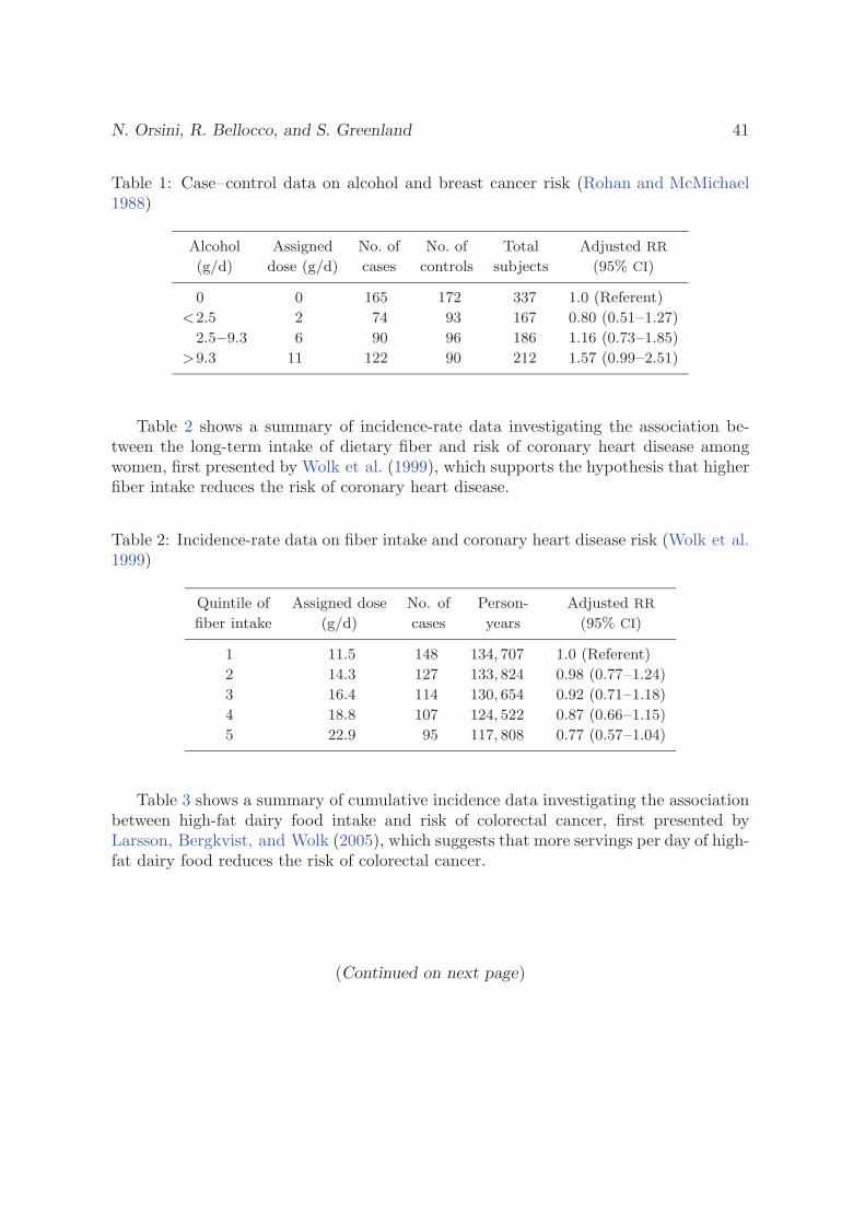
N. Orsini, R. Bellocco, and S. Greenland 41
Table 1: Case–control data on alcohol and breast cancer risk (Rohan and McMichael1988)
Alcohol Assigned No. of No. of Total Adjusted RR
(g/d) dose (g/d) cases controls subjects (95% CI)
0 0 165 172 337 1.0 (Referent)
<2.5 2 74 93 167 0.80 (0.51–1.27)
2.5−9.3 6 90 96 186 1.16 (0.73–1.85)
>9.3 11 122 90 212 1.57 (0.99–2.51)
Table 2 shows a summary of incidence-rate data investigating the association be-tween the long-term intake of dietary fiber and risk of coronary heart disease amongwomen, first presented by Wolk et al. (1999), which supports the hypothesis that higherfiber intake reduces the risk of coronary heart disease.
Table 2: Incidence-rate data on fiber intake and coronary heart disease risk (Wolk et al.1999)
Quintile of Assigned dose No. of Person- Adjusted RR
fiber intake (g/d) cases years (95% CI)
1 11.5 148 134, 707 1.0 (Referent)
2 14.3 127 133, 824 0.98 (0.77–1.24)
3 16.4 114 130, 654 0.92 (0.71–1.18)
4 18.8 107 124, 522 0.87 (0.66–1.15)
5 22.9 95 117, 808 0.77 (0.57–1.04)
Table 3 shows a summary of cumulative incidence data investigating the associationbetween high-fat dairy food intake and risk of colorectal cancer, first presented byLarsson, Bergkvist, and Wolk (2005), which suggests that more servings per day of high-fat dairy food reduces the risk of colorectal cancer.
(Continued on next page)
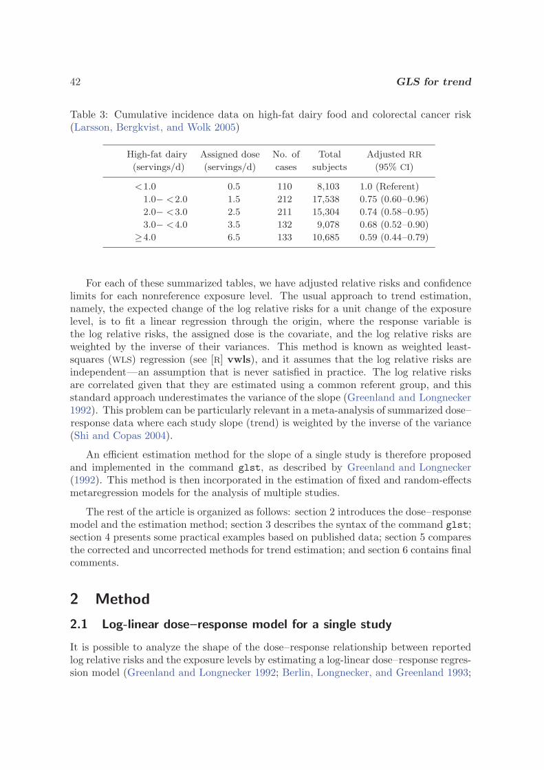
42 GLS for trend
Table 3: Cumulative incidence data on high-fat dairy food and colorectal cancer risk(Larsson, Bergkvist, and Wolk 2005)
High-fat dairy Assigned dose No. of Total Adjusted RR
(servings/d) (servings/d) cases subjects (95% CI)
<1.0 0.5 110 8,103 1.0 (Referent)
1.0− <2.0 1.5 212 17,538 0.75 (0.60–0.96)
2.0− <3.0 2.5 211 15,304 0.74 (0.58–0.95)
3.0− <4.0 3.5 132 9,078 0.68 (0.52–0.90)
≥4.0 6.5 133 10,685 0.59 (0.44–0.79)
For each of these summarized tables, we have adjusted relative risks and confidencelimits for each nonreference exposure level. The usual approach to trend estimation,namely, the expected change of the log relative risks for a unit change of the exposurelevel, is to fit a linear regression through the origin, where the response variable isthe log relative risks, the assigned dose is the covariate, and the log relative risks areweighted by the inverse of their variances. This method is known as weighted least-squares (WLS) regression (see [R] vwls), and it assumes that the log relative risks areindependent—an assumption that is never satisfied in practice. The log relative risksare correlated given that they are estimated using a common referent group, and thisstandard approach underestimates the variance of the slope (Greenland and Longnecker1992). This problem can be particularly relevant in a meta-analysis of summarized dose–response data where each study slope (trend) is weighted by the inverse of the variance(Shi and Copas 2004).
An efficient estimation method for the slope of a single study is therefore proposedand implemented in the command glst, as described by Greenland and Longnecker(1992). This method is then incorporated in the estimation of fixed and random-effectsmetaregression models for the analysis of multiple studies.
The rest of the article is organized as follows: section 2 introduces the dose–responsemodel and the estimation method; section 3 describes the syntax of the command glst;section 4 presents some practical examples based on published data; section 5 comparesthe corrected and uncorrected methods for trend estimation; and section 6 contains finalcomments.
2 Method
2.1 Log-linear dose–response model for a single study
It is possible to analyze the shape of the dose–response relationship between reportedlog relative risks and the exposure levels by estimating a log-linear dose–response regres-sion model (Greenland and Longnecker 1992; Berlin, Longnecker, and Greenland 1993;
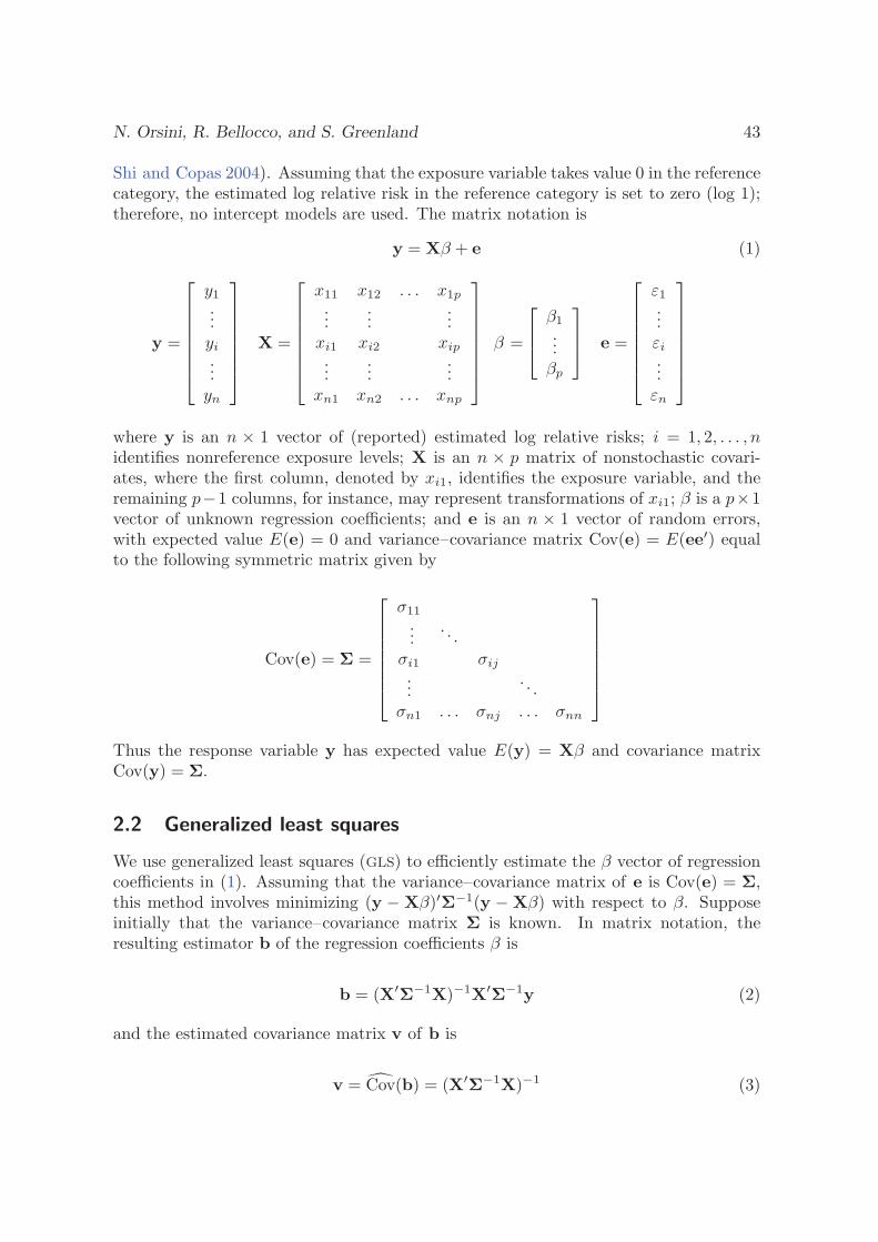
N. Orsini, R. Bellocco, and S. Greenland 43
Shi and Copas 2004). Assuming that the exposure variable takes value 0 in the referencecategory, the estimated log relative risk in the reference category is set to zero (log 1);therefore, no intercept models are used. The matrix notation is
y = Xβ + e (1)
y =
⎡⎢⎢⎢⎢⎢⎢⎣
y1
...yi
...yn
⎤⎥⎥⎥⎥⎥⎥⎦
X =
⎡⎢⎢⎢⎢⎢⎢⎣
x11 x12 . . . x1p
......
...xi1 xi2 xip
......
...xn1 xn2 . . . xnp
⎤⎥⎥⎥⎥⎥⎥⎦
β =
⎡⎢⎣
β1
...βp
⎤⎥⎦ e =
⎡⎢⎢⎢⎢⎢⎢⎣
ε1
...εi
...εn
⎤⎥⎥⎥⎥⎥⎥⎦
where y is an n × 1 vector of (reported) estimated log relative risks; i = 1, 2, . . . , nidentifies nonreference exposure levels; X is an n × p matrix of nonstochastic covari-ates, where the first column, denoted by xi1, identifies the exposure variable, and theremaining p−1 columns, for instance, may represent transformations of xi1; β is a p×1vector of unknown regression coefficients; and e is an n × 1 vector of random errors,with expected value E(e) = 0 and variance–covariance matrix Cov(e) = E(ee′) equalto the following symmetric matrix given by
Cov(e) = Σ =
⎡⎢⎢⎢⎢⎢⎢⎣
σ11
.... . .
σi1 σij
.... . .
σn1 . . . σnj . . . σnn
⎤⎥⎥⎥⎥⎥⎥⎦
Thus the response variable y has expected value E(y) = Xβ and covariance matrixCov(y) = Σ.
2.2 Generalized least squares
We use generalized least squares (GLS) to efficiently estimate the β vector of regressioncoefficients in (1). Assuming that the variance–covariance matrix of e is Cov(e) = Σ,this method involves minimizing (y − Xβ)′Σ−1(y − Xβ) with respect to β. Supposeinitially that the variance–covariance matrix Σ is known. In matrix notation, theresulting estimator b of the regression coefficients β is
b = (X′Σ−1X)−1X′Σ−1y (2)
and the estimated covariance matrix v of b is
v = Cov(b) = (X′Σ−1X)−1 (3)
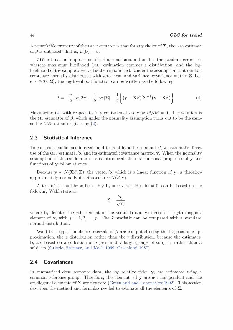
44 GLS for trend
A remarkable property of the GLS estimator is that for any choice of Σ, the GLS estimateof β is unbiased; that is, E(b) = β.
GLS estimation imposes no distributional assumption for the random errors, e,whereas maximum likelihood (ML) estimation assumes a distribution, and the log-likelihood of the sample observed is then maximized. Under the assumption that randomerrors are normally distributed with zero mean and variance–covariance matrix Σ, i.e.,e ∼ N(0, Σ), the log-likelihood function can be written as the following:
l = −n
2log(2π) − 1
2log |Σ| − 1
2
{(y − Xβ
)′Σ−1
(y − Xβ
)}(4)
Maximizing (4) with respect to β is equivalent to solving ∂l/∂β = 0. The solution isthe ML estimator of β, which under the normality assumption turns out to be the sameas the GLS estimator given by (2).
2.3 Statistical inference
To construct confidence intervals and tests of hypotheses about β, we can make directuse of the GLS estimate, b, and its estimated covariance matrix, v. When the normalityassumption of the random error e is introduced, the distributional properties of y andfunctions of y follow at once.
Because y ∼ N(Xβ,Σ), the vector b, which is a linear function of y, is thereforeapproximately normally distributed b ∼ N(β,v).
A test of the null hypothesis, H0: bj = 0 versus HA: bj �= 0, can be based on thefollowing Wald statistic,
Z =bj√vj
where bj denotes the jth element of the vector b and vj denotes the jth diagonalelement of v, with j = 1, 2, . . . , p. The Z statistic can be compared with a standardnormal distribution.
Wald test–type confidence intervals of β are computed using the large-sample ap-proximation, the z distribution rather than the t distribution, because the estimates,b, are based on a collection of n presumably large groups of subjects rather than nsubjects (Grizzle, Starmer, and Koch 1969; Greenland 1987).
2.4 Covariances
In summarized dose–response data, the log relative risks, y, are estimated using acommon reference group. Therefore, the elements of y are not independent and theoff-diagonal elements of Σ are not zero (Greenland and Longnecker 1992). This sectiondescribes the method and formulas needed to estimate all the elements of Σ.
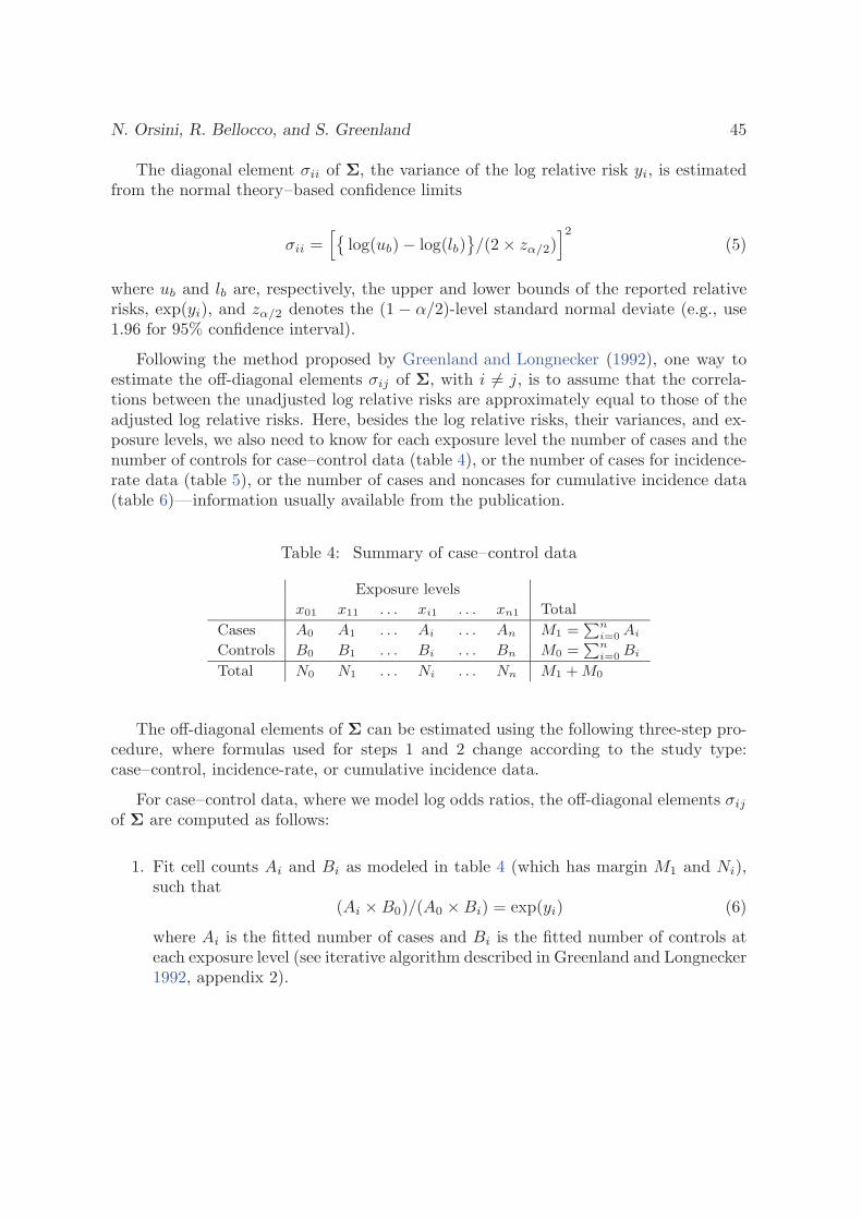
N. Orsini, R. Bellocco, and S. Greenland 45
The diagonal element σii of Σ, the variance of the log relative risk yi, is estimatedfrom the normal theory–based confidence limits
σii =[{
log(ub) − log(lb)}/(2 × zα/2)
]2(5)
where ub and lb are, respectively, the upper and lower bounds of the reported relativerisks, exp(yi), and zα/2 denotes the (1 − α/2)-level standard normal deviate (e.g., use1.96 for 95% confidence interval).
Following the method proposed by Greenland and Longnecker (1992), one way toestimate the off-diagonal elements σij of Σ, with i �= j, is to assume that the correla-tions between the unadjusted log relative risks are approximately equal to those of theadjusted log relative risks. Here, besides the log relative risks, their variances, and ex-posure levels, we also need to know for each exposure level the number of cases and thenumber of controls for case–control data (table 4), or the number of cases for incidence-rate data (table 5), or the number of cases and noncases for cumulative incidence data(table 6)—information usually available from the publication.
Table 4: Summary of case–control data
Exposure levels
x01 x11 . . . xi1 . . . xn1 Total
Cases A0 A1 . . . Ai . . . An M1 =Pn
i=0 Ai
Controls B0 B1 . . . Bi . . . Bn M0 =Pn
i=0 Bi
Total N0 N1 . . . Ni . . . Nn M1 + M0
The off-diagonal elements of Σ can be estimated using the following three-step pro-cedure, where formulas used for steps 1 and 2 change according to the study type:case–control, incidence-rate, or cumulative incidence data.
For case–control data, where we model log odds ratios, the off-diagonal elements σij
of Σ are computed as follows:
1. Fit cell counts Ai and Bi as modeled in table 4 (which has margin M1 and Ni),such that
(Ai × B0)/(A0 × Bi) = exp(yi) (6)
where Ai is the fitted number of cases and Bi is the fitted number of controls ateach exposure level (see iterative algorithm described in Greenland and Longnecker1992, appendix 2).
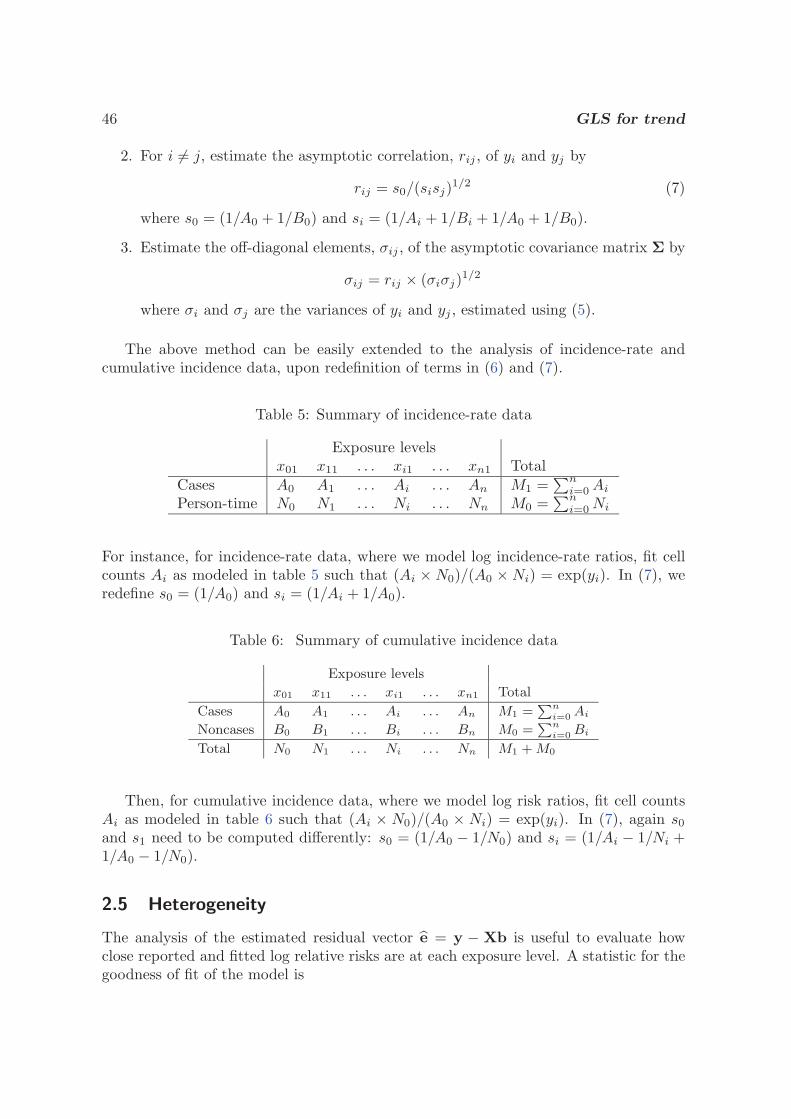
46 GLS for trend
2. For i �= j, estimate the asymptotic correlation, rij , of yi and yj by
rij = s0/(sisj)1/2 (7)
where s0 = (1/A0 + 1/B0) and si = (1/Ai + 1/Bi + 1/A0 + 1/B0).
3. Estimate the off-diagonal elements, σij , of the asymptotic covariance matrix Σ by
σij = rij × (σiσj)1/2
where σi and σj are the variances of yi and yj , estimated using (5).
The above method can be easily extended to the analysis of incidence-rate andcumulative incidence data, upon redefinition of terms in (6) and (7).
Table 5: Summary of incidence-rate data
Exposure levelsx01 x11 . . . xi1 . . . xn1 Total
Cases A0 A1 . . . Ai . . . An M1 =∑n
i=0 Ai
Person-time N0 N1 . . . Ni . . . Nn M0 =∑n
i=0 Ni
For instance, for incidence-rate data, where we model log incidence-rate ratios, fit cellcounts Ai as modeled in table 5 such that (Ai × N0)/(A0 × Ni) = exp(yi). In (7), weredefine s0 = (1/A0) and si = (1/Ai + 1/A0).
Table 6: Summary of cumulative incidence data
Exposure levels
x01 x11 . . . xi1 . . . xn1 Total
Cases A0 A1 . . . Ai . . . An M1 =Pn
i=0 Ai
Noncases B0 B1 . . . Bi . . . Bn M0 =Pn
i=0 Bi
Total N0 N1 . . . Ni . . . Nn M1 + M0
Then, for cumulative incidence data, where we model log risk ratios, fit cell countsAi as modeled in table 6 such that (Ai × N0)/(A0 × Ni) = exp(yi). In (7), again s0
and s1 need to be computed differently: s0 = (1/A0 − 1/N0) and si = (1/Ai − 1/Ni +1/A0 − 1/N0).
2.5 Heterogeneity
The analysis of the estimated residual vector e = y − Xb is useful to evaluate howclose reported and fitted log relative risks are at each exposure level. A statistic for thegoodness of fit of the model is
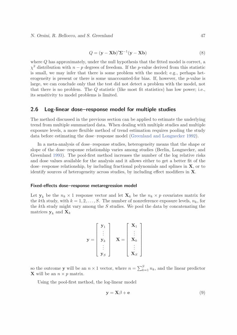
N. Orsini, R. Bellocco, and S. Greenland 47
Q = (y − Xb)′Σ−1(y − Xb) (8)
where Q has approximately, under the null hypothesis that the fitted model is correct, aχ2 distribution with n− p degrees of freedom. If the p-value derived from this statisticis small, we may infer that there is some problem with the model; e.g., perhaps het-erogeneity is present or there is some unaccounted-for bias. If, however, the p-value islarge, we can conclude only that the test did not detect a problem with the model, notthat there is no problem. The Q statistic (like most fit statistics) has low power; i.e.,its sensitivity to model problems is limited.
2.6 Log-linear dose–response model for multiple studies
The method discussed in the previous section can be applied to estimate the underlyingtrend from multiple summarized data. When dealing with multiple studies and multipleexposure levels, a more flexible method of trend estimation requires pooling the studydata before estimating the dose–response model (Greenland and Longnecker 1992).
In a meta-analysis of dose–response studies, heterogeneity means that the shape orslope of the dose–response relationship varies among studies (Berlin, Longnecker, andGreenland 1993). The pool-first method increases the number of the log relative risksand dose values available for the analysis and it allows either to get a better fit of thedose–response relationship, by including fractional polynomials and splines in X, or toidentify sources of heterogeneity across studies, by including effect modifiers in X.
Fixed-effects dose–response metaregression model
Let yk be the nk × 1 response vector and let Xk be the nk × p covariates matrix forthe kth study, with k = 1, 2, . . . , S. The number of nonreference exposure levels, nk, forthe kth study might vary among the S studies. We pool the data by concatenating thematrices yk and Xk
y =
⎡⎢⎢⎢⎢⎢⎢⎣
y1...
yk...
yS
⎤⎥⎥⎥⎥⎥⎥⎦
X =
⎡⎢⎢⎢⎢⎢⎢⎣
X1
...Xk
...XS
⎤⎥⎥⎥⎥⎥⎥⎦
so the outcome y will be an n× 1 vector, where n =∑S
k=1 nk, and the linear predictorX will be an n × p matrix.
Using the pool-first method, the log-linear model
y = Xβ + e (9)
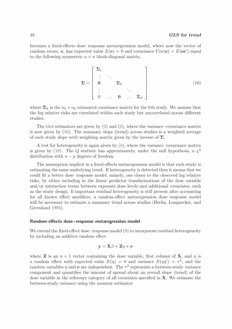
48 GLS for trend
becomes a fixed-effects dose–response metaregression model, where now the vector ofrandom errors, e, has expected value E(e) = 0 and covariance Cov(e) = E(ee′) equalto the following symmetric n × n block-diagonal matrix,
Σ =
⎡⎢⎢⎢⎢⎢⎢⎣
Σ1
.... . .
0 Σk
.... . .
0 . . . 0 . . . ΣS
⎤⎥⎥⎥⎥⎥⎥⎦
(10)
where Σk is the nk ×nk estimated covariance matrix for the kth study. We assume thatthe log relative risks are correlated within each study but uncorrelated across differentstudies.
The GLS estimators are given by (2) and (3), where the variance–covariance matrixis now given by (10). The summary slope (trend) across studies is a weighted averageof each study slope with weighting matrix given by the inverse of Σ.
A test for heterogeneity is again given by (8), where the variance–covariance matrixis given by (10). The Q statistic has approximately, under the null hypothesis, a χ2
distribution with n − p degrees of freedom.
The assumption implicit in a fixed-effects metaregression model is that each study isestimating the same underlying trend. If heterogeneity is detected then it means that wecould fit a better dose–response model, namely, one closer to the observed log relativerisks, by either including in the linear predictor transformations of the dose variableand/or interaction terms between exposure dose levels and additional covariates, suchas the study design. If important residual heterogeneity is still present after accountingfor all known effect modifiers, a random-effect metaregression dose–response modelwill be necessary to estimate a summary trend across studies (Berlin, Longnecker, andGreenland 1993).
Random-effects dose–response metaregression model
We extend the fixed-effect dose–response model (9) to incorporate residual heterogeneityby including an additive random effect
y = Xβ + Zη + e
where Z is an n × 1 vector containing the dose variable, first column of X, and η isa random effect with expected value E(η) = 0 and variance E(ηη′) = τ2, and therandom variables η and e are independent. The τ2 represents a between-study variancecomponent and quantifies the amount of spread about an overall slope (trend) of thedose variable in the reference category of all covariates specified in X. We estimate thebetween-study variance using the moment estimator
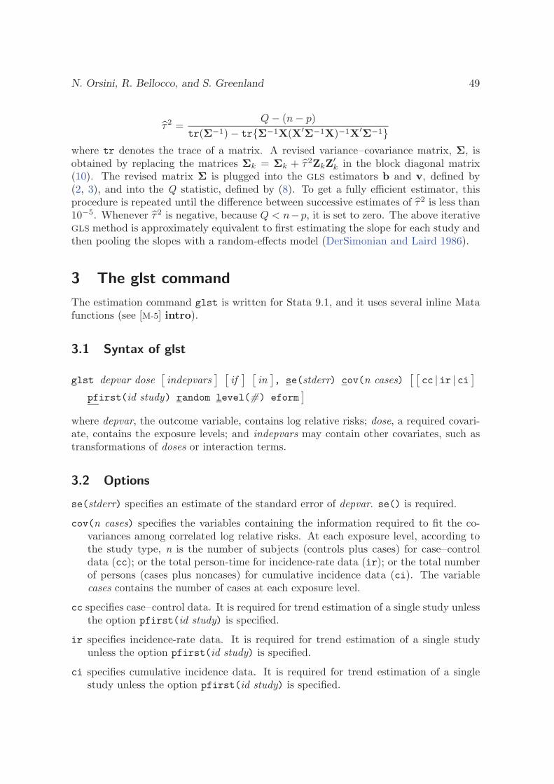
N. Orsini, R. Bellocco, and S. Greenland 49
τ2 =Q − (n − p)
tr(Σ−1) − tr{Σ−1X(X′Σ−1X)−1X′Σ−1}where tr denotes the trace of a matrix. A revised variance–covariance matrix, Σ, isobtained by replacing the matrices Σk = Σk + τ2ZkZ′
k in the block diagonal matrix(10). The revised matrix Σ is plugged into the GLS estimators b and v, defined by(2, 3), and into the Q statistic, defined by (8). To get a fully efficient estimator, thisprocedure is repeated until the difference between successive estimates of τ2 is less than10−5. Whenever τ2 is negative, because Q < n−p, it is set to zero. The above iterativeGLS method is approximately equivalent to first estimating the slope for each study andthen pooling the slopes with a random-effects model (DerSimonian and Laird 1986).
3 The glst command
The estimation command glst is written for Stata 9.1, and it uses several inline Matafunctions (see [M-5] intro).
3.1 Syntax of glst
glst depvar dose[indepvars
] [if] [
in], se(stderr) cov(n cases)
[ [cc | ir | ci ]
pfirst(id study) random level(#) eform]
where depvar, the outcome variable, contains log relative risks; dose, a required covari-ate, contains the exposure levels; and indepvars may contain other covariates, such astransformations of doses or interaction terms.
3.2 Options
se(stderr) specifies an estimate of the standard error of depvar. se() is required.
cov(n cases) specifies the variables containing the information required to fit the co-variances among correlated log relative risks. At each exposure level, according tothe study type, n is the number of subjects (controls plus cases) for case–controldata (cc); or the total person-time for incidence-rate data (ir); or the total numberof persons (cases plus noncases) for cumulative incidence data (ci). The variablecases contains the number of cases at each exposure level.
cc specifies case–control data. It is required for trend estimation of a single study unlessthe option pfirst(id study) is specified.
ir specifies incidence-rate data. It is required for trend estimation of a single studyunless the option pfirst(id study) is specified.
ci specifies cumulative incidence data. It is required for trend estimation of a singlestudy unless the option pfirst(id study) is specified.
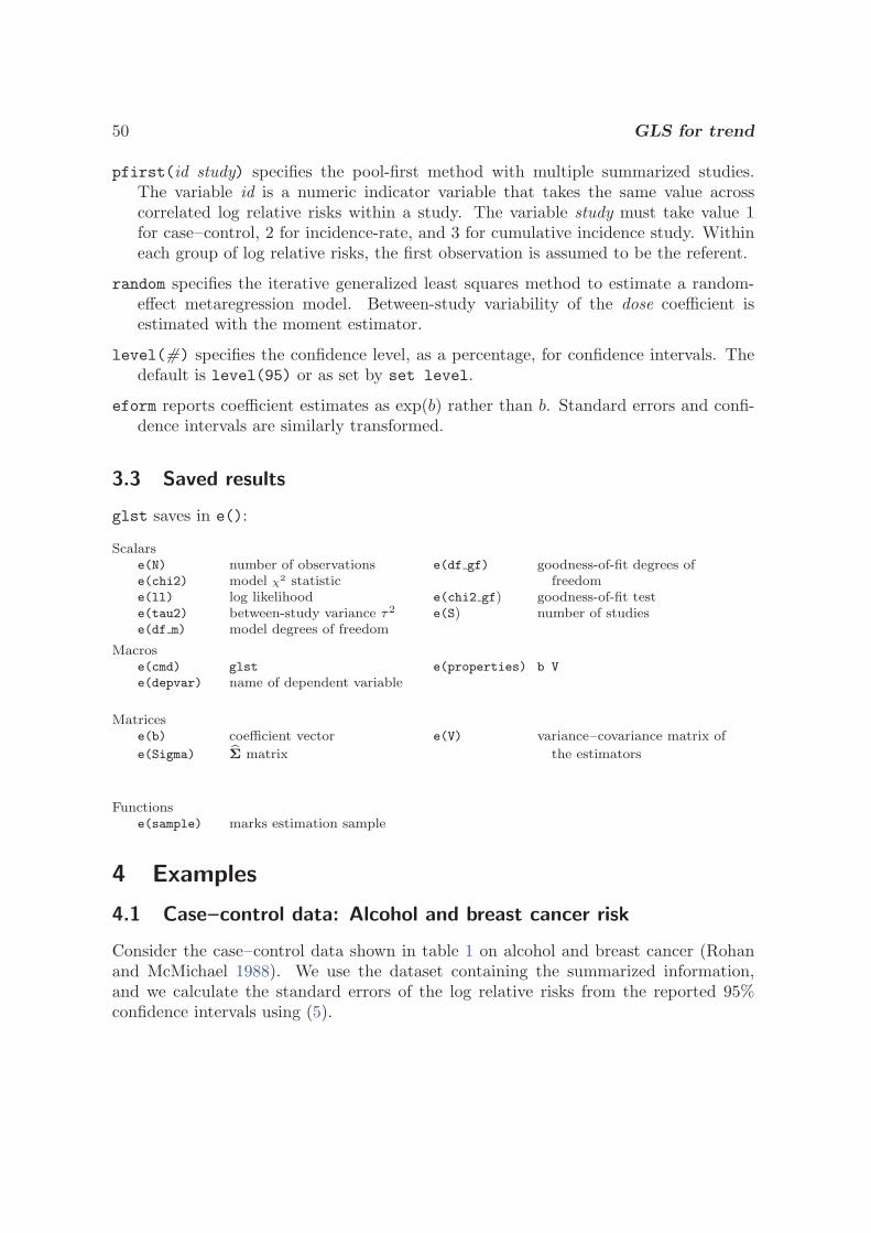
50 GLS for trend
pfirst(id study) specifies the pool-first method with multiple summarized studies.The variable id is a numeric indicator variable that takes the same value acrosscorrelated log relative risks within a study. The variable study must take value 1for case–control, 2 for incidence-rate, and 3 for cumulative incidence study. Withineach group of log relative risks, the first observation is assumed to be the referent.
random specifies the iterative generalized least squares method to estimate a random-effect metaregression model. Between-study variability of the dose coefficient isestimated with the moment estimator.
level(#) specifies the confidence level, as a percentage, for confidence intervals. Thedefault is level(95) or as set by set level.
eform reports coefficient estimates as exp(b) rather than b. Standard errors and confi-dence intervals are similarly transformed.
3.3 Saved results
glst saves in e():
Scalarse(N) number of observations e(df gf) goodness-of-fit degrees ofe(chi2) model χ2 statistic freedome(ll) log likelihood e(chi2 gf) goodness-of-fit teste(tau2) between-study variance τ2 e(S) number of studiese(df m) model degrees of freedom
Macrose(cmd) glst e(properties) b V
e(depvar) name of dependent variable
Matricese(b) coefficient vector e(V) variance–covariance matrix of
e(Sigma) bΣ matrix the estimators
Functionse(sample) marks estimation sample
4 Examples
4.1 Case–control data: Alcohol and breast cancer risk
Consider the case–control data shown in table 1 on alcohol and breast cancer (Rohanand McMichael 1988). We use the dataset containing the summarized information,and we calculate the standard errors of the log relative risks from the reported 95%confidence intervals using (5).

N. Orsini, R. Bellocco, and S. Greenland 51
. use cc_ex
. gen double se = (logub - loglb)/(2*invnormal(.975))
We fit the log-linear dose–response model (1) to regress the log relative risks on theexposure level. The command glst fits the covariances and uses the GLS estimator toprovide a correct estimate of the linear trend.
. glst logrr dose, se(se) cov(n case) cc
Generalized least-squares regression Number of obs = 3Goodness-of-fit chi2(2) = 1.93 Model chi2(1) = 4.83Prob > chi2 = 0.3816 Prob > chi2 = 0.0279
logrr Coef. Std. Err. z P>|z| [95% Conf. Interval]
dose .0454288 .0206639 2.20 0.028 .0049284 .0859293
The command glst stores the fitted covariance matrix of the log relative risks ine(Sigma)
. matrix list e(Sigma)
symmetric e(Sigma)[3,3]c1 c2 c3
r1 .05417235r2 .01881768 .05627467r3 .01943145 .02068682 .05632754
The exponentiated linear trend for a change of 11 g/d of alcohol level is 1.65 (95%CI = 1.06, 2.57).
. lincom dose*11, eform
( 1) 11 dose = 0
logrr exp(b) Std. Err. z P>|z| [95% Conf. Interval]
(1) 1.648255 .3746524 2.20 0.028 1.055709 2.573384
The goodness-of-fit p-value (Q = 1.93, Pr = 0.3816) is large. Thus this test detected noproblems with the fitted model.
4.2 Incidence-rate data: Fiber intake and coronary heart disease
Consider now the incidence-rate data shown in table 2 on long-term intake of dietaryfiber and risk of coronary heart disease among women (Wolk et al. 1999). As we did forcase–control data, we use the command glst to get an efficient estimate of the slope.
. use ir_ex
. gen double se = (logub - loglb)/(2*invnormal(.975))
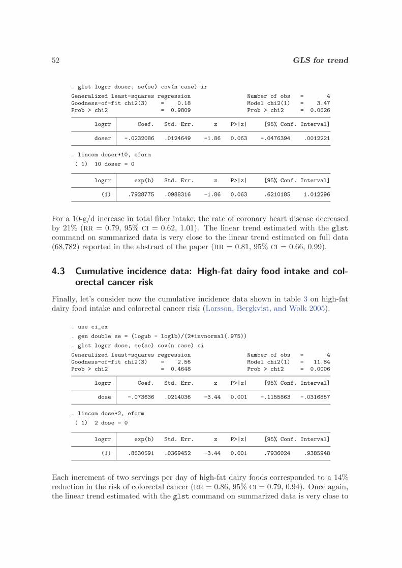
52 GLS for trend
. glst logrr doser, se(se) cov(n case) ir
Generalized least-squares regression Number of obs = 4Goodness-of-fit chi2(3) = 0.18 Model chi2(1) = 3.47Prob > chi2 = 0.9809 Prob > chi2 = 0.0626
logrr Coef. Std. Err. z P>|z| [95% Conf. Interval]
doser -.0232086 .0124649 -1.86 0.063 -.0476394 .0012221
. lincom doser*10, eform
( 1) 10 doser = 0
logrr exp(b) Std. Err. z P>|z| [95% Conf. Interval]
(1) .7928775 .0988316 -1.86 0.063 .6210185 1.012296
For a 10-g/d increase in total fiber intake, the rate of coronary heart disease decreasedby 21% (RR = 0.79, 95% CI = 0.62, 1.01). The linear trend estimated with the glstcommand on summarized data is very close to the linear trend estimated on full data(68,782) reported in the abstract of the paper (RR = 0.81, 95% CI = 0.66, 0.99).
4.3 Cumulative incidence data: High-fat dairy food intake and col-orectal cancer risk
Finally, let’s consider now the cumulative incidence data shown in table 3 on high-fatdairy food intake and colorectal cancer risk (Larsson, Bergkvist, and Wolk 2005).
. use ci_ex
. gen double se = (logub - loglb)/(2*invnormal(.975))
. glst logrr dose, se(se) cov(n case) ci
Generalized least-squares regression Number of obs = 4Goodness-of-fit chi2(3) = 2.56 Model chi2(1) = 11.84Prob > chi2 = 0.4648 Prob > chi2 = 0.0006
logrr Coef. Std. Err. z P>|z| [95% Conf. Interval]
dose -.073636 .0214036 -3.44 0.001 -.1155863 -.0316857
. lincom dose*2, eform
( 1) 2 dose = 0
logrr exp(b) Std. Err. z P>|z| [95% Conf. Interval]
(1) .8630591 .0369452 -3.44 0.001 .7936024 .9385948
Each increment of two servings per day of high-fat dairy foods corresponded to a 14%reduction in the risk of colorectal cancer (RR = 0.86, 95% CI = 0.79, 0.94). Once again,the linear trend estimated with the glst command on summarized data is very close to
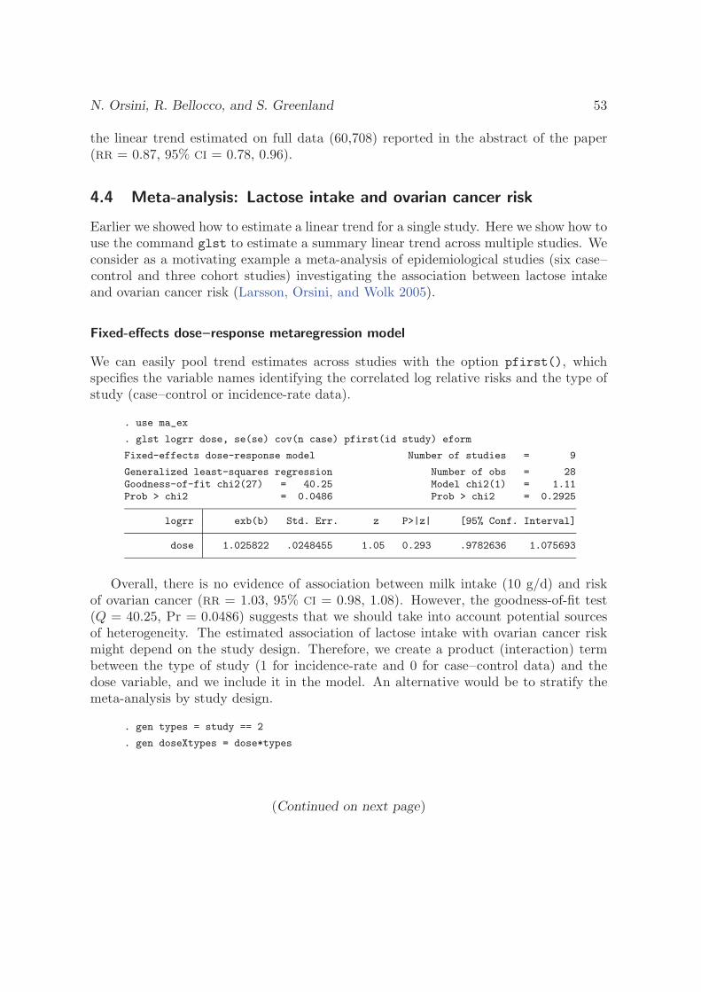
N. Orsini, R. Bellocco, and S. Greenland 53
the linear trend estimated on full data (60,708) reported in the abstract of the paper(RR = 0.87, 95% CI = 0.78, 0.96).
4.4 Meta-analysis: Lactose intake and ovarian cancer risk
Earlier we showed how to estimate a linear trend for a single study. Here we show how touse the command glst to estimate a summary linear trend across multiple studies. Weconsider as a motivating example a meta-analysis of epidemiological studies (six case–control and three cohort studies) investigating the association between lactose intakeand ovarian cancer risk (Larsson, Orsini, and Wolk 2005).
Fixed-effects dose–response metaregression model
We can easily pool trend estimates across studies with the option pfirst(), whichspecifies the variable names identifying the correlated log relative risks and the type ofstudy (case–control or incidence-rate data).
. use ma_ex
. glst logrr dose, se(se) cov(n case) pfirst(id study) eform
Fixed-effects dose-response model Number of studies = 9
Generalized least-squares regression Number of obs = 28Goodness-of-fit chi2(27) = 40.25 Model chi2(1) = 1.11Prob > chi2 = 0.0486 Prob > chi2 = 0.2925
logrr exb(b) Std. Err. z P>|z| [95% Conf. Interval]
dose 1.025822 .0248455 1.05 0.293 .9782636 1.075693
Overall, there is no evidence of association between milk intake (10 g/d) and riskof ovarian cancer (RR = 1.03, 95% CI = 0.98, 1.08). However, the goodness-of-fit test(Q = 40.25, Pr = 0.0486) suggests that we should take into account potential sourcesof heterogeneity. The estimated association of lactose intake with ovarian cancer riskmight depend on the study design. Therefore, we create a product (interaction) termbetween the type of study (1 for incidence-rate and 0 for case–control data) and thedose variable, and we include it in the model. An alternative would be to stratify themeta-analysis by study design.
. gen types = study == 2
. gen doseXtypes = dose*types
(Continued on next page)
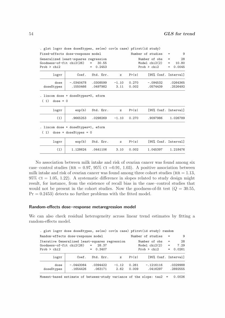
54 GLS for trend
. glst logrr dose doseXtypes, se(se) cov(n case) pfirst(id study)
Fixed-effects dose-response model Number of studies = 9
Generalized least-squares regression Number of obs = 28Goodness-of-fit chi2(26) = 30.55 Model chi2(2) = 10.80Prob > chi2 = 0.2453 Prob > chi2 = 0.0045
logrr Coef. Std. Err. z P>|z| [95% Conf. Interval]
dose -.0340478 .0308599 -1.10 0.270 -.094532 .0264365doseXtypes .1550466 .0497982 3.11 0.002 .0574439 .2526492
. lincom dose + doseXtypes*0, eform
( 1) dose = 0
logrr exp(b) Std. Err. z P>|z| [95% Conf. Interval]
(1) .9665253 .0298269 -1.10 0.270 .9097986 1.026789
. lincom dose + doseXtypes*1, eform
( 1) dose + doseXtypes = 0
logrr exp(b) Std. Err. z P>|z| [95% Conf. Interval]
(1) 1.128624 .0441106 3.10 0.002 1.045397 1.218476
No association between milk intake and risk of ovarian cancer was found among sixcase–control studies (RR = 0.97, 95% CI =0.91, 1.03). A positive association betweenmilk intake and risk of ovarian cancer was found among three cohort studies (RR = 1.13,95% CI = 1.05, 1.22). A systematic difference in slopes related to study design mightresult, for instance, from the existence of recall bias in the case–control studies thatwould not be present in the cohort studies. Now the goodness-of-fit test (Q = 30.55,Pr = 0.2453) detects no further problems with the fitted model.
Random-effects dose–response metaregression model
We can also check residual heterogeneity across linear trend estimates by fitting arandom-effects model.
. glst logrr dose doseXtypes, se(se) cov(n case) pfirst(id study) random
Random-effects dose-response model Number of studies = 9
Iterative Generalized least-squares regression Number of obs = 28Goodness-of-fit chi2(26) = 28.37 Model chi2(2) = 7.29Prob > chi2 = 0.3407 Prob > chi2 = 0.0261
logrr Coef. Std. Err. z P>|z| [95% Conf. Interval]
dose -.0443064 .0394422 -1.12 0.261 -.1216116 .0329988doseXtypes .1654426 .063171 2.62 0.009 .0416297 .2892555
Moment-based estimate of between-study variance of the slope: tau2 = 0.0026
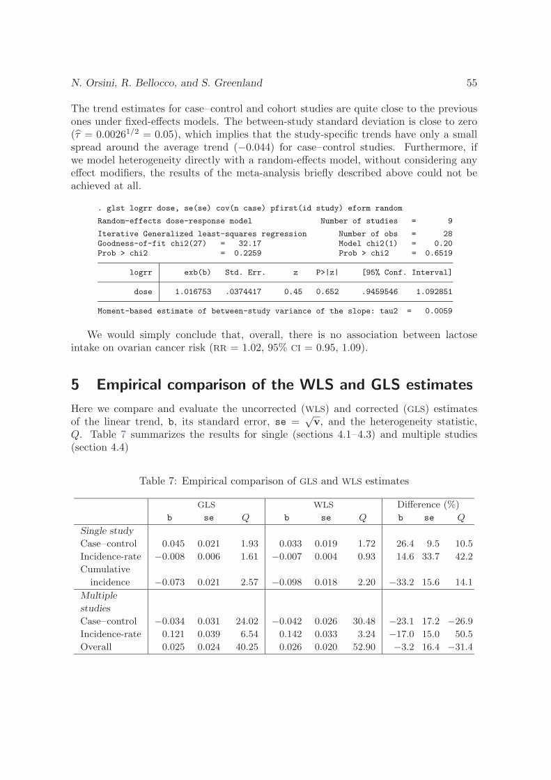
N. Orsini, R. Bellocco, and S. Greenland 55
The trend estimates for case–control and cohort studies are quite close to the previousones under fixed-effects models. The between-study standard deviation is close to zero(τ = 0.00261/2 = 0.05), which implies that the study-specific trends have only a smallspread around the average trend (−0.044) for case–control studies. Furthermore, ifwe model heterogeneity directly with a random-effects model, without considering anyeffect modifiers, the results of the meta-analysis briefly described above could not beachieved at all.
. glst logrr dose, se(se) cov(n case) pfirst(id study) eform random
Random-effects dose-response model Number of studies = 9
Iterative Generalized least-squares regression Number of obs = 28Goodness-of-fit chi2(27) = 32.17 Model chi2(1) = 0.20Prob > chi2 = 0.2259 Prob > chi2 = 0.6519
logrr exb(b) Std. Err. z P>|z| [95% Conf. Interval]
dose 1.016753 .0374417 0.45 0.652 .9459546 1.092851
Moment-based estimate of between-study variance of the slope: tau2 = 0.0059
We would simply conclude that, overall, there is no association between lactoseintake on ovarian cancer risk (RR = 1.02, 95% CI = 0.95, 1.09).
5 Empirical comparison of the WLS and GLS estimates
Here we compare and evaluate the uncorrected (WLS) and corrected (GLS) estimatesof the linear trend, b, its standard error, se =
√v, and the heterogeneity statistic,
Q. Table 7 summarizes the results for single (sections 4.1–4.3) and multiple studies(section 4.4)
Table 7: Empirical comparison of GLS and WLS estimates
GLS WLS Difference (%)
b se Q b se Q b se Q
Single study
Case–control 0.045 0.021 1.93 0.033 0.019 1.72 26.4 9.5 10.5
Incidence-rate −0.008 0.006 1.61 −0.007 0.004 0.93 14.6 33.7 42.2
Cumulative
incidence −0.073 0.021 2.57 −0.098 0.018 2.20 −33.2 15.6 14.1
Multiple
studies
Case–control −0.034 0.031 24.02 −0.042 0.026 30.48 −23.1 17.2 −26.9
Incidence-rate 0.121 0.039 6.54 0.142 0.033 3.24 −17.0 15.0 50.5
Overall 0.025 0.024 40.25 0.026 0.020 52.90 −3.2 16.4 −31.4
56 GLS for trend
The relative differences, expressed as percentages, between the GLS and WLS esti-mates are calculated as (GLS − WLS)/GLS ×100. The GLS estimates of the linear trend,b, could be higher or lower than the WLS estimates, and the small differences are notsurprising because both estimators are consistent (Greenland and Longnecker 1992).The Q statistic based on GLS estimates could be higher or lower than the one based onWLS estimates. In the WLS procedure the off-diagonal elements of Σ, covariances amonglog relative risks, are set to zeros, whereas in the GLS the covariances are not zeros (seesection 2.4). Therefore, the weighting matrix, Σ−1, in the Q statistic depends bothon variances and covariances of the log relative risks. As expected, the GLS estimatesof the standard errors, se, are always higher than the WLS estimates of the standarderrors for single and multiple studies. The underestimation of the standard error ofthe uncorrected WLS method somewhat overstates the precision of the trend estimate.Further empirical comparisons between the corrected and uncorrected methods can befound in Greenland and Longnecker (1992).
6 Conclusion
We presented a command, glst, to efficiently estimate the trend from summarized epi-demiological dose–response data. As shown with several examples, the method can beapplied for published case–control, incidence-rate, and cumulative incidence data, fromeither a single study or multiple studies. In the latter case, the command glst fitsfixed-effects and random-effects metaregression models to allow a better fit of the dose–response relation and the identification of sources of heterogeneity. Adjusting the stan-dard error of the slope for the within-study covariance is just one of the statistical issuesarising in the synthesis of information from different studies. Other important issues,not considered in this paper, are the exposure scale, publication bias, and methodologicbias (Berlin, Longnecker, and Greenland 1993; Shi and Copas 2004; Greenland 2005).A limitation of the method proposed by Greenland and Longnecker (1992) is the as-sumption that the correlation matrices of the unadjusted and adjusted log relative risksare approximately equal. In future developments of the command, upper and lowerbounds of the covariance matrix will be implemented to assess the sensitivity of the GLS
estimators, as pointed out by Berrington and Cox (2003).
7 ReferencesBerlin, J. A., M. P. Longnecker, and S. Greenland. 1993. Meta-analysis of epidemiologic
dose–response data. Epidemiology 4: 218–228.
Berrington, A., and D. R. Cox. 2003. Generalized least squares for the synthesis ofcorrelated information. Biostatistics 4: 423–431.
DerSimonian, R., and N. Laird. 1986. Meta-analysis in clinical trials. Controlled ClinicalTrials 7.
N. Orsini, R. Bellocco, and S. Greenland 57
Greenland, S. 1987. Quantitative methods in the review of epidemiologic literature.Epidemiologic Reviews 9: 1–30.
———. 2005. Multiple-bias modeling for analysis of observational data (with discus-sion). Journal of the Royal Statistical Society, Series A 168: 267–308.
Greenland, S., and M. P. Longnecker. 1992. Methods for trend estimation from sum-marized dose–reponse data, with applications to meta-analysis. American Journal ofEpidemiology 135: 1301–1309.
Grizzle, J. E., C. F. Starmer, and G. G. Koch. 1969. Analysis of categorical data bylinear models. Biometrics 25: 489–504.
Larsson, S. C., L. Bergkvist, and A. Wolk. 2005. High-fat dairy food and conjugatedlinoleic acid intakes in relation to colorectal cancer incidence in the Swedish Mam-mography Cohort. American Journal of Clinical Nutrition 82: 894–900.
Larsson, S. C., N. Orsini, and A. Wolk. 2005. Milk, milk products and lactose intakeand ovarian cancer risk: A meta-analysis of epidemiological studies. InternationalJournal of Cancer 118: 431–441.
Rohan, T. E., and A. J. McMichael. 1988. Alcohol consumption and risk of breastcancer. International Journal of Cancer 41: 695–699.
Shi, J. Q., and J. B. Copas. 2004. Meta-analysis for trend estimation. Statistics inMedicine 23: 3–19.
Wolk, A., J. E. Manson, M. J. Stampfer, G. A. Colditz, F. Hu, F. E. Speizer, C. H. Hen-nekens, and W. C. Willett. 1999. Long-term intake of dietary fiber and decreased riskof coronary heart disease among women. Journal of the American Medical Association281: 1998–2004.
About the authors
Nicola Orsini is a Ph.D. student, Division of Nutritional Epidemiology, the National Instituteof Environmental Medicine, Karolinska Institutet, Stockholm, Sweden.
Rino Bellocco is Associate Professor of Biostatistics, Department of Medical Epidemiology andBiostatistics, Karolinska Institutet, Stockholm, Sweden, and Associate Professor of Biostatis-tics, Department of Statistics, University of Milano Bicocca, Milan, Italy.
Sander Greenland is Professor of Epidemiology, UCLA School of Public Health, and Professorof Statistics, UCLA College of Letters and Science, Los Angeles, CA.
The Stata Journal (2009)9, Number 1, pp. 57–69
Meta-analysis with missing data
Ian R. WhiteMRC Biostatistics Unit
Cambridge, UK
Julian P. T. HigginsMRC Biostatistics Unit
Cambridge, UK
Abstract. A new command, metamiss, performs meta-analysis with binary out-comes when some or all studies have missing data. Missing values can be imputedas successes, as failures, according to observed event rates, or by a combination ofthese according to reported reasons for the data being missing. Alternatively, theuser can specify the value of, or a prior distribution for, the informative missingnessodds ratio.
Keywords: st0157, metamiss, meta-analysis, missing data, informative missingnessodds ratio
1 Introduction
Just as missing outcome data present a threat to the validity of any research study, sothey present a threat to the validity of any meta-analysis of research studies. Typically,analyses assume that the data are missing completely at random or missing at random(MAR) (Little and Rubin 2002). If the data are not MAR (i.e., they are informativelymissing) but are analyzed as if they were missing completely at random or MAR, thennonresponse bias typically occurs. The threat of bias carries over to meta-analysis,where the problem can be compounded by nonresponse bias applied in a similar way indifferent studies.
Many methods for dealing with missing outcome data require detailed data for eachparticipant. Dealing with missing outcome data in a meta-analysis raises particularproblems because limited information is typically available in published reports. Al-though a meta-analyst would ideally seek any important but unreported data from theauthors of the original studies, this approach is not always successful, and it is un-common to have access to more than group-level summary data at best. We thereforeaddress the meta-analysis of summary data, focusing on the case of an incomplete binaryoutcome.
A central concept is the informative missingness odds ratio (IMOR), defined as theodds ratio between the missingness, M , and the true outcome, Y , within groups (White,Higgins, and Wood 2008). A value of 1 indicates MAR, while IMOR = 0 means thatmissing values are all failures, and IMOR = ∞ means that missing values are all successes.We allow the IMOR to differ across groups and across subgroups of individuals definedby reasons for missingness, or to be specified with uncertainty.
We will describe metamiss in the context of a meta-analysis of randomized controlledtrials comparing an “experimental group” with a “control group”, but it could be used
c© 2009 StataCorp LP st0157
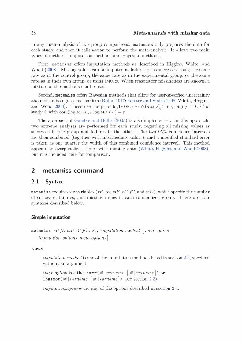
58 Meta-analysis with missing data
in any meta-analysis of two-group comparisons. metamiss only prepares the data foreach study, and then it calls metan to perform the meta-analysis. It allows two maintypes of methods: imputation methods and Bayesian methods.
First, metamiss offers imputation methods as described in Higgins, White, andWood (2008). Missing values can be imputed as failures or as successes; using the samerate as in the control group, the same rate as in the experimental group, or the samerate as in their own group; or using IMORs. When reasons for missingness are known, amixture of the methods can be used.
Second, metamiss offers Bayesian methods that allow for user-specified uncertaintyabout the missingness mechanism (Rubin 1977; Forster and Smith 1998; White, Higgins,and Wood 2008). These use the prior logIMORij ∼ N(mij , s
2ij) in group j = E,C of
study i, with corr(logIMORiE , logIMORiC) = r.
The approach of Gamble and Hollis (2005) is also implemented. In this approach,two extreme analyses are performed for each study, regarding all missing values assuccesses in one group and failures in the other. The two 95% confidence intervalsare then combined (together with intermediate values), and a modified standard erroris taken as one quarter the width of this combined confidence interval. This methodappears to overpenalize studies with missing data (White, Higgins, and Wood 2008),but it is included here for comparison.
2 metamiss command
2.1 Syntax
metamiss requires six variables (rE, fE, mE, rC, fC, and mC ), which specify the numberof successes, failures, and missing values in each randomized group. There are foursyntaxes described below.
Simple imputation
metamiss rE fE mE rC fC mC, imputation method[imor option
imputation options meta options]
where
imputation method is one of the imputation methods listed in section 2.2, specifiedwithout an argument.
imor option is either imor(# | varname[# | varname
]) or
logimor(# | varname[# | varname
]) (see section 2.3).
imputation options are any of the options described in section 2.4.

I. R. White and J. P. T. Higgins 59
meta options are any of the meta-analysis options listed in section 2.6, as wellas any valid option for metan, including random, by(), and xlabel() (see sec-tion 2.6).
Imputation using reasons
metamiss rE fE mE rC fC mC, imputation method1 impuation method2[imputation method3 . . .
] [imor option imputation options meta options
]
where
imputation method1, imputation method2, etc., are any imputation method listedin section 2.2 except icab and icaw, specified with arguments to indicate numbersof missing values to be imputed by each method.
imor option, imputation options, and meta options are the same as documentedin Simple Imputation.
Bayesian analysis using priors
metamiss rE fE mE rC fC mC, sdlogimor(# | varname[# | varname
])[
imor option bayes options meta options]
where
imor option and meta options are the same as documented in Simple Imputation.
bayes options are any of the options described in section 2.5.
Gamble–Hollis analysis
metamiss rE fE mE rC fC mC, gamblehollis[meta options
]
where
gamblehollis specifies to use the Gamble–Hollis analysis.
meta options are the same as documented in Simple Imputation.
2.2 imputation method
For simple imputation, specify one of the following options without arguments. Forimputation using reasons, specify two or more of the following options with arguments.The abbreviations ACA, ICA-0, etc., are explained by Higgins, White, and Wood (2008).
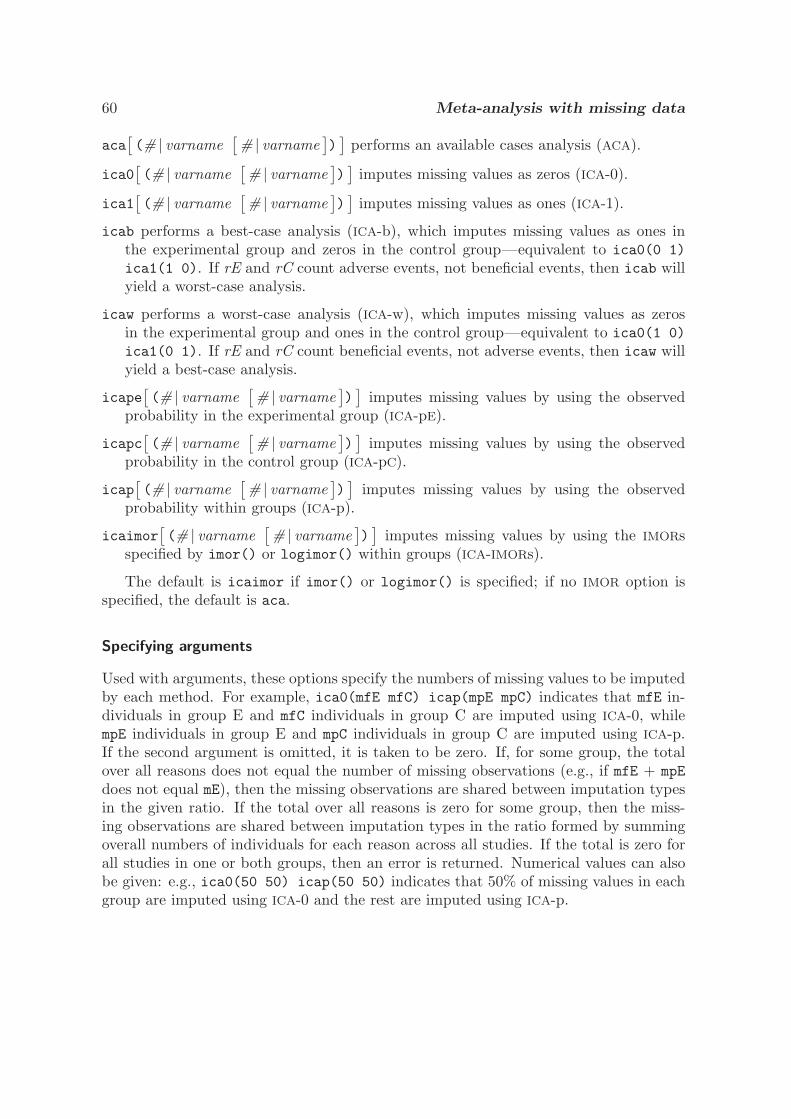
60 Meta-analysis with missing data
aca[(# | varname
[# | varname
])]
performs an available cases analysis (ACA).
ica0[(# | varname
[# | varname
])]
imputes missing values as zeros (ICA-0).
ica1[(# | varname
[# | varname
])]
imputes missing values as ones (ICA-1).
icab performs a best-case analysis (ICA-b), which imputes missing values as ones inthe experimental group and zeros in the control group—equivalent to ica0(0 1)ica1(1 0). If rE and rC count adverse events, not beneficial events, then icab willyield a worst-case analysis.
icaw performs a worst-case analysis (ICA-w), which imputes missing values as zerosin the experimental group and ones in the control group—equivalent to ica0(1 0)ica1(0 1). If rE and rC count beneficial events, not adverse events, then icaw willyield a best-case analysis.
icape[(# | varname
[# | varname
])]
imputes missing values by using the observedprobability in the experimental group (ICA-pE).
icapc[(# | varname
[# | varname
])]
imputes missing values by using the observedprobability in the control group (ICA-pC).
icap[(# | varname
[# | varname
])]
imputes missing values by using the observedprobability within groups (ICA-p).
icaimor[(# | varname
[# | varname
])]
imputes missing values by using the IMORsspecified by imor() or logimor() within groups (ICA-IMORs).
The default is icaimor if imor() or logimor() is specified; if no IMOR option isspecified, the default is aca.
Specifying arguments
Used with arguments, these options specify the numbers of missing values to be imputedby each method. For example, ica0(mfE mfC) icap(mpE mpC) indicates that mfE in-dividuals in group E and mfC individuals in group C are imputed using ICA-0, whilempE individuals in group E and mpC individuals in group C are imputed using ICA-p.If the second argument is omitted, it is taken to be zero. If, for some group, the totalover all reasons does not equal the number of missing observations (e.g., if mfE + mpEdoes not equal mE), then the missing observations are shared between imputation typesin the given ratio. If the total over all reasons is zero for some group, then the miss-ing observations are shared between imputation types in the ratio formed by summingoverall numbers of individuals for each reason across all studies. If the total is zero forall studies in one or both groups, then an error is returned. Numerical values can alsobe given: e.g., ica0(50 50) icap(50 50) indicates that 50% of missing values in eachgroup are imputed using ICA-0 and the rest are imputed using ICA-p.

I. R. White and J. P. T. Higgins 61
2.3 imor option
imor(# | varname[# | varname
]) sets the IMORs or (if the Bayesian method is being
used) the prior medians of the IMORs. If one value is given, it applies to bothgroups; if two values are given, they apply to the experimental and control groups,respectively. Both values default to 1. Only one of imor() or logimor() can bespecified.
logimor(# | varname[# | varname
]) does the same as imor() but on the log scale.
Thus imor(1 1) is the same as logimor(0 0). Only one of imor() or logimor()can be specified.
2.4 imputation options
w1 specifies that standard errors be computed, treating the imputed values as if theywere observed. This is included for didactic purposes and should not be used in realanalyses. Only one of w1, w2, w3, or w4 can be specified.
w2 specifies that standard errors from the ACA be used. This is useful in separatingsensitivity to changes in point estimates from sensitivity to changes in standarderrors. Only one of w1, w2, w3, or w4 can be specified.
w3 specifies that standard errors be computed by scaling the imputed data down tothe number of available cases in each group and treating these data as if they wereobserved. Only one of w1, w2, w3, or w4 can be specified.
w4, the default, specifies that standard errors be computed algebraically, conditional onthe IMORs. Conditioning on the IMORs is not strictly correct for schemes includingICA-pE or ICA-pC, but the conditional standard errors appear to be more realisticthan the unconditional standard errors in this setting (Higgins, White, and Wood2008). Only one of w1, w2, w3, or w4 can be specified.
listnum lists the reason counts for each study implied by the imputation method option.
listall lists the reason counts for each study after scaling to match the number ofmissing values and imputing missing values for studies with no reasons.
listp lists the imputed probabilities for each study.
2.5 bayes options
sdlogimor(# | varname[# | varname
]) sets the prior standard deviation for log IMORs
for the experimental and control groups, respectively. Both values default to 0.
corrlogimor(# | varname) sets the prior correlation between log IMORs in the experi-mental and control groups. The default is corrlogimor(0).
method(gh | mc | taylor) determines the method used to integrate over the distributionof the IMORs. method(gh) uses two-dimensional Gauss–Hermite quadrature and is

62 Meta-analysis with missing data
the recommended method (and the default). method(mc) performs a full Bayesiananalysis by sampling directly from the posterior. This is time consuming, so dotsdisplay progress, and you can request more than one of the measures or, rr, and rd.method(taylor) uses a Taylor-series approximation, as in section 4 of Forster andSmith (1998), and is faster than the default but typically inaccurate for sdlogimor()larger than one or two.
nip(#) specifies the number of integration points under method(gh). The default isnip(10).
reps(#) specifies the number of Monte Carlo draws under method(mc). The default isreps(100).
missprior(##[##
]) and respprior(##) apply when method(mc) is used, but
they are unlikely to be much used. They specify the parameters of the beta priorsfor P (M) and P (Y |M = 0): the parameters for the first group are given by thefirst two numbers, and the parameters for the second group are given by the nexttwo numbers or are the same as for the first group. The defaults are both beta(1, 1).
nodots suppresses the dots that are displayed to mark the number of Monte Carlo drawscompleted.
2.6 meta options
or, rr, and rd specify the measures to be analyzed. Usually, only one measure can bespecified; the default is rr. However, when using method(mc), all three measurescan be obtained for no extra effort, so any combination is allowed. When more thanone measure is specified, the formal meta-analysis is not performed, but measuresand their standard errors are saved (see section 2.7).
log has the results reported on the log risk-ratio (RR) or log odds-ratio scale.
id(varname) specifies a study identifier for the results table and forest plot.
Most other options allowed with metan are also allowed, including by(), random, andnograph.
2.7 Saved results
metamiss saves results in the same way as metan: ES, selogES, etc. The sample size,SS, excludes the missing values, but an additional variable, SSmiss, gives the totalnumber of missing values. When method(mc) is run, the log option is assumed for themeasures or and rr, and the following variables are saved for each measure (logor,logrr, or rd): the ACA estimate, ESTRAW measure; the ACA variance, VARRAW measure;the corrected estimate, ESTSTAR measure; and the corrected variance, VARSTAR measure.If these variables already exist, then they are overwritten.
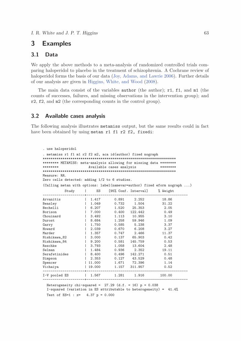
I. R. White and J. P. T. Higgins 63
3 Examples
3.1 Data
We apply the above methods to a meta-analysis of randomized controlled trials com-paring haloperidol to placebo in the treatment of schizophrenia. A Cochrane review ofhaloperidol forms the basis of our data (Joy, Adams, and Lawrie 2006). Further detailsof our analysis are given in Higgins, White, and Wood (2008).
The main data consist of the variables author (the author); r1, f1, and m1 (thecounts of successes, failures, and missing observations in the intervention group); andr2, f2, and m2 (the corresponding counts in the control group).
3.2 Available cases analysis
The following analysis illustrates metamiss output, but the same results could in facthave been obtained by using metan r1 f1 r2 f2, fixedi:
. use haloperidol
. metamiss r1 f1 m1 r2 f2 m2, aca id(author) fixed nograph*************************************************************************** METAMISS: meta-analysis allowing for missing data **************** Available cases analysis ***************************************************************************Measure: RR.Zero cells detected: adding 1/2 to 6 studies.
(Calling metan with options: label(namevar=author) fixed eform nograph ...)
Study | ES [95% Conf. Interval] % Weight---------------------+---------------------------------------------------Arvanitis | 1.417 0.891 2.252 18.86Beasley | 1.049 0.732 1.504 31.22Bechelli | 6.207 1.520 25.353 2.05Borison | 7.000 0.400 122.442 0.49Chouinard | 3.492 1.113 10.955 3.10Durost | 8.684 1.258 59.946 1.09Garry | 1.750 0.585 5.238 3.37Howard | 2.039 0.670 6.208 3.27Marder | 1.357 0.747 2.466 11.37Nishikawa_82 | 3.000 0.137 65.903 0.42Nishikawa_84 | 9.200 0.581 145.759 0.53Reschke | 3.793 1.058 13.604 2.48Selman | 1.484 0.936 2.352 19.11Serafetinides | 8.400 0.496 142.271 0.51Simpson | 2.353 0.127 43.529 0.48Spencer | 11.000 1.671 72.396 1.14Vichaiya | 19.000 1.157 311.957 0.52---------------------+---------------------------------------------------I-V pooled ES | 1.567 1.281 1.916 100.00---------------------+---------------------------------------------------
Heterogeneity chi-squared = 27.29 (d.f. = 16) p = 0.038I-squared (variation in ES attributable to heterogeneity) = 41.4%
Test of ES=1 : z= 4.37 p = 0.000
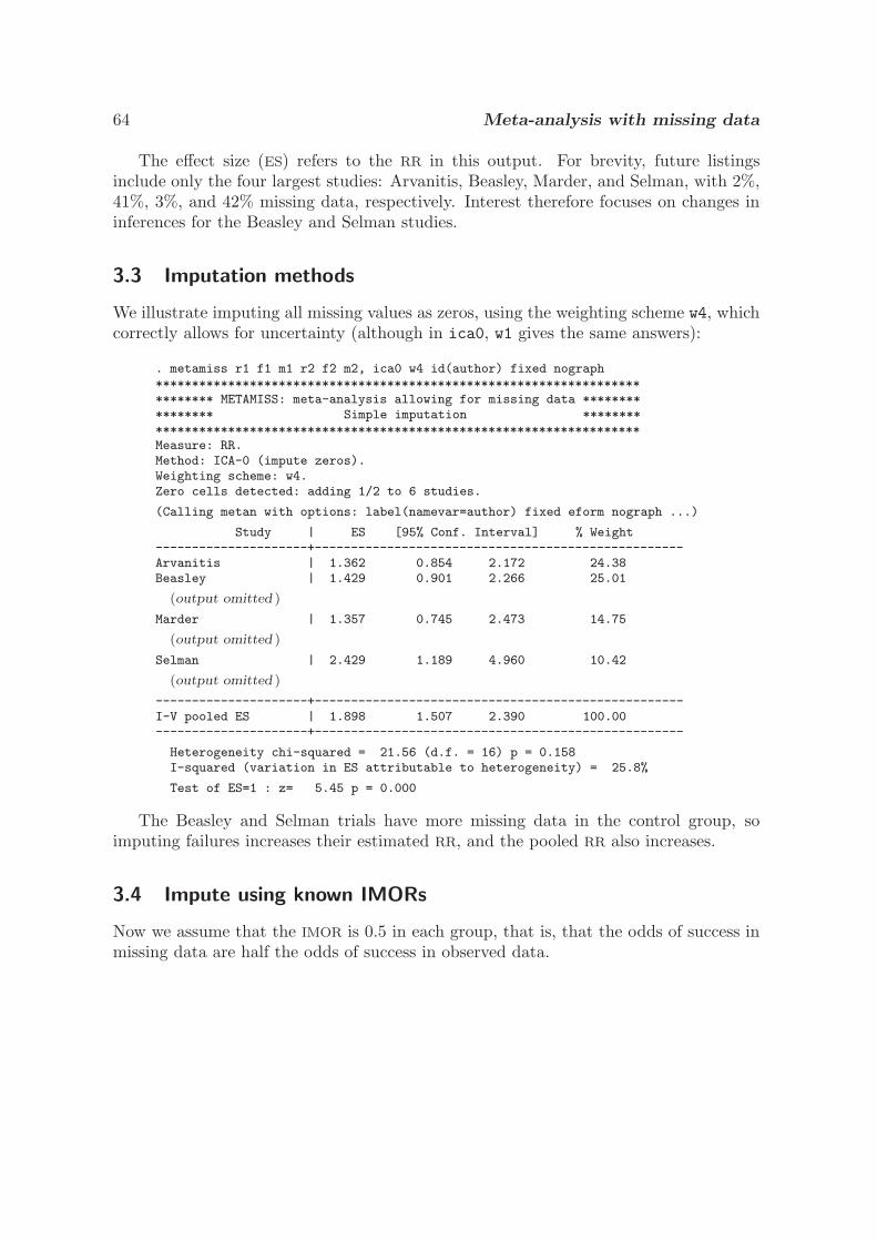
64 Meta-analysis with missing data
The effect size (ES) refers to the RR in this output. For brevity, future listingsinclude only the four largest studies: Arvanitis, Beasley, Marder, and Selman, with 2%,41%, 3%, and 42% missing data, respectively. Interest therefore focuses on changes ininferences for the Beasley and Selman studies.
3.3 Imputation methods
We illustrate imputing all missing values as zeros, using the weighting scheme w4, whichcorrectly allows for uncertainty (although in ica0, w1 gives the same answers):
. metamiss r1 f1 m1 r2 f2 m2, ica0 w4 id(author) fixed nograph*************************************************************************** METAMISS: meta-analysis allowing for missing data **************** Simple imputation ***************************************************************************Measure: RR.Method: ICA-0 (impute zeros).Weighting scheme: w4.Zero cells detected: adding 1/2 to 6 studies.
(Calling metan with options: label(namevar=author) fixed eform nograph ...)
Study | ES [95% Conf. Interval] % Weight---------------------+---------------------------------------------------Arvanitis | 1.362 0.854 2.172 24.38Beasley | 1.429 0.901 2.266 25.01
(output omitted )
Marder | 1.357 0.745 2.473 14.75
(output omitted )
Selman | 2.429 1.189 4.960 10.42
(output omitted )
---------------------+---------------------------------------------------I-V pooled ES | 1.898 1.507 2.390 100.00---------------------+---------------------------------------------------
Heterogeneity chi-squared = 21.56 (d.f. = 16) p = 0.158I-squared (variation in ES attributable to heterogeneity) = 25.8%
Test of ES=1 : z= 5.45 p = 0.000
The Beasley and Selman trials have more missing data in the control group, soimputing failures increases their estimated RR, and the pooled RR also increases.
3.4 Impute using known IMORs
Now we assume that the IMOR is 0.5 in each group, that is, that the odds of success inmissing data are half the odds of success in observed data.
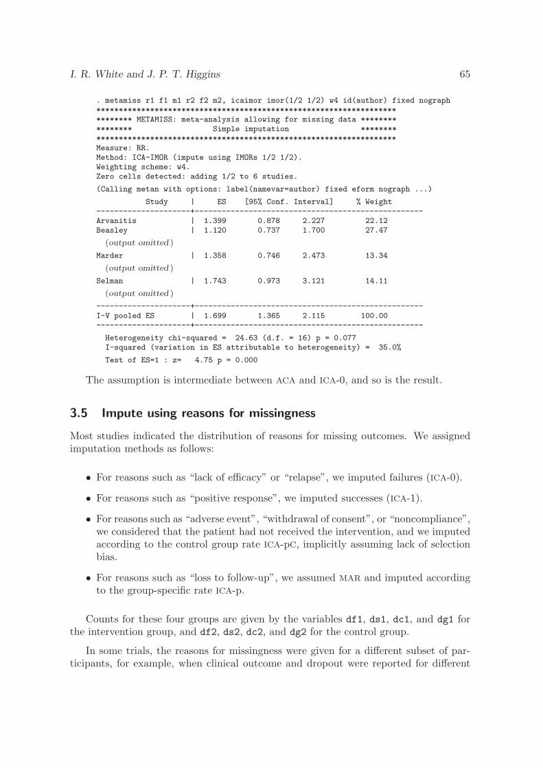
I. R. White and J. P. T. Higgins 65
. metamiss r1 f1 m1 r2 f2 m2, icaimor imor(1/2 1/2) w4 id(author) fixed nograph*************************************************************************** METAMISS: meta-analysis allowing for missing data **************** Simple imputation ***************************************************************************Measure: RR.Method: ICA-IMOR (impute using IMORs 1/2 1/2).Weighting scheme: w4.Zero cells detected: adding 1/2 to 6 studies.
(Calling metan with options: label(namevar=author) fixed eform nograph ...)
Study | ES [95% Conf. Interval] % Weight---------------------+---------------------------------------------------Arvanitis | 1.399 0.878 2.227 22.12Beasley | 1.120 0.737 1.700 27.47
(output omitted )
Marder | 1.358 0.746 2.473 13.34
(output omitted )
Selman | 1.743 0.973 3.121 14.11
(output omitted )
---------------------+---------------------------------------------------I-V pooled ES | 1.699 1.365 2.115 100.00---------------------+---------------------------------------------------
Heterogeneity chi-squared = 24.63 (d.f. = 16) p = 0.077I-squared (variation in ES attributable to heterogeneity) = 35.0%
Test of ES=1 : z= 4.75 p = 0.000
The assumption is intermediate between ACA and ICA-0, and so is the result.
3.5 Impute using reasons for missingness
Most studies indicated the distribution of reasons for missing outcomes. We assignedimputation methods as follows:
• For reasons such as “lack of efficacy” or “relapse”, we imputed failures (ICA-0).
• For reasons such as “positive response”, we imputed successes (ICA-1).
• For reasons such as “adverse event”, “withdrawal of consent”, or “noncompliance”,we considered that the patient had not received the intervention, and we imputedaccording to the control group rate ICA-pC, implicitly assuming lack of selectionbias.
• For reasons such as “loss to follow-up”, we assumed MAR and imputed accordingto the group-specific rate ICA-p.
Counts for these four groups are given by the variables df1, ds1, dc1, and dg1 forthe intervention group, and df2, ds2, dc2, and dg2 for the control group.
In some trials, the reasons for missingness were given for a different subset of par-ticipants, for example, when clinical outcome and dropout were reported for different
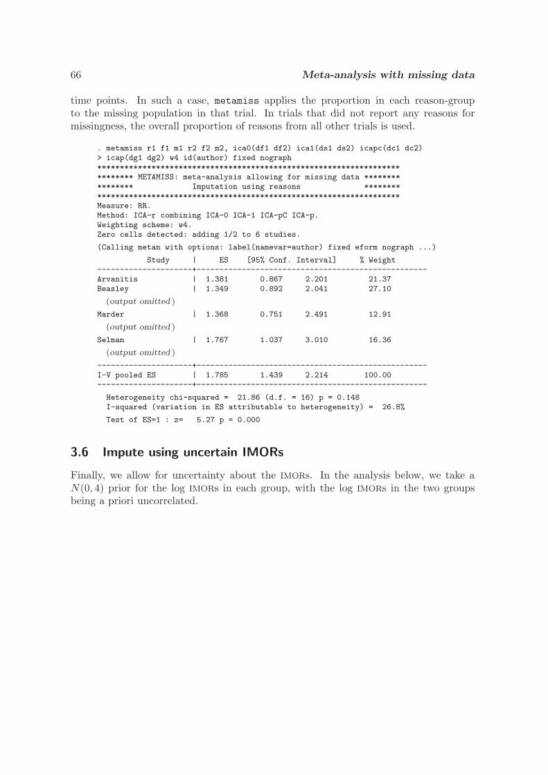
66 Meta-analysis with missing data
time points. In such a case, metamiss applies the proportion in each reason-groupto the missing population in that trial. In trials that did not report any reasons formissingness, the overall proportion of reasons from all other trials is used.
. metamiss r1 f1 m1 r2 f2 m2, ica0(df1 df2) ica1(ds1 ds2) icapc(dc1 dc2)> icap(dg1 dg2) w4 id(author) fixed nograph*************************************************************************** METAMISS: meta-analysis allowing for missing data **************** Imputation using reasons ***************************************************************************Measure: RR.Method: ICA-r combining ICA-0 ICA-1 ICA-pC ICA-p.Weighting scheme: w4.Zero cells detected: adding 1/2 to 6 studies.
(Calling metan with options: label(namevar=author) fixed eform nograph ...)
Study | ES [95% Conf. Interval] % Weight---------------------+---------------------------------------------------Arvanitis | 1.381 0.867 2.201 21.37Beasley | 1.349 0.892 2.041 27.10
(output omitted )
Marder | 1.368 0.751 2.491 12.91
(output omitted )
Selman | 1.767 1.037 3.010 16.36
(output omitted )
---------------------+---------------------------------------------------I-V pooled ES | 1.785 1.439 2.214 100.00---------------------+---------------------------------------------------
Heterogeneity chi-squared = 21.86 (d.f. = 16) p = 0.148I-squared (variation in ES attributable to heterogeneity) = 26.8%
Test of ES=1 : z= 5.27 p = 0.000
3.6 Impute using uncertain IMORs
Finally, we allow for uncertainty about the IMORs. In the analysis below, we take aN(0, 4) prior for the log IMORs in each group, with the log IMORs in the two groupsbeing a priori uncorrelated.
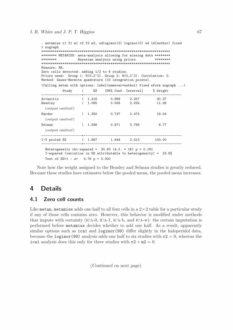
I. R. White and J. P. T. Higgins 67
. metamiss r1 f1 m1 r2 f2 m2, sdlogimor(2) logimor(0) w4 id(author) fixed> nograph*************************************************************************** METAMISS: meta-analysis allowing for missing data **************** Bayesian analysis using priors ***************************************************************************Measure: RR.Zero cells detected: adding 1/2 to 6 studies.Priors used: Group 1: N(0,2^2). Group 2: N(0,2^2). Correlation: 0.Method: Gauss-Hermite quadrature (10 integration points).
(Calling metan with options: label(namevar=author) fixed eform nograph ...)
Study | ES [95% Conf. Interval] % Weight---------------------+---------------------------------------------------Arvanitis | 1.416 0.889 2.257 30.37Beasley | 1.085 0.506 2.324 11.36
(output omitted )
Marder | 1.350 0.737 2.472 18.04
(output omitted )
Selman | 1.596 0.671 3.799 8.77
(output omitted )
---------------------+---------------------------------------------------I-V pooled ES | 1.867 1.444 2.413 100.00---------------------+---------------------------------------------------
Heterogeneity chi-squared = 20.93 (d.f. = 16) p = 0.181I-squared (variation in ES attributable to heterogeneity) = 23.6%
Test of ES=1 : z= 4.76 p = 0.000
Note how the weight assigned to the Beasley and Selman studies is greatly reduced.Because these studies have estimates below the pooled mean, the pooled mean increases.
4 Details
4.1 Zero cell counts
Like metan, metamiss adds one half to all four cells in a 2×2 table for a particular studyif any of those cells contains zero. However, this behavior is modified under methodsthat impute with certainty (ICA-0, ICA-1, ICA-b, and ICA-w): the certain imputation isperformed before metamiss decides whether to add one half. As a result, apparentlysimilar options such as ica1 and logimor(99) differ slightly in the haloperidol data,because the logimor(99) analysis adds one half to six studies with r2 = 0, whereas theica1 analysis does this only for three studies with r2 + m2 = 0.
(Continued on next page)
68 Meta-analysis with missing data
4.2 Formula
For the imputation methods, in a given group of a given study, let r, f , and m be thenumber of observed successes, failures, and missing observations; let π = r/(r + f) bethe observed success fraction; and let N = r + f + m be the total count. Let k indexreason-groups with counts mk and IMOR θk, so that, for example, a group imputed byICA-0 has θk = 0. Then the estimated success fraction is
π∗ =1N
(r +
∑k
mkθkπ
1 − π + θkπ
)
with the variance obtained by a Taylor-series expansion (Higgins, White, and Wood2008).
For the Bayesian methods, let δj be the log IMOR in group j. Then
π∗j (δj) =
1Nj
(rj +
mjeδj πj
1 − πj + eδj πj
)
and, for example, the log risk ratio is obtained by finding the expectation of
logπ∗E(δE) − logπ∗
C(δC)
over the prior p(δE , δC) by numerical integration. The variance is obtained by combiningthe variance conditional on p(δE , δC) with the variance over p(δE , δC) (White, Higgins,and Wood 2008).
5 Discussion
We believe that ACA is a suitable starting point for a sensitivity analysis that might en-compass, for example, imor(1/2 1/2), imor(1/2 2), sdlogimor(2) corrlogimor(1),and sdlogimor(2) corrlogimor(0) (Higgins, White, and Wood 2008; White, Higgins,and Wood 2008). However, a “best” analysis might use reasons for missingness togetherwith subject matter knowledge to assign suitable IMORs. Future work will explore howto integrate the two approaches.
6 ReferencesForster, J. J., and P. W. F. Smith. 1998. Model-based inference for categorical survey
data subject to non-ignorable non-response. Journal of the Royal Statistical Society,Series B (Statistical Methodology) 60: 57–70.
Gamble, C., and S. Hollis. 2005. Uncertainty method improved on best–worst caseanalysis in a binary meta-analysis. Journal of Clinical Epidemiology 58: 579–588.
Higgins, J. P. T., I. R. White, and A. M. Wood. 2008. Imputation methods for missingoutcome data in meta-analysis of clinical trials. Clinical Trials 5: 225–239.
I. R. White and J. P. T. Higgins 69
Joy, C. B., C. E. Adams, and S. M. Lawrie. 2006. Haloperidol versus placebo forschizophrenia. Cochrane Database of Systematic Reviews 4: CD003082.
Little, R. J. A., and D. B. Rubin. 2002. Statistical Analysis with Missing Data. 2nded. Hoboken, NJ: Wiley.
Rubin, D. B. 1977. Formalizing subjective notions about the effect of nonrespondentsin sample surveys. Journal of the American Statistical Association 72: 538–543.
White, I. R., J. P. T. Higgins, and A. M. Wood. 2008. Allowing for uncertainty due tomissing data in meta-analysis - Part 1: Two-stage methods. Statistics in Medicine27: 711–727.
About the authors
Ian White is a senior statistician at the MRC Biostatistics Unit in Cambridge, UK. His re-search interests include missing data, noncompliance and measurement error in clinical trials,observational studies, and meta-analysis.
Julian Higgins is a senior statistician at the MRC Biostatistics Unit in Cambridge, UK. His
main research interest is methods for meta-analysis and systematic reviews, and he contributes
extensively to The Cochrane Collaboration.
The Stata Journal (2009)9, Number 1, pp. 40–56
Multivariate random-effects meta-analysis
Ian R. WhiteMRC Biostatistics Unit
Cambridge, UK
Abstract. Multivariate meta-analysis combines estimates of several related pa-rameters over several studies. These parameters can, for example, refer to multipleoutcomes or comparisons between more than two groups. A new Stata command,mvmeta, performs maximum likelihood, restricted maximum likelihood, or method-of-moments estimation of random-effects multivariate meta-analysis models. Autility command, mvmeta make, facilitates the preparation of summary datasetsfrom more detailed data. The commands are illustrated with data from the Fib-rinogen Studies Collaboration, a meta-analysis of observational studies; I estimatethe shape of the association between a quantitative exposure and disease eventsby grouping the quantitative exposure into several categories.
Keywords: st0156, mvmeta, mvmeta make, mvmeta l, meta-analysis, multivariatemeta-analysis, individual participant data, observational studies
1 Introduction
Standard meta-analysis combines estimates of one parameter over several studies(Normand 1999). Multivariate meta-analysis is an extension that can combine esti-mates of several related parameters (van Houwelingen, Arends, and Stijnen 2003). Insuch work, it is important to allow for heterogeneity between studies, usually by fittinga random-effects model (Thompson 1994).
Multivariate meta-analysis has a variety of applications in randomized controlledtrials. The simplest is modeling the outcome separately in each arm of a clinicaltrial (van Houwelingen, Arends, and Stijnen 2003). Other published applications ex-plore treatment effects simultaneously on two clinical outcomes (Berkey, Anderson,and Hoaglin 1996; Berkey et al. 1998; Riley et al. 2007a,b) or on cost and effective-ness (Pinto, Willan, and O’Brien 2005), and explore combining trials comparing morethan one treatment (Hasselblad 1998; Lu and Ades 2004). Further applications havebeen reviewed by Riley et al. (2007b).
There are also possible applications of multivariate meta-analysis in observationalstudies. These applications include assessing the shape of the association between aquantitative exposure and a disease, which will be illustrated in this article.
One difficulty in random-effects meta-analysis is estimating the between-studiesvariance. In the univariate case, this is commonly performed by using the methodof DerSimonian and Laird (1986). However, maximum likelihood (ML) and restrictedmaximum likelihood (REML) methods are alternatives (van Houwelingen, Arends, and
c© 2009 StataCorp LP st0156

I. R. White 41
Stijnen 2003); in Stata, they are not available in metan but can be obtained frommetareg (Sharp 1998). This article describes a new command, mvmeta, that performsREML and ML estimation in the multivariate case by using a Newton–Raphson proce-dure. mvmeta requires a dataset of study-specific point estimates and their variance–covariance matrix. I also describe a utility command, mvmeta make, that facilitatesforming this dataset.
2 Multivariate random-effects meta-analysis withmvmeta
2.1 Syntax
mvmeta b V[if] [
in] [
, reml ml mm fixed vars(varlist) corr(expression)
start(matrix |matrix expression | mm) showstart showchol
keepmat(bname Vname) nouncertainv eform(name) bscorr bscov
missest(#) missvar(#) maximize options]
where the data are arranged with one line per study, the point estimates are held invariables whose names start with b (excluding b itself), the variance of bx is held invariable Vxx, and the covariance of bx and by is held in variable Vxy or Vyx (or thecorr() option is specified).
If the dataset includes variables whose names start with b that do not representpoint estimates, then the vars() option must be used.
2.2 Options
reml, the default, specifies that REML be used for estimation. Specify only one of thereml, ml, mm, or fixed options.
ml specifies that ML be used for estimation. ML is likely to underestimate the variance,so REML is usually preferred. Specify only one of the reml, ml, mm, or fixed options.
mm specifies that the multivariate method-of-moments procedure (Jackson, White, andThompson Forthcoming) be used for estimation. This procedure is a multivariategeneralization of the procedure of DerSimonian and Laird (1986) and is faster thanthe likelihood-based methods. Specify only one of the reml, ml, mm, or fixed options.
fixed specifies that the fixed-effects model be used for estimation. Specify only one ofthe reml, ml, mm, or fixed options.
vars(varlist) specifies which variables are to be used. By default, all variables b* areused (excluding b itself). The order of variables in varlist does not affect the modelitself but does affect the parameterization.
42 Multivariate random-effects meta-analysis
corr(expression) specifies that all within-study correlations take the given value. Thismeans that covariance variable Vxy need not exist. (If it does exist, corr() isignored.)
start(matrix |matrix expression | mm) specifies a starting value for the between-studiesvariance, except start(mm) specifies that the starting value is computed by the mmmethod. If start() is not specified, the starting value is the weighted between-studies variance of the estimates, not allowing for the within-study variances; thisensures that the starting value is greater than zero (the iterative procedure nevermoves away from zero). start(0) uses a starting value of 0.001 times the default.The starting value for the between-studies mean is the fixed-effects estimate.
showstart reports the starting values used.
showchol reports the estimated values of the basic parameters underlying the between-studies variance matrix (the Cholesky decomposition).
keepmat(bname Vname) saves the vector of study-specific estimates and the vector ofthe variance–covariance matrix for study i as bnamei and Vnamei, respectively.
nouncertainv invokes alternative (smaller) standard errors that ignore the uncertaintyin the estimated variance–covariance matrix and therefore agree with results pro-duced by procedures such as SAS PROC MIXED (without the ddfm=kr option) andmetareg. (Note, however, that the confidence intervals do not agree because mvmetauses a normal approximation, whereas the other procedures approximate the degreesof freedom of a t distribution.)
eform(name) exponentiates the reported mean parameters, labeling them name.
bscorr reports the between-studies variance–covariance matrix as the standard devia-tions and reports the correlation matrix. This is the default if bscov is not specified.
bscov reports the between-studies variance–covariance matrix without transformation.
missest(#) specifies the value to be used for missing point estimates; the default ismissest(0). This is of minor importance because the variance of these missingestimates is specified to be very large.
missvar(#) is used in imputing the variance of missing point estimates. For a specificvariable, the variance used is the largest observed variance multiplied by the specifiedvalue. The default is missvar(1E4); this value is unlikely to need to be changed.
maximize options are any options allowed by ml maximize.
3 Details of mvmeta
3.1 Notation
The data for mvmeta comprise the point estimate, yi, and the within-study variance–covariance matrix, Si, for each study i = 1 to n.

I. R. White 43
We assume the model
yi ∼ N(μi, Si)μi ∼ N(μ,Σ)
Σ =
⎛⎝ τ2
1 κ12τ1τ2 .κ12τ1τ2 τ2
2 .. . .
⎞⎠
where yi, μi, and μ are p×1 vectors, and Si and Σ are p×p matrices. The within-studyvariance, Si, is assumed to be known. Our aim is to estimate μ and Σ.
We set Wi = (Σ + Si)−1, noting that this depends on the unknown Σ. If Σ wereknown (or assumed to be the zero matrix, as in fixed-effects meta-analysis), then wewould have
μ =
(∑i
Wi
)−1(∑i
Wiyi
)
3.2 Estimating Σ
Methods proposed for estimating Σ in the multivariate setting include extensions ofCochran’s method (Berkey et al. 1998), of the DerSimonian and Laird method (Pinto,Willan, and O’Brien 2005) for diagonal Wi, and of likelihood-based methods (vanHouwelingen, Arends, and Stijnen 2003). We use the latter because of their gener-ality and optimality properties. Respectively, the likelihood and restricted likelihoodare
−2L =∑
i
{log |Σ + Si | + (yi − μ)′Wi(yi − μ)} + nplog2π
− 2RL = −2L + log |∑
i
Wi | − plog2π (1)
where Wi is a function of the unknown Σ, as noted above.
We maximize the (restricted) likelihood with a Newton–Raphson algorithm by usingStata’s ml procedure. To ensure that Σ is nonnegative definite (for example, in thebivariate case, to ensure that the between-studies variances are nonnegative and thatthe between-studies correlation lies between −1 and 1), the basic model parameters aretaken as the elements of a Cholesky decomposition of Σ (Riley et al. 2007b).
3.3 Saved results
As well as the usual e() information, mvmeta returns the estimated overall mean ine(Mu) and the between-studies variance–covariance matrix, the standard deviation vec-tor, and the correlation matrix in e(Sigma), e(Sigma SD), and e(Sigma corr), respec-tively.

44 Multivariate random-effects meta-analysis
3.4 Files required
mvmeta uses the likelihood program mvmeta l.ado.
4 A utility command to produce data in the correct for-mat: mvmeta make
4.1 Syntax
mvmeta make regression command[if] [
in] [
weight], by(by variable)
saving(savefile)[replace append names(bname Vname) keepmat
usevars(varlist) useconstant esave(namelist) nodetails pause
ppfix(none | check | all) augwt(#) noauglist ppcmd(regcmd[, options
])
hard regression options]
mvmeta make performs regression command for each level of by variable and storesthe results in savefile in the format required by mvmeta. weight is any weight allowedby regression command.
4.2 Options
by(by variable) is required; it identifies the studies in which the regression commandwill be performed.
saving(savefile) is required; it specifies to save the regression results to savefile.
replace specifies to overwrite the existing file called savefile.
append specifies to append the current results to the existing file called savefile.
names(bname Vname) specifies that the estimated coefficients for variable x are tobe stored in variable bnamex and that the estimated covariance between coefficientsbnamex and bnamey is to be stored in variable Vnamexy. The default is names(y S).
keepmat specifies that the results are also to be stored as matrices. The estimate vectorand the covariance matrix for study i are stored as matrices bnamei and Vnamei,respectively, where bname and Vname are specified with names().
usevars(varlist) identifies the variables whose regression coefficients are of interest.The default is all variables in the model, excluding the constant.
useconstant specifies that the constant is also of interest.
esave(namelist) adds the specified e() statistics to the saved data. For example,esave(N ll) saves e(N) and e(ll) as variables e N and e ll.
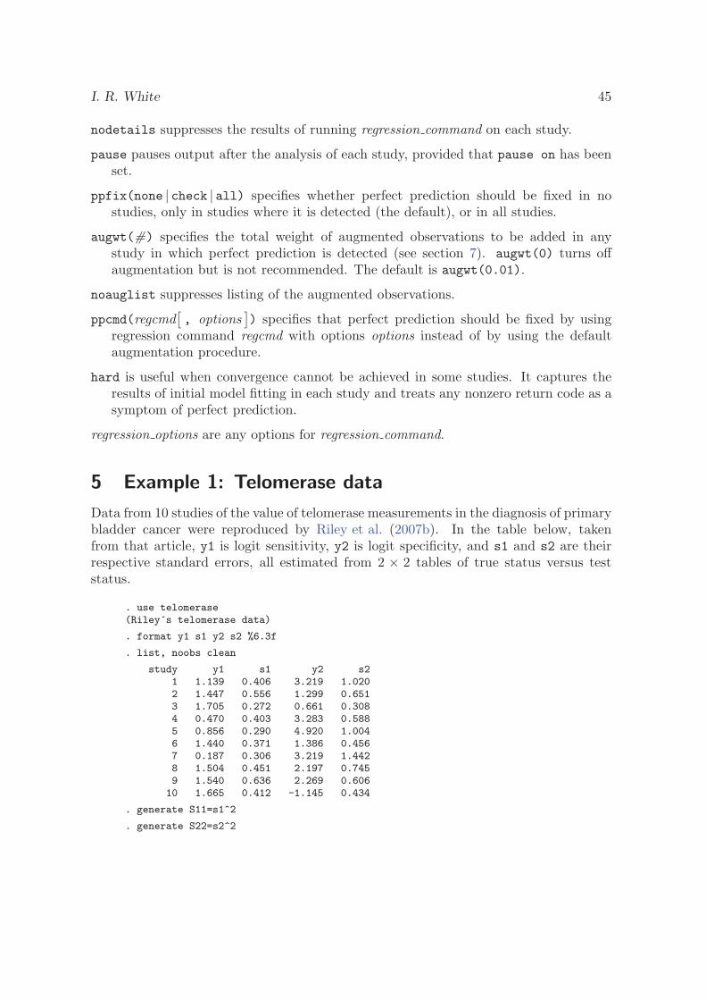
I. R. White 45
nodetails suppresses the results of running regression command on each study.
pause pauses output after the analysis of each study, provided that pause on has beenset.
ppfix(none | check | all) specifies whether perfect prediction should be fixed in nostudies, only in studies where it is detected (the default), or in all studies.
augwt(#) specifies the total weight of augmented observations to be added in anystudy in which perfect prediction is detected (see section 7). augwt(0) turns offaugmentation but is not recommended. The default is augwt(0.01).
noauglist suppresses listing of the augmented observations.
ppcmd(regcmd[, options
]) specifies that perfect prediction should be fixed by using
regression command regcmd with options options instead of by using the defaultaugmentation procedure.
hard is useful when convergence cannot be achieved in some studies. It captures theresults of initial model fitting in each study and treats any nonzero return code as asymptom of perfect prediction.
regression options are any options for regression command.
5 Example 1: Telomerase data
Data from 10 studies of the value of telomerase measurements in the diagnosis of primarybladder cancer were reproduced by Riley et al. (2007b). In the table below, takenfrom that article, y1 is logit sensitivity, y2 is logit specificity, and s1 and s2 are theirrespective standard errors, all estimated from 2 × 2 tables of true status versus teststatus.
. use telomerase(Riley´s telomerase data)
. format y1 s1 y2 s2 %6.3f
. list, noobs clean
study y1 s1 y2 s21 1.139 0.406 3.219 1.0202 1.447 0.556 1.299 0.6513 1.705 0.272 0.661 0.3084 0.470 0.403 3.283 0.5885 0.856 0.290 4.920 1.0046 1.440 0.371 1.386 0.4567 0.187 0.306 3.219 1.4428 1.504 0.451 2.197 0.7459 1.540 0.636 2.269 0.606
10 1.665 0.412 -1.145 0.434
. generate S11=s1^2
. generate S22=s2^2
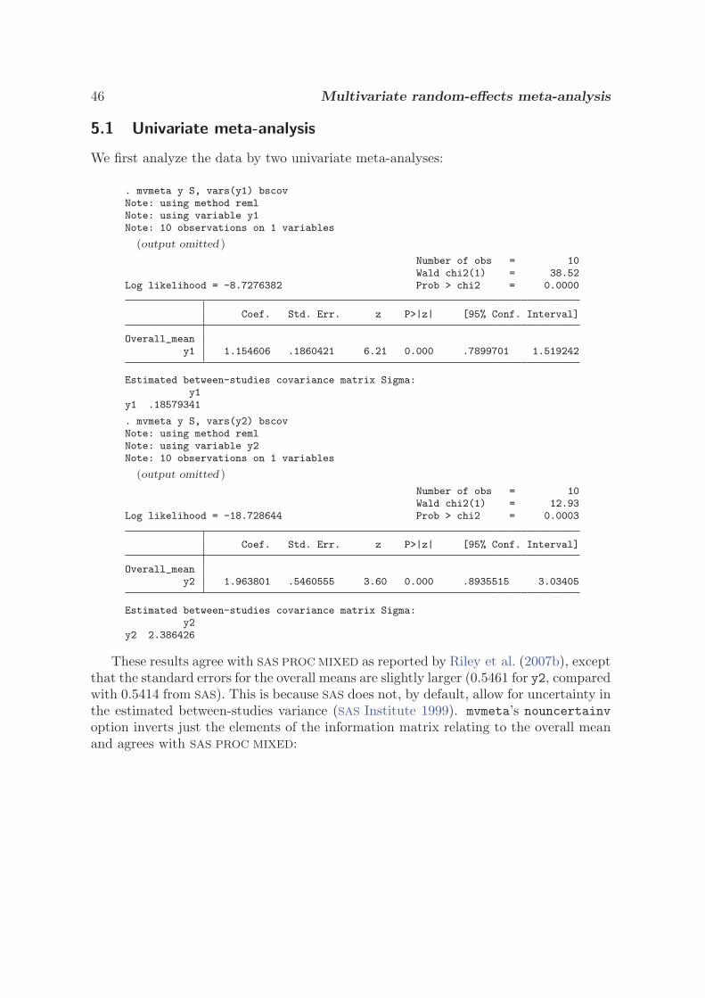
46 Multivariate random-effects meta-analysis
5.1 Univariate meta-analysis
We first analyze the data by two univariate meta-analyses:
. mvmeta y S, vars(y1) bscovNote: using method remlNote: using variable y1Note: 10 observations on 1 variables
(output omitted )
Number of obs = 10Wald chi2(1) = 38.52
Log likelihood = -8.7276382 Prob > chi2 = 0.0000
Coef. Std. Err. z P>|z| [95% Conf. Interval]
Overall_meany1 1.154606 .1860421 6.21 0.000 .7899701 1.519242
Estimated between-studies covariance matrix Sigma:y1
y1 .18579341
. mvmeta y S, vars(y2) bscovNote: using method remlNote: using variable y2Note: 10 observations on 1 variables
(output omitted )
Number of obs = 10Wald chi2(1) = 12.93
Log likelihood = -18.728644 Prob > chi2 = 0.0003
Coef. Std. Err. z P>|z| [95% Conf. Interval]
Overall_meany2 1.963801 .5460555 3.60 0.000 .8935515 3.03405
Estimated between-studies covariance matrix Sigma:y2
y2 2.386426
These results agree with SAS PROC MIXED as reported by Riley et al. (2007b), exceptthat the standard errors for the overall means are slightly larger (0.5461 for y2, comparedwith 0.5414 from SAS). This is because SAS does not, by default, allow for uncertainty inthe estimated between-studies variance (SAS Institute 1999). mvmeta’s nouncertainvoption inverts just the elements of the information matrix relating to the overall meanand agrees with SAS PROC MIXED:
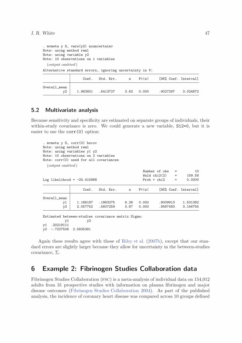
I. R. White 47
. mvmeta y S, vars(y2) nouncertainvNote: using method remlNote: using variable y2Note: 10 observations on 1 variables
(output omitted )
Alternative standard errors, ignoring uncertainty in V:
Coef. Std. Err. z P>|z| [95% Conf. Interval]
Overall_meany2 1.963801 .5413727 3.63 0.000 .9027297 3.024872
5.2 Multivariate analysis
Because sensitivity and specificity are estimated on separate groups of individuals, theirwithin-study covariance is zero. We could generate a new variable, S12=0, but it iseasier to use the corr(0) option:
. mvmeta y S, corr(0) bscovNote: using method remlNote: using variables y1 y2Note: 10 observations on 2 variablesNote: corr(0) used for all covariances
(output omitted )
Number of obs = 10Wald chi2(2) = 159.58
Log likelihood = -24.415968 Prob > chi2 = 0.0000
Coef. Std. Err. z P>|z| [95% Conf. Interval]
Overall_meany1 1.166187 .1863275 6.26 0.000 .8009913 1.531382y2 2.057752 .5607259 3.67 0.000 .9587493 3.156755
Estimated between-studies covariance matrix Sigma:y1 y2
y1 .20219111y2 -.7227506 2.5835381
Again these results agree with those of Riley et al. (2007b), except that our stan-dard errors are slightly larger because they allow for uncertainty in the between-studiescovariance, Σ.
6 Example 2: Fibrinogen Studies Collaboration data
Fibrinogen Studies Collaboration (FSC) is a meta-analysis of individual data on 154,012adults from 31 prospective studies with information on plasma fibrinogen and majordisease outcomes (Fibrinogen Studies Collaboration 2004). As part of the publishedanalysis, the incidence of coronary heart disease was compared across 10 groups defined
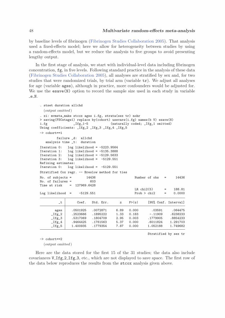
48 Multivariate random-effects meta-analysis
by baseline levels of fibrinogen (Fibrinogen Studies Collaboration 2005). That analysisused a fixed-effects model; here we allow for heterogeneity between studies by usinga random-effects model, but we reduce the analysis to five groups to avoid presentinglengthy output.
In the first stage of analysis, we start with individual-level data including fibrinogenconcentration, fg, in five levels. Following standard practice in the analysis of these data(Fibrinogen Studies Collaboration 2005), all analyses are stratified by sex and, for twostudies that were randomized trials, by trial arm (variable tr). We adjust all analysesfor age (variable ages), although in practice, more confounders would be adjusted for.We use the esave(N) option to record the sample size used in each study in variablee N.
. stset duration allchd
(output omitted )
. xi: mvmeta_make stcox ages i.fg, strata(sex tr) nohr> saving(FSCstage1) replace by(cohort) usevars(i.fg) names(b V) esave(N)i.fg _Ifg_1-5 (naturally coded; _Ifg_1 omitted)Using coefficients: _Ifg_2 _Ifg_3 _Ifg_4 _Ifg_5
-> cohort==1
failure _d: allchdanalysis time _t: duration
Iteration 0: log likelihood = -5223.9564Iteration 1: log likelihood = -5135.3888Iteration 2: log likelihood = -5129.5633Iteration 3: log likelihood = -5129.551Refining estimates:Iteration 0: log likelihood = -5129.551
Stratified Cox regr. -- Breslow method for ties
No. of subjects = 14436 Number of obs = 14436No. of failures = 603Time at risk = 127969.6428
LR chi2(5) = 188.81Log likelihood = -5129.551 Prob > chi2 = 0.0000
_t Coef. Std. Err. z P>|z| [95% Conf. Interval]
ages .0501925 .0072871 6.89 0.000 .03591 .064475_Ifg_2 .2523666 .1895222 1.33 0.183 -.11909 .6238233_Ifg_3 .5317069 .1804709 2.95 0.003 .1779905 .8854233_Ifg_4 .9464425 .1761563 5.37 0.000 .6011824 1.291703_Ifg_5 1.400935 .1779354 7.87 0.000 1.052188 1.749682
Stratified by sex tr
-> cohort==2
(output omitted )
Here are the data stored for the first 15 of the 31 studies; the data also includecovariances V Ifg 2 Ifg 3, etc., which are not displayed to save space. The first row ofthe data below reproduces the results from the stcox analysis given above.
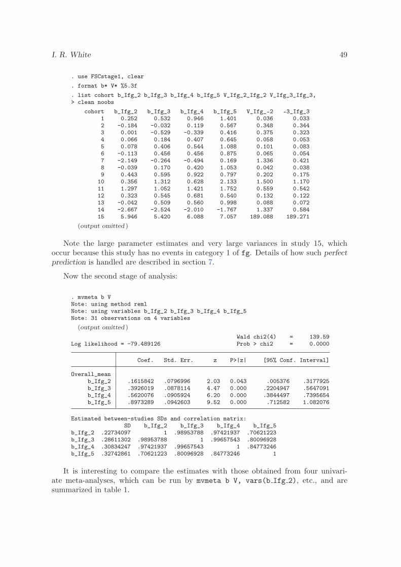
I. R. White 49
. use FSCstage1, clear
. format b* V* %5.3f
. list cohort b_Ifg_2 b_Ifg_3 b_Ifg_4 b_Ifg_5 V_Ifg_2_Ifg_2 V_Ifg_3_Ifg_3,> clean noobs
cohort b_Ifg_2 b_Ifg_3 b_Ifg_4 b_Ifg_5 V_Ifg_~2 ~3_Ifg_31 0.252 0.532 0.946 1.401 0.036 0.0332 -0.184 -0.032 0.119 0.567 0.348 0.3443 0.001 -0.529 -0.339 0.416 0.375 0.3234 0.066 0.184 0.407 0.645 0.058 0.0535 0.078 0.406 0.544 1.088 0.101 0.0836 -0.113 0.456 0.456 0.875 0.065 0.0547 -2.149 -0.264 -0.494 0.169 1.336 0.4218 -0.039 0.170 0.420 1.053 0.042 0.0389 0.443 0.595 0.922 0.797 0.202 0.175
10 0.356 1.312 0.628 2.133 1.500 1.17011 1.297 1.052 1.421 1.752 0.559 0.54212 0.323 0.545 0.681 0.540 0.132 0.12213 -0.042 0.509 0.560 0.998 0.088 0.07214 -2.667 -2.524 -2.010 -1.767 1.337 0.58415 5.946 5.420 6.088 7.057 189.088 189.271
(output omitted )
Note the large parameter estimates and very large variances in study 15, whichoccur because this study has no events in category 1 of fg. Details of how such perfectprediction is handled are described in section 7.
Now the second stage of analysis:
. mvmeta b VNote: using method remlNote: using variables b_Ifg_2 b_Ifg_3 b_Ifg_4 b_Ifg_5Note: 31 observations on 4 variables
(output omitted )
Wald chi2(4) = 139.59Log likelihood = -79.489126 Prob > chi2 = 0.0000
Coef. Std. Err. z P>|z| [95% Conf. Interval]
Overall_meanb_Ifg_2 .1615842 .0796996 2.03 0.043 .005376 .3177925b_Ifg_3 .3926019 .0878114 4.47 0.000 .2204947 .5647091b_Ifg_4 .5620076 .0905924 6.20 0.000 .3844497 .7395654b_Ifg_5 .8973289 .0942603 9.52 0.000 .712582 1.082076
Estimated between-studies SDs and correlation matrix:SD b_Ifg_2 b_Ifg_3 b_Ifg_4 b_Ifg_5
b_Ifg_2 .22734097 1 .98953788 .97421937 .70621223b_Ifg_3 .28611302 .98953788 1 .99657543 .80096928b_Ifg_4 .30834247 .97421937 .99657543 1 .84773246b_Ifg_5 .32742861 .70621223 .80096928 .84773246 1
It is interesting to compare the estimates with those obtained from four univari-ate meta-analyses, which can be run by mvmeta b V, vars(b Ifg 2), etc., and aresummarized in table 1.
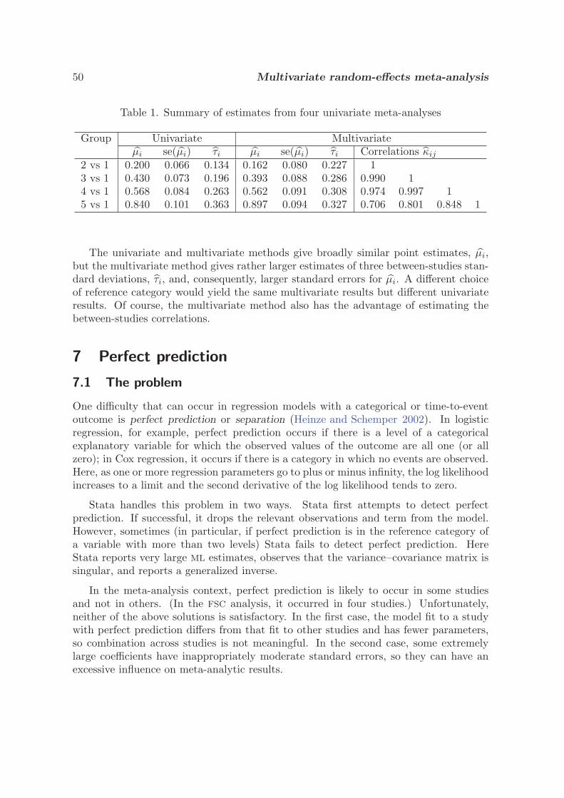
50 Multivariate random-effects meta-analysis
Table 1. Summary of estimates from four univariate meta-analyses
Group Univariate Multivariateμi se(μi) τi μi se(μi) τi Correlations κij
2 vs 1 0.200 0.066 0.134 0.162 0.080 0.227 13 vs 1 0.430 0.073 0.196 0.393 0.088 0.286 0.990 14 vs 1 0.568 0.084 0.263 0.562 0.091 0.308 0.974 0.997 15 vs 1 0.840 0.101 0.363 0.897 0.094 0.327 0.706 0.801 0.848 1
The univariate and multivariate methods give broadly similar point estimates, μi,but the multivariate method gives rather larger estimates of three between-studies stan-dard deviations, τi, and, consequently, larger standard errors for μi. A different choiceof reference category would yield the same multivariate results but different univariateresults. Of course, the multivariate method also has the advantage of estimating thebetween-studies correlations.
7 Perfect prediction
7.1 The problem
One difficulty that can occur in regression models with a categorical or time-to-eventoutcome is perfect prediction or separation (Heinze and Schemper 2002). In logisticregression, for example, perfect prediction occurs if there is a level of a categoricalexplanatory variable for which the observed values of the outcome are all one (or allzero); in Cox regression, it occurs if there is a category in which no events are observed.Here, as one or more regression parameters go to plus or minus infinity, the log likelihoodincreases to a limit and the second derivative of the log likelihood tends to zero.
Stata handles this problem in two ways. Stata first attempts to detect perfectprediction. If successful, it drops the relevant observations and term from the model.However, sometimes (in particular, if perfect prediction is in the reference category ofa variable with more than two levels) Stata fails to detect perfect prediction. HereStata reports very large ML estimates, observes that the variance–covariance matrix issingular, and reports a generalized inverse.
In the meta-analysis context, perfect prediction is likely to occur in some studiesand not in others. (In the FSC analysis, it occurred in four studies.) Unfortunately,neither of the above solutions is satisfactory. In the first case, the model fit to a studywith perfect prediction differs from that fit to other studies and has fewer parameters,so combination across studies is not meaningful. In the second case, some extremelylarge coefficients have inappropriately moderate standard errors, so they can have anexcessive influence on meta-analytic results.
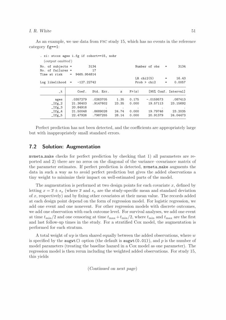
I. R. White 51
As an example, we use data from FSC study 15, which has no events in the referencecategory fg==1:
. xi: stcox ages i.fg if cohort==15, nohr
(output omitted )
No. of subjects = 3134 Number of obs = 3134No. of failures = 17Time at risk = 9465.954814
LR chi2(5) = 16.43Log likelihood = -127.22742 Prob > chi2 = 0.0057
_t Coef. Std. Err. z P>|z| [95% Conf. Interval]
ages .0357279 .0263705 1.35 0.175 -.0159573 .087413_Ifg_2 21.36403 .9147602 23.35 0.000 19.57113 23.15692_Ifg_3 20.84916 . . . . ._Ifg_4 21.50048 .8689028 24.74 0.000 19.79746 23.2035_Ifg_5 22.47926 .7987255 28.14 0.000 20.91379 24.04473
Perfect prediction has not been detected, and the coefficients are appropriately largebut with inappropriately small standard errors.
7.2 Solution: Augmentation
mvmeta make checks for perfect prediction by checking that 1) all parameters are re-ported and 2) there are no zeros on the diagonal of the variance–covariance matrix ofthe parameter estimates. If perfect prediction is detected, mvmeta make augments thedata in such a way as to avoid perfect prediction but gives the added observations atiny weight to minimize their impact on well-estimated parts of the model.
The augmentation is performed at two design points for each covariate x, defined byletting x = x± sx (where x and sx are the study-specific mean and standard deviationof x, respectively) and by fixing other covariates at their mean value. The records addedat each design point depend on the form of regression model. For logistic regression, weadd one event and one nonevent. For other regression models with discrete outcomes,we add one observation with each outcome level. For survival analyses, we add one eventat time tmin/2 and one censoring at time tmax + tmin/2, where tmin and tmax are the firstand last follow-up times in the study. For a stratified Cox model, the augmentation isperformed for each stratum.
A total weight of wp is then shared equally between the added observations, where wis specified by the augwt() option (the default is augwt(0.01)), and p is the number ofmodel parameters (treating the baseline hazard in a Cox model as one parameter). Theregression model is then rerun including the weighted added observations. For study 15,this yields
(Continued on next page)
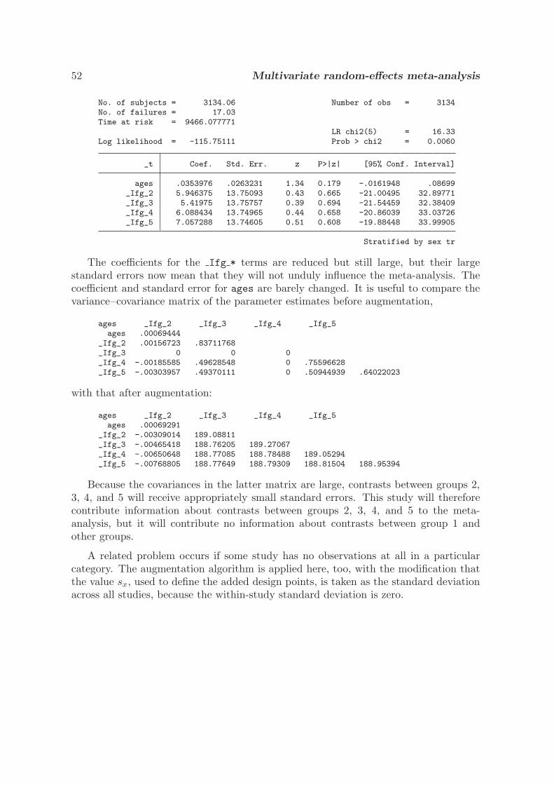
52 Multivariate random-effects meta-analysis
No. of subjects = 3134.06 Number of obs = 3134No. of failures = 17.03Time at risk = 9466.077771
LR chi2(5) = 16.33Log likelihood = -115.75111 Prob > chi2 = 0.0060
_t Coef. Std. Err. z P>|z| [95% Conf. Interval]
ages .0353976 .0263231 1.34 0.179 -.0161948 .08699_Ifg_2 5.946375 13.75093 0.43 0.665 -21.00495 32.89771_Ifg_3 5.41975 13.75757 0.39 0.694 -21.54459 32.38409_Ifg_4 6.088434 13.74965 0.44 0.658 -20.86039 33.03726_Ifg_5 7.057288 13.74605 0.51 0.608 -19.88448 33.99905
Stratified by sex tr
The coefficients for the Ifg * terms are reduced but still large, but their largestandard errors now mean that they will not unduly influence the meta-analysis. Thecoefficient and standard error for ages are barely changed. It is useful to compare thevariance–covariance matrix of the parameter estimates before augmentation,
ages _Ifg_2 _Ifg_3 _Ifg_4 _Ifg_5ages .00069444
_Ifg_2 .00156723 .83711768_Ifg_3 0 0 0_Ifg_4 -.00185585 .49628548 0 .75596628_Ifg_5 -.00303957 .49370111 0 .50944939 .64022023
with that after augmentation:
ages _Ifg_2 _Ifg_3 _Ifg_4 _Ifg_5ages .00069291
_Ifg_2 -.00309014 189.08811_Ifg_3 -.00465418 188.76205 189.27067_Ifg_4 -.00650648 188.77085 188.78488 189.05294_Ifg_5 -.00768805 188.77649 188.79309 188.81504 188.95394
Because the covariances in the latter matrix are large, contrasts between groups 2,3, 4, and 5 will receive appropriately small standard errors. This study will thereforecontribute information about contrasts between groups 2, 3, 4, and 5 to the meta-analysis, but it will contribute no information about contrasts between group 1 andother groups.
A related problem occurs if some study has no observations at all in a particularcategory. The augmentation algorithm is applied here, too, with the modification thatthe value sx, used to define the added design points, is taken as the standard deviationacross all studies, because the within-study standard deviation is zero.
I. R. White 53
8 Discussion
8.1 Difficulties and limitations
The main difficulty that might be encountered in fitting multivariate random-effectsmeta-analysis models is a nonpositive-definite Σ. However, the parameterization usedhere ensures that Σ is positive semidefinite and achieves a nonpositive-definite Σ if oneor more elements of the Cholesky decomposition approach zero. I have encountered non-convergence of the Newton–Raphson algorithm only when the starting value is Σ = 0,which is avoided by a suitable nonzero choice of starting values, or when inappropriatelyhandled perfect prediction has led to extreme parameter estimates with small standarderrors.
The standard error provided for an REML analysis allows for uncertainty in estimat-ing Σ by inverting the second derivative matrix of the restricted likelihood (1). Thisis not the standard approach (Kenward and Roger 1997), and its properties requirefurther investigation. Confidence intervals based on a t distribution would be a usefulenhancement.
At present, the augmentation routine in mvmeta make effectively ignores any cat-egory in which perfect prediction occurs but allows information to be drawn fromother categories from that study. A larger augmentation would allow informationto be drawn from categories with perfect prediction. For example, if the data con-sist of 2 × 2 tables, then standard practice would add 0.5 observations to each cell(Sweeting, Sutton, and Lambert 2004). This amounts to assigning to the augmentedobservations a total weight equal to the number of parameters, and it is tempting toapply this rule more widely (by using augment(1)). However, larger augmentationweights have the undesirable property of not being invariant to reparameterization; forexample, a different choice of reference category for the fg variable in section 6 wouldlead to somewhat different results. Larger augmentation is probably best implementedby the user.
There are alternate ways to handle perfect prediction, including various forms ofpenalized likelihood. The methods of Le Cessie and van Houwelingen (1992) and Ver-weij and van Houwelingen (1994) have been implemented in Stata by the plogit andstpcox commands, respectively, and both are currently being updated to allow for per-fect prediction (G. Ambler, pers. comm.). The method of Firth (1993) is invariant toreparameterization and is being implemented by the author. When suitable routinesbecome available in Stata, they can be called by the ppcmd() option in mvmeta make.
8.2 Comparison to other procedures
All the models considered here can also be fit in SAS PROC MIXED, although someprogramming effort is required to specify the known within-study variances, Si. Thetwo approaches are very similar, but by default, SAS produces standard errors that ignorethe uncertainty in Σ, and produces confidence intervals by using the t distribution on
54 Multivariate random-effects meta-analysis
n− 1 degrees of freedom. Further, SAS optionally provides a standard error adjusted toallow for uncertainty in estimating Σ and provides the approximate degrees of freedomof Kenward and Roger (1997), which has good small-sample properties.
Multivariate meta-analysis models cannot be fit by using existing Stata commands,but univariate models can. metan differs from mvmeta because it uses DerSimonianand Laird (1986) estimation of the random-effects variance. metareg offers the choiceof DerSimonian and Laird, ML, or REML estimation, so if run without covariates, itcan be compared to mvmeta. The original metareg (Sharp 1998) used the algorithmof Hardy and Thompson (1996) and did not always find the best solution. Version 2of metareg, by Harbord and Higgins (2008), uses Newton–Raphson maximization viaml, and produces the same point estimates as mvmeta and the same standard er-rors as mvmeta with the nouncertainv option. metareg produces confidence inter-vals that allow for nonnormality of the sampling distributions by using the methodof Knapp and Hartung (2003); its z option produces confidence intervals that agreewith mvmeta. Of course, metareg also has the enormous advantage of handling meta-regression.
8.3 More than two outcomes
Although mvmeta handles several outcomes perfectly well, its computing time increasessharply as the number of outcomes increases. mvmeta can even computationally handlesituations where there are more quantities of interest than studies (p > n); however,fitting such large models can be unwise and results can be untrustworthy.
9 Acknowledgments
I thank the FSC for providing access to their data for illustrative analyses: a full list ofthe FSC collaborators is given in Fibrinogen Studies Collaboration (2005). I also thankLi Su and Dan Jackson for helping me rediscover the Cholesky decomposition parameter-ization; Stephen Kaptoge and Sebhat Erquo for helpful comments on the programming;James Roger for help in understanding SAS PROC MIXED; and Patrick Royston andGareth Ambler for discussions about augmentation and penalized likelihoods.
10 ReferencesBerkey, C. S., J. J. Anderson, and D. C. Hoaglin. 1996. Multiple-outcome meta-analysis
of clinical trials. Statistics in Medicine 15: 537–557.
Berkey, C. S., D. C. Hoaglin, A. Antczak-Bouckoms, F. Mosteller, and G. A. Colditz.1998. Meta-analysis of multiple outcomes by regression with random effects. Statisticsin Medicine 17: 2537–2550.
DerSimonian, R., and N. Laird. 1986. Meta-analysis in clinical trials. Controlled ClinicalTrials 7: 177–188.
I. R. White 55
Fibrinogen Studies Collaboration. 2004. Collaborative meta-analysis of prospectivestudies of plasma fibrinogen and cardiovascular disease. European Journal of Cardio-vascular Prevention and Rehabilitation 11: 9–17.
———. 2005. Plasma fibrinogen level and the risk of major cardiovascular diseasesand nonvascular mortality: An individual participant meta-analysis. Journal of theAmerican Medical Association 294: 1799–1809.
Firth, D. 1993. Bias reduction of maximum likelihood estimates. Biometrika 80: 27–38.
Harbord, R. M., and J. P. T. Higgins. 2008. Meta-regression in Stata. Stata Journal 8:493–519.
Hardy, R. J., and S. G. Thompson. 1996. A likelihood approach to meta-analysis withrandom effects. Statistics in Medicine 30: 619–629.
Hasselblad, V. 1998. Meta-analysis of multitreatment studies. Medical Decision Making18: 37–43.
Heinze, G., and M. Schemper. 2002. A solution to the problem of separation in logisticregression. Statistics in Medicine 21: 2409–2419.
Jackson, D., I. R. White, and S. G. Thompson. Forthcoming. Extending DerSimo-nian and Laird’s methodology to perform multivariate random effects meta-analyses.Statistics in Medicine.
Kenward, M. G., and J. H. Roger. 1997. Small sample inference for fixed effects fromrestricted maximum likelihood. Biometrics 53: 983–997.
Knapp, G., and J. Hartung. 2003. Improved tests for a random-effects meta-regressionwith a single covariate. Statistics in Medicine 22: 2693–2710.
Le Cessie, S., and J. C. van Houwelingen. 1992. Ridge estimators in logistic regression.Applied Statistics 41: 191–201.
Lu, G., and A. E. Ades. 2004. Combination of direct and indirect evidence in mixedtreatment comparisons. Statistics in Medicine 23: 3105–3124.
Normand, S. L. T. 1999. Meta-analysis: Formulating, evaluating, combining and re-porting. Statistics in Medicine 18: 213–259.
Pinto, E., A. Willan, and B. O’Brien. 2005. Cost-effectiveness analysis for multinationalclinical trials. Statistics in Medicine 24: 1965–1982.
Riley, R. D., K. R. Abrams, P. C. Lambert, A. J. Sutton, and J. R. Thompson. 2007a.An evaluation of bivariate random-effects meta-analysis for the joint synthesis of twocorrelated outcomes. Statistics in Medicine 26: 78–97.
Riley, R. D., K. R. Abrams, A. J. Sutton, P. C. Lambert, and J. R. Thompson. 2007b.Bivariate random-effects meta-analysis and the estimation of between-study correla-tion. BMC Medical Research Methodology 7: 3.

56 Multivariate random-effects meta-analysis
SAS Institute. 1999. SAS OnlineDoc Version Eight. Cary, NC: SAS Institute.http://www.technion.ac.il/docs/sas/.
Sharp, S. 1998. sbe23: Meta-analysis regression. Stata Technical Bulletin 42: 16–22.Reprinted in Stata Technical Bulletin Reprints, vol. 7, pp. 148–155. College Station,TX: Stata Press.
Sweeting, M. J., A. J. Sutton, and P. C. Lambert. 2004. What to add to nothing? Useand avoidance of continuity corrections in meta-analysis of sparse data. Statistics inMedicine 23: 1351–1375.
Thompson, S. G. 1994. Why sources of heterogeneity in meta-analysis should be inves-tigated. British Medical Journal 309: 1351–1355.
van Houwelingen, H. C., L. R. Arends, and T. Stijnen. 2003. Advanced methods inmeta-analysis: multivariate approach and meta-regression. Statistics in Medicine 21:589–624.
Verweij, P. J. M., and J. C. van Houwelingen. 1994. Penalized likelihood in Cox regres-sion. Statistics in Medicine 13: 2427–2436.
About the author
Ian White is a senior statistician at the MRC Biostatistics Unit in Cambridge, UK. His re-
search interests include missing data, noncompliance and measurement error in clinical trials,
observational studies, and meta-analysis.

5 Appendixes
What meta-analysis features are available in Stata?
Title User-written packages for meta-analysis in Stata Authors Jonathan A. C. Sterne, University of Bristol
Ross J. Harris, University of Bristol Roger M. Harbord, University of Bristol Thomas J. Steichen, RJRT
Date
January 2007; updated April 2009; minor revisions July 2009
Stata does not have a meta-analys is co mmand. Stata users, however, have
developed an excellent suite of commands for performing meta-analyses.
In 2009, Stata publis hed Meta-Analysis in Stata: An Updated Collection from the
Stata Journal, which brings together all the Stata Journal articles about meta-analysis.
This book is available for purchase at http://www.stata-press.com/books/mais.html.
We have created a command to download a ll user-written commands discussed in
this collection, except for those commands listed in the appendix. For instructions on
obtaining this command, see http://www.stata-press.com/data/mais.html.
The following meta-analysis commands are all described in Meta-Analysis in Stata:
An Updated Collection from the Stata Journal.
1. metan
metan is the main Stata meta-analysis command. Its latest version allows the user to
input the cell frequencies from the 2 × 2 table for eac h study (for binary outcomes),
the mean and standard deviation in each group (for numeric al outcomes), or the
effect esti mate and standard error from ea ch study. It provides a comprehensiv e
range of methods for meta-a nalysis, including inv erse-variance-weighted meta-
analysis, and creates new variables containi ng the treatment effe ct estimate and its
standard error for each study. These variabl es can then be us ed as input to other
Stata meta-analysis c ommands. Meta-analyses may be conducted in subgroups b y
using the by() option.
All the meta-analysis calculations available in metan are based on standard methods,
an overview of which may be found in c hapter 15 of Deeks, Alt man, and Bradburn
(2001).
The version of the metan command that used Stata 7 graphics has been renamed
metan7 and is downloaded as part of the metan package currently available on the
SSC archive.

The most recent help file for metan provides several clickable examples of using the
command.
2. labbe
labbe draws a L’Abbe plot for event data (proportion of successes in the two groups).
It is available via the metan package as a version 7 command that uses version 6
graphics.
3. metacum
metacum performs cumulative meta-analyses and graphs the results.
4. metap
metap combines p-values by using Fisher’s method, Edgington’s additive method, or
Edgington’s normal curve method. It was re leased in 1999 as a version 6 command
(no graphics) and last updated in 2000. It requires the user to input a p-value for each
study.
5. metareg
metareg does meta-regression. It was first released in 1998 and has been updated to
take account of improvements in Stata estimation facilities and recent methodological
developments. It requires t he user to input the treatm ent effect estimate and it s
standard error for each study.
6. metafunnel
metafunnel plots funnel plots. It was releas ed in 2004 and uses Stata 8 graphics. It
requires the user to input the treatment effect estimate and its standard error for each
study.
7. confunnel
confunnel plots contour-enhanced funnel plots. The command has been designed to
be flexible, allowing the user to add extra features to the funnel plot.
8. metabias

metabias provides statistical tests for funnel plot asymmetry. It was first released in
1997, but it has been updated to provide recent ly proposed tests that maintain better
control of the false-positive rate than those available in the original command.
9. metatrim
metatrim implements the “trim and fill” method to adjust for publication bias in funnel
plots. It requires the user to input the tr eatment effect estimate and its standard error
for each study.
10. metandi and metandiplot
metandi facilitates the fitting of hierarchic al logistic regression models for
meta-analysis of diagnostic test accuracy studies. metandiplot produces a graph of
the model fit by metandi, which must be the last estimation-class command
executed.
11. glst
glst calculates a log-linear dose-response regression model us ing generalized least
squares for trend estimation of single or multiple summarized dose-respons e
epidemiological studies. Out put from this command ma y be useful in deriving
summary effects and their st andard errors for inclusion in meta-analyses of such
studies.
12. metamiss
metamiss performs meta-analysis with binary out comes when some or all studies
have missing data.
13. mvmeta and mvmeta_make
mvmeta performs maximum likelihood, re stricted maximum likelihood, or
method-of-moments estimation of random-effects multivariate meta-analysis models.
mvmeta_make facilitates the preparation of su mmary datasets from more detaile d
data.
The following commands are documented in the Appendix:

14. metannt
metannt is intended to aid interpretation of meta-analyses of binary data b y
presenting intervention effect sizes in abs olute terms, as the number needed to treat
(NNT) and the number of events avoided (o r added) per 1,000. The user inputs
design parameters, and metannt uses the metan command to calculate the required
statistics. This command is available as part of the metan package.
15. metaninf
metaninf i s a port of the metainf command to use metan as its analysis engine
rather than meta. It w as released in 2001 as a version 6 command using v ersion 6
graphics and was las t updated in 2004. It require s the user to provide input in the
form needed by metan. To install the package, type ssc install metaninf in Stata.
16. midas
midas provides statistical and graphical rout ines for undertaking meta-analysis of
diagnostic test performance in Stat a. To install the package, type ssc install midas
in Stata.
17. meta_lr
meta_lr graphs positive and negative likelihood rati os in diagnos tic tests. It can do
stratified meta-analysis of individual estima tes. The user must provide the effect
estimates (log positiv e likelihood ratio and log negative likelihood ratio) and their
standard errors. Commands meta and metareg are used for internal calculations .
This is a v ersion 8 command released in 2004. To insta ll the package, type ssc install meta_lr in Stata.
18. metaparm
metaparm performs meta-analyses and calculates confidence intervals and p-values
for differences or rati os between paramet ers for different s ubpopulations for data
stored in the parmest format. To install the package, type ssc install metaparm in
Stata.
Appendix: Further Stata meta-analysiscommands
Stata users have written meta-analysis commands that have not, so far, been acceptedfor publication in the Stata Journal. Here are brief descriptions of commands knownto the editor at the time of publishing this collection. Readers should note that thesecommands have not undergone the review process required for publication in the StataJournal. This list is likely to be incomplete, and the editor apologizes to authors ofany commands that have been overlooked. For the most up-to-date information onthese and other meta-analysis commands, readers are encouraged to check the Statafrequently asked question on meta-analysis:
http://www.stata.com/support/faqs/stat/meta.html
• metannt is intended to aid interpretation of meta-analyses of binary data by pre-senting intervention effect sizes in absolute terms, as the number needed to treat(NNT) and the number of events avoided (or added) per 1,000. The user inputs de-sign parameters, and metannt uses the metan command to calculate the requiredstatistics. This command is available as part of the metan package.
The NNT is the number of individuals required to experience the intervention inorder to expect there to be one additional event to be observed. It is defined asthe reciprocal of the absolute value of the risk difference (risk of the outcome inthe intervention group minus risk in control).
NNT =1
|risk difference|Assuming the event is undesirable, this is termed the number needed to treat tobenefit. If the intervention arm experiences more events, this is commonly referredto as the number needed to treat to harm. Because most meta-analyses are basedon ratio measures, the risk difference is calculated based on an assumed value ofthe risk in the control group. The metannt command calculates this by derivingan estimate of the intervention effect (e.g., a risk ratio), applying it to a populationwith a given outcome event risk, and deriving from this a projected event risk if
249
250 Appendix
the population were to receive the intervention. The number of avoided or excessevents (respectively) per 1,000 population is the difference between the two eventrisks multiplied by 1,000. Optionally, a confidence interval is also presented, usingthe confidence limits for the estimated intervention effect applied to the controlgroup event rate.
• metaninf investigates the influence of one study on the overall meta-analysis es-timate and shows graphically the results when the meta-analysis estimates arecomputed, omitting one study in each turn. This command makes repeated callsto the metan command for its analyses. It was released in 2001 and was lastupdated in 2004. It requires the user to provide input in the form needed bymetan. To install the package, type ssc install metaninf in Stata. Articlesdescribing metainf, a previous version of the command, were published in theStata Technical Bulletin (Tobias 1999, 2000).
• midas provides statistical and graphical routines for undertaking meta-analysis ofdiagnostic test performance in Stata. Primary data synthesis is performed withinthe bivariate mixed-effects binary regression modeling framework. Model speci-fication, estimation, and prediction are carried out with xtmelogit in Stata 10or the gllamm command in Stata 9 by adaptive quadrature. Using the estimatedcoefficients and variance–covariance matrices, midas calculates summary operat-ing sensitivity and specificity (with confidence and prediction contours in sum-mary receiver operating characteristic space), summary likelihood, and odds ra-tios. Global and relevant test performance metric-specific heterogeneity statisticsare provided. midas facilitates extensive statistical and graphical data synthesisand exploratory analyses of heterogeneity, covariate effects, publication bias, andinfluence. Bayes’ nomograms and likelihood-ratio matrices can be obtained andused to guide clinical decision making. The minimum required input data arevariables containing the elements of the 2 × 2 contingency tables (true positives,false positives, false negatives, and true negatives) of test results from each study.To install the package, type ssc install midas in Stata.
Further information on the comprehensive suite of facilities provided by midasis available at http://www.sitemaker.umich.edu/metadiagnosis/midas home. Inparticular, two presentations given at Stata Users Group meetings are availableat http://www.sitemaker.umich.edu/metadiagnosis/presentations and via RePEcat http://econpapers.repec.org/paper/bocasug07/4.htm andhttp://ideas.repec.org/p/boc/wsug07/1.html.
• meta lr graphs positive and negative likelihood ratios in diagnostic tests. It can dostratified meta-analysis of individual estimates. The user must provide the effectestimates (log positive likelihood ratio and log negative likelihood ratio) and theirstandard errors. Commands meta and metareg are used for internal calculations.This is a version 8 command released in 2004. To install the package, type sscinstall meta lr in Stata.
• metaparm performs meta-analyses and calculates confidence intervals and p-valuesfor differences or ratios between parameters for different subpopulations, for data
251
stored in the parmest format (Newson 2003). To install the package, type sscinstall metaparm in Stata.
11 ReferencesNewson, R. 2003. Confidence intervals and p-values for delivery to the end user. Stata
Journal 3: 245–269.
Tobias, A. 1999. sbe26: Assessing the influence of a single study in the meta-analysisestimate. Stata Technical Bulletin 47: 15–17. Reprinted in Stata Technical BulletinReprints, vol. 8, pp. 108–110. College Station, TX: Stata Press.
———. 2000. sbe26.1: Update of metainf. Stata Technical Bulletin 56: 15. Reprintedin Stata Technical Bulletin Reprints, vol. 10, p. 72. College Station, TX: Stata Press.
The Stata Journal (2004)4, Number 2, pp. 124–126
Submenu and dialogs for meta-analysis
commands
Thomas J. [email protected]
Abstract. The metadialog package provides Stata dialog boxes for the publiclyavailable meta-analysis commands. It includes the commands needed to create aMeta-Analysis submenu on the StataCorp-defined User menu.
Keywords: pr0012, dialog, menu, meta-analysis
1 Description
User-written dialog boxes and menus were introduced in Stata 8 to provide an alternativeto the standard command-line interface. The metadialog package provides dialog boxes(.dlg files) and the commands needed to create a Meta-Analysis submenu that willcontain the publicly available meta-analysis commands. The 14 commands includedin this package that may be placed on the menu are meta, metan, metap, metareg,metacum, funnel, metafunnel, labbe, metannt, metaninf, metainf, galbr, metabias,and metatrim.
This package, which was announced on Statalist, was made available originally atthe Statistical Software Components (SSC) archive site hosted by the Boston College De-partment of Economics at http://ideas.repec.org/s/boc/bocode.html. Many of the un-derlying meta-analysis programs were introduced in the Stata Technical Bulletin (STB),though some subsequently may have been updated and republished via the SSC archives.Some programs were published only on the SSC archives site. The metadialog pack-age is reintroduced here to allow update pointers to be placed to the underlying STB
programs and to announce it to those users who may not participate on Statalist.
The dialogs were written for a specific version of each program file (see the listingbelow). If you do not have these versions installed, you should update the specificprograms before using the related dialogs. Use the net search name command to findand install the appropriate versions of these programs.
You may choose not to create the menu and, instead, run the dialogs directly fromthe Stata command line via the db name command. If so,
c© 2004 StataCorp LP pr0012
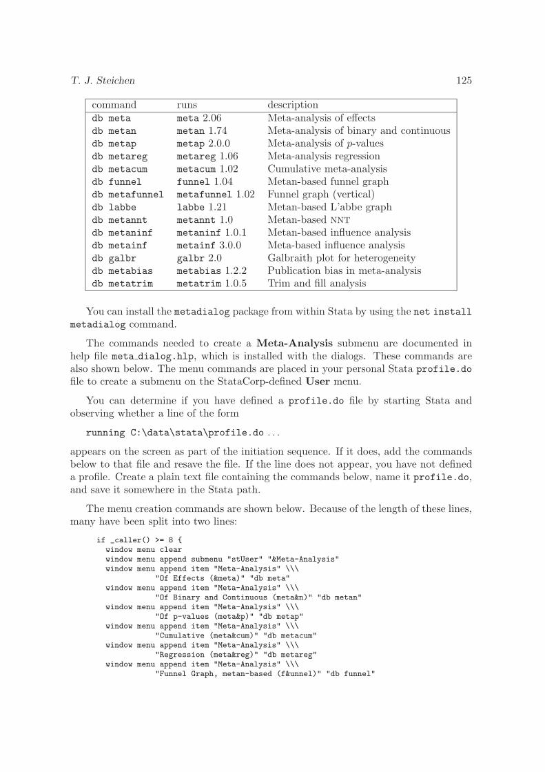
T. J. Steichen 125
command runs descriptiondb meta meta 2.06 Meta-analysis of effectsdb metan metan 1.74 Meta-analysis of binary and continuousdb metap metap 2.0.0 Meta-analysis of p-valuesdb metareg metareg 1.06 Meta-analysis regressiondb metacum metacum 1.02 Cumulative meta-analysisdb funnel funnel 1.04 Metan-based funnel graphdb metafunnel metafunnel 1.02 Funnel graph (vertical)db labbe labbe 1.21 Metan-based L’abbe graphdb metannt metannt 1.0 Metan-based NNT
db metaninf metaninf 1.0.1 Metan-based influence analysisdb metainf metainf 3.0.0 Meta-based influence analysisdb galbr galbr 2.0 Galbraith plot for heterogeneitydb metabias metabias 1.2.2 Publication bias in meta-analysisdb metatrim metatrim 1.0.5 Trim and fill analysis
You can install the metadialog package from within Stata by using the net installmetadialog command.
The commands needed to create a Meta-Analysis submenu are documented inhelp file meta dialog.hlp, which is installed with the dialogs. These commands arealso shown below. The menu commands are placed in your personal Stata profile.do
file to create a submenu on the StataCorp-defined User menu.
You can determine if you have defined a profile.do file by starting Stata andobserving whether a line of the form
running C:\data\stata\profile.do . . .
appears on the screen as part of the initiation sequence. If it does, add the commandsbelow to that file and resave the file. If the line does not appear, you have not defineda profile. Create a plain text file containing the commands below, name it profile.do,and save it somewhere in the Stata path.
The menu creation commands are shown below. Because of the length of these lines,many have been split into two lines:
if _caller() >= 8 {window menu clearwindow menu append submenu "stUser" "&Meta-Analysis"window menu append item "Meta-Analysis" \\\
"Of Effects (&meta)" "db meta"window menu append item "Meta-Analysis" \\\
"Of Binary and Continuous (meta&n)" "db metan"window menu append item "Meta-Analysis" \\\
"Of p-values (meta&p)" "db metap"window menu append item "Meta-Analysis" \\\
"Cumulative (meta&cum)" "db metacum"window menu append item "Meta-Analysis" \\\
"Regression (meta®)" "db metareg"window menu append item "Meta-Analysis" \\\
"Funnel Graph, metan-based (f&unnel)" "db funnel"

126 Metadialog package
window menu append item "Meta-Analysis" \\\"Funnel Graph, &vertical (metafunnel)" "db metafunnel"
window menu append item "Meta-Analysis" \\\"L’abbe Graph, metan-based (&labbe)" "db labbe"
window menu append item "Meta-Analysis" \\\"NNT, metan-based (metann&t)" "db metannt"
window menu append item "Meta-Analysis" \\\"Influence Analysis, metan-based (metan&inf)" "db metaninf"
window menu append item "Meta-Analysis" \\\"Influence Analysis, meta-based (metain&f)" "db metainf"
window menu append item "Meta-Analysis" \\\"Galbraith Plot for Heterogeneity (&galbr)" "db galbr"
window menu append item "Meta-Analysis" \\\"Publication Bias (meta&bias)" "db metabias"
window menu append item "Meta-Analysis" \\\"Trim and Fill Analysis (metatrim)" "db met&atrim"
window menu refresh}
Dialogs are available only in Stata 8 or later; thus, the leading
if caller() >= 8 {
and trailing
}
lines above are needed only if you also run Stata 7. Leaving these lines in will not causeproblems.
The easiest way to capture these commands is to open the help file in your texteditor, copy the lines, and then paste them into your profile.do file.
About the Author
Thomas J. Steichen is an industrial statistician who has used Stata for many years. He hascontributed programs to the Stata user community on several problems, including duplicateobservations, meta-analysis, violin plots, and noncentral distributions, and has authored severalinserts in the Stata Journal and the Stata Technical Bulletin.
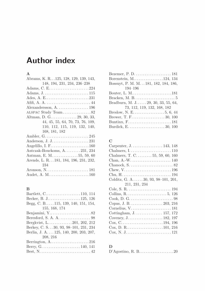
Author index
AAbrams, K. R.. .125, 128, 129, 139, 143,
148, 194, 231, 234, 236–238Adams, C. E. . . . . . . . . . . . . . . . . . . . . . . 224Adams, J. . . . . . . . . . . . . . . . . . . . . . . . . . 115Ades, A. E. . . . . . . . . . . . . . . . . . . . . . . . . 231Afifi, A. A. . . . . . . . . . . . . . . . . . . . . . . . . . 44Alexandersson, A. . . . . . . . . . . . . . . . . . 196ALSPAC Study Team . . . . . . . . . . . . . . . . 82Altman, D. G. . . . . . . . . . . . . . . 29, 30, 33,
44, 45, 55, 64, 70, 73, 76, 109,110, 112, 115, 119, 132, 140,168, 181, 182
Ambler, G. . . . . . . . . . . . . . . . . . . . . . . . . 245Anderson, J. J. . . . . . . . . . . . . . . . . . . . . 231Angelillo, I. F. . . . . . . . . . . . . . . . . . . . . . 160Antczak-Bouckoms, A. . . . . . . . . 231, 234Antman, E. M. . . . . . . . . . . . . . . 55, 59, 60Arends, L. R. . . 181, 184, 196, 231, 232,
234Aronson, N. . . . . . . . . . . . . . . . . . . . . . . . 181Audet, A. M. . . . . . . . . . . . . . . . . . . . . . . 160
BBartlett, C. . . . . . . . . . . . . . . . . . . . 110, 114Becker, B. J. . . . . . . . . . . . . . . . . . .125, 126Begg, C. B. . . . . 115, 139, 140, 151, 154,
155, 168, 174Benjamini, Y.. . . . . . . . . . . . . . . . . . . . . . .82Beresford, S. A. A. . . . . . . . . . . . . . . . . . 98Bergkvist, L. . . . . . . . . . . . . . 201, 202, 212Berkey, C. S. . . 30, 93, 98–101, 231, 234Berlin, J. A. . . . 125, 140, 200, 203, 207,
208, 216Berrington, A. . . . . . . . . . . . . . . . . . . . . . 216Berry, G. . . . . . . . . . . . . . . . . . . . . . 140, 141Best, N. . . . . . . . . . . . . . . . . . . . . . . . . . . . . 42
Bezemer, P. D. . . . . . . . . . . . . . . . . . . . . 181Borenstein, M. . . . . . . . . . . . . . . . . 124, 134Bossuyt, P. M. M. . . 181, 182, 184, 186,
194–196Bouter, L. M.. . . . . . . . . . . . . . . . . . . . . .181Bracken, M. B. . . . . . . . . . . . . . . . . . . . . . . 5Bradburn, M. J. . . . . . 29, 30, 33, 55, 64,
73, 112, 119, 132, 168, 182Breslow, N. E. . . . . . . . . . . . . . . . . . 5, 6, 44Brewer, T. F. . . . . . . . . . . . . . . . . . . 30, 100Buntinx, F. . . . . . . . . . . . . . . . . . . . . . . . . 181Burdick, E. . . . . . . . . . . . . . . . . . . . . 30, 100
CCarpenter, J. . . . . . . . . . . . . . . . . . 143, 148Chalmers, I. . . . . . . . . . . . . . . . . . . . . . . . 110Chalmers, T. C. . . . . . . . . 55, 59, 60, 160Chan, A.-W. . . . . . . . . . . . . . . . . . . . . . . 140Chanock, S. . . . . . . . . . . . . . . . . . . . . . . . . 82Chew, V. . . . . . . . . . . . . . . . . . . . . . . . . . . 196Chu, H. . . . . . . . . . . . . . . . . . . . . . . . . . . . 194Colditz, G. A. . . . . . 30, 93, 98–101, 201,
211, 231, 234Cole, S. R. . . . . . . . . . . . . . . . . . . . . . . . . 194Collins, R. . . . . . . . . . . . . . . . . . . . . . . 5, 126Cook, D. G. . . . . . . . . . . . . . . . . . . . . . . . . 98Copas, J. B. . . . . . . . . . . . . . . . . . . 203, 216Cornelius, V. . . . . . . . . . . . . . . . . . . . . . . 181Cottingham, J. . . . . . . . . . . . . . . . 157, 172Coveney, J. . . . . . . . . . . . . . . . . . . . 182, 197Cox, C. . . . . . . . . . . . . . . . . . . . . . . . 194, 196Cox, D. R. . . . . . . . . . . . . . . . . . . . .101, 216Cox, N. J. . . . . . . . . . . . . . . . . . . . . . . . . . 121
DD’Agostino, R. B.. . . . . . . . . . . . . . . . . . .20
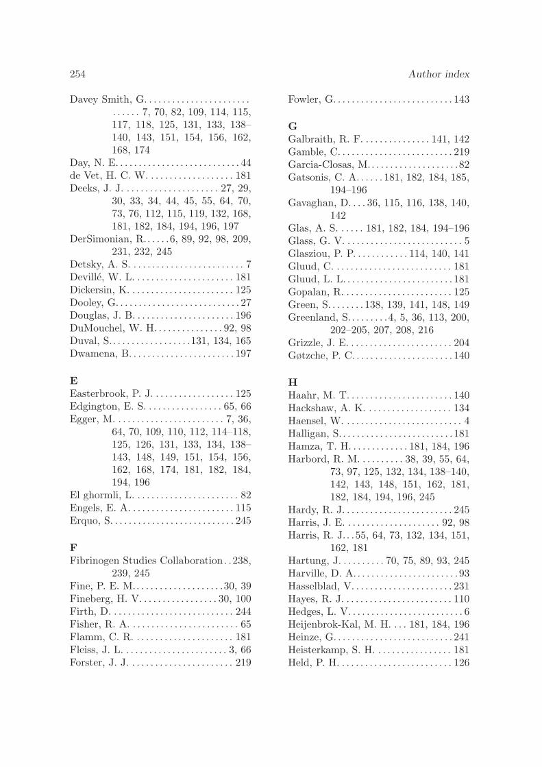
254 Author index
Davey Smith, G. . . . . . . . . . . . . . . . . . . . . . .. . . . . . 7, 70, 82, 109, 114, 115,117, 118, 125, 131, 133, 138–140, 143, 151, 154, 156, 162,168, 174
Day, N. E. . . . . . . . . . . . . . . . . . . . . . . . . . . 44de Vet, H. C. W. . . . . . . . . . . . . . . . . . . 181Deeks, J. J. . . . . . . . . . . . . . . . . . . . . 27, 29,
30, 33, 34, 44, 45, 55, 64, 70,73, 76, 112, 115, 119, 132, 168,181, 182, 184, 194, 196, 197
DerSimonian, R.. . . . .6, 89, 92, 98, 209,231, 232, 245
Detsky, A. S. . . . . . . . . . . . . . . . . . . . . . . . . 7Deville, W. L. . . . . . . . . . . . . . . . . . . . . . 181Dickersin, K. . . . . . . . . . . . . . . . . . . . . . . 125Dooley, G. . . . . . . . . . . . . . . . . . . . . . . . . . . 27Douglas, J. B. . . . . . . . . . . . . . . . . . . . . . 196DuMouchel, W. H. . . . . . . . . . . . . . . 92, 98Duval, S.. . . . . . . . . . . . . . . . .131, 134, 165Dwamena, B. . . . . . . . . . . . . . . . . . . . . . . 197
EEasterbrook, P. J. . . . . . . . . . . . . . . . . . 125Edgington, E. S. . . . . . . . . . . . . . . . . 65, 66Egger, M. . . . . . . . . . . . . . . . . . . . . . . . 7, 36,
64, 70, 109, 110, 112, 114–118,125, 126, 131, 133, 134, 138–143, 148, 149, 151, 154, 156,162, 168, 174, 181, 182, 184,194, 196
El ghormli, L. . . . . . . . . . . . . . . . . . . . . . . 82Engels, E. A. . . . . . . . . . . . . . . . . . . . . . . 115Erquo, S. . . . . . . . . . . . . . . . . . . . . . . . . . . 245
FFibrinogen Studies Collaboration. .238,
239, 245Fine, P. E. M.. . . . . . . . . . . . . . . . . . .30, 39Fineberg, H. V. . . . . . . . . . . . . . . . . 30, 100Firth, D. . . . . . . . . . . . . . . . . . . . . . . . . . . 244Fisher, R. A. . . . . . . . . . . . . . . . . . . . . . . . 65Flamm, C. R. . . . . . . . . . . . . . . . . . . . . . 181Fleiss, J. L. . . . . . . . . . . . . . . . . . . . . . . 3, 66Forster, J. J. . . . . . . . . . . . . . . . . . . . . . . 219
Fowler, G. . . . . . . . . . . . . . . . . . . . . . . . . . 143
GGalbraith, R. F. . . . . . . . . . . . . . . 141, 142Gamble, C. . . . . . . . . . . . . . . . . . . . . . . . . 219Garcia-Closas, M.. . . . . . . . . . . . . . . . . . .82Gatsonis, C. A. . . . . . 181, 182, 184, 185,
194–196Gavaghan, D. . . . 36, 115, 116, 138, 140,
142Glas, A. S. . . . . . 181, 182, 184, 194–196Glass, G. V. . . . . . . . . . . . . . . . . . . . . . . . . . 5Glasziou, P. P. . . . . . . . . . . . 114, 140, 141Gluud, C. . . . . . . . . . . . . . . . . . . . . . . . . . 181Gluud, L. L. . . . . . . . . . . . . . . . . . . . . . . . 181Gopalan, R. . . . . . . . . . . . . . . . . . . . . . . . 125Green, S. . . . . . . . 138, 139, 141, 148, 149Greenland, S.. . . . . . . .4, 5, 36, 113, 200,
202–205, 207, 208, 216Grizzle, J. E. . . . . . . . . . . . . . . . . . . . . . . 204Gøtzche, P. C. . . . . . . . . . . . . . . . . . . . . . 140
HHaahr, M. T. . . . . . . . . . . . . . . . . . . . . . . 140Hackshaw, A. K. . . . . . . . . . . . . . . . . . . 134Haensel, W. . . . . . . . . . . . . . . . . . . . . . . . . . 4Halligan, S. . . . . . . . . . . . . . . . . . . . . . . . . 181Hamza, T. H. . . . . . . . . . . . . 181, 184, 196Harbord, R. M. . . . . . . . . . 38, 39, 55, 64,
73, 97, 125, 132, 134, 138–140,142, 143, 148, 151, 162, 181,182, 184, 194, 196, 245
Hardy, R. J. . . . . . . . . . . . . . . . . . . . . . . . 245Harris, J. E. . . . . . . . . . . . . . . . . . . . . 92, 98Harris, R. J. . .55, 64, 73, 132, 134, 151,
162, 181Hartung, J. . . . . . . . . . 70, 75, 89, 93, 245Harville, D. A. . . . . . . . . . . . . . . . . . . . . . . 93Hasselblad, V. . . . . . . . . . . . . . . . . . . . . . 231Hayes, R. J. . . . . . . . . . . . . . . . . . . . . . . . 110Hedges, L. V. . . . . . . . . . . . . . . . . . . . . . . . . 6Heijenbrok-Kal, M. H. . . . 181, 184, 196Heinze, G. . . . . . . . . . . . . . . . . . . . . . . . . . 241Heisterkamp, S. H. . . . . . . . . . . . . . . . . 181Held, P. H. . . . . . . . . . . . . . . . . . . . . . . . . 126
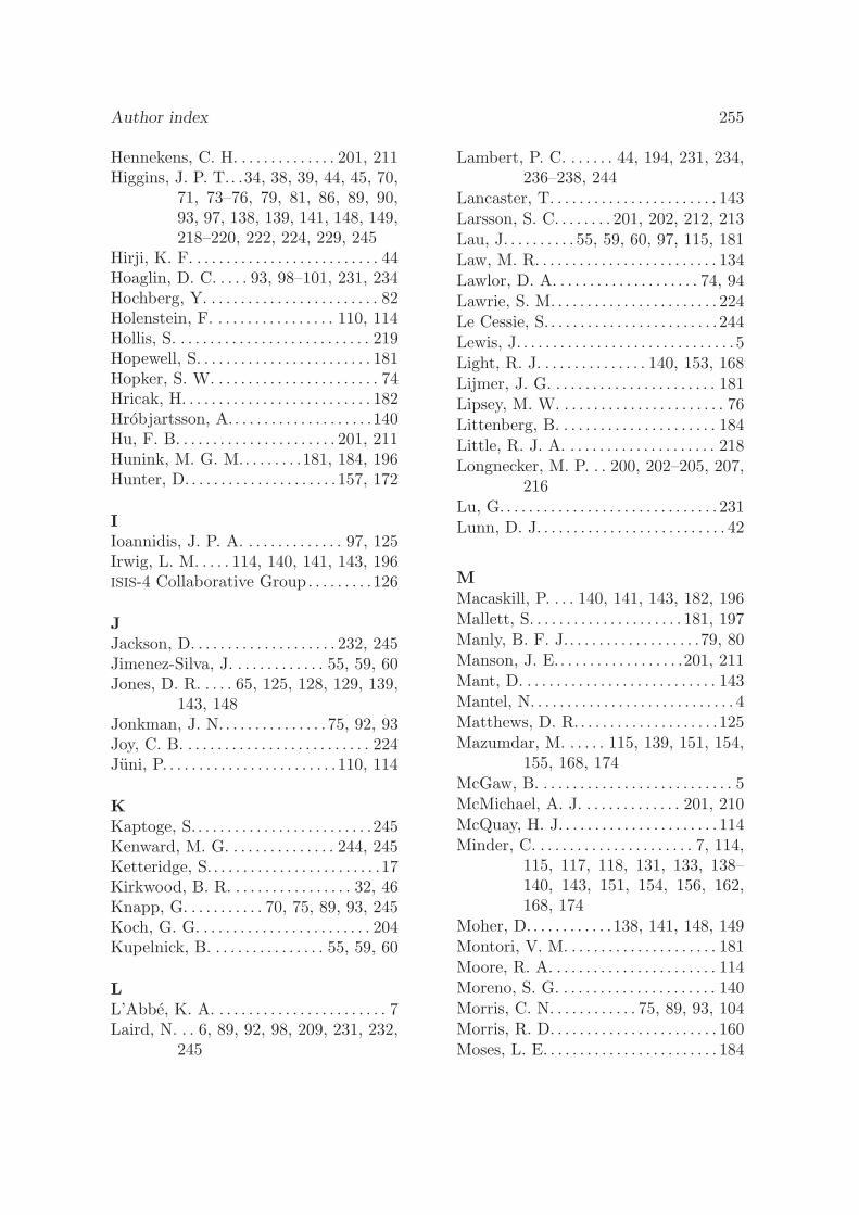
Author index 255
Hennekens, C. H. . . . . . . . . . . . . . 201, 211Higgins, J. P. T.. .34, 38, 39, 44, 45, 70,
71, 73–76, 79, 81, 86, 89, 90,93, 97, 138, 139, 141, 148, 149,218–220, 222, 224, 229, 245
Hirji, K. F. . . . . . . . . . . . . . . . . . . . . . . . . . 44Hoaglin, D. C. . . . . 93, 98–101, 231, 234Hochberg, Y. . . . . . . . . . . . . . . . . . . . . . . . 82Holenstein, F. . . . . . . . . . . . . . . . . 110, 114Hollis, S. . . . . . . . . . . . . . . . . . . . . . . . . . . 219Hopewell, S. . . . . . . . . . . . . . . . . . . . . . . . 181Hopker, S. W. . . . . . . . . . . . . . . . . . . . . . . 74Hricak, H. . . . . . . . . . . . . . . . . . . . . . . . . . 182Hrobjartsson, A.. . . . . . . . . . . . . . . . . . .140Hu, F. B. . . . . . . . . . . . . . . . . . . . . . 201, 211Hunink, M. G. M.. . . . . . . .181, 184, 196Hunter, D. . . . . . . . . . . . . . . . . . . . . 157, 172
IIoannidis, J. P. A. . . . . . . . . . . . . . 97, 125Irwig, L. M. . . . . 114, 140, 141, 143, 196ISIS-4 Collaborative Group. . . . . . . . .126
JJackson, D. . . . . . . . . . . . . . . . . . . . 232, 245Jimenez-Silva, J. . . . . . . . . . . . . 55, 59, 60Jones, D. R. . . . . 65, 125, 128, 129, 139,
143, 148Jonkman, J. N. . . . . . . . . . . . . . . 75, 92, 93Joy, C. B. . . . . . . . . . . . . . . . . . . . . . . . . . 224Juni, P. . . . . . . . . . . . . . . . . . . . . . . . 110, 114
KKaptoge, S. . . . . . . . . . . . . . . . . . . . . . . . .245Kenward, M. G. . . . . . . . . . . . . . . 244, 245Ketteridge, S. . . . . . . . . . . . . . . . . . . . . . . .17Kirkwood, B. R. . . . . . . . . . . . . . . . . 32, 46Knapp, G. . . . . . . . . . . 70, 75, 89, 93, 245Koch, G. G. . . . . . . . . . . . . . . . . . . . . . . . 204Kupelnick, B. . . . . . . . . . . . . . . . 55, 59, 60
LL’Abbe, K. A. . . . . . . . . . . . . . . . . . . . . . . . 7Laird, N. . . 6, 89, 92, 98, 209, 231, 232,
245
Lambert, P. C. . . . . . . 44, 194, 231, 234,236–238, 244
Lancaster, T. . . . . . . . . . . . . . . . . . . . . . . 143Larsson, S. C. . . . . . . . 201, 202, 212, 213Lau, J. . . . . . . . . . 55, 59, 60, 97, 115, 181Law, M. R. . . . . . . . . . . . . . . . . . . . . . . . . 134Lawlor, D. A. . . . . . . . . . . . . . . . . . . . 74, 94Lawrie, S. M. . . . . . . . . . . . . . . . . . . . . . . 224Le Cessie, S. . . . . . . . . . . . . . . . . . . . . . . . 244Lewis, J. . . . . . . . . . . . . . . . . . . . . . . . . . . . . . 5Light, R. J. . . . . . . . . . . . . . . 140, 153, 168Lijmer, J. G. . . . . . . . . . . . . . . . . . . . . . . 181Lipsey, M. W. . . . . . . . . . . . . . . . . . . . . . . 76Littenberg, B. . . . . . . . . . . . . . . . . . . . . . 184Little, R. J. A. . . . . . . . . . . . . . . . . . . . . 218Longnecker, M. P. . . 200, 202–205, 207,
216Lu, G. . . . . . . . . . . . . . . . . . . . . . . . . . . . . . 231Lunn, D. J. . . . . . . . . . . . . . . . . . . . . . . . . . 42
MMacaskill, P. . . . 140, 141, 143, 182, 196Mallett, S. . . . . . . . . . . . . . . . . . . . . 181, 197Manly, B. F. J.. . . . . . . . . . . . . . . . . .79, 80Manson, J. E.. . . . . . . . . . . . . . . . .201, 211Mant, D. . . . . . . . . . . . . . . . . . . . . . . . . . . 143Mantel, N. . . . . . . . . . . . . . . . . . . . . . . . . . . . 4Matthews, D. R. . . . . . . . . . . . . . . . . . . .125Mazumdar, M. . . . . . 115, 139, 151, 154,
155, 168, 174McGaw, B. . . . . . . . . . . . . . . . . . . . . . . . . . . 5McMichael, A. J. . . . . . . . . . . . . . 201, 210McQuay, H. J. . . . . . . . . . . . . . . . . . . . . . 114Minder, C. . . . . . . . . . . . . . . . . . . . . . 7, 114,
115, 117, 118, 131, 133, 138–140, 143, 151, 154, 156, 162,168, 174
Moher, D. . . . . . . . . . . . 138, 141, 148, 149Montori, V. M. . . . . . . . . . . . . . . . . . . . . 181Moore, R. A. . . . . . . . . . . . . . . . . . . . . . . 114Moreno, S. G. . . . . . . . . . . . . . . . . . . . . . 140Morris, C. N. . . . . . . . . . . . 75, 89, 93, 104Morris, R. D. . . . . . . . . . . . . . . . . . . . . . . 160Moses, L. E. . . . . . . . . . . . . . . . . . . . . . . . 184
256 Author index
Mosteller, F. . . . . . . . . 30, 55, 59, 60, 93,98–101, 160, 231, 234
NNewson, R. . . . . . . . . . . . . . . . . . . . . . . . . . 82Nordic Cochrane Centre . . . . . . . . . . . 186Norman, S. L. T. . . . . . . . . . . . . . . . . . . 231
OO’Brien, B. . . . . . . . . . . . . . . . . . . . 231, 234O’Rourke, K. . . . . . . . . . . . . . . . . . . . . . . . . 7Olkin, I. . . . . . . . . . . . . . . . . . . . . . . . . 6, 115Orsini, N. . . . . . . . . . . . . . . . . . . . . . . . . . 213
PPaliwal, P. . . . . . . . . . . . . . . . . . . . . . . . . .181Palmer, T. M. . . . . . . . . . . . . . . . . . . . . . 140Peters, J. L. . . . 125, 128, 129, 139, 140,
143, 148Peto, R. . . . . . . . . . . . . . . . . . . . . . . . . 5, 126Phillips, A. N. . . . . . . . . . . . . . . . . . . . . . . 70Pickles, A. . . . . . . . . . . . . . . . 191, 192, 197Pillemer, D. B. . . . . . . . . . . .140, 153, 168Pinto, E. . . . . . . . . . . . . . . . . . . . . . 231, 234Pocock, S. J. . . . . . . . . . . . . . . . . . . . . . . . 98Poole, C. . . . . . . . . . . . . . . . . . . . . . . 36, 113
RRabe-Hesketh, S. . . . . . . . . . 189–192, 197Reis, I. M. . . . . . . . . . . . . . . . . . . . . . . . . . . 44Reitsma, J. B. . . 181, 182, 184, 194–196Reynolds, D. J. M. . . . . . . . . . . . . . . . . 114Riley, R. D.. . . . .194, 231, 234, 236–238Robins, J. . . . . . . . . . . . . . . . . . . . . . . . . . 4, 5Roger, J. H. . . . . . . . . . . . . . . . . . . 244, 245Rohan, T. E. . . . . . . . . . . . . . . . . . 201, 210Rosenthal, R. . . . . . . . . . . . . . . . . . . . . 6, 65Rothman, N. . . . . . . . . . . . . . . . . . . . . . . . 82Rothstein, H. R. . . . . . . . . . . . . . . 124, 134Royston, P. . . . . . . . . . . . . . . . . . . . . 27, 245Rubenstein, L. Z. . . . . . . . . . . . . . . . . . . 115Rubin, D. B.. . . . . . . . . . . . . . . . . .218, 219Rushton, L. . . . .125, 128, 129, 139, 143,
148Rutjes, A. W. S. . . . . . . . . 181, 182, 184,
194–196
Rutter, C. M. . . . . . . 181, 182, 184, 185,194–196
Rucker, G. . . . . . . . . . . . . . . . . . . . . 143, 148
SSalvan, A. . . . . . . . . . . . . . . . . . . . . . . . . . . . 5Samson, D. J. . . . . . . . . . . . . . . . . . . . . . 181SAS Institute . . . . . . . . . . . . . . . . . . . . . . 237Scheidler, J. . . . . . . . . . . . . . . . . . . . . . . . 182Schemper, M.. . . . . . . . . . . . . . . . . . . . . .241Schmid, C. H. . . . . . . . . . . . . . 97, 115, 181Schneider, M. . . . . 7, 114, 115, 117, 118,
131, 133, 151, 154, 156, 162,168, 174
Scholten, R. J. P. M. . . . . 181, 182, 184,194–196
Schulz, K. F. . . . . . . . . . . . . . . . . . . . . . . 110Schwarzer, G. . . . . . . . . . . . . . . . . . 143, 148Segal, M. R. . . . . . . . . . . . . . . . . . . . . . . . 182Shaffer, J. P.. . . . . . . . . . . . . . . . . . . . . . . .82Shapiro, D. . . . . . . . . . . . . . . . . . . . . . . . . 184Sharp, S. J. . . 35, 64, 67, 70, 73–75, 87,
92–94, 101, 104, 116, 171, 176,232, 245
Shi, J. Q. . . . . . . . . . . . . . . . . . . . . . 203, 216Sidik, K. . . . . . . . . . . . . . . . . . . . . 75, 92, 93Siegmund, D. . . . . . . . . . . . . . . . . . . . . . . . 82Silagy, C. . . . . . . . . . . . . . . . . . . . . . . 17, 143Simes, R. J. . . . . . . . . . . . . . . . . . . . . . . . 110Sinclair, J. C. . . . . . . . . . . . . . . . . . . . . . . . . 5Siu, A. L.. . . . . . . . . . . . . . . . . . . . . . . . . .115Skrondal, A. . . . . . . . . . . . . . 189–192, 197Sleight, P. . . . . . . . . . . . . . . . . . . . . . . . . . . . 5Smith, M. L. . . . . . . . . . . . . . . . . . . . . . . . . .5Smith, P. W. F. . . . . . . . . . . . . . . . . . . . 219Snell, E. J. . . . . . . . . . . . . . . . . . . . . . . . . 101Speizer, F. E. . . . . . . . . . . . . . . . . . 201, 211Spiegelhalter, D. J. . . . . . . . . . . . . . .42, 86Stampfer, M. J. . . . . . . . . . . . . . . . 201, 211Starmer, C. F. . . . . . . . . . . . . . . . . . . . . . 204Stead, L. . . . . . . . . . . . . . . . . . . . . . . . . . . 143Steichen, T. J. . . 20, 112, 115, 121, 138,
149, 162, 168, 181Stern, J. M. . . . . . . . . . . . . . . . . . . . . . . . 110
Author index 257
Sterne, J. A. C. . . . . . . . . . . . . . . . . . . . . . . .. . . . . 35, 36, 46, 55, 64, 67, 70,73, 82, 101, 105, 110, 112, 114–116, 125, 126, 132, 134, 138–143, 148, 149, 151, 162, 168,171, 176, 181, 182, 184, 194,196
Stijnen, T. . . . . . 181, 184, 196, 231, 232,234
Storey, J. D. . . . . . . . . . . . . . . . . . . . . . . . . 82Stuck, A. E. . . . . . . . . . . . . . . . . . . . . . . . 115Su, L. . . . . . . . . . . . . . . . . . . . . . . . . . . . . . 245Subak, L. . . . . . . . . . . . . . . . . . . . . . . . . . . 182Sutton, A. J. . . . . . 44, 93, 124, 125, 128,
129, 134, 139, 140, 143, 148,194, 231, 234, 236–238, 244
Sweeting, M. J. . . . . . . . . . . . . . . . . 44, 244
TTatsioni, A. . . . . . . . . . . . . . . . . . . . . . . . 181Taylor, J. E. . . . . . . . . . . . . . . . . . . . . . . . . 82Teo, K. K. . . . . . . . . . . . . . . . . . . . . . . . . . 126Terrin, N. . . . . . . . . . . . . . . . . . . . . . . . . . 115Thomas, A. . . . . . . . . . . . . . . . . . . . . . . . . . 42Thompson, J. R. . . . . . . . . 194, 231, 234,
236–238Thompson, S. G. . . . . . . . . . . . . . . . . . . . 34,
38, 42, 44, 45, 70, 71, 73–76,79, 81, 86, 89, 90, 92–94, 101,104, 105, 116, 231, 232, 245
Tramer, M. R. . . . . . . . . . . . . . . . . . . . . . 114Tweedie, R. . . . . . . . . . . . . . . 131, 134, 165
Vvan der Windt, D. A. W. M.. . . . . . .181van Houwelingen, H. C. . . 231, 232, 234van Houwelingen, J. C. . . 181, 184, 196,
244Verweij, P. J. M. . . . . . . . . . . . . . . . . . . 244
WWacholder, S. . . . . . . . . . . . . . . . . . . . . . . .82Wald, N. J. . . . . . . . . . . . . . . . . . . . . . . . . 134Walter, S. D.. . . . . . . . . . . . .143, 184, 196Warn, D. E. . . . . . . . . . . . . . . . . . . . . . . . . 42
Weintraub, M. . . . . . . . . . . . . . . . . . . . . . . 20Westfall, P. H. . . . . . . . . . . . . . . . . . . 80, 82White, I. R. . . . .105, 218–220, 222, 224,
229, 232Whitehead, A. . . . . . . . . . . . . . . . . . . . . . 142Whitehead, J. . . . . . . . . . . . . . . . . . . . . . 142Whiting, P.. . . . .181, 182, 184, 194, 196Wieland, G. D. . . . . . . . . . . . . . . . . . . . . 115Willan, A. . . . . . . . . . . . . . . . . . . . . 231, 234Willett, W. C. . . . . . . . . . . . . . . . . 201, 211Wilson, D. B. . . . . . . . . . . . . . . . . . . . . . . . 76Wilson, M. E. . . . . . . . . . . . . . . . . . .30, 100Wolk, A. . . . . . . . . . . . . 201, 202, 211–213Wood, A. M. . . . 218–220, 222, 224, 229Woolf, B. . . . . . . . . . . . . . . . . . . . . . . . . . . 141
YYoung, S. S. . . . . . . . . . . . . . . . . . . . . 80, 82Yu, K. K.. . . . . . . . . . . . . . . . . . . . . . . . . .182Yusuf, S. . . . . . . . . . . . . . . . . . . . . . . . . 5, 126
ZZarin, D. A. . . . . . . . . . . . . . . . . . . . . . . . 181Zwinderman, A. H. . . . . . . 181, 182, 184,
186, 194–196
Command index
Cconfunnel command. . . . . . . . . .124–137
Ffunnel command . . . . . . . . . . . . . . . 15, 20
Gglst command. . . . . . . . . . . . . . . .200–217
Llabbe command . . . . . . . . . . . . . 16–17, 20
Mmeta command. . . . . . . . . . . . . . . .101–102meta lr command . . . . . . . . . . . . . . . . . 250metabias command . . . . . . . . . . . 138–164metacum command . . . . . . . . . . . . . . 55–64metafunnel command . . . . . . . . 109–123,
126–127, 145metamiss command . . . . . . . . . . . 218–230metan command. . . . . . . . .3–54, 61, 120,
144–145metandi command . . . . . . . . . . . . 181–199
predict after . . . . . . . .188–191, 193metandiplot command. . . . . . .186–188,
192–193metaninf command . . . . . . . . . . . . . . . 250metannt command . . . . . . . . . . . . 249–250metap command. . . . . . . . . . . . . . . . .65–68metaparm command . . . . . . . . . . . 250–251metareg command . . . . . . . . . . . . . 70–106metatrim command . . . . . . . . . . . 165–177midas command . . . . . . . . . . . . . . . . . . . 250mvmeta command . . . . . . . . . . . . . 231–247mvmeta make command . . . 235–236, 239
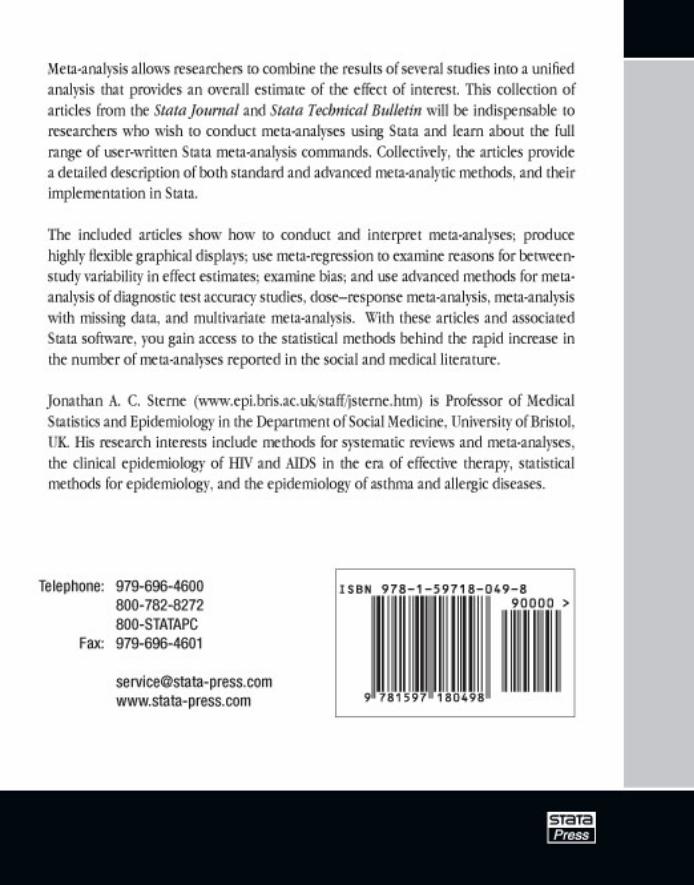
Related Documents