STAT6101 CHEATSHEET SAMPLE STATISTICS Sample Population Size n N Mean Standard Deviation Variance Proportion p Skewness : Positively skewed: mean > median Negatively skewed: mean < median FIVE FIGURE SUMMARY: Min, Q1, Median (Q2), Q3, Max The median may be a better indicator of the most typical value if a set of scores has an outlier. An outlier is an extreme value that differs greatly from other values. However, when the sample size is large and does not include outliers, the mean score usually provides a better measure of central tendency. Normal Distribution: Mean and SD Skewed Distribution: Median and IQR

Welcome message from author
This document is posted to help you gain knowledge. Please leave a comment to let me know what you think about it! Share it to your friends and learn new things together.
Transcript
STAT6101 CHEATSHEET
SAMPLE STATISTICS
Sample Population
Size n N
Mean
Standard Deviation
Variance
Proportion p
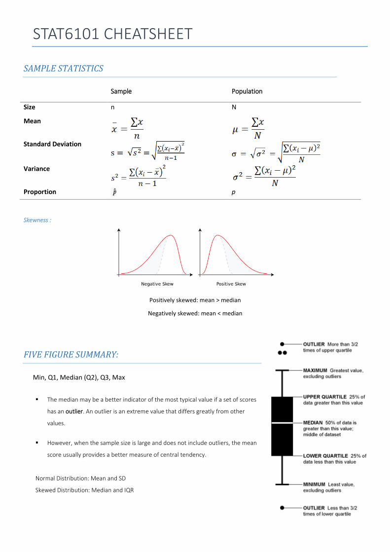
Skewness :
Positively skewed: mean > median
Negatively skewed: mean < median
FIVE FIGURE SUMMARY:
Min, Q1, Median (Q2), Q3, Max
The median may be a better indicator of the most typical value if a set of scores
has an outlier. An outlier is an extreme value that differs greatly from other
values.
However, when the sample size is large and does not include outliers, the mean
score usually provides a better measure of central tendency.
Normal Distribution: Mean and SD
Skewed Distribution: Median and IQR
BIVARIATE DATA
Bivariate data. When we conduct a study that examines the relationship between two variables, we are
working with bivariate data. Suppose we conducted a study to see if there were a relationship between the
height and weight of high school students. Since we are working with two variables (height and weight), we
would be working with bivariate data.
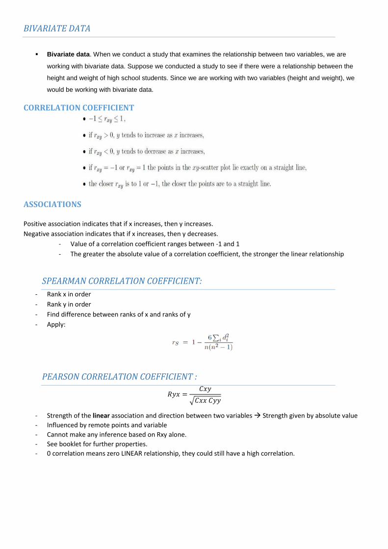
CORRELATION COEFFICIENT
ASSOCIATIONS
Positive association indicates that if x increases, then y increases.
Negative association indicates that if x increases, then y decreases.
- Value of a correlation coefficient ranges between -1 and 1
- The greater the absolute value of a correlation coefficient, the stronger the linear relationship
SPEARMAN CORRELATION COEFFICIENT:
- Rank x in order
- Rank y in order
- Find difference between ranks of x and ranks of y
- Apply:
PEARSON CORRELATION COEFFICIENT :
𝑅𝑦𝑥 =𝐶𝑥𝑦
√𝐶𝑥𝑥 𝐶𝑦𝑦
- Strength of the linear association and direction between two variables Strength given by absolute value
- Influenced by remote points and variable
- Cannot make any inference based on Rxy alone.
- See booklet for further properties.
- 0 correlation means zero LINEAR relationship, they could still have a high correlation.
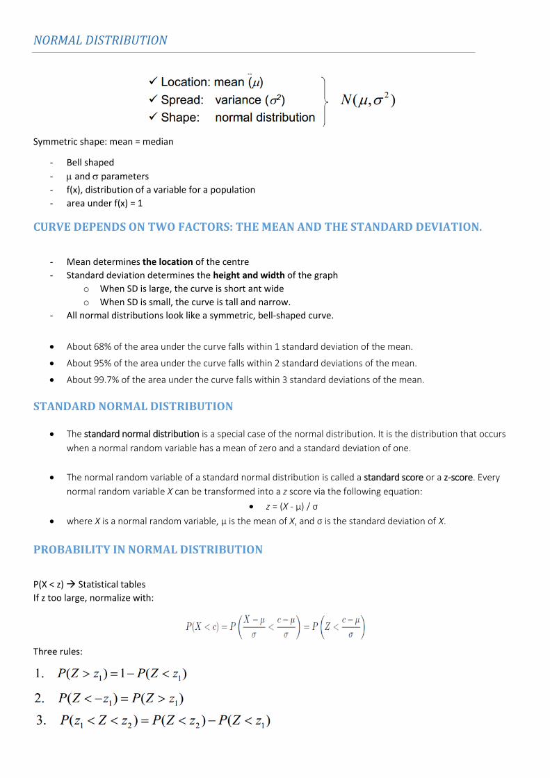
NORMAL DISTRIBUTION
Symmetric shape: mean = median
- Bell shaped
- and parameters
- f(x), distribution of a variable for a population
- area under f(x) = 1
CURVE DEPENDS ON TWO FACTORS: THE MEAN AND THE STANDARD DEVIATION.
- Mean determines the location of the centre
- Standard deviation determines the height and width of the graph
o When SD is large, the curve is short ant wide
o When SD is small, the curve is tall and narrow.
- All normal distributions look like a symmetric, bell-shaped curve.
About 68% of the area under the curve falls within 1 standard deviation of the mean.
About 95% of the area under the curve falls within 2 standard deviations of the mean.
About 99.7% of the area under the curve falls within 3 standard deviations of the mean.
STANDARD NORMAL DISTRIBUTION
The standard normal distribution is a special case of the normal distribution. It is the distribution that occurs
when a normal random variable has a mean of zero and a standard deviation of one.
STANDARD SCORE (AKA, Z SCORE)
The normal random variable of a standard normal distribution is called a standard score or a z-score. Every
normal random variable X can be transformed into a z score via the following equation:
z = (X - μ) / σ
where X is a normal random variable, μ is the mean of X, and σ is the standard deviation of X.
PROBABILITY IN NORMAL DISTRIBUTION
P(X < z) Statistical tables
If z too large, normalize with:
Three rules:
THE Z SCORE (STANDARD SCORE)
Indicates how many standard deviations an elements is from the mean.
When it is equal to 1 for example, it represents an element that is 1 standard deviation greater than the mean.
PERCENTAGE POINTS
Eg. span exceeded by only 5% men or eg. required delivery time to ensure 95% of packages are delivered before
guaranteed time.
P(X > K) = 0.05
P (X < k) = 0.95
𝑃 (𝑍 < 𝑘 − 𝜇
𝜎) = 0.95
Take average between two Z probabilities if Z-value is not precise
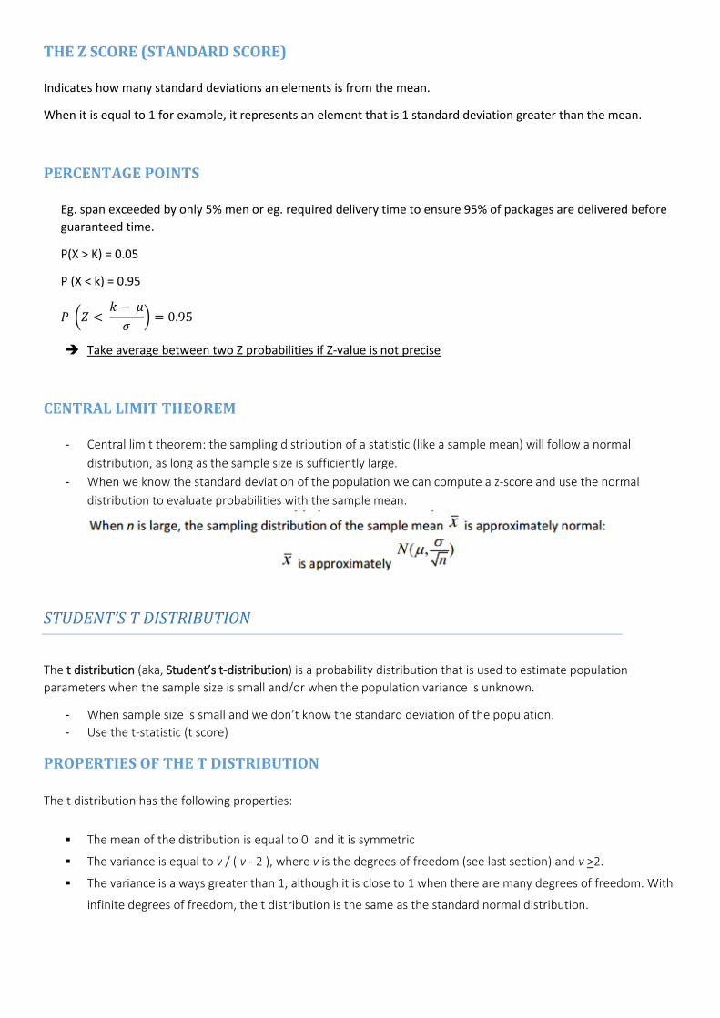
CENTRAL LIMIT THEOREM
- Central limit theorem: the sampling distribution of a statistic (like a sample mean) will follow a normal
distribution, as long as the sample size is sufficiently large.
- When we know the standard deviation of the population we can compute a z-score and use the normal
distribution to evaluate probabilities with the sample mean.
STUDENT’S T DISTRIBUTION
The t distribution (aka, Student’s t-distribution) is a probability distribution that is used to estimate population
parameters when the sample size is small and/or when the population variance is unknown.
- When sample size is small and we don’t know the standard deviation of the population.
- Use the t-statistic (t score)
PROPERTIES OF THE T DISTRIBUTION
The t distribution has the following properties:
The mean of the distribution is equal to 0 and it is symmetric
The variance is equal to v / ( v - 2 ), where v is the degrees of freedom (see last section) and v >2.
The variance is always greater than 1, although it is close to 1 when there are many degrees of freedom. With
infinite degrees of freedom, the t distribution is the same as the standard normal distribution.
WHEN TO USE THE T DISTRIBUTION
The t distribution can be used with any statistic having a bell-shaped distribution (i.e., approximately normal).
The central limit theorem states that the sampling distribution of a statistic will be normal or nearly normal, if any of
the following conditions apply.
The population distribution is normal.
The sampling distribution is symmetric, unimodal, without outliers, and the sample size is 15 or less.
The sampling distribution is moderately skewed, unimodal, without outliers, and the sample size is between
16 and 40.
The sample size is greater than 40, without outliers.
The t distribution should not be used with small samples from populations that are not approximately normal.
CHI SQUARE DISTRIBUTION
The chi-square distribution has the following properties:
The mean of the distribution is equal to the number of degrees of freedom: μ = v.
The variance is equal to two times the number of degrees of freedom: σ2 = 2 * v
When the degrees of freedom are greater than or equal to 2, the maximum value for Y occurs when Χ2 = v - 2.
As the degrees of freedom increase, the chi-square curve approaches a normal distribution.
The chi-square distribution is constructed so that the total area under the curve is equal to 1. The area under the
curve between 0 and a particular chi-square value is a cumulative probability associated with that chi-square value.
Cumulative probability: probability that the value of a random variable falls within a specified range
BINOMIAL DISTRIBUTION
Properties of Binomial:
The experiment consists of n repeated trials.
Each trial can result in just two possible outcomes. We call one of these outcomes a success and the other, a
failure.
The probability of success, denoted by P, is the same on every trial.
The trials are independent; that is, the outcome on one trial does not affect the outcome on other trials.
The number of success is a random variable that follows a Binomial distribution
Mean:
Variance:
Standard Deviation:
Probability: 𝑃 ( 𝑋 = 𝑟) = (𝑛𝑟
) 𝑝𝑟(1 − 𝑝)𝑛−𝑟
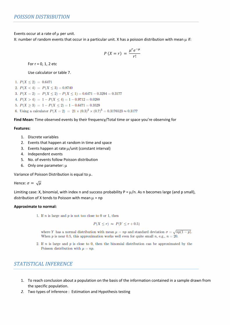
POISSON DISTRIBUTION
Events occur at a rate of per unit.
X: number of random events that occur in a particular unit. X has a poisson distribution with mean if:
𝑃 (𝑋 = 𝑟) = 𝜇𝑟𝑒−𝜇
𝑟!
For r = 0, 1, 2 etc
Use calculator or table 7.
Find Mean: Time observed events by their frequency/Total time or space you’re observing for
Features:
1. Discrete variables
2. Events that happen at random in time and space
3. Events happen at rate /unit (constant interval)
4. Independent events
5. No. of events follow Poisson distribution
6. Only one parameter:
Variance of Poisson Distribution is equal to .
Hence: 𝜎 = √𝜇
Limiting case: X, binomial, with index n and success probability P = /n. As n becomes large (and p small),
distribution of X tends to Poisson with mean = np
Approximate to normal:
STATISTICAL INFERENCE
1. To reach conclusion about a population on the basis of the information contained in a sample drawn from
the specific population.
2. Two types of inference : Estimation and Hypothesis testing
ESTIMATION AND SAMPLING DISTRIBUTION
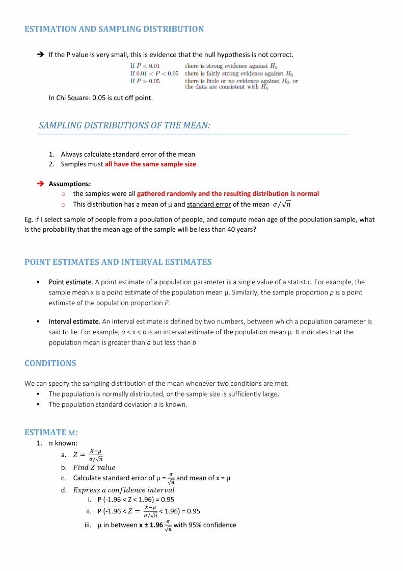
If the P value is very small, this is evidence that the null hypothesis is not correct.
In Chi Square: 0.05 is cut off point.
SAMPLING DISTRIBUTIONS OF THE MEAN:
1. Always calculate standard error of the mean
2. Samples must all have the same sample size
Assumptions:
o the samples were all gathered randomly and the resulting distribution is normal
o This distribution has a mean of µ and standard error of the mean 𝜎 √𝑛⁄
Eg. if I select sample of people from a population of people, and compute mean age of the population sample, what
is the probability that the mean age of the sample will be less than 40 years?
POINT ESTIMATES AND INTERVAL ESTIMATES
Point estimate. A point estimate of a population parameter is a single value of a statistic. For example, the
sample mean x is a point estimate of the population mean μ. Similarly, the sample proportion p is a point
estimate of the population proportion P.
Interval estimate. An interval estimate is defined by two numbers, between which a population parameter is
said to lie. For example, a < x < b is an interval estimate of the population mean μ. It indicates that the
population mean is greater than a but less than b
CONDITIONS
We can specify the sampling distribution of the mean whenever two conditions are met:
The population is normally distributed, or the sample size is sufficiently large.
The population standard deviation σ is known.
ESTIMATE : 1. known:
a. 𝑍 = 𝑋−𝜇
𝜎/√𝑛
b. 𝐹𝑖𝑛𝑑 𝑍 𝑣𝑎𝑙𝑢𝑒
c. Calculate standard error of µ = 𝝈
√𝒏 and mean of x = µ
d. 𝐸𝑥𝑝𝑟𝑒𝑠𝑠 𝑎 𝑐𝑜𝑛𝑓𝑖𝑑𝑒𝑛𝑐𝑒 𝑖𝑛𝑡𝑒𝑟𝑣𝑎𝑙
i. P (-1.96 < Z < 1.96) = 0.95
ii. P (-1.96 < 𝑍 = 𝑋−𝜇
𝜎/√𝑛 < 1.96) = 0.95
iii. µ in between x ± 1.96 𝝈
√𝒏 with 95% confidence
2. not known
a. T = 𝑋−𝜇
𝑠/√𝑛
b. Student t- distribution with degrees of freedom n - 1
c. Find t value
d. Calculate estimate standard error of µ = 𝒔
√𝒏
e. Find a 95% confidence interval
i. µ in between x ± Tn-1,0.025 𝒔
√𝒏 with 95% confidence
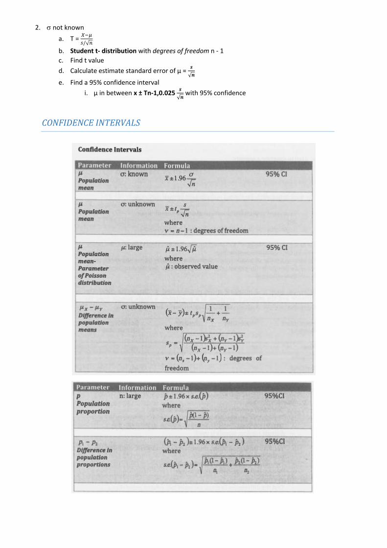
CONFIDENCE INTERVALS
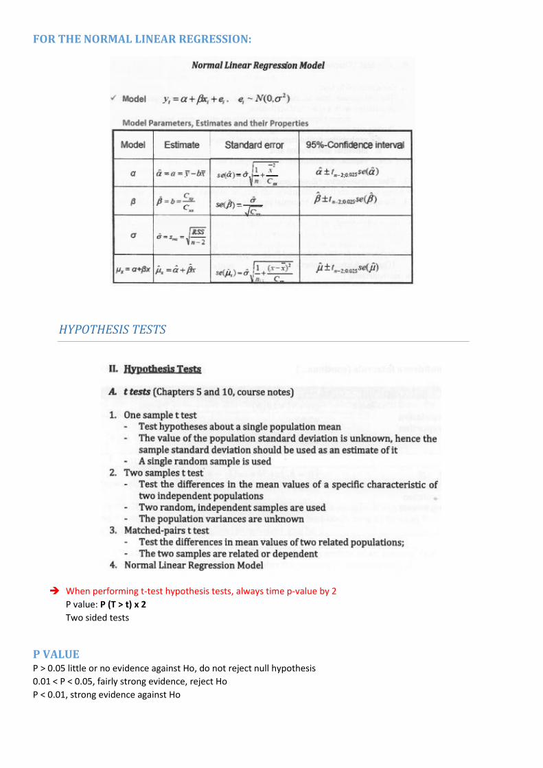
FOR THE NORMAL LINEAR REGRESSION:
HYPOTHESIS TESTS
When performing t-test hypothesis tests, always time p-value by 2
P value: P (T > t) x 2
Two sided tests
P VALUE P > 0.05 little or no evidence against Ho, do not reject null hypothesis
0.01 < P < 0.05, fairly strong evidence, reject Ho
P < 0.01, strong evidence against Ho
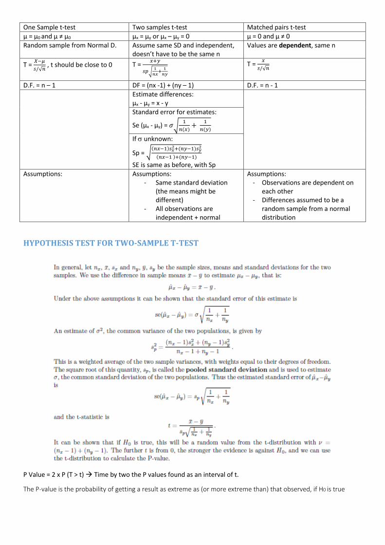
One Sample t-test Two samples t-test Matched pairs t-test
µ = µ0 and µ ≠ µ0 µx = µy or µx – µy = 0 µ = 0 and µ ≠ 0
Random sample from Normal D. Assume same SD and independent, doesn’t have to be the same n
Values are dependent, same n
T = 𝑋−𝜇
𝑠/√𝑛 , t should be close to 0
T = 𝑥+𝑦
𝑠𝑝√1
𝑛𝑥+
1
𝑛𝑦
T = 𝑥
𝑠/√𝑛
D.F. = n – 1 DF = (nx -1) + (ny – 1) D.F. = n - 1
Estimate differences: µx - µy = x - y
Standard error for estimates:
Se (µx - µy) = 𝜎√1
𝑛(𝑥)+
1
𝑛(𝑦)
If unknown:
Sp = √(𝑛𝑥−1)𝑠𝑥
2+(𝑛𝑦−1)𝑠𝑦2
(𝑛𝑥−1 )+(𝑛𝑦−1)
SE is same as before, with Sp
Assumptions: Assumptions: - Same standard deviation
(the means might be different)
- All observations are independent + normal
Assumptions: - Observations are dependent on
each other - Differences assumed to be a
random sample from a normal distribution
HYPOTHESIS TEST FOR TWO-SAMPLE T-TEST
P Value = 2 x P (T > t) Time by two the P values found as an interval of t.
The P-value is the probability of getting a result as extreme as (or more extreme than) that observed, if H0 is true
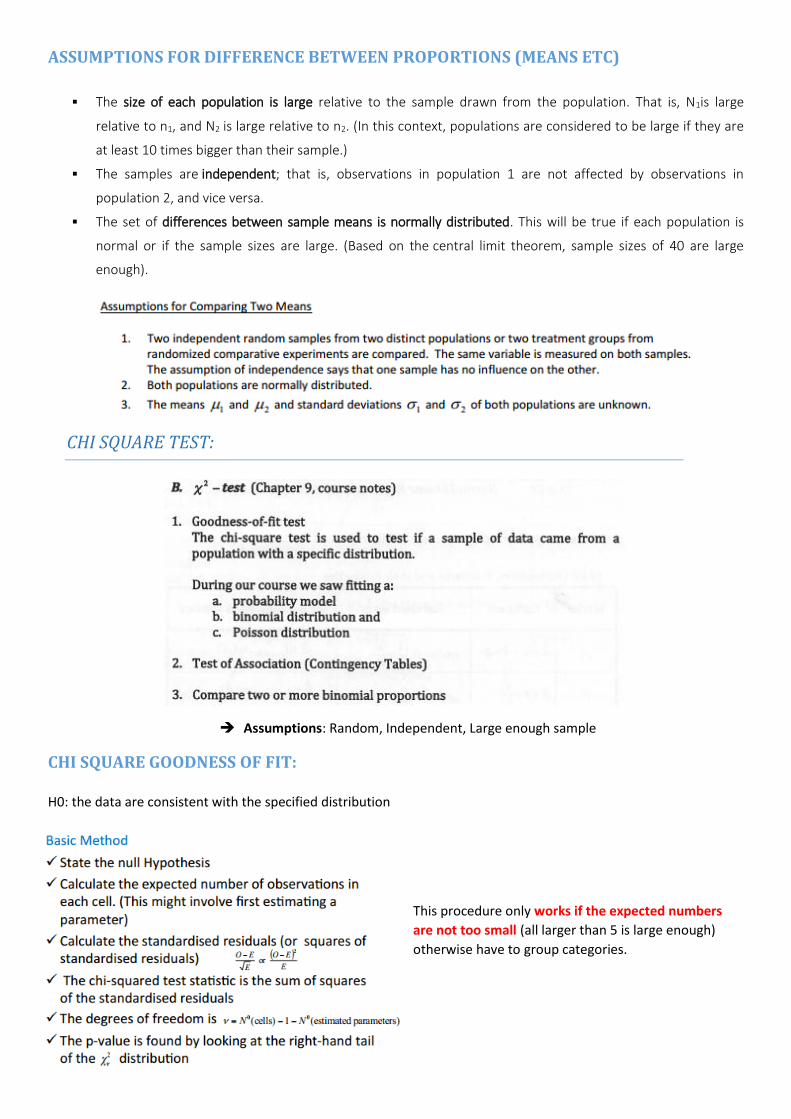
ASSUMPTIONS FOR DIFFERENCE BETWEEN PROPORTIONS (MEANS ETC)
The size of each population is large relative to the sample drawn from the population. That is, N1is large
relative to n1, and N2 is large relative to n2. (In this context, populations are considered to be large if they are
at least 10 times bigger than their sample.)
The samples are independent; that is, observations in population 1 are not affected by observations in
population 2, and vice versa.
The set of differences between sample means is normally distributed. This will be true if each population is
normal or if the sample sizes are large. (Based on the central limit theorem, sample sizes of 40 are large
enough).
CHI SQUARE TEST:
Assumptions: Random, Independent, Large enough sample
CHI SQUARE GOODNESS OF FIT:
H0: the data are consistent with the specified distribution
This procedure only works if the expected numbers
are not too small (all larger than 5 is large enough)
otherwise have to group categories.
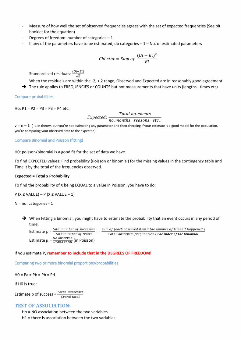
- Measure of how well the set of observed frequencies agrees with the set of expected frequencies (See bit
booklet for the equation)
- Degrees of freedom: number of categories – 1
- If any of the parameters have to be estimated, do categories – 1 – No. of estimated parameters
𝐶ℎ𝑖 𝑠𝑡𝑎𝑡 = 𝑆𝑢𝑚 𝑜𝑓 (𝑂𝑖 − 𝐸𝑖)2
𝐸𝑖
Standardised residuals: (𝑂𝑖−𝐸𝑖)
√𝐸
When the residuals are within the -2, + 2 range, Observed and Expected are in reasonably good agreement.
The rule applies to FREQUENCIES or COUNTS but not measurements that have units (lengths.. times etc)
Compare probabilities
Ho: P1 = P2 = P3 = P3 = P4 etc..
𝐸𝑥𝑝𝑒𝑐𝑡𝑒𝑑: 𝑇𝑜𝑡𝑎𝑙 𝑛𝑜. 𝑒𝑣𝑒𝑛𝑡𝑠
𝑛𝑜. 𝑚𝑜𝑛𝑡ℎ𝑠, 𝑠𝑒𝑎𝑠𝑜𝑛𝑠, 𝑒𝑡𝑐. .
v = n – 1 (- 1 in theory, but you’re not estimating any parameter and then checking if your estimate is a good model for the population,
you’re comparing your observed data to the expected)
Compare Binomial and Poisson (fitting)
H0: poisson/binomial is a good fit for the set of data we have.
To find EXPECTED values: Find probability (Poisson or binomial) for the missing values in the contingency table and
Time it by the total of the frequencies observed.
Expected = Total x Probability
To find the probability of X being EQUAL to a value in Poisson, you have to do:
P (X ≤ VALUE) – P (X ≤ VALUE – 1)
N = no. categories - 1
When Fitting a binomial, you might have to estimate the probability that an event occurs in any period of
time:
Estimate p = 𝑡𝑜𝑡𝑎𝑙 𝑛𝑢𝑚𝑏𝑒𝑟 𝑜𝑓 𝑠𝑢𝑐𝑐𝑒𝑠𝑠𝑒𝑠
𝑡𝑜𝑡𝑎𝑙 𝑛𝑢𝑚𝑏𝑒𝑟 𝑜𝑓 𝑡𝑟𝑖𝑎𝑙𝑠=
𝑆𝑢𝑚 𝑜𝑓 (𝑒𝑎𝑐ℎ 𝑜𝑏𝑠𝑒𝑟𝑣𝑒𝑑 𝑖𝑡𝑒𝑚 𝑥 𝑡ℎ𝑒 𝑛𝑢𝑚𝑏𝑒𝑟 𝑜𝑓 𝑡𝑖𝑚𝑒𝑠 𝑖𝑡 ℎ𝑎𝑝𝑝𝑒𝑛𝑒𝑑 )
𝑇𝑜𝑡𝑎𝑙 𝑜𝑏𝑠𝑒𝑟𝑣𝑒𝑑 𝑓𝑟𝑒𝑞𝑢𝑒𝑛𝑐𝑖𝑒𝑠 𝑥 𝑻𝒉𝒆 𝒊𝒏𝒅𝒆𝒙 𝒐𝒇 𝒕𝒉𝒆 𝒃𝒊𝒏𝒐𝒎𝒊𝒂𝒍
Estimate = 𝑁𝑜 𝑜𝑏𝑠𝑒𝑟𝑣𝑒𝑑𝐺𝑟𝑎𝑛𝑑 𝑡𝑜𝑡𝑎𝑙 (in Poisson)
If you estimate P, remember to include that in the DEGREES OF FREEDOM!
Comparing two or more binomial proportions/probabilities
H0 = Pa = Pb = Pb = Pd
If H0 is true:
Estimate p of success = 𝑇𝑜𝑡𝑎𝑙 𝑠𝑢𝑐𝑐𝑒𝑠𝑠𝑒𝑠
𝐺𝑟𝑎𝑛𝑑 𝑡𝑜𝑡𝑎𝑙
TEST OF ASSOCIATION: Ho = NO association between the two variables
H1 = there is association between the two variables.
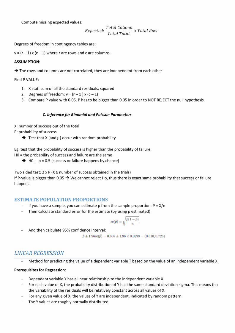
Compute missing expected values:
𝐸𝑥𝑝𝑒𝑐𝑡𝑒𝑑: 𝑇𝑜𝑡𝑎𝑙 𝐶𝑜𝑙𝑢𝑚𝑛
𝑇𝑜𝑡𝑎𝑙 𝑇𝑜𝑡𝑎𝑙 𝑥 𝑇𝑜𝑡𝑎𝑙 𝑅𝑜𝑤
Degrees of freedom in contingency tables are:
v = (r – 1) x (c – 1) where r are rows and c are columns.
ASSUMPTION:
The rows and columns are not correlated, they are independent from each other
Find P VALUE:
1. X stat: sum of all the standard residuals, squared
2. Degrees of freedom: v = (r – 1 ) x (c – 1)
3. Compare P value with 0.05. P has to be bigger than 0.05 in order to NOT REJECT the null hypothesis.
C. Inference for Binomial and Poisson Parameters
X: number of success out of the total
P: probability of success
Test that X (and ) occur with random probability
Eg. test that the probability of success is higher than the probability of failure.
H0 = the probability of success and failure are the same
H0 : p = 0.5 (success or failure happens by chance)
Two sided test: 2 x P (X ≥ number of success obtained in the trials)
If P-value is bigger than 0.05 We cannot reject Ho, thus there is exact same probability that success or failure
happens.
ESTIMATE POPULATION PROPORTIONS - If you have a sample, you can estimate p from the sample proportion: P = X/n
- Then calculate standard error for the estimate (by using p estimated)
- And then calculate 95% confidence interval:
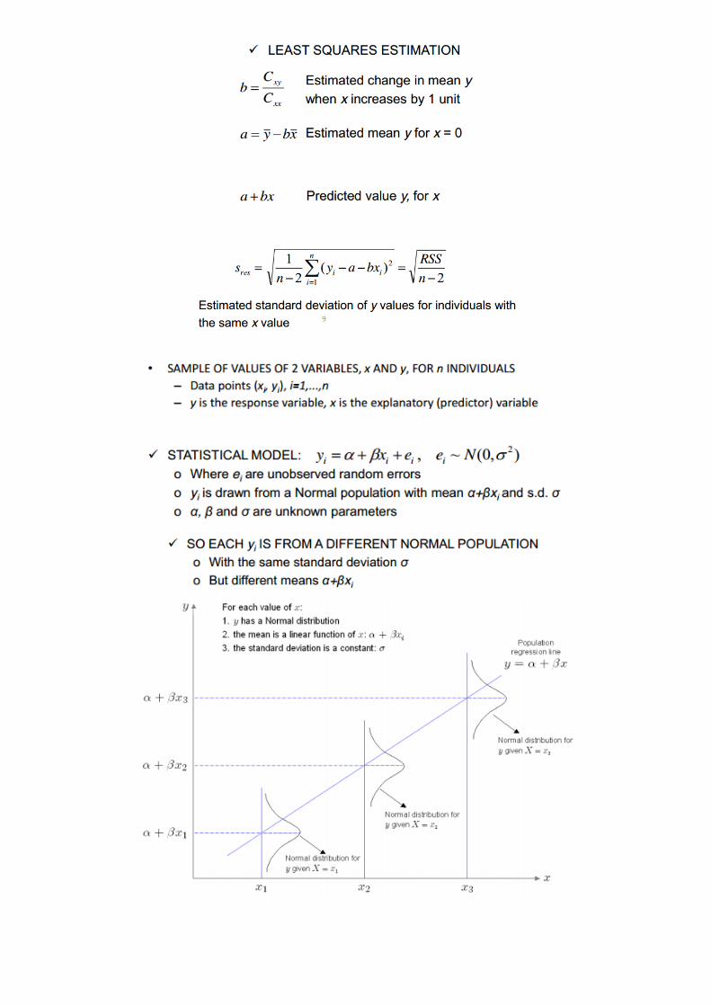
LINEAR REGRESSION
- Method for predicting the value of a dependent variable T based on the value of an independent variable X
Prerequisites for Regression:
- Dependent variable Y has a linear relationship to the independent variable X
- For each value of X, the probability distribution of Y has the same standard deviation sigma. This means tha
the variability of the residuals will be relatively constant across all values of X.
- For any given value of X, the values of Y are independent, indicated by random pattern.
- The Y values are roughly normally distributed
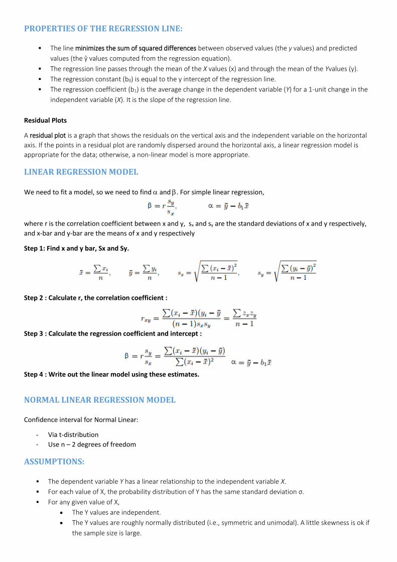
PROPERTIES OF THE REGRESSION LINE:
The line minimizes the sum of squared differences between observed values (the y values) and predicted
values (the ŷ values computed from the regression equation).
The regression line passes through the mean of the X values (x) and through the mean of the Yvalues (y).
The regression constant (b0) is equal to the y intercept of the regression line.
The regression coefficient (b1) is the average change in the dependent variable (Y) for a 1-unit change in the
independent variable (X). It is the slope of the regression line.
Residual Plots
A residual plot is a graph that shows the residuals on the vertical axis and the independent variable on the horizontal
axis. If the points in a residual plot are randomly dispersed around the horizontal axis, a linear regression model is
appropriate for the data; otherwise, a non-linear model is more appropriate.
LINEAR REGRESSION MODEL
We need to fit a model, so we need to find and . For simple linear regression,
where r is the correlation coefficient between x and y, sx and sy are the standard deviations of x and y respectively,
and x-bar and y-bar are the means of x and y respectively
Step 1: Find x and y bar, Sx and Sy.
Step 2 : Calculate r, the correlation coefficient :
Step 3 : Calculate the regression coefficient and intercept :
Step 4 : Write out the linear model using these estimates.
NORMAL LINEAR REGRESSION MODEL
Confidence interval for Normal Linear:
- Via t-distribution
- Use n – 2 degrees of freedom
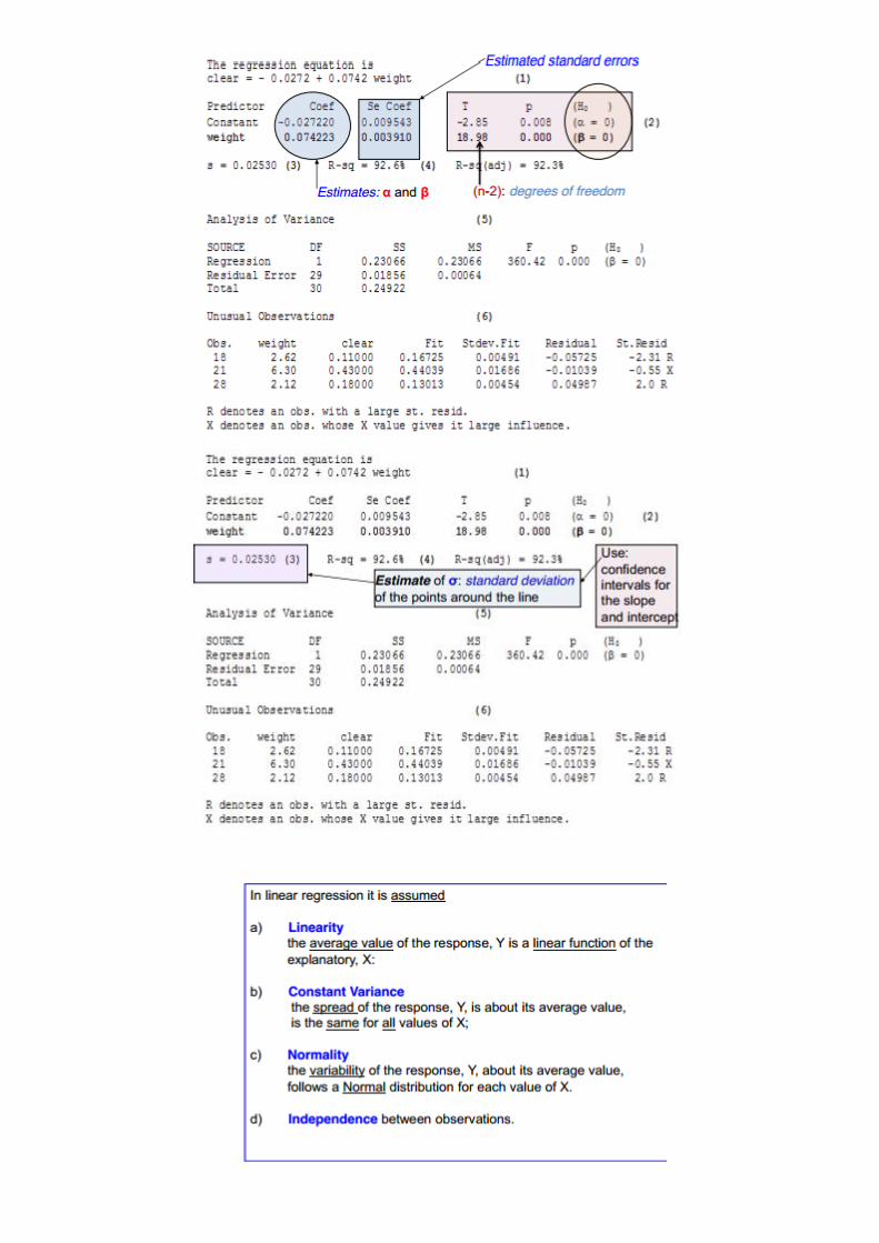
ASSUMPTIONS:
The dependent variable Y has a linear relationship to the independent variable X.
For each value of X, the probability distribution of Y has the same standard deviation σ.
For any given value of X,
The Y values are independent.
The Y values are roughly normally distributed (i.e., symmetric and unimodal). A little skewness is ok if
the sample size is large.
PROBABILITY RULES
- Pr (A) = P
- Direct correspondence between Probability of event A and PROPORTION in the population with attribute A
- For any event A: P(not A) = 1 – P(A)
Pr(A|B): probability of A, given B (individuals with A amongst those with B)
Pr(A|B) ≠ Pr (B|A)
Pr (A|B) is a CONDITIONAL probability
Pr (A and B) is a JOINT probability
P(A or B) = P(A) + P(B) - P(A and B)
Pr (A and B) = Pr (A|B) x Pr (B) = Pr (B|A) x Pr (A)
CONDITIONAL PROBABILITIES
𝑃𝑟 (𝐴|𝐵) = 𝑃𝑟 (𝐴 𝑎𝑛𝑑 𝐵)
𝑃𝑟 (𝐵)
𝑃𝑟 (𝐵|𝐴) = 𝑃𝑟 (𝐴 𝑎𝑛𝑑 𝐵)
𝑃𝑟 (𝐴)
MUTUALLY EXCLUSIVE EVENTS
if one occurs, the other cannot. P(A or B) = P(A) + P(B) - P(A and B) = P (A) + p (B), only if mutually exclusive
JOINT PROBABILITIES
P(A) = P(A|B)P(B) + P(A|not B) P(not B)
Known as the generalised addition law.
INDEPENDENCE
P (A and B) = P(A) x P(B)
It follows that: P (A|B) = P (A|not B) = P(A), because P(A) is independent from P(B)
If independent, the following are always true
P(A|B) = P(A), for all values of A and B.
P(A and B) = P(A) * P(B), for all values of A and B.
BAYES THEOREM
𝑃𝑟 (𝐴|𝐵) =𝑃𝑟 (𝐵|𝐴) 𝑃𝑟(𝐴)
𝑃𝑟(𝐵)
Means of calculating P (A|B) when we know the other variables.
Joint probabilities can be imagines as a table, as if they were numbers of a total population of 1.
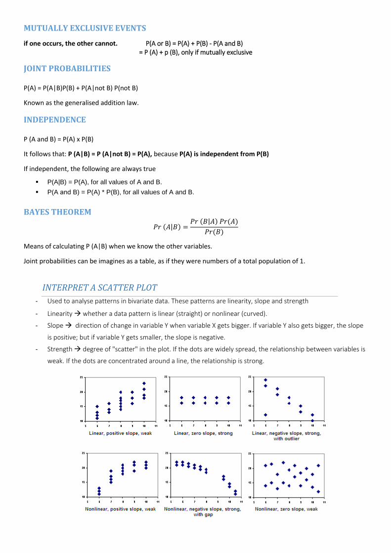
INTERPRET A SCATTER PLOT
- Used to analyse patterns in bivariate data. These patterns are linearity, slope and strength
- Linearity whether a data pattern is linear (straight) or nonlinear (curved).
- Slope direction of change in variable Y when variable X gets bigger. If variable Y also gets bigger, the slope
is positive; but if variable Y gets smaller, the slope is negative.
- Strength degree of "scatter" in the plot. If the dots are widely spread, the relationship between variables is
weak. If the dots are concentrated around a line, the relationship is strong.
COMPARE DATA SETS
Center. Graphically, the center of a distribution is the point where about half of the observations are on either
side.
Spread. The spread of a distribution refers to the variability of the data. If the observations cover a wide
range, the spread is larger. If the observations are clustered around a single value, the spread is smaller.
Shape. The shape of a distribution is described by symmetry, skewness, number of peaks, etc.
Unusual features. Unusual features refer to gaps (areas of the distribution where there are no observations)
and outliers.
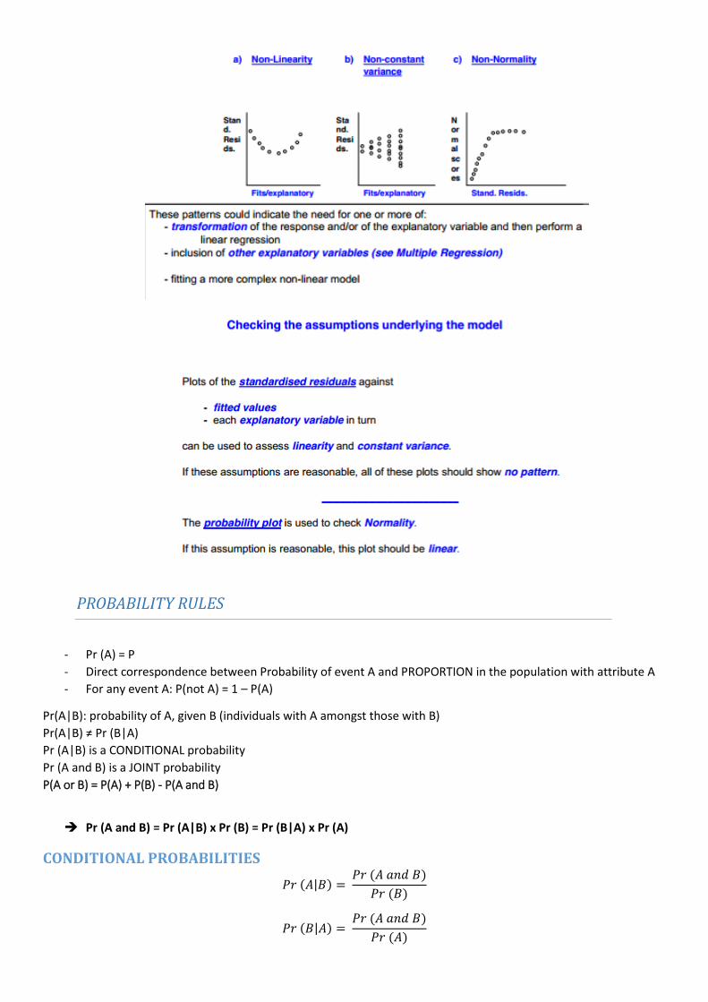
PLOT OF RESIDUALS TO ESTABLISH IF REGRESSION LINE IS A GOOD FIT
- Has to have no pattern
- Values equally distributed on either side
- Have to be randomly dispersed, otherwise not a good fit.
Linearity, Constant Variance, Normality (see before)
CALCULATOR:
MODE button
3 for STAT
1 for 1-VAR
Enter your data 1, enter, 1, enter, etc
SHIFT 1 for [STAT]
5 for Var
3 for population standard deviation or 4 for sample standard deviation. Also, 2 for mean.
Related Documents