Stat Mech

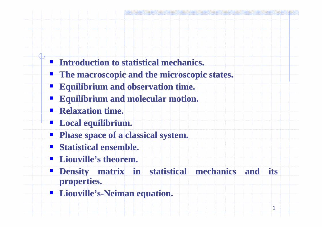
IntroductionIntroduction toto statisticalstatistical mechanicsmechanics IntroductionIntroduction toto statisticalstatistical mechanicsmechanics.. TheThe macroscopicmacroscopic andand thethe microscopicmicroscopic statesstates.. EquilibriumEquilibrium andand observationobservation timetimeEquilibriumEquilibrium andand observationobservation timetime.. EquilibriumEquilibrium andand molecularmolecular motionmotion.. RelaxationRelaxation timetime..RelaxationRelaxation timetime.. LocalLocal equilibriumequilibrium.. PhasePhase spacespace ofof aa classicalclassical systemsystem..pp yy StatisticalStatistical ensembleensemble.. Liouville’sLiouville’s theoremtheorem.. DensityDensity matrixmatrix inin statisticalstatistical mechanicsmechanics andand itsits

propertiesproperties..Li ill ’Li ill ’ N iN i titi

1

Liouville’sLiouville’s--NeimanNeiman equationequation..

Introduction to statistical mechanics.Introduction to statistical mechanics.

F th t th t d it li d th tFrom the seventeenth century onward it was realized that material systemsmaterial systems could often be described by a small small number of descriptive parametersnumber of descriptive parameters that were related tonumber of descriptive parametersnumber of descriptive parameters that were related to one another in simple lawlike ways.

These parameters referred to geometric dynamical andgeometric dynamical andThese parameters referred to geometric, dynamical and geometric, dynamical and thermal propertiesthermal properties of matter.

T i l f th l th id l lid l l th t l t dTypical of the laws was the ideal gas lawideal gas law that related product of pressure pressure and volumevolume of a gas to the temperaturetemperature of the gastemperaturetemperature of the gas.

2

Bernoulli (1738)

Krönig (1856)Joule (1851)

Cl i (1857)C. Maxwell (1860)

L B lt (1871)

Krönig (1856)Clausius (1857)

L. Boltzmann (1871)

H. Poincaré (1890)

J. Loschmidt (1876)

T Ehrenfest( ) T. Ehrenfest J. Gibbs (1902)

Planck (1900)Ei t i (1905)

( )Einstein (1905)

Pauli (1925)Smoluchowski (1906)

Langevin (1908)

Compton (1923)Bose (1924)

Pauli (1925)

Thomas (1927)

Dirac (1927)

Thomas (1927)Debye (1912)

3Fermi (1926)

Dirac (1927)Landau (1927)

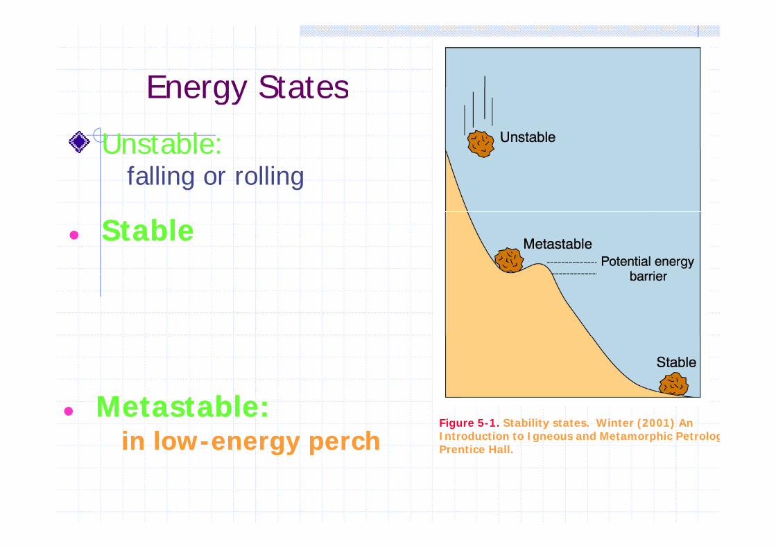
Energy StatesEnergy States

Unstable:Unstable:falling or rolling

StableStable

M t t blM t t bl MetastableMetastable::in lowin low--energy perchenergy perch

Figure 5-1. Stability states. Winter (2001) An Introduction to Igneous and Metamorphic PetrologPrentice Hall.

We work with systems which are in equilibriumWe work with systems which are in equilibrium

How do we define equilibrium ?q

The system can be in Mechanical, Chemicald h l ilib iand Thermal equilibrium

We call all these three together as “ThermodynamicEquilibrium”Equilibrium .

Which means : all the energy states are equallygy q yaccessible for all the particles

H d di i i h b Cl i l dHow do we distinguish between Classical and Quantum systems?

5

Mi i d iMicroscopic and macroscopic states

The main aim of this course is the investigation of general properties of themacroscopic systems with a large number of degrees of dynamicallyfreedom (with N ~ 1020 particles for example).

From the mechanical point of view, such systems are very complicated. Butin the usual case only a few physical parameters, say temperature, the

d th d it d b f hi h th ’’ t t ’’ fpressure and the density, are measured, by means of which the ’’state’’ ofthe system is specified.

A state defined in this cruder manner is called aa macroscopicmacroscopic statestate orA state defined in this cruder manner is called aa macroscopicmacroscopic statestate orthermodynamic state. On the other hand, from a dynamical point of view,each state of a system can be defined, at least in principle, as precisely aspossible by specifying all of the dynamical variables of the system Such apossible by specifying all of the dynamical variables of the system. Such astate is called aa microscopicmicroscopic statestate.

6

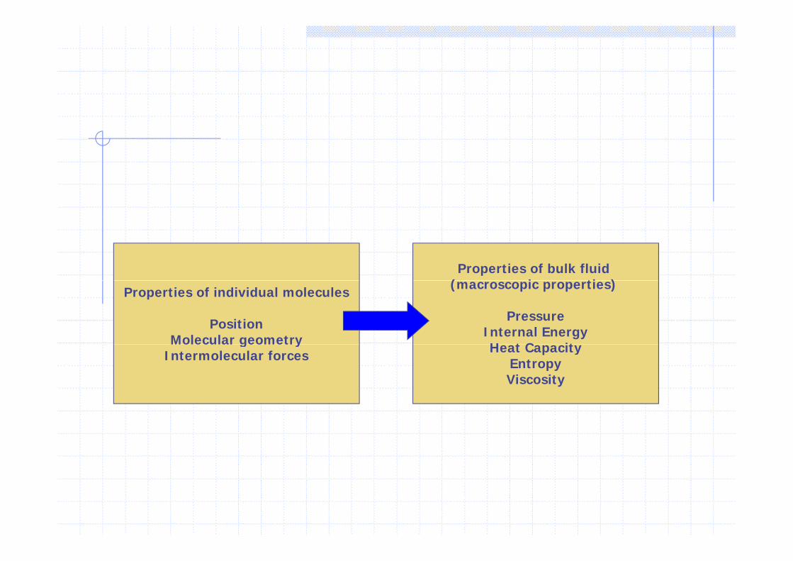
Properties of bulk fluid ( i ti )Properties of individual molecules

PositionMolecular geometry

(macroscopic properties)

PressureInternal EnergyH t C itMolecular geometry

Intermolecular forces Heat CapacityEntropyViscosity

What we know

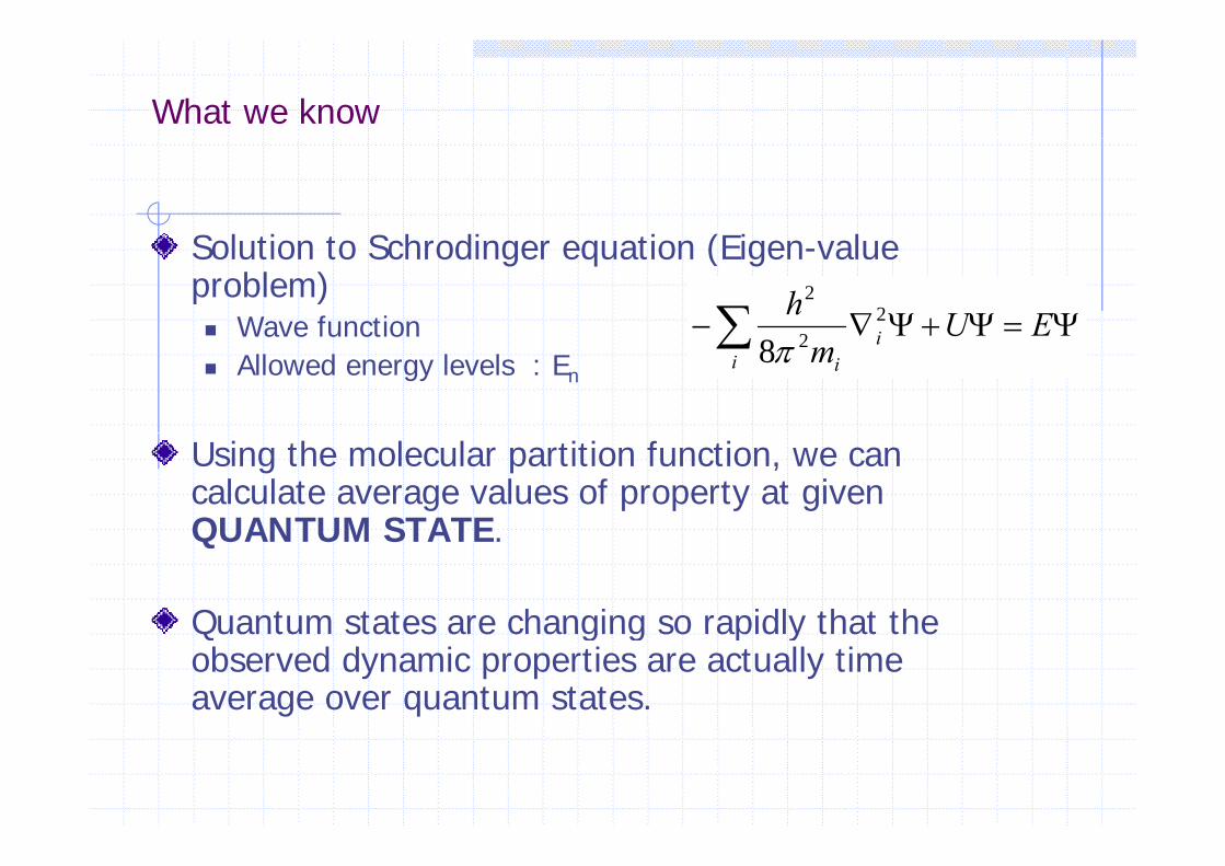
S l ti t S h di ti (Ei lSolution to Schrodinger equation (Eigen-value problem) Wave function i EUh 2

2

2

Wave function Allowed energy levels : En

i

ii

EUm28

Using the molecular partition function, we can calculate average values of property at given QUANTUM STATEQUANTUM STATE.

Quantum states are changing so rapidly that theQuantum states are changing so rapidly that the observed dynamic properties are actually time average over quantum states.

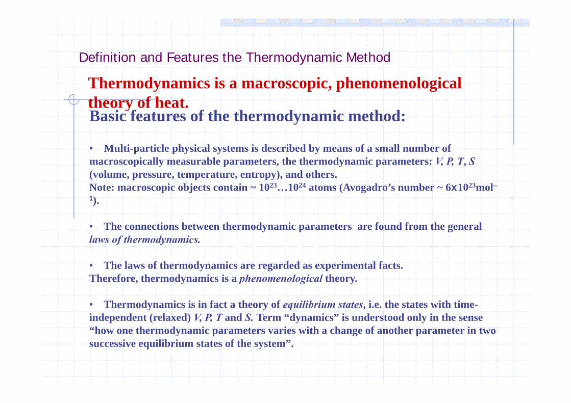
Definition and Features the Thermodynamic Method

Thermodynamics is a macroscopic, phenomenological theory of heat.

y

Basic features of the thermodynamic method:

• Multi-particle physical systems is described by means of a small number of

y

macroscopically measurable parameters, the thermodynamic parameters: V, P, T, S (volume, pressure, temperature, entropy), and others. Note: macroscopic objects contain ~ 1023…1024 atoms (Avogadro’s number ~ 6x1023mol–

1)).

• The connections between thermodynamic parameters are found from the general laws of thermodynamics.

• The laws of thermodynamics are regarded as experimental facts. Therefore, thermodynamics is a phenomenological theory.

• Thermodynamics is in fact a theory of equilibrium states, i.e. the states with time-independent (relaxed) V, P, T and S. Term “dynamics” is understood only in the sense “how one thermodynamic parameters varies with a change of another parameter in two successive equilibrium states of the system”.

Classification of Thermodynamic Parameters

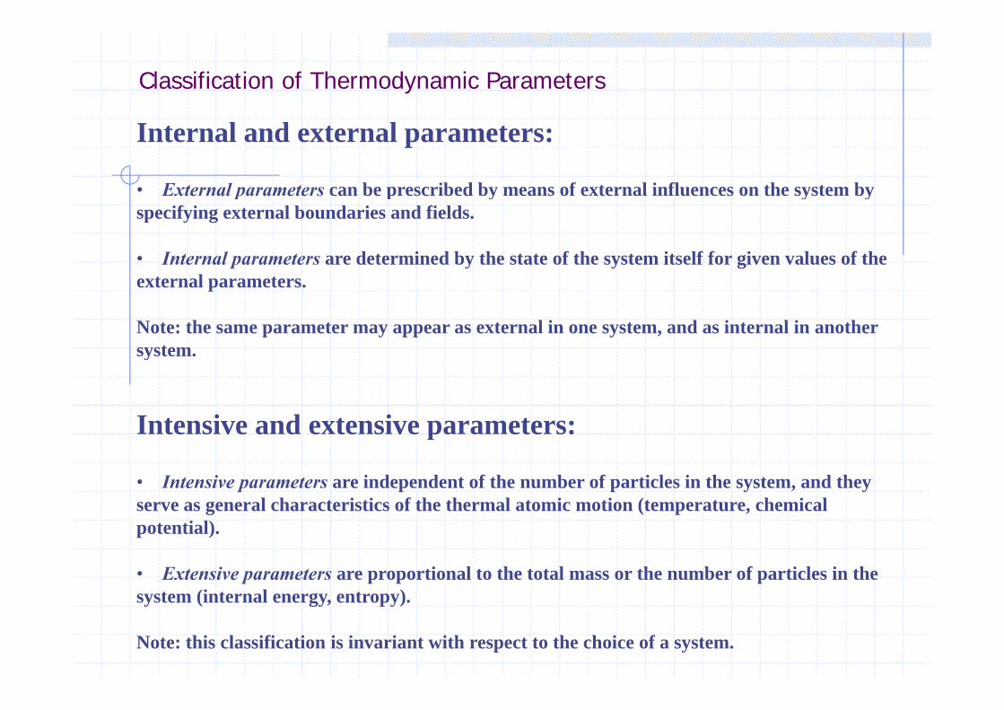
Internal and external parameters:

• External parameters can be prescribed by means of external influences on the system byExternal parameters can be prescribed by means of external influences on the system by specifying external boundaries and fields.

• Internal parameters are determined by the state of the system itself for given values of the external parameters.

Note: the same parameter may appear as external in one system, and as internal in another system.system.

Intensive and extensive parameters:p

• Intensive parameters are independent of the number of particles in the system, and they serve as general characteristics of the thermal atomic motion (temperature, chemical potential).

• Extensive parameters are proportional to the total mass or the number of particles in the system (internal energy entropy)system (internal energy, entropy).

Note: this classification is invariant with respect to the choice of a system.

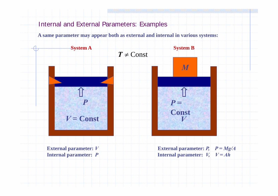
Internal and External Parameters: Examples

A same parameter may appear both as external and internal in various systems:

System A System BConstT

M

ConstT

P

V = Const

P = Const

VV Const V

External parameter: V External parameter: P, P = Mg/AInternal parameter: P Internal parameter: V, V = Ah

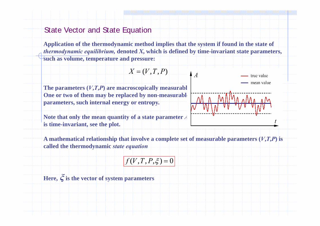
State Vector and State Equation

Application of the thermodynamic method implies that the system if found in the state of thermodynamic equilibrium, denoted X, which is defined by time-invariant state parameters, such as volume, temperature and pressure:p p

The parameters (V T P) are macroscopically measurable

( , , )X V T P

The parameters (V,T,P) are macroscopically measurable. One or two of them may be replaced by non-measurable parameters, such internal energy or entropy.

Note that only the mean quantity of a state parameter Ais time-invariant, see the plot.

A mathematical relationship that involve a complete set of measurable parameters (V T P) isA mathematical relationship that involve a complete set of measurable parameters (V,T,P) is called the thermodynamic state equation

( , , , ) 0f V T P

Here, ξ is the vector of system parameters

( , , , )f

AveragingAveraging

The physical quantities observed in the macroscopic state are the resultof these variables averagingaveraging in the warrantable microscopic states. Theof these variables averagingaveraging in the warrantable microscopic states. Thestatistical hypothesis about the microscopic state distribution isrequired for the correctcorrect averagingaveraging.

To find the rightright methodmethod ofof averagingaveraging is the fundamental principle ofthe statistical method for investigation of macroscopic systems.

Th d i ti f l h i l l f th i t l ltThe derivation of general physical lows from the experimental resultswithout consideration of the atomic-molecular structure is the mainprinciple of thermodynamic approach.

13

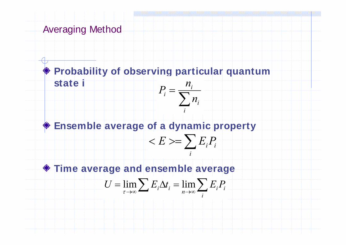
Averaging Method

Probability of observing particular quantum state i

i

inP

E bl f d i t

i

ii n

Ensemble average of a dynamic property

ii PEE

Time average and ensemble average

i

ii

inii PEtEU limlim

Thermodynamics and Statistical Mechanics

Probabilities

15

Pair of Dice

For one die, the probability of any face i i th 1/6 Th f itcoming up is the same, 1/6. Therefore, it

is equally probable that any number from one to six will come up.

For two dice, what is the probability that the total will come up 2, 3, 4, etc up to 12?

16

Probability

To calculate the probability of a ti l t t th b fparticular outcome, count the number of

all possible results. Then count the number that give the desired outcome. The probability of the desired outcome isThe probability of the desired outcome is equal to the number that gives the desired outcome divided by the totaldesired outcome divided by the total number of outcomes. Hence, 1/6 for one di

17

die.

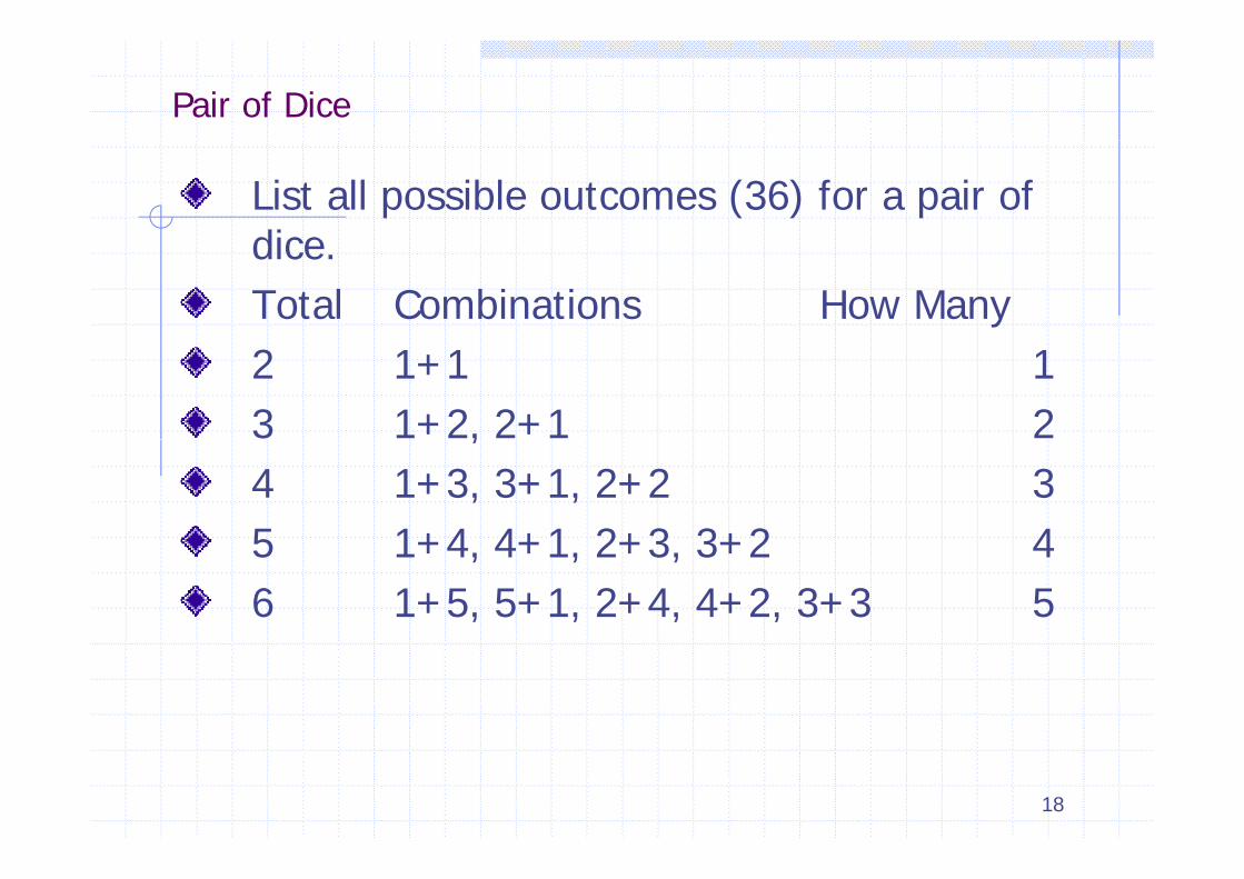
Pair of Dice

List all possible outcomes (36) for a pair of dicedice.Total Combinations How Many2 1+1 13 1+2, 2+1 2,4 1+3, 3+1, 2+2 35 1+4 4+1 2+3 3+2 45 1+4, 4+1, 2+3, 3+2 46 1+5, 5+1, 2+4, 4+2, 3+3 5

18

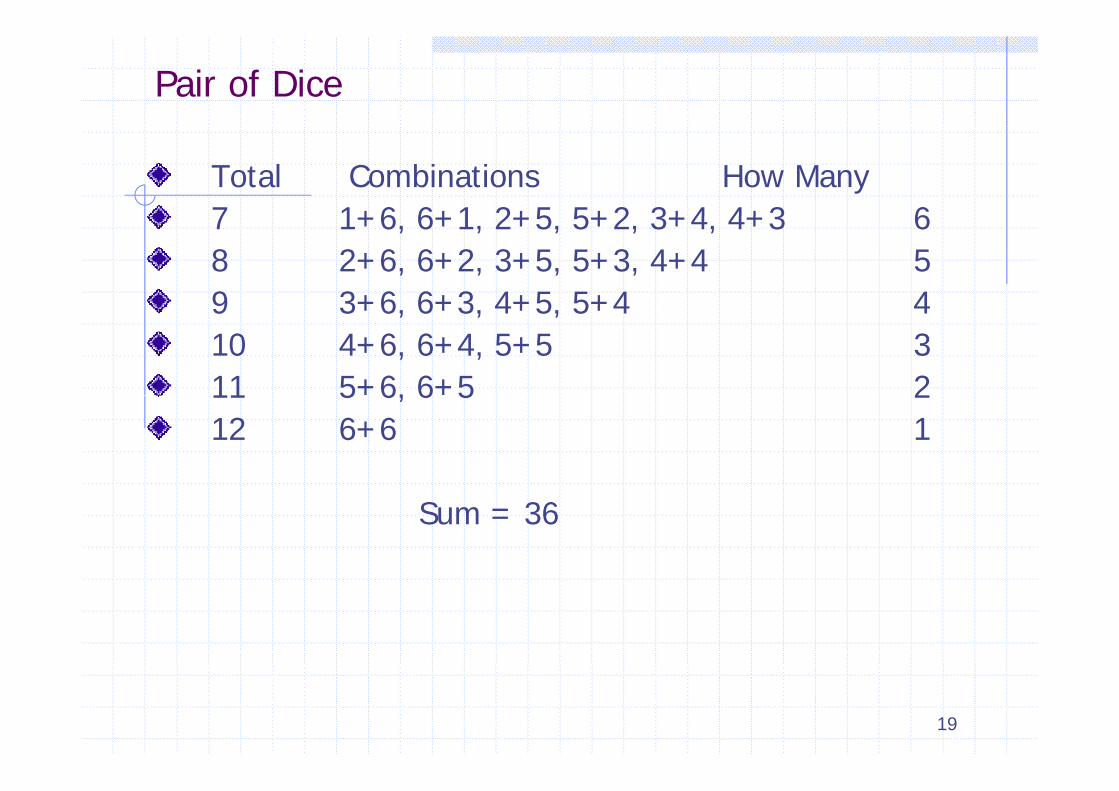
Pair of Dice

Total Combinations How Many7 1+6 6+1 2+5 5+2 3+4 4+3 67 1+6, 6+1, 2+5, 5+2, 3+4, 4+3 68 2+6, 6+2, 3+5, 5+3, 4+4 59 3+6 6+3 4+5 5+4 49 3+6, 6+3, 4+5, 5+4 410 4+6, 6+4, 5+5 311 5+6, 6+5 211 5+6, 6+5 212 6+6 1

Sum = 36

19

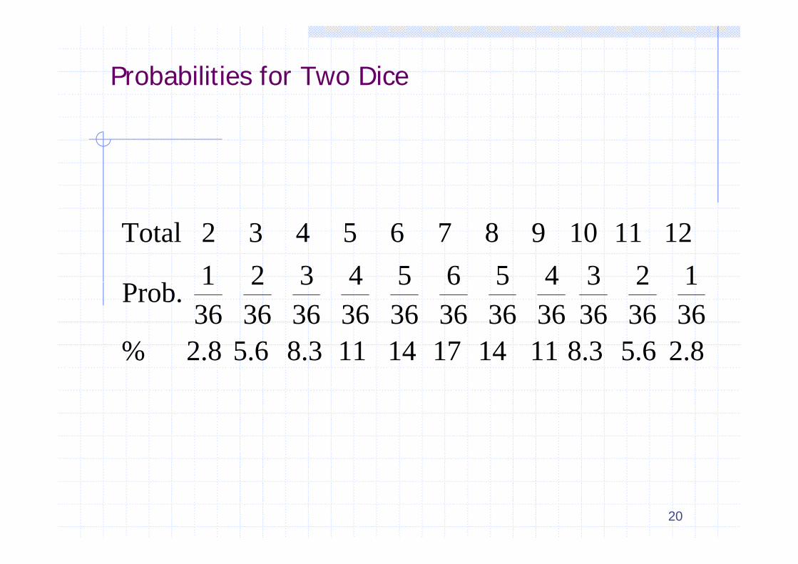
Probabilities for Two Dice

1234565432112 11 10 9 8 7 6 5 4 3 2 Total

2 85 68 311141714118 35 62 8%

361

362

363

364

365

366

365

364

363

362

361 Prob.

2.8 5.6 8.3 11 14 17 14 11 8.3 5.6 2.8 %

20

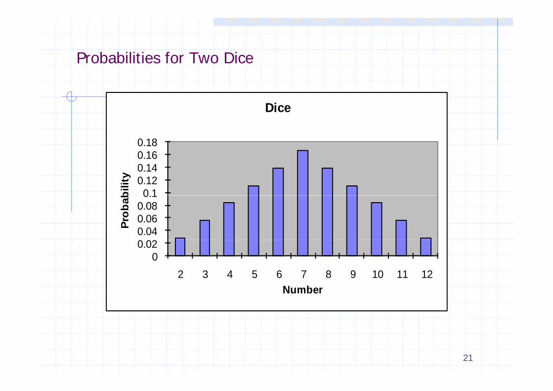
Probabilities for Two DiceProbabilities for Two Dice

Dice

0 160.18

Dice

0 10.120.140.16

bilit

y

0 020.040.060.080.1

Prob

ab

00.02

2 3 4 5 6 7 8 9 10 11 12Number

21

Microstates and Macrostates

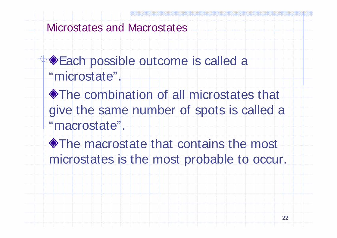
Each possible outcome is called aEach possible outcome is called a “microstate”.

The combination of all microstates thatThe combination of all microstates that give the same number of spots is called a “macrostate”.

The macrostate that contains the mostThe macrostate that contains the most microstates is the most probable to occur.

22

Combining Probabilitiesg

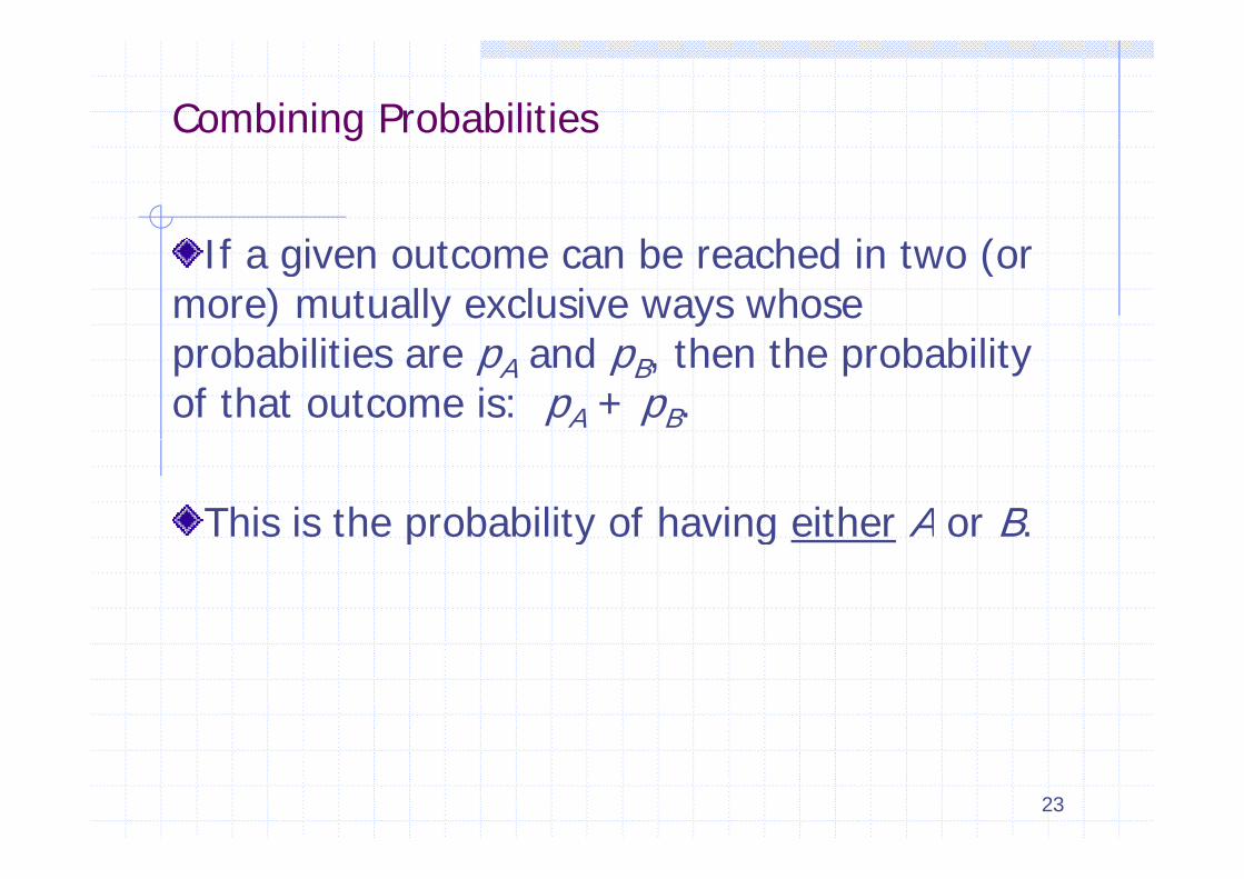
If i t b h d i t (If a given outcome can be reached in two (or more) mutually exclusive ways whose

b biliti d th th b bilitprobabilities are pA and pB, then the probability of that outcome is: pA + pB.

This is the probability of having either A or B.p y g

23

Combining Probabilities

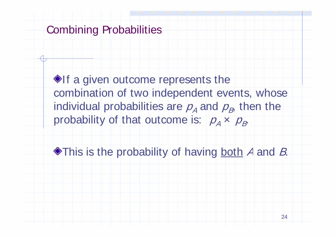
If a given outcome represents the combination of two independent events whosecombination of two independent events, whose individual probabilities are pA and pB, then the probability of that outcome is: p × pprobability of that outcome is: pA × pB.

This is the probability of having both A and B.

24

Example

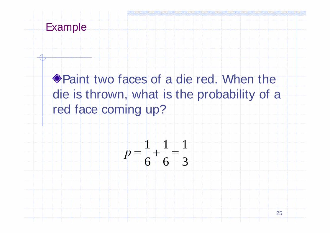
Paint two faces of a die red. When the di i th h t i th b bilit fdie is thrown, what is the probability of a red face coming up?

11131

61

61 p

25

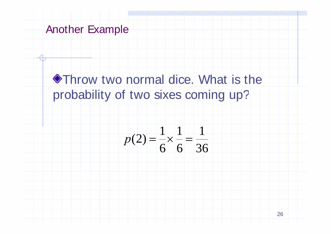
Another Example

Throw two normal dice. What is the b bilit f t i i ?probability of two sixes coming up?

111)2( p3666

)(p

26

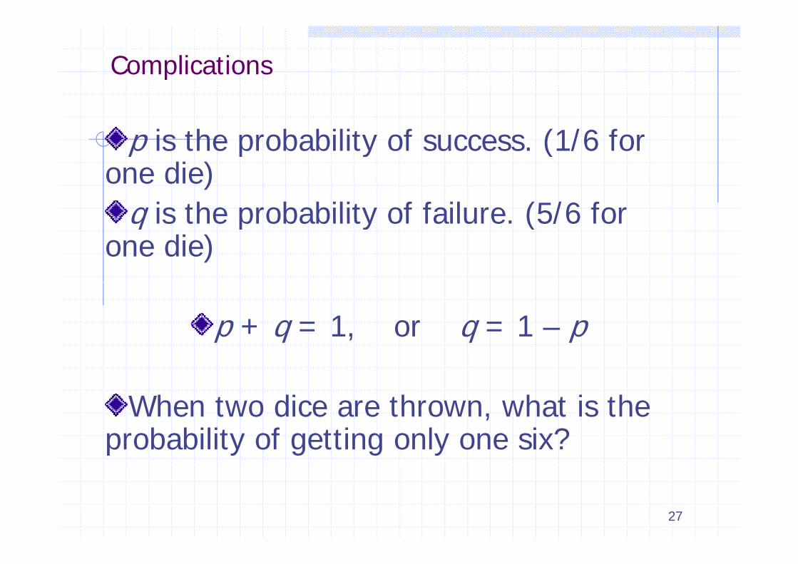
Complications

p is the probability of success. (1/6 for p p y ( /one die)

q is the probability of failure (5/6 forq is the probability of failure. (5/6 for one die)

p + q = 1, or q = 1 – p

When two dice are thrown what is theWhen two dice are thrown, what is the probability of getting only one six?

27

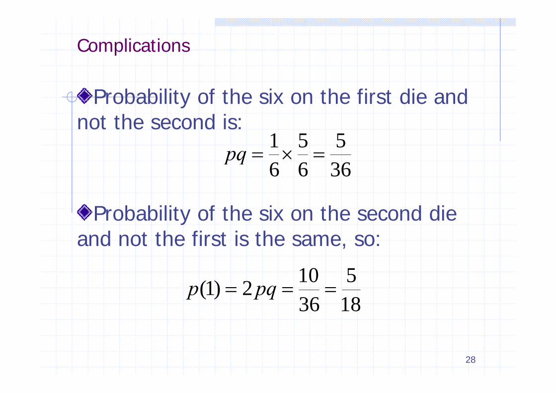
Complications

Probability of the six on the first die and ynot the second is:

551pq3666

pq

Probability of the six on the second die and not the first is the same so:and not the first is the same, so:

5102)1( pqp1836

2)1( pqp

28

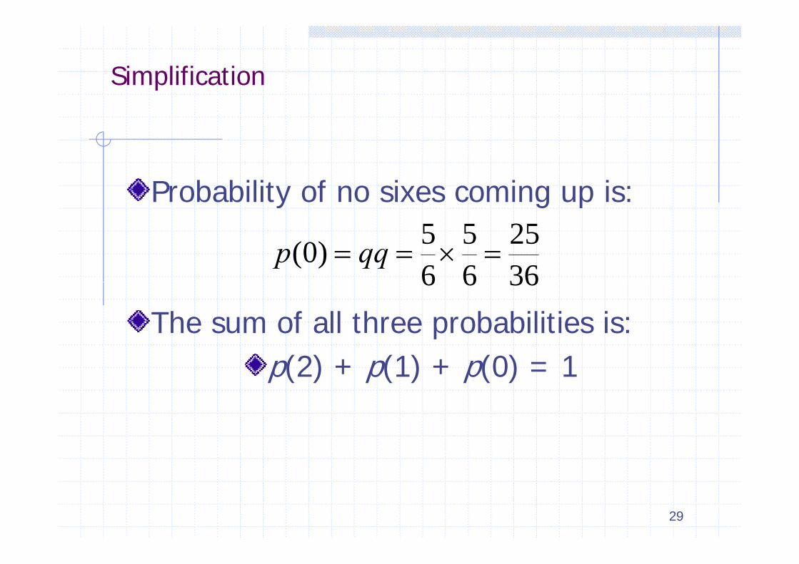
Simplificationp

Probability of no sixes coming up is:

3625

65

65)0( qqp

The sum of all three probabilities is:

3666

p(2) + p(1) + p(0) = 1

29

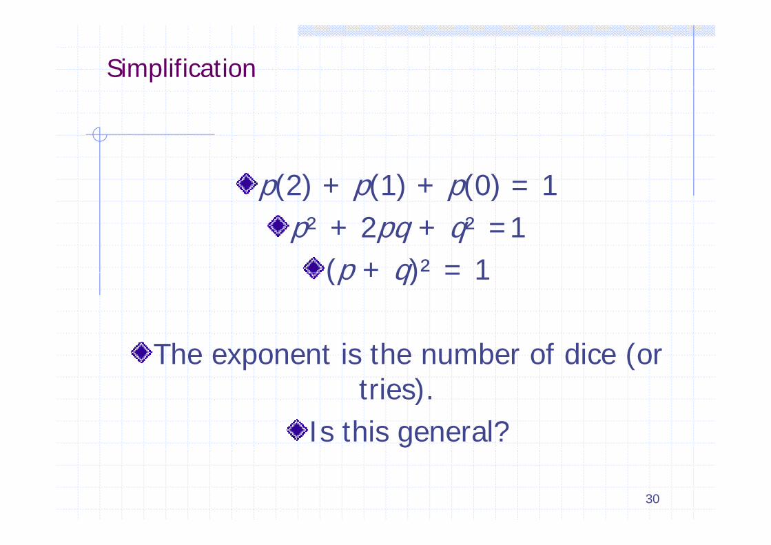
Simplification

p(2) + p(1) + p(0) = 1p² + 2pq + q² =1

(p + q)² = 1(p + q) = 1

The exponent is the number of dice (or tries).tries).

Is this general?

30

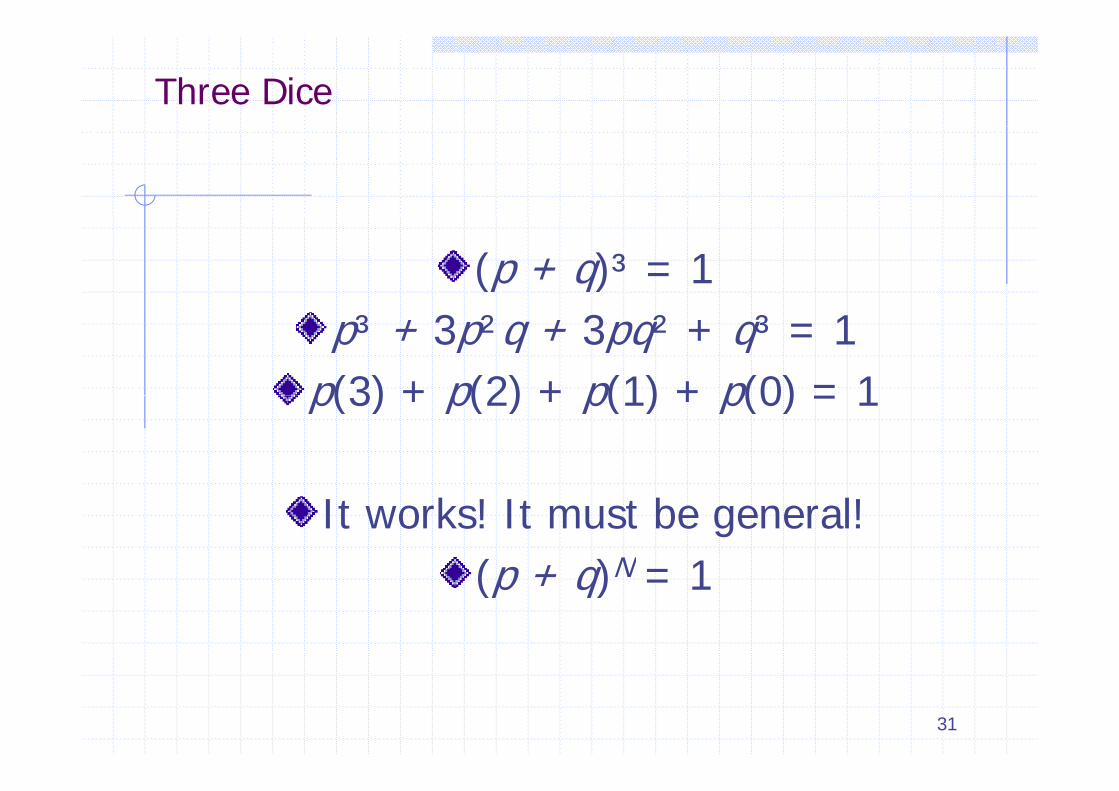
Three Dice

(p + q)³ = 1p³ + 3p²q + 3pq² + q³ = 1

p(3) + p(2) + p(1) + p(0) = 1p(3) + p(2) + p(1) + p(0) = 1

It works! It must be general!(p + q)N = 1(p + q)N = 1

31

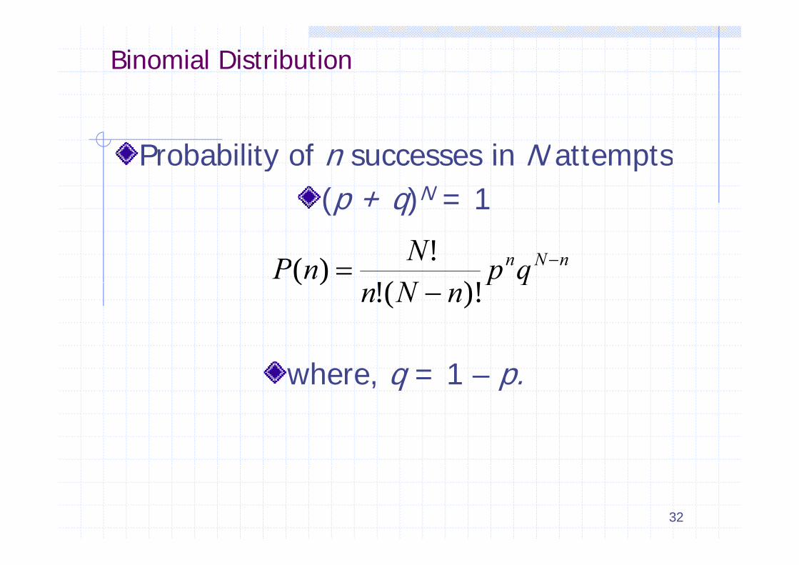
Binomial Distribution

Probability of n successes in N attemptsProbability of n successes in N attempts(p + q)N = 1

nNnqpNNnP

)!(!!)( qp

nNn )!(!)(

where, q = 1 – p.

32

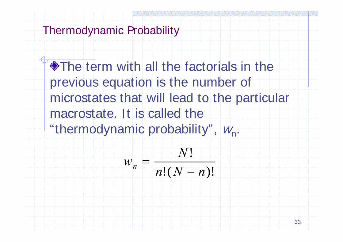
Thermodynamic Probability

The term with all the factorials in theThe term with all the factorials in the previous equation is the number of

i t t th t ill l d t th ti lmicrostates that will lead to the particular macrostate. It is called the “thermodynamic probability”, wn.

!N)!(!

!nNn

Nwn

)(

33

Microstates

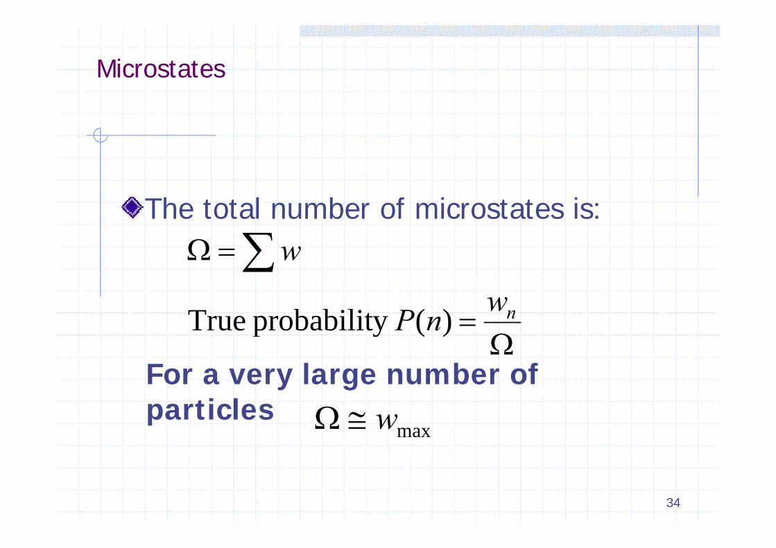
The total number of microstates is:The total number of microstates is: w

nwnP )(y probabilitTrue

)(yp

For a very large number of i lparticles

maxw

34

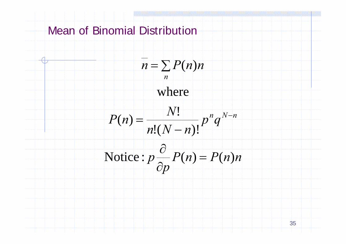
Mean of Binomial Distribution

nnPn )( nnPnn

where

)(

qpNnP nNn!)(

where

qpnNn

nP)!(!

)(

nnPnPp

p )()(:Notice

35

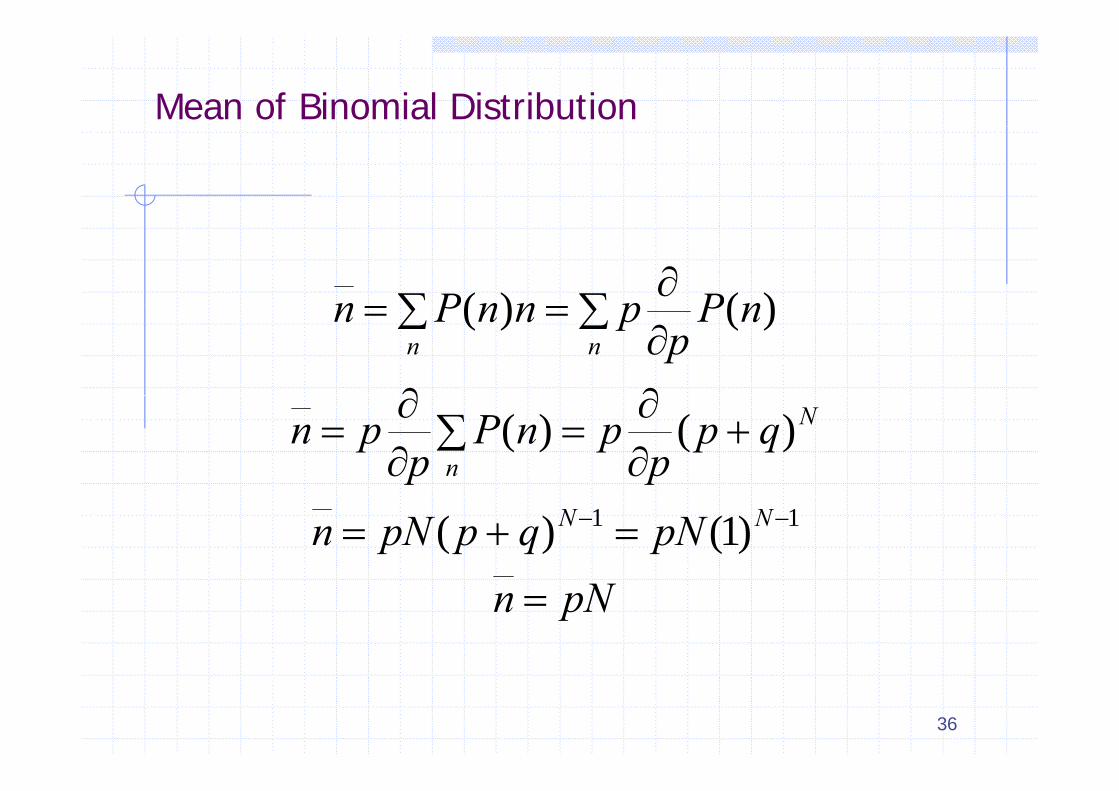
Mean of Binomial Distribution

nPpnnPn

)()( nPp

pnnPnnn

)()(

qpp

pnPp

pn N

n

)()(

pNqppNn NN 11 )1()(pNn

36

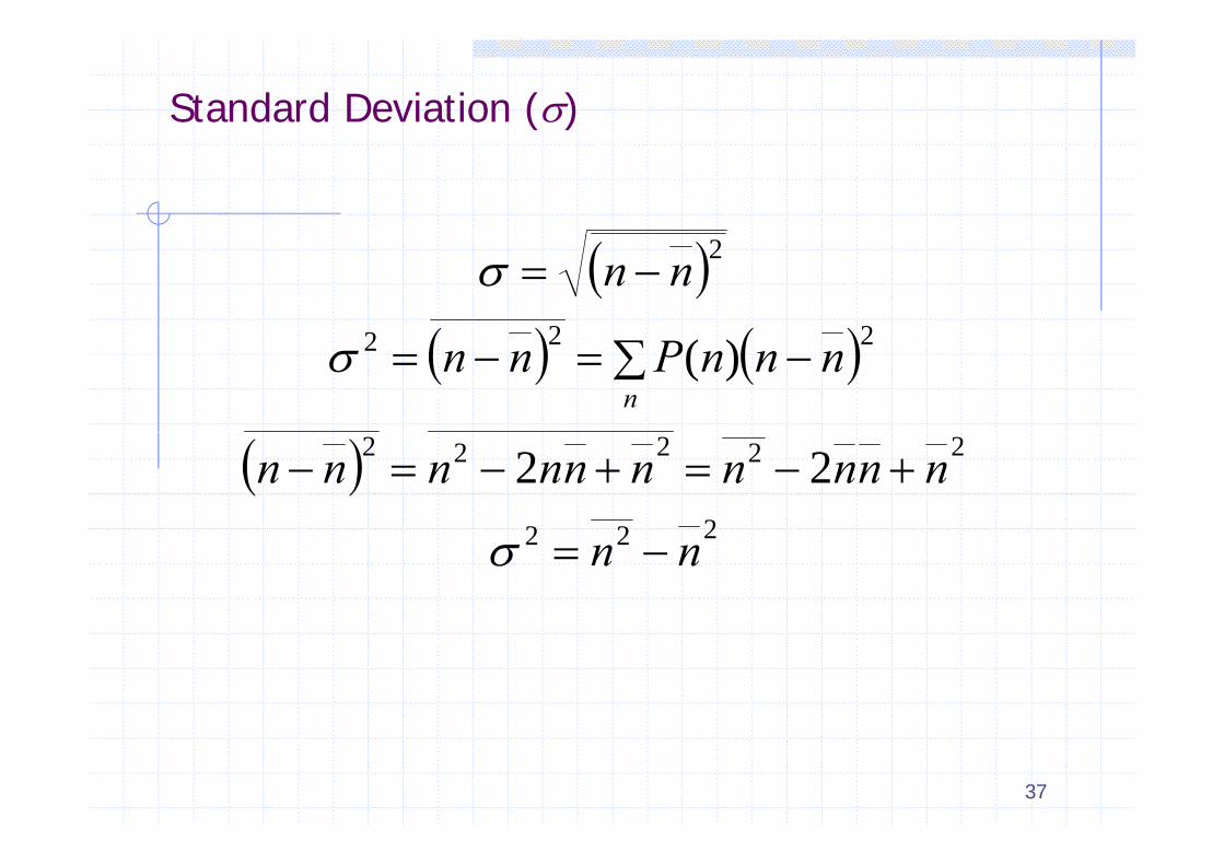
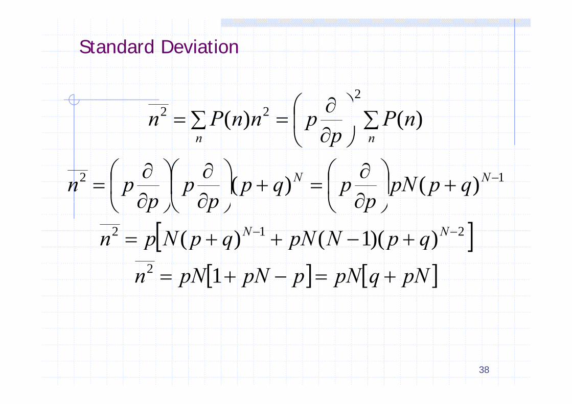
Standard Deviation ()

222

2nn

222 )( nnnPnnn

222

22222 22 nnnnnnnnnn 222 nn

37

Standard Deviation

222 nP

ppnnPn

nn

)()( 22

qppNp

pqpp

pp

pn NN

)()( 12

qpNpNqpNpn

pppNN

))(1()( 212

pNqpNppNpNn

qppqpp

1

))(()(2

38

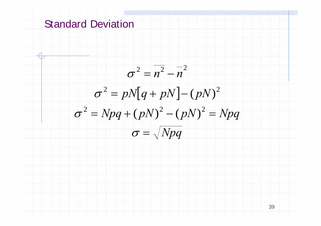
Standard Deviation

nn

22

222

NpqpNpNNpq

pNpNqpN

222

22

)()(

)(

NpqNpqpNpNNpq

)()(

pq

39

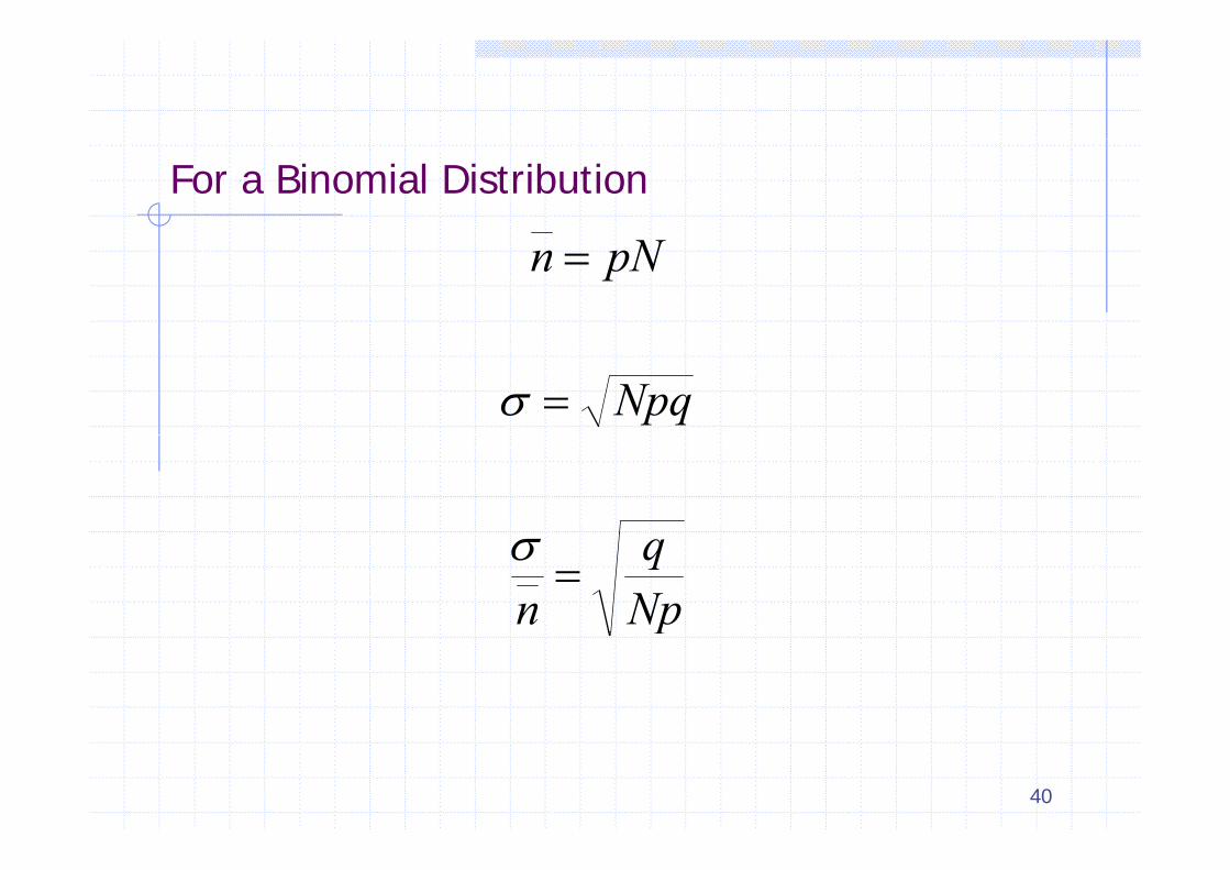
For a Binomial Distribution

pNn

Npq

Npq

n

p

40

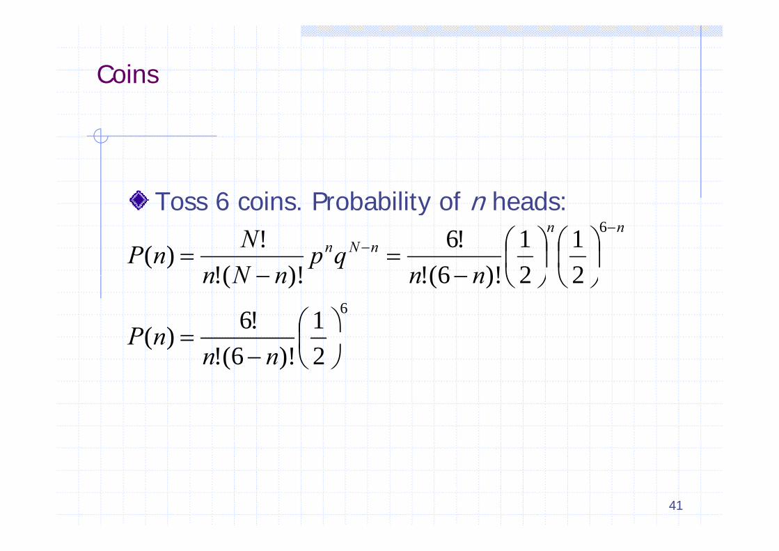
Coins

Toss 6 coins. Probability of n heads:y6

21

21

)!6(!!6

)!(!!)(

nnqp

nNnNnP

nnnNn

61!6)(

22)!6(!)!(!

nP

nnnNn

2)!6(!)(

nn

nP

41

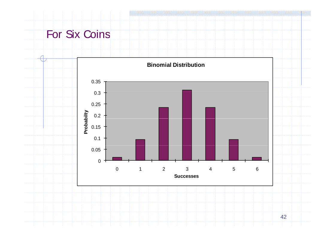
For Six CoinsFor Six Coins

Binomial Distribution

0 3

0.35

Binomial Distribution

0.2

0.25

0.3bi

lty

0.1

0.15

Prob

ab

0

0.05

0 1 2 3 4 5 6Successes

42

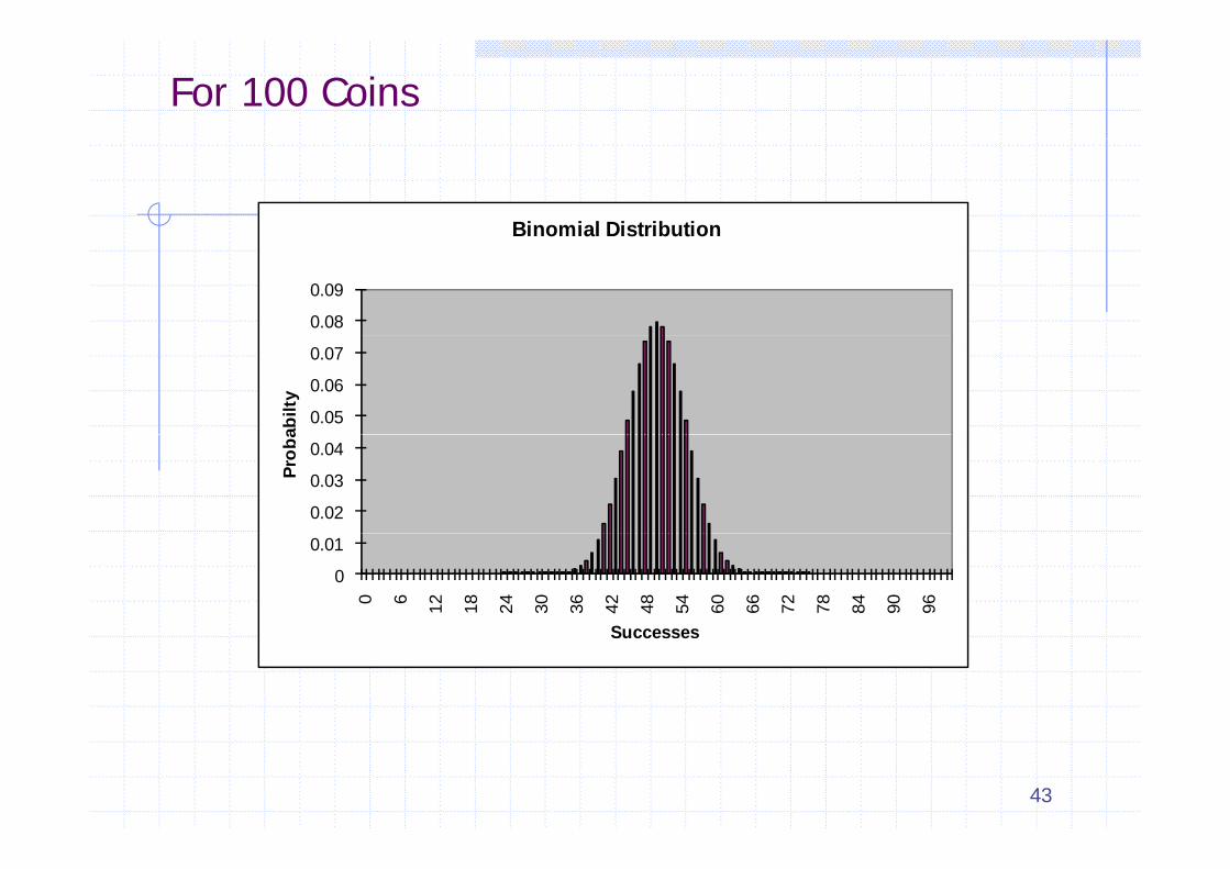
For 100 Coins

Binomial Distribution

0.08

0.09

0.05

0.06

0.07

abilt

y

0.02

0.03

0.04

Prob

a

0

0.01

0 6 12 18 24 30 36 42 48 54 60 66 72 78 84 90 96

SuccessesSuccesses

43

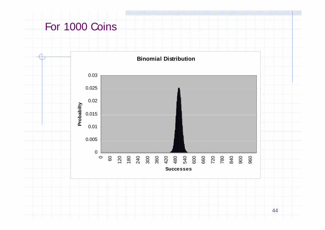
For 1000 Coins

Binomial Distribution

0 025

0.03

0.015

0.02

0.025

abilt

y

0.005

0.01

0.015

Prob

0

0 60 120

180

240

300

360

420

480

540

600

660

720

780

840

900

960

SSuccesses

44

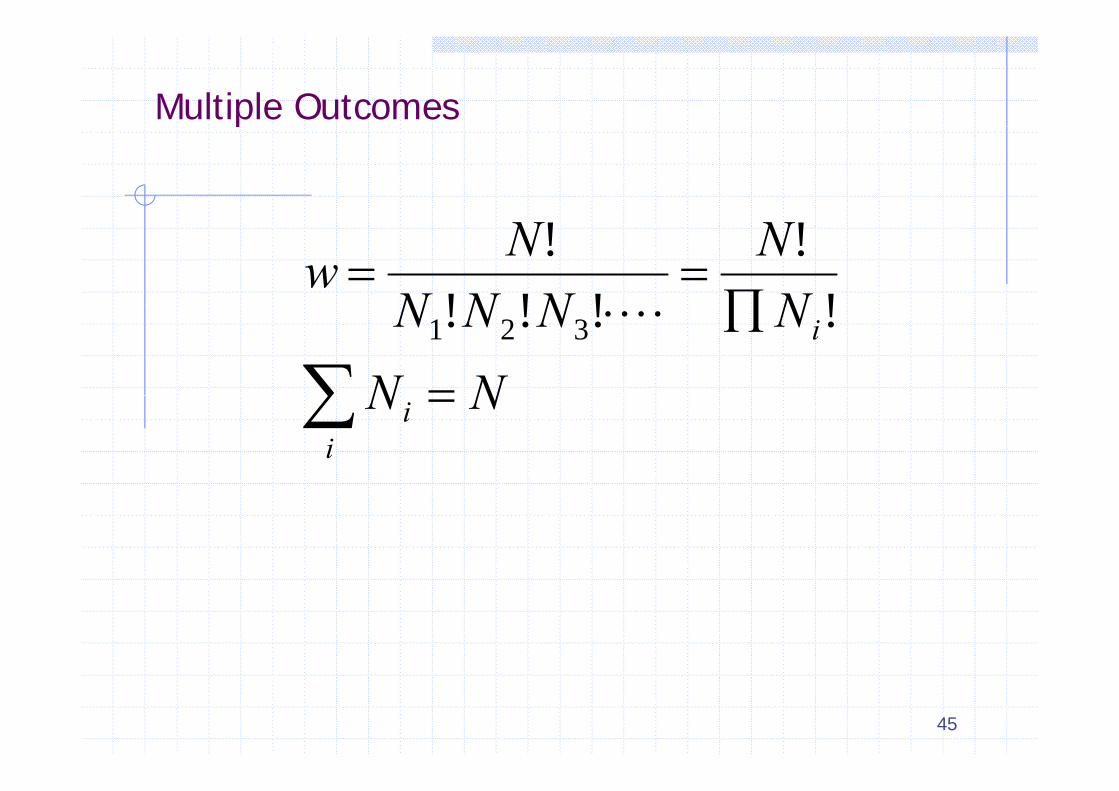
Multiple Outcomesp

NN

NNNNw

!!

!!!!

NNNNNN i

!!!! 321

NNi

i

45

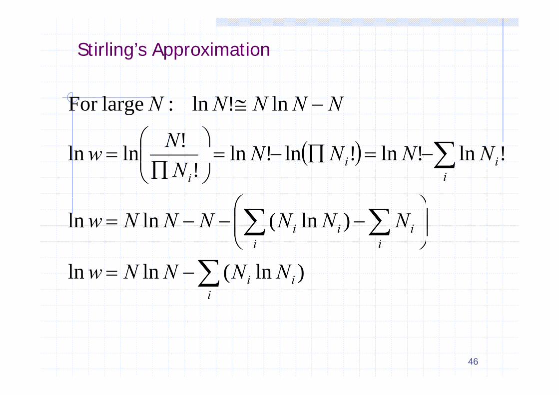
Stirling’s Approximation

NNNNN ln!ln:largeFor

NNNNNw

NNNNN

!ln!ln!ln!ln!lnln

ln!ln: largeFor

i

iii

NNNNN

w !ln!ln!ln!ln!

lnln

i iiii NNNNNNw )ln(lnln

ii

i i

NNNNw )ln(lnlni

46

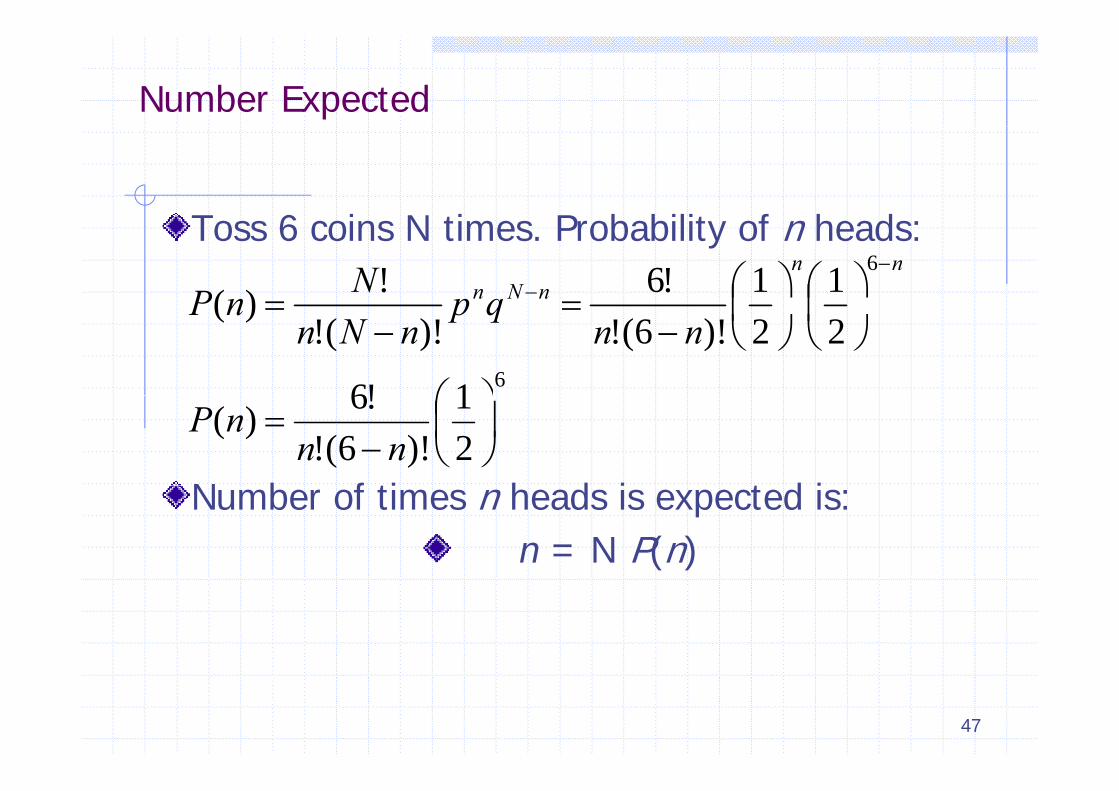
Number Expected

T 6 i N ti P b bilit f h dToss 6 coins N times. Probability of n heads:611!6!)(

qpNnP

nnnNn

61!6

22)!6(!)!(!)(

nn

qpnNn

nP

N b f ti h d i t d i21

)!6(!!6)(

nnnP

Number of times n heads is expected is:n = N P(n)

47

Zero Low of ThermodynamicsZero Low of Thermodynamics

One of the main significant points in thermodynamics (some times theycall it the zero low of thermodynamics) is the conclusion that everyenclosure (isolated from others) system in time come into theequilibrium state where all the physical parameters characterizing thesystem are not changing in time. The process of equilibrium setting iscalled the relaxation process of the system and the time of this processp f y f pis the relaxation time.

Equilibrium means that the separate parts of the system (subsystems)are also in the state of internal equilibrium (if one will isolate themnothing will happen with them). The are also in equilibrium with eachother- no exchange by energy and particles between them.g y gy p

48

Local equilibriumLocal equilibrium

Local equilibriumLocal equilibrium means that the system is consist from the subsystemssubsystems that by themselves are in thefrom the subsystemssubsystems, that by themselves are in the state of internal equilibrium but there is no any equilibrium between the subsystems. q y

The number of macroscopic parameters is increasing with digression of the system from the totalwith digression of the system from the total equilibrium

49

Classical phase systemClassical phase system

Let (q(q11,, qq22 .......... qqss)) be the generalized coordinates of a systemwith ii degrees of freedom and (p(p11 pp22.......... ppss)) their conjugate

t A i i t t f th t i d fi d bmoment. A microscopic state of the system is defined byspecifying the values of (q(q11,, qq22 .......... qqss,, pp11 pp22.......... ppss))..

The 2s-dimensional space constructed from these 2s variablesas the coordinates in the phasephase spacespace of the system. Eachpoint in the phase space (phase(phase point)point) corresponds to apoint in the phase space (phase(phase point)point) corresponds to amicroscopic state. Therefore the microscopic states in classicalstatistical mechanics make a continuous set of points in phasep pspace.

50

Ph SPhase Space Np

2t2

2

1t Phase space

1 NN rrrrpppp ,...,,,,,...,,, 311321

Nrr

Phase Orbit

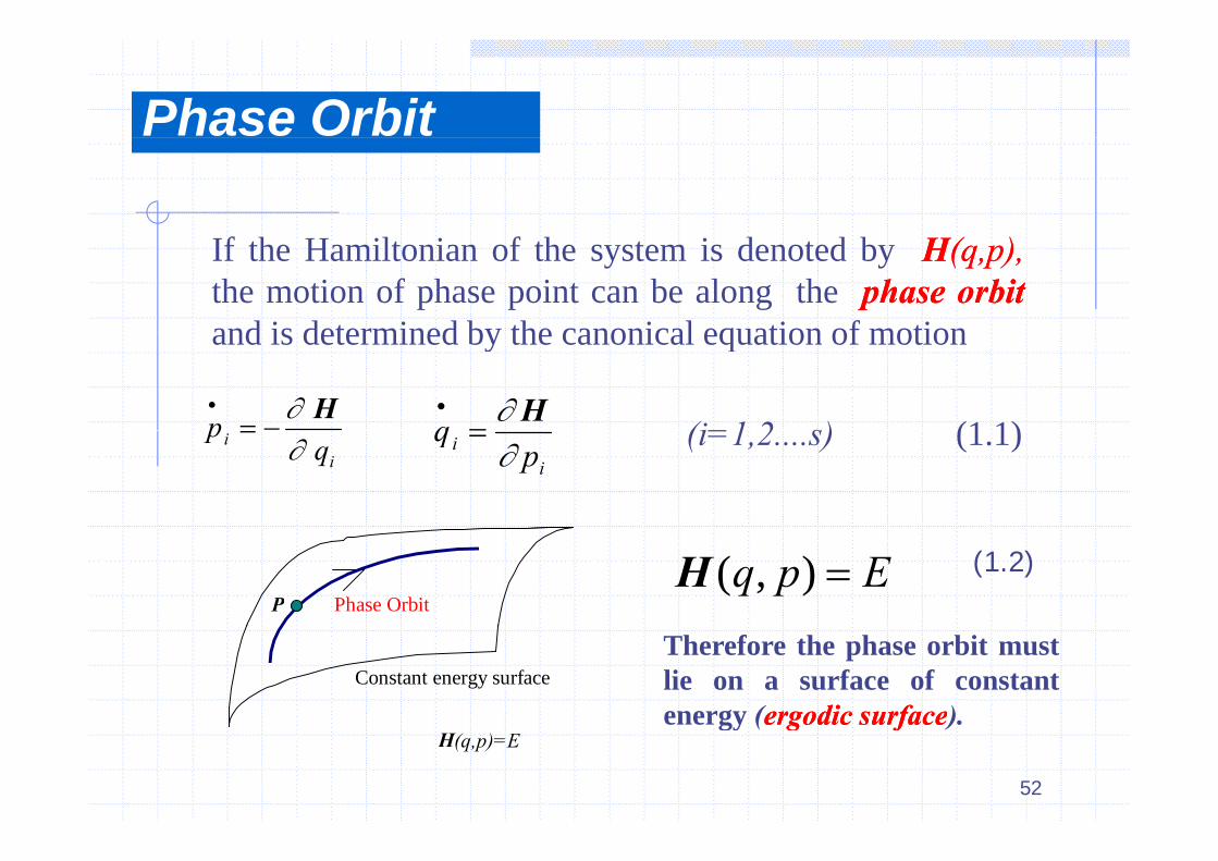
If the Hamiltonian of the system is denoted by HH(q,p),(q,p),the motion of phase point can be along the phasephase orbitorbitand is determined by the canonical equation of motionand is determined by the canonical equation of motion

p H

q H

(i=1 2 s) (1 1)i

i qp

ii p

q

(i=1,2....s) (1.1)

P Phase Orbit Epq ),(H (1.2)

Constant energy surface

Therefore the phase orbit mustlie on a surface of constantenergy (ergodicergodic surfacesurface).

52

H(q,p)=E energy (ergodicergodic surfacesurface).

- space and -space space and space

Let us define spacespace as phase space of one particle (atom or molecule)Let us define -- spacespace as phase space of one particle (atom or molecule). The macrosystem phase space (--spacespace) is equal to the sum of -- spacesspaces.

The set of possible microstates can be presented by continues set of phaseThe set of possible microstates can be presented by continues set of phase points. Every point can move by itself along it’s own phase orbit. The overall picture of this movement possesses certain interesting features, which are best appreciated in terms of what we call a density functiondensity functionwhich are best appreciated in terms of what we call a density functiondensity function(q,p;t).(q,p;t).

This function is defined in such a way that at any time tt, the number of y y ,representative points in the ’volume element’’volume element’ (d(d3N3Nq dq d3N3Np)p) around the point (q,p)(q,p) of the phase space is given by the product (q,p;t) d(q,p;t) d3N3Nq dq d3N3Npp.

Clearly, the density functiondensity function (q,p;t)(q,p;t) symbolizes the manner in which the members of the ensemble are distributed over various possible microstates at various instants of time.

53

Function of Statistical DistributionFunction of Statistical Distribution

Let us suppose that the probability of system detection in the volume dddpdqdpdqdpdp11.... dp.... dpss dqdq11..... dq..... dqss near point (p,q)(p,q) equal dw (p,q)= dw (p,q)= (q,p)d(q,p)d..The function of statistical distributionfunction of statistical distribution (density function) of the system over microstates in the case of nonequilibrium systems is also depends on time. The statistical average of a given dynamical physical quantity f(p,q)f(p,q)is equalq

pqddtpq

pqddtpqqpff

NN

NN

33

33

);(

);,(),(

(1.3)

pqddtpq );,(

The right ’’phase portrait’’’’phase portrait’’ of the system can be described by the set of g p pp p f y y fpoints distributed in phase space with the density . This number can be considered as the description of great (number of points) number of systems each of which has the same structure as the system under

54

systems each of which has the same structure as the system under observation copies of such system at particular time, which are by themselves existing in admissible microstates

Statistical EnsembleStatistical Ensemble

Th b f i ll id ti l t di t ib t d lThe number of macroscopically identical systems distributed alongadmissible microstates with density defined as statisticalstatistical ensembleensemble. Astatistical ensembles are defined and named by the distribution functionwhich characterizes it. The statisticalstatistical averageaverage valuevalue have the samemeaning as the ensemble average value.

A bl i id b i if d d d li i lAn ensemble is said to be stationary if does not depend explicitlyon time, i.e. at all times

(1 4) t

0

Clearly for such an ensemble the averageaverage valuevalue <f><f> of any physical

(1.4)

Clearly, for such an ensemble the averageaverage valuevalue <f><f> of any physicalquantity f(p,q)f(p,q) will be independentindependent ofof timetime. Naturally, then, a stationaryensemble qualifies to represent a system in equilibrium. To determine thei d hi h E (1 4) h ld h k h

55

circumstances under which Eq. (1.4) can hold, we have to make a ratherstudy of the movement of the representative points in the phase space.

Lioville’s theorem and its consequencesLioville s theorem and its consequences

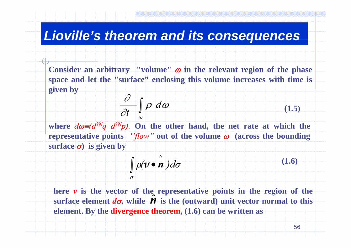
C id bit " l " i th l t i f th hConsider an arbitrary "volume" in the relevant region of the phasespace and let the "surface” enclosing this volume increases with time isgiven by

dt

(1.5)

h dd ((dd33NN dd33NN )) O th th h d th t t t hi h thwhere dd((dd33NNqq dd33NNp)p).. On the other hand, the net rate at which therepresentative points ‘’flow’’‘’flow’’ out of the volume (across the boundingsurface ) is given by

)dσ(ρσ

nν (1.6)

here v is the vector of the representative points in the region of thesurface element d, while is the (outward) unit vector normal to thisl B h di h (1 6) b i

n

56

element. By the divergence theorem, (1.6) can be written as

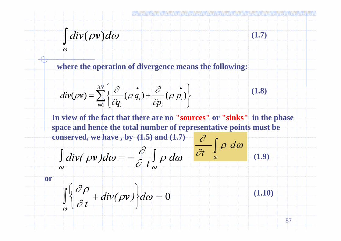
ddiv )( v (1.7)

ddiv )( v ( )

where the operation of divergence means the following:

N

di3

)()()( (1.8)

where the operation of divergence means the following:

ii

ii

i

pp

qq

div1

)()()(

v (1.8)

In view of the fact that there are no "sources" or "sinks" in the phase pspace and hence the total number of representative points must be conserved, we have , by (1.5) and (1.7)

ddiv d( )

v t d (1.9)

dt

t

div d( )v 0 (1.10)

or

57

t

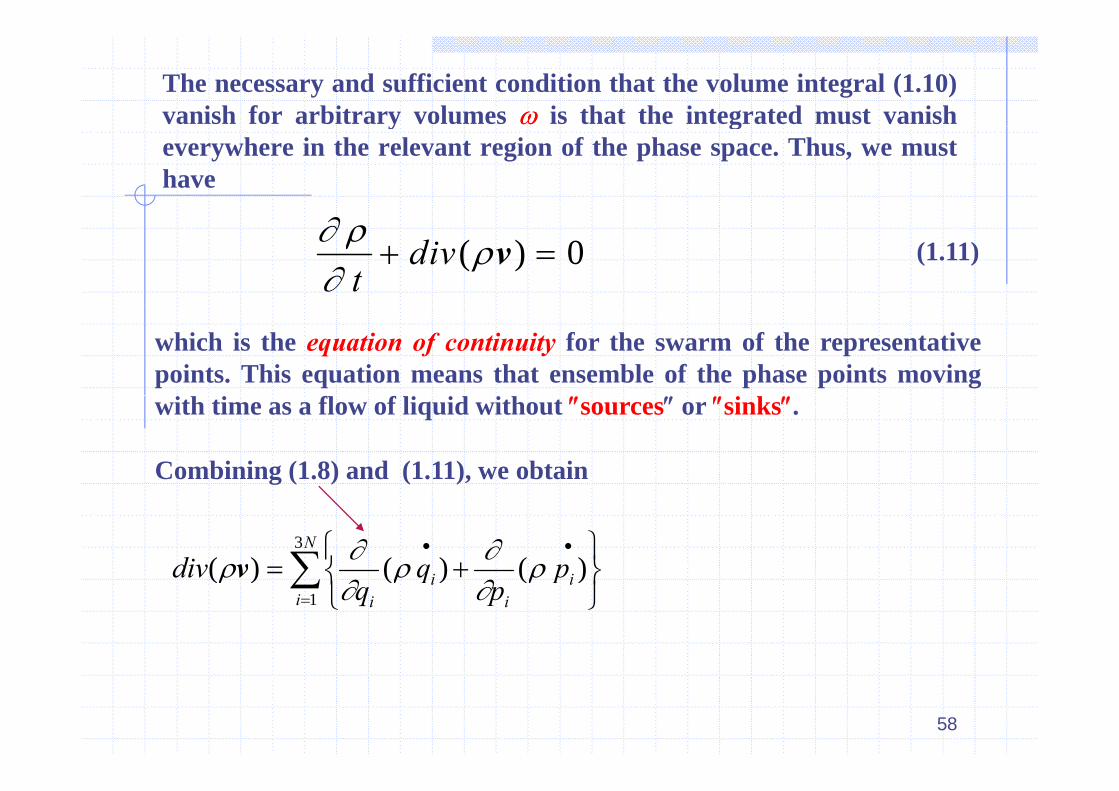
The necessary and sufficient condition that the volume integral (1.10)vanish for arbitrary volumes is that the integrated must vanishy geverywhere in the relevant region of the phase space. Thus, we musthave

t

div ( )v 0 (1.11)

which is the equation of continuity for the swarm of the representativepoints. This equation means that ensemble of the phase points movingwith time as a flow of liquid without sources or sinks.

Combining (1.8) and (1.11), we obtain

N

ii pqdiv3

)()()( v

ii

ii

i

pp

qq

div1

)()()(

v

58

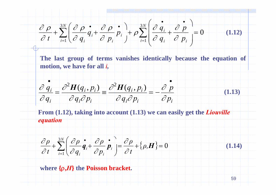
0 33

Ni

N pq (1 12)0

11

i ii

i

ii

ii

i pp

qqp

pq

qt

(1.12)

The last group of terms vanishes identically because the equation ofmotion, we have for all ii,

qq

q pq p

q pq p

pp

i i i i i

2 2H H( , ) ( , ) (1.13)

q q p q p pi i i i i i

From (1.12), taking into account (1.13) we can easily get the Liouville equationequation

3

ρρρρ N 0

1

Hpq ρ, tρ

pρ

q ρ

tρ

ii

ii

i

(1.14)

59

where {,H} the Poisson bracket.

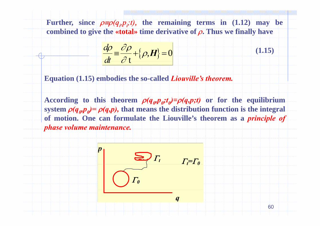
Further, since (q(qii,p,pii;;t)t),, the remaining terms in (1.12) may becombined to give the «total» time derivative of . Thus we finally have

ddt

t

,H 0 (1.15)dt t

Equation (1.15) embodies the so-called Liouville’s theorem.

According to this theorem (q0,p0;t0)=(q,p;t) or for the equilibriumsystem (q0,p0)= (q,p), that means the distribution function is the integraly q0 p0 q p gof motion. One can formulate the Liouville’s theorem as a principle ofphase volume maintenance.

t

p

t=0

0

t 0

60

q

Density matrix in statistical mechanicsy

The microstates in quantum theory will be characterized by a (common) Hamiltonian, which may be denoted by the operator. At time

H

tt the physical state of the various systems will be characterized by the correspondent wave functions (ri,t), where the rri,i, denote the position coordinates relevant to the system under studycoordinates relevant to the system under study.

Let k(ri t) denote the (normalized) wave function characterizing theLet (ri,t), denote the (normalized) wave function characterizing the physical state in which the kk--thth system of the ensemble happens to be at time tt ; naturally, k=1,2....Nk=1,2....N. The time variation of the function k(t) will be determined by the Schredinger equation

61

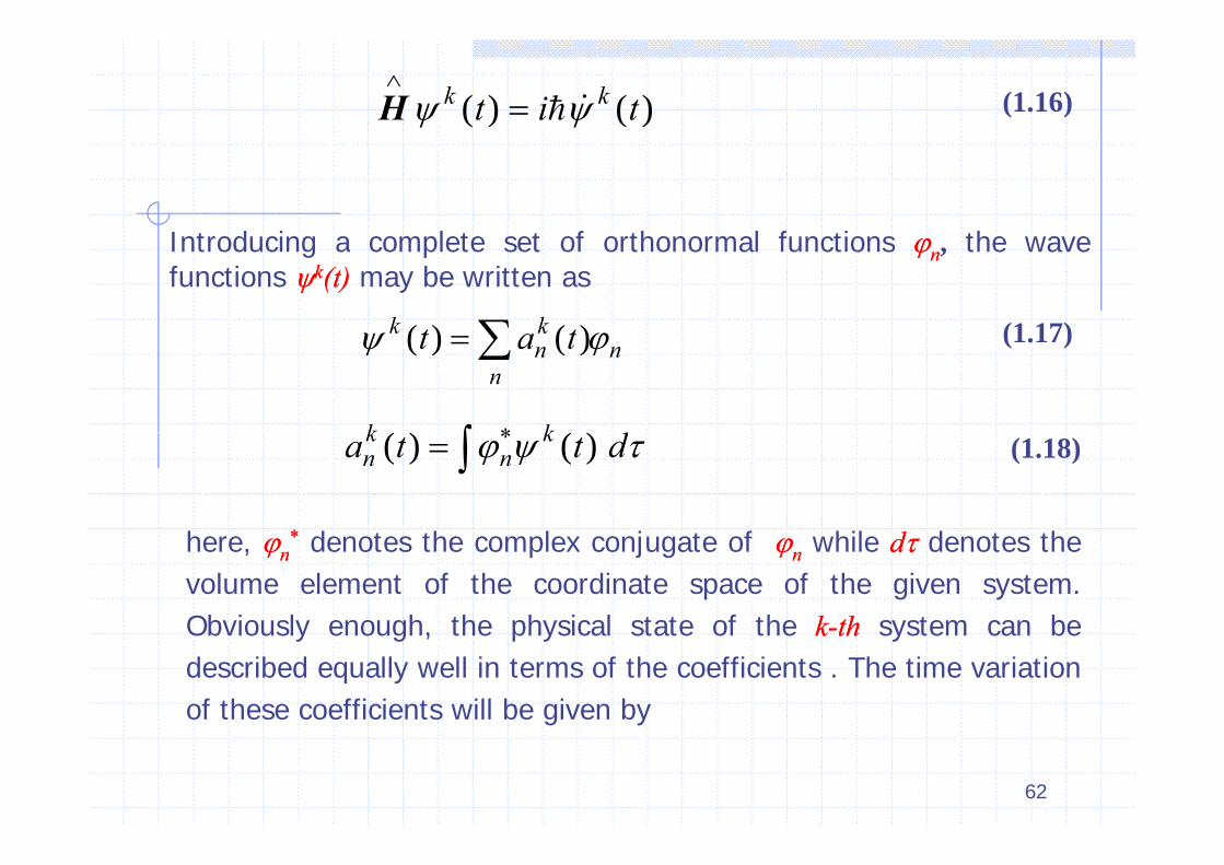
H

k kt i t( ) ( ) (1.16)

Introducing a complete set of orthonormal functions the wave

k kt a t( ) ( )

Introducing a complete set of orthonormal functions nn, the wavefunctions kk(t)(t) may be written as

(1 17) nn

nt a t( ) ( ) (1.17)

dk k( ) ( )a t t dnk

nk( ) ( ) (1.18)

h ** d h l j f hil d hhere, nn** denotes the complex conjugate of nn while dd denotes the

volume element of the coordinate space of the given system.Obviously enough the physical state of the kk--thth system can beObviously enough, the physical state of the kk--thth system can bedescribed equally well in terms of the coefficients . The time variationof these coefficients will be given by

62

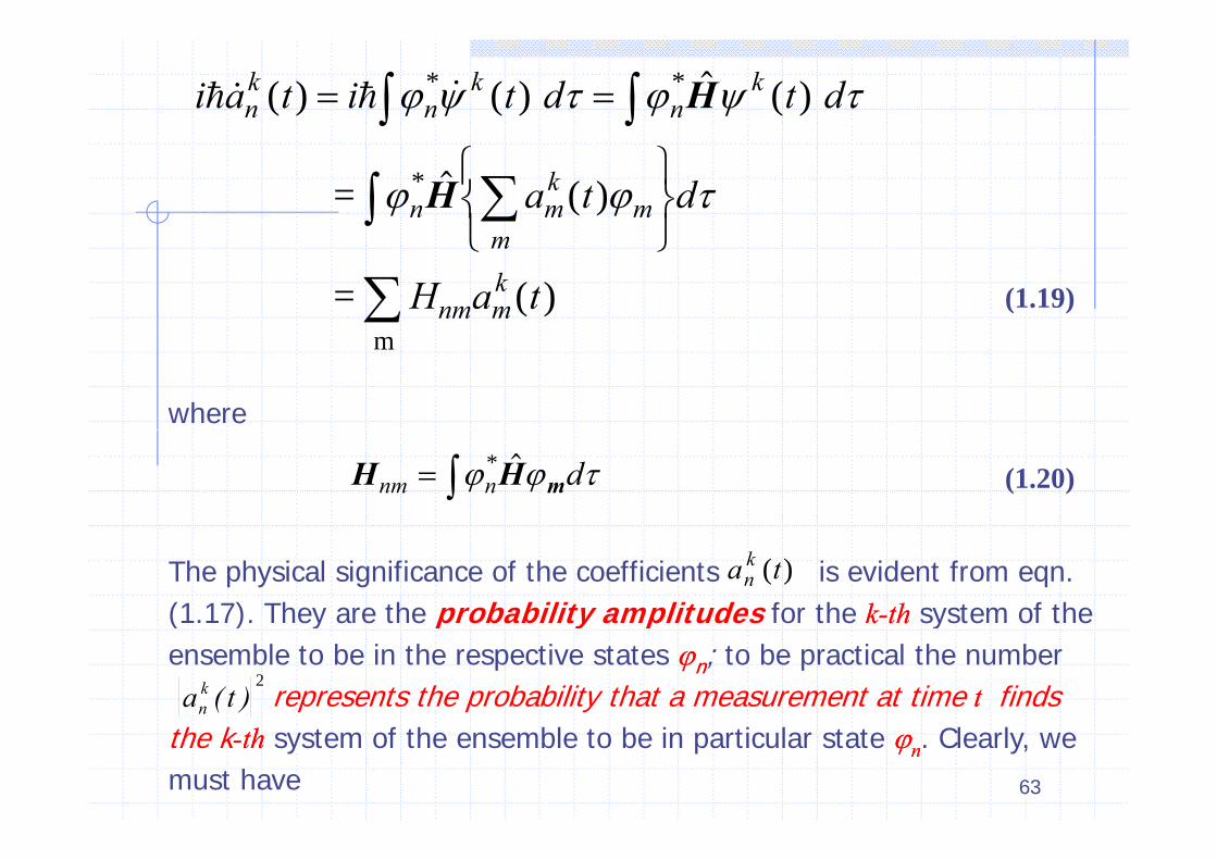
i a t i t d t dnk

nk

nk ( ) ( ) ( )* * H

a t dn mk

m ( )*

= H

H a tm

nm mk ( )

= (1.19)m

where

H H mnm n d * (1.20)

The physical significance of the coefficients is evident from eqn. (1.17). They are the probability amplitudes for the kk--thth system of the

a tnk ( )

( ) y p y p yensemble to be in the respective states nn; to be practical the number

represents the probability that a measurement at time t t finds a tnk ( )

2

63

the k--thth system of the ensemble to be in particular state nn. Clearly, we must have

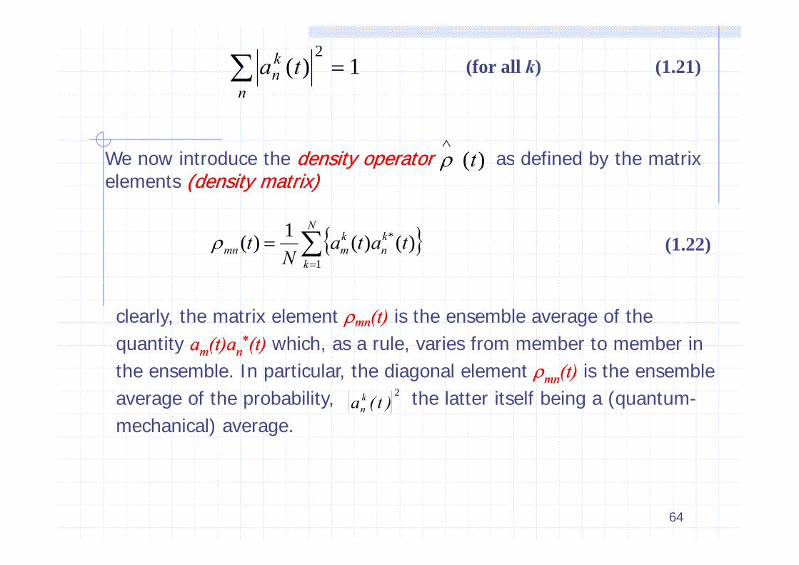
a tnk ( )

21 (for all k) (1.21)

n

We no int od e the densitdensit ope atoope ato as defined b the mat i

( )tWe now introduce the densitydensity operatoroperator as defined by the matrixelements (density(density matrix)matrix)

( )t

N

k

kn

kmmn tata

Nt

1

* )()(1)( (1.22)

clearly, the matrix element mnmn(t)(t) is the ensemble average of the quantity aa (t)a(t)a **(t)(t) which as a rule varies from member to member inquantity aamm(t)a(t)ann (t)(t) which, as a rule, varies from member to member in the ensemble. In particular, the diagonal element mnmn(t)(t) is the ensemble average of the probability, the latter itself being a (quantum-a tn

k ( )2

mechanical) average. n ( )

64

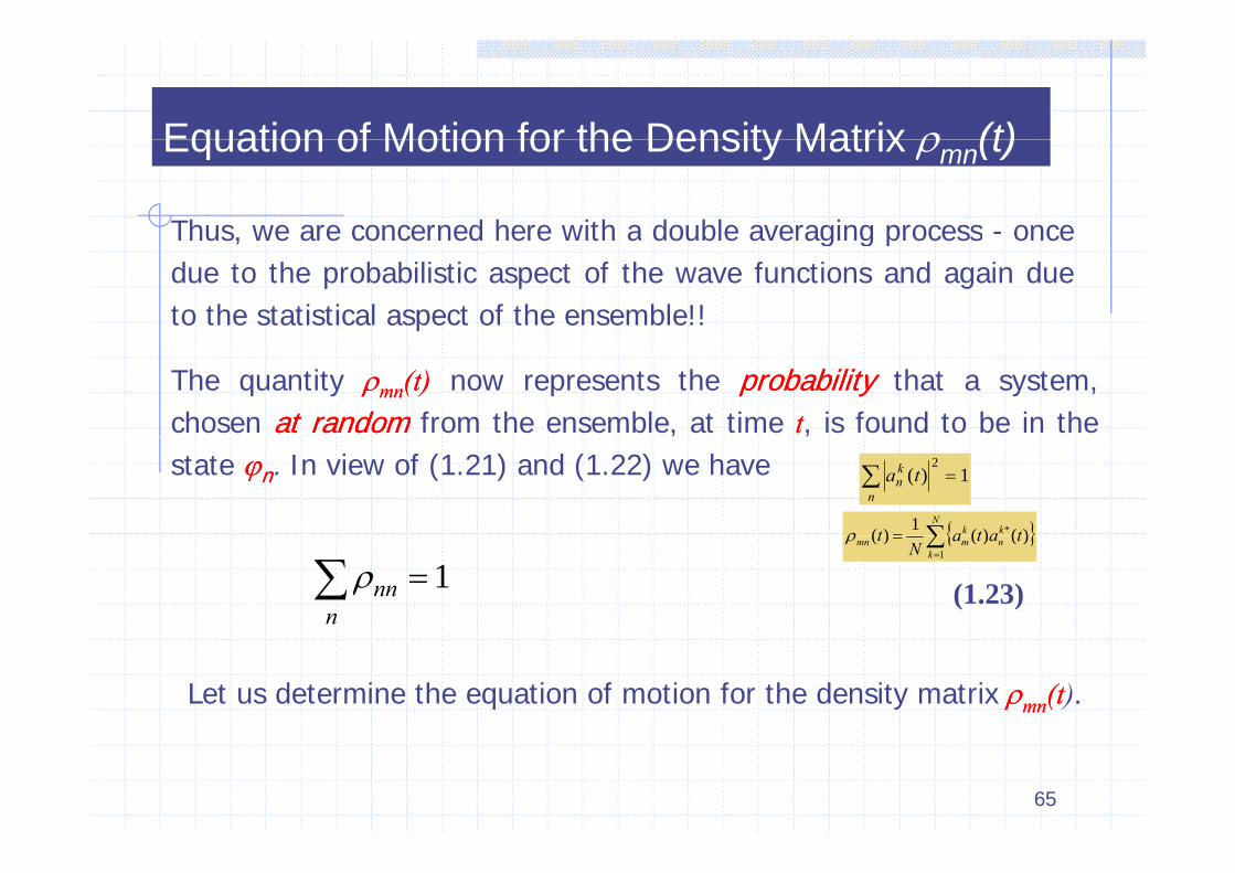
Equation of Motion for the Density Matrix (t)Equation of Motion for the Density Matrix mn(t)

Thus, we are concerned here with a double averaging process - onceThus, we are concerned here with a double averaging process oncedue to the probabilistic aspect of the wave functions and again dueto the statistical aspect of the ensemble!!

The quantity mnmn(t)(t) now represents the probabilityprobability that a system,chosen atat randomrandom from the ensemble, at time tt, is found to be in the

a tnk

n( )

21

, ,state nn. In view of (1.21) and (1.22) we have

N

kk tatat * )()(1)(

nnn

1 (1.23)

k

nmmn tataN

t1

)()()(

Let us determine the equation of motion for the density matrix mnmn(t(t).

65

i tN

i a t a t a t a tmn mk

nk

mk

nk

N ( ) ( ) ( ) ( ) ( )* * 1 N

H a t a t a t H a t

mn m n m nk

ml lk

nk

mk

nl lk

N

( ) ( ) ( ) ( ) ( )

( ) ( ) ( ) ( )* * *

11

=

N

H t t H

mll

l n m nll

lk

ml mll

( ) ( ) ( ) ( )

( ) ( )ln ln

1

=l

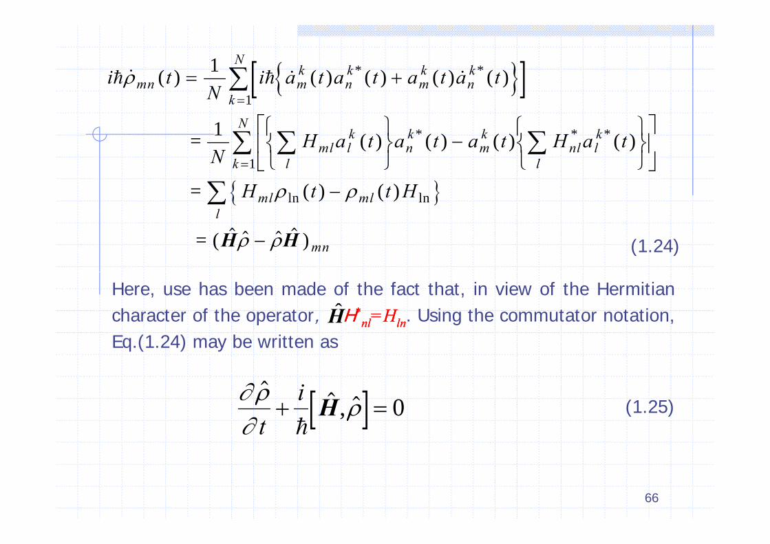
mn ) = (H H (1.24)

Here, use has been made of the fact that, in view of the Hermitiancharacter of the operator, HH**

nlnl=H=Hlnln. Using the commutator notation,HEq.(1.24) may be written as

i

, t

i

H 0 (1.25)

66

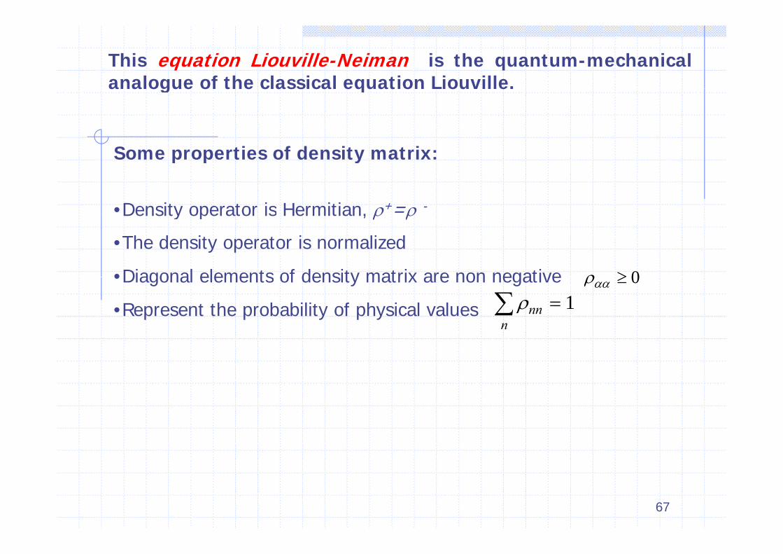
This equation Liouville-Neiman is the quantum-mechanicalanalogue of the classical equation Liouville.analogue of the classical equation Liouville.

Some properties of density matrix:Some properties of density matrix:

•Density operator is Hermitian, += -Density operator is Hermitian,

•The density operator is normalized

•Diagonal elements of density matrix are non negative 0•Diagonal elements of density matrix are non negative

•Represent the probability of physical values nnn

1 0

67