SPM/Conn Coursesarakimmich.weebly.com/.../spmconncoursenotes.pdf · SPM/Conn Course Kimmich 2014 Overview Direct questions throughout course to : [email protected] In connectivity,

SPM/Conn Course

Kimmich 2014

Overview Direct questions throughout course to : [email protected] In connectivity, particularly resting state, the preprocessing is essentially the same but

you use a band instead of a high­pass filter regression is a question of understanding the influence of one brain area on another

remote area Workflow: 1) preprocessing 2) right model 3) second level processing (group diff)

You can also manually alter the Conn data preprocessing pipeline, I believe from >>Functional: >options

MUST use SPM 12 for Conn 14 because the spatial normalization is much better (done by John Ashburn)

ensures that the stats in group space are registered so that the areas are additively modulated when subjects are put together (rather can canceling out from blurry lines creating false negatives at the group level)

Doing first level processing up to spatial normalization in negative space, then do spatial register at an individual level before moving to group levels

turns out, it doesn’t really matter, the resolution of our data is worse than both methods. You’re pretty much going to get the same answers either way

with patients with lesions, you’ll need to do everything in negative space because normalized images aren’t valid for those populations

if you are doing seed to voxel or roi with conn in native space, then those have to be defined in native space

Regional Specialization

subjects engage in tasks which differ, then use subtractive logic to isolate those brain processes (difference of activity pattern gives the regional specialization)

this was conceived in reaction times, from the chronoscope around 1850 most of these experiments were redone when fMRI became available, so the

subtractive logic stuck (broadway show that no one is buying tickets for anymore) Regional Interaction

the brain is a model of regional areas that interact with each other (functional connectivity and effective connectivity)

functional: based on correlations between brain areas bivariate correlation multivariate modeling (PCA, ICA, PLS)

effective: modeling directed influences psychophysiological interaction (PPI)

interesting bridge between resting and task based analysis mediation analysis structural equation modeling (SEM) multivariate autoregressive modeling (Granger causality) dynamic causal modeling (DCM)

1

SPM/Conn Course

Kimmich 2014

There is a difference in the experimental strategies too, effective connectivity crowds don’t tend to try to get huge Ns, while some functional researchers do

Preprocessing

NOTE: Conn calls on previously developed SPM models to do these corrections, and as SPM improves, Conn improves without any additional effort

Slice Timing Correction Slice Timing Problem: In clinical scanners (Echo Planar Imaging), that

were really initially designed for structural scanning: machines image slice by slice, which takes about 60­80 milliseconds per slice (2­3 seconds from top to bottom of brain

our statistical models all assume that the data were collected at the same time

Interleaved Acquisition: slice order is 1,3,5 down then 2,4,6 up, the only way to get reasonable data early on in the field’s conception

Problem: if someone moves their head, you will get a herringbone pattern (those stripes in the data you see sometimes) and it can’t be reconstructed

Two approaches to Slice TIming Correction: Addition of Temporal basis functions to the first­level statistical

model Correction using temporal interpolation

TR: Time it takes to get from top slice to bottom slice, and we are only at 1 of about 5 slices at any given time, which is 2% of the brain

you have to use a reference slice to create a linear interpolation of a weighted sum for a given voxel, which means that literally 98% of the brain data is a model, made up from probability, not data collected

with BOLD signal, temporal smoothness is about 3 seconds, so not a big problem with TRs of less than that

this is a very serious problem with long TRs, because it exceeds temporal smoothness

Multiband EPI ­ takes several slices at once, and can really help with both spatial resolution and temporal smoothing

need field of 3T or above, with high channel coil (16 or above, more is better)

With low coils, you have to trade off TR with spatial resolution because you have to use larger slices

sometime soon there may be real echo planer imaging which will be way better

2

SPM/Conn Course

Kimmich 2014

Solution: a python script which does head motion and slice time correction at the same time

great masters: do slice time then head motion then head motion and slice time and see the difference

good paper to read: Sladky et al. Neuroimage (2011) When is the best time to do slice timing?

Depends on amount of head motion: lots of movement: realignment then slice timing correction low movement: slice timing correction then realignment

super cool: apparently snipers have no movement because they’ve learned to keep their head still even with respiratory and cardiac motion

Geometric Distortion Correction Collect information about residual magnetic distortion, the you should be

able to know the differences between structural and functional scans and use that information to unwrap them before moving to standard space

Field map correction helps to remove the distortions (often the brain is elongated)

Head Motion Correction (all these slides come from FIL Methods Group) motion effects on signal amplitude are nonlinear and complex task correlated motion is particularly problematic Mitigation Methods

prevention prospective correction

online motion correction from the scanner itself: don’t use, they don’t work

realignment spatial realignment requires registration and reslicing even after alignment there can be a considerable amount

of variance still from data movement between and within slice acquisition interpolation artifacts due to resampling non­linear distortions and drop­out due to magnetic

distortion covariate correction with head motion estimates

Fiston et al. wrote a good paper on this this is a standard way in spm to handle task­based motion

if head motion and task are correlated, then if you add regressors, it will take out brain data correlated to task activation too (takes away beta, also throughs of t stats because denominator gets huge)

you can use unwarp correction instead of covariate correction to take care of this

3

SPM/Conn Course

Kimmich 2014

movement­by­distortion interactions orbitofrontal cortex is very likely to have head­movement

distortion, and unwrap correction will be able to remove that head motion while maintaining results in back of head, where there was low movement (regional correction)

Temporal FIltering Intensity Normalization Spatial Filtering

fMRI Quality Assurance: Task and Rest

Processing Pre Processes Artifact Check

check registration check motion parameters generate design matrix template check for stimulus correlated motion (only for task) check global signal correlation with task review power spectra (most resting state is 1/f, so cut off is about .1

Hurtz) detect outliers in time series:motion: determine scans to omit interpret or

de­weight add a covariate for each artifact scrubbing is another option (physically deleting those timepoints,

much better to do covariates) GLM Artifact Check

review statistics (Mask/Resms/etc.) RFX Artifact Check Conn

Artifact Detection Global mean (time series top) Std. Dev. from mean (time series bottom) Movement in mm (motion) (movement top) Movement in radians (rotation) (movement bottom)

Setting thresholds click ‘use differences’ at the top, then it takes the difference from

the time point right before, not the first timepoint z­threshold 3

you may need to bump up the z­threshold to keep exclusions around 10­20%

movement threshold 5

4

SPM/Conn Course

Kimmich 2014

rotation threshold .5 All outliers will be shown at the bottom

global signal is just as important as motion, look at both Art tool saves two regressors:

art_regression_outliers_sw2brun1_001.mat art_regression_outliers_and_movement_sw2brun1_00

1.mat always use this one for resting state data

in art, make sure to file > save the spm regressor file View in Movie Format

Art_movie (lets you look at things on a slice by slice basis) Spm_movie (cycles through all the scans on a particular slice

plane Residual Movement Related Variance

Sources movement­x­susceptibility­x­distortion interaction (unwarp) movement­x­susceptibility­x­dropout interaction spin­history effects inter­volume movement Goal

maximize sensitivity to true activations while minimizing false activation

Solution include motion parameters in design which removes variance from

all of these and can increase sensitivity many subjects in block design exhibit stimulus related

motion, this is les of a problem in vent­related designs (Johnstone, HBM 2006)

some groups (clinical) will tend to move more than the other, this can help with that

Stimulus Correlated Motion (SCM) Collect field maps then do distortion regression (regresses regionally to

correct the data) Power Spectra: HPF Cutoff Selection (resting state 1/f) Masking

Masking takes place at first and second level in the top down (review stats)

Mask/ResMS/RPV How do you know?

artifacts in Beta, contract, Tmaps and ResMS images missing activation activation cut

5

SPM/Conn Course

Kimmich 2014

SPM MAsk Image: Binary mask of “in brain voxels” to be included in statistical analysis (in best of world you’d get a perfect binary mask that is white around the whole brain) its supposed to (SPM now lets you do this through ART directly as well

SNR Profiles shows the signal for coils/where in brain

when you visualize this in the actual scan, sometimes you can loose parts in the very center of the brain (loss of t value in putamen, thalamus, basal ganglia etc.)

Areas of the brain which contain iron diffuse faster, so they sometimes loose t­value

the threshold is at 80% of the mean (Christina Triantafyllou) There is a brain mask in SPM (its in EEG) that you can use SPM does NOT allow for missing voxels AT ALL

Flex GLM is a second level processing program run through SPM that will allow this, so that you only have decreased power and don’t have to lose someone

but now, you have runs of different length, so that changes your beta (the more images you throw away, the less certain you are about the true Beta, but the more normal your distribution will be)

Keep threshold the same OR maintain amount of outliers removed: some argue throw away the worst 10% for all members, which means you’ll have to choose the specific z­threshold that gives you that many timepoints no matter their movement

Global Signal is NOT normally distributed Is Regressing Motion enough?

Power et al. (Neuroimage, 2012) showed positive effects of scrubbing also has really good examples of motion differences with age

Solutions for Resting State Movement Reject Outliers

linear regression Match Groups AnCovas

Interpretations of Literature (what you need to pay attention to) Age

DMN develops with age (MPFC­PCC becomes more coupled over time) and declines in elderly

BUT DMN coupling in children might be hidden because their is more movement, and the correlation gets regressed out with the movement

6

SPM/Conn Course

Kimmich 2014

anterior to posterior networks don’t show up because they are moving more

Regressing outliers drastically increases anticorrelations in older brains (Gabrieli suggests that elderly brains have less anticorrelation of prefrontal cortex with DMN)

Clinical Populations tend to have more movement

Analogous to astronomy, resting state are like the people interested in dark matter USING ART

The z­threshold in the threshold is mm, so 3 is 3 mm movement USING CONN

fMRI heat maps are representatives of R values of temporal synchrony R values continue to build over time, max asymptote around 15 min other networks likely haven’t been detected because scans are typically so short

CompCor Approach (Behzadi et al 2007) Noise effects are not distributed homogeneously across brain. Compared to

previous methods that subtract global signal across brain, this method is more flexible in its characterization of noise. It models in the influence of noise as a voxel­specific linear combination of multiple empirically­estimated noise sources

Covariates First Level Covariates

add in the realignment THEN add in a derivative of the realignment Second Level Covariates

You can add these at any time and go straight to second level analysis REMEMBER: it’s a vector, must be same n as subject number entered

initially Options

Suggest to click the seed­to­voxel r­maps so that you can show the mean r maps in addition to the z maps

Preprocessing When you are looking at the distributions of correlation coefficients, you see the

BOLD values i the grey, and the corrected values in the blue GLM Defining Confounds

CSF: Make derivatives 0 and dimensions (3­5) Band­pass filters (Hz) ­ set to .01­.1

Analyses First­level analysis, the connectivity threshold of the brain is an R­Value Second­Level Analysis Results ­ the threshold of the brain is a P­Value

Results Specification of Second Level Results

1) Select “All” in the subjects list: test connectivity across all subjects

7

SPM/Conn Course

Kimmich 2014

2) Select both “Group A” and “Group B”, contract of [1,­1] Seed­to­voxel results explorer exports the defined second­level model to SPM

(second­level SPM.mat, beta and contract volumes are saved in the results/second level folder)

ROIS IMPORTING FREESURFER ROIs

if you can find the text file that has the labels, but you have to choose the subject­specific file tht was defined for each individual

If doing surface based analysis ­ if you export the mask form the second level analysis in Conn, this can be imported and used as an ROI file in COnn, this mask will be used to project onto each subject’s cortical surface

BUT only works if you originally have freesurfer data for each subject

SIMULATIE GSR

in ROI, you can run with “regress out covariates” checked for Grey, white, and CSF (this will be the same essentially as GSR, then run without to compare ­ absolutely do this before sending to reviewers

Loading ROIS you can load an ROI set into the CONN Directory File for that version and

those will load automatically for all data sets opened through that conn source after that

you know which file it is by stating “which conn” in matlab you can also view the art file same way: “which art” ­ after stating

the conn directory file in set path Calculator

in the top right corner, there is a button called “tools” click on that and it gives you a calculator where you can view basic graphs of the data for individual ROIs (they look a lot like SPSS outputs)

Options

Analysis Units ­ you may need to change this if the preprocessing has been done elsewhere and loaded in

On Right side ­ you can also make a confound corrected time series through this Denoising

In Analysis Type:Defaults to Dynamics Connectivity (Weighted GLM) but now you can now do a task based PPI analysis (at bottom left)

PPI will allow you to enter a vector rather than an onset ­ you have to create a first level covariate with the vector

Allowing Multiple Dimensions:

8

SPM/Conn Course

Kimmich 2014

Set Confounds > Derivatives Order > 1 (you can use this for motion, and you can add this whether or not you’ve done art first, but there isn’t really a need because you won’t have to be putting in motion as a covariate

Dimensions 5 > this allows different subsets of voxels to vary independently, which means that you can get spatial components in the white matter that are related to differences in coil sensitivity, just from noise from a single coil, but its not apparent when looking at the whole brain analysis.

This is why compcore might work better than just a global repressor

you have have up to 24, and it does help, but you do lose degrees of freedom

better to start with a baroque model, then to reduce down as far as you can while maintaining the variance, its better science

Also helps to look at things in denoising and get a less biased idea of how good your data is (it’s easy to become too hypothesis driven in second­level analysis)

Second Level Analysis when you press “seed to voxel” button on top, it will open a new window with the

explorer, which shows a map and gives you the p­values ­ this is the great place to export and move into another stats file

Its defined by brodmann's areas, in the right hand table you can see the percentage of coverage of a particular area

Explore Clusters ­ bottom right corner ­ this will take the mean z­value for each cluster that are significant

you’ll see the mean effect size as a bar, then also show you the spatial image in the bottom right

the mean z­value for individual subjects for a given cluster is on the bottom left corner

Movement usually looks like rings of correlated activity on the outer edges of the brain

Viewing Conn Updates from Alfonso (Conn Change Log) Just go into matlab and write m.m and it should pull up all updates with dates

modified Second Level Analysis Features

ROI to ROI explorer, not very important to input ROIs in advance, but VERY Important for seed to voxel

REX

9

SPM/Conn Course

Kimmich 2014

you can load in rex directly from matlab, you can do it concurrently from Conn and use those files for a slightly different analysis

REX ­ select rois and you can get the mean value for that RIO for any or all files, save it as a text file and extract

COMPARING TIME COURSES rex can allow you to get the individual­level time course for two different

networks and compare them ­ get for anti correlation analysis good to do this after creating each subjects r or z map OUTPUT THESE FILES ­ for publication level graph, you can read

in the rex outputs into R or into SPSS ­ much better than the basic rex output graph

Conn is very good at understanding spatial distributions, but to get at inter and intra­network analysis, we need better workflows. rex > SPPS or R may be best

Plotting Time Series in Rex enter the denoised time series after fon (SW... files) then you can choose the roi that you are interested in Choose Extract Mean this should output the individual timepoints, and then you can take that

output file and load it into a workspace with a better graphical interface Subject Z maps

to find where the files are for the z­maps for every subject, load this into matlab >> load SPM.mat >> SPM.xY.VY.fname

Checking Anticorrelations Save the file output from second level analysis save in a clearly marked file ..rex open this file (cluster image of the paired t­test for the two groups) extract z values from cluster for each ROI

extract to understand if pos/neg/or anticorrelated, understand that the

mean is driven by the correlations (a histogram can more clearly show this, if you export

Getting new Covariates from Analyzed Data

Downloading the ResultsROI for a given condition will allow you t take those values into an excel/matlab/spss file and evaluate them

doing these calcs for each subject independently, you can then take those values and input them as second level covariates into the data in the Conn interface

Defining ROIs ­ theory and methods

10

SPM/Conn Course

Kimmich 2014

SPM is voxel based and ROI analyses allow to investigate the mean activity of a particular region as opposed to peak voxel

Scaling Options global scaling ­ to scale the output data based on the global mean ­ use

when you want to extract time series in units of percent signal change referenced to SPM default of 100

within­ROI scaling InCalc in SMP will let you do user­specified algebraic manipulations on a set of

images To make intersection of two images i1 .* i2 (image 1 and image 2) NOTE: You can do this same analysis in FSL MATHS, may need to convert file

to RAS from the NII file that is created through the SPM/Conn workflow an apriori hypothesis about a particular region of the brain SVC (small volume

correction) allows for the correction of multiple comparisons look at .001 corrected, which can make sure you can see if you have significance

for an apriori hypothesis xjview ­ functional ROI definition wfu_pick & Marina ­ anatomical ROI definition Small volume Correction (SVC­SPM8) Rex (ROI extraction) ­ extracting connectivity values within ROi Importance of Understanding betas/correlations

Percent Sigal Change is calculated very differently from the way it is done in AFNI for FSL, it doesn’t really matter if you are comparing to another data set from ROI

(You can use Marsbar or Rex to get comparable numbers to these other programs, as they reference to the ROI)

Voodoo correlations/Double Dipping If you do a whole brain correlation, and you have a cluster in which you plot the

peak, then try to correlate it with behavior, that’s double dipping. you can take the value then independently report it, you can’t have it

clustered and defined based on behavior False Positive control

Cross Validation Methods ­ should be across subjects, not sessions LOOCV ­ Leave one out cross validation ­ involves using a single observation

from the original sample as the validation data, and the remaining observations as the training data. This is repeated such that observation in the sample is used once as the validation data

Independent ROI Definitions (Functional and Anatomy) Anatomical Definition

RAPID, Freesurfer, WFU_PIckatlas, Marica or use from Literature (e.g. spheres around peak coordinates)

Functional Definition Independent ROI: Multiple data sets

11

SPM/Conn Course

Kimmich 2014

Second Level Analysis All second level analysis results are always saved in second level analysis

outputs, and these can be put directly into SOM NOTE: opening SPM automatically closes Conn SPM files can also be read out as images into Matlab

>> figure; imagesc (FILENAME) WHEN COMPARING GROUPS ­ highlight both covariate groups,

then put [1 ­1] right below GROUP BY CONDITION INTERACTIONS

If you’ve already put in the covariate values for Group A, to get the opposite for Group be just write All­GroupA

highlight group a and GroupB below [1 ­1]

highlight session 1 and 2 below [1 ­1], can also right click and get options

After this, if you go into ROI to ROI, you can get the ROI level group difference T values

NeuroSynth

Neurosynth.org is a great metaanalysis tool for neuro data and anatomical encylopedia can be searched in many ways, can do meta search with terms like “emotion”

and it will search the whole papers, not just the abstract to get this you can also download the meta files at .nii files and input them into your

workflow easily great to get a list of references

Special Case Second Level Analysis

f­contrast ­ anova Clinical Studies

Often times you have multiple time points and multiple covariates, and there’s often the problem of needing to pull apart collinearity

Using PPI In first level covariates you’d need to make a files that shows all scans as

individual numbers, then in conditions >>task modulation factor > condition blocks ‘covariate realignment’

THEN in first level analysis you choose >> analysis type > task modulation effects (PPI)

then you can also choose to use regression (bivariate) right below that Looking at change within scan

To interpret effect size from beginning to end of scan, you must put in a covariate which has a value for each slice of scan (I think?) then all the analysis you see

12

SPM/Conn Course

Kimmich 2014

from here can be a relationship of the percentage of voxel change during that time in the scan

Dynamic Connectivity Analysis Resting state analyses treat connectivity as a static/steady state property task related analyses compute dynamic changes in FC associated with known

task/experimental conditions Analyzing Temporal/dynamic properties of FC measures:

frequency­decomposition there is a lot of discussion as to whether there are changes in

connectivity at different HZ bands, so should run through different band windows

Higher frequencies need more investigation in resting state (there’s power under about 2 Hz)

you can do this in the denoising step BETTER: in setups > conditions>time­frequency

decomposition >> choose frequency decomposition (filter bank) and this will make different condition results for particular frequency bands

you can then run an f­test to see if there are any differences in those frequency bands

Steve Smith did some work on this having people in a scanner for over an hour

There is not yet a way to combine frequency decomposition with a sliding window

CREATING Manual Filter Manually Create Condition for each band, >>time­frequency

decomposition >>type in the HZ that you want to look at

temporal­decomposition (sliding­window) data­driven characterization of dynamic connectivity Good background papers:

Slide­Winder Clustering (allen at al. 2014, Yang et al. 2014) Dynamic Connectivity Regression (Cribben et al. 2012)

Temporal Decomposition

>>time­frequency decomposition >>temporal decomposition (sliding­window), then i will ask you for the window length that you want

the smaller your window the more noisy the data will be the bigger the window, the less robust

Typically do 40­60 second windows You typically want to set the onset of those sliding windows to the length

of your session (so if you

13

SPM/Conn Course

Kimmich 2014

if doing block condition, set the onset to the beginning of your tasks

if resting state just use the onset of the scan Data­driven characterization of dynamic Connectivity

PPI model: for any given temporal­modulation time series we can compute the associated temporal changes in FC

if you want to export just the time series of dynamic factors, yo can do so by doing first level Analysis >>temporal modulation effects and choose the factors that you want OR you can just check “estimate 1st level analysis” in the dynamic FC panel

Problem:dynamic changes in resting state FC are driven by internal/unknown factors

Solution: use iterative EM procedure to estimate these factors assume temporal­factors known and compute associated FC changes Assume FC changes known and compute associated temporal­factors Repeat the above two steps: converge to largest temporal­modulation

effects in your data For Multiple Subjects: ICA­Style approach. Concatenate Bold time series across

time. EM procedure assumes same fC changes across subjects. PPI model then estimates subject specific changes from the resulting temporal­modulation factors

ROI to ROI connectivity Matrix (the circle that comes up from second level results) Shows the increase/decrease ­ BUT remember that it shows the contrast

between them, meaning that you might get false positives if one group reduced more like an anticorrelation in the strength of correlation you’ll have one of these circle outputs for each of the factors and it will

show you changes across time Changing Nodes

Select Specific ROIS in the Define Connectivity Matrix Box Comparing Group Differences

Second Level Analysis > choose the who groups, but [1 ­1] underneath, then you’ll be able to see those effects in the circle (likely best to do p­uncorrected

for example, of covarying with age, you’ll see the overall increase of decrease of co­activity for age

Why Connectome Analyses?

Looking at entire pattern of connectivity in the whole brain Whole brain is about 250,000 2 mm voxels, about 2000 resels

voxel to voxel connections is on the order of 30 billion controlling family wise false positive level on this many connections gives very

poor sensitivity

14

SPM/Conn Course

Kimmich 2014

SOLUTION: use atlases: Brodmann's, etc. Representing Information for meaning

Hierarchical Clustering ­ ROIs that show similar connectivity effects are contiguous/near

minimum degree algorithm (RIOs that are in same subnetwork are contiguous) Reverse Cuthill Mckee Algorithm (minimize connection lengths

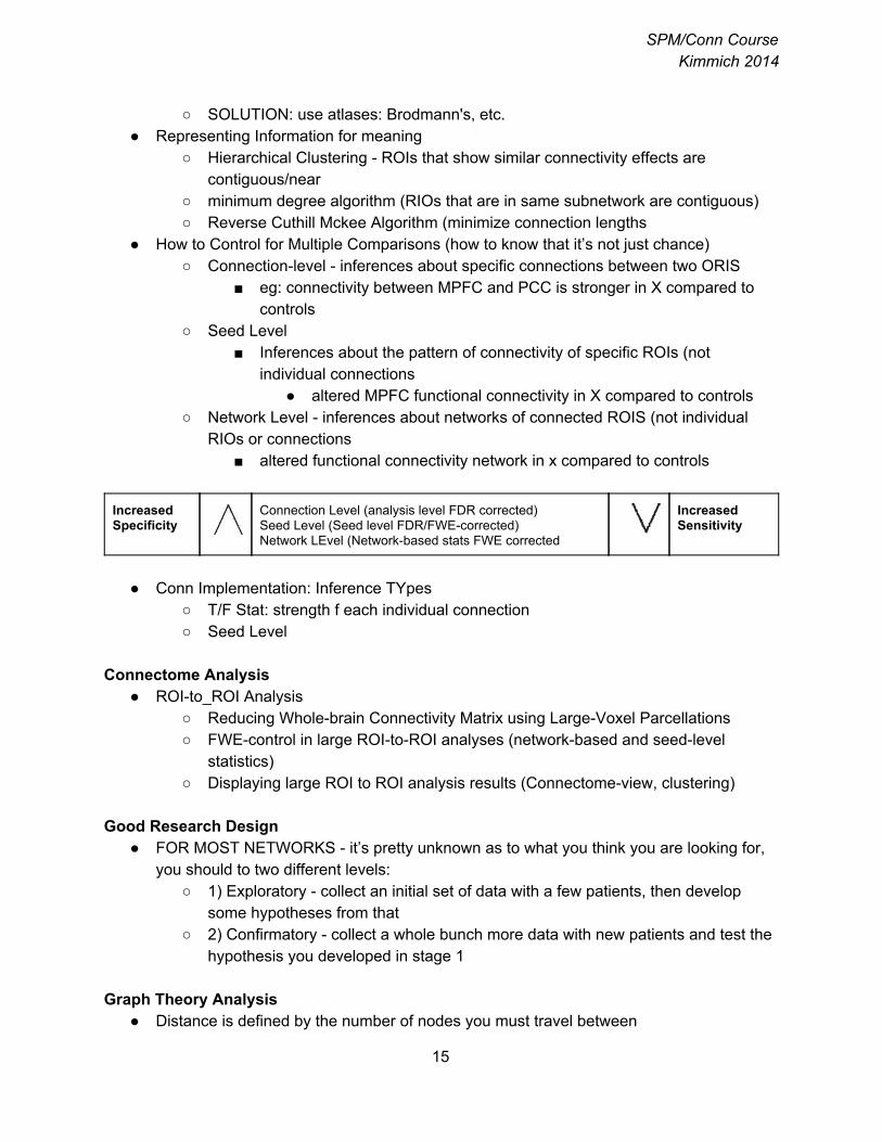
How to Control for Multiple Comparisons (how to know that it’s not just chance) Connection­level ­ inferences about specific connections between two ORIS

eg: connectivity between MPFC and PCC is stronger in X compared to controls

Seed Level Inferences about the pattern of connectivity of specific ROIs (not

individual connections altered MPFC functional connectivity in X compared to controls

Network Level ­ inferences about networks of connected ROIS (not individual RIOs or connections

altered functional connectivity network in x compared to controls

Increased Specificity

Connection Level (analysis level FDR corrected) Seed Level (Seed level FDR/FWE­corrected) Network LEvel (Network­based stats FWE corrected

Increased Sensitivity

Conn Implementation: Inference TYpes

T/F Stat: strength f each individual connection Seed Level

Connectome Analysis

ROI­to_ROI Analysis Reducing Whole­brain Connectivity Matrix using Large­Voxel Parcellations FWE­control in large ROI­to­ROI analyses (network­based and seed­level

statistics) Displaying large ROI to ROI analysis results (Connectome­view, clustering)

Good Research Design

FOR MOST NETWORKS ­ it’s pretty unknown as to what you think you are looking for, you should to two different levels:

1) Exploratory ­ collect an initial set of data with a few patients, then develop some hypotheses from that

2) Confirmatory ­ collect a whole bunch more data with new patients and test the hypothesis you developed in stage 1

Graph Theory Analysis

Distance is defined by the number of nodes you must travel between

15

SPM/Conn Course

Kimmich 2014

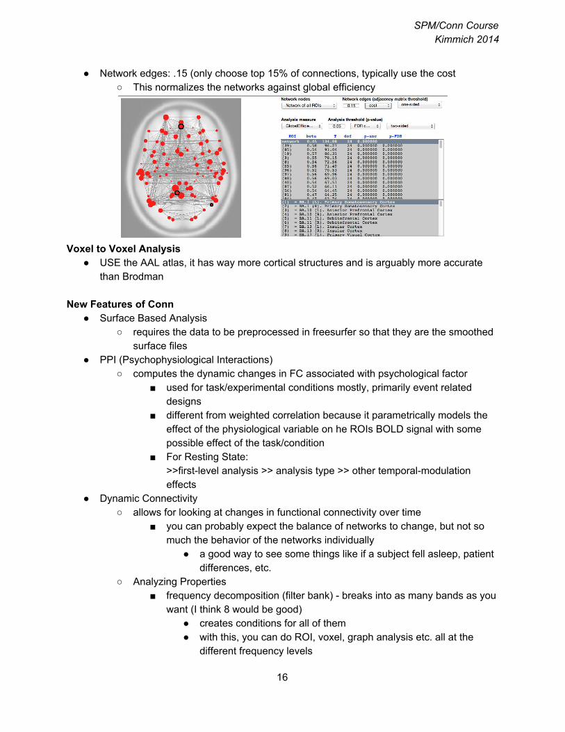
Network edges: .15 (only choose top 15% of connections, typically use the cost This normalizes the networks against global efficiency

Voxel to Voxel Analysis

USE the AAL atlas, it has way more cortical structures and is arguably more accurate than Brodman

New Features of Conn

Surface Based Analysis requires the data to be preprocessed in freesurfer so that they are the smoothed

surface files PPI (Psychophysiological Interactions)

computes the dynamic changes in FC associated with psychological factor used for task/experimental conditions mostly, primarily event related

designs different from weighted correlation because it parametrically models the

effect of the physiological variable on he ROIs BOLD signal with some possible effect of the task/condition

For Resting State: >>first­level analysis >> analysis type >> other temporal­modulation effects

Dynamic Connectivity allows for looking at changes in functional connectivity over time

you can probably expect the balance of networks to change, but not so much the behavior of the networks individually

a good way to see some things like if a subject fell asleep, patient differences, etc.

Analyzing Properties frequency decomposition (filter bank) ­ breaks into as many bands as you

want (I think 8 would be good) creates conditions for all of them with this, you can do ROI, voxel, graph analysis etc. all at the

different frequency levels

16

SPM/Conn Course

Kimmich 2014

Temporal Decomposition (in set up) create a specific condition that is related to the onsets that you

want, lets you create sliding windows Data­driven characterization of dynamic connectivity

Publishing

There’s really a problem in the field right now about be explicit about all of the choices that you make

every time that you have to choose a selection, note it making a log of your choices Cite Rizzotti and Colleagues, and Chai (Compare and anticorrelations papers)

Preprocessing and QA always explicitly address motion

always remember that the p­value only addresses the probability that you can reject the hypothesis that the two groups arre significantly different

effect size tells the difference between the samples in motion do t test on the time points you are regressing

you can match on motion and artifacts (if you have enough to throw out some), or lower the threshold

report the p­values, always, even if not significant If you keep all participants, may need to regress out time points

Dealing with low Ns anything under 15 is best to state as “exploratory” and in “need of further

analysis” and state that it is “biologically plausible” Fallacy of Large Numbers ­ in frequency statistics, no matter how small

the true difference is at the relationship to effect, there will be some sample size, approaching the limit, at which the difference is significant

Connectivity analyses balancing paper length with need to be clear with methods

write methods WHILE doing analysis Strongly suggest to write a long, detailed methods for the online

supplemental methods, then reduce that into an abstract form for the published paper

Limitations its best to clearly, and healthily state your limitations, but not enough to

undermine your main point point out the things that are limitations of every study (ex: BOLD signal

has limitations) General Biases

no reason to leave out left­handed subjects if not a language study R­Doc structure (dimension) VS. DSM*

17

SPM/Conn Course

Kimmich 2014

NIHMH s really interested in R­Doc, but other brain institutes are still interested in DSM diagnostics

TRs

if you have an experiment with different TRs when you specify TR in basic, you can specify a different TR for each

BE CAREFUL, this affects frequency bands**** for example, for TR 6, the highest frequency is 1/12

(it’s 1 over 2 over TR, so 1/2/6 = 1/12 conn will try to use the highest frequency it can, but you

have to manually check to make sure that you aren’t exceeding the maximum frequency range

ALSO, you have twice as many data points for TR 2 vs TR 6

SPM has some ways of working with these as permutation tests ­ it’s a Statistical NON­parametric model toolbox

Strongest effects of different TRs are mostly in network anti­correlations may be cognitively interesting may also just be artifacts of having the higher band frequencies

interacting with lower

18