Speed Estimation Techniques for Sensorless Vector ...etd.lib.metu.edu.tr/upload/12606863/index.pdfSPEED ESTIMATION TECHNIQUES FOR SENSORLESS VECTOR CONTROLLED INDUCTION MOTOR DRIVE

SPEED ESTIMATION TECHNIQUES FOR SENSORLESS VECTOR CONTROLLED INDUCTION MOTOR DRIVE

A THESIS SUBMITTED TO THE GRADUATE SCHOOL OF NATURAL AND APPLIED SCIENCES

OF MIDDLE EAST TECHNICAL UNIVERSITY

BY

TALİP MURAT ERTEK

IN PARTIAL FULFILLMENT OF THE REQUIREMENTS FOR

THE DEGREE OF MASTER OF SCIENCE IN

ELECTRICAL AND ELECTRONICS ENGINEERING

DECEMBER 2005

Approval of the Graduate School of Natural and Applied Sciences

_____________________ Prof. Dr. Canan ÖZGEN Director

I certify that this thesis satisfies all the requirements as a thesis for the degree of Master of Science.

_____________________ Prof. Dr. İsmet ERKMEN Head of Department

This is to certify that we have read this thesis and that in our opinion it is fully adequate, in scope and quality, as a thesis for the degree of Master of Science.

_____________________ Prof. Dr. Aydın ERSAK Supervisor

Examining Committee Members Prof. Dr. Muammer ERMİŞ (METU, EE) _______________________

Prof. Dr. Aydın ERSAK (METU, EE) _______________________

Prof. Dr. Işık ÇADIRCI (Hacettepe Unv., EE) _______________________

Assist. Prof. Dr. Ahmet M. HAVA (METU, EE) _______________________

Dr. Erbil NALÇACI (Energy Mar. Reg. Authority) _______________________

III

I hereby declare that all information in this document has been obtained and

presented in accordance with academic rules and ethical conduct. I also declare

that, as required by these rules and conduct, I have fully cited and referenced

all material and results that are not original to this work.

Name, Last name : TALİP MURAT ERTEK

Signature :

IV

ABSTRACT

SPEED ESTIMATION TECHNIQUES FOR SENSORLESS VECTOR CONTROLLED INDUCTION MOTOR DRIVE

ERTEK, Talip Murat

M. Sc. Department of Electrical and Electronics Engineering

Supervisor: Prof. Dr. Aydın Ersak

December 2005, 132 pages

This work focuses on speed estimation techniques for sensorless closed-loop speed

control of an induction machine based on direct field-oriented control technique.

Details of theories behind the algorithms are stated and their performances are

verified by the help of simulations and experiments.

The field-oriented control as the vector control technique is mainly implemented in

two ways: indirect field oriented control and direct field oriented control. The field to

be oriented may be rotor, stator, or airgap flux-linkage. In the indirect field-oriented

control no flux estimation exists. The angular slip velocity estimation based on the

measured or estimated rotor speed is required, to compute the synchronous speed of

the motor. In the direct field oriented control the synchronous speed is computed

with the aid of a flux estimator. Field Oriented Control is based on projections which

transform a three phase time and speed dependent system into a two co-ordinate time

invariant system. These projections lead to a structure similar to that of a DC

machine control. The flux observer used has an adaptive structure which makes use

of both the voltage model and the current model of the machine.

The rotor speed is estimated via Kalman filter technique which has a recursive state

estimation feature. The flux angle estimated by flux observer is processed taking the

V

angular slip velocity into account for speed estimation. For closed-loop speed control

of system, torque, flux and speed producing control loops are tuned by the help of PI

regulators. The performance of the closed-loop speed control is investigated by

simulations and experiments. TMS320F2812 DSP controller card and the Embedded

Target for the TI C2000 DSP tool of Matlab are utilized for the real-time

experiments.

Keywords: Speed estimation, sensorless closed-loop direct field oriented control,

flux estimation.

VI

ÖZ

HIZ DUYAÇSIZ VEKTÖR DENETİMLİ ENDÜKSİYON MOTOR

SÜRÜCÜSÜ İÇİN HIZ KESTİRİM TEKNİKLERİ

ERTEK, Talip Murat

Yüksek Lisans, Elektrik ve Elektronik Mühendisliği Bölümü

Tez Yöneticisi: Prof. Dr. Aydın Ersak

Aralık 2005, 132 sayfa

Bu çalışma, hız duyaçsız vektör denetimli motor sürücüsü için hız kestirim

tekniklerine odaklanmıştır. Çalışma sırasında kullanılan kestirme yöntemlerinin

kuramsal içeriklerinin detayları ayrıntılı olarak anlatılmış ve başarımları benzetim ve

denemelerle incelenmiştir.

Vektör denetim tekniği olarak, alan yönlendirmeli denetim, temel olarak dolaylı

yönlendirmeli ve doğrudan yönlendirmeli olmak üzere iki farklı yöntem ile

gerçekleştirilmektedir. Yönlendirme, rotor, stator ya da hava boşluğu akısına göre

yapılabilmektedir. Dolaylı alan yönlendirmede akı kestirmesi yapılmamaktadır.

Senkron hız tahmini için ölçülen veya kestirilen rotor hızı slip tahmininde kullanılır.

Alan yönlendirmeli denetim zamana ve hıza bağlı üç eksenli sistemlerin, hızdan

bağımsız iki eksenli sistemlere dönüştürülmesi yöntemine dayanır. Bu dönüşümler

ile DC motor denetimine benzer bir denetim yapısı elde edilir. Kullanılan akı

kestiricisi, motorun gerilim modelini, akım modelini kullanan uyarlamalı bir yapıda

olup, rotor akısının yerini yüksek doğrulukla kestirebilmektedir.

Rotor hızı durum kestirmesi yapabilen ve tekrarlamalı olarak çalışan, Kalman filtre

yöntemiyle kestirilmiştir. Rotor hızının kestirilmesinde, akı gözlemleyicisinin akı

VII

açısı kestirmesi ve rotor hızının bu akı açı hızı ile olan kayması dikkate almıştır.

Kapalı döngü hız kontrolü için PI denetleçler kullanılmış; burma, akı ve hız isteği

döngülerinin parametreleri ayarlanmıştır. Kapalı döngü hız kontrolünün performansı

yapılan benzetim ve denemeler ile araştırılmıştır. TMS320F2812 kontrol kartı ve

Matlab programı “Embedded Target for the TI C2000 DSP” yazılımı kullanılarak

gerçek zamanlı denemeler gerçekleştirilmiştir.

Anahtar Kelimeler: Hız kestirme yöntemi, duyaçsız kapalı-döngü alan

yönlendirmeli denetim, akı kestirme yöntemi.

VIII

ACKNOWLEDGEMENTS

I would like to express my sincere gratitude to my supervisor Prof. Dr. Aydın

Ersak for his encouragement and valuable supervision throughout the study.

I would like to thank to ASELSAN Inc. for the facilities provided and my

colleagues for support during the course of the thesis.

Thanks a lot to my friends, Eray ÖZÇELİK, Günay ŞİMŞEK, Evrim Onur ARI for

their helps during experimental stage of this work.

I appreciate my family due to their great trust, encouragement and continuous

emotional support.

IX

TABLE OF CONTENTS

PLAGIARISM....................................................................................................................................III

ABSTRACT.................................................................................................................................. ......IV

ÖZ........................................................................................................................................................VI

ACKNOWLEDGEMENTS............................................................................................................VIII

TABLE OF CONTENTS................................................................................................................... IX

LIST OF TABLES .............................................................................................................................XI

LIST OF FIGURES ..........................................................................................................................XII

LIST OF SYMBOLS.........................................................................................................................XV

CHAPTER

1 INTRODUCTION............................................................................................................................ 1

1.1. INTRODUCTION TO INDUCTION MACHINE CONTROL LITERATURE ....................................... 1 1.2. THE FIELD ORIENTED CONTROL OF INDUCTION MACHINES ................................................ 1 1.3. INDUCTION MACHINE FLUX OBSERVATION ......................................................................... 2 1.4. INDUCTION MACHINE SPEED ESTIMATION........................................................................... 4 1.5. STRUCTURE OF THE CHAPTERS ............................................................................................ 6

2 INDUCTION MACHINE MODELING, FIELD ORIENTED CONTROL AND PWM WITH SPACE VECTOR THEORY .............................................................................................................. 8

2.1. SYSTEM EQUATIONS IN THE STATIONARY A,B,C REFERENCE FRAME .................................. 8 2.1.1. Determination of Induction Machine Inductances ....................................................... 11 2.1.2. Three-Phase to Two-Phase Transformations ............................................................... 15

2.1.2.1. The Clarke Transformation............................................................................................... 16 2.1.2.2. The Park Transformation .................................................................................................. 17

2.1.3. Circuit Equations in Arbitrary dq0 Reference Frame.................................................. 18 2.1.3.1. qd0 Voltage Equations...................................................................................................... 19 2.1.3.2. qd0 Flux Linkage Relation................................................................................................ 21 2.1.3.3. qd0 Torque Equations....................................................................................................... 22

2.1.4. qd0 Stationary and Synchronous Reference Frames.................................................... 23 2.2. FIELD ORIENTED CONTROL (FOC) .................................................................................... 25 2.3. SPACE VECTOR PULSE WIDTH MODULATION (SVPWM) .................................................. 29

2.3.1. Voltage Fed Inverter (VSI) ........................................................................................... 29 2.3.2. Voltage Space Vectors.................................................................................................. 32 2.3.3. SVPWM Application to the Static Power Bridge.......................................................... 35

3 FLUX ESTIMATION FOR SENSORLESS DIRECT FIELD ORIENTED CONTROL OF INDUCTION MACHINE.................................................................................................................. 44

3.1. FLUX ESTIMATION ............................................................................................................. 44 3.1.1. Estimation of the Flux Linkage Vector ......................................................................... 45

3.1.1.1. Flux Estimation in Continuous Time ................................................................................ 45 3.1.1.2. Flux Estimation in Discrete Time ..................................................................................... 49 3.1.1.3. Flux Estimation in Discrete Time and Per-Unit................................................................ 51

4 SPEED ESTIMATION FOR SENSORLESS DIRECT FIELD ORIENTED CONTROL OF INDUCTION MACHINE.................................................................................................................. 56

4.1. REACTIVE POWER MRAS SCHEME.................................................................................... 56

X

4.1.1. Reference Model Continuous Time Representation ..................................................... 61 4.1.2. Adaptive Model Continuous Time Representation ....................................................... 62 4.1.3. Discrete Time Representation ...................................................................................... 64

4.1.3.1. Reference Model............................................................................................................... 64 4.1.3.2. Adaptive Model ................................................................................................................ 65

4.2. OPEN LOOP SPEED ESTIMATOR.......................................................................................... 67 4.3. KALMAN FILTER FOR SPEED ESTIMATION ......................................................................... 70

4.3.1. Discrete Kalman Filter................................................................................................. 70 4.3.2. Computational Origins of the Filter............................................................................. 72 4.3.3. The Discrete Kalman Filter Algorithm......................................................................... 74

5 SIMULATIONS AND EXPERIMENTAL WORK .................................................................... 77

5.1. SIMULATIONS..................................................................................................................... 77 5.1.1. Comparison of MRAS Speed Estimator, Open Loop Speed Estimator and Kalman

Filter Speed Estimators .............................................................................................................. 78 5.1.2. Speed Estimator Performance Verification.................................................................. 81

5.2. EXPERIMENTAL WORK ...................................................................................................... 84 5.2.1. Experiments to Compare Speed Estimate with Actual Speed of Motor ........................ 86 5.2.2. Experiments of the Speed Estimator in No-Load.......................................................... 91 5.2.3. The Speed Estimator Performance under Loading .................................................... 104

6 CONCLUSION............................................................................................................................. 121

REFERENCES................................................................................................................................. 123

APPENDIX ....................................................................................................................................... 128

XI

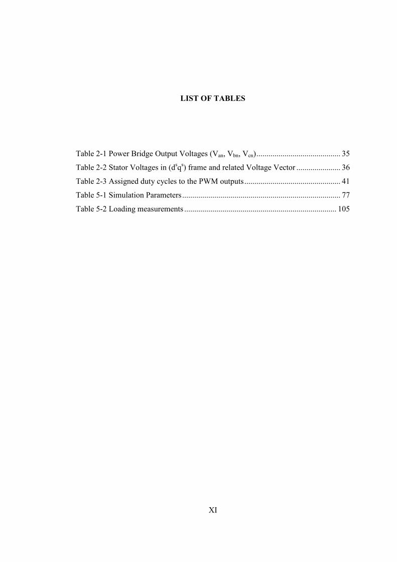
LIST OF TABLES

Table 2-1 Power Bridge Output Voltages (Van, Vbn, Vcn).......................................... 35

Table 2-2 Stator Voltages in (dsqs) frame and related Voltage Vector ...................... 36

Table 2-3 Assigned duty cycles to the PWM outputs................................................ 41

Table 5-1 Simulation Parameters ............................................................................... 77

Table 5-2 Loading measurements ............................................................................ 105

XII

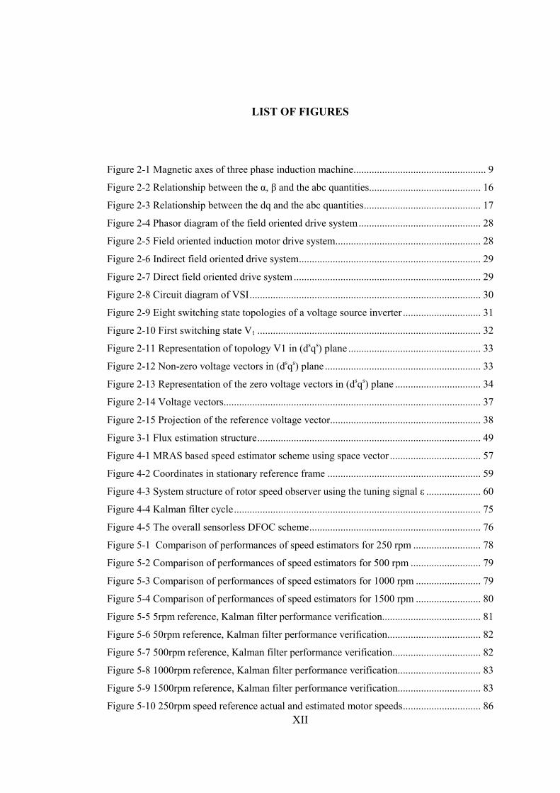
LIST OF FIGURES

Figure 2-1 Magnetic axes of three phase induction machine................................................... 9

Figure 2-2 Relationship between the α, β and the abc quantities........................................... 16

Figure 2-3 Relationship between the dq and the abc quantities............................................. 17

Figure 2-4 Phasor diagram of the field oriented drive system............................................... 28

Figure 2-5 Field oriented induction motor drive system........................................................ 28

Figure 2-6 Indirect field oriented drive system...................................................................... 29

Figure 2-7 Direct field oriented drive system........................................................................ 29

Figure 2-8 Circuit diagram of VSI......................................................................................... 30

Figure 2-9 Eight switching state topologies of a voltage source inverter .............................. 31

Figure 2-10 First switching state V1 ...................................................................................... 32

Figure 2-11 Representation of topology V1 in (dsqs) plane ................................................... 33

Figure 2-12 Non-zero voltage vectors in (dsqs) plane ............................................................ 33

Figure 2-13 Representation of the zero voltage vectors in (dsqs) plane ................................. 34

Figure 2-14 Voltage vectors................................................................................................... 37

Figure 2-15 Projection of the reference voltage vector.......................................................... 38

Figure 3-1 Flux estimation structure...................................................................................... 49

Figure 4-1 MRAS based speed estimator scheme using space vector ................................... 57

Figure 4-2 Coordinates in stationary reference frame ........................................................... 59

Figure 4-3 System structure of rotor speed observer using the tuning signal ε ..................... 60

Figure 4-4 Kalman filter cycle............................................................................................... 75

Figure 4-5 The overall sensorless DFOC scheme.................................................................. 76

Figure 5-1 Comparison of performances of speed estimators for 250 rpm .......................... 78

Figure 5-2 Comparison of performances of speed estimators for 500 rpm ........................... 79

Figure 5-3 Comparison of performances of speed estimators for 1000 rpm ......................... 79

Figure 5-4 Comparison of performances of speed estimators for 1500 rpm ......................... 80

Figure 5-5 5rpm reference, Kalman filter performance verification...................................... 81

Figure 5-6 50rpm reference, Kalman filter performance verification.................................... 82

Figure 5-7 500rpm reference, Kalman filter performance verification.................................. 82

Figure 5-8 1000rpm reference, Kalman filter performance verification................................ 83

Figure 5-9 1500rpm reference, Kalman filter performance verification................................ 83

Figure 5-10 250rpm speed reference actual and estimated motor speeds.............................. 86

XIII

Figure 5-11 500rpm speed reference actual and estimated motor speeds.............................. 87

Figure 5-12 1000rpm speed reference actual and estimated motor speeds............................ 87

Figure 5-13 1500rpm speed reference actual and estimated motor speeds............................ 88

Figure 5-14 250rpm 0.1Hz sinusoidal speed reference actual and estimated motor speeds.. 89

Figure 5-15 500rpm 0.1Hz sinusoidal speed reference actual and estimated motor speeds.. 89

Figure 5-16 1000rpm 0.1Hz sinusoidal speed reference actual and estimated motor speeds 90

Figure 5-17 1500rpm 0.1Hz sinusoidal speed reference actual and estimated motor speeds 90

Figure 5-18 250rpm speed reference, motor phase currents................................................. 91

Figure 5-19 250rpm speed reference, motor phase voltages.................................................. 92

Figure 5-20 250rpm speed reference, motor speed estimate.................................................. 92

Figure 5-21 500rpm speed reference, motor phase currents .................................................. 93

Figure 5-22 500rpm speed reference, motor phase voltages.................................................. 93

Figure 5-23 500rpm speed reference, motor speed estimate.................................................. 94

Figure 5-24 1000rpm speed reference, motor phase currents ................................................ 94

Figure 5-25 1000rpm speed reference, motor phase voltages................................................ 95

Figure 5-26 1000rpm speed reference, motor speed estimate................................................ 95

Figure 5-27 1500rpm speed reference, motor phase currents ................................................ 96

Figure 5-28 1500rpm speed reference, motor phase voltages................................................ 96

Figure 5-29 1500rpm speed reference, motor phase speed estimate ..................................... 97

Figure 5-30 250rpm 0.1 Hz speed reference, motor phase currents ...................................... 98

Figure 5-31 250rpm 0.1 Hz speed reference, motor phase voltages...................................... 98

Figure 5-32 250rpm 0.1 Hz speed reference, motor speed estimate...................................... 99

Figure 5-33 500rpm 0.1 Hz speed reference, motor phase current........................................ 99

Figure 5-34 500rpm 0.1 Hz speed reference, motor phase voltages.................................... 100

Figure 5-35 500rpm 0.1 Hz speed reference, motor speed estimate.................................... 100

Figure 5-36 1000rpm 0.1 Hz speed reference, motor phase current.................................... 101

Figure 5-37 1000rpm 0.1 Hz speed reference, motor phase voltages.................................. 101

Figure 5-38 1000rpm 0.1 Hz speed reference, motor speed estimate.................................. 102

Figure 5-39 1500rpm 0.1 Hz speed reference, motor phase current.................................... 102

Figure 5-40 1500rpm 0.1 Hz speed reference, motor phase voltages.................................. 103

Figure 5-41 1500rpm 0.1 Hz speed reference, motor speed estimate.................................. 103

Figure 5-42 Load system electrical block diagram.............................................................. 104

Figure 5-43 Kalman filter response improvement for better dynamic response.................. 106

Figure 5-44 250rpm speed reference, motor phase currents constant under loading........... 107

Figure 5-45 250rpm speed reference, motor phase voltages constant under loading .......... 107

XIV

Figure 5-46 250rpm speed reference, motor speed estimate constant under loading .......... 108

Figure 5-47 500rpm speed reference, motor phase currents constant under loading........... 108

Figure 5-48 500rpm speed reference, motor phase voltages constant under loading .......... 109

Figure 5-49 500rpm speed reference, motor speed estimate constant under loading .......... 109

Figure 5-50 1000rpm speed reference, motor phase currents constant under loading........ 110

Figure 5-51 1000rpm speed reference, motor phase voltages under constant loading ........ 110

Figure 5-52 1000rpm speed reference, motor speed estimate under constant loading ........ 111

Figure 5-53 1500rpm speed reference, motor phase currents under constant loading......... 111

Figure 5-54 1500rpm speed reference, motor phase voltages under constant loading ........ 112

Figure 5-55 1500rpm speed reference, motor speed estimate under constant loading ........ 112

Figure 5-56 250rpm speed reference, motor phase currents under switched loading.......... 113

Figure 5-57 250rpm speed reference, motor phase voltages under switched loading ......... 114

Figure 5-58 250rpm speed reference, motor speed estimate under switched loading ......... 114

Figure 5-59 500rpm speed reference, motor phase currents under switched loading.......... 115

Figure 5-60 500rpm speed reference, motor phase voltages under switched loading ......... 115

Figure 5-61 500rpm speed reference, motor speed estimate under switched loading ......... 116

Figure 5-62 1000rpm speed reference, motor phase currents under switched loading........ 116

Figure 5-63 1000rpm speed reference, motor phase voltages under switched loading ....... 117

Figure 5-64 1000rpm speed reference, motor speed estimate under switched loading ....... 117

Figure 5-65 1500rpm speed reference, motor phase currents under switched loading........ 118

Figure 5-66 1500rpm speed reference, motor phase voltages under switched loading ....... 118

Figure 5-67 1500rpm speed reference, motor speed estimate under switched loading ....... 119

Figure A-1 The Experimental Set Up .................................................................................. 130

Figure A-2 The Experimental Set Up Block Diagram......................................................... 131

Figure A-3 Drive System software Matlab Simulink Block Diagram................................. 132

XV

LIST OF SYMBOLS

SYMBOL

emd Back emf d-axis component

emq Back emf q-axis component

ieds d-axis stator current in synchronous frame

ieqs q-axis stator current in synchronous frame

isds d-axis stator current in stationary frame

isqs q-axis stator current in stationary frame

iar Phase-a rotor current

ibr Phase-b rotor current

icr Phase-c rotor current

ias Phase-a stator current

ibs Phase-b stator current

ics Phase-c stator current

Lm Magnetizing inductance

Lls Stator leakage inductance

Llr Rotor leakage inductance

Ls Stator self inductance

Lr Rotor self inductance

Kk Kalman gain

Pk Kalman filter error covariance matrix

qmd Reactive power d-axis component

qmq Reactive power q-axis component

Rs Stator resistance

Rr Referred rotor resistance

Tem Electromechanical torque

τr Rotor time-constant

Vas Phase-a stator voltage

Vbs Phase-b stator voltage

Vcs Phase-c stator voltage

XVI

Var Phase-a rotor voltage

Vbr Phase-b rotor voltage

Vcr Phase-c rotor voltage

Vsds d-axis stator voltage in stationary frame

Vsqs q-axis stator voltage in stationary frame

Veds d-axis stator voltage in synchronous frame

Veqs q-axis stator voltage in synchronous frame

Vdc DC-link voltage

we Angular synchronous speed

wr Angular rotor speed

wsl Angular slip speed

kx Kalman filter a priori state estimate

kx Kalman filter a posteriori state estimate

zk Kalman filter measurement

θe Angle between the synchronous frame and the stationary frame

θd Angle between the synchronous frame and the stationary frame when d-axis

is leading

θq Angle between the synchronous frame and the stationary frame when q-axis

is leading

θψr Rotor flux angle

ψsds d-axis stator flux in stationary frame

ψsqs q-axis stator flux in stationary frame

ψeds d-axis stator flux in synchronous frame

ψeqs q-axis stator flux in synchronous frame

ψas Phase-a stator flux

ψbs Phase-b stator flux

ψcs Phase-c stator flux

ψar Phase-a rotor flux

ψbr Phase-b rotor flux

ψcr Phase-c rotor flux

1

CHAPTER 1

INTRODUCTION

1.1. Introduction to Induction Machine Control Literature

Induction machines have many advantages over other types of electrical machines.

They are relatively rugged and inexpensive. They do not have brushes like DC

machines and not require periodic maintenance, and their compact structure is

insensitive to environment conditions. Therefore much attention is given to control

for induction machines, but, due to their non-linear and complex mathematical

model, an induction machine requires more sophisticated control techniques

compared to DC motors. For long time, open-loop V/f control which adjusts a

constant volts-per-Hertz ratio of the stator voltage is used, however, dynamic

performance of this type of control methods was unsatisfactory because of saturation

effect and the electrical parameter variation with temperature. Recent improvements

with lower loss and fast switching semiconductor power switches on power

electronics, fast and powerful digital signal processors on controller technology made

advanced control techniques of induction machine drives applicable.

1.2. The Field Oriented Control of Induction Machines

The most common induction motor drive control scheme is the field oriented

control (FOC). The field oriented control consists of controlling the stator currents

represented by a vector. This control is based on projections which transform a three

phase time and speed dependent system into a two co-ordinate (d and q co-ordinates)

time invariant system. These projections lead to a structure similar to that of a DC

machine control.

2

Moreover, flux and speed estimation are main issues on the field oriented control in

the recent years. The induction machine drives without mechanical speed sensors

have the attractions of low cost and high reliability. Estimating the magnitude and

spatial orientation of the flux in the stator or rotor is also required for such drives.

Rotor flux field orientation is divided mainly into two. These are the direct field

orientation, which relies on direct measurement and estimation of rotor flux

magnitude and angle, and the indirect field orientation, which utilizes slip relation.

Indirect field orientation is a feedforward approach and is naturally parameter

sensitive, especially to the rotor time constant. This has lead to numerous parameter

adapting strategies. [1]- [7]

Direct field oriented control (DFOC) uses flux angle eθ which is calculated by

sensing the air-gap flux with the flux sensing coils. This adds to the cost and

complexity of the drive system. To avoid from using these flux sensors on the

induction machine drive systems, many different algorithms are proposed for last

three decades, to estimate both the rotor flux vector and/or rotor shaft speed. The

recent trend in field-oriented control is towards avoiding the use of speed sensors and

using algorithms based on the terminal quantities of the machine for the estimation of

the fluxes.

Saliency based with fundamental or high frequency signal injection is one of these

above referred flux and speed estimation techniques (algorithms).The advantage of

the saliency technique is that the saliency is not sensitive to actual motor parameters,

however this method does not have sufficient performance at low and zero speed

level. Also, when applied with high frequency signal injection, the method may

cause torque ripples, vibration and audible noise [8].

1.3. Induction Machine Flux Observation

The special flux sensors and coils can be avoided by estimating the rotor flux from

the terminal quantities (stator voltages and currents) [9]. This technique requires the

knowledge of the stator resistance along with the stator-leakage, and rotor-leakage

3

inductances and the magnetizing inductance. The method is commonly known as the

Voltage Model Flux Observer (VMFO).

Voltage Model Flux Observer utilizes the measured stator voltage and current and

requires a pure integration without feedback. Thus it is difficult to implement them

for low excitation frequencies due to the offset and initial condition problems. Due to

the lack of feedback which is necessary for convergence, low pass filter is often used

to provide stability in practice. Accuracy of voltage model based observer is

completely insensitive to rotor resistance but is most sensitive to stator resistance at

low velocities. At high velocities the stator resistance IR drop is less significant

relative to the speed voltage. This reduces sensitivity to stator resistance. The study

of parameter sensitivity shows that the leakage inductance can significantly affect the

system performance regarding to stability, dynamic response and utilization of the

machine and the inverter.

To overcome the problems caused by the changes in leakage inductance and stator

resistance at low speed the Current Model Flux Observer (CMFO) is introduced as

alternative approach. Current model based observers use the measured stator currents

and rotor velocity. The velocity dependency of the current model is a drawback since

this means that even though using the estimated flux eliminates the flux sensor,

position sensor is still required. Furthermore, at zero or low speed operation rotor

flux magnitude response is sensitive primarily to the rotor resistance, although the

phase angle is insensitive to all parameters. Near rated slip, both of them are

sensitive to the rotor resistance and magnetizing inductance. In whole speed range

accuracy is unaffected by the rotor leakage inductance.

Moreover, there is an estimator type based on pole/zero cancellation. In these

methods approximate differentiation of signals is used to cancel the effects of

integration. Due to differentiation, such approaches are insensitive to measurement

and quantization noise. A full order open-loop observer on the other hand can be

formed using only the measured stator voltage and rotor velocity as inputs where the

stator current appears as an estimated quantity. Because of its dependency on the

stator current estimation, the full order observer will not exhibit better performance

4

than the current model. Furthermore, parameter sensitivity and observer gain are the

problems to be tuned in a full order observer design [10].

The observer structures above are open-loop schemes, based on the induction

machine model and they do not use any feedback. Therefore, they are quite sensitive

to parameter variations.

A method which provides a smooth transition between current and voltage models

was developed by Takahashi and Noguchi. They combined two stator flux models

via a first order lag-summing network [11]. Inputs of the current model are measured

stator currents and rotor position. The current model is implemented in rotor flux

frame because; implementation in stationary frame requires measured rotor velocity.

Transformation to the rotor flux frame permits the use of rotor position instead of

velocity. Voltage model utilizes measured stator voltages and currents. The smooth

transition between current and voltage models flux estimates is governed by rotor

flux regulator. A rotor-flux-regulated and oriented system is sensitive to leakage

inductance under high slip operation. Both stator-flux-regulated, oriented systems

have reduced parameter sensitivity.

A smooth and deterministic transition between flux estimates produced by current

and voltage models is given in closed-loop observer approach proposed in [12] [13]

[14] which combines the best accuracy attributes of current and voltage models. In

[15] stator-flux-regulated, rotor-flux-oriented closed-loop observer is used for direct

torque control (DTC) algorithm. The fluxes obtained by current model are compared

with those obtained by the voltage model with reference to the current model, or the

current model with reference to the voltage model according to the range in which

one of these models is superior to other [22].

1.4. Induction Machine Speed Estimation

The torque control problem is overcome in DTC algorithm but to achieve good

speed response, rotor speed also must be known. Verghese have approached speed

estimation problem from a parameter identification point of view [16] [17] [18]. The

5

idea is to consider the speed as an unknown constant parameter, and to find the

estimated speed that best fits the measured or calculated data to the dynamic

equations of the motor. However, parameter variations have significant impact on

performance of the estimator. Possible stator resistance variation due to ohmic

heating results in deterioration in performance [19].

The method proposed in [20] [21] estimates the speed without assuming that the

speed is slowly varying compared to electrical variables studied on non-linear

method. They constructed two estimators; main flux estimator and complementary

flux estimator. Main flux estimator could not guarantee convergence for all operating

conditions. In these operating conditions such as start up complementary estimator is

used. Significant sensitivity to parameter uncertainty is observed with this method.

Speed estimator based on Model Reference Adaptive System (MRAS) is studied in

[23] [24]. In MRAS, in general a comparison is made between the outputs of two

estimators. The estimator which does not contain the quantity to be estimated can be

considered as a reference model of the induction machine. The other one, which

contains the estimated quantity, is considered as an adjustable model. The error

between these two estimators is used as an input to an adaptation mechanism. For

sensorless control algorithms most of the times the quantity which differ the

reference model from the adjustable model is the rotor speed. When the estimated

rotor speed in the adjustable model is changed in such a way that the difference

between two estimators converges to zero asymptotically, the estimated rotor speed

will be equal to actual rotor speed. In [25], [26], [27] voltage model is assumed as

reference model, current model is assumed as the adjustable model and estimated

rotor flux is assumed as the reference parameter to be compared. In [24] similar

speed estimators are proposed based on the MRAS and a secondary variable is

introduced as the reference quantity by putting the rotor flux through a first-order

delay instead of a pure integration to nullify the offset. However their algorithm

produces inaccurate estimated speed if the excitation frequency goes below certain

level. In addition these algorithms suffer from the machine parameter uncertainties

because of the reference model since the parameter variation in the reference model

6

cannot be corrected. [23] Suggests an alternative MRAS based on the electromotive

force rather than rotor flux as reference quantity for speed estimation where the

integration problem has been overcome. Further in [23], another new auxiliary

variable is introduced which represents the instantaneous reactive power for

maintaining the magnetizing current. In this MRAS algorithm stator resistance

disappear from the equations making the algorithm robust to that parameter.

This work is mainly focused on estimating rotor flux angle by model reference

adaptive system and estimating rotor speed by Kalman filter technique. A

combination of well-known open-loop observers, voltage model and current model is

used to estimate the rotor flux angle and speed which are employed in direct field

orientation. For the speed estimation reactive power MRAS speed estimator, open

loop speed estimator and Kalman Filter speed estimator using flux angle estimate of

the flux observer compared in simulations utilizing real data of closed-speed loop

running system. Moreover, closed-speed performance of induction motor system

using Kalman filter as speed estimator and adaptive flux estimator as flux observer is

verified for whole speed range with no-load and with loading conditions.

1.5. Structure of the Chapters

Chapter 2 presents the induction machine modeling and dynamical mathematical

model of the machine in different reference frames. Space vector pulse width

modulation technique is given. Also, field oriented control structure is described.

Chapter 3 is related to the adaptive flux estimator and its implementation. Voltage

model and current model are explained in detail.

Chapter 4 devoted to speed estimation techniques for sensorless direct field

oriented control of induction machine. MRAS speed estimator, open-loop speed

estimator and Kalman filter speed estimator are described.

Chapter 5 demonstrates the performance closed-loop speed control of the induction

motor drive system by the simulations and experimental analysis. The comparison of

the speed estimators are studied in simulations. Moreover, both no-load and with

7

load tests are conducted for drive system to observe performance of the vector

control and that of estimation.

Chapter 6 summarizes the overall study done in the scope of the thesis and

concludes the performance of the closed speed loop vector controlled induction

motor.

8

CHAPTER 2

INDUCTION MACHINE MODELING, FIELD ORIENTED

CONTROL and PWM with SPACE VECTOR THEORY

This chapter focuses on the, modeling of the induction machine for different

reference frames. The state equations of induction machine, which are necessary to

develop observers explained in the next chapters are described. Moreover, field

orientation is introduced. Finally, the space vector PWM technique is explained in

detail.

2.1. System Equations in the Stationary a,b,c Reference Frame

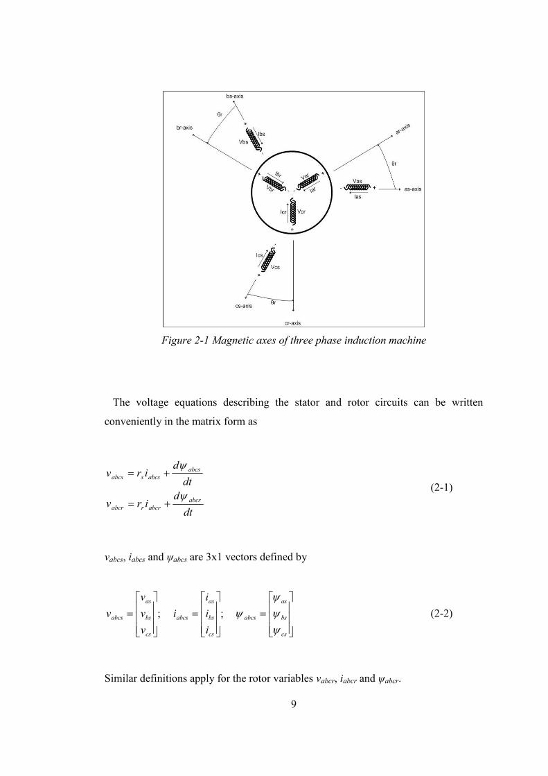
In particular we will assume the winding configuration shown in the Figure 2-1. In

this case the winding placement is only conceptually shown with the center line of

equivalent inductors directed along the magnetic axes of the windings. An

elementary two pole machine is considered. Balanced 3ph windings are assumed for

both stator and rotor. That is all 3 stator windings designated as the as, bs and cs

windings are assumed to have the same number of effective turns, Ns, and the bs and

cs windings are symmetrically displaced from the as winding by ±120o. The

subscript ‘s’ is used to denote that these windings are stator or stationary windings.

The rotor windings are similarly arranged but have Nr turns. These windings are

designated by ar, br and cr in which second subscript reminds us that these three

windings are rotor or rotating windings.

9

Figure 2-1 Magnetic axes of three phase induction machine

The voltage equations describing the stator and rotor circuits can be written

conveniently in the matrix form as

dt

dirv

dt

dirv

abcr

abcrrabcr

abcs

abcssabcs

ψ

ψ

+=

+= (2-1)

vabcs, iabcs and ψabcs are 3x1 vectors defined by

=

=

=

cs

bs

as

abcs

cs

bs

as

abcs

cs

bs

as

abcs

i

i

i

i

v

v

v

v

ψψψ

ψ ; ; (2-2)

Similar definitions apply for the rotor variables vabcr, iabcr and ψabcr.

10

In general coupling clearly exists between all of the stator and rotor phases. The

flux linkages are therefore related to the machine currents by the following matrix

equation.

)()(

)()(

rabcrsabcrabcr

rabcssabcsabcs

ψψψ

ψψψ

+=

+=

(2-3)

where

abcs

csbcsacs

bcsbsabs

acsabsas

sabcs i

LLL

LLL

LLL

=)(ψ (2-4)

abcr

crcsbrcsarcs

crbsbrbsarbs

crasbrasaras

rabcs i

LLL

LLL

LLL

=

,,,

,,,

,,,

)(ψ (2-5)

abcr

crbcracr

bcrbrabr

acrabrar

rabcr i

LLL

LLL

LLL

=)(ψ (2-6)

abcs

cscrbscrascr

csbrbsbrasbr

csarbsarasar

sabcr i

LLL

LLL

LLL

=

,,,

,,,

,,,

)(ψ (2-7)

Note that as a result of reciprocity, the inductance matrix in the third flux linkage

equation, (2-7), above is simply transpose of the inductance matrix in the second

equation, (2-5), because, mutual inductances are equal. (i.e., asbrbras LL ,, = )

11

2.1.1. Determination of Induction Machine Inductances

While the number of inductances defined is large, task of solving for all of these

inductances is straightforward.

The mutual inductance between winding x and winding y is calculated according to

equation

απ

µ cos40

=

g

rlNNL yxxy (2-8)

Where r is radius, l is length of the motor and g is the length of airgap. Nx is the

number of effective turns of the winding x and Ny is the number of effective turns of

the winding y. Notice that alpha is the angle between magnetic axes of the phases x

and y.

The self inductance of stator phase as is obtained by simply setting α=0, and by

setting Nx and Ny in (2-8) to Ns. Whereby,

=

42

0

πµ

g

rlNL sam (2-9)

The subscript m is again used to denote the fact that this inductance is magnetizing

inductance. That is, it is associated with flux lines which cross the air gap and link

rotor as well as stator windings. In general, it is necessary to add a relatively small,

but important, leakage term to (2-9) to account for leakage flux. This term accounts

for flux lines which do not cross the gap but instead close with the stator slot itself

(slot leakage), in the air gap (belt and harmonic leakage) and at the ends of the

machine (end winding leakage). Hence, the total self inductance of phase as can be

expressed.

12

amlsas LLL += (2-10) where Lls represents the leakage term. Since the windings of the bs and the cs phases

are identical to phase as, it is clear that the magnetizing inductances of these

windings are the same as phase as so that, also

cmlscs

bmlsbs

LLL

LLL

+=

+=

(2-11)

It is apparent that Lam, Lbm, Lcm are equal making the self inductances also equal. It

is therefore useful to define stator magnetizing inductance

=

42

0

πµ

g

rlNL sms (2-12)

so that

mslscsbsas LLLLL +=== (2-13)

The mutual inductance between phases as and bs, bs and cs, and cs and as are

derived by simply setting α=2π/3 and Nx =Ny=Ns in (2-8). The result is

−===

82

0

πµ

g

rlNLLL scasbcsabs (2-14)

or, in terms of (2-12),

2ms

casbcsabs

LLLL −=== (2-15)

The flux linkages of phases as, bs and cs resulting from currents flowing in the

stator windings can now be expressed in matrix form as

13

abcs

mslsmsms

msmsls

ms

msmsmsls

sabcs i

LLLL

LLL

L

LLLL

+−−

−+−

−−+

=

22

22

22

)(ψ (2-16)

Let us now turn our attention to the mutual coupling between the stator and rotor

windings. Referring to Figure 2-1, we can see that the rotor phase ar is displaces by

stator phase as by the electrical angle θr where θr in this case is a variable. Similarly

the rotor phases br and cr are displaced from stator phases bs and cs respectively by

θr. Hence, the corresponding mutual inductances can be obtained by setting Nx=Ns,

Ny=Nr, and α= θr in (2-8).

rms

s

r

rrscrcsbrbsaras

LN

N

g

rlNNLLL

θ

θπ

µ

cos

cos40,,,

=

===

(2-17)

The angle between the as and br phases is θr+2π/3, so that

( )3/2cos,,, πθ +=== rms

s

rarcscrbsbras L

N

NLLL (2-18)

Finally, the stator phase as is displaced from the rotor cr phase by angle 3/2πθ −r .

Therefore,

( )3/2cos,,, πθ −=== rms

s

rbrcsarbscras L

N

NLLL (2-19)

The above inductances can now be used to establish the flux linking the stator

phases due to currents in the rotor circuits. In matrix form,

14

( ) ( )

( ) ( )( ) ( )

abcr

rrr

rrr

rrr

ms

s

rrabcs iL

N

N

−+

+−

−+

=

θπθπθπθθπθπθπθθ

ψcos3/2cos3/2cos

3/2coscos3/2cos

3/2cos3/2coscos

)( (2-20)

The total flux linking the stator windings is clearly the sum of the contributions

from the stator and the rotor circuits, (2-16) and (2-20),

)()( rabcssabcsabcs ψψψ += (2-21)

It is not difficult to continue the process to determine the rotor flux linkages. In

terms of previously defined quantities, the flux linking the rotor circuit due to rotor

currents is

abcr

ms

s

rlrms

s

rms

s

r

ms

s

rms

s

rlrms

s

r

ms

s

rms

s

rms

s

rlr

rabcr i

LN

NLL

N

NL

N

N

LN

NL

N

NLL

N

N

LN

NL

N

NL

N

NL

+

−

−

−

+

−

−

−

+

=

222

222

222

)(

21

21

21

21

21

21

ψ (2-22)

where Llr is the rotor leakage inductance. The flux linking the rotor windings due to

currents in the stator circuit is

( ) ( )( ) ( )( ) ( )

abcs

rrr

rrr

rrr

ms

s

rsabcr iL

N

N

+−

−+

+−

=

θπθπθπθθπθπθπθθ

ψcos3/2cos3/2cos

3/2coscos3/2cos

3/2cos3/2coscos

)( (2-23)

Note that the matrix of (2-23) is the transpose of (2-20).

The total flux linkages of the rotor windings are again the sum of the two

components defined by (2-22) and (2-23), that is

15

)()( sabcrrabcrabcr ψψψ += (2-24)

2.1.2. Three-Phase to Two-Phase Transformations

It is apparent that extensive amount of coupling between the six circuits makes the

analysis of this machine a rather formidable task. However we are now in position to

determine if there is any simplification that can be expected between these coupled

equations.

In the study of generalized machine theory, mathematical transformations are often

used to decouple variables, to facilitate the solutions of difficult equations with time

varying coefficients, or to refer all variables to a common reference frame. For this

purpose, the method of symmetrical components uses a complex transformation to

decouple the abc phase variables:

]][[][ 012012 abcfTf = (2-25)

The variable, fabc in (2-25) may be the three-phase ac currents, voltages or fluxes.

The subscripts a,b and c indicate three distinct phases of three phase systems. The

transformation is given by:

=

aa

aaT2

2012

1

1

111

3

1][

(2-26)

where 3

2πj

ea = . Its inverse is given by:

[ ]

=−

2

21012

1

1

111

3

1

aa

aaT (2-27)

16

The symmetrical component transformation is applicable to steady-state vectors or

instantaneous quantities equally. The important subsets of general n-phase to two

phase transformation are briefly introduced in the following subsections.

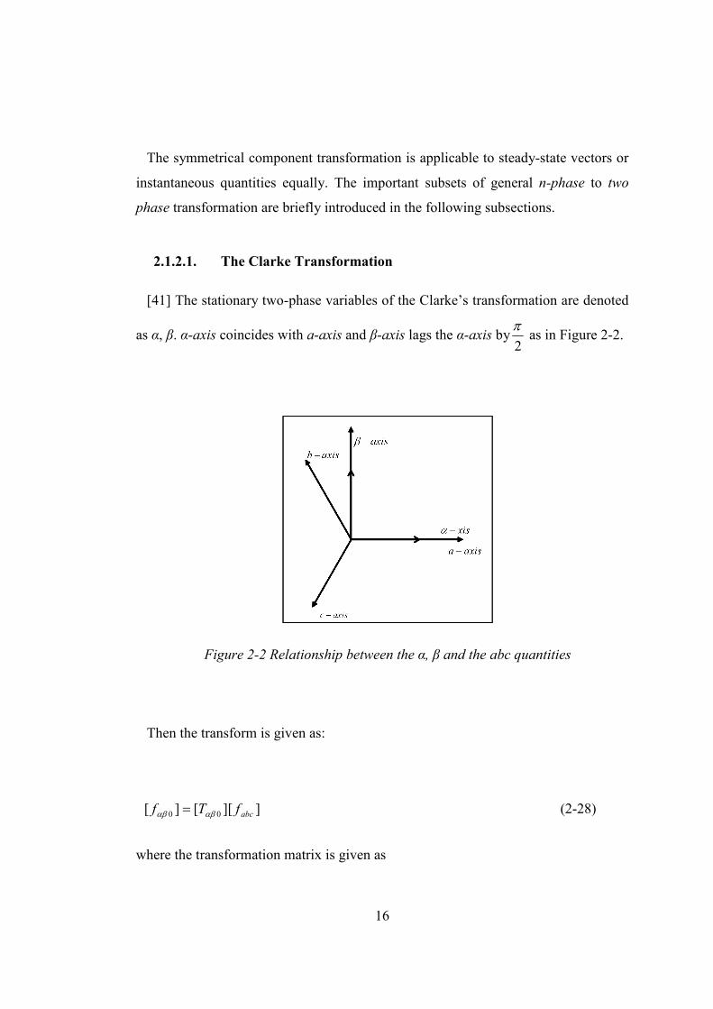
2.1.2.1. The Clarke Transformation

[41] The stationary two-phase variables of the Clarke’s transformation are denoted

as α, β. α-axis coincides with a-axis and β-axis lags the α-axis by2

π as in Figure 2-2.

Figure 2-2 Relationship between the α, β and the abc quantities

Then the transform is given as:

]][[][ 00 abcfTf αβαβ = (2-28)

where the transformation matrix is given as

17

[ ]

−

−−

=

2

1

2

1

2

12

3

2

30

2

1

2

11

3

20αβT (2-29)

And its inverse is:

[ ]

−−

−=−

12

3

2

1

12

3

2

1101

10αβT (2-30)

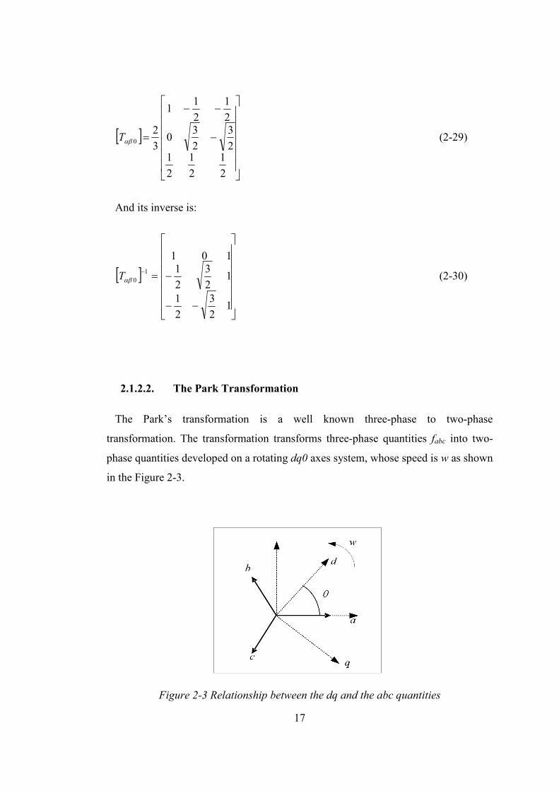
2.1.2.2. The Park Transformation

The Park’s transformation is a well known three-phase to two-phase

transformation. The transformation transforms three-phase quantities fabc into two-

phase quantities developed on a rotating dq0 axes system, whose speed is w as shown

in the Figure 2-3.

Figure 2-3 Relationship between the dq and the abc quantities

18

])][([][ 00 abcdqdq fTf θ= (2-31)

where the dq0 transformation matrix is defined as:

+−

−−−

+

−

=

2

1

2

1

2

132

sin32

sinsin

3

2cos

3

2coscos

32

)]([ 0

πθ

πθθ

πθ

πθθ

θdqT (2-32)

and the inverse is given by:

+−

+

−−

−

−

=−

132

sin32

cos

132

sin32

cos

1sincos

)]([ 10

πθ

πθ

πθ

πθ

θθ

θdqT (2-33)

where θ is the angle between the phases a and d. Notice that, θ is time integral of w,

which is the rotation speed of the dq reference frame and it is chosen arbitrarily for

the sake of generality.

2.1.3. Circuit Equations in Arbitrary dq0 Reference Frame

The dq0 reference frames are usually selected on the basis of conveniences or

computational reduction. The two common reference frames used in the analysis of

induction machine are the stationary frame (i.e. w = 0), with a frame notation dsqs,

and synchronously rotating frame (i.e. w = ws, synchronous speed), with a frame

notation deqe. Each has an advantage for some purpose. In the stationary reference

frame, the dsqs variables of the machine are in the same frame as those normally used

19

for the supply network. In the synchronously rotating frame, the deqe variables are dc

in steady state. First of all, the equations of the induction machine in the arbitrary

reference frame, which is rotating at a speed w, in the direction of the rotor rotation,

will be derived. When the induction machine runs in the stationary frame, these

equations of the induction machine, can then be obtained by setting w = 0. These

equations can also be obtained in the synchronously rotating frame by setting w = we.

2.1.3.1. qd0 Voltage Equations

In matrix notation, the stator winding abc voltage equations can be expressed as:

dt

dirv abcs

abcssabcs

ψ+= (2-34)

Applying the transformations given in (2-32) and (2-33), to the voltage, current and

flux linkages, (2-34) becomes

[ ] [ ] [ ]( ) [ ] [ ] [ ]( )sdqqdsqd

sdqqd

qdsdq iTrTdt

TdTv 0

100

01

000 )()(

)()( −

−

+= θθψθ

θ (2-35)

applying the chain rule in (2-35)

[ ] [ ] [ ] [ ] [ ]

[ ][ ] [ ]sdqqdqds

sdq

qdsdq

qd

qdsdq

iTTr

dt

dT

dt

TdTv

01

00

0100

10

00

)()(

)()(

)(

−

−−

+

+

=

θθ

ψθψ

θθ

(2-36)

which is equal to

20

[ ] [ ] [ ] [ ][ ] [ ]

[ ][ ] [ ]sdqqdqds

sdq

qdqdsdq

qd

qdsdq

iTTr

dt

dTT

dt

TdTv

01

00

01000

10

00

)()(

)()()(

)(

−

−−

+

+

=

θθ

ψθθψ

θθ

(2-37)

Note that

[ ] [ ]

−=

−

000

001

01010

0dt

d

dt

TdT

dq

dq

θ (2-38)

Then (2-37) becomes:

sdqsdq

sdq

sdqsdq irdt

dwv 00

000

000

001

010

++

−=ψ

ψ (2-39)

where

==

100

010

001

0 ssdq rranddt

dw

θ (2-40)

Likewise, the rotor voltage equation becomes:

rdqrdq

rdq

rdqrrdq irdt

dwwv 00

000

000

001

010

)( ++

−−=ψ

ψ (2-41)

21

2.1.3.2. qd0 Flux Linkage Relation

The stator qd0 flux linkages are obtained by applying )]([ 0 θqdT to the stator abc

flux linkages equation.

abcsqdsdq T ψθψ )]([ 00 = (2-42)

referring (2-21), (2-42) is written as

( ))()(00 )]([ rabcssabcsqdsdq T ψψθψ += (2-43)

putting (2-22) and (2-23) into (2-43);

( )[ ]

( )[ ]( ) ( )

( ) ( )( ) ( )

abcr

rrr

rrr

rrr

ms

s

r

dq

abcs

msls

msms

ms

msls

ms

msms

msls

dqsdq

iLN

NT

i

LLLL

LLL

L

LLLL

T

−+

+−

−+

+

+−−

−+−

−−+

=

θπθπθπθθπθπθπθθ

θ

θψ

cos3/2cos3/2cos

3/2coscos3/2cos

3/2cos3/2coscos

22

22

22

0

00

(2-44)

skipping the transformation steps the stator and the rotor flux linkage relationships

can be expressed compactly:

′

′

′

′

′

′=

′

′

′

r

dr

qr

s

ds

qs

lr

rm

rm

ls

ms

ms

r

dr

qr

s

ds

qs

i

i

i

i

i

i

L

LL

LL

L

LL

LL

0

0

0

0

00000

0000

0000

00000

0000

0000

ψ

ψ

ψ

ψ

ψ

ψ

(2-45)

Where primed quantities denote referred values to the stator side.

22

mlrr

mlss

LLL

LLL

+′=′

+=

(2-46)

and

lr

r

slrsmsm L

N

NL

g

rlNLL 2

02 )(,

42

3

2

3=′

==

πµ (2-47)

2.1.3.3. qd0 Torque Equations

The sum of the instantaneous input power to all six windings of the stator and rotor

is given by:

WivivivivivivP crcrbrbrararcscsbsbsasasin

′′+′′+′′+++= (2-48)

in terms of dq quantities

)22(2

30000 rrdrdrqrqrssdsdsqsqsin ivivivivivivP ′′+′′+′′+++= W (2-49)

Using stator and rotor voltages to substitute for the voltages on the right hand side

of (2-49), we obtain three kinds of terms: iwanddt

diri ψ

ψ,,2 . ri 2 terms are the

cupper losses. The dt

di

ψ terms represent the rate of exchange of magnetic field

energy between windings. The electromechanical torque developed by the machine is

given by the sum of the iwψ terms divided by mechanical speed, that is:

[ ] Nmiiwwiiww

pT drqrqrdrrdsqsqsds

r

em ))(()(22

3′′−′′−+−= ψψψψ (2-50)

23

using the flux linkage relationships one can show that:

)()( dsqrqsdrmdrqrqrdrdsqsqsds iiiiLiiii −=′′−′′−=− ψψψψ (2-51)

Thus (2-50) can also be expressed as:

NmiiiiLp

Nmiip

Nmiip

T

dsqrqsdrm

dsqsqsds

qrdrdrqrem

)(22

3

)(22

3

)(22

3

′−′=

−=

′′−′′=

ψψ

ψψ

(2-52)

2.1.4. qd0 Stationary and Synchronous Reference Frames

There is seldom a need to simulate an induction machine in the arbitrary rotating

reference frame. But it is useful to convert a unified model to other frames. The most

commonly used ones are, two marginal cases of the arbitrary rotating frame,

stationary reference frame and synchronously rotating frame. For transient studies of

adjustable speed drives, it is usually more convenient to simulate an induction

machine and its converter on a stationary reference frame. Moreover, calculations

with stationary reference frame are less complex due to zero frame speed (some

terms cancelled). For small signal stability analysis about some operating condition,

a synchronously rotating frame which yields dc values of steady-state voltages and

currents under balanced conditions is used.

Since we have derived the circuit equations of induction machine for the general

case that is in the arbitrary rotating reference frame, the circuit equations of the

machine in the stationary reference frame (denoted as dsqs) and synchronously

rotating reference frame (denoted as deqe) can be obtained by simply setting w to zero

and we, respectively. To distinguish these two frames from each other, an additional

24

superscript will be used, s for stationary frame variables and e for synchronously

rotating frame variables.

Stator qsds voltage equations:

dss

s

dss

dss

qss

s

qss

qss

irdt

dv

irdt

dv

+=

+=

ψ

ψ

(2-53)

Rotor qsds voltage equations:

drs

rqrs

r

drs

drs

qrs

rdrs

r

qrs

qrs

irwdt

dv

irwdt

dv

′′+′+′

=′

′′+′−+′

=′

ψψ

ψψ

)(

)(

(2-54)

where

′

′

′

′=

′

′

drs

qrs

dss

qss

rm

rm

ms

ms

drs

qrs

dss

qss

i

i

i

i

LL

LL

LL

LL

00

00

00

00

ψψψψ

(2-55)

Torque Equations:

NmiiiiLp

Nmiip

Nmiip

T

dss

qrs

qss

drs

m

dss

qss

qss

dss

qrs

drs

drs

qrs

em

)(22

3

)(22

3

)(22

3

′−′=

−=

′′−′′=

ψψ

ψψ

(2-56)

25

Stator qede voltage equations:

dse

sqse

e

dse

dse

qse

sdse

e

qse

qse

irwdt

dv

irwdt

dv

+−=

++=

ψψ

ψψ

(2-57)

Rotor qede voltage equations:

dre

rqre

re

dre

dre

qre

rdre

re

qre

qre

irwwdt

dv

irwwdt

dv

′′+′−−′

=′

′′+′−+′

=′

ψψ

ψψ

)(

)(

(2-58)

where

′

′

′

′=

′

′

dre

qre

dse

qse

rm

rm

ms

ms

dre

qre

dse

qse

i

i

i

i

LL

LL

LL

LL

00

00

00

00

ψψψψ

(2-59)

Torque Equations:

Nmiip

Nmiip

T

dse

qse

qse

dse

qre

dre

dre

qre

em

)(22

3

)(22

3

ψψ

ψψ

−=

′′−′′=

(2-60)

2.2. Field Oriented Control (FOC)

The concept of field orientation control is used to accomplish a decoupled control

of flux and torque, and has three requirements [28]:

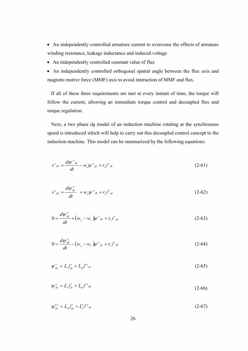
26

• An independently controlled armature current to overcome the effects of armature

winding resistance, leakage inductance and induced voltage

• An independently controlled constant value of flux

• An independently controlled orthogonal spatial angle between the flux axis and

magneto motive force (MMF) axis to avoid interaction of MMF and flux.

If all of these three requirements are met at every instant of time, the torque will

follow the current, allowing an immediate torque control and decoupled flux and

torque regulation.

Next, a two phase dq model of an induction machine rotating at the synchronous

speed is introduced which will help to carry out this decoupled control concept to the

induction machine. This model can be summarized by the following equations:

dse

sqse

e

dse

dse irw

dt

dv +−= ψ

ψ (2-61)

qse

sdse

e

e

qsqs

e irwdt

dv ++= ψ

ψ (2-62)

( ) qre

rdre

re

e

qrirww

dt

d+−+= ψ

ψ0 (2-63)

( ) dre

rqre

re

e

dr irwwdt

d+−−= ψ

ψ0 (2-64)

qre

m

e

qss

e

qs iLiL ′+=ψ (2-65)

dre

m

e

dss

e

ds iLiL ′+=ψ (2-66)

qre

r

e

qsm

e

qr iLiL ′′+=′ψ (2-67)

27

dre

r

e

dsm

e

dr iLiL ′′+=′ψ (2-68)

( )e

ds

e

qr

e

qs

e

dr

r

m

em iiL

LpT ψψ ′−′=

23

(2-69)

Lrr

em TBwdt

dwJT ++= (2-70)

This model is quite significant to synthesize the concept of field-oriented control.

In this model it can be seen from the torque expression (2-69) that if the rotor flux

along the q-axis is zero, then all the flux is aligned along the d-axis and therefore the

torque can be instantaneously controlled by controlling the current along q-axis.

Then the question will be how it can be guaranteed that all the flux is aligned along

the d-axis of the machine. When a three-phase voltage is applied to the machine, it

produces a three-phase flux both in the stator and rotor. The three-phase fluxes can

be converted into equivalents developed in two-phase stationary (dsqs) frame. If this

two phase fluxes along (dsqs) axes are converted into an equivalent single vector then

all the machine flux will be considered as aligned along that vector. This vector

commonly specifies us de-axis which makes an angle eθ with the stationary frame ds-

axis. The qe-axis is set perpendicular to the de-axis. The flux along the qe-axis in that

case will obviously be zero. The phasor diagram Figure 2-4 shows these axes. The

angle eθ keeps changing as the machine input currents change. Knowing the angle

eθ accurately, d-axis of the deqe frame can be locked with the flux vector.

The control input can be specified in terms of two phase synchronous frame ieds and

ieqs. i

eds is aligned along the d

e-axis i.e. the flux vector, so does ieqs with the qe-axis.

These two-phase synchronous control inputs are converted into two-phase stationary

and then to three-phase stationary control inputs. To accomplish this, the flux angle

eθ must be known precisely. The angle eθ can be found either by Indirect Field

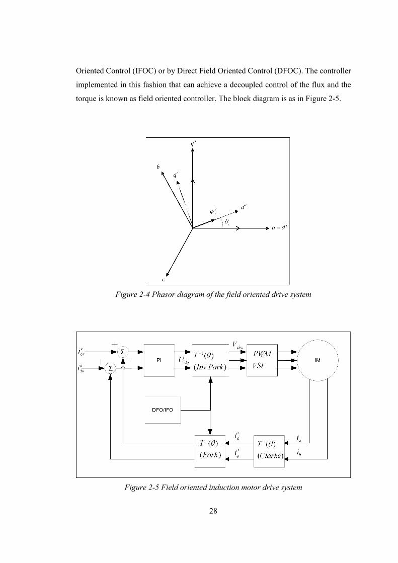
28

Oriented Control (IFOC) or by Direct Field Oriented Control (DFOC). The controller

implemented in this fashion that can achieve a decoupled control of the flux and the

torque is known as field oriented controller. The block diagram is as in Figure 2-5.

Figure 2-4 Phasor diagram of the field oriented drive system

Figure 2-5 Field oriented induction motor drive system

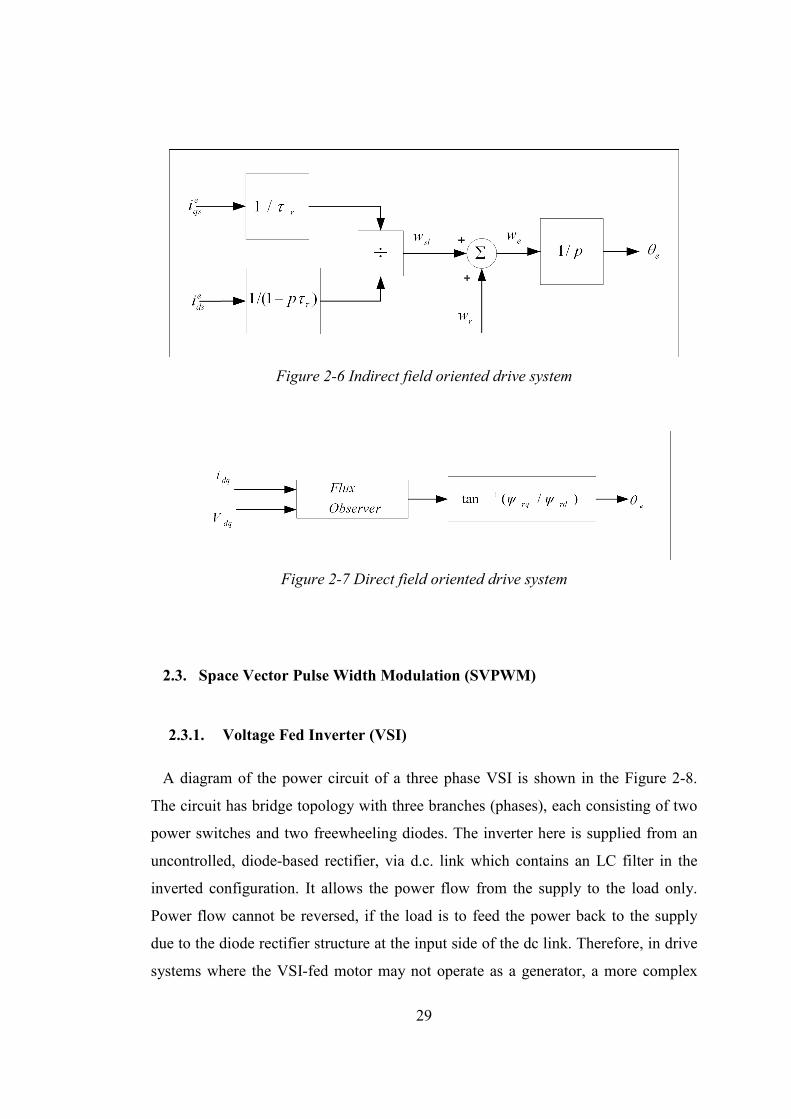
29

Figure 2-6 Indirect field oriented drive system

Figure 2-7 Direct field oriented drive system

2.3. Space Vector Pulse Width Modulation (SVPWM)

2.3.1. Voltage Fed Inverter (VSI)

A diagram of the power circuit of a three phase VSI is shown in the Figure 2-8.

The circuit has bridge topology with three branches (phases), each consisting of two

power switches and two freewheeling diodes. The inverter here is supplied from an

uncontrolled, diode-based rectifier, via d.c. link which contains an LC filter in the

inverted configuration. It allows the power flow from the supply to the load only.

Power flow cannot be reversed, if the load is to feed the power back to the supply

due to the diode rectifier structure at the input side of the dc link. Therefore, in drive

systems where the VSI-fed motor may not operate as a generator, a more complex

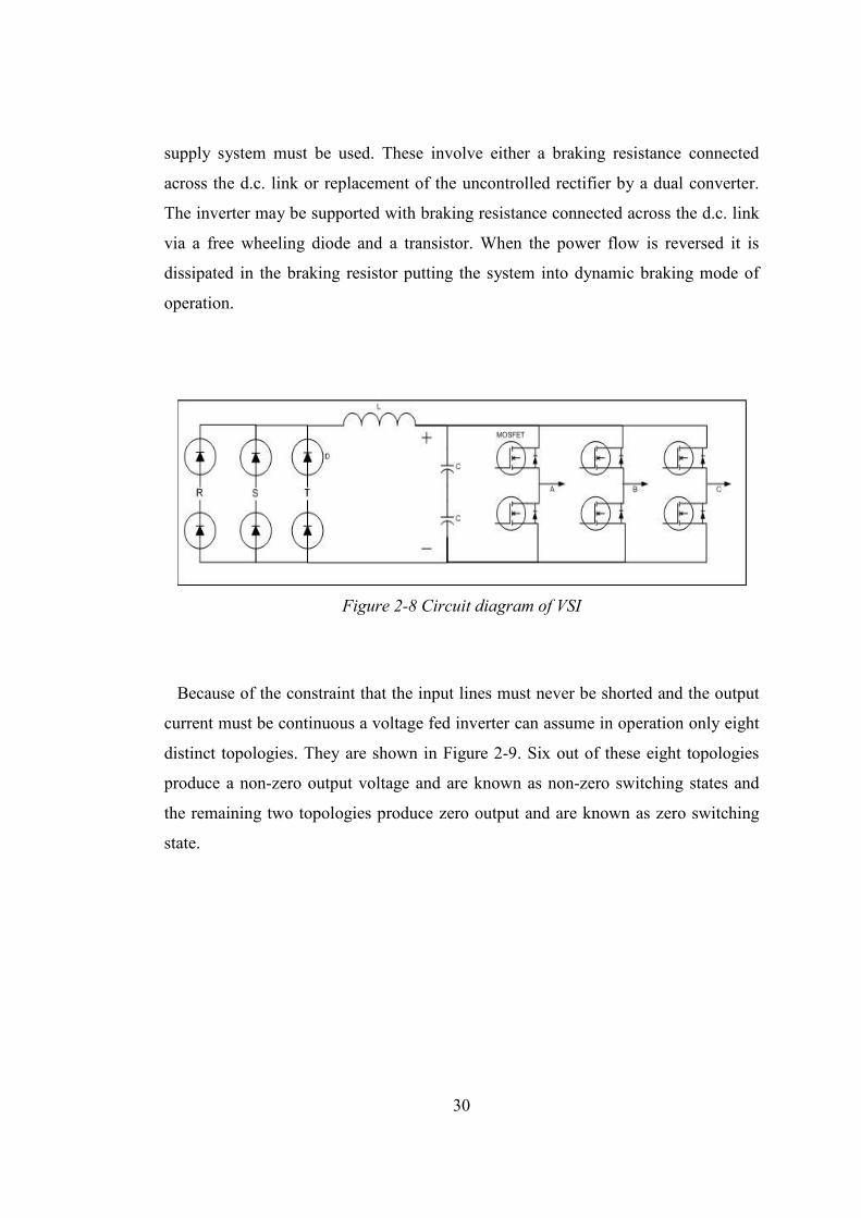
30

supply system must be used. These involve either a braking resistance connected

across the d.c. link or replacement of the uncontrolled rectifier by a dual converter.

The inverter may be supported with braking resistance connected across the d.c. link

via a free wheeling diode and a transistor. When the power flow is reversed it is

dissipated in the braking resistor putting the system into dynamic braking mode of

operation.

Figure 2-8 Circuit diagram of VSI

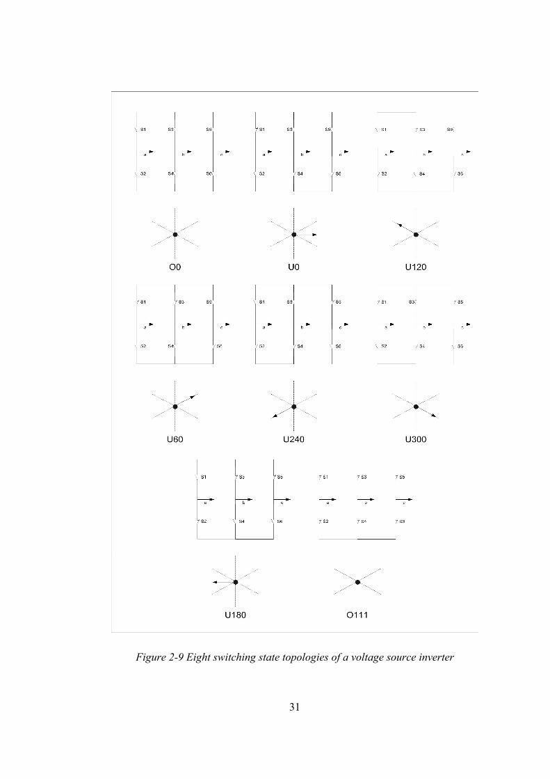
Because of the constraint that the input lines must never be shorted and the output

current must be continuous a voltage fed inverter can assume in operation only eight

distinct topologies. They are shown in Figure 2-9. Six out of these eight topologies

produce a non-zero output voltage and are known as non-zero switching states and

the remaining two topologies produce zero output and are known as zero switching

state.

31

Figure 2-9 Eight switching state topologies of a voltage source inverter

32

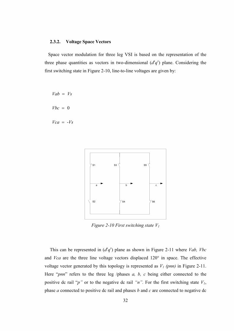
2.3.2. Voltage Space Vectors

Space vector modulation for three leg VSI is based on the representation of the

three phase quantities as vectors in two-dimensional (dsqs) plane. Considering the

first switching state in Figure 2-10, line-to-line voltages are given by:

-VsVca

Vbc

VsVab

=

=

=

0

S1 S3 S5

S2

a b c

S4 S6

Figure 2-10 First switching state V1

This can be represented in (dsqs) plane as shown in Figure 2-11 where Vab, Vbc

and Vca are the three line voltage vectors displaced 120° in space. The effective

voltage vector generated by this topology is represented as V1 (pnn) in Figure 2-11.

Here “pnn” refers to the three leg /phases a, b, c being either connected to the

positive dc rail “p” or to the negative dc rail “n”. For the first switching state V1,

phase a connected to positive dc rail and phases b and c are connected to negative dc

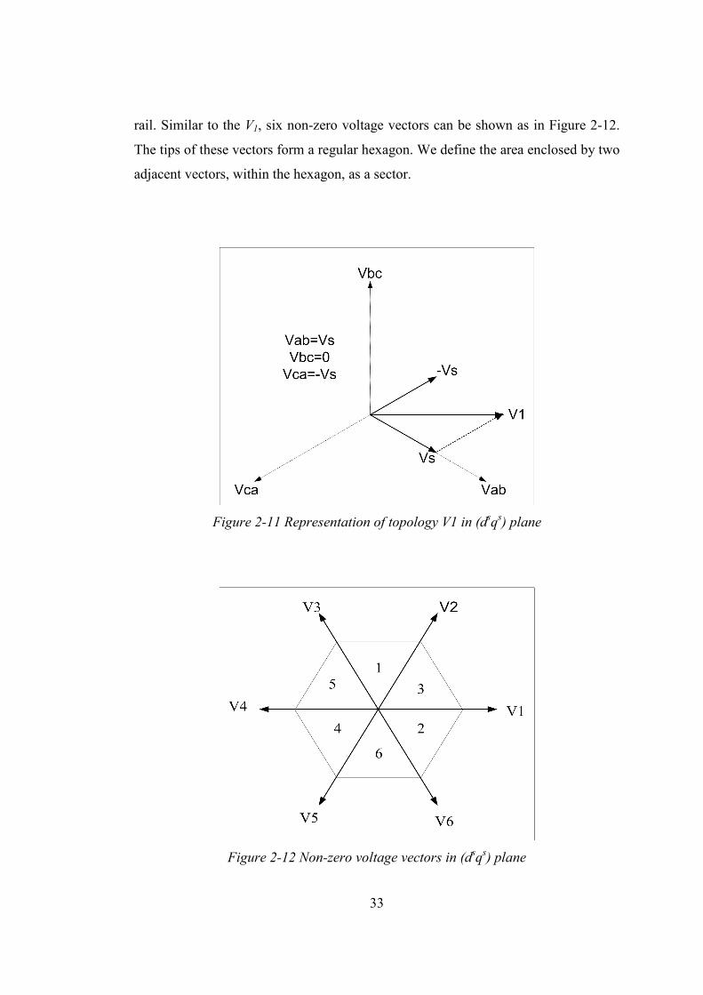
33

rail. Similar to the V1, six non-zero voltage vectors can be shown as in Figure 2-12.

The tips of these vectors form a regular hexagon. We define the area enclosed by two

adjacent vectors, within the hexagon, as a sector.

Figure 2-11 Representation of topology V1 in (dsqs) plane

Figure 2-12 Non-zero voltage vectors in (dsqs) plane

34

The first and the last two topologies of Figure 2-9 are zero state vectors. The output

line voltages in these topologies are zero.

0

0

0

=

=

=

Vca

Vbc

Vab

These are represented as vectors which have zero magnitude and hence are referred

as zero switching state vectors. They are represented with dot at the origin instead of

vectors as shown in Figure 2-13.

Figure 2-13 Representation of the zero voltage vectors in (dsqs) plane

35

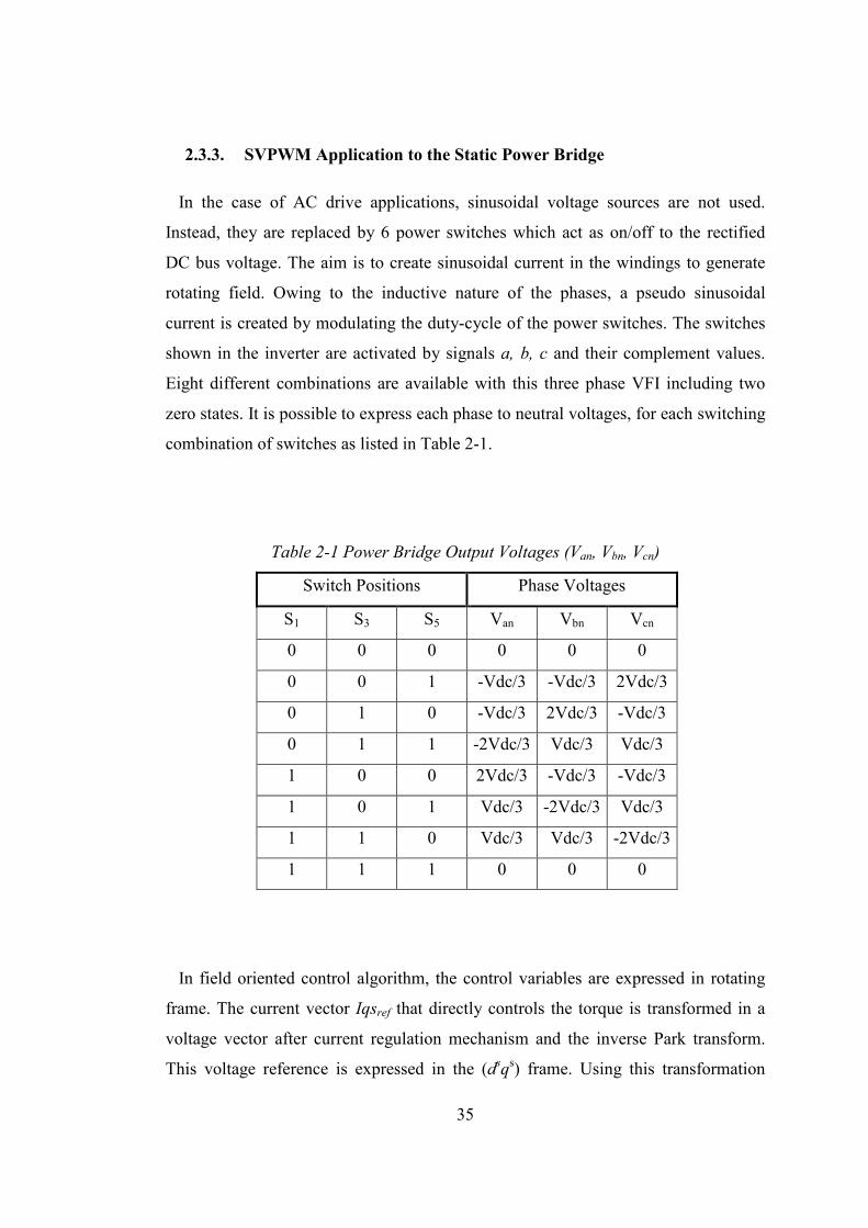
2.3.3. SVPWM Application to the Static Power Bridge

In the case of AC drive applications, sinusoidal voltage sources are not used.

Instead, they are replaced by 6 power switches which act as on/off to the rectified

DC bus voltage. The aim is to create sinusoidal current in the windings to generate

rotating field. Owing to the inductive nature of the phases, a pseudo sinusoidal

current is created by modulating the duty-cycle of the power switches. The switches

shown in the inverter are activated by signals a, b, c and their complement values.

Eight different combinations are available with this three phase VFI including two

zero states. It is possible to express each phase to neutral voltages, for each switching

combination of switches as listed in Table 2-1.

Table 2-1 Power Bridge Output Voltages (Van, Vbn, Vcn)

Switch Positions Phase Voltages

S1 S3 S5 Van Vbn Vcn

0 0 0 0 0 0

0 0 1 -Vdc/3 -Vdc/3 2Vdc/3

0 1 0 -Vdc/3 2Vdc/3 -Vdc/3

0 1 1 -2Vdc/3 Vdc/3 Vdc/3

1 0 0 2Vdc/3 -Vdc/3 -Vdc/3

1 0 1 Vdc/3 -2Vdc/3 Vdc/3

1 1 0 Vdc/3 Vdc/3 -2Vdc/3

1 1 1 0 0 0

In field oriented control algorithm, the control variables are expressed in rotating

frame. The current vector Iqsref that directly controls the torque is transformed in a

voltage vector after current regulation mechanism and the inverse Park transform.

This voltage reference is expressed in the (dsqs) frame. Using this transformation

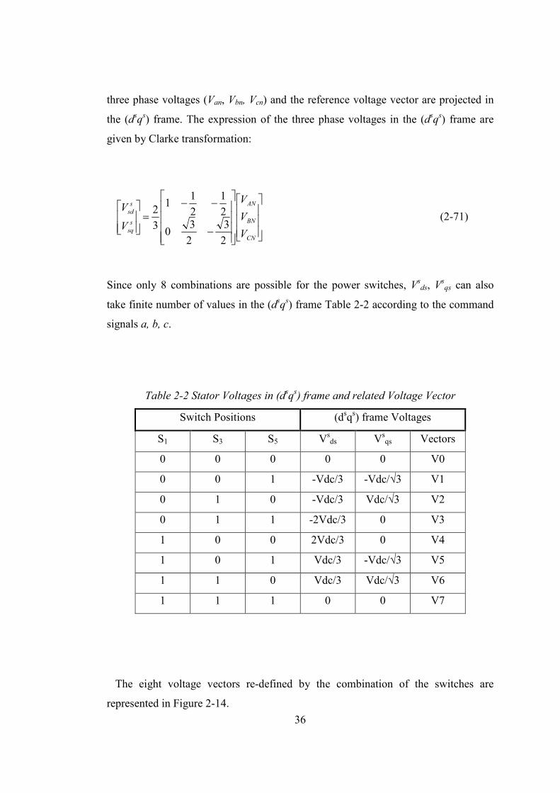
36

three phase voltages (Van, Vbn, Vcn) and the reference voltage vector are projected in

the (dsqs) frame. The expression of the three phase voltages in the (dsqs) frame are

given by Clarke transformation:

−

−−=

CN

BN

AN

s

sq

s

sd

V

V

V

V

V

2

3

2

30

21

21

1

32

(2-71)

Since only 8 combinations are possible for the power switches, Vs

ds, Vsqs can also

take finite number of values in the (dsqs) frame Table 2-2 according to the command

signals a, b, c.

Table 2-2 Stator Voltages in (d

sqs) frame and related Voltage Vector

Switch Positions (dsqs) frame Voltages

S1 S3 S5 Vsds Vs

qs Vectors

0 0 0 0 0 V0

0 0 1 -Vdc/3 -Vdc/√3 V1

0 1 0 -Vdc/3 Vdc/√3 V2

0 1 1 -2Vdc/3 0 V3

1 0 0 2Vdc/3 0 V4

1 0 1 Vdc/3 -Vdc/√3 V5

1 1 0 Vdc/3 Vdc/√3 V6

1 1 1 0 0 V7

The eight voltage vectors re-defined by the combination of the switches are

represented in Figure 2-14.

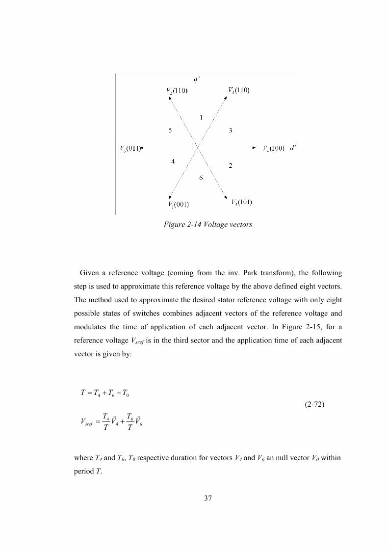
37

Figure 2-14 Voltage vectors

Given a reference voltage (coming from the inv. Park transform), the following

step is used to approximate this reference voltage by the above defined eight vectors.

The method used to approximate the desired stator reference voltage with only eight

possible states of switches combines adjacent vectors of the reference voltage and

modulates the time of application of each adjacent vector. In Figure 2-15, for a

reference voltage Vsref is in the third sector and the application time of each adjacent

vector is given by:

66

44

064

VT

TV

T

TV

TTTT

sref

rr+=

++=

(2-72)

where T4 and T6, T0 respective duration for vectors V4 and V6 an null vector V0 within

period T.

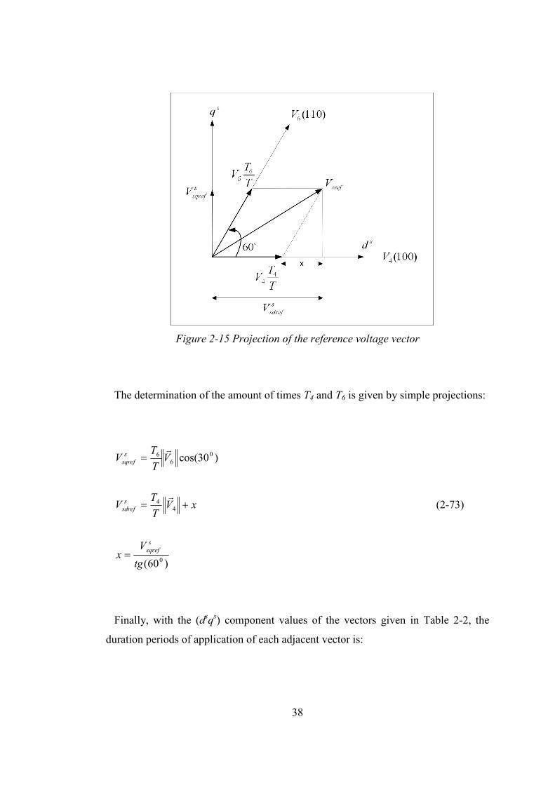
38

Figure 2-15 Projection of the reference voltage vector

The determination of the amount of times T4 and T6 is given by simple projections:

)60(

)30cos(

0

44

06

6

tg

Vx

xVT

TV

VT

TV

s

sqref

s

sdref

s

sqref

=

+=

=

r

r

(2-73)

Finally, with the (dsqs) component values of the vectors given in Table 2-2, the

duration periods of application of each adjacent vector is:

39

)3(24

s

sq

s

sd VVT

T −= (2-74)

s

sqTVT =6 (2-75)

where the vector magnitudes are “ 3/2 dcV ” and both sides are normalized by

maximum phase to neutral voltage 3/DCV .

The rest of the period spent in applying the null vector (T0=T-T6-T4). For every

sector, commutation duration is calculated. The amount of times of vector

application can all be related to the following variables:

s

sd

s

sq

s

sd

s

sq

s

sq

VVZ

VVY

VX

2

3

2

1

2

3

2

1

−=

+=

=

(2-76)

In the previous example for sector 3, T4 = -TZ and T6 =TX. Extending this logic,

one can easily calculate the sector number belonging to the related reference voltage

vector. Then, three phase quantities are calculated by inverse Clarke transform to get

sector information. The following basic algorithm helps to determine the sector

number systematically.

If s

sqref VV =1 > 0 then set A=1 else A=0

If )3(2

12

s

sq

s

sdref VVV −= > 0 then set B=1 else B=0

40

If )3(2

13

s

sq

s

sdref VVV −−= > 0 then set C=1 else C=0

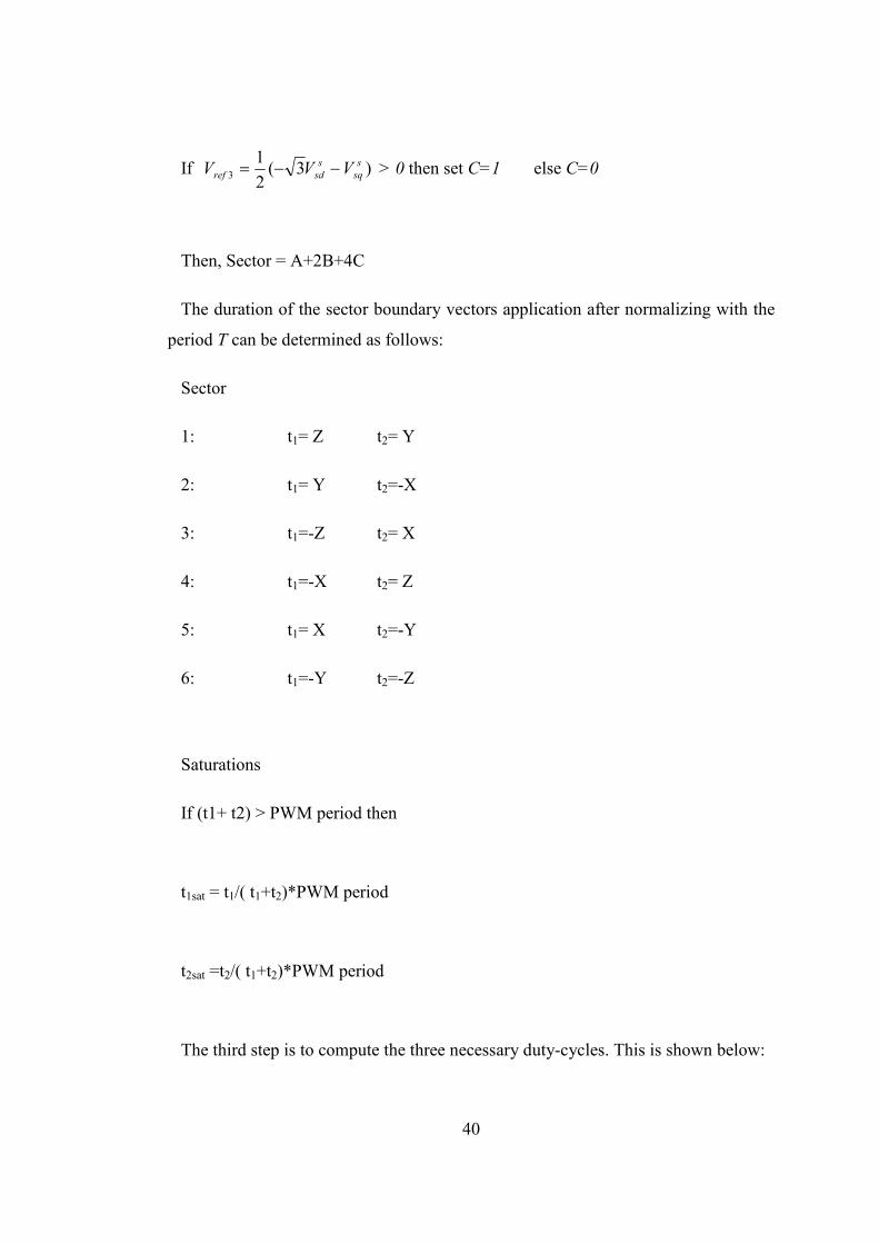
Then, Sector = A+2B+4C

The duration of the sector boundary vectors application after normalizing with the

period T can be determined as follows:

Sector

1: t1= Z t2= Y

2: t1= Y t2=-X

3: t1=-Z t2= X

4: t1=-X t2= Z

5: t1= X t2=-Y

6: t1=-Y t2=-Z

Saturations

If (t1+ t2) > PWM period then

t1sat = t1/( t1+t2)*PWM period

t2sat =t2/( t1+t2)*PWM period

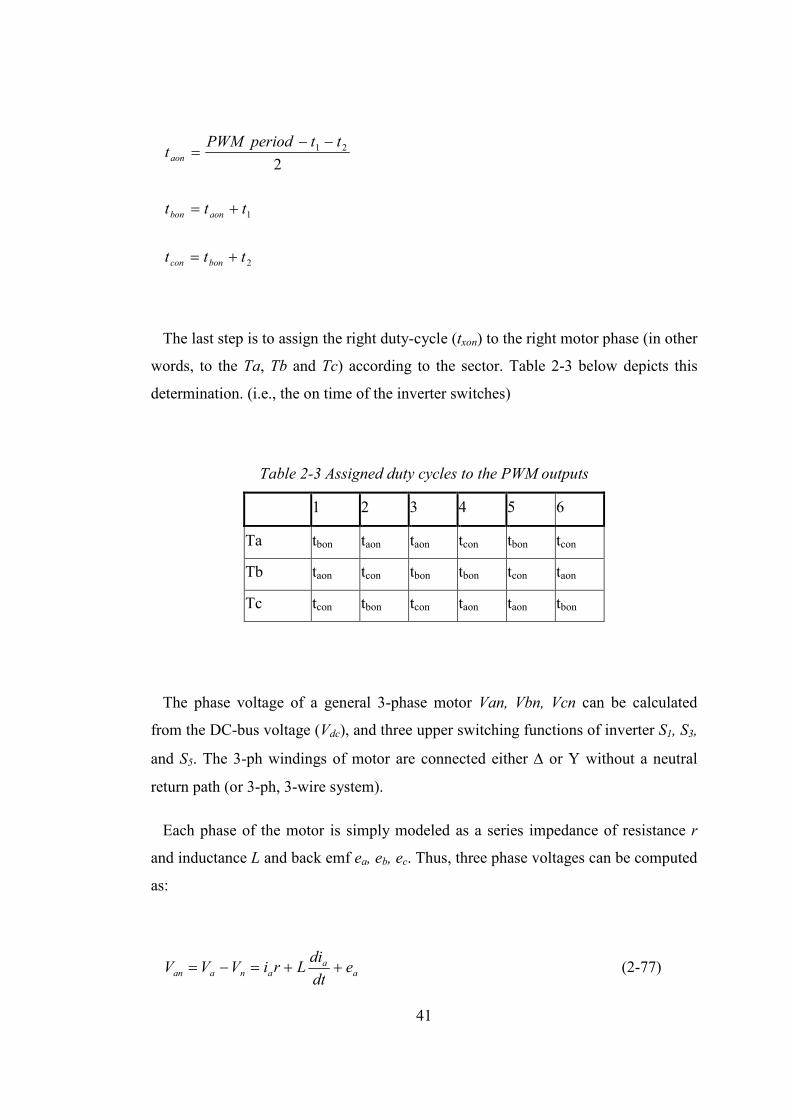
The third step is to compute the three necessary duty-cycles. This is shown below:

41

2

1

21

2

ttt

ttt

ttperiodPWMt

boncon

aonbon

aon

+=

+=

−−=

The last step is to assign the right duty-cycle (txon) to the right motor phase (in other

words, to the Ta, Tb and Tc) according to the sector. Table 2-3 below depicts this

determination. (i.e., the on time of the inverter switches)

Table 2-3 Assigned duty cycles to the PWM outputs

1 2 3 4 5 6

Ta tbon taon taon tcon tbon tcon

Tb taon tcon tbon tbon tcon taon

Tc tcon tbon tcon taon taon tbon

The phase voltage of a general 3-phase motor Van, Vbn, Vcn can be calculated

from the DC-bus voltage (Vdc), and three upper switching functions of inverter S1, S3,

and S5. The 3-ph windings of motor are connected either ∆ or Y without a neutral

return path (or 3-ph, 3-wire system).

Each phase of the motor is simply modeled as a series impedance of resistance r

and inductance L and back emf ea, eb, ec. Thus, three phase voltages can be computed

as:

aa

anaan edt

diLriVVV ++=−= (2-77)

42

bb

bnbbn edt

diLriVVV ++=−= (2-78)

cc

cnccn edt

diLriVVV ++=−= (2-79)

Summing these three phase voltages, yields

cbacba

cbancba eeedt

iiidLriiiVVVV +++

+++++=−++

)()(3 (2-80)

For a 3-phase system with no neutral path and balanced back emfs, ia+ib+ic=0, and

ea+eb+ec,=0. Therefore, (2-80) becomes, Van+Vbn+Vcn,=0. Furthermore, the neutral

voltage can be simply derived from (2-80) as

)(31

cban VVVV ++= (2-81)

Now three phase voltages can be calculated as:

cbacbaaan VVVVVVVV31

31

32

)(31

−−=++−= (2-82)

cabcbabbn VVVVVVVV31

31

32

)(31

−−=++−= (2-83)

baccbaccn VVVVVVVV31

31

32

)(31

−−=++−= (2-84)

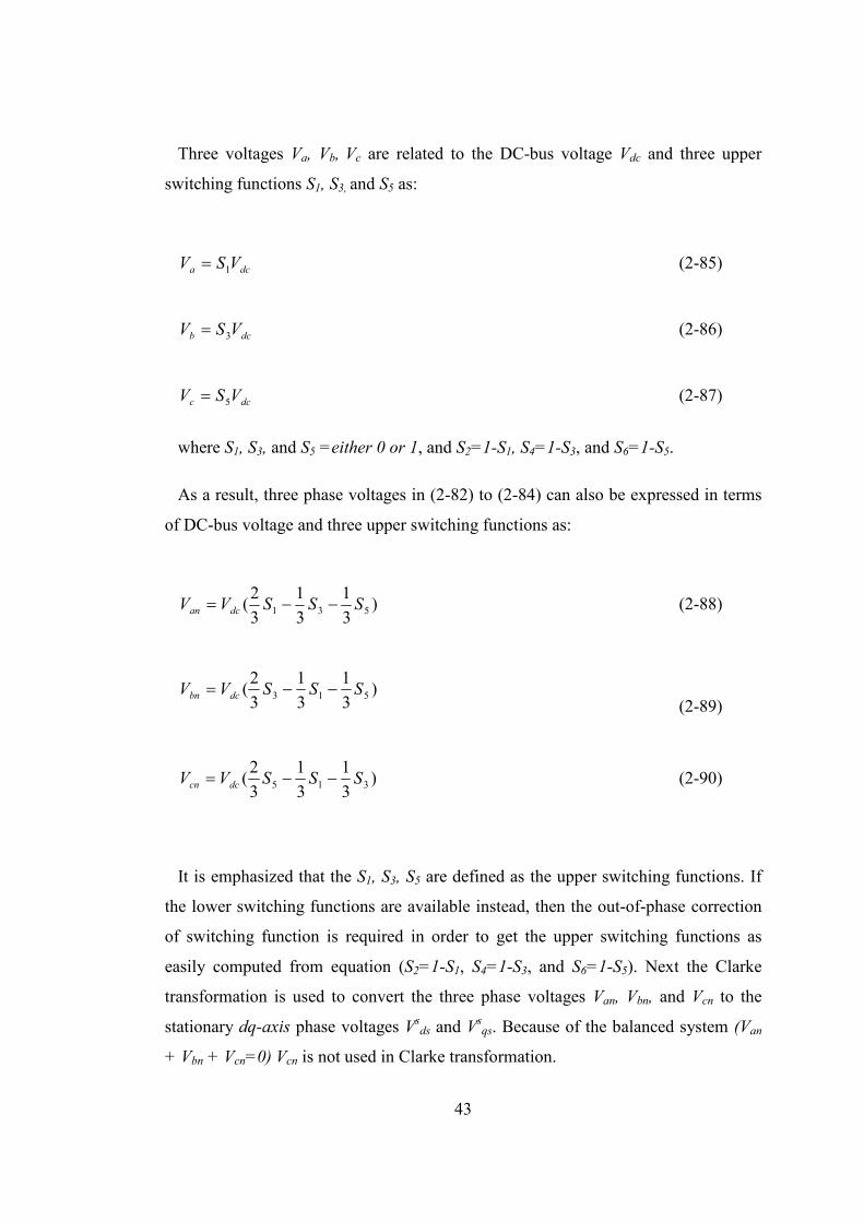
43

Three voltages Va, Vb, Vc are related to the DC-bus voltage Vdc and three upper

switching functions S1, S3, and S5 as:

dca VSV 1= (2-85)

dcb VSV 3= (2-86)

dcc VSV 5= (2-87)

where S1, S3, and S5 =either 0 or 1, and S2=1-S1, S4=1-S3, and S6=1-S5.

As a result, three phase voltages in (2-82) to (2-84) can also be expressed in terms

of DC-bus voltage and three upper switching functions as:

)3

1

3

1

3

2( 531 SSSVV dcan −−= (2-88)

)3

1

3

1

3

2( 513 SSSVV dcbn −−=

(2-89)

)3

1

3

1

3

2( 315 SSSVV dccn −−= (2-90)

It is emphasized that the S1, S3, S5 are defined as the upper switching functions. If

the lower switching functions are available instead, then the out-of-phase correction

of switching function is required in order to get the upper switching functions as

easily computed from equation (S2=1-S1, S4=1-S3, and S6=1-S5). Next the Clarke

transformation is used to convert the three phase voltages Van, Vbn, and Vcn to the

stationary dq-axis phase voltages Vsds and V

sqs. Because of the balanced system (Van

+ Vbn + Vcn=0) Vcn is not used in Clarke transformation.

44

CHAPTER 3

FLUX ESTIMATION FOR SENSORLESS DIRECT FIELD

ORIENTED CONTROL OF INDUCTION MACHINE

This chapter focuses on adaptive flux observer for direct field-orientation (DFO).

The field orientation is implemented in two ways as Direct Field Orientation and

Indirect Field Orientation. The basic difference of these methods underlies in the

manner of detecting the synchronous speed. In IFO, the slip angle is computed and

added to the rotor angle to find the synchronous speed. One must calculate, therefore,

the slip-angle and estimate the rotor angle. In the current model employed in the IFO,

dq-axes stator currents and precise rotor time-constants are needed to find the slip

angle. However, in DFO, the rotor angle is computed from the ratio of dq-axes

fluxes.

3.1. Flux Estimation

The logic underlying this flux observer is basically an advanced voltage model

approach in which integration of the back-emf is calculated and compensated for the

errors associated with pure integrator and stator resistance Rs measurement at low

speeds. At high speeds, the voltage model provides an accurate stator flux estimate

because the machine back emf dominates the measured terminal voltage. However,

at low speeds, the stator IR drop becomes significant, causing the accuracy of the

flux estimate to be sensitive to the estimated stator resistance. Due to this effect, at

low excitation frequencies flux estimation based upon voltage model are generally

not capable of achieving high dynamic performance at low speeds [15].

Consequences of these problems are compensated with the addition of a closed-loop

in the flux observer. Basically, the fluxes obtained by current model are compared

with those obtained by the voltage model with reference to the current model, or the

45

current model with reference to the voltage model according to the range in which

one of these models is superior to other [22]. In this flux observer the voltage model

is corrected by the current model through a basic PI block. In the end, the stator

fluxes are used to obtain rotor fluxes and rotor flux angle. In the following parts, the

superscript “v” and “i” corresponds to the values of voltage model and the values of

current model respectively.

3.1.1. Estimation of the Flux Linkage Vector

Most of the sensorless control schemes rely directly or indirectly on the estimation

of the stator flux linkage vector, ψs being defined as the time integral of the induced

voltage,

v

s

v

s

offsss

vs

uiRudt

d

0

,

)0(

,

ψψ

ψ

=

+−=

(3-1)

where, ψ vs0 is the initial value of flux linkage vector, uoff represents all disturbances

such as offsets, unbalances and other errors present in the estimated induced emf. A

major source of error in the emf is due to the changes in the model parameter Rs. The

estimation of the flux vectors requires the integration of (3-1) in real-time. The

integrator, however, will have an infinite gain at zero frequency, and the unavoidable

offsets contained in the integrator input then make its output gradually drift away

beyond limits.

3.1.1.1. Flux Estimation in Continuous Time

The rotor flux linkage dynamics in synchronously rotating reference frame

(w=we=wψr) being as;

46

ie

qrre

ie

dr

r

e

ds

r

m

ie

dr wwiL

dt

d ,,,

)(1

ψψττ

ψ−+−= (3-2)

ie

drre

ie

qr

r

e

qs

r

m

ie

qrwwi

L

dt

d,,

,

)(1

ψψττ

ψ−+−= (3-3)

where mL is the magnetizing inductance (H), rrr RL /=τ is the rotor time-constant

(sec), and rw is the electrical angular velocity of the rotor (rad/sec). These equations

are derived from the equations (2-64) and (2-68) of the previous chapter. In the

current model, the total rotor flux-linkage is aligned with the d-axis component, and

hence;

0,

,,

=

=

ie

qr

ie

dr

ie

r

ψ

ψψ

Substitution of 0, =ie

qrψ into (3-2) and (3-3) yields the oriented rotor flux dynamics

as;

ie

dr

r

e

ds

r

m

ie

dr iL

dt

d ,, 1

ψττ

ψ−= (3-4)

0, =ie

qrψ (3-5)

Note that (3-4) and (3-5) are the commonly recognized forms of the rotor flux

vector equations. When, the rotor flux linkages in (3-4) and (3-5) undergoes the

inverse park transformation in the stationary reference frame the result becomes.

47

)cos()sin()cos( ,,,,

rrr

ie

dr

ie

qr

ie

dr

is

dr ψψψ θψθψθψψ =−= (3-6)

)sin()sin()cos( ,,,,

rrr

ie

dr

ie

dr

ie

qr

is

qr ψψψ θψθψθψψ =+= (3-7)

where rψθ is the rotor flux angle (rad). The stator flux linkages in stationary

reference frame are then computed using (3-6), (3-7) and (2-68) as;

is

dr

r

ms

ds

r

mrss

drm

s

dss

is

dsL

Li

L

LLLiLiL ,

2, ψψ +

−=+= (3-8)

is

qr

r

ms

qs

r

mrss

qrm

s

qss

is

qsL

Li

L

LLLiLiL ,

2, ψψ +

−=+=

(3-9)

The stator flux linkages in the voltage model, however, are computed by

integrating the back emf’s and compensated voltages taken into account.

( )∫ −−= dtuRiu dscomps

s

ds

s

ds

vs

ds ,,ψ (3-10)

( )∫ −−= dtuRiu qscomps

s

qs

s

qs

vs

qs ,,ψ

(3-11)

The compensated voltages, on the other hand, are computed by the PI control law

as follows:

( ) ( )∫ −+−= dtT

KKu is

ds

vs

ds

I

pis

ds

vs

dspdscomp

,,,,, ψψψψ (3-12)

48

( ) ( )∫ −+−= dtT

KKu is

qs

vs

qs

I

pis

qs

vs

qspqscomp

,,,,, ψψψψ

(3-13)

The proportional gain Kp and the reset time TI are chosen such that the flux

linkages computed by the current model becomes dominant at low speed. The reason

for that is the back emfs computed by the voltage model result to be extremely low at

this speed range (even zero for back emfs at zero speed). While the motor is running

at high speed range, the flux linkages computed by voltage model becomes dominant

over the flux linkage components computed through the current model.

Once the stator flux linkages in (3-10) and (3-11) are calculated, the rotor flux

linkages based on the voltage model are computed once more through (3-14) and (3-

15) which are only rearranged forms of (3-8) and (3-9), as

vs

ds

m

rs

ds

m

mrsvs

drL

Li

L

LLL,

2, ψψ +

−−= (3-14)

vs

qs

m

rs

qs

m

mrsvs

qrL

Li

L

LLL,

2, ψψ +

−−= (3-15)

It is then a straight process to compute the rotor flux angle based on the voltage

model as;

= −

vs

dr

vs

qr

r ,

,1tanψ

ψθψ (3-16)

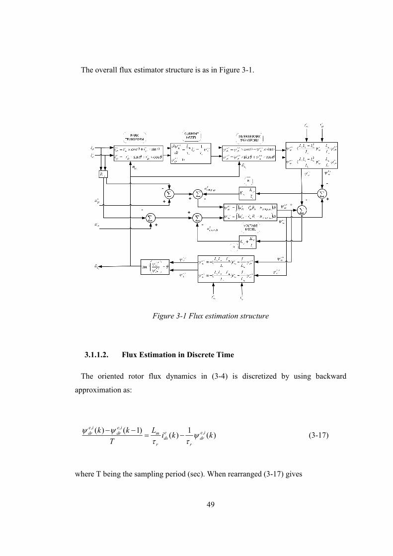
49

The overall flux estimator structure is as in Figure 3-1.

Figure 3-1 Flux estimation structure

3.1.1.2. Flux Estimation in Discrete Time

The oriented rotor flux dynamics in (3-4) is discretized by using backward

approximation as:

)(1

)()1()( ,

,,

kkiL

T

kk ie

dr

r

e

ds

r

m

ie

dr

ie

dr ψττ

ψψ−=

−− (3-17)

where T being the sampling period (sec). When rearranged (3-17) gives

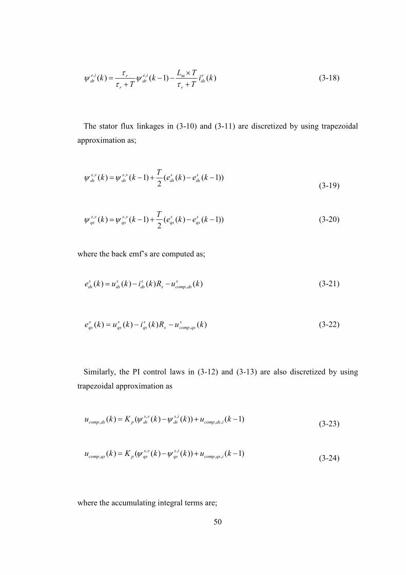
50

)()1()( ,, kiT

TLk

Tk e

ds

r

mie

dr

r

rie

dr +×

−−+

=τ

ψττ

ψ (3-18)

The stator flux linkages in (3-10) and (3-11) are discretized by using trapezoidal

approximation as;

))1()((2

)1()( ,, −−+−= kekeT

kk s

ds

s

ds

vs

ds

vs

ds ψψ (3-19)

))1()((2

)1()( ,, −−+−= kekeT

kk s

qs

s

qs

vs

qs

vs

qs ψψ (3-20)

where the back emf’s are computed as;

)()()()( , kuRkikuke s

dscomps

s

ds

s

ds

s

ds −−= (3-21)

)()()()( , kuRkikuke s

qscomps

s

qs

s

qs

s

qs −−= (3-22)

Similarly, the PI control laws in (3-12) and (3-13) are also discretized by using

trapezoidal approximation as

)1())()(()( ,,

,,, −+−= kukkKku idscomp

is

ds

vs

dspdscomp ψψ (3-23)

)1())()(()( ,,,,

, −+−= kukkKku iqscomp

is

qs

vs

qspqscomp ψψ (3-24)

where the accumulating integral terms are;

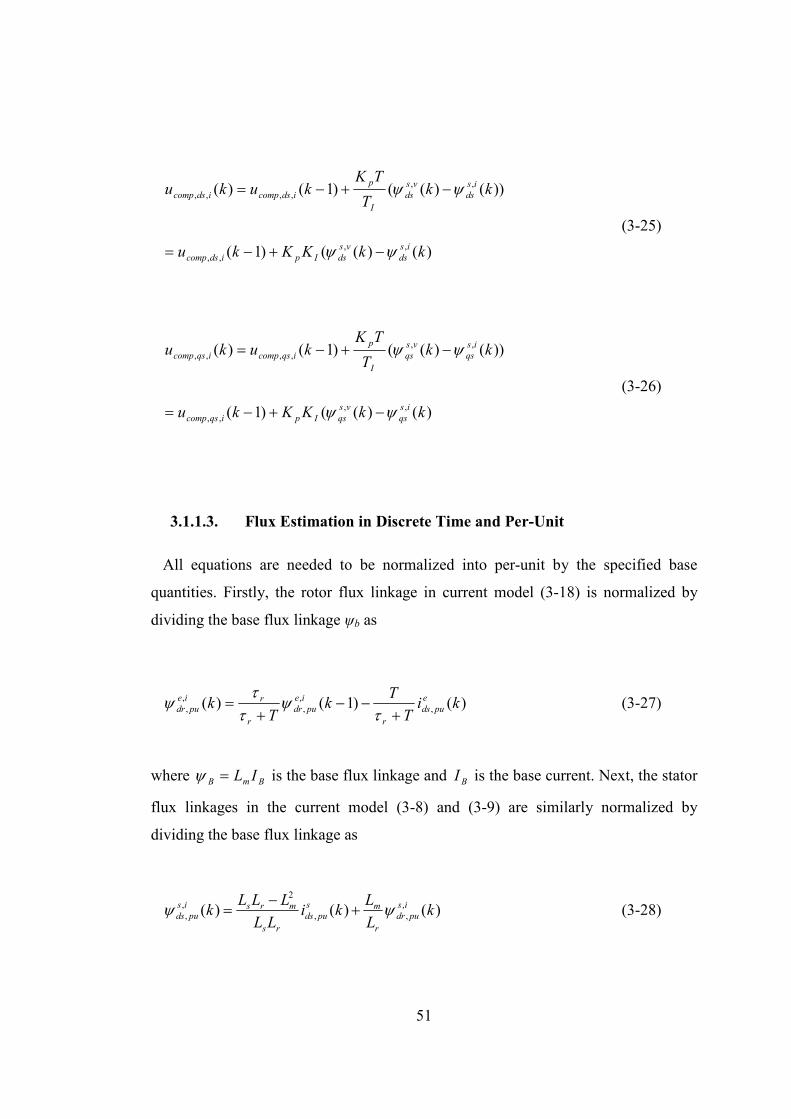
51

)()(()1(

))()(()1()(

,,,,

,,,,,,

kkKKku

kkT

TKkuku

is

ds

vs

dsIpidscomp

is

ds

vs

ds

I

p

idscompidscomp

ψψ

ψψ

−+−=

−+−=

(3-25)

)()(()1(

))()(()1()(

,,,,

,,,,,,

kkKKku

kkT

TKkuku

is

qs

vs

qsIpiqscomp

is

qs

vs

qs

I

p

iqscompiqscomp

ψψ

ψψ

−+−=

−+−=

(3-26)

3.1.1.3. Flux Estimation in Discrete Time and Per-Unit

All equations are needed to be normalized into per-unit by the specified base

quantities. Firstly, the rotor flux linkage in current model (3-18) is normalized by

dividing the base flux linkage ψb as

)()1()( ,,,

,, ki

T

Tk

Tk e

puds

r

ie

pudr

r

rie

pudr +−−

+=

τψ

ττ

ψ (3-27)

where BmB IL=ψ is the base flux linkage and BI is the base current. Next, the stator

flux linkages in the current model (3-8) and (3-9) are similarly normalized by

dividing the base flux linkage as

)()()( ,,,

2,, k

L

Lki

LL

LLLk is

pudr

r

ms

puds

rs

mrsis

puds ψψ +−

= (3-28)

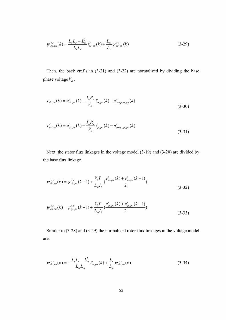
52

)()()( ,,,

2,, k

L

Lki

LL

LLLk is

puqr

r

ms

puqs

rs

mrsis

puqs ψψ +−

= (3-29)

Then, the back emf’s in (3-21) and (3-22) are normalized by dividing the base

phase voltage BV .

)()()()( ,,,,, kukiV

RIkuke s

pudscomp

s

puds

b

sbs

puds

s

puds −−= (3-30)

)()()()( ,,,,, kukiV

RIkuke s

puqscomp

s

puqs

b

sbs

puqs

s

puqs −−= (3-31)

Next, the stator flux linkages in the voltage model (3-19) and (3-20) are divided by

the base flux linkage.

)2

)1()(()1()( ,,,

,,,

−++−=

keke

IL

TVkk

s

puds

s

puds

bm

bvs

puds

vs

puds ψψ (3-32)

)2

)1()(()1()( ,,,

,,,

−++−=

keke

IL

TVkk

s

puqs

s

puqs

bm

bvs

puqs

vs

puqs ψψ (3-33)

Similar to (3-28) and (3-29) the normalized rotor flux linkages in the voltage model

are:

)()()( ,,,

2,, k

L

Lki

LL

LLLk vs

puds

m

rs

puds

mm

mrsvs

pudr ψψ +−

−= (3-34)

53

)()()( ,,,

2,, k

L

Lki

LL

LLLk vs

puqs

m

rs

puqs

mm

mrsvs

puqr ψψ +−

−= (3-35)

In conclusion, the discrete-time, per-unit equations are rewritten in terms of

constants.

The rotor flux linkages developed by the current model in synchronously rotating

reference frame (w=wψr) are:

)()1()( ,2,,1

,, kiKkKk e

puds

ie

pudr

ie

pudr −−= ψψ (3-36)

where

T

TK

TK

r

r

r

+=

+=

τ

ττ

2

1

(3-37)

The rotor flux linkages developed by the current model in the stationary reference

frame (w=0) are:

)()()( ,,3,4

,, kKkiKk is

pudr

s

puds

is

puds ψψ += (3-38)

)()()( ,,3,4

,, kKkiKk is

puqr

s

puqs

is

puqs ψψ += (3-39)

54

r

m

rs

mrs

L

LK

LL

LLLK

=

−=

3

2

4

(3-40)

The back emf’s developed by the voltage model in the stationary reference frame

(w=0) is

)()()()( ,,,5,, kukiKkuke s

pudscomp

s

puds

s

puds

s

puds −−= (3-41)

)()()()( ,,,5,, kukiKkuke s

puqscomp

s

puqs

s

puqs

s

puqs −−= (3-42)

b

sb

V

RIK =5 (3-43)

The stator flux linkages developed by the voltage model in the stationary reference

frame (w=0) are:

)2

)1()(()1()( ,,

6,,

,,

−++−=

kekeKkk

s

puds

s

pudsvs

puds

vs

puds ψψ (3-44)

)2

)1()(()1()( ,,

6,,

,,

−++−=

kekeKkk

s

puqs

s

puqsvs

puqs

vs

puqs ψψ (3-45)

bm

b

IL

TVK =6 (3-46)

The rotor flux linkages developed by the voltage model in the stationary reference

frame (w=0) are:

55

)()()( ,,7,8

,, kKkiKk vs

puds

s

puds

vs

pudr ψψ +−= (3-47)

m

r

mm

mrs

L

LK

LL

LLLK

=

−=

7

2

8

(3-48)

The rotor flux angle developed by the voltage model

= −

)()(

tan21

)(,

,

,,

1,

k

kk

pudrvs

puqrvs

pur ψψ

πθψ (3-49)

The required parameters for this module are summarized as follows:

• The machine Parameters:

• Stator resistance (Rs)

• Rotor resistance (Rr)

• Stator leakage inductance (Lls)

• Rotor leakage inductance (Llr)

• Magnetizing inductance (Lm)

• The based quantities:

• Base current (Ib)

• Base phase voltage (Vb)

• The sampling period(T)

The stator self inductance is Ls=Lls+Lm and the rotor self inductance is Lr=Llr+Lm.

56

CHAPTER 4

SPEED ESTIMATION FOR SENSORLESS DIRECT FIELD

ORIENTED CONTROL OF INDUCTION MACHINE

The rotor speed estimation is examined with three estimation schemes. The

reactive power MRAS speed estimator, open-loop speed estimator, speed estimator

using Kalman filter are implemented.

4.1. Reactive Power MRAS Scheme

Model Reference Adaptive System (MRAS) is one of the most popular adaptive

control method used in motor control applications for tracking and observing system

parameters and states [23-27, 30-31]. There exist a number of different model

reference adaptive control techniques such as parallel model, series model, direct

model and indirect model etc. MRAS used in this thesis is parallel model MRAS that

compares both the outputs of a reference model and adaptive model and processes

the error between these two according to the appropriate adaptive laws that do not

deteriorate the stability requirements of the applied system.

In a MRAS system, some state variables qd xx , (e.g. back e.m.f components

( mqmd ee , ) reactive power components ( mqmd qq , ) , rotor flux components ( rqrd ψψ , )

etc.) of the induction machine, which are obtained from sensed variables such as

stator voltage and currents, are estimated in reference model and are then compared

with state variables dx and qx estimated by using adaptive model. The difference

between these state variables is then used in adaptation mechanism, which outputs

the estimated value of the rotor speed ( rw ) and adjusts the adaptive model until

satisfactory performance is obtained. Such a scheme is shown in Figure 4-1

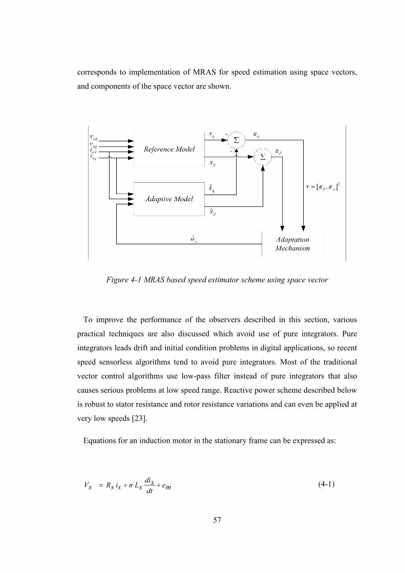
57

corresponds to implementation of MRAS for speed estimation using space vectors,

and components of the space vector are shown.

Figure 4-1 MRAS based speed estimator scheme using space vector

To improve the performance of the observers described in this section, various

practical techniques are also discussed which avoid use of pure integrators. Pure

integrators leads drift and initial condition problems in digital applications, so recent

speed sensorless algorithms tend to avoid pure integrators. Most of the traditional

vector control algorithms use low-pass filter instead of pure integrators that also

causes serious problems at low speed range. Reactive power scheme described below

is robust to stator resistance and rotor resistance variations and can even be applied at

very low speeds [23].

Equations for an induction motor in the stationary frame can be expressed as:

medt

sdisLσsisRsV ++= (4-1)

58

where )(12

cofficientleakageLL

L

sr

m−=σ .

sir

mir

mirw

dt

mdi

ττ11

+−×= (4-2)

where

rw is a vector whose magnitude wr is rotor electrical angular velocity, and

whose direction is determined according to right hand system of coordinates as

shown in Figure 4-2 “×” denotes the cross product of vectors respectively

From (4-1) and (4-2), me and structure of MRAS can be derived as follows:

+−=

dt

diLiRVe sssssm σ (4-3)

dt

diLe mmm′= (4-4)

+−×′= s

r

m

r

mrm iiiwLττ11

(4-5)

where r

mm

L

LL

2

=′ and r

rr

R

L=τ

If we rewrite the equations above for the direct and quadrature-axis back-emf in the

following forms:

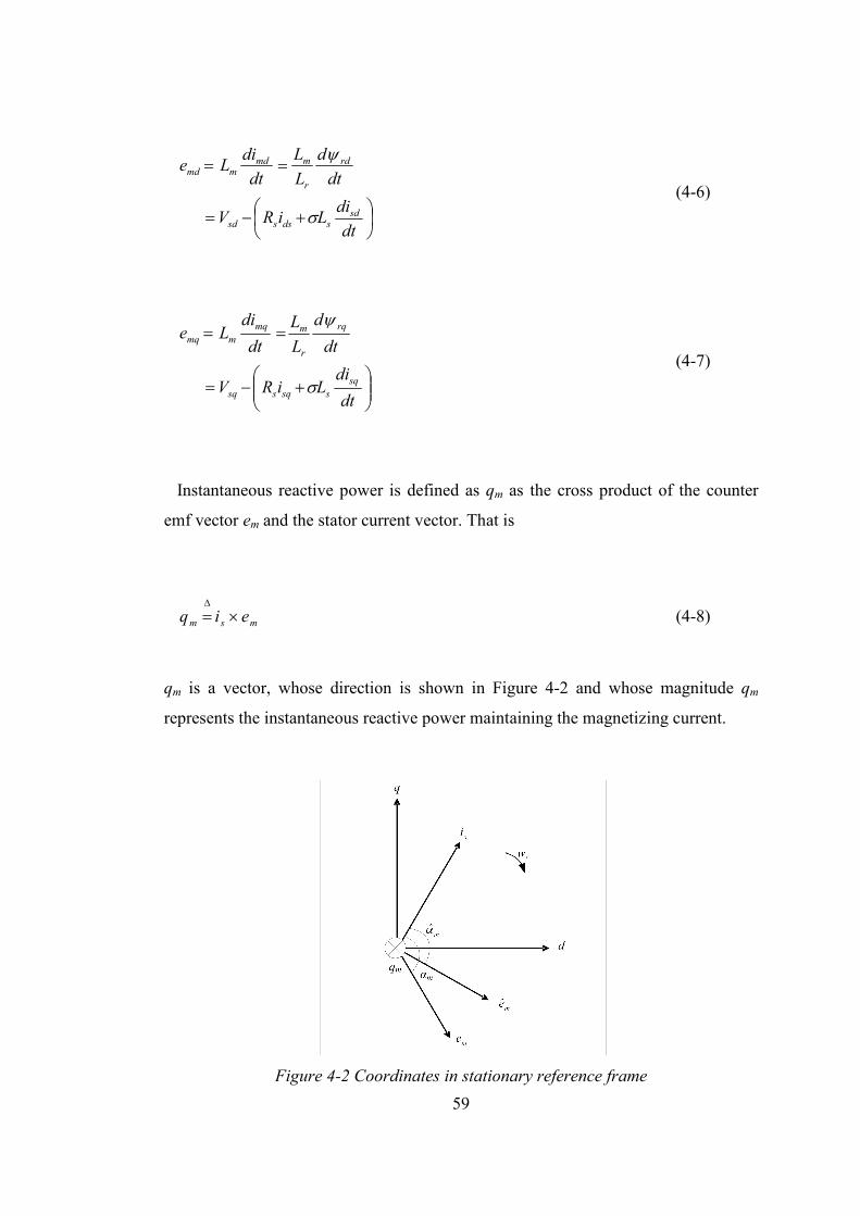
59

+−=

==

dt

diLiRV

dt

d

L

L

dt

diLe

sdsdsssd

rd

r

mmdmmd

σ

ψ

(4-6)

+−=

==

dt

diLiRV

dt

d

L

L

dt

diLe

sq

ssqssq

rq

r

mmq

mmq

σ

ψ

(4-7)

Instantaneous reactive power is defined as qm as the cross product of the counter

emf vector em and the stator current vector. That is

msm eiq ×=∆

(4-8)

qm is a vector, whose direction is shown in Figure 4-2 and whose magnitude qm

represents the instantaneous reactive power maintaining the magnetizing current.

Figure 4-2 Coordinates in stationary reference frame

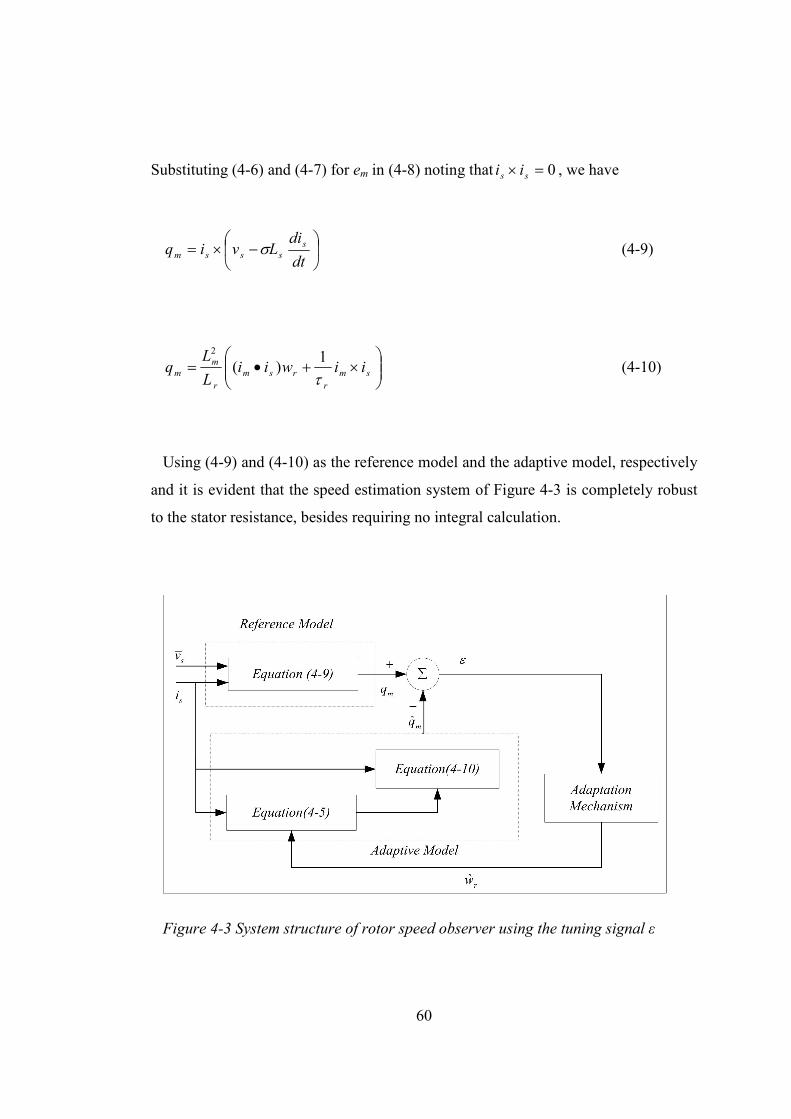
60

Substituting (4-6) and (4-7) for em in (4-8) noting that 0=× ss ii , we have

−×=

dt

diLviq s

sssm σ (4-9)

×+•= sm

r

rsm

r

m

m iiwiiL

Lq

τ1

)(2

(4-10)

Using (4-9) and (4-10) as the reference model and the adaptive model, respectively

and it is evident that the speed estimation system of Figure 4-3 is completely robust

to the stator resistance, besides requiring no integral calculation.

Figure 4-3 System structure of rotor speed observer using the tuning signal ε

61

The information required for this module is stator voltage and stator current

components in the dq stationary reference frame. Two sets of equations are

developed to compute reactive power of the induction motor in the reference and

adaptive models. The reference model does not involve the rotor speed while the

adaptive model needs the estimated rotor speed to adjust the computed reactive

power to that computed from the reference model. Notice that the representation of

complex number is defined for the stator voltages and currents in the stationary

reference frame i.e., sqsds jvvv += and sqsds jiii += .

4.1.1. Reference Model Continuous Time Representation

The back-emf of the induction motor can be expressed in the stationary frame as

follows

dt

diLiRv

dt

d

L

Le sd

ssdssdrd

r

mmd σ

ψ−−==ˆ (4-11)

dt

diLiRv

dt

d

L

Le

sq

ssqssq

rq

r

mmq σ

ψ−−==ˆ (4-12)

mqmdm jeee += (4-13)

The reactive power of the induction motor can be computed from cross product of

stator currents and back-emf vectors as follows:

62

dt

idLivi

dt

idLiRvieiq s

sssss

sssssmsm σσ ×−×=

−−×=×= (4-14)

where 0=−=× sdsqsqsdss iiiiii . As a result the reactive power shown in (4-14) can

further be derived as

−−−=

dt

dii

dt

diiLviviq sd

sq

sq

sdssdsqsqsdm σ (4-15)

4.1.2. Adaptive Model Continuous Time Representation

The estimated back-emf computed in the adaptive model can be expressed as

follows:

( )sdmdmqrr

r

mmd

r

mmd iiiw

L

L

dt

di

L

Le +−−== ˆˆ

22

τ (4-16)

( )sqmqmdrr

r

mmq

r

mmq iiiw

L

L

dt

di

L

Le +−−== ˆˆ

22

τ (4-17)

mqmdm ejee ˆˆˆ += (4-18)

where r

rr

R

L=τ is the rotor time constant, imd, imq are computed from the following

equations:

sd

r

md

r

mqrmd iiiwdt

di

ττ11

ˆ +−−= (4-19)

63

sq

r

mq

r

mdr

mqiiiw

dt

di

ττ11

ˆ +−−= (4-20)

Once the estimated back-emf computed by (4-16)-(4-20), the estimated reactive

power can be computed as follows:

mdsqmqsdmsm eieieiq ˆˆˆˆ −=×= (4-21)

Then, the PI controller tunes the estimated rotor speed such that the reactive power

generated by adaptive model matches that generated by reference model. The speed

tuning signal is the error of reactive power that can be expressed as follows:

mmmmse qqeei ˆ)ˆ( −=−×=∆ε (4-22)

When this observer is used in a vector-controlled drive, it is possible to obtain

satisfactory performance even at very low speeds. The observer can track the actual

rotor speed with a bandwidth that is only limited by noise, so the PI controller gains

should be as large as possible. The scheme is insensitive to stator resistance

variations. The parameter τr has a negligible influence on the operation of both of the

overall MRAS vector control systems. If the MRAS successfully maintains nearly

zero error, and if the same value of τr is used in the MRAS adjustable models and in

the function block for calculating wsl, then we have the following relations:

ee ww ˆ= and slrslr ww ˆττ =

64

where variables without “^” are actual values, and ones with “^” represent the

corresponding values used in the MRAS vector control systems. Thus, if rr ττ ˆ≠ ,

then slsl ww ˆ≠ , but ee ww ˆ= , which is used for orienting the stator current vector.

Therefore, complete field orientation can be achieved even if the value of τr is quite

wrong. The error in the value of τr, however, produces an error in the speed

feedback, thus affecting the accuracy of the speed control as follows:

sl

r

rrrw www

−=−=ττ

εˆ

1ˆ (4-23)

This also holds for the previous MRAS scheme. However, the accuracy of the

speed estimation system discussed depends on the transient stator inductance and

also referred magnetizing inductance. The latter quantity is not too problematic, since

it does not change with temperature. Furthermore, deviations of τr from its correct

value produce a steady-state error in the estimated speed and this error become

significant at low speeds.

4.1.3. Discrete Time Representation

For implementation on digital system, the differential equations need to be

transformed to difference equations. Due to high sampling frequency compared to

bandwidth of the system, the simple approximation of numerical integration , such as

forward ,backward, or trapezoidal rules, can be adopted [34] . Consequently, the

reactive power equations in both the reference and the adaptive models are

discretized as follows:

4.1.3.1. Reference Model

According to (4-15) reference model reactive power is given as:

65

−−−=

dt

dii

dt

diiLviviq sd

sq

sq

sdssdsqsqsdm σ

Using backward approximation:

−−−

−−

−−=

T

kikiki

T

kikikiL

kvkikvkikq

sdsdsq

sqsq

sds

sdsqsqsdm

)1()()(

)1()()(

)()()()()(

σ (4-24)

and this equation can be further simplified as:

( ))1()()()1(

)()()()()(

−−−

−−=

kikikikiT

L

kvkikvkikq

sqsdsqsds

sdsqsqsdm

σ (4-25)

where T is the sampling time.

4.1.3.2. Adaptive Model

According to (4-21), reactive power in adaptive model is derived as

mdsqmqsdmsm eieieiq ˆˆˆˆ −=×=

whose discrete time representation is:

)(ˆ)()(ˆ)()(ˆ kekikekikq mdsqmqsdm −= (4-26)

66

where )(ˆ kemd and )(ˆ kemq are computed as follows:

Continuous time representation:

( )

( )sqmqmdrr

r

mmq

r

mmq

sdmdmqrr

r

mmd

r

m

md

iiiwL

L

dt

di

L

Le

iiiwL

L

dt

di

L

Le

+−−==

+−−==

ˆˆ

ˆˆ

22

22

τ

τ

(4-27)

Discrete time representation:

( )

( ))()()()(ˆ)(ˆ

)()()()(ˆ)(ˆ

2

2

kikikikwL

Lke

kikikikwL

Lke

sqmqmdrr

r

mmq

sdmdmqrr

r

mmd

+−−=

+−−=

τ

τ

(4-28)

and )(),( kiki mqmd can be solved by using trapezoidal integration method, it yields

Continuous time representation:

sq

r

mq

r

mdr

mq

sd

r

md

r

mqrmd

iiiwdt

di

iiiwdt

di

ττ

ττ

11ˆ

11ˆ

+−−=

+−−=

(4-29)

67

Discrete time representation:

−

−+

−−

−

+−+−−=

r

rsq

rr

sd

r

rmq

rr

rmdmd

Tkwki

T

T

Tki

TTkwki

TTkw

Tkiki

τ

ττ

ττ

2)(ˆ)(

2)()(ˆ)1(

1)(ˆ2

)1()(

2

2

22

2

22

(4-30)

−

−+

−−

−

+−+−−=

r

rsd

rr

sq

r

rmd

rr

rmqmq

Tkwki

T

T

Tki

TTkwki

TTkw

Tkiki

τ

ττ

ττ

2)(ˆ)(

2)()(ˆ)1(

1)(ˆ2

)1()(

2

2

22

2

22

(4-31)

4.2. Open Loop Speed Estimator

The open loop speed estimator based on the equations of the induction motor in the

stationary reference frame [35]. Rotor flux linkage equations are as given below in

(4-32) and (4-33).

s

dsmdrs

rdrs iLiL +=ψ (4-32)

68

s

qsmqrs

rqrs iLiL +=ψ (4-33)

The rotor currents can be expressed as in (4-34), (4-35).

)(1 s

dsmdrs

r

drs iL

Li −= ψ (4-34)

)(1 s

qsmqrs

r

qrs iL

Li −= ψ (4-35)

The rotor voltage equations are used to find rotor flux dynamics as in (4-36),

(4-37).

dt

dwiR

s

drs

qrr

s

drr

ψψ ++=0 (4-36)

dt

dwiR

s

qrs

drr

s

qrr

ψψ ++=0 (4-37)

Substituting the current equations (4-34), (4-35) into (4-36), (4-37) rotor flux

dynamics can be stated as in (4-38), (4-39).

s

qrr

s

ds

r

ms

dr

r

s

dr wiL

dt

dψ

τψ

τψ

−+−=1

(4-38)

69

s

drr

s

qs

r

ms

qr

r

s

qrwi

L

dt

dψ

τψ

τ

ψ++−=

1 (4-39)

where r

rr

R

L=τ is the rotor time constant.

Then rotor flux linkage magnitude and the angle can be computed as:

22 s

dr

s

qr

s

r ψψψ += (4-40)

= −

s

dr

s

qr

r ψ

ψθψ

1tan (4-41)

This method is sensitive to parameter estimation. Nevertheless, the open-loop

speed estimation is changed that uses computed flux angle; the flux angle from

adaptive flux estimator is used instead which gives a better estimate for flux angle

due to its adaptive mechanism. Then the electrically angular velocity is calculated

taking the derivative of the flux angle in (4-41).

( )( ) ( )

−

==22

2

s

dr

s

drs

qr

s

qrs

dr

s

r

s

dre

dt

d

dt

d

dt

dw r

ψ

ψψ

ψψ

ψ

ψθψ (4-42)

Substituting equations (4-38), (4-39) into (4-42) and rearranging (4-43) is obtained.

70

( )( )s

ds

s

qr

s

qs

s

dr

r

m

s

r

re iiL

wdt

dw r ψψ

τψ

θψ −+==2

1 (4-43)

The second term in the right hand side is the angular slip velocity term wsl=(1-S)we

which is proportional to the electromagnetic torque while the rotor flux magnitude is

maintained constant. Then the rotor speed can be found as:

( )

( )s

ds

s

qr

s

qs

s

dr

r

m

s

r

er iiL

ww ψψτψ

−−=2

1 (4-44)

The rotor speed output is filtered with a first order low pass filter to eliminate high

frequency noise which comes from the differentiation.

4.3. Kalman Filter for Speed Estimation

4.3.1. Discrete Kalman Filter

In 1960, R.E. Kalman published recursive solution to the discrete data linear

filtering problem Kalman60. Since that time, due in large part to advances in digital

computing; the Kalman filter has been the subject of extensive research and

application, particularly in the area of autonomous or assisted navigation. The

Kalman filter addresses the general problem of trying to estimate the state nx ℜ∈ of

a discrete-time controlled process that is governed by the linear stochastic difference

equation [36]:

,111 −−− ++= kkkk wBuAxx (4-45)

71

with a measurement mz ℜ∈ that is

kkk vHxz += . (4-46)

The random variables kw and kv represent the process and measurement noise

(respectively). They are assumed to be independent (of each other), white, and with

normal probability distributions

),,0()( QNwp ≈ (4-47)

).,0()( RNvp ≈ (4-48)

In practice, the process noise covariance Q and measurement noise covariance R

matrices might change with each time step or measurement, however here it is

assumed that they are constant. The n x n matrix A in the difference equation (4-45)

relates the state at the previous time k-1 step to the state at the current step k, in the

absence of either a driving function or process noise. In practice A might change with

each time step, but here we assume it is constant. The matrix B relates the optional

control input lu ℜ∈ to the state x. The m x n matrix H in the measurement equation

(4-46) relates the state to the measurement kz . In practice H might change with each

time step or measurement, but here we assume it is constant.

72

4.3.2. Computational Origins of the Filter

Kalman Filter has two state estimates of the process a priori state estimate

n

kx ℜ∈−ˆ at step k given knowledge of the process prior to step k, and n

kx ℜ∈ˆ to be

our a posteriori state estimate at step k given measurement kz . Then, a priori and a

posteriori estimate errors are defined.

−− −≡ kkk xxe ˆ , and (4-49)

kkk xxe ˆ−≡ . (4-50)

The a priori estimate error covariance is then

[ ]T

kkk eeEP −−− = , (4-51)

and the a posteriori estimate error covariance is

[ ]T

kkk eeEP = . (4-52)

An equation that computes an a posteriori state estimate as a linear combination of

an a priori estimate and a weighted difference between an actual measurement and a

measurement prediction is derived as shown below in (4-53).

)ˆ(ˆˆ −− −+= kkkk xHzKxx (4-53)

73

The difference )ˆ( −− kk xHz in (4-53) is called the measurement innovation, or the

residual. The residual reflects the discrepancy between the predicted measurement

−kxHˆ and the actual measurement kz . A residual of zero means that the two are in

complete agreement.

The matrix K in (4-53) is chosen to be the gain or blending factor that minimizes

the a posteriori error covariance (4-52). This minimization can be accomplished by

first substituting (4-53) into the above definition for ke , substituting that into (4-52),

performing the indicated expectations, taking the derivative of the trace of the result

with respect to K, setting that result equal to zero, and then solving for K

Maybeck79, Brown92, Jacobs93. One form of the resulting K that minimizes (4-52)

is given by Brown92 [36].

1)( −−− += RHHPHPK T

k

T

kk (4-54)

From this it can be seen that when the measurement error covariance matrix R

reaches zero, the Kalman gain will weigh the residual more heavily:

1

0lim

−

→= HK k

Rk

.

If this is the case, the actual measurement kz is trusted more and more. At the same

time, the predicted measurement −kxHˆ is trusted less and less. If however the a priori

estimate error covariance matrix −kP reaches zero, the Kalman gain will weigh the

residual less heavily:

74

0 lim0

=→−

kP

Kk

.

When this is the situation, as covariance matrix −kP approaches zero, the actual

measurement is trusted less and less; on the other hand predicted measurement −kxHˆ

is trusted more and more.

4.3.3. The Discrete Kalman Filter Algorithm

The Kalman filter estimates a process by using a form of feedback control: the

filter estimates the process state at some time and then obtains feedback in the form

of (noisy) measurements. As such, the equations for the Kalman filter fall into two

groups: time update equations and measurement update equations. The time update

equations are responsible for projecting forward (in time) the current state and error

covariance estimates to obtain the a priori estimates for the next time step. The

measurement update equations are responsible for the feedback, i.e. for incorporating

a new measurement into the a priori estimate to obtain an improved a posteriori

estimate. The time update equations can also be thought of as predictor equations,

while the measurement update equations can be thought of as corrector equations.

Indeed the final estimation algorithm resembles that of a predictor-corrector

algorithm for solving numerical problems.

Then the time update equations can be expressed as in (4-55), (4-56).

11ˆˆ −−− += kkk BuxAx (4-55)

QAAPP T

kk += −−

1 (4-56)

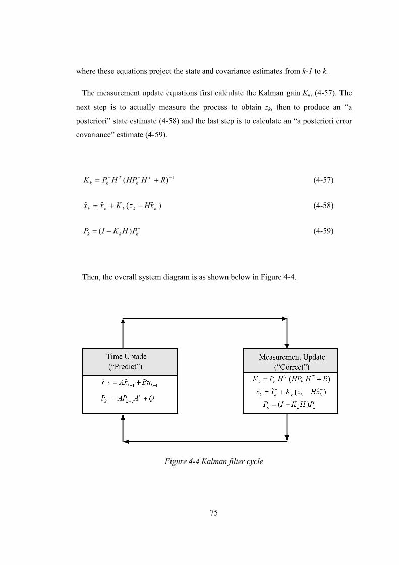
75

where these equations project the state and covariance estimates from k-1 to k.

The measurement update equations first calculate the Kalman gain Kk, (4-57). The

next step is to actually measure the process to obtain zk, then to produce an “a

posteriori” state estimate (4-58) and the last step is to calculate an “a posteriori error

covariance” estimate (4-59).

1)( −−− += RHHPHPK T

k

T

kk (4-57)

)ˆ(ˆˆ −− −+= kkkkk xHzKxx (4-58)

−−= kkk PHKIP )( (4-59)

Then, the overall system diagram is as shown below in Figure 4-4.

Figure 4-4 Kalman filter cycle

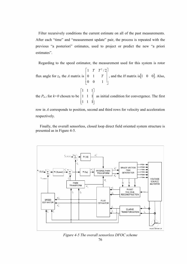
76

Filter recursively conditions the current estimate on all of the past measurements.

After each “time” and “measurement update” pair, the process is repeated with the

previous “a posteriori” estimates, used to project or predict the new “a priori

estimates”.

Regarding to the speed estimator, the measurement used for this system is rotor

flux angle for zk; the A matrix is

100

10

2/1 2

T

TT

, and the H matrix is [ ]001 . Also,

the Pk-1 for k=0 chosen to be

111

111

111

as initial condition for convergence. The first

row in A corresponds to position, second and third rows for velocity and acceleration

respectively.

Finally, the overall sensorless, closed loop direct field oriented system structure is presented as in Figure 4-5.

Figure 4-5 The overall sensorless DFOC scheme

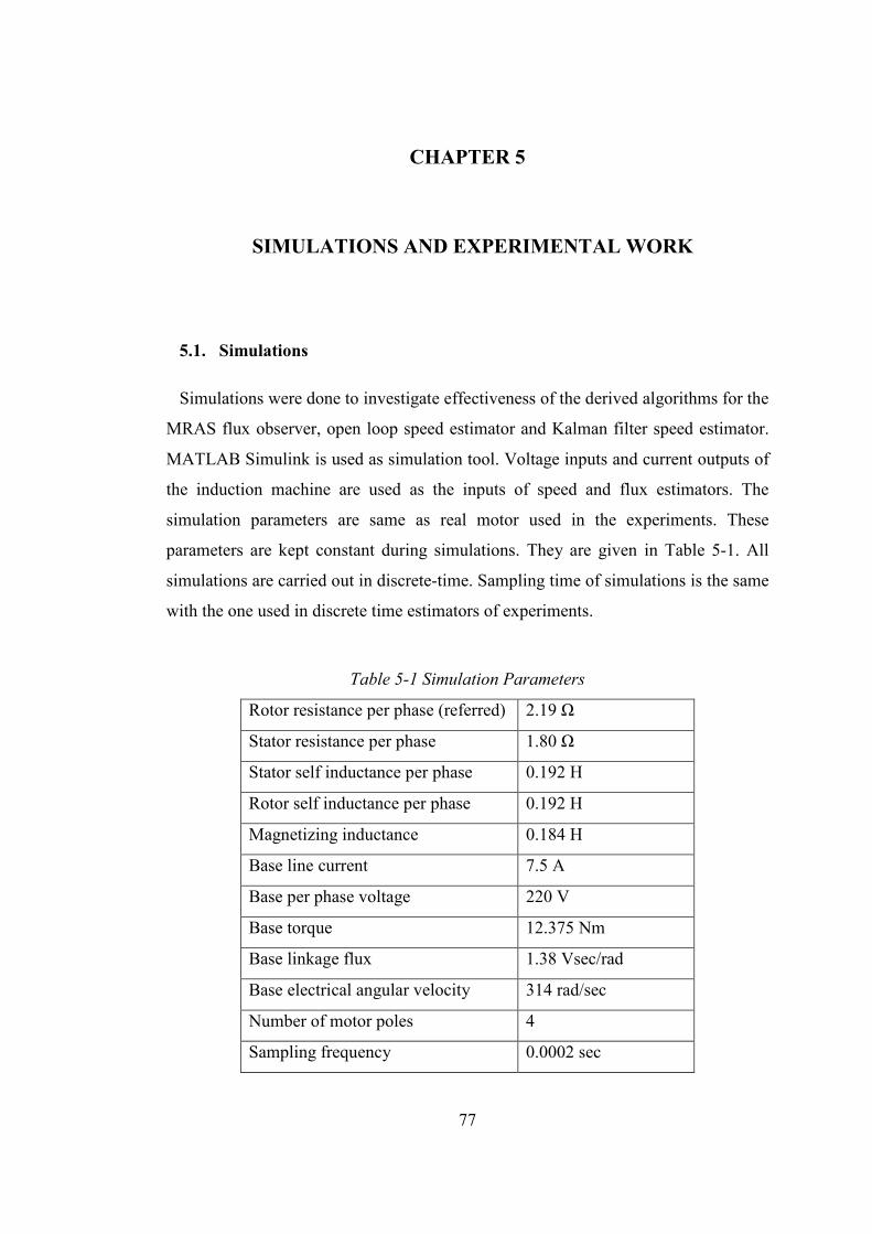
77

CHAPTER 5

SIMULATIONS AND EXPERIMENTAL WORK

5.1. Simulations

Simulations were done to investigate effectiveness of the derived algorithms for the

MRAS flux observer, open loop speed estimator and Kalman filter speed estimator.

MATLAB Simulink is used as simulation tool. Voltage inputs and current outputs of

the induction machine are used as the inputs of speed and flux estimators. The

simulation parameters are same as real motor used in the experiments. These

parameters are kept constant during simulations. They are given in Table 5-1. All

simulations are carried out in discrete-time. Sampling time of simulations is the same

with the one used in discrete time estimators of experiments.

Table 5-1 Simulation Parameters

Rotor resistance per phase (referred) 2.19 Ω

Stator resistance per phase 1.80 Ω

Stator self inductance per phase 0.192 H

Rotor self inductance per phase 0.192 H

Magnetizing inductance 0.184 H

Base line current 7.5 A

Base per phase voltage 220 V

Base torque 12.375 Nm

Base linkage flux 1.38 Vsec/rad

Base electrical angular velocity 314 rad/sec

Number of motor poles 4

Sampling frequency 0.0002 sec

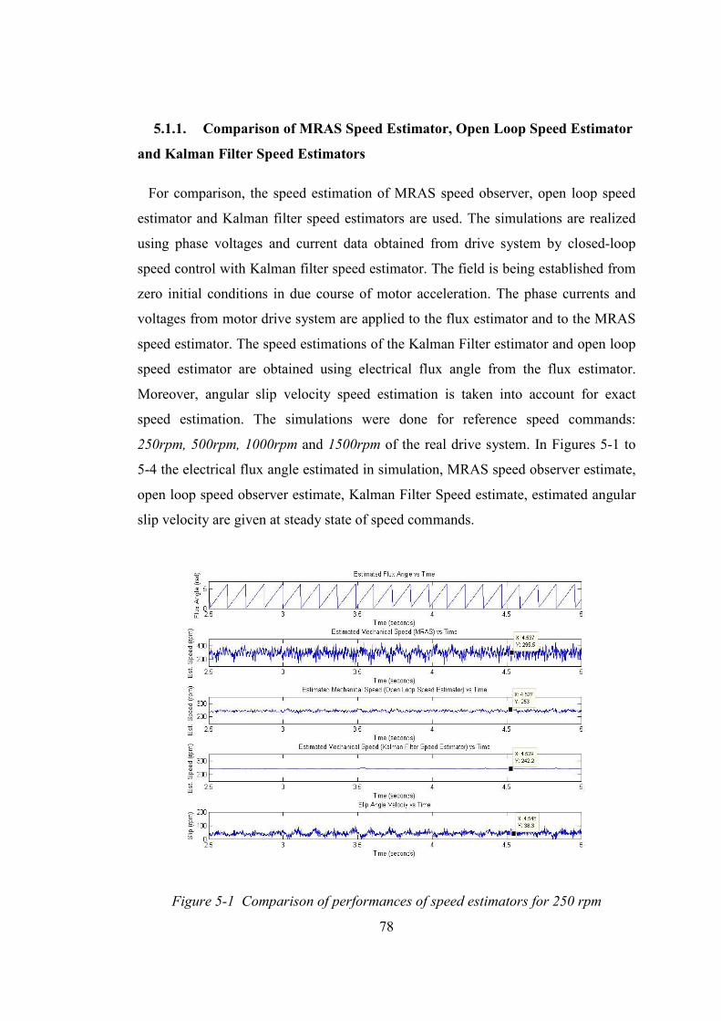
78

5.1.1. Comparison of MRAS Speed Estimator, Open Loop Speed Estimator

and Kalman Filter Speed Estimators

For comparison, the speed estimation of MRAS speed observer, open loop speed

estimator and Kalman filter speed estimators are used. The simulations are realized

using phase voltages and current data obtained from drive system by closed-loop

speed control with Kalman filter speed estimator. The field is being established from

zero initial conditions in due course of motor acceleration. The phase currents and

voltages from motor drive system are applied to the flux estimator and to the MRAS

speed estimator. The speed estimations of the Kalman Filter estimator and open loop

speed estimator are obtained using electrical flux angle from the flux estimator.

Moreover, angular slip velocity speed estimation is taken into account for exact

speed estimation. The simulations were done for reference speed commands:

250rpm, 500rpm, 1000rpm and 1500rpm of the real drive system. In Figures 5-1 to

5-4 the electrical flux angle estimated in simulation, MRAS speed observer estimate,

open loop speed observer estimate, Kalman Filter Speed estimate, estimated angular

slip velocity are given at steady state of speed commands.

Figure 5-1 Comparison of performances of speed estimators for 250 rpm

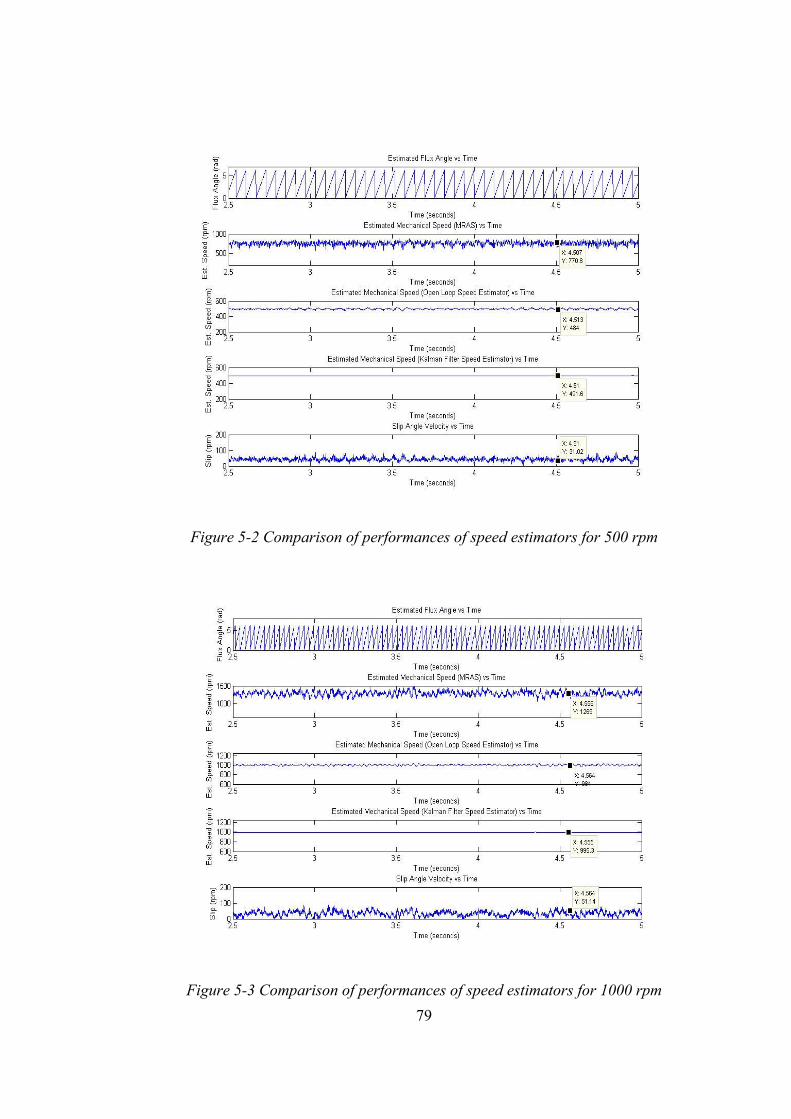
79

Figure 5-2 Comparison of performances of speed estimators for 500 rpm

Figure 5-3 Comparison of performances of speed estimators for 1000 rpm

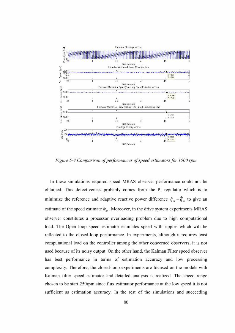
80

Figure 5-4 Comparison of performances of speed estimators for 1500 rpm

In these simulations required speed MRAS observer performance could not be

obtained. This defectiveness probably comes from the PI regulator which is to

minimize the reference and adaptive reactive power difference mm qq ˆˆ − to give an

estimate of the speed estimate mw . Moreover, in the drive system experiments MRAS

observer constitutes a processor overloading problem due to high computational

load. The Open loop speed estimator estimates speed with ripples which will be

reflected to the closed-loop performance. In experiments, although it requires least

computational load on the controller among the other concerned observers, it is not

used because of its noisy output. On the other hand, the Kalman Filter speed observer

has best performance in terms of estimation accuracy and low processing

complexity. Therefore, the closed-loop experiments are focused on the models with

Kalman filter speed estimator and detailed analysis is realized. The speed range

chosen to be start 250rpm since flux estimator performance at the low speed it is not

sufficient as estimation accuracy. In the rest of the simulations and succeeding

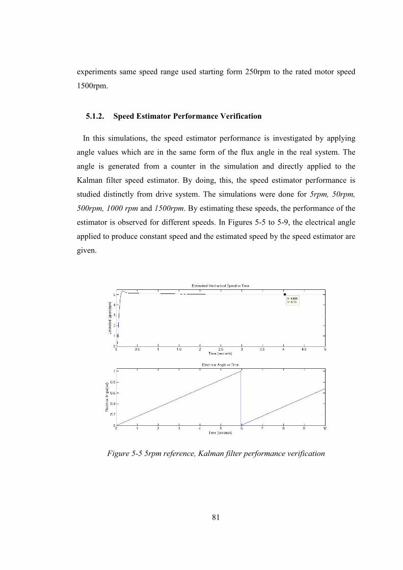
81

experiments same speed range used starting form 250rpm to the rated motor speed

1500rpm.

5.1.2. Speed Estimator Performance Verification

In this simulations, the speed estimator performance is investigated by applying

angle values which are in the same form of the flux angle in the real system. The

angle is generated from a counter in the simulation and directly applied to the

Kalman filter speed estimator. By doing, this, the speed estimator performance is

studied distinctly from drive system. The simulations were done for 5rpm, 50rpm,

500rpm, 1000 rpm and 1500rpm. By estimating these speeds, the performance of the

estimator is observed for different speeds. In Figures 5-5 to 5-9, the electrical angle

applied to produce constant speed and the estimated speed by the speed estimator are

given.

Figure 5-5 5rpm reference, Kalman filter performance verification

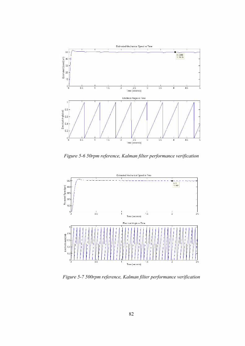
82

Figure 5-6 50rpm reference, Kalman filter performance verification

Figure 5-7 500rpm reference, Kalman filter performance verification

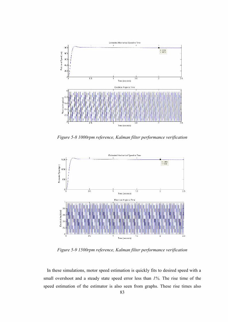
83

Figure 5-8 1000rpm reference, Kalman filter performance verification

Figure 5-9 1500rpm reference, Kalman filter performance verification

In these simulations, motor speed estimation is quickly fits to desired speed with a

small overshoot and a steady state speed error less than 1%. The rise time of the

speed estimation of the estimator is also seen from graphs. These rise times also

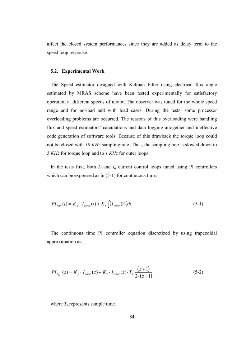
84

affect the closed system performances since they are added as delay term to the

speed loop response.

5.2. Experimental Work

The Speed estimator designed with Kalman Filter using electrical flux angle

estimated by MRAS scheme have been tested experimentally for satisfactory

operation at different speeds of motor. The observer was tuned for the whole speed

range and for no-load and with load cases. During the tests, some processor

overloading problems are occurred. The reasons of this overloading were handling

flux and speed estimators’ calculations and data logging altogether and ineffective

code generation of software tools. Because of this drawback the torque loop could

not be closed with 10 KHz sampling rate. Thus, the sampling rate is slowed down to

5 KHz for torque loop and to 1 KHz for outer loops.

In the tests first, both Id and Iq current control loops tuned using PI controllers

which can be expressed as in (5-1) for continuous time.

( )∫+⋅= dttIKtIKtPI errorIerrorpIout )()()( (5-1)

The continuous time PI controller equation discretized by using trapezoidal

approximation as;

( )( )12

1)()()(

−⋅+

⋅⋅+⋅=z

zTzIKzIKzPI SerrorIerrorpIOut

(5-2)

where Ts represents sample time.

85

For superior performance of speed loop, the proportional gain Kp and integral gain

Ki parameters of these current loops must be fitted well to minimize the current

errors. During the tuning of the PI regulator also some commonly used methods are

tried; one of them is Ziegler-Nichols tuning criterion which is described as follows.

Step1: Set Ki = 0 and Kd = 0. Increase Kp in steps until the closed-loop response

reaches a state of sustained oscillations. Mark this so-called ultimate gain denoted as

Kpu. Measure the corresponding period of oscillation at the output, call it Tu.

Step2: Now set the parameters of the controller as pup KK *45.0= ,

upui TKK /*54.0= , 0=dK .

With tuning of the current loops, closed loop torque control is achieved.

Then, the speed estimator is tuned by setting entries of the measurement noise

covariance R matrix and the process noise covariance Q matrix to obtain fast and

dynamic response and estimation accuracy. For the performance analysis of the

estimator the machine is controlled in the speed loop with the Kalman filter speed

estimator and closed loop speed control is achieved for induction motor. In order to,

fulfill this operation again a PI controller is used which has same equations described

in (5-1) and (5-2). The closed loop experiments first handled with an encoder

coupled to the shaft of the induction motor to verify the estimation performance.

Secondly, in no load case with the estimator to obtain the motor current and voltage

data. Then, a permanent magnet motor is coupled with resolver to the induction

motor to load the drive system and closed-loop speed control is verified under

loading.

During the experiments, two of the three phase currents were measured. The phase

voltages were calculated internally using measured DC-Link voltage. The current

measurements and the DC-Link measurement were done with isolated transducers

and 16-bit A/D conversion.

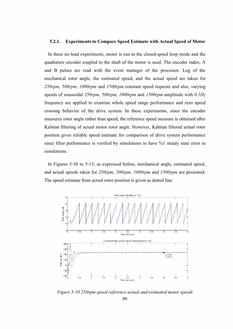
86

5.2.1. Experiments to Compare Speed Estimate with Actual Speed of Motor

In these no-load experiments, motor is run in the closed-speed loop mode and the

quadrature encoder coupled to the shaft of the motor is used. The encoder index, A

and B pulses are read with the event manager of the processor. Log of the

mechanical rotor angle, the estimated speed, and the actual speed are taken for

250rpm, 500rpm, 1000rpm and 1500rpm constant speed requests and also, varying

speeds of sinusoidal 250rpm, 500rpm, 1000rpm and 1500rpm amplitude with 0.1Hz

frequency are applied to examine whole speed range performance and zero speed

crossing behavior of the drive system. In these experiments, since the encoder

measures rotor angle rather than speed, the reference speed measure is obtained after

Kalman filtering of actual motor rotor angle. However, Kalman filtered actual rotor

position gives reliable speed estimate for comparison of drive system performance

since filter performance is verified by simulations to have %1 steady state error in

simulations.

In Figures 5-10 to 5-13; as expressed before, mechanical angle, estimated speed,

and actual speeds taken for 250rpm, 500rpm, 1000rpm and 1500rpm are presented.

The speed estimate from actual rotor position is given as dotted line.

Figure 5-10 250rpm speed reference actual and estimated motor speeds

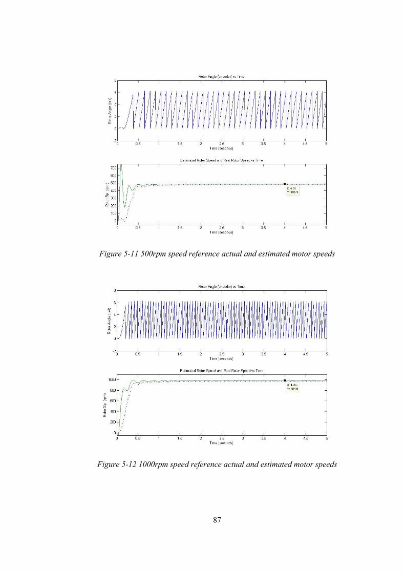
87

Figure 5-11 500rpm speed reference actual and estimated motor speeds

Figure 5-12 1000rpm speed reference actual and estimated motor speeds

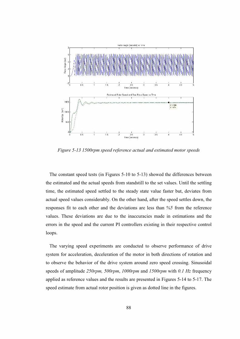
88

Figure 5-13 1500rpm speed reference actual and estimated motor speeds

The constant speed tests (in Figures 5-10 to 5-13) showed the differences between

the estimated and the actual speeds from standstill to the set values. Until the settling

time, the estimated speed settled to the steady state value faster but, deviates from

actual speed values considerably. On the other hand, after the speed settles down, the

responses fit to each other and the deviations are less than %5 from the reference

values. These deviations are due to the inaccuracies made in estimations and the

errors in the speed and the current PI controllers existing in their respective control

loops.

The varying speed experiments are conducted to observe performance of drive

system for acceleration, deceleration of the motor in both directions of rotation and

to observe the behavior of the drive system around zero speed crossing. Sinusoidal

speeds of amplitude 250rpm, 500rpm, 1000rpm and 1500rpm with 0.1 Hz frequency

applied as reference values and the results are presented in Figures 5-14 to 5-17. The

speed estimate from actual rotor position is given as dotted line in the figures.

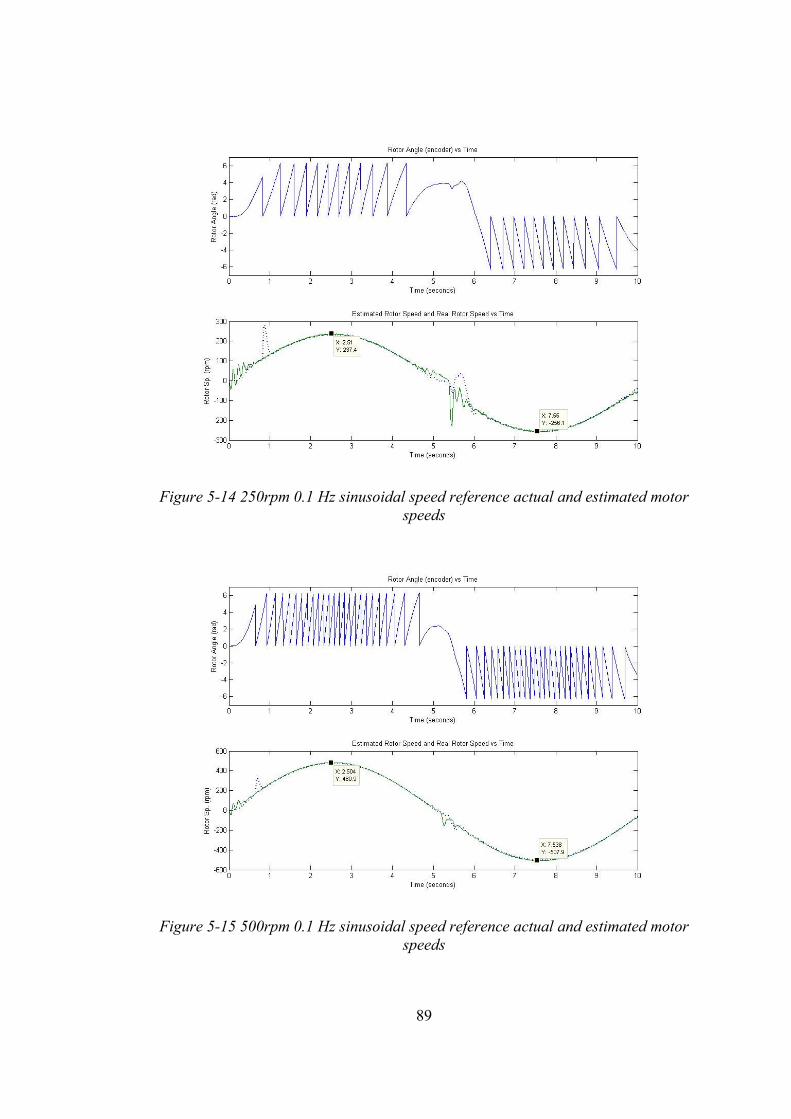
89

Figure 5-14 250rpm 0.1 Hz sinusoidal speed reference actual and estimated motor speeds

Figure 5-15 500rpm 0.1 Hz sinusoidal speed reference actual and estimated motor speeds

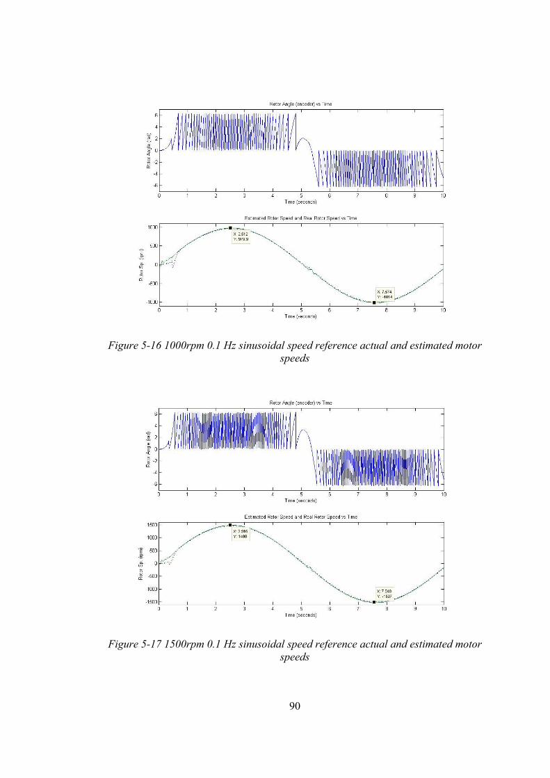
90

Figure 5-16 1000rpm 0.1 Hz sinusoidal speed reference actual and estimated motor speeds

Figure 5-17 1500rpm 0.1 Hz sinusoidal speed reference actual and estimated motor speeds

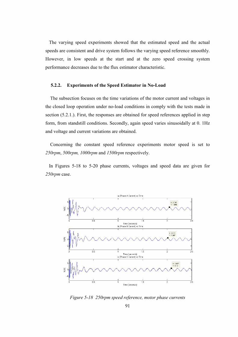
91

The varying speed experiments showed that the estimated speed and the actual

speeds are consistent and drive system follows the varying speed reference smoothly.

However, in low speeds at the start and at the zero speed crossing system

performance decreases due to the flux estimator characteristic.

5.2.2. Experiments of the Speed Estimator in No-Load

The subsection focuses on the time variations of the motor current and voltages in

the closed loop operation under no-load conditions in comply with the tests made in

section (5.2.1.). First, the responses are obtained for speed references applied in step

form, from standstill conditions. Secondly, again speed varies sinusoidally at 0. 1Hz

and voltage and current variations are obtained.

Concerning the constant speed reference experiments motor speed is set to

250rpm, 500rpm, 1000rpm and 1500rpm respectively.

In Figures 5-18 to 5-20 phase currents, voltages and speed data are given for

250rpm case.

Figure 5-18 250rpm speed reference, motor phase currents

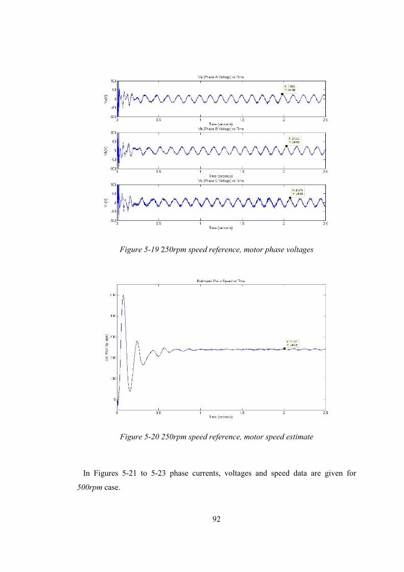
92

Figure 5-19 250rpm speed reference, motor phase voltages

Figure 5-20 250rpm speed reference, motor speed estimate

In Figures 5-21 to 5-23 phase currents, voltages and speed data are given for

500rpm case.

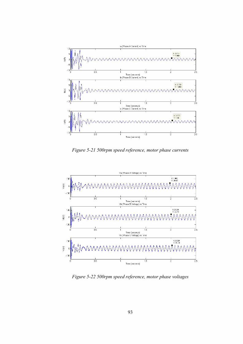
93

Figure 5-21 500rpm speed reference, motor phase currents

Figure 5-22 500rpm speed reference, motor phase voltages

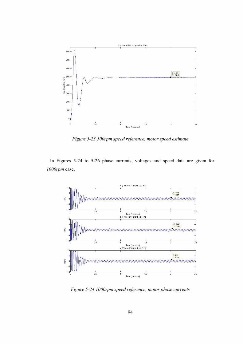
94

Figure 5-23 500rpm speed reference, motor speed estimate

In Figures 5-24 to 5-26 phase currents, voltages and speed data are given for

1000rpm case.

Figure 5-24 1000rpm speed reference, motor phase currents

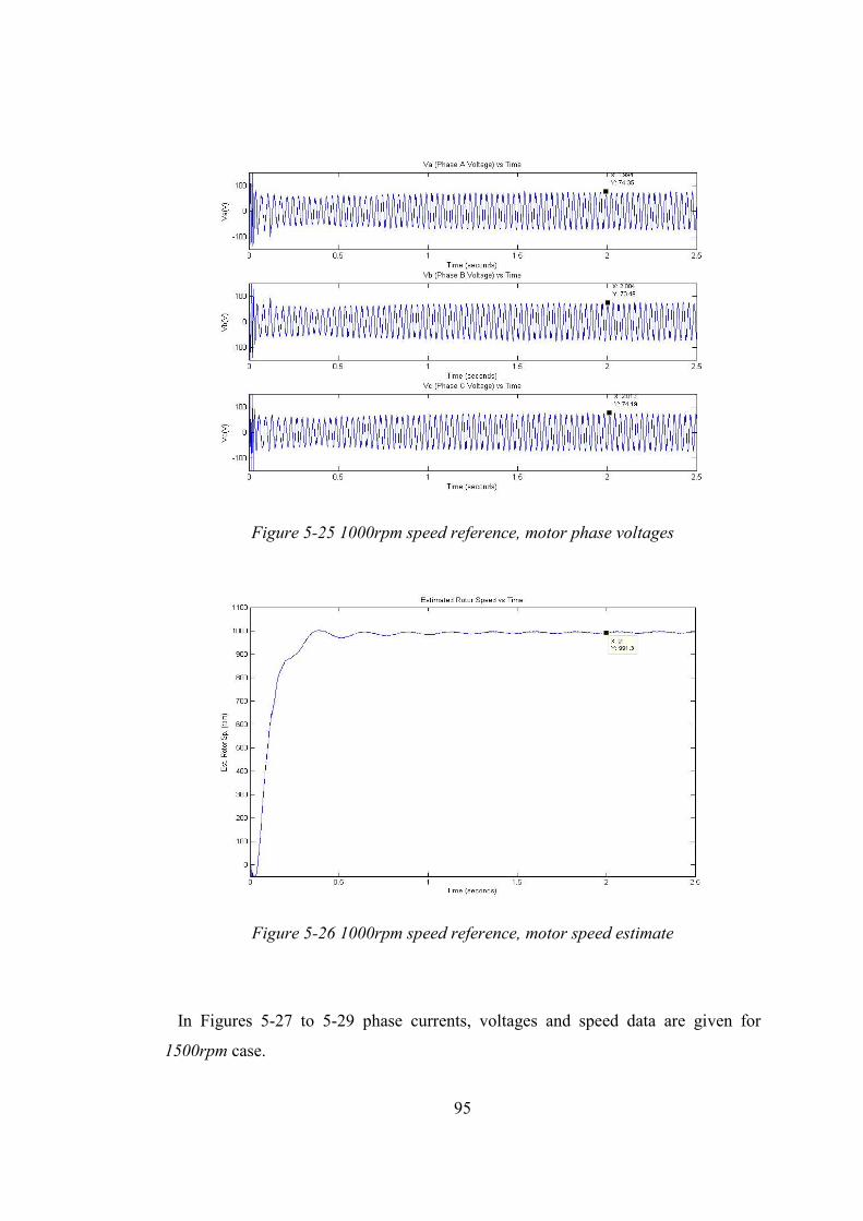
95

Figure 5-25 1000rpm speed reference, motor phase voltages

Figure 5-26 1000rpm speed reference, motor speed estimate

In Figures 5-27 to 5-29 phase currents, voltages and speed data are given for

1500rpm case.

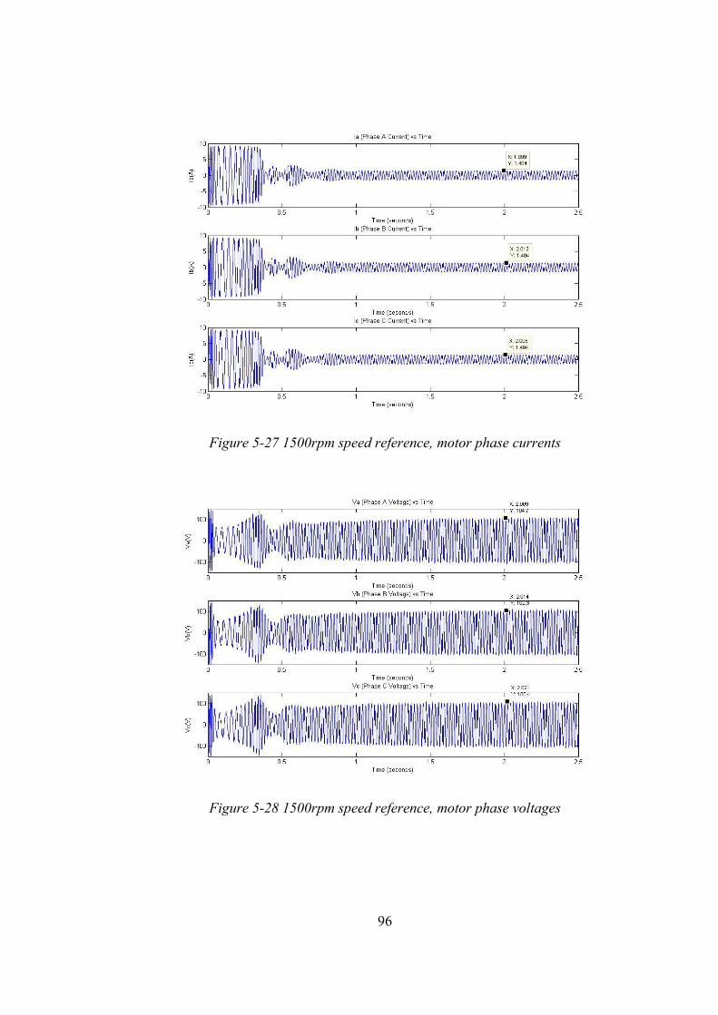
96

Figure 5-27 1500rpm speed reference, motor phase currents

Figure 5-28 1500rpm speed reference, motor phase voltages

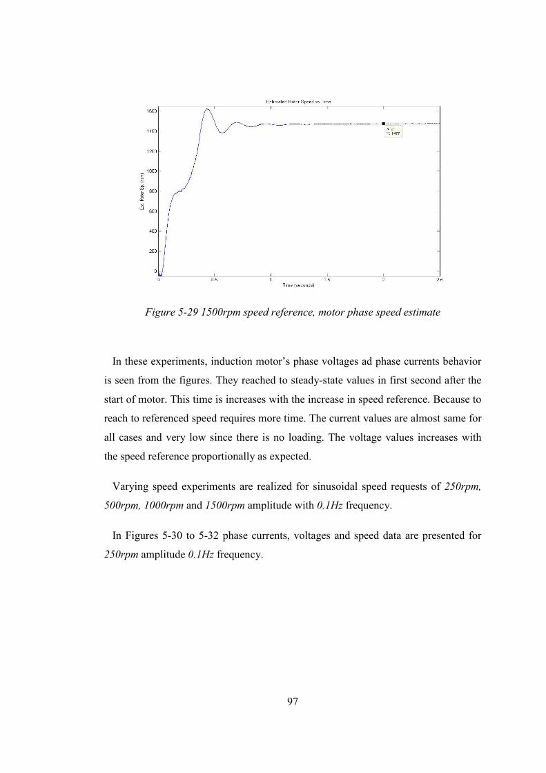
97

Figure 5-29 1500rpm speed reference, motor phase speed estimate

In these experiments, induction motor’s phase voltages ad phase currents behavior

is seen from the figures. They reached to steady-state values in first second after the

start of motor. This time is increases with the increase in speed reference. Because to

reach to referenced speed requires more time. The current values are almost same for

all cases and very low since there is no loading. The voltage values increases with

the speed reference proportionally as expected.

Varying speed experiments are realized for sinusoidal speed requests of 250rpm,

500rpm, 1000rpm and 1500rpm amplitude with 0.1Hz frequency.

In Figures 5-30 to 5-32 phase currents, voltages and speed data are presented for

250rpm amplitude 0.1Hz frequency.

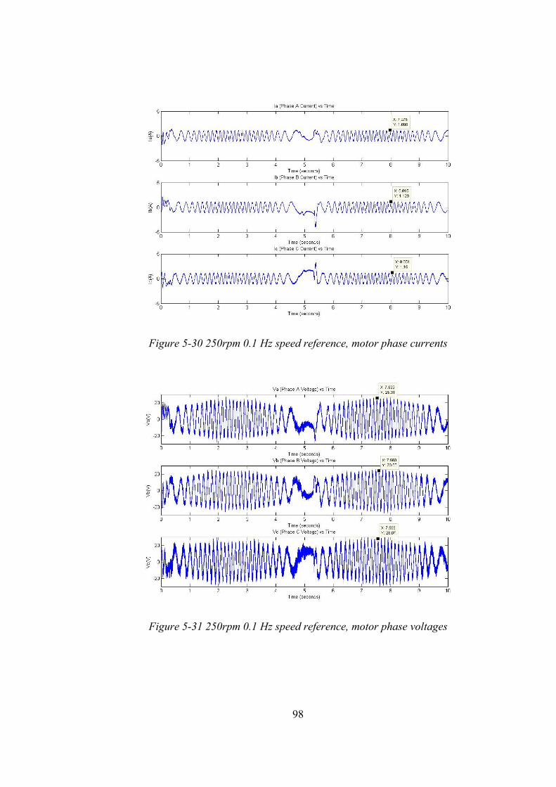
98

Figure 5-30 250rpm 0.1 Hz speed reference, motor phase currents

Figure 5-31 250rpm 0.1 Hz speed reference, motor phase voltages

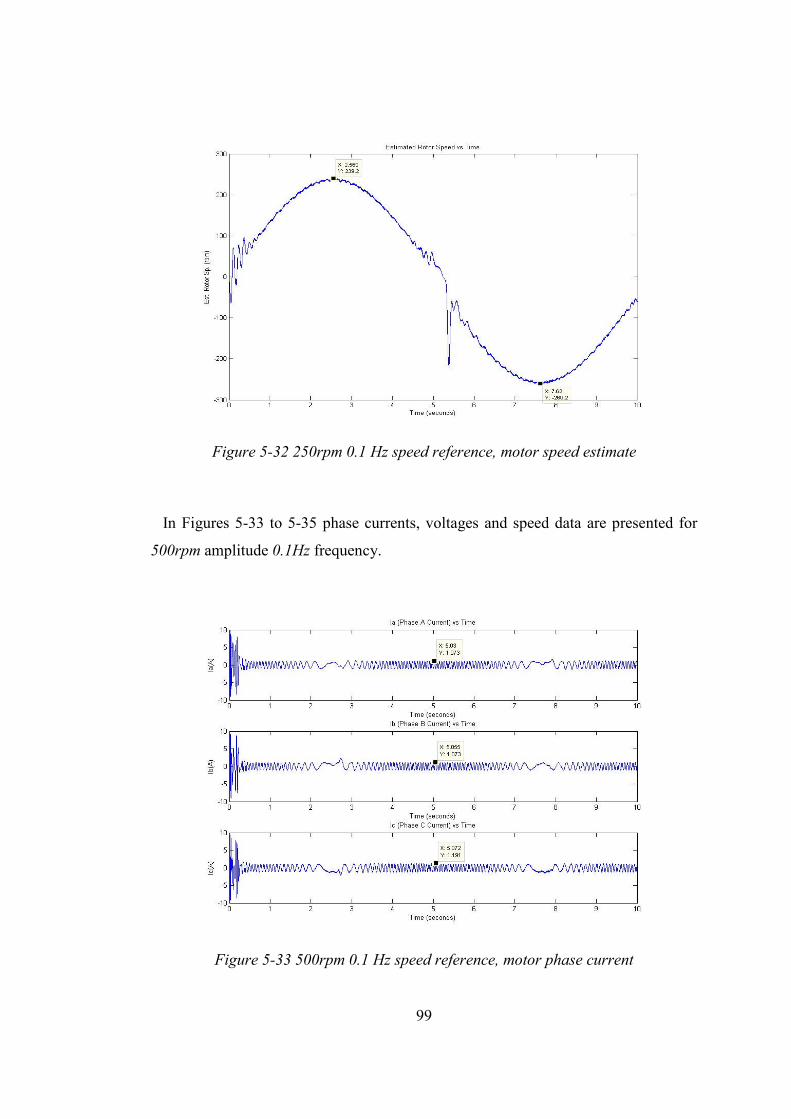
99

Figure 5-32 250rpm 0.1 Hz speed reference, motor speed estimate

In Figures 5-33 to 5-35 phase currents, voltages and speed data are presented for

500rpm amplitude 0.1Hz frequency.

Figure 5-33 500rpm 0.1 Hz speed reference, motor phase current

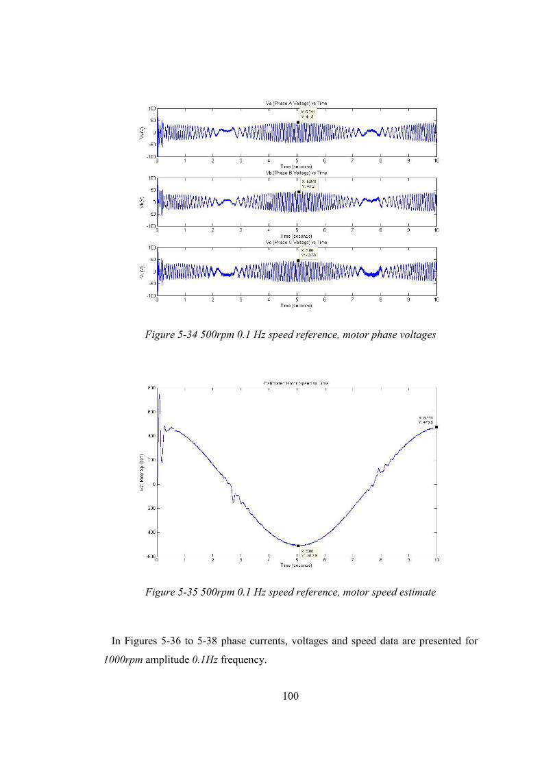
100

Figure 5-34 500rpm 0.1 Hz speed reference, motor phase voltages

Figure 5-35 500rpm 0.1 Hz speed reference, motor speed estimate

In Figures 5-36 to 5-38 phase currents, voltages and speed data are presented for

1000rpm amplitude 0.1Hz frequency.

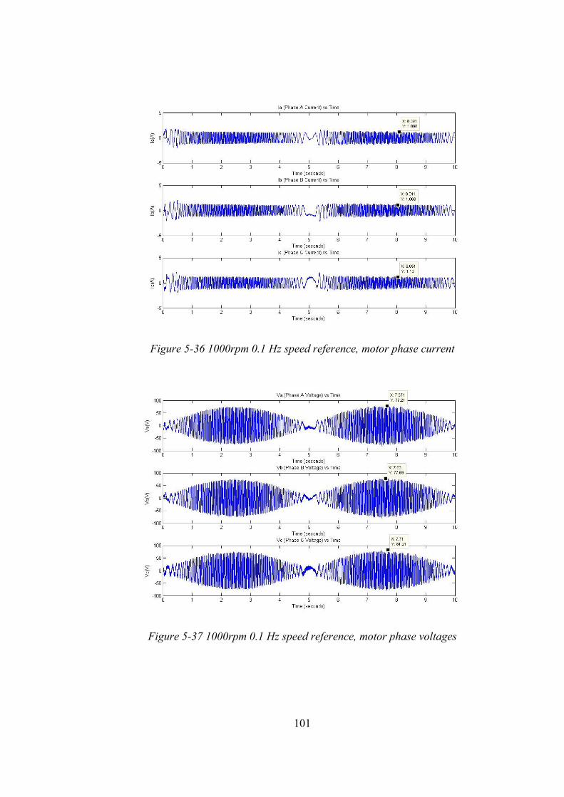
101

Figure 5-36 1000rpm 0.1 Hz speed reference, motor phase current

Figure 5-37 1000rpm 0.1 Hz speed reference, motor phase voltages

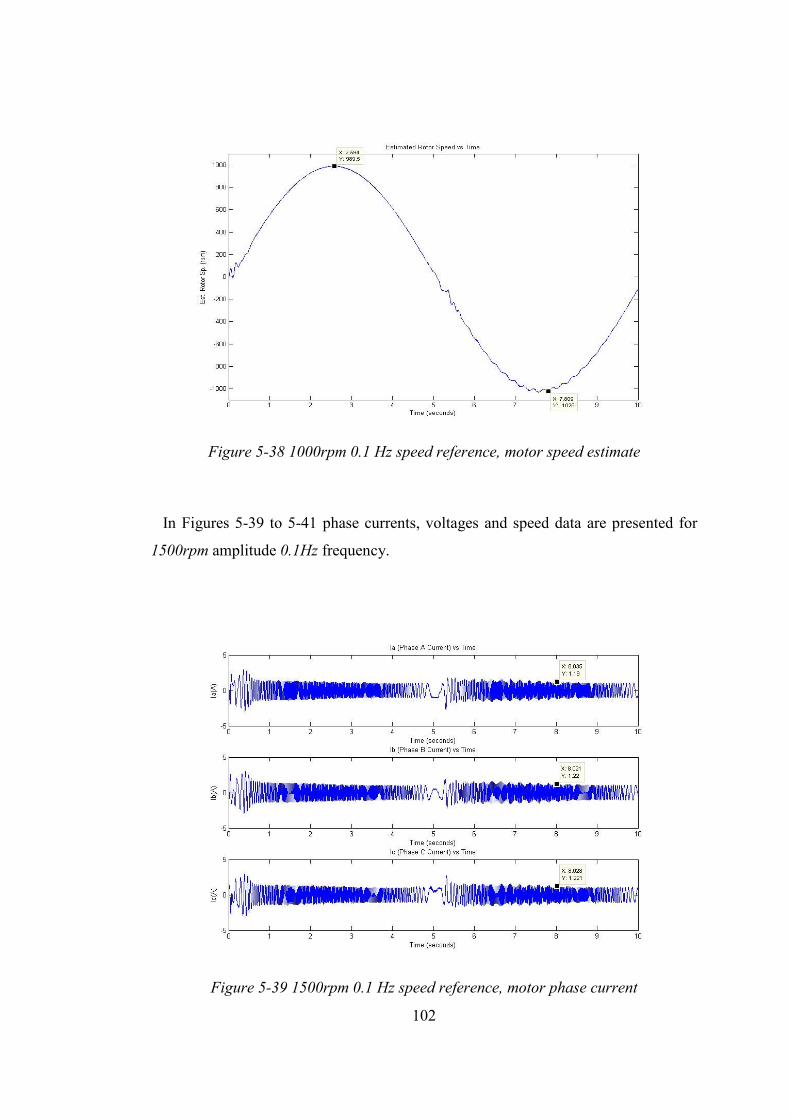
102

Figure 5-38 1000rpm 0.1 Hz speed reference, motor speed estimate

In Figures 5-39 to 5-41 phase currents, voltages and speed data are presented for

1500rpm amplitude 0.1Hz frequency.

Figure 5-39 1500rpm 0.1 Hz speed reference, motor phase current

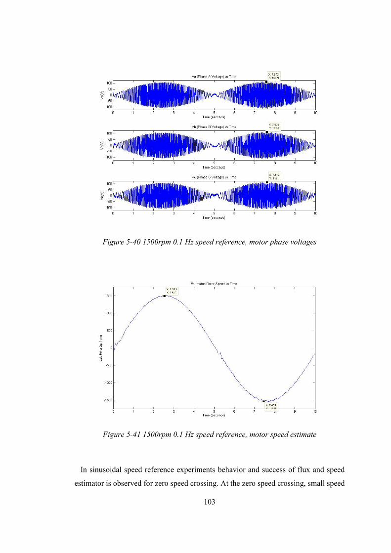
103

Figure 5-40 1500rpm 0.1 Hz speed reference, motor phase voltages

Figure 5-41 1500rpm 0.1 Hz speed reference, motor speed estimate

In sinusoidal speed reference experiments behavior and success of flux and speed

estimator is observed for zero speed crossing. At the zero speed crossing, small speed

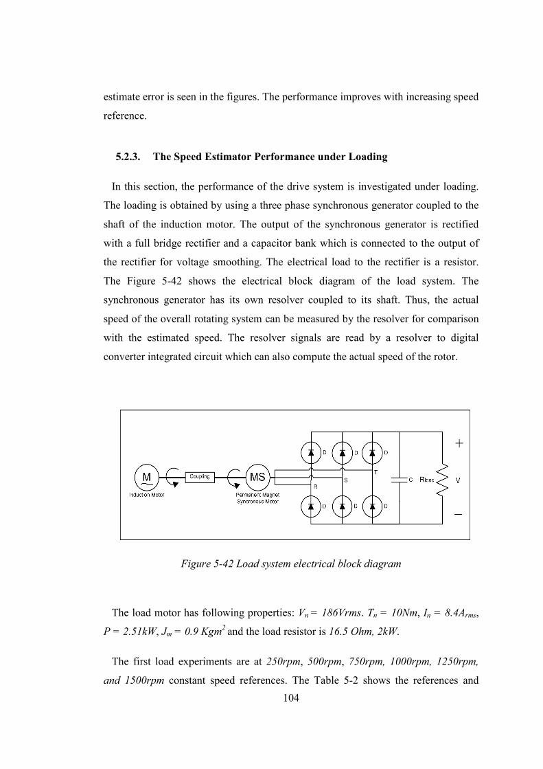
104

estimate error is seen in the figures. The performance improves with increasing speed

reference.

5.2.3. The Speed Estimator Performance under Loading

In this section, the performance of the drive system is investigated under loading.

The loading is obtained by using a three phase synchronous generator coupled to the

shaft of the induction motor. The output of the synchronous generator is rectified

with a full bridge rectifier and a capacitor bank which is connected to the output of

the rectifier for voltage smoothing. The electrical load to the rectifier is a resistor.

The Figure 5-42 shows the electrical block diagram of the load system. The

synchronous generator has its own resolver coupled to its shaft. Thus, the actual

speed of the overall rotating system can be measured by the resolver for comparison

with the estimated speed. The resolver signals are read by a resolver to digital

converter integrated circuit which can also compute the actual speed of the rotor.

Figure 5-42 Load system electrical block diagram

The load motor has following properties: Vn = 186Vrms. Tn = 10Nm, In = 8.4Arms,

P = 2.51kW, Jm = 0.9 Kgm2 and the load resistor is 16.5 Ohm, 2kW.

The first load experiments are at 250rpm, 500rpm, 750rpm, 1000rpm, 1250rpm,

and 1500rpm constant speed references. The Table 5-2 shows the references and

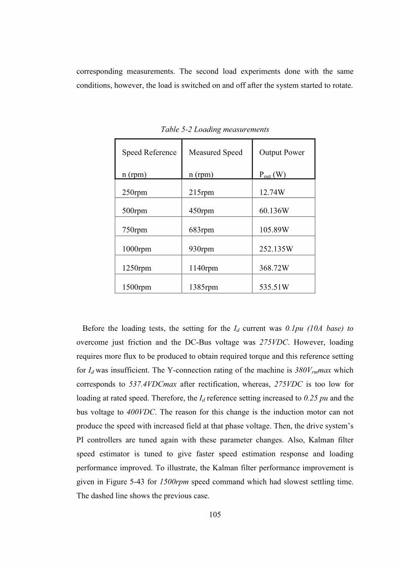
105

corresponding measurements. The second load experiments done with the same

conditions, however, the load is switched on and off after the system started to rotate.

Table 5-2 Loading measurements

Speed Reference

n (rpm)

Measured Speed

n (rpm)

Output Power

Pout (W)

250rpm 215rpm 12.74W

500rpm 450rpm 60.136W

750rpm 683rpm 105.89W

1000rpm 930rpm 252.135W

1250rpm 1140rpm 368.72W

1500rpm 1385rpm 535.51W

Before the loading tests, the setting for the Id current was 0.1pu (10A base) to

overcome just friction and the DC-Bus voltage was 275VDC. However, loading

requires more flux to be produced to obtain required torque and this reference setting

for Id was insufficient. The Y-connection rating of the machine is 380Vrmmax which

corresponds to 537.4VDCmax after rectification, whereas, 275VDC is too low for

loading at rated speed. Therefore, the Id reference setting increased to 0.25 pu and the

bus voltage to 400VDC. The reason for this change is the induction motor can not

produce the speed with increased field at that phase voltage. Then, the drive system’s

PI controllers are tuned again with these parameter changes. Also, Kalman filter

speed estimator is tuned to give faster speed estimation response and loading

performance improved. To illustrate, the Kalman filter performance improvement is

given in Figure 5-43 for 1500rpm speed command which had slowest settling time.

The dashed line shows the previous case.

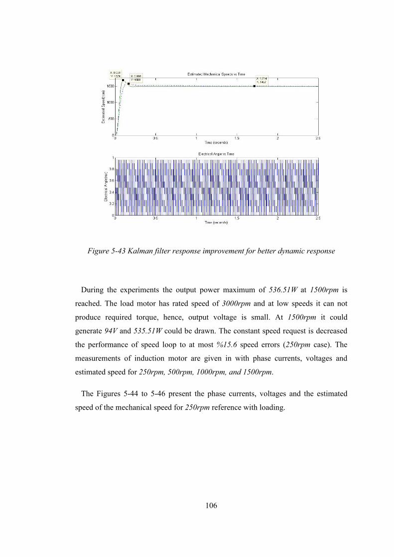
106

Figure 5-43 Kalman filter response improvement for better dynamic response

During the experiments the output power maximum of 536.51W at 1500rpm is

reached. The load motor has rated speed of 3000rpm and at low speeds it can not

produce required torque, hence, output voltage is small. At 1500rpm it could

generate 94V and 535.51W could be drawn. The constant speed request is decreased

the performance of speed loop to at most %15.6 speed errors (250rpm case). The

measurements of induction motor are given in with phase currents, voltages and

estimated speed for 250rpm, 500rpm, 1000rpm, and 1500rpm.

The Figures 5-44 to 5-46 present the phase currents, voltages and the estimated

speed of the mechanical speed for 250rpm reference with loading.

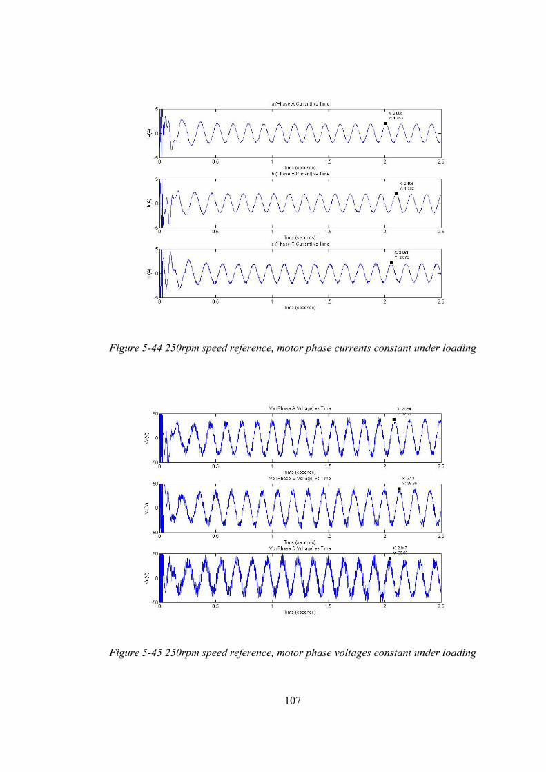
107

Figure 5-44 250rpm speed reference, motor phase currents constant under loading

Figure 5-45 250rpm speed reference, motor phase voltages constant under loading

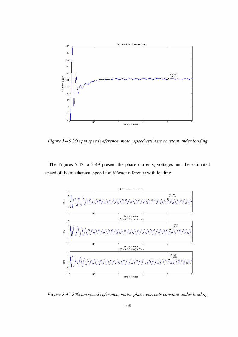
108

Figure 5-46 250rpm speed reference, motor speed estimate constant under loading

The Figures 5-47 to 5-49 present the phase currents, voltages and the estimated

speed of the mechanical speed for 500rpm reference with loading.

Figure 5-47 500rpm speed reference, motor phase currents constant under loading

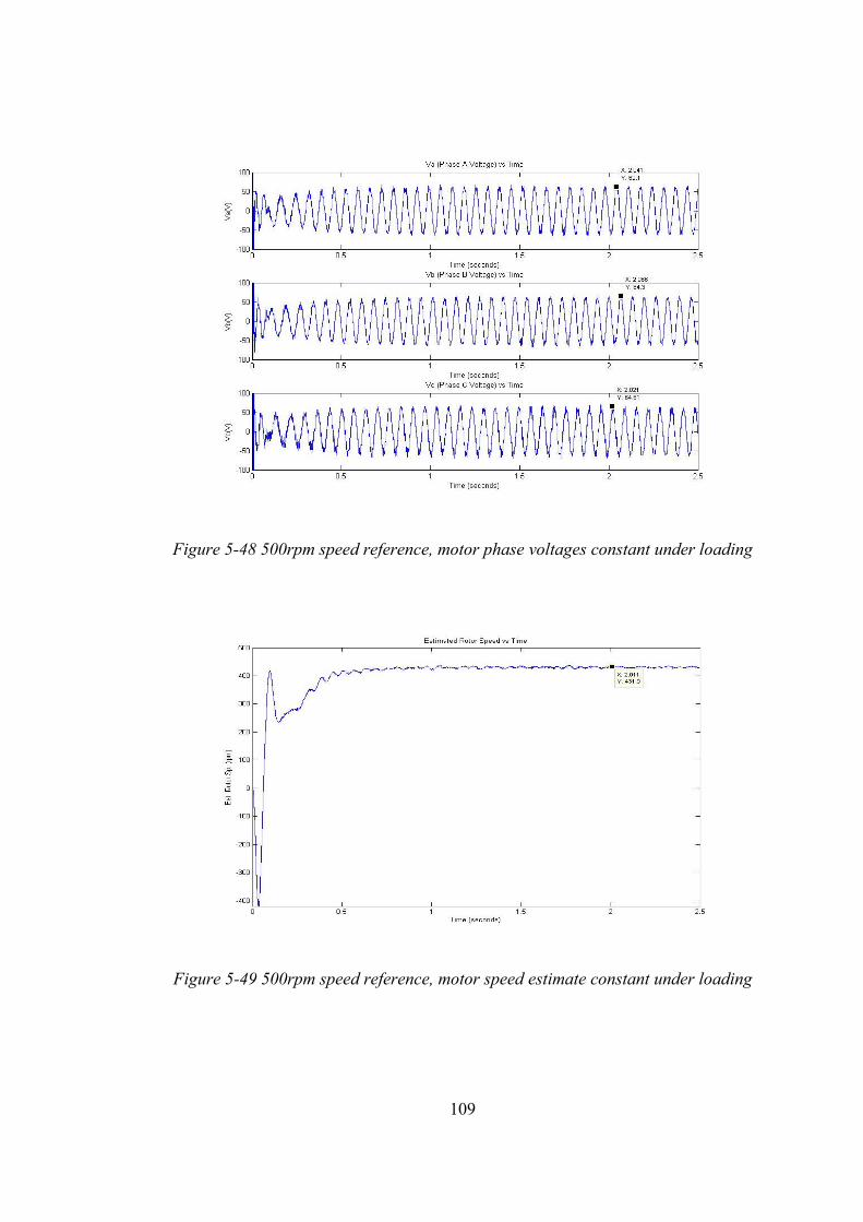
109

Figure 5-48 500rpm speed reference, motor phase voltages constant under loading

Figure 5-49 500rpm speed reference, motor speed estimate constant under loading

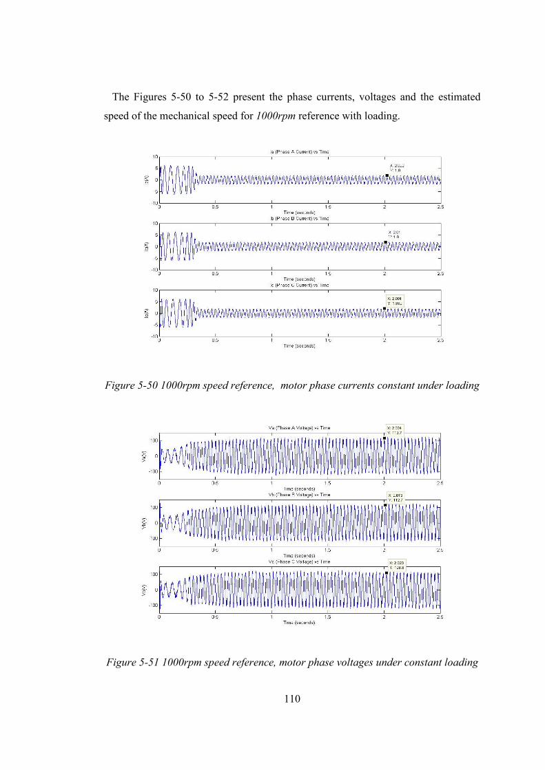
110

The Figures 5-50 to 5-52 present the phase currents, voltages and the estimated

speed of the mechanical speed for 1000rpm reference with loading.

Figure 5-50 1000rpm speed reference, motor phase currents constant under loading

Figure 5-51 1000rpm speed reference, motor phase voltages under constant loading

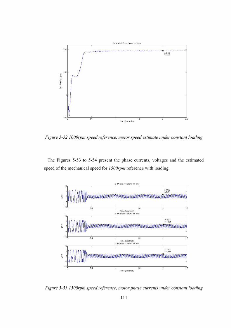
111

Figure 5-52 1000rpm speed reference, motor speed estimate under constant loading

The Figures 5-53 to 5-54 present the phase currents, voltages and the estimated

speed of the mechanical speed for 1500rpm reference with loading.

Figure 5-53 1500rpm speed reference, motor phase currents under constant loading

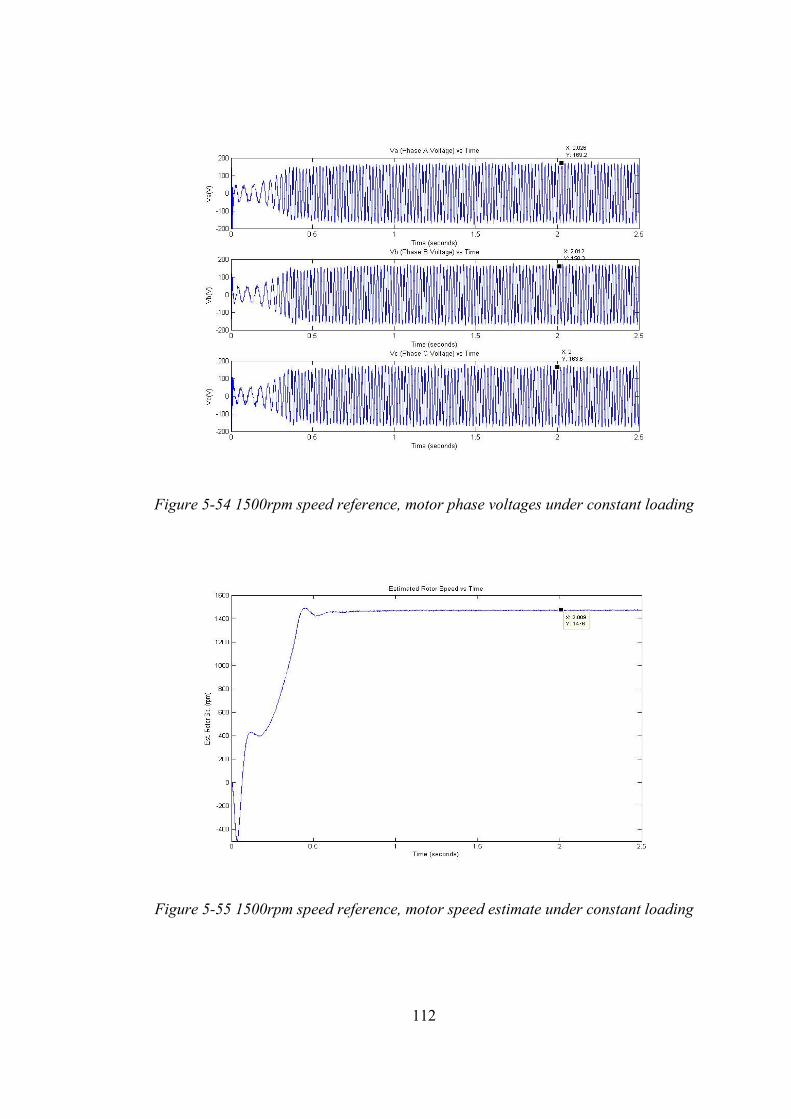
112

Figure 5-54 1500rpm speed reference, motor phase voltages under constant loading

Figure 5-55 1500rpm speed reference, motor speed estimate under constant loading

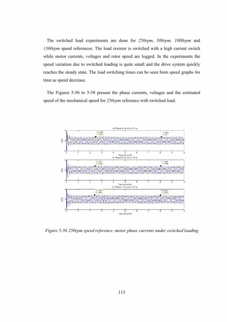
113

The switched load experiments are done for 250rpm, 500rpm, 1000rpm and

1500rpm speed references. The load resistor is switched with a high current switch

while motor currents, voltages and rotor speed are logged. In the experiments the

speed variation due to switched loading is quite small and the drive system quickly

reaches the steady state. The load switching times can be seen form speed graphs for

time as speed decrease.

The Figures 5-56 to 5-58 present the phase currents, voltages and the estimated

speed of the mechanical speed for 250rpm reference with switched load.

Figure 5-56 250rpm speed reference, motor phase currents under switched loading

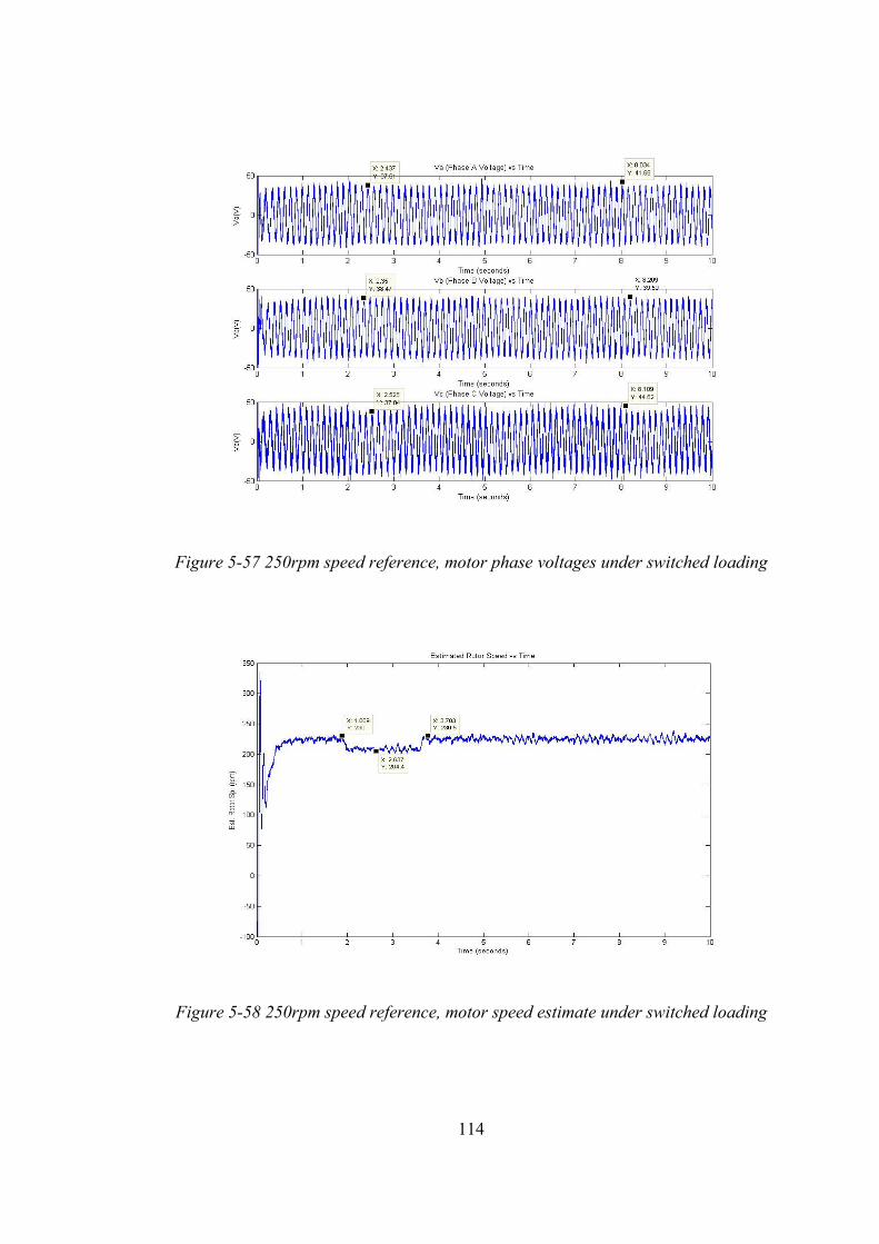
114

Figure 5-57 250rpm speed reference, motor phase voltages under switched loading

Figure 5-58 250rpm speed reference, motor speed estimate under switched loading

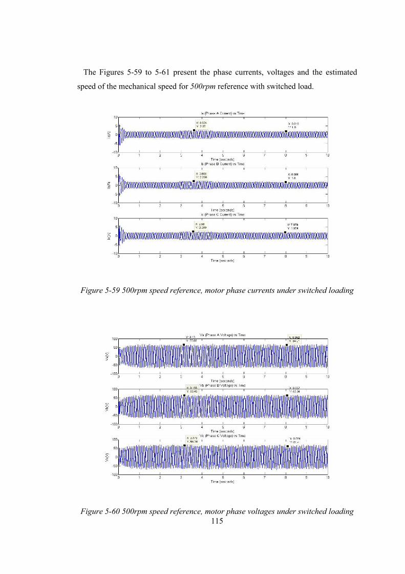
115

The Figures 5-59 to 5-61 present the phase currents, voltages and the estimated

speed of the mechanical speed for 500rpm reference with switched load.

Figure 5-59 500rpm speed reference, motor phase currents under switched loading

Figure 5-60 500rpm speed reference, motor phase voltages under switched loading

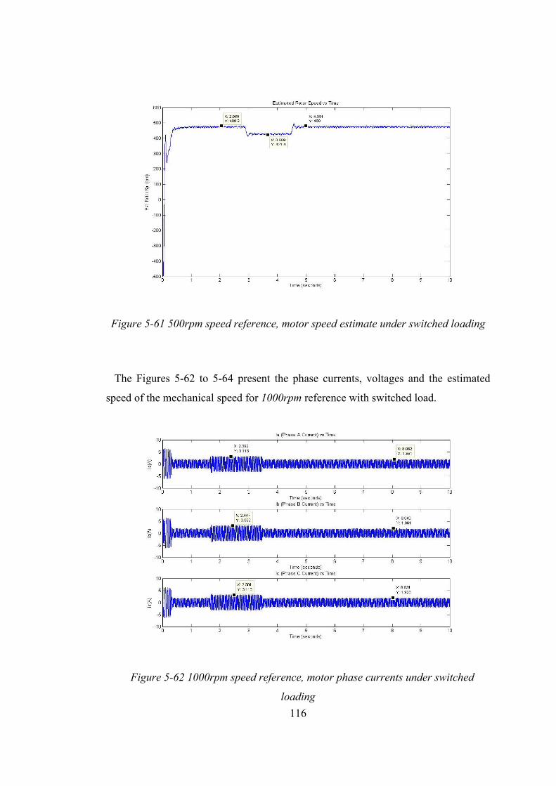
116

Figure 5-61 500rpm speed reference, motor speed estimate under switched loading

The Figures 5-62 to 5-64 present the phase currents, voltages and the estimated

speed of the mechanical speed for 1000rpm reference with switched load.

Figure 5-62 1000rpm speed reference, motor phase currents under switched

loading

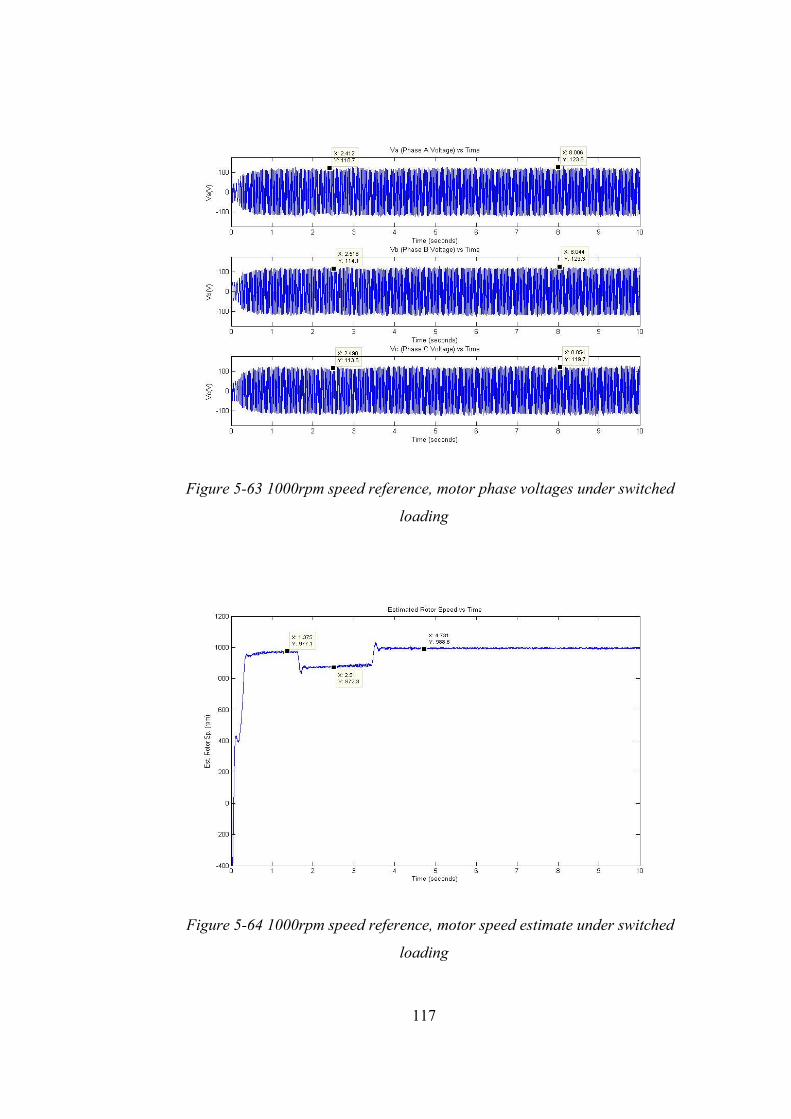
117

Figure 5-63 1000rpm speed reference, motor phase voltages under switched

loading

Figure 5-64 1000rpm speed reference, motor speed estimate under switched

loading

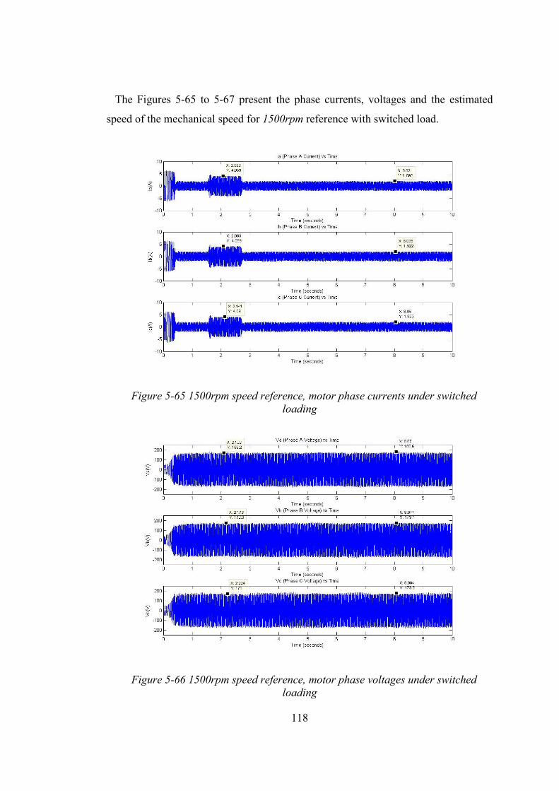
118

The Figures 5-65 to 5-67 present the phase currents, voltages and the estimated

speed of the mechanical speed for 1500rpm reference with switched load.

Figure 5-65 1500rpm speed reference, motor phase currents under switched

loading

Figure 5-66 1500rpm speed reference, motor phase voltages under switched

loading

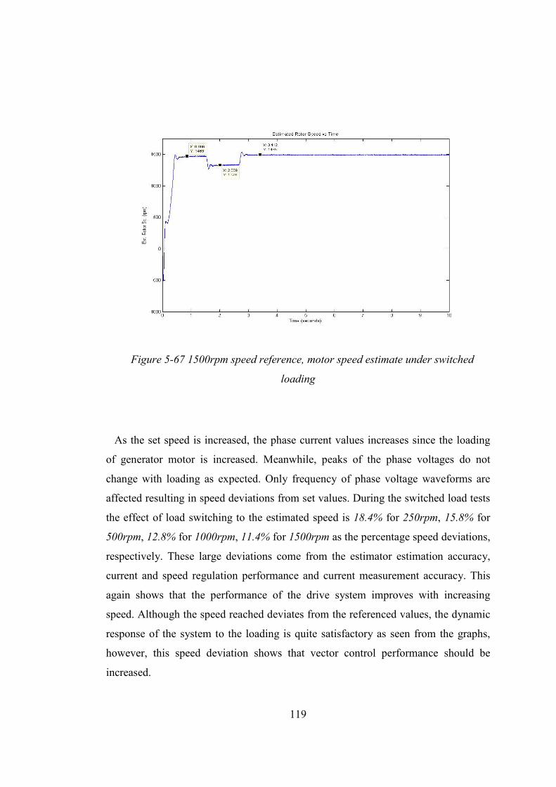
119

Figure 5-67 1500rpm speed reference, motor speed estimate under switched

loading

As the set speed is increased, the phase current values increases since the loading

of generator motor is increased. Meanwhile, peaks of the phase voltages do not

change with loading as expected. Only frequency of phase voltage waveforms are

affected resulting in speed deviations from set values. During the switched load tests

the effect of load switching to the estimated speed is 18.4% for 250rpm, 15.8% for

500rpm, 12.8% for 1000rpm, 11.4% for 1500rpm as the percentage speed deviations,

respectively. These large deviations come from the estimator estimation accuracy,

current and speed regulation performance and current measurement accuracy. This

again shows that the performance of the drive system improves with increasing

speed. Although the speed reached deviates from the referenced values, the dynamic

response of the system to the loading is quite satisfactory as seen from the graphs,

however, this speed deviation shows that vector control performance should be

increased.

120

The experiments showed that, speed estimator based on Kalman Filter and closed-

loop rotor flux observer has very high tracking capability for whole speed range and

for no-load and with load cases. However, the loop performance, the flux and the

speed estimation accuracies should be improved for whole loading range and for low

speeds.

121

CHAPTER 6

CONCLUSION

The focus of this work has been design and implementation of a speed estimator

for sensorless closed-loop speed control of induction machine using direct field

orientation technique. A Kalman filter has been considered for the estimator in the

study. The application requires the use of another estimator for the estimation of the

flux components and the rotor flux angle. This has been selected as a MRAS flux

estimator scheme which uses integrals of back emfs. The flux observer relies on both

current and voltage models of the machine to improve the dynamic performance of

the estimator. The induction machine has been modeled both stationary and

synchronously rotating dq axes system. The control system uses space vector PWM

and field orientation concepts. They are introduced in the thesis in detailed form.

MRAS speed estimator using reactive power and open-loop speed estimator using

the estimated flux angle are also implemented for comparison of the speed estimation

techniques. The performances of these speed estimators compared by simulations.

The Kalman filter technique is chosen as speed estimation scheme because of its

estimation accuracy and low processing complexity. The closed-loop experiments

are focused on detailed analysis of the model with Kalman filter speed estimator.

Both simulations and experiments have been conducted to optimize and tune the

controller parameters of the estimators, current and speed loops for both no-load and

with load cases covering the entire speed range.

The simulations and experiments show that the sensorless speed control of the

induction machine with described system is applicable; however, the performance of

the system needs to be improved particularly for low speed range and for full loading

of the machine. Also, the system stability against changes in loading should be

improved to achieve better vector control performance.

122

For future work, the estimation accuracy and the dynamic response of the

estimators may be improved by further efforts of re-tuning them; also the online

parameter estimation techniques can be inserted into the algorithms to observe the

effects of the change of motor parameters during operation. The estimators can be

designed by other techniques, such as, extended Kalman filter (EKF) technique,

neural networks based estimators, sliding mode estimators. Furthermore, more

advanced control structures can be investigated for better control of both motor

current loop and speed loop.

123

REFERENCES

[1] H. Kubota and K. Matsuse “Flux observer of induction motor with parameter

adaptation for wide speed range motor drives,” in Proc. IPEC’90, Tokyo, Japan,

1990, pp. 1213-1218.

[2] R. Nilsen and M. Kazmierkowski, “New reduced-order observer with

parameter adaptation for flux estimation in induction motors,” in Proc. PESC’92,

1992, pp. 245-252.

[3] R. Lorenz and D. Lawson, “A simplified approach to continuous, on-line

tuning of field-oriented induction machine drives,” IEEE Trans. Ind. Applicat., vol.

26, pp.420-425, May/Jun 1990.

[4] K. T. Hung and R. D. Lorenz, “A rotor flux error-based adaptive tuning

approach for feedforward field-oriented machine drives,” in Proc. 1990 IEEE-IAS,

Annu. Meeting, pp. 589-594.

[5] L. Garces, “Parameter adaptation for the speed-controlled static AC drive

with a squirrel cage induction motor,” IEEE Trans. Ind. Applicat., vol. 16, pp. 173-

178, Mar./Apr. 1980.

[6] T. M. Rowan, R. J. Kerkman, and D. Leggate, “A simple on-line adaptation

for indirect field-orientation of an induction machine,” in Proc. 1989 IEEE-IAS

Annu. Meeting, pp.579-587.

[7] J. Moreira, K. Hung and T. Lipo, “A simple and robust adaptive controller for

the tuning correction in field-oriented induction machines,” IEEE Trans. Ind.

Applicat., vol. 28, pp. 1359-1366, Nov./Dec. 1992.

124

[8] P.L.Jansen and R.D.Lorenz “Transducerless position and velocity estimation

in induction and salient ac machines”, IEEE Tran. IA, vol. 31, no.2, pp.240-247,

Mar/April, 1995

[9] R.Gabriel, W.Leonhard and C.Nordby “ Field oriented control of standard

AC motor using microprocessor”, IEEE Tran. IA, vol.16, no.2, pp.186.192, 1980

[10] B.Robyns, B.Frederique, “A methodology to determine gains of induction

motor flux observers based on a theoretical parameter sensitivity analysis”, IEEE

Trans. PE, vol. 15, no.6, pp.983-995, 2000

[11] Takahashi and T. Noguchi, “A new quick-response and high-efficiency

control strategy of an induction motor,” IEEE Trans. Ind. Applicat., vol. 22, pp.820-

827, Sep./Oct. 1986.

[12] P. L. Jansen and R. D. Lorenz, “A physically insightful approach to the

design and accuracy assessment of flux observers for field-oriented induction

machine drives,” in Proc. IEEE-IAS Annu. Meeting, Oct.1992, pp. 570-577.

[13] P. L. Jansen, C. O. Thompson, and R. D. Lorenz, “Observer based direct field

orientation for both zero and very high speed operation,” in Proc. PCC, Yokohama,

Japan, Apr. 1993, pp.432-437.

[14] P. L. Jansen and R. D. Lorenz, “Accuracy limitations of velocity and flux

estimation in direct field-oriented induction machines,” in Proc. EPE Conf.,

Brighton, England, Sep. 1993

[15] P.L.Jansen and R.D.Lorenz “Observer based direct field orientation: Analysis

and comparison of alternative methods”, IEEE Tran. IA, vol. 30, no.4, pp.945-953,

Jul/Aug, 1994

125

[16] K Minami, M. Vélez-Reyes, D. Elten, G. C. Verghese and D. Filbert, “Multi-

stage speed and parameter estimation for induction machines,” IEEE Power

Electronics Specialist’s Conference, Boston MA, Jun. 1991.

[17] M. Vélez-Reyes and G. C. Verghese, “Decomposed algorithms for speed and

parameter estimation in induction machines,” IFAC Symposium on Non-linear

Control System Design, Bordeaux, France, 1992.

[18] M. Vélez-Reyes, K Minami, G. C. Verghese, “Recursive speed and parameter

estimation for induction machines,” IEEE Ind. Applicat. Society Meeting, San

Diego, 1989

[19] M. Bodson and J. Chiasson, “A comparison of sensorless speed estimation

methods for induction motor control,” Proc ACC, Anchorage, AK May.2002, pp.

3076-3081

[20] I. J. Ha and S. H. Lee, “An on-line identification method for both stator and

rotor resistances of induction motors without rotational transducers,” ISIE’96,

Warsaw, Poland, Jun. 1996.

[21] H. S. Yoo and I. J. Ha, “A polar coordinate-oriented method of identifying

rotor flux and speed of induction motors without rotational transducers,” IEEE Trans.

on Control Systems Technology, vol. 4, no. 3, pp. 230-243, May. 1996.

[22] C.Lascu, I.Boldea, F.Blaabjerg “A Modified Direct Torque Control for

Induction Motor Sensorless Drive” IEEE Tran. IA vol. 36, no. 1, pp. 122-130, Jan

2000

[23] F.Z.Peng, T.Fukao “Robust Speed Identification for Speed Sensorless Vector

Control of Induction Motors” IEEE Tran. IA vol. 30, no. 5, pp.1234-1239, Oct.1994

126

[24] C.Schauder “Adaptive Speed Identification for Vector Control of Induction

Motor without Rotational Transducers” IEEE Tran. IA vol. 28, no. 5, pp. 1054-1061,

Oct.1992

[25] G.Yang and T.Chin “Adaptive-Speed identification scheme for a vector

controlled speed sensorless inverter induction motor drive” ,IEEE Tran. IA, vol. 29,

no.4, pp.820-825, 1993

[26] M.Elbuluk, N.Langovsky and D.Kankam “Design and Implementation of a

Closed Loop Observer and Adaptive Controller for Induction Motor Drives” IEEE

Tran. IA vol. 34 no. 3 pp. 435-443, May/June 1998

[27] H.Tajima, Y.Hori “Speed Sensorless Field Orientation Control of the

Induction Machine” IEEE Tran. IA vol. 29, no. 1, pp. 175-180, Feb.1993

[28] D.W.Novotny and T.A.Lipo, “Vector Control and Dynamics of AC Drives”,

Oxford University Press Inc., Oxford, New York, 1997.

[29] H.Butler "Model Reference Adaptive Systems" London: Printice Hall,(1992)

[30] L.Zhen and L. Xu “Sensorless Field Orientation Control of Induction

Machines Based on Mutual MRAS Scheme” IEEE Tran. IE vol. 45 no. 5, pp. 824-

831, October 1998

[31] C.Attainese, Alfonso Damiano “Induction Motor Drive Parameters

Identification” IEEE Tran. PE vol. 13, no. 6, pp. 1112-1123, Nov. 1998

[32] H.Sugimoto and S.Tamai “Secondary Resistance Identification of an

Induction Motor Applied Model Reference Adaptive System and its Characteristics”

IEEE Tran. IA vol. 23, no. 2 pp. 296-303 March/April 1987

127

[33] R.Krishnan, F.C.Doran “Study of parameter sensitivity in high performance

inverter-fed induction motor drive systems” IEEE Tran. IA, vol. 23, pp.623-635,

1987

[34] Texas Instruments, “Digital Motor Control Software Library” Literature

number: SPRU 485 August 2001

[35] A.M. Trzynadlowski, “The Field Orientation Princple in Control of Induction

Motors, Kluwer Academic Publishers, pp. 176-180, 1994

[36] G. Welch and G. Bishop, “An Introduction to the Kalman Filter”, April 5 2004

[37] J. Holtz, “ Sensorless Control of Induction Motor Drives”, Proc. IEEE, vol. 90,

No. 8, pp. 1359-1394, August 2002

[38] G. Şimşek, “Sensorless Direct Field Oriented Control of Induction Machine by

Flux and Speed Estimators Using Model Reference Adaptive System” M.S Thesis

EE Dept. Metu, April 2004

[39] E. Özçelik, “Speed Sensorless Vector Control of Induction Motor Drive” M.S

Thesis EE Dept. Metu, April 2005

[40] Gi-Won Chang, G. Espinosa-Pérez, E. Mendes, and R. Ortega, ”Tuning Rules

for the PI Gains of Field-Oriented Controllers of Induction Motors”, IEEE Tran. on

Industrial. Electronics, Vol. 47, No. 3, June 2000

[41] Ong, Chee-Mun., “Dynamic Simulation of Electric Machinery”, Prentice Hall,

1998

[42] Ned Mohan, “ Advanced Electric Drives” MNPERE, Minneapolis, 2001

128

APPENDIX

The Experimental Set-Up

The rectifier used in this drive is Semikron bridge rectifier (SKD-28) which is

1300V, 28A that consists of six uncontrolled diodes. The three-phase voltage is

supplied over an autotransformer to the rectifier. The rectified voltage is filtered by

two dc-link capacitors each being 1000µF and connected in series. 30KΩ, 1W

resistors are connected across each capacitor for proper voltage sharing. The voltage

at the beginning applied with a soft start resistor to limit the inrush current at starting.

Then, when the capacitors are charged to predefined level, a relay disconnects the

resistor and rectified voltage is applied directly. The inverter used in the drive system

is Semikron IGBT module (SKM 40 GDL 123 D) with rated values 1200V and 40 A.

IGBTs in this module are driven by a gate drive card, Semikron IGBT driver (SKHI

60 H4). The gate drive card provides short-circuit protection for all six IGBTs in the

full bridge by real-time tracking of the collector-emitter voltage of the switches.

In order to run the real-time control algorithm and create PWM signals, Texas

Instruments’ TMS320 processor is used in this work. F2812 eZdsp board is used as

DSP card. The F2812 is a member of the “C2000 DSP” platform, and is optimized

specifically for motor control applications. It uses a 16-bit word length along with

32-bit registers. The F2812 has application-optimized peripheral units, coupled with

the high-performance DSP core, enables the use of advanced control techniques for

high-precision and high-efficiency full variable-speed control of motors. The event

managers of F2812 include special pulse-width modulation (PWM) generation

functions, such as a programmable dead-band function and a space-vector PWM

state machine for 3-phase motors that provides quite a high efficiency in the

switching of power transistors also, quadrature encoder pulse circuit module to read

encoder signals. F2812 also contains 16 channels, 12-bit A/Ds, enhanced controller

area network (eCAN), serial communication interface (SCI) and general purpose

digital I/Os (GPIO) as peripherals.

129

The dc-link voltage is sensed with a voltage sensor (LV25-P) on the interface card.

The magnitude of the dc-link voltage is sensed to re-build the phase voltages in the

control software with the information of duty-cycles of the IGBTs. Another aim of

the voltage sensor is to sense the overcharge on the dc-link capacitors. If the voltage

level exceeds the predefined limit that is determined by the user, a comparator gives

an error signal to set all the IGBTs to off-state. Also for used in the relay operation at

the first power up. Moreover, the PWM signals generated by DSP are amplified to

make them compatible with the gate drive card inputs. For this purpose, six PWM

signals are adjusted to 15V peak without any other change. Finally, all the errors,

(gate drive card errors, over-voltage error, over-current error, and an external error)

are OR gated to set off IGBTs.

The other sensed variables are stator currents using current-sensors on the current

measurement interface card. For this purpose (LA 25-NP) current transducers are

used. These sensors are capable of sensing AC, DC and mixed current waveforms.

The sensor has multi-range current sensing options depending on the pin

connections. The sensors use hall-effect phenomena to sense the current. The output

of these sensors is between ±15V and unipolar. Since the ADCs on the DSP board

cannot sense the negative voltage and requires signal between 0-3.3V, our current

sensors are used with current interface card.

In case of noisy phase currents, optional low-pass filters are placed on the interface

card with 1kHz cut-off frequency. The outputs of the current transducers are also

used to provide over-current protection. The overall set-up is as in Figure A-1.

Moreover, the block diagram of the set-up is given in Figure A-2 and the software

block diagram from Matlab Simulink is as in Figure A-3.

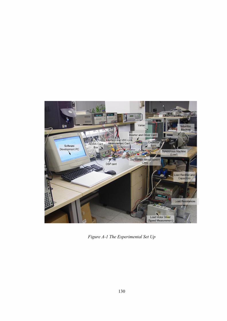
130

Figure A-1 The Experimental Set Up

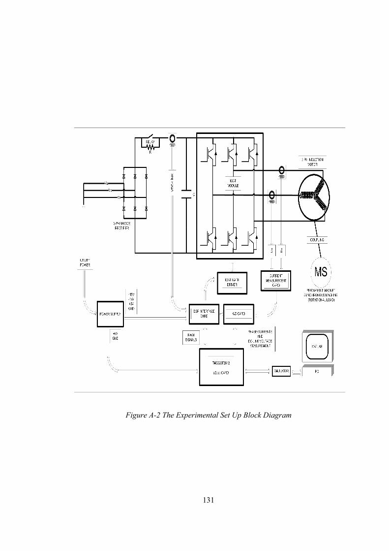
131

Figure A-2 The Experimental Set Up Block Diagram

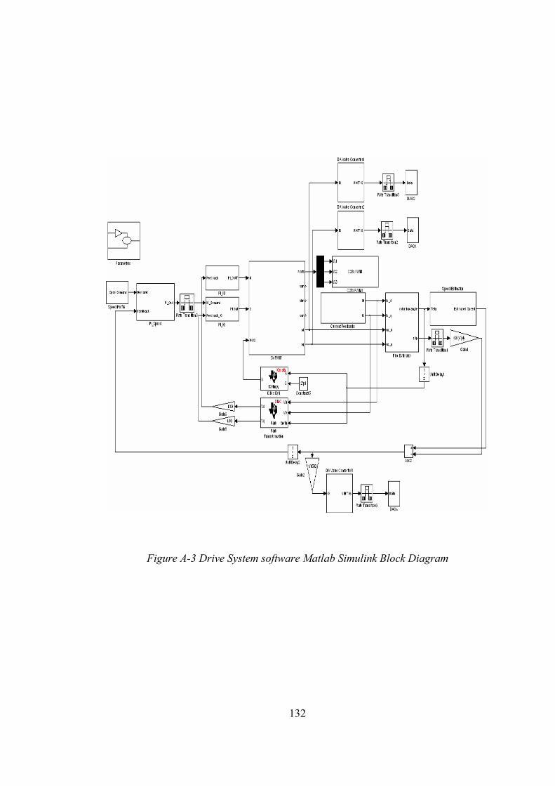
132

Figure A-3 Drive System software Matlab Simulink Block Diagram