© Gray Cancer Institute, 2005 1 Spectral imaging applied to histology: (almost) all you wanted to know but were too afraid to ask….…............... B. Vojnovic and P. Barber Gray Cancer Institute, UK This document is intended as a basic introduction to the GCI spectral imager, describing its mode of operation and describing the means of analysis of the resulting image stack. It is not intended to be an exhaustive or rigorous document, but rather it seeks to explain some of the underlying principles, to define some commonly used terms which may not be familiar to individuals versed in the application of histology to biological investigations. It also attempts to summarise some measures and inferences that the spectral imaging method cannot be used for. Imaging basics Transmitted light microscopy (bright-field microscopy) is the most commonly used method in the examination of histological samples, i.e. tissue sections stained with one or more dyes or stains, more generally called chromophores. These chromophores have been developed and perfected over many decades, are universally used in the field, and in general are optimised to stain sub- cellular features of ‘thin’ tissue sections. The expression of a particular chromophore is very much a function of the particular protocol used in the preparation of the slide. This document does not address this issue and the reader is referred to more specialist texts. In general, the intention is to achieve as great a dynamic range of staining intensity (i.e. contrast) with the minimum of staining of unwanted or unspecific features. Direct visual observation is clearly the simplest and to a large extent the most versatile technique but is limited in the ability to quantify the resulting images. The human eye-brain combination is an excellent sensor for observing and identifying particular morphological features but is extremely limited in its ability to quantify these features, either in terms of morphology areas or in terms of distributions of ‘amounts’ of material present in a particular area. Most ‘measures’ have thus been limited to the adoption of some arbitrary scale (e.g. high, medium, low) or to some form of counting (e.g. cell nuclei observed at high magnifying power) The combination of an electronic imager (i.e. camera) with an image processing device (i.e. computer) forms a tool which is very good at quantifying features but is generally limited in its ability to recognise features of interest, particularly when several such features are partially or wholly superimposed. The use of a spectrally-resolved imager is an attempt at enhancing the ability of an electronic device to ‘segment’ or delineate wanted features. The GCI spectral imager is an accessory to a standard microscope camera and is used to acquire a number of images that are processed to derive spectral information. It is assumed that the microscope has been set up in the ‘correct’ manner, i.e. for Koehler illumination. This is Figure 1: Typical arrangement of lenses / images in a microscope set up for Koehler illumination. Note where images of lamp (right) and images of sample (left) are in focus. Only when the condenser is at the ‘right’ distance from the sample will the light through the sample be parallel and sample illumination will be uniform. Spectral imager views this image plane Eye Eyepiece Field diaphragm of eyepiece Objective aperture Objective Condenser Illuminating aperture diaphragm Illuminated field diaphragm Lamp collector lens Lamp Lamp filament Image of lamp filament Image of lamp filament Exit pupil of microscope (Ramsden disc) Image of sample on retina Primary image of sample Sample

Welcome message from author
This document is posted to help you gain knowledge. Please leave a comment to let me know what you think about it! Share it to your friends and learn new things together.
Transcript
© Gray Cancer Institute, 2005 1
Spectral imaging applied to histology: (almost) all you wanted to know but were too afraid to ask….…...............
B. Vojnovic and P. Barber Gray Cancer Institute, UK
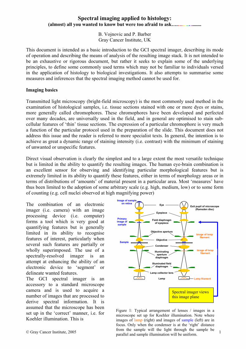
This document is intended as a basic introduction to the GCI spectral imager, describing its mode of operation and describing the means of analysis of the resulting image stack. It is not intended to be an exhaustive or rigorous document, but rather it seeks to explain some of the underlying principles, to define some commonly used terms which may not be familiar to individuals versed in the application of histology to biological investigations. It also attempts to summarise some measures and inferences that the spectral imaging method cannot be used for. Imaging basics Transmitted light microscopy (bright-field microscopy) is the most commonly used method in the examination of histological samples, i.e. tissue sections stained with one or more dyes or stains, more generally called chromophores. These chromophores have been developed and perfected over many decades, are universally used in the field, and in general are optimised to stain sub-cellular features of ‘thin’ tissue sections. The expression of a particular chromophore is very much a function of the particular protocol used in the preparation of the slide. This document does not address this issue and the reader is referred to more specialist texts. In general, the intention is to achieve as great a dynamic range of staining intensity (i.e. contrast) with the minimum of staining of unwanted or unspecific features. Direct visual observation is clearly the simplest and to a large extent the most versatile technique but is limited in the ability to quantify the resulting images. The human eye-brain combination is an excellent sensor for observing and identifying particular morphological features but is extremely limited in its ability to quantify these features, either in terms of morphology areas or in terms of distributions of ‘amounts’ of material present in a particular area. Most ‘measures’ have thus been limited to the adoption of some arbitrary scale (e.g. high, medium, low) or to some form of counting (e.g. cell nuclei observed at high magnifying power) The combination of an electronic imager (i.e. camera) with an image processing device (i.e. computer) forms a tool which is very good at quantifying features but is generally limited in its ability to recognise features of interest, particularly when several such features are partially or wholly superimposed. The use of a spectrally-resolved imager is an attempt at enhancing the ability of an electronic device to ‘segment’ or delineate wanted features. The GCI spectral imager is an accessory to a standard microscope camera and is used to acquire a number of images that are processed to derive spectral information. It is assumed that the microscope has been set up in the ‘correct’ manner, i.e. for Koehler illumination. This is
Figure 1: Typical arrangement of lenses / images in a microscope set up for Koehler illumination. Note where images of lamp (right) and images of sample (left) are in focus. Only when the condenser is at the ‘right’ distance from the sample will the light through the sample be parallel and sample illumination will be uniform.
Spectral imager views this image plane
Eye
Eyepiece
Field diaphragm of eyepiece
Objective aperture
Objective
Condenser
Illuminating aperture
diaphragm
Illuminated field diaphragm
Lamp collector lens
Lamp Lamp filament
Image of lamp filament
Image of lamp filament
Exit pupil of microscope (Ramsden disc)
Image of sample on retina
Primary image of sample
Sample
© Gray Cancer Institute, 2005 2
illustrated in Figure 1, in particular the correct condenser position. The spectral imager also relies on the fact that most lenses in a modern microscope are achromatic (i.e. they transmit and focus all wavelengths/colours equally well), in contrast to older types where e.g. chromatic eyepieces were used to correct for objective chromaticity).
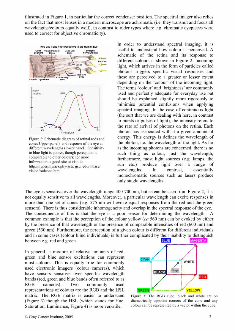
In order to understand spectral imaging, it is useful to understand how colour is perceived. A schematic of the retina and its response to different colours is shown in Figure 2. Incoming light, which arrives in the form of particles called photons triggers specific visual responses and these are perceived to a greater or lesser extent depending on the ‘colour’ of the incoming light. The terms ‘colour’ and ‘brightness’ are commonly used and perfectly adequate for everyday use but should be explained slightly more rigorously to minimise potential confusions when applying spectral imaging. In the case of continuous light (the sort that we are dealing with here, in contrast to bursts or pulses of light), the intensity refers to the rate of arrival of photons on the retina. Each photon has associated with it a given amount of energy. This energy is defines the wavelength of the photon, i.e. the wavelength of the light. As far as the incoming photons are concerned, there is no such thing as colour, just the wavelength; furthermore, most light sources (e.g. lamps, the sun etc.) produce light over a range of wavelengths. In contrast, essentially monochromatic sources such as lasers produce only single wavelengths.
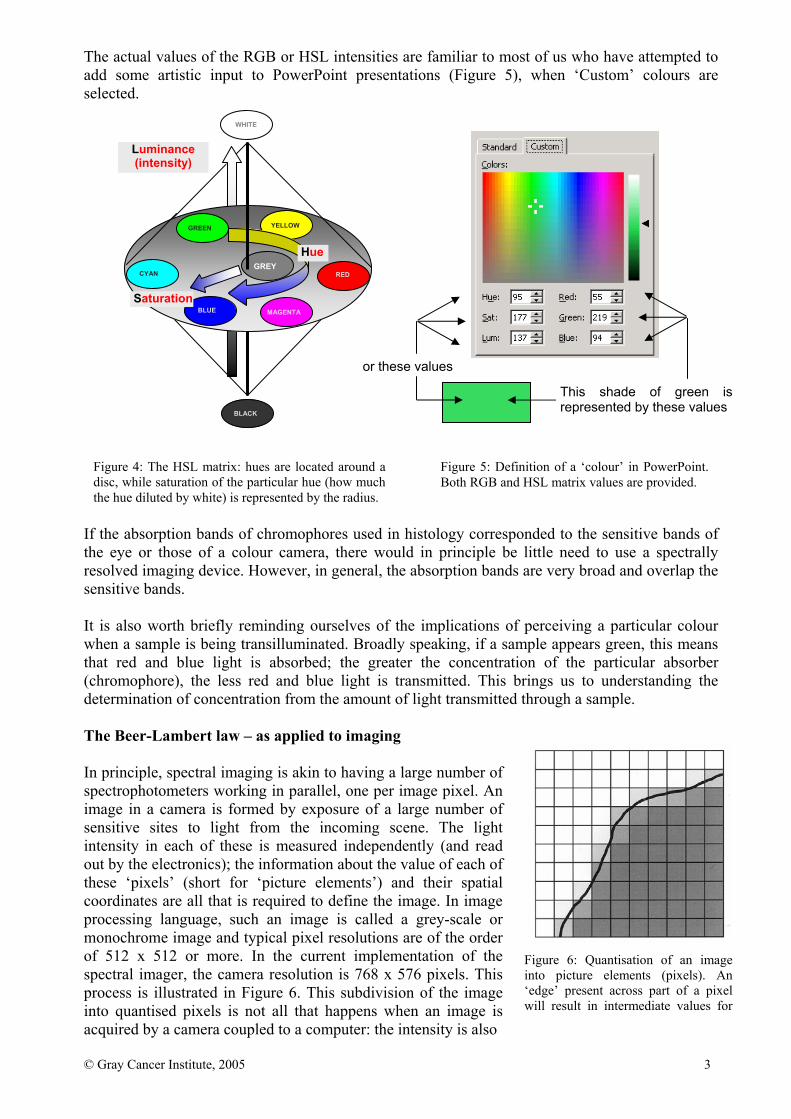
The eye is sensitive over the wavelength range 400-700 nm, but as can be seen from Figure 2, it is not equally sensitive to all wavelengths. Moreover, a particular wavelength can excite responses in more than one set of cones (e.g. 575 nm will evoke equal responses from the red and the green sensors). There is thus considerable inhomogeneity and overlap in the spectral response of the eye. The consequence of this is that the eye is a poor sensor for determining the wavelength. A common example is that the perception of the colour yellow (ca 560 nm) can be evoked by either by the presence of that wavelength or the presence of comparable intensities of red (600 nm) and green (530 nm). Furthermore, the perception of a given colour is different for different individuals and in some cases (colour blind individuals) is further complicated by their inability to distinguish between e.g. red and green. In general, a mixture of relative amounts of red, green and blue sensor excitations can represent most colours. This is equally true for commonly used electronic imagers (colour cameras), which have sensors sensitive over specific wavelength bands (red, green and blue bands often referred to as RGB cameras). Two commonly used representations of colours are the RGB and the HSL matrix. The RGB matrix is easier to understand (Figure 3) though the HSL (which stands for Hue, Saturation, Luminance, Figure 4) is more versatile.
Figure 2: Schematic diagram of retinal rods and cones Upper panel) and response of the eye at different wavelengths (lower panel). Sensitivity to blue light is poorer, though perception is comparable to other colours; for more information, a good site to visit is: http://hyperphysics.phy-astr. gsu. edu/ hbase/ vision/rodcone.html
Figure 3: The RGB cube: black and white are on diametrically opposite corners of the cube and any colour can be represented by a vector within the cube.
BLACKGreys
BLUE
RED
MAGENTA
GREEN
CYAN
YELLOW
WHITE
© Gray Cancer Institute, 2005 3
The actual values of the RGB or HSL intensities are familiar to most of us who have attempted to add some artistic input to PowerPoint presentations (Figure 5), when ‘Custom’ colours are selected. If the absorption bands of chromophores used in histology corresponded to the sensitive bands of the eye or those of a colour camera, there would in principle be little need to use a spectrally resolved imaging device. However, in general, the absorption bands are very broad and overlap the sensitive bands. It is also worth briefly reminding ourselves of the implications of perceiving a particular colour when a sample is being transilluminated. Broadly speaking, if a sample appears green, this means that red and blue light is absorbed; the greater the concentration of the particular absorber (chromophore), the less red and blue light is transmitted. This brings us to understanding the determination of concentration from the amount of light transmitted through a sample. The Beer-Lambert law – as applied to imaging In principle, spectral imaging is akin to having a large number of spectrophotometers working in parallel, one per image pixel. An image in a camera is formed by exposure of a large number of sensitive sites to light from the incoming scene. The light intensity in each of these is measured independently (and read out by the electronics); the information about the value of each of these ‘pixels’ (short for ‘picture elements’) and their spatial coordinates are all that is required to define the image. In image processing language, such an image is called a grey-scale or monochrome image and typical pixel resolutions are of the order of 512 x 512 or more. In the current implementation of the spectral imager, the camera resolution is 768 x 576 pixels. This process is illustrated in Figure 6. This subdivision of the image into quantised pixels is not all that happens when an image is acquired by a camera coupled to a computer: the intensity is also
Figure 6: Quantisation of an image into picture elements (pixels). An ‘edge’ present across part of a pixel will result in intermediate values for
Figure 4: The HSL matrix: hues are located around a disc, while saturation of the particular hue (how much the hue diluted by white) is represented by the radius.
GREEN
CYAN
YELLOW
RED
MAGENTA BLUE Saturation
Luminance (intensity)
BLACK
WHITE
GREY Hue
Figure 5: Definition of a ‘colour’ in PowerPoint. Both RGB and HSL matrix values are provided.
This shade of green is represented by these values
or these values
© Gray Cancer Institute, 2005 4
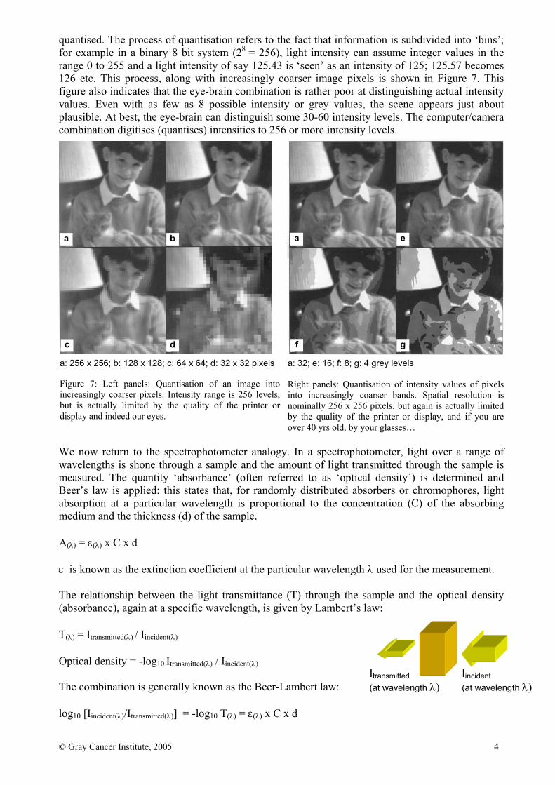
quantised. The process of quantisation refers to the fact that information is subdivided into ‘bins’; for example in a binary 8 bit system (28 = 256), light intensity can assume integer values in the range 0 to 255 and a light intensity of say 125.43 is ‘seen’ as an intensity of 125; 125.57 becomes 126 etc. This process, along with increasingly coarser image pixels is shown in Figure 7. This figure also indicates that the eye-brain combination is rather poor at distinguishing actual intensity values. Even with as few as 8 possible intensity or grey values, the scene appears just about plausible. At best, the eye-brain can distinguish some 30-60 intensity levels. The computer/camera combination digitises (quantises) intensities to 256 or more intensity levels. We now return to the spectrophotometer analogy. In a spectrophotometer, light over a range of wavelengths is shone through a sample and the amount of light transmitted through the sample is measured. The quantity ‘absorbance’ (often referred to as ‘optical density’) is determined and Beer’s law is applied: this states that, for randomly distributed absorbers or chromophores, light absorption at a particular wavelength is proportional to the concentration (C) of the absorbing medium and the thickness (d) of the sample. A(λ) = ε(λ) x C x d ε is known as the extinction coefficient at the particular wavelength λ used for the measurement. The relationship between the light transmittance (T) through the sample and the optical density (absorbance), again at a specific wavelength, is given by Lambert’s law: T(λ) = Itransmitted(λ) / Iincident(λ) Optical density = -log10 Itransmitted(λ) / Iincident(λ) The combination is generally known as the Beer-Lambert law: log10 [Iincident(λ)/Itransmitted(λ)] = -log10 T(λ) = ε(λ) x C x d
a b
c d
a e
f g
a: 32; e: 16; f: 8; g: 4 grey levels Right panels: Quantisation of intensity values of pixels into increasingly coarser bands. Spatial resolution is nominally 256 x 256 pixels, but again is actually limited by the quality of the printer or display, and if you are over 40 yrs old, by your glasses…
Iincident (at wavelength λ)
Itransmitted (at wavelength λ)
a: 256 x 256; b: 128 x 128; c: 64 x 64; d: 32 x 32 pixels Figure 7: Left panels: Quantisation of an image into increasingly coarser pixels. Intensity range is 256 levels, but is actually limited by the quality of the printer or display and indeed our eyes.
© Gray Cancer Institute, 2005 5
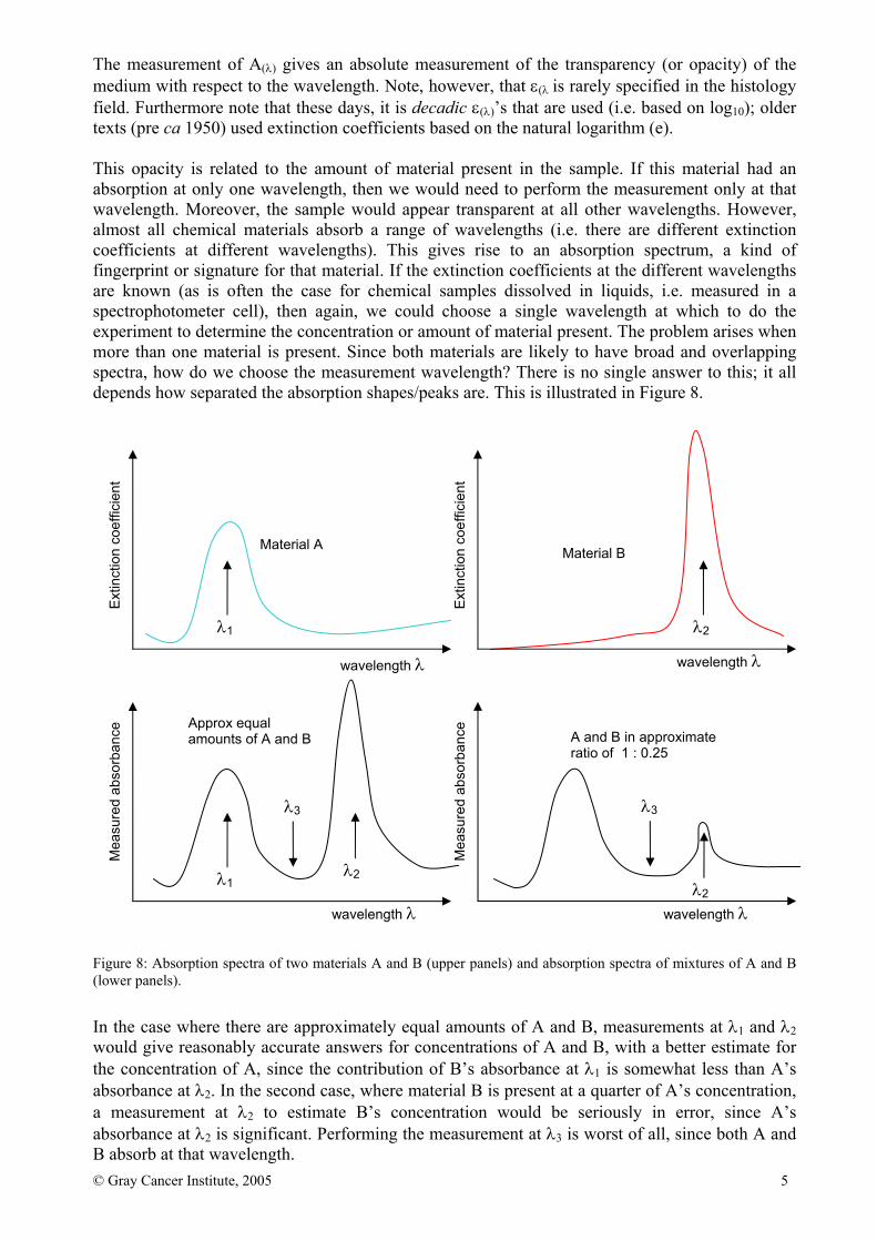
The measurement of A(λ) gives an absolute measurement of the transparency (or opacity) of the medium with respect to the wavelength. Note, however, that ε(λ is rarely specified in the histology field. Furthermore note that these days, it is decadic ε(λ)’s that are used (i.e. based on log10); older texts (pre ca 1950) used extinction coefficients based on the natural logarithm (e). This opacity is related to the amount of material present in the sample. If this material had an absorption at only one wavelength, then we would need to perform the measurement only at that wavelength. Moreover, the sample would appear transparent at all other wavelengths. However, almost all chemical materials absorb a range of wavelengths (i.e. there are different extinction coefficients at different wavelengths). This gives rise to an absorption spectrum, a kind of fingerprint or signature for that material. If the extinction coefficients at the different wavelengths are known (as is often the case for chemical samples dissolved in liquids, i.e. measured in a spectrophotometer cell), then again, we could choose a single wavelength at which to do the experiment to determine the concentration or amount of material present. The problem arises when more than one material is present. Since both materials are likely to have broad and overlapping spectra, how do we choose the measurement wavelength? There is no single answer to this; it all depends how separated the absorption shapes/peaks are. This is illustrated in Figure 8.
In the case where there are approximately equal amounts of A and B, measurements at λ1 and λ2 would give reasonably accurate answers for concentrations of A and B, with a better estimate for the concentration of A, since the contribution of B’s absorbance at λ1 is somewhat less than A’s absorbance at λ2. In the second case, where material B is present at a quarter of A’s concentration, a measurement at λ2 to estimate B’s concentration would be seriously in error, since A’s absorbance at λ2 is significant. Performing the measurement at λ3 is worst of all, since both A and B absorb at that wavelength.
Ext
inct
ion
coef
ficie
nt
wavelength λ
Mea
sure
d ab
sorb
ance
Figure 8: Absorption spectra of two materials A and B (upper panels) and absorption spectra of mixtures of A and B (lower panels).
Ext
inct
ion
coef
ficie
nt
Mea
sure
d ab
sorb
ance
wavelength λ wavelength λ
Material A Material B
Approx equal amounts of A and B A and B in approximate
ratio of 1 : 0.25
λ1 λ2
λ1 λ2 λ2
λ3 λ3
wavelength λ
© Gray Cancer Institute, 2005 6
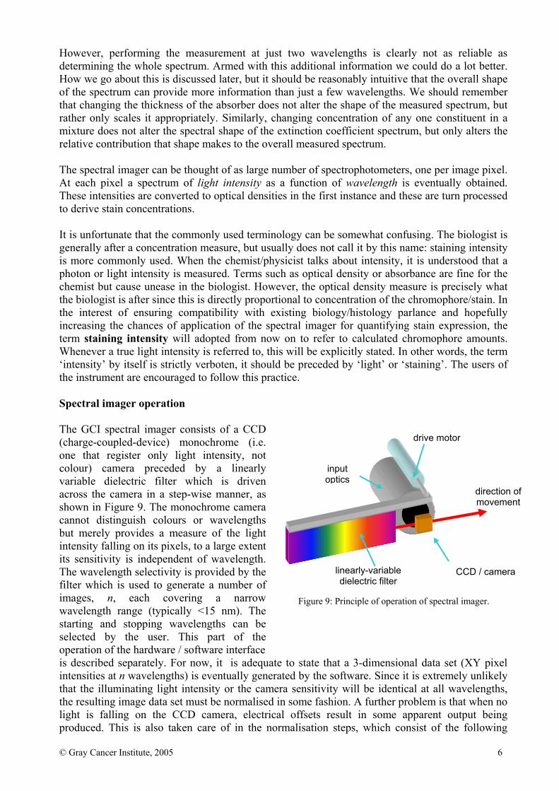
However, performing the measurement at just two wavelengths is clearly not as reliable as determining the whole spectrum. Armed with this additional information we could do a lot better. How we go about this is discussed later, but it should be reasonably intuitive that the overall shape of the spectrum can provide more information than just a few wavelengths. We should remember that changing the thickness of the absorber does not alter the shape of the measured spectrum, but rather only scales it appropriately. Similarly, changing concentration of any one constituent in a mixture does not alter the spectral shape of the extinction coefficient spectrum, but only alters the relative contribution that shape makes to the overall measured spectrum. The spectral imager can be thought of as large number of spectrophotometers, one per image pixel. At each pixel a spectrum of light intensity as a function of wavelength is eventually obtained. These intensities are converted to optical densities in the first instance and these are turn processed to derive stain concentrations. It is unfortunate that the commonly used terminology can be somewhat confusing. The biologist is generally after a concentration measure, but usually does not call it by this name: staining intensity is more commonly used. When the chemist/physicist talks about intensity, it is understood that a photon or light intensity is measured. Terms such as optical density or absorbance are fine for the chemist but cause unease in the biologist. However, the optical density measure is precisely what the biologist is after since this is directly proportional to concentration of the chromophore/stain. In the interest of ensuring compatibility with existing biology/histology parlance and hopefully increasing the chances of application of the spectral imager for quantifying stain expression, the term staining intensity will adopted from now on to refer to calculated chromophore amounts. Whenever a true light intensity is referred to, this will be explicitly stated. In other words, the term ‘intensity’ by itself is strictly verboten, it should be preceded by ‘light’ or ‘staining’. The users of the instrument are encouraged to follow this practice. Spectral imager operation The GCI spectral imager consists of a CCD (charge-coupled-device) monochrome (i.e. one that register only light intensity, not colour) camera preceded by a linearly variable dielectric filter which is driven across the camera in a step-wise manner, as shown in Figure 9. The monochrome camera cannot distinguish colours or wavelengths but merely provides a measure of the light intensity falling on its pixels, to a large extent its sensitivity is independent of wavelength. The wavelength selectivity is provided by the filter which is used to generate a number of images, n, each covering a narrow wavelength range (typically <15 nm). The starting and stopping wavelengths can be selected by the user. This part of the operation of the hardware / software interface is described separately. For now, it is adequate to state that a 3-dimensional data set (XY pixel intensities at n wavelengths) is eventually generated by the software. Since it is extremely unlikely that the illuminating light intensity or the camera sensitivity will be identical at all wavelengths, the resulting image data set must be normalised in some fashion. A further problem is that when no light is falling on the CCD camera, electrical offsets result in some apparent output being produced. This is also taken care of in the normalisation steps, which consist of the following
drive motor
CCD / camera
input optics
linearly-variable dielectric filter
direction of movement
Figure 9: Principle of operation of spectral imager.
© Gray Cancer Institute, 2005 7
procedure. A ‘black’ (i.e. zero light) image (Iblack) is acquired by energising a shutter in front of the camera; this image is temporarily stored. Next, a data set is acquired with the shutter open but with no sample present; this data set (Iwhite, λ ) is also temporarily stored. During this acquisition, it is essential that the microscope is set up under conditions identical to those that will be used for final data acquisition, i.e. that the appropriate objective has been selected and focused, ideally on a blank slide with similar optical properties to those of the data/sample slide. During sample/data acquisition, the series of images (Isample, λ) is acquired. These are then processed using the following simple algebra, to generate a normalised data set (Idata, λ ): Idata, λ = {(Isample, λ) - (Iblack)}/ {(Iwhite, λ) - (Iblack)} It should be obvious that the resulting light intensities in each pixel in this normalised data set will have values ranging from 0 to 1. However, it should be remembered that the digitisation process, to determine the light intensity in each pixel results in quantised values. In the case of the spectral imager, the images are digitised to 8-bit resolution, i.e. the pixel light intensities can assume one of 256 possible values (28 = 256). It is thus convenient to multiply the normalised data set by 255, such that 0 will now represent zero light intensity falling on that pixel and 255 will represent the maximum light intensity capable of being handled by the system. This algebra is adequate if we were interested only in determining light intensity, but as was stated before, the eventual aim is determine staining intensity, i.e. optical density. This requires knowledge of the incoming light intensity and the algebra must now include a logarithmic operation, to derive an optical density data set (IODdata, λ): I(ODdata, λ) = log10 [Iincident(λ)/Itransmitted(λ)] = log10 {(Iwhite, λ) - (Iblack)}/{(Isample, λ) - (Iblack)} We again remember that the values are digitised to 8-bit resolution and the values of I(ODdata, λ) can thus never exceed about 2.3 or so. An OD value of value of 0 implies 100% light transmission, a value of 1 implies 10% light transmission, a value of 2 implies 1% light transmission and so on. With an 8 bit system it is not possible to resolve differences in very absorbing samples. If such samples are used then a greater digitisation resolution is required. This can only be obtained readily by averaging a large number of images to overcome signal-to-noise limitations of the camera. However, a dynamic range covering optical densities up to 2 is more than adequate for most purposes. These limitations are mentioned here only to emphasise the fact that the ‘darker’ the sample, the greater the error in determining staining intensity and hence it is more advantageous to use thin (i.e. more transparent) samples than thick (i.e. more absorbing samples). Now that we have our data set, it is worth examining possible ways of utilising the spectral information to the full. Although there are many ways to maximise the additional information, we shall briefly consider two approaches: Spectral similarity mapping and spectral deconvolution. However, before discussing this, it is worthwhile to explain how a conventional-looking ‘colour’ image is generated by the spectral imager. In a conventional RGB colour camera, there are three sets of light-sensitive sensors, one for a ‘R’ or red wavelength band, one for a ‘G’ or green wavelength band and one for a ‘B’ or blue wavelength band. These bands extend from 580 – 680 nm, 500-580 nm and 420-500 nm. Since we already have the information about light intensities in even finer wavelength bands, it is a simple matter to combine appropriate bands together to generate the R, G and B pixel intensities that would have been produced by a colour camera with its appropriately broader wavelength bandpass filters. In effect, we are making use of an approximation, taking into account the response of the ‘average’ human eye, to generate a scene which is reasonably similar to that which would have been ‘seen’ down the microscope eyepieces. A similar approximation is used when displaying the images at single wavelengths, during and following acquisition by the spectral imager. Although the information provided by the camera is merely pixel light intensity, the image is ‘painted’ by the software, with approximate values of RGB components to provide a ‘colour’ on the screen. This colour is similar to that had the viewer
© Gray Cancer Institute, 2005 8
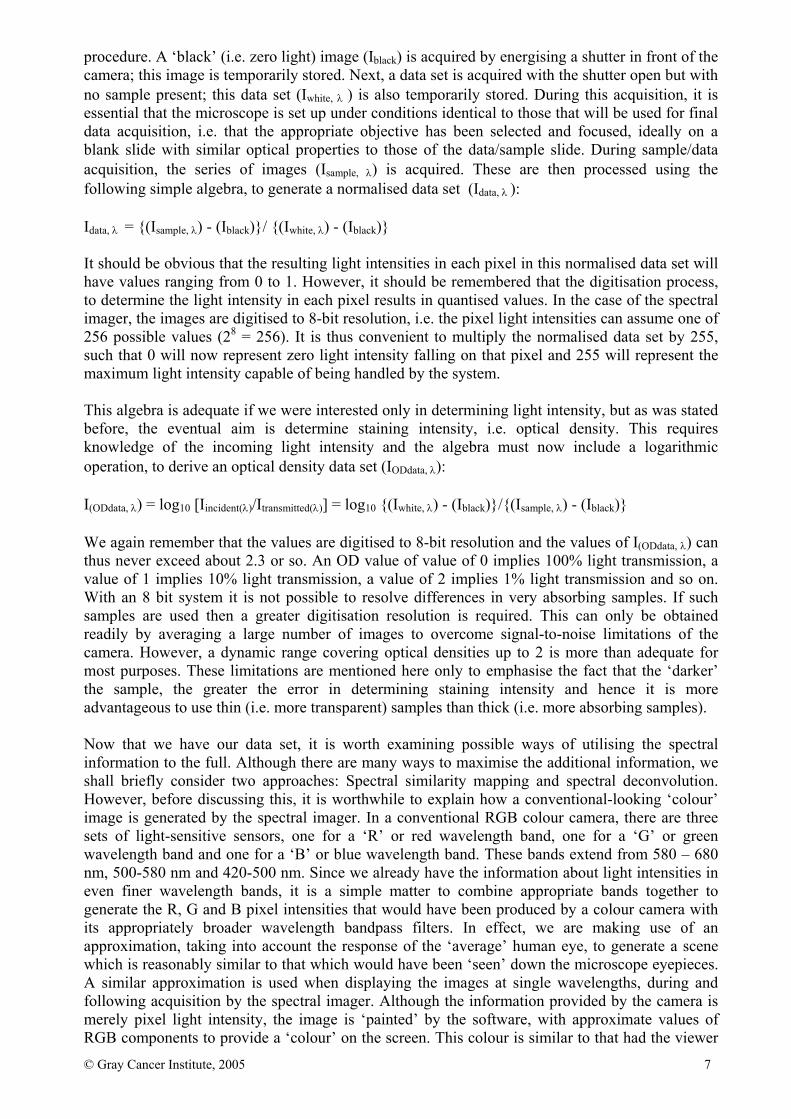
looked in the eyepieces through a filter of corresponding wavelength. The approximation is reasonably good over most of the wavelength range but will fail at the extremes (to some extent this will depend on the viewer’s eye response. Spectral Similarity Mapping Spectral Similarity Mapping (SSM) is a convenient method which is applicable when we are not really interested in determining the contributions that each chromophore makes to the overall spectrum determined at each pixel, but rather when we wish to identify all the regions of the image, i.e. all the pixels that have a similar absorption spectrum. In other words, we wish to identify the parts of the section that have a similar staining intensity but are not necessarily concerned about what biology/biochemistry has caused the staining. Clearly we need to define a reference (i.e. reference spectrum) with which to compare all the pixels in the image. The result of doing this on 3 separate regions of a slide is shown in Figure 10. The software compares the spectrum at every pixel with that taken from the reference region(s). The more similar they are, the greater the brightness value assigned to that pixel and hence ‘similar’ regions become apparent. But of course there must be some formalised way of defining this similarity. The comparison is performed mathematically by defining the spectral difference between the wanted (reference) spectrum and the actual spectrum at every pixel. This is performed in a ‘weighted’ fashion as shown in the equation below, where Io is the reference spectrum and I is the pixel spectrum: In the above example, a metastatic squamous cell carcinoma has been labelled with pimonidazole (pink/red regions) and Ki-67 (brown regions). In panel (d) blood vessels have been segmented reasonably successfully, even though the differences between spectra are small, and certainly hard to see by eye.
Figure 10: Spectral similarity mapping in action. (a) original; (b) selected regions from original and their spectra which act as references; (c), d) and (e) show the regions emphasized where the three selected spectra most closely match.
(a)
(b)
(c)
(d) (e)
( ) ( )[ ]2
1
20,
2
1
−= ∫
λ
λ
λλλ dIIDifferenceSpectral yx
© Gray Cancer Institute, 2005 9
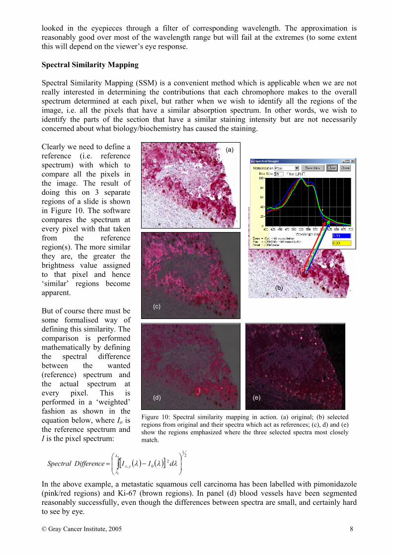
Spectral Deconvolution Spectral Deconvolution (SD) or decomposition is most useful when we suspect (as is often the case) that spectral absorption contributions from more than one chromophore are present in some or each of the pixels. This process starts with a set of reference spectra for the chromophores in question. These spectra can be obtained from the sample itself if there regions which are deemed to be singly-stained. Alternatively (and more commonly applicable), accurate spectra of individual dyes can be obtained from singly-stained slides. The best fit to the actual spectrum is then obtained by varying the ‘proportions’ of A and B reference spectra. This process is shown in Figure 11. If you recall the previous descriptions about optical densities, each of the reference spectra can be thought of as representing an amount or concentration of a particular chromophore. While we do not know the actual value of concentration (because we do not know extinction coefficients nor path lengths), we can express the concentration or amount in every pixel of our sample as a percentage in relation to the reference spectrum. In other words, if the software finds, as in the above example, that, at a given pixel, A’s spectrum needs to be reduced by scaling to ½ its reference spectrum amplitude, and B’s spectrum needs to be reduced by scaling to ¾ its reference spectrum amplitude in order to obtain a good fit to the actual spectrum, it is acceptable to conclude one of the following: • If the tissue thicknesses used are the same in the reference and sample slides, then A’s staining
intensity is half that present in A’s reference slide and B’s staining intensity is ¾ of that present in its reference slide.
• If the tissue thicknesses are not the same, than an appropriate correction must be made. For example, if A’s reference slide was twice as thick as the sample slide, then the sample and reference actually contain the same concentration of material.
• If we find, at some other pixel, that A’s contribution has dropped to ¼, then that pixel can be said to contain ½ the amount of material compared to the first pixel.
Figure 11: Reference absorption spectra of two materials A and B (upper panels) and absorption spectrum of a mixture of A and B (lower panel, thick line). The deconvolution process ‘tries’ a range of scaling values for A and B spectra until the best fit is obtained to the actual data. In the example shown this corresponds to around 50% of A and 75% of B. ‘Percent’ in this case is relative to the reference spectra.
Ref
eren
ce o
ptic
al d
ensi
ty
wavelength λ
Mea
sure
d op
tical
den
sity
wavelength λ
Reference spectrum of Material A
Reference spectrum of Material B
Change proportions of materials A & B
wavelength λ
Ref
eren
ce o
ptic
al d
ensi
ty
© Gray Cancer Institute, 2005 10
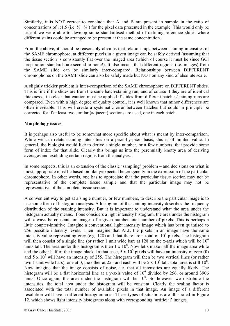
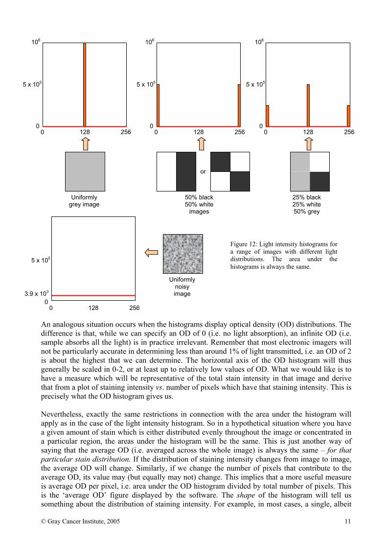
Similarly, it is NOT correct to conclude that A and B are present in sample in the ratio of concentrations of 1:1.5 (i.e. ½ : ¾ ) for the pixel data presented in the example. This would only be true if we were able to develop some standardised method of defining reference slides where different stains could be arranged to be present at the same concentration. From the above, it should be reasonably obvious that relationships between staining intensities of the SAME chromophore, at different pixels in a given image can be safely derived (assuming that the tissue section is consistently flat over the imaged area (which of course it must be since GCI preparation standards are second to none!). It also means that different regions (i.e. images) from the SAME slide can be similarly inter-compared. Relationships between DIFFERENT chromophores on the SAME slide can also be safely made but NOT on any kind of absolute scale. A slightly trickier problem is inter-comparison of the SAME chromophore on DIFFERENT slides. This is fine if the slides are from the same batch/staining run, and of course if they are of identical thickness. It is clear that caution must be applied if slides from different batches/staining runs are compared. Even with a high degree of quality control, it is well known that minor differences are often inevitable. This will create a systematic error between batches but could in principle be corrected for if at least two similar (adjacent) sections are used, one in each batch. Morphology issues It is perhaps also useful to be somewhat more specific about what is meant by inter-comparison. While we can relate staining intensities on a pixel-by-pixel basis, this is of limited value. In general, the biologist would like to derive a single number, or a few numbers, that provide some form of index for that slide. Clearly this brings us into the perennially knotty area of deriving averages and excluding certain regions from the analysis. In some respects, this is an extension of the classic ‘sampling’ problem – and decisions on what is most appropriate must be based on likely/expected heterogeneity in the expression of the particular chromophore. In other words, one has to appreciate that the particular tissue section may not be representative of the complete tissue sample and that the particular image may not be representative of the complete tissue section. A convenient way to get at a single number, or few numbers, to describe the particular image is to use some form of histogram analysis. A histogram of the staining intensity describes the frequency distribution of the staining intensity. But it is important to understand what the area under the histogram actually means. If one considers a light intensity histogram, the area under the histogram will always be constant for images of a given number total number of pixels. This is perhaps a little counter-intuitive. Imagine a conventional light intensity image which has been quantised to 256 possible intensity levels. Then imagine that ALL the pixels in an image have the same intensity value representing grey (e.g. 128) and that there are a total of 106 pixels. The histogram will then consist of a single line (or rather 1 unit wide bar) at 128 on the x-axis which will be 106 units tall. The area under this histogram is then 1 x 10⁶. Now let’s make half the image area white and the other half of the image black. In that case, 5 x 105 pixels will have an intensity of zero (0) and 5 x 10⁵ will have an intensity of 255. The histogram will then be two vertical lines (or rather two 1 unit wide bars), one at 0, the other at 255 and each will be 5 x 10⁵ tall: total area is still 106. Now imagine that the image consists of noise, i.e. that all intensities are equally likely. The histogram will be a flat horizontal line at a y-axis value of 106 divided by 256, or around 3906 units. Once again, the area under the histogram will be 106. So however we distribute the intensities, the total area under the histogram will be constant. Clearly the scaling factor is associated with the total number of available pixels in that image. An image of a different resolution will have a different histogram area. These types of situations are illustrated in Figure 12, which shows light intensity histograms along with corresponding ‘artificial’ images.
© Gray Cancer Institute, 2005 11
An analogous situation occurs when the histograms display optical density (OD) distributions. The difference is that, while we can specify an OD of 0 (i.e. no light absorption), an infinite OD (i.e. sample absorbs all the light) is in practice irrelevant. Remember that most electronic imagers will not be particularly accurate in determining less than around 1% of light transmitted, i.e. an OD of 2 is about the highest that we can determine. The horizontal axis of the OD histogram will thus generally be scaled in 0-2, or at least up to relatively low values of OD. What we would like is to have a measure which will be representative of the total stain intensity in that image and derive that from a plot of staining intensity vs. number of pixels which have that staining intensity. This is precisely what the OD histogram gives us. Nevertheless, exactly the same restrictions in connection with the area under the histogram will apply as in the case of the light intensity histogram. So in a hypothetical situation where you have a given amount of stain which is either distributed evenly throughout the image or concentrated in a particular region, the areas under the histogram will be the same. This is just another way of saying that the average OD (i.e. averaged across the whole image) is always the same – for that particular stain distribution. If the distribution of staining intensity changes from image to image, the average OD will change. Similarly, if we change the number of pixels that contribute to the average OD, its value may (but equally may not) change. This implies that a more useful measure is average OD per pixel, i.e. area under the OD histogram divided by total number of pixels. This is the ‘average OD’ figure displayed by the software. The shape of the histogram will tell us something about the distribution of staining intensity. For example, in most cases, a single, albeit
128 256 0
106
5 x 10⁵
0 128 2560
106
5 x 10⁵
0 128 2560
106
5 x 10⁵
0
Uniformly grey image
50% black 50% white
images
25% black 25% white 50% grey
or
128 256 0
5 x 10⁵
0
Uniformly noisy image 3.9 x 10³
Figure 12: Light intensity histograms for a range of images with different light distributions. The area under the histograms is always the same.
© Gray Cancer Institute, 2005 12
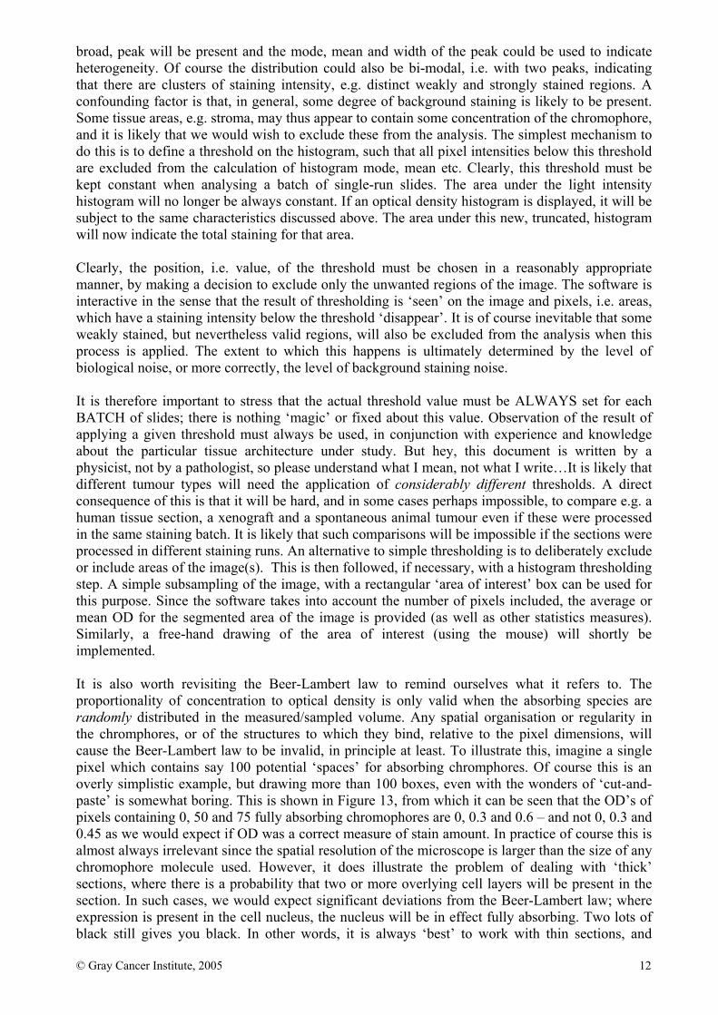
broad, peak will be present and the mode, mean and width of the peak could be used to indicate heterogeneity. Of course the distribution could also be bi-modal, i.e. with two peaks, indicating that there are clusters of staining intensity, e.g. distinct weakly and strongly stained regions. A confounding factor is that, in general, some degree of background staining is likely to be present. Some tissue areas, e.g. stroma, may thus appear to contain some concentration of the chromophore, and it is likely that we would wish to exclude these from the analysis. The simplest mechanism to do this is to define a threshold on the histogram, such that all pixel intensities below this threshold are excluded from the calculation of histogram mode, mean etc. Clearly, this threshold must be kept constant when analysing a batch of single-run slides. The area under the light intensity histogram will no longer be always constant. If an optical density histogram is displayed, it will be subject to the same characteristics discussed above. The area under this new, truncated, histogram will now indicate the total staining for that area. Clearly, the position, i.e. value, of the threshold must be chosen in a reasonably appropriate manner, by making a decision to exclude only the unwanted regions of the image. The software is interactive in the sense that the result of thresholding is ‘seen’ on the image and pixels, i.e. areas, which have a staining intensity below the threshold ‘disappear’. It is of course inevitable that some weakly stained, but nevertheless valid regions, will also be excluded from the analysis when this process is applied. The extent to which this happens is ultimately determined by the level of biological noise, or more correctly, the level of background staining noise. It is therefore important to stress that the actual threshold value must be ALWAYS set for each BATCH of slides; there is nothing ‘magic’ or fixed about this value. Observation of the result of applying a given threshold must always be used, in conjunction with experience and knowledge about the particular tissue architecture under study. But hey, this document is written by a physicist, not by a pathologist, so please understand what I mean, not what I write…It is likely that different tumour types will need the application of considerably different thresholds. A direct consequence of this is that it will be hard, and in some cases perhaps impossible, to compare e.g. a human tissue section, a xenograft and a spontaneous animal tumour even if these were processed in the same staining batch. It is likely that such comparisons will be impossible if the sections were processed in different staining runs. An alternative to simple thresholding is to deliberately exclude or include areas of the image(s). This is then followed, if necessary, with a histogram thresholding step. A simple subsampling of the image, with a rectangular ‘area of interest’ box can be used for this purpose. Since the software takes into account the number of pixels included, the average or mean OD for the segmented area of the image is provided (as well as other statistics measures). Similarly, a free-hand drawing of the area of interest (using the mouse) will shortly be implemented. It is also worth revisiting the Beer-Lambert law to remind ourselves what it refers to. The proportionality of concentration to optical density is only valid when the absorbing species are randomly distributed in the measured/sampled volume. Any spatial organisation or regularity in the chromphores, or of the structures to which they bind, relative to the pixel dimensions, will cause the Beer-Lambert law to be invalid, in principle at least. To illustrate this, imagine a single pixel which contains say 100 potential ‘spaces’ for absorbing chromphores. Of course this is an overly simplistic example, but drawing more than 100 boxes, even with the wonders of ‘cut-and-paste’ is somewhat boring. This is shown in Figure 13, from which it can be seen that the OD’s of pixels containing 0, 50 and 75 fully absorbing chromophores are 0, 0.3 and 0.6 – and not 0, 0.3 and 0.45 as we would expect if OD was a correct measure of stain amount. In practice of course this is almost always irrelevant since the spatial resolution of the microscope is larger than the size of any chromophore molecule used. However, it does illustrate the problem of dealing with ‘thick’ sections, where there is a probability that two or more overlying cell layers will be present in the section. In such cases, we would expect significant deviations from the Beer-Lambert law; where expression is present in the cell nucleus, the nucleus will be in effect fully absorbing. Two lots of black still gives you black. In other words, it is always ‘best’ to work with thin sections, and
© Gray Cancer Institute, 2005 13
indeed with ‘weak’ labelling. This has the further advantage that the measured OD’s will be shifted towards 1 rather than 2. Since the ability of the instrument to differentiate between OD’s of 1 and 1.1 is better than differentiating between 1.9 and 2, the results obtained are likely to be biologically more ‘accurate’. The type of example in Figure 13 also helps to illustrate why we should not fall into the temptation of using such optical density analysis as a surrogate for counting cells/nuclei. This approach is repeatedly suggested and discussed (and even sometimes used!), but it is just plain wrong. Imagine that cell nuclei are represented in Figure 13, i.e. that the large boxes are images rather than pixels. When there is a large number of ‘nuclei’, the average image OD is definitely not proportional to the number of nuclei. You could argue that when there are few ‘nuclei’ in the image (<<10% of total image area), the average OD is very roughly proportional to their number, but in those instances, you may just as easily count the number directly. Any overlying nuclei make the situation even worse. There may be some rare instances where the nuclei are intentionally heavily stained, or the slices thick, but not so thick as to contain overlying cells; in such cases it is permissible to use light intensity measures to derive relative numbers of nuclei in images (relative to an image with known numbers of nuclei). But please take care if using such an approach – take a close look at the image and think about what is being measured. For example, if the staining intensity of each nucleus is not significantly high (i.e. OD <1.5-2), it becomes increasingly important to ensure that the nuclei are evenly stained. Sometimes a thresholded image can be used, i.e. any pixel below a given light intensity becomes fully black. Analysis of such a ‘binary’ mask could indeed provide an indication of relative cell numbers, but the image should be examined and compared to the mask to ensure that nuclei (and only nuclei) have been appropriately segmented. Discussion of this topic and of appropriate software tools will be presented separately. Finally, this brings forward other, perhaps practically more relevant constraints. When determining low OD’s, we must be more careful in choosing and cleaning our ‘blank’ sample when compensating for illumination inhomogeneities, more careful in centering and focusing the condenser etc. Moreover if the samples are too thin, they will look ‘wrong’ and any transmitted light images will give the impression that the histologist should be sacked. So in general, working with 5-20 micron thick sections is adequate, but for thicker sections, it is best to adjust the staining conditions so that excessively high optical densities are not present.
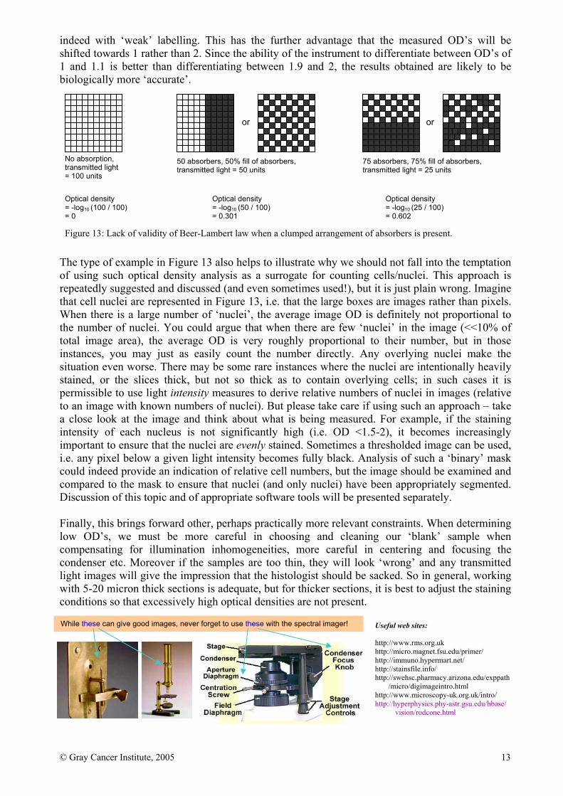
Useful web sites: http://www.rms.org.uk http://micro.magnet.fsu.edu/primer/ http://immuno.hypermart.net/ http://stainsfile.info/ http://swehsc.pharmacy.arizona.edu/exppath
/micro/digimageintro.html http://www.microscopy-uk.org.uk/intro/ http://hyperphysics.phy-astr.gsu.edu/hbase/
vision/rodcone.html
No absorption, transmitted light = 100 units
Optical density = -log10 (100 / 100) = 0
50 absorbers, 50% fill of absorbers, transmitted light = 50 units
or
Optical density = -log10 (50 / 100) = 0.301
75 absorbers, 75% fill of absorbers, transmitted light = 25 units
or
Optical density = -log10 (25 / 100) = 0.602
Figure 13: Lack of validity of Beer-Lambert law when a clumped arrangement of absorbers is present.
While these can give good images, never forget to use these with the spectral imager!
Related Documents