Spatial Price Equilibrium with Convex Marginal Costs of ... · Spatial Price Equilibrium with Convex Marginal Costs of Transportation: Applications to the Brent-WTI Spread ... oil

Spatial Price Equilibrium with Convex Marginal Costs of

Transportation: Applications to the Brent-WTI Spread

Max S. Bennett∗

March 20, 2012

Abstract

Standard models of spatial price equilibrium assume that transportation costs are constantand therefore conclude that a spatial price spread must be bound by the constant marginal costof transportation. However, the empirics of many spatial price spreads, such as the Brent-WTIspread, demonstrate clear violations of this condition. This paper explains this phenomenon byinstead assuming that the marginal cost of transportation is convex. Furthermore, this paperrationalizes the sensitivity of spatial price spreads to localized demand and supply schedulesas well as to expected future costs of transportation, an endogeneity that standard models areunable to explain.

∗I would like to thank Bruce Petersen for his incredible support, insight, and inspiration throughout the entireprocess of writing this paper; he has been a wonderful mentor. I would also like to thank Sebastian Galiani for hisvaluable feedback and advice. And I want to express the utmost gratitude to Dorothy Petersen for providing mewith the opportunity to engage my fascination with economics by writing a thesis, and for helping me navigate myundergraduate academic career.

1 Introduction

Understanding the determinants of commodity prices is central to the study of economics; it al-lows us to examine and develop policy, construct micro-foundations for macroeconomic theory,and more accurately predict future prices. However, our understanding is incomplete withoutincorporating the interconnectedness of spatially separated markets. The possibility of trans-portation makes the price of a commodity in one region endogenous to the demand and supplyschedules in other regions. As such, without understanding the relevance of transportation, eco-nomics would be wholly unable to study and address many problems in agriculture, energy, andfinancial markets. In fact, the first explicit description of price determination as the intersectionof demand and supply curves was given by A. A. Cournot (1838) partially in attempt to describeprice relations between spatially separated markets. The integration of markets is so importantbecause of the value it provides: it allows commodities to be allocated from the cheapest suppliersto the consumers with the highest demand. If spatially separated markets become decoupled fromone another, there is value to be earned by reconnecting them. As such, from a policy perspective,understanding the causes of changing spatial price spreads is important because it allows us tomore accurately prescribe effective policy to address the issue and reintegrate spatially separatedmarkets.

Models of spatial price equilibrium have been developed in order to incorporate the inter-connectedness of spatially separated markets into commodity price determination. A standardassumption in the literature is that the marginal cost of transportation is constant (independentof volume). As such, standard models, as exemplified by Samuelson (1952) and Takayama andJudge (1964), conclude that the price differential between any two regions1 is bound by the con-stant marginal cost of transportation. These models thereby conclude that transportation willoccur if and only if the spatial price spread is exactly equal to the transportation cost. Thekey empirical implication of such models is that once transportation occurs, the spatial pricespread cannot increase further. However, we somewhat regularly observe dramatic violationsof this condition in many commodity markets, such as within the US crude oil market during2011. To address this empirical problem theorists have attempted to relax assumptions in thestandard models. One such example is a paper by Coleman (2009), which shows that if trans-portation is non-instantaneous, than spatial price spreads can increase without bound and notviolate no-arbitrage.

This paper will show that if we instead relax the assumption that the marginal cost scheduleof transportation is constant, then even with instantaneous transport spatial price spreads canincrease without bound and not violate no-arbitrage. I will go on to show that under suchassumptions, spatial price spreads become endogenous to localized demand and supply schedules,an endogeneity that I will provide empirical support for. It is important to note that standardmodels of which assume that the marginal cost schedule of transportation is constant cannotexplain this relationship. I will go on to include the possibility of storage which will illuminatethe endogeneity of the current spread to expected future costs of transportation, a relationshipthat I have not found described in the literature.

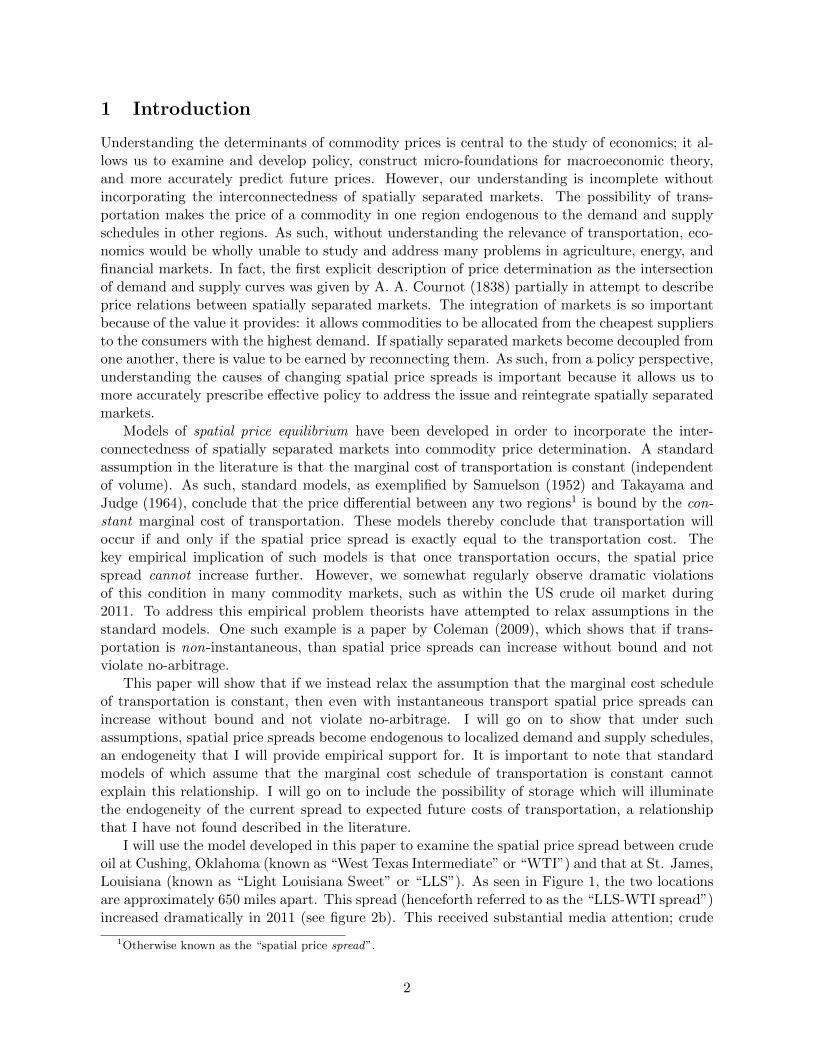
I will use the model developed in this paper to examine the spatial price spread between crudeoil at Cushing, Oklahoma (known as “West Texas Intermediate” or “WTI”) and that at St. James,Louisiana (known as “Light Louisiana Sweet” or “LLS”). As seen in Figure 1, the two locationsare approximately 650 miles apart. This spread (henceforth referred to as the “LLS-WTI spread”)increased dramatically in 2011 (see figure 2b). This received substantial media attention; crude

1Otherwise known as the “spatial price spread”.

2

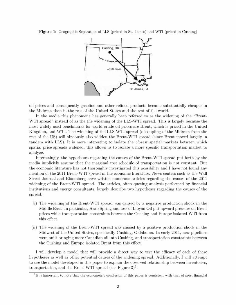
Figure 1: Geographic Separation of LLS (priced in St. James) and WTI (priced in Cushing)

oil prices and consequently gasoline and other refined products became substantially cheaper inthe Midwest than in the rest of the United States and the rest of the world.

In the media this phenomena has generally been referred to as the widening of the “Brent-WTI spread” instead of as the the widening of the LLS-WTI spread. This is largely because themost widely used benchmarks for world crude oil prices are Brent, which is priced in the UnitedKingdom, and WTI. The widening of the LLS-WTI spread (decoupling of the Midwest from therest of the US) will obviously also widden the Brent-WTI spread (since Brent moved largely intandem with LLS). It is more interesting to isolate the closest spatial markets between whichspatial price spreads widened; this allows us to isolate a more specific transportation market toanalyze.

Interestingly, the hypotheses regarding the causes of the Brent-WTI spread put forth by themedia implicitly assume that the marginal cost schedule of transportation is not constant. Butthe economic literature has not thoroughly investigated this possibility and I have not found anymention of the 2011 Brent-WTI spread in the economic literature. News centers such as the WallStreet Journal and Bloomberg have written numerous articles regarding the causes of the 2011widening of the Brent-WTI spread. The articles, often quoting analysis performed by financialinstitutions and energy consultants, largely describe two hypotheses regarding the causes of thespread:

(i) The widening of the Brent-WTI spread was caused by a negative production shock in theMiddle East. In particular, Arab Spring and loss of Libyan Oil put upward pressure on Brentprices while transportation constraints between the Cushing and Europe isolated WTI fromthis effect.

(ii) The widening of the Brent-WTI spread was caused by a positive production shock in theMidwest of the United States, specifically Cushing, Oklahoma. In early 2011, new pipelineswere built bringing more Canadian oil into Cushing, and transportation constraints betweenthe Cushing and Europe isolated Brent from this effect.

I will develop a model that will provide a direct way to test the efficacy of each of thesehypotheses as well as other potential causes of the widening spread. Additionally, I will attemptto use the model developed in this paper to explain the observed relationship between inventories,transportation, and the Brent-WTI spread (see Figure 3)2.

2It is important to note that the econometric conclusion of this paper is consistent with that of most financial

3

1.1 Background of Oil Market at Cushing, Oklahoma

Figure 2: Prices

(a) Monthly LLS spot price and WTI spot price from 1983 through 2011. 1983 was thefirst year Bloomberg reports data for the spot price of LLS crude oil.

(b) Monthly LLS spot price minus WTI spot price (LLS-WTI spread) from 1983 through2011

1.1 Background of Oil Market at Cushing, Oklahoma

The most easily refined crude oil, and thus the most valuable, is light sweet crude. WTI, Brent,and LLS are all light sweet crude oils, and are almost identical in physical composition. As such,any substantial deviation in price between these crude oils can only be a consequence of spatialprice equilibrium and not differences in intrinsic value.

Cushing, Oklahoma is the delivery point for the NYMEX oil futures contract and thereforerefineries, storage facilities, and pipelines have all developed substantial infrastructure in theperiphery of the city. As of 2011, it is estimated that storage capacity at Cushing is around 48million barrels of crude oil, and as much as 600 thousand barrels flow into Cushing daily.

The transportation infrastructure between Cushing and St. James primarily consists ofpipelines. Most pipelines transport liquid at a speed of approximately 3 to 13 miles-per-hour;therefore it should only take between two and nine days to transport crude oil from Cushing toSt. James. There are, however, additional modes of transportation between Cushing and St.James: notably, rail and trucking. Transportation from Cushing to St. James is estimated tocost between $7 to $10 per barrel by rail and between $11 and $15 per barrel by trucking, whichis much more expensive than the estimated $2 per barrel by pipeline.3 As noted above, a con-

institutions and energy consultants: specifically, this paper will provide econometric support for hypothesis (ii).3CommodityOnline, quoting analysis by Bank of American Merrill Lynch.

4

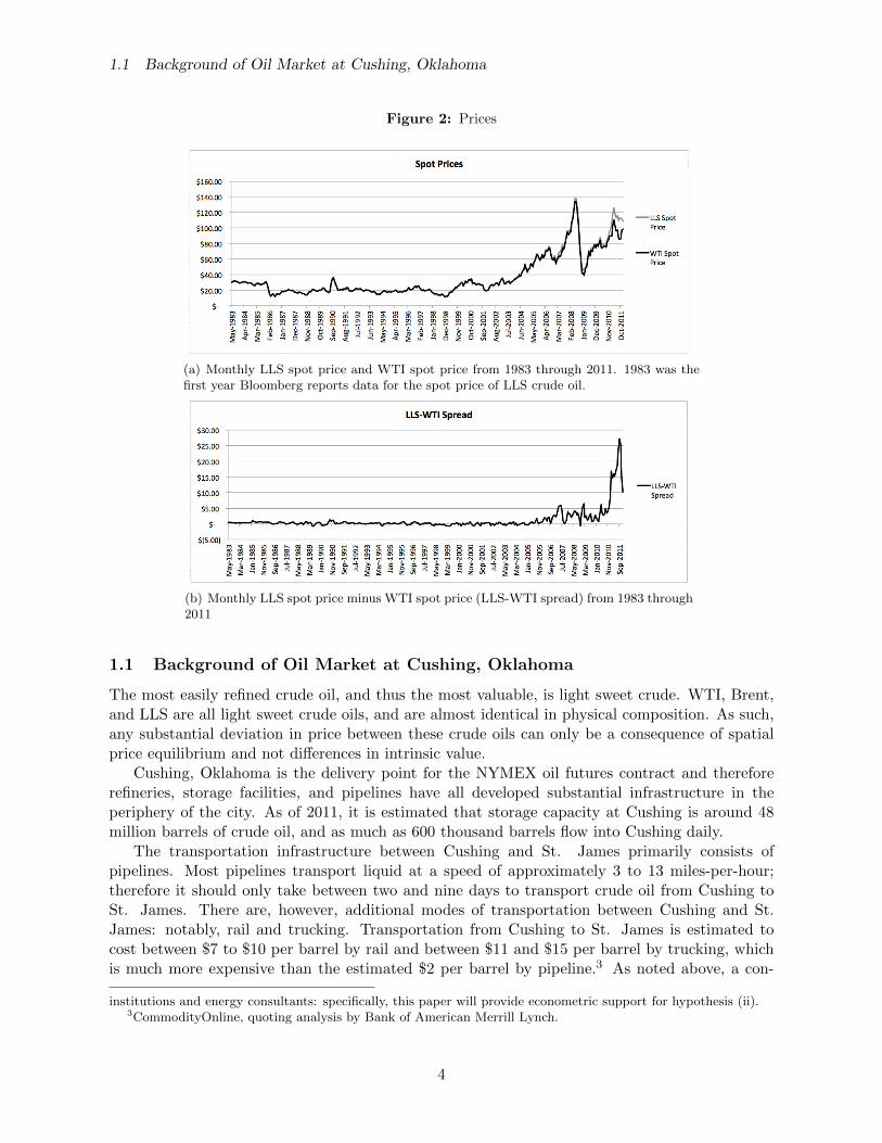
Figure 3: Spread, Storage, and Transport

(a) Monthly average Brent-WTI Spread and month-end storage of crude oil in Cushing (in 10 million bar-rels) from 2004 to 2011.

(b) Monthly average Brent-WTI Spread and totalmonthly shipments of crude oil out of PADD2 (inmonthly-million barrels) from 2004 to 2011.

stant marginal cost schedule of transportation has been the standard assumption in the literature,which is clearly at odds with transportation costs of oil from Cushing to the Gulf Coast if pipelinecapacity is insufficient and therefore some oil must be shipped by other, more expensive, modesof transportation.

In late 2010 and early 2011, two large new pipelines that directed oil from Canada to Cushingwent online, substantially increasing the availability of crude in Cushing. This occurred overthe backdrop of steadily increasing production of crude oil in the midwest over the past decade.These two forces dramatically increased the quantity of crude flowing into Cushing. Modelsof spatial price equilibrium with a constant marginal cost of transportation would suggest thatthis would have no effect on the LLS-WTI spread, as the additional oil would be immediatelydirected towards the coast via transportation infrastructure. However, I will argue in this paperthat because of rising marginal costs, a positive supply shock at Cushing is a theoretically soundexplanation for the widening of the LLS-WTI spread.

2 Building A Model of Spatial Price Equilibrium

2.1 Constant Marginal Costs of Transportation Without Storage

Consider a non-perishable and non-depreciating commodity, called ”x”, that trades in two loca-tions, point A and point B. Production of x at both A and B during a given period t, denoted QA

t

and QBt respectively, is assumed to be given as exogenous to arbitrageurs. This is consistent with

a commodity whose production occurs in earlier periods, such as oil, or commodities that haveperfectly inelastic supply curves. The corresponding price of x at each point is denoted pAt , p

Bt .

In this model, arbitrageurs are risk-neutral and have the opportunity to transport commodity xfrom point A to point B at marginal cost kTt,AB, or from point B to point A at marginal cost

kTt,BA.Before building a model with convex marginal costs of transportation with storage, let us

first build intuition by describing a model where the marginal cost of transportation between Aand B is constant and where there is no option to store commodity x from period t to periodt + 1. These are the assumptions in the standard spatial price equilibrium models described bySamuelson (1952) and Takayama and Judge (1962b).

5

2.1 Constant Marginal Costs of Transportation Without Storage

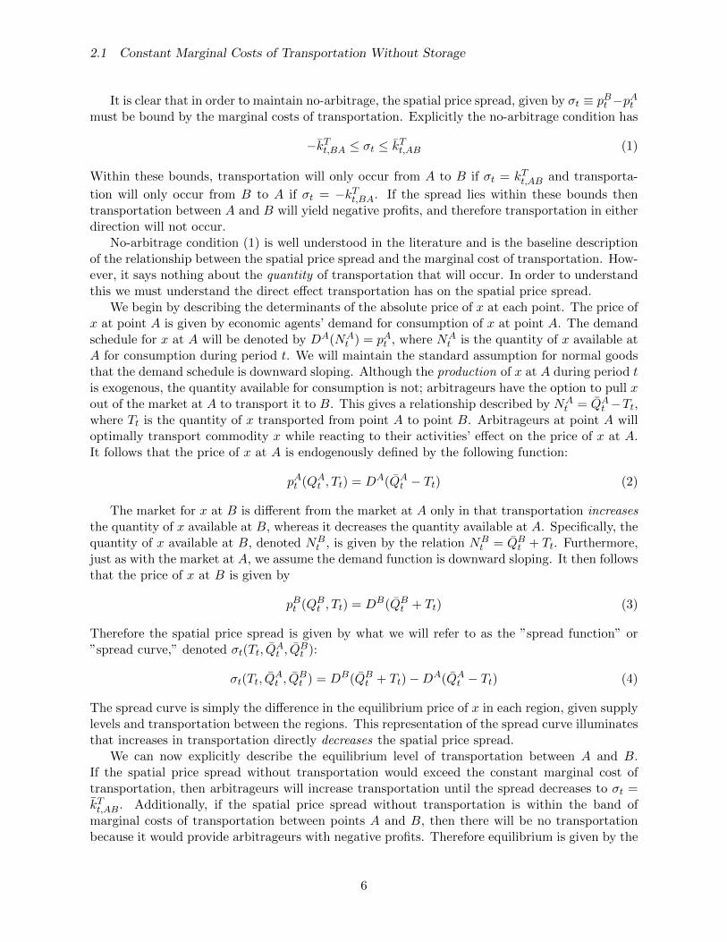
It is clear that in order to maintain no-arbitrage, the spatial price spread, given by σt ≡ pBt −pAtmust be bound by the marginal costs of transportation. Explicitly the no-arbitrage condition has

−k̄Tt,BA ≤ σt ≤ k̄Tt,AB (1)

Within these bounds, transportation will only occur from A to B if σt = kTt,AB and transporta-

tion will only occur from B to A if σt = −kTt,BA. If the spread lies within these bounds thentransportation between A and B will yield negative profits, and therefore transportation in eitherdirection will not occur.

No-arbitrage condition (1) is well understood in the literature and is the baseline descriptionof the relationship between the spatial price spread and the marginal cost of transportation. How-ever, it says nothing about the quantity of transportation that will occur. In order to understandthis we must understand the direct effect transportation has on the spatial price spread.

We begin by describing the determinants of the absolute price of x at each point. The price ofx at point A is given by economic agents’ demand for consumption of x at point A. The demandschedule for x at A will be denoted by DA(NA

t ) = pAt , where NAt is the quantity of x available at

A for consumption during period t. We will maintain the standard assumption for normal goodsthat the demand schedule is downward sloping. Although the production of x at A during period tis exogenous, the quantity available for consumption is not; arbitrageurs have the option to pull xout of the market at A to transport it to B. This gives a relationship described by NA

t = Q̄At −Tt,

where Tt is the quantity of x transported from point A to point B. Arbitrageurs at point A willoptimally transport commodity x while reacting to their activities’ effect on the price of x at A.It follows that the price of x at A is endogenously defined by the following function:

pAt (QAt , Tt) = DA(Q̄A

t − Tt) (2)

The market for x at B is different from the market at A only in that transportation increasesthe quantity of x available at B, whereas it decreases the quantity available at A. Specifically, thequantity of x available at B, denoted NB

t , is given by the relation NBt = Q̄B

t + Tt. Furthermore,just as with the market at A, we assume the demand function is downward sloping. It then followsthat the price of x at B is given by

pBt (QBt , Tt) = DB(Q̄B

t + Tt) (3)

Therefore the spatial price spread is given by what we will refer to as the ”spread function” or”spread curve,” denoted σt(Tt, Q̄

At , Q̄

Bt ):

σt(Tt, Q̄At , Q̄

Bt ) = DB(Q̄B

t + Tt)−DA(Q̄At − Tt) (4)

The spread curve is simply the difference in the equilibrium price of x in each region, given supplylevels and transportation between the regions. This representation of the spread curve illuminatesthat increases in transportation directly decreases the spatial price spread.

We can now explicitly describe the equilibrium level of transportation between A and B.If the spatial price spread without transportation would exceed the constant marginal cost oftransportation, then arbitrageurs will increase transportation until the spread decreases to σt =k̄Tt,AB. Additionally, if the spatial price spread without transportation is within the band ofmarginal costs of transportation between points A and B, then there will be no transportationbecause it would provide arbitrageurs with negative profits. Therefore equilibrium is given by the

6

2.2 Convex Marginal Costs of Transportation Without Storage

following conditions:

σt(Tt, ...)|Tt=0 ≥ k̄Tt,AB =⇒ T ∗t ∈ R+ � DB(Q̄B

t + T ∗t )−DA(Q̄A

t − T ∗t ) = k̄Tt,AB (5)

− k̄Tt,BA < σt(Tt, ...)|Tt=0 < k̄Tt,AB =⇒ T ∗t = 0 (6)

Clearly, the level of transportation is endogenous to the production levels at both A and B, andfurthermore, if the marginal cost of transportation is constant, the equilibrium spread will neverexceed k̄Tt,AB.

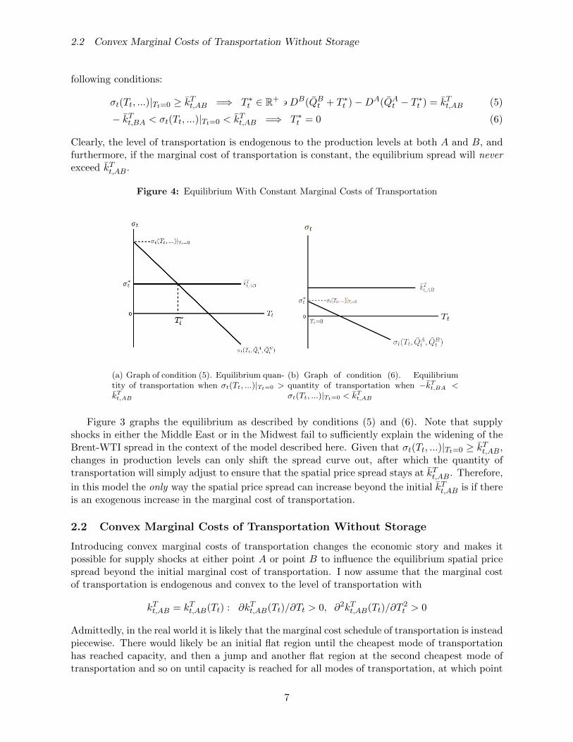
Figure 4: Equilibrium With Constant Marginal Costs of Transportation

(a) Graph of condition (5). Equilibrium quan-tity of transportation when σt(Tt, ...)|Tt=0 >k̄Tt,AB

(b) Graph of condition (6). Equilibriumquantity of transportation when −k̄Tt,BA <σt(Tt, ...)|Tt=0 < k̄Tt,AB

Figure 3 graphs the equilibrium as described by conditions (5) and (6). Note that supplyshocks in either the Middle East or in the Midwest fail to sufficiently explain the widening of theBrent-WTI spread in the context of the model described here. Given that σt(Tt, ...)|Tt=0 ≥ k̄Tt,AB,changes in production levels can only shift the spread curve out, after which the quantity oftransportation will simply adjust to ensure that the spatial price spread stays at k̄Tt,AB. Therefore,

in this model the only way the spatial price spread can increase beyond the initial k̄Tt,AB is if thereis an exogenous increase in the marginal cost of transportation.

2.2 Convex Marginal Costs of Transportation Without Storage

Introducing convex marginal costs of transportation changes the economic story and makes itpossible for supply shocks at either point A or point B to influence the equilibrium spatial pricespread beyond the initial marginal cost of transportation. I now assume that the marginal costof transportation is endogenous and convex to the level of transportation with

kTt,AB = kTt,AB(Tt) : ∂kTt,AB(Tt)/∂Tt > 0, ∂2kTt,AB(Tt)/∂T2t > 0

Admittedly, in the real world it is likely that the marginal cost schedule of transportation is insteadpiecewise. There would likely be an initial flat region until the cheapest mode of transportationhas reached capacity, and then a jump and another flat region at the second cheapest mode oftransportation and so on until capacity is reached for all modes of transportation, at which point

7

2.3 Final Model: Convex Marginal Costs of Transportation With Storage

the marginal cost schedule should be perfectly inelastic. However, in order to approximate theeffect of multiple modes of transportation I will simply assume that the schedule is convex. Thissimplifying approximation makes the mathematics easier to deal with, and does not affect the keyresults of the paper.

The no-arbitrage condition (1), briefly restated, becomes −kTt,BA(Tt,BA) ≤ σt(Tt, Q̄At , Q̄

Bt ) ≤

kTt,AB(Tt,AB), where we will just refer to Tt,AB, the quantity of transportation from A to B, asTt. The equilibrium conditions (5) and (6) are no longer based on constant marginal costs oftransportation, and instead are described by the following conditional statements

σt(Tt, ...)|Tt=0 ≥ kTt,AB(0) =⇒ Tt ∈ R+ � DB(Q̄Bt + Tt)−DA(Q̄A

t − Tt) = kTt,AB(Tt) (7)

−kTt,BA(0) < σt(Tt, ...)|Tt=0 < kTt,AB(0) =⇒ Tt = 0 (8)

Where no transportation occurs if and only if the spatial price spread is less than the cost oftransporting the first unit of x.

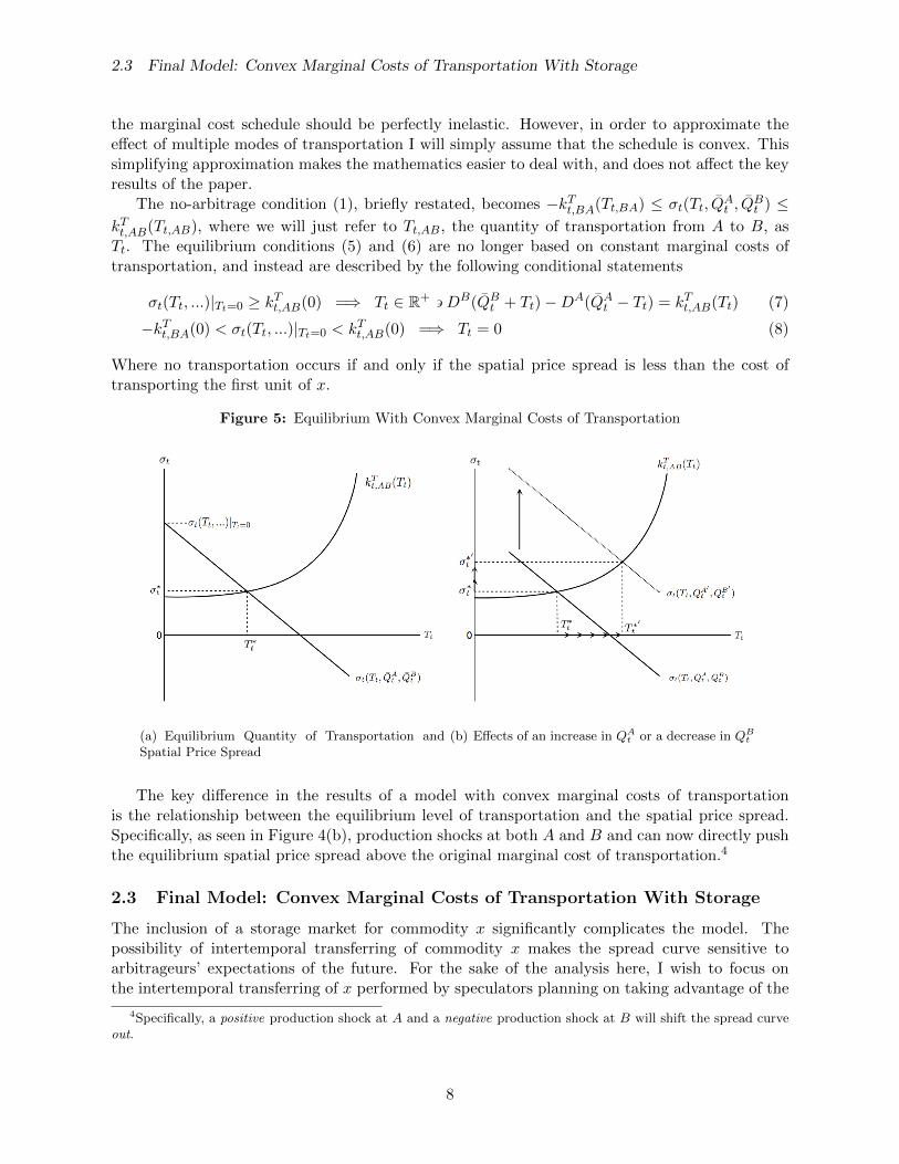
Figure 5: Equilibrium With Convex Marginal Costs of Transportation

(a) Equilibrium Quantity of Transportation andSpatial Price Spread

(b) Effects of an increase in QAt or a decrease in QBt

The key difference in the results of a model with convex marginal costs of transportationis the relationship between the equilibrium level of transportation and the spatial price spread.Specifically, as seen in Figure 4(b), production shocks at both A and B and can now directly pushthe equilibrium spatial price spread above the original marginal cost of transportation.4

2.3 Final Model: Convex Marginal Costs of Transportation With Storage

The inclusion of a storage market for commodity x significantly complicates the model. Thepossibility of intertemporal transferring of commodity x makes the spread curve sensitive toarbitrageurs’ expectations of the future. For the sake of the analysis here, I wish to focus onthe intertemporal transferring of x performed by speculators planning on taking advantage of the

4Specifically, a positive production shock at A and a negative production shock at B will shift the spread curveout.

8

2.3 Final Model: Convex Marginal Costs of Transportation With Storage

spatial price spread in the future. However, it is important to note that there are a plethora ofreasons why economic agents would want to store a commodity.

A key result of this analysis will be that the current spatial price spread will decrease asexpectations of future transportation costs decrease.5 Specifically, a storage market allows aspeculator to purchase a unit of x during period t and store it until period t+ 1 at the marginalcost of storage kSt . The marginal cost schedule of storage is given by

kSt = kSt (St) : ∂kSt (St)/∂St > 0, ∂2kSt (St)/∂S2t > 0

The convexity of the marginal cost schedule of storage is regularly described in the storage liter-ature (see Working, 1948 and Brennan, 1958) . The economic theory suggests that infrastructureconstraints make the marginal cost of storage increase as the quantity of storage approachescapacity.

The first way the storage market enters our model is by changing the spread function. Asspeculators increase storage at A, they directly take units of x out of the market at A, holdingall else equal. It follows that the availability of x at A, denoted NA

t , now equals Q̄At −∆St − Tt,

where the change in storage from period t− 1 to t is denoted by ∆St = St−St−1. Therefore, ournew spread function is described by σt = DB(Q̄B

t + Tt)−DA(Q̄At + St−1 − St − Tt).

Risk-neutral speculators seeking to benefit from expectations about the spread in the futurewill engage in storage if the net present value of the following risk-free transaction is non-negative:buying x at A at price pAt , storing it from period t to t+ 1 at marginal cost kSt (St), transportingit to point B at the expected future marginal cost of transportation E[kTt+1], and selling the unitof x at the expected future price of x at B during period t+ 1, denoted E[pBt+1]. The net presentvalue of this storage transaction, denoted πS , is given by

πS = 11+rE[pBt+1]− 1

1+rE[kTt+1]− kSt (St)− pAt (Q̄At , St, Tt)

where r is the 1-period risk-free interest rate. The no-arbitrage hypothesis suggests that the netpresent value of this risk-free transaction must be non-positive.6 Therefore, given small enoughvalues of the first unit of storage kSt (0), arbitrageurs will store positive levels of x at A up untilthey no longer perceive that act of storage to be a positive net present value transaction. Thisleaves us with the following no-arbitrage condition

11+rE[pBt+1] = 1

1+rE[kTt+1] + kSt (St) +DA(Q̄At + St−1 − St − Tt)

We can now describe general equilibrium in this model with convex marginal costs of trans-portation and storage. Given sufficient differentials in Q̄A

t and Q̄Bt such that both transportation

and storage are positive, the equilibrium quantities of storage and transportation can be describedby the following two conditions:

(i) No-Arbitrage Condition in Transportation Market: σ∗t = DB(Q̄Bt + T ∗

t )−DA(Q̄At + St−1 −

S∗t − T ∗

t ) = kTt (T ∗t )

(ii) No-Arbitrage Condition in Storage Market: 11+rE[pBt+1] = 1

1+rE[kTt+1] + kSt (S∗t ) +DA(Q̄A

t +St−1 − S∗

t − T ∗t )

5One motivation for presenting this result is the announcement that Enbridge made in November 2011 thatthey plan on adding to the pipeline capacity out of Cushing, which should have decreased expected future costs oftransportation.

6In other words, the following condition must hold: 11+r

E[pBt+1] ≤ 11+r

E[kTt+1]+kSt (St)+DA(Q̄At +St−1−St−Tt)

9

2.4 Determinants of The Equilibrium Quantity of Storage

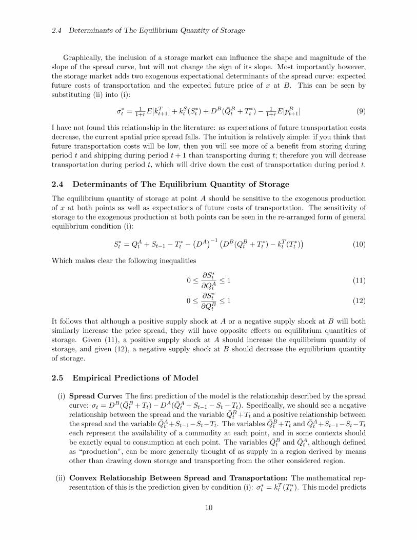
Graphically, the inclusion of a storage market can influence the shape and magnitude of theslope of the spread curve, but will not change the sign of its slope. Most importantly however,the storage market adds two exogenous expectational determinants of the spread curve: expectedfuture costs of transportation and the expected future price of x at B. This can be seen bysubstituting (ii) into (i):

σ∗t = 11+rE[kTt+1] + kSt (S∗

t ) +DB(Q̄Bt + T ∗

t )− 11+rE[pBt+1] (9)

I have not found this relationship in the literature: as expectations of future transportation costsdecrease, the current spatial price spread falls. The intuition is relatively simple: if you think thatfuture transportation costs will be low, then you will see more of a benefit from storing duringperiod t and shipping during period t+ 1 than transporting during t; therefore you will decreasetransportation during period t, which will drive down the cost of transportation during period t.

2.4 Determinants of The Equilibrium Quantity of Storage

The equilibrium quantity of storage at point A should be sensitive to the exogenous productionof x at both points as well as expectations of future costs of transportation. The sensitivity ofstorage to the exogenous production at both points can be seen in the re-arranged form of generalequilibrium condition (i):

S∗t = QA

t + St−1 − T ∗t −

(DA

)−1 (DB(QB

t + T ∗t )− kTt (T ∗

t ))

(10)

Which makes clear the following inequalities

0 ≤ ∂S∗t

∂QAt

≤ 1 (11)

0 ≤ ∂S∗t

∂QBt

≤ 1 (12)

It follows that although a positive supply shock at A or a negative supply shock at B will bothsimilarly increase the price spread, they will have opposite effects on equilibrium quantities ofstorage. Given (11), a positive supply shock at A should increase the equilibrium quantity ofstorage, and given (12), a negative supply shock at B should decrease the equilibrium quantityof storage.

2.5 Empirical Predictions of Model

(i) Spread Curve: The first prediction of the model is the relationship described by the spreadcurve: σt = DB(Q̄B

t + Tt)−DA(Q̄At +St−1−St− Tt). Specifically, we should see a negative

relationship between the spread and the variable Q̄Bt +Tt and a positive relationship between

the spread and the variable Q̄At +St−1−St−Tt. The variables Q̄B

t +Tt and Q̄At +St−1−St−Tt

each represent the availability of a commodity at each point, and in some contexts shouldbe exactly equal to consumption at each point. The variables Q̄B

t and Q̄At , although defined

as “production”, can be more generally thought of as supply in a region derived by meansother than drawing down storage and transporting from the other considered region.

(ii) Convex Relationship Between Spread and Transportation: The mathematical rep-resentation of this is the prediction given by condition (i): σ∗t = kTt (T ∗

t ). This model predicts

10

that, in the short-run, where transportation infrastructure is relatively unchanged and thusthe marginal cost schedule of transportation and storage are both not shifting, we should seea convex relationship between the spatial price spread and the quantity of transportation.

(iii) Delay Between Increases in Transportation and Widening of Spread: The con-vexity of the marginal cost schedule of transportation and storage can explain why storageand transportation spiked before the Brent-WTI spread widened, as seen in Figure 2. Givenprogressive changes in production differentials, the spread curve would, over time, shift alongthe flat region of the marginal cost schedule of transportation, increasing transportation sub-stantially but not the price spread. Eventually, the spread curve would reach the convexportion of the marginal cost schedule, and small increases in transportation would correlatewith very large increases in the spatial price spread.

(iv) Direct Relationship Between Current Spread and Expected Future Costs ofTransportation: Given equation (9), we should observe a positive relationship betweenexpected future costs of transportation between a region and the current spatial price spread.

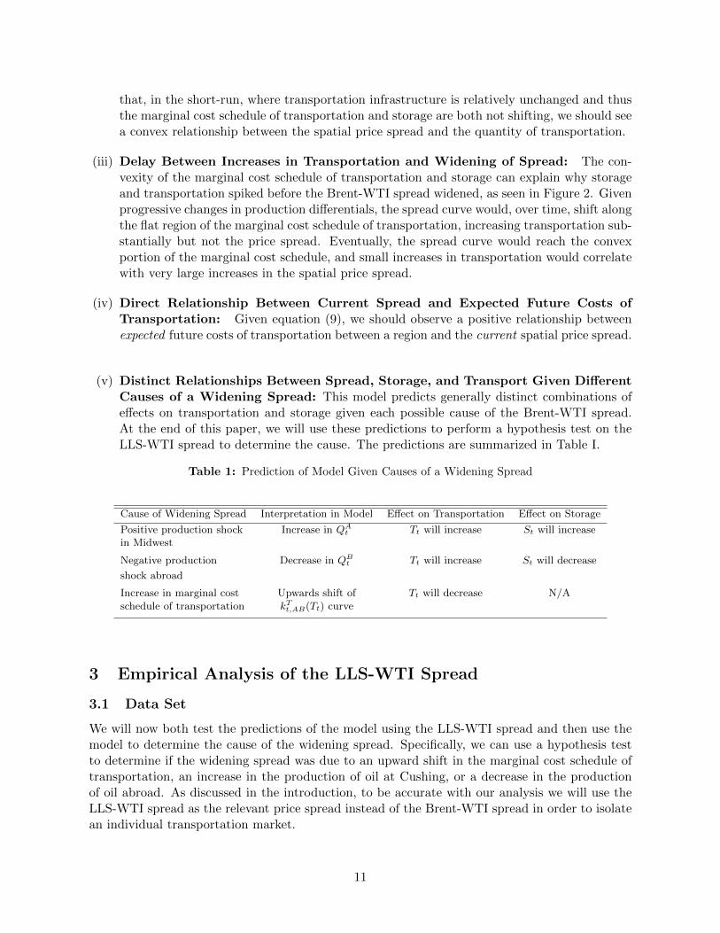
(v) Distinct Relationships Between Spread, Storage, and Transport Given DifferentCauses of a Widening Spread: This model predicts generally distinct combinations ofeffects on transportation and storage given each possible cause of the Brent-WTI spread.At the end of this paper, we will use these predictions to perform a hypothesis test on theLLS-WTI spread to determine the cause. The predictions are summarized in Table I.

Table 1: Prediction of Model Given Causes of a Widening Spread

Cause of Widening Spread Interpretation in Model Effect on Transportation Effect on Storage

Positive production shock Increase in QAt Tt will increase St will increasein Midwest

Negative production Decrease in QBt Tt will increase St will decrease

shock abroad

Increase in marginal cost Upwards shift of Tt will decrease N/Aschedule of transportation kTt,AB(Tt) curve

3 Empirical Analysis of the LLS-WTI Spread

3.1 Data Set

We will now both test the predictions of the model using the LLS-WTI spread and then use themodel to determine the cause of the widening spread. Specifically, we can use a hypothesis testto determine if the widening spread was due to an upward shift in the marginal cost schedule oftransportation, an increase in the production of oil at Cushing, or a decrease in the productionof oil abroad. As discussed in the introduction, to be accurate with our analysis we will use theLLS-WTI spread as the relevant price spread instead of the Brent-WTI spread in order to isolatean individual transportation market.

11

3.1 Data Set

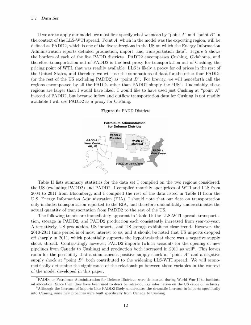
If we are to apply our model, we must first specify what we mean by “point A” and “point B” inthe context of the LLS-WTI spread. Point A, which in the model was the exporting region, will bedefined as PADD2, which is one of the five subregions in the US on which the Energy InformationAdministration reports detailed production, import, and transportation data7. Figure 5 showsthe borders of each of the five PADD districts. PADD2 encompasses Cushing, Oklahoma, andtherefore transportation out of PADD2 is the best proxy for transportation out of Cushing, thepricing point of WTI, that was readily available. LLS is likely a proxy for oil prices in the rest ofthe United States, and therefore we will use the summations of data for the other four PADDs(or the rest of the US excluding PADD2) as “point B”. For brevity, we will henceforth call theregions encompassed by all the PADDs other than PADD2 simply the “US”. Undeniably, theseregions are larger than I would have liked. I would like to have used just Cushing at “point A”instead of PADD2, but because inflow and outflow transportation data for Cushing is not readilyavailable I will use PADD2 as a proxy for Cushing.

Figure 6: PADD Districts

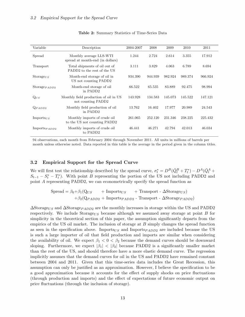
Table II lists summary statistics for the data set I compiled on the two regions considered:the US (excluding PADD2) and PADD2. I compiled monthly spot prices of WTI and LLS from2004 to 2011 from Bloomberg, and I compiled the rest of the data listed in Table II from theU.S. Energy Information Administration (EIA). I should note that our data on transportationonly includes transportation reported to the EIA, and therefore undoubtably underestimates theactual quantity of transportation from PADD2 to the rest of the US.

The following trends are immediately apparent in Table II: the LLS-WTI spread, transporta-tion, storage in PADD2, and PADD2 production each consistently increased from year-to-year.Alternatively, US production, US imports, and US storage exhibit no clear trend. However, the2010-2011 time period is of most interest to us, and it should be noted that US imports droppedoff sharply in 2011, which potentially supports the hypothesis that there was a negative supplyshock abroad. Contrastingly however, PADD2 imports (which accounts for the opening of newpipelines from Canada to Cushing) and production both increased in 2011 as well8. This leavesroom for the possibility that a simultaneous positive supply shock at ”point A” and a negativesupply shock at ”point B” both contributed to the widening LLS-WTI spread. We will econo-metrically determine the significance of the relationships between these variables in the contextof the model developed in this paper.

7PADDs or Petroleum Administration for Defense Districts, were delineated during World War II to facilitateoil allocation. Since then, they have been used to describe intra-country information on the US crude oil industry.

8Although the increase of imports into PADD2 likely understates the dramatic increase in imports specificallyinto Cushing, since new pipelines were built specifically from Canada to Cushing.

12

3.2 Empirical Support for the Spread Curve

Table 2: Summary Statistics of Time-Series Data

Variable Description 2004-2007 2008 2009 2010 2011

Spread Monthly average LLS-WTI 1.244 2.724 2.614 3.355 17.912spread at month-end (in dollars)

Transport Total shipments of oil out of 3.111 3.829 4.063 6.789 8.694PADD2 to the rest of the US

StorageUS Month-end storage of oil in 934.390 944.939 982.924 989.374 966.924US not counting PADD2

StoragePADD2 Month-end storage of oil 66.522 65.535 83.889 92.475 98.994in PADD2

QUS Monthly field production of oil in US 143.928 134.583 145.073 145.522 147.121not counting PADD2

QPADD2 Monthly field production of oil 13.762 16.402 17.977 20.989 24.543in PADD2

ImportsUS Monthly imports of crude oil 261.065 252.120 231.346 238.225 225.432to the US not counting PADD2

ImportsPADD2 Monthly imports of crude oil 46.441 46.271 42.794 42.013 46.034to PADD2

94 observations, each month from February 2004 through November 2011. All units in millions of barrels permonth unless otherwise noted. Data reported in this table is the average in the period given in the column titles.

3.2 Empirical Support for the Spread Curve

We will first test the relationship described by the spread curve, σ∗t = DB(Q̄Bt + T ∗

t )−DA(Q̄At +

St−1 − S∗t − T ∗

t ). With point B representing the portion of the US not including PADD2 andpoint A representing PADD2, we can econometrically specify the spread function as

Spread = β0+β1(QUS + ImportsUS + Transport - ∆StorageUS)

+β2(QPADD2 + ImportsPADD2 - Transport - ∆StoragePADD2)

∆StorageUS and ∆StoragePADD2 are the monthly increases in storage within the US and PADD2respectively. We include StorageUS because although we assumed away storage at point B forsimplicity in the theoretical section of this paper, the assumption significantly departs from theempirics of the US oil market. The inclusion of storage at B simply changes the spread functionas seen in the specification above. ImportsUS and ImportsPADD2 are included because the USis such a large importer of oil that field production and imports are similar when consideringthe availability of oil. We expect β1 < 0 < β2 because the demand curves should be downwardsloping. Furthermore, we expect |β1| < |β2| because PADD2 is a significantly smaller marketthan the rest of the US, and should therefore have a more elastic demand curve. The regressionimplicitly assumes that the demand curves for oil in the US and PADD2 have remained constantbetween 2004 and 2011. Given that this time-series data includes the Great Recession, thisassumption can only be justified as an approximation. However, I believe the specification to bea good approximation because it accounts for the effect of supply shocks on price fluctuations(through production and imports) and the effect of expectations of future economic output onprice fluctuations (through the inclusion of storage).

13

3.2 Empirical Support for the Spread Curve

Table 3: Regression Set 1Dependent variable = ”Spread,” as defined in Table II

Independent Variables Coefficients

(1) (2)

QUS+ImportsUS+Transport -0.082***(0.000)

QPADD2+ImportsPADD2-Transport 0.605***(0.000)

QUS+ImportsUS+Transport-∆StorageUS -0.097***(0.000)

QPADD2+ImportsPADD2-Transport-∆StoragePADD2 0.616***(0.000)

Constant 1.534 6.865(0.887) (0.425)

R2 0.260 0.311AdjR2 0.244 0.296SE Est. 4.965 4.791F-Stat 15.981 20.523

The symbols *, **, and *** mean statistical significance at the 10%, 5%, and1% level, respectively.

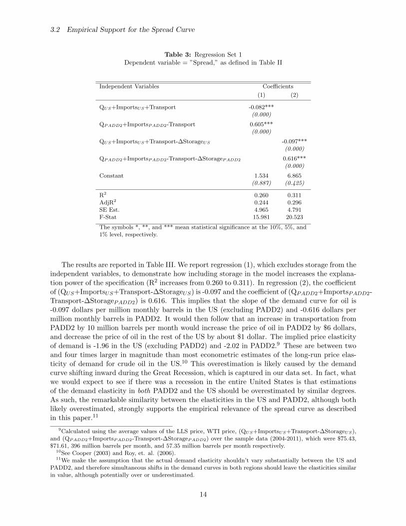
The results are reported in Table III. We report regression (1), which excludes storage from theindependent variables, to demonstrate how including storage in the model increases the explana-tion power of the specification (R2 increases from 0.260 to 0.311). In regression (2), the coefficientof (QUS+ImportsUS+Transport-∆StorageUS) is -0.097 and the coefficient of (QPADD2+ImportsPADD2-Transport-∆StoragePADD2) is 0.616. This implies that the slope of the demand curve for oil is-0.097 dollars per million monthly barrels in the US (excluding PADD2) and -0.616 dollars permillion monthly barrels in PADD2. It would then follow that an increase in transportation fromPADD2 by 10 million barrels per month would increase the price of oil in PADD2 by $6 dollars,and decrease the price of oil in the rest of the US by about $1 dollar. The implied price elasticityof demand is -1.96 in the US (excluding PADD2) and -2.02 in PADD2.9 These are between twoand four times larger in magnitude than most econometric estimates of the long-run price elas-ticity of demand for crude oil in the US.10 This overestimation is likely caused by the demandcurve shifting inward during the Great Recession, which is captured in our data set. In fact, whatwe would expect to see if there was a recession in the entire United States is that estimationsof the demand elasticity in both PADD2 and the US should be overestimated by similar degrees.As such, the remarkable similarity between the elasticities in the US and PADD2, although bothlikely overestimated, strongly supports the empirical relevance of the spread curve as describedin this paper.11

9Calculated using the average values of the LLS price, WTI price, (QUS+ImportsUS+Transport-∆StorageUS),and (QPADD2+ImportsPADD2-Transport-∆StoragePADD2) over the sample data (2004-2011), which were $75.43,$71.61, 396 million barrels per month, and 57.35 million barrels per month respectively.

10See Cooper (2003) and Roy, et. al. (2006).11We make the assumption that the actual demand elasticity shouldn’t vary substantially between the US and

PADD2, and therefore simultaneous shifts in the demand curves in both regions should leave the elasticities similarin value, although potentially over or underestimated.

14

3.3 Empirical Support for the Convex Relationship Between the Spread and Quantity ofTransportation

3.3 Empirical Support for the Convex Relationship Between the Spread andQuantity of Transportation

The most obvious econometric specification for equilibrium condition (i), given our assumptionthat the marginal cost schedule is convex, is

Spread = β0 + β1Transport + β2Transport2 + β3Transport3

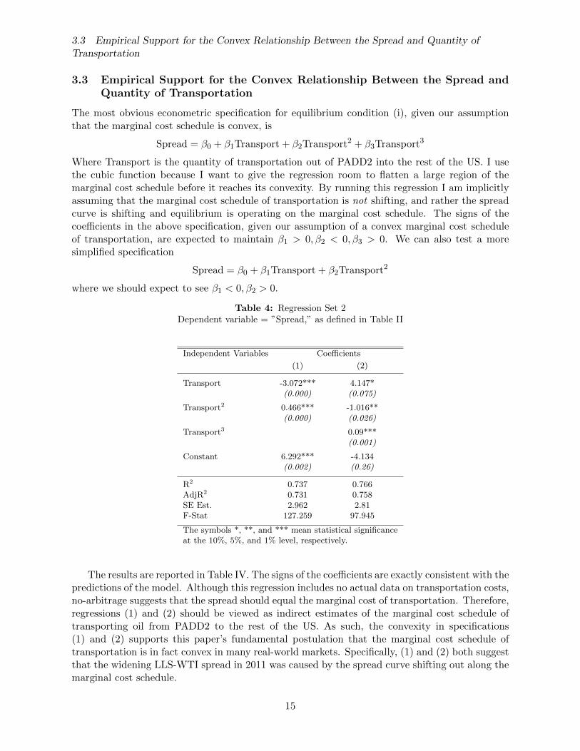
Where Transport is the quantity of transportation out of PADD2 into the rest of the US. I usethe cubic function because I want to give the regression room to flatten a large region of themarginal cost schedule before it reaches its convexity. By running this regression I am implicitlyassuming that the marginal cost schedule of transportation is not shifting, and rather the spreadcurve is shifting and equilibrium is operating on the marginal cost schedule. The signs of thecoefficients in the above specification, given our assumption of a convex marginal cost scheduleof transportation, are expected to maintain β1 > 0, β2 < 0, β3 > 0. We can also test a moresimplified specification

Spread = β0 + β1Transport + β2Transport2

where we should expect to see β1 < 0, β2 > 0.

Table 4: Regression Set 2Dependent variable = ”Spread,” as defined in Table II

Independent Variables Coefficients

(1) (2)

Transport -3.072*** 4.147*(0.000) (0.075)

Transport2 0.466*** -1.016**(0.000) (0.026)

Transport3 0.09***(0.001)

Constant 6.292*** -4.134(0.002) (0.26)

R2 0.737 0.766AdjR2 0.731 0.758SE Est. 2.962 2.81F-Stat 127.259 97.945

The symbols *, **, and *** mean statistical significanceat the 10%, 5%, and 1% level, respectively.

The results are reported in Table IV. The signs of the coefficients are exactly consistent with thepredictions of the model. Although this regression includes no actual data on transportation costs,no-arbitrage suggests that the spread should equal the marginal cost of transportation. Therefore,regressions (1) and (2) should be viewed as indirect estimates of the marginal cost schedule oftransporting oil from PADD2 to the rest of the US. As such, the convexity in specifications(1) and (2) supports this paper’s fundamental postulation that the marginal cost schedule oftransportation is in fact convex in many real-world markets. Specifically, (1) and (2) both suggestthat the widening LLS-WTI spread in 2011 was caused by the spread curve shifting out along themarginal cost schedule.

15

3.4 The Role of Expectations

3.4 The Role of Expectations

The model developed here predicts that a decrease in expected future costs of transportation willdecrease the current spatial price spread. But because I have been unable to find a good empiricalmetric for expected future costs of transportation from Cushing to St. James, I have been unableto develop a robust and direct way to test this prediction. However, the abrupt tightening ofthe spread on November 16th, 2011, following the announcement that pipeline capacity out ofCushing would be increased in 2012, is at least consistent with the predictions of the model.

Figure 7: Daily Percentage Change in LLS-WTI Spread

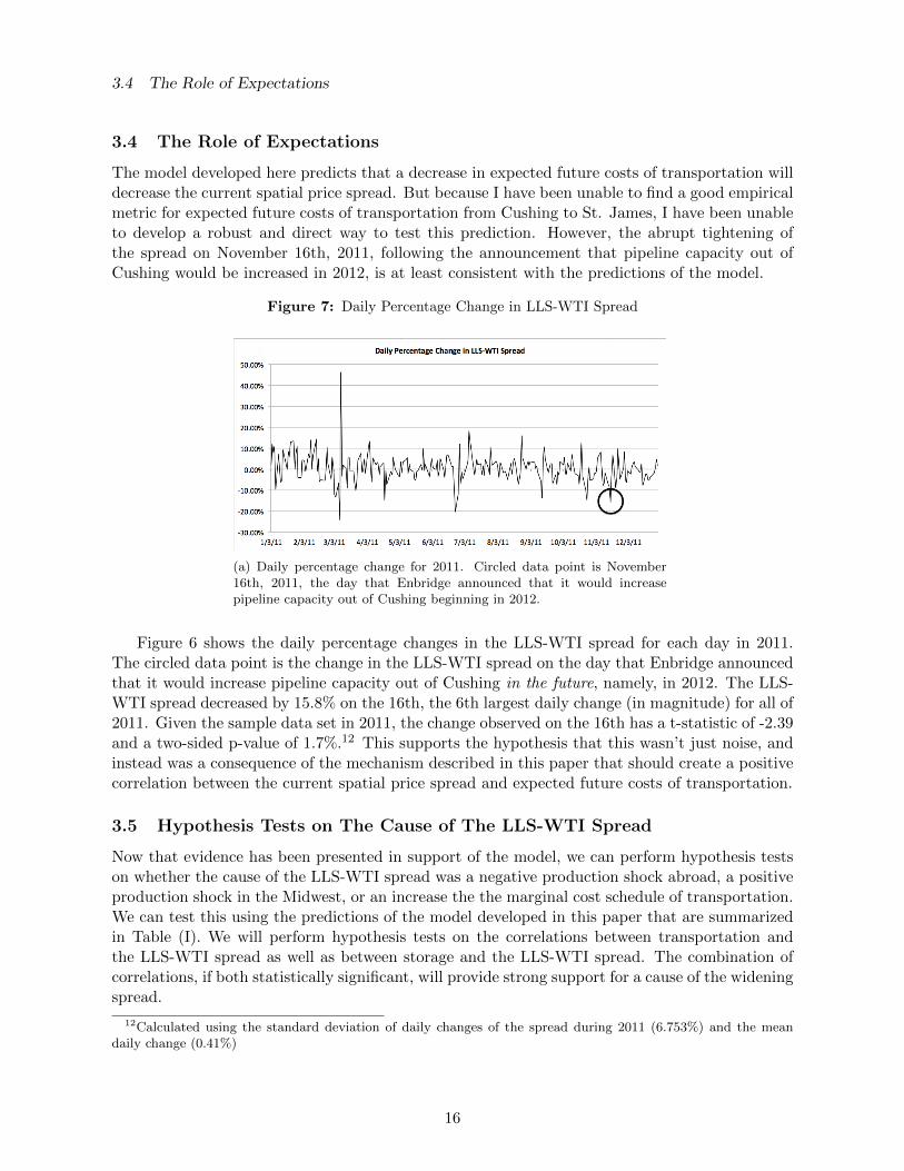
(a) Daily percentage change for 2011. Circled data point is November16th, 2011, the day that Enbridge announced that it would increasepipeline capacity out of Cushing beginning in 2012.

Figure 6 shows the daily percentage changes in the LLS-WTI spread for each day in 2011.The circled data point is the change in the LLS-WTI spread on the day that Enbridge announcedthat it would increase pipeline capacity out of Cushing in the future, namely, in 2012. The LLS-WTI spread decreased by 15.8% on the 16th, the 6th largest daily change (in magnitude) for all of2011. Given the sample data set in 2011, the change observed on the 16th has a t-statistic of -2.39and a two-sided p-value of 1.7%.12 This supports the hypothesis that this wasn’t just noise, andinstead was a consequence of the mechanism described in this paper that should create a positivecorrelation between the current spatial price spread and expected future costs of transportation.

3.5 Hypothesis Tests on The Cause of The LLS-WTI Spread

Now that evidence has been presented in support of the model, we can perform hypothesis testson whether the cause of the LLS-WTI spread was a negative production shock abroad, a positiveproduction shock in the Midwest, or an increase the the marginal cost schedule of transportation.We can test this using the predictions of the model developed in this paper that are summarizedin Table (I). We will perform hypothesis tests on the correlations between transportation andthe LLS-WTI spread as well as between storage and the LLS-WTI spread. The combination ofcorrelations, if both statistically significant, will provide strong support for a cause of the wideningspread.

12Calculated using the standard deviation of daily changes of the spread during 2011 (6.753%) and the meandaily change (0.41%)

16

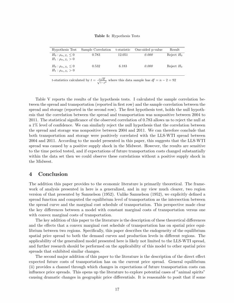
Table 5: Hypothesis Tests

Hypothesis Test Sample Correlation t-statistic One-sided p-value Result

H0 : ρσt,Tt ≤ 0 0.783 12.051 0.000 Reject H0

H1 : ρσt,Tt > 0

H0 : ρσt,St ≤ 0 0.532 6.183 0.000 Reject H0

H1 : ρσt,St > 0

t-statistics calculated by t = ρ√df√

1−ρ2where this data sample has df = n− 2 = 92

Table V reports the results of the hypothesis tests. I calculated the sample correlation be-tween the spread and transportation (reported in first row) and the sample correlation between thespread and storage (reported in the second row). The first hypothesis test, holds the null hypoth-esis that the correlation between the spread and transportation was nonpositive between 2004 to2011. The statistical significance of the observed correlation of 0.783 allows us to reject the null ata 1% level of confidence. We can similarly reject the null hypothesis that the correlation betweenthe spread and storage was nonpositive between 2004 and 2011. We can therefore conclude thatboth transportation and storage were positively correlated with the LLS-WTI spread between2004 and 2011. According to the model presented in this paper, this suggests that the LLS-WTIspread was caused by a positive supply shock in the Midwest. However, the results are sensitiveto the time period tested, and if expectations of future transportation costs changed substantiallywithin the data set then we could observe these correlations without a positive supply shock inthe Midwest.

4 Conclusion

The addition this paper provides to the economic literature is primarily theoretical. The frame-work of analysis presented in here is a generalized, and in my view much clearer, two regionversion of that presented by Samuelson (1952). Unlike Samuelson (1952), we explicitly defined aspread function and computed the equilibrium level of transportation as the intersection betweenthe spread curve and the marginal cost schedule of transportation. This perspective made clearthe key differences between a model with constant marginal costs of transportation versus onewith convex marginal costs of transportation.

The key addition of this paper to the literature is the description of these theoretical differencesand the effects that a convex marginal cost schedule of transportation has on spatial price equi-librium between two regions. Specifically, this paper describes the endogeneity of the equilibriumspatial price spread to both the demand curves and production levels in different regions. Theapplicability of the generalized model presented here is likely not limited to the LLS-WTI spread,and further research should be performed on the applicability of this model to other spatial pricespreads that exhibited similar changes.

The second major addition of this paper to the literature is the description of the direct effectexpected future costs of transportation has on the current price spread. General equilibrium(ii) provides a channel through which changes in expectations of future transportation costs caninfluence price spreads. This opens up the literature to explore potential cases of ”animal spirits”causing dramatic changes in geographic price differentials. It is reasonable to posit that if some

17

REFERENCES

market participants’ expectations of future costs of transportation were to increase, the subsequentwidening of the spread and increase in the cost of transportation today would cause expectationsof future costs of transportation to rise even further. This spiraling effect could lead the pricespread to increase without bound.

Further theoretical work should be performed to generalize this model to multiple regions tomore directly contrast it with the multiple-region models developed by Samuelson (1952) andTakayama and Judge (1964).

My econometric analysis of the LLS-WTI spread could be improved and expanded uponsubstantially. First, a sufficient metric for expected future costs of transportation should be used totest equilibrium condition (ii) directly. Second, regression set 2 should be more rigorously specifiedto isolate two distinct locations instead of the massive regions encompassed by PADD2 and therest of the US. Third, and most important, econometric analysis should be performed on a spatialprice spread with data on the marginal cost of transportation. The most convincing empiricalsupport for the model presented in this paper would be through direct data on transportationcosts. I was unable to find transportation cost data on the LLS-WTI spread, but if such datawere found it would be a powerful test of this model’s empirical legitimacy.

In sum, this paper provides a necessary generalization of the literature that addresses the inter-connectedness of spatially separated commodity markets. In doing so this paper has rationalizedthe empirical phenomena of abruptly widening spatial price spreads, opened the door for furthereconometric analysis on the effect of expected future costs of transportation on current spatialprice spreads, and developed the foundation for developing a model of spatial price equilibriumwith multiple regions in the presence of a convex marginal cost schedule of transportation.

References

[1] Merle D. Faminow and Bruce L. Benson, Integration of Spatial Markets. American Journal ofAgricultural Economics, February 1990, 72(1): 49-62

[2] Michael J. Brennan, The Supply of Storage. The American Economic Review, March 1958,48(1): 50-72

[3] Andrew Coleman, Storage, Slow Transport, and The Law of One Price: Theory With EvidenceFrom Nineteenth-Century U.S. Corn Markets. The Review of Economics and Statistics, May2009, 91(2): 332-350

[4] John C.B. Cooper, Price elasticity of demand for crude oil: estimates for 23 countries. OPECReview, March 2003, 27(1): 1-8

[5] A. A. Cournot, Mathematical Principles of the Theory of Wealth. 1838, Chapter 10

[6] Nikolas T. Milonas and Thomas Henker, Price spread and convenience yield behavior in theinternational oil market. Applied Financial Economics, 2001, 11: 23-26

[7] T. Takayama and G. G. Judge, An Intertemporal Price Equilibrium Model. Journal of FarmEconomics, May 1964, 46(2): 477-484

[8] T. Takayama and G. G. Judge, Equilibrium among Spatially Separated Markets: A Reformu-lation. Econometrica, October 1964, 32(4): 510-524

18

REFERENCES

[9] Michael Florian and Marc Los, A New Look at Static Spatial Price Equilibrium Models. Re-gional Science and Urban Economics, 1982, 12: 579-597

[10] Joyashree Roy, Alan H. Sanstad, Jayant A. Sathate, Raman Khaddaria, Substitution andprice elasticity estimates using inter-country pooled data in a translog cost model. LawrenceBerkeley National Laboratory, June 2006

[11] Paul A. Samuelson, Spatial Price Equilibrium and Linear Programming. The American Eco-nomic Review, June 1952, 42(3): 283-303

[12] Carol H. Shiue, Transport Costs and the Geography of Arbitrage in Eighteenth-Century China.The American Economic Review, December 2002, 92(5): 1406-1419

[13] Holbrook Working, Theory of the Inverse Carrying Charge in Futures Markets. Journal ofFarm Economics, February 1948, 30(1): 1-28

[14] Jeffrey C. Williams and Brian Wright, Storage and commodity markets. Cambridge UniversityPress, 1991

19