Spatial Econometrics Modeling of Poverty - · PDF fileKey-Words: - Spatial econometrics, spatial effects, spatial poverty traps 1 Introduction ... series analysis where the errors

Spatial Econometrics Modeling of Poverty

FERDINAND J. PARAGUAS1 AND ANTON ABDULBASAH KAMIL2

School of Mathematical Sciences Universiti Sains Malaysia

11800, USM Pulau Pinang MALAYSIA

http://www.mat.usm.my/math/

Abstract: - The analysis of spatial dependence and spatial heterogeneity as well as issues on model choice and model selection- how to decide between specification, both nested and non-nested have been predominant in spatial econometric modeling. This paper highlights the concept of spatial econometrics, and applies it to analyze the spatial dimensions of poverty and its determinants using data from Bangladesh. It is shown both theoretically and empirically that the OLS estimates of the poverty function suffer from upward bias. Alternative spatial econometric models showed that both spatial lag and spatial error are statistically significant, indicating that the OLS model is misspecified. The significance of the spatial effects parameters also suggest that spatial poverty trap exist in the country suggesting a more targeted-anti poverty intervention. Key-Words: - Spatial econometrics, spatial effects, spatial poverty traps 1 Introduction Spatial econometric has rapidly matured over the last decade, with many developments in model specification, estimation and testing (see for example [1]). The analysis of spatial dependence and spatial heterogeneity as well as issues on model choice and model selection- how to decide between specification, both nested and non-nested have been predominant in spatial econometric modeling.

The purpose of this paper is twofold. In the first part on a theoretical level, we look at the concept of spatial econometrics. We also look at the existing literature of econometrics about spatial autoregressive models and relate them with their counter part in time series analysis. The second part of the paper is an empirical application were the autoregressive models are applied to analyse the spatial dimensions of poverty and its determinants using data from Bangladesh. 2 Problem Formulation Consider the problem of fitting a regression model to a spatial data (e.g., poverty incidence) using the ordinary least squares (OLS) procedure:

y xα β ε= + + ; (1) where y is the latent variable, x a n x 1 vector of k independent variables, α and β are parameters to be

estimated and ε is the error term with mean zero and constant variance (σ2).

Due to spatial and aggregate nature of the data, a violated assumption is that of spherical disturbances and the presence of spatial patterns in general. Spatial patterns cause a number of measurement problems, referred to as spatial effects, such as the spatial dependence or spatial autocorrelation.

In particular, there are two forms of spatial dependence [2]. The first is the spatial lag, which pertains to the spatial autocorrelation of the dependent variable.

( ) , 1,...,i jy f y i n j i= = ≠ . (2)

If this form of spatial autocorrelation is ignored, the OLS estimates will be biased and all inferences based on the regression model will be incorrect ([3] and [4]. The problem can be best described as an omitted variable bias. To illustrate, let the true model of that includes the omitted variable z:

y x zα β δ ε= + + + . (3) The estimator b for the regression coefficient β in equation 1 is:

( )( ) ( )( ) ( ) ( )

1

1

1 1 1

' '

' ' (4)

' ' ' ' ' ' .

b x x x v

x x x x z

x x x x x x x z x x x

β δ ε

β δ ε

−

−

− − −

=

= + +

⎡ ⎤ ⎡ ⎤= + +⎣ ⎦ ⎣ ⎦

Proceedings of the 8th WSEAS International Conference on APPLIED MATHEMATICS, Tenerife, Spain, December 16-18, 2005 (pp159-164)

And the expected value for the estimator b is: ( ) ( ) ( ){ }

( ) ( ){ } ( )

( )

( ) ( )

1 1

1 1

1

' ' ' '

' ' ' '

' '

, . (5)

E b E x x x z x x x

E E x x x z E x x x

x x x z

Cov x z Var x

β δ ε

β δ ε

β δ

β δ

− −

− −

−

⎡ ⎤= + +⎣ ⎦

⎡ ⎤ ⎡ ⎤= + +⎣ ⎦ ⎣ ⎦

⎡ ⎤= + ⎣ ⎦= + ⎡ ⎤⎣ ⎦

Thus, the estimator b is (upwardly) bias by the term ( ) ( ),Cov x z Var x δ⎡ ⎤⎣ ⎦ .

The second form of spatial dependence is referred to as spatial error, which pertains to spatial autocorrelation of the error term. Recall in the traditional regression model defined in (1). The Gauss-Markov assumptions are that: ( ), 0i jE ε ε = ,

which translate through the fixed X’s assumption to

( ), 0i jE y y = . This form of spatial dependence is

referred to as a nuisance but may help us to capture important facets of the realities of economic processes. If this type of spatial error is ignored, the OLS estimator remains unbiased, but is no longer efficient, since it ignores the correlation between error terms. As a result, inference based on t- and F- statistics will be misleading and indications of fit based on R2 will be incorrect [3].

3 Problem Solution 3.1 Spatial Autoregressive Models 3.1.1 General spatial process model To account for spatial effect, a group of spatial autoregressive models, which follow from parameter restrictions of the “general spatial process model” [3] also known as “spatial autoregressive model” (SAC model) [4] was formulated. The general specification of the SAC model combines a spatially autoregressive dependent variable (spatial lag) among the set of explanatory variables and spatially autoregressive lagged disturbances (spatial error). For the first order process, the SAC model is given:

);,0(~ 22

1

nIN

uWuuXyWy

σε

ελβρ

+=++=

(6)

where y, x, and β are as defined in (1), W is a spatial weight matrix with (n x n) elements ijw that contains the neighborhood structure of the locations

(observations), ρ and λ are parameters to be estimated. In particular, ρ is a scalar spatially autoregressive parameter which determines the importance of spatial lag; λ the scalar spatial autoregressive disturbance parameter which determines the importance of spatial error, and µ is an (n × 1) independently and identically distributed vector of error terms.

These formulations correspond directly to the time series specifications of moving average or MA (correlation across time captured in the residual) and autoregressive or AR (correlation captured through lagged dependent variables). 3.1.2 Spatial Lag Model (SAR) From the SAC model restricting the spatial effects parameters equal to 0 can derive other models. When λ = 0, a “spatial lag” model or following [4], a mixed regressive-spatial autoregressive model (SAR) can be derived which is analogous to the time-series lagged dependent variable model. The SAR model then reads as:

).,0(~ 2nINe

XWyyσ

εβρ ++= (7)

3.1.3 Spatial Error Model (SEM) When the ρ in the SAC model (6) is set to 0, a spatial error model (SEM) with spatial autocorrelation in the disturbances can be derived of the form:

);,0(~ 2nIN

WuuXy

σε

ελβ

+=+=

(8)

This model corresponds to the model in time series analysis where the errors show some temporal correlation process. 3.14 First Order Autoregressive Model (FAR) The simplest among these models is the first order (FAR) model, which takes the form:

);,0(~ 2nIN

Wyyσε

ερ += (9)

As it does not involve any covariate (independent variables), the coefficient ρ can be considered as pure measure of spatial autocorrelation [4].


3.2 Spatial Weight Matrix (W) The W merits more discussion. It is the building block of spatial econometric models and a fundamental characteristic that distinguishes spatial econometrics from time series counterparts. Formally, given spatial framework of n locations,

{ } 1

ni i

S s=

= , and a neighbor relation N S X S⊂ ,

sites si and sj are neighbors iff ( ), ,i js s N i j∈ ≠ .

Let ( ) ( ){ }: ,i j i jN s s s s N= ∈ denotes si ‘s

neighborhood. The elements of normalized W are ( ) ( ), 1 iw i j N s= iff ( ),i js s N∈ and

( ), 0w i j = otherwise. The form of the spatial weight matrix can vary from a contiguity/adjacency relation to distance functions and eventually with a cut-off point (k) or k-nearest neighbor [5]. The k-nearest neighbors weight matrix W(k) is of the form:

⎪⎪⎪

⎩

⎪⎪⎪

⎨

⎧

>=

=≤=

∀==

∑;)(0)(

)(/)()()(1)(

,0)(

*

**

*

kddifkw

kwkwkwandkddifkw

kjiifkw

iijij

jijijijiijij

ij

(10) where ( )ijw k is an element of the standardized

weight matrix and ( )jd k is a critical cut-off distance defined for each location. More precisely,

( )jd k is the kth order shortest distance between location i and all other units such that each unit i has exactly k neighbors. 3.3 Estimation Procedure When there is spatial dependence in the spatial models, the OLS estimators will be biased as well as inconsistent (see [3] and [4]). Two alternative approaches are the instrumental variable (IV) estimation [6] and Maximum Likelihood (ML) approach [3]. For the ML approach of the FAR model, the log-likelihood to be maximized is given by:

( ) ( )

( ) ( )

22 2

2

1,2

1exp2

n

n

L y

I W

y Wy y Wy

ρ σπσ

ρ

ρ ρσ

=

−

⎧ ⎫′− − −⎨ ⎬⎩ ⎭

(11)

In order to simplify the maximization problem, a

concentrated log-likelihood function based on

eliminating the parameter 2σ for the variance of the disturbances is obtained [4]. This is accomplished

by substituting ( ) ( ) ( )2ˆ 1 n y Wy y Wyσ ρ ρ′= − − in the likelihood function define above and taking logs which yields:

( ) ( ) ( )ln ln2 nnLn L y Wy y Wy I Wρ ρ ρ′∝ − − − + − . (12)

This expression can be maximized with respect to ρ using a simplex univariate optimization routine [4]. Using the value of ρ that maximizes the log-likelihood function (say, ρ% ) in

( ) ( ) ( )2ˆ 1 n y Wy y Wyσ ρ ρ′= − − , the estimate

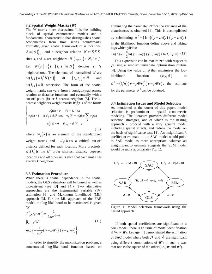
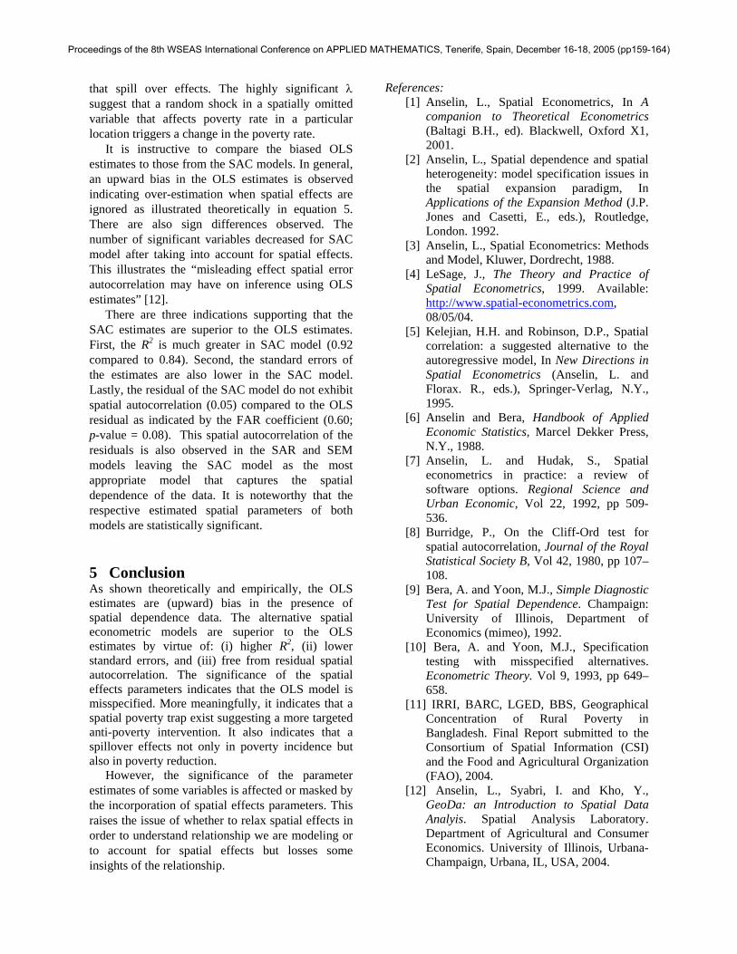
for the parameter 2σ can be obtained. 3.4 Estimation Issues and Model Selection As mentioned at the outset of this paper, model selection is predominant in spatial econometric modeling. The literature provides different model selection strategies, one of which is the nesting approach - proceed with a very general model including spatial effects, and reduce the model on the basis of significance tests [4]. An insignificant λ coefficient estimate in the SAC model would point to SAR model as more appropriate, whereas an insignificant ρ estimate suggests the SEM model would be more appropriate (Fig. 1).

Figure 1. Model selection framework using the nested approach.

If both spatial coefficients are significant in a

SAC model, there is an issue of model identification if W1 = W2. LeSage [4] demonstrated the estimation of SAC model where both ρ and λ are significant using different combinations of W’s in such a way that one is the square of the other (i.e., W and W2).

SAC

SAR

OLS

SEM

0( : 0 | 0)H λ ρ= ≠ 0( : 0 | 0)H ρ λ= ≠

0( : 0 0)H andλ ρ= =

0ρ = 0λ =


3.5 Test for Spatial Dependence As model specification issues have become an integral part of spatial econometrics, an extensive toolbox of diagnostic tests–comprising unidirectional, multidirectional and robust tests for OLS residuals had been developed (see [3] and [7] for a comprehensive review). In general, all these tests are based on the null hypothesis of no spatial dependence against the alternative of spatial dependence. 3.5.1 Lagrange Multiplier Test for Spatial Error (LM-ERR) A test on spatial dependence of the residual is the LM-ERR denoted by [8]:

)1(~]/)')[(/1( 222 χsWeeTERRLM =− (13)

where 2 's e e R= and ( )2T tr W W W′= + , with

tr as the matrix trace operator. The LM-ERR test is a test that is conditional to

no spatial lag dependence, i.e., 0 : 0H λ = , conditional upon 0ρ = . 3.5.2 Robust Lagrange Multiplier Test for Spatial Error (LM-EL) A test that is robust to local misspecification in the form of spatial lag error (LM-EL) is computed as [8]:

)1(~])~([

)]/'()~(/'[ 212

2212

χβρ

βρ−

−

−−

−

−=−

JRTT

sWyeJRTsWeeELLM

(14) where ( ) ( ) ( )

11 ' 2RJ T WX M WX sρ β β β−−

−⎡ ⎤= +⎣ ⎦

% and where

WX β is a spatial lag of the predicted values from

an OLS regression, ( ) 1' 'M I X X X X−= − is a projection matrix. 3.5.3 Lagrange Multiplier Test for Spatial Lag (LM-Lag) A counterpart of LM-ERR is the conditional test on spatial lag dependence of the dependent variable (LM-Lag), i.e. 0 : 0H ρ = , conditional upon 0λ = . The LM-Lag can be computed by:

( )( )

22'e Wy sLM Lag

RJ ρ β−

− =%

(15)

where .* is as defined earlier.

3.5.4 Robust Lagrange Multiplier Test for Spatial Lag (LM-LE) The corresponding robust to local misspecification in the form of spatial lag term (LM-LE) is computed as [9;10]:

)1(~)~(

)]/'()/'[( 2222

χβρ TJR

sWeesWyeELLM

−

−=−

−

(16)

3.5.5 Joint test on Residual Spatial Autocorrelation and Spatially Lagged Endogenous Variable A Lagrange multiplier test for a joint test on spatial lag (Autoregressive) and spatial (moving average) error ( 0 : 0H λ = and 0ρ = ) by combining LM-ERR and LM-LE, denoted by LM-SARMA, is given by [7]:

)2(~)/'()

~(

)]/'()/'[( 222222

χβρ T

sWeeTJR

sWeesWyeSARMALM +−

−=−

−

(17) 4 Empirical Application In what follows is an application to the analysis of poverty using Data from Bangladesh. An Upazillaa level of rural poverty rates measured by headcount index (HCI)b is used. All the data were taken from the Bangladesh Country Almanac (BCA)c.

To start with, we specify a poverty function of the form:

15

1i j ij i

j

Y a b X e=

= + +∑ (18)

where subscripts i and j refer to the ith Upazilla and jth explanatory variable (x), respectively; Y refers to rural HCPI; X1 represents % highland area of the ith Upazilla, X2 is % medium highland 1, X3 is % medium highland 2, X4 is % lowland, X5 is % very lowland, X6 is % area affected by severe drought, X7 % is area affected by moderate drought, X8 is % area with clay or loamy clay soil, X9 is % net crop area served by modern irrigation, X10 is of household with electricity supply, X11 is % average travel time by road to main service facilities, X12 is percent of landless households, X13 is % agricultural area under

a A rural sub-district of Bangladesh. b HCI is the proportion of households with cost of basic needs below the poverty line. c The BCA is a compilation of digital data sets, both spatial and non-spatial attributes in a CD-ROM with Mud Springs Awhere-ACT Spatial Information System tools developed using MapObjects programming. In particular, the HCI was estimated and mapped by the International Rice Research Institute (IRRI) and partner Institute [11].


tenancy, X14 is % average number of livestock per household (HH), X15 is % average years of schooling of adult HH members.

All tests and estimation concerning spatial dependence are done in GeoDaT [12], Spatial Econometrics Toolbox of Matlab developed by LeSage[4], and the Statistical Analysis System (SAS). In addition, it is hypothesized that an interaction between irrigation (X9) and drought (X6 and X7) exists. So, another model is estimated (Model 2) which include these interactions defined by X16 = X6 x X9 and X17 = X7 x X9. Results of Model 2 (not shown) however showed that both the coefficients of X16 and X17, as well as the joint test are not statistically significant.

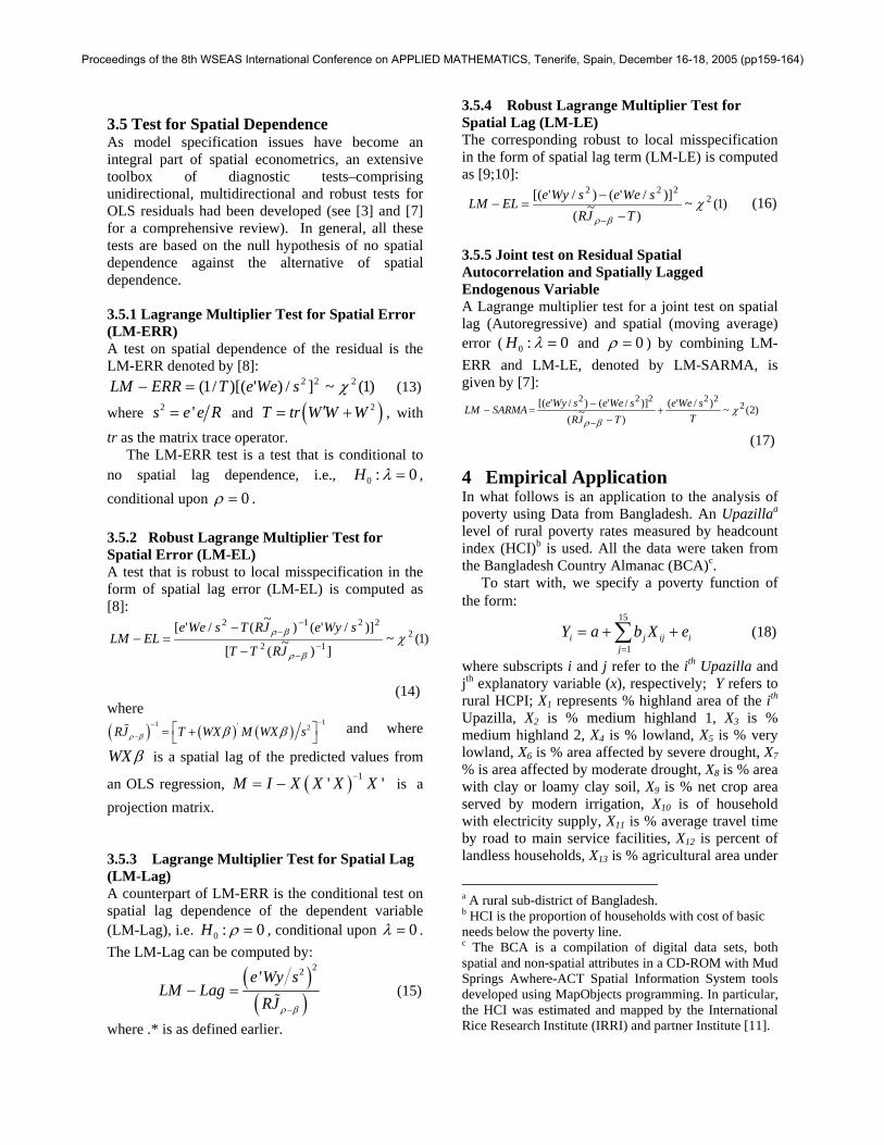
The next step was to establish that Model 1 suffer from spatial effects, either spatial lag dependence or residual spatial dependence, or both. For this purpose, the test defined in equations 14- 18 are conducted on Model 1d. Results showed that all the tests are statistically significant (Table 1). This indicates that the OLS model is misspecified and that spatial effects should be included in the model.

In what follows is the estimation of econometric

models defined in equations 7-10 that accounts or spatial effects. To select the most appropriate model, a model selection is employed using the nested approach [4] as illustrated in Fig 1. A SAC

d Model 1 was also subjected to diagnostic for normality, tests on the presence of heteroskedasticity of the errors and multicolliniarity among independent variables. All these tests resulted to the acceptance of the respective alternative hypothesis.

model was first estimated using different combinations of W1 and W2 where 2

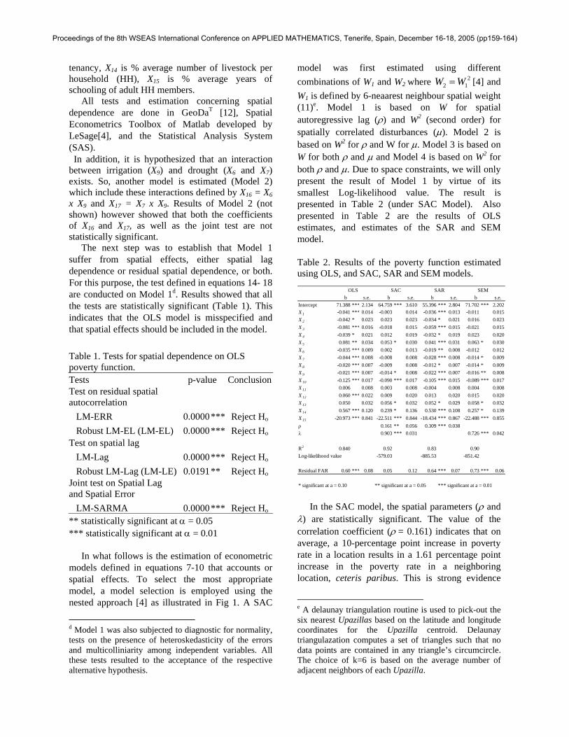
2 1W W= [4] and W1 is defined by 6-neaarest neighbour spatial weight (11)e. Model 1 is based on W for spatial autoregressive lag (ρ) and W2 (second order) for spatially correlated disturbances (µ). Model 2 is based on W2 for ρ and W for µ. Model 3 is based on W for both ρ and µ and Model 4 is based on W2 for both ρ and µ. Due to space constraints, we will only present the result of Model 1 by virtue of its smallest Log-likelihood value. The result is presented in Table 2 (under SAC Model). Also presented in Table 2 are the results of OLS estimates, and estimates of the SAR and SEM model. Table 2. Results of the poverty function estimated using OLS, and SAC, SAR and SEM models.

s.e. s.e. s.e. s.e.Intercept 71.388 *** 2.134 64.759 *** 3.610 55.396 *** 2.804 71.702 *** 2.202X 1 -0.041 *** 0.014 -0.003 0.014 -0.036 *** 0.013 -0.011 0.015X 2 -0.042 * 0.023 0.023 0.023 -0.034 * 0.021 0.016 0.023X 3 -0.081 *** 0.016 -0.018 0.015 -0.059 *** 0.015 -0.021 0.015X 4 -0.039 * 0.021 0.012 0.019 -0.032 * 0.019 0.023 0.020X 5 0.081 ** 0.034 0.053 * 0.030 0.041 *** 0.031 0.063 * 0.030X 6 -0.035 *** 0.009 0.002 0.013 -0.019 ** 0.008 -0.012 0.012X 7 -0.044 *** 0.008 -0.008 0.008 -0.028 *** 0.008 -0.014 * 0.009X 8 -0.020 *** 0.007 -0.009 0.008 -0.012 * 0.007 -0.014 * 0.009X 9 -0.021 *** 0.007 -0.014 * 0.008 -0.022 *** 0.007 -0.016 ** 0.008X 10 -0.125 *** 0.017 -0.090 *** 0.017 -0.105 *** 0.015 -0.089 *** 0.017X 11 0.006 0.008 0.003 0.008 -0.004 0.008 0.004 0.008X 12 0.060 *** 0.022 0.009 0.020 0.013 0.020 0.015 0.020X 13 0.050 0.032 0.056 * 0.032 0.052 * 0.029 0.058 * 0.032X 14 0.567 *** 0.120 0.239 * 0.136 0.530 *** 0.108 0.257 * 0.139X 15 -20.973 *** 0.841 -22.511 *** 0.844 -18.434 *** 0.867 -22.488 *** 0.855ρ 0.161 ** 0.056 0.309 *** 0.038λ 0.903 *** 0.031 0.726 *** 0.042

R2 0.840 0.92 0.83 0.90Log-likelihood value -579.03 -885.53 -851.42

Residual FAR 0.60 *** 0.08 0.05 0.12 0.64 *** 0.07 0.73 *** 0.06

* significant at a = 0.10 ** significant at a = 0.05 *** significant at a = 0.01

b b b bOLS SAC SAR SEM

In the SAC model, the spatial parameters (ρ and

λ) are statistically significant. The value of the correlation coefficient (ρ = 0.161) indicates that on average, a 10-percentage point increase in poverty rate in a location results in a 1.61 percentage point increase in the poverty rate in a neighboring location, ceteris paribus. This is strong evidence

e A delaunay triangulation routine is used to pick-out the six nearest Upazillas based on the latitude and longitude coordinates for the Upazilla centroid. Delaunay triangulazation computes a set of triangles such that no data points are contained in any triangle’s circumcircle. The choice of k=6 is based on the average number of adjacent neighbors of each Upazilla.

Table 1. Tests for spatial dependence on OLS poverty function. Tests p-value ConclusionTest on residual spatial autocorrelation LM-ERR 0.0000 *** Reject Ho Robust LM-EL (LM-EL) 0.0000 *** Reject Ho Test on spatial lag LM-Lag 0.0000 *** Reject Ho Robust LM-Lag (LM-LE) 0.0191 ** Reject Ho Joint test on Spatial Lag and Spatial Error LM-SARMA 0.0000 *** Reject Ho ** statistically significant at α = 0.05 *** statistically significant at α = 0.01


that spill over effects. The highly significant λ suggest that a random shock in a spatially omitted variable that affects poverty rate in a particular location triggers a change in the poverty rate.

It is instructive to compare the biased OLS estimates to those from the SAC models. In general, an upward bias in the OLS estimates is observed indicating over-estimation when spatial effects are ignored as illustrated theoretically in equation 5. There are also sign differences observed. The number of significant variables decreased for SAC model after taking into account for spatial effects. This illustrates the “misleading effect spatial error autocorrelation may have on inference using OLS estimates” [12].

There are three indications supporting that the SAC estimates are superior to the OLS estimates. First, the R2 is much greater in SAC model (0.92 compared to 0.84). Second, the standard errors of the estimates are also lower in the SAC model. Lastly, the residual of the SAC model do not exhibit spatial autocorrelation (0.05) compared to the OLS residual as indicated by the FAR coefficient (0.60; p-value = 0.08). This spatial autocorrelation of the residuals is also observed in the SAR and SEM models leaving the SAC model as the most appropriate model that captures the spatial dependence of the data. It is noteworthy that the respective estimated spatial parameters of both models are statistically significant.

5 Conclusion As shown theoretically and empirically, the OLS estimates are (upward) bias in the presence of spatial dependence data. The alternative spatial econometric models are superior to the OLS estimates by virtue of: (i) higher R2, (ii) lower standard errors, and (iii) free from residual spatial autocorrelation. The significance of the spatial effects parameters indicates that the OLS model is misspecified. More meaningfully, it indicates that a spatial poverty trap exist suggesting a more targeted anti-poverty intervention. It also indicates that a spillover effects not only in poverty incidence but also in poverty reduction.

However, the significance of the parameter estimates of some variables is affected or masked by the incorporation of spatial effects parameters. This raises the issue of whether to relax spatial effects in order to understand relationship we are modeling or to account for spatial effects but losses some insights of the relationship.

References: [1] Anselin, L., Spatial Econometrics, In A

companion to Theoretical Econometrics (Baltagi B.H., ed). Blackwell, Oxford X1, 2001.

[2] Anselin, L., Spatial dependence and spatial heterogeneity: model specification issues in the spatial expansion paradigm, In Applications of the Expansion Method (J.P. Jones and Casetti, E., eds.), Routledge, London. 1992.

[3] Anselin, L., Spatial Econometrics: Methods and Model, Kluwer, Dordrecht, 1988.

[4] LeSage, J., The Theory and Practice of Spatial Econometrics, 1999. Available: http://www.spatial-econometrics.com, 08/05/04.

[5] Kelejian, H.H. and Robinson, D.P., Spatial correlation: a suggested alternative to the autoregressive model, In New Directions in Spatial Econometrics (Anselin, L. and Florax. R., eds.), Springer-Verlag, N.Y., 1995.

[6] Anselin and Bera, Handbook of Applied Economic Statistics, Marcel Dekker Press, N.Y., 1988.

[7] Anselin, L. and Hudak, S., Spatial econometrics in practice: a review of software options. Regional Science and Urban Economic, Vol 22, 1992, pp 509-536.

[8] Burridge, P., On the Cliff-Ord test for spatial autocorrelation, Journal of the Royal Statistical Society B, Vol 42, 1980, pp 107–108.

[9] Bera, A. and Yoon, M.J., Simple Diagnostic Test for Spatial Dependence. Champaign: University of Illinois, Department of Economics (mimeo), 1992.

[10] Bera, A. and Yoon, M.J., Specification testing with misspecified alternatives. Econometric Theory. Vol 9, 1993, pp 649–658.

[11] IRRI, BARC, LGED, BBS, Geographical Concentration of Rural Poverty in Bangladesh. Final Report submitted to the Consortium of Spatial Information (CSI) and the Food and Agricultural Organization (FAO), 2004.

[12] Anselin, L., Syabri, I. and Kho, Y., GeoDa: an Introduction to Spatial Data Analyis. Spatial Analysis Laboratory. Department of Agricultural and Consumer Economics. University of Illinois, Urbana-Champaign, Urbana, IL, USA, 2004.


Spatial Econometrics Modeling of Poverty - · PDF fileKey-Words: - Spatial econometrics, spatial effects, spatial poverty traps 1 Introduction ... series analysis where the errors

Documents