AEROSPACE REPORT NO. ATR-74(7334)-1. VOL. IV PART 2 Space Shuttle/Payload Interface Analysis (Study 2.4) Final Report Volume IV Business Risk and Value of Operations in Space (BRAVO) Part 2 - User's Manual Prepared by ADVANCED VEHICLE SYSTEMS DIRECTORATE Systems Planning Division 15 February 1974 Prepared for OFFICE OF MANNED SPACE FLIGHT NATIONAL AERONAUTICS AND SPACE ADMINISTRATION Washington, D. C. Conrifct No. NASW,2472 Systems Engineering Operations THE AEROSPACE CORPORATION '(MASA-CR-139590) SPACE SHUTTLE/PAYLOAD N74-3228 7 INTERFACE ANALYSIS. (STUDY 2.4) VOLUME 4: BUSINESS RISK AND VALUL OF OPERATIONS (Aerospace Corp., El Segundo, Unclas Calif.) 263 p HC $16.25 CSCL 22B G3/31 17103 https://ntrs.nasa.gov/search.jsp?R=19740024174 2018-05-15T09:10:14+00:00Z

Welcome message from author
This document is posted to help you gain knowledge. Please leave a comment to let me know what you think about it! Share it to your friends and learn new things together.
Transcript
AEROSPACE REPORT NO.ATR-74(7334)-1. VOL. IVPART 2
Space Shuttle/Payload Interface Analysis
(Study 2.4) Final ReportVolume IV
Business Risk and Value of Operations in Space(BRAVO)
Part 2 - User's Manual
Prepared byADVANCED VEHICLE SYSTEMS DIRECTORATE
Systems Planning Division
15 February 1974
Prepared for OFFICE OF MANNED SPACE FLIGHTNATIONAL AERONAUTICS AND SPACE ADMINISTRATION
Washington, D. C.
Conrifct No. NASW,2472
Systems Engineering Operations
THE AEROSPACE CORPORATION
'(MASA-CR-139590) SPACE SHUTTLE/PAYLOAD N74-3228 7
INTERFACE ANALYSIS. (STUDY 2.4) VOLUME
4: BUSINESS RISK AND VALUL OFOPERATIONS (Aerospace Corp., El Segundo, UnclasCalif.) 263 p HC $16.25 CSCL 22B G3/31 17103
https://ntrs.nasa.gov/search.jsp?R=19740024174 2018-05-15T09:10:14+00:00Z
Aerospace Report No.ATR-74(7334)-I, Vol. IVPart 2
SPACE SHUTTLE/PAYLOAD INTERFACE ANALYSIS
(STUDY 2.4) FINAL REPORT
Volume IV: Business Risk and Value of Operations in Space
(BRAVO)
Part 2: User's Manual
Prepared by
Advanced Vehicle Systems DirectorateSystems Planning Division
15 February 1974
Systems Engineering OperationsTHE AEROSPACE CORPORATION
El Segundo, California
Prepared for
OFFICE OF MANNED SPACE FLIGHT
NATIONAL AERONAUTICS AND SPACE ADMINISTRATIONWashington, D. C.
Contract No. NASW-2472
Aerospace Report No.ATR-74(7334)-I, Vol. IVPart 2
.- DACE SHUTTLE/PAYLOAD INTERFACE ANALYSIS (Study 2.4)
NAL RE PORT
)lume IV: Business Risk and Value of Operations in Space (BRAVO)
Part 2: User's Manual
Approved by
nest . Pritchard L. R. Sitnev. Associate ,roup Directorrector, Study 2. 4 Office Advanced Vehicle Syste nFs Directoratevanced Vehicle Systems Systems Planning DivisionDirectorate
ii
FOREWORD
The Space Shuttle/Payload Interface Analysis (Study 2.4) Final
Report is comprised of five volumes, which are titled as follows:
/,, 7 , / Volume I - Executive Summary : 4/2', / 3'
/5 '7 7 . Volume II - Space Shuttle Traffic Analysis
'7 7 Y Volume III - New Expendable Vehicle with Reusable SolidRocket Motors
\' Volume IV - Business Risk and Value of Operations InSpace (BRAVO)
!',1 , Part 1 - Summary
- 1 b / Part 2 - User's Manual
Part 3 - Workbook
Si 3 0 Y Part 4, - Computer Programs and Data Look-up
-7 7 Volume V - Payload Community Analysis
iii
TABLE OF CONTENTS
1. INTRODUCTION ................................ 1-1
2. GENERAL PROCEDURE .......................... 2-1
A. Step 1 - Definition of the Problem (BRAVO Input) ...... 2-1
B. Step 2 - Space System Analysis .................. 2-3
1. Step 2(a) - Select System Approach(es) andGoals ............................... 2-3
2. Step 2(b) - Satellite Mission Equipment Selection . 2-3
3. Step 2(c) - Select Specific Satellite InterfaceConcepts ................... ....... . . 2-4
4. Step 2(d) - Spacecraft Synthesis . ............. 2-4
5. Step 2(e) - Space System Cost Estimating . ...... 2-6
6. Step 2(f) - Satellite System Optimization Analysis . 2-6
C. Step 3 - Terrestrial System Analysis . ............. 2-10
D. Step 4 - Cost-Effectiveness Analysis . ............. 2-10
3. DEFINITION OF THE PROBLEM .................... 3-1
4. SPACE SYSTEM ANALYSIS ........................ 4-1
A. System Approaches and Goals ................... 4-1
1. System Capacity Goal .................... 4-1
2. Location of Ground Link Stations and CoverageGoal .................... ............ 4-1
3. Cost Goals .................. .......... 4-1
4. System Availability Goal .................. 4-3
5. Checklist for System Goals . ............... 4-4
6. Launch Vehicle ......................... 4-4
7. Satellite Approaches ..................... 4-4
B. Satellite Mission Equipment .................... 4-9
1. Telecommunications Type . ................ 4-9
2. Earth Observation Type ................... 4-42
iv
TABLE OF CONTENTS (CONT'D)
C. Satellite Synthesis . ............... ...... 4-45
1. Introduction ........................... 4-45
2. Synthesis Program Operation ...... . . . . . . . . . 4-45
3. Program Operating Procedure ...... ...... * .o 4-46
4. Satellite Synthesis Computer Program ...... . ... 4-58
D. Satellite Interface Concepts ......... . . . . . .. . . . . 4-71
1. Satellite Transportation Accommodation . ....... 4-71
2. Satellite Ground Terminal Definition and Cost
Estimate .... . .... .. .. .. ...... . 4-83
3. References ...................... 4-100
E. Space System Cost Estimating ................... 4-101
1. Background ........ ... ***. o. .... . 4-101
2. Payload Program Cost Model ............... 4-101
3. Cost Model Inputs ....................... 4-102
4. Cost Model Output ...... . ................ 4- 1 1 1
5. Compatibility with Satellite Synthesis ProgramOutput ..................00. .0.0.. . 4-117
F. Space System Optimization, Risk, and Logistics
Analysis ................ o* . . . 0.00.0. . 4-118
1. Introduction .... ........... ..... o . .... 4-118
2. Procedures ............ ............... 4-119
5. TERRESTRIAL SYSTEMS ANALYSIS .................. 5-1
A. Telecommunication Systems .......... .... ...... 5-1
1. Alternate System Options .................. 5-1
2. System Selection . ......... * o ........ 5-1
3. Estimating Costs of Leasing from CommonCarriers . .... . ....................... 5-2
4. Dedicated Microwave Relay System ........... 5-12
5. Calculation of Submarine Telephone Cable
System Costs .......................... 5-14
v
TABLE OF CONTENTS (CONT'D)
B. U. S. Postal Service Costs .... ................. 5-24
1. Inputs Required ....... .................... 5-262. Selection of Mail Classification........ ..... . 5-273. Calculation of Mailing Costs............. .... 5-27
C. Aircraft Costs ................................... 5-271. Calculations ..... . . ........... ..... ... 5-37
COST EFFECTIVENESS ... .... .. .. ............. 6-1A. Introduction ............. *.................. 6-1B. Cost Effectiveness Analysis Procedure ............ 6-1
1. Space System Comparison and Selection .... ... 6-22. Cost Effectiveness of Space System(s) vs
Terrestrial System(s) .................. 6-5C. Background Information . ..... ...... . . . 6-7
1. Nomenclature ...................... ....... 6-72. Economic Relationships. .. ... . .................. 6-83. Cost/Revenue Analysis Worksheets .... . ...... 6-11
vi
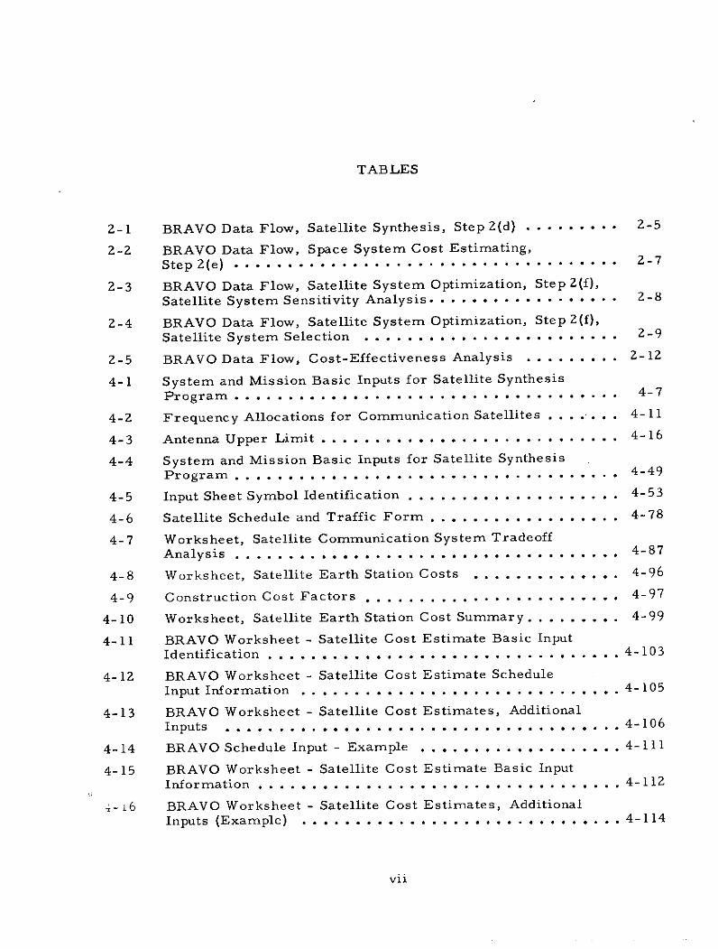
TABLES
2-1 BRAVO Data Flow, Satellite Synthesis, Step 2(d) ..... .... 2-5
2- BRAVO Data Flow, Space System Cost Estimating,Step 2(e) ...... ..................................... 2-7
2-3 BRAVO Data Flow, Satellite System Optimization, Step 2(f),Satellite System Sensitivity Analysis . . . . ................. 2-8
Z-4 BRAVO Data Flow, Satellite System Optimization, Step 2(f),Satellite System Selection .................... . 2-9
2-5 BRAVO Data Flow, Cost-Effectiveness Analysis . ........ 2-12
4-1 System and Mission Basic Inputs for Satellite Synthesis
Program ................ .......... ... *... 4-7
4-2 Frequency Allocations for Communication Satellites .... . . . 4-11
4-3 Antenna Upper Limit ............................ 4-16
4-4 System and Mission Basic Inputs for Satellite Synthesis
Program.... ...................... ..... 4-49
4-5 Input Sheet Symbol Identification .................... 4-53
4-6 Satellite Schedule and Traffic Form . ................. 4-78
4-7 Worksheet, Satellite Communication System Tradeoff
Analysis .................................... 4-87
4-8 Worksheet, Satellite Earth Station Costs . ............. 4-96
4-9 Construction Cost Factors ........................ 4-97
4-10 Worksheet, Satellite Earth Station Cost Summary ......... 4-99
4-11 BRAVO Worksheet - Satellite Cost Estimate Basic InputIdentification ..................... ............ 4-103
4-12 BRAVO Worksheet - Satellite Cost Estimate Schedule
Input Information .............................. 4-105
4-13 BRAVO Worksheet - Satellite Cost Estimates, Additional
Inputs ....................................... 4-106
4-14 BRAVO Schedule Input - Example ................... 4-111
4-15 BRAVO Worksheet - Satellite Cost Estimate Basic InputInformation . . . .. .. ..... . . . . . . . 4-112
-- 16 BRAVO Worksheet - Satellite Cost Estimates, AdditionalInputs (Example) .............................. 4-114
vii
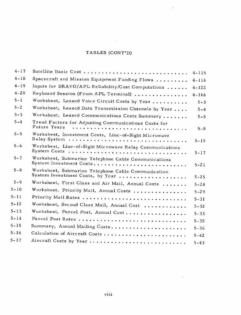
TABLES (CONT'D)
4-17 Satellite Basic Cost ......... ....... ............ 4-1154-18 Spacecraft and Mission Equipment Funding Flows ..... . . . . 4-1164-19 Inputs for BRAVO/APL Reliability/Cost Computations . ..... 4-1224-20 Keyboard Session (From APL Terminal) . ............. 4-1665-1 Worksheet, Leased Voice Circuit Costs by Year .. ....... . . 5-35-2 Worksheet, Leased Data Transmission Channels by Year .. . 5-45-3 Worksheet, Leased Communications Costs Summary . . .... . 5-55-4 Trend Factors for Adjusting Communications Costs for
Future Years ... ............... ...*.*.............. 5-85-5 Worksheet, Investment Costs, Line-of-Sight Microwave
Relay System ........ **..................... 5-155-6 Worksheet, Line-of-Sight Microwave Relay Communications
System Costs .................. ............. * 5-175-7 Worksheet, Submarine Telephone Cable Communications
System Investment Costs ..... ........ ... . . ........... 5-215-8 Worksheet, Submarine Telephone Cable Communication
System Investment Costs, by Year .. ........ . . . . . . 5-255-9 Worksheet, First Class and Air Mail, Annual Costs . ...... . . 5-28
5-10 Worksheet, Priority Mail, Annual Costs . ........ . . . . . . 5-295-11 Priority MailRates ....... ....... ..................... 5-315-12 Worksheet, Second Class Mail, Annual Cost ... ... .... . 5-325-13 Worksheet, Parcel Post, Annual Cost . .............. .. 5-335-14 Parcel Post Rates ................................... 5-355-15 Summary, Annual Mailing Costs . ................ . . . . 5-365-16 Calculation of Aircraft Costs . .................. . . . . 5-425-17 Aircraft Costs by Year ...................................... 5-43
viii
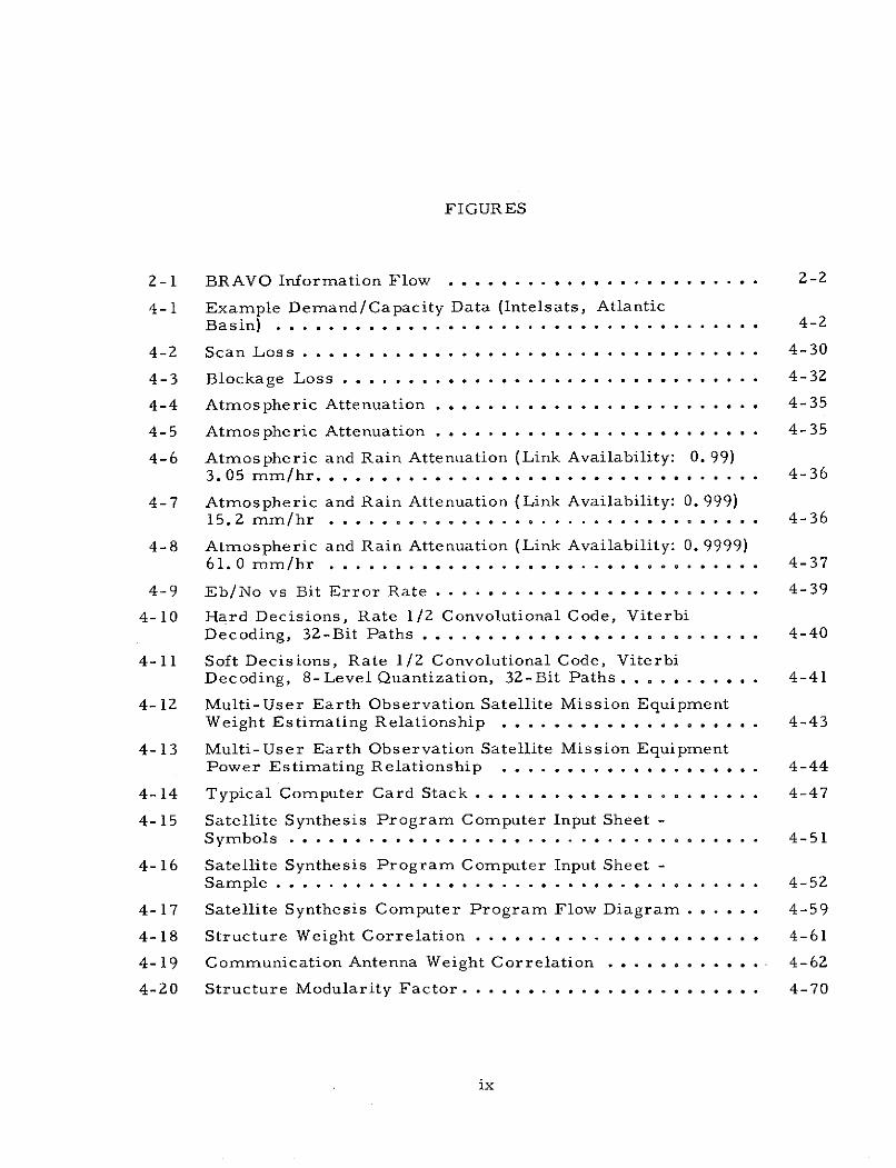
FIGURES
2-1 BRAVO Information Flow ........................ 2-2
4-1 Example Demand/Capacity Data (Intelsats, AtlanticBasin) ........................................ 4-2
4-2 Scan Loss ................................... 4-30
4-3 Blockage Loss .......................... .... .. 4-32
4-4 Atmospheric Attenuation ......................... 4-35
4-5 Atmospheric Attenuation ......................... 4-35
4-6 Atmospheric and Rain Attenuation (Link Availability: 0. 99)3.05 mm/hr .................................. 4-36
4-7 Atmospheric and Rain Attenuation (Link Availability: 0.999)15.2 mm/hr ................................. 4-36
4-8 Atmospheric and Rain Attenuation (Link Availability: 0. 9999)61.0 mm/hr ................................. 4-37
4-9 Eb/No vs Bit Error Rate ......................... 4-39
4-10 Hard Decisions, Rate 1/2 Convolutional Code, ViterbiDecoding, 32-Bit Paths .......................... 4-40
4-11 Soft Decisions, Rate 1/2 Convolutional Code, ViterbiDecoding, 8-Level Quantization, 32-Bit Paths. ...... ..... 4-41
4-12 Multi-User Earth Observation Satellite Mission EquipmentWeight Estimating Relationship . .................. . 4-43
4-13 Multi-User Earth Observation Satellite Mission EquipmentPower Estimating Relationship .................... 4-44
4-14 Typical Computer Card Stack ...................... 4-47
4-15 Satellite Synthesis Program Computer Input Sheet -Symbols .................................... 4-51
4-16 Satellite Synthesis Program Computer Input Sheet -Sample ................................... .. 4-52
4-17 Satellite Synthesis Computer Program Flow Diagram . . . . .. 4-59
4-18 Structure Weight Correlation ...................... 4-61
4-19 Communication Antenna Weight Correlation . . . ........ 4-62
4-20 Structure Modularity Factor . .................. .... 4-70
ix
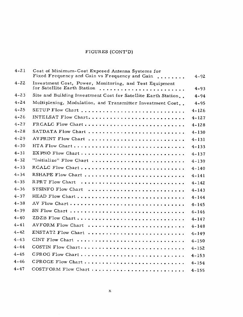
FIGURES (CONT'D)
4-21 Cost of Minimum-Cost Exposed Antenna Systems forFixed Frequency and Gain vs Frequency and Gain ...... .. 4-92
4-22 Investment Cost, Power, Monitoring, and Test Equipmentfor Satellite Earth Station ......... .................. 4-93
4-23 Site and Building Investment Cost for Satellite Earth Station. . 4-94
4-24 Multiplexing, Modulation, and Transmitter Investment Cost.. 4-954-25 SETUP Flow Chart ............................. 4-126
4-26 INTELSAT Flow Chart. ................. . . . . . .. 4-127
4-27 FRCALC Flow Chart ............................ 4-128
4-28 SATDATA Flow Chart ................. ........ 4-130
4-29 AVPRINT Flow Chart .......................... 4-131
4-30 HTA Flow Chart ............................... 4-133
4-31 EXPNO Flow Chart ............................. 4-137
4-32 "Initialize" Flow Chart .......................... 4-13-9
4-33 RCALC Flow Chart ................ . . . ... .......... 4-140
4-34 RSHAPE Flow Chart ....... . . .......... . . . . 4-141
4-35 RPRT Flow Chart ................. .......... 4-142
4-36 SYSINFO Flow Chart .............. ... ....... . . . . . 4-143
4-37 HEAD Flow Chart ............ ...... .... . . . 4-144
4-38 AV Flow Chart ............................... 4-145
4-39 SN Flow Chart ................... . .......... 4-146
4-40 ZDZB Flow Chart ........................... . .4-147
4-41 AVFORM Flow Chart ................. ....... 4-148
4-42 ENSTAT2 Flow Chart . . . ........ ............ 4-149
4-43 CINT Flow Chart ........................ 4-150
4-44 COSTIN Flow Chart ..................... 4-152
4-45 CPROG Flow Chart ............................. 4-153
4-46 CPROGE Flow Chart ........................... 4-154
4-47 COSTFORM Flow Chart .......................... 4-155
x
FIGURES (CONT'D)
4-48 ENFORM Flow Chart ................................ 4-156
4-49 ACT Flow Chart .................... ........ 4-157
4-50 STDBY Flow Chart ... ,,,,,,................. 4-158
4-51 RPTR Flow Chart ............................ . 4-159
4-52 SIMPMAT Flow Chart .................. ....... 4-160
4-53 PICK Flow Chart ............................ * . 4-161
4-54 MODULES Flow Chart ......... .......... ... 4-162
4-55 CF Flow Chart . . .. ..................... 4-163
4-56 Minimum Program Cost Comparison, 12-Year Program,1972 Dollars, Intelsat IV Example, 7-Satellite System,X Factor = 1.0 ................... ......... .... 4-170
4-57 Effect of Launch Delay on System Risk . ............... 4-171
4-58 Sensitivity of Availability and System Cost to SatelliteFailure Rate, Seven-Satellite System . .............. . . 4-173
4-59 Sensitivity of Availability and System Cost to Satellite
Failure Rate, Four-Satellite System . . . . . . . . . . . . . . . . . 4-174
4-60 Sensitivity of System Availability to Spare Turn-On Delay . . . 4-175
5-1 Leased Duplex Voice Circuit Costs, Overland 1973 ........ 5-6
5-2 Leased Duplex Voice Circuit Costs, Transoceanic, 1973 .... 5-7
5-3 Communications Line Lease Cost/km vs Data Rate at
1609 km (1000 mi), 1973 ................... .. . . . . . 5-9
5-4 Communication Line Lease Costs, Data TransmissionRelative to Costs at 1609 km (1000 mi) . ......... . .. . 5-10
5-5 Communication Terminal Equipment Lease Costs,Digital Data Transmission ........................ 5-11
5-6 Line-of-Sight Microwave Relay Station and Terminal
Investment Cost vs Capacity ....................... 5-18
5-7 Capacity Cost Factor, Microwave Relay System Terminals .. 5-19
5-8 Investment Cost of Submarine Telephone Cable per Half-
Circuit Per Kilometer ................... ....... 5-22
5-9 Relative Cost per Unit Length vs Length for Submarine
Telephone Cable Systems . . . . . . . . . . . . . . . . . . . . . . 5-23
5-10 Aircraft Operating Cost per Mile vs Payload Weight ....... 5-38
5-11 Aircraft Investment Cost vs Gross Weight ........ .. . . . . 5-39
5-12 Aircraft Speed vs Gross Weight ................. ... 5-40
xi
1. INTRODUCTION
The purpose of the BRAVO User's Manual is to describe the
BRAVO methodology in terms of step-by-step procedures. The BRAVO
methodology then becomes a tool which a team of analysts can utilize to
perform cost-effectiveness analyses on potential future space applications
with a relatively general set of input information (see Section 3) and a
relatively small expenditure of resources.
An overview of the BRAVO procedure is given by describing
the complete procedure in a general form in Section 2.
1-1
2. GENERAL PROCEDURE
For each user problem the BRAVO team accomplishes an
analysis by carrying out the following steps:
(1) Definition of the problem (BRAVO input)
(2) Space system analysis
(a) Select system approach(es) and goals
(b) Satellite mission equipment selection
(c) Select specific satellite interface concepts
(d) Spacecraft synthesis
(e) Space system cost estimating
(f) Satellite system optimization analysis
(3) Terrestrial system analysis
(a) Define
(b) Estimate costs/revenues
(4) Cost-effectiveness analysis
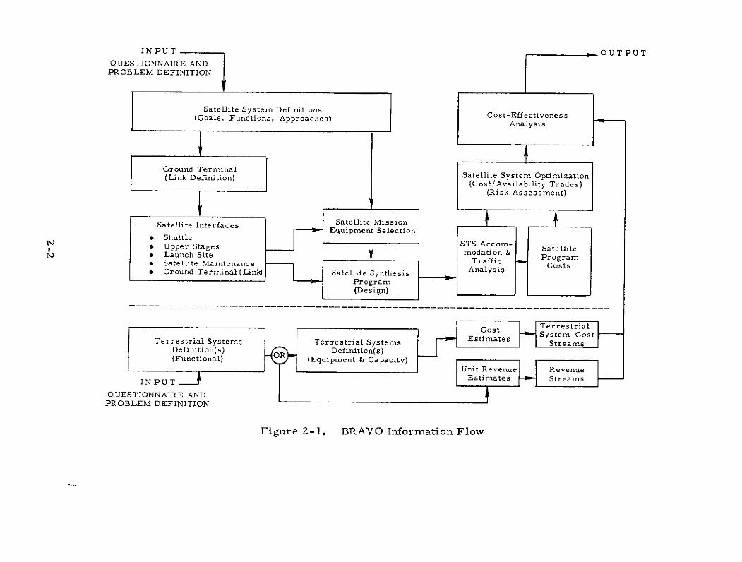
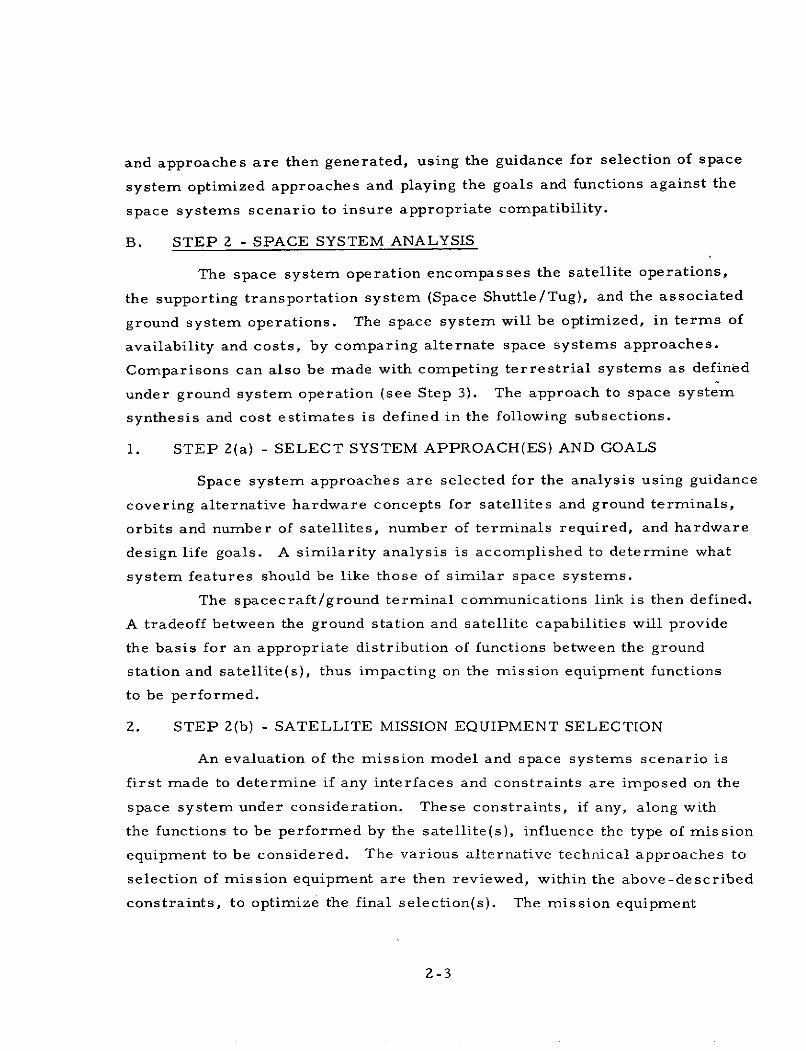
The above activities are carried out in discrete steps, with
sufficient interrelationships to minimize iteration (see Figure 2-1).
The terrestrial system analysis is worked in parallel with the space
system analysis. The following subsections describe the above steps:
A. STEP 1 - DEFINITION OF THE PROBLEM (BRAVO INPUT)
The general input information provided by the system user source
is first reviewed and certified to assess its content and insure its consistency.
This information is then redefined (if required) as technical analysis
inputs, along with additional technical inputs specified by the analyst to
complete the data package, and the resultant technical information re-
certified with the user source. The satellite system goals, functions,
2-1
INPUT a OUTPUT
QUESTIONNAIRE ANDPROBLEM DEFINITION
Satellite System Definitions(Goals, Functions, Approaches) Cost-Effectiveness
Analysis
Ground Terminal(Link Definition) Satellite System Optimization
(Cost/Availability Trades)(Risk Assessment)
Satellite Interfaces Satellite MissionSShuttle Equipment Selection
* Shuttle* Upper Stages Satellite
N* Launch Site modation & Program* Satellite Maintenance Traffic Costs* Ground Terminal(Lin Satellite Synthesis Analysis
Program(Design)
------------------------- -------------------------------------------
Cost TerrestrialSystem Cst
Terrestrial Systems TerrestrialEstimates Sytreams
Definition(s) Definition(s)(Functional) (Equipment & Capacity)
Unit Revenue Revenue~INPUTEstimates Streams
QUESTIONNAIRE ANDPROBLEM DEFINITION
Figure 2-1. BRAVO Information Flow
and approaches are then generated, using the guidance for selection of space
system optimized approaches and playing the goals and functions against the
space systems scenario to insure appropriate compatibility.
B. STEP 2 - SPACE SYSTEM ANALYSIS
The space system operation encompasses the satellite operations,
the supporting transportation system (Space Shuttle/Tug), and the associated
ground system operations. The space system will be optimized, in terms of
availability and costs, by comparing alternate space systems approaches.
Comparisons can also be made with competing terrestrial systems as defined
under ground system operation (see Step 3). The approach to space system
synthesis and cost estimates is defined in the following subsections.
1. STEP 2(a) - SELECT SYSTEM APPROACH(ES) AND GOALS
Space system approaches are selected for the analysis using guidance
covering alternative hardware concepts for satellites and ground terminals,
orbits and number of satellites, number of terminals required, and hardware
design life goals. A similarity analysis is accomplished to determine what
system features should be like those of similar space systems.
The spacecraft/ground terminal communications link is then defined.
A tradeoff between the ground station and satellite capabilities will provide
the basis for an appropriate distribution of functions between the ground
station and satellite(s), thus impacting on the mission equipment functions
to be performed.
2. STEP 2(b) - SATELLITE MISSION EQUIPMENT SELECTION
An evaluation of the mission model and space systems scenario is
first made to determine if any interfaces and constraints are imposed on the
space system under consideration. These constraints, if any, along with
the functions to be performed by the satellite(s), influence the type of mission
equipment to be considered. The various alternative technical approaches to
selection of mission equipment are then reviewed, within the above-described
constraints, to optimize the final selection(s). The mission equipment
2-3
configuration(s) are then generated in sufficient depth for cost estimating
and system optimization purposes. The configuration information required
includes equipment weights, types, sizes, performance, etc. Use is made
of the mission equipment data bank, telecommunications mission equipment
definition calculation forms, or the computer program used for spacecraft
synthesis, to define the mission equipment.
3. STEP 2(c) - SELECT SPECIFIC SATELLITE INTERFACE CONCEPTS
Launch vehicle satellite transportation accommodation and traffic
analyses are conducted to establish the vehicle types and traffic rate parame-
ters necessary to deliver and support the satellite system. The analyses are
performed in accordance with the procedures, rules, and assumptions des-
cribed in the BRAVO User's Manual. Computer programs are not used.Logistic strategies for support of the alternative satellite maintenance approaches
are considered in determining the nominal number of launches required.
Launch sites supporting the satellites and launch vehicles are determined.
The number and general location of the ground terminals needed to
provide coverage are determined.
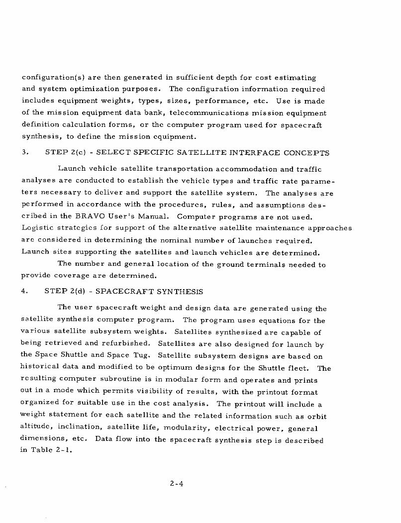
4. STEP 2(d) - SPACECRAFT SYNTHESIS
The user spacecraft weight and design data are generated using thesatellite synthesis computer program. The program uses equations for thevarious satellite subsystem weights. Satellites synthesized are capable ofbeing retrieved and refurbished. Satellites are also designed for launch bythe Space Shuttle and Space Tug. Satellite subsystem designs are based onhistorical data and modified to be optimum designs for the Shuttle fleet. Theresulting computer subroutine is in modular form and operates and printsout in a mode which permits visibility of results, with the printout formatorganized for suitable use in the cost analysis. The printout will include aweight statement for each satellite and the related information such as orbitaltitude, inclination, satellite life, modularity, electrical power, generaldimensions, etc. Data flow into the spacecraft synthesis step is describedin Table 2-1.
2-4
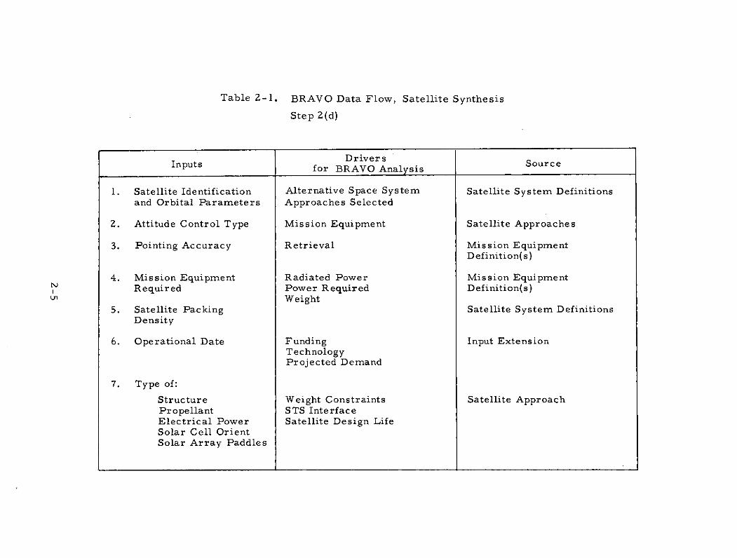
Table 2-1. BRAVO Data Flow, Satellite Synthesis
Step 2(d)
DriversInputDrivers SourceInputs for BRAVO Analysis
1. Satellite Identification Alternative Space System Satellite System Definitionsand Orbital Parameters Approaches Selected
2. Attitude Control Type Mission Equipment Satellite Approaches
3. Pointing Accuracy Retrieval Mission EquipmentDefinition(s)
4. Mission Equipment Radiated Power Mission Equipment, Required Power Required Definition(s)
U1 Weight5. Satellite Packing Satellite System Definitions
Density
6. Operational Date Funding Input ExtensionTechnologyProjected Demand
7. Type of:
Structure Weight Constraints Satellite ApproachPropellant STS InterfaceElectrical Power Satellite Design LifeSolar Cell OrientSolar Array Paddles
5. STEP 2(e) - SPACE SYSTEM COST ESTIMATING
The satellite program costs are estimated using a console-type
computerized individual payload program cost model. The computer model
is coded in APL language and operated from a remote console that affords
simple, rapid, and routine operation. The operation requires filling out an
input sheet that contains the pertinent payload design and traffic information.
The input data can be fed directly into the remote console to produce an out-
put in various formats (although the basic output is a fiscal year funding flow).
Nominal inputs are set in the computer automatically when a particular input
is unknown to the user.
The satellite program costs include the total payload costs, the
launch vehicle direct operating costs, and the launch support costs. In
addition to these costs, the associated ground systems costs, in support of
the satellite system, will also be estimated to arrive at the composite cost
of the entire space system.
Data flow into the space system cost estimating step is described
in Table 2-2.
6. STEP 2(f) - SATELLITE SYSTEM OPTIMIZATION ANALYSIS
The reliability versus time characteristics of the alternative com-
binations of mission equipment and spacecraft devised as conceptual options
for the space system are evaluated in the light of the availability goals
established for the space system. The logistic strategies appropriate to
support these alternatives, and consequently the launch vehicle traffic, also
are evaluated and compared to the system availability goals. These resultant
data are then used to select the optimum strategy and satellite system for
minimum space system cost subject to meeting the availability goals.
Data flow into the satellite system optimization analysis is described
in Tables 2-3 and 2-4.
2-6
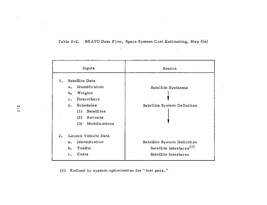
Table 2-2. BRAVO Data Flow, Space System Cost Estimating, Step Z(e)
Inputs Source
1. Satellite Data
a. Identification Satellite Synthesis
b. Weights
c. Describers
d. Schedules Satellite System Definition
(1) Satellites
(2) Revisits
(3) Modifications
2. Launch Vehicle Data
a. Identification Satellite System Definition
b. Traffic Satellite Interfaces(1)
c. Costs Satellite Interfaces
(1) Refined by system optimization for "last pass."
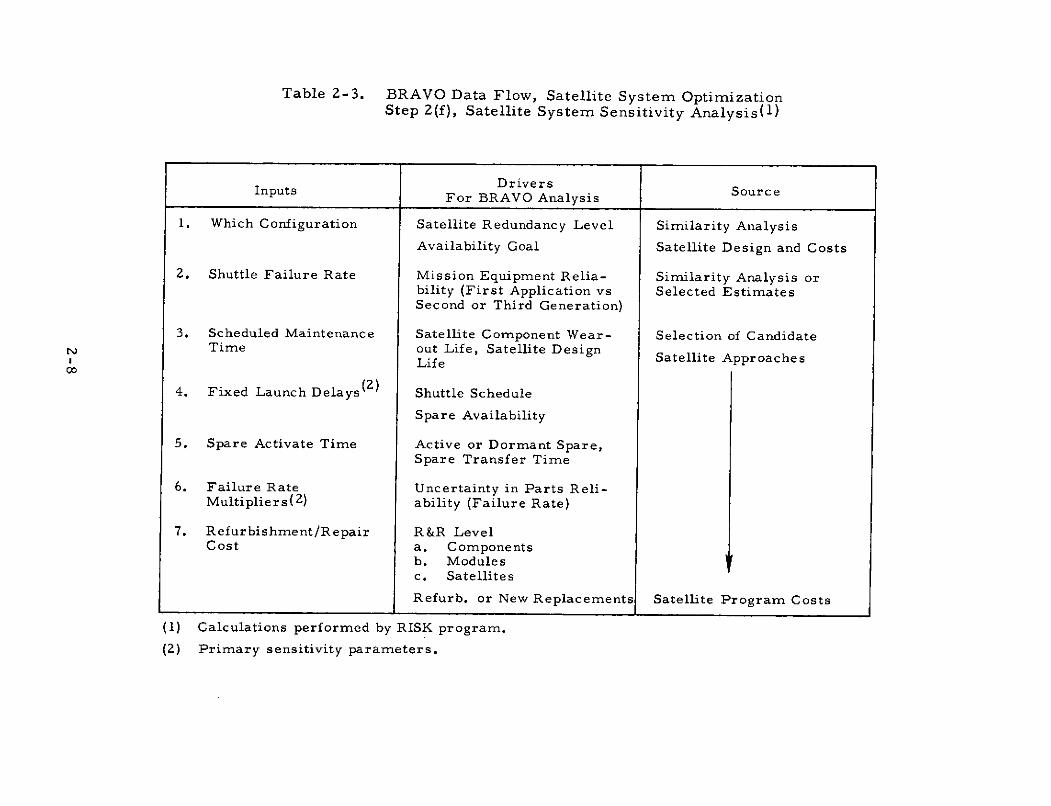
Table 2-3. BRAVO Data Flow, Satellite System OptimizationStep 2(f), Satellite System Sensitivity Analysis(l)
DriversInputs Drivers SourceFor BRAVO Analysis Source
1. Which Configuration Satellite Redundancy Level Similarity Analysis
Availability Goal Satellite Design and Costs
2. Shuttle Failure Rate Mission Equipment Relia- Similarity Analysis orbility (First Application vs Selected EstimatesSecond or Third Generation)
3. Scheduled Maintenance Satellite Component Wear- Selection of CandidateTime out Life, Satellite Design
Life Satellite Approaches
4. Fixed Launch Delays ( 2 ) Shuttle Schedule
Spare Availability
5. Spare Activate Time Active or Dormant Spare,Spare Transfer Time
6. Failure Rate Uncertainty in Parts Reli-Multipliers(2) ability (Failure Rate)
7. Refurbishment/Repair R&R LevelCost a. Components
b. Modulesc. Satellites
Refurb. or New Replacements Satellite Program Costs
(1) Calculations performed by RISK program.
(2) Primary sensitivity parameters.
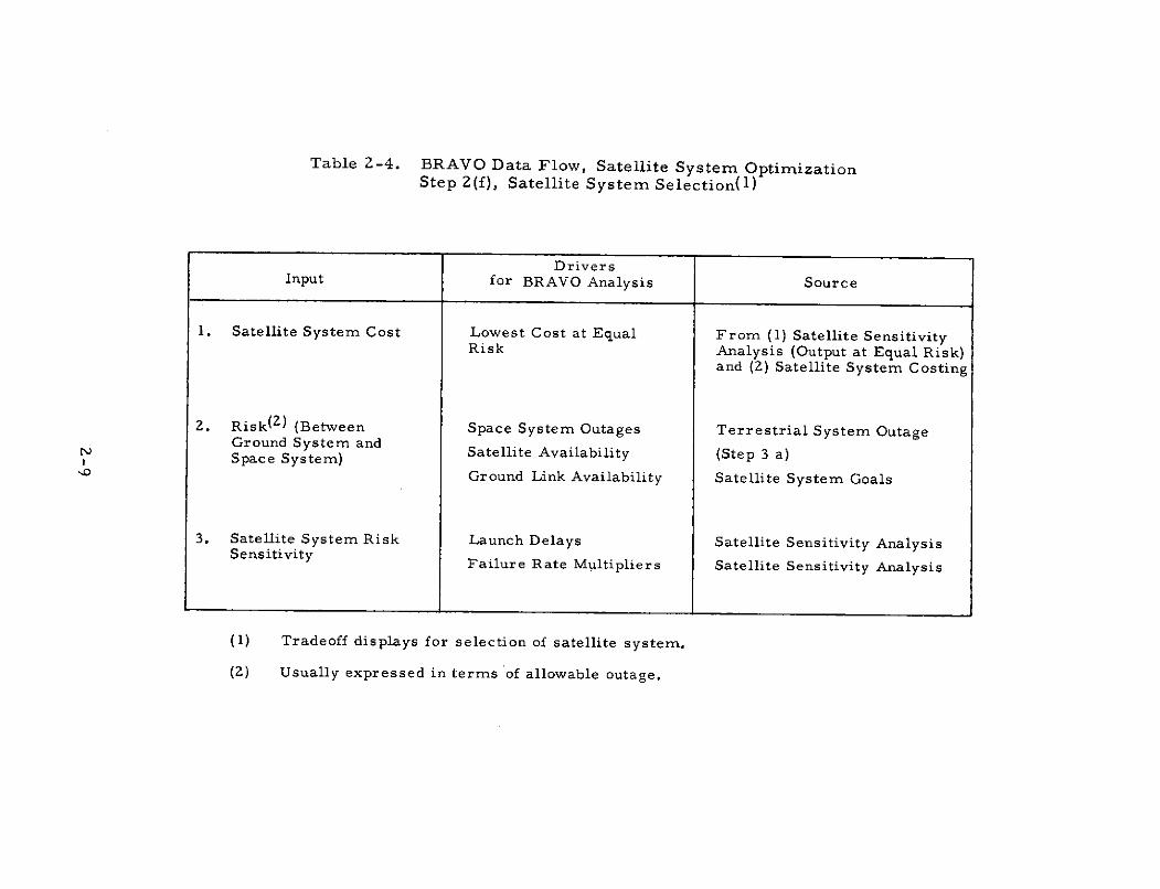
Table 2-4. BRAVO Data Flow, Satellite System OptimizationStep 2(f), Satellite System Selection(l)
DriversInput for BRAVO Analysis Source
1. Satellite System Cost Lowest Cost at Equal From (1) Satellite SensitivityRisk Analysis (Output at Equal Risk)
and (2) Satellite System Costing
2. Risk(Z ) (Between Space System Outages Terrestrial System OutageGround System andGrouSpacend System and Satellite Availability (Step 3 a)
Ground Link Availability Satellite System Goals
3. Satellite System Risk Launch Delays Satellite Sensitivity AnalysisSensitivity Failure Rate Multipliers Satellite Sensitivity Analysis
(1) Tradeoff displays for selection of satellite system.
(2) Usually expressed in terms of allowable outage.

C. STEP 3 - TERRESTRIAL SYSTEM ANALYSIS
In those cases where the intent is to compare a space-oriented
system with a competing terrestrial (ground-based) system, both systems
must be evaluated on an equal capability basis (e. g., performance, avail-
ability, lifetime, etc.). Thus, definition of the terrestrial system requires
the use of criteria for synthesizing ground-based application capability for
comparison with space systems. Estimating the costs for the terrestrial
system may be approached by either of two methods, depending on the extent
of detailed information available on the terrestrial system. The first method
involves a detailed cost buildup, itemizing the total costs associated with
development, investment, and operations. The second method involves
estimating the effective terrestrial system costs or total revenues based on
existing charge rates and user capacity. This second method is more appro-
priate for comparing existing terrestrial systems, where detailed system
definition is difficult to obtain, with conceptual space systems.
D. STEP 4 - COST-EFFECTIVENESS ANALYSIS
The objective of the cost-effectiveness analysis is to compare
alternative advanced space system concepts in order to select the system
alternatives which offer the greatest benefit per dollar. The selected space
system concept(s) are then compared with competing terrestrial systems
to evaluate the economic benefits associated with the space systcm(s). The
cost-effectiveness analysis culminates the entire BRAVO analysis.
The cost-effectiveness analysis is performed on tabular work sheets
requiring the following inputs:
(a) Satellite system costs
/ Mission equipment and spacecraft costs
* R&D, investment, and operations costs
/ Launch vehicle direct operating costs
2.- 10
(b) Ground System Costs
/ Electronics and Support Facilities Costs
. Investment and Operating Costs
(c) Anticipated Unit Demand Rate Schedules (Product Delivered)
The data flow into the cost-effectiveness step is described
in Table 2-5.
Using the above inputs, the revenue required (in constant
or current dollars as desired) to return the invested capital plus interest
is computed in accordance with the following steps:
(a) The rate of return on invested capital (interest rate) andthe anticipated inflation rate are defined.
(b) Using the previously defined interest and inflation rates, thenet present value (NPV) of the cost streams is computed.The NPV of the total cost stream is broken down into discreteincrements (e. g., mission equipment R&D, investment, etc.)to permit early writeoff and return of invested capital ondesired portions of the space system.
(c) The NPV of the revenue stream is equated to the NPV of thecost stream to enable computation of the required revenue.The revenue stream is defined in terms of anticipated unitdemand to first calculate the unit charge rates, and then therequired revenue stream as a function of the unit demandstream. The required revenue can be expressed in constantor current dollar streams by appropriate choice of economicrelationships.
The analysis output is revenue streams, in constant or currentdollars, to return all invested capital plus interest on investedcapital. These revenue streams are then used to comparealternative advanced space systems and terrestrial systemsin order to evaluate their relative economic benefits.
Interpretation of the results of the cost-effectiveness analysesand the comparisons made between (1) space system approachesand (2) space systems and ground systems are reported. Rela-tive value of the space system approaches on an economicbasis, break-even points, the influence of growth in demand,and the relative risk between space systems and ground sys-tems carrying out the potential user's functions will bediscussed.
2-11
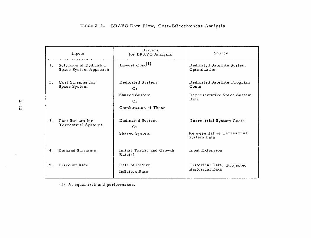
Table 2-5. BRAVO Data Flow, Cost-Effectiveness Analysis
DriversInputs for BRAVO Analysis Source
1. Selection of Dedicated Lowest Cost ( 1 ) Dedicated Satellite SystemSpace System Approach Optimization
2. Cost Streams for Dedicated System Dedicated Satellite ProgramSpace System Or Costs
Shared System Representative Space SystemOr Data
Combination of These
3. Cost Stream for Dedicated System Terrestrial System CostsTerrestrial Systems Or
Shared System Representative TerrestrialSystem Data
4. Demand Stream(s) Initial Traffic and Growth Input ExtensionRate(s)
5. Discount Rate Rate of Return Historical Data, Projected
Inflation Rate Historical Data
(1) At equal risk and performance.
3. DEFINITION OF THE PROBLEM
A BRAVO analysis starts with an interview with a potential user
of space. Normally this interviewer prepares:
(1) List of areas which could be of interest to the potentialuser, and
(2) Descriptions of similar space applications and BRAVOanalyses.
and briefs the potential user on the advantages of space applications and
the BRAVO approach. For each potential space application of interest,
the interviewer asks questions and discusses each item on the BRAVO
check list with the potential user and records the resulting information.
The interviewer obtains as much data and information as possible on each
item. Quantitative data is preferred; relative and qualitative information
is acceptable. If specific information is proprietary to the potential
user, it should be so noted. If the check list item is not applicable or
the information unavailable, it should be so noted.
The minimum amount of information with which an analysis can
be initiated is items l(a), l(b), 2(a), 2(b)(5), 2(b)(6), 3(a), 4(a), or items
l(a), l(b), 2(alternative)(a), 2(alternative)(c), 3(a), 4(a). The remainder
of the data requested for this analysis then is filled in by the BRAVO
team using information from similar applications to complete the problem
description.
The completed problem description is reviewed with the potential
user to close the loop.
3-1
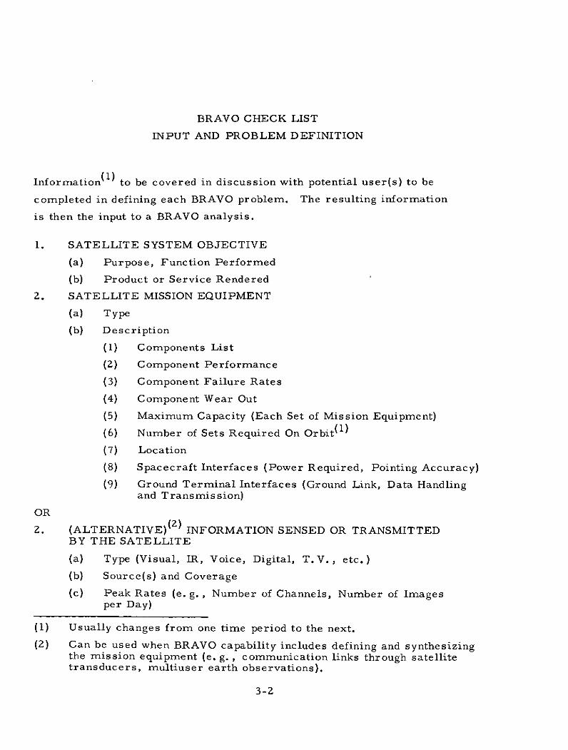
BRAVO CHECK LIST
INPUT AND PROBLEM DEFINITION
Information ( 1 ) to be covered in discussion with potential user(s) to be
completed in defining each BRAVO problem. The resulting information
is then the input to a BRAVO analysis.
1. SATELLITE SYSTEM OBJECTIVE
(a) Purpose, Function Performed
(b) Product or Service Rendered
2. SATELLITE MISSION EQUIPMENT
(a) Type
(b) Description
(1) Components List
(2) Component Performance
(3) Component Failure Rates
(4) Component Wear Out
(5) Maximum Capacity (Each Set of Mission Equipment)
(6) Number of Sets Required On Orbit ( 1 )
(7) Location
(8) Spacecraft Interfaces (Power Required, Pointing Accuracy)
(9) Ground Terminal Interfaces (Ground Link, Data Handlingand Transmission)
OR
2. (ALTERNATIVE) ( 2 ) INFORMATION SENSED OR TRANSMITTEDBY THE SATELLITE
(a) Type (Visual, IR, Voice, Digital, T.V., etc.)
(b) Source(s) and Coverage
(c) Peak Rates (e. g., Number of Channels, Number of Imagesper Day)
(1) Usually changes from one time period to the next.
(2) Can be used when BRAVO capability includes defining and synthesizingthe mission equipment (e. g. , communication links through satellitetransducers, multiuser earth observations).
3-2
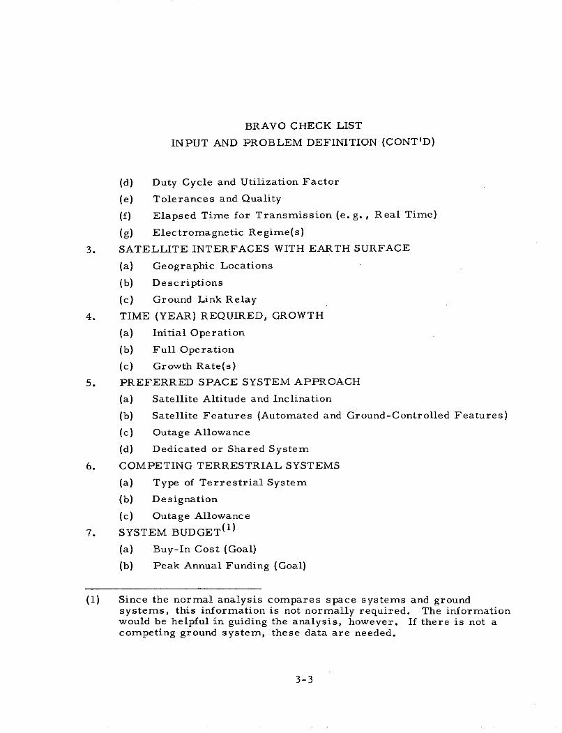
BRAVO CHECK LIST
INPUT AND PROBLEM DEFINITION (CONT'D)
(d) Duty Cycle and Utilization Factor
(e) Tolerances and Quality
(f) Elapsed Time for Transmission (e. g., Real Time)
(g) Electromagnetic Regime(s)
3. SATELLITE INTERFACES WITH EARTH SURFACE
(a) Geographic Locations
(b) Descriptions
(c) Ground Link Relay
4. TIME (YEAR) REQUIRED, GROWTH
(a) Initial Operation
(b) Full Operation
(c) Growth Rate(s)
5. PREFERRED SPACE SYSTEM APPROACH
(a) Satellite Altitude and Inclination
(b) Satellite Features (Automated and Ground-Controlled Features)
(c) Outage Allowance
(d) Dedicated or Shared System
6. COMPETING TERRESTRIAL SYSTEMS
(a) Type of Terrestrial System
(b) Designation
(c) Outage Allowance
7. SYSTEM BUDGET ( 1 )
(a) Buy-In Cost (Goal)
(b) Peak Annual Funding (Goal)
(1) Since the normal analysis compares space systems and groundsystems, this information is not normally required. The informationwould be helpful in guiding the analysis, however. If there is not acompeting ground system, these data are needed.
3-3
BRAVO CHECK LIST
INPUT AND PROBLEM DEFINITION (CONT'D)
8. SPECIAL PROBLEMS
(a) Advanced State of the Art Required
(1) Advanced Technology
(2) Advanced Operating Mode
(b) Non-Standard STS Requirements
9. REFERENCES
(a) Related Space System References
(b) Related Terrestrial System References
3-4
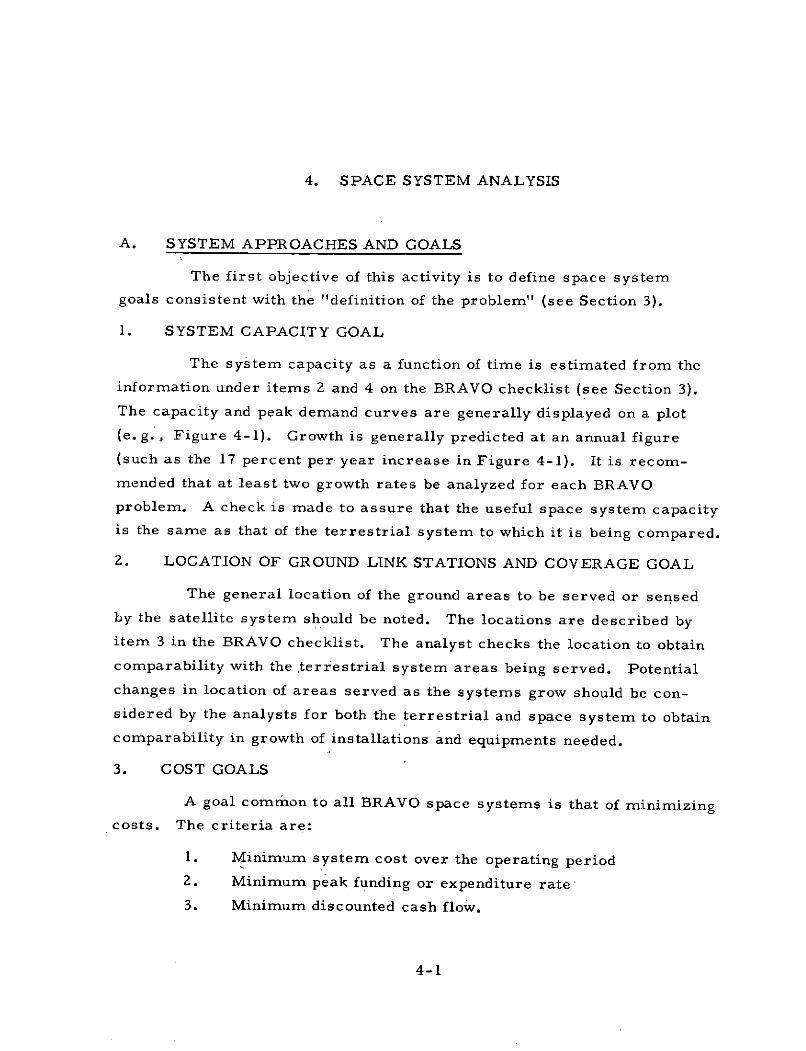
4. SPACE SYSTEM ANALYSIS
A. SYSTEM APPROACHES AND GOALS
The first objective of this activity is to define space system
goals consistent with the "definition of the problem" (see Section 3).
1. SYSTEM CAPACITY GOAL
The system capacity as a function of time is estimated from the
information under items 2 and 4 on the BRAVO checklist (see Section 3).
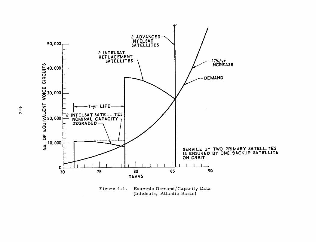
The capacity and peak demand curves are generally displayed on a plot
(e. g., Figure 4-1). Growth is generally predicted at an annual figure
(such as the 17 percent per year increase in Figure 4-1). It is recom-
mended that at least two growth rates be analyzed for each BRAVO
problem. A check is made to assure that the useful space system capacity
is the same as that of the terrestrial system to which it is being compared.
2. LOCATION OF GROUND LINK STATIONS AND COVERAGE GOAL
The general location of the ground areas to be served or sensed
by the satellite system should be noted. The locations are described byitem 3 in the BRAVO checklist. The analyst checks the location to obtaincomparability with the terrestrial system areas being served. Potential
changes in location of areas served as the systems grow should be con-sidered by the analysts for both the terrestrial and space system to obtaincomparability in growth of installations and equipments needed.
3. COST GOALS
A goal common to all BRAVO space systems is that of minimizingcosts. The criteria are:
1. Minimum system cost over the operating period
2. Minimum peak funding or expenditure rate
3. Minimum discounted cash flow.
4-1
2 ADVANCEDINTELSAT
50, 000 SATELLITES
2 INTELSATREPLACEMENT
SATELLITES 17%/yrt 4 INCREASEb 40, 000
5 -- DEMAND
wY 30, 000
z 7-yr LIFE
2 INTELSAT SATELLITES> 20,000 NOMINAL CAPACITY5 DEGRADED
0
10, 000
z SERVICE BY TWO PRIMARY SATELLITESIS ENSURED BY ONE BACKUP SATELLITEON ORBIT
70 75 80 85 90YEARS
Figure 4-1. Example Demand/Capacity Data(Intelsats, Atlantic Basin)
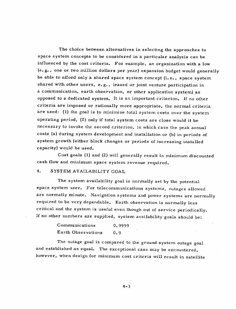
The choice between alternatives in-selecting the approaches to
space system concepts to be considered in a particular analysis can be
influenced by the cost criteria. For example, an organization with a low
(e. g., one or two million dollars per year) expansion budget would generally
be able to afford only a shared space system concept (i. e., space system
shared with other users, e. g., leased or joint venture participation in
a communication, earth observation, or other application system) as
opposed to a dedicated system. It is an important criterion. If no other
criteria are imposed or rationally more appropriate, the normal criteriaare used: (1) the goal is to minimize total system costs over the system
operating period, (2) only if total system costs are close would it be
necessary to invoke the second criterion, in which case the peak annual
costs (a) during system development and installation or (b) in periods of
system growth (either block changes or periods of increasing installed
capacity) would be used.
Cost goals (1) and (2) will generally result in minimum discounted
cash flow and minimum space system revenue required.
4. SYSTEM AVAILABILITY GOAL
The system availability goal is normally set by the potential
space system user. For telecommunications systems, outages allowed
are normally minute. Navigation systems and power systems are normally
required to be very dependable. Earth observation is normally less
critical and the system is useful even though out of service periodically.
If no other numbers are supplied, system availability goals should be:
Communications 0. 9999
Earth Observations 0.9
The outage goal is compared to the ground system outage goaland established as equal. The exceptional case may be encountered,
however, when design for minimum cost criteria will result in satellite
4-3
outage which is very low (on the order of 0. 001 or less) with adequate
spares on the ground. This is the result of the high cost of transporta-
tion for the purpose of satellite repair. Larger outages can result if
spares or transport capacity are not adequate to support rapid (e. g.,
two month) replacement but may not increase outages to equal the terrestrial
system. This is acceptable to the analysis.
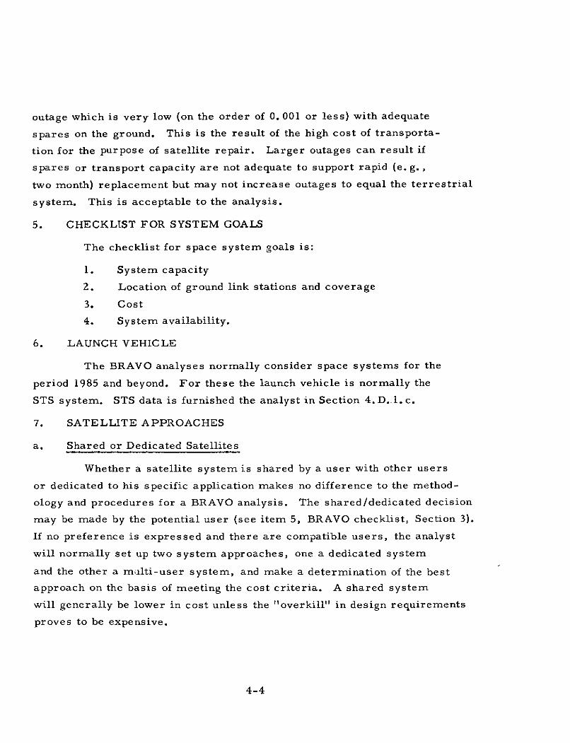
5. CHECKLIST FOR SYSTEM GOALS
The checklist for space system goals is:
1. System capacity
2. Location of ground link stations and coverage
3. Cost
4. System availability.
6. LAUNCH VEHICLE
The BRAVO analyses normally consider space systems for the
period 1985 and beyond. For these the launch vehicle is normally the
STS system. STS data is furnished the analyst in Section 4. D..1.c.
7. SATELLITE APPROACHES
a. Shared or Dedicated Satellites
Whether a satellite system is shared by a user with other users
or dedicated to his specific application makes no difference to the method-
ology and procedures for a BRAVO analysis. The shared/dedicated decision
may be made by the potential user (see item 5, BRAVO checklist, Section 3).
If no preference is expressed and there are compatible users, the analyst
will normally set up two system approaches, one a dedicated system
and the other a muilti-user system, and make a determination of the best
approach on the basis of meeting the cost criteria. A shared system
will generally be lower in cost unless the "overkill" in design requirements
proves to be expensive.
4-4
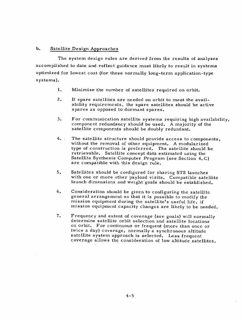
b. Satellite Design Approaches
The system design rules are derived from the results of analyses
accomplished to date and reflect guidance most likely to result in systems
optimized for lowest cost (for these normally long-term application-type
systems).
1. Minimize the number of satellites required on orbit.
2. If spare satellites are needed on orbit to meet the avail-ability requirements, the spare satellites should be activespares as opposed to dormant spares.
3. For communication satellite systems requiring high availability,component redundancy should be used. A majority of thesatellite components should be doubly redundant.
4. The satellite structure should provide access to components,without the removal of other equipment. A modularizedtype of construction is preferred. The satellite should beretrievable. Satellite concept data estimated using theSatellite Synthesis Computer Program (see Section 4. C)are compatible with this design rule.
5. Satellites should be configured for sharing STS launcheswith one or more other payload visits. Compatible satellitelaunch dimensions and weight goals should be established.
6. Consideration should be given to configuring the satellitegeneral arrangement so that it is possible to modify themission equipment during the satellite's useful life, ifmission equipment capacity changes are likely to be needed.
7. Frequency and extent of coverage (see goals) will normallydetermine satellite orbit selection and satellite locationson orbit. For continuous or frequent (more than once ortwice a day) coverage, normally a synchronous altitudesatellite system approach is selected. Less frequentcoverage allows the consideration of low altitude satellites.
4-5
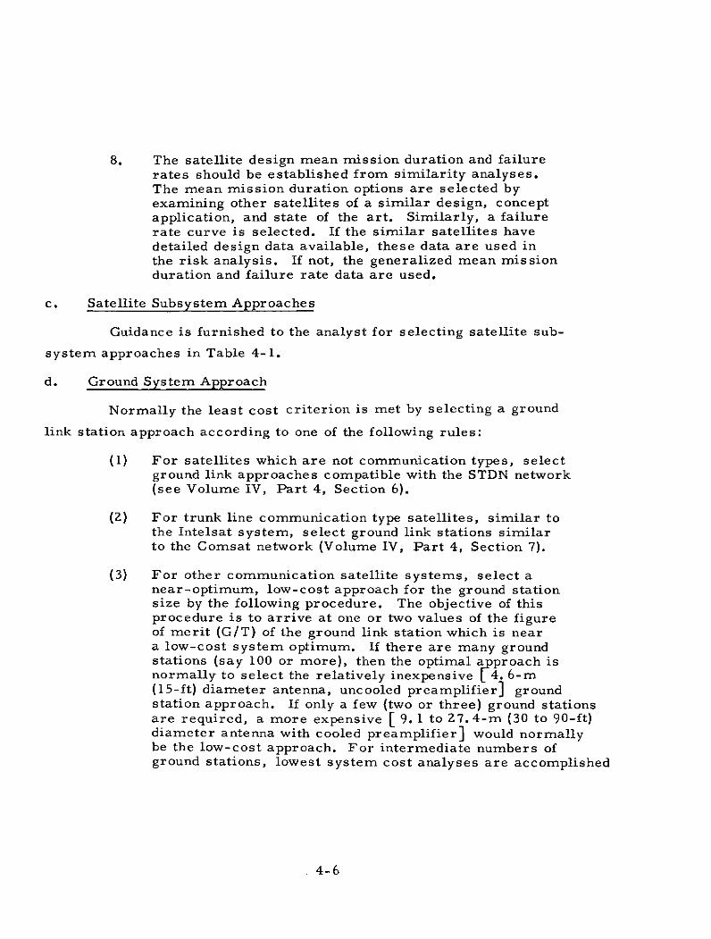
8. The satellite design mean mission duration and failurerates should be established from similarity analyses.The mean mission duration options are selected byexamining other satellites of a similar design, conceptapplication, and state of the art. Similarly, a failurerate curve is selected. If the similar satellites havedetailed design data available, these data are used inthe risk analysis. If not, the generalized mean missionduration and failure rate data are used.
c. Satellite Subsystem Approaches
Guidance is furnished to the analyst for selecting satellite sub-
system approaches in Table 4-1.
d. Ground System Approach
Normally the least cost criterion is met by selecting a ground
link station approach according to one of the following rules:
(1) For satellites which are not communication types, selectground link approaches compatible with the STDN network(see Volume IV, Part 4, Section 6).
(2) For trunk line communication type satellites, similar tothe Intelsat system, select ground link stations similarto the Comsat network (Volume IV, Part 4, Section 7).
(3) For other communication satellite systems, select anear-optimum, low-cost approach for the ground stationsize by the following procedure. The objective of thisprocedure is to arrive at one or two values of the figureof merit (G/T) of the ground link station which is neara low-cost system optimum. If there are many groundstations (say 100 or more), then the optimal approach isnormally to select the relatively inexpensive [ 4. 6-m(15-ft) diameter antenna, uncooled preamplifier] groundstation approach. If only a few (two or three) ground stationsare required, a more expensive [ 9.1 to 27.4-m (30 to 90-ft)diameter antenna with cooled preamplifier] would normallybe the low-cost approach. For intermediate numbers ofground stations, lowest system cost analyses are accomplished
4-6
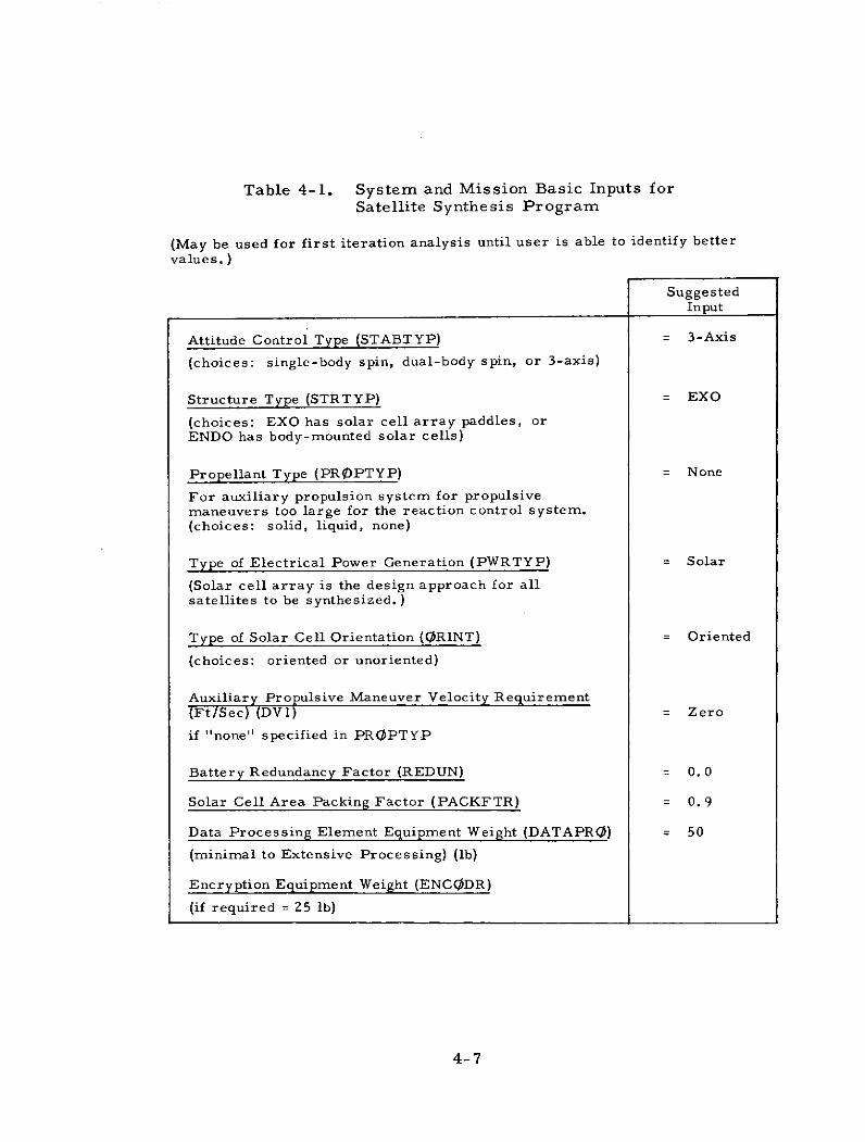
Table 4-1. System and Mission Basic Inputs forSatellite Synthesis Program
(May be used for first iteration analysis until user is able to identify better
values.)
SuggestedInput
Attitude Control Type (STABTYP) = 3-Axis
(choices: single-body spin, dual-body spin, or 3-axis)
Structure Type (STRTYP) = EXO
(choices: EXO has solar cell array paddles, orENDO has body-mounted solar cells)
Propellant Type (PROPTYP) = None
For auxiliary propulsion system for propulsivemaneuvers too large for the reaction control system.(choices: solid, liquid, none)
Type of Electrical Power Generation (PWRTYP) = Solar
(Solar cell array is the design approach for allsatellites to be synthesized.)
Type of Solar Cell Orientation (ORINT) = Oriented
(choices: oriented or unoriented)
Auxiliary Propulsive Maneuver Velocity Requirement(Ft/Sec) (DVI) = Zero
if "none" specified in PROPTYP
Battery Redundancy Factor (REDUN) = 0.0
Solar Cell Area Packing Factor (PACKFTR) = 0.9
Data Processing Element Equipment Weight (DATAPRO) = 50
(minimal to Extensive Processing) (lb)
Encryption Equipment Weight (ENCODR)
(if required = 25 lb)
4-7

by analyzing the system with two alternative stationapproaches and choosing the lowest cost approach betweenthem. The procedure for accomplishing this analysisis described below.
(a) Knowing the frequency at which the down link is tooperate (see Section 4.B. 1), enter Figure 4-21(page 4-92) at that frequency and select one or twoantenna diameters. Normally a low-cost antenna of4. 6 to 6. 1 m (15 to 20 ft) in diameter would be oneoption and a larger diameter antenna, about twiceas expensive, would be selected unless the numberof ground stations falls into the greater than 100or two to three categories described above.
(b) Read the antenna gain (Gain dB) from Figure 4-21for the options to be analyzed.
(c) Refer to page 4-90 and select the uncooled pre-amplifier approach for 4. 6 or 6. 1 m (15 or 20 ft)diameter antennas and either the cooled preamplifieror both the cooled and uncooled preamplifiers asalternates for larger diameter antennas.
(d) Compute the figure of merit (G/T) for the groundlink station using the formula G/T = G - T whereG = antenna gain from Step (b) and T = receivingsystem equivalent noise temperature.
(e) Compare the figure of merit G/T with the correspond-ing ground system G/T from procedures in Section4. B. 1. The same value would be used for bothanalyses.
(f) The G/T value(s) are ready for use in the analysisdescribed in Section 4. D. 2.
4-8
B. SATELLITE MISSION EQUIPMENT
1. TELECOMMUNICATIONS TYPE
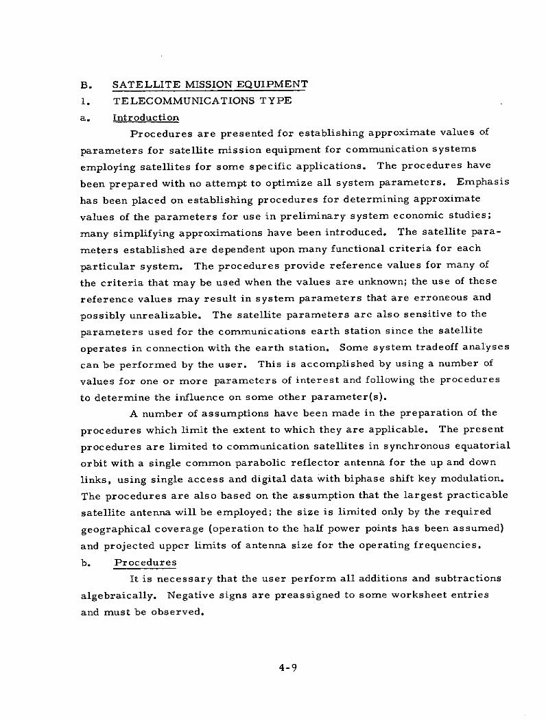
a. Introduction
Procedures are presented for establishing approximate values of
parameters for satellite mission equipment for communication systems
employing satellites for some specific applications. The procedures have
been prepared with no attempt to optimize all system parameters. Emphasis
has been placed on establishing procedures for determining approximate
values of the parameters for use in preliminary system economic studies;
many simplifying approximations have been introduced. The satellite para-
meters established are dependent upon many functional criteria for each
particular system. The procedures provide reference values for many of
the criteria that may be used when the values are unknown; the use of these
reference values may result in system parameters that are erroneous and
possibly unrealizable. The satellite parameters are also sensitive to the
parameters used for the communications earth station since the satellite
operates in connection with the earth station. Some system tradeoff analyses
can be performed by the user. This is accomplished by using a number of
values for one or more parameters of interest and following the procedures
to determine the influence on some other parameter(s).
A number of assumptions have been made in the preparation of the
procedures which limit the extent to which they are applicable. The present
procedures are limited to communication satellites in synchronous equatorial
orbit with a single common parabolic reflector antenna for the up and down
links, using single access and digital data with biphase shift key modulation.
The procedures are also based on the assumption that the largest practicable
satellite antenna will be employed; the size is limited only by the required
geographical coverage (operation to the half power points has been assumed)
and projected upper limits of antenna size for the operating frequencies.
b. Procedures
It is necessary that the user perform all additions and subtractions
algebraically. Negative signs are preassigned to some worksheet entries
and must be observed.
4-9
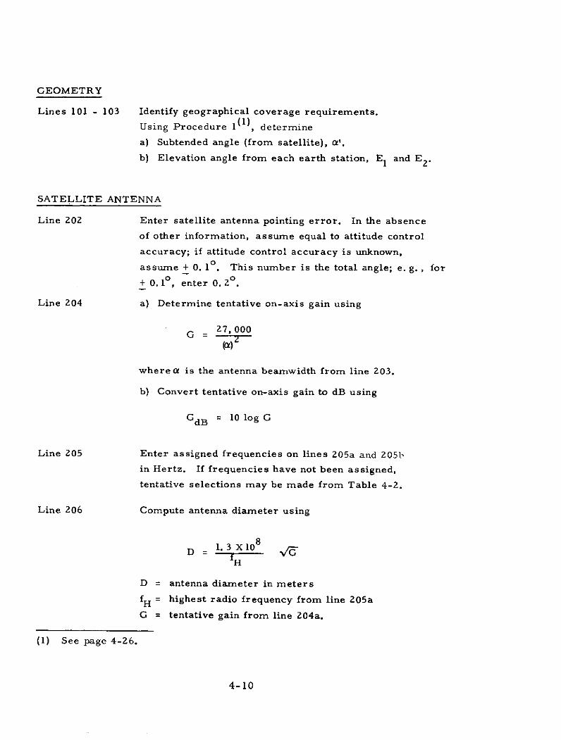
GEOMETRY
Lines 101 - 103 Identify geographical coverage requirements.
Using Procedure 1 1), determine
a) Subtended angle (from satellite), 0'.
b) Elevation angle from each earth station, E1 and E 2.
SATELLITE ANTENNA
Line 202 Enter satellite antenna pointing error. In the absence
of other information, assume equal to attitude control
accuracy; if attitude control accuracy is unknown,
assume + 0. 10. This number is the total angle; e. g., for
+ 0. 10, enter 0. 20.
Line 204 a) Determine tentative on-axis gain using
G 27,000(ar)
where a is the antenna beamwidth from line 203.
b) Convert tentative on-axis gain to dB using
GdB = 10 log G
Line 205 Enter assigned frequencies on lines 205a and 205b
in Hertz. If frequencies have not been assigned,
tentative selections may be made from Table 4-2.
Line 206 Compute antenna diameter using
D -1. 3 X 10H
D = antenna diameter in meters
fH = highest radio frequency from line 205a
G = tentative gain from line 204a.
(1) See page 4-26.
4-10
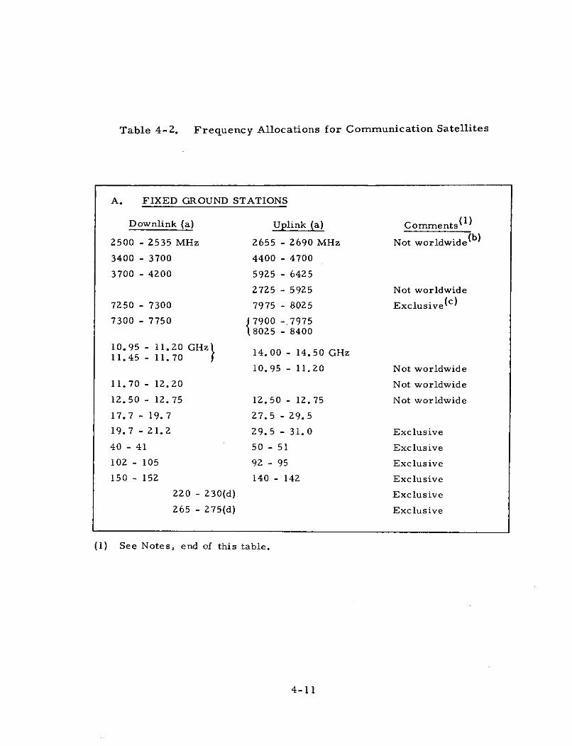
Table 4-2. Frequency Allocations for Communication Satellites
A. FIXED GROUND STATIONS
Downlink (a) Uplink (a) Comments (1)
2500 - 2535 MHz 2655 - 2690 MHz Not worldwide(b)
3400 - 3700 4400 - 4700
3700 - 4200 5925 - 6425
2725 - 5925 Not worldwide
7250 - 7300 7975 - 8025 Exclusive(c)
7300 - 7750 7900 -,79758025 - 8400
10.95 - 11.20 GHz11.45 - 11.70 14.00 - 14.50 GHz
10. 95 - 11.20 Not worldwide
11.70 - 12. 20 Not worldwide
12. 50 - 12. 75 12. 50 - 12. 75 Not worldwide
17.7 - 19.7 27.5 - 29.5
19.7 - 21.2 29.5 - 31.0 Exclusive
40 - 41 50 - 51 Exclusive
102 - 105 92 - 95 Exclusive
150 - 152 140 - 142 Exclusive
220 - 230(d) Exclusive
265 - 275(d) Exclusive
(1) See Notes, end of this table.
4-11
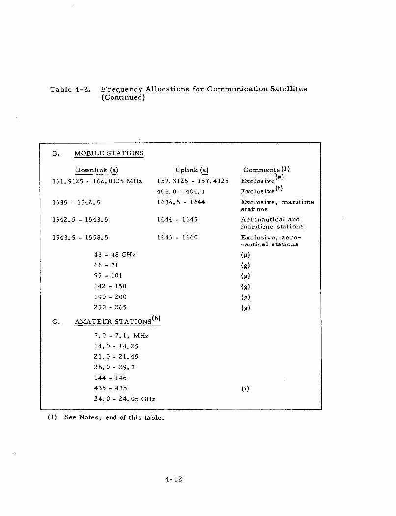
Table 4-2. Frequency Allocations for Communication Satellites
(Continued)
B. MOBILE STATIONS
Downlink (a) Uplink (a) Comments (1)
161.9125 - 162. 0125 MHz 157. 3125 - 157. 4125 Exclusive(e)(f)406. 0 - 406. 1 Exclusive
1535 - 1542.5 1636.5 - 1644 Exclusive, maritimestations
1542.5 - 1543. 5 1644 - 1645 Aeronautical andmaritime stations
1543.5 - 1558.5 1645 - 1660 Exclusive, aero-nautical stations
43 - 48 GHz (g)
66- 71 (g)
95 - 101 (g)
142 - 150 (g)
190 - 200 (g)
250 - 265 (g)
C. AMATEUR STATIONS(h)
7.0 - 7. 1, MHz
14.0 - 14.25
21.0 - 21.45
28.0 - 29.7
144 - 146
435 - 438 (i)
24.0 - 24. 05 GHz
(1) See Notes, end of this table.
4-12
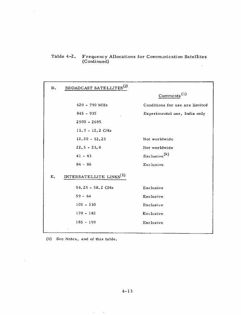
Table 4-2. Frequency Allocations for Communication Satellites(Continued)
D. BROADCAST SATELLITES
Comments (1)
620 - 790 MHz Conditions for use are limited
845 - 935 Experimental use, India only
2500 - 2695
11.7 - 12.2 GHz
12.20 - 12.25 Not worldwide
22. 5 - 23. 0 Not worldwide
41 - 43 Exclusive ( k )
84 - 86 Exclusive
E. INTERSATELLITE LINKS ( 1 )
54.25 - 58.2 GHz Exclusive
59 - 64 Exclusive
105 - 130 Exclusive
170 - 182 Exclusive
185 - 190 Exclusive
(1) See Notes, end of this table.
4-13
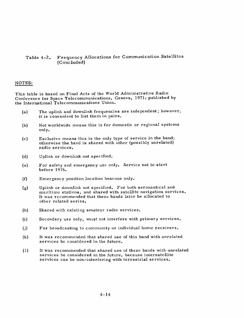
Table 4-2. Frequency Allocations for Communication Satellites
(Concluded)
NOTES:
This table is based on Final Acts of the World Administrative RadioConference for Space Telecommunications, Geneva, 1971; published bythe International Telecommunications Union.
(a) The uplink and downlink frequencies are independent; however,it is convenient to list them in pairs.
(b) Not worldwide means this is for domestic or regional systemsonly.
(c) Exclusive means this is the only type of service in the band;otherwise the band is shared with other (possibly unrelated)radio services.
(d) Uplink or downlink not specified.
(e) For safety and emergency use only. Service not to startbefore 1976.
(f) Emergency position location beacons only.
(g) Uplink or downlink not specified. For both aeronautical andmaritime stations, and shared with satellite navigation services.It was recommended that these bands later be allocated toother related series.
(h) Shared with existing amateur radio services.
(i) Secondary use only, must not interfere with primary services.
(j) For broadcasting to community or individual home receivers.
(k) It was recommended that shared use of this band with unrelatedservices be considered in the future.
(1) It was recommended that shared use of these bands with unrelatedservices be considered in the future, because intersatelliteservices can be non-interfering with terrestrial services.
4-14

Compare with upper limit in Table 4-3. If diameter
exceeds limit, decrease diameter and/or frequency
so combination is within limits and recompute
tentative high frequency gain (line 204a) using
-17 2 2G = 5. 9 X0 - 1 7 D FH
D = antenna diameter in meters
FH = highest radio frequency from line 205a
Recompute line 204b if necessary.
Line 207 Compute preliminary antenna low frequency gain using
GL = 20 log + GH
GH = tentative highest frequency gain from line 204b
FL = lowest radio frequency from line 205b
FH = highest radio frequency from line 205a
Line 208 Choose the frequency from line 205a or 205b for the
uplink. The higher of the two frequencies (line 205a)
should be chosen for the uplink unless there is a reason
for doing otherwise.
Line 209 The preliminary uplink gain is taken from line 204b if the
high frequency is used on the uplink or from line 207 if the
low frequency is used on the uplink.
Line 210 The uplink multiple factor is 0 dB for a single beam.
For multiple beams, the factor is obtained from Procedure 2(1)
Line 212 The preliminary downlink gain is taken from line 207
if the low frequency is used for the downlink or from line
204b if the high frequency is used for the downlink.
Line 213 The downlink multiple beam factor is 0 dB for a single beam.
For multiple beams, the factor is obtained from Procedure 2 ( 1 ) .
(1) See page 4-29.
4-15
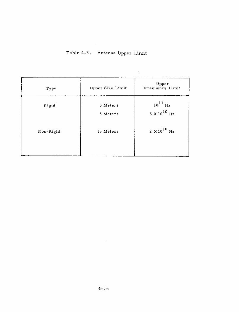
Table 4-3. Antenna Upper Limit
UpperType Upper Size Limit Frequency Limit
Rigid 3 Meters 1011 Hz
5 Meters 5 X10¹⁰ Hz
Non-Rigid 15 Meters 2 X10¹⁰ Hz
4-16

Line 215 The number of transponders is 1 for a single beam. For
multiple beams, it is obtained from Procedure 2(1)
PRELIMINARY ESTIMATE, EARTH STATION TRANSMISSIONS
The uplink analysis in the next section requires input data on the earth station
transmission characteristics. If the earth station effective isotropic radiated
power (EIRP) on the earth station transmitter power and antenna gain are known,
omit lines 251 through 260. If the earth station transmission characteristics
are not known, this set of calculations can be used to obtain initial values.
Line 253 Compute 20 log F where F is the uplink frequency inu u
Hertz from line 208a.
Line 254 Set bandwidth equal to the data rate (DR) in bits per second.
(This assumes the use of non-return-to-zero bit represen-
tation.) Check frequency allocation, or Table 4-2, to verify
that there is enough bandwidth available. If not, reduce
data rate. Compute
BdB = 10 log DR
Line 255 Atmospheric and rain attenuation is obtained from Procedure
3 ( 2 ) . A value of 0 dB may be used if line 208a is 8 X 10⁹
Hertz or less.
Line 256 The uplink carrier-to-noise ratio required by the system
should be entered. If it is unknown, 20 dB is an appropriate
initial value for systems known to have large transmitting
earth stations; if the system uses small ground stations
or if the nature of the ground stations is unknown, 15 dB
is an appropriate initial value.
Line 257 PT + GT is the sum of the transmitter power (PT) in dBW
and the antenna gain (GT) in dB of the earth station.
Any combination of PT and GT that provides the required
sum can be used. However, the remaining analysis can be
performed without apportionment between PT and GT. If
it is desired to make an apportionment, lines 258 through
260 may be used for this purpose.
(1) See page 4-29.
(2) See page 4-34.
4-17

Line 258 Some value for the earth station antenna gain is entered.
Line 260 The earth station transmitter power in dBW (PT) on line
259 may be converted to watts by
PPW = antilog T-
UPLINK
If the preliminary estimate of the earth station transmissions (lines 251 through
260) has been utilized, this uplink section should be omitted until more specific
information regarding the earth station becomes known or is postulated.
If the earth station EIRP is known, enter on line 305 and omit lines 301 through
304.
Line 301 Express earth transmitter power in dBW using
PdBW = 10 log PT
PT = power in watts
This line may be left blank if the value of EIRP
is entered on line 305.
Line 302 Enter earth transmitting antenna gain in dB. This
line may be left blank if the value of EIRP is
entered on line 305.
Line 303 The value for line 303 is obtained by adding lines
301 and 302..
Line 304 Enter transmitter circuit losses in dB. A value of
2 dB may be used in the absence of other information.
Line 306 Determine free space loss (SL) in dB using
SL = 4. 1 + 20 log F U
where FU is uplink frequency from line 208a.
4-18
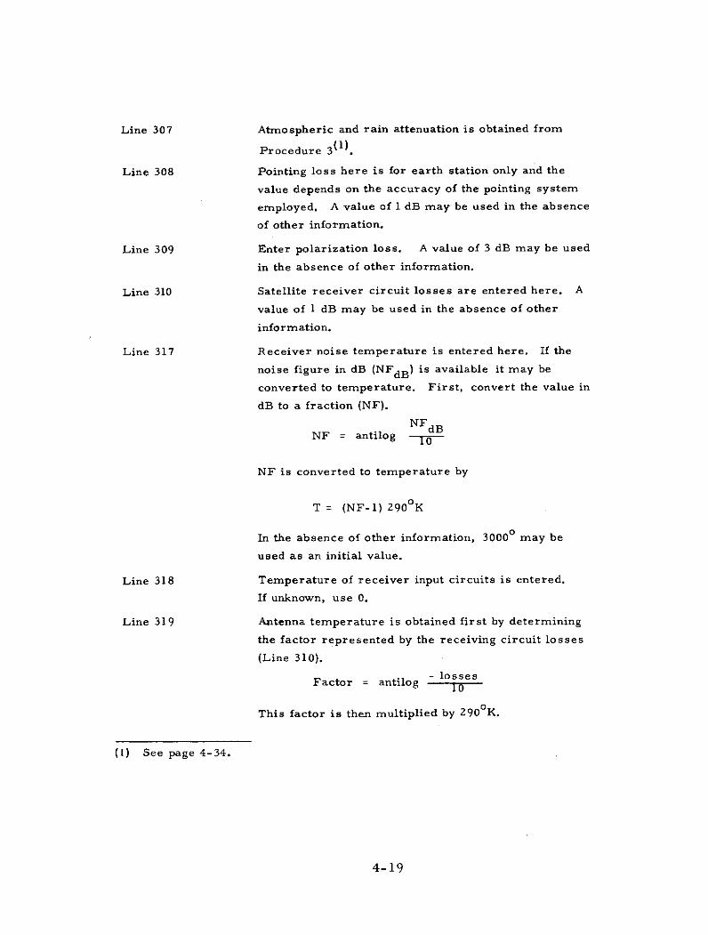
Line 307 Atmospheric and rain attenuation is obtained from
Procedure 3(1)
Line 308 Pointing loss here is for earth station only and the
value depends on the accuracy of the pointing system
employed. A value of 1 dB may be used in the absence
of other information.
Line 309 Enter polarization loss. A value of 3 dB may be used
in the absence of other information.
Line 310 Satellite receiver circuit losses are entered here. A
value of 1 dB may be used in the absence of other
information.
Line 317 Receiver noise temperature is entered here. If the
noise figure in dB (NFdB) is available it may be
converted to temperature. First, convert the value in
dB to a fraction (NF).
NFdBNF = antilog NFdB
NF is converted to temperature by
T = (NF-1) 2900K
In the absence of other information, 30000 may be
used as an initial value.
Line 318 Temperature of receiver input circuits is entered.
If unknown, use 0.
Line 319 Antenna temperature is obtained first by determining
the factor represented by the receiving circuit losses
(Line 310).
- lossesFactor = antilog ---
This factor is then multiplied by 290 0 K.
(1) See page 4-34.
4-19
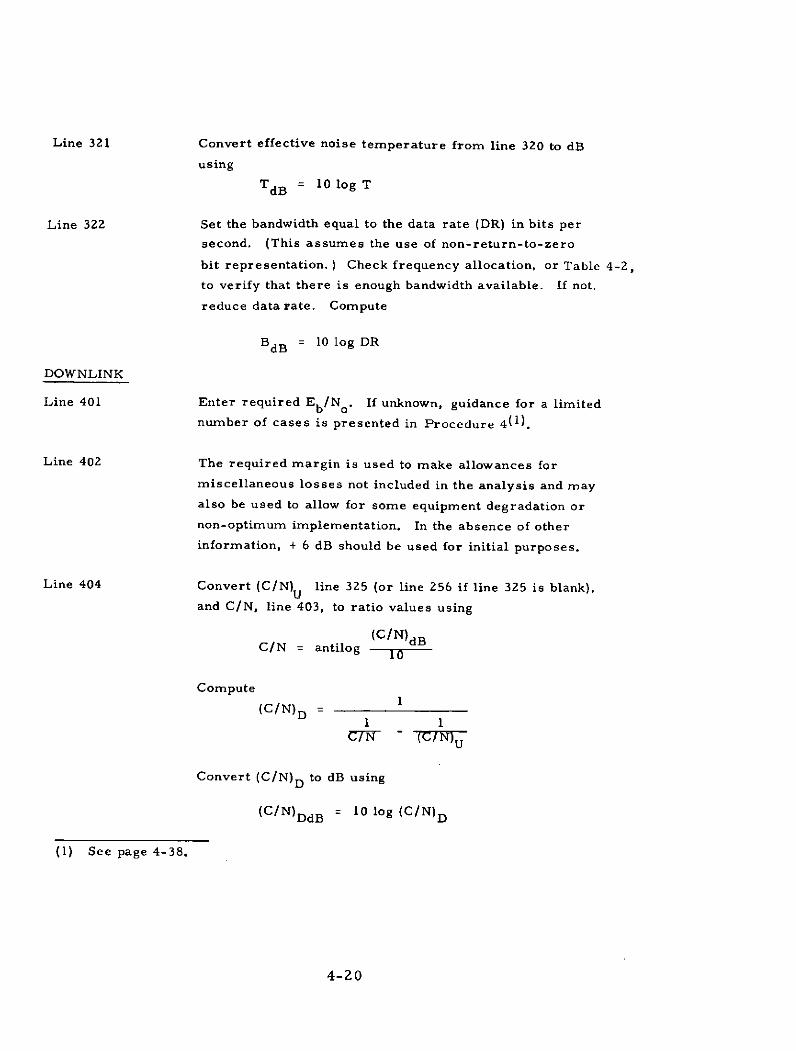
Line 321 Convert effective noise temperature from line 320 to dB
using
TdB = 10 log T
Line 322 Set the bandwidth equal to the data rate (DR) in bits per
second. (This assumes the use of non-return-to-zero
bit representation.) Check frequency allocation, or Table 4-2,to verify that there is enough bandwidth available. If not,
reduce data rate. Compute
BdB = 10 log DR
DOWNLINK
Line 401 Enter required Eb/N . If unknown, guidance for a limited
number of cases is presented in Procedure 4(1)
Line 402 The required margin is used to make allowances for
miscellaneous losses not included in the analysis and may
also be used to allow for some equipment degradation or
non-optimum implementation. In the absence of other
information, + 6 dB should be used for initial purposes.
Line 404 Convert (C/N)U line 325 (or line 256 if line 325 is blank),
and C/N, line 403, to ratio values using
(C/N)dBC/N = antilog Cn
Compute
(C/N)D1 1
C71 (C/N) U
Convert (C/N)D to dB using
(C/N)DdB = 10 log (C/N)D
(1) See page 4-38.
4-20
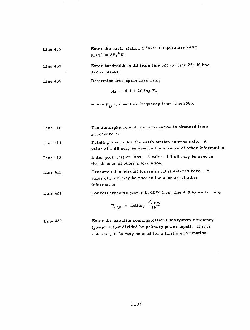
Line 406 Enter the earth station gain-to-temperature ratio
(G/T) in dB/oK.
Line 407 Enter bandwidth in dB from line 322 (or line 254 if line
322 is blank).
Line 409 Determine free space loss using
SL = 4 . 1 + 20 log F D
where FD is downlink frequency from line 208b.
Line 410 The atmospheric and rain attenuation is obtained from
Procedure 3.
Line 411 Pointing loss is for the earth station antenna only. A
value of 1 dB may be used in the absence of other information.
Line 412 Enter polarization loss. A value of 3 dB may be used in
the absence of other information.
Line 415 Transmission circuit losses in dB is entered here. A
value of 2 dB may be used in the absence of other
information.
Line 421 Convert transmit power in dBW from line 420 to watts using
dBWPTW = antilog Pd
Line 422 Enter the satellite communications subsystem efficiency
(power output divided by primary power input). If it is
unknown, 0.20 may be used for a first approximation.
4-21
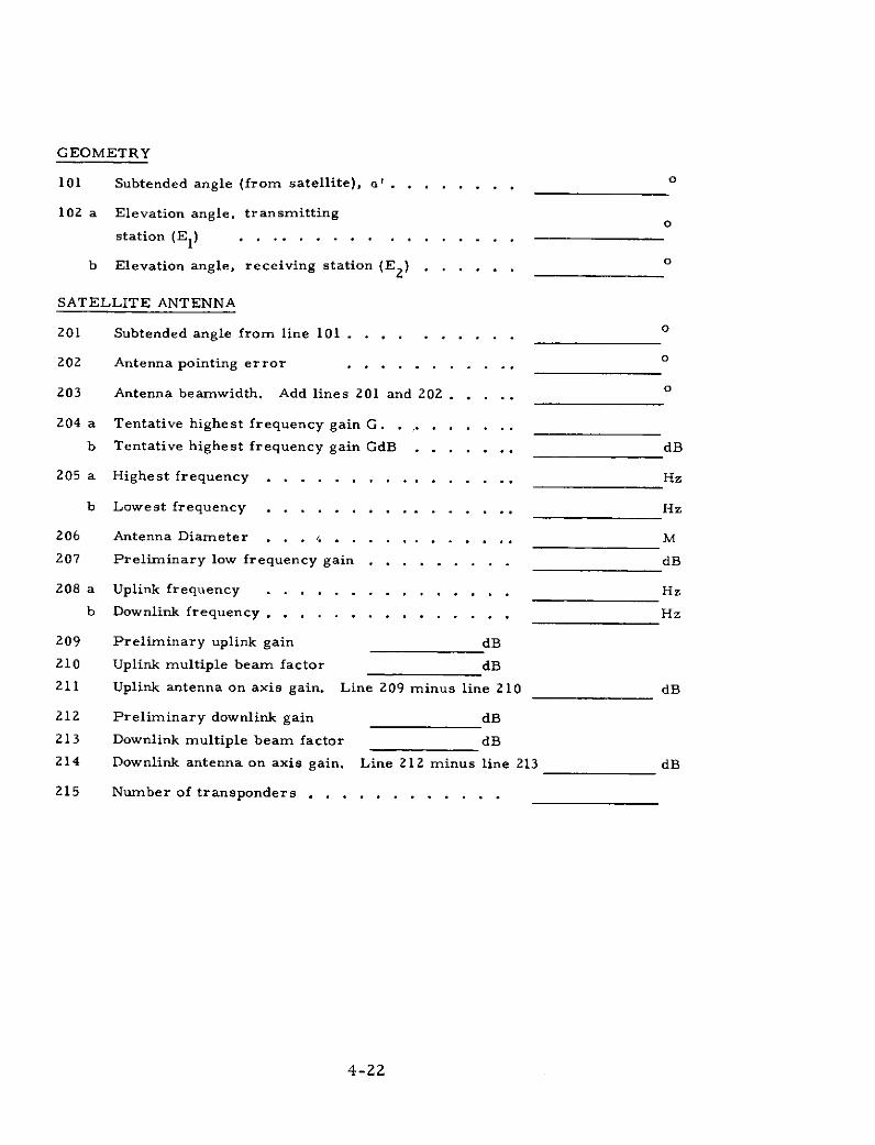
GEOMETRY
101 Subtended angle (from satellite), a' ........ o
102 a Elevation angle, transmittingo
station (E 1) . . .. . . . . . . . . . . . . .
b Elevation angle, receiving station (E2) ...... o
SATELLITE ANTENNA
201 Subtended angle from line 101 . . . .. .... o
202 Antenna pointing error . . . . . . . . . .o.
203 Antenna beamwidth. Add lines 201 and 202 . . . .. o
204 a Tentative highest frequency gain G. . .. . . . . ..
b Tentative highest frequency gain GdB .. . . . .. dB
205 a Highest frequency . .... . . . ......... . Hz
b Lowest frequency .............. .... Hz
206 Antenna Diameter . .. . . . . . . . . . .. M
207 Preliminary low frequency gain . . . . . . . . . dB
208 a Uplink frequency ................ Hz
b Downlink frequency ....... ....... . Hz
209 Preliminary uplink gain dB
210 Uplink multiple beam factor dB
211 Uplink antenna on axis gain. Line 209 minus line 210 dB
212 Preliminary downlink gain dB
213 Downlink multiple beam factor dB
214 Downlink antenna on axis gain. Line 212 minus line 213 dB
215 Number of transponders . . . . . . . . . . . .
4-22
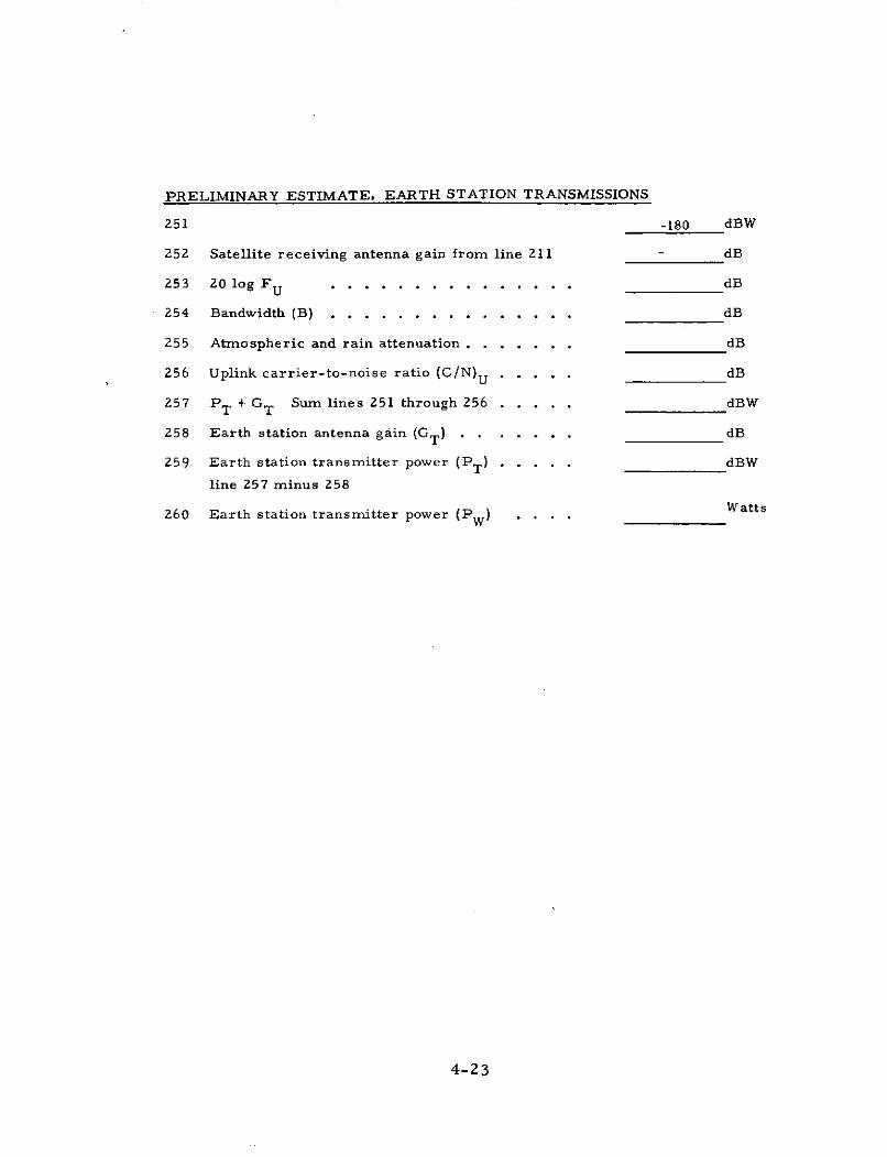
PRELIMINARY ESTIMATE, EARTH STATION TRANSMISSIONS
251 -180 dBW
252 Satellite receiving antenna gain from line 211 - dB
253 20 log F U .. .. ... .... .. .. dB
254 Bandwidth (B) ................ dB
255 Atmospheric and rain attenuation . . . . . .. dB
256 Uplink carrier-to-noise ratio (C/N)U . .. . . dB
257 PT + GT Sum lines 251 through 256 .... . dBW
258 Earth station antenna gain (GT) . ..... . dB
259 Earth station transmitter power (PT) . . . . . dBW
line 257 minus 258
260 Earth station transmitter power (PW) . . . . Watts
4-23
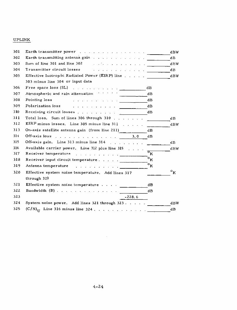
UPLINK
301 Earth transmitter power . . .. .. . .. .. . . . . . dBW
302 Earth transmitting antenna gain . . .. . .. . . . . ... dB
303 Sum of line 301 and line 302 . ... .. . . .... . dBW
304 Transmitter circuit losses . . .. .. . . . . .. . dB
305 Effective Isotropic Radiated Power (EIRP) line ... . . dBW
303 minus line 304 or input data
306 Free space loss (SL) . . .... . .. .. . dB
307 Atmospheric and rain attenuation ' dB
308 Pointing loss .......... dB
309 Polarization loss . ......... dB
310 Receiving circuit losses . . . . . . . . dB
311 Total loss. Sum of lines 306 through 310 ... . .. .. dB
312 EIRP minus losses. Line 305 minus line 311 ..... dBW
313 On-axis satellite antenna gain (from line 211) dB
314 Off-axis loss . . . . . . . . . 3. 0 dB
315 Off-axis gain. Line 313 minus line 314 . . . . . . dB
316 Available carrier power. Line 312 plus line 315 . . . . dBW317 Receiver temperature . . . . . . .... K
318 Receiver input circuit temperature ..... OK
319 Antenna temperature . . . . . . . . . OK
320 Effective system noise temperature. Add lines 317 OK
through 319
321 Effective system noise temperature . . .. dB
322 Bandwidth (B) . .. ... .. . .... . dB
323 -228. 6
324 System noise power. Add lines 321 through 323 . .. . dBW
325 (C/N) U Line 316 minus line 324 . ... ..... . . .. dB
4-24
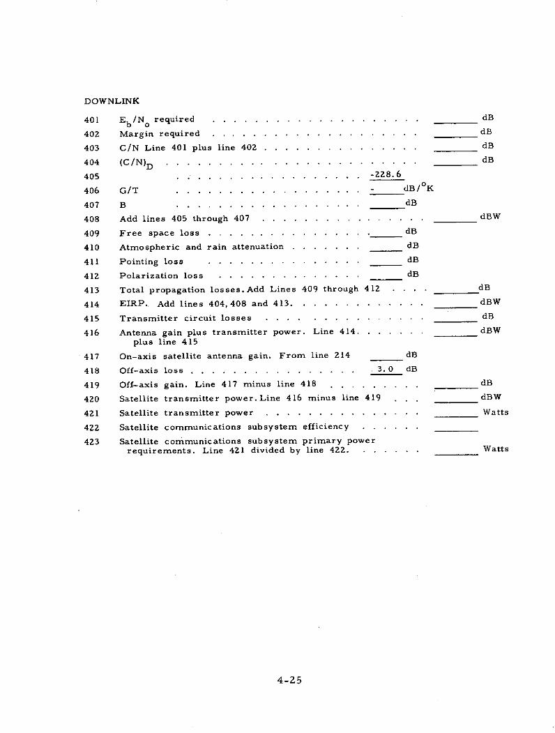
DOWNLINK
401 Eb/N0 required . . . . . . . . . . . . . . . . . . . . dB
402 Margin required . .. . . . . . . . . . . . . . . . . . dB
403 C/N Line 401 plus line 402 . .... . .. . ... ... dB
404 (C/N)D .......... ............. dB
405 . . . . . . . . . . . . . . . . . . -228.6
406 G/T . . . . . . . . . . . . . . .... dB/ K
407 B . . . . . . . . . . . . .. . .. . dB
408 Add lines 405 through 407 . . . . . . . ... . . .. . . dBW
409 Free space loss . . . ... . ... .... . dB
410 Atmospheric and rain attenuation . ...... . dB
411 Pointing loss ............... __ dB
412 Polarization loss . . . . . . . . . . . . . . dB
413 Total propagation losses. Add Lines 409 through 412 . . . . dB
414 EIRP.. Add lines 404,408 and 413 .... .... . . . . ... dBW
415 Transmitter circuit losses . . .. . . . . . . . . . . . dB
416 Antenna gain plus transmitter power. Line 414. .. . . . dBW
plus line 415
417 On-axis satellite antenna gain. From line 214 dB
418 Off-axis loss ............. ... 3.0 dB
419 Off-axis gain. Line 417 minus line 418 . . . . . . . . . dB
420 Satellite transmitter power.Line 416 minus line 419 . . . dBW
421 Satellite transmitter power . ........... . ... Watts
422 Satellite communications subsystem efficiency ......
423 Satellite communications subsystem primary power
requirements. Line 421 divided by line 422. ...... Watts
4-25
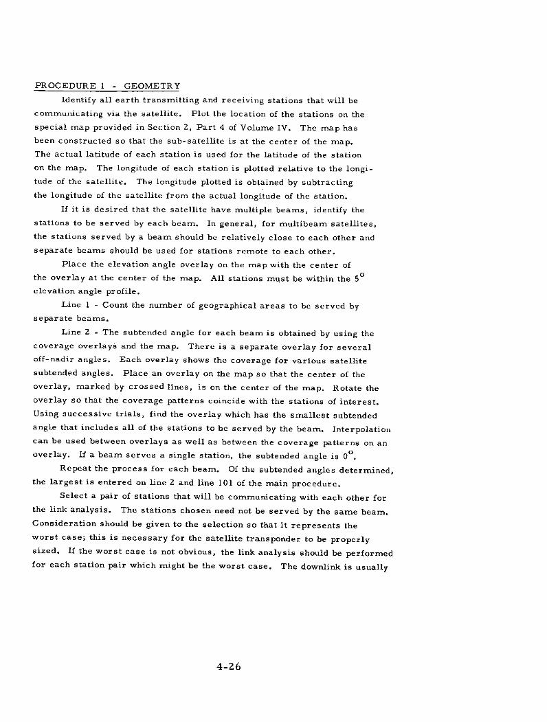
PROCEDURE 1 - GEOMETRY
Identify all earth transmitting and receiving stations that will be
communicating via the satellite. Plot the location of the stations on the
special map provided in Section 2, Part 4 of Volume IV. The map has
been constructed so that the sub-satellite is at the center of the map.
The actual latitude of each station is used for the latitude of the station
on the map. The longitude of each station is plotted relative to the longi-
tude of the satellite. The longitude plotted is obtained by subtracting
the longitude of the satellite from the actual longitude of the station.
If it is desired that the satellite have multiple beams, identify the
stations to be served by each beam. In general, for multibeam satellites,
the stations served by a beam should be relatively close to each other and
separate beams should be used for stations remote to each other.
Place the elevation angle overlay on the map with the center of
the overlay at the center of the map. All stations must be within the 50
elevation angle profile.
Line 1 - Count the number of geographical areas to be served by
separate beams.
Line 2 - The subtended angle for each beam is obtained by using the
coverage overlays and the map. There is a separate overlay for several
off-nadir angles. Each overlay shows the coverage for various satellite
subtended angles. Place an overlay on the map so that the center of the
overlay, marked by crossed lines, is on the center of the map. Rotate the
overlay so that the coverage patterns coincide with the stations of interest.
Using successive trials, find the overlay which has the smallest subtended
angle that includes all of the stations to be served by the beam. Interpolation
can be used between overlays as well as between the coverage patterns on an
overlay. If a beam serves a single station, the subtended angle is 00
Repeat the process for each beam. Of the subtended angles determined,
the largest is entered on line 2 and line 101 of the main procedure.
Select a pair of stations that will be communicating with each other for
the link analysis. The stations chosen need not be served by the same beam.
Consideration should be given to the selection so that it represents the
worst case; this is necessary for the satellite transponder to be properly
sized. If the worst case is not obvious, the link analysis should be performed
for each station pair which might be the worst case. The downlink is usually
4-26
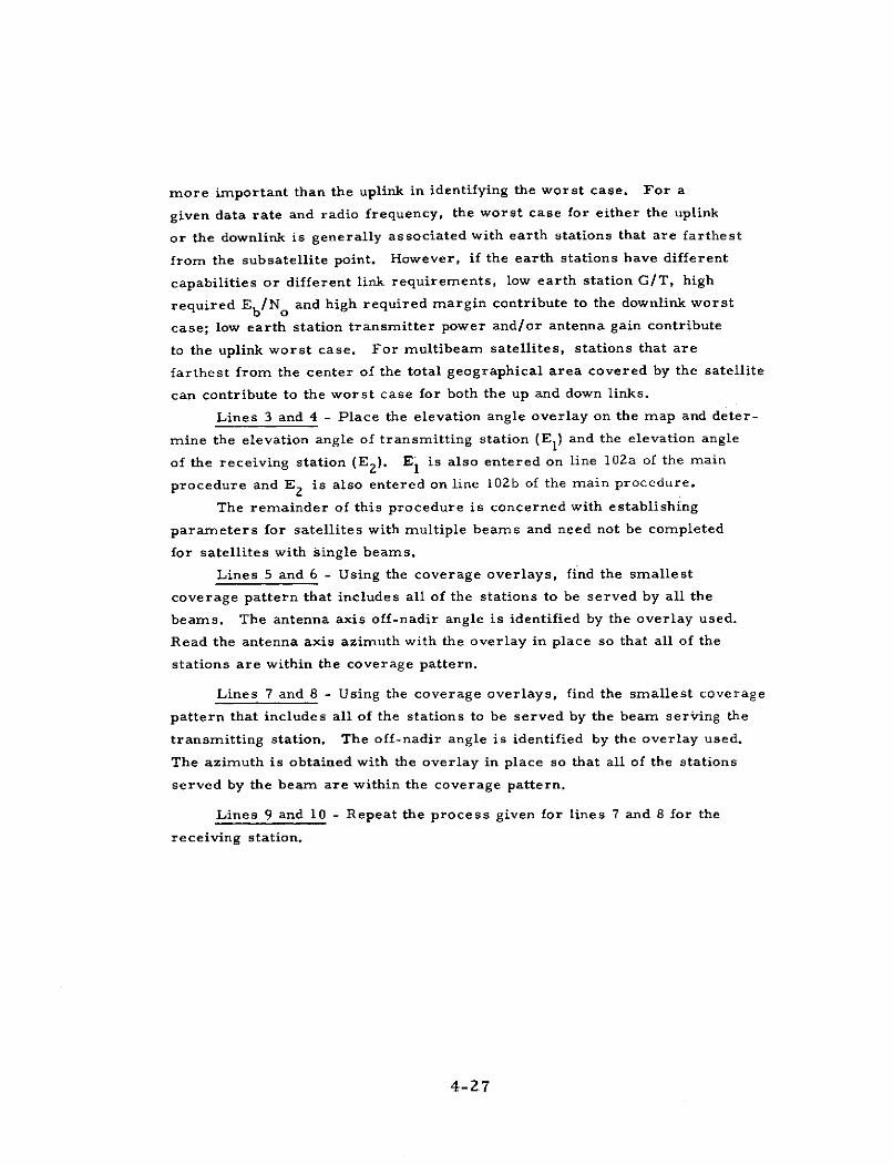
more important than the uplink in identifying the worst case. For a
given data rate and radio frequency, the worst case for either the uplink
or the downlink is generally associated with earth stations that are farthest
from the subsatellite point. However, if the earth stations have different
capabilities or different link requirements, low earth station G/T, high
required Eb/N and high required margin contribute to the downlink worst
case; low earth station transmitter power and/or antenna gain contribute
to the uplink worst case. For multibeam satellites, stations that are
farthest from the center of the total geographical area covered by the satellite
can contribute to the worst case for both the up and down links.
Lines 3 and 4 - Place the elevation angle overlay on the map and deter-
mine the elevation angle of transmitting station (E 1) and the elevation angle
of the receiving station (E 2 ). El is also entered on line 102a of the main
procedure and E 2 is also entered on line 102b of the main procedure.
The remainder of this procedure is concerned with establishing
parameters for satellites with multiple beams and need not be completed
for satellites with single beams.
Lines 5 and 6 - Using the coverage overlays, find the smallest
coverage pattern that includes all of the stations to be served by all the
beams. The antenna axis off-nadir angle is identified by the overlay used.
Read the antenna axis azimuth with the overlay in place so that all of the
stations are within the coverage pattern.
Lines 7 and 8 - Using the coverage overlays, find the smallest coverage
pattern that includes all of the stations to be served by the beam serving the
transmitting station. The off-nadir angle is identified by the overlay used.
The azimuth is obtained with the overlay in place so that all of the stations
served by the beam are within the coverage pattern.
Lines 9 and 10 - Repeat the process given for lines 7 and 8 for the
receiving station.
4-27

PROCEDURE I - GEOMETRY
1. Number of geographical areas N ................
2. Subtended angle a ' .......................... o
3. Elevation angle, transmitting station E 1 .. ........ o
4. Elevation angle, receiving station E 2 . . . . . .. . . . . . . . . o
5. Antenna axis off-nadir angle ON0 . .............. o
6. Antenna axis azimuth AZ .................... o
7. Uplink beam off-nadir angle ON 1 . .............. o
8. Uplink beam azimuth AZ 1 .. . . . . . . . . . . . . . .. . . . . o
9. Downlink beam off-nadir angle ON 2 . . . . . . . . . . . . . . o
10. Downlink beam azimuth AZ 2 . . .. . . . . . . . . . . . . . . . o
4-28

PROCEDURE 2 - MULTIPLE BEAM FACTOR
This procedure provides the means of establishing an estimate of
antenna gain degradation due to the use of multiple beams. It is based
on a focal length-to-diameter ratio of 0. 5 and an aperture illumination
taper of 10 dB, which are considered satisfactory for general sizing
purposes. However, if there is a reason to use other values for these
parameters, other methods must be employed for accurate results. The
procedure is also based on the assumption that the beamwidth of the satellite
antenna is the same for both the uplink and downlink. This will provide
reasonable results for the usual situation with the uplink and downlink
frequencies relatively close to each other. If the uplink and downlink
frequencies are widely separated, the procedure should be changed for
accurate results.
Line 1 - Compute the scan angle
1= cos sin ON 1 sin ON cos (AZ - AZ )L 1 o] l o
+ cos ON1 cos ON]
where ON , AZo, ON1, and AZ 1 are from lines 5, 6, 7,and 8 of Procedure 1.
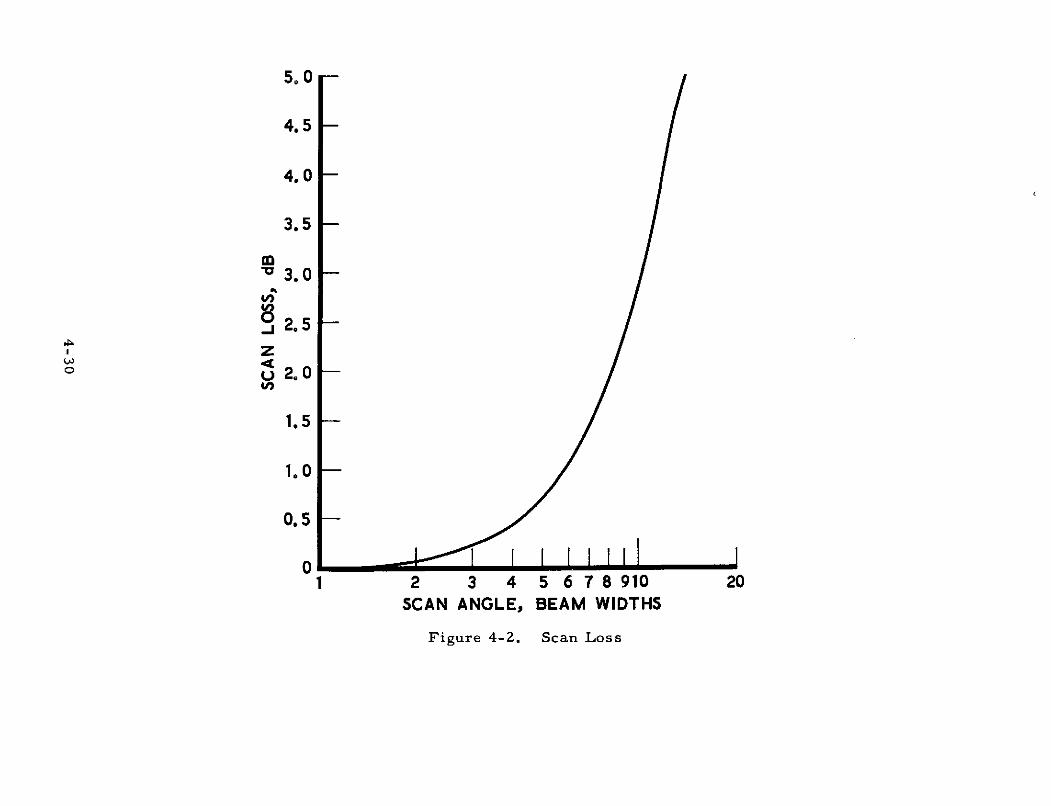
Line 2 - Divide the scan angle on line 1 by the antenna beamwidth
from the main procedure line 203.
Line 3 - The scan angle from line 2 is used with Figure 4-2 to
determine the scan loss.
Line 4a - The number of geographical areas served appears on line 1
of Procedure 1. Determinethe maximum number of these areas which
contain stations that will communicate via the satellite simultaneously --
this is,the number of antenna beams.
4-29
5.0
4.5 -
4.0 -
3.5 -
S3.0 -
2.5z
2.0 -
1.5 -
1.0 -
0.5 -
01 2 3 4 5 6 7 8 910 20
SCAN ANGLE, BEAM WIDTHS
Figure 4-2. Scan Loss
Line 4 b - Determine the maximum number of areas that contain
stations that will be receiving simultaneously -- this is the number of
transponders. Also enter on line 215 of the main procedure.
Line 5 - Compute
d 3x10⁸ /n
n from line 4a
D from main procedure line 206
F U from main procedure line 208a
Line 6 - The value of d/D from line 5 is used with Figure 4-3
to determine the blockage loss.
Line 7 - The uplink multiple beam factor is obtained by adding the
values on lines 3 and 6. This value is also entered in main procedure line
210.
Line 21 - Compute the scan angle
= cos-1 sin ON 2 sin ON cos (AZ 2 - AZo
+ cos ON 2 cos ON]
where ON o , AZ o , ON 2 , and ON 2 are from lines 5, 6, 9,
and 10 of Procedure 1.
Line 22 - Divide the scan angle on line 21 by the antenna beamwidth
from the main procedure line 203.
Line 23 - The scan angle from line 22 is used with Figure 4-2 to
determine the scan loss.
Line 25 - The downlink multiple beam factor is obtained by adding the
values on lines 23 and 24. This value is also entered on main procedure line
213.
4-31
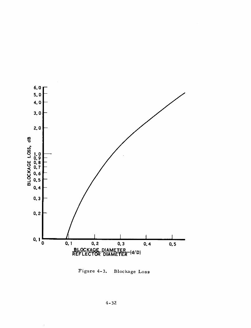
6.0
5.0 -
4.0 -
3.0 -
2. 0
0.0. 08-
0. -0.6
I 0.5
0.4
0. 3
0. 2
0. 10 0.1 0.2 0.3 0.4 0.5
BLOCKAGE DIAMETERREFLECTOR DIAMETER (d/D)
Figure 4-3. Blockage Loss
4-32
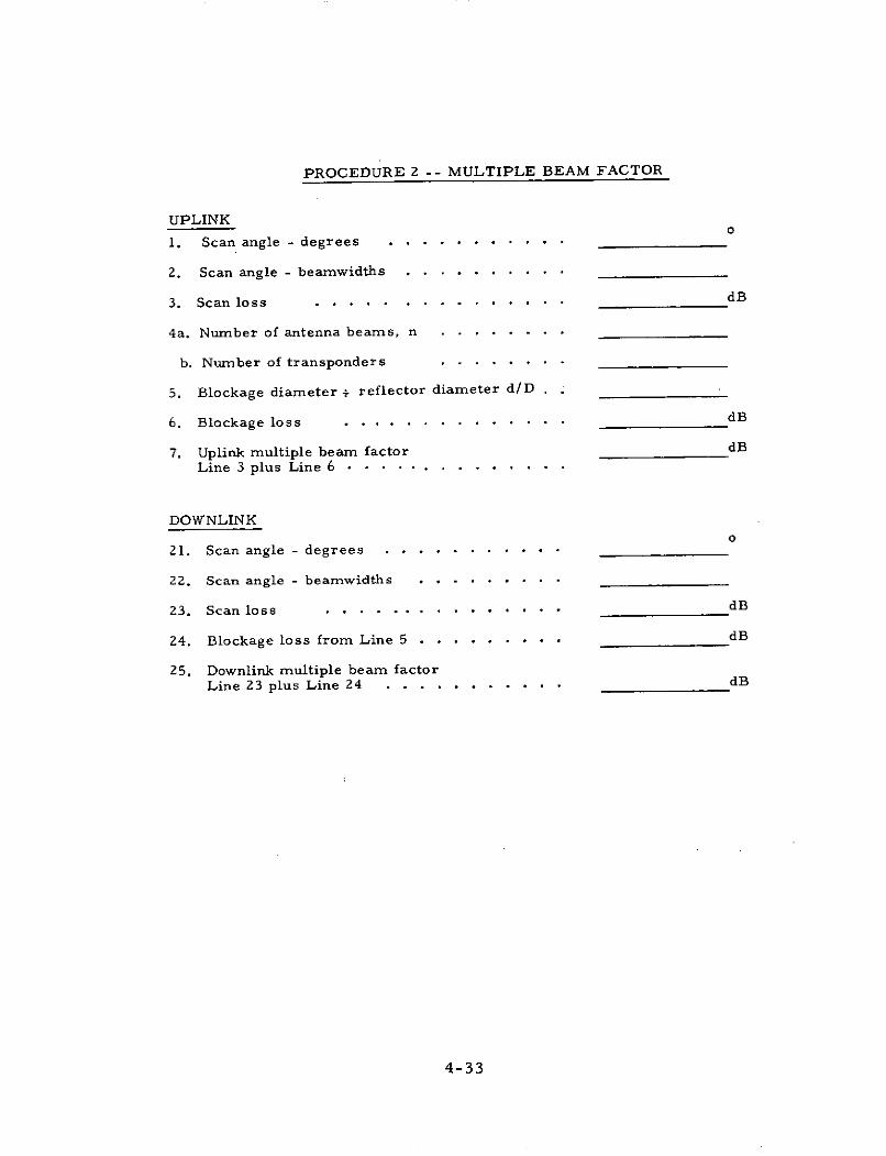
PROCEDURE 2 -- MULTIPLE BEAM FACTOR
UPLINK
1. Scan angle - degrees . . . .......... 0
2. Scan angle - beamwidths . . . . . . . . . .
3. Scan loss . . . . . . . . . . . . . . .dB
4a. Number of antenna beams, n . . . . . . . .
b. Number of transponders . . .......
5. Blockage diameter + reflector diameter d/D . .
6. Blockage loss ..... .......... dB
7. Uplink multiple beam factor dBLine 3 plus Line 6 .... .... ......
DOWNLINKo
21. Scan angle - degrees . . . .......... 0
22. Scan angle - beamwidths . . . . . . . ..
23. Scan loss .... ... ... . * * *... dB
24. Blockage loss from Line 5 . .... ... . . dB
25. Downlink multiple beam factorLine 23 plus Line 24 . . . . . . . . . . . dB
4-33
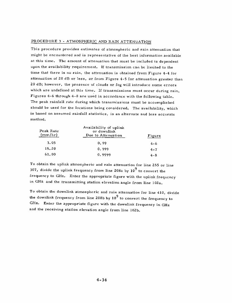
PROCEDURE 3 - ATMOSPHERIC AND RAIN ATTENUATION
This procedure provides estimates of atmospheric and rain attenuation that
might be encountered and is representative of the best information available
at this time. The amount of attenuation that must be included is dependent
upon the availability requirement. If transmission can be limited to the
time that there is no rain, the attenuation is obtained from Figure 4-4 for
attenuation of 20 dB or less, or from Figure 4-5 for attenuation greater than
20 dB; however, the presence of clouds or fog will introduce some errors
which are undefined at this time. If transmissions must occur during rain,
Figures 4-6 through 4-8 are used in accordance with the following table.
The peak rainfall rate during which transmissions must be accomplished
should be used for the locations being considered. The availability, which
is based on assumed rainfall statistics, is an alternate and less accurate
method.
Availability of uplinkPeak Rate or downlink(mm/hr) Due to Attenuation Figure
3.05 0.99 4-6
15.20 0. 999 4-7
61.00 0.9999 4-8
To obtain the uplink atmospheric and rain attenuation for line 255 or line
307, divide the uplink frequency from line 208a by 109 to convert the
frequency to GHz. Enter the appropriate figure with the uplink frequency
in GHz and the transmitting station elevation angle from line 102a.
To obtain the downlink atmospheric and rain attenuation for line 410, divide
the downlink frequency from line 208b by 109 to convert the frequency toGHz. Enter the appropriate figure with the downlink frequency in GHzand the receiving station elevation angle from line 102b.
4-34
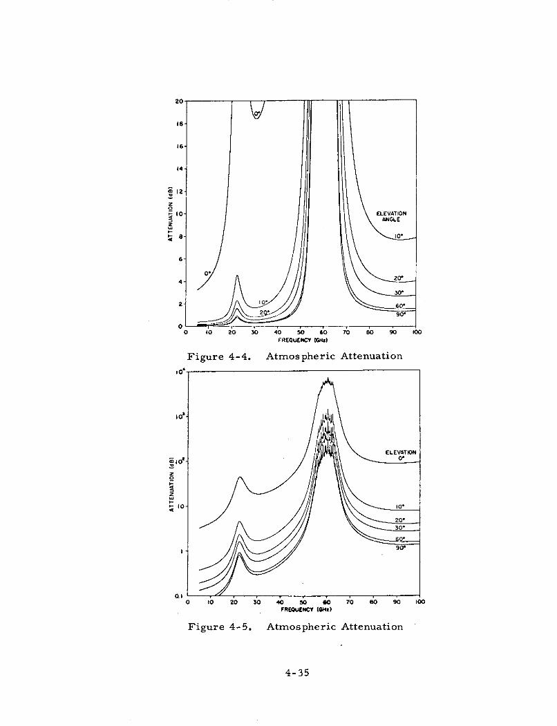
20
18
16
14-
8 12-z0
Io- ELEVATIONANGLE
a. 110,
6-
0*4- 20,
30so*
90,
00 10 20 30 40 0 o60 70 80 90 100
FREQUENCY IGHa)
Figure 4-4. Atmospheric Attenuation
10'
ELEVATION
lo- 10,
20"30'
90,
0-O 10 20 30 0 0 *o 80 90 too
FREQUENCY (GHM)
Figure 4-5. Atmospheric Attenuation
4-35
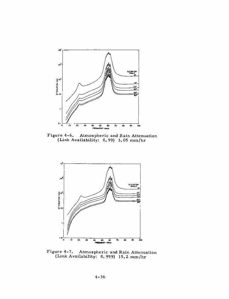
10,
,0,
0 1
FREQUENCY (Gi)
Figure 4-6. Atmospheric and Rain Attenuation(Link Availability: 0. 99) 3. 05 mm/hr
.10
ELEVATIONANGLE
10
I2
1.0
0 O 10 20 30 40 SO 60 TO7 s0 90 100FJC ENCY (GM)
Figure 4-7. Atmospheric and Rain Attenuation(Link Availability: 0. 999) 15. 2 mm/hr
4-36
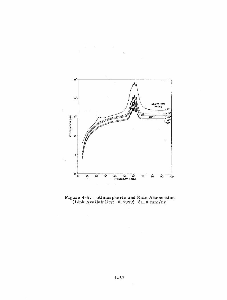
O- -
ELEVATIONANGLE
o00I-IO
o U
I
0-0 10 20 30 40 5O 60 70 80 90 100
FREQUEKCY (GHz)
Figure 4-8. Atmospheric and Rain Attenuation(Link Availability: 0. 9999) 61. 0 mm/hr
4-37
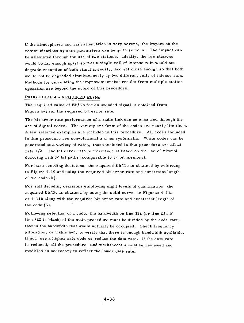
If the atmospheric and rain attenuation is very severe, the impact on the
communications system parameters can be quite serious. The impact can
be alleviated through the use of two stations. Ideally, the two stations
would be far enough apart so that a single cell of intense rain would not
degrade reception of both simultaneously, and yet close enough so that both
would not be degraded simultaneously by two different cells of intense rain.
Methods for calculating the improvement that results from multiple station
operation are beyond the scope of this procedure.
PROCEDURE 4 - REQUIRED Eb/No
The required value of Eb/No for an uncoded signal is obtained from
Figure 4-9 for the required bit error rate.
The bit error rate performance of a radio link can be enhanced through the
use of digital codes. The variety and form of the codes are nearly limitless.
A few selected examples are included in this procedure. All codes included
in this procedure are convolutional and nonsystematic. While codes can be
generated at a variety of rates, those included in this procedure are all at
rate 1/2. The bit error rate performance is based on the use of Viterbi
decoding with 32 bit paths (comparable to 32 bit memory).
For hard decoding decisions, the required Eb/No is obtained by referring
to Figure 4-10 and using the required bit error rate and constraint length
of the code (K).
For soft decoding decisions employing eight levels of quantization, the
required Eb/No is obtained by using the solid curves in Figures 4-11a
or 4 - lb along with the required bit error rate and constraint length of
the code (K).
Following selection of a code, the bandwidth on line 322 (or line 254 if
line 322 is blank) of the main procedure must be divided by the code rate;
that is the bandwidth that would actually be occupied. Check frequency
allocation, or Table 4-2, to verify that there is enough bandwidth available.
If not, use a higher rate code or reduce the data rate. If the data rate
is reduced, all the procedures and worksheets should be reviewed and
modified as necessary to reflect the lower data rate.
4-38
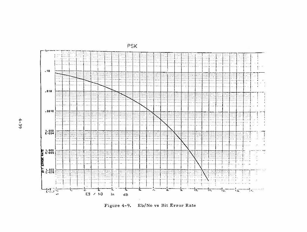
PSK.......... . .... ... .. .... .. . ........
...iji i~ j ... ... .. ... ......................................................................
.............................................................................................0 ... ....
- - - - - -- - - - - - - - - - - - - - - . ... ... .
E.0.. .... ....
.01.
..... .... .... ..... .... .. ..... .
I I~ - I - I
_._...._...._....
F r010 4-.. b/N v i r R
( - .... .... ......... ...... ...... ...... : * * 1:: ... .. ... . .. .. ....... ..... .. ......... .. .... ........... .. .... .... ....... .... ... .. ... .. .... ....... .... ..... ... ... .. .... ...... .... .... ... .... .. ..... ... .... ... .... .... ... .... . ... .... .... ..
, 11 : :::: : : :::: : ::: :: : :. . .. . . .. . . .. . . . . .. . . j -
E-004... . .. . .. .. . ... ...
... . .. .. . ... .... ....... ...... .. ... .. ...... .. ...... ...... .. ..I . .. ..... ... .. ...... ...... .. .... .... ... ... ...... .... .. ... ... ...... ... ... .. .... ...... ... ... ...... .. ... ...... ... ...
000 .. ........ ........ ... .. 17.
1.000C-006 .... ... i ..... .... .... .... .... .... .... .... ....
E-cas iiiiiif'.............. .... :::.. .... .... ... ..... .1 . . : . . .
....... .... .... .... ..--- ....1 . :
(..... .... .. .... ....
'9- Ak::t: :1:: - -- : : 11 - lt '~iiiE-~E9 NO in dB I '~'~'''' :::::i:\:I:'' .
::::I:Figure 4-9. Eb/ No vs Bit Error Rate~~
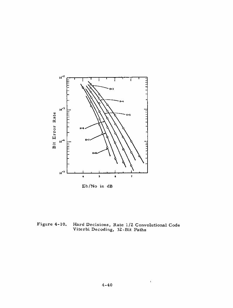
10-2
-K-3
o K
K-8
10I I I
Eb/No in dB
Figure 4-10. Hard Decisions, Rate 1/2 Convolutional CodeViterbi Decoding, 32-Bit Paths
4-40
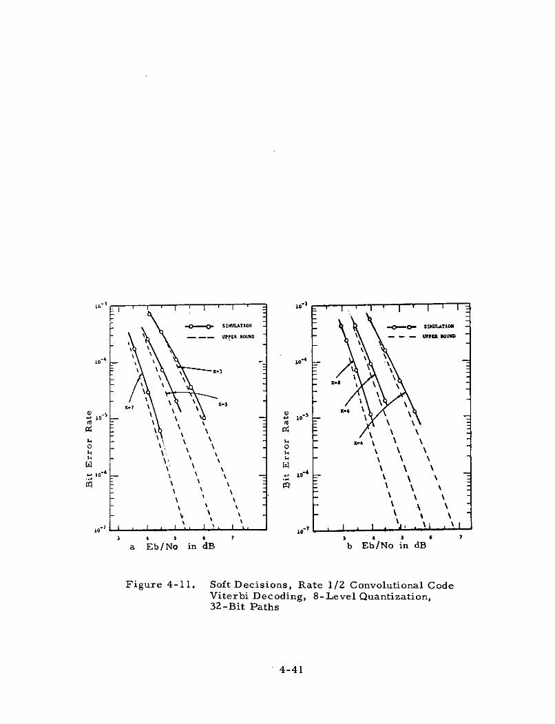
s-ot.-- . stUATIN0 -0-- SULATIoN
--- UPPER BOUND - - - UPPE 0DMD
10 10
S\
\ \ \
,, - o\ \
o" I I I I I I I os I \ 1 1
3 4 5 6 7
a Eb/No in dB b Eb/No in dB
Figure 4-11. Soft Decisions, Rate 1/2 Convolutional CodeViterbi Decoding, 8-Level Quantization,32-Bit Paths
4-41
2. EARTH OBSERVATION TYPE
The weight and power required for earth observation from a
low-altitude, multiuser, automated earth observation satellite is obtained
from the curves in this section. The mission equipment weight depends
on the year of initial operation (see Figure 4-12). The mission equipment
power required is related to the mission equipment weight (see Figure 4-13).
Mission equipment after 1980 can include active (future) sensors (e. g.,
radar and lidar) as well as the passive types of sensors. Multiuser earth
observation satellites are assumed to embody scanning and multiple band
radiometers, spectrometers, and mappers as well as advanced sensors.
4-42
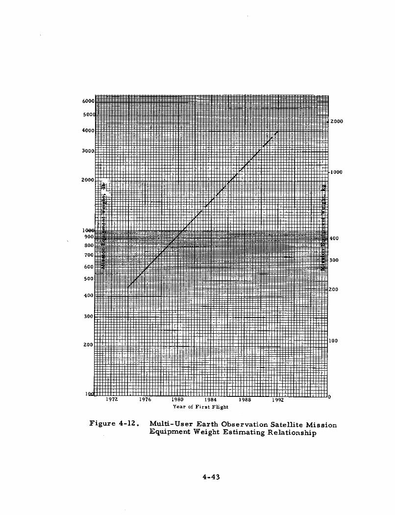
700
300
600
500
200
400
300
100
2000-- 1
00
001
500
1972 1976 1980 1984 1988 1992Year of First Flight
Figure 4-12. Multi-User Earth Observation Satellite MissionEquipment Weight Estimating Relationship
4-43
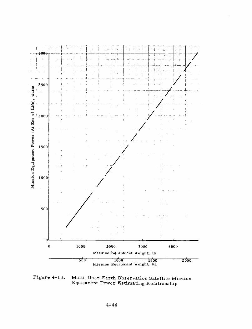
S . . . . . .. .LS- .-.- -.---- i .---i..
a 2000
, 1500
1000
500
1000 Z0 00 3000 4000
Mission Equipment Weight, lb
10 ot) 100 2000Mission Equipment Weight, kg
Figure 4-13. Multi-User Earth Observation Satellite MissionEquipment Power Estimating Relationship
4-44
C. SATELLITE SYNTHESIS
1. INTRODUCTION
The objective of the BRAVO Satellite Synthesis Program is to
generate satellite weights and other satellite data in a short time with
minimal input requirements. The basic inputs, such as orbit altitude,
if not known by the system user, may be estimated from data in the
Satellite System Definition section of this manual.
The synthesis program may also be readily used to perform
sensitivity and optimization studies of spacecraft as a function of such
basic parameters as electrical power producing capability.
This portion of the manual includes a description of the synthesis
program, a typical deck setup and operating instructions, the procedure
for using the workbook associated with this manual, and a typical example.
Also included is a discussion of the derivation of the program, the logic
used, and the development of the equations used therein. The applicable
limits of the program are identified.
2. SYNTHESIS PROGRAM OPERATION
a. Program Description
The Satellite Synthesis Program described herein has been
developed for use in the BRAVO and other NASA payload studies in the
FORTRAN IV language and is usable on various computers. Many of the
variables in the program are automatically accommodated by the use of
internal equations instead of requiring the operator to input values from
graphs. An example of this is the mean mission duration variable. By
inputting a specific value, or series of values, for this parameter the
correct influence is automatically produced. Insertion of the satellite
type on the input sheet (i. e., communication, navigation, or observation)
will result in the automatic selection of appropriate equation constants
within the computer program. Iterative subroutines are also automatic
in the program.
4-45
The computer develops subsystem weights and other pertinent
data as functions of the input parameters. It uses these computations to
generate the structure weight and size. Finally, the weight and length
of the adapter structure is computed. The printout itemizes these data.
A typical printout is included in Volume IV, Part 4 of this Final Report.
The synthesis program and the equations used therein were
developed in English rather than metric units and are presented here
in those units.
The development of the subsystem weight equations, Shuttle
application factors, and program logic is described in Paragraph 4
of this section of the Manual.
b. Instructions
The user operates the program by inputting basic data on one
of the input sheets supplied in the workbook. These data are used by
a programmer familiar with the synthesis program to prepare the eight
data input cards. These are placed in the card stack as shown in Figure 4-14
and the program is operated.
If the synthesis program is not operating in a service area
available to the user, a programmer experienced in the use of FORTRAN IV
language may set up the program using the listing included in the printout
in Volume IV, Part 4 of this Final Report.
A step-by-step procedure for operating the program and the
workbook is supplied in the following paragraphs.
3. PROGRAM OPERATING PROCEDURE
The steps outlined below will permit the user to operate the
synthesis program successfully. The workbook provided as Volume IV,
Part 3 of this Final Report is used as part of this procedure.
4-46
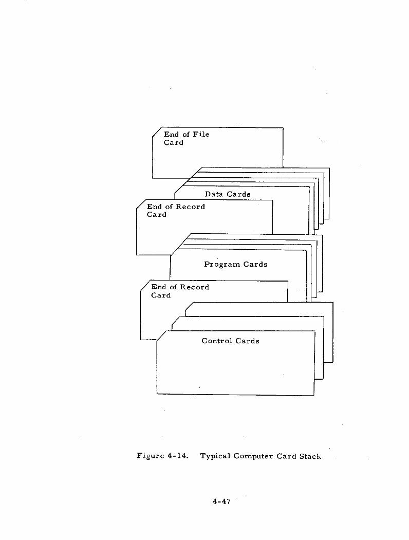
End of FileCard
Data Cards
End of RecordCard
Program Cards
End of RecordCard
Control Cards
Figure 4-14. Typical Computer Card Stack
4-47
a. Basic Inputs
Approximately 40 inputs are required to operate the program.
These include basic items such as orbit altitude and inclination, mission
equipment weight, volume and electrical power requirements, pointing
accuracy, etc.
b. Input Sources
Ideally the user will obtain satellite synthesis inputs from
the "Satellite System Definitions" and "Mission Equipment Definitions"
steps accomplished earlier in this analysis. Suggested values suitable
for preliminary operation of the program are, however, included in
this report in Table 4-4 for consideration by the user in case other values
have not been specified. Unusual mission equipment data could, of course,
be determined with the assistance of an expert familiar with the develop-
ment of that equipment.
c. Input Sheets
Copies of an input sheet identified as the "Satellite Synthesis
Program Input Sheet" are supplied in the Workbook (Volume IV, Part 3)
of this Final Report. All of the basic inputs must be listed on this sheet
for successful program operation.
The required locations for the basic input data on the input sheets
are identified on Figure 4-15 in computer symbol form. Sample input
values are shown on Figure 4-16 which is typical of a form ready for
key punching. The sample input values are consistent with the results
shown in the sample printout provided in Volume IV, Part 4, of this
report. A symbol list is given in Table 4-5. Blank copies of the form
in Figure 4-15 are supplied in the Workbook. As with most computer
input sheets, the input data must be carefully written as shown in the
sample sheet. Numbers must be placed within the correct 10-column
section and must include a decimal point. Letter symbols must be written
and placed exactly as shown as these words are used as tests (i. e.,
start in left side of section).
4-48

Table 4-4. System and Mission Basic Inputs forSatellite Synthesis Program
Note: May be used for first iteration analysis until user is able to identifybetter values.
Suggested Input
Attitude Control Type (STABTYP) = 3-Axis(Choices: single-body spin, dual-body spin or3-axis)
Structure Type (STRTYP) = EXO(Choices: EXO has solar cell array paddles orENDO has body-mounted solar cells)
Propellant Type (PROPTYP) = NoneFor auxiliary propulsion system for propulsivemaneuvers too large for the reaction controlsystem. (Choices: solid, liquid, none)
Type of Electrical Power Generation (PWRTYP) = Solar(Solar cell array is the design approach for allsatellites to be synthesized.)
Type of Solar Cell Orientation (ORINT) = Oriented(Choices: oriented or unoriented)
Auxiliary Propulsive Maneuver Velocity Require-ment (ft/sec) (DVI) = Zero(If-none" specified in PROPTYP)
Type of ACS Propellant (ACSPROP) = Hot Gas(Choices: hot gas or cold gas)
Number of Tape Recorders in CDPI (XNTAPRC) = As Required
Number of Down Links in CDPI (XNDNLNK) = 1.0
4-49
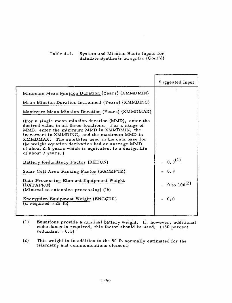
Table 4-4. System and Mission Basic Inputs forSatellite Synthesis Program (Cont'd)
Suggested Input
Minimum Mean Mission Duration (Years) (XMMDMIN)
Mean Mission Duration Increment (Years) (XMMDINC)
Maximum Mean Mission Duration (Years) (XMMDMAX)
(For a single mean mission duration (MMD), enter thedesired value in all three locations. For a range ofMMD, enter the minimum MMD in XMMDMIN, theincrement in XMMDINC, and the maximum MMD inXMMDMAX. The satellites used in the data base forthe weight equation derivation had an average MMDof about Z. 5 years which is equivalent to a design lifeof about 3 years.)
Battery Redundancy Factor (REDUN) = 0.0 ( 1 )
Solar Cell Area Packing Factor (PACKFTR) = 0. 9
Data Processing Element Equipment Weight(DATAPR() = 0 to 100 ( 2 )
(Minimal to extensive processing) (lb)
Encryption Equipment Weight (ENCODR) = 0.0(if required = 25 lb)
(1) Equations provide a nominal battery weight. If, however, additionalredundancy is required, this factor should be used. (+50 percentredundant = 0.5)
(2) This weight is in addition to the 50 lb normally estimated for thetelemetry and communications element.
4-50
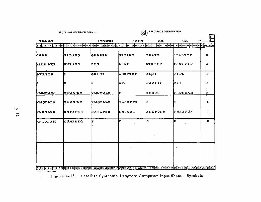
65 COLUMN KEYPUNCH FORM - 1 AEROSPACE CORPORATION
PROGRAMMER KEYPUNCHED VERIFIED _ DATE PAGE OF IL1123 14 5 16 7 1 1112131 11617192 21 2324 25 272829 3132333435 3637 6941 2 43445 46 1 2 154 5561 62 63 64 6
CODE 0R:BAPO ORBPER ORBI NC PBATF STABTYP 1
XMI5 PWR PNTACC DEN X i0c STRTYP PROPTYP
PW1TYP S ORI NT ACSPROP XMEI TYPE -3
A B C CFI PADTYP DVI 4
_MMDMIN X'MMDINC XMMDMAX R REDUN PROGRAM s
XMODMIN XMODINC XMODMAX PACKFTR D T 6
KNDNLNK XNTAPRC DATAPRO ENCODR XNXPOND PWRXPON 7
NTDIAM COMFREQ E F G H 8
1 2 3 4 5 6 7 i8 9 10 11112 13'14 15116!17 18119 20 122 232425 26 27 2829 1 323334513637 38 3940 41i42i43 44i45i4647i48i49 50 51 5253 54 5556 575859 6 663
AER Figure 4-15 Satellite SynthesiOSPAC Program ComputerFOR 4123
Figure 4-15. Satellite Synthesis Program Computer Input Sheet - Symbols
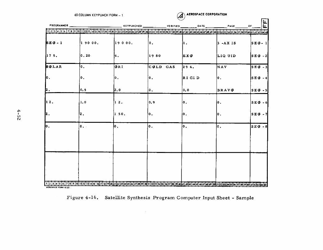
65 COLUMN KEYPUNCH FORM - 1 AEROSPACE CORPORATION
PROGRAMMER KEYPUNCHED VERIFIED DATE PAGE OF
1 2 3 14 $6 718 9 10 11112 131 1415 16 17 1811920 21 22 2324 25126 27 2829 30 313233343536313839 41 42 43 44 4546471489 50 512 53 545556 575859 6 16263 64
5EQ - 1 1 90 00. 19 0 00. 0. 1. 3 -AX IS SEQ- 1
17 5. 0. 20 4. 19 80 EXQ LIQ UID SEQ -2
SQLAR 0. ORI COLD GAS 29 4. NAV SEQ -3
0. 0. 0. 0. RI GI D 0. SEQ -4
2. 0.5 2.0 0. 0.0 BRAVQ SEQ -5
12. 1.0 1 2. 0.9 0. 0. SEQ -6
2. 2. 1 50. 0. 0. 0. SEQ -7
0. 0. 0. 0. 0. 0. SEQ -8
1 12 34 15 6 7 8 9 10111121314151617181 222324252627 2829 3132 33 234 235 36 37 38 39 40 4142 3U 45 46147W 50 5 2 2'55411IS 5 571515596 6, 3AEROSPACE FORM 4123
Figure 4-16. Satellite Synthesis Program Computer Input Sheet - Sample
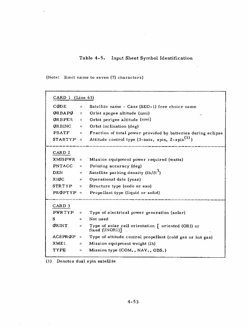
Table 4-5. Input Sheet Symbol Identification
(Note: limit name to seven (7) characters)
CARD 1 (Line 63)
CODE = Satellite name - Case (SEO-1) free choice name
ORBAPO = Orbit apogee altitude (nmi)
ORBPER = Orbit perigee altitude (nmi)
ORBINC = Orbit inclination (deg)
PBATF = Fraction of total power provided by batteries during eclipse
STABTYP = Attitude control type (3-axis, spin, 2 -spin ( 1 ) )
CARD 2
XMISPWR = Mission equipment power required (watts)
PNTACC = Pointing accuracy (deg)
DEN = Satellite packing density (lb/ft3)
XIOC = Operational date (year)
STRTYP = Structure type (endo or exo)
PROPTYP = Propellant type (liquid or solid)
CARD 3
PWRTYP = Type of electrical power generation (solar)
S = Not used
ORINT = Type of solar cell orientation [ oriented (ORI) orfixed (UNORI)]
ACSPROP = Type of attitude control propellant (cold gas or hot gas)
XME1 = Mission equipment weight (lb)
TYPE = Mission type (COM., NAV., OBS.)
(1) Denotes dual spin satellite
4-53
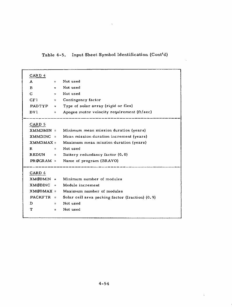
Table 4-5. Input Sheet Symbol Identification (Cont'd)
CARD 4
A = Not used
B = Not used
C = Not used
CF1 = Contingency factor
PADTYP = Type of solar array (rigid or flex)
DVI = Apogee motor velocity requirement (ft/sec)
CARD 5
XMMDMIN = Minimum mean mission duration (years)
XMMDINC = Mean mission duration increment (years)
XMMDMAX = Maximum mean mission duration (years)
R = Not used
REDUN = Battery redundancy factor (0. 0)
PROGRAM = Name of program (BRAVO)
CARD 6
XMODMIN = Minimum number of modules
XMODINC = Module increment
XMODMAX = Maximum number of modules
PACKFTR = Solar cell area packing factor (fraction) (0. 9)
D = Not used
T = Not used
4-54
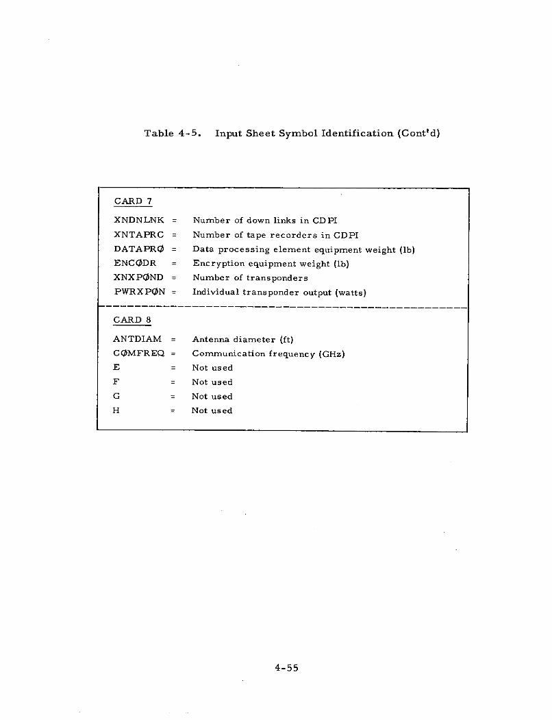
Table 4-5. Input Sheet Symbol Identification (Cont'd)
CARD 7
XNDNLNK = Number of down links in CDPI
XNTAPRC = Number of tape recorders in CDPI
DATAPRO = Data processing element equipment weight (ib)
ENCODR = Encryption equipment weight (ib)
XNXPOND = Number of transponders
PWRXPON = Individual transponder output (watts)
----------------------------------------------------
CARD 8
ANTDIAM = Antenna diameter (ft)
COMFREQ = Communication frequency (GHz)
E = Not used
F = Not used
G = Not used
H = Not used
4-55
d. Data Input Cards
An experienced programmer transfers the data from the input
sheets to the data cards and places them in the stack as shown in Figure 4-14.
The program is then operated. The user need not be involved in this
operation.
e. Results
The results of the computation are tabulated at the end of the
printout and are readable without the assistance of the programmer. A
sample printout which reflects the data shown on the input sheet, Figure
4-16, is provided in Volume IV, Part 4, of this Final Report. The user
evaluates the results and then, if desired, re-operates the program
with different values using new input sheets. Results may be plotted to
depict trends. The selected data are now available for input to the
Satellite Cost Analysis Program.
f. Limits
The parameters used in the Satellite Synthesis Program reflect
experience of existing satellite programs and extending values for them
beyond these delineated limits will reduce the accuracy of the results.
Satellite weight = not over 11, 340 kg (25, 000 lb)
Electrical power = not more than 5000 watts
Design life = not to exceed 10 years
Pointing accuracy = not less than 0.01 deg
Transponder power output = not more than 300 watts each
Antenna diameter (D , feet) 0 5 2.5F 0
D = not more than 10, 000Antenna frequency (F, GHz) a
4-56
Also, when items are incremented (such as XMMD on Card 5
and XMOD on Card 6), the following rules must be observed:
(1) XMMDMIN (value may be zero)
(2) XMMDINC (value must not be zero)
(3) XMMDMAX (value as required)
If only one MMD period (2 years) is required (as in the example
of Figure 4-16) use:
(1) XMMDMIN = 2. 0 years
(2) XMMDINC = 0.5 years
(3) XMMDMAX = 2. 0 years
The system used is that the computer adds the incremental time
(0. 5) to the minimum time (2. 0) for a total of 2. 5. It compares this to
the maximum time (2. 0) and since the 2. 5 year total is greater than the
maximum time (2.0 years) required, the program goes on to the next
case. If, however, the incremental time (XMMDINC) is inadvertently
entered as zero, then the sum of the minimum time (2. 0), plus the incre-
ment (0. 0), will never be longer than the maximum (2. 0) and the computer
will continue to perform the same calculation until a built-in time limit
is reached which will terminate the run.
It should also be noted that a normal communication satellite
will have either mission equipment (XME1, Card 3) or an antenna (ANTDIAM,
Card 7) and a transponder (XNXPOND, Card 7), but not both.
Also note, the satellite packing density factor (DEN1) on Card 2.
The program contains equations which will select a normal packing density
ranging from a high of 176 kg/m 3 (11 lb/ft 3 ) for a small [450 kg (1000 lb)]satellite to a low of 32 kg/m 3 (2 lb/ft 3 ) for a 4500 kg (10, 000 lb) (or greater)satellite. If these equations are to be used, the DEN1 factor must be zero.
If, however, the operator wishes to bypass the equations in the program,he can do so by inserting the packing density of his choice in the DEN1
position on Card 2.
4-57
4. SATELLITE SYNTHESIS COMPUTER PROGRAM
A brief discussion of the BRAVO Satellite Synthesis Computer
Program is provided herein for reference. The user is not required to
be familiar with this development to operate the program.
a. Derivation
The Satellite Synthesis Program has been prepared for the pur-
pose of determining candidate satellite vehicle physical data as required
for the BRAVO User's Manual. The program is in FORTRAN IV language
for use on various computers. Every effort was made to minimize input
data and auxiliary computations by the user and therefore the iteration
subroutines and graphic data are automatic in the program. Once the
user has access to the synthesis program in his service area, he is only
required to input basic data on an input sheet.
The synthesis program contains satellite subsystem weight
equations, also referred to as weight-estimating relationships (WERs),
prepared as functions of basic influencing parameters. These equations
are explained subsequently.
The sequence of the synthesis program operation is shown
herein in a highly simplified flow diagram, Figure 4-17. The overall
program for the BRAVO User's Manual is shown in a diagram in a prior
section of this report. The interaction of the synthesis and other programs
is shown on that diagram.
b. Equations
The synthesis program contains basic equations for estimating
the weight of current expendable satellite subsystems for which much
data were available for analysis. Factors are used with these equations
to modify the satellite for Shuttle application. These equations are
described in the following paragraphs. The satellite synthesis program
and the equations used therein were developed in English rather than
metric units.
4-58
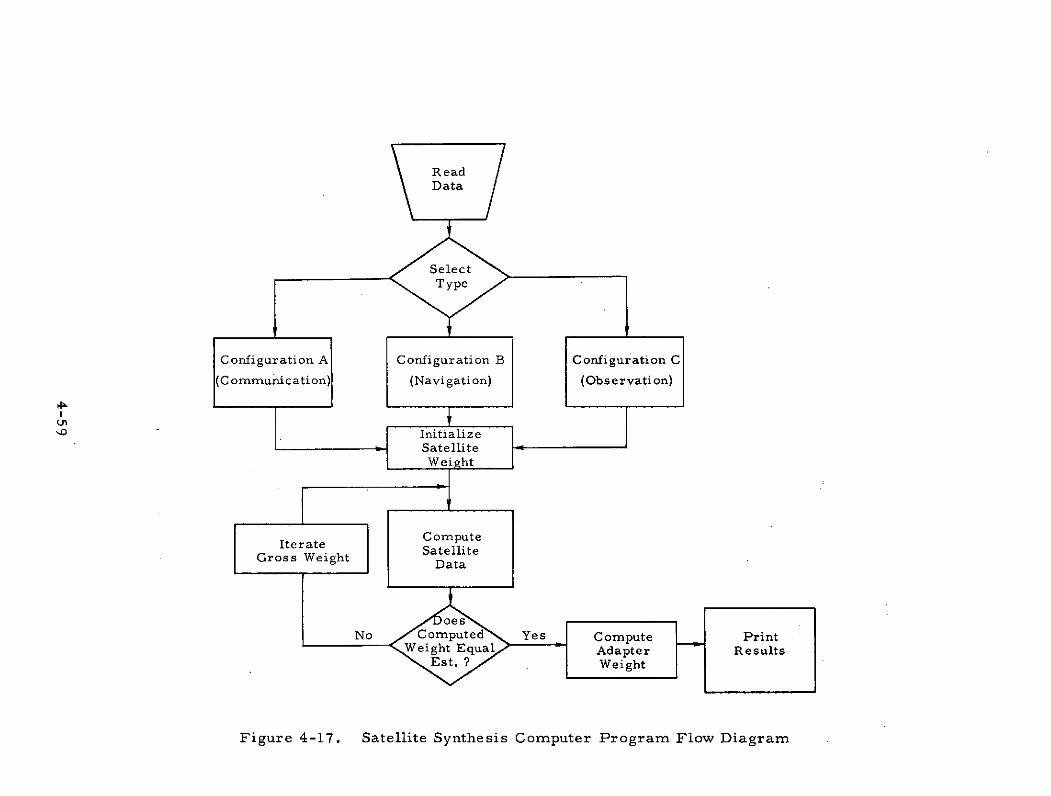
ReadData
SelectType
Configuration A Configuration B Configuration C
(Communication) (Navigation) (Observation)
IU,
InitializeSatelliteWeight
Iterate ComputeIterate SatelliteGross Weight Data
oesNo Computed Yes Compute Print
Weight Equal Adapter ResultsEst. C? Weight
Figure 4-17. Satellite Synthesis Computer Program Flow Diagram
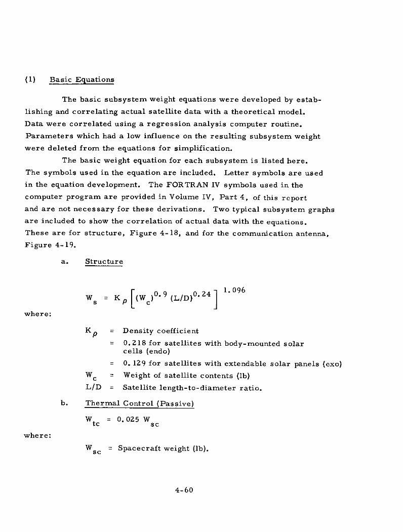
(1) Basic Equations
The basic subsystem weight equations were developed by estab-
lishing and correlating actual satellite data with a theoretical model.
Data were correlated using a regression analysis computer routine.
Parameters which had a low influence on the resulting subsystem weight
were deleted from the equations for simplification.
The basic weight equation for each subsystem is listed here.
The symbols used in the equation are included. Letter symbols are used
in the equation development. The FORTRAN IV symbols used in the
computer program are provided in Volume IV, Part 4, of this report
and are not necessary for these derivations. Two typical subsystem graphs
are included to show the correlation of actual data with the equations.
These are for structure, Figure 4-18, and for the communication antenna,
Figure 4-19.
a. Structure
W Kp [(W) (L/D)0 4 1.096
where:
Kp = Density coefficient
= 0.218 for satellites with body-mounted solarcells (endo)
0. 129 for satellites with extendable solar panels (exo)
Wc = Weight of satellite contents (lb)
L/D = Satellite length-to-diameter ratio.
b. Thermal Control (Passive)
Wtc = 0.025 Wsc
where:
Wsc = Spacecraft weight (lb).
4-60
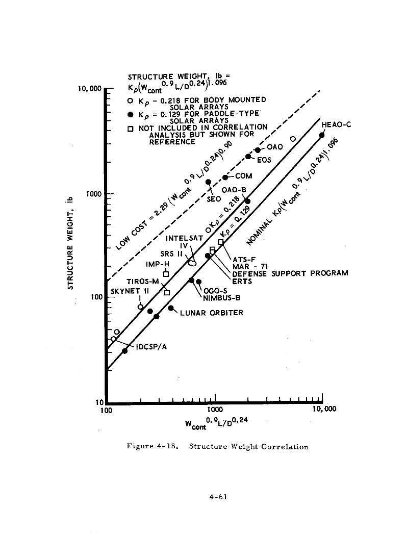
STRUCTURE WEIGHT, lb =
10,000 Kp(Wcont 9 L/D0 024)1 096
O Kp = 0.218 FOR BODY MOUNTED /SOLAR ARRAYS
Kp = 0.129 FOR PADDLE-TYPE /SOLAR ARRAYS
O NOT INCLUDED IN CORRELATION HEAO-CANALYSIS BUT SHOWN FOR /REFERENCE / OAO O
o OEOS
--
1000 OAO-B
1000 -
O // INTELSAT ?A IV
a,/ SRS II/ RATS-F/ IMP-H MAR - 71
-/ DEFENSE SUPPORT PROGRAMS TIROS-M ERTS
SSKYNET II OGO-S100 NIMBUS-B
m- ALUNAR ORBITER
IDCSP/A
10100 1000 10, 000
Wcont0. 9L/DO
. 24
Figure 4-18. Structure Weight Correlation
4-61
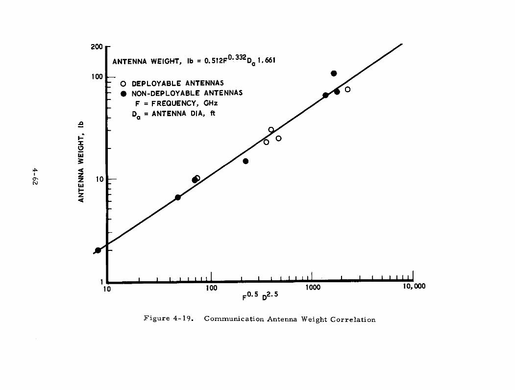
200
ANTENNA WEIGHT, Ib = 0.512F 0 3 32 D 1.661
100O DEPLOYABLE ANTENNAS
* NON-DEPLOYABLE ANTENNAS
F = FREQUENCY, GHz
Da = ANTENNA DIA, ft
z 10
10 100 1000 10,000F 0 . 5 D2 .5
Figure 4-19. Communication Antenna Weight Correlation
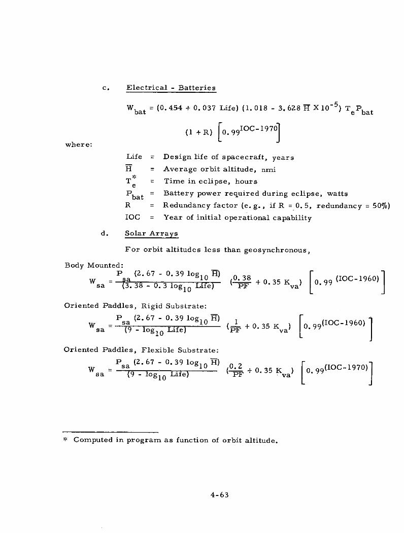
c. Electrical - Batteries
Wbat = (0. 454 + 0. 037 Life) (1. 018 - 3. 628 X 10 - 5 ) Te Pbat
(1 + R) 0. 9 9 IOC-1970]
where:
Life = Design life of spacecraft, years
H = Average orbit altitude, nmi
T = Time in eclipse, hourse
Pbat = Battery power required during eclipse, watts
R = Redundancy factor (e. g., if R = 0. 5, redundancy = 50%0)
IOC = Year of initial operational capability
d. Solar Arrays
For orbit altitudes less than geosynchronous,
Body Mounted:
Pa (167 - 039 logl ) 0. 35 K [. 99 (IOC-1960)sa (3. 38 - 0. 3 logl 0 Life) PF va
Oriented Paddles, Rigid Substrate:
SP (2. 67 - 0. 39 log 0 H)- )sa (9 - logl 0 Life) PF va 0
Oriented Paddles, Flexible Substrate:
P (2. 67 - 0. 39 log1 0 H) 0 2W sa 0 2 + 0. 35 K 0.99(IOC-1970)
sa (9 - logl0 Life) PF + 0.35 va)
* Computed in program as function of orbit altitude.
4-63
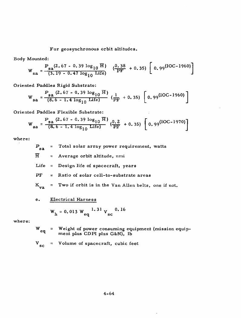
For geosynchronous orbit altitudes.
Body Mounted:
P (2. 67 - 0. 3 9 log 0 H 0. 38 + 0.35)[ 0 9 9 (IOC-1960)]
sa (3. 19 - 0.47 log 1 0 Life)
Oriented Paddles Rigid Substrate:
P (2. 67 - 0. 39 logl0 H) 1s sa 10 1 9 9 (IOC-1960)Ssa (8.6 - 1.4 logl0 Life) PF0.35)
Oriented Paddles Flexible Substrate:
P sa (2. 67- 0. 39 log1 0 HI 0.2 0.35) [ ( 97W + 0.35) 0.99sa (8.6 - 1.4 logl 0 Life) PF
where:
Psa = Total solar array power requirement, watts
H = Average orbit altitude, nmi
Life = Design life of spacecraft, years
PF = Ratio of solar cell-to-substrate areas
K = Two if orbit is in the Van Allen belts, one if not.va
e. Electrical Harness
1.31 0. 16W h = 0. 013 W 1.31 Vsch eq sc
where:
W = Weight of power consuming equipment (mission equip-eq ment plus CDPI plus G&N), lb
Vsc = Volume of spacecraft, cubic feet
4-64
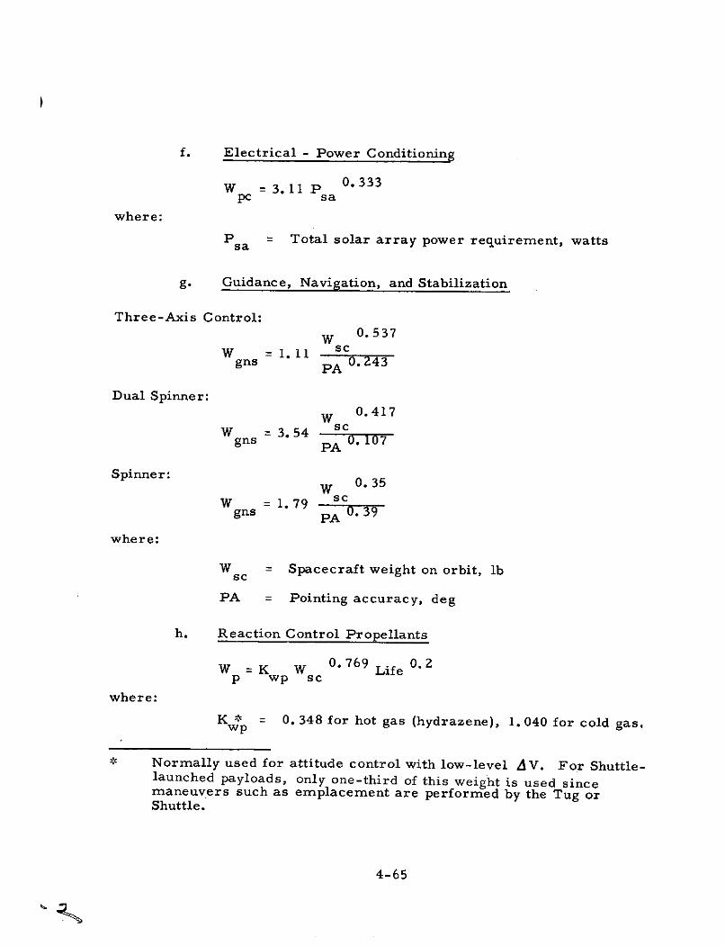
f. Electrical - Power Conditioning
W = 3.11 P 0.333pc sa
where:
Psa = Total solar array power requirement, watts
g. Guidance, Navigation, and Stabilization
Three-Axis Control:0.537
W g = .11 scgns 0. 243PA
Dual Spinner:W 0.417
W = 3.54 scgns PA0. 107PA
Spinner: 0.35W
W = 1. 79 scgns PA 0. 39
where:
W = Spacecraft weight on orbit, lb
PA = Pointing accuracy, deg
h. Reaction Control Propellants
0. 769 0. 2W =K W Lifep wp sc
where:
K w = 0. 348 for hot gas (hydrazene), 1. 040 for cold gas.wp
- Normally used for attitude control with low-level AV. For Shuttle-launched payloads, only one-third of this weight is used sincemaneuvers such as emplacement are performed by the Tug orShuttle.
4-65
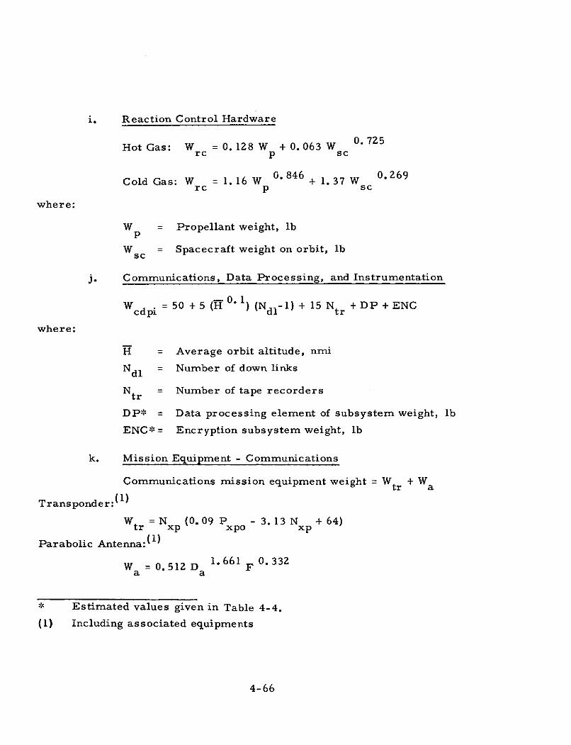
i. Reaction Control Hardware
Hot Gas: W = 0. 128 W + 0. 063 W 0.725rc p sc
G. 846 0. 269Cold Gas: W = 1. 16 W + 1. 37 W
rc p sc
where:
W = Propellant weight, lb
W = Spacecraft weight on orbit, lbsc
j. Communications, Data Processing, and Instrumentation
Wcdpi 50 + 5 ( ) (Ndl 1 ) + 15 Ntr + DP + ENC
where:
H = Average orbit altitude, nmi
Ndl = Number of down links
Ntr = Number of tape recorders
DP* = Data processing element of subsystem weight, lb
ENC = Encryption subsystem weight, lb
k. Mission Equipment - Communications
Communications mission equipment weight = Wtr + Wa
Transponder: 1)
Wtr = N (0. 09 P - 3. 13 N + 64)tr xp xpo xp
Parabolic Antenna: ( 1)
1. 661 0.332W = 0.512 D F
a a
Estimated values given in Table 4-4.
(1) Including associated equipments
4-66
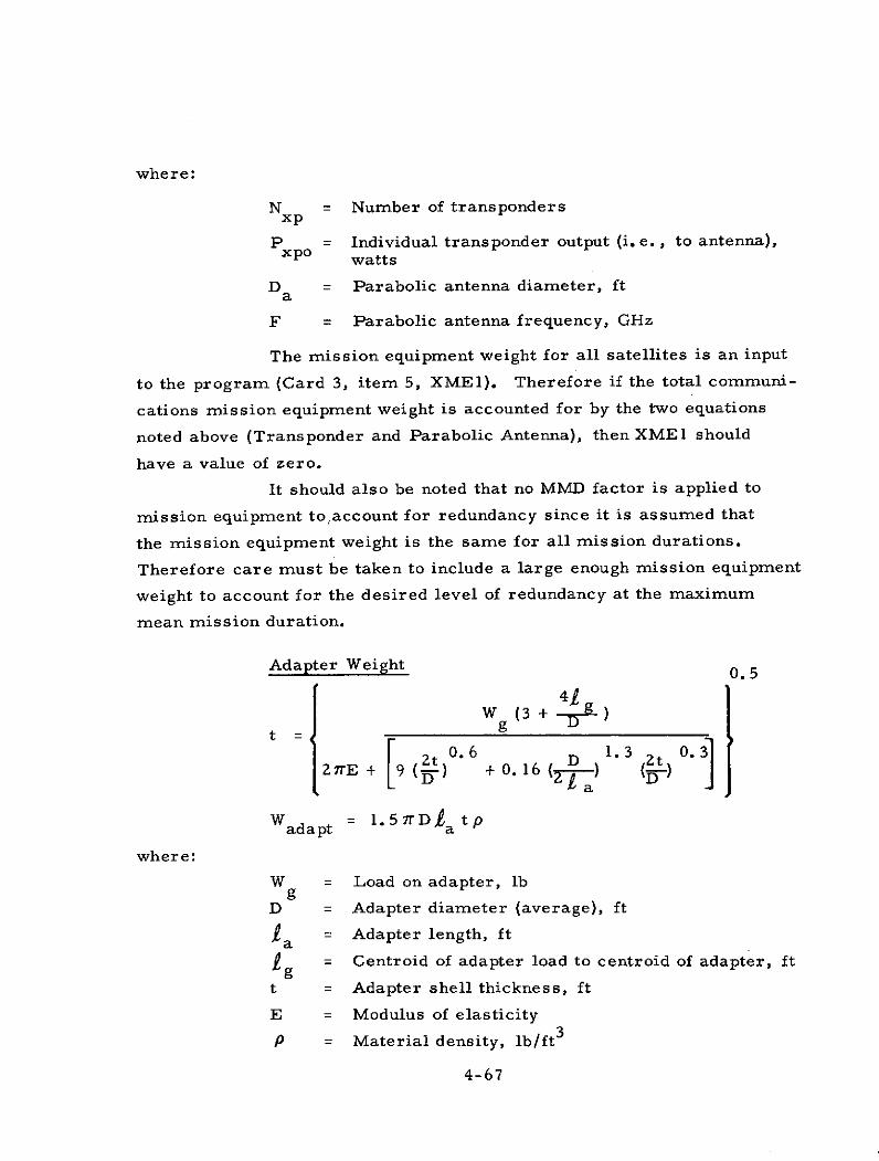
where:
N = Number of transpondersxp
P = Individual transponder output (i. e., to antenna),xpo watts
D = Parabolic antenna diameter, ft
F = Parabolic antenna frequency, GHz
The mission equipment weight for all satellites is an input
to the program (Card 3, item 5, XME1). Therefore if the total communi-
cations mission equipment weight is accounted for by the two equations
noted above (Transponder and Parabolic Antenna), then XME1 should
have a value of zero.
It should also be noted that no MMD factor is applied to
mission equipment to,account for redundancy since it is assumed that
the mission equipment weight is the same for all mission durations.
Therefore care must be taken to include a large enough mission equipment
weight to account for the desired level of redundancy at the maximum
mean mission duration.
Adapter Weight 0. 5
41W (3 + )
{0E.[ 316(W6Y(L 0.3]Zt D Zt2 7TE + 9 (L) + 0. 16 ( -) (D-)
Wadapt = 1. 5 7rDa t
where:
W = Load on adapter, lb
D = Adapter diameter (average), ft
La = Adapter length, ft
g = Centroid of adapter load to centroid of adapter, ft
t = Adapter shell thickness, ft
E = Modulus of elasticity
P = Material density, lb/ft 3
4-67
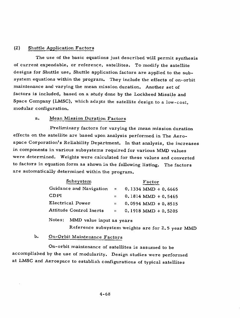
(2) Shuttle Application Factors
The use of the basic equations just described will permit synthesis
of current expendable, or reference, satellites. To modify the satellite
designs for Shuttle use, Shuttle application factors are applied to the sub-
system equations within the program. They include the effects of on-orbit
maintenance and varying the mean mission duration. Another set of
factors is included, based on a study done by the Lockheed Missile and
Space Company (LMSC), which adapts the satellite design to a low-cost,
modular configuration.
a. Mean Mission Duration Factors
Preliminary factors for varying the mean mission duration
effects on the satellite are based upon analysis performed in The Aero-
space Corporation's Reliability Department. In that analysis, the increases
in components in various subsystems required for various MMD values
were determined. Weights were calculated for these values and converted
to factors in equation form as shown in the following listing. The factors
are automatically determined within the program.
Subsystem Factor
Guidance and Navigation = 0. 1334 MMD + 0. 6665
CDPI = 0. 1814 MMD + 0. 5465
Electrical Power = 0. 0594 MMD + 0. 8515
Attitude Control Inerts = 0. 1918 MMD + 0. 5205
Notes: MMD value input as years
Reference subsystem weights are for 2. 5 year MMD
b. On-Orbit Maintenance Factors
On-orbit maintenance of satellites is assumed to be
accomplished by the use of modularity. Design studies were performed
at LMSC and Aerospace to establish configurations of typical satellites
4-68
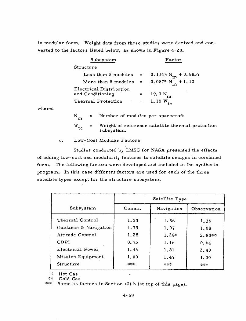
in modular form. Weight data from these studies were derived and con-
verted to the factors listed below, as shown in Figure 4-20.
Subsystem Factor
Structure
Less than 8 modules = 0. 1143 N + 0. 8857m
More than 8 modules = 0. 0875 N + 1. 10mElectrical Distributionand Conditioning = 19. 7 N mThermal Protection = 1. 10 Wtc
where:
N = Number of modules per spacecraftm
Wtc = Weight of reference satellite thermal protectionsubsystem.
c. Low-Cost Modular Factors
Studies conducted by LMSC for NASA presented the effects
of adding low-cost and modularity features to satellite designs in combined
form. The following factors were developed and included in the synthesis
program. In this case different factors are used for each of the three
satellite types except for the structure subsystem.
Satellite Type
Subsystem Comm. Navigation Observation
Thermal Control 1. 33 1. 36 1. 36
Guidance & Navigation 1. 79 1.07 1.08
Attitude Control 1.28 1. 28* 2. 80 -*4
CDPI 0.75 1. 16 0.64
Electrical Power 1.45 1.81 2. 40
Mission Equipment 1. 00 1.47 1. 00
Structure ..... **.....
: Hot Gas... Cold Gas
*",' Same as factors in Section (2) b (at top of this page).
4-69
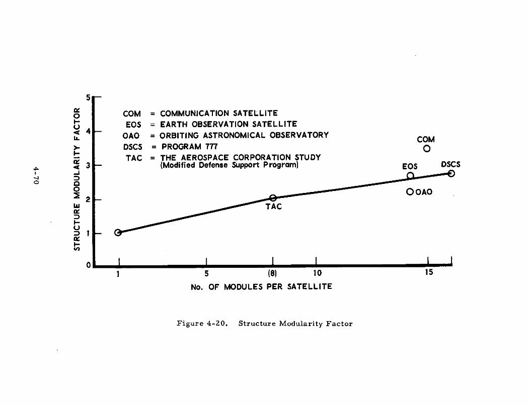
5
o COM = COMMUNICATION SATELLITEU EOS = EARTH OBSERVATION SATELLITE
4W OAO = ORBITING ASTRONOMICAL OBSERVATORY COM>DSCS = PROGRAM 777 O
TAC = THE AEROSPACE CORPORATION STUDY3 (Modified Defense Support Program) EOS DSCS
-J-
0 OOAO
w TAC
I-D 1I-
1
1 5 (8) 10 15
No. OF MODULES PER SATELLITE
Figure 4-20. Structure Modularity Factor
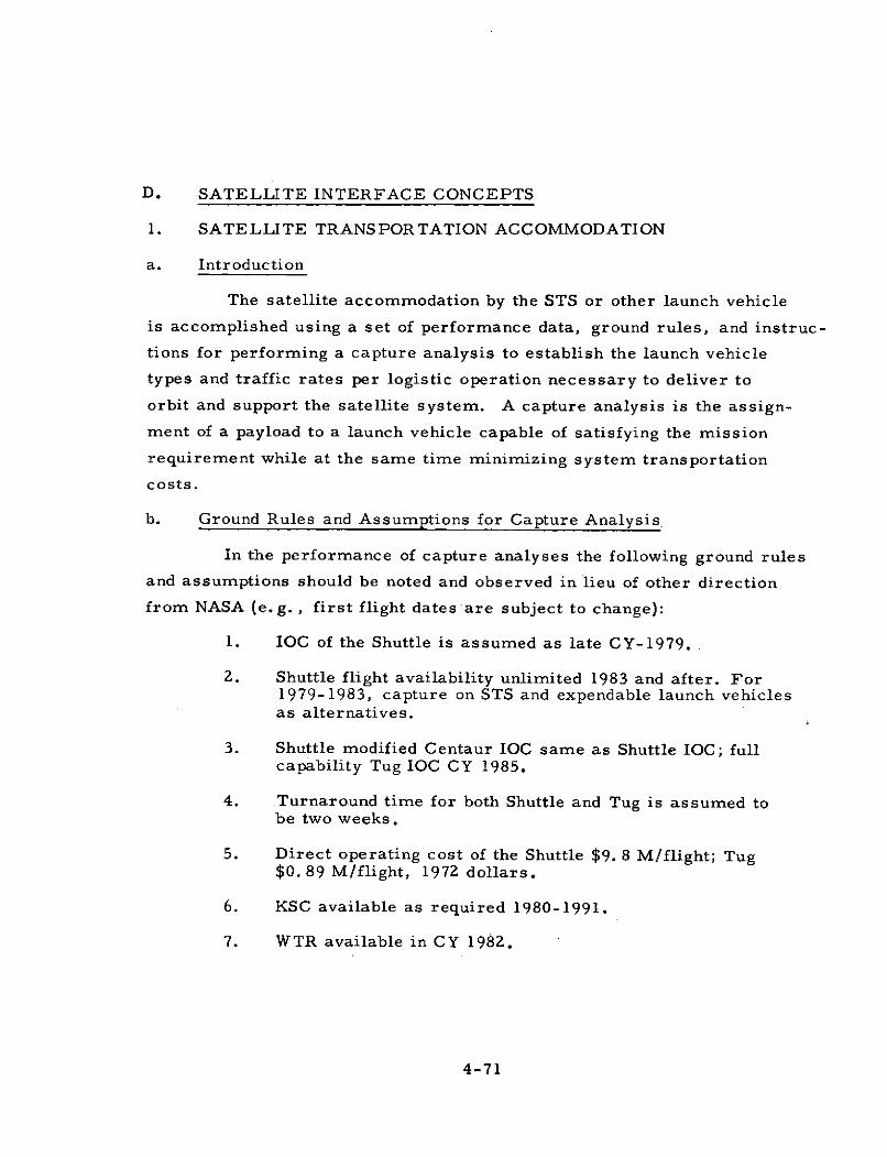
D. SATELLITE INTERFACE CONCEPTS
1. SATELLITE TRANSPORTATION ACCOMMODATION
a. Introduction
The satellite accommodation by the STS or other launch vehicle
is accomplished using a set of performance data, ground rules, and instruc-
tions for performing a capture analysis to establish the launch vehicle
types and traffic rates per logistic operation necessary to deliver to
orbit and support the satellite system. A capture analysis is the assign-
ment of a payload to a launch vehicle capable of satisfying the mission
requirement while at the same time minimizing system transportation
costs.
b. Ground Rules and Assumptions for Capture Analysis
In the performance of capture analyses the following ground rules
and assumptions should be noted and observed in lieu of other direction
from NASA (e. g., first flight dates are subject to change):
1. IOC of the Shuttle is assumed as late CY-1979.
2. Shuttle flight availability unlimited 1983 and after. For1979-1983, capture on STS and expendable launch vehiclesas alternatives.
3. Shuttle modified Centaur IOC same as Shuttle IOC; fullcapability Tug IOC CY 1985.
4. Turnaround time for both Shuttle and Tug is assumed tobe two weeks.
5. Direct operating cost of the Shuttle $9. 8 M/flight; Tug$0.89 M/flight, 1972 dollars.
6. KSC available as required 1980-1991.
7. WTR available in CY 1982.
4-71
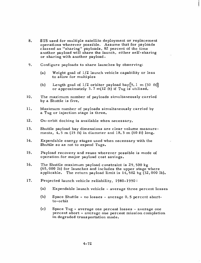
8. STS used for multiple satellite deployment or replacementoperations wherever possible. Assume that for payloadsclassed as "sharing" payloads, 82 percent of the timeanother payload will share the launch, either self-sharingor sharing with another payload.
9. Configure payloads to share launches by observing:
(a) Weight goal of 1/2 launch vehicle capability or lessto allow for multiples
(b) Length goal of 1/2 orbiter payload bay[9. I m (30 ft)]or approximately 3. 7 m(12 ft) if Tug is utilized.
10. The maximum number of payloads simultaneously carriedby a Shuttle is five.
11. Maximum number of payloads simultaneously carried bya Tug or injection stage is three.
12. On-orbit docking is available when necessary.
13. Shuttle payload bay dimensions are clear volume measure-ments, 4. 5 m (15 ft) in diameter and 18. 3 m (60 ft) long.
14. Expendable energy stages used when necessary with theShuttle so as not to expend Tugs.
15. Payload recovery and reuse wherever possible is mode ofoperation for major payload cost savings.
16. The Shuttle maximum payload constraint is 29, 500 kg(65, 000 Ib) for launches and includes the upper stage whereapplicable. The return payload limit is 14, 502 kg (32, 000 lb).
17. Projected launch vehicle reliability, 1980-1990:
(a) Expendable launch vehicle - average three percent losses
(b) Space Shuttle - no losses - average 0. 5 percent abort-to-orbit
(c) Space Tug - average one percent losses - average onepercent abort - average one percent mission completionin degraded transportation mode.
4-72
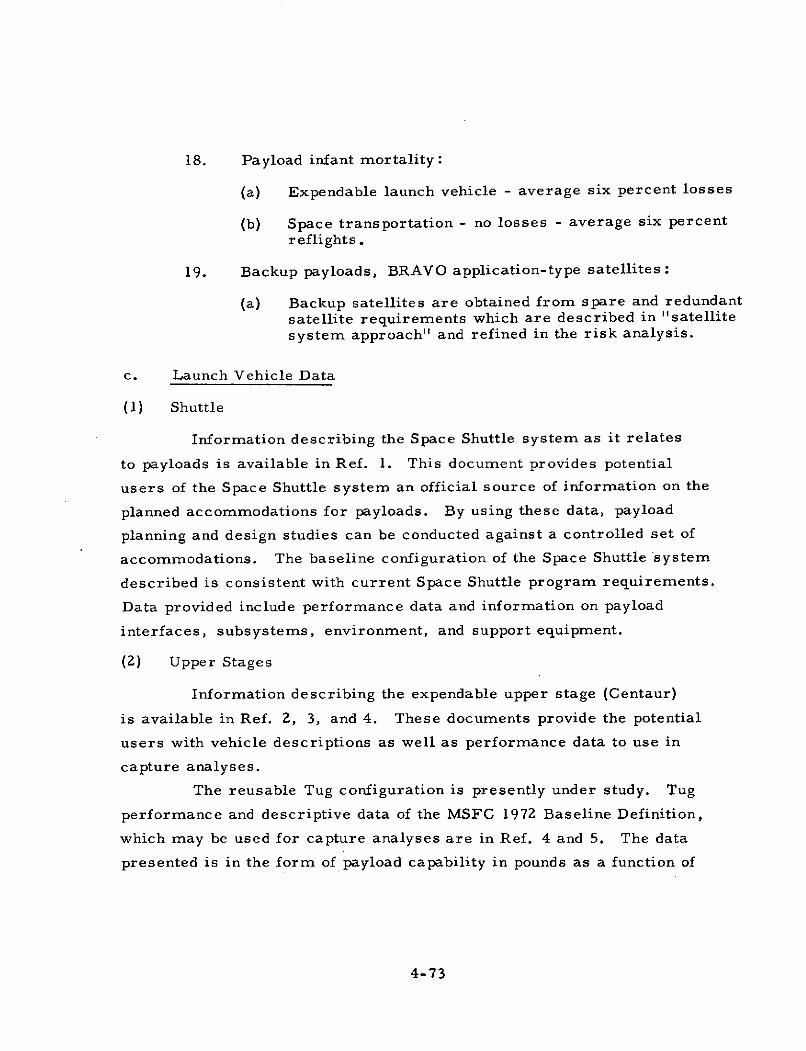
18. Payload infant mortality:
(a) Expendable launch vehicle - average six percent losses
(b) Space transportation - no losses - average six percent
reflights.
19. Backup payloads, BRAVO application-type satellites:
(a) Backup satellites are obtained from spare and redundantsatellite requirements which are described in "satellitesystem approach" and refined in the risk analysis.
c. Launch Vehicle Data
(1) Shuttle
Information describing the Space Shuttle system as it relates
to payloads is available in Ref. 1. This document provides potential
users of the Space Shuttle system an official source of information on the
planned accommodations for payloads. By using these data, payload
planning and design studies can be conducted against a controlled set of
accommodations. The baseline configuration of the Space Shuttle system
described is consistent with current Space Shuttle program requirements.
Data provided include performance data and information on payload
interfaces, subsystems, environment, and support equipment.
(2) Upper Stages
Information describing the expendable upper stage (Centaur)
is available in Ref. 2, 3, and 4. These documents provide the potential
users with vehicle descriptions as well as performance data to use in
capture analyses.
The reusable Tug configuration is presently under study. Tug
performance and descriptive data of the MSFC 1972 Baseline Definition,
which may be used for capture analyses are in Ref. 4 and 5. The data
presented is in the form of payload capability in pounds as a function of
4-73
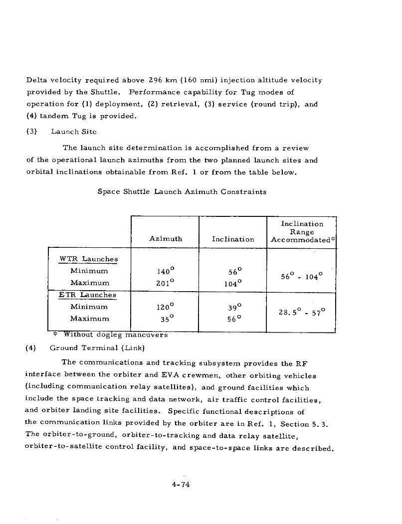
Delta velocity required above 296 km (160 nmi) injection altitude velocity
provided by the Shuttle. Performance capability for Tug modes of
operation for (1) deployment, (2) retrieval, (3) service (round trip), and
(4) tandem Tug is provided.
(3) Launch Site
The launch site determination is accomplished from a review
of the operational launch azimuths from the two planned launch sites and
orbital inclinations obtainable from Ref. 1 or from the table below.
Space Shuttle Launch Azimuth Constraints
InclinationRange
Azimuth Inclination Accommodated:
WTR Launches
Minimum 1400 560 560 104
Maximum 2010 1040
ETR Launches
Minimum 1200 390 0 028.5 ° - 57 °
Maximum 350 560
4 Without dogleg maneuvers
(4) Ground Terminal (Link)
The communications and tracking subsystem provides the RF
interface between the orbiter and EVA crewmen, other orbiting vehicles
(including communication relay satellites), and ground facilities which
include the space tracking and data network, air traffic control facilities,
and orbiter landing site facilities. Specific functional descriptions of
the communication links provided by the orbiter are in Ref. 1, Section 5. 3.
The orbiter-to-ground, orbiter-to-tracking and data relay satellite,orbiter-to-satellite control facility, and space-to-space links are described.
4-74
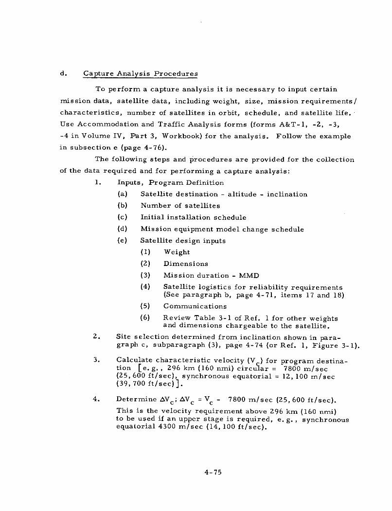
d. Capture Analysis Procedures
To perform a capture analysis it is necessary to input certain
mission data, satellite data, including weight, size, mission requirements/
characteristics, number of satellites in orbit, schedule, and satellite life.
Use Accommodation and Traffic Analysis forms (forms A&T-1, -2, -3,
-4 in Volume IV, Part 3, Workbook) for the analysis. Follow the example
in subsection e (page 4-76).
The following steps and procedures are provided for the collection
of the data required and for performing a capture analysis:
1. Inputs, Program Definition
(a) Satellite destination - altitude - inclination
(b) Number of satellites
(c) Initial installation schedule
(d) Mission equipment model change schedule
(e) Satellite design inputs
(1) Weight
(2) Dimensions
(3) Mission duration - MMD
(4) Satellite logistics for reliability requirements(See paragraph b, page 4-71, items 17 and 18)
(5) Communications
(6) Review Table 3-1 of Ref. 1 for other weightsand dimensions chargeable to the satellite.
2. Site selection determined from inclination shown in para-graph c, subparagraph (3), page 4-74 (or Ref. 1, Figure 3-1).
3. Calculate characteristic velocity (Vc) for program destina-tion [e.g., 296 km (160 nmi) circular = 7800 m/sec(25, 600 ft/sec), synchronous equatorial = 12, 100 m/sec(39, 700 ft/sec)].
4. Determine AVc; AV = V c - 7800 m/sec (25, 600 ft/sec).
This is the velocity requirement above 296 km (160 nmi)to be used if an upper stage is required, e. g., synchronousequatorial 4300 m/sec (14, 100 ft/sec).
4-75
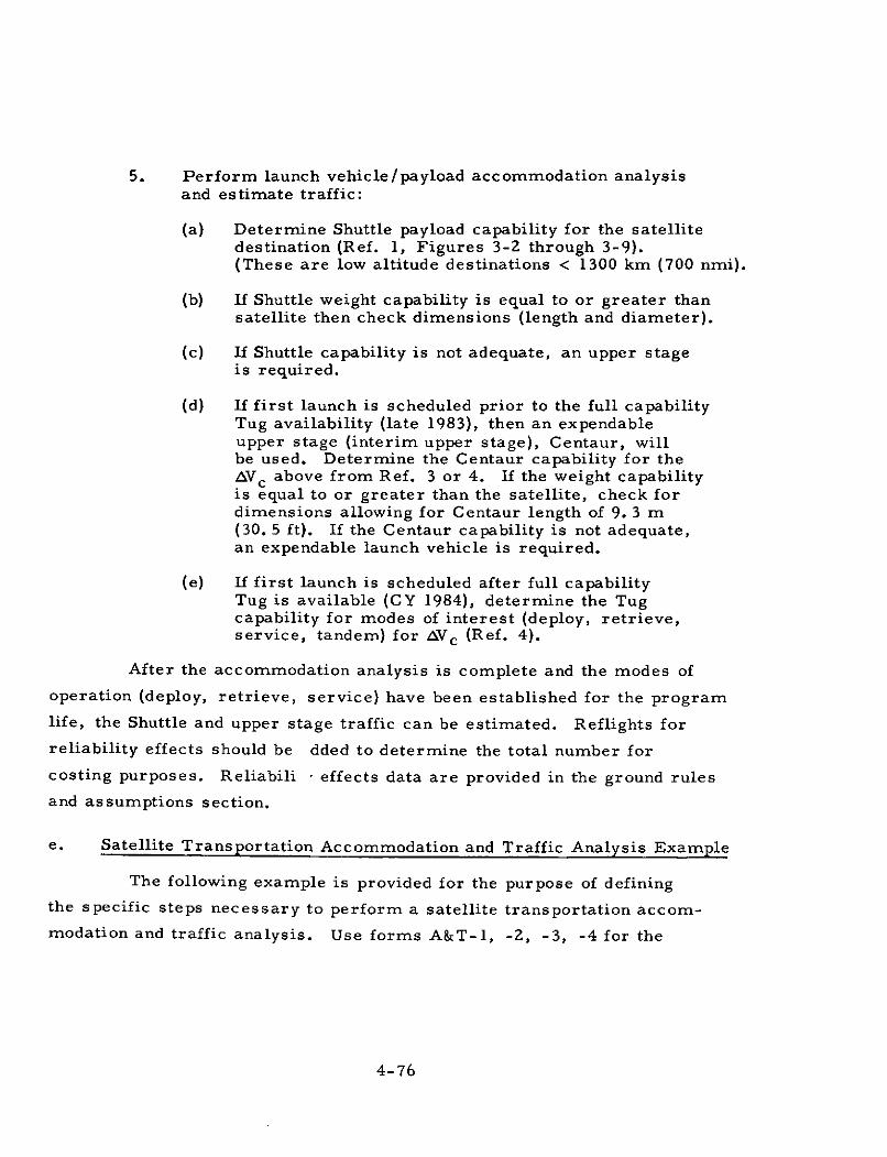
5. Perform launch vehicle/payload accommodation analysisand estimate traffic:
(a) Determine Shuttle payload capability for the satellitedestination (Ref. 1, Figures 3-2 through 3-9).(These are low altitude destinations < 1300 km (700 nmi).
(b) If Shuttle weight capability is equal to or greater thansatellite then check dimensions (length and diameter).
(c) If Shuttle capability is not adequate, an upper stageis required.
(d) If first launch is scheduled prior to the full capabilityTug availability (late 1983), then an expendableupper stage (interim upper stage), Centaur, willbe used. Determine the Centaur capability for theAVc above from Ref. 3 or 4. If the weight capabilityis equal to or greater than the satellite, check fordimensions allowing for Centaur length of 9. 3 m(30. 5 ft). If the Centaur capability is not adequate,an expendable launch vehicle is required.
(e) If first launch is scheduled after full capabilityTug is available (CY 1984), determine the Tugcapability for modes of interest (deploy, retrieve,service, tandem) for AVc (Ref. 4).
After the accommodation analysis is complete and the modes of
operation (deploy, retrieve, service) have been established for the program
life, the Shuttle and upper stage traffic can be estimated. Reflights for
reliability effects should be dded to determine the total number for
costing purposes. Reliabili , effects data are provided in the ground rules
and assumptions section.
e. Satellite Transportation Accommodation and Traffic Analysis Example
The following example is provided for the purpose of defining
the specific steps necessary to perform a satellite transportation accom-
modation and traffic analysis. Use forms A&T-1, -2, -3, -4 for the
4-76
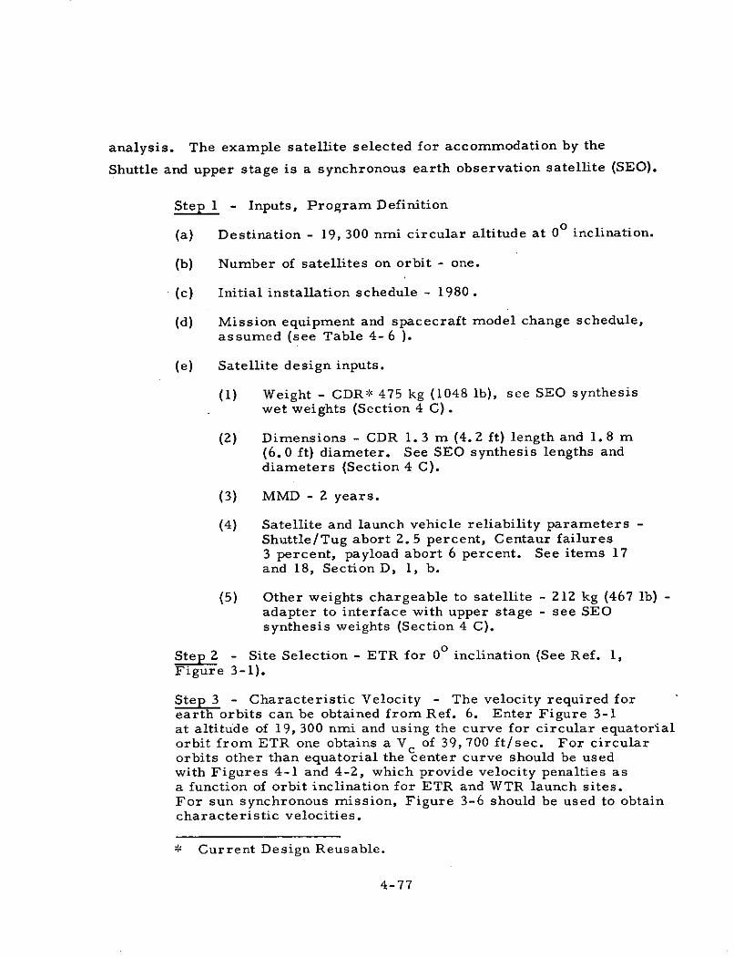
analysis. The example satellite selected for accommodation by the
Shuttle and upper stage is a synchronous earth observation satellite (SEO).
Step 1 - Inputs, Program Definition
(a) Destination - 19, 300 nmi circular altitude at 00 inclination.
(b) Number of satellites on orbit - one.
(c) Initial installation schedule - 1980.
(d) Mission equipment and spacecraft model change schedule,assumed (see Table 4-6 ).
(e) Satellite design inputs.
(1) Weight - CDR* 475 kg (1048 lb), see SEO synthesiswet weights (Section 4 C) .
(2) Dimensions - CDR 1. 3 m (4. 2 ft) length and 1. 8 m(6.0 ft) diameter. See SEO synthesis lengths anddiameters (Section 4 C).
(3) MMD - 2 years.
(4) Satellite and launch vehicle reliability parameters -Shuttle/Tug abort 2.5 percent, Centaur failures3 percent, payload abort 6 percent. See items 17and 18, Section D, 1, b.
(5) Other weights chargeable to satellite - 212 kg (467 lb) -adapter to interface with upper stage - see SEOsynthesis weights (Section 4 C).
Step2 - Site Selection - ETR for 00 inclination (See Ref. 1,Figure 3-1).
Step 3 - Characteristic Velocity - The velocity required forearth orbits can be obtained from Ref. 6. Enter Figure 3-1at altitude of 19, 300 nmi and using the curve for circular equatorialorbit from ETR one obtains a Vc of 39, 700 ft/sec. For circularorbits other than equatorial the center curve should be usedwith Figures 4-1 and 4-2, which provide velocity penalties asa function of orbit inclination for ETR and WTR launch sites.For sun synchronous mission, Figure 3-6 should be used to obtaincharacteristic velocities.
* Current Design Reusable.
4-77
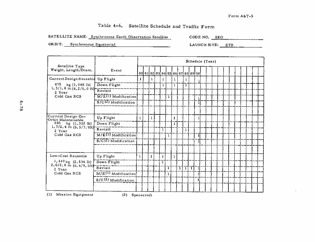
Form A&T-5
Table 4-6. Satellite Schedule and Traffic Form
SATELLITE NAME: Synchronous Earth Observation Satellite CODE NO. SEO
ORBIT: Synchronous Equatorial LAUNCH SITE: ETR
Schedule (Year)
Satellite TypeWeight, Length/Diam. Event
80 81 82 83 84 85 86 87 88 89 90
CurrentDesignReusablo Up Flight 1 1 1 1 1
475 kg (1, 048 lb) Down Flight 1 1 11.3/1.8 m(4.2/6.0 ft) Revisit
2 YearCold Gas RCS M/E[1TModification 1
S/C(-) Modification- 1
oo
Current Design On- Up Flight 1 1 1 1Orbit Maintainable686 kg (1,512 lb) Down Flight 1
1.7/2.4 m (5. 5/7. 9ft)2 Year evi
Cold Gas RCS Mi/ET1Modification
S-/C ) Modification- - - - - - - - - -- -f-t-- -1-1--ll-
Low-Cost Reusable Up Flight 1 1 1 1
1, 1 4 9 kg (2, 534 lb) Down Flight 12. 0/2. 8 m (6. 4/9. Ift
2 Year Revisit 1 1 1 1 1
Cold Gas RCS M/E(l Modification - .1 .1 -- -
S/C( 2 ) Modification 1
(1) Mission Equipment (2) Spacecraft
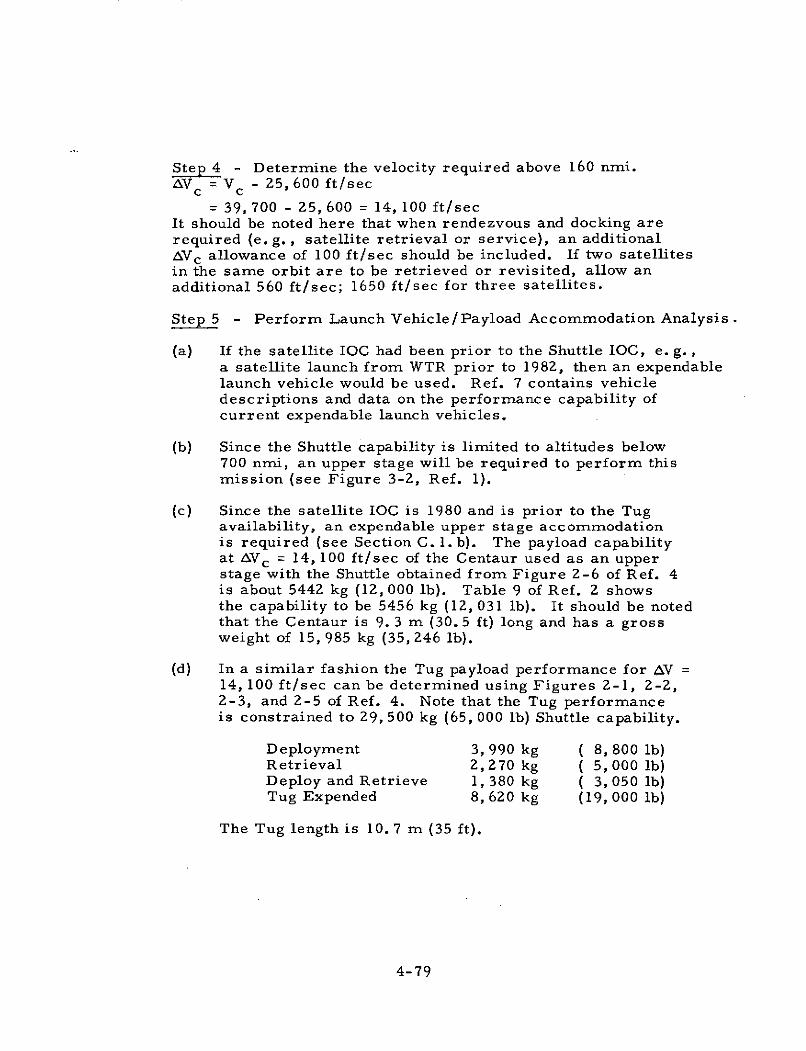
Step 4 - Determine the velocity required above 160 nmi.AV = V c - 25, 600 ft/sec
= 39, 700 - 25, 600 = 14, 100 ft/secIt should be noted here that when rendezvous and docking arerequired (e. g., satellite retrieval or service), an additionalAVc allowance of 100 ft/sec should be included. If two satellitesin the same orbit are to be retrieved or revisited, allow anadditional 560 ft/sec; 1650 ft/sec for three satellites.
Step5 - Perform Launch Vehicle/Payload Accommodation Analysis .
(a) If the satellite IOC had been prior to the Shuttle IOC, e. g.,a satellite launch from WTR prior to 1982, then an expendablelaunch vehicle would be used. Ref. 7 contains vehicledescriptions and data on the performance capability ofcurrent expendable launch vehicles.
(b) Since the Shuttle capability is limited to altitudes below700 nmi, an upper stage will be required to perform thismission (see Figure 3-2, Ref. 1).
(c) Since the satellite IOC is 1980 and is prior to the Tugavailability, an expendable upper stage accommodationis required (see Section C. l.b). The payload capabilityat AVc = 14, 100 ft/sec of the Centaur used as an upperstage with the Shuttle obtained from Figure 2-6 of Ref. 4is about 5442 kg (12, 000 lb). Table 9 of Ref. 2 showsthe capability to be 5456 kg (12, 031 lb). It should be notedthat the Centaur is 9. 3 m (30. 5 ft) long and has a grossweight of 15, 985 kg (35, 246 lb).
(d) In a similar fashion the Tug payload performance for AV =14, 100 ft/sec can be determined using Figures 2-1, 2-2,2-3, and 2-5 of Ref. 4. Note that the Tug performanceis constrained to 29, 500 kg (65, 000 lb) Shuttle capability.
Deployment 3, 990 kg ( 8, 800 lb)Retrieval 2,270 kg ( 5, 000 lb)Deploy and Retrieve 1, 380 kg ( 3, 050 lb)Tug Expended 8, 620 kg (19, 000 lb)
The Tug length is 10. 7 m (35 ft).
4-79
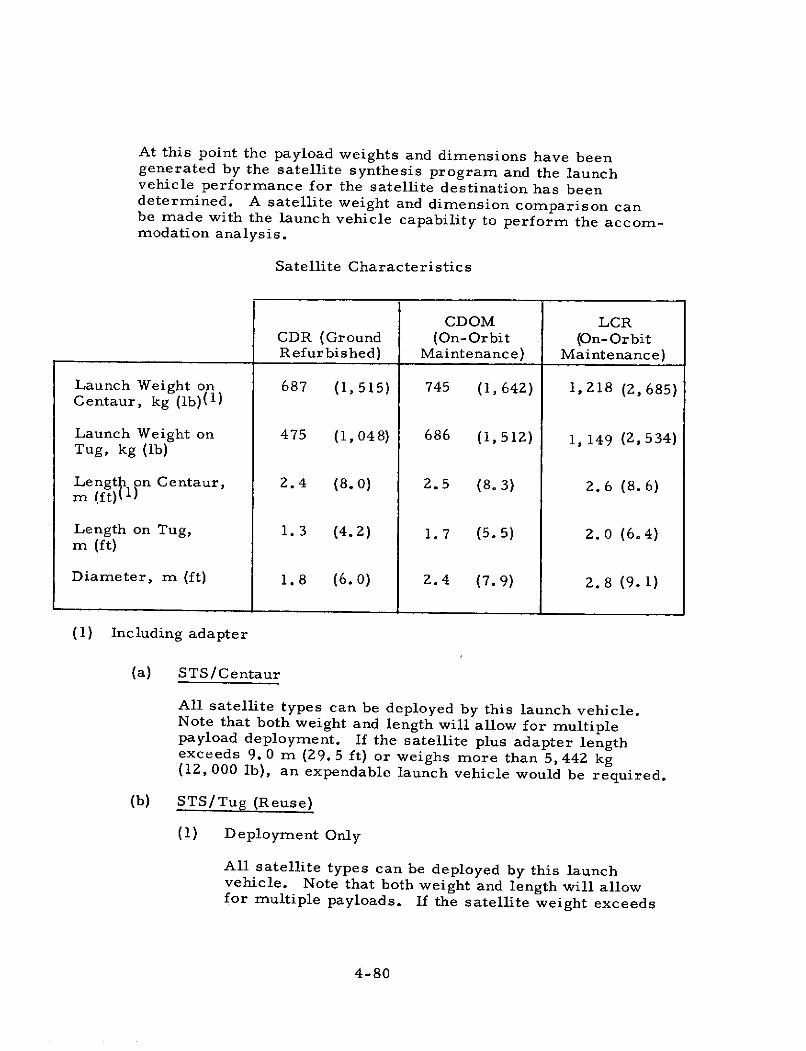
At this point the payload weights and dimensions have beengenerated by the satellite synthesis program and the launchvehicle performance for the satellite destination has beendetermined. A satellite weight and dimension comparison canbe made with the launch vehicle capability to perform the accom-modation analysis.
Satellite Characteristics
CDOM LCRCDR (Ground (On- Orbit (On- OrbitRefurbished) Maintenance) Maintenance)
Launch Weight on 687 (1,515) 745 (1,642) 1,218 (2,685)Centaur, kg (Ib)( 1 )
Launch Weight on 475 (1,048) 686 (1,512) 1, 149 (2,534)Tug, kg (lb)
Length on Centaur, 2.4 (8.0) 2. 5 (8.3) 2. 6 (8. 6)m (ft)(1)
Length on Tug, 1. 3 (4. 2) 1. 7 (5.5) 2. 0 (6.4)m (ft)
Diameter, m (ft) 1.8 (6.0) 2.4 (7.9) 2. 8 (9. 1)
(1) Including adapter
(a) STS/Centaur
All satellite types can be deployed by this launch vehicle.Note that both weight and length will allow for multiplepayload deployment. If the satellite plus adapter lengthexceeds 9. 0 m (29. 5 ft) or weighs more than 5, 442 kg(12, 000 lb), an expendable launch vehicle would be required.
(b) STS/Tug (Reuse)
(1) Deployment Only
All satellite types can be deployed by this launchvehicle. Note that both weight and length will allowfor multiple payloads. If the satellite weight exceeds
4-80
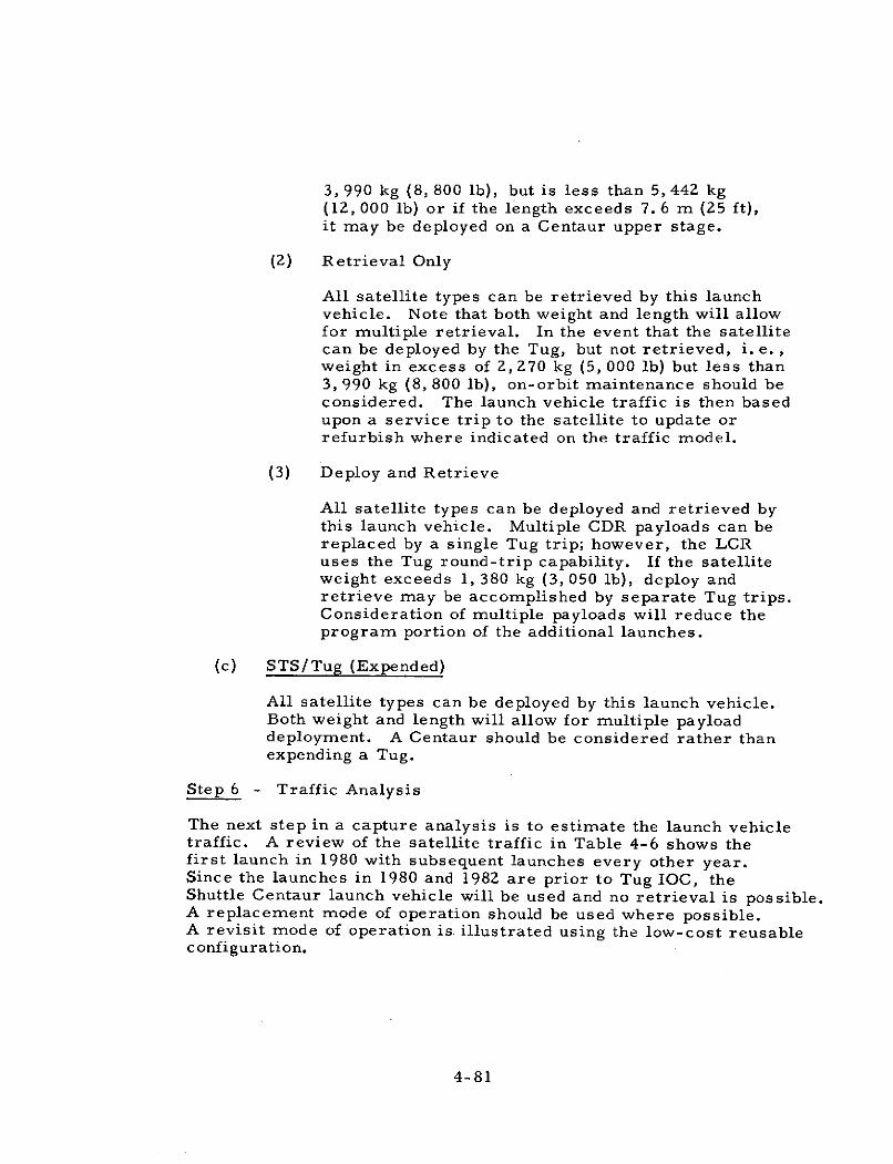
3, 990 kg (8, 800 lb), but is less than 5, 442 kg(12, 000 lb) or if the length exceeds 7. 6 m (25 ft),it may be deployed on a Centaur upper stage.
(2) Retrieval Only
All satellite types can be retrieved by this launchvehicle. Note that both weight and length will allowfor multiple retrieval. In the event that the satellitecan be deployed by the Tug, but not retrieved, i.e.,weight in excess of 2, 270 kg (5, 000 lb) but less than3, 990 kg (8, 800 lb), on-orbit maintenance should beconsidered. The launch vehicle traffic is then basedupon a service trip to the satellite to update orrefurbish where indicated on the traffic model.
(3) Deploy and Retrieve
All satellite types can be deployed and retrieved bythis launch vehicle. Multiple CDR payloads can bereplaced by a single Tug trip; however, the LCRuses the Tug round-trip capability. If the satelliteweight exceeds 1, 380 kg (3, 050 lb), deploy andretrieve may be accomplished by separate Tug trips.Consideration of multiple payloads will reduce theprogram portion of the additional launches.
(c) STS/Tug (Expended)
All satellite types can be deployed by this launch vehicle.Both weight and length will allow for multiple payloaddeployment. A Centaur should be considered rather thanexpending a Tug.
Step 6 - Traffic Analysis
The next step in a capture analysis is to estimate the launch vehicletraffic. A review of the satellite traffic in Table 4-6 shows thefirst launch in 1980 with subsequent launches every other year.Since the launches in 1980 and 1982 are prior to Tug IOC, theShuttle Centaur launch vehicle will be used and no retrieval is possible.A replacement mode of operation should be used where possible.A revisit mode of operation is illustrated using the low-cost reusableconfiguration.
4-81
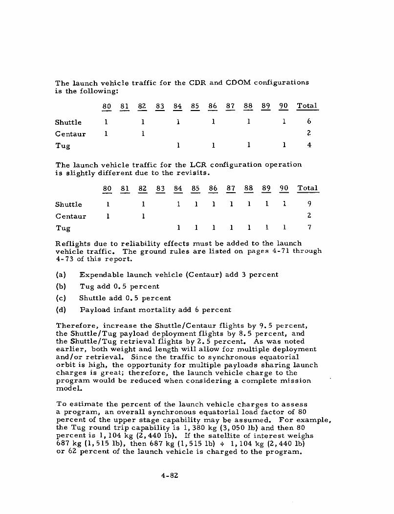
The launch vehicle traffic for the CDR and CDOM configurationsis the following:
80 81 82 83 84 85 86 87 88 89 90 Total
Shuttle 1 1 1 1 1 1 6
Centaur 1 1 2
Tug 1 1 1 1 4
The launch vehicle traffic for the LCR configuration operationis slightly different due to the revisits.
80 81 82 83 84 85 86 87 88 89 90 Total
Shuttle 1 1 1 1 1 1 1 1 1 9
Centaur 1 1 2
Tug 1 1 1 1 1 1 1 7
Reflights due to reliability effects must be added to the launchvehicle traffic. The ground rules are listed on pages 4-71 through4-73 of this report.
(a) Expendable launch vehicle (Centaur) add 3 percent
(b) Tug add 0. 5 percent
(c) Shuttle add 0.5 percent
(d) Payload infant mortality add 6 percent
Therefore, increase the Shuttle/Centaur flights by 9.5 percent,the Shuttle/Tug payload deployment flights by 8. 5 percent, andthe Shuttle/Tug retrieval flights by 2. 5 percent. As was notedearlier, both weight and length will allow for multiple deploymentand/or retrieval. Since the traffic to synchronous equatorialorbit is high, the opportunity for multiple payloads sharing launchcharges is great; therefore, the launch vehicle charge to theprogram would be reduced when considering a complete missionmodel.
To estimate the percent of the launch vehicle charges to assessa program, an overall synchronous equatorial load factor of 80percent of the upper stage capability may be assumed. For example,the Tug round trip capability is 1, 380 kg (3, 050 lb) and then 80percent is 1, 104 kg (2,440 lb). If the satellite of interest weighs687 kg (1, 515 lb), then 687 kg (1, 515 lb) + 1, 104 kg (2,440 lb)or 62 percent of the launch vehicle is charged to the program.
4-82
f. Background
Capture analyses using essentially the methodology described
above have been performed in Study A, Integrated Operations/Payloads/
Fleet Analysis (FY 1971); Study.2. 1, Space Shuttle Mission and Payload
Capture Analysis (FY 1972); and in Study 2. 4, Space Shuttle/Payload
Interface Analysis (FY 1973). Many of the ground rules and assumptions
have evolved from early capture analyses for use in future captures. The
launch vehicle fleets varied from expendable, as used in today's space
program, to a fully reusable Space Shuttle system. Both ETR and WTR
launch sites were involved.
2. SATELLITE GROUND TERMINAL DEFINITION AND COST ESTIMATE
a. Earth Stations Supporting Non-Communications Satellites
Earth stations are required by satellite systems other than
communication satellite systems for receiving and relaying data from
the satellite and for telemetry, tracking, and command of the satellite
and its mission equipment.
The most extensive data and experience on supporting earth
stations and communication nets for non-communications satellites
have been accumulated on NASA's Space Tracking and Data Network
(STDN). Data on STDN system capabilities and equipment for the late 1970sare provided in Vol. IV, Part 4, Section 6 in order that the requirements for
data communications, telemetry, tracking, and command support for
a prospective satellite mission may be compared with STDN capabilities.
Costs for STDN support and cost data for particular stations
(of interest if additional mission-dedicated stations were to be required)
have not been made available by NASA. These data have been the subject
of extensive studies for purposes of establishing a basis for equitable
charges to users of the system, particularly non-NASA users; however,
the studies had not been concluded and their release authorized to allow
4-83

the data to be included herein. For information on the availability of
such data, refer to William Pfeiffer, Code 361, Goddard Space Flight
Center, Greenbelt, Maryland.
b. Telecommunication Satellite System G/T Selection
The procedures herein apply specifically to the most common
configuration of communication satellite systems, which employ satellites
in geosynchronous orbit and earth stations which transmit and receive
through tracking antennas capable of pointing at one or another of the
satellites in the system (at least two satellites in orbit are usually
required for redundancy and reliability of operations).
The system design of such a satellite system is influenced
primarily by the numbers and location of earth stations and satellites
and by traffic requirements, which determine the communication capacities
of earth stations and satellites. In addition, design is affected by the
transmission frequencies of the system which are limited by regulations
on the use of the electromagnetic frequency spectrum.
In order to design earth stations and satellites to meet these
requirements at the least cost, the individual satellite-earth station
links must be analyzed to determine the power, antenna gains, and
receiving electronics of satellites and earth stations which will result
in minimum cost for the system as a whole. The procedure for accomp-lishing this requires iterative calculations, a few of which will be adequate
in most instances to establish the variation in total system cost, and
the minimum cost, with variation of the interrelated satellite and earthstation parameters. The calculations determine the power requirements
and antenna sizes of satellites for communication with an earth station
with a selected receiving system "Figure of Merit", G/T ( 1 ) . Costs
(1) G/T is the ratio of antenna gain to the receiving system noisetemperature equivalent in degrees Kelvin, which includes noisefrom the antenna system and receiving preamplifier. The ratiois expressed in decibels (10 times the logarithm of the ratio) perdegree Kelvin.
4-84
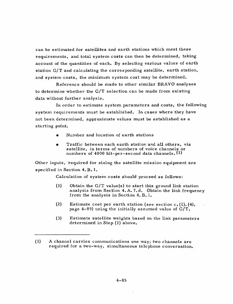
can be estimated for satellites and earth stations which meet these
requirements, and total system costs can then be determined, taking
account of the quantities of each. By selecting various values of earth
station G/T and calculating the corresponding satellite, earth station,
and system costs, the minimum system cost may be determined.
Reference should be made to other similar BRAVO analyses
to determine whether the G/T selection can be made from existing
data without further analysis.
In order to estimate system parameters and costs, the following
system requirements must be established. In cases where they have
not been determined, approximate values must be established as a
starting point.
* Number and location of earth stations
* Traffic between each earth station and all others, viasatellite, in terms of numbers of voice channels ornumbers of 4000 bit-per-second data channels. (1)
Other inputs, required for sizing the satellite mission equipment are
specified in Section 4. B. 1.
Calculation of system costs should proceed as follows:
(1) Obtain the G/T value(s) to start this ground link stationanalysis from Section 4. A. 7. d. Obtain the link frequencyfrom the analysis in Section 4. B. 1.
(2) Estimate cost per earth station (see section c. (1). (4),page 4-89) using the initially assumed value of G/T.
(3) Estimate satellite weights based on the link parametersdetermined in Step (1) above.
(1) A channel carries communications one way; two channels arerequired for a two-way, simultaneous telephone conversation.
4-85
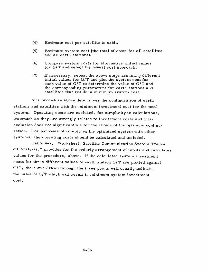
(4) Estimate cost per satellite in orbit.
(5) Estimate system cost (the total of costs for all satellitesand all earth stations).
(6) Compare system costs for alternative initial valuesfor G/T and select the lowest cost approach.
(7) If necessary, repeat the above steps assuming differentinitial values for G/T and plot the system cost foreach value of G/T to determine the value of G/T andthe corresponding parameters for earth stations andsatellites that result in minimum system cost.
The procedure above determines the configuration of earth
stations and satellites with the minimum investment cost for the total
system. Operating costs are excluded, for simplicity in calculations,
inasmuch as they are strongly related to investment costs and their
exclusion does not significantly alter the choice of the optimum configu-
ration. For purposes of comparing the optimized system with other
systems, the operating costs should be calculated and included.
Table 4-7, "Worksheet, Satellite Communication System Trade-
off Analysis, " provides for the orderly arrangement of inputs and calculates
values for the procedure, above. If the calculated system investment
costs for three different values of earth station G/T are plotted against
G/T, the curve drawn through the three points will usually indicate
the value of G/T which will result in minimum system investment
cost.
4-86
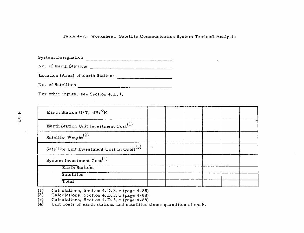
Table 4-7. Worksheet, Satellite Communication System Tradeoff Analysis
System Designation
No. of Earth Stations
Location (Area) of Earth Stations
No. of Satellites
For other inputs, see Section 4. B. 1.
Earth Station G/T, dB/oK
00
Earth Station Unit Investment Cost ( 1 )
Satellite Weight ( 2 )
Satellite Unit Investment Cost in Orbit ( 3 )
System Investment Cost ( 4 )
Earth Stations
Satellites
Total
(1) Calculations, Section 4. D.2.c (page 4-88)(2) Calculations, Section 4. D. 2. c (page 4-88)(3) Calculations, Section 4. D. 2. c (page 4-88)(4) Unit costs of earth stations and satellites times quantities of each.
c.. Telecommunications Satellite Earth Station Definition and Cost Estimate
A satellite earth station provides the communications connection
between satellites and points on the earth's surface or in the atmosphere.
The discussion herein is limited to permanent installations on land employ-
ing steerable parabolic antennas.
The functions performed by earth stations are: (1) receive
communications from terrestrial points (originating either at the station
or at remote points in the terrestrial communications network), multiplex
the signals (arrange in frequency and time sequence); (2) modulate the
transmitter, the output of which is beamed at the satellite by the antenna;
and (3) receive communications from the satellite through the antenna,
amplify and demultiplex the signals, and connect them into the terrestrial
communications network.
The earth station facilities include, typically, a building forhousing the electronic equipment, a standby power source, connections
to commercial power, one or more antenna systems (including the antenna
reflectors and feeds, mounting structure, and servo systems for antennapointing), and other facilities such as fencing, roadways, and parking
provisions.
Earth station antennas are designed to produce very narrow
beams, on the order of one degree beam width, in order to achieve highgain and reduce power requirements and to avoid interference with othercommunications facilities using the same frequency. Thus, one antenna
beam is required for each satellite that must be communicated withsimultaneously. In practice, one antenna system is required per beam.Multiple feeds and beams using a single antenna reflector, though possible,require larger and more costly reflectors to offset losses from mutual
blockage by the feeds, and the loss of reflector efficiency when a beamdeviates from the reflector axis by more than a few degrees severelyrestricts operating flexibility.
4-88
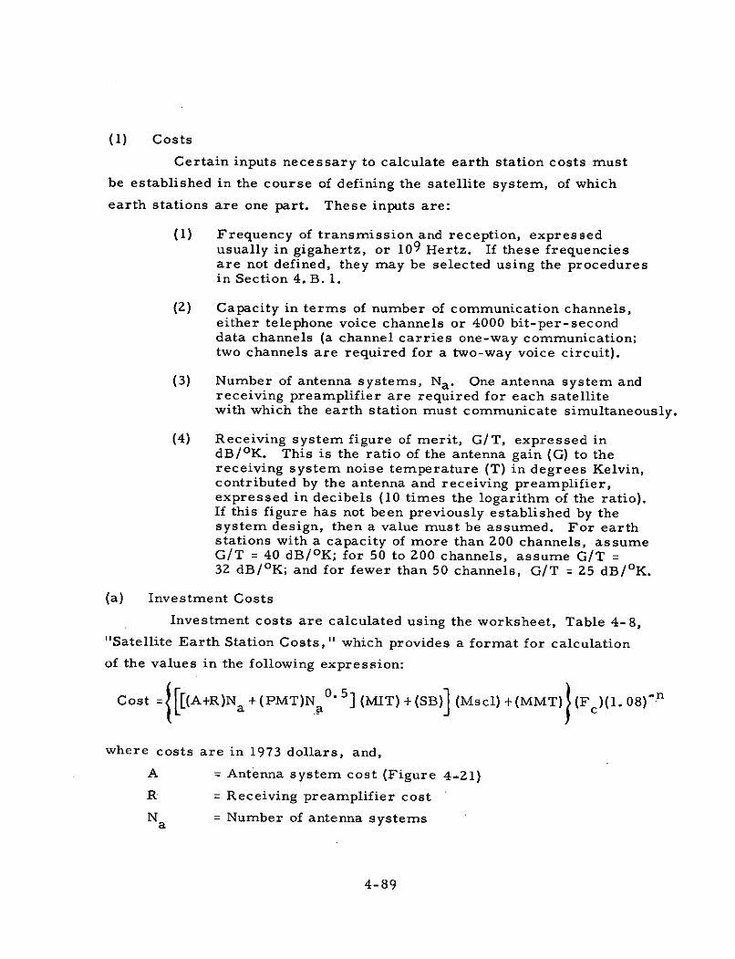
(1) Costs
Certain inputs necessary to calculate earth station costs must
be established in the course of defining the satellite system, of which
earth stations are one part. These inputs are:
(1) Frequency of transmission and reception, expressedusually in gigahertz, or 109 Hertz. If these frequenciesare not defined, they may be selected using the proceduresin Section 4. B. 1.
(2) Capacity in terms of number of communication channels,either telephone voice channels or 4000 bit-per-seconddata channels (a channel carries one-way communication;two channels are required for a two-way voice circuit).
(3) Number of antenna systems, Na. One antenna system andreceiving preamplifier are required for each satellitewith which the earth station must communicate simultaneously.
(4) Receiving system figure of merit, G/T, expressed indB/oK. This is the ratio of the antenna gain (G) to thereceiving system noise temperature (T) in degrees Kelvin,contributed by the antenna and receiving preamplifier,expressed in decibels (10 times the logarithm of the ratio).If this figure has not been previously established by thesystem design, then a value must be assumed. For earthstations with a capacity of more than 200 channels, assumeG/T = 40 dB/ 0 K; for 50 to 200 channels, assume G/T =32 dB/oK; and for fewer than 50 channels, G/T = 25 dB/oK.
(a) Investment Costs
Investment costs are calculated using the worksheet, Table 4-8,
"Satellite Earth Station Costs, " which provides a format for calculation
of the values in the following expression:
Cost = [(A+R)N a + (PMT)N 0 5] (MIT) + (SB)1 (Mscl) +(MMT) (F)(. 0 8 )
where costs are in 1973 dollars, and,
A = Antenna system cost (Figure 4-21)
R = Receiving preamplifier cost
N a = Number of antenna systems
4-89
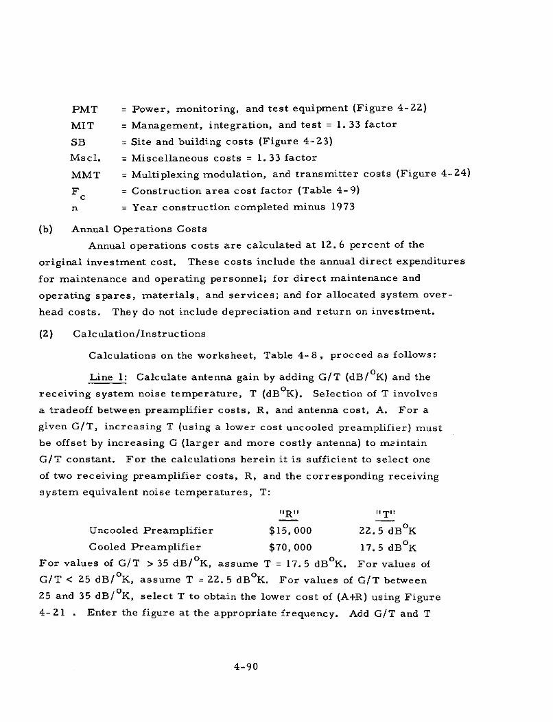
PMT = Power, monitoring, and test equipment (Figure 4-22)
MIT = Management, integration, and test = 1. 33 factor
SB = Site and building costs (Figure 4-23)
Mscl. = Miscellaneous costs = 1. 33 factor
MMT = Multiplexing modulation, and transmitter costs (Figure 4-24)
F = Construction area cost factor (Table 4- 9)
n = Year construction completed minus 1973
(b) Annual Operations Costs
Annual operations costs are calculated at 12. 6 percent of the
original investment cost. These costs include the annual direct expenditures
for maintenance and operating personnel; for direct maintenance and
operating spares, materials, and services; and for allocated system over-
head costs. They do not include depreciation and return on investment.
(2) Calculation/Instructions
Calculations on the worksheet, Table 4- 8, proceed as follows:
Line 1: Calculate antenna gain by adding G/T (dB/oK) and the
receiving system noise temperature, T (dBoK). Selection of T involves
a tradeoff between preamplifier costs, R, and antenna cost, A. For a
given G/T, increasing T (using a lower cost uncooled preamplifier) must
be offset by increasing G (larger and more costly antenna) to maintain
G/T constant. For the calculations herein it is sufficient to select one
of two receiving preamplifier costs, R, and the corresponding receiving
system equivalent noise temperatures, T:
"R" "T"
Uncooled Preamplifier $15,000 22. 5 dBoK
Cooled Preamplifier $70,000 17.5 dBoK
For values of G/T > 35 dB/oK, assume T = 17.5 dBoK. For values of
G/T < 25 dB/oK, assume T = 22.5 dBoK. For values of G/T between
25 and 35 dB/OK, select T to obtain the lower cost of (A+R) using Figure
4- 21 . Enter the figure at the appropriate frequency. Add G/T and T
4-90
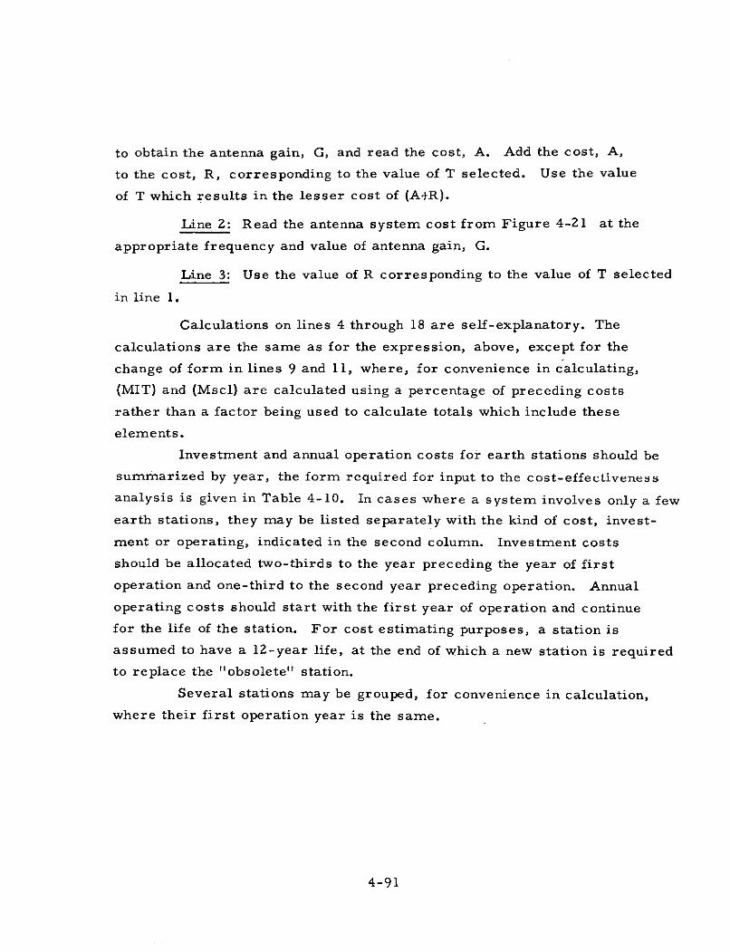
to obtain the antenna gain, G, and read the cost, A. Add the cost, A,
to the cost, R, corresponding to the value of T selected. Use the value
of T which results in the lesser cost of (A+R).
Line 2: Read the antenna system cost from Figure 4-21 at the
appropriate frequency and value of antenna gain, G.
Line 3: Use the value of R corresponding to the value of T selected
in line 1.
Calculations on lines 4 through 18 are self-explanatory. The
calculations are the same as for the expression, above, except for the
change of form in lines 9 and 11, where, for convenience in calculating,
(MIT) and (Mscl) are calculated using a percentage of preceding costs
rather than a factor being used to calculate totals which include these
elements.
Investment and annual operation costs for earth stations should be
summarized by year, the form required for input to the cost-effectiveness
analysis is given in Table 4-10. In cases where a system involves only a few
earth stations, they may be listed separately with the kind of cost, invest-
ment or operating, indicated in the second column. Investment costs
should be allocated two-thirds to the year preceding the year of first
operation and one-third to the second year preceding operation. Annual
operating costs should start with the first year of operation and continue
for the life of the station. For cost estimating purposes, a station is
assumed to have a 12-year life, at the end of which a new station is required
to replace the "obsolete" station.
Several stations may be grouped, for convenience in calculation,
where their first operation year is the same.
4-91
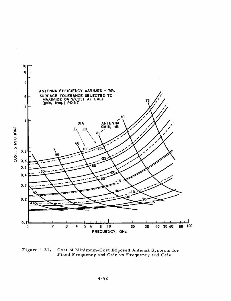
10
8
6
ANTENNA EFFICIENCY ASSUMED = 70%
4 SURFACE TOLERANCE SELECTED TOMAXIMIZE GAIN/COST AT EACH 75 /(gain, freq.) POINT
70 /DIA ANTENNA 7
St GAIN, dB /0
65
-25-0
0.6 800.5
" s..50-20-0.4
40---- 4 150
0.1
1 2 3 4 5 6 8 10 20 30 40 50 60 80 100FREQUENCY, GHz
Figure 4-21. Cost of Minimum-Cost Exposed Antenna Systems forFixed Frequency and Gain vs Frequency and Gain
4-92
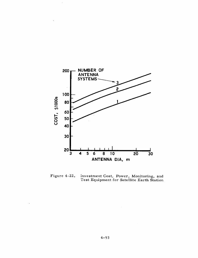
200 NUMBER OFANTENNASYSTEMS-
100
o 80
60
500
40
30
203 4 5 6 8 10 20 30
ANTENNA DIA, m
Figure 4-22. Investment Cost, Power, Monitoring, andTest Equipment for Satellite Earth Station
4-93
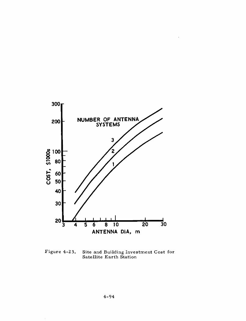
300
200 NUMBER OF ANTENNASYSTEMS
3
o' 100 2
80
60
0 5040
30
203 4 5 6 8 10 20 30
ANTENNA DIA, m
Figure 4-23. Site and Building Investment Cost forSatellite Earth Station
4-94
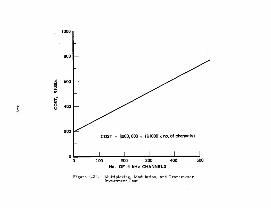
1000
800
o" 600
400U
200COST = $200, 000 + ($1000 x no. of channels)
0 100 200. 300 400 500No. OF 4 kHz CHANNELS
Figure 4-24. Multiplexing, Modulation, and TransmitterInvestment Cost
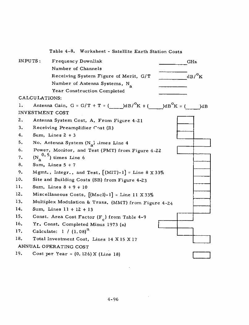
Table 4-8. Worksheet - Satellite Earth Station Costs
INPUTS: Frequency Downlink GHz
Number of Channels
Receiving System Figure of Merit, G/T dB/oK
Number of Antenna Systems, NaYear Construction Completed
CALCULATIONS:
1. Antenna Gain, G = G/T + T =( )dB/oK + ( )dBK = ( )dBINVESTMENT COST
2. Antenna System Cost, A, From Figure 4-21
3. Receiving Preamplifier Cost (R)
4. Sum, Lines 2 + 3
5. No. Antenna System (Na) imes Line 4
6. Power, Monitor, and Test (PMT) from Figure 4-220. 5
7. (Na ) times Line 6
8. Sum, Lines 5 + 7
9. Mgmt., Integr., and Test, [(MIT)-1] = Line 8 X 33%
10. Site and Building Costs (SB) from Figure 4-2311. Sum, Lines 8 + 9 + 10
12. Miscellaneous Costs, [(Mscl)-1] = Line 11 X 33%
13. Multiplex Modulation & Trans. (MMT) from Figure 4-2414. Sum, Lines 11 + 12 + 13
15. Const. Area Cost Factor (Fc) from Table 4-9
16. Yr. Const. Completed Minus 1973 (n)
17. Calculate: 1 / (1.0 8 )n
18. Total Investment Cost, Lines 14 X 15 X 17
ANNUAL OPERATING COST
19. Cost per Year = (0. 126) X (Line 18) I
4-96
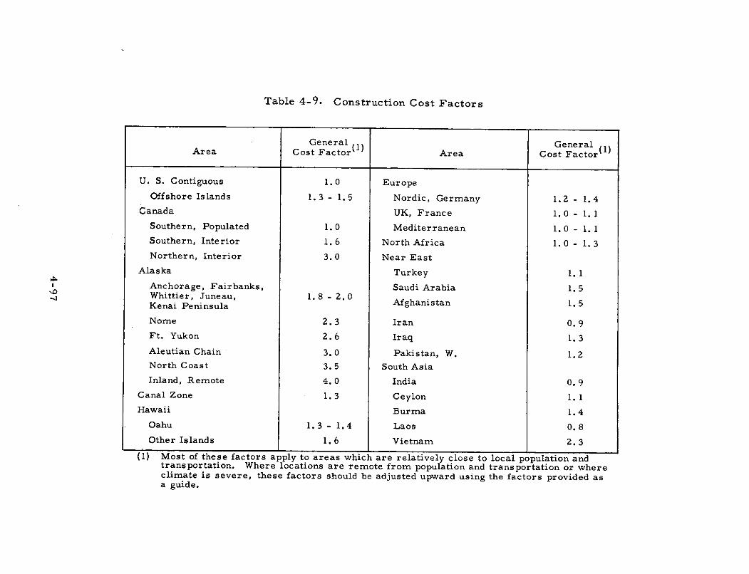
Table 4-9. Construction Cost Factors
General GeneralArea Cost Factor 1 Area Cost Factor (1
U. S. Contiguous 1.0 Europe
Offshore Islands 1.3 - 1.5 Nordic, Germany 1.2 - 1.4Canada UK, France 1.0 - 1. 1
Southern, Populated 1.0 Mediterranean 1.0 - 1. 1Southern, Interior 1.6 North Africa 1.0 - 1.3
Northern, Interior 3.0 Near East
Alaska Turkey 1. 1
Anchorage, Fairbanks, Saudi Arabia 1.5Whittier, Juneau, 1.8 - 2.0 Afghanistan 1.5Kenai Peninsula Afghanistan . 5
Nome 2.3 Iran 0.9
Ft. Yukon 2.6 Iraq 1.3
Aleutian Chain 3. 0 Pakistan, W. 1.2North Coast 3. 5 South Asia
Inland, Remote 4.0 India 0.9Canal Zone 1.3 Ceylon 1. 1
Hawaii Burma 1.4
Oahu 1.3 - 1.4 Laos 0.8
Other Islands 1. 6 Vietnam 2.3
(1) Most of these factors apply to areas which are relatively close to local population andtransportation. Where locations are remote from population and transportation or whereclimate is severe, these factors should be adjusted upward using the factors provided asa guide.
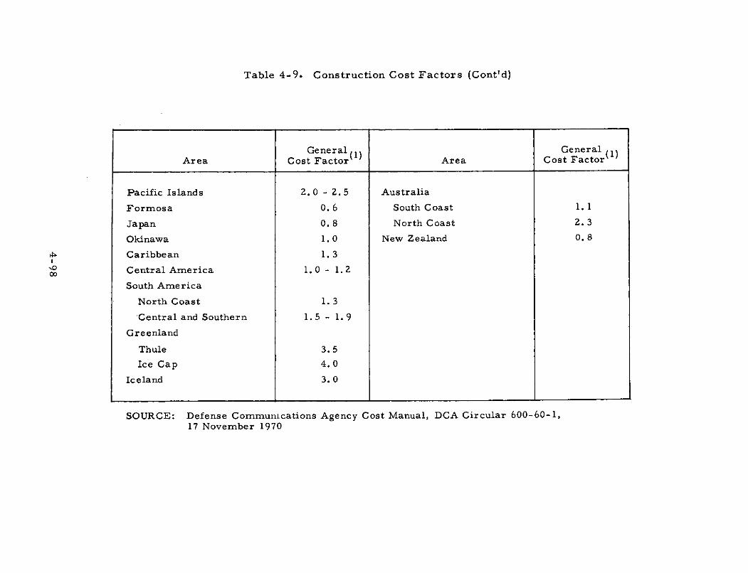
Table 4-9. Construction Cost Factors (Cont'd)
General GeneralArea Cost Factor 1 Area Cost Factor
Pacific Islands 2.0 - 2.5 Australia
Formosa 0.6 South Coast 1. 1
Japan 0.8 North Coast 2.3
Okinawa 1.0 New Zealand 0.8
Caribbean 1.3
Central America 1.0 - 1.2
South America
North Coast 1. 3
Central and Southern 1.5 - 1.9
Greenland
Thule 3.5
Ice Cap 4.0
Iceland 3.0
SOURCE: Defense Communications Agency Cost Manual, DCA Circular 600-60-1,17 November 1970
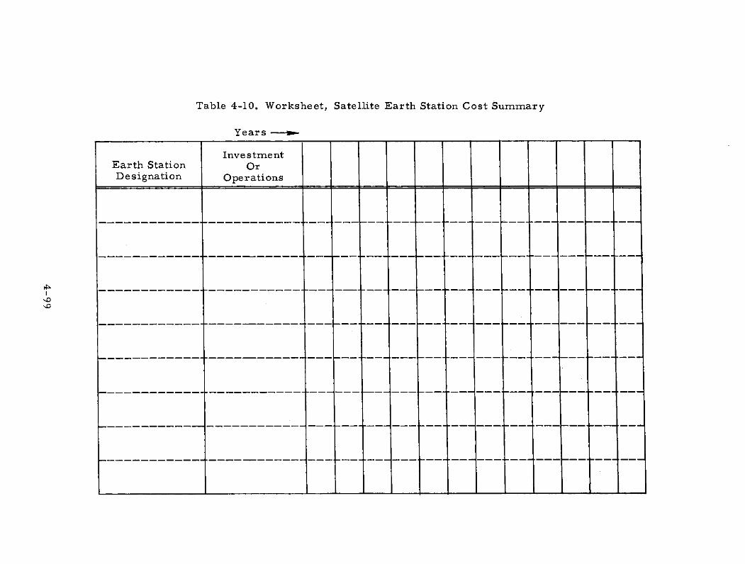
Table 4-10. Worksheet, Satellite Earth Station Cost Summary
Years
InvestmentEarth Station OrDesignation Operations
'0NO
3. REFERENCES
Space Shuttle
1. Space Shuttle System Payload Accommodations, JohnsonSpacecraft Center, JSC 07700, Vol. XIV (13 April 1973).
Centaur
2. Centaur/Shuttle Integration Study, Convair AerospaceDivision of General Dynamics, GDCA-BNE 73-006-5(15 June 1973).
3. Compatibility of a Cryogenic Upper Stage with the SpaceShuttle, Convair Aerospace Division of General Dynamics,GDCA-BNE 71-020-7 (April 1972).
Tug
4. Space Shuttle/Payload Interface Analysis Final ReportVolume II, Space Shuttle Traffic Analysis, The AerospaceCorporation, ATR-74(7334)-l, Vol. II (August 1973).
5. Baseline Tug Definition Document, NASA Marshall SpaceFlight Center (15 March 1972).
General
6. Launch Vehicle Estimating Factors for Advance MissionPlanning, NASA-NHB 7100.5A, 1972 Edition.
7. Integrated Operations / Payloads /Fleet Analysis Mid- TermReport, Volume IV, Launch Systems, The AerospaceCorporation, ATR-71(7231)-9, Vol. IV (19 March 1971).
4-100
E. SPACE SYSTEM COST ESTIMATING
1. BACKGROUND
From past studies, a comprehensive payload program cost model
has evolved that is primarily used for analyzing total space plans com-
posed of numerous individual payload (satellite) programs. This basic
cost model has been simplified and transferred to a remote console com-
puter system so that single payload programs can be estimated quickly
and efficiently for BRAVO analyses. The purpose of this section is (1) to
provide a description of the basic cost model, (2) to define the inputs it
requires, and (3) to discuss the output of the cost model.
2. PAYLOAD PROGRAM COST MODEL
The computerized model is composed of two major sections; the
payload cost model estimates costs and the launch cost model deals with
launch vehicle chargeable costs. In the case of expendable vehicles,
expendable hardware costs and launch site operations and support are
included. For Shuttle and Tug launches, NASA cost per flight includes
such items as expendable drop tank hardware, prorata solid motor hard-
ware, propellants (solid and liquid), recovery, refurbishment, spares,
and all direct costs at the launch site for facility maintenance, launch
operations, and launch support.
Satellite cost is defined as all costs required to design, develop,
manufacture, and test satellites and support them during launch and
orbital operation. Typically, a satellite program is divided into RDT&E
(nonrecurring), investment (recurring), and operations (recurring) cost
categories. The model spreads the RDT&E costs over three years(1)
RDT&E covers design, development and test; investment includes procure-
ment of satellite hardware; operations covers support during and-after
launch. In cases where reuse through ground refurbishment is considered,
the operations cost category also includes satellite repair and refurbishmeni
(1) User may vary spread from two to five years.
4-101
The payload cost model calculates basic RDT&E and unit
costs from payload data input to the program. Cost-estimating relation-
ships (CERs) stored in the program are automatically applied to these
inputs. Launch vehicle cost per flight is also an input. Based on pay-
load and launch vehicle schedules, total direct costs are calculated
and fiscal funding requirements are determined by the model, all of
which are printed in suitable formats.
3. COST MODEL INPUTS
The physical and performance data and the descriptive and
schedule information required for operating the cost model are set
forth in worksheet form in Tables 4-11through 4-13. (Table 4-13contains input data that are nominal values set in the computer program;
however, they can be overridden as occasion demands.) Descriptions
of all these inputs and the necessary assumptions that relate to their
use are presented in this section.
a. Title and Satellite Type
For identification purposes, a title is required; the input for-mat, i.e., NAME- ' ................ ', is shown in Table 4-11. The
program demands that the type of satellite be noted, i. e., current designreusable (CDR) or low-cost reusable (LCR); TYPE - 2 (or 3, respectively).Current design reusable means that current technology and design pro-cedures are used but that they are modified to allow for reuse throughground refurbishment. Low-cost designs are based on data fromLMSC( 1 ) and assume that payload weight and volume constraints maybe relaxed so that (1) lower cost components and materials can beused, (2) less testing is needed for design verification and qualification,and (3) fewer parts are needed for tests. These low-cost designs arealso compatible with ground-based refurbishment.
(1) Design Guide for Low-Cost Standardized Payloads, LMSC-D154696,Volumes I, II, NASA Contract NAS W-2312 (30 April 1972)
4-102
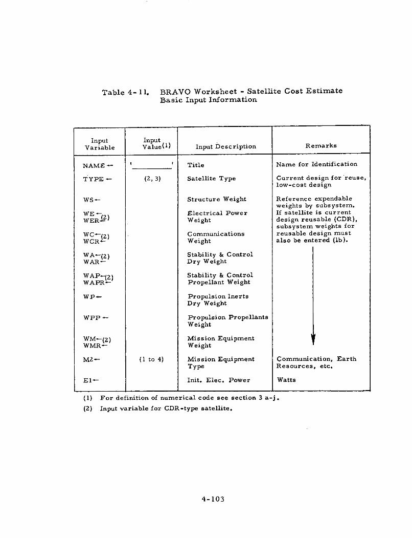
Table 4- 11. BRAVO Worksheet - Satellite Cost EstimateBasic Input Information
Input InputVariable Value(1) Input Description Remarks
NAME - ' Title Name for Identification
TYPE - (2, 3) Satellite Type Current design for reuse,low-cost design
WS- Structure Weight Reference expendableweights by subsystem.
WE Electrical Power If satellite is currentWER- ) Weight design reusable (CDR),
subsystem weights for
WC-( ) Communications reusable design mustWCR- Weight also be entered (lb).
WA-(Z) Stability & ControlWAR- Dry Weight
WAP-(2) Stability & ControlWAPR- Propellant Weight
WP- Propulsion InertsDry Weight
WPP - Propulsion PropellantsWeight
WM-(Z) Mission EquipmentWMR- Weight
M2- (1 to 4) Mission Equipment Communication, Earth
Type Resources, etc.
El- Init. Elec. Power Watts
(1) For definition of numerical code see section 3 a-j.
(2) Input variable for CDR-type satellite.
4-103
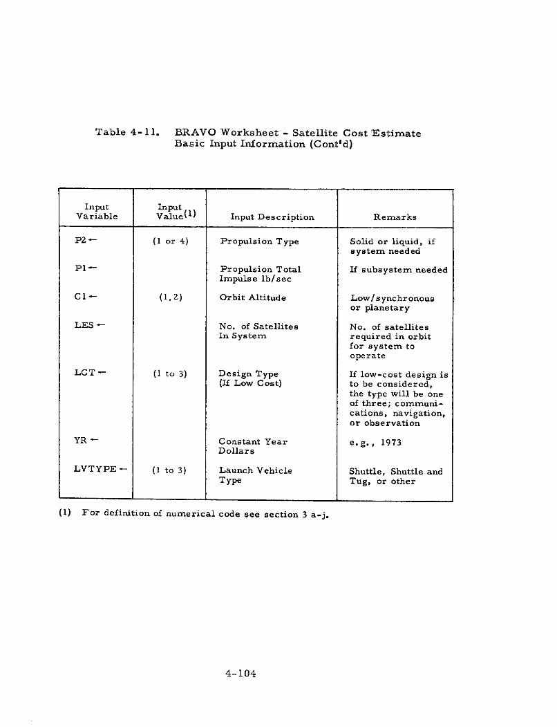
Table 4- 11. BRAVO Worksheet - Satellite Cost EstimateBasic Input Information (Cont'd)
Input InputVariable Value( 1 ) Input Description Remarks
P2- (1 or 4) Propulsion Type Solid or liquid, ifsystem needed
P1- Propulsion Total If subsystem neededImpulse lb/sec
Cl - (1,2) Orbit Altitude Low/synchronousor planetary
LES - No. of Satellites No. of satellitesIn System required in orbit
for system tooperate
LCT - (1 to 3) Design Type If low-cost design is(If Low Cost) to be considered,
the type will be oneof three; communi-cations, navigation,or observation
YR Constant Year e.g., 1973Dollars
LVTYPE- (1 to 3) Launch Vehicle Shuttle, Shuttle andType Tug, or other
(1) For definition of numerical code see section 3 a-j.
4-104
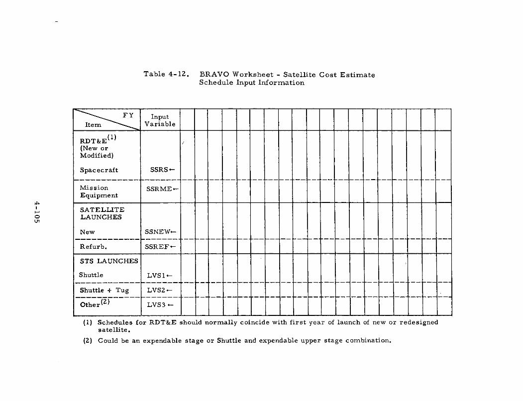
Table 4-12. BRAVO Worksheet - Satellite Cost EstimateSchedule Input Information
FY InputItem Variable
RDT&E(1)(New orModified)
Spacecraft SSRS -
Mission SSRME -Equipment
SATELLITELAUNCHES
New SSNEW-
Refurb. SSREF*-
STS LAUNCHES
Shuttle LVS 1-
Shuttle + Tug LVS2.-
Other(z) LVS3 -
(1) Schedules for RDT&E should normally coincide with first year of launch of new or redesignedsatellite.
(2) Could be an expendable stage or Shuttle and expendable upper stage combination.
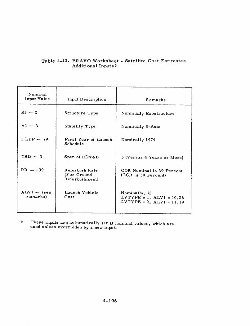
Table 4-13. BRAVO Worksheet - Satellite Cost EstimatesAdditional Inputs*
NominalInput Value Input Description Remarks
S1 - 2 Structure Type Nominally Exostructure
Al - 3 Stability Type Nominally 3-Axis
FLYP - 79 First Year of Launch Nominally 1979Schedule
YRD - 3 Span of RDT&E 3 (Versus 4 Years or More)
RR - .39 Refurbish Rate CDR Nominal is 39 Percent(For Ground (LCR is 30 Percent)Refurbishment)
ALV1 - (see Launch Vehicle Nominally, ifremarks) Cost LVTYPE = 1, ALVI = 10.26
LVTYPE = 2, ALV1 = 11. 19
These inputs are automatically set at nominal values, which areused unless overridden by a new input.
4-106
b. Subsystem Weights
Reference (current design expendable satellite) weights
are an input to the cost-estimating relationships (CERs) which arebased on current expendable satellites. Factors are applied to thereference estimates to give effect to low-cost reusable design costestimates. For current design reusable satellites, cost factors arebased on differences in weight from reference subsystems and thusrequire reusable satellite subsystem weight data. The computer inputsare set forth in Table 4-11 and are split into two groups; one representsthe reference weights and the second represents the current designreusable weights. Only one input is required for structure, i.e.,the final structure weight. Similarly, the propulsion weights, if appli-cable, need single values only.
c. Mission Equipment Type
Four types of mission equipment are identified in the cost model:(1) communications, (2) navigation, (3) earth resources, and (4) meteoro-logy. For a particular estimate the most appropriate category must beselected from the list. Thus, the input would be M2 - 1 for communica-tions mission equipment.
d. Initial Electrical Power
Input requires initial output of the electrical subsystem to begiven in watts, e.g., El - 150.
e. Propulsion Type and Total Impulse
An integral propulsion system may occasionally be required byan STS satellite. (A propulsion system requirement should not be con-fused with the reaction control propulsion, which is included in thestability and control subsystem.) The type of propulsion system refers
4-107
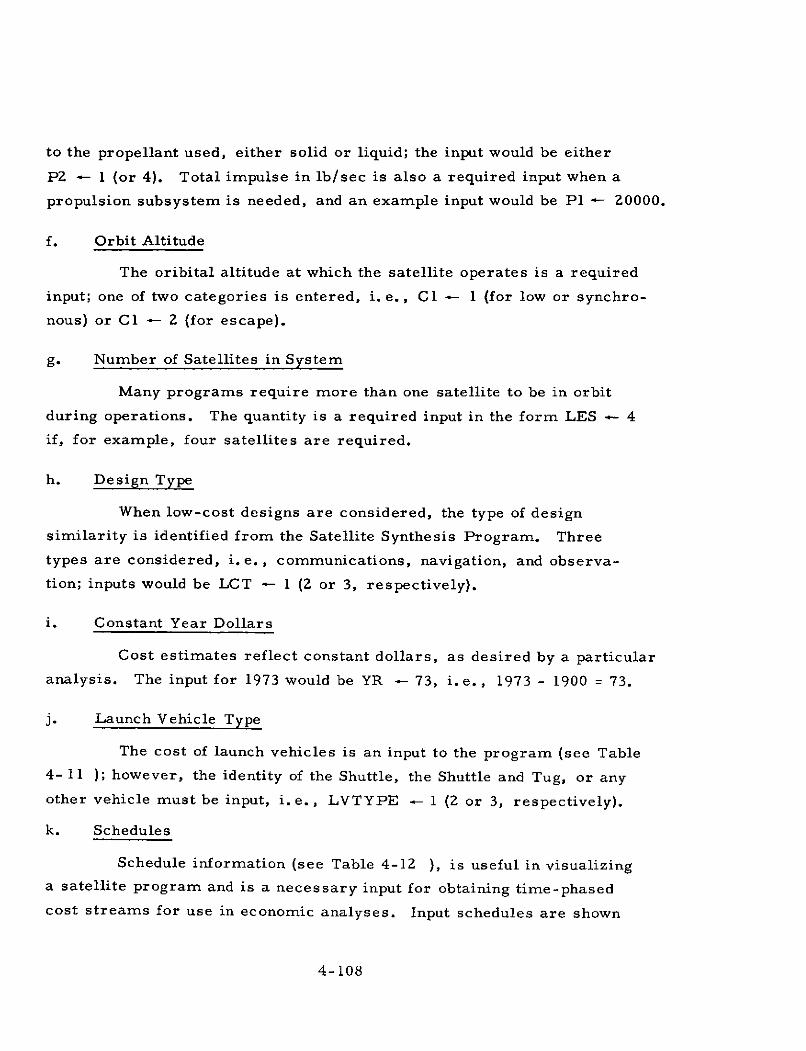
to the propellant used, either solid or liquid; the input would be either
P2 - 1 (or 4). Total impulse in lb/sec is also a required input when a
propulsion subsystem is needed, and an example input would be P1 - 20000.
f. Orbit Altitude
The oribital altitude at which the satellite operates is a required
input; one of two categories is entered, i. e., C1 - 1 (for low or synchro-
nous) or Cl - 2 (for escape).
g. Number of Satellites in System
Many programs require more than one satellite to be in orbit
during operations. The quantity is a required input in the form LES - 4
if, for example, four satellites are required.
h. Design Type
When low-cost designs are considered, the type of design
similarity is identified from the Satellite Synthesis Program. Three
types are considered, i.e., communications, navigation, and observa-
tion; inputs would be LCT - 1 (2 or 3, respectively).
i. Constant Year Dollars
Cost estimates reflect constant dollars, as desired by a particular
analysis. The input for 1973 would be YR - 73, i.e., 1973 - 1900 = 73.
j. Launch Vehicle Type
The cost of launch vehicles is an input to the program (see Table
4-11 ); however, the identity of the Shuttle, the Shuttle and Tug, or any
other vehicle must be input, i.e., LVTYPE - 1 (2 or 3, respectively).
k. Schedules
Schedule information (see Table 4-12 ), is useful in visualizing
a satellite program and is a necessary input for obtaining time-phased
cost streams for use in economic analyses. Input schedules are shown
4-108
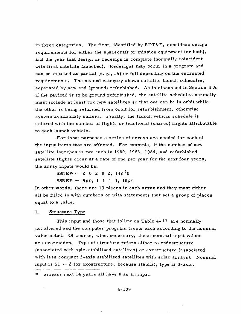
in three categories. The first, identified by RDT&E, considers design
requirements for either the spacecraft or mission equipment (or both),
and the year that design or redesign is complete (normally coincident
with first satellite launched). Redesigns may occur in a program and
can be inputted as partial (e. g., .5) or full depending on the estimated
requirements. The second category shows satellite launch schedules,
separated by new and (ground) refurbished. As is discussed in Section 4 A
if the payload is to be ground refurbished, the satellite schedules normally
must include at least two new satellites so that one can be in orbit while
the other is being returned from orbit for refurbishment, otherwise
system availability suffers. Finally, the launch vehicle schedule is
entered with the number of flights or fractional (shared) flights attributable
to each launch vehicle.
For input purposes a series of arrays are needed for each of
the input items that are affected. For example, if the number of new
satellite launches is two each in 1980, 1982, 1984, and refurbished
satellite flights occur at a rate of one per year for the next four years,
the array inputs would be:
SSNEW - 2 0 2 0 2, 14 p 0
SSREF - 5p0, 1 1 1 1, 10p0
In other words, there are 19 places in each array and they must either
all be filled in with numbers or with statements that set a group of places
equal to a value.
1. Structure Type
This input and those that follow on Table 4- 13 are normally
not altered and the computer program treats each according to the nominal
value noted. Of course, when necessary, these nominal input values
are overridden. Type of structure refers either to endostructure
(associated with spin-stabilized satellites) or exostructure (associated
with less compact 3-axis stabilized satellites with solar arrays). Nominal
input is Sl - 2 for exostructure, because stability type is 3-axis.
* p means next 14 years all have 0 as an input.
4-109
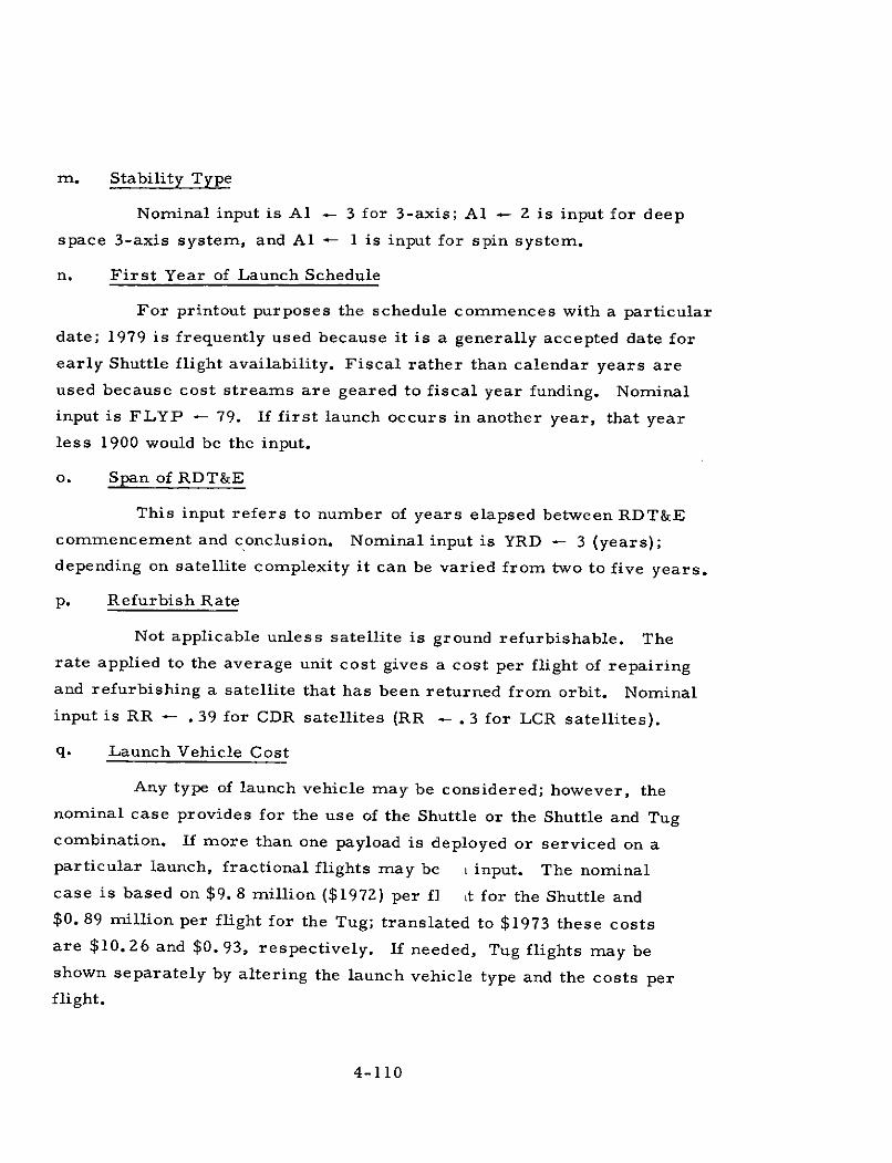
m. Stability Type
Nominal input is Al - 3 for 3-axis; Al - 2 is input for deep
space 3-axis system, and Al - 1 is input for spin system.
n. First Year of Launch Schedule
For printout purposes the schedule commences with a particular
date; 1979 is frequently used because it is a generally accepted date for
early Shuttle flight availability. Fiscal rather than calendar years are
used because cost streams are geared to fiscal year funding. Nominal
input is FLYP - 79. If first launch occurs in another year, that year
less 1900 would be the input.
o. Span of RDT&E
This input refers to number of years elapsed between RDT&E
commencement and conclusion. Nominal input is YRD - 3 (years);
depending on satellite complexity it can be varied from two to five years.
p. Refurbish Rate
Not applicable unless satellite is ground refurbishable. The
rate applied to the average unit cost gives a cost per flight of repairing
and refurbishing a satellite that has been returned from orbit. Nominal
input is RR - . 39 for CDR satellites (RR - . 3 for LCR satellites).
q. Launch Vehicle Cost
Any type of launch vehicle may be considered; however, the
nominal case provides for the use of the Shuttle or the Shuttle and Tug
combination. If more than one payload is deployed or serviced on a
particular launch, fractional flights may be L input. The nominal
case is based on $9. 8 million ($1972) per f] Lt for the Shuttle and
$0. 89 million per flight for the Tug; translated to $1973 these costs
are $10. 26 and $0. 93, respectively. If needed, Tug flights may be
shown separately by altering the launch vehicle type and the costs per
flight.
4-110

4. COST MODEL OUTPUT
The payload program model output is designed to show basic
RDT&E and unit cost estimates by subsystem and to show the time-
phased funding for each major category; RDT&E, investment, and
operations by mission equipment, by spacecraft, and by total. These
funding categories are included in the output to facilitate economic analyses.
RDT&E and unit costs are presented to highlight cost drivers. Total
launch vehicle cost (time-phased) is included separately and in the program
grand total.
An example has been developed to illustrate the output (and to
show the input requirements) for a typical satellite. Tables 4-14
through 4-16 contain example input data; Tables 4-17 and 4-18 show
the example output generated by the computer program based on the
input data. Table 4-17 contains the basic satellite cost data together
with payload, launch vehicle, and total fiscal funding estimates. Table 4-18
provides a further breakdown of these costs into spacecraft and mission
equipment funding flows.
Table 4-14 BRAVO Schedule Input - Example
SSRS - 1, 18p0 ( 1 )
SSRME - 1, 18p0
SSNEW - 4, 4p0, 3, 13p0
SSREF - 0 0 1 2 1 0 0 1 1 0 1, 8p0
LVS2-4 0 1 2 1 3 0 1 1 0 1, 8p0
(1) 18p0 means the next 18 years all have 0 as an input.
4-111
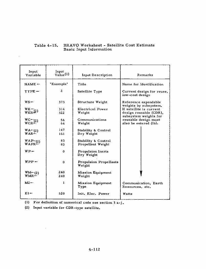
Table 4-15. BRAVO Worksheet - Satellite Cost EstimateBasic Input Information
Input InputVariable Value(l) Input Description Remarks
NAME - 'Example' Title Name for Identification
TYPE - 2 Satellite Type Current design for reuse,low-cost design
WS- 373 Structure Weight Reference expendableweights by subsystem.
WE -: 314 Electrical Power If satellite is currentWERV) 322 Weight design reusable (CDR),
subsystem weights forWC-(Z) 56 Communications reusable design mustWCR- 64 Weight also be entered (lb).
WA-(2) 147 Stability & ControlWAR- 161 Dry Weight
WAP-(z) 83 Stability & ControlWAPR- 83 Propellant Weight
WP- 0 Propulsion InertsDry Weight
WPP - 0 Propulsion PropellantsWeight
WM-(2 ) 240 Mission EquipmentWMR- 240 Weight
MZ- 1 Mission Equipment Communication, EarthType Resources, etc.
El- 520 Init. Elec. Power Watts
(1) For definition of numerical code see section 3 a-j.
(2) Input variable for CDR-type satellite.
4-112
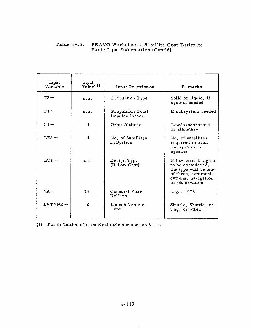
Table 4-15. BRAVO Worksheet - Satellite Cost EstimateBasic Input Information (Cont'd)
Input InputVariable Value(l) Input Description Remarks
PZ'- n.a. Propulsion Type Solid or liquid, ifsystem needed
P1 - n. a. Propulsion Total If subsystem neededImpulse lb/sec
Cl - 1 Orbit Altitude Low / s ync hr onousor planetary
LES - 4 No. of Satellites No. of satellitesIn System required in orbit
for system tooperate
LCT - n. a. Design Type If low-cost design is(If Low Cost) to be considered,
the type will be oneof three; communi-cations, navigation,or observation
YR 73 Constant Year e.g., 1973Dollars
LVTYPE - 2 Launch Vehicle Shuttle, Shuttle andType Tug, or other
(1) For definition of numerical code see section 3 a-j.
4-113
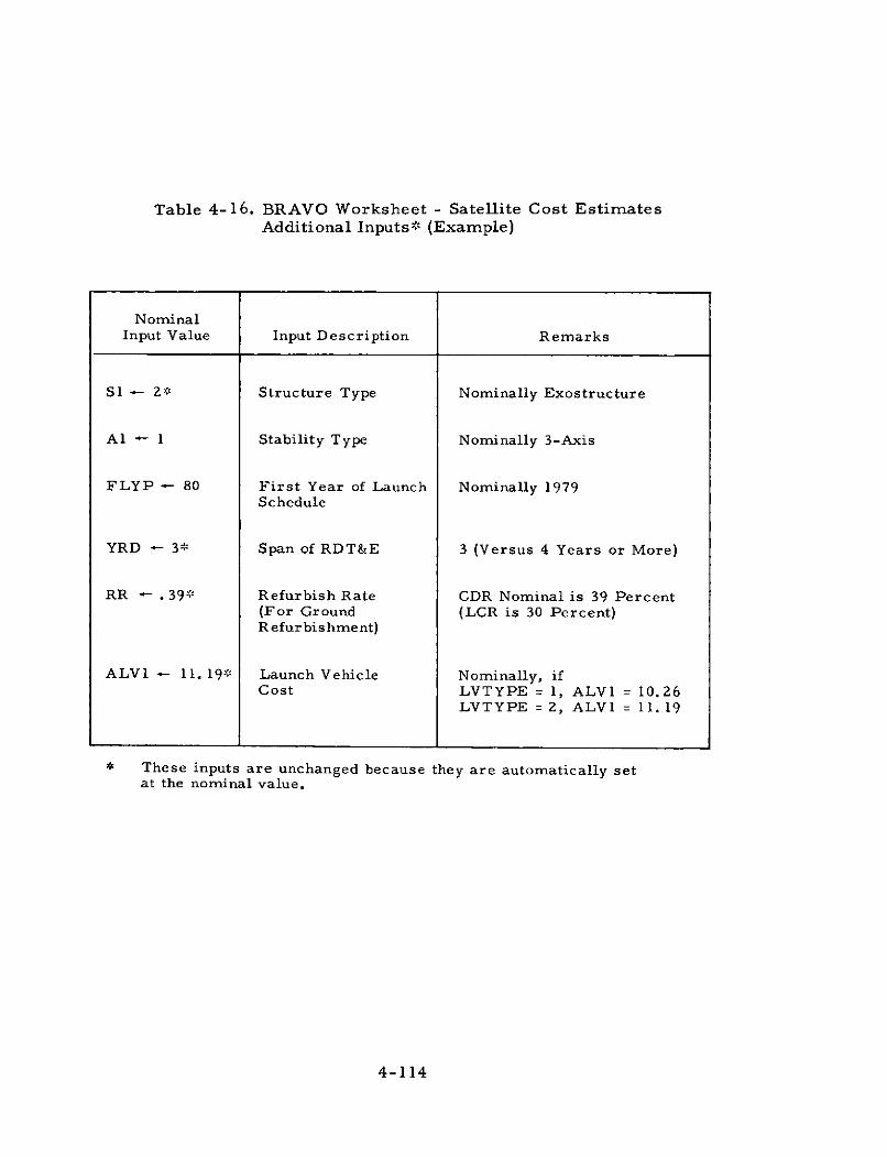
Table 4-16. BRAVO Worksheet - Satellite Cost EstimatesAdditional Inputs* (Example)
NominalInput Value Input Description Remarks
S1 - 2* Structure Type Nominally Exostructure
Al - 1 Stability Type Nominally 3-Axis
FLYP - 80 First Year of Launch Nominally 1979Schedule
YRD - 3* Span of RDT&E 3 (Versus 4 Years or More)
RR - .39* Refurbish Rate CDR Nominal is 39 Percent(For Ground (LCR is 30 Percent)Refurbishment)
ALV1 - 11. 19* Launch Vehicle Nominally, ifCost LVTYPE = 1, ALV1 = 10.26
LVTYPE = 2, ALVI = 11.19
* These inputs are unchanged because they are automatically setat the nominal value.
4-114
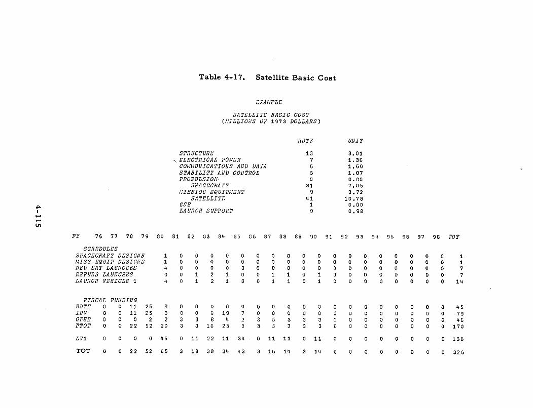
Table 4-17. Satellite Basic Cost
bAAI!PLE
SATELLITE BASIC COST(!,'ILLIOilS OF 1973 DOLLARS)
DTE UIIIT
STRUCTUR1; 13 3.01\ ELECTRICAL POWRI 7 1.36
COIII.UHRICATIOIiS AilD DATA 6 1.60STABILITY AND COiTROL 5 1.07PROPULSIO- 0 0.00
SPACECRAFT 31 7.05UISSIOD EQUIP'EIIT 9 3.72
SATELLITE 41 10.78GSE 1 0.00LAUlCH SUPPORT 0 0.98
FY 76 77 78 79 80 81 82 33 84 85 06 87 88 89 90 91 92 93 94 95 96 97 98 TOT
SCHEDULESSPACECRAFT DESICiJS 1 0 0 0 0 0 0 0 0 0 0 0 0 0 0 0 0 0 0 1MISS EQUIP DESIGIRS 1 0 0 0 0 0 0 0 0 0 0 0 0 0 0 0 0 0 0 1liEW SAT LAUNCHES 4 0 0 0 0 3 0 0 0 0 0 0 0 0 0 0 0 0 0 7REFURB LAUNCHES 0 0 1 2 1 0 0 1 1 0 1 0 0 0 0 0 0 0 0 7LAUNCH VEHICLE 1 4 0 1 2 1 3 0 1 1 0 1 0 0 0 0 0 0 0 0 14
FISCAL FUNDIINGRDTE 0 0 11 25 0 0 0 0 0 0 0 0 0 0 0 0 0 0 0 0 0 0 0 45IlV 0 0 11 25 9 0 0 3 19 7 0 0 0 0 0 3 0 0 0 0 0 0 0 79OPER 0 0 0 2 2 3 8 8 4 2 3 5 3 3 3 0 0 0 0 0 0 0 0 46PTOT 0 0 22 52 20 3 0 16 23 9 3 5 3 3 3 0 0 0 0 0 0 0 0 170
LV1 0 0 0 0 45 0 11 22 11 34 . 0 11 11 0 11 0 0 0 0 0 0 0 0 156
TOT 0 0 22 52 65 3 19 38 34 43 3 10 14 3 14 0 0 0 0 0 0 0 0 326
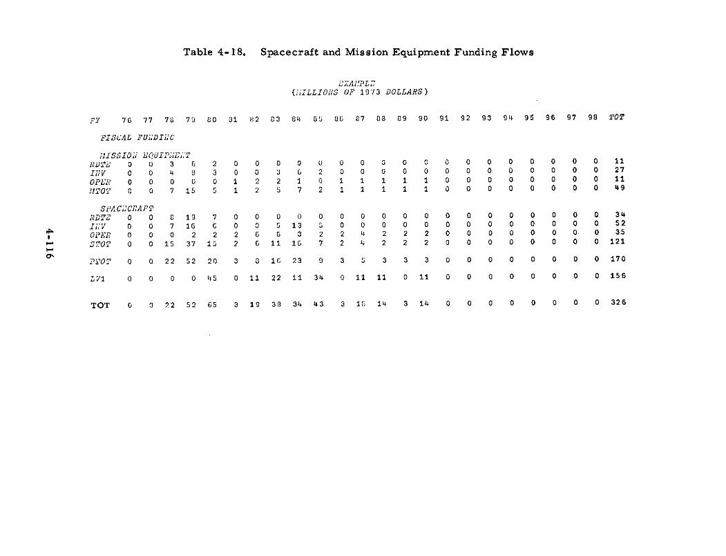
Table 4-18. Spacecraft and Mission Equipment Funding Flows
L'ZAZPL
(KILLIOIIS OF 1973 DOLLARS)
PFY 76 77 78 79 80 81 82 83 84 85 86 87 88 89 90 91 92 93 94 95 96 97 98 TOT
FISCAL FUL'DIijG
[1ISSIO E QUIPijEJT7RDTi 0 0 3 6 2 0 0 0 0 0 0 0 0 0 0 0 0 0 0 0 0 0 0 11
IIV 0 0 4 9 3 0 0 3 6 2 0 0 0 0 0 0 0 0 0 0 0 0 0 27
OPER 0 0 0 0 0 1 2 2 1 0 1 1 1 1 1 0 0 0 0 0 0 0 0 11
[.fTOT 0 0 7 15 5 1 2 5 7 2 1 1 1 1 1 0 0 0 0 0 0 0 0 49
SPA CLCRAPTRDTE 0 0 8 19 7 0 0 0 0 0 0 0 0 0 0 0 0 0 0 0 0 0 0 34
1;V 0 0 7 16 6 0 0 5 13 5 0 0 0 0 0 0 0 0 0 0 0 0 0 52
OPER 0 0 0 2 2 2 6 6 3 2 2 4 2 2 2 0 0 0 0 0 0 0. 0 35
STOT 0 0 15 37 15 2 6 11 16 7 2 4 2 2 2 0 0 0 0 0 0 0 0 121
P'TO T 0 0 22 52 20 3 8 16 23 9 3 5 3 3 3 0 0 0 0 0 0 0 0 170
LV1 0 0 0 0 45 0 11 22 11 34 0 11 11 0 11 0 0 0 0 0 0 0 0 156
TOT 0 0 22 52 65 3 19 33 34 43 3 10 14 3 14 0 0 0 0 0 0 0 0 326
5. COMPATIBILITY WITH SATELLITE SYNTHESIS PROGRAMOUTPUT
The primary source of input information for the cost model
is the Satellite Synthesis Program. With the exception of NAME,
TYPE, LES, YR, LVTYPE, FLYP, and schedules, all cost inputs
needed for any particular case will be found in the synthesis output.
Accordingly, wherever possible the payload cost model and the synthesis
model have used the same program coding to facilitate identification
and transfer of input data. For example, WS identifies structure
weight under REFERENCE WEIGHTS, CDR GROUND REFURB, or
LCR and it also identifies the cost input for structure weight. WE
similarly identifies electrical weight; however, if the satellite is CDR
the WE cost input will be found in the REFERENCE WEIGHT column
and the WER cost input will be found under the CDR GROUND REFURB
column. (Recall, however, that for LCR designs the weights to use
are REFERENCE WEIGHTS.) Two synthesis outputs (cost inputs)
are not as easily identified. The first, mission equipment type (cost
input M2) is identifiable as NAV, COM, or OBS under TYPE MISS.
EQUIP. If the satellite type is a low-cost design, it also identifies
the value to use for LCT, the second input. All other cost input codes
needed are the same as the synthesis outputs.
The other cost inputs mentioned above are obtainable from
either the capture analysis (refer to Section D 1) or from the facts
surrounding the case to be studied. NAME, TYPE, LES and YR generally
are known from the case itself. LVTYPE, FLYP, and schedule infor-
mation should be obtainable from the capture output.
4-117
F. SPACE SYSTEM OPTIMIZATION, RISK, AND LOGISTICS ANALYSIS
1. INTRODUCTION
When a normal analysis gets to this point, there will be several
problems which remain to be solved in order to arrive at an optimized
solution and be assured of meeting the system outage requirements.
All satellite systems have been configured to meet the functional require-
ments. The problem then is to establish an optimum configuration (for
lowest cost) by choosing between the alternative satellite design approaches
and satellite design life (mean mission duration) options and to decide
how many spare satellites are required on orbit. This is accomplished
by completing the analyses of all reasonable approaches and quantizing the
tradeoffs.
The satellite design alternatives available from which to choose
would normally include current design satellites suitable for ground refur-
bishment, or current design satellites suitable for on-orbit repair (or
ground refurbishment), or low-cost satellites suitable for on-orbit repair
(or ground refurbishment). The two current design satellite approaches
would normally have three or four mean mission duration designs from
which to choose. (Such variations in mean mission duration are obtained
by changing satellite component redundancy.) Another option available
to the analyst is to add spare satellites on orbit for any of these configurations.
Since all satellite systems meet the functional requirements,
the problem becomes (1) selecting the satellite systems which meet the
risk (outage) requirement and eliminating those which do not; (2) determin-
ing which of the satellite systems that meet the risk (outage) requirements
show the lowest system cost estimate; (3) of those configuration alternatives
which display the lowest cost estimate or are close to it, which ones
exhibit outage which is the least sensitive to launch, delays, and satellite
failure rates; and (4) for the satellite system selected from the above
considerations, what is the satellite traffic required to maintain the
space capability on orbit (logistics).
4-118
2. PROCEDURES
The calculations required to carry out the method of analysis
appropriately have been coded as an interactive computer program called
RISK using the APL program language. Therefore, the methodology is
best described by the computer program itself. The computer program
accepts input data for each of the space system alternatives which are
mentioned in the introduction. The output tabulated numerically quantifies
the availability (1 minus the outage), program cost estimate, and expected
number of launches for each of the alternative configurations as a function
of (1) launch delay for replacement of or on-orbit repair of a satellite,
(2) satellite failure rate, (3) satellite turn-on delay for on-orbit spare
satellites, (4) satellite preventative maintenance launch interval, and
(5) a launch-on-warning strategy instead of the launch-on-failure logistics
strategy. The methodology is a very complete simulation of satellite
system logistics which also sums the program costs and number of
launches required for each simulation.
After the operation of the computer program, the quantitative
results are then plotted so that the system tradeoffs are displayed and
the selection procedure described in the introduction is accomplished.
An example of this procedure is shown in section 4. F. 2. d.
a. Inputs
The inputs for the computer program consist of the cost estimates
for each satellite to be studied; unit costs, satellite development costs,satellite operations costs, and transportation cost estimates are included.
The configuration of satellite equipment and the associated failure rates
for every identified element of each satellite are also inputs. An alternative
input would be the estimated survival curve for each satellite. The
probability of mission completion for the Shuttle and upper stage (if
the latter is used) and an estimate of the infant mortality satellite loss
factor are used.
4-119
Inputs for the subject APL computations are of two kinds familiar
to APL terminal operators:
(1) Global Variables
Global variables are constants which are stored in thecommon APL workspace under distinctive alphanumericcode names, and which are available to any executing pro-gram within the same workspace, provided that the codename used has not also been previously declared "local"within the executing program. Global variables may beleft as constants throughout the computations, such asnumerical tables giving the failure rates for a set ofmodules. However, they may also be purposely modifiedby the computations of the program during its execution;this is not normally done to variables which are intendedas inputs in subsequent executions of the same mainprogram. Thus, as many different inputs as desired maybe stored permanently as global variables for multipleexecutions of the same program, or they may be purposelychanged before an execution as a means of varying the inputdata or program parameters.
(2) Interactive Inputs
One of the main purposes of such computer facilities asAPL is the interaction between computer and terminaloperator in flexible computations, using a dialog betweenthem as a means of allowing the operator to make decisionsas to data inputs or program execution. In both cases,a program must have been stored previously which causesthe computer to interrogate the operator, asking for theprecise information needed at the moment.
Both of the above forms of input are used in the BRAVO APL
computations.
Global inputs are used primarily as a means of storing all of
the computational data and program parameters which will be used over
and over as many different cases are computed. They could be "hard-
programmed" into the programs, but that is a much more difficult form
of input to alter purposely than global variables.
4-120
Interactive inputs are used as a convenient means of setting up
the input data for different cases of interest. This is done in the APL
subroutine SETUP, which then immediately causes execution of the
remainder of the program.
Table 4-19 shows the required inputs for the BRAVO logistics
analysis program.
b. Computer Program Listing and Flow Chart
The APL functions (program listing) is presented in Part 4
of this volume of the final report. It is intended that the flow charts
described in the next section should be used for tracing the order in which
the computations occur in the computer program. The copies of the APL
functions themselves are only required to set up the program on the computer
or if the details of the algorithms are needed by the analyst. It is assumed
that the analyst will have available to him or his computational aide an
IBM APL terminal for carrying out the calculations.
Once several input variables have been defined in the APL"workspace, " the entire program of computations is executed by typing
in the name of the APL function SETUP, which is the beginning flow
chart. SETUP allows initializing several other program parameters and
variables, and then automatically executes the function INTELSAT.
The remaining functions are executed as branches within INTELSAT.
Since the art of flow-charting is not perfectly defined, these flow
charts were drawn by adapting some of the conventions used in FORTRAN
flow charting, sometimes using FORTRAN conventions not actually followed
in APL programming. The flow charts are meant to show the intent of
the algorithms rather than their actual mechanization, so that one is
justified in taking some liberties with the conventions. For example,APL branches to other APL functions by merely using the function name(with proper input syntax), whereas FORTRAN must use a "CALL"
4-121
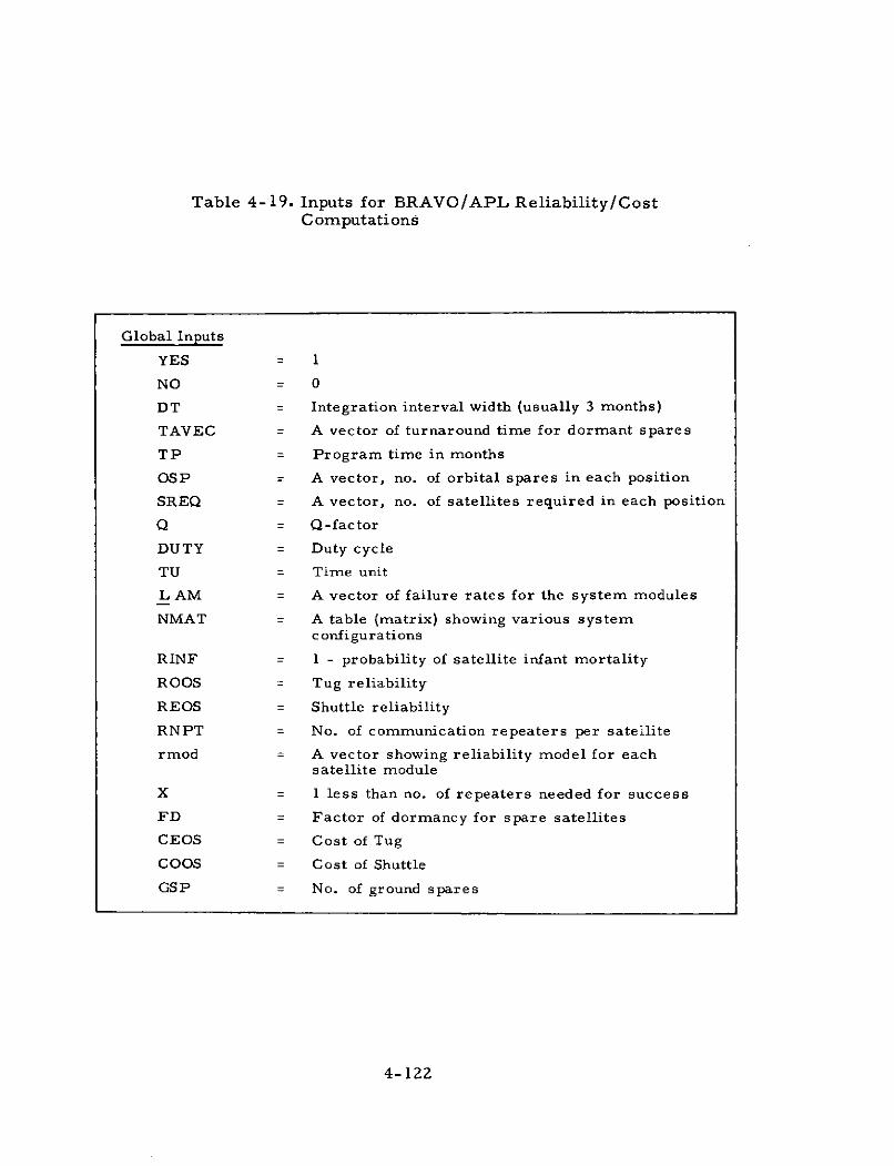
Table 4-19. Inputs for BRAVO/APL Reliability/CostComputations
Global Inputs
YES = 1
NO = 0
DT = Integration interval width (usually 3 months)
TAVEC = A vector of turnaround time for dormant spares
TP = Program time in months
OSP = A vector, no. of orbital spares in each position
SREQ = A vector, no. of satellites required in each position
Q = Q-factor
DUTY = Duty cycle
TU = Time unit
L AM = A vector of failure rates for the system modules
NMAT = A table (matrix) showing various systemconfigurations
RINF = 1 - probability of satellite infant mortality
ROOS = Tug reliability
REOS = Shuttle reliability
RNPT = No. of communication repeaters per satellite
rmod = A vector showing reliability model for eachsatellite module
X = 1 less than no. of repeaters needed for success
FD = Factor of dormancy for spare satellites
CEOS = Cost of Tug
COOS = Cost of Shuttle
GSP = No. of ground spares
4-122
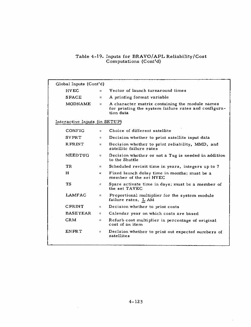
Table 4-19. Inputs for BRAVO/APL Reliability/CostComputations (Cont'd)
Global Inputs (Cont'd)
HVEC = Vector of launch turnaround times
SPACE = A printing format variable
MODNAME = A character matrix containing the module namesfor printing the system failure rates and configura-tion data
Interactive Inputs (in SETUP)
CONFIG = Choice of different satellite
SVPRT = Decision whether to print satellite input data
RPRINT = Decision whether to print reliability, MMD, andsatellite failure rates
NEEDTUG = Decision whether or not a Tug is needed in additionto the Shuttle
TR = Scheduled revisit time in years, integers up to 7
H = Fixed launch delay time in months; must be amember of the set HVEC
TS = Spare activate time in days; must be a member ofthe set TAVEC
LAMFAC = Proportional multiplier for the system modulefailure rates, L AM
CPRINT = Decision whether to print costs
BASEYEAR = Calendar year on which costs are based
CRM = Refurb cost multiplier in percentage of originalcost of an item
ENPRT = Decision whether to print out expected numbers ofsatellites
4-123
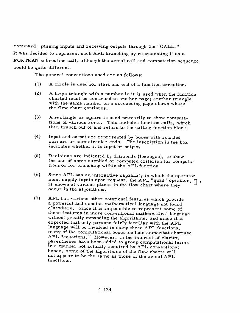
command, passing inputs and receiving outputs through the "CALL."
It was decided to represent such APL branching by representing it as a
FORTRAN subroutine call, although the actual call and computation sequence
could be quite different.
The general conventions used are as follows:
(1) A circle is used for start and end of a function execution.
(2) A large triangle with a number in it is used when the functioncharted must be continued to another page; another trianglewith the same number on a succeeding page shows wherethe flow chart continues.
(3) A rectangle or square is used primarily to show computa-tions of various sorts. This includes function calls, whichthen branch out of and return to the calling function block.
(4) Input and output are represented by boxes with roundedcorners or semicircular ends. The inscription in the boxindicates whether it is input or output.
(5) Decisions are indicated by diamonds (lozenges), to showthe use of some supplied or computed criterion for computa-tions or for branching within the APL function.
(6) Since APL has an interactive capability in which the operatormust supply inputs upon request, the APL "quad" operator, ,is shown at various places in the flow chart where theyoccur in the algorithms.
(7) APL has various other notational features which providea powerful and concise mathematical language not foundelsewhere. Since it is impossible to represent some ofthese features in more conventional mathematical languagewithout greatly expanding the algorithms, and since it isexpected that only persons fairly familiar with the APLlanguage will be involved in using these APL functions,many of the computational boxes include somewhat abstruseAPL "equations." However, in the interest of clarity,parentheses have been added to group computational termsin a manner not actually required by APL conventions;hence, some of the algorithms of the flow charts willnot appear to be the same as those of the actual APLfunctions.
4-124
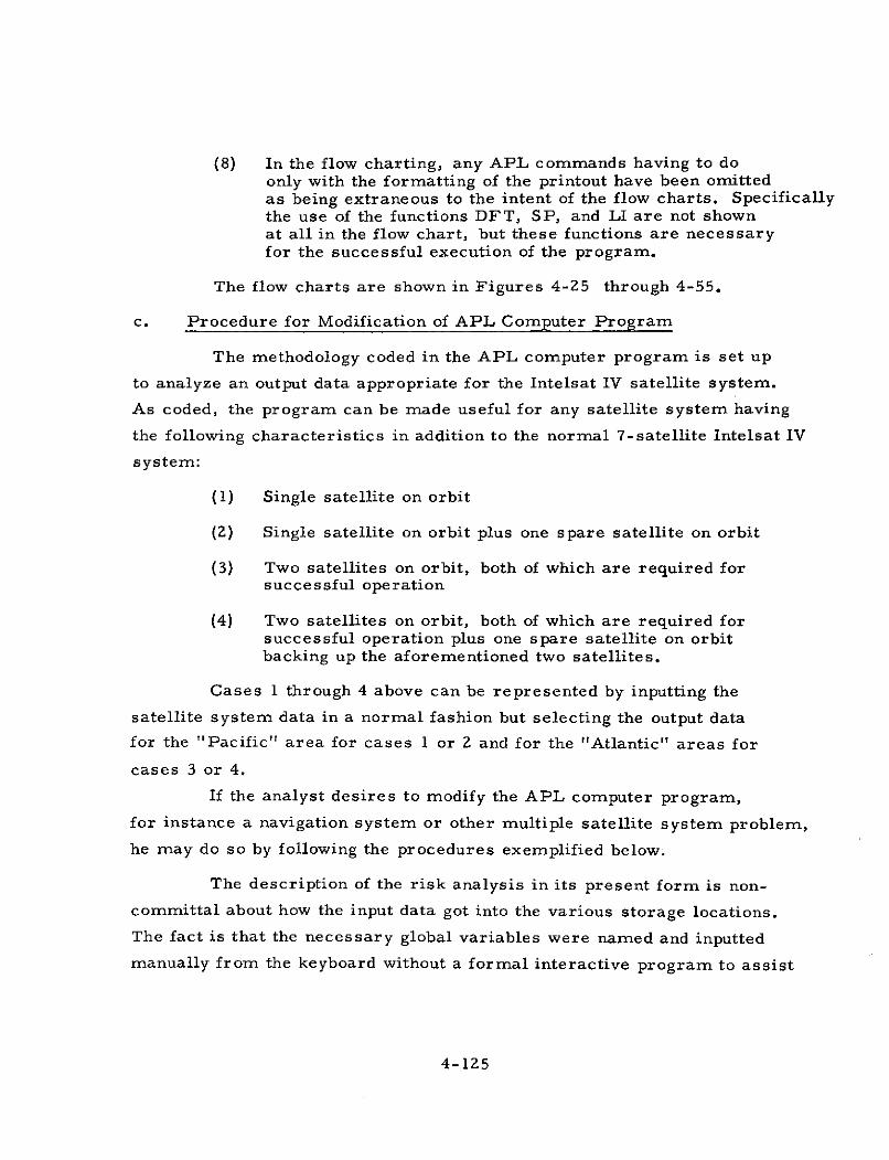
(8) In the flow charting, any APL commands having to doonly with the formatting of the printout have been omittedas being extraneous to the intent of the flow charts. Specificallythe use of the functions DFT, SP, and LI are not shownat all in the flow chart, but these functions are necessaryfor the successful execution of the program.
The flow charts are shown in Figures 4-25 through 4-55.
c. Procedure for Modification of APL Computer Program
The methodology coded in the APL computer program is set up
to analyze an output data appropriate for the Intelsat IV satellite system.
As coded, the program can be made useful for any satellite system having
the following characteristics in addition to the normal 7-satellite Intelsat IV
system:
(1) Single satellite on orbit
(2) Single satellite on orbit plus one spare satellite on orbit
(3) Two satellites on orbit, both of which are required forsuccessful operation
(4) Two satellites on orbit, both of which are required forsuccessful operation plus one spare satellite on orbitbacking up the aforementioned two satellites.
Cases 1 through 4 above can be represented by inputting the
satellite system data in a normal fashion but selecting the output data
for the "Pacific" area for cases 1 or 2 and for the "Atlantic" areas for
cases 3 or 4.
If the analyst desires to modify the APL computer program,
for instance a navigation system or other multiple satellite system problem,
he may do so by following the procedures exemplified below.
The description of the risk analysis in its present form is non-
committal about how the input data got into the various storage locations.
The fact is that the necessary global variables were named and inputted
manually from the keyboard without a formal interactive program to assist
4-125
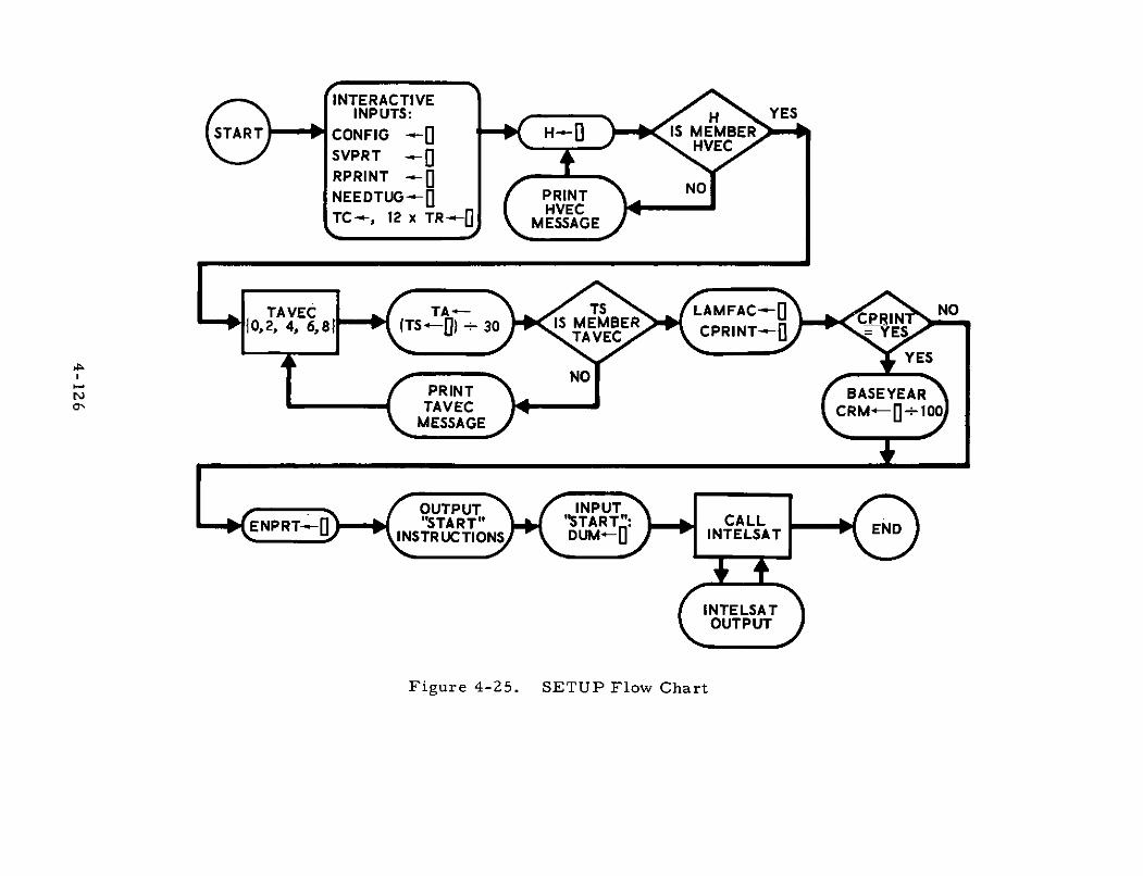
,, TA VEC T--TLAMFAC-0,10,2, 4, 6, 8) T - )+3 STAVCRC RN -
NN
NNTERACTI VE
TAVECC
INPUTS: HNYES
SVPRT A T :CA
RPRINT A NONEEDTUG-( PRINT
OUTPUT
, igure 4-5. SETUP Flow Chart
E TA VEC TA- TS LAMFAC-0 I NO10,2, 4, 6,81 (TS-) -. 30 IS MEMBER PIT ETA VEC PIc Y
YES
NJ PRINT BASEYEAR(7 TAVEC CRM-0 -100
MESSAGE
OUTPUT INPUT
ENPRT-0O "START" "START": CALL ENDINSTR UCTIONS DUM-0' INTELSATT
INTELSATTOUTPUT
Figure 4-Z5. SETUP Flow Chart
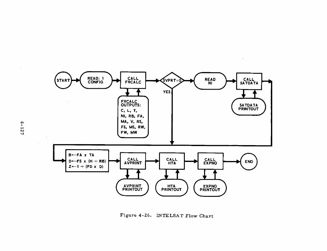
STRT READ: I CALL VPT0READ CALLCONFIG FRCALC NI ~7 SATDATA
YES
FRCALCOUTPUTS: SATDATAC, L, T, PRINTOUT
NI, RB, FA,
p MA, V, RS,
I FS, MS, RW,
k FW, MW
B-FA x TAx (H xRTA CALL CALL CALLD:-:FS x (H RB) AVPRINT CHTA EXPNO ENDZ-1 - (FD x D)
AVPRINT HTA EXPNOPRINTOUT PRINTOUT PRINTOUT
Figure 4-26. INTELSAT Flow Chart
"INITIALIZE" RSHAPEOUTPUTS: RA-RCALC OUTPUTS:
C, L, T, NI, TC, MMDMI, V, WARN
RB
ERFA - 1 MA -1 IMMD CALL RS-(RSHAPE 1, RA) V -- RCALC RA x RNW
N
RNW-RCALC
READ: CALL FS -1 (RSHAPE 1, RS) MS*-1 MMD1, RA RSHAPE WARN-1
RSHAPEOUTPUTS:TC, MMD
Figure 4-27. FRCALC Flow Chart
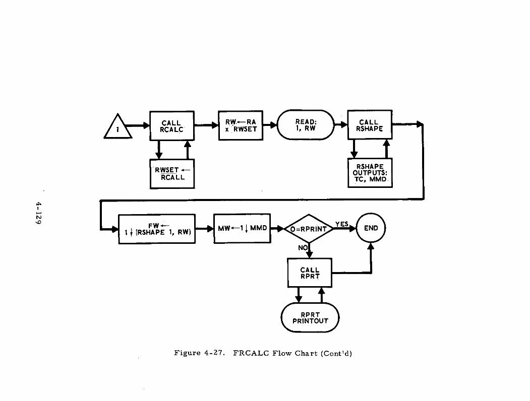
CALL RW-RA I ~READ: CALL1\ I RCALC x WSET 1, RW RSHAPE
RWSET -RSHAPE OUTPUTS:RCALL TC, MMD.
N N•1 S FW MW.-1 MMD =RPRIN END
I f [RSHAPE 1, RW)
CALLRPRT
RPRTPRINTOUT
Figure 4-27. FRCALC Flow Chart (Cont'd)
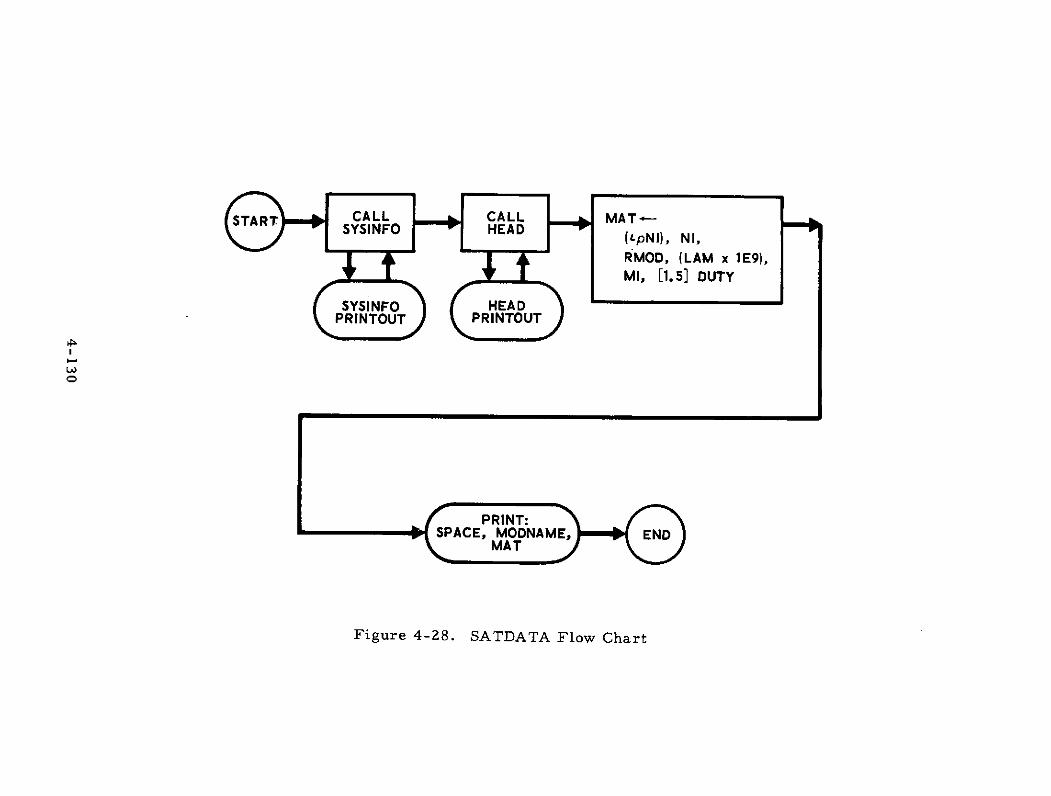
SYSINFO HEAD , 1. p ,
MI, [1.5] DUTY
PRINTOUT PRINTOUT
S PRINT:SPACE, MODNAME, END
MAT
Figure 4-28. SATDATA Flow Chart
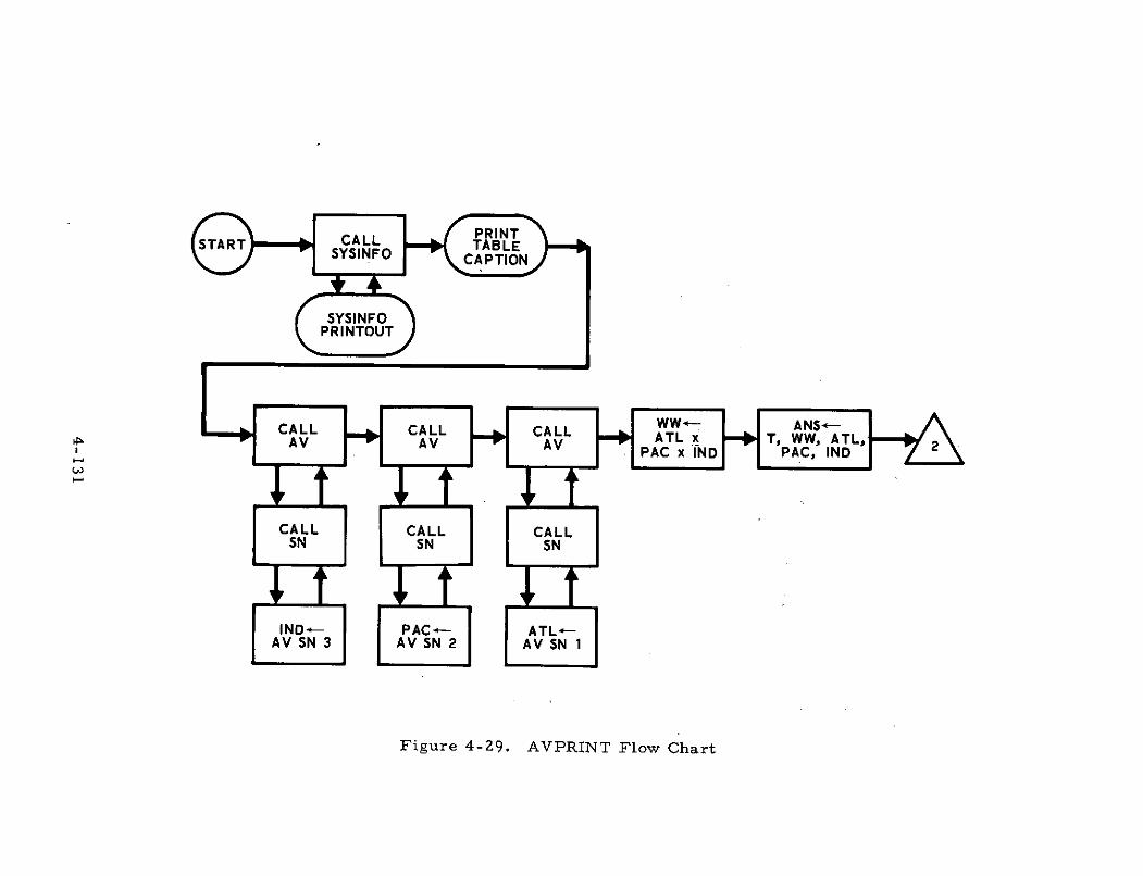
WW-- ANS-CALL CALL CALL ATL T, WW, AAV AV AV 2
CALL CALL CALLSN SN I SN
IND- PAC- ATL-AV SN 3 AV SN 2 AV SN 1
Figure 4-29. AVPRINT Flow Chart
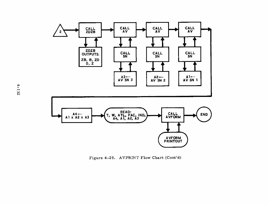
CALL CALL I ICALL I ICALL
D, Z
A3- A2- Al-AV SN 3 AV SN 2 AV SN 1
N
READ:TEe CALL ENDA4T, W, ATL PAC IND, CALLAl x A2 x A3 A4, A1, A2, 3 AVFORM
AVFORM
PRINTOUT
Figure 4-29. AVPRINT Flow Chart (Cont'd)
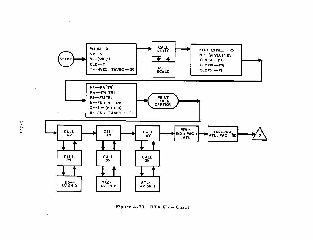
WARN--0 "CALC RTA--(pHVEC)I RSVV---V RH-(pHVEC) t RSVSTART V-(pNI) pl OLDFA *-FAOLD-T OLDFW -FWT--HVEC, TAVEC - 30 RSA-
RCALC OLDFS -FS
FA4-FA[TR]
FW'-FW[TR]
FS-FS[TR] PRINT
D.-FS x (H - RB) CAPTION
Z-1 - (FD x D)B-FS x (TAVEC - 30)
IWW- FuCALL CALL CALL ANS -WWAV IND x PAC AV AV ATL, PAC, thD 3
CALL CALL CALLSN SN SN
IND- I PAC-- ATL--AVSN3 AV SN 2 AVSN 1
Figure 4-30. HTA Flow Chart
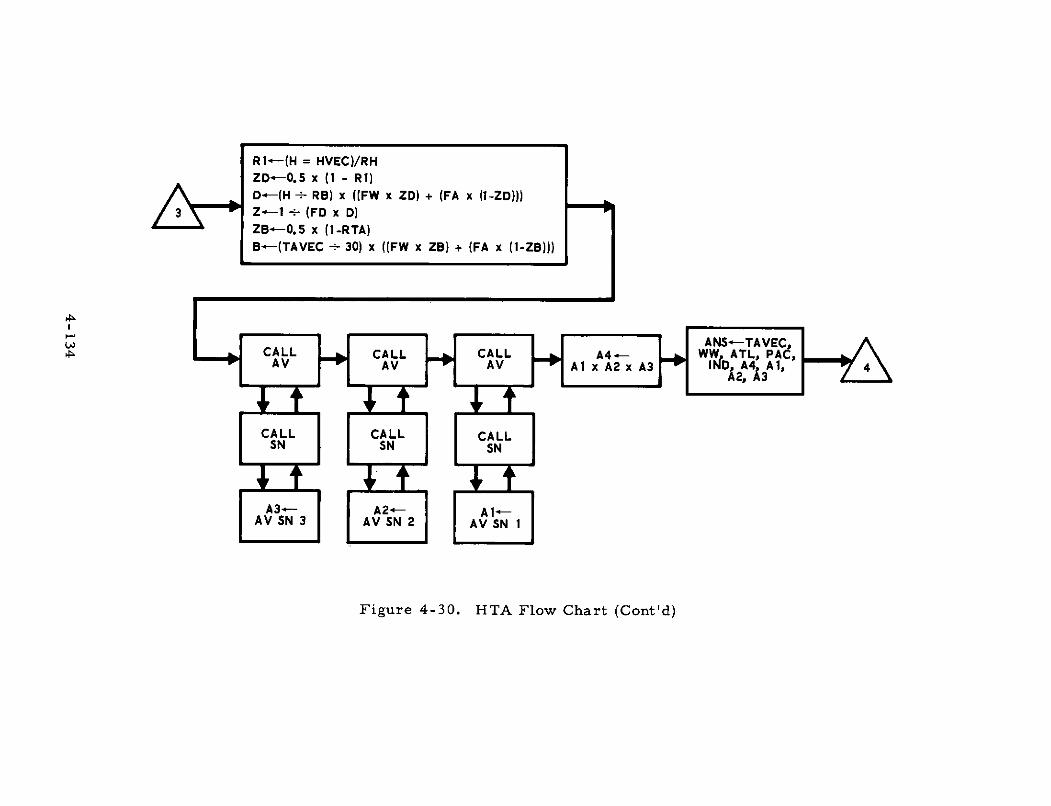
Rl-(H = HVEC)/RHZD-0.5 x (1 - R1)D-(H - RB) x ((FW x ZD) + (FA x (1-ZD)))
3 Z-1 -- (FD x D)ZB--0.5 x (I-RTA)B-(TAVEC - 30) x ((FW x ZB) + (FA x (1-ZB)))
ANS-TAVECCALL CALL CALL A4- WW ATL, PAe,
AV AV AV Al x A2 x A3 ID, A4 Al,A2, A3
CALL CALL CALLSN SN SN
A3- A2t AltAV SN 3 AV SN 2 AV SN 1
Figure 4-30. HTA Flow Chart (Cont'd)
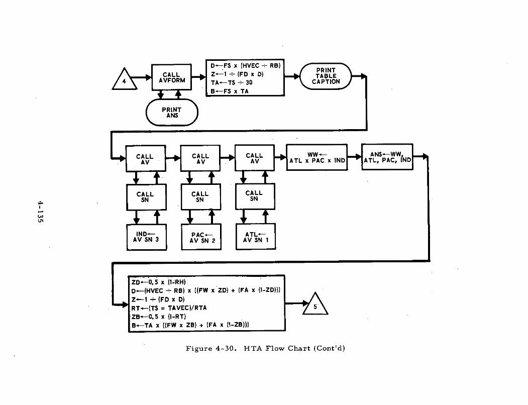
CALCALL CALL CALLWW- (FD ) TABLE
4 AVFORM TATS - 30 CAPTIONZOFS x TA
AV AV AV ATL x PAC x IND ATL, PAC,
CALL CALL CALLSN SN SN
IND PACe ATL*-AV SN 3 AV SN 2 AV SN 1
Dl-. 5 x (1-R H)
D-(HVEC - RB) x ((FW x ZD) + (FA x (1-ZD)))
Z-1 - (FD x D)
RT-(TS = TAVEC)/RTA 5
ZB+-0.5 x (I-RT)
B--TA x ((FW x ZB) + (FA x (1-ZB)))
Figure 4-30. HTA Flow Chart (Cont'd)
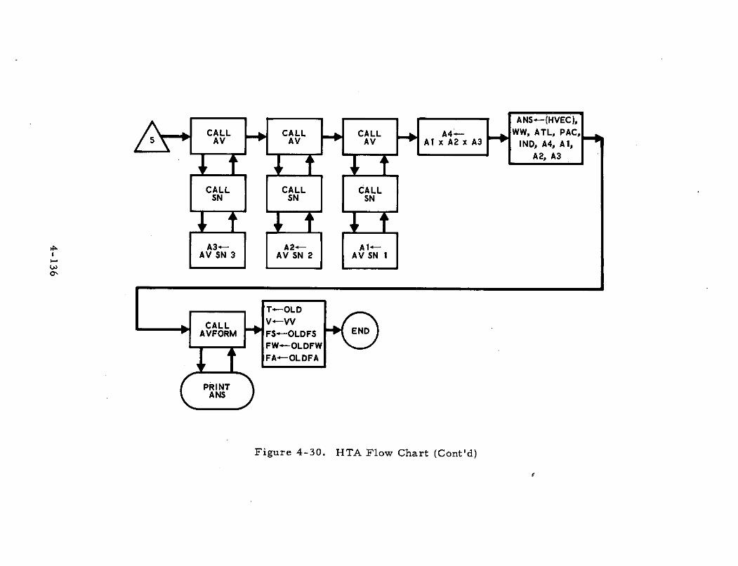
SN SN SN
A3'- A2-- AleAV SN 3 AV SN 2 AV SN 1
T-OLD
CALL V-AVFORM FS'-OLDFS END
FWI--OLDFWFA"-OLDFA
PRINTANS
Figure 4-30. HTA Flow Chart (Cont'd)
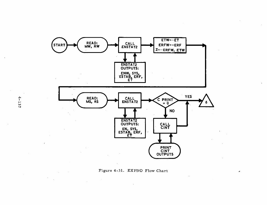
ENSTAT2OUTPUTS:ENW SYS,
ESTAB5 ERF,
READ: CALL C PRINTMS, RS ENSTAT2 6
NO
ENSTAT2OUTPUTS: CALL
EN, SYS, CINTESTAB ERF,
Et
PRINTCINT
OUTPUTS
Figure 4-31. EXPNO Flow Chart
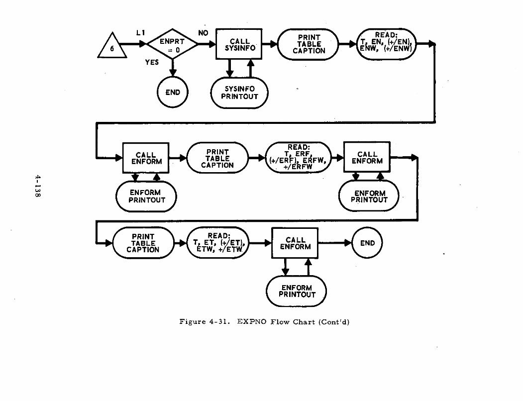
CALLIN PRN TN ERF CALL
PRINT READ: P
TALENPR T E, +/ET CALL EN (ND
6 0T SYSINFO CAPTION E+T ENENR
YES
SYSNINFFO
PRINTOUPRINTOUT
Figure 4-31. EXPNO Flow Chart (Cont'd)EAD:
CALLPRINT T ERF CALLW, WENFORM TABLE (/ER Flk , E&W,I ENFORMCAPTION +/
00 ENFORM C ENFORMPRINTOUT PRINTOUT
PRINT READ: CLTABLE T, ET, ET) ENFORM END
CAPTION ETW, /ETW": NFR
ENFORMPRINTOUT
Figure 4-31. EXPNO Flow Chart (Cont'd)
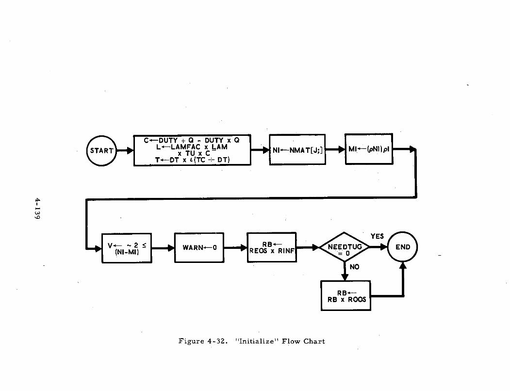
CDUTY + 0 - DUTY x 0
START L LLAMFAC x LAM N1-NMAT[J;1 MI.-(pNIplTo DT x L (TC D T)
YES
V M*- 2 < WARN-0 RB- NEEDTUG END(NI-MI) REOS x RINF 0
NO
RBRB x ROOS
Figure 4-32. "Initialize" Flow Chart
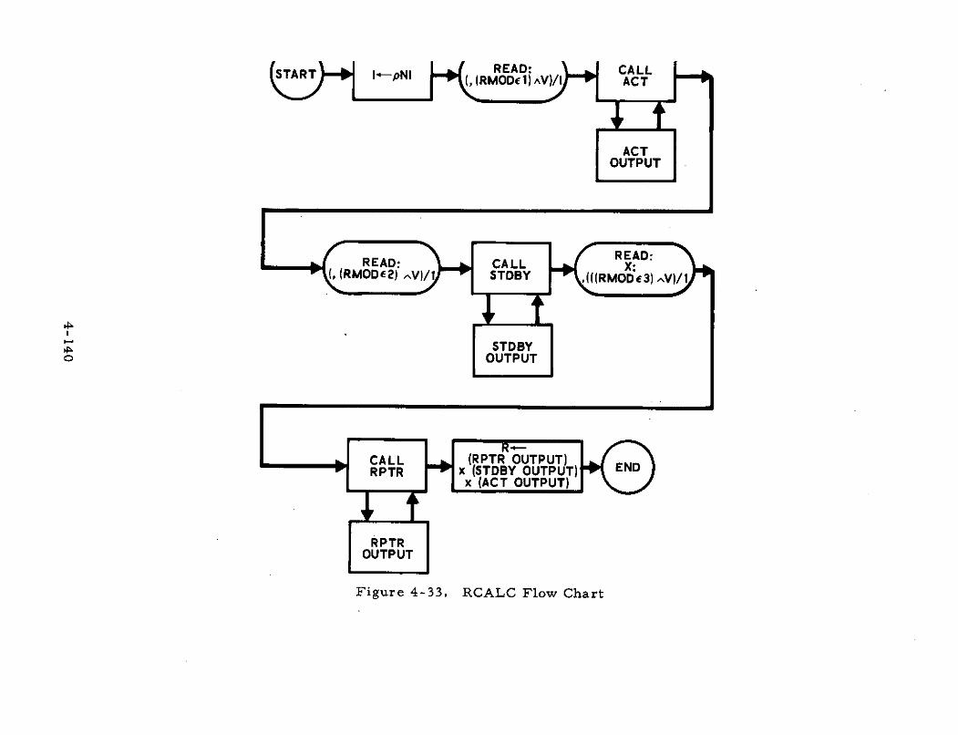
RD READ: CALL
((RMOD() VV)/I) ACT
ACT
STDBY OUTPUOUTPUT
R -
CALL (RPTR OUTPUT)RPTR x (STDBY OUTPUT) END
x (ACT OUTPUT)
RPTROUTPUT
Figure 4-33. RCALC Flow Chart
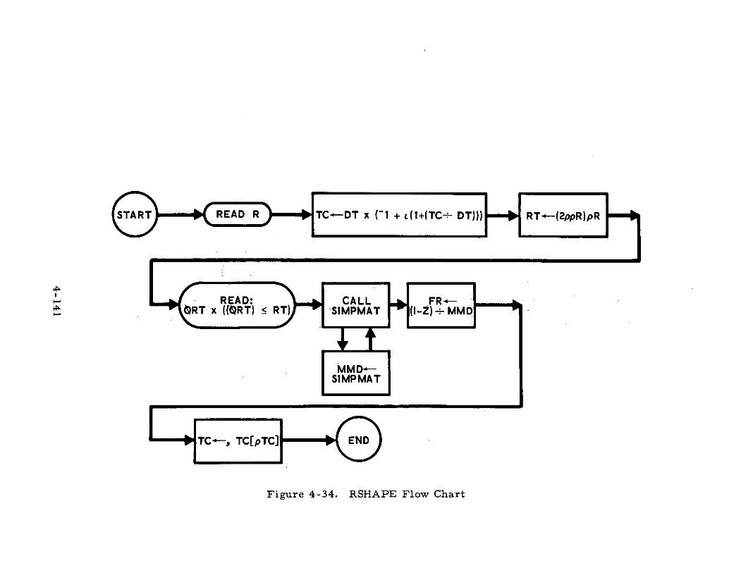
START READ R TCoDT x ('1 + L(1+(TC+ DT))) RT--(2ppR)pR
READ: CALL FRtORT x ((ORT) 5 RT) SIMPMAT (I-Z)~MM
MM D1-SIMPMAT
TC-, TC[pTC] END
Figure 4-34. RSHAPE Flow Chart
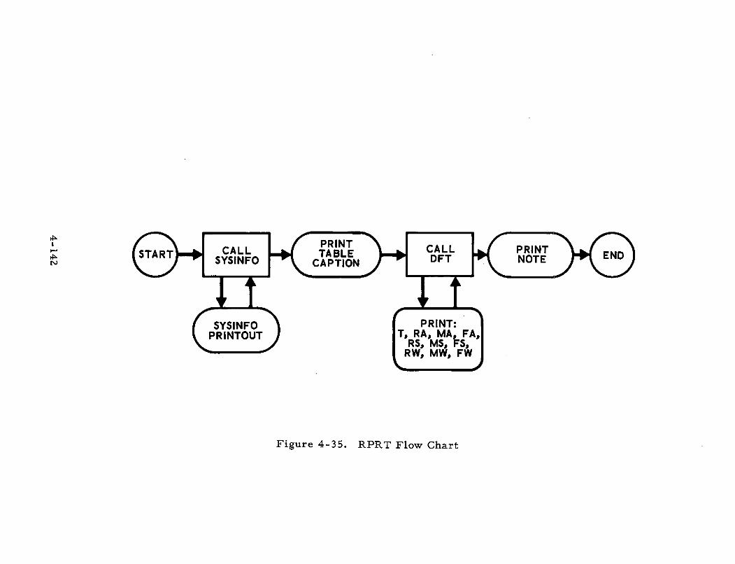
PRINTSTART CALL CALL PRINTSTARTLTABLE ENDSYSINFO CAPTION DFT NOTE
SYSINFO PRINT:PRINTOUT Tq RA, MA, FA,
RS, MS FS,RW, MW, FW
Figure 4-35. RPRT Flow Chart
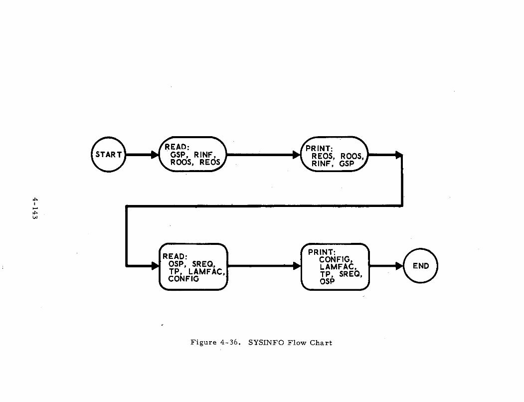
READ: PRINT:START GSP, RINF, R EOS, R OOS,
ROOS, REOS RINF, GSP
I
PRINT:READ: CONFIG,OSP, SREQ, LAMFAC ENDTP, LAMFAC, TP, RE,CONFIG OSP
Figure 4-36. SYSINFO Flow Chart
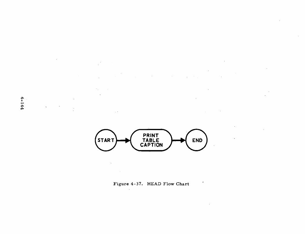
START TABLE EN-3 CAPTION
Figure 4-37. HEAD Flow Chart
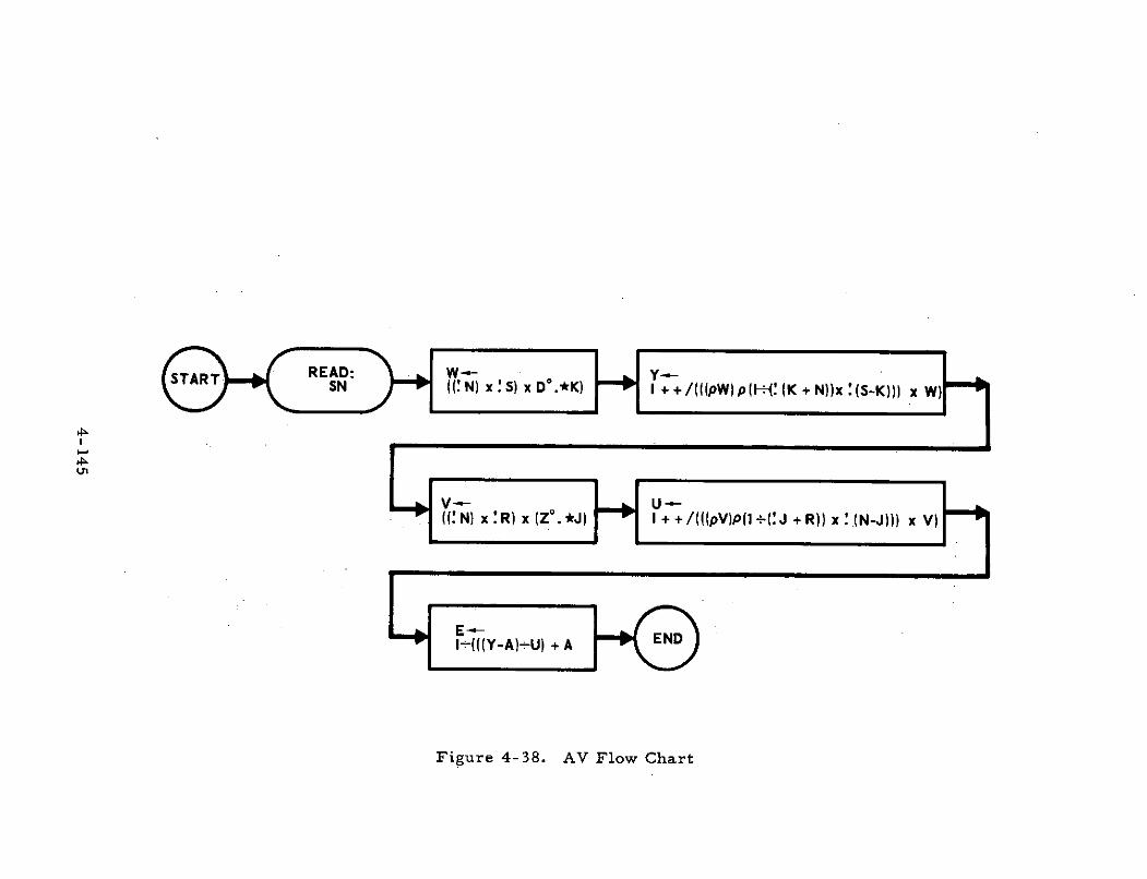
S READ: WY _ YSN ((:N) x : S) x D.*K) I + + /(((pW) p(I--: (K + N))x : (S-K))) x W
V R U-((N) x R) x (Z.*J) I + + /(((pV)P( (J + R)) x :(N-J))) x V)
EI-(((Y-A)-U) + A s
Figure 4-38. AV Flow Chart
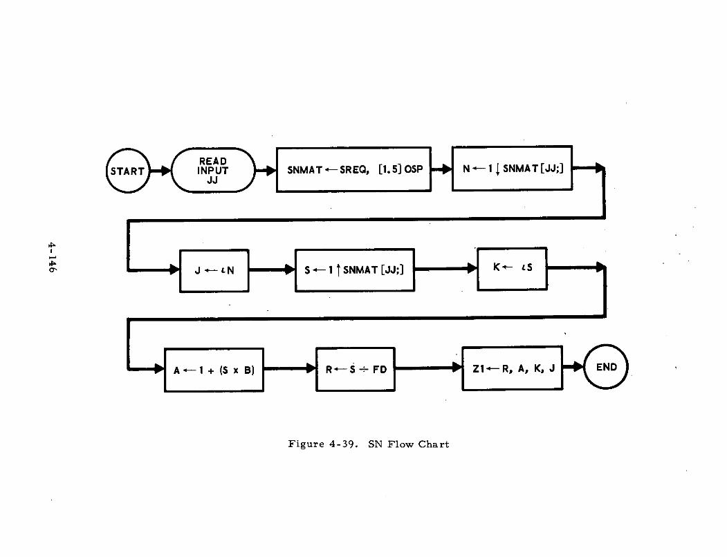
I
, J ,-- N S -1SNMAT [JJ; K- LS
A -1 + (S x B) R"-- S FD Zl- R, A, K, J
Figure 4-39. SN Flow Chart
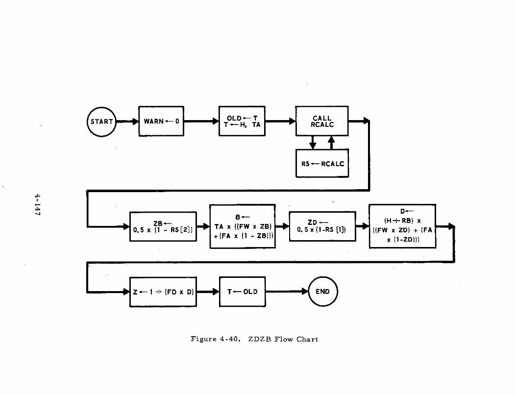
OLDT 0 CALL
WARN - 0 T H, TA RCALC
I RS- RCA LC
Bt
0.5 x (I - RS[2]) TA x ((FW x ZB) 0.5 x (-RS [1]) ((FW x ZD) + (FA
Z-1 (FD x D) ( T-OLD END
Figure 4-40. ZDZB Flow Chart
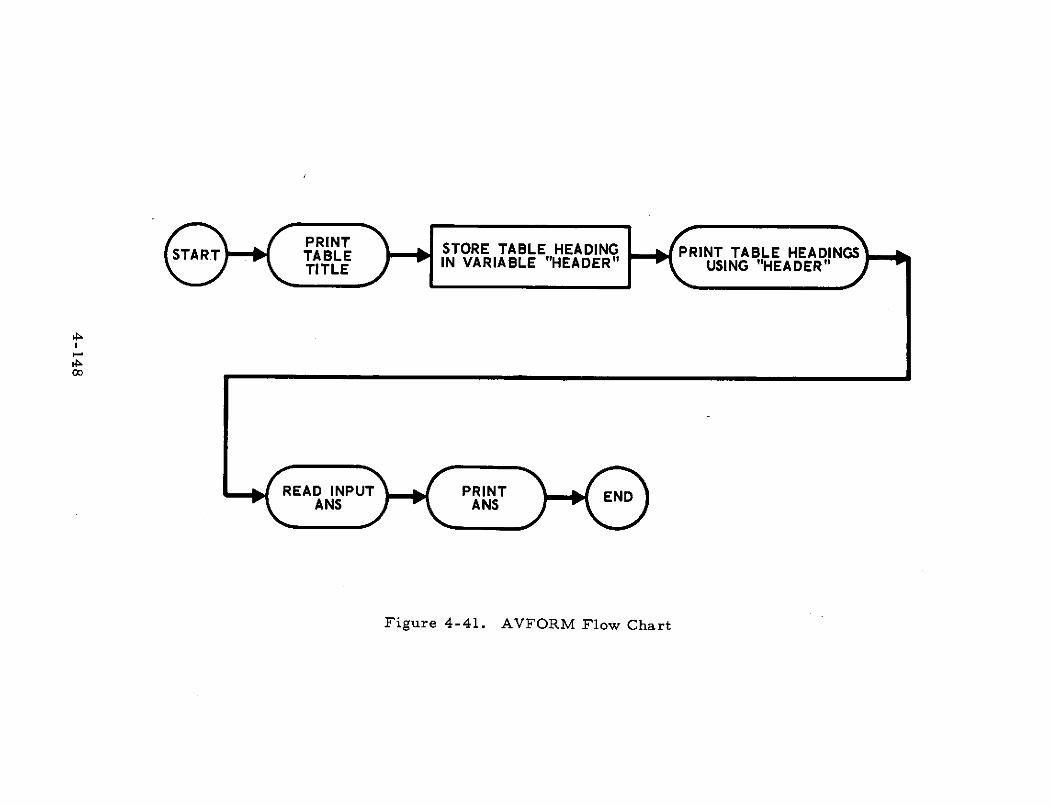
PRINTT STORE TABLE HEADING KPRINT TABLE HEADINGS& +CNDLE IN VARIABLE "HEADER" USING "HEA i371
READ INPUT PRINT ENDANS ANS
Figure 4-41. AVFORM Flow Chart
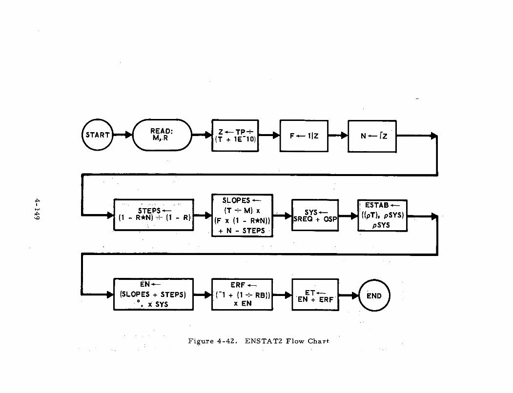
READ: Z t TP -NerSTART M, R (T + 1E-10) FIIZN F
SLOPES --ESTAB-
STEPS - (T + M) x~P SYS ~-((pT), pSYS)1 - R*N) (- R) (F x ( - R*N)) SRE + OSP " ppSYS
+ N - STEPS (
EN-EN + ERF(SLOPES + STEPS) :(-I + (I + R]B)) ETOEF N
,xSYS x EN
Figure 4-42. ENSTAT2 Flow Chart
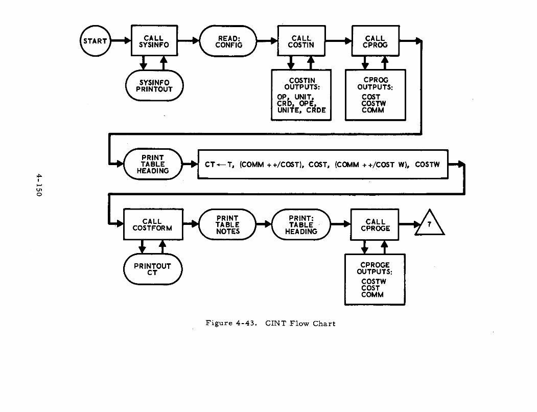
SYSINFO COSTIN CPROGPRINTOUT OUTPUTS: OUTPUTS:
OP, UNIT, COSTCRD, OPE, COSTWUNITE, CRDE COMM
PRINTTABLE CT-T, (COMM ++/COST), COST, (COMM ++/COST W), COSTW
HEADING
OUTPUTS:
COSTWCOST
COMM
Figure 4-43. CINT Flow Chart
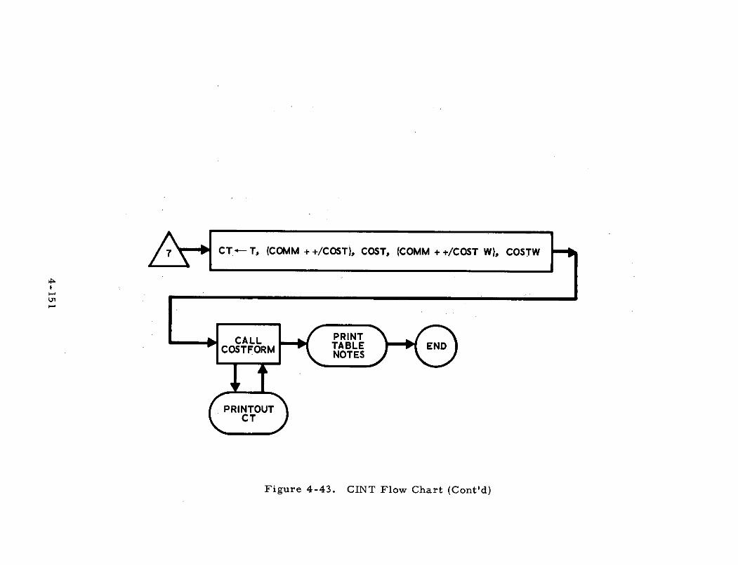
7 CT.- T, (COMM + +/COST), COST, (COMM + +/COST W), COSTW
CALL PRINTCOSTFORM TABLE END
NOTES
PRINTOUT
Figure 4-43. CINT Flow Chart (Cont'd)
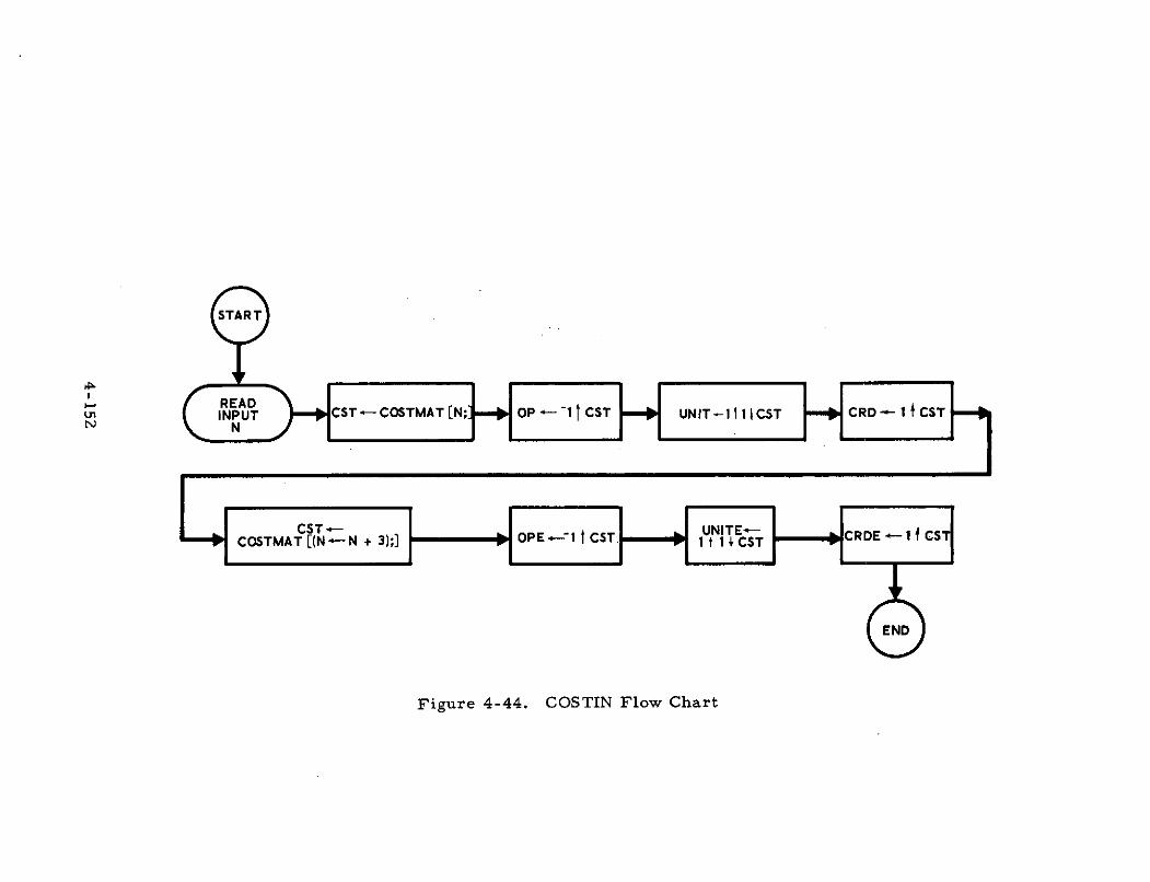
START
READINPUT CST-- COSTMAT [N; OP-- -1 CST UNIT-1 t 1 CST
N N
CST - UNITE4.- -ST CtCOSTMAT [(N"-N + 3);] OPE---1 t CST. 1 t 1I CST CRI
(END
Figure 4-44. COSTIN Flow Chart
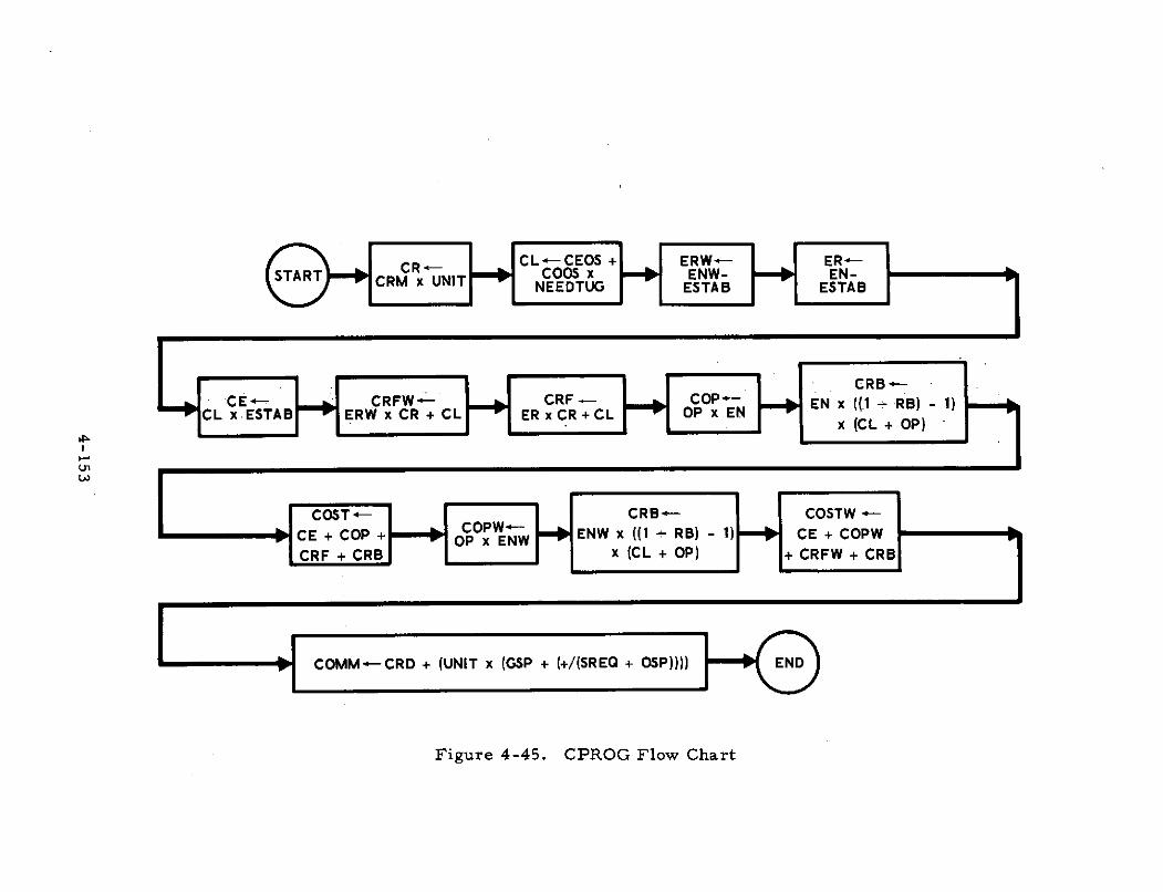
I NEEDTUG ESTAB I ESTAB_
CRB-CEt- CRFW- L CRF c COP- EN x ((1 RB) - 1)
CL x ESTAB ERW x CR + CL ER x CR + CL OP x ENx (CL + OP)
COST - COPW- CRB- COSTW -
CE + COP + C OPW x ENW ENW x ((1 RB) - 1) - CE + COPW
CRF + CRB x (CL + OP) + CRFW + CRB
COMM-CRD + (UNIT x (GSP + (+/(SREO + OSP))))
Figure 4-45. CPROG Flow Chart
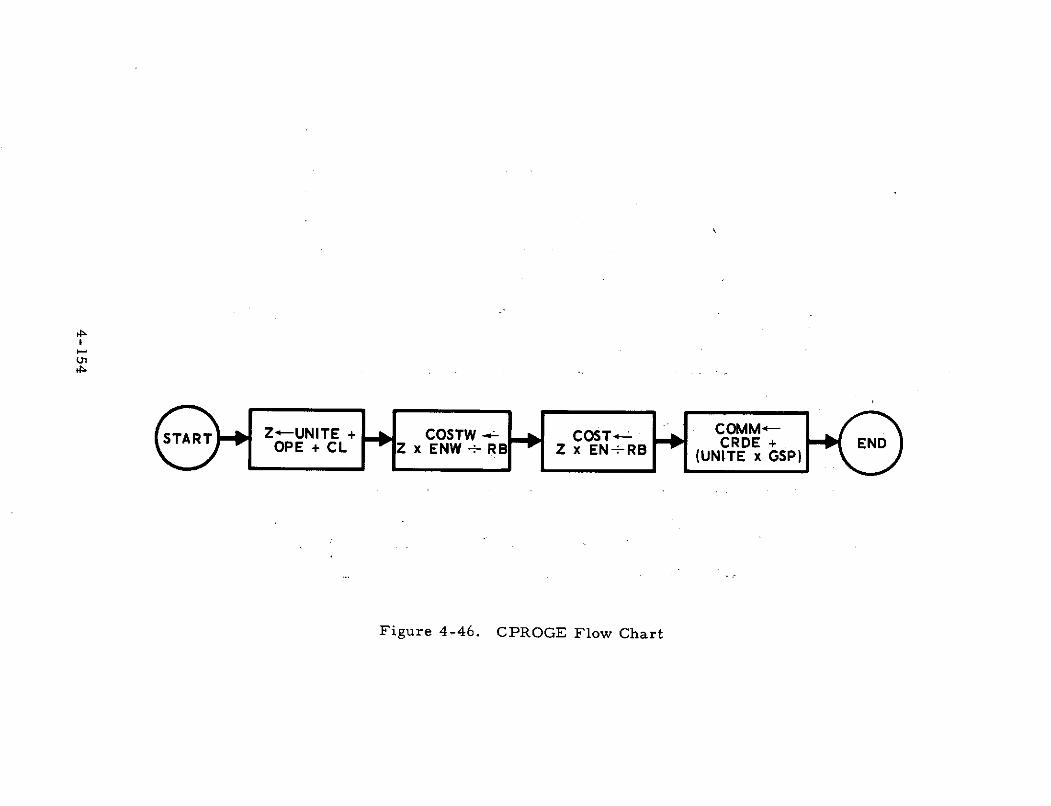
START Z-UNITE + COSTW- COST COMMOPE + CL Z x ENW RB Z x EN-RB (UNITE x GSP)
Figure 4-46. CPROGE Flow Chart
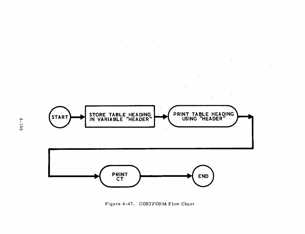
STA RTSTORE TABLE HEADING PRINT TABLE HEADING,-" ,"IN VARIABLE "HEADER" USING "HEADER"
PRINT ENDCT
Figure 4-47. COSTFORM Flow Chart

PRINTSTART TABLE READ: CALLEND
CAPTION ANS DFT
PRINTANS
Figure 4-48. ENFORM Flow Chart
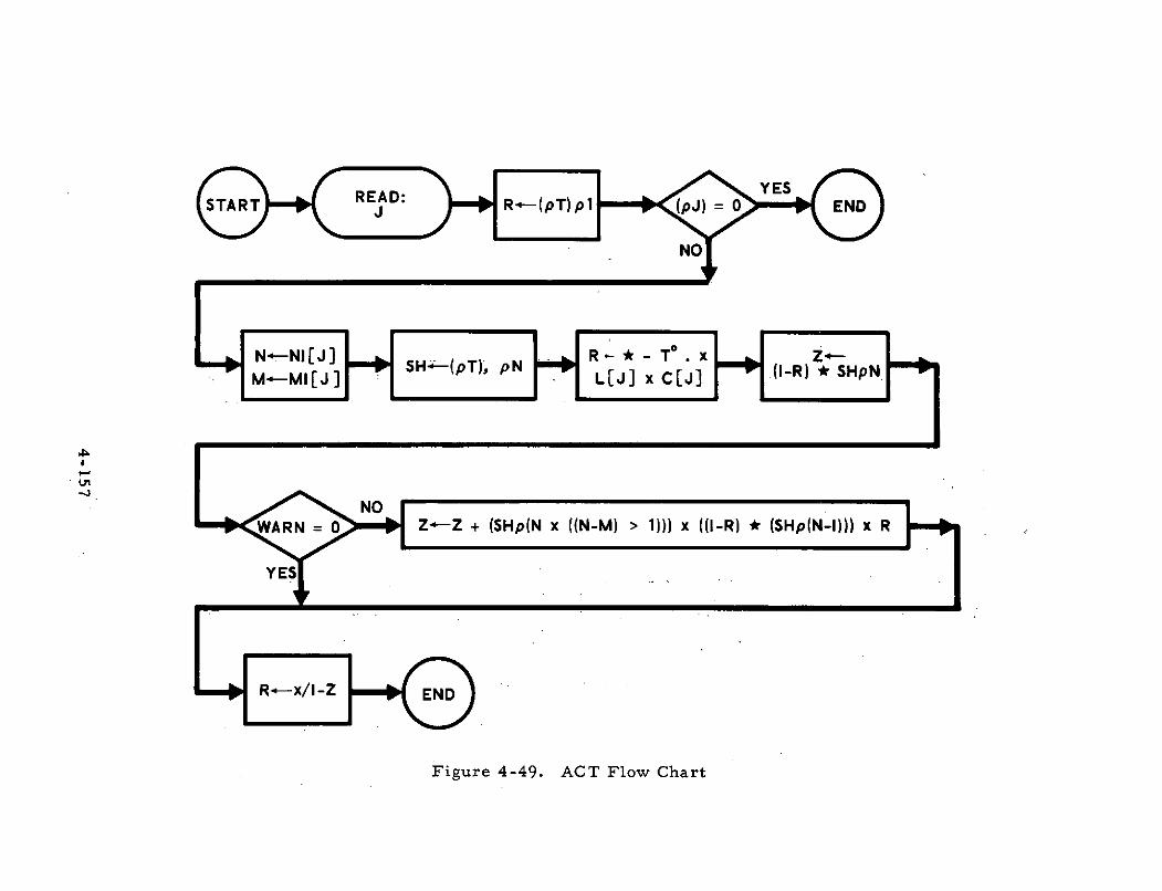
YESSTART READ: R(pT) pT(pJ) = YS END
NO
1, JCJ R - TO x Z*SH4-(pT)., pN (I-R) SHpN
M-MICJ3 L[J] x C[J]
NOWARN= 0 Z*-Z + (SHp(N x ((N-M) > 1))) x ((I-R) " (SHp(N-))) x R
YES
R---x/I-Z END
Figure 4-49. ACT Flow Chart
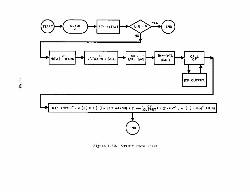
ZK-- - SHl- SH-(pT), CALLNI[J] - WARN Lr/(WARN + (Z-1)) (pK), (pZ) (OSH1) CF
(CF OUTPUT)
RT-x/((*-To. xL[J] x (C[J] + (0 x WARN))) x (1 ++/(OUCPUT) x ((1-*(-T. x(L(J] x 0))).*K))
END
Figure 4-50. STDBY Flow Chart
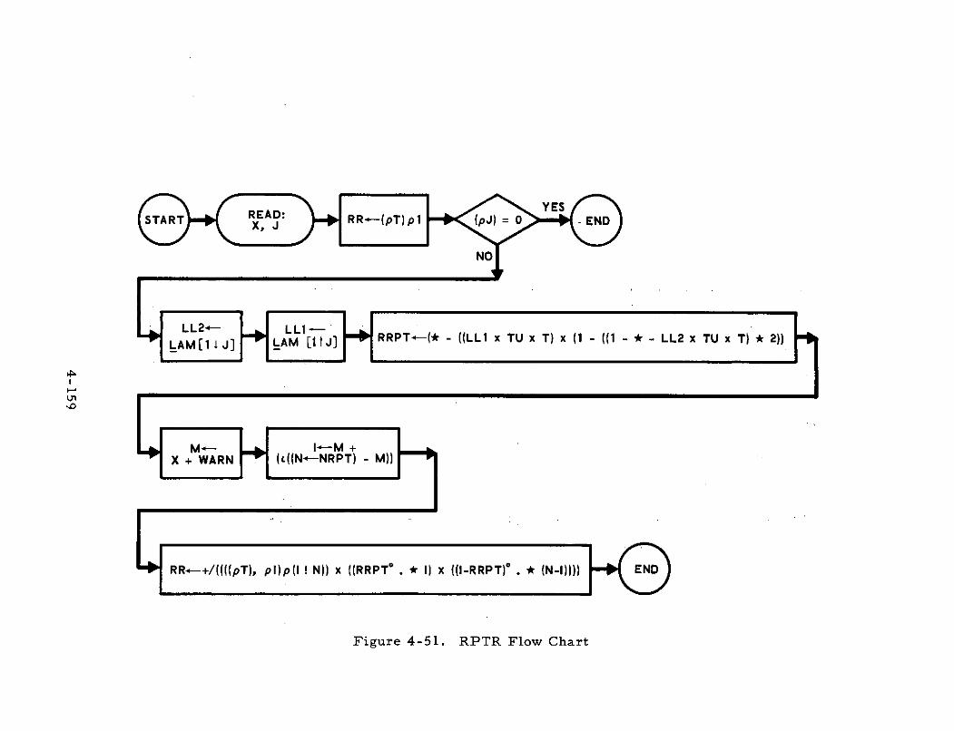
LL2- LL-LAM[1J] IAM [itJ] RRPT+-(* - ((LL1 x TU x T) x (1 - ((1 - A - LL2 x TU x T) * 2))
M- r I-M +X + WARN H (t((N.-NRPT) - M))
RR-+/((((pT), pl)p(I ! N)) x ((RRPT 0 . * I) x ((I-RRPT)° . * (N-1))))
Figure 4-51. RPTR Flow Chart
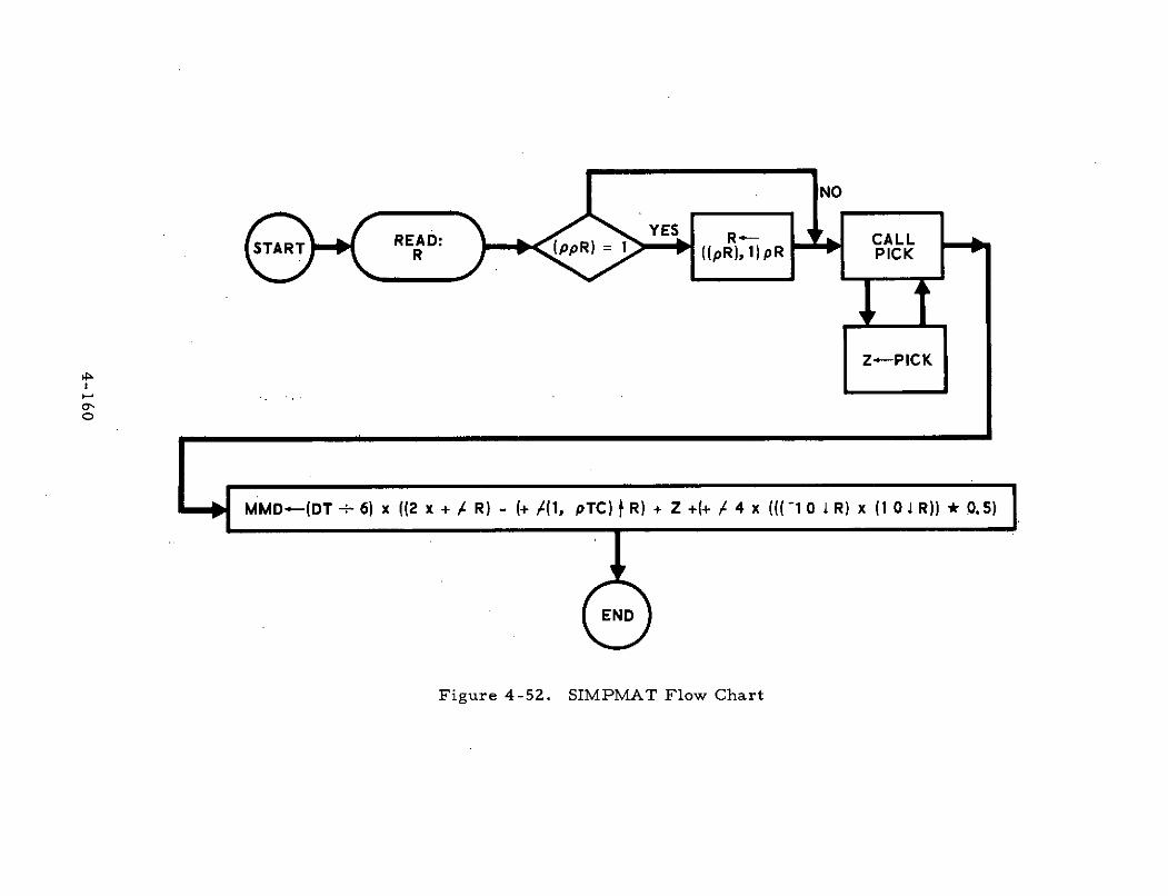
Z
END
Figure 4-52. SIMPMAT Flow ChartFigure 4-52. SIMPMAT Flow Chart
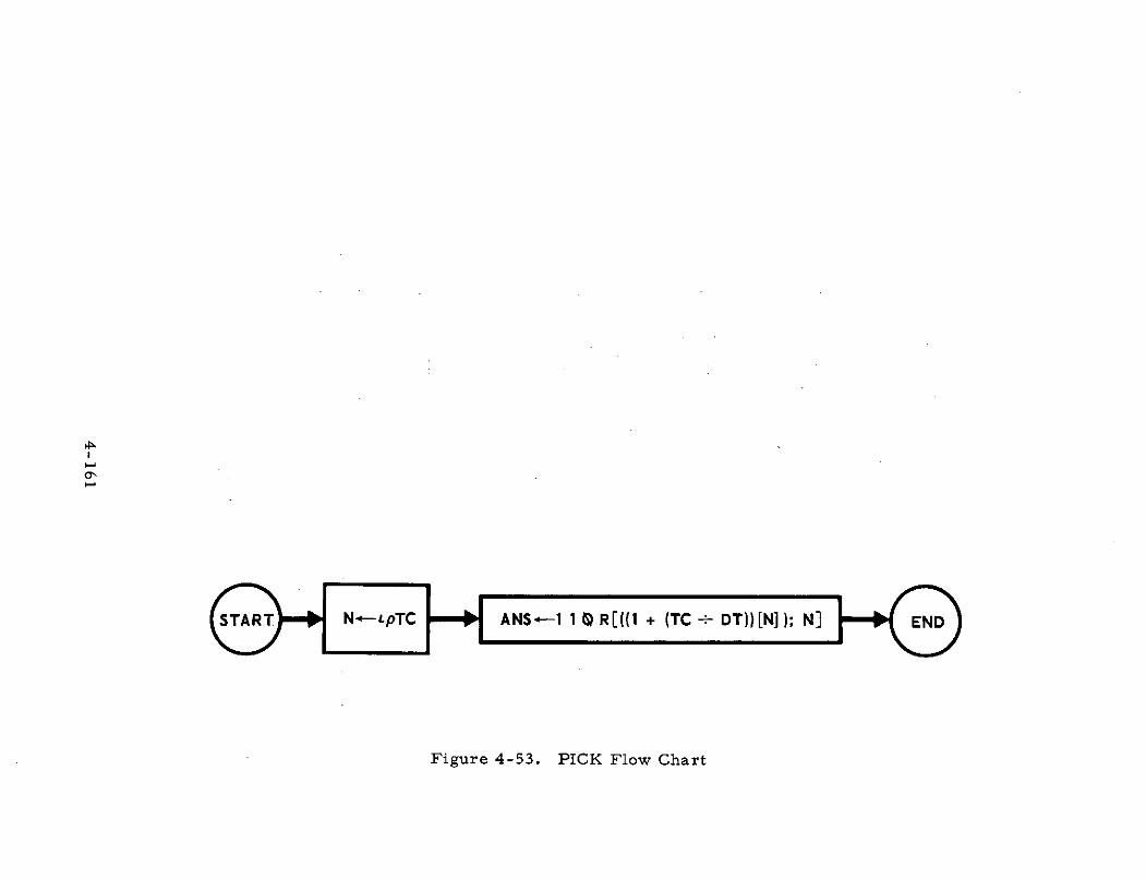
START N pTC ANS 1 R((1 + (TC DT))[N]); N]
Figure 4-53. PICK Flow Chart
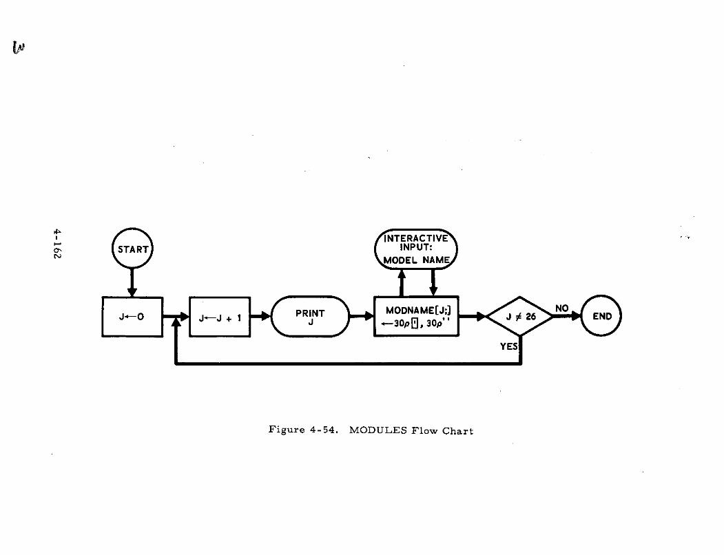
INTERACTIVESTART INPUT:
MODEL NAME
-0 J-J 1 PRINT MODNAME[J; J 26 NO ENDJ ,-30p, 30p''
YES
Figure 4-54. MODULES Flow Chart
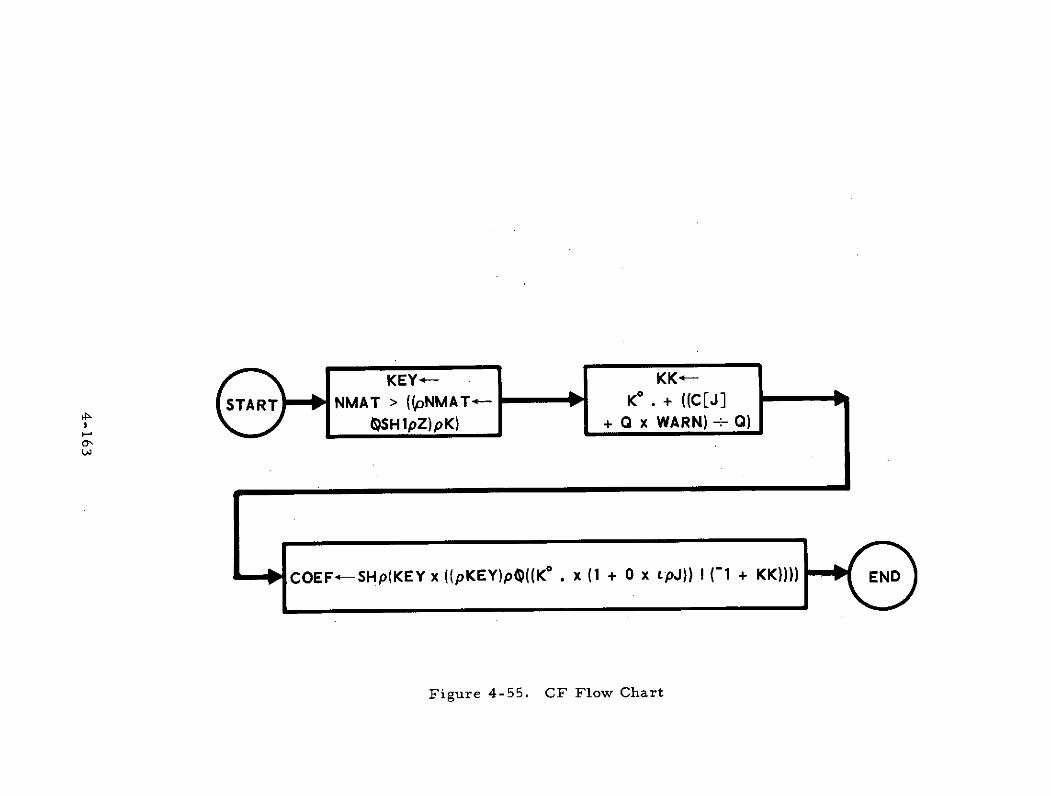
f SHipZ)pK) + 0 x WARN) Q)
COEF-SHp(KEY x ((pKEY)pD((K° . x (1 + 0 x pJ)) ! (-1 + KK)))) END
Figure 4-55. CF Flow Chart
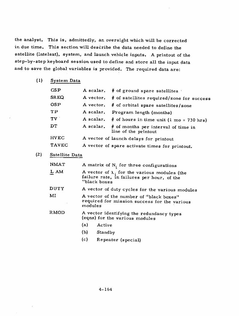
the analyst. This is, admittedly, an oversight which will be corrected
in due time. This section will describe the data needed to define the
satellite (Intelsat), system, and launch vehicle inputs. A printout of thestep-by-step keyboard session used to define and store all the input dataand to save the global variables is provided. The required data are:
(1) System Data
GSP A scalar. # of ground spare satellites
SREQ A vector. # of satellites required/zone for successOSP A vector. # of orbital spare satellites/zone
TP A scalar. Program length (months)
TV' A scalar. # of hours in time unit (1 mo = 730 hrs)DT A scalar. # of months per interval of time in
line of the printout
HVEC A vector of launch delays for printout
TAVEC A vector of spare activate times for printout.
(2) Satellite Data
NMAT A matrix of N i for three configurations
L AM A vector of X. for the various modules (thefailure rate, in failures per hour, of the"black boxes
DUTY A vector of duty cycles for the various modulesMI A vector of the number of "black boxes"
required for mission success for the variousmodules
RMOD A vector identifying the redundancy types(eqns) for the various modules
(a) Active
(b) Standby
(c) Repeater (special)
4-164
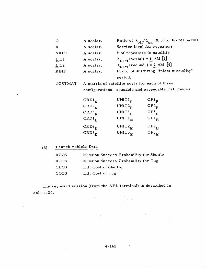
Q A scalar. Ratio of X off/ on (0.5 for hi-rel parts)
X A scalar. Service level for repeaters
NRPT A scalar. # of repeaters in satellite
LL1 A scalar. X RPT(serial) = LAM [3]
LL2 A scalar. RPT(redund.) = LAM (4]
RINF A scalar. Prob. of surviving "infant mortality"
period.
COSTMAT A matrix of satellite costs for each of three
configurations, reusable and expendable P/L modes
CRDLR UNIT 1R OP1RCRD2 R UNIT2R OP 2 R
CRD 3 R UNIT 3 R OP3 R
CRD1E UNIT1E OP 1E
CRD2E UNIT2E OP2ECRD 3 E UNIT 3 E OP3 E
(3) Launch Vehicle Data
REOS Mission Success Probability for Shuttle
ROOS Mission Success Probability for Tug
CEOS Lift Cost of Shuttle
COOS Lift Cost of Tug
The keyboard session (from the APL terminal) is described in
Table 4-20.
4-165
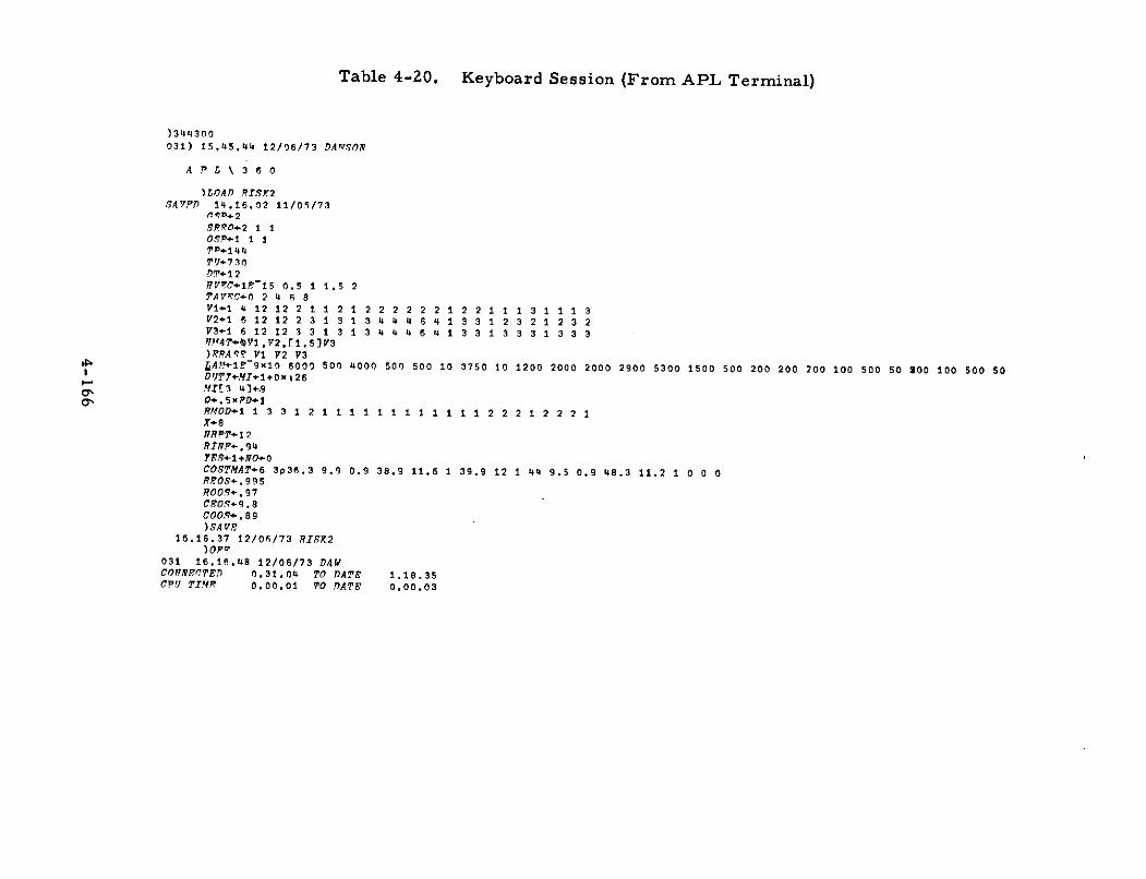
Table 4-20. Keyboard Session (From APL Terminal)
)344300031) 15.45.44 12/06/73 DAYSON
APL \ 3 6 0
)LOAD RISK2sAVYP 14.16.02 11/05/73
SRTOD2 1 1OSP-1 1 17V-144TY-730DT 12RVRC+1-15 0.5 1 1.5 2TAV7r0 2 4 6 8V1I 4 12 12 2 1 1 2 1 2 2 2 2 2 2 1 2 2 1 1 1 3 1 1 1 3V2+1 6 12 12 2 3 1 3 1 3 4 4 4 6 4 1 3 3 1 2 3 2 1 2 3 2V3+1 6 12 12 3 3 1 3 1 3 4 4 4 6 4 1 3 3 1 3 3 3 1 3 3 3N #A' I?,V72,r1.51V3)PPRAq VI V2 V3SAM+1E-10o 6000 500 4000 500 500 10 3750 10 1200 2000 2000 2900 5300 1500 500 200 200 200 100 500 50 200 100 500 50DUTYMII+O1+0x26MIr3 41-.9O+.5xPDeIRMOD.1 1 3 3 1 2 1 1 1 1 1 1 1 1 1 1 1 1 2 2 2 1 2 2 2 1X+8
NRPT+12RINP-.94YRS+I+NO-0COSTMAT-6 3036.3 9.9 0.9 38.9 11.6 1 39.9 12 1 44 9.5 0.9 48.3 11.2 1 0 0 0REOS+.995ROOS. 97COSq9.8
COOR-.89)SAVE
16.16.37 12/06/73 RISK2)OPF
031 16.16.48 12/06/73 DAWCONNECTED 0.31.04 TO DATE 1.18.35CPY TIM 0.00.01 TO DATE 0.00.03
d. Sample Optimization and Selection Analysis
The objective of this analysis is to select the lowest cost satellite
system approach from the options available. The system selected must
meet the availability requirement to obtain comparable risk to the ground
system. The flight rate is determined for each of the options as it is
analyzed so that when the lowest cost option is selected the flight rate
is also selected.
The procedures are developed to provide closed-form solutions
for system availability and to derive the associated costs and flight
rate. The utility of the computed data in the analysis is in the tradeoff
and sensitivity display for the optimization and selection analysis. This
section of the report gives the user guidance in the selection procedure
by use of an example.
For a general description of the functional aspect of the analysis
the reader is referred to Section 2. B. 6 of this document. The actual
steps that the user goes through in order to accomplish this analysis are:
1. Obtain input data from previous BRAVO steps
2. Follow the computing procedures described in Sections4. F. 2(a), (b) - and 4. F. 2(c) if needed
3. Analyze the tabulated results from the computer runsto complete the selection analysis. This is normallyaccomplished by plotting the data as described in thefollowing example.
Before getting into the example itself, some understanding of
the case being illustrated is helpful. The example analysis is for an
Intelsat case originally accomplished and described in Study 2. 1(1).
(1) Space Shuttle Mission and Payload Capture Analysis (Study 2. 1)Final Report, Volume I1, The Aerospace Corporation, ATR-73(7311)-1, Vol. II, (15 June 1973)
4-167
The APL computer program, RISK, was used to simulate each of the
cases from Study 2. 1 plus one additional satellite option, a 3-axis,
stabilized satellite designed according to LMSC low-cost principles.
The calculated outputs are on file at The Aerospace Corporation. Thus
the options analyzed from which a selection of the lowest cost is to be
made are:
1. A dual-spin satellite with the Intelsat IV configurationas it was built and flown. This is a dual-spin satellite andcarries the lable "CDR dual-spin (as built)." Design lifeof this satellite is seven years limited by wearout.
2. A dual-spin Intelsat IV design resembling the as-builtsatellite but with redundancy increased on a weight-optimized basis. The redundancy increase has two effects;first the reliability curve of the satellite is improved,second the number of redundant components for whichfailures could be tolerated before a launch-on-warningis increased. Design life of this satellite is seven yearslimited by wearout. This satellite option is labeledCDR (weight-optimized dual-spin).
3. A 3-axis satellite design carrying the Intelsat IV missionequipment (transponders, antennas, and supportingcommunications). This satellite has a five-year designlife. It is designed according to the LMSC low-costdesign principles; it is fully modularized and can bemaintained on orbit or on the ground. This option islabeled LCR (3-axis).
Each of the options was, analyzed in two orbital-deployment
configurations. The first is a four-satellite system with one over the
Pacific, one over the Indian, and two over the Atlantic oceans. For
this system there are no spare satellites in orbit, only two on the ground.
The second on-orbit deployed configuration is a seven-satellite system
with one active spare added over each ocean area. All failed satellites
are repaired on the ground.
For the CDR satellite design options, each orbital deployment
configuration is analyzed for launch-on-warning and launch-on-failure
strategy satellite replacement. The analysis simulates logistics for
4-168
replacement of failed or failing satellites and repair or refurbishment
on the ground. The analyses in Study 2. 1 have shown that periodic pre-
ventative maintenance at intervals less than seven years (the satellite
wearout time) was more expensive; therefore, this analysis used seven-
year preventative maintenance intervals. For the purpose of obtaining
program costs, a twelve-year Intelsat program duration was assumed.
(1) Discussion of Detailed Steps and the Optimization and SelectionProcedure
Once the computer program (RISK) has been used, the system optimi-
zation (against satellite design and logistics options) data are available in
tabulated form from the RISK computer program printout. These results
are then analyzed by making appropriate graphs and plots which illustrate
the relative costs and risks of the various options analyzed so that
conclusive observations may be made from the data by the user. The
availability requirement for the example (Intelsat) system is 0. 9999.
Step 1 - Plot Data
Step 1 is for the user to plot the data according to the example
format to provide rapid comparison and analysis with visibility into the
system tradeoffs. The bar graph (Figure 4-56) displays the relative costs
of the various options analyzed at normal operating conditions. In this
case normal conditions are a two-month delay for satellite replacement,
no satellite turn-on delay, and a failure rate multiplier (X factor) of
1.0. Figure 4-57 displays the effects on availability of perturbing the
launch delay in replacing the failed satellite. Satellite replacement
delay is primarily a matter of the availability of the launch vehicle for
a replacement mission on short notice. It is assumed that the cost
differences between less than one month delay and up to four months.
delay is negligible.
4-169
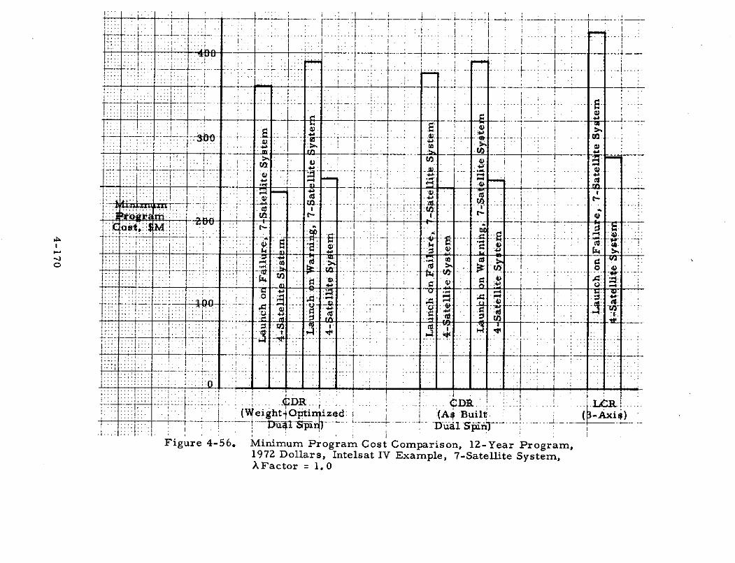
OL
T-t
P
-I--
--
t I
I _
I ..
....
.. ..
..
..
.-..
..
7....
....
'.. :.
..
...
..
: ..
i
:
I.;
lifi.
l .€. :'
;:
...
S- .
...
-
ra
t l
~ --
7r77
-'
.. ....
...
.
, 7....Lh
..
.. .
..
..
..
...
I : ,: ..
J 4...- II
i:$,
s
I.
.!
Mr
..•
I
I .
:
..
--
_ _
_7-
L
audi
. nch
4
10
i~r-.
, T
-Stit
e I
y S te
m
--
:4-S4
ati 11te
.yi 6ter
m ..
.' :
•
~f
I-
..
:
.t
: .
1•~
j :
.-)
?:-7 • : .
..
-...
...
,- : ..-
i -
--
....
.'
_N
tt
--:
-l
unge
l h nW
e n
ig
-S
1:t
yte
-_
-o
i
.I
...
!
.I
4 ae
I
.• I1 " I ! .
I
4 -..
..
-..
..
....
-+ -
:. ..- -
--
,
;" : " ' i
I 'I
_
.' -• .:
I .
! ..:.
.
.d u
':-
-i
l
tlr~
h
rcIt
~I
7-
ati
ite
7Sqt
e
0
.I
: I
-.. t .
: .
, ~~~~
~~~
~~~
"-Tf.
!"- ..
,.,,
.w n~g -se"es'
.t
..
.--
: I .'4 .i ..,k
I
., .
-..: -I .:-, .
_ .
c r-. ' i
• t ...
..
1 ..
t ...
S.nc.
..
'ail , , .
f
., .,(,
0 :.
:
IP :1
$ .
' '. .
'
"S
--C
+ D
-Sif
l(e-
I
tei
C+
0 ....
".
''
..
... ..
.
a.l
.l.
i:
'r .
:!
: i- : .i.t i..-
:
i / .: 1
! : 1 .
! !
i A
:L
Am
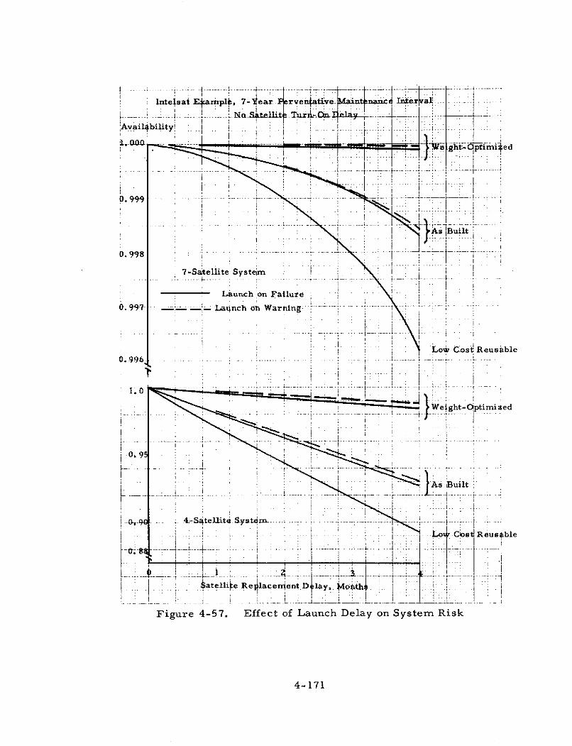
........ ...... ... i ..... .. ..- (...... . .. . . .... --- --- t -'-- -- ..... .
Intelsat tampl, 7- ear rve ativ e tnanc Iera
'Avail4bility. I
-. 4Wohtotiini ed
OI..,
0. 997 Launch oni Warning
Lo Cos Reusable0.q96-- -----
4-StellitSys-....t rm--tm- - -
e e4ae . •ao -
.9.... .. i s . e .. .. .......L . .. ... ... _ _. .. ...
Figure 4-57. Effect of Launch Delay on System Risk
: 4-171 o ostReusble
0 ---- -- -- - :-, :--------
: I l , -- rWiqght-O, timied
Figure 4-57. Effect of Launch Delay on System Risk
Figures 4-58 and 4-59 display the effects of satellite failurerate multiplier (or A factor) on system availability and program cost.
A failure rate multiplier of 1. 0 indicates that the satellite performance
matched the design reliability curve. A failure rate multiplier of 1. 5indicates that the satellite failure rates increased 50 percent over thedesign values in actual operation. These data are primarily usefulin checking the sensitivity of system parameters to failure rate.
Step 2 - General Observations
The user makes general observations on satellite costs forcandidate systems for the purpose of eliminating as many candidatesas possible. From the plotted data (see Figure 4-56), it is noted thatthe 3-axis system is more expensive and from Figure 4-57 it is notedthat the 3-axis system exhibits lower availability in each case, thusthe 3-axis system can be eliminated.
It is noted that the systems with four satellites on orbit (insteadof seven) all exhibit outages in excess of the allowable 0. 0001 (seeFigure 4-57), thus four-satellite on-orbit systems may be eliminated.
Surviving candidates are the seven-satellite system with dual-spin designs. It is noted that the as-built dual-spin design will meetthe availability requirement if the satellites can 1 eplaced with delaysof three weeks or less (see Figure 4-57). It is a noted that the weight-optimized dual-spin design will meet the availabi, requirement withup to four months replacement delay for a launch -failure strategy(see Figure 4-57).
It is noted that the spare satellite turn-on delay rapidly lowersavailability below the required 0. 9999 (see Figure 4-60). It is thereforeconcluded that spare satellites on orbit for this system should be activespares.
4-172
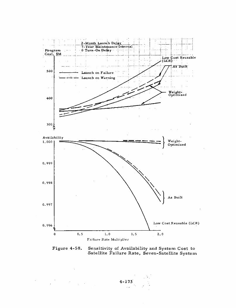
2-Month Launc h Dely : ay _ : i7- Yearainte~ance Intera .
Progam i - 0 Turn-On De ay . ..
Cost, $M ...: Low post Reusable
- A- B Alilt500 Launch on Failure
-.. .... Launch on Warning
Weight; .Optimized
400
300
Availability
Optimized
0. 999
0.998
SAs Built
0. 997
0.996 Low Cost Reusable (LCR)
0 0.5 1.0 1.5 2.0
Failure Rate Multiplier
Figure 4-58. Sensitivity of Availability and System Cost toSatellite Failure Rate, Seven-Satellite System
4- 173
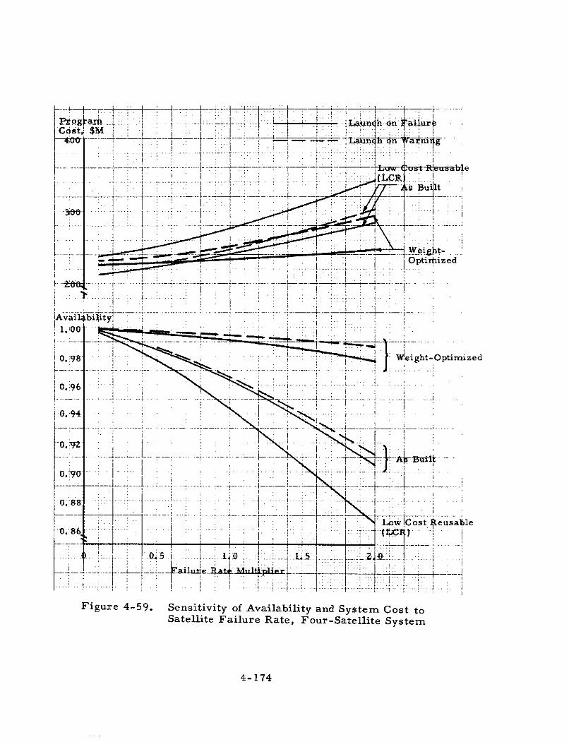
C-st,i $M _ H u -
Weight-'-i SOp I ti ized
-- i--- --- -- ------- l------- _----- :- -t--
Avail 4biity2.................. .... ..i .... i ...1. i00
i . . L : .. ..
0. Z
0.
Low lCost keusable
... . . 0.. . 1 ..- 5
il T e N.a4. lti p
. l~l -- - ... i- ...... ------ ---I-- .a,]L -: _ " ¢ -- -,|i:ier L - '- - . .... i
Figure 4-59. Sensitivity of Availability and System Cost toSatellite Failure Rate, Four-Satellite System
4-174
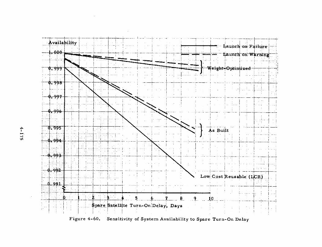
----- -------4-- . . - -- - - -- . . ... . " ..... ". . . .... - ..... ........... ; -........- ... ... ..... ..... . . .. .. . .
vaila ilty• -. -997 -. .-.-.. .. Launch o F i-r
9•"""" •.- t---.. - n--.- -o------ - T
U, .9-9 r-5
-. . . . .--- . . . .... .
. .. .i . .. . i.
pae Sateljte Tukn-OnDelay, Days
Figure 4-60. Sensitivity of System Availability to Spare Turn-On Delay
" : I-- -- - -- . ... .. -' --.. .. -: ... ....... t .. .... .* ....... ------ - .....--
4 ..: ( | . . ..... --- i--- . . I .. . . .. . . .. .. .. . . . , . .. .. . . . . ... . .I. . i '
Fiue4-0 eniity of ysem valabliy t SareTun-O Dl
Step 3 - Select Lowest Cost System Meeting Equal Risk Criteria
The remaining options are seven-satellite orbital configurations
for both current reusable design (CDR) satellites, the weight-optimized
dual-spin version, and the as-built dual-spin version. The weight-
optimized dual-spin design is the lowest cost operating with a launch-on-
failure logistics strategy (see Figure 4-56), however, the costs for the
as-built dual-spin system is close ($370 million vs $350 million) and
should not be eliminated on the basis of cost only. For example, the
lower initial cost could make the CDR as-built dual-spin design more
attractive than the CDR weight-optimized dual-spin design.
Step 4 - Assess Satellite System Risk Sensitivity
Since the costs for the as-built design and weight-optimized
design are close, the sensitivities of the risk assumptions become
an important consideration. The sensitivity of availability to failure
rate is low (see Figure 4-58) for the weight-optimized design compared
to the as-built design. For the weight-optimized design an increase in
failure rate of 60 percent still exhibits an availability of 0. 9999.
In addition, it is noted that the sensitivity of the availability
of the weight-optimized design to launch delay (see Figure 4-57) also
supports the selection of the xweight-optimized dual-spin satellite design
as the representative approach for the space system. Launch-on-failure
could be the preferred strategy for satellite replacement.
The output of this analysis is (1) the confirmation of the ability
of the selected system to meet the availability requirement of 0. 9999,
thus establishing equal risk with the competitive ground systems, and (2)
the selection of the weight-optimized dual-spin satellite with active spares
using the launch-on-failure logistics strategy as the lowest cost space
system approach. The output of the RISK computer program also shows
17 STS launches required to support the twelve-year program using
the selected satellite approach.
4-176

Other general observations may be of interest, although they
have no bearing on the specific problem illustrated here.
1. At a lower availability requirement (0. 999 or lower), theas-built dual-spin satellite design would have to be
compared with the weight-optimized dual-spin designon the basis of net present value (see Economics AnalysisSection) to determine the best selection.
2. The payoff for launch-on-warning strategy is limited to
very high availability requirements and enriched (highlyredundant) satellites such as the weight-optimized dual-spin version analyzed here (see Figures 4-58 and 4-59).
4-177
5. TERRESTRIAL SYSTEMS ANALYSIS
A. TELECOMMUNICATION SYSTEMS
1. ALTERNATE SYSTEM OPTIONS
The costs of satellite communication systems may be compared
with the costs of terrestrial communications systems of three types: (1)
common carrier telephone systems (e. g., ITT, ATT, GT, etc.), and (2)
dedicated systems constructed to perform a specific mission or furnish
specialized carrier system leased services (e. g., Microwave Communi-
cations, Inc. or DATRAN).
The character of the mission requirements will determine the
most economical terrestrial system approach. In general, the communica-
tion requirements between terminals in population centers in all but
"emerging" nations can be satisfied by common carrier telephone networks.
Under some circumstances, specialized carriers may provide
more economical service than common carriers owing to their design to
perform specialized service (e. g., narrow and wide band data with fast
switching to accommodate short message length) between pairs of population
centers with large demand for the service. However, such systems do
not serve remote, light-traffic areas.
Dedicated systems may be required where the mission requires
capacity too large to be provided by parts of the existing common carrier
network, as, for example, in sparsely populated areas or "emerging"
nations.
2. SYSTEM SELECTION
To define an appropriate terrestrial system, the following five
steps should be taken:
5-1
(1) Define communication requirements to provide the sameservice for comparison, as the satellite system. Specifycommunication traffic peak load requirements for alllinks, year-by-year, in terms of number of voice circuitsrequired and number and bit rate of data channels.
(2) State country in which each communication terminal islocated.
(3) Calculate distances of links between pairs of terminalsand specify whether each is U. S. domestic, foreigndomestic, foreign international, or trans-oceanic (e. g.,for use in Table 5-1).
(4) Calculate costs for each option (common carrier, leasedcircuits, and dedicated systems and compare cost streams).
(5) Specify whether each link is to be leased, common carrier,or constructed as a dedicated link on the basis of lowestcost.
3. ESTIMATING COSTS OF LEASING FROM COMMON CARRIERS
For leased circuits, calculate costs as follows:
(1) Calculate voice circuit costs using the worksheet, Table5-1 ).
(2) Calculate data transmission channel (2 ) costs using theworksheet, Table 5-2(1)
(3) Calculate total annual costs for each year using the work-sheet, Table 5-3.
Total annual costs for all links, as calculated above for each
year, are the annual costs for the leased terrestrial system for input
to the economic analysis. These costs are all annual operating costs
where the system is entirely leased (no purchased equipment).
(1) Terminal costs should be excluded for comparison with satellitesystems costs.
(2) A circuit is two (one-way each) channels. Charges for one-wayand two-way data transmission are the same. Two-way (duplex)voice circuits cost 10 percent more than one-way (simplex) voicechannels.
5-2
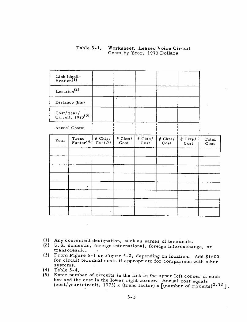
Table 5-1. Worksheet, Leased Voice CircuitCosts by Year, 1973 Dollars
Link Identi-fication(1)
Location (2 )
Distance (krn)
Cost/Year/Circuit, 1973 (3)
Annual Costs: II I I
Trend # Ckts/ # Ckts/ # Ckts/ # Ckts/ # Ckts/ TotalYear Factor( 4 ) Cost(5) Cost Cost Cost Cost Cost
(1) Any convenient designation, such as names of terminals.(2) U.S. domestic, foreign international, foreign interexchange, or
transoceanic.(3) From Figure 5-1 or Figure 5-2, depending on location. Add $1600
for circuit terminal costs if appropriate for comparison with othersystems.
(4) Table 5-4.(5) Enter number of circuits in the link in the upper left corner of each
box and the cost in the lower right corner. Annual cost equals(cost/year/circuit, 1973) x (trend factor) x [(number of circuits) 0 .72].
5-3

Table 5-2. Worksheet, Leased Data TransmissionChannels by Year, 1973 Dollars
1. Link Identi-fication(1)
2. Location(2 )
3. Data Rate (kbps)
4. Distance (km)
5. Cost/Yr/km @1609 km, Fig. 5-3
6. Distance FactorFig 5-4
7. Comm. LineCost (4x5x6)
8. Terminal Cost( 3 )Fig. 5-5
9. Line & Term.Cost (7+8)
10. LocationFactor(4)
Annual Cost(5)
Trend Factor TotalYear Table 5-4 Cost
(1) Any convenient designation, such as names of terminals.(2) Location: U.S. domestic, U.S. transoceanic, foreign interexchange,
or foreign international.(3) One set of terminal equipment is required at each end of a link. Include
if terminal costs are included for systems with which this system iscompared.
(4) U. S. domestic factor = 1. 0; U. S. transoceanic factor = 3. 0; foreigninterchange factor = 1. 8; foreign international factor = 2. 9.
(5) Annual cost = (line 7) x (line 10) x (trend factor), or Annual cost(line 9) x (line 10) x (trend factor) if terminal costs are included.
5-4
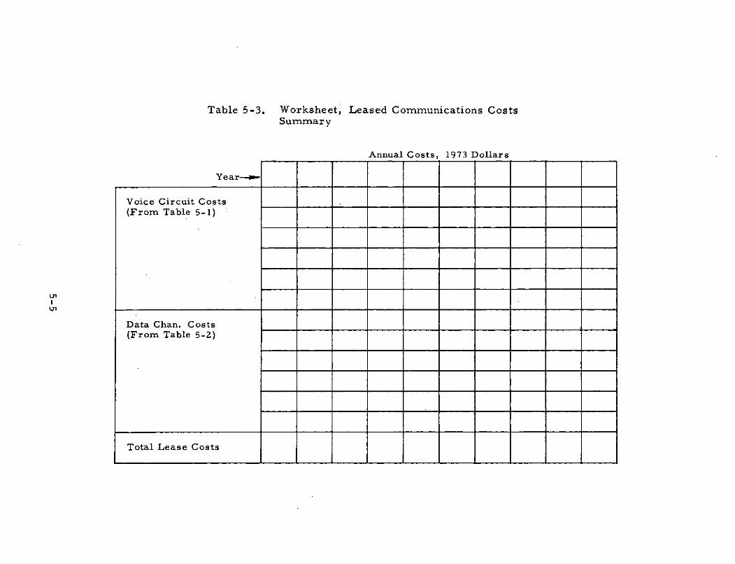
Table 5-3. Worksheet, Leased Communications CostsSummary
Annual Costs, 1973 Dollars
Year-
Voice Circuit Costs
(From Table 5-1)
U1
Data Chan. Costs(From Table 5-2)
Total Lease Costs
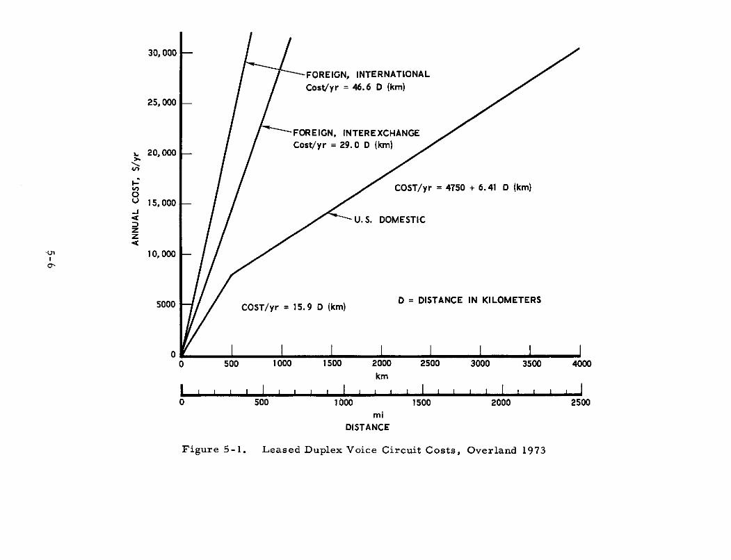
30, 000
FOREIGN, INTERNATIONAL
Cost/yr = 46.6 D (km)
25, 000 -
FOREIGN, INTEREXCHANGE
20,000 Cost/yr = 29.0 D (km)
5 COST/yr = 4750 + 6.41 D (km)O
S15,000.j
U. S. DOMESTIC
z
S10, 000
5000 COST/yr = 15.9 D (k) D = DISTANCE IN KILOMETERS500 COST/yr = 15.9 D (km)
0 500 1000 1500 2000 2500 3000 3500 4000km
Il i Il I , , I I l I I I0 500 1000 1500 2000 2500
mi
DISTANCE
Figure 5-1. Leased Duplex Voice Circuit Costs, Overland 1973
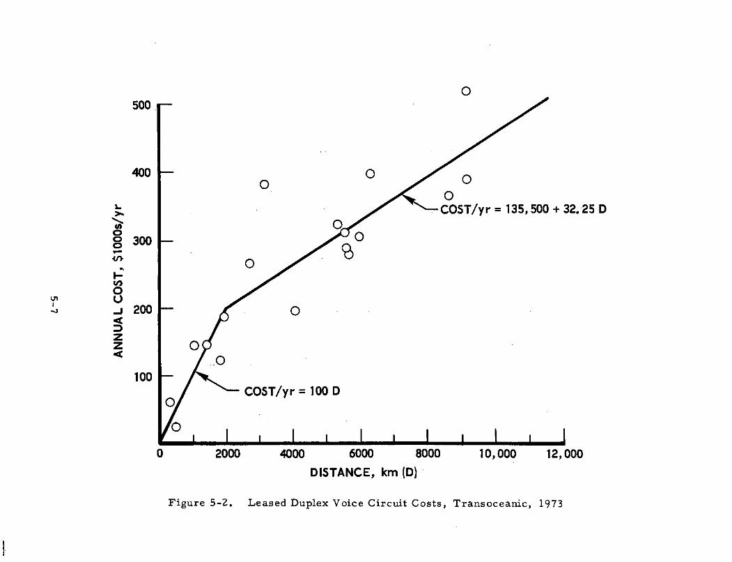
500
400 O0
COST/yr = 135,500 + 32.25 D
08 300 -
I-
UU200 - O
zz 0
O100
SCOST/yr = 100 D
0 2000 4000 6000 8000 10,000 12,000
DISTANCE, km (D)
Figure 5-2. Leased Duplex Voice Circuit Costs, Transoceanic, 1973

Table 5-4. Trend Factors for Adjusting CommunicationsCosts for Future Years
Calendar y Trend FactorYear (year-1973) (0. 9 6 )y
1973 0 1.001974 1 0.961975 2 0.921976 3 0.881977 4 0.851978 5 0.821979 6 0.781980 7 0.751981 8 0.721982 9 0.691983 10 0.661984 11 0.641985 12 0.611986 13 0.591987 14 0.561988 15 0.541989 16 0.521990 17 0.501991 18 0.481992 19 0.461993 20 0.441994 21 0.421995 22 0.411996 23 0.391997 24 0.381998 25 0.361999 26 0.352000 27 0.33
5-8
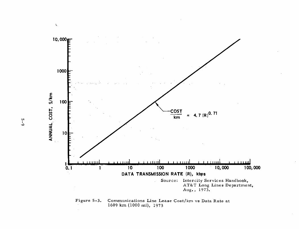
10, 000
1000
3 100
COST0 = 4. 7 (R)0 km
z 10Z
0.1 1 10 100 1000 10, 000 100, 000DATA TRANSMISSION RATE (R), kbps
Source: Intercity Services Handbook,AT&T Long Lines Department,Aug., 1973.
Figure 5-3. Communications Line Lease Cost/km vs Data Rate at1609 km (1000 mi), 1973
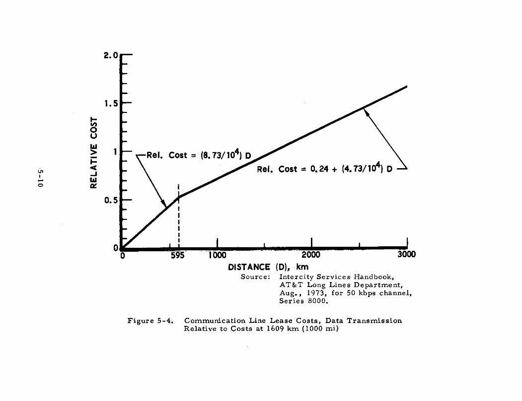
2.0
1.5
0OUw> 1 Rel. Cost = (8.73/104) D
- -w
0. 5
0 595 000 2000 3000DISTANCE (D), km
Source: Intercity Services Handbook,AT&T Long Lines Department,Aug., 1973, for 50 kbps channel,Series 8000.
Figure 5-4. Communication Line Lease Costs, Data TransmissionRelative to Costs at 1609 km (1000 mi)
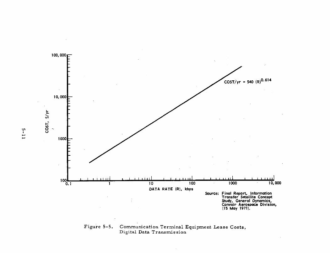
100, 000
COST/yr = 540 (R)0.6 14
10, 000 -
--0U
1000
0.1 1 10 100 1000 10,000DATA RATE (R), kbps
Source: Final Report, InformationTransfer Satellite ConceptStudy, General Dynamics,Convair Aerospace Division,(15 May 1971).
Figure 5-5. Communication Terminal Equipment Lease Costs,Digital Data Transmission

4. DEDICATED MICROWAVE RELAY SYSTEM
For dedicated communication circuits over land, where common
carrier or specialized carrier facilities are not adequate, calculate
costs of a microwave relay system dedicated to the mission. Relays
in a typical system are spaced 48 km apart, on the average. Equipment
for transmission of voice or data at a frequency of 4-6 GHz is assumed
for basic calculations, and it is assumed that a switching system will
be used in the interest of efficiency in utilizing transmission capability.
Availability of 99. 98 percent and P. 01 service (no more than 0.01 probability
that caller receives busy signal during the busiest hour of the day) are typical
of these systems. The inputs required for calculation are:
(1) Relay line distance in kilometers (D), or number ofrelay stations (R) at 48 kilometer spacing
(2) Number of terminals (T)
(3) Number of 4 KHz voice or 4000 bit-per-second datachannels, each terminal (Ct)
(4) Schedule of completions of terminals and relay stations.
If these inputs are not defined, they should be approximated.
Relay trunk lines should be laid out on a map (or transparent overlays
on Atlas maps) using the shortest single-line trunk to interconnect the
terminal points (the same terminal points as specified for the comparable
satellite system). The number of relay stations is calculated assuming
one station every 48 km (30 mi) along the trunk routes between terminals.
Communication traffic capacity for each terminal should be 30 percent
greater than that specified for the system to allow for equipment outages ( 1 )
The schedule of completions of terminals and the interconnecting relay
stations should be consistent with the comparable satellite system schedule.
(1) Satellite system nominal, or working, capacities are augmented,typically, by redundant capacity in spare satellites and earth stationsof 50 to 100 percent of the nominal capacity to assure reliableservice. Similarly, for microwave relay systems common carrierstypically provide redundant capacity of 20 to 33 percent, which isapproximated as 30 percent for the calculations herein.
5-12

Investment costs for relays and terminals are based on the
following relationship (system design costs are included and development
costs are not necessary for the equipment used):
t =T 0.855Cost = R ($184K) + C $156K + (3. 31K) (Ct) + ($1. 16K) (Ct)
t= 1
where t is the terminal number, ranging from 1 to T.
Instead of calculating costs using this expression, costs for
individual relay stations and terminals may be read directly from Figure
5-6 which shows the cost of relay stations and terminals versus terminal
capacity in numbers of channels. The expression above is in terms of
standard 4 kHz voice or equivalent data rate (4000 bps) channels; the
effect of higher bit rate channels on cost is provided for by adjustments
to the basic system cost in the calculations below. Additional adjustments
allow for variations in construction cost according to geographic area.
To calculate system costs, use the worksheet, Table 5-5, to
calculate investment costs of relay stations and terminals and the work-
sheet, Table 5-6, to summarize annual costs by year (in 1973 dollars) for
input to the cost effectiveness analysis. For convenience of calculation,
group terminals with the same capacity, year of completion, and con-
struction cost factor; group relays with the same year of completion and
construction cost factor.
Calculate costs in 1973 dollars for relays and terminals on the
worksheet, Table 5-5, as follows:
1. Enter the numbers of terminals and relay stations,appropriately grouped according to year of completion,terminal capacity, and construction cost factor.
2. Calculate costs of terminals.
a. Determine unit cost per terminal according tochannel capacity (Figure 5-6).
b. Calculate "basic cost" of individual terminals orgroups of terminals by multiplying together theunit cost, the number of terminals in the group,and the construction cost factor.
5-13
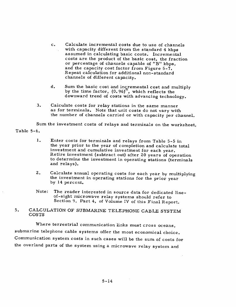
c. Calculate incremental costs due to use of channelswith capacity different from the standard 4 kbpsassumed in calculating basic costs. Incrementalcosts are the product of the basic cost, the fractionor percentage of channels capable of "B" kbps,and the capacity cost factor from Figure 5-7.Repeat calculation for additional non-standardchannels of different capacity.
d. Sum the basic cost and incremental cost and multiplyby the time factor, (0. 9 6 )n , which reflects thedownward trend of costs with advancing technology.
3. Calculate costs for relay stations in the same manneras for terminals. Note that unit costs do not vary withthe number of channels carried or with capacity per channel.
Sum the investment costs of relays and terminals on the worksheet,
Table 5-6.
1. Enter costs for terminals and relays from Table 5-5 inthe year prior to the year of completion and calculate totalinvestment and cumulative investment for each year.Retire investment (subtract out) after 20 years of operationto determine the investment in operating stations (terminalsand relays).
2. Calculate annual operating costs for each year by multiplyingthe investment in operating stations for the prior yearby 14 percent.
Note: The reader interested in source data for dedicated line-of-sight microwave relay systems should refer toSection 9, Part 4, of Volume IV of this Final Report.
5. CALCULATION OF SUBMARINE TELEPHONE CABLE SYSTEMCOSTS
Where terrestrial communication links must cross oceans,submarine telephone cable systems offer the most economical choice.Communication system costs in such cases will be the sum of costs forthe overland parts of the system using a microwave relay system and
5-14
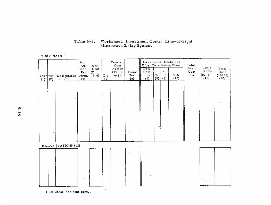
Table 5-5. Worksheet, Investment Costs, Line-of-SightMicrowave Relay System
TERMINALS
No. Constr. Incremental Costs ForOf Unit Cost Other Data Rates/Chan. Total,
Chan. Cost Factor Data Basic Time Total
Per (Fig. (Table Basic Rate F Cost Factor Cost
Year "n" Designation Term. 5-6) Qty. 4-9) Cost bps % $ A +A (0.96) n (1973$)(1) (2) (3) (4) (5) (6) (7) (8) (9) (10) (11) (12)
RELAY STATIONS (13)
Footnotes: See next page.

Table 5-5. Worksheet, Investment Costs, Line-of-SightMicrowave Relay System (Cont'd)
Footnotes:
(1) Year of construction completion.
(2) n = (year of construction completion) - (1973)
(3) Any convenient designation of individual terminals or relay stations,or groups of terminals of the same capacity and construction costfactor, or groups of relays with the same construction cost factor.
(4) Capacity per terminal, number of channels.
(5) Number of terminals or channels being calculated as a group.
(6) Basic cost, assuming standard 4 kHz voice or 4000 bps data channels.
(7) Data rate per channel, in bits-per-second, for non-standard channels.If more than one non-standard data rate, use additional line(s) forcalculation.
(8) Ratio, number of non-standard channels of a particular data rate tothe total number of channels, expressed as a percent.
(9) F c = channel capacity cost factor. See Figure 5-7.
(10) Incremental cost due to non-standard channels = (basic cost) x (%) x (F c - ).
(11) Time factor to reduce costs four percent per year to reflect trend oftechnology advances.
(12) Total cost (1973 dollars) = (time factor) x (total basic cost + A's) forterminals, or (time factor) x (basic cost) for relay stations.
(13) Column headings for calculating relay station costs are the same asfor terminals, except for the 4th and 9th through 13th columns, whichare not required in relay station calculations.
5-16
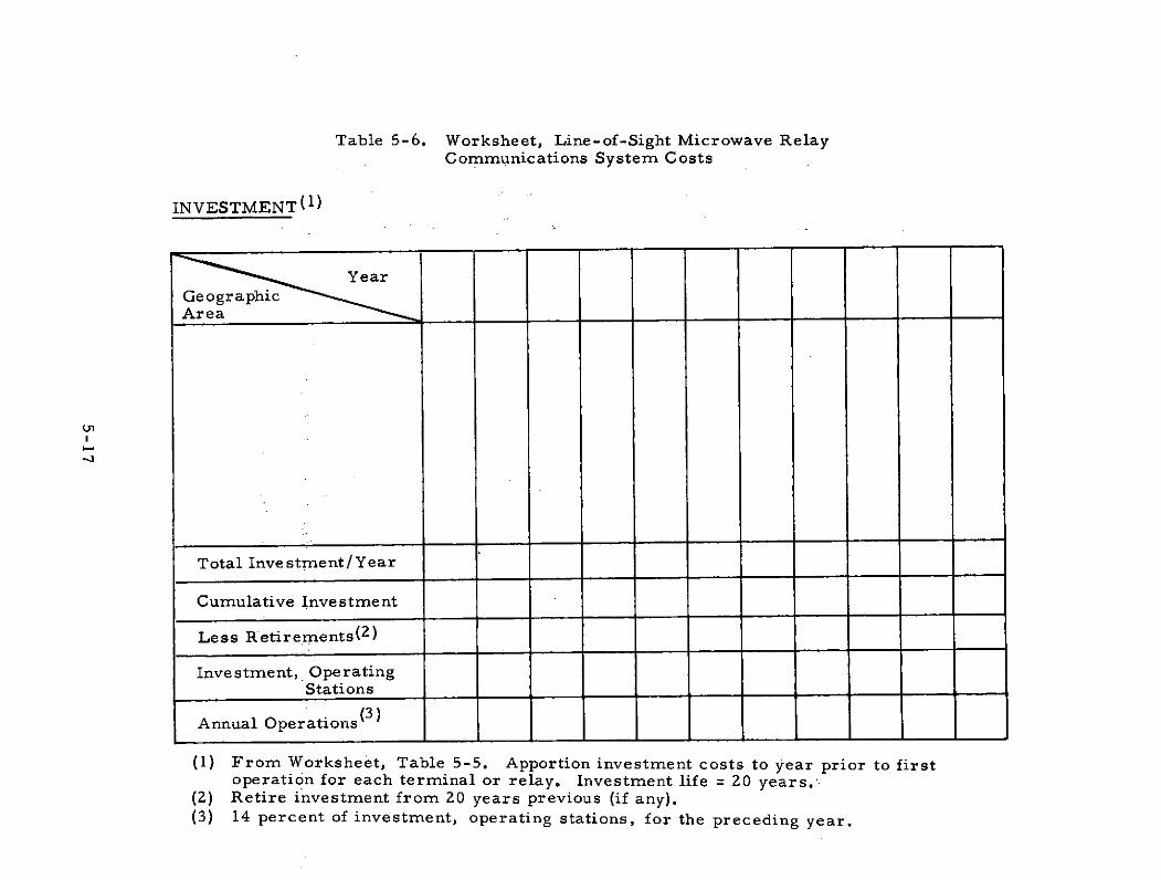
Table 5-6. Worksheet, Line-of-Sight Microwave RelayCommunications System Costs
INVESTMENT (1 )
YearGeographicArea
-3
Total Investment/Year
Cumulative Investment
Less Retirements( 2 )
Investment, OperatingStations
Annual Operations (3)
(1) From Worksheet, Table 5-5. Apportion investment costs to year prior to firstoperation for each terminal or relay. Investment life = 20 years.
(2) Retire investment from 20 years previous (if any).(3) 14 percent of investment, operating stations, for the preceding year.
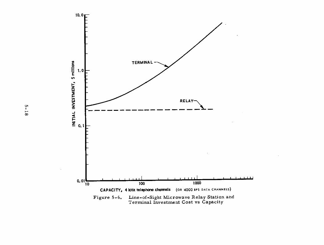
10.0
m ITERMINAL
S1.0E
zw
w RELAY
1-
Z 0.1
0.01I I I i l I I
10 100 1000
CAPACITY, 4 kHz telephone channels (OR 4000 BPS DATA CHANNELS)
Figure 5-6. Line-of-Sight Microwave Relay Station andTerminal Investment Cost vs Capacity
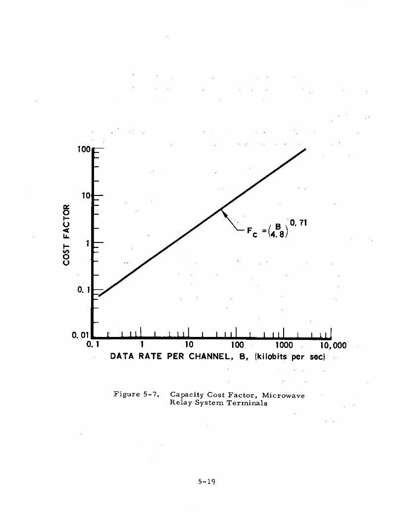
100
10
8O-U B 0. 7 1
LL = 4.81
0. 1
0. 010. 1 1 10 100 1000 10, 000
DATA RATE PER CHANNEL, B, (kilobits per sec)
Figure 5-7. Capacity Cost Factor, MicrowaveRelay System Terminals
5-19
the transoceanic submarine telephone cable system, consisting of the
cable itself, repeaters every 10 to 15 km (approximately 6 to 10 mi),
and one terminal at each end which interfaces the overland system.
a. Investment Costs
Investment costs are calculated using the worksheet, Table 5-7.
For each cable the following inputs must be provided and entered on
the worksheet:
(1) The cable terminal points (for identification)
(2) The first year in service
(3) The capacity in number of 4 kHz * half-circuits (twohalf-circuits, or channels, one-way each, are requiredfor a two-way telephone circuit)
(4) The length of cable between terminals, in kilometers.
The unit investment cost per half-circuit per kilometer is read
from Figure 5-8 and entered on the worksheet. Four cost curves
are shown in the figure, for 1970, 1980, 1990, and 2000, indicating an
estimated 3. 1 percent per year decline in investment costs. Unit invest-
ment cost points for other years should be interpolated. For example,
the unit investment cost for a 10, 000 half-circuit cable system, first
operational in 1996, would be $13. 50, about six-tenths of the distance
from the 1990 curve down toward the 2000 curve on the line for 10, 000
half-circuits. Asterisks at the ends of the cost curves indicate the
approximate capacity limits for single cables in 1970, 1980, and 1990.
The length factor is read from Figure 5-9 for the cable length
and entered on the worksheet. This factor is used to adjust the investment
costs per unit length from Figure 5-8, which are normalized to 4000 kilo-
meters, for other cable lengths.
* Note that the usual submarine cable telephone half-circuit band-width is 3 kHz. Calculations herein are based on 4 kHz bandwidthsfor comparability with overland and satellite systems.
5-20
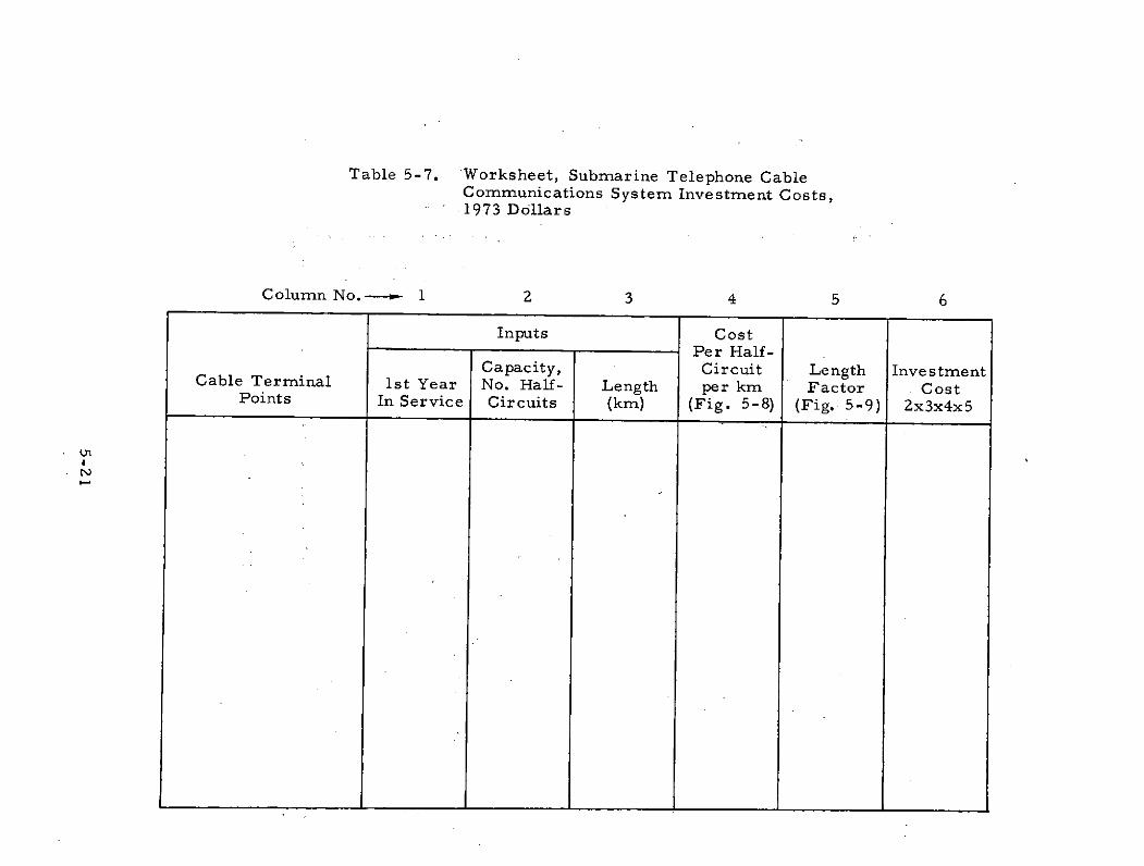
Table 5-7. -Worksheet, Submarine Telephone CableCommunications System Investment Costs,1973 Dollars
Column No.- 1 2 3 4 5 6
Inputs CostPer Half-
Capacity, Circuit Length InvestmentCable Terminal 1st Year No. Half- Length per km Factor Cost
Points In Service Circuits (km) (Fig. 5-8) (Fig. 5-9) 2x3x4x5
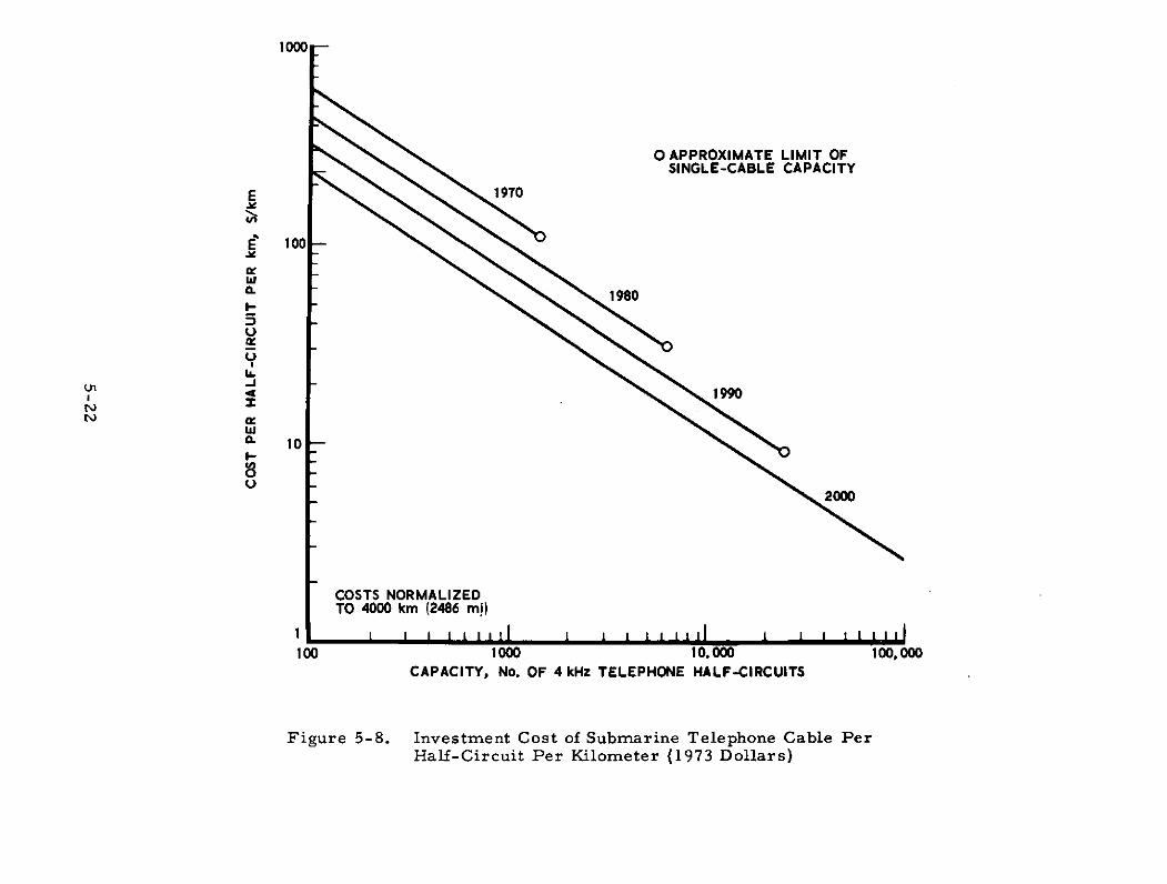
1000
0 APPROXIMATE LIMIT OFSINGLE-CABLE CAPACITY
E 1970
E 100
1980
U
I-
I0 1990N
S10
i-
U2000
COSTS NORMALIZEDTO 4000 km (2486 mi)
10 1000 10.000 100,000CAPACITY, No. OF 4 kHz TELEPHONE HALF-CIRCUITS
Figure 5-8. Investment Cost of Submarine Telephone Cable PerHalf-Circuit Per Kilometer (1973 Dollars)
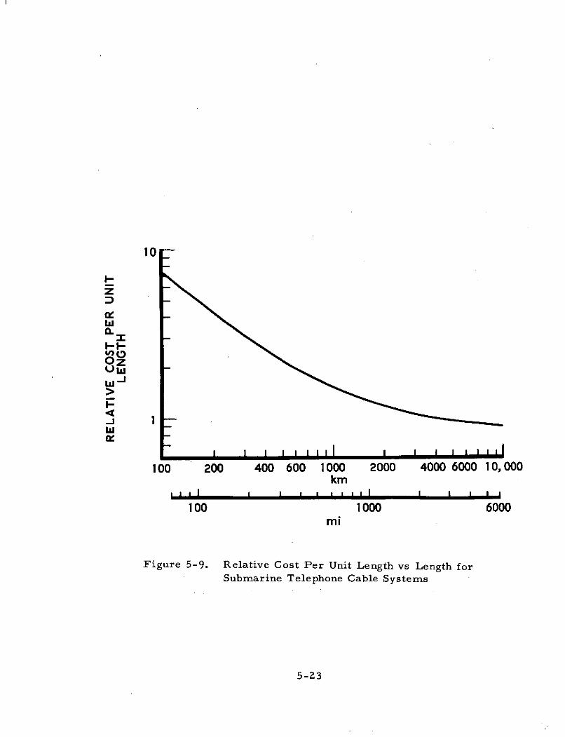
10
I-r
aI0ZI-I-Oz
1- 1w
100 200 400 600 1000 2000 4000 6000 10,000km
, i I I 1 ,I II I I I I i 1
100 1000 6000mi
Figure 5-9. Relative Cost Per Unit Length vs Length forSubmarine Telephone Cable Systems
5-23
The cable system cost is then calculated in the right-hand column
of Table 5-7 by multiplying together the unit cost per half-circuit per
kilometer, the capacity in half-circuits, the length in kilometers, and the
length factor.
The worksheet, Table 5-8, is used to show costs in the year
of expenditure. The investment cost determined in Table 5-7 for each
cable system should be allocated approximately in the proportions 2:4:4
to the third, second, and first year, respectively, prior to the year
of first operation. Use a 24-year service life as the basis for estimating
residual values where cable useful life exceeds the time period for which
cost comparisons are made.
Operating costs for each year of service life are calculated
by multiplying the cable system investment cost by 8.5 percent. These
operating costs include the costs of maintaining and operating the cable
and terminal facilities, 2.8 percent, and personnel costs for servicing
customers' requirements, accounting, billing, advertising, etc., 5. 6
percent of investment.
B. U. S. POSTAL SERVICE COSTS
Transmission of information by a satellite system is an alternative
to transmission using mail. Mail service is relatively much slower than
telecommunication by satellite; however, in cases where realtime, or
near realtime transmission is not a paramount requirement, the lower
cost, slower but still reliable mail may be attractive.
Calculating the relative cost effectiveness of satellite systems
and mail service requires placing a value on time of communication.
It is not practicable to determine this value in the procedures herein
because the value of time varies with the nature and use of the information
transmitted. In some cases the value of time far outweighs cost differences,
e. g., TV coverage of daily news or sports events of national interest. In
5-24
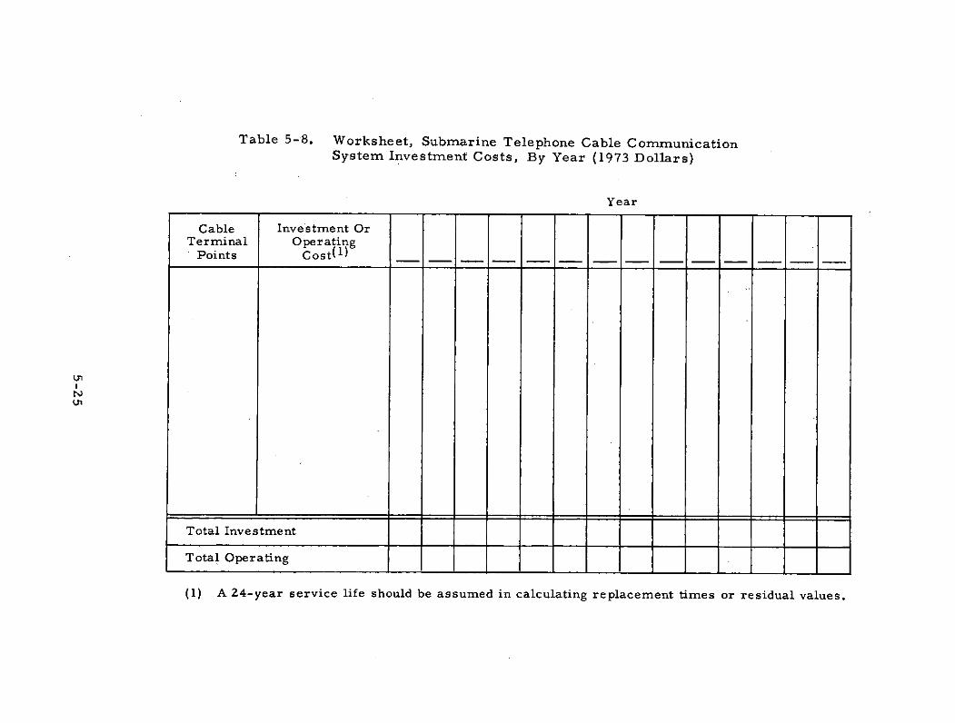
Table 5-8. Worksheet, Submarine Telephone Cable CommunicationSystem Investment Costs, By Year (1973 Dollars)
Year
Cable Investment OrTerminal OperatingPoints Cost(l)
Total Investment
Total Operating
(1) A 24-year service life should be assumed in calculating replacement times or residual values.
other cases time is less critical and relative cost of alternative trans-
mission or transportation is important, e. g., CATV showing of special
features or movies.
-The costs of information transmission by mail can be calculated
using the procedures below with sufficient accuracy to provide a basis
for cost comparison with satellite system transmission. Comparisons
of effectiveness will depend on the purpose of the satellite system
communications.
Postal Service mail classifications and rates are complex, owing
to variations in priority of handling, size and weight of pieces of mail,
quantity per mailing, distance covered, transportation mode, and pre-
ferences granted in the public interest to some senders and some kinds
of mail. In addition, a large proportion of total costs are costs for
facilities used in common for all mail classes, and the allocation of these
costs to determine rates has been necessarily arbitrary.
Thus, simple relationships between parameters such as weight,
distance, priority of handling, or quantity per mailing and the rates charged
are not adequate to describe the rate variations for all classes of mail.
To determine the cost of mail service, it is necessary to segregate mail
by mail class and determine costs by mail class. Simplified relationships
are used herein to approximate the actual Postal Service rate schedules
for particular classes of mail in the interest of simplifying calculations.
1. INPUTS REQUIRED
In order to determine mail classifications, the following informa-
tion must be provided in the system definition:
(1) Nature of business of sender - non-profit publisher,publisher of classroom materials, library, mail-orderretailer, etc.
(2) Kind of material - advertising, general reading matter,books, magazines, etc.
5-26
(3) Weight per piece or a range or distribution of weightsper piece.
(4) Quantity mailed per year, number of pieces, weight.
(5) Distance to destination or the quantities of mail to severaldestination distances.
2. SELECTION OF MAIL CLASSIFICATION
Table 10-2 in Volume IV, Part 4, Section 10, provides a basis
for relating the characteristics of the sender and the nature of the mail
to the major mail classes and sub-classes. Select the appropriate classi-
fication and calculate mailing costs using the worksheets in Part 3 of
Volume IV for the appropriate classification.
3. CALCULATION OF MAILING COSTS
Calculate annual costs for mailing using the worksheets in:
(1) Table 5-9 for first class and air mail
(2) Table 5-10 for priority mail
(3) Table 5-12 for second class publications
(4) Table 5-13 for parcel post (fourth-class).
Summarize costs per year in Table 5-15.
C. AIRCRAFT COSTS
The specific objectives of earth observation missions and the
sensors used will determine payload requirements for the aircraft, the
width of observation strip, the observation altitude, restrictions on suitable
times of day or year for observation, and so on, all of which will affect,
in one way or another, the selection of aircraft, their numbers, and
their initial costs or operating costs.
It is not practicable to anticipate all possible missions and to
devise uncomplicated procedures for selecting specific aircraft to satisfy
mission requirements and for estimating their costs. The procedures
5-27
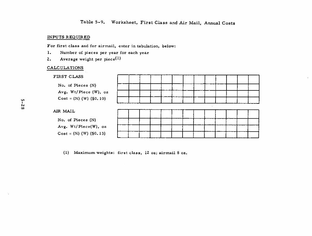
Table 5-9. Worksheet, First Class and Air Mail, Annual Costs
INPUTS REQUIRED
For first class and for airmail, enter in tabulation, below:
1. Number of pieces per year for each year
2. Average weight per piece(l)
CALCULATIONS
FIRST CLASS
No. of Pieces (N)
Avg. Wt/Piece (W), oz
Cost = (N) (W) ($0. 10)
AIR MAIL
No. of Pieces (N)
Avg. Wt/Piece(W), oz
Cost = (N) (W) ($0. 13)
(1) Maximum weights: first class, 12 oz; airmail 8 oz.
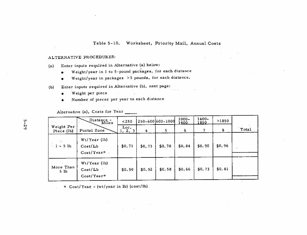
Table 5-10. Worksheet, Priority Mail, Annual Costs
ALTERNATIVE PROCEDURES:
(a) Enter inputs required in Alternative (a) below:
* Weight/year in 1 to 5-pound packages, for each distance
* Weight/year in packages >5 pounds, for each distance.
(b) Enter inputs required in Alternative (b), next page:
* Weight per piece
* Number of pieces per year to each distance
Alternative (a), Costs for Year
U' Distance - 1000- 1400-Miles <250 250-600 600-100 1400 >1850
Weight Per Loc.Piece (lb) Postal Zone 1, 2, 3 4 5 6 7 8 Total
Wt/Year (lb)
1 - 5 lb Cost/Lb $0.71 $0.73 $0.78 $0.84 $0.90 $0.96
Cost/Year.*
Wt/Year (lb)
Morb Cost/Lb $0.50 $0.52 $0.58 $0.66 $0. 73 $0.81
Cost/Year*
* Cost/Year = (wt/year in lb) (cost/lb)
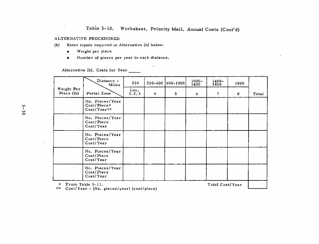
Table 5-10. Worksheet, Priority Mail, Annual Costs (Cont'd)
ALTERNATIVE PROCEDURES:
(b) Enter inputs required in Alternative (b) below:
* Weight per piece
* Number of pieces per year to each distance.
Alternative (b), Costs for Year
Distance - 1000- 1400-Miles 250 250-600 600-1000 1400 1850 1850
Weight Per Loc.Piece (Ib) Postal Zone 1, 2, 3 4 5 6 7 8 Total
No. Pieces/YearCost/Piece::Cost/Year *
No. Pieces/YearCost/ PieceCost/Year
No. Pieces/YearCost/PieceCost/ Year
No. Pieces/YearCost/PieceCost/Year
No. Pieces/YearCost/ PieceCost/ Year
* From Table 5-11. Total Cost/YearCost/Year = (No. pieces/year) (cost/piece)
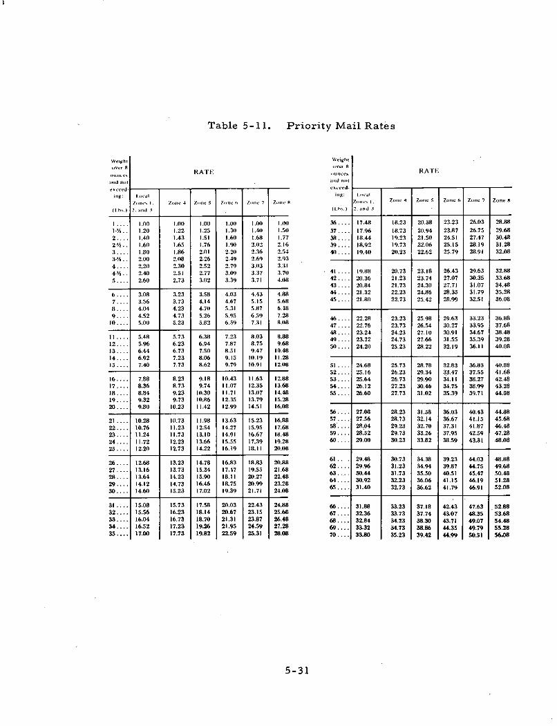
Table 5-11. Priority Mail Rates
Weight Weightover 9 over 8RATE ,une RATE
ounce%and nol and ,nt
exceed- exceed-
ing: Local ing: Local
Zolnc I. Zoe 4 ZII 5 Z( ce Z.o c 7 Z e Zon: . Zone 4 Zone 5 Zone 6 Zone 7 Zone 8
( .) and . (Lh .) 2. and 3
I .. . 1.00 1.00 1.00 1.00 1.00 1.00 36 .... 17.48 18.23 20.38 23.23 26.03 28.88
- . . 1.20 1.22 1.25 1.30 1.40 1.150 37 .... 17.96 18.73 20.94 23.87 26.75 29.682.... 1.40 1.43 1.51 1.60 1.68 1.77 38 .... 18.44 19.23 21.50 24.51 27.47 30.482-/2.. 1.60 1.65 1.76 1.90 2.02 2.16 39.... 18.92 19.73 22.06 25.15 28.19 31.283 .... 1.80 1.86 2.011 2.20 2.36 2.54 40 .... 19.40 20.23 22.62 25.79 28.91 32.083- . . 2.00 2.08 2.26 2.49 2.69 2.93
4 .... 2.201 2.30 2.52 2.79 3.03 3.31
4-'.. 2.40 2.51 2.77 3.09 3.37 3.70 41 .... 19.88 20.73 23.18 26.43 29.63 32.88
5.... 2.60 2.73 3.02 3.39 3.71 4.08 42 .... 20.36 21.23 23.74 27.07 30.35 33.6843 .... 20.84 21.73 24.30 27.71 31.07 34.48
6 .... 3.08 3.23 3.58 4.03 4.43 4.88 44 .... 21.32 22.23 24.86 28.35 31.79 35.28
7 .... 3.56 3.73 4.14 4.67 5.15 5.68 45 .... 21.80 22.73 25.42 28.99 32.51 36.08
8 .... 4.04 4.23 4.70 5.31 5.87 6.48
9 .... 4.52 4.73 5.26 5.95 6.59 7.28 46 .... 22.28 23.23 25.98 29.63 33.23 36.8810 .... 5.00 5.23 5.82 6.59 7.31 8.08 47 .... 22.76 23.73 26.54 30.27 33.95 37.68
48... . 23.24 24.23 27.10 30.91 34.67 38.48I .... 5.48 5.73 6.38 7.23 8.03 8.88 49 .... 23.72 24.73 27.66 31.55 35.39 39.28
12 ... 5.96 6.23 6.94 7.87 8.75 9.68 50 .... 24.20 25.23 28.22 32.19 36.11 40.0813 .... 6.44 6.73 7.50 8.51 9.47 10.4814 .... 6.92 7.23 8.06 9.15 10.19 1 1.28
15 .... 7.40 7.73 8.62 9.79 10.91 12.08 51 .... 24.68 25.73 28.78 32.83 36.83 40.8852.... 25.16 26.23 29.34 33.47 37.55 41.68
16 .... 7.88 8.23 9.18 10.43 11.63 12.88 53.... 25.64 26.73 29.90 34.11 38.27 42.4817 .... 8.36 8.73 9.74 11.07 12.35 13.68 54.... 26.12 27.23 30.46 34.75 38.99 43.2818 .... 8.84 9.23 10.30 11.71 13.07 14.48 55.... 26.60 27.73 31.02 35.39 39.71 44.0819.... 9.32 9.73 10.86 12.35 13.79 15.2820.... 9.801 10.23 11.42 12.99 14.51 16.08
56.... 27.08 28.23 31.58 36.03 40.43 44.88
21 .... 10.28 10.73 11.98 13.63 15.23 16.88 57 .... 27.56 28.73 32.14 36.67 41.15 45.68
22 .... 10.76 11.23 12.54 14.27 15.95 17.68 58.... 28.04 29.23 32.70 37.31 41.87 46.48
23.... 11.24 11.73 13.10 14.91 16.67 18.48 59.... 28.52 29.73 33.26 37.95 42.59 47.28
24 .... 11.72 12.23 13.66 15.55 17.39 19.28 60.... 29.00 30.23 33.82 38.59 43.31 48.08
25.... 12.20 12.73 14.22 16.19 18.11 20.08
61.. . 29.48 30.73 34.38 39.23 44.03 48.8826 .... 12.68 13.23 14.78 16.83 18.83 20.88 62.... 29.96 31.23 3.94 39.87 44.75 49.6827 .... 13.16 13.73 15.34 17.17 19.55 21.68 6 .... 30.44 31.73 35.50 40.51 45.47 50.4828 .... 13.64 14.23 15.90 18.11 20.27 22.48 6 .... 30.92 32.23 36.06 41.15 46.19 51.2829 .... 14.12 14.73 16.46 18.75 20.99 23.28 65.... 31.40 32.73 36.62 41.79 46.91 52.0830 .... 14.60 15.23 17.02 19.39 21.71 24.08
31 .... 15.08 15.73 17.58 20.03 22.43 24.88 66.... 31.88 33.23 37.18 42.43 47.63 .52.88
32.... 15.56 16.23 18.14 20.67 23.15 25.68 67.... 32.36 33.73 37.74 43.07 48.35 53.6833.... 16.04 16.73 18.70 21.31 23.87 26.48 68.... 32.84 34.23 38.30 43.71 49.07 54.4834.... 16.52 17.23 19.26 21.95 24.59 27.28 69.... 33.32 34.73 38.86 44.35 49.79 55.2835.... 17.00 17.73 19.82 22.59 25.31 28.08 70 .... 33.80 35.23 39.42 44.99 50.51 56.08
5-31

Table 5-12. Worksheet, Second Class Mail, Annual Cost
INPUTS REQUIRED
" Classification(1)
. Line out the two columns of rates not used
" Total weight of publications/year by distance or postal zone
* No. of pieces/year, enter in table
* No. pounds reading matter/year, enter in table
CALCULATIONS
Year
Rates j/Lb(1 )
Weight Cost Weight Cost Weight CostZ C1 NP (lb) ( l) (lb) ($) (lb) ($)
1. Reading Matter 4.0 2.3 2.4
2. Advertising
Zone Distance (Miles)
1&2 50-125 6.0 3.6 4.4
3 125-250 7.2 4.4 5.2
4 250-600 9.6 5.9 6.9
5 600-1000 11.9 7.4 8.6
6 1000-1400 14.4 9.0 9.4
7 1400-1850 15.3 9.5 9.5
8 1850 & Up 17.8 11.1 9.7
Total Advertising:
Rates, j Each
Z Cl NP # Pcs. Cost$ # Pcs.Cost$ # Pcs. Cost$
3. Per-Piece Cost 0.2 0.1 0.04
4. Minimum Total Costs 1. 3 0. 8 0. 2
5. Total Calculated Cost Z(1 + 2 + 3)
6. Total Cost (Larger of 4 or 5)
(1) Regular zone-rate publications (Z), classroom publication (Cl), or non-profit publications (NP)
5-32
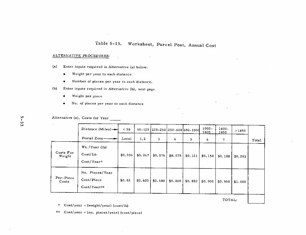
Table 5-13. Worksheet, Parcel Post, Annual Cost
ALTERNATIVE PROCEDURES:
(a) Enter inputs required in Alternative (a) below:
* Weight per year to each distance
* Number of pieces per year to each distance.
(b) Enter inputs required in Alternative (b), next page
* Weight per piece
* No. of pieces per year to each distance
Un Alternative (a), Costs for Year
Distance (Miles)-- < 50 50-125 125-250 250-600 600-100 1000- 1400- >18501400 1850
Postal Zone a Local 1,2 3 4 5 6 7 Total
Wt. /Year (lb)
Costs For Cost/Lb $0.036 $0.067 $0.076 $0.078 $0. 121 $0. 150 $0. 188 $0.203Weight
Cost/Year*
No. Pieces/Year
Per-PieceCosts Cost/Piece $0. 55 $0. 600 $0. 680 $0. 800 $0. 850 $0. 900 $0. 950 $1. 000
Cost/Year**
TOTAL:
* Cost/year = (weight/year) (cost/lb)
** Cost/year = (no. pieces/year) (cost/piece)
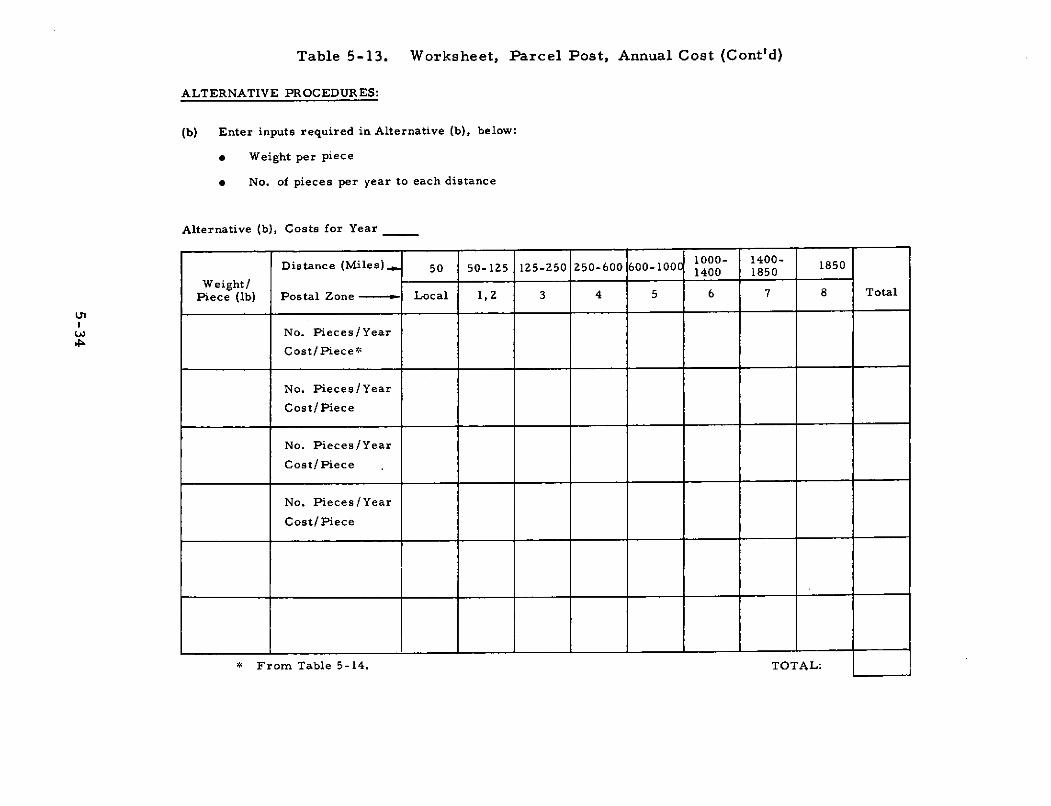
Table 5-13. Worksheet, Parcel Post, Annual Cost (Cont'd)
ALTERNATIVE PROCEDURES:
(b) Enter inputs required in Alternative (b), below:
* Weight per piece
* No. of pieces per year to each distance
Alternative (b), Costs for Year
Distance (Miles). 50 50-125 125-250 250-600 600-100C 18501400 1850
Weight/Piece (lb) Postal Zone - Local 1,2 3 4 5 6 7 8 Total
UlIU No. Pieces/Year
Cost/Piece*
No. Pieces/Year
Cost/Piece
No. Pieces/Year
Cost/Piece
No. Pieces/Year
Cost/Piece
* From Table 5-14. TOTAL:
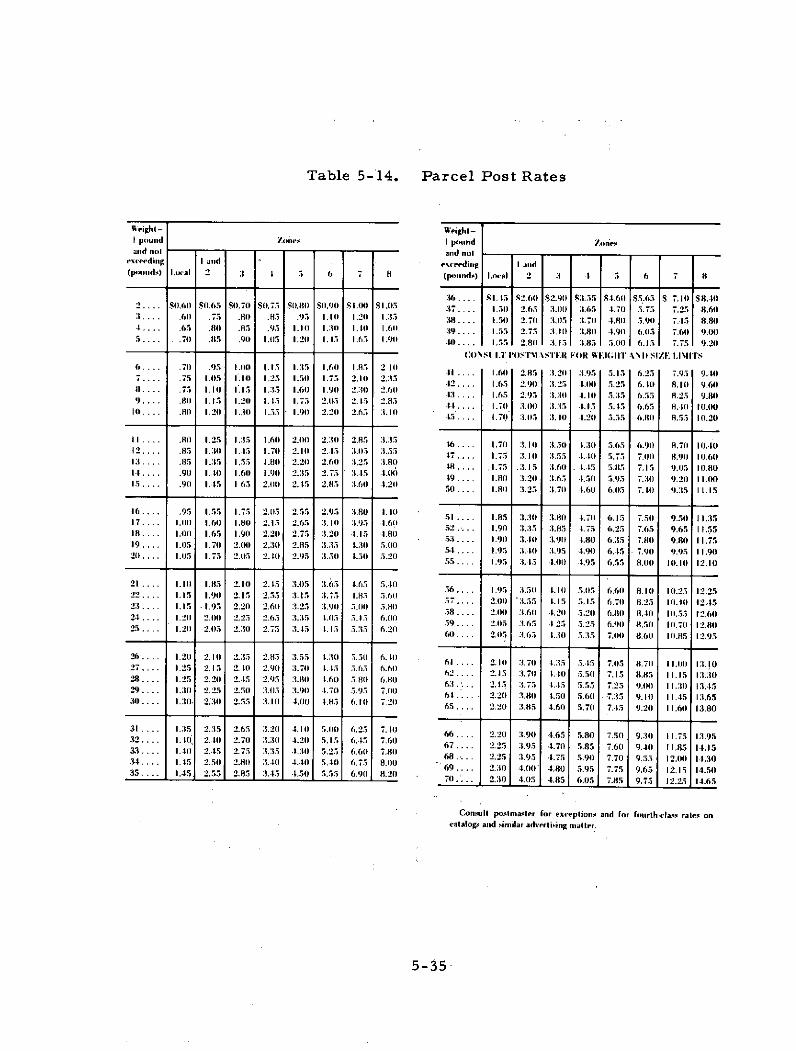
Table 5-14. Parcel Post Rates
Weight- Weighl-I pound Zones I pound Ionesand not and not I
exceeding I and - eceedind g I and(pounds) Local 2 3 1 6 7 8 (pand.) Loal 2 6 7 8
:16 .... 81.15 2.60 $2.90 $3.55 .4.60 $5.65 $ 7.110 $ 8.402 .... $0.60 $11.65 $0.7011 $1.75 $1.811 $1911 1.111 $1.t05 :17 .... 1.50 2.65 1.001 31.65 I -. 711 5.75 7.25 8.60:1 .... .601 .75 .811 .85 .95 1.11 1.20 1.35 :I .... 1.50 2.70 3:.0115 .7011 -1.80 5.91 7.45 8.801 .... .65 .8110 .85 .93 1.10 1.30 1. to 1.61) 39 .... 1.55 2.75 3.11 3:.811 4.90 6.05 7.60 9.005.... .70 .815 .90 1.05 1.211 1.15 1.65 1.91 .1 .... 1.55 2.80 3.15 :t.85 5.001 6.15 7.75 9.20
1 --- CONS ( I.T POSTM.STER FOR EI(;IIT AI) SIZE LIMITS
6 .... .711 .95 1.11 1.15 1.5 1.60 1.85 2 10 .... .60 2.85 3. 3.95 5.13 6.25 7.95 9.0.... .75 1.05 1.1 1.25 1.511 1.7 2.10 2.35 42.... .6 9 3.2 .2 . .6
8 .... .75 1.10 1.15 1.35 1.611 1.911 2.301 2.6.65 2.9 . .1 5.35 6.55 8.25 9.89 .... .810 1.15 1.201 1. 15 1.75 2.05 2. 15 2.83 4 .... 1.7 3. 35 4.1 .45 6.6 8.4 10.001) .... .8011 1.20 1.31 1.5 1.9 2.2 2.65 :1.1 7 . . . 1.20,5 .... 1.70 L 05 3. to t.2 5.55 6.10 8.55 10.20
II .... .8 1.25 1.35 1.610 2.10 2.30 2.85 3.35 16.... 1.711 3.10 3.5 1.301 5.65 6.9011 8.70 10.4012 .... .8 1.3 1.5 1.70 2.111 2.5 3.05 5.75 7.1 8.91 .6(
1 .... .90 ..10 1.65 1.190 2.35 2.1 5 3.25 . .{ 4 . . . . . 1.75 3.15 3:.611 1. 5 5.85 7.15 9.115 101.80
9 . . . .. 1.110 3.20 :1.65 .. 5 5.95 7.:10 9.211 11.0015 .... .90 1.S I 65 2.1111 2.15 2.85 :1.611 -1.20 5 1.8 .23 .7 4.6 6.5 7. 95 11.1550.... 1.80 3.25 3.70 4.65 6.15 7.10 9.15 12.15
16.... .951 1.55 1.75 2.15 2.55 1.0 1.10 1.85 6.15 7.5 9.517 .... 1.00 1.60 .180 2.15 2.65 3.75 1 1 .953 .6) 52 ... I.9 31.35 :1.85 1.75 6.25 7.65 9.65 11.5518 .... 1.1 1.65 1.911 2.20 2.75 3:1.20 1. 15 4.8 5 ... . . 4. 15 7 8 9.1 1.5
5:1.... 1.90 :3.10 3.910 t.80 6.35 7.80 9.80 11.7519 .... 1.05 1.70 2.10 2,31 2.85 1.35 t.305 5.1111.... .95 1.10 :.95 4.9) 6.45 7.90 9.95 11.9054 .... 1.95 3.40 4.95 4.90 6..I5 7.90 19.95 I 1.912(.... 1.115 1.75 2.115 2..11 2.95 .511 ( .51) 5.2155.... I.95 :1.-5 .1.011 1.95 6.55 8.00 10.10 12.10
21 .... 1.1 1.85 2.1 2.15 .05 .65 .65 5.40 .95 5 . 5.115 6.6I6 .... .205 .910 4.10 5.,15 6.60 8. I : 10.25 112.2522.... 1.15 1.911 2.15 2.55 :1.15 1.75 4.85 5.612.2 .55 4.15 5.15 6.7 8.25 11 12.45
2:3 .... 1.15 1.95 2.20 2.611 :.253 :1.911 5.00) 5.88. 58 .... 2.0 3.60 4.2 5.210 6.80 8..5 1.550 12.602-1 .... 1.2(0 2.00{I 2.25 2.65 3.3:1:15 1.5 5.15 6.0) 59 2.5 .65 .25 5.25 6.9 8.5 1.71 2.825.... 1.20 2.05 2.:3 2.75 1.5 .1.15 5.35 6.21
611 .... 2.115 :1.65 1.:111 5.:15 7.111) 8.611 111.85 12.95
26 .... 1.20 2.1 2.5 2.115 : .5 30 5 .5 6. ) 61.... 2.10 .70 1 4.35 5.45 7.05 8.70 1.10 13.1027 .... 1.25 2.15 2.111 2.911 3.7t4 1.15 5.65 6.611 62.. 2.15 3.70 1. to 5.50 7.15 8.85 11.15 13.3028 .... 1.25 2.21 2.-15 2.95 31.81 1.61) 5.11180 6.81 6 .. . 2.15 :1.75 .5 5.55 7.25 9. 11 13.529 .... 130 2.25 2.51 3.5 .911 1.711 5.95 7.110 64 . 2.20 :1.8 4.5 5.6 5 9.1 11.45 1:1.65
:1) .... I 2 2.55 3. 1 . 4.85 6.I 7.21) 65.... 2.20 :.85 4.60 5.70 7.-15 9.21 11.60 13.80
:11 .... I..15 2.15 2.65 3.42 1 1.10 5.005 6.25 7.10 66.. 2.20 :1.90 4.65 5.80 7.50 9.310 11.75 1:.95:12 . 1.t 2. 2.70 .0 4.2 .15 6.45 7.6 67.... 2.25 :1.95 4.711 5.85 7.60 9.411 11.85 14.15
33 .... 1.) 2.15 2.75 3.35 1.111 5.25 6.611 7.81 8.... 2.25 :1.95 4.75 5.9 7.70 9.55 12. 140
34 .... 1.45 2.5(1 2.811 3. 4.1(1 5.55Ill 6.75 8.20
.... 2.30 4.05 4.85 6.05 7.85 9.75 12.25 14.65
Consult postmaster for exceplions and for fourth-class rates oncatalogs and similar advertising matter.
5-35
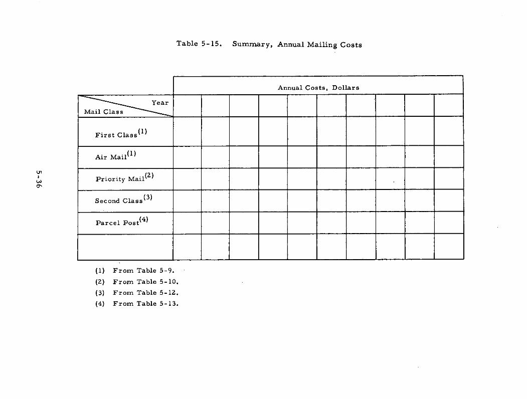
Table 5-15. Summary, Annual Mailing Costs
Annual Costs, Dollars
First Class ( 1)
Air Mail (1 )
Priority Mail(Z)
Second Class ( 3 )
Parcel Post ( 4 )
(1) From Table 5-9.(2) From Table 5-10.
(3) From Table 5-12.
(4) From Table 5-13.
below, however, allow rapid calculation of costs for commercially available
aircraft which should provide suitable platforms for the sensors of most
prospective missions. These aircraft provide a wide range of payload
capability and all may be assumed for purposes of estimates to be capable
of 1,609 km (1,:000 mi) range and 6, 090 m (20, 000 ft) altitude. The unique
combinations of payload, range, speed, altitude, and other characteristics
of individual aircraft are generalized for the purposes of estimating costs
herein.
The weight of mission equipment determines the aircraft gross
weight, based on a payload-to-gross weight ratio of one to four. The
gross weight required determines operating cost per mile, from Figure 5-10
and investment cost, from Figure 5-11. Aircraft speed is obtained
from gross weight versus speed relationships in Figure 5-12, which is
necessary in calculating the numbers of aircraft required.
Figure 5-10, operating costs per mile, is based on the cost
curves in Part B, page 5-24, for fuel and oil, maintenance, storage, and
insurance; pilot costs are included. The figure shows costs for the most
economical type of aircraft; piston powered below 4, 536 kg (10, 000 lb)
gross weight and jet powered above 4, 536 kg (10, 000 lb), based on pilot
costs of $18, 000 per year for 1000 flight hours, or $18 per flight hour.
One pilot is required for the piston aircraft, two for the turbine aircraft.
Turboprop aircraft costs are not shown. This does not mean
that turboprops' might not be the preferred choice under some combina-
tions of requirements. It does mean that costs in such cases would be
represented with adequate accuracy by the curves shown.
1. CALCULATIONS
a. Inputs Required
Cost calculations require the following inputs to be available
from the definition of the observation system:
(1) Weight of aircraft payload (mission equipment weight,including any operating personnel other than the pilot)
5-37
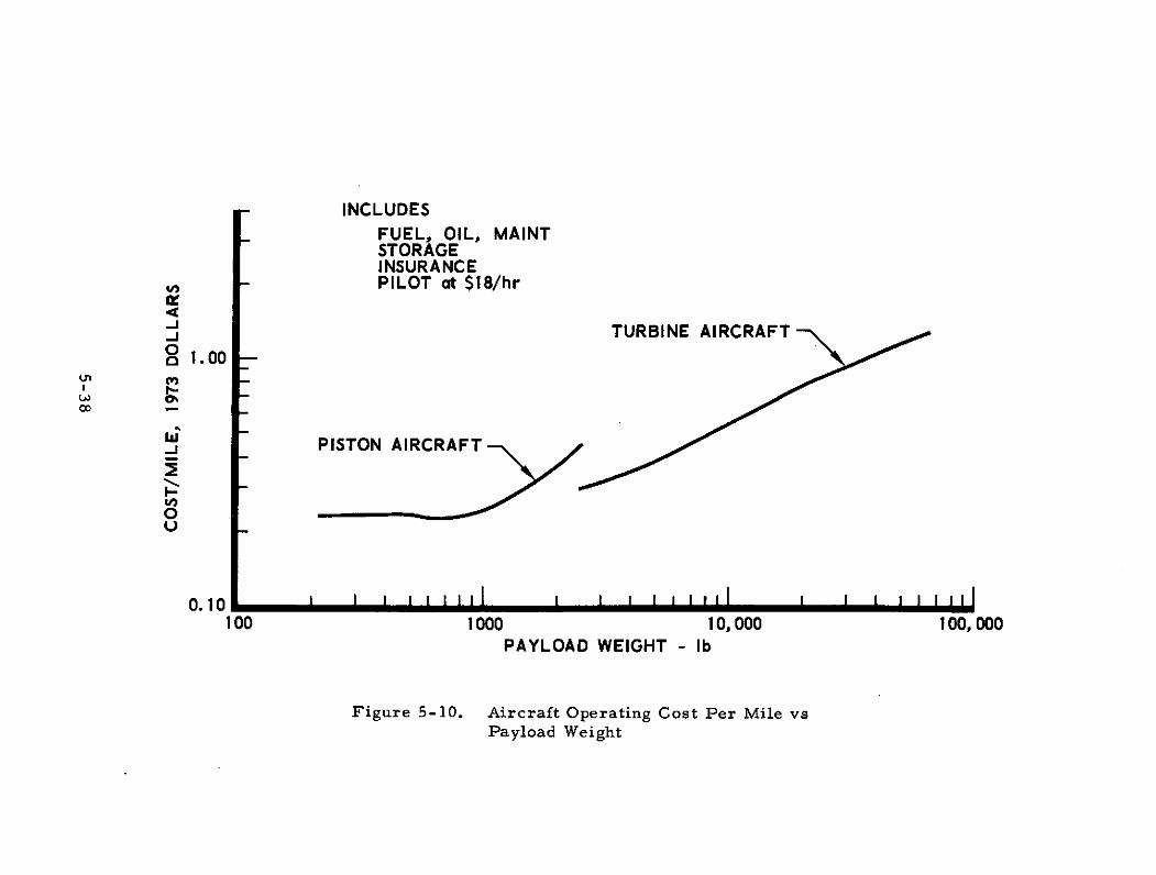
INCLUDESFUEL, OIL, MAINTSTORAGEINSURANCE
SPILOT at $18/hr
0 TURBINE AIRCRAFT
8 .00
PISTON AIRCRAFT
0
0.10
100 1000 10, 000 100, 000PAYLOAD WEIGHT - Ib
Figure 5-10. Aircraft Operating Cost Per Mile vsPayload Weight
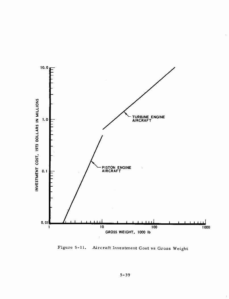
10.0
z
z 1.0 AIRCRAFT
0a
0
-
- "PISTON ENGINEz 0.1 -- AIRCRAFT
z
0.011 10 100 1000
GROSS WEIGHT, 1000 Ib
Figure 5-11. Aircraft Investment Cost vs Gross Weight
5-39
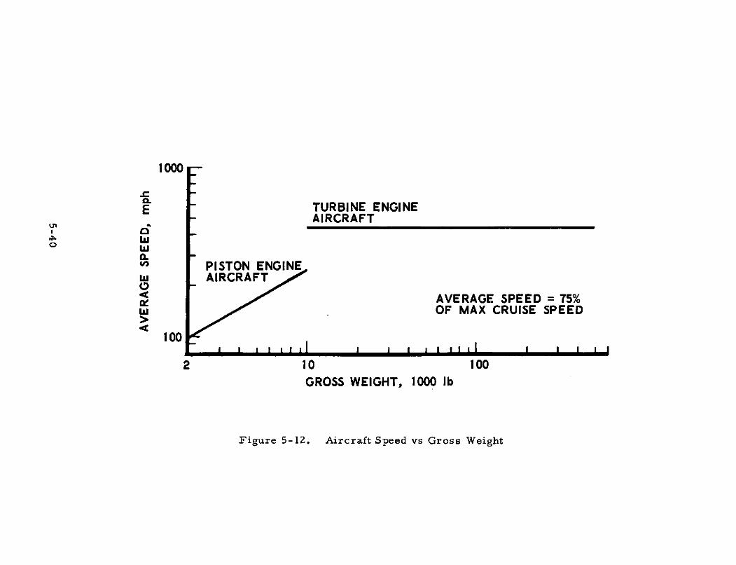
1000
E TURBINE ENGINEAIRCRAFT
w
VPISTON ENGINEw AIRCRAFT
0: AVERAGE SPEED = 75%w OF MAX CRUISE SPEED
100
2 10 100GROSS WEIGHT, 1000 Ib
Figure 5-12. Aircraft Speed vs Gross Weight
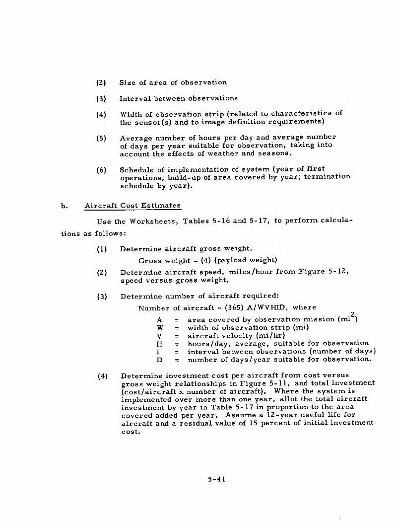
(2) Size of area of observation
(3) Interval between observations
(4) Width of observation strip (related to characteristics of
the sensor(s) and to image definition requirements)
(5) Average number of hours per day and average number
of days per year suitable for observation, taking intoaccount the effects of weather and seasons.
(6) Schedule of implementation of system (year of. first
operations; build-up of area covered by year; termination
schedule by year).
b. Aircraft Cost Estimates
Use the Worksheets, Tables 5-16 and 5-17, to perform calcula-
tions as follows:
(1) Determine aircraft gross weight.
Gross weight = (4) (payload weight)
(2) Determine aircraft speed, miles/hour from Figure 5-12,
speed versus gross weight.
(3) Determine number of aircraft required:
Number of aircraft = (365) A/WVHID, where
A = area covered by observation mission (mi2)W = width of observation strip (mi)V = aircraft velocity (mi/hr)H = hours/day, average, suitable for observationI = interval between observations (number of days)D = number of days/year suitable for observation.
(4) Determine investment cost per aircraft from cost versus
gross weight relationships in Figure 5-11, and total investment
(cost/aircraft x number of aircraft). Where the system isimplemented over more than one year, allot the total aircraftinvestment by year in Table 5-17 in proportion to the areacovered added per year. Assume a 12-year useful life foraircraft and a residual value of 15 percent of initial investmentcost.
5-41
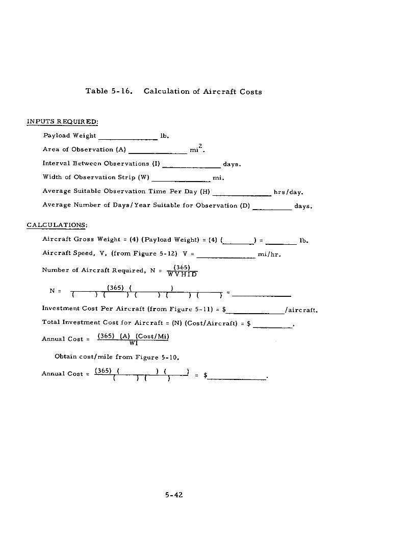
Table 5-16. Calculation of Aircraft Costs
INPUTS REQUIRED:
Payload Weight lb.
Area of Observation (A) mi .
Interval Between Observations (I) days.
Width of Observation Strip (W) mi.
Average Suitable Observation Time Per Day (H) hrs/day.
Average Number of Days/Year Suitable for Observation (D) days.
CALCULATIONS:
Aircraft Gross Weight = (4) (Payload Weight) = (4) ( ) = lb.
Aircraft Speed, V, (from Figure 5-12) V = mi/hr.
Number of Aircraft Required, N = (365)WVHID
N (365) ( )
Investment Cost Per Aircraft (from Figure 5-11) = $ /aircraft.
Total Investment Cost for Aircraft = (N) (Cost/Aircraft) = $
Annual Cost = (365) (A) (Cost/Mi)WI
Obtain cost/mile from Figure 5-10.
Annual Cost= (365) ( ) ( )
5-42
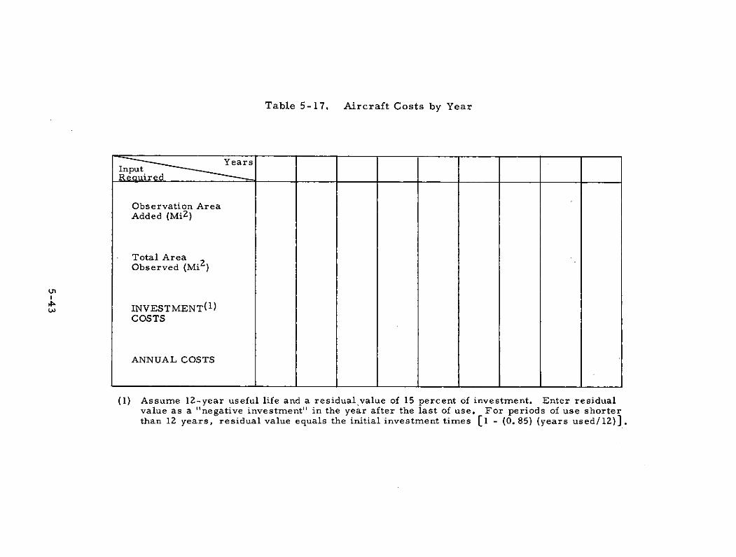
Table 5-17. Aircraft Costs by Year
YearsInput.Required
Observation AreaAdded (Mi2)
Total AreaObserved (Mi 2)
Un
SINVESTMENT( 1 )COSTS
ANNUAL COSTS
(1) Assume 12-year useful life and a residual value of 15 percent of investment. Enter residualvalue as a "negative investment" in the year after the last of use. For periods of use shorterthan 12 years, residual value equals the initial investment times [1 - (0. 85) (years used/12)]
(5) Determine annual operating cost:
Annual cost = (365) (A) (cost/mi)WI
where (cost/mi) is read from Figure 5-10, cost/mileversus payload weight. If the area covered is not the samefor all years, then annual cost for each year in Table 5-17is based on the area "A" being covered in that year.
5-44
6. COST EFFECTIVENESS
A. INTRODUCTION
The purpose of the cost effectiveness analysis is to compare
costs and required revenues of various alternative systems, designed
to perform a similar mission, in order to select the most cost effective
alternatives. These alternatives include both space and terrestrial-
based systems. This analysis normally culminates and concludes a
BRAVO analysis.
The following subsections give the instructions and informa-
tion necessary to complete the cost effectiveness analysis, using the
cost/revenue forms presented in the Workbook, Part 3 of Volume IVof this report.
The analysis is carried out routinely without reference to the
background information (Section C) or discussion of work sheets (Section
D) by following the procedure in Section B. It is recommended, however,
that the analyst familiarize himself with Sections C and D the first
time through as an aid to understanding the instructions in the procedures.
B. COST EFFECTIVENESS ANALYSIS PROCEDURE
The cost effectiveness analysis is accomplished in two phases:
1. Space system comparison and selection
2. Cost effectiveness of space system(s) versus terrestrialsystem(s).
These phases are outlined in the following two subsections.
6-1
1. SPACE SYSTEM COMPARISON AND SELECTION
This phase accomplishes the selection and sequencing (to best
match the projected demand and to hold costs down) of the space system
approaches. Candidate space systems surviving the cost/risk analysis
are included in this selection process, as well as the comparative
terrestrial system. The cost comparisons between the alternative space
systems are made on the basis of constant dollars. The specific steps
involved in this phase of the analysis are outlined below:
Step 1 - Before starting the cost effectiveness analysis, the
analyst should have the following inputs in hand:
1. The list of space system approaches selected. This listis obtained from the output of the space system optimiza-tion studies.
2. Cost streams for each space system approach selected.These cost streams are obtained as an output from thespace system cost estimating program.
3. Cost streams for the ground system electronics andfacilities portion of the selected space systems. Thesecosts are obtained as an output of the terrestrial systemcost estimation.
4. Cost streams, or revenue required streams in constantdollars, for the terrestrial system(s). The terrestrialsystem(s) competes with the space systems on an equalcapability basis. The terrestrial system costs, orrequired revenues, are also obtained as an output ofthe terrestrial system cost estimation.
5. Demand stream. The product or service demand streamis obtained from the terrestrial system definition output.
6. System "start" date. The start date is the first yearthat costs are incurred by the space system (and support-ing ground system). This date is specified by the spaceor supporting ground system cost stream outputs.
6-2
7. Discount rate factor, (1 + F). The discount rate factor,(1 + F), is computed from the rate of return on currentdollars, r, and the inflation rate, f. The rate of returnon current dollars is either defined by the user, or selectedon the basis of industry average return rates. Typicalaverage industry rates are as follows:
r = TBD for farming industryr = TBD for industrial communityr = TBD for utilities
The inflation rate is either defined by the user or basedon the average U. S. inflation rate over recent years ofapproximately four percent*.
Step2 - Use the form "Cost/Revenue Analysis for Constant
Dollars," page 9-3 in the Workbook (Part 3 of Volume IV of this report) forcalculating the costs and revenue required in constant dollars and the netpresent value (NPV) of costs.and revenues. The following discrete stepsshould be followed in completing the form for each of the selected spacesystems and for the competing terrestrial system (as the form applies).
1. Mark start date in first year column heading, and fill-inremaining years in sequence until the desired completiondate. Note: Different equipment may be replaced atvarying intervals (e. g., mission equipment, spacecraft,ground electronics, etc. ). To permit different write-offperiods for different equipment, the residual value andtotal columns should be inserted after the appropriateyears corresponding to the different write-off periods.
2. Fill in the "System Cost Estimate" data input rows.These rows are identified by an asterisk. Note: Theresidual value and total columns should be filled inonly as appropriate for the write-off period of eachequipment. The total column should include a summationof the yearly costs, since the last summation, less theresidual value.
3. Complete the "System Cost Estimate" summary rows:(1), (4), (9), and (13).
* Reference BLS Wholesale Price Index from 1967 to 1972.
6-3

4. Fill in row (14), under "System Revenues, " starting witha 0 for the first year (NPV start date) and adding 1 foreach succeeding year (i.e., 0, 1, 2, 3, etc. years).
5. Complete input and calculation rows: (15) - (17), (19) -(24), (26) - (31), (33) - (35), (37) - (39), (41) - (46),and (48) - (50).
Note 1) Complete the total column for row (17), andthe residual value and total columns for rows (19),(22), (26), (29), (33), (37), (41), (44), and (48) onlyas appropriate for the equipment respective write-offperiods (see Step 2 above). The totals should only includethe summation of yearly NPVs, less residual NPV, afterthe last summation period. (Row (17) does not includeany residual values.)
Note 2) Unit charge entries for rows (20), (23), (27),(30), (34), (38), (42), (45), and (49) are only made inthe appropriate total column(s), as applicable to thespecific equipment write-off periods.
Note 3) The individual revenue, rows (21), (24), (28),(31), (35), (39), (43), (46), and (50), are computed usingthe unit charge for the appropriate write-off periods.
6. Complete the "System Revenue" and "NPV of Costs"rows: (18), (25), (32), (36), (40), (47), (51), (52), and(53). Note: Rows (51) and (53) only include the totalcolumn(s).
Step 3 - Tabulate and compare the following parameters for
each of the alternative space systems considered, and the competing
terrestrial system (as applicable for the terrestrial system).
1. Total NPV of system costs. The total NPV of systemcosts is indicated in the form on page 9- 3 in the Workbook,Part 3 of this report, row (53). The total is the summationof the individual years, or a summation of the severaltotal columns, for each.item.
2. Peak funding of each system. The peak total funding inany year is the peak costs as indicated in row (13) ofthe form on page 9- 3 in the Workbook, Part 3 of thisreport.
6-4
3. Revenue required for each system. This is the yearlyfunding as indicated in row (52) in the form on page 9-3of the Workbook. Tabulate the above three parametersin the form on page 9-15 in the Workbook, Part 3 of Volume IVof this report, for convenient comparison. The NPV is onlyentered in the total column, the peak revenue is only enteredin the year corresponding to peak funding for each systemconsidered and the revenue is entered yearly.
Step 4 - Select the best space system alternative based on
the comparisons conducted in Step 3. The following procedure should
be adhered to in optimum system selection.
1. First, review peak funding for each space system toascertain if any budgetary constraints are violated.If any systems exceed the budgeted limit, these systemsmust be either deleted from the selection process orreworked through the BRAVO cycle to avoid exceedingbudgetary limits.
2. Next, review the required revenue. If the requiredrevenue of any space system appears unusually excessive,in relation to the terrestrial system revenue, this maybe cause for deleting this system from the selectionprocess or possibly reworking through the BRAVO cycle.
3. Finally, compare the NPVs of the competing spacesystems. Barring system deletions or concerns relatingto peak funding or required revenues, the space systemwith the lowest NPV should be selected as the optimumsystem. This indicates the most economical system..
2. COST EFFECTIVENESS OF SPACE SYSTEM(S) VS TERRESTRIALSYSTEM(S)
This phase involves the comparison of the selected space
system(s) with the competing terrestrial system. This comparison is
done on the basis of current dollars as an aid to corporate management
in conducting funding predictions and cash flow analyses. The same
input data required for the Space System Comparison and Selection
procedures will be used for this phase of the study. The specific stepsinvolved in this phase of the analysis are outlined below.
6-5
Step 1 - Use the form "Cost/Revenue Analysis for Current
Dollars, " page 9-9 in the Workbook, Part 3 of Volume IV of this report,
for calculating the costs and revenue required in current dollars and the
net present value (NPV) of costs and revenues. The procedure for com-
pleting this form is quite similar to the form on page 9-3 in the Workbook
with a few minor exceptions to arrive at revenue in current dollars. The
following discrete steps for completing the form (page 9-9 in the Workbook)
are delineated as an aid for the analyst who has previously completed the
form on page 9-3 in the Workbook for the same systems.
1. Complete the heading information (i. e., years, residualvalue, and totals) as was done for the "Constant Dollars"form on page 9-3 in the Workbook.
2. Complete the "System Cost Estimate" rows .(1) through(14) by copying similar row data from the "ConstantDollars" form.
3. Complete the "System Cost Estimate" data rows (15) and(16). Note: The inflation rate, f, was previously determinedas input information for computing the constant dollardiscount factor, F.
4. Complete input and calculation rows (17) - (20), (22) - (27),(29) - (34), (36) - (38), (40) - (42), (44) - (49), (51) - (53).
Note 1) Some of the system revenue data from the "ConstantDollar" form (page 9-3 in the Workbook) to this "CurrentDollar" form (page 9-9 in the Workbook) for the came systemsand should be copies directly. Due to the different rownumbering systems between the two forms, after row (14)the rows must be compared as follows:
"Constant Dollars" Form "Current Dollars" FormPage 9-3 in the Workbook Page 9-9 in the Workbook
(15) (17)(16) (19)(22) (25)(26) (29)(29) (32)(33) (36)(37) (40)(41) (44)(44) (47)(48) (51)
6-6
Note 2) Entries for rows (23), (26), (30), (33), (37),(41), (45), and (48) are only made as appropriate to thespecific equipment write-off periods.
5. Complete the "System Revenue Summary" rows (21),(28), (35), (39), (43), (50), (54), and (55).
Step - Tabulate and compare the current dollar cash flows,
both costs and revenues, for the selected space system(s) and the terrestrial
system [rows (16) and (53)]. The terrestrial costs and revenues are
computed using the "Current Dollars" form (page 9-9 in the Workbook),
as described for the space systems, to the extent applicable. If estimated
costs for the terrestrial system are not available, then only the revenues
can be compared with the space system(s). Use the form on page 9-15 in
the Workbook, Part 3 of Volume IV of this report, for tabulating these
cash flows.
Step3 - The analyst must carefully review the findings in
Step 2 prior to making a comparative recommendation between the space
system(s) and the terrestrial system. The primary criteria should be
economic. From this standpoint the system requiring the lower revenue
to recover investment plus return on investment is the most economical
system. Other factors, however, such as cash flow requirements (current
dollar costs) may be deciding criteria in the event budgetary allowances
are exceeded or estimated revenues are very close. Therefore, all
pertinent economic factors determined by this cost effectiveness analysis
should be played against the specific study objectives and ground rules to
insure that any recommendation made does not violate case constraints.
C. BACKGROUND INFORMATION
1. NOMENCLATURE
The nomenclature used in defining the various economic terms
and equations in presented below for easy reference.
6-7
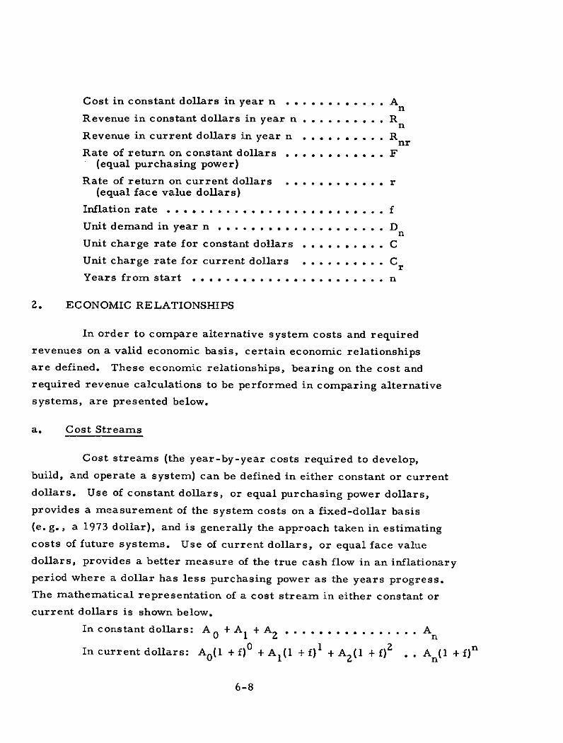
Cost in constant dollars in year n . . . . . . . . . .... An
Revenue in constant dollars in year n . .. .... .. . R nRevenue in current dollars in year n . . .. . . . . .. R nrRate of return on constant dollars . . . .. . ....... F
(equal purchasing power)
Rate of return on current dollars ............ r(equal face value dollars)
Inflation rate .......................... f
Unit demand in year n ................... . D nUnit charge rate for constant dollars ... . .. ..... C
Unit charge rate for current dollars . . . ........ C
Years from start ................... .... n
2. ECONOMIC RELATIONSHIPS
In order to compare alternative system costs and required
revenues on a valid economic basis, certain economic relationships
are defined. These economic relationships, bearing on the cost and
required revenue calculations to be performed in comparing alternative
systems, are presented below.
a. Cost Streams
Cost streams (the year-by-year costs required to develop,
build, and operate a system) can be defined in either constant or current
dollars. Use of constant dollars, or equal purchasing power dollars,
provides a measurement of the system costs on a fixed-dollar basis
(e. g., a 1973 dollar), and is generally the approach taken in estimating
costs of future systems. Use of current dollars, or equal face value
dollars, provides a better measure of the true cash flow in an inflationary
period where a dollar has less purchasing power as the years progress.
The mathematical representation of a cost stream in either constant or
current dollars is shown below.
In constant dollars: A 0 + A +A 2 ................ An
In current dollars: A 0 (1 + f)0 + A(1 + f)1 + A 2 (l + f)2. . An(1 + f)n
6-8
b. Revenue Streams
Revenue streams (the year-by-year dollar return from an
investment) can also be expressed in constant or current dollars as
follows:
In constant dollars: R 0 + R 1 + R ........... Rn
In current dollars: R 0 (l + f)0 + R 1 ( + f) + R 2 (1 + f)2 . . Rn(1 + f)
orIn current dollars: R0 r +Rr +Rr . . . . . . . . Rnr
(where R includes the effects of inflation)nr
c. Rate of Return Relationship
The relationship between the rate of return on constant dollars
and current dollars, showing the effect of inflation, is presented below.
(l +F) = (l+r)
This equation points out the fact that the rate of return on current dollars,
(r), which is similar to bank interest rate, must be higher than the
inflation rate, (f), if the equal purchasing power rate of return, (F),
is to be a positive number.
d. Net Present Value (NPV)
The NPV relates future cost or revenue streams to their present
economic value, based on a specified rate of return. The NPV of a
stream of constant or current dollars is exactly the same, provided
the rate of returns are consistent and the present year of reference is
the same (obviously a 1973 current dollar is the same as a 1973 constant
dollar). The NPV derivation for the cost and revenue streams is pre-
sented below.
6-9
Cost Stream: NPV = j A (1 +F) - n
0
nRevenue Stream: NPV = E Rn (1 + F)-n
oor n
Revenue Stream: NPV = Rnr ( + r)-no
e. Unit Charge Rates
The charge rate per unit of product delivered (e. g., communica-
tion circuits, kilowatts of power, etc.) is a constant over a specified
period of time. The revenue returned per year is the charge rate times
the demand for units per year. This relationship is presented in the
following equations for constant and current dollar revenues:
RIn constant dollars: R = CD , or C = n
n n D n
R nrIn current dollars: Rnr = CD or C
n
f. Revenue Calculation
The total revenue required from an operating system should
return all of the capital invested in the system (R&D, investment, and
operations) plus an appropriate rate of return (interest) on all of the
capital invested. A simple, yet economically viable, method of calcula-
ting the revenue required is to set the NPV of the total revenue equal to
the NPV of the total costs. The revenue required can be defined in
terms of constant dollars or current dollars by using the appropriate
relationships. Using the economic relationships previously defined,
the equations for the required revenues are presented in both constant
and current dollars as follows.
6-10
(1) Revenue in Constant Dollars
n nR ( + F)-n = An (1 + F)-n
o o
n nor i CDn(1 + F) - n = An (1 + F)-n
o 0
n
A n (1 + F)-n
then C on
D n (1 + F) - n
0
and R = R = CDn n n
(2) Revenue in Current Dollars
n n
o 0
n no r n(l + r) n = An (1 + F)-n
o o
n
then Cr = C An (1 + F) "n0
n
E-D (1 + r) " n
and R = CDnr r n
3. COST/REVENUE ANALYSIS WORK SHEETS
Computation of cost and revenue streams is accomplished
on analysis worksheets. Sample worksheets are provided in the
Workbook, Part 3 of Volume IV of this Study 2. 4 final report. The
following two subsections describe these worksheets for cost and revenue
streams in constant dollars and in current dollars.
6-11
a. Cost/Revenue Streams in Constant Dollars
The form "Cost/Revenue Analysis for Constant Dollars, " page
9-3 in the Workbook, Part 3 of Volume IV of this report, presents a
sample worksheet for computing both satellite system costs and required
revenue streams in constant dollars.
All calculations are accomplished on a year-by-year basis,with the total being a summation of the yearly results. The residualvalue specifically refers to the system cost estimates. It defines theresidual constant dollar value remaining in each satellite or ground
system investment (if any) at the conclusion of the write-off period forthat particular investment. The residual value appears as a negativecost in the year the specific equipment is to be written off, and wouldbe subtracted from the corresponding investment costs occuring in thatyear (possibly resulting in a negative investment).
The system cost estimates are broken down into satellite,launch vehicle, and ground system costs. The satellite costs are furtherdivided into R&D, investment, and operations. In order to providefor the possibility of writing off the satellite mission equipment or space-craft over different time periods (the mission equipment may be revisedseveral times over the life of the spacecraft), their costs are accountedfor separately for the satellite R&D and investments. The same is truefor ground system investment where the electronics and support facilitiesare separately listed to permit different write-off periods. The totalsystem cost, for space systems, is the summation of the separatesatellite, launch vehicle, and ground system costs. For terrestrialsystems, the total system cost would be only that included under theground system costs.
6-12
The computation of the required system revenues (to return
invested capital plus interest) is carried out separately for each cost
element. In this manner, differing write-off periods can be considered
for each element (e. g., spacecraft, mission equipment, etc.). Calcula-
tion of revenues requires determining the NPV of each of the cost elements
and the unit demand. Using the sample worksheets in the Workbook,
Part 3 of Volume IV of this report, the unit charge rate is obtained
separately for each of the cost elements and the element required
revenue is simply the multiple of its unit charge rate and the unit demand.
The total system unit charge rate and revenue is the summation of the
individual element charge rates and revenues.
b. Cost/Revenue Streams in Current Dollars
The form "Cost/Revenue Analyses for Current Dollars, " page
9-9 in the Workbook, presents a sample worksheet for computing both
satellite system cost and required revenue streams in current dollars.
The calculations are accomplished in exactly the same manner
as for the "Constant Dollar" form on page 9-2 in the Workbook, with
the following exceptions:
1. Though the system costs are individually computed in
terms of constant dollars, as per the "Constand Dollars"
form, the total system costs are computed both in constant
and current dollars.
2. The required revenue is computed in current dollars.
This is accomplished, as described in Section B, by
calculating the element charge rates in current dollars
rather than constant dollars. The computed revenue
is then also in current dollars.
6-13
4
Related Documents