Welcome message from author
This document is posted to help you gain knowledge. Please leave a comment to let me know what you think about it! Share it to your friends and learn new things together.
Transcript


A Hybrid Approach with Multi-channel I-Vectors and
Convolutional Neural Networks for Acoustic Scene Classification
Hamid Eghbal-zadeh, Bernhard Lehner, Matthias Dorfer and Gerhard Widmer
A closer look into our winning submission at IEEE DCASE-2016 challenge1 for Acoustic Scene Classification
1) www.cs.tut.fi/sgn/arg/dcase2016/

Introduction
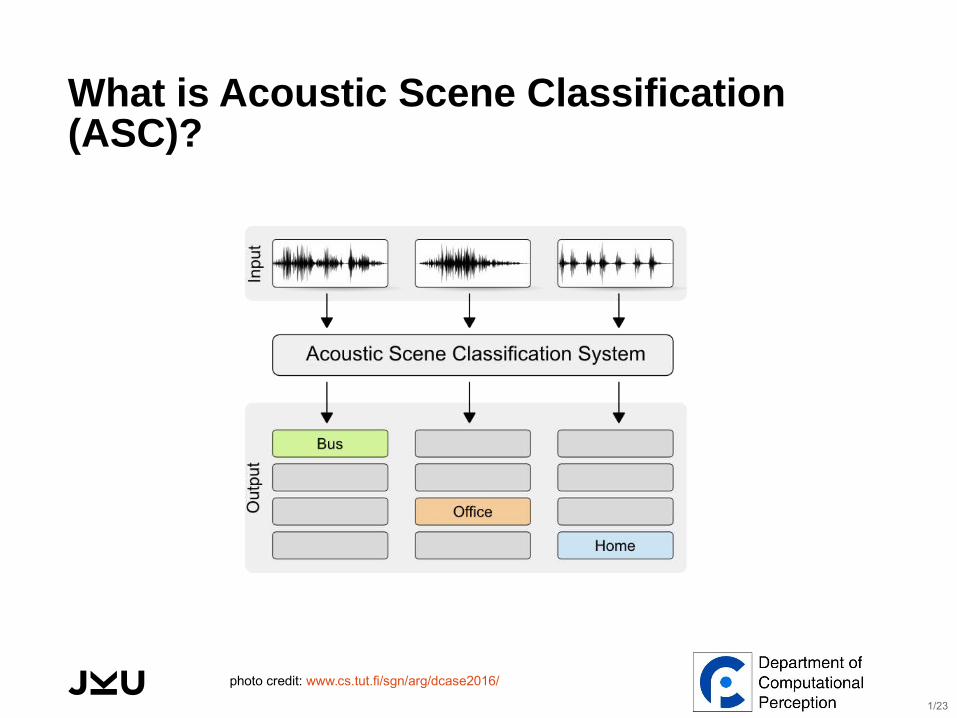
What is Acoustic Scene Classification (ASC)?
photo credit: www.cs.tut.fi/sgn/arg/dcase2016/
1/23
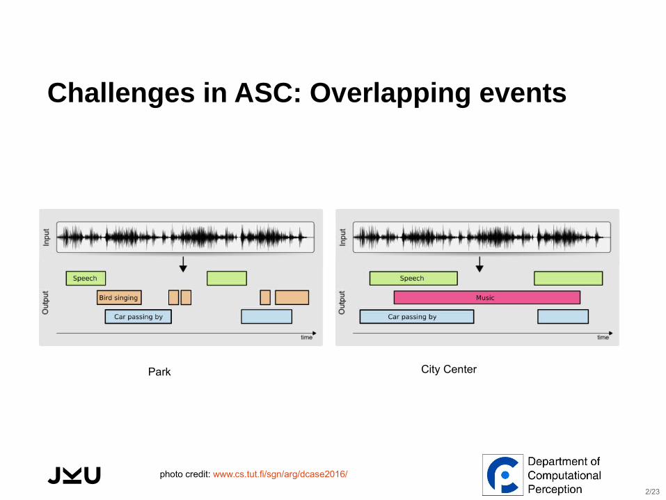
Challenges in ASC: Overlapping events
Park City Center
photo credit: www.cs.tut.fi/sgn/arg/dcase2016/
2/23
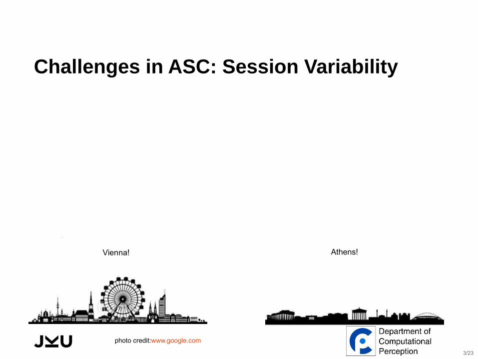
Challenges in ASC: Session Variability
Vienna! Athens!
photo credit:www.google.com
3/23
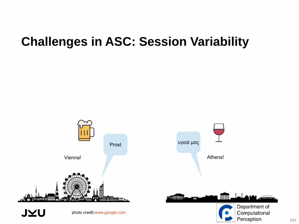
Challenges in ASC: Session Variability
Vienna! Athens!
υγειά μαςProst
photo credit:www.google.com
3/23
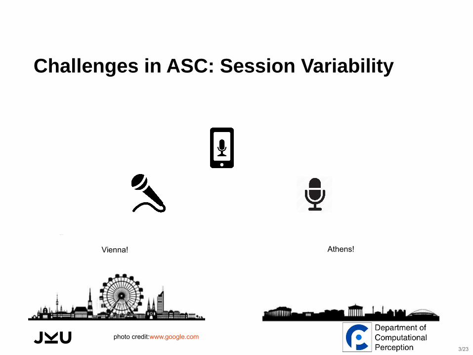
Challenges in ASC: Session Variability
Vienna! Athens!
photo credit:www.google.com
3/23


Methods for ASC
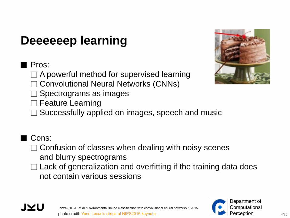
Deeeeeep learning
⬛ Pros:⬜ A powerful method for supervised learning⬜ Convolutional Neural Networks (CNNs)⬜ Spectrograms as images⬜ Feature Learning⬜ Successfully applied on images, speech and music
⬛ Cons:⬜ Confusion of classes when dealing with noisy scenes
and blurry spectrograms⬜ Lack of generalization and overfitting if the training data does
not contain various sessions
Piczak, K. J., et al "Environmental sound classification with convolutional neural networks.", 2015.
photo credit: Yann Lecun's slides at NIPS2016 keynote 4/23
Factor Analysis
⬛ Pros:⬜ Session Variability reduction ⬜ Use of a Universal Background Model (UBM)⬜ Better generalization due to the unsupervised methodology⬜ Successfully applied on sequential data such as Speech and
Music
⬛ Cons:⬜ Relying on engineered features⬜ Limits to use specialized features for Audio Scene Analysis
because of the independence and Gaussian assumptions in FA
[1] Dehak, Najim, et al. "Front-end factor analysis for speaker verification.",2011.[2] Elizalde, B, et al. "An i-vector based approach for audio scene detection." (2013).
5/23
A Hybrid system to overcome the complexities ...
photo credit: www.imgflip.com
A hybrid approach to ASC
⬛ We combine a CNN with an I-Vector based ASC system:⬜ A CNN is trained on spectrograms⬜ I-Vector features (based on FA) are extracted from MFCCs
⬛ Late fusion⬜ A score fusion technique is used to combine the two methods
⬛ Model averaging for better generalization⬜ Multiple models are trained and the decision from different
models are averaged
Brummer, N., et al. "On calibration of language recognition scores." , 2006.
6/23

CNNs for ASC
A hybrid approach to ASC
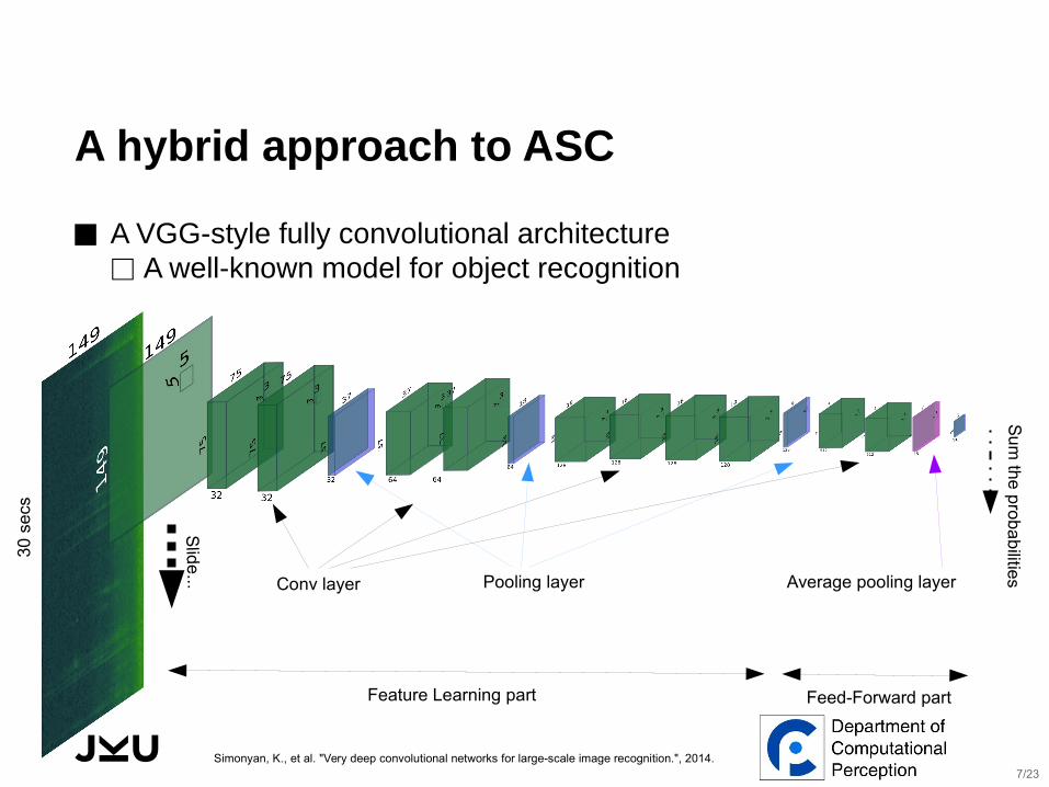
⬛ A VGG-style fully convolutional architecture ⬜ A well-known model for object recognition
Conv layer Pooling layer Average pooling layer
Slid
e...
Su
m th
e p
rob
ab
ilities
30 s
ecs
Feature Learning part Feed-Forward part
Simonyan, K., et al. "Very deep convolutional networks for large-scale image recognition.", 2014.7/23

I-Vectors for ASC
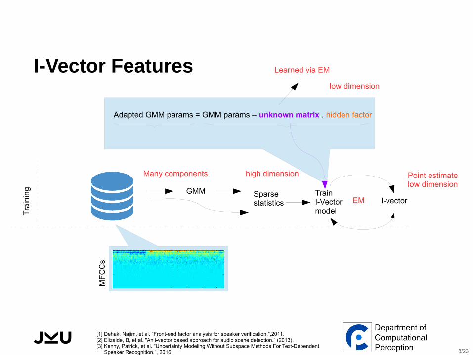
I-Vector Features
GMM Train I-Vector model
Sparse statistics
Adapted GMM params = GMM params – unknown matrix . hidden factor
Learned via EM
Tra
inin
g
MF
CC
s
Many components high dimension
[1] Dehak, Najim, et al. "Front-end factor analysis for speaker verification.",2011.[2] Elizalde, B, et al. "An i-vector based approach for audio scene detection." (2013).[3] Kenny, Patrick, et al. "Uncertainty Modeling Without Subspace Methods For Text-Dependent Speaker Recognition.", 2016.
low dimension
I-vector
Point estimate low dimension
EM
8/23
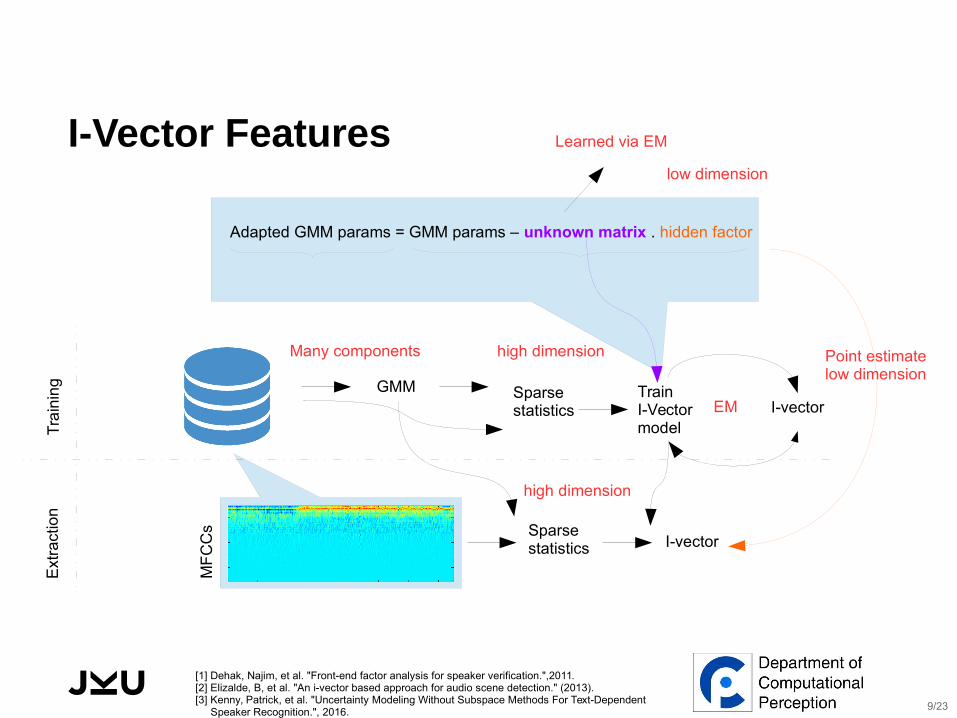
I-Vector Features
GMM
MF
CC
s
Sparse statistics
I-vector
Adapted GMM params = GMM params – unknown matrix . hidden factor
Sparse statistics
Tra
inin
gE
xtra
ctio
n
Learned via EM
Many components
high dimension
high dimension
Train I-Vector model
I-vector
Point estimate low dimension
EM
[1] Dehak, Najim, et al. "Front-end factor analysis for speaker verification.",2011.[2] Elizalde, B, et al. "An i-vector based approach for audio scene detection." (2013).[3] Kenny, Patrick, et al. "Uncertainty Modeling Without Subspace Methods For Text-Dependent Speaker Recognition.", 2016.
low dimension
9/23
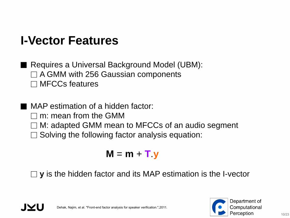
I-Vector Features
⬛ Requires a Universal Background Model (UBM):⬜ A GMM with 256 Gaussian components⬜ MFCCs features
⬛ MAP estimation of a hidden factor:⬜ m: mean from the GMM⬜ M: adapted GMM mean to MFCCs of an audio segment⬜ Solving the following factor analysis equation:
M = m + T.y
⬜ y is the hidden factor and its MAP estimation is the I-vector
Dehak, Najim, et al. "Front-end factor analysis for speaker verification.",2011.
10/23
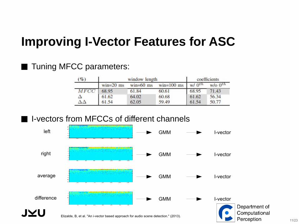
Improving I-Vector Features for ASC
GMM I-vectorleft
right
average
difference
GMM I-vector
GMM I-vector
GMM I-vector
⬛ Tuning MFCC parameters:
⬛ I-vectors from MFCCs of different channels
Elizalde, B, et al. "An i-vector based approach for audio scene detection." (2013).11/23
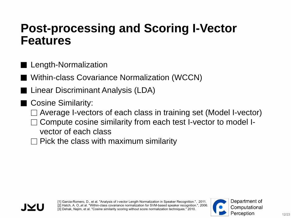
Post-processing and Scoring I-Vector Features
⬛ Length-Normalization
⬛ Within-class Covariance Normalization (WCCN)
⬛ Linear Discriminant Analysis (LDA)
⬛ Cosine Similarity:⬜ Average I-vectors of each class in training set (Model I-vector)⬜ Compute cosine similarity from each test I-vector to model I-
vector of each class⬜ Pick the class with maximum similarity
[1] Garcia-Romero, D., et al. "Analysis of i-vector Length Normalization in Speaker Recognition.", 2011.[2] Hatch, A. O.,et al. "Within-class covariance normalization for SVM-based speaker recognition.", 2006.[3] Dehak, Najim, et al. "Cosine similarity scoring without score normalization techniques." 2010.
12/23

Hybrid system
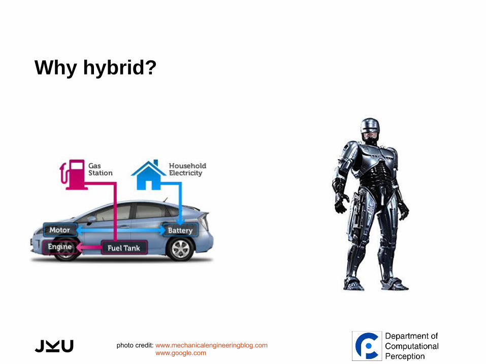
Why hybrid?
photo credit: www.mechanicalengineeringblog.com www.google.com
Linear Logistic Regression for Score Fusion
⬛ Combining cosine scores of I-vectors with CNN probabilities
⬛ A Linear Logistic Regression (LLR) model is trained on validation set
⬛ A coefficient is learned for each model and a bias term for each class.
⬛ Final score is computed by applying the learned coefficients and the bias terms on the test set scores.
13/23
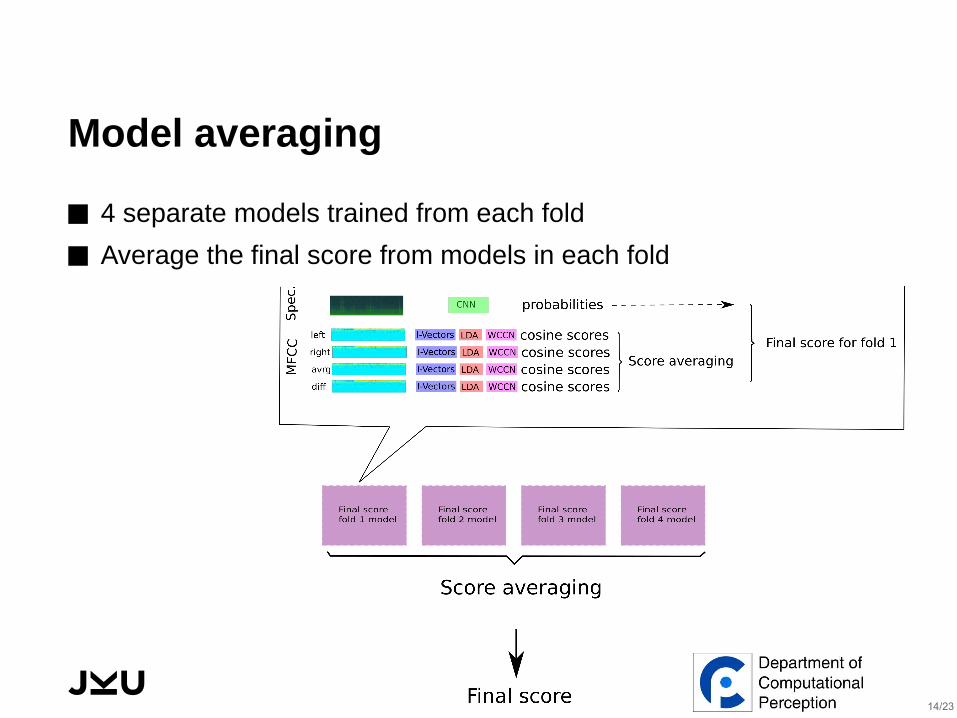
Model averaging
⬛ 4 separate models trained from each fold
⬛ Average the final score from models in each fold
14/23

Dataset
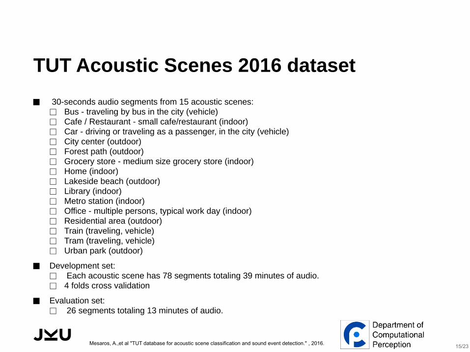
TUT Acoustic Scenes 2016 dataset
⬛ 30-seconds audio segments from 15 acoustic scenes:⬜ Bus - traveling by bus in the city (vehicle)⬜ Cafe / Restaurant - small cafe/restaurant (indoor)⬜ Car - driving or traveling as a passenger, in the city (vehicle)⬜ City center (outdoor)⬜ Forest path (outdoor)⬜ Grocery store - medium size grocery store (indoor)⬜ Home (indoor)⬜ Lakeside beach (outdoor)⬜ Library (indoor)⬜ Metro station (indoor)⬜ Office - multiple persons, typical work day (indoor)⬜ Residential area (outdoor)⬜ Train (traveling, vehicle)⬜ Tram (traveling, vehicle)⬜ Urban park (outdoor)
⬛ Development set:⬜ Each acoustic scene has 78 segments totaling 39 minutes of audio.⬜ 4 folds cross validation
⬛ Evaluation set:⬜ 26 segments totaling 13 minutes of audio.
Mesaros, A.,et al "TUT database for acoustic scene classification and sound event detection." , 2016.15/23

Results
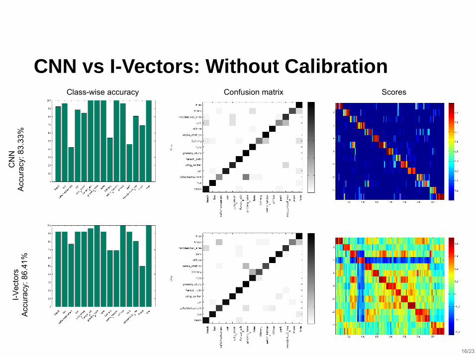
CNN vs I-Vectors: Without Calibration
CN
NA
ccu
racy
: 8
3.3
3%
I-V
ecto
rsA
ccu
racy
: 8
6.4
1%
Class-wise accuracy Confusion matrix Scores
16/23
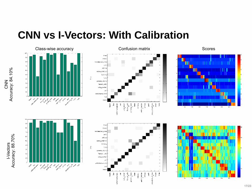
CNN vs I-Vectors: With Calibration
CN
NA
ccu
racy
: 8
4.1
0%
I-V
ecto
rsA
ccu
racy
: 8
8.7
0%
Class-wise accuracy Confusion matrix Scores
17/23
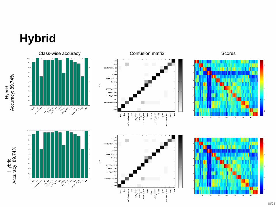
Hybrid
Hyb
ridA
ccu
racy
: 8
9.7
4%
Hyb
ridA
ccu
racy
: 8
9.7
4%
Class-wise accuracy Confusion matrix Scores
18/23
Analysis: Score Calibration
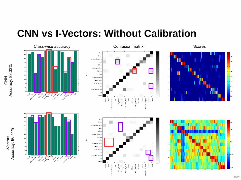
CNN vs I-Vectors: Without Calibration
CN
NA
ccu
racy
: 8
3.3
3%
I-V
ecto
rsA
ccu
racy
: 8
6.4
1%
Class-wise accuracy Confusion matrix Scores
19/23
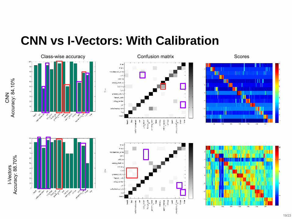
CNN vs I-Vectors: With Calibration
CN
NA
ccu
racy
: 8
4.1
0%
I-V
ecto
rsA
ccu
racy
: 8
8.7
0%
Class-wise accuracy Confusion matrix Scores
19/23
Analysis: Score Fusion
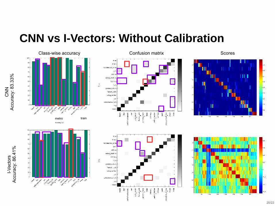
CNN vs I-Vectors: Without Calibration
CN
NA
ccu
racy
: 8
3.3
3%
I-V
ecto
rsA
ccu
racy
: 8
6.4
1%
metro train
Class-wise accuracy Confusion matrix Scores
20/23
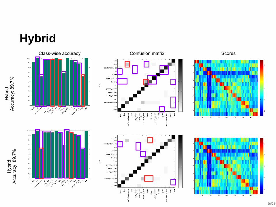
Hybrid
Hyb
ridA
ccu
racy
: 8
9.7
%H
ybrid
Acc
ura
cy:
89
.7%
Class-wise accuracy Confusion matrix Scores
20/23
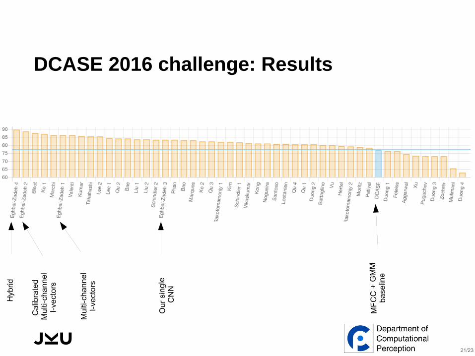
DCASE 2016 challenge: Results
Hyb
rid
Ca
libra
ted
Mu
lti-c
ha
nn
el
I-ve
cto
rs
Mu
lti-c
ha
nn
el
I-ve
cto
rs
Ou
r si
ng
le
CN
N
MF
CC
+ G
MM
ba
selin
e
21/23
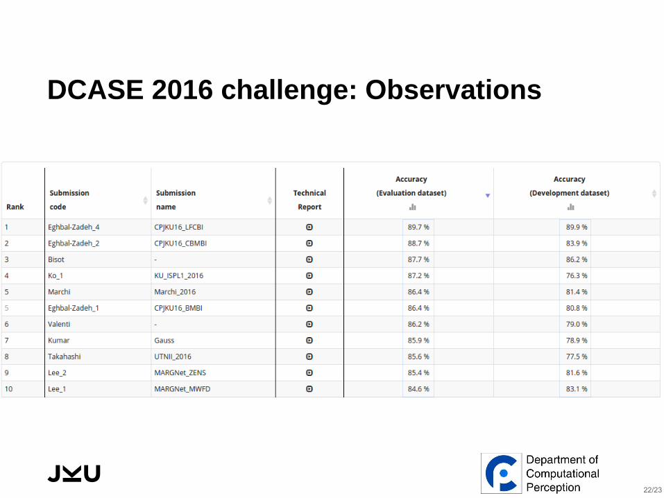
DCASE 2016 challenge: Observations
22/23
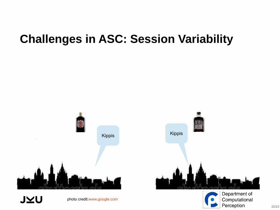
Challenges in ASC: Session Variability
Kippis Kippis
photo credit:www.google.com
22/23

Conclusion
⬛ Performance of I-Vectors can be noticeably improved by tuning MFCCs
⬛ Different channels contain different information from a scene that is beneficial to the I-vector system
⬛ I-Vectors and CNNs are complementary
⬛ Score Calibration improved both I-Vectors and CNN
⬛ A late-fusion can efficiently combine the two system’s predictions
⬛ This method is easily adaptable to new conditions
23/23


JOHANNES KEPLERUNIVERSITY LINZAltenberger Str. 694040 Linz, Austriawww.jku.at
Thank you!
For more information about this presentation, don’t hesitate to contact me via:[email protected]
Slides available at:https://www.slideshare.net/heghbalzCode soon will be available at:https://github.com/cpjku
Related Documents