skew heap, leftist heap - Department of Computer Science and

CSE 4080 PROJECT:

SKEW HEAP, LEFTIST HEAP AND ALTERNATIVES

Winter Term 2007

York UniversityDepartment of Computer Science and Engineering

4700 Keele St. Toronto, Ontario, Canada, M3J 1P3

By: Soheil Pourhashemi

Supervisor: Professor Andranik Mirzaian

2

TABLE OF CONTENTS

1 GLOSSARY............................................................................................................ 32 INTRODUCTION.................................................................................................. 33 PROJECT SCOPE................................................................................................. 34 PRIORITY QUEUES............................................................................................. 4

4.1 Definition........................................................................................................ 44.2 Applications .................................................................................................... 44.3 Heaps .............................................................................................................. 5

5 LEFTIST HEAP .................................................................................................... 65.1 Definition........................................................................................................ 65.2 Algorithm........................................................................................................ 75.3 AAW Animation ............................................................................................. 95.4 Applications .................................................................................................... 9

6 SKEW HEAP ....................................................................................................... 106.1 Definition...................................................................................................... 106.2 Algorithm...................................................................................................... 106.3 AAW Animation ........................................................................................... 126.4 Applications .................................................................................................. 13

7 SKEW HEAP vs LEFTIST HEAP USER INTERFACE..................................... 137.1 Overview....................................................................................................... 137.2 High-level Walkthrough................................................................................ 14

8 SOFT HEAP ........................................................................................................ 158.1 Background................................................................................................... 158.2 Introduction................................................................................................... 168.3 Motivation..................................................................................................... 178.4 Other Applications ........................................................................................ 228.5 Ideas/Thoughts .............................................................................................. 22

9 RUNNING TIME COMPARISONS .................................................................... 2310 CONCLUSION................................................................................................. 2311 BIBLIOGRAPHY............................................................................................. 2512 APPENDIX A................................................................................................... 26

12.1 Ackermann Function ..................................................................................... 2612.2 Heap Array Implementation .......................................................................... 26

13 APPENDIX B................................................................................................... 27

3

1 GLOSSARYTerm/Acronym DefinitionAAW Algorithms Animation WorkshopADT Abstract Data TypeURL An acronym for "Uniform Resource Locator," this is the address of a

resource on the Internet.MST Minimum Spanning Tree

2 INTRODUCTION

This project is primarily focused on Priority Queues, specifically various implementations of priority queues are explored, mainly Skew and Leftist Heaps. As part of this project, Online Interactive Animations have been implemented for aiding users in understanding how skew and leftist heap algorithms are executed.These animations can be found at the following URL:http://www.cse.yorku.ca/~aaw/Pourhashemi

In addition, a relatively new Heap is explored, called “Soft Heap”. This project will explore this heap and its various applications.

Professor Andranik Mirzaian has supervised this project.

3 PROJECT SCOPE

The following topics will be discussed:

• Priority QueuesØ DefinitionØ ApplicationsØ Heaps

• Leftist HeapØ DefinitionØ AlgorithmØ AAW Animation Ø Applications

• Skew HeapØ DefinitionØ AlgorithmØ AAW Animation Ø Applications

• Skew Heap vs Leftist Heap User InterfaceØ OverviewØ High-level Walkthrough

4

• Soft HeapØ BackgroundØ IntroductionØ Motivation

§ Minimum Spanning Tree Problem• Background of MST• Previous Solutions• Soft Heap Solution

Ø Other ApplicationsØ Ideas/Thoughts

4 PRIORITY QUEUES

4.1 DefinitionA priority queue is an abstract data structure on sets of objects, with some property of an object that allows it to be prioritized with respect to other objects, supporting the following operations:

Minimum-Priority Queue:• Insert(S, x) – insert element x into set S, • Minimum(S) – return the smallest element in S• DeleteMin(S) –remove the smallest element in S and return it• Decreasekey (S,x,k): decrease the value of x’s key to the new value k

NOTE you can also have a similar maximum-priority Queue

Priority queues are useful data structures in simulations, particularly for maintaining a set of future events ordered by time. They are called ``priority'' queues because they enable you to retrieve items not by the insertion time (as in a stack or queue), nor by an element match (as in a dictionary), but by which item has the highest priority of retrieval and because of this they have various applications.

4.2 Applications

o Operating Systems (CPU Scheduling, I/O Scheduling, Process Scheduling, etc.)o Scheduling events in a simulation: where the keys might correspond to event

times, to be processed in chronological ordero Scheduling jobs on a workstation: where the keys might correspond to priorities

indicating which users are to be served firsto Numerical Computation: where the keys might be computational errors,

indicating that the largest should be dealt with firsto Sorting Algorithms: Heap Sorto Graph Searching Algorithms: Prim’s Minimal Spanning tree Algorithm and

Dijkstra’s shortest path problemo Data Compression: Huffman codes

5

o Computational Number Theory: Sum of Powerso Artificial Intelligence: A* Searcho Statistics: Maintaining largest M values in a sequenceo Discrete Optimization: bin packing, schedulingo Spam Filtering: Bayesian Spam Filter o Geometric Computation: Line Segment intersection

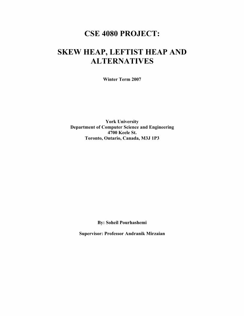
4.3 HeapsHeaps are a specialized tree-based data structure. They are of particular interest for implementing Priority Queues because they must maintain the heap property.

The heap property (min-heap): if X is a child of Y, then key(Y) ≤ key(X).

Because of this property the element with the smallest key (largest key in the case of max-heap) is always at the root node.

The following is a graphical representation of a Binary Min-Heap:

Binary Min Heap

Heaps can either be implemented using Arrays or Links depending on their structure. Generally array implementation is used when the heap has a fixed structure otherwise the linked implementation is practiced.

Refer to APPENDIX A for the array implementation of a heap.

There exists a wide variety of heaps:

o Binary Heapo Leftist Heapo Skew Heapo Soft Heapo Binomial Heap

6

o Fibonacci Heapo Treapo Beapo and etc.

All these heaps have their own respective properties and applications. We will explore the following Heaps:

1. Leftist Heap2. Skew Heap3. Soft Heap

5 LEFTIST HEAP

Leftist heaps are one of the possible implementations of priority queues. A leftist heap is a binary heap-ordered tree for which the operations are based on a special way of performing the Union operation. Unlike Binary Heaps these binary trees do not have a fixed structure and because of this it is very hard to use arrays for their implementation. Their unfixed structure makes the computation of the children and parent addresses difficult. Instead, leftist heaps and the other heap structures presented in the remainder of this paper are based on linked structures. Linking the nodes together facilitates finding the children or parent nodes, but requires additional memory.

5.1 DefinitionTo explain this heap more clearly I will define the following term:

Dist [x]: Length of the shortest path from x to a descendent external node – 1.

This path is very important in leftist heaps as the leftist property states:

Leftist Property:For all x: dist [right[x]] ≤ dist [left[x]]

Leftist Heap:Is a binary tree that is heap-ordered with all nodes maintaining the leftist property.

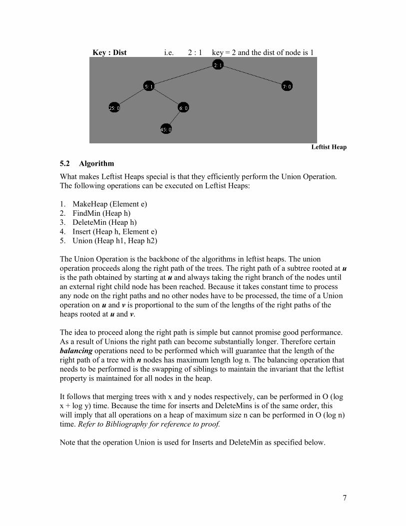
The following diagram is a graphical representation of a Leftist Heap.

This diagram represents each node as follows:

7

Key : Dist i.e. 2 : 1 key = 2 and the dist of node is 1

Leftist Heap

5.2 AlgorithmWhat makes Leftist Heaps special is that they efficiently perform the Union Operation.The following operations can be executed on Leftist Heaps:

1. MakeHeap (Element e)2. FindMin (Heap h)3. DeleteMin (Heap h)4. Insert (Heap h, Element e)5. Union (Heap h1, Heap h2)

The Union Operation is the backbone of the algorithms in leftist heaps. The union operation proceeds along the right path of the trees. The right path of a subtree rooted at u is the path obtained by starting at u and always taking the right branch of the nodes until an external right child node has been reached. Because it takes constant time to process any node on the right paths and no other nodes have to be processed, the time of a Union operation on u and v is proportional to the sum of the lengths of the right paths of the heaps rooted at u and v.

The idea to proceed along the right path is simple but cannot promise good performance. As a result of Unions the right path can become substantially longer. Therefore certain balancing operations need to be performed which will guarantee that the length of the right path of a tree with n nodes has maximum length log n. The balancing operation that needs to be performed is the swapping of siblings to maintain the invariant that the leftist property is maintained for all nodes in the heap.

It follows that merging trees with x and y nodes respectively, can be performed in O (log x + log y) time. Because the time for inserts and DeleteMins is of the same order, this will imply that all operations on a heap of maximum size n can be performed in O (log n) time. Refer to Bibliography for reference to proof.

Note that the operation Union is used for Inserts and DeleteMin as specified below.

8

MakeHeap (Element e)

return new Heap(e);

FindMin (Heap h)

if (h == null)return null;

elsereturn h.key

DeleteMin (Heap h)

Element e = h.key;h = Union (h.left, h.right);return e;

Insert (Heap h, Element e)

z = MakeHeap(e);h = Union (h, z);

Union (Heap h1, heap h2)if (h1 == null)

return h2;else if (h2 == null)

return h1;else{// Assure that the key of h1 is smallestif (h1.key > h2.key){

Node dummy = h1; h1 = h2; h2 = dummy;}

}if (h1.right == null) // Hook h2 directly to h1

h1.right = h2;else // Union recursively

h1.right = Union (h1.right, h2);// Conditionally swap children of h1 if (h1.left == null || h1.right.dist > h1.left.dist)

{Node dummy = h1.right; h1.right = h1.left; h1.left = dummy; }

9

// Update dist valuesif (h1.right == null)

h1.dist = 0;else

h1.dist = h1.right.dist + 1;return h1;

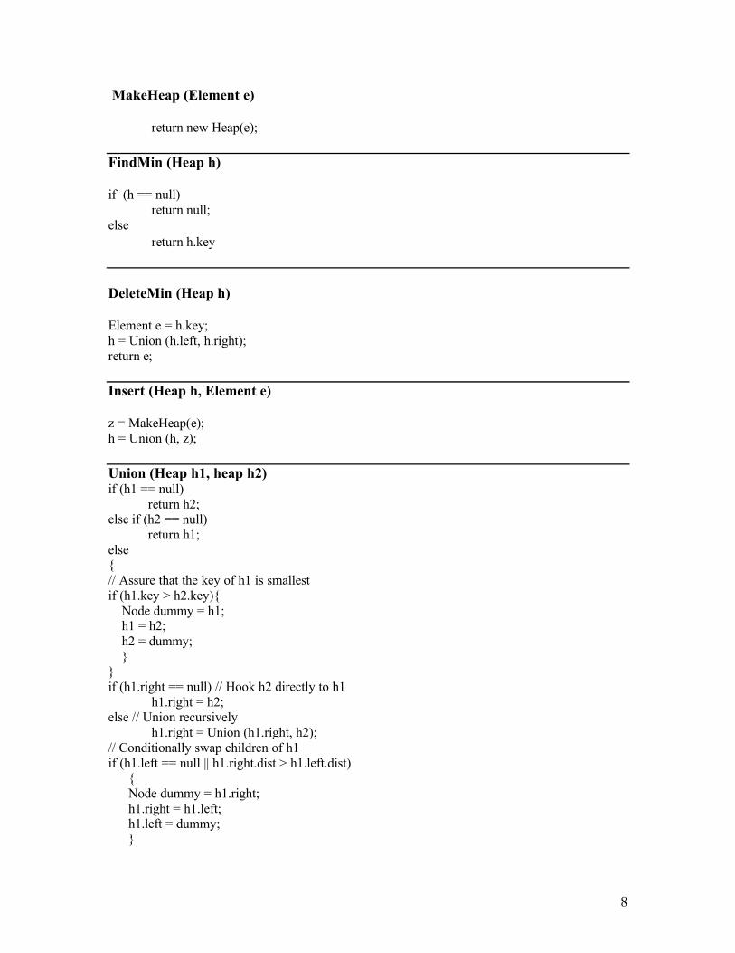
5.3 AAW AnimationAs part of this project an Online Interactive Applet has been implemented and can be found at the following URL:

http://www.cse.yorku.ca/~aaw/Pourhashemi/

This Applet aids users in understanding the algorithms that are used in implementing Leftist Heaps. Users are able to follow all the algorithms step by step as they actively explore the various operations that are executed on the Heap.

Leftist Heap Start Up Screen

5.4 Applications

Because of the Leftist Property the right path of every element in the heap has the shortest path to an external node. Therefore the Union Operation has sufficiently enhanced and runs in O (log n) time.

In some applications, pairs of heaps are repeatedly unioned; spending linear time per union operation would be out of the question. Leftist Heap supports union in O (log n) time and therefore is a good candidate for applications that will repeatedly call the Union operation.

10

6 SKEW HEAP

Skew heaps are one of the possible implementations of priority queues.A skew heap is a self-adjusting form of a leftist heap, which may grow arbitrarily unbalanced because they do not maintain balancing information.

6.1 DefinitionSkew Heaps are a self-adjusting form of Leftist Heap. By unconditionally swapping all nodes in the merge path Skew Heaps attempt to maintain a short right path from the root.

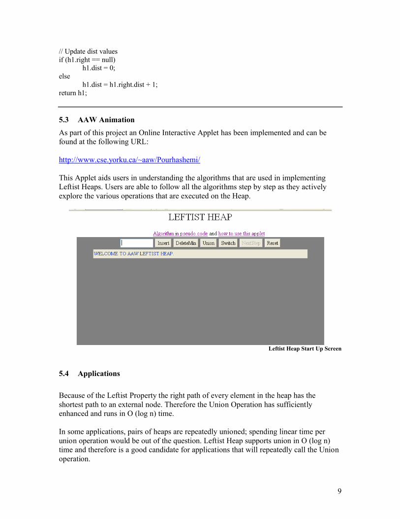
The following diagram is a graphical representation of a Skew Heap.

Skew Heap

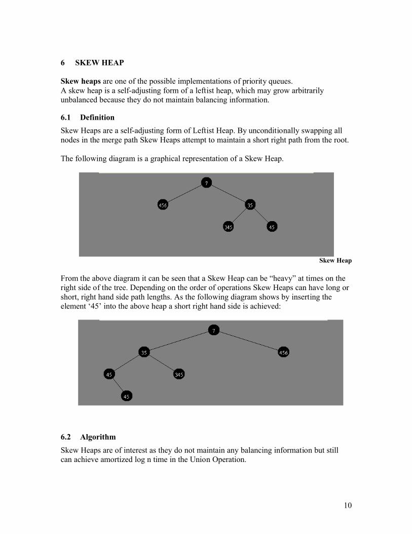
From the above diagram it can be seen that a Skew Heap can be “heavy” at times on the right side of the tree. Depending on the order of operations Skew Heaps can have long or short, right hand side path lengths. As the following diagram shows by inserting the element ‘45’ into the above heap a short right hand side is achieved:

6.2 AlgorithmSkew Heaps are of interest as they do not maintain any balancing information but still can achieve amortized log n time in the Union Operation.

11

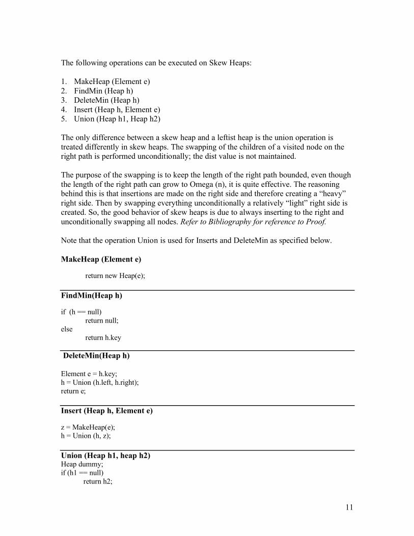
The following operations can be executed on Skew Heaps:

1. MakeHeap (Element e)2. FindMin (Heap h)3. DeleteMin (Heap h)4. Insert (Heap h, Element e)5. Union (Heap h1, Heap h2)

The only difference between a skew heap and a leftist heap is the union operation is treated differently in skew heaps. The swapping of the children of a visited node on the right path is performed unconditionally; the dist value is not maintained.

The purpose of the swapping is to keep the length of the right path bounded, even though the length of the right path can grow to Omega (n), it is quite effective. The reasoning behind this is that insertions are made on the right side and therefore creating a “heavy” right side. Then by swapping everything unconditionally a relatively “light” right side is created. So, the good behavior of skew heaps is due to always inserting to the right and unconditionally swapping all nodes. Refer to Bibliography for reference to Proof.

Note that the operation Union is used for Inserts and DeleteMin as specified below.

MakeHeap (Element e)

return new Heap(e);

FindMin(Heap h)

if (h == null)return null;

elsereturn h.key

DeleteMin(Heap h)

Element e = h.key;h = Union (h.left, h.right);return e;

Insert (Heap h, Element e)

z = MakeHeap(e);h = Union (h, z);

Union (Heap h1, heap h2)Heap dummy;if (h1 == null)

return h2;

12

else if (h2 == null) return h1;

else{// Assure that the key of h1 is smallestif (h1.key > h2.key){Node dummy = h1; h1 = h2; h2 = dummy;}}if (h1.right == null) // Hook h2 directly to h1

h1.right = h2;else // Union recursively

h1.right = Union (h1.right, h2);// Swap children of h1 dummy = h1.right; h1.right = h1.left;h1.left = dummy; return h1;

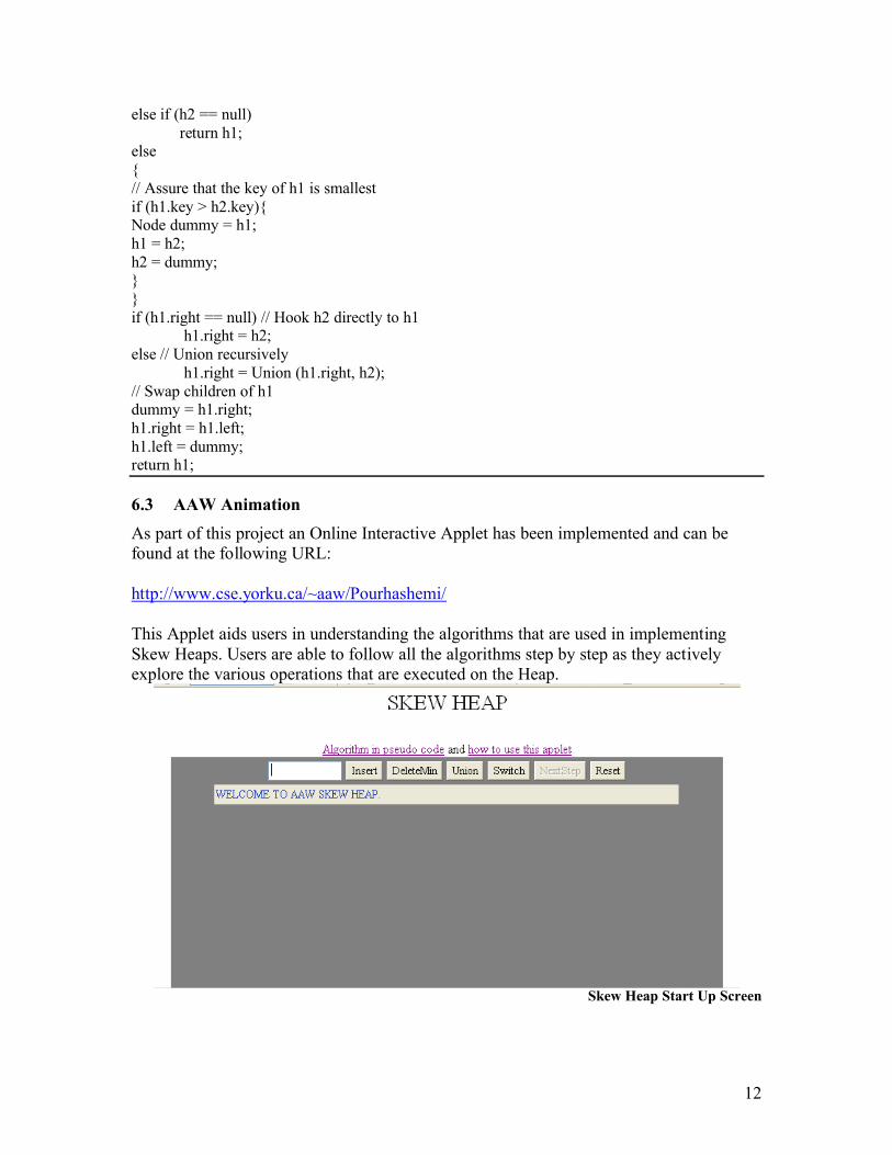
6.3 AAW AnimationAs part of this project an Online Interactive Applet has been implemented and can be found at the following URL:

http://www.cse.yorku.ca/~aaw/Pourhashemi/

This Applet aids users in understanding the algorithms that are used in implementing Skew Heaps. Users are able to follow all the algorithms step by step as they actively explore the various operations that are executed on the Heap.

Skew Heap Start Up Screen

13

6.4 ApplicationsBecause of the self-adjusting nature of this Heap the Union Operation has sufficiently enhanced and runs in O (log n) amortized time.

In some applications, pairs of heaps are repeatedly unioned; spending linear time per union operation would be out of the question. Skew Heap supports union in O (log n) amortized time and therefore are a good candidate for applications that will repeatedly call the Union operation.

The self-adjustment in skew heaps has important advantages over the balancing in leftist heaps:

• Reduction of memory consumption (no balancing information needs to be stored)• Reduction of time consumption (saving the updates of the dist information) • Unconditional execution (saving one test for every processed node)

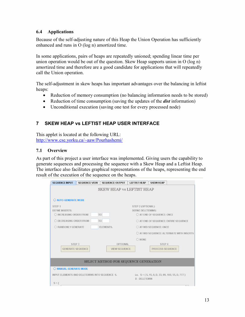
7 SKEW HEAP vs LEFTIST HEAP USER INTERFACE

This applet is located at the following URL:http://www.cse.yorku.ca/~aaw/Pourhashemi/

7.1 OverviewAs part of this project a user interface was implemented. Giving users the capability to generate sequences and processing the sequence with a Skew Heap and a Leftist Heap. The interface also facilitates graphical representations of the heaps, representing the end result of the execution of the sequence on the heaps.

14

The main purpose of this interface is giving users the capability of creating large sequences and observing the execution of that sequence on Leftist and Skew Heaps.

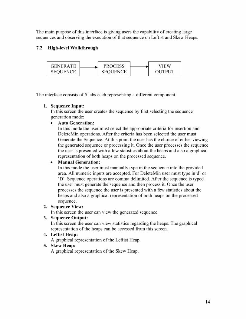
7.2 High-level Walkthrough

The interface consists of 5 tabs each representing a different component.

1. Sequence Input:In this screen the user creates the sequence by first selecting the sequence generation mode:• Auto Generation:

In this mode the user must select the appropriate criteria for insertion and DeleteMin operations. After the criteria has been selected the user must Generate the Sequence. At this point the user has the choice of either viewing the generated sequence or processing it. Once the user processes the sequence the user is presented with a few statistics about the heaps and also a graphical representation of both heaps on the processed sequence.

• Manual Generation:In this mode the user must manually type in the sequence into the provided area. All numeric inputs are accepted. For DeleteMin user must type in‘d’ or ‘D’. Sequence operations are comma delimited. After the sequence is typed the user must generate the sequence and then process it. Once the user processes the sequence the user is presented with a few statistics about the heaps and also a graphical representation of both heaps on the processed sequence.

2. Sequence View:In this screen the user can view the generated sequence.

3. Sequence Output:In this screen the user can view statistics regarding the heaps. The graphical representation of the heaps can be accessed from this screen.

4. Leftist Heap:A graphical representation of the Leftist Heap.

5. Skew Heap:A graphical representation of the Skew Heap.

GENERATE SEQUENCE

PROCESS SEQUENCE

VIEW OUTPUT

15

8 SOFT HEAP

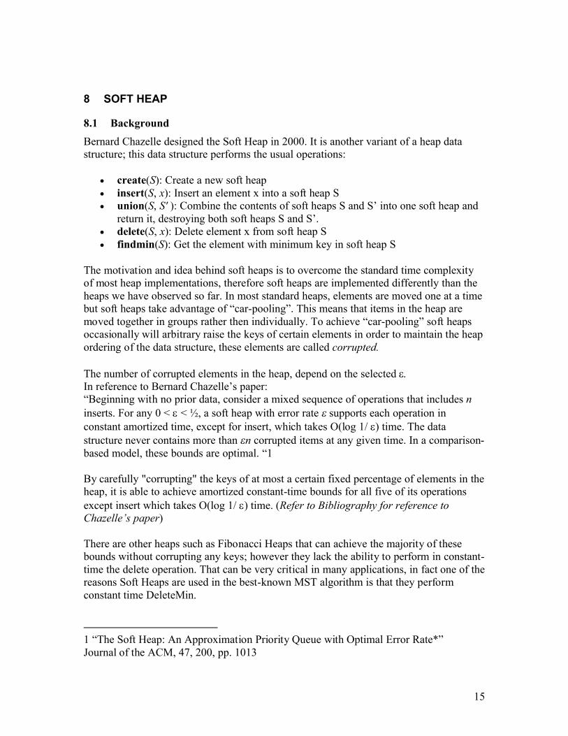
8.1 BackgroundBernard Chazelle designed the Soft Heap in 2000. It is another variant of a heap data structure; this data structure performs the usual operations:

• create(S): Create a new soft heap• insert(S, x): Insert an element x into a soft heap S• union(S, S' ): Combine the contents of soft heaps S and S’ into one soft heap and

return it, destroying both soft heaps S and S’.• delete(S, x): Delete element x from soft heap S• findmin(S): Get the element with minimum key in soft heap S

The motivation and idea behind soft heaps is to overcome the standard time complexity of most heap implementations, therefore soft heaps are implemented differently than the heaps we have observed so far. In most standard heaps, elements are moved one at a time but soft heaps take advantage of “car-pooling”. This means that items in the heap are moved together in groups rather then individually. To achieve “car-pooling” soft heaps occasionally will arbitrary raise the keys of certain elements in order to maintain the heap ordering of the data structure, these elements are called corrupted.

The number of corrupted elements in the heap, depend on the selected ε. In reference to Bernard Chazelle’s paper:“Beginning with no prior data, consider a mixed sequence of operations that includes ninserts. For any 0 < ε < ½, a soft heap with error rate ε supports each operation in constant amortized time, except for insert, which takes O(log 1/ ε) time. The data structure never contains more than εn corrupted items at any given time. In a comparison-based model, these bounds are optimal. “1

By carefully "corrupting" the keys of at most a certain fixed percentage of elements in the heap, it is able to achieve amortized constant-time bounds for all five of its operations except insert which takes O(log 1/ ε) time. (Refer to Bibliography for reference to Chazelle’s paper)

There are other heaps such as Fibonacci Heaps that can achieve the majority of these bounds without corrupting any keys; however they lack the ability to perform in constant-time the delete operation. That can be very critical in many applications, in fact one of the reasons Soft Heaps are used in the best-known MST algorithm is that they perform constant time DeleteMin.

1 “The Soft Heap: An Approximation Priority Queue with Optimal Error Rate*” Journal of the ACM, 47, 200, pp. 1013

16

The percentage of elements which are corrupted can be chosen freely, but the lower this is set, the more time insertions require (as was mentioned previously the insertion operation is bounded by O(log 1/ε) for an error rate of ε)

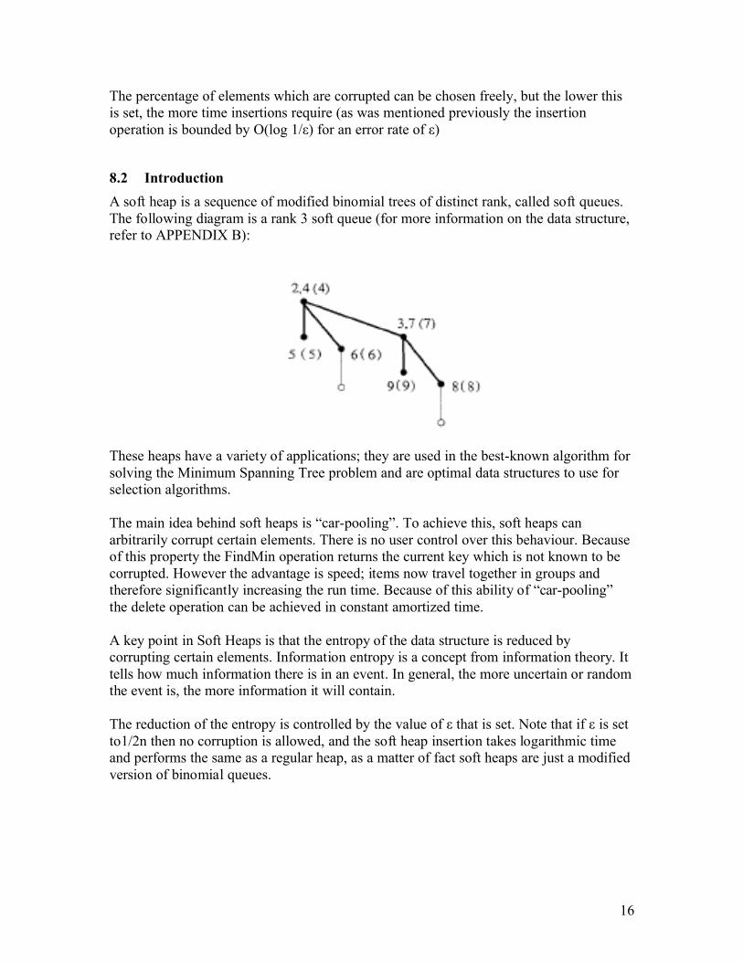
8.2 IntroductionA soft heap is a sequence of modified binomial trees of distinct rank, called soft queues.The following diagram is a rank 3 soft queue (for more information on the data structure, refer to APPENDIX B):

These heaps have a variety of applications; they are used in the best-known algorithm for solving the Minimum Spanning Tree problem and are optimal data structures to use for selection algorithms.

The main idea behind soft heaps is “car-pooling”. To achieve this, soft heaps can arbitrarily corrupt certain elements. There is no user control over this behaviour. Because of this property the FindMin operation returns the current key which is not known to be corrupted. However the advantage is speed; items now travel together in groups and therefore significantly increasing the run time. Because of this ability of “car-pooling” the delete operation can be achieved in constant amortized time.

A key point in Soft Heaps is that the entropy of the data structure is reduced by corrupting certain elements. Information entropy is a concept from information theory. It tells how much information there is in an event. In general, the more uncertain or randomthe event is, the more information it will contain.

The reduction of the entropy is controlled by the value of ε that is set. Note that if ε is set to1/2n then no corruption is allowed, and the soft heap insertion takes logarithmic time and performs the same as a regular heap, as a matter of fact soft heaps are just a modified version of binomial queues.

17

8.3 MotivationThe main motivation behind the invention of Soft Heaps was a faster solution to the MST problem. Chazelle’s algorithm uses Soft Heaps in the best-known algorithm to date for solving the MST problem. The Minimum Spanning Tree is one of the oldest open problems in computer science and is of great importance in combinatorial optimization.

A brief background on Minimum Spanning Trees will be given with the most common algorithms that execute in Polynomial time. Following that, an overview of Chazelle’s algorithm will be given for solving this problem.

8.3.1 Minimum Spanning Tree Problem8.3.1.1 Background

The Minimum Spanning Tree problem has a long history. I will begin by first giving a definition of what a minimum spanning tree is.

The minimum spanning tree of a graph defines the cheapest subset of edges that keeps the graph in one connected component.

Or In reference to wikipedia:

“Given a connected, undirected graph, a spanning tree of that graph is a subgraph which is a tree and connects all the vertices together. A single graph can have many different spanning trees. We can also assign a weight to each edge, which is a number representing how unfavorable it is, and use this to assign a weight to a spanning tree by computing the sum of the weights of the edges in that spanning tree. A minimum spanning tree or minimum weight spanning tree is then a spanning tree with weight less than or equal to the weight of every other spanning tree. More generally, any undirected graph has a minimum spanning forest.”2

2 http://en.wikipedia.org/wiki/Minimum_spanning_tree

18

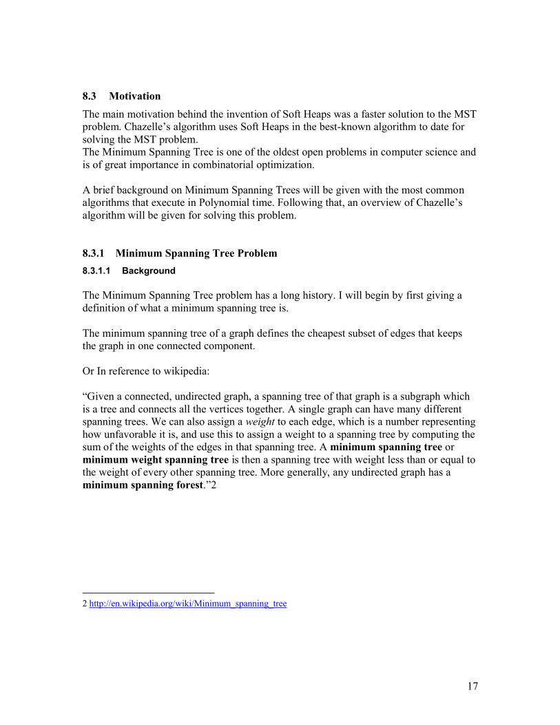
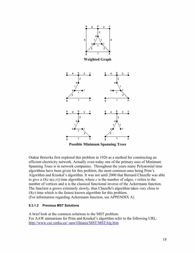
Weighted Graph

Possible Minimum Spanning Trees

Otakar Boruvka first explored this problem in 1926 as a method for constructing an efficient electricity network. Actually even today one of the primary uses of Minimum Spanning Trees is in network companies. Throughout the years many Polynomial time algorithms have been given for this problem, the most common ones being Prim’s Algorithm and Kruskal’s algorithm. It was not until 2000 that Bernard Chazelle was able to give a O(e α(e,v)) time algorithm, where e is the number of edges, v refers to the number of vertices and α is the classical functional inverse of the Ackermann function. The function α grows extremely slowly, thus Chazelle's algorithm takes very close to O(e) time which is the fastest known algorithm for this problem. (For information regarding Ackermann function, see APPENDIX A)

8.3.1.2 Previous MST Solutions

A brief look at the common solutions to the MST problem:For AAW animations for Prim and Kruskal’s algorithm refer to the following URL:http://www.cse.yorku.ca/~aaw/Ghiassi/MST/MSTAlg.htm

19

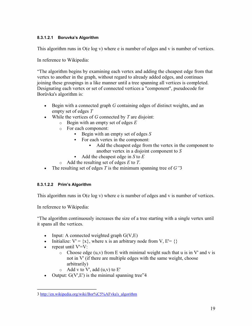
8.3.1.2.1 Boruvka’s Algorithm

This algorithm runs in O(e log v) where e is number of edges and v is number of vertices.

In reference to Wikipedia:

“The algorithm begins by examining each vertex and adding the cheapest edge from that vertex to another in the graph, without regard to already added edges, and continues joining these groupings in a like manner until a tree spanning all vertices is completed. Designating each vertex or set of connected vertices a "component", pseudocode for Borůvka's algorithm is:

• Begin with a connected graph G containing edges of distinct weights, and an empty set of edges T

• While the vertices of G connected by T are disjoint: o Begin with an empty set of edges Eo For each component:

§ Begin with an empty set of edges S§ For each vertex in the component:

§ Add the cheapest edge from the vertex in the component to another vertex in a disjoint component to S

§ Add the cheapest edge in S to Eo Add the resulting set of edges E to T.

• The resulting set of edges T is the minimum spanning tree of G”3

8.3.1.2.2 Prim’s Algorithm

This algorithm runs in O(e log v) where e is number of edges and v is number of vertices.

In reference to Wikipedia:

“The algorithm continuously increases the size of a tree starting with a single vertex until it spans all the vertices.

• Input: A connected weighted graph G(V,E)• Initialize: V' = {x}, where x is an arbitrary node from V, E'= {}• repeat until V'=V:

o Choose edge (u,v) from E with minimal weight such that u is in V' and v is not in V' (if there are multiple edges with the same weight, choose arbitrarily)

o Add v to V', add (u,v) to E'• Output: G(V',E') is the minimal spanning tree”4

3 http://en.wikipedia.org/wiki/Bor%C5%AFvka's_algorithm

20

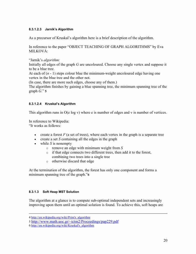
8.3.1.2.3 Jarnik’s Algorithm

As a precursor of Kruskal’s algorithm here is a brief description of the algorithm.

In reference to the paper “OBJECT TEACHING OF GRAPH ALGORITHMS” by Eva MILKOVÁ:

“Jarnik’s algorithm: Initially all edges of the graph G are uncoloured. Choose any single vertex and suppose it to be a blue tree.At each of (n - 1) steps colour blue the minimum-weight uncoloured edge having one vertex in the blue tree and the other not. (In case, there are more such edges, choose any of them.)The algorithm finishes by gaining a blue spanning tree, the minimum spanning tree of the graph G.” 5

8.3.1.2.4 Kruskal’s Algorithm

This algorithm runs in O(e log v) where e is number of edges and v is number of vertices.

In reference to Wikipedia:“It works as follows:

• create a forest F (a set of trees), where each vertex in the graph is a separate tree• create a set S containing all the edges in the graph• while S is nonempty

o remove an edge with minimum weight from So if that edge connects two different trees, then add it to the forest,

combining two trees into a single treeo otherwise discard that edge

At the termination of the algorithm, the forest has only one component and forms a minimum spanning tree of the graph.”6

8.3.1.3 Soft Heap MST Solution

The algorithm at a glance is to compute sub-optimal independent sets and increasingly improving upon them until an optimal solution is found. To achieve this, soft heaps are

4 http://en.wikipedia.org/wiki/Prim's_algorithm5 http://www.math.uoc.gr/~ictm2/Proceedings/pap229.pdf6 http://en.wikipedia.org/wiki/Kruskal's_algorithm

21

used because of their ability to perform deleteMin’s in constant amortized time and the ability of moving data in groups rather than individually.

For a subgraph C of G, C is contractible if C ∩ MST (G) is connected. This is important because the MST(G) can be computed from the MST(C) and the MST(G’), where G’ is the graph derived from G by contracting C into a single vertex.

The idea in this algorithm is to certify the contractibility of C before computing MST varies previous algorithms identified contractible subgraph as the MST of the graph was growing. This method provides a great advantage as computing MST(C) is easier if it is certified that C is contractible. At this point we only need to look at edges with both endpoints in C. Because of this advantage a non-greedy approach can be made towards solving this problem.

We use soft heaps to be able to identify and compute a contractible subgraph before computing its MST first. Once the contractible subgraphs have been identified it is simpler to compute the MST of those subgraphs and then gluing them together to form the MST of the original graph.

The importance of this algorithm is its divide-and-conquer approach and non-greedy nature, varies the previous algorithms were all greedy.

At a high-level the algorithm does the following:

By iterating the following:Decompose à Contract à Glue A hierarchy tree is constructed with each vertex of the graph being a leaf of the hierarchy tree.

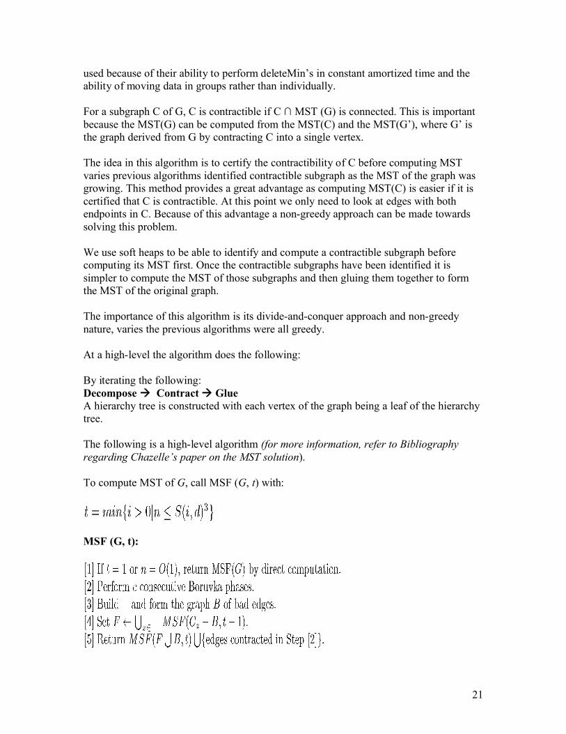
The following is a high-level algorithm (for more information, refer to Bibliography regarding Chazelle’s paper on the MST solution).

To compute MST of G, call MSF (G, t) with:

MSF (G, t):

22

8.4 Other ApplicationsBesides giving the most efficient algorithm to date for the MST problem, soft heaps have other applications also. The following is a list of other useful applications of Soft Heaps:

• Dynamic maintenance of percentiles• Computing Medians in linear time• Approximate Sorting

8.5 Ideas/ThoughtsI believe the reasoning behind Chazelle’s invention of the Soft Heap was to be able to achieve an efficient way of identifying contractible subgraphs. The way soft heaps are implemented makes them a good candidate for selecting appropriate edges.

Chazelle wanted the ability of identifying contractible subgraphs so he can take a divide-and-conquer approach to this problem, recursively computing the MST of the contractible subgraphs and then gluing them together to form the MST of the graph. To be able to achieve this in an efficient manner, soft heaps were invented.

Another interesting fact about Soft Heaps is in the way they approach the implementation of the sift operation which is the key operation in these heaps. The approach in calling the sift operation is of particular interest. The method recursively calls itself and creates a path in the computation tree but occasionally the method will recursively call itself twice and in this way Chazelle was able to achieve recursion tree branching. This makes the operations run much more efficiently giving way to a more efficient solution to the MST problem and other applications.

23

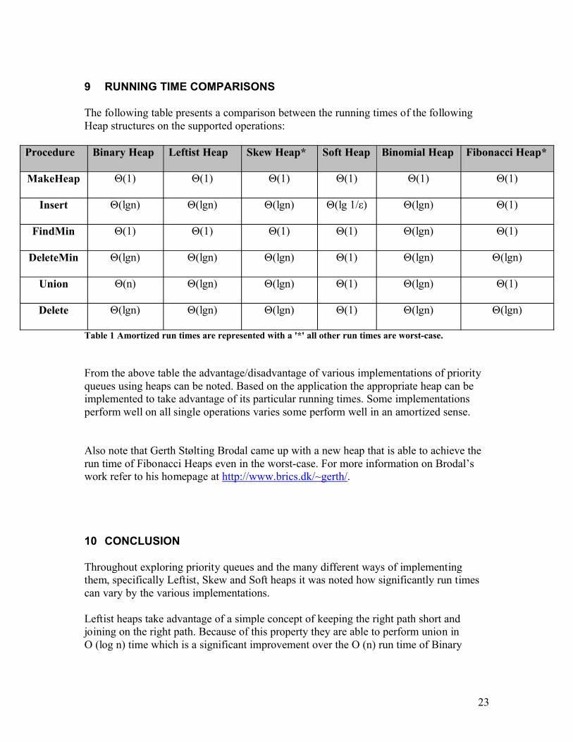
9 RUNNING TIME COMPARISONS

The following table presents a comparison between the running times of the following Heap structures on the supported operations:

Procedure Binary Heap Leftist Heap Skew Heap* Soft Heap Binomial Heap Fibonacci Heap*

MakeHeap Θ(1) Θ(1) Θ(1) Θ(1) Θ(1) Θ(1)

Insert Θ(lgn) Θ(lgn) Θ(lgn) Θ(lg 1/ε) Θ(lgn) Θ(1)

FindMin Θ(1) Θ(1) Θ(1) Θ(1) Θ(lgn) Θ(1)

DeleteMin Θ(lgn) Θ(lgn) Θ(lgn) Θ(1) Θ(lgn) Θ(lgn)

Union Θ(n) Θ(lgn) Θ(lgn) Θ(1) Θ(lgn) Θ(1)

Delete Θ(lgn) Θ(lgn) Θ(lgn) Θ(1) Θ(lgn) Θ(lgn)

Table 1 Amortized run times are represented with a '*' all other run times are worst-case.

From the above table the advantage/disadvantage of various implementations of priority queues using heaps can be noted. Based on the application the appropriate heap can be implemented to take advantage of its particular running times. Some implementations perform well on all single operations varies some perform well in an amortized sense.

Also note that Gerth Stølting Brodal came up with a new heap that is able to achieve the run time of Fibonacci Heaps even in the worst-case. For more information on Brodal’s work refer to his homepage at http://www.brics.dk/~gerth/.

10 CONCLUSION

Throughout exploring priority queues and the many different ways of implementing them, specifically Leftist, Skew and Soft heaps it was noted how significantly run times can vary by the various implementations.

Leftist heaps take advantage of a simple concept of keeping the right path short and joining on the right path. Because of this property they are able to perform union in O (log n) time which is a significant improvement over the O (n) run time of Binary

24

heaps. Many applications can take advantage of this improved performance where the operation union is performed repeatedly.

Skew heaps being a self-adjusting version of Leftist Heaps are able to perform as well in an amortized sense as Leftist Heaps without maintaining any balancing information. Because of this quality they perform well on large inputs (remember they perform well in an amortized sense, therefore on larger inputs) and do not waste any space for maintaining balancing information and save CPU time on updates and comparisons.

What was really interesting was the concept behind implementing Soft Heaps. By simply corrupting arbitrary elements in the heap they reduce the information entropy and being completely pointer based (in contrast to array based) they achieve significant increase in the operation run times. Because they are able to move groups of elements rather than individual elements and therefore all operations besides insert are performed in constant amortized time. The particularly important application of this heap is in the MST solution where they are used in computing the contractibility of a subgraph. By first certifying the contractibility of a subgraph before growing the MST a divide-and-conquer approach can be taken towards this problem, moving away from the previous greedy algorithms. This is a significant step towards this problem.

Overall two key points stood out for me about Chazelle’s Soft Heaps:His approach of corrupting data randomly for the purpose of decreasing the information

entropy of the data structure, and because Soft Heaps are pointer based they can move data in groups and not individually. The second idea of calling recursion (occasionally) twice in the sift operation.

It is these approaches in implementing new data structures that give way to more efficient implementations of data structures which in effect give us the ability to solve problems faster and more efficiently.

25

11 BIBLIOGRAPHY

The following references were used:

JOURNALS:

1. D. Sleator and R. Tarjan, Self-adjusting heaps, SIAM J. Computing, 15, 1, pp. 52-69, 1986.

2. C. Crane, Linear Lists and Priority Queues as Balanced Binary Trees, Tech. Rep. CS-72-259, Dept. of Comp. Sci., Stanford University, 1972.

3. The Soft Heap: An Approximation Priority Queue with Optimal Error Rate*” B. Chazelle, Journal of the ACM, 47, 200, pp. 1015 – 1027

4. A Minimum Spanning Tree Algorithm with Inverse-Ackermann Type ComplexityB. Chazelle, Journal ACM 47 (2000), 1028-1047

BOOKS:

1. Thomas H. Cormen, Charles E. Leiserson, Ronald L. Rivest, and Clifford Stein. Introduction to Algorithms, Second Edition. MIT Press and McGraw-Hill, 2001. ISBN 0-262-03293-7.

WWW:

1. http://www.awprofessional.com/articles/article.asp?p=29793&rl=12. http://en.wikipedia.org/wiki/Ackermann_function (Ackermann function)3. http://en.wikipedia.org/wiki/Binary_heap (Array Implementation)4. http://www.cse.yorku.ca/~andy/courses/4101/lecture-notes/LN4.pdf). (Leftist Heap

Proof)5. http://www.cse.yorku.ca/~andy/courses/4101/lecture-notes/LN5.pdf). (Skew Heap

Proof)6. http://en.wikipedia.org/wiki/Soft_heap7. http://en.wikipedia.org/wiki/Information_entropy8. http://www.cse.yorku.ca/~andy/courses/4101/index.html9. http://www.cs.princeton.edu/~chazelle/10. http://en.wikipedia.org/wiki/Otakar_Bor%C5%AFvka11. http://www.brics.dk/~gerth/.

26

12 APPENDIX A

12.1 Ackermann Function

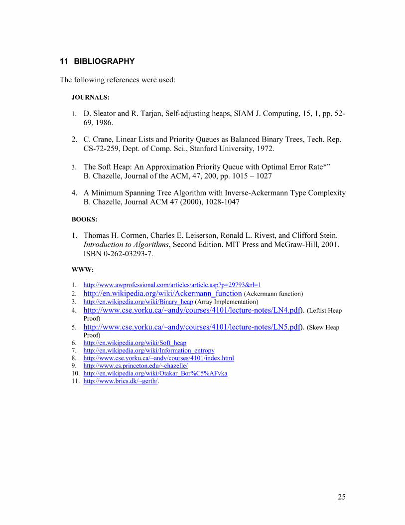
In reference to Wikipedia:

“The Ackermann function is defined recursively for non-negative integer’s m and n as follows

“

12.2 Heap Array Implementation

The advantage of using an array is that items can be randomly accessed by their node number, and the necessity for all the linkage is removed. However, the linkage does allow for efficient binary type searches in the tree, so the advantage is not all to the array implementation.

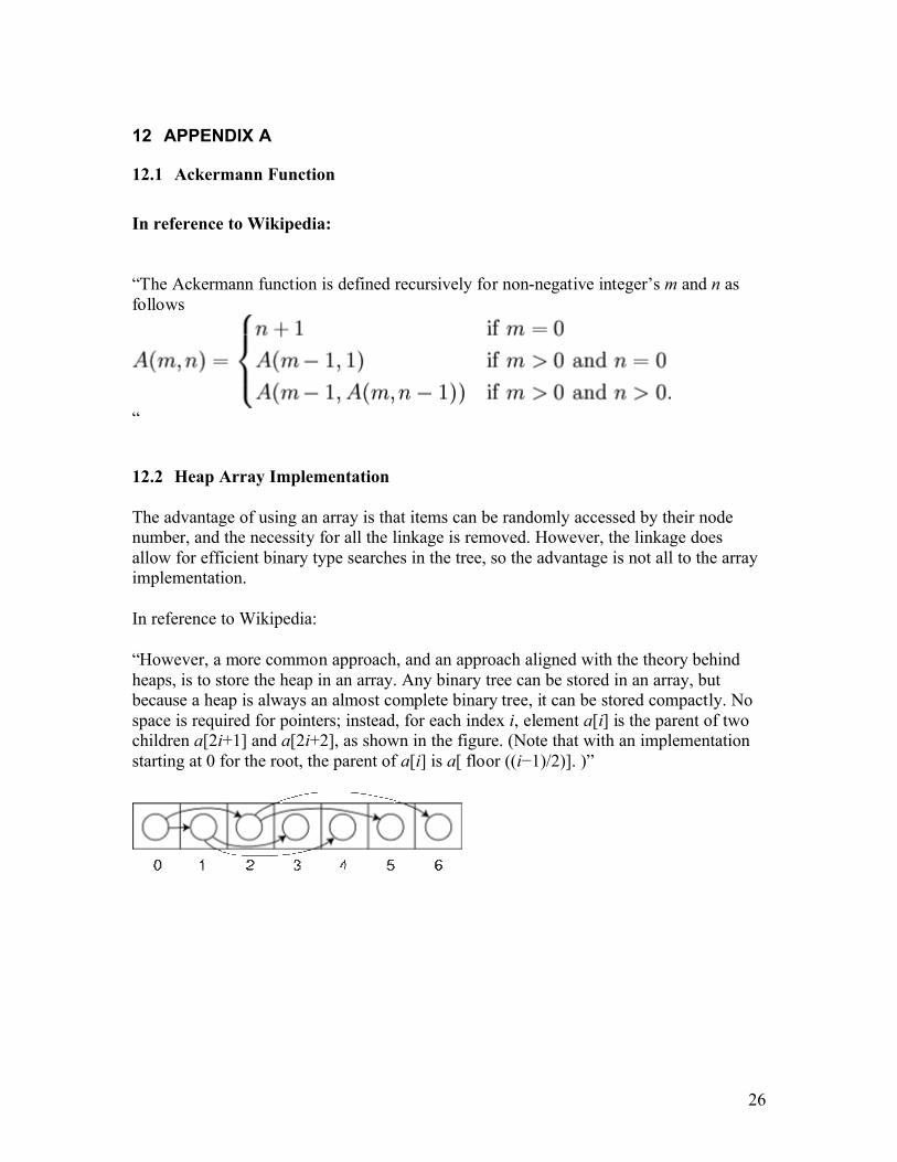
In reference to Wikipedia:

“However, a more common approach, and an approach aligned with the theory behind heaps, is to store the heap in an array. Any binary tree can be stored in an array, but because a heap is always an almost complete binary tree, it can be stored compactly. No space is required for pointers; instead, for each index i, element a[i] is the parent of two children a[2i+1] and a[2i+2], as shown in the figure. (Note that with an implementation starting at 0 for the root, the parent of a[i] is a[ floor ((i−1)/2)]. )”

27

13 APPENDIX B

The Soft Heap Data Structure implementation with C code is given here. This information is taken from Bernard Chazelle’s paper as indicated in the bibliography:“The Soft Heap: An Approximation Priority Queue with Optimal Error Rate*” Journal of the ACM, 47, 200, pp. 1015 - 1027

The Data Structure:

“The data structure is simple but somewhat subtle. This makes it all the more useful to include the actual code of our implementation of soft heaps in C. (It is very short: about 100 lines!) The code should be viewed as a bonus, not a hindrance. We do not base our discussion on it and, in fact, it is possible to skip it in a first reading and still understand soft heaps.Recall that a binomial tree [Vuillemin 1978] of rank k is a rooted tree of 2k nodes: it is formed by the combination of two binomial trees of rank k 2 1, where the root of one becomes the new child of the other root. A soft heap is a sequence of modified binomial trees of distinct ranks, called soft queues. The modifications come in two ways:

–A soft queue q is a binomial tree with subtrees possibly missing (somewhat like the trees of a Fibonacci heap [Fredman and Tarjan 1987] after a few deletions). The binomial tree from which q is derived is called its master tree. The rank of a node of q is the number of children of the corresponding node in the master tree. Obviously, it is an upper bound on the number of children in q. We enforce the following rank invariant: the number of children of the root should be no smaller than floor of rank (root)/2.

–A node v may store several items, in fact, a whole item-list. The ckey of v denotes the common value of all the current keys of the items in item-list(v): it is an upper bound on the original keys. The soft queue is heap-ordered with respect to ckeys, that is, a ckey of a node does not exceed the ckeys of any of its children. We fix an integer parameter r =r(ε), and we require that all corrupted items be stored at nodes of rank greater than r.

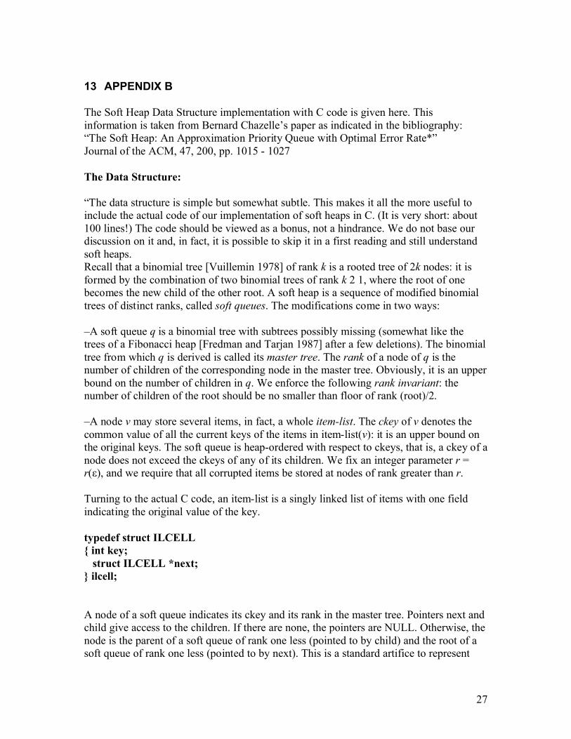
Turning to the actual C code, an item-list is a singly linked list of items with one field indicating the original value of the key.

typedef struct ILCELL{ int key;

struct ILCELL *next;} ilcell;

A node of a soft queue indicates its ckey and its rank in the master tree. Pointers next and child give access to the children. If there are none, the pointers are NULL. Otherwise, the node is the parent of a soft queue of rank one less (pointed to by child) and the root of a soft queue of rank one less (pointed to by next). This is a standard artifice to represent

28

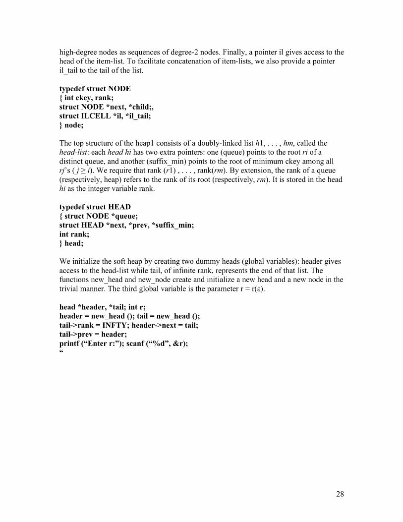
high-degree nodes as sequences of degree-2 nodes. Finally, a pointer il gives access to the head of the item-list. To facilitate concatenation of item-lists, we also provide a pointer il_tail to the tail of the list.

typedef struct NODE{ int ckey, rank;struct NODE *next, *child;,struct ILCELL *il, *il_tail;} node;

The top structure of the heap1 consists of a doubly-linked list h1, . . . , hm, called the head-list: each head hi has two extra pointers: one (queue) points to the root ri of a distinct queue, and another (suffix_min) points to the root of minimum ckey among all rj’s ( j ≥ i). We require that rank (r1) , . . . , rank(rm). By extension, the rank of a queue (respectively, heap) refers to the rank of its root (respectively, rm). It is stored in the head hi as the integer variable rank.

typedef struct HEAD{ struct NODE *queue;struct HEAD *next, *prev, *suffix_min;int rank;} head;

We initialize the soft heap by creating two dummy heads (global variables): header gives access to the head-list while tail, of infinite rank, represents the end of that list. The functions new_head and new_node create and initialize a new head and a new node in the trivial manner. The third global variable is the parameter r = r(ε).

head *header, *tail; int r;header = new_head (); tail = new_head ();tail->rank = INFTY; header->next = tail;tail->prev = header;printf (“Enter r:”); scanf (“%d”, &r);“