Simulation of Ductile Crack Propagation in Pipeline Steels ...

Page 1

Simulation of Ductile Crack Propagation in

Pipeline Steels Using Cohesive Zone Modeling

Written by

Andrew John Dunbar, B.Eng.

a thesis submitted to

the Faculty of Graduate Studies and Research in partial

fulfillment of the requirements for the Degree of Masters in

Applied Science, Mechanical

Ottawa-Carleton Institute for

Mechanical and Aerospace Engineering

Department of

Mechanical and Aerospace Engineering

Carleton University

Ottawa, Ontario

August, 2011

© Copyright

2011, Andrew Dunbar

Page 2

1*1 Library and Archives Canada

Published Heritage Branch

395 Wellington Street OttawaONK1A0N4 Canada

Bibliotheque et Archives Canada

Direction du Patrimoine de I'edition

395, rue Wellington OttawaONK1A0N4 Canada

Your file Votre reference ISBN: 978-0-494-83055-0 Our file Notre reference ISBN: 978-0-494-83055-0

NOTICE: AVIS:

The author has granted a non­exclusive license allowing Library and Archives Canada to reproduce, publish, archive, preserve, conserve, communicate to the public by telecommunication or on the Internet, loan, distribute and sell theses worldwide, for commercial or non­commercial purposes, in microform, paper, electronic and/or any other formats.

L'auteur a accorde une licence non exclusive permettant a la Bibliotheque et Archives Canada de reproduire, publier, archiver, sauvegarder, conserver, transmettre au public par telecommunication ou par Nntemet, preter, distribuer et vendre des theses partout dans le monde, a des fins commerciales ou autres, sur support microforme, papier, electronique et/ou autres formats.

The author retains copyright ownership and moral rights in this thesis. Neither the thesis nor substantial extracts from it may be printed or otherwise reproduced without the author's permission.

L'auteur conserve la propriete du droit d'auteur et des droits moraux qui protege cette these. Ni la these ni des extraits substantiels de celle-ci ne doivent etre imprimes ou autrement reproduits sans son autorisation.

In compliance with the Canadian Privacy Act some supporting forms may have been removed from this thesis.

Conformement a la loi canadienne sur la protection de la vie privee, quelques formulaires secondares ont ete enleves de cette these.

While these forms may be included in the document page count, their removal does not represent any loss of content from the thesis.

Bien que ces formulaires aient inclus dans la pagination, il n'y aura aucun contenu manquant.

1*1

Canada

Page 3

Abstract

Finite element simulations of ductile crack propagation are carried out using cohesive zone

modeling. Two sets of materials are modeled. The first material set was defined by Tvergaard

and Hutchinson (1992), and has four traction-separation (TS) laws of varying strength and

toughness. The second set is modeled after X70 pipeline steel, and is referred to as C2 steel.

Three TS laws are used to model this C2 material. The specimens analyzed include small-scale

yielding (SSY) and drop-weight tear test (DWTT). The fracture propagation characteristics and

CTOA values are obtained. It is shown that cohesive zone models can be successfully used to

simulate ductile crack propagation and to numerically measure CTOAs.

From SSY simulations, steady-state CTOAs for the TH materials were measured to range from

2° - 6°. The CTOAs for the C2 materials were higher than those of the TH materials due to

higher fracture resistance, but no steady-state values were obtained from the SSY simulations.

From simulations of the DWTT specimens, steady-state CTOA values for the TH materials

ranged from 2° - 4.5°, and therefore had good agreement with the SSY results. Estimated steady-

state CTOA values for the C2 materials ranged from 14° - 26°. The measured CTOAs agree

reasonably well between the SSY and DWTT simulations for both the TH and C2 material sets,

indicating that these values are transferable among specimens. Direct comparisons of the CTOAs

obtained from DWTT simulations to the experimental observations (12.4° - 18.5°) have

reasonable agreement as well.

in

Page 4

Acknowledgements

I would like to thank my thesis supervisor, Professor Xin Wang. This thesis wouldn't have been

possible without his invaluable insight and guidance. He never failed to provide encouragement

and moral support when necessary, and his teachings during both this degree and my undergrad

will not be forgotten.

I am grateful for the financial support from CANMET-MTL, Carleton University and NSERC,

that I received to undertake this research project.

I would also like to thank the fast fracture team at CANMET-MTL, as their direction, advice,

and wisdom made this thesis possible. Thanks to Bill Tyson, Su Xu, and George Roy.

IV

Page 5

Table of Contents

Acceptance Sheet ii

Abstract Hi

Acknowledgements iv

Table of Contents v

List of Tables vii

List of Figures ix

Nomenclature xi

Chapter 1 Introduction 1

1.1 Thesis Outline 3

Chapter 2 Background and Literature Review 5

2.1 Crack Tip Opening Angle 5

2.2 Cohesive Zone Modeling 7

2.2.1 Introduction of Concepts 7

2.2.2 Implementation of Cohesive Zone Modeling 10

2.3 Experimental Methods 10

2.3.1 The DWTT Specimen 11

2.3.2 Experimental Setup and Data Collection 11

2.3.3 Measuring the Crack Tip Opening Angle 13

Chapter 3 Finite Element Implementation of Cohesive Zone Modeling 24

3.1 Finite Element Implementation of CZM 24

3.1.1 Cohesive Zone Model 24

3.1.2 Traction-Separation-Based Modeling 25

3.1.3 Determining Model Parameters 29

v

Page 6

3.2 Unit Cell Analysis 31

Chapter 4 FE Simulation of Small-Scale Yielding Models 47

4.1 Model Specifications 47

4.2 Results 50

4.2.1 Results of TH Simulations 51

4.2.2 Results ofC2 Simulations 54

4.3 Conclusions 55

Chapter 5 FE Simulation of Drop-Weight Tear Tests 76

5.1 Model Specifications 76

5.2 Simulation Using Plane Strain Elastic-Plastic Model 79

5.3 Simulation Results for TH Materials 80

5.4 Simulation Results for C2 Materials 82

5.5 Conclusions 84

Chapter 6 Conclusions and Recommendations 105

6.1 Conclusions 105

6.2 Recommendations for Future Work 107

References 109

VI

Page 7

List of Tables

Chapter 2

Table 2.1: P vs. LLD Data - C 2 Steel - Corrected for Compliance (Xu, 2010a) 15

Chapter 3

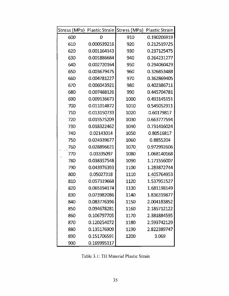
Table 3.1: TH Material Plastic Strain 35

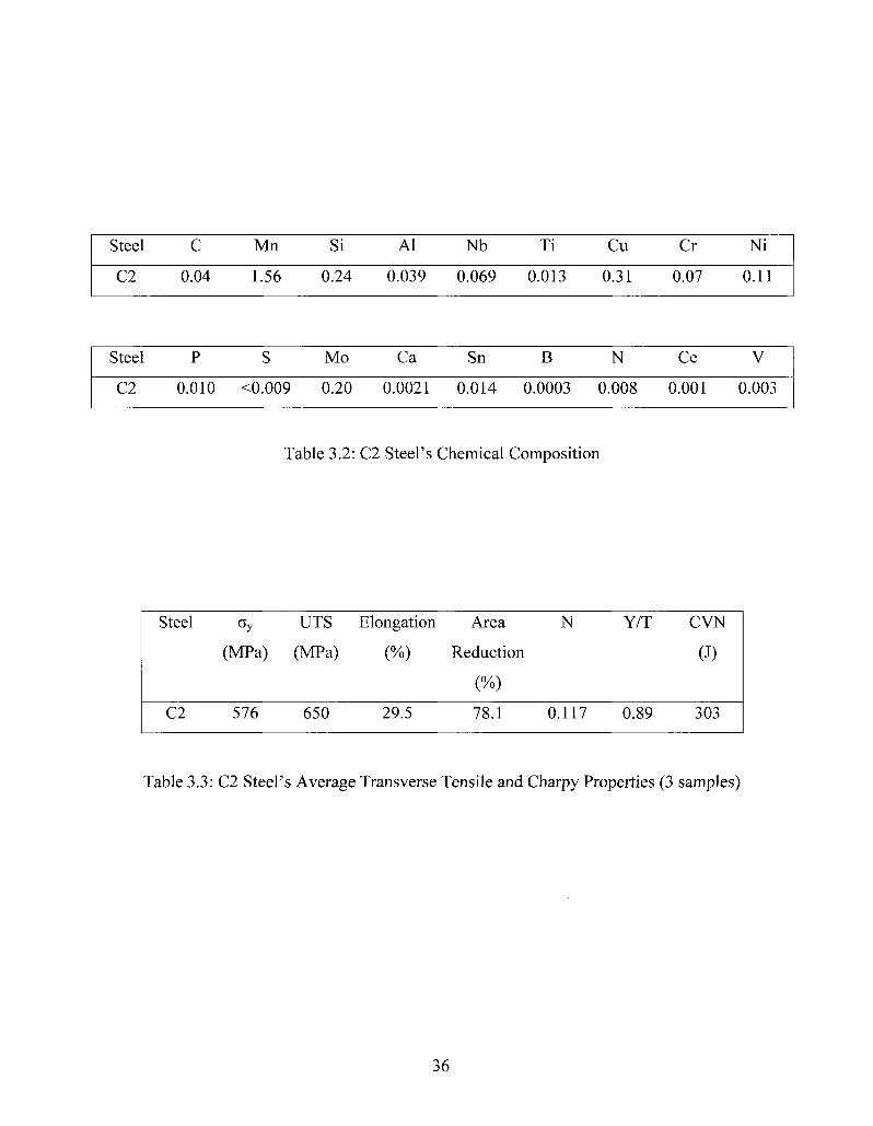
Table 3.2: C2 steel's Chemical Composition 36

Table 3.3: C2 steel's Average Transverse Tensile and Charpy Properties (3 samples) 36

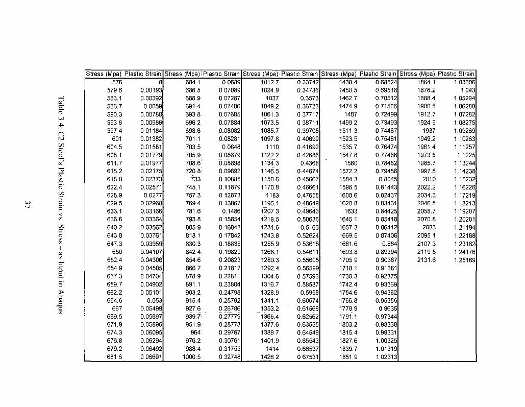
Table 3.4: C2 steel's Plastic Strain vs. Stress - as Input in Abaqus 37

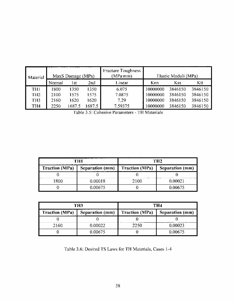
Table 3.5: Cohesive Parameters - TH Materials 38

Table 3.6: Desired TS Laws for TH Materials, Cases 1-4 38

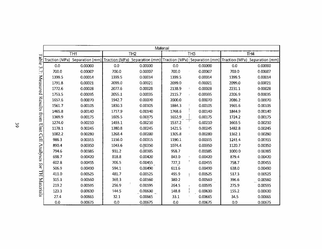
Table 3.7: Measured Results from Unit Cell Analyses for TH Materials 39

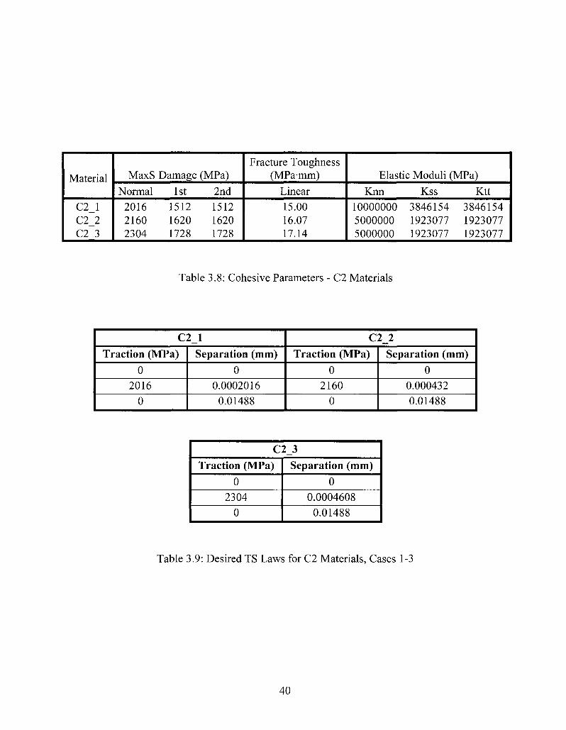
Table 3.8: Cohesive Parameters - C2 Materials 40

Table 3.9: Desired TS Laws for C2 Materials, Cases 1-3 40

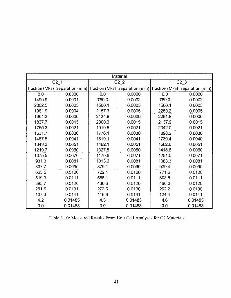
Table 3.10: Measured Results from Unit Cell Analyses for C2 Materials 41

Chapter 4

Table 4.1: Displacement Field - Maximum Applied Displacements 56

Table 4.2: J-Integral Data for TH Materials 57

Table 4.3: Model Parameters - (a) TH Materials, (b) C2 Materials 58

Table 4.4: SSY Sample Resistance Curve Data for TH1 Material 59

Table 4.5: SSY Sample Resistance Curve Data for TH2 Material 60

Table 4.6: SSY Sample Resistance Curve Data for TH3 Material 61

Table 4.7: SSY Sample Resistance Curve Data for TH4 Material 62

Table 4.8: SSY CTOA Data-TH1 63

Table 4.9: SSY CTOA Data - TH2 63

Table 4.10: SSY CTOA Data-TH3 64

Table 4.11: SSY CTOA Data-TH4 64

Table 4.12: SSY Sample Resistance Curve Data for C 2 1 Material 65

vn

Page 8

Table 4.13: SSY Sample Resistance Curve Data for C2_2 Material 66

Table 4.14: SSY Sample Resistance Curve Data for C2_3 Material 67

Table 4.15: SSY CTOA Data - C2 Materials 68

Chapter 5

Table 5.1: P vs. LLD Data from CANMET - C2 Steel - Corrected for Compliance 86

Table 5.2: P vs. LLD Sample data: Plane Strain Simulation 87

Table 5.3 (a) - (d): Sample P vs. LLD data - TH Materials 88

Table 5.4 (a) - (d): Sample 21a vs. LLD data - TH Materials 89

Table 5.5 (a) - (d): Sample CTOA vs. An data - TH Materials 90

Table 5.6 (a) - (c): P vs. LLD data - C2 Materials 91

Table 5.7 (a) - (c): Aa vs. LLD data - C2 Materials 92

Table 5.8 (a) - (c): CTOA vs. Aa data - C2 Materials 93

vm

Page 9

List of Figures

Chapter 2

Figure 2.1: Partially Fractured Charpy Sample (post test) (Xu et al, 2004) 16

Figure 2.2: Representation of the Ductile Failure Process by CZM (Cornec, 2003) 16

Figure 2.3: Four Examples of Various Shapes of TS Laws (Alfano, 2006) 17

Figure 2.4: C(T) Test: P vs. LLD Curves for Various TS Law Shapes (Alfano, 2006) 17

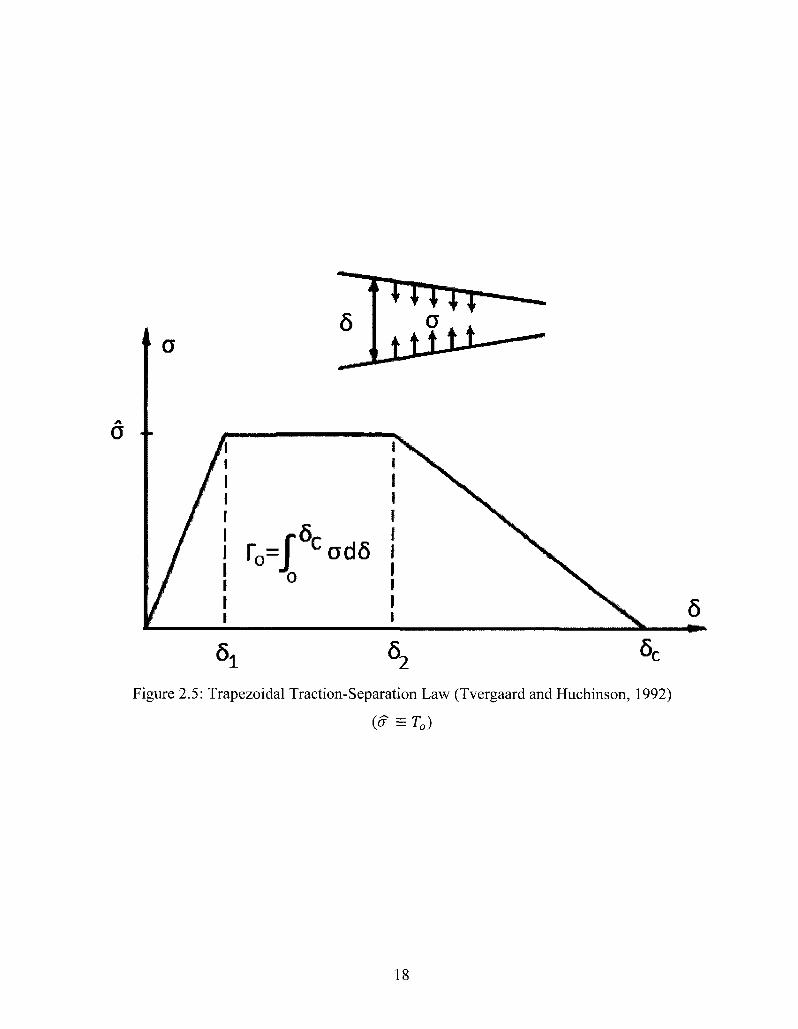
Figure 2.5: Trapezoidal Traction-Separation Law (Tvergaard and Huchinson, 1992) 18

Figure 2.6: DWTT Geometry (a) Full Specimen, (b) Notch Geometry 19

Figure 2.7: Experimental DWTT Set-up (Xu, 2010b) 20

Figure 2.8: P vs. LLD Data for C2 steel - Corrected for Compliance (Xu, 2010a) 21

Figure 2.9: Surface Measurement of CTOA 22

Figure 2.10: Slow-rate-tested X70 Pipe Sample Showing Wavy Crack Flanks 23

Chapter 3

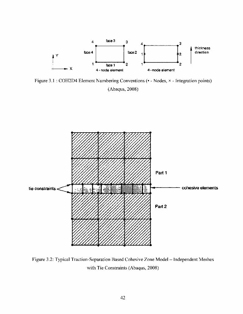
Figure 3.1 : COH2D4 Element Numbering Conventions (Abaqus, 2008) 42

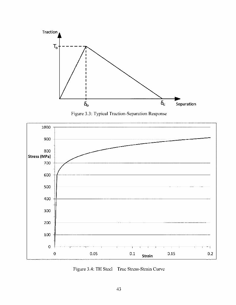
Figure 3.2: Typical Traction-Separation Based Cohesive Zone Model (Abaqus, 2008) 42

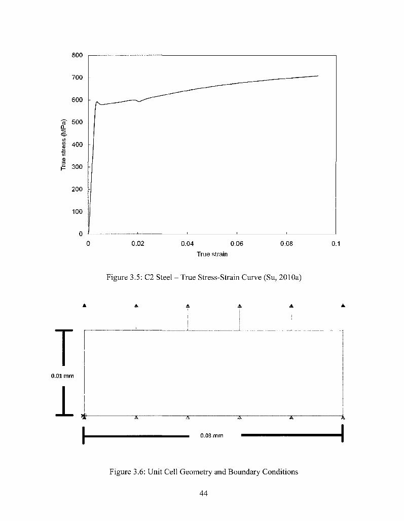
Figure 3.3: Typical Traction-Separation Response (Abaqus, 2008) 43

Figure 3.4: TH Steel - True Stress-Strain Curve 43

Figure 3.5: C2 Steel - True Stress-Strain Curve (Su, 2010a) 44

Figure 3.6: Unit Cell Geometry and Boundary Conditions 44

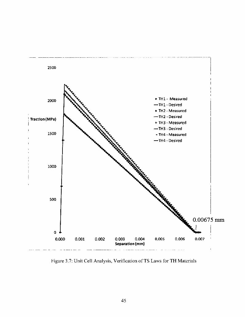
Figure 3.7: Unit Cell Analysis, Verification of TS Laws for TH Materials 45

Figure 3.8: Unit Cell Analysis, Verification of TS Laws for C2 Materials 46

Chapter 4

Figure 4.1: SSY Model - Geometry 69

Figure 4.2: Loading Conditions 70

Figure 4.3: Mesh Design - Full Model 70

Figure 4.4 (a) - (c): Crack Tip Mesh Design 71

Figure 4.5 : SSY- Normalized Resistance Curves - TH Materials - With Literature Data 72

IX

Page 10

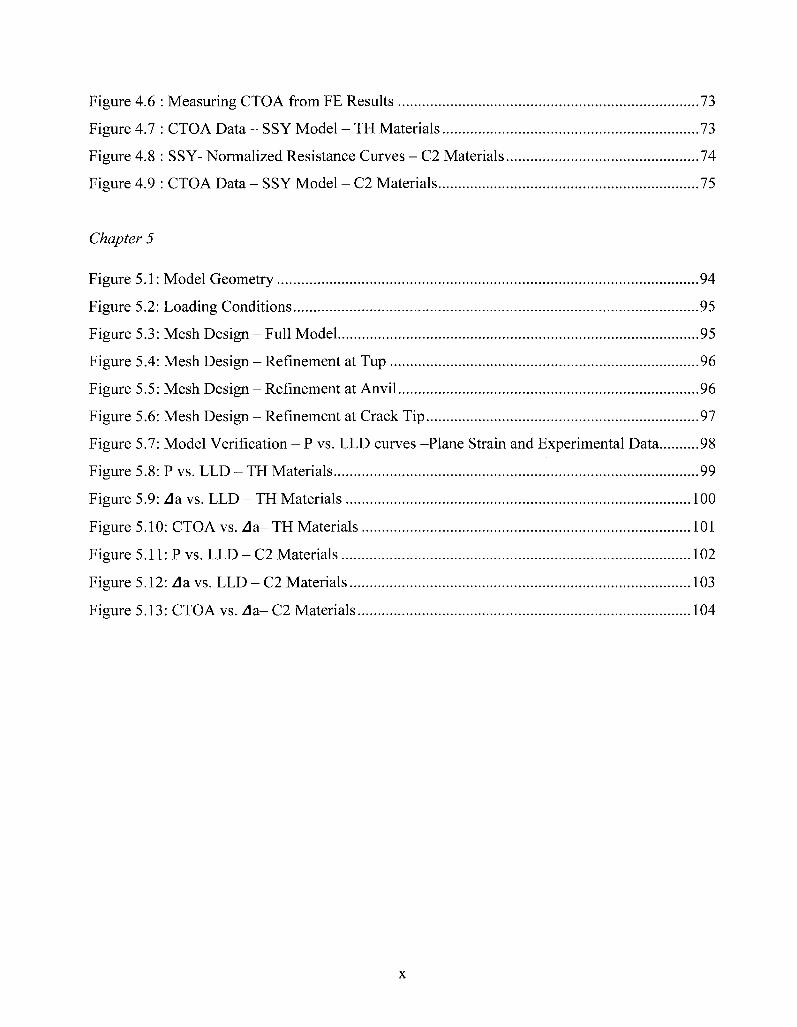
Figure 4.6 : Measuring CTOA from FE Results 73

Figure 4.7 : CTOA Data - SSY Model - TH Materials 73

Figure 4.8 : SSY- Normalized Resistance Curves - C2 Materials 74

Figure 4.9 : CTOA Data - SSY Model - C2 Materials 75

Chapter 5

Figure 5.1: Model Geometry 94

Figure 5.2: Loading Conditions 95

Figure 5.3: Mesh Design - Full Model 95

Figure 5.4: Mesh Design - Refinement at Tup 96

Figure 5.5: Mesh Design - Refinement at Anvil 96

Figure 5.6: Mesh Design - Refinement at Crack Tip 97

Figure 5.7: Model Verification - P vs. LLD curves -Plane Strain and Experimental Data 98

Figure 5.8: P vs. LLD - TH Materials 99

Figure 5.9: Aa vs. LLD - TH Materials 100

Figure 5.10: CTOA vs. Aa- TH Materials 101

Figure 5.11: P vs. LLD - C2 Materials 102

Figure 5.12: Aa vs. LLD - C2 Materials 103

Figure 5.13: CTOA vs. Aa- C2 Materials 104

x

Page 11

Nomenclature

a: crack length

a0: initial crack length

A0: radius of the small-scale yielding model

b: length of the remaining ligament

B: thickness of specimen

Bo: twice the length of cohesive zone

CTOA: crack-tip opening angle

CTOAc: critical crack-tip opening angle

CTOAss: crack-tip opening angle during steady-state crack propagation

CTOD: crack-tip opening displacement

CVN: Charpy V-notch energy

CZM: Cohesive Zone Model

D: damage function

DWTT: drop-weight tear test

E: Young's Modulus

F: force

G, \i: Shear Modulus

(5: Griffith criterion for crack advance

Kn: stiffness of cohesive elements (i = n,s,t)

Kr: applied stress intensity factor

K0: critical stress intensity factor

LLD: load-line displacement

n: strain-hardening exponent of power-law stress-strain representation (defined by El290-2)

N: strain-hardening exponent of Ramburg-Osgood stress-strain representation (N=l/n)

P:load

R0: estimated plastic zone size

rp: plastic rotation factor

S: span between two load points

SE(B): single-edge bend specimen

S-SSM: simplified single-specimen method for measuring CTOA

xi

Page 12

T, T(8): traction, traction as a function of separation

T0 or a: maximum or peak traction

ux,uy: Displacement in the x and y directions

W: width of specimen

6: separation

Sc: critical separation, (D = 1.0, T = 0)

So', separation that induces damage

S™aXm- maximum effective separation attained during the complete loading history of the element

A0: the length of the smallest elastic-plastic elements adjacent to the cohesive layer

e: strain

oy: yield stress, 0.2% proof strength at the temperature of the fracture test

v: Poisson's ratio

ro: fracture energy/ work of separation - (Expressed in MPa-mm, equivalent to kJ/m2)

rr: crack growth resistance

xn

Page 13

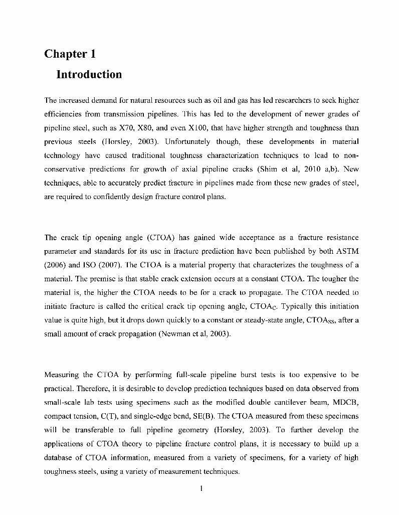
Chapter 1

Introduction

The increased demand for natural resources such as oil and gas has led researchers to seek higher

efficiencies from transmission pipelines. This has led to the development of newer grades of

pipeline steel, such as X70, X80, and even XI00, that have higher strength and toughness than

previous steels (Horsley, 2003). Unfortunately though, these developments in material

technology have caused traditional toughness characterization techniques to lead to non-

conservative predictions for growth of axial pipeline cracks (Shim et al, 2010 a,b). New

techniques, able to accurately predict fracture in pipelines made from these new grades of steel,

are required to confidently design fracture control plans.

The crack tip opening angle (CTOA) has gained wide acceptance as a fracture resistance

parameter and standards for its use in fracture prediction have been published by both ASTM

(2006) and ISO (2007). The CTOA is a material property that characterizes the toughness of a

material. The premise is that stable crack extension occurs at a constant CTOA. The tougher the

material is, the higher the CTOA needs to be for a crack to propagate. The CTOA needed to

initiate fracture is called the critical crack tip opening angle, CTOAc. Typically this initiation

value is quite high, but it drops down quickly to a constant or steady-state angle, CTOAss, after a

small amount of crack propagation (Newman et al, 2003).

Measuring the CTOA by performing full-scale pipeline burst tests is too expensive to be

practical. Therefore, it is desirable to develop prediction techniques based on data observed from

small-scale lab tests using specimens such as the modified double cantilever beam, MDCB,

compact tension, C(T), and single-edge bend, SE(B). The CTOA measured from these specimens

will be transferable to full pipeline geometry (Horsley, 2003). To further develop the

applications of CTOA theory to pipeline fracture control plans, it is necessary to build up a

database of CTOA information, measured from a variety of specimens, for a variety of high

toughness steels, using a variety of measurement techniques.

1

Page 14

There are many techniques for measuring the CTOA, both experimentally and numerically. In

this thesis, finite element analyses were performed to numerically measure the CTOA for two

different high strength, high toughness, steels. The first steel is referred to as a TH steel, as it is

an ideal steel with properties defined by Tvergaard and Hutchinson (1992). The second steel is a

real material, referred to as a C2 steel. This pipeline steel was characterized by Xu (2010a). An

experimental drop-weight tear test was performed using this C2 steel. Load vs. load-line

displacement and CTOA data, measured using optical techniques and the simplified single-

specimen method (Xu et al, 2007), were provided for comparison to the numerical results of the

DWTT simulations conducted in this thesis.

The main focus of this thesis is to explore the determination of CTOA using cohesive zone (CZ)

models. A CZ model uses a thin layer of cohesive elements along the crack path. These cohesive

elements are typically governed by a traction vs. separation (TS) law that defines the element's

load transferring capability based on the separation, or strain, of the element. Each element has a

peak stress, or traction, that decreases to zero as the element reaches a critical separation. When a

cohesive element's load transferring capability is reduced to zero, it is said to have failed. This

allows the crack to propagate. Various shapes of TS laws have been proposed but bilinear TS

laws were chosen for this thesis. Abaqus/Explicit (2008) is used to perform the cohesive zone

modeling in this thesis.

The first step of this thesis was to verify the chosen traction-separation laws through analysis of a

unit cell in Abaqus. A total of seven bilinear TS laws were considered, with four used to model

the TH material, and three used to model the C2 material. The four TH cases were modeled after

those defined by Tvergaard and Hutchinson. Each TS law had different peak tractions and

fracture toughnesses.

Following this verification, a small-scale yielding model was used to measure how changes to

the peak traction and fracture energy changed the macroscopic response of a model when the

2

Page 15

elastic-plastic material parameters were held constant. This was done by modeling with four

different TS laws for the TH material, and three different TS laws for the C2 material. Resistance

curves were generated for all seven cases, and the TH cases were compared to the data published

by Tvergaard and Hutchinson. CTOA data was also measured for all seven cases.

Finally, drop-weight tear tests were simulated using the TH and C2 material sets. The fracture

resistance and crack propagation was observed by generating load vs. load-line displacement and

crack length vs. load-line displacement curves. The load-line displacement curves generated

from the three C2 simulations were compared with the experimental observations provided by

Xu (2010a). CTOA data from the DWTT simulations were compared to CTOA data from the

SSY simulations. CTOA data from the C2 DWTT simulations were compared to the

experimental observations of Xu et al (2010b).

1.1 Thesis Outline

The objective of this thesis is to conduct finite element simulations of ductile crack propagation

for a wide range of high strength pipeline steels (four TH steels, three C2 steels). The specimens

analyzed include SSY and DWTT specimens. The fracture resistance curves and CTOA values

are obtained. It is shown that cohesive zone models can be successfully used to simulate ductile

crack propagation and to numerically measure CTOAs. The CTOAs are found to be transferable

between the SSY and DWTT specimens. The CTOAs are comparable to experimentally obtained

values.

Chapter 2 provides a review of the theory behind the crack tip opening angle and the cohesive

zone model, as well as the experimental techniques. The theory of cohesive zone elements, as

well as verification of Abaqus cohesive elements is presented in Chapter 3. Chapter 4 details the

results of small-scale yielding simulations performed to test the finite element techniques.

Chapter 5 documents the results of DWTT simulations of the TH and C2 materials, and provides

3

Page 16

comparisons of CTOA data between materials and specimens, as well as direct comparison of

the CTOA measured from the model to experimental observations for the C2 steel.

Page 17

Chapter 2

Background and Literature Review

This chapter will introduce the crack tip opening angle (CTOA), a fracture parameter that has

been widely accepted to provide superior prediction capabilities than traditional techniques.

Following this, cohesive zone modeling (CZM) will be described as a technique for simulating

crack propagation and numerically predicting the CTOA. Finally, the methods used to gather the

experimental data that will be used to verify the finite element results will be documented.

2.1 Crack Tip Opening Angle

The development of newer grades of pipeline steel, that have higher strength and toughness, was

required to increase the efficiency of pipelines, and improve their reliability. These developments

have reduced the accuracy of traditional elastic-plastic fracture mechanics techniques and in

many cases have led to non-conservative predictions for growth of axial pipeline cracks (Shim et

al, 2010 a,b; Horsley, 2003).

The Charpy test has traditionally been used to characterize the toughness of a material. The

Charpy V-notch energy (CVN) is then typically used in semi-empirical models to predict

minimum arrest toughness to prevent unstable fracture. The Charpy specimen though has some

key deficiencies that degrade its prediction abilities for high toughness steels (Shim, 2010a).

First, the blunt notch causes resistance data to include energy from crack initiation as well as

crack propagation. Secondly, the specimen is usually smaller than the full thickness of a pipeline

and toughness has been found to relate to thickness. Additionally, the length of the fracture

ligament is not long enough to reach steady-state fracture and fracture resistance has been shown

to vary with crack length. Finally, for many of the higher toughness steels, Charpy samples are

only incompletely fractured, as in Figure 2.1 (Xu et al, 2004). It is for these reasons that the

drop-weight tear test (DWTT) has been proposed as an alternative method to characterize

5

Page 18

fracture resistance for new grades of ductile steels. Experimental data from this technique will be

used to validate the numerical modeling results in Chapter 5.

A traditional method for predicting full-scale pipeline fracture speed and minimum arrest

toughness is called the Battelle Two-Curve Method (TCM) (Maxey et al, 1976). The TCM

empirically combines the influence of factors including the material fracture toughness, gas

decompression behaviour, and backfill conditions. Traditionally this method relies on fracture

resistance R, a constant material property. Researchers at TransCanada PipeLines Limited and

Engineering Mechanics Corporation of Columbus (Shim et al, 2010, a,b) have concluded though

that this method is inadequate and have made attempts to modify and improve the method by

instead using a speed dependent fracture resistance in order to apply it to newer, tougher, grades

of pipeline steel. This is still an empirical method and relies on the ability to accurately produce

resistance curves that correspond to the real world application.

The crack tip opening angle, proposed by Rice and Sorensen (1978), has been proposed as an

alternative to these previous techniques to characterize fracture resistance. The CTOA has been

approved by the International Standards Organization to quantify the resistance to stable crack

extension in ISO 22889 (2007). The CTOA is also approved by ASTM International as a method

for determining fracture resistance in ASTM E2472 (2006). It is believed that the CTOA

measured during stable or steady-state crack propagation is a material property. Therefore, the

steady-state CTOA measured during a lab test, a drop-weight tear test (DWTT) for example,

should be transferrable to a simulation of crack propagation in a full-scale pipeline.

There are several techniques commonly used for measuring the CTOA, both experimentally and

numerically. These include, but are not limited to, optical microscopy, digital image correlation,

microtopography, and calculation from finite element results (ISO, 2007). In the current work,

CTOAs will be calculated from finite element results of small-scale yielding and drop-weight

tear test simulations using a method outlined in Section 4.2.2. For the DWTT simulations in

6

Page 19

Chapter 5, the CTOAs calculated from finite element results will be compared to reported

CTOAs that were determined using digital image correlation, as well as a method called the

simplified single-specimen method developed by Xu et al (2007). These measurement techniques

will be outlined in Section 2.3.3. The steady-state CTOAs determined from the two different

models (SSY and DWTT) will be compared, and the feasibility of using cohesive zone modeling

to predict reliable steady-state CTOAs will be discussed in Chapter 5.

2.2 Cohesive Zone Modeling

2.2.1 Introduction of Concepts

The idea of a cohesive layer at a crack tip was originally introduced by Dugdale (1960) and

Barenblatt (1962). Since its introduction, the field on cohesive zone modeling has since grown in

popularity and is now being used in civil, aerospace, and mechanical engineering applications.

Recently there have been many groups researching the use of CZM to predict crack growth in

thin sheets for applications such as aircraft fuselage and oil and natural gas transmission

pipelines including Keller et al (1999), Chen et al (2003), Chandra et al (2002), Elices et al

(2002), Cornec et al (2003), de Borst (2003), and Scheider and Brocks (2006).

The CZM was originally proposed as a phenomenological approach to model brittle fracture by

assigning a degradation vs. separation law to a process zone along the crack front. In the real

world, ductile fracture occurs through void initiation, growth, and coalescence. By assigning a

cohesive or Traction-Separation (TS) law to a layer of cohesive elements this ductile fracture

process can be modeled by performing a finite element analysis. A diagram representing this

process can be found in Figure 2.2 (Cornec, 2003). Here, T(5) represents the traction, T, vs.

separation, S, A a represents the crack growth, and the subscripts N, S, and 0 respectively

represent normal, shear, and critical values of traction and separation.

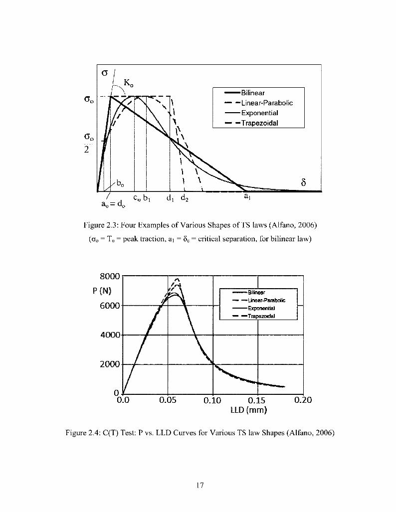
A TS law is a progressive damage model that defines the maximum traction based on the

separation or strain history of the element. The shape of the TS law can vary depending on the

7

Page 20

application and researchers' methodology. Four examples of TS laws can be found in Figure 2.3

(Alfano, 2006). These include bilinear, linear-parabolic, exponential, and trapezoidal laws.

Regardless of the shape, TS laws all have some important features in common:

• An initial stiffness curve for 8 < S0,

• A portion of increasing damage and reduced ability to transfer loading (reduced traction)

beginning at initiation point <50; and

• A final separation value, 8C, after which ability to transfer loading has been completely

removed (T=0).

The three defining parameters are the maximum cohesive strength, a0 or T0, the final separation,

5C; and the work of separation, T0, which is represented by the area under the curve. While

initially some authors, including Tvergaard and Hutchinson (1992), found minimal influence of

the shape, more extensive studies carried out by Chandra et al (2002), Cornec et al (2003) and

Alfano (2006) have determined that the shape of the TS law plays an important role in

determining the macroscopic results of the fracture process. Figure 2.4 (Alfano, 2006) shows

how the four TS shapes defined in Figure 2.3 affect the load vs. displacement curves of a C(T)

specimen. While all four TS laws have the same peak traction and work of separation, the peak

load predicted in the C(T) specimens varies between laws. This work highlights the importance

of choosing a consistent TS law, and modeling with it in various geometries to fully understand

its properties. In the present work, only the bilinear shape will be used.

TS Laws as They Relate to EPFM

The first authors to apply the CZM to ductile fracture were Tvergaard and Hutchinson (1992).

They demonstrated the ability of cohesive zone models (CZMs) to predict resistance curves for

plane strain, mode I crack growth in small-scale yielding (SSY). This work was an important

first step towards developing CZMs that can be used for predictive purposes in design using

ductile materials. The TS law proposed by Tvergaard and Hutchinson was a trapezoidal law, as

seen in Figure 2.5 (Tvergaard and Hutchinson, 1992).

8

Page 21

It is possible to relate the traction-separation laws to classical fracture mechanics. The Griffith

criterion for crack advance, ©, is equal to the crack growth resistance, TR(Ad):

© = Tr(Aa) (2.1)

under conditions of small-scale yielding, where the growth resistance varies with the crack

extension due to the changing plastic zone. This can be related to the stress intensity factor, K, at

the crack tip by:

(5 = ( J ~ /V (2-2)

where v is Poisson's ratio, E is Young's modulus, and K=Kr(Aa), the stress intensity at the crack

tip as a function of crack length. The stress-intensity factor at the crack tip can now be directly

related to the crack growth resistance by:

"-- IcS) (2J)

Therefore, the critical stress intensity factor, Ko, that will cause the crack to initiate for a

particular TS law can be found by:

K° - l u ^ <2-4)

For a trapezoidal separation law the work of separation per unit area, T0, can be written as:

9

Page 22

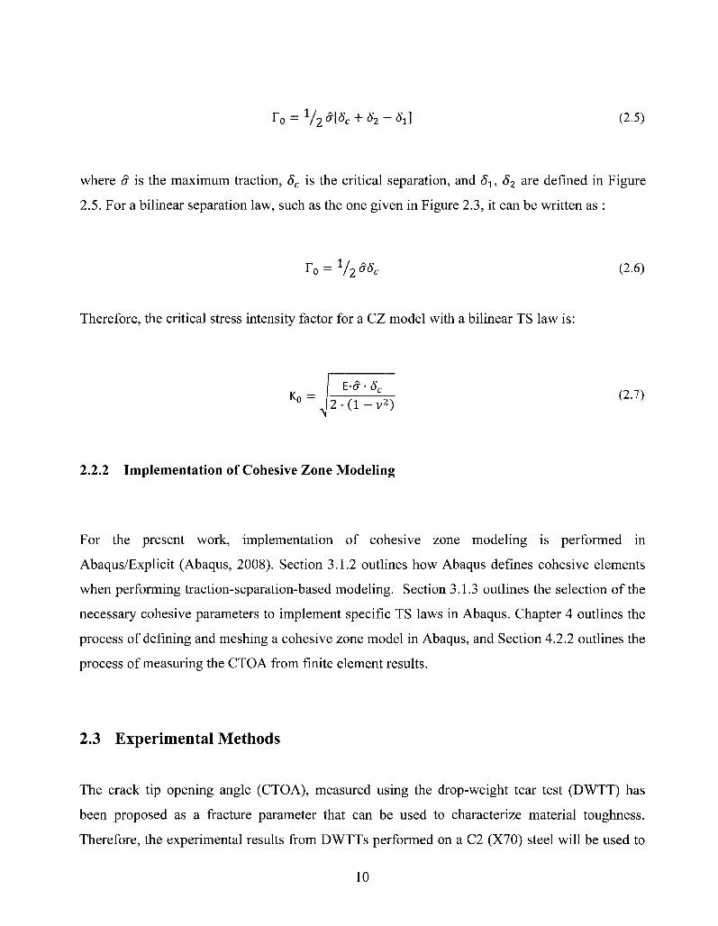
T0 = 1/2a[Sc + S2-S1] (2.5)

where a is the maximum traction, 8C is the critical separation, and 81, S2 are defined in Figure

2.5. For a bilinear separation law, such as the one given in Figure 2.3, it can be written as :

T0 = 1/2aSc (2.6)

Therefore, the critical stress intensity factor for a CZ model with a bilinear TS law is:

«•- k%^>

2.2.2 Implementation of Cohesive Zone Modeling

For the present work, implementation of cohesive zone modeling is performed in

Abaqus/Explicit (Abaqus, 2008). Section 3.1.2 outlines how Abaqus defines cohesive elements

when performing traction-separation-based modeling. Section 3.1.3 outlines the selection of the

necessary cohesive parameters to implement specific TS laws in Abaqus. Chapter 4 outlines the

process of defining and meshing a cohesive zone model in Abaqus, and Section 4.2.2 outlines the

process of measuring the CTOA from finite element results.

2.3 Experimental Methods

The crack tip opening angle (CTOA), measured using the drop-weight tear test (DWTT) has

been proposed as a fracture parameter that can be used to characterize material toughness.

Therefore, the experimental results from DWTTs performed on a C2 (X70) steel will be used to

10

Page 23

verify and calibrate finite element results. Here, the DWTT model is introduced and

experimental procedures for obtaining the crack tip opening angle and other experimental data

are outlined.

2.3.1 The DWTT Specimen

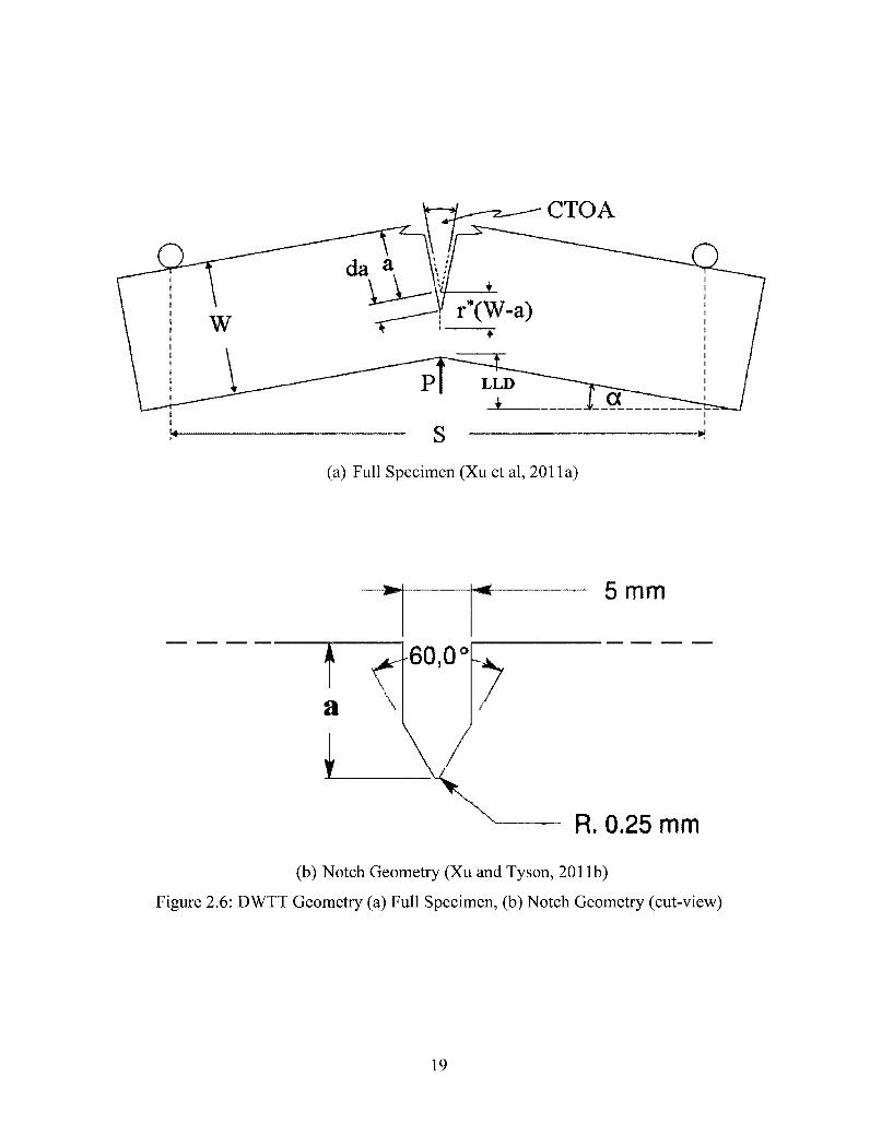
The drop-weight tear test specimen is special case of a single-edge bend specimen (SE(B)).

General geometry for the DWTT specimen is found in Figure 2.6 (a) (Xu et al, 2011a). Two

anvils are used to support the specimen while a 'tup' is used to apply a load to the centerline

opposite the notch. The DWTT specimen had a width, W, of 76.2 mm, span between anvils, S, of

250.4 mm, thickness, B, of 13.7 mm. Typical notch geometry can be seen in Figure 2.6 (b) (Xu

and Tyson, 2011b). The depth of the notch can vary from specimen to specimen depending on

the researcher's preference and can range from 10-38 mm.

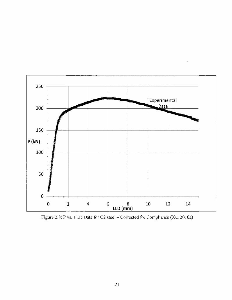
An experimental quasi-static DWTT was performed by Xu from CANMET-MTL (Xu, 2010a),

and load vs. load-line displacement data was provided to verify the modeling performed in this

work. The experiment performed by Xu had an original notch depth, a, of 14.7 mm. The

specimen was a C2 (X70) steel, and was flattened from a pipeline section. The specimen was

machined from the pipe so the crack would grow in what was the axial direction of the pipe.

2.3.2 Experimental Setup and Data Collection

The quasi-static test set-up for measuring CTOA from a DWTT specimen can be seen in Figure

2.7 (Xu et al, 2010b). Along the bottom are the two anvils used to support the specimen. The

load is applied to the center of the specimen at the top by the 'tup'. There are anti-buckling plates

to ensure the specimen remains in-plane.

The applied load is determined by measuring the reaction force due to the displacement applied

by the 'tup'. The load-line displacement is measured as the displacement of the loading jig. This

is a potential source of error however, as there will be elastic compression in the fixture, and

11

Page 24

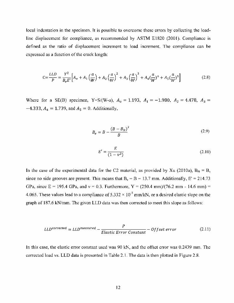
local indentation in the specimen. It is possible to overcome these errors by collecting the load-

line displacement for compliance, as recommended by ASTM El820 (2001). Compliance is

defined as the ratio of displacement increment to load increment. The compliance can be

expressed as a function of the crack length:

C= LLD Y2 \ . fa\ , c u 2 / a x

3 . . . . . . - 5

BeE' / d\ / a \^ / a \ J a . a

A°+AAW)+A^W) + ^ y +A^ +A^ (2.8)

Where for a SE(B) specimen, Y=S/(W-a), A0 = 1.193, Ax = -1.980, A2 = 4.478, A3 =

-4 .333, A4 = 1.739, andA5 = 0. Additionally,

5 _ ( B - ^ v ) 2 ( 2 9 )

6 B

E' = T, K (2-10) (1 - v2)

In the case of the experimental data for the C2 material, as provided by Xu (2010a), BN = B,

since no side grooves are present. This means that Be = B = 13.7 mm. Additionally, E' = 214.73

GPa, since E = 195.4 GPa, and v = 0.3. Furthermore, Y = (250.4 mm)/(76.2 mm - 14.6 mm) =

4.065. These values lead to a compliance of 5.332 x 10"3 mm/kN, or a desired elastic slope on the

graph of 187.6 kN/mm. The given LLD data was then corrected to meet this slope as follows:

L L £ )corrected _ LLDmeasured Offset error (2.11)

Elastic Error Constant

In this case, the elastic error constant used was 90 kN, and the offset error was 0.2439 mm. The

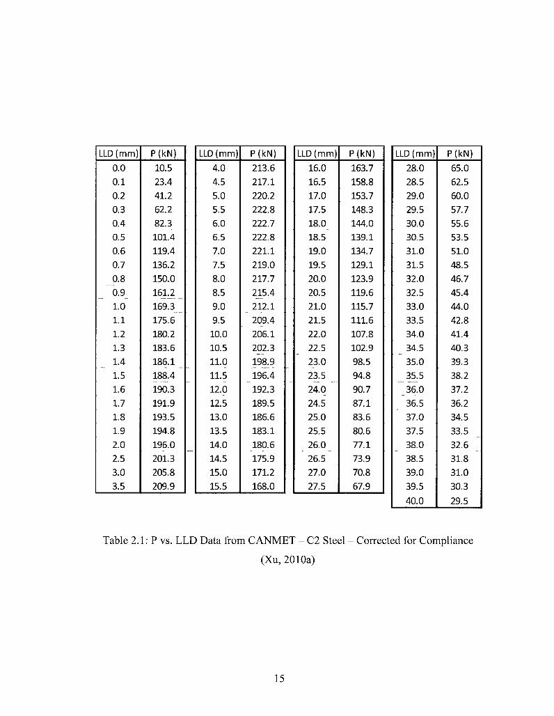
corrected load vs. LLD data is presented in Table 2.1. The data is then plotted in Figure 2.8.

12

Page 25

2.3.3 Measuring the Crack Tip Opening Angle

There have been many experimental techniques proposed for measuring the CTOA, each with

their own advantages and drawbacks. The methods that will be discussed here are direct or

optical measurement and the simplified single-specimen method. Theory relating the CTOA to

other toughness parameters will also be discussed.

Measuring CTOA Using Optical Techniques

The most common optical technique for measuring the CTOA is direct surface measurement. It

is typically difficult to accurately identify the crack tip when performing direct surface

measurement so a method has been developed that does not require identification of the exact

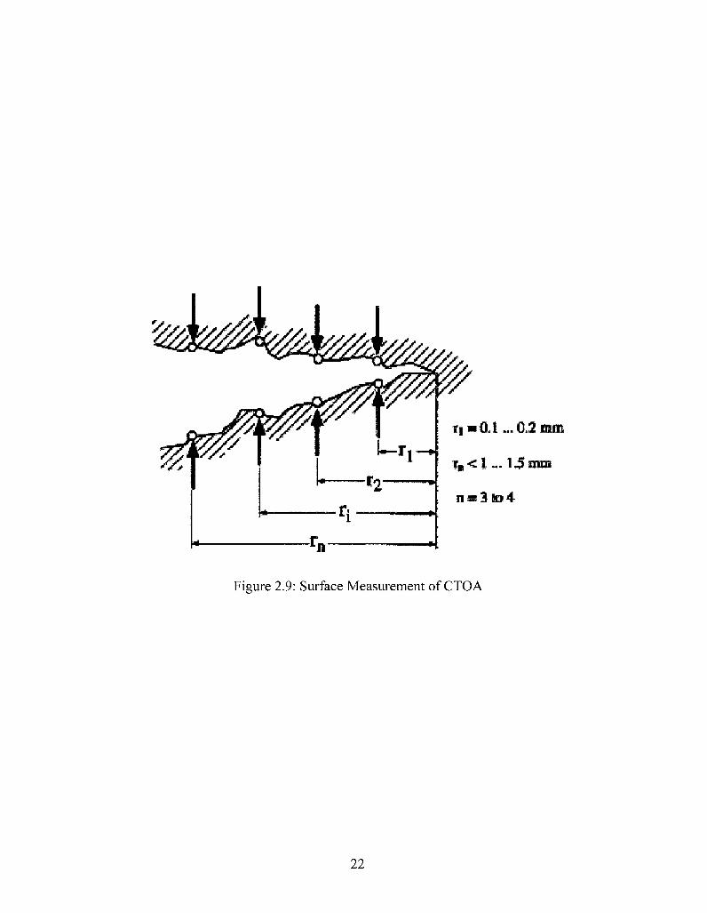
crack tip. The method requires finding the average of 3-5 four point measurements of CTOA by

determining the angle between the lines created by joining two points on the upper and lower

surfaces. A set of points at an original reference is used with 3-5 other pairs of points all within

0.5 - 1.5 mm behind the estimated crack tip. Figure 2.9 demonstrates the technique. This

averaging technique helps to minimize discrepancies in results when measuring the CTOA for

wavy crack flanks, as seen in Figure 2.10 (Xu et al, 2008).

It is agreed that the CTOA measured by direct surface measurement is higher than the CTOA

that would be at the mid-plane of the specimen. This is due to the three-dimensional nature of the

crack propagation (crack tunnelling effect, flat-to-shear transition, etc.).

Measuring CTOA with the Simplified Single-Specimen Method

A method for calculating the CTOA from DWTT specimens has been proposed by Xu et al

(2007). It is called the simplified single-specimen method (S-SSM), and was been adapted from

the single-specimen method proposed by Martinelli and Venzi (1996). The S-SSM proposes that

the CTOA for a DWTT specimen can be calculated as follows:

13

Page 26

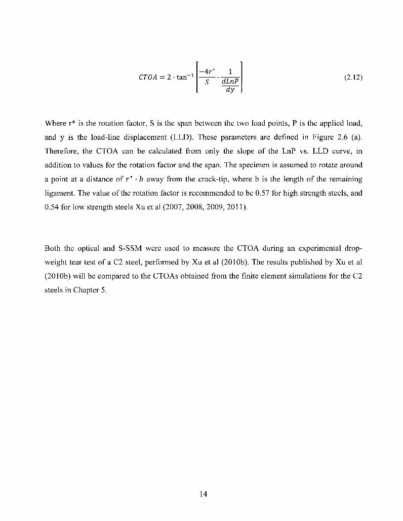
CTOA = 2 • tan - 1

S dLnP dy

Where r* is the rotation factor, S is the span between the two load points, P is the applied load,

and y is the load-line displacement (LLD). These parameters are defined in Figure 2.6 (a).

Therefore, the CTOA can be calculated from only the slope of the LnP vs. LLD curve, in

addition to values for the rotation factor and the span. The specimen is assumed to rotate around

a point at a distance of r* • b away from the crack-tip, where b is the length of the remaining

ligament. The value of the rotation factor is recommended to be 0.57 for high strength steels, and

0.54 for low strength steels Xu et al (2007, 2008, 2009, 2011).

Both the optical and S-SSM were used to measure the CTOA during an experimental drop-

weight tear test of a C2 steel, performed by Xu et al (2010b). The results published by Xu et al

(2010b) will be compared to the CTOAs obtained from the finite element simulations for the C2

steels in Chapter 5.

14

Page 27

LLD (mm)

16.0 16.5 17.0 17.5 18.0 18.5 19.0 19.5 20.0 20.5 21.0 21.5 22.0 22.5 23.0 23.5 24.0 24.5 25.0 25.5 26.0 26.5 27.0 27.5

P(kN) 163.7 158.8 153.7 148.3 144.0 139.1 134.7 129.1 123.9 119.6 115.7 111.6 107.8 102.9 98.5 94.8 90.7 87.1 83.6 80.6 77.1 73.9 70.8 67.9

LLD (mm)

0.0 0.1 0.2 0.3 0.4 0.5 0.6 0.7 0.8 0.9 1.0 1.1 1.2 1.3 1.4 1.5 1.6 1.7 1.8 1.9 2.0 2.5 3.0 3.5

P(kN)

10.5 23.4 41.2 62.2 82.3 101.4 119.4 136.2 150.0 161.2 169.3 175.6 180.2 183.6 186.1 188.4 190.3 191.9 193.5 194.8 196.0 201.3 205.8 209.9

LLD (mm)

4.0 4.5 5.0 5.5 6.0 6.5 7.0 7.5 8.0 8.5 9.0 9.5 10.0 10.5 11.0 11.5 12.0 12.5 13.0 13.5 14.0 14.5 15.0 15.5

P(kN)

213.6 217.1 220.2 222.8 222.7 222.8 221.1 219.0 217.7 215.4 212.1 209.4 206.1 202.3 198.9 196.4 192.3 189.5 186.6 183.1 180.6 175.9 171.2 168.0

LLD (mm)

28.0 28.5 29.0 29.5 30.0 30.5 31.0 31.5 32.0 32.5 33.0 33.5 34.0 34.5 35.0 35.5 36.0 36.5 37.0 37.5 38.0 38.5 39.0 39.5

40.0

P(kN)

65.0 62.5 60.0 57.7 55.6 53.5 51.0 48.5 46.7 45.4 44.0 42.8 41.4 40.3 39.3 38.2 37.2 36.2 34.5 33.5 32.6 31.8 31.0 30.3

29.5

Table 2.1: P vs. LLD Data from CANMET - C2 Steel - Corrected for Compliance

(Xu, 2010a)

15

Page 28

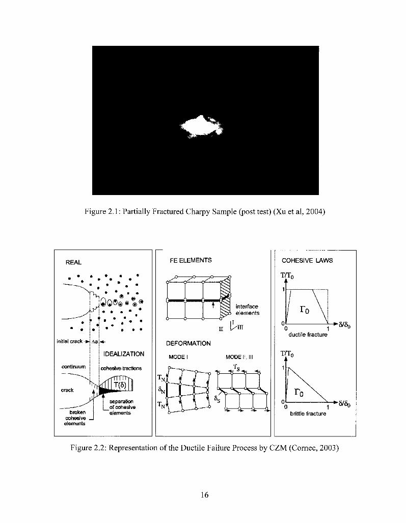
Figure 2.1: Partially Fractured Charpy Sample (post test) (Xu et al, 2004)

REAL

® Qo®®i ®<* * • • . • •

initial crack -»-: Aa .-+-

continuum

IDEALIZATION

cohesive tractions

broken cohesive elements

separation of cohesive elements

FE ELEMENTS

f^f^f^M 0 0

interface elements

DEFORMATION

MODE I

ra

MODE I

l 3 - ^ - ^ * ^ f c

7V—^V-^V—\

^r—^r-^r-^.

COHESIVE LAWS

T/T,

^ 5 / 5 o ductile fracture

T/T,

V^5/5o brittle fracture

Figure 2.2: Representation of the Ductile Failure Process by CZM (Cornec, 2003)

16

Page 29

Bilinear — —Linear-Parabolic

Exponential — —Trapezoidal

Figure 2.3: Four Examples of Various Shapes of TS laws (Alfano, 2006)

(a0 = T0 = peak traction, ai = 5C = critical separation, for bilinear law)

8000

P(N)

6000

4000

2000

— — Trapezoidal

0.10 0.15 LLD (mm)

0.20

Figure 2.4: C(T) Test: P vs. LLD Curves for Various TS law Shapes (Alfano, 2006)

17

Page 30

a ••

c ad6 l O

6 C "1 ~2

Figure 2.5: Trapezoidal Traction-Separation Law (Tvergaard and Huchinson, 1992)

(° = T0)

18

Page 31

CTOA

(a) Full Specimen (Xu et al, 201 la)

5 mm

T

a c 60,0

7

FL 0,25 mm

(b) Notch Geometry (Xu and Tyson, 201 lb)

Figure 2.6: DWTT Geometry (a) Full Specimen, (b) Notch Geometry (cut-view)

19

Page 32

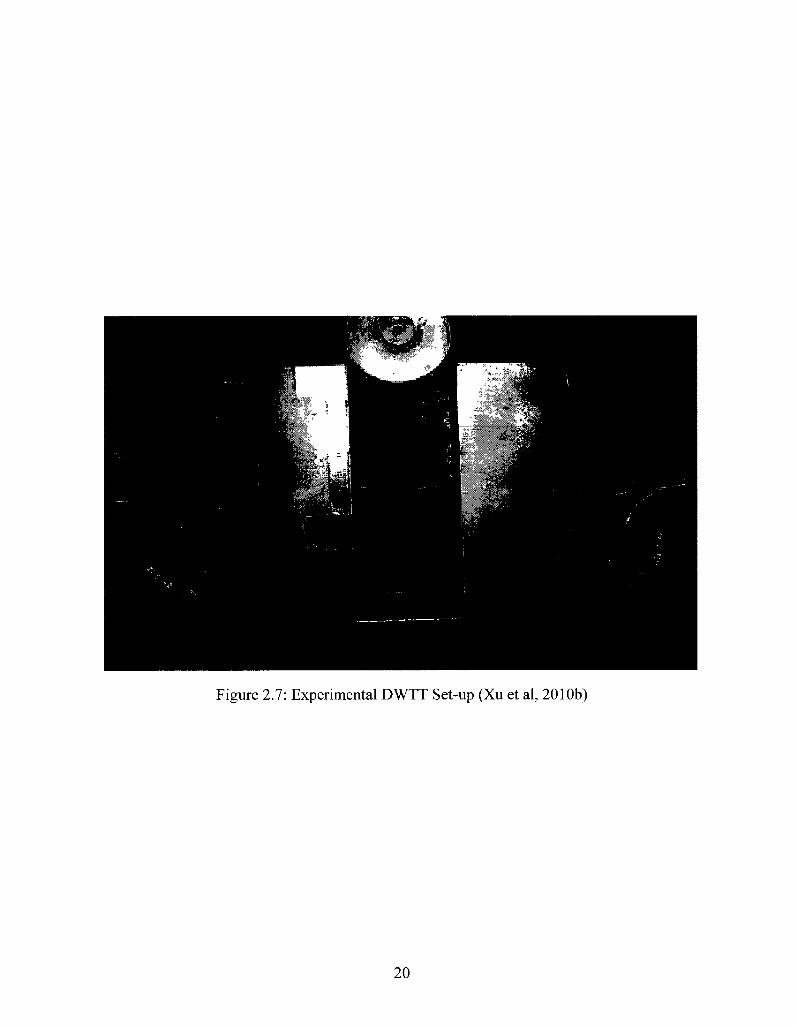
Figure 2.7: Experimental DWTT Set-up (Xu et al, 2010b)

20

Page 33

250

200

150

P(kN)

100

50

0

-

w

' i

1 1 1

Experime Hfe^Data

ntal

0 6 8 LLD (mm)

10 12 14

Figure 2.8: P vs. LLD Data for C2 steel - Corrected for Compliance (Xu, 2010a)

21

Page 34

f j m(kl... 0,2 mm

? , < ! . . . 1,5 mm

n = 3 BD4

Figure 2.9: Surface Measurement of CTOA

22

Page 35

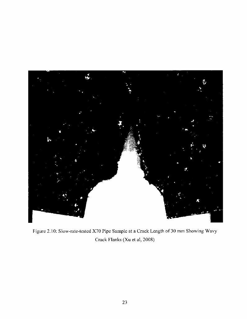
Figure 2.10: Slow-rate-tested X70 Pipe Sample at a Crack Length of 30 mm Showing Wavy

Crack Flanks (Xu et al, 2008)

23

Page 36

Chapter 3

Finite Element Implementation of Cohesive Zone

Modeling

This chapter will discuss the implementation of cohesive zone modeling (CZM) in Abaqus

(2008) using finite element techniques. The process of defining model parameters will be

outlined and analysis of a unit cell is performed to validate the theory.

3.1 Finite Element Implementation of CZM

A cohesive element is a type of finite element that has a built-in damage evolution law. The

cohesive element will have an elastic response until subjected to certain maximum damage

criteria. Once the damage criterion has been met, the element stiffness will degrade based on

some damage evolution law, as defined by the user. A cohesive zone model uses a layer of

cohesive elements to model separation of two parts. To predict fracture, it is possible to imagine

an infmitesimally thin layer of cohesive elements along the crack path that fail sequentially as

the crack grows.

3.1.1 Cohesive Zone Model

It is possible to use Abaqus to perform cohesive zone modeling. Various cohesive element

definitions exist in both Abaqus/Standard and Abaqus/Explicit for both two-dimensional

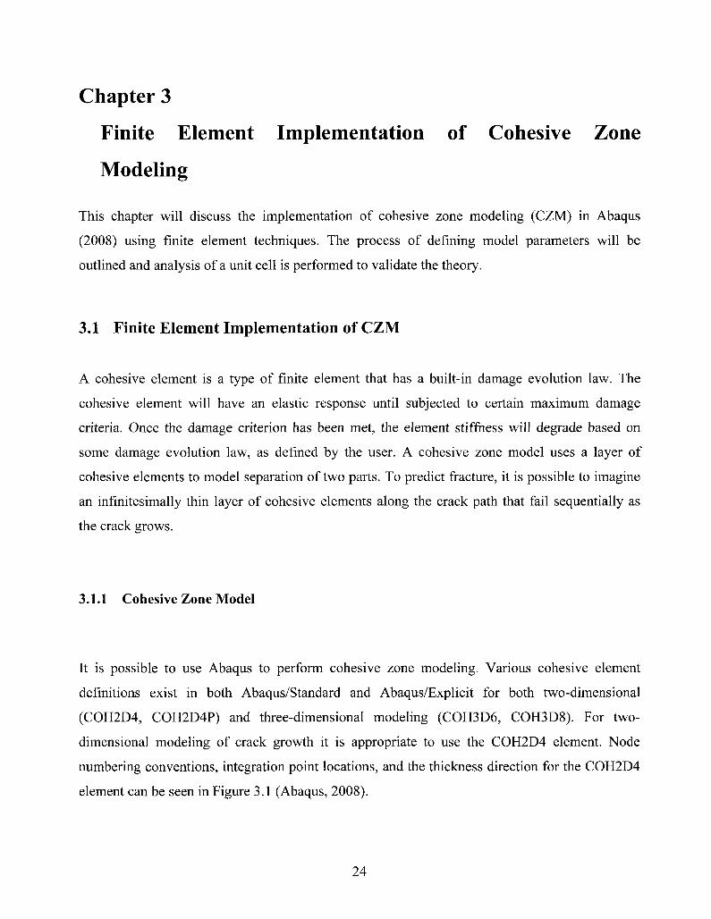
(COH2D4, COH2D4P) and three-dimensional modeling (COH3D6, COH3D8). For two-

dimensional modeling of crack growth it is appropriate to use the COH2D4 element. Node

numbering conventions, integration point locations, and the thickness direction for the COH2D4

element can be seen in Figure 3.1 (Abaqus, 2008).

24

Page 37

Typical uses of cohesive elements in Abaqus are continuum-based modeling, traction-separation-

based modeling, and modeling of gaskets or laterally unconstrained adhesive patches.

Continuum-based modeling would be used for situations where two parts are bonded together by

an adhesive layer of some finite thickness. Traction-separation-based modeling would be used

for situations where the interface between two parts can be considered to have zero thickness.

The response of gaskets can be modeled assuming a uniaxial stress state and requires only

macroscopic properties like material strength and stiffness. When modeling crack growth along a

known crack path, it is recommended to use a traction-separation-based approach using a layer

of cohesive elements along the crack path of close to zero-thickness (Abaqus, 2008).

Figure 3.2 (Abaqus, 2008) shows a typical design for a cohesive zone model. The model is

divided into three separate parts, each meshed independently and constrained to act as one part.

A thin layer of cohesive elements is connected to the surrounding parts using tie constraints that

cause the entire assembly to act as one structure. Parts 1 and 2 are meshed using continuum

elements with a built in elastic-plastic response. This type of model would allow a crack to grow

through the cohesive layer as the cohesive elements fail. A similar approach will be used and

described in Chapters 4 and 5 to predict crack growth in small-scale yielding and DWTT models.

Further meshing considerations will be discussed in Chapter 4.

3.1.2 Traction-Separation-Based Modeling

Traction-separation-based modeling allows the user to define a progressive degradation law that

defines the stiffness of cohesive element based on some damage evolution process which is

controlled by the element's built in damage variable, D. A typical bilinear traction-separation

(TS) law is defined in Figure 3.3.

There are three important values on the traction-separation curve that must be defined:

25

Page 38

• t° is the peak traction, or maximum normal stress that the element can resist without

damage. Damage initiates at ol — t°

• 5i is the separation that causes damage to initiate, damage D = 0

• 8t is the separation where damage D = 1, and the element's ability to transfer loading is

completely eliminated, (tt = 0 when 8t > 8t and D > 1)

The built-in traction-separation models in Abaqus (2008) assume an initial linear elastic portion,

followed by initiation of damage at some maximum traction and a progressive degradation of

stiffness based on a defined damage evolution process.

Linear Elastic Behaviour

The initial elastic behaviour of a cohesive element is defined as

Knn Kns ^nt\ (£n

Kns Kss Kst

Knt Kst Ktt

KE (3.1)

where t is the element's traction, K is the stiffness, and s is strain. The subscripts n, s, and t

represent the normal, shear and tangential directions respectively. Nominal strains are defined as

zr, i' = n ,s , t (3.2)

where St represents the element separation, and T0 represents the initial thickness of the cohesive

element, usually defined as equal to 1.0 regardless of element geometry so that the strains in each

direction are equal to the separations in that direction.

When using uncoupled traction-separation laws, as will always be the case in this thesis, it is

only required to define Knn, Kss, and Ktt as the strain in one direction has no effect on the strain in

the others for the cohesive elements (Kns, Knt, Kst = 0)

26

Page 39

Damage Initiation

Damage initiation occurs at a point where the maximum traction or maximum separation of the

element has been reached. Abaqus (2008) has four methods for defining the maximum damage

of a TS law. These are the maximum nominal stress criterion (Maxs), the maximum nominal

strain criterion (Maxe), the quadratic nominal stress criterion (Quads) and the quadratic nominal

strain criterion (Quade). The maximum nominal stress criterion has been used exclusively in this

thesis. This means that damage initiates when:

[(tn) ^s_ h.\ -\t°n 'trtn

max\^r,-^,-^\ = l (3.3)

The angular brackets on tn indicate that only positive traction (tension) is considered, and that

compression does not cause damage to initiate or grow.

Damage Evolution

The selected damage evolution law is what defines the portion of the traction-separation curve

between the damage initiation at <5°and complete element failure at 8?. Abaqus (2008) controls

this evolution process by using a scalar damage variable, D. This damage variable takes into

account one or more damage mechanisms as defined by the user, and represents the overall

damage in the material. The actual stress components in a cohesive element are then defined as

{{1-D)tn, in >0 r , . - , j - > tn = j - - {no damage from compressive loading )

ts = (t-D)ts (3-4)

tt = (t- D)tt

where tractions tn, is , tt are pre-damage values predicted by equation (3.1).

Abaqus allows damage evolution to be defined based on effective displacement, energy, or by

directly defining damage variable, D, as a tabular function.

27

Page 40

When defining the damage evolution based on effective displacement, Abaqus requires the user

to define the quantity 8^ — 8^, or the effective displacement at failure minus the effective

displacement at damage initiation. The softening law between 8^ and 8^ can then be chosen to

be linear, exponential, or with a specified damage, D defined as a tabular function of the

effective displacement after initiation. The effective displacement, 8m, is defined as:

8m = J<<U2 + Si + St 2

(3.5)

Where the brackets on (Sn) mean that only positive values of 8n are considered. If a linear

softening law is chosen such as in Figure 3.3, then the damage variable is defined as follows:

l) = z (3.6) 8max(8> - 8°} um \um umJ

where 8^[ax refers to the maximum effective displacement attained by the cohesive element

throughout its complete loading history. It is seen that damage variable D increases linearly from

0 to 1 between 8^ and 8^. While the damage variable continues increasing past a separation of

SJn, it no longer matters for the macroscopic response of the model as the cohesive element will

no longer be able to transfer any load.

For this work however, the traction-separation laws are all defined in terms of the fracture

energy, T0, (the area under the TS curve) to better relate them to fracture mechanics. The same

equation defined by equation (3.6) applies still, but now the effective displacement at failure is

defined by the equation:

$L = -^~ (3.7) leff

28

Page 41

where T°eff is the effective traction at the point of damage initiation (the user input Maxs).

3.1.3 Determining Model Parameters

Cohesive Parameters

For this work, all the traction-separation laws used are bilinear, with damage evolution defined

by the fracture energy. This was done in part because Abaqus version 6.8-2 does not have a

built-in method for defining trapezoidal TS laws. The bilinear laws were thus chosen as a first

approach to model fracture propagation of C2 steels. The bilinear shape was chosen for its

simplicity, its numerical stability, and evidence of its predictive ability from work by Alfano

(2006) and Chandra et al (2002). Alfano has concluded that the trapezoidal law, first used by

Tvergaard and Hutchinson (1992), was the least numerically stable and the farthest away from

achieving convergence to the exact solution of the four shapes investigated. Therefore to fully

define the traction-separation response of the cohesive elements in Abaqus/Explicit, the

following parameters must be defined:

• Mass density (p)

• Elastic stiffnesses (Km, Kss, and Ktt)

• The maximum nominal stress in the normal, shear, and tangential directions (t„, t°, t° )

• The fracture energy (T0)

The simulations performed in this work are all for high strength steels, and the density has been

selected accordingly as 7.85 x 10* kg/mm .

The elastic stiffness parameter, Km,, is treated as a penalty parameter. In order for the cohesive

layer to have negligible effect on the total stiffness of the model, it is desirable to have infinite

cohesive stiffness. While this isn't realistic for numerical simulations, it is still desirable to have

a cohesive stiffness, Knn, that is much higher than the elastic-plastic stiffness, E, of the

surrounding elastic-plastic elements. A value of 10,000,000 MPa has been chosen for K^, in

most of the TS laws used in this work. Through trial and error this value has been determined to

be stiff enough to limit the macroscopic effect of the cohesive layer's stiffness, and small enough

29

Page 42

to maintain a reasonable time-step for most simulations presented here. For this work, just as G =

E/2(l+u), Kss and Ktt are set equal to Knn/2(1+ u). Poisson's ratio, v, is set as 0.3, as appropriate

for steel. Therefore Kss and Kttare both equal to 3,846,150 MPa for most TS laws in this work.

The maximum nominal stress varies for each simulation in this work, but is always a multiple of

the surrounding elastic-plastic material's yield strength. Typical values for t„ range from (3.0 —

4.0)-(jy. For all cases t° and t° are set equal to 0.75-t„, as the actual values are unknown, and

shear strength is typically equal to approximately 3A of the yield strength. Note, since the

simulations performed in this work all involve only mode-I loading and damage initiation always

occurs due to the (tn)/t^ term of equation (3.3), these values of t° and t° have no effect on the

simulation results.

The fracture energy, T0, is a function of the peak traction and the maximum desired separation.

Calibration of this parameter is further discussed in Chapters 4 and 5. Typical values for this

work range from 6-18 MPa-mm.

Continuum Material Parameters

Two different steels are considered in this work. The first is defined by Tvergaard and

Hutchinson (1992) as an ideal ductile steel that follows a true-stress-logarithmic strain curve

specified by:

a e = - a<oyi

-©£ i/w (3.8)

where N = 0.1, ay/E = 0.003, and D = 0.3. Picking a typical high-strength steel yield stress of 600

MPa gives a value of 200,000 MPa for Young's Modulus, well within the expected range for

ductile steels. This material shall hereafter be referred to as the TH material. This TH material

can be input into Abaqus with the given elastic properties, and a stress vs. plastic strain tabular

function as given in Table 3.1. The elastic-plastic curve is found in Figure 3.4. The tabular values

30

Page 43

are obtained based on Equation 3.8. It is necessary to use the tabular function approximation of

stress vs. plastic strain as it is not possible to define the plastic deformation with an equation in

Abaqus/Explicit.

The other steel used is from work done by Xu et al (2010 a,b) on DWTT specimens machined

from pipelines. It is a C2 steel, with a yield strength of 576 MPa a Young's modulus of 195,400

MPa and a Poisson's ratio of 0.3. Chemical composition of this C2 steel can be found in Table

3.2, and material properties can be found in Table 3.3. A true stress-strain curve provided by S.

Xu for the C2 material is given in Figure 3.5 (Xu, 2010a). The plastic strain data entered into

Abaqus to model this curve is given in Table 3.4. This material shall hereafter be referred to as

the C2 material.

3.2 Unit Cell Analysis

TH Materials

A unit cell analysis was carried out to verify how cohesive elements function in Abaqus/Explicit.

For the TH materials, a single cohesive element was created with a length of 0.03 mm and

thickness of 0.01 mm. The nominal thickness defined in Abaqus was left as the default 1.0. This

allows direct comparison between the separation and strain of the cohesive elements. The bottom

surface of the cohesive element was subject to a fixed constraint in the y-direction, with node 1

also fixed in the x-direction. A ramped displacement was then applied to the top surface that

increased from 0-0.007 mm as the simulation time increased from 0 - Is. The geometry and

boundary conditions of the element are shown in Figure 3.6.

Tvergaard and Hutchinson (1992) defined four separate cases for their trapezoidal TS law, each

with a different peak traction. The maximum separation remained constant for each case, so the

fracture energy also varied from case to case. The maximum tractions were equal to 3.0-o~y,

31

Page 44

3.5-Oy, 3.6-Oy, and 3.75-o~y for cases 1-4 respectively. If a yield strength of 600 MPa is assumed

as decided earlier, this leads to maximum normal stresses of 1800, 2100, 2160, and 2250 MPa

for cases 1-4 respectively.

For each case, 8C/A0— 0.1, 81/8C = 0.15, and S2/8C — 0.5, where 51? 82, and 8C are as defined

in Figure 2.5, and A0 is the length of the smallest elastic-plastic element in the small-scale

yielding mesh model that will be outlined in Chapter 4. As will be seen later, for the TH

materials, A0= 0.1mm. That means that 81 = 0.001, 82 = 0.005 and 8C = 0.01 mm. Inserting

these values along with the peak traction for each case into Equation 2.5 allows for calculation of

the total fracture energy for each case. When assigning the fracture energy in Abaqus for the

small-scale yielding simulations, it is necessary to cut the energy in half since only a half model

is used. Therefore, the calculated fracture energies, ro , were 6.075, 7.0875, 7.29, and 7.59375

MPa-mm (kJ/m2) for TH1-4, respectively.

Bilinear TS laws are used for the small-scale yielding simulations described in Chapter 4 for

reasons discussed in Section 3.1.3. The peak traction and fracture energy were set equal to those

defined by Tvergaard and Hutchinson so the change in shape caused a necessary modification to

the critical separation, 8C. Values for 8C can therefore be determined by substituting the

calculated values of r0 and T0 into Equation 2.6. For all TH materials, 8C = 0.00675 mm. This

decision was made to minimize the effect of the substituted TS law shape on the macroscopic

response of the system. Therefore, the final cohesive parameters for cases 1-4 can be seen in

Table 3.5.

Based on the cohesive parameters defined in Table 3.5, it is expected that the bilinear traction-

separation response of the cohesive element would have data points as defined by Table 3.6.

Figure 3.7 shows the desired bilinear responses for cases 1-4 overlaid by the measured stress

(traction) vs. applied displacement (separation) from the finite element analysis of the unit cell. It

can be observed that the measured response of the cohesive elements matches exactly with the

32

Page 45

desired response for all four TH materials. As expected, all four of the TH traction-separation

laws have a measured critical separation, 5C, of 0.00675 mm. The measured data from Figure 3.7

is compiled in Table 3.7.

C2 Materials

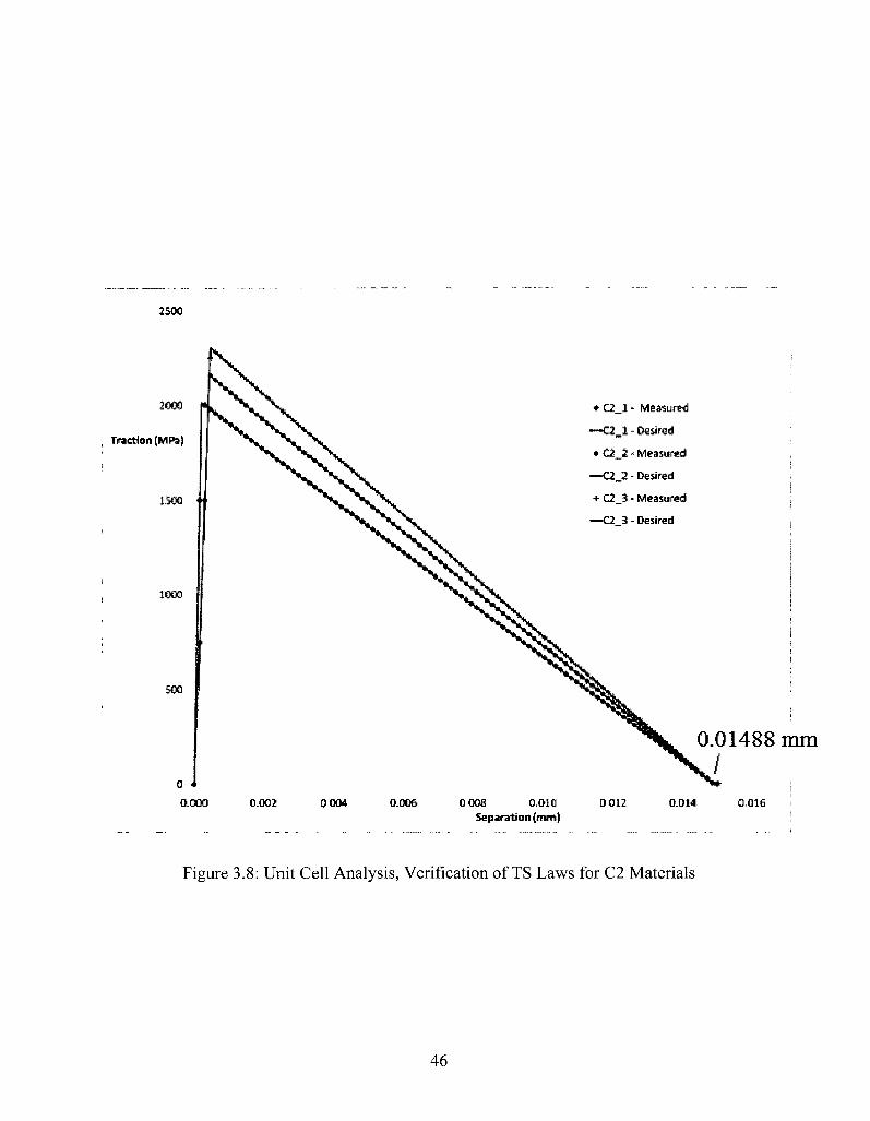
A similar unit cell analysis was performed for three sets of cohesive parameters to be used in

future simulations with the C2 material. These cohesive materials are referred to as C2_l, C2_2,

and C 2 3 . Cohesive parameters for these C2 materials can be found in

Table 3.8. These parameters were selected by comparing the C2 material's DWTT simulations

with experimental data provided by CANMET.

The key points of the desired TS laws for the C2 materials can be found in

Table 3.9. The traction-separation response of these unit cell simulations can be found in Table

3.10 and Figure 3.8. The response of these cohesive elements in Abaqus perfectly matches the

desired TS law for all three C2 materials.

As expected, C2_2 and C2_3 have a lower slope than C 2 1 in the elastic portion because they

have reduced stiffness. The stiffnesses are reduced on these two materials to improve numerical

stability in the SSY and DWTT simulations. The critical separation value, 8C, is 0.01488 mm for

all three C2 materials. The thickness of the cohesive elements used for the C2 simulations is 0.03

mm, rather than the 0.01 mm used for the TH materials, due to this much larger value of 8C. The

mesh deformation would be too great if a thinner element was used.

33

Page 46

Conclusions

It can be concluded that the parameters calculated to model the cohesive laws defined by

Tvergaard and Hutchinson work as desired. The parameters chosen for the C2 materials also

respond as desired.

The next step in the validation process is to re-create the small-scale yielding model developed

by Tvergaard and Hutchinson (1992) to determine if that the bilinear laws outlined in this

Chapter give equivalent results as the published trapezoidal laws when measuring the

macroscopic response of the model. Resistance curves and CTOA data will be measured for each

TS law for both the TH and C2 materials in Chapter 4. The CTOAs of the C2 and TH materials

will be compared to each other.

Following this, the TS laws defined here will be used to simulate drop-weight tear tests in

Chapter 5. Load vs. load-line displacement curves, crack extension vs. load-line displacement

curves, and CTOA vs. crack extension curves will be measured for each of the seven materials.

CTOAs measured during the DWTT simulations will be compared to those measured in the SSY

simulations, and the CTOAs of the C2 materials will be compared to experimental observations.

34

Page 47

Stress (MPa)

600 610 620 630 640 650 660 670 680 690 700 710 720 730 740 750 760 770 780 790 800 810 820 830 840 850 860 870 880 890 900

Plastic Strain

0 0.000539216

0.001164143

0.001886684

0.002720164

0.003679475

0.004781227

0.006043921

0.007488126

0.009136673

0.011014872

0.013150733

0.015575209

0.018322462

0.02143014

0.024939677 1 0.028896621

0.03335097

0.038357548

0.043976393

0.05027318

0.057319668

0.065194174

0.073982086

0.083776396

0.094678281

0.106797705

0.120254072

0.135176909

0.151706591

0.169995117

Stress (MPa)

910 920 930 940 950 960 970 980 990 1000

1010

1020

1030

1040

1050

1060

1070

1080

1090

1100

1110

1120

1130

1140

1150

1160

1170

1180

1190

1200

Plastic Strain

0.190206919

0.212519725

0.237125475

0.264231277

0.294060429

0.326853488

0.362869405

0.402386711

0.445704781

0.493145151

0.545052911

0.60179817

0.663777594

0.731416024

0.80516817

0.8855204

0.972992606

1.068140168

1.171556007

! 1.283872744

1.405764953

1.537951527

1.681198149

1.836319877

2.004183852

2.185712122

2.381884595

2.593742129

2.822389747

3.069

Table 3.1: TH Material Plastic Strain

35

Page 48

Steel

C2

C

0.04

Mn

1.56

Si

0.24

Al

0.039

Nb

0.069

Ti

0.013

Cu

0.31

Cr

0.07

Ni

0.11

Steel

C2

P

0.010

s O.009

Mo

0.20

Ca

0.0021

Sn

0.014

B

0.0003

N

0.008

Ce

0.001

V

0.003

Table 3.2: C2 Steel's Chemical Composition

Steel

C2

oy

(MPa)

576

UTS

(MPa)

650

Elongation

(%)

29.5

Area

Reduction

(%)

78.1

N

0.117

Y/T

0.89

CVN

(J)

303

Table 3.3: C2 Steel's Average Transverse Tensile and Charpy Properties (3 samples)

36

Page 49

- J

H

tiT

n bo CO r-

n>

t/i

o" GO

p

5' <i en GO CT CD

C/5

P

3

& 5' >

Stress (Mpa)

576 579 6 583.1

586.7

590.3

593 8 597 4

601 604.5 608.1 611.7 615.2

618 8 622.4

625.9 629.5 633.1 636.6

640.2

643 8

647.3

650 652.4

654 9

657 3 659.7 662.2

664.6 667

669.5 671.9 674.3

676.8

679.2

681 6

3lastic Strain

0 0.00193 0.00392

0 0059

0.00788

0.00986 0 01184

0.01382

0.01581 0.01779 0.01977 0.02175

0 02373 0.02571 0.0277

0.02968 0.03166 0.03364

0.03562

0.03761

0.03959 0.04107

0.04306

0 04505

0 04704 0.04902

0 05101

0.053 0.05499 0.05697 0.05896 0.06095

0.06294

0.06492 0 06691

Stress (Mpa) I

684.1 686.5 688.9

691 4

693.8 696 2

698.6 701.1

703.5

705.9, 708.6' 720.8"

733 745.1

757.3 769.4 781.6 793.8

805.9

818.1

830.3 842 4,

854.6 866 7

878 9

891.1 903.2 915.4 927.6 939.7' 951.9, 964'

976.2

988.4

1000.5

3lastic Strain

0 0689 0 07089 0 07287

0.07486 0.07685

0.07884

0.08082

0.08281

0.0848

0.08679 0.08898 0.09892

0 10885 0.11879

012873 0.13867 0.1486

0 15854

0.16848 017842

0.18835 0.19829

0.20823

0.21817

0.22811 0.23804

0.24798 0.25792 0.26786 0.27779 0.28773 0.29767

0.30761

0.31755

0 32748

Stress (Mpa) •

1012.7 1024.9 1037

1049.2

1061.3

1073.5

1085.7

1097.8

1110 1122.2

11343 1146.5

11586 1170.8 1183

1195.1 1207 3

1219.5 1231.6

1243.8

1255.9"

1268.1 1280.3

1292.4

1304.6 1316.7

1328.9 1341.1

1353.2

1365~4 1377.6 1389 7 1401.9

1414 1426 2

Plastic Strain

0.33742 0.34736 0.3573

0.36723

0 37717

0 38711

0.39705

0 40699 0.41692

0.42686 0.4368

0~44674

0.45667

0.46661 0.47655 0.48649

0.49643 0.50636

0.5163

0.52624

0 53618 0.54611

0.55605

0.56599

0 57593 0.58587

0.5958 0.60574 0.61568 0.62562

0.63555 0.64549

0.65543

0.66537 0 67531

Stress (Mpa)

1438.4

1450.5 1462 7

1474 9

1487

1499 2

1511 3 1523.5

1535.7

1547.8 1560

1572.2

1584.3

1596.5 1608.6 1620.8 1633

1645 1

1657 3

1669.5

1681.6

1693.8

1705 9

1718.1

1730.3 1742.4

1754.6

1766.8 1778.9 179T.1 1803.2 1815.4

1827.6 1839.7

1851 9

Elastic Strain

0.68524

0.69518 0.70512

0 71506 0.72499

0.73493

0 74487

0.75481

0.76474

0.77468 0.78462 0.79456

0.8045 0.81443 0.82437

0.83431 0.84425

0 85418 0 86412

0 87406

0.884

0.89394 0 90387

0.91381

0.92375

0 93369 0.94362

0.95356 0.9635 0.97344

0.98338 0.99331

1.00325

1.01319 1 02313

Stress (Mpa)

1864.1 1876.2 1888.4

1900.5

1912.7

1924 9

1937 1949.2

1961 4

1973.5 1985.7 1997.8

2010 2022.2 2034.3 2046.5 2058.7 2070.8

2083

2095 1

2107 3

21195

2131.6

Plastic Strain

1 03306 1 043

1.05294

1.06288 1.07282

1.08275

1.09269

1 10263 1 11257

1.1225 1 13244

1.14238 1 1 1 1 1 1 1 1 1

15232

16226 17219 18213 19207

20201

21194

22188 23182

1 24176 1.25169

Page 50

Material MaxS Damage (MPa) Fracture Toughness

(MPa-mm) Elastic Moduli (MPa)

THl TH2 TH3 TH4

Normal 1st 2nd 1800 1350 1350 2100 1575 1575 2160 1620 1620 2250 1687.5 1687.5

Linear 6.075 7.0875

7.29 7.59375

Table 3.5: Cohesive Parameters - Tt

Knn Kss Ktt 10000000 3846150 3846150 10000000 3846150 3846150 10000000 3846150 3846150 10000000 3846150 3846150 Materials

THl

Traction (MPa) 0

1800 0

Separation (mm) 0

0.00018 0.00675

TH2 Traction (MPa)

0 2100

0

Separation (mm) 0

0.00021 0.00675

TH3 Traction (MPa)

0 2160

0

Separation (mm)

0 0.00022 0.00675

TH4 Traction (MPa)

0 2250

0

Separation (mm) 0

0.00023 0.00675

Table 3.6: Desired TS Laws for TH Materials, Cases 1-4

38

Page 51

H cr CD

^

£ CD CO

CD

CD

& CO

O

3_

o CD

if CO

CD CO

O

H

& r-t-CD

5] CO

Material TH1

Traction (MPa)

0.0

700.0

1399.5

1791.8

1772.6

1753.5

1657.6

1561.7

1465.8

1369.9

1274.0

1178.1

1082.2

986.3

890.4

794.6

698.7

602.8

506.9

411.0

315.1

219.2

123.3

27.4

0.0

Separation (mm)

0.00000

0.00007

0.00014

0.00021

0.00028

0.00035

0.00070

0.00105

0.00140

0.00175

0.00210

0.00245

0.00280

0.00315

0.00350

0.00385

0.00420

0.00455

0.00490

0.00525

0.00560

0.00595

0.00630

0.00665

0.00675

TH2

Traction (MPa)

0.0

700.0

1399.5

2099.0

2077.6

2055.1

1942.7

1830.3

1717.9

1605.5

1493.1

1380.8

1268.4

1156.0

1043.6

931.2

818.8

706.5

594.1

481.7

369.3

256.9

144.5

32.1

0.0

Separation (mm)

0.00000

0.00007

0.00014

0.00021

0.00028

0.00035

0.00070

0.00105

0.00140

0.00175

0.00210

0.00245

0.00280

0.00315

0.00350

0.00385

0.00420

0.00455

0.00490

0.00525

0.00560 1 0.00595

0.00630

0.00665

0.00675

TH3

Traction (MPa) | Separation (mm)

0.0 0.00000

700.0 ' 0.00007

1399.5 0.00014

2099.0 0.00021

2138.9 " 0.00028

2115.7 i 0.00035

2000.0 0.00070

1884.3 ' 0.00105

1768.6 ! 0.00140

1652.9 I 0.00175

1537.2 0.00210

1421.5 ( 0.00245

1305.8 i 0.00280

1190.1 0.00315

1074.4 0.00350

958.7 0.00385

843.0 " 0.00420

727.3 ' 0.00455

611.6 I 0.00490

495.9 i 0.00525

380.2 0.00560

264.5 i 0.00595

148.8 ! 0.00630

33.1 ' 0.00665

0.0 0.00675

TH4

Traction (MPa)

0.0

700.0

1399.5

2099.0

2231.1

2206.9

2086.2

1965.6

1844.9

1724.2

1603.5

1482.8

1362.1

1241.4

1120.7

1000.0

879.4

758.7

638.0

517.3

396.6

275.9

155.2

34.5

0.0

Separation (mm)

0.00000

0.00007

0.00014

0.00021

0.00028

0.00035

0.00070

0.00105

0.00140

0.00175

0.00210

0.00245

0.00280

0.00315

0.00350

0.00385

0.00420

0.00455

0.00490

0.00525

0.00560

0.00595

0.00630

0.00665

0.00675

Page 52

Material

C2 1 C2 2 C2 3

MaxS Damage (MPa)

Normal 1 st 2nd 2016 1512 1512 2160 1620 1620 2304 1728 1728

Fracture Toughness (MPa-mm)

Linear 15.00 16.07 17.14

Elastic Moduli (MPa)

Knn Kss Ktt 10000000 3846154 3846154 5000000 1923077 1923077 5000000 1923077 1923077

Table 3.8: Cohesive Parameters - C2 Materials

C2 1

Traction (MPa) 0

2016 0

Separation (mm) 0

0.0002016 0.01488

C2_2 Traction (MPa)

0 2160

0

Separation (mm) 0

0.000432 0.01488

C2_3 Traction (MPa)

0 2304

0

Separation (mm) 0

0.0004608 0.01488

Table 3.9: Desired TS Laws for C2 Materials, Cases 1-3

40

Page 53

Material C2 1

Traction (MPa) Separation (mm) 0.0

1499.9 2002.5 1981.9 1961.3 1837.7 1755.3 1631.7 1487.5 1343.3 1219.7 1075.5 931.3 807.7 663.5 519.3 395.7 251.5 107.3 4.2 0.0

0.0000 0.0001 0.0003 0.0004 0.0006 0.0015 0.0021 0.0030 0.0041 0.0051 0.0060 0.0070 ~ 0.0081" ~ 0.0090 0.0100 0.0111 0.0120 0.0131 0.0141

0.01485 0.01488

C2 2

Traction (MPa) Separation (mm) 0.0

750.0 1500.1 2157.3 2134.9 2000.3 1910.6 1776.1 1619.1 1462.1 1327.5 1170.6 1013.6 879.1 722.1 565.1 430.6 273.6 116.6 4.5 0.0

0.0000 0.0002 0.0003 0.0005 0.0006 0.0015 0.0021 0.0030 0.0041 0.0051 0.0060 0.0071 0.0081 0.0090 0.0100 0.0111 0.0120 0.0130 0.0141

0.01485 0.01488

C2 3

Traction (MPa) 0.0

750.0 1500.1 2250.2 2281.8 2137.9 " 2042.0 1898.2 1730.4 1562.6 1418.8 1251.0 1083.3 939.4 771.6 603.8 460.0 292.2 124.4 4.6 0.0

Separation (mm) 0.0000 0.0002 0.0003 0.0005 0.0006 0.0015 0.0021 0.0030 0.0040 0.0051 0.0060 0.0071 0.0081 0.0090 0.0100 0.0111 0.0120 0.0130 0.0141

0.01485 0.01488

Table 3.10: Measured Results From Unit Cell Analyses for C2 Materials

41

Page 54

face 4

- X 1 fecel

4 - nocte elt&ment

thickness direction

4 - nodes element

Figure 3.1 : COH2D4 Element Numbering Conventions (• - Nodes, x - Integration points)

(Abaqus, 2008)

tie constraints

Part t

Part 2

cohesive elements

Figure 3.2: Typical Traction-Separation Based Cohesive Zone Model - Independent Meshes

with Tie Constraints (Abaqus, 2008)

42

Page 55

Traction

6t, "c Separation

Figure 3.3: Typical Traction-Separation Response

Figure 3.4: TH Steel - True Stress-Strain Curve

43

Page 56

800

700

600

re" 500 Q.

1 400

,§ 300

200

100

0.02 0.04 0.06 0.08

True strain

0.1

Figure 3.5: C2 Steel - True Stress-Strain Curve (Su, 2010a)

0.01 mm

0.05 mm

Figure 3.6: Unit Cell Geometry and Boundary Conditions

44

Page 57

2500

2000

Traction (MPa)

1500

1000

500

• THl - Measured —THl - Desired • TH2 - Measured

—TH2 - Desired + TH3 - Measured

—TH3 - Desired - TH4 - Measured

—TH4-Desired

0.000 0.001 0.002 0.003 0.004 0.005 Separation (mm)

0.00675 mm

0.006 0.007

Figure 3.7: Unit Cell Analysis, Verification of TS Laws for TH Materials

45

Page 58

2500

• C2_l • Measured

—C2_l - Desired

• C2_2 - Measured

—<C2_2 - Desired

+ C2_3 - Measured

—-C2 3 - Desired

0.002 • 004 0.006 0 008 0.O10 Separation (mm)

0.01488 mm

0 012 0.014 0.016

Figure 3.8: Unit Cell Analysis, Verification of TS Laws for C2 Materials

46

Page 59

Chapter 4

FE Simulation of Small-Scale Yielding Models

This chapter will explore implementation of cohesive zone (CZ) modeling in Abaqus by

performing finite element analysis of a small-scale yielding (SSY) model. The SSY model will

be defined and simulation results for a set of ideal materials, as defined by Tvergaard and

Hutchinson (1992), and a set of real-world materials (C2 steel) will be presented. Tvergaard and

Hutchinson used a CZ model to perform analysis of plane strain mode I crack growth under

conditions of small-scale yielding. A small-scale yielding analysis is performed here to verify

that the techniques used here are able to recreate the results of Tvergaard and Hutchinson (1992).

Verifying the techniques used here by comparing with Tvergaard and Hutchinson's results will

increase the confidence in the DWTT results detailed in Chapter 5. In addition, the crack

propagation in C2 steels is simulated using the SSY model. Simulation results for both the TH

and C2 materials include normalized resistance curves and crack tip opening angle data.

4.1 Model Specifications

Geometry

A small scale yielding model is used to simulate a pre-existing horizontal crack surrounded by an

infinite plate. Figure 4.1 shows the geometry for the small-scale yielding model. The initial crack

extends along the bottom edge from the left side of the semicircle to the center. Only the top side

of the crack needs to be modeled due to the inherent symmetry about the crack front for mode-I

crack growth. The crack is modeled by leaving the current crack face unconstrained and

constraining the material to the right of center in the y-direction, along the line of symmetry. A0

is the radius of the circle, and the initial length of the crack. A value of 200 mm was chosen for

A0. B0 is the equal to twice the length of the cohesive zone, which in this case was 9mm. This

allows for up to 4.5 mm of crack growth. A0 is the length of the smallest elastic-plastic elements

at the crack tip, and is set to 0.1 mm. This means that VzBo = 45A0 and A0 = 2000Ao. These

values were selected to meet small-scale yielding requirements which require the plastic zone to

47

Page 60

be less than 5% of the radius of the model. The largest plastic zone simulated here is 2.354 mm,

which is only about 1.2% of the radius.

Material Properties

Two different sets of materials were used in this model, with each set having one elastic-plastic

response, and varying cohesive parameters. The first set of four materials was defined by

Tvergaard and Hutchinson (1992) and is representative of an ideal high strength steel. These are

the TH materials defined in Chapter 3. The second material set is the C2 steel. The C2 steel is an

X70 steel characterized by CANMET/MTL (Xu, 2010a) and is representative of modern high

toughness pipeline steels. The C2 material is also defined in Chapter 3. Cohesive parameters for

the TH materials can be found in Table 3.5. Cohesive parameters for the C2 materials can be

found in Table 3.8. As mentioned in Chapter 3, bilinear traction-separation laws were used for

these simulations, rather than the trapezoidal laws used by Tvergaard and Hutchinson.

Loading Conditions

It is possible to apply a ramped displacement field to the outer edges of the model to generate a

known stress intensity factor at the crack tip. To do this, the semicircle is broken up into 36

wedges, each 5 degrees of the circle, as shown in Figure 4.2. Displacements ux(t) and uy(t) are

then applied to the nodes at the outer edges based on the following equations (Williams, 1957):

^w={Si i cO[K -1 + 2s '"2©]}-i7 • , = 0 ^ (4-D

V ' ) = {g J i s O [« + 1 - 2 cos2 Q] j -± , t = 0 - t/ (4.2)

Where Kr is the maximum desired stress intensity at the crack tip (set high enough to allow

complete propagation of the crack though the cohesive zone), \i is the shear modulus and

K = 3 — 4v, where v is Poisson's ratio. 9 is measured counter-clockwise from the crack front.

48

Page 61

Time varies from 0 to 1 second, which causes the displacements to increase linearly throughout

the simulation.

Table 4.1(a) details the maximum displacements applied for the TH materials. These

displacements are based on a maximum applied stress intensity of 9135 MPaVmm. This value is

equal to 5 • KjH4, and was chosen to be sufficiently large to allow the crack to propagate

completely through the cohesive layer. KlHA is the K0 for the TH4 material based on Equation

(2.7) and represents the largest K0 among the TH materials.

Table 4.1(b) details the maximum displacements applied for the C2 materials. These

displacements are based on a maximum applied stress intensity of 41,952 MPaVmm. This value

is -15.5 -Kg2-3, and was large enough to allow full propagation of the crack for the C2

simulations. Kg2-3 is the K0 for the C 2 3 material based on Equation (2.7) and represents the

largest K0 among the C2 materials.

Mesh Design

The model is divided into two separate parts for meshing. There is the main semicircular section

which is divided into 1,533 solid quadrilateral plane-strain elements with reduced integration

(CPE4R elements), and a cohesive layer along the crack front composed of 150 cohesive

(COH2D4) elements. The two sections are joined together using surface-to-surface tie

constraints. Figure 4.3 and Figure 4.4 (a) - (c) show the mesh used for these simulations at

increasing levels of magnification of the crack tip. To mesh the elastic-plastic region, a swept

meshing technique is used away from the crack tip and a structured meshing technique is used at

the crack tip. A free meshing technique joins the gap between these two sections. The cohesive

layer is meshed using a swept meshing technique, as required by the element type. For the TH

material the cohesive elements have a length of 0.03 mm, and a thickness of 0.01 mm. This is too

thin for the tougher C2 materials though, as the required maximum separation value of 0.01488

49

Page 62

mm would cause too much mesh distortion. Therefore, cohesive elements with a length of 0.03

mm and a thickness of 0.03 mm were used when modeling the C2 materials.

The smallest elastic-plastic elements, those that are tied to the cohesive elements, have

dimensions of 0.1 x 0.1 mm. Diehl (2007) recommends that 3-5 cohesive elements be used per

adjacent continuum element. The dimensions used here means that there are 3 1/3 cohesive

elements per adjacent continuum element. It was found to be particularly important that the

cohesive nodes do not line up with the elastic-plastic nodes too often, as it would allow the mesh

to deform in an undesirable fashion.

Verification of Applied Stress Intensity

A simulation was performed without the cohesive layer to verify that the applied displacement

field is yielding the desired stress intensity at the crack tip. Using the TH materials, a

displacement field was applied, based on Equations 4.1 and 4.2, until a stress intensity higher

than the highest critical stress intensity was reached (that of the TH4 material). The assumed

stress intensity at the crack tip was compared with the measured J-integral for 8 contours in

Abaqus. The J-integral data can be found in Table 4.2. Table 4.2 also provides incremental

percentage difference information between the theoretical and measured intensities. It is seen

that the two sets of data agree almost perfectly, with errors of less than 0.5% throughout the

simulation.

4.2 Results

Simulations were completed in Abaqus/Explicit, version 6.8-2 (Abaqus, 2008), using the CAE

platform on Windows 7 computers. Abaqus/Explicit was chosen rather than Abaqus/Standard

because it is more numerically stable for the simulations performed here. To simulate quasi-static

conditions, dynamic, explicit steps were used with a time period of one second. Results were

recorded at 8000 increments, divided into approximately equal intervals based on time. Mass

densities of 7.85 x 10" kg/mm were used for all materials. Typical run times for these

simulations ranged from 3-5 minutes for the TH1 simulation to up to 120 minutes for the C 2 3

50

Page 63

simulation. The range of simulation time was due to the reduction of the stable time increment

caused by increased fracture energy at the crack tip.

4.2.1 Results of TH Simulations

Resistance Curves

Four small-scale yielding simulations were run with the same mesh, loading conditions, and TH

elastic-plastic material (Table 3.1). The TH material has a yield stress, ay, of 600 MPa, Young's

Modulus, E, of 200,000 MPa, and Poisson's ratio, v, of 0.3. The applied displacement field for

the TH simulations can be found in Table 4.1(a). Each case had increasingly tough cohesive

parameters, as defined in Table 3.5. These sets of cohesive parameters are referred to as TH1-

TH4. The peak traction in the normal direction was defined as 3.0- ery, 3.5- ay, 3.6- oy, and

3.75- oy for TH1-TH4 respectively. These peak tractions can be found in Table 4.3 (a). Fracture

energies, ro, were calculated as if a trapezoidal TS law was used, as per Equation 2.5. As in the

simulations performed by Tvergaard and Hutchinson (1992), oc = 0.1Ao, - 1 = 0.15 , and "c

-^ = 0.5. These calculated fracture energies were then inserted into the bilinear TS laws in

Abaqus, so the only the shape of the TS laws used here is different than the TS laws used by

Tvergaard and Hutchinson (1992). The fracture energy input into Abaqus was defined as half the

fracture energy calculated for the model as only a half-model was analyzed. Values quoted for

fracture energies in this thesis are those entered as material parameters into Abaqus (equal to half

the fracture energy of the whole model). These fracture energies can be found in Table 4.3 (a).

It was possible to measure the crack length from the simulation results by measuring the traction

stresses in each element in the cohesive layer. The cohesive elements are numbered sequentially

from 1-150, with element 1 at the original crack tip. The current crack tip is defined as the

highest element number to have failed completely, with traction capability reduced to zero.

Tables 4.4-4.7 show sample traction data from the simulations for TH1-4 respectively. The crack

length, Aa, can be determined by multiplying the length of the cohesive element by the element

51

Page 64

number of the current crack tip. The crack length is then normalized by the size of the plastic

zone (R0) for each case. R0 can be found by:

R 1 Ef0 1 (K0\2

0 3n(l-v2)ayl 3n\ay)

( 4 3 )

Values for the ratio of the peak traction to yield stress, d/ay, fracture energy, T0, critical stress

intensity, K0, and plastic zone length, R0, for each TH case can be found in Table 4.3(a).

The tractions are then compared to the applied displacement in the x-direction at the outer node

at 0°. This displacement is converted into a theoretical applied stress intensity, Kr, using Equation

(4.1), which is then normalized by the critical stress intensity, K0, for each case. The normalized

values Kr/Ko can be found for each increment in Tables 4.4-4.7.

Figure 4.5 shows the results of these four simulations by plotting Kr/K0 vs. Aa/R0. As expected,

increasing the toughness of the cohesive elements increases the fracture resistance. On the same

graph, the results published by Tvergaard and Hutchison (1992) are displayed with dashed lines.

It is seen that the steady-state resistance from these four simulations agrees quite closely with the

Tvergaard and Hutchinson steady-state resistance data. Differences in the shape of the resistance

curves before steady-state can likely be attributed to the difference in shape between the two sets

of traction-separation laws.

Crack Tip Opening Angle

The crack tip opening angle was measured for each simulation at several increments. The ISO

defines the CTOA as the angle of the crack surfaces measured (or calculated) at 1 mm from the

current crack tip (ISO, 2007). The crack tip in the CZ simulations performed here is defined to

be located at the shared nodes between the last cohesive element to fail (element fully damaged,

52

Page 65

with no ability to transfer loads), and the next cohesive element that will fail. The elastic-plastic

nodes do not line up exactly 1 mm behind this crack tip due to the length difference between the

cohesive and elastic-plastic elements, but to remain consistent with the spirit of the ISO

approach, the CTOA was calculated by measuring the y-displacement of the node of an elastic-

plastic element that was nearest to 1 mm behind the current crack tip. This displacement was

used as the crack tip opening displacement (CTOD). The CTOA was then calculated using from

the CTOD using trigonometry and calculating with the true distance behind the crack tip. Figure

4.6 shows an example of how the CTOA is calculated by overlaying the original transparent

mesh by a darkened mesh after the crack has extended about 3.2 mm. The cohesive layer is

hidden to allow the CTOA to be seen more clearly. It can be seen that the new surface created by

the crack propagation is not completely flat. This will introduce some 'noise' into the CTOA

data when using this calculation method, but the average measured CTOA at steady-state should

provide a reasonable approximation of the true results. No data for CTOA is calculated until the

crack length reaches ~1 mm.

Table 4.8 shows some sample displacement data for the TH1 case for nodes labelled by their

distance from the original crack tip to demonstrate the process of calculating the CTOA. Tables

4.9-4.11 present the CTOA data calculated from the results of the simulations for TH2-TH4,

respectively. The CTOA vs. crack length, Aa, has been plotted for all four cases in Figure 4.7.

Power law trendlines were fitted using MS Excel. As expected, increasing fracture toughness

causes increasing critical CTOAs. Additionally, the numerical results follow the expected trends,

as the CTOA values are initially high, but drop towards a steady-state value after a small amount

of propagation. The length of the cohesive zone (4.5mm) was not enough to conclusively achieve

steady-state CTOAs for TH2-4, but it can be seen that a steady-state value of about 1.9° was

determined for the TH1 material. Values for steady-state CTOAs are estimated from their power

law trendlines as about 2.5°, 3.5°, and 6° for TH2-4 respectively. These values will be compared

to the steady-state CTOAs measured for these materials during DWTT simulations in Chapter 5.

53

Page 66

4.2.2 Results of C2 Simulations

Resistance Curves

Three small-scale yielding simulations were run with the same mesh, loading conditions, and C2

elastic-plastic material (Table 3.4). The C2 material has a yield stress, ay, of 576 MPa, Young's

Modulus, E, of 195,400 MPa, and Poisson's ratio, v, of 0.3. The applied displacement field for

the C2 simulations can be found in Table 4.1(b). Each case had increasingly tough cohesive

parameters, as defined in Table 3.8. These sets of cohesive parameters are referred to as C 2 1 -

C 2 3 . The peak traction in the normal direction was defined as 3.5- ay, 3.75- ay, and 4.0- oy for

C2_l-C2_3 respectively. Values for a/ay, F0, K0, and R0 for each TH case can be found in

Table 4.3(b). Fracture energies were calculated as per Equation 2.5 again, as if 8C = 0.1Ao,

-^ = 0.15 , and -^ = 0.5. This technique for choosing ro, and therefore 8C, is used to remain

consistent with the TH simulations instead of arbitrarily assigning values. Tables 4.12-4.14 show

sample resistance curve data from the simulations for C2_l-C2_3 materials respectively.

Figure 4.8 shows the results of these three simulations by plotting Kr/K0 vs. Aa/R0. Again as

expected, increasing the toughness of the cohesive elements increases the fracture resistance.

Data for the C 2 3 simulation is slightly more sporadic as the high toughness of the cohesive

elements meant there was a much larger amount of mesh deformation required for crack

propagation. This can be seen in the CTOA data presented below. It is likely that a larger model

with coarser mesh would be able to achieve more data points along this resistance curve, but as

the same issues are not experienced for the DWTT simulations with the same parameters, it is

not further explored here.

Crack Tip Opening Angle

CTOA data for the C 2 1 - C 2 3 materials can be found in Table 4.15(a) - (c). The CTOAs are

obtained following the same procedure used for the TH1-TH4 materials. This data is plotted in

Figure 4.9. Again, the length of the cohesive zone (4.5mm) was not enough to conclusively

54

Page 67

achieve steady-state CTOAs for these materials, and no estimates of the steady-state CTOA will

be given here. Trendlines were fitted to the CTOA data using power laws in Excel. The trendline

for the C2_3 data is extended forward 1 period to give a better idea of what the limited data is

predicting. The CTOA values are -30° - 80° at initiation and drop to -20° - 60° after 2 mm of

propagation for the C2 materials. As expected, due to the higher fracture energy of the C2

materials, the CTOAs for the C2 materials are much higher than those of the TH materials. These

results will be compared to the CTOAs measured for these materials during DWTT simulations

in Chapter 5.

4.3 Conclusions

Small-scale yielding simulations were carried out for two different sets of materials. Verification

of the model design was performed by first measuring the theoretical applied vs. measured stress

intensity at the crack tip. Following this, simulations performed by Tvergaard and Hutchinson

(1992) were recreated and the results were compared. It was seen that there was very good

correlation between the resistance curves found here, and those published by Tvergaard and

Hutchinson. CTOA data was collected for the TH materials, and it was seen, as expected, that

tougher cohesive elements resulted in higher values of the CTOA. Additionally, the CTOA

values followed trends observed experimentally (Newman, 2003), as they started high, and

steadily dropped towards steady-state values. Steady-state CTOA values ranged from -2-6° for

the TH materials. These values will be compared to the values found during the DWTT

simulations in Chapter 5.

The tougher C2 materials were seen to yield even higher resistance curves, and higher values for

the CTOAs. While steady-state values for CTOA were not achieved, measured values of CTOA

ranged from -30° - 80° at initiation, to -20° - 60° after 2 mm of propagation for the C2

materials. These values will be compared to the values found during the DWTT simulations in

Chapter 5.

55

Page 68

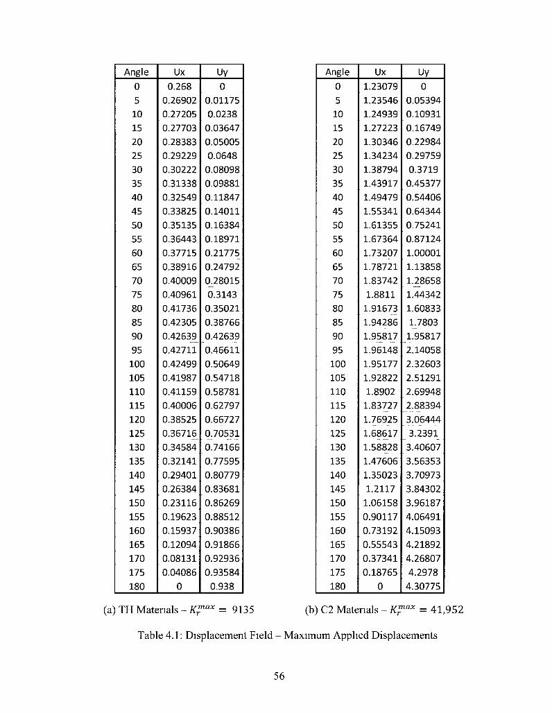
Angle

0 5 10 15 20 25 30 35 40 45 50 55 60 65 70 75 80 85 90 95 100 105 110 115 120 125 130 135 140 145 150 155 160 165 170 175 180

Ux 0.268

0.26902

0.27205

0.27703

0.28383

0.29229

0.30222

0.31338

0.32549

0.33825

0.35135

0.36443

0.37715

0.38916

0.40009

0.40961

0.41736

0.42305

0.42639

0.42711

0.42499

0.41987

0.41159

0.40006

0.38525

0.36716

0.34584

0.32141

0.29401

0.26384

0.23116

0.19623

0.15937

0.12094

0.08131

0.04086

0

Uy 0

0.01175

0.0238

0.03647

0.05005

0.0648

0.08098

0.09881

0.11847

0.14011

0.16384

0.18971

0.21775

0.24792

0^28015

0.3143

0.35021

0.38766

0.42639

0.46611

0.50649

0.54718

0.58781

0.62797

0.66727

0.70531

0.74166

0.77595

0.80779

0.83681

0.86269

0.88512

0.90386

0.91866

0.92936

0.93584

0.938

Angle

0 5 10 15 20 25 30 35 40 45 50 55 60 65 70 75 80 85 90 95 100 105 110 115 120 125 130 135 140 145 150 155 160 165 170 175 180

Ux

1.23079

1.23546

1.24939

1.27223

1.30346

1.34234

1.38794

1.43917

1.49479

1.55341

1.61355

1.67364

1.73207

1.78721

1.83742

1.8811

1.91673

1.94286

1.95817

1.96148

1.95177

1.92822

1.8902

1.83727

1.76925_

1.68617

1.58828

1.47606

1.35023

1.2117

1.06158

0.90117

0.73192

0.55543

0.37341

0.18765

0

Uy 0

0.05394

0.10931

0.16749

0.22984

0.29759

0.3719

0.45377

0.54406

0.64344

0.75241

0.87124

1.00001

1.13858

1.28658

1.44342

1.60833

1.7803

1.95817

2.14058

2.32603

2.51291

2.69948

2.88394

3.06444

3.2391

3.40607

3.56353

3.70973

3.84302

3.96187

4.06491

4.15093

4.21892

4.26807

4.2978

4.30775

(a) TH Materials - K™ax = 9135 (b) C2 Materials - K™ax = 41,952

Table 4.1: Displacement Field - Maximum Applied Displacements

56

Page 69

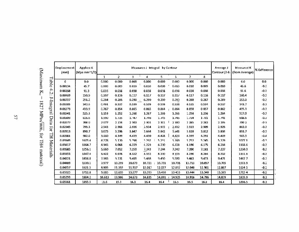
P X

3

to -4

P

3s

H 4^

3 P

H

to

CD

5 o H

a)

P]

Displacement

(mm)

0

0.00134

0.00258

0.00469

0.00737

0.01005

0.01273

0.01541

o.oii ioa

0 02077

0.02345

0.02513

0.02S81

0 03149

0.03417

0.03585

0.03353

0.04221

0.04489

0.04757

0.05025

0.05293

0.05561

Appliec K

(Mpa m m A l / 2 )

0.0

45.7

91.3

159.9

251.2

342.6

433.9

525.3

blb.b

7 0 8 0

799.3

890.7

982.0

1073 4

1164.7

1256.1

1347.4

1438.8

1530.1

1521.5

1712.8

1S04.2

1895.5

1

O.OOO

0.003

0.035

0.107

0.264

0.491

0.787

1.153

1.590

2 077

2.543

3.075

3.660

4 77R

4.945

5.660

6.422

7.185

7.977

8.805

9.035

10.613

11.6

2

0.000

o.ooa

0.038

0.116

0.286

0.532

0.854

1.252

1. /25

2 274

2.908

3.596

4.349

5 170

6.068

7.052

8.078

9.131

10.239

11.392

12.020

13.906

15.3

M e a s u r e d Intcg

3

0.000

0.010

0.038

0.117

0.290

0.539

0.865

1.268

1. ' 4 /

2 302

2.936

3.547

4.439

5 ->9R

6.229

7.250

8.322

9.461

10.673

11.937

13.277

14.673

16.1

1 4

0.000 1 0.010

1 C.038

1 0.117

i 0.29O

0.539

0.865

1.267

l . / 4 b

| 2 301

1 2.934

3.644

4.430

1 •< 797 1 r £.229

7.243

8.332

5.488

10.721 |

1 12.017

13.393 ! 14.835

16.4

ral byCcntour

5

0.000

0.010

0.038

0.117

0.250

0.539

0.864

1.266

1. /45

2 301

2.933

3.642

4.428

5 7^1

6.230

7.244

8.330

9.450

10.731

12.037

13.430

14.891

16.4

i

5

0.000 1 0.010

0.038

0.117

0.290

0.538

, 0.364

1.266

1. /45

1 2 3O0

1 2.932

3.b41

4.426

S 7R9

6.228

7.242

8 333

9.5O0

10.738

12.052

13 453

1 14.925 1 16.5

7

O.OOO

0.010

0.038

0.117

0.28S

0.535

0.858

1.258

1./34

2 285

2.913

3.618

4.399

S 757

6.190

7.2O0

8.290

9.463

10.713

12.040

13.444

14.916

16.5

8

O.OOO

O.OOO

0.038

0.116

0.287

0.534

0 857

1.256

1 /31

2 212

2.909

3.612

4.391

5 745

6.175

7.181

8.264

9.423

10.657

11.961

13.340

14.796

16.3

Average J

Contour(2-8i

0.003

0.010

0.033

0.117

0.289

0.537

0.862

1.264

1. /41

2 295

2.925

3.634

4.419

5 779

6.214

7.227

8.312

9.471

10.705

12.007

13.3&9

14.839

16.4

Measured K

(from Average)

0.0

45.0

91.6

160.4

252.0

313.7

435.3

527.0

618. b

710 2

802.0

853.7

985.5

1077 1

1158.6

1250.3

1351.6

1442 7

1533.9

1624 5

1715 4

1835.9

1896.5

% niffprRnrp /u L l 1 11 C I C U ^ C

0.0

- o . :

-0.3

-0.3

-0.3

-0.3

-0.3

-0.3

-O.J

-0 3

-0.3

-0.3

-0.4

-0 a

-0.3

-0.3

-0.3

-0.3

-0.2

-0.2

-0.2

-0.1

-0.1

Page 70

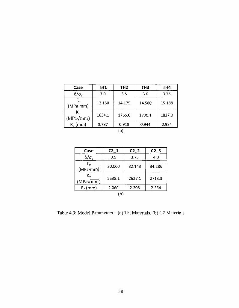
Case

6/CJy

To (MPa-mm)

Ko

(MPaVmm) Ro(mm)

TH1

3.0

12.150

1634.1

0.787

TH2

3.5

14.175

1765.0

0.918

TH3

3.6

14.580

1790.1

0.944

TH4

3.75

15.188

1827.0

0.984

(a)

Case

6/Oy

To

(MPa-mm)

Ko

(MPaVmm) Ro(mm)

C2_l

3.5

30.000

2538.1

2.060

C2_2

3.75

32.143

2627.1

2.208

C2_3

4.0

34.286

2713.3

2.354

(b)

Table 4.3: Model Parameters - (a) TH Materials, (b) C2 Materials

58

Page 71

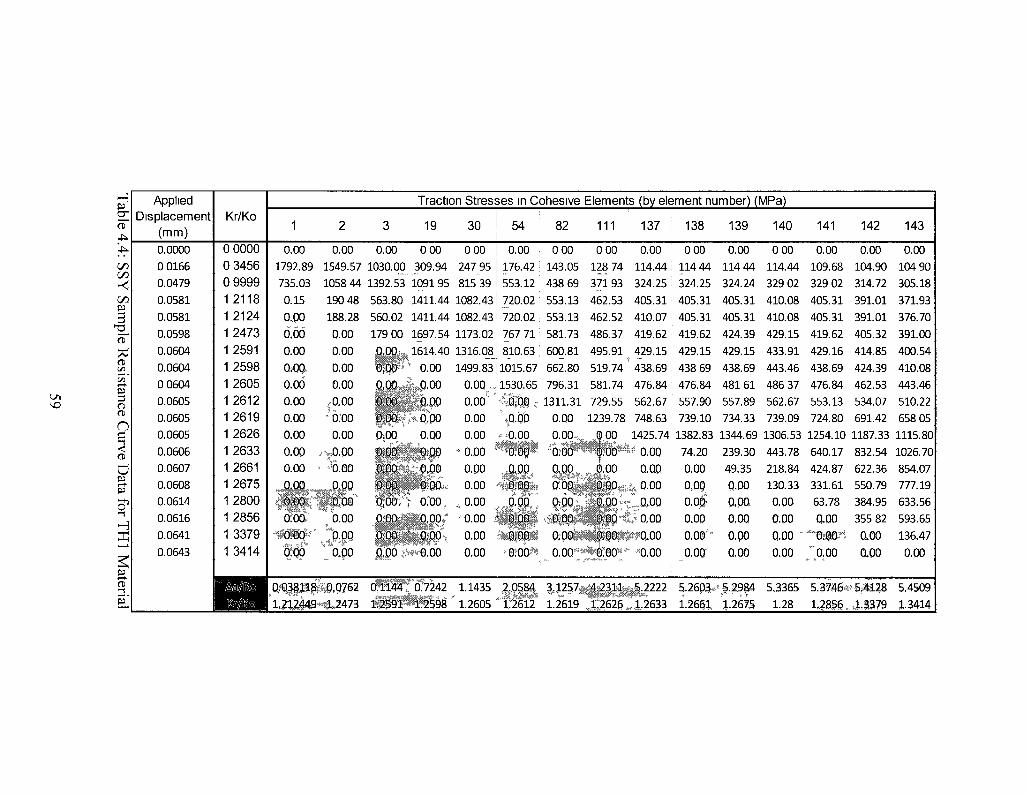
73

o CD

O

I a

3s

H

Applied Displacement

(mm) Kr/Ko

Traction Stresses in Cohesive Elements (by element number) (MPa)

1 19 30 54 82 111 137 138 139 140 141 142 143

0.0000 0 0166 0.0479 0.0581 0.0581 0.0598 0.0604 0.0604 0 0604 0.0605 0.0605 0.0605 0.0606 0.0607 0.0608 0.0614 0.0616 0.0641 0.0643

0 0000 0 3456 0 9999

1 2118 1 2124 1 2473 1 2591 1 2598 1 2605 1 2612 1 2619 1 2626 1 2633 1 2661 12675 1 2800 1 2856 1 3379 1 3414

0.00

1792.89

735.03

0.15

0.00

0,00

0.00

aoo, o.oo o.oo o.oo o.oo o.oo o.oo

aoa

iiflo*** 0?Q0

0.00 1549.57 1058 44 190 48 188.28

0.00

0.00

0.00 Q.OO

,0.00 •O.'OO

0.00

>0.Q0 "0,60

@"

0.00

b.oo 0.00

0.00

1030.0£

1392.53

563.80

560.02

179 00

0.00

0.00

0.00 0.00 0.00 0.00 0.00 0.00 0.00 0.00 ' 0.00 0.00

0.00

0 00 J09.94 1091 95 1411.44 1411.44 1697.54 1614.40

0.00 0.00

0.00 0,00 0.00

0.00 0.00 o.oo 0.00.

0.00

0.00

aoo

0 00

247 95 I

815 39 i

1082.431

1082.431

1173.02

1316.0_8_|

1499.83] a 0 Q , 1 0.00* * 0.00

0.00

' 0 .00

o.po 0.00

,0 .00 jaoo aoo o.oo

o.oo 176.42 553.12 720.02 720.02 767 71 810.63 1015.67 1530.65

^Q>00 0.00 0.00 0.00 0,00 0.00 0.00 0.00 0.00

0 00 143.05 438 69 553.13 553.13

581.73

600.81

662.80 796.31

1311.31 0.Q0

0.00

0.00 0.00 0.00 0.00 0.00

0.00

0.00

0 00 128 74 37193 462.53 462.52 486.37 495.91 519.74 581.74 729.55

0.00 114.44 324.25 405.31 410.07 419.62 429.15 438.69 476.84 562.67

1239.78 748.63

0 00 1425.74

0.00

0.00

ado* 0.00 0.00 0.00 0.00 0.00 0.00

0.00

o.oo 0.00

0.00

0.00

0 00 114 44 324.25 405.31 405.31

419.62

429.15

438 69 476.84

557.90 739.10

1382.83

74.20

0.00

0.0Q, o.op. aoo aoo'-0.00"

o.oo 114 44 324.24 405.31 405.31 424.39 429.15 438.69 48161 557.89 734.33 1344.69 239.30 49.35 0,00

aoa o.oo o.oo aoo

ooo 114.44

329 02

410.08

410.08

429.15

433.91

443.46

486 37

562.67

739.09

1306.53

443.78

218.84

130.33

0.00

0-00

0.00 '

0.00

0.00

109.68

329 02

405.31

405.31

419.62

429.16

438.69

476.84

553.13

724.80

1254.10

640.17

424.87

331.61

63.78

0.00 **"B!>!0**

"aoo

o.oo 104.90

314.72

391.01

391.01

405.32

414.85

424.39

462.53

534.07

691.42

1187.33

832.54

622.36

550.79

384.95

355 82

aoo aoo

0.00

104 90

305.18

371.93

376.70

391.00

400.54

410.08

443.46

510.22

658 05

1115.80

1026.70

854.07

777.19

633.56

593.65

136.47

0.00

Q%!PfPftQ7S2 0.1144 0.7242^1.1435 ^ g g ^ i^^Bffifafapil 5.2603^#,«9f4 5,3365 5.3*1&»MU8 5.4509

lJ12J4a«gl>2473 1.2591 1.2598' 1.2605 '11612 1.2619 32626,1 .2633 1.2661 1>2675 1.28 1.28S6, ,11379 1-3414

Page 72

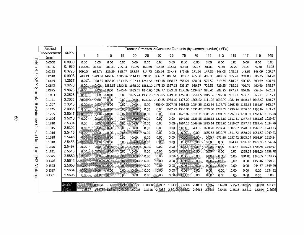
0 \ O

H

oT 4^

GO CO

< CO

t ?T CD CO

CO r-t

3 o CD

O

<

d ft P W o H

2 ft CD £J_ P

Applied

Displacement

(mm)

0.0000

0.0100

0.0193

0.0518

0.0649

0.0843

0.0975

0 1063

0.1141

0.1207

0.1245

0.1295

0.1306

0.1310

0.1315

0.1316

0.1318

0.1318

0.1320

0.1321

0.1325

0.1326

0.1328

0.1329

0.1331

Kr/Ko

0.0000

0.1936

0.3723

0.9998

1.2527

1.6276

1.8826

2.0526

2.2038

2 3318

2 4035

2.5017

2 5216

2.5304

2.5392

2.5413

2.5445

2.5455

2.5497

2 5518

2.5580

2.5612

2.5653

2.5664

2.5695

Traction Stresses in Cohesive Elements (by element number) (MPa)

1

0.00

1153.96

2090.54

789.19

t-Ofti 0.00

0.00

0.00

0.00

0.00

0.00

0.00

0.00

0.00

0.00

0.00

Q.00

0.00

0.00

0.00

0.00

o.pg 0.00

0.00

0.00

5

0.00

362.40

662.79

1749.98

1940.85

0.00

0.00

0.00

0.00

0.00

0.00

0,00

0.00

0.00

0.00

0.00

0.00

0,00

O.QO

0.00

0.00

0.00

0,00

0.00

0.00

10

0.00

281.33

529.29

1468.65

1688.00

1882.53

0.00

0,00

0.00

. 0.00

0.00

" 0 . 0 0

0:CQ

O.CO

0.C0 .

O.CO

O.CO

,. 0,00

0.00

0.00

0.00

0.00

0.00

.. 0,00

0.00

15

0.00

205.04

395.77

1306.54

1530.65

1850.13

1846.44

0.00

0.00

0.00

0.00

0.00

0.00

0.00 ^

0,00 *

O.OOlf

d.oo 0.00

0.00

0,00

0.00

o:oo d.oo 0.00

0.00

20

0.00

185.97

338.55

1144.41

1397.13

1688.00

1955.01

1895.24

0.00

0.00

0.00

0.00

0.00

0.00

* 0.00

25 30

0.00 0.00

166.88 152.58

314.70 295.64

991.81 886.92

1244.54 1149.18

1583.10 1478.20

1840.60 1692.77

1950 26 1893.05

1669.65 2039.25

35

0.00

133.51

257.49

810.61

1068.12

1397.13

1583.09

1749 98

1974.10

0,00 1856.04 2007.49

0.00 0.00

0*°0 0.QQ

o.'oo 0.00

^ 0 0 % 0,00

O.QO* 0,00

j lp l i l lp io .oo o.tij iO.00.

0.00

0.00

0.00

0.00

0.00

0.00

o.do 0.00

0,00 0.00

0,00, 0.00

O.QO ^ 0.00,

0.00 0.00*

0.00 !s*§%0

0.00 *OTO0

o.QO'- !i#d6 0.00 AilQfOO

1617.25

0.00 i

0.00

0.0Q.-J

0.00

0.00

0.00

o.og o.oo ; a-°o ;

o.oo : 0.00

O.QO .

0.00

o.oo

75

0.00

90.60

171.66

500.67

658.04

939.37

1130.09

1254 08

1373.29

1463.89

1544.95

1626.02

1649.86

1664.15

0.00

0.00

0.00

0.00

0.00

0.00

0.00

0.00

0.00

0.00

0.00

76

0.00

95.37

171.66

495.90

658.04

939.37

1134.87

1258 85

1368.52

1454.35

1535.42

1611.71

1635.55

1649.86

343.95

0.00

0.00

0.00

0,00

0.00

0.00

0.00

0.00

0.00

0*00

111

0.00

81.06

147.82

405.30

524.52

729.56

896.45

1015 66

1111.02

1182.56

1249 30

1311.29

1330.38

1335.14

1630.78

1635.55

0.00

O.QO

0.00

0.00

0.00

0.00

0.00

0,00

o.oo"

113

0.00

76.29

143.05

400.53

519.74

729.55

882.15

996.58

1096.73

1177.79

1239.78

1301.76

1316.07

1325.60

1597.40

1630.78

675.96

0.00

o-|o o.oo 0.00

o.do 0.00

o.oo O.QO

115

0.00

76.29

143.05

395.78

510.22

715.25

877.37

991.82

1087.19

1168.25

1230.24

1292.23

1311.31

1316.07

1587.87

1611.72

1537.42

994.48

403.57

0.00

0.00

O.QO

O.fJO

O.QO

O.QO

117

0.00

76.29

143.05

391.00

500.68

705.71

867.83

972.75

1068.12

1153.95

1206.40

1268.39

1287.46

1287.46

1578.33

1568.79

119

0.00

76.30

143.06

386.25

500.69

700.95

853.54

963.21

1058.59

1139.64

1196.87

1263.63

1282.69

1287.47

1549.73

1554.51

2005.04 2069.94

1736.80

1345.78

1225.23

804.01

Q.00

0.00

0,00

OjOQ

1979.36

1702.95

1665.23

1346.72

1150.02

244.67

9,-QO

0*0

148

0.00

61.98

109.67

314.70

400.55

548.37

672.33

767.73

848.77

915.57

963.22

1015.68

1029.97

1034.76

1249.33

1249.43

1516.24

1554.56

1549.97

1558.78

1579.73

1598.91

1649.29

1634.32

0.00

SlK^^I 0.0327

1.2527

0.1634

1.6276

0.3267

1.8826

0.4901

2.0526

0.6535

2.2038

0.8168tft%802

2.3318 '2.4035

1.1435J

2.5017

2.4504

2.5392'

2.4831

2.5413

3 ip? 3.6820

2.5455

3.7,573

2.5518

jj i i t8227

2.S612

3J«8SQ

25664

4.8355

2.5695

Page 73

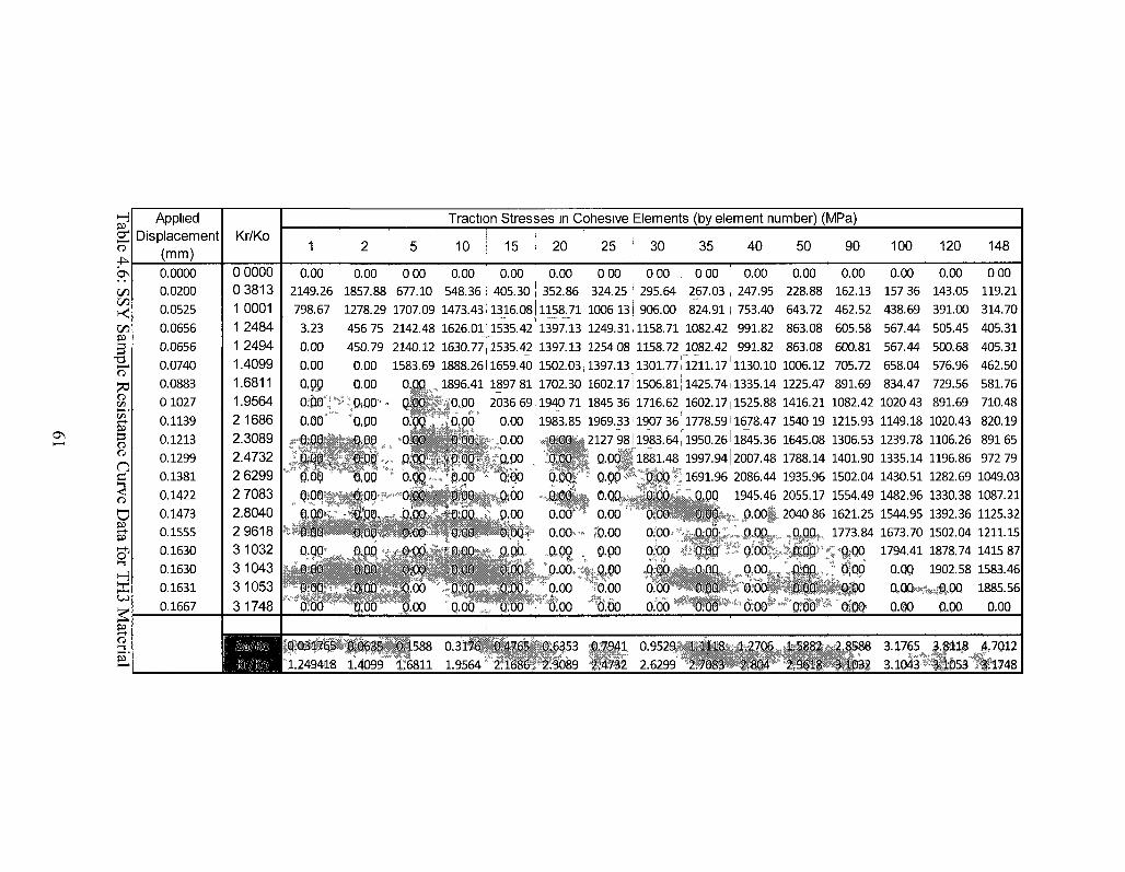
2

b\ t>0 00

00

3 CD

^

Qfi '

£3

5 o CD

n 3 CD o P5

H

CD H-1 •

EL

Applied Displacement

(mm) 0.0000 0.0200

0.0525

0.0656

0.0656 0.0740

0.0883

0 1027

0.1139

0.1213

0.1299

0.1381

0.1422

0.1473 0.1555

0.1630

0.1630

0.1631

0.1667

Kr/Ko

0 0000 0 3813

1 0001

1 2484

1 2494

1.4099

1.6811 1.9564

2 1686

2.3089 2.4732

2 6299

2 7083

2.8040

2 9618 3 1032

3 1043

3 1053

3 1748

Traction St resses in Cohesive Elements (by element number) (MPa)

1

0.00 2149.26

798.67

3.23

0.00

0.00

Q,QP Ofiioi*

O.OO"*""

0.00

0,00 ;

0.00

0.00

0.00

0.00

0.Q0

0.00

0;00

0.00

2

0.00

1857.88

1278.29

456 75

450.79

0.00

0.00

0.00

0.00

0.00

aoo 0,00

0.00

••-o/oo -

Q.oq 0.00

0.00

• 0:00

0.00

5

0 00 677.10

1707.09

2142.48

2140.12

10

0.00

15 i 20 25

0.00 0.00 0 00 548.36 I 405.30 352.86 324.25

1473.43

1626.01

1316.08 115a7111006 13

1535.42T 1397.13 1249.31

1630.7711535.42 1397.13 1254 08

1583.69 1888.2611659.40,1502.03,1397.13

0.00

p. 00

0.00

0.00

0,00

0.00

0.00

0.00

0.00

. 0 00 ' 0.00

0.00

0.00

1896.41

0.00

. 0.00

0.00

0.00 • 0.00

0.00

^0:00

0.00

0.00 0.00

0.00

0.00

1897 8111702.30 1602.17

2036 69! 1940 71 1845 36

0.00 1983.85 1969.33

0.00 0.00 2127 98

aoo 0.00 o.oo

Q.QO 0.00. Q.QO

o,6o o.oo''' o.oo 0.00 0.00 0.00

o,oof> a o o ^ ro.oo O.ojl. ,Q„Pp . 0-PO

o.cM^.oo<iaoo •o.dJr*o.oo moo o.oo -U00 "0.00

30

0 00 295.64

906.00

1158.71

1158.72

1301.77

1506.81

1716.62

1907 36

1983.64

1881.48

0.00

0:00

0.00 0.00

o.:oo 0.00

0.00

0.00

35

0 00 267.03

40 50

0.00 0.00 247.95 228.88

824.91 1 753.40 643.72

1082.42

1082.42

1211.17

1425.74

1602.17

991.82 863.08

991.82 863.08

1130.10 1006.12

1335.14 1225.47

1525.88 1416.21

1778.59 H678.47 154019

1950.26

1997.94

1691.96

0.00

0.00 0.00

0.00

0.00

0,00

0.00

1845.36 1645.08

2007.48 1788.14

2086.44 1935.96

1945.46 2055.17

,p.00j| 2040 86

0:ot%,||tolr, o.oo , "o)oo 0.00 0.00

0.00 0.00

90

0.00 162.13 462.52

605.58

600.81 705.72

891.69 1082.42

1215.93

1306.53

1401.90 1502.04

1554.49

1621.25

1773.84

a aoo o.oo 0.00

100

0.00 157 36 438.69

567.44

567.44 658.04

834.47

1020 43

1149.18

1239.78 1335.14

1430.51

1482.96

1544.95

1673.70 1794.41

0,00

120

0.00 143.05

391.00

505.45

500.68 576.96

729.56

891.69

1020.43

1106.26

1196.86

1282.69

1330.38

1392.36

1502.04 1878.74

1902.58

0,00*^8^00 0.00 Q.QO

148

0 00 119.21

314.70

405.31

405.31 462.50

581.76

710.48

820.19

89165

972 79

1049.03

1087.21

1125.32

1211.15

1415 87

1583.46

1885.56

0.00

0.031765

1.249418

0.0635

1.4099

0.1588

1.6811

0.3176

1.9564

0.4765 0.6353 0.79|1,

2.1686 2.3089 2.473?

0.9529

2.6299 1.1118 2.7083

1.2706 1.5882

2.804 2,9618

2.8588

3.1032

3.1765 UttV 3.1043*11053

$,7012 S|,1748

Page 74

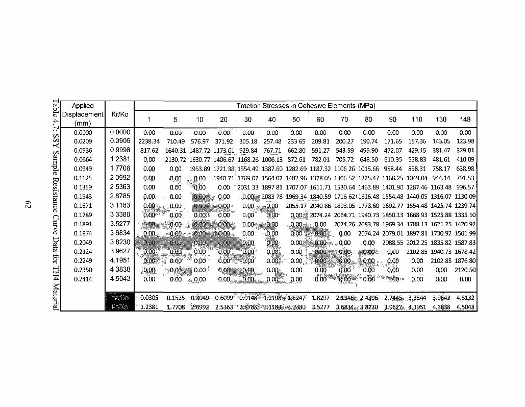
ON

H

1 ciT 4^

OO on

oo

3

3 o CD

n n CD

8-

« 4^

P ft> >-t p "

Applied

Displacement (mm) 0.0000 0.0209

0.0536

0.0664

0.0949

0.1125

0 1359

0.1543

0.1671

0.1789

0.1891

0.1974

0.2049

0.2124

0.2249

0.2350

0.2414

Kr/Ko

0 0000 0.3905

0 9998

1 2381

1 7708

2 0992

2 5363

2.8785

3 1183

3 3380

3.5277

3 6834

3 8230

3 9627

4.1951

4 3838

4 5043

Traction S t r e s s e s in Cohesive Elements (MPa)

1

0.00

2238.34

817.62

0.00

0-QQ

0.00

0-00.

,"l}lfttt ftppp 0.00

0.00

0.00

0.00

0-0QL

iwfii£" 0.00

» 0.0305

' 1,2381

5

0.00

710.49

1640.31

2130.72

Q.Q0

0.00

, o.oo •S^PJDO safe % *

0.00

0.00

0.00

0.00

0-QP

/#^§|l 0.00

0.1525

1.7708

10

0.00

576.97

1487.72

1630.77

1953.89

*%jo 0.00

o.otf' 0.00 .

0.00

0.00

0.00

0.00

0.00

1 0 , 0 ° ' * 0 . 0 0

0.3049.

2*8992

20

0.00

371.92

1173^01

1406.67

1721.38

1940.71

0.00 "

o.oo Q.00-

o.oo**1" 0.00

0.00

0.00

0.00

0.00

0.00

0.00

30 40

0.00 0.00

305.18 257.48

929.84 767.71

1168.26 1006.13

1554.49 1387.60

1769.07 1564 02

203133 1897 81

4) , f i J | | 2083 78

o.goiS^Ho' 0.0Q- 0.00

0.00 0.00

0.00 0 00

0.00 0.00

0.00 0.00

0.00 0.00

0.00 0.00

50

0.00

233 65

662.80

872.61

1282.69

1482.96

1707.07

196934

60

0.00 209.81

591.27

782.01

1187.32

1378.05

1611.71

1840.59

70 80

0.00 0.00 200.27 190.74

543.59 495.90

705.72 648.50

1106 26 1015.66

1306 52 1225.47

1530.64 1463.89

1716 62U616.48

2055.17 2040 86 1893.05 1778.60

0.00*2074.24 2064.71 1940.73

0.00

0,00 -j

0.00

0.00

0.00, ;

0.00

0.00

Ceogg"1" l0?9148%S19i!il l |5f47f

2.5363 • i J 2 « € « # « » 1 8 S i t * 3 S 8 0 !

0.00

0.00

0.00

0.00

0.00

0.00

2074.26 2083.78

90

0.00

171.65

472.07

610.35

958.44

1168.25

1401.90

1554.48

1692.77

1850.13

1969.34

0.00 2074.24 2079.01

0.00 0.QQ

0.00 0.00

0.00 0.00

Q.00 0.00

o^f"P^j$tt>? d?el *

1.8297

3.5277

2 ; i 3 4 % 2.4196

3,683,4*13.8230

2088.55

o,ao 0.QP

0.00

4 <lf!p, *

^> ' ^ ' j ^ i p i ^

110

0.00

157.36

429.15

538.83

858.31

1049.04

1287.46

1440.05

1554.48

1668 93

1788.13

1897.81

2012.25

2102.85

0.0Q

0.00

p.oo

^%S§^%*

3,9&llt 4 J951

130

0.00

143.05

381.47

481.61

758.17

944.14

1163.48

1316.07

1425.74

1525.88

1621.25

1730.92

1835.82

1940.73

2102.85

0;PO

OtPO

3.9fJ3

4.3138

148

0.00

123.98

329 01

410.09

638.98

791.53

996.57

1130.09

1239.74

1335.10

1420.92

1501.99

1587.83

1678.42

1876.80

2120.50

0.00

4,5132

4,5043

Page 75

Aa (mm)

1.62

2.46

3.33

Aa-1

(rounded)

0.6

1.5

2.3

Measured

CTOD(mm)

0.0163

0.0161

0.0170

CTOA O

1.8329

1.9227

1.8875

Opening Displacement of EL-PL Nodes (labelled by distance from original crack tip) (mm)

0.5 0.6 0.7 1.4 1.5 1.6 2.2 2.3 2.4

0.0170 0.0163 0.0154 0.0107 0.0091 0.0073 0.0002 0.0002 0.0001

0.0216 0.0210 0.0202 0.0173 0.0161 0.0149 0.0116 0.0100 0.0083

0.0254 0.0249 0.0242 0.0220 0.0210 0.0200 0.0181 0.0170 0.0157

Table 4.8: SSY CTOA Data - THl

Aa(mm)

1.010

1.130

2.270

3.350

CTOA (°)

5.69

5.33

2.97

2.71

Table 4.9: SSY CTOA Data - TH2

63

Page 76

Aa(mm)

1.010 1.520 1.760

CTOA (°)

6.61 5.45 5.19

Table 4.10: SSY CTOA Data - TH3

Aa(mm)

1.005 1.515 2.025

2.505 3.045 3.510

CTOA (°)

8.06 6.95 6.75

6.39 6.52 6.15

Table 4.11: SSY CTOA Data - TH4

64

Page 77

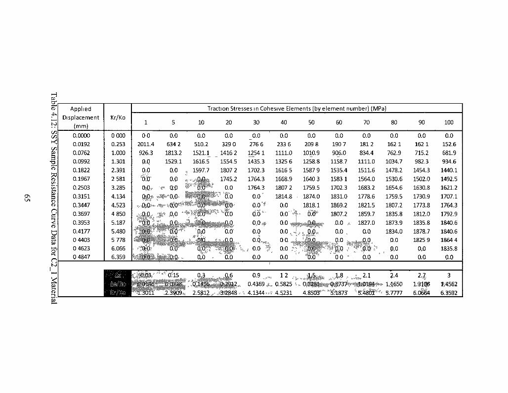
£ CO

C/3 P

ft)

CD

O

a O I CD

a P <—t-

P

3> o

Applied

Displacement

(mm)

0.0000

0.0192

0.0762

0.0992

0.1822

0.1967

0.2503

0.3151

0.3447

0.3697

0.3953

0.4177

0 4403

0 4623

0 4847

Kr/Ko

0 000

0.253

1.000

1.301

2.391

2 581

3.285

4.134

4.523

4 850

5.187

5.480

5 778

6.066

6.359

1

0 0

2011.4

926.3

0.Q 0.0

0.0

0.0

0.0

0.0

0.0

O.Q

0.0

Q.,0.

o.d 0.0

0.03

0.0146

1.3011

5

0.0

634 2

1813.2

1529.1

0.0

0.0

0.0

0.0

0,0

0.0

0.0

0.0

o.o 0.0 0.0

0.15

0.0728

2.3909

Traction Stresses in Cohesive Elements (by

10

0.0

510.2

1521.1

1616.5

1597.7

0.0

0.0

0.D

0,0

o.o o'.o 0,0

0?0

0.0

0.0

0.3

0.1456

2.5812

20

0.0

329 0

1416 2

1554.5

1807 2

1745.2

0.0

0.0

0.0'

0.0

0.0.

0.01

0.0

0.0

0.0

0.6

°-291§* 3.2848 -

30

0.0

276 6

1254 1

1435.3

1702.3

1764.3

1764.3

o.o' o.o'f o.o4* 0,01#

O.Q

, i U.U f, f 0.0

i

0-9 ^ 0.4369 A .

\ 4.1344n-f

40

0.0

233 6

1111.0

1325 6

1616 5

1668.9

1807 2

1814.8 i

0.0

0.0

0.0

0.0 1

QQ : 0.0

0.0 i

12 , t

0.5825 tv

4.5231

50

0.0

209 8

1010.9

1258.8

1587 9

1640 3

1759.5

1874.0

1818.1

0.0

0.0

0.0

0.0 .

0.0

"o:o"

1.5

0.7281

4.8503

element number) (MPa)

60

0.0

190 7

906.0

1158.7

1535.4

1583 1

1702.3

1831.0

1869.2

1807.2

O.O A

0.0 „

S;° iu

0 0 "

,158 , %

70 80

0.0 0.0

1812 162 1

834.4 762.9

1111.0 1034.7

1511.6 1478.2

1564.0 1530.6

1683.2 1654.6

1778.6 1759.5

1821.5 1807.2

1859.7 1835.8

1827.0 1873.9

Q.Q 1834.0

^ _ a o o.o f>fSi"> , f),o

O.Q * ' 0,0

<• 2 1 2 4

0 . p 3 ? r ^ | # ! l i i # i * 14650

5.18731 >igk^ggnf#, jj.7777

90

0.0

162 1

715.2

982.3

1454.3

1502.0

1630.8

1730.9

1773.8

1812.0

1835.8

1878.7

1825 9

0,0 Q.O

2,1

IMijS 6.06*64

100

0.0

152.6

681.9

934.6

1440.1

1492.5

1621.2

1707.1

1764.3

1792.9

1840.6

1840.6

1864 4

1835.8

0.0

3

114562

6.3592 p

Page 78

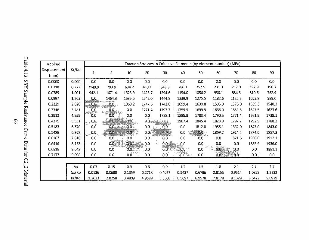
ON

CD

GO CO

CO p

o n>

O

<

o

o 'to P r-h CD

Applied Displacement

(mm)

0.0000 0.0218 0.0789 0.0997

0.2229

0.2746

0.3912

0.4379

0.5183 0.5489 0.6167

0.6416

0.6818 0.7177

Kr/Ko

0.000 0.277

1.001

1.263

2.826

3.481

4.959

5.551

6.570 6.958

7.818 8.133 8.642

9.098

Aa

Aa/Ro

Kr/Ko

1

0.0 2149.9 942.1

0.0

0.0 0.0

0.0

0.0

0.0

0.0

Q.Q 0.0

0.0 0.0

0.03

0.0136

1.2633

5

0.0 793.9 1671.4

1464.3

0.0

0.0

Q.0

0.0

o.o 0.0

0.0

0.0 0.0

0.0

0.15

0.0680

2.8258

Traction

10

0.0 634.2

1525.9

1635.5

1969.2

0.0 0.0

0.0

0.0 0.0

0.0

0.0

O.CUo 0.0 \

0.3

0.1359

3.4809

Stresses

20

0.0 410.1 1425.7

1545.0

1747.6

1771.4

0.0

0.0 0.0 0.0

0.0

r*1

0.0

0.6

0.2718

4.9589

n Cohesive

30

0.0 343.3 1294.6

1444.8

1742.8 |

1797.7

1788.1 0.0

0.0 0.0

0.0 0.0

0.0 0.0

i

0.9 0.4077

5.5508 i

Elements (by element number) (MPa)

40

0.0

286.1 1154.0

1339.9

1659.4

1759.5

1885.9

1907.4

0.0 0.0

0.0 0.0

0.0"" o.b fk >

1.2

0.5437

6.5697

50

0.0

257.5 1056.2

1275.5

1630.8

1699.9

1783.4

1845.4

1812.0 0.0

0.0 0.0

0.0 0.0

1.5 0.6796

6.9578

60

0.0 231.3

956.1

1182.6

1595.0

1668.9

1790.5

1823.9

1955.1 1869.2

0.0

ao

70

0.0 217.0

884.5 1125.3

1576.0

1654.6

1771.4 1797.7

1862.0 1914.5

1871.6 0.0

§JSjalF#0»ir

1.8

0.8155

7.8178

2.1

0.9514

8.1329

80

0.0 197.9 810.6

1053.8

1559.3

1647.5

1761.9

1792.9 1843.0

1874.0

1936.0 1885.9

o.o * *

o.o*„

2.4

1.0873 8.6422

90

0.0 190.7 762.9

999.0

1540.2

1623.6

1738.1 1788.2

1843.0

1857.3 1912.1

1936.0

1881.1 0.0

2.7

1.2232

9.0979

Page 79

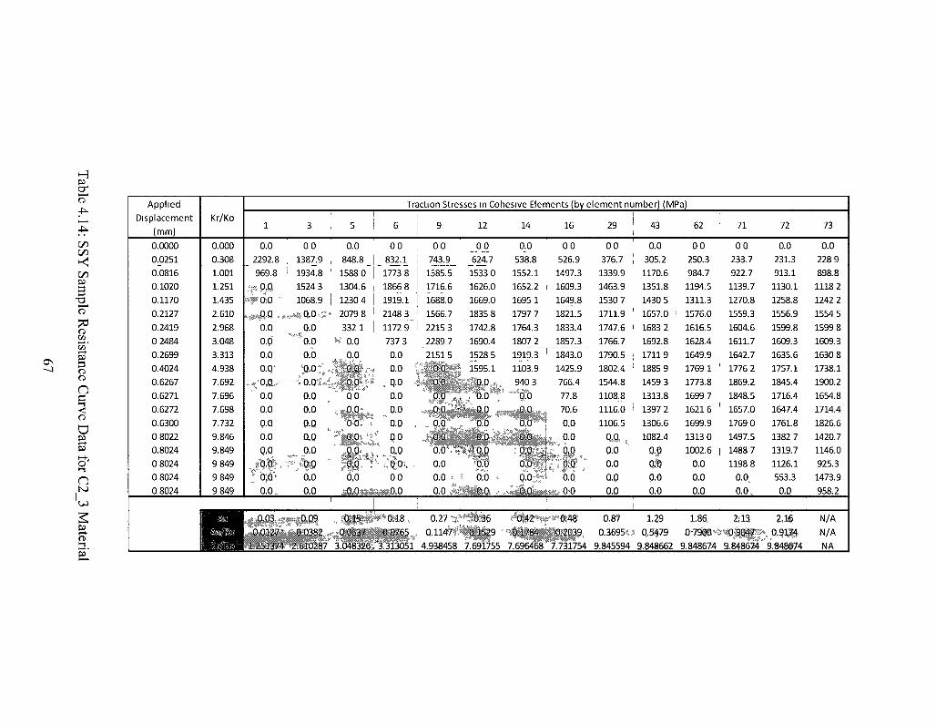
ON - J

in

CO

CO

f CD CO

o CD

O

<

a

O

CD

p "

Applied

Displacement

(mm)

0.0000

0.0251 0.0816

0.1020

0.1170

0.2127

0.2419

0 2484

0.2699

0.4024 0.6267

0.6271 0.6272

0.6300

0 8022 0.8024 0 8024

0 8024

0 8024

Kr/Ko

0.000

0.308

1.001 1.251

1.435

2.610

2.968

3.048

3.313

4.938 7.692

7.696

7.698

7.732

9.846 g.84g 9 849

9 84g

g849

BHH|

1

0.0

2292.8

969.8

"», 0,0 sg»0r0 "

3

0 0

, 1387.9 1 1934.8

1524 3

1068.9

HSI#|-Q fts%^iQi0ij;

0.0

ap 0.Q

Q.QX

. . " P ^

" 0.0 0.0

p.o 0.0

Q,0

4#' f o;!*" 0.0

0.03

0.0127

1.251374

, r 0 - 0

""^0.0 0.0

1 l , 5 1

0.0

, 848.8 1 1588 0

1304.6

1230 4

• 2079_8

332 1 U. o.O

. 9A

i o.o*i«f*Sibt,f» 0.Q 0.0

o.a o,o

do 0.0

0.09

0.0382

2.610287

~ PP

;;' o:o '!*"

Traction Stresses in Coh

6

0 0

832.1

1773 8 1866 8

1919.1

2148 3

1172 9

737 3 0.0

0.0

, Q.0 0.0

"o.o . 0 0

0,0

0.0

0.15

0.0637

3.048326:

0 0

0.0

0.18

0.0765

3.313051

9

0 0

743.9 __

1585.5 1716.6

1688.0

1566.7

2215 3 2289 7

21515

0.0

0.0

.0.0 ,„, o.b "-' 0,0 .. o.o

"0.0'."?

0.0 0.0 -

0.0 *

0.27 ,

Q.1147 4.938458

12

_A9_ 624.7

J1533 0 1626.0

1669.0

1835 8

1742.8

1690.4

1528 5

1595.1

0.0

, 0.0

• 0.0 0.0

0.0

(IP 0.0

0.0

0.36 : 0.1529

7.6gi755

esive Elements (bye

14

0.0

538.8 1552.1

1652.2

1695 1

17972 1764.3

1807 2

1919.3

1103.9

940 3

po P.P

0.0

0.0

o.o 0.0

0,42

0,1784 .

7.696468

16

0 0

526.g 1497.3

1609.3

1649.8

1821.5

1833.4

1857.3 1 1843.0

1425.9 766.4

77.8

70.6

0,0

, °-° ,- "* do

0.0

0 0 1

0-48

0-203?, 7.731754

lement number) (MPa)

29 1 i

0 0

376.7 ! 1339.9

1463.9 1530 7

1711.9 '

1747.6 i

1766.7

1790.5 ;

1802.4 !

1544.8

1108.8

1116.0 1

1106.5

^J^^ t

0.0 **

0.0

o-o 0.0

i 0.87

0.36g5»,3

g.845594

43

0.0

305.2 1170.6

1351.8

1430 5

1657.0

1683 2

1692.8

17119

1885 9 1459 3

1313.8 1397 2

1306.6

1082.4

0-1 oil p.o 0.0

1,29 P,S§79

9.848662

62

0 0

250.3 984.7

1194.5

1311.3

1576.0

1616.5

1628.4

1649.g

1769 1 1773.8

1699 7

16216

169g.9

1313 0 1002.6

0.0

Q.0 0.0

1.86

71

0 0 233.7

922.7

1139.7 1270.8

1559.3

1604.6

1611.7

1642.7 1776 2

1869.2

1848.5

1657.0

1769 0

1497.5 1488 7 1198 8

0-0, o.o „

2! 13

oim^mjUgpf g. 848674 9.848674

72

0.0

231.3 913.1

1130.1

1258.8

1556.9

159g.8

160g.3

1635.6 1757.1

1845.4

1716.4

1647.4

1761.8

1382 7 1319.7 1126.1

553.3

0.Q

2 ,1 |

, 0,9,1^

9.848f74

73

0.0

228 9 898.8

1118 2 1242 2

1554 5

159g8

160g.3

1630 8

1738.1 igoo.2

1654.8 1714.4

1826.6

1420.7 1146.0 925.3

1473.9

958.2

N/A

N/A

NA

Page 80

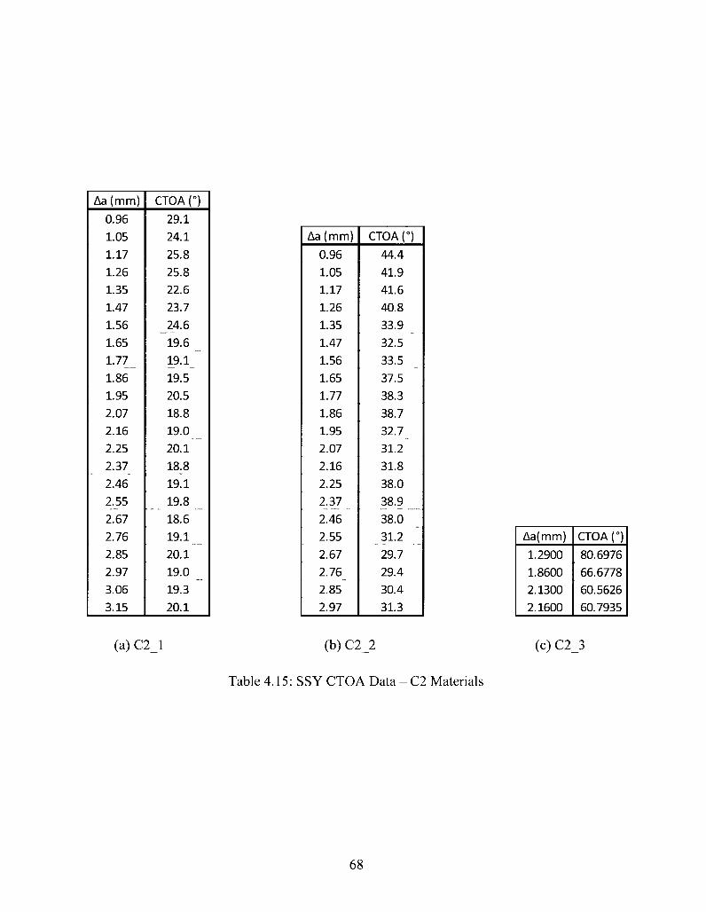
Aa (mm)

0.96

1.05

1.17

1.26

1.35

1.47

1.56

1.65

1.77

1.86

1.95

2.07

2.16

2.25

2.37

2.46

2.55

2.67

2.76

2.85

2.97

3.06

3.15

CTOA {")

29.1

24.1

25.8

25.8

22.6

23.7

24.6

19.6

19.1

19.5

20.5

18.8

19.0

20.1

18.8

19.1

19.8

18.6

19.1

20.1

19.0

19.3

20.1

Aa (mm)

0.96

1.05

1.17

1.26

1.35

1.47

1.56

1.65

1.77

1.86

1.95

2.07

2.16

2.25

2.37

2.46

2.55

2.67

2.76

2.85

2.97

CTOA (°)

44.4

41.9

41.6

40.8

33.9

32.5

33.5

37.5

38.3

38.7

32.7

31.2

31.8

38.0

38.9

38.0

31.2

29.7

29.4

30.4

31.3

Aa(mm)

1.2900

1.8600

2.1300

2.1600

CTOA (°)

80.6976

66.6778

60.5626

60.7935

(a) C2_l (b) C2_2 (c) C 2 3

Table 4.15: SSY CTOA Data - C2 Materials

68

Page 81

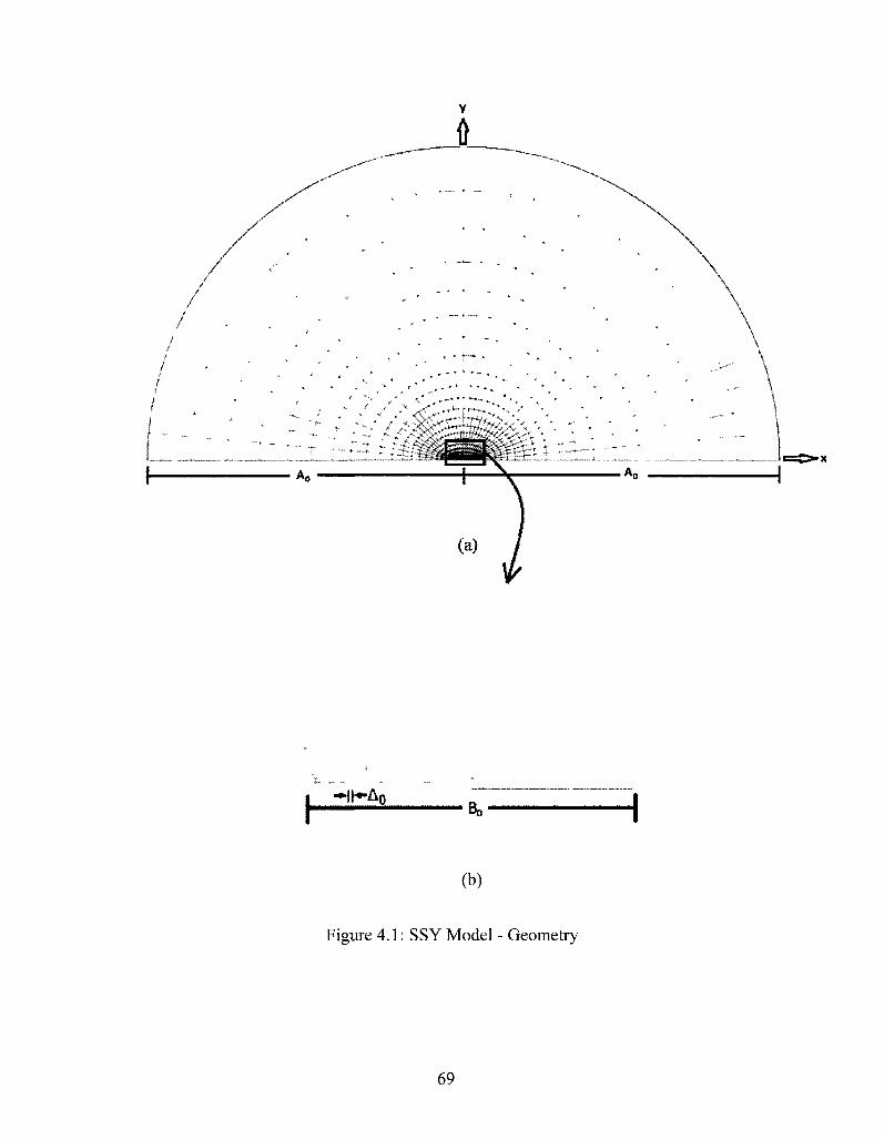
-Hh*&o. Be

(b)

Figure 4.1: SSY Model - Geometry

69

Page 82

90° \ A «

180

Figure 4.2: Loading Conditions

Figure 4.3: Mesh Design - Full Model

70

Page 83

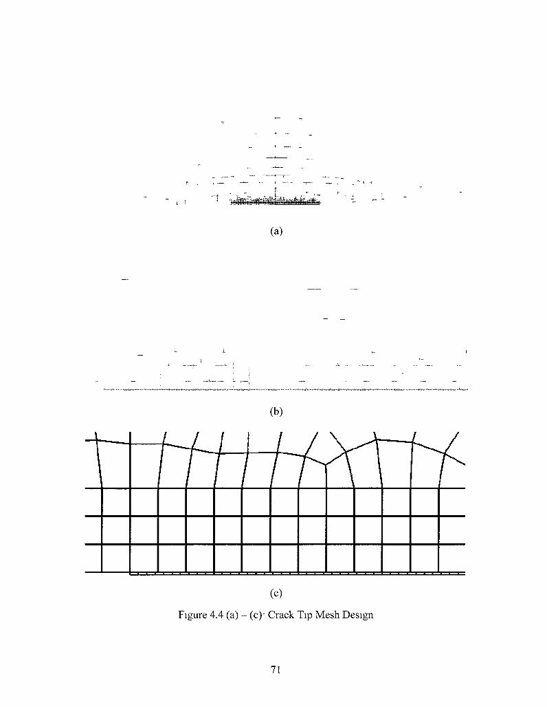
(a)

_ - . L

(b)

(c)

Figure 4.4 (a) - (c)- Crack Tip Mesh Design

71

Page 84

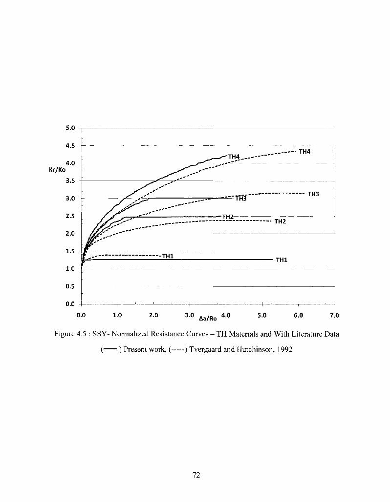
5.0

Kr/Ko

0.0 1.0 2.0 3 0 Aa/Ro 4 0 5.0 6.0 7.0

Figure 4.5 : SSY- Normalized Resistance Curves - TH Materials and With Literature Data

( — ) Present work, ( ) Tvergaard and Hutchinson, 1992

72

Page 85

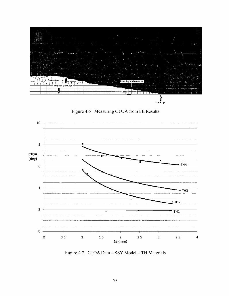
original crack tip

1mm behind crack t i p |

crack tip

10

CTOA (deg)

Figure 4.6 Measuring CTOA from FE Results

05 1 5 25 35 Aa (mm)

Figure 4.7 CTOA Data - SSY Model - TH Materials

73

Page 86

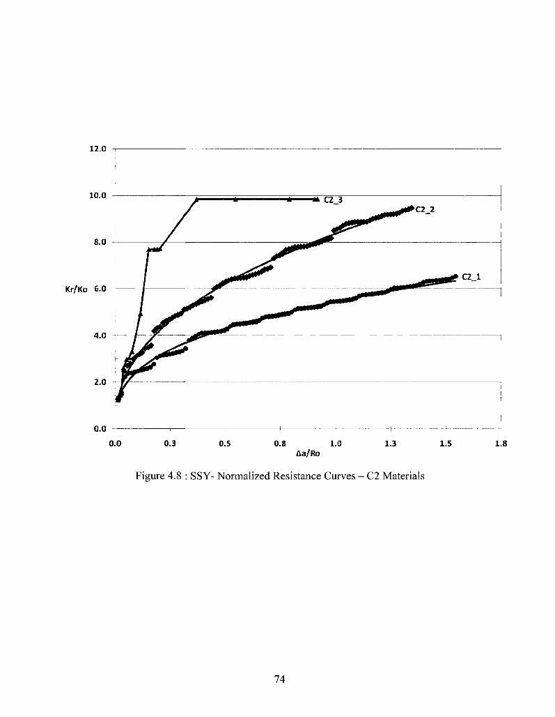
12.0

10.0

8.0

Kr/Ko 6.0

4.0

2.0

0.0

0.0 0.3 0.5 0.8 1.0 Aa/Ro

1.3 1.5 1.8

Figure 4.8 : SSY- Normalized Resistance Curves - C2 Materials

74

Page 87

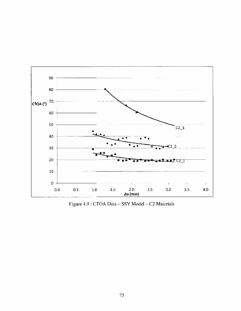
CTOA (°)

Figure 4.9 : CTOA Data - SSY Model - C2 Materials

75

Page 88

Chapter 5

FE Simulation of Drop-Weight Tear Tests

This chapter presents the finite element simulation of drop-weight tear tests, DWTT, using

cohesive zone modeling. The computational model will be defined, including geometry, loading

conditions, and mesh design. The same materials sets used in Chapters 3 and 4 will be used in

this Chapter.

CANMET-MTL has performed experimental drop-weight tear tests on samples flattened and

machined from a section of X70 pipeline steel (Xu, 2010a). This material is referred to in the

present work as C2 steel. The DWTT specimen is preferable to Charpy and other test specimens

due to its long ligament length which allows for more time to reach steady-state fracture

propagation conditions. It is also relatively easy to machine. CANMET has provided load (P) vs.

load-line displacement (LLD) data, as well as CTOA measurements for this C2 steel (Xu et al,

2010b). The data collection techniques were discussed in Chapter 2, but the data itself will be

presented here.

Two sets of simulations are performed using the DWTT model. The first set of ideal or TH

materials is used as a benchmark to compare between the SSY and DWTT models. The second

set of materials is modeled upon the C2 material characterized by Xu (2010a). The results of the

C2 material's simulations will be compared to both the SSY simulations and the experimental

observations.

5.1 Model Specifications

Geometry

The geometry for the experimental DWTT specimen can be found in Chapter 2. Figure 5.1

shows the geometry of the FE model that is used to represent this DWTT specimen. As with the

SSY model, only a half-specimen is used due to symmetry about the crack front. In this model,

the crack face is along the right side of the model, with the initial crack tip located at the bottom

76

Page 89

of the cohesive layer. The cohesive layer, or ligament length, is 61 mm long. This will allow the

crack to grow much farther than the maximum growth of 4.5 mm from the SSY model so, it

becomes much more likely that a steady-state of fracture will be achieved.

As can be seen in the figure, the machined notch is ignored for these simulations, and replaced

by what is effectively a flat crack with an initial length of 15 mm. This is done to simplify the

mesh. This is an approximation and is only intended to be used as a first approach to explore the

feasibility of CZ modeling and help calibrate the cohesive parameters.

The 'tup', which is used to apply the load to the specimen in the drop-weight test, is

approximated as a displacement field with a length of 12 mm. The anvil is approximated by

constraining 6 mm of the bottom edge in the y-direction.

The model thickness in Abaqus is left as the default for two-dimensional elements of 1.0 mm.

The method used to calibrate the results for the specimen's actual thickness of 13.7 mm is

described in Section 5.2.

Material Properties

As with the SSY model, two different sets of materials were used in this model. Elastic-plastic

material properties can be found in Tables 3.1 and 3.4 for the TH and C2 materials, respectively.

The TH materials have a Young's Modulus of 200,000 MPa, a Poisson's ratio of 0.3, and a yield

stress of 600 MPa. The C2 materials have a Young's Modulus of 195,400 MPa, a Poisson's ratio

of 0.3, and a yield stress of 576 MPa. Bilinear traction-separations laws were used again, with

cohesive parameters found in Tables 3.5 and 3.8 for the TH and C2 materials, respectively. Mass ft ^

densities of 7.85 x 10" kg/mm were used for all materials to satisfy the requirements of

Abaqus/Explicit.

77

Page 90

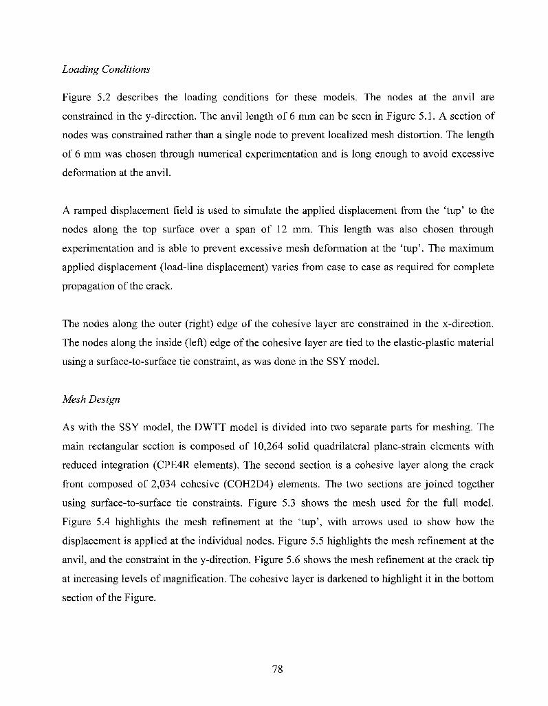
Loading Conditions

Figure 5.2 describes the loading conditions for these models. The nodes at the anvil are

constrained in the y-direction. The anvil length of 6 mm can be seen in Figure 5.1. A section of

nodes was constrained rather than a single node to prevent localized mesh distortion. The length

of 6 mm was chosen through numerical experimentation and is long enough to avoid excessive

deformation at the anvil.

A ramped displacement field is used to simulate the applied displacement from the 'tup' to the

nodes along the top surface over a span of 12 mm. This length was also chosen through

experimentation and is able to prevent excessive mesh deformation at the 'tup'. The maximum

applied displacement (load-line displacement) varies from case to case as required for complete

propagation of the crack.

The nodes along the outer (right) edge of the cohesive layer are constrained in the x-direction.

The nodes along the inside (left) edge of the cohesive layer are tied to the elastic-plastic material

using a surface-to-surface tie constraint, as was done in the SSY model.

Mesh Design

As with the SSY model, the DWTT model is divided into two separate parts for meshing. The

main rectangular section is composed of 10,264 solid quadrilateral plane-strain elements with

reduced integration (CPE4R elements). The second section is a cohesive layer along the crack

front composed of 2,034 cohesive (COH2D4) elements. The two sections are joined together

using surface-to-surface tie constraints. Figure 5.3 shows the mesh used for the full model.

Figure 5.4 highlights the mesh refinement at the 'tup', with arrows used to show how the

displacement is applied at the individual nodes. Figure 5.5 highlights the mesh refinement at the

anvil, and the constraint in the y-direction. Figure 5.6 shows the mesh refinement at the crack tip

at increasing levels of magnification. The cohesive layer is darkened to highlight it in the bottom

section of the Figure.

78

Page 91

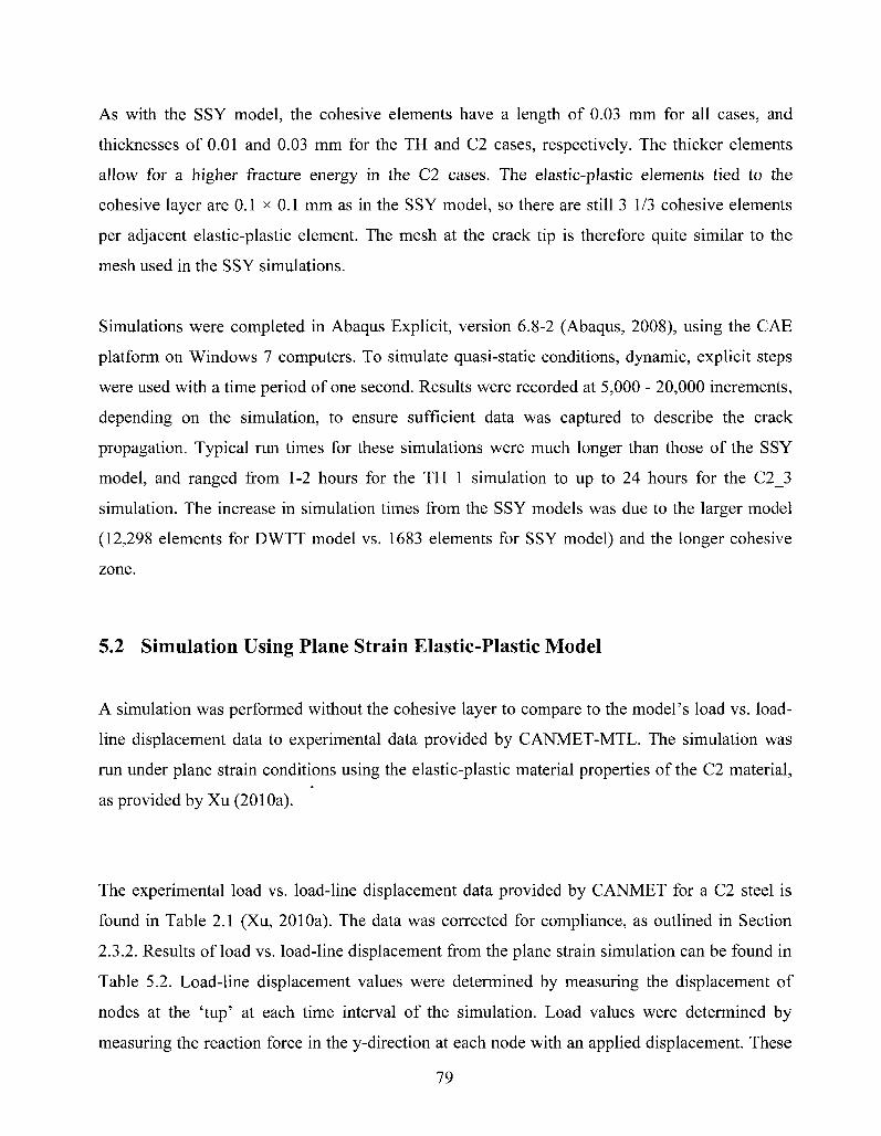
As with the SSY model, the cohesive elements have a length of 0.03 mm for all cases, and

thicknesses of 0.01 and 0.03 mm for the TH and C2 cases, respectively. The thicker elements

allow for a higher fracture energy in the C2 cases. The elastic-plastic elements tied to the

cohesive layer are 0.1 x 0.1 mm as in the SSY model, so there are still 3 1/3 cohesive elements

per adjacent elastic-plastic element. The mesh at the crack tip is therefore quite similar to the

mesh used in the SSY simulations.

Simulations were completed in Abaqus Explicit, version 6.8-2 (Abaqus, 2008), using the CAE

platform on Windows 7 computers. To simulate quasi-static conditions, dynamic, explicit steps

were used with a time period of one second. Results were recorded at 5,000 - 20,000 increments,

depending on the simulation, to ensure sufficient data was captured to describe the crack

propagation. Typical run times for these simulations were much longer than those of the SSY

model, and ranged from 1-2 hours for the TH 1 simulation to up to 24 hours for the C 2 3

simulation. The increase in simulation times from the SSY models was due to the larger model

(12,298 elements for DWTT model vs. 1683 elements for SSY model) and the longer cohesive

zone.

5.2 Simulation Using Plane Strain Elastic-Plastic Model

A simulation was performed without the cohesive layer to compare to the model's load vs. load-

line displacement data to experimental data provided by CANMET-MTL. The simulation was

run under plane strain conditions using the elastic-plastic material properties of the C2 material,

as provided by Xu (2010a).

The experimental load vs. load-line displacement data provided by CANMET for a C2 steel is

found in Table 2.1 (Xu, 2010a). The data was corrected for compliance, as outlined in Section

2.3.2. Results of load vs. load-line displacement from the plane strain simulation can be found in

Table 5.2. Load-line displacement values were determined by measuring the displacement of

nodes at the 'tup' at each time interval of the simulation. Load values were determined by

measuring the reaction force in the y-direction at each node with an applied displacement. These

79

Page 92

reaction forces were then summed, multiplied by the ratio of the thickness of the specimen (13.7

mm) to the thickness of the model (1.0 mm), and doubled because they represent the reaction

force of only one half of the full model. This is summarized by:

P(t) = 2 • 13.7 • V ^reaction ( f )

Tup Nodes

The results of this plane strain simulation can be seen in Figure 5.7, plotted along with the

experimental data from CANMET. The plane strain simulation is seen to quite closely follow the

experimental data up until almost 4 mm of load-line displacement. The simulation halted at this

point due to numerical instability. When the simulation halted, there was reaction load of 207.1

kN. This is only about 5 kN below the experimental value for the same load-line displacement.

The sharpness of the crack in the model could play a role in reducing the peak load achieved, but

overall this is quite good agreement. Additionally, it is only a 2-dimensional model and as such

is unlikely to achieve perfect agreement with the 3-dimensional lab test.

5.3 Simulation Results for TH Materials

As in Chapter 4, four simulations of the DWTT model were run with the TH elastic-plastic

material, with the same four sets of cohesive parameters (TH1-4) as the SSY simulations. The

applied displacement at the 'tup' was set to ramp up from 0 - 4 mm over 1 second of simulation.

This section presents the results of these four simulations.

Load vs. Load-line Displacement Curves

The resulting load vs. load-line displacement data for the four TH materials can be found in

Table 5.3 (a) - (d). The results are plotted in Figure 5.8. As expected, all four simulations

followed the same elastic curve until crack propagation began. This was expected as all four

simulations have the same elastic-plastic response, and cohesive element stiffnesses. The TH1

80

Page 93

and TH2 materials experience little or no plastic deformation and fail almost immediately upon

initiation of the crack. The TH3 material shows some plastic deformation before failure,

although the crack still propagates quite rapidly with little additional applied displacement. The

TH4 material shows significant amounts of plastic deformation before failure, and a much more

gradual slope during propagation of the crack due to the higher fracture toughness.

Crack Growth Rate

The crack growth, Aa, was measured by the same procedures described in Chapter 4. Data

regarding the crack growth vs. the load-line displacement of the TH materials can be found in

Table 5.4 (a) - (d). This data is plotted in Figure 5.9. It can be seen that crack initiation occurs

after load-line displacements of 0.3206, 0.3616, 0.3676, and 0.3717 mm for TH1-4, respectively.

As expected, the tougher cohesive parameters lead to an increase in the required displacement

for initiation. The crack growth rates are seen to drastically vary as well. The THl parameters

allow about 15 mm of propagation with the same applied displacement that initiates a crack 0.03

mm long in the TH4 material. The THl, 2, and 3 materials all reach a point where propagation

increases at an almost infinite rate. This signifies unstable fracture. Unlike the other three

materials, the TH4 material shows signs of stable ductile fracture.

Crack Tip Opening Angle

The CTOA was measured using the same procedures described in Chapter 4. CTOA vs. Aa data

for the four TH materials can be found in Table 5.5 (a) - (d). This data is plotted in Figure 5.10.

Power laws were fitted to the data in MS Excel.

The CTOA values were initially quite high, but steadily dropped towards steady-state values, as

expected. Steady-state values of 2.0°, 2.5°, 3.0°, and 4.5° can be estimated for TH1-TH4

respectively. These CTOA values increase with increasing toughness of the cohesive elements.

81

Page 94

The steady-state values are quite similar to those determined during the SSY simulations of 1.9°,

2.5°, 3.5°, and 6° for TH1-TH4, respectively.

5.4 Simulation Results for C2 Materials

Three simulations of the DWTT model were run with the C2 elastic-plastic material, with the

same three sets of cohesive parameters (C2_l-C2_3) as the SSY simulations discussed in

Chapter 4. The applied displacement at the 'tup' was set to ramp up from 0 - 1 0 mm over 1

second of simulation. All three simulations aborted around ~7 mm of displacement due to

numerical issues. This section presents the results of these three simulations, and compares the

results to the experimental data for the same C2 material, as provided by Xu (2010a).

Comparisons are also made with the CTOA results from the SSY simulations seen in Chapter 4.

Load vs. Load-line Displacement Curves

The resulting load vs. load-line displacement data for the three C2 materials can be found in

Table 5.6 (a) - (c). The results are plotted in Figure 5.11, along with the experimental DWTT

data (Xu, 2010a). As expected, all three simulations followed the same elastic curve until crack

propagation began. As the fracture toughness of the cohesive elements increased from C2_l-

C 2 3 , the slope decreased during the crack propagation stage of the P vs. LLD curve. None of

the three simulations were able to meet the peak load of the experimental data. It also appears

that the crack propagation in the models is beginning at a much lower applied displacement than

the experimental data shows. This could be partly explained by the higher stress concentration

the crack tip would see in the model because of the shape of the initial crack. A sharp crack, as in

the model, has a much higher stress concentration at the crack tip than a blunt notch would see.

More realistic notch geometry would need to be used in the model to improve the numerical P

vs. LLD results. Additionally, the results found by Alfano (2006) show that bilinear TS laws fail

more readily than equivalent trapezoidal and linear-parabolic TS laws (See Figure 2.4). The peak

tractions obtained between his compact tension simulation with the bilinear TS law and

82

Page 95

trapezoidal law different by up to 15%. Conceivably, experimentation with alternate TS law

shapes could also help to improve upon these numerical results for the DWTT simulations.

Crack Growth Rate

Data regarding the crack growth vs. the load-line displacement for the C2 DWTT simulations

can be found in Table 5.7 (a) - (c). This data is plotted in Figure 5.12. It can be seen that crack

initiation occurs after 0.366, 0.544, and 0.564 mm of load-line displacement for C 2 1 - C 2 3 ,

respectively. The final crack length when the simulations aborted was 12.9, 7.6, and 4.7 mm for

C2_l-C2_3, respectively.

At an applied load-line displacement of 6 mm, the crack has reached -11.5, 6, and 4 mm of

extension for C 2 1 - C 2 3 , respectively. This is a significant reduction in crack growth rate

considering the peak traction increases only from 3.5<7y - 4.0ay, and the fracture energy

increases by just 14.3 % from C2_l-C2_3. It is obvious from Figure 5.12 that all three materials

undergo stable ductile fracture.

Crack Tip Opening Angle

CTOA vs. 2la data for the three C2 materials can be found in Table 5.8 (a) - (c). This data is

plotted in Figure 5.13. Power laws were fitted to the data in MS Excel. The trendline for the

C 2 3 material was extended forwards by 1 period.

As expected, the CTOAs were initially quite high, but began to steadily drop down towards

steady-state values after a small amount of propagation. Furthermore, as the toughness increased

from C2_l to C2_3, the CTOA values increased also. A steady-state CTOA of-14° was found

for the C 2 1 material. The C 2 2 and C 2 3 simulations did not achieve steady-state CTOAs, but

using the trendlines, steady-state CTOAs of 20° and 26° can be estimated for C 2 2 and C 2 3 ,

83

Page 96

respectively. CTOA values after 1 mm of propagation start at 26.5°, 39.1°, and 51° for C2_l-

C 2 3 respectively. These are similar but lower than the values after about 1 mm crack

propagation in the SSY model which were 29.1°, 44.4°, and 80.7° for C 2 1 - C 2 3 respectively

(See Table 4.15). This is expected as the SSY simulations were unable to reach steady-state due

to the short length of the cohesive zone.

Xu, et al, (2010) have quoted the CTOA for the C2 material as 18.5°, as measured optically, and

12.4°, as calculated by the simplified single-specimen method. The CTOA values measured in

these simulations are therefore slightly higher than these experimental observations.

5.5 Conclusions

DWTT simulations were carried out for two different sets of materials. A plane strain elastic-

plastic analysis was performed for the C2 material and the simulation results were compared to

the experimental data. Following this, simulations were performed using the four TH materials,

and P vs. LLD, Aa vs. LLD, and CTOA vs. Aa were calculated and plotted. The steady-state

CTOA measurements for the TH materials were compared to the measurements from the SSY

simulations and there was found to be good agreement between the two simulations. Steady-state

CTOAs from the DWTT simulations with the TH materials ranged from 2° - 4.5".

The tougher C2 materials were then simulated and the resulting P vs. LLD curves were

compared to the experimental data provided by CANMET (Xu, 2010a). While the simulations

followed the same elastic curve, they were not able to achieve as high a peak loading value as the

experimental work. Steady-state CTOAs from the DWTT simulations with the C2 materials

ranged from 14° - 26°. These steady-state values are lower than the values measured from the

SSY simulations, but that is to be expected as the SSY simulations were not able to propagate far

enough to reach steady-state. These CTOAs are close, but slightly higher than the measured

CTOAs reported by Xu et al (2010b).

84

Page 97

The TH materials were seen to be much less tough than the C2 materials, as it took the each of

the TH materials less than 2.5 mm of applied displacement for >25 mm of crack extension. It

took 6.5 mm of applied displacement to make even the weakest C2 material (C21) propagate

just 12.9 mm. CTOA values for the C2 materials were also seen to be much higher than the TH

materials.

While the two-dimensional simulation is useful for calibrating the cohesive parameters, a more

sophisticated traction-separation law and a three-dimensional model will likely be needed to

achieve a more complete picture of what occurs during the experimental drop-weight tear test.

85

Page 98

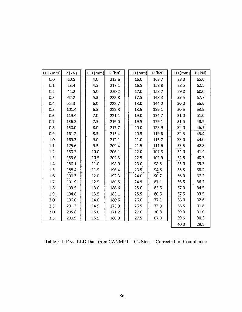
LLD (mm)

16.0

16.5

17.0

17.5

18.0

18.5

19.0

19.5

20.0

20.5

21.0

21.5

22.0

22.5

23.0

23.5

24.0

24.5

25.0

25.5

26.0

26.5

27.0

27.5

P(kN)

163.7

158.8

153.7

148.3

144.0

139.1

134.7

129.1

123.9

119.6

115.7

111.6

107.8

102.9

98.5

94.8

90.7

87.1

83.6

80.6

77.1

73.9

70.8

67.9

LLD (mm)

28.0

28.5

29.0

29.5

30.0

30.5

31.0

31.5

32.0

32.5

33.0

33.5

34.0

34.5

35.0

35.5

36.0

36.5

37.0

37.5

38.0

38.5

39.0

39.5

40.0

P(kN)

65.0

62.5

60.0

57.7

55.6

53.5

51.0

48.5

46.7_

45.4

44.0

42.8

41.4

40.3

39.3

38.2

37.2

36.2

34.5

33.5

32.6

31.8

31.0

30.3

29.5

LLD (mm)

4.0

4.5

5.0

5.5

6.0

6.5

7.0

7.5

8.0

8.5

9.0

9.5

10.0

10.5

11.0

11.5

12.0

12.5

13.0

13.5

14.0

14.5

15.0

15.5

P(kN)

213.6

217.1

220.2

222.8

222.7

222.8

221.1

219.0

217.7

215.4

212.1

209.4

206.1

202.3

198.9

196.4

192.3

189.5

186.6

183.1

180.6

175.9

171.2

168.0

LLD (mm)

0.0

0.1

0.2

0.3

0.4

0.5

0.6

0.7

0.8

0.9

1.0

1.1

1.2

1.3

1.4

1.5

1.6

1.7

1.8

1.9

2.0

2.5

3.0

3.5

P(kN)

10.5

23.4

41.2

62.2

82.3

101.4

119.4

136.2

150.0

161.2

169.3

175.6

180.2

183.6

186.1

188.4

190.3

191.9

193.5

194.8

196.0

201.3

205.8

209.9

Table 5.1: P vs. LLD Data from CANMET - C2 Steel - Corrected for Compliance

Page 99

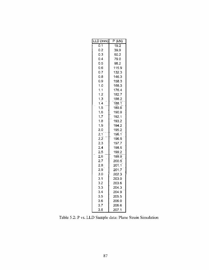
LLD (mm) 0.1 0.2 0.3 0.4 0.5 0.6 0.7 0.8 0.9 1.0 1.1 1.2 1.3 1.4 1.5 "" 1.6 1.7 1.8 1.9 2.0 2 . 1 " " " 2 2 -2.3 2.4 2.5 2.6 2.7 2.8 2.9^ 3.0 3.1 3.2 3.3 3.4 3.5 3.6 3.7 3.8

P (kN) 19.2 39.9 60.2 79.0 98.2 115.9 132.3 146.3 158.3 168.3 176.4 182.7 186.2 188.1 189.6 190.9 192.1

" 193.2 194.2 195.2 196.1" 196.9 " 197.7 198.5 199.2 " 199.9

" 200.5 201.1" 201.7" 202.3 203.0 203.6 204.3 204.9 "" 205.5 206.0 206.6 207.1

Table 5.2: P vs. LLD Sample data: Plane Strain Simulation

87

Page 100

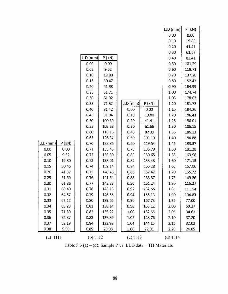
LLD (mm)

0.00

0.10

0.20

0.30

0.40

0.50

0.60

0.70

0.80

0.90

1.00

1.05

1.10

1.15

1.20

1.25

1.30

1.35

1.40

1.45

1.50

1.55

1.60

1.65

1.70

1.75

1.80

1.85

1.90

1.95

2.00

2.05

2.10

2.15

2.20

P(kN)

0.00

19.80

41.41

61.67

82.41

101.29

119.71

137.28

152.47

164.99

174.74

178.63

181.72

184.26

186.41

186.01

186.15

186.13

184.88

183.37

181.28

169.98

171.13

167.06

155.72

149.86

116.27

111.94

104.63

77.00

59.27

34.62

37.20

32.02

24.05

LLD (mm)

0.00

0.05

0.10

0.15

0.20

0.25

0.30

0.35

0.40

0.45

0.50

0.55

0.60

0.65

0.70

0.71

0.72

0.73

0.74

0.75

0.76

0.77

0.78

0.79

0.80

0.81

0.82

0.83

0.84

0.85

P(kN)

0.00

9.52

19.80

30.47

41.38

51.71

61.92

71.52

81.42

91.04

100.39

109.63

118.16

126.37

133.86

135.45

136.80

138.01

139.14

140.43

141.64

143.23

143.16

146.85

139.65

138.14

135.22

135.89

133.98

29.98

LLD (mm)

0.00

0.10

0.20

0.30

0.40

0.50

0.60

0.70

0.80

0.82

0.84

0.86

0.88

0.90

0.92

0.94

0.96

0.98

1.00

1.02

1.04

1.06

P(kN)

0.00

19.80

41.41

61.66

82 39

101.19

119.54

136.79

150.65

153 43

155 28

157.47

158.87

161.24

162.55

155.13

167.73

163.12

162.55

148.76

144.15

22.31

LLD (mm)

0.00

0.05

0.10

0.15

0.20

0.25

0.30

0.31

0.32

0.33

0.34

0.35

0.36

0.37

0.38

P(kN)

0.00

9.52

19.80

30.46

41.37

51.69

61.86

63.40

64.87

67.12

69.23

71.30

72.87

52.19

5.50

(a) THl (b)TH2 (c) TH3 (d) TH4

Table 5.3 (a) - (d): Sample P vs. LLD data - TH Materials

88

Page 101

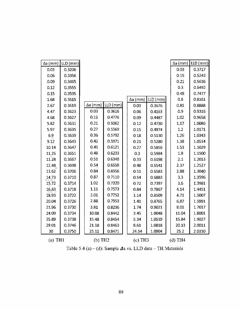
Aa (mm)

0.03

0.15

0.21

0.3

0.48

0.6

0.81

0.9

1.02

1.17

1.2

1.26

1.38

1.53

1.8 2.1

2.37

2.88

3.3

3.6

4.14

4.71

6.87

8.01

11.04

15.84

20.13

25.2

LLD (mm)

0.3717

0.5243

0.5636

0.6492

0.7477

0.8161

0.8888

0.9316

0.9658

1.0086

1.0171

1.0343

1.0514

1.1029

1.1500

1.2013

1.2527

1.3040

1.3596

1.3981

1.4451

1.5007

1.5991

1.7017

1.8001

1.9027

2.0011

2.0310

Aa (mm)

0.03

0.06

0.09

0.12

0.15

1.68

2.67

4.47

4.68

5.82

5.97

6.9

9.12

10.14

11.25

11.28

12.48

13.62

14.73

15.72

16.83

18.93

20.04

21.96

24.09

25.89

29.01

30

LLD (mm)

0.3206

0.3356

0.3465

0.3555

0.3595

0.3615

0.3619

0.3623

0.3627

0.3631

0.3635

0.3639

0.3643

0.3647

0.3651

0.3667

0.3698

0.3706

0.3710

0.3714

0.3718

0.3722

0.3726

0.3730

0.3734

0.3738

0.3746

0.3750

Aa (mm)

0.03

0.06

0.09

0.12

0.15

0.18

0.21

0.27

0.3

0.33

0.48

0.51

0.54

0.72

0.84

1.14

1.41

1.74

3.45

5.34

8.61

24.54

LLD (mm)

0.3676

0.4163

0.4487

0.4730

0.4974

0.5130

0.5280

0.5856

0.5984

0.6198

0.6541

0.6583

0.6883

0.7397

0.7867

0.8509

0.8765

0.9021

1.0048

1.0519

1.0818

1.0904

Aa (mm)

0.03

0.15

0.21

0.27

0.36

0.42

0.45

0.48

0.51

0.54

0.84

0.87

1.02

1.11

2.01

2.88

3.81

10.08

15.48

21.18

25.11

LLD (mm)

0.3616

0.4776

0.5062

0.5569

0.5792

0.5971

0.6121

0.6233

0.6348

0.6558

0.6956

0.7110

0.7320

0.7573

0.7752

0.7953

0.8236

0.8442

0.8454

0.8463

0.8471

(a) TH1 (b)TH2 (c) TH3 (d) TH4

Table 5.4 (a) - (d): Sample Aa vs. LLD data - TH Materials

89

Page 102

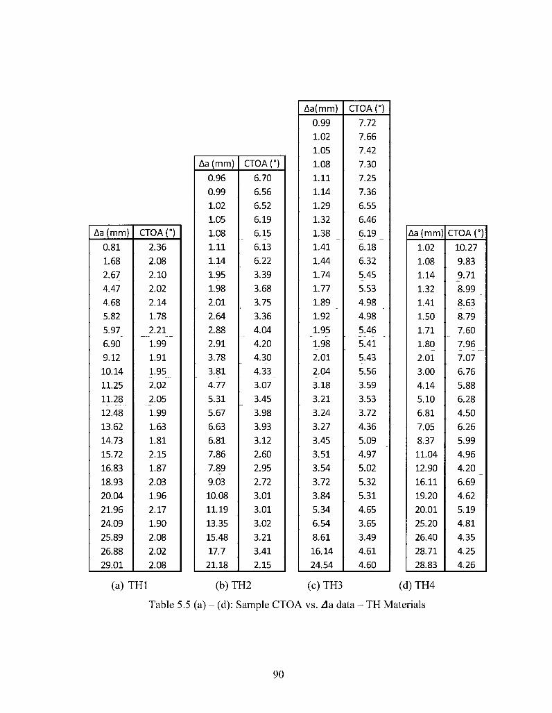
Aa(mm)

0.99

1.02

1.05

1.08

1.11

1.14

1.29

1.32

1.38

1.41

1.44

1.74

1.77

1.89

1.92

1.95

1.98

2.01

2.04

3.18

3.21

3.24

3.27

3.45

3.51

3.54

3.72

3.84

5.34

6.54

8.61

16.14

24.54

CTOA (°)

7.72

7.66

7.42

7.30

7.25

7.36

6.55

6.46

6.19

6.18

6.32

5.45

5.53

4.98

4.98

5.46

5.41

5.43

5.56

3.59

3.53

3.72

4.36

5.09

4.97

5.02

5.32

5.31

4.65

3.65

3.49

4.61

4.60

Aa (mm)

0.96

0.99

1.02

1.05

1.08

1.11

1.14

1.95

1.98

2.01

2.64

2.88

2.91

3.78

3.81

4.77

5.31

5.67

6.63

6.81

7.86

7.89

9.03

10.08

11.19

13.35

15.48

17.7

21.18

CTOA (°)

6.70

6.56

6.52

6.19

6.15

6.13

6.22

3.39

3.68

3.75

3.36

4.04

4.20

4.30

4.33

3.07

3.45

3.98

3.93

3.12

2.60

2.95

2.72

3.01

3.01

3.02

3.21

3.41

2.15

Aa (mm)

0.81

1.68

2.67

4.47

4.68

5.82

5.97

6.90

9.12

10.14

11.25

11.28

12.48

13.62

14.73

15.72

16.83

18.93

20.04

21.96

24.09

25.89

26.88

29.01

CTOA (°)

2.36

2.08

2.10

2.02

2.14

1.78

2.21

1.99

1.91

1.95

2.02

2.05

1.99

1.63

1.81

2.15

1.87

2.03

1.96

2.17

1.90

2.08

2.02

2.08

Aa (mm)

1.02

1.08

1.14

1.32

1.41

1.50

1.71

1.80

2.01

3.00

4.14

5.10

6.81

7.05

8.37

11.04

12.90

16.11

19.20

20.01

25.20

26.40

28.71

28.83

CTOA (°)

10.27

9.83

9.71

8.99

8.63

8.79

7.60

7.96

7.07

6.76

5.88

6.28

4.50

6.26

5.99

4.96

4.20

6.69

4.62

5.19

4.81

4.35

4.25

4.26

(a) THl (b) TH2 (c) TH3 (d) TH4

Table 5.5 (a) - (d): Sample CTOA vs. da data - TH Materials

90

Page 103

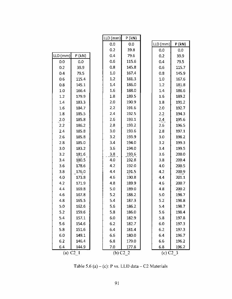
LLD (mm)

0.0

0.2

0.4

0.6

0.8

1.0

1.2

1.4

1.6

1.8

2.0

2.2

2.4

2.6

2.8

3.0

3.2

3.4

3.6

3.8

4.0

4.2

4.4

4.6

4.8

5.0

5.2

5.4

5.6

5.8

6.0

6.2

6.4

6.6

6.8

7.0

P(klM)

0.0

39.8

79.6

115.6

145.8

167.4

181.3

186.0

188.0

189.5

190.9

191.6

192.5

193.1

193.2

193.6

193.9

194.0

194.0

193.6

192.8

192.0

191.5

190.8

189.9

189.0

188.2

187.3

186.2

186.0

182.9

182.7

181.4

180.0

179.0

177.8

LLD (mm)

0.0

0.2

0.4

0.6

0.8

1.0

1.2

1.4

1.6

1.8

2.0

2.2

2.4

2.6

2.8

3.0

3.2

3.4

3.6

3.8

4.0

4.2

4.4

4.6

4.8

5.0

5.2

5.4

5.6

5.8

6.0

6.2

6.4

6.6

6.8

P(kN)

0.0

39.9

79.5

115.7

145.9

167.6

181.8

186.6

189.2

191.2

192.7

194.3

195.6

196.5

197.1

198.2

199.3

199.5

200.0

200.4

200.5

200.9

201.1

200.7

200.2

198.7

198.8

198.7

198.4

197.8

197.3

197.3

196.7

196.2

196.2

LLD (mm)

0.0

0.2

0.4

0.6

0.8

1.0

1.2

1.4

1.6

1.8

2.0

2.2

2.4

2.6

2.8

3.0

3.2

3.4

3.6

3.8

4.0

4.2

4.4

4.6

4.8

5.0

5.2

5.4

5.6

5.8

6.0

6.2

6.4

P(kN)

0.0

39.9

79.5

115.4

145.1

166.4

179.9

183.3

184.7

185.5

185.8

186.2

185.8

185.8

185.0

183.2

181.6

180.5

178.6

176.0

173.8

171.9

169.8

167.8

165.5

162.6

159.6

157.1

154.6

151.6

149.1

146.4

144.9

(a) C2_l (b) C2_2 (c) C2_3

Table 5.6 (a) - (c): P vs. LLD data - C2 Materials

91

Page 104

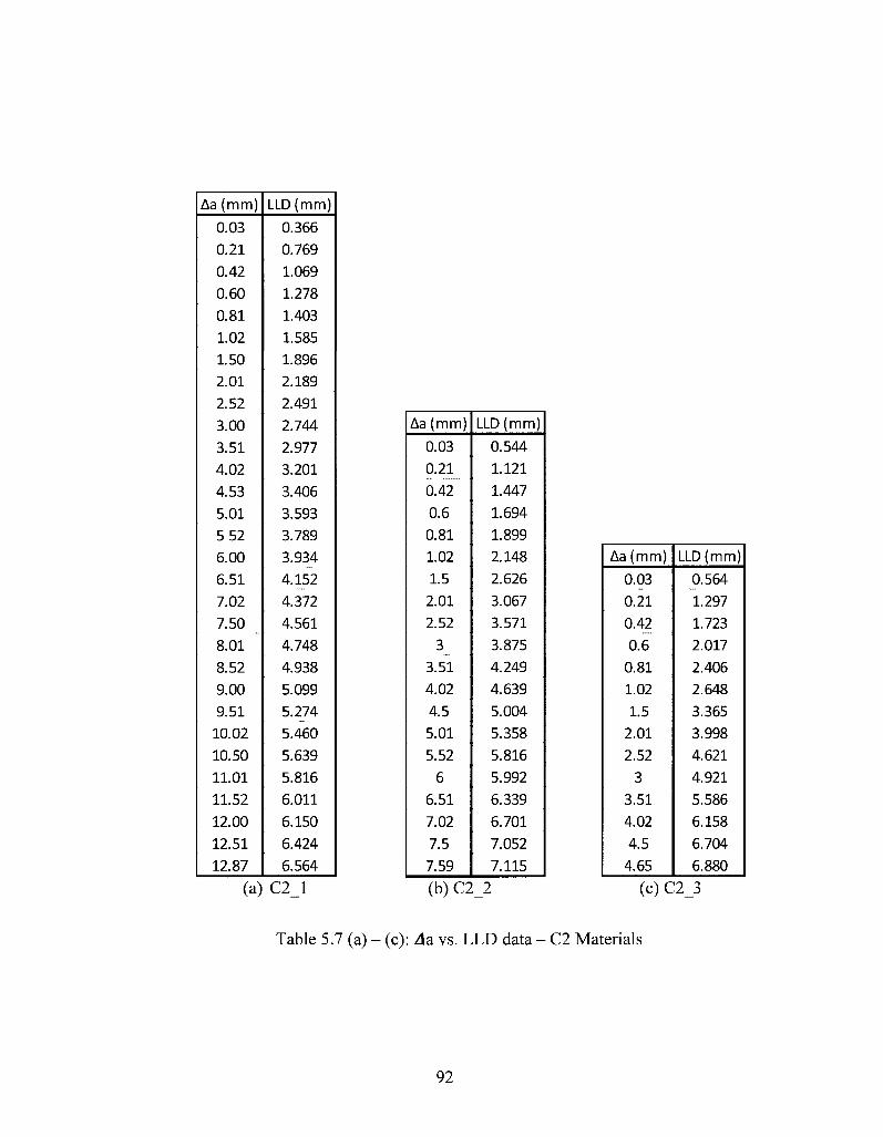
Aa (mm)

0.03

0.21

0.42

0.60

0.81

1.02

1.50

2.01

2.52

3.00

3.51

4.02

4.53

5.01

5 52

6.00

6.51

7.02

7.50

8.01

8.52

9.00

9.51

10.02

10.50

11.01

11.52

12.00

12.51

12.87

LLD (mm)

0.366

0.769

1.069

1.278

1.403

1.585

1.896

2.189

2.491

2.744

2.977

3.201

3.406

3.593

3.789

3.934

4.152

4.372

4.561

4.748

4.938

5.099

5.274

5.460

5.639

5.816

6.011

6.150

6.424

6.564

Aa (mm)

0.03

0.21

0.42

0.6

0.81

1.02

1.5

2.01

2.52

3

3.51

4.02

4.5

5.01

5.52

6

6.51

7.02

7.5

7.59

LLD (mm)

0.544

1.121

1.447

1.694

1.899

2.148

2.626

3.067

3.571

3.875

4.249

4.639

5.004

5.358

5.816

5.992

6.339

6.701

7.052

7.115

Aa (mm)

0.03

0.21

0.42

0.6

0.81

1.02

1.5

2.01

2.52

3

3.51

4.02

4.5

4.65

LLD (mm)

0.564

1.297

1.723

2.017

2.406

2.648

3.365

3.998

4.621

4.921

5.586

6.158

6.704

6.880

(a) C2_l (b) C 2 2 (c) C2_3

Table 5.7 (a) - (c): 4a vs. LLD data - C2 Materials

92

Page 105

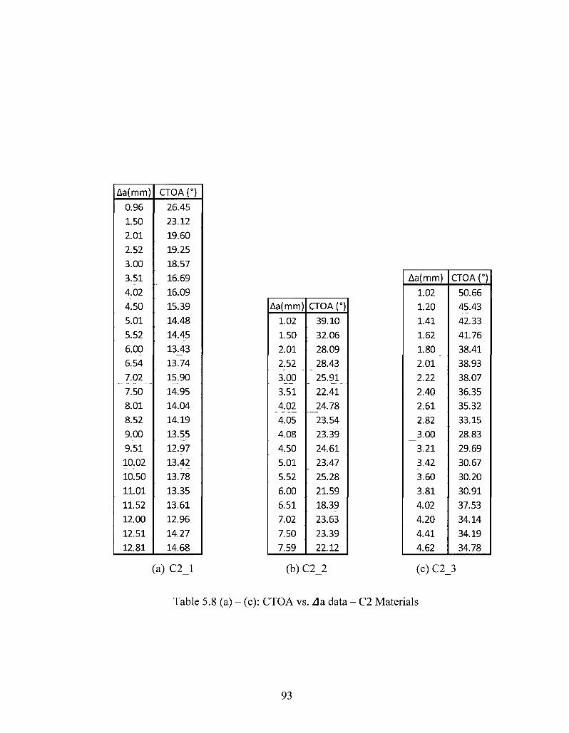
Aa(mm)

0.96 1.50 2.01 2.52 3.00 3.51 4.02 4.50 5.01 5.52 6.00 6.54 7.02 7.50 8.01 8.52 9.00 9.51 10.02 10.50 11.01 11.52 12.00 12.51 12.81

CTOA (°)

26.45 23.12 19.60 19.25 18.57 16.69 16.09 15.39 14.48 14.45 13.43 13.74 15.90 14.95 14.04 14.19 13.55 12.97 13.42 13.78 13.35 13.61 12.96 14.27 14.68

Aa(mm)

1.02 1.20 1.41 1.62 1.80 2.01 2.22 2.40 2.61 2.82 3.00 3.21 3.42 3.60 3.81 4.02 4.20 4.41 4.62

CTOA (°)

50.66 45.43 42.33 41.76 38.41 38.93 38.07 36.35 35.32 33.15 28.83 29.69 30.67 30.20 30.91 37.53 34.14 34.19 34.78

Aa(mm)

1.02 1.50 2.01 2.52 3.00 3.51 4.02 4.05 4.08 4.50 5.01 5.52 6.00 6.51 7.02 7.50 7.59

CTOA (")

39.10 32.06 28.09 28.43 25.91 22.41 24.78 23.54 23.39 24.61 23.47 25.28 21.59 18.39 23.63 23.39 22.12

(a) C2_l (b) C 2 2 (c) C2_3

Table 5.8 (a) - (c): CTOA vs. Aa data - C2 Materials

93

Page 106

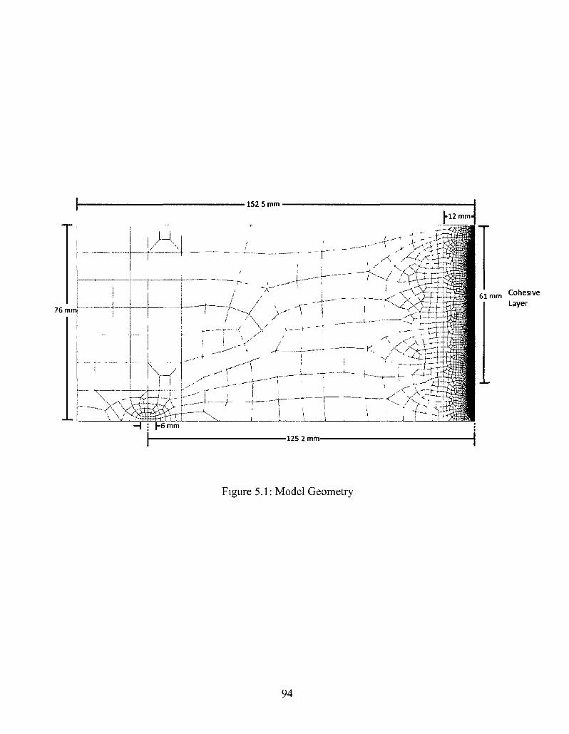
76 mm

-H : f-6mm

61 mm Cohesive Layer

-125 2 mm-

Figure 5.1: Model Geometry

94

Page 107

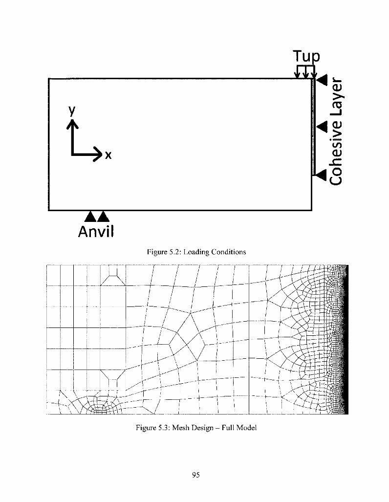
J^ o

Figure 5.2: Loading Conditions

Figure 5.3: Mesh Design - Full Model

95

Page 108

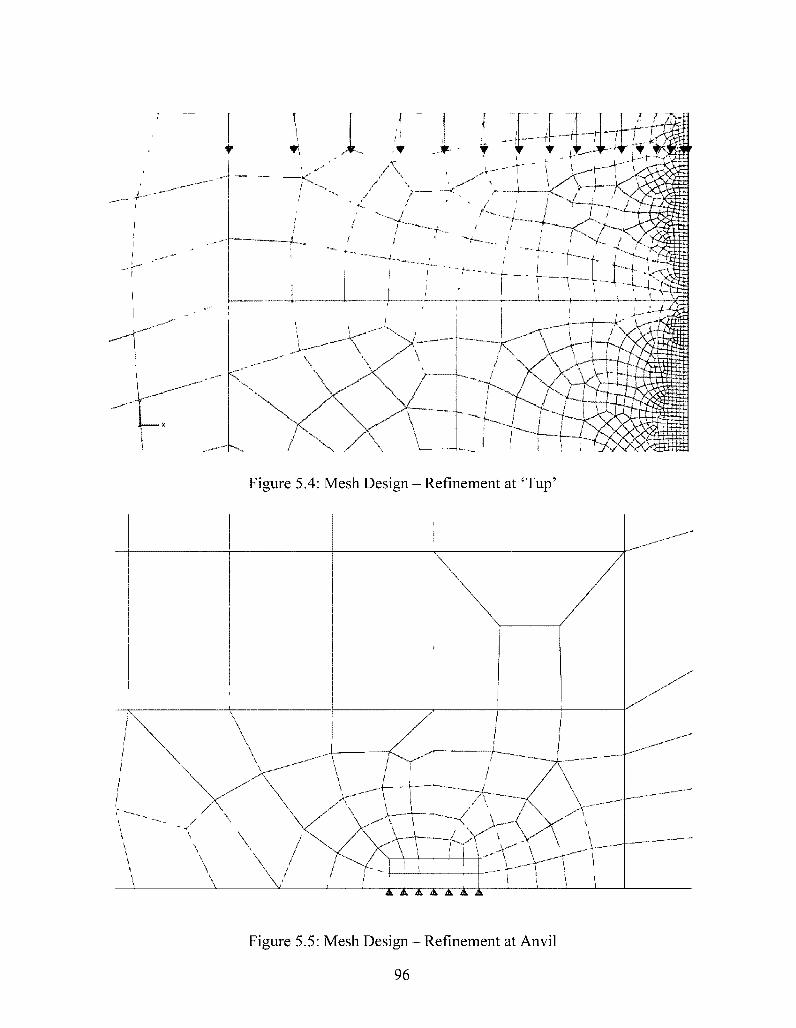
Figure 5.4: Mesh Design - Refinement at 'Tup'

fa A\A, A , A A , .A

Figure 5.5: Mesh Design - Refinement at Anvil

96

Page 109

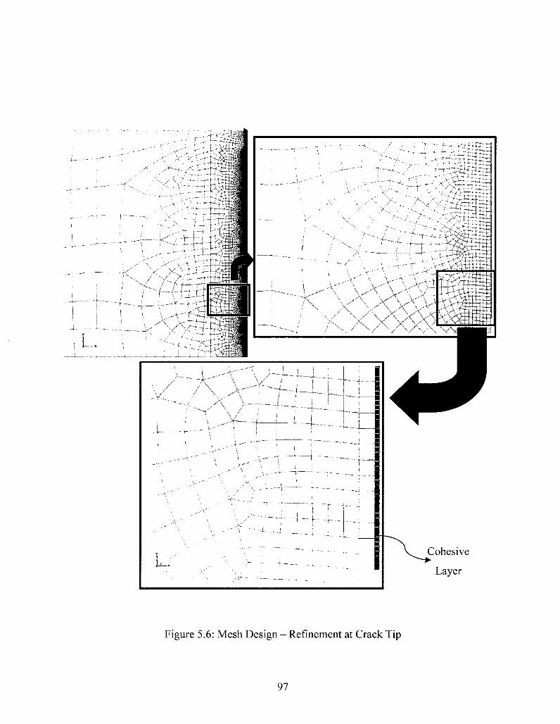
Cohesive

Layer

Figure 5.6: Mesh Design - Refinement at Crack Tip

97

Page 110

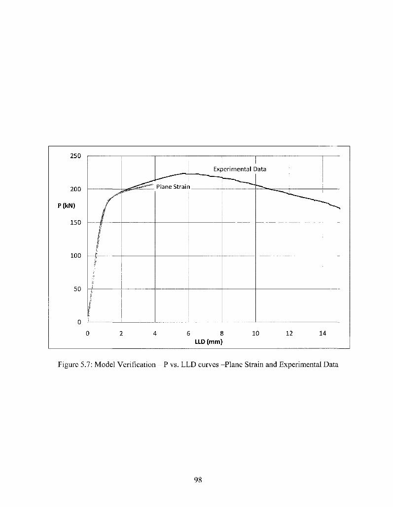
250

200

P(kN)

150

100

50

0

C

/

3

s i

I

Plane Strair

Experimental Data

l

) 2 4 6 8 10 12 14 LLD (mm)

Figure 5.7: Model Verification - P vs. LLD curves -Plane Strain and Experimental Data

98

Page 111

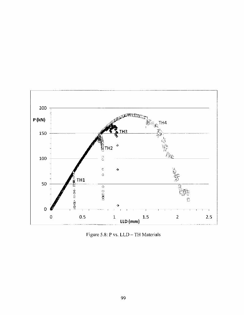
Figure 5.8: P vs. LLD - TH Materials

99

Page 112

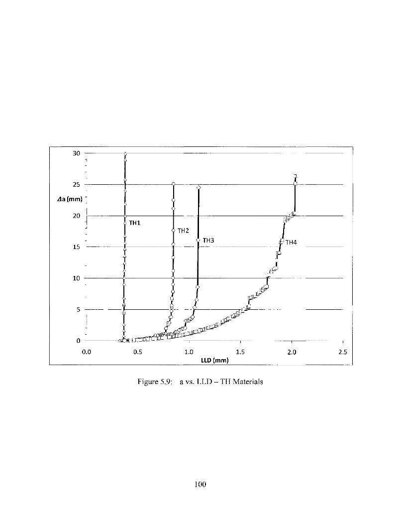
30

25

Aa(mm)

20

15

10

5

0.0 0.5

C-TH3

m

lyrludF—

tr

JTH4

r

C00"

W^ •jy

1.0 1.5 LLD (mm)

2.0 2.5

Figure 5.9: a vs. LLD - TH Materials

100

Page 113

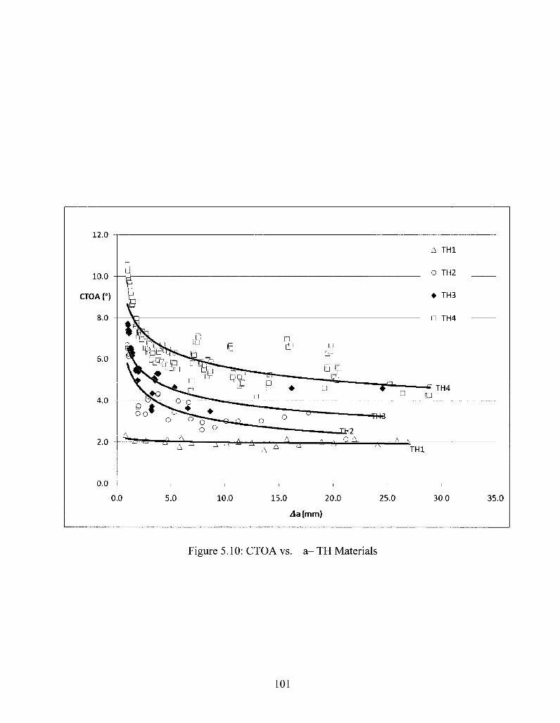
12.0

A TH1

O TH2

• TH3

• TH4

TH4

0.0

0.0 5.0 10.0 15.0 20.0

da (mm)

25.0 30.0 35.0

Figure 5.10: CTOA vs. a- TH Materials

101

Page 114

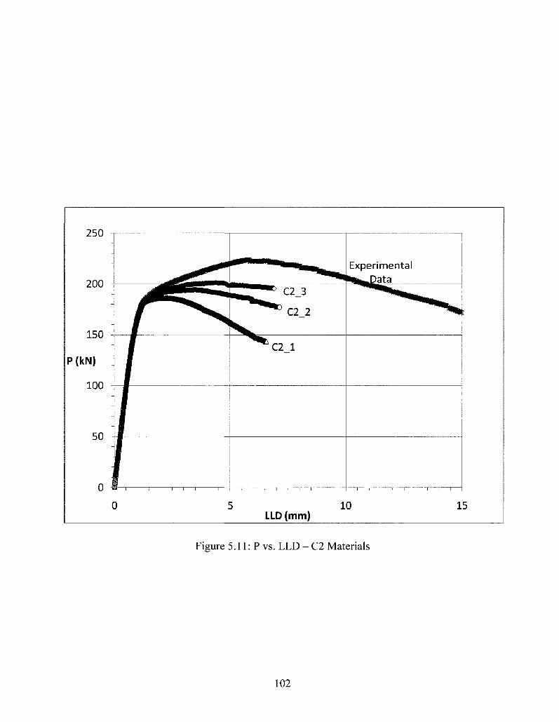
250

200

150

P(kN)

100

50

1

J^^^^^^^^_

- m

1 •

• S i l l I I I i

I " —> C2_3

^ C2_2

C2_l

Experimental Ute^Data

• ^ i f c ^ ^

i i i i i i i i

5 10 LLD (mm)

15

Figure 5.11: P vs. LLD - C2 Materials

102

Page 115

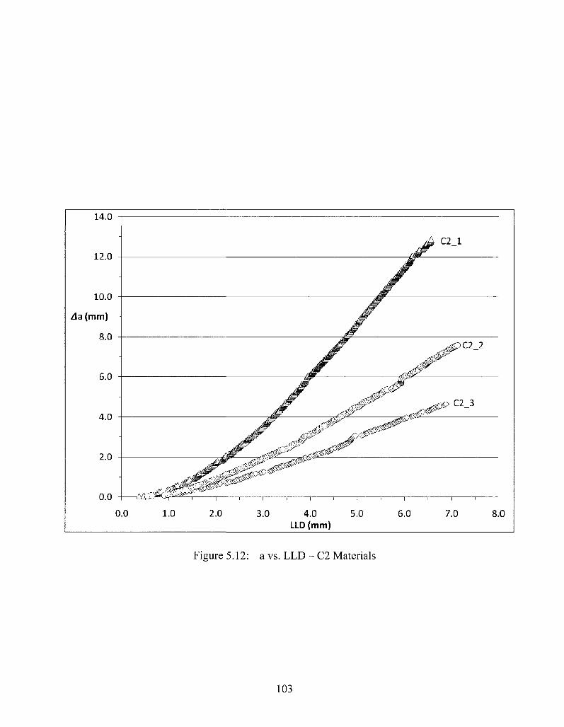
14.0

12.0

10.0

Aa (mm)

8.0

6.0

4.0

2.0

0.0 -£a:>x

:i> C2_3

• y 0.0 1.0 2.0 3.0 4.0 5.0

LLD (mm) 6.0 7.0 8.0

Figure 5.12: a vs. LLD - C2 Materials

103

Page 116

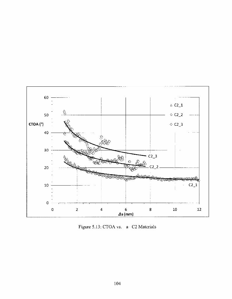
60

50

CTOA ("J

40

30

20

10

A

6 .Aa(mm)

A C2_l

o C2_2

O C2 3

^^A^^'^^T^J C2 1

10 12

Figure 5.13: CTOA vs. a- C2 Materials

104

Page 117

Chapter 6

Conclusions and Recommendations

6.1 Conclusions

In this thesis, extensive finite element simulations of ductile crack propagation using cohesive

zone modes were conducted. The following conclusions are summarized:

Unit cell models were used to verify the traction-separation laws that were implemented in this

thesis. Two sets of materials were used in this thesis. The first set, the TH materials, were

modeled after the ductile steel defined by Tvergaard and Hutchinson (1992). Four bilinear

traction-separation laws, referred to as TH1-4, were used along with the shared elastic-plastic TH

material. The second set of materials is referred to as the C2 materials. They were modeled after

an X70 steel characterised by Xu (2010a). Three bilinear traction-separation laws were

associated with the C2 elastic-plastic material. To verify the TS laws, a unit cell analysis was

performed in Abaqus/Explicit (2008) for each of the seven laws used. All seven materials were

found to respond exactly as expected.

Small-scale yielding simulations were performed to model crack propagation using the seven TH

and C2 materials. An elastic-plastic simulation, with no cohesive elements, was carried out using

the TH material, and it was verified that the stress intensity at the crack tip closely matched the

expected stress intensity due to the applied displacement field. From the simulations with

cohesive zone elements, the resistance curves (Kr/K0 vs. Aa/R0) determined from simulation for

the four TH materials were found to agree quite closely with those published by Tvergaard and

Hutchinson (1992). The resistance curves for the three C2 materials were also determined. Crack

tip opening angle data was measured for all seven simulations. Typical values of steady-state

CTOA ranged from 2° - 6° for TH1-4 respectively. While steady-state values of CTOA were not

105

Page 118

achieved for the C2 materials due to the short length of the cohesive zone, the CTOA at initiation

ranged from 30° - 80°. The CTOAs for the C2 materials ranged from 20° - 60° after 2 mm of

propagation.

Drop-weight tear test (DWTT) simulations were carried out for the seven TH and C2 materials.

A plane strain elastic-plastic analysis was carried out for the C2 material with no cohesive

elements, and the resulting load vs. load-line displacement data was found to agree quite closely

to the experimental observations (Xu, 2010a) before crack initiation. Simulations were then

carried out with cohesive zone elements. Load vs. load-line displacement data was collected for

all seven simulations, and the C2 simulations were seen to have reasonable agreement with the

experimental data (Xu, 2010a). Crack length vs. load-line displacement data was collected for all

seven simulations. CTOA data was also collected for all simulations. The steady-state CTOAs of

the TH materials during the DWTT simulations were in the range of 2° - 4.5°, which is in close

agreement to the steady-state CTOAs measured from the SSY simulations. The estimated steady-

state CTOAs of the C2 materials during the DWTT simulations were in the range of 14° - 26°.

While these values are lower than those measured from the SSY results, that is to be expected as

the SSY simulations did not have time to reach steady-state. These values are also reasonably

close to the optically measured CTOA of 18.5°, and the CTOA calculated by the simplified

single-specimen method of 12.4° (Xu et al, 2010b).

Overall, cohesive zone (CZ) modeling can be used to simulate crack propagation in ductile

steels, as has been demonstrated for the two steels referred to here as TH and C2. It is possible

to consistently measure the CTOA when using CZ modeling. Various TS laws have been

investigated, and the effects of toughening the cohesive parameters were found to be consistent

with expectations. Higher peak tractions and fracture energies led to increased fracture

resistance, and increased values for steady-state CTOA, as demonstrated by both the TH and C2

simulations. The measured CTOAs agreed reasonably between the SSY and DWTT simulations

for both the TH and C2 material sets. It is therefore likely that these CTOA values would be

transferable to real structures such as pipelines. Direct comparison between the C2 material's

106

Page 119

CTOAs measured from the DWTT simulations and the experimental observations (Su, 2010b),

had reasonable agreement.

6.2 Recommendations for Future Work

The long-term goal of the research in this area is to develop stable and computationally-efficient

cohesive zone models that could be used to predict fracture of full-scale pipeline specimens. A

secondary goal is to improve the measurement of CTOA by gaining a more thorough

understanding of the crack tip. Many steps must be completed to get this work to that point.

The first step is to gain a more thorough understanding of the results found during this work.

More work needs to be done to understand the differences between the published data by

Tvergaard and Hutchinson (1992), and the data found in this work for the TH materials (Figure

4.5). It is likely that the shape of the TS law played a large role in the discrepancies. These

simulations should be repeated using alternative TS law shapes, such as trapezoidal, exponential

and linear-parabolic, to analyze the effect that shape has on fracture resistance of both the SSY

and DWTT models, as well as the effect that shape has on the CTOA measurements from these

two models. Additionally, more work should be done to understand the oscillations seen in the

CTOA data presented in Figures 4.9, 5.10, and 5.13. It remains unknown whether this is caused

by the stiffness of the cohesive elements, or a dynamic effect of the explicit simulations. Finally,

work should be done to see if the C2 material's DWTT simulations could be fine-tuned to allow

for additional crack propagation. The abortion of these simulations due to numerical difficulties

prevents the CTOA from reaching its steady-state values.

A second step would be to improve upon the two-dimensional results found here. For example,

the current SSY model did not have a long enough cohesive zone to reach steady-state fracture

propagation for all of the materials used. Extending this CZ could increase the confidence in the

quoted steady-state values. Secondly, parametric studies could be performed to isolate the effect

that each of the three bilinear TS law parameters has on fracture resistance and CTOA

107

Page 120

measurements. These parametric studies could lead to closer representation of the experimental

observations by the numerical simulations. Moreover, these simulations could be repeated using

plane stress conditions, rather than plane strain, to determine the effect on fracture resistance and

CTOA measurements. The real test specimen, with a thickness of around 13 mm, is actually

somewhere between the two conditions.

Finally, the TS laws used here should be applied to three-dimensional SSY and DWTT models to

investigate their ability to predict trends such as crack tunnelling. Furthermore, while it seems

that 3D effects such as slant-fracture would be impossible to model using the current state of the

cohesive zone elements in Abaqus, it could be possible to model this using Extended Finite

Element Methods (XFEM) techniques.

108

Page 121

References

Abaqus (2008), Abaqus Analysis User's Manual. Abaqus Online Documentation, Dassault

Systemes, Version 6.8.

ASTM El 820-01 (2001), Standard Test Method for Measurement of Fracture Toughness, ASTM

International

ASTM E2472-06 (2006), Standard Test Method for Determination of Resistance to Stable Crack

Extension under Low-Constraint Conditions, ASTM International

G. Alfano (2006), On the influence of the shape of the interface law on the application of

cohesive-zone models, Composites Science and Technology, Vol. 66, pp. 723-730

G.I. Barenblatt (1962), The mathematical theory of equilibrium cracks in brittle fracture,

Advances in Applied Mechanics, Vol. 7, pp. 55-129

R. de Borst (2003), Numerical aspects of cohesive-zone models. Engineering Fracture

Mechanics, Vol. 70, pp. 1743-1757

N. Chandra, H. Li, C. Shet, H. Ghonem (2002), Some issues in the application of cohesive zone

models for metal-ceramic interfaces. International Journal of Solids and Structures, Vol. 39, pp.

2827-2855

C.R. Chen, O. Kolednik, I. Scheider, T. Siegmund, A. Tatschl, F.D. Fischer (2003), On the

determination of the cohesive zone parameters for the modeling of microOductile crack growth in

thick specimens. International Journal of Fracture, Vol. 120, pp. 517-536

A. Cornec, I. Scheider, K-H. Schwalbe (2003), On the practical application of the cohesive

model, Engineering Fracture Mechanics, Vol. 70, pp. 1963-1987

T. Diehl (2008), On using a penalty-based cohesive-zone finite element approach, Part I: Elastic

solution benchmarks, International Journal of Adhesion andAdhesives, Vol. 28, pp. 237-255

D.S. Dugdale (1960), Yielding of steel sheets containing slits, Journal of the Mechanics and

Physics of Solids, Vol. 8, pp. 100-104

109

Page 122

M. Elices, G.V. Guinea, J. Gomez, J. Planas (2002). The cohesive zone model: advantages,

limitations and challenges. Engineering Fracture Mechanics, Vol. 69, pp. 137-163

D.J. Horsley (2003), Background to the use of CTOA for prediction of dynamic ductile fracture

arrest in pipelines. Engineering Fracture Mechanics, Vol. 70, pp. 547-552.

ISO 22889:2007(E) (2007), Metallic materials - Method of test for the determination of

resistance to stable crack extension using specimens of low constraint. International Standards

Organization

K. Keller, S. Weihe, T. Siegmund, B. Kroplin (1999), Generalized cohesive zone model:

incorporating triaxiality dependent failure mechanisms. Computational Materials Science, Vol.

16, pp. 267-274.

A. Martinelli, S. Venzi (1996), Tearing modulus, J-integral, CTOA and crack profile shape

obtained from the load-displacement curve only. Engineering Fracture Mechanics, Vol. 53, pp.

263-277.

W. Maxey, J.F. Keifner, R.J. Eiber (1976), Ductile Fracture Arrest in Gas Pipelines, A.G.A.

catalogue number L32176

J.C. Newman, M.A. James, U. Zerbst (2003) A review of the CTOA/CTOD fracture criterion.

Engineering Fracture Mechanics, Vol. 70, pp. 371-385

J. R. Rice, E. P. Sorensen (1978), Continuing crack-tip deformation and fracture for plane-strain

crack growth in elastic-plastic solids. Journal of the Mechanics and Physics of Solids, Vol. 26,

pp. 163-186

I. Scheider, W. Brocks (2006), Cohesive elements for thin-walled structures. Computational

Materials Science, Vol. 37, pp. 101-109

D.J. Shim, G. Wilkowski, D.M. Duan, J. Zhou (2010a), Effect of fracture speed on ductile

fracture resistance - Part 1: Experimental. Proceedings of the 8th International Pipeline

Conference, IPC2010-31310.

110

Page 123

D.J. Shim, G. Wilkowski, D.M. Duan, J. Zhou (2010b), Effect of fracture speed on ductile

fracture resistance - Part 2: Results and application. Proceedings of the 8th International Pipeline

Conference, IPC2010-31021.

V. Tvergaard, J.W. Hutchinson, (1992), The relation between crack growth resistance and

fracture process parameters in elastic-plastic solids. Journal of the Mechanics and Physics of

Solids, Vol. 40, pp. 1377-1397

Williams, M.L., (1957), On the stress distribution at the base of a stationary crack. J. Appl. Mech

Vol. 24, pp. 109-114

S. Xu, R. Bouchard, W.R. Tyson (2004), Flow Behavior and Ductile Fracture Toughness of a

High Toughness Steel. Proceedings of IPC 2004, IPC04-192

S. Xu, R. Bouchard, W.R. Tyson (2007). Simplified single-specimen method for evaluating

CTOA. Engineering Fracture Mechanics, Vol. 74, pp. 2459-2464.

S. Xu, W.R. Tyson (2008), CTOA Measurement of Pipe Steels Using DWTT Specimen.

Proceedings of IPC 2008, IPC2008-64060

S. Xu, W.R. Tyson, R. Bouchard (2009). "Experimental Validation of Simplified Single-

Specimen CTOA Method for DWTT Specimens", Proceedings of 12th International Conference

on Fracture (ICF12), July 12-17, Ottawa, ON, Canada, ICF2009-269

S. Xu (2010a), Private correspondence between S. Xu and Andrew Dunbar regarding

experimental results of a DWTT for a C2 (X70) Steel and it's stress-strain curve.

S. Xu, W.R. Tyson, R. Eagleson, C.N. McCowan, E.S. Drexler, J.D. McColskey, Ph.P. Darcis

(2010b), Measurement of CTOA of pipe steels using MDCB and DWTT specimens, Proceedings

of the 8th International Pipeline Conference, IPC2010-31076.

S. Xu, G. Shen, G. Roy, W.R. Tyson (2011a), Application of plastic hinge model to single-edge-

notched bend SE(B) specimen, Report No. 2011-01 (TR), CANMET-MTL, Ottawa, ON, Canada,

April 2011

111

Page 124

S. Xu, W.R. Tyson (201 lb), Recommended practice for determination of crack-tip opening angle

of structural steels using DWTT specimens, Report No. 2011-03(TRR), CANMET-MTL,

Ottawa, ON, Canada, May 2011

112