Signature redacted / - DSpace@MIT

1

Hybrid Damping System for High-Rise Building Outriggers

by

Jing Feng

B.Eng Of Engineering (Civil)

Nanyang Technological University, 2013

Submitted to the Department of Civil and Environmental Engineering in Partial

Fulfillment of the requirements for the Degree of

Master of Engineering in Civil and Environmental Engineering

at the

Massachusetts Institute of Technology

June 2014

C2014 Jing Feng, All rights reserved

\AASSACH IN E

F TECHNOLOGY

JUN 1 3 2014

\ A N I E) b

The author hereby grants to MIT permission to reproduce and distribute publicly

paper and electronic copies of this thesis document in whole or in part in any mediumnow known or hereafter created.

Signature of Author

Certified by

Signature redactedU

Jing Feng

Department of Civil and Environmental Engineering

May 9th 2014

Signature redacted/ Jerome J. Connor

Professor of Civil and Environmental Engineering/ esis Supervisor

Accepted by_Signature redacted

Heidi MAepfChair, Departmental Committee for Graduate Students

9 1

2

3

Hybrid Damping System for High-Rise building Outriggers

by

Jing Feng

Submitted to the Department of Civil and Environmental Engineering in May 9 th 2014

in Partial Fulfillment of the Requirements for

the Degree of Master of Engineering

in Civil and Environmental Engineering

ABSTRACT

Recent design of buildings utilizes different strategies to mitigate the lateraldisplacement and acceleration from wind and earthquake excitation. One of thestrategies is to dissipate external energy with dampers. For high-rise buildings,outrigger systems which connect the core and perimeter columns are innovativesystem, which to combine stiffness of both the core and perimeter columns to resistoverturning moment. The bending moment is transferred through shear through theoutrigger system. It is an efficient lateral resistance system and an ideal location for

building damping systems. However, current damping for outriggers are limited topassive dampers. Although they can mitigate the fundamental vibration mode

effectively, their non-adjustable property limits their efficiency. The objective of thisthesis is to examine in-depth damping systems for high-rise building outriggers and to

investigate the efficiency of hybrid damping system for outriggers. Fundamentaldynamic analysis for structures are investigated and presented. Two hybrid dampingschemes are discussed in terms of efficiency and performance under earthquakeexcitation. Finally, a hybrid outrigger damping system is recommended and

simulation for a simplified Two Degree of Freedom outrigger with the recommendhybrid damping system are conducted. The results indicate that hybrid-damping

outriggers have better performance compared to passive damping system for high-risebuilding outrigger systems.

Thesis Supervisor: Jerome J. Connor.

Professor of Civil and Environmental Engineering, MIT

4

5

Acknowledgements

I would like to express my special gratitude to Dr. Xianhong Wu and his family.

Thank them for their generous funding and support; otherwise I wouldn't have been

able to complete this M.Eng Program and this report. I would like to express my

appreciation to Mr.Zhongchi Zhuo, Ms. Xia Rao, No.2 Foreign Language School in

Chongqing, China for their help.

I would like to thank Professor J. J. Connor for his guidance and care during my

process of report and through M.Eng Program.

I would like to express my gratitude towards authors for Dynamics of Structures-

Theory and Application to Earthquake Engineering and Smart Structures-Innovative

Svstemsfor Seismic Response Controls for their enlightening idea and knowledge.

Many thanks to Yiyue Zhang, David Chen, Cindy Wang, Yang Chen, Bingrui Gong,

Heng Li, Suteng Ni, Miao Shi, Ming Zheng, Siyuan Cao, Shuyue Liu and Zhuyun Gu

for their friendship, help and support through out the year. It's hard to see us part

ways. I would like to wish you all the best possible.

I would like to express my gratitude to my friend Mr.Guangzhi Xie for his

encouragement, accompany and support.

The help from Singapore University of Technology and Design is much appreciated.

Thanks to their generous funds.

I would like to express my gratitude to my parents and my family; who not only

showed me support but also gave me ultimate care.

Finally, I would love to express my gratitude towards the MEng group of 2014 for

their friendship.

6

Table of Contents

Hybrid Damping System for High-Rise Building Outriggers ............... 1....

Hybrid Damping System for High-Rise building Outriggers............................. 3

ABSTRACT...................................................................................................................3

Acknowledgements ................................................................................................. 5

List of Figures........................................................................................................ 8

List of Tables .............................................................................................................. 10

Chapter 1 Introduction ........................................................................................ 11

1.1. M otivation.....................................................................................................11

1.2. Thesis Outlines ........................................................................................ 11

Chapter 2 Structural Dynamics........................................................................... 13

2.1. Theory of Structural Dynamics .................................................................. 13

2.1.1. Basic Equations and Assumptions ........................................................ 13

2.1.2. Formulation of equation of a structural system ...................................... 13

2.1.3. Single-Degree of Freedom System ............................................................ 16

2.1.4. M ultiple- Degree of Freedom System........................................................16

2.2. Typical Damping Systems ........................................................................... 19

2.2.1. Damping in Structures .......................................................................... 19

2.2.2. Typical Damping Systems .................................................................... 21

2.2.3. Hybrid Damping Systems...................................................................... 24

Chapter 3 Structures using Semi-active and Hybrid Seismic Control Systems...26

3.1. Introduction..................................................................................................26

3.1.1. Semi-active System ................................................................................ 26

3.1.2. y y ...................................................................................... 29

3.2. Form ulation of General M odels ............................................................... 34

3.3 State-Variable Representation of Structures with Motion Controlled Devices.

.............................................................................................................................. 3 8

3.4 Control Strategy and Efficiency of HDABC Hybrid System .................... 40

Chapter 4 High-rise Building Outriggers Damping System..............................45

4.1. Introduction of High-rise Building Outriggers ........................................ 45

4.1.1. High-Rise Building Outrigger Types.................................................... 47

7

4.1.2. Necessity of Damping System for High-rise building...........................47

4.2. Typical Damping System for High-rise Building Outrigger Systems........48

4.2.1. Types of D am ping System .................................................................... 48

4.3.2. Locations of D am pers........................................................................... 49

4.3.3 Some Case Studies for Hybrid Motion Control System for Outriggers ..... 52

Chapter 5 Hybrid Damping System for High-rise Building Outriggers ...... 58

5.1. Recommended Hybrid Damping System for High-rise Building.......58

Chapter 6 Numerical Analysis of Hybrid Damping System for High-rise Building

...................................................................................................................................... 60

6.1 Simplified Modal as Two Degree of Freedom System...............62

Chapter 7 Conclusion ............................................................................................. 66

Appendix A Building Properties ............................................................................ 68

Appendix B MATLAB Codes .............................................................................. 69

Appendix C Simulation Figures .......................................................................... 77

Bibliography ..................................... ............ 79

8

List of Figures

Figure 3.1 Typical Configuration of HDABC Control System

Figure 3.2 Configuration of the Actuator in HDABC System

Figure 3.3 Configuration of the Viscous Fluid Damper

Figure 3.4 Idealization for the Viscous Fluid Damper

Figure 3.5 Liquid Mass Damper and Spring Mass Damper

Figure 3.6 Shear Building with HDABC System

Figure 3.7 Schematic and Free Body Diagram of a Shear Building with HDABC

Devices on Each Floor

Figure 3.8 Three Types of Control System (a) Open-Loop, (b) Closed-Loop, (c)

Open-Closed Loop

Figure 3.9 Three-story building model with HDABC

Figure 3.10 Required Active Control Force for El-Centro Earthquake for 0.5cm

Structural Response and 0.54cm Structural Response

Figure 4.1 New York Times Tower Lateral System

Figure 4.2(a) Behavior of Building with Outrigger under Wind Load

Figure 4.2(b) Interaction between Shear Floor with Bending Core

Figure 4.3 Outrigger Beam Attached to Shear Wall and Perimeter Columns

Figure 4.4 Locations of the Damper at Outrigger Levels

Figure 4.5 Damper Connection Details at Outrigger Level

Figure 4.6 Spring and Damper in Series and Parallel Arrangement

Figure 4.7 Frequency Based Response of the 40-Storey Building

Figure 4.8 Period Based Response of the 40-Storey Building

Figure 4.9 Simplification of the Outrigger and its Damping system

Figure 4.10 Natural Frequency and Modal Damping Ratio for each mode

Figure 4.11(a) Structure Response under the El Centro excitation

Figure 4.11(b) Structural Response under the Kobe excitation

Figure 4.12 Control Flow of the Real-Time Hybrid Simulation

Figure 4.13 Simulation and Real-Time results from Smart Outrigger

Figure 4.14 Floor Acceleration of the Smart outrigger system under (a)El Centro

earthquake and (b)Kobe earthquake

Figure 5.1 Hybrid Damping System for High-Rise Building Outriggers

Figure 6.1 Building Simplification Assumption

Figure 6.2 First Three Modes of the 40-Storey Building with Outriggers at 21'

9

Floor

Figure 6.3 El-Centro Earthquake Data

Figure 6.4 Simplified two Degree of Freedom System

Figure 6.5 Time-History Response for Comparison of Hybrid Damping System

and Passive Damping Outriggers

10

List of Tables

Table 2.1 Damping Ratio for Different Type of Structures

Table 3.1 Parameters for MR dampers

Table 6.1 Natural frequency and period of first three modes

11

Chapter 1 Introduction

1.1. Motivation

High-rise buildings are commonly built as functional features in urban cities.

Restraints such as acceleration and lateral displacement caused by wind limit the

height of the building if no motion control strategies are applied to the high-rise

building. Traditionally, tall buildings tend to use bracing system to mitigate the lateral

movement of the building. However, with the increasing height of the building,

bracing systems are not efficient for building higher than 40-storey. A damped

outrigger system such as belt truss, which ties the building core and perimeter

columns together, is implemented as an innovative system to increase the bending

rigidity of the structure and to overcome the overturning moment of the core in the

same time. Current damping systems for high-rise buildings are limited to mass and

liquid dampers; however, an alternative choice of implementing hybrid-damping

system for outriggers is a very attractive method.

This report presents an integrated study for the hybrid-damping system for the high-

rise building outriggers. Simulation studies for a simplified high-rise building were

conducted and processing schemes are identified.

1.2. Thesis Outlines

This report starts with the dynamic theory for civil structures. The basic theory and

the approach for single degree of freedom system and multiple degree of freedom

system are introduced in the first part of this report. Typical damping types are

included as well.

The second part of the report presents the design principle and theory for the semi-

active and hybrid damping system for civil structures. The state-variable formulation

and the control algorithm will be discussed in this part. Also, a shaking table test for a

three-story building model with hybrid damping system will be briefly looked into for

the efficiency comparison between hybrid damping systems to other possible systems

for structures.

12

The last part of the report presents the high-rise building outrigger system and

investigates the system with or without the dampers. The typical damped outrigger

system is studied. Two simulations and lab tests for hybrid damped outrigger system

are investigated. The efficiency for the hybrid damping outriggers is compared with

those outrigger systems without damper or with passive dampers. A computer

simulation for a simplified two-degree of freedom system is developed and

conducted. Conclusion is drawn on this part and recommendations for hybrid

damping outrigger system are offered.

13

Chapter 2 Structural Dynamics

2.1. Theory of Structural Dynamics

2.1.1. Basic Equations and Assumptions

Predicting the response of the structure from knowing stiffness k, mass m, damping

ratio c and external excitations such as forces, accelerations and displacements, is the

purpose of the structural dynamics.

For instance, viscous damped system with excitation force po, the motional equation

is expressed as:

mii +c+ku=p 0 2.1.1(1)

where m is matrix of mass, c is matrix for damping, k is the matrix for stiffness, u is

the displacement and pois the external excitation.

In actual conditions, the external excitation can be an arbitrary, step, periodic and

pulse and the damping can be viscous, friction, etc.

2.1.2. Formulation of equation of a structural system

In this section, the formulation of the equations for a structure under ground

movement and external forces will be investigated and general formulation for the

system will be combined to give an expression of the structural system assuming the

system is elastic and linear.

1). Elastic Forces

The elastic forces can be obtained by the method of superposition and the concept of

stiffness influence coefficients. If a unit displacement is applied along DOFj but all

other displacements are zero, then the forces need to keep those zero displacements

are the forces required along all other DOFs when unit displacement occurs in DOFj.

(Chopra, 2001)

14

For instance, kii (i = 1 to N) is the required force for DOFi to keep the deflected

shape when ui = 1 and all other uj = 0. The force fsi at DOFi are the superposed

forces of all the kij together with associated displacements uj (j = 1 to N).

fsi = k11u1 + ki 2u2 + -- + kijuj + --- kiNUN 2.1.2(1)

2). Damping Forces

Similar to the stiffness influence coefficients, the damping coefficients cij is the

external force in DOFi due to unit velocity in DOFj. So force fi at DOFi associated

with velocities it1 ,j = 1 to N is:

fDi = C1 h1U + Ciz2 2 + ---+ CijfQU + -- CiN fN 2.1.2(2)

3). Inertia Forces

According to D' Alembert's principle, the fictitious inertia forces oppose acceleration

applied in a mass. The mass influence coefficients mi is the external force in DOFi

due to unit acceleration along DOFj (Chopra, 2001). So force fui at DOFI associated

with acceleration njj = 1 to N is: (Connor, 1996)

fi = m1 ii + mi 2 U2 + + mijGj + --- MiN N 2.1.2(3)

For practical purpose, the vertical rotational inertia of the lumped mass is negligible.

4). Ground Motion

When a ground motion is applied to the structure, the inertia forces for the mass

equals to the mass times the total acceleration. The total acceleration equals to the

ground acceleration plus the relative acceleration between the mass and the ground.

However, only the relative motion between each floor produces the elastic and

damping forces.

From the procedure above, the structure under the ground acceleration R'g(t) is the

same as the force -m 1 iig(t). Effective earthquake forces can replace the ground

acceleration:

Peff (t) = -miR(t) 2.1.2(4)

15

5). Natural Vibration and Modes

Structure system may have various characteristic deflected shapes, associate with

different position of the applied forces. Each of the characteristic deflected shape is a

natural mode of vibration of a multiple degree of freedom system. The point of zero

displacement, which is the null point, doesn't change in one particular mode.

Structure will have different modes for one excitation due to the multiple degrees of

freedom. Those modes can be superimposed together to generate the final

displacement. Each mode is notated as Ojn (j = 1,2 ... N). In order to get the modes

of the structure, an eigenvalue analysis is required.

For a simple harmonic function with time qn(t) = An cos Oint + B sin wnt; one of

its natural vibration mode can be expressed as:

u(t) = q.(t)4n 2.1.2(5)

Where 4)n is the mode and the displacement u(t) becomes:

u(t) = (An cos wot + B, sin wnt)#/, 2.1.2(6)

As for free vibration,

nii + ku = 0 2.1.2(7)

Gives:

[-wnm4n + k#n]qn(t) = 0 2.1.2(8)

Leads to:

(k - Wm)jn = 0 2.1.2(9)

Thus, the solution is:

det[k - U)m] = 0 2.1.2(10)

which is the characteristic equation and the roots of it gives the eigenvalues. Thus, the

natural frequency of each mode is known and the solution of equation 2.1.3(9) gives

the corresponding On. In summary, a vibrating system with N DOFs has N natural

vibration frequencies and natural modes.

Three algorithms or their combinations can solve Eigen values for large structure

system. They are: 1). Vector iteration methods; 2). Transformation methods; 3).

Polynomial iteration techniques. (Chopra, 2001) Basic rational behind the iterative

methods above are finding the roots of the equation:

)= det[k - Wm] = 0 2.1.2(11)

16

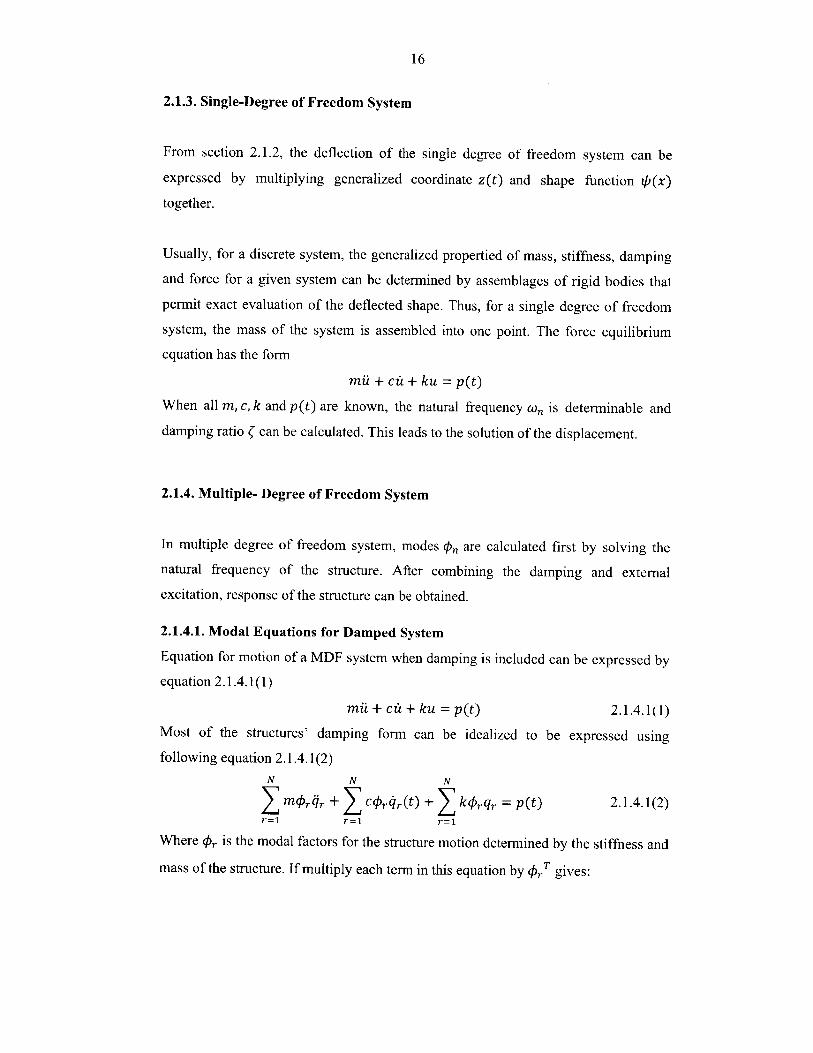
2.1.3. Single-Degree of Freedom System

From section 2.1.2, the deflection of the single degree of freedom system can be

expressed by multiplying generalized coordinate z(t) and shape function 4/(x)

together.

Usually, for a discrete system, the generalized propertied of mass, stiffness, damping

and force for a given system can be determined by assemblages of rigid bodies that

permit exact evaluation of the deflected shape. Thus, for a single degree of freedom

system, the mass of the system is assembled into one point. The force equilibrium

equation has the form

mu + cn + ku = p(t)

When all m, c, k and p(t) are known, the natural frequency &j, is determinable and

damping ratio ( can be calculated. This leads to the solution of the displacement.

2.1.4. Multiple- Degree of Freedom System

In multiple degree of freedom system, modes 0, are calculated first by solving the

natural frequency of the structure. After combining the damping and external

excitation, response of the structure can be obtained.

2.1.4.1. Modal Equations for Damped System

Equation for motion of a MDF system when damping is included can be expressed by

equation 2.1.4.1(1)

mii + c + ku = p(t) 2.1.4.1(1)

Most of the structures' damping form can be idealized to be expressed using

following equation 2.1.4.1(2)

N N N

r MOir + COJrr (t) +Y kr qr = p(t) 2.1.4.1(2)r=1 r=1 r=1

Where 4Pr is the modal factors for the structure motion determined by the stiffness and

mass of the structure. If multiply each term in this equation by O' gives:

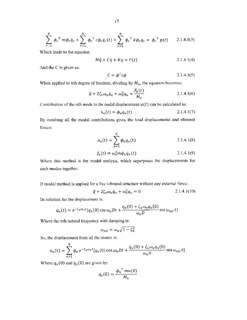
17

N N N

I Or m r + Y O T Cprr(t) + Or k rqr = PrT p(t) 2.1.4.1(3)r=1 r=1 r=1

Which leads to the equation

MO + C4 + Kq = P(t) 2.1.4.1(4)

And the C is given as:

C = pOc4 2.1.4.1(5)

When applied to nth degree of freedom, dividing by Mn, the equation becomes:

+ W2 Pn tM+ 2W + ng = Mn 2.1.4.1(6)

Contribution of the nth mode to the nodal displacement u(t) can be calculated as:

un(t) = Ongn(t) 2.1.4.1(7)

By combing all the modal contributions gives the total displacements and element

forces:

N

un(t) = Onqn(t) 2.1.4.1(8)n=1

fn(t) = 2 m#.q,(t) 2.1.4.1(9)

Where this method is the modal analysis, which superposes the displacements for

each modes together.

If modal method is applied for a free vibrated structure without any external force:

q + 2( Wo4n + Wnqn = 0 2.1.4.1(10)

Its solution for the displacement is:

qn(t) = e-nwnt[qn(0) cos OnDt + 4 nD sin oinD t]Wn D

Where the nth natural frequency with damping is:

WnD =(n- (

So, the displacement from all the modes is:

N 4n(0)±< n qn(OuN(t) = n e-n nt [qn(O) cos WnDt + O D sin WnD t]

n=1

Where qn(0) and 4n(0) are given by:

q,(0) = tT MU(0)AI

18

qn (0) =Mn

Noticeably, only the Rayleigh modal damping result in a diagonal matrix C and

represents N-uncoupled differential equations in the modal coordinates q,. The

solution of above equations is only valid when these systems have the same natural

modes with the undamped system. Non-diagonal C may be caused by different

distribution of damping properties of the structure. Classical analysis is not applicable

to this system since the modes are different from the modes for the undamped system

(Chopra, 2001). One needs to work with complex variables when C is arbitrary

(Connor, 1996).

19

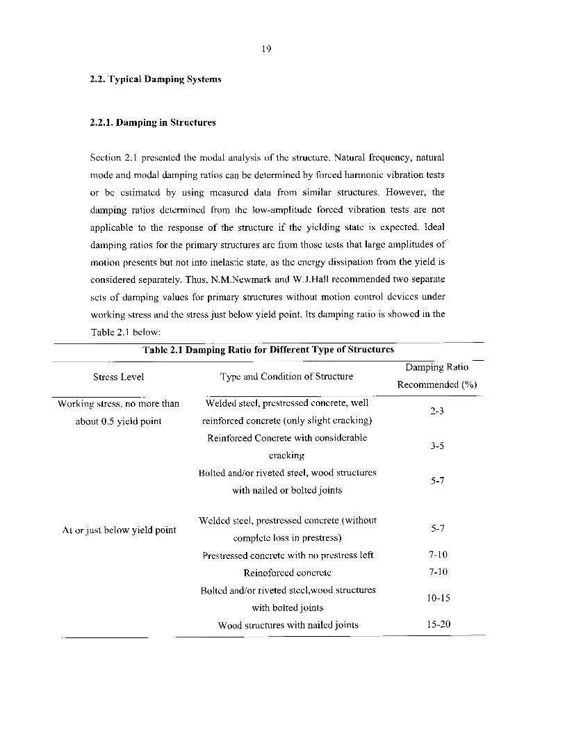
2.2. Typical Damping Systems

2.2.1. Damping in Structures

Section 2.1 presented the modal analysis of the structure. Natural frequency, natural

mode and modal damping ratios can be determined by forced harmonic vibration tests

or be estimated by using measured data from similar structures. However, the

damping ratios determined from the low-amplitude forced vibration tests are not

applicable to the response of the structure if the yielding state is expected. Ideal

damping ratios for the primary structures are from those tests that large amplitudes of

motion presents but not into inelastic state, as the energy dissipation from the yield is

considered separately. Thus, N.M.Newmark and W.J.Hall recommended two separate

sets of damping values for primary structures without motion control devices under

working stress and the stress just below yield point. Its damping ratio is showed in the

Table 2.1 below:

Table 2.1 Damping Ratio for Different Type of Structures

Damping RatioStress Level Type and Condition of Structure

Recommended (%)

Working stress, no more than Welded steel, prestressed concrete, well2-3

about 0.5 yield point reinforced concrete (only slight cracking)

Reinforced Concrete with considerable3-5

cracking

Bolted and/or riveted steel, wood structures5-7

with nailed or bolted joints

Welded steel, prestressed concrete (withoutAt or just below yield point cmltlosiprtes)5-7

complete loss in prestress)

Prestressed concrete with no prestress left 7-10

Reinoforced concrete 7-10

Bolted and/or riveted steel,wood structures10-15

with bolted joints

Wood structures with nailed joints 15-20

20

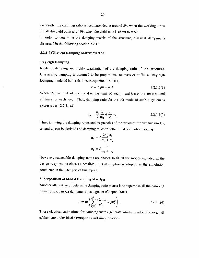
Generally, the damping ratio is recommended at around 5% when the working stress

is half the yield point and 10% when the yield state is about to reach.

In order to determine the damping matrix of the structure, classical damping is

discussed in the following section 2.2.1.1

2.2.1.1 Classical Damping Matrix Method

Rayleigh Damping

Rayleigh damping are highly idealization of the damping ratio of the structures.

Classically, damping is assumed to be proportional to mass or stiffness. Rayleigh

Damping modeled both relations as equation 2.2.1.1(1)

c = a0 m + alk 2.2.1.1(1)

Where ao has unit of sec-1 and a1 has unit of sec, m and k are the masses and

stiffness for each level. Thus, damping ratio for the nth mode of such a system is

expressed as 2.2.1.1(2)

a0 1 a1n = + Wn 2.2.1.1(2)2 w,, 2

Thus, knowing the damping ratios and frequencies of the structure for any two modes,

ao and a, can be derived and damping ratios for other modes are obtainable as:

2wgoao =- 2 ){

&, + (Ij.

2a1 =a, Ui + WIj

However, reasonable damping ratios are chosen to fit all the modes included in the

design response as close as possible. This assumption is adopted in the simulation

conducted in the later part of this report.

Superposition of Modal Damping Matrices

Another alternative of determine damping ratio matrix is to superpose all the damping

ratios for each mode damping ratios together (Chopra, 200 1).

N2 nwn Dc = M M On n M 2.2.1.1(4)

(n=1

Those classical estimations for damping matrix generate similar results. However, all

of them are under ideal assumptions and simplifications.

21

2.2.2. Typical Damping Systems

2.2.2.1 Tuned Mass Damper

High-rise building usually use tuned mass damper for vibration absorption. It can

effective control the building motion for the fundamental mode. The absorber is tuned

to the natural frequency of the main building and connected to the main building. The

response amplitude of the main system can be reduced to zero near natural frequency

of the main system. However, this kind of damping system is usually applicable for a

very narrow band of excitation frequencies (Franklin Y. Cheng, 2008). For building

wind motion mitigation, it is used when the motion exceeding the comfortable zone

for the occupancy. Vibration of other modes will need to be mitigated using

supplemental damping systems.

2.2.2.2 Tuned Liquid Dampers

Tuned liquid damper uses liquid instead of solid mass in motion control. The kinetic

energy is transferred to thermal energy through the shake. Generally, there are two

types of tuned liquid dampers. One is the sloshing damper which use meshes or rods

in the liquid to generate damping forces. The other one is the column damper, which

uses flow in its orifice to achieve damping. One disadvantage of the liquid mass

damper is that more space is required and the design process is complicated due to its

high non-linearity (Tamura, 1995).

2.2.2.3 Friction Devices, Metallic Yield Devices and Viscoelastic Dampers

Bracing system is the common lateral displacement resistance system us pioneered by

Pall and Marsh (Pall, 1982). It makes the friction devices on the bracings become

popular. Its function is achieved by relative friction between two solid bodies that

slide relative to each other such as the structure and the braces (Aiken, 1992). The

advantages of the friction devices are the convenience of installation and effectiveness

of seismic mitigation. However, its performance is affected by the long reaction time

interval and deformation associate with temperature and corrosion.

22

Inelastic deformation creates a way to dissipate energy as well. Metallic hysteric

devices can be installed in a structure to absorb energy. Common models are Tyler's

yielding steel bracing system and added damping and stiffness (ADAS) devices.

However, nonlinearity deficiency of this type of dampers affects the design process

(Franklin Y. Cheng, 2008). Adding this kind of damper increase the stiffness of the

structure, which may not be preferable.

Another damping system is viscoelastic (VE) dampers, which exploit shear

deformation of the VE material (rubber, polymers and glassy substances) to generate

high damping. VE dampers usually are installed as part of the chord or the bracing

system. Shear deformation is activated if relative motion is induced between steel

outer flange and center plate. VE dampers have the advantage of linearity behavior

due to the linearity property of the materials. However, temperatures and frequency

related with the property of the material are not reflected in the design process as VE

materials can only be expressed by shear storage modulus and shear loss modulus.

Viscous fluid damper in full scale was first implemented for bridges in Italy in the

1970s (Soong T. D., 1997). It consists of classical dashpot, piston and thick viscous

fluid. Kinetic energy is transformed to thermal energy through piston motions.

Damping piston moves in the damper fluid in damper housing in all six degrees of

freedom. A innovative version of the viscous fluid damper is viscous damping wall

which consist a steel piston to move in long rectangular steel container filled with

viscous fluid with pistons attached to the floor above and container attached to the

floor below (Arima, 1088). It behaves linearly but also temperature and frequency

dependent.

2.2.2.4 Semiactive Damping System

Hrovat et al. proposed a semiactive tuned mass damper for wind vibration mitigation

in tall buildings. This semiactive tuned mass damper consists of normal tuned mass

damper with actuator, which will generate a control force to adjust the damping force

of the tuned mass damper (Hrovat, 1983). It only requires small energy input to

change the damping force of the tuned mass damper as it is relatively small compare

to the whole building.

23

Also, semi-active liquid damper regulates the direction of the fluid to control the

orientation of the liquid by dividing the tank of the liquid damper into numbers of sub

chambers (Franklin Y. Cheng, 2008). Change of the chamber length will achieve the

purpose of changing the natural frequency of the damper. To achieve these only

requires small amount of energy.

Semi-active friction damper was developed by using a compressing piston vertically

to the friction interface to adjust the pressure (Akbay, 1991). The pressing devices can

be mechanical or electromechanical and it provides efficient energy dissipation.

There are other semi-active damper systems such as semi-active vibration absorbers,

stiffness control devices, electroheological dampers, magnetorheological dampers and

viscous fluid dampers. Their details will be presented in Chapter 3.

2.2.2.5 Active Damping System

One of the disadvantages for passive damping system is that it can't adjust itself

based on the external excitation conditions. Even the semi-active damper system can

only modify the system within its passive damping capacity. Active system can

overcome those disadvantages by using powerful actuators to enhance control

effectiveness. Thus it can adopt to ground motion and apply to different excitation

mechanisms. Active damper system consist of sensors to detect excitation or system

response, controllers to generate necessary control signals and at last the actuators to

generate the resisting force to the excitations (Nishimura, 1992).

Active bracing damping system can be installed in diagonal, K-braces and X-braces.

The hydraulic actuator is mounted on the floor and connected to the brace (Yang J. G.,

1982). In this configuration, pressure difference in two actuator chambers generates

the resisting force.

Another promising active damping system is pulse generation system, which utilizes

the gas pressure to generate a pulse force opposite to the detected velocity on the

point of the installation when the velocity is high. Although the pulse generation

system is very economical, the power scale of the system may not be sufficient for the

24

whole structure and the nonlinearity of the system may not generate an ideal

rectangular shape pulse (Franklin Y. Cheng, 2008).

2.2.3. Hybrid Damping Systems

Semi-active system utilize the changeable property of the structural damping property

while the hybrid systems apply external energy or force direct to the structure.

Capacity of the semi-active system is limited by the capacity of its passive part while

the hybrid system can have additional control capacity. However the active control

device relies on external powers and its stability and cost effectiveness are its major

concerns (Connor, 1996). Thus, hybrid system consists of passive and active damper,

which would take advantage of both systems.

Typical hybrid control systems are: hybrid mass dampers, hybrid base isolation and

damper-actuator systems (Franklin Y. Cheng, 2008).

2.2.3.1 Hybrid Mass Dampers

Hybrid Mass damping system amounts an active mass damper to control the tuned

mass damper (Fujita, 1994). The scale of the active damper can be 10%-15% of the

tuned mass damper and it can improve the control for higher mode by generating a

control force to tuned mass damper. Although it is widely used in full-scale structures,

the requirement of sufficient space limits its application.

2.2.3.2 Hybrid Base-Isolation System

The hybrid base-isolation system usually consists of a bracing tendon system and a

MR fluid base-isolation system (Yang J. D., 1991). It can adapt the changing

earthquake intelligently due to the MR fluid base-isolation system.

2.2.3.3 Hybrid Damper-Actuator Bracing Control

Cheng and his associates proposed the hybrid damper-actuator bracing control, by

mounting on K-braces of the structure (Cheng F. a., 1998). The system combined

active control with passive control in one bracing unit. Active control system is the

hydraulic actuator and the passive control system is the fluid damper. The hybrid

25

damping system has more capacity than passive damping system and requires less

power than the active damping system.

26

Chapter 3 Structures using Semi-active and Hybrid Seismic Control Systems

3.1. Introduction

Chapter 2 has introduced different types of damping systems used so far. Most cases

in high-rise building, the seismic control systems are limited to mass damping system.

This chapter will conduct some detailed discussion on the semi-active and hybrid

control systems for seismic response control of building structures. The

electrorheological(ER) and magnetorheological(MR) dampers will be presented as the

example for the semi-active systems. Hybrid damper actuator bracing control

(HDABC) will be the example of passive-active hybrid damping system.

To elaborate the design of the damping systems, a general model which as both

passive and active control devices on each floor will be presented. The effective of the

hybrid damping system will be demonstrated through the numerical study results.

Research has revealed that damping ratio for hydraulic actuators, MR dampers and

viscous fluid dampers are not proportional with the input (Franklin Y. Cheng, 2008).

Thus, this chapter will also suggest the analysis methods for the actuators and

dampers.

3.1.1. Semi-active System

Most semi-active dampers are nonlinear manner. Electrorheological and

magnetorheological fluids are the lately developed potential fluids, which can be used

to achieve high efficiency.

3.1.1.1 Electrorheological(ER) Dampers

Total shear of the electrorheological damper is proposed by Bingham viscous-plastic

model which relate the plastic viscosity with the slope of shear stress as:

T = TU + rif 3.1.1.1(1)

Where -ru is the yield stress induced by the electric field and 71 is the viscosity of the

fluid, and k is the shear rate. It is idealized as a Coulomb friction element placed in

27

parallel with a linear viscous damper. The force generates by the viscous damper is

proportional to the relative velocity between the damper and friction element. Force

generates by the device is:

fsa(t) = fc sin(A(t)) + cOA(t) 3.1.1.1(2)

Where f, is friction force related to the fluid yield stress, co is damping coefficient

and A(t) is the relative velocity between the piston and the structure.

3.1.1.2 Magnetorheological(MR) Dampers

This promising dampers has an immediate reaction time to excitations, not only create

far higher yield stress than ER fluid, but also has stable yield stress unaffected by

temperature, insensitive to impurities and can be controlled by low voltage. The

energy requirement by this system is also very low. However, long term durability is

a problem for this damper.

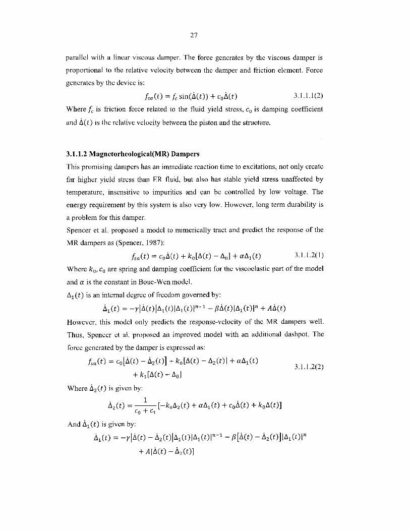
Spencer et al. proposed a model to numerically tract and predict the response of the

MR dampers as (Spencer, 1987):

fsa(t) = cOA(t) + ko[A(t) - A0] + aA,(t) 3.1.1.2(1)

Where ko, co are spring and damping coefficient for the viscoelastic part of the model

and a is the constant in Bouc-Wen model.

A1 (t) is an internal degree of freedom governed by:

A1(t) = -yIA(t)A1(t)IA1(t)In-1 - pA(t)IA1 (t)In + AA(t)

However, this model only predicts the response-velocity of the MR dampers well.

Thus, Spencer et al. proposed an improved model with an additional dashpot. The

force generated by the damper is expressed as:

fsa(t) = co[A(t) - A2 (t)] + ko[A(t) - A2(t)]+ aA(t) 3.1.1.2(2)

+ kl[A(t) - A0]

WhereA 2 (t) is given by:

1A2 (t) = [-kOA2 (t) + aA,(t) + cOA(t) + kOA(t)]

CO + C,

And A1(t) is given by:

A1(t) = -YIA(t) - A2 (t) 1 (t)IA1(t)n-1 - p[A(t) - A2(0]IA,(t)ln

+ A[A(t) - A 2(t)]

28

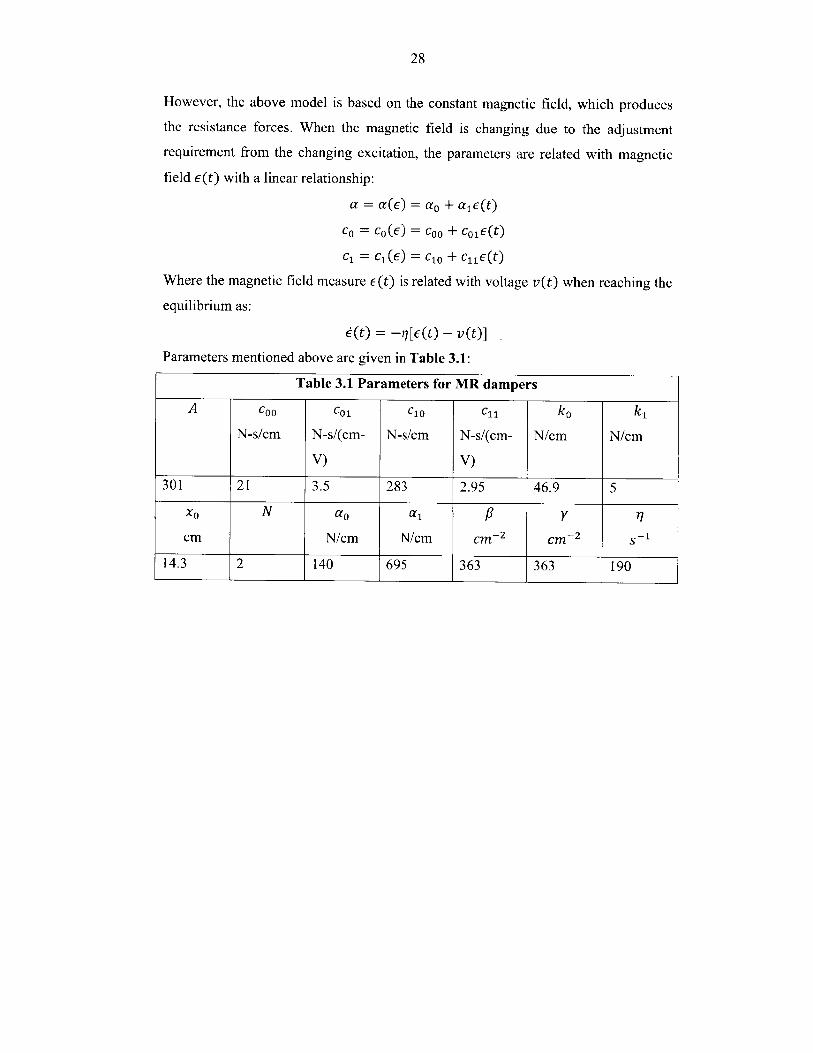
However, the above model is based on the constant magnetic field, which produces

the resistance forces. When the magnetic field is changing due to the adjustment

requirement from the changing excitation, the parameters are related with magnetic

field e(t) with a linear relationship:

a= a(e) = ao + ae(t)

CO= cO(E) = coo + C0 1 E()

C= c1(E) = C10 + C11E(t)

Where the magnetic field measure E(t) is related with voltage v(t) when reaching the

equilibrium as:

= -r7[E(t) - v(t)]

Parameters mentioned above are given in Table 3.1:

Table 3.1 Parameters for MR dampers

A Coo Col CIO C1 ko k,

N-s/cm N-s/(cm- N-s/cm N-s/(cm- N/cm N/cm

V) V)

301 21 3.5 283 2.95 46.9 5

XO N ao a1 p y 7

cm N/cm N/cm cm- 2 cm~2 s-2

14.3 2 140 695 363 363 190

29

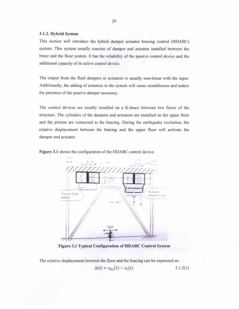
3.1.2. Hybrid System

This section will introduce the hybrid damper actuator bracing control (HDABC)

system. This system usually consists of damper and actuator installed between the

brace and the floor system. It has the reliability of the passive control device and the

additional capacity of its active control device.

The output from the fluid dampers or actuators is usually non-linear with the input.

Additionally, the adding of actuators to the system will cause unstableness and makes

the presence of the passive damper necessary.

The control devices are usually installed on a K-brace between two floors of the

structure. The cylinders of the dampers and actuators are installed on the upper floor

and the pistons are connected to the bracing. During the earthquake excitation, the

relative displacement between the bracing and the upper floor will activate the

damper and actuator.

Figure 3.1 shows the configuration of the HDABC control device.

Figure 3.1 Typical Configuration of HDABC Control System

The relative displacement between the floor and the bracing can be expressed as:

A(t) = xbj (0 - xi(t) 3.1.2(1)

30

Where xi (t) is the floor displacement and Xbj (t) is the bracing displacement. The

relative displacements drive'the control devices to generate forces.

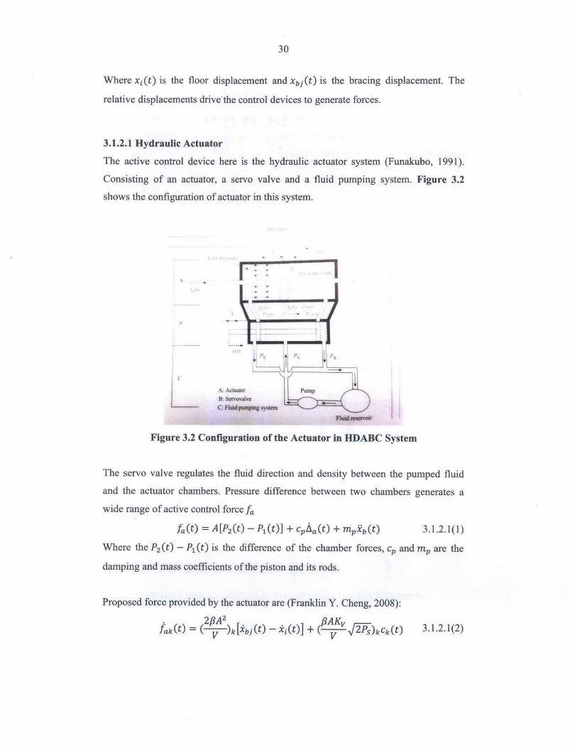
3.1.2.1 Hydraulic Actuator

The active control device here is the hydraulic actuator system (Funakubo, 1991).

Consisting of an actuator, a servo valve and a fluid pumping system. Figure 3.2

shows the configuration of actuator in this system.

A: Actuator PumpTB: SCIVevaivcC: Flipunping syum

Figure 3.2 Configuration of the Actuator in HDABC System

The servo valve regulates the fluid direction and density between the pumped fluid

and the actuator chambers. Pressure difference between two chambers generates a

wide range of active control force fa

fa(t) = A[P2(t) - P1(t)] + CpAa(t) + mPxb(t) 3.1.2.1(1)

Where the P2(t) - P (t) is the difference of the chamber forces, c, and mp are the

damping and mass coefficients of the piston and its rods.

Proposed force provided by the actuator are (Franklin Y. Cheng, 2008):

fak t) = [ 0 0 ] IAKv - iPN)kck(t) 3.1.2.1(2)

31

1 1(t) = -- Ck(t) + -uk(t) 3.1.2.1(3)

Tk Tk

Where fl, K, A, Ps are device parameters and Ck (t) are control force parameters.

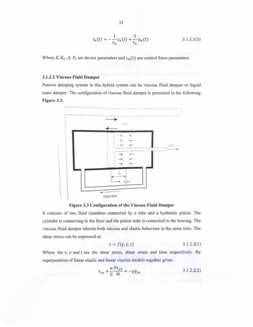
3.1.2.2 Viscous Fluid Damper

Passive damping system in this hybrid system can be viscous fluid damper or liquid

mass damper. The configuration of viscous fluid damper is presented in the following

Figure 3.3.

Fluid flOwk

Figure 3.3 Configuration of the Viscous Fluid Damper

It consists of two fluid chambers connected by a tube and a hydraulic piston. The

cylinder is connecting to the floor and the piston rode is connected to the bracing. The

viscous fluid damper inherits both viscous and elastic behaviors in the same time. The

shear stress can be expressed as:

-r = f(y, , t) 3.1.2.2(1)

Where the r, y and t are the shear stress, shear strain and time respectively. By

superposition of linear elastic and linear viscous models together gives:

YX + aT = -pfyx 3.1.2.2(2)G at

32

Where G is the shear modulus and It is the viscosity of the material. If P is replaced

with relaxation modulus CO, and P replaced with material viscosity AO, then it can be

rewritten as:

T + AO -T = -Coy 3.1.2.2(3)atThis equation indicates the material has memory characteristic as the shear stress not

only relates to the present time t but also depends on the rate of strain at all past time

t'. The relaxation factor CO decreases when going backwards in time. The integration

of the above stress-strain relationship will give the force-displacement relationship as:

Ced d dfp(t) + k dt fp(t) = CO A1 (t) + Co - A2 (t) 3.1.2.2(4)

If -is represented by A* then the force- displacement is given as:k

*fp(t) + fp(t) = COAP(t) 3.1.2.2(5)

Where the force is fp (t), Ap (t) is the displacement, A* is the relaxation time factor

and CO is the damping coefficient.

The kth damper in the jth bracing with ith floor with piston displacement defined by

Apk(t) = xb](t) - xi(t) is given as:

A*OkfPk M + fPk(t) = COkAPk(t) 3.1.2.2(6)

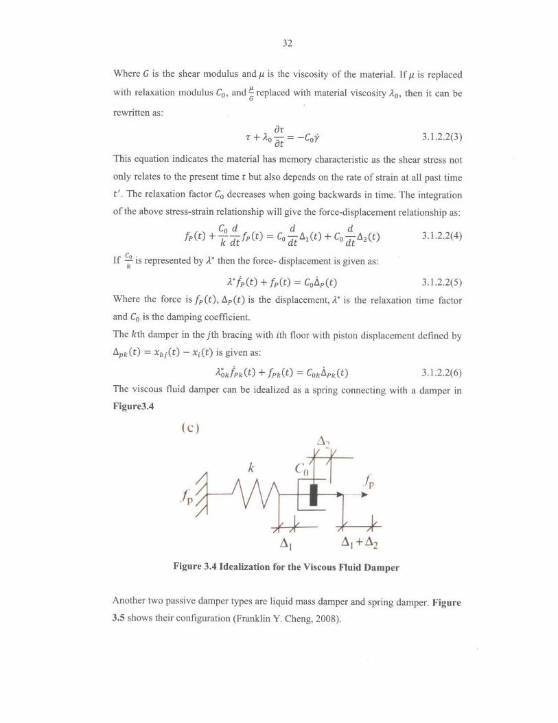
The viscous fluid damper can be idealized as a spring connecting with a damper in

Figure3.4

(C)A'

Figure 3.4 Idealization for the Viscous Fluid Damper

Another two passive damper types are liquid mass damper and spring damper. Figure

3.5 shows their configuration (Franklin Y. Cheng, 2008).

33

Tube

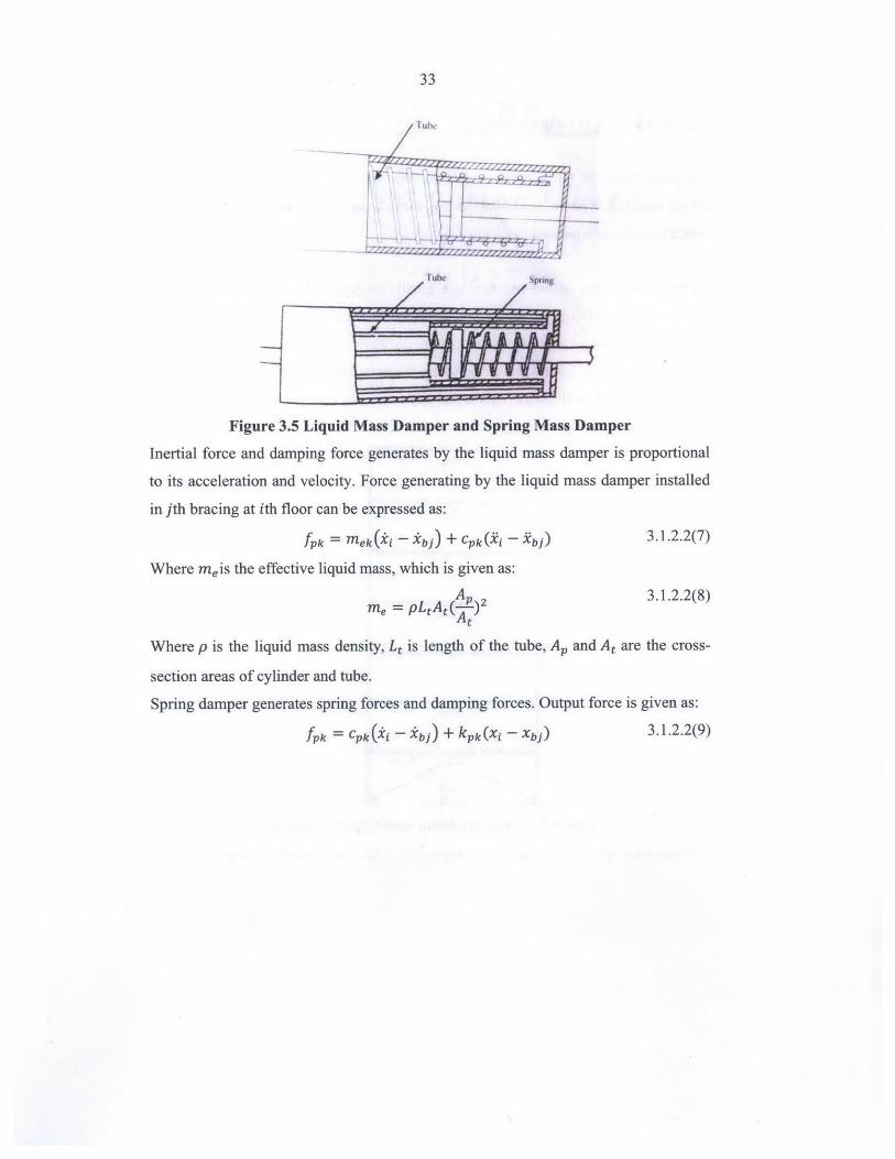
Figure 3.5 Liquid Mass Damper and Spring Mass Damper

Inertial force and damping force generates by the liquid mass damper is proportional

to its acceleration and velocity. Force generating by the liquid mass damper installed

in jth bracing at ith floor can be expressed as:

fpk - mek(ki - 'bi) + CPk(Xi - Xtbi) 3.1.2.2(7)

Where meis the effective liquid mass, which is given as:

Me (AP)2 3.1.2.2(8)me = p~At

Where p is the liquid mass density, Lt is length of the tube, AP and At are the cross-

section areas of cylinder and tube.

Spring damper generates spring forces and damping forces. Output force is given as:

fpk = Cpk(i - 4j) + kpk(xi - Xbj) 3.1.2.2(9)

34

3.2. Formulation of General Models

The formulation of the general models for the high-rise building with braces and

hybrid damping system is similar to the formulation of the Multiple- Degree of

Freedom system mentioned in Chapter 2.

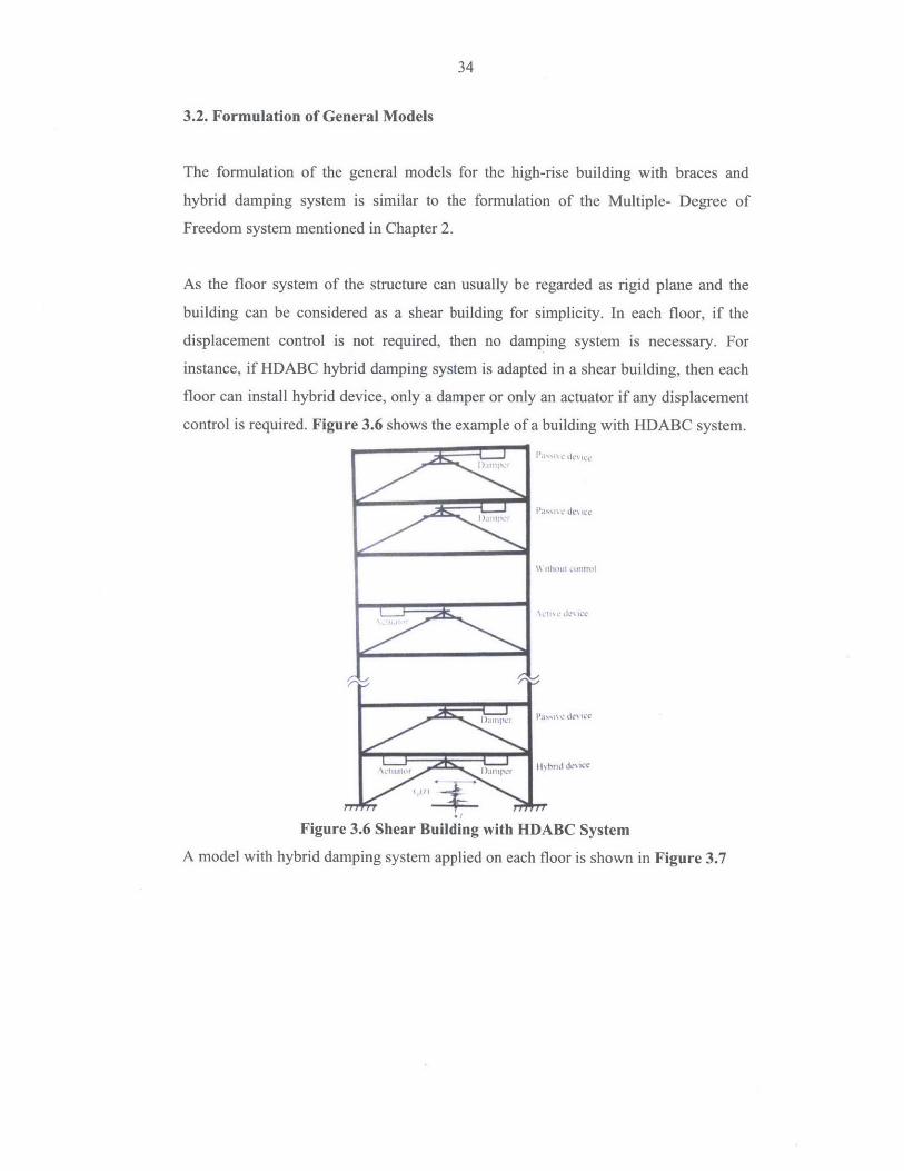
As the floor system of the structure can usually be regarded as rigid plane and the

building can be considered as a shear building for simplicity. In each floor, if the

displacement control is not required, then no damping system is necessary. For

instance, if HDABC hybrid damping system is adapted in a shear building, then each

floor can install hybrid device, only a damper or only an actuator if any displacement

control is required. Figure 3.6 shows the example of a building with HDABC system.

Figure 3.6 Shear Building with HDABC System

A model with hybrid damping system applied on each floor is shown in Figure 3.7

35

1 71 4 )k,

A, (A~

Fiur 3.7 (AA

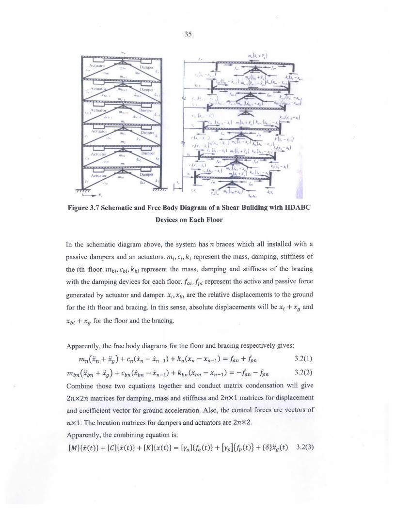
Figure 3.7 Schematic and Free Body Diagram of a Shear Building with HDABC

Devices on Each Floor

In the schematic diagram above, the system has n braces which all installed with a

passive dampers and an actuators. mi, ci, ki represent the mass, damping, stiffness of

the ith floor. mbi, Cbi, kbi represent the mass, damping and stiffness of the bracing

with the damping devices for each floor. &, fpi represent the active and passive force

generated by actuator and damper. xi, Xbj are the relative displacements to the ground

for the ith floor and bracing. In this sense, absolute displacements will be xi + xg and

Xbi + Xg for the floor and the bracing.

Apparently, the free body diagrams for the floor and bracing respectively gives:

mn(31n + 3g) + cn(in - in-1) + kn(xn - xn_1) = fan + fpn 3.2(1)

mbn(xbn + 3tg) + cbn(-ibn - in_1) + kbn(xbn - xn_1 = -fan - fpn 3.2(2)

Combine those two equations together and conduct matrix condensation will give

2nx 2n matrices for damping, mass and stiffness and 2nx 1 matrices for displacement

and coefficient vector for ground acceleration. Also, the control forces are vectors of

nx1. The location matrices for dampers and actuators are 2nx2.

Apparently, the combining equation is:

[M]{!(t)} + [C]{i(t)} + [K]{x(t)} = [Ya]tfa(t)} + [yp]tfp(t)} + {6Vlg(t) 3.2(3)

A_ x

f(At-, _x

Xclljator Damix-

I Ij

36

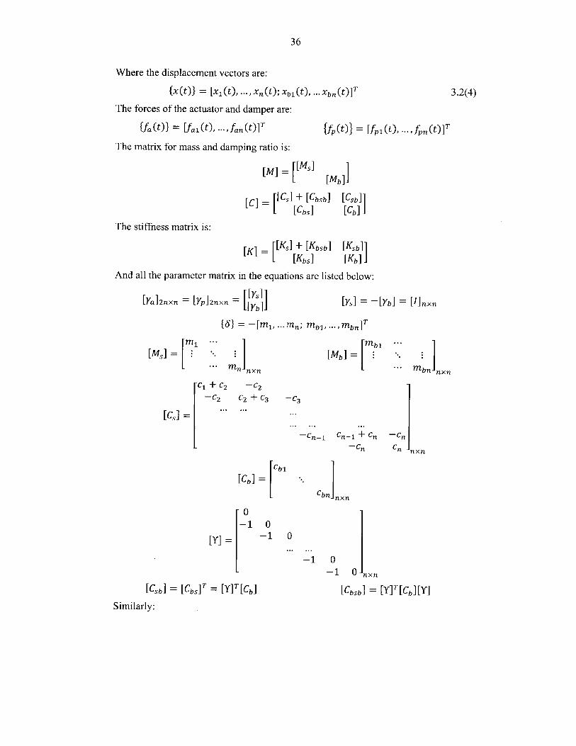
Where the displacement vectors are:

{x(t)} = [x 1 (t), ... , xf(t); xb1

The forces of the actuator and damper are:

ffa(t)} = [fai(t), ... ,fan(t)] T

The matrix for mass and damping ratio is:

(t), ... xbf(t)]T 3.2(4)

{fp(t)} = [fp1(t), ... fpn(t)]T

[M] =I [M5] [Mb] ]

[C] = I[CS] + [Cbsb] [Csb]

[Cbs] [Cb]

The stiffness matrix is:

And a

[K] = [[Ks] + [Kbsb] [Ksb]][KKI [Ks] [Kb]]

li the parameter matrix in the equations are listed below:

[Ya]2nxn = [Yp]2nxn = [YS [Ys] -

f{5 = -[n 1 , ... mn; Mbl, -- ,bn]

= mi --

... Mn- nxn

_C1 + C2 -C 2

-C 2 C2 + C3

[C5] -

Cbi

ICb]-

[Mb] - [b

-C 3

-Cn-1 Cn-I + Cn

-Cn

Cbn] nxn

ICSb] = [Cbs]T

Similarly:

0-1

[Y] =

= [Y]T [Cb]

0-1 0

-1 0-1 0-nxn

[Cbsb] = [ym [Cb][Y]

[MS

[Yb=] -[I=nn

... Mbn- nxn

-Cn

Cn -nxn

37

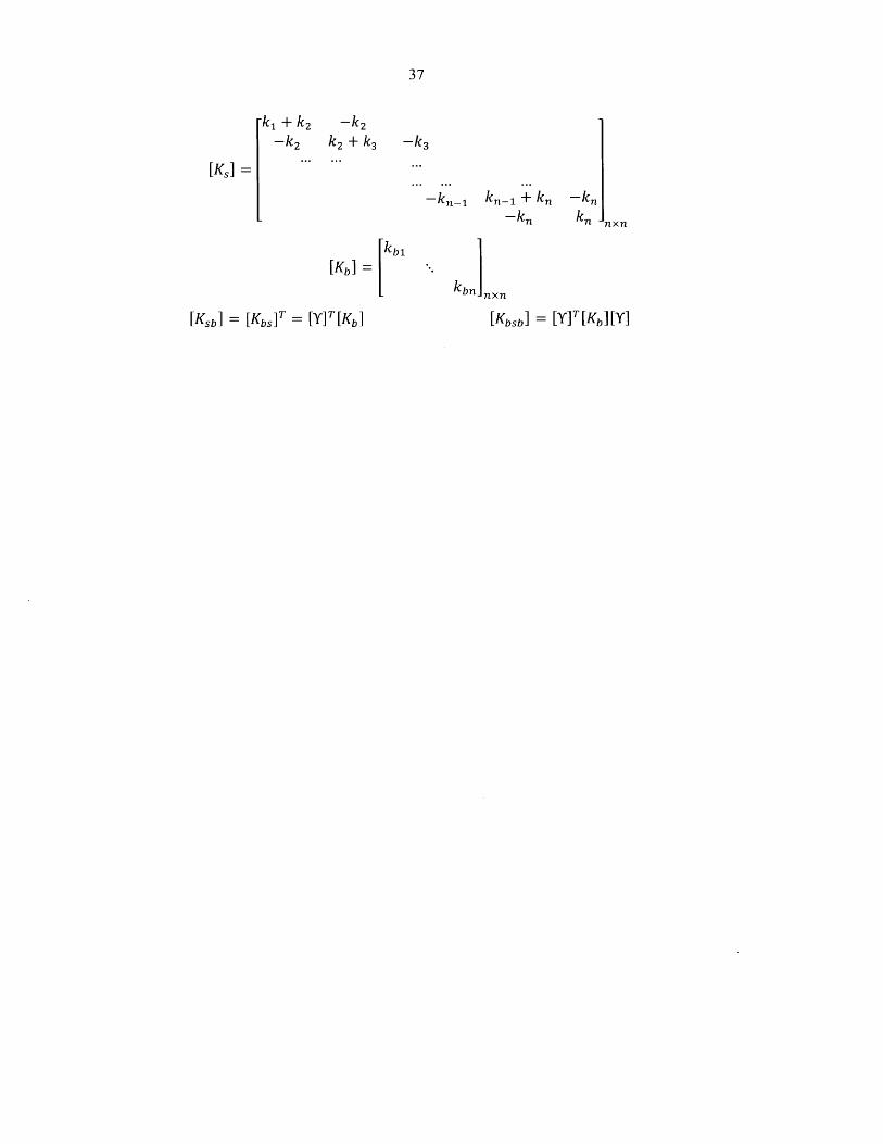
k1 + k2 -k 2-k 2 k2 +k3

[Ks] =

kbl

[Kb] -

[Ksb] = [Kbs]T = (y]T[Kb]

-kn 1 kn 1 + kn-kn

kb-.nx

[Kbyb] = [Y]T [Kb][Y]

-kn

kn .nxn

38

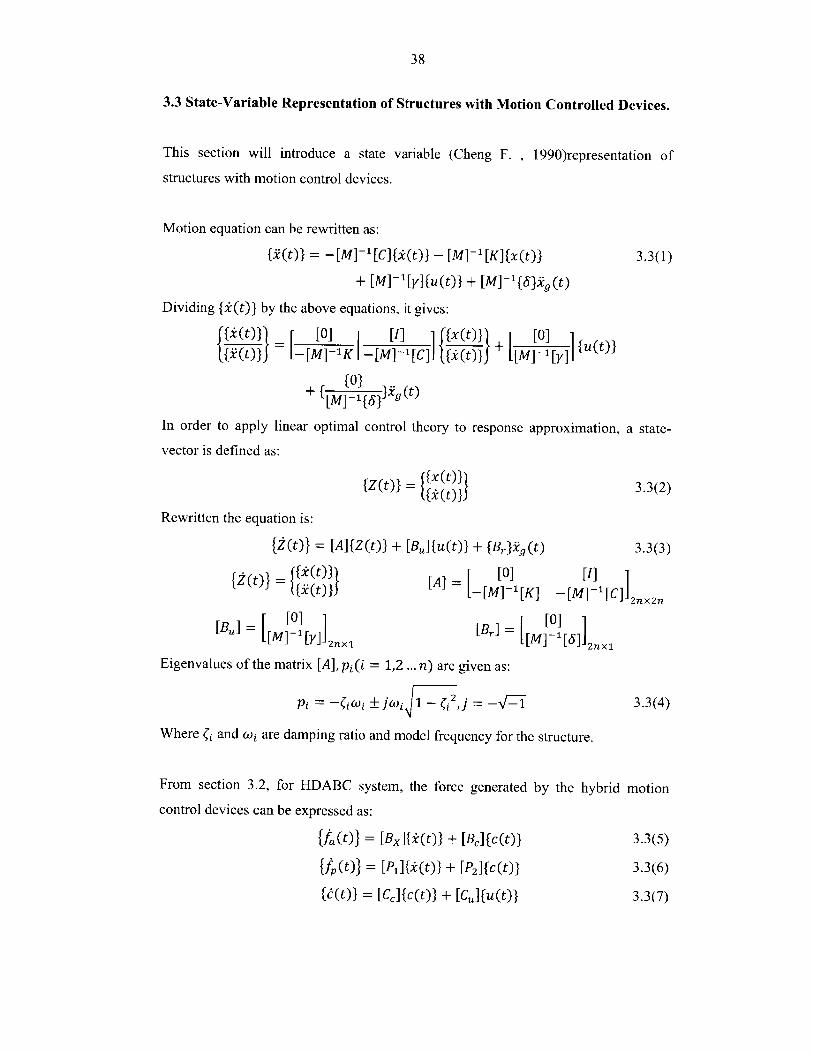
3.3 State-Variable Representation of Structures with Motion Controlled Devices.

This section will introduce a state variable (Cheng F. , 1990)representation of

structures with motion control devices.

Motion equation can be rewritten as:

{U(t)} = -[M]-1[C]{i(t)} - [M]~1[K]{x(t)} 3.3(1)

+ [M]-1[y]u(t)} + [M]V{6}ig(t)

Dividing {i(t)} by the above equations, it gives:I{i(t)}j [0] [] x(t)} [0]{t(t)}J -[M]-'K I -[M]'1[C]J tu(t)}) [M]~1[y]J {u(t)}

[to)ll (t)

In order to apply linear optimal control theory to response approximation, a state-

vector is defined as:

tZ(t)} = 3.3(2)

Rewritten the equation is:

{2(t)} = [A]{Z(t)} + [Bu]{u(t)} + {Br}Zg(t) 3.3(3)

{t)} = {i(t)}i) [A] 0 [I]]f2t~ {=It(t)} -M]lK -[M]-'[C]l nJ

[Bu] = I[Ir 1 ][y-2 -[Br ] ]=

Eigenvalues of the matrix [A], pi(i = 1,2 ... n) are given as:

Pi = -(w ±iwi 1 - 2, = - -I 3.3(4)

Where <j and oi are damping ratio and model frequency for the structure.

From section 3.2, for HDABC system, the force generated by the hybrid motion

control devices can be expressed as:

{fa(01 = [Bx]ti(t)} + [Bc]{c(t)} 3.3(5)

{ti(t)} = [P]I(t)} + [P2 ]{c(t)} 3.3(6)

{O(t)} = [Ce]{c(t)} + [CU]{u(t)} 3.3(7)

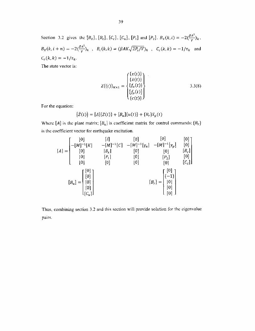
39

Section 3.2 gives the [Bx], [Be], [Ce], [Ca], [P 1 ] and [P 2]. Bx(k, i) = -2( ,J~A 2

Bx(k, i + n) = -2(flAk,

Cc (k, k) = -1/Tk.

The state vector is:

Bc(k,k) = (fAK 2PS/V)k Cc(k, k) = -1/Tk

Z{(t}NX1 = t{x(t)}IV{k(t)}

{fp(t)}I{c(t)

3.3(8)

For the equation:

{2(t)} = [A]{Z(t)} + [Bu]tu(t)} + {Brji&g(t)

Where [A] is the plant matrix; [Bj] is coefficient matrix for control commands; {Br}

is the coefficient vector for earthquake excitation.

- [0]-[M]-'[K]

[A] = [0][0]

- [0]

[0] -[0]

[Ba] = [0]

(0].(CU].

[1] [0] [0] [0]

-[M]-1[C] -[M]-1[Ya] -[M]-1 [yp] [0][Br] [0] [0] [Bc]

[P 1] [0] [P2] [0][0] [0] [0] [CC]-

[0]t-1}

[Br] = [0]

[0][0] .

Thus, combining section 3.2 and this section will provide solution for the eigenvalue

pairs.

and

40

3.4 Control Strategy and Efficiency of HDABC Hybrid System

This section addresses the control strategy of the hybrid seismic control system of

HDABC. A three-story height building installed the HDABC hybrid system isinvestigated for the efficiency of the system and results are presented in this section as

well.

Basically, the control systems are state control and state slope control respectively,

first one feeds back the structure displacement and the second one feeds back the

structure accelerations. Thus, state control system is more suitable for reducing

structure displacement. However, to ensure the stability of the structure, the system

should be carefully designed. State-slope control system is usually employed by

hybrid system using liquid mass dampers.

For both the semi-active and hybrid system, the classical feedback algorithm can be

applied. Optimization of the control system is to achieve the maximum reduction for

system response while input minimum energy to control it (Soong T. , 1990). The

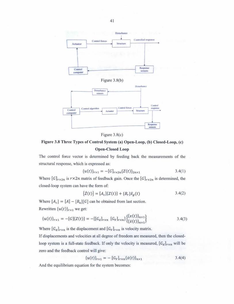
rational behind the control system is shown in Figure 3.8.

Diturbancc

Control

algorithm

Control forcesActuator C Structure

Figure 3.8(a)

41

Disturbunce

Contol frcesControlled response

Actutor Coto fre Structure I

Controlcomputer

Figure 3.8(b)Ditturbauc

4ns7

Control

Control algornthm - Control forces -respon

coptr Structue Actuator S..rt.re

Reqxxisesensors

Figure 3.8(c)

Figure 3.8 Three Types of Control System (a) Open-Loop, (b) Closed-Loop, (c)

Open-Closed Loop

The control force vector is determined by feeding back the measurements of the

structural response, which is expressed as:

{u(t)}rx1 = -[G]rx 2n{Z(t)}2nxi 3.4(1)

Where [G]rx2n is rx2n matrix of feedback gain. Once the [G]rX2n is determined, the

closed-loop system can have the form of:

{Z(t)} = [Ac]{Z(t)} + {Brig(t) 3.4(2)

Where [Ac] = [A] - [Bu] [G] can be obtained from last section.

Rewritten fu(t)lrxi we get:

{u(t)}rxi = -[G]{Z(t)} = -[[Gd]rxn [Gv]rxn] ( 3.4(3)

Where [Gd]rxn is the displacement and [Gvlrxn is velocity matrix.

If displacements and velocities at all degree of freedom are measured, then the closed-

loop system is a full-state feedback. If only the velocity is measured, [Gd]rxn will be

zero and the feedback control will give:

{U(t)}rxi = - [GV]rxnfx(t)}nx1 3.4(4)

And the equilibrium equation for the system becomes:

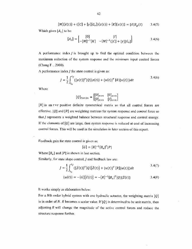
42

[M]{f(t)} + ([C] + [y][Gv]){jc(t)} + [K]tx(t)} = {}&,(t) 3.4(5)

Which gives [Ac] to be:

[A] = [ 0] 1] 3.4(6)[ -[M]'[K] -[M]- 1 ([C] + [y][G]]

A performance index J is brought up to find the optimal condition between the

maximum reduction of the system response and the minimum input control forces

(Cheng F. , 2000).

A performance index J for state control is given as:

1 (tf 3.4(6)J = 2f ({z(t)}T [Q]{z(t)} + tu(t)}T [R]{u(t)})dt

to

Where

-[[lnxn [I]Jnxn

[R] is an rxr positive definite symmetrical matrix so that all control forces are

effective. [Q] and [R] are weighting matrices for system response and control force so

thatJ represents a weighted balance between structural response and control energy.

If the elements of [Q] are large, then system response is reduced at cost of increasing

control forces. This will be used in the simulation in later section of this report.

Feedback gain for state control is given as:

[G] = [R]-1 [BU]T [p]

Where [Ba] and [P] is shown in last section.

Similarly, for state slope control, J and feedback law are:

J = 2f (t(t)}T[Q]{2(t)} + {u(t)}T [R]{u(t)})dt 3.4(7)

tu(t)} = -[G]f2(t)} = -[R]-1[BU] T [Q]{2(t)} 3.4(8)

It works simply as elaboration below:

For a Nth order hybrid system with one hydraulic actuator, the weighting matrix [Q]

is in order of N. R becomes a scalar value. If [Q] is determined to be unit matrix, then

adjusting R will change the magnitude of the active control forces and reduce the

structure response further.

43

To investigate the effectiveness of a hybrid control system, a case study of a three-

story building model with HDABC on a shaking table test was investigated (Franklin

Y. Cheng, 2008). In order to compare the effectiveness between the passive control

system, active control system and hybrid control system, the shaking table tests were

conducted four times. Each test has different schematic installation for the motion

control system. 1). only the primary structure; 2). passive control on bracing in the

first floor; 3). active control on bracing in the first floor; and 4). hybrid devices on the

bracing in the first floor. The passive device is viscous fluid damper and the active

device is a hydraulic actuator.

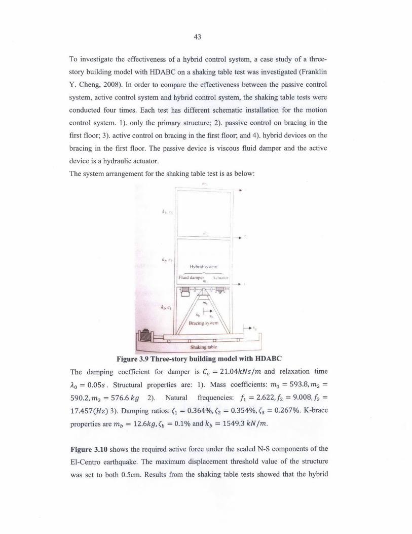
The system arrangement for the shaking table test is as below:

I Fluid damrwr

Shakng table

Figure 3.9 Three-story building model with HDABC

The damping coefficient for damper is C, = 21.04kNs/m and relaxation time

A0 = 0.05s. Structural properties are: 1). Mass coefficients: m, = 593.8, m 2 =

590.2, m 3 = 576.6 kg 2). Natural frequencies: f, = 2.622,f2 = 9.008,f3 =

17.457(Hz) 3). Damping ratios: <j = 0.364%, <2 = 0.354%, <3 = 0.267%. K-brace

properties are mb = 12.6kg, <b = 0.1% and kb = 1549.3 kNIm.

Figure 3.10 shows the required active force under the scaled N-S components of the

El-Centro earthquake. The maximum displacement threshold value of the structure

was set to both 0.5cm. Results from the shaking table tests showed that the hybrid

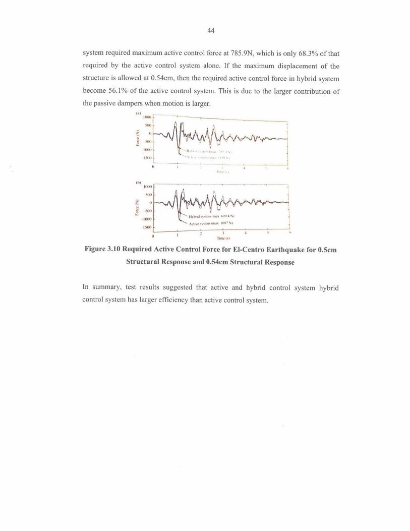
44

system required maximum active control force at 785.9N, which is only 68.3% of that

required by the active control system alone. If the maximum displacement of the

structure is allowed at 0.54cm, then the required active control force in hybrid system

become 56.1% of the active control system. This is due to the larger contribution of

the passive dampers when motion is larger.

OW

Figure 3.10 Required Active Control Force for El-Centro Earthquake for 0.5cm

Structural Response and 0.54cm Structural Response

In summary, test results suggested that active and hybrid control system hybrid

control system has larger efficiency than active control system.

45

Chapter 4 High-rise Building Outriggers Damping System

4.1. Introduction of High-rise Building Outriggers

In last chapter, some samples of semi-active and hybrid damping systems were given.

A case study for investigation of the efficiency of the hybrid damping system was

presented. The general formulations for the structure with hybrid motion control

devices were also discussed. This chapter will introduce the high-rise building

outrigger system, the damping system for it and some case studies.

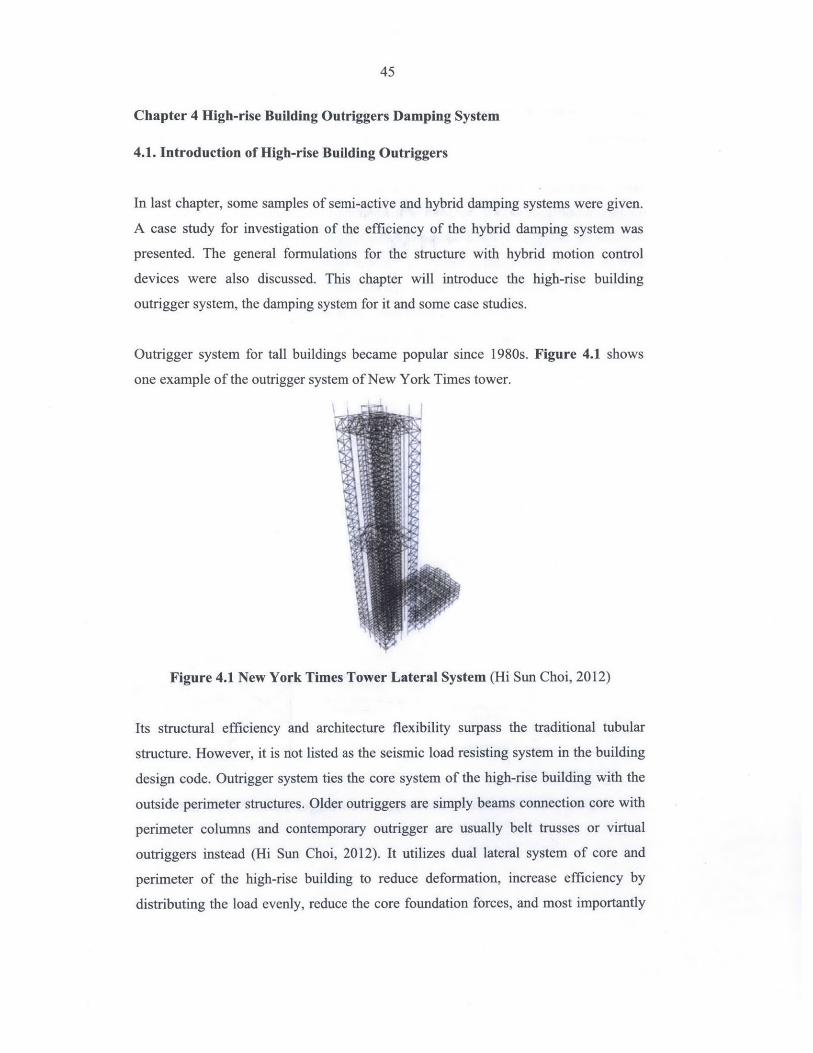
Outrigger system for tall buildings became popular since 1980s. Figure 4.1 shows

one example of the outrigger system of New York Times tower.

Figure 4.1 New York Times Tower Lateral System (Hi Sun Choi, 2012)

Its structural efficiency and architecture flexibility surpass the traditional tubular

structure. However, it is not listed as the seismic load resisting system in the building

design code. Outrigger system ties the core system of the high-rise building with the

outside perimeter structures. Older outriggers are simply beams connection core with

perimeter columns and contemporary outrigger are usually belt trusses or virtual

outriggers instead (Hi Sun Choi, 2012). It utilizes dual lateral system of core and

perimeter of the high-rise building to reduce deformation, increase efficiency by

distributing the load evenly, reduce the core foundation forces, and most importantly

46

reduce the over turning moment for the core. For buildings more than 40 stories, the

efficiency for the core alone resisting the overturning moment is small.

Many considerations affect the performance of the outriggers. For instance, the

number of outrigger floors, the depth of the belt truss and its presents, the interaction

between the outrigger and the perimeter columns, etc. The outrigger system together

with the floor system helps reduction of the over turning moment of the core and the

moment at the foundation level. Often when the building flexural is dominant than the

shear force, outrigger system will be suitable as it impact little on the shear force.

Application of outrigger system will reduce the story drift and provide more

occupancy comfort.

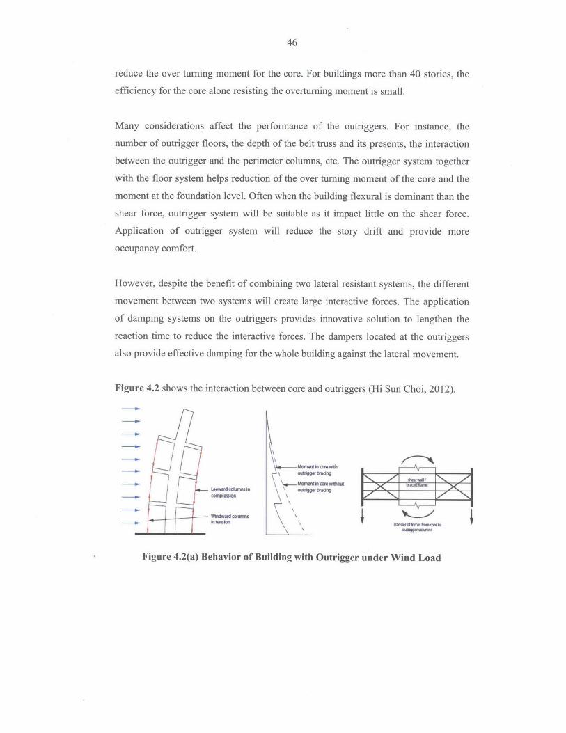
However, despite the benefit of combining two lateral resistant systems, the different

movement between two systems will create large interactive forces. The application

of damping systems on the outriggers provides innovative solution to lengthen the

reaction time to reduce the interactive forces. The dampers located at the outriggers

also provide effective damping for the whole building against the lateral movement.

Figure 4.2 shows the interaction between core and outriggers (Hi Sun Choi, 2012).

Leeward colum in

Widadcolumns

Moment in core with"nw rain

\.4. MomenscorewithoutoutIger bracing

Twkfoomnfrm coto

Figure 4.2(a) Behavior of Building with Outrigger under Wind Load

47

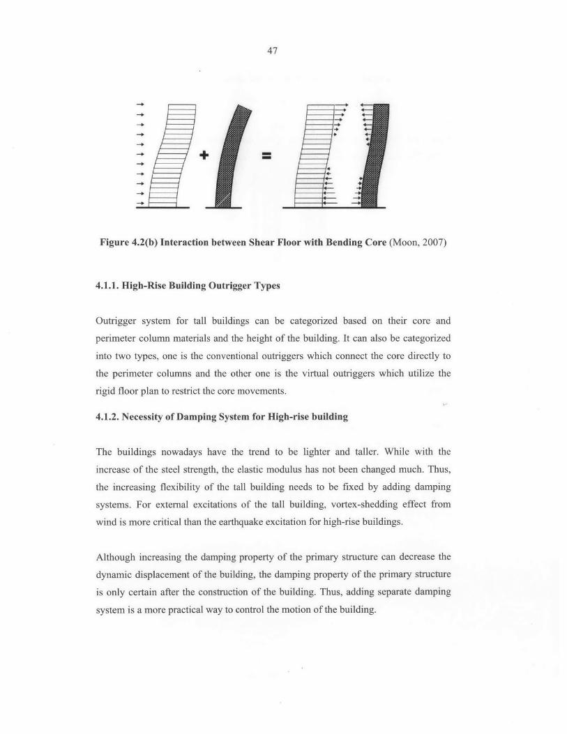
Figure 4.2(b) Interaction between Shear Floor with Bending Core (Moon, 2007)

4.1.1. High-Rise Building Outrigger Types

Outrigger system for tall buildings can be categorized based on their core and

perimeter column materials and the height of the building. It can also be categorized

into two types, one is the conventional outriggers which connect the core directly to

the perimeter columns and the other one is the virtual outriggers which utilize the

rigid floor plan to restrict the core movements.

4.1.2. Necessity of Damping System for High-rise building

The buildings nowadays have the trend to be lighter and taller. While with the

increase of the steel strength, the elastic modulus has not been changed much. Thus,

the increasing flexibility of the tall building needs to be fixed by adding damping

systems. For external excitations of the tall building, vortex-shedding effect from

wind is more critical than the earthquake excitation for high-rise buildings.

Although increasing the damping property of the primary structure can decrease the

dynamic displacement of the building, the damping property of the primary structure

is only certain after the construction of the building. Thus, adding separate damping

system is a more practical way to control the motion of the building.

48

4.2. Typical Damping System for High-rise Building Outrigger Systems

4.2.1. Types of Damping System

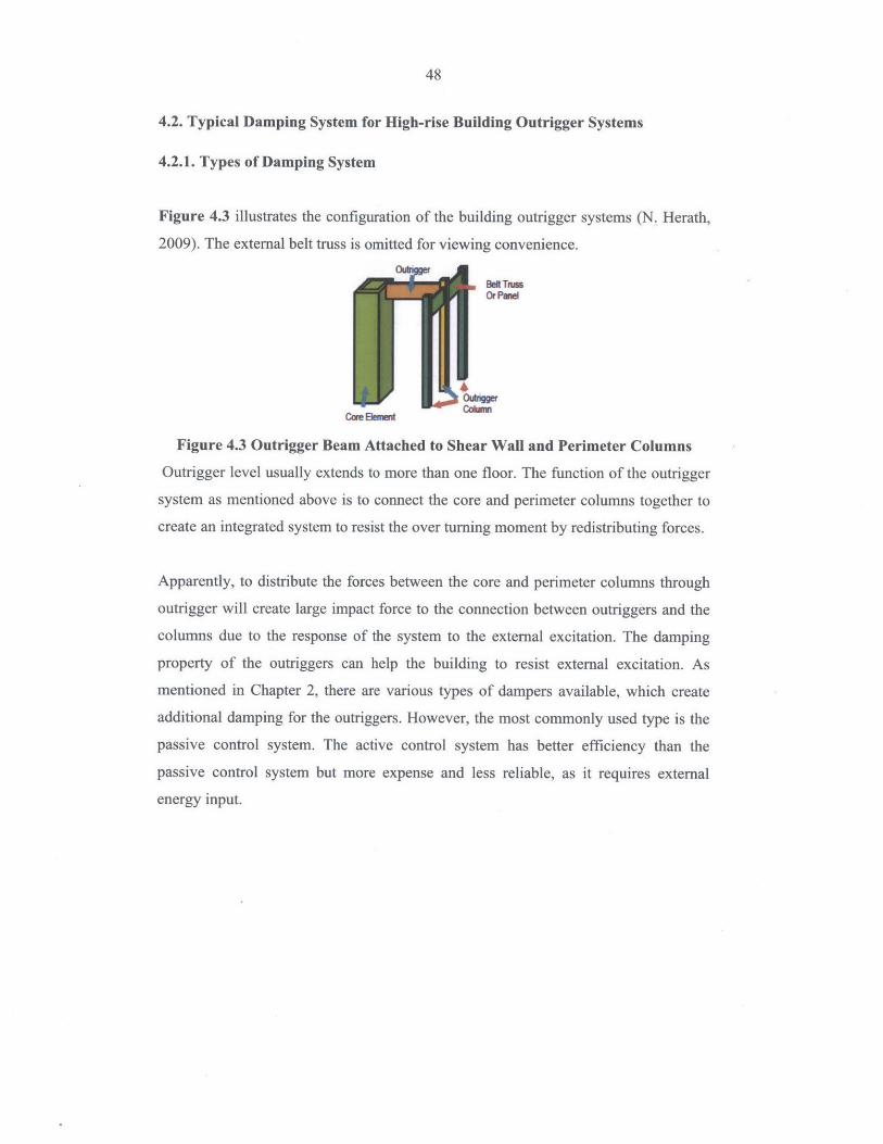
Figure 4.3 illustrates the configuration of the building outrigger systems (N. Herath,

2009). The external belt truss is omitted for viewing convenience.

Be TinsOr Pane

Core aement

Figure 4.3 Outrigger Beam Attached to Shear Wall and Perimeter Columns

Outrigger level usually extends to more than one floor. The function of the outrigger

system as mentioned above is to connect the core and perimeter columns together to

create an integrated system to resist the over turning moment by redistributing forces.

Apparently, to distribute the forces between the core and perimeter columns through

outrigger will create large impact force to the connection between outriggers and the

columns due to the response of the system to the external excitation. The damping

property of the outriggers can help the building to resist external excitation. As

mentioned in Chapter 2, there are various types of dampers available, which create

additional damping for the outriggers. However, the most commonly used type is the

passive control system. The active control system has better efficiency than the

passive control system but more expense and less reliable, as it requires external

energy input.

49

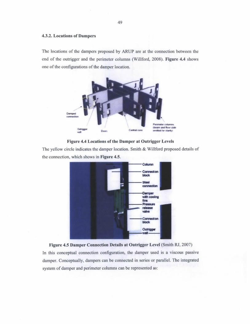
4.3.2. Locations of Dampers

The locations of the dampers proposed by ARUP are at the connection between the

end of the outrigger and the perimeter columns (Willford, 2008). Figure 4.4 shows

one of the configurations of the damper location.

CPmOW comm

Figure 4.4 Locations of the Damper at Outrigger Levels

The yellow circle indicates the damper location. Smith & Willford proposed details of

the connection, which shows in Figure 4.5.

CnneSm i

COnnec10eo

vith oo"n

In this conceptual connection configuration, the damper used is a viscous passive

damper. Conceptually, dampers can be connected in series or parallel. The integrated

system of damper and perimeter columns can be represented as:

50

k

' 7 777-7

C

k

7AT

k c

7 p- 77 7

k C

'7 7- -.7

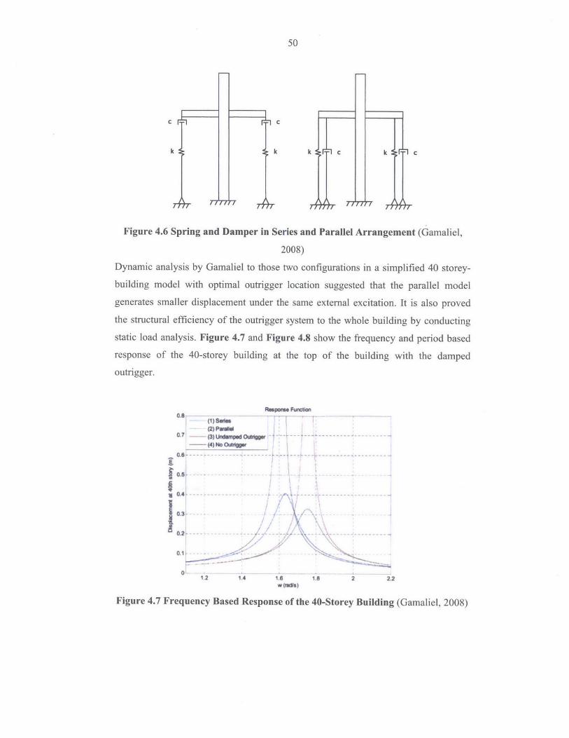
Figure 4.6 Spring and Damper in Series and Parallel Arrangement (Gamaliel,

2008)

Dynamic analysis by Gamaliel to those two configurations in a simplified 40 storey-

building model with optimal outrigger location suggested that the parallel model

generates smaller displacement under the same external excitation. It is also proved

the structural efficiency of the outrigger system to the whole building by conducting

static load analysis. Figure 4.7 and Figure 4.8 show the frequency and period based

response of the 40-storey building at the top of the building with the damped

outrigger.

O.sR..pois. Funebon

(1) ses(2) PMW

0.7 (3) UnW 0~(4) No OAlgger

0.8 - --- - -

0

0*1.2 1,4 1.6

w (MWs)

Figure 4.7 Frequency Based Response of the

18 2 2.2

40-Storey Building (Gamaliel, 2008)

0.5

0.3

0,2-

51

Pwtoda.seM panS Fwuc tn0.5

1)ons

0.45-(2)P, MW

10.2

k 0.8 -- ---

0-

010 0.5 1 1.5 2 2.5 3 3.5 4 4.5 5

T (sond)

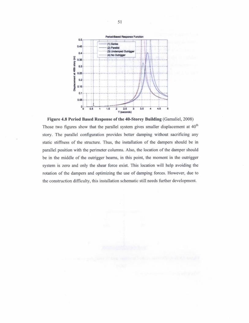
Figure 4.8 Period Based Response of the 40-Storey Building (Gamaliel, 2008)

Those two figures show that the parallel system gives smaller displacement at 40'h

story. The parallel configuration provides better damping without sacrificing any

static stiffness of the structure. Thus, the installation of the dampers should be in

parallel position with the perimeter columns. Also, the location of the damper should

be in the middle of the outrigger beams, in this point, the moment in the outrigger

system is zero and only the shear force exist. This location will help avoiding the

rotation of the dampers and optimizing the use of damping forces. However, due to

the construction difficulty, this installation schematic still needs further development.

52

4.3.3 Some Case Studies for Hybrid Motion Control System for Outriggers

Although passive damper installed between the outriggers and the perimeter columns

can effectively reduce the fundamental mode displacement excited by wind load. The

inability to adjust itself to future change of external forces and the This shortage can

be overcome by semi-active motion control system and hybrid motion control system.

This section will look through some simulation case studies for semi-active and

hybrid motion control system for outriggers.

1). Semi-active Magnetorheological(MR) dampers

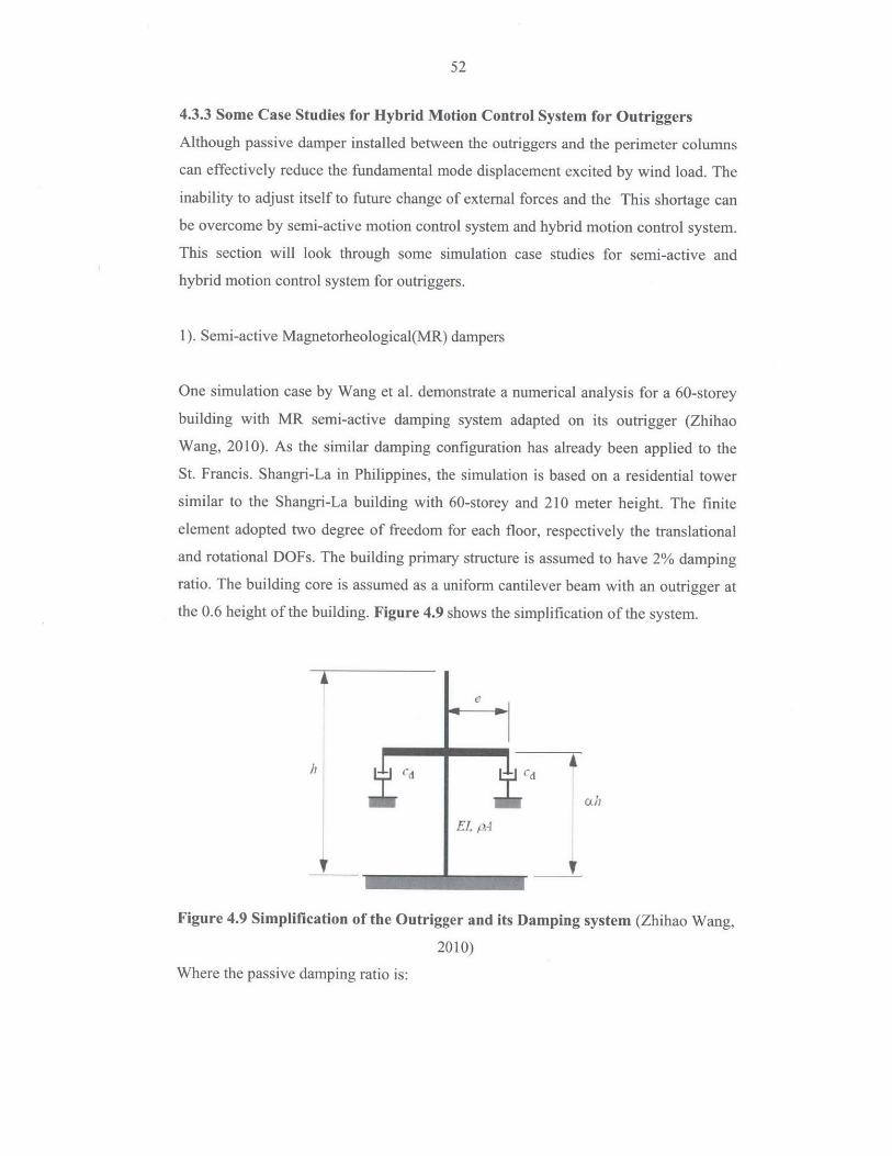
One simulation case by Wang et al. demonstrate a numerical analysis for a 60-storey

building with MR semi-active damping system adapted on its outrigger (Zhihao

Wang, 2010). As the similar damping configuration has already been applied to the

St. Francis. Shangri-La in Philippines, the simulation is based on a residential tower

similar to the Shangri-La building with 60-storey and 210 meter height. The finite

element adopted two degree of freedom for each floor, respectively the translational

and rotational DOFs. The building primary structure is assumed to have 2% damping

ratio. The building core is assumed as a uniform cantilever beam with an outrigger at

the 0.6 height of the building. Figure 4.9 shows the simplification of the system.

e

Figure 4.9 Simplification of the Outrigger and its Damping system (Zhihao Wang,

2010)

Where the passive damping ratio is:

53

C 8cde 2 , i=j=2pSq to, else

p is the floor number where the damper is attached. The damper location is at the 0.6

height of the building, p is 36. There are in total 4 groups of dampers, each group has

two dampers.

The state matrix can be obtained from Chapter 3 as:

As [ 0 I=-M-K -M-'(Ci + Cs)I

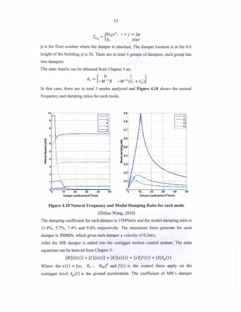
In this case, there are in total 5 modes analyzed and Figure 4.10 shows the natural

frequency and damping ratios for each mode.

- -- -- - -- - ------ - - ---- -2-1~ -

- - -4-

0 10 20 30 40Dimir coefficients(10 7 Nm(s)

50

0.8~

0.7

fi6A

0.5

OA

0.3

0.2

0.1

* ----23

... .

0 10 20 30 40Damper coefficitts(1 ONmfs)

Figure 4.10 Natural Frequency and Modal Damping Ratio for each mode

(Zhihao Wang, 2010)

The damping coefficient for each damper is 15MNmI/s and the model-damping ratio is

11.8%, 5.7%, 7.4% and 9.6% respectively. The maximum force generate for each

damper is 3000kN, which gives each damper a velocity of 0.2m/s.

After the MR damper is added into the outrigger motion control system. The state

equations can be derived from Chapter 3:

[M]{i(t)} + [C]tx(t)} + [K]{x(t)} = [y]{f(t)} + {S}tg(t)

Where the x(t) = [() 1 01 ... 06 0 ]T and f(t) is the control force apply on the

outrigger level. ig(t) is the ground acceleration. The coefficient of MR's damper

10

7is

5

3

2

50

54

model are adjusted to be sufficient for the control, the out-put force is amplified to be

1000 times of the original forces. In order to ensure the safety and stability of the

design, the capacity of the MR damper to the response of the structure acceleration

and displacement are 0.6 of its original capacity.

The linear displacement of the building is:

m

x(t) = 4pih)qi t) = (Dq

As the semi-active damping system is affected by the response of the system. The

accelerations of 10, 20, 30, 40, 50 and 60 story were measured. There were four

controllers, which are to minimize the generalized acceleration, velocity, several

stories' acceleration and velocity respectively.

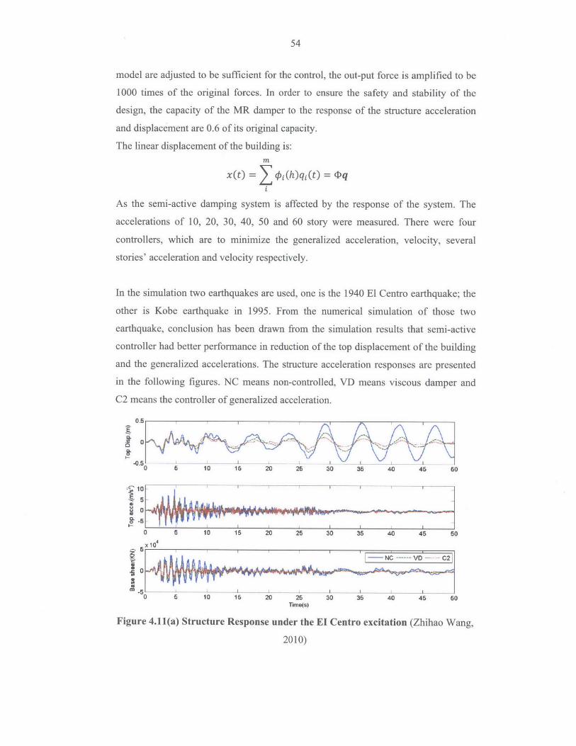
In the simulation two earthquakes are used, one is the 1940 El Centro earthquake; the

other is Kobe earthquake in 1995. From the numerical simulation of those two

earthquake, conclusion has been drawn from the simulation results that semi-active

controller had better performance in reduction of the top displacement of the building

and the generalized accelerations. The structure acceleration responses are presented

in the following figures. NC means non-controlled, VD means viscous damper and

C2 means the controller of generalized acceleration.

0.5

0

-0 .5 1 2 40 5 10 15 20 25 30 36 40 45 50

1 0'1- -1 _ _ _ - _ 1

.11 14

Umg.. 0 Al

0 5 10 15 20 25 30 35 40 45 5

x10

m0

0 5 10 16 20 25 30 36 40 45 60TUie(s)

Figure 4.11(a) Structure Response under the El Centro excitation (Zhihao Wang,

2010)

0

55

5 10 15 20 26

Tkme(s)

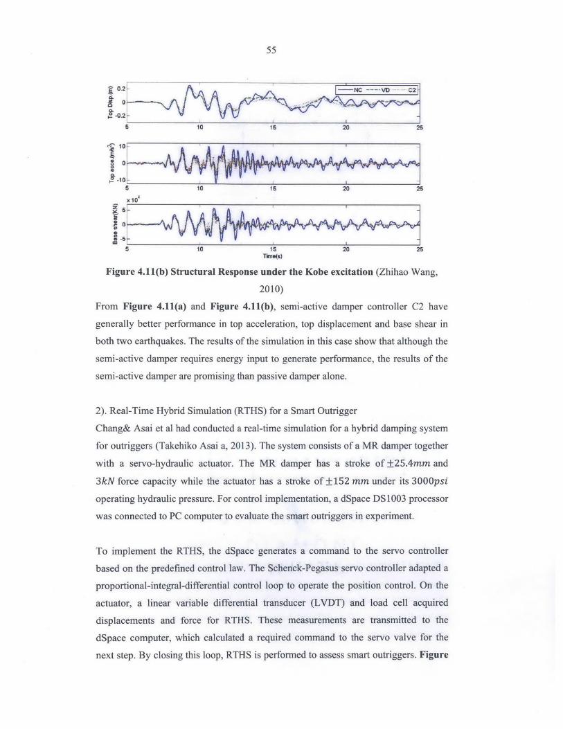
Figure 4.11(b) Structural Response under the Kobe excitation (Zhihao Wang,

2010)

From Figure 4.11(a) and Figure 4.11(b), semi-active damper controller C2 have

generally better performance in top acceleration, top displacement and base shear in

both two earthquakes. The results of the simulation in this case show that although the

semi-active damper requires energy input to generate performance, the results of the

semi-active damper are promising than passive damper alone.

2). Real-Time Hybrid Simulation (RTHS) for a Smart Outrigger

Chang& Asai et al had conducted a real-time simulation for a hybrid damping system

for outriggers (Takehiko Asai a, 2013). The system consists of a MR damper together

with a servo-hydraulic actuator. The MR damper has a stroke of ±25.4mm and

3kN force capacity while the actuator has a stroke of +152 mm under its 3000psi

operating hydraulic pressure. For control implementation, a dSpace DS1003 processor

was connected to PC computer to evaluate the smart outriggers in experiment.

To implement the RTHS, the dSpace generates a command to the servo controller

based on the predefined control law. The Schenck-Pegasus servo controller adapted a

proportional-integral-differential control loop to operate the position control. On the

actuator, a linear variable differential transducer (LVDT) and load cell acquired

displacements and force for RTHS. These measurements are transmitted to the

dSpace computer, which calculated a required command to the servo valve for the

next step. By closing this loop, RTHS is performed to assess smart outriggers. Figure

0.2 NC -- VD C 2

0 - -

-0.2-

S10 is 20 26

10

56

4.12 shows the control flow of the testing:

F Structure Servo-hydrualic s m xnim wodlel actualorS i

Feedback ijinteraction

d-

G, q) Inner loop _________

Feedforward f ev ddruic

controllor ' cotoDJ autr

I~~~ ~ _ _ _ _ _a . _ _

Figure 4.12 Control Flow of the Real-Time Hybrid Simulation (Takehiko Asai a,

2013)

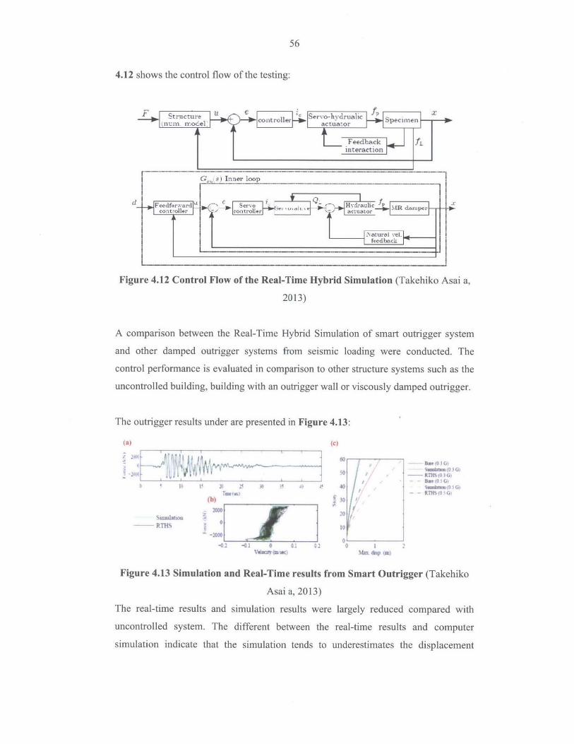
A comparison between the Real-Time Hybrid Simulation of smart outrigger system

and other damped outrigger systems from seismic loading were conducted. The

control performance is evaluated in comparison to other structure systems such as the

uncontrolled building, building with an outrigger wall or viscously damped outrigger.

The outrigger results under are presented in Figure 4.13:

I 17(b)

PTIVWO

(c)

B~f~(4

2 44,

RTh'~~x~4) 4,

mib4~ 4,

KTh'~

M d

kb,,,*~ 4 W

Figure 4.13 Simulation and Real-Time results from Smart Outrigger (Takehiko

Asai a, 2013)

The real-time results and simulation results were largely reduced compared with

uncontrolled system. The different between the real-time results and computer

simulation indicate that the simulation tends to underestimates the displacement

57

slightly. Thus, in the application for large structure as tall buildings, the modal

experiment of the non-linear damping devices are needed before implementation onto

real world structure.

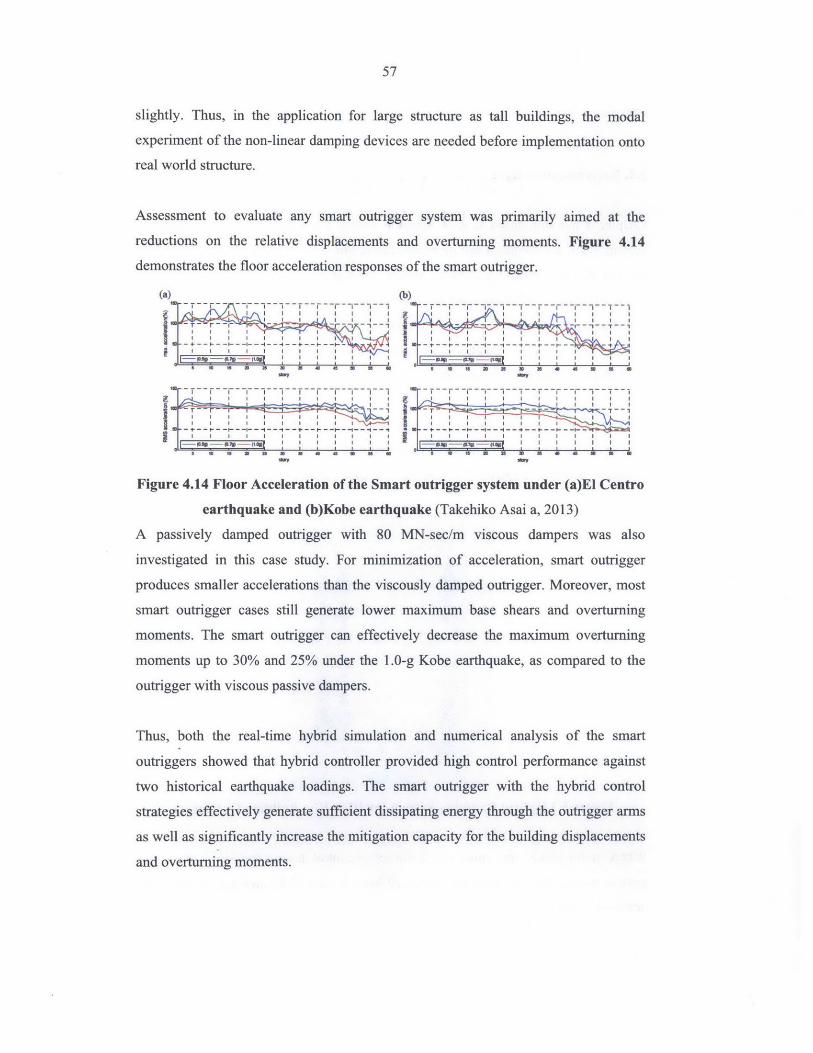
Assessment to evaluate any smart outrigger system was primarily aimed at the

reductions on the relative displacements and overturning moments. Figure 4.14

demonstrates the floor acceleration responses of the smart outrigger.

(a) (b)

--------q---k-- an bKb a tok (Tak----k---As-----,-2--3)

d smae acc6eaioNs a i n is X A s d i M mos

---- -- -

S I I I . S W Z

Figuents.1 Theo sceeaino h mart outrigger sy fetveydcestem maiunder ECturo

moentseathquak% and 5 ndrth .0gKobe earthquake, Aas a, pae t20the

A asvl apdoutrigger with80M -e/ viscouspsse damperswsas

Thusigae b th s ae stuyr ination f aceratian, smart utrigger

smtouger shawes shtihybridnerateroer pravied bagh shars pefranoertagainsg

moments up to 30 ad 25 une th 1.0 eaqa as comare oh

two historical earthquake loadings. The smart outrigger with the hybrid control

strategies effectively generate sufficient dissipating energy through the outrigger arms

as well as significantly increase the mitigation capacity for the building displacements

and overturning moments.

58

Chapter 5 Hybrid Damping System for High-rise Building Outriggers

5.1. Recommended Hybrid Damping System for High-rise Building

Chapter 4 has introduced several damping system for high-rise building outrigger

system. Two case studies based on a semi-active MR damper system and a hybrid MR

damper & Servo-hydraulic actuator system for high-rise building was investigated.

Their integrated performance for the minimization of the top and floor accelerations

and displacements were studied and presented. Both the case study in Chapter 4 and

shaking table test in Chapter 3 showed that hybrid-damping system has better

performance generally than passive damping system or active damping system alone.

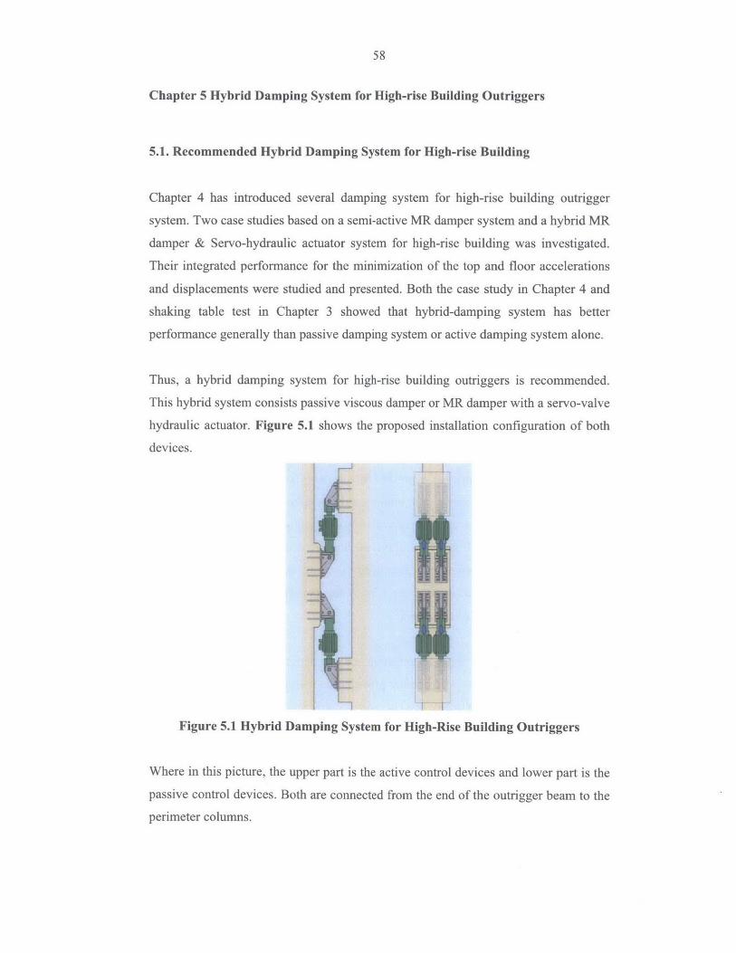
Thus, a hybrid damping system for high-rise building outriggers is recommended.

This hybrid system consists passive viscous damper or MR damper with a servo-valve

hydraulic actuator. Figure 5.1 shows the proposed installation configuration of both

devices.

Figure 5.1 Hybrid Damping System for High-Rise Building Outriggers

Where in this picture, the upper part is the active control devices and lower part is the

passive control devices. Both are connected from the end of the outrigger beam to the

perimeter columns.

59

This configuration will keep both devices as series with the perimeter columns. The

system is using a close-loop feed back system, which measures the acceleration of the

system response and adjusts the force from the actuator with the measurement at the

outrigger level. Ideally, if the control devices' is activated only when the maximum

structure response threshold is reached, the efficiency of the system will be assured.

This configuration can also give emergency reassurance if one of the two systems

fails as the other one can still function well to mitigate the lateral excitation. It also

provides the advantage of changing the capacity of the damping ratio of the building

easily by adding more actuator in the future. The other modes of the building can be

addressed by the active system effectively as it can adjust the control force according

to the system acceleration response.

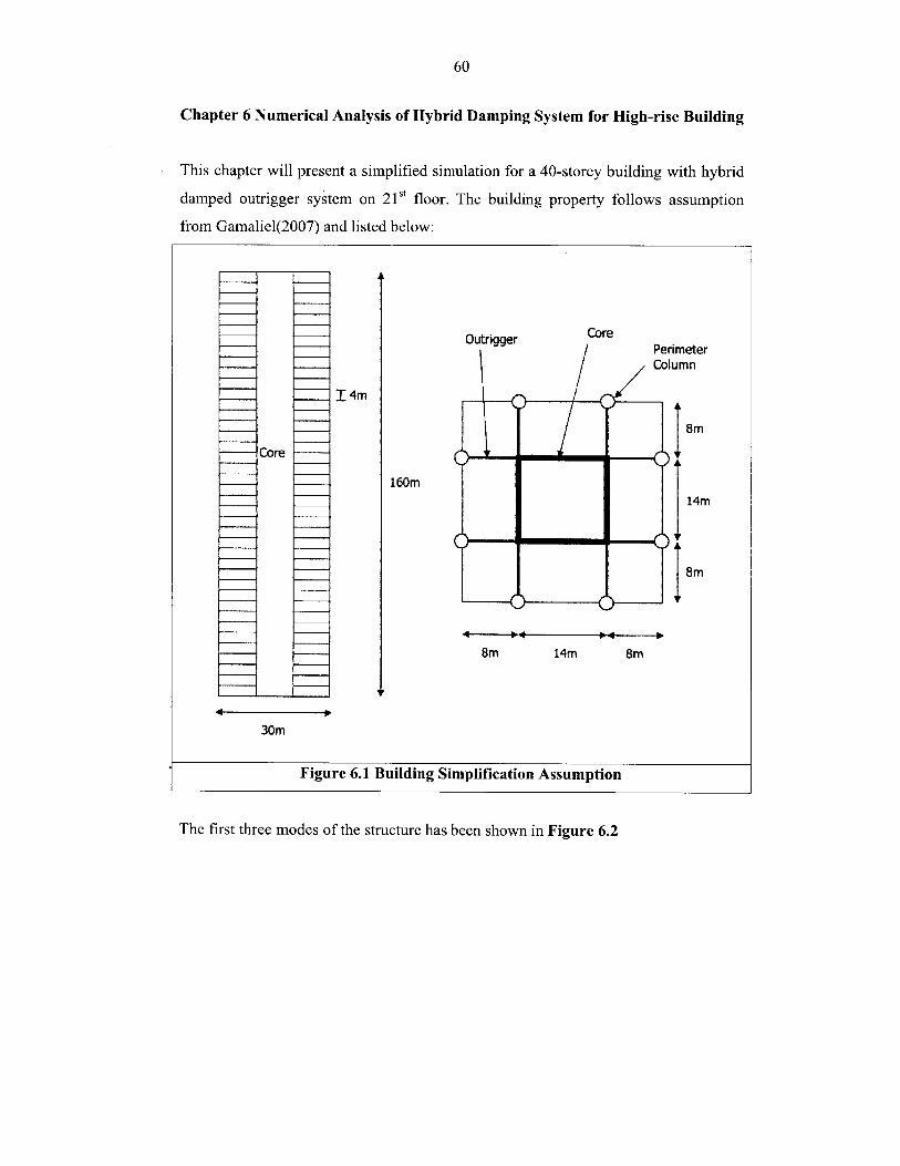
60

Chapter 6 Numerical Analysis of Hybrid Damping System for High-rise Building

This chapter will present a simplified simulation for a 40-storey building with hybrid

damped outrigger system on 21 s floor. The building property follows assumption

from Gamaliel(2007) and listed below:

OutriggerPerimeter

-f Column

]T4m

8m

Core

160m14m

I~8m

8m 14m 8m

30m

Figure 6.1 Building Simplification Assumption

The first three modes of the structure has been shown in Figure 6.2

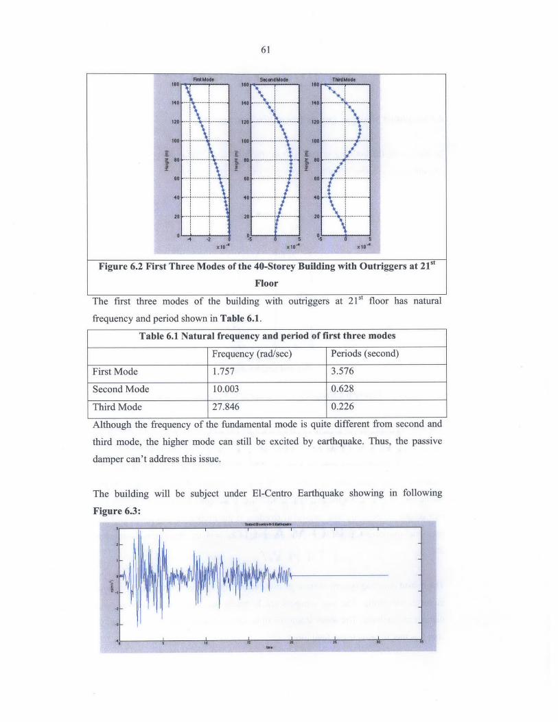
61

Figure 6.2 First Three Modes of the 40-Storey Building with Outriggers at 21't

Floor

The first three modes of the building with outriggers at 21st floor has natural

frequency and period shown in Table 6.1.

Table 6.1 Natural frequency and period of first three modes

Frequency (rad/sec) Periods (second)

First Mode 1.757 3.576

Second Mode 10.003 0.628

Third Mode 27.846 0.226

Although the frequency of the fundamental mode is quite different from second and

third mode, the higher mode can still be excited by earthquake. Thus, the passive

damper can't address this issue.

The building will be subject under El-Centro Earthquake showing in following

Figure 6.3:

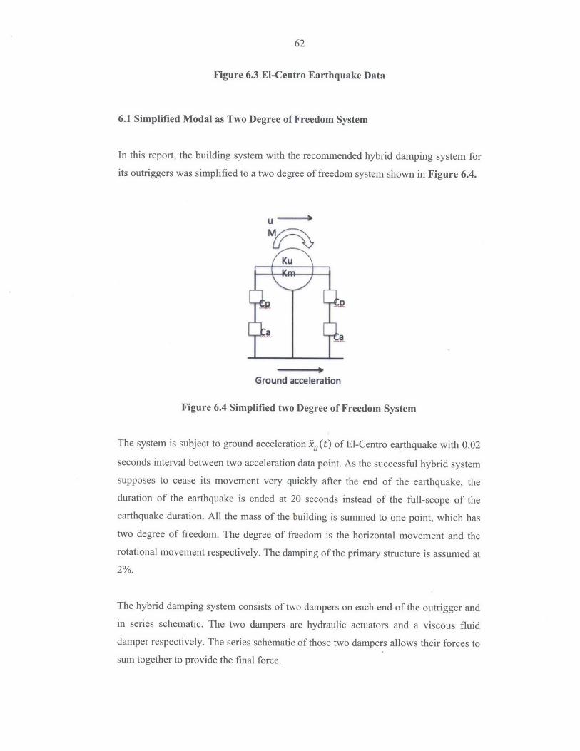
62

Figure 6.3 El-Centro Earthquake Data

6.1 Simplified Modal as Two Degree of Freedom System

In this report, the building system with the recommended hybrid damping system for

its outriggers was simplified to a two degree of freedom system shown in Figure 6.4.

M

Ku

Ground acceleration

Figure 6.4 Simplified two Degree of Freedom System

The system is subject to ground acceleration ig(t) of EI-Centro earthquake with 0.02

seconds interval between two acceleration data point. As the successful hybrid system

supposes to cease its movement very quickly after the end of the earthquake, the

duration of the earthquake is ended at 20 seconds instead of the full-scope of the

earthquake duration. All the mass of the building is summed to one point, which has

two degree of freedom. The degree of freedom is the horizontal movement and the

rotational movement respectively. The damping of the primary structure is assumed at

2%.

The hybrid damping system consists of two dampers on each end of the outrigger and

in series schematic. The two dampers are hydraulic actuators and a viscous fluid

damper respectively. The series schematic of those two dampers allows their forces to

sum together to provide the final force.

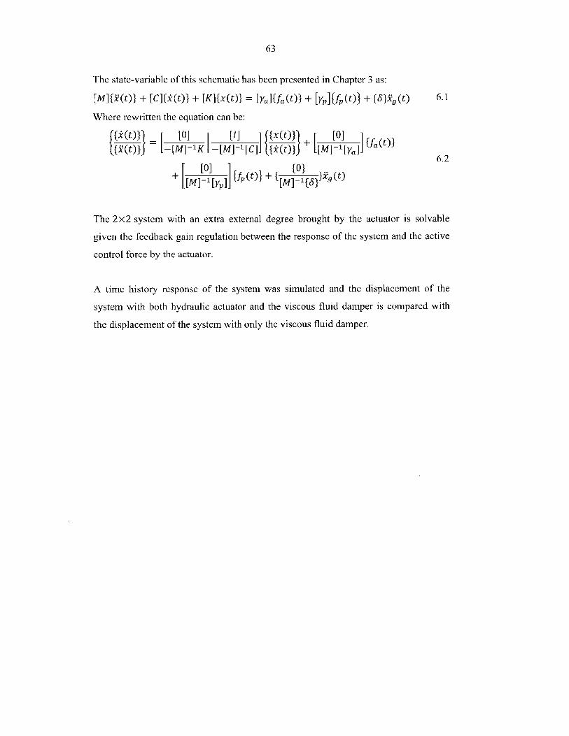
63

The state-variable of this schematic has been presented in Chapter 3 as:

[M]{(t)} + [C]ti(t)} + [K]tx(t)} = [a]tfa(t)} + [yp]{ff(t)} + {Sig(t) 6.1

Where rewritten the equation can be:

{{i(t)}l - 01 [0] [1]] {x(t)} r[ 0 ])f{(t)} -[M]-K -[M]-[[C]J {I(t)} ±[M]-1[Ya]] tfa(t)}6

6.2

+ 101[M]-[y f(t)} + t[to)]i{ ()

The 2x2 system with an extra external degree brought by the actuator is solvable

given the feedback gain regulation between the response of the system and the active

control force by the actuator.

A time history response of the system was simulated and the displacement of the

system with both hydraulic actuator and the viscous fluid damper is compared with

the displacement of the system with only the viscous fluid damper.

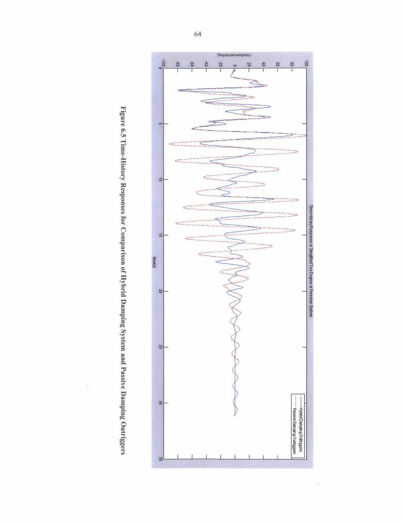
I V

IDamping Outriggers

ve Dam

ping Outdggerm

10

Fig

ure 6.5 T

ime-H

istory

Responses fo

r Com

pariso

n o

f Hybrid

Dam

pin

g S

ystem an

d P

assive Dam

pin

g O

utrig

gers

Tme-istoryneupone of Simpn.ed Tw

o Degree of Freedom

Syeminn80604020

II

.IUU 0

-40

-60-80

1520

2530

5

65

Blue curve of Figure 6.5 presented the response of the hybrid damping outriggers.

The red curve of Figure 6.5 showed the response of the passive damping outriggers.

The hybrid damped system showed better performance with the earthquake excitation

time. As the active system can adjust the system according to the external excitation,

it can stop the building's movement quickly after the external excitation ceases, while

the passive system won't stop the movement as quickly as the hybrid damping system.

The reduction of the displacement compared with passive damping system ranges

from 20% to 50%, which gives quite good results.

In conclusion, the recommended hybrid damping system for the high-rise outrigger

system generate better performance compare to the passive damping system. Thus,

this is an attractive alternative choice for the damping system for the high-rise

building outrigger system.

66

Chapter 7 Conclusion

Tall buildings are subjected to wind-induced external force and earthquake-induced

vibration. The occupants' feeling in the high-rise building must be considered into the

design. Thus, the governing design criteria are usually the motion limitation such as

lateral displacement and acceleration.

There are various ways to provide lateral resistance systems for tall buildings; not

only the traditional way to increase the stiffness of the building available, but also a

smart way to adjust the damping properties of the building by adding damping

systems. With the increasing of the building's height, the traditional bracing systems

are no longer efficient to provide the lateral resistance that needed by the building.

High-rise building outrigger system was proposed as an innovative system to integrate

the strength of core and perimeter columns. It helps overcome the overturning

moment in the core by connecting the core with outriggers to the perimeter columns

or belt trusses. The forces generated between the outriggers and the perimeter

columns during the redistribution of the moment could be large. With the damping

requirement from the building and the large interactive force generated between the

outriggers and perimeter columns, damped outriggers are an effective way to satisfy

both requirement. In addition to that, the damped outriggers will improve the lateral

resistance for the whole building. Although current damped outrigger system are

limited to passive dampers, hybrid damping system are an attractive alternative choice

which worth the study, as hybrid damping system can have additional adjustable

damping ratio and in the same time inherit the stability of the passive damping

system. It also make the future system upgrade easy not mention that it can address

the high-rise building's higher modal response.

Through the introduction of dynamic analysis for single degree of freedom structures

and multiple degree of freedom structures, presentation of various damping systems

and the analysis rational behind the hybrid damping system, this report summarized

the analytical method for the motional design of the structure. One case study of a

hybrid HDABC damping system suggested that hybrid damping system has surpass

the active and passive motion control system in terms of the efficiency and stability in

general civil structural design. The two case studies of a semi-active MR damped

67

outrigger system and a passive-active hybrid MR & actuator damped outrigger system

both suggested the promising results of better performance and more displacement

reduction.

Thus, a hybrid damping system consist of viscous fluid damper as passive part and

servo-valve actuator as active part both installed in between the end of the outriggers

and perimeter columns were proposed in the report. This system will generate better

performance than the passive system alone during the simplified simulation

developed in Chapter 6. Although the simulation didn't include the threshold limit for

the system adjustment consideration, the results were still very promising by giving

20% to 50% of displacement reduction.

However, the simulation for a fictitious hybrid damped high-rise building is very

ideal. More complicated model should be further developed and studied. Additionally,

this report didn't touch the economy optimization for the hybrid damped outrigger

system, which is a major consideration for this field. This should be included in

further researches for the hybrid-damped outriggers as well.

In summary, the hybrid-damped outriggers surpass the active and passive damping

system and are an attractive alternative choice for the outrigger damping system.

However, its economics and system reliability still requires improvements and should

be included in the future studies.

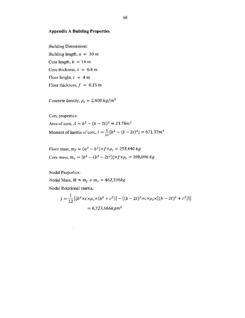
68

Appendix A Building Properties

Building Dimensions:

Building length, a = 30 m

Core length, b = 14 m

Core thickness, t = 0.4 m

Floor height, c = 4 m

Floor thickness, f = 0.15 m

Concrete density, pc = 2,400 kg/m 3

Core properties:

Area of core, A = b - (b - 2t) 2 = 21.76M 2

Moment of Inertia of core, I = [b4 - (b - 2t)4 ] = 671.37m 412

Floor mass, m = (a2 - b2 )xf xpc = 253,440 kg

Core mass, mc = [b 2 - (b2 _ 2t 2 )]xf xpc = 208,896 kg

Nodal Properties:

Nodal Mass, M = mf + mr = 462,336kg

Nodal Rotational inertia,

J = t[b2 xcxpcx(b 2 + c2 )] - {(b - 2t)2 xcxpcx[(b - 2t) 2 + c211112

= 6,723,666kgm 2

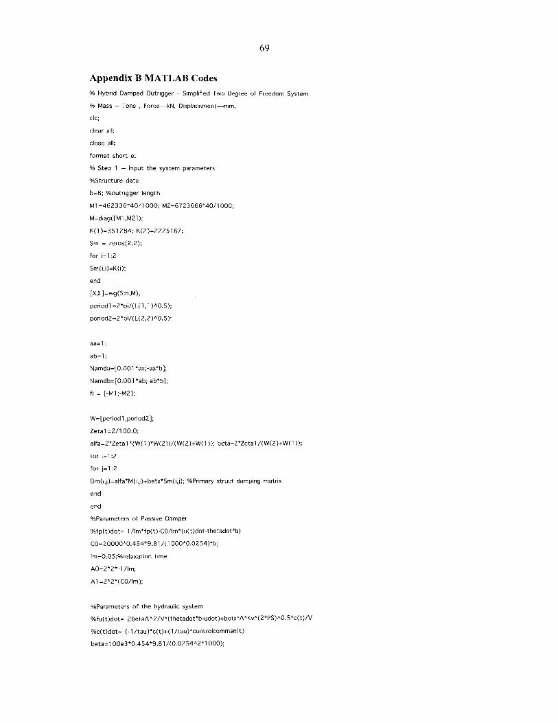
69

Appendix B MATLAB Codes

% Hybrid Damped Outrigger - Simplified Two Degree of Freedom System

% Mass - Tons , Force-kN, Displacement-mm,

cdc;

clear all;

close all;

format short e;

% Step 1 -- Input the system parameters

%Structure data

b=8; %outrigger length

M1=462336*40/1000; M2=6723666*40/1000;

M=diag([M1,M2]);

K(1)=351284; K(2)=2225167;

Sm = zeros(2,2);

for i=1:2

Sm(i,i)=K(i);

end

[X,L]=eig(Sm,M);

periodl =2*pi/(L(1,1 )AO.5);

period2=2*pi/(L(2,2)AO.5);

aa=1;

ab=1;

Namda=[0.001 *aa;-aa*b];

Namdb=[0.001 *ab;-ab*b];

fi = [-M1;-M2];

W=[periodl1,period2];

Zeta 1=2/100.0;

alfa=2*Zetal *(W( 1 )*W(2))/(W(2)+W(1)); beta=2*Zetal /(W(2)+W(1));

for i=1:2

for j=1 :2

Dm(i,j)=alfa*M(i,j)+beta*Sm(i,j); %Primary struct damping matrix

end

end

%Parameters of Passive Damper

%fp(t)dot=-1 /lm*fp(t)-CO/lm*(u(t)dot-thetadot*b)

CO=20000*0.454*9.81/(1 000*0.0254)*b;

lm=0.05;%relaxation time

A0=2*2*-1/m;

Al =2*2*(CO/Im);

%Parameters of the hydraulic system

%fa(t)dot= 2betaAA2/V*(thetadot*b-udot)+beta*A*Kv*(2*PS)A0.5*c(t)/V

%c(t)dot= (-1 /tau)*c(t)+(1/tau)*controlcomman(t)

beta=1 00e3*0.454*9.81/(0.0254A2*1 000);

70

Ps=3000*0.454*9.81/(0.0254A2*1 000);

%Moog 760-102A Actuator parameters

Kv=3.85*(0.0254A3)*1 5/sqrt(1 000*0.454*9.81/(0.0254A2*1 000));

tau=2*1 /(2*pi*3563);

A=0.4; V=2.0; Mp=0.005; Zetap=0.002; %Mp,Zetap are assumed

Kp=2*2*2*beta*Kv*A*sqrt(Ps/2)/V;

Cp=2*2*2*Zetap*Mp*sqrt(Kp/Mp);

C1=-1/tau;

C2=-C1;

% Step 2 -- Load the Excitation Data

Te=0.02; TT=31.18; %el-centro: sampling rate: 100 Hz, total: 10 sec.

Ts=0.02; %sampling time for controller

np=TT/Te; %total points

%t=0:Ts:(TT-Ts);

xg=[0.00630 0.00364 0.00099

-0.00128

0.00021

0.00416

0.00926

-0.03346

-0.08166

0.01338

-0.08513

-0.09324

0.08099

0.14562

-0.09334

-0.11309

0.16554

-0.00421

0.08163

0.03661

0.10487

0.01013

0.00715

0.19508

0.17311

0.02021

-0.02278

0.02280

-0.08585

-0.04069

0.05141

-0.10789

-0.17561

0.00368

0.00444

0.00528

0.00892

-0.03201

-0.06846

0.03221

-0.12858

-0.09166

0.13350

0.16143

-0.13843

-0.04451

0.09912

0.29099

0.14491

0.00295

0.05895

-0.03071

-0.06350

0.12301

0.11283

-0.02530

-0.07686

-0.00996

-0.12148

0.00623

0.10420

-0.20051

-0.22369

0.00864

0.00867

0.01653

-0.00486

-0.03056

-0.05527

0.05104

-0.17204

-0.09478

0.18600

0.17725

-0.18353

0.02407

0.03270

0.22380

0.20820

-0.03071

0.01303

-0.07156

-0.13415

0.05094

0.05255

-0.07081

-0.13095

-0.04272

-0.15711

0.05316

0.15699

-0.06786

-0.27177

0

0

0

-0

-0.

-0.

0

-0.

-0.

0

0

-0.

0

-0

0

0

-0

-0

-0.

-0.

-0

-0

-0.

-0.

-0.

-0.

0

0

0.

-0.

0.00428 0.00758 0.01087 0.00682 0.00277...

.01360 0.00727 0.00094 0.00420 0.00221...

.01290 0.01713 -0.00343 -0.02400 -0.00992...

.02779 0.03904 0.02449 0.00995 0.00961...

.01864 -0.03242 -0.03365 -0.05723 -0.04534...

02911 -0.02766 -0.04116 -0.05466 -0.06816...

04208 -0.04259 -0.04311 -0.02428 -0.00545...

.06987 0.08870 0.04524 0.00179 -0.04167...

12908 -0.08613 -0.08902 -0.09192 -0.09482...

09789 -0.12902 -0.07652 -0.02401 0.02849...

.23850 0.21993 0.20135 0.18277 0.16420...

.13215 0.08705 0.04196 -0.00314 -0.04824...

22863 -0.27372 -0.31882 -0.25024 -0.18166...

.09265 0.16123 0.22981 0.29839 0.23197...

.03372 -0.10014 -0.16656 -0.23299 -0.29941...

.15662 0.08943 0.02224 -0.04495 0.01834...

.18973 0.17125 0.13759 0.10393 0.07027...

.00561 0.01948 0.04458 0.06468 0.08478...

.03289 -0.07882 -0.03556 0.00771 0.05097...

11240 -0.15324 -0.11314 -0.07304 -0.03294...

20480 -0.12482 -0.04485 0.03513 0.11510...

.02113 -0.09320 -0.02663 0.03995 0.10653...

.00772 0.01064 0.02900 0.04737 0.06573...

04107 -0.01133 0.00288 0.01709 0.03131...

18504 -0.14347 -0.10190 -0.06034 -0.01877...

02147 -0.00021 0.02104 -0.01459 -0.05022...

19274 -0.22837 -0.18145 -0.13453 -0.08761...

.10008 0.14700 0.09754 0.04808 -0.00138...

.20979 0.26258 0.16996 0.07734 -0.01527...

06479 0.01671 -0.03137 -0.07945 -0.12753...

15851 -0.04525 0.06802 0.18128 0.14464...

0.15860 0.22053 0.18296 0.14538...0.10800 0.07137 0.03473 0.09666

71

0.10780 0.07023 0.03265 0.06649 0.10033 0.13417 0.10337 0.07257...

0.04177

-0.03315

-0.09060

-0.01952

0.01770

0.01460

-0.00915

-0.00215

0.01863

0.01099

-0.05999

-0.00231

-0.04574

-0.00501

-0.04045

-0.02619

-0.02972

-0.00139

0.03507

0.01097 -0.01983

-0.10180 -0.07262

-0.12578 -0.16095

-0.03605 -0.05259

0.02213 0.02656

0.05337 0.02428

-0.02509 -0.04103

0.00708 0.00496

0.03365 0.04867

0.00823 0.00547

-0.07768 -0.09538

-0.02235 0.01791

-0.02071 0.00432

-0.01795 -0.03089

-0.02398 -0.00750

-0.04082 -0.05545

-0.01642 -0.00311

-0.02714 -0.00309

0.03357 0.03207

0.04438

-0.04344

-0.19613

-0.04182

0.00419

-0.00480

-0.05698

0.00285

0.03040

0.00812

-0.06209

0.05816

0.02935

-0.01841

0.00897

-0.04366

0.01020

0.02096

0.03057

0.02350

0.04501

0.03250

-0.00942 -0.03231 -0.02997 -0.03095 -0.03192

-0.01449

0.09864

-0.12112

0.03745

-0.03310

0.05924

-0.03674

0.05023

-0.01071

-0.01388

-0.06324

0.04028

-0.05317

0.04511

0.02611

0.02724

0.05098

0.09009

-0.02690

-0.12494

0.08247

0.10616

0.00549

-0.06243

-0.00389

-0.02123 0.01523 0.05170

0.06741 0.03618 0.00495

-0.18303 -0.12043 -0.05782

0.06979 0.10213 -0.03517

-0.03647 -0.03984 -0.00517

-0.01503 -0.08929 -0.16355

-0.06287 -0.08899 -0.05430

0.01600

0.00829

0.01274

-0.09215

0.01880

-0.03124

0.06087

0.04543

0.06080

0.07985

0.12196

-0.04817

-0.16500

0.07576

0.09057

-0.02281

-0.01823 -0.05246

-0.00314 0.02966

0.00805 0.03024

-0.12107 -0.08450

0.04456

-0.00930

0.07663

0.01571

0.03669

0.06915

0.10069

-0.06944

-0.20505

0.06906

0.07498

-0.05444

0.07032

0.01263

0.09239

-0.01402

0.01258

0.03681

0.06906

0.03444

-0.02588

0.08816

0.00420

0.00479

-0.17247

0.02950

-0.06096

-0.01961

-0.08669

0.06246

0.05243

-0.04794

0.09608

0.03457

0.05742

-0.04374

0.10860 0.17281

-0.01426 0.01492

-0.14784 -0.09955

-0.03106 -0.02903

-0.01819 -0.04057

-0.03389 -0.00557

-0.01826 0.02046

0.00074 -0.00534

0.01213 -0.00614

0.01077 -0.00692

-0.02880 0.00448

0.03738 0.01660

0.01526 0.01806

-0.00593 0.00655

0.00384 -0.00129

-0.03188 -0.06964

-0.01153 -0.03564 -0.00677...

0.05845 0.04775 0.03706 0.02636...

0.07943 0.05816 0.03689 0.01563...

-0.09070 -0.11197 -0.11521 -0.11846...

-0.15713 -0.10921 -0.06129 -0.01337...

0.06236 0.08735 0.11235 0.13734...

0.08011 0.08524 0.09037 0.06208...

-0.04030 -0.02615 -0.01201 -0.02028...

-0.03524 -0.00805 -0.04948 -0.03643 -0.02337 -0.03368...

0.01100 0.02589 0.01446 0.00303 -0.00840 0.00463...

0.10416 0.03551...

-0.02025 -0.05543...

-0.05127 -0.00298...

-0.02699 0.02515...

-0.06294 -0.02417...

0.02274 0.00679...

0.00454 -0.01138...

-0.01141 0.00361...

-0.02441 0.01375...

-0.02461 -0.04230...

0.03777 0.01773...

-0.00418 -0.02496...

0.02086 0.00793...

-0.02519 -0.05693...

-0.00642 -0.01156...

-0.05634 -0.04303...

0.05011 0.02436...

0.05773 0.04640...

0.03637 0.01348...

-0.01984 -0.01379...

0.12463 0.16109...

0.00345 0.00269...

0.06740 0.13001...

-0.13763 -0.10278...

0.06417 0.09883...

0.04164 0.01551...

0.01508 0.04977...

-0.06769 -0.04870...

-0.00234 -0.06714 ...

0.02351 -0.00541..

-0.01137 0.02520...

0.12184 0.06350...

0.03283 0.03109...

0.02245 -0.01252...

-0.07347 -0.03990...

-0.00775

0.12987

-0.05922

0.08373

-0.06794

0.13350

-0.01061

0.08446

-0.02970

-0.04051

-0.03432

0.06177

0.00517

0.02935

0.00680

-0.00633

0.02210

0.05822

-0.00564

-0.12170

0.03455

0.12175

0.03378

-0.02855

-0.01879

72

0.01766

-0.02819

-0.07707

0.05301

0.01985

0.02975

0.00342

-0.00407

0.00182

0.03069 0.04372 0.02165 -0.00042

-0.02001 -0.01182 -0.02445 -0.03707

-0.08620 -0.09533 -0.06276 -0.03018

0.03176 0.01051 -0.01073 -0.03198

-0.01726 -0.05438 -0.01204 0.03031

-0.01288 0.01212 0.03711 0.03517

-0.02181 -0.04704 -0.07227 -0.09750

0.03549 0.07504 0.11460 0.07769

-0.05513 0.04732 0.05223 0.05715

0.02705 -0.01779 -0.06263

-0.04668 -0.02027 0.00614

-0.03322 -0.00315 0.02691

0.02239 0.04215 0.06191

-0.05274 -0.02544 0.00186

-0.02074 0.00722 0.03517

-0.03646 -0.01989 -0.00332

-0.00563 0.01536 0.03635

0.01589 -0.01024 -0.03636

-0.08200 -0.04980 -0.01760

-0.01550 -0.00102 0.01347

-0.00041 -0.01952 -0.00427

-0.00874 -0.03726 -0.06579

0.02429 -0.01026 -0.04480

-0.01564 -0.00626 -0.01009

0.00733 -0.00632 -0.01997

0.02403 0.01642 0.00982

-0.10747 -0.15232

0.03255 0.00859

0.01196 -0.00300

0.08167 0.03477

0.02916 0.05646

-0.00528 -0.04572

0.01325 0.02982

0.05734

-0.06249

0.01460

0.02795

0.01098

-0.02600

-0.01083

-0.01392

0.00767

0.00322

-0.10228 -0.07847 -0.05466 -0.03084

0.02483 0.01809 -0.00202 -0.02213

0.07459 0.06203 0.04948 0.03692

0.03037 0.03626 0.04215 0.04803

0.03611 0.03166 0.00614 -0.01937

-0.05899 -0.04052 -0.02206 -0.00359

-0.00441 -0.00923 -0.01189 -0.01523

0.01431 0.00335 -0.00760 -0.01856

0.01016 -0.00590 -0.02196 -0.00121

0.00424 0.00196 -0.00031 -0.00258

-0.01396 -0.01750 -0.02104 -0.02458

-0.04889 -0.03559 -0.02229 -0.00899

-0.01383 0.01314 0.04011 0.06708

-0.02733

0.05559

-0.02685

0.03015

-0.00095

-0.05207

0.04256

-0.04621 -0.03155

0.03253 0.00946

-0.01161 0.00363

0.03159

-0.04780

0.04680

0.04244

0.02623

0.01380

-0.01869

0.01490

0.03532

-0.00339

-0.00703

-0.00278

-0.00145

0.05392

-0.04489

0.01487

-0.01856

-0.00737

0.01953

-0.00486

-0.02813

0.00431

0.04820

-0.01688 -0.00222

-0.01360 -0.01432

0.01887 0.03411

-0.02249 -0.04456 -0.03638...

-0.04969 -0.05882 -0.06795...

0.00239 0.03496 0.04399...

-0.05323 0.00186 0.05696...

0.07265 0.11499 0.07237...

0.03323 0.01853 0.00383...

-0.12273 -0.08317 -0.04362...

0.04078 0.00387 0.00284...

0.06206 0.06698 0.07189...

-0.12591 -0.09950 -0.07309...

-0.01537 -0.03932 -0.06328...

0.00335 0.00970 0.01605...

-0.01212 -0.01309 -0.01407...

0.08376 0.01754 -0.04869...

-0.08617 -0.06960 -0.05303...

0.01101 -0.00781 -0.02662...

0.00584 -0.01992 -0.00201...

-0.03311

0.07900

0.05692

0.04148

0.05359

-0.02655

0.04372

0.03409

0.02202

0.01678

0.01656

0.04599

0.04947

-0.07040

0.01005

-0.04941 -0.06570...

0.04750 0.01600...

0.03781 0.01870...

0.01821 -0.00506...

0.09338 0.05883...

-0.03441 -0.02503...

0.03463 0.02098...

0.03287 0.03164...

-0.01941 -0.06085...

0.01946 0.02214...

0.03590 0.05525...

0.04079 0.03558...

0.04502 0.04056...

-0.09592 -0.07745...

0.00523 0.00041...

-0.02190 -0.00983 0.00224...

0.00383 0.01502 0.02622...

0.04027 0.02826 0.01625...

-0.00713 -0.00941 -0.01168...

-0.03167 -0.03521 -0.04205...

0.01762 0.00714 -0.00334...

0.02932 0.01043 -0.00845...

0.01244 0.02683 0.04121...

-0.01504 -0.01576 -0.04209...

0.03115 0.02819 0.02917...

0.03113 0.00388 -0.02337 -0.05062 -0.03820 -0.02579 -0.01337...

0.01146 0.02388 0.03629 0.01047 -0.01535 -0.04117 -0.06699...

-0.03715 -0.02222 -0.00730 0.00762 0.02254 0.03747 0.04001.

0.04507 0.04759 0.05010 0.04545 0.04080 0.02876 0.01671...

73

0.00467 -0.00738 -0.00116 0.00506 0.01128

-0.04135 -0.06096

-0.01310 -0.00063

-0.00932 -0.02884

0.02851 0.04779

-0.03120 -0.01262

0.06452 0.03019

-0.03231 -0.03028

-0.04843 -0.06562

0.02698 0.03379

0.01598 0.01574

0.03009 0.03989

0.04931 0.05550

-0.03681 -0.03678

-0.08058 -0.06995 -0.05931

0.01185 0.02432 0.03680

-0.04837 -0.06790 -0.04862

0.02456 0.00133 -0.02190

0.00596 0.02453 0.04311

-0.00414 -0.03848 -0.07281

-0.02824 -0.00396 0.02032

-0.05132 -0.03702 -0.02272

0.04061

0.00747

0.03478

0.06168

-0.03675

0.05866 0.03556 0.01245

-0.02131 -0.00946 0.00239

-0.00851 -0.00503 -0.00154

0.03590 0.04818 0.06045

-0.04134 -0.03199 -0.03135

0.01570 0.02714 0.03858

0.03061 0.03304 0.01371

-0.01353 -0.01261 -0.01170

0.04838 0.03749 0.02660

0.00136 0.01052 0.01968

0.00759 0.02310 0.00707

-0.00137 0.02645 0.05428

-0.02281 -0.00784 0.00713

0.03085 -0.02027 -0.07140

0.05792 0.09400 0.13009

-0.01846 -0.00861 -0.03652

0.04742 0.05423

-0.00080 -0.00907

0.02967 0.02457

-0.00526 -0.07220

-0.03672 -0.01765

-0.01066 -0.03376

-0.00208 -0.00654

0.00195 0.00051

0.01750 -0.00211

-0.04868 -0.03805

0.04927 0.02974

-0.02934 -0.01006

-0.04513 -0.06836

0.06169 0.08027

-0.05999 -0.04717

0.00313 -0.01406

-0.00843 0.00587

0.03535 0.01647

0.00072 0.01051

0.03075 0.03694

-0.06336 -0.05451

0.00143 0.02051

-0.05687 -0.04502

-0.01101 -0.01548

-0.00092 0.01135

-0.02173...

-0.02557...

0.01021...

0.00922...

-0.04978...

0.09885...

-0.03435...

-0.03124...

0.02017...

0.01622...

0.02030...

0.04313 ...

-0.04566...

0.03958...

-0.03317 ...

-0.01200...

0.02363...

0.07273 0.02847 -0.01579 -0.06004 -0.05069...

-0.03071 -0.03007 -0.01863 -0.00719 0.00425...

0.02975 0.02092 0.02334 0.02576 0.02819...

-0.00561 -0.02494 -0.02208 -0.01923 -0.01638...

-0.00169 0.00833 0.01834 0.02835 0.03836...

0.01571 0.00482 -0.00607 -0.01696 -0.00780...

0.02884 -0.00504 -0.03893 -0.02342 -0.00791...

-0.00895 -0.02498 -0.04100 -0.05703 -0.02920...

0.03587 0.01746 -0.00096 -0.01937 -0.03778...

0.02210 0.03707 0.05204 0.06701 0.08198...

-0.12253 -0.08644 -0.05035 -0.01426 0.02183...

0.03611 -0.05787 -0.04802 -0.03817 -0.02832...

-0.06444 -0.06169 -0.05894 -0.05618 -0.06073...

-0.06528 -0.04628 -0.02728 -0.00829 0.01071 0.02970 0.03138 0.03306...

0.03474 0.03642 0.04574 0.05506 0.06439 0.07371 0.08303 0.03605...

-0.01092 -0.05790 -0.04696 -0.03602 -0.02508 -0.01414 -0.03561 -0.05708...

-0.07855 -0.06304

0.02970 0.03993

-0.07032 -0.05590

-0.06798 -0.03710

0.08715 0.02615

0.02837 0.05321

-0.03696 -0.01608

0.13008 0.10995

0.01158 0.00780

-0.00450 -0.00120

-0.06319 -0.05046

0.01355 0.01791

-0.01401 -0.00526

-0.04753 -0.03203 -0.01652 -0.00102 0.00922

0.05017 0.06041 0.07065 0.08089 -0.00192

-0.04148 -0.05296 -0.06443 -0.07590 -0.08738

-0.00623 0.02465 0.05553 0.08640 0.11728

-0.03485 -0.09584 -0.07100 -0.04616 -0.02132

-0.00469 -0.06258 -0.12048 -0.09960 -0.07872

0.00480 0.02568 0.04656 0.06744 0.08832

0.08982 0.06969 0.04955 0.04006 0.03056

0.00402 0.00024 -0.00354 -0.00732 -0.01110

0.00210 0.00540 -0.00831 -0.02203 -0.03575

-0.03773 -0.02500 -0.01227 0.00046 0.00482

0.02228 0.00883 -0.00462 -0.01807 -0.03152

0.00350 0.01225 0.02101 0.01437 0.00773

0.01946...

-0.08473...

-0.09885...

0.1481 5...

0.00353...

-0.05784...

0.10920...

0.02107...

-0.00780...

-0.04947...

0.0091 9...

-0.02276...

0.00110...

74

0.00823 0.01537 0.02251

0.02852 0.03591 0.04329

-0.00898 -0.00126 0.00645

0.04527 0.03639 0.02750

-0.04171 -0.02812 -0.01453

-0.00177 -0.01111 -0.02044

0.01965 0.03434 0.02054

-0.01860 -0.01057 -0.00254

0.01488 0.00791 0.00093

0.04128 0.02707 0.01287

-0.02828 -0.02044 -0.01260

0.00768 0.00661 0.01234

0.02042 0.01300 -0.03415

-0.00596 -0.00590 -0.00583

-0.00545 -0.00539 -0.00532

-0.00494 -0.00488 -0.00482

-0.00444 -0.00437 -0.00431

-0.00393 -0.00387 -0.00380

-0.00342 -0.00336 -0.00330

0.01713

0.03458

0.01417

0.01862

-0.00094

-0.02977

0.00674

-0.00063

-0.00605

-0.00134

-0.00476

0.01807

-0.00628

-0.00577

-0.00526

-0.00475

-0.00425

-0.00374

-0.00323

-0.00292 -0.00285 -0.00279 -0.00273

-0.00241 -0.00235 -0.00228 -0.00222

-0.00190 -0.00184 -0.00178 -0.00171

-0.00139 -0.00133 -0.00127 -0.00120

-0.00089 -0.00082 -0.00076 -0.00070

-0.00038 -0.00032 -0.00025 -0.00019

xg = xg*9810;

xg(1 001:1 559)=0*xg(1:559);

tt=0:Ts:(31.18-Te);

num=Te/Ts;

if(num>1)

xO(num:num:np)=xg;

clear xg;

dx0=xO(num)/num; num1=num-1;

for j=1 :numl

xO(j)=dxO*j;

end

nxl =count-1;

for i=1:nxl

il=num*i; i2=num*(i+1);

dx0=(xO(i2)-xO(il ))/num;

for j=1:numi

ij=il +j; xO(ij)=xO(il )+dxO*j;

end

end

xg=xO; clear xO;

end

0.01175 0.00637 0.01376 0.02114...

0.02587 0.01715 0.00844 -0.00027...

0.02039 0.02661 0.03283 0.03905...

0.00974 0.00086 -0.01333 -0.02752...

0.01264 0.02623 0.01690 0.00756...

-0.03911 -0.02442 -0.00973 0.00496...

-0.00706 -0.02086 -0.03466 -0.02663...

0.00128 0.00319 0.00510 0.00999...

0.00342 0.01288 0.02235 0.03181...

-0.01554 -0.02975 -0.04395 -0.03612...

0.00307 0.01091 0.00984 0.00876...

0.02380 0.02953 0.03526 0.02784 ...

-0.00621 -0.00615 -0.00609 -0.00602...

-0.00571 -0.00564 -0.00558 -0.00552...

-0.00520 -0.00513 -0.00507 -0.00501...

-0.00469 -0.00463 -0.00456 -0.00450...

-0.00418 -0.00412 -0.00406 -0.00399...

-0.00368 -0.00361 -0.00355 -0.00349...

-0.00317 -0.00311 -0.00304 -0.00298...

-0.00266 -0.00260 -0.00254 -0.00247...

-0.00216 -0.00209 -0.00203 -0.00197...

-0.00165 -0.00158 -0.00152 -0.00146...

-0.00114 -0.00108 -0.00101 -0.00095...

-0.00063 -0.00057 -0.00051 -0.00044...

-0.00013 -0.00006 0.00000]

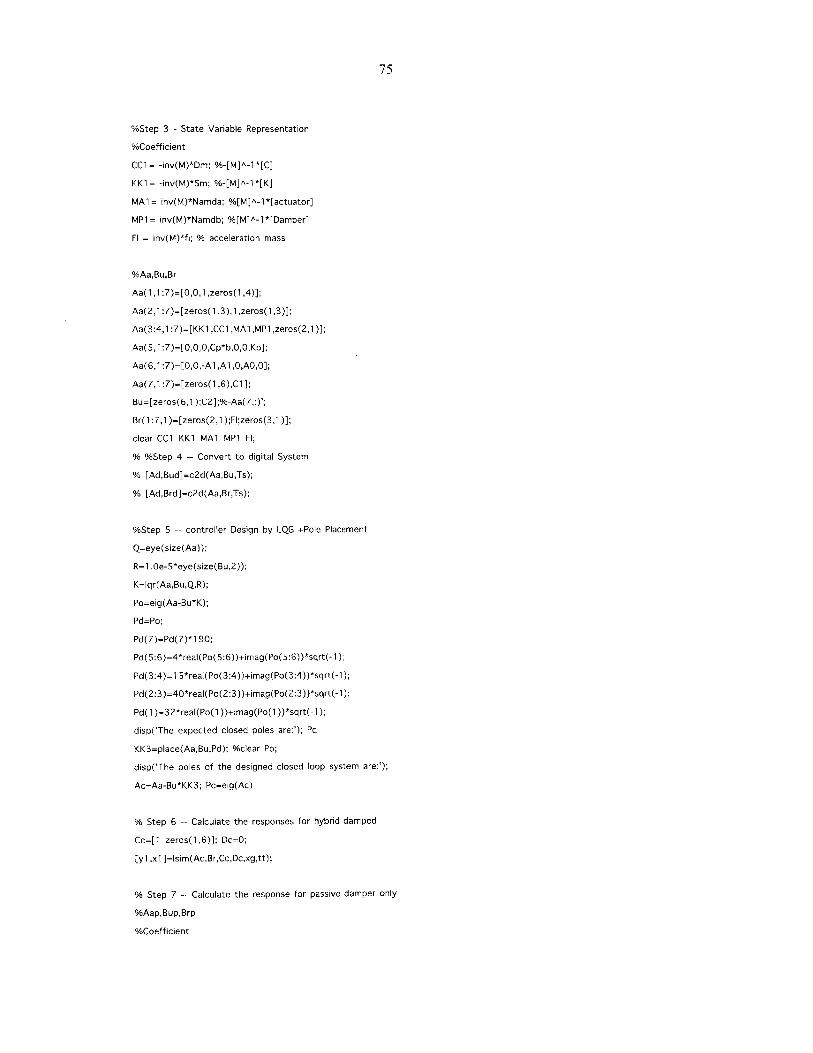
75

%Step 3 - State Variable Representation

%Coefficient

CC1= -inv(M)*Dm; %-[M]A-1*[C]

KK1= -inv(M)*Sm; %-[M]A-1*[K]

MAI= inv(M)*Namda; %[M]A-1 *[actuator]

MP1= inv(M)*Namdb; %[M]A-1*[Damper]

Fl = inv(M)*fi; % acceleration mass

%Aa,Bu,Br

Aa(1,1:7)=[0,0,1,zeros(1,4)];

Aa(2,1:7)=[zeros(1,3),1,zeros(1,3)];

Aa(3:4,1:7)=[KK1,CC1,MA1,MP1,zeros(2,1)];

Aa(5,1:7)=[0,0,0,Cp*b,0,0,Kp];

Aa(6,1:7)=[0,0,-A1,Al,0,AO,0];

Aa(7,1:7)=[zeros(1,6),C1 1;

Bu=[zeros(6,1 );C2];%-Aa(7,:)';

Br(1:7,1 )=[zeros(2,1 );Fl;zeros(3,1)];

clear CC1 KK1 MAI MP1 Fl;

% %Step 4 -- Convert to digital System

% [Ad,Bud]=c2d(Aa,Bu,Ts);

% [Ad,Brd]=c2d(Aa,Br,Ts);

%Step 5 -- controller Design by LQG +Pole Placement

Q=eye(size(Aa));

R=1.0e-5*eye(size(Bu,2));

K=lqr(Aa,Bu,Q,R);

Po=eig(Aa-Bu*K);

Pd=Po;

Pd(7)=Pd(7)*1 90;

Pd(5:6)=4*real(Po(5:6) )+imag(Po(5:6))*sqrt(-1);

Pd(3:4)=1 5*real(Po(3:4))+imag(Po(3:4))*sqrt(-1);

Pd(2:3)=40*real(Po(2:3))+imag(Po(2:3))*sqrt(-1);

Pd(1 )=32*real(Po(1 ))+imag(Po(1 ))*sqrt(-1);

disp('The expected closed poles are:'); Pd

KK3=place(Aa,Bu,Pd); %clear Po;

disp('The poles of the designed closed loop system are:');

Ac=Aa-Bu*KK3; Pc=eig(Ac)

% Step 6 -- Calculate the responses for hybrid damped

Cc=[1 zeros(1,6)]; Dc=0;

[yI,x1 ]=lsim(Ac,Br,Cc,Dc,xg,tt);

% Step 7 -- Calculate the response for passive damper only

%Aap,Bup,Brp

%Coefficient

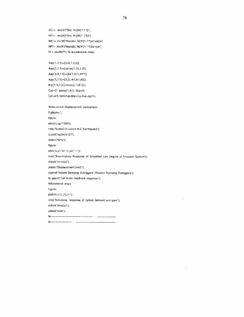
76

CC1= -inv(M)*Dm; %-[M]A-1*[C]

KK1= -inv(M)*Sm; %-[M]A-1*[K]

MAI= inv(M)*Namda; %[M]A-1 *[actuator]

MP1= inv(M)*Namdb; %[M]A-1 *[Damper]

F = inv(M)*fi; % acceleration mass

Aap(1,1:5)=[0,0,1,0,0];

Aap(2,1:5)=[zeros(1,3),1,O];

Aap(3:4,1:5)=[KK1,CC1,MP1];

Aap(5,1:5)=[O,O,-A1,A1,AD];

Brp(1:5,1)=[zeros(2,1);Fl;O];

Ccp=[1 zeros(1,4)]; Dcp=O;

[y2,x2]=Isim(Aap,Brp,Ccp,Dcp,xg,tt);

%Horizontal Displacement comparison

FigNum=1;

figure;

plot(tt,xg/1 000);

title('Scaled El-centro N-S Earthquake');

ylabel('xg(m/sA2)');

xlabel('time');

figure;

plot (t t,y I ,'b-', tt,y2,'r--');

title('Time-History Response of Simplified Two Degree of Freedom System');

xlabel('time(s)');

ylabel('Displacement(mm)');

legend('Hybrid Damping Outriggers','Passive Damping Outriggers');

% gtext('Full-State feedback response');

%Rotational angle

figure;

plot(tt, x1 (:, 2),'r-');

title('Rotational response of hybrid damped outrigger');

xlabel('time(s)');

ylabel('rads');

%-------------------------------------

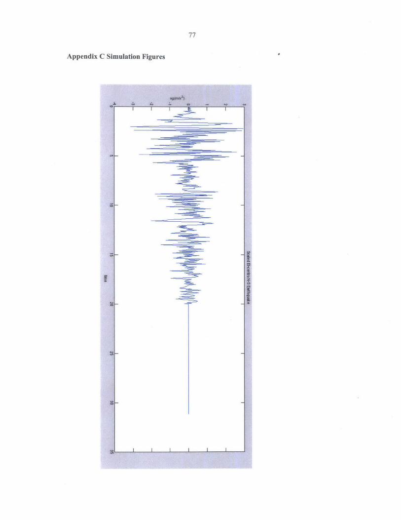
77

Appendix C Simulation Figures

41mmm

* *

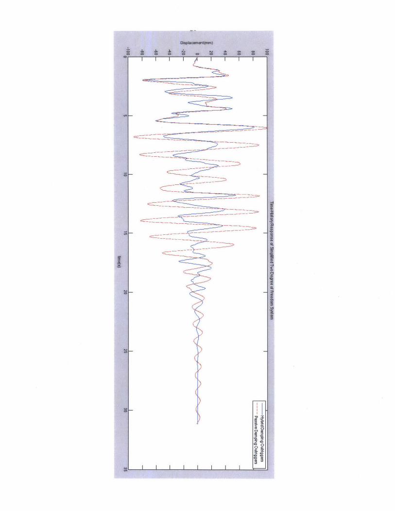
____Hybeid Dvnpm

~g Outtiggers

' P

aveDenipingO

uttiggers

~ I

I ~II

I

ft II

I ~

Ifl~

-I

I

III

-I

I~I

lIlt,?I

t'tjlj

II l~

~

'~

~JIt

it

-I

~

ii\)

kI~

79

Bibliography

Willford, R. S. (2008, 3). Damped outriggers for tall buildings. The Arup Journal ,

15-21.

P. Tan, C. F. (2012). Experimental Study on the Outrigger Damping System for High-

Rise Building. 15 WCEE LISBOA 2012. LISBOA.

Chia-Ming Chang & Takehiko Asai, Z. W. (2012). Smart Outriggers for Seismic

Protection of High-rise Buildings. 15 WCEE LISBOA 2012. LISBOA.

Gamaliel, R. (2008). Frequency-Based Response of Damped Outrigger Systems fbr

Tall Buildings. Cambridge: Massachusetts Institute of Technology.

N. Herath, N. H. (2009). Behaviour of Outrigger Beams in High rise Buildings under

Earthquake Loads. Australian Earthquake Engineering Society 2009 Conference. The

University of Melbourne, Parkville, Victoria.

Jr., J. C. (2006). Application of Damping in High-rise Buildings. Cambridge:

Massachusetts Institute of Technology.

Periods of vibration of braced frames with outriggers. (2012). M. Nicoreaca * and

J.C.D. Hoenderkampb.

Takehiko Asai a, C.-M. C. (2013). Real-time hybrid simulation of a smart outrigger

damping system for high-rise buildings. Engineering Structures (57), 177-188.

X. L. Lua, H. J. (2011). Research and Practice of Response Control for Tall Buildings

in Mainland China. Procedia Engineering (14), pp. 73-83.

Fernando Pereira-Mosqueira Ingeniero de Caminos, C. y. (2010). Case study of a 39-

Story Building: Model Verificaiton and Performance Comparison with a Semi-active

Device. Cambridge: Massachusetts Institute of Technology.

Hi Sun Choi, G. H. (2012). Outrigger Designfor High-rise buildings. council on Tall

buildings and Urban Habitat.

Franklin Y. Cheng, H. J. (2008). Smart Structures-innovative Systems fbr Seismic

Response Control. New York: CRC press Taylor&Francis Group.

Chopra, A. K. (2001). Dynamics of Structures-- Theory and Applications to earthquak

Engineering. New Jersey: Prentise Hall.

Connor, J. J. (1996). Introduction to motion based Design. Boston: Computational

Mechanics Publications.

Tamura, Y. e. (1995). Effectiveness of Tuned Liquid Dampers under Wind

Excitation. Engineering Structures, 609, 17.

80

Pall, A. C. (1982). Response of friction damperd braced frames. ASCE Journal of

Structural Division , 108.

Aiken, I. K. (1992). Comparative study of four passive energy dissipation systems.

Bulletin of New Zealand National Society of Earthquake Engineering, p. 175.

Soong, T. D. (1997). Passive Energy Dissipation System in Structural Engineering

(1st ed. ed.). Chichester, England: John Wiley & Sons.

Arima, F. e. (1088). A study on buildings with large damping using viscous damping

walls. Proceddings of the Ninth World Conference on Earthquake Engineering (p.

821). Tokyo: International Association for Earthquake Engineering.

Hrovat, D. a. (1983). Semiactive versus passive or active tuned mass dmaper for

structural control. ASCE Journal of Engineering Mechanics , 109.

Akbay, A. A. (1991). Actively regulated friction slip braces. Proceedings of the Sixth

Canadian Conference on Earthquake Engineering, (p. 367). Toronto.

Nishimura, I. e. (1992). Active tuned mass damper. Journal of Smart Materials and

Structures , 306.

Yang, J. G. (1982). Active tendon control of structures. ASCE Journal ofEngineering

Mechanics Division , 108.

Fujita, T. (1994). Development of hybrid mass damper with convertible active and

passive modes using AC-servomotor for vibration control of tall buildings.

Proceeding of the First World Conference on Structural Control (p. 3). Los Angeles:

International Association for Structural Control.

Yang, J. D. (1991). A Seismic hybrid control systems for building structures. ASCE

Journal ofEngineering Mechanics, (p. 117).

Cheng, F. a. (1998). Optimum control of a hybrid system for seismic excitations with

state observer techniques. Smart Materials and Structures , 7.

Funakubo, H. (1991). Actuatorsfor Control. New York: Gordon and Breach Science

Publishers.

Spencer, B. a. (1987). Phenomenological model of a magneto rheological damper.

ASCE Journal of Engineering Mechanics, 20.

Cheng, F. (1990). Optimum design and control of tall buildings. Proceeding of the

Fourth World Congress:200 and Beyond, Council on Tall Buildings and Urban

Habitat. Bethlehem.

Soong, T. (1990). Active Structural Control: Theory and Practice (1st edition ed.).

New York: Longman Scientific & Technical, UK.

81

Cheng, F. (2000). Generalized optimal active control algorithm for seismic resistant

structures with active and hybrid control. International Journal of Computer

Applications in Technology, 13.

Smith RJ, a. W. (2007). The damped outrigger concept for tall buildings. The

Structural Design of Tall and Special Buildings journal.

Zhihao Wang, C.-M. C. (2010). Controllable outrigger damping system for high rise

building with MR dampers. Proc. of'SPIE, Vol. 7647, 76473Z.

Moon, M. M. (2007). Structural Developments in Tall Buildings: Current Trends and

Future Prospects. Architectural Science Review, 205-223.