SIGNAL AND IMAGE PROCESSING ALGORITHMS USING INTERVAL CONVEX PROGRAMMING AND SPARSITY a dissertation submitted to the department of electrical and electronics engineering and the graduate school of engineering and science of bilkent university in partial fulfillment of the requirements for the degree of doctor of philosophy By Kıvan¸cK¨ ose September, 2012

Welcome message from author
This document is posted to help you gain knowledge. Please leave a comment to let me know what you think about it! Share it to your friends and learn new things together.
Transcript
SIGNAL AND IMAGE PROCESSINGALGORITHMS USING INTERVAL CONVEX
PROGRAMMING AND SPARSITY
a dissertation submitted to
the department of electrical and electronics
engineering
and the graduate school of engineering and science
of bilkent university
in partial fulfillment of the requirements
for the degree of
doctor of philosophy
By
Kıvanc Kose
September, 2012
I certify that I have read this thesis and that in my opinion it is fully adequate,
in scope and in quality, as a dissertation for the degree of Doctor of Philosophy.
Prof. Dr. Ahmet Enis Cetin(Advisor)
I certify that I have read this thesis and that in my opinion it is fully adequate,
in scope and in quality, as a dissertation for the degree of Doctor of Philosophy.
Prof. Dr. Orhan Arıkan
I certify that I have read this thesis and that in my opinion it is fully adequate,
in scope and in quality, as a dissertation for the degree of Doctor of Philosophy.
Assoc. Prof. Ugur Gudukbay
ii
I certify that I have read this thesis and that in my opinion it is fully adequate,
in scope and in quality, as a dissertation for the degree of Doctor of Philosophy.
Prof. Dr. Omer Morgul
I certify that I have read this thesis and that in my opinion it is fully adequate,
in scope and in quality, as a dissertation for the degree of Doctor of Philosophy.
Asst. Prof. Behcet Ugur Toreyin
Approved for the Graduate School of Engineering and Science:
Prof. Dr. Levent OnuralDirector of the Graduate School
iii
ABSTRACT
SIGNAL AND IMAGE PROCESSING ALGORITHMSUSING INTERVAL CONVEX PROGRAMMING AND
SPARSITY
Kıvanc Kose
Ph.D. in Electrical and Electronics Engineering
Supervisor: Prof. Dr. Ahmet Enis Cetin
September, 2012
In this thesis, signal and image processing algorithms based on sparsity and in-
terval convex programming are developed for inverse problems. Inverse signal
processing problems are solved by minimizing the ℓ1 norm or the Total Varia-
tion (TV) based cost functions in the literature. A modified entropy functional
approximating the absolute value function is defined. This functional is also
used to approximate the ℓ1 norm, which is the most widely used cost function
in sparse signal processing problems. The modified entropy functional is contin-
uously differentiable, and convex. As a result, it is possible to develop iterative,
globally convergent algorithms for compressive sensing, denoising and restoration
problems using the modified entropy functional. Iterative interval convex pro-
gramming algorithms are constructed using Bregman’s D-Projection operator.
In sparse signal processing, it is assumed that the signal can be represented using
a sparse set of coefficients in some transform domain. Therefore, by minimizing
the total variation of the signal, it is expected to realize sparse representations
of signals. Another cost function that is introduced for inverse problems is the
Filtered Variation (FV) function, which is the generalized version of the Total
Variation (VR) function. The TV function uses the differences between the pixels
of an image or samples of a signal. This is essentially simple Haar filtering. In FV,
high-pass filter outputs are used instead of differences. This leads to flexibility in
algorithm design adapting to the local variations of the signal. Extensive simu-
lation studies using the new cost functions are carried out. Better experimental
restoration, and reconstructions results are obtained compared to the algorithms
in the literature.
Keywords: Interval Convex Programming, Sparse Signal Processing, Total Vari-
ation, Filtered Variation, D-Projection, Entropic Projection, Inverse Problems.
iv
OZET
ARALIK DISBUKEY PROGRAMLAMA VE
SEYREKLIK KULLANAN IMGE VE SINYAL ISLEME
ALGORITMALARI
Kıvanc Kose
Elektrik ve Elektronik Muhendisligi, Doktora
Tez Yoneticisi: Prof. Dr. Ahmet Enis Cetin
Eylul 2012
Bu tezde ters problemleri cozmek icin kullanılabilecek aralık dısbukey pro-
gramlama ve seyreklik bilgilerini kullanan algoritmalar gelistirilmistir. Sinyal
isleme literaturunde ters problemler ℓ1 normu ya da Toplam Degisinti bazlı
maliyet fonksiyonları kullanılarak cozulur. Bu tezde mutlak deger fonksiyonunu
yaklasıklayan degistirilmis entropi fonksiyonelini tanımladık. Bu fonksiyonel
aynı zamanda seyrek sinyal isleme konusunda en sıklıkla kullanılan maliyet
fonksiyonu olan ℓ1 normunuda yaklasıksamaktadır. Onerdigimiz degistirilmis
entropi fonksiyoneli surekli, dısbukey ve her yerde turevlenebilirdir. Bu
ozelliklerinden dolayı degistirilmis entropi fonksiyonelini kullanarak sıkıstırmalı
algılama, gurultu temizleme ve geri catım gibi problemlere dongulu, her yerde
yakınsayan algoritmalar gelistirmek mumkundur. Bregman tarafından bulu-
nan D-Izdusumu isletmeni kullanılarak dongulu aralık dısbukey programlama
algoritmaları gelistirilebilir. Seyrek sinyal islemede, bir sinyalin herhangi bir
donusum uzayında seyrek oldugu varsayılır. Bu varsayımdan yola cıkarak, bir
sinyalin Toplam Degisintisinin enkucuklenmesi ile sinyalin seyrek temsillerinin
gercellenmesi saglanması umulmaktadır. Biz bu tezde Filtrelenmis Degisinti
adını verdigimiz, yeni bir maliyet fonksiyonu onermekteyiz. Bu fonksiyon
aynı zamanda Toplam Degisinti fonksiyonunun genellestirilmis halidir. Toplam
Degisinti sinyalin sadece yanyana iki orneginin ya da yanyana iki pikselinin
farkını kullanır. Bu aslında basit bir Haar filtrelemesinden baska birsey degildir.
Filtrelenmis Degisinti ise farklar yerine yuksek gecirgenli filtre cıktıları kul-
lanılır. Bu bize sinyal icindeki farklı yerel degisintilere adaptasyon olanagı
saglar. Bu tez kapsamında onerilen yeni maliyet fonksiyonlarını kullanan kap-
samlı simulasyon yapılmıstır. Bu onerilen yeni maliyet fonksiyonları sinyal geri
catımı, sinyallerin gurultuden arındırılması, ve birden fazla bogumlu aglarda,
v

vi
bogum cıktılarının gurultuden arındırılması ve tahmin edilmesi problemleri kul-
lanılarak test edilmistir. Literaturdeki yontemlere kıyasla daha basarılı sinyal
geri catımı ve olusturulması sonucları gozlemlenmistir.
Anahtar sozcukler : Aralık Dısbukey programlama, Seyrek Sinyal Isleme, Toplam
Degisinti, Filterelenmis Degisinti, D-izdusum, Entropik Izdusum, Ters Problem-
ler.
Acknowledgement
First of all I would like to thank Prof Cetin for bringing light to my path in the
dark labyrinth of research. Sometimes he believed in me more than myself and
motivated me like a father. He has showed a patience of job against me. I would
like to thank him for all his patience and belief in me.
I would also like to specially thank to Dr. Gudukbay for not only his sug-
gestions during my research but also treating me like a colleague and being a so
good travel mate.
I would like to thank Prof Arikan, Prof Morgul and Dr. Toreyin for reading
this thesis and giving me very fruitful feedback about my research.
I dedicate a big portion of this thesis to my significant other, best friend, and
love Bilge. She supported me at every day of my Ph.D., believed in me and my
research even if she does not understand a single equation of it. In my most
desperate days, she cheered me up and put up with my all caprices. She became
the complementary part of my life and soul.
I also would like to thank to my father Mustafa, mom Guler and brother
Uygur for their support and encouragement. Especially, I would like to thank my
mom for calling me every day and giving daily tips about protecting myself from
cold, hunger and more importantly reminding me nothing is more important than
my health.
Thanks to Ali and Sevgi Kasli for treating me like a mad scientist and ac-
knowledge all my absurdity.
I would like to specially thank to Ayca and Mehmet for helping and supporting
me not only in academic but also other aspects of my life and be very close friends.
Thanks to Alican, Namik, and Serdar for the Tabldot and afternoon break sessions
during which we talk about everything but nothing.
Thanks to Alex for supporting me at my darkest hours, and passing me his
vii
viii
wisdom. He also deserves a special thanks to put up with minutely ringing
telephones to me. I also would like to thank Erdem, Elif, Asli, Erdem S, Ali
Ozgur, Gokhan Bora, Yigitcan, Fahri, and all my other Bilkent EE friends for
not only considering me as a colleague but also as a part of their life.
Bilkent SPG team members especially Osman, Serdar, Ihsan and Ahmet, also
deserves a special thanks for being so supportive and sharing.
Also Muruvet Parlakay deserves a special thanks for organizing everything in
the department and making our lives much simpler.
I also want to mention my gratitude to Tabldot for serving hot meals daily
even during the emptiest days of summer when all the other places are closed.
With its perfect diet, we have carried out our brain development and pursued our
research.
In this limited space, I may have forgotten to utter some of my friends’ and
colleagues’ names however this does not mean that they are less valuable to me.
Thanks to all of them.
The research that we present in this research is funded by TUBITAK with
project number 111E057. I would like to thank them for their support.
Contents
1 INTRODUCTION 1
1.2 Compressive Sensing . . . . . . . . . . . . . . . . . . . . . . . . . 4
1.2.1 Compressed Sensing Reconstructions Algorithms . . . . . . 7
1.2.2 Applications of Compressed Sensing . . . . . . . . . . . . . 11
1.3 Total Variational Methods in Signal Processing . . . . . . . . . . 13
1.3.1 The Total Variation based Denoising . . . . . . . . . . . . 14
1.3.2 The TV based Compressed Sensing . . . . . . . . . . . . . 17
1.4 Motivation . . . . . . . . . . . . . . . . . . . . . . . . . . . . . . . 18
2 ENTROPY FUNCTIONAL AND ENTROPIC PROJECTION 20
3 FILTERED VARIATION 27
3.1 Filtered Variation Algorithm and Transform Domain Constraints 30
3.1.1 Constraint-I: ℓ1 FV Bound . . . . . . . . . . . . . . . . . . 31
3.1.2 Constraint-II: Time and Space Domain Local Variational
Bounds . . . . . . . . . . . . . . . . . . . . . . . . . . . . 31
ix
CONTENTS x
3.1.3 Constraint-III: Bound on High Frequency Energy . . . . . 32
3.1.4 Constraint-IV: User Designed High-pass Filter . . . . . . . 33
3.1.5 Constraint-V: The Mean Constraint . . . . . . . . . . . . . 33
3.1.6 Constraint-VI: Image bit-depth constraint . . . . . . . . . 34
3.1.7 Constraint-VI: Sample Value Locality Constraint . . . . . 34
4 SIGNAL RECONSTRUCTION 36
4.1 Signal Reconstruction from Irregular Samples . . . . . . . . . . . 37
4.1.1 Experimental Results . . . . . . . . . . . . . . . . . . . . . 43
4.2 Signal Reconstruction from Random Samples . . . . . . . . . . . . 59
4.2.1 Experimental Results . . . . . . . . . . . . . . . . . . . . . 63
5 SIGNAL DENOISING 73
5.1 Locally Adaptive Total Variation . . . . . . . . . . . . . . . . . . 73
5.2 Filtered Variation based Signal Denoising . . . . . . . . . . . . . . 81
6 ADAPTATION AND LEARNING IN MULTI-NODE NET-
WORKS 95
6.1 LMS-Based Adaptive Network Structure and Problem Formulation 96
6.2 Modified Entropy Functional based Adaptive Learning . . . . . . 99
6.3 The TV and FV based robust adaptation and learning . . . . . . 102
7 CONCLUSIONS 116
CONTENTS xi
Bibliography 119
APPENDIX 119
A Proof of Convergence of the Iterative Algorithm 119
B Proof of Convexity of the Filtered Variation Constraints 121
B.1 ℓ1 Filtered Variation Bound . . . . . . . . . . . . . . . . . . . . . 121
B.2 Time and Space Domain Local Variation Bounds . . . . . . . . . 122
B.3 Bound on High Frequency Energy . . . . . . . . . . . . . . . . . . 123
B.4 Sample Value Locality Constraint . . . . . . . . . . . . . . . . . . 124
List of Figures
1.1 Shock filtered version of a sinusoidal signal after 450, 1340, and
2250 shock filtering iterations. To generate this figure, the code
in [1] is used. . . . . . . . . . . . . . . . . . . . . . . . . . . . . . 15
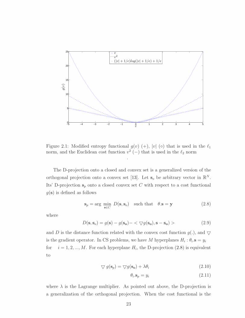
2.1 Modified entropy functional g(v) (+), |v| () that is used in the ℓ1
norm, and the Euclidean cost function v2 (−) that is used in the
ℓ2 norm . . . . . . . . . . . . . . . . . . . . . . . . . . . . . . . . 23
3.1 It is possible to design special high-pass filters according to the
structure of the data. The black and white stripes (texture) in
the fingerprint image corresponds to a specific band in the Fourier
domain. A high pass filter that corresponds to this band can be
designed and used as a FV constraint. . . . . . . . . . . . . . . . 29
3.2 An example high pass filter with exponentially decaying transition
band. . . . . . . . . . . . . . . . . . . . . . . . . . . . . . . . . . . 30
4.1 (i) 32 point irregularly sampled version of the Heavisine function
and the original noisy signal (σ = 0.2). (ii) The 1024 point inter-
polated versions of the function given at (i) using different inter-
polation methods. . . . . . . . . . . . . . . . . . . . . . . . . . . . 48
xii
LIST OF FIGURES xiii
4.2 (i) 32 point irregularly sampled version of the Heavisine function
and the original noisy signal (σ = 0.5). (ii) The 1024 point inter-
polated versions of the function given at (i) using different inter-
polation methods. . . . . . . . . . . . . . . . . . . . . . . . . . . . 49
4.3 (i) 32 point irregularly sampled version of the Heavisine function
and the original noiseless signal. (ii) The 1024 point interpolated
versions of the function given at (i) using different interpolation
methods. . . . . . . . . . . . . . . . . . . . . . . . . . . . . . . . . 50
4.4 (i) 32 point irregularly sampled version of the Heavisine function
and the original noiseless signal. (ii) The 1024 point interpolated
versions of the function given at (i) using different interpolation
methods. . . . . . . . . . . . . . . . . . . . . . . . . . . . . . . . . 51
4.5 (i) 128 point irregularly sampled version of the Heavisine func-
tion and the original noisy signal (σ = 0.2). (ii) The 1024 point
interpolated versions of the function given at (i) using different
interpolation methods. . . . . . . . . . . . . . . . . . . . . . . . . 52
4.6 (i) 128 point irregularly sampled version of the Heavisine function
and the original noiseless signal. (ii) The 1024 point interpolated
versions of the function given at (i) using different interpolation
methods. . . . . . . . . . . . . . . . . . . . . . . . . . . . . . . . . 53
4.7 (i) 256 point irregularly sampled version of the Heavisine func-
tion and the original noisy signal (σ = 0.2). (ii) The 1024 point
interpolated versions of the function given at (i) using different
interpolation methods. . . . . . . . . . . . . . . . . . . . . . . . . 54
4.8 4 of the other test signals that we used in our experiments. The
related reconstruction results are presented in Table 4.2 . . . . . . 55
4.9 Restored Heavisine signal after 1, 10, 20 and 58 iteration rounds. . 56
LIST OF FIGURES xiv
4.10 The original terrain model. The original model consists of 225×425
samples . . . . . . . . . . . . . . . . . . . . . . . . . . . . . . . . 56
4.11 The terrain model in Figure4.10 reconstructed using one-fourth of
the randomly chosen samples of the original model. The recon-
struction parameters are wc =π4, δs = 0.03, and ei = 0.01. . . . . 57
4.12 The terrain model in Figure 4.10 reconstructed using 18of the ran-
domly chose samples of the original model. The reconstruction
parameters are wc =π8, δs = 0.03, and ei = 0.01. . . . . . . . . . 58
4.13 Geometric interpretation of the entropic projection method:
Sparse representation si corresponding to decision functions at each
iteration are updated so as to satisfy the hyperplane equations de-
fined by the measurements yi and the measurement vector θi. Lines
in the figure represent hyperplanes in RN . Sparse representation
vector si converges to the intersection of the hyperplanes. Notice
that D-projections are not orthogonal projections. . . . . . . . . . 61
4.14 Geometric interpretation of the block iterative entropic projection
method: Sparse representation si corresponding to decision func-
tions at each iteration are updated by taking individual projec-
tions onto the hyperplanes defined by the lines in the figure and
then combining these projections. Sparse representation vector si
converges to the intersection of the hyperplanes. Notice that D-
projections are not orthogonal projections. . . . . . . . . . . . . . 62
4.15 The cusp signal with N = 1024 samples . . . . . . . . . . . . . . . 64
4.16 Hisine signal with N = 256 samples . . . . . . . . . . . . . . . . . 64
4.17 The cusp signal with 1024 samples reconstructed from M = 204
(a) and M = 716 (b) measurements using the iterative entropy
functional based method. . . . . . . . . . . . . . . . . . . . . . . . 65
LIST OF FIGURES xv
4.18 Random sparse signal with 128 samples is reconstructed from (a)
M = 3S and (b) M = 4S measurements using the iterative, en-
tropy functional based method. . . . . . . . . . . . . . . . . . . . 66
4.19 The reconstructed cusp signal with N = 1024 samples . . . . . . . 67
4.20 The reconstruction error for a hisine signal with N = 256 samples. 68
4.21 The impulse signal withN = 256 samples. The signal consists of 25
random amplitude impulses that are located at random locations
in the signal. . . . . . . . . . . . . . . . . . . . . . . . . . . . . . 69
4.22 Detail from resulting reconstruction of the Fingerprint image using
(a) the proposed and (b) Fowler’s [2] method. . . . . . . . . . . . 70
4.23 Detail from resulting reconstruction of the Mandrill image using
(a) the proposed and (b) Fowler’s [2] method. . . . . . . . . . . . 71
4.24 Detail from resulting reconstruction of the Goldhill image using
(a) the proposed and (b) Fowler’s [2] method. . . . . . . . . . . . 72
5.1 TV images of (a) original, (b) noisy, and (c) low-pass filtered noisy
Cameraman images. All images are rescaled in [0, 1] interval. . . . 77
5.2 The denoising result for (a) 256-by-256 kodim23 image from Ko-
dak dataset, using (b) TV regularized denoising, (c) LTV, and (d)
LATV algorithms. Details that are extracted from the reconstruc-
tion results are also presented in the right column of the respective
images. The original image is corrupted by Gaussian noise with a
standard deviation σ = 0.1. . . . . . . . . . . . . . . . . . . . . . 80
5.3 (a) Original image. (b) noisy image. (c) ℓp denoising with bounded
total variation and additional constraints [3] (Fig. 15 from [3])
(p=1.1). (d) ℓp denoising without the total variation constraint [3]
(Fig. 16 from [3]). (e) Denoised image using the FV method using
C2, C4 and C5. . . . . . . . . . . . . . . . . . . . . . . . . . . . . 84
LIST OF FIGURES xvi
5.4 NRMSE vs. iteration curves for FV denoising the image shown in
Fig. 5.3. ε1o and ε3o correspond to the ℓ1 and ℓ2 energy of the
original image. Bounds are selected ε1a = 0.8ε1o, ε1b = 0.6ε1o, and
ε3a = 0.8ε3o . . . . . . . . . . . . . . . . . . . . . . . . . . . . . . 85
5.5 (a) Original fingerprint image, (b) fingerprint image with AWGN
(SNR = 4.9 dB). (c) Image restored using the TV constraint (
SNR=7.45dB). (d) Image restored using the proposed algorithm
using C2, C4 and C5 (SNR=12.75 dB) . . . . . . . . . . . . . . . . 86
5.6 (a) The wall image from the Kodak dataset. The mask images
regarding the Wall image after (b) 1, (c) 3, and (d)8 iterations of
the algorithm. The masks are binary and white pixels represent
the samples that are classified as high-pass. . . . . . . . . . . . . . 88
5.7 The (c) TV and (d) FV based denoising result for (b) the noisy ver-
sion of the (a) 256-by-256 original cameraman image. Details that
are extracted from the reconstruction results are also presented in
the right column of the respective images. The original image is
corrupted by Gaussian noise with a standard deviation σ = 0.1. . 90
5.8 The (c) TV and (d) FV based denoising result for (b) the noisy
version of the (a) 256-by-256 original kodim23 image from Kodak
dataset. Details that are extracted from the reconstruction results
are also presented in the right column of the respective images.
The original image is corrupted by Gaussian noise with a standard
deviation σ = 0.1. . . . . . . . . . . . . . . . . . . . . . . . . . . . 91
5.9 The (c) TV and (d) FV based denoising result for (b) the noisy
version of the (a) 256-by-256 original kodim19 image from Kodak
dataset. Details that are extracted from the reconstruction results
are also presented in the right column of the respective images.
The original image is corrupted by Gaussian noise with a standard
deviation σ = 0.1. . . . . . . . . . . . . . . . . . . . . . . . . . . . 92
LIST OF FIGURES xvii
5.10 The (c) TV and (d) FV based denoising result for (b) the noisy
version of the (a) 256-by-256 original kodim01 image from Kodak
dataset. Details that are extracted from the reconstruction results
are also presented in the right column of the respective images.
The original image is corrupted by Gaussian noise with a standard
deviation σ = 0.1. . . . . . . . . . . . . . . . . . . . . . . . . . . . 93
5.11 The (c) TV and (d) FV based denoising result for (b) the noisy
version of the (a) 256-by-256 original House image. Details that
are extracted from the reconstruction results are also presented in
the right column of the respective images. The original image is
corrupted by Gaussian noise with a standard deviation σ = 0.1. . 94
6.1 Adaptive filtering algorithm for the estimation of the impulse re-
sponse of a single node. . . . . . . . . . . . . . . . . . . . . . . . . 97
6.2 ATC and CTA diffusion adaptation schemes on a two node network
topology [4]. . . . . . . . . . . . . . . . . . . . . . . . . . . . . . . 99
6.3 EMSE comparison between LMS and Entropic projection based
adaptation in single node topologies under (a) ε-contaminated
Gaussian, (b) white Gaussian noise. The noise parameters are
given in Table 6.1, and 6.3 . . . . . . . . . . . . . . . . . . . . . . 102
6.4 EMSE comparison between LMS and Entropic projection based
ATC schemes in two node topologies under (a) ε-contaminated
Gaussian, (b) white Gaussian noise.The noise parameters are given
in Table 6.1, and 6.3 . . . . . . . . . . . . . . . . . . . . . . . . . 103
6.5 (a) Correlation between the nodes (A) in the network topology
shown in (b). EMSE comparison between two node topologies un-
der (c) ε-contaminated Gaussian (first row in Table 6.3), and (d)
white Gaussian noise (seventh row in Table 6.3). The proposed ro-
bust methods produce better EMSE results under ε-contaminated
Gaussian noise. . . . . . . . . . . . . . . . . . . . . . . . . . . . . 111
LIST OF FIGURES xviii
6.6 (a) Correlation between the nodes (A) in the network topology
shown in (b). EMSE comparison between five node topologies un-
der (c) ε-contaminated Gaussian (first row in Table 6.3), and (d)
white Gaussian noise (seventh row in Table 6.3). The proposed ro-
bust methods produce better EMSE results under ε-contaminated
Gaussian noise. . . . . . . . . . . . . . . . . . . . . . . . . . . . . 112
6.7 (a) Correlation between the nodes (A) in the network topology
shown in (b). EMSE comparison between five node topologies un-
der (c) ε-contaminated Gaussian (first row in Table 6.3), and (d)
white Gaussian noise (seventh row in Table 6.3). The proposed ro-
bust methods produce better EMSE results under ε-contaminated
Gaussian noise. . . . . . . . . . . . . . . . . . . . . . . . . . . . . 113
6.8 (a) Correlation between the nodes (A) in the network topology
shown in (b). EMSE comparison between five node topologies un-
der (c) ε-contaminated Gaussian (first row in Table 6.3), and (d)
white Gaussian noise (seventh row in Table 6.3). The proposed ro-
bust methods produce better EMSE results under ε-contaminated
Gaussian noise. . . . . . . . . . . . . . . . . . . . . . . . . . . . . 114
6.9 EMSE comparison between LMS and Entropic projection based
adaptation schemes in Algorithm 1. Node topology shown in Fig.
6.7 (b) under ε-contaminated Gaussian, is used in the experiment.
The noise parameters are given in Tables 6.1 and 6.3 . . . . . . . 114
A.1 The plot of the entropic cost function, its first, and second derivatives.120
List of Tables
4.1 Simulation parameters used in the tests. . . . . . . . . . . . . . . 46
4.2 Reconstruction results for signals in Figure 4.8. All the SNR results
are given in dB. . . . . . . . . . . . . . . . . . . . . . . . . . . . . 47
4.3 Image reconstruction results. The images are reconstructed using
measurements that are 30 % of the total number of the pixels in
the image. . . . . . . . . . . . . . . . . . . . . . . . . . . . . . . . 70
5.1 The denoising results of the dataset images, which are corrupted
by Gaussian noise with a standard deviation σ = 0.1. . . . . . . . 78
5.2 The denoising results of the dataset images, which are corrupted
by Gaussian noise with a standard deviation σ = 0.2. . . . . . . . 79
6.1 Simulation parameters. . . . . . . . . . . . . . . . . . . . . . . . . 101
6.2 Parameters of the additive white Gaussian noise on different
topologies. . . . . . . . . . . . . . . . . . . . . . . . . . . . . . . . 107
6.3 ε-contaminated Gaussian noise parameters in the simulations . . . 108
6.4 EMSE comparison for different topologies under various noise
modes that are given in Table 6.3 . . . . . . . . . . . . . . . . . . 115
xix
List of Abbreviations
Abbreviation Description
AWGN Additive White Gaussian Noise
ATC Adapt and Combine
CS Compressive Sensing
CSM Compressive Sensing Microarrays
CTA Combine and Adapt
DCT Discrete Cosine Transform
DFT Discrete Fourier Transform
DHT Discrete Hartley Transform
DMD Digital Micromirror Device
DTFT Discrete Time Fourier Transform
EMSE Excess Mean-Square Error
FFT Fast Fourier Transform
FIR Finite Impulse Response
FV Filtered Variation
HPF High Pass Filter
LATV Locally Adaptive Total Variation
LTV Local Total Variation
MRI Magnetic Resonance Imaging
NRMSE Normalized Root Mean-Square Error
POCS Projection onto Convex Sets
TV Total Variation
xx
Chapter 1
INTRODUCTION
In many signal processing applications, it may not be possible to have a direct
access to the original signal. Instead, we can only access to measurements, which
are noisy, irregularly taken, or sometimes below the sampling rate limit deter-
mined by Shannon-Nyquist theorem [5]. The inverse problem of reconstructing
or estimating the original signal from this incomplete or defective set of mea-
surements has always drawn the attention of the researchers. Recently, with the
introduction of the Compressive Sensing (CS) [6] framework, research on sparsity
has reached to a peak. Most signals such as speech, sound, image, and video
signals are sparse in some transform domain such as DCT, and DFT. CS takes
advantage of this fact and researchers developed methods for reconstructing the
original signal from randomized measurements. Concept of sparsity has already
been used in other inverse problems including deconvolution, image restoration
from noisy and blurred measurements [7–10].
In this thesis, new signal processing algorithms for inverse problems are de-
veloped. These algorithms are based on sparsity [11] and interval convex pro-
gramming [12]. Bregman’s D-Projection [13], convex programming [12, 14, 15]
and Total Variation (TV) [16] concepts from the literature are utilized to develop
these algorithms. New CS signal reconstruction, signal denoising, and adaptive
filtering methods are developed using these fundamental concepts.
1
The rest of the thesis is organized as follows. In the succeeding parts of
Chapter 1, related algorithms in the literature are reviewed. In Section 1.2, the
CS framework and some of the CS reconstruction algorithms are presented. The
notation that is used throughout this thesis is also introduced in this section.
In Section 1.3, the TV concept and its signal processing applications are briefly
presented.
In Chapter 2, the modified entropy functional is defined. This functional
approximates the ℓ1 norm, which is the preferred cost function in sparse signal
processing. Then, Bregman’s D-Projection [13] operator is linked to the modified
entropy functional, and entropy projection operator is introduced. This projec-
tion operator allows us to solve sparse signal processing problems as interval
convex programming problems. Using row-action methods, large problems can
be divided into smaller subproblems, and solved in an iterative manner through
local D-projections. The proposed iterative algorithm is globally convergent, if
certain starting point conditions are satisfied [13].
In Chapter 3, first the Filtered Variation (FV) concept is linked to the well
known Total Variation (TV) function. Instead of using a single differencing op-
erator as in TV, it is possible to use “high-pass filters” in FV. High-pass filter
design is a well-established field in signal processing. As a result, the FV ap-
proach allowed high-pass filters to be incorporated into the TV framework. In
Section 3.1, six different FV constraints, which impose bounds on the signal in
different transform domains (e.g. spatial, Fourier, DCT) are introduced. These
FV constraints will be used for signal reconstruction, and denosing purposes in
Sections 4.1 and 5.2.
Starting from Chapter 4, signal reconstruction (Chapter 4), and signal denois-
ing (Chapter 5) problems are discussed respectively, and new signal processing
algorithms based on interval convex programming, modified entropy functional,
and FV concepts are introduced. In Section 4.1, FV method is used for re-
constructing signals from irregularly sampled data. Typically, low-pass filtering
based interpolation algorithms are used for this purpose. In this thesis, an iter-
ative approach, in which alternating time and frequency domain constraint are
2
applied on the irregularly sampled data to estimate its regularly sampled ver-
sion. Reconstruction results using different amount of samples, as well as the
performance of the algorithm in noisy scenarios are presented.
In Section 4.2, a novel CS reconstruction algorithm, that uses modified entropy
function based D-projections and row action methods is presented. The proposed
algorithm divides the large problem into smaller subproblems defined by the rows
of the measurement matrix. Each linear measurement defined by the rows of the
measurement matrix defines a hyperplane constraint. The proposed algorithm
individually solves these smaller subproblems in an iterative manner by taking
D-projections onto these hyperplanes. The iterative algorithm converges to the
solution of the large problem, in this way. Since the modified entropy functional
is a convex cost function, projection on convex sets (POCS) theorem guarantees
the convergence of the proposed iterative approach [17]. Simulation results on
1D and 2D signals, as well as a comparison with a well known algorithm from
the literature called CoSaMP [18] are presented.
Signal denoising is another application area that we covered in this thesis.
Both, a locally adaptive version of the TV denoising algorithm presented in [19]
and FV based novel denoising algorithm are developed in this thesis. In Sec-
tion 5.1, a locally adaptive TV denoising algorithm for signal denoising is pre-
sented. The TV denoising algorithms in the literature tries to minimize the same
TV cost function on the entire image at once. This approach has two main draw-
backs. All portions of a signal may not have similar edge content or may not have
the same texture. Therefore, using the same TV minimization parameters on the
entire image may oversmooth the edges or can not clean the noise at smooth
regions effectively. Moreover, as the signal gets larger, the TV minimization
approach may become computationally too complex to solve.
The developed locallly adaptive total variation (LATV) approach overcomes
these drawbacks by block processing the image, and solving the TV minimization
problem locally in each block. This block based approach also enables us to vary
the TV denosing parameters according to the edge content of the blocks. The
advantages of the proposed LATV approach over the TV denoising method are
3
illustrated through image denoising examples.
In Section 5.2, a FV constraints based image denoising algorithm is presented.
The proposed algorithm applies a set of FV constraints on the noisy image in a
cascaded and cyclic manner. Through this cascaded and cyclic approach, the
denoised signal that lies in the intersection of the FV constraints set is obtained.
The proposed algorithm is compared with the results of the denoising method
in [3].
In Chapter 6, entropy projection and FV constraints are used on a multi-node
network for adaptation and learning purposes [20]. First the multi-node network
framework by Sayed et al. [4] is introduced. Then, in Section 6.2, an entropy
projection based adaptation scheme is presented. Since the modified entropy
functional estimated the ℓ1 norm much better than the ℓ2 norm, it has much
better adaptation performance under heavy-tailed noise such as ε-contaminated
Gaussian noise. The adaptation algorithm presented in [4] and the proposed
algorithm are compared against different noise scenarios.
In Section 6.3 new diffusion adaptation algorithms that uses the Total Vari-
ation (TV) and Filtered Variation (FV) frameworks are introduced. The TV
and FV based schemes combine the information based on both spatially neigh-
boring nodes and the last temporal state of the node of interest in the network.
Experimental results indicate that the proposed algorithms lead to more robust
systems, which provide improvements compared to the reference approach under
heavy tailed noise such as ε-contaminated Gaussian noise.
1.2 Compressive Sensing
In discrete time signal processing applications, sampling is the first processing
step. In this process, samples from a continuous time signal are collected by
making equidistant measurements from the signal. Nyquist-Shannon sampling
theorem [5] defines the necessary perfect reconstruction conditions that should
be considered while discretizing a continuous time signal. When a bandlimited
4
continuous time signal is sampled with a sampling frequency that is at least two
times larger than its bandwidth, perfect reconstruction is possible using simple
low pass filtering (sinc interpolation). The sampling rate offered by Nyquist-
Shannon sampling theorem constitutes a lower bound for perfect reconstruction
in time/spatial domain.
In most of the signal processing applications, first the signal is sampled ac-
cording to the Nyquist-Shannon sampling criteria, and then transformed into
another domain (e.g., Fourier, wavelet, discrete cosine transform domains), in
which it has a simple representation. This simple representation can be obtained
by getting rid of the negligibly small coefficients in the transform domain. This
is an ineffective way of sampling a signal, because the information that will be
thrown away after the signal transformation stage is also measured through the
sampling process. However, sampling process is carried out by analog electronic
circuits in many practical systems and it is very difficult to impose intelligence
on analog systems. Therefore, we have to sample signals and images in a uniform
manner in practice.
The sampling procedure would be more effective if it would be possible to
sample the signal directly at the sparsifying transform domain, and just mea-
sure those few non-zero entries of the transformed signal. However, there are
two problems with this approach: (i) the user may not have a prior knowledge
about which transform domain to use, (ii) the user may not apriori know which
transform domain coefficients are non-zero.
Let’s assume that we have a mixture of two pure sinusoidal signals, whose
frequencies are f1, and f2 respectively. According to Nyquist-Shannon sampling
theorem, this signal should be sampled at least at rate of 2|f1−f2| Hz (two times
its bandwidth). On the other hand, the same signal can be represented using just
four impulses in frequency domain. Therefore, it has a 4-sparse representation in
frequency domain. If the sampling is done in the frequency domain, making only
four measurements at the location of the impulses would be enough for perfect
reconstruction.
However, in a typical signal processing application, the locations of those
5
four non-zero coefficients cannot be known beforehand. Therefore, one needs to
sample the signal at the Nyquist sampling rate and after that he/she can find the
location of those impulses.
The CS framework [6, 11, 21] tries to provide a solution to this problem by
making compressed measurements over the signal of interest. Assume that we
have a signal x[n], and a transformation matrix ψ that can transform the signal
into another domain. The transformation procedure is simply finding the inner
product of the signal x[n] with the rows ψi of the transformation matrix ψ as
follows
si =< x, ψi >, i = 1, 2, ..., N, (1.1)
where x is a column vector, whose entries are samples of the signal x[n] . The orig-
inal signal x[n] can be reconstructed using the inverse transformation operation
in a similar fashion as
x =N∑
i=1
si.ψi (1.2)
or in vector form as
x = ψ.s (1.3)
where s is a vector containing the transform domain coefficients, si. The basic
idea in digital waveform coding is that the signal should be approximately re-
constructed from only a few of its non-zero transform coefficients. In most cases
including JPEG image coding standard, the transform matrix ψ is chosen such
that the new signal s is easily representable in the transform domain with a small
number of coefficients. A signal x is compressible, if it has a few large valued
si coefficients in the transform domain and the rest of the coefficients are either
zeros or very small valued.
In compressive sensing framework, the signal is assumed to be a K-Sparse
signal in a transformation domain such as DFT domain, DCT domain, or wavelet
domain. A signal with length N is K-Sparse, if it has K non-zero and (N −K)
zero coefficients in a transform domain. The case of interest in CS problems is
when K << N i.e., sparse in the transform domain.
6
The CS theory introduced in [11,21–23] tries to provides answers to the ques-
tion of reconstructing a signal from its compressed measurements y, which is
defined as follows;
y = φ.x = φ.ψ.s = θ.s (1.4)
where φ, and θ are the M × N measurement matrices in signal and transform
domains respectively, and M << N . Applying simple matrix inversion or inverse
transformation techniques on compressed measurements y does not results in
a sparse solution. A sparse solution can be obtained by solving the following
optimization problem
sp = argmin ||s||0 such that θ.s = y. (1.5)
However this problem is a NP-complete optimization problem, therefore its so-
lution can not be found easily. If certain conditions such as Restricted Isometry
Property (RIP) [5,6] hold for the measurement matrix φ , then the ℓ0 norm min-
imization problem (1.5) can be approximated by the ℓ1 norm minimization as
follows
sp = argmin ||s||1 such that θ.s = y. (1.6)
It is shown in [21, 22] that constructing φ matrix from random numbers, which
are i.i.d Gaussian random variables, and choosing the number of measurements
as cKlog(N/K) < M ≪ N satisfies the RIP conditions. This lower boundary
for the number of the measurements can be decreased, if more constraints can
be imposed on the signal model as in Model based Compressed Sensing approach
in [24]
1.2.1 Compressed Sensing Reconstructions Algorithms
In the following parts of the thesis, a brief summary of the CS reconstruction
algorithms is presented. The algorithms are categorized into 3 main groups as:
ℓ1 minimization, greedy, and combinatorial algorithms.
7
1.2.1.1 ℓ1 Minimization Algorithms
As mentioned in Section 1.2, the CS reconstruction algorithm can be formulated
as an ℓ1 regularized optimization problem and can be solved accurately if certain
conditions such as RIP are satisfied. On the other hand, through some modifi-
cation the basis problem can be relaxed and converted to a convex optimization
problem, which can be accurately and efficiently solved using numerical solvers.
The equality constraint
argmins
||s||1
subject to θ.s = y
(1.7)
version of the CS problem can be solved using linear programming methods. If
the measurements are contaminated by noise then the CS problem can be relaxed
asargmin
s
||s||1
subject to ||θ.s− y||22 < ε(1.8)
where ε > 0 constant depends on the noise power. This version of the problem
can be solved using a conic constraint techniques respectively.
Basis Pursuit [25, 26] is one of the most famous algorithm of this type. It
is a variant of linear programming that can be solved using standard convex
optimization methods. Several researchers also developed and adapted other
convex optimization techniques to solve the CS recovery problem. They convert
the ℓ1 minimization based CS reconstruction algorithms in unconstrained
x = argmin1
2||θs− y||22 + λ||s||1 (1.9)
or the constrainedargmin
s
||s||1
subject to ||θs− y||22 < ǫ(1.10)
minimization problems, which can be solved efficiently using convex optimization
techniques [27–30]. For each ǫ in (1.10), there exits a conjugate λ value in (1.9),
using which both of the formulations will lead to the same results.
8
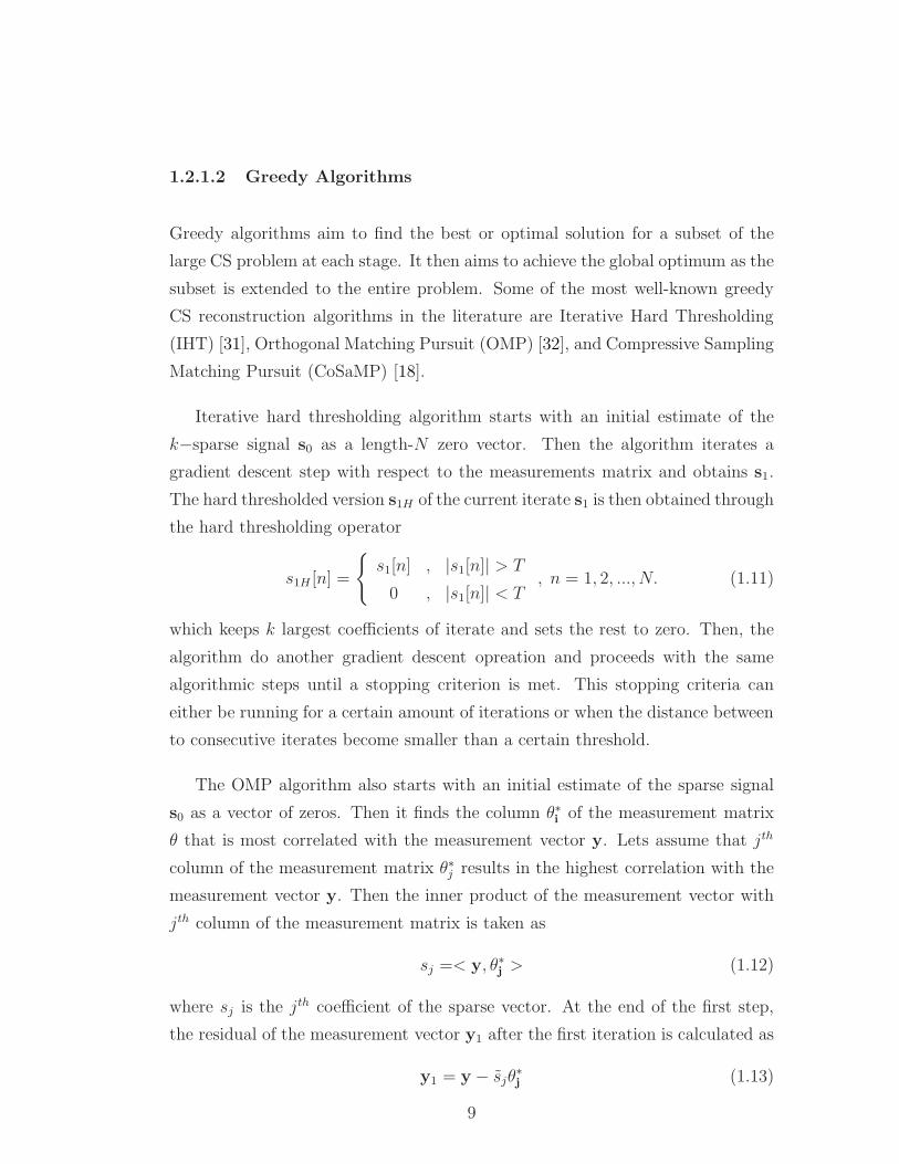
1.2.1.2 Greedy Algorithms
Greedy algorithms aim to find the best or optimal solution for a subset of the
large CS problem at each stage. It then aims to achieve the global optimum as the
subset is extended to the entire problem. Some of the most well-known greedy
CS reconstruction algorithms in the literature are Iterative Hard Thresholding
(IHT) [31], Orthogonal Matching Pursuit (OMP) [32], and Compressive Sampling
Matching Pursuit (CoSaMP) [18].
Iterative hard thresholding algorithm starts with an initial estimate of the
k−sparse signal s0 as a length-N zero vector. Then the algorithm iterates a
gradient descent step with respect to the measurements matrix and obtains s1.
The hard thresholded version s1H of the current iterate s1 is then obtained through
the hard thresholding operator
s1H [n] =
s1[n] , |s1[n]| > T
0 , |s1[n]| < T, n = 1, 2, ..., N. (1.11)
which keeps k largest coefficients of iterate and sets the rest to zero. Then, the
algorithm do another gradient descent opreation and proceeds with the same
algorithmic steps until a stopping criterion is met. This stopping criteria can
either be running for a certain amount of iterations or when the distance between
to consecutive iterates become smaller than a certain threshold.
The OMP algorithm also starts with an initial estimate of the sparse signal
s0 as a vector of zeros. Then it finds the column θ∗i of the measurement matrix
θ that is most correlated with the measurement vector y. Lets assume that jth
column of the measurement matrix θ∗j results in the highest correlation with the
measurement vector y. Then the inner product of the measurement vector with
jth column of the measurement matrix is taken as
sj =< y, θ∗j > (1.12)
where sj is the jth coefficient of the sparse vector. At the end of the first step,
the residual of the measurement vector y1 after the first iteration is calculated as
y1 = y − sjθ∗j (1.13)
9
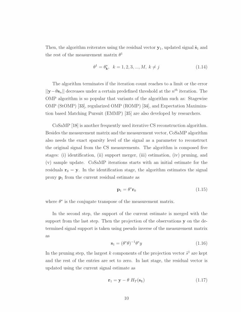
Then, the algorithm reiterates using the residual vector y1, updated signal s1 and
the rest of the measurement matrix θ1
θ1 = θ∗k, k = 1, 2, 3, ...,M, k 6= j (1.14)
The algorithm terminates if the iteration count reaches to a limit or the error
||y−θsn|| decreases under a certain predefined threshold at the nth iteration. The
OMP algorithm is so popular that variants of the algorithm such as: Stagewise
OMP (StOMP) [33], regularized OMP (ROMP) [34], and Expectation Maximiza-
tion based Matching Pursuit (EMMP) [35] are also developed by researchers.
CoSaMP [18] is another frequently used iterative CS reconstruction algorithm.
Besides the measurement matrix and the measurement vector, CoSaMP algorithm
also needs the exact sparsity level of the signal as a parameter to reconstruct
the original signal from the CS measurements. The algorithm is composed five
stages: (i) identification, (ii) support merger, (iii) estimation, (iv) pruning, and
(v) sample update. CoSaMP iterations starts with an initial estimate for the
residuals r0 = y. In the identification stage, the algorithm estimates the signal
proxy p1 from the current residual estimate as
p1 = θ∗r0 (1.15)
where θ∗ is the conjugate transpose of the measurement matrix.
In the second step, the support of the current estimate is merged with the
support from the last step. Then the projection of the observations y on the de-
termined signal support is taken using pseudo inverse of the measurement matrix
as
s1 = (θ∗θ)−1θ∗y (1.16)
In the pruning step, the largest k components of the projection vector s1 are kept
and the rest of the entries are set to zero. In last stage, the residual vector is
updated using the current signal estimate as
r1 = y − θ HT (s1) (1.17)
10
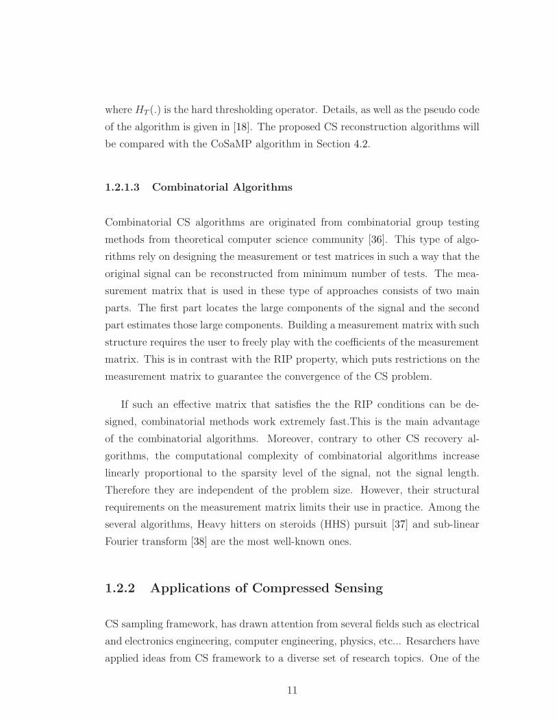
where HT (.) is the hard thresholding operator. Details, as well as the pseudo code
of the algorithm is given in [18]. The proposed CS reconstruction algorithms will
be compared with the CoSaMP algorithm in Section 4.2.
1.2.1.3 Combinatorial Algorithms
Combinatorial CS algorithms are originated from combinatorial group testing
methods from theoretical computer science community [36]. This type of algo-
rithms rely on designing the measurement or test matrices in such a way that the
original signal can be reconstructed from minimum number of tests. The mea-
surement matrix that is used in these type of approaches consists of two main
parts. The first part locates the large components of the signal and the second
part estimates those large components. Building a measurement matrix with such
structure requires the user to freely play with the coefficients of the measurement
matrix. This is in contrast with the RIP property, which puts restrictions on the
measurement matrix to guarantee the convergence of the CS problem.
If such an effective matrix that satisfies the the RIP conditions can be de-
signed, combinatorial methods work extremely fast.This is the main advantage
of the combinatorial algorithms. Moreover, contrary to other CS recovery al-
gorithms, the computational complexity of combinatorial algorithms increase
linearly proportional to the sparsity level of the signal, not the signal length.
Therefore they are independent of the problem size. However, their structural
requirements on the measurement matrix limits their use in practice. Among the
several algorithms, Heavy hitters on steroids (HHS) pursuit [37] and sub-linear
Fourier transform [38] are the most well-known ones.
1.2.2 Applications of Compressed Sensing
CS sampling framework, has drawn attention from several fields such as electrical
and electronics engineering, computer engineering, physics, etc... Resarchers have
applied ideas from CS framework to a diverse set of research topics. One of the
11
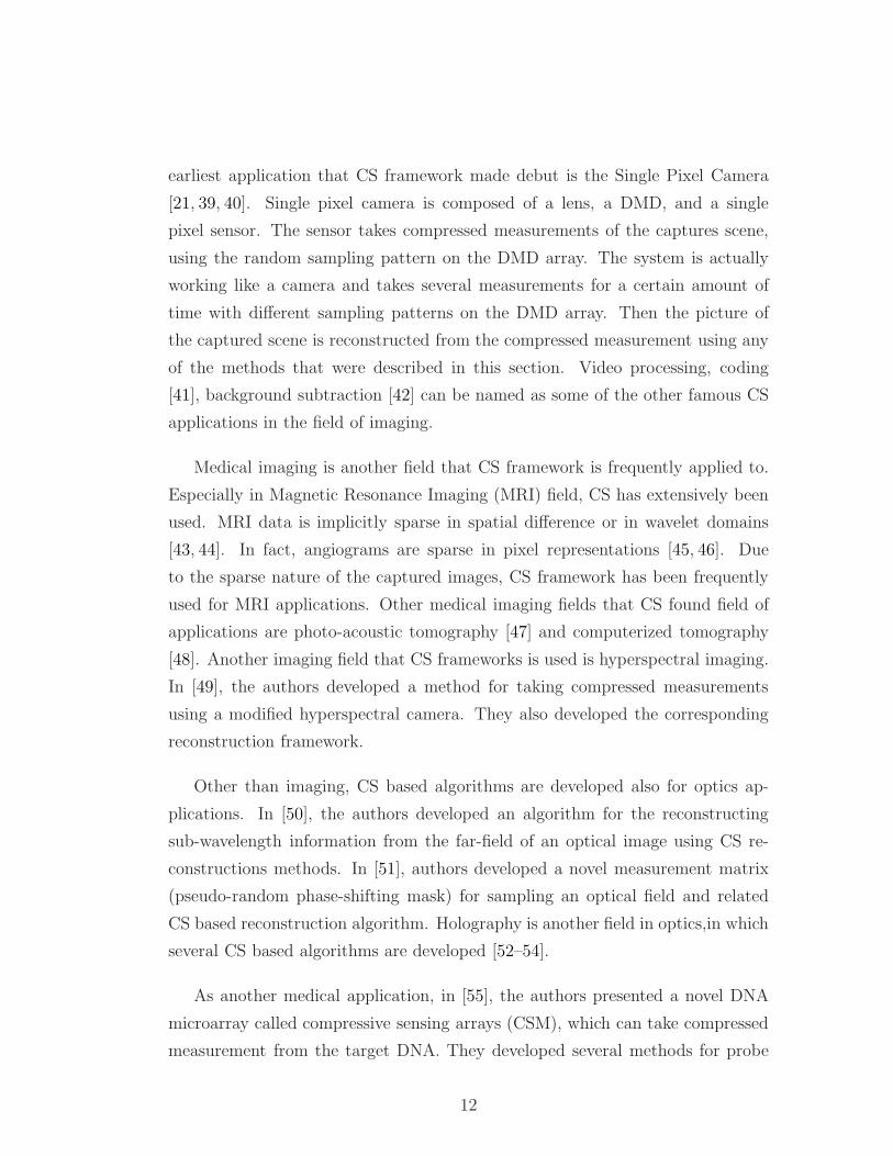
earliest application that CS framework made debut is the Single Pixel Camera
[21, 39, 40]. Single pixel camera is composed of a lens, a DMD, and a single
pixel sensor. The sensor takes compressed measurements of the captures scene,
using the random sampling pattern on the DMD array. The system is actually
working like a camera and takes several measurements for a certain amount of
time with different sampling patterns on the DMD array. Then the picture of
the captured scene is reconstructed from the compressed measurement using any
of the methods that were described in this section. Video processing, coding
[41], background subtraction [42] can be named as some of the other famous CS
applications in the field of imaging.
Medical imaging is another field that CS framework is frequently applied to.
Especially in Magnetic Resonance Imaging (MRI) field, CS has extensively been
used. MRI data is implicitly sparse in spatial difference or in wavelet domains
[43, 44]. In fact, angiograms are sparse in pixel representations [45, 46]. Due
to the sparse nature of the captured images, CS framework has been frequently
used for MRI applications. Other medical imaging fields that CS found field of
applications are photo-acoustic tomography [47] and computerized tomography
[48]. Another imaging field that CS frameworks is used is hyperspectral imaging.
In [49], the authors developed a method for taking compressed measurements
using a modified hyperspectral camera. They also developed the corresponding
reconstruction framework.
Other than imaging, CS based algorithms are developed also for optics ap-
plications. In [50], the authors developed an algorithm for the reconstructing
sub-wavelength information from the far-field of an optical image using CS re-
constructions methods. In [51], authors developed a novel measurement matrix
(pseudo-random phase-shifting mask) for sampling an optical field and related
CS based reconstruction algorithm. Holography is another field in optics,in which
several CS based algorithms are developed [52–54].
As another medical application, in [55], the authors presented a novel DNA
microarray called compressive sensing arrays (CSM), which can take compressed
measurement from the target DNA. They developed several methods for probe
12
design and CS recovery, based on the new measuring procedure that they devel-
oped.
Audio coding [56], Radar signal processing [57–59], Remote Sensing [60, 61],
Communications [62–64], and Physics [65,66] are some of the other research fields
that CS framework found application ares.
1.3 Total Variational Methods in Signal Pro-
cessing
The ℓp norm based regularized optimization problems take the signal as a whole
and uses the ℓp−norm based energy of the signal of interest as the cost metric.
However, most of the signals that are addressed in signal processing applications
are low-pass in nature, which means that the neighboring samples are highly
correlated with each other in general. Instead of considering the p−norm energy
of the signal samples, the TV norm considers the ℓ1 energy of the derivatives
around each sample. So, it uses the relation between the samples rather than
considering them individually. In this way, the TV norm based solutions preserve
the edges and boundaries in an image more accurately, and result in sharper
image reconstruction results. Therefore, the TV norm is more appropriate for
image processing applications [67, 68].
Total Variation (TV) functional was introduced to signal and image processing
problems by Rudin et al. in 1990’s [3,16,69–74]. For a 1-D signal x of length N ,
the TV of x is defined as,
||x||TV =
N−1∑
n=1
√
(x[n]− x[n + 1])2. (1.18)
or in N-Dimension,
||I||TV =
∫
Ω
|I|dI (1.19)
where I is an N-dimensional signal, is the gradient operator and Ω ⊆ RN is
the set of the samples of the signal. TV functional is utilized by several purposes
13
in the signal, and image processing literature. In the forthcoming subsections of
the thesis, only the ones that are related to compressive sensing, and denoising
applications are covered.
1.3.1 The Total Variation based Denoising
In this section, signal denoising problems in literature and their formulations are
reviewed. Formulations regarding the two-dimensional case (e.g. image denois-
ing) are used through the review, however extending the ideas to RN is straight-
forward. Let the observed signal y be a corrupted version of the original signal
x by some noise u as follows
yi,j = xi,j + ui,j. (1.20)
where [i, j] ∈ Ω, and yi,j, xj,j, uj,j are the pixels at the [i, j]th location of the
observed, original, and noise signals respectively. The aim of the denoising al-
gorithms are to estimate the original signal x from the noisy observations with
highest possible SNR. The initial attempts to achieve variational denoising in-
volves least squares ℓ2 fit, because it leads to linear equations [75–77]. These
type of methods try to solve the following minimization problem
min
∫
Ω
(d2x
di2+d2x
dj2)2
subject to
∫
Ω
y =
∫
Ω
x and
∫
Ω
(x− y)2 = σ2.
(1.21)
where x is the estimated image, and d2xdi2
+ d2xdj2
are the second derivatives in
horizontal and vertical directions of the image respectively. The system given
in (1.21) is easy to solve using numerical linear algebraic methods. However the
results are not satisfactory [16].
Using the ℓ1 norm based regularizations in (1.21) is avoided because they
can not be handled by purely algebraic frameworks [16]. However, when the
solutions of the two norms are compared, the ℓ1 norm based estimations are
visually much better than the ℓ2 norms based approximations [69]. In [67], the
14
authors introduced the concept of shock filters to the image denoising literature.
In [67], the shock filtered version of an image ISF is defined as follows
ISF = −(I)F (2(I)) (1.22)
where F is a function that satisfies F (0) = 0, sign(s)F (s) ≥ 0. The shock filter
is iteratively applied to an image as
In+1 = In − InSF (1.23)
where In and In+1 are the image after nth and n + 1st iterations. The authors
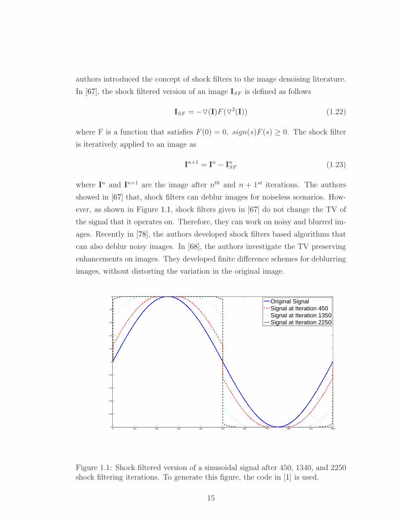
showed in [67] that, shock filters can deblur images for noiseless scenarios. How-
ever, as shown in Figure 1.1, shock filters given in [67] do not change the TV of
the signal that it operates on. Therefore, they can work on noisy and blurred im-
ages. Recently in [78], the authors developed shock filters based algorithms that
can also deblur noisy images. In [68], the authors investigate the TV preserving
enhancements on images. They developed finite difference schemes for deblurring
images, without distorting the variation in the original image.
0 100 200 300 400 500 600 700 800 900 1000−1
−0.8
−0.6
−0.4
−0.2
0
0.2
0.4
0.6
0.8
1
Original SignalSignal at Iteration 450Signal at Iteration 1350Signal at Iteration 2250
Figure 1.1: Shock filtered version of a sinusoidal signal after 450, 1340, and 2250shock filtering iterations. To generate this figure, the code in [1] is used.
15
In [16], a TV constrained minimization algorithm for image denoising is pro-
posed. This article is one of the first article that introduced the TV functional to
the signal processing society. The algorithm solves the denoising problem through
the following constrained minimization formulation
min
∫
Ω
√
(xi+1,j − xi,j)2 + (xi,j+1 − xi,j)2 = ||x||TV
subject to
∫
Ω
y =
∫
Ω
x
∫
Ω
1
2(y− x)2 = σ2,
(1.24)
where σ > 0 is a constant, which heavily depends on noise and ||x||TV is the TV
norm. The authors used Euler-Lagrange method to solve (1.24).
Another formulation for the image denoising problem is proposed by Cham-
bolle in [19] as follows
minx
||x||TV
subject to ||y − x|| ≤ ε.(1.25)
or in Lagrangian formulation
minx
||y− x||2 + λ||x||TV (1.26)
where ε is the error tolerance, and λ is the Lagrange multiplier. For each ε
parameter in (1.25), there exists a conjugate λ parameter in (1.26), using which
the solution of both formulations attain the same results. It is important to note
that both (1.25), and (1.26) try to bound the variation between the pixels on
the entire image. Therefore, some of the high-frequency details in the image may
be over-smoothed or some the noise at low-frequency regions cannot be cleaned
effectively.
In the Section 5.1 of this thesis, the formulation of Chambolle’s image denois-
ing algorithm [19] is revisited and a locally adaptive version of the this algorithm
is presented.
16
1.3.2 The TV based Compressed Sensing
Most of the CS reconstruction algorithms in literature use the ℓp norm based
regularization schemes where p ∈ [0, 1]. A brief review of such algorithms was
given in Section 1.2. However, as mentioned in Section 1.3, the TV norm is more
appropriate for image processing applications [67, 68]. The reason why the TV
norm is more appropriate for CS reconstruction is as follows. The transitions
between the pixels of a natural image are smooth, therefore the underlying gradi-
ent of an image should be sparse. As the ℓp norm based regularization results in
sparse signal reconstruction, the TV norm based regularization results in signals
with sparse gradients. This observation lead the researchers to develop new CS
reconstruction algorithms, by replacing the ℓp norm based regularization with the
TV regularization steps as follows
argminx
||x||TV
subject to θ.s = y
(1.27)
where ||x||TV is defined as in (1.24) and the relation between s and x is de-
fined as in (1.3). However, the model in (1.27) is hard to solve, since the TV
norm term is non-linear and non-differentiable. Some of the most well-known
CS reconstruction algorithms that solves the TV regularized CS problem are:
Total Variation minimization by Augmented Lagrangian and Alternating Direc-
tion Minimization (TVAL3) [79], Second Order Cone Programming (SOCP) [80],
ℓ1-Magic [11, 22, 81], and Nesterov’s Algorithm (NESTA) [82].
In [79] Li introduced TVAL3 algorithm that efficiently solves the TV mini-
mization problem in (1.27) using a combination of Augmented Lagrangian Model
and Alternating Minimization schemes. In the thesis, the author also introduces
some measurement matrices with special structures that accelerates the TVAL3
algorithm.
The SOCP algorithm given in [80] reformulated the TV minimization problem
as a second-order cone program, and solves it using interior point algorithms.
SOCP is very slow since it uses interior-point algorithm and solves a large linear
17
system at each iteration.
The ℓ1-Magic algorithm also reformulated the TV regularized CS problem
as a second-order cone problem. But instead of using interior-point method, it
uses log-barrier method to solve the problem. The ℓ1-Magic algorithm is more
efficient than SOCP in terms of computational complexity, because it solves the
linear system in an iterative manner. However, it is not effective in large-scale
problems, since it uses Newton’s method at each iteration to approximate the
intermediate solution.
The NESTA [82] algorithm is a first order method of solving Basis Pursuit
problems. The developers used Nesterov’s smoothing techniques [83] to speed up
the algorithm. It is possible to use the NESTA algorithm for the TV regulariza-
tion based CS recovery, by modifying the smooth approximation of the objective
function [79].
1.4 Motivation
Inverse problems cover a wide range of applications in signal processing. An
algorithm developed for a specific problem can easily be adapted to several other
type of inverse problems. For example TV functional is first introduced to the
signal processing literature as a method for denoising in [16]. Then it found
wide range of applications in signal reconstruction problems such as compressive
sensing. Actually compressive sensing itself is example for this situation.
CS was first introduced as an alternative sampling scheme. During recent
years, both sampling and reconstruction parts of the CS algorithms became a
subject of research. Several scientists developed new methods for constructing
more efficient measurement matrices for finding more effective ways of taking
compressed measurements, whereas some other scientists developed new recon-
struction methods. Moreover, the efforts to apply the CS framework to different
applications can not be underestimated.
18
Besides developing novel tools, researchers also took several other algorithms
and methods from literature and adapted/applied them to inverse problems. TV
functional and interval convex programming are two of the several algorithm of
this kind. Especially from optimization literature countlessly many algorithms
are migrated to the signal processing field and used succesfully.
In this thesis, our motivation is to develop novel methods that can be used
in several different type of inverse problems. In that sense, our aim is not only
developing a specific algorithm but also a generic tool that can be widely used.
Inspired from Bregman’s D-Projection operation and related row-action methods,
two new tools are developed for sparse signal processing applications. First the
D-Projection concept is integrated with a convex cost functional called modified
entropy functional, which is a shifted and even-symmetric version of the original
entropy function. The proposed functional well estimates the ℓ1 norm; therefore,
it is well suited for obtaining sparse solutions from convex integer programming
problems. Moreover, due the convex nature of its cost function, entropic projec-
tion is suitable for row-iteration type of operations, in which smaller and indepen-
dent subproblems in the entire problem are solved individually in an iterative and
cyclic manner and yet the solution converges the solution of the large problem.
Then, the well-known TV functional based methods are improved through
a high-pass filtering based variation regularization scheme called Filtered varia-
tion (FV). FV framework enables the user to integrate various types of filtering
schemes into the signal processing problems that can be formulated as variation
regularization based optimization problems.
As mentioned earlier, the applicability of the new tools are not limited to a
specific inverse problem. In this thesis, the efficacy of the new tools are illustrated
on three different problems. However, the applicability of the proposed methods
to other signal processing examples is also possible. Starting from next chapter,
first these new tools are defined, then they are applied to three different type of
inverse problems namely as signal reconstruction, signal denoising and adaptation
and learning in multi node networks.
19
Chapter 2
ENTROPY FUNCTIONAL
AND ENTROPIC
PROJECTION
In this section, the modified entropy functional is introduced as an alternative
cost function against the ℓ1 and the ℓ0 norms, and entropic projection operator
is defined. Bregman’s D-Projection operator introduced in [13] is utilized for this
purpose. Bregman developed D-Projection, and related convex optimization algo-
rithms in 1960’s and his algorithms are widely used in many signal reconstruction
and inverse problems [3, 12, 15, 17, 70, 84–90].
The ℓp norm of a signal x ∈ RN is defined as follows
||x||p =
(
∑
i
xpi
)1
p
, i = 1...N. (2.1)
The ℓp norm is frequently used as a cost function in optimization problems such
as the ones in [4, 21, 22]. Assume that M measurements yi are taken from a
length-N signal x as
θi.s = yi for i = 1, 2, ...,M, (2.2)
where θi is the ith row of the measurement matrix θ and s is the k-sparse trans-
form domain representation of the signal x. Each equation in (2.2) represents
20
a hyperplane Hi ∈ RN , which are closed and convex sets in R
N . In many in-
verse problem, the main aim is to estimate the original signal vector x or its
transform domain representation s using the measurement vector y. If M = N
and the columns of the measurement matrix are uncorrelated (hyperplanes are
orthogonal to each other), then the solution can be found through inversion of
the measurement matrix θ.
However, in most of the signal processing applications, we either have less
number of measurements (M < N), e.g. CS, or the measurements are noisy,
e.g. denoising. In this case, the best we can do is to find the solution that lies
at the intersection of the hyperplanes or hyperslabs defined by the rows of the
measurement matrix. This problem can be converted to an optimization problem
as followsmin g(s)
subject to θi.s = yi, i = 1, 2, ...,M.(2.3)
where g(s) is the cost function, and it can be chosen as any ℓp norm. When p > 1
the ℓp norm cost function is convex. Therefore, convex optimization tools can be
utilized. However, when p ∈ [0, 1], e.g. CS problems defined in (1.5) and (1.6),
the cost function is neither convex, nor differentiable everywhere. Due to this
reason, convex optimization tool cannot be used directly.
Several researcher replaced the ℓ0 norm in (1.5) with the ℓp norm, where
p ∈ (0, 1) [91] for solving the CS problems. Even if the resulting optimization
problem is not convex, several studies in the literature have addressed these ℓp
norm based non-convex optimization problems and apply their results to the
sparse signal reconstruction example [92,93]. In this thesis, an entropy functional
based cost function is used to find approximate solutions to the inverse problems
defined in (2.3), which will lead us to the entropic projection operator.
The entropy functional
g(v) = −v log v (2.4)
has already been used to approximate the solution of ℓ1 optimization and linear
programming problems in signal and image reconstruction by Bregman [13], and
others [12, 84, 87, 89, 94]. However, the original entropy function −vlog(v) is not
21
valid for negative values of v. In signal processing applications, entries of the
signal vector may take both positive and negative values. Therefore, the entropy
function in (2.4) is modified and extended to negative real numbers as follows
ge(v) =
(
|v|+1
e
)
ln
(
|v|+1
e
)
+1
e, (2.5)
and the multi-dimensional version of (2.5) is given by
ge(v) =
N∑
i=1
(
|vi|+1
e
)
ln
(
|vi|+1
e
)
+1
e, (2.6)
where v is a length-N vector with vi as its entries and e is the base of natural
logarithm or the Euler’s number. Actually, by changing the base of the logarithm,
a family of cost functions can be defined. For any base b, the modified entropy
function can be defined as
gb(v) =
(
|v|+1
bln(b)
)
logb
(
|v|+1
bln(b)
)
+1
bln(b) ln(b), (2.7)
Through out the thesis we will use ln and log interchangeably, and if we would
like to use logarithm with another base we will write the base of the logarithm
explicitly.
The modified entropy function is a new cost function that is used as an alterna-
tive way to approximate the CS problem. In Figure 2.1, plots of the different cost
functions including the modified entropy function with base e as well as the abso-
lute value g(v) = |v| and g(v) = v2 are shown. The modified entropy functional
(2.5) is convex, and continuously differentiable, and it slowly increases compared
to g(v) = v2, because ln(v) is much smaller than v for high v values as seen in
Figure 2.1. Moreover, it well approximates ℓ1 norm, which is frequently used in
sparse signal processing applications such as compressed sensing and denoising.
Bregman provides globally convergent iterative algorithms for problems with
convex, continuous and differentiable cost functionals. His iterative reconstruc-
tion algorithm starts with an initial estimate s0 = 0 = [0, 0, ...0]T . In each step of
the iterative algorithm, successive D-projections are performed onto the hyper-
planes Hi, i = 1, 2, ...,M with respect to a cost function g(s), that are defined as
in (2.3).
22
−5 −4 −3 −2 −1 0 1 2 3 4 50
5
10
15
20
25
v
g(v
)
vv2
(|v| + 1/e)log(|v| + 1/e) + 1/e
Figure 2.1: Modified entropy functional g(v) (+), |v| () that is used in the ℓ1norm, and the Euclidean cost function v2 (−) that is used in the ℓ2 norm
.
The D-projection onto a closed and convex set is a generalized version of the
orthogonal projection onto a convex set [13]. Let so be arbitrary vector in RN .
Its’ D-projection sp onto a closed convex set C with respect to a cost functional
g(s) is defined as follows
sp = arg mins∈C
D(s, so) such that θ.s = y (2.8)
where
D(s, so) = g(s)− g(so)− < g(so), s− so) > (2.9)
and D is the distance function related with the convex cost function g(.), and
is the gradient operator. In CS problems, we haveM hyperplanes Hi : θi.s = yi
for i = 1, 2, ...,M . For each hyperplane Hi, the D-projection (2.8) is equivalent
to
g(sp) = g(so) + λθi (2.10)
θi.sp = yi (2.11)
where λ is the Lagrange multiplier. As pointed out above, the D-projection is
a generalization of the orthogonal projection. When the cost functional is the
23
Euclidean cost functional g(s) =∑
n s[n]2 the distance D(s1, s2) becomes the
ℓ2 norm of difference vector (s1 − s2), and the D-projection simply becomes the
well-known orthogonal projection onto a hyperplane.
The orthogonal projection of an arbitrary vector so = [so[1], so[2], ..., so[N ]]
onto the hyperplane Hi is given by
sp[n] = so[n] + λθi[n], n = 1, 2, ..., N (2.12)
where θi(n) is the n-th entry of the vector θi and the Lagrange multiplier λ is
given by,
λ =yi −
∑Nn=1 so[n]θi[n]
∑Nn=1 θi
2[n]. (2.13)
When the cost functional is the entropy functional g(s) =∑
n s(n) ln(s(n)), the
D-projection onto the hyperplane Hi leads to the following equations
sp[n] = so[n].e(λ.θi[n]), n = 1, 2, ..., N (2.14)
where the Lagrange multiplier λ is obtained by inserting (2.14) into the hyper-
plane equation given in (2.2); therefore, the D-projection sp must be on the
hyperplane Hi. The previous set of equations are used in signal reconstruction
from Fourier Transform samples [89] and the tomographic reconstruction prob-
lem [84]. However, the entropy functional is defined only for positive real numbers.
As mentioned earlier, the original entropy function can be extended to negative
real numbers by modifying the original entropy function as in (2.5), and (2.6).
The modified entropy functional ge(s) based version of the optimization prob-
lem given in (2.3) can be defined as
mins
ge(s),
subject to θ.s = y .(2.15)
The continuous cost functional ge(s) satisfies the following conditions,
(i) ∂ge(0)∂si
= 0, i = 1, 2, ..., N and
(ii) ge is strictly convex everywhere and continuously differentiable.
24
On the other hand, the ℓ1 norm is not a continuously differentiable function;
therefore, non-differentiable minimization techniques such as sub-gradient meth-
ods [95] should be used for solving ℓ1 based optimization problems. On the other
hand, the ℓ1 norm can be well approximated by the modified entropy functional
as shown in Figure 2.1. Another way of approximating the ℓ1 penalty function
using an entropic functional is available in [96].
To obtain the D-projection of so onto a hyperplane Hi with respect to the en-
tropic cost functional (2.6), we need to minimize the generalized distance D(s, so)
between s0 and the hyperplane Hi:
D(s, so) = ge(s)− ge(so)− < ge(so), s− so > (2.16)
with the condition that θis = yi. Using (2.10), entries of the projection vector sp
can be obtained as follows
sgn(sp(n)).
[
ln(|sp(n)|+1
e)
]
= sgn(so(n)).
[
ln(|so(n)|+1
e)
]
+ λθi[n], n = 1, . . . , N
(2.17)
where λ is the Lagrange multiplier, which can be obtained from θis = yi. The
D-projection vector sp satisfies the set of equations (2.17), and the hyperplane
equation Hi : θi.s = yi.
In Section 4.2, the entropic projection operator based iterative algorithm is
utilized in CS reconstruction problem. First the ℓ1 norm in (1.6) is replaced
by the modified entropy function based norm. Using a convex function such
as the modified entropy function, enables us to solve CS problem using the D-
projection based iterative algorithms. The CS problem can be divided into M
subproblems defined by the rows of the measurement matrix as given in (2.3).
Interval convex programming techniques enables us to solve the large CS problem
by solving the subproblems using the row-iteration methods [12]. The details, as
well as numerical results of the modified entropy functional based iterative CS
reconstruction method are presented in Section 4.2.
In Chapter 6, an entropic projection based adaptive filtering algorithm for
multi-node networks is presented. The multi-node network estimation problem
defined in [4] is composed of two main parts namely as; adaptation and combina-
tion. Typically ℓ2 cost function based projection (orthogonal projection) operator
25
is used in the adaptation stage of this algorithm. In this thesis, the adaptation
stage is replaced with the entropy projection. As the modified entropy functional
estimates the ℓ1 norm, it results in sparse projections. Therefore, the resulting
projection is more robust than the orthogonal projection against heavy-tailed
noise such as ε-contaminated Gaussian noise. In Section 6.2, details of the pro-
posed algorithm as well as experimental results are presented. In Section 6.3, this
time the combination stage is replaced by a TV or FV based scheme. The new
scheme uses high-pass filtering based constraints while combining the information
from neighboring nodes. It is also possible to use the new combination scheme
together with new adaptation scheme introduced in Section 6.2. The proposed
adaptation and combination constraints are closed and convex sets, therefore, the
new diffusion adaptation algorithm can be solved in an iterative manner. The
details of the new diffusion adaptation algorithm as well as the simulations re-
sults with different node topologies under white Gaussian and ε-contaminated
Gaussian noise models are given in Section 6.3.
26
Chapter 3
FILTERED VARIATION
Total Variation (TV) based solutions are quite popular for inverse problems such
as denoising and signal reconstruction [3, 16, 69, 71–74, 97]. In discrete TV func-
tional, the difference between neighboring samples are computed and the ℓ1 or
ℓ2-norm of the difference vector is minimized. Hence, the TV method inherently
assumes that the signal (or image) is a low-pass signal and tries to minimize
the high-pass energy. Instead of computing just the one-neighborhood difference
between the samples, it can be possible to filter the signal using an appropriate
high-pass filter and minimize the ℓ1 or ℓ2 energy of the output signal. Further-
more, it is also possible to use diagonal or even custom designed directional high-
pass filters in image and video processing applications according to the needs of
the user or the characteristics of the signal.
As pointed out in Chapter 1, for a 1-D signal x of length N, the discretized
TV functional of x is defined as,
||x||TV =N∑
n=1
√
(x[n]− x[n + 1])2 (3.1)
where a discrete-gradient of the signal is the key component of the TV functional.
We note that the discrete gradient operation v[n] = x[n] − x[n + 1] in (3.1) is
a rough high-pass filtered version of x. This filter is the high-pass filter used in
Haar wavelet transform. Therefore, the relation between the signals x and v can
27
be represented via convolution denoted by the operator ∗ as follows:
v[n] = h[n] ∗ x[n] (3.2)
where h[n] = −1, 1 is the impulse response of the Haar high-pass filter. In
the DFT domain the same relationship can be represented by a multiplication
operation as follows:
V [k] = H [k]X [k], k = 1, 2, ..., N. (3.3)
provided that the DFT size N is larger than the length of convolution.
In (3.3), X [k], H [k], V [k] are the N -point DFT of the desired signal x[n],
high-pass filter h[n] and the output v[n], respectively. The TV cost function is
equivalent to filtering the signal with a Haar high-pass filter and computing the ℓ1
or ℓ2 energy of the filtered output signal corresponding to anisotropic or isotropic
cases, respectively.
The Haar filter has an ideal normalized angular cut-off frequency of π2. It
is possible to apply other high-pass filters and compute the output energy or it
is possible to use the Parseval’s relation and other Fourier domain relations to
impose sparsity conditions on the desired signal. It is well-known [98] that:
√
∑
n
|v[n]|2 =
√
∑
k
1
N|V [k]|2 ≤ max
k|V [k]| ≤
∑
n
|v[n]| . (3.4)
for an arbitrary discrete-time signal v[n]. In Section 3.1, based on the above rela-
tions, both time (space) and frequency domain FV constraints, which correspond
to closed and convex sets for the CS problem are defined.
FV framework has two major advantages over the TV framework. First of all,
if the user has prior knowledge about the frequency content of the signal, it be-
comes possible to design custom filters for that specific band. In some application
areas such as biomedical, satellite, forensics etc . . . image processing applications,
a pool of similar images exists. From this pool, one can find a model of the high
frequency information or, more generally, the structure of the signal. Using this
information, one can design custom FV constraints appropriate for the structure
of the signal. For example, if a set of images contain specific texture character-
istics, e.g.the fingerprint image in Figure 3.1, FV constraints that preserve this
28
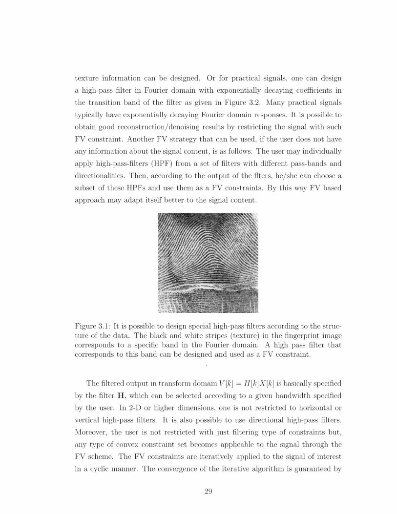
texture information can be designed. Or for practical signals, one can design
a high-pass filter in Fourier domain with exponentially decaying coefficients in
the transition band of the filter as given in Figure 3.2. Many practical signals
typically have exponentially decaying Fourier domain responses. It is possible to
obtain good reconstruction/denoising results by restricting the signal with such
FV constraint. Another FV strategy that can be used, if the user does not have
any information about the signal content, is as follows. The user may individually
apply high-pass-filters (HPF) from a set of filters with different pass-bands and
directionalities. Then, according to the output of the flters, he/she can choose a
subset of these HPFs and use them as a FV constraints. By this way FV based
approach may adapt itself better to the signal content.
Figure 3.1: It is possible to design special high-pass filters according to the struc-ture of the data. The black and white stripes (texture) in the fingerprint imagecorresponds to a specific band in the Fourier domain. A high pass filter thatcorresponds to this band can be designed and used as a FV constraint.
.
The filtered output in transform domain V [k] = H [k]X [k] is basically specified
by the filter H, which can be selected according to a given bandwidth specified
by the user. In 2-D or higher dimensions, one is not restricted to horizontal or
vertical high-pass filters. It is also possible to use directional high-pass filters.
Moreover, the user is not restricted with just filtering type of constraints but,
any type of convex constraint set becomes applicable to the signal through the
FV scheme. The FV constraints are iteratively applied to the signal of interest
in a cyclic manner. The convergence of the iterative algorithm is guaranteed by
29
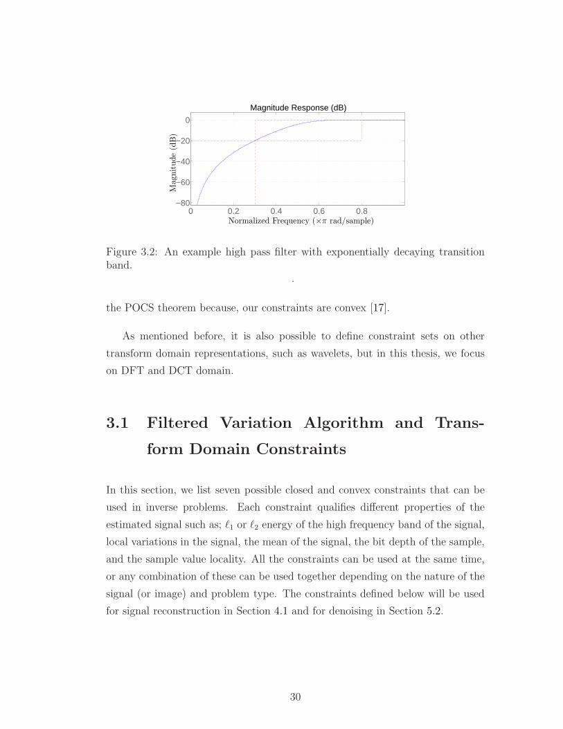
0 0.2 0.4 0.6 0.8−80
−60
−40
−20
0
Normalized Frequency (×π rad/sample)
Mag
nit
ude
(dB
)
Magnitude Response (dB)
Figure 3.2: An example high pass filter with exponentially decaying transitionband.
.
the POCS theorem because, our constraints are convex [17].
As mentioned before, it is also possible to define constraint sets on other
transform domain representations, such as wavelets, but in this thesis, we focus
on DFT and DCT domain.
3.1 Filtered Variation Algorithm and Trans-
form Domain Constraints
In this section, we list seven possible closed and convex constraints that can be
used in inverse problems. Each constraint qualifies different properties of the
estimated signal such as; ℓ1 or ℓ2 energy of the high frequency band of the signal,
local variations in the signal, the mean of the signal, the bit depth of the sample,
and the sample value locality. All the constraints can be used at the same time,
or any combination of these can be used together depending on the nature of the
signal (or image) and problem type. The constraints defined below will be used
for signal reconstruction in Section 4.1 and for denoising in Section 5.2.
30
3.1.1 Constraint-I: ℓ1 FV Bound
The first constraint is based on the ℓ1 energy of high frequency coefficients
C1 =
x :N−1∑
k=0
|H [k]X [k]| ≤ ε1
. (3.5)
It is possible to perform orthogonal projections onto this set in Discrete Time
domain as described in [87]. Since, the DFT is a complex transform, it is easier
to work with a real transform such as DCT or DHT. In this case the boundary
hyperplanes of the region specified by the constraint set are real. The projection
operation is essentially equivalent to making orthogonal projections onto hyper-
planes forming the boundary, and it is similar to projection onto an ℓ1 ball but
it is on the transform domain and only high-frequency coefficients are updated.
Since we perform projections onto an ℓ1 ball type region, the solution turns out
to be sparse.
3.1.2 Constraint-II: Time and Space Domain Local Vari-
ational Bounds
The second constraint is based on the change in intensity between the consecutive
samples of a signal (pixels of the image). In real-life, there is strong correlations
between the samples of discrete-time signals (or images), and there is very little
correlation between different parts of the signals (or images). Therefore, it is
possible to remove the summation operator in the TV or the FV and consider
regional TV or FV constraints on the signal. This leads to a high-pass constraint
set for each sample of the signal (or pixel of the image)
C2,n =
x :
∣
∣
∣
∣
∣
l∑
i=−l
h[i]x[n − i]
∣
∣
∣
∣
∣
≤ P
, (3.6)
where h[i] is a high-pass filter with support length 2l+ 1 and P is a user defined
bound. Selecting the P value, effects the smoothness level of the target signal
31
significantly. Projection onto hyperslabs C2,n do not correspond to low-pass fil-
tering, because projections are essentially non-linear operations. If the current
iterate does not satisfy the bound, it is projected onto the hyperslab given in
(3.6).
If the user does not have a clear knowledge about the signal content, a very
large bound (P = 128) for the high-pass filter h = −14, 12, −1
4 is selected to avoid
distorting the high frequency parts of the signal. When there is an impulse within
the analysis window of the filter, the filter output will be high and the samples
within that window are modified by the projection. For example, the C2,n family
of sets turn out to be useful for Laplacian noise. In image processing applications,
it is also possible to apply filters in vertical and diagonal directions depending of
the nature of the original image.
3.1.3 Constraint-III: Bound on High Frequency Energy
The following anisotropic constraint on high-frequency energy of the signal x is
a closed and convex set:
C3a =
x :
N−k0∑
k=k0
|X [k]|2 ≤ ε3a
(3.7)
where ε3a is an upper bound. This corresponds to filtering the signal x with a
high-pass filter whose cut-off frequency index is k0 in the DFT domain
H [k] =
0, for k < k0 or k > N − k0
1, for k0 ≤ k ≤ N − k0(3.8)
where N is the size of the DFT. Although this filter suffers from the Gibbs phe-
nomenon in time-domain, it is possible to use it in signal processing applications
such as denoising. The index k0 is equal to N4for the normalized angular cut-off
frequency of π2, but any 0 < k0 <
N2can be selected for a desired smoothness level.
The set given in Eq. (3.7) is a convex set and it is easy to perform orthogonal
projections onto this set. Let so[n] be an arbitrary signal and S0[k] be its DFT.
32
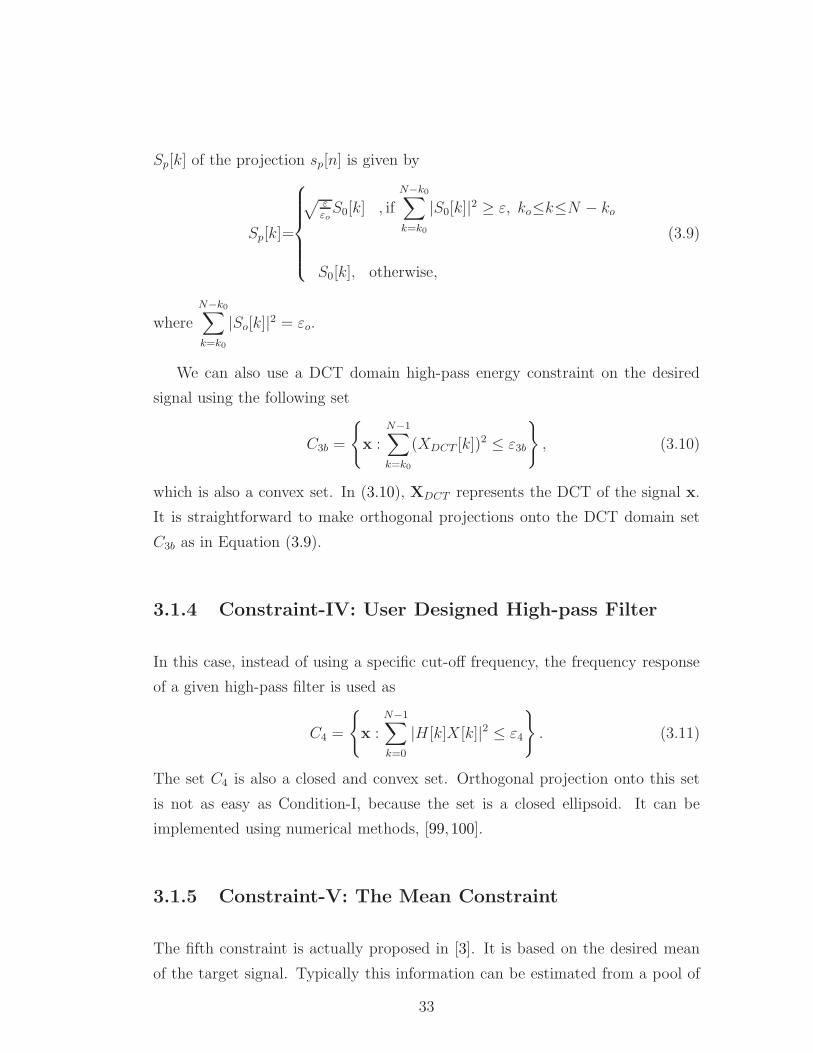
Sp[k] of the projection sp[n] is given by
Sp[k]=
√
εεoS0[k] , if
N−k0∑
k=k0
|S0[k]|2 ≥ ε, ko≤k≤N − ko
S0[k], otherwise,
(3.9)
where
N−k0∑
k=k0
|So[k]|2 = εo.
We can also use a DCT domain high-pass energy constraint on the desired
signal using the following set
C3b =
x :N−1∑
k=k0
(XDCT [k])2 ≤ ε3b
, (3.10)
which is also a convex set. In (3.10), XDCT represents the DCT of the signal x.
It is straightforward to make orthogonal projections onto the DCT domain set
C3b as in Equation (3.9).
3.1.4 Constraint-IV: User Designed High-pass Filter
In this case, instead of using a specific cut-off frequency, the frequency response
of a given high-pass filter is used as
C4 =
x :
N−1∑
k=0
|H [k]X [k]|2 ≤ ε4
. (3.11)
The set C4 is also a closed and convex set. Orthogonal projection onto this set
is not as easy as Condition-I, because the set is a closed ellipsoid. It can be
implemented using numerical methods, [99, 100].
3.1.5 Constraint-V: The Mean Constraint
The fifth constraint is actually proposed in [3]. It is based on the desired mean
of the target signal. Typically this information can be estimated from a pool of
33
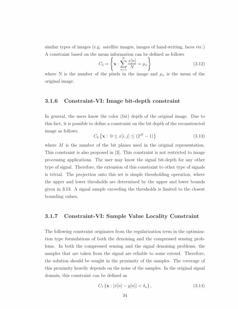
similar types of images (e.g. satellite images, images of hand-writing, faces etc.)
A constraint based on the mean information can be defined as follows
C5 =
x :
N∑
n=1
x[n]
N= µx
(3.12)
where N is the number of the pixels in the image and µx is the mean of the
original image.
3.1.6 Constraint-VI: Image bit-depth constraint
In general, the users know the color (bit) depth of the original image. Due to
this fact, it is possible to define a constraint on the bit depth of the reconstructed
image as follows:C6
x : 0 ≤ x[i, j] ≤ (2M − 1)
(3.13)
where M is the number of the bit planes used in the original representation.
This constraint is also proposed in [3]. This constraint is not restricted to image
processing applications. The user may know the signal bit-depth for any other
type of signal. Therefore, the extension of this constraint to other type of signals
is trivial. The projection onto this set is simple thresholding operation, where
the upper and lower thresholds are determined by the upper and lower bounds
given in 3.13. A signal sample exceeding the thresholds is limited to the closest
bounding values.
3.1.7 Constraint-VI: Sample Value Locality Constraint
The following constraint originates from the regularization term in the optimiza-
tion type formulations of both the denoising and the compressed sensing prob-
lems. In both the compressed sensing and the signal denoising problems, the
samples that are taken from the signal are reliable to some extend. Therefore,
the solution should be sought in the proximity of the samples. The coverage of
this proximity heavily depends on the noise of the samples. In the original signal
domain, this constraint can be defined as
C7 x : |x[n]− y[n]| < δn , (3.14)
34
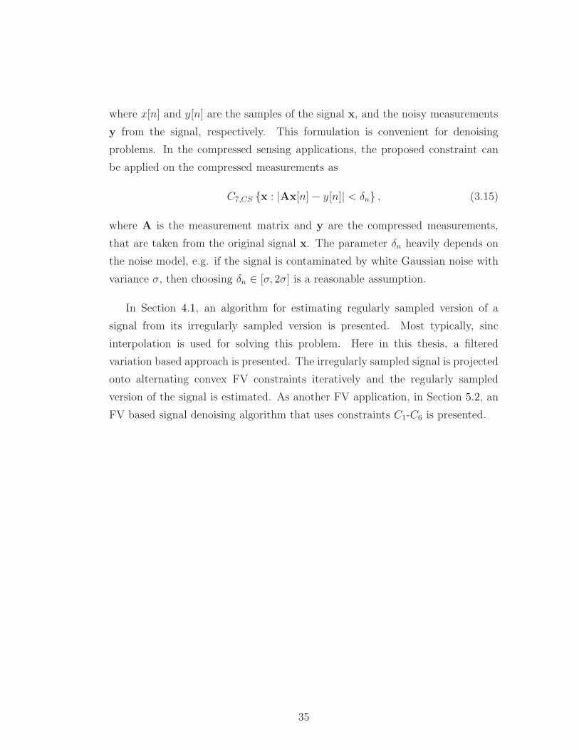
where x[n] and y[n] are the samples of the signal x, and the noisy measurements
y from the signal, respectively. This formulation is convenient for denoising
problems. In the compressed sensing applications, the proposed constraint can
be applied on the compressed measurements as
C7,CS x : |Ax[n]− y[n]| < δn , (3.15)
where A is the measurement matrix and y are the compressed measurements,
that are taken from the original signal x. The parameter δn heavily depends on
the noise model, e.g. if the signal is contaminated by white Gaussian noise with
variance σ, then choosing δn ∈ [σ, 2σ] is a reasonable assumption.
In Section 4.1, an algorithm for estimating regularly sampled version of a
signal from its irregularly sampled version is presented. Most typically, sinc
interpolation is used for solving this problem. Here in this thesis, a filtered
variation based approach is presented. The irregularly sampled signal is projected
onto alternating convex FV constraints iteratively and the regularly sampled
version of the signal is estimated. As another FV application, in Section 5.2, an
FV based signal denoising algorithm that uses constraints C1-C6 is presented.
35
Chapter 4
SIGNAL RECONSTRUCTION
The problem of reconstructing a signal from its uniform samples has been well
studied in the literature. However, there is a variety of scenarios in the literature,
where uniforms samples from a signal can not be collected. For examples, in CT
and MRI, only non-uniform frequency domain samples are available [101]. If the
average sampling rate is above twice the bandwidth of the signal, the signal can
be reconstructed from its nonuniform samples [101]. The theory on nonuniform
sampling and reconstruction was well studied by Yao and Thomas in [102], and
Yen [103]. Yen considered to spread the samples taken from a signal in an ar-
bitrarily nonuniform manner, as well as taking groups of uniform samples from
a signal in a periodic manner. In [104], Jerri presented a review of nonuniform
sampling schemes in the Literature, as well as the related reconstruction algo-
rithms.
However, none of the above papers introduces a practical reconstruction
method that can be implemented on a computer [101]. In [105], and [106] Finite-
impulse filtering (FIR) based approaches are introduced for non-periodic and pe-
riodic signals, respectively. In [107], and [108], iterative reconstruction methods
for reconstructing band-limited signals from their nonuniform samples have been
presented. In [109], a non-iterative block based method is proposed. However,
these methods are computationally complex and works only for a special set of
nonuniform samples. Recently, in [101], Margolis and Eldar derived closed form
36
algorithms for reconstructing periodic band-limited signals from nonuniform sam-
ples. Another recent research direction in nonuniform sampling is compressive
sensing.
In this chapter, two different signal reconstruction algorithms are presented.
In the first algorithm, a signal is reconstructed from its irregularly sampled version
through low-pass filtering. The proposed method works like Filtered Variation
constraints in the sense that the high frequency part of the signal spectrum is
bounded during the reconstruction process. In the second algorithm, a CS re-
construction method that utilizes entropy projection and row-action methods is
presented.
4.1 Signal Reconstruction from Irregular Sam-
ples
Let us assume that samples xc(ti), i = 0, 1, 2, ..., L − 1, of a continuous time-
domain signal xc(t) are available. These samples may not be on an uniform
sampling grid. Let us define xd[n] = xc(nTs) as the uniformly sampled version of
this signal. The sampling period Ts is assumed to be sufficiently small (below the
Nyquist period) for the signal xc(t). In a typical discrete-time filtering problem,
one do have xd[n] or its noisy version and apply a discrete-time low-pass filter
to the uniformly sampled signal xd[n]. However, xd[n] is not available in this
problem. Only nonuniformly sampled data xc(ti), i = 0, 1, 2, ...L−1 are available
in this problem.
Our goal is to low-pass filter the nonuniformly sampled data xc(ti) according
to a given cut-off frequency. One can try to interpolate available samples to
the regular grid and apply a discrete-time filter to the data. However, this will
amplify the noise because the available samples may be corrupted by noise [110].
In fact, only noisy samples are available in some problems [111]
The proposed filtering algorithm is essentially a variant of the well-known
37
Papoulis - Gerchberg interpolation method [17,70,85,112–115] and the FIR filter
design method presented in [116]. The proposed solution is based on Projections
onto Convex Sets framework (POCS). In this approach, specifications in time and
frequency domain are formulated as convex sets and a signal in the intersection
of constraint sets is defined as the solution, which can be obtained in an iterative
manner. In each iteration, the fast Fourier Transform algorithm (FFT) is used
to go back and forth between the time and frequency domains.
In many signal reconstruction and band-limited interpolation problems [17,70,
112, 114] Fourier domain information is represented using a set, which is defined
as follows
Cp = x : X(ejw) = 0 for wc ≤ w ≤ π, (4.1)
where X(ejw) is the discrete-time Fourier Transform (DTFT) of the discrete-time
signal x[n] and wc is the band-limitedness boundary or the desired normalized
angular low-pass cut-off frequency [17,112,114]. This constraint is similar to the
“C1” filtered variation constraint defined in (3.5), which uses an ideal high-pass
filter with a specific cut-off frequency and ε1 = 0. As in the filtered variation
method, this condition is imposed on a given signal xo[n] by orthogonal projec-
tion onto the set Cp. The projection xp[n] is obtained by simply imposing the
frequency domain constraint on the signals
Xp(ejw) =
Xo(ejw) for 0 ≤ w ≤ wc
0 for w > wc ,(4.2)
where Xo(ejw) and Xp(e
jw) are the DTFTs of xo and xp, respectively. Mem-
bers of the set Cp are infinite extent signals so the FFT size should be large
during the implementation of the projection onto the set Cp. However, strict
band-limitedness constraints as in Cp may induce ringing artifacts due to Gibbs
phenomenon.
The band-limitedness constraint can be relaxed by allowing the signal to have
some high-frequency components according to the tolerance parameter δs. The
use of the stop-band and the transition regions eliminates ringing artifacts due to
Gibbs phenomenon. In this respect, the proposed approach is different from the
Papoulis-Gerchberg type method, which uses strict band-limitedness condition.
38
This new constraint corresponding to the stop-band condition in Fourier do-
main is defined as follows
Cs = x : |X(ejw)| ≤ δs for ws ≤ w ≤ π (4.3)
where the stop-band frequency ws > wc. The set Cs is also a convex set [17,117]
and this condition can be imposed on iterates during iterative filtering. A member
xg of the set Cs corresponding to a given signal xo[n] can be defined as follows
Xg(ejw) =
Xo(ejw) for 0 < w < ws
Xo(ejw) for |Xo(e
jw)| ≤ δs, w ≥ ws
δsejφo(w) for |Xo(e
jw)| ≥ δs, w ≥ ws
(4.4)
where φo(w) is the phase of Xo(ejw). Clearly, Xg(e
jw) is in the set Cs. In our
implementation the set Cs plays the key role rather than the set Cp because
almost all signals that we encounter in practice are not perfect band-limited
signals. Most signals have high-frequency content. The frequency band (wc, ws)
corresponds to the transition band used in ordinary discrete-time filter design.
This relaxed version of the band-limitedness constraint in (4.4) also works like
an FV constraints in the sense that it controls the behavior of the reconstructed
signal in a specific band (e.g. high pass frequencies).
This constraint is also a variant of the set C1 defined in (3.5). Instead of
putting a bound on the ℓ1 energy of the highpass filtered version of the signal as
in C1, the Cs limits the behavior of the transform domain coefficients in the high-
pass band individually. On the other hand, it is also possible to replace Cs with
C1. As C1 corresponds to projection onto ℓ1 ball, it results in sparse projections
with few non-zero transform domain coefficients in the high-pass band. The
corresponding C1 type constraint can be defined as
C1 =
x :N−1∑
k=0
|H [k]X [k]| ≤ ε1
, (4.5)
H [k] =
1, k < kc or k > N − kc
0, kc ≤ k ≤ N − kc, (4.6)
where kc =Nwc
2πand ε1 = (N − kc)δs in our experiments. It is possible to use any
ε1 > 0 depending on the desired smoothness level of the regularly sampled signal.
39
Since, ℓ1 projection is used while implementing this constraint, it is named as ℓ1
projection based interpolation throughout the experiments.
It is also possible to use C3a defined in (3.7), which represents bound on high
frequency energy constraint defined in (3.7) to restrict the high-pass components
of the restored signal. In this case, the stop band energy parameter is choosen as
ε3a = (N − kc)δs. This constraints corrensponds finding the ℓ2 projection of the
high frequency components of the signal onto the set defined in (3.7). Therefore,
it is refered as ℓ2 based interpolation throughout the experiments.
It is also possible to replace the ℓ2 projection operation with entropic pro-
jection operator. ℓ1, and entropic projection based constraints results in sparse
reconstructions [21,36]. Therefore, they may induce ringing artifacts due to Gibbs
phenomenon. Since the ℓ2 projection based constraints, limits all the stop-band
coefficients in an evenly manner, it produces much smooth reconstructions. On
the other hand, ℓ1, and entropic projection based algorithms are more robust
against noise, since they produce sparse projections. In the experimental re-
sults section of this chapter, these claims will be illustrated through numerical
examples.
Besides the frequency domain constraints defined by sets (4.1), and (4.3),
another set of constraints should be defined in time domain, so that it would be
possible to realize the aformentioned Papoulis-Gerchberg type of iterations. As
pointed out above a sampling period, which is smaller than the Nyquist period
is used. Let’s assume that 0, Ts, 2Ts, ..., (N − 1)Ts is a dense grid covering ti, i =
0, 1, 2, ..., L − 1 and let’s also assume that all ti < ti+1 and ti ≥ 0 and tL−1 ≤
(N − 1)Ts without loss of generality.
The set describing the time-domain information is defined using the regular
sampling grid 0, Ts, 2Ts, ..., (N−1)Ts. The sample at t = ti is assumed to be close
to nTs. The upper and lower bounds that are imposed on x[n] as follows:
xc(ti)− εi ≤ x[n] ≤ xc(ti) + εi, (4.7)
and the corresponding time-domain set is defined as
Ci = x : xc(ti)− εi ≤ x[n] ≤ xc(ti) + εi, (4.8)
40
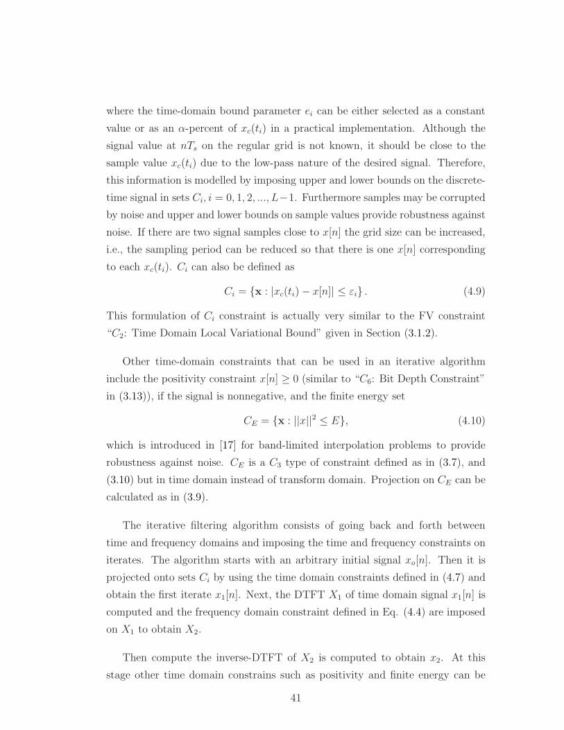
where the time-domain bound parameter ei can be either selected as a constant
value or as an α-percent of xc(ti) in a practical implementation. Although the
signal value at nTs on the regular grid is not known, it should be close to the
sample value xc(ti) due to the low-pass nature of the desired signal. Therefore,
this information is modelled by imposing upper and lower bounds on the discrete-
time signal in sets Ci, i = 0, 1, 2, ..., L−1. Furthermore samples may be corrupted
by noise and upper and lower bounds on sample values provide robustness against
noise. If there are two signal samples close to x[n] the grid size can be increased,
i.e., the sampling period can be reduced so that there is one x[n] corresponding
to each xc(ti). Ci can also be defined as
Ci = x : |xc(ti)− x[n]| ≤ εi . (4.9)
This formulation of Ci constraint is actually very similar to the FV constraint
“C2: Time Domain Local Variational Bound” given in Section (3.1.2).
Other time-domain constraints that can be used in an iterative algorithm
include the positivity constraint x[n] ≥ 0 (similar to “C6: Bit Depth Constraint”
in (3.13)), if the signal is nonnegative, and the finite energy set
CE = x : ||x||2 ≤ E, (4.10)
which is introduced in [17] for band-limited interpolation problems to provide
robustness against noise. CE is a C3 type of constraint defined as in (3.7), and
(3.10) but in time domain instead of transform domain. Projection on CE can be
calculated as in (3.9).
The iterative filtering algorithm consists of going back and forth between
time and frequency domains and imposing the time and frequency constraints on
iterates. The algorithm starts with an arbitrary initial signal xo[n]. Then it is
projected onto sets Ci by using the time domain constraints defined in (4.7) and
obtain the first iterate x1[n]. Next, the DTFT X1 of time domain signal x1[n] is
computed and the frequency domain constraint defined in Eq. (4.4) are imposed
on X1 to obtain X2.
Then compute the inverse-DTFT of X2 is computed to obtain x2. At this
stage other time domain constrains such as positivity and finite energy can be
41
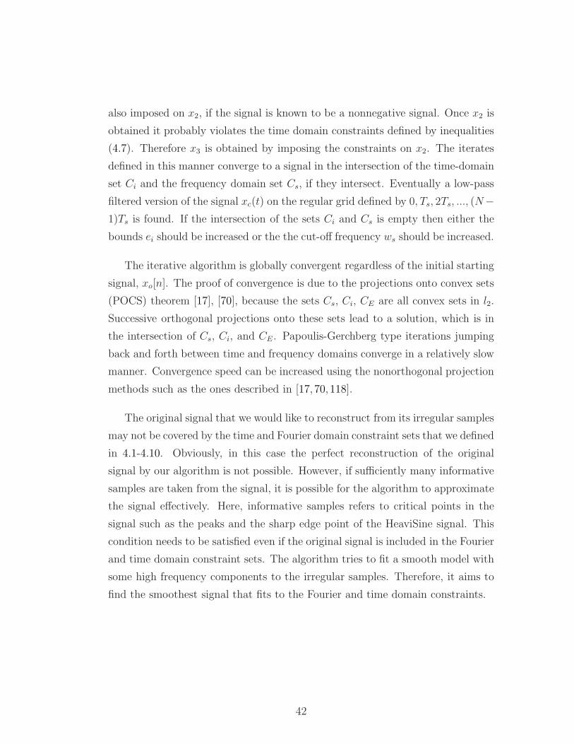
also imposed on x2, if the signal is known to be a nonnegative signal. Once x2 is
obtained it probably violates the time domain constraints defined by inequalities
(4.7). Therefore x3 is obtained by imposing the constraints on x2. The iterates
defined in this manner converge to a signal in the intersection of the time-domain
set Ci and the frequency domain set Cs, if they intersect. Eventually a low-pass
filtered version of the signal xc(t) on the regular grid defined by 0, Ts, 2Ts, ..., (N−
1)Ts is found. If the intersection of the sets Ci and Cs is empty then either the
bounds ei should be increased or the the cut-off frequency ws should be increased.
The iterative algorithm is globally convergent regardless of the initial starting
signal, xo[n]. The proof of convergence is due to the projections onto convex sets
(POCS) theorem [17], [70], because the sets Cs, Ci, CE are all convex sets in l2.
Successive orthogonal projections onto these sets lead to a solution, which is in
the intersection of Cs, Ci, and CE . Papoulis-Gerchberg type iterations jumping
back and forth between time and frequency domains converge in a relatively slow
manner. Convergence speed can be increased using the nonorthogonal projection
methods such as the ones described in [17, 70, 118].
The original signal that we would like to reconstruct from its irregular samples
may not be covered by the time and Fourier domain constraint sets that we defined
in 4.1-4.10. Obviously, in this case the perfect reconstruction of the original
signal by our algorithm is not possible. However, if sufficiently many informative
samples are taken from the signal, it is possible for the algorithm to approximate
the signal effectively. Here, informative samples refers to critical points in the
signal such as the peaks and the sharp edge point of the HeaviSine signal. This
condition needs to be satisfied even if the original signal is included in the Fourier
and time domain constraint sets. The algorithm tries to fit a smooth model with
some high frequency components to the irregular samples. Therefore, it aims to
find the smoothest signal that fits to the Fourier and time domain constraints.
42
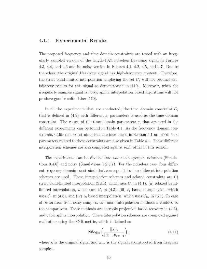
4.1.1 Experimental Results
The proposed frequency and time domain constraints are tested with an irreg-
ularly sampled version of the length-1024 noiseless Heavisine signal in Figures
4.3, 4.4, and 4.6 and its noisy version in Figures 4.1, 4.2, 4.5, and 4.7. Due to
the edges, the original Heavisine signal has high-frequency content. Therefore,
the strict band-limited interpolation employing the set Cp will not produce sat-
isfactory results for this signal as demonstrated in [110]. Moreover, when the
irregularly samples signal is noisy, spline interpolation based algorithms will not
produce good results either [110].
In all the experiments that are conducted, the time domain constraint Ci
that is defined in (4.9) with different εi parameters is used as the time domain
constraint. The values of the time domain parameters εi that are used in the
different experiments can be found in Table 4.1. As the frequency domain con-
straints, 6 different constraints that are introduced in Section 4.1 are used. The
parameters related to these constraints are also given in Table 4.1. These different
interpolation schemes are also compared against each other in this section.
The experiments can be divided into two main groups: noiseless (Simula-
tions 3,4,6) and noisy (Simulations 1,2,5,7). For the noiseless case, four differ-
ent frequency domain constraints that corresponds to four different interpolation
schemes are used. These interpolation schemes and related constraints are (i)
strict band-limited interpolation (SBL), which uses Cp in (4.1), (ii) relaxed band-
limited interpolation, which uses Cs in (4.3), (iii) ℓ1 based interpolation, which
uses C1 in (4.6), and (iv) ℓ2 based interpolation, which uses C3a in (3.7). In case
of restoration from noisy samples, two more interpolation methods are added to
the comparisons. These methods are entropic projection based recovery in (4.6),
and cubic spline interpolation. These interpolation schemes are compared against
each other using the SNR metric, which is defined as
20log10
(
||x||2||x− xrec||2
)
, (4.11)
where x is the original signal and xrec is the signal reconstructed from irregular
samples.
43
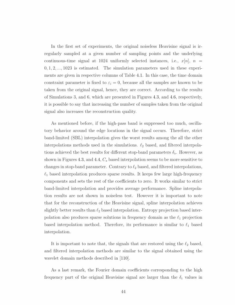
In the first set of experiments, the original noiseless Heavisine signal is ir-
regularly sampled at a given number of sampling points and the underlying
continuous-time signal at 1024 uniformly selected instances, i.e., x[n], n =
0, 1, 2, ..., 1023 is estimated. The simulation parameters used in these experi-
ments are given in respective columns of Table 4.1. In this case, the time domain
constraint parameter is fixed to εi = 0, because all the samples are known to be
taken from the original signal, hence, they are correct. According to the results
of Simulations 3, and 6, which are presented in Figures 4.3, and 4.6, respectively,
it is possible to say that increasing the number of samples taken from the original
signal also increases the reconstruction quality.
As mentioned before, if the high-pass band is suppressed too much, oscilla-
tory behavior around the edge locations in the signal occurs. Therefore, strict
band-limited (SBL) interpolation gives the worst results among the all the other
interpolations methods used in the simulations. ℓ2 based, and filtered interpola-
tions achieved the best results for different stop-band parameters δs. However, as
shown in Figures 4.3, and 4.4, Cs based interpolation seems to be more sensitive to
changes in stop-band parameter. Contrary to ℓ2 based, and filtered interpolations,
ℓ1 based interpolation produces sparse results. It keeps few large high-frequency
components and sets the rest of the coefficients to zero. It works similar to strict
band-limited interpolation and provides average performance. Spline interpola-
tion results are not shown in noiseless test. However it is important to note
that for the reconstruction of the Heavisine signal, spline interpolation achieves
slightly better results than ℓ2 based interpolation. Entropy projection based inter-
polation also produces sparse solutions in frequency domain as the ℓ1 projection
based interpolation method. Therefore, its performance is similar to ℓ1 based
interpolation.
It is important to note that, the signals that are restored using the ℓ2 based,
and filtered interpolation methods are similar to the signal obtained using the
wavelet domain methods described in [110].
As a last remark, the Fourier domain coefficients corresponding to the high
frequency part of the original Heavisine signal are larger than the δc values in
44
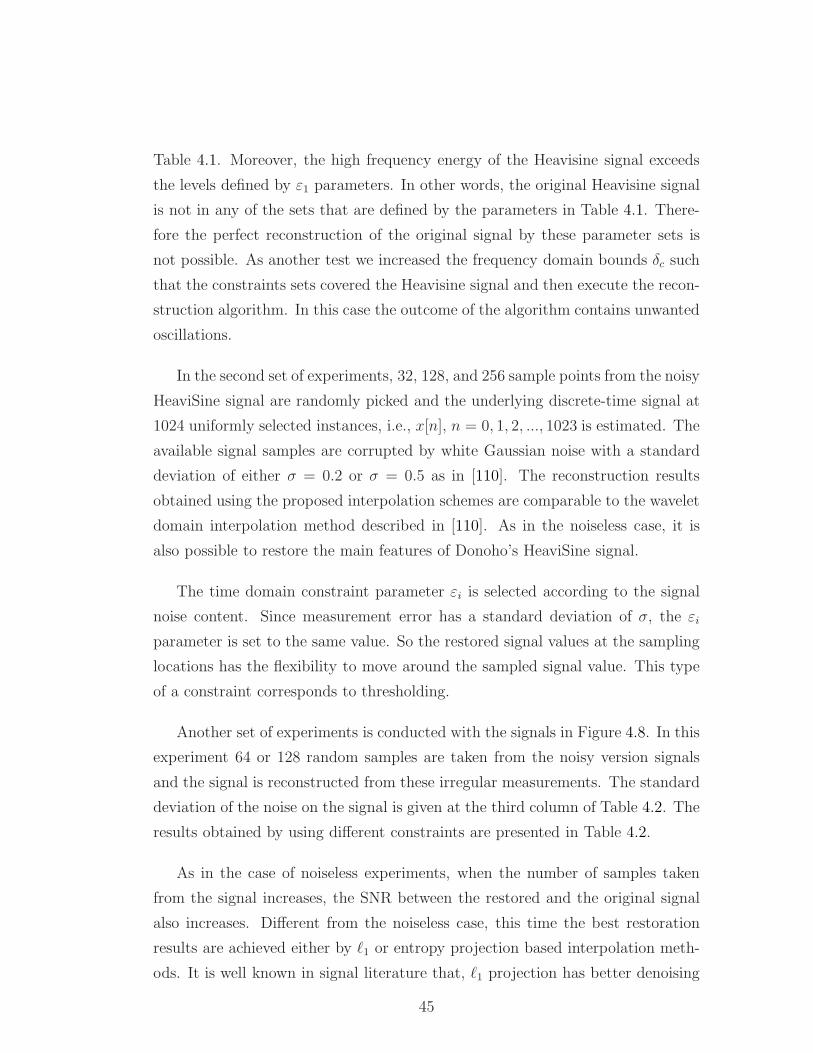
Table 4.1. Moreover, the high frequency energy of the Heavisine signal exceeds
the levels defined by ε1 parameters. In other words, the original Heavisine signal
is not in any of the sets that are defined by the parameters in Table 4.1. There-
fore the perfect reconstruction of the original signal by these parameter sets is
not possible. As another test we increased the frequency domain bounds δc such
that the constraints sets covered the Heavisine signal and then execute the recon-
struction algorithm. In this case the outcome of the algorithm contains unwanted
oscillations.
In the second set of experiments, 32, 128, and 256 sample points from the noisy
HeaviSine signal are randomly picked and the underlying discrete-time signal at
1024 uniformly selected instances, i.e., x[n], n = 0, 1, 2, ..., 1023 is estimated. The
available signal samples are corrupted by white Gaussian noise with a standard
deviation of either σ = 0.2 or σ = 0.5 as in [110]. The reconstruction results
obtained using the proposed interpolation schemes are comparable to the wavelet
domain interpolation method described in [110]. As in the noiseless case, it is
also possible to restore the main features of Donoho’s HeaviSine signal.
The time domain constraint parameter εi is selected according to the signal
noise content. Since measurement error has a standard deviation of σ, the εi
parameter is set to the same value. So the restored signal values at the sampling
locations has the flexibility to move around the sampled signal value. This type
of a constraint corresponds to thresholding.
Another set of experiments is conducted with the signals in Figure 4.8. In this
experiment 64 or 128 random samples are taken from the noisy version signals
and the signal is reconstructed from these irregular measurements. The standard
deviation of the noise on the signal is given at the third column of Table 4.2. The
results obtained by using different constraints are presented in Table 4.2.
As in the case of noiseless experiments, when the number of samples taken
from the signal increases, the SNR between the restored and the original signal
also increases. Different from the noiseless case, this time the best restoration
results are achieved either by ℓ1 or entropy projection based interpolation meth-
ods. It is well known in signal literature that, ℓ1 projection has better denoising
45
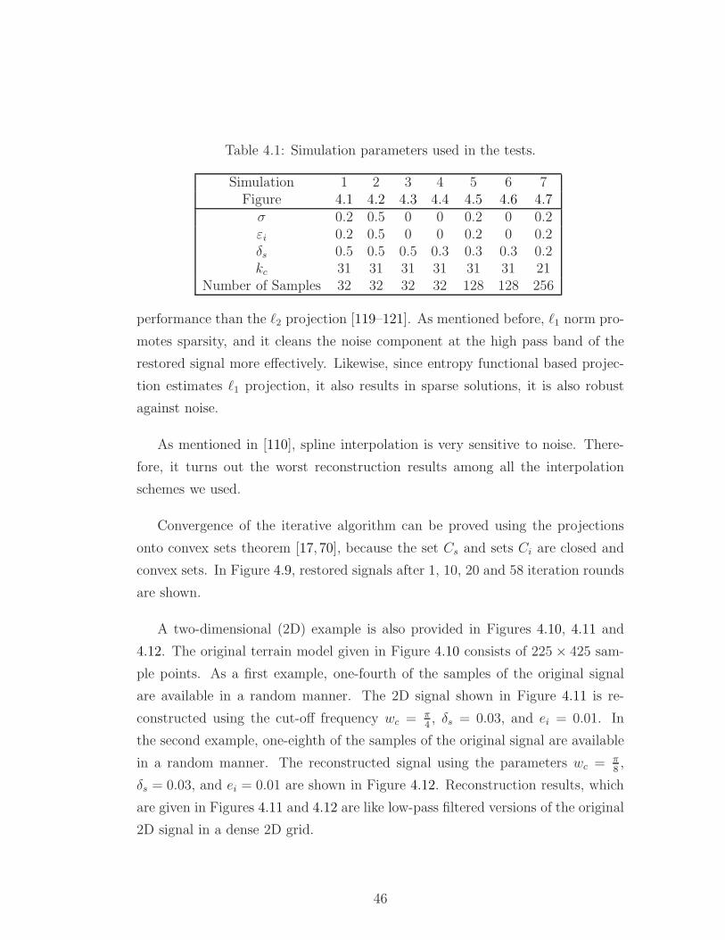
Table 4.1: Simulation parameters used in the tests.
Simulation 1 2 3 4 5 6 7Figure 4.1 4.2 4.3 4.4 4.5 4.6 4.7σ 0.2 0.5 0 0 0.2 0 0.2εi 0.2 0.5 0 0 0.2 0 0.2δs 0.5 0.5 0.5 0.3 0.3 0.3 0.2kc 31 31 31 31 31 31 21
Number of Samples 32 32 32 32 128 128 256
performance than the ℓ2 projection [119–121]. As mentioned before, ℓ1 norm pro-
motes sparsity, and it cleans the noise component at the high pass band of the
restored signal more effectively. Likewise, since entropy functional based projec-
tion estimates ℓ1 projection, it also results in sparse solutions, it is also robust
against noise.
As mentioned in [110], spline interpolation is very sensitive to noise. There-
fore, it turns out the worst reconstruction results among all the interpolation
schemes we used.
Convergence of the iterative algorithm can be proved using the projections
onto convex sets theorem [17, 70], because the set Cs and sets Ci are closed and
convex sets. In Figure 4.9, restored signals after 1, 10, 20 and 58 iteration rounds
are shown.
A two-dimensional (2D) example is also provided in Figures 4.10, 4.11 and
4.12. The original terrain model given in Figure 4.10 consists of 225 × 425 sam-
ple points. As a first example, one-fourth of the samples of the original signal
are available in a random manner. The 2D signal shown in Figure 4.11 is re-
constructed using the cut-off frequency wc = π4, δs = 0.03, and ei = 0.01. In
the second example, one-eighth of the samples of the original signal are available
in a random manner. The reconstructed signal using the parameters wc = π8,
δs = 0.03, and ei = 0.01 are shown in Figure 4.12. Reconstruction results, which
are given in Figures 4.11 and 4.12 are like low-pass filtered versions of the original
2D signal in a dense 2D grid.
46
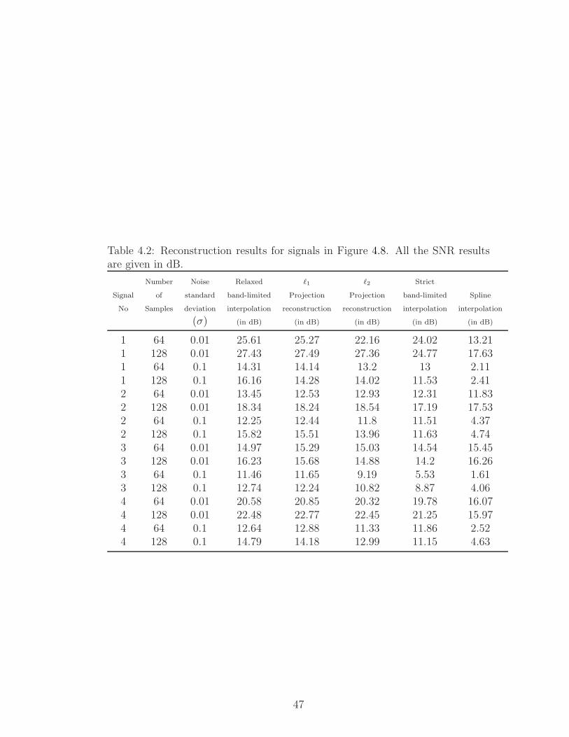
Table 4.2: Reconstruction results for signals in Figure 4.8. All the SNR resultsare given in dB.
Number Noise Relaxed ℓ1 ℓ2 Strict
Signal of standard band-limited Projection Projection band-limited Spline
No Samples deviation interpolation reconstruction reconstruction interpolation interpolation
(σ) (in dB) (in dB) (in dB) (in dB) (in dB)
1 64 0.01 25.61 25.27 22.16 24.02 13.211 128 0.01 27.43 27.49 27.36 24.77 17.631 64 0.1 14.31 14.14 13.2 13 2.111 128 0.1 16.16 14.28 14.02 11.53 2.412 64 0.01 13.45 12.53 12.93 12.31 11.832 128 0.01 18.34 18.24 18.54 17.19 17.532 64 0.1 12.25 12.44 11.8 11.51 4.372 128 0.1 15.82 15.51 13.96 11.63 4.743 64 0.01 14.97 15.29 15.03 14.54 15.453 128 0.01 16.23 15.68 14.88 14.2 16.263 64 0.1 11.46 11.65 9.19 5.53 1.613 128 0.1 12.74 12.24 10.82 8.87 4.064 64 0.01 20.58 20.85 20.32 19.78 16.074 128 0.01 22.48 22.77 22.45 21.25 15.974 64 0.1 12.64 12.88 11.33 11.86 2.524 128 0.1 14.79 14.18 12.99 11.15 4.63
47
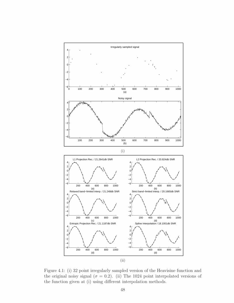
0 100 200 300 400 500 600 700 800 900 1000−6
−4
−2
0
2
4
(a)
Irregularly sampled signal
100 200 300 400 500 600 700 800 900 1000
−6
−4
−2
0
2
4
(b)
Noisy signal
(i)
200 400 600 800 1000−6
−4
−2
0
2
4L1 Projection Rec. / 21.2641db SNR
(a)200 400 600 800 1000
−6
−4
−2
0
2
4L2 Projection Rec. / 20.824db SNR
(b)
200 400 600 800 1000−6
−4
−2
0
2
4Relaxed band−limited interp. / 21.248db SNR
(c)200 400 600 800 1000
−6
−4
−2
0
2
4Strict band−limited interp. / 20.1665db SNR
(d)
200 400 600 800 1000−6
−4
−2
0
2
4Entropic Projection Rec. / 21.1187db SNR
(d)200 400 600 800 1000
−6
−4
−2
0
2
4Spline Interpolation / 18.1001db SNR
(d)
(ii)
Figure 4.1: (i) 32 point irregularly sampled version of the Heavisine function andthe original noisy signal (σ = 0.2). (ii) The 1024 point interpolated versions ofthe function given at (i) using different interpolation methods.
48
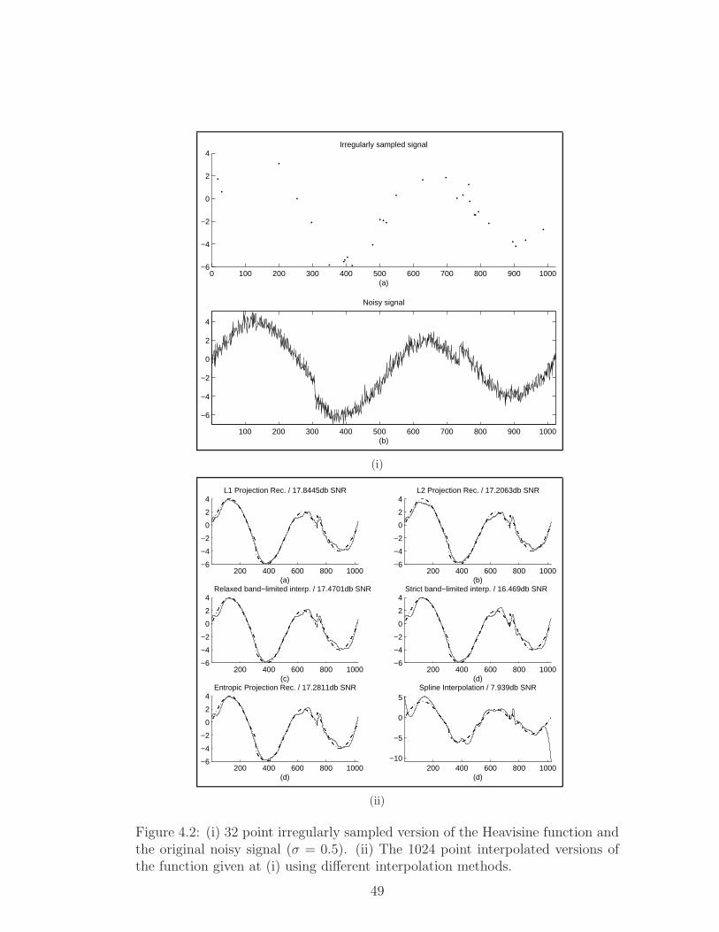
0 100 200 300 400 500 600 700 800 900 1000−6
−4
−2
0
2
4
(a)
Irregularly sampled signal
100 200 300 400 500 600 700 800 900 1000
−6
−4
−2
0
2
4
(b)
Noisy signal
(i)
200 400 600 800 1000−6
−4
−2
0
2
4L1 Projection Rec. / 17.8445db SNR
(a)200 400 600 800 1000
−6
−4
−2
0
2
4L2 Projection Rec. / 17.2063db SNR
(b)
200 400 600 800 1000−6
−4
−2
0
2
4Relaxed band−limited interp. / 17.4701db SNR
(c)200 400 600 800 1000
−6
−4
−2
0
2
4Strict band−limited interp. / 16.469db SNR
(d)
200 400 600 800 1000−6
−4
−2
0
2
4Entropic Projection Rec. / 17.2811db SNR
(d)200 400 600 800 1000
−10
−5
0
5Spline Interpolation / 7.939db SNR
(d)
(ii)
Figure 4.2: (i) 32 point irregularly sampled version of the Heavisine function andthe original noisy signal (σ = 0.5). (ii) The 1024 point interpolated versions ofthe function given at (i) using different interpolation methods.
49

0 100 200 300 400 500 600 700 800 900 1000−6
−4
−2
0
2
4
(a)
Irregularly sampled signal
100 200 300 400 500 600 700 800 900 1000−6
−4
−2
0
2
4
(b)
Original signal
(i)
200 400 600 800 1000−6
−4
−2
0
2
4L1 Projection Rec. / 21.5534db SNR
(a)200 400 600 800 1000
−6
−4
−2
0
2
4L2 Projection Rec. / 21.7335db SNR
(b)
200 400 600 800 1000−6
−4
−2
0
2
4Relaxed band−limited interp. / 21.9514db SNR
(c)200 400 600 800 1000
−6
−4
−2
0
2
4Strict band−limited interp. / 17.901db SNR
(d)
(ii)
Figure 4.3: (i) 32 point irregularly sampled version of the Heavisine functionand the original noiseless signal. (ii) The 1024 point interpolated versions of thefunction given at (i) using different interpolation methods.
50
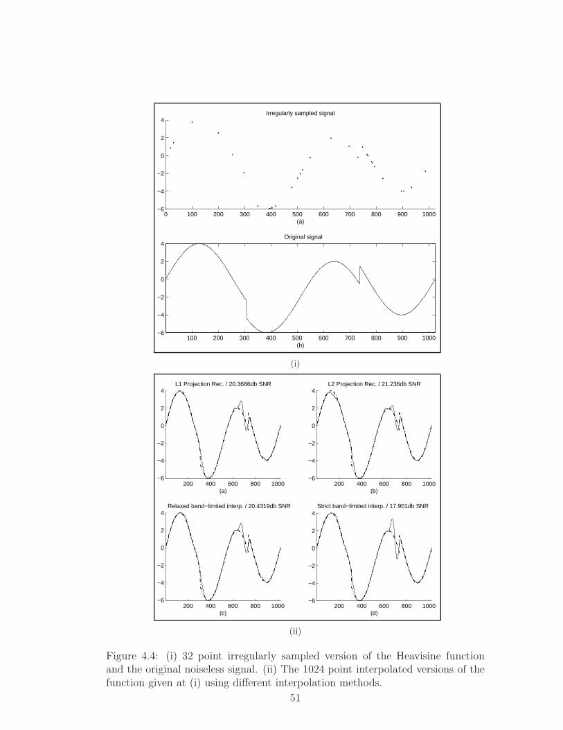
0 100 200 300 400 500 600 700 800 900 1000−6
−4
−2
0
2
4
(a)
Irregularly sampled signal
100 200 300 400 500 600 700 800 900 1000−6
−4
−2
0
2
4
(b)
Original signal
(i)
200 400 600 800 1000−6
−4
−2
0
2
4L1 Projection Rec. / 20.3686db SNR
(a)200 400 600 800 1000
−6
−4
−2
0
2
4L2 Projection Rec. / 21.236db SNR
(b)
200 400 600 800 1000−6
−4
−2
0
2
4Relaxed band−limited interp. / 20.4319db SNR
(c)200 400 600 800 1000
−6
−4
−2
0
2
4Strict band−limited interp. / 17.901db SNR
(d)
(ii)
Figure 4.4: (i) 32 point irregularly sampled version of the Heavisine functionand the original noiseless signal. (ii) The 1024 point interpolated versions of thefunction given at (i) using different interpolation methods.
51
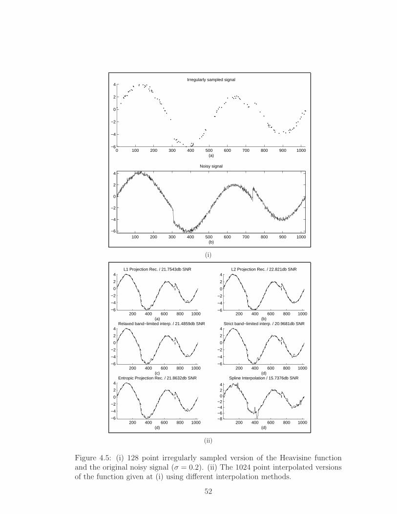
0 100 200 300 400 500 600 700 800 900 1000−6
−4
−2
0
2
4
(a)
Irregularly sampled signal
100 200 300 400 500 600 700 800 900 1000−6
−4
−2
0
2
4
(b)
Noisy signal
(i)
200 400 600 800 1000−6
−4
−2
0
2
4L1 Projection Rec. / 21.7543db SNR
(a)200 400 600 800 1000
−6
−4
−2
0
2
4L2 Projection Rec. / 22.821db SNR
(b)
200 400 600 800 1000−6
−4
−2
0
2
4Relaxed band−limited interp. / 21.4859db SNR
(c)200 400 600 800 1000
−6
−4
−2
0
2
4Strict band−limited interp. / 20.9681db SNR
(d)
200 400 600 800 1000−6
−4
−2
0
2
4Entropic Projection Rec. / 21.8632db SNR
(d)200 400 600 800 1000
−8−6−4−2
024
Spline Interpolation / 15.7376db SNR
(d)
(ii)
Figure 4.5: (i) 128 point irregularly sampled version of the Heavisine functionand the original noisy signal (σ = 0.2). (ii) The 1024 point interpolated versionsof the function given at (i) using different interpolation methods.
52
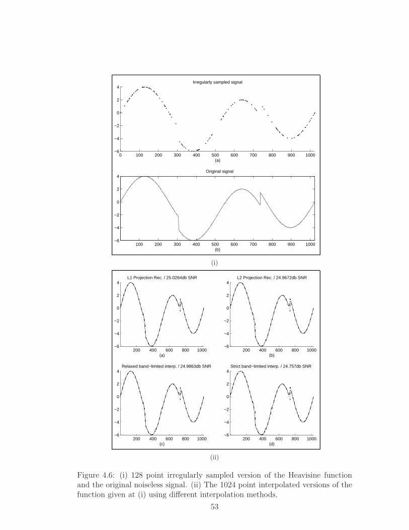
0 100 200 300 400 500 600 700 800 900 1000−6
−4
−2
0
2
4
(a)
Irregularly sampled signal
100 200 300 400 500 600 700 800 900 1000−6
−4
−2
0
2
4
(b)
Original signal
(i)
200 400 600 800 1000−6
−4
−2
0
2
4L1 Projection Rec. / 25.0264db SNR
(a)200 400 600 800 1000
−6
−4
−2
0
2
4L2 Projection Rec. / 24.9672db SNR
(b)
200 400 600 800 1000−6
−4
−2
0
2
4Relaxed band−limited interp. / 24.9863db SNR
(c)200 400 600 800 1000
−6
−4
−2
0
2
4Strict band−limited interp. / 24.757db SNR
(d)
(ii)
Figure 4.6: (i) 128 point irregularly sampled version of the Heavisine functionand the original noiseless signal. (ii) The 1024 point interpolated versions of thefunction given at (i) using different interpolation methods.
53

0 100 200 300 400 500 600 700 800 900 1000−6
−4
−2
0
2
4
(a)
Irregularly sampled signal
100 200 300 400 500 600 700 800 900 1000
−6
−4
−2
0
2
4
(b)
Noisy signal
(i)
200 400 600 800 1000−6
−4
−2
0
2
4L1 Projection Rec. / 23.5373db SNR
(a)200 400 600 800 1000
−6
−4
−2
0
2
4L2 Projection Rec. / 22.0995db SNR
(b)
200 400 600 800 1000−6
−4
−2
0
2
4Relaxed band−limited interp. / 23.2962db SNR
(c)200 400 600 800 1000
−6
−4
−2
0
2
4Strict band−limited interp. / 23.2646db SNR
(d)
200 400 600 800 1000−6
−4
−2
0
2
4Entropic Projection Rec. / 23.3612db SNR
(d)200 400 600 800 1000
−6
−4
−2
0
2
4
Spline Interpolation / 18.7433db SNR
(d)
(ii)
Figure 4.7: (i) 256 point irregularly sampled version of the Heavisine functionand the original noisy signal (σ = 0.2). (ii) The 1024 point interpolated versionsof the function given at (i) using different interpolation methods.
54
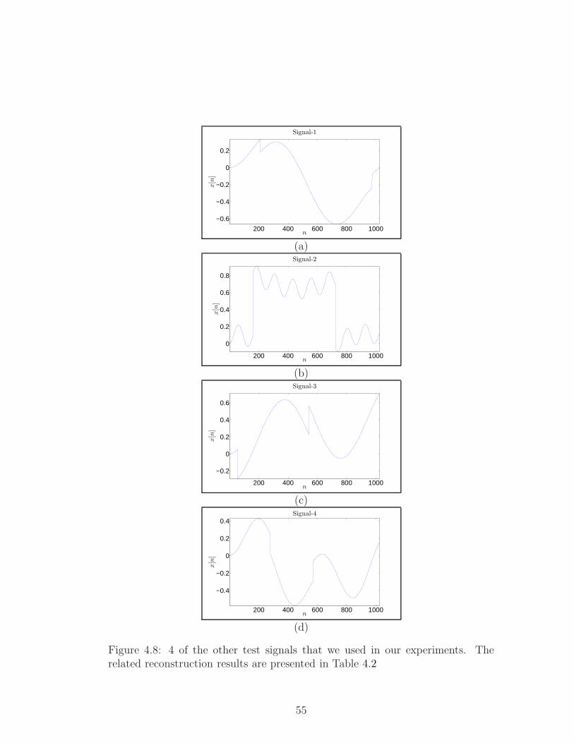
200 400 600 800 1000
−0.6
−0.4
−0.2
0
0.2
n
x[n]
Signal-1
(a)
200 400 600 800 1000
0
0.2
0.4
0.6
0.8
n
x[n]
Signal-2
(b)
200 400 600 800 1000
−0.2
0
0.2
0.4
0.6
n
x[n]
Signal-3
(c)
200 400 600 800 1000
−0.4
−0.2
0
0.2
0.4
n
x[n]
Signal-4
(d)
Figure 4.8: 4 of the other test signals that we used in our experiments. Therelated reconstruction results are presented in Table 4.2
55
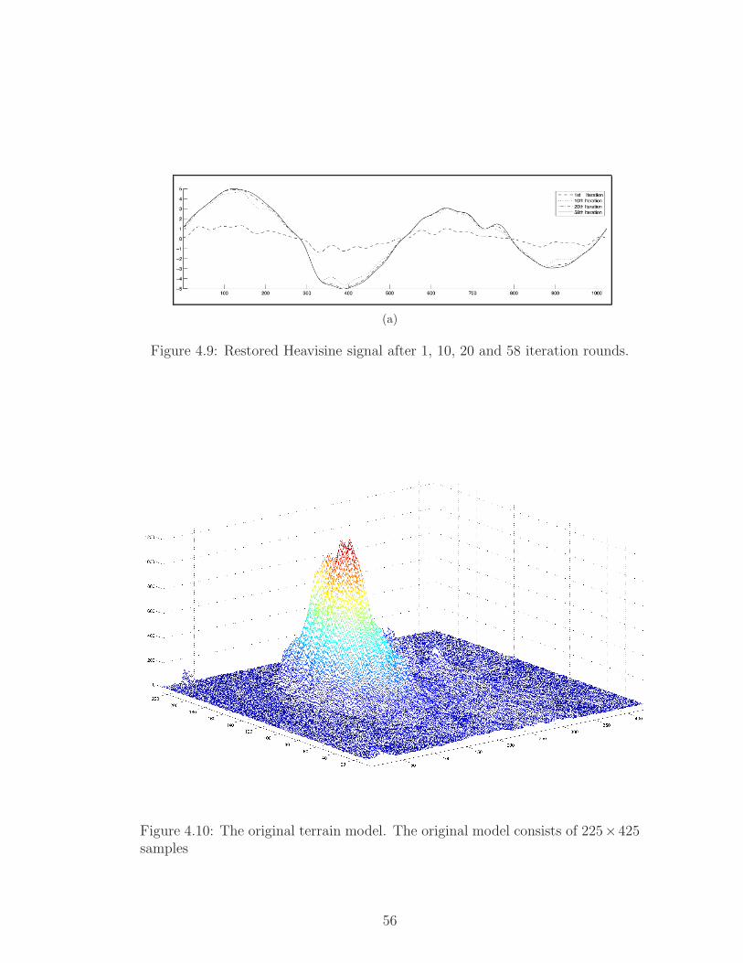
(a)
Figure 4.9: Restored Heavisine signal after 1, 10, 20 and 58 iteration rounds.
Figure 4.10: The original terrain model. The original model consists of 225×425samples
56

Figure 4.11: The terrain model in Figure4.10 reconstructed using one-fourth ofthe randomly chosen samples of the original model. The reconstruction parame-ters are wc =
π4, δs = 0.03, and ei = 0.01.
57
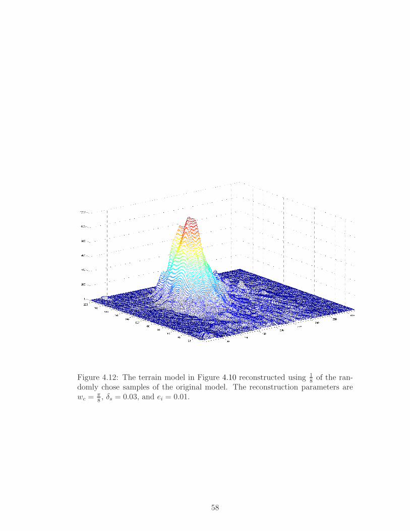
Figure 4.12: The terrain model in Figure 4.10 reconstructed using 18of the ran-
domly chose samples of the original model. The reconstruction parameters arewc =
π8, δs = 0.03, and ei = 0.01.
58
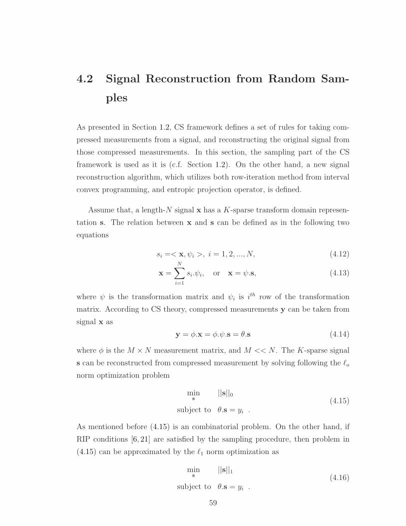
4.2 Signal Reconstruction from Random Sam-
ples
As presented in Section 1.2, CS framework defines a set of rules for taking com-
pressed measurements from a signal, and reconstructing the original signal from
those compressed measurements. In this section, the sampling part of the CS
framework is used as it is (c.f. Section 1.2). On the other hand, a new signal
reconstruction algorithm, which utilizes both row-iteration method from interval
convex programming, and entropic projection operator, is defined.
Assume that, a length-N signal x has a K-sparse transform domain represen-
tation s. The relation between x and s can be defined as in the following two
equations
si =< x, ψi >, i = 1, 2, ..., N, (4.12)
x =N∑
i=1
si.ψi, or x = ψ.s, (4.13)
where ψ is the transformation matrix and ψi is ith row of the transformation
matrix. According to CS theory, compressed measurements y can be taken from
signal x as
y = φ.x = φ.ψ.s = θ.s (4.14)
where φ is the M ×N measurement matrix, and M << N . The K-sparse signal
s can be reconstructed from compressed measurement by solving following the ℓo
norm optimization problem
mins
||s||0
subject to θ.s = yi .(4.15)
As mentioned before (4.15) is an combinatorial problem. On the other hand, if
RIP conditions [6, 21] are satisfied by the sampling procedure, then problem in
(4.15) can be approximated by the ℓ1 norm optimization as
mins
||s||1
subject to θ.s = yi .(4.16)
59
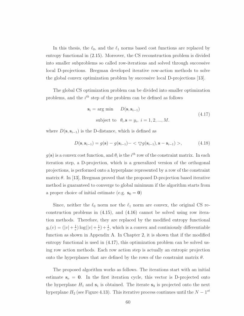
In this thesis, the ℓ0, and the ℓ1 norms based cost functions are replaced by
entropy functional in (2.15). Moreover, the CS reconstruction problem is divided
into smaller subproblems so called row-iterations and solved through successive
local D-projections. Bregman developed iterative row-action methods to solve
the global convex optimization problem by successive local D-projections [13].
The global CS optimization problem can be divided into smaller optimization
problems, and the ith step of the problem can be defined as follows
si = arg min D(s, si−1)
subject to θi.s = yi, i = 1, 2, ...,M.(4.17)
where D(s, si−1) is the D-distance, which is defined as
D(s, si−1) = g(s)− g(si−1)− < g(si−1), s− si−1) >, (4.18)
g(s) is a convex cost function, and θi is the ith row of the constraint matrix. In each
iteration step, a D-projection, which is a generalized version of the orthogonal
projections, is performed onto a hyperplane represented by a row of the constraint
matrix θ. In [13], Bregman proved that the proposed D-projection based iterative
method is guaranteed to converge to global minimum if the algorithm starts from
a proper choice of initial estimate (e.g. s0 = 0)
Since, neither the ℓ0 norm nor the ℓ1 norm are convex, the original CS re-
construction problems in (4.15), and (4.16) cannot be solved using row itera-
tion methods. Therefore, they are replaced by the modified entropy functional
ge(v) = (|v|+ 1e) log(|v|+ 1
e)+ 1
e, which is a convex and continiously differentiable
function as shown in Appendix A. In Chapter 2, it is shown that if the modified
entropy functional is used in (4.17), this optimization problem can be solved us-
ing row action methods. Each row action step is actually an entropic projection
onto the hyperplanes that are defined by the rows of the constraint matrix θ.
The proposed algorithm works as follows. The iterations start with an initial
estimate so = 0. In the first iteration cycle, this vector is D-projected onto
the hyperplane H1 and s1 is obtained. The iterate s1 is projected onto the next
hyperplaneH2 (see Figure 4.13). This iterative process continues until theN − 1st
60
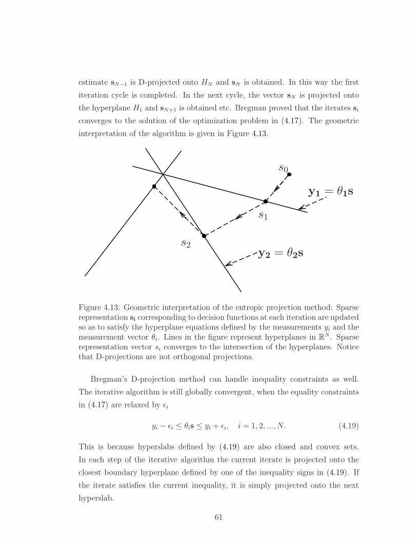
estimate sN−1 is D-projected onto HN and sN is obtained. In this way the first
iteration cycle is completed. In the next cycle, the vector sN is projected onto
the hyperplane H1 and sN+1 is obtained etc. Bregman proved that the iterates si
converges to the solution of the optimization problem in (4.17). The geometric
interpretation of the algorithm is given in Figure 4.13.
s0
s1
s2
y1 = θ1s
y2 = θ2s
Figure 4.13: Geometric interpretation of the entropic projection method: Sparserepresentation si corresponding to decision functions at each iteration are updatedso as to satisfy the hyperplane equations defined by the measurements yi and themeasurement vector θi. Lines in the figure represent hyperplanes in R
N . Sparserepresentation vector si converges to the intersection of the hyperplanes. Noticethat D-projections are not orthogonal projections.
Bregman’s D-projection method can handle inequality constraints as well.
The iterative algorithm is still globally convergent, when the equality constraints
in (4.17) are relaxed by ǫi
yi − ǫi ≤ θis ≤ yi + ǫi, i = 1, 2, ..., N. (4.19)
This is because hyperslabs defined by (4.19) are also closed and convex sets.
In each step of the iterative algorithm the current iterate is projected onto the
closest boundary hyperplane defined by one of the inequality signs in (4.19). If
the iterate satisfies the current inequality, it is simply projected onto the next
hyperslab.
61
The globally convergent row-action method described above can be easily
extended to a block iterative version by combining the entropic D-projections to
several rows of the θ matrix. However, we can not give a convergence proof of
the block-iterative method at this point.
Instead of performing successive D-projections onto each hyperplane con-
straint, as in (4.17), it is also possible to perform groups of projections. In [122],
a parallel version of the POCS algorithm called the block iterative approach is
presented. In this version, one may project the current iterate si−1 onto a set of
hyperplanes defined by the rows of the measurement matrix θ. The selection of
the rows of the measurement matrix onto which the current iterate will be pro-
jected onto can be selected either consecutively, randomly or according to a rule.
The geometric interpretation of the parallel algorithm is illustrated in Figure 4.14
Typically, the parallel algorithm converges faster. However, the convergence of
the algorithm for this problem cannot be proved at this stage.
Figure 4.14: Geometric interpretation of the block iterative entropic projectionmethod: Sparse representation si corresponding to decision functions at each iter-ation are updated by taking individual projections onto the hyperplanes definedby the lines in the figure and then combining these projections. Sparse repre-sentation vector si converges to the intersection of the hyperplanes. Notice thatD-projections are not orthogonal projections.
62
4.2.1 Experimental Results
For the validation and testing of the entropic minimization method, experiments
with 3 different one-dimensional (1D) signals, and 6 different images are carried
out. The cusp signal, which consists of 1024 samples, and hisine signal, which
consists of 256 samples are shown in Figures 4.15, 4.16, respectively. The cusp
and the hisine signals can be sparsely approximated in DCT domain. The 4
random signal is composed of 128 samples and it consists of 4 randomly located
non-zero samples. The measurement matrices φ are chosen as Gaussian random
matrices.
In the first set of experiments M = 204, 717 measurements are taken from
the cusp signal and M = 24, 40 measurements are taken from the S = 5 random
signal. The original signals are reconstructed from those measurements. The re-
constructed signals using the entropy based cost functional are shown in Figures
4.17(a), 4.17(b), 4.18(a), and 4.18(b). The cusp signal has 76 DCT coefficients,
whose magnitudes are larger than 10−2. Therefore, it can be approximated by a
S = 76 sparse signal in DCT domain. 39 and 44 dB SNR are achieved by the
reconstructing the original signal using the proposed method from M = 204, 717
measurements respectively. In case of the experiment with random signals, the
proposed method missed one sample from the original signal using 30 measure-
ment and perfectly reconstructed the original signal using 50 measurements.
63
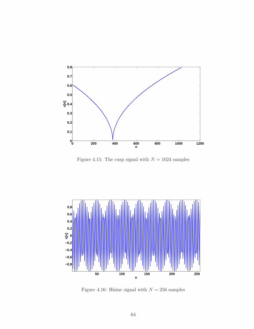
0 200 400 600 800 1000 12000
0.1
0.2
0.3
0.4
0.5
0.6
0.7
0.8
n
x[n]
Figure 4.15: The cusp signal with N = 1024 samples
50 100 150 200 250
−0.8
−0.6
−0.4
−0.2
0
0.2
0.4
0.6
0.8
n
x[n]
Figure 4.16: Hisine signal with N = 256 samples
64
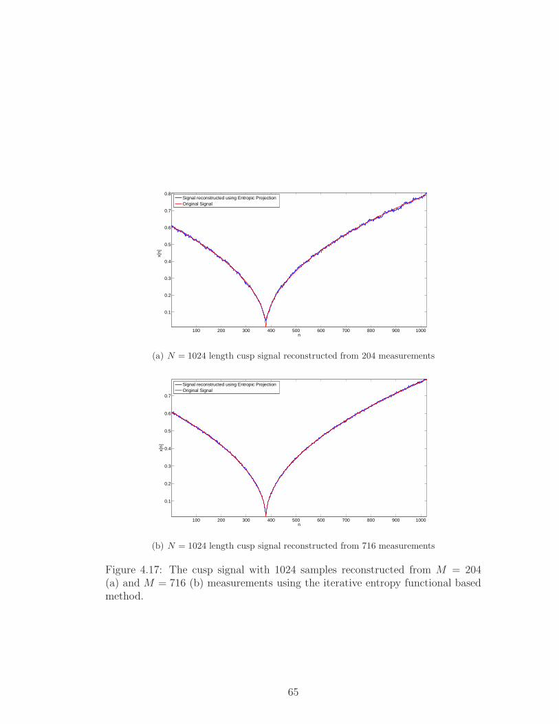
100 200 300 400 500 600 700 800 900 1000
0.1
0.2
0.3
0.4
0.5
0.6
0.7
0.8
n
x[n]
Signal reconstructed using Entropic ProjectionOriginal Signal
(a) N = 1024 length cusp signal reconstructed from 204 measurements
100 200 300 400 500 600 700 800 900 1000
0.1
0.2
0.3
0.4
0.5
0.6
0.7
n
x[n]
Signal reconstructed using Entropic ProjectionOriginal Signal
(b) N = 1024 length cusp signal reconstructed from 716 measurements
Figure 4.17: The cusp signal with 1024 samples reconstructed from M = 204(a) and M = 716 (b) measurements using the iterative entropy functional basedmethod.
65
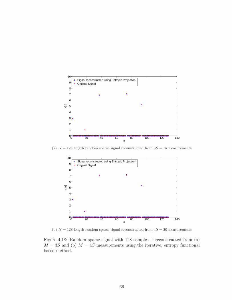
0 20 40 60 80 100 120 1400
1
2
3
4
5
6
7
8
9
10
n
x[n]
Signal reconstructed using Entropic ProjectionOriginal Signal
(a) N = 128 length random sparse signal reconstructed from 3S = 15 measurements
0 20 40 60 80 100 120 1400
1
2
3
4
5
6
7
8
9
10
n
x[n]
Signal reconstructed using Entropic ProjectionOriginal Signal
(b) N = 128 length random sparse signal reconstructed from 4S = 20 measurements
Figure 4.18: Random sparse signal with 128 samples is reconstructed from (a)M = 3S and (b) M = 4S measurements using the iterative, entropy functionalbased method.
66
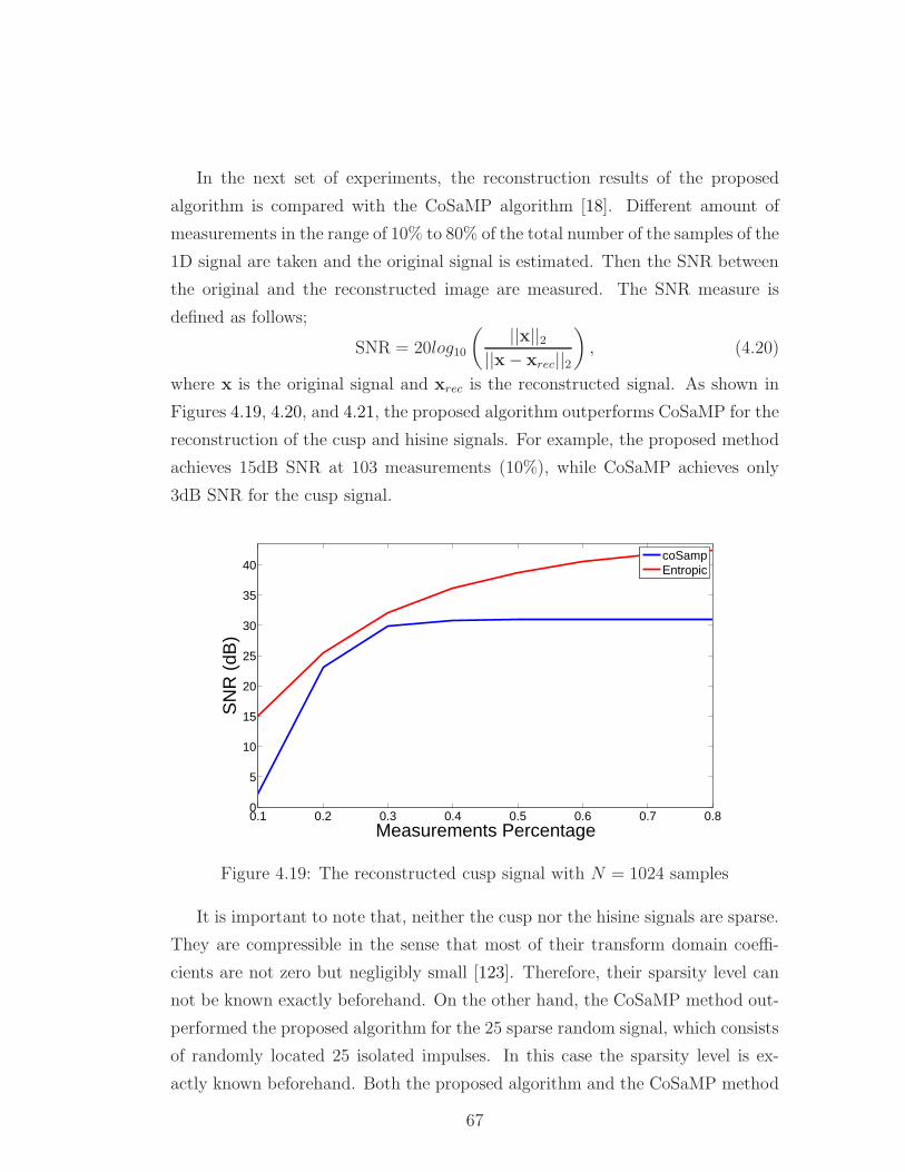
In the next set of experiments, the reconstruction results of the proposed
algorithm is compared with the CoSaMP algorithm [18]. Different amount of
measurements in the range of 10% to 80% of the total number of the samples of the
1D signal are taken and the original signal is estimated. Then the SNR between
the original and the reconstructed image are measured. The SNR measure is
defined as follows;
SNR = 20log10
(
||x||2||x− xrec||2
)
, (4.20)
where x is the original signal and xrec is the reconstructed signal. As shown in
Figures 4.19, 4.20, and 4.21, the proposed algorithm outperforms CoSaMP for the
reconstruction of the cusp and hisine signals. For example, the proposed method
achieves 15dB SNR at 103 measurements (10%), while CoSaMP achieves only
3dB SNR for the cusp signal.
0.1 0.2 0.3 0.4 0.5 0.6 0.7 0.80
5
10
15
20
25
30
35
40
Measurements Percentage
SN
R (
dB)
coSampEntropic
Figure 4.19: The reconstructed cusp signal with N = 1024 samples
It is important to note that, neither the cusp nor the hisine signals are sparse.
They are compressible in the sense that most of their transform domain coeffi-
cients are not zero but negligibly small [123]. Therefore, their sparsity level can
not be known exactly beforehand. On the other hand, the CoSaMP method out-
performed the proposed algorithm for the 25 sparse random signal, which consists
of randomly located 25 isolated impulses. In this case the sparsity level is ex-
actly known beforehand. Both the proposed algorithm and the CoSaMP method
67
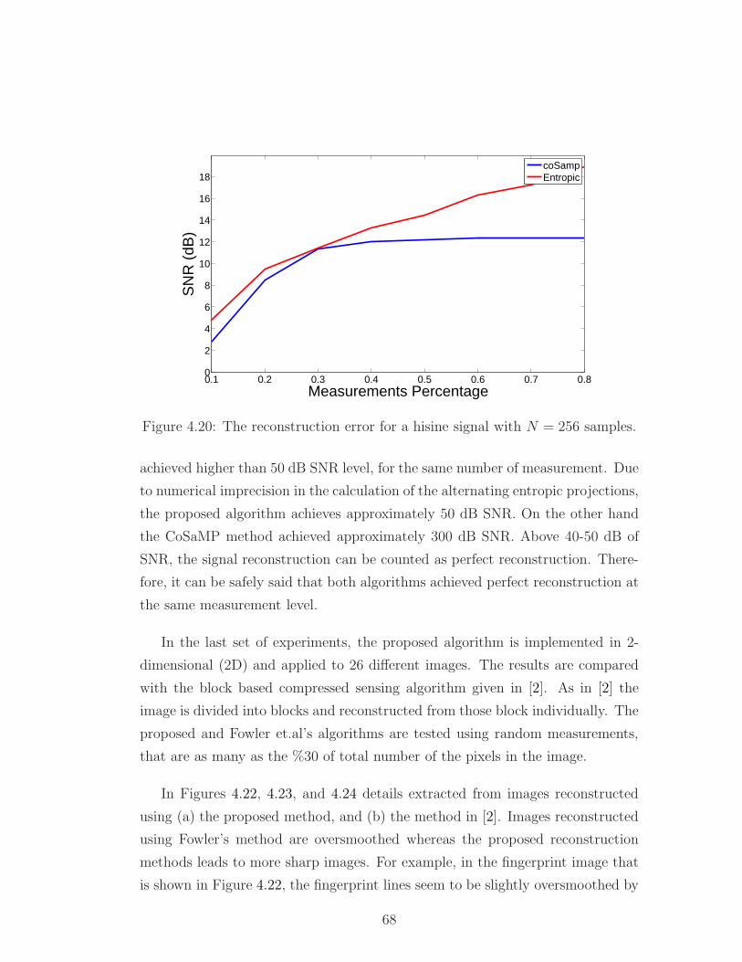
0.1 0.2 0.3 0.4 0.5 0.6 0.7 0.80
2
4
6
8
10
12
14
16
18
Measurements Percentage
SN
R (
dB)
coSampEntropic
Figure 4.20: The reconstruction error for a hisine signal with N = 256 samples.
achieved higher than 50 dB SNR level, for the same number of measurement. Due
to numerical imprecision in the calculation of the alternating entropic projections,
the proposed algorithm achieves approximately 50 dB SNR. On the other hand
the CoSaMP method achieved approximately 300 dB SNR. Above 40-50 dB of
SNR, the signal reconstruction can be counted as perfect reconstruction. There-
fore, it can be safely said that both algorithms achieved perfect reconstruction at
the same measurement level.
In the last set of experiments, the proposed algorithm is implemented in 2-
dimensional (2D) and applied to 26 different images. The results are compared
with the block based compressed sensing algorithm given in [2]. As in [2] the
image is divided into blocks and reconstructed from those block individually. The
proposed and Fowler et.al’s algorithms are tested using random measurements,
that are as many as the %30 of total number of the pixels in the image.
In Figures 4.22, 4.23, and 4.24 details extracted from images reconstructed
using (a) the proposed method, and (b) the method in [2]. Images reconstructed
using Fowler’s method are oversmoothed whereas the proposed reconstruction
methods leads to more sharp images. For example, in the fingerprint image that
is shown in Figure 4.22, the fingerprint lines seem to be slightly oversmoothed by
68
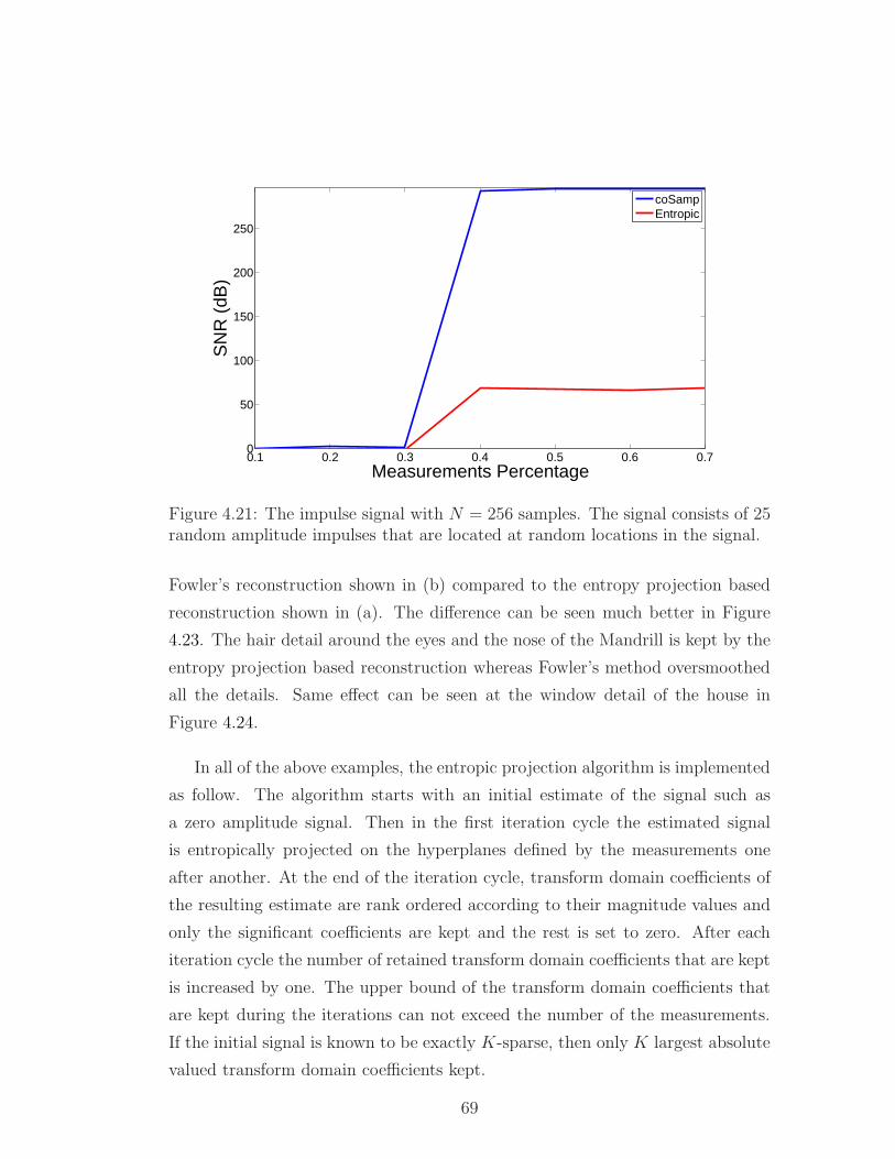
0.1 0.2 0.3 0.4 0.5 0.6 0.70
50
100
150
200
250
Measurements Percentage
SN
R (
dB)
coSampEntropic
Figure 4.21: The impulse signal with N = 256 samples. The signal consists of 25random amplitude impulses that are located at random locations in the signal.
Fowler’s reconstruction shown in (b) compared to the entropy projection based
reconstruction shown in (a). The difference can be seen much better in Figure
4.23. The hair detail around the eyes and the nose of the Mandrill is kept by the
entropy projection based reconstruction whereas Fowler’s method oversmoothed
all the details. Same effect can be seen at the window detail of the house in
Figure 4.24.
In all of the above examples, the entropic projection algorithm is implemented
as follow. The algorithm starts with an initial estimate of the signal such as
a zero amplitude signal. Then in the first iteration cycle the estimated signal
is entropically projected on the hyperplanes defined by the measurements one
after another. At the end of the iteration cycle, transform domain coefficients of
the resulting estimate are rank ordered according to their magnitude values and
only the significant coefficients are kept and the rest is set to zero. After each
iteration cycle the number of retained transform domain coefficients that are kept
is increased by one. The upper bound of the transform domain coefficients that
are kept during the iterations can not exceed the number of the measurements.
If the initial signal is known to be exactly K-sparse, then only K largest absolute
valued transform domain coefficients kept.
69
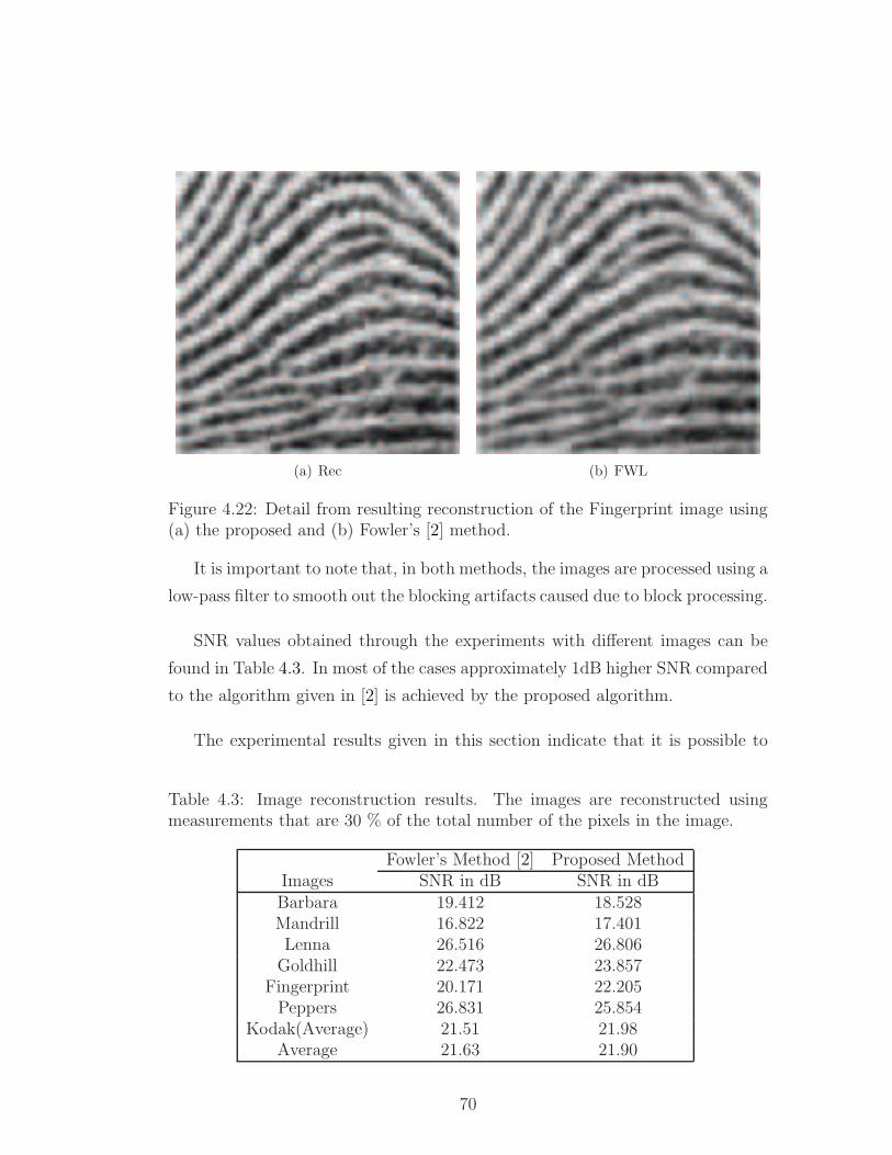
(a) Rec (b) FWL
Figure 4.22: Detail from resulting reconstruction of the Fingerprint image using(a) the proposed and (b) Fowler’s [2] method.
It is important to note that, in both methods, the images are processed using a
low-pass filter to smooth out the blocking artifacts caused due to block processing.
SNR values obtained through the experiments with different images can be
found in Table 4.3. In most of the cases approximately 1dB higher SNR compared
to the algorithm given in [2] is achieved by the proposed algorithm.
The experimental results given in this section indicate that it is possible to
Table 4.3: Image reconstruction results. The images are reconstructed usingmeasurements that are 30 % of the total number of the pixels in the image.
Fowler’s Method [2] Proposed MethodImages SNR in dB SNR in dBBarbara 19.412 18.528Mandrill 16.822 17.401Lenna 26.516 26.806Goldhill 22.473 23.857
Fingerprint 20.171 22.205Peppers 26.831 25.854
Kodak(Average) 21.51 21.98Average 21.63 21.90
70
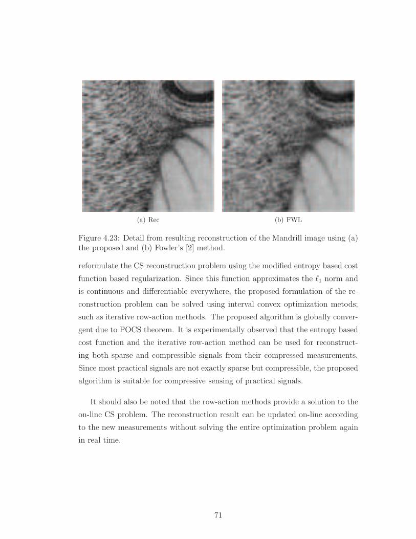
(a) Rec (b) FWL
Figure 4.23: Detail from resulting reconstruction of the Mandrill image using (a)the proposed and (b) Fowler’s [2] method.
reformulate the CS reconstruction problem using the modified entropy based cost
function based regularization. Since this function approximates the ℓ1 norm and
is continuous and differentiable everywhere, the proposed formulation of the re-
construction problem can be solved using interval convex optimization metods;
such as iterative row-action methods. The proposed algorithm is globally conver-
gent due to POCS theorem. It is experimentally observed that the entropy based
cost function and the iterative row-action method can be used for reconstruct-
ing both sparse and compressible signals from their compressed measurements.
Since most practical signals are not exactly sparse but compressible, the proposed
algorithm is suitable for compressive sensing of practical signals.
It should also be noted that the row-action methods provide a solution to the
on-line CS problem. The reconstruction result can be updated on-line according
to the new measurements without solving the entire optimization problem again
in real time.
71
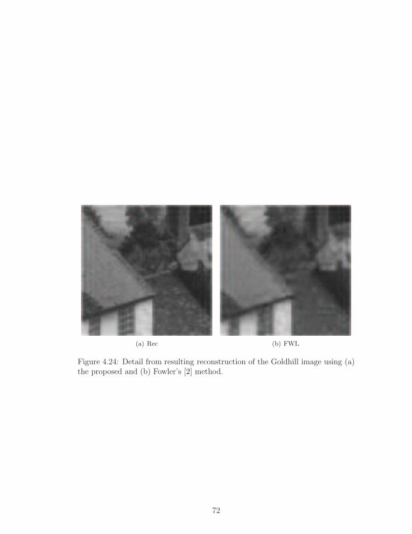
(a) Rec (b) FWL
Figure 4.24: Detail from resulting reconstruction of the Goldhill image using (a)the proposed and (b) Fowler’s [2] method.
72
Chapter 5
SIGNAL DENOISING
This chapter comprises of two different signal denoising algorithms. In Section
5.1, an algorithm that makes use of block processing to solve the TV denoising
problem. The algorithm adapts itself to the local content of the image blocks
and adjusts the TV denoising parameters accordingly. In Section 5.2, an image
denoising algorithm, which utilizes the filtered variations contraints defined in
3.1, is presented.
5.1 Locally Adaptive Total Variation
In this section, a local Total Variation (LTV), and a locally adaptive Total Vari-
ation (LATV) regularized denoising scheme are introduced. In the proposed
approaches an N-by-M image x is reconstructed from its noisy observation y us-
ing LTV or LATV denoising algorithm. In ordinary TV approach, the TV cost
function is minimized over the entire image. However, the correlation between
the samples in a typical signal or an image decreases as the distance between
two samples increases. Therefore, globally minimization of a cost function over
the whole signal may not be necessary in denoising problems. Block processing
is a commonly referred technique in image processing to take advantage of local
processing and computational efficiency. On the other hand, the disadvantage
73
of block processing techniques is that they may introduce artificial edges at the
boundaries of the blocks in the restored image.
Both LTV and LATV methods are block based algorithms. They work like a
nonlinear filter and produces a single output for each input block. Therefore, they
do not suffer from blocking artifacts. Furthermore, LATV enables the possibility
of adapting optimization parameters according to the block content and introduce
adaptivity to the TV cost functional.
In image denoising problem, it is assumed that the original signal x is cor-
rupted by additive noise u as follows
y = x + u. (5.1)
In TV regularization based denoising approach, the original signal is estimated
by solving the following minimization problem:
minx
||x||TV
subject to ||y − x|| ≤ ε.(5.2)
or in Lagrangian formulation
minx
||y− x||2 + λ||x||TV (5.3)
where ε is the error tolerance, and λ is the Lagrange multiplier. There exists
an ε corresponding to each λ such that both optimization problems result in the
same solution [124, 125]. These parameters can also be used for adjusting the
smoothness level of the solution. In [19], an iterative algorithm was proposed to
solve the optimization problem given in (5.2) and (5.3). This algorithm solves
the TV minimization optimization on the whole image; therefore, as the image
size increases, the problem size also increases, and therefore the computational
complexity of the algorithm increases.
In regular TV denoising only a single optimization problem is solved for the
entire image. Due to this global approach, some of the high-frequency details of
the image may be over-smoothed or the noise may not be cleaned effectively at
74
smooth regions. To deal with this problem, a local adaptation strategy is devel-
oped. The proposed LTV and LATV methods overcome this problem through a
block-based local adaptation strategy.
Let wn be a window centered at the pixel n = (n1, n2). The window can be
a rectangular window, or it can take any shape. Furthermore, one can apply
decaying weights to the samples within each window. LTV algorithm solves the
following problem for each pixel
minx[n]
∑
k∈wn
x[k]
subject to∑
k∈w[n]
(x[k]− y[k])2 < ε(5.4)
where k = (k1, k2). Chambolle’s algorithm [19] actually restores all the pixels
in w[n], but only the center pixel is picked as the restored output. To restore
the next pixel, the analysis window is moved one pixel to the left (k1, k2 + 1), or
down (k1 + 1, k2), and the problem described in (5.4) is solved once again. The
entire noisy image is processed pixel by pixel in this manner. The optimization
problem described in (5.4) is solved in a small neighborhood unlike (5.3), which
is solved for the entire image. Therefore, the computational complexity of the
LTV method is low.
The optimization parameter ε in (5.4) can be used to set the smoothness level
of the solution. As ε value increases, the minimization part will turn out more
smooth regions. Ideally, it should be selected close to the standard deviation of
the signal noise [19], which can be estimated from the flat regions of the image.
In the first set of experiments that is summarized in the first two columns of
Tables 5.1 and 5.2, we used the same optimization parameter (just scaled by the
number of the pixels in the processing area) for both the ordinary TV and the
proposed LTV methods.
We tested the proposed approach on 35 different images. We used 24 images
from the Kodak dataset taken from http://r0k.us/graphics/kodak/ and some well
known images from image processing literature. We selected the block size as 9×9.
According to the results summarized in Table 5.1 and 5.2, the LTV approach
75
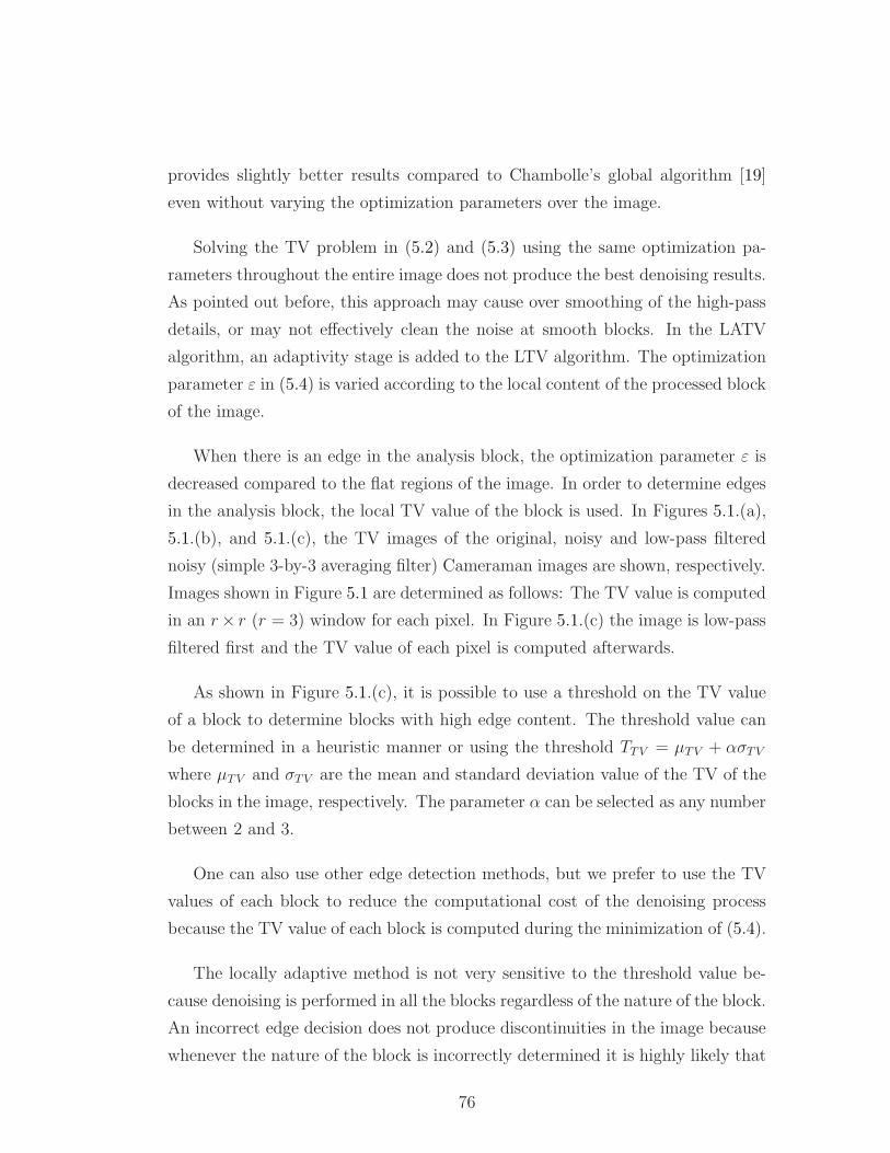
provides slightly better results compared to Chambolle’s global algorithm [19]
even without varying the optimization parameters over the image.
Solving the TV problem in (5.2) and (5.3) using the same optimization pa-
rameters throughout the entire image does not produce the best denoising results.
As pointed out before, this approach may cause over smoothing of the high-pass
details, or may not effectively clean the noise at smooth blocks. In the LATV
algorithm, an adaptivity stage is added to the LTV algorithm. The optimization
parameter ε in (5.4) is varied according to the local content of the processed block
of the image.
When there is an edge in the analysis block, the optimization parameter ε is
decreased compared to the flat regions of the image. In order to determine edges
in the analysis block, the local TV value of the block is used. In Figures 5.1.(a),
5.1.(b), and 5.1.(c), the TV images of the original, noisy and low-pass filtered
noisy (simple 3-by-3 averaging filter) Cameraman images are shown, respectively.
Images shown in Figure 5.1 are determined as follows: The TV value is computed
in an r× r (r = 3) window for each pixel. In Figure 5.1.(c) the image is low-pass
filtered first and the TV value of each pixel is computed afterwards.
As shown in Figure 5.1.(c), it is possible to use a threshold on the TV value
of a block to determine blocks with high edge content. The threshold value can
be determined in a heuristic manner or using the threshold TTV = µTV + ασTV
where µTV and σTV are the mean and standard deviation value of the TV of the
blocks in the image, respectively. The parameter α can be selected as any number
between 2 and 3.
One can also use other edge detection methods, but we prefer to use the TV
values of each block to reduce the computational cost of the denoising process
because the TV value of each block is computed during the minimization of (5.4).
The locally adaptive method is not very sensitive to the threshold value be-
cause denoising is performed in all the blocks regardless of the nature of the block.
An incorrect edge decision does not produce discontinuities in the image because
whenever the nature of the block is incorrectly determined it is highly likely that
76
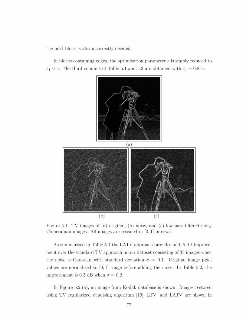
the next block is also incorrectly decided.
In blocks containing edges, the optimization parameter ε is simply reduced to
ε1 < ε. The third columns of Table 5.1 and 5.2 are obtained with ε1 = 0.85ε.
(a)
(b) (c)
Figure 5.1: TV images of (a) original, (b) noisy, and (c) low-pass filtered noisyCameraman images. All images are rescaled in [0, 1] interval.
As summarized in Table 5.1 the LATV approach provides an 0.5 dB improve-
ment over the standard TV approach in our dataset consisting of 35 images when
the noise is Gaussian with standard deviation σ = 0.1. Original image pixel
values are normalized to [0, 1] range before adding the noise. In Table 5.2, the
improvement is 0.3 dB when σ = 0.2.
In Figure 5.2.(a), an image from Kodak database is shown. Images restored
using TV regularized denoising algorithm [19], LTV, and LATV are shown in
77
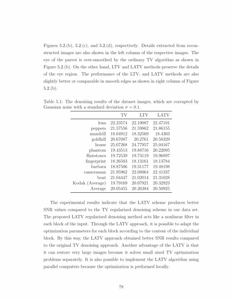
Figures 5.2.(b), 5.2.(c), and 5.2.(d), respectively. Details extracted from recon-
structed images are also shown in the left column of the respective images. The
eye of the parrot is over-smoothed by the ordinary TV algorithm as shown in
Figure 5.2.(b). On the other hand, LTV and LATV methods preserve the details
of the eye region. The performance of the LTV, and LATV methods are also
slightly better or comparable in smooth edges as shown in right column of Figure
5.2.(b).
Table 5.1: The denoising results of the dataset images, which are corrupted byGaussian noise with a standard deviation σ = 0.1.
TV LTV LATV
lena 22.23574 22.19087 22.47191peppers 21.57556 21.59862 21.86155mandrill 18.04912 18.32569 18.4303goldhill 20.67087 20.2761 20.58329house 25.07268 24.77957 25.04167
phantom 19.43513 19.88716 20.22095flintstones 19.72539 19.73119 19.96897fingerprint 18.26503 18.13161 18.13784
barbara 18.87506 19.31177 19.48198cameraman 21.95962 22.08064 22.41337
boat 21.04447 21.02014 21.31028Kodak (Average) 19.79169 20.07921 20.32923
Average 20.05455 20.26384 20.50925
The experimental results indicate that the LATV scheme produces better
SNR values compared to the TV regularized denoising scheme in our data set.
The proposed LATV regularized denoising method acts like a nonlinear filter in
each block of the input. Through the LATV approach, it is possible to adapt the
optimization parameters for each block according to the content of the individual
block. By this way, the LATV approach obtained better SNR results compared
to the original TV denoising approach. Another advantage of the LATV is that
it can restore very large images because it solves small sized TV optimization
problems separately. It is also possible to implement the LATV algorithm using
parallel computers because the optimization is performed locally.
78
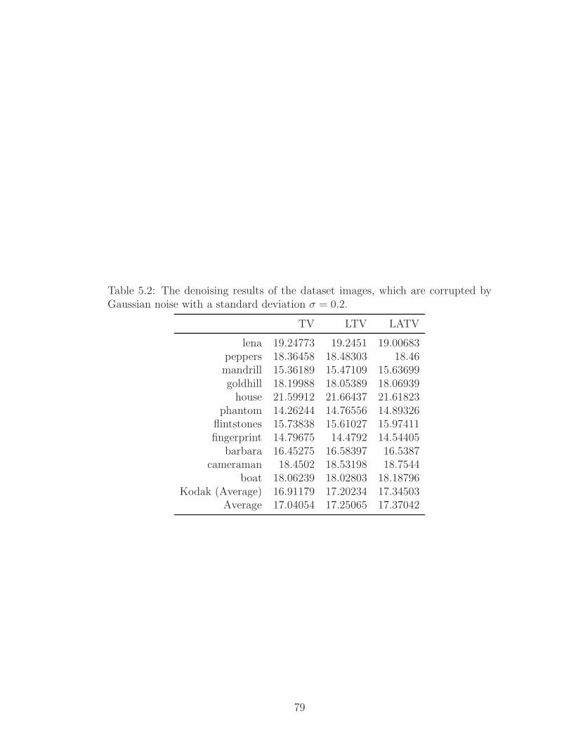
Table 5.2: The denoising results of the dataset images, which are corrupted byGaussian noise with a standard deviation σ = 0.2.
TV LTV LATV
lena 19.24773 19.2451 19.00683peppers 18.36458 18.48303 18.46mandrill 15.36189 15.47109 15.63699goldhill 18.19988 18.05389 18.06939house 21.59912 21.66437 21.61823
phantom 14.26244 14.76556 14.89326flintstones 15.73838 15.61027 15.97411fingerprint 14.79675 14.4792 14.54405
barbara 16.45275 16.58397 16.5387cameraman 18.4502 18.53198 18.7544
boat 18.06239 18.02803 18.18796Kodak (Average) 16.91179 17.20234 17.34503
Average 17.04054 17.25065 17.37042
79
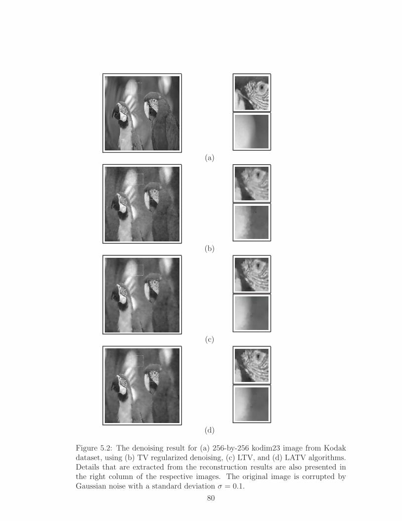
(a)
(b)
(c)
(d)
Figure 5.2: The denoising result for (a) 256-by-256 kodim23 image from Kodakdataset, using (b) TV regularized denoising, (c) LTV, and (d) LATV algorithms.Details that are extracted from the reconstruction results are also presented inthe right column of the respective images. The original image is corrupted byGaussian noise with a standard deviation σ = 0.1.
80
5.2 Filtered Variation based Signal Denoising
In this section, an algorithm that denoises the noisy signal y by putting bounds
on the variation of the reconstructed signal is introduced. These bounds can be in
spatial domain, as well as in a signal transform domain (e.g. DFT, DCT, DHT).
The signal model is the same as in Section 5.1. The original signal x is corrupted
by additive noise u as in (5.1).
In FV based denoising, the goal is to find a solution to the following optimiza-
tion problem:
min FVp(x) (5.5)
s.t. ‖x− y‖ ≤ δ (5.6)
where FV stands for the filtered variation and it is defined as follows:
FVp(x) = ‖HDx‖p , p = 1, 2 (5.7)
where X,D and H represent the signal, the signal transform (e.g., DCT, DHT,
DFT) and the discrete-time filter in the transform domain, respectively and p
denotes which ℓp-norm is used. In (5.6) and (5.7) the norm can be selected as the
ℓ1 or ℓ2 norms, which correspond to anisotropic and isotropic FV, respectively.
In the FV approach, denoising is achieved by minimizing the high-frequency
energy of the observations, subject to the constraint given in (5.6). In (5.5)-(5.7)
we posed the problem in frequency domain because for any given fixed transform,
noise is typically in coherent with the transform, therefore it is spread out. By
means of a proper filtering operation in the transform domain, one can exploit this
fact to effectively denoise the signal. Besides, it is possible to solve the problem
completely in time (or space) domain as well.
We solve this regularized signal denoising problem by applying several different
time (space) and frequency domain constraints on filtered versions of the signal x.
This approach is similar to the methodology described in [85, 87, 126]. Since the
FV cost function is convex it is also possible to solve FV based problems using
convex programming. We provide a solution using the Projections onto Convex
81
Sets (POCS) method. The following FV based constraints correspond to a class
of convex sets:
Cpi = FVp(x) =
‖HDx‖p ≤ ε
, p = 1, 2 and i = 1, . . . ,M. (5.8)
where p = 1, 2 corresponds to the ℓ1 and the ℓ2-norms respectively. Other closed
and convex sets, described in Section 5.2 can be also imposed on the desired signal
x. The solution of the denoising problem is assumed to lie in the intersection of
M different constraint sets as follows:
x ∈ C =
M⋂
i=1
Ci, (5.9)
where the constraint sets (Ci) are defined by the convex constraints as given at
(5.8). Therefore, it is possible to reconstruct the original signal by performing
successive orthogonal projections onto the closed and convex sets Ci [13, 17].
The POCS based iterative algorithm consists of making successive operations in
time (or space) and transform domains, and it converges to a solution in the
intersection of constraint sets Ci.
Extension to 2-D or higher dimensional signals is straightforward. Instead of
a 1-D high-pass filter, 2-D or higher dimensional high-pass filters can be used in
(5.9).
For image denoising applications, 6 different filtered variation constraints are
designed in this thesis. These contraints are defined in Section 3.1. In each test,
a subset of these constraints are applied on the noisy signal one-by-one, and the
solution at the intersection the constraints in the set is obtained.
We first present a denoising example from [3]. Combettes and Pesquet used
the image shown in Fig.5.3-(a) in [3], to test their TV based denoising algorithm.
They added i.i.d. Laplacian noise to the original 128x128 grayscale image. The
signal-to-noise ratio is 1dB. To compare the FV algorithm to the TV denoising, we
cropped the original image (Fig. 5.3-(a)) from their paper and added Laplacian
noise to the image. In [3] the pixel range was [-261,460]. In our case the pixel
range turns out to be [-391,511].
82
As shown in Fig. 5.3, the characters in the image that are recovered by FV
based denoising algorithm (Fig.5.3-(e)) are visually sharper compared to Fig.5.3-
(c) and the impulsive noise is significantly reduced compared to ℓ1 denoising.
In [3], the authors used Normalized Root Mean Square Error (NRMSE) as
the error metric. They measure the error between the original signal x and
reconstructed signal xo as
||x− xo||/||xo||. (5.10)
The progress of the decrease in reconstruction error, is shown in Fig. 5.4. FV
based denoising algorithm converges to an NRMSE level of -9 dB in 10-to-12
iterations. On the other hand, the time-domain TV algorithm takes around 100
iterations to converge as shown in Fig. 18 in [3].
ℓ1 and ℓ2 high-frequency energy bounds ε1 and ε3 can be estimated from the
noisy image. In another set of experiments, the bounds are selected as 80%
of ℓ1 (ε1a), 60% of ℓ1 (ε1b) and 80% of the ℓ2 (ε3a) energies of the noisy image,
respectively. ε1o corresponds to the ℓ1 energy of the original image. Experimental
results indicate that estimating ε1 and ε3 are possible from flat portions of the
image and the FV algorithm is not sensitive to the ε1 and ε3 values. As shown in
Fig. 5.4, in all cases NRMSE values for the restored images are very close to each
other. Convergence graphs closely overlap with each other as shown in Fig.5.3
In another experiment the fingerprint shown in Fig.5.5-(a) is used. A noisy
version of the image (Fig. 5.5-(b)) with SNR=4.9dB, is obtained by adding
White Gaussian Noise to the original signal. Using FV constraints, lead to the
reconstructed signal with SNR=12.75 dB (Fig. 5.5-(d)). On the other hand, TV
constraint leads to an image with SNR=7.45dB (Fig. 5.5-(c)).
83
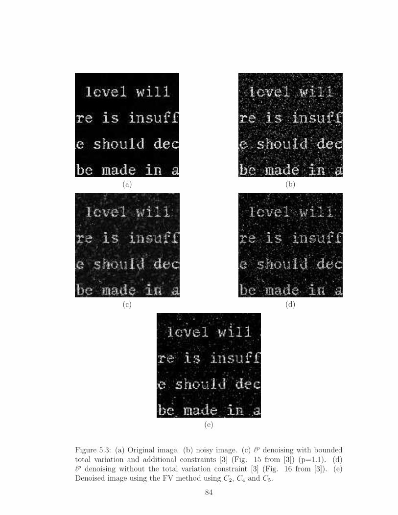
(a) (b)
(c) (d)
(e)
Figure 5.3: (a) Original image. (b) noisy image. (c) ℓp denoising with boundedtotal variation and additional constraints [3] (Fig. 15 from [3]) (p=1.1). (d)ℓp denoising without the total variation constraint [3] (Fig. 16 from [3]). (e)Denoised image using the FV method using C2, C4 and C5.
84
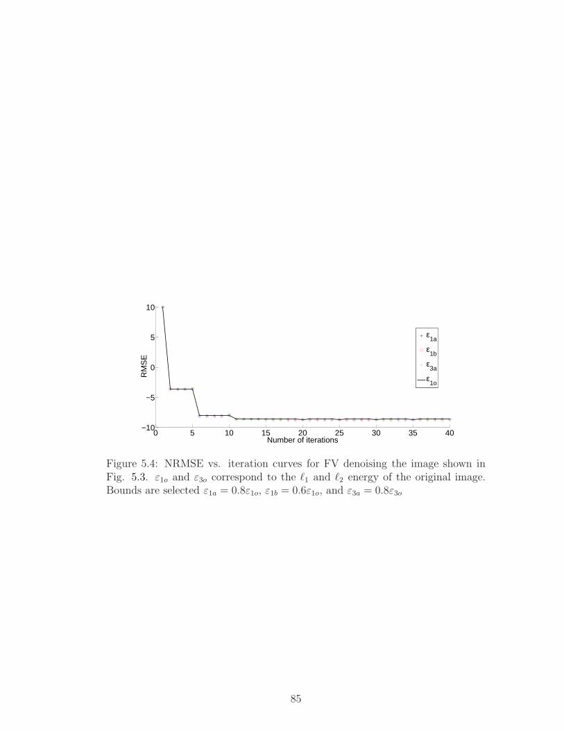
0 5 10 15 20 25 30 35 40−10
−5
0
5
10
Number of iterations
RM
SE
ε1a
ε1b
ε3a
ε1o
Figure 5.4: NRMSE vs. iteration curves for FV denoising the image shown inFig. 5.3. ε1o and ε3o correspond to the ℓ1 and ℓ2 energy of the original image.Bounds are selected ε1a = 0.8ε1o, ε1b = 0.6ε1o, and ε3a = 0.8ε3o
85
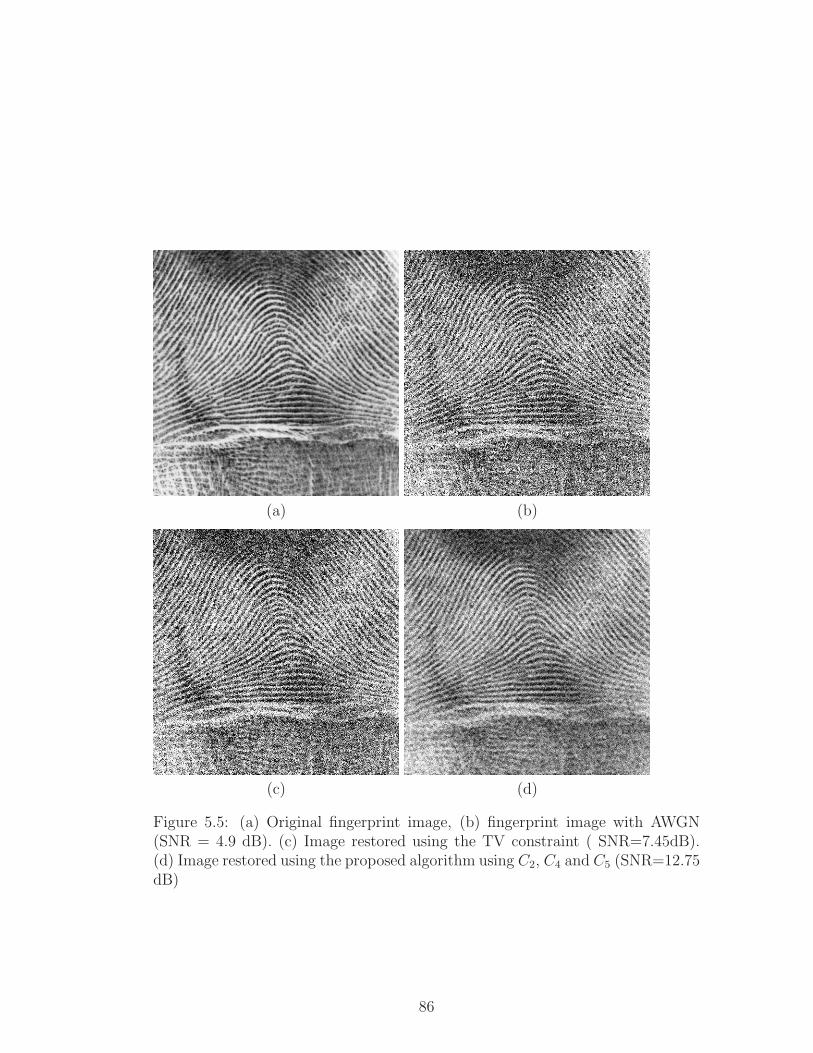
(a) (b)
(c) (d)
Figure 5.5: (a) Original fingerprint image, (b) fingerprint image with AWGN(SNR = 4.9 dB). (c) Image restored using the TV constraint ( SNR=7.45dB).(d) Image restored using the proposed algorithm using C2, C4 and C5 (SNR=12.75dB)
86
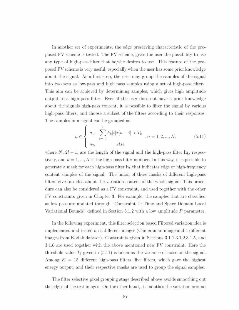
In another set of experiments, the edge preserving characteristic of the pro-
posed FV scheme is tested. The FV scheme, gives the user the possibility to use
any type of high-pass filter that he/she desires to use. This feature of the pro-
posed FV scheme is very useful, especially when the user has some prior knowledge
about the signal. As a first step, the user may group the samples of the signal
into two sets as low-pass and high pass samples using a set of high-pass filters.
This aim can be achieved by determining samples, which gives high amplitude
output to a high-pass filter. Even if the user does not have a prior knowledge
about the signals high-pass content, it is possible to filter the signal by various
high-pass filters, and choose a subset of the filters according to their responses.
The samples in a signal can be grouped as
n ∈
n1,
l∑
i=−l
hk[i]x[n− i] > Tk
n2, else
, n = 1, 2, ..., N. (5.11)
where N , 2l + 1, are the length of the signal and the high-pass filter hk, respec-
tively, and k = 1, ..., N is the high-pass filter number. In this way, it is possible to
generate a mask for each high-pass filter hk that indicates edge or high-frequency
content samples of the signal. The union of these masks of different high-pass
filters gives an idea about the variation content of the whole signal. This proce-
dure can also be considered as a FV constraint, and used together with the other
FV constraints given in Chapter 3. For example, the samples that are classified
as low-pass are updated through “Constraint II: Time and Space Domain Local
Variational Bounds” defined in Section 3.1.2 with a low amplitude P parameter.
In the following experiment, this filter selection based Filtered variation idea is
implemented and tested on 5 different images (Cameraman image and 4 different
images from Kodak dataset). Constraints given in Sections 3.1.1,3.1.2,3.1.5, and
3.1.6 are used together with the above mentioned new FV constraint. Here the
threshold value Tk given in (5.11) is taken as the variance of noise on the signal.
Among K = 15 different high-pass filters, five filters, which gave the highest
energy output, and their respective masks are used to group the signal samples.
The filter selective pixel grouping stage described above avoids smoothing out
the edges of the test images. On the other hand, it smoothes the variation around
87
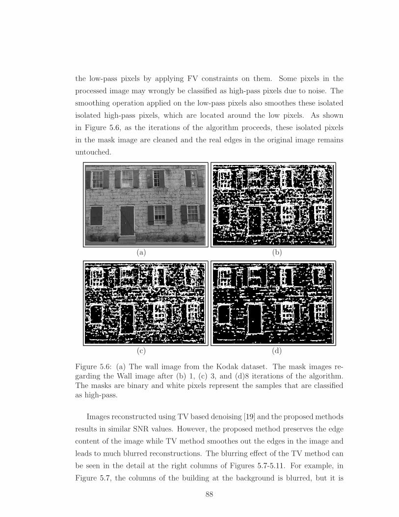
the low-pass pixels by applying FV constraints on them. Some pixels in the
processed image may wrongly be classified as high-pass pixels due to noise. The
smoothing operation applied on the low-pass pixels also smoothes these isolated
isolated high-pass pixels, which are located around the low pixels. As shown
in Figure 5.6, as the iterations of the algorithm proceeds, these isolated pixels
in the mask image are cleaned and the real edges in the original image remains
untouched.
(a) (b)
(c) (d)
Figure 5.6: (a) The wall image from the Kodak dataset. The mask images re-garding the Wall image after (b) 1, (c) 3, and (d)8 iterations of the algorithm.The masks are binary and white pixels represent the samples that are classifiedas high-pass.
Images reconstructed using TV based denoising [19] and the proposed methods
results in similar SNR values. However, the proposed method preserves the edge
content of the image while TV method smoothes out the edges in the image and
leads to much blurred reconstructions. The blurring effect of the TV method can
be seen in the detail at the right columns of Figures 5.7-5.11. For example, in
Figure 5.7, the columns of the building at the background is blurred, but it is
88
preserved by the proposed method. In Figures 5.8, 5.9, 5.10, and 5.11, same kind
of an effect can be seen at the head of the parrots, the fences of the lighthouse,
the texture on the wall and the window of the house respectively.
In this section, Filtered variation framework is applied to signal denoising
problem. In the proposed algorithm, regularization is achieved by using discrete-
time high-pass filters instead of taking the difference of neighboring signal samples
as in the TV method. The FV based denoising problem is solved by making
alternating projections in space and transform domains. It is experimentally
observed that FV approach provides better denoising results compared to the
TV approach. If some prior knowledge about the original signal exists, it is
possible to design high-pass filters according to the signal and incorporate it to
the FV framework.
89
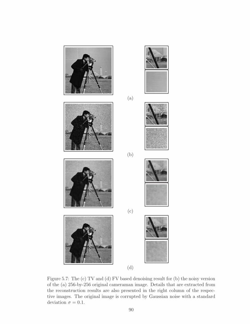
(a)
(b)
(c)
(d)
Figure 5.7: The (c) TV and (d) FV based denoising result for (b) the noisy versionof the (a) 256-by-256 original cameraman image. Details that are extracted fromthe reconstruction results are also presented in the right column of the respec-tive images. The original image is corrupted by Gaussian noise with a standarddeviation σ = 0.1.
90
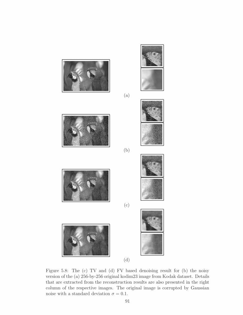
(a)
(b)
(c)
(d)
Figure 5.8: The (c) TV and (d) FV based denoising result for (b) the noisyversion of the (a) 256-by-256 original kodim23 image from Kodak dataset. Detailsthat are extracted from the reconstruction results are also presented in the rightcolumn of the respective images. The original image is corrupted by Gaussiannoise with a standard deviation σ = 0.1.
91
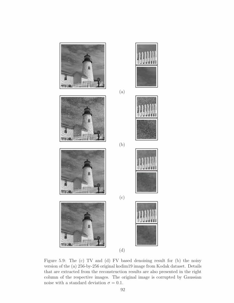
(a)
(b)
(c)
(d)
Figure 5.9: The (c) TV and (d) FV based denoising result for (b) the noisyversion of the (a) 256-by-256 original kodim19 image from Kodak dataset. Detailsthat are extracted from the reconstruction results are also presented in the rightcolumn of the respective images. The original image is corrupted by Gaussiannoise with a standard deviation σ = 0.1.
92
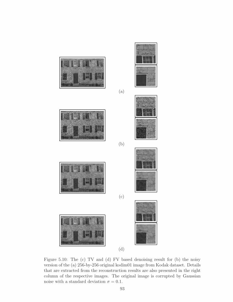
(a)
(b)
(c)
(d)
Figure 5.10: The (c) TV and (d) FV based denoising result for (b) the noisyversion of the (a) 256-by-256 original kodim01 image from Kodak dataset. Detailsthat are extracted from the reconstruction results are also presented in the rightcolumn of the respective images. The original image is corrupted by Gaussiannoise with a standard deviation σ = 0.1.
93
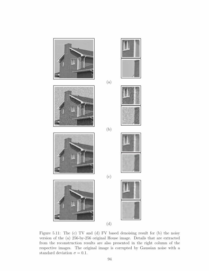
(a)
(b)
(c)
(d)
Figure 5.11: The (c) TV and (d) FV based denoising result for (b) the noisyversion of the (a) 256-by-256 original House image. Details that are extractedfrom the reconstruction results are also presented in the right column of therespective images. The original image is corrupted by Gaussian noise with astandard deviation σ = 0.1.
94
Chapter 6
ADAPTATION AND
LEARNING IN MULTI-NODE
NETWORKS
In this chapter, we describe modified entropy, Total Variation (TV), and Filtered
Variation (FV) functional based adaptation and learning algorithms for multi-
node networks. New algorithms learn the environment and converge faster than
ℓ2-norm based algorithms under ε-contaminated Gaussian noise. The modified
entropy functional based adaptive learning algorithms have two stages similar to
the adapt and combine (ATC) and combine and adapt (CTA) frameworks intro-
duced by Sayed et. al. [4]. In a multi-node network, each adaptation step in the
original ATC and CTA frameworks consist of Least mean squares (LMS) or Nor-
malized LMS (NLMS) algorithms, which are essentially an orthogonal projection
operation onto the hyperplane defined by
di,t = hi,tu′i,t, (6.1)
where dt, ht, and ut are the output of the ith node, estimated node impulse
response and the node input vector at time t, respectively. Bregman generalized
the orthogonal projection concept by introducing the concept of D-projection
in [13]. This allows the use of any convex function other than g(x) = x2 as a
95
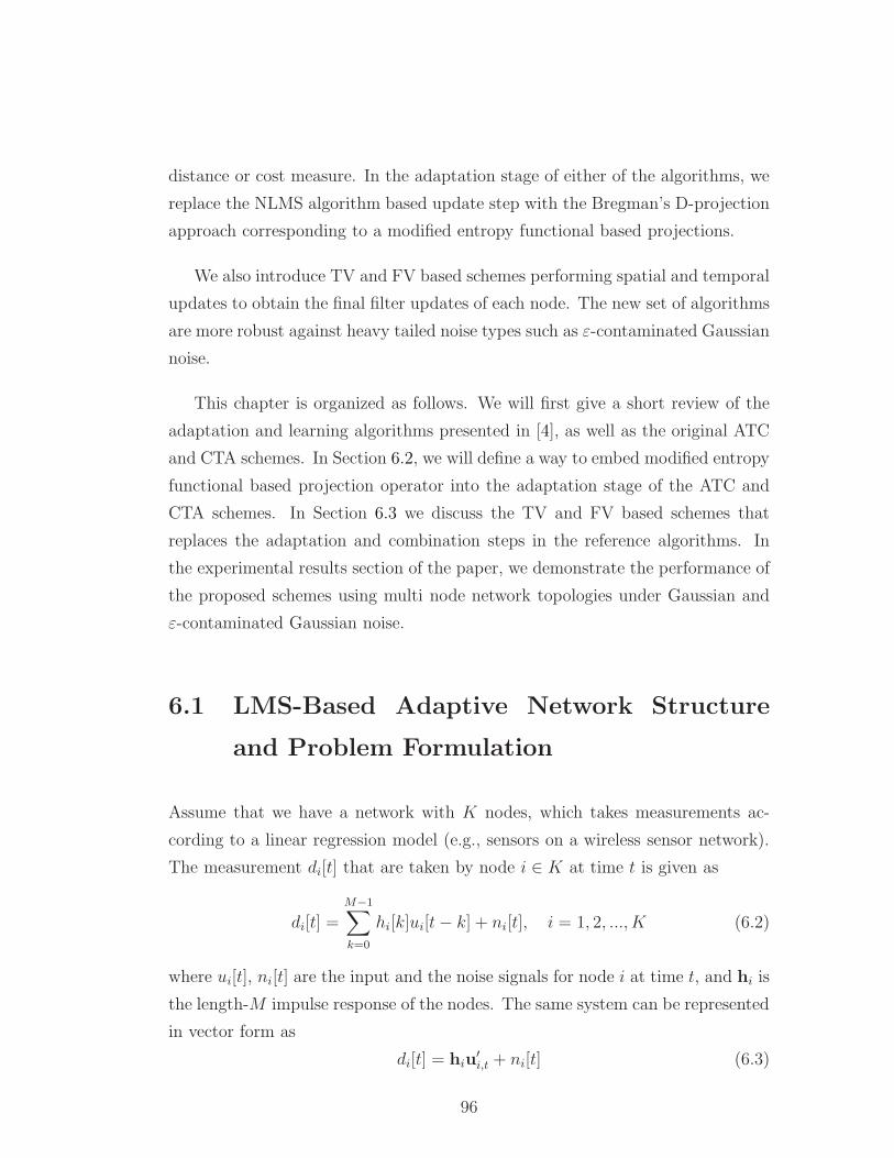
distance or cost measure. In the adaptation stage of either of the algorithms, we
replace the NLMS algorithm based update step with the Bregman’s D-projection
approach corresponding to a modified entropy functional based projections.
We also introduce TV and FV based schemes performing spatial and temporal
updates to obtain the final filter updates of each node. The new set of algorithms
are more robust against heavy tailed noise types such as ε-contaminated Gaussian
noise.
This chapter is organized as follows. We will first give a short review of the
adaptation and learning algorithms presented in [4], as well as the original ATC
and CTA schemes. In Section 6.2, we will define a way to embed modified entropy
functional based projection operator into the adaptation stage of the ATC and
CTA schemes. In Section 6.3 we discuss the TV and FV based schemes that
replaces the adaptation and combination steps in the reference algorithms. In
the experimental results section of the paper, we demonstrate the performance of
the proposed schemes using multi node network topologies under Gaussian and
ε-contaminated Gaussian noise.
6.1 LMS-Based Adaptive Network Structure
and Problem Formulation
Assume that we have a network with K nodes, which takes measurements ac-
cording to a linear regression model (e.g., sensors on a wireless sensor network).
The measurement di[t] that are taken by node i ∈ K at time t is given as
di[t] =M−1∑
k=0
hi[k]ui[t− k] + ni[t], i = 1, 2, ..., K (6.2)
where ui[t], ni[t] are the input and the noise signals for node i at time t, and hi is
the length-M impulse response of the nodes. The same system can be represented
in vector form as
di[t] = hiu′i,t + ni[t] (6.3)
96
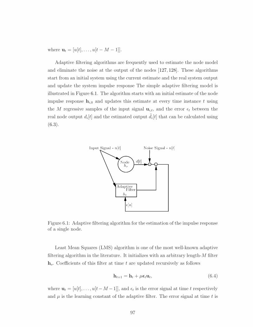
where ut = [u[t], . . . , u[t−M − 1]].
Adaptive filtering algorithms are frequently used to estimate the node model
and eliminate the noise at the output of the nodes [127, 128]. These algorithms
start from an initial system using the current estimate and the real system output
and update the system impulse response The simple adaptive filtering model is
illustrated in Figure 6.1. The algorithm starts with an initial estimate of the node
impulse response hi,0 and updates this estimate at every time instance t using
the M regressive samples of the input signal ui,t, and the error ǫt between the
real node output di[t] and the estimated output di[t] that can be calculated using
(6.3).
Figure 6.1: Adaptive filtering algorithm for the estimation of the impulse responseof a single node.
Least Mean Squares (LMS) algorithm is one of the most well-known adaptive
filtering algorithm in the literature. It initializes with an arbitrary length-M filter
ho. Coefficients of this filter at time t are updated recursively as follows
ht+1 = ht + µǫtut, (6.4)
where ut = [u[t], . . . , u[t−M−1]], and ǫt is the error signal at time t respectively
and µ is the learning constant of the adaptive filter. The error signal at time t is
97
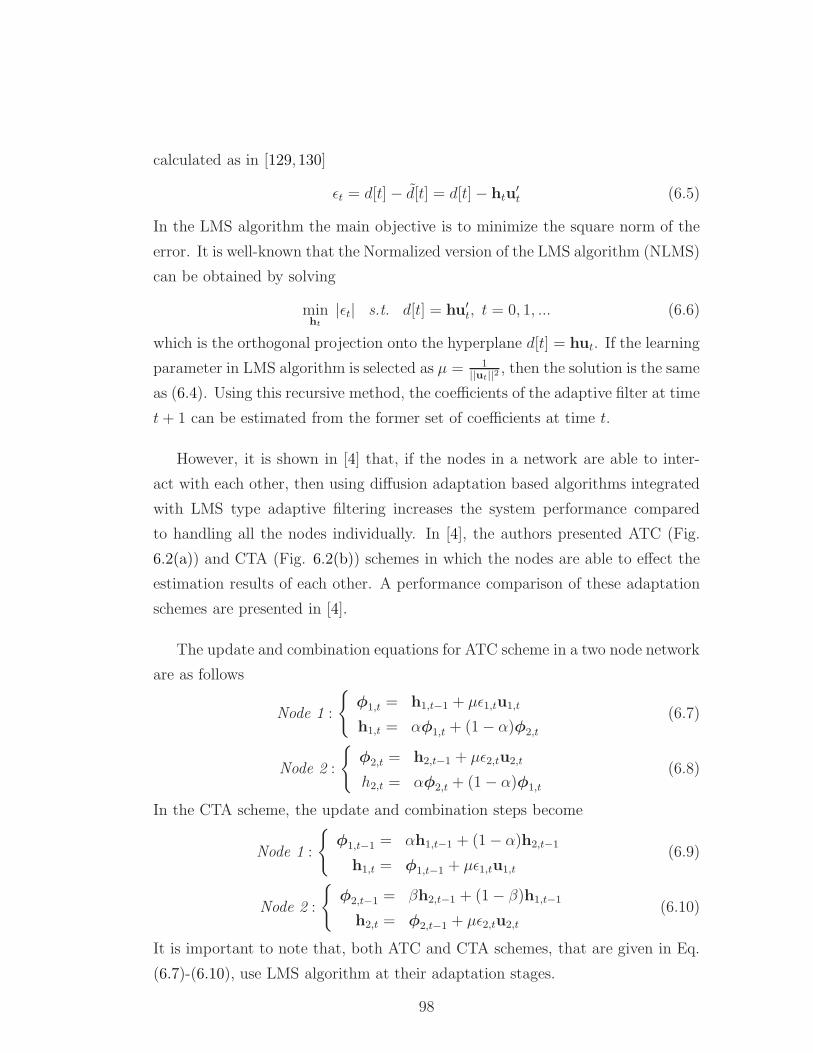
calculated as in [129, 130]
ǫt = d[t]− d[t] = d[t]− htu′t (6.5)
In the LMS algorithm the main objective is to minimize the square norm of the
error. It is well-known that the Normalized version of the LMS algorithm (NLMS)
can be obtained by solving
minht
|ǫt| s.t. d[t] = hu′t, t = 0, 1, ... (6.6)
which is the orthogonal projection onto the hyperplane d[t] = hut. If the learning
parameter in LMS algorithm is selected as µ = 1||ut||2
, then the solution is the same
as (6.4). Using this recursive method, the coefficients of the adaptive filter at time
t+ 1 can be estimated from the former set of coefficients at time t.
However, it is shown in [4] that, if the nodes in a network are able to inter-
act with each other, then using diffusion adaptation based algorithms integrated
with LMS type adaptive filtering increases the system performance compared
to handling all the nodes individually. In [4], the authors presented ATC (Fig.
6.2(a)) and CTA (Fig. 6.2(b)) schemes in which the nodes are able to effect the
estimation results of each other. A performance comparison of these adaptation
schemes are presented in [4].
The update and combination equations for ATC scheme in a two node network
are as follows
Node 1 :
φ1,t = h1,t−1 + µǫ1,tu1,t
h1,t = αφ1,t + (1− α)φ2,t
(6.7)
Node 2 :
φ2,t = h2,t−1 + µǫ2,tu2,t
h2,t = αφ2,t + (1− α)φ1,t
(6.8)
In the CTA scheme, the update and combination steps become
Node 1 :
φ1,t−1 = αh1,t−1 + (1− α)h2,t−1
h1,t = φ1,t−1 + µǫ1,tu1,t
(6.9)
Node 2 :
φ2,t−1 = βh2,t−1 + (1− β)h1,t−1
h2,t = φ2,t−1 + µǫ2,tu2,t
(6.10)
It is important to note that, both ATC and CTA schemes, that are given in Eq.
(6.7)-(6.10), use LMS algorithm at their adaptation stages.
98
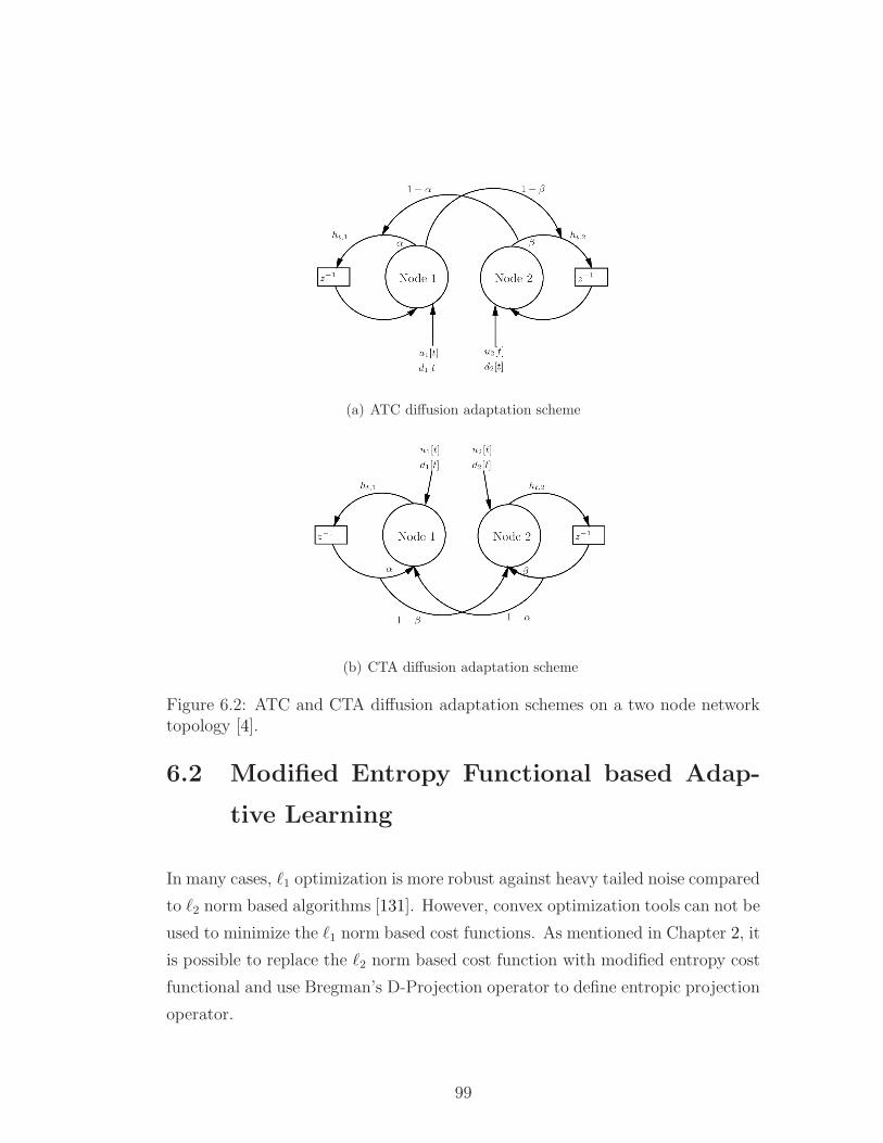
(a) ATC diffusion adaptation scheme
(b) CTA diffusion adaptation scheme
Figure 6.2: ATC and CTA diffusion adaptation schemes on a two node networktopology [4].
6.2 Modified Entropy Functional based Adap-
tive Learning
In many cases, ℓ1 optimization is more robust against heavy tailed noise compared
to ℓ2 norm based algorithms [131]. However, convex optimization tools can not be
used to minimize the ℓ1 norm based cost functions. As mentioned in Chapter 2, it
is possible to replace the ℓ2 norm based cost function with modified entropy cost
functional and use Bregman’s D-Projection operator to define entropic projection
operator.
99
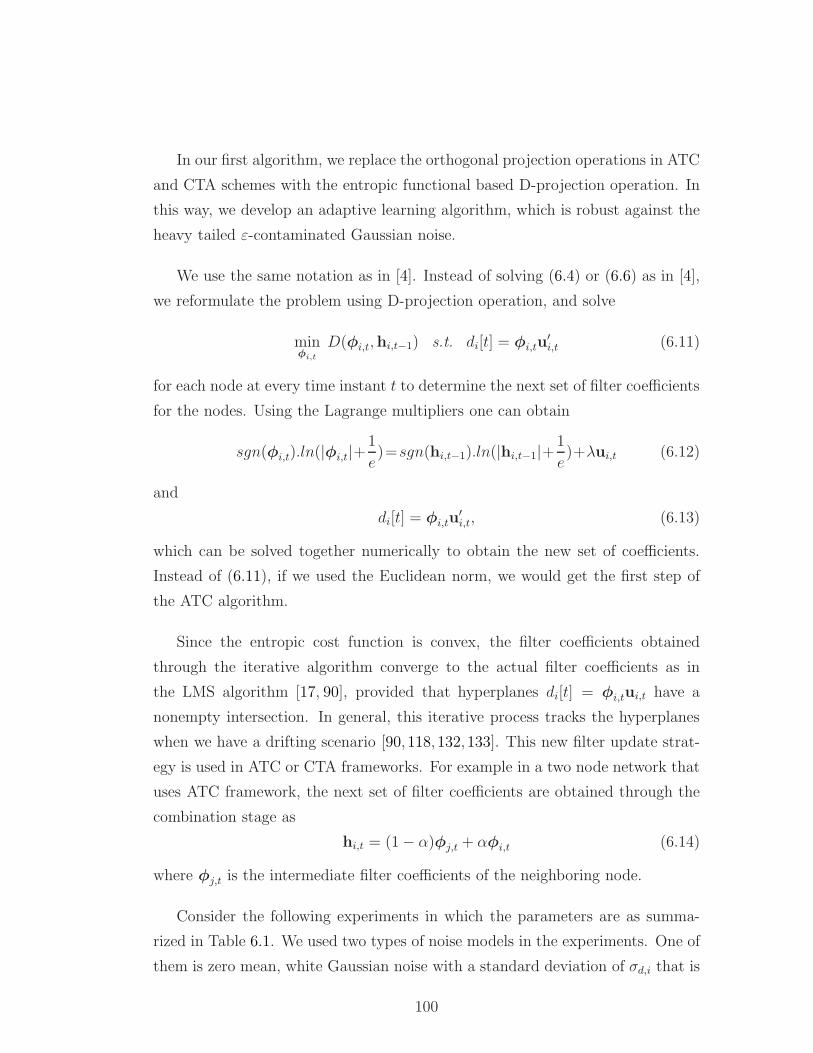
In our first algorithm, we replace the orthogonal projection operations in ATC
and CTA schemes with the entropic functional based D-projection operation. In
this way, we develop an adaptive learning algorithm, which is robust against the
heavy tailed ε-contaminated Gaussian noise.
We use the same notation as in [4]. Instead of solving (6.4) or (6.6) as in [4],
we reformulate the problem using D-projection operation, and solve
minφi,t
D(φi,t,hi,t−1) s.t. di[t] = φi,tu′i,t (6.11)
for each node at every time instant t to determine the next set of filter coefficients
for the nodes. Using the Lagrange multipliers one can obtain
sgn(φi,t).ln(|φi,t|+1
e)=sgn(hi,t−1).ln(|hi,t−1|+
1
e)+λui,t (6.12)
and
di[t] = φi,tu′i,t, (6.13)
which can be solved together numerically to obtain the new set of coefficients.
Instead of (6.11), if we used the Euclidean norm, we would get the first step of
the ATC algorithm.
Since the entropic cost function is convex, the filter coefficients obtained
through the iterative algorithm converge to the actual filter coefficients as in
the LMS algorithm [17, 90], provided that hyperplanes di[t] = φi,tui,t have a
nonempty intersection. In general, this iterative process tracks the hyperplanes
when we have a drifting scenario [90, 118, 132, 133]. This new filter update strat-
egy is used in ATC or CTA frameworks. For example in a two node network that
uses ATC framework, the next set of filter coefficients are obtained through the
combination stage as
hi,t = (1− α)φj,t + αφi,t (6.14)
where φj,t is the intermediate filter coefficients of the neighboring node.
Consider the following experiments in which the parameters are as summa-
rized in Table 6.1. We used two types of noise models in the experiments. One of
them is zero mean, white Gaussian noise with a standard deviation of σd,i that is
100
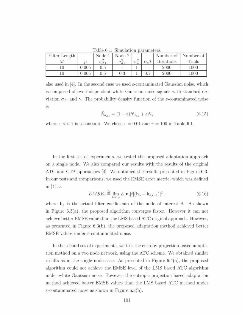
Table 6.1: Simulation parameters.Filter Length Node 1 Node 2 Number of Number of
M µ σ2d,1 σ2
d,2 σ2u α,β Iterations Trials
10 0.005 0.5 - 1 - 2000 100010 0.005 0.5 0.3 1 0.7 2000 1000
also used in [4]. In the second case we used ε-contaminated Gaussian noise, which
is composed of two independent white Gaussian noise signals with standard de-
viation σd,i and γ. The probability density function of the ε-contaminated noise
is
Nσd,i= (1− ε)Nσd,i
+ εNγ (6.15)
where ε << 1 is a constant. We chose ε = 0.01 and γ = 100 in Table 6.1.
In the first set of experiments, we tested the proposed adaptation approach
on a single node. We also compared our results with the results of the original
ATC and CTA approaches [4]. We obtained the results presented in Figure 6.3.
In our tests and comparisons, we used the EMSE error metric, which was defined
in [4] as
EMSEd= lim
t→∞E|ui[t](ho − hd,t−1)|
2 , (6.16)
where ho is the actual filter coefficients of the node of interest d. As shown
in Figure 6.3(a), the proposed algorithm converges faster. However it can not
achieve better EMSE value than the LMS based ATC original approach. However,
as presented in Figure 6.3(b), the proposed adaptation method achieved better
EMSE values under ε-contaminated noise.
In the second set of experiments, we test the entropy projection based adapta-
tion method on a two node network, using the ATC scheme. We obtained similar
results as in the single node case. As presented in Figure 6.4(a), the proposed
algorithm could not achieve the EMSE level of the LMS based ATC algorithm
under white Gaussian noise. However, the entropic projection based adaptation
method achieved better EMSE values than the LMS based ATC method under
ε-contaminated noise as shown in Figure 6.3(b).
101
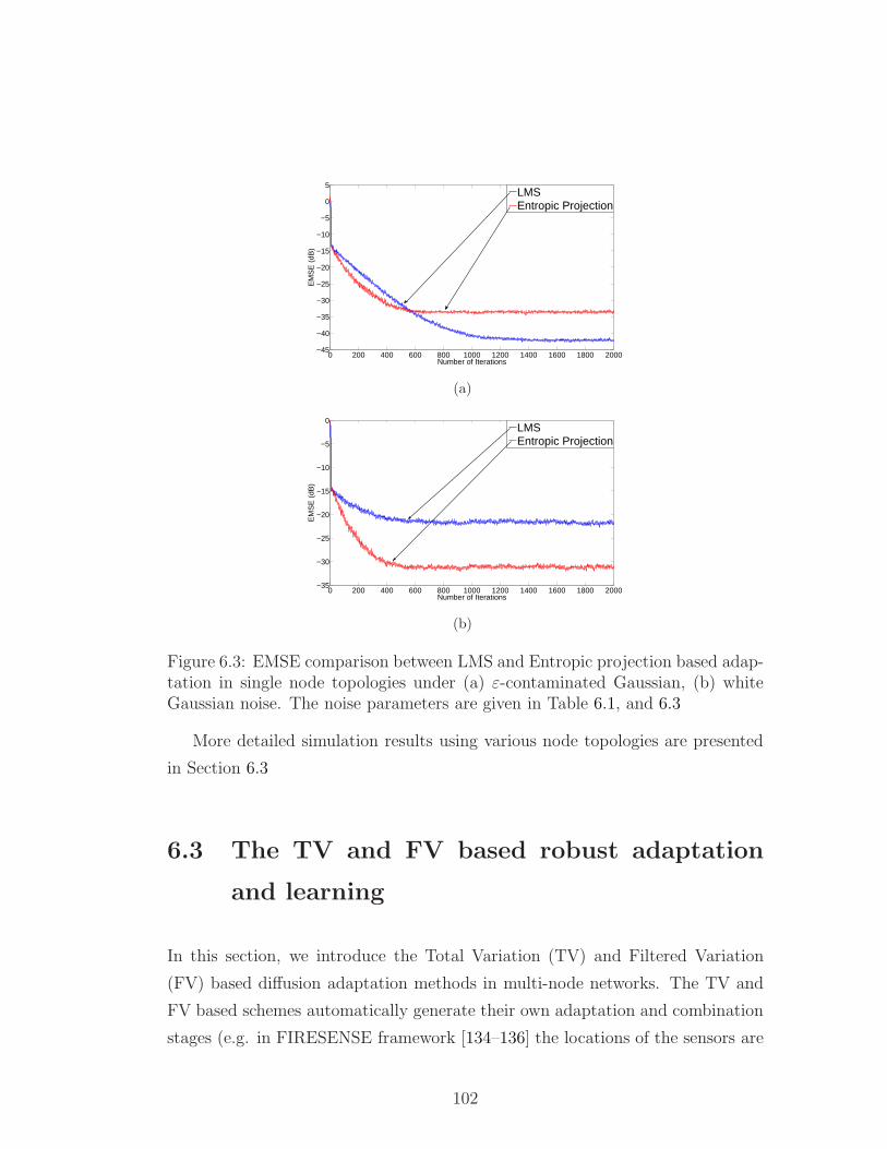
0 200 400 600 800 1000 1200 1400 1600 1800 2000−45
−40
−35
−30
−25
−20
−15
−10
−5
0
5
Number of Iterations
EM
SE
(dB
)
LMSEntropic Projection
(a)
0 200 400 600 800 1000 1200 1400 1600 1800 2000−35
−30
−25
−20
−15
−10
−5
0
Number of Iterations
EM
SE
(dB
)
LMSEntropic Projection
(b)
Figure 6.3: EMSE comparison between LMS and Entropic projection based adap-tation in single node topologies under (a) ε-contaminated Gaussian, (b) whiteGaussian noise. The noise parameters are given in Table 6.1, and 6.3
More detailed simulation results using various node topologies are presented
in Section 6.3
6.3 The TV and FV based robust adaptation
and learning
In this section, we introduce the Total Variation (TV) and Filtered Variation
(FV) based diffusion adaptation methods in multi-node networks. The TV and
FV based schemes automatically generate their own adaptation and combination
stages (e.g. in FIRESENSE framework [134–136] the locations of the sensors are
102
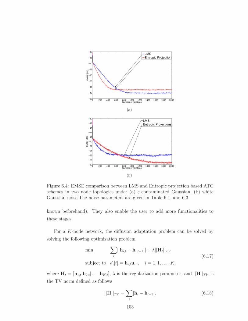
0 200 400 600 800 1000 1200 1400 1600 1800 2000−50
−45
−40
−35
−30
−25
−20
−15
−10
Number of Iterations
EM
SE
(dB
)
LMSEntropic Projection
(a)
0 200 400 600 800 1000 1200 1400 1600 1800 2000−30
−28
−26
−24
−22
−20
−18
−16
−14
−12
−10
Number of Iterations
EM
SE
(dB
)
LMSEntropic Projections
(b)
Figure 6.4: EMSE comparison between LMS and Entropic projection based ATCschemes in two node topologies under (a) ε-contaminated Gaussian, (b) whiteGaussian noise.The noise parameters are given in Table 6.1, and 6.3
known beforehand). They also enable the user to add more functionalities to
these stages.
For a K-node network, the diffusion adaptation problem can be solved by
solving the following optimization problem
min∑
i
||hi,t − hi,t−1||+ λ||Ht||TV
subject to di[t] = hi,tui,t, i = 1, 1, . . . , K,
(6.17)
where Ht = [h1,t|h2,t| . . . |hK,t], λ is the regularization parameter, and ||H||TV is
the TV norm defined as follows
||H||TV =∑
i
|hi − hi−1|. (6.18)
103
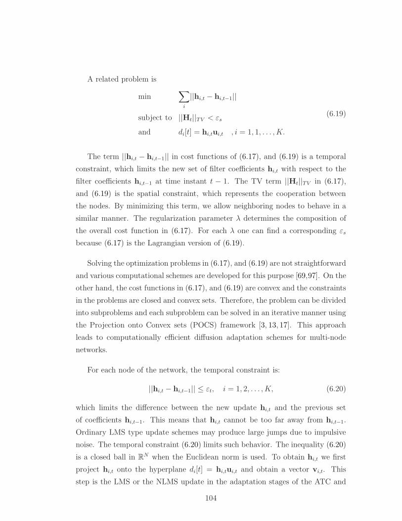
A related problem is
min∑
i
||hi,t − hi,t−1||
subject to ||Ht||TV < εs
and di[t] = hi,tui,t , i = 1, 1, . . . , K.
(6.19)
The term ||hi,t − hi,t−1|| in cost functions of (6.17), and (6.19) is a temporal
constraint, which limits the new set of filter coefficients hi,t with respect to the
filter coefficients hi,t−1 at time instant t − 1. The TV term ||Ht||TV in (6.17),
and (6.19) is the spatial constraint, which represents the cooperation between
the nodes. By minimizing this term, we allow neighboring nodes to behave in a
similar manner. The regularization parameter λ determines the composition of
the overall cost function in (6.17). For each λ one can find a corresponding εs
because (6.17) is the Lagrangian version of (6.19).
Solving the optimization problems in (6.17), and (6.19) are not straightforward
and various computational schemes are developed for this purpose [69,97]. On the
other hand, the cost functions in (6.17), and (6.19) are convex and the constraints
in the problems are closed and convex sets. Therefore, the problem can be divided
into subproblems and each subproblem can be solved in an iterative manner using
the Projection onto Convex sets (POCS) framework [3, 13, 17]. This approach
leads to computationally efficient diffusion adaptation schemes for multi-node
networks.
For each node of the network, the temporal constraint is:
||hi,t − hi,t−1|| ≤ εt, i = 1, 2, . . . , K, (6.20)
which limits the difference between the new update hi,t and the previous set
of coefficients hi,t−1. This means that hi,t cannot be too far away from hi,t−1.
Ordinary LMS type update schemes may produce large jumps due to impulsive
noise. The temporal constraint (6.20) limits such behavior. The inequality (6.20)
is a closed ball in RN when the Euclidean norm is used. To obtain hi,t we first
project hi,t onto the hyperplane di[t] = hi,tui,t and obtain a vector vi,t. This
step is the LMS or the NLMS update in the adaptation stages of the ATC and
104
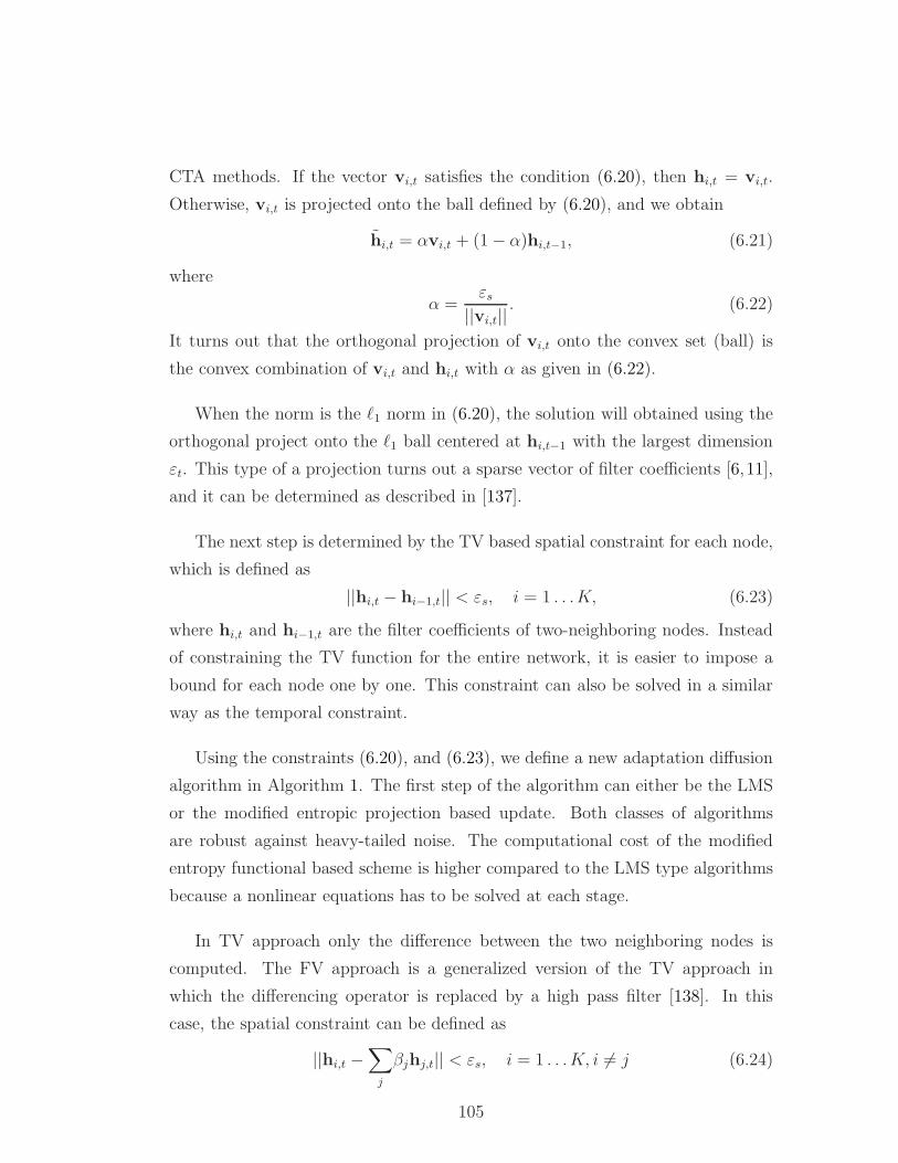
CTA methods. If the vector vi,t satisfies the condition (6.20), then hi,t = vi,t.
Otherwise, vi,t is projected onto the ball defined by (6.20), and we obtain
hi,t = αvi,t + (1− α)hi,t−1, (6.21)
where
α =εs
||vi,t||. (6.22)
It turns out that the orthogonal projection of vi,t onto the convex set (ball) is
the convex combination of vi,t and hi,t with α as given in (6.22).
When the norm is the ℓ1 norm in (6.20), the solution will obtained using the
orthogonal project onto the ℓ1 ball centered at hi,t−1 with the largest dimension
εt. This type of a projection turns out a sparse vector of filter coefficients [6,11],
and it can be determined as described in [137].
The next step is determined by the TV based spatial constraint for each node,
which is defined as
||hi,t − hi−1,t|| < εs, i = 1 . . .K, (6.23)
where hi,t and hi−1,t are the filter coefficients of two-neighboring nodes. Instead
of constraining the TV function for the entire network, it is easier to impose a
bound for each node one by one. This constraint can also be solved in a similar
way as the temporal constraint.
Using the constraints (6.20), and (6.23), we define a new adaptation diffusion
algorithm in Algorithm 1. The first step of the algorithm can either be the LMS
or the modified entropic projection based update. Both classes of algorithms
are robust against heavy-tailed noise. The computational cost of the modified
entropy functional based scheme is higher compared to the LMS type algorithms
because a nonlinear equations has to be solved at each stage.
In TV approach only the difference between the two neighboring nodes is
computed. The FV approach is a generalized version of the TV approach in
which the differencing operator is replaced by a high pass filter [138]. In this
case, the spatial constraint can be defined as
||hi,t −∑
j
βjhj,t|| < εs, i = 1 . . .K, i 6= j (6.24)
105
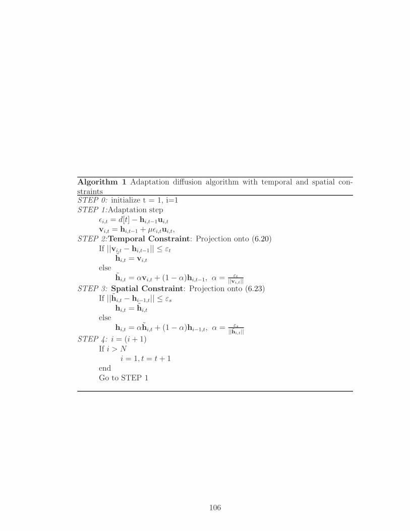
Algorithm 1 Adaptation diffusion algorithm with temporal and spatial con-straintsSTEP 0: initialize t = 1, i=1STEP 1:Adaptation step
ǫi,t = d[t]− hi,t−1ui,t
vi,t = hi,t−1 + µǫi,tui,t,STEP 2:Temporal Constraint: Projection onto (6.20)
If ||vi,t − hi,t−1|| ≤ εthi,t = vi,t
elsehi,t = αvi,t + (1− α)hi,t−1, α = εt
||vi,t||
STEP 3: Spatial Constraint: Projection onto (6.23)If ||hi,t − hi−1,t|| ≤ εs
hi,t = hi,t
elsehi,t = αhi,t + (1− α)hi−1,t, α = εs
||hi,t||
STEP 4: i = (i+ 1)If i > N
i = 1, t = t+ 1endGo to STEP 1
106
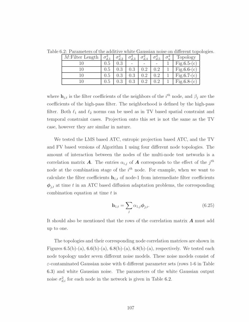
Table 6.2: Parameters of the additive white Gaussian noise on different topologies.M :Filter Length σ2
d,1 σ2d,2 σ2
d,3 σ2d,4 σ2
d,5 σ2u Topology
10 0.5 0.3 - - - 1 Fig.6.5-(c)10 0.5 0.3 0.3 0.2 0.2 1 Fig.6.6-(c)10 0.5 0.3 0.3 0.2 0.2 1 Fig.6.7-(c)10 0.5 0.3 0.3 0.2 0.2 1 Fig.6.8-(c)
where hj,t is the filter coefficients of the neighbors of the ith node, and βj are the
coefficients of the high-pass filter. The neighborhood is defined by the high-pass
filter. Both ℓ1 and ℓ2 norms can be used as in TV based spatial constraint and
temporal constraint cases. Projection onto this set is not the same as the TV
case, however they are similar in nature.
We tested the LMS based ATC, entropic projection based ATC, and the TV
and FV based versions of Algorithm 1 using four different node topologies. The
amount of interaction between the nodes of the multi-node test networks is a
correlation matrix A. The entries αi,j of A corresponds to the effect of the jth
node at the combination stage of the ith node. For example, when we want to
calculate the filter coefficients h1,t of node-1 from intermediate filter coefficients
φj,t at time t in an ATC based diffusion adaptation problems, the corresponding
combination equation at time t is
h1,t =∑
j
α1,jφj,t. (6.25)
It should also be mentioned that the rows of the correlation matrix A must add
up to one.
The topologies and their corresponding node correlation matrices are shown in
Figures 6.5(b)-(a), 6.6(b)-(a), 6.8(b)-(a), 6.8(b)-(a), respectively. We tested each
node topology under seven different noise models. These noise models consist of
ε-contaminated Gaussian noise with 6 different parameter sets (rows 1-6 in Table
6.3) and white Gaussian noise. The parameters of the white Gaussian output
noise σ2d,i for each node in the network is given in Table 6.2.
107
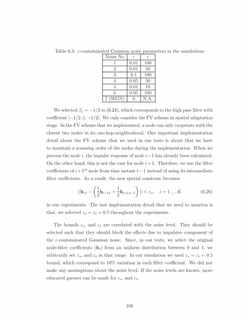
Table 6.3: ε-contaminated Gaussian noise parameters in the simulationsNoise No ε γ
1 0.01 1002 0.01 503 0.1 1004 0.05 505 0.01 106 0.05 100
7 (WGN) 0 N.A.
We selected βj = −1/2 in (6.24), which corresponds to the high pass filter with
coefficient [−1/2, 1,−1/2]. We only consider the FV scheme in spatial adaptation
stage. In the FV scheme that we implemented, a node can only cooperate with the
closest two nodes in its one-hop-neighborhood. One important implementation
detail about the FV scheme that we used in our tests is about that we have
to maintain a scanning order of the nodes during the implementation. When we
process the node i, the impulse response of node i−1 has already been calculated.
On the other hand, this is not the case for node i+1. Therefore, we use the filter
coefficients of i+1st node from time instant t−1 instead of using its intermediate
filter coefficients. As a result, the new spatial constrain becomes
||hi,t −
(
1
2hi−1,t +
1
2hi+1,t−1
)
|| < εs, i = 1 . . .K (6.26)
in our experiments. The last implementation detail that we need to mention is
that, we selected εs = εt = 0.5 throughout the experiments.
The bounds εs, and εt are correlated with the noise level. They should be
selected such that they should block the effects due to impulsive component of
the ε-contaminated Gaussian noise. Since, in our tests, we select the original
node-filter coefficients (hi) from an uniform distribution between 0 and 1, we
arbitrarily set εs, and εt in that range. In our simulation we used εs = εt = 0.5
bound, which correspond to 10% variation in each filter coefficient. We did not
make any assumptions about the noise level. If the noise levels are known, more
educated guesses can be made for εs, and εt.
108
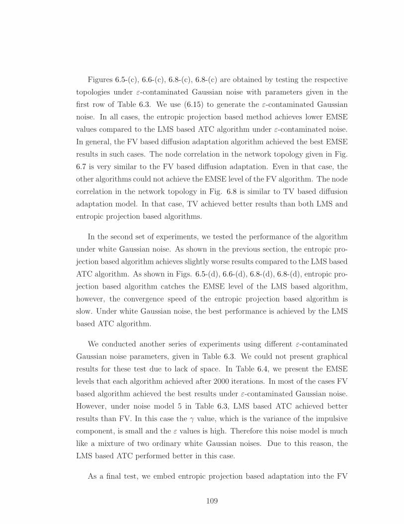
Figures 6.5-(c), 6.6-(c), 6.8-(c), 6.8-(c) are obtained by testing the respective
topologies under ε-contaminated Gaussian noise with parameters given in the
first row of Table 6.3. We use (6.15) to generate the ε-contaminated Gaussian
noise. In all cases, the entropic projection based method achieves lower EMSE
values compared to the LMS based ATC algorithm under ε-contaminated noise.
In general, the FV based diffusion adaptation algorithm achieved the best EMSE
results in such cases. The node correlation in the network topology given in Fig.
6.7 is very similar to the FV based diffusion adaptation. Even in that case, the
other algorithms could not achieve the EMSE level of the FV algorithm. The node
correlation in the network topology in Fig. 6.8 is similar to TV based diffusion
adaptation model. In that case, TV achieved better results than both LMS and
entropic projection based algorithms.
In the second set of experiments, we tested the performance of the algorithm
under white Gaussian noise. As shown in the previous section, the entropic pro-
jection based algorithm achieves slightly worse results compared to the LMS based
ATC algorithm. As shown in Figs. 6.5-(d), 6.6-(d), 6.8-(d), 6.8-(d), entropic pro-
jection based algorithm catches the EMSE level of the LMS based algorithm,
however, the convergence speed of the entropic projection based algorithm is
slow. Under white Gaussian noise, the best performance is achieved by the LMS
based ATC algorithm.
We conducted another series of experiments using different ε-contaminated
Gaussian noise parameters, given in Table 6.3. We could not present graphical
results for these test due to lack of space. In Table 6.4, we present the EMSE
levels that each algorithm achieved after 2000 iterations. In most of the cases FV
based algorithm achieved the best results under ε-contaminated Gaussian noise.
However, under noise model 5 in Table 6.3, LMS based ATC achieved better
results than FV. In this case the γ value, which is the variance of the impulsive
component, is small and the ε values is high. Therefore this noise model is much
like a mixture of two ordinary white Gaussian noises. Due to this reason, the
LMS based ATC performed better in this case.
As a final test, we embed entropic projection based adaptation into the FV
109
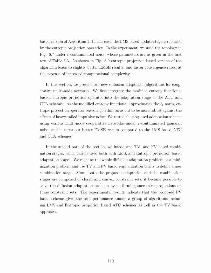
based version of Algorithm 1. In this case, the LMS based update stage is replaced
by the entropic projection operation. In the experiment, we used the topology in
Fig. 6.7 under ε-contaminated noise, whose parameters are as given in the first
row of Table 6.3. As shown in Fig. 6.9 entropic projection based version of the
algorithm leads to slightly better EMSE results, and faster convergence rates, at
the expense of increased computational complexity.
In this section, we present two new diffusion adaptation algorithms for coop-
erative multi-node networks. We first integrate the modified entropy functional
based, entropic projection operator into the adaptation stage of the ATC and
CTA schemes. As the modified entropy functional approximates the ℓ1 norm, en-
tropic projection operator based algorithm turns out to be more robust against the
effects of heavy-tailed impulsive noise. We tested the proposed adaptation scheme
using various multi-node cooperative networks under ε-contaminated gaussian
noise, and it turns out better EMSE results compared to the LMS based ATC
and CTA schemes.
In the second part of the section, we introduced TV, and FV based combi-
nation stages, which can be used both with LMS, and Entropic projection based
adaptation stages. We redefine the whole diffusion adaptation problem as a mini-
mization problem and use TV and FV based regularization terms to define a new
combination stage. Since, both the proposed adaptation and the combination
stages are composed of closed and convex constraint sets, it became possible to
solve the diffusion adaptation problem by performing successive projections on
these constraint sets. The experimental results indicate that the proposed FV
based scheme gives the best perfomance among a group of algorithms includ-
ing LMS and Entropic projection based ATC schemes as well as the TV based
approach.
110
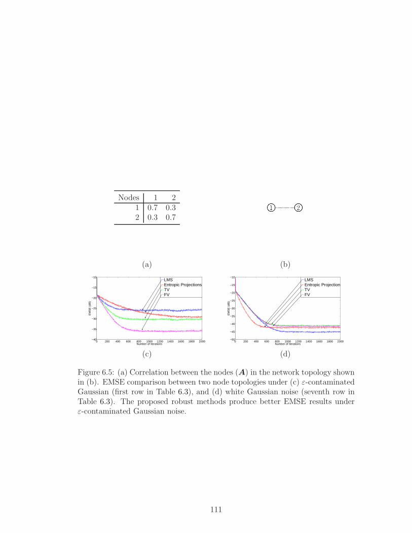
Nodes 1 21 0.7 0.32 0.3 0.7
(a) (b)
0 200 400 600 800 1000 1200 1400 1600 1800 2000−40
−35
−30
−25
−20
−15
−10
Number of Iterations
EM
SE
(dB
)
LMSEntropic ProjectionsTVFV
0 200 400 600 800 1000 1200 1400 1600 1800 2000−50
−45
−40
−35
−30
−25
−20
−15
−10
Number of Iterations
EM
SE
(dB
)
LMSEntropic ProjectionTVFV
(c) (d)
Figure 6.5: (a) Correlation between the nodes (A) in the network topology shownin (b). EMSE comparison between two node topologies under (c) ε-contaminatedGaussian (first row in Table 6.3), and (d) white Gaussian noise (seventh row inTable 6.3). The proposed robust methods produce better EMSE results underε-contaminated Gaussian noise.
111
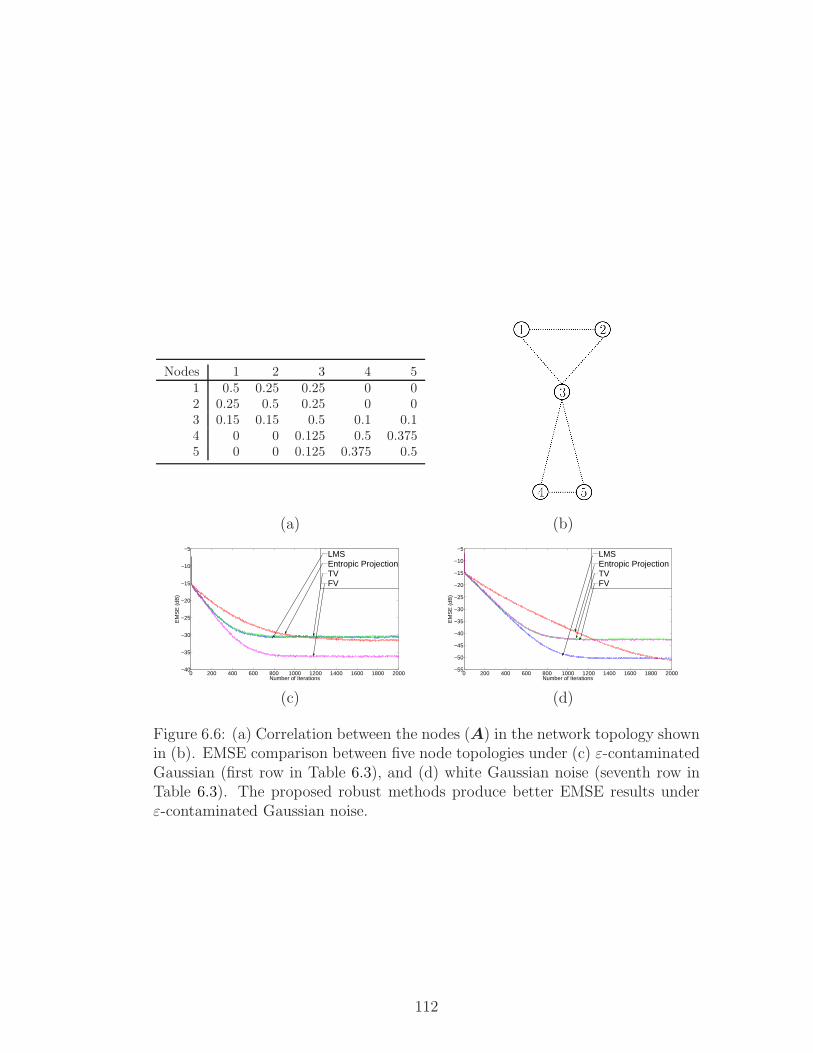
Nodes 1 2 3 4 51 0.5 0.25 0.25 0 02 0.25 0.5 0.25 0 03 0.15 0.15 0.5 0.1 0.14 0 0 0.125 0.5 0.3755 0 0 0.125 0.375 0.5
(a) (b)
0 200 400 600 800 1000 1200 1400 1600 1800 2000−40
−35
−30
−25
−20
−15
−10
−5
EM
SE
(dB
)
Number of Iterations
LMSEntropic ProjectionTVFV
0 200 400 600 800 1000 1200 1400 1600 1800 2000−55
−50
−45
−40
−35
−30
−25
−20
−15
−10
−5
Number of Iterations
EM
SE
(dB
)
LMSEntropic Projection TV FV
(c) (d)
Figure 6.6: (a) Correlation between the nodes (A) in the network topology shownin (b). EMSE comparison between five node topologies under (c) ε-contaminatedGaussian (first row in Table 6.3), and (d) white Gaussian noise (seventh row inTable 6.3). The proposed robust methods produce better EMSE results underε-contaminated Gaussian noise.
112
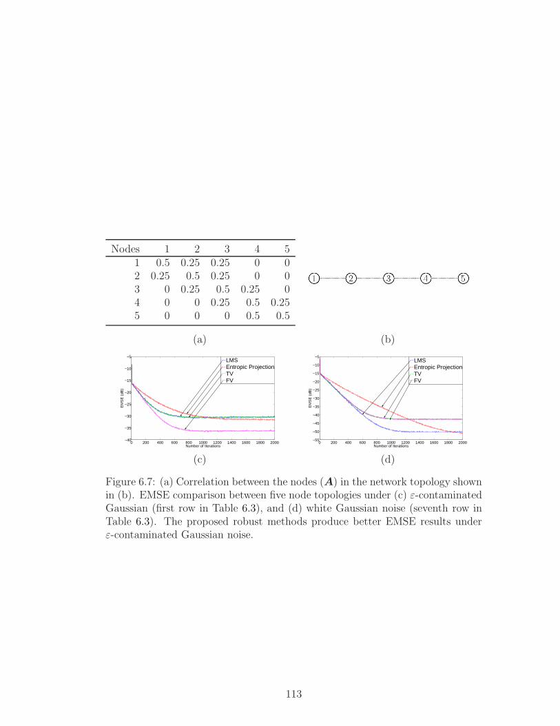
Nodes 1 2 3 4 51 0.5 0.25 0.25 0 02 0.25 0.5 0.25 0 03 0 0.25 0.5 0.25 04 0 0 0.25 0.5 0.255 0 0 0 0.5 0.5
(a) (b)
0 200 400 600 800 1000 1200 1400 1600 1800 2000−40
−35
−30
−25
−20
−15
−10
−5
Number of Iterations
EM
SE
(dB
)
LMSEntropic ProjectionTVFV
0 200 400 600 800 1000 1200 1400 1600 1800 2000−55
−50
−45
−40
−35
−30
−25
−20
−15
−10
−5
Number of Iterations
EM
SE
(dB
)
LMSEntropic ProjectionTVFV
(c) (d)
Figure 6.7: (a) Correlation between the nodes (A) in the network topology shownin (b). EMSE comparison between five node topologies under (c) ε-contaminatedGaussian (first row in Table 6.3), and (d) white Gaussian noise (seventh row inTable 6.3). The proposed robust methods produce better EMSE results underε-contaminated Gaussian noise.
113
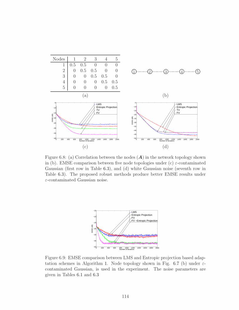
Nodes 1 2 3 4 51 0.5 0.5 0 0 02 0 0.5 0.5 0 03 0 0 0.5 0.5 04 0 0 0 0.5 0.55 0 0 0 0 0.5
(a) (b)
0 200 400 600 800 1000 1200 1400 1600 1800 2000−40
−35
−30
−25
−20
−15
−10
−5
Number of Iterations
EM
SE
(dB
)
LMSEntropic ProjectionTVFV
0 200 400 600 800 1000 1200 1400 1600 1800 2000−50
−45
−40
−35
−30
−25
−20
−15
−10
−5
Number of Iterations
EM
SE
(dB
)
LMSEntropic ProjectionTVFV
(c) (d)
Figure 6.8: (a) Correlation between the nodes (A) in the network topology shownin (b). EMSE comparison between five node topologies under (c) ε-contaminatedGaussian (first row in Table 6.3), and (d) white Gaussian noise (seventh row inTable 6.3). The proposed robust methods produce better EMSE results underε-contaminated Gaussian noise.
0 200 400 600 800 1000 1200 1400 1600 1800 2000−40
−35
−30
−25
−20
−15
−10
EM
SE
(dB
)
Number of Iterations
LMSEntropic ProjectionFVFV −Entropic Projection
Figure 6.9: EMSE comparison between LMS and Entropic projection based adap-tation schemes in Algorithm 1. Node topology shown in Fig. 6.7 (b) under ε-contaminated Gaussian, is used in the experiment. The noise parameters aregiven in Tables 6.1 and 6.3
114
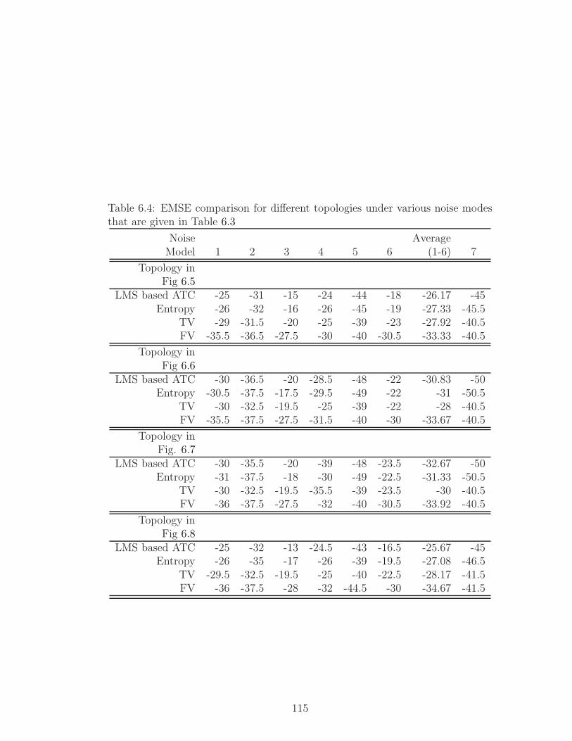
Table 6.4: EMSE comparison for different topologies under various noise modesthat are given in Table 6.3
Noise AverageModel 1 2 3 4 5 6 (1-6) 7
Topology inFig 6.5
LMS based ATC -25 -31 -15 -24 -44 -18 -26.17 -45Entropy -26 -32 -16 -26 -45 -19 -27.33 -45.5
TV -29 -31.5 -20 -25 -39 -23 -27.92 -40.5FV -35.5 -36.5 -27.5 -30 -40 -30.5 -33.33 -40.5
Topology inFig 6.6
LMS based ATC -30 -36.5 -20 -28.5 -48 -22 -30.83 -50Entropy -30.5 -37.5 -17.5 -29.5 -49 -22 -31 -50.5
TV -30 -32.5 -19.5 -25 -39 -22 -28 -40.5FV -35.5 -37.5 -27.5 -31.5 -40 -30 -33.67 -40.5
Topology inFig. 6.7
LMS based ATC -30 -35.5 -20 -39 -48 -23.5 -32.67 -50Entropy -31 -37.5 -18 -30 -49 -22.5 -31.33 -50.5
TV -30 -32.5 -19.5 -35.5 -39 -23.5 -30 -40.5FV -36 -37.5 -27.5 -32 -40 -30.5 -33.92 -40.5
Topology inFig 6.8
LMS based ATC -25 -32 -13 -24.5 -43 -16.5 -25.67 -45Entropy -26 -35 -17 -26 -39 -19.5 -27.08 -46.5
TV -29.5 -32.5 -19.5 -25 -40 -22.5 -28.17 -41.5FV -36 -37.5 -28 -32 -44.5 -30 -34.67 -41.5
115
Chapter 7
CONCLUSIONS
In many signal processing problems, it is possible to have blurred, noisy and/or
irregularly sampled versions of a signal or an image. The inverse problem of
restoring the original signal or image is studied in this thesis. It is assumed that
the signal is sparse in some transform domain such as Fourier, DCT or wavelet
domain. This means that the signal or image can be accurately represented with
some large valued transform coefficients. This assumption has also been used in
transform domain digital waveform coding since 1960’s. In this thesis, inverse
signal processing methods are developed based on sparsity and interval convex
programming.
Inverse signal processing problems are solved by minimizing the ℓ1 norm or
the Total Variation (TV) based cost functions in the literature. In this thesis, a
modified entropy functional approximating the absolute value function is defined.
This functional is also used to approximate the ℓ1 norm, which is the most widely
used cost function in sparse signal processing problems. The modified entropy
functional is continuous, differentiable and convex. As a result a globally con-
vergent iterative compressive sensing (CS) method using the modified entropy
functional is developed. This method is computationally superior to other CS
algorithms because it divides the large inverse problem into smaller problems de-
fined by the rows of the CS measurement matrix. At each step of the algorithm a
D-projection is performed on a hyperplane defined by a row of the measurement
116
matrix. In this way it is possible to solve very large CS problems. Moreover the
solution can be updated online, if a new measurement comes.
Total Variation (TV) based cost functions became recently popular in inverse
signal processing problems using sparsity assumption. We are able to solve the
TV based cost functions using Bregman’s interval convex programming methods
and projection onto convex sets (POCS) theory. Using TV based cost function,
a locally adaptive TV denoising method is developed. The main feature of the
method is that it can relax the TV based cost bound when there is an edge in the
local analysis window. In this way, it is possible to achieve smoothing the image
without blurring the edges.
We generalized the TV concept to Filtered Variation approach by replacing
the differencing operator with a discrete-time high-pass filter. This allows us to
use filters according to the frequency content of the signal, which is more or less
available in some problems.
In this thesis, we also developed two new diffusion adaptation algorithms for
cooperative multi-node networks. The first algorithm uses the modified entropy
functional as the cost functional and the projection operator based on this func-
tional defines an adaptation strategy. We then integrate the entropic projection
operator into the adaptation stage of the problem. According to the experi-
mental results, the new adaptation scheme turns out to be more effective than
the ordinary LMS algorithm against impulsive noise, such as the ǫ-contaminated
Gaussian noise. Since the entropy functional approximates the ℓ1 norm, it is more
robust against the effects of heavy tailed impulsive noise.
In the second class of algorithms, the TV and FV concepts are used to de-
velop diffusion adaptation methods in multi-node networks. By minimizing the
TV and FV cost functions, new adaptation and spatial combination stage equa-
tions in both temporal and spatial dimensions are obtained. In [4], the spatial
combination stage was achieved using alpha-blending. Here the relation between
the alpha-blending and the similarity between the filters of the neighboring nodes
or the similarity between the old set of filter coefficients and the new ones are
established using closed and convex sets, which limit the deviation between the
117
node filters.
Since the adaptation, temporal and spatial combination constraints that are
used in the diffusion adaptation problem are closed and convex sets, it is possible
to solve the individual subproblems in an iterative manner by performing succes-
sive orthogonal projections onto the sets. Moreover, this approach enables the
users to insert any other convex and closed constraint into the diffusion adap-
tation problem, according to their needs. It is possible to embed the entropy
functional based algorithm into adaptation stage if the TV and FV based frame-
works. The experimental results indicate that the new class of the algorithms
perform similar to ATC and CTA methods [4] under white Gaussian noise. They
perform better under ε-contaminated Gaussian noise. As in the original ATC
and CTA frameworks, when the cooperation between the nodes increases, the
performance of the proposed algorithms also increases.
Sparsity assumption is a reasonable assumption and it helps the signal inter-
polation, reconstruction, and restoration process in inverse problems. However,
it sometimes oversimplifies or oversmoothes the signal because practical signals
cannot be represented with a couple of transform domain coefficients in general.
For example in transform domain signal, image, and video coding, the signal is
divided into blocks and some smooth blocks are represented with a few trans-
form domain coefficients. On the other hand, some block contain high-frequency
information and the coder may even have to use all the transform domain co-
efficients to represent the block. In signal interpolation problem, a signal with
sharp edge is used as an example. Interpolators using the sparsity assumption
do not produce any good interpolation results. To solve this problem, transition
band and stopband concepts from the discrete-time filtering theory is used. In
this way, the reconstructed signal is allowed to have some high-frequency coeffi-
cients in transform domain. This led to better interpolation results than sparsity
assumption.
118
APPENDIX A
Proof of Convergence of the
Iterative Algorithm
The problem described in (2.2) and(2.8) is a convex programming problem
mins∈H
g(s)
subject to θi.s = yi for i = 1, 2, ...,M ,(A.1)
where g(s) is a strictly convex and differentiable cost function in RN , H is
the intersection of M hyperplanes θi.s = yi, and s ∈ RN . In [13], Bregman
solved the convex optimization problem (A.1) using D-Projections. He proved
in [13](Theorem 3) that starting from an initial point s0 = 0, and making suc-
cessive D-projections on convex hyperplanes as defined by θi.s = yi (Chapter 3),
converges to the solution of the convex optimization problem, provided that H is
non empty.
Statement 1: The function g(x) = (|x|+ 1e) log(|x|+ 1
e) + 1
eis continuously
differentiable in R.
Proof: The derivative of the cost function g(x) can be computed using the
119
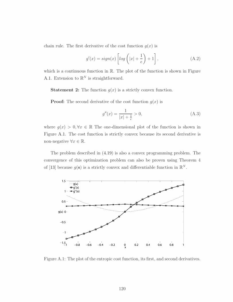
chain rule. The first derivative of the cost function g(x) is
g′(x) = sign(x)
[
log
(
|x|+1
e
)
+ 1
]
, (A.2)
which is a continuous function in R. The plot of the function is shown in Figure
A.1. Extension to RN is straightforward.
Statement 2: The function g(x) is a strictly convex function.
Proof: The second derivative of the cost function g(x) is
g′′(x) =1
|x|+ 1e
> 0, (A.3)
where g(x) > 0, ∀x ∈ R The one-dimensional plot of the function is shown in
Figure A.1. The cost function is strictly convex because its second derivative is
non-negative ∀x ∈ R.
The problem described in (4.19) is also a convex programming problem. The
convergence of this optimization problem can also be proven using Theorem 4
of [13] because g(s) is a strictly convex and differentiable function in RN .
Figure A.1: The plot of the entropic cost function, its first, and second derivatives.
120
APPENDIX B
Proof of Convexity of the
Filtered Variation Constraints
B.1 ℓ1 Filtered Variation Bound
The set
C1 =
x :N−1∑
k=0
|H [k]X [k]| ≤ ε1
(B.1)
defines the ℓ1 filtered variation bound constraint set. Let’s assume that X1,X2 ∈
C1. To prove the convexity of set C1, we need to check if
X3 = αX1 + (1− α)X2, ∀α ∈ [0, 1] (B.2)
satisfies the following condition
N−1∑
k=0
|H [k]X3[k]| ≤ ε1. (B.3)
Using (B.2), one can rewrite (B.3) as follows
|H [k]X3[k]| =
N−1∑
k=0
|H [k](αX1[k] + (1− α)X2[k]))| (B.4)
=N−1∑
k=0
|(αH [k]X1[k]) + ((1− α)H [k]X2[k]))| (B.5)
121
. Using triangle inequality in (B.5)
|H [k]X3[k]| ≤N−1∑
k=0
α |(H [k]X1[k])|+ (1− α) |(H [k]X2[k]))| (B.6)
=α
(
N−1∑
k=0
|(H [k]X1[k])|
)
+ (1− α)
(
N−1∑
k=0
|(H [k]X2[k])|
)
(B.7)
≤ε1. (B.8)
Therefore, C1 is a convex constraint set.
B.2 Time and Space Domain Local Variation
Bounds
Let’s consider the time and space domain local variation bound
C2 =
x :
∣
∣
∣
∣
∣
l∑
i=−l
h[i]x[n − i]
∣
∣
∣
∣
∣
≤ P
, (B.9)
Let’s assume that x1,x2 ∈ C2. We would like to check if x3 = αx1 + (1− α)x2 ∈
C2, ∀α ∈ [0, 1]. If this condition is satisfied, then C2 defines a convex constraint
set.
For the convexity of C2 set, x3 should satisfy the condition (B.9) as
∣
∣
∣
∣
∣
l∑
i=−l
h[i]x3[n− i]
∣
∣
∣
∣
∣
≤ P. (B.10)
It is possible to rewrite (B.10) as
∣
∣
∣
∣
∣
l∑
i=−l
h[i]x3[n− i]
∣
∣
∣
∣
∣
=
∣
∣
∣
∣
∣
l∑
i=−l
h[i](αx1[n− i] + (1− α)x2[n− i]
∣
∣
∣
∣
∣
. (B.11)
=
∣
∣
∣
∣
∣
l∑
i=−l
(αh[i]x1[n− i]) + ((1− α)h[i]x2[n− i])
∣
∣
∣
∣
∣
. (B.12)
122
. Using triangle inequality in (B.12)
≤α
∣
∣
∣
∣
∣
l∑
i=−l
(h[i]x1[n− i])
∣
∣
∣
∣
∣
+ (1− α)
∣
∣
∣
∣
∣
l∑
i=−l
(h[i]x2[n− i])
∣
∣
∣
∣
∣
. (B.13)
≤P (B.14)
Therefore, C2 is a convex constraint.
B.3 Bound on High Frequency Energy
Let’s consider the bound on high frequency energy
C3 =
x :
N−k0∑
k=k0
|X [k]|2 ≤ ε3
. (B.15)
Let’s assume that X1,X2 ∈ C3. we would like to check if X3 = αX1+(1−α)X2 ∈
S3, ∀α ∈ [0, 1]. If this condition is satisfied, then C3 is a convex constraint set.
For the convexity of C3 set, X3 should satisfy the condition (B.15) as
N−k0∑
k=k0
|X3[k]|2 ≤ ε3 (B.16)
It is possible to rewrite (B.16) as
N−k0∑
k=k0
|X3[k]|2 =
N−k0∑
k=k0
|αX1[k] + (1− α)X2[k]|2 (B.17)
Since |.|2 is a convex function, using definition of convexity of a function given in
(3.1) of [139], one can rewrite (B.17) as
N−k0∑
k=k0
|αX1[k] + (1− α)X2[k]|2 ≤α
(
N−k0∑
k=k0
|X1[k]
)
+ (1− α)
(
N−k0∑
k=k0
|X2[k]
)
(B.18)
≤ε3 (B.19)
Therefore, C3 is a convex constraint.
123
B.4 Sample Value Locality Constraint
The Sample Value Locality Constraint is defined as
C7 = x : |x[n]− y[n]| < δ , (B.20)
where x[n] and y[n] are nth samples from the signals x, and y. Let’s assume that
for x1[n], x2[n] ∈ C7. Let’s assume that x1[n], x2[n] ∈ C7. We would like to check
if x3[n] = αx1[n] + (1 − α)x2[n] ∈ C7, ∀α ∈ [0, 1]. If this condition is satisfied,
then C7 is a convex constraint set.
Therefore, one needs to check if the following condition holds:
|x3[n]− y[n]| << δ. (B.21)
It is possible to rewrite (B.21) as
|x3[n]− y[n]| = |αx1[n] + (1− α)x2[n]− y[n]| (B.22)
= |α(x1[n]− y[n]) + (1− α)(x2[n]− y[n])| (B.23)
= α |(x1[n]− y[n]) |+(1− α)| (x2[n]− y[n])| (B.24)
≤ δ (B.25)
Therefore, C7 is a convex constraint.
124
Bibliography
[1] G. Gilboa, “Shock Filters” Accessed at September 2012. [Online].
Available: http://visl.technion.ac.il/∼gilboa/PDE-filt/shock filters.html
[2] J. E. Fowler, S. Mun, and E. W. Tramel, “Block-based compressed sensing
of images and video,” Foundations and Trends in Signal Processing, vol. 4,
no. 4, pp. 297–416, March 2012.
[3] P. L. Combettes and J. Pesquet, “Image restoration subject to a total vari-
ation constraint,” IEEE Transactions on Image Processing, vol. 13, pp.
1213–1222, 2004.
[4] X. Zhao and A. H. Sayed, “Performance limits of lms-based adaptive net-
works,” in International Conference on Acoustics, Speech and Signal Pro-
cessing (ICASSP), IEEE, May 2011, pp. 3768 –3771.
[5] C. E. Shannon, “Communication in the presence of noise,” Proceedings of
the Institute of Radio Engineers, vol. 37, no. 1, pp. 10–21, 1949. [Online].
Available: http://ieeexplore.ieee.org/xpls/abs all.jsp?arnumber=1697831
[6] E. Candes, “Compressive sampling,” in Proceedings of International
Congress of Mathematics, vol. 3, 2006, pp. 1433–1452.
[7] J.-L. Starck and F. Murtagh, Astronomical Image and Data Analysis.
Springer-Verlag, 2006.
[8] W. Hardle, G. Kerkyacharian, D. Picard, and A. Tsybakov, Wavelets, Ap-
proximation and Statistical Applications, W. Hardle, G. Kerkyacharian,
D. Picard, and A. Tsybakov, Eds. Springer, 1998.
125
[9] I. M. Johnstone, “Wavelets and the theory of nonparametric function es-
timation,” Philosophical Transactions of the Royal Society of London, vol.
357, pp. 2475–2493, September S1999.
[10] J.-L. Starck, M. F., and J. M. Fadilli, Sparse Image and Signal Processing:
Wavelets, Curvelets, Morphological Diversity. Cambridge University Press,
2010.
[11] E. J. Candes and T. Tao, “Near-optimal signal recovery from random
projections: Universal encoding strategies?” IEEE Transactions on Infor-
mation Theory, vol. 52, no. 12, pp. 5406–5425, 2006. [Online]. Available:
http://ieeexplore.ieee.org/lpdocs/epic03/wrapper.htm?arnumber=4016283
[12] Y. Censor and A. Lent, “An iterative row-action method for interval convex
programming,” Journal of Optimization Theory and Applications, vol. 34,
no. 3, pp. 321–353, 1981.
[13] L. M. Bregman, “The Relaxation Method of Finding the Common Point
of Convex Sets and Its Application to the Solution of Problems in Con-
vex Programming,” USSR Computational Mathematics and Mathematical
Physics, vol. 7, pp. 200–217, 1967.
[14] S. Osher, Y. Mao, B. Dong, and W. Yin, “Fast linearized bregman iter-
ation for compressive sensing and sparse denoising,” Communications in
Mathematical Sciences, vol. 8(1), pp. 93–111, 2010.
[15] J.-F. Cai, S. Osher, and Z. Shen, “Linearized bregman iterations for com-
pressed sensing,” Mathematics of Computation, vol. 78, no. 267, pp. 1515–
1536, 2009.
[16] L. I. Rudin, S. Osher, and E. Fatemi, “Nonlinear total variation based
noise removal algorithms,” Phys. D, vol. 60, pp. 259–268, November 1992.
[Online]. Available: http://dx.doi.org/10.1016/0167-2789(92)90242-F
[17] D. C. Youla and H. Webb, “Image restoration by the method of convex
projections, part i-theory,” IEEE Transactions on Medical Imaging, vol.
MI-I-2, pp. 81–94, 1982.
126
[18] D. Needell and J. A. Tropp, “CoSaMP: Iterative signal recovery from in-
complete and inaccurate samples,” 2008, arXiv:0803.2392v2.
[19] A. Chambolle, “An algorithm for total variation minimization and appli-
cations,” Journal of Mathematical Imaging and Vision, vol. 20, pp. 89–97,
2004.
[20] K. Kose, A. Cetin, and O. Gunay, “Entropy minimization based robust
algorithm for adaptive networks,” in Proceedings of Signal Processing and
Communications Applications Conference (SIU), April 2012, pp. 1 –4.
[21] G. Baraniuk, “Compressed sensing [lecture notes],” IEEE Signal Processing
Magazine, vol. 24, no. 4, pp. 118–124, 2007.
[22] E. J. Candes, J. Romberg, and T. Tao, “Robust uncertainty
principles: exact signal reconstruction from highly incomplete fre-
quency information,” IEEE Transactions on Information Theory,
vol. 52, no. 2, pp. 489–509, February 2006. [Online]. Available:
http://dx.doi.org/10.1109/TIT.2005.862083
[23] Y. Tsaig and D. L. Donoho, “Compressed sensing,” IEEE Transaction on
Information Theory, vol. 52, pp. 1289–1306, 2006.
[24] R. Baraniuk, V. Cevher, M. Duarte, and C. Hegde, “Model-based compres-
sive sensing,” IEEE Transactions on Information Theory, vol. 56, no. 4,
pp. 1982 –2001, April 2010.
[25] S. S. Chen, “Basis pursuit,” Ph.D. dissertation, Stanford University, 1995.
[26] S. S. Chen, D. L. Donoho, and M. A. Saunders, “Atomic decomposition by
basis pursuit,” SIAM Review, vol. 43, pp. 129–159, 2001.
[27] A. Beck and M. Teboulle, “A fast iterative shrinkage-thresholding algorihm
for linear inverse problems,” SIAM Journal of Imaging Sciences, vol. 2,
no. 1, pp. 183–202, 209.
[28] M. A. T. Figueiredo, D. R. Nowak, and S. J. Wright, “Gradient projection
for sparse reconstruction: Application to compressed sensing and other
127
inverse problems,” IEEE Journal of Selected Topics in Signal Processing,
vol. 1, no. 4, pp. 586 –597, December 2007.
[29] J. Friedman, T. Hastie, and R. Tibshirani, “Regularization paths for gener-
alized linear models via coordinate descent,” Journal of Statistical Software,
vol. 33(1), pp. 1–22, 2010.
[30] E. T. Hale, W. Yin, and Y. Zhang, “A fixed-point continuation method
for l1 -regularized minimization with applications to compressed sensing,”
Rice University, Technical Report, TR07-07, 2007.
[31] T. Blumensath and M. E. Davies, “Iterative hard thresholding for com-
pressed sensing,” Applied and Computational Harmonic Analysis, vol. 27
(3), pp. 265–274, November 2009.
[32] J. A. Tropp, Anna, and C. Gilbert, “Signal recovery from random mea-
surements via orthogonal matching pursuit,” IEEE Trans. Inform. Theory,
vol. 53, pp. 4655–4666, 2007.
[33] D. L. Donoho, Y. Tsaig, I. Drori, and J. luc Starck, “Sparse solution of un-
derdetermined linear equations by stagewise orthogonal matching pursuit,”
Technical Report, 2006.
[34] D. Needell and R. Vershynin, “Signal recovery from incomplete and inac-
curate measurements via regularized orthogonal matching pursuit.”
[35] M. Pilanci, A. C. Gurbuz, and A. O., “Expectation maximization based
matching pursuit,” in IEEE International Conference on Acoustics, Speech
and Signal Processing (ICASSP), March 2012.
[36] D. Mark A., D. Marco F., E. Yonina, and K. Gitta, Compressed Sensing:
Theory and Applications, E. Yonina and G. Kutyniok., Eds. Cambridge
University Press, June, 2012.
[37] A. C. Gilbert, M. J. Strauss, J. A. Tropp, and R. Vershynin, “One
sketch for all: fast algorithms for compressed sensing,” in Proceedings of
the Thirty-Ninth Annual ACM Symposium on Theory of Computing, ser.
128
STOC ’07. New York, NY, USA: ACM, 2007, pp. 237–246. [Online].
Available: http://doi.acm.org/10.1145/1250790.1250824
[38] M. A. Iwen, “Combinatorial sublinear-time fourier algorithms,” Founda-
tions of Computational Mathematics, vol. 10 (3), pp. 303–338, 2010.
[39] M. F. Duarte, M. A. Davenport, D. Takhar, J. N. Laska, T. Sun, K. F.
Kelly, and R. G. Baraniuk, “Single-pixel imaging via compressive sam-
pling,” IEEE Signal Processing Magazine, vol. 25, no. 2, pp. 83 –91, 2008.
[40] M. B. Wakin, J. N. Laska, M. F. Duarte, D. Baron, S. Sarvotham,
D. Takhar, K. F. Kelly, and R. G. Baraniuk, “An architecture for compres-
sive imaging,” in Proceedings of IEEE International Conference on Image
Processing (ICIP), 2006, pp. 1273–1276.
[41] ——, “Compressive imaging for video representation and coding,” in Pro-
ceedings of Picture Coding Symposium (PCS), 2006.
[42] V. Cevher, A. Sankaranarayanan, M. F. Duarte, D. Reddy, and R. G. Bara-
niuk, “Compressive sensing for background subtraction,” in Proceedings of
European Conference on Computer Vision (ECCV), 2008, pp. 155–168.
[43] M. Lustig, J. M. Santos, J. hyung Lee, D. L. Donoho, and J. M. Pauly,
“Application of compressed sensing for rapid MR imaging,” in Proceed-
ings of Signal Processing with Adaptative Sparse Structured Representations
(SPARS), 2005.
[44] J. Trzasko and S. Member, “Highly undersampled magnetic resonance
image reconstruction via homotopic ℓ0-minimization,” IEEE Trans. Med.
Imaging, pp. 106–121, 2009.
[45] T. Cukur, M. Lustig, E. Saritas, and D. Nishimura, “Signal compensation
and compressed sensing for magnetization-prepared mr angiography,” IEEE
Transactions on Medical Imaging, vol. 30, no. 5, pp. 1017–1027, May 2011.
[46] T. Cukur, M. Lustig, and D. Nishimura, “Improving non-contrast-enhanced
steady-state free precession angiography with compressed sensing,” Mag-
netic Resonance Med., vol. 61, no. 5, pp. 1122–1131, May 2009.
129
[47] J. Provost and F. Lesage, “The application of compressed sensing for photo-
acoustic tomography,” Medical Imaging, IEEE Transactions on, vol. 28,
no. 4, pp. 585 –594, april 2009.
[48] J. Choi, M. W. Kim, W. Seong, and J. C. Ye, “Compressed sensing metal
artifact removal in dental ct,” in Proceedings of IEEE International Sym-
posium on Biomedical Imaging: From Nano to Macro, 2009.
[49] R. Willettt, M. Gehm, and D. Brady, “Multiscale reconstruction for com-
putational spectral imaging,” in SPIE Electronic Imaging, Computational
Imaging V., vol. 6498, 2007, p. 64980L.
[50] S. Gazit, A. Szameit, Y. C. Eldar, and M. Segev, “Super-resolution and
reconstruction of sparse sub-wavelength images,” Optics Express, vol. 17,
no. 26, pp. 23 920–23 946, December 2009.
[51] A. Bourquard, F. Aguet, and M. Unser, “Optical imaging using binary
sensors,” Optics Express, vol. 18, no. 5, pp. 4876–4888, March 2010.
[52] D. J. Brady, K. Choi, D. L. Marks, R. Horisaki, and S. Lim, “Compressive
holography,” Optics Express, vol. 17, no. 15, pp. 13 040–13 049, July 2009.
[53] Y. Rivenson, A. Stern, and J. Rosen, “Compressive multiple view projec-
tion incoherent holography,” Optics Express, vol. 19, no. 7, pp. 6109–6118,
March 2011.
[54] L. Denis, D. Lorenz, E. Thiebaut, C. Fournier, and D. Trede, “Inline
hologram reconstruction with sparsity constraints,” Optics Letters, vol. 34,
no. 22, pp. 3475–3477, November 2009.
[55] W. Dai, M. A. Sheikh, O. Milenkovic, and R. G. Baraniuk, “Compres-
sive sensing dna microarrays,” EURASIP Journal on Bioinformatics and
Systems Biology, vol. 2009, no. 1, 2009.
[56] A. Griffin, T. Hirvonen, C. Tzagkarakis, A. Mouchtaris, and P. Tsakalides,
“Single-channel and multi-channel sinusoidal audio coding using com-
pressed sensing,” IEEE Transactions on Audio, Speech, and Language Pro-
cessing, vol. 19, no. 5, pp. 1382 –1395, July 2011.
130

[57] R. Baraniuk, “Compressive radar imaging,” in Proceedings of IEEE Radar
Conference, 2007, pp. 128–133.
[58] J. H. Ender, “On compressive sensing applied to radar,” Signal Processing,
vol. 90, no. 5, pp. 1402 – 1414, 2010.
[59] R. Moses, M. Cetin, and L. Potter, “Wide angle SAR imaging,” in Proceed-
ings of SPIE Algorithms for Synthetic Aperture Radar Imagery XI, 2004.
[60] J. Ma, “Improved iterative curvelet thresholding for compressed sensing and
measurement,” IEEE Transactions on Instrumentation and Measurement,
vol. 60, no. 1, pp. 126 –136, January 2011.
[61] ——, “Single-pixel remote sensing,” IEEE Geoscience and Remote Sensing
Letters, vol. 6, no. 2, pp. 199 –203, April 2009.
[62] M. Mishali and Y. C. Eldar, “Wideband spectrum sensing at sub-nyquist
rates [Applications Corner],” IEEE Signal Processing Magazine, vol. 28,
no. 4, pp. 102–135, 2011.
[63] C. R. Berger, Z. Wang, J. Huang, and S. Zhou, “Application of compressive
sensing to sparse channel estimation,” IEEE Communications Magazine,
vol. 48, no. 11, pp. 164–174, 2010.
[64] C. R. Berger, S. Zhou, J. C. Preisig, and P. Willett, “Sparse channel esti-
mation for multicarrier underwater acoustic communication: from subspace
methods to compressed sensing,” IEEE Transactions on Signal Processing,
vol. 58, no. 3, pp. 1708–1721, 2010.
[65] D. Gross, Y.-K. Liu, S. T. Flammia, S. Becker, and J. Eisert, “Quantum
state tomography via compressed sensing,” Physical Review Letters, vol.
105, p. 150401, October 2010.
[66] A. Shabani, R. L. Kosut, M. Mohseni, H. Rabitz, M. A. Broome, M. P.
Almeida, A. Fedrizzi, and A. G. White, “Efficient measurement of quan-
tum dynamics via compressive sensing,” Physical Review Letters, vol. 106,
March 2011.
131
[67] L. Rudin, “Images, Numerical Analysis of Singularities and Shock Filters,”
Ph.D. dissertation, California Institute of Technology, Pasadena, California,
1987.
[68] S. Osher and L. I. Rudin, “Feature oriented image enhancement using shock
filters,” SIAM Journal of Numerical Analysis, vol. 27, p. 919, 1990.
[69] S. Osher, M. Burger, D. Goldfarb, J. Xu, and W. Yin, “An iterative reg-
ularization method for total variation-based image restoration,” Multiscale
Modelling and Simulation, vol. 4, pp. 460–489, 2005.
[70] P. Combettes, “The foundations of set theoretic estimation,” Proceedings
of the IEEE, vol. 81, no. 2, pp. 182 –208, February 1993.
[71] D. Butnariu, R. Davidi, G. Herman, and I. Kazantsev, “Stable convergence
behavior under summable perturbations of a class of projection methods
for convex feasibility and optimization problems,” IEEE Journal of Selected
Topics in Signal Processing, vol. 1, no. 4, pp. 540 –547, December 2007.
[72] F. Malgouyres, “Minimizing the total variation under a general convex con-
straint for image restoration,” IEEE Transactions on Image Processing,
vol. 11, no. 12, pp. 1450 – 1456, December 2002.
[73] M. Persson, D. Bone, and H. Elmqvist, “Total variation norm for three-
dimensional iterative reconstruction in limited view angle tomography,”
Physics in Medicine and Biology, vol. 46, no. 3, p. 853, 2001.
[74] T. F. Chan, S. Esedoglu, F. Park, and A. Yip, Mathematical Models in
Computer Vision: The Handbook, ch. Recent developments in total varia-
tion image restoration. Springer, 2005.
[75] B. R. Frieden, “Restoring with maximum likehood and maximum entropy,”
Journal of Optical Society of America, vol. 62, p. 511, 1972.
[76] D. L. Phillps, “A technique for numerical solution of certain integral equa-
tions of the first kind,” Journal of ACM, vol. 9, p. 84, 1962.
132
[77] S. .Twomey, “On the numerical solution of fredholm integral equations of
the first kind by the inversion of the linear system procduced by quadra-
tures,” Journal of ACM, vol. 10, p. 97, 1963.
[78] G. Gilboa, N. Sochen, and Y. Zeevi, “Image enhancement and denoising by
complex diffusion processes,” IEEE Transactions on Pattern Analysis and
Machine Intelligence, vol. 26, no. 8, pp. 1020 –1036, August 2004.
[79] C. Li, “An efficient algorithm for total variation regularization with appli-
cations to the single pixel camera and compressive sensing,” Ph.D. disser-
tation, Rice University, September 2009.
[80] D. Goldfarb and W. Yin, “Second-order cone programming methods for
total variation-based image restoration,” SIAM Journal of Scientific Com-
puting, vol. 27, pp. 622–645, 2004.
[81] E. Candes and T. Tao, “Decoding by linear programming,” IEEE Trans-
actions on Information Theory, vol. 51, no. 12, pp. 4203 – 4215, December
2005.
[82] S. Becker, J. Bobin, and E. J. Candes, “Nesta: A fast and accurate first-
order method for sparse recovery,” SIAM Journal on Imaging Sciences,,
vol. 4 (1), pp. 1–39, 2011.
[83] Y. Nesterov, “Smooth minimization of non-smooth functions,” Mathemat-
ical Programming, vol. 103, pp. 127–152, 2005.
[84] G. T. Herman, “Image reconstruction from projections,” Real-Time Imag-
ing, vol. 1, no. 1, pp. 3–18, 1995.
[85] H. Trussell and M. R. Civanlar, “The landweber iteration and projection
onto convex set,” IEEE Transactions on Acoustics, Speech and Signal Pro-
cessing, vol. 33, no. 6, pp. 1632–1634, 1985.
[86] I. Sezan and H. Stark, “Image restoration by the method of convex projec-
tions: Part 2-applications and numerical results,” IEEE Transactions on
Medical Imaging, vol. 1, no. 2, pp. 95–101, 1982.
133
[87] A. E. Cetin, “An iterative algorithm for signal reconstruction from bis-
pectrum,” IEEE Transactions on Signal Processing, vol. 39, no. 12, pp.
2621–2628, 1991.
[88] A. E. Cetin and R. Ansari, “Signal recovery from wavelet transform max-
ima,” IEEE Transactions on Signal Processing, vol. 42-1, pp. 194–196, 1994.
[89] ——, “Convolution-based framework for signal recovery and applications,”
Journal of the Optical Society of America, vol. 5, pp. 1193–1200, 1988.
[90] K. S. Theodoridis and I. Yamada, “Adaptive learning in a world of pro-
jections,” IEEE Signal Processing Magazine, vol. 28, no. 1, pp. 97–123,
2011.
[91] R. Chartrand, “Exact reconstruction of sparse signals via nonconvex min-
imization,” IEEE Signal Processing Letters, vol. 14, no. 10, pp. 707 –710,
oct. 2007.
[92] M. Ehler, “Shrinkage rules for variational minimization problems and appli-
cations to analytical ultracentrifugation,” Journal Inverse Ill-Posed Prob-
lems, vol. 19, pp. 593–614, 2011.
[93] K. Bredies and D. A. Lorenz, “Minimization of non-smooth, non-convex
functionals by iterative thresholding,” submitted (DFG SPP 1324 Preprint
10), April 2009.
[94] H. T. Lent, “An iterative method for the extrapolation of band-limited func-
tions,” Journal of Mathematical Analysis and Applications, 83 (2), pp.1981,
vol. 83, pp. 554–565, 1981.
[95] J.-B. Hiriart-Urruty and C. Lemarechal, Convex Analysis and Minimization
Algorithms II. Springer, October 1993.
[96] M. C. Pinar and S. A. Zenios, “An entropic approximation of ℓ1 penalty
function,” Transactions on Operational Research, pp. 101–120, 1995.
[97] R. Davidi, G. Herman, and Y. Censor, “Perturbation-resilient block-
iterative projection methods with application to image reconstruction from
134
projections,” International Transactions in Operational Research, vol. 16,
no. 4, pp. 505–524, 2009.
[98] A. E. Cetin, “Reconstruction of signals from fourier transform samples,”
Signal Processing, vol. 16, pp. 129–148, 1989.
[99] M. Elad and A. Feuer, “Restoration of a single superresolution image from
several blurred, noisy, and undersampled measured images,” IEEE Trans-
actions on Image Processing, vol. 6, no. 12, pp. 1646 –1658, December 1997.
[100] Y.-H. Dai, “Fast algorithms for projection on an ellipsoid,” SIAM Journal
on Optimization, vol. 16, no. 4, pp. 986–1006, 2006.
[101] E. Margolis and Y. Eldar, “Nonuniform sampling of periodic bandlimited
signals,” IEEE Transaction on Signal Processing, vol. 56, no. 7, pp. 2728–
2745, July 2008.
[102] K. Yao and J. Thomas, “On some stability and interpolatory properties of
nonuniform sampling expansions,” IEEE Transactions on Circuit Theory,
vol. 14, no. 4, pp. 404 –408, December 1967.
[103] J. Yen, “On nonuniform sampling of bandwidth-limited signals,” IEEE
Transactions on Circuit Theory, vol. 3, no. 4, pp. 251 – 257, December
1956.
[104] A. Jerri, “The shannon sampling theorem - its various extensions and ap-
plications: A tutorial review,” Proceedings of the IEEE, vol. 65, no. 11, pp.
1565 – 1596, nov. 1977.
[105] R. Prendergast, B. Levy, and P. Hurst, “Reconstruction of band-limited pe-
riodic nonuniformly sampled signals through multirate filter banks,” IEEE
Transactions on Circuits and Systems I: Regular Papers, vol. 51, no. 8, pp.
1612 – 1622, August 2004.
[106] H. Johansson, P. Lowenborg, and K. Vengattaramane, “Least-squares and
minimax design of polynomial impulse response fir filters for reconstruc-
tion of two-periodic nonuniformly sampled signals,” IEEE Transactions on
135
Circuits and Systems I: Regular Papers, vol. 54, no. 4, pp. 877 –888, April
2007.
[107] F. Marvasti, M. Analoui, and M. Gamshadzahi, “Recovery of signals from
nonuniform samples using iterative methods,” IEEE Transactions on Signal
Processing, vol. 39, no. 4, pp. 872 –878, April 1991.
[108] H. G. Feichtinger, K. Grchenig, and T. Strohmer, “Efficient numerical meth-
ods in non-uniform sampling theory,” Numerical Mathematics, vol. 69, pp.
423–440, 1995.
[109] T. E. Tuncer, “Block-based methods for the reconstruction of finite-length
signals from nonuniform samples,” IEEE Transactions on Signal Process-
ing, vol. 55, no. 2, pp. 530 –541, February 2007.
[110] H. Choi and R. Baraniuk, “Interpolation and denoising of nonuniformly
sampled data using wavelet-domain processing,” in Prooceedings of IEEE
International Conference on Acoustics, Speech, and Signal Processing,
vol. 3, March 1999, pp. 1645 –1648.
[111] A. Ozbek, “Adaptive seismic noise and interference attenuation method,”
US Patent 6 446 008, 2002.
[112] A. Papoulis, “A new algorithm in spectral analysis and band-limited ex-
trapolation,” IEEE Transactions on Circuits and Systems, vol. 22, no. 9,
pp. 735–742, September 1975.
[113] W. Lertniphonphun and J. McClellan, “Complex frequency response fir
filter design,” in Proceedings of the 1998 IEEE International Conference on
Acoustics, Speech and Signal Processing, vol. 3, May 1998, pp. 1301 –1304
vol.3.
[114] J. Munson, D. and E. Ullman, “Support-limited extrapolation of offset
fourier data,” in Proceedings of IEEE International Conference on Acous-
tics, Speech, and Signal Processing (ICASSP), vol. 11, April 1986, pp. 2483–
2486.
136
[115] K. Haddad, H. Stark, and N. Galatsanos, “Constrained fir filter design by
the method of vector space projections,” IEEE Transactions on Circuits
and Systems II: Analog and Digital Signal Processing, vol. 47, no. 8, pp.
714–725, August 2000.
[116] A. Cetin, O. Gerek, and Y. Yardimci, “Equiripple fir filter design by the
fft algorithm,” IEEE Signal Processing Magazine, vol. 14, no. 2, pp. 60–64,
March 1997.
[117] A. E. Cetin and R. Ansari, “Signal recovery from wavelet transform max-
ima,” IEEE Transactions on Signal Processing, vol. 42, pp. 194–196, 1994.
[118] K. Slavakis, S. Theodoridis, and I. Yamada, “Online kernel-based classifi-
cation using adaptive projection algorithms,” IEEE Transactions on Signal
Processing, vol. 56, pp. 2781–2796, 2008.
[119] S. Alliney, “A property of the minimum vectors of a regularizing functional
defined by means of the absolute norm,” IEEE Transactions on Signal
Processing, vol. 45, no. 4, pp. 913–917, April 1997.
[120] M. Nikolova, “A variational approach to remove outliers and impulse noise,”
J. Math. Imaging Vis., vol. 20, no. 1-2, pp. 99–120, Jan. 2004. [Online].
Available: http://dx.doi.org/10.1023/B:JMIV.0000011920.58935.9c
[121] C. Micchelli, L. Shen, Y. Xu, and X. Zeng, “Proximity algorithms for the
l1/tv image denoising model,” Advances in Computational Mathematics,
pp. 1–26, 2011.
[122] G. Pierra, “Decomposition through formalization in a
product space,” Mathematical Programming, vol. 28,
pp. 96–115, 1984, 10.1007/BF02612715. [Online]. Available:
http://dx.doi.org/10.1007/BF02612715
[123] V. Cevher, C. Hegde, M. F. Duarte, and R. G. Baraniuk, “Sparse signal
recovery using markov random fields,” in Proceedings of the Workshop on
Neural Information Processing Systems (NIPS), 2008.
137
[124] J. A. Tropp, “Just relax: Convex programming methods for subset selection
and sparse approximation,” Univ. Texas at Austin, Technical Report ICES
Report 04-04, February 2004.
[125] J.-J. Fuchs, “On sparse representations in arbitrary redundant bases,” IEEE
Transactions on Information Theory, vol. 50, no. 6, pp. 1341–1344, June
2004.
[126] K. Kose and A. Cetin, “Low-pass filtering of irregularly sampled signals
using a set theoretic framework,” IEEE Signal Processing Magazine, vol. 28,
no. 4, pp. 117 –121, July 2011.
[127] M. H. Hayes, Statistical Digital Signal Processing and Modeling. Wiley,
1996.
[128] A. H. Sayed, Adaptive Filters. John Wiley & Sons, 2008.
[129] N. Bershad, “Analysis of the normalized lms algorithm with gaussian
inputs,” IEEE Transactions on Acoustics Speech and Signal Processing,
vol. 34, no. 4, pp. 793–806, 1986.
[130] A. Weiss and D. Mitra, “Digital adaptive filters: Conditions for conver-
gence, rates of convergence, effects of noise and errors arising from the im-
plementation,” IEEE Transactions on Information Theory, vol. 25, no. 6,
pp. 637–652, November 1979.
[131] O. Arikan, M. Belge, A. Cetin, and E. Erzin, “Adaptive filtering approaches
for non-gaussian stable processes,” in Proceedings of IEEE International
Conference on Acoustics, Speech, and Signal Processing (ICASSP), vol. 2,
May 1995, pp. 400–14 031.
[132] O. Gunay, B. Toreyin, K. Kose, and A. Cetin, “Entropy-functional-based
online adaptive decision fusion framework with application to wildfire de-
tection in video,” IEEE Transactions on Image Processing, vol. 21, no. 5,
pp. 2853–2865, May 2012.
[133] K. Slavakis, S. Theodoridis, and I. Yamada, “Adaptive constrained learning
in reproducing kernel hilbert spaces: the robust beamforming case,” IEEE
138
Transactions on Signal Processing, vol. 57, no. 12, pp. 4744–4764, Dec.
2009. [Online]. Available: http://dx.doi.org/10.1109/TSP.2009.2027771
[134] N. Grammalidis, A. E. Cetin, and et al., “Fire detection and management
through a multi-sensor network for the protection of cultural heritage ar-
eas from the risk of fire and extreme weather conditions (FIRESENSE),”
Grant no: FP7-ENV-2009-1-244088: EC FP7 Project.
[135] K. Dimitropoulos, K. Kose, N. Grammalidis, and E. Cetin, “Fire detection
and 3-d fire propagation estimation for the protection of cultural heritage
areas,” ISPRS Technical Commission VIII Symposium, vol. 38, pp. 620–
625, 2010.
[136] N. Grammalidis, A. E. Cetin, K. Dimitropoulos, F. Tsalakanidou, K. Kose,
O. Gunay, B. Gouverneur, D. Torri, E. Kuruoglu, S. Tozzi, A. Benazza,
F. Chaabana, B. Kosucu, and C. Ersoy, “A multi-sensor network for the
protection of cultural heritage,” in Proceedings of European Signal Process-
ing Conference (EUSIPCO), 2011.
[137] J. Duchi, S. S. Shwartz, Y. Singer, and T. Chandra, “Efficient projections
onto the l1-ball for learning in high dimensions,” in Proceedings of the 25th
International Conference on Machine Learning, ser. ICML. ACM, 2008,
pp. 272–279.
[138] K. Kose, V. Cevher, and A. E. Cetin, “Filtered variation method for de-
noising and sparse signal processing,” in Proceedings of IEEE International
Conference on Acoustics, Speech and Signal Processing (ICASSP), March
2012.
[139] S. Boyd and L. Vandenberghe, Convex Optimization, S. Boyd and L. Van-
denberghe, Eds. Cambridge University Press, 2004.
139
Related Documents