Ship Hydrostatics and Stability A.B. Biran Technion - Faculty of Mechanical Engineering Ltd. .n v« aQit.m Ltd. $N. Karanfil Sofcak No: 27 Kizilay / ANKARA Tel: (0.312) 417 51 70 Pbx Fax (0.312)4178146 nk 0 : 168 fl06 3351 e-ma!!:info(gbicak!ar.corn.i TTERWORTH I N E M A N N AMSTERDAM BOSTON HEIDELBERG LONDON NEW YORK OXFORD PARIS SAN DIEGO SAN FRANCISCO SINGAPORE SYDNEY TOKYO

Welcome message from author
This document is posted to help you gain knowledge. Please leave a comment to let me know what you think about it! Share it to your friends and learn new things together.
Transcript
Ship Hydrostatics andStability
A.B. BiranTechnion - Faculty of Mechanical Engineering
Ltd..n v« aQit.m Ltd. $N.
Karanfil Sofcak No: 27 Kizilay / ANKARATel: (0.312) 417 51 70 Pbx Fax (0.312)4178146nk 0: 168 fl06 3351 e-ma!!:info(gbicak!ar.corn.i
T T E R W O R T HI N E M A N N
AMSTERDAM BOSTON HEIDELBERG LONDON NEW YORK OXFORDPARIS SAN DIEGO SAN FRANCISCO SINGAPORE SYDNEY TOKYO
Butterworth-HeinemannAn imprint of ElsevierLinacre House, Jordan Hill, Oxford OX2 8DP200 Wheeler Road, Burlington, MA 01803
First published 2003
Copyright © 2003, A.B. Biran. All rights reserved
The right of A.B. Biran to be identified as the author of this workhas been asserted in accordance with the Copyright, Designs andPatents Act 1988
No part of this publication may be reproduced in any material form (includingphotocopying or storing in any medium by electronic means and whetheror not transiently or incidentally to some other use of this publication) withoutthe written permission of the copyright holder except in accordance with theprovisions of the Copyright, Designs and Patents Act 1988 or under the terms ofa licence issued by the Copyright Licensing Agency Ltd, 90 Tottenham Court Road,London, England WIT 4LP. Applications for the copyright holder's writtenpermission to reproduce any part of this publication should be addressedto the publisher
Permissions may be sought directly from Elsevier's Science andTechnology Rights Department in Oxford, UK. Phone: (+44) (0) 1865 843830;fax: (+44) (0) 1865 853333; e-mail: [email protected]. You may alsocomplete your request on-line via the Elsevier homepage(http://www.elsevier.com), by selecting 'Customer Support' and then 'ObtainingPermissions'
British Library Cataloguing in Publication DataA catalogue record for this book is available from the British Library
Library of Congress Cataloguing in Publication DataA catalogue record for this book is available from the Library of Congress
ISBN 0 7506 4988 7
For information on all Butterworth-Heinemann publicationsvisit our website at www.bh.com
Typeset by Integra Software Services Pvt. Ltd, Pondicherry, Indiawww.integra-india.comPrinted and bound in Great Britain by Biddies Ltd, www.biddles.co.uk
To my wife Suzi
Contents
Preface xiiiAcknowledgements xvii
1 Definitions, principal dimensions 11.1 Introduction 11.2 Marine terminology 21.3 The principal dimensions of a ship 31.4 The definition of the hull surface 9
1.4.1 Coordinate systems 91.4.2 Graphic description 111.4.3 Fairing 131.4.4 Table of offsets 15
1.5 Coefficients of form 151.6 Summary 191.7 Example 201.8 Exercises 21
2 Basic ship hydrostatics 232.1 Introduction 232.2 Archimedes'principle 24
2.2.1 A body with simple geometrical form 242.2.2 The general case 29
2.3 The conditions of equilibrium of a floating body . . . . . . . . 322.3.1 Forces 332.3.2 Moments 34
2.4 A definition of stability 362.5 Initial stability 372.6 Metacentric height 392.7 A lemma on moving volumes or masses 402.8 Small angles of inclination 41
2.8.1 A theorem on the axis of inclination 412.8.2 Metacentric radius 44
2.9 The curve of centres of buoyancy 452.10 The metacentric evolute . 472.11 Metacentres for various axes of inclination 47
Jjgntgnts
2-12 Summary 48
2-13 Examples 50
2-14 Exercises 672-15 Appendix - Water densities 70
3 Numerical integration in naval architecture 713.1 Introduction 713.2 The trapezoidal rule 72
3.2.1 Error of integration by the trapezoidal rule 753.3 Simpson's rule 77
3.3.1 Error of integration by Simpson's rule 793.4 Calculating points on the integral curve 803.5 Intermediate ordinates 833.6 Reduced ordinates 843.7 Other procedures of numerical integration 853.8 Summary 863.9 Examples 873.10 Exercises 90
4 Hydrostatic curves 914.1 Introduction 914.2 The calculation of hydrostatic data 92
4.2.1 Waterline properties 924.2.2 Volume properties 954.2.3 Derived data 964.2.4 Wetted surface area 98
4.3 Hydrostatic curves 994.4 Bonjean curves and their use 1014.5 Some properties of hydrostatic curves 1044.6 Hydrostatic properties of affine hulls 1074.7 Summary 1084.8 Example 1094.9 Exercises 109
5 Statical stability at large angles of heel 1115.1 Introduction Ill5.2 The righting arm Ill5.3 The curve of statical stability 1145.4 The influence of trim and waves 1165.5 Summary 1175.6 Example 1195.7 Exercises 119
6 Simple models of stability 1216.1 Introduction 121
Contents ix
6.2 Angles of statical equilibrium 1246.3 The wind heeling arm 1246.4 Heeling arm in turning 1266.5 Other heeling arms 1276.6 Dynamical stability 1286.7 Stability conditions - a more rigorous derivation 1316.8 Roll period 1336.9 Loads that adversely affect stability 135
6.9.1 Loads displaced transversely 1356.9.2 Hanging loads . 1366.9.3 Free surfaces of liquids 1376.9.4 Shifting loads 1416.9.5 Moving loads as a case of positive feedback 142
6.10 The stability of grounded or docked ships 1446.10.1 Grounding on the whole length of the keel . . . . . . . 1446.10.2 Grounding on one point of the keel 145
6.11 Negative metacentric height 1466.12 The limitations of simple models 1506.13 Other modes of capsizing 1516.14 Summary . 1526.15 Examples 1546.16 Exercises 155
7 Weight and trim calculations 1597.1 Introduction 1597.2 Weight calculations 160
7.2.1 Weight groups 1607.2.2 Weight calculations 161
7.3 Trim 1647.3.1 Finding the trim and the draughts at perpendiculars . . 1647.3.2 Equilibrium at large angles of trim 165
7.4 The inclining experiment 1667.5 Summary 1717.6 Examples 1727.7 Exercises 174
8 Intact stability regulations I 1778.1 Introduction 1778.2 The IMO code on intact stability 178
8.2.1 Passenger and cargo ships 1788.2.2 Cargo ships carrying timber deck cargoes 1828.2.3 Fishing vessels 1828.2.4 Mobile offshore drilling units 1838.2.5 Dynamically supported craft 1838.2.6 Container ships greater than 100m 185
x Contents
8.2.7 icing 1858.2.8 Inclining and rolling tests 185
8.3 The regulations of the US Navy 1858.4 The regulations of the UK Navy 1908.5 A criterion for sail vessels 1928.6 A code of practice for small workboats and pilot boats 1948.7 Regulations for internal-water vessels 196
8.7.1 EC regulations 1968.7.2 Swiss regulations 196
8.8 Summary 1978.9 Examples 1988.10 Exercises 201
9 Parametric resonance 2039.1 Introduction 2039.2 The influence of waves on ship stability 2049.3 The Mathieu effect - parametric resonance 207
9.3.1 The Mathieu equation - stability 2079.3.2 The Mathieu equation - simulations 2119.3.3 Frequency of encounter 215
9.4 Summary 2169.5 Examples 2179.6 Exercise 219
10 Intact stability regulations II 22110.1 Introduction 22110.2 The regulations of the German Navy 221
10.2.1 Categories of service 22210.2.2 Loading conditions 22210.2.3 Trochoidal waves 22310.2.4 Righting arms 22710.2.5 Free liquid surfaces 22710.2.6 Wind heeling arm 22810.2.7 The wind criterion 22910.2.8 Stability in turning 23010.2.9 Other heeling arms 231
10.3 Summary 23110.4 Examples 23210.5 Exercises 236
11 Flooding and damage condition 23911.1 Introduction 23911.2 A few definitions 24111.3 Two methods for finding the ship condition after flooding . . . 243
11.3.1 Lost buoyancy 246
Contents xi
11.3.2 Added weight 24811.3.3 The comparison 250
11.4 Details of the flooding process 25111.5 Damage stability regulations 252
11.5.1 SOLAS 25211.5.2 Probabilistic regulations 25411.5.3 The US Navy 25611.5.4 TheUKNavy 25711.5.5 The German Navy 25811.5.6 A code for large commercial sailing or motor vessels . 25911.5.7 A code for small workboats and pilot boats 25911.5.8 EC regulations for internal-water vessels 26011.5.9 Swiss regulations for internal-water vessels 260
11.6 The curve of floodable lengths 26111.7 Summary 26311.8 Examples 26511.9 Exercise 268
12 Linear ship response in waves 26912.1 Introduction 26912.2 Linear wave theory 27012.3 Modelling real seas 27312.4 Wave induced forces and motions 27712.5 A note on natural periods 28112.6 Roll stabilizers 28312.7 Summary 28612.8 Examples 28712.9 Exercises 29012.10 Appendix - The relationship between curl and rotation 290
13 Computer methods 29313.1 Introduction 29313.2 Geometric introduction 294
13.2.1 Parametric curves 29413.2.2 Curvature 29513.2.3 Splines 29613.2.4 Bezier curves 29813.2.5 B-splines 30213.2.6 Parametric surfaces 30313.2.7 Ruled surfaces 30513.2.8 Surface curvatures 305
13.3 Hull modelling 30813.3.1 Mathematical ship lines 30813.3.2 Fairing 30813.3.3 Modelling with MultiSurf and SurfaceWorks 308
xlj Contents
13.4 Calculations without and with the computer 31613.4.1 Hydrostatic calculations 317
13.5 Simulations 31913.5.1 A simple example of roll simulation 322
13.6 Summary 32413.7 Examples 32613.8 Exercises 326
Bibliography 327
Index 337
Preface
This book is based on a course of Ship Hydrostatics delivered during a quarter of acentury at the Faculty of Mechanical Engineering of the Technion-Israel Instituteof Technology. The book reflects the author's own experience in design and R&Dand incorporates improvements based on feedback received from students.
The book is addressed in the first place to undergraduate students for whomit is a first course in Naval Architecture or Ocean Engineering. Many sectionscan be also read by technicians and ship officers. Selected sections can be usedas reference text by practising Naval Architects.
Naval Architecture is an age-old field of human activity and as such it is muchaffected by tradition. This background is part of the beauty of the profession.The book is based on this tradition but, at the same time, the author tried to writea modern text that considers more recent developments, among them the theoryof parametric resonance, also known as Mathieu effect, the use of personalcomputers, and new regulations for intact and damage stability.
The Mathieu effect is believed to be the cause of many marine disasters.German researchers were the first to study this hypothesis. Unfortunately, inthe first years of their research they published their results in German only. TheGerman Federal Navy - Bundesmarine - elaborated stability regulations thatallow for the Mathieu effect. These regulations were subsequently adopted by afew additional navies. Proposals have been made to consider the effect of wavesfor merchant vessels too.
Very powerful personal computers are available today; their utility is enhancedby many versatile, user-friendly software packages. PC programmes for hydro-static calculations are commercially available and their prices vary from severalhundred dollars, for the simplest, to many thousands for the more powerful.Programmes for particular tasks can be written by a user familiar with a goodsoftware package. To show how to do it, this book is illustrated with a fewexamples calculated in Excel and with many examples written in MATLAB.MATLAB is an increasingly popular, comprehensive computing environmentcharacterized by an interactive mode of work, many built-in functions, imme-diate graphing facilities and easy programming paradigms. Readers who haveaccess to MATLAB, even to the Students' Edition, can readily use those exam-ples. Readers who do not work in MATLAB can convert the examples to otherprogramming languages.
Several new stability regulations are briefly reviewed in this book. Studentsand practising Naval Architects will certainly welcome the description of suchrules and examples of how to apply them.
xlv Preface
This book is accompanied by a selection of freely downloadable MATLABfiles for hydrostatic and stability calculations. In order to access this mate-rial please visit www.bh.com/companions/ and follow the instructions on thescreen.
About this book
Theoretical developments require an understanding of basic calculus and analyticgeometry. A few sections employ basic vector calculus, differential geometry orordinary differential equations. Students able to read them will gain more insightinto matters explained in the book. Other readers can skip those sections withoutimpairing their understanding of practical calculations and regulations describedin the text.
Chapter 1 introduces the reader to basic terminology and to the subject ofhull definition. The definitions follow new ISO and ISO-based standards. Trans-lations into French, German and Italian are provided for the most importantterms.
The basic concepts of hydrostatics of floating bodies are described in Chap-ter 2; they include the conditions of equilibrium and initial stability. By the endof this chapter, the reader knows that hydrostatic calculations require many inte-grations. Methods for performing such integrations in Naval Architecture aredeveloped in Chapter 3.
Chapter 4 shows how to apply the procedures of numerical integration to thecalculation of actual hydrostatic properties. Other matters covered in the samechapter are a few simple checks of the resulting plots, and an analysis of howthe properties change when a given hull is subjected to a particular class oftransformations, namely the properties of affine hulls.
Chapter 5 discusses the statical stability at large angles of heel and the curveof statical stability.
Simple models for assessing the ship stability in the presence of various heel-ing moments are developed in Chapter 6. Both static and dynamic effects areconsidered, as well as the influence of factors and situations that negatively affectstability. Examples of the latter are displaced loads, hanging loads, free liquid sur-faces, shifting loads, and grounding and docking. Three subjects closely relatedto practical stability calculations are described in Chapter 7: Weight and trimcalculations and the inclining experiment.
Ships and other floating structures are approved for use only if they complywith pertinent regulations. Regulations applicable to merchant ships, ships of theUS Navy and UK Navy, and small sail or motor craft are summarily describedin Chapter 8.
The phenomenon of parametric resonance, or Mathieu effect, is briefly descri-bed in Chapter 9. The chapter includes a simple criterion of distinguishingbetween stable and unstable solutions and examples of simple simulations inMATLAB.
Preface xv
Ships of the German Federal Navy are designed according to criteria that takeinto account the Mathieu effect: they are introduced in Chapter 10.
Chapters 8 and 10 deal with intact ships. Ships and some other floating struc-tures are also required to survive after a limited amount of flooding. Chapter 11shows how to achieve this goal by subdividing the hull by means of watertightbulkheads. There are two methods of calculating the ship condition after dam-age, namely the method of lost buoyancy and the method of added weight. Thedifference between the two methods is explained by means of a simple example.The chapter also contains short descriptions of several regulations for merchantand for naval ships.
Chapters 8, 10 and 11 inform the reader about the existence of requirementsissued by bodies that approve the design and the use of ships and other floatingbodies, and show how simple models developed in previous chapters are appliedin engineering calculations. Not all the details of those regulations are includedin this book, neither all regulations issued all over the world. If the reader hasto perform calculations that must be submitted for approval, it is highly recom-mended to find out which are the relevant regulations and to consult the complete,most recent edition of them.
Chapter 12 goes beyond the traditional scope of Ship Hydrostatics and pro-vides a bridge towards more advanced and realistic models. The theory of linearwaves is briefly introduced and it is shown how real seas can be described by thesuperposition of linear waves and by the concept of spectrum. Floating bodiesmove in six degrees of freedom and the spectrum of those motions is relatedto the sea spectrum. Another subject introduced in this chapter is that of tankstabilizers, a case in which surfaces of free liquids can help in reducing the rollamplitude.
Chapter 13 is about the use of modern computers in hull definition, hydro-static calculations and simulations of motions. The chapter introduces the basicconcepts of computer graphics and illustrates their application to hull defini-tion by means of the MultiSurf and SurfaceWorks packages. A roll simulationin SIMULINK, a toolbox of MATLAB, exemplifies the possibilities of modernsimulation software.
Using this book
Boldface words indicate a key term used for the first time in the text, for instancelength between perpendiculars. Italics are used to emphasize, for exampleequilibrium of moments. Vectors are written with a line over their name: KB,GM. Listings of MATLAB programmes, functions and file names are writtenin typewriter characters, for instance mathisim. m.
Basic ideas are exemplified on simple geometric forms for which analyticsolutions can be readily found. After mastering these ideas, the students shouldpractise on real ship data provided in examples and exercises, at the end of eachchapter. The data of an existing vessel, called Lido 9, are used throughout the
xvi Preface
book to illustrate the main concepts. Data of a few other real-world vessels aregiven in additional examples and exercises.
I am closing this preface by paying a tribute to the memory of those whotaught me the profession, Dinu Hie and Nicolae Paraianu, and of my colleaguein teaching, Pinkhas Milkh.
Acknowledgements
The first acknowledgements should certainly go to the many students who tookthe course from which emerged this book. Their reactions helped in identifyingthe topics that need more explanations. Naming a few of those students wouldimply the risk of being unfair to others.
Many numerical examples were calculated with the aid of the programmesystem ARCHIMEDES. The TECHNION obtained this software by the courtesyof Heinrich Soding, then at the Technical University of Hannover, now at theTechnical University of Hamburg. Included with the programme source therewas a set of test data that describe a vessel identified as Ship No. 83074. Someexamples in this book are based on that data.
Sol Bodner, coordinator of the Ship Engineering Program of the Technion,provided essential support for the course of Ship Hydrostatics. Itzhak Shahamand Jack Yanai contributed to the success of the programme.
Paul Munch provided data of actual vessels and Lido Kineret, Ltd and theOzdeniz Group, Inc. allowed us to use them in numerical examples. EliezerKantorowitz read initial drafts of the book proposal. Yeshayahu Hershkowitz, ofLloyd's Register, and Arnon Nitzan, then student in the last graduate year, readthe final draft and returned helpful comments. Reinhard Siegel, of AeroHydro,provided the drawing on which the cover of the book is based, and helped in theapplication of MultiSurf and SurfaceWorks. Antonio Tiano, of the Universityof Pavia, gave advice on a few specialized items. Dan Livneh, of the IsraeliAdministration of Shipping and Ports, provided updating on international codesof practice. C.B. Barrass reviewed the first eleven chapters and provided helpfulcomments.
Richard Barker drew the attention of the author to the first uses of the termNaval Architecture. The common love for the history of the profession enableda pleasant and interesting dialogue.
Naomi Fernandes of MathWorks, Baruch Pekelman, their agent in Israel, andhis assistants enabled the author to use the latest MATLAB developments.
The author thanks Addison-Wesley Longman, especially Karen Mosman andPauline Gillet, for permission to use material from the book MATLAB for Engi-neers written by him and Moshe Breiner.
The author thanks the editors of Elsevier, Rebecca Hamersley, Rebecca Rue,Sallyann Deans and Nishma Shah for their cooperation and continuous help.It was the task of Nishma Shah to bring the project into production. Finally,the author appreciates the way Padma Narayanan, of Integra Software Services,managed the production process of this book.

1Definitions, principaldimensions
1.1 Introduction
The subjects treated in this book are the basis of the profession called NavalArchitecture. The term Naval Architecture comes from the titles of books pub-lished in the seventeenth century. For a long time, the oldest such book we wereaware of was Joseph Furttenbach's Architectura Navalis published in Frankfurtin 1629. The bibliographical data of a beautiful reproduction are included inthe references listed at the end of this book. Close to 1965 an older Portuguesemanuscript was rediscovered in Madrid, in the Library of the Royal Academyof History. The work is due to Joao Baptista Lavanha and is known as LivroPrimeiro da Architectura Naval, that is 'First book on Naval Architecture'. Thetraditional dating of the manuscript is 1614. The following is a quotation froma translation due to Richard Barker:
Architecture consists in building, which is the permanent construc-tion of any thing. This is done either for defence or for religion, andutility, or for navigation. And from this partition is born the divisionof Architecture into three parts, which are Military, Civil and NavalArchitecture.
And Naval Architecture is that which with certain rules teaches thebuilding of ships, in which one can navigate well and conveniently.
The term may be still older. Thomas Digges (English, 1546-1595) publishedin 1579 an Arithmeticall Militarie Treatise, named Stratioticos in which hepromised to write a book on 'Architecture Nautical'. He did not do so. Boththe British Royal Institution of Naval Architects - RINA - and the AmericanSociety of Naval Architects and Marine Engineers - SNAME - opened theirwebsites for public debates on a modern definition of Naval Architecture. Out ofthe many proposals appearing there, that provided by A. Blyth, FRINA, lookedto us both concise and comprehensive:
Naval Architecture is that branch of engineering which embracesall aspects of design, research, developments, construction, trials
2 Ship Hydrostatics and Stability
and effectiveness of all forms of man-made vehicles which operateeither in or below the surface of any body of water.
If Naval Architecture is a branch of Engineering, what is Engineering? In theNew Encyclopedia Britannica (1989) we find:
Engineering is the professional art of applying science to theoptimum conversion of the resources of nature to the uses ofmankind. Engineering has been defined by the Engineers Councilfor Professional Development, in the United States, as the creativeapplication of "scientific principles to design or develop structures,machines..."
This book deals with the scientific principles of Hydrostatics and Stability. Thesesubjects are treated in other languages in books bearing titles such as Ship theory(for example Doyere, 1927) or Ship statics (for example Hervieu, 1985). Furtherscientific principles to be learned by the Naval Architect include Hydrodynamics,Strength, Motions on Waves and more. The 'art of applying' these principlesbelongs to courses in Ship Design.
1.2 Marine terminology
Like any other field of engineering, Naval Architecture has its own vocabularycomposed of technical terms. While a word may have several meanings in com-mon language, when used as a technical term, in a given field of technology,it has one meaning only. This enables unambigous communication within theprofession, hence the importance of clear definitions.
The technical vocabulary of people with long maritime tradition has peculiar-ities of origins and usage. As a first important example in English let us considerthe word ship; it is of Germanic origin. Indeed, to this day the equivalent Dan-ish word is skib, the Dutch, schep, the German, Schiff (pronounce 'shif'), theNorwegian skip (pronounce 'ship'), and the Swedish, skepp. For mariners andNaval Architects a ship has a soul; when speaking about a ship they use thepronoun'she'.
Another interesting term is starboard; it means the right-hand side of a shipwhen looking forward. This term has nothing to do with stars. Pictures of Vikingvessels (see especially the Bayeux Tapestry) show that they had a steering board(paddle) on their right-hand side. In Norwegian a 'steering board' is called 'styribord'. In old English the Nordic term became 'steorbord' to be later distorted tothe present-day 'starboard'. The correct term should have been 'steeringboard'.German uses the exact translation of this word, 'Steuerbord'.
The left-hand side of a vessel was called larboard. Hendrickson (1997) tracesthis term to 'lureboard', from the Anglo-Saxon word 'laere' that meant empty,because the steersman stood on the other side. The term became 'lade-board' and
Definitions, principal dimensions 3
'larboard' because the ship could be loaded from this side only. Larboard soundedtoo much like starboard and could be confounded with this. Therefore, more than200 years ago the term was changed to port. In fact, a ship with a steering boardon the right-hand side can approach to port only with her left-hand side.
1.3 The principal dimensions of a ship
In this chapter we introduce the principal dimensions of a ship, as defined inthe international standard ISO 7462 (1985). The terminology in this documentwas adopted by some national standards, for example the German standard DIN81209-1. We extract from the latter publication the symbols to be used in draw-ings and equations, and the symbols recommended for use in computer programs.Basically, the notation agrees with that used by SNAME and with the ITTCDictionary of Ship Hydrodynamics (RINA, 1978). Much of this notation hasbeen used for a long time in English-speaking countries.
Beyond this chapter, many definitions and symbols appearing in this book arederived from the above-mentioned sources. Different symbols have been in use incontinental Europe, in countries with a long maritime tradition. Hervieu (1985),for example, opposes the introduction of Anglo-Saxon notation and justifieshis attitude in the Introduction of his book. If we stick in this book to a certainnotation, it is not only because the book is published in the UK, but also becauseEnglish is presently recognized as the world's lingua franca and the notationis adopted in more and more national standards. As to spelling, we use theBritish one. For example, in this book we write 'centre', rather than 'center' asin the American spelling, 'draught' and not 'draft', and 'moulded' instead of'molded'.
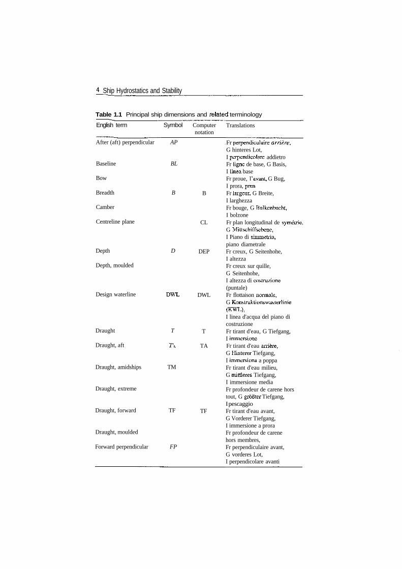
To enable the reader to consult technical literature using other symbols, weshall mention the most important of them. For ship dimensions we do this inTable 1.1, where we shall give also translations into French and German of themost important terms, following mainly ISO 7462 and DIN 81209-1. In addition,Italian terms will be inserted and they conform to Italian technical literature, forexample Costaguta (1981). The translations will be marked by Tr' for French,'G' for German and T for Italian. Almost all ship hulls are symmetric with respectwith a longitudinal plane (plane xz in Figure 1.6). In other words, ships presenta 'port-to-starboard' symmetry. The definitions take this fact into account. Thosedefinitions are explained in Figures 1.1 to 1.4.
The outer surface of a steel or aluminium ship is usually not smooth becausenot all plates have the same thickness. Therefore, it is convenient to define the hullsurface of such a ship on the inner surface of the plating. This is the Moulded sur-face of the hull. Dimensions measured to this surface are qualified as Moulded.By contrast, dimensions measured to the outer surface of the hull or of anappendage are qualified as extreme. The moulded surface is used in the firststages of ship design, before designing the plating, and also in test-basin studies.
Ship Hydrostatics and Stability
Table 1.1 Principal ship dimensions and related terminology
English term Symbol Computernotation
Translations
After (aft) perpendicular AP
Baseline BL
Bow
Breadth B
Camber
Centreline plane
Depth D
Depth, moulded
Design waterline DWL
Draught T
Draught, aft TA
Draught, amidships TM
Draught, extreme
Draught, forward TF
Draught, moulded
Forward perpendicular FP
Fr perpendiculaire arriere,G hinteres Lot,I perpendicolare addietroFr ligne de base, G Basis,I linea baseFr proue, 1'avant, G Bug,I prora, prua
B Fr largeur, G Breite,I larghezzaFr bouge, G Balkenbucht,I bolzone
CL Fr plan longitudinal de symetrie,G Mittschiffsebene,I Piano di simmetria,piano diametrale
DEP Fr creux, G Seitenhohe,I altezzaFr creux sur quille,G Seitenhohe,I altezza di costruzione(puntale)
DWL Fr flottaison normale,G Konstruktionswasserlinie(KWL),I linea d'acqua del piano dicostruzione
T Fr tirant d'eau, G Tiefgang,I immersione
TA Fr tirant d'eau arriere,G Hinterer Tiefgang,I immersiona a poppaFr tirant d'eau milieu,G mittleres Tiefgang,I immersione mediaFr profondeur de carene horstout, G groBter Tiefgang,I pescaggio
TF Fr tirant d'eau avant,G Vorderer Tiefgang,I immersione a proraFr profondeur de carenehors membres,Fr perpendiculaire avant,G vorderes Lot,I perpendicolare avanti
Definitions, principal dimensions 5
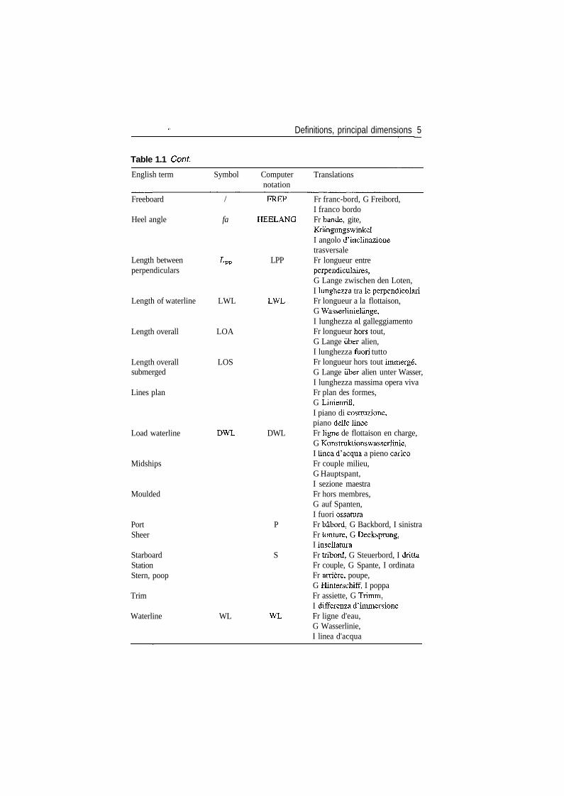
Table 1.1 Cont
English term
Freeboard
Heel angle
Symbol Computernotation
/ FREP
fa HEELANG
Translations
Fr franc-bord, G Freibord,I franco bordoFr bande, gite,
Length between Lpp LPPperpendiculars
Length of waterline LWL LWL
Length overall LOA
Length overall LOSsubmerged
Lines plan
Load waterline DWL DWL
Midships
Moulded
Port PSheer
Starboard SStationStern, poop
Trim
Waterline WL WL
KrangungswinkelI angolo d'inclinazionetrasversaleFr longueur entreperpendiculaires,G Lange zwischen den Loten,I lunghezza tra le perpendicolariFr longueur a la flottaison,G Wasserlinielange,I lunghezza al galleggiamentoFr longueur hors tout,G Lange u'ber alien,I lunghezza fuori tuttoFr longueur hors tout immerge,G Lange iiber alien unter Wasser,I lunghezza massima opera vivaFr plan des formes,G Linienrifi,I piano di costruzione,piano delle lineeFr ligne de flottaison en charge,G Konstruktionswasserlinie,I linea d'acqua a pieno caricoFr couple milieu,G Hauptspant,I sezione maestraFr hors membres,G auf Spanten,I fuori ossaturaFr babord, G Backbord, I sinistraFr tonture, G Decksprung,I insellaturaFr tribord, G Steuerbord, I drittaFr couple, G Spante, I ordinataFr arriere, poupe,G Hinterschiff, I poppaFr assiette, G Trimm,I differenza d'immersioneFr ligne d'eau,G Wasserlinie,I linea d'acqua
6 Ship Hydrostatics and Stability
Sheer at AP Midships, , Sheer at FP
vN Deck
AP
Baseline
LOS
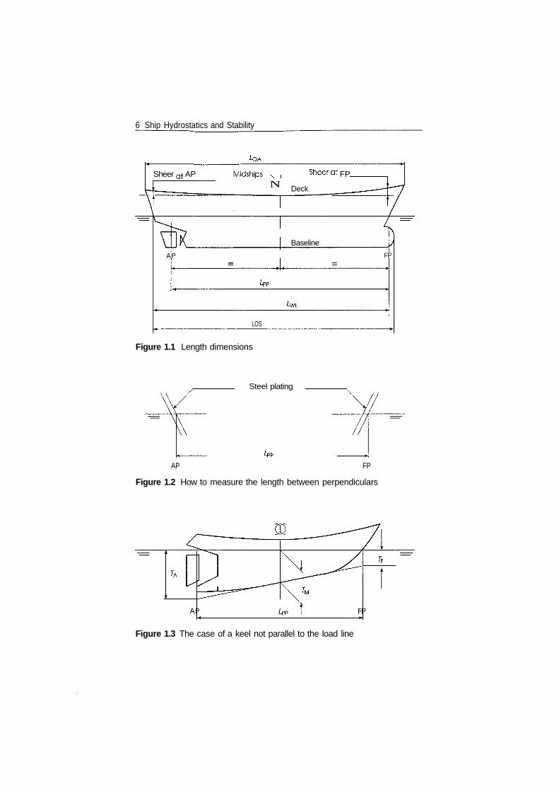
Figure 1.1 Length dimensions
Steel plating
L
FP
AP FP
Figure 1.2 How to measure the length between perpendiculars
Figure 1.3 The case of a keel not parallel to the load line
Definitions, principal dimensions 7
Camber
D
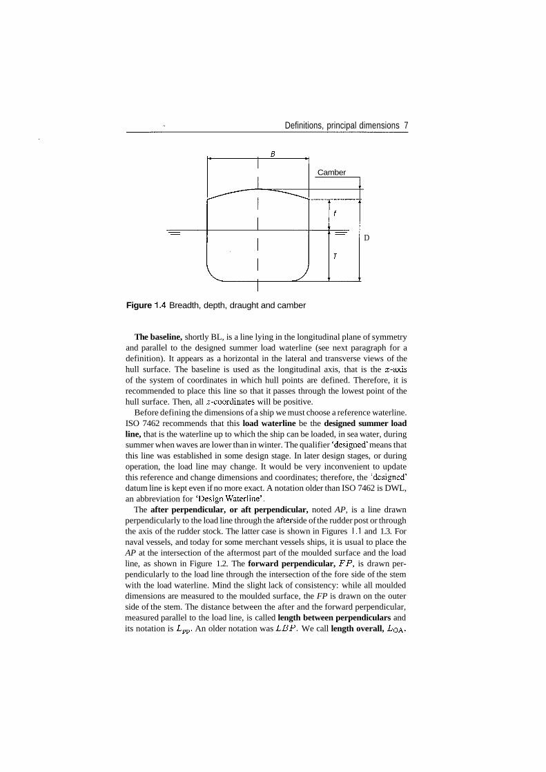
Figure 1.4 Breadth, depth, draught and camber
The baseline, shortly BL, is a line lying in the longitudinal plane of symmetryand parallel to the designed summer load waterline (see next paragraph for adefinition). It appears as a horizontal in the lateral and transverse views of thehull surface. The baseline is used as the longitudinal axis, that is the x-axisof the system of coordinates in which hull points are defined. Therefore, it isrecommended to place this line so that it passes through the lowest point of thehull surface. Then, all z-coordinates will be positive.
Before defining the dimensions of a ship we must choose a reference waterline.ISO 7462 recommends that this load waterline be the designed summer loadline, that is the waterline up to which the ship can be loaded, in sea water, duringsummer when waves are lower than in winter. The qualifier 'designed' means thatthis line was established in some design stage. In later design stages, or duringoperation, the load line may change. It would be very inconvenient to updatethis reference and change dimensions and coordinates; therefore, the 'designed'datum line is kept even if no more exact. A notation older than ISO 7462 is DWL,an abbreviation for 'Design Waterline'.
The after perpendicular, or aft perpendicular, noted AP, is a line drawnperpendicularly to the load line through the after side of the rudder post or throughthe axis of the rudder stock. The latter case is shown in Figures 1.1 and 1.3. Fornaval vessels, and today for some merchant vessels ships, it is usual to place theAP at the intersection of the aftermost part of the moulded surface and the loadline, as shown in Figure 1.2. The forward perpendicular, FP, is drawn per-pendicularly to the load line through the intersection of the fore side of the stemwith the load waterline. Mind the slight lack of consistency: while all mouldeddimensions are measured to the moulded surface, the FP is drawn on the outerside of the stem. The distance between the after and the forward perpendicular,measured parallel to the load line, is called length between perpendiculars andits notation is Lpp. An older notation was LBP. We call length overall, LOA>
8 Ship Hydrostatics and Stability
the length between the ship extremities. The length overall submerged, I/os>is the maximum length of the submerged hull measured parallel to the designedload line.
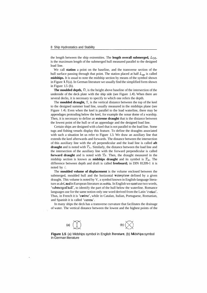
We call station a point on the baseline, and the transverse section of thehull surface passing through that point. The station placed at half Lpp is calledmidships. It is usual to note the midship section by means of the symbol shownin Figure 1.5 (a). In German literature we usually find the simplified form shownin Figure 1.5 (b).
The moulded depth, D, is the height above baseline of the intersection of theunderside of the deck plate with the ship side (see Figure 1.4). When there areseveral decks, it is necessary to specify to which one refers the depth.
The moulded draught, T, is the vertical distance between the top of the keelto the designed summer load line, usually measured in the midships plane (seeFigure 1.4). Even when the keel is parallel to the load waterline, there may beappendages protruding below the keel, for example the sonar dome of a warship.Then, it is necessary to define an extreme draught that is the distance betweenthe lowest point of the hull or of an appendage and the designed load line.
Certain ships are designed with a keel that is not parallel to the load line. Sometugs and fishing vessels display this feature. To define the draughts associatedwith such a situation let us refer to Figure 1.3. We draw an auxiliary line thatextends the keel afterwards and forwards. The distance between the intersectionof this auxiliary line with the aft perpendicular and the load line is called aftdraught and is noted with TA. Similarly, the distance between the load line andthe intersection of the auxiliary line with the forward perpendicular is calledforward draught and is noted with Tp. Then, the draught measured in themidship section is known as midships draught and its symbol is TM- Thedifference between depth and draft is called freeboard; in DIN 81209-1 it isnoted by /.
The moulded volume of displacement is the volume enclosed between thesubmerged, moulded hull and the horizontal waterplane defined by a givendraught. This volume is noted by V, a symbol known in English-language litera-ture as del, and in European literature as nabla. In English we must use two words,'submerged hull', to identify the part of the hull below the waterline. Romancelanguages use for the same notion only one word derived from the Latin 'carina'.Thus, in French it is 'carene', while in Catalan, Italian, Portuguese, Romanian,and Spanish it is called 'carena'.
In many ships the deck has a transverse curvature that facilitates the drainageof water. The vertical distance between the lowest and the highest points of the
(a)
Figure 1.5 (a) Midships symbol in English literature, (b) Midships symbolin German literature
Definitions, principal dimensions 9
deck, in a given transverse section, is called camber (see Figure 1.4). Accordingto ISO 7460 the camber is measured in mm, while all other ship dimensions aregiven in m. A common practice is to fix the camber amidships as 1/50 of thebreadth in that section and to fair the deck towards its extremities (for the term'fair' see Subsection 1.4.3). In most ships, the intersection of the deck surfaceand the plane of symmetry is a curved line with the concavity upwards. Usually,that line is tangent to a horizontal passing at a height equal to the ship depth,D, in the midship section, and runs upwards towards the ship extremities. It ishigher at the bow. This longitudinal curvature is called sheer and is illustrated inFigure 1.1. The deck sheer helps in preventing the entrance of waves and is takeninto account when establishing the load line in accordance with internationalconventions.
1.4 The definition of the hull surface
1.4.1 Coordinate systems
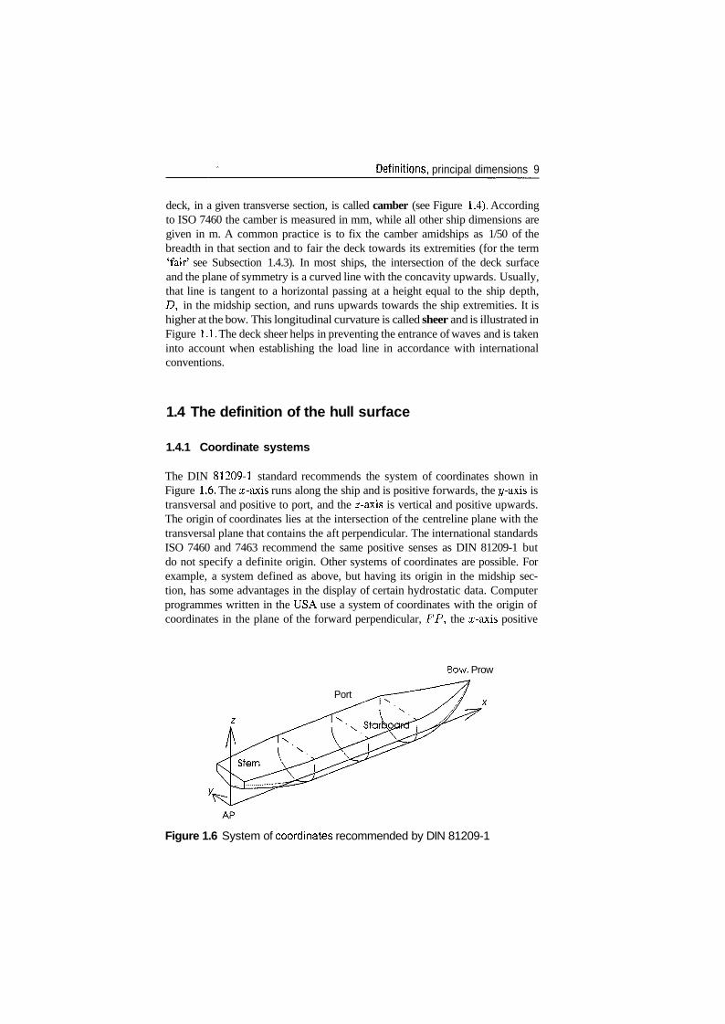
The DIN 81209-1 standard recommends the system of coordinates shown inFigure 1.6. The x-axis runs along the ship and is positive forwards, the y-axis istransversal and positive to port, and the z-axis is vertical and positive upwards.The origin of coordinates lies at the intersection of the centreline plane with thetransversal plane that contains the aft perpendicular. The international standardsISO 7460 and 7463 recommend the same positive senses as DIN 81209-1 butdo not specify a definite origin. Other systems of coordinates are possible. Forexample, a system defined as above, but having its origin in the midship sec-tion, has some advantages in the display of certain hydrostatic data. Computerprogrammes written in the USA use a system of coordinates with the origin ofcoordinates in the plane of the forward perpendicular, FP, the x-axis positive
Bow, Prow
Port
Figure 1.6 System of coordinates recommended by DIN 81209-1
10 Ship Hydrostatics and Stability
afterwards, the y-axis positive to starboard, and the z-axis positive upwards.For dynamic applications, taking the origin in the centre of gravity simplifies theequations. However, it should be clear that to each loading condition correspondsone centre of gravity, while a point like the intersection of the aft perpendicularwith the base line is independent of the ship loading. The system of coordinatesused for the hull surface can be also employed for the location of weights. By itsvery nature, the system in which the hull is defined is fixed in the ship and moveswith her. To define the various floating conditions, that is the positions that thevessel can assume, we use another system, fixed in space, that is defined in ISO7463 as XQ, y$, ZQ. Let this system initially coincide with the system x, y, z.A vertical translation of the system x, y, z with respect to the space-fixed system£o> 2/o» ZQ produces a draught change.
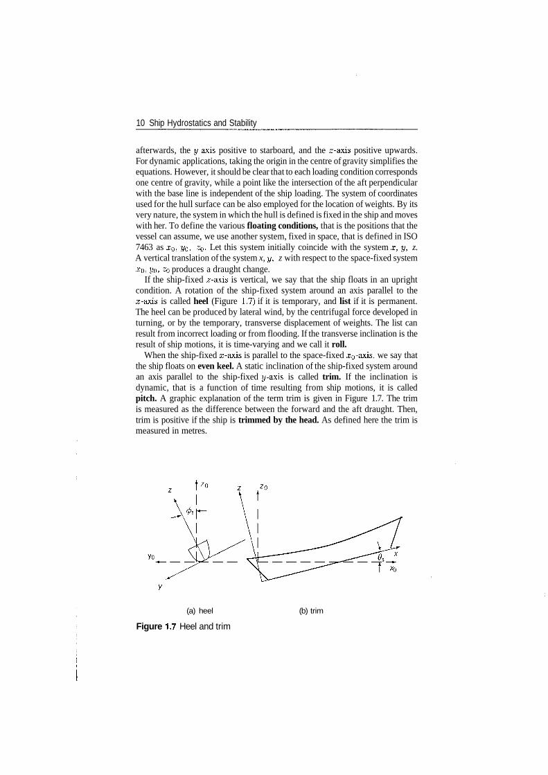
If the ship-fixed z-axis is vertical, we say that the ship floats in an uprightcondition. A rotation of the ship-fixed system around an axis parallel to thex-axis is called heel (Figure 1.7) if it is temporary, and list if it is permanent.The heel can be produced by lateral wind, by the centrifugal force developed inturning, or by the temporary, transverse displacement of weights. The list canresult from incorrect loading or from flooding. If the transverse inclination is theresult of ship motions, it is time-varying and we call it roll.
When the ship-fixed x-axis is parallel to the space-fixed x0-axis, we say thatthe ship floats on even keel. A static inclination of the ship-fixed system aroundan axis parallel to the ship-fixed y-axis is called trim. If the inclination isdynamic, that is a function of time resulting from ship motions, it is calledpitch. A graphic explanation of the term trim is given in Figure 1.7. The trimis measured as the difference between the forward and the aft draught. Then,trim is positive if the ship is trimmed by the head. As defined here the trim ismeasured in metres.
(a) heel (b) trim
Figure 1.7 Heel and trim
Definitions, principal dimensions 11
1.4.2 Graphic description
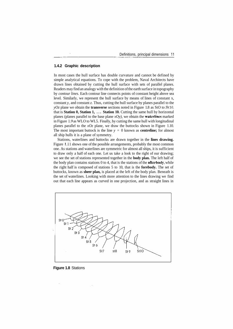
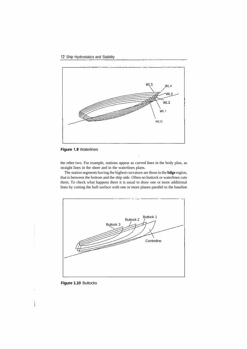
In most cases the hull surface has double curvature and cannot be defined bysimple analytical equations. To cope with the problem, Naval Architects havedrawn lines obtained by cutting the hull surface with sets of parallel planes.Readers may find an analogy with the definition of the earth surface in topographyby contour lines. Each contour line connects points of constant height above sealevel. Similarly, we represent the hull surface by means of lines of constant x,constant y, and constant z. Thus, cutting the hull surface by planes parallel to theyOz plane we obtain the transverse sections noted in Figure 1.8 as StO to StlO,that is Station 0, Station 1, . . . Station 10. Cutting the same hull by horizontalplanes (planes parallel to the base plane xOy), we obtain the waterlines markedin Figure 1.9 as WLO to WL5. Finally, by cutting the same hull with longitudinalplanes parallel to the xOz plane, we draw the buttocks shown in Figure 1.10.The most important buttock is the line y = 0 known as centreline; for almostall ship hulls it is a plane of symmetry.
Stations, waterlines and buttocks are drawn together in the lines drawing.Figure 1.11 shows one of the possible arrangements, probably the most commonone. As stations and waterlines are symmetric for almost all ships, it is sufficientto draw only a half of each one. Let us take a look to the right of our drawing;we see the set of stations represented together in the body plan. The left half ofthe body plan contains stations 0 to 4, that is the stations of the afterbody, whilethe right half is composed of stations 5 to 10, that is the forebody. The set ofbuttocks, known as sheer plan, is placed at the left of the body plan. Beneath isthe set of waterlines. Looking with more attention to the lines drawing we findout that each line appears as curved in one projection, and as straight lines in
St7 st8 St9 St lO
Figure 1.8 Stations
12 Ship Hydrostatics and Stability
WL5 WL4
WLO
Figure 1.9 Waterlines
the other two. For example, stations appear as curved lines in the body plan, asstraight lines in the sheer and in the waterlines plans.
The station segments having the highest curvature are those in the bilge region,that is between the bottom and the ship side. Often no buttock or waterlines cutsthem. To check what happens there it is usual to draw one or more additionallines by cutting the hull surface with one or more planes parallel to the baseline
Buttock 2Buttock 1
Buttock 3
Centreline
Figure 1.10 Buttocks
Definitions, principal dimensions 13
Sheer plan Body plan
Buttock 3 Buttock 2 Buttock 1 Afterbody Forebody\ \ ^ \ y
StO SH St2 St3 St4 St5 St6 St 7 St8 St9 St 10
Waterlines plan
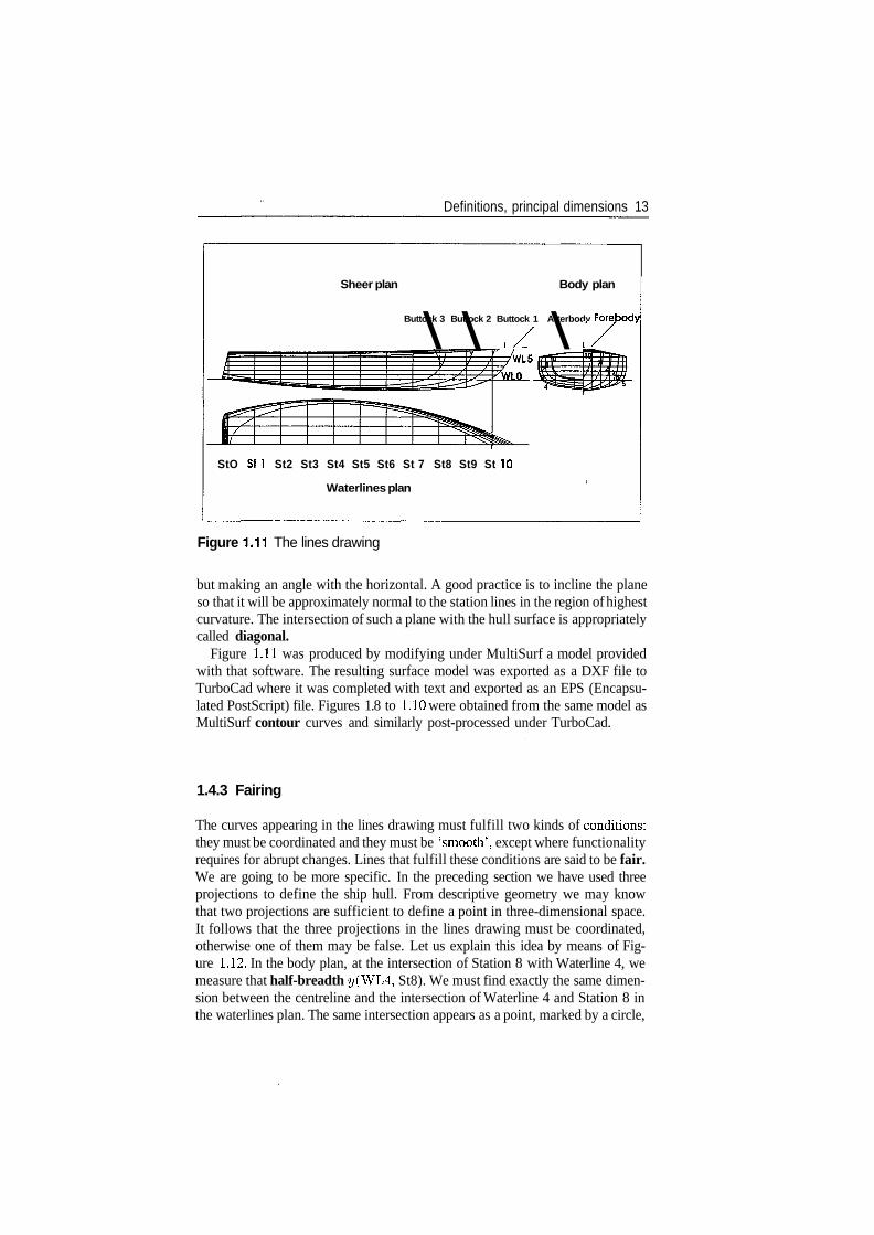
Figure 1.11 The lines drawing
but making an angle with the horizontal. A good practice is to incline the planeso that it will be approximately normal to the station lines in the region of highestcurvature. The intersection of such a plane with the hull surface is appropriatelycalled diagonal.
Figure 1.11 was produced by modifying under MultiSurf a model providedwith that software. The resulting surface model was exported as a DXF file toTurboCad where it was completed with text and exported as an EPS (Encapsu-lated PostScript) file. Figures 1.8 to 1.10 were obtained from the same model asMultiSurf contour curves and similarly post-processed under TurboCad.
1.4.3 Fairing
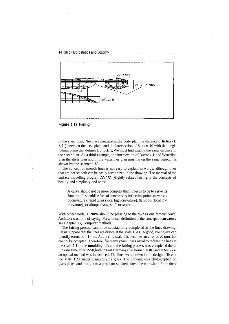
The curves appearing in the lines drawing must fulfill two kinds of conditions:they must be coordinated and they must be 'smooth', except where functionalityrequires for abrupt changes. Lines that fulfill these conditions are said to be fair.We are going to be more specific. In the preceding section we have used threeprojections to define the ship hull. From descriptive geometry we may knowthat two projections are sufficient to define a point in three-dimensional space.It follows that the three projections in the lines drawing must be coordinated,otherwise one of them may be false. Let us explain this idea by means of Fig-ure 1.12. In the body plan, at the intersection of Station 8 with Waterline 4, wemeasure that half-breadth y(WL4, St8). We must find exactly the same dimen-sion between the centreline and the intersection of Waterline 4 and Station 8 inthe waterlines plan. The same intersection appears as a point, marked by a circle,
14 Ship Hydrostatics and Stability
XWL4, St8)
z(Buttockl,SHO)
Figure 1.12 Fairing
in the sheer plan. Next, we measure in the body plan the distance z(Buttockl,StlO) between the base plane and the intersection of Station 10 with the longi-tudinal plane that defines Buttock 1. We must find exactly the same distance inthe sheer plan. As a third example, the intersection of Buttock 1 and Waterline1 in the sheer plan and in the waterlines plan must lie on the same vertical, asshown by the segment AB.
The concept of smooth lines is not easy to explain in words, although linesthat are not smooth can be easily recognized in the drawing. The manual of thesurface modelling program MultiSurf rightly relates fairing to the concepts ofbeauty and simplicity and adds:
A curve should not be more complex than it needs to be to serve itsfunction. It should be free of unnecessary inflection points (reversalsof curvature), rapid turns (local high curvature), flat spots (local lowcurvature), or abrupt changes of curvature . . .
With other words, a 'curve should be pleasing to the eye' as one famous NavalArchitect was fond of saying. For a formal definition of the concept of curvaturesee Chapter 13, Computer methods.
The fairing process cannot be satisfactorily completed in the lines drawing.Let us suppose that the lines are drawn at the scale 1:200. A good, young eye canidentify errors of 0.1 mm. At the ship scale this becomes an error of 20 mm thatcannot be accepted. Therefore, for many years it was usual to redraw the lines atthe scale 1:1 in the moulding loft and the fairing process was completed there.
Some time after 1950, both in East Germany (the former DDR) and in Sweden,an optical method was introduced. The lines were drawn in the design office atthe scale 1:20, under a magnifying glass. The drawing was photographed onglass plates and brought to a projector situated above the workshop. From there
Definitions, principal dimensions 15
Table 1.2 Table of offsets
S t 0 1 2 3 4 5 6 7 8 9 1 0
X O.QQQ 0.893 1.786 2.678 3.571 4.464 5.357 6.249 7.142 8.035 8.928
WL z Half breadths
01
2
3
4
5
0.360
0512
0.665
0.817
0.969
1 122
0894
1.014
1.055
1.070
1 069
0.900
1 167
1.240
1.270
1.273
1 260
1.189
1 341
1.397
1.414
1.412
1 395
1.325
1 440
1.482
1.495
1.491
1 474
1.377
1 463
1.501
1.514
1.511
1 496
1.335
1 417
1.455
1.470
1.471
1 461
1.219
1 300
1.340
1.361
1.369
1 363
1.024
1 109
1.156
1.184
1.201
1 201
0.749
0842
0.898
0.936
0.962
0972
0.389
0496
0.564
0.614
0.648
0671
0067
0.149
0.214
0.257
0295
the drawing was projected on plates so that it appeared at the 1:1 scale to enablecutting by optically guided, automatic burners.
The development of hardware and software in the second half of the twentiethcentury allowed the introduction of computer-fairing methods. Historical high-lights can be found in Kuo (1971) and other references cited in Chapter 13. Whenthe hull surface is defined by algebraic curves, as explained in Chapter 13, thelines are smooth by construction. Recent computer programmes include toolsthat help in completing the fairing process and checking it, mainly the calcu-lation of curvatures and rendering. A rendered view is one in which the hullsurface appears in perspective, shaded and lighted so that surface smoothnesscan be summarily checked. For more details see Chapter 13.
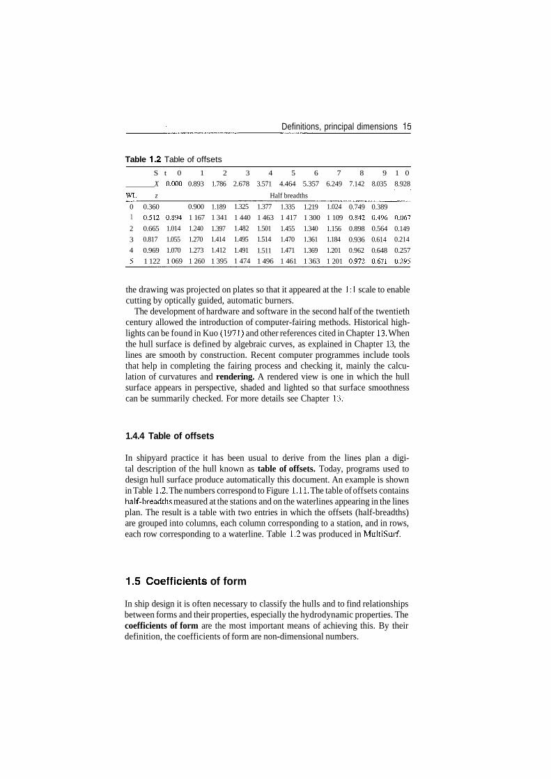
1.4.4 Table of offsets
In shipyard practice it has been usual to derive from the lines plan a digi-tal description of the hull known as table of offsets. Today, programs used todesign hull surface produce automatically this document. An example is shownin Table 1.2. The numbers correspond to Figure 1.11. The table of offsets containshalf-breadths measured at the stations and on the waterlines appearing in the linesplan. The result is a table with two entries in which the offsets (half-breadths)are grouped into columns, each column corresponding to a station, and in rows,each row corresponding to a waterline. Table 1.2 was produced in MultiSurf.
1.5 Coefficients of form
In ship design it is often necessary to classify the hulls and to find relationshipsbetween forms and their properties, especially the hydrodynamic properties. Thecoefficients of form are the most important means of achieving this. By theirdefinition, the coefficients of form are non-dimensional numbers.
16 Ship Hydrostatics and Stability
DWL
Submerged hull
Figure 1.13 The submerged hull
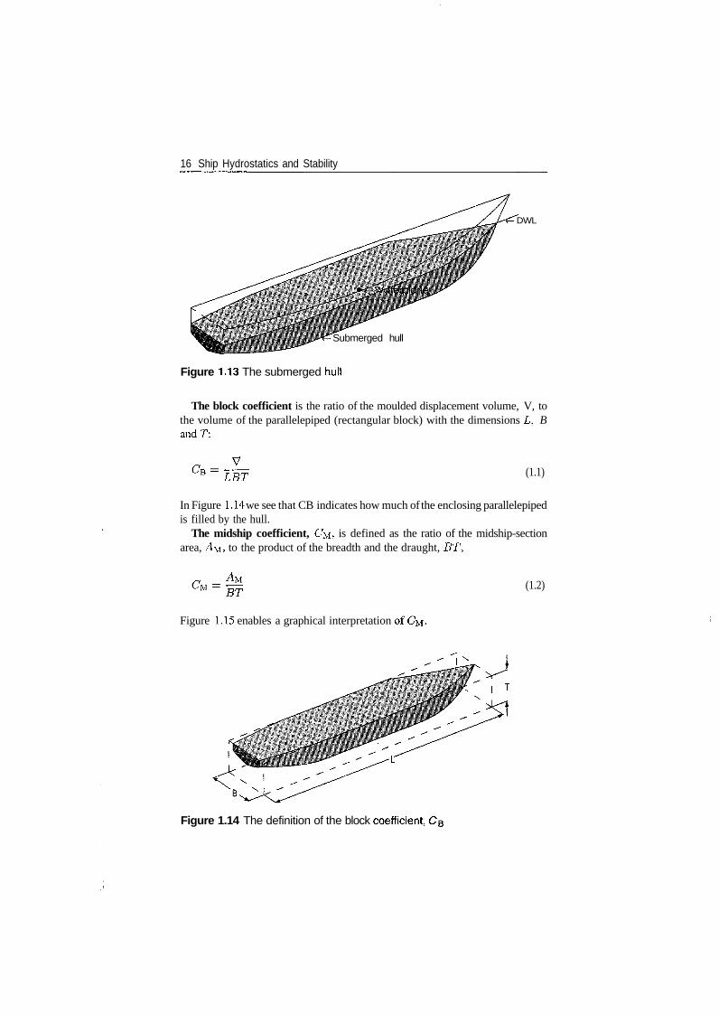
The block coefficient is the ratio of the moulded displacement volume, V, tothe volume of the parallelepiped (rectangular block) with the dimensions L, BandT:
(1.1)LET
In Figure 1.14 we see that CB indicates how much of the enclosing parallelepipedis filled by the hull.
The midship coefficient, CM, is defined as the ratio of the midship-sectionarea, AM, to the product of the breadth and the draught, BT,
(1.2)
Figure 1.15 enables a graphical interpretation
Figure 1.14 The definition of the block coefficient,

Definitions, principal dimensions 17
Figure 1.15 The definition of the midship-section coefficient, CM
The prismatic coefficient, Cp, is the ratio of the moulded displacement vol-ume, V, to the product of the midship-section area, AU, and the length, L:
r _ V _ CBLBT _ CB_A.y[L (^>y[BT L CM
(1-3)
In Figure 1.16 we can see that Cp is an indicator of how much of a cylinderwith constant section AM and length L is filled by the submerged hull. Letus note the waterplane area by Ayj. Then, we define the waterplane-areacoefficient by
(1.4)
Figure 1.16 The definition of the prismatic coefficient, Cp
18 Ship Hydrostatics and Stability
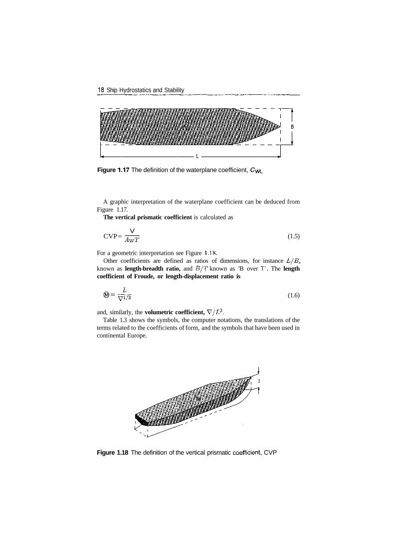
Figure 1.17 The definition of the waterplane coefficient,
A graphic interpretation of the waterplane coefficient can be deduced fromFigure 1.17.
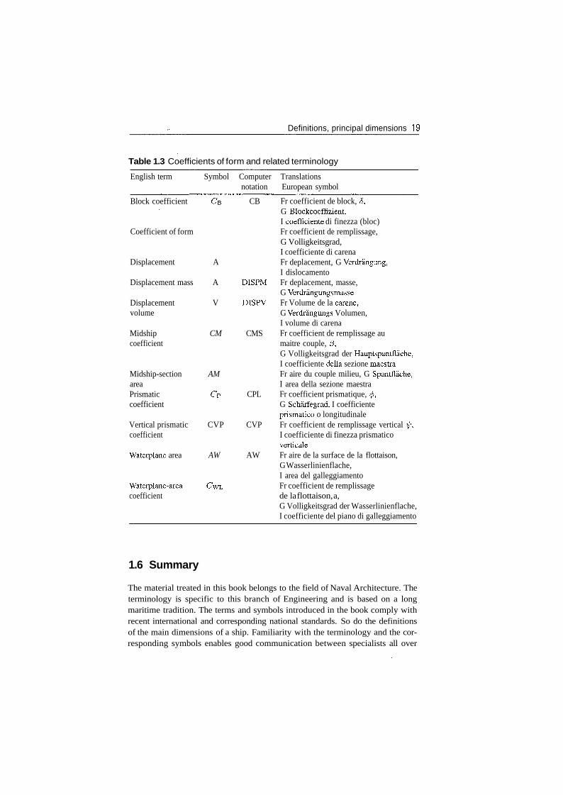
The vertical prismatic coefficient is calculated as
CVP =V
AWT (1.5)
For a geometric interpretation see Figure 1.18.Other coefficients are defined as ratios of dimensions, for instance L/B,
known as length-breadth ratio, and B/T known as 'B over T'. The lengthcoefficient of Froude, or length-displacement ratio is
(1.6)
and, similarly, the volumetric coefficient, V/L3.Table 1.3 shows the symbols, the computer notations, the translations of the
terms related to the coefficients of form, and the symbols that have been used incontinental Europe.
Figure 1.18 The definition of the vertical prismatic coefficient, CVP
Definitions, principal dimensions 19
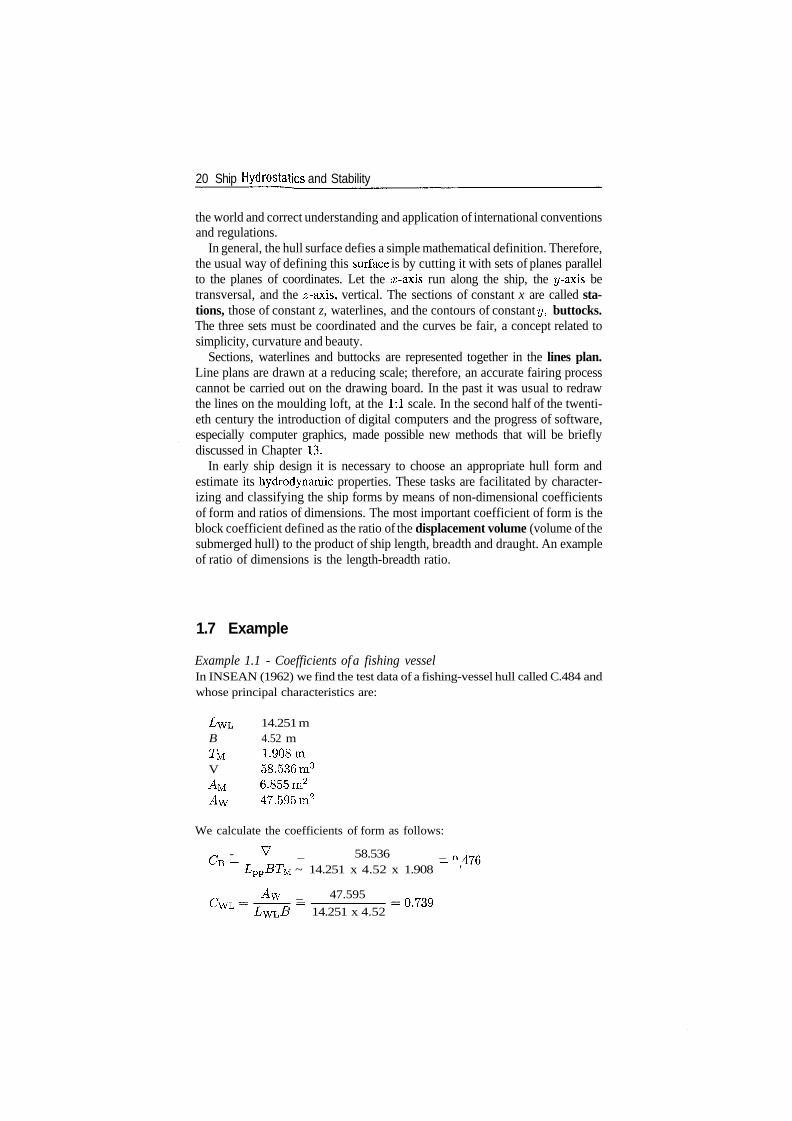
Table 1.3 Coefficients of form and related terminology
English term Symbol Computer Translationsnotation European symbol
Block coefficient CB CB
Coefficient of form
Displacement A
Displacement mass A DISPM
Displacement V DISPVvolume
Midship CM CMScoefficient
Midship-section AMareaPrismatic CP CPLcoefficient
Vertical prismatic CVP CVPcoefficient
Waterplane area AW AW
Waterplane-areacoefficient
Fr coefficient de block, J,G Blockcoeffizient,I coefficiente di finezza (bloc)Fr coefficient de remplissage,G Volligkeitsgrad,I coefficiente di carenaFr deplacement, G Verdrangung,I dislocamentoFr deplacement, masse,G VerdrangungsmasseFr Volume de la carene,G Verdrangungs Volumen,I volume di carenaFr coefficient de remplissage aumaitre couple, /?,G Volligkeitsgrad der Hauptspantflache,I coefficiente della sezione maestraFr aire du couple milieu, G Spantflache,I area della sezione maestraFr coefficient prismatique, 0,G Scharfegrad, I coefficienteprismatico o longitudinaleFr coefficient de remplissage vertical ifr,I coefficiente di finezza prismaticoverticaleFr aire de la surface de la flottaison,G Wasserlinienflache,I area del galleggiamentoFr coefficient de remplissagede la flottaison, a,G Volligkeitsgrad der Wasserlinienflache,I coefficiente del piano di galleggiamento
1.6 Summary
The material treated in this book belongs to the field of Naval Architecture. Theterminology is specific to this branch of Engineering and is based on a longmaritime tradition. The terms and symbols introduced in the book comply withrecent international and corresponding national standards. So do the definitionsof the main dimensions of a ship. Familiarity with the terminology and the cor-responding symbols enables good communication between specialists all over
20 Ship Hydrostatics and Stability
the world and correct understanding and application of international conventionsand regulations.
In general, the hull surface defies a simple mathematical definition. Therefore,the usual way of defining this surface is by cutting it with sets of planes parallelto the planes of coordinates. Let the x-axis run along the ship, the y-axis betransversal, and the z-axis, vertical. The sections of constant x are called sta-tions, those of constant z, waterlines, and the contours of constant y, buttocks.The three sets must be coordinated and the curves be fair, a concept related tosimplicity, curvature and beauty.
Sections, waterlines and buttocks are represented together in the lines plan.Line plans are drawn at a reducing scale; therefore, an accurate fairing processcannot be carried out on the drawing board. In the past it was usual to redrawthe lines on the moulding loft, at the 1:1 scale. In the second half of the twenti-eth century the introduction of digital computers and the progress of software,especially computer graphics, made possible new methods that will be brieflydiscussed in Chapter 13.
In early ship design it is necessary to choose an appropriate hull form andestimate its hydrodynamic properties. These tasks are facilitated by character-izing and classifying the ship forms by means of non-dimensional coefficientsof form and ratios of dimensions. The most important coefficient of form is theblock coefficient defined as the ratio of the displacement volume (volume of thesubmerged hull) to the product of ship length, breadth and draught. An exampleof ratio of dimensions is the length-breadth ratio.
1.7 Example
Example 1.1 - Coefficients of a fishing vesselIn INSEAN (1962) we find the test data of a fishing-vessel hull called C.484 andwhose principal characteristics are:
14.251 mB 4.52 mTM 1.908mV 58.536m3
AU 6.855 rn2
47.595m2
We calculate the coefficients of form as follows:
- V _ 58.536 _B ~ LPPBTM ~ 14.251 x 4.52 x 1.908 ~~ '
Aw _ 47.595CwL 14.251 x 4.52
Definitions, principal dimensions 21
6.8554.52 x 1.908
V 58.536~ ~ 6.855 x 14.251 ~
and we can verify that
C B _ 0.476Cp~C^~ 0.795
1.8 Exercises
Exercise LI - Vertical prismatic coefficientFind the relationship between the vertical prismatic coefficient, Cyp, thewaterplane-area coefficient, CWL> and the block coefficient, CB-
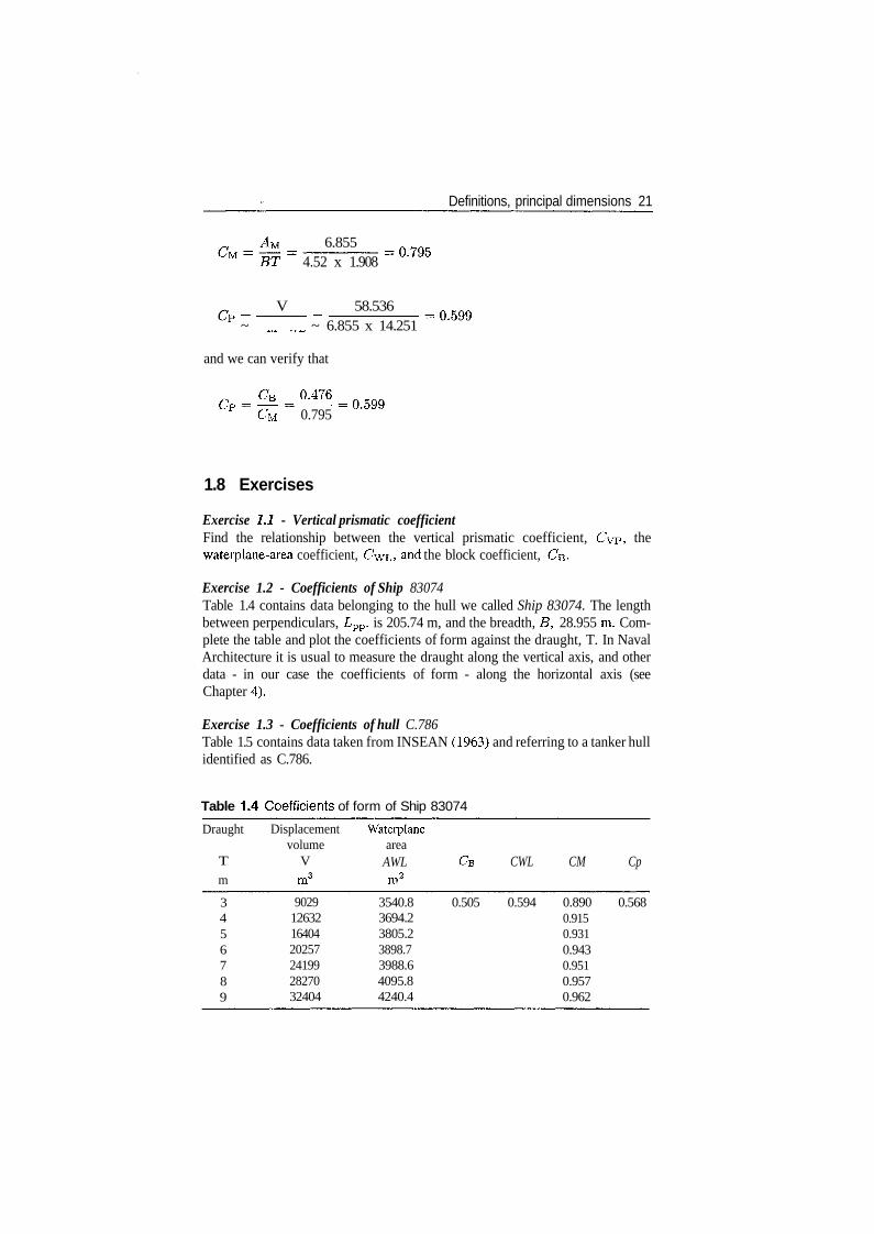
Exercise 1.2 - Coefficients of Ship 83074Table 1.4 contains data belonging to the hull we called Ship 83074. The lengthbetween perpendiculars, Lpp, is 205.74 m, and the breadth, B, 28.955 m. Com-plete the table and plot the coefficients of form against the draught, T. In NavalArchitecture it is usual to measure the draught along the vertical axis, and otherdata - in our case the coefficients of form - along the horizontal axis (seeChapter 4).
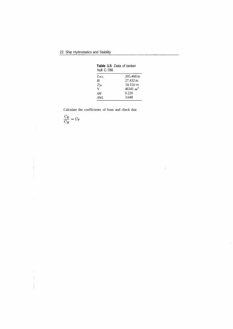
Exercise 1.3 - Coefficients of hull C.786Table 1.5 contains data taken from INSEAN (1963) and referring to a tanker hullidentified as C.786.
Table 1.4 Coefficients of form of Ship 83074
Draught
T
m
3456789
Displacementvolume
V
m3
9029126321640420257241992827032404
Waterplanearea
AWLm2
3540.83694.23805.23898.73988.64095.84240.4
CB CWL CM Cp
0.505 0.594 0.890 0.5680.9150.9310.9430.9510.9570.962
22 Ship Hydrostatics and Stability
Table 1.5 Data of tankerhull C.786
Z/WL
BTMVAMAWL
205.468 m27.432 m10.750m46341 m3
0.2203.648
Calculate the coefficients of fonn and check that
Basic ship hydrostatics
2.1 Introduction
This chapter deals with the conditions of equilibrium and initial stabilityof floating bodies. We begin with a derivation of Archimedes' principle andthe definitions of the notions of centre of buoyancy and displacement.Archimedes' principle provides a particular formulation of the law of equilibriumof forces for floating bodies. The law of equilibrium of moments is formulatedas Stevin's law and it expresses the relationship between the centre of gravityand the centre of buoyancy of the floating body. The study of initial stability isthe study of the behaviour in the neighbourhood of the position of equilibrium.To derive the condition of initial stability we introduce Bouguer's concept ofmetacentre.
To each position of a floating body correspond one centre of buoyancy and onemetacentre. Each position of the floating body is defined by three parameters,for instance the triple {displacement, angle of heel, angle of trim}', we call themthe parameters of the floating condition. If we keep two parameters constantand let one vary, the centre of buoyancy travels along a curve and the metacentrealong another. If only one parameter is kept constant and two vary, the centreof buoyancy and the metacentre generate two surfaces. In this chapter we shallbriefly show what happens when the displacement is constant. The discussionof the case in which only one angle (that is, either heel or trim) varies leads tothe concept of metacentric evolute.
The treatment of the above problems is based on the following assumptions:
1. the water is incompressible;2. viscosity plays no role;3. surface tension plays no role;4. the water surface is plane.
The first assumption is practically exact in the range of water depths we areinterested in. The second assumption is exact in static conditions (that is withoutmotion) and a good approximation at the very slow rates of motion discussed inship hydrostatics. In Chapter 12 we shall point out to the few cases in which vis-cosity should be considered. The third assumption is true for the sizes of floatingbodies and the wave heights we are dealing with. The fourth assumption is never
24 Shjp Hydrostatics and Stability
true, not even in the sheltered waters of a harbour. However, this hypothesisallows us to derive very useful, general results, and calculate essential propertiesof ships and other floating bodies. It is only in Chapter 9 that we shall leave theassumption of a plane water surface and see what happens in waves. In fact, thetheory of ship hydrostatics was developed during 200 years under the hypothesisof a plane water surface and only in the middle of the twentieth century it wasrecognized that this assumption cannot explain the capsizing of a few ships thatwere considered stable by that time.
The results derived in this chapter are general in the sense that they do notassume particular body shapes. Thus, no symmetry must be assumed such asit usually exists in ships (port-to-starboard symmetry) and still less symmetryabout two axes, as encountered, for instance, in Viking ships, some ferries, someoffshore platforms and most buoys. The results hold the same for single-hullships as for catamarans and trimarans. The only problem is that the treatment ofthe problems for general-form floating bodies requires 'more' mathematics thanthe calculations for certain simple or symmetric solids. To make this chapteraccessible to a larger audience, although we derive the results for body shapeswithout any form restrictions, we also exemplify them on parallelepipedic andother simply defined floating body forms. Reading only those examples is suf-ficient to understand the ideas involved and the results obtained in this chapter.However, only the general derivations can provide the feeling of generality anda good insight into the problems discussed here.
2.2 Archimedes' principle
2.2.1 A body with simple geometrical form
A body immersed in a fluid is subjected to an upwards force equalto the weight of the fluid displaced.
The above statement is known as Archimedes' principle. One legend has itthat Archimedes (Greek, lived in Syracuse - Sicily - between 287 and 212 BC)discovered this law while taking a bath and that he was so happy that he ran nakedin the streets shouting T have found' (in Greek Heureka, see entry 'eureka' inMerriam-Webster, 1991). The legend may be nice, but it is most probably nottrue. What is certain is that Archimedes used his principle to assess the amountof gold in gold-silver alloys.
Archimedes' principle can be derived mathematically if we know anotherlaw of general hydrostatics. Most textbooks contain only a brief, unconvincingproof based on intuitive considerations of equilibrium. A more elaborate proofis given here and we prefer it because only thus it is possible to decide whetherArchimedes' principle applies or not in a given case. Let us consider a fluid whosespecific gravity is 7. Then, at a depth z the pressure in the fluid equals 72. Thisis the weight of the fluid column of height z and unit area cross section. The
Basic ship hydrostatics 25
pressure at a point is the same in all directions and this statement is known asPascals principle. The proof of this statement can be found in many textbookson fluid mechanics, such as Douglas, Gasiorek and Swaffiled (1979: 24), orPnueli and Gutfinger (1992: 30-1).
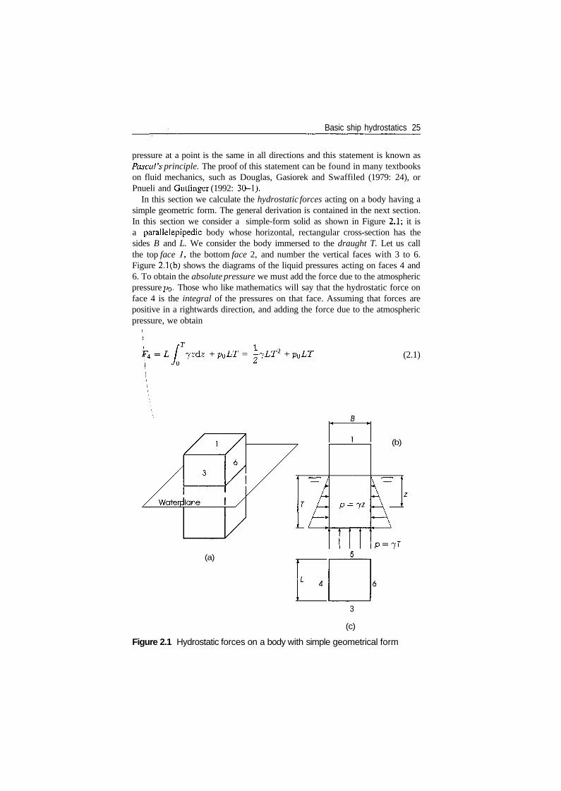
In this section we calculate the hydrostatic forces acting on a body having asimple geometric form. The general derivation is contained in the next section.In this section we consider a simple-form solid as shown in Figure 2.1; it isa parallelepipedic body whose horizontal, rectangular cross-section has thesides B and L. We consider the body immersed to the draught T. Let us callthe top face 1, the bottom face 2, and number the vertical faces with 3 to 6.Figure 2.1(b) shows the diagrams of the liquid pressures acting on faces 4 and6. To obtain the absolute pressure we must add the force due to the atmosphericpressure pQ. Those who like mathematics will say that the hydrostatic force onface 4 is the integral of the pressures on that face. Assuming that forces arepositive in a rightwards direction, and adding the force due to the atmosphericpressure, we obtain
jzdz + pQLT = -7LT2 + p0LT (2.1)
(b)
(a)
3
(c)
Figure 2.1 Hydrostatic forces on a body with simple geometrical form
26 Ship Hydrostatics and Stability
Similarly, the force on face 6 is
F6 = -L I -yzdz - PoLT = ~^-fLT2 - PoLT (2.2)Jo *
As the force on face 6 is equal and opposed to that on face 4 we conclude thatthe two forces cancel each other.
The reader who does not like integrals can reason in one of the following twoways.
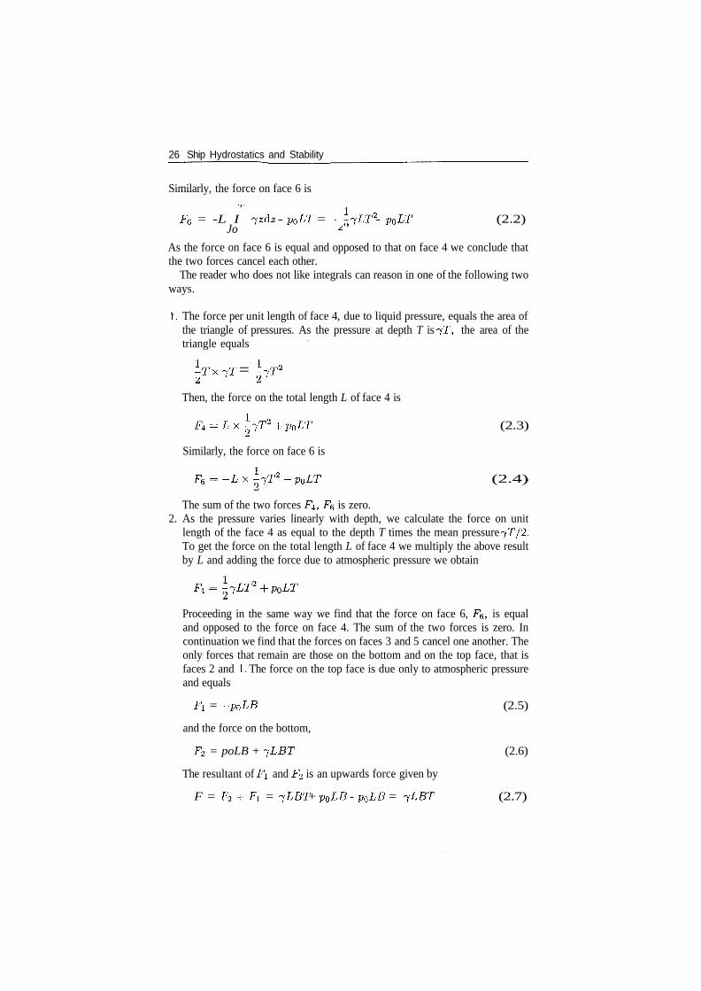
1. The force per unit length of face 4, due to liquid pressure, equals the area ofthe triangle of pressures. As the pressure at depth T is jT, the area of thetriangle equals
I-T x 7T = iyr2
Then, the force on the total length L of face 4 is
F4-Lxi7T2+p0Lr (2.3)
Similarly, the force on face 6 is
F6 = -Lx^T2-PoLT (2.4)
The sum of the two forces F±, FQ is zero.2. As the pressure varies linearly with depth, we calculate the force on unit
length of the face 4 as equal to the depth T times the mean pressure jT/2.To get the force on the total length L of face 4 we multiply the above resultby L and adding the force due to atmospheric pressure we obtain
F4=-
Proceeding in the same way we find that the force on face 6, FQ, is equaland opposed to the force on face 4. The sum of the two forces is zero. Incontinuation we find that the forces on faces 3 and 5 cancel one another. Theonly forces that remain are those on the bottom and on the top face, that isfaces 2 and 1. The force on the top face is due only to atmospheric pressureand equals
F1 = -poLB (2.5)
and the force on the bottom,
F2 = poLB + -yLBT (2.6)
The resultant of F\ and F^ is an upwards force given by
F = F2 + F1 = -fLBT + PQLB - pGLB = <yLBT (2.7)
Basic ship hydrostatics 27
The product LET is actually the volume of the immersed body. Then, theforce F given by Eq. (2.7) is the weight of the volume of liquid displaced bythe immersed body. This verifies Archimedes' principle for the solid consideredin this section.
We saw above that the atmospheric pressure does not play a role in thederivation of Archimedes' principle. Neither does it play any role in most otherproblems we are going to treat in this book; therefore, we shall ignore it infuture.
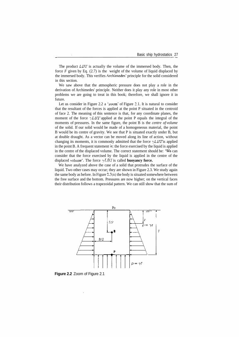
Let us consider in Figure 2.2 a 'zoom' of Figure 2.1. It is natural to considerthat the resultant of the forces is applied at the point P situated in the centroidof face 2. The meaning of this sentence is that, for any coordinate planes, themoment of the force ^LBT applied at the point P equals the integral of themoments of pressures. In the same figure, the point B is the centre of volumeof the solid. If our solid would be made of a homogeneous material, the pointB would be its centre of gravity. We see that P is situated exactly under B, butat double draught. As a vector can be moved along its line of action, withoutchanging its moments, it is commonly admitted that the force ^LBT is appliedin the point B. A frequent statement is: the force exercised by the liquid is appliedin the centre of the displaced volume. The correct statement should be: 'We canconsider that the force exercised by the liquid is applied in the centre of thedisplaced volume'. The force ^LBT is called buoyancy force.
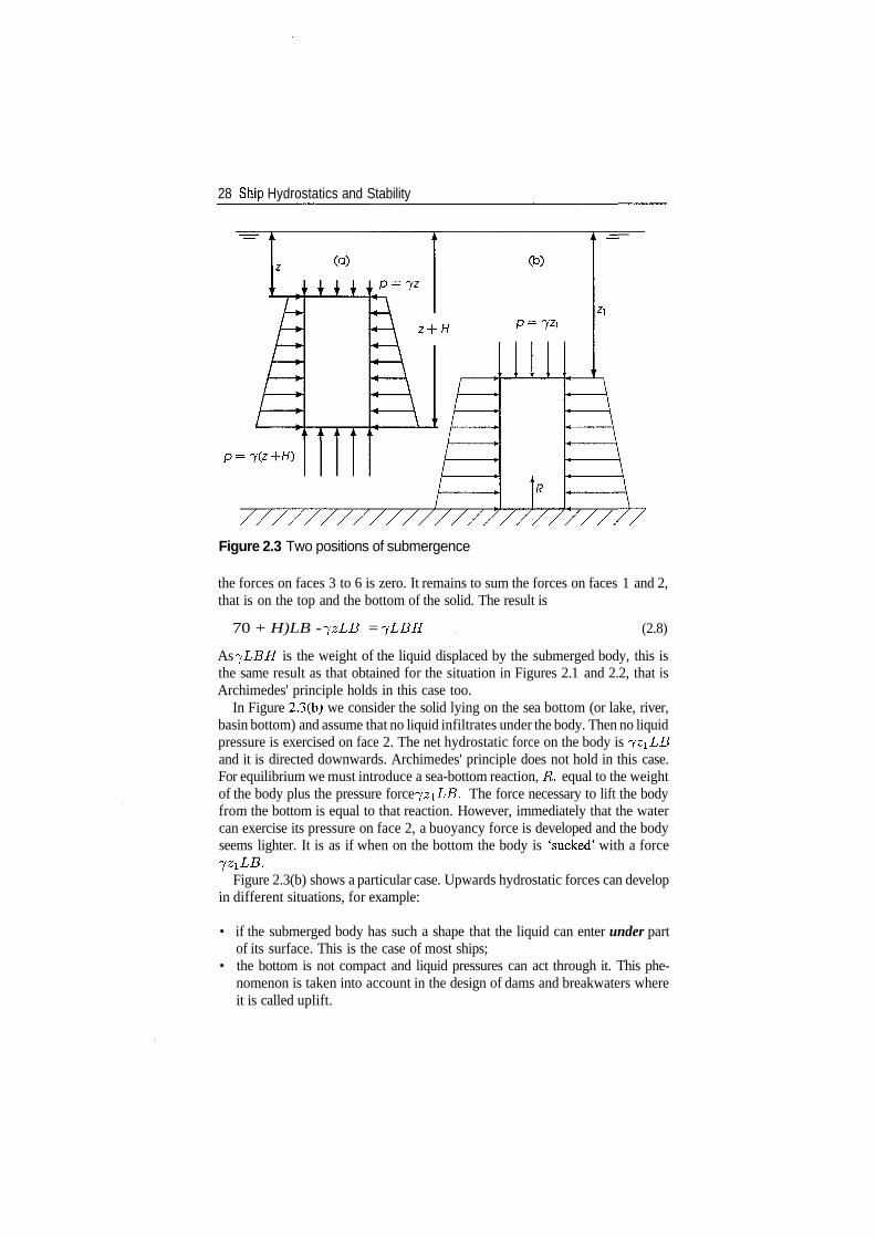
We have analyzed above the case of a solid that protrudes the surface of theliquid. Two other cases may occur; they are shown in Figure 2.3. We study againthe same body as before. In Figure 2.3(a) the body is situated somewhere betweenthe free surface and the bottom. Pressures are now higher; on the vertical facestheir distribution follows a trapezoidal pattern. We can still show that the sum of
Po
7/2
B/2
Figure 2.2 Zoom of Figure 2.1
28 Ship Hydrostatics and Stability
Figure 2.3 Two positions of submergence
the forces on faces 3 to 6 is zero. It remains to sum the forces on faces 1 and 2,that is on the top and the bottom of the solid. The result is
70 + H)LB - jzLB = jLBH (2.8)
As jLBH is the weight of the liquid displaced by the submerged body, this isthe same result as that obtained for the situation in Figures 2.1 and 2.2, that isArchimedes' principle holds in this case too.
In Figure 2.3(b) we consider the solid lying on the sea bottom (or lake, river,basin bottom) and assume that no liquid infiltrates under the body. Then no liquidpressure is exercised on face 2. The net hydrostatic force on the body is ̂ z\LBand it is directed downwards. Archimedes' principle does not hold in this case.For equilibrium we must introduce a sea-bottom reaction, R, equal to the weightof the body plus the pressure force jziLB. The force necessary to lift the bodyfrom the bottom is equal to that reaction. However, immediately that the watercan exercise its pressure on face 2, a buoyancy force is developed and the bodyseems lighter. It is as if when on the bottom the body is 'sucked' with a force
Figure 2.3(b) shows a particular case. Upwards hydrostatic forces can developin different situations, for example:
• if the submerged body has such a shape that the liquid can enter under partof its surface. This is the case of most ships;
• the bottom is not compact and liquid pressures can act through it. This phe-nomenon is taken into account in the design of dams and breakwaters whereit is called uplift.
Basic ship hydrostatics 29
In the two cases mentioned above, the upwards force can be less than the weightof the displaced liquid. A designer should always assume the worst situation.Thus, to be on the safe side, when calculating the force necessary to bringa weight to the surface one should not count on the existence of the uplift. Onthe other hand, when calculating a deadweight - such as a concrete block - foran anchoring system, the existence of uplift forces should be taken into accountbecause they can reduce the friction forces (between deadweight and bottom)that oppose horizontal pulls.
2.2.2 The general case
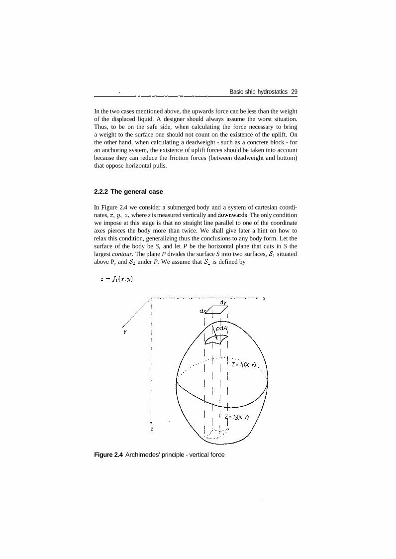
In Figure 2.4 we consider a submerged body and a system of cartesian coordi-nates, x, y, z, where z is measured vertically and downwards. The only conditionwe impose at this stage is that no straight line parallel to one of the coordinateaxes pierces the body more than twice. We shall give later a hint on how torelax this condition, generalizing thus the conclusions to any body form. Let thesurface of the body be S, and let P be the horizontal plane that cuts in S thelargest contour. The plane P divides the surface S into two surfaces, Si situatedabove P, and 8*2 under P. We assume that Si is defined by
*• x
Figure 2.4 Archimedes' principle - vertical force
30 Ship^Hydrostatics and Stability
and <$2 by
z = f 2 ( x , y )
The hydrostatic force on an element dA of Si is pdA. This force is directed alongthe normal, n, to Si in the element of area. If the cosine of the angle betweenn and the vertical axis is cos(n, z), the vertical component of the pressure forceon dA equals 7/1(0:, y) cos(n, z)dA As cos(n, z)dA is the projection of dAon a horizontal plane, that is dxdy, we conclude that the vertical hydrostaticforce on Si is
/ / fi(x,y)dxdy (2.9)
Let us consider now an element of <$2 'opposed' to the one we considered on Si .We reason as above, taking care to change signs. We conclude that the hydrostaticforce on £2 is
~7 / / h(x, y}dxty (2.10)J JS<2
and the total force on <$,
The integral in Eq. (2.11) yields the volume of the submerged body. Thus,F equals the weight of the liquid displaced by the submerged body. It remainsto show that the horizontal components of the resultant of hydrostatic pressuresare equal to zero. We use Figure 2.5 to prove this for the component parallel tothe x-axis. The force component parallel to the x-axis acting on the element ofarea dA is
pcos(n, x)d^l = jzdydz
On the other side of the surface, at the same depth z, there is an element of areasuch that the hydrostatic force on it equals
pcos(n, x)d^4 = — jzdydz
The sum of both forces is zero. As the whole surface <$ consists of such 'opposed'pairs d^4, the horizontal component in the x direction is zero. By a similarreasoning we conclude that the horizontal component in the y direction is zerotoo. This is also the result predicted by intuition. In fact, if the resultant of thehorizontal components would not be zero we would obtain a 'free' propulsionforce.
This completes the proof of Archimedes' principle for a body shape subjectedto the only restriction that no straight line parallel to one of the coordinate axesintersects the body more than twice.
Basic ship hydrostatics 31
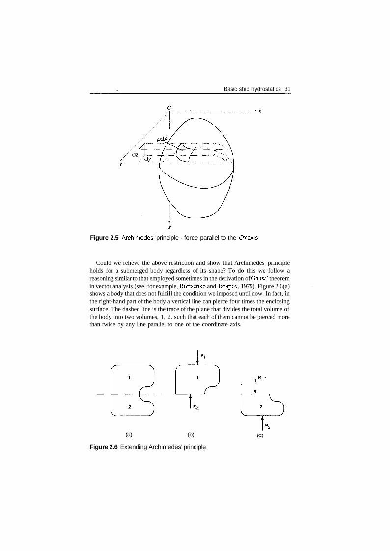
Figure 2.5 Archimedes' principle - force parallel to the Ox axis
Could we relieve the above restriction and show that Archimedes' principleholds for a submerged body regardless of its shape? To do this we follow areasoning similar to that employed sometimes in the derivation of Gauss' theoremin vector analysis (see, for example, Borisenko and Tarapov, 1979). Figure 2.6(a)shows a body that does not fulfill the condition we imposed until now. In fact, inthe right-hand part of the body a vertical line can pierce four times the enclosingsurface. The dashed line is the trace of the plane that divides the total volume ofthe body into two volumes, 1, 2, such that each of them cannot be pierced morethan twice by any line parallel to one of the coordinate axis.
(a) (b)
Figure 2.6 Extending Archimedes' principle
(C)
32 Ship Hydrostatics and Stability
Let us consider now the upper volume, 1, in Figure 2.6(b). Two forces act onthis body:
1. the resultant of hydrostatic pressures, PI, on the external surface;2. the force R2,i exercised by the volume 2 on volume 1.
Similarly, let us consider the lower volume, 2, in Figure 2.6(c). Two forces acton this body:
1. the resultant of hydrostatic pressures, P2, acting on the external surface;2. the force Ri)2 exercised by the volume 1 on volume 2.
As the forces R2,i and Ri,2 are equal and opposed, putting together the volumes1 and 2 means that the sum of all forces acting on the total volume is PI -f ?2,that is the force predicted by Archimedes' principle. Let us find the x andy -coordinates of the point through which acts the buoyancy force. To do so wecalculate the moments of this force about the xOz and yOz planes and dividethem by the total force. The results are
J JsS7*[/i(s, y) - fr(x, y)]dxdyI Is 7^[/i(X y} ~ h(x, y)]dxdy
J fsxz[fi(xi y) - / 2p ,ffsz[fi(x, y) - f2(x, y)]dxdy
J /$2/7*[/iQp, y) - h(x, y)]dxdyf fsiz[fi(x, y) ~ h(z, y)]dxdy
These are simply the x and y-coordinates of the centre of the submerged volume.We conclude that the buoyancy force passes through the centre of the submergedvolume, B (centre of the displaced volume of liquid).
2.3 The conditions of equilibrium of a floating body
A body is said to be in equilibrium if it is not subjected to accelerations. Newton'ssecond law shows that this happens if the sum of all forces acting on that body iszero and the sum of the moments of those forces is also zero. Two forces alwaysact on a floating body: the weight of that body and the buoyancy force. In thissection we show that the first condition for equilibrium, that is the one regardingthe sum of forces, is expressed as Archimedes' principle. The second condition,regarding the sum of moments, is stated as Stevin's law.
Basic ship hydrostatics 33
Further forces can act on a floating body, for example those produced by wind,by centrifugal acceleration in turning or by towing. The influence of those forcesis discussed in Chapter 6.
2.3.1 Forces
Let us assume that the bodies appearing in Figures 2.1, 2.3(a) float freely. Then,the weight of each body and the hydrostatic forces acting on it are in equilibrium.Archimedes' principle can be reformulated as:
The weight of the volume of water displaced by a floating body isequal to the weight of that body.
The weight of the fluid displaced by a floating body is appropriately calleddisplacement. We denote the displacement by the upper-case Greek letter delta,that is A. If the weight of the floating body is W, then we can express theequilibrium of forces acting on the floating body by
A = W (2.16)
For the volume of the displaced liquid we use the symbol V defined in Chapter 1 .In terms of the above symbols Archimedes' principle yields the equation
7V = W (2.17)
If the floating body is a ship, we rewrite Eq. (2.17) as
X?=lWi (2.18)
where Wi is the weight of the ith item of ship weight. For example, W\ can bethe weight of the ship hull, W^, of the outfit, W%, of the machinery, and so on.The symbol CB and the letters L, B, T have the meanings defined in Chapter 1.
In hydrostatic calculations Eq. (2.18) is often used to find the draught cor-responding to a given displacement, or the displacement corresponding to ameasured draught. In Ship Design Eq. (2.18) is used either as a design equa-tion (see, for example, Manning, 1956), or as an equality constraint in designoptimization problems (see, for example, Kupras, 1976).
Instead of the displacement weight we may work with the displacement mass,pV, where p is the density of the surrounding water. Then, Eq. (2.18) can berewritten as
PCBLBT = E^rai (2.19)
where m^ is the mass of the ith ship item. The DIN standards define, indeed,A as mass, and use Ap for displacemnt weight. The subscript T" stands for'force'. In later chapters of this book we shall use the displacement mass ratherthan the displacement weight.
34 Ship Hydrostatics and Stability
Table 2.1 Some foreign names for the point B
Language
FrenchGermanItalianPortuguese
Term
Centre de careneFormschwerpunktCentre di carenaCentre do carena
Meaning
Centre of submerged hullCentre of gravity of solidCentre of submerged hullCentre of submerged hull
To remember the meaning of the symbol A, let us think that the word 'delta'begins with a 'd', like the word 'displacement' (we ignore the fact that incontemporary-Greek pronunciation 'delta' is actually read as 'thelta'). As tothe symbol V, it resembles 'V, the initial letter of the word 'volume'.
The point B is called in English centre of buoyancy. There are languages inwhich the name of the point B recognizes the fact that B is not a centre of pressure.Table 2.1 gives a few examples. This is, of course, a matter of semantics. Theline of action of the buoyancy force always passes through the point B.
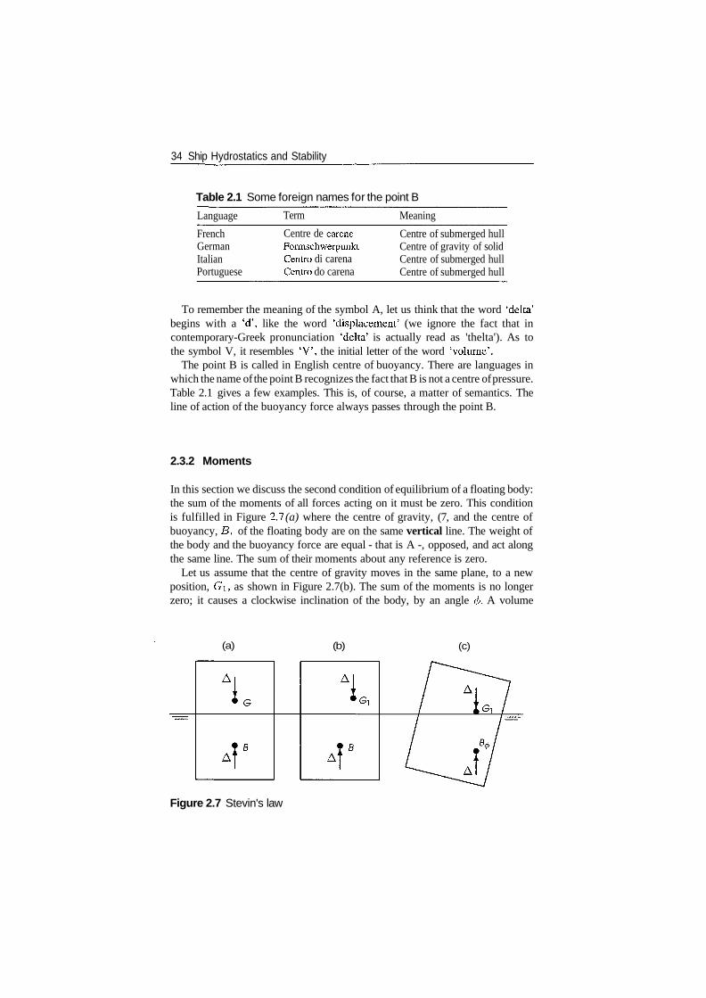
2.3.2 Moments
In this section we discuss the second condition of equilibrium of a floating body:the sum of the moments of all forces acting on it must be zero. This conditionis fulfilled in Figure 2.1 (a) where the centre of gravity, (7, and the centre ofbuoyancy, B, of the floating body are on the same vertical line. The weight ofthe body and the buoyancy force are equal - that is A -, opposed, and act alongthe same line. The sum of their moments about any reference is zero.
Let us assume that the centre of gravity moves in the same plane, to a newposition, GI, as shown in Figure 2.7(b). The sum of the moments is no longerzero; it causes a clockwise inclination of the body, by an angle <p. A volume
(a) (b) (c)
Figure 2.7 Stevin's law
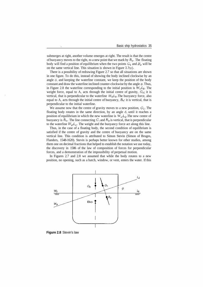
Basic ship hydrostatics 35
submerges at right, another volume emerges at right. The result is that the centreof buoyancy moves to the right, to a new point that we mark by B$. The floatingbody will find a position of equilibrium when the two points G\ and B^ will beon the same vertical line. This situation is shown in Figure 2.7(c).
There is a possibility of redrawing Figure 2.7 so that all situations are shownin one figure. To do this, instead of showing the body inclined clockwise by anangle </>, and keeping the waterline constant, we keep the position of the bodyconstant and draw the waterline inclined counter-clockwise by the angle 0. Thus,in Figure 2.8 the waterline corresponding to the initial position is WQ-^O- Theweight force, equal to A, acts through the initial centre of gravity, GO; it isvertical, that is perpendicular to the waterline W^LQ. The buoyancy force, alsoequal to A, acts through the initial centre of buoyancy, BQ: it is vertical, that isperpendicular to the initial waterline.
We assume now that the centre of gravity moves to a new position, G\. Thefloating body rotates in the same direction, by an angle <f>, until it reaches aposition of equilibrium in which the new waterline is W^L^. The new centre ofbuoyancy is B^. The line connecting GI and B^ is vertical, that is perpendicularto the waterline W^I/0. The weight and the buoyancy force act along this line.
Thus, in the case of a floating body, the second condition of equilibrium issatisfied if the centre of gravity and the centre of buoyancy are on the samevertical line. This condition is attributed to Simon Stevin (Simon of Bruges,Flanders, 1548-1620). Stevin is perhaps better known for other studies, amongthem one on decimal fractions that helped to establish the notation we use today,the discovery in 1586 of the law of composition of forces for perpendicularforces, and a demonstration of the impossibility of perpetual motion.
In Figures 2.7 and 2.8 we assumed that while the body rotates to a newposition, no opening, such as a hatch, window, or vent, enters the water. If this
Bo I
Figure 2.8 Stevin's law
36 Ship Hydrostatics and Stability
assumption is not correct, the body can either reach equilibrium under morecomplex conditions (see Chapter 11), or sink.
2.4 A definition of stability
In the preceding section we learnt the conditions of equilibrium of a floatingbody. The question we ask in the next section is how to determine if a conditionof equilibrium is stable or not. Before answering this question we must definethe notion of stability. This concept is general; we are interested here in itsapplication to floating bodies.
Let us consider a floating body in equilibrium and assume that some force ormoment causes a small change in its position. Three situations can occur whenthat force or moment ceases to act.
1. The body returns to its initial position; we say that the condition of equilibriumis stable.
2. The position of the body continues to change. We say in this case that theequilibrium is unstable. In practical terms this can mean, for example, thatthe floating body capsizes.
3. The body remains in the displaced position until the smallest perturbationcauses it to return to the initial position or to continue to move away from theinitial position. We call this situation neutral equilibrium.
As an example let us consider the body shown in Figure 2.1. If this body floatsfreely at the surface we conclude from Eq. (2.17) that the total volume is largerthan the weight divided by the specific gravity of the fluid. This body floats instable equilibrium as to draught. To show this let us imagine that some forcecauses it to move downwards so that its draught increases by the quantity 5T.Archimedes' principle tells us that a new force, ^LB6T, appears and that it isdirected upwards. Suppose now that the cause that moved the body downwardsdecreases slowly. Then, the force ̂ LB8T returns the body to its initial position.In fact, as the body moves (slowly) upwards, ST decreases until it becomes zeroand then the motion ceases. If the force that drove the body downwards ceasesabruptly, the body oscillates around its initial position and, if damping forcesare active - they always exist in nature -, the body will eventually come to restin its initial position.
Next, we assume that some force moved the body upwards so that its draughtdecreases by ST. A force —^LBST appears now and it is directed downwards.Therefore, if the body is released slowly it will descend until 6T = 0. Thiscompletes the proof that the body floating freely at the surface is in stableequilibrium with regard to its draught. We mention 'with regard to draught'because, as shown in the next section, the body may be unstable with regardto heel.
Basic ship hydrostatics 37
When a body floats freely, but is completely submerged, its weight equalsexactly its volume multiplied by the specific gravity of the liquid. This body isin neutral equilibrium because it can float at any depth. Any small perturbationwill move the body from a depth to another one. If the weight of the body islarger than its total volume multiplied by the specific gravity of the liquid, thenthe body will sink.
Summing-up, we may distinguish three cases.
1 . The total volume of a body is larger than its weight divided by the specificgravity of the water:
Ftotal > Wh
The body floats at the surface and we can control the draught by adding orreducing weights.
2. The weight of the body exactly equals the total volume multiplied by thespecific gravity of the liquid:
The body can float at any depth and we cannot control the position by addingor reducing weights. Any additional weight would cause the body to sinkbringing it into case 3. Reducing even slightly its weight will cause the bodyto come to the surface; its situation changes to case 1.
3. The weight of the body is larger than its volume multiplied by the specificgravity of the water:
Vtotal < Wh
The body will sink. To change its position we must either reduce the weightuntil we reach at least situation 2, or add buoyancy in some way.
In the above analysis we assumed that the specific gravity of the liquid, 7, is con-stant throughout the liquid volume. This assumption may not be correct if largevariations in temperature or salinity are present, or if the liquid volume consistsof layers of different liquids. Interesting situations can arise in such cases. Othersituations can arise at large depths at which the water density increases whilethe volume of the floating body shrinks because of the compressibility of itsstructure. These cases are beyond the scope of this book.
2.5 Initial stability
Figure 2.9(a) is a vertical, transverse section through a ship in upright condition,that is unheeled. If this section passes through the centre of buoyancy, B, weknow from Stevin's law that it contains the centre of gravity, G. The water line is
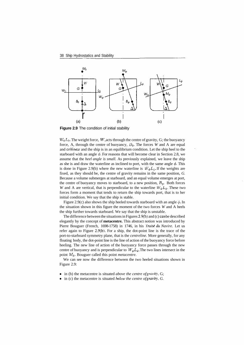
38 Ship Hydrostatics and Stability
W0
W
r(a) (b)
Figure 2.9 The condition of initial stability
(c)
Wo I/o- The weight force, W, acts through the centre of gravity, G; the buoyancyforce, A, through the centre of buoyancy, J50. The forces W and A are equaland collinear and the ship is in an equilibrium condition. Let the ship heel to thestarboard with an angle <j>. For reasons that will become clear in Section 2.8, weassume that the heel angle is small. As previously explained, we leave the shipas she is and draw the waterline as inclined to port, with the same angle 0. Thisis done in Figure 2.9(b) where the new waterline is W^L^. If the weights arefixed, as they should be, the centre of gravity remains in the same position, G.Because a volume submerges at starboard, and an equal volume emerges at port,the centre of buoyancy moves to starboard, to a new position, B^. Both forcesW and A are vertical, that is perpendicular to the waterline W^L^. These twoforces form a moment that tends to return the ship towards port, that is to herinitial condition. We say that the ship is stable.
Figure 2.9(c) also shows the ship heeled towards starboard with an angle <p. Inthe situation shown in this figure the moment of the two forces W and A heelsthe ship further towards starboard. We say that the ship is unstable.
The difference between the situations in Figures 2.9(b) and (c) can be describedelegantly by the concept of metacentre. This abstract notion was introduced byPierre Bouguer (French, 1698-1758) in 1746, in his Traite du Navire. Let usrefer again to Figure 2.9(b). For a ship, the dot-point line is the trace of theport-to-starboard symmetry plane, that is the centreline. More generally, for anyfloating body, the dot-point line is the line of action of the buoyancy force beforeheeling. The new line of action of the buoyancy force passes through the newcentre of buoyancy and is perpendicular to W^L^. The two lines intersect in thepoint M^. Bouguer called this point metacentre.
We can see now the difference between the two heeled situations shown inFigure 2.9:
in (b) the metacentre is situated above the centre of gravity, G;in (c) the metacentre is situated below the centre of gravity, G.

Basic ship hydrostatics 39
We conclude that the equilibrium of the floating body is stable if the metacentreis situated above the centre of gravity.
For his contributions of overwhelming importance, Bouguer was sometimesdescribed as 'the father of naval architecture' (quotation in Stoot, 1959). It mustbe emphasized here that the definition of the metacentre is not connected at allwith the form of a ship. Therefore, the fact that in the above figures the meta-centre is the intersection of the new line of action of the buoyancy force and thecentreline is true only for symmetrical hulls heeled from the upright condition.For a general floating body we can reformulate the definition as follows:
Let us consider a floating body and its centre of buoyancy B^. Letthe line of action of the buoyancy force be R. If the body changesits inclination by an angle <50, the centre of buoyancy changes itsposition to B^+SJ and the new line of action of the buoyancy forcewill be, say, 5. When S(f> tends to zero, the intersection of the linesR and S tends to a point that we call metacentre.
Readers familiar with elementary differential geometry will recognize that,defined as above, the metacentre is the the centre of curvature of the curve ofcentres of buoyancy. The notion of curvature is defined in Chapter 13.
2.6 Metacentric height
In the preceding section we learnt that a surface ship is initially stable if its initialmetacentre is above the centre of gravity. For actual calculations we must find aconvenient mathematical formulation. We do this with the help of Figure 2.9(a).We choose a reference point, K, at the intersection of the centreline and thebaseline and we measure vertical coordinates from it, upwards. Thus defined,K is the origin of ^-coordinates. A good recommendation is to choose K as thelowest point of the ship keel; then, there will be no negative ^-coordinates. Weremember easily the chosen notation because K is the initial letter of the wordkeel.
In the same figure M0 is the initial metacentre, that is the metacentre corre-sponding to the upright condition. Dropping the subscripts 0 we can write
BM - KG (2.20)
and the condition of initial stability is expressed as
GM > 0 (2.21)
The vector GM is called metacentric height. The vector KB is the ^-coordinateof the centre of buoyancy; it is calculated as the ^-coordinate of the centroid ofthe submerged hull as one of the results of hydrostatic calculations. The vectorBM is the metacentric radius whose calculation we are going to discuss in
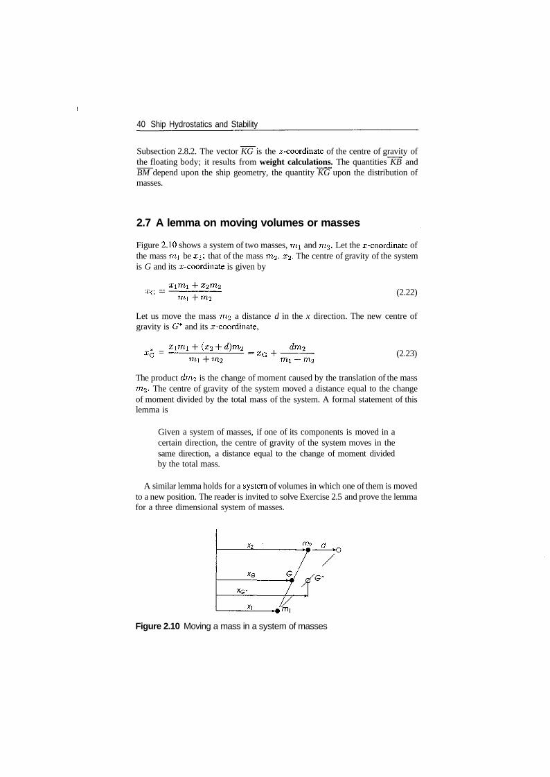
40 Ship Hydrostatics and Stability
Subsection 2.8.2. The vector KG is the ^-coordinate of the centre of gravity ofthe floating body; it results from weight calculations. The quantities KB andBM depend upon the ship geometry, the quantity KG upon the distribution ofmasses.
2.7 A lemma on moving volumes or masses
Figure 2.10 shows a system of two masses, mi and m2. Let the x-coordinate ofthe mass mi be x\\ that of the mass m,2, #2- The centre of gravity of the systemis G and its x-coordinate is given by
XG =mi (2.22)
Let us move the mass m2 a distance d in the x direction. The new centre ofgravity is G* and its x-coordinate,
XG =(x2 XG
-f- m2(2.23)
The product dm2 is the change of moment caused by the translation of the massm2. The centre of gravity of the system moved a distance equal to the changeof moment divided by the total mass of the system. A formal statement of thislemma is
Given a system of masses, if one of its components is moved in acertain direction, the centre of gravity of the system moves in thesame direction, a distance equal to the change of moment dividedby the total mass.
A similar lemma holds for a system of volumes in which one of them is movedto a new position. The reader is invited to solve Exercise 2.5 and prove the lemmafor a three dimensional system of masses.
/Tb cf
Figure 2.10 Moving a mass in a system of masses
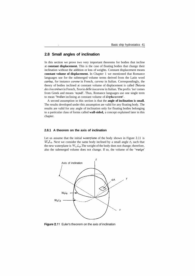
Basic ship hydrostatics 41
2.8 Small angles of inclination
In this section we prove two very important theorems for bodies that inclineat constant displacement. This is the case of floating bodies that change theirinclination without the addition or loss of weights. Constant displacement meansconstant volume of displacement. In Chapter 1 we mentioned that Romancelanguages use for the submerged volume terms derived from the Latin wordcarina, for instance carene in French, carena in Italian. Correspondingly, thetheory of bodies inclined at constant volume of displacement is called Theoriedes isocarenes in French, Teoria delle isocarene in Italian. The prefix 'iso' comesfrom Greek and means 'equal'. Thus, Romance languages use one single termto mean 'bodies inclining at constant volume of displacement'.
A second assumption in this section is that the angle of inclination is small.The results developed under this assumption are valid for any floating body. Theresults are valid for any angle of inclination only for floating bodies belongingto a particular class of forms called wall-sided, a concept explained later in thischapter.
2.8.1 A theorem on the axis of inclination
Let us assume that the initial waterplane of the body shown in Figure 2.11 isWQ Z/o- Next we consider the same body inclined by a small angle </>, such thatthe new waterplane is W^L^. The weight of the body does not change; therefore,also the submerged volume does not change. If so, the volume of the 'wedge'
Axis of inclination
Figure 2.11 Euler's theorem on the axis of inclination
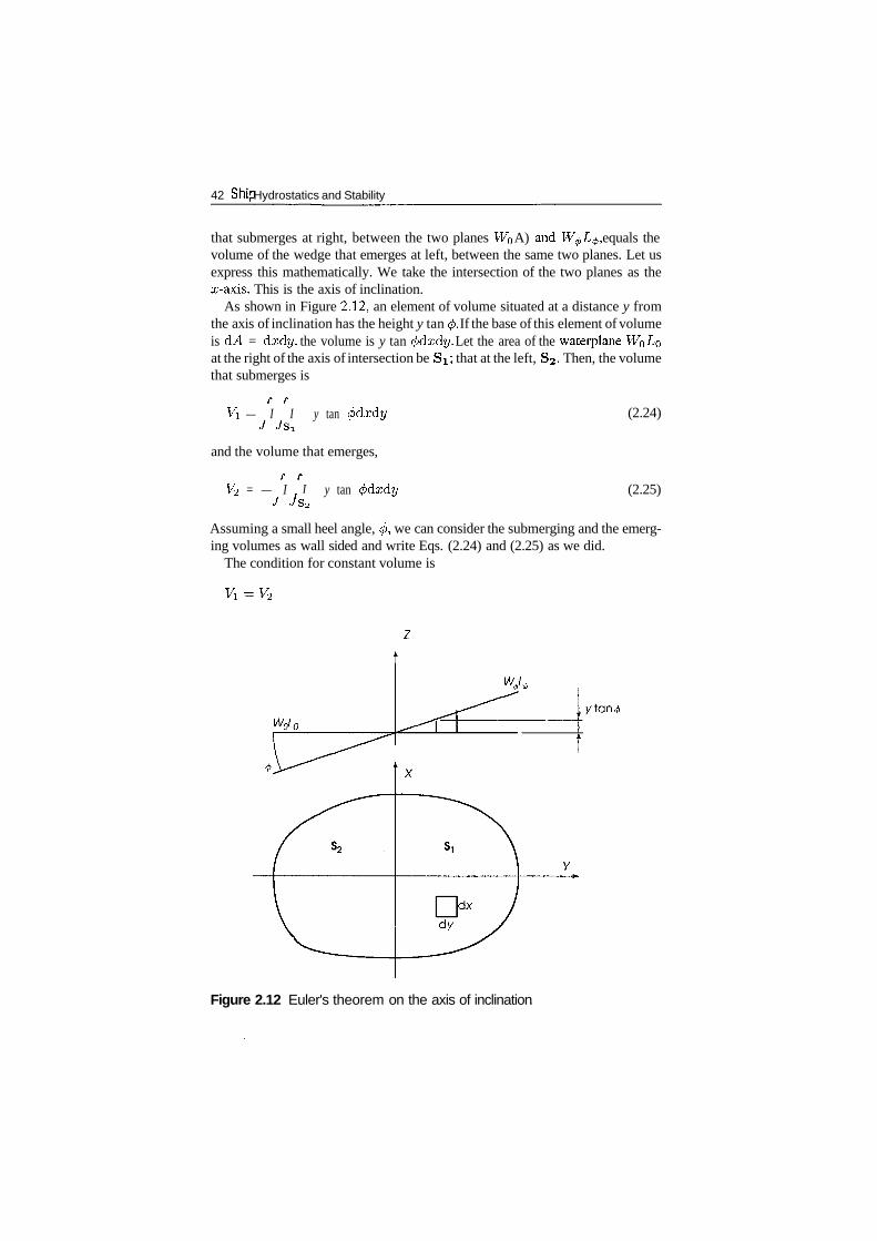
42 Ship Hydrostatics and Stability
that submerges at right, between the two planes WQ A) and W^L^, equals thevolume of the wedge that emerges at left, between the same two planes. Let usexpress this mathematically. We take the intersection of the two planes as thex-axis. This is the axis of inclination.
As shown in Figure 2.12, an element of volume situated at a distance y fromthe axis of inclination has the height y tan (/). If the base of this element of volumeis dA = dxdy, the volume is y tan <pdxdy. Let the area of the waterplane WQ^Oat the right of the axis of intersection be Si; that at the left, S2. Then, the volumethat submerges is
Vi — I I y tan (f)dxdy
and the volume that emerges,
V<2 = — I I y tan (/)dxdyJ 7s2
(2.24)
(2.25)
Assuming a small heel angle, 0, we can consider the submerging and the emerg-ing volumes as wall sided and write Eqs. (2.24) and (2.25) as we did.
The condition for constant volume is
Figure 2.12 Euler's theorem on the axis of inclination
Basic ship hydrostatics 43
Combining this with Eqs. (2.24) and (2.25) yields
y tan (pdxdy = — y tan <pdxdy (2.26)J 7si J Js2
and, finally,
ydxdy = 0 (2.27)s
where S = Si -f 82 is the whole waterplane. In words, the first moment of thewaterplane area, with respect with the axis of inclination, is zero. This happensonly if the axis of inclination passes through the centroid of the waterplane area.We remind the reader that the coordinates of the centroid of a surface 5 aredefined by
/ fsxdxdy f fsydxdyXG= /• r i i > ye = r r , ,J Js dxdy J Js dxdy
Or, as the Webster's Ninth New Collegiate Dictionary puts it, 'corresponds tothe center of mass of a thin plate of uniform thickness'. The centroid of thewaterplane area is known as centre of flotation and is noted by F. The corre-sponding French term is 'centre de gravite de la flottaison', the German term is'Wasserlinien-Schwerpunkt', and the Italian, 'centre del galleggiamento'.
A statement of the property proven above is
Let the initial waterplane of a floating body be WoZ/o- After aninclination, at constant volume of displacement, with an angle 0, thenew waterplane is W^L^. The intersection of the two waterplanesis the axis of inclination. If the angle of inclination tends to zero,the axis of inclination tends to a straight line passing through thecentroid of the waterplane area.
In practice, this property holds if the angle of inclination is sufficiently small.For heeling of a vessel, this can mean a few degrees, 5° for some forms, even15° for others. If the inclination is the trimming of an intact vessel, the angles areusually small enough and this property always holds. The property also holdsfor larger heel angles if the floating body is wall sided. This is the name givento floating bodies whose surface includes a cylinder (in the broader geometricalsense), with generators perpendicular to the initial waterplane. An illustration ofsuch a case is given in Example 2.5. In French and Italian, for example, the termused for wall-sided bodies is cylindrical floating bodies.
The term used in some languages, such as French or Italian, for an axis passingthrough the centroid of an area is barycentric axis. This term is economic andwe shall use it whenever it will help us to express ideas more concisely.
44 Ship Hydrostatics and Stability
2.8.2 Metacentric radius
Let us refer again to Figure 2.9. As we shall see, the vector B^M^ plays animportant role in stability. Leaving the subscript </>, we genetically call BMmetacentric radius; in this section we calculate its magnitude. To do so we mustfind the shift of the centre of buoyancy, B, for a small angle of inclination 0.Here we use the lemma on moving volumes and we calculate
change of moment of volumechange or coordinate = - - - - -
total volume
As seen from Figures 2.11 and 2.12, the elemental change of volume isy tan fidxdy. To find the changes of moment respective to the coordinate planeswe must multiply the elemental volume by the coordinates of its centroid. Tomake things easier, we take the origin of coordinates in the initial centre of buoy-ancy, £?o, measure the x-coordinate parallel to the axis of inclination, positiveforwards, the ̂ /-coordinate transversely, positive leftwards, and the z-coordinatevertically, positive upwards. The coordinates of the centre of buoyancy B^ areobtained by integrating the changes of moment of the elemental volume, overthe waterplane area S.
The results are
f fc ^V2 tan2 6dxdy II 0
ZB = S 2 y - - = 2 y tan * (230)
Above, / is the moment of inertia of the waterplane area about the axis ofinclination (remember, it is a barycentric axis), and Ixy, the product of inertiaof the same area about the axes x and y. In German and some other languagesIxy is called centrifugal moment of inertia.
As we assumed that the angle </> is small, we can further write
VB = (2-31)
11
The coordinate ZB is of second order and we can neglect it if </> is small. Asto the ^-coordinate let us remember that conventional ships in upright conditionenjoy a port-to-starboard symmetry. This means that for such ships, in upright
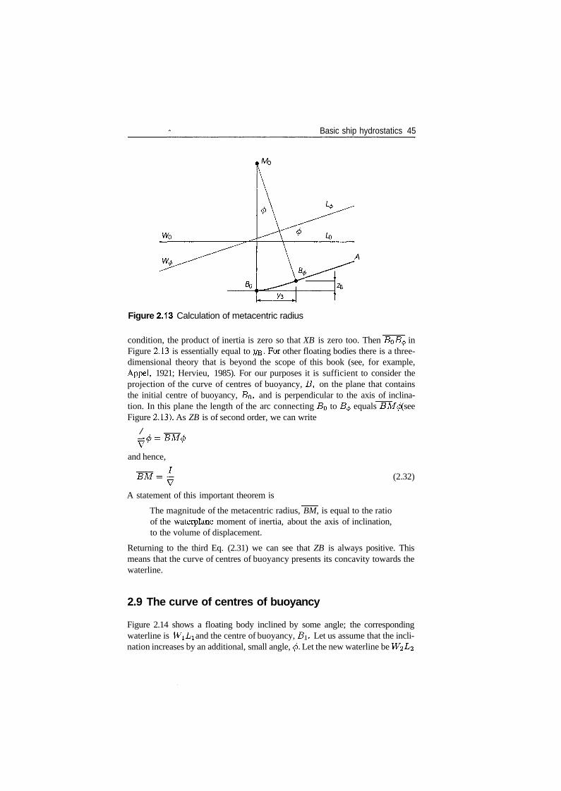
Basic ship hydrostatics 45
Figure 2.13 Calculation of metacentric radius
condition, the product of inertia is zero so that XB is zero too. Then B^B^ inFigure 2.13 is essentially equal to T/B- F°r other floating bodies there is a three-dimensional theory that is beyond the scope of this book (see, for example,Appel, 1921; Hervieu, 1985). For our purposes it is sufficient to consider theprojection of the curve of centres of buoyancy, B, on the plane that containsthe initial centre of buoyancy, BQ, and is perpendicular to the axis of inclina-tion. In this plane the length of the arc connecting B0 to B^ equals BMfi (seeFigure 2.13). As ZB is of second order, we can write
/
Vand hence,
(2.32)
A statement of this important theorem is
The magnitude of the metacentric radius, BM, is equal to the ratioof the waterplane moment of inertia, about the axis of inclination,to the volume of displacement.
Returning to the third Eq. (2.31) we can see that ZB is always positive. Thismeans that the curve of centres of buoyancy presents its concavity towards thewaterline.
2.9 The curve of centres of buoyancy
Figure 2.14 shows a floating body inclined by some angle; the correspondingwaterline is WiLi and the centre of buoyancy, B\. Let us assume that the incli-nation increases by an additional, small angle, <j>. Let the new waterline be
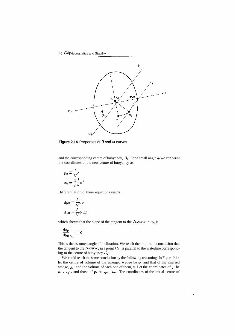
46 Ship Hydrostatics and Stability
Figure 2.14 Properties of Band M curves
and the corresponding centre of buoyancy, £?2. For a small angle 0 we can writethe coordinates of the new centre of buoyancy as
_ /
1 / ,o
Differentiation of these equations yields
_ I
V/
V
which shows that the slope of the tangent to the 5-curve in B2 is
B-2
This is the assumed angle of inclination. We reach the important conclusion thatthe tangent to the B-curve, in a point B^, is parallel to the waterline correspond-ing to the centre of buoyancy B^.
We could reach the same conclusion by the following reasoning. In Figure 2.14let the centre of volume of the emerged wedge be gi and that of the imersedwedge, 02, and the volume of each one of them, v. Let the coordinates of gi be2/pi, zgi, and those of 02 be yg2, zg2. The coordinates of the initial centre of
Basic ship hydrostatics 47
buoyancy, B\, are yBi, zBl , and those of B2 are yB2, zs2 • Applying the lemmaon moving volumes we write
V= ( Z g 2 - Z g l ) -
ygi
which shows that B^B^ is parallel to g\Q2- When 0 tends to zero, g\g% tends tothe initial waterline and J3i J32 to the tangent in BI to the £?-curve.
2.10 The metacentric evolute
The buoyancy force is always normal to the waterline. As the tangent to the5-curve is parallel to the corresponding waterline, it follows that the buoyancyforce is normal to the J3-curve. In Figure 2.14 the normals to the 5-curve inthe points BI and B^ intersect in a point M. In some languages this point iscalled metacentric point. When BI —> B%, the metacentric point tends to themetacentre.
Let the curve M be the locus of the metacentres corresponding to a givencurve B. The curve M is the locus of centres of curvature of the curve B itis also the envelope of the normals to the curve B By definition, the curveM is the evolute of the curve B (see, for example Struik, 1961); it is calledmetacentric evolute. The term used in French is developpee metacentrique•, inGerman, Metazentrische Evolute, and in Italian, evoluta metacentric a.
Conversely, the curve B intersects at right angles the tangents to the meta-centric evolute. Then, by definition, the curve B is the involute of the curve M.The term used in French is developpante', in German, Evolvente, and in Italian,evolventa.
The concepts of B and M curve are illustrated in Examples 2.5 and 2.6. Somereaders may be familiar with another example of a pair of curves that stay oneto the other in the relationship evolute-involute. The shape of the tooth flanksused today in most gears is that of an involute of circle.
2.11 Metacentres for various axes of inclination
In Eq. (2.32) the moment of inertia, /, is calculated about the axis of inclination.This axis passes through the centroid, F, of the waterplane and so does any otheraxis of inclination. It can be shown that there is a pair of orthogonal axes such
48 Ship Hydrostatics and Stability
that the moment of inertia about one of them is minimum and about the othermaximum. Then, the metacentric radius corresponding to the former axis is min-imum, and the moment about the latter axis is maximum. Correspondingly, oneof the metacentric radii is minimum and the other maximum. In some Europeancountries the smallest radius is denoted by r and is called small metacentricradius, while the largest radius is denoted R and is called large metacentricradius.
In the theory of moments of inertia the two axes for which we obtain theextreme values of moments of inertia are called principal axes and the corre-sponding moments, principal moments of inertia. When the waterplane areahas an axis of symmetry, this axis is one of the principal axes; the other oneis perpendicular to the first. The waterplane area of ships in upright conditionhas an axis of symmetry: the intersection of the waterplane and the centrelineplane. The moment of inertia about this axis is the smallest one; it is used tocalculate the transverse metacentric radius. The moment of inertia about theaxis perpendicular in F to the centreline is the largest; it enters in the calculationof the longitudinal metacentric radius.
To give an idea of the relative orders of magnitude of the transverse andlongitudinal metacentric radii, let us consider a parallelepipedic barge whoselength is L, breadth, B, and draught, T. The volume of displacement equalsV = LET. The transverse metacentric radius results from
LB3/12 B2
BM —~ LET ~ 12T
The longitudinal metacentric radius is given by
BL3/12 L2
- - = 12T
The ratio of the two metacentric radii is
BM \B
The length-breadth ratio ranges from 3.1, for some motor boats, to 10.5, for fastcruisers. Correspondingly, the ratio of the longitudinal to the transverse metacen-tric radius varies roughly between 10 and 110. As a rule of thumb, the longitudinalmetacentric radius is of the same order of magnitude as the ship length.
2.12 Summary
A body submersed in a fluid is subjected to an upwards force equal to the weight ofthe displaced fluid. This is Archimedes' principle. The hydrostatic force predictedby this principle passes through the centre of volume of the displaced fluid; wecall that point centre of buoyancy and denote it by the letter B.
Basic ship hydrostatics 49
For a floating body the weight of the displaced fluid equals the weight of thatbody. The symbol for the immersed volume is V; that for the displacement mass,A. If the density of the fluid is p, we can write
Values of the density of water in different navigation ways are given in theAppendix of this chapter.
If a floating body is inclined by a small angle, the new waterplane intersectsthe initial one along a line that passes through its centroid, that is, through thecentre of flotation.
If the floating body is a ship, using the notations described in Chapter 1 wewrite
>yCBLBT = E^mi
where m* is the mass of the ith item aboard and n, the total number of ship items.A is called displacement mass and V, displacement volume. The above equationexpresses the condition of equilibrium offerees. The condition of equilibrium ofmoments requires that the centre of gravity, G, of the floating body and its centreof buoyancy, J5, lie on the same vertical. This condition is known as Stevin'slaw.
We say that a floating body is initially 'stable' if after a small perturbation ofits position of equilibrium, that body returns to its initial position. To study initialstability, Bouguer introduced the notion of metacentre. Let the line of action ofthe buoyancy force in the initial position be R. If the floating body is inclinedby a small angle, 5<j), the buoyancy force acts along a new line, say S. When 5(j>tends to zero, the intersection of the two lines, R and 5, tends to a point, M,called metacentre.
The equilibrium of a floating body is stable if its metacentre lies above itscentre of gravity. The distance from the centre of gravity to the metacentre, GM,is called metacentric height and is considered positive upwards. The conditionof initial stability can be expressed as
G M > 0
The distance from the centre of buoyancy to the metacentre, BM, is calledmetacentric radius. Its value is given by
BM=-
where / is the moment of inertia of the waterplane about the axis of inclination,a line that passes through the centroid of the area, that is through the centre offlotation, F. Let K be the origin of vertical coordinates. We can write
GM = KB + BM - KG
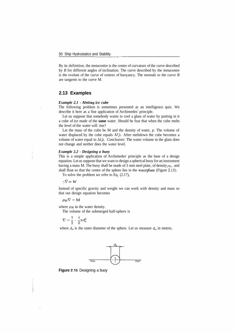
50 Ship Hydrostatics and Stability
By its definition, the metacentre is the centre of curvature of the curve describedby B for different angles of inclination. The curve described by the metacentreis the evolute of the curve of centres of buoyancy. The normals to the curve Bare tangents to the curve M.
2.13 Examples
Example 2.1 - Melting ice cubeThe following problem is sometimes presented as an intelligence quiz. Wedescribe it here as a fine application of Archimedes' principle.
Let us suppose that somebody wants to cool a glass of water by putting in ita cube of ice made of the same water. Should he fear that when the cube meltsthe level of the water will rise?
Let the mass of the cube be M and the density of water, p. The volume ofwater displaced by the cube equals M/ p. After meltdown the cube becomes avolume of water equal to M/ p. Conclusion: The water volume in the glass doesnot change and neither does the water level.
Example 2.2 - Designing a buoyThis is a simple application of Archimedes' principle as the base of a designequation. Let us suppose that we want to design a spherical buoy for an instrumenthaving a mass M. The buoy shall be made of 3 mm steel plate, of density p$, andshall float so that the centre of the sphere lies in the waterplane (Figure 2.15).
To solve the problem we refer to Eq. (2.17),
7V = W
Instead of specific gravity and weight we can work with density and mass sothat our design equation becomes
= M
where pw is the water density.The volume of the submerged half-sphere is
v-i.i*where d0 is the outer diameter of the sphere. Let us measure d0 in metres.
Figure 2.15 Designing a buoy
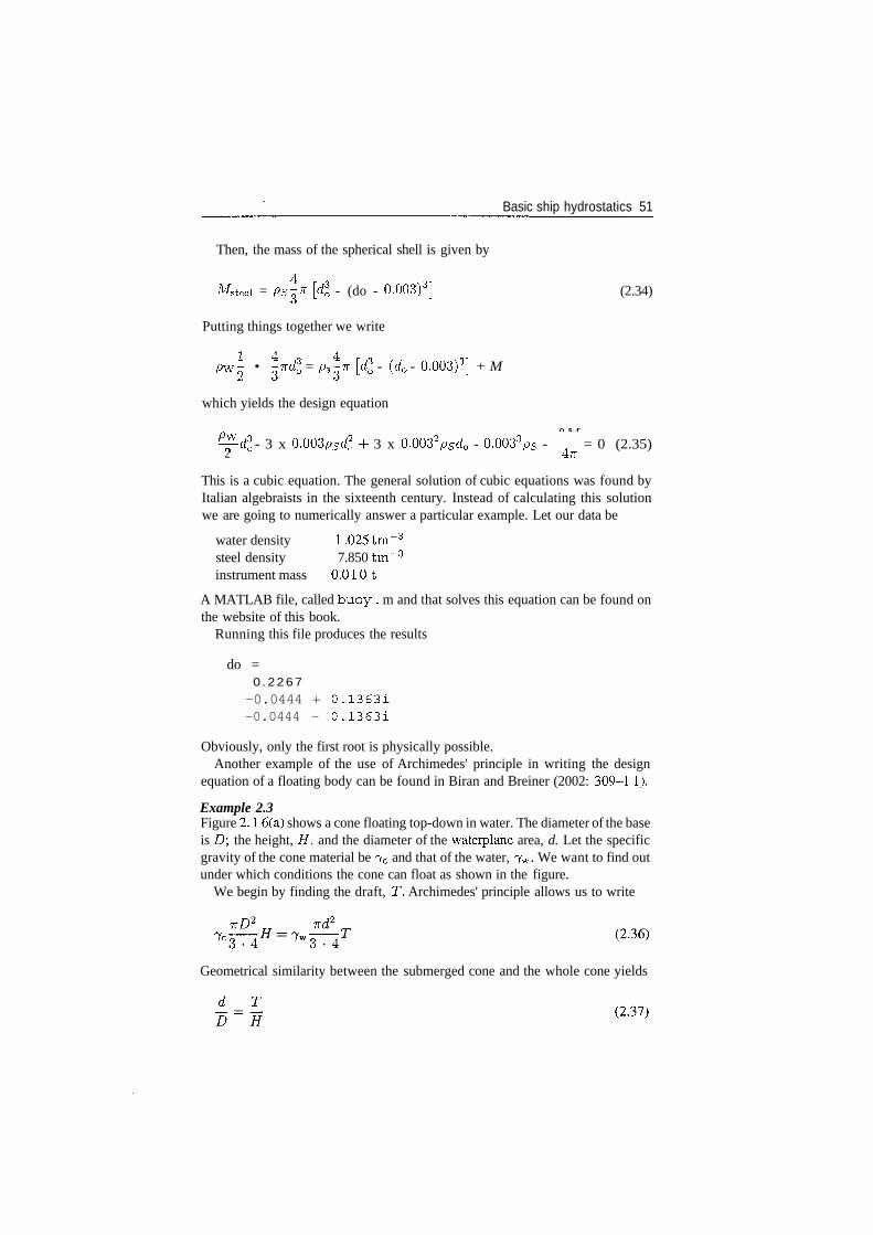
Basic ship hydrostatics 51
Then, the mass of the spherical shell is given by
MBteei = Ps^ [d30 - (do - 0.003)3] (2.34)
Putting things together we write
Pw\ • \vdl = p^-K [dl - (d0 - 0.003)3] + M
which yields the design equation
^dl - 3 x 0.003psd* + 3 x 0.0032psd0 - 0.0033p5 - = 0 (2.35)2 4vr
This is a cubic equation. The general solution of cubic equations was found byItalian algebraists in the sixteenth century. Instead of calculating this solutionwe are going to numerically answer a particular example. Let our data be
water density 1 .025 tm~3
steel density 7.850 tm~3
instrument mass 0.0 1 0 1
A MATLAB file, called buoy . m and that solves this equation can be found onthe website of this book.
Running this file produces the results
do =0 . 2 2 6 7
-0.0444 + 0.13631-0.0444 - 0.13631
Obviously, only the first root is physically possible.Another example of the use of Archimedes' principle in writing the design
equation of a floating body can be found in Biran and Breiner (2002: 309-1 1).
Example 2.3Figure 2. 1 6(a) shows a cone floating top-down in water. The diameter of the baseis D\ the height, H, and the diameter of the waterplane area, d. Let the specificgravity of the cone material be 7C and that of the water, 7W. We want to find outunder which conditions the cone can float as shown in the figure.
We begin by finding the draft, T. Archimedes' principle allows us to write
Geometrical similarity between the submerged cone and the whole cone yields
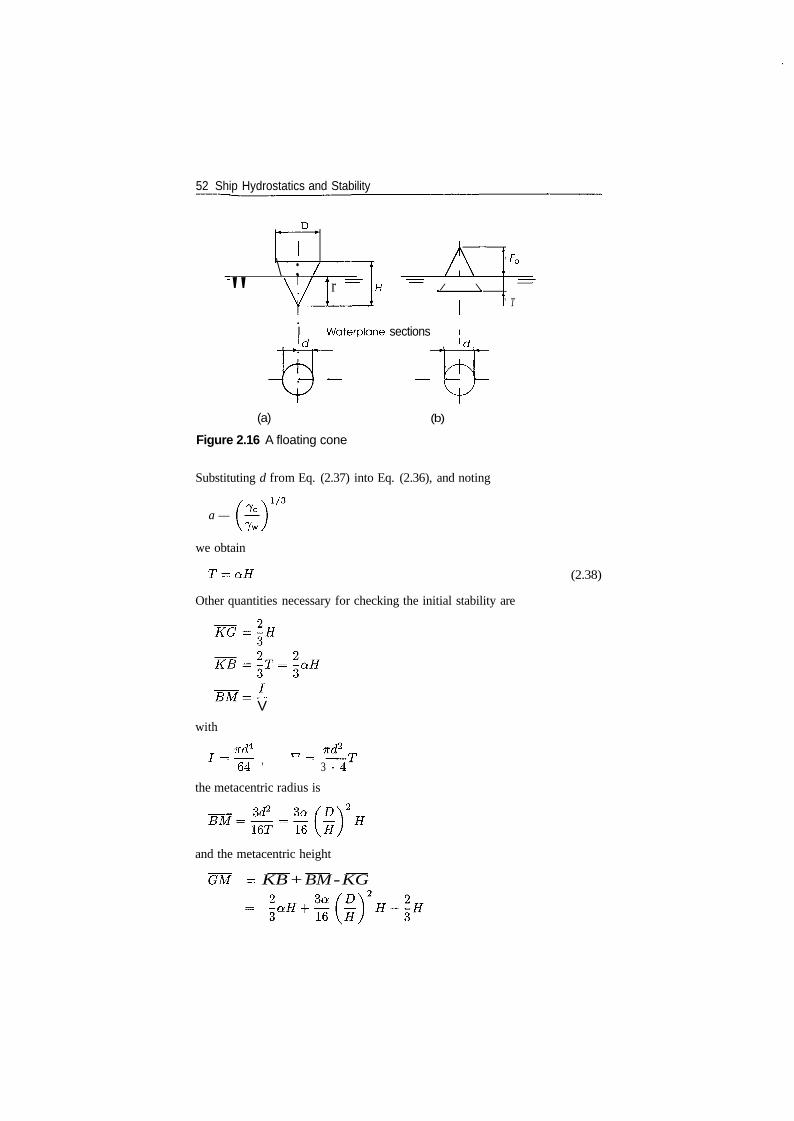
52 Ship Hydrostatics and Stability
1\ ; /
" V ri
H •= / \
' Fb
—
' T
I Waterplane sections'of , ld
(a)
Figure 2.16 A floating cone
(b)
Substituting d from Eq. (2.37) into Eq. (2.36), and noting
a —
we obtain
Other quantities necessary for checking the initial stability are
(2.38)
I_
V
with
7T<i4
= ~64~ ' = 3
the metacentric radius is
=16U
and the metacentric height
- KB + BM - KG
Basic ship hydrostatics 53
The cone is stable if
2 3a fD\2 2- 3 > 0 (239)
From Eq. (2.39) we can deduce a condition for the specific gravity of the conematerial
a > FT (2.40)
or, a condition for the D/H ratio:
D\2 321-aJf) >^" (2-41)H I 9 a./
Obviously, for the cone to float, the ratio a must be smaller than one. Thus, thecomplete condition for the cone material is
< a < 1 (2.42)32 (H)
Example 2.4Figure 2.16(b) shows a cone floating top-up. Noting by F^ the freeboard, that isthe difference H — T, Archimedes' principle yields the equation
-7T
= 7 w ( I > 2 ^ - d2Fb) (2.43)
We obtain
Similarity gives us
d = ^Fb (2.45)nCombining Eqs. (2.44) and (2.45) we obtain
fi -i \1/3
Fh=(^—^) H\ /Y /\ 7w /
with
54 Ship Hydrostatics and Stability
we write for the freeboard
Fb = /3H (2.46)
and for the draught,
T = H-Fb = (l-/3)H (2.47)
The diameter of the waterplane section is given by
d = § Fb = /?£> (2.48)12
To find the vertical coordinate of the centre of buoyancy we use the formula thatgives the height of the centroid of a trapeze (see books on elementary geometryor engineering handbooks):
J - 64 '
we obtain
3 84 D2
3 1 + /3 161-/33^ 3
The cone is stable if
1 + /3 16 1 - /33
We obtain a condition for the D to H ratio:
'ZA2 32 1-/33 1
(2'49)
We calculate the metacentric radius as
5M = L (2.50)
with
(2'52)
The height of the centre of gravity is
~KG = H/3 (2.53)
and the resulting metacentric height is
BM - KG
1-13 1 + 2/3 3 /34 D* H (2.54)
(2-56)
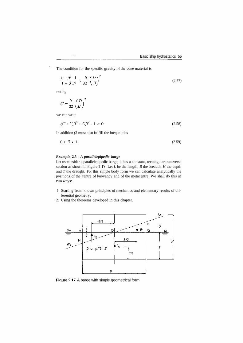
Basic ship hydrostatics 55
The condition for the specific gravity of the cone material is
2
-f3 P2 < 32 \H
noting
c- 9 (DC~
we can write
(C + l)/33 + C/32 - 1 > 0
In addition (3 must also fulfill the inequalities
0 < / ? < 1
(2.57)
(2.58)
(2.59)
Example 2.5 - A parallelepipedic bargeLet us consider a parallelepipedic barge; it has a constant, rectangular transversesection as shown in Figure 2.17. Let L be the length, B the breadth, H the depthand T the draught. For this simple body form we can calculate analytically thepositions of the centre of buoyancy and of the metacentre. We shall do this intwo ways:
1. Starting from known principles of mechanics and elementary results of dif-ferential geometry;
2. Using the theorems developed in this chapter.
WQ M
-B/3
O Bi
Btan0/(3-2) FT̂/2
Figure 2.17 A barge with simple geometrical form
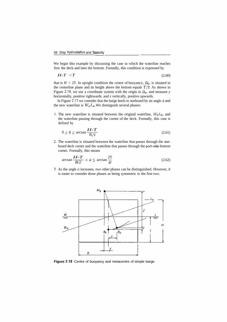
56 Ship Hydrostatics and Stability
We begin this example by discussing the case in which the waterline reachesfirst the deck and later the bottom. Formally, this condition is expressed by
H-T <T (2.60)
that is H < 2T. In upright condition the centre of buoyancy, BQ, is situated inthe centreline plane and its height above the bottom equals T/2. As shown inFigure 2.18, we use a coordinate system with the origin in BQ, and measure yhorizontally, positive rightwards, and z vertically, positive upwards.
In Figure 2.17 we consider that the barge heels to starboard by an angle <j> andthe new waterline is W^L^. We distinguish several phases:
1. The new waterline is situated between the original waterline, Wol/o, andthe waterline passing through the corner of the deck. Formally, this case isdefined by
0 < 6 < arctanH-TB/2
(2.61)
2. The waterline is situated between the waterline that passes through the star-board deck corner and the waterline that passes through the port-side bottomcorner. Formally, this means
arctan :H-TB/2
2T< arctan — (2.62)
3. As the angle </> increases, two other phases can be distinguished. However, itis easier to consider those phases as being symmetric to the first two.
Figure 2.18 Centre of buoyancy and metacentre of simple barge
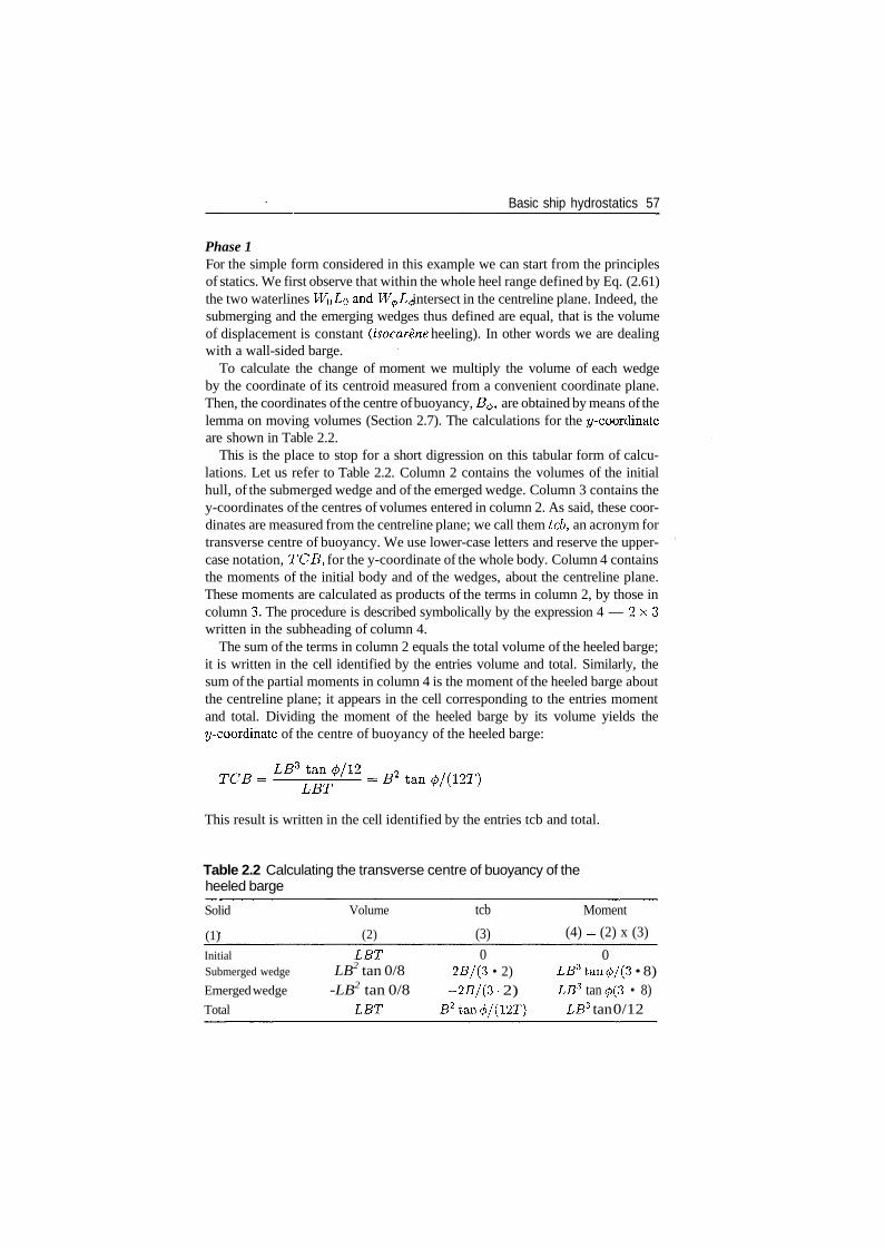
Basic ship hydrostatics 57
Phase 1For the simple form considered in this example we can start from the principlesof statics. We first observe that within the whole heel range defined by Eq. (2.61)the two waterlines WQ^O and W^L^ intersect in the centreline plane. Indeed, thesubmerging and the emerging wedges thus defined are equal, that is the volumeof displacement is constant (isocarene heeling). In other words we are dealingwith a wall-sided barge.
To calculate the change of moment we multiply the volume of each wedgeby the coordinate of its centroid measured from a convenient coordinate plane.Then, the coordinates of the centre of buoyancy, B^, are obtained by means of thelemma on moving volumes (Section 2.7). The calculations for the y-coordinateare shown in Table 2.2.
This is the place to stop for a short digression on this tabular form of calcu-lations. Let us refer to Table 2.2. Column 2 contains the volumes of the initialhull, of the submerged wedge and of the emerged wedge. Column 3 contains they-coordinates of the centres of volumes entered in column 2. As said, these coor-dinates are measured from the centreline plane; we call them tcb, an acronym fortransverse centre of buoyancy. We use lower-case letters and reserve the upper-case notation, TCB, for the y-coordinate of the whole body. Column 4 containsthe moments of the initial body and of the wedges, about the centreline plane.These moments are calculated as products of the terms in column 2, by those incolumn 3. The procedure is described symbolically by the expression 4 — 2 x 3written in the subheading of column 4.
The sum of the terms in column 2 equals the total volume of the heeled barge;it is written in the cell identified by the entries volume and total. Similarly, thesum of the partial moments in column 4 is the moment of the heeled barge aboutthe centreline plane; it appears in the cell corresponding to the entries momentand total. Dividing the moment of the heeled barge by its volume yields they-coordinate of the centre of buoyancy of the heeled barge:
This result is written in the cell identified by the entries tcb and total.
Table 2.2 Calculating the transverse centre of buoyancy of theheeled barge
Solid
(1)
InitialSubmerged wedge
Emerged wedge
Total
Volume
(2)
LETLB2 tan 0/8
-LB2 tan 0/8LET
tcb
(3)
02J3/(3 • 2)
-2£/(3 - 2)£2tan0/(12T)
Moment
(4) = (2) x (3)
0L£3tan0/(3 • 8)LB3 tan 0(3 • 8)
LB3 tan 0/12
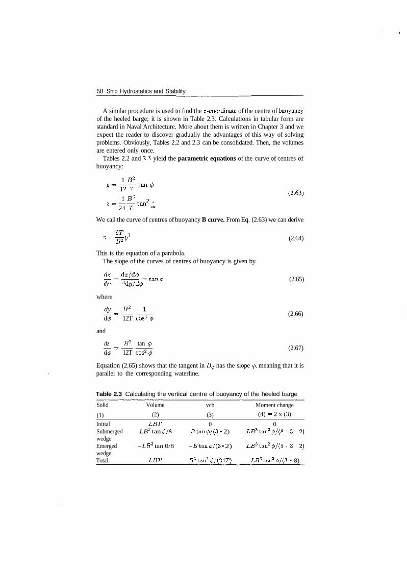
58 Ship Hydrostatics and Stability
A similar procedure is used to find the z-coordinate of the centre of buoyancyof the heeled barge; it is shown in Table 2.3. Calculations in tabular form arestandard in Naval Architecture. More about them is written in Chapter 3 and weexpect the reader to discover gradually the advantages of this way of solvingproblems. Obviously, Tables 2.2 and 2.3 can be consolidated. Then, the volumesare entered only once.
Tables 2.2 and 2.3 yield the parametric equations of the curve of centres ofbuoyancy:
1 B2
y = 19T~ tan<^1 , (2-63)1 B 2 j.
Z=U~Ti&n *
We call the curve of centres of buoyancy B curve. From Eq. (2.63) we can derive
z=%y2 (2.64)
This is the equation of a parabola.The slope of the curves of centres of buoyancy is given by
dz- r - - r n = t a n 0 (2.65)dy dy/dcf)
where
dy B2 1d</> 12T cos2
and
dz B2 tan <d</> 12T cos2 <
(2.66)
(2.67)
Equation (2.65) shows that the tangent in B^ has the slope <f>, meaning that it isparallel to the corresponding waterline.
Table 2.3 Calculating the vertical centre of buoyancy of the heeled barge
Solid
(1)
InitialSubmergedwedgeEmergedwedgeTotal
Volume
(2)
LETLB2 tan 0/8
-.LB2 tan 0/8
LET
vcb
(3)
0J3tan0/(3 • 2)
-£tan0/(3 • 2)
£2tan20/(24T)
Moment change
(4) = 2 x (3)
0L£3tan20/(8 - 3 - 2 )
L£3tan2</>/(8 - 3 - 2 )
LB3 tan2 0/(3 • 8)
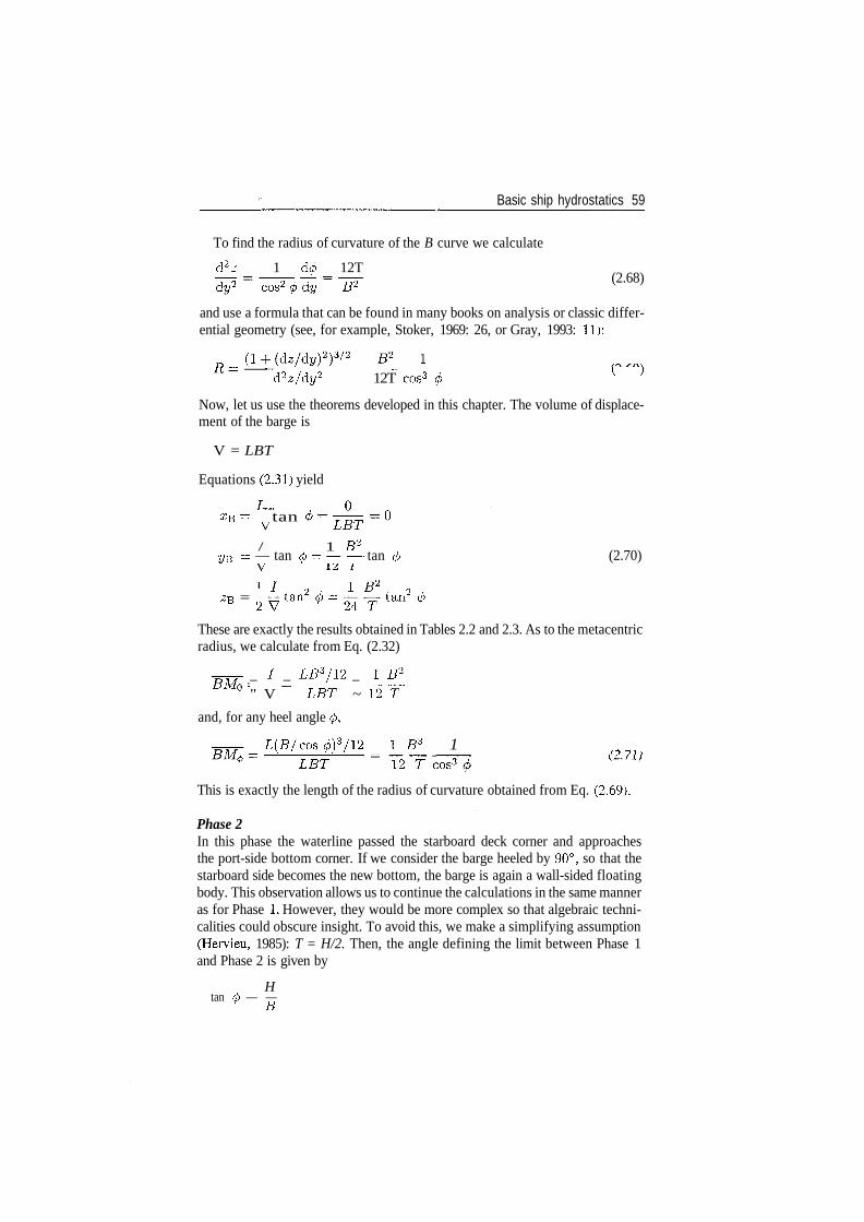
Basic ship hydrostatics 59
To find the radius of curvature of the B curve we calculate
d2z 1 d</> 12Tdy2 cos2 (j) dy B2 (2.68)
and use a formula that can be found in many books on analysis or classic differ-ential geometry (see, for example, Stoker, 1969: 26, or Gray, 1993: 11):
_
d2z/dy2 12T cos3 <t> ^ }
Now, let us use the theorems developed in this chapter. The volume of displace-ment of the barge is
V = LBT
Equations (2.31) yield
XB = tan 0=
/ 1 B2
yB = — tan ^— — -— tan 0 (2.70)
*B = 2 y t an 2 ^ -—tan 2 </>
These are exactly the results obtained in Tables 2.2 and 2.3. As to the metacentricradius, we calculate from Eq. (2.32)
_ I_ _ Lff3/12 _ \_B?_" V ~~ LET ~ 12 "r"
and, for any heel angle </>,
L(B/cos^)3/12 I B3 1 ^^LET 1 2 T
This is exactly the length of the radius of curvature obtained from Eq. (2.69).
Phase 2In this phase the waterline passed the starboard deck corner and approachesthe port-side bottom corner. If we consider the barge heeled by 90°, so that thestarboard side becomes the new bottom, the barge is again a wall-sided floatingbody. This observation allows us to continue the calculations in the same manneras for Phase 1. However, they would be more complex so that algebraic techni-calities could obscure insight. To avoid this, we make a simplifying assumption(Hervieu, 1985): T = H/2. Then, the angle defining the limit between Phase 1and Phase 2 is given by
Htan <p — —
JD
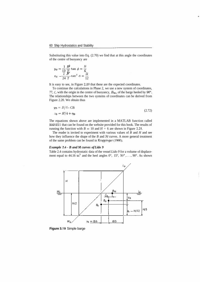
60 Ship Hydrostatics and Stability
Substituting this value into Eq. (2.70) we find that at this angle the coordinatesof the centre of buoyancy are
1 B B
1 R2 W2 / -"ZR — tan © = —
24 T 12
It is easy to see, in Figure 2.19 that these are the expected coordinates.To continue the calculations in Phase 2, we use a new system of coordinates,
77, £, with the origin in the centre of buoyancy, £?90, of the barge heeled by 90°.The relationships between the two systems of coordinates can be derived fromFigure 2.20. We obtain thus
yB = B/4 - CB(2.72)
The equations shown above are implemented in a MATLAB function calledBARGE 1 that can be found on the website provided for this book. The results ofrunning the function with B = 10 and H = 6 are shown in Figure 2.21.
The reader is invited to experiment with various values of B and H and seehow they influence the shape of the B and M curves. A more general treatmentof the same problem can be found in Krappinger (1960).
Example 2.6 - B and M curves of Lido 9Table 2.4 contains hydrostatic data of the vessel Lido 9 for a volume of displace-ment equal to 44.16 m3 and the heel angles 0°, 15°, 30°,..., 90°. As shown
Figure 2.19 Simple barge
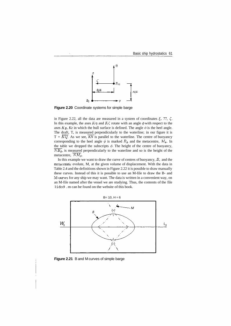
Basic ship hydrostatics 61
£90 —T
H/4
Figure 2.20 Coordinate systems for simple barge
in Figure 2.22, all the data are measured in a system of coordinates £, 77, £.In this example, the axes Kr\ and AT£ rotate with an angle (f> with respect to theaxes Ky, Kz in which the hull surface is defined. The angle <p is the heel angle.The draft, T, is measured perpendicularly to the waterline; in our figure it isT = KQ. As we see, KN is parallel to the waterline. The centre of buoyancycorresponding to the heel angle </> is marked B^ and the metacentre, M^. Inthe table we dropped the subscripts (/>. The height of the centre of buoyancy,NB<p, is measured perpendicularly to the waterline and so is the height of themetacentre, NM^.
In this example we want to draw the curve of centres of buoyancy, B, and themetacentric evolute, M, at the given volume of displacement. With the data inTable 2.4 and the definitions shown in Figure 2.22 it is possible to draw manuallythese curves. Instead of this it is possible to use an M-file to draw the B- andM-curves for any ship we may want. The data is written in a convenient way, onan M-file named after the vessel we are studying. Thus, the contents of the file1 ido9 . m can be found on the website of this book.
B= 10, H = 6
Figure 2.21 B and M curves of simple barge
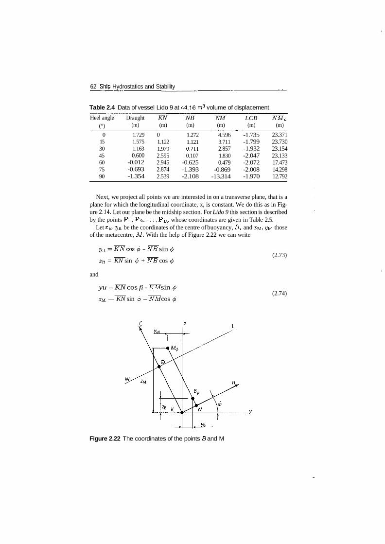
62 Ship Hydrostatics and Stability
Table 2.4 Data of vessel Lido 9 at 44.16 m3 volume of displacement
Heel angle(°)
0153045607590
Draught(m)
1.7291.5751.1630.600
-0.012-0.693-1.354
KN(m)
01.1221.9792.5952.9452.8742.539
NB(m)
1.2721.1210.7110.107
-0.625-1.393-2.108
NM(m)
4.5963.7112.8571.8300.479
-0.869-13.314
LCB(m)
-1.735-1.799-1.932-2.047-2.072-2.008-1.970
NML
(m)
23.37123.73023.15423.13317.47314.29812.792
Next, we project all points we are interested in on a transverse plane, that is aplane for which the longitudinal coordinate, x, is constant. We do this as in Fig-ure 2.14. Let our plane be the midship section. For Lido 9 this section is describedby the points PI, P2, . . . , PIS whose coordinates are given in Table 2.5.
Let XB, y-& be the coordinates of the centre of buoyancy, B, and XM, yu thoseof the metacentre, M. With the help of Figure 2.22 we can write
2/s - NB sin
= KN sin </> + NB cos(2.73)
and
yu = KN cos fi - KM sin
zu — KN sin 0 -h NM cos(2.74)
Figure 2.22 The coordinates of the points B and M
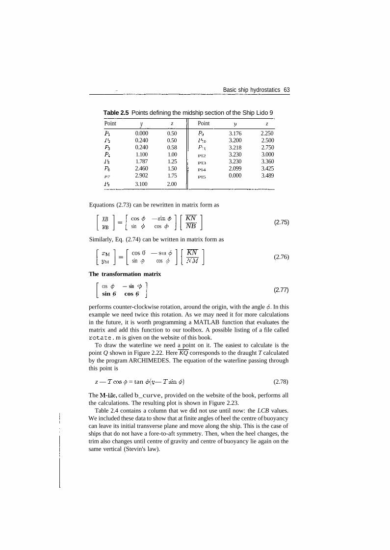
Basic ship hydrostatics 63
Table 2.5 Points defining the midship section of the Ship Lido 9
Point
PiP2
PaP4
P5
PeP7
PS
y0.0000.2400.2401.1001.7872.4602.9023.100
z
0.500.500.581.001.251.501.75
2.00
Point
P9
PioPnPl2
Pl3
Pl4
Pl5
2/
3.1763.2003.2183.2303.2302.0990.000
z
2.2502.5002.7503.0003.3603.4253.489
Equations (2.73) can be rewritten in matrix form as
XB cossin .
— sincos d
KNNB
Similarly, Eq. (2.74) can be written in matrix form as
yucos 0 — sinsin (j> cos </
KNNM
The transformation matrix
cos <j> — sin <sin 6 cos 6
(2.75)
(2.76)
(2.77)
performs counter-clockwise rotation, around the origin, with the angle 0. In thisexample we need twice this rotation. As we may need it for more calculationsin the future, it is worth programming a MATLAB function that evaluates thematrix and add this function to our toolbox. A possible listing of a file calledrotate. m is given on the website of this book.
To draw the waterline we need a point on it. The easiest to calculate is thepoint Q shown in Figure 2.22. Here KQ corresponds to the draught T calculatedby the program ARCHIMEDES. The equation of the waterline passing throughthis point is
z — Tcos 0 = tan </>(y — Tsin (2.78)
The M-file, called b_curve, provided on the website of the book, performs allthe calculations. The resulting plot is shown in Figure 2.23.
Table 2.4 contains a column that we did not use until now: the LCB values.We included these data to show that at finite angles of heel the centre of buoyancycan leave its initial transverse plane and move along the ship. This is the case ofships that do not have a fore-to-aft symmetry. Then, when the heel changes, thetrim also changes until centre of gravity and centre of buoyancy lie again on thesame vertical (Stevin's law).
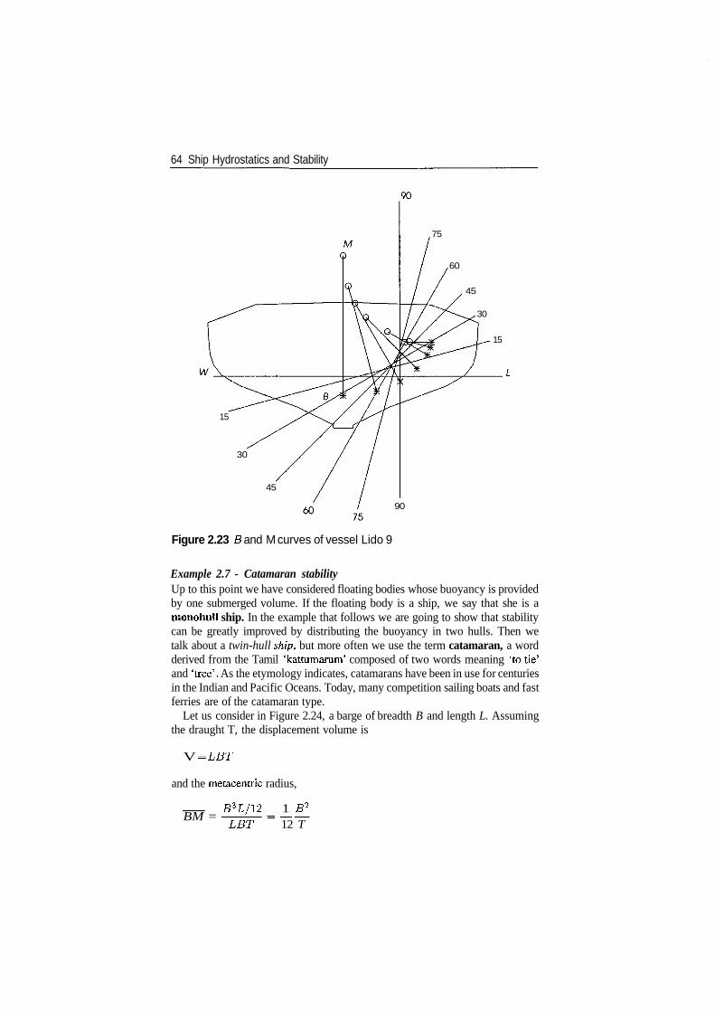
64 Ship Hydrostatics and Stability
75
60
45
30
15
15
30
45
90
Figure 2.23 B and M curves of vessel Lido 9
Example 2.7 - Catamaran stabilityUp to this point we have considered floating bodies whose buoyancy is providedby one submerged volume. If the floating body is a ship, we say that she is amonohull ship. In the example that follows we are going to show that stabilitycan be greatly improved by distributing the buoyancy in two hulls. Then wetalk about a twin-hull ship, but more often we use the term catamaran, a wordderived from the Tamil 'kattumarum' composed of two words meaning 'to tie'and 'tree'. As the etymology indicates, catamarans have been in use for centuriesin the Indian and Pacific Oceans. Today, many competition sailing boats and fastferries are of the catamaran type.
Let us consider in Figure 2.24, a barge of breadth B and length L. Assumingthe draught T, the displacement volume is
V - LET
and the metacentric radius,
£3L/12 1 J52
BM =LET 12 T
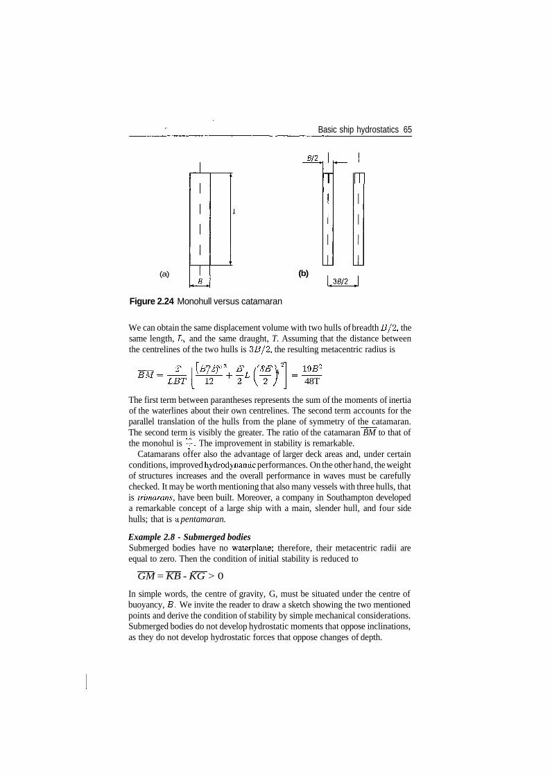
Basic ship hydrostatics 65
B/2
(a)
T m
(b)
Figure 2.24 Monohull versus catamaran
We can obtain the same displacement volume with two hulls of breadth B/2, thesame length, L, and the same draught, T. Assuming that the distance betweenthe centrelines of the two hulls is 3B/2, the resulting metacentric radius is
-=-_ 2 \(B/1)Z BT(3B\2
BM=LBT[U+^L(^)19B2
48T
The first term between parantheses represents the sum of the moments of inertiaof the waterlines about their own centrelines. The second term accounts for theparallel translation of the hulls from the plane of symmetry of the catamaran.The second term is visibly the greater. The ratio of the catamaran BM to that ofthe monohul is —-. The improvement in stability is remarkable.
Catamarans offer also the advantage of larger deck areas and, under certainconditions, improved hydrodynamic performances. On the other hand, the weightof structures increases and the overall performance in waves must be carefullychecked. It may be worth mentioning that also many vessels with three hulls, thatis trimarans, have been built. Moreover, a company in Southampton developeda remarkable concept of a large ship with a main, slender hull, and four sidehulls; that is a pentamaran.
Example 2.8 - Submerged bodiesSubmerged bodies have no waterplane; therefore, their metacentric radii areequal to zero. Then the condition of initial stability is reduced to
GM = KB - KG > 0
In simple words, the centre of gravity, G, must be situated under the centre ofbuoyancy, B. We invite the reader to draw a sketch showing the two mentionedpoints and derive the condition of stability by simple mechanical considerations.Submerged bodies do not develop hydrostatic moments that oppose inclinations,as they do not develop hydrostatic forces that oppose changes of depth.
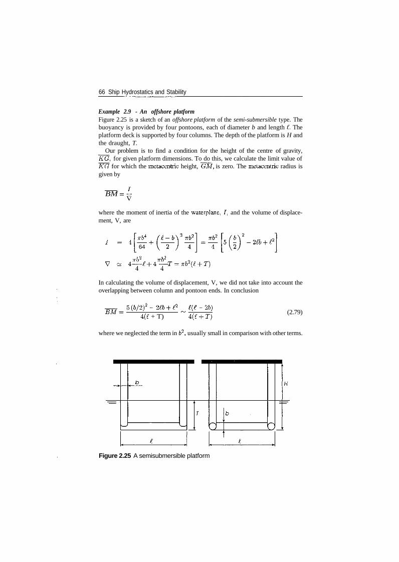
66 Ship Hydrostatics and Stability
Example 2.9 - An offshore platformFigure 2.25 is a sketch of an offshore platform of the semi-submersible type. Thebuoyancy is provided by four pontoons, each of diameter b and length L Theplatform deck is supported by four columns. The depth of the platform is H andthe draught, T.
Our problem is to find a condition for the height of the centre of gravity,KG, for given platform dimensions. To do this, we calculate the limit value ofKG for which the metacentric height, GM, is zero. The metacentric radius isgiven by
BM = -
where the moment of inertia of the waterplane, /, and the volume of displace-ment, V, are
7 = 4 TTb^64
7T& 2 ,~
In calculating the volume of displacement, V, we did not take into account theoverlapping between column and pontoon ends. In conclusion
'-26)(2.79)
4(7 + T) 4(^ + T)
where we neglected the term in 62, usually small in comparison with other terms.
Figure 2.25 A semisubmersible platform
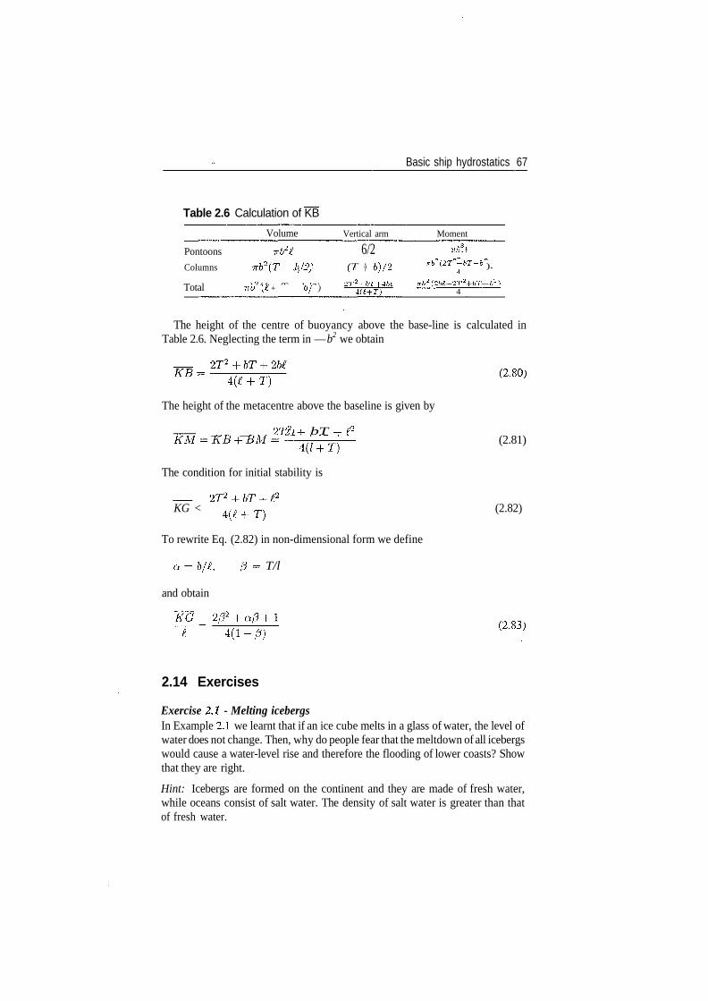
Basic ship hydrostatics 67
Table 2.6 Calculation of KB
Pontoons
Columns
Total
Volume
7Tb2l
-rrtfiT b/9}
7TO (t + Of )
Vertical arm Moment
6/2 Z£L(T \ M /r> 7rb (2T +bT~b )(J. \ O)/* 4
2T2+bT+4b£ -rrb2 (2b£+2T2 +bT — b2)4(l+T) 4
4(1 + T)
The height of the metacentre above the baseline is given by
_ _ 2T2 4- bT 4- /2Z1
The condition for initial stability is
The height of the centre of buoyancy above the base-line is calculated inTable 2.6. Neglecting the term in — b2 we obtain
(2'80)
(2.81)
KG < 4(£ + T) (2.82)
To rewrite Eq. (2.82) in non-dimensional form we define
a = b/l, /3 = T/l
and obtain
T/r S~1 f ) /O2 I /Q I "I
¥ - ̂ iirrlr (183)
2.14 Exercises
Exercise 2.1 - Melting icebergsIn Example 2.1 we learnt that if an ice cube melts in a glass of water, the level ofwater does not change. Then, why do people fear that the meltdown of all icebergswould cause a water-level rise and therefore the flooding of lower coasts? Showthat they are right.
Hint: Icebergs are formed on the continent and they are made of fresh water,while oceans consist of salt water. The density of salt water is greater than thatof fresh water.
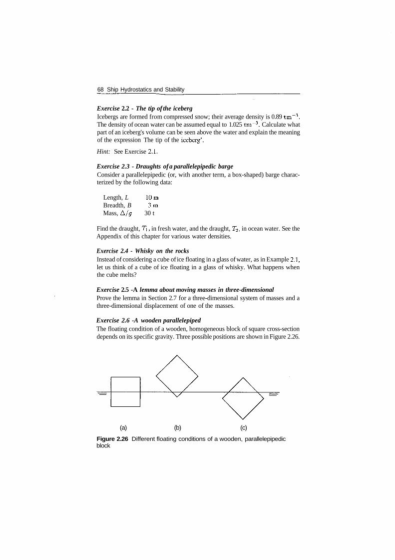
68 Ship Hydrostatics and Stability
Exercise 2.2 - The tip of the icebergIcebergs are formed from compressed snow; their average density is 0.89 tm~3.The density of ocean water can be assumed equal to 1.025 tm~3. Calculate whatpart of an iceberg's volume can be seen above the water and explain the meaningof the expression The tip of the iceberg'.
Hint: See Exercise 2.1.
Exercise 2.3 - Draughts of a parallelepipedic bargeConsider a parallelepipedic (or, with another term, a box-shaped) barge charac-terized by the following data:
Length, L 10mBreadth, B 3mMass, A/0 30 t
Find the draught, TI, in fresh water, and the draught, T2, in ocean water. See theAppendix of this chapter for various water densities.
Exercise 2.4 - Whisky on the rocksInstead of considering a cube of ice floating in a glass of water, as in Example 2.1,let us think of a cube of ice floating in a glass of whisky. What happens whenthe cube melts?
Exercise 2.5 -A lemma about moving masses in three-dimensionalProve the lemma in Section 2.7 for a three-dimensional system of masses and athree-dimensional displacement of one of the masses.
Exercise 2.6 -A wooden parallelepipedThe floating condition of a wooden, homogeneous block of square cross-sectiondepends on its specific gravity. Three possible positions are shown in Figure 2.26.
(a) (b) (c)
Figure 2.26 Different floating conditions of a wooden, parallelepipedicblock
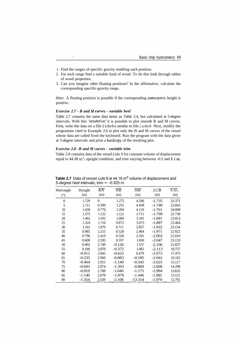
Basic ship hydrostatics 69
1. Find the ranges of specific gravity enabling each position.2. For each range find a suitable kind of wood. To do this look through tables
of wood properties.3. Can you imagine other floating positions? In the affirmative, calculate the
corresponding specific-gravity range.
Hint: A floating position is possible if the corresponding metacentric height ispositive.
Exercise 2.7 - B and Mcurves - variable heelTable 2.7 contains the same data items as Table 2.4, but calculated at 5-degreeintervals. With this 'resolution' it is possible to plot smooth B and M curves.First, write the data on a file lido9a similar to file lido9. Next, modify theprogramme cited in Example 2.6 to plot only the B and M curves of the vesselwhose data are called from the keyboard. Run the program with the data givenat 5-degree intervals and print a hardcopy of the resulting plot.
Exercise 2.8 -B and M curves - variable trimTable 2.8 contains data of the vessel Lido 9 for constant volume of displacementequal to 44.16 m3, upright condition, and trim varying between -0.3 and l.lm.
Table 2.7 Data of vessel Lido 9 at 44.16 m3 volume of displacement and5-degree heel intervals, trim = -0.325 m
Heel angle(°)
05
1015202530354045505560657075808590
Draught(m)
1.7291.7111.6591.5751.4621.3241.1630.9850.7960.6000.4020.198
-0.012-0.235-0.464-0.693-0.919-1.140-1.354
KN(m)
00.3990.7761.1221.4321.7161.9792.2152.4192.5952.7492.8702.9452.9602.9312.8742.7882.6782.539
NB(m)
1.2721.2551.2041.1211.0090.8720.7110.5280.3260.107
-0.126-0.372-0.625-0.883-1.140-1.393-1.640-1.878-2.108
NM(m)
4.5964.4384.1193.7113.3413.0732.8572.4642.1051.8301.5371.0820.479
-0.185-0.543-0.869-1.171-1.446
-13.314
LCB(m)
-1.735-1.740-1.761-1.799-1.841-1.887-1.932-1.971-2.002-2.047-2.106-2.113-2.072-2.041-2.025-2.008-1.994-1.981-1.970
NML
(m)
23.37123.69324.00823.73023.81323.46423.15422.82222.81023.13321.83719.75717.47316.16215.11714.29813.63313.12112.792
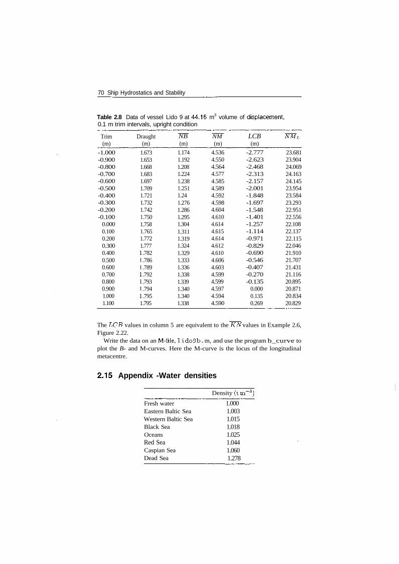
70 Ship Hydrostatics and Stability
Table 2.8 Data of vessel Lido 9 at 44.16 m3 volume of displacement,0.1 m trim intervals, upright condition
Trim(m)
-1.000-0.900-0.800-0.700-0.600-0.500-0.400-0.300-0.200-0.100
0.0000.1000.2000.3000.4000.5000.6000.7000.8000.9001.0001.100
Draught(m)
1.6731.6531.6681.6831.6971.7091.7211.7321.7421.7501.7581.7651.7721.777.782.786.789.792.793.794.795
1.795
NB(m)
1.1741.1921.2081.2241.2381.2511.241.2761.2861.2951.3041.3111.3191.3241.3291.3331.3361.3381.3391.3401.3401.338
NM(m)
4.5364.5504.5644.5774.5854.5894.5924.5984.6044.6104.6144.6154.6144.6124.6104.6064.6034.5994.5994.5974.5944.590
LCB(m)
-2.777-2.623-2.468-2.313-2.157-2.001-1.848-1.697-1.548-1.401-1.257-1.114-0.971-0.829-0.690-0.546-0.407-0.270-0.135
0.0000.1350.269
NML
23.68123.90424.06924.16324.14523.95423.58423.29322.95122.55622.10822.13722.11522.04621.91021.70721.43121.11620.89520.87120.83420.829
The LCB values in column 5 are equivalent to the KN values in Example 2.6,Figure 2.22.
Write the data on an M-file, Iido9b. m, and use the program b_curve toplot the B- and M-curves. Here the M-curve is the locus of the longitudinalmetacentre.
2.15 Appendix -Water densities
Density (tm~3)
Fresh waterEastern Baltic SeaWestern Baltic SeaBlack SeaOceansRed SeaCaspian SeaDead Sea
1.0001.0031.0151.0181.0251.0441.0601.278
Numerical integration in navalarchitecture
3.1 Introduction
In Chapter 2, we have learnt that the evaluation of ship properties, such as dis-placement and stability, requires the calculation of areas, centroids and momentsof plane figures, and of volumes and centres of volumes. Such properties are cal-culated by integration. In the absence of an explicit definition of the hull surface,in terms of calculable mathematical functions, the integrations cannot be car-ried out by analytic methods. The established practice has been to describe thehull surface by tabulated data, as shown in Chapter 1, and to use these data innumerical calculations.
Two methods for numerical integration are described in this chapter: the trape-zoidal and Simpson's rules. The treatment is based on Biran and Breiner (2002).The rules are exemplified on integrands defined by explicit mathematical expres-sions; this is done to convince the reader that the two methods of numericalintegration are efficient, and to allow an evaluation of errors. The first examplesare followed in Chapter 4 by Naval-Architectural applications to real ship datapresented in tabular form.
Many Naval-Architectural problems require the calculation of the definiteintegral
•&f ( x ) d x
of a function bounded in the finite interval [a, b]. We approximate the definite inte-gral by the weighted sum of a set of function values, /(zi), / (x 2 ) , . . . , /(xn),evaluated, or measured, at n points Xi G [a, 6], i = 1 ,2 , . . . , n, i.e.
fbI
-*a(3.1)
In Naval Architecture, the coefficients a^ are called multipliers; in some bookson Numerical Methods they are called weights.
72 Ship Hydrostatics and Stability
There are several ways of deriving formulae for numerical integration - alsocalled quadrature formulae - of the form shown in Eq. (3.1); three of them arementioned below:
1. By geometrical reasoning, considering fa f ( x ) dx as the area under the curve/(x), between x = a and x = b.
2. By approximating the function f ( x ) by an interpolating polynomial, P(x),and integrating the latter instead of the given function, so that
•b
P(x) dx
3. By developing the given function into a Taylor or MacLaurin series andintegrating the first terms of the series.
The first approach yields a simple intuitive interpretation of the rules for numer-ical quadrature and of the errors involved. This interpretation enables the userto derive the rules whenever required, and to adapt them to particular situations,for instance, when changing the subintervals of integration. On the other hand,each rule must be derived separately. The advantages of the other approachesare:
• The derivation is common to a group of rules which thus appears as particularcases of a more general method.
• The derivation yields an expression of the error involved.
In the next two sections, we shall use the geometrical approach to derive thetwo most popular rules, namely the trapezoidal and Simpson's rules. These twomethods are sufficient for solving most problems encountered in Naval Architec-ture. The error terms will be given without derivation; however, interpretationsof the error expressions will follow their presentation.
3.2 The trapezoidal rule
Let us consider the function f ( x ) represented in Figure 3.1. We assume that weknow the values /(:TI), /(x2), . . . , f(x$) and we want to calculate the definiteintegral
fXS
1= f ( x ) d x (3.2)
The integral in Eq. (3.2) represents the area under the curve f ( x ) . Let us connectthe points /(xi), /(#2)> . . • , f(x$) by straight line segments (the dashed-dotted
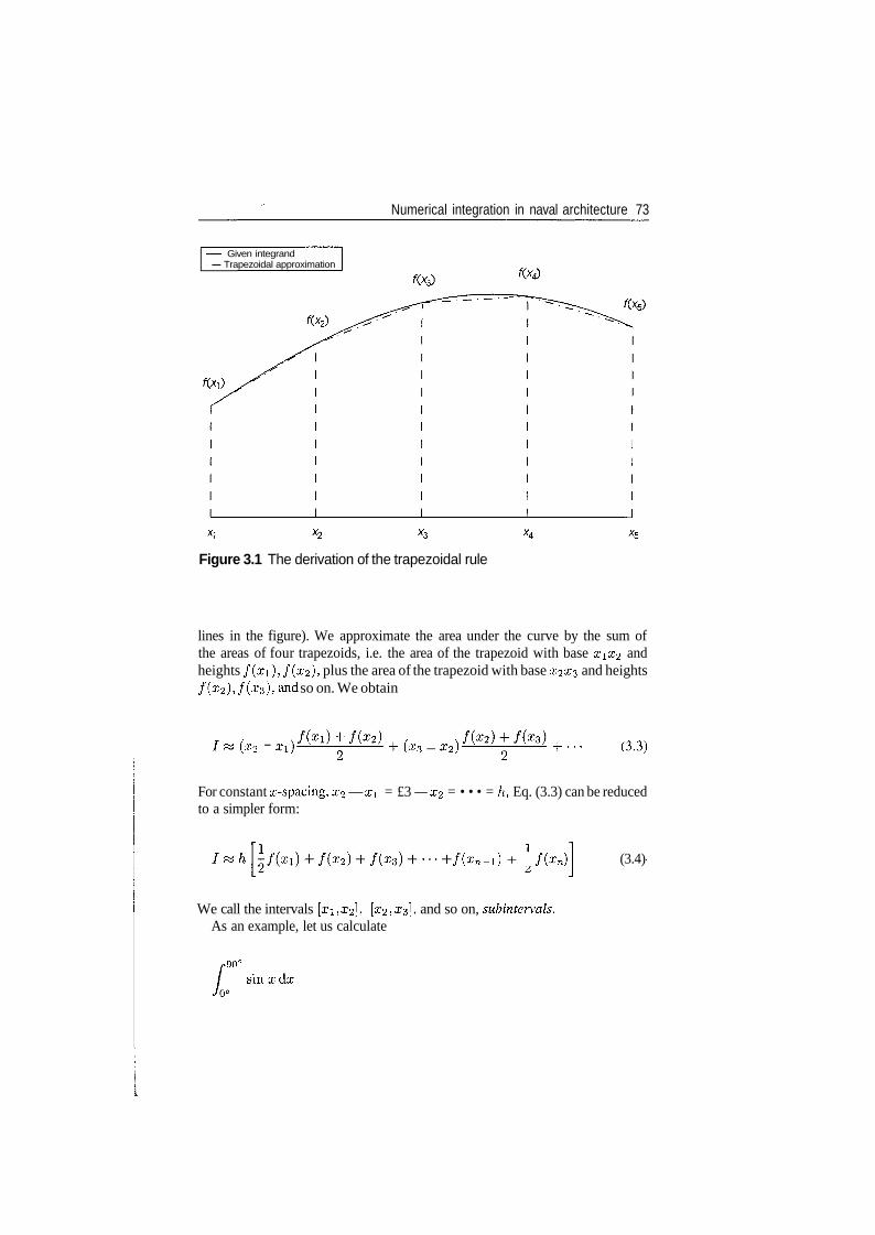
Numerical integration in naval architecture 73
Given integrandTrapezoidal approximation
X3
Figure 3.1 The derivation of the trapezoidal rule
lines in the figure). We approximate the area under the curve by the sum ofthe areas of four trapezoids, i.e. the area of the trapezoid with base #i£2 andheights /(#i), /(x2), plus the area of the trapezoid with base x2x3 and heights/(x2), /(^s)* and so on. We obtain
(X2 - (X3 _ (3.3)
For constant x-spacing, #2 — x\ = £3 — x2 = • • • = h, Eq. (3.3) can be reducedto a simpler form:
f(xn-i) + f(xn (3.4)
We call the intervals [x\, x2], [0^2, ^3], and so on, subintervals.As an example, let us calculate
•90°sin
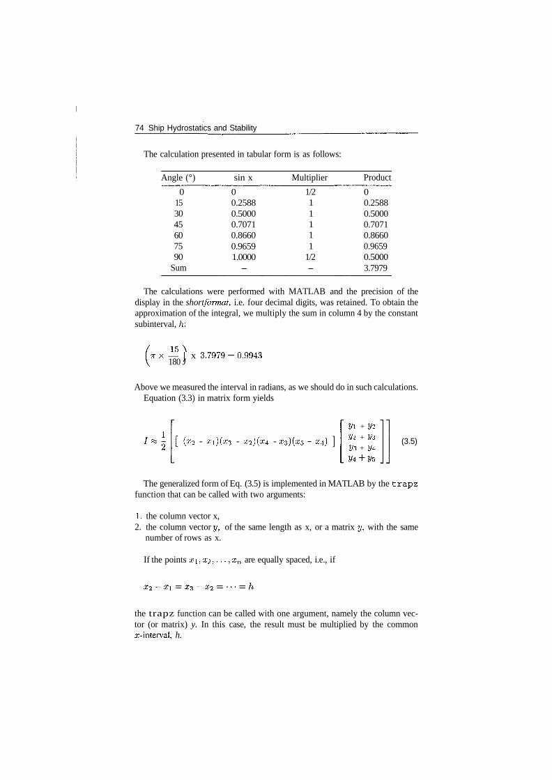
74 Ship Hydrostatics and Stability
The calculation presented in tabular form is as follows:
Angle (°)
0153045607590
Sum
sin x
00.25880.50000.70710.86600.96591.0000-
Multiplier
1/211111
1/2-
Product
00.25880.50000.70710.86600.96590.50003.7979
The calculations were performed with MATLAB and the precision of thedisplay in the short format, i.e. four decimal digits, was retained. To obtain theapproximation of the integral, we multiply the sum in column 4 by the constantsubinterval, h:
T T X — ) x 3.7979-0.9943180 J
Above we measured the interval in radians, as we should do in such calculations.Equation (3.3) in matrix form yields
(x2 - xi)(x3 - x2)(x4 - - x4)
2/1 + 2/2
2/2 + 2/3
V3 + 2/4(3.5)
The generalized form of Eq. (3.5) is implemented in MATLAB by the trapzfunction that can be called with two arguments:
1. the column vector x,2. the column vector y, of the same length as x, or a matrix y, with the same
number of rows as x.
If the points xi, x 2 , . . . , xn are equally spaced, i.e., if
the trapz function can be called with one argument, namely the column vec-tor (or matrix) y. In this case, the result must be multiplied by the commonx-interval, h.
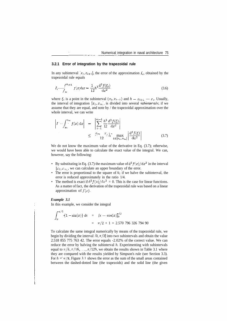
Numerical integration in naval architecture 75
3.2.1 Error of integration by the trapezoidal rule
In any subinterval [x^ atrapezoidal rule equals
/ . / f (ff> \ f\ rp •I I J\X) aX
J Xi
], the error of the approximation /;, obtained by the
12 dz2 (3.6)
where & is a point in the subinterval (o^, #i+i) and h = xi+1 — a^. Usually,the interval of integration [#i,£m], is divided into several subintervals; if weassume that they are equal, and note by / the trapezoidal approximation over thewhole interval, we can write
'- [^ /(i)daJxi 12 do;2
%m %l 7 o——— h max (3.7)
We do not know the maximum value of the derivative in Eq. (3.7); otherwise,we would have been able to calculate the exact value of the integral. We can,however, say the following:
• By substituting in Eq. (3.7) the maximum value of d2/(x)/dx2 in the interval[#i, Xm], we can calculate an upper boundary of the error.
• The error is proportional to the square of h\ if we halve the subinterval, theerror is reduced approximately in the ratio 1/4.
• The method is exact if d2/(x)/dx2 = 0. This is the case for linear functions.As a matter of fact, the derivation of the trapezoidal rule was based on a linearapproximation of f ( x ) .
Example 3.1In this example, we consider the integral
/-7T/2
L { 7T/2{1 -f sin(x)} dx = [x — COS(X)]Q
= 7T/2 + 1 = 2.570 796 326 794 90
To calculate the same integral numerically by means of the trapezoidal rule, webegin by dividing the interval [0,7r/2] into two subintervals and obtain the value2.518 855 775 763 42. The error equals -2.02% of the correct value. We canreduce the error by halving the subinterval h. Experimenting with subintervalsequal to Tr/8, Tr /16, . . . , Tr/128, we obtain the results shown in Table 3.1 wherethey are compared with the results yielded by Simpson's rule (see Section 3.3).For h =' 7T/8, Figure 3.1 shows the error as the sum of the small areas containedbetween the dashed-dotted line (the trapezoids) and the solid line (the given
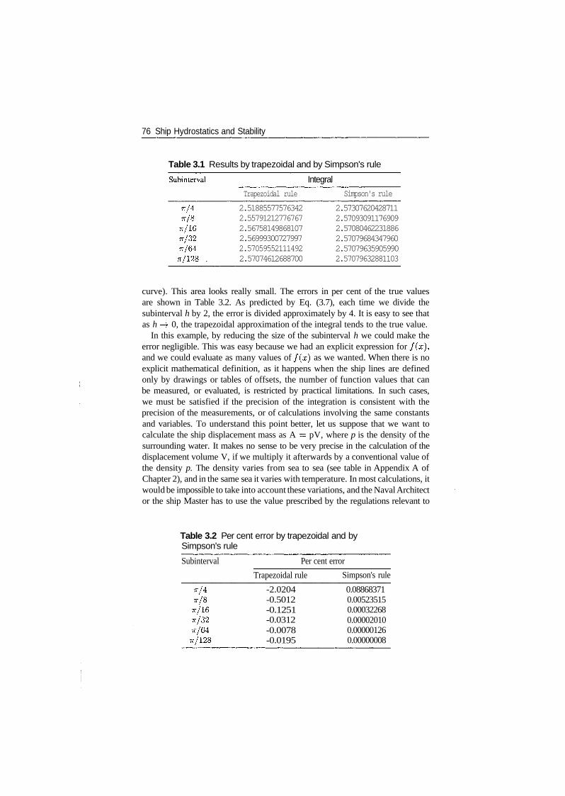
76 Ship Hydrostatics and Stability
Table 3.1 Results by trapezoidal and by Simpson's rule
Subinterval Integral
7T/4
TV/8
7T/16
7T/32
7T/64
7T/128 .
Trapezoidal rule
2.518855775763422.557912127767672.567581498681072.569993007279972.570595521114922.57074612688700
Simpson's rule
2.573076204287112.570930911769092.570804622318862.570796843479602.570796359059902.57079632881103
curve). This area looks really small. The errors in per cent of the true valuesare shown in Table 3.2. As predicted by Eq. (3.7), each time we divide thesubinterval h by 2, the error is divided approximately by 4. It is easy to see thatas h —>• 0, the trapezoidal approximation of the integral tends to the true value.
In this example, by reducing the size of the subinterval h we could make theerror negligible. This was easy because we had an explicit expression for /(#),and we could evaluate as many values of /(#) as we wanted. When there is noexplicit mathematical definition, as it happens when the ship lines are definedonly by drawings or tables of offsets, the number of function values that canbe measured, or evaluated, is restricted by practical limitations. In such cases,we must be satisfied if the precision of the integration is consistent with theprecision of the measurements, or of calculations involving the same constantsand variables. To understand this point better, let us suppose that we want tocalculate the ship displacement mass as A = pV, where p is the density of thesurrounding water. It makes no sense to be very precise in the calculation of thedisplacement volume V, if we multiply it afterwards by a conventional value ofthe density p. The density varies from sea to sea (see table in Appendix A ofChapter 2), and in the same sea it varies with temperature. In most calculations, itwould be impossible to take into account these variations, and the Naval Architector the ship Master has to use the value prescribed by the regulations relevant to
Table 3.2 Per cent error by trapezoidal and bySimpson's rule
Subinterval Per cent error
7T/4
7T/8
7T/16
7T/32
7T/64
7T/128
Trapezoidal rule
-2.0204-0.5012-0.1251-0.0312-0.0078-0.0195
Simpson's rule
0.088683710.005235150.000322680.000020100.000001260.00000008
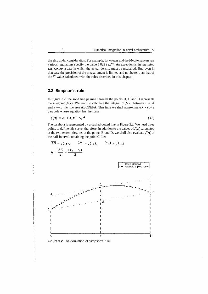
Numerical integration in naval architecture 77
the ship under consideration. For example, for oceans and the Mediterranean sea,various regulations specify the value 1.025 t m~3. An exception is the incliningexperiment, a case in which the actual density must be measured. But, even inthat case the precision of the measurement is limited and not better than that ofthe V-value calculated with the rules described in this chapter.
3.3 Simpson's rule
In Figure 3.2, the solid line passing through the points B, C and D representsthe integrand /(#). We want to calculate the integral of /(#) between x = Aand x — E, i.e. the area ABCDEFA. This time we shall approximate f ( x ) by aparabola whose equation has the form
f ( x ) = -f (3.8)
The parabola is represented by a dashed-dotted line in Figure 3.2. We need threepoints to define this curve; therefore, in addition to the values of f ( x ) calculatedat the two extremities, i.e. at the points B and D, we shall also evaluate f ( x ) atthe half-interval, obtaining the point C. Let
AB = ~FC = ~ED = f ( x 3 )
AE2
• Given integrandParabolic approximation
A F
Figure 3.2 The derivation of Simpson's rule
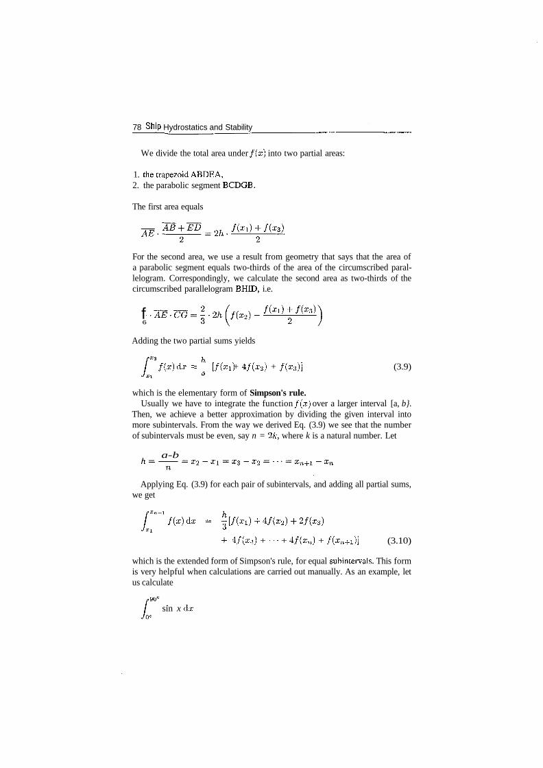
78 Ship Hydrostatics and Stability
We divide the total area under f ( x ) into two partial areas:
1. thetrapezoidABDEA,2. the parabolic segment BCDGB.
The first area equals
For the second area, we use a result from geometry that says that the area ofa parabolic segment equals two-thirds of the area of the circumscribed paral-lelogram. Correspondingly, we calculate the second area as two-thirds of thecircumscribed parallelogram BHID, i.e.
f6
Adding the two partial sums yields
f ( x ) d* « [f(Xl) + 4/(x2) + /(x3)] (3.9)
which is the elementary form of Simpson's rule.Usually we have to integrate the function f(x] over a larger interval [a, b}.
Then, we achieve a better approximation by dividing the given interval intomore subintervals. From the way we derived Eq. (3.9) we see that the numberof subintervals must be even, say n = 2/c, where k is a natural number. Let
. a-b
Applying Eq. (3.9) for each pair of subintervals, and adding all partial sums,we get
4/(x4) + ' ' ' + 4/(zn) + /(xn+1)] (3.10)
which is the extended form of Simpson's rule, for equal subintervals. This formis very helpful when calculations are carried out manually. As an example, letus calculate
.sin x dx
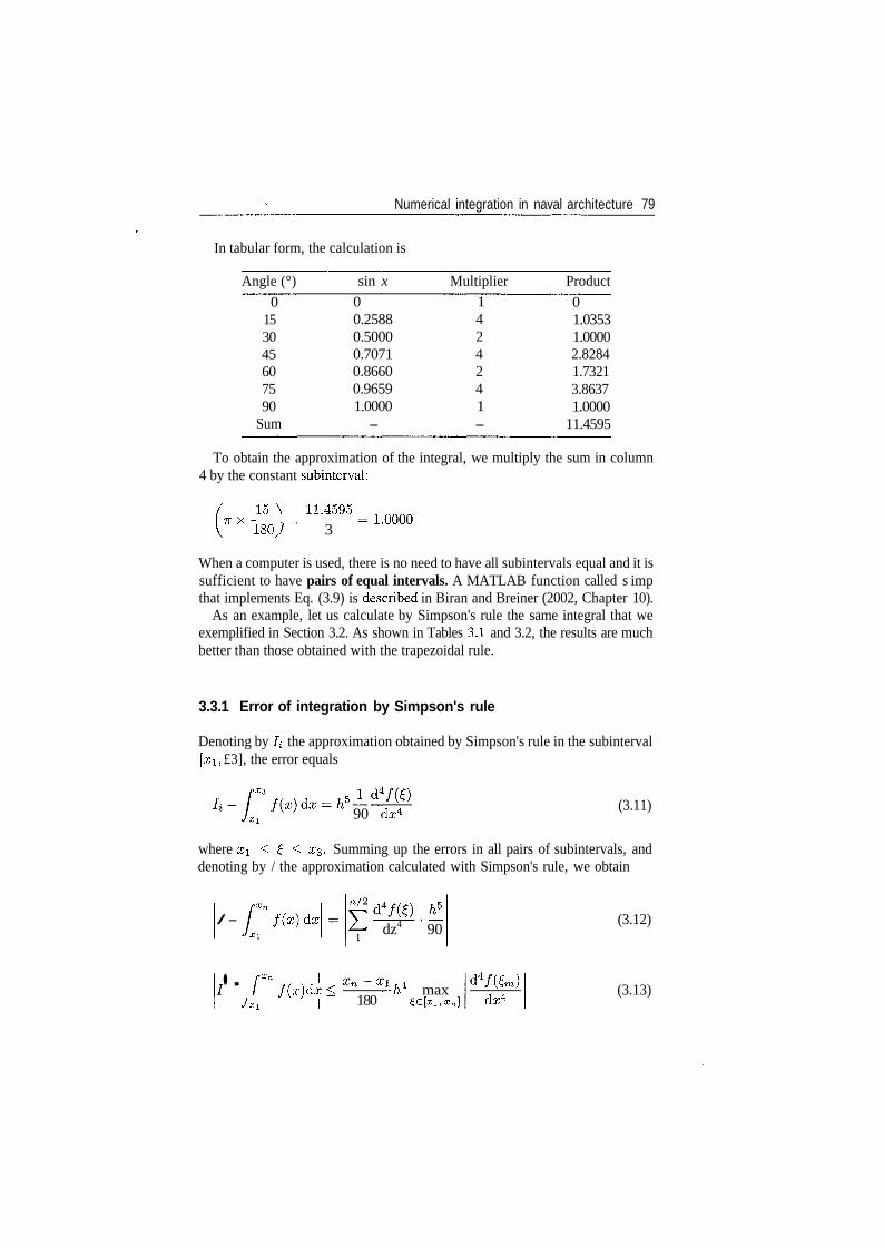
Numerical integration in naval architecture 79
In tabular form, the calculation is
Angle (°)0
153045607590
Sum
sin x
00.25880.50000.70710.86600.96591.0000
-
Multiplier1424241-
Product01.03531.00002.82841.73213.86371.0000
11.4595
To obtain the approximation of the integral, we multiply the sum in column4 by the constant subinterval:
W \ 1L4595 =
1807 3
When a computer is used, there is no need to have all subintervals equal and it issufficient to have pairs of equal intervals. A MATLAB function called s impthat implements Eq. (3.9) is described in Biran and Breiner (2002, Chapter 10).
As an example, let us calculate by Simpson's rule the same integral that weexemplified in Section 3.2. As shown in Tables 3.1 and 3.2, the results are muchbetter than those obtained with the trapezoidal rule.
3.3.1 Error of integration by Simpson's rule
Denoting by /; the approximation obtained by Simpson's rule in the subinterval[#i, £3], the error equals
(3.11)90 dz4
where x\ < £, < x3. Summing up the errors in all pairs of subintervals, anddenoting by / the approximation calculated with Simpson's rule, we obtain
/- /(#) dxdz4 90
• - r /(x)dxJxi 180
l-h* maxdx4
(3.12)
(3.13)
80 Ship Hydrostatics and Stability
At this point we can say the following about Simpson's rule:
1. If we divide h by 2, the error decreases approximately in the ratio 1/16.2. Simpson's rule yields the exact result if d4//dx4 = 0. This is certainly true
for second-degree parabolas, which is not surprising because we assumedsuch a curve when we developed the rule. It is interesting that the method isalso exact for cubics (third-degree curves).
3. For an equal number of subintervals, Simpson's rule yields better results thanthe trapezoidal rule. On the other hand, Simpson's rule imposes a seriousconstraint: the number of subintervals must be even, or, equivalently, f ( x )must be evaluated at an uneven number of equally spaced points, or, in otherwords, an uneven number of ordinates. If, for example, we calculate the areaof a waterline, we need an uneven number of equally spaced stations.
Example 3.2We refer again to Example 3.1 using this time Simpson's rule. We can experimentwith decreasing subintervals and obtain the results shown in Table 3.1, where theyare compared with the results yielded by the trapezoidal rule. The convergenceis considerably faster than that obtained in the case of the trapezoidal rule. Theper cent errors are shown in Table 3.2. As predicted by Eq. (3.13), each timewe divide the subinterval h by 2, the error decreases approximately in the ratio1/16. Note also that only two subintervals yield better results with Simpson'srule than eight with the trapezoidal rule.
3.4 Calculating points on the integral curve
The trapezoidal and Simpson's rules produce one number for an interval ofordinates, i.e.
fb
I(a,b)= \ f(x)dx
Sometimes we are interested not only in one number, but also in a sequenceof numbers that describe the integral as a function within the given interval,
I(x) = I f ( x ) dx, a < x < b (3.14)Ja
Thus, in certain hydrostatic calculations we may need to know the areas oftransverse sections (stations) as functions of draught (see Chapter 4).
Another example is that of calculations of dynamic stability which require theknowledge of the area under the curve of the righting arm as function of the heelangle. The latter subject is discussed in Chapters 6 and 8. An appropriate namefor a procedure that yields such an integral is integral with variable upperlimit.
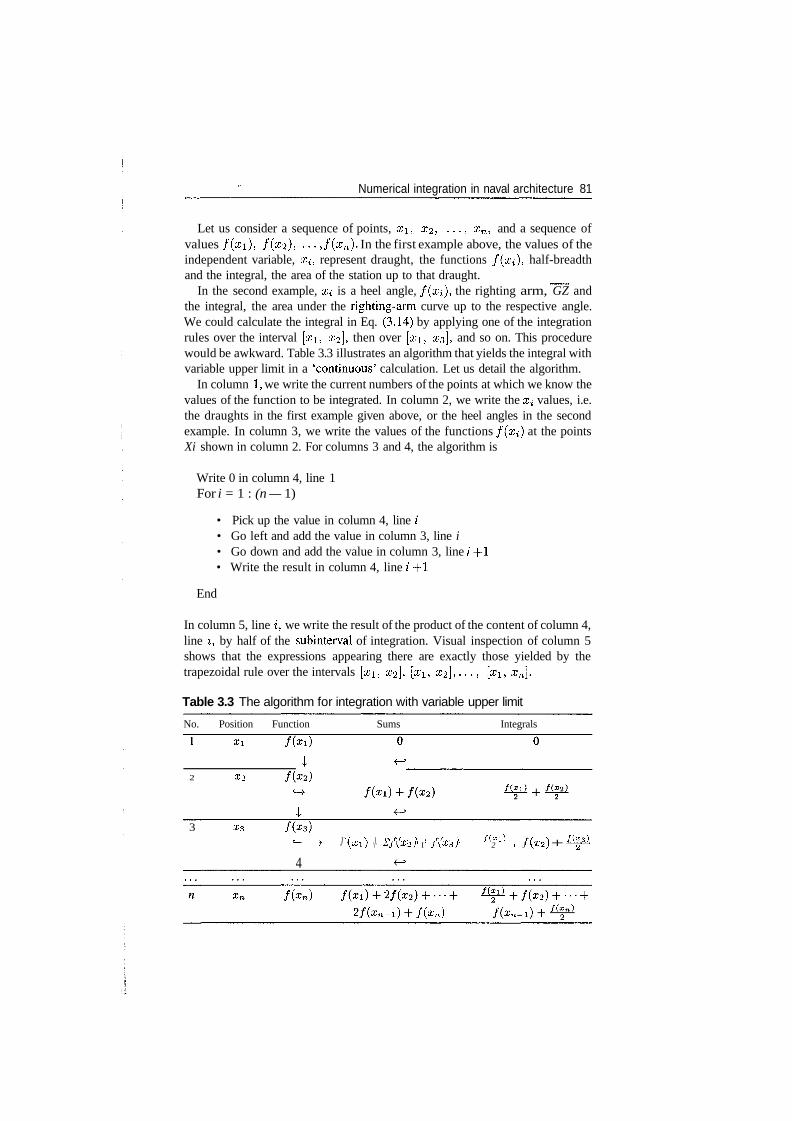
Numerical integration in naval architecture 81
Let us consider a sequence of points, #1, x2, . . . , xn, and a sequence ofvalues /(xi), /(#2)> • • • , f(xn). In the first example above, the values of theindependent variable, a^, represent draught, the functions /(#;), half-breadthand the integral, the area of the station up to that draught.
In the second example, x^ is a heel angle, f ( x i ) , the righting arm, GZ andthe integral, the area under the righting-arm curve up to the respective angle.We could calculate the integral in Eq. (3.14) by applying one of the integrationrules over the interval [#i, £2], then over [#i, #3], and so on. This procedurewould be awkward. Table 3.3 illustrates an algorithm that yields the integral withvariable upper limit in a 'continuous' calculation. Let us detail the algorithm.
In column 1, we write the current numbers of the points at which we know thevalues of the function to be integrated. In column 2, we write the X{ values, i.e.the draughts in the first example given above, or the heel angles in the secondexample. In column 3, we write the values of the functions f ( x i ) at the pointsXi shown in column 2. For columns 3 and 4, the algorithm is
Write 0 in column 4, line 1For i = 1 : (n — 1)
• Pick up the value in column 4, line /• Go left and add the value in column 3, line i• Go down and add the value in column 3, line / +1• Write the result in column 4, line / -j-1
End
In column 5, line i, we write the result of the product of the content of column 4,line z, by half of the subinterval of integration. Visual inspection of column 5shows that the expressions appearing there are exactly those yielded by thetrapezoidal rule over the intervals [#i, x2], [#i, x 2 ] , . . . , [#i, xn].
Table 3.3 The algorithm for integration with variable upper limit
No. Position Function Sums Integrals_ _ _ _ _ _
I ^2 X2
3 x3c— )• J
4
e ( r t } \ °f(ro") 1 f(r<*} /(xi) i f ( .\JsLJ \ ^J\J,2) I J\^3) 2 ' J \*r2) + ̂
/(*„)
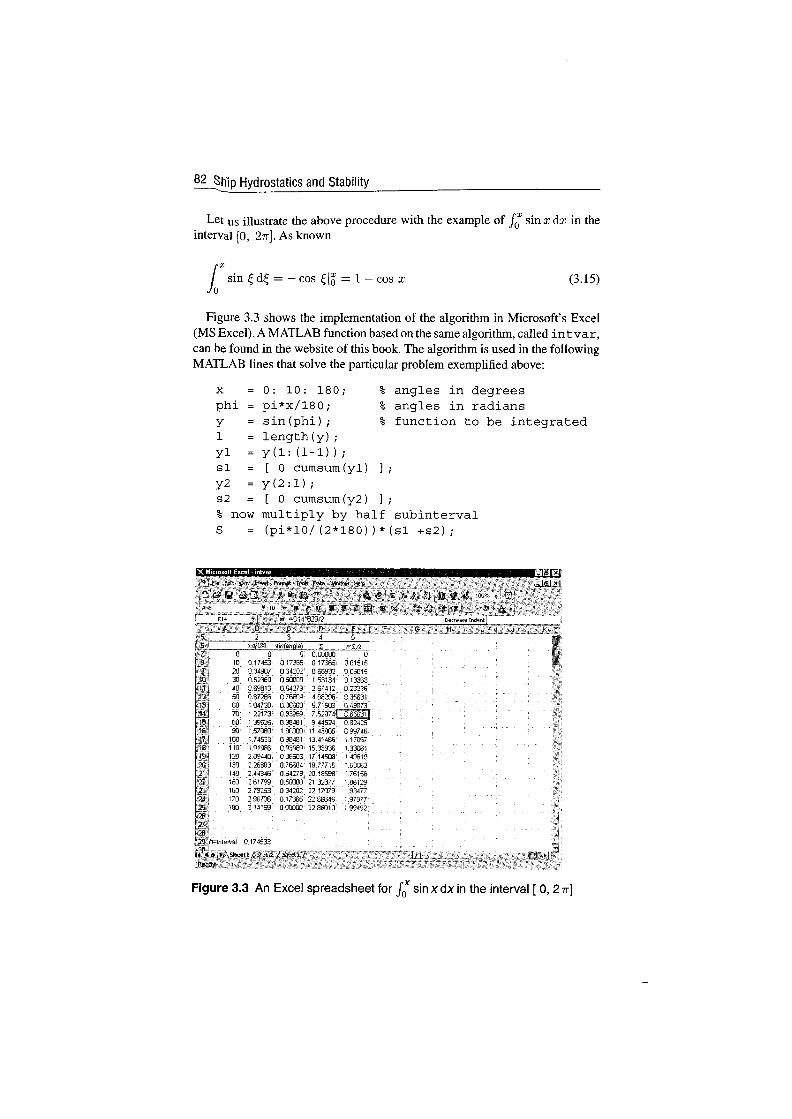
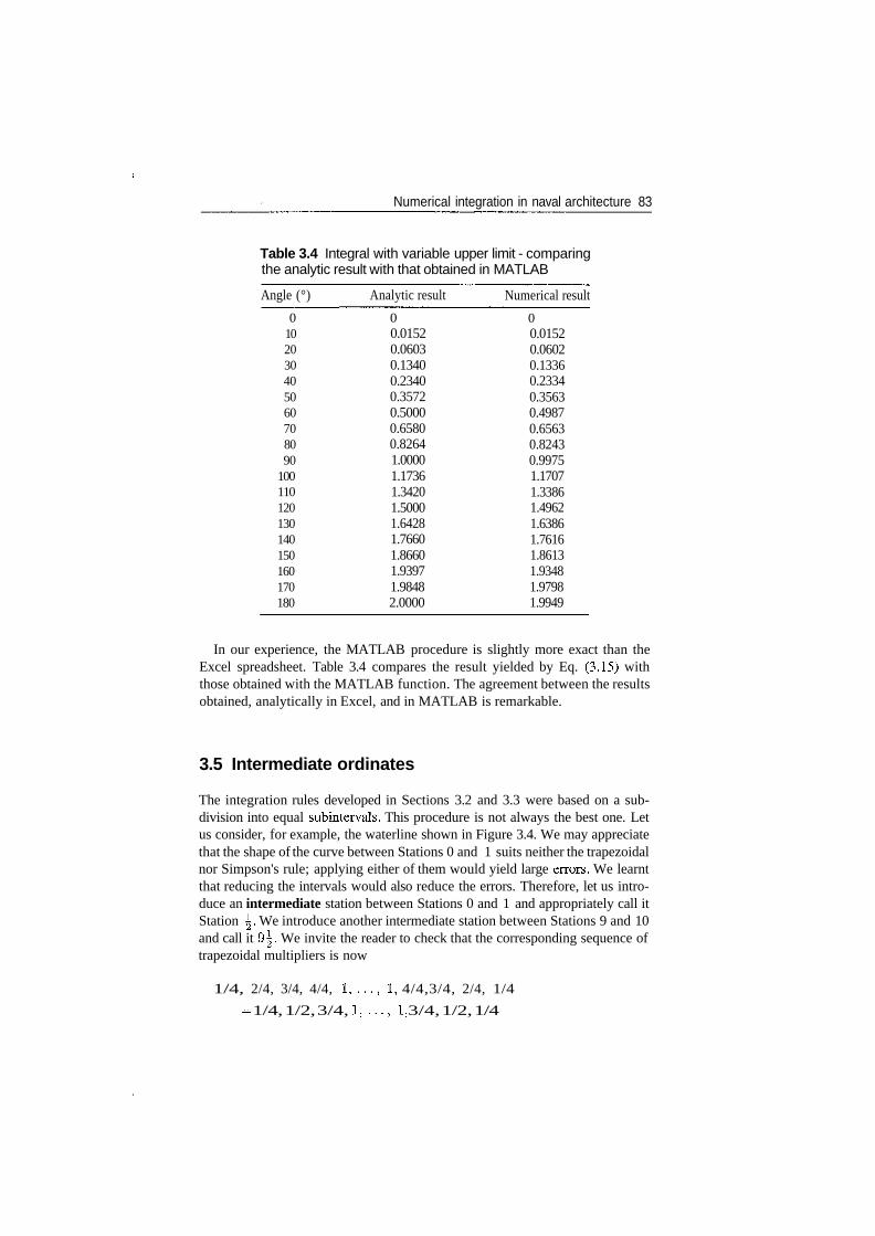
Numerical integration in naval architecture 83
Table 3.4 Integral with variable upper limit - comparingthe analytic result with that obtained in MATLAB
Angle (°)
0102030405060708090
100110120130140150160170180
Analytic result
00.01520.06030.13400.23400.35720.50000.65800.82641.00001.17361.34201.50001.64281.76601.86601.93971.98482.0000
Numerical result
00.01520.06020.13360.23340.35630.49870.65630.82430.99751.17071.33861.49621.63861.76161.86131.93481.97981.9949
In our experience, the MATLAB procedure is slightly more exact than theExcel spreadsheet. Table 3.4 compares the result yielded by Eq. (3.15) withthose obtained with the MATLAB function. The agreement between the resultsobtained, analytically in Excel, and in MATLAB is remarkable.
3.5 Intermediate ordinates
The integration rules developed in Sections 3.2 and 3.3 were based on a sub-division into equal subintervals. This procedure is not always the best one. Letus consider, for example, the waterline shown in Figure 3.4. We may appreciatethat the shape of the curve between Stations 0 and 1 suits neither the trapezoidalnor Simpson's rule; applying either of them would yield large errors. We learntthat reducing the intervals would also reduce the errors. Therefore, let us intro-duce an intermediate station between Stations 0 and 1 and appropriately call itStation \. We introduce another intermediate station between Stations 9 and 10and call it 9|. We invite the reader to check that the corresponding sequence oftrapezoidal multipliers is now
1/4, 2/4, 3/4, 4/4, !,...,!, 4/4,3/4, 2/4, 1/4
= 1/4, 1/2, 3/4, !,...,!, 3/4, 1/2, 1/4
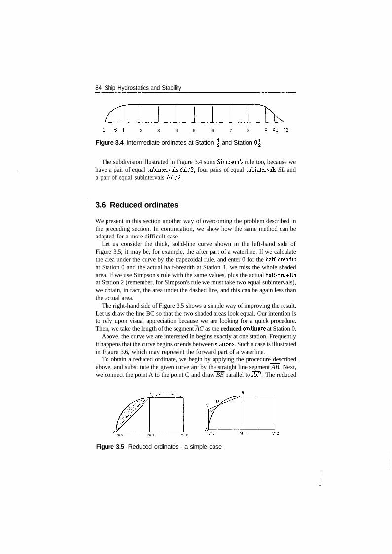
84 Ship Hydrostatics and Stability
0 1 / 2 1 2 3 4 5 6 7 8
Figure 3.4 Intermediate ordinates at Station \ and Station 9^
The subdivision illustrated in Figure 3.4 suits Simpson's rule too, because wehave a pair of equal subintervals <5I//2, four pairs of equal subintervals SL anda pair of equal subintervals 6L/2.
3.6 Reduced ordinates
We present in this section another way of overcoming the problem described inthe preceding section. In continuation, we show how the same method can beadapted for a more difficult case.
Let us consider the thick, solid-line curve shown in the left-hand side ofFigure 3.5; it may be, for example, the after part of a waterline. If we calculatethe area under the curve by the trapezoidal rule, and enter 0 for the half-breadthat Station 0 and the actual half-breadth at Station 1, we miss the whole shadedarea. If we use Simpson's rule with the same values, plus the actual half-breadthat Station 2 (remember, for Simpson's rule we must take two equal subintervals),we obtain, in fact, the area under the dashed line, and this can be again less thanthe actual area.
The right-hand side of Figure 3.5 shows a simple way of improving the result.Let us draw the line BC so that the two shaded areas look equal. Our intention isto rely upon visual appreciation because we are looking for a quick procedure.Then, we take the length of the segment AC as the reduced ordinate at Station 0.
Above, the curve we are interested in begins exactly at one station. Frequentlyit happens that the curve begins or ends between stations. Such a case is illustratedin Figure 3.6, which may represent the forward part of a waterline.
To obtain a reduced ordinate, we begin by applying the procedure describedabove, and substitute the given curve arc by the straight line segment AB. Next,we connect the point A to the point C and draw BE parallel to AC. The reduced
St 0 St 1 St 2 °' u
Figure 3.5 Reduced ordinates - a simple case
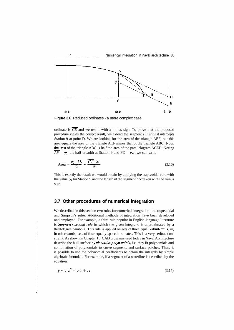
Numerical integration in naval architecture 85
St 8 St 9
Figure 3.6 Reduced ordinates - a more complex case
StlO
ordinate is CE and we use it with a minus sign. To prove that the proposedprocedure yields the correct result, we extend the segment BE until it interceptsStation 9 at point D. We are looking for the area of the triangle ABF, but thisarea equals the area of the triangle ACF minus that of the triangle ABC. Now,the_area of the triangle ABC is half the area of the parallelogram ACED. NotingAF = yg, the half-breadth at Station 9 and FC = 6L, we can write
Area =yg -6L CE- SL
(3.16)
This is exactly the result we would obtain by applying the trapezoidal rule withthe value 3/9 for Station 9 and the length of the segment CE taken with the minussign.
3.7 Other procedures of numerical integration
We described in this section two rules for numerical integration: the trapezoidaland Simpson's rules. Additional methods of integration have been developedand employed. For example, a third rule popular in English-language literatureis Simpson's second rule in which the given integrand is approximated by athird-degree parabola. This rule is applied on sets of three equal subintervals, or,in other words, sets of four equally spaced ordinates. This is a very serious con-straint. As shown in Chapter 13, CAD programs used today in Naval Architecturedescribe the hull surface by piecewise polynomials, i.e. they fit polynomials andcombination of polynomials to curve segments and surface patches. Then, itis possible to use the polynomial coefficients to obtain the integrals by simplealgebraic formulae. For example, if a segment of a waterline is described by theequation
+ C2X -f C3 (3.17)
86 Ship Hydrostatics and Stability
then the area enclosed between the curve segment, the centreline, and the stationsx = a, x = b is
j Cl 3 , C2 2ydx= —x + y^
(3.18)
Similar equations can be derived for other properties, namely moments andmoments of inertia.
3.8 Summary
Naval Architecture requires the calculation of areas, moments of areas, momentsof inertia of areas, volumes and moments of volumes. Such calculations involvedefinite integrals. Usually, the hull surface is defined by line drawings or tablesof offsets, and not by explicit mathematical expressions. Then, the integrals canbe obtained only by numerical methods. In a numerical method, we approximatethe integral by a weighted sum of a finite set of function values, i.e.
(3.19)
Two methods that implement such approximations are introduced in this chapter:the trapezoidal rule and Simpson's rule. The trapezoidal rule approximates thegiven curve by straight line segments, while Simpson's rule approximates it by aparabola. The rules are exemplified on integrands for which we know the exactsolutions. Thus, it is possible to show convincingly that the approximations yieldsatisfactory results. Also, it is possible to see that, as the number of ordinates -i.e. the number of points at which the integral is evaluated - increases, theerror decreases. The number of ordinates must be limited for practical reasons.This is possible because it is sufficient to maintain a precision consistent withmeasurements or other calculations. Simpson's rule yields, on one hand, resultscloser to the exact value. On the other hand, it imposes a serious constraint: thenumber of subintervals must be even.
By applying the rule of integration over one interval we obtain one number.In Naval Architecture, it is sometimes necessary to have a set of numbers thatdescribe the integral curve as a function of the independent variable, i.e.
- I f ( x ) d x , a<x<bJ a
This integral with variable upper limit can be obtained with the aid of an elegantalgorithm described in this chapter.
The shape of curves encountered in Naval Architecture can be such that overcertain intervals, generally towards their ends, it may be necessary to use smaller
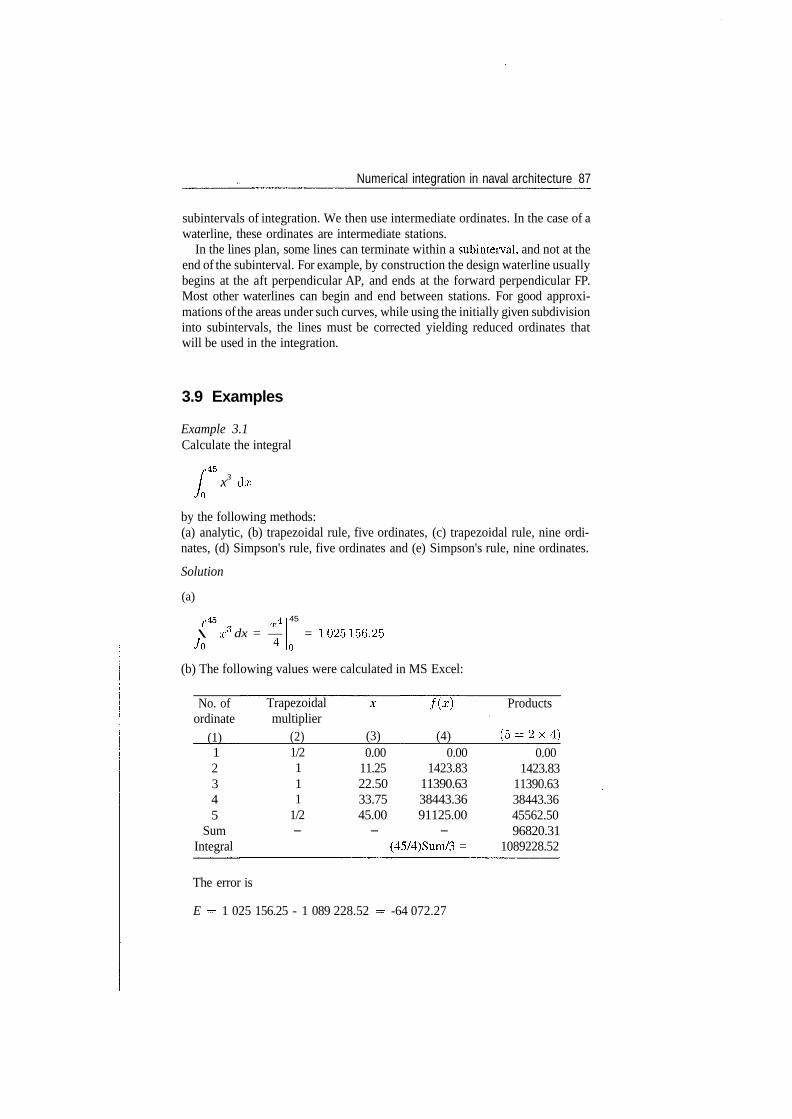
Numerical integration in naval architecture 87
subintervals of integration. We then use intermediate ordinates. In the case of awaterline, these ordinates are intermediate stations.
In the lines plan, some lines can terminate within a subinterval, and not at theend of the subinterval. For example, by construction the design waterline usuallybegins at the aft perpendicular AP, and ends at the forward perpendicular FP.Most other waterlines can begin and end between stations. For good approxi-mations of the areas under such curves, while using the initially given subdivisioninto subintervals, the lines must be corrected yielding reduced ordinates thatwill be used in the integration.
3.9 Examples
Example 3.1Calculate the integral
/•45
L -x3 dx
by the following methods:(a) analytic, (b) trapezoidal rule, five ordinates, (c) trapezoidal rule, nine ordi-nates, (d) Simpson's rule, five ordinates and (e) Simpson's rule, nine ordinates.
Solution
(a)
r4
\Jo
x6 dx = —45
= 1025156.25
(b) The following values were calculated in MS Excel:
No. ofordinate
(1)12345
SumIntegral
Trapezoidalmultiplier
(2)1/2111
1/2-
f ( x )
(3) (4)0.00 0.00
11.25 1423.8322.50 11390.6333.75 38443.3645.00 91125.00- -
(45/4)Sum/3 =
Products
( 5 - 2 x 4 )0.00
1423.8311390.6338443.3645562.5096820.31
1089228.52
The error is
E = 1 025 156.25 - 1 089 228.52 - -64 072.27
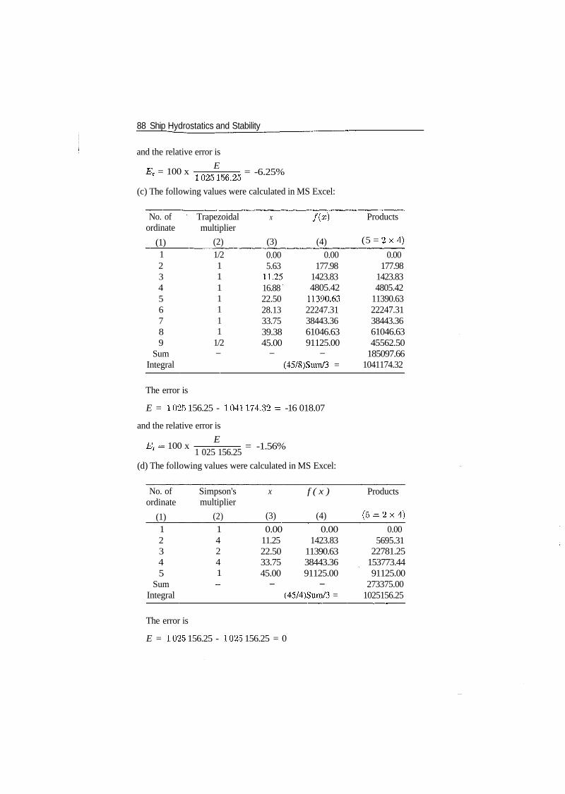
88 Ship Hydrostatics and Stability
and the relative error is
EEr = 100 x = -6.25%
1025156.25
(c) The following values were calculated in MS Excel:
No. ofordinate
(1)123456789
SumIntegral
Trapezoidalmultiplier
(2)1/21111111
1/2—
X
(3)
0.005.63
11.2516.8822.5028.1333.7539.3845.00
—
/(*)
(4)
0.00177.98
1423.834805.42
11390.6322247.3138443.3661046.6391125.00
—(45/8)Sum/3 =
Products
(5 = 2 x 4 )
0.00177.98
1423.834805.42
11390.6322247.3138443.3661046.6345562.50
185097.661041174.32
The error is
E = 1025 156.25 - 1041174.32 - -16 018.07
and the relative error is
ET = 100 xE
= -1.56%1 025 156.25
(d) The following values were calculated in MS Excel:
No. ofordinate
(1)12345
SumIntegral
Simpson'smultiplier
(2)14241_
x f ( x )
(3) (4)
0.00 0.0011.25 1423.8322.50 11390.6333.75 38443.3645.00 91125.00- -
(45/4)Sum/3 =
Products
( 5 - 2 x 4 )
0.005695.31
22781.25153773.4491125.00
273375.001025156.25
The error is
E = 1025 156.25 - 1025 156.25 = 0

Numerical integration in naval architecture 89
and the relative error is
EEr = 100 x = 0%
1025156.25
(e) The following values were calculated in MS Excel:
No. ofordinate
(1)123456789
SumIntegral
Simpson'smultiplier
(2)142424241-
X
(3)
0.005.63
11.2516.8822.5028.1333.7539.3845.00
—
/(*)
(4)
0.00177.98
1423.834805.42
11390.6322247.3138443.3661046.6391125.00
—(45/8)Sum/3 =
Products
(5 = 2 x 4 )
0.00711.91
2847.6619221.6822781.2588989.2676886.72
244186.5291125.00
546750.001025156.25
The error is
E = 1025 156.25 - 1025 156.25 = 0
and the relative error is
EET = 100 x
1025156.25= 0%
MATLAB solution
(a) Analytic:
format longa = 45~4/4 = 1.025156250000000e+006
(b) Trapezoidal rule, five ordinates:
x = 0: 45/4: 45;Y = X . ~ 3 ;b = trapz(x, y) = 1.089228515625000e+006error = a - b = -6.4072e+004percent_error = 100*(a - b)/a = -6.2500 °
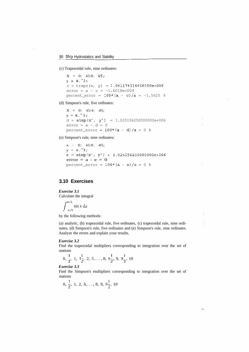
90 Ship Hydrostatics and Stability
(c) Trapezoidal rule, nine ordinates:
X = 0: 45/8: 45;
y = X . ~ 3 ;c = trapz(x, y) = 1.041174316406250e+006error = a - c = -1.6018e+004percent_error = 100*(a - c)/a = -1.5625 %
(d) Simpson's rule, five ordinates:
X = 0: 45/4: 45;y = X. " 3 ;d = simp(x', y') = 1.025156250000000e+006error = a - d = 0percent_error = 100*(a - d)/a = 0 %
(e) Simpson's rule, nine ordinates:
x = 0: 45/8: 45;
y = x . ~ 3 ;e = s imp(x ' , y 7 ) = 1 .025156250000000e+006error = a - e = 0percent_error = 100*(a - e)/a = 0 %
3.10 Exercises
Exercise 3.1Calculate the integral
2
sin x dx/-7T/2
by the following methods:
(a) analytic, (b) trapezoidal rule, five ordinates, (c) trapezoidal rule, nine ordi-nates, (d) Simpson's rule, five ordinates and (e) Simpson's rule, nine ordinates.Analyze the errors and explain your results.
Exercise 3.2Find the trapezoidal multipliers corresponding to integration over the set ofstations
0, -, 1, 1-, 2, 3 , . . . , 8, 8-, 9, 9-, 10
Exercise 3.3Find the Simpson's multipliers corresponding to integration over the set ofstations
0, i, 1, 2, 3 , . . . , 8, 9, 9^, 10
4Hydrostatic curves
4.1 Introduction
In the preceding chapter we learnt several methods of numerical integrationused in Naval Architecture. In this chapter we are going to apply them to thecalculation of areas, centroids, moments of inertia of areas, volumes, and centresof volume. We call these properties hydrostatic data and show how to plot them,as functions of draught, in curves that allow further calculations.
Another set of plots consists of Bon jean curves; they enable the user tocalculate the displacement and the centres of buoyancy for a given waterline, inan upright condition. The waterline can be not only a straight line, as is the casein still water, but also a curve. The latter case can arise when the hull is deflectedbecause of a longitudinal bending moment or thermal expansion, or when thevessel floats in waves. The vessel is said to be in a hogging condition if thekeel is concave downwards, and in a sagging condition if the keel is concaveupwards.
All the properties mentioned above are represented as functions of draught.Certain functional relationships exist between some of those curves. Three suchproperties are described in this chapter.
Another subject dealt with in this chapter is that of affine hulls, i.e. hullsobtained from given ship lines by multiplying by the same scale factor alldimensions parallel to an axis of coordinates. The properties of an affine hullcan be derived by simple formulae from the properties of the parent hull.
Within this chapter we use the following notations:
i station number, as in the lines drawing;j station number defined such that the distance from the origin of
a;-coordinates is j 6L\Xi x-coordinate of station i\Ui half-breadth of station i on a given waterline;a.i integration multiplier for station i\ for Simpson's rule
we assume that the common factor 1/3 is included in c^;SL subinterval of integration along the x-axis;ST subinterval of integration along the z-axis;
For the above definitions we have, obviously, j = 0 in the origin ofcoordinates.
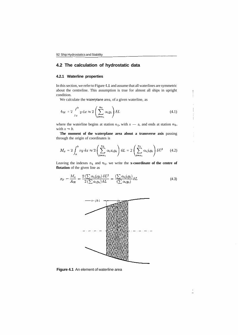
92 Ship Hydrostatics and Stability
4.2 The calculation of hydrostatic data
4.2.1 Waterline properties
In this section, we refer to Figure 4.1 and assume that all waterlines are symmetricabout the centreline. This assumption is true for almost all ships in uprightcondition.
We calculate the waterplane area, of a given waterline, as
Aw
fb= 2 y d x * .
J a(4.1)
where the waterline begins at station HI, with x — a, and ends at station 712,with x = b.
The moment of the waterplane area about a transverse axis passingthrough the origin of coordinates is
rb
= 2Ja
xydx 6L = 2 (4.2)
Leaving the indexes ni and ri2, we write the x-coordinate of the centre offlotation of the given line as
= Mx (4.3)
Figure 4.1 An element of waterline area

Hydrostatic curves 93
The notation XF corresponds to the DIN 81209 standard. The notation used inEnglish-language texts is LCF, an acronym for longitudinal centre of flotation.The corresponding curve is shown in Figure 4.2. To calculate the transversemoment of inertia of the waterplane area, i.e. the moment of inertia about thecentreline, we first write the moment of inertia of the elemental area shown ingrey in Figure 4.1:
2 3
= * dx
Then, the moment of inertia of the whole waterplane equals
rb
/
9
^- 3
(4.4)
(4.5)
The moment of inertia of the waterplane area about a transverse axis pass-ing through the origin of coordinates is calculated as
rb ( n \ ( n \y = 2 x2y dx « 2 £ a^yi } SL = 2 PT adfa 6L3
Ja \»=o / \t=o /(4.6)
-22.2
KB, KM, LCF, LCB (m), dash lines
0 1 2 3
1.6
I
£ 1.4
1.2
0.8
0.6
2.2
1.8
1.6
1.2
0.8
10 20 30 40 50 60 70 80 90
V (m3), A (t), A^m2), MCT (m4/m), KML(m), solid lines
Figure 4.2 Hydrostatic curves of Ship Lido 9
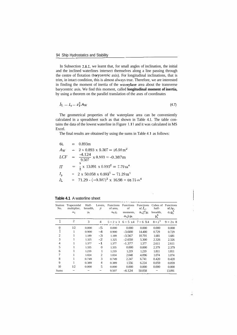
94 Ship Hydrostatics and Stability
In Subsection 2.8.1, we learnt that, for small angles of inclination, the initialand the inclined waterlines intersect themselves along a line passing throughthe centre of flotation (barycentric axis). For longitudinal inclinations, that istrim, in intact condition, this is almost always true. Therefore, we are interestedin finding the moment of inertia of the waterplane area about the transversebarycentric axis. We find this moment, called longitudinal moment of inertia,by using a theorem on the parallel translation of the axes of coordinates
— Iy — (4.7)
The geometrical properties of the waterplane area can be convenientlycalculated in a spreadsheet such as that shown in Table 4.1. The table con-tains the data of the lowest waterline in Figure 1.11 and it was calculated in MSExcel.
The final results are obtained by using the sums in Table 4.1 as follows:
6L
LCF
IT
0.893m
2 x 0.893 x 9.507= 16.98m2
-4.1249.507
x 0.893- -0.387m
- - x 13.091 x 0.8932 - 7.79m4
o= 2 x 50.058 x 0.8933 - 71.29m4
= 71.29 - (-0.387)2 x 16.98 = 68.75m4
Table 4.1 A waterline sheet
Station Trapezoidal Half- Levers, Functions Functions Functions Cubes of FunctionsNo. multiplier, breadth, ji of area, of of/x, half- of IT,
Oii m ot-iVi moments, Q-iflyi breadth, o^y3
1012345678910
Sums
2
1/2111111111
1/2-
3
0.0000.900
1.1891.3251.377
1.3351.2191.024
0.7490.3890.000-
4
-5-4-3-2-1
012345-
5 = 2 x 3
0.000
0.900
1.1891.3251.3771.335
1.2191.024
0.7490.3890.0009.507
6 = 5 x4
0.000-3.600-3.567-2.650-1.377
0.0001.2192.0482.2471.5560.000
-4.124
7 = 6 X4
0.00014.40010.7015.3001.3770.0001.2194.0966.7416.2240.000
50.058
8 = 33
0.0000.7291.6812.3262.6112.3791.8111.0740.4200.0590.000-
9 = 2x 8
0.0000.7291.6812.3262.6112.3791.8111.0740.4200.0590.000
13.091
Hydrostatic curves 95
We recommend the reader to check the plausibility of the results by comparingthem with the data of the circumscribed rectangle. For example, the area of thisrectangle is
2 x 1.377x8.928-24.559m2
that is greater than the waterplane area, and so it should be.Table 4.1 requires a few explanations. The fourth line contains column num-
bers. An expression like 5 = 2 x 3 means that the numbers in column 5 arethe products of numbers in column 2 by numbers in column 3. Similarly, thenumbers in column 7 are the products of numbers in column 6 by numbersin column 4. This means that the number 14.400, for example, is obtained byone multiplication, namely -3.600 x (-4), and not by two multiplications anda squaring operation, 1 x (—4)2 x (0.900). Proceeding in this way we sparecomputer resources and reduce the possibilities of errors. Another simplificationresults from the use of the factors j, most of them integers. Multiplication byintegers is easier when carried out manually, and it is not affected by numericalerrors. Thus, instead of multiplying the products in column 5 by rr-distances thatare 'real' numbers (fractional values), and introduce numerical errors at eachstation, we multiply by integers. Then, the sums of the products in columns6 and 7 are multiplied only once by the length, and the square of the length ofthe subinterval of integration, 8L, which can be a real number.
Let us make a final comment on the use of electronic spreadsheets forcalculations such as those in Table 4.1. The values of half-breadths, yi, areentered only once, in column 3, although they are repeatedly used in all calcu-lations. In this way, we reduce the possibilities of errors that can occur whenentering a number. Moreover, if we must change the value of a half-breadth, wedo it in one place only, and the change spreads automatically over the wholetable.
Instead of using an electronic spreadsheet, such as MS Excel, one can write aprogramme in a suitable language, for example, MATLAB. Such a programmecan be useful if the calculations are chained with other computer operations. Forthe reasons explained above, we recommend to write the programme followingthe principles used in the waterline sheet shown in Table 4.1.
4.2.2 Volume properties
We can obtain the displacement volume corresponding to a given draught, TO,by integrating 'vertically' the waterplane areas from the lowest hull point to thegiven draught:
(4.8)
96 Ship Hydrostatics and Stability
The moment of the displacement volume above the base line can also be obtainedby 'vertical' integration:
MB = / ° TAW dz * (> ^ atZiAvK } 6T = ( > ' a^AW; \ d"2T (4.9)Jo
where zi is the ̂ -coordinate of the zth waterline and ji the number of the waterlinecounted from the baseline.
From Eqs. (4.8) and (4.9), we calculate the vertical coordinate of the centreof buoyancy, ZB, as
MB-zz- ~ — 7 — : - >• - — —/ — : - r— oT (4.10)V
The notation ZB is that prescribed in the DIN 8 1209 standard. The notations com-mon in English-language books are KB, or VCB, the latter being the acronymof vertical centre of buoyancy. The procedure used with Eq. (4.10) yields badapproximations for the lowest waterlines. Therefore, we recommend to neglectthe results for the first waterlines. As shown in Section 4.4, we can also cal-culate the displacement and the vertical centre of buoyancy by 'longitudinal'integration of values read in Bonjean curves.
4.2.3 Derived data
Let us suppose that we know the displacement, AQ, corresponding to a givendraught, TO, and we want to find by how many tons that displacement willchange if the draught changes by 6T cm. Let the waterplane area be AW m2 andthe water density pvv tm~3. For a small draught change, we may neglect theslope of the shell (in other words we assume a wall-sided hull) and we write
<5A = pwAw 6T
If we measure A in tons, and 6T in centimetres, we obtain
6& = pw^xlW (4.11)ol
We call the quantity pw^w/100 tons per centimetre immersion and use forit the notation TPC. In older, English-language books, we find the notation TPIas an acronym for tons per inch. This quantity is calculated from an expressionsimilar to Eq. (4.11), but adapted for English and American units. For SI units
TPC = x pw (4'12)
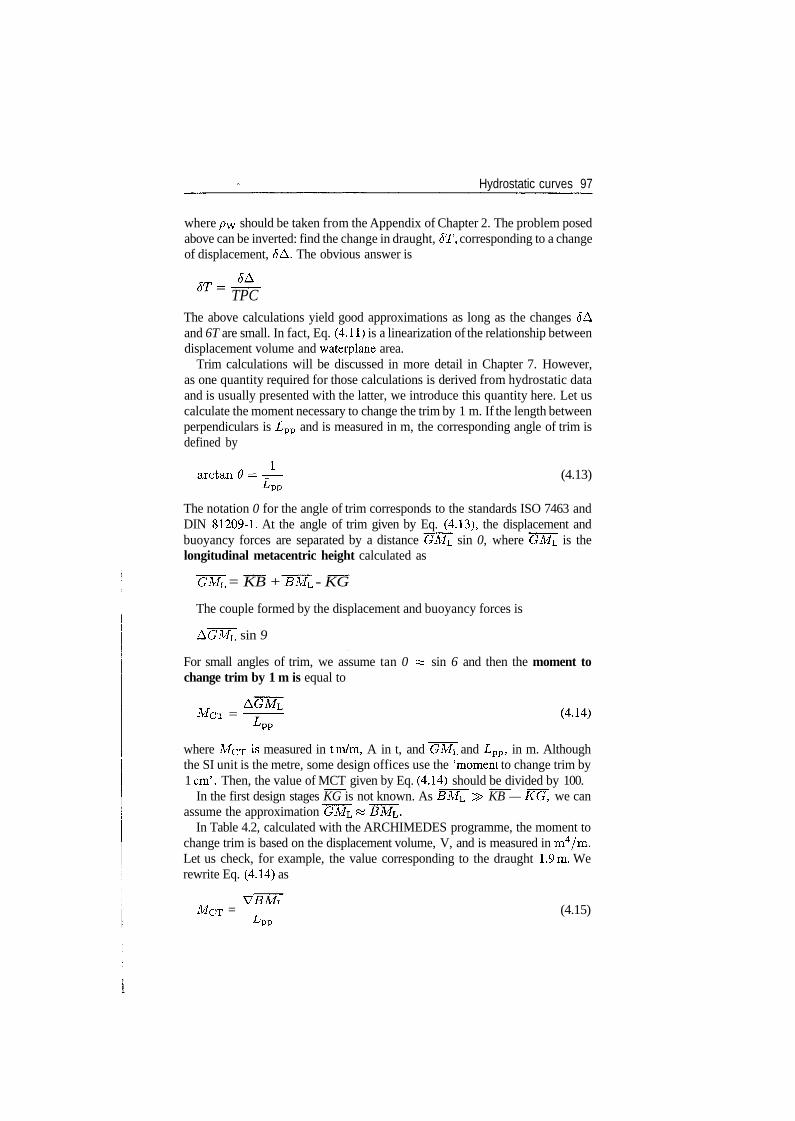
Hydrostatic curves 97
where p\y should be taken from the Appendix of Chapter 2. The problem posedabove can be inverted: find the change in draught, 6T, corresponding to a changeof displacement, JA. The obvious answer is
TPCThe above calculations yield good approximations as long as the changes $Aand 6T are small. In fact, Eq. (4.11) is a linearization of the relationship betweendisplacement volume and waterplane area.
Trim calculations will be discussed in more detail in Chapter 7. However,as one quantity required for those calculations is derived from hydrostatic dataand is usually presented with the latter, we introduce this quantity here. Let uscalculate the moment necessary to change the trim by 1 m. If the length betweenperpendiculars is Lpp and is measured in m, the corresponding angle of trim isdefined by
arctan<9=-— (4.13)
The notation 0 for the angle of trim corresponds to the standards ISO 7463 andDIN 81209-1. At the angle of trim given by Eq. (4.13), the displacement andbuoyancy forces are separated by a distance GMc sin 0, where GML is thelongitudinal metacentric height calculated as
GML = KB + BML - KG
The couple formed by the displacement and buoyancy forces is
AGML sin 9
For small angles of trim, we assume tan 0 « sin 6 and then the moment tochange trim by 1 m is equal to
MCT =
where MCT is measured in tm/m, A in t, and GM^ and Lpp, in m. Althoughthe SI unit is the metre, some design offices use the 'moment to change trim by1 cm'. Then, the value of MCT given by Eq. (4.14) should be divided by 100.
In the first design stages KG is not known. As BMi, > KB — KG, we canassume the approximation GM\.
In Table 4.2, calculated with the ARCHIMEDES programme, the moment tochange trim is based on the displacement volume, V, and is measured in m4/m.Let us check, for example, the value corresponding to the draught 1.9m. Werewrite Eq. (4.14) as
MCT = (4.15)LPP
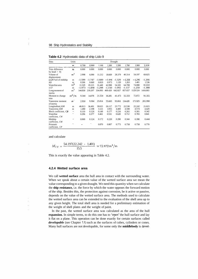
98 Ship Hydrostatics and Stability
Table 4.2 Hydrostatic data of ship Lido 9Data
Trim differenceby head > 0)Volume ofdisplacementLCB Fwd of midshipKBWaterline areaLCFLong moment ofinertiaMoment to changetrimTransverse momentof inertiaLongitudinal, KMTransverse, KMBlock coefficient, CBWaterlinecoefficient, CWMidshipcoefficient, CMPrismaticcoefficient, CP
Units
m
m
m3
mm
m2
mm4
m4/m
m4
mm-_
-
_
Draught
0.700
0.000
2.998
-1.5990.506
11.529-1.973144.830
9.344
2.950
48.8131.4900.1100.296
0.069
_
0.900
0.000
6.090
-1.7470.660
20.221-1.648218.207
14.078
9.364
36.4912.1980.1260.377
0.124
_
1.100
0.000
11.212
-1.6000.819
31.449-1.298334.093
21.554
25.814
30.6153.1210.1490.461
0.172
0.870
1.300
0.000
18.669
-1.4460.973
42.998-1.150469.420
30.285
55.665
26.1173.9550.1770.531
0.220
0.807
1.500
0.000
28.379
-1.3291.120
54.183-1.092642.827
41.473
93.061
23.7724.4000.2160.620
0.280
0.773
1.700
0.000
40.314
-1.2681.263
64.708-1.137857.657
55.333
134.428
22.5384.5980.2610.712
0.344
0.758
1.900
0.000
54.197
-1.2461.401
74.088-1.259
1129.524
72.872
171.925
22.2424.5740.3010.783
0.398
0.758
2.100
0.000
69.825
-1.2661.536
81.810-1.388
1416.003
91.355
201.990
21.8154.4290.3420.841
0.444
0.770
and calculate
54.197(22.242 - 1.401)MCT = 15.5
= 72.872 m4/m
This is exactly the value appearing in Table 4.2.
4.2.4 Wetted surface area
We call wetted surface area the hull area in contact with the surrounding water.When we speak about a certain value of the wetted surface area we mean thevalue corresponding to a given draught. We need this quantity when we calculatethe ship resistance, i.e. the force by which the water opposes the forward motionof the ship. Besides this, the protection against corrosion, be it active or passive,depends on the value of the wetted surface area. The methods used to calculatethe wetted surface area can be extended to the evaluation of the shell area up toany given height. The total shell area is needed for a preliminary estimation ofthe weight of shell plates and the weight of paint.
In the past, the wetted surface area was calculated as the area of the hullexpansion. In simple terms, to do this one has to 'open' the hull surface and layit flat on a plane. This operation can be done exactly for certain surfaces calleddevelopable (see Chapter 13) such as the surfaces of cubes, cylinders or cones.Many hull surfaces are not developable, for some only the middlebody is devel-
Hydrostatic curves 99
opable. Then, the Naval Architect must be satisfied with an approximation, suchas described in Comstock (1967, pp. 39-41). Recent computer programmes forNaval Architecture calculate the wetted surface area by methods of differentialgeometry. Approximate formulae for calculating the wetted surface area of manyship types can be found in the literature of speciality. If the chosen hull belongsto a series of models tested in a towing tank, the wetted surface area is usuallyincluded in the data supplied by the experimenting institution.
4.3 Hydrostatic curves
Table 4.2 shows the hydrostatic data of the Ship Lido 9, for draughts between 0.7and 2.1 m, as calculated by the ARCHIMEDES programme. The data appear atdiscrete draught intervals. It is usual to represent those data also as hydrostaticcurves that allow interpolation at any required draught. Such curves are part ofthe documentation that must be onboard, for use by deck officers in calculationsrequired for the operation of the vessel. Many ships are provided today withboard computers that store the input data of the vessel and enable the officers tocalculate immediately any data they need. Even in those cases the hydrostaticcurves and the knowledge to use them should be present for emergency cases inwhich the computer fails.
There are no universally accepted standards for plotting hydrostatic data andwe can find a wide variety of 'styles'. For our purposes we choose a simple modelthat can be accommodated in the space of a textbook page, but still shows themajor features common to all representations. The curves are plots of functionsof the draught, T, at constant trim and heel. In general, the trim equals zero(ship on even keel), but it is possible to plot hydrostatic curves for any given,non-zero trim. The heel is almost always zero. The hydrostatic curves representdata calculated for parallel waterplanes. Romance languages use a short, elegantterm for this situation. For instance, in French one talks about 'carenes isoclines',while Italian uses the term 'carene isocline'.
Let us refer to Figure 4.2. The draught axis is vertical, positive upwards. Thevarious properties are measured horizontally, each at its own scale, so that allcurves can be contained in the same paper format. In our example, the curves ofvolume of displacement, V, displacement in fresh water, AFW, displacementin salt water, ASW, waterplane area, AW, moment to change trim by one metre,MCT, and longitudinal metacentre above keel, KM\., are measured along thelower scale that is to be read as 0-100 m3, 0-1001, 0-100 m2, 0-100 m4/m,or 0-100 m, respectively. The vertical centre of buoyancy, KB, the transversemetacentre above keel, KM, the longitudinal centre of flotation, LCF, andthe longitudinal centre of buoyancy, LCB, are measured along the upper scalegraduated from —2 to 5 m. To simplify things, we plot the coefficients of form,CB, CM, Cp, and CWL in another graph shown in Figure 4.3.
Let us return to the volume and displacement values represented in hydrostaticcurves. The displacement volume, V, is usually the volume of the moulded hull.
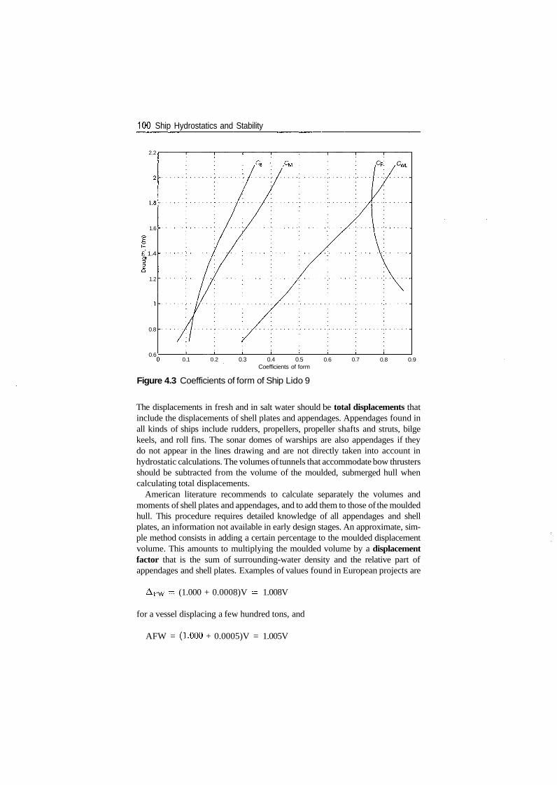
100 Ship Hydrostatics and Stability
2.2
1.6
£ 1.4
1.2
0.8
0.6
/CB '. ,CM
0.1 0.2 0.3 0.4 0.5Coefficients of form
0.6 0.7 0.8 0.9
Figure 4.3 Coefficients of form of Ship Lido 9
The displacements in fresh and in salt water should be total displacements thatinclude the displacements of shell plates and appendages. Appendages found inall kinds of ships include rudders, propellers, propeller shafts and struts, bilgekeels, and roll fins. The sonar domes of warships are also appendages if theydo not appear in the lines drawing and are not directly taken into account inhydrostatic calculations. The volumes of tunnels that accommodate bow thrustersshould be subtracted from the volume of the moulded, submerged hull whencalculating total displacements.
American literature recommends to calculate separately the volumes andmoments of shell plates and appendages, and to add them to those of the mouldedhull. This procedure requires detailed knowledge of all appendages and shellplates, an information not available in early design stages. An approximate, sim-ple method consists in adding a certain percentage to the moulded displacementvolume. This amounts to multiplying the moulded volume by a displacementfactor that is the sum of surrounding-water density and the relative part ofappendages and shell plates. Examples of values found in European projects are
AFW = (1.000 + 0.0008)V - 1.008V
for a vessel displacing a few hundred tons, and
AFW = (1-000 + 0.0005)V = 1.005V
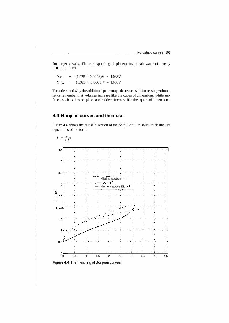
Hydrostatic curves 101
for larger vessels. The corresponding displacements in salt water of density1.025 tm"1 are
AFW - (1.025 4- 0.0008)V - 1.033V
AFW - (1.025 4- 0.0005)V = 1.030V
To understand why the additional percentage decreases with increasing volume,let us remember that volumes increase like the cubes of dimensions, while sur-faces, such as those of plates and rudders, increase like the square of dimensions.
4.4 Bonjean curves and their use
Figure 4.4 shows the midship section of the Ship Lido 9 in solid, thick line. Itsequation is of the form
* = f(y)
4.5-
3.5
^2.5
o>
I 2
1.5
0.5
0
— Midship section, m. — • Area, m2
— Moment above BL, m3
0 0.5 1 1.5 2 2.5
Figure 4.4 The meaning of Bonjean curves
3.5 4.5
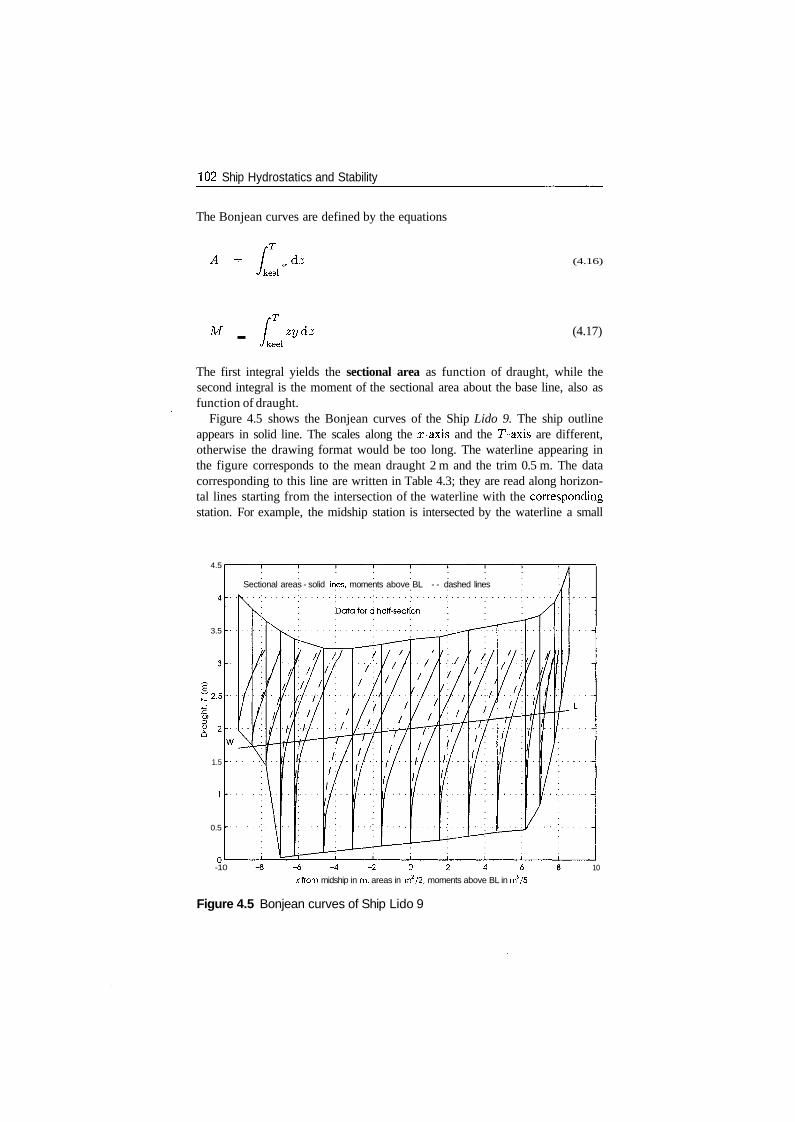
102 Ship Hydrostatics and Stability
The Bonjean curves are defined by the equations
rr dz
/keel-L (4.16)
M - fJkeelzydz (4.17)
The first integral yields the sectional area as function of draught, while thesecond integral is the moment of the sectional area about the base line, also asfunction of draught.
Figure 4.5 shows the Bonjean curves of the Ship Lido 9. The ship outlineappears in solid line. The scales along the x-axis and the T-axis are different,otherwise the drawing format would be too long. The waterline appearing inthe figure corresponds to the mean draught 2 m and the trim 0.5 m. The datacorresponding to this line are written in Table 4.3; they are read along horizon-tal lines starting from the intersection of the waterline with the correspondingstation. For example, the midship station is intersected by the waterline a small
4.5
3.5
'2.5
1.5
0.5
Sectional areas - solid lines, moments above BL - - dashed lines
-10 - 6 - 4 - 2 0 2 4 6xfrom midship in m, areas in m2/2, moments above BL in m3/5
10
Figure 4.5 Bonjean curves of Ship Lido 9
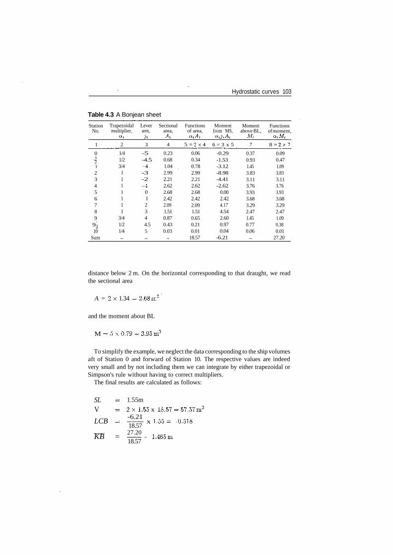
Hydrostatic curves 103
Table 4.3 A Bonjean sheet
StationNo.
1
0i21
23456789
9-10
Sum
Trapezoidalmultiplier,
2
1/41/23/41111111
3/41/21/4-
Leverarm,
3
-5-4.5—4-3-2
i
012344.55-
Sectionalarea,
4
0.230.681.042.992.212.622.682.422.091.510.870.430.03-
Functionsof area,
5 = 2 x 4
0.060.340.782.992.212.622.682.422.091.510.650.210.01
18.57
Momentfrom MS,
6 = 3 x 5
-0.29-1.53-3.12-8.98-4.41-2.62
0.002.424.174.542.600.970.04
-6.21
Momentabove BL,
7
0.370.931.453.833.113.763.933.683.292.471.450.770.06-
Functionsof moment,
8 = 2 x 7
0.090.471.093.833.113.763.933.683.292.471.090.380.01
27.20
distance below 2 m. On the horizontal corresponding to that draught, we readthe sectional area
A = 2x 1.34 = 2.68m2
and the moment about BL
M = 5x0 .79 -3.95m3
To simplify the example, we neglect the data corresponding to the ship volumesaft of Station 0 and forward of Station 10. The respective values are indeedvery small and by not including them we can integrate by either trapezoidal orSimpson's rule without having to correct multipliers.
The final results are calculated as follows:
SLV
LCB
KB =
1.55m
2 x 1.55 x 18.57-57.57m3
-6.2118.5727.20
18.57
x 1.55--0.518
- 1.465m
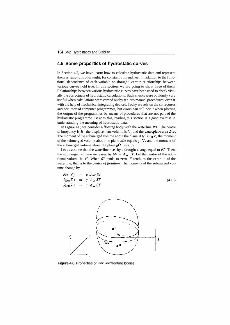
104 Ship Hydrostatics and Stability
4.5 Some properties of hydrostatic curves
In Section 4.2, we have learnt how to calculate hydrostatic data and representthem as functions of draught, for constant trim and heel. In addition to the func-tional dependence of each variable on draught, certain relationships betweenvarious curves hold true. In this section, we are going to show three of them.Relationships between various hydrostatic curves have been used to check visu-ally the correctness of hydrostatic calculations. Such checks were obviously veryuseful when calculations were carried out by tedious manual procedures, even ifwith the help of mechanical integrating devices. Today we rely on the correctnessand accuracy of computer programmes, but errors can still occur when plottingthe output of the programmes by means of procedures that are not part of thehydrostatic programme. Besides this, reading this section is a good exercise inunderstanding the meaning of hydrostatic data.
In Figure 4.6, we consider a floating body with the waterline WL. The centreof buoyancy is B, the displacement volume is V, and the waterplane area AW-The moment of the submerged volume about the plane zOy is XB V, the momentof the submerged volume about the plane xOz equals y-Q V, and the moment ofthe submerged volume about the plane yOx is z& V.
Let us assume that the waterline rises by a draught change equal to 6T. Then,the submerged volume increases by 6V = Aw 5T. Let the centre of the addi-tional volume be F. When 6T tends to zero, F tends to the centroid of thewaterline, that is to the centre of flotation. The moments of the submerged vol-ume change by
5(xB V) = XF ST
6T(4.18)
Figure 4.6 Properties of Isocline' floating bodies
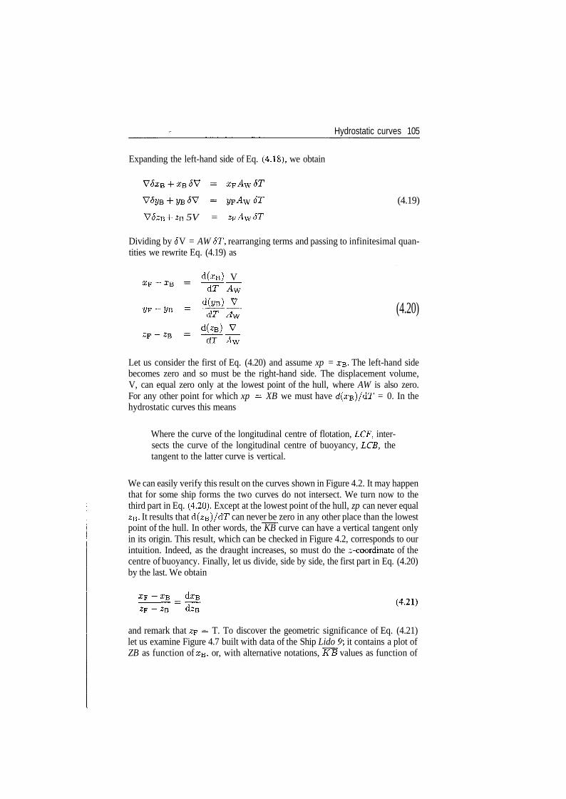
Hydrostatic curves 105
Expanding the left-hand side of Eq. (4.18), we obtain
6T (4.19)
V5zB -h zB 5V = zFAw 6T
Dividing by J V = AW ST, rearranging terms and passing to infinitesimal quan-tities we rewrite Eq. (4.19) as
d(xB) VdT Aw
«F-«B = %^ (4.20)
dT A™LL-i -Tl YY
Let us consider the first of Eq. (4.20) and assume xp = XB- The left-hand sidebecomes zero and so must be the right-hand side. The displacement volume,V, can equal zero only at the lowest point of the hull, where AW is also zero.For any other point for which xp = XB we must have d(xB)/dT = 0. In thehydrostatic curves this means
Where the curve of the longitudinal centre of flotation, LCF, inter-sects the curve of the longitudinal centre of buoyancy, LCB, thetangent to the latter curve is vertical.
We can easily verify this result on the curves shown in Figure 4.2. It may happenthat for some ship forms the two curves do not intersect. We turn now to thethird part in Eq. (4.20). Except at the lowest point of the hull, zp can never equalZB- It results that d(ze)/dT can never be zero in any other place than the lowestpoint of the hull. In other words, the KB curve can have a vertical tangent onlyin its origin. This result, which can be checked in Figure 4.2, corresponds to ourintuition. Indeed, as the draught increases, so must do the ^-coordinate of thecentre of buoyancy. Finally, let us divide, side by side, the first part in Eq. (4.20)by the last. We obtain
and remark that zp = T. To discover the geometric significance of Eq. (4.21)let us examine Figure 4.7 built with data of the Ship Lido 9\ it contains a plot ofZB as function of XB, or, with alternative notations, KB values as function of
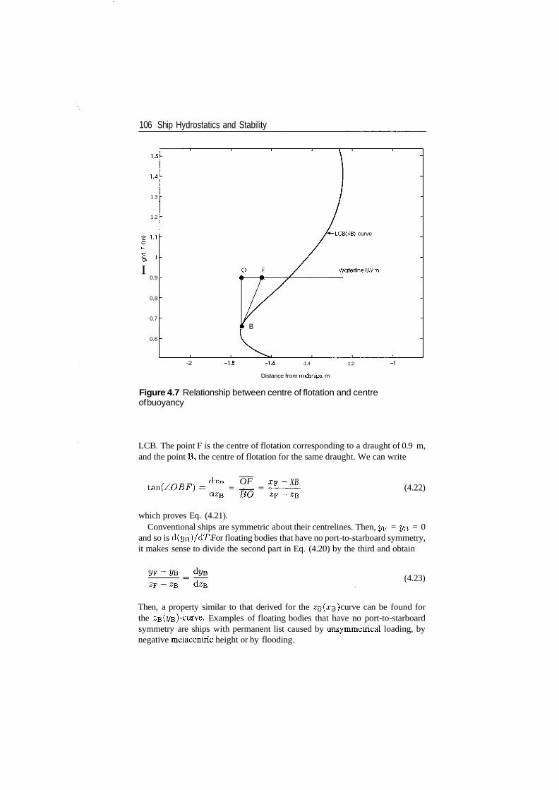
106 Ship Hydrostatics and Stability
1.5
1.3
1.2
I0.9
0,8
0.7
0.6
LCB(KB) curve
Waterline0.9m
n B
-2 -1.8 -1.6 -1.4
Distance from midships, m
-1.2
Figure 4.7 Relationship between centre of flotation and centreof buoyancy
LCB. The point F is the centre of flotation corresponding to a draught of 0.9 m,and the point B, the centre of flotation for the same draught. We can write
tan(ZOEF) = = = =OF
~BO
XB(4.22)
which proves Eq. (4.21).Conventional ships are symmetric about their centrelines. Then, yF = 2/s = 0
and so is d(y&)/dT. For floating bodies that have no port-to-starboard symmetry,it makes sense to divide the second part in Eq. (4.20) by the third and obtain
(4.23)
Then, a property similar to that derived for the ZB(XB) -curve can be found forthe 23(ye)-curve. Examples of floating bodies that have no port-to-starboardsymmetry are ships with permanent list caused by unsymmetrical loading, bynegative metacentric height or by flooding.
Hydrostatic curves 107
4.6 Hydrostatic properties of affine hulls
One way of obtaining new ship lines is to derive them by a transformation, ormapping, of some suitable, given lines. The simplest transformation is that inwhich all dimensions parallel to one of the coordinate axes are multiplied by thesame scale factor. Thus, let all dimensions parallel to the x-axis be multiplied byrx, all dimensions parallel to the y-axis be multiplied by ry, and those parallelto the z-axis, by rz. We say then that we obtain a hull affine to the parent hull,or that we obtain the new hull forms by an affine transformation. In fact, thetransformations we are talking about are a subset of what is known in geometryas affine mappings, more specifically scaling.
The case rx = ry = rz = r is particularly important; it yields a hull that isgeometrically similar to the parent hull. For example, the lines of a ship andthose of her model used in basin tests are.geometrically similar. The results ofbasin tests can be extrapolated to the actual ship size by the laws of dimensionalanalysis. When designing a new ship with the hull geometrically similar to thatof a successful ship one spares the costs of basin tests.
Modern computer programmes for hydrostatic calculations can find theproperties of affine hulls by changing only the scale factors, rx, ry, rz, andnot all the input, that is the offsets. However, it is possible to derive thehydrostatic properties of affine hulls by simple explicit expressions based ongeometric considerations. This possibility is important because it permits astraightforward calculation of the scale factors that would yield the desired prop-erties. In this section, we are going to show with a few examples how to proceed.The reader may continue by solving the exercises proposed at the end of thechapter.
Let us begin by calculating the displacement volume, Vi, of a new hull affineto a parent hull having the displacement volume
V0 = / / / dxdydz (4.24)j j j
The dimensions of the new hull change as x\ = rxx, yi = ryy, z\ — rzz sothat the new displacement volume is
Vi = / / / dxi dyi dzi = I I I rx dx • ry dy - rz dz — rxryrz VQ
(4.25)
For geometrically similar hulls, we obtain Vi = r3 VQ.With a similar reasoning, we can find that for scale factors rx, ry, rz, the
new longitudinal centre of buoyancy is LCBi — rxLCB$, the new longitudinalcentre of flotation is LCF\ = rxLCFo, and the new vertical centre of buoyancy,~KB[ = TZ~KB^.
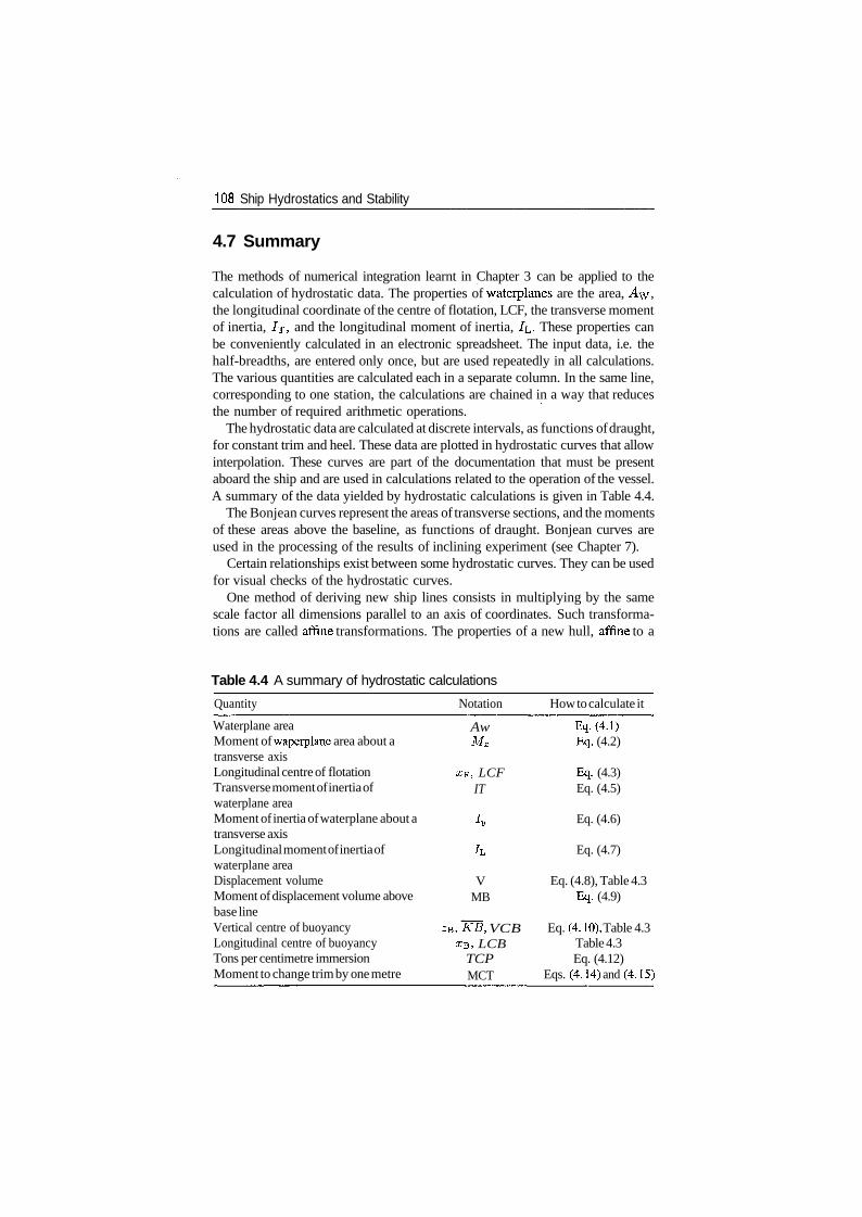
108 Ship Hydrostatics and Stability
4.7 Summary
The methods of numerical integration learnt in Chapter 3 can be applied to thecalculation of hydrostatic data. The properties of waterplanes are the area, AW ,the longitudinal coordinate of the centre of flotation, LCF, the transverse momentof inertia, 7T, and the longitudinal moment of inertia, /L. These properties canbe conveniently calculated in an electronic spreadsheet. The input data, i.e. thehalf-breadths, are entered only once, but are used repeatedly in all calculations.The various quantities are calculated each in a separate column. In the same line,corresponding to one station, the calculations are chained in a way that reducesthe number of required arithmetic operations.
The hydrostatic data are calculated at discrete intervals, as functions of draught,for constant trim and heel. These data are plotted in hydrostatic curves that allowinterpolation. These curves are part of the documentation that must be presentaboard the ship and are used in calculations related to the operation of the vessel.A summary of the data yielded by hydrostatic calculations is given in Table 4.4.
The Bonjean curves represent the areas of transverse sections, and the momentsof these areas above the baseline, as functions of draught. Bonjean curves areused in the processing of the results of inclining experiment (see Chapter 7).
Certain relationships exist between some hydrostatic curves. They can be usedfor visual checks of the hydrostatic curves.
One method of deriving new ship lines consists in multiplying by the samescale factor all dimensions parallel to an axis of coordinates. Such transforma-tions are called affine transformations. The properties of a new hull, affine to a
Table 4.4 A summary of hydrostatic calculations
Quantity
Waterplane areaMoment of waperplane area about atransverse axisLongitudinal centre of flotationTransverse moment of inertia ofwaterplane areaMoment of inertia of waterplane about atransverse axisLongitudinal moment of inertia ofwaterplane areaDisplacement volumeMoment of displacement volume abovebase lineVertical centre of buoyancyLongitudinal centre of buoyancyTons per centimetre immersionMoment to change trim by one metre
Notation
AwMx
xp, LCFIT
ty
IL
VMB
zB,#£, VCBxB, LCB
TCPMCT
How to calculate it
Eq.(4.1)Eq. (4.2)
Eq. (4.3)Eq. (4.5)
Eq. (4.6)
Eq. (4.7)
Eq. (4.8), Table 4.3Eq. (4.9)
Eq. (4. 10), Table 4.3Table 4.3Eq. (4.12)
Eqs. (4. 14) and (4. 15)
Hydrostatic curves 109
parent hull, can be derived from the properties of the parent hull by simple alge-braic expressions. An important case of affine transformation is that in whichthe three scale factors are equal. Two hulls related in this way are geometricallysimilar. Affine transformations do not change the coefficients of form.
4.8 Example
Example 4.1 - the displacement of geometrically similar hullsLet us assume, for example, that we derive a geometrically similar hull byincreasing the linear dimensions with the scale factor 10%. The displacementvolume increases by the factor l.l3 = 1.331. For a quick estimate, let us write
Vi - r3V0 (4.26)
Taking natural logarithms of both sides yields
In Vi = 3 In r + In V0 (4.27)
We differentiate both sides considering VQ constant and obtain
—- = 3— (4.28)Vi r
We have now a rule for simple and quick approximation: the percent change ofthe displacement volume equals three times the percent ratio change.
4.9 Exercises
Exercise 4.1Modify Table 4.1 for a coordinate origin in AP and repeat the calculation. Checkthe results with those shown in the original table.
Exercise 4.2Modify Table 4.1 for use with Simpson's rule and repeat the calculations.
Exercise 4.3Verify the values of MCT in Table 4.2, for the draughts 1.8 and 2.1 m, using thedisplacement-volume, KB and KMi, values shown there.
Exercise 4.4Modify Table 4.3 for a coordinate origin in AP and repeat the calculation. Checkthe results with those shown in the original table.
Exercise 4.5Modify Table 4.3 for use with Simpson's rule and repeat the calculations.

110 Ship Hydrostatics and Stability
Exercise 4.6Using the data of Ship Lido 9 plot a figure in which you can verify the propertydescribed by Eq. (4.21) for the draught values 1.7, 1.9 and 2.1 m.
Exercise 4.7Show that affine transformations leave the coefficients of form unchanged. Inmathematical terminology, the coefficients of form are invariants of affinetransformations.
Exercise 4.8Show that for affine hulls, the metacentric radius, BM, behaves like B2/T.
Statical stability at largeangles of heel
5.1 Introduction
Chapter 4 dealt with hull properties calculated as functions of draught, at constanttrim and heel. We reminded then that the maritime terminologies of Romancelanguages have a concise term for the set of submerged hulls characterized asabove. Thus, for example, the term in French is carenes isoclines. The firstpart of the term, 'iso', derives from the Greek 'isos' and means 'equal'. Themeaning of the term 'isocline' is 'equal inclination' (see Figure 4.6 in Chapter 4).In this chapter, we are going to discuss the properties of submerged hulls asfunctions of heel, at constant displacement volume. Again, Romance languageshave a concise term for the set of submerged hulls of a given vessel, havingthe same displacement volume. For example, the French term is isocarenes,while the Italian term is isocarene. The assumption of constant displacementvolume recognizes the fact that while a ship heels and rolls, her weight remainsconstant. By virtue of Archimedes' principle, constant weight implies constantdisplacement volume.
The central notion in this chapter is the righting arm. We shall show howto calculate and represent the righting arm in a set of curves known as cross-curves of stability. Another topic is the plot of the righting arm as function ofthe heel angle, for a given displacement volume and a given height of the centreof gravity. This plot is called curve of statical stability and it is used to assessthe ship stability.
5.2 The righting arm
In Figure 5.1, we consider a ship whose waterline in upright condition isThe corresponding centre of buoyancy is BQ and the centre of gravity G. Letus assume that the ship heels to starboard by an angle </>. The new waterline isW^L^ and the centre of buoyancy moves towards the submerged side, to the newposition B<j>. The weight force, equal to A, passes through G and is vertical, thatis perpendicular to W^L^. The buoyancy force, also equal to A, passes through
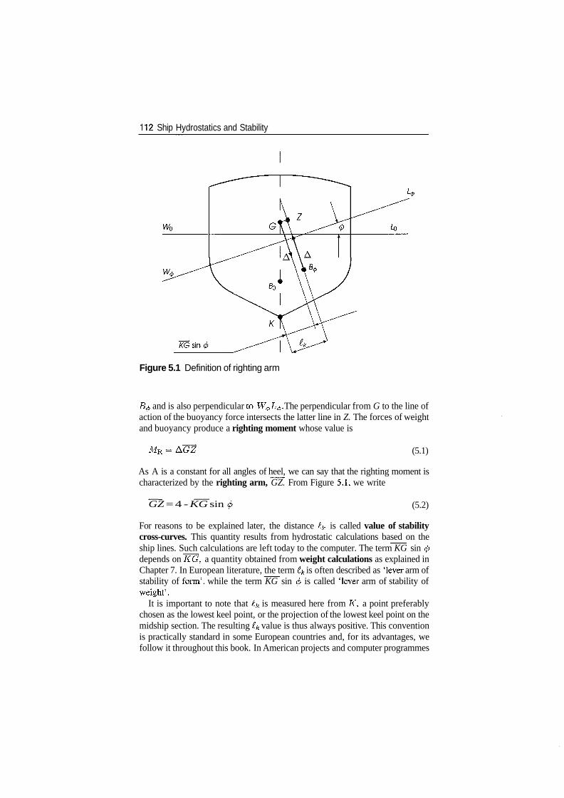
112 Ship Hydrostatics and Stability
Figure 5.1 Definition of righting arm
B^ and is also perpendicular to W^L^. The perpendicular from G to the line ofaction of the buoyancy force intersects the latter line in Z. The forces of weightand buoyancy produce a righting moment whose value is
MR - (5.1)
As A is a constant for all angles of heel, we can say that the righting moment ischaracterized by the righting arm, GZ. From Figure 5.1, we write
GZ = 4 - KG sin (5.2)
For reasons to be explained later, the distance 4 is called value of stabilitycross-curves. This quantity results from hydrostatic calculations based on theship lines. Such calculations are left today to the computer. The term KG sin <pdepends on KG, a quantity obtained from weight calculations as explained inChapter 7. In European literature, the term i^ is often described as 'lever arm ofstability of form', while the term KG sin 0 is called 'lever arm of stability ofweight'.
It is important to note that i^ is measured here from K, a point preferablychosen as the lowest keel point, or the projection of the lowest keel point on themidship section. The resulting Ik value is thus always positive. This conventionis practically standard in some European countries and, for its advantages, wefollow it throughout this book. In American projects and computer programmes
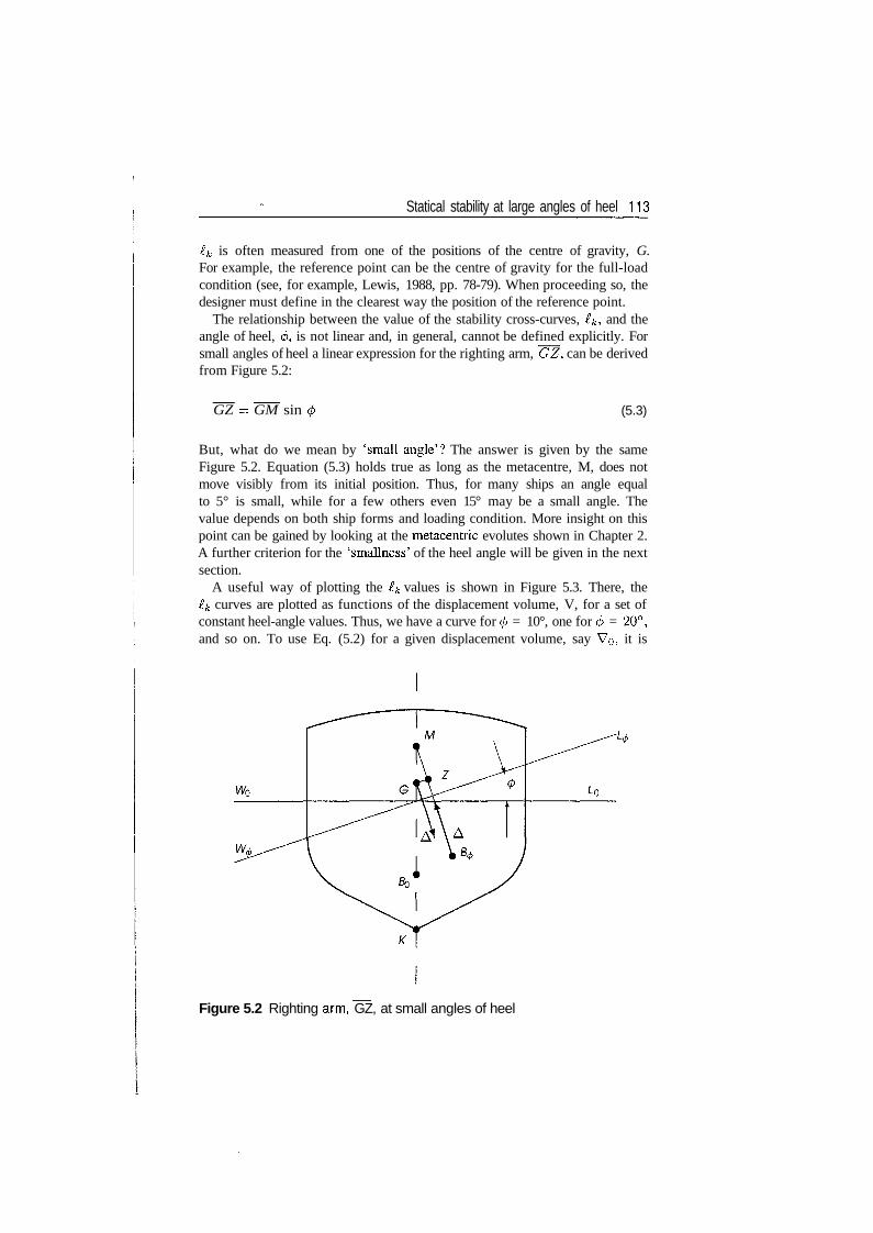
Statical stability at large angles of heel 113
ik is often measured from one of the positions of the centre of gravity, G.For example, the reference point can be the centre of gravity for the full-loadcondition (see, for example, Lewis, 1988, pp. 78-79). When proceeding so, thedesigner must define in the clearest way the position of the reference point.
The relationship between the value of the stability cross-curves, £k, and theangle of heel, 0, is not linear and, in general, cannot be defined explicitly. Forsmall angles of heel a linear expression for the righting arm, GZ, can be derivedfrom Figure 5.2:
GZ = GM sin (5.3)
But, what do we mean by 'small angle'? The answer is given by the sameFigure 5.2. Equation (5.3) holds true as long as the metacentre, M, does notmove visibly from its initial position. Thus, for many ships an angle equalto 5° is small, while for a few others even 15° may be a small angle. Thevalue depends on both ship forms and loading condition. More insight on thispoint can be gained by looking at the metacentric evolutes shown in Chapter 2.A further criterion for the 'smallness' of the heel angle will be given in the nextsection.
A useful way of plotting the lf~ values is shown in Figure 5.3. There, the£k curves are plotted as functions of the displacement volume, V, for a set ofconstant heel-angle values. Thus, we have a curve for </> = 10°, one for <p = 20°,and so on. To use Eq. (5.2) for a given displacement volume, say VQ, it is
Figure 5.2 Righting arm, GZ, at small angles of heel
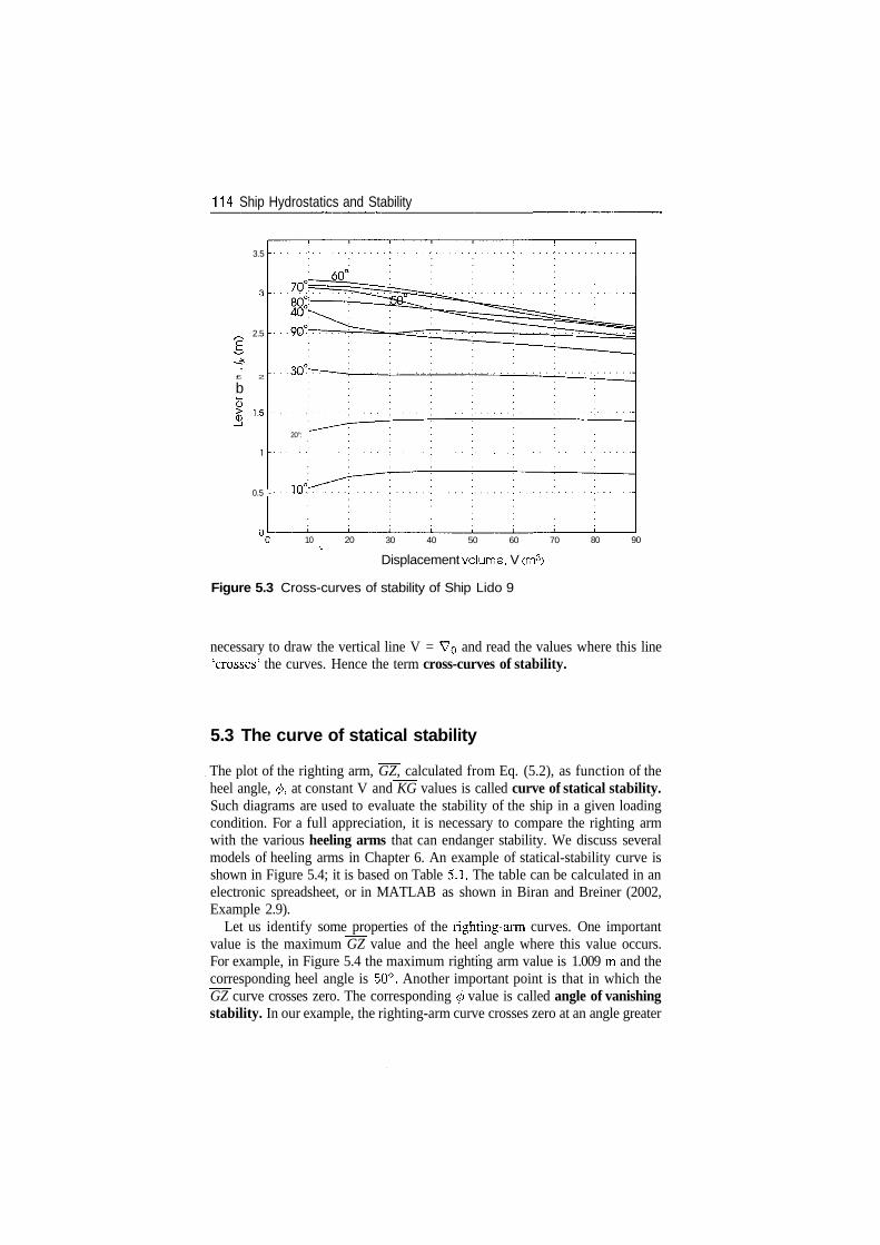
114 Ship Hydrostatics and Stability
3.5
2.5
£ 2
bCD
0.5 -
20°:
10 20 30 40 50 60 70•\.
Displacement volume, V an3)
Figure 5.3 Cross-curves of stability of Ship Lido 9
80 90
necessary to draw the vertical line V = VQ and read the values where this line'crosses' the curves. Hence the term cross-curves of stability.
5.3 The curve of statical stability
The plot of the righting arm, GZ, calculated from Eq. (5.2), as function of theheel angle, 0, at constant V and KG values is called curve of statical stability.Such diagrams are used to evaluate the stability of the ship in a given loadingcondition. For a full appreciation, it is necessary to compare the righting armwith the various heeling arms that can endanger stability. We discuss severalmodels of heeling arms in Chapter 6. An example of statical-stability curve isshown in Figure 5.4; it is based on Table 5.1. The table can be calculated in anelectronic spreadsheet, or in MATLAB as shown in Biran and Breiner (2002,Example 2.9).
Let us identify some properties of the righting-arm curves. One importantvalue is the maximum GZ value and the heel angle where this value occurs.For example, in Figure 5.4 the maximum righting arm value is 1.009 m and thecorresponding heel angle is 50°. Another important point is that in which theGZ curve crosses zero. The corresponding <p value is called angle of vanishingstability. In our example, the righting-arm curve crosses zero at an angle greater
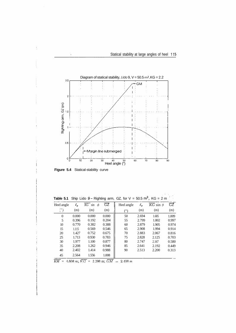
Statical stability at large angles of heel 115
Diagram of statical stability, Lido 9, V = 50.5 nrA KG = 2.2
20 30 40 50Heel angle (°)
60
Figure 5.4 Statical-stability curve
70 80 90
Table 5.1 Ship Lido 9- Righting arm, GZ, for V = 50.5 m3, KG = 2 m
Heel angle
n05
10152025303540
45
lp
(m)
0.0000.3960.7701.1151.4271.7131.9772.2082.402
2.564
KG sin '<t>
(m)
0.0000.1920.3820.5690.7520.9301.1001.2621.414
1.556
GZ(m)
0.0000.2040.3880.5460.6750.7830.8770.9460.988
1.008
Heel angle
(°)
505560657075808590
ZP(m)
2.6942.7992.8792.9082.8832.8282.7472.6412.513
KG sin 0
(m)
1.6851.8021.9051.9942.0672.1252.1672.1922.200
GZ(m)
1.0090.9970.9740.9140.8160.7030.5800.4490.313
KM = 4.608 m\KG = 2.200 m; GM - 2.408m
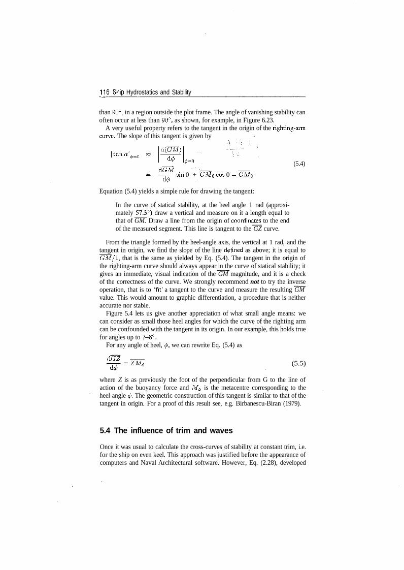
116 S-hip Hydrostatics and Stability
than 90°, in a region outside the plot frame. The angle of vanishing stability canoften occur at less than 90°, as shown, for example, in Figure 6.23.
A very useful property refers to the tangent in the origin of the righting-armcurve. The slope of this tangent is given by
d(GM)|tana|^=0
(5.4)dGM
, , sin 0 + GM0 cos 0 = GM0d(p
Equation (5.4) yields a simple rule for drawing the tangent:
In the curve of statical stability, at the heel angle 1 rad (approxi-mately ̂ 73°) draw a vertical and measure on it a length equal tothat of GM. Draw a line from the origin of coordinates to the endof the measured segment. This line is tangent to the GZ curve.
From the triangle formed by the heel-angle axis, the vertical at 1 rad, and thetangent in origin, we find the slope of the line denned as above; it is equal toGM/1, that is the same as yielded by Eq. (5.4). The tangent in the origin ofthe righting-arm curve should always appear in the curve of statical stability; itgives an immediate, visual indication of the GM magnitude, and it is a checkof the correctness of the curve. We strongly recommend not to try the inverseoperation, that is to 'fit' a tangent to the curve and measure the resulting GMvalue. This would amount to graphic differentiation, a procedure that is neitheraccurate nor stable.
Figure 5.4 lets us give another appreciation of what small angle means: wecan consider as small those heel angles for which the curve of the righting armcan be confounded with the tangent in its origin. In our example, this holds truefor angles up to 7-8°.
For any angle of heel, </>, we can rewrite Eq. (5.4) as
dGZZM^ (5.5)
where Z is as previously the foot of the perpendicular from G to the line ofaction of the buoyancy force and M0 is the metacentre corresponding to theheel angle </>. The geometric construction of this tangent is similar to that of thetangent in origin. For a proof of this result see, e.g. Birbanescu-Biran (1979).
5.4 The influence of trim and waves
Once it was usual to calculate the cross-curves of stability at constant trim, i.e.for the ship on even keel. This approach was justified before the appearance ofcomputers and Naval Architectural software. However, Eq. (2.28), developed

Statical stability at large angles of heel 117
in Chapter 2, shows that the longitudinal position of the centre of buoyancychanges if the heel angle is large. It happens so because at large heel anglesthe waterplane area ceases to be symmetric about the centreline. If the centreof buoyancy moves along the ship, while the position of the centre of gravityis constant, the trim changes too. Therefore, cross-curves calculated at constanttrim may not represent actual stability condition. Jakic (1980) has shown thattrim can greatly influence the values of cross-curves and, therefore, that influenceshould be taken into account. The stability regulations, BV 1033, of the GermanNavy require, indeed, the calculation of the cross-curves at the trim induced byheel. Modern computer programmes for Naval Architecture include this option.
As we shall show in Chapter 9, waves perpendicular or oblique to the shipvelocity influence the values of cross-curves and can cause a very dangerouseffect called parametric resonance. This effect too must be taken into accountand modern computer programmes can calculate cross-curves on waves. Thestability regulations of the German Navy take into account the variation of therighting arm in waves (see Arndt, 1965; Arndt, Brandl, and Vogt, 1982).
5.5 Summary
In this chapter, we dealt with the righting moment at large angles of heel, MR =A(7Z. The quantity GZ, called righting arm, is the length of the perpendiculardrawn from the centre of gravity, G, to the line of action of the buoyancy force. Weassume that the ship heels at constant displacement. This is the desired situationin which the ship neither loses loads nor takes water aboard. Then, the factor Ais constant and the variation of the righting moment with heel is described bythe variation of the righting arm GZ. The value of the righting arm is calculatedfrom
~GZ = 4 - ~KG sin <j>
where £&, called value of stability cross-curve, is the distance from the referencepoint K to the line of action of the buoyancy force, KG, the distance of the centreof gravity from the same point K, and 0, the heel angle. It is recommended totake the point K as the lowest hull point. The values of the stability cross-curves,Ik, are usually represented as functions of the displacement volume, with theheel angle as parameter.
One can read in this plot the values corresponding to a given displacementvolume, calculate with them the righting arm and plot its values against the heelangle. This plot is called curve of statical stability and it is used to appreciate thestability of the ship, at a given displacement and height of the centre of gravity.To check the correctness of the righting-arm curve, it is recommended to drawthe tangent in the origin. To do this, one should draw a vertical line at the angle
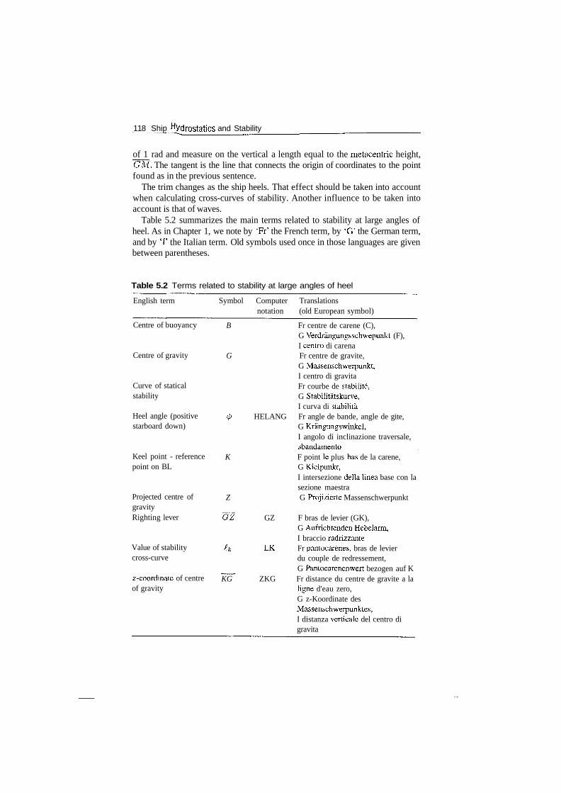
118 Ship Hydrostatics and Stability
of 1 rad and measure on the vertical a length equal to the metacentric height,GM. The tangent is the line that connects the origin of coordinates to the pointfound as in the previous sentence.
The trim changes as the ship heels. That effect should be taken into accountwhen calculating cross-curves of stability. Another influence to be taken intoaccount is that of waves.
Table 5.2 summarizes the main terms related to stability at large angles ofheel. As in Chapter 1, we note by 'Fr' the French term, by 'G' the German term,and by T the Italian term. Old symbols used once in those languages are givenbetween parentheses.
Table 5.2 Terms related to stability at large angles of heel
English term Symbol Computer Translationsnotation (old European symbol)
Centre of buoyancy
Centre of gravity
Curve of staticalstability
Heel angle (positivestarboard down)
Keel point - referencepoint on BL
Projected centre ofgravityRighting lever
Value of stabilitycross-curve
z-coordinate of centreof gravity
B Fr centre de carene (C),G Verdrangungsschwepunkt (F),I centre di carena
G Fr centre de gravite,G Massenschwerpunkt,I centro di gravitaFr courbe de stabilite,G Stabilitatskurve,I curva di stabilita
4> HELANG Fr angle de bande, angle de gite,G Krangungswinkel,I angolo di inclinazione traversale,sbandamento
K F point le plus has de la carene,G Kielpunkt,I intersezione della linea base con lasezione maestra
Z G Projizierte Massenschwerpunkt
~GZ GZ F bras de levier (GK),G Aufrichtenden Hebelarm,I braccio radrizzante
Ik LK Fr pantocarenes, bras de levierdu couple de redressement,G Pantocarenenwert bezogen auf K
KG ZKG Fr distance du centre de gravite a laligne d'eau zero,G z-Koordinate desMassenschwerpunktes,I distanza verticale del centro digravita
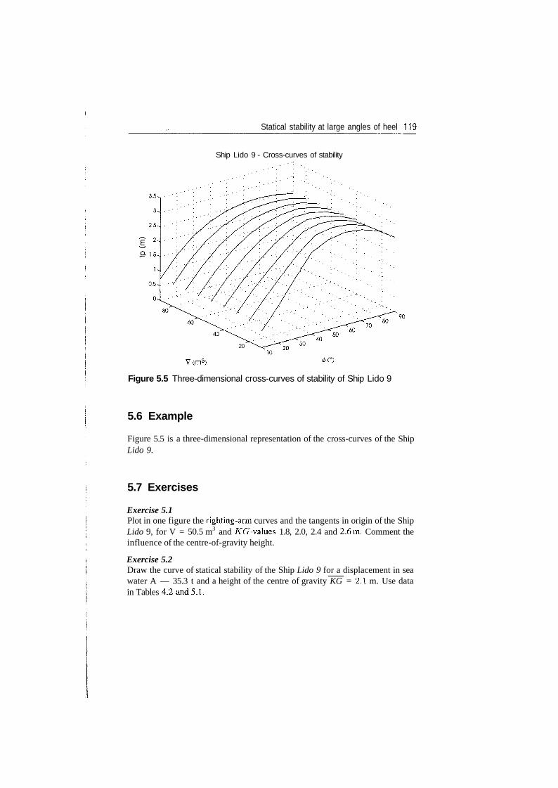
Statical stability at large angles of heel 119
Ship Lido 9 - Cross-curves of stability
20
V(m3)
Figure 5.5 Three-dimensional cross-curves of stability of Ship Lido 9
5.6 Example
Figure 5.5 is a three-dimensional representation of the cross-curves of the ShipLido 9.
5.7 Exercises
Exercise 5.1Plot in one figure the righting-arm curves and the tangents in origin of the ShipLido 9, for V = 50.5 m3 and KG-values 1.8, 2.0, 2.4 and 2.6m. Comment theinfluence of the centre-of-gravity height.
Exercise 5.2Draw the curve of statical stability of the Ship Lido 9 for a displacement in seawater A — 35.3 t and a height of the centre of gravity KG = 2.1 m. Use datain Tables 4.2 and 5.1.
6Simple models of stability
6.1 Introduction
In Chapter 5 we learnt how to calculate and how to plot the righting arm in thecurve of statical stability. It may be surprising that for a very long period themetacentric height and the curve of righting arms were considered sufficient forappreciating the ship stability. We do not proceed so in other engineering fields.As pointed out by Wendel (1965), one first finds out the resistance to ship advanceand only afterwards dimensions the engine. Also, we first calculate the load ona beam and only afterwards we dimension it. Similarly, we should determinethe heeling moments and then compare them with the righting moment. It wasonly at the beginning of the twentieth century that Middendorf proposed such aprocedure for large sailing ships. His book, Bemastung und Takelung der Schiffe,was first published in Berlin, in 1903, and it contained the first proposal for aship-stability criterion. In 1933, Pierrottet wrote in a publication of the testbasin in Rome that the stability of a ship must be assessed by comparing theheeling moments with the righting moment. He detailed his proposal in 1935,in a meeting of INA, but had no immediate followers. Thus, in 1939 Raholapublished in Helsinki his doctoral thesis; it was based on extensive statisticsand a very profound analysis of the qualities of stable and unstable vessels.Rahola proposed then a stability criterion that considered only the metacentricheight and the curve of the righting arm. The Naval-Architectural communityappreciated Rahola's work and his proposal was used, indeed, as a stabilitystandard and stood at the basis of stability regulations issued later by nationaland international authorities.
It was only after the Second World War that the issue of comparing heelingand righting arms was brought up again. German researchers used then a veryappropriate term: Lever arm balance (Hebelarm Bilanz). Eventually, newer sta-bility regulations made compulsory the comparison of lever arms and we showin this chapter how to do it.
Heeling moments can be caused by wind, by the centrifugal force developedin turning, by transverse displacements of masses, by towing or by the lateral pulldeveloped in cables that connect two vessels during the transfer of loads at sea.In Chapter 5 we have shown that, when the ship heels at constant displacement,it is sufficient to consider the righting arm as an indicator of stability. Then, toassess the ship stability it is necessary to compare the righting arm with a heeling
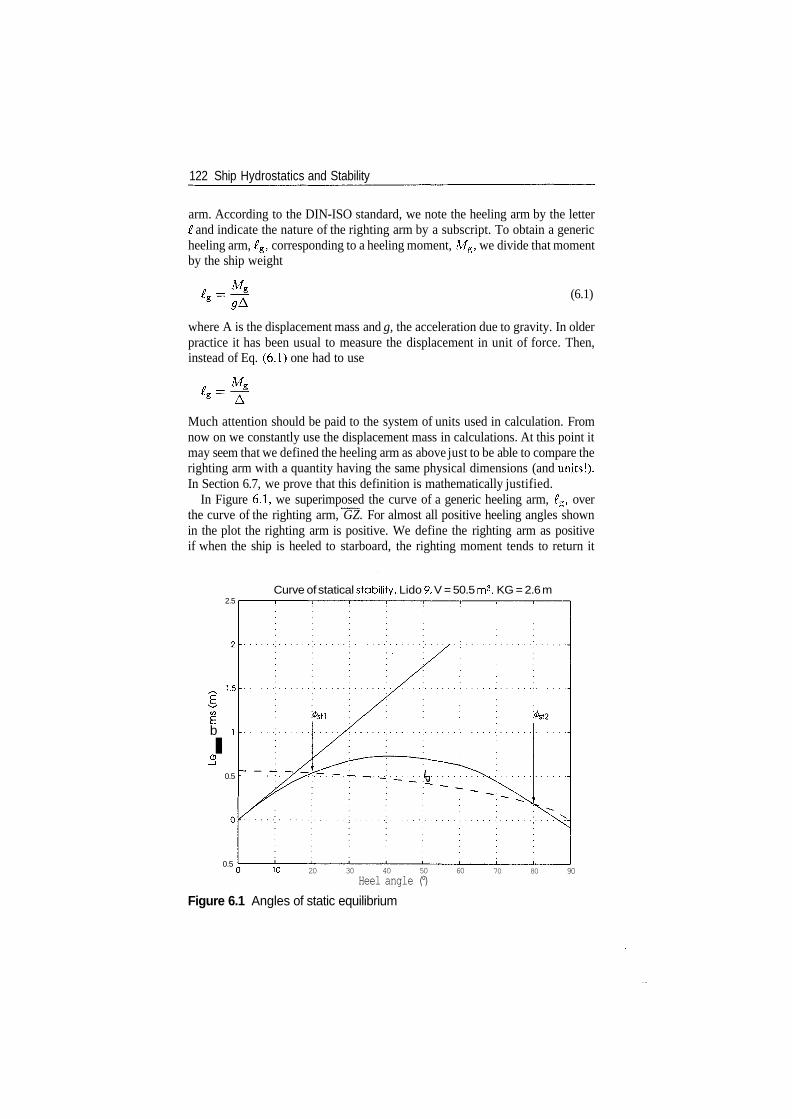
122 Ship Hydrostatics and Stability
arm. According to the DIN-ISO standard, we note the heeling arm by the letterI and indicate the nature of the righting arm by a subscript. To obtain a genericheeling arm, £g, corresponding to a heeling moment, Mg, we divide that momentby the ship weight
(6.1)
where A is the displacement mass and g, the acceleration due to gravity. In olderpractice it has been usual to measure the displacement in unit of force. Then,instead of Eq. (6.1) one had to use
Much attention should be paid to the system of units used in calculation. Fromnow on we constantly use the displacement mass in calculations. At this point itmay seem that we defined the heeling arm as above just to be able to compare therighting arm with a quantity having the same physical dimensions (and units!).In Section 6.7, we prove that this definition is mathematically justified.
In Figure 6.1, we superimposed the curve of a generic heeling arm, £g, overthe curve of the righting arm, GZ. For almost all positive heeling angles shownin the plot the righting arm is positive. We define the righting arm as positiveif when the ship is heeled to starboard, the righting moment tends to return it
2.5
1,5
bICD
0.5
0.5
Curve of statical stability, Lido 9, V = 50.5 m3, KG = 2.6 m
10 20 30 40 50 60Heel angle (°)
70 80 90
Figure 6.1 Angles of static equilibrium
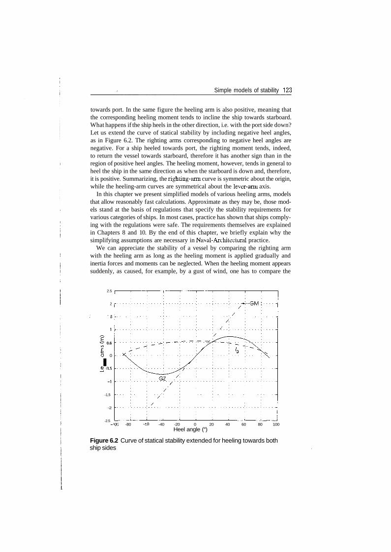
Simple models of stability 123
towards port. In the same figure the heeling arm is also positive, meaning thatthe corresponding heeling moment tends to incline the ship towards starboard.What happens if the ship heels in the other direction, i.e. with the port side down?Let us extend the curve of statical stability by including negative heel angles,as in Figure 6.2. The righting arms corresponding to negative heel angles arenegative. For a ship heeled towards port, the righting moment tends, indeed,to return the vessel towards starboard, therefore it has another sign than in theregion of positive heel angles. The heeling moment, however, tends in general toheel the ship in the same direction as when the starboard is down and, therefore,it is positive. Summarizing, the righting-arm curve is symmetric about the origin,while the heeling-arm curves are symmetrical about the lever-arm axis.
In this chapter we present simplified models of various heeling arms, modelsthat allow reasonably fast calculations. Approximate as they may be, those mod-els stand at the basis of regulations that specify the stability requirements forvarious categories of ships. In most cases, practice has shown that ships comply-ing with the regulations were safe. The requirements themselves are explainedin Chapters 8 and 10. By the end of this chapter, we briefly explain why thesimplifying assumptions are necessary in Naval-Architectural practice.
We can appreciate the stability of a vessel by comparing the righting armwith the heeling arm as long as the heeling moment is applied gradually andinertia forces and moments can be neglected. When the heeling moment appearssuddenly, as caused, for example, by a gust of wind, one has to compare the
2.5
2
1.5
0.6
£O 0
ICD -0.5
-1,5
-2
-2.5
-GM :
-100 -80 -60 -40 -20 0 20 40 60 80 100Heel angle (°)
Figure 6.2 Curve of statical stability extended for heeling towards bothship sides
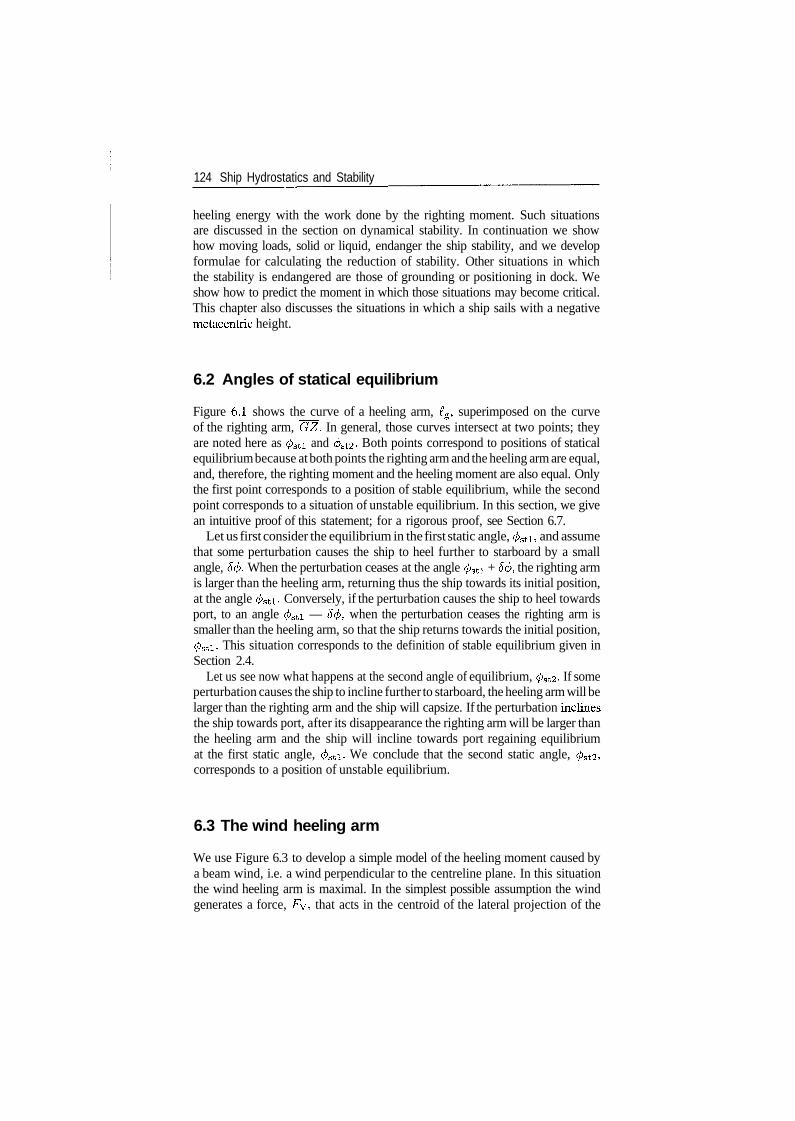
124 Ship Hydrostatics and Stability
heeling energy with the work done by the righting moment. Such situationsare discussed in the section on dynamical stability. In continuation we showhow moving loads, solid or liquid, endanger the ship stability, and we developformulae for calculating the reduction of stability. Other situations in whichthe stability is endangered are those of grounding or positioning in dock. Weshow how to predict the moment in which those situations may become critical.This chapter also discusses the situations in which a ship sails with a negativemetacentric height.
6.2 Angles of statical equilibrium
Figure 6.1 shows the curve of a heeling arm, £g, superimposed on the curveof the righting arm, GZ. In general, those curves intersect at two points; theyare noted here as </>sti and 0st2- Both points correspond to positions of staticalequilibrium because at both points the righting arm and the heeling arm are equal,and, therefore, the righting moment and the heeling moment are also equal. Onlythe first point corresponds to a position of stable equilibrium, while the secondpoint corresponds to a situation of unstable equilibrium. In this section, we givean intuitive proof of this statement; for a rigorous proof, see Section 6.7.
Let us first consider the equilibrium in the first static angle, 0sti, and assumethat some perturbation causes the ship to heel further to starboard by a smallangle, 5$. When the perturbation ceases at the angle 0stl + 8<j>, the righting armis larger than the heeling arm, returning thus the ship towards its initial position,at the angle 0sti. Conversely, if the perturbation causes the ship to heel towardsport, to an angle </>sti — 5$, when the perturbation ceases the righting arm issmaller than the heeling arm, so that the ship returns towards the initial position,0sti. This situation corresponds to the definition of stable equilibrium given inSection 2.4.
Let us see now what happens at the second angle of equilibrium, </>st2. If someperturbation causes the ship to incline further to starboard, the heeling arm will belarger than the righting arm and the ship will capsize. If the perturbation inclinesthe ship towards port, after its disappearance the righting arm will be larger thanthe heeling arm and the ship will incline towards port regaining equilibriumat the first static angle, </>sti. We conclude that the second static angle, 0st2,corresponds to a position of unstable equilibrium.
6.3 The wind heeling arm
We use Figure 6.3 to develop a simple model of the heeling moment caused bya beam wind, i.e. a wind perpendicular to the centreline plane. In this situationthe wind heeling arm is maximal. In the simplest possible assumption the windgenerates a force, Fy, that acts in the centroid of the lateral projection of the
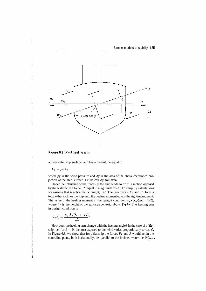
Simple models of stability 125
Figure 6.3 Wind heeling arm
above-water ship surface, and has a magnitude equal to
FV = pyAy
where py is the wind pressure and Ay is the area of the above-mentioned pro-jection of the ship surface. Let us call Ay sail area.
Under the influence of the force Fy the ship tends to drift, a motion opposedby the water with a force, R, equal in magnitude to Fy. To simplify calculationswe assume that R acts at half-draught, T/2. The two forces, Fy and R, form atorque that inclines the ship until the heeling moment equals the righting moment.The value of the heeling moment in the upright condition is pyAy(hy + T/2),where hy is the height of the sail-area centroid above W^L®. The heeling armin upright condition is
. ,ft. PvAv(hv + T/2)
How does the heeling arm change with the heeling angle? In the case of a 'flat'ship, i.e. for B = 0, the area exposed to the wind varies proportionally to cos </>.In Figure 6.3, we show that for a flat ship the forces Fy and R would act in thecentreline plane, both horizontally, i.e. parallel to the inclined waterline W^L^.
126 Ship Hydrostatics and Stability
Then, the lever arm of the torque would be proportional to cos 0. Summing up,the wind heeling arm equals
PvAv cos 6 (' T\ pvAv(hy -f T/2) 9' hv H cos 6 = —r —- cos2; ^A
(6.2)
This is the equation proposed by Middendorf and that prescribed by the stabilityregulations of the US Navy; it can be found in more than one textbook on NavalArchitecture where it is recommended for all vessels. The reader may feel somedoubts about the strong assumptions accepted above. In fact, other regulatorybodies than the US Navy adopted wind-heeling-arm curves that do not behavelike cos2 </>. The respective equations are described in Chapters 8 and 10. Ourown critique of the above model, and a justification of some of its underlyingassumptions, are presented in Section 6.12.
The wind pressure, pv» is related to the wind speed, Vw, by
Pv = CwP^w (6-3)
where cw is an aerodynamic resistance coefficient and p is the air density. Thecoefficient cw depends on the form and configuration of the sail area. An averagevalue for cw is 1.2. Wegner (1965) quotes a research that yielded 1.00 < cw <1.36, and two Japanese researchers, Kinohita and Okada, who measured cw
values ranging between 0.95 and 1 .24. Equation (6.3) shows that the wind heelingarm is proportional to the square of the wind speed. In this section, we consideredthe wind speed as constant over all the sail area. This assumption is acceptablefor a fast estimation of the wind heeling arm. However, we may know from ourown experience that wind speed increases with height above the water surface.Some stability regulations recognize this phenomenon and we show in Chapters 8and 10 how to take it into account. Calculations with variable wind speed, i.e.considering the wind gradient, yield lower, more realistic heeling arms for smallvessels whose sail area lies mainly in the low- wind-speed region. It may be worthmentioning that engineers take into account the wind gradient in the design oftall buildings and tall cranes.
6.4 Heeling arm in turning
When a ship turns with a linear speed V, in a circle of radius RTC, & centrifugalforce, FTC > develops; it acts in the centre of gravity, G, at a height KG abovethe baseline. From mechanics we know that
F2
Under the influence of the force FTC the ship tends to drift, a motion opposed bythe water with a reaction R. To simplify calculations, we assume again that the
Simple models of stability 127
water reaction acts at half-draught, i.e. at a height T/2 above the baseline. Thetwo forces, FTC and R, form a torque whose lever arm in upright condition is(KG - T/2). For a heeling, flat ship this lever arm is proportional to cos </>.Dividing by the displacement force, we obtain the heeling lever of the centri-fugal force in turning circle:
T(6.4)
9 #TC V 2
The speed V to be used in Eq. (6.4) is the speed in turning, smaller than the speedachieved when sailing on a straight line path. The turning radius, RTC> and thespeed in turning, V, are not known in the first stages of ship design. If resultsof basin tests on a ship model, or of sea trials of the ship, or of a sister ship, areavailable, they should be substituted in Eq. (6.4). The stability regulations of theGerman Navy, BV 1033, provide formulae for approximations to be used in theearly design stages of naval ships (see Chapter 10). A discussion of this subjectcan be found in Wegner (1965). This author uses a non-dimensional factor
(6.5)
where Vb is the ship speed in turning and VQ, the speed on a straight line path.Substituting into Eq. (6.4) yields
- / _ T\(KG--}cos(f> (6.6)
gLpp \ 2
Quoting Handbuch der Werften, Vol. VII, Wegner shows that for 95% of 80 cargoships the values of CD ranged between 0.19 and 0.25. For a few trawlers thevalues ranged between 0.30 and 0.35.
6.5 Other heeling arms
A dangerous situation can arise if many passengers crowd on one side of theship. There are two cases when passengers can do this: when attracted by abeautiful seascape or when scared by some dangerous event. In the latter case,passengers can also be tempted to go to upper decks. The resulting heeling armcan be calculated from
TIT)ip — — (y cos (f) -f z sin </>) (6.7)
where n is the number of passengers, p, the average person mass, y, the horizontalcoordinate of the centre of gravity of the crowd and z, the vertical translationof said centre. The second term between parentheses accounts for the virtual
128 Ship Hydrostatics and Stability
metacentric-height reduction. Wegner (1965) recommends to assume that upto seven passengers can crowd on a square metre, that the average mass of apassenger plus some luggage is 80 kg, and that the height of a passenger's centreof gravity above deck is l.lm. Smaller values are prescribed by the regulationsdescribed in Chapters 8 and 10. Wegner recommends to include in the deckarea all areas that can be occupied by panicking people, e.g. tables, benchesand skylights. Other heeling moments can occur when a tug tows a barge. Thebarge can drift and then the tension in the towing cable can be decomposed intotwo components, one parallel to the tug centreline and the other perpendicularto the first. The latter component can cause capsizing of the tug. The processis very fast and there may be no survivors. To avoid this situation tugs must beprovided with quick-release mechanisms that free instantly the towing cable.Lateral forces also appear when fishing vessels tow nets or when two vessels areconnected by cables during replenishment-at-sea operations. Special provisionsare made in stability regulations for the situations mentioned above; they arepresented in Chapters 8 and 10. Icing is a phenomenon known to ship crewssailing in very cold zones. The accumulation of ice has a double destabilizingeffect: it raises the centre of gravity and it increases the sail area. The importanceof ice formation should not be underestimated. For example, Arndt (1960a) citescases in which blocks of ice 1 m thick developed on a poop deck, or walls of 60 cmof ice formed on the front surface of a bridge. Therefore, stability regulationstake into account the effect of ice.
6.6 Dynamical stability
Until now we assumed that the heeling moments are applied gradually and thatinertial moments can be neglected. Shortly, we studied statical stability. Heelingmoments, however, can appear, or increase suddenly. For example, wind speed isusually not constant, but fluctuates. Occasionally, sudden bursts of high intensitycan occur; they are called gusts. As another example, loosing a weight on oneside of a ship can cause a sudden heeling moment that sends down the otherside. In the latter cases we are interested in dynamical stability. It is no moresufficient to compare righting with heeling arms; we must compare the energyof the heeling moment with the work done by the opposing righting moment. Itcan be easily shown that the energy of the heeling moment is proportional to thearea under the heeling-arm curve, and the work done by the righting momentis proportional to the area under the righting-arm curve. To prove this, let usremember that the work done by a force, F, which produces a motion from x\to #2 is equal to
Fdx (6.8)
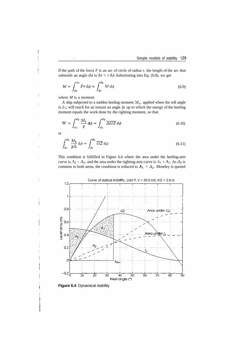
Simple models of stability 129
If the path of the force F is an arc of circle of radius r, the length of the arc thatsubtends an angle d</> is dx = r d(j>. Substituting into Eq. (6.8), we get
Wr(f>2 f4>
Mdcf) (6.9)
where M is a moment.A ship subjected to a sudden heeling moment Mh, applied when the roll angle
is 0i, will reach for an instant an angle fa up to which the energy of the heelingmoment equals the work done by the righting moment, so that
or
GZdfi
(6.10)
(6.11)
This condition is fulfilled in Figure 6.4 where the area under the heeling-armcurve is A2 + AS, and the area under the righting-arm curve is A\ + A%. As A3 iscommon to both areas, the condition is reduced to A\ = A%. Moseley is quoted
Curve of statical stability, Lido 9, V = 50.5 m3, KG = 2.6 m
•GZ • • . • • • • ; Area under GZ
0 10 20 30 40 50 60 70 80 90
Figure 6.4 Dynamical stability
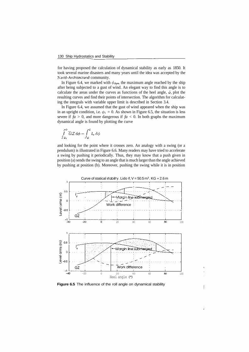
130 Ship Hydrostatics and Stability
for having proposed the calculation of dynamical stability as early as 1850. Ittook several marine disasters and many years until the idea was accepted by theNaval-Architectural community.
In Figure 6.4, we marked with </>dyn the maximum angle reached by the shipafter being subjected to a gust of wind. An elegant way to find this angle is tocalculate the areas under the curves as functions of the heel angle, </>, plot theresulting curves and find their points of intersection. The algorithm for calculat-ing the integrals with variable upper limit is described in Section 3.4.
In Figure 6.4, we assumed that the gust of wind appeared when the ship wasin an upright condition, i.e. </>i = 0. As shown in Figure 6.5, the situation is lesssevere if fa > 0, and more dangerous if fa < 0. In both graphs the maximumdynamical angle is found by plotting the curve
/*<£ _ r4>\ GZdfi- \
J 4>i J 4>id(f)
and looking for the point where it crosses zero. An analogy with a swing (or apendulum) is illustrated in Figure 6.6. Many readers may have tried to acceleratea swing by pushing it periodically. Thus, they may know that a push given inposition (a) sends the swing to an angle that is much larger than the angle achievedby pushing at position (b). Moreover, pushing the swing while it is in position
0.5
D
<D
Curve of statical stability, Lido 9, V = 50.5 m3, KG = 2.6 m
h—Margin linjscfl
Work difference :
-40 -20 20 40 60 100
-20 0 20 40
Heel angle (°)60 100
Figure 6.5 The influence of the roll angle on dynamical stability
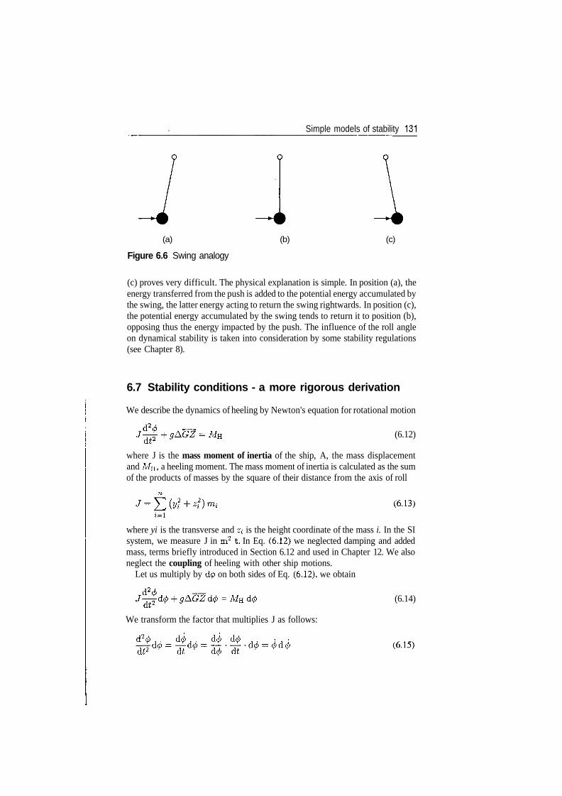
Simple models of stability 131
(a) (b) (c)
Figure 6.6 Swing analogy
(c) proves very difficult. The physical explanation is simple. In position (a), theenergy transferred from the push is added to the potential energy accumulated bythe swing, the latter energy acting to return the swing rightwards. In position (c),the potential energy accumulated by the swing tends to return it to position (b),opposing thus the energy impacted by the push. The influence of the roll angleon dynamical stability is taken into consideration by some stability regulations(see Chapter 8).
6.7 Stability conditions - a more rigorous derivation
We describe the dynamics of heeling by Newton's equation for rotational motion
MH (6.12)
where J is the mass moment of inertia of the ship, A, the mass displacementand MH, a heeling moment. The mass moment of inertia is calculated as the sumof the products of masses by the square of their distance from the axis of roll
where yi is the transverse and zi is the height coordinate of the mass i. In the SIsystem, we measure J in m2 1. In Eq. (6.12) we neglected damping and addedmass, terms briefly introduced in Section 6.12 and used in Chapter 12. We alsoneglect the coupling of heeling with other ship motions.
Let us multiply by d0 on both sides of Eq. (6.12), we obtain
= MH d<£ (6.14)
We transform the factor that multiplies J as follows:
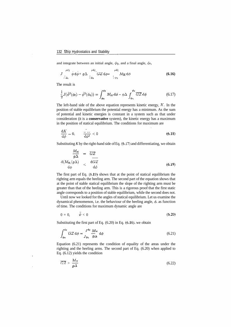
132 Ship Hydrostatics and Stability
and integrate between an initial angle, 0o, and a final angle, </>f,
/*0f r4>f _ r4>fJ <j)d<j) + gA GZd(f) = MHd</> (6.16)
J (f)Q J (/)Q J (f)Q
The result is
!- </A fJ 4>o
(6.17)
The left-hand side of the above equation represents kinetic energy, K. In theposition of stable equilibrium the potential energy has a minimum. As the sumof potential and kinetic energies is constant in a system such as that underconsideration (it is a conservative system), the kinetic energy has a maximumin the position of statical equilibrium. The conditions for maximum are
£-* w<»Substituting K by the right-hand side of Eq. (6.17) and differentiating, we obtain
_d(MH/gA) < dGZ
d(f) d(/)
The first part of Eq. (6.19) shows that at the point of statical equilibrium therighting arm equals the heeling arm. The second part of the equation shows thatat the point of stable statical equilibrium the slope of the righting arm must begreater than that of the heeling arm. This is a rigorous proof that the first staticangle corresponds to a position of stable equilibrium, while the second does not.
Until now we looked for the angles of statical equilibrium. Let us examine thedynamical phenomenon, i.e. the behaviour of the heeling angle, 0, as functionof time. The conditions for maximum dynamic angle are
0 = 0, <j> < 0 (6-20)
Substituting the first part of Eq. (6.20) in Eq. (6.16), we obtain
_GZd(f>= — d0 (6.21)
Equation (6.21) represents the condition of equality of the areas under therighting and the heeling arms. The second part of Eq. (6.20) when applied toEq. (6.12) yields the condition
~GZ > ̂ (6.22)
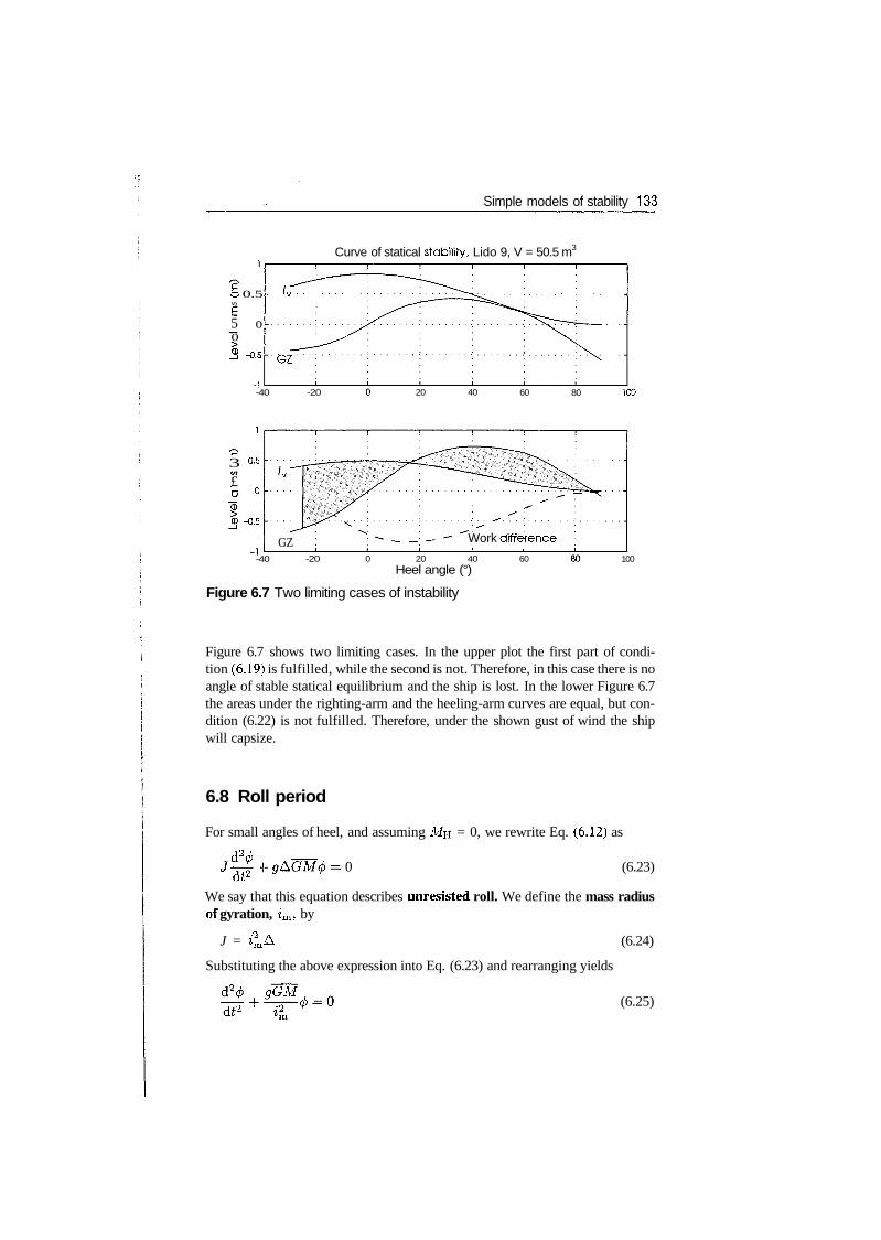
Simple models of stability 133
3 0.5V)
5 o0
5 -0.5 'GZ
-40
Curve of statical stability, Lido 9, V = 50.5 m3
-20 20 40 60 80 100
3 a5
£o o
o -0.5
GZ-40 -20
Work difference
0 20 40Heel angle (°)
60 100
Figure 6.7 Two limiting cases of instability
Figure 6.7 shows two limiting cases. In the upper plot the first part of condi-tion (6.19) is fulfilled, while the second is not. Therefore, in this case there is noangle of stable statical equilibrium and the ship is lost. In the lower Figure 6.7the areas under the righting-arm and the heeling-arm curves are equal, but con-dition (6.22) is not fulfilled. Therefore, under the shown gust of wind the shipwill capsize.
6.8 Roll period
For small angles of heel, and assuming MH = 0, we rewrite Eq. (6.12) as
d2^•- 0 (6.23)
CLC"
We say that this equation describes unresisted roll. We define the mass radiusof gyration, im, by
J = *mA (6.24)
Substituting the above expression into Eq. (6.23) and rearranging yields
9GM-T7Tdt2 (6.25)
134 Ship Hydrostatics and Stability
With the notation
(6.26)
the solution of this equation is of the form (j) — ^ sin(cjot -f e), where UQ is thenatural angular frequency of roll and e, the phase. The natural period of rollis the inverse of the roll frequency, /o, defined by
UJ$ = 27T/Q
Using algebra, we obtain
To - 2^-7^= (s) (6.27)
We conclude that the larger the metacentric height, GM, the shorter the rollperiod, TQ. If the roll period is too short, the oscillations may become unpleasantfor crew and passengers, and can induce large forces in the transported cargo.Tangential forces developed in rolling are proportional to the angular accelera-tion, i.e. to
— - -$c^ sin(u;o* + e)
a quantity directly proportional to GM.Thus, while a large metacentric height is good for stability, it may be necessary
to impose certain limits on it. IMO (1995), for example, referring to ships car-rying timber on deck, recommends to limit the metacentric height to maximum3% of the ship breadth (Paragraph 4.1.5.5). Norby (1962) quotes researches car-ried out by Kempf, in Germany, in the 1930s. Kempf defined a non-dimensionalrolling factor, T^g/B, and, on the basis of extensive statistics found that:
• for values of Kempf's factor under 8 the ship motions are stiff;• for values between 8 and 14 the roll is comfortable;• for factor values above 14 the motions are tender.
When the motions become too tender the ship master will worry because themetacentric height may be too low.
The exact value of the radius of gyration, im, can be calculated from Eq. (6.24)and requires the knowledge of all masses and their positions. This knowledge isnot always available, certainly not in the first phases of ship design. Therefore,it is usual to assume that the radius of gyration, im, is proportional to the shipbreadth, B, i.e.
zm = aB
Simple models of stability 135
Let us define
0 2*mc = 2a= —
Substituting into Eq. (6.27), we obtain
To = f (6.28)^/gGM
As TT « ^/g, we can rewrite Eq. (6.28) as
(6.29)
Rose (1952) quotes the following c values: large cargo and passenger ves-sels, 0.85; small cargo and passenger vessels, 0.77; loaded ore carriers, 0.81;tugs, 0.76; wide barges, 0.79. These values are based on old-type vessels. Morerecently, Costaguta (1981) recommends to take im = B/3 for merchant ships,andc = 0.8-0.9 for round-bilge, motor yachts. Some shipyards use im = 0.355.
For actual ships, im can be obtained experimentally by measuring the rollperiod. When im is known, Eq. (6.27) can be used to control the metacentricheight by measuring the roll period. This can be done automatically and on-linewith the help of modern technology. Wendel (1960b) describes an instrumentthat did the job many years ago. The use of the roll period as a stability indicatoris discussed, for example, by Norby (1962) and Jons (1987).
Normally, the roll period is measured in the still water of a harbour, and theship is tied by the stern and by the aft to minimize other motions than roll. Whenmeasuring the roll period in a seaway it is necessary to distinguish between theship own period and the period of encounter with the waves (see Jons, 1987 andChapter 9).
6.9 Loads that adversely affect stability
6.9.1 Loads displaced transversely
In Figure 6.8, we consider that a mass m, belonging to the ship displacement A,is moved transversely a distance d. A heeling moment appears and its value, forany heeling angle 0 is dm cos </>. As a result, the ship centre of gravity G movesto a new position, GI, the distance GGi being equal to
(6.30)
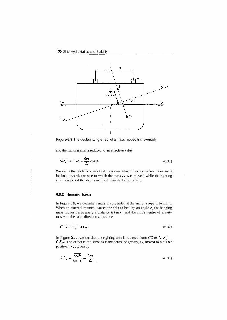
136 Ship Hydrostatics and Stability
wf
Figure 6.8 The destabilizing effect of a mass moved transversely
and the righting arm is reduced to an effective value
GZeff = GZ - cos (6.31)
We invite the reader to check that the above reduction occurs when the vessel isinclined towards the side to which the mass m was moved, while the rightingarm increases if the ship is inclined towards the other side.
6.9.2 Hanging loads
In Figure 6.9, we consider a mass m suspended at the end of a rope of length h.When an external moment causes the ship to heel by an angle 0, the hangingmass moves transversely a distance h tan </>, and the ship's centre of gravitymoves in the same direction a distance
hmGGl = —-tan (6.32)
In Figure 6.10, we see that the righting arm is reduced from GZ to G\Z\ —GZeff. The effect is the same as if the centre of gravity, G, moved to a higherposition, GV, given by
GG,tan <b
(6.33)
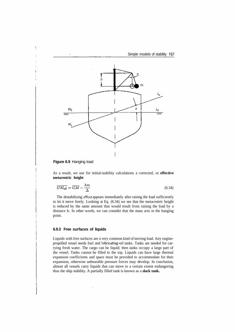
Simple models of stability 137
Figure 6.9 Hanging load
As a result, we use for initial-stability calculations a corrected, or effectivemetacentric height
(6.34)
The destabilizing effect appears immediately after raising the load sufficientlyto let it move freely. Looking at Eq. (6.34) we see that the metacentric heightis reduced by the same amount that would result from raising the load by adistance h. In other words, we can consider that the mass acts in the hangingpoint.
6.9.3 Free surfaces of liquids
Liquids with free surfaces are a very common kind of moving load. Any engine-propelled vessel needs fuel and lubricating-oil tanks. Tanks are needed for car-rying fresh water. The cargo can be liquid; then tanks occupy a large part ofthe vessel. Tanks cannot be filled to the top. Liquids can have large thermalexpansion coefficients and space must be provided to accommodate for theirexpansion, otherwise unbearable pressure forces may develop. In conclusion,almost all vessels carry liquids that can move to a certain extent endangeringthus the ship stability. A partially filled tank is known as a slack tank.
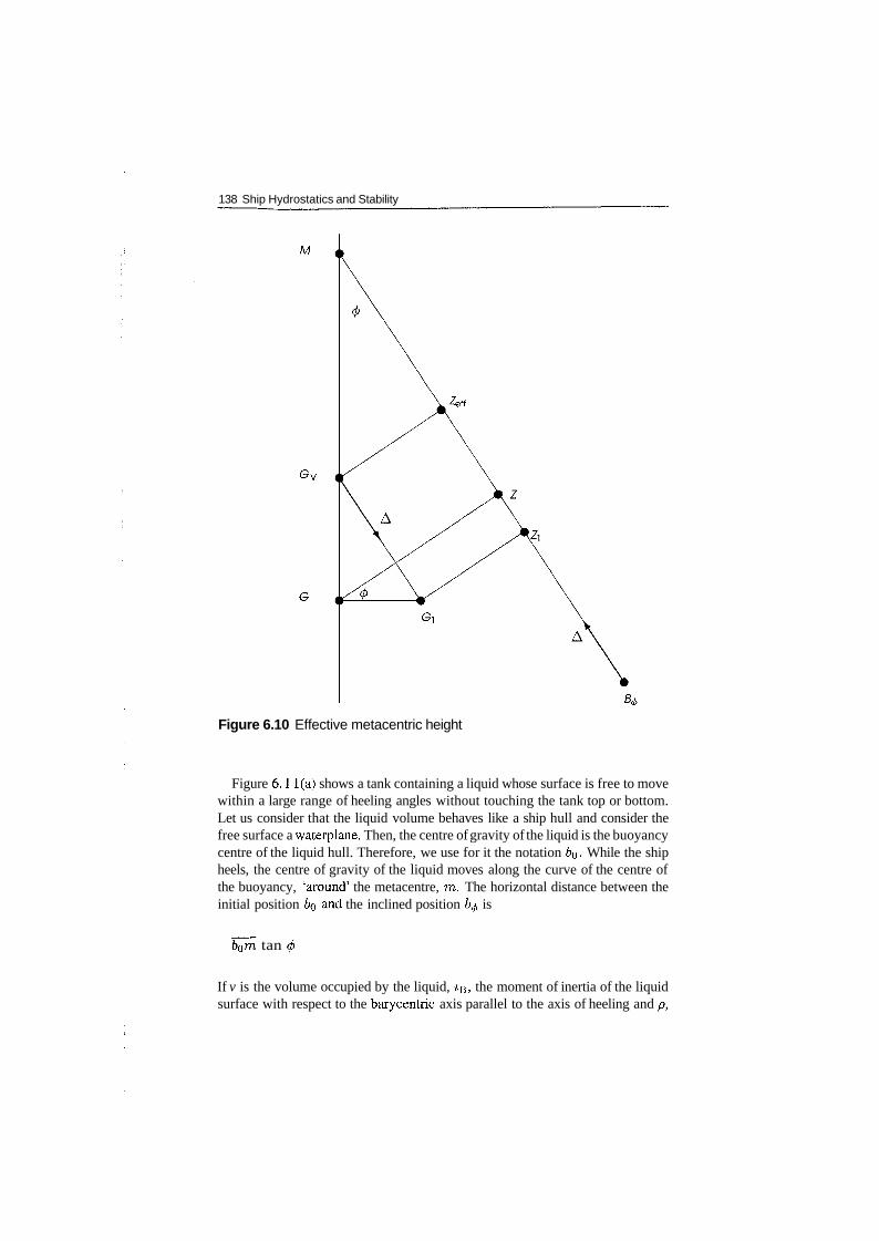
138 Ship Hydrostatics and Stability
M
Zeff
Figure 6.10 Effective metacentric height
Figure 6. 1 l(a) shows a tank containing a liquid whose surface is free to movewithin a large range of heeling angles without touching the tank top or bottom.Let us consider that the liquid volume behaves like a ship hull and consider thefree surface a waterplane. Then, the centre of gravity of the liquid is the buoyancycentre of the liquid hull. Therefore, we use for it the notation 60 . While the shipheels, the centre of gravity of the liquid moves along the curve of the centre ofthe buoyancy, 'around' the metacentre, m. The horizontal distance between theinitial position 60 and the inclined position 60 is
tan
If v is the volume occupied by the liquid, ZB, the moment of inertia of the liquidsurface with respect to the barycentric axis parallel to the axis of heeling and p,
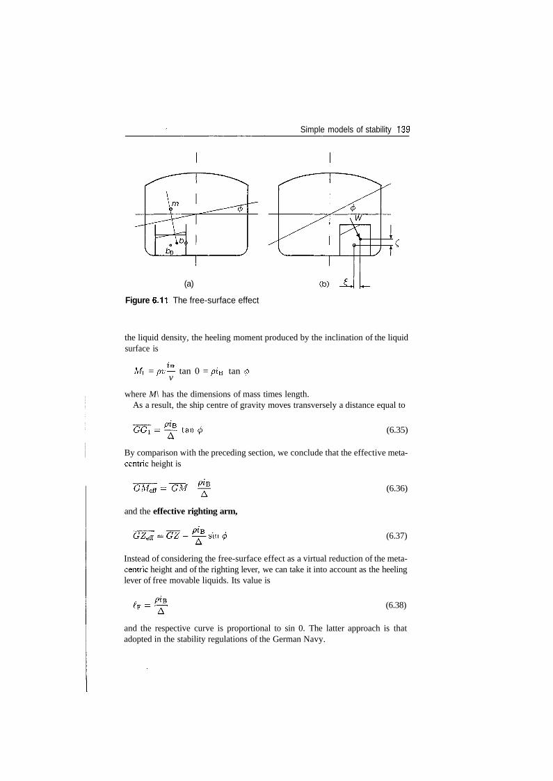
Simple models of stability 139
(a)
Figure 6.11 The free-surface effect
the liquid density, the heeling moment produced by the inclination of the liquidsurface is
M\ = pv— tan 0 = pi& tan <pv
where M\ has the dimensions of mass times length.As a result, the ship centre of gravity moves transversely a distance equal to
(6.35)
By comparison with the preceding section, we conclude that the effective meta-centric height is
GMeff = GM-
and the effective righting arm,
(6.36)
- sm (6.37)
Instead of considering the free-surface effect as a virtual reduction of the meta-centric height and of the righting lever, we can take it into account as the heelinglever of free movable liquids. Its value is
(6.38)
and the respective curve is proportional to sin 0. The latter approach is thatadopted in the stability regulations of the German Navy.
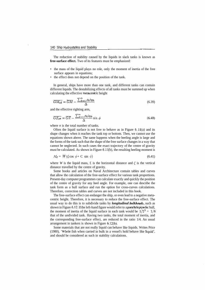
140 Ship Hydrostatics and Stability
The reduction of stability caused by the liquids in slack tanks is known asfree-surface effect. Two of its features must be emphasized:
• the mass of the liquid plays no role, only the moment of inertia of the freesurface appears in equations;
• the effect does not depend on the position of the tank.
In general, ships have more than one tank, and different tanks can containdifferent liquids. The destabilizing effects of all tanks must be summed up whencalculating the effective metacentric height
(6.39)
and the effective righting arm,
where n is the total number of tanks.Often the liquid surface is not free to behave as in Figure 6. 11 (a) and its
shape changes when it reaches the tank top or bottom. Then, we cannot use theequations shown above. The same happens when the heeling angle is large andthe forms of the tank such that the shape of the free surface changes in a way thatcannot be neglected. In such cases the exact trajectory of the centre of gravitymust be calculated. As shown in Figure 6.1 l(b), the resulting heeling moment is
Mi = W(£ cos (f) + C sin 0) (6.41)
where W is the liquid mass, £ is the horizontal distance and £ is the verticaldistance travelled by the centre of gravity.
Some books and articles on Naval Architecture contain tables and curvesthat allow the calculation of the free-surface effect for various tank proportions.Present-day computer programmes can calculate exactly and quickly the positionof the centre of gravity for any heel angle. For example, one can describe thetank form as a hull surface and run the option for cross-curves calculations.Therefore, correction tables and curves are not included in this book.
The free-surface effect can endanger the ship, or even lead to a negative meta-centric height. Therefore, it is necessary to reduce the free-surface effect. Theusual way to do this is to subdivide tanks by longitudinal bulkheads, such asshown in Figure 6.12. If the left-hand figure would refer to a parallelepipedic hull,the moment of inertia of the liquid surface in each tank would be 1/23 = 1/8that of the undivided tank. Having two tanks, the total moment of inertia, andthe corresponding free-surface effect, are reduced in the ratio 1/4. An usualarrangement in tankers is shown in Figure 6.12(b).
Some materials that are not really liquid can behave like liquids. Writes Price(1980), 'Whole fish when carried in bulk in a vessel's hold behave like liquid',and should be considered as such in stability calculations.
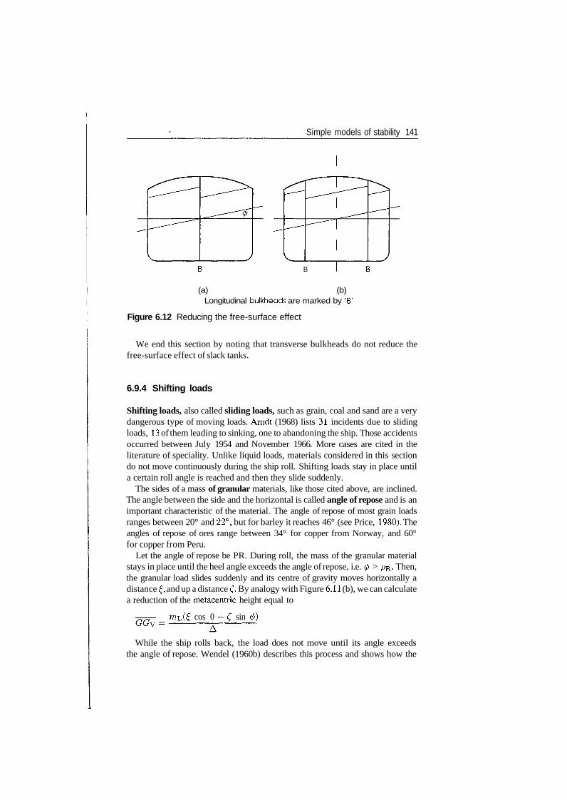
Simple models of stability 141
B
(a) (b)Longitudinal bulkheads are marked by 'B'
Figure 6.12 Reducing the free-surface effect
We end this section by noting that transverse bulkheads do not reduce thefree-surface effect of slack tanks.
6.9.4 Shifting loads
Shifting loads, also called sliding loads, such as grain, coal and sand are a verydangerous type of moving loads. Arndt (1968) lists 31 incidents due to slidingloads, 13 of them leading to sinking, one to abandoning the ship. Those accidentsoccurred between July 1954 and November 1966. More cases are cited in theliterature of speciality. Unlike liquid loads, materials considered in this sectiondo not move continuously during the ship roll. Shifting loads stay in place untila certain roll angle is reached and then they slide suddenly.
The sides of a mass of granular materials, like those cited above, are inclined.The angle between the side and the horizontal is called angle of repose and is animportant characteristic of the material. The angle of repose of most grain loadsranges between 20° and 22°, but for barley it reaches 46° (see Price, 1980). Theangles of repose of ores range between 34° for copper from Norway, and 60°for copper from Peru.
Let the angle of repose be PR. During roll, the mass of the granular materialstays in place until the heel angle exceeds the angle of repose, i.e. 0 > pR. Then,the granular load slides suddenly and its centre of gravity moves horizontally adistance f, and up a distance £. By analogy with Figure 6.11 (b), we can calculatea reduction of the metacentric height equal to
r^L (£ cos 0 -j- £ sin (f>)
While the ship rolls back, the load does not move until its angle exceedsthe angle of repose. Wendel (1960b) describes this process and shows how the
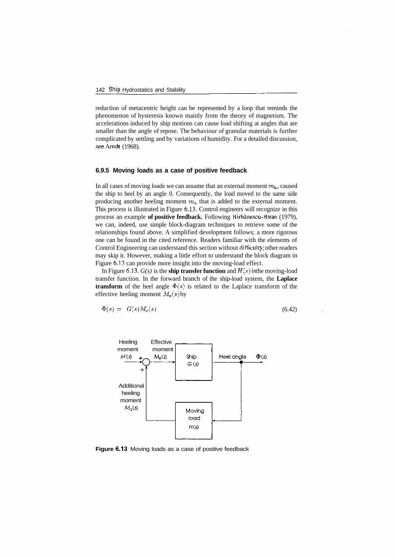
142 Ship Hydrostatics and Stability
reduction of metacentric height can be represented by a loop that reminds thephenomenon of hysteresis known mainly from the theory of magnetism. Theaccelerations induced by ship motions can cause load shifting at angles that aresmaller than the angle of repose. The behaviour of granular materials is furthercomplicated by settling and by variations of humidity. For a detailed discussion,see Arndt (1968).
6.9.5 Moving loads as a case of positive feedback
In all cases of moving loads we can assume that an external moment mh, causedthe ship to heel by an angle 0. Consequently, the load moved to the same sideproducing another heeling moment ma that is added to the external moment.This process is illustrated in Figure 6.13. Control engineers will recognize in thisprocess an example of positive feedback. Following Birbanescu-Biran (1979),we can, indeed, use simple block-diagram techniques to retrieve some of therelationships found above. A simplified development follows; a more rigorousone can be found in the cited reference. Readers familiar with the elements ofControl Engineering can understand this section without difficulty; other readersmay skip it. However, making a little effort to understand the block diagram inFigure 6.13 can provide more insight into the moving-load effect.
In Figure 6.13, G(s) is the ship transfer function and H(s)is the moving-loadtransfer function. In the forward branch of the ship-load system, the Laplacetransform of the heel angle $(s) is related to the Laplace transform of theeffective heeling moment Me(s) by
- G(s)Me(s) (6.42)
HeelingmomentM(s)
Additionalheelingmoment
Ma(s)
EffectivemomentMe(s)
Figure 6.13 Moving loads as a case of positive feedback
Simple models of stability 143
The Laplace transform of the additional heeling moment Ma(s), induced by themoving load, is related to the Laplace transform of the heel angle by
Ma(s) - H(s)$(s) (6.43)
Substituting Me(s) in Eq. (6.42) by the sum of the moments M(s) and Ma(s)yields
$(s) = G(s)(M(s) + H(s)<l>(s)) (6.44)
Finally, the transfer function of the ship-load system is given by
$(s) G(s)M(s) 1 - G(s)H(s]
(6.45)
To find the transfer function of the ship, we refer to Eq. (6.25) to which we adda heeling moment, rae, in the right-hand side
g Me (6-46)"m
Applying the Laplace transform, with zero initial conditions and rearranging,we obtain the ship transfer function
*(-) _ */£* (6.47)Afe(s) S2 + (£/£) GM
Substitution of the above transfer function into Eq. (6.45) yields
M(s) S2 + (g/il) (GM -
The factor
(6.48)
is the effective metacentric height.From the preceding sections, it can be found that the transfer function of a
hanging load is H(s) = mh, and the transfer function of a free liquid surface isH ( s ) — pi-Q. Equation (6.48) yields the condition for bounded response:
H(a)GM - -j^- > 0
Indeed, if this condition is fulfilled, </>(£) is a sinusoidal function of time withbounded amplitude. If the condition is not fulfilled, the heel angle is given by ahyperbolic sine, a function whose amplitude is not bounded. We retrieved thus,by other means, the famous condition of initial stability. A diagram such as thatin Figure 6.13 can be the basis of a SIMULINK® programme for simulating theroll of a ship with moving loads aboard.
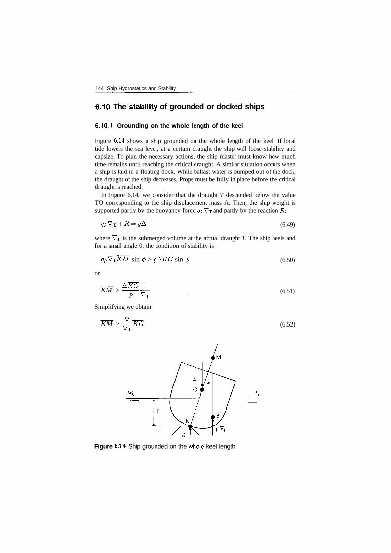
144 Ship Hydrostatics and Stability
6.10 The stability of grounded or docked ships
6.10.1 Grounding on the whole length of the keel
Figure 6.14 shows a ship grounded on the whole length of the keel. If localtide lowers the sea level, at a certain draught the ship will loose stability andcapsize. To plan the necessary actions, the ship master must know how muchtime remains until reaching the critical draught. A similar situation occurs whena ship is laid in a floating dock. While ballast water is pumped out of the dock,the draught of the ship decreases. Props must be fully in place before the criticaldraught is reached.
In Figure 6.14, we consider that the draught T descended below the valueTO corresponding to the ship displacement mass A. Then, the ship weight issupported partly by the buoyancy force gpVT and partly by the reaction R:
gpV (6.49)
where VT is the submerged volume at the actual draught T. The ship heels andfor a small angle 0, the condition of stability is
or
KM >
sin 0 > g&KG sin
AKG I
P VT
Simplifying we obtain
(6.50)
(6.51)
KM > —KGVT
(6.52)
Figure 6.14 Ship grounded on the whole keel length
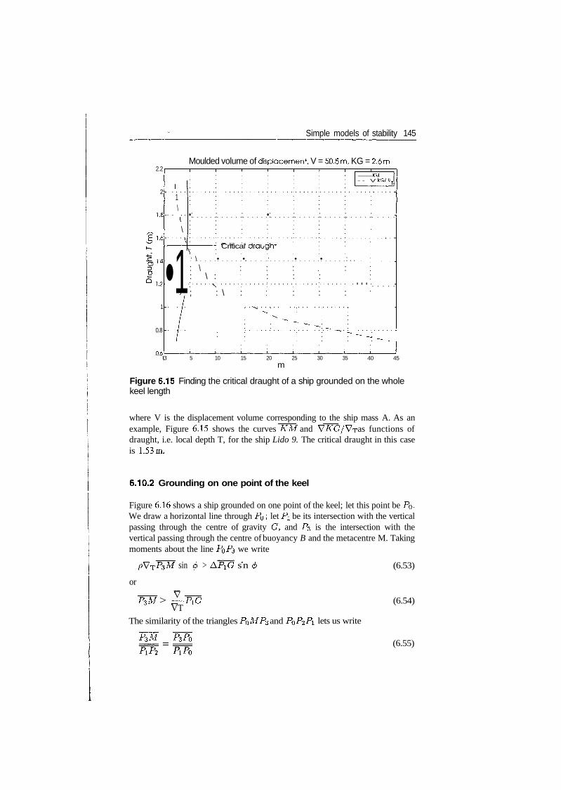
Simple models of stability 145
2.2
2
1.8
? 1-6
O)1-4
D
1
0.8
0.6t
Moulded volume of displacement, V = 50.5m, KG = 2.6m
11\.. . .^.
\
•1
KM- - V KG/ VT
•: : : •: : : ; : -
' /~ '4.1 ' 1 ^J ' UJ.Critical drauQht
: \ • •. : • • : . .: \ : : : : :: \ : : : : :
; : \ : : : : :• • • •: -
1 : ^f'h-f --'3 5 10 15 20 25 30 35 40 45
m
Figure 6.15 Finding the critical draught of a ship grounded on the wholekeel length
where V is the displacement volume corresponding to the ship mass A. As anexample, Figure 6.15 shows the curves KM and VKG/V^r as functions ofdraught, i.e. local depth T, for the ship Lido 9. The critical draught in this caseis 1.53m.
6.10.2 Grounding on one point of the keel
Figure 6.16 shows a ship grounded on one point of the keel; let this point be P0.We draw a horizontal line through PQ ; let PI be its intersection with the verticalpassing through the centre of gravity G, and PS is the intersection with thevertical passing through the centre of buoyancy B and the metacentre M. Takingmoments about the line P^Ps we write
sin <j) > sn
or
P3M > —PiGVT
The similarity of the triangles P0MP3 and
(6.53)
(6.54)
lets us write
P3M P3P0 (6.55)
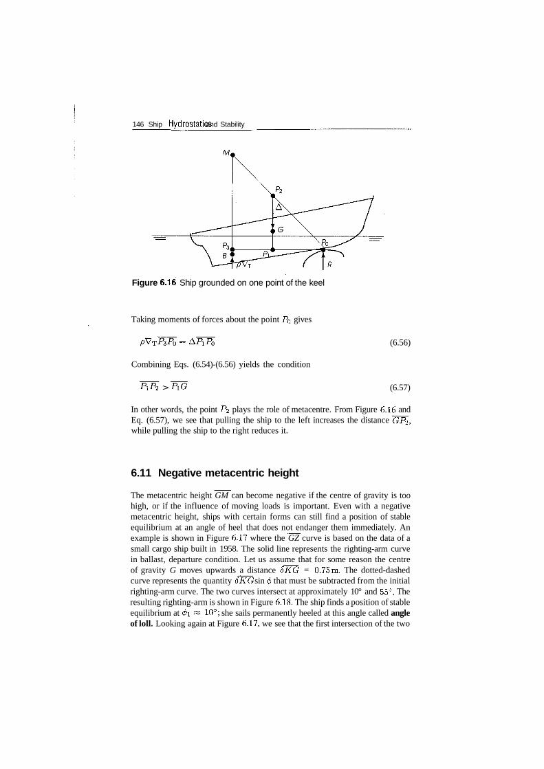
146 Ship Hydrostatics and Stability
Figure 6.16 Ship grounded on one point of the keel
Taking moments of forces about the point P0 gives
Combining Eqs. (6.54)-(6.56) yields the condition
>
(6.56)
(6.57)
In other words, the point P2 plays the role of metacentre. From Figure 6.16 andEq. (6.57), we see that pulling the ship to the left increases the distance GP2,while pulling the ship to the right reduces it.
6.11 Negative metacentric height
The metacentric height GM can become negative if the centre of gravity is toohigh, or if the influence of moving loads is important. Even with a negativemetacentric height, ships with certain forms can still find a position of stableequilibrium at an angle of heel that does not endanger them immediately. Anexample is shown in Figure 6.17 where the GZ curve is based on the data of asmall cargo ship built in 1958. The solid line represents the righting-arm curvein ballast, departure condition. Let us assume that for some reason the centreof gravity G moves upwards a distance 5KG = 0.75m. The dotted-dashedcurve represents the quantity 6KG sin </> that must be subtracted from the initialrighting-arm curve. The two curves intersect at approximately 10° and 55°. Theresulting righting-arm is shown in Figure 6.18. The ship finds a position of stableequilibrium at 0i « 10°; she sails permanently heeled at this angle called angleof loll. Looking again at Figure 6.17, we see that the first intersection of the two
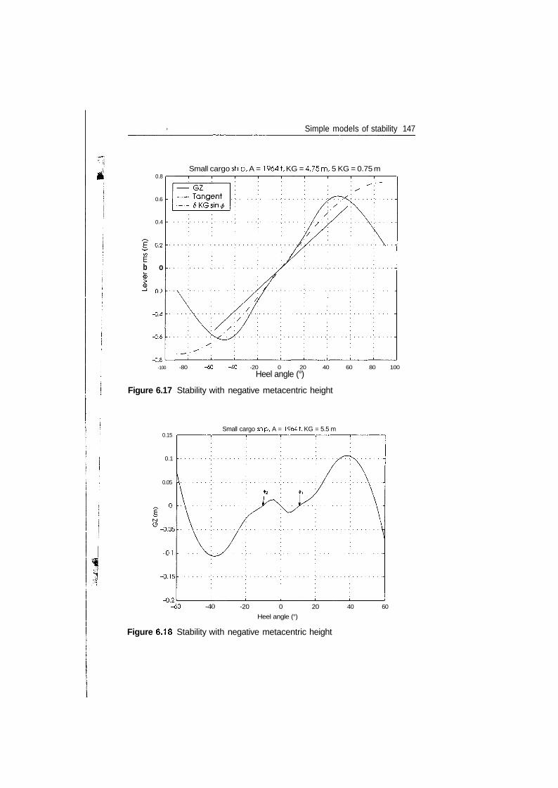
Simple models of stability 147
Small cargo ship, A = 1964t, KG = 4.75m, 5 KG = 0.75 m0.8
0.6
0.4
b o
-0.2
-0.4
-0.6
-0.8
-100 -80 -60 -40 -20 0 20 40 60 80 100Heel angle (°)
Figure 6.17 Stability with negative metacentric height
0.15
0.1
0.05
Small cargo ship, A = 1964t, KG = 5.5 m
-0.05
-0.1
-0.15
-0.2-60 -40 -20 0 20
Heel angle (°)
40 60
Figure 6.18 Stability with negative metacentric height
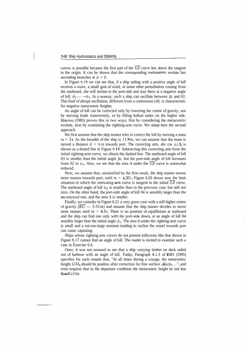
148 Ship Hydrostatics and Stability
curves is possible because the first part of the GZ curve lies above the tangentin the origin. It can be shown that the corresponding metacentric evolute hasascending branches at $ = 0.
In Figure 6.18 we can see that, if a ship sailing with a positive angle of lollreceives a wave, a small gust of wind, or some other perturbation coming fromthe starboard, she will incline to the port-side and stay there at a negative angleof loll, (f>2 — —0i- In a seaway, such a ship can oscillate between fa and 02.This kind of abrupt oscillation, different from a continuous roll, is characteristicfor negative metacentric heights.
An angle of loll can be corrected only by lowering the centre of gravity, notby moving loads transversely, or by filling ballast tanks on the higher side.Hervieu (1985) proves this in two ways, first by considering the metacentricevolute, next by examining the righting-arm curve. We adopt here the secondapproach.
We first assume that the ship master tries to correct the loll by moving a massra = 21. As the breadth of the ship is 11.9 m, we can assume that the mass ismoved a distance d = 6 m towards port. The correcting arm, dm cos (/>/A, isshown as a dotted line in Figure 6.19. Subtracting this correcting arm from theinitial righting-arm curve, we obtain the dashed line. The starboard angle of loll03 is smaller than the initial angle fa, but the port-side angle of loll increasesfrom 02 to 04. Also, we see that the area A under the GZ curve is somewhatreduced.
Next, we assume that, unsatisfied by the first result, the ship master movesmore masses towards port, until m = 4.25t. Figure 6.20 shows now the limitsituation in which the correcting-arm curve is tangent to the initial GZ curve.The starboard angle of loll 03 is smaller than in the previous case, but still notzero. On the other hand, the port-side angle of loll 04 is sensibly larger than theuncorrected one, and the area A is smaller.
Finally, we consider in Figure 6.21 a very grave case with a still higher centreof gravity (KG — 5.55m) and assume that the ship master decides to movemore masses until m = 6.51. There is no position of equilibrium at starboardand the ship can find one only with the port-side down, at an angle of loll 04sensibly larger than the initial angle 02. The area A under the righting-arm curveis small and a not-too-large moment tending to incline the vessel towards portcan cause capsizing.
Ships whose righting-arm curves do not present inflexions like that shown inFigure 6.17 cannot find an angle of loll. The reader is invited to examine such acase in Exercise 6.4.
Once, it was not unusual to see that a ship carrying timber on deck sailedout of harbour with an angle of loll. Today, Paragraph 4.1.3 of IMO (1995)specifies for such vessels that, "At all times during a voyage, the metacentricheight GMo should be positive after correction for free surface effects...", andeven requires that in the departure condition the metacentric height be not lessthan 0.1 Om.
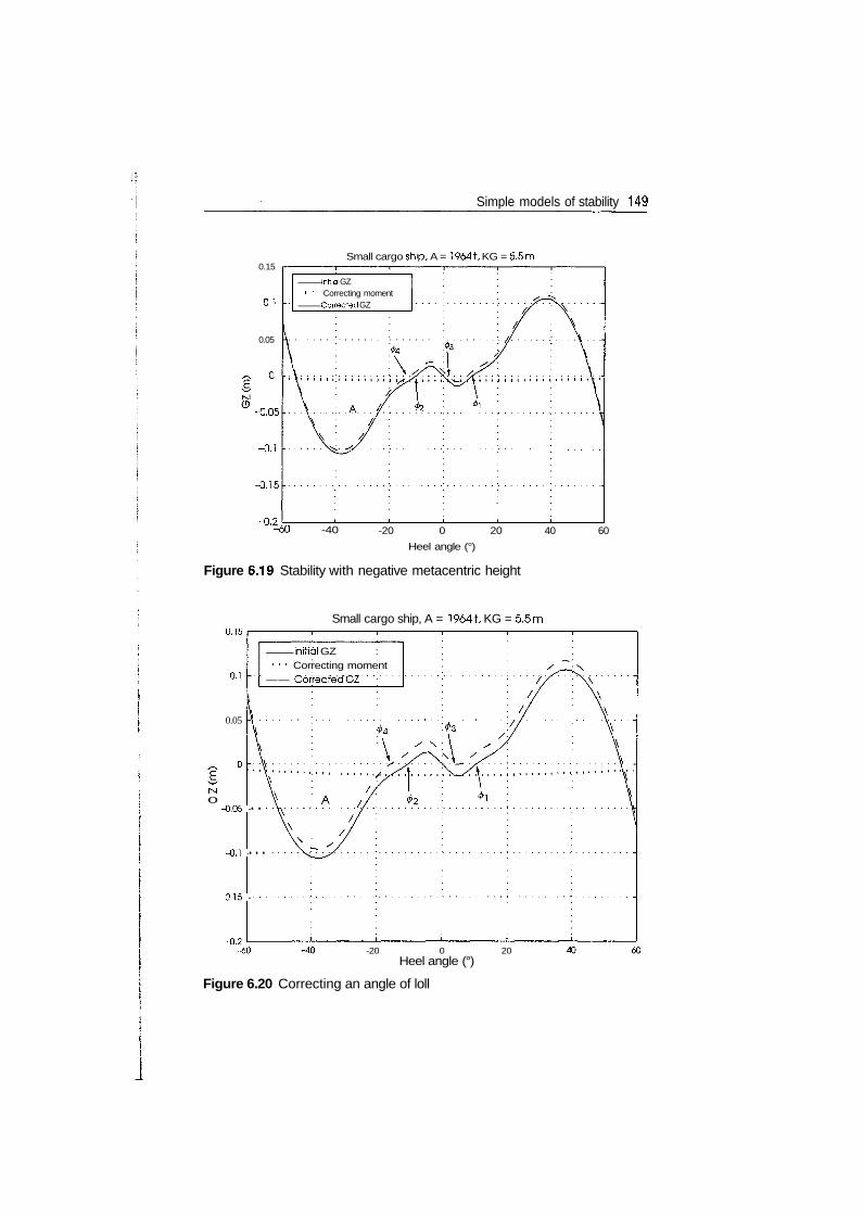
Simple models of stability 149
0.15
0.1
0.05
> oI
' -0.05
-0.1
-0.15
-0.2
Small cargo ship, A = 1964t, KG = 5.5m
Initial GZ1 ' ' Correcting moment
Corrected GZ
'-60 -40
Figure 6.19 Stability with negative metacentric height
-20 0 20
Heel angle (°)
40 60
Small cargo ship, A = 1964t, KG = 5.5m0.15
0.05
M0
Initial GZ :1 1 1 1 Correcting moment— — "Corrected GZ'
-0.05 -• •
-0.1 -• • •
-0.15 -
-0.2-60 -20 0 20
Heel angle (°)
Figure 6.20 Correcting an angle of loll
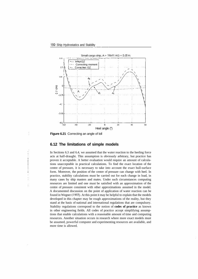
150 Ship Hydrostatics and Stability
0.15
0.1
0.05
Small cargo ship, A = 19641, KG = 5.55m
M0
-0.05
-0.1
-0.15
-0.2
— Initial GZ1 • Correcting moment-- Corrected GZ
-60 -40 -20 20 40 60
Heel angle (°)
Figure 6.21 Correcting an angle of loll
6.12 The limitations of simple models
In Sections 6.3 and 6.4, we assumed that the water reaction to the heeling forceacts at half-draught. This assumption is obviously arbitrary, but practice hasproven it acceptable. A better evaluation would require an amount of calcula-tions unacceptable in practical calculations. To find the exact location of thecentre of pressure, it is necessary to take into account the exact hull-surfaceform. Moreover, the position of the centre of pressure can change with heel. Inpractice, stability calculations must be carried out for each change in load, inmany cases by ship masters and mates. Under such circumstances computingresources are limited and one must be satisfied with an approximation of thecentre of pressure consistent with other approximations assumed in the model.A documented discussion on the point of application of water reaction can befound in Wegner (1965). At this point it may be helpful to explain that the modelsdeveloped in this chapter may be rough approximations of the reality, but theystand at the basis of national and international regulations that are compulsory.Stability regulations correspond to the notion of codes of practice as knownin other engineering fields. All codes of practice accept simplifying assump-tions that enable calculations with a reasonable amount of time and computingresources. Another situation occurs in research where more exact models mustbe assumed, powerful computer and experimenting resources are available, andmore time is allowed.
Simple models of stability 151
Equation (6.2) developed in Section 6.3 yields a heeling arm equal to zeroat the heel angle 90°. Such a result is obviously wrong as any vessel presentsa sail area exposed to the wind even when lying on the side. Figure 1.103 inHenschke (1957) illustrates well this point. At small angles the results basedon the curve proportional to cos2 (f) differ little from those obtained with otherapproximations (see Chapters 8 and 10) and, therefore, they are acceptable forlarge vessels that do not heel much under wind, such as the capital ships of theUS Navy. Smaller vessels tend to heel more under wind and then curves basedon the cos2 $ assumption may become quite unrealistic.
The models developed in this chapter are based on further simplifications. Inreal life, water opposes the motions of a ship with forces that depend on the ampli-tude of motion, the speed of motion and the acceleration of motion. Assumingnegligible roll velocity and acceleration, our models take into account only themoment that depends on the amplitude of heeling, that is the righting moment.
The moment that depends on the heeling speed, 0, is called damping moment.Damping causes energy dissipation. If a system that includes damping is dis-placed from its equilibrium position and then it is left to oscillate freely, theamplitude of oscillations will decrease with time and eventually will die out.The damping of the roll motion is mainly due to the generation of waves, butviscous effects may increase it and become important for certain bilge forms orif the vessel is fitted with bilge keels or a large keel.
The moments proportional to heel acceleration belong to a category of forcesand moments called added masses because they can be collected together withthe mass moment of inertia of the ship.
The evaluation of damping and added masses requires special computer pro-grammes or model experiments. Neglecting damping and added masses leads tooverestimation of dynamic heeling angles and this is on the safe side. Therefore,no stability regulation takes explicitly into account the effects of damping oradded masses, but some regulations consider indirectly their influence by usingdifferent parameters for ships fitted with sharp bilges, bilge keels or deep keels.
Cardo et al (1978), for example, discuss stability considering non-linear rollequations that include damping and added masses. Using advanced mathemat-ical criteria, the authors reach the same qualitative results as those obtainedin Section 6.7. An outline of the linear theory of ship motions is given inChapter 12.
Last, but not least, we neglected until now the influence of waves, and weleave the discussion of this subject for Chapters 9-11.
6.13 Other modes of capsizing
Capsizing can be defined as the sudden transition of a floating body from aposition of equilibrium to another position of equilibrium. Depending on theship forms and loading, her second position can be on the side or with the
152 Ship Hydrostatics and Stability
keel up. If in the new position water can enter in large quantities, the ship willeventually sink. Often the process is so fast that many lives are lost. Sometimesno survivor remains to tell the story.
In Chapter 2, we saw that a floating body can capsize if the metacentricheight is negative. In this chapter, we learnt that a vessel can capsize if therighting arm is too small in comparison with the heeling arm, or if the areaunder the righting-arm curve is too small in comparison with the area under theheeling-arm curve. In Chapter 9, we shall see that a ship can capsize becauseof the variation of the metacentric height and of the righting arm in waves thattravel in the same direction as the ship (head or following seas) or at someangle with her. That dangerous phenomenon is called parametric resonance orMathieu effect. What happens if the waves are parallel to the ship? Arndt (1960a)explains that a ship cannot capsize in regular, parallel waves. Adds Arndt, 'Frompractice we know cases in which captains put the ship parallel to the wave crestsin order to reduce the effect of storms, neither in experiments could anyonecause until now a model to capsize in lateral, regular waves'. Otherwise seems tohappen with freak, or breaking waves of great steepness whose impact on the shipside can be high enough to overturn the ship. Thus, for example, Morrall (1980)investigates the loss of the large stern trawler Gaul, and Dahle and Kjaerland(1980) study the capsizing of the Norwegian research vessel Helland-Hansen.These studies support the hypothesis that the discussed disasters were due tohigh breaking waves.
It seems that the process of capsizing because of freak or breaking waves is notyet well understood and the methods proposed for its prediction are probabilistic(see Dahle and Myrhaug, 1996; Myrhaug and Dahle, 1994). Kat (1990) stud-ied numerical models for the simulation of capsizing and Grochowalski (1989)describes a research on ship models. Probabilistic and simulation studies arebeyond the scope of this book.
Another mode of capsizing is broaching-to\ it is a dynamic phenomenon dueto the loss of control in severe following or quartering seas. The ship entersinto a forced turning that cannot be corrected by the rudder, heels and capsizes.Broaching-to is studied by Nicholson (1975), Spyrou (1995, 1996a,b).
It has been claimed that capsizing results from a combination of several factors.An example can be found in Hua (1996) who studied the capsize of the ferryHerald of Free Enterprise as a result of the interaction between heeling andturning motion, while great quantities of water were present on one deck.
6.14 Summary
The statical stability of ships is checked by comparing the righting-arm curvewith the curves of heeling arms. A heeling arm is calculated by dividing a heelingmoment by the ship displacement force. In general, a heeling-arm curve intersectsthe righting-arm curve at two points that correspond to positions of statical
Simple models of stability 153
equilibrium. The equilibrium is stable only at the first position; there the slopeof the righting-arm curve is larger than that of the heeling arm.
Heeling moments are caused by wind, by the centrifugal force developed inturning, by the crowding of passengers on one side of the ship, by towing orby the tension in a cable that links two vessels during a replenishment-at-seaoperation.
The wind heeling arm is proportional to the square of the wind velocity anddepends on the area of the lateral projection of the above-sea ship surface. We callthat area 'sail area'. Assuming that the wind velocity is constant over the wholesail area, the wind heeling arm is proportional to the sail area. This assumptionis acceptable for quick calculations. In reality, the wind speed increases withheight above the sea level and this 'wind gradient' is taken into account in moreexact calculations.
The heeling arm in turning is proportional to the square of the ship speed inturning, and inversely proportional to the radius of the turning circle. When theheeling moment appears or increases suddenly we must check the dynamicalstability of the vessel. This situation can be caused by a gust of wind or bylosing a mass on one side of the ship. The area under the righting arm up to themaximum angle reached momentarily by the ship is equal to the area under theheeling arm up to that point. The process depends on the angle of roll at whichthe sudden moment is applied. For a gust of wind, for example, the situation isworse if the ship is heeled to the windward side, than if the ship is caught bythe gust with the lee side down. If the area available under the righting arm issmaller than the area under the heeling arm, the ship is lost.
The period of unresisted roll is proportional to the square root of the meta-centric height. This imposes an upper limit on the GM value. If the roll periodis too short, the roll motion is stiff; it is unpleasant for passengers and crew, andmay be dangerous for equipment and cargo. If the motion is too tender, it mayindicate a dangerously low metacentric height. A load displaced transverselyreduces the stability when heeling to the same side as the load. Moving loads toodecrease the stability. Thus, a load suspended so that it can move freely producesa virtual reduction of the metacentric height as if the load were moved to thepoint of suspension. A very common type of moving loads are liquids whosesurfaces are free to move inside tanks or on the deck. The reduction of stability isproportional to the moment of inertia of the free surface about a barycentric axisparallel to the axis of ship inclination. The effect does not depend on the massof the liquid (as long as the liquid surface does not reach the tank top or bottom)or the position of the tank. The usual way of reducing the free-surface effectis to subdivide the tanks by longitudinal bulkheads. Two other methods are toempty the tank or to fill it. In the latter case the effect of the thermal expansion ofthe liquid should be considered. Granular materials constitute another categoryof moving loads. Such loads stay in place until the heel angle exceeds a valuecharacteristic for the material. This value is called angle of repose. The variationof stability reduction due to sliding loads follows a hysteresis loop. The effectof moving loads is a case of positive feedback.
154 Ship Hydrostatics and Stability
If a ship is grounded in a region where the water level is descending, at acertain draught it can lose stability. The same happens with a ship on dock. Thecalculation of the critical draught is rather simple.
A ship with negative metacentric height can find a position of stable equilib-rium, without capsizing, if the first part of the righting-arm curve lies above thetangent in the origin. This fixed angle of heel is called angle of loll. There are twoangles of loll and they are symmetric about the origin. Under moderate perturba-tions, the ship can heel suddenly from one angle of loll to the other. This motionis different from a continuous roll and is characteristic for negative metacentricheight. The angle of loll cannot be corrected by moving masses transversely;such an action can endanger the ship. Angles of loll should be corrected only bylowering the centre of gravity.
6.15 Examples
Example 6.1 - Wind pressureLet us calculate the pressure corresponding to a wind speed of 70 knots. Thisis the value specified by the German Navy for evaluating the intact stability ofvessels operating in open seas that are not exposed to tropical storms. Assumingan aerodynamic resistance coefficient equal to 1.2 and an air density equal to1.27 kgm"1, we obtain
pw = . -2 2 rrr3 \ knot
- 987.99 kg ms-2
Rounding off yields lkNm~ 2 , or, using the SI term, 1 kPa. The conversionfactor, 0.5144, results from the definition of the knot as nautical mile perhour. Substituting SI units we divide 1852 m by 3600 s and obtain 1852/3600= 0.5144 ms~Vknot-
Example 6.2 - Calculating a wind heeling armFigure 6.22 is a simplified sketch of the sail area of the Ship Lido 9 with thewaterline corresponding to a draught of 1.85m. To simplify calculations, thearea is subdivided into five simple geometrical forms, namely rectangles andtriangles. The calculations are carried out in the spreadsheet shown in Table 6.1.
If the stability of the vessel must be checked for a wind speed of 90 knots,we use the wind-pressure value of 1.5 MPa, as prescribed by the German Navystability regulations for ships that can encounter tropical storms.
Example 6.3 -The statical stability curves of HMS Captain and HMS MonarchIn the night between 6 and 7 September 1870, a British fleet was sailing-offCape Finisterre. The fleet was hit by a strong gale and one of the ships, HMSCaptain capsized, but all other ships survived. The righting arms of HMS Cap-tain are given in Anonymous (1872) and Attwood and Pengelly (1960), while
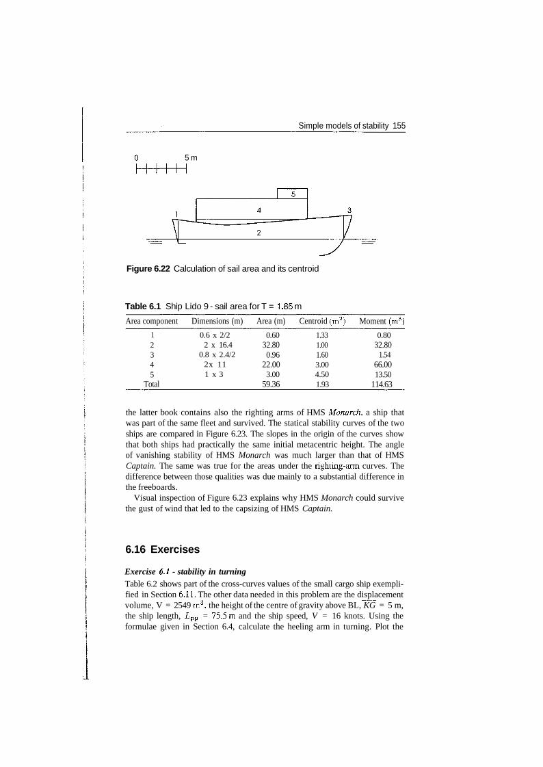
Simple models of stability 155
5 m
Figure 6.22 Calculation of sail area and its centroid
Table 6.1 Ship Lido 9 - sail area for T = 1.85 m
Area component
12345
Total
Dimensions (m)
0.6 x 2/22 x 16.4
0.8 x 2.4/22x 111 x 3
Area (m)
0.6032.800.96
22.003.00
59.36
Centroid (m2)
1.331.001.603.004.501.93
Moment (m3)
0.8032.80
1.5466.0013.50
114.63
the latter book contains also the righting arms of HMS Monarch, a ship thatwas part of the same fleet and survived. The statical stability curves of the twoships are compared in Figure 6.23. The slopes in the origin of the curves showthat both ships had practically the same initial metacentric height. The angleof vanishing stability of HMS Monarch was much larger than that of HMSCaptain. The same was true for the areas under the righting-arm curves. Thedifference between those qualities was due mainly to a substantial difference inthe freeboards.
Visual inspection of Figure 6.23 explains why HMS Monarch could survivethe gust of wind that led to the capsizing of HMS Captain.
6.16 Exercises
Exercise 6.1 - stability in turningTable 6.2 shows part of the cross-curves values of the small cargo ship exempli-fied in Section 6.11. The other data needed in this problem are the displacementvolume, V = 2549 m3, the height of the centre of gravity above BL, KG = 5 m,the ship length, I/pp = 75.5m and the ship speed, V = 16 knots. Using theformulae given in Section 6.4, calculate the heeling arm in turning. Plot the
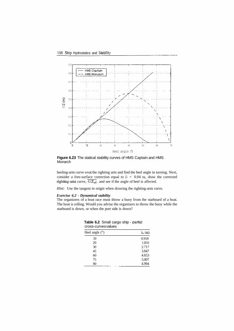
156 S>hip Hydrostatics and Stability
MCD
0.9
0.8
0.7
0.6
0.5
0.4
0.3
0.2
0.1
10 20 30 40 50
Heel angle (°)
60 70
Figure 6.23 The statical stability curves of HMS Captain and HMSMonarch
heeling-arm curve over the righting arm and find the heel angle in turning. Next,consider a free-surface correction equal to If = 0.04 m, draw the correctedrighting-arm curve, GZes, and see if the angle of heel is affected.
Hint: Use the tangent in origin when drawing the righting-arm curve.
Exercise 6.2 - Dynamical stabilityThe organizers of a boat race must throw a buoy from the starboard of a boat.The boat is rolling. Would you advise the organizers to throw the buoy while thestarboard is down, or when the port side is down?
Table 6.2 Small cargo ship - partialcross-curves values
Heel angle (°) lk
10203045607590
0.9181.8332.7173.8474.6535.0074.994
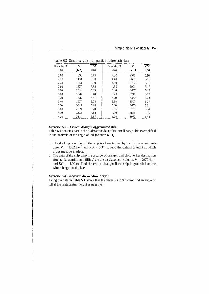
Simple models of stability 157
Table 6.3 Small cargo
Draught, T(m)
2.002.202.402.602.803.003.203.403.603.804.004.20
V(m3)
99311181243137715041640177619072045218923222471
ship - partial hydrostatic data
KM(m)
6.756.396.095.835.635.485.375.285.245.205.185.17
Draught, T(m)
4.324.404.604.805.005.205.405.605.805.966.006.20
V(m3)
254926092757290130573210335235073653378638113972
KM(m)
5.165.165.165.175.185.205.235.275.315.345.365.42
Exercise 6.3 - Critical draught of grounded shipTable 6.3 contains part of the hydrostatic data of the small cargo ship exemplifiedin the analysis of the angle of loll (Section 6.11).
1. The docking condition of the ship is characterized by the displacement vol-ume, V = 1562.8 m3 and KG = 5.34 m. Find the critical draught at whichprops must be in place.
2. The data of the ship carrying a cargo of oranges and close to her destination(fuel tanks at minimum filling) are the displacement volume, V = 2979.4 m3
and KG = 4.92 m. Find the critical draught if the ship is grounded on thewhole length of the keel.
Exercise 6.4 - Negative metacentric heightUsing the data in Table 5.1, show that the vessel Lido 9 cannot find an angle ofloll if the metacentric height is negative.
7Weight and trim calculations
7.1 Introduction
All models of stability require the knowledge of the displacement mass, A, andof the height of the centre of gravity (vertical centre of gravity), KG. Stevin's law(see Subsection 2.3.2) shows that the ship trim is determined by the longitudinalposition of the centre of gravity, LOG. The three quantities, A, KG and LCG arecalculated by summing up the masses of all ship components and their momentsabout a horizontal and a transverse plane. The centre of gravity of a ship inupright condition is situated in the plane of port-to-starboard symmetry of theship (centreline plane); therefore, the coordinate of the centre of gravity about thisplane is zero. However, individual mass ship components may not be symmetricalabout the centreline plane and it is necessary to calculate their moments aboutthat plane and ensure that the transverse coordinate (y-coordinate) of the ship'scentre of gravity is zero. It is usual to call the latter coordinate transverse centreof gravity and note it by TCG. Thus, we have a consistent notation for the tripleof coordinates LCG, VCG, TCG. Systematic calculations of displacements andcentres of gravity are known as weight calculations and they are the subject ofthe first part of this chapter. Recent literature and standards deal with massesrather than weights. We follow this trend in our book, but use the term weightcalculations because it is rooted in tradition.
Another subject of this chapter is the calculation of the trim and of the forwardand aft draughts. As mentioned in Chapter 6, the trim affects the ship stability.Also, a ship trimmed at a large angle can look unpleasant to the eye. Above all,the trim determines the forward and aft draughts and thus affects certain shipfunctions. For example, the aft draught must be large enough to ensure sufficientpropeller submergence and avoid cavitation.
Frequently weight calculations are based on approximate or insufficient data.The sources of uncertainty are explained in this chapter when introducing thenotions of reserve and margin of displacement and of KG. Because of theseuncertainties, statutory regulations require an experimental validation of thecoordinates of the centre of gravity, and of the corresponding metacentric height,GM, for all new buildings or for vessels that underwent alterations that can influ-ence their stability. This validation is carried out in the inclining experiment,also known in some shipyards as stability test.
160 Ship Hydrostatics and Stability
7.2 Weight calculations
7.2.1 Weight groups
A vessel is composed of hundreds, sometimes thousands of mass items. To sys-tematize calculations it is necessary to organize them into weight groups. Thefirst subdivision is into two main sets: lightship and deadweight. The lightship(less frequently known as lightweight) is the mass of the empty ship; it is com-posed of the hull, the outfit, and the machinery masses, including the liquids inthe machinery and various systems, but not those in tanks or storage spaces. Thedeadweight is the sum of the masses of crew, cargo and passengers, fuel, lubri-cating oil, provisions, water, stores and spare parts. The usual abbreviation fordeadweight is DWT. In simpler terms, the deadweight is the weight that theship 'carries'.
One should make a distinction between the term lightship used as above, andits homophone that designs a ship provided with a strong light and used to marka position.
In the first stages of ship design, known as preliminary design, the light-ship masses and their centres of gravity are estimated by empirical equations,based on statistics of similar ships, or are derived from the masses of agiven parent ship. This subject is treated in books on ship design such asKiss (1980), Schneekluth (1980), Schneekluth and Bertram (1998) andWatson (1998). For merchant ships, the lightship groups are the hull, the outfit andthe machinery. The classification of warship weight groups may be somewhatdifferent. Thus, the classification system of the US Navy, SWBS, distinguishesthe following main weight groups: hull structure, propulsion plant, electricplant, command and surveillance, auxiliary systems, outfit and furnishings,armament.
As the design progresses by successive iterations, the weight estimations arerefined by subdividing the weight groups into subgroups, the subgroups intolower-lever subgroups, and so on. Thus, the hull mass is subdivided into hulland superstructure, then the hull into bottom, sides, decks, bulkheads etc. Themachinery components are first subdivided into main, or propulsion machinery,and auxiliary machinery. In the final stages it is possible to calculate the massesand centres of gravity of individual items from detailed drawings or from dataprovided by equipment suppliers.
The procedure described above requires a classification of the various weightgroups, subgroups and so on that ensures that no item is forgotten and that noitem belongs to two groups. Readers who like mathematics may say that theweight groups shall be disjoint. Such readers can also see that such a classifi-cation system can be described by a tree graph (see Birbanescu-Biran, 1988).Several authorities and organizations engaged in ship design and constructionhave developed their own classification systems. An example of classificationsystem for merchant ships is shown in Kiss (1980). As mentioned above, the
Weight and trim calculations 161
classification system adopted by the US Navy is known as SWBS, an acronymfor Ship Work Breakdown Structure.
The main deadweight item is the cargo; it is pre-specified by the owner. Thenumber of crew members depends on the functions to be carried aboard: fre-quently a minimum is prescribed by regulations. The masses of fuel, lubricatingoil, and water result from the required ship speed and range, two characteristicsspecified by the owner.
To compensate for the uncertainties in weight estimation in the first designstages, Naval Architects introduce a weight item called reserve, or weight mar-gin. Some regulations consider also a KG margin; that is the calculated height ofthe centre of gravity, KG, is increased by a certain amount ensuring that stabilitycalculations fall on the safe side. As the ship design progresses, the uncertaintiesare reduced and so must be the weight reserve and the KG margin.
When the detailed ship project is delivered for construction, all weight andcentres of gravity are supposed to be exact; however, a 'building' weight reserveand a KG margin are still included in weight calculations. By doing so designerstake into account acceptable tolerances in plate, profile and pipe thicknesses,tolerances in metal densities, and changes in the catalogues of suppliers.
Even when the ship is delivered to the owner, weight calculations still include'commissioning' margins that take into account future equipment additions, trap-ping of water in places from where it cannot be pumped out, and weight increasedue to rust and paint. Certain codes of practice, such as the stability regulationsof the US Navy and those of the German Federal Navy, impose well-definedmargin values.
7.2.2 Weight calculations
Once the ship is built and in service, the lightship displacement and its centre ofgravity are taken in calculations as constants. For each possible loading case, thatis for each combination of cargo and other deadweight items, the masses of thoseitems and their moments are added to those of the lightship. The calculations yieldthe displacement and the coordinates of the centre of gravity of the loading caseunder consideration. To give an example, we return to the data of the small cargoship considered in Chapter 6. Figure 7.1 shows the calculations correspondingto the load case Homogeneous cargo, departure. By departure condition wemean the ship leaving the port, with all the fuel, lubricating oil and provisions.
Table 7.1 was calculated in MS Excel. Alternatively, the calculations can beperformed in MATLAB. Then, the weight data can be stored in a matrix, forexample in the format
where m* is the mass of the ith weight item, kg^ its vertical centre of gravity,and Icgi, its longitudinal centre of gravity. An example of calculations for theloading case considered in Figure 7.1 is
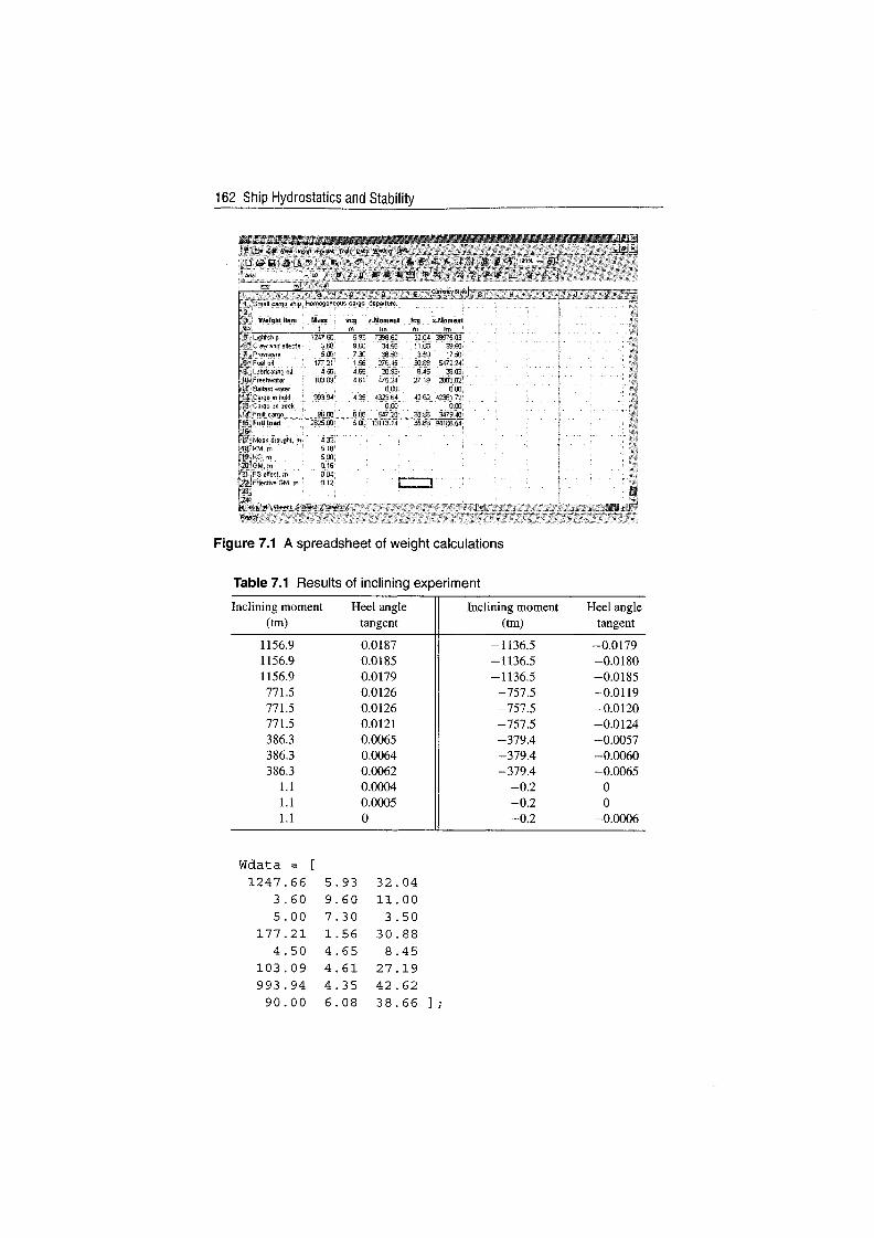
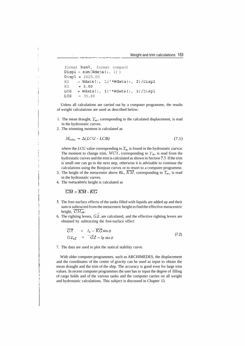
Weight and trim calculations 163
format bank, format compactDispl = sum(Wdata(:, 1) )Displ = 2625.00KG = Wdataf:, 1)'*Wdata(:, 2)/DisplKG =5.00LCG =Wdata(:, l)'*Wdata(:, 3)/DisplLCG = 35.88
Unless all calculations are carried out by a computer programme, the resultsof weight calculations are used as described below:
1. The mean draught, Tm, corresponding to the calculated displacement, is readin the hydrostatic curves.
2. The trimming moment is calculated as
Mtrim - A(LCG - LCB) (7.1)
where the LCG value corresponding to Tm is found in the hydrostatic curves.The moment to change trim, MCT, corresponding to Tm, is read from thehydrostatic curves and the trim is calculated as shown in Section 7.3. If the trimis small one can go to the next step, otherwise it is advisable to continue thecalculations using the Bonjean curves or to resort to a computer programme.
3. The height of the metacentre above BL, KM, corresponding to Tm, is readin the hydrostatic curves.
4. The metacentric height is calculated as
GM = KM - KG
5. The free-surface effects of the tanks filled with liquids are added up and theirsum is subtracted from the metacentric height to find the effective metacentricheight, GMeff. _
6. The righting levers, GZ, are calculated, and the effective righting levers areobtained by subtracting the free-surface effect
~GZ = /*_ __ (7.2)GZeff = G Z - l F s m ( f )
7. The data are used to plot the statical stability curve.
With older computer programmes, such as ARCHIMEDES, the displacementand the coordinates of the centre of gravity can be used as input to obtain themean draught and the trim of the ship. The accuracy is good even for large trimvalues. In recent computer programmes the user has to input the degree of fillingof cargo holds and of the various tanks and the computer carries on all weightand hydrostatic calculations. This subject is discussed in Chapter 13.
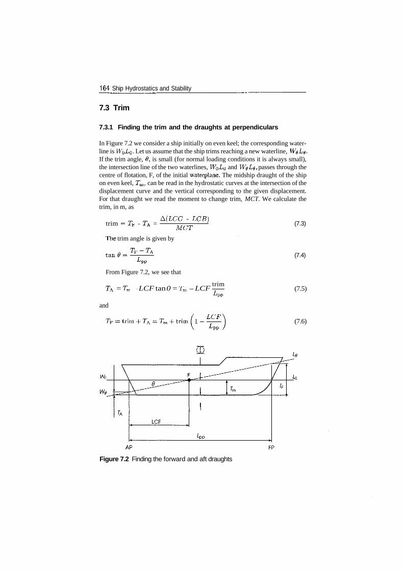
164 Ship Hydrostatics and Stability
7.3 Trim
7.3.1 Finding the trim and the draughts at perpendiculars
In Figure 7.2 we consider a ship initially on even keel; the corresponding water-line is WQ I/Q. Let us assume that the ship trims reaching a new waterline, W0L0.If the trim angle, 0, is small (for normal loading conditions it is always small),the intersection line of the two waterlines, WQ^O and W0L0, passes through thecentre of flotation, F, of the initial waterplane. The midship draught of the shipon even keel, Tm, can be read in the hydrostatic curves at the intersection of thedisplacement curve and the vertical corresponding to the given displacement.For that draught we read the moment to change trim, MCT. We calculate thetrim, in m, as
trim = TF - TA =A(LCG - LCB)
MCTThe trim angle is given by
(7.3)
(7.4)
From Figure 7.2, we see that
= Tm- LCF tan 0 = Tm- LCFtrim
(7.5)
and
LCF\i - — — (7.6)
wr
Figure 7.2 Finding the forward and aft draughts
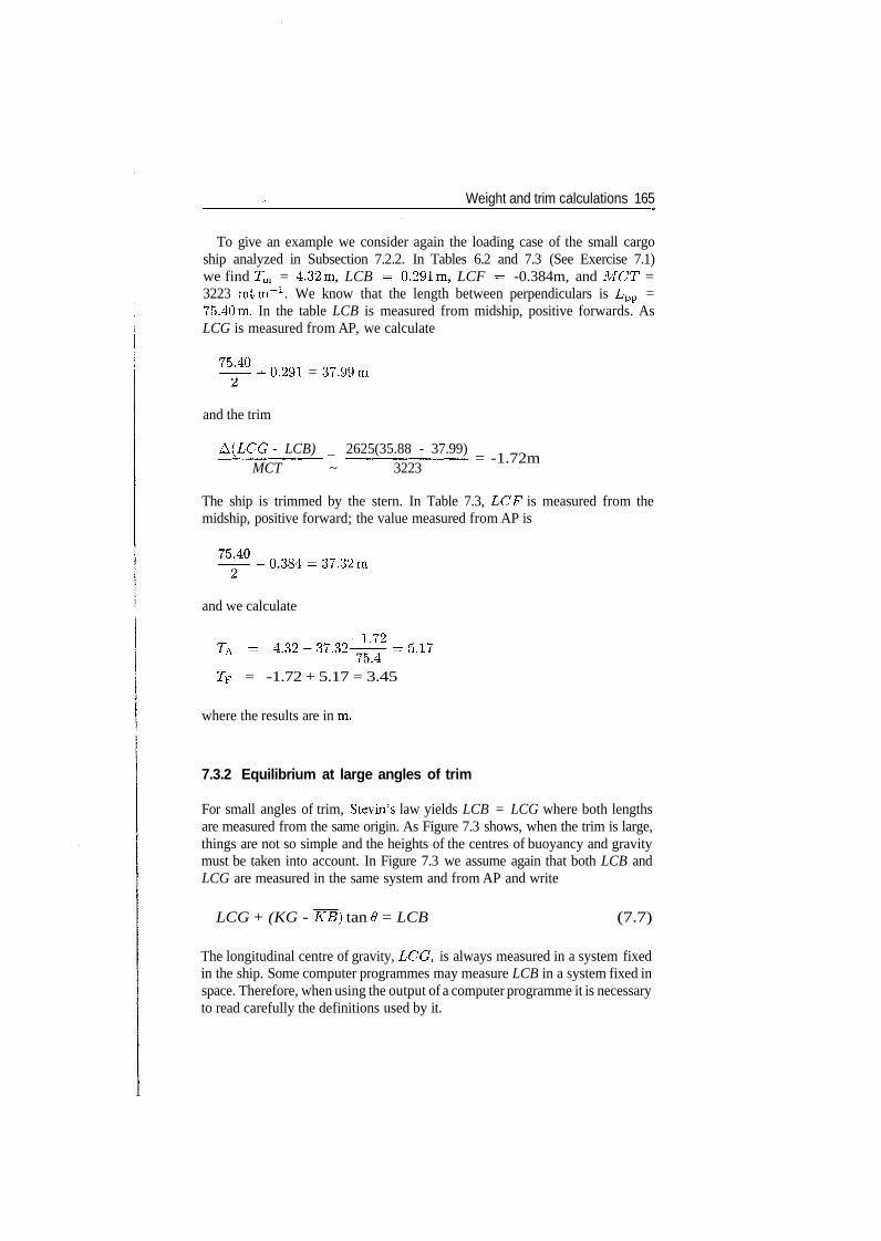
Weight and trim calculations 165
To give an example we consider again the loading case of the small cargoship analyzed in Subsection 7.2.2. In Tables 6.2 and 7.3 (See Exercise 7.1)we find Tm = 4.32m, LCB = 0.291m, LCF = -0.384m, and MCT =3223 rntm"1. We know that the length between perpendiculars is Lpp =75.40m. In the table LCB is measured from midship, positive forwards. AsLCG is measured from AP, we calculate
^-^ +0.291 = 37.99m
and the trim
&(LCG - LCB) _ 2625(35.88 - 37.99)MCT ~ 3223
= -1.72m
The ship is trimmed by the stern. In Table 7.3, LCF is measured from themidship, positive forward; the value measured from AP is
-37.32m
and we calculate
TA - 4.32-37.32—^=5.17
TF = -1.72 + 5.17 = 3.45
where the results are in m.
7.3.2 Equilibrium at large angles of trim
For small angles of trim, Stevin's law yields LCB = LCG where both lengthsare measured from the same origin. As Figure 7.3 shows, when the trim is large,things are not so simple and the heights of the centres of buoyancy and gravitymust be taken into account. In Figure 7.3 we assume again that both LCB andLCG are measured in the same system and from AP and write
LCG + (KG - TCB) tan 6 = LCB (7.7)
The longitudinal centre of gravity, LCG, is always measured in a system fixedin the ship. Some computer programmes may measure LCB in a system fixed inspace. Therefore, when using the output of a computer programme it is necessaryto read carefully the definitions used by it.
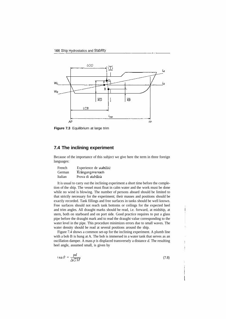
166 Ship Hydrostatics and Stability
LOG
FP
Figure 7.3 Equilibrium at large trim
7.4 The inclining experiment
Because of the importance of this subject we give here the term in three foreignlanguages:
French Experience de stabiliteGerman KrangungsversuchItalian Prova di stabilita
It is usual to carry out the inclining experiment a short time before the comple-tion of the ship. The vessel must float in calm water and the work must be donewhile no wind is blowing. The number of persons aboard should be limited tothat strictly necessary for the experiment; their masses and positions should beexactly recorded. Tank fillings and free surfaces in tanks should be well known.Free surfaces should not reach tank bottoms or ceilings for the expected heeland trim angles. All draught marks should be read, i.e. forward, at midship, atstern, both on starboard and on port side. Good practice requires to put a glasspipe before the draught mark and to read the draught value corresponding to thewater level in the pipe. This procedure minimizes errors due to small waves. Thewater density should be read at several positions around the ship.
Figure 7.4 shows a common set-up for the inclining experiment. A plumb linewith a bob B is hung at A. The bob is immersed in a water tank that serves as anoscillation damper. A mass p is displaced transversely a distance d. The resultingheel angle, assumed small, is given by
tan/9 =pd
AGM(7.8)
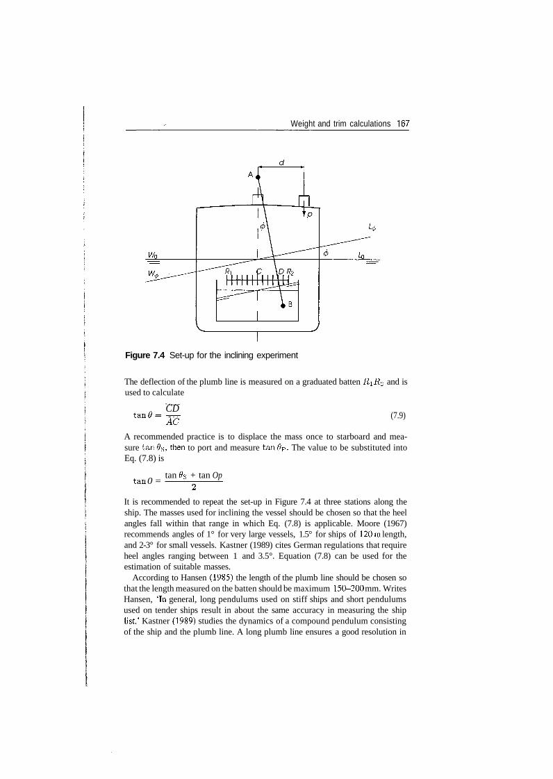
Weight and trim calculations 167
Figure 7.4 Set-up for the inclining experiment
The deflection of the plumb line is measured on a graduated batten RiR<2 and isused to calculate
CD= (7.9)
A recommended practice is to displace the mass once to starboard and mea-sure tan#s>then to port and measure tan$p. The value to be substituted intoEq. (7.8) is
tan 0 =tan #s + tan Op
It is recommended to repeat the set-up in Figure 7.4 at three stations along theship. The masses used for inclining the vessel should be chosen so that the heelangles fall within that range in which Eq. (7.8) is applicable. Moore (1967)recommends angles of 1° for very large vessels, 1.5° for ships of 120m length,and 2-3° for small vessels. Kastner (1989) cites German regulations that requireheel angles ranging between 1 and 3.5°. Equation (7.8) can be used for theestimation of suitable masses.
According to Hansen (1985) the length of the plumb line should be chosen sothat the length measured on the batten should be maximum 150-200 mm. WritesHansen, 'In general, long pendulums used on stiff ships and short pendulumsused on tender ships result in about the same accuracy in measuring the shiplist.' Kastner (1989) studies the dynamics of a compound pendulum consistingof the ship and the plumb line. A long plumb line ensures a good resolution in
168 Ship Hydrostatics and Stability
reading the graduation on the batten. On the other hand, a long plumb line canyield a large dynamic response to small-amplitude ship motions and increasereading errors. Kastner concludes that a length of 1.146 m is sufficient.
Today, the set-up shown in Figure 7.4 can be replaced by electronic instrumentsthat measure the heel angle (inclinometres, gyroscopic platforms) whose outputcan be fed directly to an on-board computer. A common way of checking theaccuracy of the results consists in plotting the tangents of heel angles, arc tan 9,against the heeling moments, pd. Equation (7.8) shows that the ideal plot shouldbe a straight line. Years ago Naval Architects fitted by eye a straight line passingthrough the plotted points. Nowadays computers and many hand calculatorsyield easily a least-squares fit. Example 1 shows how to do it.
When analyzing the results of the inclining experiment, Eq. (7.8) is rewritten as
pdtan<9
The interpretation of the results of inclining experiments requires the knowledgeof the displacement, A, and of the height of the metacentre above the baseline,KM. If the trim is small, one can read the desired values in the hydrostaticcurves, entering them with the measured mean draught, Tm, as input. Hansen(1985) quotes the limits imposed on the trim by the US Navy and the US CoastGuard. The recommended value for naval vessels is 0.67%, and for commercialships 1% of the ship length. If the trim is not small one can use the Bonjeancurves or a computer programme for hydrostatic calculations. When drawingthe waterline on the Bonjean curves we must not forget that, in general, theforward and the aft draught marks are not placed in the transverse planes of theforward and aft perpendiculars. Therefore, the values read on the marks must beadjusted and extrapolated to the FP and AP positions.
A computer programme for hydrostatic calculations can be used if the offsetsof the ship are stored in the required input format. Then, it is sufficient to runthe programme for the mean draught and the trim read during the incliningexperiment.
The ship hull behaves like a beam that can deflect under bending moments.Bending moments arise from differences between the longitudinal distributionof masses and that of hydrostatic pressures. Deflections of the hull beam alsocan be caused by differences between thermal expansions of the deck and of thebottom. The deflection can be calculated as the difference between the averageof forward and aft draught and the draught Tm measured at midship
d = rM - TF ~ TA (7.10)
Various authorities and authors publish formulae for calculating an equivalentdraught that allows the calculation of the displacement of a deflected hull. Forexample, Hansen (1985) uses a rather complicated formula recommended byNAVSEA, a design authority of the US Navy. Ziha (2002) analyzes the displace-
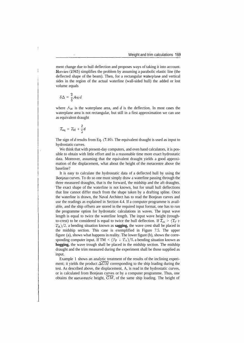
Weight and trim calculations 169
ment change due to hull deflection and proposes ways of taking it into account.Hervieu (1985) simplifies the problem by assuming a parabolic elastic line (thedeflected shape of the beam). Then, for a rectangular waterplane and verticalsides in the region of the actual waterline (wall-sided hull) the added or lostvolume equals
<5A = -Awdo
where Aw is the waterplane area, and d is the deflection. In most cases thewaterplane area is not rectangular, but still in a first approximation we can useas equivalent draught
2Teq = TU + -zd
o
The sign of d results from Eq. (7.10). The equivalent draught is used as input tohydrostatic curves.
We think that with present-day computers, and even hand calculators, it is pos-sible to obtain with little effort and in a reasonable time more exact hydrostaticdata. Moreover, assuming that the equivalent draught yields a good approxi-mation of the displacement, what about the height of the metacentre above thebaseline?
It is easy to calculate the hydrostatic data of a deflected hull by using theBonjean curves. To do so one must simply draw a waterline passing through thethree measured draughts, that is the forward, the midship and the aft draughts.The exact shape of the waterline is not known, but for small hull deflectionsthat line cannot differ much from the shape taken by a drafting spline. Oncethe waterline is drawn, the Naval Architect has to read the Bonjean curves anduse the readings as explained in Section 4.4. If a computer programme is avail-able, and the ship offsets are stored in the required input format, one has to runthe programme option for hydrostatic calculations in waves. The input wavelength is equal to twice the waterline length. The input wave height (trough-to-crest) to be considered is equal to twice the hull deflection. If Tm > (Tp -fTA)/2, a bending situation known as sagging, the wave crest shall be placed inthe midship section. This case is exemplified in Figure 7.5. The upperfigure (a), shows what happens in reality. The lower figure (b), shows the corre-sponding computer input. If TM < (Tp 4- T&}/1, a bending situation known ashogging, the wave trough shall be placed in the midship section. The midshipdraught and the trim measured during the experiment shall be those supplied asinput.
Example 1 shows an analytic treatment of the results of the inclining experi-ment; it yields the product AGM corresponding to the ship loading during thetest. As described above, the displacement, A, is read in the hydrostatic curves,or is calculated from Bonjean curves or by a computer programme. Thus, oneobtains the metacentric height, GM, of the same ship loading. The height of
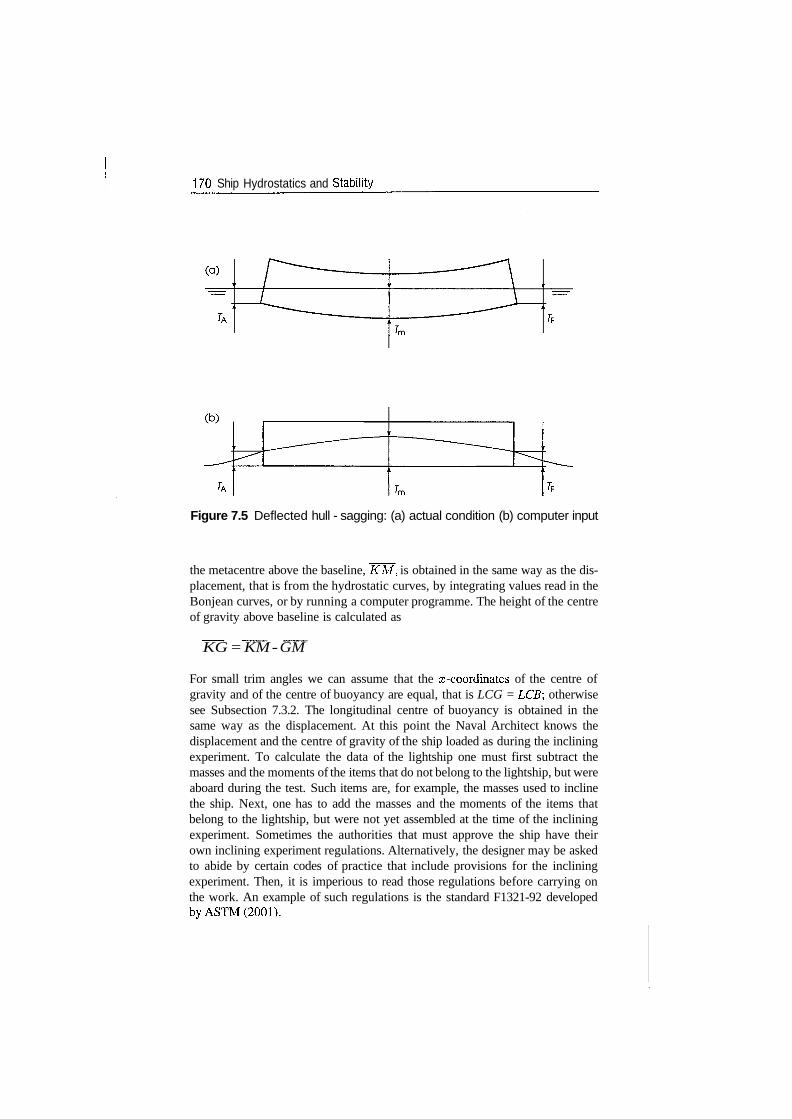
170 Ship Hydrostatics and Stability
Figure 7.5 Deflected hull - sagging: (a) actual condition (b) computer input
the metacentre above the baseline, KM, is obtained in the same way as the dis-placement, that is from the hydrostatic curves, by integrating values read in theBonjean curves, or by running a computer programme. The height of the centreof gravity above baseline is calculated as
KG = KM - GM
For small trim angles we can assume that the x-coordinates of the centre ofgravity and of the centre of buoyancy are equal, that is LCG = LCB\ otherwisesee Subsection 7.3.2. The longitudinal centre of buoyancy is obtained in thesame way as the displacement. At this point the Naval Architect knows thedisplacement and the centre of gravity of the ship loaded as during the incliningexperiment. To calculate the data of the lightship one must first subtract themasses and the moments of the items that do not belong to the lightship, but wereaboard during the test. Such items are, for example, the masses used to inclinethe ship. Next, one has to add the masses and the moments of the items thatbelong to the lightship, but were not yet assembled at the time of the incliningexperiment. Sometimes the authorities that must approve the ship have theirown inclining experiment regulations. Alternatively, the designer may be askedto abide by certain codes of practice that include provisions for the incliningexperiment. Then, it is imperious to read those regulations before carrying onthe work. An example of such regulations is the standard F1321-92 developedbyASTM(2001).
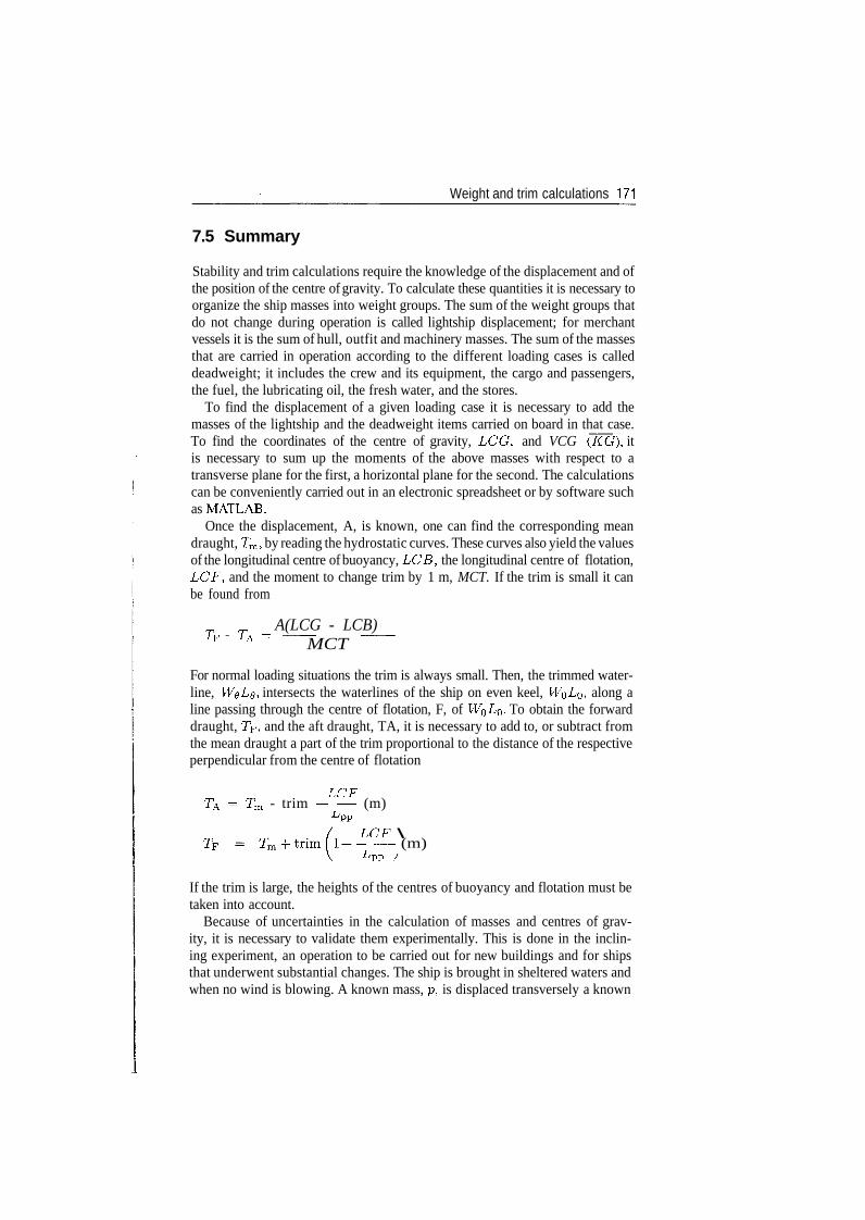
Weight and trim calculations 171
7.5 Summary
Stability and trim calculations require the knowledge of the displacement and ofthe position of the centre of gravity. To calculate these quantities it is necessary toorganize the ship masses into weight groups. The sum of the weight groups thatdo not change during operation is called lightship displacement; for merchantvessels it is the sum of hull, outfit and machinery masses. The sum of the massesthat are carried in operation according to the different loading cases is calleddeadweight; it includes the crew and its equipment, the cargo and passengers,the fuel, the lubricating oil, the fresh water, and the stores.
To find the displacement of a given loading case it is necessary to add themasses of the lightship and the deadweight items carried on board in that case.To find the coordinates of the centre of gravity, LOG, and VCG (KG), itis necessary to sum up the moments of the above masses with respect to atransverse plane for the first, a horizontal plane for the second. The calculationscan be conveniently carried out in an electronic spreadsheet or by software suchas MATLAB.
Once the displacement, A, is known, one can find the corresponding meandraught, Tm, by reading the hydrostatic curves. These curves also yield the valuesof the longitudinal centre of buoyancy, LCB, the longitudinal centre of flotation,LCF, and the moment to change trim by 1 m, MCT. If the trim is small it canbe found from
A(LCG - LCB)TF~TA = - MCT -
For normal loading situations the trim is always small. Then, the trimmed water-line, W0Lg, intersects the waterlines of the ship on even keel, WQ£O> along aline passing through the centre of flotation, F, of W$LQ. To obtain the forwarddraught, Tp, and the aft draught, TA, it is necessary to add to, or subtract fromthe mean draught a part of the trim proportional to the distance of the respectiveperpendicular from the centre of flotation
r s~i 77
TA - Tm - trim - — (m)
\I - - - (m)
^PP /
If the trim is large, the heights of the centres of buoyancy and flotation must betaken into account.
Because of uncertainties in the calculation of masses and centres of grav-ity, it is necessary to validate them experimentally. This is done in the inclin-ing experiment, an operation to be carried out for new buildings and for shipsthat underwent substantial changes. The ship is brought in sheltered waters andwhen no wind is blowing. A known mass, p, is displaced transversely a known
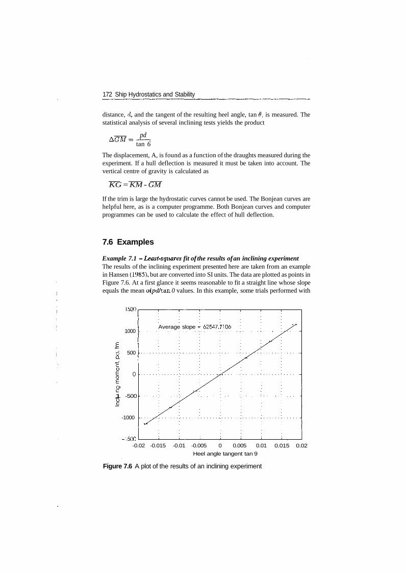
172 Ship Hydrostatics and Stability
distance, d, and the tangent of the resulting heel angle, tan 0, is measured. Thestatistical analysis of several inclining tests yields the product
pdtan 6
The displacement, A, is found as a function of the draughts measured during theexperiment. If a hull deflection is measured it must be taken into account. Thevertical centre of gravity is calculated as
KG = KM - GM
If the trim is large the hydrostatic curves cannot be used. The Bonjean curves arehelpful here, as is a computer programme. Both Bonjean curves and computerprogrammes can be used to calculate the effect of hull deflection.
7.6 Examples
Example 7.1 - Least-squares fit of the results of an inclining experimentThe results of the inclining experiment presented here are taken from an examplein Hansen (1985), but are converted into SI units. The data are plotted as points inFigure 7.6. At a first glance it seems reasonable to fit a straight line whose slopeequals the mean of pd/tan 0 values. In this example, some trials performed with
1500
1000
500-D
0
O>
1 -500oc
-1000
-1500
Average slope = 62547.7106
-0.02 -0.015 -0.01 -0.005 0 0.005 0.01
Heel angle tangent tan 9
0.015 0.02
Figure 7.6 A plot of the results of an inclining experiment
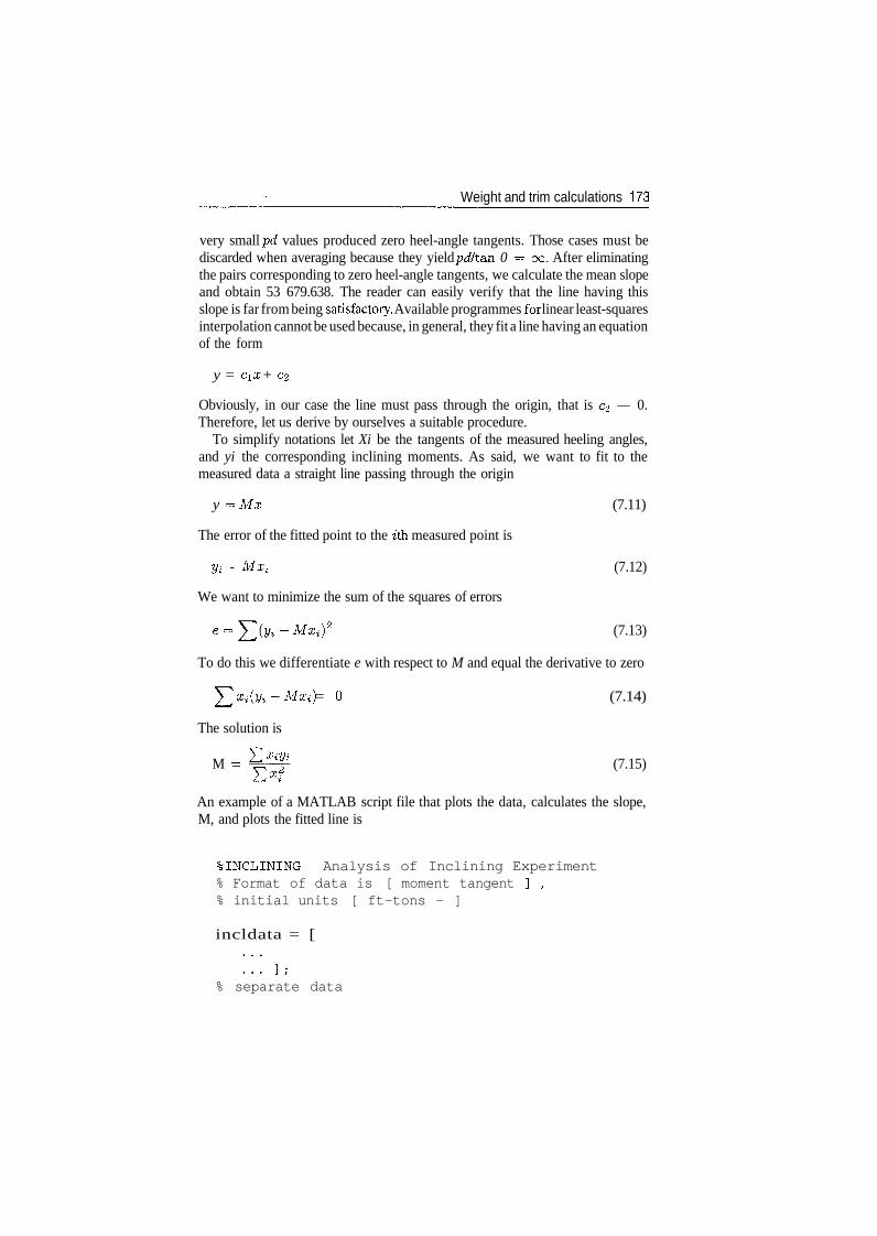
Weight and trim calculations 173
very small pd values produced zero heel-angle tangents. Those cases must bediscarded when averaging because they yield pd/t an 0 = oo. After eliminatingthe pairs corresponding to zero heel-angle tangents, we calculate the mean slopeand obtain 53 679.638. The reader can easily verify that the line having thisslope is far from being satisfactory. Available programmes for linear least-squaresinterpolation cannot be used because, in general, they fit a line having an equationof the form
y = cix + c2
Obviously, in our case the line must pass through the origin, that is c^ — 0.Therefore, let us derive by ourselves a suitable procedure.
To simplify notations let Xi be the tangents of the measured heeling angles,and yi the corresponding inclining moments. As said, we want to fit to themeasured data a straight line passing through the origin
y = Mx (7.11)
The error of the fitted point to the ith measured point is
y^ - MX, (7.12)
We want to minimize the sum of the squares of errors
2 (7.13)
To do this we differentiate e with respect to M and equal the derivative to zero
Y^Xi(yi-Mxi) = 0 (7.14)
The solution is
M = ̂ f (7.15)Exi
An example of a MATLAB script file that plots the data, calculates the slope,M, and plots the fitted line is
%INCLINING Analysis of Inclining Experiment% Format of data is [ moment tangent ] ,% initial units [ ft-tons - ]
incldata = [
% separate data
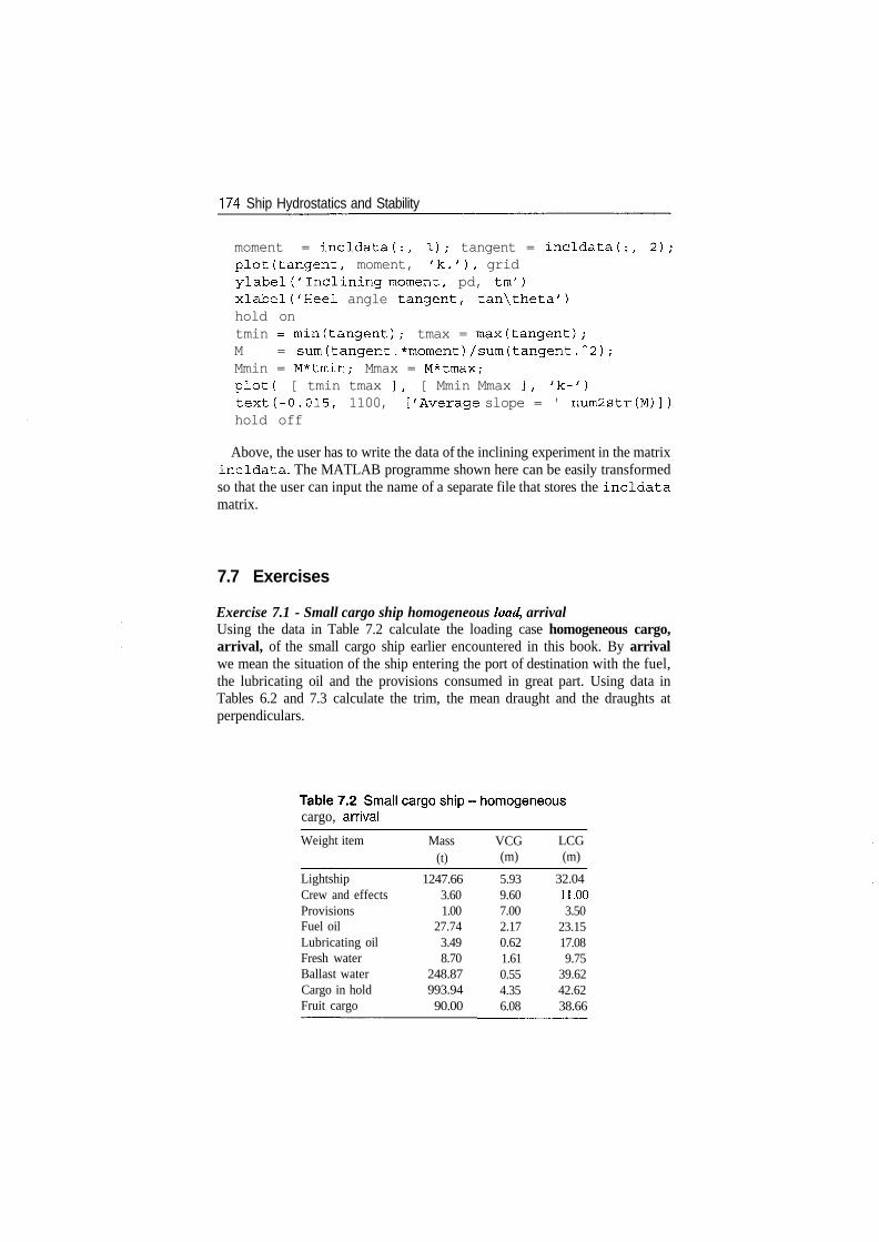
174 Ship Hydrostatics and Stability
moment = incldata(:, 1); tangent = incldata(:, 2);plot(tangent, moment, 'k.'), gridylabel('Inclining moment, pd, tm')xlabel('Heel angle tangent, tan\theta')hold ontmin = min(tangent); tmax = max(tangent);M = sum(tangent.*moment)/sum(tangent.~2);Mmin = M*tmin; Mmax = M*tmax;plot( [ tmin tmax ], [ Mmin Mmax ], 'k-')text(-0.015, 1100, ['Average slope = ' num2str(M)])hold off
Above, the user has to write the data of the inclining experiment in the matrixincldata. The MATLAB programme shown here can be easily transformedso that the user can input the name of a separate file that stores the incldatamatrix.
7.7 Exercises
Exercise 7.1 - Small cargo ship homogeneous load, arrivalUsing the data in Table 7.2 calculate the loading case homogeneous cargo,arrival, of the small cargo ship earlier encountered in this book. By arrivalwe mean the situation of the ship entering the port of destination with the fuel,the lubricating oil and the provisions consumed in great part. Using data inTables 6.2 and 7.3 calculate the trim, the mean draught and the draughts atperpendiculars.
cargo, arrival
Weight item
LightshipCrew and effectsProvisionsFuel oilLubricating oilFresh waterBallast waterCargo in holdFruit cargo
Mass(t)
1247.663.601.00
27.743.498.70
248.87993.9490.00
VCG(m)
5.939.607.002.170.621.610.554.356.08
LCG(m)
32.0411.003.50
23.1517.089.75
39.6242.6238.66
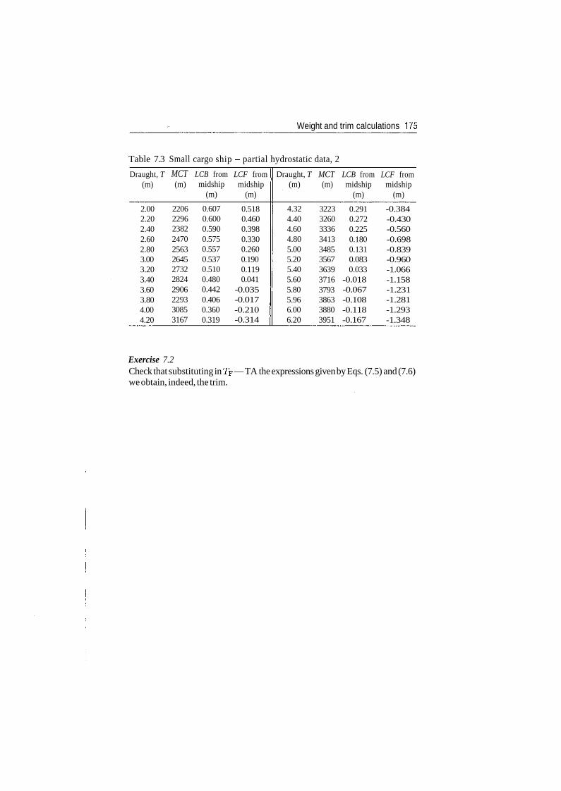
Weight and trim calculations 175
Table 7.3
Draught, T(m)
2.002.202.402.602.803.003.203.403.603.804.004.20
Small
MCT(m)
220622962382247025632645273228242906229330853167
cargo ship - partial hydrostatic data, 2
LCB frommidship
(m)
0.6070.6000.5900.5750.5570.5370.5100.4800.4420.4060.3600.319
LCF frommidship
(m)
0.5180.4600.3980.3300.2600.1900.1190.041
-0.035-0.017-0.210-0.314
Draught, T(m)
4.324.404.604.805.005.205.405.605.805.966.006.20
MCT(m)
322332603336341334853567363937163793386338803951
LCB frommidship
(m)
0.2910.2720.2250.1800.1310.0830.033
-0.018-0.067-0.108-0.118-0.167
LCF frommidship
(m)
-0.384-0.430-0.560-0.698-0.839-0.960-1.066-1.158-1.231-1.281-1.293-1.348
Exercise 7.2Check that substituting in Tp — TA the expressions given by Eqs. (7.5) and (7.6)we obtain, indeed, the trim.
8Intact stability regulations I
8.1 Introduction
In the preceding chapters, we presented the laws that govern the behaviour offloating bodies. We learnt how to find the parameters of a floating conditionand how to check whether or not that condition is stable. The models we devel-oped allow us to check the stability of a vessel under the influence of variousheeling moments. At this point we may ask what is satisfactory stability, or,in simpler terms, how much stable a ship must be. Analyzing the data of ves-sels that behaved well, and especially the data of vessels that did not survivestorms or other adverse conditions, various researchers and regulatory bodiesprescribed criteria for deciding if the stability is satisfactory. In this chapter, wepresent examples of such criteria. To use picturesque language, we may say thatin Chapters 2-7 we described laws of nature, while in this chapter we presentman-made laws. Laws of nature act independently of man's will and they alwaysgovern the phenomena to which they apply. Man-made laws, in our case stabil-ity regulations, have another meaning. Stability regulations prescribe criteria forapproving ship designs, accepting new buildings, or allowing ships to sail outof harbour. If a certain ship fulfils the requirements of given regulations, it doesnot mean that the ship can survive all challenges, but her chances of survivalare good because stability regulations are based on considerable experience andreasonable theoretic models. Conversely, if a certain ship does not fulfill certainregulations, she must not necessarily capsize, only the risks are higher and theowner has the right to reject the design or the authority in charge has the rightto prevent the ship from sailing out of harbour. Stability regulations are, in fact,codes of practice that provide reasonable safety margins. The codes are com-pulsory not only for designers and builders, but also for ship masters who mustcheck if their vessels meet the requirements in a proposed loading condition.
The codes of stability presented in this chapter take into consideration onlyphenomena discussed in the preceding chapters. The stability regulations of theGerman Federal Navy are based on the analysis of a phenomenon discussed inChapter 9; therefore, we defer their presentation until Chapter 10. For obviousreasons, it is not possible to include in this book all existing stability regulations;we only choose a few representative examples. Neither is it possible to presentall the provisions of any single regulation. We only want to draw the attention ofthe reader to the existence of such codes of practice, to show how the models
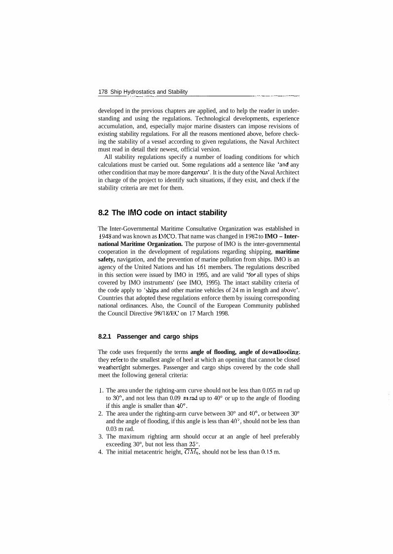
178 Ship Hydrostatics and Stability
developed in the previous chapters are applied, and to help the reader in under-standing and using the regulations. Technological developments, experienceaccumulation, and, especially major marine disasters can impose revisions ofexisting stability regulations. For all the reasons mentioned above, before check-ing the stability of a vessel according to given regulations, the Naval Architectmust read in detail their newest, official version.
All stability regulations specify a number of loading conditions for whichcalculations must be carried out. Some regulations add a sentence like 'and anyother condition that may be more dangerous'. It is the duty of the Naval Architectin charge of the project to identify such situations, if they exist, and check if thestability criteria are met for them.
8.2 The IMO code on intact stability
The Inter-Governmental Maritime Consultative Organization was established in1948 and was known as IMCO. That name was changed in 1982 to IMO - Inter-national Maritime Organization. The purpose of IMO is the inter-governmentalcooperation in the development of regulations regarding shipping, maritimesafety, navigation, and the prevention of marine pollution from ships. IMO is anagency of the United Nations and has 161 members. The regulations describedin this section were issued by IMO in 1995, and are valid 'for all types of shipscovered by IMO instruments' (see IMO, 1995). The intact stability criteria ofthe code apply to 'ships and other marine vehicles of 24 m in length and above'.Countries that adopted these regulations enforce them by issuing correspondingnational ordinances. Also, the Council of the European Community publishedthe Council Directive 98/18/EC on 17 March 1998.
8.2.1 Passenger and cargo ships
The code uses frequently the terms angle of flooding, angle of downflooding;they refer to the smallest angle of heel at which an opening that cannot be closedweathertight submerges. Passenger and cargo ships covered by the code shallmeet the following general criteria:
1. The area under the righting-arm curve should not be less than 0.055 m rad upto 30°, and not less than 0.09 mrad up to 40° or up to the angle of floodingif this angle is smaller than 40°.
2. The area under the righting-arm curve between 30° and 40°, or between 30°and the angle of flooding, if this angle is less than 40°, should not be less than0.03 m rad.
3. The maximum righting arm should occur at an angle of heel preferablyexceeding 30°, but not less than 25°.
4. The initial metacentric height, <2M0, should not be less than 0.15 m.
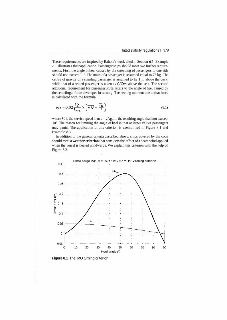
Intact stability regulations I 179
These requirements are inspired by Rahola's work cited in Section 6.1. Example8.1 illustrates their application. Passenger ships should meet two further require-ments. First, the angle of heel caused by the crowding of passengers to one sideshould not exceed 10°. The mass of a passenger is assumed equal to 75 kg. Thecentre of gravity of a standing passenger is assumed to lie 1 m above the deck,while that of a seated passenger is taken as 0.30m above the seat. The secondadditional requirement for passenger ships refers to the angle of heel caused bythe centrifugal force developed in turning. The heeling moment due to that forceis calculated with the formula
MT = 0.02 (8.1)
where VQ is the service speed in m s l. Again, the resulting angle shall not exceed10°. The reason for limiting the angle of heel is that at larger values passengersmay panic. The application of this criterion is exemplified in Figure 8.1 andExample 8.3.
In addition to the general criteria described above, ships covered by the codeshould meet a weather criterion that considers the effect of a beam wind appliedwhen the vessel is heeled windwards. We explain this criterion with the help ofFigure 8.2.
0.35
-0.05
Small cargo ship, A = 26251, KG = 5m, IMO turning criterion
10 20 30 40 50Heel angle (°)
60 70 80 90
Figure 8.1 The IMO turning criterion
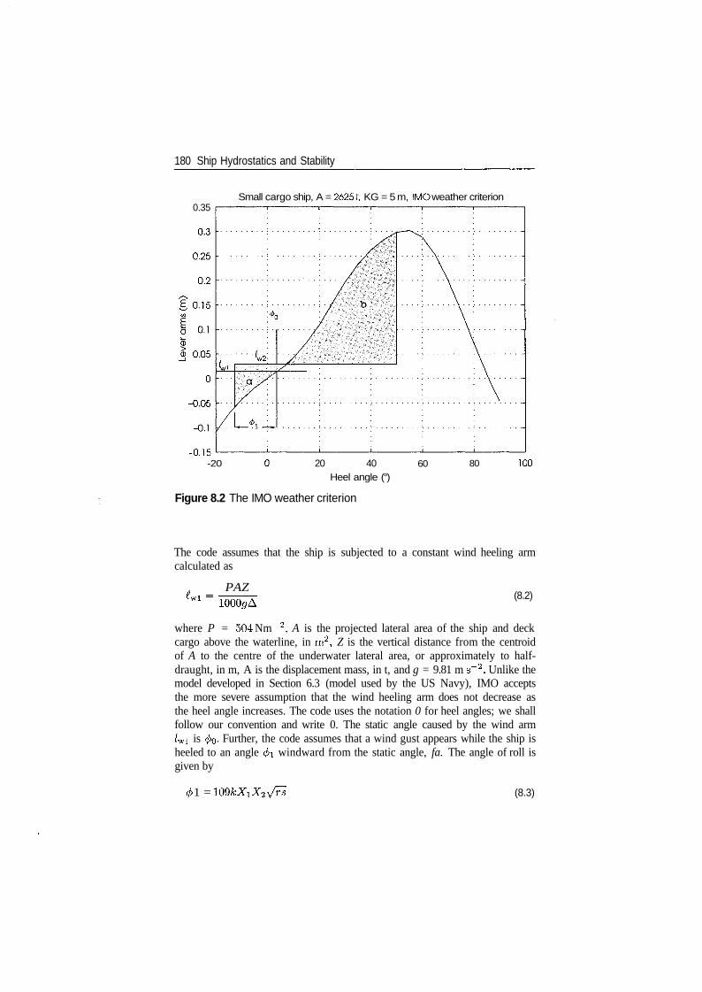
180 Ship Hydrostatics and Stability
Small cargo ship, A = 26251, KG = 5 m, IMO weather criterion0.35
-0.15-20 20 40
Heel angle (°)60 80 100
Figure 8.2 The IMO weather criterion
The code assumes that the ship is subjected to a constant wind heeling armcalculated as
PAZ(8.2)
where P = 504 Nm 2, A is the projected lateral area of the ship and deckcargo above the waterline, in m2, Z is the vertical distance from the centroidof A to the centre of the underwater lateral area, or approximately to half-draught, in m, A is the displacement mass, in t, and g = 9.81 m s~2. Unlike themodel developed in Section 6.3 (model used by the US Navy), IMO acceptsthe more severe assumption that the wind heeling arm does not decrease asthe heel angle increases. The code uses the notation 0 for heel angles; we shallfollow our convention and write 0. The static angle caused by the wind arm/wi is 0o- Further, the code assumes that a wind gust appears while the ship isheeled to an angle 0i windward from the static angle, fa. The angle of roll isgiven by
1 = (8.3)
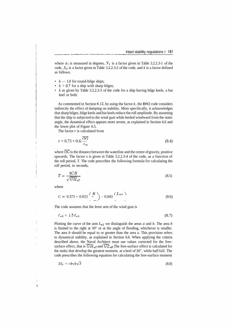
Intact stability regulations I 181
where 0i is measured in degrees, X\ is a factor given in Table 3.2.2.3-1 of thecode, X<2 is a factor given in Table 3.2.2.3-2 of the code, and k is a factor definedas follows:
• k — 1.0 for round-bilge ships;• k = 0.7 for a ship with sharp bilges;• k as given by Table 3.2.2.3-3 of the code for a ship having bilge keels, a bar
keel or both.
As commented in Section 6.12, by using the factor k, the IMO code considersindirectly the effect of damping on stability. More specifically, it acknowledgesthat sharp bilges, bilge keels and bar keels reduce the roll amplitude. By assumingthat the ship is subjected to the wind gust while heeled windward from the staticangle, the dynamical effect appears more severe, as explained in Section 6.6 andthe lower plot of Figure 6.5.
The factor r is calculated from
r = 0.73 + 0.6 — (8.4)-*m
where OG is the distance between the waterline and the centre of gravity, positiveupwards. The factor s is given in Table 3.2.2.3-4 of the code, as a function ofthe roll period, T. The code prescribes the following formula for calculating theroll period, in seconds,
(8.5)VG'Meff
where
C = 0.373 + 0.023 - J - 0.043 (8.6)
The code assumes that the lever arm of the wind gust is
*w2 = 1.5*wi (8.7)
Plotting the curve of the arm £w2 we distinguish the areas a and b. The area bis limited to the right at 50° or at the angle of flooding, whichever is smaller.The area b should be equal to or greater than the area a. This provision refersto dynamical stability, as explained in Section 6.6. When applying the criteriadescribed above, the Naval Architect must use values corrected for the free-surface effect, that is GMeR and GZefi. The free-surface effect is calculated forthe tanks that develop the greatest moment, at a heel of 30°, while half full. Thecode prescribes the following equation for calculating the free-surface moment
MF = vb-fkVS (8.8)
182 Ship Hydrostatics and Stability
where v is the tank capacity in m3, b is the maximum breadth of the tank in m,7 is the density of the liquid in tm~3, 5 is equal to the block coefficient ofthe tank, v/bth, with h, the maximum height and £, the maximum length, andk, a coefficient given in Table 3.3.3 of the code as function of b/h and heelangle. The contribution of small tanks can be ignored if Mp/Amin < 0.01 m at30°. We would like to remind the reader that present computer programmes forhydrostatic calculations yield values of the free-surface lever arms for any tankform described in the input, and for any heel angle. It is our opinon that, whenavailable, such values should be preferred to those obtained with Eq. (8.8).
The code specifies the loading cases for which stability calculations must beperformed. For example, for cargo ships the criteria shall be checked for thefollowing four conditions:
1. Full-load departure, with cargo homogeneously distributed throughout allcargo spaces.
2. Full-load arrival, with 10% stores and fuel.3. Ballast departure, without cargo.4. Ballast arrival, with 10% stores and fuel.
8.2.2 Cargo ships carrying timber deck cargoes
Section 4.1 of the code applies to cargo ships that carry on their deck timbercargo extending longitudinally between superstructures and transversally on thefull deck breadth, excepting a reasonable gunwale. Where there is no limitingsuperstructure at the aft, the cargo should extend at least to the after end of theaftermost hatch. For such ships the area under the righting-arm curve shouldnot be less than 0.08 mrad up to 40° or up to the angle of flooding, whicheveris smaller. The effective metacentric height should be positive in all stages ofloading, voyage and unloading. The calculations should take into account theabsorption of water by the deck cargo, and the water trapped within the cargo.
8.2.3 Fishing vessels
Section 4.2 of the code applies to decked seagoing vessels; they should fulfillthe first three general requirements described in Subsection 8.2.1, while themetacentric height should not be less than 0.35 m for single-deck ships. If thevessel has a complete superstructure, or the ship length is equal to or largerthan 70 m, the metacentric height can be reduced with the agreement of thegovernment under whose flag the ship sails, but it should not be less than 0.15 m.The weather criterion applies in full to ships of 45 m length and longer. For fishingvessels whose length ranges between 24 and 45 m the code prescribes a windgradient such that the pressure ranges between 316 and 504 Nm~2 for heights of1-6 m above sea level. Decked vessels shorter than 30 m must have a minimum
Intact stability regulations I 183
metacentric height calculated with a formula given in paragraph 4.2.6.1 of thecode.
8.2.4 Mobile offshore drilling units
Section 4.6 of the code applies to mobile drilling units whose keels were laid after1 March 1991. The wind force is calculated by considering the shape factors ofstructural members exposed to the wind, and a height coefficient ranging between1.0 and 1.8 for heights above the waterline varying from 0 to 256m. The areaunder the righting-arm curve up to the second static angle, or the downfloodingangle, whichever is smaller, should exceed by at least 40% the area under thewind arm. The code also describes an alternative intact-stability criterion fortwo-pontoon, column-stabilized semi-submersible units.
8.2.5 Dynamically supported craft
A vessel is a dynamically supported craft (DSC) in one of the following cases:
1 . If, in one mode of operation, a significant part of the weight is supported byother than buoyancy forces.
2. If the craft is able to operate at Froude numbers, Fu — V/^/gL, equal orgreater than 0.9.
The first category includes air-cushion vehicles and hydrofoil boats. Hydrofoilboats float, or sail, in the hull-borne or displacement mode if their weight issupported only by the buoyancy force predicted by Archimedes' principle. Athigher speeds hydrodynamic forces develop on the foils and they balance animportant part of the boat weight. Then, we say that the craft operates in thefoil-borne mode.
Section 4.8 of the code applies to DSC operating between two ports situatedin different countries. The requirements for hydrofoil boats are described inSubsection 4.8.7 of the code. The heeling moment in turning, in the displacementmode, is calculated as
where VQ is the speed in turning, in m s"1, and MR results in kN m. The formulais valid if the radius of the turning circle lies between 2L and 4L. The resultingangles of inclination should not exceed 8° .
The wind heeling moment, in the displacement mode, in kNm, should becalculated as
Mv =
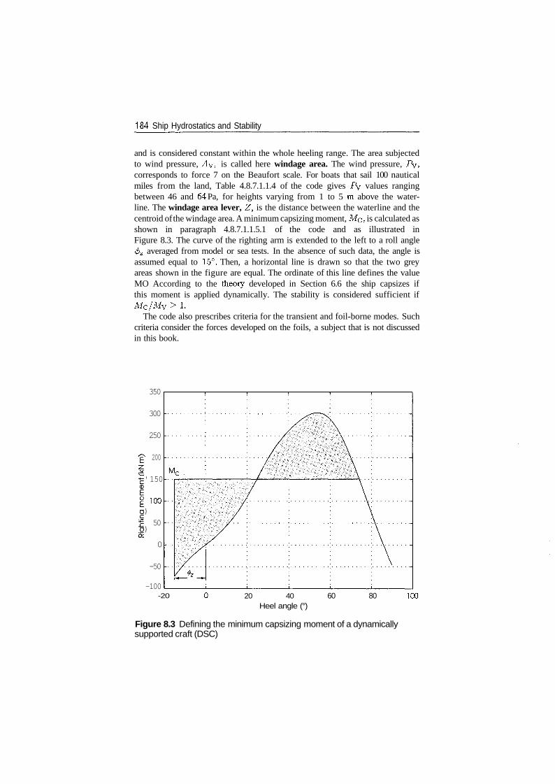
184 Ship Hydrostatics and Stability
and is considered constant within the whole heeling range. The area subjectedto wind pressure, Ay, is called here windage area. The wind pressure, Py,corresponds to force 7 on the Beaufort scale. For boats that sail 100 nauticalmiles from the land, Table 4.8.7.1.1.4 of the code gives Py values rangingbetween 46 and 64 Pa, for heights varying from 1 to 5 m above the water-line. The windage area lever, Z, is the distance between the waterline and thecentroid of the windage area. A minimum capsizing moment, MC, is calculated asshown in paragraph 4.8.7.1.1.5.1 of the code and as illustrated inFigure 8.3. The curve of the righting arm is extended to the left to a roll angle0Z averaged from model or sea tests. In the absence of such data, the angle isassumed equal to 15°. Then, a horizontal line is drawn so that the two greyareas shown in the figure are equal. The ordinate of this line defines the valueMO According to the theory developed in Section 6.6 the ship capsizes ifthis moment is applied dynamically. The stability is considered sufficient ifMC/MV > i.
The code also prescribes criteria for the transient and foil-borne modes. Suchcriteria consider the forces developed on the foils, a subject that is not discussedin this book.
350
300
250
k 200
' 150
100)
50)
0
-50
-100-20 20 40
Heel angle (°)60 80 100
Figure 8.3 Defining the minimum capsizing moment of a dynamicallysupported craft (DSC)
Intact stability regulations I 185
8.2.6 Container ships greater than 100 m
Section 4.9 of the code defines a form factor C depending on the main dimensionsof the ship and the configuration of hatches (Figure 4.9-1 in the code). Theminimum values of areas under the righting-arm curve are prescribed in theform a/C, where a is specified for several heel intervals.
8.2.7 Icing
Chapter 5 of the code bears the title 'Ice considerations'. The following values,prescribed for fishing vessels, illustrate the severity of the problem. Stabilitycalculations should be carried out assuming ice accretion (this is the term usedin the code) with the surface densities:
• 30 kg m~2 on exposed weather decks and gangways;• 7.5 kg m~2 for projected lateral areas on each side, above the waterplane.
The code specifies the geographical areas in which ice accretion can occur.
8.2.8 Inclining and rolling tests
Chapter 7 of the code contains the instructions for carrying on inclining experi-ments for all ships covered by the regulations, and roll-period tests for ships upto 70m in length. The relationship between the metacentric height, GMo, andthe roll period, T, is given as
GM0 = ( ^-)
where B is the ship breadth.An interesting part of the Annex refers to the plot of heel-angle tangents against
heeling moments; it explains the causes of deviations from a straight line, suchas free surfaces of liquids, restrictions of movements, steady wind or wind gust.
8.3 The regulations of the US Navy
In 1944, an American fleet was caught by a tropical storm in the Pacific Ocean.In a short time three destroyers capsized, a fourth one escaped because a funnelbroke down under the force of the wind. This disaster influenced the developmentof stability regulations for the US Navy. They were first published by Sarchinand Goldberg in 1962. These regulations were subsequently adopted by othernavies.
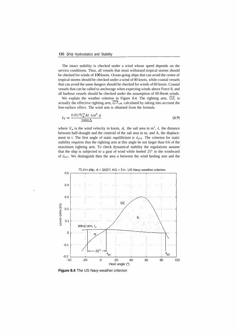
186 S-hip Hydrostatics and Stability
The intact stability is checked under a wind whose speed depends on theservice conditions. Thus, all vessels that must withstand tropical storms shouldbe checked for winds of 100 knots. Ocean-going ships that can avoid the centre oftropical storms should be checked under a wind of 80 knots, while coastal vesselsthat can avoid the same dangers should be checked for winds of 60 knots. Coastalvessels that can be called to anchorage when expecting winds above Force 8, andall harbour vessels should be checked under the assumption of 60-knots winds.
We explain the weather criterion in Figure 8.4. The righting arm, GZ, isactually the effective righting arm, GZeff, calculated by taking into account thefree-surface effect. The wind arm is obtained from the formula
O.OITV^AI cos2
1000A(8.9)
where Vw is the wind velocity in knots, A, the sail area in m2, £, the distancebetween half-draught and the centroid of the sail area in m, and A, the displace-ment in t. The first angle of static equilibrium is </>sti. The criterion for staticstability requires that the righting arm at this angle be not larger than 0.6 of themaximum righting arm. To check dynamical stability the regulations assumethat the ship is subjected to a gust of wind while heeled 25° to the windwardof </>sti. We distinguish then the area a between the wind heeling arm and the
0.5
0.4
0.3
0.2
0.1
75.4m ship, A = 26251, KG = 5m, US Navy weather criterion
-0.1
-0.2-40 -20 0 20 40
Heel angle (°)
Figure 8.4 The US Navy weather criterion
60 80 100
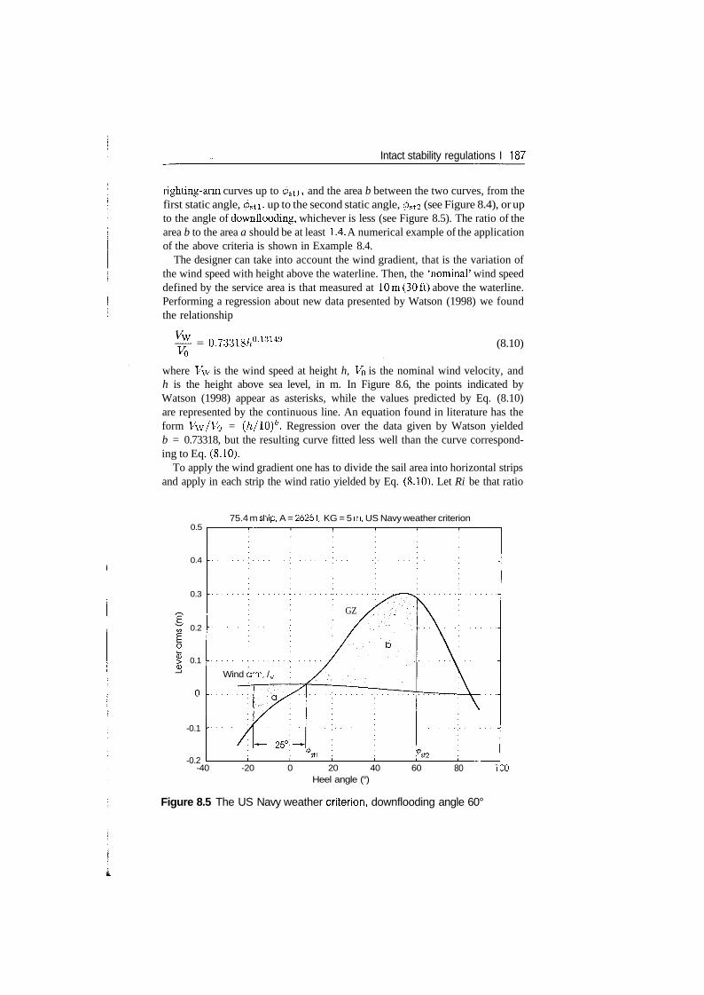
Intact stability regulations I 187
righting-arm curves up to 0sti, and the area b between the two curves, from thefirst static angle, 0sti, up to the second static angle, 0st2 (see Figure 8.4), or upto the angle of downflooding, whichever is less (see Figure 8.5). The ratio of thearea b to the area a should be at least 1.4. A numerical example of the applicationof the above criteria is shown in Example 8.4.
The designer can take into account the wind gradient, that is the variation ofthe wind speed with height above the waterline. Then, the 'nominal' wind speeddefined by the service area is that measured at 10m (30ft) above the waterline.Performing a regression about new data presented by Watson (1998) we foundthe relationship
= 0.73318/10'13149 (8.10)
where 1/w is the wind speed at height h, VQ is the nominal wind velocity, andh is the height above sea level, in m. In Figure 8.6, the points indicated byWatson (1998) appear as asterisks, while the values predicted by Eq. (8.10)are represented by the continuous line. An equation found in literature has theform Vw/Vb = (/i/10)6. Regression over the data given by Watson yieldedb = 0.73318, but the resulting curve fitted less well than the curve correspond-ing to Eq. (8.10).
To apply the wind gradient one has to divide the sail area into horizontal stripsand apply in each strip the wind ratio yielded by Eq. (8.10). Let Ri be that ratio
0.5
0.4
0.3
0.2
0.1
75.4 m ship, A = 26251 KG = 5 m, US Navy weather criterion
-0.1
-0.2
GZ
Wind arm, /,
-40 -20 0 20 40 60Heel angle (°)
80 100
Figure 8.5 The US Navy weather criterion, downflooding angle 60°
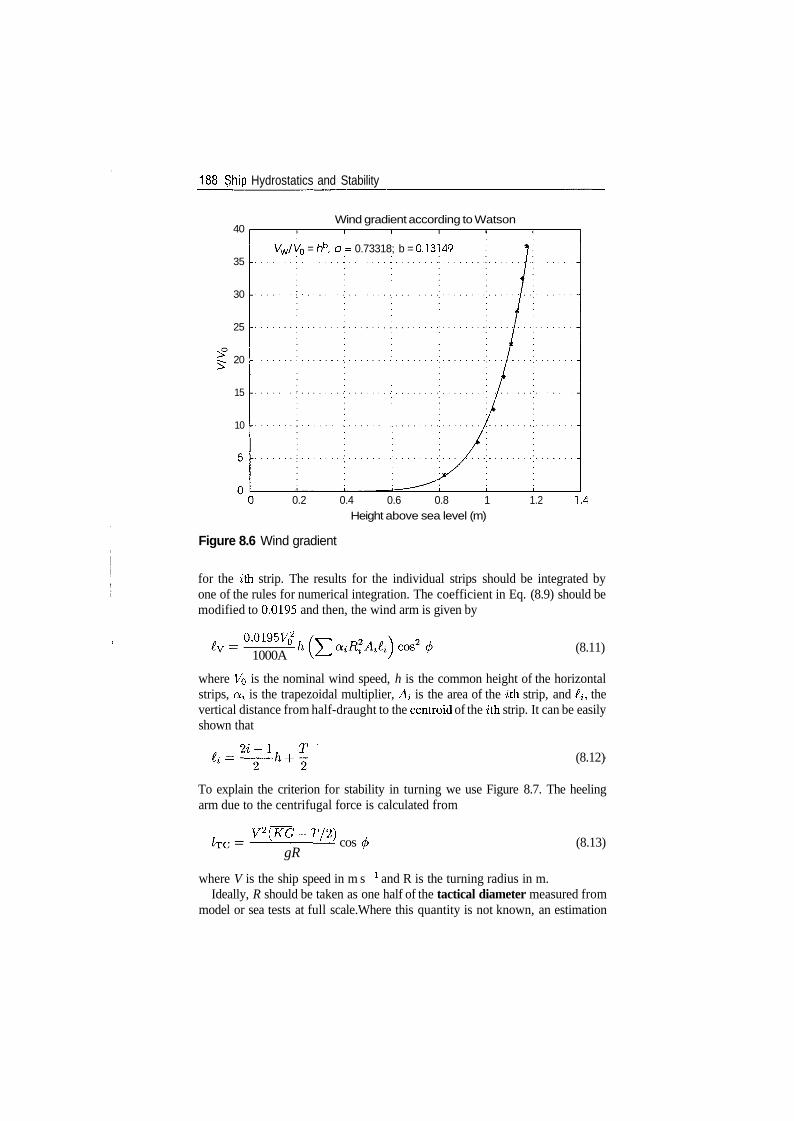
188 Ship Hydrostatics and Stability
40
35
30
25
20
15
10
Wind gradient according to Watson
= hb,a = 0.73318; b = 0.13149
0.2 0.4 0.6 0.8 1Height above sea level (m)
1.2 1.4
Figure 8.6 Wind gradient
for the ith strip. The results for the individual strips should be integrated byone of the rules for numerical integration. The coefficient in Eq. (8.9) should bemodified to 0.0195 and then, the wind arm is given by
O.Q195VQ2
1000A(8.11)
where VQ is the nominal wind speed, h is the common height of the horizontalstrips, o-i is the trapezoidal multiplier, AI is the area of the ith strip, and £j, thevertical distance from half-draught to the centroid of the ^th strip. It can be easilyshown that
(8.12)
To explain the criterion for stability in turning we use Figure 8.7. The heelingarm due to the centrifugal force is calculated from
V2(KG-T/2}gR
cos (8.13)
where V is the ship speed in m s l and R is the turning radius in m.Ideally, R should be taken as one half of the tactical diameter measured from
model or sea tests at full scale.Where this quantity is not known, an estimation
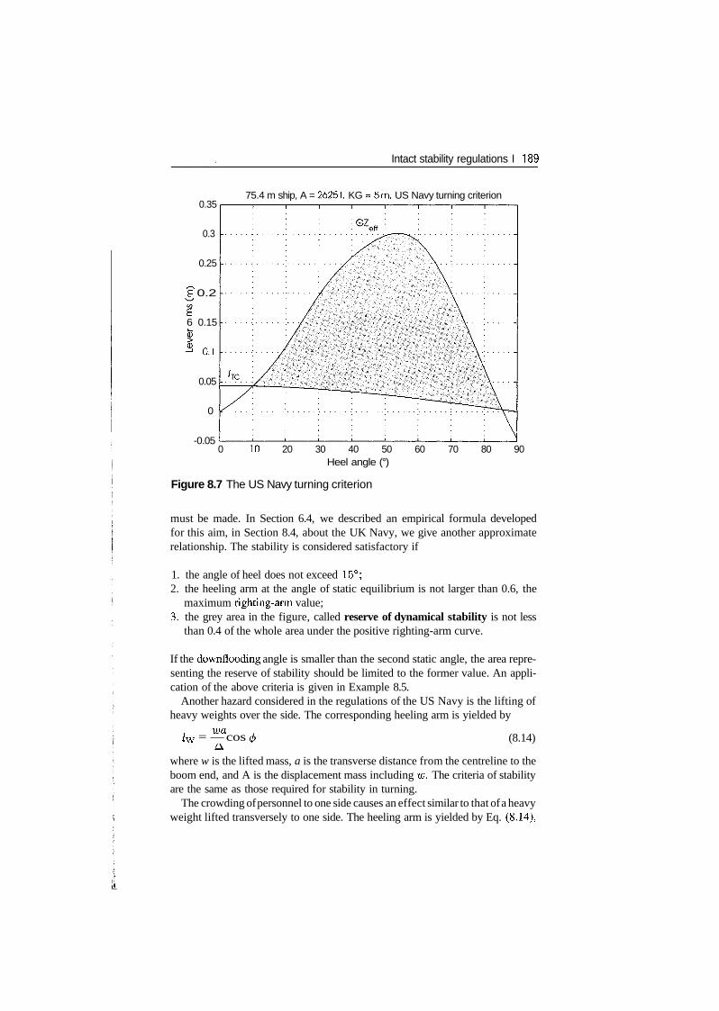
Intact stability regulations I 189
0.35
0.3
0.25
? 0.2
6 0.15
K,
0.05
0
-0.05
75.4 m ship, A = 26251, KG = 5m, US Navy turning criterion
0 10 20 30 40 50 60 70 80 90Heel angle (°)
Figure 8.7 The US Navy turning criterion
must be made. In Section 6.4, we described an empirical formula developedfor this aim, in Section 8.4, about the UK Navy, we give another approximaterelationship. The stability is considered satisfactory if
1. the angle of heel does not exceed 15°;2. the heeling arm at the angle of static equilibrium is not larger than 0.6, the
maximum righting-arm value;3. the grey area in the figure, called reserve of dynamical stability is not less
than 0.4 of the whole area under the positive righting-arm curve.
If the downflooding angle is smaller than the second static angle, the area repre-senting the reserve of stability should be limited to the former value. An appli-cation of the above criteria is given in Example 8.5.
Another hazard considered in the regulations of the US Navy is the lifting ofheavy weights over the side. The corresponding heeling arm is yielded by
walw = — cos (8.14)
where w is the lifted mass, a is the transverse distance from the centreline to theboom end, and A is the displacement mass including w. The criteria of stabilityare the same as those required for stability in turning.
The crowding of personnel to one side causes an effect similar to that of a heavyweight lifted transversely to one side. The heeling arm is yielded by Eq. (8.14),
190 Ship Hydrostatics and Stability
assuming that the personnel moved to one side as far as possible when five mencrowd in one square metre. Again, the stability is considered sufficient if therequirements given for stability in turning are met.
8.4 The regulations of the UK Navy
The stability standard of the Royal Navy evolved from the criteria published bySarchin and Goldberg in 1962. The first British publication appeared in 1980 asNES 109. The currently valid version is Issue 4 (see MoD, 1999a). The docu-ment should be read in conjunction with the publication SSP 42 (MoD, 1999b).The British standard is issued by the Ministry of Defence, shortly MoD, and isapplicable to vessels with a military role, to vessels designed to MoD standardsbut without a military role, and to auxiliary vessels. Vessels with a military roleare exposed to enemy action or to similar dangers during peacetime exercises.We shall discuss here only the provisions related to such vessels. The standardNES 109 has two parts, the first dealing with conventional ships, the second withunconventional vessels. The second category includes:
1. monohull vessels of rigid construction having a speed in knots larger than4\/I/wL» where the waterline length is measured in m;
2. multi-hull vessels;3. dynamically supported vessels.
In this book, we briefly discuss only the provisions for conventional vessels.According to NES 109 the displacement and KG values used in stability calcu-lations should include growth margins. For warships the weight growth marginshould be 0.65% of the lightship displacement, for each year of service. The KGmargin should be 0.45% of the lightship KG, for each year of service.
The shape of the righting-arm curve should be such that:
• the area under the curve, up to 30°, is not less than 0.08 m rad;• the area up to 40° is not less than 0.133 m rad;• the area between 30° and 40° is not less than 0.048 m rad;• the maximum GZ is not less than 0.3 m and should occur at an angle not
smaller than 30°.
One can immediately see that all these requirements are considerably more severethan those prescribed by IMO 95 for merchant ships.
The stability under beam winds should be checked for the following windspeeds:
• 90 knots for ocean-going vessels;• 70 knots for ocean-going or coastal vessels that can avoid extreme conditions;
Intact stability regulations I 191
50 knots for coastal vessels that can be called to anchorage to avoid windsover Force 8, and for harbour vessels.
These values are lower than those required by the US Navy and partially coincidewith those specified by the German Navy. The angle of heel caused by the windshould not exceed 30°. The criterion for statical stability is the same as thatof the US Navy, that is, the righting arm at the first static angle should not begreater than 0.6, the maximum righting arm. As in the American regulations,it is assumed that the ship rolls 25° windwards from the first static angle, andit is required that the reserve of stability should not be less than 1.4 times thearea representing the wind heeling energy. Figure 1.3 in the UK regulationsshows that the area representing the reserve of stability is limited at the right bythe downflooding angle. When checking stability in turning the correspondingship speed should be 0.65 times the speed on a straight-line course. If no betterdata are available, it should be assumed that the radius of turning equals 2.5times the length between perpendiculars. The angle of heel in turning shouldbe less than 20°, a requirement less severe than that of the US Navy. The staticcriterion, regarding the value of the righting arm at the first static angle, and thedynamic criterion, regarding the reserve of stability, are the same as those of theUS Navy.
To check stability when lifting a heavy mass over the side, the heeling armshould be calculated from
w(a cos(f) + d sin 0)/w = -r (8.15)
where a is the horizontal distance of the tip of the boom from the centreline, andd is the height of the point of suspension above the deck. Stability is consideredsufficient if the following criteria are met:
1. The angle of heel is less than 15°.2. The righting arm at the first static angle is less than half the maximum righting
arm.3. The reserve of stability is larger than half the total area under the righting-arm
curve. The area representing the reserve of stability is limited at the right bythe angle of downflooding.
It can be easily seen that criteria 2 and 3 are more stringent than those of theUS Navy.
The NES 109 standard also specifies criteria for checking stability under icing.A thickness of 150mm should be assumed for all horizontal decks, with an icedensity equal to 950kgm~3. Only the effect on displacement and KG shouldbe considered, and not the effect on the sail area.
192 Ship Hydrostatics and Stability
8.5 A criterion for sail vessels
The revival of the interest for large sailing vessels and several accidents justifiednew researches and the development of codes of stability for this category ofships. Thus, the UK Department of Transport sponsored a research carried outat the Wolfson Unit for Marine Transportation and Industrial Aerodynamics ofthe University of Southampton (Deakin, 1991). The result of the research is thecode of stability described in this section. A more recent research is presentedby Cleary, Daidola and Reyling (1996). The authors compare the stability cri-teria for sailing ships adopted by the US Coast Guard, the Wolfson Unit, theGermanischer Lloyd, the Bureau Veritas, the Ateliers & Chantiers du Havre, andDr Ing Alimento of the University of Genoa. These criteria are illustrated byapplying them to one ship, the US Coast Guard training barque Eagle, formerlyHorst Wessel built in 1936 in Germany.
In this section, we describe the intact stability criteria of The code of practicefor safety of large commercial sailing & motor vessels' issued by the UK Mari-time and Coastguard Agency (Maritime, 2001). The code 'applies to vessels incommercial use for sport or pleasure... that are 24 metres in load line length andover... and that do not carry cargo and do not carry more than 12 passengers.'For shorter sailing vessels, the UK Marine Safety Agency published anothercode, namely 'The safety of small commercial sailing vessels.'
The research carried out at the Wolfson Unit yielded a number of interestingresults:
1 . Form coefficients of sail rigs vary considerably and are difficult to predict.We mean here the coefficient c in
1 2P = CPv
where p is the pressure, p, the air density, and V, the speed of the windcomponent perpendicular to the sail.
2. The wind- arm curve behaves like cos1'3 0.3. Wind gusts do not build up instantly, as conservatively assumed (see Sec-
tion 6.6). The wind speed of gusts due to atmospheric turbulence are unlikelyto exceed 1 .4 times the hourly mean, have rise times of 10 to 20 s and durationsof less than a minute. Other gusts, due to other atmospheric phenomena, areknown as squalls and they can be much more dangerous. Because the rise-uptimes of significant gusts are usually larger than the natural roll periods ofsailing vessels, ships do not respond as described in Section 6.6, but havetime to find equilibrium positions close to the intersection of the gust-armcurve and the righting-arm curve.
4. Sails considerably increase the damping of the roll motion, limiting theresponse to a wind gust and enhancing the effect described above. Thus, the
Intact stability regulations I 193
heel angle caused by a wind gust is smaller than that predicted by the balanceof areas representing wind energy and righting-arm work (Section 6.6).
Based on the above conclusions, the criterion of intact stability adopted by theUK Maritime and Coastguard Agency does not consider the sail rig and the windmoment developed on it. The code simply provides the skipper with a means forappreciating the maximum allowable heel angle under a steady wind, if windgusts are expected. Sailing at the recommended angle will avoid the submergenceunder gusts of openings that could lead to ship loss.
The code defines the downflooding angle as the angle at which openings hav-ing an 'aggregate area' whose value in metres is greater than A/1500, submerge.The displacement, A, is measured in t. Deakin (1991) explains that under hisassumptions the mass of water flowing through the above openings during 5 min-utes equals the ship displacement. No ship is expected to float after a floodingof this extent, and five minutes are considered a maximum reasonable time ofsurvival. For those who wish to understand Deakim's reasoning we remind thatthe flow through an orifice is proportional to the orifice area multiplied by thefluid speed
where a is the orifice area, cy, a discharge coefficient always smaller than 1,g, the acceleration of gravity, and h, the level of water above the orifice. Theauthors of the code assume cy = 1 and h — 1 m. We calculate
1500x V2x9.81 x l-O.OOSAnr 1
It follows that in sea water 5.5 minutes are required for a mass of water equal tothe displacement mass.
We use Figure 8.8 to describe the criterion for intact stability. The righting-armcurve is marked GZ; it is based on the data of an actual training yacht. At thedownflooding angle we measure the value of the righting arm, GZf . We assumehere the downflooding angle fa = 60°. We calculate a gust- wind lever in uprightcondition
WLO=
The dashed line curve represents the gust arm. Under the assumptions that thegust speed is 1.4 times the speed of the steady wind, the pressure due to steadywind is one half that of the gust, and so is the corresponding heeling arm. There-fore, we draw the 'derived curve' as the dash-dot line beginning at WLO/2
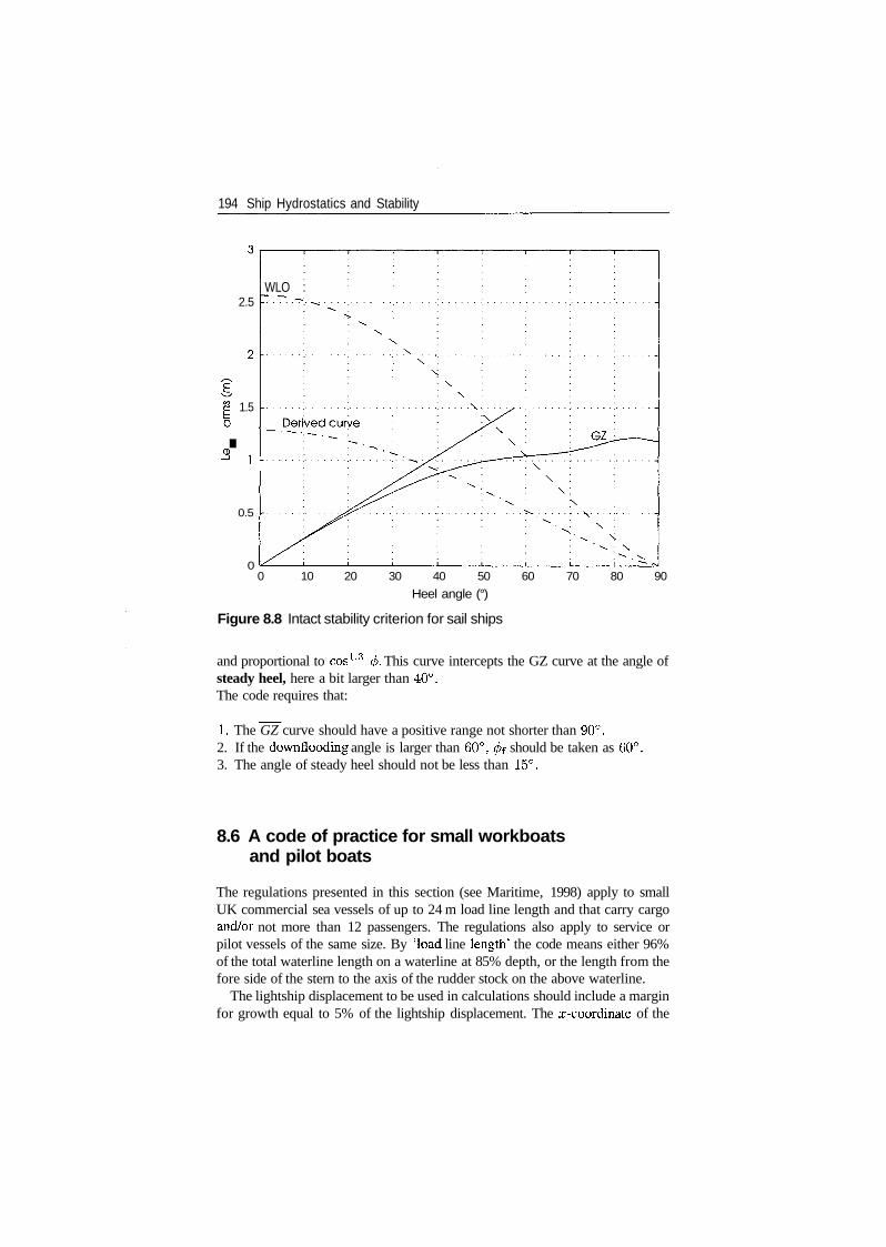
194 Ship Hydrostatics and Stability
WLO :2.5
1.50
I
0.5
00 10 20 30 40 50 60 70 80 90
Heel angle (°)
Figure 8.8 Intact stability criterion for sail ships
and proportional to cos1-3 (j>. This curve intercepts the GZ curve at the angle ofsteady heel, here a bit larger than 40°.The code requires that:
1. The GZ curve should have a positive range not shorter than 90°.2. If the downflooding angle is larger than 60°, </>f should be taken as 60°.3. The angle of steady heel should not be less than 15°.
8.6 A code of practice for small workboatsand pilot boats
The regulations presented in this section (see Maritime, 1998) apply to smallUK commercial sea vessels of up to 24 m load line length and that carry cargoand/or not more than 12 passengers. The regulations also apply to service orpilot vessels of the same size. By 'load line length' the code means either 96%of the total waterline length on a waterline at 85% depth, or the length from thefore side of the stern to the axis of the rudder stock on the above waterline.
The lightship displacement to be used in calculations should include a marginfor growth equal to 5% of the lightship displacement. The x-coordinate of the
Intact stability regulations I 195
centre of gravity of this margin shall equal LOG, and the ^-coordinate shall equaleither the height of the centre of the weather deck amidships or the lightship KG,whichever is the higher. Curves of statical stability shall be calculated for thefollowing loading cases:
• loaded departure, 100% consumables;• loaded arrival, 10% consumables;• other anticipated service conditions, including possible lifting appliances.
The stability is considered sufficient if the following two criteria are met inaddition to criteria 1-4 in Subsection 8.2.1.
1 . The maximum of the righting-arm curve should occur at an angle of heel notsmaller than 25°. _
2. The effective, initial metacentric height, GMe^, should not be less than0.35m.
If a multihull vessel does not meet the above stability criteria, the vessel shallmeet the following alternative criteria:
1. If the maximum of the righting-arm curve occurs at 15°, the area under thecurve shall not be less than 0.085 mrad. If the maximum occurs at 30°, thearea shall not be less than 0.055 mrad.
2. If the maximum of the righting-arm curve occurs at an angle ^czmax situatedbetween 15° and 30°, the area under the curve shall not be less than
A = 0.055 + 0.002(30° - 0GZmax) (8.16)
where A is measured in m rad.3. The area under the righting-arm curve between 30° and 40°, or between 30°
and the angle of downflooding, if this angle is less than 40°, shall not be lessthan 0.03 mrad.
4. The righting arm shall not be less than 0.2 m at 30°.5. The maximum righting arm shall occur at an angle not smaller than 15°.6. The initial metacentric height shall not be less than 0.35 m.
The intact stability of new vessels of less than 15m length that carry a combinedload of passengers and cargo of less than 1000kg is checked in an incliningexperiment. The passengers, the crew without the skipper, and the cargo aretransferred to one side of the ship, while the skipper may be assumed to stay atthe steering position. Under these conditions the angle of heel shall not exceed 7°.
196 Ship Hydrostatics and Stability
For vessels with a watertight weather deck the freeboard shall be not less than75 mm at any point. For open boats the freeboard to the top of the gunwale shallnot be less than 250 mm at any point.
8.7 Regulations for internal-water vessels
8.7.1 EC regulations
The European prescriptions for internal-navigation ships are contained in direc-tive 82/714/CEE of October 1982. In September 1999, a proposal for modifica-tions was submitted to the European parliament. The proposal details the internalwaterways of Europe for which it is valid.
Intact stability is considered sufficient if:
« the heel angle due to the crowding of passengers on one side does notexceed 10°;
• the angle of heel due to the combined effect of crowding, wind pressure andcentrifugal force does not exceed 12°.
In calculations it should be assumed that fuel and water tanks are half full. Theconsidered wind pressure is 0.1 kN m~2. At the angles of heel detailed above,the minimum freeboard should not be less than 0.2 m. If lateral windows can beopened, a minimum safety distance of 0.1 m should exist.
8.7.2 Swiss regulations
The Swiss regulations for internal navigation are contained in an ordinance of8 October 1978. Some modifications are contained in an ordinance of 9 March2001 of the Swiss Parliament (Der Schweizerische Bundesrat). According tothem cargo ships should be tested under a wind pressure of 0.25 kNm~2. Theheeling moment in turning, in kN m, should be calculated as
where c > 0.4 is a coefficient to be supplied by the builder or the operator.Stability is considered sufficient if under the above assumptions the heelingangle does not exceed 5° and the deck side does not submerge. The metacentricheight should not be less than 1 m. The required wind pressure is definitely lowerthan that required for sea-going ships. On the other hand, the other requirementsare more stringent.
Intact stability regulations I 197
8.8 Summary
The IMO Code on Intact Stability applies to ships and other marine vehiclesof 24 m length and above. The metacentric height of passenger and cargo shipsshould be at least 0.15 m, and the areas under the righting-arm curve, betweencertain heel angles, should not be less than the values indicated in the document.Passenger vessels should not heel in turning more than 10°. In addition, pas-senger and cargo ships should meet a weather criterion in which it is assumedthat the vessel is subjected to a wind arm that is constant throughout the heel-ing range. The heeling arm of wind gusts is assumed equal to 1.5 times the heelingarm of the steady wind. If a wind gust appears while the ship is heeledwindwards by an angle prescribed by the code, the area representing the reserveof buoyancy should not be less than the area representing the heel energy. Theformer area is limited to the right by the angle of downflooding or by 50°,whichever is less.
The IMO code contains special requirements for ships carrying timber ondeck, for fishing vessels, for mobile offshore drilling units, for dynamicallysupported craft, and for containerships larger than 100 m. The code also containsrecommendations for inclining and for rolling tests.
The stability regulations of the US Navy prescribe criteria for statical anddynamical stability under wind, in turning, under passenger crowding on oneside, and when lifting heavy weights over the side. The static criterion requiresthat the righting arm at the first static angle should not exceed 60% of the maxi-mum righting arm. When checking dynamical stability under wind, it is assumedthat the ship rolled 25° windwards from the first static angle. Then, the area rep-resenting the reserve of stability should be at least 1.4 times the area represent-ing the heeling energy. When checking stability in turning, or under crowdingor when lifting heavy weights, the angle of heel should not exceed 15° andthe reserve of stability should not be less than 40% of the total area under therighting-arm curve.
The stability regulations of the UK Navy are derived from those of theUS Navy. In addition to static and dynamic criteria such as those mentionedabove, the UK standard includes requirements concerning the areas underthe righting-arm curve. The minimum values are higher than those prescribedby IMO for merchant ships. While the wind speeds specified by the UK stan-dard are lower than those in the US regulations, the stability criteria are moresevere.
A quite different criterion is prescribed in the code for large sailing vesselsissued by the UK Ministry of Transport. As research proved that wind-pressurecoefficients of sail rigs cannot be predicted, the code does not take into accountthe sail configuration and the heeling moments developed on it. The documentpresents a simple method for finding a heel angle under steady wind, such thatthe heel angle caused by a gust of wind would be smaller than the angle leadingto downflooding and ship loss. The steady heel angle should not exceed 15°, andthe range of positive heeling arms should not be less than 90°.

198 Ship Hydrostatics and Stability
Additional regulations mentioned in this chapter are a code for small work-boats issued in the UK, and codes for internal-navigation vessels issued by theEuropean Parliament and by the Swiss Parliament.
8.9 Examples
Example 8.1 - Application of the IMO general requirements for cargo andpassenger shipsLet us check if the small cargo ship used in Subsection 7.2.2 meets the IMO gen-eral requirements. We assume the same loading condition as in that section. Thevessel was built four decades before the publication of the IMO code for intactstability; therefore, it is not surprising if several criteria are not met. Table 8.1contains the calculation of righting-arm levers and areas under the righting-armcurve. Figure 8.2 shows the corresponding statical stability curve. The areasunder the righting-arm curve are obtained by means of the algorithm describedin Section 3.4. The analysis of the results leads to the following conclusions:
1. The area under the GZ& curve, up to 30°, is 0.043 mrad, less than therequired 0.055. The area up to 40° equals 0.084mrad, less than the required0.09 mrad. The area between 30° and 40° equals 0.04mrad, more than therequired 0.03 mrad.
Table 8.1 Small cargo ship - the IMO general requirements
Heel angle(°)
0.05.0
10.015.020.025.030.035.040.045.050.055.060.065.070.075.080.085.090.0
4(m)
0.0000.4590.9181.3771.8332.2832.7173.1243.5013.8474.1594.4314.6534.8214.9375.0075.0365.0304.994
(KG + t^smt(m)
0.0000.4390.8751.3041.7242.1302.5202.8913.2403.5643.8614.1294.3654.5684.7364.8684.9635.0215.040
b GZefi Area under righting arm(m) (m2)
0.0000.0190.0430.0720.1090.1530.1970.2330.2620.2830.2980.3020.2880.2530.2010.1390.0730.009
-0.046
0.0000.0010.0040.0090.0170.0280.0430.0620.0840.1070.1330.1590.1850.2080.2280.2430.2520.2560.254
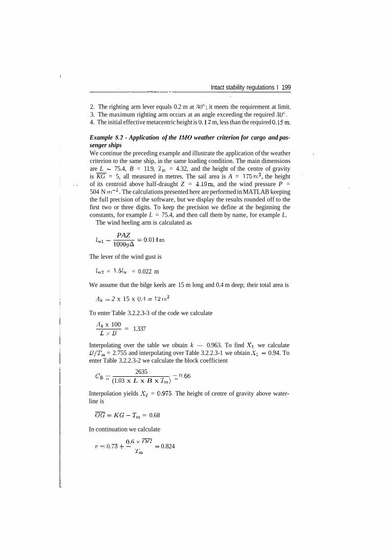
Intact stability regulations I 199
2. The righting arm lever equals 0.2 m at 30°; it meets the requirement at limit.3. The maximum righting arm occurs at an angle exceeding the required 30°.4. The initial effective metacentric height is 0. 1 2 m, less than the required 0.15m.
Example 8.2 - Application of the IMO weather criterion for cargo and pas-senger shipsWe continue the preceding example and illustrate the application of the weathercriterion to the same ship, in the same loading condition. The main dimensionsare L = 75.4, B = 11.9, Tm = 4.32, and the height of the centre of gravityis KG = 5, all measured in metres. The sail area is A = 175m2, the heightof its centroid above half-draught Z = 4.19m, and the wind pressure P =504 N m~~2 . The calculations presented here are performed in MATLAB keepingthe full precision of the software, but we display the results rounded off to thefirst two or three digits. To keep the precision we define at the beginning theconstants, for example L = 75.4, and then call them by name, for example L.
The wind heeling arm is calculated as
PAZ
The lever of the wind gust is
Zw2 = 1-5/wi = 0.022 m
We assume that the bilge keels are 15 m long and 0.4 m deep; their total area is
Ak = 2 x 15 x 0.4= 12m2
To enter Table 3.2.2.3-3 of the code we calculate
Ak x 100LxB
= 1.337
Interpolating over the table we obtain k — 0.963. To find X\ we calculateB/Tm = 2.755 and interpolating over Table 3.2.2.3-1 we obtain X\ = 0.94. Toenter Table 3.2.2.3-2 we calculate the block coefficient
2635" (1.03 x L x B x Tm) " '
Interpolation yields X<2 = 0.975. The height of centre of gravity above water-line is
-Tm = 0.68
In continuation we calculate
= 0.73 + - = 0.824
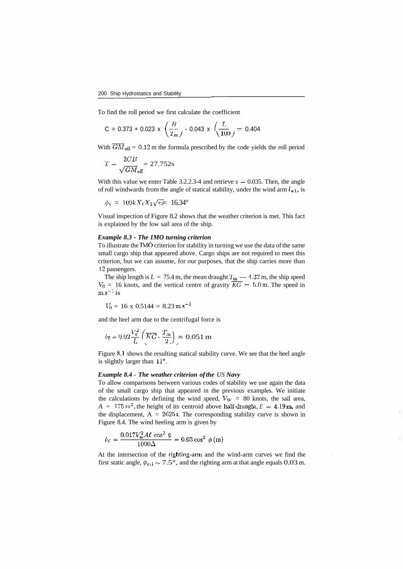
200 Ship Hydrostatics and Stability
To find the roll period we first calculate the coefficient
C = 0.373 + 0.023 x ( - - 0.043 x (-- = 0.404
With GMeff = 0.12 m the formula prescribed by the code yields the roll period
T= <2°B = 27.752s
With this value we enter Table 3.2.2.3-4 and retrieve s = 0.035. Then, the angleof roll windwards from the angle of statical stability, under the wind arm /wi, is
0i = W9kXiX2Vrs = 16.34°
Visual inspection of Figure 8.2 shows that the weather criterion is met. This factis explained by the low sail area of the ship.
Example 8.3 - The 1MO turning criterionTo illustrate the IMO criterion for stability in turning we use the data of the samesmall cargo ship that appeared above. Cargo ships are not required to meet thiscriterion, but we can assume, for our purposes, that the ship carries more than12 passengers.
The ship length is L = 75.4 m, the mean draught Tm — 4.32 m, the ship speedVQ = 16 knots, and the vertical centre of gravity KG = 5.0m. The speed inms"1 is
V0 = 16 x 0.5144 = 8.23 ms"1
and the heel arm due to the centrifugal force is
1T = 0.02^- (~KG - ^p j - 0.051 m
Figure 8.1 shows the resulting statical stability curve. We see that the heel angleis slightly larger than 11°.
Example 8.4 - The weather criterion of the US NavyTo allow comparisons between various codes of stability we use again the dataof the small cargo ship that appeared in the previous examples. We initiatethe calculations by defining the wind speed, Vw = 80 knots, the sail area,A = 175m2, the height of its centroid above half-draught, £ = 4.19m, andthe displacement, A = 26251. The corresponding stability curve is shown inFigure 8.4. The wind heeling arm is given by
cos2 6
1QQQA
At the intersection of the righting-arm and the wind-arm curves we find thefirst static angle, </>sti ~ 7.5°, and the righting arm at that angle equals 0.03 m.
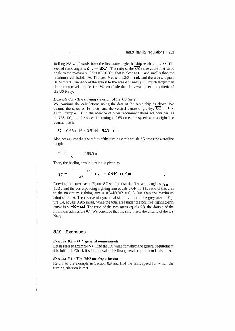
Intact stability regulations I 201
Rolling 25° windwards from the first static angle the ship reaches —17.5°. Thesecond static angle is <ftst2 — 85.7°. The ratio of the GZ value at the first staticangle to the maximum GZ is 0.03/0.302, that is close to 0.1 and smaller than themaximum admissible 0.6. The area b equals 0.235 mrad, and the area a equals0.024 mrad. The ratio of the area b to the area a is nearly 10, much larger thanthe minimum admissible 1 .4. We conclude that the vessel meets the criteria ofthe US Navy.
Example 8.5 - The turning criterion of the US NavyWe continue the calculations using the data of the same ship as above. Weassume the speed of 16 knots, and the vertical centre of gravity, KG = 5m,as in Example 8.3. In the absence of other recommendations we consider, asin NES 109, that the speed in turning is 0.65 times the speed on a straight-linecourse, that is
V0 = 0.65 x 16 x 0.5144 = 5.35ms"1
Also, we assume that the radius of the turning circle equals 2.5 times the waterlinelength
R=2- = 188.5m
Then, the heeling arm in turning is given by
= T/2) cog = Q Q44 ̂
gR
Drawing the curves as in Figure 8.7 we find that the first static angle is 0sti —10.3°, and the corresponding righting arm equals 0.044 m. The ratio of this armto the maximum righting arm is 0.044/0.302 = 0.15, less than the maximumadmissible 0.6. The reserve of dynamical stability, that is the grey area in Fig-ure 8.4, equals 0.205 mrad, while the total area under the positive righting-armcurve is 0.256mrad. The ratio of the two areas equals 0.8, the double of theminimum admissible 0.4. We conclude that the ship meets the criteria of the USNavy.
8.10 Exercises
Exercise 8.1 - IMO general requirementsLet us refer to Example 8.1. Find the KG value for which the general requirement4 is fulfilled. Check if with this value the first general requirement is also met.
Exercise 8.2 - The IMO turning criterionReturn to the example in Section 8.9 and find the limit speed for which theturning criterion is met.

202 Ship Hydrostatics and Stability
Exercise 8.3 - The IMO turning criterionReturn to the example in Exercise 8.2 and check if with the vertical centre ofgravity, KG, found in Section 8.10 the turning criterion is met.
Exercise 8.4 - The US-Navy turning criterionReturn to Example 8.4 and redo the calculations assuming a wind speed of100 knots.
Exercise 8.5 - The code for small vesselsCheck that for ^czmax — 15° and 30°, Eq. (8.16) yields the values specified incriterion 1 for multihull vessels (Section 8.6).

9Parametric resonance
9.1 Introduction
Up to this chapter we assumed that the sea surface is plane. Actually, such asituation never occurs in nature, not even in the sheltered waters of a harbour.Waves always exist, even if very small. Can waves influence ship stability? Andif yes, how? Arndt and Roden (1958) and Wendel (1965) cite French engineersthat discussed this question at the end of the nineteenth century (J. Pollard andA. Dudebout, 1892, Theorie du Navire, Vol. Ill, Paris). In the 1920s, Doyereexplained how waves influence stability and proposed a method to calculate thatinfluence. After 1950 the study of this subject was prompted by the sinking of afew ships that were considered stable.
At a first glance beam seas - that is waves whose crests are parallel to theship - seem to be the most dangerous. In fact, parallel waves cause large anglesof heel; loads can get loose and endanger stability. However, it can be shownthat the resultant of the weight force and of the centrifugal force developed inwaves is perpendicular to the wave surface. Therefore, a correctly loaded vesselwill never capsize in parallel waves, unless hit by large breaking waves. Shipscan capsize in head seas - that is waves travelling against the ship - andespecially in following seas - that is waves travelling in the same directionwith the ship. This is the lesson learnt after the sinking of the ship Irene Olden-dorff in the night between 30 and 31 December 1951. Kurt Wendel analyzed thecase and reached the conclusion that the disaster was due to the variation of therighting arm in waves. Divers that checked the wreck found it intact, an obser-vation that confirmed Wendel's hypothesis. Another disaster was that of Pamir.Again, the calculation of the righting arm in waves surprised the researchers(Arndt, 1962).
Kerwin (1955) analyzed a simple model of the variation of GM in waves andits influence on ship stability. His investigations included experiments carriedout at Delft and he reports difficulties that we attribute to the equipment availableat that time.
To confirm the results of their calculations, researchers from Hamburg carriedout model tests in a towing tank (Arndt and Roden, 1958) and with self-propelledmodels on a nearby lake (Wendel, 1965). Post-mortem analysis of other marinedisasters showed that the righting arm was severely reduced when the ship wason the wave crest. Sometimes it was even negative.
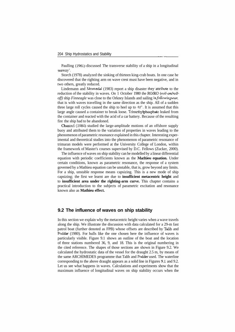
204 Ship Hydrostatics and Stability
Paulling (1961) discussed The transverse stability of a ship in a longitudinalseaway'.
Storch (1978) analyzed the sinking of thirteen king-crab boats. In one case hediscovered that the righting arm on wave crest must have been negative, and intwo others, greatly reduced.
Lindemann and Skomedal (1983) report a ship disaster they ̂ attribute to thereduction of the stability in waves. On 1 October 1980 the RO/RO (roll-on/roll'off) ship Finneagle was close to the Orkney Islands and sailing mfollowing seas,that is with waves travelling in the same direction as the ship. All of a suddenthree large roll cycles caused the ship to heel up to 40°. It is assumed that thislarge angle caused a container to break loose. Trimethylphosphate leaked fromthe container and reacted with the acid of a car battery. Because of the resultingfire the ship had to be abandoned.
Chantrel (1984) studied the large-amplitude motions of an offshore supplybuoy and attributed them to the variation of properties in waves leading to thephenomenon of parametric resonance explained in this chapter. Interesting exper-imental and theoretical studies into the phenomenon of parametric resonance oftrimaran models were performed at the University College of London, withinthe framework of Master's courses supervised by D.C. Fellows (Zucker, 2000).
The influence of waves on ship stability can be modelled by a linear differentialequation with periodic coefficients known as the Mathieu equation. Undercertain conditions, known as parametric resonance, the response of a systemgoverned by a Mathieu equation can be unstable, that is, grow beyond any limits.For a ship, unstable response means capsizing. This is a new mode of shipcapsizing; the first we learnt are due to insufficient metacentric height andto insufficient area under the righting-arm curve. This chapter contains apractical introduction to the subjects of parametric excitation and resonanceknown also as Mathieu effect.
9.2 The influence of waves on ship stability
In this section we explain why the metacentric height varies when a wave travelsalong the ship. We illustrate the discussion with data calculated for a 29-m fastpatrol boat (further denoted as FPB) whose offsets are described by Talib andPoddar (1980). For hulls like the one chosen here the influence of waves isparticularly visible. Figure 9.1 shows an outline of the boat and the locationof three stations numbered 36, 9, and 18. This is the original numbering inthe cited reference. The shapes of those sections are shown in Figure 9.2. Wecalculated the hydrostatic data of the vessel for the draught 2.5 m, by means ofthe same ARCHIMEDES programme that Talib and Fodder used. The waterlinecorresponding to the above draught appears as a solid line in Figures 9.1 and 9.2.Let us see what happens in waves. Calculations and experiments show that themaximum influence of longitudinal waves on ship stability occurs when the

Parametric resonance 205
St36 St9 Stl8
T~ _
Figure 9.1 Wave profiles on a fast patrol boat outline - S = still water,T = wave trough, C = wave crest
wave length is approximately equal to that of the ship waterline. Consequently,we choose a wave length
A = Lpp = 27.3m
The wave height prescribed by the German Navy is
A 27.3H =
10 + 0.05A 10 + 0.05 x 27.3= 2.402m
The dot-dot lines in Figures 9.1 and 9.2 represent the waterline correspondingto the situation in which the wave crest is in the midship-section plane. We saythat the ship is on wave crest. In Figure 9.2 we see that in the midship sectionthe waterline lies above the still-water line. The breadth of the waterline almostdoes not change in that section. In sections 36 and 18 the waterline descendsbelow the still-water position. In section 18 the breadth decreases. This effectoccurs in a large part of the forebody. In the calculation of the metacentric radius,jBM, breadths enter at the third power (at constant displacement!). Therefore,the overall result is a decrease of the metacentric radius.
The dash-dash lines in Figures 9.1 and 9.2 represent the situation in whichthe position of the wave relative to the ship changed by half a wave length. Thetrough of the wave reached now the midship section and we say that the ship isin a wave trough. In Figure 9.2 we see that the breadth of the waterline increasedsignificantly in the plane of station 18, decreased insignificantly in the midshipsection, and increased slightly in the plane of station 36. The overall effect is anincrease of the metacentric radius.
A quantitative illustration of the effect of waves on stability appears in Fig-ure 9.3. For some time the common belief was that the minimum metacentricradius occurs when the ship is on a wave crest. It appeared, however, that for
St9 Stl8
Figure 9.2 Wave profiles on FPB transverse sections - S = still water,T = wave trough, C = wave crest
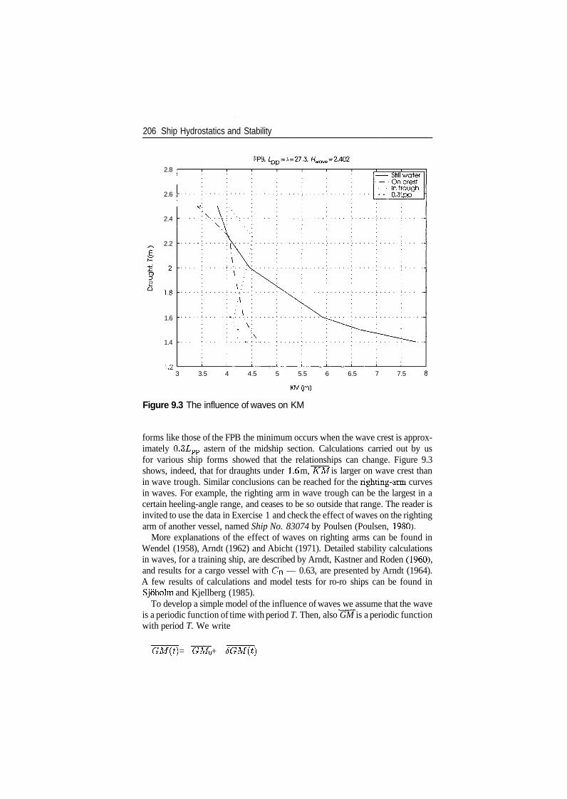
206 Ship Hydrostatics and Stability
O)DD
2.8
2.6
2.4
2.2
1.6
1.4
1.23 3.5 4 4.5 5 5.5 6 6.5 7 7.5
KM(m)
Figure 9.3 The influence of waves on KM
forms like those of the FPB the minimum occurs when the wave crest is approx-imately 0.31/pp astern of the midship section. Calculations carried out by usfor various ship forms showed that the relationships can change. Figure 9.3shows, indeed, that for draughts under 1.6 m, KM is larger on wave crest thanin wave trough. Similar conclusions can be reached for the righting-arm curvesin waves. For example, the righting arm in wave trough can be the largest in acertain heeling-angle range, and ceases to be so outside that range. The reader isinvited to use the data in Exercise 1 and check the effect of waves on the rightingarm of another vessel, named Ship No. 83074 by Poulsen (Poulsen, 1980).
More explanations of the effect of waves on righting arms can be found inWendel (1958), Arndt (1962) and Abicht (1971). Detailed stability calculationsin waves, for a training ship, are described by Arndt, Kastner and Roden (1960),and results for a cargo vessel with CB — 0.63, are presented by Arndt (1964).A few results of calculations and model tests for ro-ro ships can be found inSjoholm and Kjellberg (1985).
To develop a simple model of the influence of waves we assume that the waveis a periodic function of time with period T. Then, also GM is a periodic functionwith period T. We write
GM(t) = GM0 + 5GM(t)
Parametric resonance 207
where
SGM(t) = 5GM(t + T)
for any t. In Section 6.7 we developed a simple model of the free rolling motion.To include the variation of the metacentric height in waves we can rewrite theroll equation as
Going one step further we assume that the wave is harmonic (regular wave) sothat the free rolling motion can be modelled by
cos LJe t)(f) = 0 (9.1)
This is a Mathieu equation; those of its properties that interest us are describedin the following section.
9.3 The Mathieu effect - parametric resonance
9.3.1 The Mathieu equation - stability
A general form of a differential equation with periodic coefficients is Hill'sequation:
where h(t) = h(t + T). In the particular case in which the periodic function isa cosine we have the Mathieu equation', it is frequently written as
<j> + (6 + e cos 2t)c/) = 0 (9.2)
This equation was studied by Mathieu (Emile-Leonard, French, 1835-1900)in 1868 when he investigated the vibrational modes of a membrane with anelliptical boundary. Floquet (Gaston, French, 1847-1920) developed in 1883an interesting theory of linear differential equations with periodic coefficients.Since then many other researchers approached the subject; a historical summaryof their work can be found in McLachlan (1947).
A rigorous discussion of the Mathieu equation is beyond the scope of this book;for more details the reader is referred to specialized books, such as Arscott ( 1 964),Cartmell (1990), Grimshaw (1990) or McLachlan (1947). A comprehensive bib-liography on 'parametrically excited systems' and a good theoretic treatment aregiven by Nay f eh and Mook (1995). For our purposes it is sufficient to explainthe conditions under which the equation has stable solutions. By 'stable' weunderstand that the response, </>, is bounded. Correspondingly, 'unstable' means
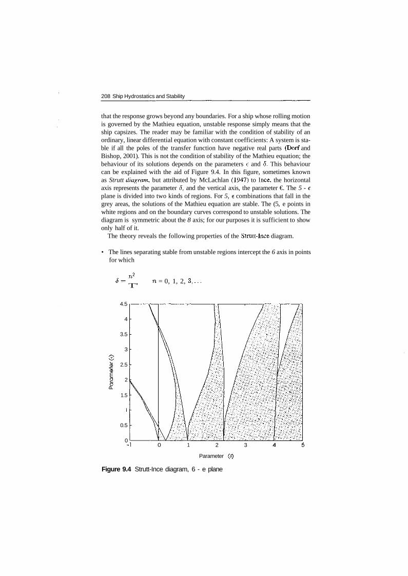
208 Ship Hydrostatics and Stability
that the response grows beyond any boundaries. For a ship whose rolling motionis governed by the Mathieu equation, unstable response simply means that theship capsizes. The reader may be familiar with the condition of stability of anordinary, linear differential equation with constant coefficients: A system is sta-ble if all the poles of the transfer function have negative real parts (Dorf andBishop, 2001). This is not the condition of stability of the Mathieu equation; thebehaviour of its solutions depends on the parameters e and 6. This behaviourcan be explained with the aid of Figure 9.4. In this figure, sometimes knownas Strutt diagram, but attributed by McLachlan (1947) to Ince, the horizontalaxis represents the parameter 6, and the vertical axis, the parameter €. The 5 - eplane is divided into two kinds of regions. For 5, e combinations that fall in thegrey areas, the solutions of the Mathieu equation are stable. The (5, e points inwhite regions and on the boundary curves correspond to unstable solutions. Thediagram is symmetric about the 8 axis; for our purposes it is sufficient to showonly half of it.
The theory reveals the following properties of the Strutt-Ince diagram.
• The lines separating stable from unstable regions intercept the 6 axis in pointsfor which
n^T'
= 0, 1, 2, 3, . . .
4.5
4
3.5
3
2.5
2
1.5
1
0.5
00 1 2 3
Parameter (<5)
Figure 9.4 Strutt-Ince diagram, 6 - e plane
Parametric resonance 209
• As S grows larger, so do the stable regions.• As e grows, the stable regions become smaller. Remember, e is the 'distur-
bance'.
Cesari (1971) considers the equation
x + (a2 4- 6 cos ujt)x = 0 (9.3)
The natural frequency of the 'undisturbed' equation - that is for e = 0 - is cr/27r,while the frequency of the periodic disturbance is UJ/27T. With the transformation
ut = 2*i (9.4)
we calculate
dx dti & dx
dx dti ^2 d2xdti dt 4 d*2
Substituting Eqs. (9.4) and (9.5) into Eq. (9.3) yields an equation in the stan-dard form
x-f - (Si -Mi cos 2*1)0; = 0
where
4cr2 46Si = —y, ei = -r-
UJ2 UJ2
The general aspect of the Si — ei plane is shown in Figure 9.5. Visual inspectionshows us that for small e values the danger of falling into an unstable regionis greater in the neighbourhoods of Si = I2, 22, 32, This means that forsmall 6 parametric resonance occurs at circular frequencies u; = 2cr/n2, wheren — 1, 2, 3, The first dangerous situation is met when u = 2<j. We reachthe important conclusion that the danger of parametric resonance is greatestwhen the frequency of the perturbation equals twice the natural frequency of theundisturbed system.
This statement is rephrased in terms of ship-stability parameters in Exam-ple 9.1 where a becomes the natural roll circular frequency, UJQ, of the ship, anduj becomes o;E, the frequency of encounter, that is the frequency with which theship encounters the waves. This theoretical conclusion was confirmed by basintests.
Surprising as it may seem, the phenomenon of parametric excitation is wellknown. The main character in Moliere's Le bourgeois gentilhomme has been
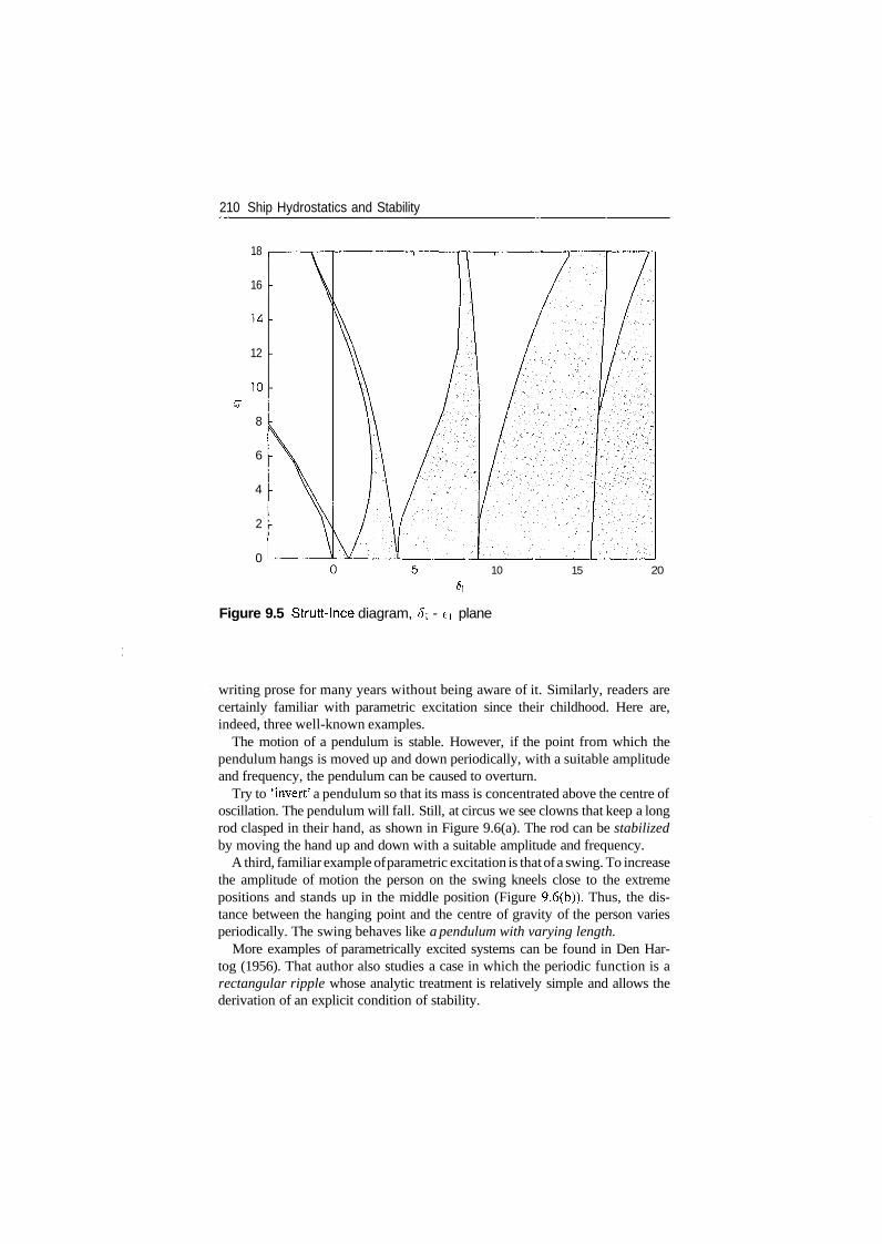
210 Ship Hydrostatics and Stability
18
16
14
12
10
8
6
4
2
010 15 20
Figure 9.5 Strutt-lnce diagram, Si - ei plane
writing prose for many years without being aware of it. Similarly, readers arecertainly familiar with parametric excitation since their childhood. Here are,indeed, three well-known examples.
The motion of a pendulum is stable. However, if the point from which thependulum hangs is moved up and down periodically, with a suitable amplitudeand frequency, the pendulum can be caused to overturn.
Try to 'invert' a pendulum so that its mass is concentrated above the centre ofoscillation. The pendulum will fall. Still, at circus we see clowns that keep a longrod clasped in their hand, as shown in Figure 9.6(a). The rod can be stabilizedby moving the hand up and down with a suitable amplitude and frequency.
A third, familiar example of parametric excitation is that of a swing. To increasethe amplitude of motion the person on the swing kneels close to the extremepositions and stands up in the middle position (Figure 9.6(b)). Thus, the dis-tance between the hanging point and the centre of gravity of the person variesperiodically. The swing behaves like a pendulum with varying length.
More examples of parametrically excited systems can be found in Den Har-tog (1956). That author also studies a case in which the periodic function is arectangular ripple whose analytic treatment is relatively simple and allows thederivation of an explicit condition of stability.
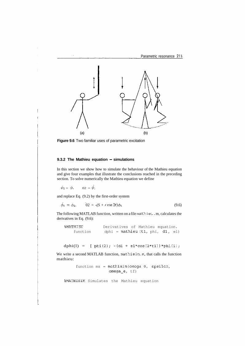
Parametric resonance 211
(a) (b)
Figure 9.6 Two familiar uses of parametric excitation
9.3.2 The Mathieu equation - simulations
In this section we show how to simulate the behaviour of the Mathieu equationand give four examples that illustrate the conclusions reached in the precedingsection. To solve numerically the Mathieu equation we define
(f)l = 0, 02 = 01
and replace Eq. (9.2) by the first-order system
0! = 02, 02 = -(S + ecos2t)0i (9.6)
The following MATLAB function, written on a file mathieu . m, calculates thederivatives in Eq. (9.6):
%MATHIEU Derivatives of Mathieu equation.function dphi = mathieu (tl, phi, dl , el)
dphi(l) = [ p h i ( 2 ) ; -(dl + e l*cos(2*t l ) )*phi (1) /
We write a second MATLAB function, mathisim.m, that calls the functionmathieu:
function ms = mathisim(omega_0, epsilon,omega_e/ tf)
%MATHISIM Simulates the Mathieu equation
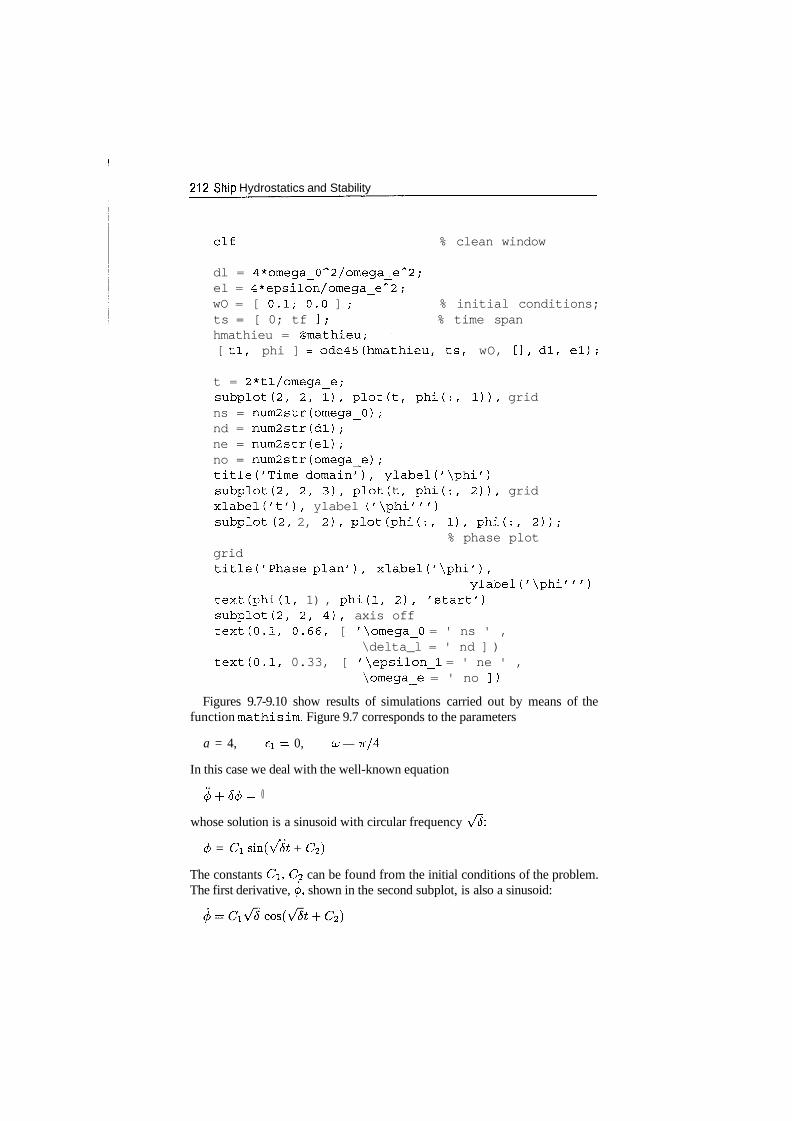
212 Ship Hydrostatics and Stability
elf % clean window
dl = 4*omega_0~2/omega_e/v2;el = 4*epsilon/omega_exs2 ;wO = [ 0.1; 0.0 ] ; % initial conditions;ts = [ 0; tf ]; % time spanhmathieu = @mathieu;[ tl, phi ] = ode45(hmathieu, ts, wO, [], dl, el);
t = 2*tl/omega_e;subplot(2, 2, 1), plot(t, phi(:, 1)), gridns = num2str(omega_0);nd = num2str(dl);ne = num2str(el);no = num2str(omega_e);title('Time domain'), ylabel('\phi')subplot(2, 2, 3), plot(t, phi(:, 2)), gridxlabel('t'), ylabel ('\phi' ")subplot (2, 2, 2), plot(phi(:, 1), phi(:, 2));
% phase plotgridtitle('Phase plan'), xlabel('\phi'),
ylabel C\phi''')text(phi(1, 1) , phi(l, 2), 'start')subplot(2, 2, 4), axis offtext(0.1, 0.66, [ '\omega_0 = ' ns ' ,
\delta_l = ' nd ] )text(0.1, 0.33, [ '\epsilon_l = ' ne ' ,
\omega_e = ' no ])
Figures 9.7-9.10 show results of simulations carried out by means of thefunction mathisim. Figure 9.7 corresponds to the parameters
a = 4, ei = 0, uj — 7T/4
In this case we deal with the well-known equation
0 + <5</> = 0
whose solution is a sinusoid with circular frequency \f&\
</> = Ci sm(\^t + C2)
The constants Ci, £2 can be found from the initial conditions of the problem.The first derivative, </>, shown in the second subplot, is also a sinusoid:
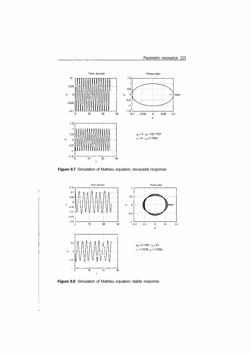
Parametric resonance 213
Time domain Phase plan
• • • Start
= 4,^=103.7529
, = 0,^=0.7854
Figure 9.7 Simulation of Mathieu equation; sinusoidal response
Time domain Phase plan
0.5
-0.5
-0.2 -0.1
1
0.5
0
-0.5
i
yV
Mv v
;A 1/ \ IMjhy. .
w0 = 2.1509,61=30
^=9.9998,^ = 0.7854
0.1 0.2
20
Figure 9.8 Simulation of Mathieu equation; stable response
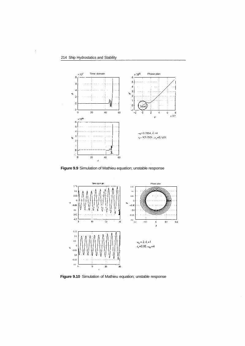
214 Ship Hydrostatics and Stability
si Time domain Phase plan
0 20
xlO32
40 60
5
4
3
2
1
.,..1
: '"4: 1
- 2 0 2 4 6xlO31
0^ = 0.7854, 5, =4
ET = 103.7529. we=0.7864
20 40 60
Figure 9.9 Simulation of Mathieu equation; unstable response
Phase planu. 10
0.1 I A A Ao.os|.|U
4111-0.05
-0.1
-0.15
-D9
, U . .V . U
A A A:
V - v U - y
\ A
y ' . v 1
0.15
0.1
0.05
0
-0.05
-0.1
-0.15
-0.2-0.2
0.15
0.1
0.05
0
-0.05
-0.1
-0.15
-0.2
v y
Figure 9.10 Simulation of Mathieu equation; unstable response
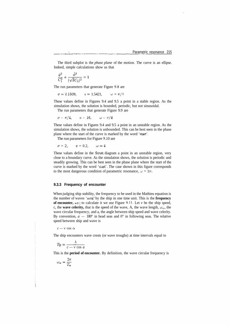
Parametric resonance 215
The third subplot is the phase plane of the motion. The curve is an ellipse.Indeed, simple calculations show us that
The run parameters that generate Figure 9.8 are
cr- 2.1509, e= 1.5421, u = Tr/4
These values define in Figures 9.4 and 9.5 a point in a stable region. As thesimulation shows, the solution is bounded, periodic, but not sinusoidal.
The run parameters that generate Figure 9.9 are
(j = 7T/4, 6 = 16, UJ = 7T/4
These values define in Figures 9.4 and 9.5 a point in an unstable region. As thesimulation shows, the solution is unbounded. This can be best seen in the phaseplane where the start of the curve is marked by the word 'start'.
The run parameters for Figure 9.10 are
a = 2, e = 0.2, c j -4
These values define in the Strutt diagram a point in an unstable region, veryclose to a boundary curve. As the simulation shows, the solution is periodic andsteadily growing. This can be best seen in the phase plane where the start of thecurve is marked by the word 'start'. The case shown in this figure correspondsto the most dangerous condition of parametric resonance, u = 2cr.
9.3.3 Frequency of encounter
When judging ship stability, the frequency to be used in the Mathieu equation isthe number of waves 'seen' by the ship in one time unit. This is the frequencyof encounter, uj&, to calculate it we use Figure 9.11. Let v be the ship speed,c, the wave celerity, that is the speed of the wave, A, the wave length, u;w, thewave circular frequency, and a, the angle between ship speed and wave celerity.By convention, a — 180° in head seas and 0° in following seas. The relativespeed between ship and wave is
c — v cos a.
The ship encounters wave crests (or wave troughs) at time intervals equal to
Ac — v cos a
This is the period of encounter. By definition, the wave circular frequency is
27T

216 Ship Hydrostatics and Stability
Figure 9.11 Calculating the frequency of encounter
where Tw is the wave period. Similarly, the circular frequency of encounter isdefined by
- —
In wave theory (see, for example, Faltinsen, 1993; Bonnefille, 1992) it is shownthat the relationship between wave length and wave circular frequency, in waterof infinite depth, is
Putting all together we obtain
— ^w -- v cos a9
(9.7)
9.4 Summary
Longitudinal and quartering waves influence the stability of ships and otherfloating bodies. The moment of inertia of the waterline surface in waves differsfrom that of the waterplane in still water and, consequently, so do the metacentricheight and the righting arms. The way in which those quantities vary depends onthe ship form; however, it can be said that in many cases the righting moment inwave trough is larger than in still water, while on wave crest it is smaller. If thewave is periodic, also the variation of the righting arm is periodic. Then, intothe equation of rolling developed in Chapter 6 we must add to the coefficient ofthe roll angle a term that is a periodic function of time:
5GM cos - 0
Parametric resonance 217
For small heel angles the above equation can be reduced to the canonical formof the Mathieu equation
4> + (6 + ecos 2t)<p = 0
The condition of stability is not the same as for a linear differential equationwith constant coefficients. In other words, the condition of positive metacentricheight, GM > 0, is no longer sufficient. The theory of differential equationswith periodic coefficients shows that the plane of the parameters 6 and e canbe subdivided into regions so that if in one of them the solution of the Mathieuequation is stable, in the adjacent regions it is not. This means that for certainpairs [J, e] the solution is unstable and we say that parametric resonance occurs.The partition of the 8 - e plane into stable and unstable regions can be bestvisualized in the Strutt-Ince diagram. Thus, it can be easily discovered that evenfor small e values a particularly dangerous situation arises when the frequencyof the periodic coefficient is twice the natural frequency of the system withoutperiodic excitation.
Parametric excitation occurs in several systems we are familiar with. Thus, theamplitude of oscillation of a swing can be increased by periodically changing theposition of the centre of gravity of the person on the swing. As another example,a conventional pendulum is usually stable, but it can be forced to overturn ifthe point of hanging is moved up and down with appropriate frequency andamplitude. Conversely, an inverted pendulum, although inherently unstable, canbe stabilized by applying a suitable periodic motion to its centre of oscillation.
Ships have capsized although they fulfilled the criteria of stability commonlyaccepted at the time of the disaster. Post-mortem analysis of some cases pin-pointed the Mathieu effect as the cause of capsizing. The surprising discoverywas that the righting arm could be negative on wave crest.
The analysis of the Mathieu effect confirms a fact well known to experiencedseafarers: following seas are more dangerous than head seas. In fact, when thedirection of the waves is the same as that of the ship, the relative velocity issmall and the time interval in which the stability is reduced is longer. Then, thereis more time to develop large heeling angles. Still worse, in following seas theeffect of reduced stability can be enhanced by waves flowing over the deck. Thelatter effect will increase the height of the centre of gravity because it means anextra weight loaded high up on the ship. It also adds a free-surface effect.
9.5 Examples
Example 9.1 - Parametric resonance in ship stabilityIn this example we are going to explain the significance of the parameters 6 and€ for ship stability. In Chapter 6 we developed the equation of free roll
(9.8)
218 Ship Hydrostatics and Stability
The natural, circular roll frequency is
ll/2
(9.9)
Let us assume that the wave produces a periodic variation of the metacentricheight equal to
8GM cos C^E
Where uj^ is the circular frequency of encounter. With this assumption and withthe notation introduced by Eq. (9.9) we rewrite Eq. (9.8) as
(9.10)
Following Cesari (1971) we use the substitution uj-^t = 2t^ and proceeding likein Subsection 9.3.1 we transform Eq. (9.10) to
2 0° ~~ Cos2t 0 =
Substituting Eq. (9.9) we obtain
cos2tl = 0 (9.12)J
Equation (9.12) can be brought to the standard Mathieu form with
^V (9.13)
We know that the most dangerous situation occurs at 5i = 1, that is forces =
Example 9.2 - 5ai7 s/w/i in longitudinal wavesThe righting-arm curve in still-water shown Figure 9.12 was calculated for anactual training yacht. We assume that the righting-arm curves on wave crest andin wave trough, and the wind heeling arm are as shown in the figure. It is obviousthat while advancing in waves the yacht will roll between points A and B. Thus,the Mathieu effect induces roll in head or following seas, a behaviour that is notpredicted by the conventional roll equation. Readers involved in yachting mayhave experienced the phenomenon.
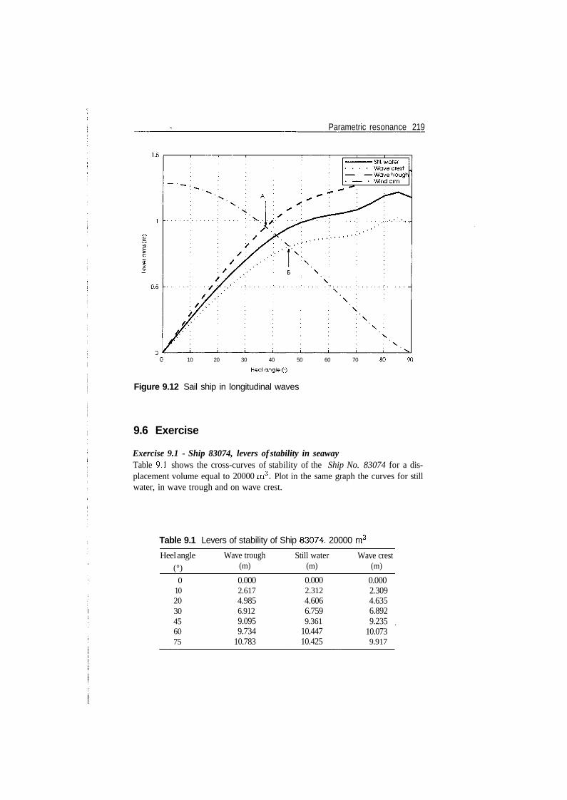
Parametric resonance 219
10 20 30 40 50 60 70
Figure 9.12 Sail ship in longitudinal waves
9.6 Exercise
Exercise 9.1 - Ship 83074, levers of stability in seawayTable 9.1 shows the cross-curves of stability of the Ship No. 83074 for a dis-placement volume equal to 20000 m3. Plot in the same graph the curves for stillwater, in wave trough and on wave crest.
Table 9.1 Levers of stability of Ship 83074, 20000 m3
Heel angle(°)
0102030456075
Wave trough(m)
0.0002.6174.9856.9129.0959.734
10.783
Still water(m)
0.0002.3124.6066.7599.361
10.44710.425
Wave crest(m)
0.0002.3094.6356.8929.235
10.0739.917
10Intact stability regulations II
10.1 Introduction
We give in this section a simplified overview of the B V 1033 regulations of theGerman Federal Navy, as an example of philosophy different from those illus-trated in Chapter 8. These are the only effectively applied regulations that con-sider the Mathieu effect. There were proposals to consider parametric excitationin other codes of ship stability; to our best knowledge they remained proposals.Our description follows the 1977 edition of the regulations and includes updat-ings received as personal communications in the 1980s. As we suggested forother regulations, for checks of stability that must be submitted for approval, itis highly recommended to inquire about the latest, complete edition of BV 1033and consult it for updatings and specific details.
10.2 The regulations of the German Navy
Kurt Wendel wrote in 1961 the first draft of stability regulations for the GermanFederal Navy. Wendel issued in 1964 a new edition known as BV 103. An earlydetailed explanation of the regulations and their background is due to Arndt(1965). His paper was soon translated into English by the British Ship ResearchAssociation and appeared as BSRA Translation No. 5052. An updated versionof the regulations was published in 1969 and since then they are known as BV1033. As pointed out by Brandl (1981), the German regulations were adoptedby the Dutch Royal Navy (see, for example, Harpen, 1971) and they also servedin the design of some ships built in Germany for several foreign navies.
In Chapter 9 we mentioned experiments performed by German researchersbefore the publication of the regulations. The authors continued to experimentafter the implementation of BV 1033 and thus confirmed the validity of therequirements and showed that the German regulations and the regulations of theU.S. Navy confer to a large extent equivalent safety against capsizing. For detailswe refer the reader to Brandl (1981) and Arndt, Brandl and Vogt (1982).
Righting arms are denoted in BV 1033 by the letter /i; heeling arms, by k.Thus, kw is the wind heeling arm, k& the heeling arm in turning, and so on.
222 Ship Hydrostatics and Stability
10.2.1 Categories of service
Stability requirements vary according to the intended use of the ships. The reg-ulations of the German Federal Navy classify vessels into five categories, asexplained below:
Group A There are no limitations to the area of operation of ships belongingto this category. Calculations for Group A should be carried out fora wind velocity equal to 90 knots.
Group B This category includes ships that can avoid winds whose velocityexceeds 70 knots. Examples of corresponding areas of operation arethe North Atlantic, the North sea, the Baltic sea, and the Mediter-ranean sea. The wind velocity to be considered for this group is 70knots.
Group C The category consists of coastal vessels that can reach a harbour if astorm warning is received. Stability calculations shall be based on awind velocity of 50 knots.
Group D It consists of ships and decked boats that operate as harbour andestuarial craft. The wind velocity to be considered is 40 knots.
Group E In this category enter open boats intended for coastal and harbouroperation, within well-defined geographical limits. Stability calcula-tions shall assume a wind velocity equal to 20 knots.
10.2.2 Loading conditions
The BV 1033 regulations require the verification of stability in a number ofloading conditions. We shall exemplify here only three of them. The detaileddescription of the loading cases involves the term empty ship ready for operation.By this the regulations mean the ship with fuel, feed water and lubricating oilin machines, piping, weapons and other systems, if necessary also with fixedballast.
Loading case 0 - Empty shipThe weight groups to be included are
• Empty ship ready for operation.• Crew and personal effects.
Loading case 1 - Limit displacement with ballast waterThe weights to be included are
• Empty ship ready for operation.• Crew and personal effects.• 10% consumables and provisions.
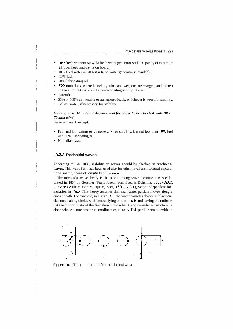
Intact stability regulations II 223
• 10% fresh water or 50% if a fresh water generator with a capacity of minimum25 1 per head and day is on board.
• 10% feed water or 50% if a fresh water generator is available.• 10% fuel.• 50% lubricating oil.• 33% munitions, where launching tubes and weapons are charged, and the rest
of the ammunition is in the corresponding storing places.• Aircraft.• 33% or 100% deliverable or transported loads, whichever is worst for stability.• Ballast water, if necessary for stability.
Loading case 1A - Limit displacement for ships to be checked with 90 or70 knot windSame as case 1, except:
• Fuel and lubricating oil as necessary for stability, but not less than 10% fueland 50% lubricating oil.
• No ballast water.
10.2.3 Trochoidal waves
According to BV 1033, stability on waves should be checked in trochoidalwaves. This wave form has been used also for other naval-architectural calcula-tions, mainly those of longitudinal bending.
The trochoidal wave theory is the oldest among wave theories; it was elab-orated in 1804 by Gerstner (Franz Joseph von, lived in Bohemia, 1756-1832).Rankine (William John Macquam, Scot, 1820-1872) gave an independent for-mulation in 1863. This theory assumes that each water particle moves along acircular path. For example, in Figure 10.1 the water particles shown as black cir-cles move along circles with centres lying on the x-axis and having the radius r.Let the x coordinate of the first shown circle be 0, and consider a particle on acircle whose centre has the x coordinate equal to xo-This particle rotated with an
Figure 10.1 The generation of the trochoidal wave
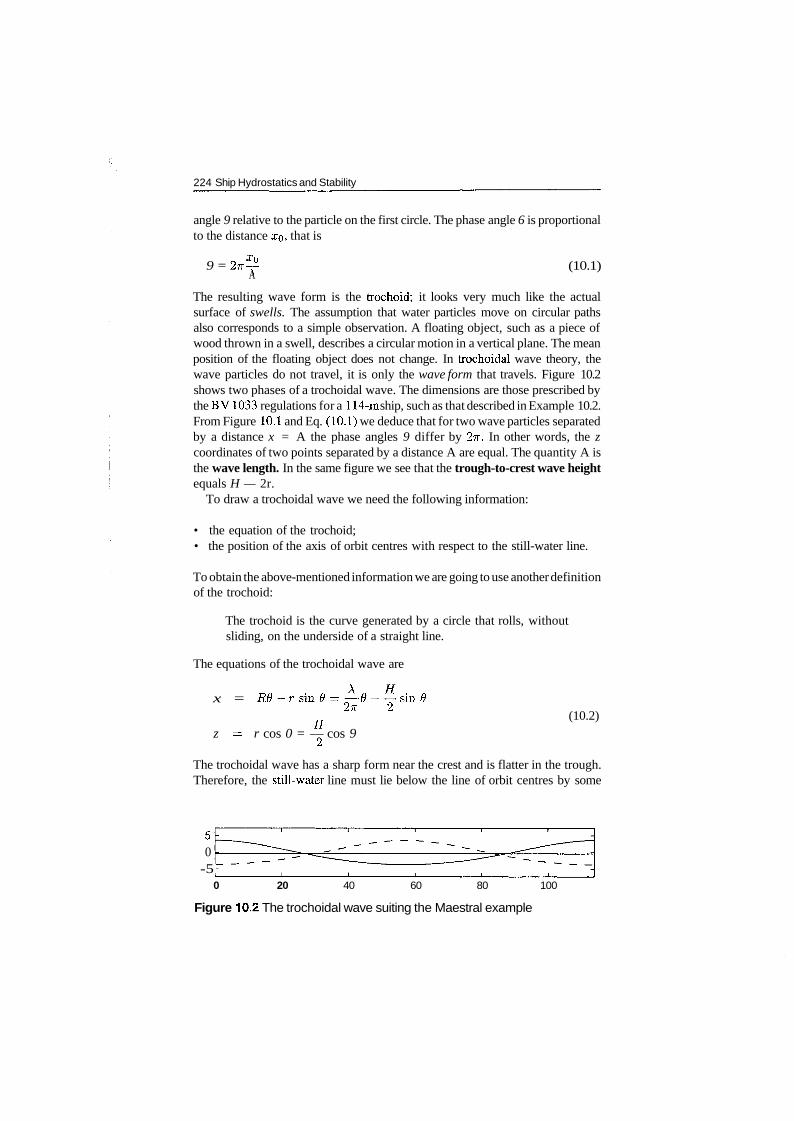
224 Ship Hydrostatics and Stability
angle 9 relative to the particle on the first circle. The phase angle 6 is proportionalto the distance XQ, that is
9 = 2vr^ (10.1)A
The resulting wave form is the trochoid; it looks very much like the actualsurface of swells. The assumption that water particles move on circular pathsalso corresponds to a simple observation. A floating object, such as a piece ofwood thrown in a swell, describes a circular motion in a vertical plane. The meanposition of the floating object does not change. In trochoidal wave theory, thewave particles do not travel, it is only the wave form that travels. Figure 10.2shows two phases of a trochoidal wave. The dimensions are those prescribed bythe B V1033 regulations for a 114-m ship, such as that described in Example 10.2.From Figure 10.1 and Eq. (10.1) we deduce that for two wave particles separatedby a distance x = A the phase angles 9 differ by 27r. In other words, the zcoordinates of two points separated by a distance A are equal. The quantity A isthe wave length. In the same figure we see that the trough-to-crest wave heightequals H — 2r.
To draw a trochoidal wave we need the following information:
• the equation of the trochoid;• the position of the axis of orbit centres with respect to the still-water line.
To obtain the above-mentioned information we are going to use another definitionof the trochoid:
The trochoid is the curve generated by a circle that rolls, withoutsliding, on the underside of a straight line.
The equations of the trochoidal wave are
x = RO-rsmO=—0-—smO
H ^ 2 (10.2)z = r cos 0 = — cos 9
Zi
The trochoidal wave has a sharp form near the crest and is flatter in the trough.Therefore, the still-water line must lie below the line of orbit centres by some
0-5 r
0 20 40 60 80 100
Figure 10.2 The trochoidal wave suiting the Maestral example
Intact stability regulations II 225
distance a. As the volume of water above the still-water line must equal thatbelow the same line, we can write
/
ZTT(z - a)dx = 0 (10.3)
_
We can separate the above integral into two integrals that we calculate separately.The first integral is
/•2-7T />2?r
/ zdx = r cos 9(R — r cos 0}d9Jo Jo (10-4)
The second integral is
/•27T
/
Joadx = ax\Q = 27taR (10.5)
o
Equating Eqs. (10.4) and (10.5) we obtain
a = ~^R (1°'6)
We mention here, without proving, two interesting hydrodynamical propertiesof the trochoidal wave.
1. Motion decay with depthThe radius of orbits decays exponentially with depth. For a given depth /i, theamplitude of the orbital motion is
rh = re~h/R (10.7)
The amplitude on the sea bottom should be zero. In our model this onlyhappens at an infinite depth; therefore, the trochoidal wave model is correctonly in infinite depth seas. However, let us calculate the radius of the orbit ata depth equal to half a wave length:
r_A/2 = r exp f 2fl ) ^ 0'0043r
that is practically zero.2. Virtual gravity
A water particle moving along a circular orbit is subjected to two forces:
• its weight, mg\• a centrifugal force, mru2, where u is the angular velocity of the particle.
It can be shown that a;2 = g/R.
226 Ship Hydrostatics and Stability
In the trough the two forces add up to
while on a wave crest the result is
Thus, a floating body experiences the action of a virtual gravity accelerationwhose value varies between g(l — r/R) and g(l -f g/R). One wave height-to-length ratio frequently employed in Naval Architecture is 1/20. With this valuethe apparent gravity varies between 0.843# and 1.157g.
The variation of apparent gravity, and consequently of buoyancy, in waves isknown as the Smith effect, after the name of the researcher who described it firstin 1883. The reduction of virtual gravity on wave crest was considered anothercause of loss of stability in waves. To quote Attwood and Pengelly (1960):
This is the explanation of the well-known phenomenon of the ten-derness of sailing boats on the crest of a wave.
As the vessel seems to weigh less on the crest, so does the righting moment thatis the product of displacement and righting arm. As the wind moment does notchange, a boat 'of sufficient stiffness in smooth water, is liable to be blown overto a large angle and possibly capsize.'
On the other hand, Devauchelle (1986) considers that in real seas, character-ized by the irregularity of waves (see Chapter 12), the effect of virtual gravityvariation can be neglected. Model tests described by Wendel (1965) revealed thatthe influence of the orbital motion can be neglected when compared with theeffect of the variation of the waterline in waves. Calculations carried out wheninvestigating the loss of a trawler showed that in that case the Smith effect wascompletely negligible for heel angles up to 20° (Morrall, 1980).
More details on the theory of trochoidal waves can be found in Attwoodand Pengelly (1960), Bouteloup (1979), Susbielles and Bratu (1981), Bonnefille(1992) and Rawson and Tupper (1994). To conclude this section, we state thecharacteristics of the wave specified by the BV 1033 regulations:
wave form trochoidalwave length equal to ship length, that is, A = Lwave height H = A/(10 + 0.05A)
The relationship between wave length and height is based on statistics and proba-bilistic considerations. We may mention here that a slightly different relationship
Intact stability regulations II 227
was proposed for merchant ships by the maritime registers of the former GermanDemocratic Republic and of Poland (Helas, 1982):
4.14 + 0.14LPP
A value frequently used by other researchers is H — A/20.We described here the trochoidal wave because the BV regulations require
its use in stability calculations, while other codes of practice specify this wavefor bending-moment calculations. Other wave theories are preferred in otherbranches of Naval Architecture. Thus, in Chapter 12, we introduce the sinusoidalwaves. There is no great difference in shape between the trochoidal and the sinewave, but some other properties are significantly different.
10.2.4 Righting arms
The cross-curves of stability shall be calculated in still water and in waves. For thelatter, ten wave phases shall be considered. More specifically, the calculationsshall be performed with the wave crest at distances equal to 0.5L, 0.4L, . . .OL, . . . — 0.4L from midship. The average of the cross-curves in waves shallbe compared with the cross-curves in still water and the smaller values shall beused in the calculation of righting arms. The BV 1033 regulations denote by /IGthe righting arm in still water, and by h$ the righting arm in waves. It is easy toremember the latter notation if we relate the subscript S to the word 'seaway', thetranslation of the German term 'Seegang'. The reason for considering the meanof the righting arms in waves, and not the smallest values, is that, in general,there is not enough time for the Mathieu effect to fully develop.
Most ships are not symmetric about a transverse plane (notable exceptionsare Viking ships and some ferries). Therefore, during heeling the centre of buoy-ancy travels in the longitudinal direction causing trim changes. According to theGerman regulations this effect must be considered in the calculation of cross-curves. In the terminology of BV 1033 the calculations shall be performed withtrim compensation. The data in Table 9.1 and in Example 10.2 are calculatedwith trim compensation.
10.2.5 Free liquid surfaces
The German regulations consider the influence of free liquid surfaces as a heelingarm, rather than a quantity to be deducted from metacentric height and rightingarms. The first formula to be used is
£ pjijkF = ^—— sin 0 (10.8)
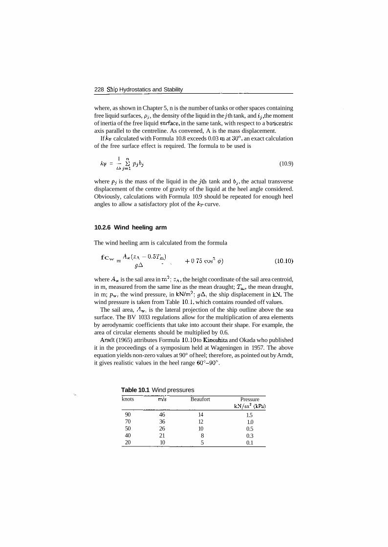
228 Sftip Hydrostatics and Stability
where, as shown in Chapter 5, n is the number of tanks or other spaces containingfree liquid surfaces, PJ , the density of the liquid in the j th tank, and ij, the momentof inertia of the free liquid surface, in the same tank, with respect to a baricentricaxis parallel to the centreline. As convened, A is the mass displacement.
If /cp calculated with Formula 10.8 exceeds 0.03 m at 30°, an exact calculationof the free surface effect is required. The formula to be used is
A* = ~ E Pjbj (10.9)L\ j=l
where PJ is the mass of the liquid in the jth tank and bj, the actual transversedisplacement of the centre of gravity of the liquid at the heel angle considered.Obviously, calculations with Formula 10.9 should be repeated for enough heelangles to allow a satisfactory plot of the kp curve.
10.2.6 Wind heeling arm
The wind heeling arm is calculated from the formula
fcw - ^w(*A-0.5Tm) + Q ̂ cog3
g&
where Aw is the sail area in m2; ZA, the height coordinate of the sail area centroid,in m, measured from the same line as the mean draught; Tm, the mean draught,in m; pw, the wind pressure, in kN/m2; gA, the ship displacement in kN. Thewind pressure is taken from Table 10.1, which contains rounded off values.
The sail area, Aw, is the lateral projection of the ship outline above the seasurface. The BV 1033 regulations allow for the multiplication of area elementsby aerodynamic coefficients that take into account their shape. For example, thearea of circular elements should be multiplied by 0.6.
Arndt (1965) attributes Formula 10.10 to Kinoshita and Okada who publishedit in the proceedings of a symposium held at Wageningen in 1957. The aboveequation yields non-zero values at 90° of heel; therefore, as pointed out by Arndt,it gives realistic values in the heel range 60°-90°.
Table 10.1 Wind pressuresknots
9070504020
m/s
4636262110
Beaufort
14121085
PressurekN/m2 (kPa)
1.51.00.50.30.1
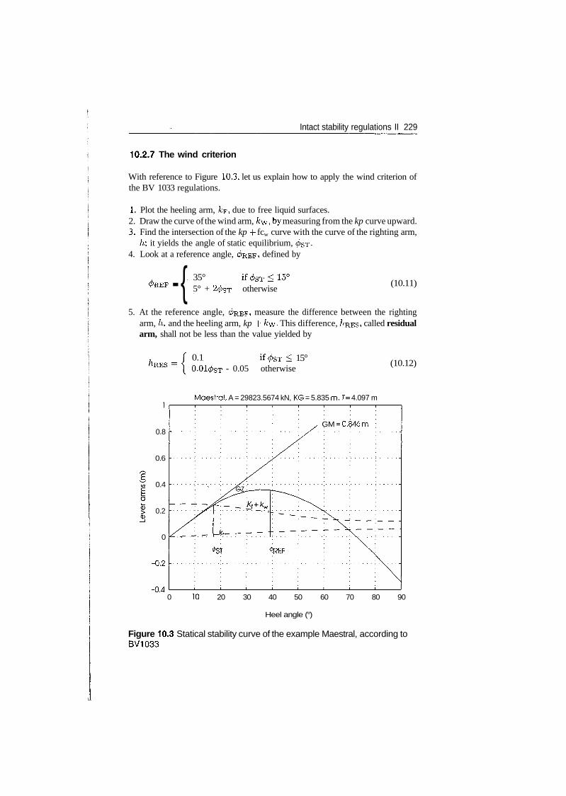
Intact stability regulations II 229
10.2,7 The wind criterion
With reference to Figure 10.3, let us explain how to apply the wind criterion ofthe BV 1033 regulations.
1. Plot the heeling arm, kp, due to free liquid surfaces.2. Draw the curve of the wind arm, &\y»by measuring from the kp curve upward.3. Find the intersection of the kp -f fcw curve with the curve of the righting arm,
/i; it yields the angle of static equilibrium,4. Look at a reference angle, </>REF> defined by
-{ 35°5° + 20ST otherwise
(10.11)
5. At the reference angle, </>REF, measure the difference between the rightingarm, h, and the heeling arm, kp + A?w This difference, /IRES> called residualarm, shall not be less than the value yielded by
0.1 15°- 0.05 otherwise
(10.12)
Maestral, A = 29823.5674 kN, KG = 5.835 m, f= 4.097 m
0.8
0.6
0.4
0.2
0
-0.2
-0.4
GM = 0.846m
0 10 20 30 40 50 60 70 80 90
Heel angle (°)
Figure 10.3 Statical stability curve of the example Maestral, according toBV1033
230 Ship Hydrostatics and Stability
The explicit display of the free liquid surface effect as a heeling arm makes itpossible to compare its influence to that of the wind and take correcting mea-sures, if necessary. For example, a too large surface effect, compared to the windarm, can mean that it is desirable to subdivide some tanks. The heelangle caused by winds up to Beaufort 10 shall not exceed 15°. The reader mayhave observed that the regulations assume a wind blowing perpendicularly onthe centreline plane, while the waves run longitudinally. Arndt, Brandl and Vogt(1982) write:
This combination is accounting for the fact that even strong windsmay change their direction in short time only, whereas the wavesare proceeding in the direction in which they were excited. Wavesand winds from different directions can be observed especially nearstorm centres...
Figure 10.3 was plotted with the help of the function described in Example 10.1.Example 10.2 details the data used in the above-mentioned figure. Both examplescan provide a better insight into the techniques of BV 1033.
10.2.8 Stability in turning
The heeling arm due to the centrifugal force developed in turning is calculatedfrom
m- cos 0 (10.13)
where v is the speed of approach, in m s"1, and I/DWL, the length of the designwaterline, in m. The value of this speed should not exceed 0.5\A?£DWL- Thecoefficient CD can be used in the design stage when neither speed in turning,nor turning diameter are known. Recommended values are CD = 0.3 for Froudenumbers smaller than 1, and CD = 0.18 for faster vessels. When basin or seatrials have been performed, their results shall be used to calculate the actualvalue of the coefficient. The meaning of the coefficient CD can be explained asfollows. Usually, in the first design stages neither the speed in turning, VTC> northe radius of the turning circle, jR-rc* is known. The speed in turning is smallerthan the speed in straight-line sailing; therefore, let us write
Cy <1
The radius of the turning circle is usually a multiple of the ship length. Let uswrite
RTC = CR,LDWL> CR > 1
Intact stability regulations II 231
The factor V^C/RTC in the equation of the centrifugal force (see Section 6.4)can be written as
2 V2
CR.Z/DWL=CD
with CD = C^/CR.Stability in turning is considered satisfactory if the heel angle does not
exceed 15°.
10.2.9 Other heeling arms
Other heeling arms can act on the ship, for instance, hanging loads or crowdingof passengers on one side. The following data shall be considered in calculatingthe latter. The mass of a passenger, including 5 kg of equipment, shall be takento be equal to 80 kg. The centre of gravity of a person shall be assumed as placedat 1 m above deck. Finally, a passenger density of 5 men per square metre shallbe considered in general, and only 3 passengers per square metre for craft inGroup E.
Replenishment at sea requires some connection between two vessels. A trans-verse pull develops; it can be translated into a heeling arm. A transverse pullalso can appear during towing. The German regulations contain provisions forcalculating these heeling arms. The heel angle caused by replenishment at seaor by crowding of passengers shall not exceed 15°.
10.3 Summary
In Chapter 9 we have shown that longitudinal and quartering waves affect stabil-ity by changing the instantaneous moment of inertia that enters into the calcu-lation of the metacentric radius. This effect is taken into account in the stabilityregulations of the German Federal Navy and it has been proposed to con-sider it also for merchant ships (Helas, 1982). As shown in Chapter 9, Germanresearchers were the first to investigate parametric resonance in ship stability.They also took into consideration this effect when they elaborated stability reg-ulations for the German Federal Navy. These regulations, known as BV 1033,require that the righting arm be calculated both in still water and in waves. Morespecifically, cross-curves shall be calculated for ten wave phases, that is forten positions of the wave crest relative to the midship section. The average ofthose cross-curves shall be compared with the cross-curves in still water and thesmaller values shall be used in the stability diagram.
In the German regulations, the criterion of stability under wind regards thedifference between the righting arm and the wind heeling arm. This difference,
— GZ — fcw, is called residual arm. If the angle of static equilibrium is> stability shall be checked at a reference angle, </>REF> defined by
232 Ship Hydrostatics and Stability
35°PREF - S 0 otherwise
At this reference angle, the residual arm shall be not smaller than the valuegiven by
, f 0.1\ 0.0RES 0.01<feT - 0.05 otherwise
Finally, a few words about ship forms. Traditionally ship forms have been chosenas a compromise between contradictory requirements of reduced hydrodynamicresistance, good seakeeping qualities, convenient space arrangements and sta-bility in still water. The study of the Mathieu effect has added another criterion:small variation of righting arms in waves. A formulation of this subject can befound in Burcher (1979). Perez and Sanguinetti (1995) experimented with mod-els of two small fishing vessels of similar size but different forms. They show thatthe model with round stern and round bilge displayed less metacentric heightvariation in wave than the model with transom stern.
10.4 Examples
Example 10.1 - Computer function for BV1033In this example we describe a function, written in MATLAB 6, that automaticallychecks the wind criterion of BV 1033. The input consists of four arguments:cond, w, sail, V. The argument cond is an array whose elements are:
1. the displacement, A, in kN;2. the height of the centre of gravity above BL, KG, in m;3. the mean draft, T, in m; <4. the height of the metacentre above BL, KM, in m;5. the free-surface arm in upright condition, fcp(O), in m.
The argument w is a two dimensional array whose first column contains heelangles, in degrees, and the second column, the lever arms w, in metres. Forinstance, the following lines are taken from Example 10.2:
Maestral = [0 05 0.582
90 5.493 ] ;
The argument sail is an array with two elements: the sail area, in m2, and theheight of the sail-area centroid above BL, in m. Finally, the argument V is the
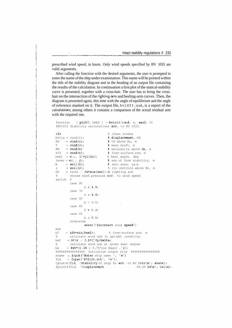
Intact stability regulations II 233
prescribed wind speed, in knots. Only wind speeds specified by BV 1033 arevalid arguments.
After calling the function with the desired arguments, the user is prompted toenter the name of the ship under examination. This name will be printed withinthe title of the stability diagram and in the heading of an output file containingthe results of the calculation. In continuation a first plot of the statical-stabilitycurve is presented, together with a cross-hair. The user has to bring the cross-hair on the intersection of the righting-arm and heeling-arm curves. Then, thediagram is presented again, this time with the angle of equilibrium and the angleof reference marked on it. The output file, bv!033 .out, is a report of thecalculations; among others it contains a comparison of the actual residual armwith the required one.
function [ phiST, hRES ] = bv!033(cond, w, sail, V)%BV1033 Stability calculations ace. to BV 1033.
clc % clean windowDelta = cond(l)KG = cond(2)T = cond(3)KM = cond(4)kfO = cond(5)
lever = w(: , 2)A = sail(1)z = sail(2)
displacement, kNCG above BL, mmean draft, mmetacentre above BL, mfree-surface arm, m
heel = w(:, l)*pi/180; % heel angle, degarm of form stability, msail area, sq m
% its centroid above BL, mGZ = lever - KG*sin(heel);% righting arm% choose wind pressure ace. to wind speedswitch V
case 90P = 1.5;
case 70P = 1.0;
case 50p = 0.5;
case 40P = 0.3;
case 20p = 0.1;
otherwiseerror('Incorrect wind speed')
endkf = kf0*sin(heel); % free-surface arm, m% calculate wind arm in upright conditionkwO = A*(z - 0.5*T)*p/Delta;% calculate wind arm at given heel angleskw = kwO*(0.25 + 0.75*cos (heel) .~3);%%%%%%%%%%%%%%%% Initialize output file %%%%%%%%%%%%%%%%sname = input('Enter ship name ', 's')fid = fopen('BV1033.out', 'w');fprintf(fid, 'Stability of ship %s ace. to BV 1033\n', sname);fprintf(fid, 'Displacement %9.3f kN\n', Delta),
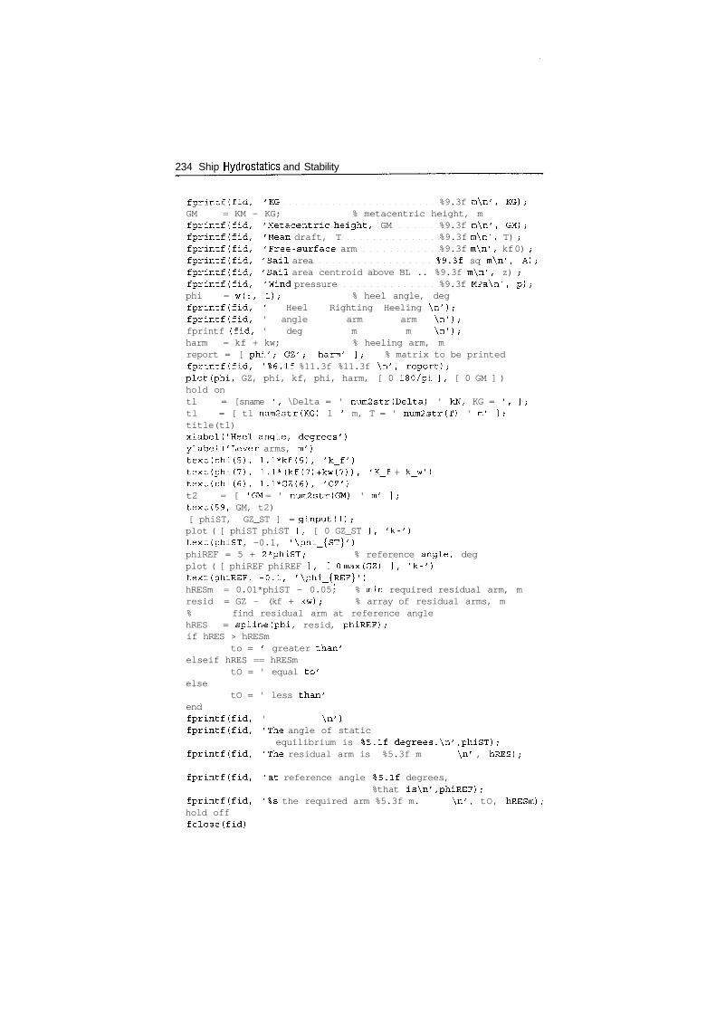
234 Ship Hydrostatics and Stability
fprintf(fid, 'KG %9.3f m\n', KG);GM = KM - KG; % metacentric height, mfprintf(fid, 'Metacentric height, GM %9.3f m\n', GM);fprintf(fid, 'Mean draft, T %9.3f m\n', T) ;fprintf(fid, 'Free-surface arm %9.3f m\n', kf 0) ;fprintf(fid, 'Sail area %9.3f sq m\n', A);fprintf(fid, 'Sail area centroid above BL .. %9.3f m\n', z) ;fprintf(fid, 'Wind pressure %9.3f MPa\n', p);phi = w(:, 1); % heel angle, degfprintf(fid, ' Heel Righting Heeling \n');fprintf(fid, ' angle arm arm \n');fprintf (fid, ' deg m m \n');harm = kf + kw; % heeling arm, mreport = [ phi'; GZ'; harm' ]; % matrix to be printedfprintf(fid, '%6.1f %11.3f %11.3f \n', report);plot(phi, GZ, phi, kf, phi, harm, [ 0 180/pi ], [ 0 GM ] )hold ontl = [sname ', \Delta = ' num2str(Delta) ' kN, KG = ', ];tl = [ tl num2str(KG) 1 ' m, T = ' num2str(T) ' m' ];title(tl)xlabel('Heel angle, degrees')ylabel('Lever arms, m')text(phi(5), l.l*kf(5), 'k_f')text(phi(7), 1.1*(kf(7)+kw(7)), 'K_f + k_w')text(phi(6), 1.1*GZ(6), 'GZ')t2 = [ 'GM = ' num2str(GM) ' m' ];text(59, GM, t2)[ phiST, GZ_ST ] = ginput(l);plot ( [ phiST phiST ], [ 0 GZ_ST ], 'k-')text(phiST, -0.1, '\phi_{ST}')phiREF = 5 + 2*phiST; % reference angle, degplot ( [ phiREF phiREF ], [0 max(GZ) ], 'k-')text(phiREF, -0.1, '\phi_{REF}')hRESm = 0.01*phiST - 0.05; % min required residual arm, mresid = GZ - (kf + kw); % array of residual arms, m% find residual arm at reference anglehRES = spline(phi, resid, phiREF);if hRES > hRESm
to = ' greater than'elseif hRES == hRESm
tO = ' equal to'else
tO = ' less than'endfprintf(fid, ' \n')fprintf(fid, 'The angle of static
equilibrium is %5.1f degrees.\n',phiST);fprintf(fid, 'The residual arm is %5.3f m \n' , hRES);
fprintf(fid, 'at reference angle %5.1f degrees,%that is\n',phiREF);
fprintf(fid, '%s the required arm %5.3f m. \n', tO, hRESm),hold offfclose(fid)
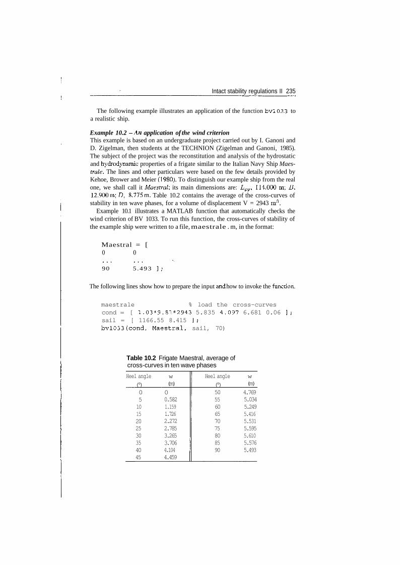
Intact stability regulations II 235
The following example illustrates an application of the function bv!033 toa realistic ship.
Example 10.2 -An application of the wind criterionThis example is based on an undergraduate project carried out by I. Ganoni andD. Zigelman, then students at the TECHNION (Zigelman and Ganoni, 1985).The subject of the project was the reconstitution and analysis of the hydrostaticand hydrodynamic properties of a frigate similar to the Italian Navy Ship Maes-trale. The lines and other particulars were based on the few details provided byKehoe, Brower and Meier (1980). To distinguish our example ship from the realone, we shall call it Maestral, its main dimensions are: I/pp, 114.000 m; J3,12.900m; D, 8.775m. Table 10.2 contains the average of the cross-curves ofstability in ten wave phases, for a volume of displacement V = 2943 m3.
Example 10.1 illustrates a MATLAB function that automatically checks thewind criterion of BV 1033. To run this function, the cross-curves of stability ofthe example ship were written to a file, maestrale . m, in the format:
Maestral = [0 0
90 5 .493 ] ;
The following lines show how to prepare the input and how to invoke the function.
maestrale % load the cross-curvescond = [ 1.03*9.81*2943 5.835 4.097 6.681 0.06 ];sail = [ 1166.55 8.415 ];bv!033(cond, Maestral, sail, 70)
Table 10.2 Frigate Maestral, average ofcross-curves in ten wave phases
Heel angle
(°)051015202530354045
w(m)
00.5821.1591.7262.2722.7853.2653.7064.1044.459
Heel angle
(°)505560657075808590
w(m)
4.7695.0345.2495.4165.5315.5955.6105.5765.493
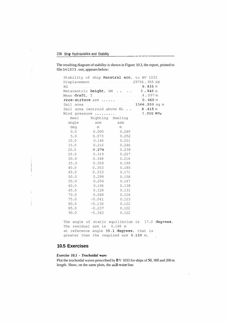
236 Ship Hydrostatics and Stability
The resulting diagram of stability is shown in Figure 10.3, the report, printed tofile bv!033 . out, appears below:
Stability of ship Maestral ace. to BV 1033Displacement 29736 . 955 kNKGMetacentric height,Mean draft, TFree- surf ace arm .Sail areaSail area centroid aWind pressure
Heel Rightingangle armdeg m0.0 0.0005.0 0.07310.0 0.14615.0 0.21620.0 ;0.27625.0 0.31930.0 0.34835.0 0.35940.0 0.35345.0 0.33350.0 0.29955.0 0.25460.0 0.19665.0 0.12870.0 0.04875.0 -0.04180.0 -0.13685.0 -0.23790.0 -0.342
5. 835 mGM . . . . 0 . 846 m
4 . 097 m0 . 060 m
1166 .550 sq mbove BL . . 8 .415 m
1.000 MPaHeelingarmm0.2490.2520.2510.2460.2380.2270.2140.1990.1850.1710.1580.1470.1380.1310.1260.1230.1220.1220.122
The angle of static equilibrium is 17.0 degrees.The residual arm is 0.168 mat reference angle 39.1 degrees, that isgreater than the required arm 0.120 m.
10.5 Exercises
Exercise 10.1 - Trochoidal wavePlot the trochoidal waves prescribed by B V 1033 for ships of 50,100 and 200 mlength. Show, on the same plots, the still-water line.
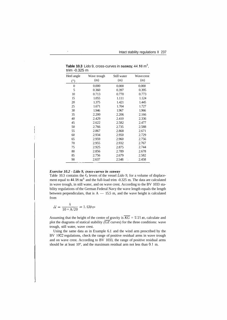
Intact stability regulations II 237
Table 10.3 Lido 9, cross-curves in seaway, 44.16 m3,trim -0.325 m
Heel angle
(°)
05
1015202530354045505560657075808590
Wave trough(m)
0.0000.3600.7131.0551.3751.6711.9462.2002.4292.6222.7662.8672.9342.9592.9552.9252.8562.7562.637
Still water(m)
0.0000.3970.7701.1111.4211.7041.9672.2062.4102.5822.7352.8682.9502.9602.9322.8752.7892.6792.548 X
Wave crest(m)
0.0000.3950.7731.1241.4451.7271.9662.1662.3362.4772.5882.6712.7292.7562.7672.7442.6782.5822.458
Exercise 10.2 - Lido 9, cross-curves in seawayTable 10.3 contains the Ik levers of the vessel Lido 9, for a volume of displace-ment equal to 44.16 m3 and the full-load trim -0.325 m. The data are calculatedin wave trough, in still water, and on wave crest. According to the BV 1033 sta-bility regulations of the German Federal Navy the wave length equals the lengthbetween perpendiculars, that is A — 15.5 m, and the wave height is calculatedfrom
TT A10 + A/20
-1.439m
Assuming that the height of the centre of gravity is KG = 2.21m, calculate andplot the diagrams of statical stability (GZ curves) for the three conditions: wavetrough, still water, wave crest.
Using the same data as in Example 6.1 and the wind arm prescribed by theBV 1022 regulations, check the range of positive residual arms in wave troughand on wave crest. According to BV 1033, the range of positive residual armsshould be at least 10°, and the maximum residual arm not less than 0.1 m.
11Flooding and damagecondition
11.1 Introduction
In the preceding chapters, we discussed the buoyancy and stability of intactships. Ships, however, can suffer damages during their service. Hull damagesthat affect the buoyancy can be caused by collision, by grounding or by enemyaction. Water can enter the damaged compartment and cause changes of draught,trim and heel. Above certain limits, such changes can lead to ship loss. We expecta ship to survive a reasonable amount of damage, that is an amount compatiblewith the size and tasks of the vessel. More specifically, we require that a ship thatsuffered hull damage, to an extent not larger than defined by pertinent regulations,should continue to float and be stable under moderate environmental conditions.Then, passengers and crew can be saved. Possibly the ship herself can be towedto a safe harbour.
To achieve survivability as defined above, the ship hull is subdivided into anumber of watertight compartments. The lengths of the compartments should besuch that after the flooding of a certain number of adjacent compartments, thewaterline shall not lie above a line prescribed by relevant regulations. The sameregulations specify the number of adjacent compartments that should be assumedflooded. This number depends on the size and the mission of the ship. The reasonfor considering adjacent compartments is simple. Collision, grounding or sin-gle enemy action usually damage adjacent compartments. Flooding of adjacentcompartments also can be more dangerous than flooding of two non-adjacentcompartments. Adjacent compartments situated at some distance from the mid-ship section can cause large trim and submerge openings above the deck, leadingthus to further flooding. Also, submerging part of the deck reduces the waterplanearea and can cause a substantial decrease of the metacentric radius. Flooding ofnon-adjacent compartments, for example one in the forebody, the other in theafterbody, can produce negligible trim. Then, even with relatively large draughtincreases, the deck does not submerge, the waterplane area is not reduced, and themetacentric height may be sufficient. If the deck does not submerge, no openingsare submerged. The need for international regulations governing the subdivisionof the hull into watertight compartments became clear after the Titanic disaster,
240 Ship Hydrostatics and Stability
in April 1912. A meeting was convened in London leading to the adoption on20 January 1914 of an International Convention of the Safety of Life at Sea.The convention is better known under its acronym, SOLAS. The first conven-tion should have been applied in July 1915, but the First World War stoppedthe process. In 1929, a new conference was held in London. The adopted textentered into force in 1933. Technical developments made necessary a new con-ference; it was held in 1948. The next edition was the 1960 SOLAS Convention,organized this time by IMO (about IMO see Section 8.2). Several amendmentswere adopted in the following years. The 1974 SOLAS Convention was againheld in London. Since then many important amendments were issued, some ofthem influenced by major marine disasters, such as those of the roll-on/roll-offpassenger ferries Herald of the Free Enterprise, near Zeebrugge, in March 1987,and Estonia, on 28 September 1994. At the moment of this publication SOLAS1974 together with all its amendments is the convention in force (see SOLAS2001).
SOLAS prescriptions cover many aspects of ship safety, among them fire pro-tection, life boats and rafts, radars, radio equipment, and emergency lighting.What interests us in this book are the prescriptions referring to subdivision anddamage stability. A detailed history of SOLAS activities can be found on a web-site organized by Metal Safe Sign International Ltd, http://www.mss-int.com.A short history of damage regulations appears in Gilbert and Card (1990).A commented history of the SOLAS achievements can be read in Payne (1994).Because of the overwhelming importance of the SOLAS regulations we givehere the translations of the official title in three other languages:
Fr Convention Internationale pour la sauvegarde de la vie humaineen mer
G Internationales Ubereinkommen zum Schutz des menschlichenLebens auf See
I Convenzione internazionale per la salvaguardia della vita umanain mare
The SOLAS regulations apply to merchant ships. Damage regulations for war-ships are provided in the same regulations that deal with their intact stability (seeChapters 8 and 10).
The European Commission sponsored researches on survivability in damagecondition, mainly the project HARDER. The Nordic countries established aproject entitled 'Safety of passenger/ro-ro vessels' (Svensen and Vassalos, 1998).
An alternative term used in damage considerations is bilging. Derrett andBarrass (2000) define it as follows: 'let an empty compartment be holed... belowthe waterline to such an extent that the water may ... flow freely into and out ofthe compartment. A vessel holed in this way is said to be bilged.'
Roll-on/Roll-off ships, shortly Ro/Ro, are particularly sensitive to damage. Toenable easy loading and unloading of vehicles these vessels are provided with adeck space uninterrupted by bulkheads. For the same reasons, that deck is closeto the waterline. Damage can easily cause deck flooding with consequences like
Flooding and damage condition 241
KG increase, large free-surface effect and added weight. Little and Hutchin-son (1995) quote, 'Over the past 14 years, 44 RO/RO vessels have capsized.'Pawlowski (1999) appreciates, 'Roll-on/roll-off (RO/RO) ships are consideredby the maritime profession ... as the most unsafe ships in operation.' Statisticson loss of life due to RO/RO disasters are simply frightening. For example, Ross,Roberts and Tighe (1997) quote 193 casualties in the case on the Herald of FreeEnterprise, 910 in the Estonia disaster. A few Ro/Ro's sank in one and a halfminute after an accident. No wonder that many studies have been dedicated tothis type of vessel. As some of them refer to constructive measures, we think thattheir treatment belongs to books on Ship Design, not here. We cite, however, thepapers whose contents are close to the subject of this chapter.
In this chapter, we give the definitions related to flooding and explain theprinciples on which flooding and damage calculations are based. To illustratethese principles we apply them to box shaped vessels. We also summarize a fewpertinent regulations and codes of practice. When performing calculations forreal-life projects, the reader is advised to refer to the full text of the most recentedition of the regulations to be applied.
Flooding and damage stability calculations for real ship forms are rather com-plex and tedious. Finding the floating condition requires iterative procedures.Today, such calculations are performed on computers; therefore, we do notdescribe them. We also give in this chapter the translations of the most importantterms introduced in it.
11.2 A few definitions
In this section, we introduce a few terms defined in the SOLAS conventions; theyare also used by other regulations. The hull is subdivided into compartmentsby means of watertight bulkheads. This term is translated into three otherlanguages as
Fr cloisons etanchesG SchottenI parade stagne
The deck up to which these bulkheads extend is called in English bulkheaddeck, in other languages
Fr pont de cloisonnementG SchottendeckI ponte delle parade
After flooding of a prescribed number of compartments the ship shall notsubmerge beyond a line situated at least 76 mm (3 in) below the deck at side.The said line is called in English margin line, in other languages
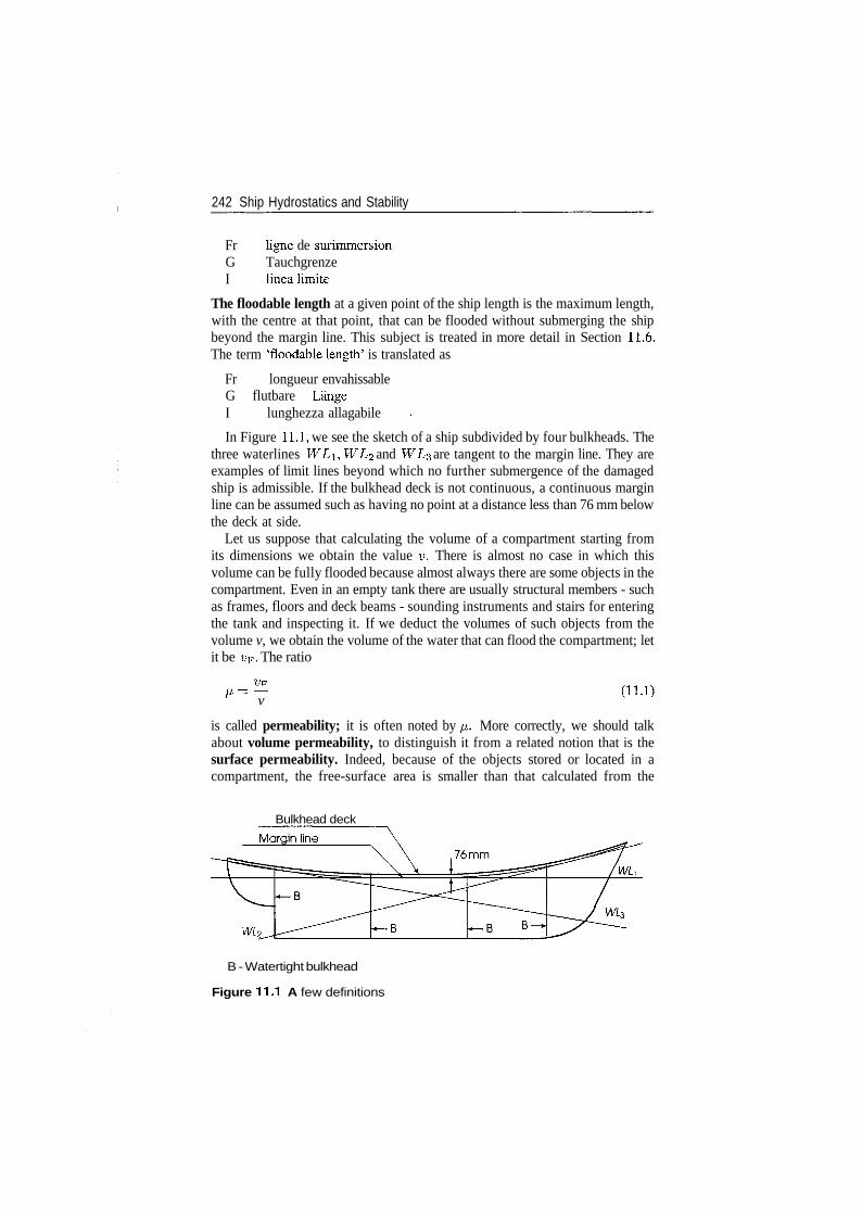
242 Ship Hydrostatics and Stability
Fr ligne de surimmersionG TauchgrenzeI linea limite
The floodable length at a given point of the ship length is the maximum length,with the centre at that point, that can be flooded without submerging the shipbeyond the margin line. This subject is treated in more detail in Section 11.6.The term 'floodable length' is translated as
Fr longueur envahissableG flutbare LangeI lunghezza allagabile
In Figure 11.1, we see the sketch of a ship subdivided by four bulkheads. Thethree waterlines WLi, WL<2 and WL% are tangent to the margin line. They areexamples of limit lines beyond which no further submergence of the damagedship is admissible. If the bulkhead deck is not continuous, a continuous marginline can be assumed such as having no point at a distance less than 76 mm belowthe deck at side.
Let us suppose that calculating the volume of a compartment starting fromits dimensions we obtain the value v. There is almost no case in which thisvolume can be fully flooded because almost always there are some objects in thecompartment. Even in an empty tank there are usually structural members - suchas frames, floors and deck beams - sounding instruments and stairs for enteringthe tank and inspecting it. If we deduct the volumes of such objects from thevolume v, we obtain the volume of the water that can flood the compartment; letit be VF. The ratio
M = — (H.l)v
is called permeability; it is often noted by p,. More correctly, we should talkabout volume permeability, to distinguish it from a related notion that is thesurface permeability. Indeed, because of the objects stored or located in acompartment, the free-surface area is smaller than that calculated from the
Bulkhead deck
WL2
B - Watertight bulkhead
Figure 11.1 A few definitions
Flooding and damage condition 243
dimensions of the compartment. Also the moment of inertia of the free-surfacearea is calculated on the basis of the dimensions of the compartment. For exam-ple, if the calculations are carried out by a computer programme, they are basedon an input that describes only the geometry of the tank and not its contents.The moment of inertia of the surface free to heel is smaller than the value foundas above because the area considered is partially occupied by fixed objects thatdo not contribute to the free-surface effect. Then, it is necessary to multiply thecalculated value by the surface permeability.
Typical values of volume permeability can be found in textbooks and in variousregulations. Examples of the latter are given in this chapter. When the recom-mended values do not seem plausible, it is necessary to calculate in detail thevolume of the objects found in the compartment. When there are no better data,the surface permeability can be assumed equal to the volume permeability of thesame compartment.
The term 'permeability' is translated into other languages as follows
Fr (coefficient de) permeabiliteG FlutbarkeitI (coefficiente di) permeabilita
Usually, permeabilities are given in percent, for example 85 for machineryspaces. In calculations, however, we must multiply by 0.85, and not by 85. More-over, some computer programmes, such as ARCHIMEDES, require as input thenumber 0.85 and not 85. Therefore, in the following sections permeabilities aremainly given in the format 0.95, 0.85 etc., rather than as percentages.
11.3 Two methods for finding the ship condition afterflooding
There are two ways of calculating the effect of flooding. One way is known asthe method of lost buoyancy, the other as the method of added weight.
The method of lost buoyancy assumes that a flooded compartment does notsupply buoyancy. This is what happens in reality. If we refer to Figures 2.4and 2.5, we can imagine that if there is open communication between a com-partment and the surrounding water, the water inside the compartment exercisespressures equal to and opposed to those of the external water. Then, the buoyancyforce predicted by the Archimedes' principle is cancelled by the weight of theflooding water.
In the method of lost buoyancy the volume of the flooded compartment doesnot belong anymore to the vessel, while the weight of its structures is still part ofthe displacement. The 'remaining' vessel must change position until force andmoment equilibria are re-established. During the process not only the displace-ment, but also the position of the centre of gravity remains constant. The method
244 Ship Hydrostatics and Stability
is also known as method of constant displacement. As the flooding water doesnot belong to the ship, it causes no free-surface effect.
In the method of added weight the water entering a damaged compartment isconsidered as belonging to the ship; its mass must be added to the ship displace-ment. Hence the term 'added weight'. Following modern practice, we actuallywork with masses; however, we keep the traditional name of the method, i.e. weuse the word 'weight'. Another reason may be the need to avoid confusion withthe term added mass mentioned in Section 6.12 and detailed in Chapter 12. Thelatter term does not belong to the theory of flooding and damage stability.
In the method of added weight the displacement of the flooded vessel is cal-culated as the sum of the intact displacement and the mass of the flooding water.The position of the centre of gravity of the damaged vessel is obtained from thesums of the moments of the intact vessel and of the flooding water. Becomingpart of the vessel, the flooding water produces a free-surface effect that must becalculated and considered in all equations. For very small trim and negligibleheel changes we can write
AF = AI + p - v
LCGF • AF = LCGi -Ai + lcg-p-v (11.2)
TCGF • AF = teg - p • v
where the subscript F distinguishes the properties of the flooded vessel, andthe subscript I those of the intact ship. By leg we mean the longitudinal centreof gravity of the flooding water volume, v, and by teg its transverse centre ofgravity. We assume TCGi = 0. When the trim and the heel are not negligible,we must consider the vertical coordinates of the centres of gravity of the intactship and of the flooding water volume. Example 11.1 shows how to do this fornon-zero trim and zero heel.
To exemplify the above principles we follow an idea presented in Handbuchder Werften and later used by Watson (1998). While the latter solves algebraicallythe general problem, we prefer to solve it numerically and thus allow the readerto visualize the differences between methods and those between the intact andthe damaged vessel. We choose the very simple example of the pontoon shownin Figure 11.2. Two transverse bulkheads subdivide the hull into three watertightcompartments. In the following two sections we assume that Compartment 2 isdamaged and calculate the consequences of its flooding. We choose deliberatelya compartment symmetric about the midship transverse plane of symmetry ofthe pontoon. Thus, the flooding of Compartment 2 produces no trim. Also, thecompartment extends for the full ship breadth and its flooding produces no heel.The only change of position is parallel sinking. Thus, the complex calcula-tions necessary for conventional ship forms, for large trim, or for unsymmetricalflooding, do not obscure the principles and it is possible to obtain immediatelya good insight of the processes involved. For the same reasons we assume thatthe volume and surface permeabilities are equal to 1. We leave to an exercise the
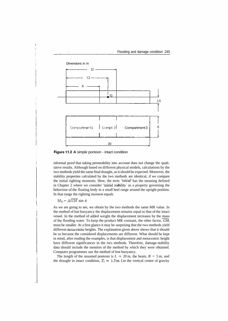
Flooding and damage condition 245
Dimensions in m
12
10
G
1.5
Comportment 1 Compt.: Compartment 3
20
Figure 11.2 A simple pontoon - intact condition
informal proof that taking permeability into account does not change the quali-tative results. Although based on different physical models, calculations by thetwo methods yield the same final draught, as it should be expected. Moreover, thestability properties calculated by the two methods are identical, if we comparethe initial righting moments. Here, the term 'initial' has the meaning definedin Chapter 2 where we consider 'initial stability' as a property governing thebehaviour of the floating body in a small heel range around the upright position.In that range the righting moment equals
MR = A(7M sin 0
As we are going to see, we obtain by the two methods the same MR value. Inthe method of lost buoyancy the displacement remains equal to that of the intactvessel. In the method of added weight the displacement increases by the massof the flooding water. To keep the product MR constant, the other factor, GM,must be smaller. At a first glance it may be surprising that the two methods yielddifferent metacentric heights. The explanation given above shows that it shouldbe so because the considered displacements are different. What should be keptin mind, after reading the examples, is that displacement and metacentric heighthave different significances in the two methods. Therefore, damage-stabilitydata should include the mention of the method by which they were obtained.Computer programmes use the method of lost buoyancy.
The length of the assumed pontoon is L = 20 m, the beam, B = 5 m, andthe draught in intact condition, TI = 1.5m. Let the vertical centre of gravity
246 Ship Hydrostatics and Stability
be KG\ = 1.5m. The following calculations were carried out in MATLAB,using the full precision of the software. The results are rounded off to a reason-able number of decimal digits. We first find the data of the intact pontoon. Thedisplacement volume is
Vi = LBTi = 20 x 5 x 1.5 = 150m3
The mass displacement equals
A! = pVi - 1.025 x 150 = 153.751
The moment of inertia of the waterplane area about the centreline equals
and the resulting metacentric radius is
/i 208.3333BMi = — = = 1.389 m
For such a simple form we could have found directly the metacentric radius as
B3L/12 B2 52
The height of the centre of buoyancy is
rji
~KBi = — -0.75mZi
and the metacentric height is
= KBi 4- BMi - KGi = 0.75 + 1.389 - 1.50 = 0.639m
For small heel angles the righting moment in intact condition is calculated as
= AiGMisin<£ = 153.75 x 0.693 x sm</> = 98.229sin0tin
11.3.1 Lost buoyancy
The translations of the term 'method of lost buoyancy' in three other languagesare
Fr La methode des carenes perduesG Methode des wegfallender VerdrangungI II metodo per perdita di galleggiabilita
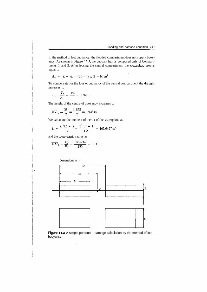
Flooding and damage condition 247
In the method of lost buoyancy, the flooded compartment does not supply buoy-ancy. As shown in Figure 11.3, the buoyant hull is composed only of Compart-ments 1 and 3. After loosing the central compartment, the waterplane area isequal to
AL = (L- 1}B = (20 - 4) x 5 = 80m2
To compensate for the loss of buoyancy of the central compartment the draughtincreases to
VT 150TL = ̂ = - = 1.875m
The height of the centre of buoyancy increases to
TT 1 875
We calculate the moment of inertia of the waterplane as
B3(L-l) 53(20-4)/L = —J2— = 12 = 16
and the metacentric radius as
IT. 166.6667 . . „ _
Dimensions in m
12
10
Figure 11.3 A simple pontoon - damage calculation by the method of lostbuoyancy
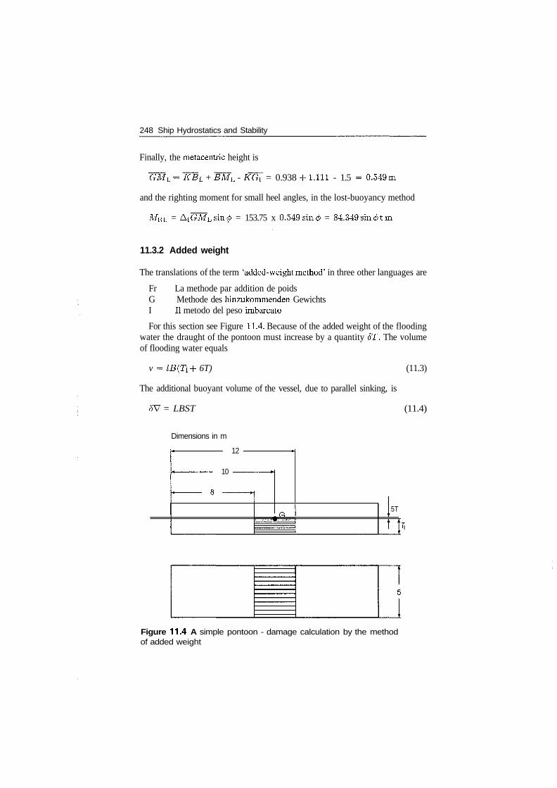
248 Ship Hydrostatics and Stability
Finally, the metacentric height is
GML = KBL + BML - KGi = 0.938 4-1.111 - 1.5 - 0.549m
and the righting moment for small heel angles, in the lost-buoyancy method
MRL = AiGMLsin0 = 153.75 x 0.549 sin 0 = 84.349sin</>tm
11.3.2 Added weight
The translations of the term 'added-weight method' in three other languages are
Fr La methode par addition de poidsG Methode des hinzukommenden GewichtsI II metodo del peso imbarcato
For this section see Figure 11.4. Because of the added weight of the floodingwater the draught of the pontoon must increase by a quantity ST. The volumeof flooding water equals
v = lB(Ti + 6T) (11.3)
The additional buoyant volume of the vessel, due to parallel sinking, is
SV = LBST (11.4)
Dimensions in m
12
10
5T
Figure 11.4 A simple pontoon - damage calculation by the methodof added weight
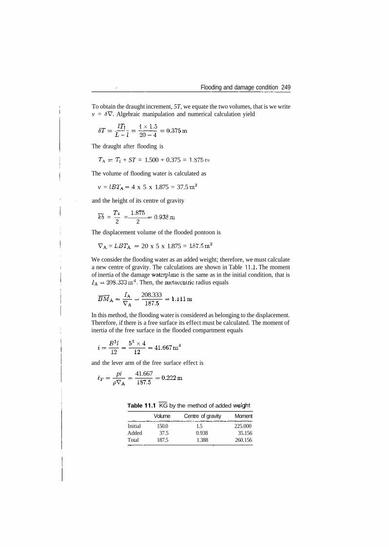
Flooding and damage condition 249
To obtain the draught increment, 5T, we equate the two volumes, that is we writev = JV. Algebraic manipulation and numerical calculation yield
The draught after flooding is
TA - TI + ST = 1.500 + 0.375 = 1.875m
The volume of flooding water is calculated as
v = IBTA = 4 x 5 x 1.875 = 37.5 m3
and the height of its centre of gravity
kb = — = = 0.938m2 2
The displacement volume of the flooded pontoon is
VA = LET p. - 20 x 5 x 1.875 = 187.5m3
We consider the flooding water as an added weight; therefore, we must calculatea new centre of gravity. The calculations are shown in Table 11.1. The momentof inertia of the damage waterplane is the same as in the initial condition, that is/A = 208.333 m4. Then, the metacentric radius equals
JA 208.333 .. .
In this method, the flooding water is considered as belonging to the displacement.Therefore, if there is a free surface its effect must be calculated. The moment ofinertia of the free surface in the flooded compartment equals
and the lever arm of the free surface effect is
pi 41.667
Table 11.1 KG by the method of added weight
Volume Centre of gravity Moment
Initial 150.0 1.5 225.000Added 37.5 0.938 35.156Total 187.5 1.388 260.156
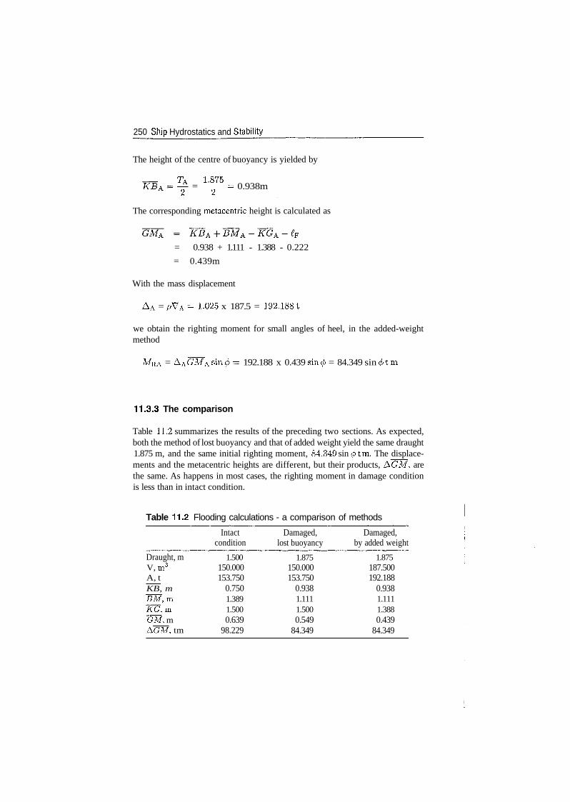
250 SWp Hydrostatics and Stability
The height of the centre of buoyancy is yielded by
= = 0.938m
The corresponding metacentric height is calculated as
= 0.938 + 1.111 - 1.388 - 0.222
= 0.439m
With the mass displacement
AA = pVA = 1-025 x 187.5 = 192.188 1
we obtain the righting moment for small angles of heel, in the added-weightmethod
MRA = AAGMAsin0= 192.188 x 0.439 sin0 = 84.349 sin </>tm
11.3.3 The comparison
Table 11.2 summarizes the results of the preceding two sections. As expected,both the method of lost buoyancy and that of added weight yield the same draught1.875 m, and the same initial righting moment, 84.349 sin <fi tm. The displace-ments and the metacentric heights are different, but their products, AGM, arethe same. As happens in most cases, the righting moment in damage conditionis less than in intact condition.
Table 11.2 Flooding calculations - a comparison of methods
Draught, mV, m3
A, tKB, mBM,mKG,mGM, mAGM, tm
Intactcondition
1.500150.000153.750
0.7501.3891.5000.639
98.229
Damaged,lost buoyancy
1.875150.000153.750
0.9381.1111.5000.549
84.349
Damaged,by added weight
1.875187.500192.188
0.9381.1111.3880.439
84.349
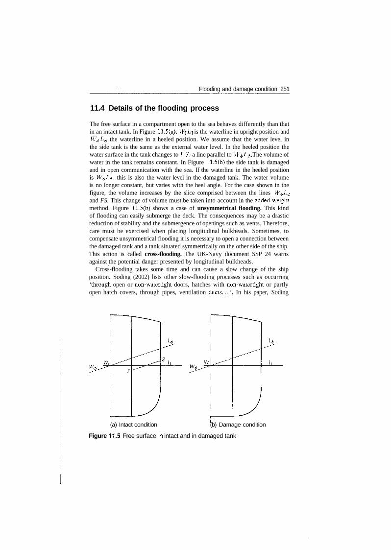
Flooding and damage condition 251
11.4 Details of the flooding process
The free surface in a compartment open to the sea behaves differently than thatin an intact tank. In Figure 11.5(a), W\L\ is the waterline in upright position andW^L^, the waterline in a heeled position. We assume that the water level inthe side tank is the same as the external water level. In the heeled position thewater surface in the tank changes to FS, a line parallel to W^L^. The volume ofwater in the tank remains constant. In Figure 11.5(b) the side tank is damagedand in open communication with the sea. If the waterline in the heeled positionis W0L0, this is also the water level in the damaged tank. The water volumeis no longer constant, but varies with the heel angle. For the case shown in thefigure, the volume increases by the slice comprised between the lines W^L^and FS. This change of volume must be taken into account in the added-weightmethod. Figure 11.5(b) shows a case of unsymmetrical flooding. This kindof flooding can easily submerge the deck. The consequences may be a drasticreduction of stability and the submergence of openings such as vents. Therefore,care must be exercised when placing longitudinal bulkheads. Sometimes, tocompensate unsymmetrical flooding it is necessary to open a connection betweenthe damaged tank and a tank situated symmetrically on the other side of the ship.This action is called cross-flooding. The UK-Navy document SSP 24 warnsagainst the potential danger presented by longitudinal bulkheads.
Cross-flooding takes some time and can cause a slow change of the shipposition. Soding (2002) lists other slow-flooding processes such as occurring'through open or non-watertight doors, hatches with non-watertight or partlyopen hatch covers, through pipes, ventilation ducts...'. In his paper, Soding
(a) Intact condition (b) Damage condition
Figure 11.5 Free surface In intact and in damaged tank
252 Ship Hydrostatics and Stability
describes the mathematics of such water flows. Air can be trapped above theflooding-water surface. If the top envelope of the compartment is airtight floodingis stopped. If not, it is only slowed down.
Between the position of intact condition and the final damage position (pro-vided that an equilibrium position can be found) the vessel can pass throughintermediate positions more dangerous than the final one. It is necessary tocheck if such positions exist and if the ship can survive them.
11.5 Damage stability regulations
11.5.1 SOLAS
Regulation 5 of the convention specifies how to calculate the permeabilities tobe considered. Thus, the permeability, in percentage, throughout the machineryspace shall be
where a is the volume of passenger spaces situated under the margin line, withinthe limits of the machinery space, c is the volume of between-deck spaces, inthe same zone, appropriated to cargo, coal, or store, and v, the whole volume ofthe machinery space below the margin line.
The percent permeability of spaces forward or abaft of the machinery spacesshould be found from
63 + 35-v
where a is the volume of passenger spaces under the margin line, in the respectivezone, and v, the whole volume, under the margin line, in the same zone.
The maximum permissible length of a compartment having its centre at agiven point of the ship length is obtained from the floodable length by multiplyingthe latter by an appropriate number called factor of subdivision. For example, afactor of subdivision equal to 1 means that the margin line should not submergeif one compartment is submerged, while a factor of subdivision equal to 0.5means that the margin line should not submerge when two compartments areflooded.
Regulation 6 of the convention shows how to calculate the factor of subdivisionas a function of the ship length and the nature of the ship service. First, SOLASdefines a factor, A, applicable to ships primarily engaged in cargo transportation
Flooding and damage condition 253
ForL = 131, A = 1. Another f actor, B, is applicable for ships primarily engagedin passenger transportation
ForL = 79, B = 1.A criterion of service numeral, Cs, is calculated as function of the ship length,
L, the volume of machinery and bunker spaces, M, the volume of passengerspaces below the margin line, P, the number of passengers for which the ship iscertified, TV, and the whole volume of the ship below the margin line, V. Thereare two formulas for calculating Cs; their choice depends upon the productPI = KN, where K = 0.056L. If Pl is greater than P,
3 V + P.-P
otherwise
M + 2P- 72-V
For ships of length 131 m and above, having a criterion numeral Cs < 23, thesubdivision abaft the forepeak is governed by the factor A. If Cs > 123 thesubdivision is governed by the factor B. For 23 < Cs < 123, the subdivisionfactor should be interpolated as
F=A100
If 79 < L < 131, a number S should be calculated from
3.754 - 25L5 =
13
If Cs = 5, F = 1. If Cs > 123, the subdivision is governed by the factor B. IfCs lies between 5 and 123, the subdivision factor is interpolated as
123-5
If 79 < L < 131 and Cs < 5, or if L < 79, F = 1.Regulation 7 of the convention contains special requirements for the subdi-
vision of passenger ships. Regulation 8 specifies the criteria of stability in thefinal condition after damage. The heeling arm to be considered as the one thatresults from the largest of the following moments:
254 Ship Hydrostatics and Stability
• crowding of all passengers on one side;• launching of all fully loaded, davit-operated survival craft on one side;• due to wind pressure.
We call residual righting lever arm the difference
GZ — heeling arm
The range of positive residual arm shall be not less than 15°. The area under therighting-arm curve should be at least 0.015 mrad, between the angle of staticequilibrium and the smallest of the following:
• angle of progressive flooding;• 22° if one compartment is flooded, 27° if two or more adjacent compartments
are flooded.
The moment due to the crowding of passengers shall be calculated assuming4 persons per m2 and a mass of 75 kg for each passenger. The moment due to thelaunching of survival craft shall be calculated assuming all lifeboats and rescueboats fitted on the side that heeled down, while the davits are swung out andfully loaded. The wind heeling moment shall be calculated assuming a pressureof 120 Nm~2 .
11.5.2 Probabilistic regulations
Wendel (1960a) introduces the notion of probability of survival after dam-age. A year later, a summary in French appears in Anonymous (1961). Thispaper mentions a translation into French of Wendel's original paper (in Bul-letin Technique du Bureau Veritas, February 1961) and calls the method 'unenouvelle voie', that is 'a new way'. Much has been written since then on the prob-abilistic approach; we mention here only a few publications, such as Rao (1968),Wendel (1970), Abicht and Bakenhus (1970), Abicht, Kastner and Wendel (1977),Wendel (1977). Over the years Wendel used new and better statistics to improvethe functions of probability density and probability introduced by him. The gen-eral idea is to consider the probability of occurrence of a damage of length y andtransverse extent t, with the centre at a position x on the ship length. Statisticsof marine accidents should allow the formulation of a function of probabilitydensity, /(#, y, t). The probability itself is obtained by triple integration of thedensity function. The IMO regulation A265 introduces probabilistic regulationsfor passenger ships, and SOLAS 1974, Part Bl, defines probabilistic rules forcargo ships. Concisely, Regulation 25 of the SOLAS convention defines a degreeof subdivison
R= (0.002 + 0.0009L3)1/3
Flooding and damage condition 255
where L is measured in metres. An attained subdivision index shall be calcu-lated as
A = Ylplsi
where pi represents the probability that the ith compartment or group of com-partments may be flooded, and Si is the probability of survival after flooding thezth compartment or group of compartments. The attained subdivision index, A,should not be less than the required subdivision index, R.
Early details of the standard for subdivision and damage stability of dry cargoships are given by Gilbert and Card (1990). A critical discussion of the IMO 1992probabilistic damage criteria for dry cargo ships appears in Sonnenschein andYang (1993). The probabilistic SOLAS regulations are discussed in some detailby Watson (1998) who also exemplifies them numerically. Ravn et al. (2002)exemplify the application of the rules to Ro-Ro vessels.
Serious criticism of the SOLAS probabilistic approach to damage can be foundin Bjorkman (1995). Quoting from the title of the paper, 'apparent anomaliesin SOLAS and MARPOL requirements'. Watson (1998) writes, 'There wouldseem to be two main objections to the probabilistic rules. The first of these is theextremely large amount of calculations required, which although acceptable inthe computer age, is scarcely to be welcomed. The other objection is the lack ofguidance that it gives to a designer, who may be even driven to continuing use ofthe deterministic method in initial design, changing to the probabilistic later -and hoping this does not entail major changes!'
The 'CORDIS RTD PROJECTS' database of the European Communities,2000, defines as follows the objective of project HARDER:
The process of harmonisation of damage stability regulationsaccording to the probabilistic approach is undergoing scrutiny...before being proposed for adoption by IMO... However, ongoinginvestigations started revealing serious lack of robustness and con-sistency and more importantly a worrying lack of rationale in thechoice of parameters that are likely to affect the evolution of theoverall design and safety of ships.
A recent application of existing tools by a committee of the relevantIMO working group... revealed that, before confidence in the wholeprocess is irreversibly affected, concerted effort at European levelmust address the thorough validation of calculations, the properchoice of parameters and the definition of levels of acceptance
A report on the progress of the project HARDER is contained in the IMO doc-ument SLF 45/3/3 of 19 April 2002. The report covers 'Investigations and pro-posed formulations for the factor "S": the probability of survival after flooding'.The approach adopted in the project HARDER is explained by Rusas (2002). Asthe probabilistic regulations are bound to change, we do not detail them in thisbook.
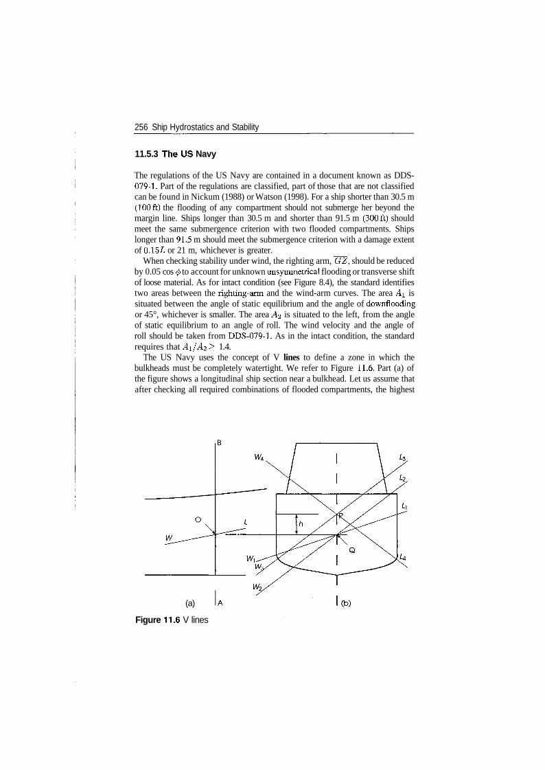
256 Ship Hydrostatics and Stability
11.5.3 The US Navy
The regulations of the US Navy are contained in a document known as DDS-079-1. Part of the regulations are classified, part of those that are not classifiedcan be found in Nickum (1988) or Watson (1998). For a ship shorter than 30.5 m(100ft) the flooding of any compartment should not submerge her beyond themargin line. Ships longer than 30.5 m and shorter than 91.5 m (300ft) shouldmeet the same submergence criterion with two flooded compartments. Shipslonger than 91.5 m should meet the submergence criterion with a damage extentof 0.15L or 21 m, whichever is greater.
When checking stability under wind, the righting arm, GZ, should be reducedby 0.05 cos <j> to account for unknown unsymmetrical flooding or transverse shiftof loose material. As for intact condition (see Figure 8.4), the standard identifiestwo areas between the righting-arm and the wind-arm curves. The area AI issituated between the angle of static equilibrium and the angle of downfloodingor 45°, whichever is smaller. The area A% is situated to the left, from the angleof static equilibrium to an angle of roll. The wind velocity and the angle ofroll should be taken from DOS-079-1. As in the intact condition, the standardrequires that Ai/A^ > 1.4.
The US Navy uses the concept of V lines to define a zone in which thebulkheads must be completely watertight. We refer to Figure 11.6. Part (a) ofthe figure shows a longitudinal ship section near a bulkhead. Let us assume thatafter checking all required combinations of flooded compartments, the highest
(a)
Figure 11.6 V lines
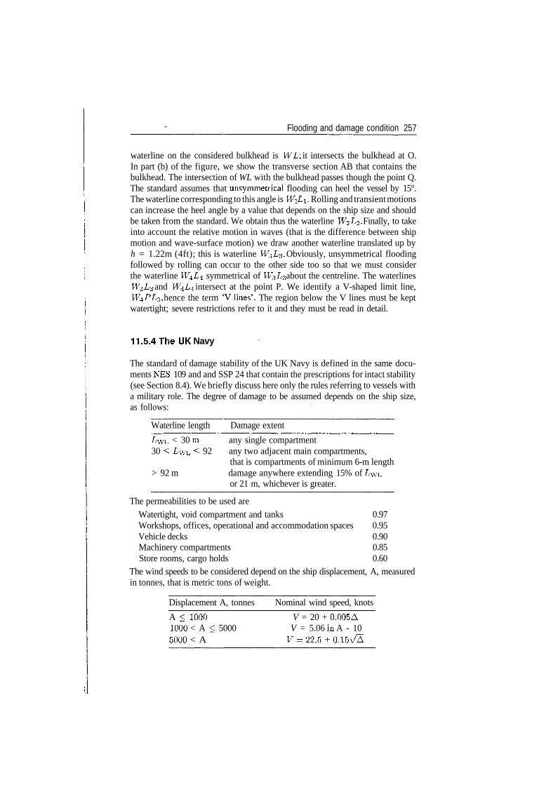
Flooding and damage condition 257
waterline on the considered bulkhead is WL\ it intersects the bulkhead at O.In part (b) of the figure, we show the transverse section AB that contains thebulkhead. The intersection of WL with the bulkhead passes though the point Q.The standard assumes that unsymmetrical flooding can heel the vessel by 15°.The waterline corresponding to this angle is W\ LI . Rolling and transient motionscan increase the heel angle by a value that depends on the ship size and shouldbe taken from the standard. We obtain thus the waterline W^L^. Finally, to takeinto account the relative motion in waves (that is the difference between shipmotion and wave-surface motion) we draw another waterline translated up byh = 1.22m (4ft); this is waterline W^L^. Obviously, unsymmetrical floodingfollowed by rolling can occur to the other side too so that we must considerthe waterline W4Z/4 symmetrical of W^L^ about the centreline. The waterlinesW^LZ and W^L^ intersect at the point P. We identify a V-shaped limit line,W^PLz, hence the term 'V lines'. The region below the V lines must be keptwatertight; severe restrictions refer to it and they must be read in detail.
11.5.4 The UK Navy
The standard of damage stability of the UK Navy is defined in the same docu-ments NES 109 and and SSP 24 that contain the prescriptions for intact stability(see Section 8.4). We briefly discuss here only the rules referring to vessels witha military role. The degree of damage to be assumed depends on the ship size,as follows:
Waterline length Damage extent
LWL < 30 m any single compartment30 < I/WL < 92 any two adjacent main compartments,
that is compartments of minimum 6-m length> 92 m damage anywhere extending 15% of LWL
or 21 m, whichever is greater.
The permeabilities to be used are
Watertight, void compartment and tanks 0.97Workshops, offices, operational and accommodation spaces 0.95Vehicle decks 0.90Machinery compartments 0.85Store rooms, cargo holds 0.60
The wind speeds to be considered depend on the ship displacement, A, measuredin tonnes, that is metric tons of weight.
Displacement A, tonnes Nominal wind speed, knots
A < 1000 V = 20 + 0.005A1000 < A < 5000 V = 5.06 In A - 105000 < A F-22.5 + 0.15V/A
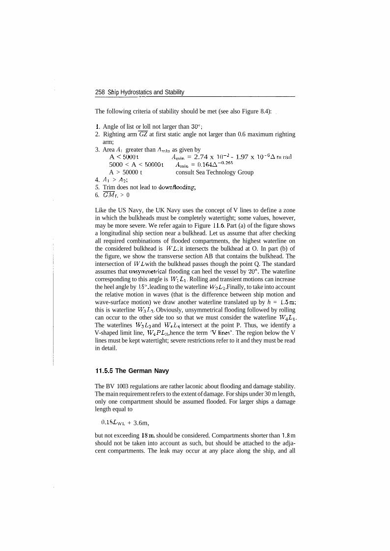
258 Ship Hydrostatics and Stability
The following criteria of stability should be met (see also Figure 8.4):
1. Angle of list or loll not larger than 30°;2. Righting arm GZ at first static angle not larger than 0.6 maximum righting
arm;3. Area A\ greater than Am-in as given by
A < SOOOt Amin = 2.74 x 10~2 - 1.97 x 10~6Amrad5000 < A < 500001 Amin = 0.164A-0-265
A > 50000 t consult Sea Technology Group4. Ai > A<2\5. Trim does not lead to downflooding;6. ~GML > 0
Like the US Navy, the UK Navy uses the concept of V lines to define a zonein which the bulkheads must be completely watertight; some values, however,may be more severe. We refer again to Figure 11.6. Part (a) of the figure showsa longitudinal ship section near a bulkhead. Let us assume that after checkingall required combinations of flooded compartments, the highest waterline onthe considered bulkhead is WL\ it intersects the bulkhead at O. In part (b) ofthe figure, we show the transverse section AB that contains the bulkhead. Theintersection of WL with the bulkhead passes though the point Q. The standardassumes that unsymmetrical flooding can heel the vessel by 20°. The waterlinecorresponding to this angle is W\L\. Rolling and transient motions can increasethe heel angle by 15°, leading to the waterline W^L^. Finally, to take into accountthe relative motion in waves (that is the difference between ship motion andwave-surface motion) we draw another waterline translated up by h = 1.5m;this is waterline W^L^. Obviously, unsymmetrical flooding followed by rollingcan occur to the other side too so that we must consider the waterline W±L±.The waterlines W^L^ and W±L± intersect at the point P. Thus, we identify aV-shaped limit line, W^PL^, hence the term 'V lines'. The region below the Vlines must be kept watertight; severe restrictions refer to it and they must be readin detail.
11.5.5 The German Navy
The BV 1003 regulations are rather laconic about flooding and damage stability.The main requirement refers to the extent of damage. For ships under 30 m length,only one compartment should be assumed flooded. For larger ships a damagelength equal to
0.18LWL + 3.6m,
but not exceeding 18m, should be considered. Compartments shorter than 1.8 mshould not be taken into account as such, but should be attached to the adja-cent compartments. The leak may occur at any place along the ship, and all
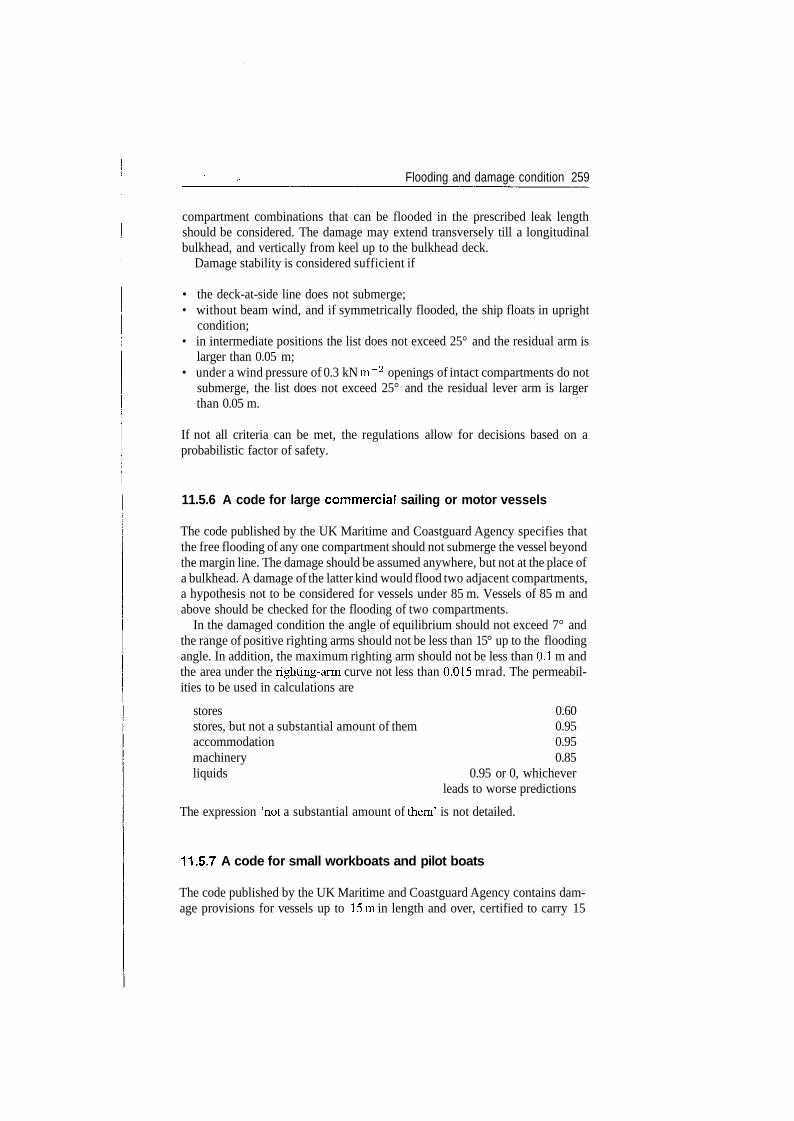
Flooding and damage condition 259
compartment combinations that can be flooded in the prescribed leak lengthshould be considered. The damage may extend transversely till a longitudinalbulkhead, and vertically from keel up to the bulkhead deck.
Damage stability is considered sufficient if
• the deck-at-side line does not submerge;• without beam wind, and if symmetrically flooded, the ship floats in upright
condition;• in intermediate positions the list does not exceed 25° and the residual arm is
larger than 0.05 m;• under a wind pressure of 0.3 kN m~2 openings of intact compartments do not
submerge, the list does not exceed 25° and the residual lever arm is largerthan 0.05 m.
If not all criteria can be met, the regulations allow for decisions based on aprobabilistic factor of safety.
11.5.6 A code for large commercial sailing or motor vessels
The code published by the UK Maritime and Coastguard Agency specifies thatthe free flooding of any one compartment should not submerge the vessel beyondthe margin line. The damage should be assumed anywhere, but not at the place ofa bulkhead. A damage of the latter kind would flood two adjacent compartments,a hypothesis not to be considered for vessels under 85 m. Vessels of 85 m andabove should be checked for the flooding of two compartments.
In the damaged condition the angle of equilibrium should not exceed 7° andthe range of positive righting arms should not be less than 15° up to the floodingangle. In addition, the maximum righting arm should not be less than 0.1 m andthe area under the righting-arm curve not less than 0.015 mrad. The permeabil-ities to be used in calculations are
stores 0.60stores, but not a substantial amount of them 0.95accommodation 0.95machinery 0.85liquids 0.95 or 0, whichever
leads to worse predictions
The expression 'not a substantial amount of them' is not detailed.
11.5.7 A code for small workboats and pilot boats
The code published by the UK Maritime and Coastguard Agency contains dam-age provisions for vessels up to 15m in length and over, certified to carry 15
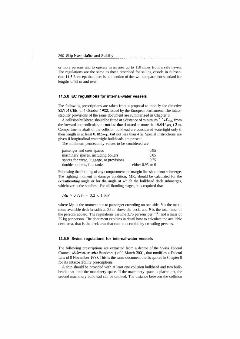
260 Ship Hydrostatics and Stability
or more persons and to operate in an area up to 150 miles from a safe haven.The regulations are the same as those described for sailing vessels in Subsec-tion 11.5.6, except that there is no mention of the two-compartment standard forlengths of 85 m and over.
11.5.8 EC regulations for internal-water vessels
The following prescriptions are taken from a proposal to modify the directive82/714 GEE, of 4 October 1982, issued by the European Parliament. The intact-stability provisions of the same document are summarized in Chapter 8.
A collision bulkhead should be fitted at a distance of minimum 0.04LWL fromthe forward perpendicular, but not less than 4 m and no more than 0.041/wL+2 m.Compartments abaft of the collision bulkhead are considered watertight only iftheir length is at least O.lOZ/wL, but not less than 4m. Special instructions aregiven if longitudinal watertight bulkheads are present.
The minimum permeability values to be considered are:
passenger and crew spaces 0.95machinery spaces, including boilers 0.85spaces for cargo, luggage, or provisions 0.75double bottoms, fuel tanks either 0.95 or 0
Following the flooding of any compartment the margin line should not submerge.The righting moment in damage condition, MR, should be calculated for thedownflooding angle or for the angle at which the bulkhead deck submerges,whichever is the smallest. For all flooding stages, it is required that
MR > 0.2MP = 0.2 x 1.56P
where Mp is the moment due to passenger crowding on one side, b is the maxi-mum available deck breadth at 0.5 m above the deck, and P is the total mass ofthe persons aboard. The regulations assume 3.75 persons per m2, and a mass of75 kg per person. The document explains in detail how to calculate the availabledeck area, that is the deck area that can be occupied by crowding persons.
11.5.9 Swiss regulations for internal-water vessels
The following prescriptions are extracted from a decree of the Swiss FederalCouncil (Schweizerische Bundesrat) of 9 March 2001, that modifies a FederalLaw of 8 November 1978. This is the same document that is quoted in Chapter 8for its intact-stability prescriptions.
A ship should be provided with at least one collision bulkhead and two bulk-heads that limit the machinery space. If the machinery space is placed aft, thesecond machinery bulkhead can be omitted. The distance between the collision
Flooding and damage condition 261
bulkhead and the intersection of the stem (bow) with the load waterline shouldlie between L\vL/12 and LwL/8. If this distance is shorter, it is necessary toprove by calculations that the fully loaded ship continues to float when the twoforemost compartments are flooded. In no intermediary position should the deck-at-side line submerge. This proof is not necessary if the ship has on both sideswatertight compartments extending longitudinally I/wL/8 from the intersectionof the stem with the load waterline, and transversely at least £?/5.
11.6 The curve of floodable lengths
Today computer programmes receive as input the descriptions of the hull surfaceand of the internal subdivision. In the simplest form, the input can consist of off-sets, bulkhead positions and compartment permeabilities. Then, it is possible tocheck in a few seconds what happens when certain compartment combinationsare flooded. If the results do not meet the criteria relevant to the project, we canchange the positions of bulkheads and run flooding and damage-stability calcu-lations for the newly defined subdivision. Before the advent of digital computersthe above procedure took a lot of time; therefore, it could not be repeated manytimes. Just to give an idea, manual flooding calculations for one compartmentcombination could take something like three hours. Usually, the calculationswere not purely manual because most Naval Architects used slide rules, addingmachines and planimetres. Still it was not possible to speed up the work. Toimprove efficiency, Naval Architects devised ingenious, very elegant methods;one of them produces the curve of floodable lengths. To explain it we refer toFigure 11.7. In the lower part of the figure, we show a ship outline with fourtransverse bulkheads; above it we show a curve of floodable lengths and how touse it.
Let us consider a point situated a distance x from the aftermost point of theship. Let us assume that we calculated the maximum length of the compartmenthaving its centre at x and that will not submerge the margin line, and that lengthis Lp. In other words, if we consider a compartment that extends from x — Lp/2to x -f Z/F/2, this is the longest compartment with centre at x that when floodedwill not submerge the ship beyond the margin line.
Now, we plot a point with the given x-coordinate and the ^/-coordinate equalto LF measured at half the scale used for x values. For example, if the shipoutline is drawn at the scale 1:100, we plot y values at the scale 1:200. Therewere Naval Architects who used the same scale for both coordinates; however,the reader will discover that there is an advantage in the procedure preferred byus. Plotting in this way all (x, LF) pairs, we obtain the curve marked 1; this isthe curve of floodable lengths.
Now, let us check if the middle compartment meets the submergence-to-the-margin-line requirement. Counting from aft forward, we talk about the compart-ment limited by the second and the third bulkhead. Let us assume that this is
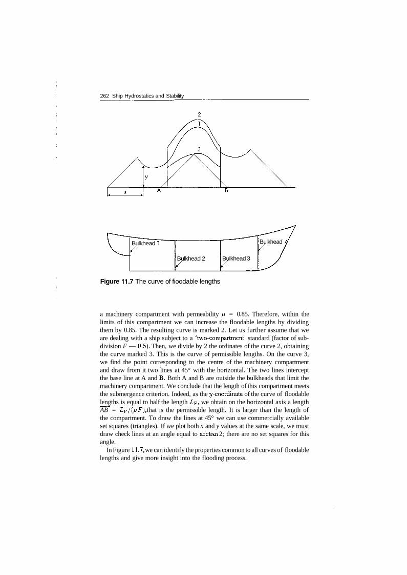
262 Ship Hydrostatics and Stability
Bulkhead 1
Bulkhead 2 Bulkhead 3
Bulkhead
Figure 11.7 The curve of fioodable lengths
a machinery compartment with permeability ^ = 0.85. Therefore, within thelimits of this compartment we can increase the floodable lengths by dividingthem by 0.85. The resulting curve is marked 2. Let us further assume that weare dealing with a ship subject to a 'two-compartment' standard (factor of sub-division F — 0.5). Then, we divide by 2 the ordinates of the curve 2, obtainingthe curve marked 3. This is the curve of permissible lengths. On the curve 3,we find the point corresponding to the centre of the machinery compartmentand draw from it two lines at 45° with the horizontal. The two lines interceptthe base line at A and B. Both A and B are outside the bulkheads that limit themachinery compartment. We conclude that the length of this compartment meetsthe submergence criterion. Indeed, as the y-coordinate of the curve of floodablelengths is equal to half the length Lp, we obtain on the horizontal axis a lengthAB = Lp/(p,F), that is the permissible length. It is larger than the length ofthe compartment. To draw the lines at 45° we can use commercially availableset squares (triangles). If we plot both x and y values at the same scale, we mustdraw check lines at an angle equal to arctan 2; there are no set squares for thisangle.
In Figure 11.7, we can identify the properties common to all curves of floodablelengths and give more insight into the flooding process.
Flooding and damage condition 263
1. At the extremities, the curve turns into straight-line segments inclined 45°with respect to the horizontal. Let us choose any point of the curve in thatregion. Drawing from it lines at 45°, that is descending along the first or thelast curve segment, we reach the extremities of the ship. These are indeed thelimits of the floodable compartments at the ship extremities because there isno vessel beyond them.
2. The straight lines at the ship extremities rise up to local maxima. Thenthe curve descends until it reaches local minima. Usually the ship breadthdecreases toward the ship extremities and frequently the keel line turns up.Thus, compartment volumes per unit length decrease toward the extremities.Therefore, floodable lengths in that region can be larger and this causes thelocal maxima.
3. As we go towards the midship the compartment volumes per unit lengthincrease, while still being remote from the midship. Flooding of such com-partments can submerge the margin line by trimming the vessel. Therefore,they must be kept short and this explains the local minima.
4. The curve has an absolute maximum close to the midship. Flooding in thatregion does not cause appreciable trim; therefore, floodable lengths can belarger.
The term 'curve of floodable lengths' is translated as
Fr Courbe des longueurs envahissableG Kurve der flutbaren LangenI curva delle lunghezze allagabili
A very elegant method for calculating points on the curve of floodable lengthswas devised by Shirokauer in 1928. A detailed description of the method canbe found in Nickum (1988), Section 4. A more concise description is givenby Schneekluth (1988), Section 7.2. The procedure begins by drawing a set ofwaterlines tangent to the margin line. For each of these lines the Naval Architectcalculates the volume and the centre of the volume of flooding water that wouldsubmerge the vessel to that waterline. The calculations are based on Equationssuch as (11.2). The boundaries of the compartment are found by trial-and-errorusing the curve of sectional areas corresponding to the given waterlines.
11.7 Summary
Ships can be damaged by collision, grounding, or enemy action. A vessel cansurvive damage of some extent if the hull is subdivided into watertight compart-ments by means of watertight bulkheads. The subdivision should be designed tomake sure that after the flooding of a given number of compartments the ship canfloat and be stable under moderate environmental conditions. The subdivisionof merchant ships should meet criteria defined by the international Conventionon the Safety of Life at Sea, shortly SOLAS. The first SOLAS conference was
264 -Ship Hydrostatics and Stability
convened in 1914, following the Titanic disaster. It was followed by the 1929,1948,1960 and 1974 conventions. The latter conference, completed with manyimportant amendments, is in force at the time of this writing. Warships are subjectto damage regulations defined by the respective navies.
The SOLAS convention defines as bulkhead deck, the deck reached by thewatertight bulkheads. The margin line is a line passing at least 76mm (3 in)below the side of the bulkhead deck. If the bulkhead deck is not continuous, themargin line should be defined as a continuous line that is everywhere at least76 mm below the bulkhead deck. The term floodable length refers to a functionof the position along the ship length. For a given position, say P, the floodablelength is the maximum length of a compartment with the centre at P and whoseflooding will not submerge the vessel beyond the margin line.
Let v be the volume of a compartment calculated from its geometrical dimen-sions. Almost always there are some objects in the compartment: therefore, thenet volume that can be flooded, VF, is less than v. We call the ratio /x = vp/v vol-ume permeability. The same objects that reduce the volume that can be flooded,reduce also the free surface area that contributes to the free-surface effect. Wedefine a surface permeability as the ratio of the net free surface to the totalfree surface calculated from the geometric dimensions of the compartment. Themoment of inertia of the free-surface calculated from the geometry of the com-partment should be multiplied by the surface permeability.
There are two methods of calculating the properties of a flooded vessel: themethod of lost buoyancy and the method of added weight. In the method of lostbuoyancy we assume that a damaged compartment does not provide buoyancy.The displacement of the vessel and the centre of gravity do not change. The shipmust change position until the undamaged compartments provide the buoyancyforce and moments that balance the weight of the vessel. As the flooding waterdoes not belong to the vessel, but to the surrounding environment, it does notcause a free-surface effect. This method corresponds to what happens in reality;it is the method used by computer programmes. In the method of added weightwe consider the flooding water as a weight added to the displacement. Thedisplacement and the centre of gravity change until the equilibrium of forcesand moments is established and the level of flooding water is equal to that of thesurrounding water. As the flooding water is now part of the vessel, it causes a free-surface effect. The two methods yield the same final equilibrium position and thesame righting moment, AGM sin </>, in damage condition. As the displacementsare different, the metacentric heights, GM also are different so as to yield thesame product AGM.
SOLAS and other codes of practice also prescribe damage-stability criteria.For example, some criteria specify minimum value and range of positive residualarms and of areas under the righting-arm curve. Flooding and damage stabilitycan be studied on ship models, in test basins, or by computer simulation. A paperdealing with the former approach is that of Ross, Roberts and Tighe (1997); itrefers to ro-ro ferries. A few papers dealing with the latter approach are quotedin Chapter 13.
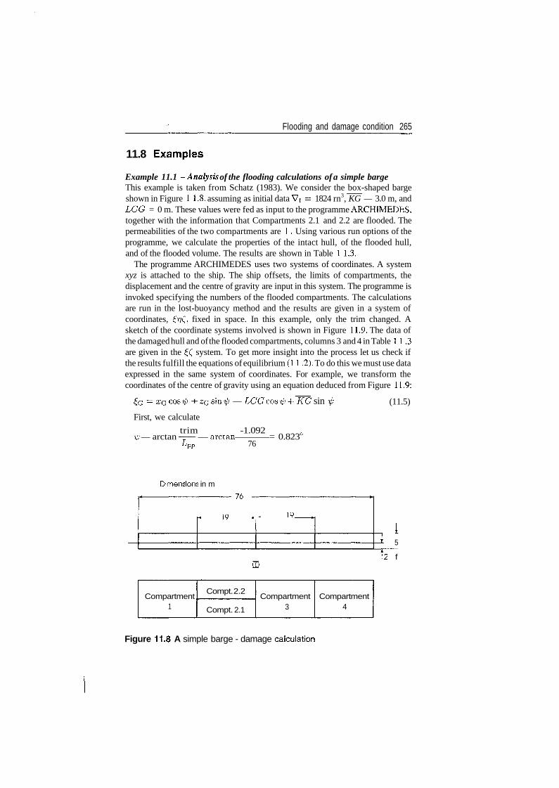
Flooding and damage condition 265
11.8 Examples
Example 11.1 -Analysis of the flooding calculations of a simple bargeThis example is taken from Schatz (1983). We consider the box-shaped bargeshown in Figure 1 1.8, assuming as initial data Vi = 1824 rn3, KG — 3.0 m, andLCG = 0 m. These values were fed as input to the programme ARCHIMEDES,together with the information that Compartments 2.1 and 2.2 are flooded. Thepermeabilities of the two compartments are 1 . Using various run options of theprogramme, we calculate the properties of the intact hull, of the flooded hull,and of the flooded volume. The results are shown in Table 1 1.3.
The programme ARCHIMEDES uses two systems of coordinates. A systemxyz is attached to the ship. The ship offsets, the limits of compartments, thedisplacement and the centre of gravity are input in this system. The programme isinvoked specifying the numbers of the flooded compartments. The calculationsare run in the lost-buoyancy method and the results are given in a system ofcoordinates, £??(", fixed in space. In this example, only the trim changed. Asketch of the coordinate systems involved is shown in Figure 11.9. The data ofthe damaged hull and of the flooded compartments, columns 3 and 4 in Table 1 1 .3are given in the ££ system. To get more insight into the process let us check ifthe results fulfill the equations of equilibrium (1 1 .2). To do this we must use dataexpressed in the same system of coordinates. For example, we transform thecoordinates of the centre of gravity using an equation deduced from Figure 11.9:
+ — LCGcosip -{-KG sin (11.5)
First, we calculate
trim -1.092ip — arctan —— — arctan = 0.823
Lrm 76
Dimensions in m
* ln * - 19
, 15
J2 f
Compartment1
Compt. 2.2
Compt. 2.1
Compartment3
Compartment4
Figure 11.8 A simple barge - damage calculation
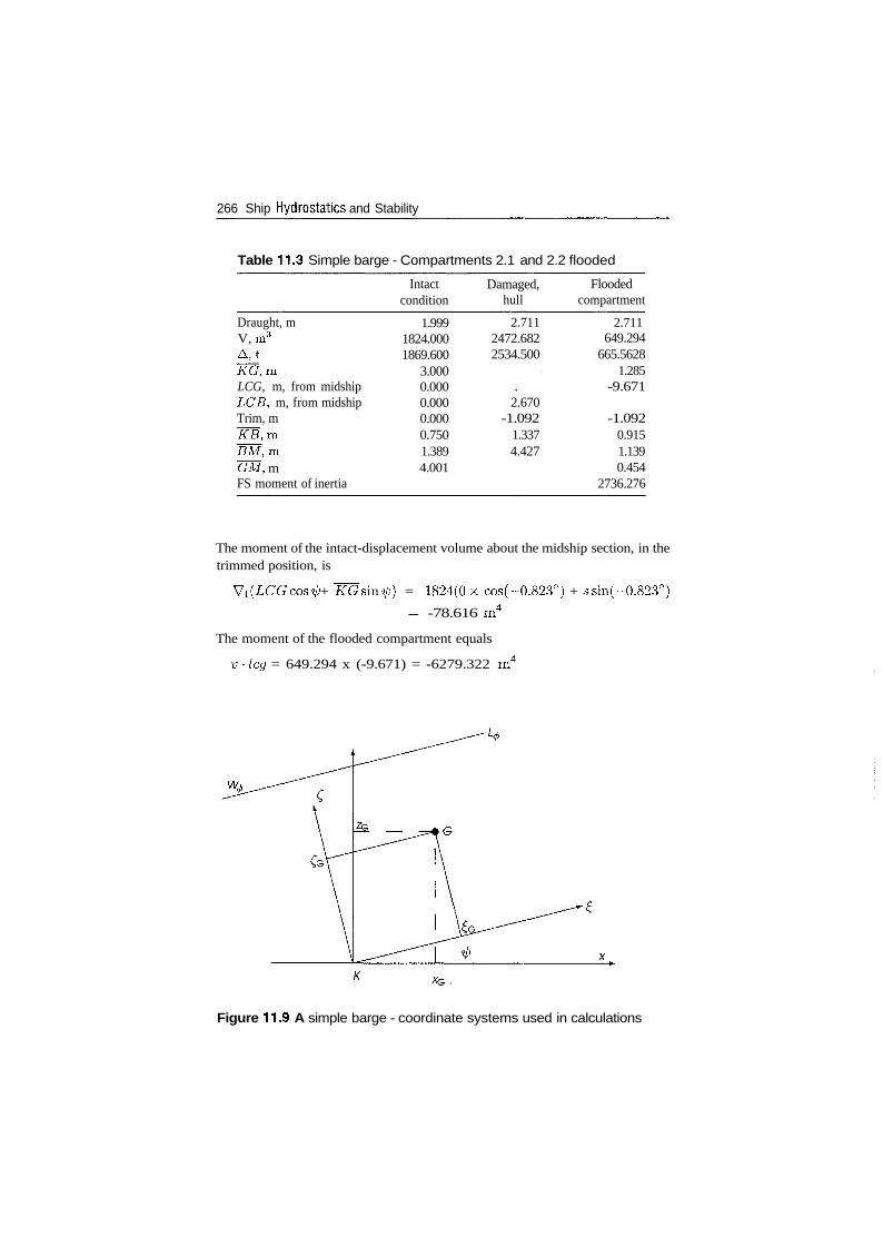
266 Ship Hydrostatics and Stability
Table 11.3 Simple barge - Compartments 2.1 and 2.2 flooded
Draught, mV, m3
A,tKG,mLCG, m, from midshipLCB, m, from midshipTrim, m~KB,mBM,mGM, mFS moment of inertia
Intactcondition
1.9991824.0001869.600
3.0000.0000.0000.0000.7501.3894.001
Damaged,hull
2.7112472.6822534.500
2.670-1.092
1.3374.427
Floodedcompartment
2.711649.294
665.56281.285
-9.671
-1.0920.9151.1390.454
2736.276
The moment of the intact-displacement volume about the midship section, in thetrimmed position, is
Vi(LCGcos^ + ~KGsm^) = 1824(0 x cos(-0.823°) + ssin(-0.823°)
- -78.616 m4
The moment of the flooded compartment equals
v-lcg = 649.294 x (-9.671) = -6279.322 m4
W,
Figure 11.9 A simple barge - coordinate systems used in calculations
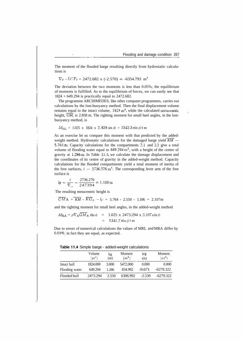
Flooding and damage condition 267
The moment of the flooded barge resulting directly from hydrostatic calcula-tions is
VF - LCFF = 2472.682 x (-2.570) - -6354.793 m4
The deviation between the two moments is less than 0.05%; the equilibriumof moments is fulfilled. As to the equilibrium of forces, we can easily see that1824 + 649.294 is practically equal to 2472.682.
The programme ARCHIMEDES, like other computer programmes, carries outcalculations by the lost-buoyancy method. Then the final displacement volumeremains equal to the intact volume, 1824m3, while the calculated metacentricheight, GM, is 2.858 m. The righting moment for small heel angles, in the lost-buoyancy method, is
MRL = 1.025 x 1824 x 2. 858 sin 0 = 5342.3sm</>tm
As an exercise let us compare this moment with that predicted by the added-weight method. Hydrostatic calculations for the damaged barge yield KM —5.764m. Capacity calculations for the compartments 2.1 and 2.2 give a totalvolume of flooding water equal to 649.294m3, with a height of the centre ofgravity at 1.286m. In Table 11.4, we calculate the damage displacement andthe coordinates of its centre of gravity in the added-weight method. Capacitycalculations for the flooded compartments yield a total moment of inertia ofthe free surfaces, i — 2736.276m3. The corresponding lever arm of the freesurface is
i 2736.276V 247394
The resulting metacentric height is
GM A = KM - KGA -1F = 5.764 - 2.550 - 1.106 = 2.107m
and the righting moment for small heel angles, in the added-weight method
MRA = pVAGMAsin0 = 1.025 x 2473.294 x 2.107sin ̂
= 5341.7sm0tm
Due to errors of numerical calculations the values of MRL and MRA differ by0.03%; in fact they are equal, as expected.
Table 11.4 Simple barge - added-weight calculations
Intact hullFlooding water
Volume(m3)
1824.000649.294
kg(m)
3.0001.286
Moment(m4)
5472.000834.992
leg(m)
0.000-9.671
Moment(m4)
0.000-6279.322
Flooded hull 2473.294 2.550 6306.992 -2.539 -6279.322
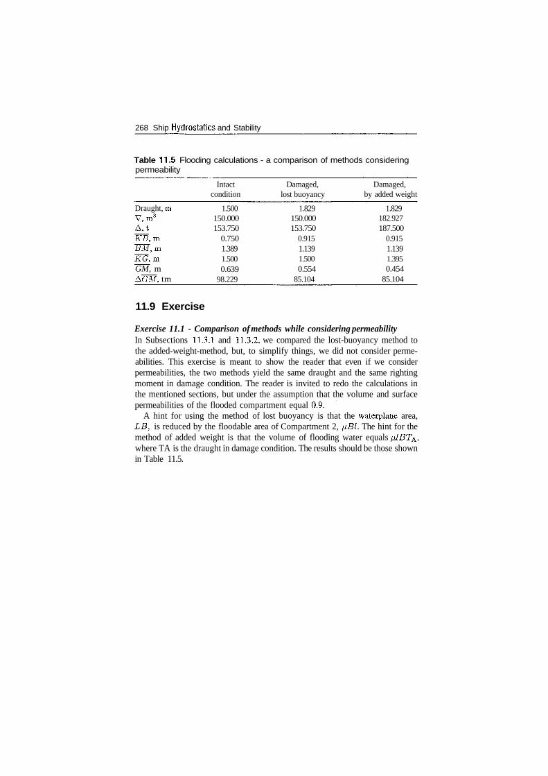
268 Ship Hydrostatics and Stability
Table 11.5 Flooding calculations - a comparison of methods consideringpermeability
Draught, mV,m3
A,tKB,mBM,mKG,mGM, mAGM, tm
Intactcondition
1.500150.000153.750
0.7501.3891.5000.639
98.229
Damaged,lost buoyancy
1.829150.000153.750
0.9151.1391.5000.554
85.104
Damaged,by added weight
1.829182.927187.500
0.9151.1391.3950.454
85.104
11.9 Exercise
Exercise 11.1 - Comparison of methods while considering permeabilityIn Subsections 11.3.1 and 11.3.2, we compared the lost-buoyancy method tothe added-weight-method, but, to simplify things, we did not consider perme-abilities. This exercise is meant to show the reader that even if we considerpermeabilities, the two methods yield the same draught and the same rightingmoment in damage condition. The reader is invited to redo the calculations inthe mentioned sections, but under the assumption that the volume and surfacepermeabilities of the flooded compartment equal 0.9.
A hint for using the method of lost buoyancy is that the waterplane area,LB, is reduced by the floodable area of Compartment 2, ^Bl. The hint for themethod of added weight is that the volume of flooding water equals f^lBT^,where TA is the draught in damage condition. The results should be those shownin Table 11.5.
12Linear ship responsein waves
12.1 Introduction
The title of the book is 'Ship hydrostatics and stability'. This chapter describesprocesses that are not hydrostatic, but can affect stability. We elaborate here onsome reservations expressed in Section 6.12 and sketch the way towards morerealistic models. First, we need a wave theory that can be used in the descriptionof real seas. Therefore, we introduce the theory of linear waves. Next, we showhow real seas can be described as a superposition of regular waves. This leadsto the introduction of sea spectra. A floating body moves in six degrees offreedom. The oscillating body generates waves that absorb part of its energy.The integration of pressures over the hull surface yields the forces and momentsacting on the body. We return here, without detailing, to the notions of addedmass and damping coefficients introduced in Section 6.12. A full treatmentwould go far beyond the scope of the book; therefore, we limit ourselves tomentioning a few important results.
The problems of mooring and anchoring deserve special treatment and theirimportance has grown with the development of offshore structures. We cannotdiscuss here the behaviour of compliant floating structures, that is mooredfloating structures, but give an example of how the mooring can change thenatural frequencies of a floating body. We mention in this chapter a few methodsof reducing ship motions, mainly the roll. This allows us to show that under veryparticular conditions, free water surfaces can help, a result that seems surprisingin the light of the theory developed in Chapter 6.
The models introduced in this chapter are too complex to yield explicit mathe-matical expressions that can be directly applied in engineering practice. It is onlypossible to implement the models in computer programmes that yield numeri-cal results. The input to such programmes is a statistical description of the seaconsidered as a random process. Correspondingly, the output, that is the shipresponse, is also a random process.
This chapter assumes the knowledge of more mathematics than the rest ofthe book. Mathematical developments are concise, leaving to the interestedreader the task of completing them or to refer to specialized books. The reader
270 Ship Hydrostatics and Stability
who cannot follow the mathematical treatment can find in the summary a non-mathematical description of the main subjects.
12.2 Linear wave theory
In Subsection 10.2.3, we introduced the theory of trochoidal waves. Trochoidalwaves approximate well the shape of swells and are prescribed by certain codesof practice for stability and bending-moment calculations. Another wave theoryis preferred for the description of real seas and for the calculation of ship motions;it is the theory of linear waves. The basic assumptions are
1. the sea water is incompressible;2. there is no viscosity, i.e. the sea water is inviscid;3. there is no surface tension;4. no fluid particle turns around itself, i.e. the motion is irrotational;5. the wave amplitude is much smaller than the wave length.
The first assumption, that of incompressibility, is certainly valid at the smalldepth and the wave velocities experienced by surface vessels. This is a sub-stantial difference from phenomena experienced in aerodynamics. Exceptingroll damping, the second assumption, the lack of viscous phenomena, leads toresults confirmed by experience. For roll, certain corrections are necessary; oftenthey are done by empiric means. Surface tension plays a role only for very smallwaves, such as the ripple that can be seen on the surface of a swell. We shall seehow the fourth hypothesis, that is irrotational flow, makes possible the devel-opment of an elegant potential theory that greatly simplifies the analysis. Thefifth hypothesis, low-amplitude waves, is not very realistic; surprisingly, it leadsto realistic results.
We consider two-dimensional waves, that is waves with parallel crests ofinfinite length, such as shown in Figure 12.1. The crests are parallel to the ydirection and we are only interested in what happens in the x and z directions.Let u be the horizontal and w the vertical velocity of a water particle. We note byp the water density. The theory of fluid dynamics shows that the rate of changeof the mass of a unit volume of water is
d(pu) d(pw)dx dz
The density of an incompressible fluid, p, is constant. Then, the condition thatthe mass of unit volume of water does not change is expressed as
Equation (12. 1) is known as the equation of continuity; it states that the diver-gence of the vector with components u, w is zero. The assumption of irrotational
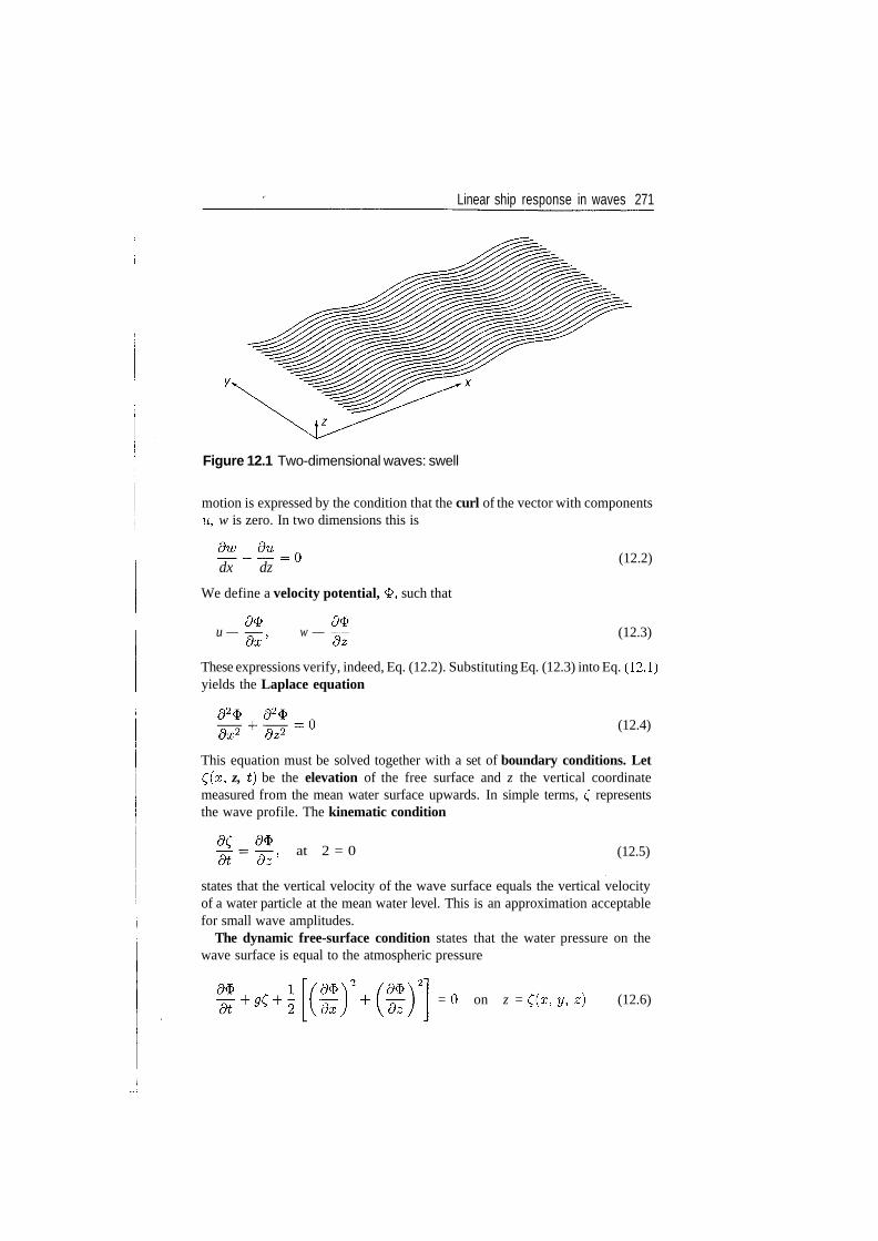
Linear ship response in waves 271
Figure 12.1 Two-dimensional waves: swell
motion is expressed by the condition that the curl of the vector with componentsu, w is zero. In two dimensions this is
dx dz
We define a velocity potential, 3>, such that
d$> <9$u — w —
~d~z
(12.2)
(12.3)
These expressions verify, indeed, Eq. (12.2). Substituting Eq. (12.3) into Eq. (12.1)yields the Laplace equation
(12.4)
This equation must be solved together with a set of boundary conditions. Let((#, z, t) be the elevation of the free surface and z the vertical coordinatemeasured from the mean water surface upwards. In simple terms, £ representsthe wave profile. The kinematic condition
dz'at 2 = 0 (12.5)
states that the vertical velocity of the wave surface equals the vertical velocityof a water particle at the mean water level. This is an approximation acceptablefor small wave amplitudes.
The dynamic free-surface condition states that the water pressure on thewave surface is equal to the atmospheric pressure
d&Vdx)
= 0 on z = £(z, y, 2) (12.6)
272 Ship Hydrostatics and Stability
Assuming small wave amplitudes we can neglect the squares of particle velocitiesand thus we remain with the condition
^+^=0 , at * = 0 (12.7)at
From Eqs. (12.5) and (12.7) we obtain the linearized free-surface condition
Additional boundary conditions must be written for the sea bottom, for walls thatlimit the water domain, and for the surfaces of bodies floating in that domain.As the water does not pass through such boundaries, the velocity componentsnormal to such boundaries should be zero.
Let the wave length be A, and the wave number k — 1ir/\. The verticalcoordinate of a water particle is z — 0 at the mean sea level, and z = — d, atthe depth d. We give the results of the theory for infinite-depth water as theseare the most interesting for sea-going ships. We leave to an exercise the proofthat these results fulfill the Laplace equation and the boundary conditions. Thesolution that interests us is the potential
LU
The equation of the sea surface is
C - C o sin(ut-kx) (12.10)
The following relationship exists between the wave length, A, and the waveperiod, T,
X=~-T2 (12.11)
Figure 12.2 shows the propagation of the wave described by Eq. (12.10). Thewave period is T = 6.5 s, and the wave length given by Eq. (12.11) is A =65.965 m. The wave height, H = 2£b» equals A/20, a ratio often used in NavalArchitecture.
The speed of propagation of the wave shape is called celerity, a term thatcomes from the Latin 'celeritas', speed. From Eq. (12.11) we find the celerity
We immediately see that long waves propagate faster than short waves. Therefore,we say that water waves are dispersive. Acoustic waves, for example, are notdispersive.
The components of the water-particle velocity are
u = uCo efcz sm(vt - kx) (12.13)
w = o;Co efcz cos(u;t - kx) (12.14)
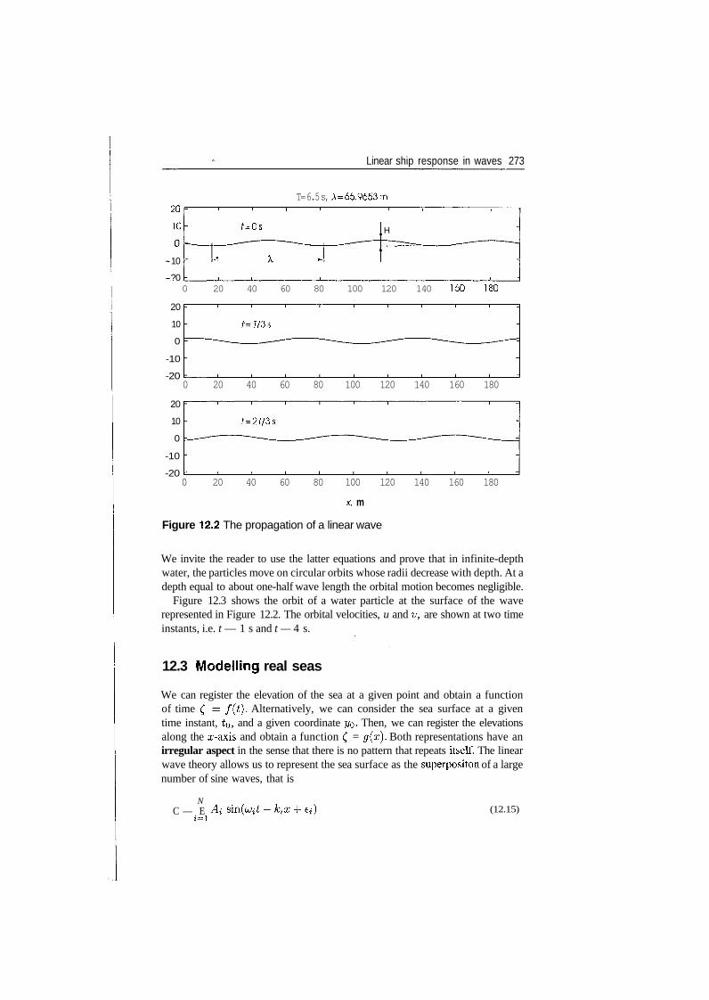
Linear ship response in waves 273
T= 6.5 s, A=65.9653mAJ
10
10
?0
I 1 1 1 1 1 I 1 1 -
f=0s
- • ^ *
H
-
i i i i i i i i i -0 20 40 60 80 100 120 140 160 180
20
10
0
-10
-20
20
10
0
-10
-20
f=r/3s
0 20 40 60 80 100 120 140 160 180
f= 2773s
0 20 40 60 80 100 120 140 160 180
x, m
Figure 12.2 The propagation of a linear wave
We invite the reader to use the latter equations and prove that in infinite-depthwater, the particles move on circular orbits whose radii decrease with depth. At adepth equal to about one-half wave length the orbital motion becomes negligible.
Figure 12.3 shows the orbit of a water particle at the surface of the waverepresented in Figure 12.2. The orbital velocities, u and v, are shown at two timeinstants, i.e. t — 1 s and t — 4 s.
12.3 Modelling real seas
We can register the elevation of the sea at a given point and obtain a functionof time C = f ( t ) . Alternatively, we can consider the sea surface at a giventime instant, to, and a given coordinate yo- Then, we can register the elevationsalong the x-axis and obtain a function £ = g ( x ) . Both representations have anirregular aspect in the sense that there is no pattern that repeats itself. The linearwave theory allows us to represent the sea surface as the superpositon of a largenumber of sine waves, that is
NC — E (12.15)
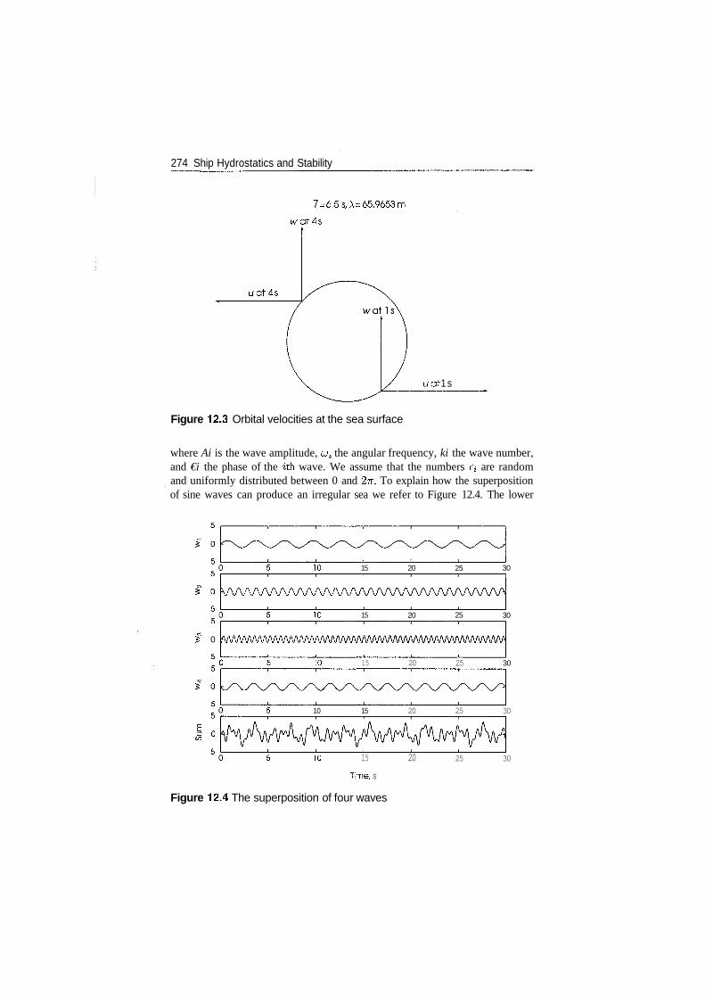
274 Ship Hydrostatics and Stability
7 = 6.5s, A=65.9653m
wat4s
uat4s
uat 1 s
Figure 12.3 Orbital velocities at the sea surface
where Ai is the wave amplitude, c^ the angular frequency, ki the wave number,and €i the phase of the ith wave. We assume that the numbers e^ are randomand uniformly distributed between 0 and 2?r. To explain how the superpositionof sine waves can produce an irregular sea we refer to Figure 12.4. The lower
10 15 20 25 30
VVWWVWVWV^^
10 15 20 25 30
£ 0 A/WWWWVWWVW^
10 15 20 25 30
10 15 20 25 30
10 15
Time, s
20 25 30
Figure 12.4 The superposition of four waves
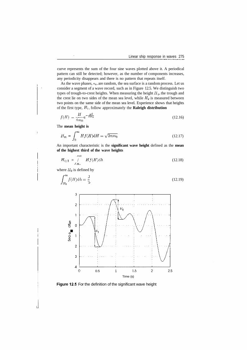
Linear ship response in waves 275
curve represents the sum of the four sine waves plotted above it. A periodicalpattern can still be detected; however, as the number of components increases,any periodicity disappears and there is no pattern that repeats itself.
As the wave phases, e$, are random, the sea surface is a random process. Let usconsider a segment of a wave record, such as in Figure 12.5. We distinguish twotypes of trough-to-crest heights. When measuring the height HI, the trough andthe crest lie on two sides of the mean sea level, while H2 is measured betweentwo points on the same side of the mean sea level. Experience shows that heightsof the first type, HI, follow approximately the Raleigh distribution
f(H) =4m0
The mean height is
Hm =
(12.16)
(12.17)
An important characteristic is the significant wave height defined as the meanof the highest third of the wave heights
/>oo
#1/3 = / Hf(H)dhJHQ
where HQ is defined by
f ( H ) d h = -
(12.18)
(12.19)
§
ICD
0.5 1 1.5
Time (s)
2.5
Figure 12.5 For the definition of the significant wave height
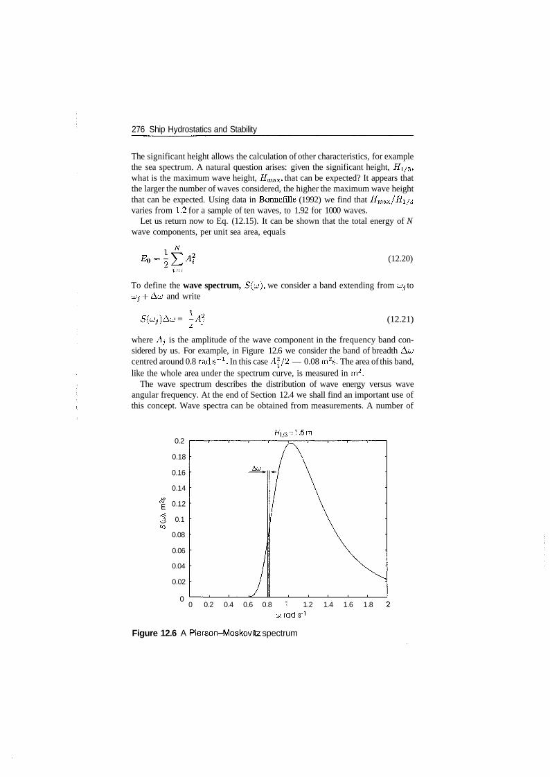
276 Ship Hydrostatics and Stability
The significant height allows the calculation of other characteristics, for examplethe sea spectrum. A natural question arises: given the significant height, #1/3,what is the maximum wave height, Hmaxi that can be expected? It appears thatthe larger the number of waves considered, the higher the maximum wave heightthat can be expected. Using data in Bonnefille (1992) we find that Hmax/#i/3varies from 1.2 for a sample of ten waves, to 1.92 for 1000 waves.
Let us return now to Eq. (12.15). It can be shown that the total energy of Nwave components, per unit sea area, equals
(12.20)1=1
To define the wave spectrum, S(u), we consider a band extending from ujj toujj -f ACJ and write
S(uj)&u = -A2 (12.21)
where A^ is the amplitude of the wave component in the frequency band con-sidered by us. For example, in Figure 12.6 we consider the band of breadth ACJcentred around 0.8 rad s"1. In this case A2/2 — 0.08 m2s. The area of this band,like the whole area under the spectrum curve, is measured in m2.
The wave spectrum describes the distribution of wave energy versus waveangular frequency. At the end of Section 12.4 we shall find an important use ofthis concept. Wave spectra can be obtained from measurements. A number of
0.2
0.18
0.16
0.14
0.12
0.1
0.08
0.06
0.04
0.02
0
H1/3=1.5m
0 0.2 0.4 0.6 0.8 1 1.2 1.4 1.6 1.8(jj, rod s-]
Figure 12.6 A Pierson-Moskovitz spectrum
Linear ship response in waves 277
formulae have been proposed for calculating standard spectra on the basis of afew given or measured sea characteristics. We shall give only one example, thePierson-Moskovitz spectrum as described by Fossen (1994)
S = AcT5 e~Buj~4 m2s (12.22)
where
A = 8.1 x 10~Vm2s~4
B = 0.0323 ( -%— ) s~4
V#l/3/
This spectrum corresponds to fully developed seas recorded in the North Atlantic;an example is shown in Figure 12.6. The theory of linear waves exposed in thissection is a first-order approximation in which the wave shape moves, but thereis no mass transport. This approximation is sufficient for moving ships as theirspeed is usually larger than the 'drift' caused by waves. For stationary structuresit may be necessary to consider higher order approximations that predict a drift.
12.4 Wave induced forces and motions
Like any other free body, a ship moves in six degrees of motion; we describethem with the aid of Figure 12.7. The six motions of a ship have traditional namesthat were adopted in the previous century also for planes and cars. We follow thenotation of Faltinsen (1993). Three motions are linear; they are described below.
1. Surge, along the x-axis; we note it by 771.2. Sway, in the direction of the t/-axis; we use the notation 772.3. Heave, along the z-axis; we note it by r/2.
The other three degrees of freedom define angular motions, as detailed below.
1. Roll, around the x-axis; we note it by 773.2. Pitch, around the y-axis; we use the notation 775.3. Yaw, around the z-axis; it is noted by 77$.
The motion of any point on a floating body is the resultant of all six motions
s = rjii + 772J 4- 773k + u x r (12.23)
where i is the unit vector on the x-axis, j, the unit vector on the y-axis, k, the unitvector on the z-axis, and x denotes the vector product. The rotation vector is
v = 774! + T/5J 4- r?6k
LL
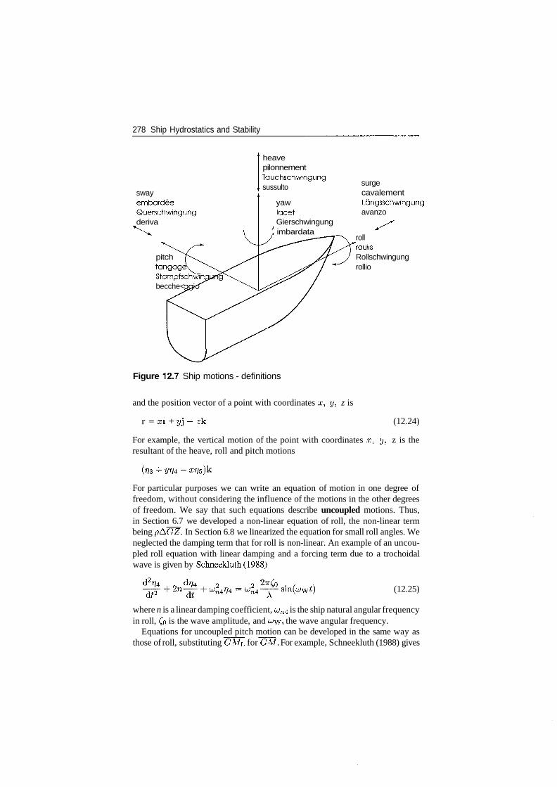
278 Ship Hydrostatics and Stability
swayembardeeQuerschwingungderiva
pitchtangagiStampfschwlnibecche<
heavepilonnementTauchschwingungsussulto
yawlacetGierschwingung
I imbardata
surgecavalementLangsschwingungavanzo
roll"VoulisRollschwingungrollio
Figure 12.7 Ship motions - definitions
and the position vector of a point with coordinates x, y, z is
r = xi + yj + zk (12.24)
For example, the vertical motion of the point with coordinates x, y, z is theresultant of the heave, roll and pitch motions
For particular purposes we can write an equation of motion in one degree offreedom, without considering the influence of the motions in the other degreesof freedom. We say that such equations describe uncoupled motions. Thus,in Section 6.7 we developed a non-linear equation of roll, the non-linear termbeing pAGZ. In Section 6.8 we linearized the equation for small roll angles. Weneglected the damping term that for roll is non-linear. An example of an uncou-pled roll equation with linear damping and a forcing term due to a trochoidalwave is given by Schneekluth (1988)
di2(12.25)
where n is a linear damping coefficient, o;n4 is the ship natural angular frequencyin roll, Co is the wave amplitude, and cj\y, the wave angular frequency.
Equations for uncoupled pitch motion can be developed in the same way asthose of roll, substituting GM\. for GM. For example, Schneekluth (1988) gives

Linear ship response in waves 279
the following equation for undamped pitch
sin — - 0^E
(12.26)
where i^ is the radius of inertia of the ship mass about the Oy axis, 7 is themaximum pitch amplitude, and TE is the period of encounter. Obviously
2/55
is the ship natural, angular frequency in pitch, and
27T
(12.27)
is the angular frequency of encounter.We use Figure 12.8 to develop an equation of the uncoupled heave motion
(m + ^33)773 + 6773 + pgAwr]3 = cos (12.28)
Above, we assumed that the wave length is large compared to the dimensions ofthe waterplane. In Figure 12.8(b) we see a mass-dashpot-spring analogy of theheaving body. This analogy holds only for the form of the governing equations.In Figure 12.8(b) the damping coefficient, 6, is a constant. In Figure 12.8(a) theadded mass in heave, ^33, and the damping coefficient, 6, are functions of the
(m + -A33)?73 -f 6773 + /cr/3 = Fk = pgAyj
F = pgAwCo cos ut m x -h
Wave SL rface
A/v —
Waterplane
area
m
= Co cos cut
F=
(a) A floating body (b) A mass-spring-damper system
Figure 12.8 A heaving, floating body as a second-order dynamic system
280 Ship Hydrostatics and Stability
frequency of oscillation. After the extinction of transients, that is in steady state,the frequency of oscillation is equal to the exciting frequency, that is the wavefrequency, o>w, for a body that does not move, and the frequency of encounter,CJE, for a moving, floating body.
Let us return to the terms that are proportional to motion in the equations ofroll, pitch and heave
These terms represent two hydrostatic moments and one hydrostatic force thatoppose the motion and tend to return the floating body to its initial position. Thecollective name for those moments and force is restoring forces. Only the roll,pitch and heave motion are opposed by hydrostatic restoring forces. There areno hydrostatic restoring forces that oppose surge, sway or yaw.
The equations of uncoupled motions are simplified models that allow us toreach a few important conclusions. In reality, certain couplings exist between thevarious motions. Thus, we already know that during roll the centre of buoyancymoves along the ship causing pitch. As pointed out by Schneekluth (1988), thecombination of roll and pitch motions causes an oscillation of the roll axis andinduces yaw. Also, the combination of roll and pitch induces heave. Moreover,one motion can influence the added masses and the damping coefficients of othermotions. The most complete model of coupled motions is
(M + A)f? + Brj + Crj = Re(Fe~ia;E<) (12.29)
Above, M is a 6-by-6 matrix whose elements are the ship mass and its momentsof inertia about the three axes of coordinates, and A is a 6-by-6 matrix of addedmasses (general term including added masses and added moments of inertia).The vectors of motions, speeds and accelerations are
77 = 77 =
1J2
The expression Re(Fe la;Et) means the real part of the vector of sinusoidalexciting forces and moments.
For a ship displaying port-to-starboard symmetry a part of the elements of thematrix M are zero, and another part are symmetric. The system of six ordinarydifferential equations can be simplified in many practical situations. Thus, for afloating structure presenting symmetry about the xOz plane, and with the centreof gravity in the position (0, 0, ZG), Faltinsen (1993) shows that the matrix ofinertias becomes
Linear ship response in waves 281
M000
MZG0
0M0
-MzG
00
00M000
0-MzG
0h0
~/46
MzG000/5
0
000
~/460
J6
where M is the mass of the floating body, /4, the moment of inertia about thex-axis, 746, the product of inertia about the x- and z-axis, and /6, the momentof inertia about the z-axis. Certain symmetries also can appear in the matricesof added masses, A, and damping coefficients, B. Remember, added massesand damping coefficients are functions of the frequency of oscillation. For astructure symmetric about the xOz plane the motions of surge, heave and pitch(vertical-plane motions) can be uncoupled from those of sway, roll and yaw.
The equations shown above are linear. Then, if for a wave amplitude equalto 1 the resulting motion amplitude is 7?a, for a wave amplitude equal to A themotion amplitude will be Arj&. Further, the principle of superposition appliesto motions as it applies to waves. The response to the sum of several waves isthe sum of the responses to the individual waves. Then, if we characterize theexciting waves by their spectrum, we can characterize the resulting motion by amotion spectrum.
In Subsection 6.9.5 we introduced the concept of transfer function for a simplecase of roll motion. The transfer function obtained from a differential equationsuch as those shown in this chapter is a function of frequency. Let the transferfunction of the ith motion be Yi(u). The spectrum of the respective motion,Sjj. (a;), is related to the wave spectrum, /^(u;), by the relationship
S,» = [Y^Y^-u]} S»(u) (12.30)
The expression between square brackets is called response amplitude operator,shortly RAO. The response amplitude operators of the various motions can beobtained from the coupled equations of all motions. All motions occur at thefrequency of the exciting force, but have different phases.
12.5 A note on natural periods
If a linear mass-dashpot-spring system, such as that shown in Figure 12.8(b),is excited by a force whose period is close to that of the system, the responseamplitude can be very large; we talk about resonance. Theoretically, at zerodamping the response is unbounded. In practice any physical system is damped toa certain extent and this limits the response to bounded values. Large-amplitudeoscillations reduce the performance of the crew and the equipment and, therefore,they should be avoided.
A very efficient means of avoiding resonance is to ensure that the natural periodof the floating body is remote from that of the waves prevailing in the region
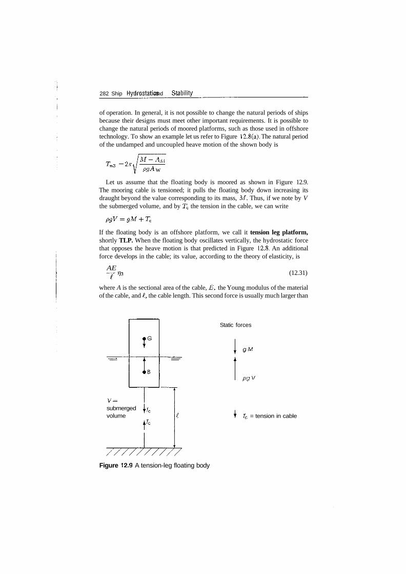
282 Ship Hydrostatics and Stability
of operation. In general, it is not possible to change the natural periods of shipsbecause their designs must meet other important requirements. It is possible tochange the natural periods of moored platforms, such as those used in offshoretechnology. To show an example let us refer to Figure 12.8(a). The natural periodof the undamped and uncoupled heave motion of the shown body is
= 27TM+ ^33
pgAw
Let us assume that the floating body is moored as shown in Figure 12.9.The mooring cable is tensioned; it pulls the floating body down increasing itsdraught beyond the value corresponding to its mass, M. Thus, if we note by Vthe submerged volume, and by Tc the tension in the cable, we can write
If the floating body is an offshore platform, we call it tension leg platform,shortly TLP. When the floating body oscillates vertically, the hydrostatic forcethat opposes the heave motion is that predicted in Figure 12.8. An additionalforce develops in the cable; its value, according to the theory of elasticity, is
AE(12.31)
where A is the sectional area of the cable, E, the Young modulus of the materialof the cable, and t, the cable length. This second force is usually much larger than
Static forces
pgv
v.=submergedvolume = tension in cable
Figure 12.9 A tension-leg floating body
Linear ship response in waves 283
the hydrostatic force. Then, a good approximation of the uncoupled, undampednatural period of heave is
(1232)
and it can differ much from that of the unmoored platform. Lateral mooring linesact like non-linear springs and can change the periods of other motions.
Natural periods can change temporarily when a ship enters confined waters.The added masses are influenced by close vertical walls and by a close bottom.Schneekluth (1988) cites the case of a barge with a B/T ratio equal to 2. Whenperforming the roll test in a depth equal to 1.25T, the added mass in roll wasfound to be 2.7 times larger than in deep water. The measured roll period appearedlarger than in deep water, leaving the impression that the stability was worsethan in reality. Schneekluth appreciates that the added mass in roll, ^33, isapproximately 15% of the ship mass, M, and that bilge keels increase the addedmass by approximately 6%.
12.6 Roll stabilizers
There are many systems of reducing roll amplitude; their aim is to produce forceswhose moment can be added to the righting moment. The simplest and cheapestsystem is represented by the bilge keels; they are steel profiles assembled onpart of the ship length, close to the bilge. Bilge keels act in two ways. First, ahydrodynamic resistance force develops on them; it is opposed to the roll motion.Second, bilge keels cause vortexes that increase the viscous damping of the rollmotion. As shown in the previous chapters, some codes of stability acknowledgethe contribution of bilge keels and provide for corresponding corrections of somerequirements. Bilge keels are passive devices.
Roll fins are wing-shaped bodies that extend transversely; usually they canbe rotated by a control system that receives as input the roll angle, velocityand acceleration. The forward ship velocity causes hydrodynamic forces on thewings, forces that oppose the roll motion. No helpful forces are produced atlow ship speeds. Rudders can be used as active anti-roll devices. Their action iscoupled with other motions and influences manoeuvering.
We do not expand on the devices mentioned above, but prefer to concentrateon another possibility because its relation to stability is evident and becauseit contradicts to some extent the theory that any liquid free surface endangersstability. We mean anti-roll tanks. To explain their action we use a simplemechanical analogy. We consider a classical oscillating system composed of amass, a spring and a dashpot. If a smaller mass is attached to the main massby a spring, and if the second mass and spring are properly dimensioned, theirvibration damps the oscillations of the main mass. This is the principle of theFrahm vibration absorber. In a similar mode, if two tanks, one on starboard,

284 Ship Hydrostatics and Stability
the other on the port side, are connected by a pipe, and water flows between themin a certain phase to the roll motion, this cross-flow opposes the roll motion. Themain mass-spring-damper system above is the analogue of the ship and the smallmass-spring system is the analogue of the anti-roll tanks.
We consider in Figure 12.10(a) a system composed of the mass mi, the linearspring &i, and the viscous damper (dashpot) c, and an auxiliary system composedof the mass 7712 and the linear spring k2. A sinusoidal force, FQ sin ut, acts onthe main mass, mi. The position of the mass mi is measured by the variable xi,that of the mass rn2 by the variable x2. If properly 'tuned', the auxiliary system(&2, 7712)» 'absorbs' the forced vibrations of the main system. To show this wefirst write the equations that govern the behaviour of the composed system. Thefirst Eq. (12.33) describes the forces that act on the mass mi, and the secondequation refers to the forces acting on the mass m2,
mid x~\
— r-at*
dx~\— — - + kiXi -f k2(xi - #2) —at
sin ut
-rr + k2(x2 -at
= 0 (12.33)
We assume that the initial conditions are all zero, that is x\ = 0, dxi/dt = 0,x2 = 0, dx2/dt — 0. Taking Laplace transforms and noting with s the Laplace-transform variable, with X\(s) the Laplace transform of x\(t), and with Xz(s)that of X2, we obtain
[mis2 + cs k2]Xl(s) - k2X2(s} = 2 QW
2
Eliminating X2(s) from Eq. (12.34) we arrive at
_ _ F$u m2s2 + k2X i ( s ) =
s2 4- cj2 (m2s cs k2 -
(12.34)
(12.35)
c
hCH
(a) I (b)
Figure 12.10 (a) A Frahm vibration absorber, (b) Flume tanks
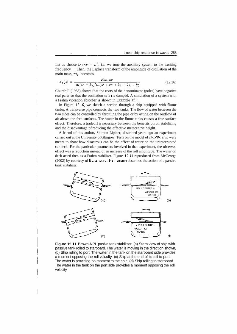
Linear ship response in waves 285
Let us choose k^/m^ = t^2, i.e. we tune the auxiliary system to the excitingfrequency w. Then, the Laplace transform of the amplitude of oscillation of themain mass, mi, becomes
Xi(s) = (12.36)(mis2 + k2)(mis2 -f cs -f ki -f- k2) - k\
Churchill (1958) shows that the roots of the denominator (poles) have negativereal parts so that the oscillation x\ (t) is damped. A simulation of a system witha Frahm vibration absorber is shown in Example 12.1.
In Figure 12.10, we sketch a section through a ship equipped with flumetanks. A transverse pipe connects the two tanks. The flow of water between thetwo sides can be controlled by throttling the pipe or by acting on the outflow ofair above the free surfaces. The water in the flume tanks causes a free-surfaceeffect. Therefore, a tradeoff is necessary between the benefits of roll stabilizingand the disadvantage of reducing the effective metacentric height.
A friend of this author, Shimon Lipiner, described years ago an experimentcarried out at the University of Glasgow. Tests on the model of a Ro/Ro ship weremeant to show how disastrous can be the effect of water on the uninterruptedcar deck. For the particular parameters involved in that experiment, the observedeffect was a reduction instead of an increase of the roll amplitude. The water ondeck acted then as a Frahm stabilizer. Figure 12.11 reproduced from McGeorge(2002) by courtesy of Butterworth-Heinemann describes the action of a passivetank stabilizer.
ROLL CENTRE f
WEIGHT OFWATER ,
(b)
(C) (d)
Figure 12.11 Brown-NPL pasive tank stabiliser: (a) Stern view of ship withpassive tank rolled to starboard. The water is moving in the direction shown,(b) Ship rolling to port. The water in the tank on the starboard side providesa moment opposing the roll velocity, (c) Ship at the end of its roll to port.The water is providing no moment to the ship, (d) Ship rolling to starboard.The water in the tank on the port side provides a moment opposing the rollvelocity
286 Ship Hydrostatics and Stability
12.7 Summary
To calculate the motion of a floating body in real waves we need an adequatedescription of a real sea. Therefore, we consider the real sea as the result of thesuperposition of a large number of linear waves. The theory of linear waves isbased on the following assumptions:
1. the sea water is incompressible;2. the sea water is inviscid (no viscous effects);3. surface tension plays no role;4. no water particle turns around itself (irrotational motion);5. the wave amplitude is small compared to the wave length.
The above assumptions allow the development of an elegant theory in which thevelocities of water particles can be derived from a velocity potential. The recordof sea elevations in a fixed point is a function of time in which we cannot findany pattern that repeats itself. We can, however, characterize the sea by statisticalquantities. One important example is the significant wave height defined as themean of the highest third of trough-to-crest heights. The heights are measuredbetween trough and crests situated on different sides of the sea level.
Another statistical characteristic of the sea is the wave spectrum, actually thedistribution of wave energy as function of the wave frequency. Sea spectra canbe measured or can be calculated on the basis of sea characteristics, such as thesignificant wave height. Formulae for standard spectra have been proposed forvarious ocean or sea regions.
Floating bodies move in six degrees of freedom. Three motions are linear:surge along the x-axis, sway along the y-axis, and heave along the z-axis, wherethe axes of coordinates are those defined in Chapter 1. The other three motionsare angular: roll around the x-axis, pitch around the y-axis, and yaw around thez-axis.
We can write a differential equation for one particular motion without consid-ering the influence of other motions. We say then that the motion is uncoupled.In reality certain couplings exist between motions. For example, we know fromChapter 2 that roll induces pitch. Moreover, one motion can influence the addedmasses and damping coefficients of other motions. The most general represen-tation of motions in six degrees of freedom is by a system of six ordinary dif-ferential equations. The port-to-starboard symmetry of many floating structuressimplifies the matrices of inertia, added masses and damping coefficients andallow the decoupling of equations. Then, for example, we can write a systemof three equations for the vertical-plane motions, heave, surge and pitch, andanother system for sway, roll and yaw.
Moorings can change the natural frequencies of motions. An example is that oftension-leg platforms. As the name says, the mooring 'tendons' are tensioned sothat they pull down the platform and increase its draught beyond that correspond-
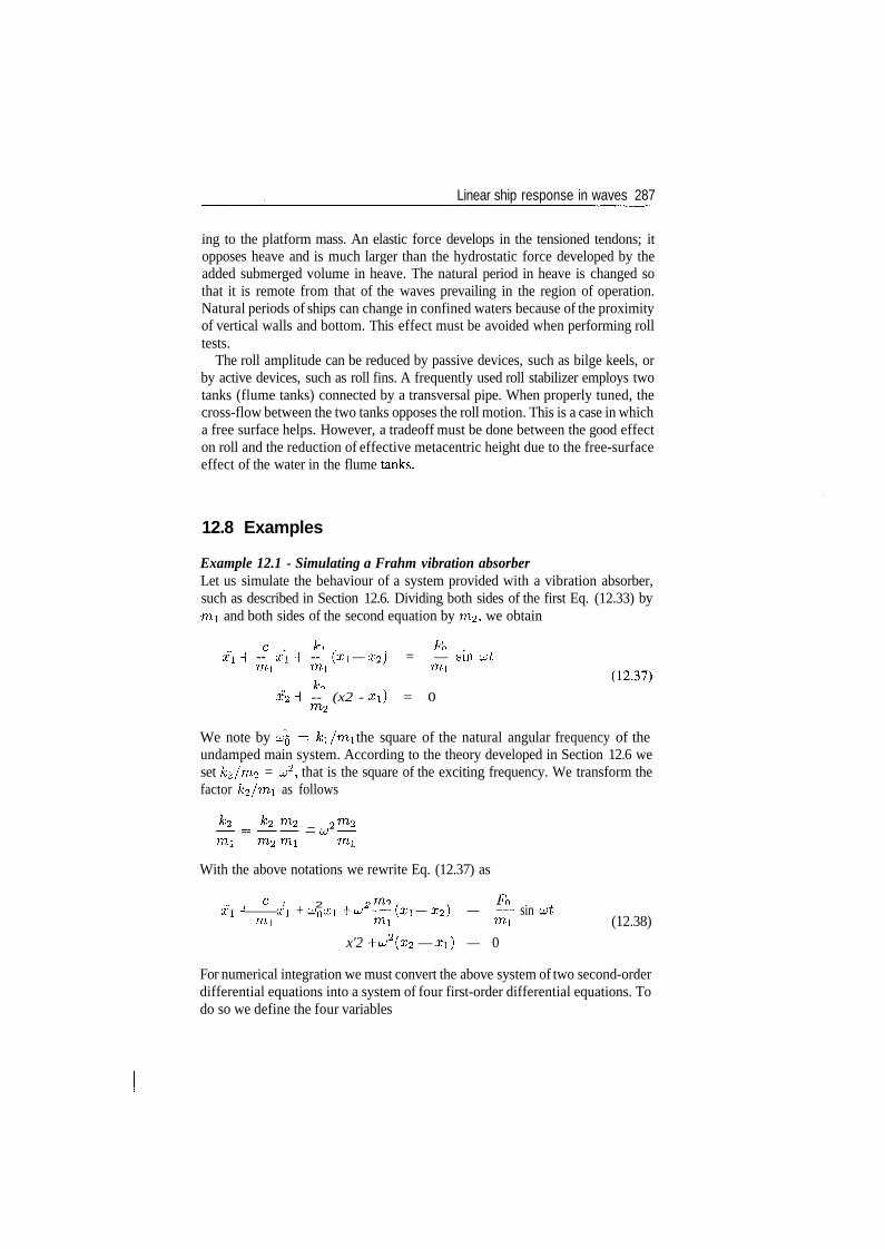
Linear ship response in waves 287
ing to the platform mass. An elastic force develops in the tensioned tendons; itopposes heave and is much larger than the hydrostatic force developed by theadded submerged volume in heave. The natural period in heave is changed sothat it is remote from that of the waves prevailing in the region of operation.Natural periods of ships can change in confined waters because of the proximityof vertical walls and bottom. This effect must be avoided when performing rolltests.
The roll amplitude can be reduced by passive devices, such as bilge keels, orby active devices, such as roll fins. A frequently used roll stabilizer employs twotanks (flume tanks) connected by a transversal pipe. When properly tuned, thecross-flow between the two tanks opposes the roll motion. This is a case in whicha free surface helps. However, a tradeoff must be done between the good effecton roll and the reduction of effective metacentric height due to the free-surfaceeffect of the water in the flume tanks.
12.8 Examples
Example 12.1 - Simulating a Frahm vibration absorberLet us simulate the behaviour of a system provided with a vibration absorber,such as described in Section 12.6. Dividing both sides of the first Eq. (12.33) bymi and both sides of the second equation by 7712, we obtain
. , x .H -- xi H -- (xi — X2) = — sin ut
mi mi mi
x'2 H -- (x2 - xi) = 0
We note by UQ = ki/mi the square of the natural angular frequency of theundamped main system. According to the theory developed in Section 12.6 weset k<2/m<2 = cj2, that is the square of the exciting frequency. We transform thefactor k'2/nrti as follows
__ _mi m,2 mi mi
With the above notations we rewrite Eq. (12.37) as
c ' 2x\ H x\ + cjnXi -f u;^ —- (xi — X2,} — —~~ sin imi mi mi (12.38)
x'2 -f u;2(x2 — xi) — 0
For numerical integration we must convert the above system of two second-orderdifferential equations into a system of four first-order differential equations. Todo so we define the four variables
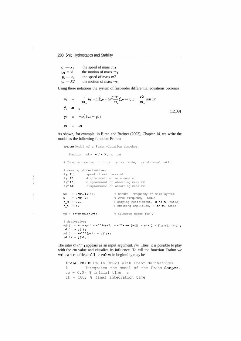
288 Ship Hydrostatics and Stability
yl — x\ the speed of mass miy2 = x\ the motion of mass m\Us — %2 the speed of mass m2y4 — X2 the motion of mass 7712
Using these notations the system of first-order differential equations becomes
c 2 2 m2 / x ^o . ,i/i = yi - LJQy2 - u —(2/2 ~ 2/4J smut
mi mi mi
2/2 = ^ (12.39)
2/3 = -^0(2/4-2/2)
2/4 = 2/3
As shown, for example, in Biran and Breiner (2002), Chapter 14, we write themodel as the following function Frahm
%FRAHM Model of a Frahm vibration absorber.
function yd = Frahm(t, y, rm)
% Input arguments: t time, y variable, rm m2-to-ml ratio
% meaning of derivatives% yd(l) speed of main mass ml% yd(2) displacement of main mass ml% yd(3) displacement of absorbing mass m2% yd(4) displacement of absorbing mass m2
wO = 2*pi/14.43; % natural frequency of main systemw = 2*pi/7; % wave frequency, rad/sc_m =0.1; % damping coefficient, c-to-ml ratioF__m = 1 ; % exciting amplitude, F-to-ml ratio
yd = zeros(size(y)); % allocate space for y
% derivativesyd(l) = -c_m*y(l)- w(T2*y(2) - w~2*rm* (y (2) - y(4)) - F_m*sin (w*t) ;yd(2) = y(l);yd(3) = -w/v2*(y(4) - y(2));yd(4) = y(3)/ }
The ratio m2/mi appears as an input argument, rm. Thus, it is possible to playwith the rm value and visualize its influence. To call the function Frahm wewrite a script file, call_Frahm; its beginning may be
%CALL_FRAHM Calls ODE23 with Frahm derivatives.% Integrates the model of the Frahm damper,to = 0.0; % initial time, stf = 100; % final integration time
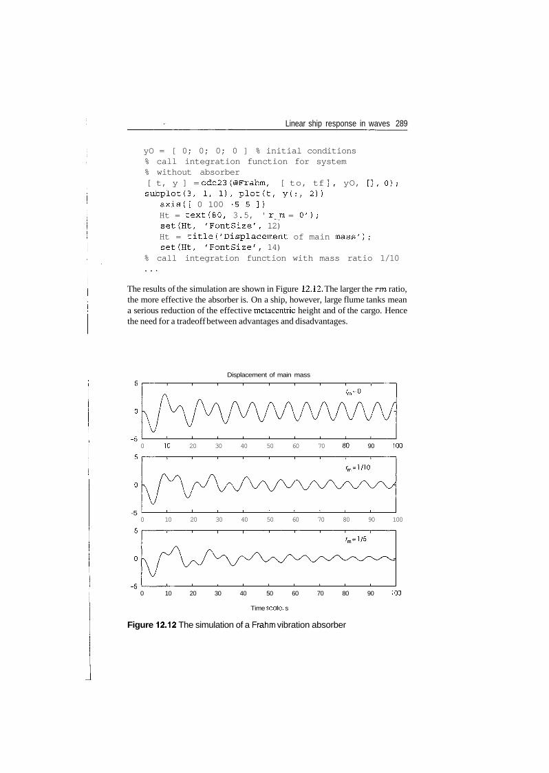
Linear ship response in waves 289
yO = [ 0; 0; 0; 0 ] % initial conditions% call integration function for system% without absorber[ t, y ] = ode23(@Frahm, [ to, tf ], yO, [], 0);subplot(3, 1, 1), plot(t, y(:, 2))
axis([ 0 100 - 5 5 ] )Ht = text(80, 3.5, ' r_m = 0');set(Ht, 'FontSize', 12)Ht = title('Displacement of main mass');set(Ht, 'FontSize', 14)
% call integration function with mass ratio 1/10
The results of the simulation are shown in Figure 12.12. The larger the rm ratio,the more effective the absorber is. On a ship, however, large flume tanks meana serious reduction of the effective metacentric height and of the cargo. Hencethe need for a tradeoff between advantages and disadvantages.
Displacement of main mass
0 10 20 30 40 50 60 70 90 100
-50 10 20 30 40 50 60 70 80 90 100
0 10 20 30 40 50 60 70 80 90 100
Time scale, s
Figure 12.12 The simulation of a Frahm vibration absorber
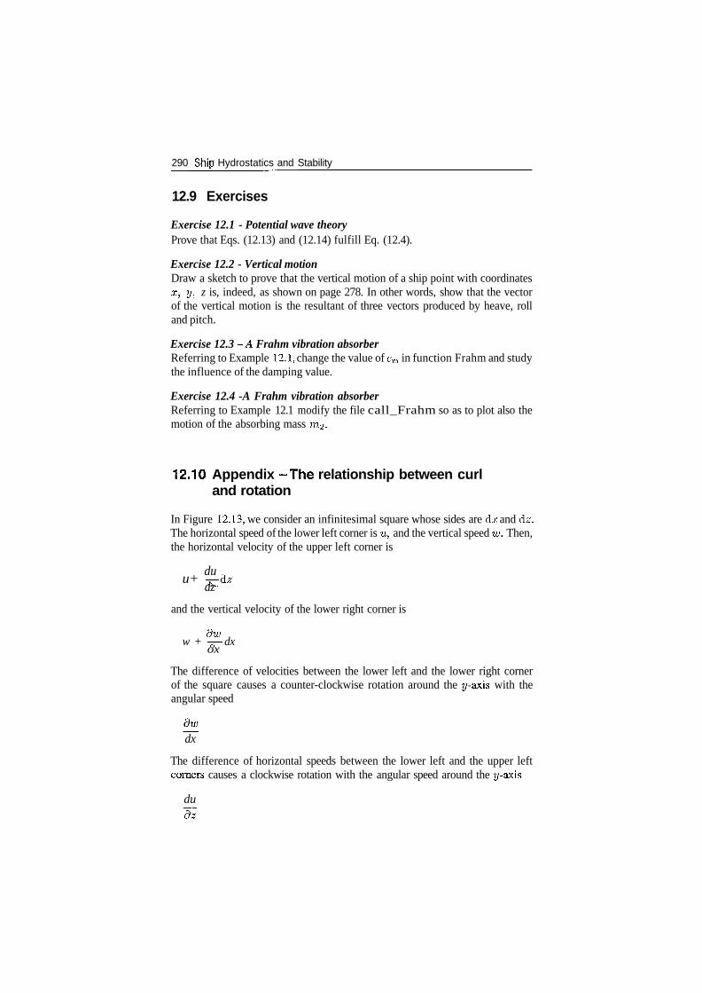
290 Ship Hydrostatics and Stability
12.9 Exercises
Exercise 12.1 - Potential wave theoryProve that Eqs. (12.13) and (12.14) fulfill Eq. (12.4).
Exercise 12.2 - Vertical motionDraw a sketch to prove that the vertical motion of a ship point with coordinatesx, y, z is, indeed, as shown on page 278. In other words, show that the vectorof the vertical motion is the resultant of three vectors produced by heave, rolland pitch.
Exercise 12.3 -A Frahm vibration absorberReferring to Example 12.1, change the value of cm in function Frahm and studythe influence of the damping value.
Exercise 12.4 -A Frahm vibration absorberReferring to Example 12.1 modify the file call_Frahm so as to plot also themotion of the absorbing mass m^.
12.10 Appendix -The relationship between curland rotation
In Figure 12.13, we consider an infinitesimal square whose sides are dx and dz.The horizontal speed of the lower left corner is u, and the vertical speed w. Then,the horizontal velocity of the upper left corner is
duu+ -^-dz
dz
and the vertical velocity of the lower right corner is
dw .w + -7-— dx
ox
The difference of velocities between the lower left and the lower right cornerof the square causes a counter-clockwise rotation around the y-axis with theangular speed
_dx
The difference of horizontal speeds between the lower left and the upper leftcomers causes a clockwise rotation with the angular speed around the y-axis
du~d~z
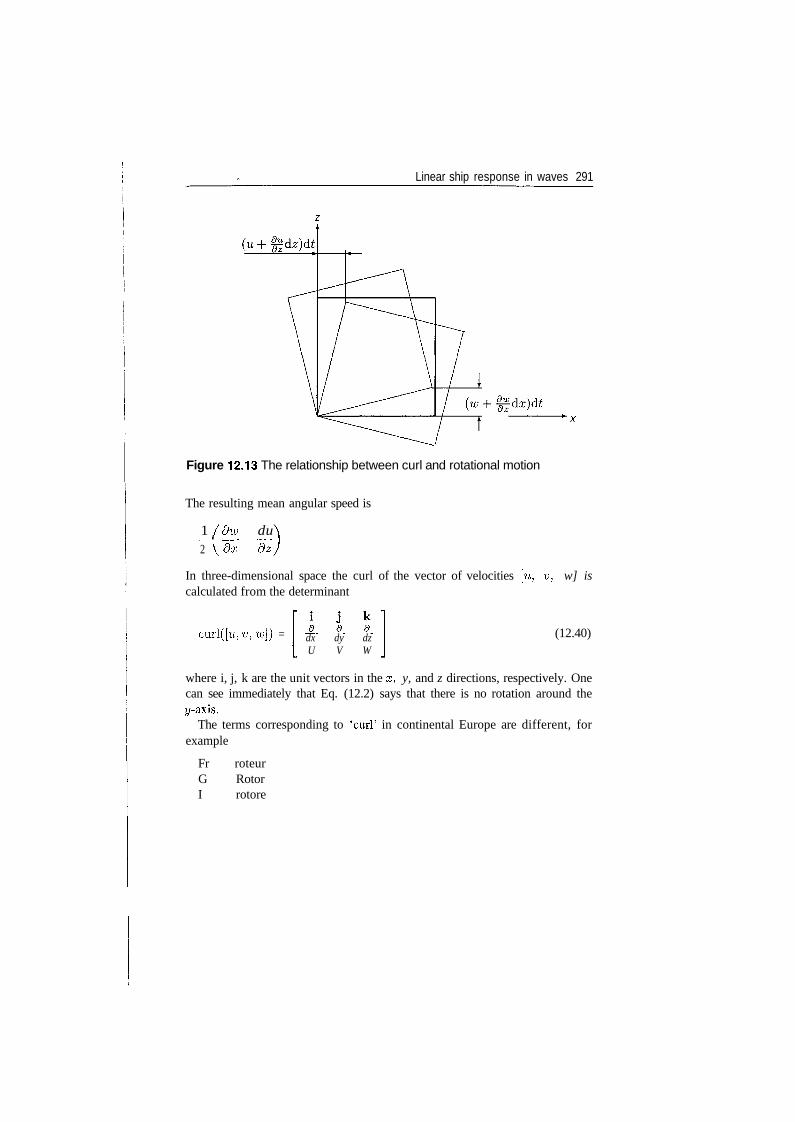
Linear ship response in waves 291
Figure 12.13 The relationship between curl and rotational motion
The resulting mean angular speed is
1 /dw du2 V ~dx~ ~d~z
In three-dimensional space the curl of the vector of velocities [u, v, w] iscalculated from the determinant
curlQ-w, u, it;]) = . . .dx dy dzU V W
(12.40)
where i, j, k are the unit vectors in the x, y, and z directions, respectively. Onecan see immediately that Eq. (12.2) says that there is no rotation around they-axis.
The terms corresponding to 'curl' in continental Europe are different, forexample
Fr roteurG RotorI rotore
13Computer methods
13.1 Introduction
The large amount of multiplications, summations and integrations required inhydrostatic calculations made necessary a systematic approach and the useof mechanical computing devices. Amsler invented in 1856 the planimeter,a mechanical instrument that yields the area enclosed by a given curve. Theplanimeter is an analogue computer. Other examples of mechanical, analoguecomputers once widely used in Naval Architecture are the integraph and the inte-grator. The integraph draws the integral curve, f* /(£)d£, °f a giyen curve,y = f ( x ) (see Section 3.4). The integrator yields the area, the first and sec-ond moments of the area bounded by a closed curve. When digital computersappeared, they gradually replaced the mechanical instruments. To our knowl-edge, the first publication of a digital computer programme for Naval Architec-ture is due to Kantorowitz (1958). More programmes for hydrostatic calculationsappeared in the following years. Today, digital computers are used extensively inmodern Naval Architecture and computer programmes are commercially avail-able. With the arrival of computer graphics, Naval Architects understood that theycan apply the new techniques to solve the problems of hull definition. Today,some of the most sophisticated software packages are used for this purpose.Moreover, once the hull surface is defined, the programmes use this definitionto perform hydrostatic and other calculations.
In this chapter we discuss concisely a few ways of using computers for thetreatment of the subjects described in the book. A detailed treatment wouldrequire a dedicated book (for Naval Architectural graphics see Nowacki, Bloorand Oleksiewicz, 1995). Besides this, computer software changes so rapidly thatit would be necessary to update the book at short intervals.
One of the first subjects treated in the book is the definition of the hull surface.It is natural to begin this chapter by showing how computers are used for thisdefinition. To do so we first introduce a few elementary concepts of computergraphics, and afterwards we give a few simple examples of application to hull-surface definition.
The next subjects discussed in the book are hydrostatic and weight calcu-lations. Correspondingly, we give in this book a few examples of computerimplementations of these matters.
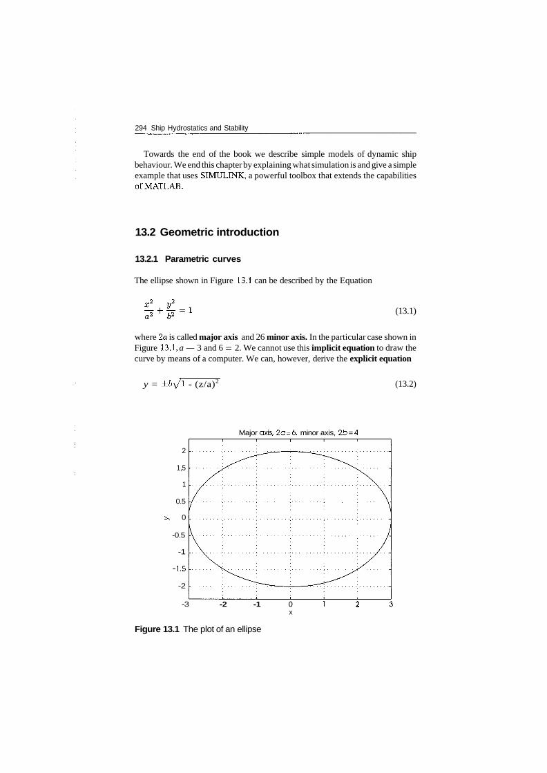
294 Ship Hydrostatics and Stability
Towards the end of the book we describe simple models of dynamic shipbehaviour. We end this chapter by explaining what simulation is and give a simpleexample that uses SIMULINK, a powerful toolbox that extends the capabilitiesofMATLAB.
13.2 Geometric introduction
13.2.1 Parametric curves
The ellipse shown in Figure 13.1 can be described by the Equation
(13.1)
where 2a is called major axis and 26 minor axis. In the particular case shown inFigure 13.1, a — 3 and 6 = 2. We cannot use this implicit equation to draw thecurve by means of a computer. We can, however, derive the explicit equation
y = ±6^1 - (z/a)2 (13.2)
Major axis, 2a=6, minor axis, 2b =
2
1,5
1
0.5
0
-0.5
-1
-1.5
-2
-3 -2 -1
Figure 13.1 The plot of an ellipse
ox
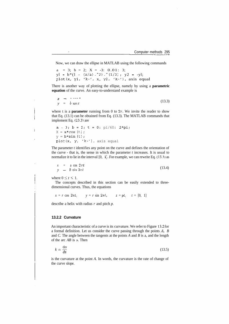
Computer methods 295
Now, we can draw the ellipse in MATLAB using the following commands
a = 3; b = 2; X = -3: 0.01: 3;yl = b*( l - (x/a) . ~ 2 ) . " (1 /2) ; y2 = -yl;plot (x, yl, ' k - ' , x, y2 , ' k - ' ) / axis equal
There is another way of plotting the ellipse, namely by using a parametricequation of the curve. An easy-to-understand example is
= h (13.3)
y = o sin t
where t is a parameter running from 0 to 27r. We invite the reader to showthat Eq. (13.1) can be obtained from Eq. (13.3). The MATLAB commands thatimplement Eq. (13.3) are
a = 3 ; b = 2 ; t = 0 : pi/60: 2*pi;X = a*COS (t) ;y = b*sin (t) ;plot(x, y, 'k-'), axis equal
The parameter t identifies any point on the curve and defines the orientation ofthe curve - that is, the sense in which the parameter t increases. It is usual tonormalize it to lie in the interval [0, 1] . For example, we can rewrite Eq. (13.3) as
x = a cos 2yrt, . 0 , (13.4)y = b sin 2?rt
where 0 < t < 1.The concepts described in this section can be easily extended to three-
dimensional curves. Thus, the equations
x = r cos 2?rt, y = r sin 2?rt, z = pt, t = [0, 1]
describe a helix with radius r and pitch p.
13.2.2 Curvature
An important characteristic of a curve is its curvature. We refer to Figure 13.2 fora formal definition. Let us consider the curve passing through the points A, Band C. The angle between the tangents at the points A and B is a, and the lengthof the arc AB is 5. Then
k = ̂ (13.5)as
is the curvature at the point A. In words, the curvature is the rate of change ofthe curve slope.
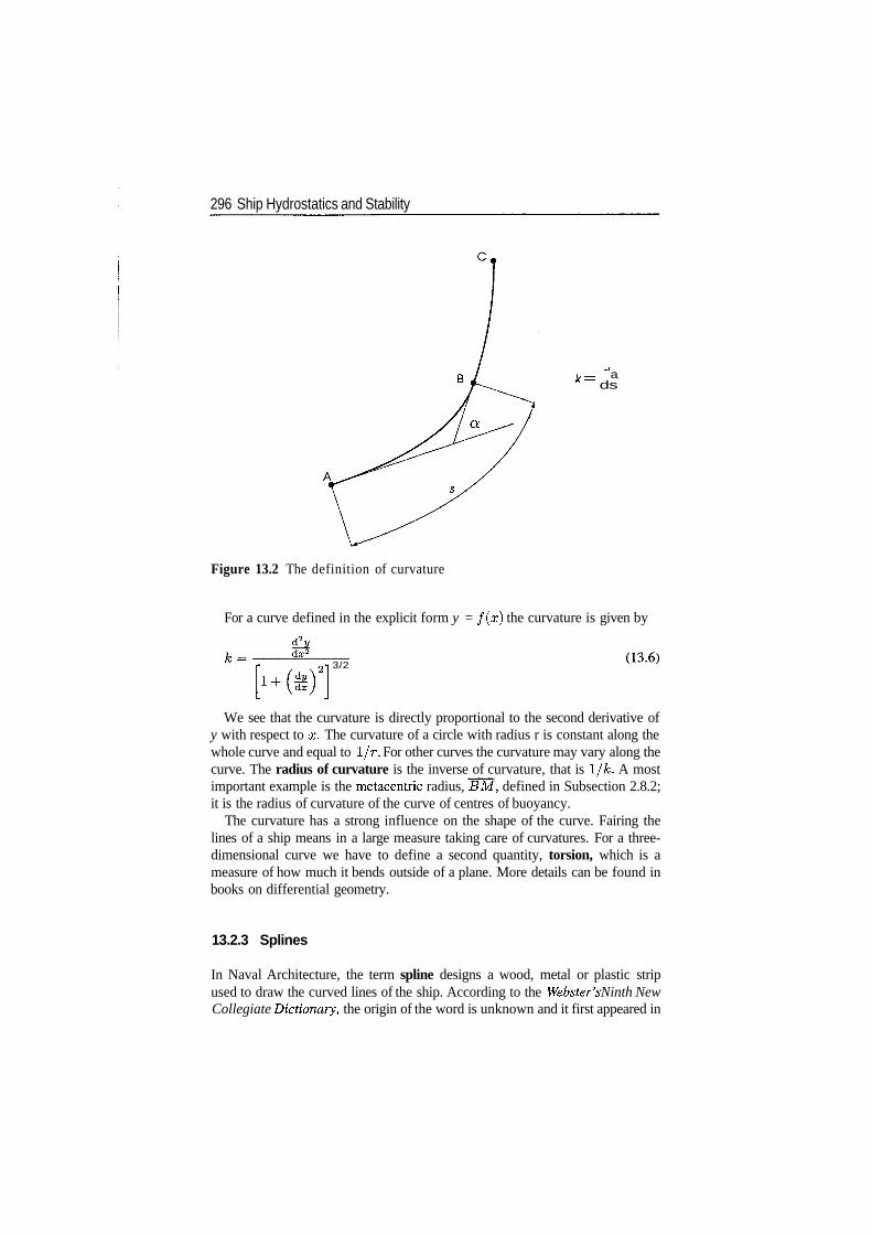
296 Ship Hydrostatics and Stability
/,— ak~ ds
Figure 13.2 The definition of curvature
For a curve defined in the explicit form y = f ( x ) the curvature is given by
3/2
We see that the curvature is directly proportional to the second derivative ofy with respect to x. The curvature of a circle with radius r is constant along thewhole curve and equal to 1/r. For other curves the curvature may vary along thecurve. The radius of curvature is the inverse of curvature, that is I/A;. A mostimportant example is the metacentric radius, BM, defined in Subsection 2.8.2;it is the radius of curvature of the curve of centres of buoyancy.
The curvature has a strong influence on the shape of the curve. Fairing thelines of a ship means in a large measure taking care of curvatures. For a three-dimensional curve we have to define a second quantity, torsion, which is ameasure of how much it bends outside of a plane. More details can be found inbooks on differential geometry.
13.2.3 Splines
In Naval Architecture, the term spline designs a wood, metal or plastic stripused to draw the curved lines of the ship. According to the Webster's Ninth NewCollegiate Dictionary, the origin of the word is unknown and it first appeared in
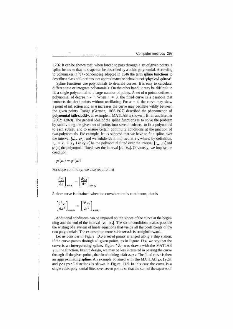
Computer methods 297
1756. It can be shown that, when forced to pass through a set of given points, aspline bends so that its shape can be described by a cubic polynomial. Accordingto Schumaker (1981) Schoenberg adopted in 1946 the term spline functions todescribe a class of functions that approximate the behaviour of 'physical splines' .
Spline functions use polynomials to describe curves. It is easy to calculate,differentiate or integrate polynomials. On the other hand, it may be difficult tofit a single polynomial to a large number of points. A set of n points defines apolynomial of degree n - 1. When n = 3, the fitted curve is a parabola thatconnects the three points without oscillating. For n = 4, the curve may showa point of inflection and as n increases the curve may oscillate wildly betweenthe given points. Runge (German, 1856-1927) described the phenomenon ofpolynomial inflexibility; an example in MATLAB is shown in Biran and Breiner(2002: 428-9). The general idea of the spline functions is to solve the problemby subdividing the given set of points into several subsets, to fit a polynomialto each subset, and to ensure certain continuity conditions at the junction oftwo polynomials. For example, let us suppose that we have to fit a spline overthe interval [za, x&], and we subdivide it into two at £;, where, by definition,xa < xi < Xb- Let y i ( x ) be the polynomial fitted over the interval [xa, Xj\ andyi(x] the polynomial fitted over the interval [xi, xb], Obviously, we impose thecondition
For slope continuity, we also require that
A nicer curve is obtained when the curvature too is continuous, that is
Additional conditions can be imposed on the slopes of the curve at the begin-ning and the end of the interval [xa, #&]. The set of conditions makes possiblethe writing of a system of linear equations that yields all the coefficients of thetwo polynomials. The extension to more subintervals is straightforward.
Let us consider in Figure 13.3 a set of points arranged along a ship station.If the curve passes through all given points, as in Figure 13.4, we say that thecurve is an interpolating spline. Figure 13.4 was drawn with the MATLABspl ine function. In ship design, we may be less interested in passing the curvethrough all the given points, than in obtaining a fair curve. The fitted curve is thenan approximating spline. An example obtained with the MATLAB polyf itand polyval functions is shown in Figure 13.5. In this case the curve is asingle cubic polynomial fitted over seven points so that the sum of the squares of
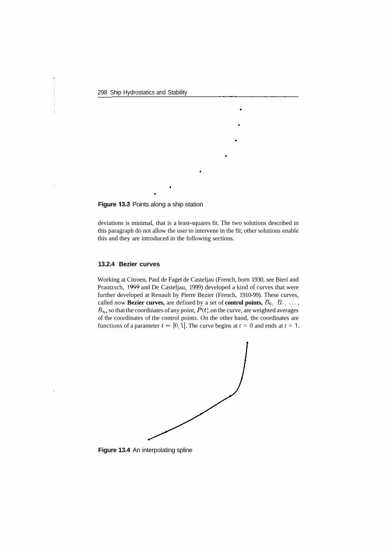
298 Ship Hydrostatics and Stability
Figure 13.3 Points along a ship station
deviations is minimal, that is a least-squares fit. The two solutions described inthis paragraph do not allow the user to intervene in the fit; other solutions enablethis and they are introduced in the following sections.
13.2.4 Bezier curves
Working at Citroen, Paul de Faget de Casteljau (French, born 1930, see Bieri andPrautzsch, 1999 and De Casteljau, 1999) developed a kind of curves that werefurther developed at Renault by Pierre Bezier (French, 1910-99). These curves,called now Bezier curves, are defined by a set of control points, BQ, BI, . . . ,Bn, so that the coordinates of any point, P(t), on the curve, are weighted averagesof the coordinates of the control points. On the other hand, the coordinates arefunctions of a parameter t= [0,1]. The curve begins at t = 0 and ends at t = 1.
Figure 13.4 An interpolating spline
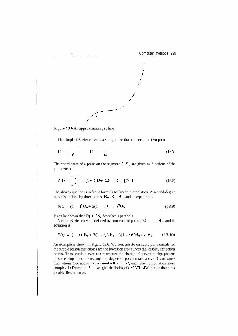
Computer methods 299
Figure 13.5 An approximating spline
The simplest Bezier curve is a straight line that connects the two points
T* R Xl
B° = ' Bl =
The coordinates of a point on the segment B0Bi are given as functions of theparameter t
P(t)=\X]=(l-t)B0 + tB1, t = [0,L " J
(13.8)
The above equation is in fact a formula for linear interpolation. A second-degreecurve is defined by three points, BQ, BI, 62, and its equation is
P(t) = (1 - t)2B0 + 2(1 - *)*Bi + t2B2 (13.9)
It can be shown that Eq. (13.9) describes a parabola.A cubic Bezier curve is defined by four control points, BO, . . . , BS, and its
equation is
P(t) = (l- t)3B0 + 3(1 - t)2tBl -}- 3(1 - t)t2B2 + t3B3 (13.10)
An example is shown in Figure 13.6. We concentrate on cubic polynomials forthe simple reason that cubics are the lowest-degree curves that display inflectionpoints. Thus, cubic curves can reproduce the change of curvature sign presentin some ship lines. Increasing the degree of polynomials above 3 can causefluctuations (see above 'polynomial inflexibility') and make computation morecomplex. In Example 1 3 . 1 , we give the listing of a M ATLAB function that plotsa cubic Bezier curve.
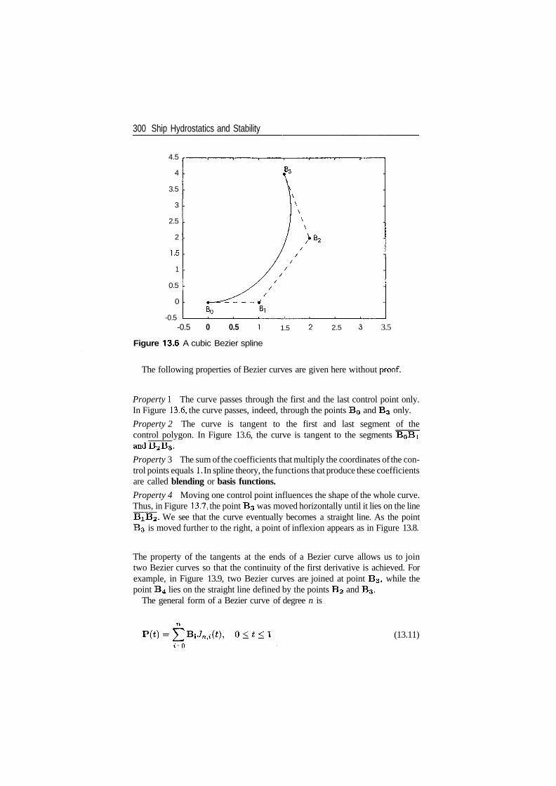
300 Ship Hydrostatics and Stability
4.5
4
3.5
3
2.5
2
1.5
1
0.5
0
-0.5-0.5 0 0.5 1
Figure 13.6 A cubic Bezier spline
1.5 2.5 3.5
The following properties of Bezier curves are given here without proof.
Property I The curve passes through the first and the last control point only.In Figure 13.6, the curve passes, indeed, through the points B0 and B3 only.
Property 2 The curve is tangent to the first and last segment of thecontrol polygon. In Figure 13.6, the curve is tangent to the segments BoBiandB2B3.
Property 3 The sum of the coefficients that multiply the coordinates of the con-trol points equals 1. In spline theory, the functions that produce these coefficientsare called blending or basis functions.
Property 4 Moving one control point influences the shape of the whole curve.Thus, in Figure 13.7, the point 63 was moved horizontally until it lies on the line6162. We see that the curve eventually becomes a straight line. As the pointB3 is moved further to the right, a point of inflexion appears as in Figure 13.8.
The property of the tangents at the ends of a Bezier curve allows us to jointwo Bezier curves so that the continuity of the first derivative is achieved. Forexample, in Figure 13.9, two Bezier curves are joined at point B3, while thepoint 64 lies on the straight line defined by the points 62 and B3.
The general form of a Bezier curve of degree n is
(13.11)i=0
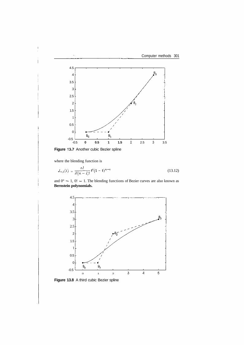
Computer methods 301
4.5
4
3.5
3
2.5
2
1.5
1
0.5
0
-0.5-0.5 0 0.5 1 1.5
Figure 13.7 Another cubic Bezier spline
where the blending function is
2.5 3.5
Jn,i(t) =nl
t!(n-i)!(13.12)
and 0° = 1, 0! = 1. The blending functions of Bezier curves are also known asBernstein polynomials.
4.5
4
3.5
3
2.5
2
1.5
1
0.5
0
-0.5B,
0 1 2
Figure 13.8 A third cubic Bezier spline
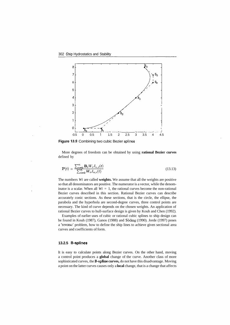
302 'Ship Hydrostatics and Stability
-0.5 0 0.5 1 1.5 2 2.5 3 3.5 4 4.5
Figure 13.9 Combining two cubic Bezier splines
More degrees of freedom can be obtained by using rational Bezier curvesdefined by
P(*) = (13.13)
The numbers Wi are called weights. We assume that all the weights are positiveso that all denominators are positive. The numerator is a vector, while the denom-inator is a scalar. When all Wi = 1, the rational curves become the non-rationalBezier curves described in this section. Rational Bezier curves can describeaccurately conic sections. As these sections, that is the circle, the ellipse, theparabola and the hyperbola are second-degree curves, three control points arenecessary. The kind of curve depends on the chosen weights. An application ofrational Bezier curves to hull-surface design is given by Kouh and Chen (1992).
Examples of earlier uses of cubic or rational cubic splines to ship design canbe found in Kouh (1987), Ganos (1988) and Soding (1990). Jorde (1997) posesa 'reverse' problem, how to define the ship lines to achieve given sectional areacurves and coefficients of form.
13.2.5 B-spllnes
It is easy to calculate points along Bezier curves. On the other hand, movinga control point produces a global change of the curve. Another class of moresophisticated curves, the B-spline curves, do not have this disadvantage. Movinga point on the latter curves causes only a local change, that is a change that affects
Computer methods 303
only the curve segment that neighbours the moved point. We give below therecursive definition of a B-spline. Given n -f1 control points, j?i, . . . , £?n+i,the position vector is
n+l
P(t) = ]T BiNitk(t), tmin < t < tmax, 2 < k < n + I (13.14)1=1
Here k is the order of the B-spline, and k — 1, the degree of the polynomialsin t. The basis functions are
- { 1 11 L>i _\ £ _ t'i-f-l / i o 1 c\n - (13.15)0 otherwise
and
A^fcO) = —^—lj^ h *+fc~* ^ H-i,fc-i— (13.16)
The set of ti values is called knot vector. If the knot values are not equallyspaced the B-spline is called non-uniform, otherwise it is called uniform. Thesum of the basis functions is
n+l
^Nitk(t) = l (13.17)1=1
for all t.The calculation of points along B-spline curves requires rather complex algo-
rithms that are beyond the scope of this chapter.The NURBS, or non-uniform rational B-splines are an extension of the
B-splines; their definition is
As in Eq. (13.13), Wi are the weights. The basis functions, N^k, are definedby Eqs. (13.15) and (13.16). A book on splines that includes historical andbiographical notes is that of Rogers (2001).
13.2.6 Parametric surfaces
Surfaces can be defined by implicit equations such as
/(x, y, z) = 0
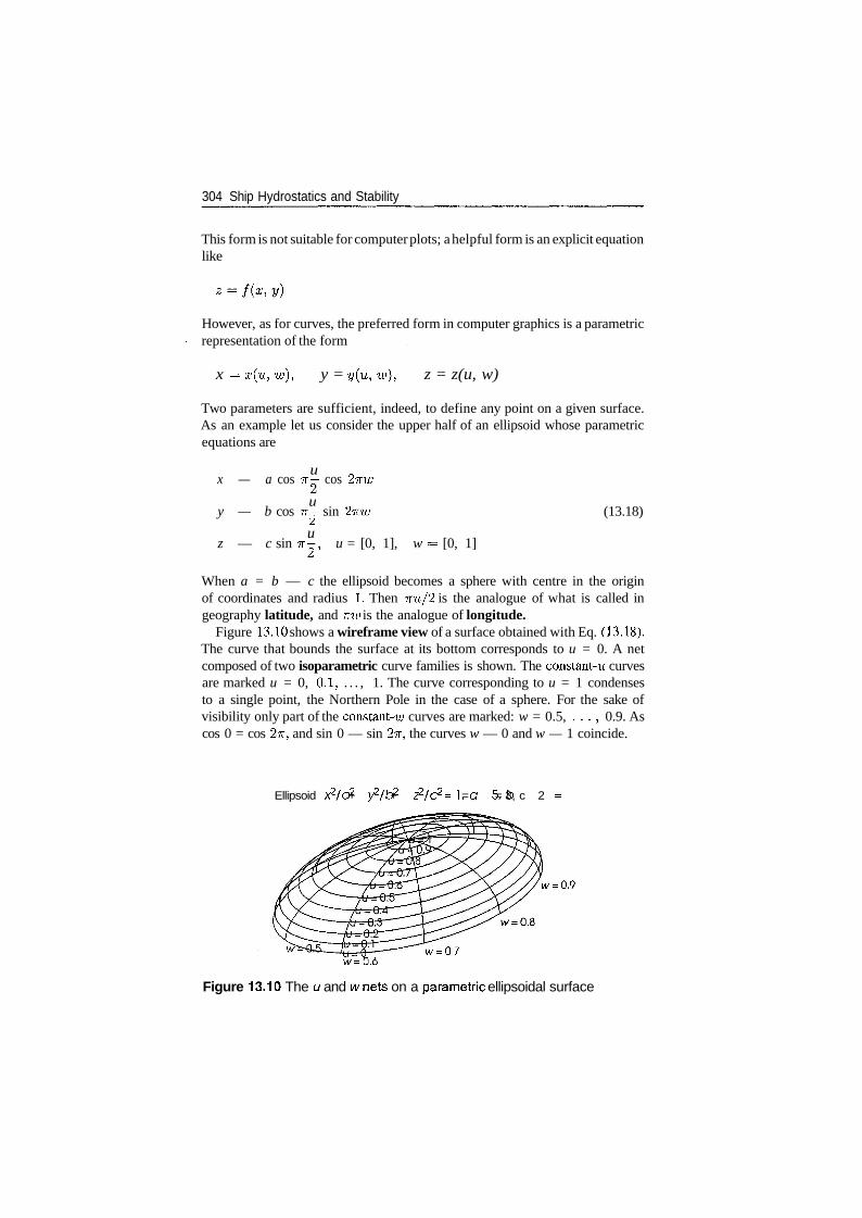
304 Ship Hydrostatics and Stability
This form is not suitable for computer plots; a helpful form is an explicit equationlike
However, as for curves, the preferred form in computer graphics is a parametricrepresentation of the form
x = x(u,w), y = y(u,w], z = z(u, w)
Two parameters are sufficient, indeed, to define any point on a given surface.As an example let us consider the upper half of an ellipsoid whose parametricequations are
ux — a cos TT— cos 2nw
uy — b cos TT— sin 2nw (13.18)
Zj
uz — c sin TT-, u = [0, 1], w = [0, 1]
When a = b — c the ellipsoid becomes a sphere with centre in the originof coordinates and radius 1. Then 7ru/2 is the analogue of what is called ingeography latitude, and TTW is the analogue of longitude.
Figure 13.10 shows a wireframe view of a surface obtained with Eq. (13.18).The curve that bounds the surface at its bottom corresponds to u = 0. A netcomposed of two isoparametric curve families is shown. The constant- w curvesare marked u = 0, 0.1, . . . , 1. The curve corresponding to u = 1 condensesto a single point, the Northern Pole in the case of a sphere. For the sake ofvisibility only part of the constant-it; curves are marked: w = 0.5, . . . , 0.9. Ascos 0 = cos 2?r, and sin 0 — sin 2?r, the curves w — 0 and w — 1 coincide.
Ellipsoid x2/d2 + y2//^ + z2/^2 =1,0 = 5, 6 = 3, c = 2
w=0.9
w=07w=lD.6
Figure 13.10 The a and wnets on a parametric ellipsoidal surface
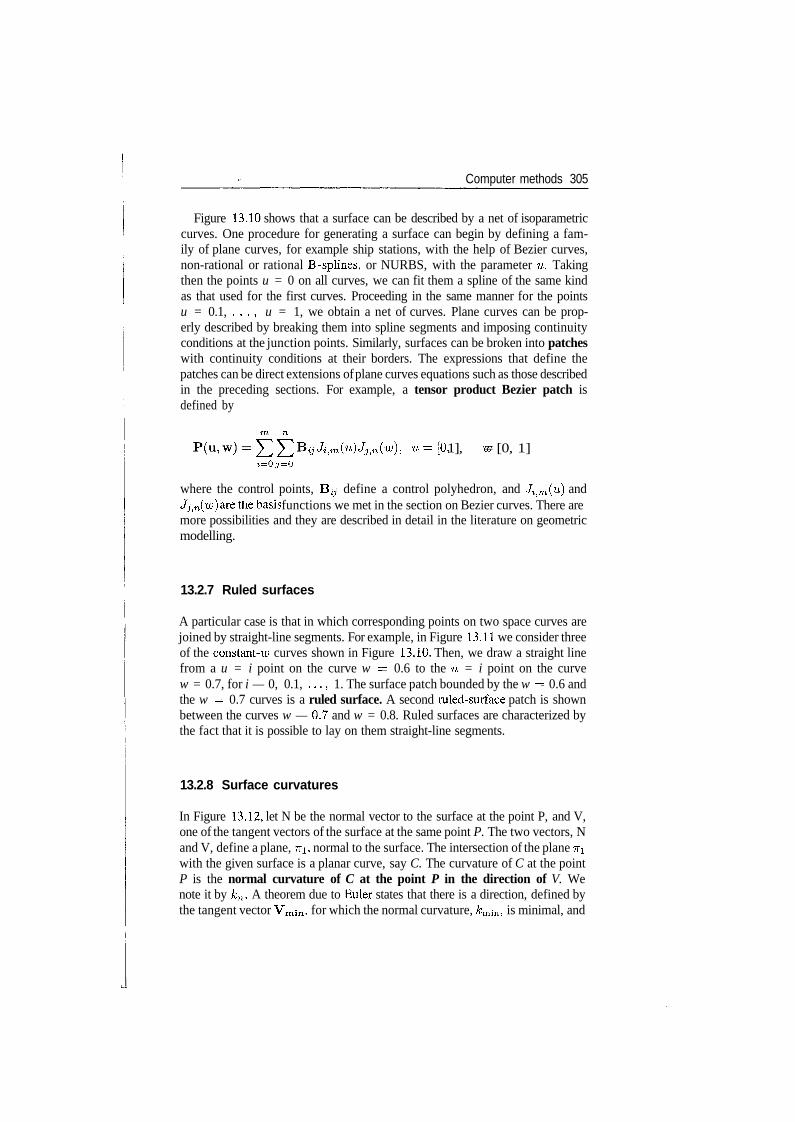
Computer methods 305
Figure 13.10 shows that a surface can be described by a net of isoparametriccurves. One procedure for generating a surface can begin by defining a fam-ily of plane curves, for example ship stations, with the help of Bezier curves,non-rational or rational B -splines, or NURBS, with the parameter u. Takingthen the points u = 0 on all curves, we can fit them a spline of the same kindas that used for the first curves. Proceeding in the same manner for the pointsu = 0.1, . . . , u = 1, we obtain a net of curves. Plane curves can be prop-erly described by breaking them into spline segments and imposing continuityconditions at the junction points. Similarly, surfaces can be broken into patcheswith continuity conditions at their borders. The expressions that define thepatches can be direct extensions of plane curves equations such as those describedin the preceding sections. For example, a tensor product Bezier patch isdefined by
ij-Ji|m(u)JJ>H, u = [ 0 , 1], ™ = [0, 1]i=0 j=0
where the control points, B^ define a control polyhedron, and Ji^m(u) andJj,n (w) are tne basis functions we met in the section on Bezier curves. There aremore possibilities and they are described in detail in the literature on geometricmodelling.
13.2.7 Ruled surfaces
A particular case is that in which corresponding points on two space curves arejoined by straight-line segments. For example, in Figure 13.11 we consider threeof the constant-it; curves shown in Figure 13.10. Then, we draw a straight linefrom a u = i point on the curve w = 0.6 to the u = i point on the curvew = 0.7, for i — 0, 0.1, . . . , 1. The surface patch bounded by the w = 0.6 andthe w = 0.7 curves is a ruled surface. A second ruled-surface patch is shownbetween the curves w — 0.7 and w = 0.8. Ruled surfaces are characterized bythe fact that it is possible to lay on them straight-line segments.
13.2.8 Surface curvatures
In Figure 13.12, let N be the normal vector to the surface at the point P, and V,one of the tangent vectors of the surface at the same point P. The two vectors, Nand V, define a plane, TTI, normal to the surface. The intersection of the plane TTIwith the given surface is a planar curve, say C. The curvature of C at the pointP is the normal curvature of C at the point P in the direction of V. Wenote it by kn. A theorem due to Euler states that there is a direction, defined bythe tangent vector Vmin, for which the normal curvature, km-m, is minimal, and
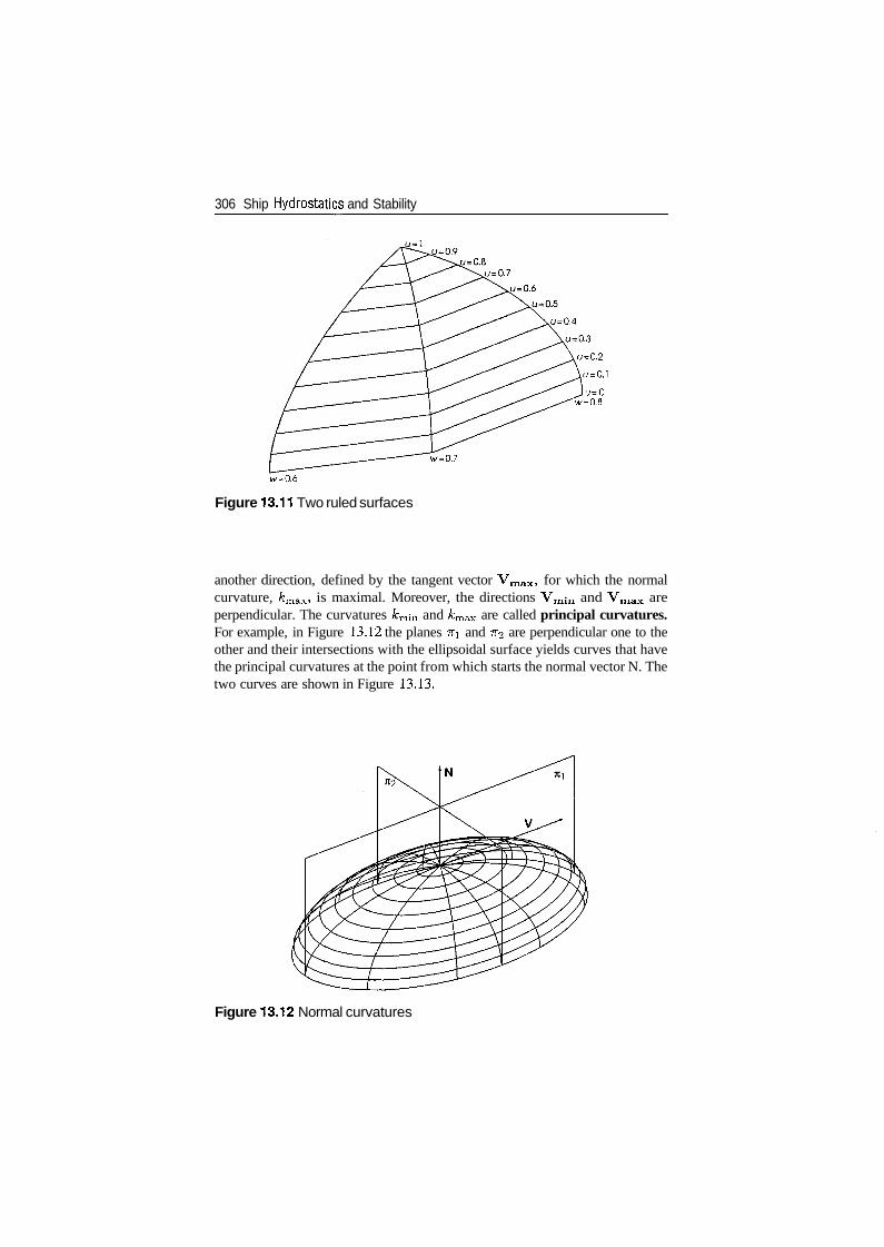
306 Ship Hydrostatics and Stability
u=0"W=0.8
w=0.7
w=0.6
Figure 13.11 Two ruled surfaces
another direction, defined by the tangent vector Vmax, for which the normalcurvature, /cmax, is maximal. Moreover, the directions Vmin and Vmax areperpendicular. The curvatures kmin and /cmax are called principal curvatures.For example, in Figure 13.12 the planes TTI and 7T2 are perpendicular one to theother and their intersections with the ellipsoidal surface yields curves that havethe principal curvatures at the point from which starts the normal vector N. Thetwo curves are shown in Figure 13.13.
Figure 13.12 Normal curvatures
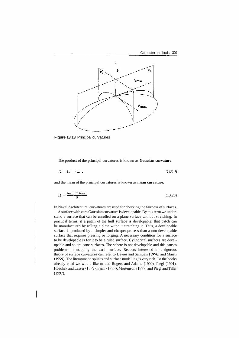
Computer methods 307
Figure 13.13 Principal curvatures
The product of the principal curvatures is known as Gaussian curvature:
•**• ~ "'min ' "'max \ij.l
and the mean of the principal curvatures is known as mean curvature:
~r(13.20)
In Naval Architecture, curvatures are used for checking the fairness of surfaces.A surface with zero Gaussian curvature is developable. By this term we under-
stand a surface that can be unrolled on a plane surface without stretching. Inpractical terms, if a patch of the hull surface is developable, that patch canbe manufactured by rolling a plate without stretching it. Thus, a developablesurface is produced by a simpler and cheaper process than a non-developablesurface that requires pressing or forging. A necessary condition for a surfaceto be developable is for it to be a ruled surface. Cylindrical surfaces are devel-opable and so are cone surfaces. The sphere is not developable and this causesproblems in mapping the earth surface. Readers interested in a rigoroustheory of surface curvatures can refer to Davies and Samuels (1996) and Marsh(1999). The literature on splines and surface modelling is very rich. To the booksalready cited we would like to add Rogers and Adams (1990), Piegl (1991),Hoschek and Lasser (1993), Farm (1999), Mortenson (1997) and Piegl and Tiller(1997).
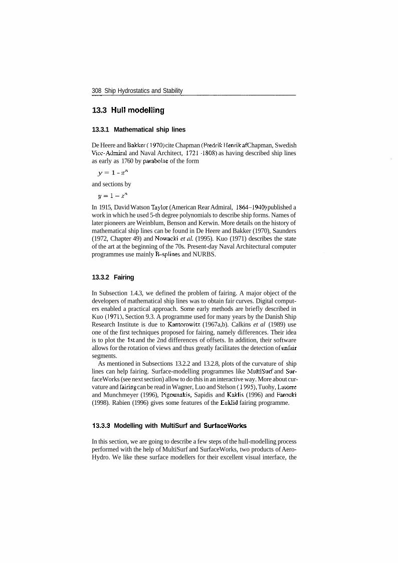
308 Ship Hydrostatics and Stability
13.3 Hull modelling
13.3.1 Mathematical ship lines
De Heere and Bakker ( 1970) cite Chapman (FredrikHenrikaf Chapman, SwedishVice- Admiral and Naval Architect, 1721-1808) as having described ship linesas early as 1760 by parabolae of the form
y = 1 - xn
and sections by
In 1915, David Watson Taylor (American Rear Admiral, 1864-1940) published awork in which he used 5-th degree polynomials to describe ship forms. Names oflater pioneers are Weinblum, Benson and Kerwin. More details on the history ofmathematical ship lines can be found in De Heere and Bakker (1970), Saunders(1972, Chapter 49) and Nowacki et al (1995). Kuo (1971) describes the stateof the art at the beginning of the 70s. Present-day Naval Architectural computerprogrammes use mainly B-splines and NURBS.
13.3.2 Fairing
In Subsection 1.4.3, we defined the problem of fairing. A major object of thedevelopers of mathematical ship lines was to obtain fair curves. Digital comput-ers enabled a practical approach. Some early methods are briefly described inKuo (1971), Section 9.3. A programme used for many years by the Danish ShipResearch Institute is due to Kantorowitz (1967a,b). Calkins et al (1989) useone of the first techniques proposed for fairing, namely differences. Their ideais to plot the 1st and the 2nd differences of offsets. In addition, their softwareallows for the rotation of views and thus greatly facilitates the detection of unfairsegments.
As mentioned in Subsections 13.2.2 and 13.2.8, plots of the curvature of shiplines can help fairing. Surface-modelling programmes like MultiSurf and Sur-faceWorks (see next section) allow to do this in an interactive way. More about cur-vature and fairing can be read in Wagner, Luo and Stelson ( 1 995), Tuohy, Latorreand Munchmeyer (1996), Pigounakis, Sapidis and Kaklis (1996) and Farouki(1998). Rabien (1996) gives some features of the Euklid fairing programme.
13.3.3 Modelling with MultiSurf and SurfaceWorks
In this section, we are going to describe a few steps of the hull-modelling processperformed with the help of MultiSurf and SurfaceWorks, two products of Aero-Hydro. We like these surface modellers for their excellent visual interface, the
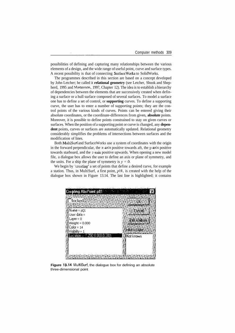
Computer methods 309
possibilities of defining and capturing many relationships between the variouselements of a design, and the wide range of useful point, curve and surface types.A recent possibility is that of connecting SurfaceWorks to SolidWorks.
The programmes described in this section are based on a concept developedby John Letcher; he called it relational geometry (see Letcher, Shook and Shep-herd, 1995 and Mortenson, 1997, Chapter 12). The idea is to establish a hierarchyof dependencies between the elements that are successively created when defin-ing a surface or a hull surface composed of several surfaces. To model a surfaceone has to define a set of control, or supporting curves. To define a supportingcurve, the user has to enter a number of supporting points; they are the con-trol points of the various kinds of curves. Points can be entered giving theirabsolute coordinates, or the coordinate-differences from given, absolute points.Moreover, it is possible to define points constrained to stay on given curves orsurfaces. When the position of a supporting point or curve is changed, any depen-dent points, curves or surfaces are automatically updated. Relational geometryconsiderably simplifies the problems of intersections between surfaces and themodification of lines.
Both MultiSurf and SurfaceWorks use a system of coordinates with the originin the forward perpendicular, the x-axis positive towards aft, the y-axis positivetowards starboard, and the z-axis positive upwards. When opening a new modelfile, a dialogue box allows the user to define an axis or plane of symmetry, andthe units. For a ship the plane of symmetry is y = 0.
We begin by 'creating' a set of points that define a desired curve, for examplea station. Thus, in MultiSurf, a first point, pOl, is created with the help of thedialogue box shown in Figure 13.14. The last line is highlighted; it contains
locked
N<ime = pQ1User data =Layer = 0Weight = 0.000Color = 14Visibility = 1
Figure 13.14 MultiSurf, the dialogue box for defining an absolutethree-dimensional point
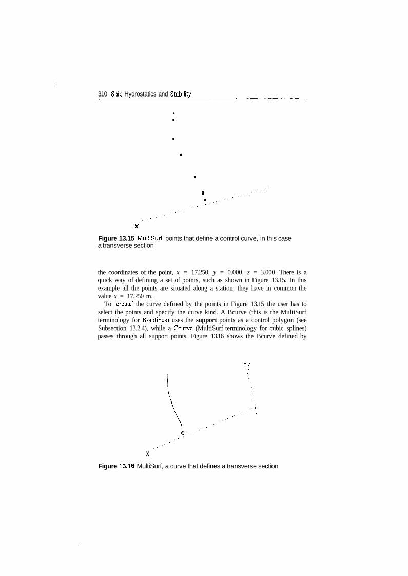
310 Ship Hydrostatics and Stability
Figure 13.15 MultiSurf, points that define a control curve, in this casea transverse section
the coordinates of the point, x = 17.250, y = 0.000, z = 3.000. There is aquick way of defining a set of points, such as shown in Figure 13.15. In thisexample all the points are situated along a station; they have in common thevalue x = 17.250 m.
To 'create' the curve defined by the points in Figure 13.15 the user has toselect the points and specify the curve kind. A Bcurve (this is the MultiSurfterminology for B-splines) uses the support points as a control polygon (seeSubsection 13.2.4), while a Ccurve (MultiSurf terminology for cubic splines)passes through all support points. Figure 13.16 shows the Bcurve defined by
Y Z
X
Figure 13.16 MultiSurf, a curve that defines a transverse section
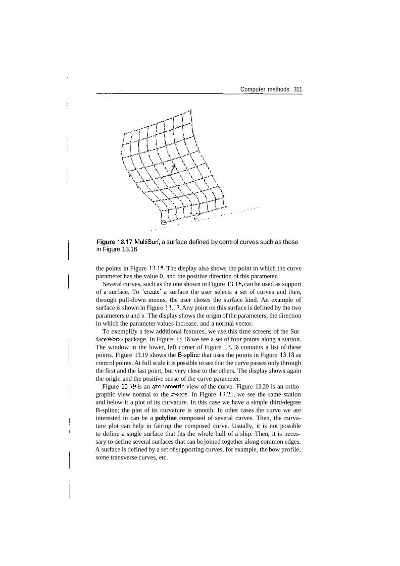
Computer methods 311
\ \ \
Figure 13.17 MultiSurf, a surface defined by control curves such as thosein Figure 13.16
the points in Figure 13.15. The display also shows the point in which the curveparameter has the value 0, and the positive direction of this parameter.
Several curves, such as the one shown in Figure 13.16, can be used as supportof a surface. To 'create' a surface the user selects a set of curves and then,through pull-down menus, the user choses the surface kind. An example ofsurface is shown in Figure 13.17. Any point on this surface is defined by the twoparameters u and v. The display shows the origin of the parameters, the directionin which the parameter values increase, and a normal vector.
To exemplify a few additional features, we use this time screens of the Sur-faceWorks package. In Figure 13.18 we see a set of four points along a station.The window in the lower, left corner of Figure 13.18 contains a list of thesepoints. Figure 13.19 shows the B-spline that uses the points in Figure 13.18 ascontrol points. At full scale it is possible to see that the curve passes only throughthe first and the last point, but very close to the others. The display shows againthe origin and the positive sense of the curve parameter.
Figure 13.19 is an axonometric view of the curve. Figure 13.20 is an ortho-graphic view normal to the x-axis. In Figure 13.21, we see the same stationand below it a plot of its curvature. In this case we have a simple third-degreeB-spline; the plot of its curvature is smooth. In other cases the curve we areinterested in can be a polyline composed of several curves. Then, the curva-ture plot can help in fairing the composed curve. Usually, it is not possibleto define a single surface that fits the whole hull of a ship. Then, it is neces-sary to define several surfaces that can be joined together along common edges.A surface is defined by a set of supporting curves, for example, the bow profile,some transverse curves, etc.
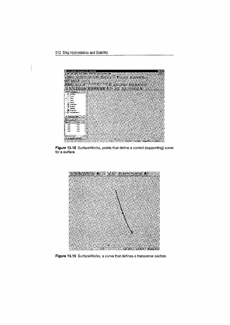
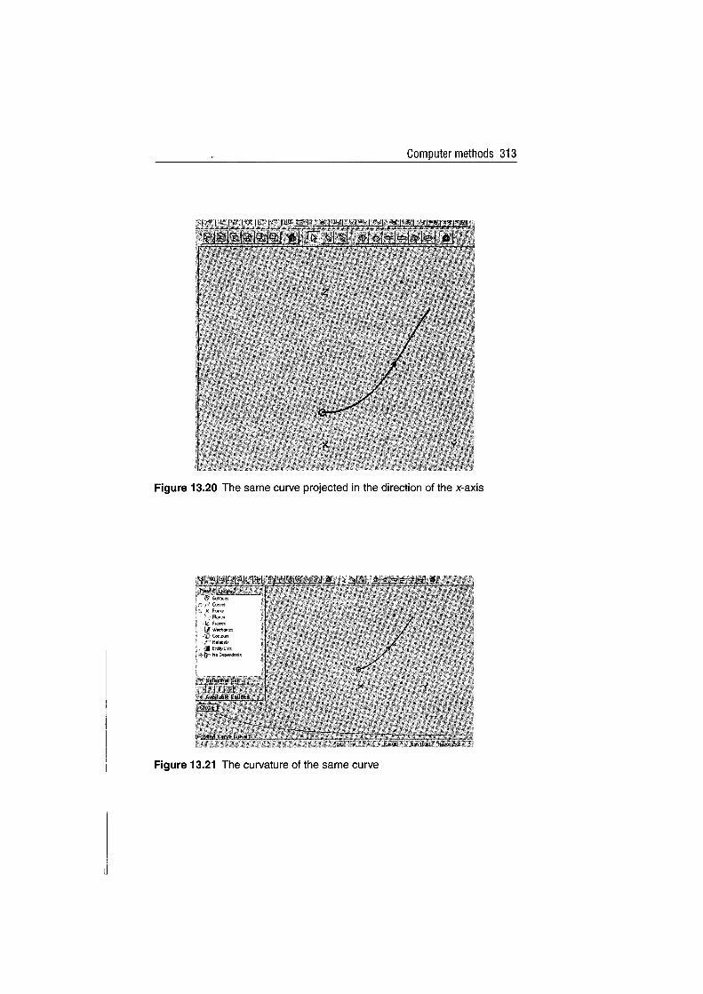
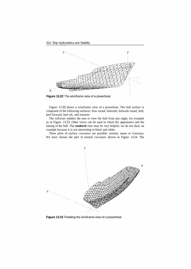
314 Ship Hydrostatics and Stability
Figure 13.22 The wireframe view of a powerboat
Figure 13.22 shows a wireframe view of a powerboat. The hull surface iscomposed of the following surfaces: bow round, bulwark, bulwark round, hull,keel forward, keel aft, and transom.
The software enables the user to view the hull from any angle, for exampleas in Figure 13.23. Other views can be used to check the appearance and thefairing of the hull. The rendered view may be very helpful; we do not show anexample because it is not interesting in black and white.
Three plots of surface curvature are possible: normal, mean or Gaussian.We have chosen the plot of normal curvature shown in Figure 13.24. The
•z
Figure 13.23 Rotating the wireframe view of a powerboat
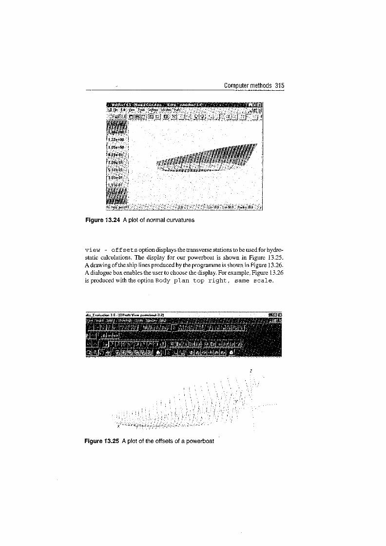
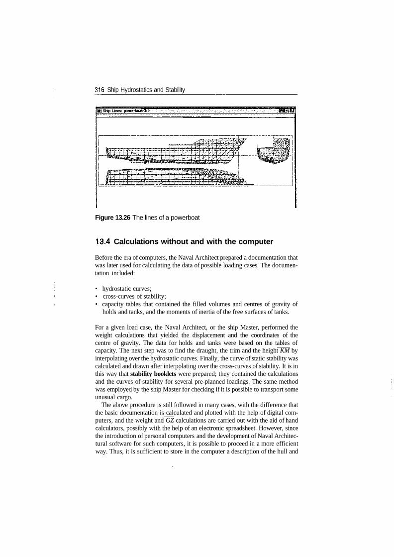
316 Ship Hydrostatics and Stability
® Ship Lines: powerboat-3:3
Figure 13.26 The lines of a powerboat
13.4 Calculations without and with the computer
Before the era of computers, the Naval Architect prepared a documentation thatwas later used for calculating the data of possible loading cases. The documen-tation included:
• hydrostatic curves;• cross-curves of stability;• capacity tables that contained the filled volumes and centres of gravity of
holds and tanks, and the moments of inertia of the free surfaces of tanks.
For a given load case, the Naval Architect, or the ship Master, performed theweight calculations that yielded the displacement and the coordinates of thecentre of gravity. The data for holds and tanks were based on the tables ofcapacity. The next step was to find the draught, the trim and the height KM byinterpolating over the hydrostatic curves. Finally, the curve of static stability wascalculated and drawn after interpolating over the cross-curves of stability. It is inthis way that stability booklets were prepared; they contained the calculationsand the curves of stability for several pre-planned loadings. The same methodwas employed by the ship Master for checking if it is possible to transport someunusual cargo.
The above procedure is still followed in many cases, with the difference thatthe basic documentation is calculated and plotted with the help of digital com-puters, and the weight and GZ calculations are carried out with the aid of handcalculators, possibly with the help of an electronic spreadsheet. However, sincethe introduction of personal computers and the development of Naval Architec-tural software for such computers, it is possible to proceed in a more efficientway. Thus, it is sufficient to store in the computer a description of the hull and
Computer methods 317
of its subdivision into holds and tanks. The model can be completed with adescription of the sail area necessary for calculating the wind arm. Then, theuser can define a loading case by entering for each hold or tank a measure ofits filling, for example the filling height, and the specific gravity of the cargo.The computer programme calculates almost instantly the parameters of the float-ing conditions and the characteristics of stability, and it does so without roughapproximations and interpolations. For example, in a manual, straightforwardtrim calculation one has to use the moment to change trim, MCT, read fromthe hydrostatic curves. Hydrostatic curves are usually calculated for the ship oneven keel; therefore, using the MCT value read in them means to assume thatthis value remains constant within the trim range. Computer calculations, onthe other hand, do not need this assumption. The floating condition is found bysuccessive iterations that stop when the conditions of equilibrium are met witha given tolerance.
The ship data stored in the computer constitute a ship model; it can be orga-nized as a data base. In this sense, Biran and Kantorowitz (1986) and Biran,Kantorowitz and Yanai (1987) describe the use of relational data bases. John-son, Glinos, Anderson et al (1990), Carnduf and Gray (1992) and Reich (1994)discuss more types of data bases. Many modern ships are provided with boardcomputers that contain the data of the ship and a dedicated computer programme.Moreover, the computer can be connected to sensors that supply on line the tankand hold filling heights.
13.4.1 Hydrostatic calculations
Some hydrostatic calculations are straightforward in the sense that we can per-form them in a single iteration. For example, if we want to calculate hydrostaticcurves we must perform integrations for a draught TO, then for a draught T\, andso on. Chapter 4 shows how to carry out such calculations. Other calculationscan be carried out only by iterations. For example, let us assume that we wantto calculate the righting arm of a given ship, for a given displacement volume,VQ, and the heel angle fa. We do not know the draught, TO, corresponding to thegiven parameters. We must start with an initial guess, Tinit, draw the waterline,WQ LQ , corresponding to this draught and the heel angle 0^, and calculate theactual displacement volume. If the guess Tjnit was not based on previous calcu-lations, almost certainly we shall find a displacement volume Vi ^ VQ. If thedeviation is larger than an acceptable value, e, we must try another waterplane,WiLi, parallel to the initial guess waterline, WQ£O- This time we proceed in amore 'educated' manner. Readers familiar with the Newton-Raphson proceduremay readily understand why we use the derivative of the displacement volumewith respect to the draught, that is the waterplane area, Ayy. We calculate adraught correction
318 Ship Hydrostatics and Stability
and we start again with a corrected draught
Ti - T^ + ST
We continue so until the stopping condition
| V 0 - V N | < 6
is met.A much more difficult, but frequent problem is that of finding the floating
condition of a ship for a given loading. The input is composed of the displacementvolume and the coordinates of the centre of gravity. The output is the triple ofparameters that define the floating condition, that is the draught, the heel andthe trim. To solve the problem we can think of a Newton-like procedure inthree variables. Such a procedure implies the calculation of a Jacobian whoseelements are nine partial derivatives. Not less difficult is the problem of findingthe floating condition of a damaged ship, provided the ship can still float. TheNaval Architect has to find the draught, trim and heel for which the conditionsdescribed in Section 11.3 are met. In physical terms, the Naval Architect mustfind the ship position in which the water level in the flooded compartments is thesame as that of the surrounding water and the centres of buoyancy and gravitylie on a common vertical. Some details of the above problems can be foundin Soding (1978). The calculations of hydrostatic data from surface patches isdiscussed by Rabien (1985).
Many ingenious methods for solving the above problems have been devised;by elegant procedures they ensured satisfactory precision in reasonable calcu-lating times. The methods based on mechanical computers are particularly inter-esting. Details can be found in older books. For example, an original publicationof a method for calculating lever arms at large heel angles is due to Leparmen-tier (1899). Other methods for calculating cross-curves of stability are describedby Rondeleux (1911), Dankwardt (1957), Attwood and Pengelly (1960), Krap-pinger (1960), Semyonov-Tyan-Shansky (no year given), De Heere and Bakker(1970), Hervieu (1985), Rawson and Tupper (1996). Methods of flooding calcu-lations are explained, for example, in Semyonov-Tyan-Shansky (no year given)and De Heere and Bakker (1970).
As mentioned, the first publication about a computer programme for NavalArchitectural calculations is that of Kantorowitz (1958); it contains also an anal-ysis of calculation errors. The first computer programmes worked in the batchmode; an input had to be submitted to the computer, the computer produced anoutput. For many years the input was contained in a set of punched cards, later itcould be written on a file. An example of such a programme is ARCHIMEDESwritten at the University of Hannover (see Poulsen, 1980). The input consists ofseveral sequences of numbers. One sequence defines the calculations to be per-formed, a second sequence describes the hull surface, a third sequence definesthe subdivision into compartments and tanks, a fourth the longitudinal distribu-tion of masses, a fifth defines run parameters such as the draught, trim, the wavecharacteristics, and the identifiers of the compartments to be considered flooded.
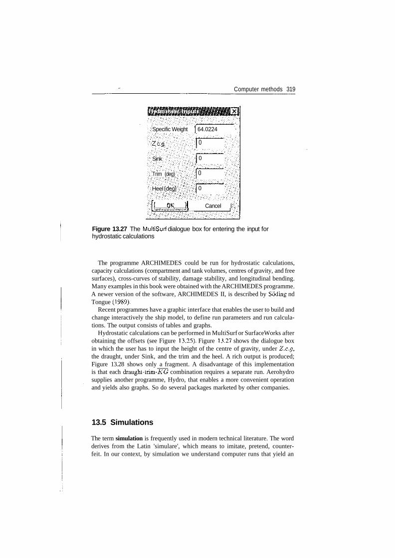
Computer methods 319
0
Specific Weight j 64.0224
Zc.g.
Sink
Trim (deg)
Heel (deg}
0
0
[ QIC jj Cancel I.Vv^'-'--r——•;";;>-»-<i t
Figure 13.27 The MultiSurf dialogue box for entering the input forhydrostatic calculations
The programme ARCHIMEDES could be run for hydrostatic calculations,capacity calculations (compartment and tank volumes, centres of gravity, and freesurfaces), cross-curves of stability, damage stability, and longitudinal bending.Many examples in this book were obtained with the ARCHIMEDES programme.A newer version of the software, ARCHIMEDES II, is described by Soding ndTongue (1989).
Recent programmes have a graphic interface that enables the user to build andchange interactively the ship model, to define run parameters and run calcula-tions. The output consists of tables and graphs.
Hydrostatic calculations can be performed in MultiSurf or SurfaceWorks afterobtaining the offsets (see Figure 13.25). Figure 13.27 shows the dialogue boxin which the user has to input the height of the centre of gravity, under Z.c.g,the draught, under Sink, and the trim and the heel. A rich output is produced;Figure 13.28 shows only a fragment. A disadvantage of this implementationis that each draught-trim-KG combination requires a separate run. Aerohydrosupplies another programme, Hydro, that enables a more convenient operationand yields also graphs. So do several packages marketed by other companies.
13.5 Simulations
The term simulation is frequently used in modern technical literature. The wordderives from the Latin 'simulare', which means to imitate, pretend, counter-feit. In our context, by simulation we understand computer runs that yield an
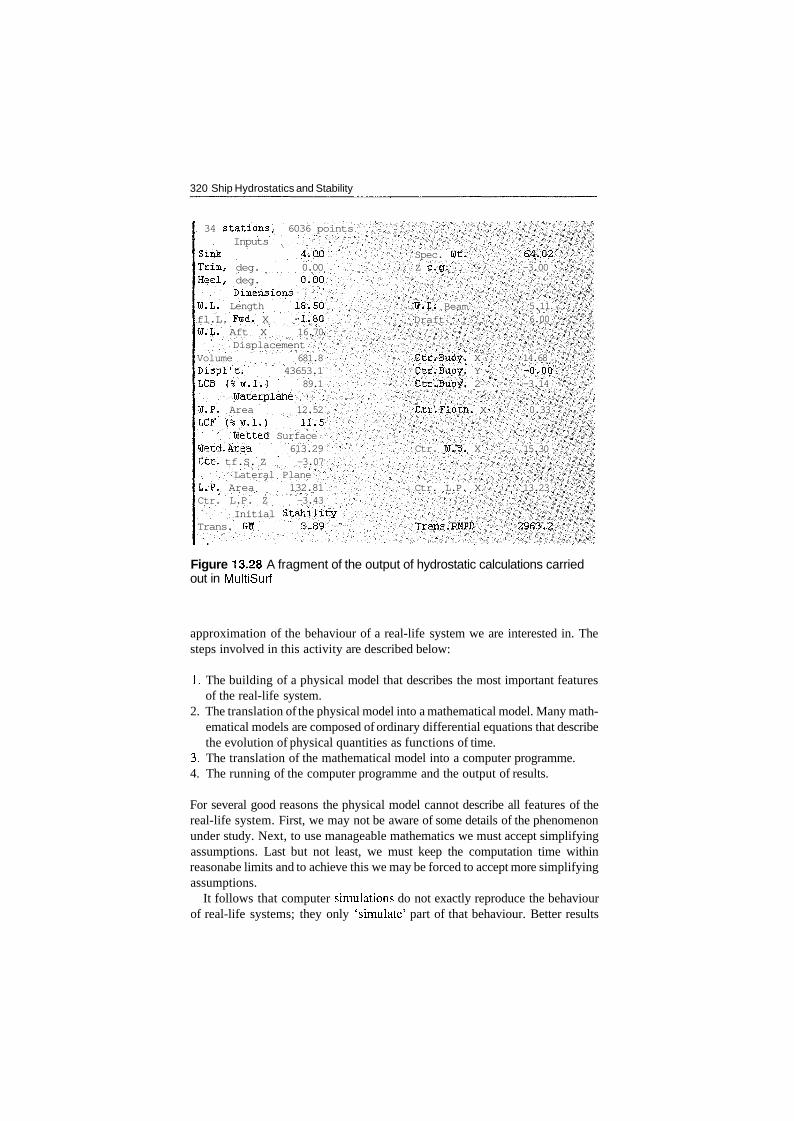
320 Ship Hydrostatics and Stability
34 stations, 6036 pointsInputs
Sink 4.00Trim, deg. 0.00Heel, deg. 0.00
Dimensions¥.L. Length 18.50fl.L. Fwd. X -1.80¥.L. Aft X 16.70
DisplacementVolume 681.8Displ't. 43653.1LCB (% w.l.) 89.1
Uaterplane¥.F. Area 12.52LCF (% TJ.I.) 11-5
Wetted Surface¥etd.Area 613.29Ctr. tf.S. Z -3.07
Lateral PlaneL.P. Area 132.81Ctr. L.P. Z -3.43
Initial StabilityTrans. GM 3.89
Spec. ¥t.Z e.g.
W.L. BeamDraft
Ctr.Buoy. XCtr.Buoy. YCtr.Buoy. 2
Ctr.Flotn. X
Ctr. U.S. X
Ctr. L.P. X
Trans.RHPD
64,02-3.00
5.116.00
14.68-0.00-3.14
0.33
15.30
13.23
2963.2
Figure 13.28 A fragment of the output of hydrostatic calculations carriedout in MultiSurf
approximation of the behaviour of a real-life system we are interested in. Thesteps involved in this activity are described below:
1. The building of a physical model that describes the most important featuresof the real-life system.
2. The translation of the physical model into a mathematical model. Many math-ematical models are composed of ordinary differential equations that describethe evolution of physical quantities as functions of time.
3. The translation of the mathematical model into a computer programme.4. The running of the computer programme and the output of results.
For several good reasons the physical model cannot describe all features of thereal-life system. First, we may not be aware of some details of the phenomenonunder study. Next, to use manageable mathematics we must accept simplifyingassumptions. Last but not least, we must keep the computation time withinreasonabe limits and to achieve this we may be forced to accept more simplifyingassumptions.
It follows that computer simulations do not exactly reproduce the behaviourof real-life systems; they only 'simulate' part of that behaviour. Better results
Computer methods 321
can be certainly obtained by experiments, especially at full scale. It is easy toimagine that full-scale experiments on ships may be very expensive so that theycannot be carried out frequently. Dangerous experiments that can lead to ship lossmay not be possible at all. Such tests can be performed only on reduced-scalemodels. Still, basin tests too are expensive and their extent is usually limitedby the available budget. Simulations may replace dangerous experiments, basintests can be completed by simulations. Then, part of the possible cases can besimulated, part tested on basin models. The basin tests can be used to correct orvalidate the computer model.
It is possible to measure the motions of a ship model in a test basin equippedwith a wave maker. Then, the motions are recorded as functions of time. It isalso possible to simulate ship motions as functions of time, that is to simu-late in the time domain. However, such measurements or simulations in thetime domain have limitations. As explained in Chapter 12, the sea surfaceis a random process; therefore, ship motions are also random processes. Tosimulate a given spectrum in the basin or in a computer programme, it isnecessary to draw a number of random phases. The resulting motions do notdescribe all possible situations, but are only an example of such possibilities. Wesay that we obtain a realization of the random process. Moreover, for practicalreasons, the duration of a basin test is limited. Then, the time span may notbe sufficient for the worst event to happen. Although we may afford simulationtimes longer than basin tests, they still may be insufficient for obtaining the worstevents.
More results can be obtained by calculating motions as functions of frequency,that is calculating in the frequency domain. Programmes that perform such cal-culaitons are available both through universities and on the market. The softwarecalculates the added masses and damping coefficients, for a series of frequen-cies, by using potential theory and certain simplifying assumptions. Next, thesoftware calculates the response amplitude operators, RAOs, of various motionsor events. For a wave frequency component, and given ship heading and speed,the programme calculates the frequency of encounter and transforms the spectrafrom functions of wave frequency to functions of the frequency of encounter.Response spectra are obtained as products of the spectra of encounter and RAOs.Statistics can be extracted from the spectra, for instance root mean square,shortly RMS values of the motions.
Taking into consideration the motion of the sea surface, the heave and the pitch,the programme yields the motion of a deck point relative to the sea surface andcalculates the probability of having waves on deck. Other events whose proba-bility can be calculated are slamming and propeller racing, while the motions,velocities and accelerations of given ship points are obtained as combinationsof motions in the various degrees of freedom. An example of ship motionssimulated in the time domain can be found in Elsimillawy and Miller (1986).Examples of studies of capsizing in the time domain are in Gawthrop, Kountzerisand Roberts (1988) and Kat and Paulling (1989). An example of simulation infrequency domain is given by Kim, Chou and Tien (1980).
322 Ship Hydrostatics and Stability
13.5.1 A simple example of roll simulation
Subsection 9.3.2 shows how to implement in MATLAB a Mathieu equation andsimulate the roll motion produced by parametric excitation. More complicatedmodels can be simulated in a similar manner by writing the governing equationsas systems of first-order differential equations and calling an integration routine.The more complex the system becomes, the more difficult it is to proceed in thisway. The programmer must write more lines and arrange them in the order inwhich information must be passed from one programme line to another. Softwarepackages have been written to make simulation easier. The common feature ofthe various packages is that the programmer does not have to care about the orderin which information must be passed. Also, routines and functions frequentlyused in simulations are available in libraries from which the user can readilycall them. The programmer has only to describe the various relationships, thesoftware will detail the equations and arrange them in the required order. In thissection we give one very simple example of the capabilities of modern simulationsoftware. As we give in the book examples in MATLAB, it is natural to use herethe related simulation package, SIMULINK. Let us consider the following rollequation
Az20 + gkGZ = MH (13.21)
where A is the displacement mass, i, the mass radius of inertia, GZ, the rightingarm, and MH, a heeling moment. We rewrite Eq. (13.21) as
rr(13.22)
In this example we neglect added mass and damping, but use a non-linear func-tion for GZ and can accept a variety of heeling moments. To represent thisequation in SIMULINK we draw the block diagram shown in Figure 13.29 byputting in blocks taken from the libraries of the software and connecting themby lines that define the relationships between blocks. At the beginning we puttwo blocks representing heeling moments, MH. For the wind moment we usea step function. Initially the moment is zero, at a given moment it jumps to aprescribed value that remains constant in continuation. For the wave moment weuse a sine function, but it is not difficult to input a sum of sines.
The next block to the right is a switch; it is used to select one of the heel-ing moments, MH. The block called Heeling arm performs the division ofthe heeling moment by the displacement value supplied by the block calleddisplacement. Follows a summation point. At this point the value gGZ issubtracted from the heeling arm. The output of the summation block is
MH *
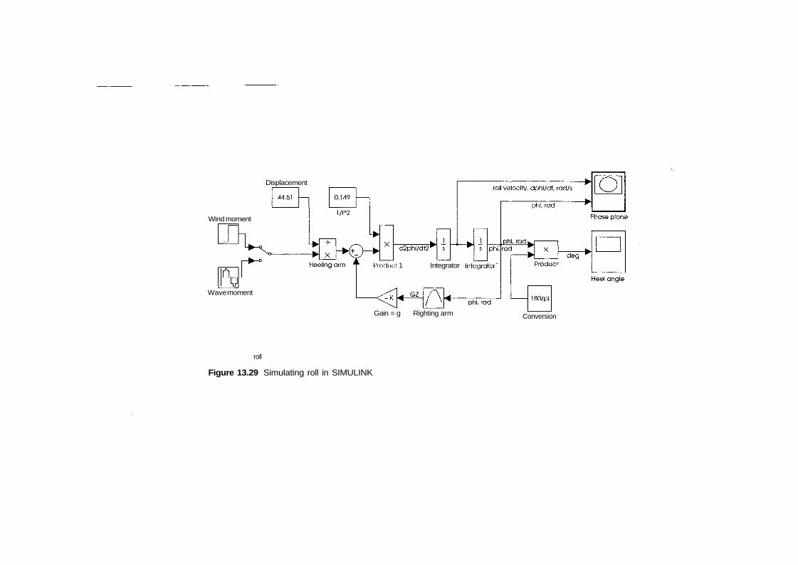
Displacement
Wind moment
Product 1 Integrator Integrator!
Wave moment
Gain = g Righting arm Conversion
roll
Figure 13.29 Simulating roll in SIMULINK
324 Ship Hydrostatics and Stability
Continuing to the right, we find a block that multiplies by l/i2 the output of thesummation block; the result is
/MH
We immediately see from Eq. (13.22) that the output of the block calledProduct 1 is the roll acceleration, <j). This acceleration is the input to an inte-grator. The symbol
15
that marks the integrator block reminds the integration of Laplace transforms.The output of the integrator is the roll velocity, 0, in radians per second. Theroll velocity is supplied as input to two output blocks. One block, above at right,is an oscilloscope, shortly scope, marked Phase plane. The other block, anintegrator marked Integrator 1, outputs the roll angle, <p.
Following a path to the left, the roll angle becomes the input of a blockcalled Righting arm. This block contains GZ values as functions of (/>. Ina gain block the GZ value is multiplied by the acceleration of gravity, g, andat the summation point, the product is subtracted from the heeling arm. Fol-lowing rightward paths, the roll angle is supplied directly to the scope Phaseplane, while converted to degrees is input to the scope Heel angle. Thescope phas e p 1 ane displays the roll velocity versus the roll angle. The scopeangle displays the roll angle versus time.
13.6 Summary
Ship projects require the drawing of lines that cannot be described by simplemathematical expressions, and also extensive calculations, mainly iterated inte-grations. Interesting attempts have been made to use mathematical ship lines,but until the second half of the last century the procedures for drawing and fair-ing ship lines remained manual. As to calculations, many elegant methods weredevised, not a few of them based on mechanical, analogue computers, such asplanimeters, integrators and integraphs. As in other engineering fields, in thedomain of Naval Architecture the advent of digital computers greatly improvedthe techniques and made possible important advances. Naval Architects wereamong the first engineers to use massive computer programmes.
The development of computer graphics has made possible the use of com-puters in the design of hull surfaces. In computer graphics, curves are definedparametrically
where the parameter, t, is frequently normalized so as to vary from 0 to 1 .
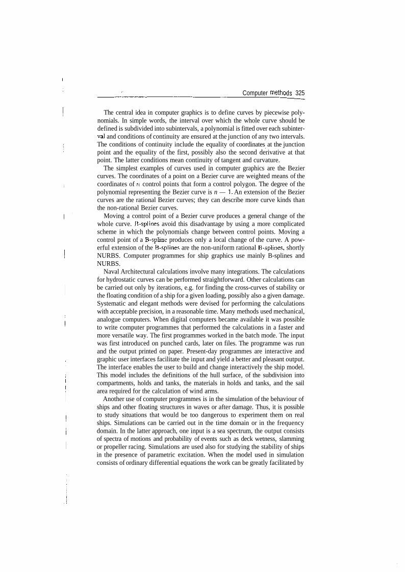
Computer methods 325
The central idea in computer graphics is to define curves by piecewise poly-nomials. In simple words, the interval over which the whole curve should bedefined is subdivided into subintervals, a polynomial is fitted over each subinter-val and conditions of continuity are ensured at the junction of any two intervals.The conditions of continuity include the equality of coordinates at the junctionpoint and the equality of the first, possibly also the second derivative at thatpoint. The latter conditions mean continuity of tangent and curvature.
The simplest examples of curves used in computer graphics are the Beziercurves. The coordinates of a point on a Bezier curve are weighted means of thecoordinates of n control points that form a control polygon. The degree of thepolynomial representing the Bezier curve is n — 1. An extension of the Beziercurves are the rational Bezier curves; they can describe more curve kinds thanthe non-rational Bezier curves.
Moving a control point of a Bezier curve produces a general change of thewhole curve. B-splines avoid this disadvantage by using a more complicatedscheme in which the polynomials change between control points. Moving acontrol point of a B-spline produces only a local change of the curve. A pow-erful extension of the B-splines are the non-uniform rational B-splines, shortlyNURBS. Computer programmes for ship graphics use mainly B-splines andNURBS.
Naval Architectural calculations involve many integrations. The calculationsfor hydrostatic curves can be performed straightforward. Other calculations canbe carried out only by iterations, e.g. for finding the cross-curves of stability orthe floating condition of a ship for a given loading, possibly also a given damage.Systematic and elegant methods were devised for performing the calculationswith acceptable precision, in a reasonable time. Many methods used mechanical,analogue computers. When digital computers became available it was possibleto write computer programmes that performed the calculations in a faster andmore versatile way. The first programmes worked in the batch mode. The inputwas first introduced on punched cards, later on files. The programme was runand the output printed on paper. Present-day programmes are interactive andgraphic user interfaces facilitate the input and yield a better and pleasant output.The interface enables the user to build and change interactively the ship model.This model includes the definitions of the hull surface, of the subdivision intocompartments, holds and tanks, the materials in holds and tanks, and the sailarea required for the calculation of wind arms.
Another use of computer programmes is in the simulation of the behaviour ofships and other floating structures in waves or after damage. Thus, it is possibleto study situations that would be too dangerous to experiment them on realships. Simulations can be carried out in the time domain or in the frequencydomain. In the latter approach, one input is a sea spectrum, the output consistsof spectra of motions and probability of events such as deck wetness, slammingor propeller racing. Simulations are used also for studying the stability of shipsin the presence of parametric excitation. When the model used in simulationconsists of ordinary differential equations the work can be greatly facilitated by
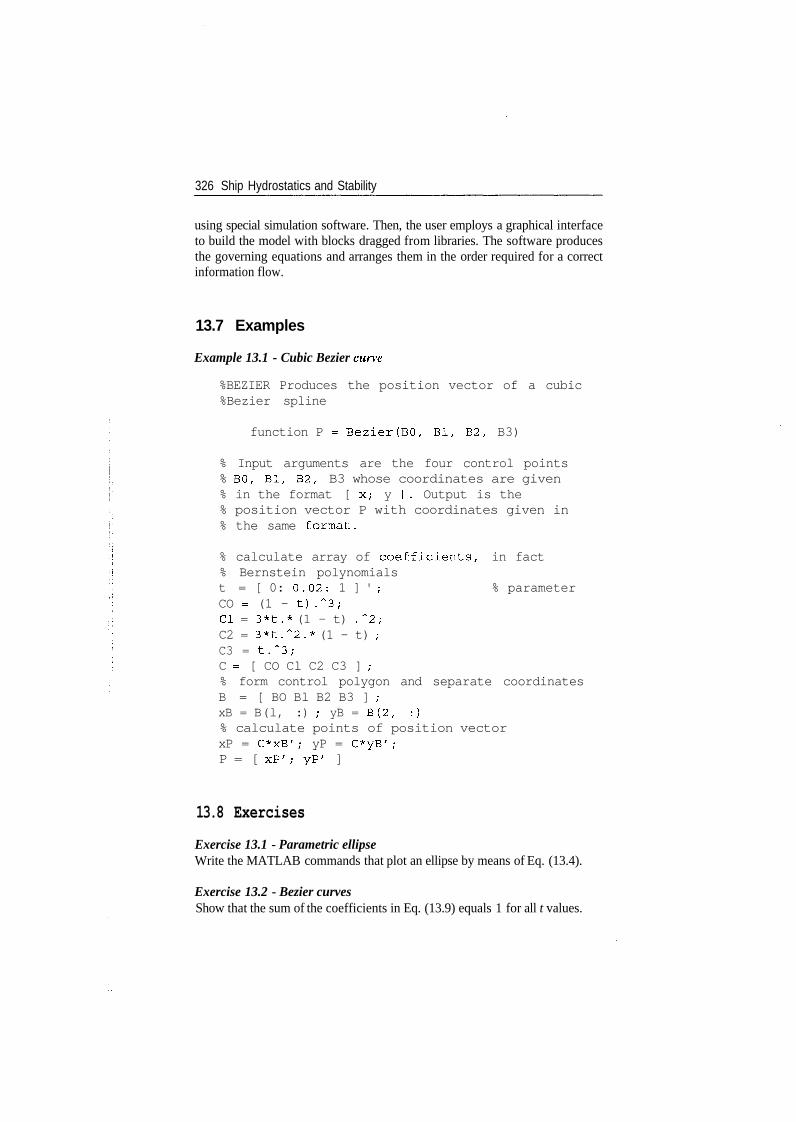
326 Ship Hydrostatics and Stability
using special simulation software. Then, the user employs a graphical interfaceto build the model with blocks dragged from libraries. The software producesthe governing equations and arranges them in the order required for a correctinformation flow.
13.7 Examples
Example 13.1 - Cubic Bezier curve
%BEZIER Produces the position vector of a cubic%Bezier spline
function P = Bezier(BO, Bl, B2, B3)
% Input arguments are the four control points% BO, Bl, B2, B3 whose coordinates are given% in the format [ x; y ]. Output is the% position vector P with coordinates given in% the same format.
% calculate array of coefficients, in fact% Bernstein polynomialst = [ 0: 0.02: 1 ] ' ; % parameterCO = (1 - t).~3;Cl = 3*t.* (1 - t) .~2;C2 = 3*t.~2.* (1 - t) ;C3 = t.~3;C = [ CO Cl C2 C3 ] ;% form control polygon and separate coordinatesB = [ BO Bl B2 B3 ] ;xB = B(l, :) ; yB = B(2, :)% calculate points of position vectorxP = C*xB'; yP = C*yB';P = [ xP'; yP' ]
13.8 Exercises
Exercise 13.1 - Parametric ellipseWrite the MATLAB commands that plot an ellipse by means of Eq. (13.4).
Exercise 13.2 - Bezier curvesShow that the sum of the coefficients in Eq. (13.9) equals 1 for all t values.
328 Bibliography
Arscott, P.M. (1964). Periodic Differential Equations -An Introduction to Mathieu, Lameand Allied Functions. Oxford: Pergamon Press.
ASTM (2001). Guide F1321-92 Standard Guide for Conducting a Stability Test (Light-weight Survey and Inclining Experiment) to Determine the light Ship Displacementand Centers of Gravity of a Vessel. http://www..astm.org/DATABASE.CART/PAGES/F1321.htm.
Attwood, E.L. and Pengelly, H.S. (1960). Theoretical Naval Architecture, new editionexpanded by Sims, A.J. London: Longmans.
Bieri, H.P. and Prautzsch, H. (1999). Preface. Computer Aided Geometric Design, 16,579-81.
Biran, A. and Breiner, M. (2002). MATLAB 6 for Engineers. Harlow, England: PrenticeHall. Previous edition translated into German as: MATLAB 5 fiir Ingenieure - System-atische und praktische Einfiihrung (1999). Bonn: Addison-Wesley. Greek translation1999, Ekdoseis Tziola.
Biran, A. and Kantorowitz, E. (1986). Ship design system integrated around a relationaldata base. In CADMO 86 (G.A. Keramidas, and T.K.S. Murthy, eds), pp. 85-94,Berlin: Springer-Verlag.
Biran, A., Kantorowitz, E. and Yanai, J. (1987). A Relational Data Base for Naval Archi-tecture. In International Symposium on Advanced Research for Ships and Shipping inthe Nineties, CETENA's 25th Anniversary, S. Margherita Ligure, Italy, 1-3 October.
Birbanescu-Biran, A. (1979). A system's theory approach in Naval Architecture. Inter-national Shipbuilding Progress, 26, No. 295, March, 55-60.
Birbanescu-Biran, A. (translated and extended) (1982). User's Guide for the Program Sys-tem "Arhimedes 76" for hydrostatic calculations. Technion. See also original, Poulsen(1980).
Birbanescu-Biran, A. (1985). User's guide for the program STABILfor intact stabilityof naval vessels, release 2. Haifa: Technion.
Birbanescu-Biran, A. (1988). Classification systems for ship items: a formal approachand its application. Marine Technology, 15, No. 1, 67-73.
Bjorkman, A. (1995). On probabilistic damage stability. The Naval Architect, Oct.,E484-5.
Bonnefille, R. (1992). Cours d'Hydraulique Maritime, 3rd edition. Paris: Masson.Borisenko, A.I. and Tarapov, I.E. (1979). Vector and Tensor Analysis with Applications,
translated and edited by Silverman, R.A. New York: Dover Publications.Bouteloup, J. (1979). Vagues, Marees, CourantsMarins. Paris: Presses Universitaires de
France.Bovet, D.M., Johnson, R.E. and Jones, E.L. (1974). Recent Coast Guard research into
vessel stability. Marine Technology, 11, No. 4, 329-39.Brandl, H. (1981). Seegangsstabilitat nach der Hebelarmbilanz auf Schiffen der Bundes-
wehr-Marine. Hansa, 118, No. 20, 1497-503.Burcher, R.K. (1979). The influence of hull shape on transverse stability. In RINA Spring
Meetings, paper No. 9.Calkins, D.E., Theodoracatos, V.E., Aguilar, G.D. and Bryant, D.M. (1989). Small craft
hull form surface definition in a high-level computer graphics design environment.SNAME Transactions, 97, 85-113.
Cardo, A., Ceschia, M., Francescutto, A. and Nabergoj, R. (1978). Stabilita della navee movimento di rollio: caso di momento sbandante non variabile, Tecnica Italiana,No. 1, 1-9.
Bibliography 329
Carnduff, T.W. and Gray, W.A. (1992). Object oriented computing techniques in shipdesign. In Computer Applications in the Automation of Shipyard Operation and ShipDesign IV, pp. 301-14.
Cartmell, M. (1990). Introduction to Linear, Parametric and Nonlinear Vibrations. Lon-don: Chapman and Hall.
Cesari, L. (1971). Asymptotic Behaviour and Stability Problems in Ordinary DifferentialEquations. Berlin: Springer-Verlag.
Chantrel, J.M. (1984). Instabilites Parametriques dans le Mouvement des Corps Flottants- Application au cas des bouees de chargement, These presentee a "Ecole NationaleSuperieure de Mecanique pour 1'obtention du diplome de Docteur-Ingenieur". Paris:Editions Technip.
Churchill, R.V. (1958). Operational Mathematics, 2nd edition. New York: McGraw-HillBook Company.
Cleary, C, Daidola, J.C. and Reyling, C.J. (1966). Sailing ship intact stability criteria.Marine Technology, 33, No. 3, 218-32.
Comstock, J.P. (ed.) (1967). Principles of Naval Architecture. N.Y.: SNAME.Costaguta, U.F. (1981). Fondamenti di Idronautica. Milano: Ulrico Hoepli.Cunningham, W.J. (1958). Introduction to Nonlinear Analysis. New York: McGraw-Hill
Book Company.Dahle, A. and Kjaerland, O. (1980). The capsizing of M/S Helland-Hansen. The investi-
gation and recommendations for preventing similar accidents. Norwegian MaritimeResearch, 8, No. 3, 2-13.
Dahle, A. and Kjaerland, O. (1980). The capsizing of M/S Helland-Hansen. The investi-gation and recommendations for preventing similar accidents. The Naval Architect,No. 3, March, 51-70.
Dahle, A.E. and Myrhaug, D. (1996). Capsize risk of fishing vessels. Schiffstechnik/ShipTechnology Research, 43, 164-71.
Dankwardt, E. (ed.) (1957) Schiffstheorie. In Schiffbautechnisches Handbuch, Vol. I,Part 1 (W. Henschke, ed.). VEB Verlag Technik Berlin.
Davies, A. and Samuels, P. (1996). An introduction to Computational Geometry forCurves and Surfaces. Oxford: Clarendon Press.
Deakin, B. (1991). The development of stability standards for U.K. sailing vessels. TheNaval Architect, Jan., 1-19.
De Casteljau, P. de F. (1999). De Casteljau's autobiaiography: My time at Citroen. Com-puter Aided Geometric Design, 16, 583-6.
De Heere, R.ES. and Bakker, A.R. (1970). Buoyancy and Stability of Ships. London:George G. Harrap & Co.
Den Hartog, J.P. (1956). Mechanical Vibrations, 4th edition. New York: McGraw-HillBook Company.
Derrett, D.R., revised by Barrass, C.B. (2000). Ship Stability for Masters and Mates, 5thedition. Oxford: Butterworth-Heinemann.
Devauchelle, P. (1986). Dynamique du Navire. Paris: Masson.DIN 81209-1 (1999). Geometrie und Stabilitdt von Schiffen - Formelzeichen, Benennun-
gen, Definitionen. Teil I: Allgemeines, Uberwasser-Einrumpfschiffe (Geometry andstability of ships - Symbols for formulae, nomenclature, deffinitions. Part 1: General,surface monohull ships).
Dorf, R.C. and Bishop, R.H. (2001). Modern Control Systems, 9th edition. Upper SaddleRiver, N.J.: Prentice-Hall.
330 Bibliography
Douglas, J.F., Gasiorek, J.M. and Swaffield, J.A. (1979). Fluid Mechanics. London:Pitman Publishing Limited.
Doyere, Ch. (1927). Theorie du Navire. Bailliere.Dun woody, A.B. (1989). Roll of a ship in astern seas - Metacentric height spectra. Jr. of
Ship Research, 33, No. 3, Sept., 221-8.Elsimillawy, N. and Miller, N.S. (1986). Time simulation of ship motions: a guide to the
factors degrading dynamic stability. SNAME Transactions, 94, 215-40.Faltinsen, O.M. (1993). Sea Loads on Ships and Offshore Structures. Cambridge: Cam-
bridge University Press.Farm, G. (1999). NURBS from Projective Geometry to Practical Use. Natick, Ma: A.K.
Peters.Farouki, R.T. (1998). On integrating lines of curvature. Computer Aided Geometric
Design, 15, 187-92.Fog, N.G. (1984). Creative definition of ship hulls using a B-spline surface. Computer-
Aided Design, 16, No. 4, July, 225-9.Fossen, T. (1994). Guidance and Control of Ocean Vehicles. Chichester: John Wiley and
Sons.Furttenbach, J. (1968). Architectura Navalis, 2nd edition. Hamburg: Germanischer Lloyd.Ganos, G.G. (1988). Methodical series of traditional Greek fishing boats. Dissertation
for the degree of Doctor of Engineering, Loukakis, Th. supervisor. National TechnicalUniversity of Athens, June.
Gawthrop, P.J., Kountzeris, A. and Roberts, J.B. (1988). Parametric excitation of nonlinearship roll motion from forced roll data. Journal of Ship Research, 32, No. 2, 101-11.
Gilbert, R.R. and Card, J.C. (1990). The new international standard for subdivision anddamage stability of dry cargo ships. Marine Technology, 27, No. 2, 117-27.
Gray, A. (1993). Modern Differential Geometry of Curves and Surfaces. Boca Raton,Florida: CRC Press.
Grimshaw, R. (1990). Nonlinear Ordinary Differential Equations. Oxford: BlackwellScientific Publications.
Grochowalski, S. (1989). Investigation into the physics of ship capsizing by combinedcaptive and free-running model tests. SNAME Transactions, 97, 169-212.
Hansen, E.O. (1985). An analytical treatment of the accuracy of the results of the incliningexperiment. Naval Engineers Journal, 97, No. 4, May, 97-115; discussion in No. 5,July, 82-4.
Harpen, N.T. van (1971). Eisen te stellen aan de stabiliteit en het reserve-drijfvermogenvan bovenwaterscheppen der Koninklijke Marine en het Loodswezen. S. enW., 38,No. 4, 1972.
Helas, G. (1982). Stabilitat von Schiffen in nachlaufenden Seegang. Seewirtschaft, 14,No. 9,440-1.
Hendrickson, R. (1997). Encyclopedia of Word and Phrase Origins, expanded edition.New York: Facts on File.
Henschke, W. (ed.) (1957). Schiffbautechnisches Handbuch, Vol. 1, 2nd edition. Berlin:VEB Verlag Technik.
Hervieu, R. (1985). Statique du Navire. Paris: Masson.Hoschek, J. and Lasser, D. (1993). Fundamentals of Computer Aided Geometric Design,
translated by Schumaker, L.L. Wellesley Ma: A.K. Peters.Hsu, C.S. (1977). On nonlinear parametric excitation problems. In Advances in Applied
Mechanics (Chia-Shun Yih, ed.), 17, 245-301.
Bibliography 331
Hua, J. (1996). A theoretical study of the capsize of the ferry "Herald of Free Enterprise".International Shipbuilding Progress. 43, No. 435, 209-35.
Ilie, D. (1974). Teoria Generald a Plutitorilor. Bucharest: Editura Academiei RepubliciiSocialiste Romania.
IMO (1995). Code on Intact Stability for All Types of Ships Covered by IMO Instruments- Re solution A749(18). London: International Maritime Organization.
INSEAN (1962). Carene di Pescherecci, Quaderno n. 1. Roma: INSEAN (Vasca Navale).INSEAN (1963). Carene di Petroliere, Quaderno n. 2. Roma: INSEAN (Vasca Navale).ISO 7460 (1983). International standard: Shipbuilding - Shiplines - Identification of
Geometric Data.ISO 7462 (1985). International standard: Shipbuilding - Principal dimensions - Termi-
nology and Definitions for Computer Applications, 5th edition, English and French.ISO 7463 (1990). International standard: Shipbuilding and Marine Structures - Symbols
for Computer Applications.Jakic, K. (1980). A new theory of minimum stability, a comparison with an earlier theory
and with existing practice. International Shipbuilding Progress, 27, No. 309, May,127-32.
Jons, O.R (1987). Stability-related guidance for the commercial fisherman. SNAMETransactions, 95, 215-37.
Johnson, B., Glinos, N., Anderson, N. et al. (1990). Database systems for hull formdesign. SNAME Transactions, 98, 537-64.
Jordan, D.W. and Smith, P. (1977). Nonlinear Ordinary Differential Equations. Oxford:Clarendon Press.
Jorde, J.H. (1997). Mathematics of a body plan. The Naval Architect, Jan., 38-41.Kantorowitz, E. (1958). Calculation of hydrostatic data for ships by means of digital
computers. Ingeni0ren International Edition, No. 2, 21-5.Kantorowitz, E. (1966). Fairing and mathematical definition of ship surface. Shipbuilding
and Shipping Record, No. 108, 348-51.Kantorowitz, E. (1967a). Experience with mathematical fairing of ship surfaces. Shipping
World and Shipbuilder, 160, No. 5, 717-20.Kantorowitz, E. (1967b). Mathematical Definition of ship surfaces. Danish Ship Research
Institute, Report No. DSF-14,Kastner, S. (1969). Das Kentern von Schiffen in unregelma'Biger langslaufender See.
Schiffstechnik, 16, No. 84, 121-32.Kastner, S. (1970). Hebelkurven in unregelma'Bigem Seegang. Schiffstechnik, 17, No.
88, 65-76.Kastner, S. (1973). Stabilitateines Schiffes im Seegang. Hansa, 110, No. 15/16,1369-80.Kastner, S. (1989). On the accuracy of ship inclining experiments. Ship Technology
Research - Schiffstechnik, 36, No. 2, 57-65.Kat de, J.O. (1990). The numerical modeling of ship motions and capsizing in severe
seas. Jr. of Ship Research, 34, No. 4, Dec., 289-301.Kat de, J.O. and Paulling, R. (1989). The simulation of ship motions and capsizing in
severe seas. SNAME Transactions, 97, 139-68.Kauderer, H. (1958). Nichtlineare Mechanik. Berlin: Springer-Verlag.Kehoe, J.W., Brower, K.S. and Meier, H.A. (1980). The Maestrale. Naval Engineers'
Journal, Oct., 92, 60-2.Kerwin, J.E. (1955). Notes on rolling in longitudinal waves. International Shipbuilding
Progress, 2, No. 16, 597-614.

332 Bibliography
Kim, C.H. Chou, F.S. and Tien, D. (1980). Motions and hydrodynamic loads of a shipadvancing in oblique waves. SNAME Transactions, 88, 225-56.
Kiss, R.K. (1980). Mission analysis and basic design. In Ship Design and Construction(R. Taggart, ed.). New York: SNAME.
Kouh, J.S. (1987). Darstellung von Schiffoberflachen mit rationalen kubischen splines.Schiffstechnik, 34, 55-75.
Kouh, J.-S. and Chen, S.-W. (1992). Generation of hull surfaces using rational cubicBezier curves. Schiffstechnik - Ship Technology Reasearch, 39, 134-44.
Krappinger, O. (1960). Schiffstabilitat und Trim. In Handbuch derWerften, 13-82. Ham-burg: Schiffahrts-Verlag "Hansa" C. Schroedter & Co.
Kupras, L.K. (1976). Optimisation method and parametric study in precontracted shipdesign. International Shipbuilding Progress, May, 138-55.
Kuo, Ch. (1971). Computer Methods for Ship Surface Design. London: Longman.Leparmentier, M, (1899). Nouvelle methode pour le calcul des carenes inclinees. Bulletin
de I 'Association Technique Maritime, 10, 45 and following.Letcher, J.S., Shook, D.M. and Shepherd, S.G. (1995). Relational geometric synthesis:
Part 1 -framework. Computer-Aided Design, 27, No. 11, 821-32.Lewis, E.V. (ed.) (1988). Principles of Naval Architecture - Second Revision, Vol. I -
Stability and Strength. Jersey City, N.J.: The Society of Naval Architects and MarineEngineers.
Lindemann, K. and Skomedal, N. (1983). Modern hullforms and parametric excitationof the roll motion. Norwegian Maritime Research, 11, No. 2, 2-20.
Little, RE. and Hutchinson, B.L. (1995). Ro/ro safety after the Estonia - A report onthe activities of the ad hoc panel on ro/ro safety. Marine Technology, 32, No. 3, July,159-63.
McGeorge, H.D. (2002). Marine Auxiliary Systems. Oxford: Butterworth-Heinemann.McLachlan, N.W. (1947). Theory and Application ofMathieu Functions. Oxford: Claren-
don Press.Magnus, K. (1965). Vibrations. London: Blackie & Son Limited.Manning, G.C. (1956). The Theory and Technique of Ship Design. New York: The Tech-
nology Press of M.I.T. and John Wiley & Sons.Maritime and Coastguard Agency (1998). The code of practice for safety of small work-
boats & pilot boats. London: The Stationery Office.Maritime and Coastguard Agency (2001). The code of practice for safety of large com-
mercial sailing & motor vessels, 4th impression. London: The Stationery Office.Marsh, D. (1999). Applied Geometry for Computer Graphics and CAD. London: Springer.Merriam-Webster (1990). Webster's Ninth New Collegiate Dictionary. Springfield, MA:
Merriam Webster.Merriam-Webster (1991). The Merriam-Webster New Book of Word Histories. Spring-
field, MA: Merriam-Webster.MoD (1999a). Naval Engineering Standard NFS 109 - Stability standard for surface
ships - Part 1, Conventional ships, Issue 4.MoD (1999b). SSP 24 - Stability of surface ships - Part 1 - Conventional ships. Issue 2.
Abbey Wood, Bristol: Defence Procurement Agency. Unauthorized version circulatedfor comments.
Morrall, A. (1980). The GAUL disaster: an investigation into the loss of a large sterntrawler. Transactions RINA, 391-440.
Mortenson, M.E. (1997). Geometric Modeling. New York: John Wiley and Sons.
Bibliography 333
Myrhaug, D. and Dahle, E.Aa. (1994). Ship capsize in breaking waves. In Fluid structureinteraction in Ocean Engineering (S.K. Chakrabarti, ed.), pp. 43-84. Southampton:Computational Mechanics Publications.
Nayfeh, A.H. and Mook, D.T. (1995). Nonlinear Oscillations. New York: John Wileyand Sons.
Nicholson, K. (1975). Some parametric model experiments to investigate broaching-to.In The dynamics of marine vehicles and structures in waves International Symposium(R.E. Bishop and W.G. Price, eds). London: The Institution of Mechanical Engineers,Paper 17, pp. 160-6.
Nickum, G. (1988). Subdivision and damage stability. In Principles of Naval Architecture,2nd revision (E.V. Lewis, ed.). Vol. 1, pp. 143-204. Jersey: SNAME.
Norby, R. (1962). The stability of coastal vessels. Trans. RINA, 104, 517-44.Nowacki, H.,Bloor, M.I.G., Oleksiewicz, B. etal. (1995). Computational Geometry for
Ships. Singapore: World Scientific.Paulling, J.R. (1961). The transverse stability of a ship in a longitudinal seaway. Jr. of
Ship Research, 5, No. 1, March, 37-49.Pawlowski, M. (1999). Subdivision of ro/ro ships for enhanced safety in the damaged
condition. Marine Technology, 36, No. 4, Winter, 194-202.Payne, S. (1994). Tightening the grip on passenger ship safety: the evolution of SOLAS.
The Naval Architect, Oct., E482-7.Perez, N. and Sanguinetti, C. (1995). Experimental results of parametric resonance phe-
nomenon of roll motion in longitudinal waves for small fishing vessels. InternationalShipbuilding Progress, 42, No. 431, 221-34.
Piegl, L. (1991). On NURBS: a survey. IEEE Computer Graphics & Applications, Jan.,11,55-71.
Piegl, L.A. and Tiller, W. (1997). The NURBS Book, 2nd edition. Berlin: Springer.Pigounakis, K.G., Sapidis, N.S. and Kaklis, P.D. (1996). Fairing spatial B-Splines Curves.
Journal of Ship Research, 40, No. 4, Dec., 351-67.Pnueli, D. and Gutfinger, Ch. (1992). Fluid Mechanics. Cambridge: Cambridge Univer-
sity Press.Poulsen, I. (1980). User's manual for the program system ARCHIMEDES 76, ESS Report
No. 36. Hannover: Technische Universitat Hannover.Price, R.I. (1980). Design for transport of liquid and hazardous cargos. In Ship design
and construction (R. Taggart, ed.). New York: SNAME, pp. 475-516.Rabien, U. (1985). Integrating patch models for hydrostatics. Computer-Aided Geometric
Design, 2, 207-12.Rabien, U. (1996). Ship geometry modelling. Schiffstechnik-Ship Technology Research,
43,115-23.Rao, K.A.V. (1968). Einflufi der Lecklange auf den Sicherheitsgrad von Schiffen. Schiff-
bautechnik, 18, No. 1, 29-31.Ravn, E.S., Jensen, JJ. and Baatrup, J. et al (2002). Robustness of the probabilistic
damage stability concept to the degree of details in the subdivision. Lecture notesfor the Graduate Course Stability of Ships given at the Department of MechanicalEngineering, Maritime Engineering, of the Technical University of Denmark, Lyngby,10-18 June.
Rawson, KJ. and Tupper, B.C. (1994). Basic Ship Theory, Vol. 1, 4th edition. Harlow,Essex: Longman Scientific & Technical.
334 Bibliography
Reich, Y. (1994). Information Management for Marine Engineering Projects. In Proceed-ings of the 25th Israel Conference on Mechanical Engineering. Technion City, Haifa,May 25-26, pp. 408-10.
RINA (1978). ITTC Dictionary of Ship Hydrodynamics. London: The Royal Institutionof Naval Architects.
Rogers, D.R (2001). An Introduction to NURBS with Historical Perspective. San Fran-cisco: Morgan Kaufmann Publishers.
Rogers, D.F. and Adams, J.A. (1990). Mathematical Elements for Computer Graphics,2nd edition. New York: McGraw-Hill Publishing Company.
Rondeleux, M. (1911). Stabilite du Navire en Eau Calme et par Mer Agitee. Paris:Augustin Challamel.
Rose, G. (1952). Stabilitdt und Trim von Seeschiffen. Leipzig: Fachbuchverlag GMBH.Ross, C.T.F., Roberts, H.V. and Tighe, R. (1997). Tests on conventional and novel model
ro-ro ferries. Marine Technology, 34, No. 4, Oct., 233-40.Rusas, S. (2002). Stability of ships: probability of survival. Lecture notes for the Grad-
uate Course Stability of Ships given at the Department of Mechanical Engineering,Maritime Engineering, of the Technical University of Denmark, Lyngby, 10-18 June.
Saunders, H.E. (1972). Hydrodynamics in Ship Design, Vol. 2, 2nd printing of the 1957edition. New York: SNAME.
Schatz, E. (1983). User's guide for the program DAMAGE. Haifa: Techion - Departmentof Computer Sciences amd Faculty of Mechanical Engineering.
Schneekluth, H. (1980). Entwerfen von Schiffen, 2nd edition. Herford: Koehler.Schneekluth, H. (1988). Hydromechanik zum Schiffsentwurf. Herford: Kohler.Schneekluth, H. and Bertram, V. (1998). Ship Design for Efficiency & Economy, 2nd
edition. Oxford: Butterworth-Heinemann.Schumaker, L.L. (1981). Spline Functions: Basic Theory. New York: John Wiley and
Sons.Semyonov-Tyan-Shanski, V. (no year indicated). Statics and Dynamics of the Ships,
translated from the Russian by Konyaeva, M. Moscow: Peace Publishers.Sjoholm, U. and Kjellberg, A. (1985). RoRo ship hull form: stability and seakeeping
properties. The Naval Architect, Jan., E12-14.Soding, H. (1978). Naval Architectural Calculations. In WEGEMT1978 (I.L. Buxton,
ed.), pp. E2, 29-50.Soding, H. and Tongue, E. (1989). Archimedes II -A program for evaluating hydrostatics
and space utilization in ships and offshore structures. Schiffstechnik, 36, 97-104.Soding, H. (1990). Computer handling of ship hull shapes and other surfaces. Schiff-
stechnik, 37, 85-91.Soding, H. (2002). Water ingress, down- and cross-flooding. Lecture notes for the Grad-
uate Course Stability of Ships given at the Department of Mechanical Engineering,Maritime Engineering, of the Technical University of Denmark, Lyngby, 10-18 June.
SOLAS (2001). SOLAS Consolidated Edition 2001 - Consolidated text of the Interna-tional Convention for the Safety of Life at Sea, 1974, and its Protocol of 1988, Articles,Annexes and Certificates. Incorporating all amendments in effect from 1 January 2001.London: International Maritime Organization.
Sonnenschein, R.J. and Yang, Ch. (1993). One-compartment damage survivability versus1992 IMO probabilistic damage criteria for dry cargo ships. Marine Technology, 30,No. 1, Jan., 3-27.
Spyrou, K. (1995). Surf-riding, yaw instability and large heeling of ships in follow-ing/quartering waves. Schiffstechnik/Ship Technology Research, 42, 103-12.
Bibliography 335
Spyrou, KJ. (1996A). Dynamic instability in quartering seas: the behavior of a shipduring broaching. Jr. of Ship Research, 40, No. 1, March, 46-59.
Spyrou, KJ. (1996B). Dynamic instability in quartering seas - Part II: Analysis of shiproll capsize for broaching. Jr. of Ship Research, 40, No. 4, Dec., 326-36.
Stoker, JJ. (1950). Nonlinear Vibrations. New York: Interscience Publishers.Stoker, JJ. (1969). Differential Geometry. New York: Wiley Interscience.Stoot, W.F. (1959). Some aspects of naval architecture in the eighteenth century. Trans-
actions of the Institution of Naval Architects, 101, 31-46.Storch, R.L. (1978). Alaskan king crab boats. Marine Technology, 15, No. 1, Jan., 75-83.Struik, DJ. (1961). Lectures on Classical Differential Geometry. Reading MA: Addison-
Wesley Publishing Company.Susbielles, G. and Bratu, Ch. (1981). Vagues et Ouvrages Petroliers en Mer. Paris:
Editions Technip.Svensen, T.E. and Vassalos, D. (1998). Safety of passenger/ro-ro vessels: lessons learned
from the North-West European R&D Project. Marine Technology, 35, No. 4, Oct.,191-9.
Talib, A. and Poddar, P. (1980). User's manual for the program system ARCHIMEDES76, translated from the original of Poulsen. Technical University of Hannover, ESSReport No. 36.
The New Encyclopedia Britannica (1989). Vol. 18. Chicago: Encyclopedia Britannica.Tuohy, S., Latorre, R. and Munchmeyer, F. (1996). Developments in surface fairing pro-
cedures. International Shipbuilding Progress, 43, No. 436, 281-313.Wagner, PH., Luo, X. and Stelson, K.A. (1995). Smoothing curvature and torsion with
spring splines. Computer-Aided Design, 27, No. 8, Aug., 615-26.Watson, D.G. (1998). Practical Ship Design. Amsterdam: Elsevier.Wegner, U. (1965). Untersuchungen und Uberlegungen zur Hebelarmbilanz. Hansa, 102,
No. 22, 2085-96.Wendel, K. (1958). Sicherheit gegen Kentern. VDI-Zeitschrift, 100, No. 32, 1523-33.Wendel, K. (1960a). Die Wahrscheinlichkeit des Uberstehens von Verletzungen. Schiff-
stechnik,7,No.36,41-6l.Wendel, K. (1960b). Safety from capsizing. In Fishing boats of the world: 2 (J.O. Traung,
ed.). London: Fishing News (Books), pp. 496-504.Wendel, K. (1965). Bemessung und Uberwachung der Stabilitat. Jahrb. S.T.G., 59,
609-27.Wendel, K. (1970). Unterteilung von Schiffen. In Handbuch der Werften, Vol. X, pp.
17-37.Wendel, K. (1977). Die Bewertung von Unterteilungen. In Zeitschrift der Technischen
Universitdt Hannover, Volume published at 25 years of existence of the Departmentof Ship Technique, pp. 5-23.
Zigelman, D. and Ganoni, I. (1985). Frigate seakeeping -A comparison between resultsobtained with two computer programs. Haifa: Technion - Department of ComputerSciences and Faculty of Mechanical Engineering.
Ziha, K. (2002). Displacement of a deflected hull. Marine Technology, 39, No. 1, Jan.,54-61.
Zucker, S. (2000). Theoretical analysis for parametric roll resonance in trimaran. MScwork, University College of London.
Index
Note: Page numbers in italics refer to tables and figures
A see Displacement massV see Displacement volumeAdded mass, 151,279-80Added weight, method of, 243, 248-50Affine hulls, 107Afterbody, 11Angle:
of downflooding, of flooding, 178of loll, 146of repose, 141of static equilibrium, 122, 124of vanishing stability, 114-15
Archimedes' principle, 24-32Area:
sail, 125sectional, 102
Arm:heeling, 122-41
in turning, 126-7, 230-1wind, 124-6, 154, 228-30
righting, 111-14,227effective, 136, 139
Arrival (load condition), 174Axis of inclination, 41-3
Barycentric axis, 43Bezier curves, 298-302, 326Bilge, 12Bilging, 240BM, see Metacentric radiusBody plan, 11Bonjean:
curves, 101-103sheet, 103
Bouguer, Pierre, 38Breadth, 4Broaching to, 152
B-splines, 302-303Bulkhead:
deck, 241longitudinal, 140-1watertight, 241
Buoyancy force, 27Buttocks, 11BV1033, see German Navy
regulations
Camber, 4, 7, 9Capsizing, 151-2Captain, HMS, 154-5Cargo ships, intact
stability, 178-82Catamaran stability, 64-5Centre:
of buoyancy, 34longitudinal, LCB, 103vertical, TtB, VCB, 96
of flotation, 43longitudinal, LCF, 92-3
of gravity, 34-5longitudinal, LCG, 159, 161transverse, TCG, 159vertical, "KG, 159
Codes:of practice, 150, 177
Coefficient:block, CB, 16length coefficient of
Froude, 18midship, CM, 16prismatic, Cp, 17vertical prismatic, CVP, 18volumetric, 18waterplane area, CWL, 17
338 Index
Coefficients:of a fishing vessel, 20-1of form, 15-19
of Ship 83074, 21ofhullC786,21,22
Control points, see Bezier curvesCoordinate systems, 9Criterion of service
numeral, 253Cross-curves of
stability, 113-14in seaway, 237
Curl, relation to rotation, 290-1Curvature:
(of curves), 295-296surface, 305-307
Gaussian, 307mean, 307normal, 305principal, 306
Curve:Bezier, 298-302of centres of buoyancy, 45-7of floodable lengths, 261-3of statical stability, 114-16
tangent in origin, 116points on integral, 80-3
Curves:BandM,ofLzYfo9,6Q-3Bonjean, 101-103cross-curves, 113-14hydrostatic, 91-110parametric, 294-5
Damage condition, 239-68Damping moment, 151Deadweight, 160Decay, of water motion, 225Departure (load condition), 161Depth, moulded, 4, 7, 8Design equation, 33Diagonal, 13Displacement:
factor, 100-101mass, 33of geometrically similar
hulls, 109volume, 8, 95-6
Docked ships, see Grounded ships
Draught, 4, 7critical, of grounded ships, 157definition, 8equivalent (deflected hull), 168-9
Dynamically supported craft,IMO, 183-4
Equilibrium, 36Even keel, 10Evolute, metacentric, 47EXCEL, see SpreadsheetExtreme, dimensions, 3
Factor of subdivision, 252Fair, 13Fairing, 13-15, 308Fishing vessels, IMO, 182-3Flooding, see Damage condition
cross, 251unsymmetrical, 251
Flume tanks, 285Forebody, 11Frahm vibration absorber, 283-5
simulation of, 287-9Free surface of liquids, 137-41,
227-8Freeboard, 8Frequency:
natural of roll, 134of encounter, 215-16
Geometrically similarhulls, 107, 109
German Navy regulations:damage condition, 258-9intact, 221-37GM, see Metacentric heightGZ, see Arm, righting
Granular materials, 141-2Grounded ships, 144-6Grounding:
on one point, 145-6on the whole keel, 144-5
Half-breadth, 13Heave:
definition, 277equation, 279-80
Heel, 10
Index 339
Hogging, 169Hydrostatic:
calculations, summary, 108,317-19
curves, 92-100properties of curves, 104-106
Iceberg, tip of, 68Icebergs, melting, 67Icing:
definition, 128IMO rules, 185
IMO code, intact stability, 178-85Inclining experiment, 166-70, 185Inertia:
moment of, 44product of, 44
Integral curve, points on, 80-3Integraph, 293Integration, numerical, 71-90Integrator, 293Intermediate ordinate, 83^Internal-water vessels:
damage condition, 260-1intact stability, 196
KG, see Centre of gravity, vertical
Laplace transform of heelangle, 142-3
LCF, see Longitudinal centre offlotation
LCG, see Centre of gravity,longitudinal
Least-squares fit, incliningexperiment, 168, 172-4
Length:between perpendiculars, 6,1overall, 6, 7overall submerged, 6, 8
Length-breadth ratio, 18Length-displacement ratio, 18Lightship, 160Linear waves theory, 270-3Lines:
drawing, 11mathematical, 308
List, 10Load waterline, 7
Loading conditions, GermanNavy, 222-3
Loads:displaced transversely, 135-6hanging, 136-7moving, as positive feedback, 142-3shifting, sliding, 141-2
Longitudinal centre of flotation(LCF), 93
Lost buoyancy, method of, 243-4,246-8
Margin line, 241Mathieu:
effect, see Parametric resonanceequation, 207-11simulation of equation, 211-15
MATLAB:calculating points on the integral
curve, 80-3cubic Bezier, 326for BV1033, 232-5, 235-6inclining experiment, 162-3, 173-4integral JQ
45 x3 dx, 89-90simulation of Frahm vibration
absorber, 287-9simulation of Mathieu equation,
211-15weight calculations, 162-3
Maximum permissible length, 252Metacentre:
definition, 38initial, 39
Metacentres for various axes ofinclination, 47-8
Metacentric:evolute, 47height, GM, 39-40
effective, 137negative, 146-50radius, BM, 44-5radius, transverse, 48radius, longitudinal, 48
Midships:definition, 8symbol, 8
Mobile offshore drilling units, 183Modelling with MultiSurf and
Surface Works, 309-16
340 Index
Moment:mass, of inertia, 131of inertia of waterplane, 93-5of waterplane, 92-3righting, 112to change trim, 97-8
Motions:coupled, 280-1in six degrees of
freedom, 277-81Moulded, surface and
dimensions, 3Moulding loft, 14
Naval Architecture, definition, 1Negative metacentric height, 146-50NES 109, see UK NavyNumerical integration, 71-90NURBS, 303
Offsets, table of, 15Ordinates:
intermediate, 83-4reduced, 84-5
Parameter (of curve), 295Parametric:
curves, 294-5resonance, 152, 203-19surfaces, 303-305
Passenger ships:IMO intact stability, 178-82
Period:natural of heave, 282natural of roll, 134of encounter, 215of tension leg platform, 282-3wave, 272
Permeability, 242-3Perpendicular, aft, forward, 7Pierson-Moskovitz spectrum, 277Pitch:
definition, 10, 277equation, 278-9
Planimeter, 293Port (side of ship), 3Principal ship dimensions, 3-9Probabilistic regulations, 254-5Product of inertia, 44
Radius:metacentric, BM, 44of curvature, 296of gyration, 133of turning, 126-7
Rational Bezier curves, 302Reduced ordinates, 84-5Relational geometry, 309Reserve:
weight, see Weight margin ofdynamical stability, 189
Response amplitude operator(RAO), 281
Roll:definition, 10period, 133-5stabilizers, 283-5
Sagging, 169Sail area, 125, 155Sail ships, vessels:
damage stability, 259-60in longitudinal waves, 218-19intact stability, 192-4
Sectional area, 102Sheer, 6, 9Sheer plan, 11Significant wave height, 275-6Simpson's rule, 77-80Simulation, 319-21
of Mathieu equation, 211-15of roll, 322-4
SIMULINK, roll simulation, 322-4Small workboats:
damage stability, 259-60intact stability, 194-6
Smith effect, 226SOLAS, 240, 252-5Spectrum, 276-7Splines, 296-8Spreadsheet:
integral with variable upperlimit, 82
weight calculations, 162SSP24,«?eUKNavyStability:
conditions, 131-3definition, 36dynamical, 128-31

Index 341
in turning, 155-6, 179, 188-9IMO, 200US Navy, 201
initial, 37-9intact, 178-201
German Navy, 221-37internal-water, 196sail vessels, 192-4small workboats, 194-6
Mathieu equation, 208-10of grounded ships, 144—6statical at large angles, 111-19terms related to, 118vanishing, 114-15
Stable, 36Starboard, definition, 2Station, 8, 11Stevin's law, 34-5Strutt-Ince diagram, 208Subdivision, 239
degree of, 254factor of, 252
Submerged bodies, stabilityof, 65
Surfaces:parametric, 303-305ruled, 305
Surge, 277Sway, 277Swing analogy, 130-1Swiss regulations, 196, 260-1
TCG, see Centre of gravity,transverse
Tension leg platform(TLP), 282
Tons per centimetreimmersion, 96-7
Tons per inch, 96TPC, TPI, see Tons per centimetre
immersionTransfer function:
of ship, 142of ship-load system, 143
Trapezoidal rule, 72-7Trim:
calculations, 164-6definition, 10influence on stability, 116-17
Trimmed by the head, 10Trochoidal waves, 223-7
UK Navy:damage condition, 257-8intact stability, 190-1
Unstable, 36Uplift, 28US Navy regulations:
damage condition, 256-7intact stability, 185-90
V lines, 256-7, 258VCB, see Vertical centre of buoyancyVertical centre of buoyancy, KB,
(VCB), 96Volume:
of displacement, moulded, 8properties, 95-6
Wall sided, 43Water densities, 70Waterline:
properties, 92-5sheet, 94-5
Waterlines, 11,72Wave:
celerity, 215, 272crest, 205height, 224, 227number, 272period, 272spectrum, 276-7trough, 205
Waves:influence on stability, 116-17,
204-207linear, 270-3trochoidal, 223-37
Weather criterion:IMO, 179-82, 199-200US Navy, 186-8, 200-201
Weight:calculations, 159-63groups, 160margin, 161
Weights:(of rational Bezier), 302of NURBS, 303


Related Documents