Riccardo Raheli — Introduction to Per-Survivor Processing — c 2004 by CNIT, Italy Introduction to Per-Survivor Processing second edition Riccardo Raheli Universit` a degli Studi di Parma Dipartimento di Ingegneria dell’Informazione Parco Area delle Scienze 181A I-43100 Parma - Italia E-mail: [email protected] http://www.tlc.unipr.it/raheli June 2004

Welcome message from author
This document is posted to help you gain knowledge. Please leave a comment to let me know what you think about it! Share it to your friends and learn new things together.
Transcript
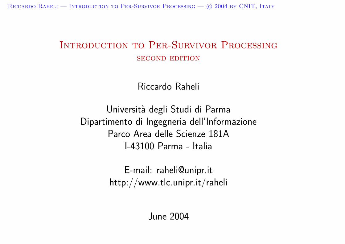
Riccardo Raheli — Introduction to Per-Survivor Processing — c© 2004 by CNIT, Italy
Introduction to Per-Survivor Processingsecond edition
Riccardo Raheli
Universita degli Studi di ParmaDipartimento di Ingegneria dell’Informazione
Parco Area delle Scienze 181AI-43100 Parma - Italia
E-mail: [email protected]://www.tlc.unipr.it/raheli
June 2004
Riccardo Raheli — Introduction to Per-Survivor Processing — c© 2004 by CNIT, Italy
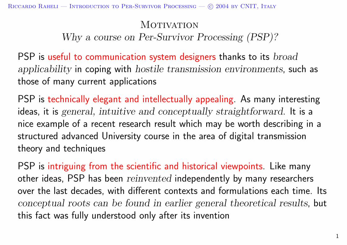
MotivationWhy a course on Per-Survivor Processing (PSP)?
PSP is useful to communication system designers thanks to its broadapplicability in coping with hostile transmission environments, such asthose of many current applications
PSP is technically elegant and intellectually appealing. As many interestingideas, it is general, intuitive and conceptually straightforward. It is anice example of a recent research result which may be worth describing in astructured advanced University course in the area of digital transmissiontheory and techniques
PSP is intriguing from the scientific and historical viewpoints. Like manyother ideas, PSP has been reinvented independently by many researchersover the last decades, with different contexts and formulations each time. Itsconceptual roots can be found in earlier general theoretical results, butthis fact was fully understood only after its invention
1

Riccardo Raheli — Introduction to Per-Survivor Processing — c© 2004 by CNIT, Italy
Foreword
Unfortunately, this course might be unclear (and likely will !)
Please, feel free to ask questions. Doing so you will help:∗
; Yourself understanding what is going on
→ Your colleagues understanding questions they had not even thought of
The instructor realizing what is unclear and should be better explained
You will also:
Avoid falling behind (if you do in the first lectures, you will hardlyrecover)
# Contribute to make the lectures more stimulating and pleasant
∗Arrows by LATEX and AMSLATEX
2
Riccardo Raheli — Introduction to Per-Survivor Processing — c© 2004 by CNIT, Italy
Outline
1. Review of detection techniques
2. Detection under parametric uncertainty
3. Per-Survivor Processing (PSP): concept and historical review
4. Classical applications of PSP
4.1 Complexity reduction
4.2 Linear predictive detection for fading channels
4.3 Adaptive detection
5. Advanced applications of PSP
Prerequisite: A course in Digital Transmission Theory
3
Riccardo Raheli — Introduction to Per-Survivor Processing — c© 2004 by CNIT, Italy
1. Review of detection techniques
Outline
1. Review of detection techniques
2. Detection under parametric uncertainty
3. Per-Survivor Processing (PSP): concept and historical review
4. Classical applications of PSP
4.1 Complexity reduction
4.2 Linear predictive detection for fading channels
4.3 Adaptive detection
5. Advanced applications of PSP
4
Riccardo Raheli — Introduction to Per-Survivor Processing — c© 2004 by CNIT, Italy
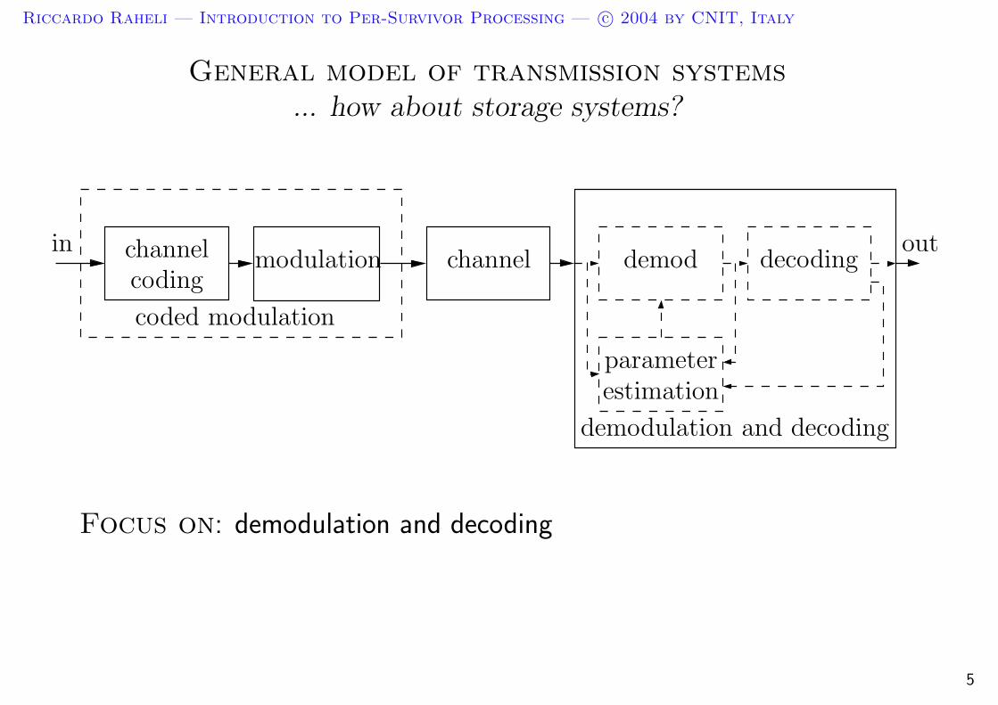
General model of transmission systems... how about storage systems?
coding
channel
parameter
estimation
coded modulation
channelmodulation demod decoding
demodulation and decoding
outin
Focus on: demodulation and decoding
5

Riccardo Raheli — Introduction to Per-Survivor Processing — c© 2004 by CNIT, Italy
Principal channel models
Additive White Gaussian Noise (AWGN) channel
Static dispersive channel
Flat fading channel
Dispersive fading channel
Phase uncertain channel
Like-signal (or cochannel) interference channel
Nonlinear channel
Transition noise channel
Combinations
6

Riccardo Raheli — Introduction to Per-Survivor Processing — c© 2004 by CNIT, Italy
AWGN channel
r(t) = s(t) + w(t)
w(t): circular complex AWGN
7
Riccardo Raheli — Introduction to Per-Survivor Processing — c© 2004 by CNIT, Italy
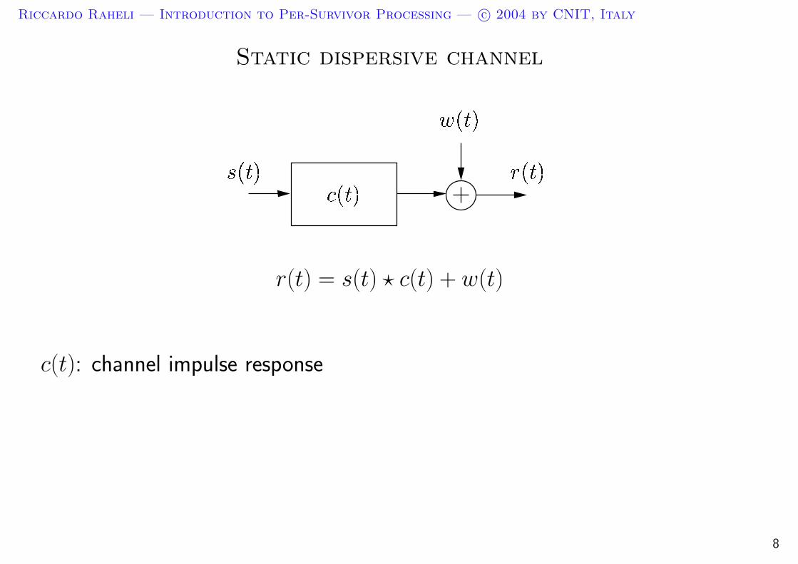
Static dispersive channel
r(t) = s(t) ? c(t) + w(t)
c(t): channel impulse response
8
Riccardo Raheli — Introduction to Per-Survivor Processing — c© 2004 by CNIT, Italy
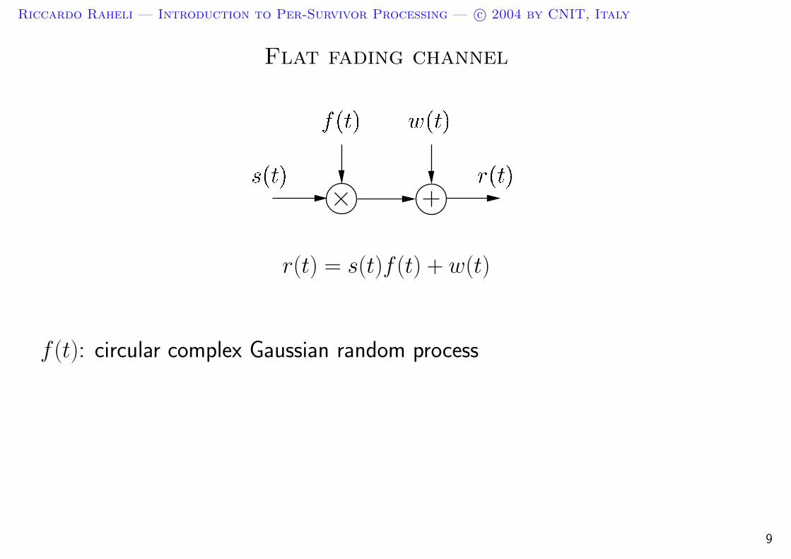
Flat fading channel
r(t) = s(t)f (t) + w(t)
f (t): circular complex Gaussian random process
9

Riccardo Raheli — Introduction to Per-Survivor Processing — c© 2004 by CNIT, Italy
Dispersive fading channel
∆τ1 ∆τ2
s(t)
f0(t) f1(t) f2(t)
r(t)
w(t)
r(t) =
L∑
l=0
fl(t)s(t − τl) + w(t) τl = τ0 +
l∑
i=1
∆τi
fl(t): independent circular complex Gaussian random processes
The l-th dominant propagation path has delay τl
10

Riccardo Raheli — Introduction to Per-Survivor Processing — c© 2004 by CNIT, Italy
Phase-uncertain channel
r(t) = s(t)ej[2πν(t)t+θ(t)] + w(t)
ν(t): frequency shift
θ(t): phase shift
Special cases:
– Phase noncoherent channel (ν(t) = 0, θ(t) = θ)
– Frequency offset (or Doppler shift) channel (ν(t) 6= 0, θ(t) = θ)
– Phase noisy channel (ν(t) = 0, θ(t) is a Wiener random process)
11

Riccardo Raheli — Introduction to Per-Survivor Processing — c© 2004 by CNIT, Italy
Principal channel modelsOverview
∆τ1 ∆τ2
s(t)
c(t)s(t) r(t)
w(t)
f0(t) f1(t) f2(t)
r(t)
w(t)r(t)s(t)
w(t)f(t)
w(t)
(a) (b)
(c) (d)
s(t) r(t)
s(t)
ej[2πν(t)t+θ(t)]
(e)
r(t)
w(t)
12
Riccardo Raheli — Introduction to Per-Survivor Processing — c© 2004 by CNIT, Italy
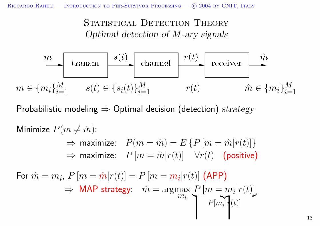
Statistical Detection TheoryOptimal detection of M -ary signals
m ∈ miMi=1 s(t) ∈ si(t)M
i=1 r(t) m ∈ miMi=1
Probabilistic modeling ⇒ Optimal decision (detection) strategy
Minimize P (m 6= m):
⇒ maximize: P (m = m) = E P [m = m|r(t)]⇒ maximize: P [m = m|r(t)] ∀r(t) (positive)
For m = mi, P [m = m|r(t)] = P [m = mi|r(t)] (APP)
⇒ MAP strategy: m = argmaxmi
P [m = mi|r(t)]︸ ︷︷ ︸P [mi|r(t)]
13

Riccardo Raheli — Introduction to Per-Survivor Processing — c© 2004 by CNIT, Italy
Statistical Detection TheoryComputation of the APPs
Discretization (finite dimensionality) ⇒ Sufficient statistic
APPs: P (mi|r) =p(r|mi)P (mi)
p(r)∼ p(r|mi)P (mi)
∼ : monotonic relationship with respect to the variable of interest
MAP strategy: m = argmaxmi
P (mi|r) = argmaxmi
p(r|mi)P (mi)
Statistical information:
P (mi) : information source
p(r|mi) : overall system (transmitter, channel, discretizer)
14
Riccardo Raheli — Introduction to Per-Survivor Processing — c© 2004 by CNIT, Italy
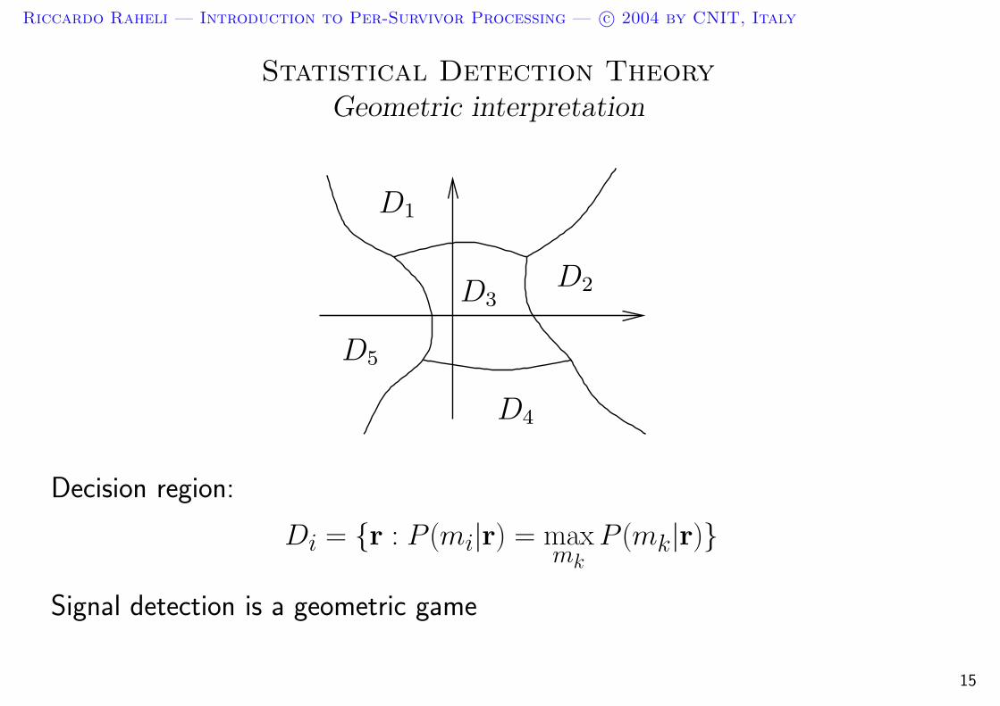
Statistical Detection TheoryGeometric interpretation
D5
D2D3
D1
D4
Decision region:
Di = r : P (mi|r) = maxmk
P (mk|r)
Signal detection is a geometric game
15

Riccardo Raheli — Introduction to Per-Survivor Processing — c© 2004 by CNIT, Italy
Statistical Detection TheorySpecial case: Strategy for the AWGN channel
Discretization: signal space spanned by si(t)Mi=1 is relevant:
rk =
∫ T
0r(t)ϕ∗
k(t)dt with ϕk(t)Qk=1 (basis)
m = mi ⇒ r(t) = si(t) + w(t) ⇒ r = si + w
APPs (but for a factor):
p(r|mi)P (mi) =1
(πσ2)Qexp
[− 1
σ2||r − si||2
]P (mi)
∼ −||r − si||2 + σ2 ln P (mi)
∼ Re(rTs∗i
)− 1
2||si||2 +
1
2σ2 ln P (mi)
= Re
[∫ T
0r(t)s∗i (t)dt
]− 1
2
∫ T
0|si(t)|2dt +
1
2σ2 ln P (mi)
16

Riccardo Raheli — Introduction to Per-Survivor Processing — c© 2004 by CNIT, Italy
Statistical Detection TheorySpecial case: Receiver for the AWGN channel
Re(·)
Re(·)
Re(·)
t = T
t = T
t = T
m
r(t)
s∗2(T − t)
s∗
1(T − t)
s∗M
(T−t)
C1
C2
CM
argmaxmi
......
...
...
Ci =1
2σ2 ln P (mi) −
1
2
∫ T
0|si(t)|2dt
si(t)Mi=1 and σ2 must be known (unless ML)
17

Riccardo Raheli — Introduction to Per-Survivor Processing — c© 2004 by CNIT, Italy
Statistical Detection TheorySpecial case: Decision regions for the AWGN channel
s1 s2 s3 s4
d
s5 s6 s7 s8
s9 s10 s11 s12
s13 s14 s15 s16
Decision regions are polytopes
2D example: 16QAM (quadrature amplitude modulation)
18
Riccardo Raheli — Introduction to Per-Survivor Processing — c© 2004 by CNIT, Italy
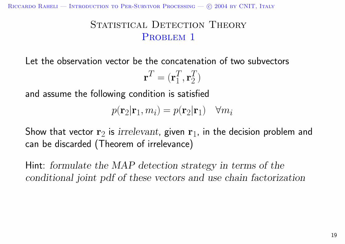
Statistical Detection TheoryProblem 1
Let the observation vector be the concatenation of two subvectors
rT = (rT1 , rT
2 )
and assume the following condition is satisfied
p(r2|r1,mi) = p(r2|r1) ∀mi
Show that vector r2 is irrelevant, given r1, in the decision problem andcan be discarded (Theorem of irrelevance)
Hint: formulate the MAP detection strategy in terms of theconditional joint pdf of these vectors and use chain factorization
19

Riccardo Raheli — Introduction to Per-Survivor Processing — c© 2004 by CNIT, Italy
Statistical Detection TheoryProblem 2
Consider an M -ary signaling scheme with signal set si(t)Mi=1
Assuming signal si(t) is sent, the received signal at the output of anAWGN phase noncoherent channel is
r(t) = si(t) ejθ + w(t)
where θ is uniformly distributed over 2π
A. Determine a discretization process of the received signal which provides asufficient statistic for MAP detection
Hint: Extend the results for the simple AWGN channel
B. Derive the non coherent MAP strategy
C. Give examples of signal sets suitable for non coherent detection
20

Riccardo Raheli — Introduction to Per-Survivor Processing — c© 2004 by CNIT, Italy
Review of detection techniquesBibliography
General references:
– J. G. Proakis, Digital Communications. New York: McGraw-Hill, 1989, 2nd ed..
– S. Benedetto, E. Biglieri and V. Castellani. Digital Transmission Theory. Prentice-Hall,Englewood Cliffs, U.S.A., 1987.
Fading and phase-uncertain channel models:
– G. L. Stuber, Principles of Mobile Communication, Kluwer Academic Publishers, 1996.
– U. Mengali and A. N. D’Andrea, Synchronization techniques for digital receivers. NewYork: Plenum, 1997.
Statistical detection theory:
– J. M. Wozencraft and I. M. Jacobs, Principles of Communication Engineering. NewYork: John Wiley & Sons, 1965.
– H. L. Van Trees, Detection, Estimation, and Modulation Theory, Part I. New York:John Wiley & Sons, 1968.
21

Riccardo Raheli — Introduction to Per-Survivor Processing — c© 2004 by CNIT, Italy
Systems with memoryWhere does this memory come from?
Any practical system transmits by periodical repetitions of M -ary signalingacts (log2 M bits/signaling period or bits/channel use)
In memoryless systems different signaling acts do not influence each other
In systems with memory the detection process may benefit from theobservation of the received signal over “present,” “past,” and possibly“future” signaling periods
Memory arises if (e.g.):
– Channel coding is employed for error control
– The transmission channel is dispersive (Inter-Symbol Interference (ISI))
– The transmission channel includes stochastic parameters, such as a phaserotation or a complex fading weight
– The channel additive Gaussian noise is colored, i.e., its power spectraldensity is not constant
22

Riccardo Raheli — Introduction to Per-Survivor Processing — c© 2004 by CNIT, Italy
Systems with memoryGeneral system model
Information sequence: a = aK−10 = (aK−1, . . . , a1, a0)
T
Transmitted signal: s(t, a)
Received signal: r(t) = x(t, a) + n(t)
Notation: xk2k1
= (xk2, . . . , xk1+1, xk1
)T
Detection strategy? (What is a message?)
23

Riccardo Raheli — Introduction to Per-Survivor Processing — c© 2004 by CNIT, Italy
Sequence and symbol detectionWhat is a message?
MAP sequence detection
a = argmaxa
P [a|r(t)] = argmaxa
P (a|r)
MAP symbol detection
ak = argmaxak
P [ak|r(t)] = argmaxak
P (ak|r)
r(t) is observed over the entire information bearing interval T0 ⊃ (0,KT )
Performance is similar and tends to be equal for high SNR
Complexity is different: sequence detection is less complex
Symbol APPs are the route to iterative detection
Discretization is the key to the computation of the APPs. One or morediscrete observables per information symbol may be used
24

Riccardo Raheli — Introduction to Per-Survivor Processing — c© 2004 by CNIT, Italy
Causal systemsThe viewpoint of detection
A system is causal if:p(rk
0 |a) = p(rk0 |ak
0)
This property involves the cascade of encoder, modulator, channel, and signaldiscretizer
It is formulated in terms of statistical dependence of the discrete observablesequence on the information sequence
Any physical system is causal
25
Riccardo Raheli — Introduction to Per-Survivor Processing — c© 2004 by CNIT, Italy
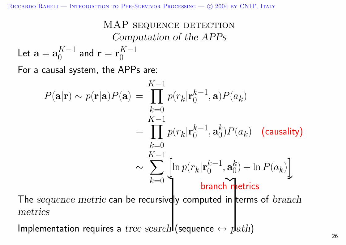
MAP sequence detectionComputation of the APPs
Let a = aK−10 and r = rK−1
0
For a causal system, the APPs are:
P (a|r) ∼ p(r|a)P (a) =
K−1∏
k=0
p(rk|rk−10 , a)P (ak)
=
K−1∏
k=0
p(rk|rk−10 , ak
0)P (ak) (causality)
∼K−1∑
k=0
[ln p(rk|rk−1
0 , ak0) + ln P (ak)
]
︸ ︷︷ ︸branch metrics
The sequence metric can be recursively computed in terms of branchmetrics
Implementation requires a tree search (sequence ↔ path)26

Riccardo Raheli — Introduction to Per-Survivor Processing — c© 2004 by CNIT, Italy
Path-search algorithmsOn a tree diagram
time →
An example of binary tree:
Branch metric:
ln p(rk|rk−1
0 , ak, ak−1
0 ) + ln P (ak)
ak = −1
ak = +1
Branch metrics depend on the entire previous path history:
⇒ unlimited memory (complexity is exponential with K)
Tree reduced-search (approximate) algorithms:
– M-algorithm, T-algorithm (breadth-first)
– Fano-algorithm (single-stack algorithm) (depth-first)
– Jelinek-algorithm (stack algorithm) (metric-first)
27

Riccardo Raheli — Introduction to Per-Survivor Processing — c© 2004 by CNIT, Italy
Finite-memory causal systemsThe viewpoint of detection
A system is causal and finite memory if:
p(rk|rk−10 , ak
0) = p(rk|rk−10 , ak
k−C, µk−C)
C is a suitable integer (finite memory parameter)
µk−C is a suitable state, at epoch k − C, of the encoder/modulator
In the computation of the APPs (or metrics), the system can be modeled as aFinite State Machine (FSM)
Minimal folding condition: the tree folds into a trellis diagram
Path search can be implemented efficiently
28
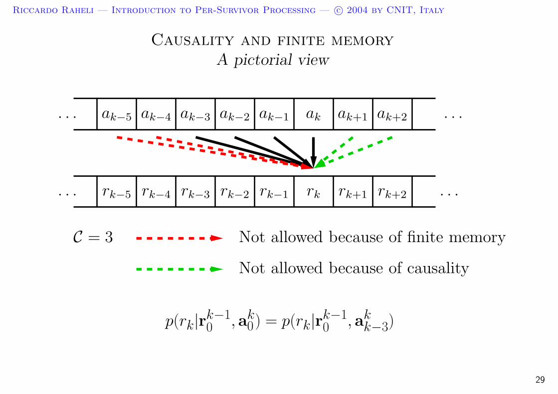
Riccardo Raheli — Introduction to Per-Survivor Processing — c© 2004 by CNIT, Italy
Causality and finite memoryA pictorial view
rk−3rk−4rk−5 rk−2 rk−1 rk+1rk rk+2
ak−3ak−4ak−5 ak−2 ak−1 ak+1ak ak+2 . . .
. . .
. . .
. . .
Not allowed because of finite memory
Not allowed because of causality
C = 3
p(rk|rk−10 , ak
0) = p(rk|rk−10 , ak
k−3)
29
Riccardo Raheli — Introduction to Per-Survivor Processing — c© 2004 by CNIT, Italy
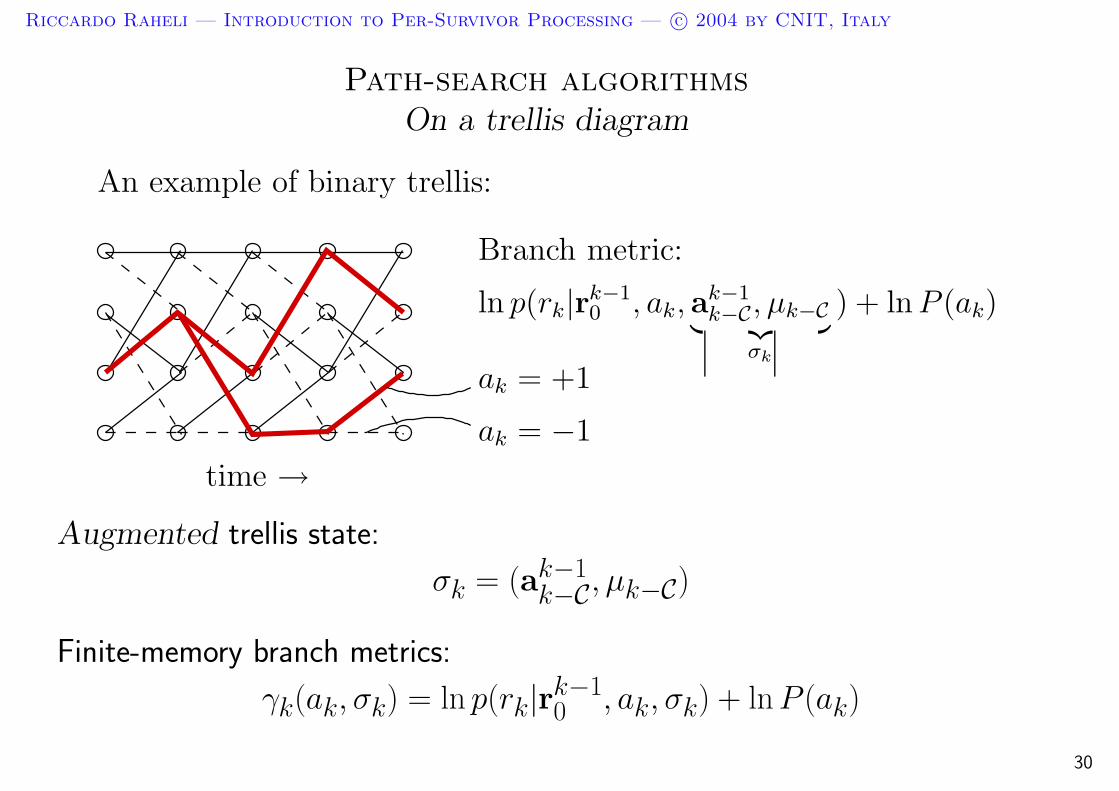
Path-search algorithmsOn a trellis diagram
time →
An example of binary trellis:
ak = +1
ln p(rk|rk−1
0 , ak, ak−1
k−C, µk−C
︸ ︷︷ ︸
σk
) + ln P (ak)
Branch metric:
ak = −1
Augmented trellis state:
σk = (ak−1k−C, µk−C)
Finite-memory branch metrics:
γk(ak, σk) = ln p(rk|rk−10 , ak, σk) + ln P (ak)
30

Riccardo Raheli — Introduction to Per-Survivor Processing — c© 2004 by CNIT, Italy
Viterbi algorithmBasic recursions
I Path metric:
Γk(σk) =
k∑
i=0
γi(ai, σi) =
k∑
i=0
[ln p(ri|ri−1
0 , ai, σi) + ln P (ai)]
I Path metric update step (Add-Compare-Select):
Γk+1(σk+1) = max(ak,σk):σk+1
[Γk(σk) + γk(ak, σk)]
I Survivor update step: the survivor of the maximizing state is extendedby the label ak of the winning branch
31

Riccardo Raheli — Introduction to Per-Survivor Processing — c© 2004 by CNIT, Italy
Viterbi algorithmAdd-Compare-Select: a pictorial view
ak = −1
ak = +1
survivors at k+1
k k+1k−1survivors at k
= max(ak ,σk):σk+1
[Γk(σk) + γk(ak, σk)]
Γk+1(σk+1)
Candidates:
32

Riccardo Raheli — Introduction to Per-Survivor Processing — c© 2004 by CNIT, Italy
MAP symbol detectionComputation of the APPs (1)
By (conditional) marginalization:
P (ak|r) =∑
ak−1k−C
∑
µk−C
P (ak, ak−1k−C︸ ︷︷ ︸
akk−C
, µk−C|r)
∼∑
ak−1k−C
∑
µk−C
p(r|akk−C, µk−C)P (ak
k−C, µk−C)
By (conditional) chain factorization:
p(r|akk−C, µk−C) = p(rk−1
0 , rk, rK−1k+1 |ak
k−C, µk−C)
= p(rK−1k+1 | rk−1
0 , rk︸ ︷︷ ︸rk0
, akk−C, µk−C) p(rk|rk−1
0 , akk−C, µk−C)
· p(rk−10 |ak
k−C, µk−C)
Three factors: future given the past and present, present given the past,and past, respectively
33
Riccardo Raheli — Introduction to Per-Survivor Processing — c© 2004 by CNIT, Italy
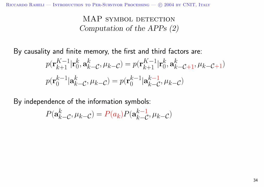
MAP symbol detectionComputation of the APPs (2)
By causality and finite memory, the first and third factors are:
p(rK−1k+1 |rk
0 , akk−C, µk−C) = p(rK−1
k+1 |rk0 , a
kk−C+1, µk−C+1)
p(rk−10 |ak
k−C, µk−C) = p(rk−10 |ak−1
k−C, µk−C)
By independence of the information symbols:
P (akk−C, µk−C) = P (ak)P (ak−1
k−C, µk−C)
34
Riccardo Raheli — Introduction to Per-Survivor Processing — c© 2004 by CNIT, Italy
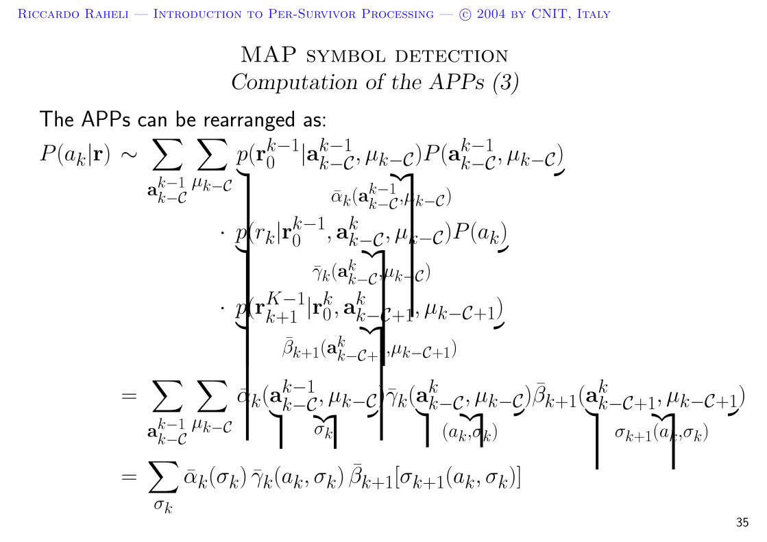
MAP symbol detectionComputation of the APPs (3)
The APPs can be rearranged as:
P (ak|r) ∼∑
ak−1k−C
∑
µk−C
p(rk−10 |ak−1
k−C, µk−C)P (ak−1k−C, µk−C)︸ ︷︷ ︸
αk(ak−1k−C,µk−C)
· p(rk|rk−10 , ak
k−C, µk−C)P (ak)︸ ︷︷ ︸γk(ak
k−C,µk−C)
· p(rK−1k+1 |rk
0 , akk−C+1, µk−C+1)︸ ︷︷ ︸
βk+1(akk−C+1,µk−C+1)
=∑
ak−1k−C
∑
µk−C
αk(ak−1k−C, µk−C︸ ︷︷ ︸
σk
)γk(akk−C, µk−C︸ ︷︷ ︸
(ak,σk)
)βk+1(akk−C+1, µk−C+1︸ ︷︷ ︸
σk+1(ak,σk)
)
=∑
σk
αk(σk) γk(ak, σk) βk+1[σk+1(ak, σk)]
35
Riccardo Raheli — Introduction to Per-Survivor Processing — c© 2004 by CNIT, Italy
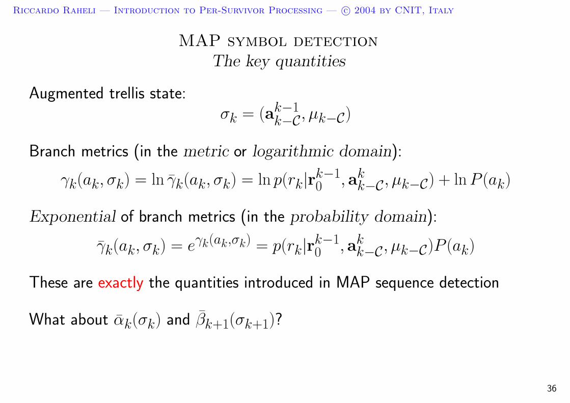
MAP symbol detectionThe key quantities
Augmented trellis state:σk = (ak−1
k−C, µk−C)
Branch metrics (in the metric or logarithmic domain):
γk(ak, σk) = ln γk(ak, σk) = ln p(rk|rk−10 , ak
k−C, µk−C) + ln P (ak)
Exponential of branch metrics (in the probability domain):
γk(ak, σk) = eγk(ak,σk) = p(rk|rk−10 , ak
k−C, µk−C)P (ak)
These are exactly the quantities introduced in MAP sequence detection
What about αk(σk) and βk+1(σk+1)?
36

Riccardo Raheli — Introduction to Per-Survivor Processing — c© 2004 by CNIT, Italy
MAP symbol detectionForward recursion
By averaging, chain factorization, and causality:
αk+1(σk+1) = p(rk0 |ak
k−C+1, µk−C+1)P (akk−C+1, µk−C+1)
=∑
(ak−C,µk−C):σk+1
p(rk0 |ak
k−C, µk−C)P (akk−C, µk−C)
=∑
(ak−C,µk−C):σk+1
p(rk|rk−10 , ak
k−C, µk−C)P (ak)︸ ︷︷ ︸γk(ak,σk)
· p(rk−10 |ak
k−C, µk−C)︸ ︷︷ ︸p(rk−1
0 |ak−1k−C,µk−C)
P (ak−1k−C, µk−C)
︸ ︷︷ ︸αk(σk)
=∑
(ak,σk):σk+1
γk(ak, σk) αk(σk)
37

Riccardo Raheli — Introduction to Per-Survivor Processing — c© 2004 by CNIT, Italy
MAP symbol detectionBackward recursion
By averaging, independence of the information symbols, chain factorization,and finite memory:
βk(σk) = p(rK−1k |rk−1
0 , ak−1k−C, µk−C)
=∑
ak
p(rK−1k |rk−1
0 , akk−C, µk−C) P (ak|rk−1
0 , ak−1k−C, µk−C)︸ ︷︷ ︸
P (ak)
=∑
ak
p(rK−1k+1 |rk
0 , akk−C, µk−C)︸ ︷︷ ︸
p(rK−1k+1 |rk
0 ,akk−C+1,µk−C+1)︸ ︷︷ ︸
βk+1[σk+1(ak,σk)]
p(rk|rk−10 , ak
k−C, µk−C)P (ak)︸ ︷︷ ︸γk(ak,σk)
=∑
ak
βk+1[σk+1(ak, σk)] γk(ak, σk)
38
Riccardo Raheli — Introduction to Per-Survivor Processing — c© 2004 by CNIT, Italy
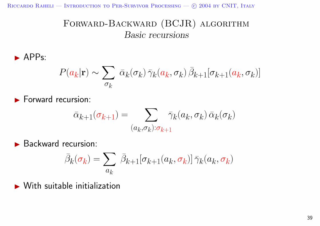
Forward-Backward (BCJR) algorithmBasic recursions
I APPs:
P (ak|r) ∼∑
σk
αk(σk) γk(ak, σk) βk+1[σk+1(ak, σk)]
I Forward recursion:
αk+1(σk+1) =∑
(ak,σk):σk+1
γk(ak, σk) αk(σk)
I Backward recursion:
βk(σk) =∑
ak
βk+1[σk+1(ak, σk)] γk(ak, σk)
I With suitable initialization
39
Riccardo Raheli — Introduction to Per-Survivor Processing — c© 2004 by CNIT, Italy
MAP symbol detectionComparison with MAP sequence detection
Processing the “exponential metrics” γk(ak, σk) in the FSM trellis diagram issufficient (again!)
Sum-product algorithm (complexity is much larger than Viterbi)
The entire observation rK−10 must be processed before the APPs can be
computed
Block processing (or approximations): latency delay
40
Riccardo Raheli — Introduction to Per-Survivor Processing — c© 2004 by CNIT, Italy
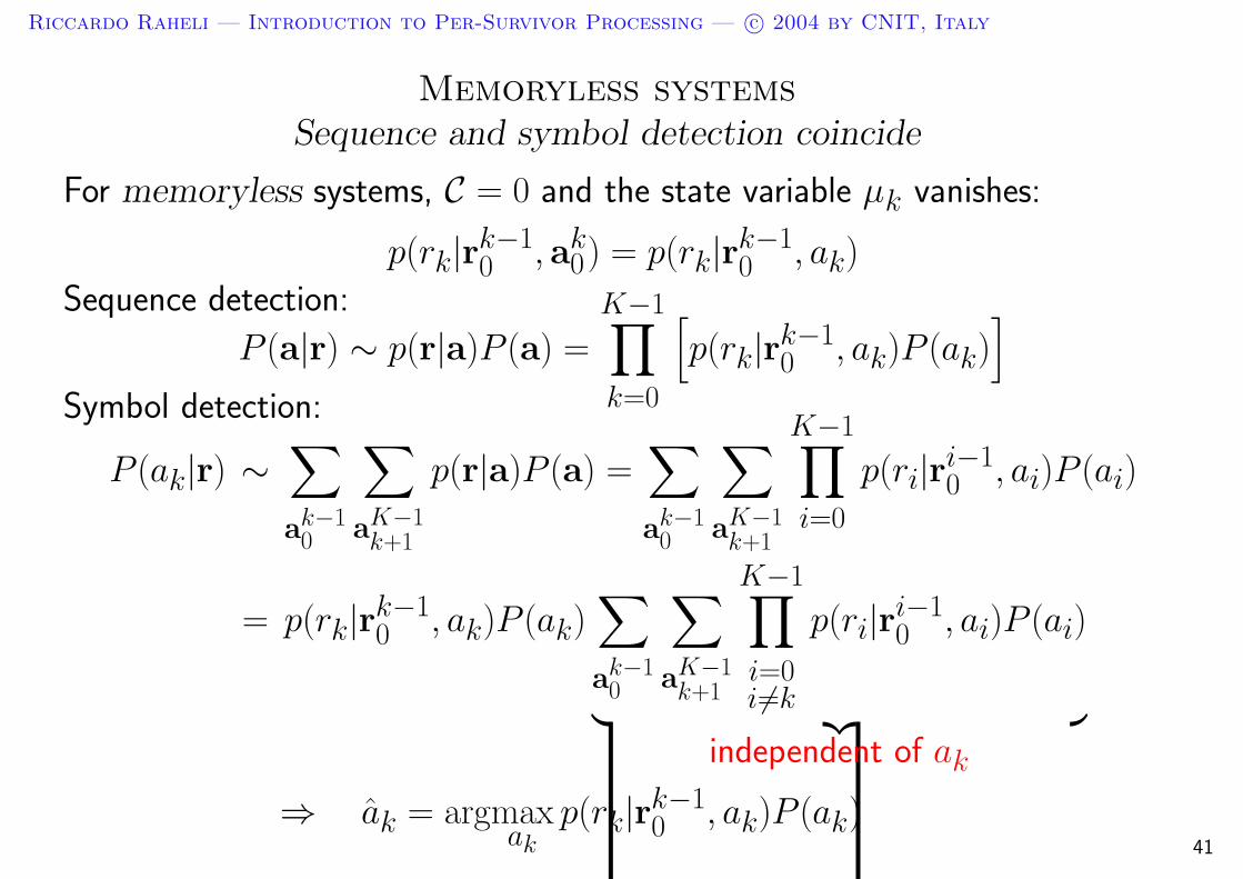
Memoryless systemsSequence and symbol detection coincide
For memoryless systems, C = 0 and the state variable µk vanishes:
p(rk|rk−10 , ak
0) = p(rk|rk−10 , ak)
Sequence detection:
P (a|r) ∼ p(r|a)P (a) =
K−1∏
k=0
[p(rk|rk−1
0 , ak)P (ak)]
Symbol detection:
P (ak|r) ∼∑
ak−10
∑
aK−1k+1
p(r|a)P (a) =∑
ak−10
∑
aK−1k+1
K−1∏
i=0
p(ri|ri−10 , ai)P (ai)
= p(rk|rk−10 , ak)P (ak)
∑
ak−10
∑
aK−1k+1
K−1∏
i=0i6=k
p(ri|ri−10 , ai)P (ai)
︸ ︷︷ ︸independent of ak
⇒ ak = argmaxak
p(rk|rk−10 , ak)P (ak)
41

Riccardo Raheli — Introduction to Per-Survivor Processing — c© 2004 by CNIT, Italy
Forward-Backward (BCJR) algorithmMax-log-MAP approximation: APPs
We could equivalently formulate the algorithm in the logarithmic (or metric)domain:
ln P (ak|r) ∼ ln∑
σk
αk(σk) γk(ak, σk) βk+1[σk+1(ak, σk)]
= ln∑
σk
eαk(σk)+γk(ak,σk)+βk+1[σk+1(ak,σk)]
' maxσk
αk(σk) + γk(ak, σk) + βk+1[σk+1(ak, σk)]
where αk(σk) = ln αk(σk) and βk+1(σk+1) = ln βk+1(σk+1)
For large |x − y| ⇒ ln(ex + ey) ' max(x, y) and by extension:
ln(ex1 + ex2 + · · · + exn) ' max(x1, x2, . . . , xn)
42

Riccardo Raheli — Introduction to Per-Survivor Processing — c© 2004 by CNIT, Italy
Forward-Backward (BCJR) algorithmMax-log-MAP approximation: FB recursions
αk+1(σk+1) = ln αk+1(σk+1) = ln∑
(ak,σk):σk+1
γk(ak, σk) αk(σk)
' max(ak,σk):σk+1
[γk(ak, σk) + αk(σk)]
βk(σk) = ln βk(σk) = ln∑
ak
βk+1[σk+1(ak, σk)] γk(ak, σk)
' maxak
βk+1[σk+1(ak, σk)] + γk(ak, σk)
43
Riccardo Raheli — Introduction to Per-Survivor Processing — c© 2004 by CNIT, Italy
Forward-Backward (BCJR) algorithmMax-log-MAP approximation: key features
Forward and backward recursions can be implemented by two Viterbialgorithms running in direct and inverse time
αk(σk) and βk(σk) can be interpreted as forward and backward survivormetrics
The max-log-MAP algorithm is computationally efficient, at the cost of aslight degradation in performance
Various degrees of approximations have been studied (intermediate betweenthe “full-complexity” forward-backward algorithm and the max-log-MAPapproximation)
44

Riccardo Raheli — Introduction to Per-Survivor Processing — c© 2004 by CNIT, Italy
Forward-Backward (BCJR) algorithmMax-log-MAP approximation: a pictorial view
Forward survivor metrics αk(σk) = ln αk(σk)
Backward survivor metrics βk+1(σk+1) = ln βk+1(σk+1)
maxσk
αk(σk) + γk(ak, σk) + βk+1[σk+1(ak, σk)]∣
∣
∣
ak=+1
maxσk
αk(σk) + γk(ak, σk) + βk+1[σk+1(ak, σk)]∣
∣
∣
ak=−1
k k+1
45

Riccardo Raheli — Introduction to Per-Survivor Processing — c© 2004 by CNIT, Italy
Summary of MAP detection
I For causal finite-memory systems:
p(rk|rk−10 , ak
0) = p(rk|rk−10 , ak, σk)
I In the computation of the APPs, the system can be modeled as a FiniteState Machine (FSM) with state σk. The underlying FSM model isidentical for sequence and symbol detection
I Branch metrics (our focus in the following):
γk(ak, σk) = ln p(rk|rk−10 , ak, σk) + ln P (ak)
I MAP sequence detection can be implemented efficiently by the Viterbialgorithm
I MAP symbol detection can be implemented by a sum-productforward-backward algorithm (complex)
I The max-log-MAP approximation of the forward-backward algorithm canbe implemented efficiently by means of two Viterbi algorithms running indirect and inverse time
46

Riccardo Raheli — Introduction to Per-Survivor Processing — c© 2004 by CNIT, Italy
MAP sequence and symbol detectionProblem 3
Assuming a system is causal and finite memory:
A. Work out the derivation of the Viterbi algorithm for MAP sequencedetection
B. Work out the derivation of the forward-backward algorithm for MAPsymbol detection
Rederive the main recursions in each case
47
Riccardo Raheli — Introduction to Per-Survivor Processing — c© 2004 by CNIT, Italy
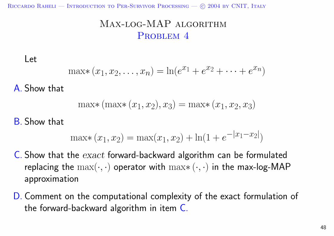
Max-log-MAP algorithmProblem 4
Letmax∗ (x1, x2, . . . , xn) = ln(ex1 + ex2 + · · · + exn)
A. Show that
max∗ (max∗ (x1, x2), x3) = max∗ (x1, x2, x3)
B. Show that
max∗ (x1, x2) = max(x1, x2) + ln(1 + e−|x1−x2|)
C. Show that the exact forward-backward algorithm can be formulatedreplacing the max(·, ·) operator with max∗ (·, ·) in the max-log-MAPapproximation
D. Comment on the computational complexity of the exact formulation ofthe forward-backward algorithm in item C.
48

Riccardo Raheli — Introduction to Per-Survivor Processing — c© 2004 by CNIT, Italy
MAP detection for systems with memoryExamples of application
Linear modulation on static dispersive channel
Linear modulation on flat fading channel
49
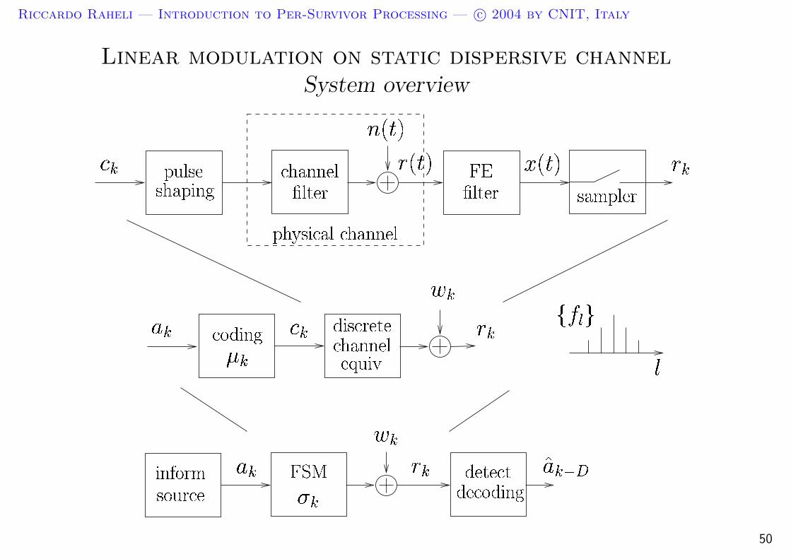
Riccardo Raheli — Introduction to Per-Survivor Processing — c© 2004 by CNIT, Italy
Linear modulation on static dispersive channelSystem overview
! " #
$ %&
' (
# #
! ) (
) ! * # "
) + !
* # "$,
! - ) "
!' "
. ' " - ' (
/
50
Riccardo Raheli — Introduction to Per-Survivor Processing — c© 2004 by CNIT, Italy
Linear modulation on static dispersive channelSystem model
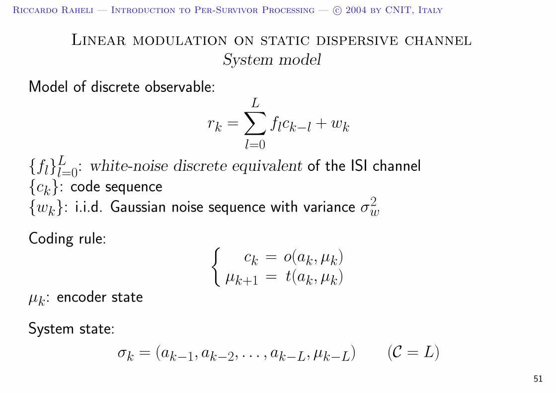
Model of discrete observable:
rk =
L∑
l=0
flck−l + wk
flLl=0: white-noise discrete equivalent of the ISI channel
ck: code sequence
wk: i.i.d. Gaussian noise sequence with variance σ2w
Coding rule: ck = o(ak, µk)
µk+1 = t(ak, µk)
µk: encoder state
System state:
σk = (ak−1, ak−2, . . . , ak−L, µk−L) (C = L)
51

Riccardo Raheli — Introduction to Per-Survivor Processing — c© 2004 by CNIT, Italy
Linear modulation on static dispersive channelComputation of the branch metrics
Conditional statistics of the observation:
p(rk|rk−10 , ak
0) = p(rk|ak0) (conditionally independent observations)
= p(rk|ak, σk) =1
πσ2w
exp
[− |rk − xk(ak, σk)|2
σ2w
]
xk(ak, σk) =
L∑
l=0
flck−l
Branch metrics:
γk(ak, σk) = ln p(rk|ak, σk) + ln P (ak)
∝ −|rk − xk(ak, σk)|2 + σ2w ln P (ak)
∝ Re[rkx
∗k(ak, σk)
]− 1
2|xk(ak, σk)|2 +
1
2σ2
w ln P (ak)
∝ : proportionality plus a constant term52
Riccardo Raheli — Introduction to Per-Survivor Processing — c© 2004 by CNIT, Italy
Linear modulation on static dispersive channelProblem 5
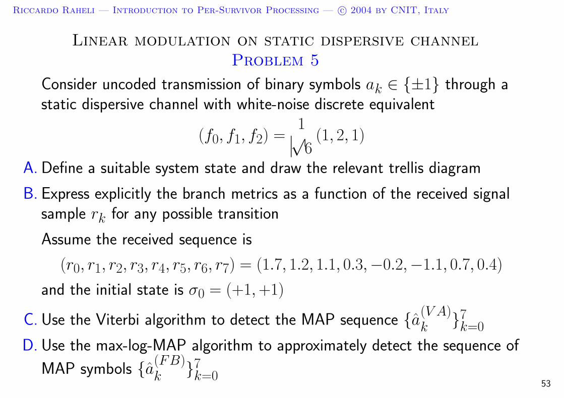
Consider uncoded transmission of binary symbols ak ∈ ±1 through astatic dispersive channel with white-noise discrete equivalent
(f0, f1, f2) =1√6
(1, 2, 1)
A. Define a suitable system state and draw the relevant trellis diagram
B. Express explicitly the branch metrics as a function of the received signalsample rk for any possible transition
Assume the received sequence is
(r0, r1, r2, r3, r4, r5, r6, r7) = (1.7, 1.2, 1.1, 0.3,−0.2,−1.1, 0.7, 0.4)
and the initial state is σ0 = (+1, +1)
C. Use the Viterbi algorithm to detect the MAP sequence a(V A)k 7
k=0
D. Use the max-log-MAP algorithm to approximately detect the sequence of
MAP symbols a(FB)k 7
k=053

Riccardo Raheli — Introduction to Per-Survivor Processing — c© 2004 by CNIT, Italy
Linear modulation on flat fading channelSystem overview
! "
Discretization provides a sufficient statistic if f (t) is constant (i.e., a randomvariable). It is a good approximation if f (t) varies very slowly (small Dopplerbandwidth)
In general, one sample per signaling interval is not sufficient. Oversampling,e.g., two (or more) samples per symbol, provides a sufficient statistic
54

Riccardo Raheli — Introduction to Per-Survivor Processing — c© 2004 by CNIT, Italy
Linear modulation on flat fading channelSystem model
Model of discrete observable:
rk = fk ck + wk
fk: circular complex Gaussian random sequence
ck: code sequence
wk: i.i.d. Gaussian noise sequence with variance σ2w
Coding rule: ck = o(ak, µk)
µk+1 = t(ak, µk)
µk: encoder state
Conditional statistics of the observation are Gaussian
55
Riccardo Raheli — Introduction to Per-Survivor Processing — c© 2004 by CNIT, Italy
Linear modulation on flat fading channelDoes a FSM model hold? (1)
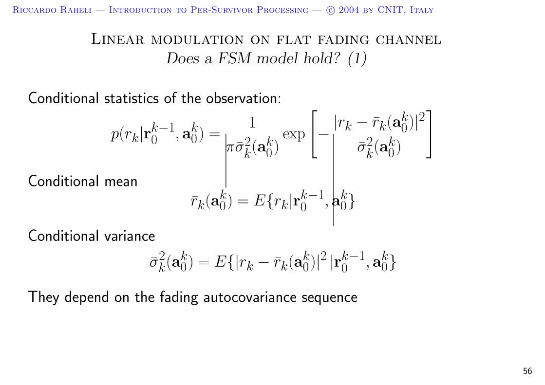
Conditional statistics of the observation:
p(rk|rk−10 , ak
0) =1
πσ2k(ak
0)exp
[− |rk − rk(ak
0)|2
σ2k(ak
0)
]
Conditional meanrk(ak
0) = Erk|rk−10 , ak
0
Conditional variance
σ2k(ak
0) = E|rk − rk(ak0)|2 |rk−1
0 , ak0
They depend on the fading autocovariance sequence
56

Riccardo Raheli — Introduction to Per-Survivor Processing — c© 2004 by CNIT, Italy
Linear modulation on flat fading channelDoes a FSM model hold? (2)
For Gaussian random variables, the conditional mean (i.e., the mean squareestimate) is linear in the observation
rk(ak0) = Erk|rk−1
0 , ak0 =
k∑
i=1
pi(ak0) rk−i ' ck
k∑
i=1
p′irk−i
ck−i
The sequence-dependent linear prediction coefficients of the observation attime k can be approximated as
pi(ak0) ' ck
p′ick−i
for high SNR
where p′iki=1 are the linear prediction coefficients of the fading process
Efk|fk−10 =
k∑
i=1
p′ifk−i
The conditional mean depends on all the previous code symbols:
⇒ unlimited memory57
Riccardo Raheli — Introduction to Per-Survivor Processing — c© 2004 by CNIT, Italy
Linear modulation on flat fading channelSpecial case: slow fading
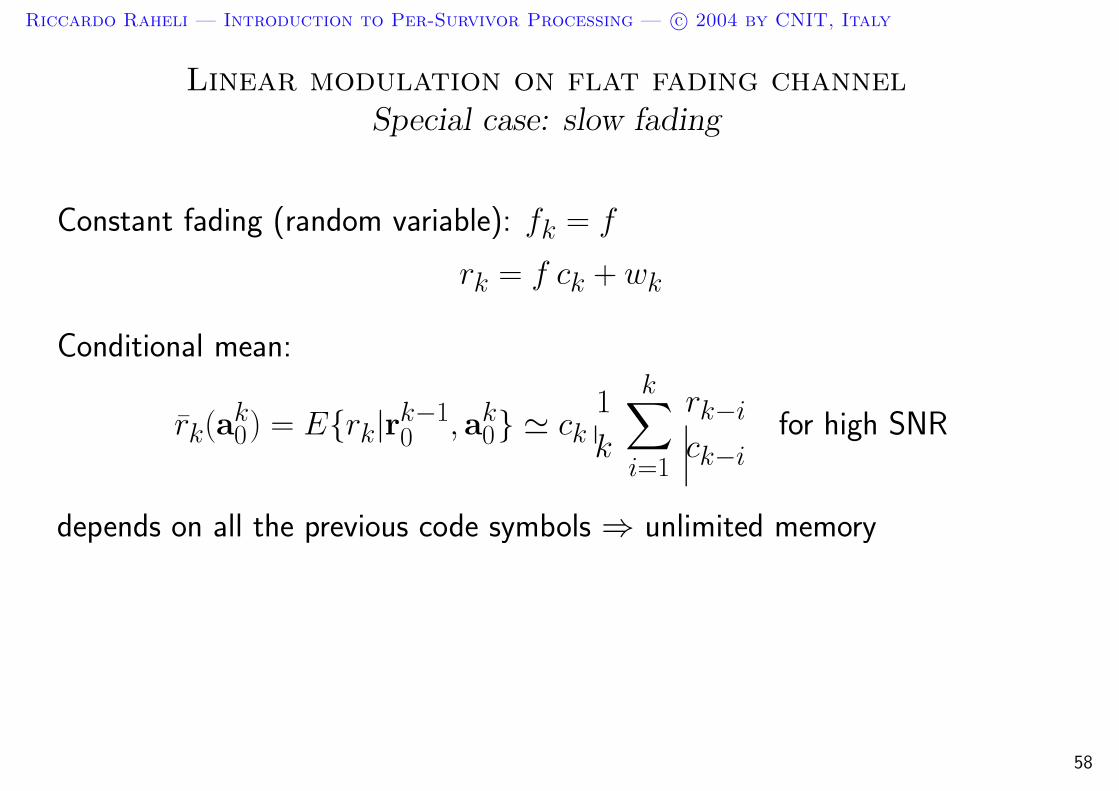
Constant fading (random variable): fk = f
rk = f ck + wk
Conditional mean:
rk(ak0) = Erk|rk−1
0 , ak0 ' ck
1
k
k∑
i=1
rk−i
ck−ifor high SNR
depends on all the previous code symbols ⇒ unlimited memory
58

Riccardo Raheli — Introduction to Per-Survivor Processing — c© 2004 by CNIT, Italy
Linear modulation on static dispersive channelProblem 6
Consider the flat fading model
rk = fk ck + wk
with negligible noise power σ2w ' 0
A. Show that the linear prediction coefficients of the observation and fadingprocesses are related by
pi(ak0) ' ck
p′ick−i
i = 1, 2, . . . , k
B. Show that for slow (constant) fading
p′i '1
k
Hint: Use the fading model in the conditional mean
59

Riccardo Raheli — Introduction to Per-Survivor Processing — c© 2004 by CNIT, Italy
Review of detection techniquesBibliography
MAP sequence and symbol detection:
– G. D. Forney, “Maximum-likelihood sequence estimation of digital sequences in thepresence of intersymbol interference,” IEEE Trans. Inform. Theory, pp. 363–378,May 1972.
– L. R. Bahl, J. Cocke, F. Jelinek, and R. Raviv, “Optimal decoding of linear codes forminimizing symbol error rate,” IEEE Trans. Inform. Theory,, pp. 284-284, March 1974.
– J. G. Proakis, Digital Communications. New York: McGraw-Hill, 1989, 2nd ed..
– S. Benedetto, E. Biglieri and V. Castellani. Digital Transmission Theory. Prentice-Hall,Englewood Cliffs, U.S.A., 1987.
– K. M. Chugg, A. Anastasopoulos, X. Chen, Iterative Detection: Adaptivity,Complexity Reduction, and Applications. Kluwer Academic Publishers, 2001.
– G. Ferrari, G. Colavolpe, R. Raheli, Detection Algorithms for WirelessCommunications, with Applications to Wired and Storage Systems, John Wiley &Sons, London, (August) 2004.
– G. Ferrari, G. Colavolpe, R. Raheli, “A unified framework for finite-memory detection,”March 2004.
60

Riccardo Raheli — Introduction to Per-Survivor Processing — c© 2004 by CNIT, Italy
2. Detection under parametric uncertainty
Outline
1. Review of detection techniques
2. Detection under parametric uncertainty
3. Per-Survivor Processing (PSP): concept and historical review
4. Classical applications of PSP:
4.1 Complexity reduction
4.2 Linear predictive detection for fading channels
4.3 Adaptive detection
5. Advanced applications of PSP
61
Riccardo Raheli — Introduction to Per-Survivor Processing — c© 2004 by CNIT, Italy
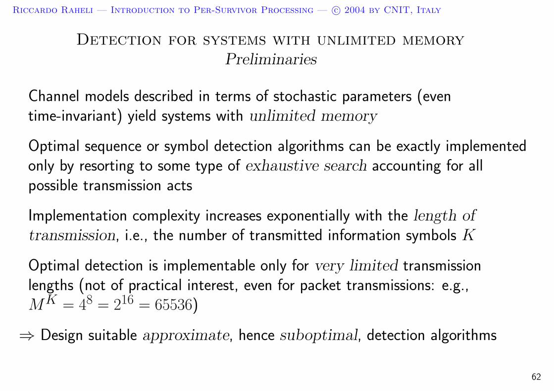
Detection for systems with unlimited memoryPreliminaries
Channel models described in terms of stochastic parameters (eventime-invariant) yield systems with unlimited memory
Optimal sequence or symbol detection algorithms can be exactly implementedonly by resorting to some type of exhaustive search accounting for allpossible transmission acts
Implementation complexity increases exponentially with the length oftransmission, i.e., the number of transmitted information symbols K
Optimal detection is implementable only for very limited transmissionlengths (not of practical interest, even for packet transmissions: e.g.,MK = 48 = 216 = 65536)
⇒ Design suitable approximate, hence suboptimal, detection algorithms
62

Riccardo Raheli — Introduction to Per-Survivor Processing — c© 2004 by CNIT, Italy
Estimation-Detection decompositionA suboptimal solution
Idea of “decomposing” the functions of data detection and parameterestimation:
1. Derive the detection algorithms under the assumption of knowledge, to acertain degree of accuracy, of some (channel) parameters
2. Devise an estimation algorithm for extracting information about theseparameters
This approach is viable alternative if a statistical characterization of theparameter is not available or not usable because of constrainedimplementation complexity
A statistical characterization is not available if static (or slow varying)parameters are modeled as unknown deterministic quantities
63

Riccardo Raheli — Introduction to Per-Survivor Processing — c© 2004 by CNIT, Italy
Estimation-Detection decompositionSystem model
θk denotes an estimate of a parameter vector θk, at the k-th time-discreteinstant
The estimation process observes explicitly the received signal r(t) andpossibly the detected data sequence a
64
Riccardo Raheli — Introduction to Per-Survivor Processing — c© 2004 by CNIT, Italy
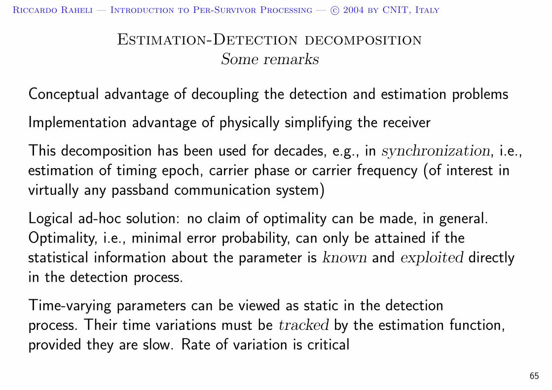
Estimation-Detection decompositionSome remarks
Conceptual advantage of decoupling the detection and estimation problems
Implementation advantage of physically simplifying the receiver
This decomposition has been used for decades, e.g., in synchronization, i.e.,estimation of timing epoch, carrier phase or carrier frequency (of interest invirtually any passband communication system)
Logical ad-hoc solution: no claim of optimality can be made, in general.Optimality, i.e., minimal error probability, can only be attained if thestatistical information about the parameter is known and exploited directlyin the detection process.
Time-varying parameters can be viewed as static in the detectionprocess. Their time variations must be tracked by the estimation function,provided they are slow. Rate of variation is critical
65
Riccardo Raheli — Introduction to Per-Survivor Processing — c© 2004 by CNIT, Italy
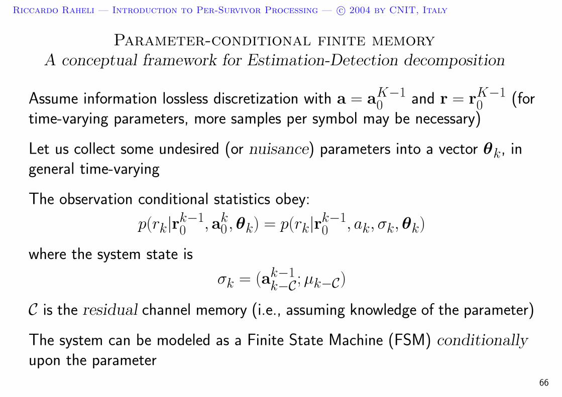
Parameter-conditional finite memoryA conceptual framework for Estimation-Detection decomposition
Assume information lossless discretization with a = aK−10 and r = rK−1
0 (fortime-varying parameters, more samples per symbol may be necessary)
Let us collect some undesired (or nuisance) parameters into a vector θk, ingeneral time-varying
The observation conditional statistics obey:
p(rk|rk−10 , ak
0 ,θk) = p(rk|rk−10 , ak, σk,θk)
where the system state is
σk = (ak−1k−C; µk−C)
C is the residual channel memory (i.e., assuming knowledge of the parameter)
The system can be modeled as a Finite State Machine (FSM) conditionallyupon the parameter
66

Riccardo Raheli — Introduction to Per-Survivor Processing — c© 2004 by CNIT, Italy
Parameter-conditional finite memoryAn example: Linear modulation on flat fading channel
Model of discrete observable:
rk = fk ck + wk
fk: circular complex Gaussian random sequence
ck: code sequence
wk: i.i.d. Gaussian noise sequence with variance σ2w
The system is not finite memory
⇒ Viewing fk as a nuisance parameter:
p(rk|rk−10 , ak
0 , fk) = p(rk|ck, fk) =1
πσ2w
exp
[− |rk − fkck|2
σ2w
]
The system is conditionally finite memory because the code symbols are theoutput of a finite state machine
For an uncoded system (ck = ak), the observation is conditionally memoryless
67

Riccardo Raheli — Introduction to Per-Survivor Processing — c© 2004 by CNIT, Italy
Parameter-conditional finite memorySome remarks
I By a clever choice of the nuisance parameters, it is possible to transformthe transmission system into conditionally finite-memory.
I This property holds conditionally on the undesired parameters; hence,only if they are known. It is the route to a decomposedestimation-detection design
I One can assume that some undesired parameters are known in devisingthe detection algorithms, thus avoiding intractable complexity, and devotesome implementation complexity to the estimation of these undesiredparameters.
I The parameter-conditional finite memory property suggests to view thepresence of stochastic or unknown deterministic parameters asparametric uncertainty affecting the detection problem.
68

Riccardo Raheli — Introduction to Per-Survivor Processing — c© 2004 by CNIT, Italy
Parameter estimationThe “dual” problem
The parameter estimation problem can be viewed as the “dual” of thedetection problem.
The “undesired” parameters become parameters of interest, whereas the“parameters” of interest in the detection process, namely the data symbols,are now just nuisance (or undesired) parameters.
Like the knowledge of the undesired parameters simplifies the detectionproblem, the possible knowledge of the data sequence may facilitate theestimation of the nuisance parameters.
An exact knowledge of the data symbols may reduce the “degree ofrandomness” of the received signal and facilitate the estimation of theparameters of interest
69

Riccardo Raheli — Introduction to Per-Survivor Processing — c© 2004 by CNIT, Italy
Parameter estimationData-aided parameter estimation
In coded systems the transmitted signal is modulated by the code sequence:knowledge of this sequence may be helpful in parameter estimation
We assume the code sequence is a data sequence aiding the parameterestimation process.
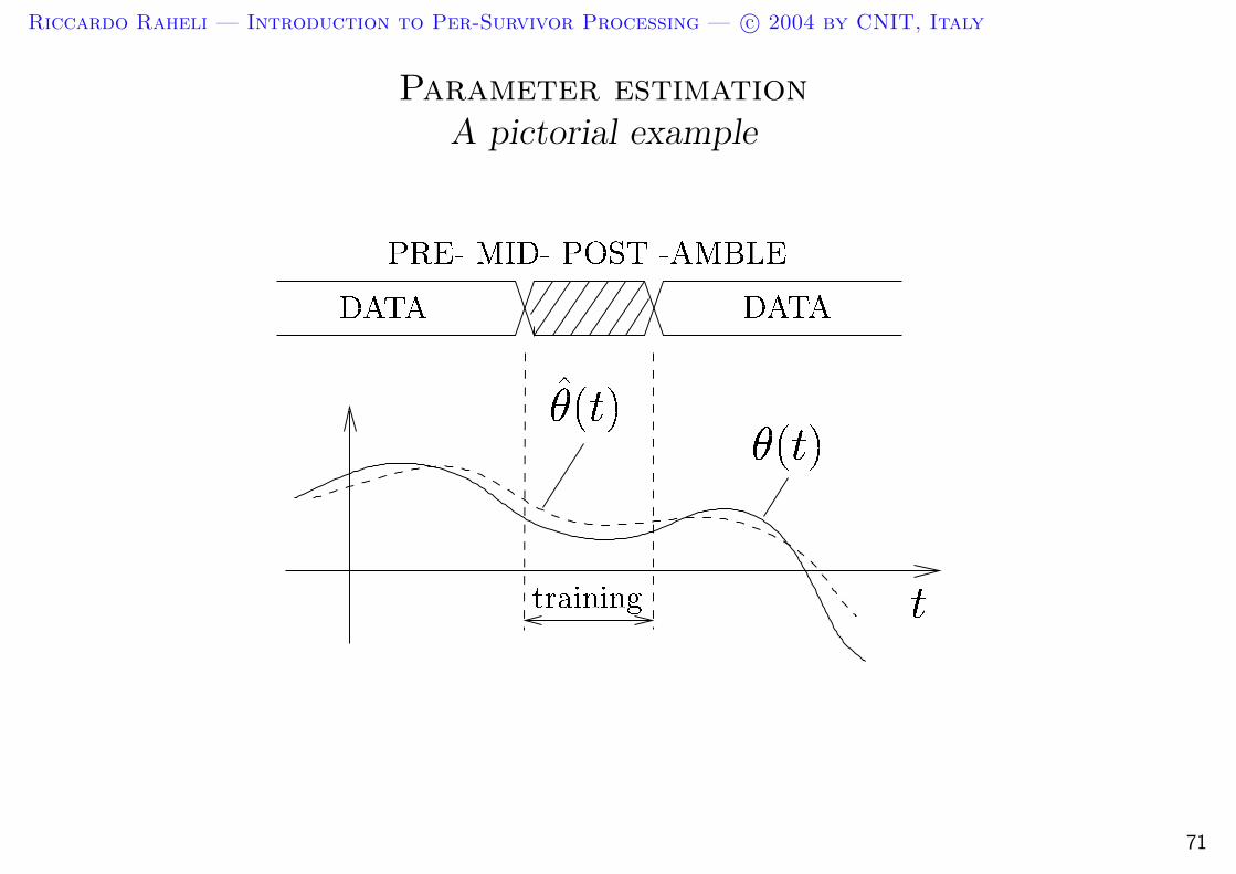
The data sequence is known during the (initial) training mode: preamble,midamble, postamble
During the transmission of the training sequence there is no transfer ofinformation: training must be limited
In long term tracking of the channel parameters, detected data can be used:decision-directed estimation
Non-data-aided estimation is more complex: requires averaging over thedata
70
Riccardo Raheli — Introduction to Per-Survivor Processing — c© 2004 by CNIT, Italy
Parameter estimationA pictorial example
71
Riccardo Raheli — Introduction to Per-Survivor Processing — c© 2004 by CNIT, Italy
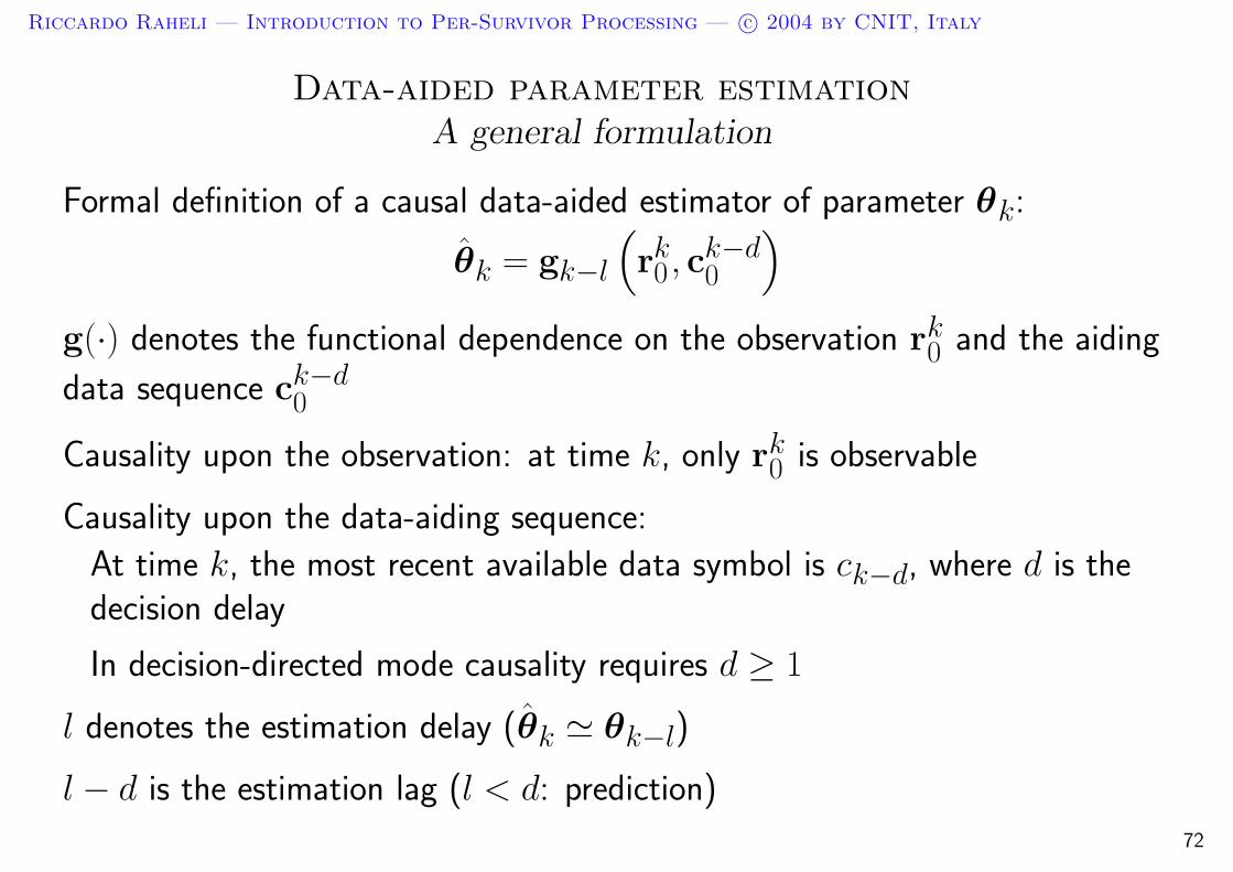
Data-aided parameter estimationA general formulation
Formal definition of a causal data-aided estimator of parameter θk:
θk = gk−l
(rk0 , c
k−d0
)
g(·) denotes the functional dependence on the observation rk0 and the aiding
data sequence ck−d0
Causality upon the observation: at time k, only rk0 is observable
Causality upon the data-aiding sequence:
At time k, the most recent available data symbol is ck−d, where d is thedecision delay
In decision-directed mode causality requires d ≥ 1
l denotes the estimation delay (θk ' θk−l)
l − d is the estimation lag (l < d: prediction)
72

Riccardo Raheli — Introduction to Per-Survivor Processing — c© 2004 by CNIT, Italy
Causal data-aided parameter estimationA pictorial view
!
"$# % # &
73
Riccardo Raheli — Introduction to Per-Survivor Processing — c© 2004 by CNIT, Italy
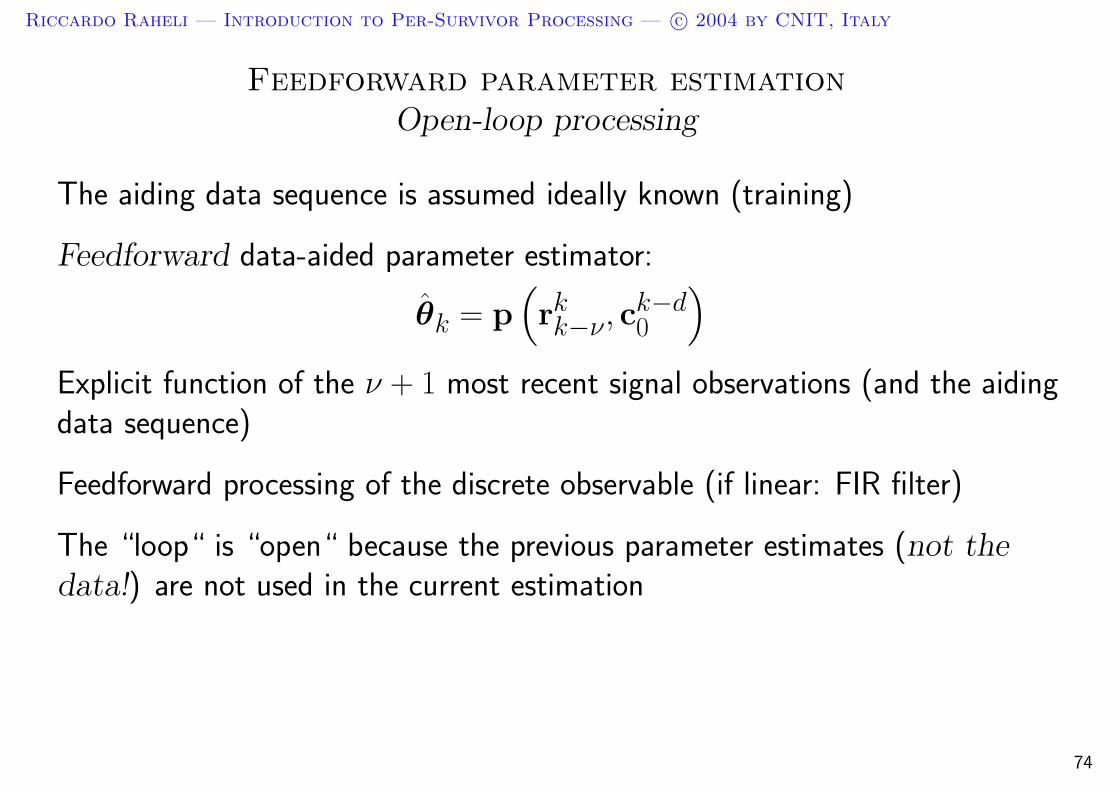
Feedforward parameter estimationOpen-loop processing
The aiding data sequence is assumed ideally known (training)
Feedforward data-aided parameter estimator:
θk = p(rkk−ν, c
k−d0
)
Explicit function of the ν + 1 most recent signal observations (and the aidingdata sequence)
Feedforward processing of the discrete observable (if linear: FIR filter)
The “loop“ is “open“ because the previous parameter estimates (not thedata!) are not used in the current estimation
74
Riccardo Raheli — Introduction to Per-Survivor Processing — c© 2004 by CNIT, Italy
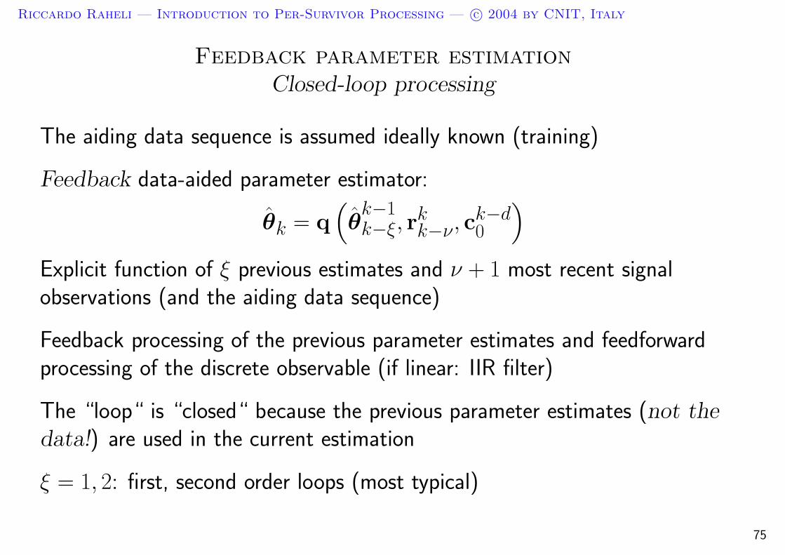
Feedback parameter estimationClosed-loop processing
The aiding data sequence is assumed ideally known (training)
Feedback data-aided parameter estimator:
θk = q(θ
k−1k−ξ, r
kk−ν, c
k−d0
)
Explicit function of ξ previous estimates and ν + 1 most recent signalobservations (and the aiding data sequence)
Feedback processing of the previous parameter estimates and feedforwardprocessing of the discrete observable (if linear: IIR filter)
The “loop“ is “closed“ because the previous parameter estimates (not thedata!) are used in the current estimation
ξ = 1, 2: first, second order loops (most typical)
75
Riccardo Raheli — Introduction to Per-Survivor Processing — c© 2004 by CNIT, Italy
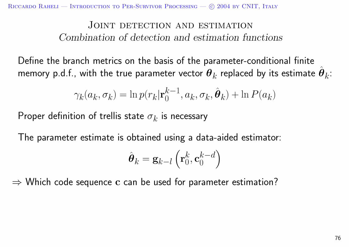
Joint detection and estimationCombination of detection and estimation functions
Define the branch metrics on the basis of the parameter-conditional finitememory p.d.f., with the true parameter vector θk replaced by its estimate θk:
γk(ak, σk) = ln p(rk|rk−10 , ak, σk, θk) + ln P (ak)
Proper definition of trellis state σk is necessary
The parameter estimate is obtained using a data-aided estimator:
θk = gk−l
(rk0 , c
k−d0
)
⇒ Which code sequence c can be used for parameter estimation?
76

Riccardo Raheli — Introduction to Per-Survivor Processing — c© 2004 by CNIT, Italy
Joint detection and estimationFinal versus preliminary decisions
During training the data sequence is readily available
Tracking can be based on previous data decisions: decision-directed mode
The detection scheme outputs data decisions with a delay D
E.g., detection delay of the Viterbi algorithm (survivor merge)
E.g., processing delay of the forward-backward algorithm (possible latencydue to the packet duration)
The detection delay of the sequence aiding in parameter estimation should besmall because it directly carries over to a delay in the parameter estimate:
Preliminary or tentative decisions with delay d < D
77

Riccardo Raheli — Introduction to Per-Survivor Processing — c© 2004 by CNIT, Italy
Joint detection and estimationSystem model
D : “final” decision delay
d : “preliminary” or “tentative” decision delay
ˆck−d : sequence of tentative decisions
78
Riccardo Raheli — Introduction to Per-Survivor Processing — c© 2004 by CNIT, Italy
Joint detection and estimationSummary
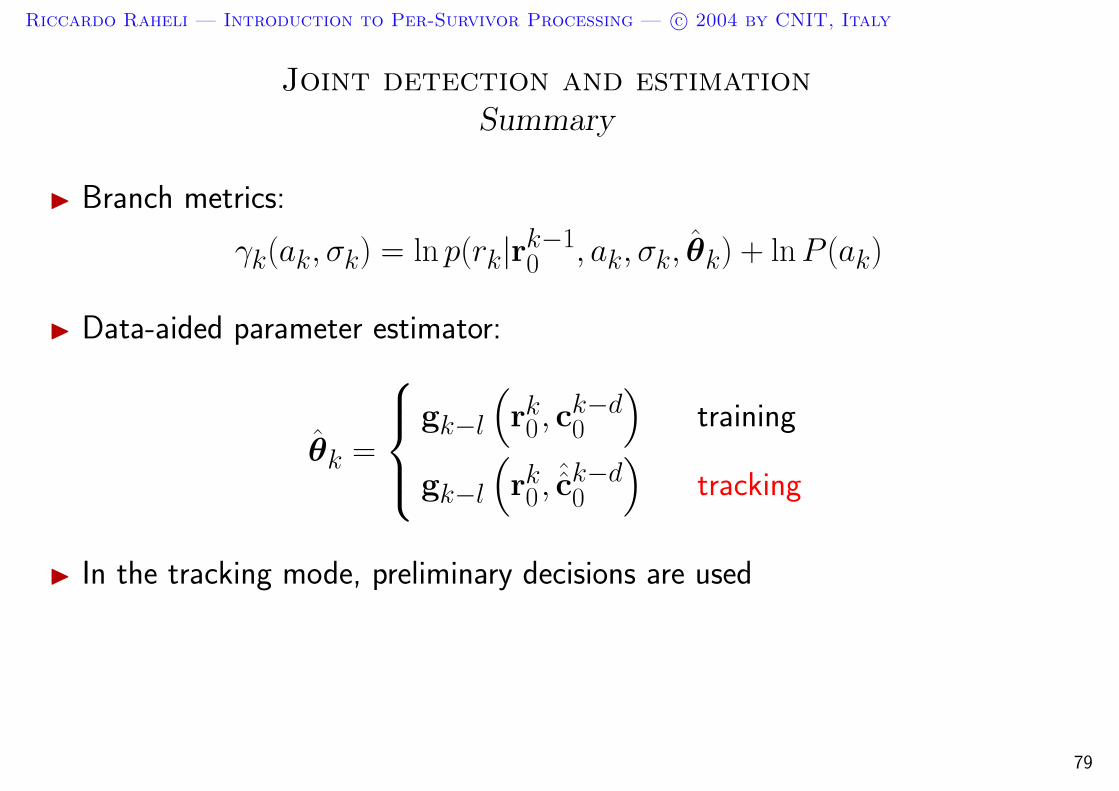
I Branch metrics:
γk(ak, σk) = ln p(rk|rk−10 , ak, σk, θk) + ln P (ak)
I Data-aided parameter estimator:
θk =
gk−l
(rk0 , c
k−d0
)training
gk−l
(rk0 ,
ˆck−d0
)tracking
I In the tracking mode, preliminary decisions are used
79
Riccardo Raheli — Introduction to Per-Survivor Processing — c© 2004 by CNIT, Italy
Detection under parametric uncertaintyExamples of application
Linear modulation on phase-uncertain channel
Linear modulation on dispersive fading channel
80

Riccardo Raheli — Introduction to Per-Survivor Processing — c© 2004 by CNIT, Italy
Linear modulation on phase-uncertain channelSynchronization-Detection decomposition
Model of discrete observable (usual notation):
rk = ejθk ck + wk
θk : channel-induced phase rotation
ck : code sequence with FSM model of state µk
wk : i.i.d. Gaussian noise sequence with variance σ2w
Unlimited memory (observation not even conditionally Gaussian)
Considering θk as undesired, the parameter-conditional finite-memoryproperty is verified:
p(rk|rk−10 , ak
0 , θk) = p(rk|ak, µk, θk)
=1
πσ2w
exp
[− |rk − ejθk ck(ak, µk)|2
σ2w
]
ck(ak, µk) : code symbol branch label81
Riccardo Raheli — Introduction to Per-Survivor Processing — c© 2004 by CNIT, Italy
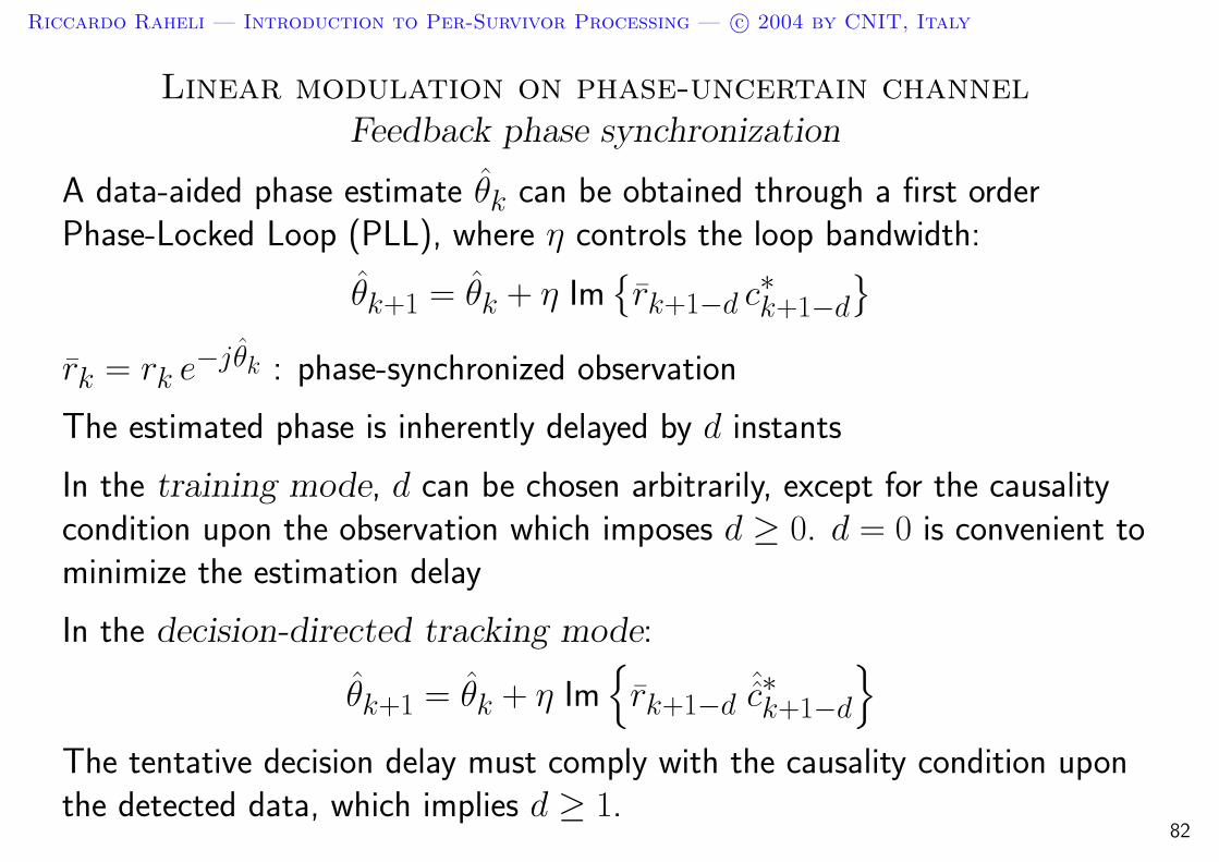
Linear modulation on phase-uncertain channelFeedback phase synchronization
A data-aided phase estimate θk can be obtained through a first orderPhase-Locked Loop (PLL), where η controls the loop bandwidth:
θk+1 = θk + η Imrk+1−d c∗k+1−d
rk = rk e−jθk : phase-synchronized observation
The estimated phase is inherently delayed by d instants
In the training mode, d can be chosen arbitrarily, except for the causalitycondition upon the observation which imposes d ≥ 0. d = 0 is convenient tominimize the estimation delay
In the decision-directed tracking mode:
θk+1 = θk + η Im
rk+1−dˆc∗k+1−d
The tentative decision delay must comply with the causality condition uponthe detected data, which implies d ≥ 1.
82

Riccardo Raheli — Introduction to Per-Survivor Processing — c© 2004 by CNIT, Italy
Linear modulation on phase-uncertain channelJoint detection and synchronization
The estimated phase can be used in place of the true unknown phase in thecomputation of the branch metrics:
γk(ak, µk) = ln p(rk|ak, µk, θk) + ln P (ak)
∝ −|rk − ejθk ck(ak, µk)|2 + σ2w ln P (ak)
= −|rk − ck(ak, µk)|2 + σ2w ln P (ak)
The detection and synchronization functions can be based on thephase-synchronized observation
rk = rk e−jθk
83

Riccardo Raheli — Introduction to Per-Survivor Processing — c© 2004 by CNIT, Italy
Linear modulation on phase-uncertain channelProblem 7
Consider the model of discrete observable
rk = ejθ ck + wk
where θ is the overall phase rotation induced by the channel. Let θ be a
phase estimate and define the phase-synchronized observation rk = rk e−jθ
A. Derive an explicit expression of the mean square error (MSE)
E|rk − ck|2 as a function of θ
B. Obtain an estimate of θ minimizing the MSE
C. Formulate a data-aided iterative stochastic gradient algorithm forminimizing the MSE
D. Comment on the functional relationship of the obtained synchronizationscheme with a first-order PLL
Hint: Define a stochastic gradient by differentiating the MSE withrespect to θ and discarding the expectation
84
Riccardo Raheli — Introduction to Per-Survivor Processing — c© 2004 by CNIT, Italy
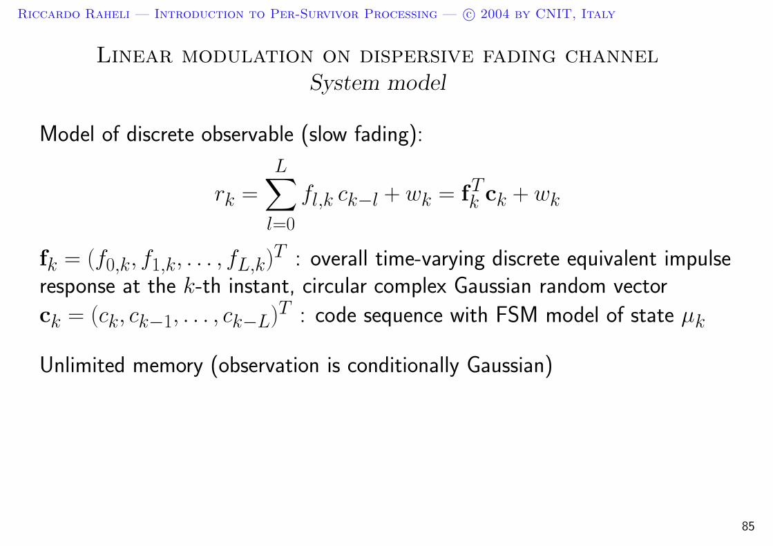
Linear modulation on dispersive fading channelSystem model
Model of discrete observable (slow fading):
rk =
L∑
l=0
fl,k ck−l + wk = fTk ck + wk
fk = (f0,k, f1,k, . . . , fL,k)T : overall time-varying discrete equivalent impulseresponse at the k-th instant, circular complex Gaussian random vector
ck = (ck, ck−1, . . . , ck−L)T : code sequence with FSM model of state µk
Unlimited memory (observation is conditionally Gaussian)
85

Riccardo Raheli — Introduction to Per-Survivor Processing — c© 2004 by CNIT, Italy
Linear modulation on dispersive fading channelEstimation-Detection decomposition
Considering fk as undesired, the system is parameter-conditionallyfinite-memory:
γk(ak, σk) = ln p(rk|rk−10 , ak
0 , fk) + ln P (ak)
= ln p(rk|ak, σk, fk) + ln P (ak)
= ln
1
πσ2w
exp
[−|rk − fT
k ck(ak, σk)|2σ2
w
]+ ln P (ak)
∝ −|rk − fTk ck(ak, σk)|2 + σ2
w ln P (ak)
σk = (ak−1, ak−2, . . . , ak−L; µk−L) : system state
ck(ak, σk) = [ck(ak, µk), ck−1(ak−1, µk−1), . . . , ck−L(ak−L, µk−L)]T :code symbol vector uniquely associated with the considered trellis branch(ak, σk), in accordance with the coding rule
86
Riccardo Raheli — Introduction to Per-Survivor Processing — c© 2004 by CNIT, Italy
Linear modulation on dispersive fading channelFeedback parameter estimation
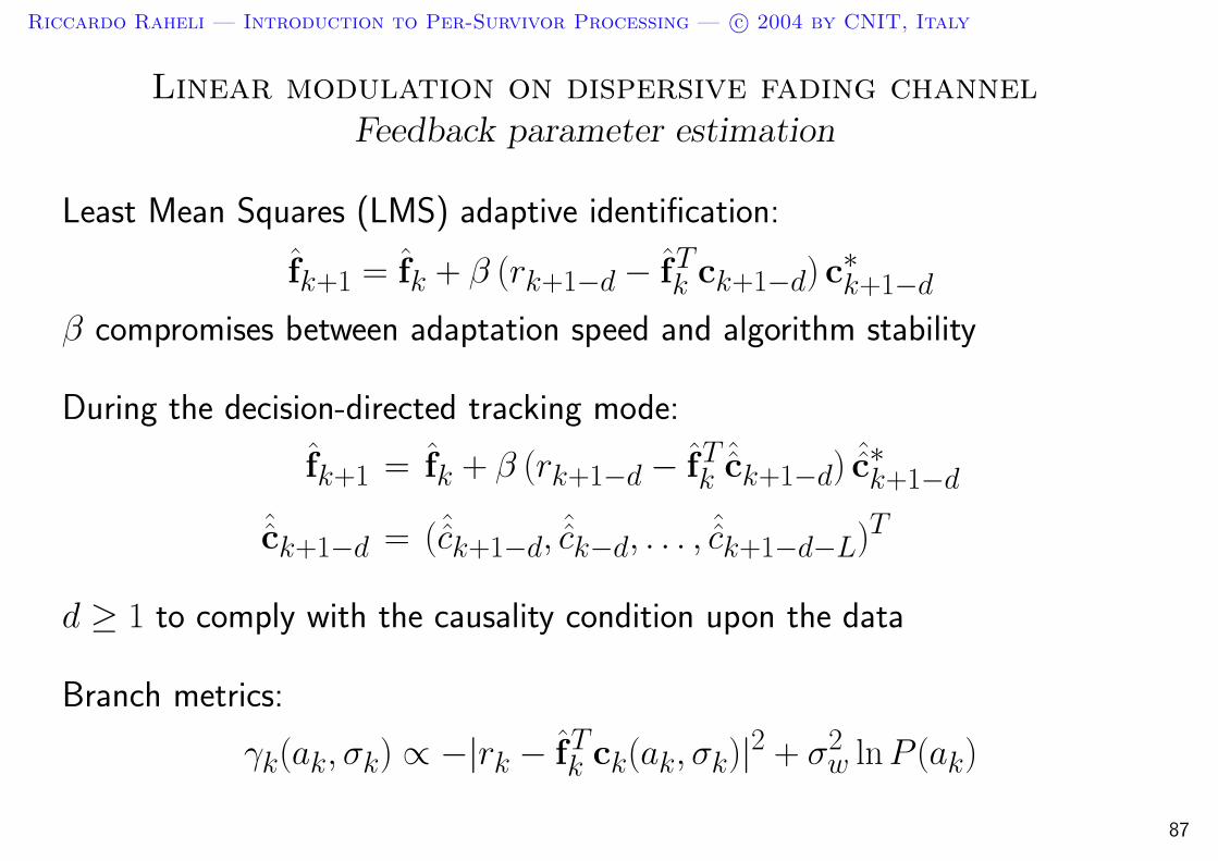
Least Mean Squares (LMS) adaptive identification:
fk+1 = fk + β (rk+1−d − fTk ck+1−d) c∗k+1−d
β compromises between adaptation speed and algorithm stability
During the decision-directed tracking mode:
fk+1 = fk + β (rk+1−d − fTk
ˆck+1−d)ˆc∗k+1−d
ˆck+1−d = (ˆck+1−d, ˆck−d, . . . , ˆck+1−d−L)T
d ≥ 1 to comply with the causality condition upon the data
Branch metrics:
γk(ak, σk) ∝ −|rk − fTk ck(ak, σk)|2 + σ2
w ln P (ak)
87

Riccardo Raheli — Introduction to Per-Survivor Processing — c© 2004 by CNIT, Italy
Linear modulation on dispersive fading channelProblem 8
Consider the model of discrete observable
rk = fTck + wk
where f is the overall discrete equivalent channel impulse response. Let f
be an estimate of the channel response. Assume the code symbols arezero-mean and uncorrelated
A. Derive an explicit expression of the mean square error (MSE)E|rk − fTck|2 as a function of f
B. Formulate a data-aided iterative stochastic gradient algorithm forminimizing the MSE
C. Comment on the functional relationship of the obtained identificationscheme and the LMS algorithm
Hint: Define a stochastic gradient by differentiating the MSE withrespect to f and discarding the expectation
88

Riccardo Raheli — Introduction to Per-Survivor Processing — c© 2004 by CNIT, Italy
Joint detection and estimationError propagation
A decision-feedback mechanism characterizes the decision-directed trackingphase: decisions are used for parameter estimation and, hence, for detectingthe successive data
Error propagation may take place, namely wrong data decisions maynegatively affect the parameter estimate and cause further decision errors
This effect is usually non catastrophic but it affects the overall performance
89

Riccardo Raheli — Introduction to Per-Survivor Processing — c© 2004 by CNIT, Italy
Joint detection and estimationOptimization of the tentative decision delay
Preliminary decisions with delay d < D can be considerably worse than thefinal decisions. E.g., in the Viterbi algorithm, decisions with reduced delayd < D are affected by the probability of unmerged survivors
⇒ Large values of tentative decision delay d may be best
The delay d of the aiding data sequence yields a delay in the parameterestimate which may affect the detection quality when the true parameter istime-varying
⇒ Small values of d may be best, possibly the minimal value d = 1.
Good values of tentative decision delay d must be the result of a trade-offbetween two conflicting requirements
⇒ In practice, one would have to experiment several values of d and select agood compromise value (minimize error propagation)
90

Riccardo Raheli — Introduction to Per-Survivor Processing — c© 2004 by CNIT, Italy
Detection under parametric uncertaintyBibliography
– H. L. Van Trees, Detection, Estimation, and Modulation Theory, Part I. New York:John Wiley & Sons, 1968.
– H. Kobayashi, “Simultaneous adaptive estimation and decision algorithm for carriermodulated data transmission systems,” IEEE Trans. Commun., pp. 268-280, June 1971.
– F. R. Magee, Jr. and J. G. Proakis, “Adaptive maximum-likelihood sequence estimation fordigital signaling in the presence of intersymbol interference,” IEEE Trans. Inform.Theory, pp. 120–124, Jan. 1973.
– S. U. H. Qureshi and E. E. Newhall, “An adaptive receiver for data transmission overtime-dispersive channels,” IEEE Trans. Inform. Theory, pp. 448-457, July 1973.
– G. Ungerboeck, “Adaptive maximum-likelihood receiver for carrier modulateddata-transmission systems,” IEEE Trans. Commun., pp. 624-636, May 1974.
– G. Ungerboeck, “Channel coding with multilevel/phase signals,” IEEE Trans. Inform.Theory, pp. 55-67, Jan. 1982.
– S. Benedetto, E. Biglieri and V. Castellani. Digital Transmission Theory. Prentice-Hall,Englewood Cliffs, U.S.A., 1987.
– J. G. Proakis, Digital Communications. New York: McGraw-Hill, 1989, 2nd ed..– R. Raheli, A. Polydoros, C. K. Tzou, “Per-survivor processing: a general approach to MLSE
in uncertain environments,” IEEE Trans. Commun., pp. 354-364, Feb.-Apr. 1995.91
Riccardo Raheli — Introduction to Per-Survivor Processing — c© 2004 by CNIT, Italy
3. Per-Survivor Processing: concept
Outline
1. Review of detection techniques
2. Detection under parametric uncertainty
3. Per-Survivor Processing (PSP): concept and historical review
4. Classical applications of PSP:
4.1 Complexity reduction
4.2 Linear predictive detection for fading channels
4.3 Adaptive detection
5. Advanced applications of PSP
92

Riccardo Raheli — Introduction to Per-Survivor Processing — c© 2004 by CNIT, Italy
Per-Survivor Processing (PSP)A step toward a unification of estimation and detection
The Estimation-Detection decomposition is a general suboptimal designapproach to force a finite-memory property and achieve feasible detectioncomplexity
Optimal processing is not compatible with the decomposition approach andwould require a unified detection function (often of infeasible complexity)
Per-Survivor Processing is an alternative general design approach which stillexploits the forced finite-memory property but reduces the degree ofseparation between the detection and estimation functions
In this technique, the code sequences associated with each survivor are usedas the aiding data sequence for a set of per-survivor estimators of theunknown parameters
93

Riccardo Raheli — Introduction to Per-Survivor Processing — c© 2004 by CNIT, Italy
Per-Survivor ProcessingA formal description
Let σk be the trellis state descriptive of the overall parameter-conditionalfinite state machine which models the transmission system
Let ck−10 (σk) denote the code sequence associated with the survivor of
state σk
Per-survivor estimates of the parameter vector θk based on a data-aidedestimator can be expressed as
θk(σk) = gk−l
[rk0 , c
k−d0 (σk)
]
These per-survivor estimates can be used in the computation of the branchmetrics:
γk(ak, σk) = ln p(rk|rk−10 , ak, σk, θk(σk)) + ln P (ak)
94

Riccardo Raheli — Introduction to Per-Survivor Processing — c© 2004 by CNIT, Italy
Per-Survivor ProcessingSome remarks
I The structure of the branch metrics is inherently different, with respect tothe previous cases, in the fact that it also depends on the state σkthrough the parameter estimate
I There is now a data-aided parameter estimator per trellis state. Thisestimator uses the data sequence associated with the survivor of thisstate as aiding sequence. The resulting parameter estimates, one perstate, are inherently associated with the survivor sequences—hence,the terminology “per-survivor processing”
I Compared to a conventional decomposed estimation-detection schemebased on tentative decisions, the complexity of per-survivor processing islarger
95

Riccardo Raheli — Introduction to Per-Survivor Processing — c© 2004 by CNIT, Italy
Per-Survivor ProcessingSystem model
discret detection
PSP-based detection
r(t)
decoding
θk(σk) ck−d(σk)
ak−Drk
parameterestimation
A “tentative” block diagram: a set of parameter estimators observe thereceived sequence rk and are aided by the survivor sequences ck−d
0 (σk). A
corresponding set of per-survivor parameter estimates θk(σk) are passed tothe detection block
96
Riccardo Raheli — Introduction to Per-Survivor Processing — c© 2004 by CNIT, Italy
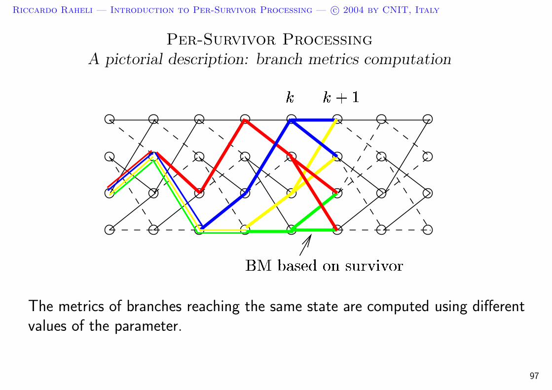
Per-Survivor ProcessingA pictorial description: branch metrics computation
The metrics of branches reaching the same state are computed using differentvalues of the parameter.
97

Riccardo Raheli — Introduction to Per-Survivor Processing — c© 2004 by CNIT, Italy
Per-Survivor ProcessingA pictorial description: evolution of the parameter estimates
“universal” estimation
θk−1 θk θk+1
σk
PSP-based estimation
σk−1
σk+1
θk−1(σk−1)
θ(σk)
θ(σk+1)
In the “universal” scheme, only one parameter estimate is used forcomputation of all the branch metrics at the k-th step
In the PSP-based scheme the parameter estimates evolve along the survivors
98

Riccardo Raheli — Introduction to Per-Survivor Processing — c© 2004 by CNIT, Italy
Per-Survivor ProcessingAn intuitive rationale
Whenever the incomplete knowledge of some quantities prevents us fromcalculating a particular branch metric in a precise and predictable form, we useestimates of those quantities based on the data sequence associated with thesurvivor leading to that branch. If any particular survivor is correct (an eventof high probability under normal operating conditions), the correspondingestimates are evaluated using the correct data sequence. Since at each stageof decoding we do not know which survivor is correct (or the best), we extendeach survivor based on estimates obtained using its associated data sequence.
Roughly speaking, the best survivor is extended using the best data sequenceavailable (which is the sequence associated to it), regardless of our temporaryignorance as to which survivor is the best.
99
Riccardo Raheli — Introduction to Per-Survivor Processing — c© 2004 by CNIT, Italy
Per-Survivor ProcessingIs a delay d necessary?
The best survivor is extended according to its associated data sequence,despite the fact that we do not know which survivor is the best at the currenttime (we will know the best survivor after D further steps)
There are no reasons for delaying the aiding data sequence of the best survivorbeyond the minimal delay d = 1 complying with the causality condition
Since all survivors eventually merge, the quality of the data sequencesassociated to all survivors improves for increasing values of d
⇒ The minimal value d = 1 offers the best overall performance because itattains simultaneously good quality of the aiding data sequence and a smalldelay in the parameter estimate
⇒ PSP allows one to design receivers particularly robust when the undesiredparameters are time-varying
100
Riccardo Raheli — Introduction to Per-Survivor Processing — c© 2004 by CNIT, Italy
Per-Survivor ProcessingError propagation
PSP is a mechanism for virtually using “final” decisions for aiding theparameter estimation (with no delay!)
Only errors in the final decisions, the so-called error events, are “fed back” tothe parameter estimator of the best survivor
As the aiding data sequence along the best survivor is of best possible quality,the effects of error propagation are reduced (compared with the traditionalscheme that uses tentative decisions)
Parameter estimators of other survivors use data sequences of worse quality,but they do not affect future decisions provided these survivors are laterdiscarded
101

Riccardo Raheli — Introduction to Per-Survivor Processing — c© 2004 by CNIT, Italy
Linear modulation on phase-uncertain channelPSP-based detection and phase synchronization
Branch metrics:
γk(ak, µk) ∝ −|rk e−jθk(µk) − ck(ak, µk)|2 + σ2w ln P (ak)
Phase estimate update recursion:
θk+1(µk+1) = θk(µk) + η Im
rk+1−d e−jθk(µk) c∗k+1−d(µk)
c∗k+1−d(µk) is the code symbol at epoch k + 1 − d in the survivor sequenceof state µk
The phase estimate update recursions must take place along the brancheswhich extend the survivor of state µk, i.e., after the usual add-compare-selectstep at time k
Remember: d = 1 for best performance
102

Riccardo Raheli — Introduction to Per-Survivor Processing — c© 2004 by CNIT, Italy
Linear modulation on dispersive fading channelPSP-based detection and channel estimation
Branch metrics:
γk(ak, σk) ∝ −|rk − fk(σk)Tck(ak, σk)|2 + σ2w ln P (ak)
Channel estimate update recursions:
fk+1(σk+1) = fk(σk) + β[rk+1−d − fk(σk)T ck+1−d(σk+1)
]c∗k+1−d(σk+1)
ck+1−d(σk+1) = [ck+1−d(σk+1), ck−d(σk+1), . . . , ck+1−d−L(σk+1)]T
Channel estimate update recursions must take place over those branches(σk → σk+1) which comply with the Viterbi algorithm add-compare-selectstep at time k
Remember: d = 1 for best performance
103

Riccardo Raheli — Introduction to Per-Survivor Processing — c© 2004 by CNIT, Italy
Per-Survivor ProcessingHybrid version
The survivor merge is normally a few steps backward from current time
Only the most recent code symbols should be searched for in the survivorhistory; earlier symbols can be reliably based on preliminary decisions
Formulation:θk(σk) = gk−l
[rk0 ,
ˆck−d0 , ck−1
k−d+1(σk)]
104
Riccardo Raheli — Introduction to Per-Survivor Processing — c© 2004 by CNIT, Italy
Per-Survivor ProcessingA pictorial description: Hybrid version
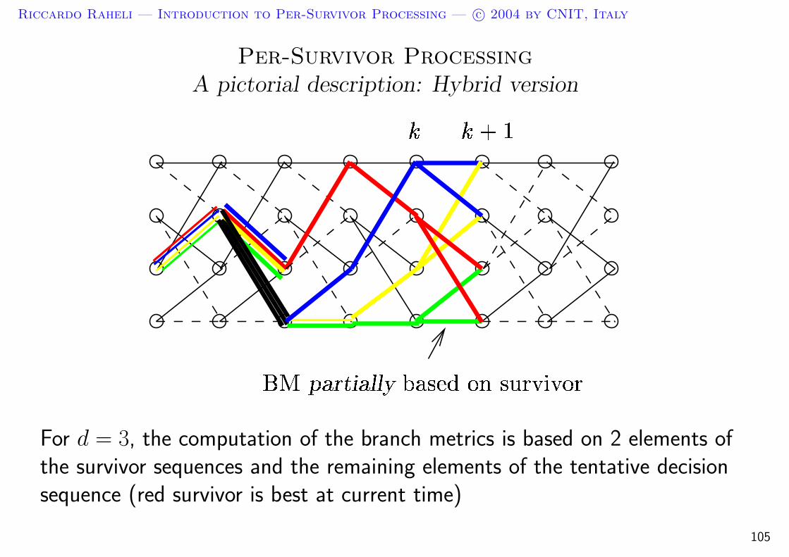
For d = 3, the computation of the branch metrics is based on 2 elements ofthe survivor sequences and the remaining elements of the tentative decisionsequence (red survivor is best at current time)
105
Riccardo Raheli — Introduction to Per-Survivor Processing — c© 2004 by CNIT, Italy
Per-Survivor ProcessingReduced-estimator version
In PSP, the number of parameter estimators equals the number of survivors
In a conventional decomposed design, there is one parameter estimator
What is in between?
The number N of parameter estimators can be adjusted independently of thenumber S of survivors: 1 ≤ N ≤ S (N = 1 ⇒ tentative decisions;N = S ⇒ PSP):
– Select the best survivor and the N best survivors;
– Extend each of the N best survivors using its associated parameterestimate;
– Extend each of the remaining S −N survivors using the parameter estimateassociated with the best survivor;
– Update each of the N parameter estimates along the extensions of the Nbest survivors.
106

Riccardo Raheli — Introduction to Per-Survivor Processing — c© 2004 by CNIT, Italy
Per-Survivor ProcessingA pictorial description: Reduced-estimator version
2
4 2
1 3
(a)
2
3 1
1 3
2
3 1
4
4 4
(b)Figure reproduced from:
– R. Raheli, G. Marino, P. Castoldi, “Per-survivor processing and tentative decisions: what isin between?,” IEEE Trans. Commun., pp. 127-129, Feb. 1996.
107
Riccardo Raheli — Introduction to Per-Survivor Processing — c© 2004 by CNIT, Italy
Per-Survivor ProcessingUpdate-first version
The temporal sequence: ACS step followed by parameter update can beinverted
Update-first version of PSP:
1. The per-survivor parameter update recursions are run along all possiblecandidate survivors
2. The branch metrics are computed using these updated parameterestimates
3. The ACS step is performed
In this version, there is one parameter estimator per candidate (complexity islarger)
PSP allows d = 0 in parameter estimation (in a scheme based on tentativedecisions this would violate the causality condition)
108
Riccardo Raheli — Introduction to Per-Survivor Processing — c© 2004 by CNIT, Italy
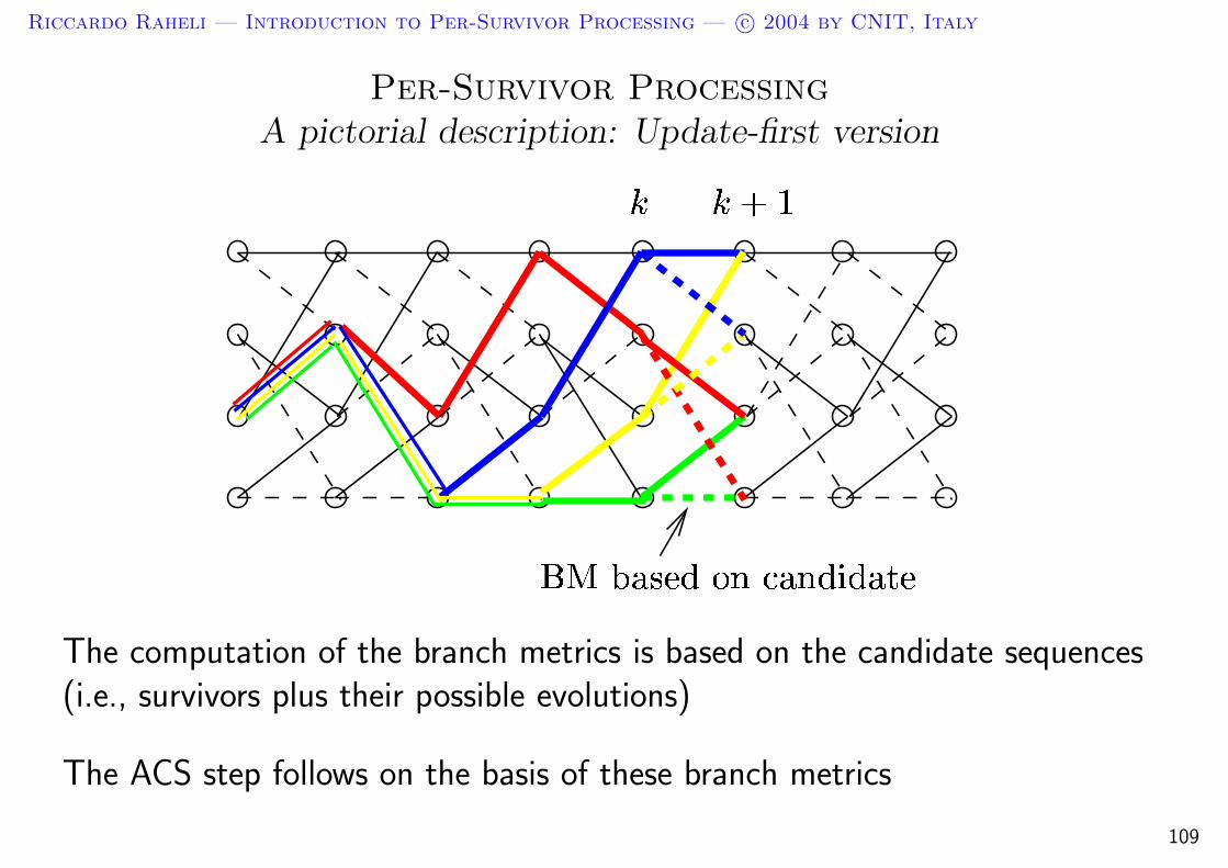
Per-Survivor ProcessingA pictorial description: Update-first version
The computation of the branch metrics is based on the candidate sequences(i.e., survivors plus their possible evolutions)
The ACS step follows on the basis of these branch metrics
109
Riccardo Raheli — Introduction to Per-Survivor Processing — c© 2004 by CNIT, Italy
Per-Survivor ProcessingApplication to reduced-search (sequential) algorithms
Per-survivor processing can be directly applied to any tree or trellisreduced-search algorithm, also referred to as sequential detection algorithms
Reduced-search algorithms may be used to search a small part of a large FSMtrellis diagram or non-FSM tree diagram
The M-algorithm keeps a list of M best paths: at each step, each path isextended in all possible way, say N ; from the resulting list of MN paths, thebest M are retained for further extension (breadth-first)
Depth-first and metric-first algorithms keep one or more paths andbacktrack whenever the retained paths are judged of insufficient quality,according to some criterion
An alternative terminology could be Per-Path Processing, or P3
110

Riccardo Raheli — Introduction to Per-Survivor Processing — c© 2004 by CNIT, Italy
Per-Survivor ProcessingA pictorial description: Application to M-algorithm
M = 2 Branch metrics based on maintaned paths (survivors)
111

Riccardo Raheli — Introduction to Per-Survivor Processing — c© 2004 by CNIT, Italy
Per-Survivor ProcessingApplication to list Viterbi algorithms
The Viterbi algorithm detects the “best” MAP (or ML) path or sequence
Nothing is known about the second, third, etc. best paths
List Viterbi algorithms release the ordered list of V best paths by maintainingV survivors per state
These algorithms may be used in concatenated coding schemes: whenever theouter code detects an error, the second, third, etc. sequence at the output ofthe inner decoder can be tried out
Per-survivor processing can be readily applied to list Viterbi algorithms byassociating a parameter estimator to each survivor
112
Riccardo Raheli — Introduction to Per-Survivor Processing — c© 2004 by CNIT, Italy
Per-Survivor Processing: conceptBibliography
– A. Polydoros, R. Raheli, “The Principle of Per-Survivor Processing: A General Approach toApproximate and Adaptive ML Sequence Estimation,” University of Southern California,Technical Report CSI-90-07-05, July 1990. Also presented at the IEEE Commun.Theory Workshop, Rhodes, Greece, July 1991.
– R. Raheli, A. Polydoros, C. K. Tzou, “The Principle of Per-Survivor Processing: A GeneralApproach to Approximate and Adaptive MLSE,” in Proc. IEEE Global Commun. Conf.(GLOBECOM ’91), Phoenix, Arizona, USA, Dec. 1991, pp. 1170-1175.
– R. Raheli, A. Polydoros, C. K. Tzou, “Per-survivor processing: a general approach to MLSEin uncertain environments,” IEEE Trans. Commun., pp. 354-364, Feb.-Apr. 1995.
– A. Polydoros, R. Raheli, “System and method for estimating data sequences in digitaltransmission,” University of Southern California, U.S. Patent No. 5,432,821, July 1995.
– R. Raheli, G. Marino, P. Castoldi, “Per-survivor processing and tentative decisions: what isin between?,” IEEE Trans. Commun., pp. 127-129, Feb. 1996.
– G. Marino, “Hybrid decision feed-back sequence estimation”, in Proc. Intern. Conf.Telecommun., Istanbul, Turkey, Apr. 1996, pp. 132-135.
– K. M. Chugg, A. Polydoros, “MLSE for an unknown channel—Parts I and II,” IEEETrans. Commun., pp. 836-846 and 949-958, July and Aug. 1996.
113
Riccardo Raheli — Introduction to Per-Survivor Processing — c© 2004 by CNIT, Italy
3. Per-Survivor Processing: historical review
Outline
1. Review of detection techniques
2. Detection under parametric uncertainty
3. Per-Survivor Processing (PSP): concept and historical review
4. Classical applications of PSP:
4.1 Complexity reduction
4.2 Linear predictive detection for fading channels
4.3 Adaptive detection
5. Advanced applications of PSP
114
Riccardo Raheli — Introduction to Per-Survivor Processing — c© 2004 by CNIT, Italy
Historical reviewThe beginning and afterwards ...
The general concept of per-survivor processing was understood and proposedin the early nineties as a generalization of per-survivor DFE-like ISIcancellation techniques of reduced-state sequence detection (RSSD), alsoknown as (delayed) decision-feedback sequence detection (DFSD)
RSSD and DFSD appeared and established in the late eighties, except forisolated seminal contributions which date back to the seventies
In the early nineties, a number of independent research results appeared indiverse technical areas which could be interpreted as special cases of thegeneral PSP concept (not yet known)
During the nineties (and currently) PSP has emerged as a broad approach todetection in hostile transmission environments
As we will see, sometimes PSP arises naturally from the analyticaldevelopment itself, when devising detection algorithms
115
Riccardo Raheli — Introduction to Per-Survivor Processing — c© 2004 by CNIT, Italy
Reduced-state sequence detectionThe main references
– J. W. M. Bergmans, S. A. Rajput, F. A. M. Van De Laar, “On the use of DecisionFeedback for Simplifying the Viterbi Decoder,” Philips Journal of Research, No. 4, 1987.
– K. Wesolowski, “Efficient Digital Receiver Structure for Trellis-Coded Signals Transmittedthrough Channels with Intersymbol Interference,” Electronics Letters, Nov. 1987.
– T. Hashimoto, “A List-Type Reduced-Constraint Generalization of the Viterbi Algorithm,”IEEE Trans. Inform. Theory, pp. 866-876, Nov. 1987.
– M. V. Eyuboglu, S. U. H. Qureshi, “Reduced-State Sequence Estimation with Set Partitionand Decision Feedback,” IEEE Trans. Commun., pp. 13-20, Jan. 1988.
– A. Duel Hallen, C. Heegard, “Delayed Decision-Feedback Sequence Estimation,” IEEETrans. Commun., pp. 428-436, May 1989.
– P. R. Chevillat, E. Eleftheriou, “Decoding of Trellis-Encoded Signals in the Presence ofIntersymbol Interference and Noise,” IEEE Trans. Commun., pp. 669-676, July 1989.
– M. V. Eyuboglu, S. U. H. Qureshi, “Reduced-State Sequence Estimation for CodedModulation on Intersymbol Interference Channels,” IEEE J. Sel. Areas Commun., pp.989-995, Aug. 1989.
– A. Svensson, “Reduced state sequence detection of full response continuous phasemodulation,“ IEE Electronics Letters, pp. 652 -654, 1 May 1990.
116
Riccardo Raheli — Introduction to Per-Survivor Processing — c© 2004 by CNIT, Italy
Reduced-state sequence detectionThere was earlier work ...
– F. L. Vermeulen and M. E. Hellman, ”Reduced state Viterbi decoders for channels withintersymbol interference,’ in Proc. IEEE Int. Conf. Commun. (ICC ’74), Minneapolis,MN, June 1974, pp. 37B1-37B4.
– F. L. Vermeulen, ”Low complexity decoders for channels with intersymbol interference,”Ph.D. dissertation, Dep. Elect. Eng., Stanford Univ., Aug. 1975.
– G. J. Foschini, “A reduced state variant of maximum likelihood sequence detectionattaining optimum performance for high signal-to-noise ratios,” IEEE Trans. Inform.Theory, pp. 553-651, Sept. 1977
– A. Polydoros, “Maximum-likelihood sequence estimation in the presence of infiniteintersymbol interference,” Master’s Thesis, Graduate School of State University of NewYork at Buffalo, Dec. 1978.
– A. Polydoros, D. Kazakos, “Maximum-Likelihood Sequence Estimation in the Presence ofInfinite Intersymbol Interference,” in Proc. ICC ’79, June 1979.
117
Riccardo Raheli — Introduction to Per-Survivor Processing — c© 2004 by CNIT, Italy
Independent results interpretable as PSPWhen the time has come ...
Sequence detection for a time-varying statistically known channel:– J. Lodge, M. Moher, “ML estimation of CPM signals transmitted over Rayleigh flat fading
channels,” IEEE Trans. Commun., pp. 787-794, June 1990.– D. Makrakis, P. T. Mathiopoulos, D. P. Bouras, “Optimal decoding of coded PSK and
QAM signals in correlated fast fading channels and AWGN: a combined envelope, multipledifferential and coherent detection approach,” IEEE Trans. Commun., pp.63-75,Jan. 1994.
Joint ML estimation of a deterministic channel and data detection:– R. Iltis, “A Bayesian MLSE algorithm for a priori unknown channels and symbol timing,”
IEEE J. Sel. Areas Commun., April 1992.– N. Seshadri, “Joint data and channel estimation using blind trellis search techniques,”
IEEE Trans. Commun., Feb.-Apr. 1994.
118

Riccardo Raheli — Introduction to Per-Survivor Processing — c© 2004 by CNIT, Italy
Independent results interpretable as PSPWhen the time has come ... (cntd)
Adaptive sequence detection with tracking of a time-varying deterministicchannel:– Z. Xie, C. Rushforth, R. Short, T. Moon, “Joint signal detection and parameter estimation
in multiuser communications,” IEEE Trans. Commun., Aug. 1993.– H. Kubo, K. Murakami, T. Fujino, “An adaptive MLSE for fast time-varying ISI channels,”
IEEE Trans. Commun., pp, 1872-1880, Feb.-Apr. 1994.
Trellis coded quantization (source encoding):– M. W. Marcellin, T. R. Fischer, “Trellis coded quantization of memoryless Gauss-Markov
sources,” IEEE Trans. Commun., Jan. 1990.
Joint sequence detection and carrier phase synchronization:– A. J. Macdonald and J. B. Anderson, “PLL synchronization for coded modulation,” in
Proc. ICC ’91, June 1991.– A. Reichman and R. A. Scholtz, “Joint phase estimation and data decoding for tcm
systems,” in Proc. First Intern. Symp. Commun. Theory and Applications,Scotland, U.K., Sept. 1991.
119
Riccardo Raheli — Introduction to Per-Survivor Processing — c© 2004 by CNIT, Italy
Earlier work... and beforehand
Analog FM demodulation with discrete phase approximation based on theViterbi algorithm (there are no data !)
In an extended-memory version, a procedure similar to PSP was proposed
– C. Cahn, “Phase tracking and demodulation with delay,” IEEE Trans. Inform. Theory,Jan. 1974.
120

Riccardo Raheli — Introduction to Per-Survivor Processing — c© 2004 by CNIT, Italy
The rootsGeneralized likelihood
Model the parameter as deterministic or random with unknown distribution
Joint ML parameter estimation and sequence detection viewed as acomposite hypotheses test:
a = argmaxa
max
θ
p (r|a,θ)
︸ ︷︷ ︸⇒ θ (a)
⇒ A per-hypothesis parameter estimate is obtained as a side result
– H. L. Van Trees, Detection, Estimation, and Modulation Theory, Part I. New York:John Wiley & Sons, 1968.
121

Riccardo Raheli — Introduction to Per-Survivor Processing — c© 2004 by CNIT, Italy
The rootsEstimation-Correlation detection
Detection of M -ary random signals in AWGN: s(t) is conditionally Gaussian,given mi
! #"
$ % &
⇒ Per-hypothesis conditional mean square estimate of s(t)
For deterministic signals: s(t) ∈ si(t)Mi=1 ⇒ si(t) = si(t)
– T. Kailath, “Correlation detection of signals perturbed by a random channel,” IRE Trans.Inform. Theory, June 1960.
– T. Kailath, “A general likelihood ratio formula for random signals in Gaussian noise,”IEEE Trans. Inform. Theory, May 1969.
122
Riccardo Raheli — Introduction to Per-Survivor Processing — c© 2004 by CNIT, Italy
Further references on PSP... this is not an exhaustive list ...
– A. N. D’Andrea, U. Mengali, and G. M. Vitetta, “Approximate ML decoding of coded PSKwith no explicit carrier phase reference,” IEEE Trans. Commun., pp. 1033-1039,Feb.-Apr. 1994.
– Q. Dai, E. Shwedyk, “Detection of bandlimited signals over frequency selective Rayleighfading channels,” IEEE Trans. Commun., pp. 941-950, Feb.-Apr. 1994.
– J. Lin, F. Ling, J. Proakis, “Joint data and channel estimation for TDMA mobile channels,”Plenum Intern. J. Wireless Inform. Networks, vol. 1, no. 4, pp. 229-238, 1994.
– X. Yu, S. Pasupathy, “Innovations-based MLSE for Rayleigh fading channels,” IEEETrans. Commun., pp. 1534-1544, Feb.-Apr. 1995.
– G. M. Vitetta, D. P. Taylor, “Maximum likelihood decoding of uncoded and coded PSKsignal sequences transmitted over Rayleigh flat-fading channels,” IEEE Trans.Commun., vol. 43, pp. 2750-2758, Nov. 1995
– K. Hamied, G. Stuber, “An adaptive truncated MLSE receiver for Japanese personal digitalcellular,” IEEE Trans. Veh. Techn., Feb. 1996.
– G. M. Vitetta, D. P. Taylor, U. Mengali, “Double filtering receivers for PSK signalstransmitted over Rayleigh frequency-flat fading channels,” IEEE Trans. Commun., vol.44, pp. 686-695, June 1996.
123
Riccardo Raheli — Introduction to Per-Survivor Processing — c© 2004 by CNIT, Italy
Further references on PSP... this is not an exhaustive list ... (cntd)
– M. E. Rollins, S. J. Simmons, “Simplified per-survivor Kalman processing in fastfrequency-selective fading channels,” IEEE Trans. Commun., pp. 544-553, May 1997.
– B. C. Ng, S. N. Diggavi, A. Paulray, “Joint structured channel and data estimation overtime-varying channels,” in Proc. IEEE Globecom, 1997.
– A. Anastasopoulos, A. Polydoros, “Adaptive soft-decision algorithms for mobile fadingchannels,” European Trans. Telecommun.., vol. 9, no. 2, pp. 183-190, Mar-Apr. 1998.
– K. M. Chugg, “Blind acquisition characteristics of PSP-based sequence detectors,” IEEEJ. Sel. Areas Commun., vol. 16, pp. 1518-1529, Oct. 1998.
– F. Rice, B. Cowley, M. Rice, B. Moran, “Spectrum analysis using a trellis algorithm,” inProc. IEEE Intern. Conf. Signal Process. (ICTS ’98), Oct. 1998.
124

Riccardo Raheli — Introduction to Per-Survivor Processing — c© 2004 by CNIT, Italy
4. Classical applications of PSP
4.1 Complexity reduction
Outline
1. Review of detection techniques
2. Detection under parametric uncertainty
3. Per-Survivor Processing (PSP): concept and historical review
4. Classical applications of PSP:
4.1 Complexity reduction
4.2 Linear predictive detection for fading channels
4.3 Adaptive detection
5. Advanced applications of PSP
125

Riccardo Raheli — Introduction to Per-Survivor Processing — c© 2004 by CNIT, Italy
Reduction of trellis state-complexityMotivation
Consider a FSM system model based on some finite memory property(strict-sense or conditional)
Detection schemes are based on branch metrics: γk(ak, σk)
System state: σk = (ak−1, ak−2, . . . , ak−L; µk−L) (C = L)
Encoder state: µk
Coding rule:
ck = o(ak, µk)
µk+1 = t(ak, µk)
Number of FSM states: S = ScML
Example: Sc = M = L = 4 ⇒ S = 4 × 44 = 4 × 28 = 1024
⇒ State-complexity may be large!
126

Riccardo Raheli — Introduction to Per-Survivor Processing — c© 2004 by CNIT, Italy
Reduction of trellis state-complexityAn alternative definition of system state
Assume an invertible coding rule
Solving for given (ck−1, µk)
o(ak−1, µk−1) = ck−1t(ak−1, µk−1) = µk
⇒ (ak−1, µk−1)
input seq.: . . . ak−L ak−L+1 . . . ak−2 ak−1 ak . . .
state seq.: . . . µk−L µk−L+1 . . . µk−2 µk−1 µk . . .
code seq.: . . . ck−L ck−L+1 . . . ck−2 ck−1 ck . . .
System state can be equivalently defined as:
σk = (µk; ck−1, ck−2, . . . , ck−L)
State transition and corresponding branch metrics can be equivalently definedas (ck, σk) and γk(ck, σk), respectively
127
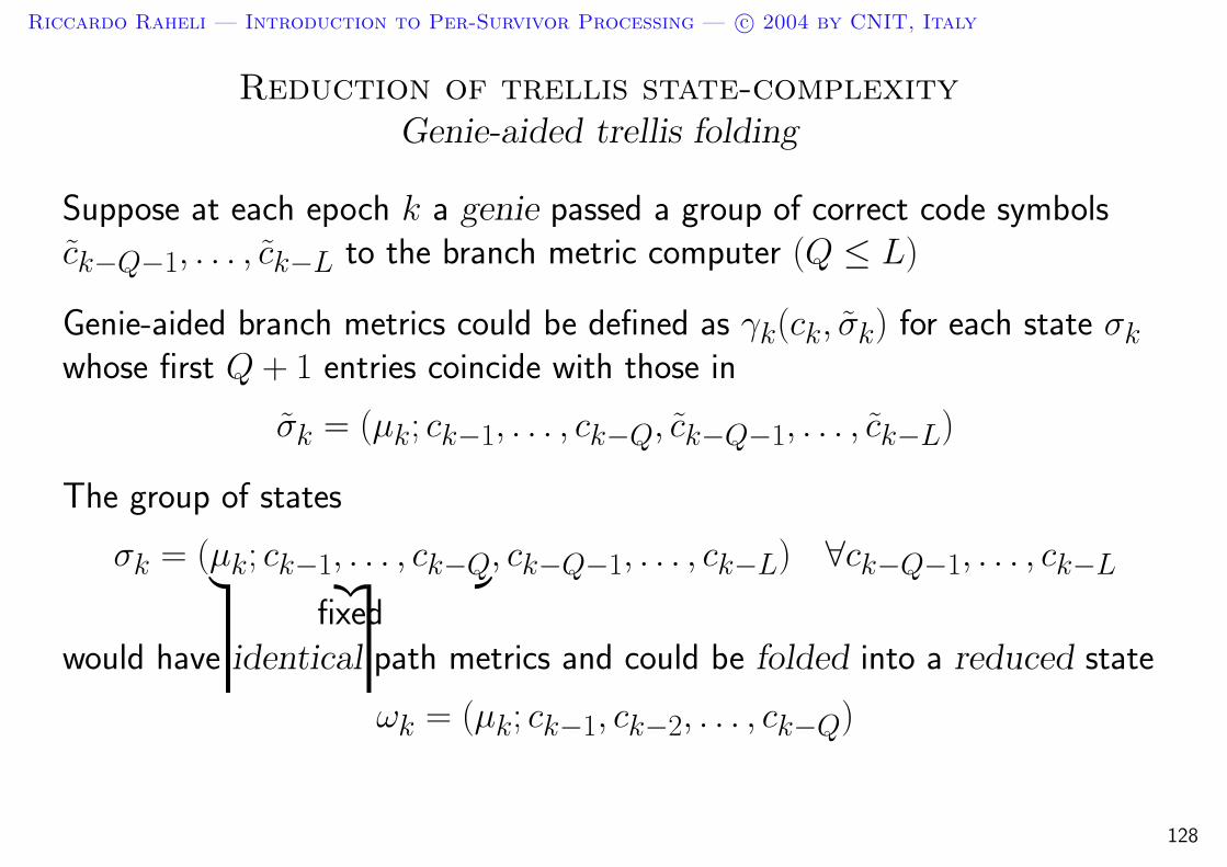
Riccardo Raheli — Introduction to Per-Survivor Processing — c© 2004 by CNIT, Italy
Reduction of trellis state-complexityGenie-aided trellis folding
Suppose at each epoch k a genie passed a group of correct code symbolsck−Q−1, . . . , ck−L to the branch metric computer (Q ≤ L)
Genie-aided branch metrics could be defined as γk(ck, σk) for each state σkwhose first Q + 1 entries coincide with those in
σk = (µk; ck−1, . . . , ck−Q, ck−Q−1, . . . , ck−L)
The group of states
σk = (µk; ck−1, . . . , ck−Q︸ ︷︷ ︸fixed
, ck−Q−1, . . . , ck−L) ∀ck−Q−1, . . . , ck−L
would have identical path metrics and could be folded into a reduced state
ωk = (µk; ck−1, ck−2, . . . , ck−Q)
128
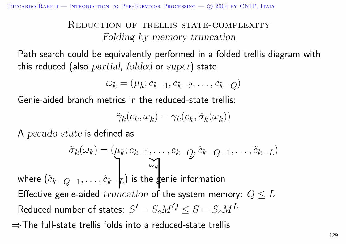
Riccardo Raheli — Introduction to Per-Survivor Processing — c© 2004 by CNIT, Italy
Reduction of trellis state-complexityFolding by memory truncation
Path search could be equivalently performed in a folded trellis diagram withthis reduced (also partial, folded or super) state
ωk = (µk; ck−1, ck−2, . . . , ck−Q)
Genie-aided branch metrics in the reduced-state trellis:
γk(ck, ωk) = γk(ck, σk(ωk))
A pseudo state is defined as
σk(ωk) = (µk; ck−1, . . . , ck−Q︸ ︷︷ ︸ωk
, ck−Q−1, . . . , ck−L)
where (ck−Q−1, . . . , ck−L) is the genie information
Effective genie-aided truncation of the system memory: Q ≤ L
Reduced number of states: S′ = ScMQ ≤ S = ScM
L
⇒The full-state trellis folds into a reduced-state trellis129
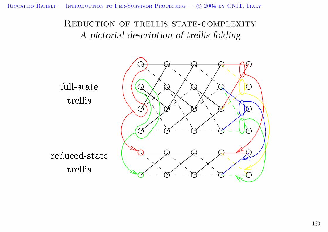
Riccardo Raheli — Introduction to Per-Survivor Processing — c© 2004 by CNIT, Italy
Reduction of trellis state-complexityA pictorial description of trellis folding
130

Riccardo Raheli — Introduction to Per-Survivor Processing — c© 2004 by CNIT, Italy
Reduction of trellis state-complexityInterpretation of trellis folding by memory truncation
The code symbols (ck−Q−1, . . . , ck−L) can be viewed as an undesired setof parameters
A parameter-conditional reduced memory property holds
The Estimation-Detection decomposition can be (again) the route to theapproximation of the branch metrics in the presence of this special parametricuncertainty
The genie information (ck−Q−1, . . . , ck−L) must be estimated in order toimplement detection schemes with reduced state-complexity
Curiosity: we do not need a data-aided parameter estimator but only theaiding code sequence
We can use tentative decisions or per-survivor processing131

Riccardo Raheli — Introduction to Per-Survivor Processing — c© 2004 by CNIT, Italy
Reduction of trellis state-complexityBranch metrics based on tentative-decision feedback
Branch metrics in the original full-state trellis: γk(ck, σk)
Branch metrics in the reduced-state trellis:
γk(ck, ωk) = γk(ck, σk(ωk))
The pseudo state is defined as
σk(ωk) = (µk; ck−1, . . . , ck−Q︸ ︷︷ ︸ωk
, ˆck−Q−1, . . . , ˆck−L)
ˆck−Q−1, . . . , ˆck−L are preliminary decisions on the code sequence
132

Riccardo Raheli — Introduction to Per-Survivor Processing — c© 2004 by CNIT, Italy
Reduction of trellis state-complexityBranch metrics based on PSP
Branch metrics in the original full-state trellis: γk(ck, σk)
Branch metrics in the reduced-state trellis:
γk(ck, ωk) = γk(ck, σk(ωk))
The pseudo state is defined as
σk(ωk) = (µk; ck−1, . . . , ck−Q︸ ︷︷ ︸ωk
, ck−Q−1(ωk), . . . , ck−L(ωk))
ck−Q−1(ωk), . . . , ck−L(ωk) are the code symbols in the survivor of state ωk
The pseudo state depends on ωk through the feedback of survivor symbols aswell
133
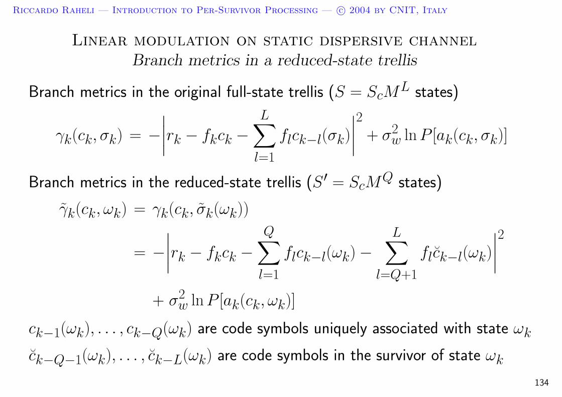
Riccardo Raheli — Introduction to Per-Survivor Processing — c© 2004 by CNIT, Italy
Linear modulation on static dispersive channelBranch metrics in a reduced-state trellis
Branch metrics in the original full-state trellis (S = ScML states)
γk(ck, σk) = −∣∣∣∣rk − fkck −
L∑
l=1
flck−l(σk)
∣∣∣∣2
+ σ2w ln P [ak(ck, σk)]
Branch metrics in the reduced-state trellis (S ′ = ScMQ states)
γk(ck, ωk) = γk(ck, σk(ωk))
= −∣∣∣∣rk − fkck −
Q∑
l=1
flck−l(ωk) −L∑
l=Q+1
flck−l(ωk)
∣∣∣∣2
+ σ2w ln P [ak(ck, ωk)]
ck−1(ωk), . . . , ck−Q(ωk) are code symbols uniquely associated with state ωk
ck−Q−1(ωk), . . . , ck−L(ωk) are code symbols in the survivor of state ωk
134

Riccardo Raheli — Introduction to Per-Survivor Processing — c© 2004 by CNIT, Italy
Reduction of trellis state-complexityFolding by set partitioning
State-complexity reduction can also be achieved replacing the code symbolsck−i in the “full” state
σk = (µk; ck−1, ck−2, . . . , ck−L)
with subsets of the code symbol alphabet (or constellation)
Define a reduced state
ωk = (µk; Ik−1(1), Ik−2(2), . . . , Ik−L(L))
At epoch k, for i = 1, 2, . . . , L:
Ik−i(i) ∈ Ω(i) are subsets of the code constellation AΩ(i) are partitions of the code constellation AA given reduced state specifies only the constellation subsets Ik−i(i)
ck−i ∈ Ik−i(i) are code symbols compatible with the given state
135
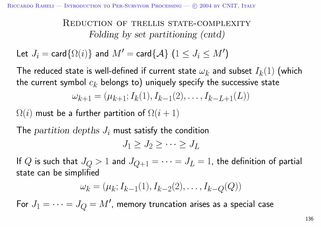
Riccardo Raheli — Introduction to Per-Survivor Processing — c© 2004 by CNIT, Italy
Reduction of trellis state-complexityFolding by set partitioning (cntd)
Let Ji = cardΩ(i) and M ′ = cardA (1 ≤ Ji ≤ M ′)
The reduced state is well-defined if current state ωk and subset Ik(1) (whichthe current symbol ck belongs to) uniquely specify the successive state
ωk+1 = (µk+1; Ik(1), Ik−1(2), . . . , Ik−L+1(L))
Ω(i) must be a further partition of Ω(i + 1)
The partition depths Ji must satisfy the condition
J1 ≥ J2 ≥ · · · ≥ JL
If Q is such that JQ > 1 and JQ+1 = · · · = JL = 1, the definition of partialstate can be simplified
ωk = (µk; Ik−1(1), Ik−2(2), . . . , Ik−Q(Q))
For J1 = · · · = JQ = M ′, memory truncation arises as a special case
136
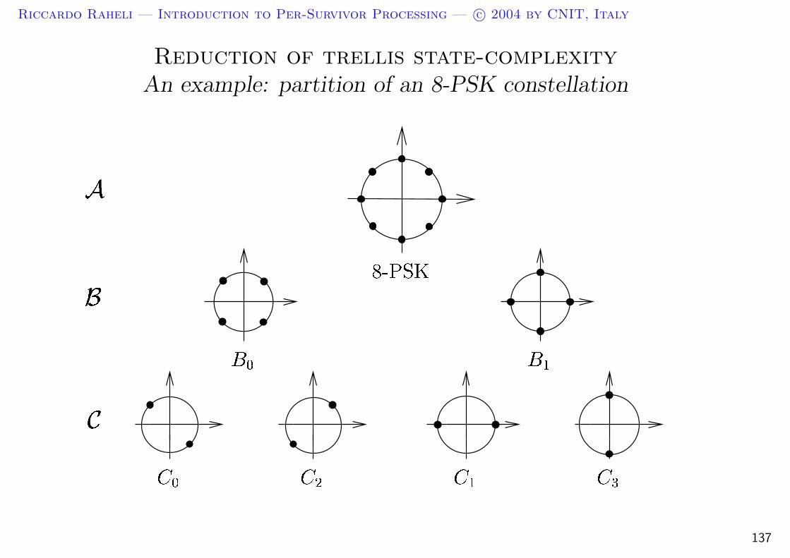
Riccardo Raheli — Introduction to Per-Survivor Processing — c© 2004 by CNIT, Italy
Reduction of trellis state-complexityAn example: partition of an 8-PSK constellation
137
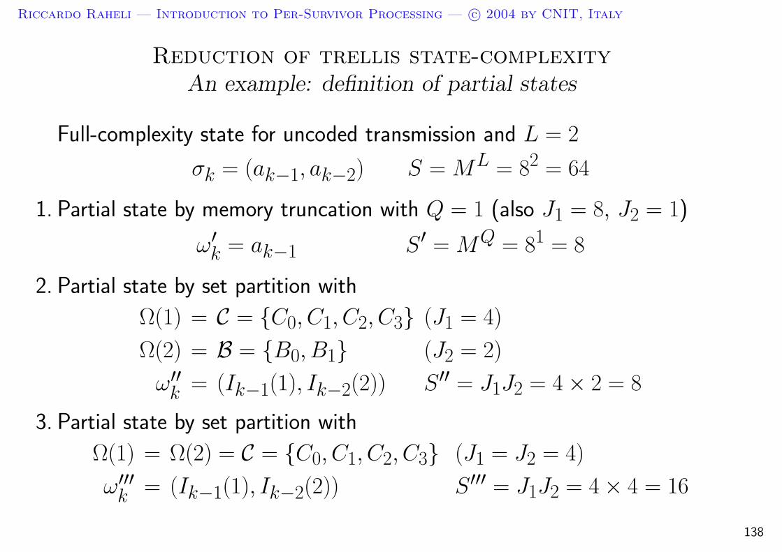
Riccardo Raheli — Introduction to Per-Survivor Processing — c© 2004 by CNIT, Italy
Reduction of trellis state-complexityAn example: definition of partial states
Full-complexity state for uncoded transmission and L = 2
σk = (ak−1, ak−2) S = ML = 82 = 64
1. Partial state by memory truncation with Q = 1 (also J1 = 8, J2 = 1)
ω′k = ak−1 S′ = MQ = 81 = 8
2. Partial state by set partition with
Ω(1) = C = C0, C1, C2, C3 (J1 = 4)
Ω(2) = B = B0, B1 (J2 = 2)
ω′′k = (Ik−1(1), Ik−2(2)) S′′ = J1J2 = 4 × 2 = 8
3. Partial state by set partition with
Ω(1) = Ω(2) = C = C0, C1, C2, C3 (J1 = J2 = 4)
ω′′′k = (Ik−1(1), Ik−2(2)) S′′′ = J1J2 = 4 × 4 = 16
138
Riccardo Raheli — Introduction to Per-Survivor Processing — c© 2004 by CNIT, Italy
Reduction of trellis state-complexityFolding by set partitioning: some remarks
Set partition should follow the partition rules used in Trellis CodedModulation (TCM)
If J1 < M ′, parallel transitions may be present (they are in the uncodedcase)
If J1 < M ′, state transitions and corresponding branch metrics are defined as(Ik(1), ωk) and γk(Ik(1), ωk), respectively
139
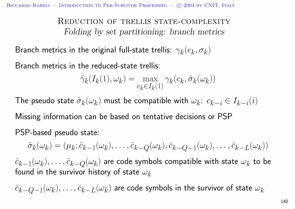
Riccardo Raheli — Introduction to Per-Survivor Processing — c© 2004 by CNIT, Italy
Reduction of trellis state-complexityFolding by set partitioning: branch metrics
Branch metrics in the original full-state trellis: γk(ck, σk)
Branch metrics in the reduced-state trellis:
γk(Ik(1), ωk) = maxck∈Ik(1)
γk(ck, σk(ωk))
The pseudo state σk(ωk) must be compatible with ωk: ck−i ∈ Ik−i(i)
Missing information can be based on tentative decisions or PSP
PSP-based pseudo state:
σk(ωk) = (µk; ck−1(ωk), . . . , ck−Q(ωk), ck−Q−1(ωk), . . . , ck−L(ωk))
ck−1(ωk), . . . , ck−Q(ωk) are code symbols compatible with state ωk to befound in the survivor history of state ωk
ck−Q−1(ωk), . . . , ck−L(ωk) are code symbols in the survivor of state ωk
140
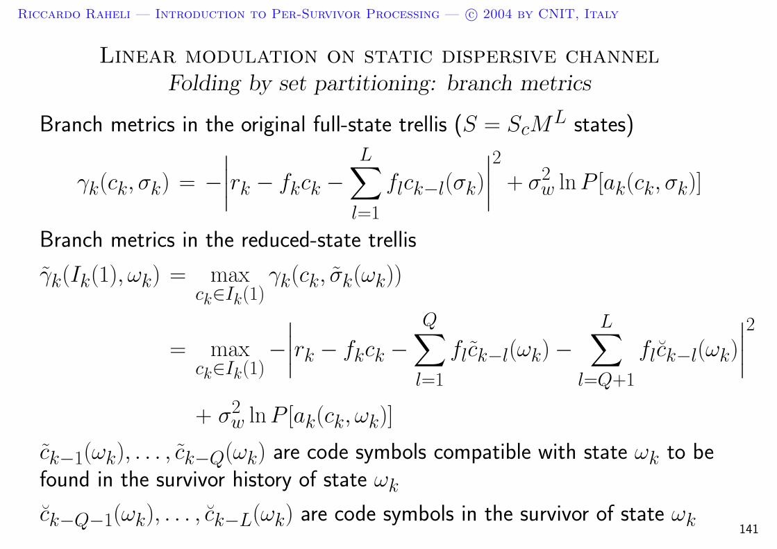
Riccardo Raheli — Introduction to Per-Survivor Processing — c© 2004 by CNIT, Italy
Linear modulation on static dispersive channelFolding by set partitioning: branch metrics
Branch metrics in the original full-state trellis (S = ScML states)
γk(ck, σk) = −∣∣∣∣rk − fkck −
L∑
l=1
flck−l(σk)
∣∣∣∣2
+ σ2w ln P [ak(ck, σk)]
Branch metrics in the reduced-state trellis
γk(Ik(1), ωk) = maxck∈Ik(1)
γk(ck, σk(ωk))
= maxck∈Ik(1)
−∣∣∣∣rk − fkck −
Q∑
l=1
flck−l(ωk) −L∑
l=Q+1
flck−l(ωk)
∣∣∣∣2
+ σ2w ln P [ak(ck, ωk)]
ck−1(ωk), . . . , ck−Q(ωk) are code symbols compatible with state ωk to befound in the survivor history of state ωk
ck−Q−1(ωk), . . . , ck−L(ωk) are code symbols in the survivor of state ωk141
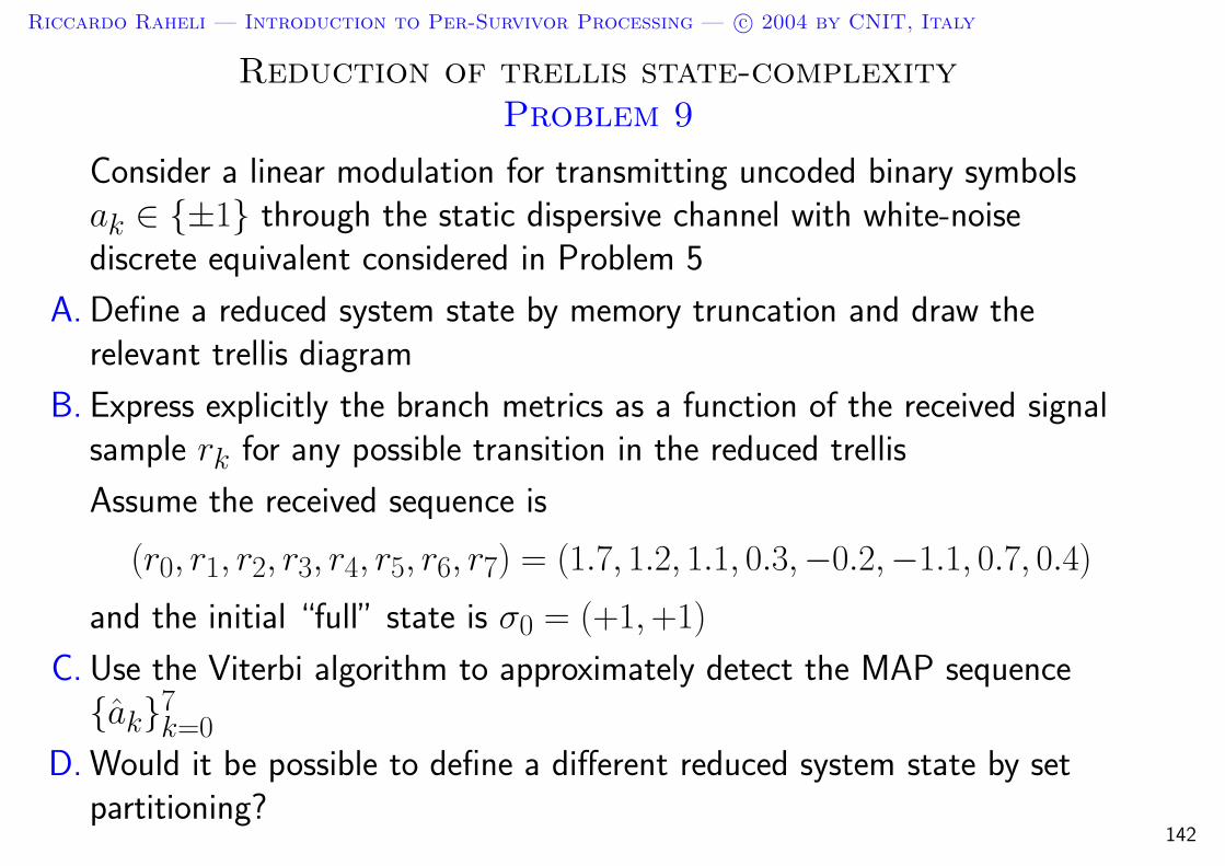
Riccardo Raheli — Introduction to Per-Survivor Processing — c© 2004 by CNIT, Italy
Reduction of trellis state-complexityProblem 9
Consider a linear modulation for transmitting uncoded binary symbolsak ∈ ±1 through the static dispersive channel with white-noisediscrete equivalent considered in Problem 5
A. Define a reduced system state by memory truncation and draw therelevant trellis diagram
B. Express explicitly the branch metrics as a function of the received signalsample rk for any possible transition in the reduced trellis
Assume the received sequence is
(r0, r1, r2, r3, r4, r5, r6, r7) = (1.7, 1.2, 1.1, 0.3,−0.2,−1.1, 0.7, 0.4)
and the initial “full” state is σ0 = (+1, +1)
C. Use the Viterbi algorithm to approximately detect the MAP sequenceak7
k=0
D. Would it be possible to define a different reduced system state by setpartitioning?
142

Riccardo Raheli — Introduction to Per-Survivor Processing — c© 2004 by CNIT, Italy
A case-study: TCM on ISI channelSystem model: encoder
! " #
$ %$ #
& &
& &
Information and code bits: a(i)k and c
(j)k
Gross spectral efficiency: 3 bit/s/Hz (to be reduced by the bandwidthexpansion factor 1 + α = 1.3 ⇒ net spectral efficiency is 2.3 bit/s/Hz)
143

Riccardo Raheli — Introduction to Per-Survivor Processing — c© 2004 by CNIT, Italy
TCM on ISI channelSystem model: set partition and mapping rule
2 bits per parallel transition (code trellis)144
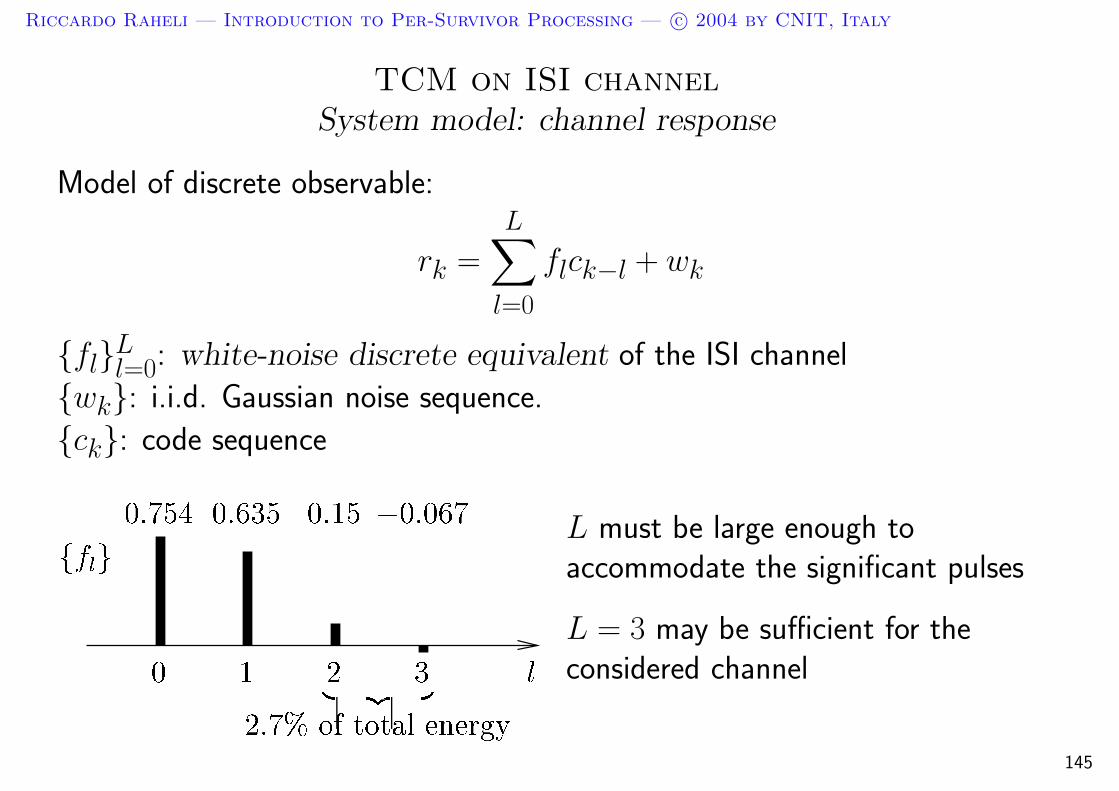
Riccardo Raheli — Introduction to Per-Survivor Processing — c© 2004 by CNIT, Italy
TCM on ISI channelSystem model: channel response
Model of discrete observable:
rk =
L∑
l=0
flck−l + wk
flLl=0: white-noise discrete equivalent of the ISI channel
wk: i.i.d. Gaussian noise sequence.
ck: code sequence
L must be large enough toaccommodate the significant pulses
L = 3 may be sufficient for theconsidered channel
145

Riccardo Raheli — Introduction to Per-Survivor Processing — c© 2004 by CNIT, Italy
TCM on ISI channelDefinition of partial states
0. Full-complexity state for L = 3
σk = (µk; ck−1, ck−2, ck−3) S = ScML = 4 × 83 = 4 × 29 = 2048
1. Partial state by memory truncation with Q = 1 (J1 = 16, J2 = J3 = 1)
ω′k = (µk; ck−1) S′ = ScM
Q = 4 × 81 = 32
2. Partial state by set partition with
Ω(1) = D = D0, D1, . . . , D7 (J1 = 8)
Ω(2) = Ω(3) = A (J2 = J3 = 1)
ω′′k = (µk; Ik−1(1)) S′′ = Sc
J1
2= 4 × 4 = 16
146
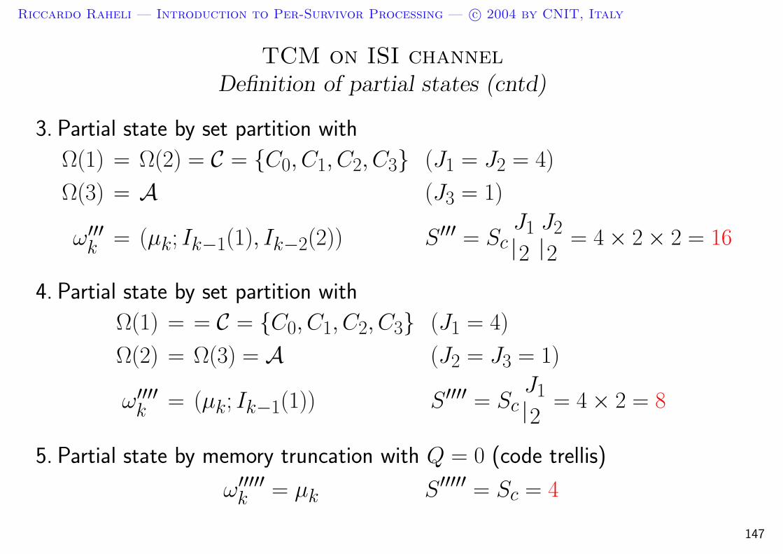
Riccardo Raheli — Introduction to Per-Survivor Processing — c© 2004 by CNIT, Italy
TCM on ISI channelDefinition of partial states (cntd)
3. Partial state by set partition with
Ω(1) = Ω(2) = C = C0, C1, C2, C3 (J1 = J2 = 4)
Ω(3) = A (J3 = 1)
ω′′′k = (µk; Ik−1(1), Ik−2(2)) S′′′ = Sc
J1
2
J2
2= 4 × 2 × 2 = 16
4. Partial state by set partition with
Ω(1) = = C = C0, C1, C2, C3 (J1 = 4)
Ω(2) = Ω(3) = A (J2 = J3 = 1)
ω′′′′k = (µk; Ik−1(1)) S′′′′ = Sc
J1
2= 4 × 2 = 8
5. Partial state by memory truncation with Q = 0 (code trellis)
ω′′′′′k = µk S′′′′′ = Sc = 4
147
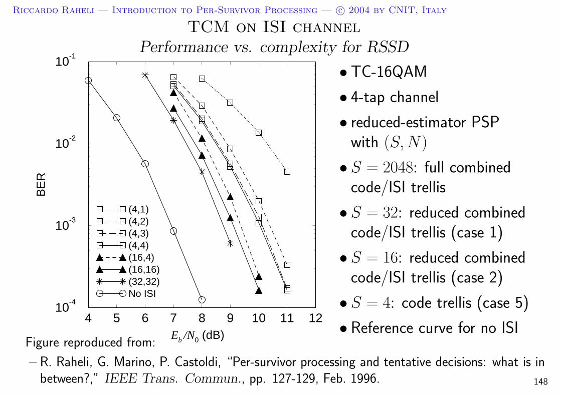
Riccardo Raheli — Introduction to Per-Survivor Processing — c© 2004 by CNIT, Italy
TCM on ISI channelPerformance vs. complexity for RSSD
4 5 6 7 8 9 10 11 12Eb /N0 (dB)
10-4
10-3
10-2
10-1
BE
R
(4,1)(4,2)(4,3)(4,4) (16,4)(16,16)(32,32)No ISI
• TC-16QAM
• 4-tap channel
• reduced-estimator PSPwith (S,N )
• S = 2048: full combinedcode/ISI trellis
• S = 32: reduced combinedcode/ISI trellis (case 1)
• S = 16: reduced combinedcode/ISI trellis (case 2)
• S = 4: code trellis (case 5)
• Reference curve for no ISIFigure reproduced from:
– R. Raheli, G. Marino, P. Castoldi, “Per-survivor processing and tentative decisions: what is inbetween?,” IEEE Trans. Commun., pp. 127-129, Feb. 1996. 148

Riccardo Raheli — Introduction to Per-Survivor Processing — c© 2004 by CNIT, Italy
Reduced-search algorithmsMotivation
Reduced-search (or sequential) algorithms may be used to search a small partof a large FSM trellis diagram or non-FSM tree diagram
As opposed to state-complexity reduction, the original full-complexity trellis(or tree) diagram is searched in a partial fashion
These algorithms date back to the pre-Viterbi algorithm era. They were firstproposed for decoding convolutional codes. The denomination “sequential”emphasizes the “novelty” compared to the then-established algebraicdecoding of block codes
These algorithms can be applied to any system characterized by large memoryor state complexity (if a FSM model hold)
If optimal processing is infeasible, any type of suboptimal processing maydeserve our attention. Ranking of suboptimal solutions is difficult because oflacking of reference criteria
RSSD must be considered but an alternative among many others149

Riccardo Raheli — Introduction to Per-Survivor Processing — c© 2004 by CNIT, Italy
Reduced-search algorithmsA general formulation of breadth-first detection
Assume a FSM model hold and let S be the number of states (full-size trellis)
Partition the S states into C (disjoint) classes
Mantain B paths per class selecting those which maximize the APPs underthe constraint imposed by the partition rule and class structure
The resulting search algorithm may be denoted as SA(B,C)
Special cases:
B > 1 and C = S ⇒ list Viterbi algorithms with B survivors per state
B = 1 and C = S ⇒ classical Viterbi algorithm
B = 1 and C < S ⇒ RSSD with C states
B > 1 and C < S ⇒ list RSSD with B survivors per state and C states
B = M and C = 1 ⇒ M-algorithm
150
Riccardo Raheli — Introduction to Per-Survivor Processing — c© 2004 by CNIT, Italy
Reduced-search algorithmsA general formulation of breadth-first detection (cntd)
Whenever C < S, PSP allows the branch metrics to be defined
PSP also allows the above formalization to be applied when an FSM modeldoes not hold (S → ∞)
Define the complexity level as the total number of paths being traced, i.e.,BC
Imposing a constraint on complexity, i.e., BC ≤ η, constrained optimalitycan be defined
According to this criterion, the M-algorithm is considered the constrainedoptimal search algorithm
– T. Aulin, “Breadth-first maximum likelihood sequence detection: basics,” IEEE Trans.Commun., pp. 208-216, Feb. 1999.
151
Riccardo Raheli — Introduction to Per-Survivor Processing — c© 2004 by CNIT, Italy
Complexity reductionBibliography
– J. B. Anderson, S. Mohan, “Sequential coding algorithms: A survey and cost analysis,”IEEE Trans. Commun., vol. 32, pp. 169-176, Feb. 1984.
– J. W. M. Bergmans, S. A. Rajput, F. A. M. Van De Laar, “On the use of DecisionFeedback for Simplifying the Viterbi Decoder,” Philips Journal of Research, No. 4, 1987.
– K. Wesolowski, “Efficient Digital Receiver Structure for Trellis-Coded Signals Transmittedthrough Channels with Intersymbol Interference,” Electronics Letters, Nov. 1987.
– T. Hashimoto, “A List-Type Reduced-Constraint Generalization of the Viterbi Algorithm,”IEEE Trans. Inform. Theory, pp. 866-876, Nov. 1987.
– M. V. Eyuboglu, S. U. H. Qureshi, “Reduced-State Sequence Estimation with Set Partitionand Decision Feedback,” IEEE Trans. Commun., pp. 13-20, Jan. 1988.
– A. Duel Hallen, C. Heegard, “Delayed Decision-Feedback Sequence Estimation,” IEEETrans. Commun., pp. 428-436, May 1989.
– P. R. Chevillat, E. Eleftheriou, “Decoding of Trellis-Encoded Signals in the Presence ofIntersymbol Interference and Noise,” IEEE Trans. Commun., pp. 669-676, July 1989.
– M. V. Eyuboglu, S. U. H. Qureshi, “Reduced-State Sequence Estimation for CodedModulation on Intersymbol Interference Channels,” IEEE J. Sel. Areas Commun., pp.989-995, Aug. 1989.
152

Riccardo Raheli — Introduction to Per-Survivor Processing — c© 2004 by CNIT, Italy
Complexity reductionBibliography (cntd)
– J. B. Anderson, “Limited search trellis decoding of convolutional codes,” IEEE Trans.Inform. Theory, pp. 944-955, Sept. 1989.
– S. J. Simmons, “Breadth-first trellis decoding with adaptive effort,” IEEE Trans.Commun., vol. 38, pp. 3-12, Jan. 1990.
– A. Svensson, “Reduced state sequence detection of full response continuous phasemodulation,“ IEE Electronics Letters, pp. 652 -654, 1 May 1990.
– J. B. Anderson, E. Offer, “Reduced-state sequence detection with convolutional codes,”IEEE Trans. Inform. Theory, pp. 965-972, May 1994.
– R. Raheli, A. Polydoros, C. K. Tzou, “Per-survivor processing: a general approach to MLSEin uncertain environments,” IEEE Trans. Commun., pp. 354-364, Feb.-Apr. 1995.
– R. Raheli, G. Marino, P. Castoldi, “Per-survivor processing and tentative decisions: what isin between?,” IEEE Trans. Commun., pp. 127-129, Feb. 1996.
– T. Aulin, “Breadth-first maximum likelihood sequence detection: basics,” IEEE Trans.Commun., pp. 208-216, Feb. 1999.
153

Riccardo Raheli — Introduction to Per-Survivor Processing — c© 2004 by CNIT, Italy
4. Classical applications of PSP
4.2 Linear predictive detection for fading channels
Outline
1. Review of detection techniques
2. Detection under parametric uncertainty
3. Per-Survivor Processing (PSP): concept and historical review
4. Classical applications of PSP:
4.1 Complexity reduction
4.2 Linear predictive detection for fading channels
4.3 Adaptive detection
5. Advanced applications of PSP
154

Riccardo Raheli — Introduction to Per-Survivor Processing — c© 2004 by CNIT, Italy
Linear modulation on flat fading channelSystem model
Model of discrete observable:
rk = fk ck + wk
fk: circular complex Gaussian random sequence
ck: code sequence
wk: i.i.d. Gaussian noise sequence with variance σ2w
Coding rule: ck = o(ak, µk)
µk+1 = t(ak, µk)
µk: encoder state
Conditional statistics of the observation are Gaussian
155

Riccardo Raheli — Introduction to Per-Survivor Processing — c© 2004 by CNIT, Italy
Linear modulation on flat fading channelDoes a FSM model hold?
Conditional statistics of the observation:
p(rk|rk−10 , ak
0) =1
πσ2k(ak
0)exp
[− |rk − rk(ak
0)|2
σ2k(ak
0)
]
Conditional meanrk(ak
0) = Erk|rk−10 , ak
0
Conditional variance
σ2k(ak
0) = E|rk − rk(ak0)|2 |rk−1
0 , ak0
The conditional mean and variance depend on the entire previous codesequence:
⇒ unlimited memory
156
Riccardo Raheli — Introduction to Per-Survivor Processing — c© 2004 by CNIT, Italy
Linear predictive detectionMarkov assumption
These receivers are based on the approximation
p(rk|rk−10 , ak
0) ' p(rk|rk−1k−ν, a
k0)
where integer ν > 0 must be sufficiently large
Intuitive motivation: “old” observations do not add up much information tothe current observation, given the immediately preceding ones
If this condition were strictly met, the random sequence rk would be Markovof order ν, conditionally upon ak
0
This Markov assumption is never verified in an exact sense for realistic fadingmodels. Even assuming a Markov fading model, thermal noise destroys theMarkovianity in the observation.
The quality of this approximation depends on the autocovariance sequence ofthe fading process fk and the value of ν, which is an important designparameter
157
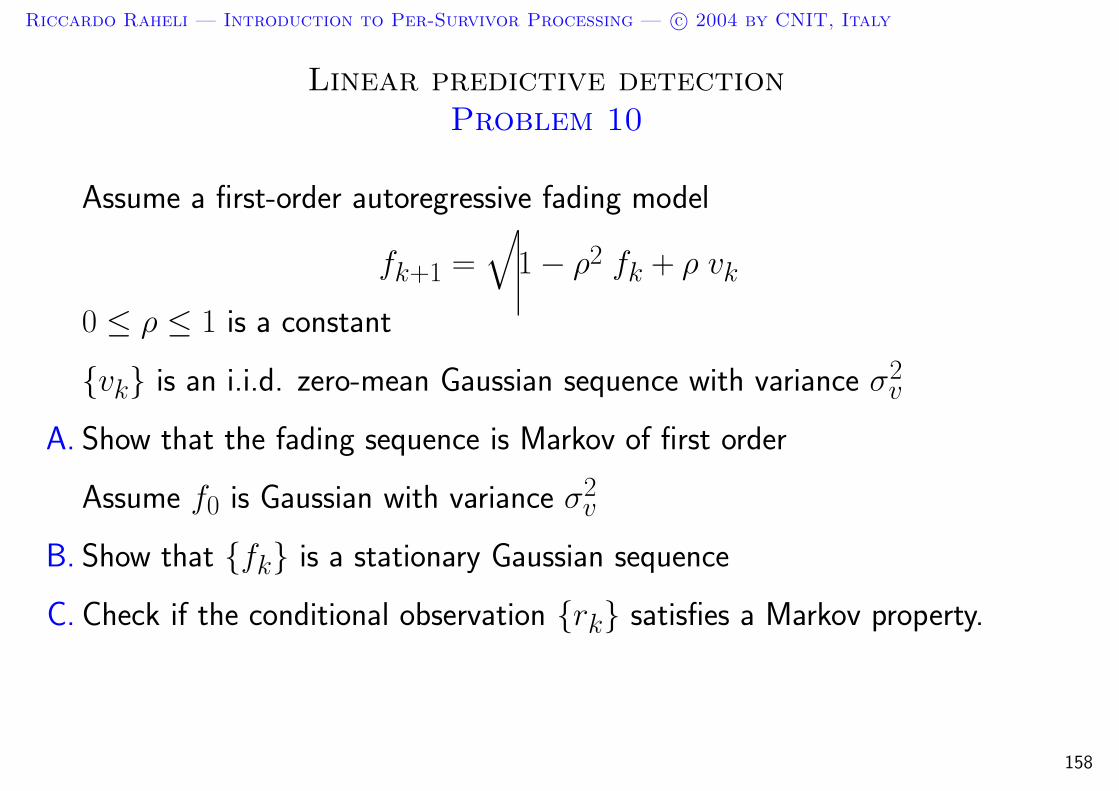
Riccardo Raheli — Introduction to Per-Survivor Processing — c© 2004 by CNIT, Italy
Linear predictive detectionProblem 10
Assume a first-order autoregressive fading model
fk+1 =
√1 − ρ2 fk + ρ vk
0 ≤ ρ ≤ 1 is a constant
vk is an i.i.d. zero-mean Gaussian sequence with variance σ2v
A. Show that the fading sequence is Markov of first order
Assume f0 is Gaussian with variance σ2v
B. Show that fk is a stationary Gaussian sequence
C. Check if the conditional observation rk satisfies a Markov property.
158
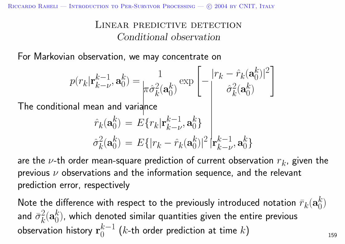
Riccardo Raheli — Introduction to Per-Survivor Processing — c© 2004 by CNIT, Italy
Linear predictive detectionConditional observation
For Markovian observation, we may concentrate on
p(rk|rk−1k−ν, a
k0) =
1
πσ2k(ak
0)exp
[− |rk − rk(ak
0)|2
σ2k(ak
0)
]
The conditional mean and variance
rk(ak0) = Erk|rk−1
k−ν, ak0
σ2k(ak
0) = E|rk − rk(ak0)|2 |rk−1
k−ν, ak0
are the ν-th order mean-square prediction of current observation rk, given theprevious ν observations and the information sequence, and the relevantprediction error, respectively
Note the difference with respect to the previously introduced notation rk(ak0)
and σ2k(ak
0), which denoted similar quantities given the entire previous
observation history rk−10 (k-th order prediction at time k)
159
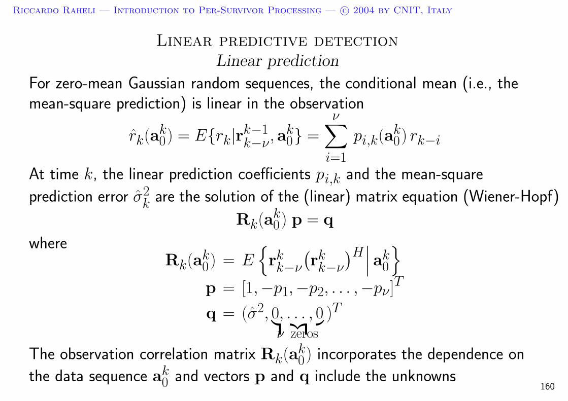
Riccardo Raheli — Introduction to Per-Survivor Processing — c© 2004 by CNIT, Italy
Linear predictive detectionLinear prediction
For zero-mean Gaussian random sequences, the conditional mean (i.e., themean-square prediction) is linear in the observation
rk(ak0) = Erk|rk−1
k−ν, ak0 =
ν∑
i=1
pi,k(ak0) rk−i
At time k, the linear prediction coefficients pi,k and the mean-square
prediction error σ2k are the solution of the (linear) matrix equation (Wiener-Hopf)
Rk(ak0) p = q
whereRk(ak
0) = Erkk−ν
(rkk−ν
)H∣∣∣ ak
0
p = [1,−p1,−p2, . . . ,−pν]T
q = (σ2, 0, . . . , 0︸ ︷︷ ︸ν zeros
)T
The observation correlation matrix Rk(ak0) incorporates the dependence on
the data sequence ak0 and vectors p and q include the unknowns
160
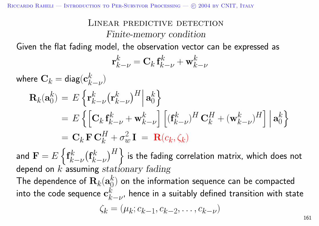
Riccardo Raheli — Introduction to Per-Survivor Processing — c© 2004 by CNIT, Italy
Linear predictive detectionFinite-memory condition
Given the flat fading model, the observation vector can be expressed as
rkk−ν = Ck fk
k−ν + wkk−ν
where Ck = diag(ckk−ν)
Rk(ak0) = E
rkk−ν
(rkk−ν
)H∣∣∣ ak
0
= E[
Ck fkk−ν + wk
k−ν
] [(fk
k−ν)H CHk + (wk
k−ν)H] ∣∣∣ ak
0
= Ck FCHk + σ2
w I = R(ck, ζk)
and F = Efkk−ν
(fkk−ν
)H
is the fading correlation matrix, which does not
depend on k assuming stationary fading
The dependence of Rk(ak0) on the information sequence can be compacted
into the code sequence ckk−ν, hence in a suitably defined transition with state
ζk = (µk; ck−1, ck−2, . . . , ck−ν)161
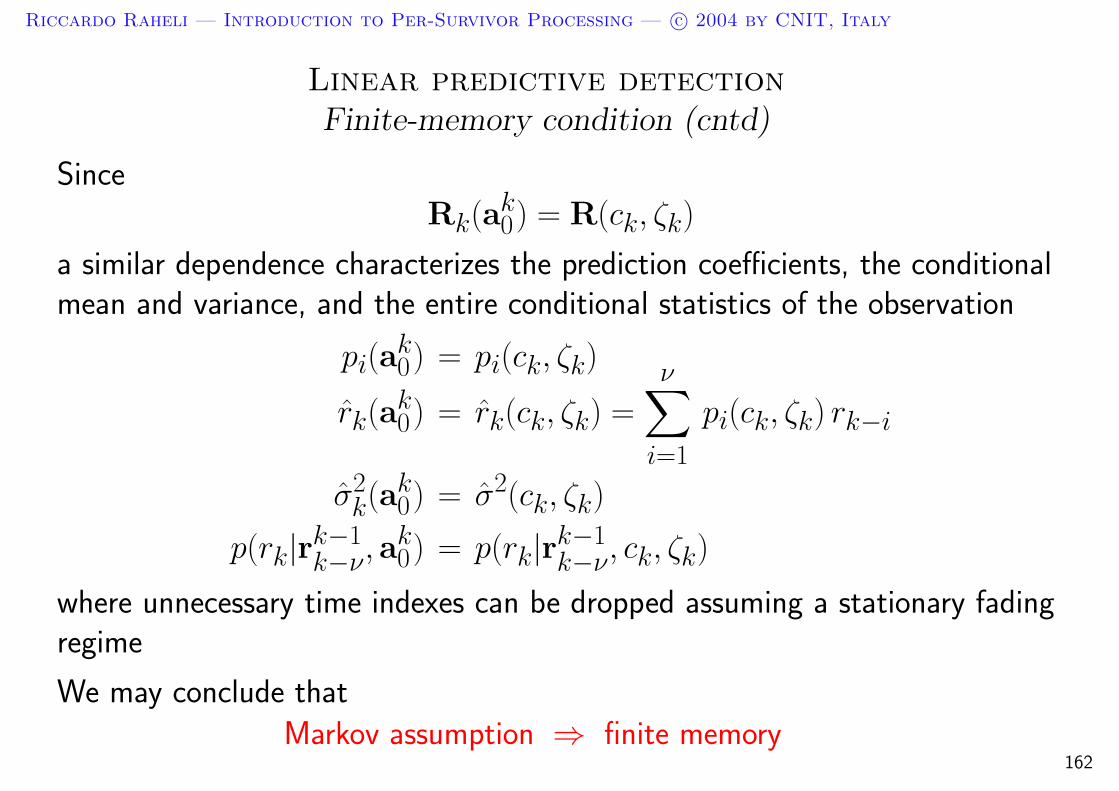
Riccardo Raheli — Introduction to Per-Survivor Processing — c© 2004 by CNIT, Italy
Linear predictive detectionFinite-memory condition (cntd)
SinceRk(ak
0) = R(ck, ζk)
a similar dependence characterizes the prediction coefficients, the conditionalmean and variance, and the entire conditional statistics of the observation
pi(ak0) = pi(ck, ζk)
rk(ak0) = rk(ck, ζk) =
ν∑
i=1
pi(ck, ζk) rk−i
σ2k(ak
0) = σ2(ck, ζk)
p(rk|rk−1k−ν, a
k0) = p(rk|rk−1
k−ν, ck, ζk)
where unnecessary time indexes can be dropped assuming a stationary fadingregime
We may conclude that
Markov assumption ⇒ finite memory162

Riccardo Raheli — Introduction to Per-Survivor Processing — c© 2004 by CNIT, Italy
Linear predictive detectionProblem 11
Assume xk is a stationary time-discrete random process withautocorrelation sequence Exk+mx∗k = ρm
Let xk =∑ν
i=1 pixk−i denote the linear prediction of xk, given theprevious ν samples xk−1, xk−2, . . . , xk−ν. The prediction coefficientspiν
i=1 minimize the mean-square prediction error σ2 = E|xk − xk|2A. Show that the prediction coefficients piν
i=1 and the minimum
prediction error σ2 are the solution of the Wiener-Hopf equation
X p = q
whereX = E
xk
k−ν
(xk
k−ν
)H
p = [1,−p1,−p2, . . . ,−pν]T
q = (σ2, 0, . . . , 0︸ ︷︷ ︸ν zeros
)T
B. Show that the linear prediction coincides with the mean-square predictionwhen xk is a zero-mean Gaussian sequence 163
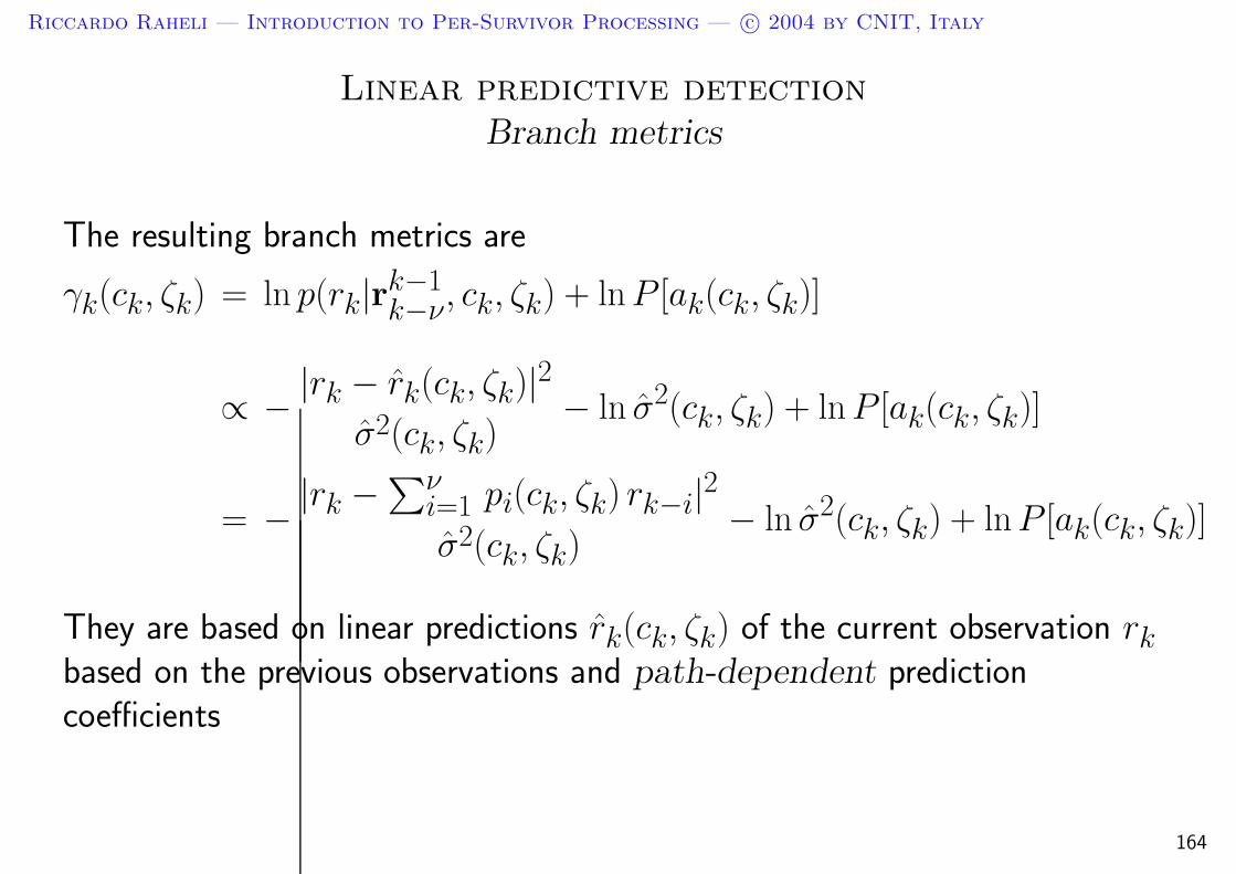
Riccardo Raheli — Introduction to Per-Survivor Processing — c© 2004 by CNIT, Italy
Linear predictive detectionBranch metrics
The resulting branch metrics are
γk(ck, ζk) = ln p(rk|rk−1k−ν, ck, ζk) + ln P [ak(ck, ζk)]
∝ − |rk − rk(ck, ζk)|2σ2(ck, ζk)
− ln σ2(ck, ζk) + ln P [ak(ck, ζk)]
= − |rk −∑ν
i=1 pi(ck, ζk) rk−i|2σ2(ck, ζk)
− ln σ2(ck, ζk) + ln P [ak(ck, ζk)]
They are based on linear predictions rk(ck, ζk) of the current observation rkbased on the previous observations and path-dependent predictioncoefficients
164
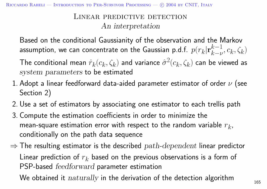
Riccardo Raheli — Introduction to Per-Survivor Processing — c© 2004 by CNIT, Italy
Linear predictive detectionAn interpretation
Based on the conditional Gaussianity of the observation and the Markovassumption, we can concentrate on the Gaussian p.d.f. p(rk|rk−1
k−ν, ck, ζk)
The conditional mean rk(ck, ζk) and variance σ2(ck, ζk) can be viewed assystem parameters to be estimated
1. Adopt a linear feedforward data-aided parameter estimator of order ν (seeSection 2)
2. Use a set of estimators by associating one estimator to each trellis path
3. Compute the estimation coefficients in order to minimize themean-square estimation error with respect to the random variable rk,conditionally on the path data sequence
⇒ The resulting estimator is the described path-dependent linear predictor
Linear prediction of rk based on the previous observations is a form ofPSP-based feedforward parameter estimation
We obtained it naturally in the derivation of the detection algorithm165
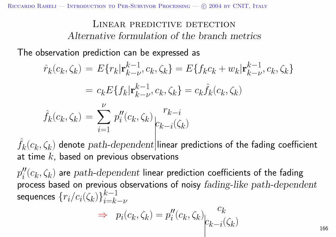
Riccardo Raheli — Introduction to Per-Survivor Processing — c© 2004 by CNIT, Italy
Linear predictive detectionAlternative formulation of the branch metrics
The observation prediction can be expressed as
rk(ck, ζk) = Erk|rk−1k−ν, ck, ζk = Efkck + wk|rk−1
k−ν, ck, ζk
= ckEfk|rk−1k−ν, ck, ζk = ckfk(ck, ζk)
fk(ck, ζk) =
ν∑
i=1
p′′i (ck, ζk)rk−i
ck−i(ζk)
fk(ck, ζk) denote path-dependent linear predictions of the fading coefficientat time k, based on previous observations
p′′i (ck, ζk) are path-dependent linear prediction coefficients of the fadingprocess based on previous observations of noisy fading-like path-dependentsequences ri/ci(ζk)k−1
i=k−ν
⇒ pi(ck, ζk) = p′′i (ck, ζk)ck
ck−i(ζk)166

Riccardo Raheli — Introduction to Per-Survivor Processing — c© 2004 by CNIT, Italy
Linear predictive detectionAlternative formulation of the branch metrics (cntd)
The mean-square prediction error of observation and fading are similarlyrelated by
σ2(ck, ζk) = E|rk − rk(ck, ζk)|2|rk−1k−ν, ck, ζk
= E|fkck + wk − ckfk(ck, ζk)|2|rk−1k−ν, ck, ζk
= |ck|2ε2(ck, ζk) + σ2w
ε2(ck, ζk) = E|fk − fk(ck, ζk)|2|rk−1k−ν, ck, ζk
The branch metrics can be expressed as
γk(ck, ζk) = − |rk − ckfk(ck, ζk)|2|ck|2ε2(ck, ζk) + σ2
w− ln
[|ck|2ε2(ck, ζk) + σ2
w
]
+ ln P [ak(ck, ζk)]
167
Riccardo Raheli — Introduction to Per-Survivor Processing — c© 2004 by CNIT, Italy
Linear predictive detectionAn interpretation of the alternative formulation
The observation model rk = fkck + wk satisfies a parameter-conditionalfinite memory property by viewing fk as an undesired parameter (seeSection 2)
For estimating this parameter we could:
1. Adopt a linear feedforward data-aided parameter estimator of order ν (seeSection 2)
2. Use a set of estimators by associating one estimator to each trellis path
3. Compute the estimation coefficients in order to minimize themean-square estimation error with respect to the random variable rk/ck,conditionally on the path data sequence
⇒ The resulting estimator is exactly the described path-dependent linearpredictor
Linear prediction of fk based on the previous observations is a form ofPSP-based feedforward parameter estimation
168

Riccardo Raheli — Introduction to Per-Survivor Processing — c© 2004 by CNIT, Italy
Linear predictive detectionComputation of the fading prediction coefficients
The fading prediction coefficients p′′i (ck, ζk) and mean-square prediction error
ε2(ck, ζk) are the solution of the following Wiener-Hopf equation(F + σ2
wCk
)p′′ = q′′
whereF = E
fkk−ν
(fkk−ν
)H
Ck = diag(
1|ck|2
, 1|ck−1|2
, . . . , 1|ck−ν|2
)
p′′ =[1,−p′′1 ,−p′′2 , . . . ,−p′′ν
]T
q′′ = (ε2 +σ2
w|ck|2
, 0, . . . , 0︸ ︷︷ ︸ν zeros
)T
The dependence of the solution on the hypothetical sequence is only throughthe moduli of the code symbols
For code symbols with constant modulus, the solution is path-independent169
Riccardo Raheli — Introduction to Per-Survivor Processing — c© 2004 by CNIT, Italy
Linear predictive detectionSpecial case: Coded PSK
For code symbols with constant modulus |ck| = 1 (e.g., PSK), the fadingprediction coefficients p′′i and mean-squared prediction error ε2 arepath-independent
The branch metrics simplify as
γk(ck, ζk) = − |rk − ckfk(ζk)|2 + (ε2 + σ2w) ln P [ak(ck, ζk)]
= −∣∣∣∣rk − ck
ν∑
i=1
p′′irk−i
ck−i(ζk)
∣∣∣∣2
+ (ε2 + σ2w) ln P [ak(ck, ζk)]
This solution is remarkably similar to what we would obtain in a decomposedestimation-detection design by estimating the “undesired” parameter fkaccording to PSP
The (Gaussian) prediction error variance ε2 affects the “overall” thermal noisepower
170
Riccardo Raheli — Introduction to Per-Survivor Processing — c© 2004 by CNIT, Italy
Linear predictive detectionProblem 12
Consider the mean-square prediciton of fk given the previous ν fading
samples fk−1k−ν and let p′iν
i=1 denote the linear prediction coefficients forthis problem
A. Show that the fading prediction coefficients p′′i (ck, ζk)νi=1 equal
p′iνi=1 in the limit of vanishing noise power
Consider the first-order autoregressive fading model described inProblem 10 in a stationary regime and a constellation of unit-moduluscode symbols
B. Show that the ν-th order prediction coefficients p′iνi=1 satisfy p′1 = ρ,
p′2 = · · · = p′ν = 0
C. Show that the ν-th order prediction coefficients p′′i νi=1 are not zero for
σ2w 6= 0
171

Riccardo Raheli — Introduction to Per-Survivor Processing — c© 2004 by CNIT, Italy
Linear predictive detectionState-complexity reduction
The state-complexity of a linear predicition receiver can be naturallydecoupled from the prediction order ν by means of state reduction techniques
For simplicity we consider folding by memory truncation, but set partitioningcould be used as well
Let Q < ν denote the memory parameter to be taken into account in thedefinition of reduced trellis state
ωk = (µk; ck−1, ck−2, . . . , ck−Q)
The branch metrics can be obtained by defining a pseudo state
ζk(ωk) = (µk; ck−1, . . . , ck−Q︸ ︷︷ ︸ωk
, ck−Q−1(ωk), . . . , ck−ν(ωk))
ck−Q−1(ωk), . . . , ck−L(ωk) are the code symbols in the survivor of state ωk
172

Riccardo Raheli — Introduction to Per-Survivor Processing — c© 2004 by CNIT, Italy
Linear predictive detectionState-complexity reduction: branch metrics
The branch metrics in the reduced-state trellis can be defined as usualaccording to
γk(ck, ωk) = γk(ck, ζk(ωk))
For coded PSK the branch metrics are
γk(ck, ωk) = − |rk − ckfk(ζk(ωk))|2 + (ε2 + σ2w) ln P [ak(ck, ωk)]
= −∣∣∣∣rk − ck
Q∑
i=1
p′′irk−i
ck−i(ωk)− ck
ν∑
i=Q+1
p′′irk−i
ck−i(ωk)
∣∣∣∣2
+ (ε2 + σ2w) ln P [ak(ck, ωk)]
The prediction order ν and assumed memory Q are design parameters to bejointly optimized by experiment to yield a good compromise betweenperformance and complexity
173

Riccardo Raheli — Introduction to Per-Survivor Processing — c© 2004 by CNIT, Italy
Linear predictive detectionPerformance vs. ideal CSI
•QPSK (M = 4)
• time-varying flat Rayleigh fading
•BT : max Doppler rate
• ν = 10, Q = 2 (16 states)
• Periodically inserted pilot symbols(one every 9 data symbols)
• Reference curve for idealchannel state information (CSI)
Figure reproduced from:
– G. M. Vitetta, D. P. Taylor, “Maximum likelihood decoding of uncoded and coded PSK signalsequences transmitted over Rayleigh flat-fading channels,” IEEE Trans. Commun., vol. 43,pp. 2750-2758, Nov. 1995 174

Riccardo Raheli — Introduction to Per-Survivor Processing — c© 2004 by CNIT, Italy
Linear predictive detectionBibliography
– J. Lodge, M. Moher, “ML estimation of CPM signals transmitted over Rayleigh flat fadingchannels,” IEEE Trans. Commun., pp. 787-794, June 1990.
– D. Makrakis, P. T. Mathiopoulos, D. P. Bouras, “Optimal decoding of coded PSK andQAM signals in correlated fast fading channels and AWGN: a combined envelope, multipledifferential and coherent detection approach,” IEEE Trans. Commun., pp.63-75,Jan. 1994.
– Q. Dai, E. Shwedyk, “Detection of bandlimited signals over frequency selective Rayleighfading channels,” IEEE Trans. Commun., pp. 941-950, Feb.-Apr. 1994.
– X. Yu, S. Pasupathy, “Innovations-based MLSE for Rayleigh fading channels,” IEEETrans. Commun., pp. 1534-Feb.-Apr. 1995.
– G. M. Vitetta, D. P. Taylor, “Maximum likelihood decoding of uncoded and coded PSKsignal sequences transmitted over Rayleigh flat-fading channels,” IEEE Trans.Commun., vol. 43, pp. 2750-2758, Nov. 1995
– G. M. Vitetta, D. P. Taylor, U. Mengali, “Double filtering receivers for PSK signalstransmitted over Rayleigh frequency-flat fading channels,” IEEE Trans. Commun., vol.44, pp. 686-695, June 1996.
175
Riccardo Raheli — Introduction to Per-Survivor Processing — c© 2004 by CNIT, Italy
Linear predictive detectionBibliography (cntd)
– D. M. Matolak, S. G. Wilson, “Detection for a statistically known, time-varying dispersivechannel,” vol. 44, pp. 1673-1683, Dec. 1996.
– M. E. Rollins, S. J. Simmons, “Simplified per-survivor Kalman processing in fastfrequency-selective fading channels,” IEEE Trans. Commun., pp. 544-553, May 1997.
– P. Castoldi, R. Raheli, “On recursive optimal detection of linear modulations in thepresence of random fading”, European Trans. Telecommun. (ETT), vol. 9, no. 2, pp.209-220, March-April 1998.
– G. Colavolpe, P. Castoldi, R. Raheli, “Linear predictive receivers for fading channels”, IEEElectronics Letters, vol. 34, no. 13, pp. 1289-1290, 25th June 1998.
176

Riccardo Raheli — Introduction to Per-Survivor Processing — c© 2004 by CNIT, Italy
4. Classical applications of PSP
4.3 Adaptive detection
Outline
1. Review of detection techniques
2. Detection under parametric uncertainty
3. Per-Survivor Processing (PSP): concept and historical review
4. Classical applications of PSP:
4.1 Complexity reduction
4.2 Linear predictive detection for fading channels
4.3 Adaptive detection
5. Advanced applications of PSP
177

Riccardo Raheli — Introduction to Per-Survivor Processing — c© 2004 by CNIT, Italy
Adaptive detectionMotivation
Channel model parameters can be time-varying (e.g., carrier phase, timingepoch, and channel impulse response)
A receiver based on the estimation-detection decomposition must be able totrack these time variations, provided they are not too fast
The receiver must adapt itself to the time-varying channel conditions
PSP may be useful in adaptive receivers:
a) The per-survivor estimator associated with the best survivor is derived fromdata information which can be perceived as high-quality zero-delay decisions
⇒ Useful in fast time-varying channels
b) Many hypothetical data sequences are simultaneously considered in theparameter estimation process
⇒ Acquisition without training (blind) may be facilitated
178

Riccardo Raheli — Introduction to Per-Survivor Processing — c© 2004 by CNIT, Italy
Adaptive detectionPSP-based feedforward parameter estimation
Assume a parameter-conditional FSM model with state σk
PSP-based feedforward data-aided parameter estimator at time k
θk(σk) = p[rk−1k−ν, c
k−10 (σk)
]
Function of the ν most recent signal observations rk−1k−ν and the per-survivor
aiding data sequence ck−10 (σk)
Branch metrics at time k
γk(ak, σk) = ln p[rk|rk−1
0 , ak, σk, θk(σk)]
+ ln P (ak)
Update of the parameter estimator at time k + 1
θk+1(σk+1) = p[rkk−ν+1, c
k0(σk+1)
]
These estimates are simply recomputed for the new observation vectorrkk−ν+1 and each new survivor sequence ck
0(σk+1)
An example is the linear predictive receiver for fading channels 179

Riccardo Raheli — Introduction to Per-Survivor Processing — c© 2004 by CNIT, Italy
Adaptive detectionPSP-based feedback parameter estimation
Assume a parameter-conditional FSM model with state σk
PSP-based feedback data-aided parameter estimator θk(σk)
Branch metrics
γk(ak, σk) = ln p[rk|rk−1
0 , ak, σk, θk(σk)]
+ ln P (ak)
Update of the parameter estimator
θk+1(σk+1) = q[θ
kk−ξ+1(σk), rk
k−ν+1, ck0(σk+1)
]
These estimates are computed for the ν most recent observations rkk−ν+1
and each new survivor sequence ck0(σk+1)
The previous ξ parameter values θkk−ξ+1(σk) are those associated with the
survivors of states σk in the transitions (σk → σk+1) selected during the ACSstep
Feedback parameter estimation is usually implied in adaptive receivers 180

Riccardo Raheli — Introduction to Per-Survivor Processing — c© 2004 by CNIT, Italy
Adaptive detectionTentative decisions can be used
In feedforward and feedback parameter estimation, tentative decisions ˆck0
can be used in place of the survivor data sequences ck0(σk+1) for updating
the parameter estimate
The parameter estimate becomes universal, i.e., identical for all survivors
Formally, the updating recursions yield identical estimates for all survivors
The parameter estimator becomes external to the detection block
During training the correct data sequence would be used
181

Riccardo Raheli — Introduction to Per-Survivor Processing — c© 2004 by CNIT, Italy
Tracking of a dispersive time-varying channelSystem model and notation
Model of linearly modulated discrete observable (slow variation)
rk =
L∑
l=0
fl,k ck−l + wk = fTk ck + wk
fk = (f0,k, f1,k, . . . , fL,k)T : overall time-varying discrete equivalent impulseresponse at the k-th instant
ck = (ck, ck−1, . . . , ck−L)T : code sequence with FSM model of state µk
σk = (ak−1, ak−2, . . . , ak−L; µk−L) : system state
ck(ak, σk) = [ck(ak, µk), ck−1(ak−1, µk−1), . . . , ck−L(ak−L, µk−L)]T :code symbol vector uniquely associated with the considered trellis branch(ak, σk), in accordance with the coding rule
182

Riccardo Raheli — Introduction to Per-Survivor Processing — c© 2004 by CNIT, Italy
Tracking of a dispersive time-varying channelLMS adaptive identification
Least Mean Squares (LMS) adaptive identification
fk+1 = fk + β (rk+1−d − fTk ck+1−d) c∗k+1−d
β compromises between adaptation speed and algorithm stability
Branch metrics
γk(ak, σk) = −|rk − fTk ck(ak, σk)|2 + σ2
w ln P (ak)
In the (tentative) decision-directed tracking mode
fk+1 = fk + β (rk+1−d − fTk
ˆck+1−d)ˆc∗k+1−d
ˆck+1−d = (ˆck+1−d, ˆck−d, . . . , ˆck+1−d−L)T
d ≥ 1 to comply with the causality condition upon the data
183
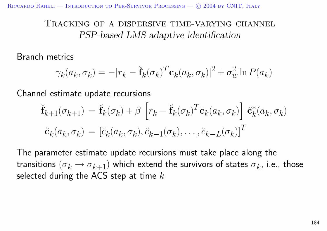
Riccardo Raheli — Introduction to Per-Survivor Processing — c© 2004 by CNIT, Italy
Tracking of a dispersive time-varying channelPSP-based LMS adaptive identification
Branch metrics
γk(ak, σk) = −|rk − fk(σk)Tck(ak, σk)|2 + σ2w ln P (ak)
Channel estimate update recursions
fk+1(σk+1) = fk(σk) + β[rk − fk(σk)T ck(ak, σk)
]c∗k(ak, σk)
ck(ak, σk) = [ck(ak, σk), ck−1(σk), . . . , ck−L(σk)]T
The parameter estimate update recursions must take place along thetransitions (σk → σk+1) which extend the survivors of states σk, i.e., thoseselected during the ACS step at time k
184
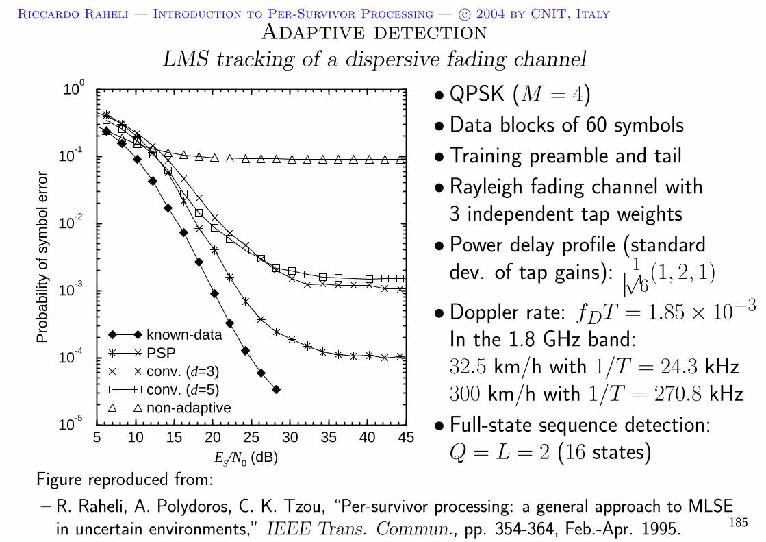
Riccardo Raheli — Introduction to Per-Survivor Processing — c© 2004 by CNIT, Italy
Adaptive detectionLMS tracking of a dispersive fading channel
5 10 15 20 25 30 35 40 45ES/N0 (dB)
10-5
10-4
10-3
10-2
10-1
100
Pro
babi
lity
of s
ymbo
l err
or
known-dataPSPconv. (d=3)conv. (d=5)non-adaptive
• QPSK (M = 4)
• Data blocks of 60 symbols
• Training preamble and tail
• Rayleigh fading channel with3 independent tap weights
• Power delay profile (standarddev. of tap gains): 1√
6(1, 2, 1)
• Doppler rate: fDT = 1.85 × 10⁻³
In the 1.8 GHz band:32.5 km/h with 1/T = 24.3 kHz300 km/h with 1/T = 270.8 kHz
• Full-state sequence detection:Q = L = 2 (16 states)
Figure reproduced from:
– R. Raheli, A. Polydoros, C. K. Tzou, “Per-survivor processing: a general approach to MLSEin uncertain environments,” IEEE Trans. Commun., pp. 354-364, Feb.-Apr. 1995. 185

Riccardo Raheli — Introduction to Per-Survivor Processing — c© 2004 by CNIT, Italy
Adaptive detectionLMS tracking of a dispersive fading diversity channel
5 10 15 20 25 30 35 40 45Es/N0 (dB)
10-5
10-4
10-3
10-2
10-1
100
Pro
babi
lity
of s
ymbo
l err
or
known dataPSPconv. (d=3)conv. (d=5)
•QPSK (M = 4)
•Data blocks of 60 symbols
• Training preamble and tail
• Rayleigh fading channel with3 independent tap weights
• Power delay profile (standarddev. of tap gains): 1√
6(1, 2, 1)
•Doppler rate: fDT = 3.69 × 10⁻³
In the 1.8 GHz band:65 km/h with 1/T = 24.3 kHz600 km/h with 1/T = 270.8 kHz
•Dual diversity
• Full-state sequence detection:Q = L = 2 (16 states)
186
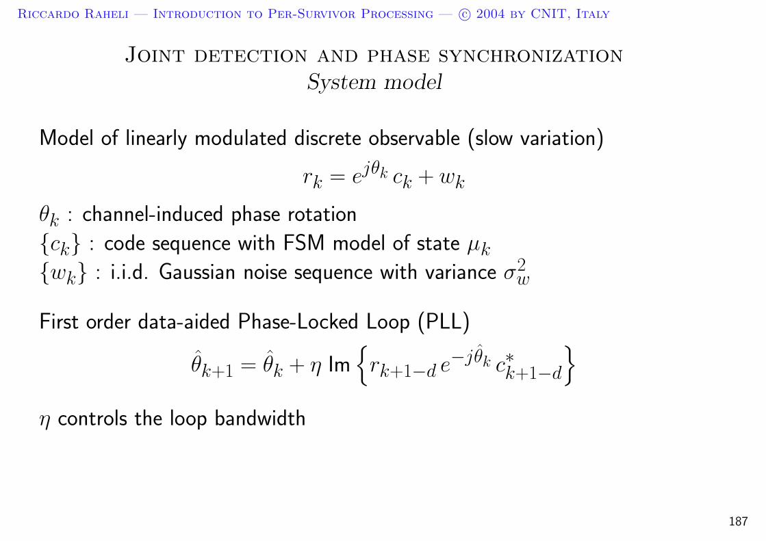
Riccardo Raheli — Introduction to Per-Survivor Processing — c© 2004 by CNIT, Italy
Joint detection and phase synchronizationSystem model
Model of linearly modulated discrete observable (slow variation)
rk = ejθk ck + wk
θk : channel-induced phase rotation
ck : code sequence with FSM model of state µk
wk : i.i.d. Gaussian noise sequence with variance σ2w
First order data-aided Phase-Locked Loop (PLL)
θk+1 = θk + η Im
rk+1−d e−jθk c∗k+1−d
η controls the loop bandwidth
187

Riccardo Raheli — Introduction to Per-Survivor Processing — c© 2004 by CNIT, Italy
Joint detection and phase synchronizationDecision-directed phase tracking
Branch metrics
γk(ak, µk) = −|rke−jθk − ck(ak, µk)|2 + σ2
w ln P (ak)
ck(ak, σk) : code symbol branch label
PLL phase-update (feedback) recursion
θk+1 = θk + η Im
rk+1−d e−jθk ˆc∗k+1−d
The tentative decision delay must comply with the causality condition uponthe detected data, which implies d ≥ 1.
188
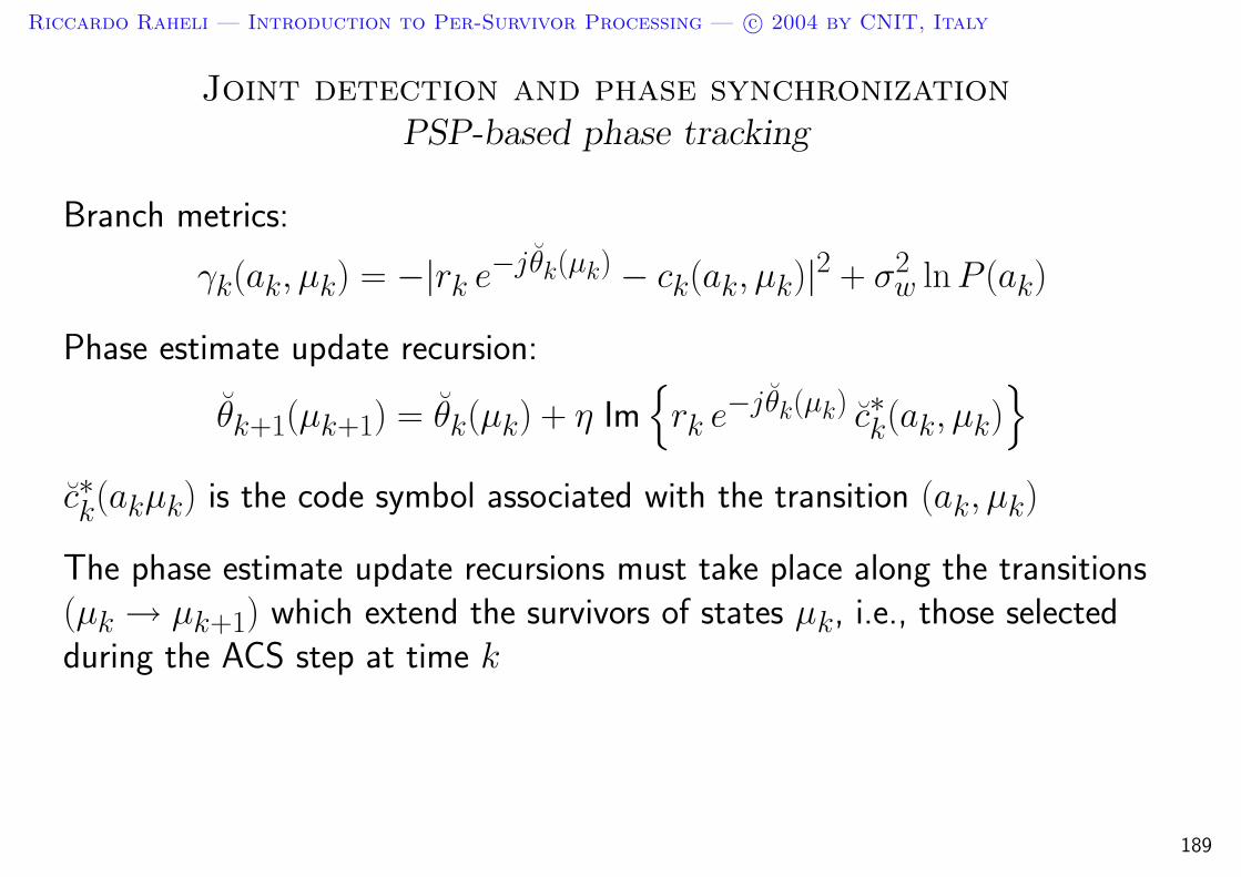
Riccardo Raheli — Introduction to Per-Survivor Processing — c© 2004 by CNIT, Italy
Joint detection and phase synchronizationPSP-based phase tracking
Branch metrics:
γk(ak, µk) = −|rk e−jθk(µk) − ck(ak, µk)|2 + σ2w ln P (ak)
Phase estimate update recursion:
θk+1(µk+1) = θk(µk) + η Imrk e−jθk(µk) c∗k(ak, µk)
c∗k(akµk) is the code symbol associated with the transition (ak, µk)
The phase estimate update recursions must take place along the transitions(µk → µk+1) which extend the survivors of states µk, i.e., those selectedduring the ACS step at time k
189

Riccardo Raheli — Introduction to Per-Survivor Processing — c© 2004 by CNIT, Italy
Adaptive detectionJoint TCM decoding and phase synchronization
5 10 15ES/N0 (dB)
10-5
10-4
10-3
10-2
10-1
100
Pro
babi
lity
of s
ymbo
l err
or
kn.-phasekn.-dataPSPconv. (d=2)
• TC-8PSK (4 states)
• Phase noise with Wienermodel:
θk+1 = θk + ∆k
∆k are Gaussian, i.i.d. withstandard deviation 2
Figure reproduced from:
– R. Raheli, A. Polydoros, C. K. Tzou, “Per-survivor processing: a general approach to MLSEin uncertain environments,” IEEE Trans. Commun., pp. 354-364, Feb.-Apr. 1995. 190

Riccardo Raheli — Introduction to Per-Survivor Processing — c© 2004 by CNIT, Italy
Adaptive detectionPhase acquisition of PLL and VT
• TC-8PSK (4 states)
• 1st order PLL
• 1st order vector tracker (VT)
•With system in lock, a phase step∆φ is applied at time zero
• Phase evolution is monitored untilthe phase error reduces to ±10
• Acquisition time in symbolperiods vs. ∆φ
•Es/N0 = 10 dB
•BEQT = 10−2
Figure reproduced from:
– A. N. D’Andrea, U. Mengali, and G. M. Vitetta, “Approximate ML decoding of coded PSKwith no explicit carrier phase reference,” IEEE Trans. Commun., pp. 1033-1039, Feb.-Apr.1994. 191
Riccardo Raheli — Introduction to Per-Survivor Processing — c© 2004 by CNIT, Italy
Adaptive detectionBibliography
– A. N. D’Andrea, U. Mengali, and G. M. Vitetta, “Approximate ML decoding of coded PSKwith no explicit carrier phase reference,” IEEE Trans. Commun., pp. 1033-1039,Feb.-Apr. 1994.
– H. Kubo, K. Murakami, T. Fujino, “An adaptive MLSE for fast time-varying ISI channels,”IEEE Trans. Commun., pp, 1872-1880, Feb.-Apr. 1994.
– H. Kubo, K. Murakami, T. Fujino, “Adaptive MLSE by means of combined equalizationand decoding in fading environments,” IEEE J. Sel. Areas Commun., pp, 102-109, vol.13, Jan. 1995.
– R. Raheli, A. Polydoros, C. K. Tzou, “Per-survivor processing: a general approach to MLSEin uncertain environments,” IEEE Trans. Commun., pp. 354-364, Feb.-Apr. 1995.
– R. Raheli, G. Marino, P. Castoldi, “Per-survivor processing and tentative decisions: what isin between?,” IEEE Trans. Commun., pp. 127-129, Feb. 1996.
– K. M. Chugg, A. Polydoros, “MLSE for an unknown channel—Parts I and II,” IEEETrans. Commun., pp. 836-846 and 949-958, July and Aug. 1996.
– K. M. Chugg, “Blind acquisition characteristics of PSP-based sequence detectors,” IEEEJ. Sel. Areas Commun., vol. 16, pp. 1518-1529, Oct. 1998.
192

Riccardo Raheli — Introduction to Per-Survivor Processing — c© 2004 by CNIT, Italy
5. Advanced applications of PSP
Outline
1. Review of detection techniques
2. Detection under parametric uncertainty
3. Per-Survivor Processing (PSP): concept and historical review
4. Classical applications of PSP:
4.1 Complexity reduction
4.2 Linear predictive detection for fading channels
4.3 Adaptive detection
5. Advanced applications of PSP
193

Riccardo Raheli — Introduction to Per-Survivor Processing — c© 2004 by CNIT, Italy
Iterative detectionMotivation
Iterative, or turbo, detection/decoding was first proposed as a suboptimalalgorithm for decoding special very powerful channel codes, widely known asturbo codes
Turbo codes are a parallel concatenation of simple component recursiveconvolutional codes through a long permuter, or interleaver
The principle of iterative detection/decoding can be applied to any parallel orserial concatenation of FSM models:
a) Each FSM model is detected/decoded by means of a suitable soft-inputsoft-output (SISO) module accounting for that model
b) The soft-outputs of the various modules are passed to other modules, whichrefine the detection/decoding process in a next iteration
c) The process can be iterated several times and usually converges in a few steps
Since the channel can be typically modeled as a FSM, exactly orapproximately, joint iterative detection of the received signal and decoding ofa possible channel code can be performed
194

Riccardo Raheli — Introduction to Per-Survivor Processing — c© 2004 by CNIT, Italy
Iterative detectionSoft-input soft-output (SISO) modules
A SISO module processes the soft-information received from other modulesand combines it with the possible observation of the channel output
The input soft-information can be accounted for by assigning proper values tothe a priori probabilities of the information or code symbols
⇒ This is the reason for having so diligently accounted for these probabilitiesin the various branch-metric expressions
In non-iterative detection, we are allowed to eliminate the a priori symbolprobabilities from the very beginning, on the basis of the reasonableassumption that they have equal values (hence, they are irrelevant)
The output soft-information is computed on the basis of the APPs of thepossible information or code symbols
195
Riccardo Raheli — Introduction to Per-Survivor Processing — c© 2004 by CNIT, Italy
Iterative detectionPSP-based SISO modules
A SISO module computes the APPs of the information symbols by means ofa forward-backward (FB) or soft-output Viterbi algorithm
Soft-output Viterbi algorithms estimate a reliability value of any decision bycomparing the metrics of best paths to those of their competitors
The max-log approximation of the FB algorithm allows a direct application ofPSP to the two counter-running Viterbi algorithms (in direct and inverse time)
Soft-output Viterbi algorithms can be readily augmented with PSP
These remarks entitle us to exploit any possible application of PSP in thesoft-output modules used in iterative decoding, e.g. for:
Complexity reduction
Linear predictive detection
Adaptive detection196
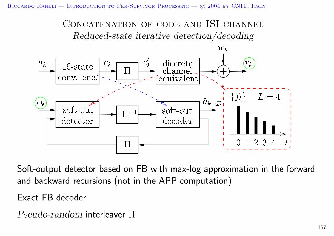
Riccardo Raheli — Introduction to Per-Survivor Processing — c© 2004 by CNIT, Italy
Concatenation of code and ISI channelReduced-state iterative detection/decoding
! " #
$ % "
&' ( )
* *,+
Soft-output detector based on FB with max-log approximation in the forwardand backward recursions (not in the APP computation)
Exact FB decoder
Pseudo-random interleaver Π197
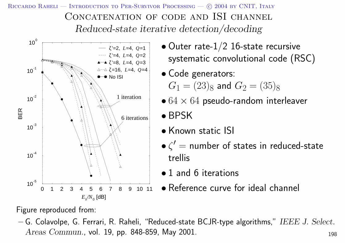
Riccardo Raheli — Introduction to Per-Survivor Processing — c© 2004 by CNIT, Italy
Concatenation of code and ISI channelReduced-state iterative detection/decoding
0 1 2 3 4 5 6 7 8 9 10 11Eb/N0 [dB]
10-5
10-4
10-3
10-2
10-1
100
BE
R
ζ ’=2, L=4, Q=1ζ ’=4, L=4, Q=2ζ ’=8, L=4, Q=3ζ=16, L=4, Q=4No ISI
1 iteration
6 iterations
• Outer rate-1/2 16-state recursivesystematic convolutional code (RSC)
• Code generators:G1 = (23)8 and G2 = (35)8
• 64 × 64 pseudo-random interleaver
• BPSK
• Known static ISI
• ζ ′ = number of states in reduced-statetrellis
• 1 and 6 iterations
• Reference curve for ideal channel
Figure reproduced from:
– G. Colavolpe, G. Ferrari, R. Raheli, “Reduced-state BCJR-type algorithms,” IEEE J. Select.Areas Commun., vol. 19, pp. 848-859, May 2001. 198

Riccardo Raheli — Introduction to Per-Survivor Processing — c© 2004 by CNIT, Italy
Concatenation of code and fading channelLinear-predictive iterative detection/decoding
!
"
#
$ &% '
# % (
#
) *+ ,
Soft-output detector based on FB with linear prediction and state reduction(bit APPs)
Exact FB decoder
Pseudo-random bit interleaver Π199
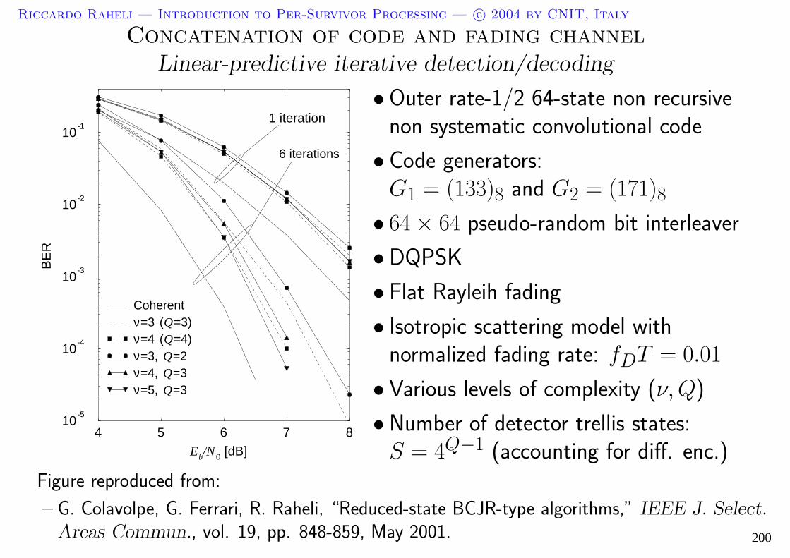
Riccardo Raheli — Introduction to Per-Survivor Processing — c© 2004 by CNIT, Italy
Concatenation of code and fading channelLinear-predictive iterative detection/decoding
4 5 6 7 8Eb/N0 [dB]
10-5
10-4
10-3
10-2
10-1
BE
R
Coherentν=3 (Q=3)ν=4 (Q=4)ν=3, Q=2ν=4, Q=3ν=5, Q=3
1 iteration
6 iterations
• Outer rate-1/2 64-state non recursivenon systematic convolutional code
• Code generators:G1 = (133)8 and G2 = (171)8
• 64 × 64 pseudo-random bit interleaver
• DQPSK
• Flat Rayleih fading
• Isotropic scattering model withnormalized fading rate: fDT = 0.01
• Various levels of complexity (ν,Q)
• Number of detector trellis states:S = 4Q−1 (accounting for diff. enc.)
Figure reproduced from:
– G. Colavolpe, G. Ferrari, R. Raheli, “Reduced-state BCJR-type algorithms,” IEEE J. Select.Areas Commun., vol. 19, pp. 848-859, May 2001. 200
Riccardo Raheli — Introduction to Per-Survivor Processing — c© 2004 by CNIT, Italy
Noncoherent detectionMotivation
In virtually any bandpass transmission system, the carrier phase reference isnot known by the receiver
In coherent detection this phase reference must be recovered by the receiver,provided it is sufficiently stable, according to the synchronization-detectiondecomposition
Noncoherent detection assumes complete absence of knowledge about thephase reference—an effective approach if the phase is unstable
A nonchoerent channel introduces unlimited memory in thesignal—suboptimal detection algorithms are in order
201

Riccardo Raheli — Introduction to Per-Survivor Processing — c© 2004 by CNIT, Italy
Noncoherent detectionUnlimited memory
Discrete channel model
rk = ckejθ + wk
The conditional p.d.f. of the observation is
p(rk|rk−10 , ak
0) =p(rk
0 |ak0)
p(rk−10 |ak−1
0 )=
e−(|rk|2+|ck|2)/σ2w
πσ2w
I0
[2
σ2w
∣∣(rk0)Hck
0
∣∣]
I0
[2
σ2w
∣∣(rk−10 )Hck−1
0
∣∣]
In fact
p(rk0 |ak
0) =1
2π
∫ 2π
0p(rk
0 |ak0 , θ)dθ
=1
2π(πσ2w)k+1
∫ 2π
0e−(||rk
0−ck0e
jθ||2)/σ2w dθ
=1
2π(πσ2w)k+1
e−(||rk0 ||2+||ck
0 ||2)/σ2w
∫ 2π
0e(2Re(rk
0)Hck0e
jθ)/σ2w dθ
=1
(πσ2w)k+1
e−(||rk0 ||2+||ck
0 ||2)/σ2w I0
[2
σ2w
∣∣(rk0)Hck
0
∣∣]
202

Riccardo Raheli — Introduction to Per-Survivor Processing — c© 2004 by CNIT, Italy
Noncoherent detectionFeedforward PSP-based phase estimation
Data-aided mean-square phase estimate based on N most recent observationsrk−1k−N
e−jθ =(rk−1
k−N )Hck−1k−N∣∣(rk−1
k−N )Hck−1k−N
∣∣
Branch metrics:
γk(ck, µk) = −∣∣rk e−jθk(µk) − ck
∣∣2 + σ2w ln P [ak(ck, µk)]
∝ Rerkc
∗k e−jθk(µk) − |ck|2
2+
1
2σ2
w ln P [ak(ck, µk)]
=Re
rkc
∗k · (rk−1
k−N )H ck−1k−N (µk)
∣∣(rk−1
k−N )H ck−1k−N (µk)
∣∣ − |ck|22
+σ2
w
2ln P [ak(ak, µk)]
The trellis state µk can be augmented to include part of the phase memory
ωk = (µk; ck−1, ck−2, . . . , ck−Q) Q ≤ N203
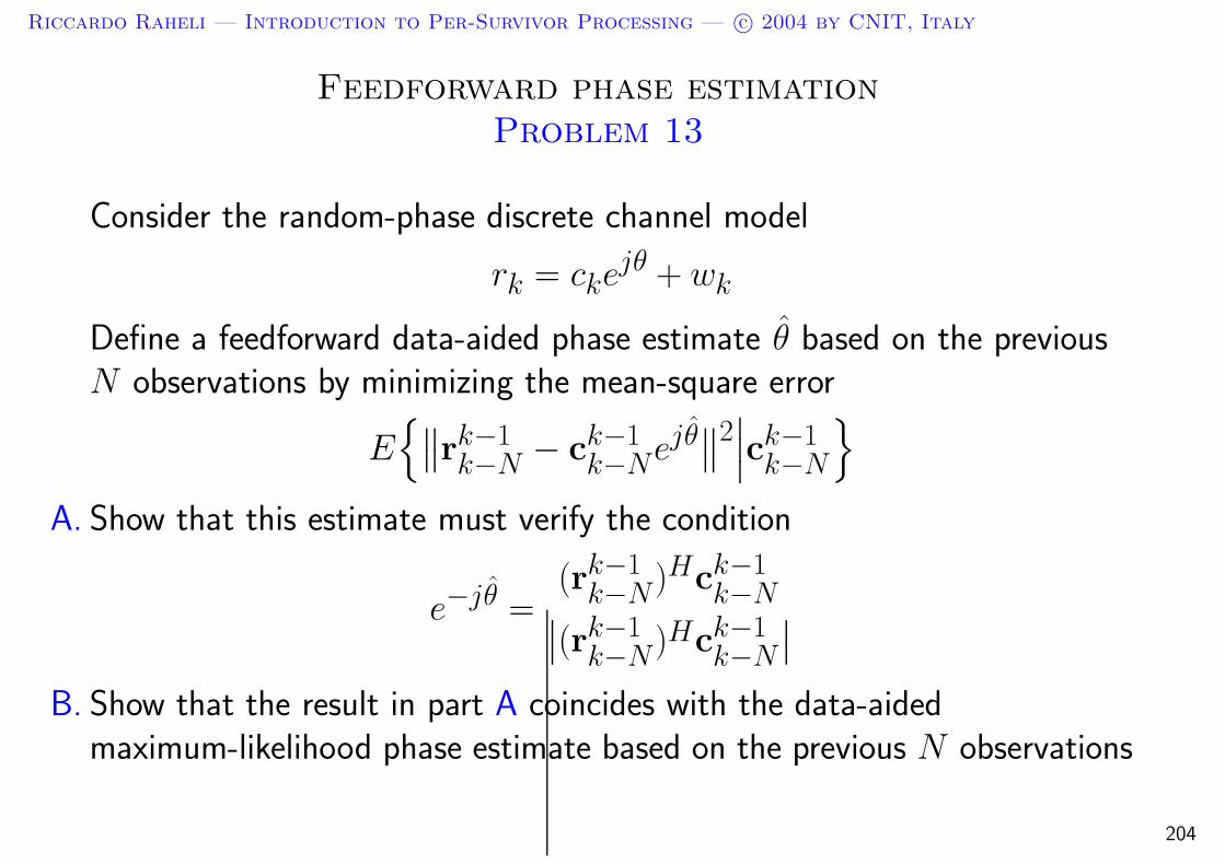
Riccardo Raheli — Introduction to Per-Survivor Processing — c© 2004 by CNIT, Italy
Feedforward phase estimationProblem 13
Consider the random-phase discrete channel model
rk = ckejθ + wk
Define a feedforward data-aided phase estimate θ based on the previousN observations by minimizing the mean-square error
E∥∥rk−1
k−N − ck−1k−Nejθ
∥∥2∣∣∣ck−1
k−N
A. Show that this estimate must verify the condition
e−jθ =(rk−1
k−N )Hck−1k−N∣∣(rk−1
k−N )Hck−1k−N
∣∣
B. Show that the result in part A coincides with the data-aidedmaximum-likelihood phase estimate based on the previous N observations
204
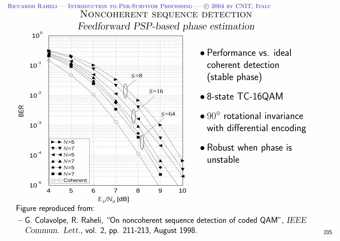
Riccardo Raheli — Introduction to Per-Survivor Processing — c© 2004 by CNIT, Italy
Noncoherent sequence detectionFeedforward PSP-based phase estimation
4 5 6 7 8 9 10E b/N0 [dB]
10-5
10-4
10-3
10-2
10-1
100
BER
NN
N
=5
=5NN
N
=5=7
=7
=7
Coherent
=64S
=16S
=8S
• Performance vs. idealcoherent detection(stable phase)
• 8-state TC-16QAM
• 90 rotational invariancewith differential encoding
• Robust when phase isunstable
Figure reproduced from:
– G. Colavolpe, R. Raheli, “On noncoherent sequence detection of coded QAM”, IEEECommun. Lett., vol. 2, pp. 211-213, August 1998. 205
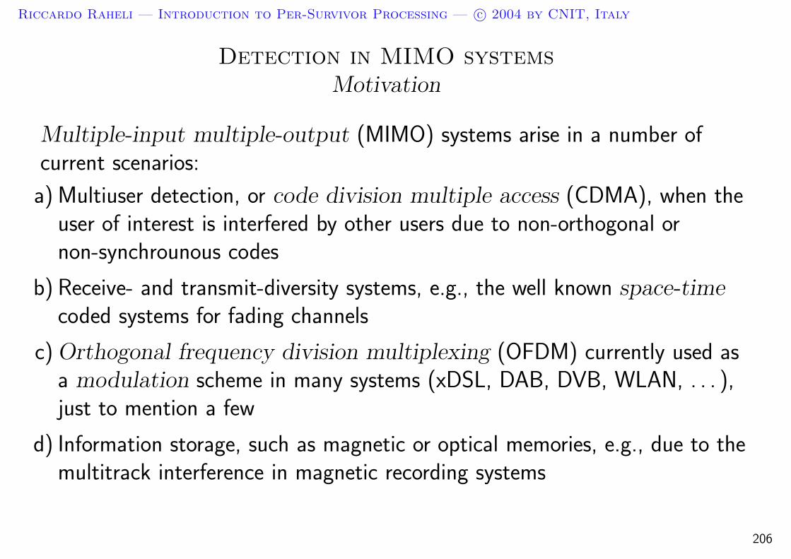
Riccardo Raheli — Introduction to Per-Survivor Processing — c© 2004 by CNIT, Italy
Detection in MIMO systemsMotivation
Multiple-input multiple-output (MIMO) systems arise in a number ofcurrent scenarios:
a) Multiuser detection, or code division multiple access (CDMA), when theuser of interest is interfered by other users due to non-orthogonal ornon-synchrounous codes
b) Receive- and transmit-diversity systems, e.g., the well known space-timecoded systems for fading channels
c) Orthogonal frequency division multiplexing (OFDM) currently used asa modulation scheme in many systems (xDSL, DAB, DVB, WLAN, . . . ),just to mention a few
d) Information storage, such as magnetic or optical memories, e.g., due to themultitrack interference in magnetic recording systems
206
Riccardo Raheli — Introduction to Per-Survivor Processing — c© 2004 by CNIT, Italy
Detection in MIMO systemsThe basic approach
MIMO systems are multidimensional versions of transmission (or storage)systems and can be described by a suitable vector or matrix notation
In some cases the increased system dimensionality can be exploited, e.g. inspace-time coding
Most detection techniques can be applied to MIMO systems in a conceptuallystraightforward manner by a proper notational extension
The complexity may be an issue due to the increased dimensionality (not onlynotationwise)
207

Riccardo Raheli — Introduction to Per-Survivor Processing — c© 2004 by CNIT, Italy
Detection in MIMO systemsGeneral system model
encoder det./dec.
MAP
MIMO
channelMIMO
MIMO
(ST)...
... ...
C RA A
...
A : input information matrix (N × K) (or N ′ × K)
C : code matrix (N × K)
R : received matrix (M × K)
A : detected information matrix (N × K) (or N ′ × K)
Rows and columns may represent the “space” and time dimensions, respectively
Notation: for an (N ×K) matrix X, nXk is element (n, k), nX is the n-th
row, Xk is the k-th column, andn2n1X
k2k1
is an (n2−n1)× (k2−k1) submatrix208
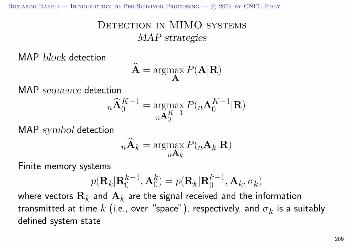
Riccardo Raheli — Introduction to Per-Survivor Processing — c© 2004 by CNIT, Italy
Detection in MIMO systemsMAP strategies
MAP block detectionA = argmax
AP (A|R)
MAP sequence detection
nAK−10 = argmax
nAK−10
P (nAK−10 |R)
MAP symbol detection
nAk = argmaxnAk
P (nAk|R)
Finite memory systems
p(Rk|Rk−10 ,Ak
0) = p(Rk|Rk−10 ,Ak, σk)
where vectors Rk and Ak are the signal received and the informationtransmitted at time k (i.e., over “space”), respectively, and σk is a suitablydefined system state
209

Riccardo Raheli — Introduction to Per-Survivor Processing — c© 2004 by CNIT, Italy
Advanced applications of PSPBibliography
Iterative detection:– V. Franz and J. B. Anderson, “Concatenated decoding with a reduced-search BCJR
algorithm,” IEEE J. Selet. Areas Commun., vol. 16, pp. 186-195, February 1998.
– K. R. Narayanan, G. L. Stuber, “List decoding of turbo codes”, IEEE Trans. Commun.,vol. 46, pp.754-762, June 1998.
– P. Hoeher, J. Lodge, “‘Turbo DPSK’: iterative differential PSK demodulation and channeldecoding”, IEEE Trans. Commun., vol. 47, pp. 837-843, June 1999.
– G. Colavolpe, G. Ferrari, R. Raheli, “Noncoherent iterative (turbo) decoding”, IEEETrans. Commun., vol. 48, pp. 1488-1498, September 2000.
– G. Colavolpe, G. Ferrari, R. Raheli, “Reduced-state BCJR-type algorithms,” IEEE J.Select. Areas Commun. Special Issue-The Turbo Principle: from Theory to Practice, vol.19, pp. 848-859, May 2001.
Noncoherent detection:– G. Colavolpe, R. Raheli, “On noncoherent sequence detection of coded QAM”, IEEE
Commun. Lett., vol. 2, pp. 211-213, August 1998.
– G. Colavolpe, R. Raheli, “Noncoherent sequence detection”, IEEE Trans. Commun., vol.47, pp. 1376-1385, September 1999.
– G. Colavolpe, R. Raheli, “Noncoherent sequence detection of continuous phasemodulations”, IEEE Trans. Commun., vol. 47, pp. 1303-1307, September 1999. 210
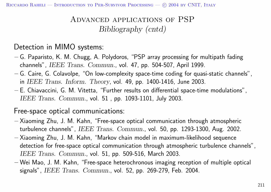
Riccardo Raheli — Introduction to Per-Survivor Processing — c© 2004 by CNIT, Italy
Advanced applications of PSPBibliography (cntd)
Detection in MIMO systems:– G. Paparisto, K. M. Chugg, A. Polydoros, “PSP array processing for multipath fading
channels”, IEEE Trans. Commun., vol. 47, pp. 504-507, April 1999.
– G. Caire, G. Colavolpe, “On low-complexity space-time coding for quasi-static channels”,in IEEE Trans. Inform. Theory, vol. 49, pp. 1400-1416, June 2003.
– E. Chiavaccini, G. M. Vitetta, “Further results on differential space-time modulations”,IEEE Trans. Commun., vol. 51 , pp. 1093-1101, July 2003.
Free-space optical communications:– Xiaoming Zhu, J. M. Kahn, “Free-space optical communication through atmospheric
turbulence channels”, IEEE Trans. Commun., vol. 50, pp. 1293-1300, Aug. 2002.
– Xiaoming Zhu, J. M. Kahn, “Markov chain model in maximum-likelihood sequencedetection for free-space optical communication through atmospheric turbulence channels”,IEEE Trans. Commun., vol. 51, pp. 509-516, March 2003.
– Wei Mao, J. M. Kahn, “Free-space heterochronous imaging reception of multiple opticalsignals”, IEEE Trans. Commun., vol. 52, pp. 269-279, Feb. 2004.
211
Related Documents