Searching Images: Recent research at Southampton

Searching ImagesRecent research at Southampton Joint work with Paul Lewis, David Dupplaw & Sina Samangooei

Jonathon Hare 21 February 2011

2

http://www.livingknowledge-project.eu

http://www.livememories.org

http://www.arcomem.eu

Contents• Image feature representation

• Highly scalable content-based image search –Demo: Guessing tags and geo location of images –Compressed single-pass indexing to build an augmented

index –Using Map-Reduce for scalability

• Diversity in search result ranking –Implicit image search diversification –Explicit search diversification

• Classifying images to aid search and diversification –Sentiment classification

3

Image Feature Representation

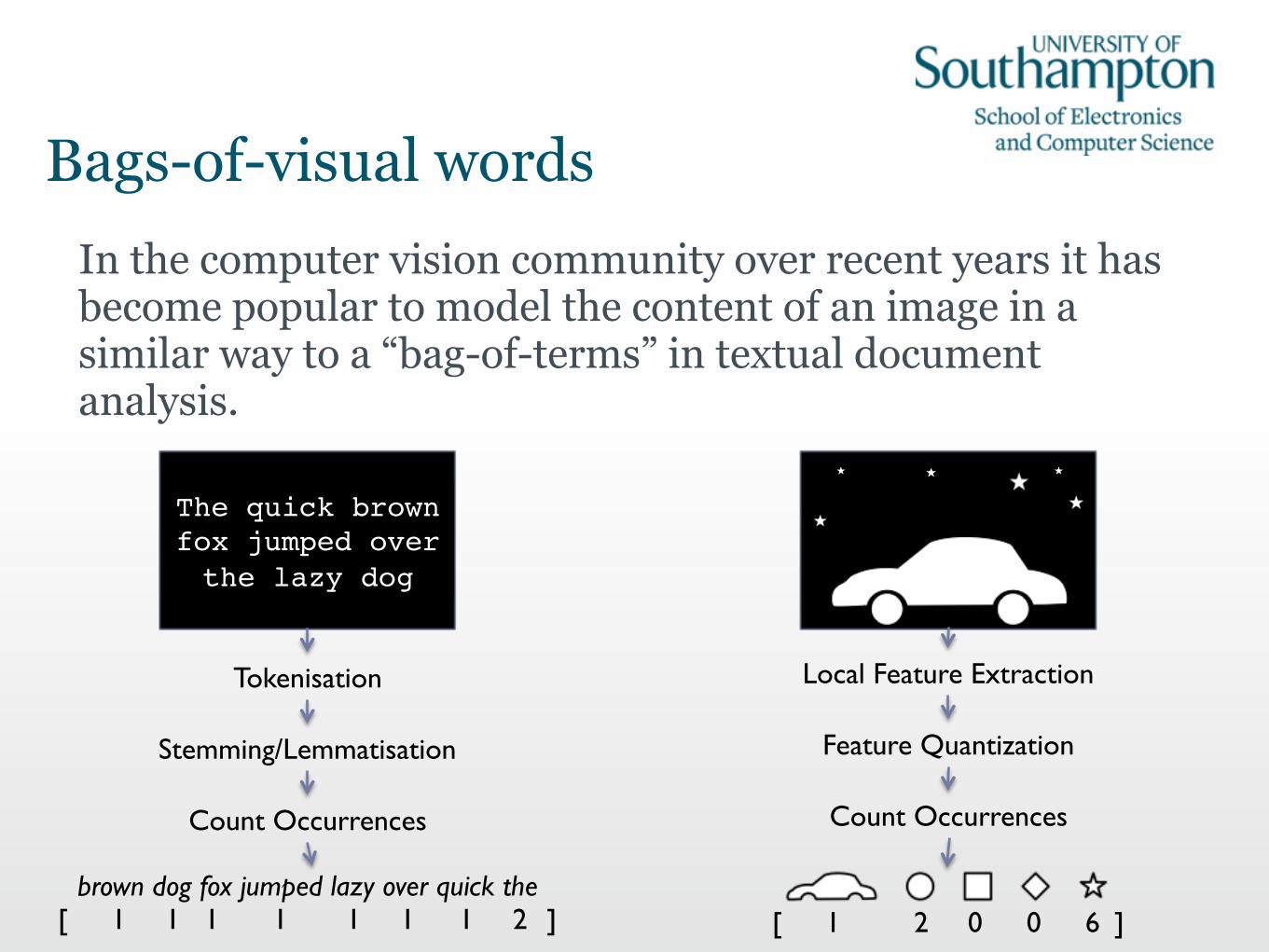
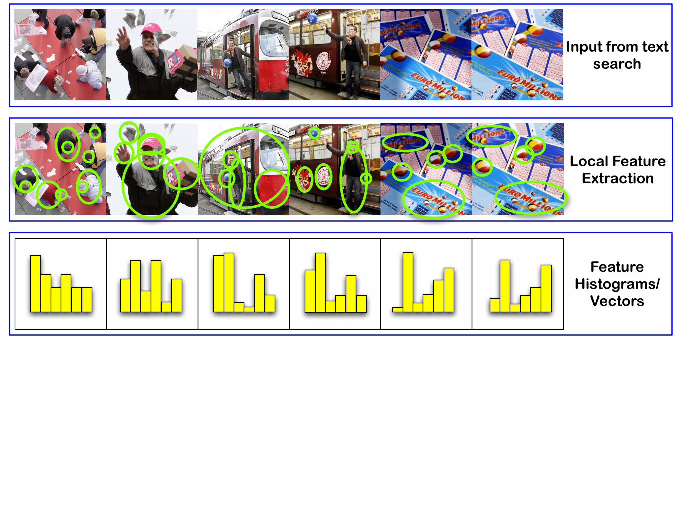
Bags-of-visual wordsIn the computer vision community over recent years it has become popular to model the content of an image in a similar way to a “bag-of-terms” in textual document analysis.

The quick brown fox jumped over the lazy dog!

Tokenisation

Stemming/Lemmatisation

Count Occurrences

Local Feature Extraction

Feature Quantization

Count Occurrences

brown dog fox jumped lazy over quick the 1 1 1 1 1 1 1 2 [ ] 1 [ 2 0 0 6 ]

The quick brown fox jumped over the lazy dog!

BoVW using local features

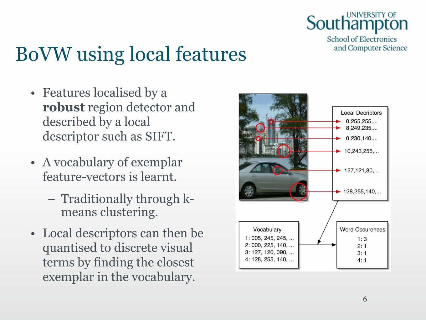
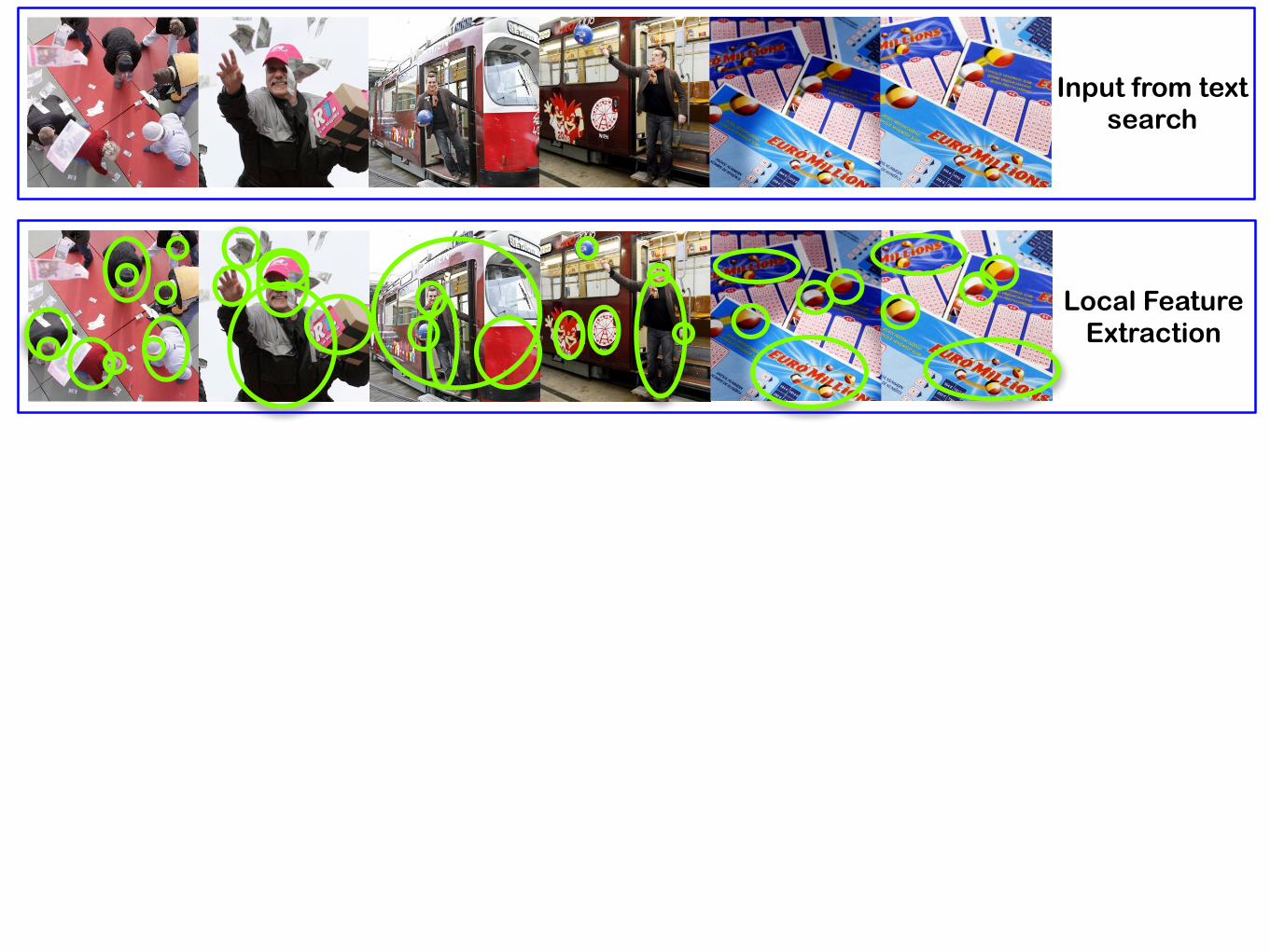
• Features localised by a robust region detector and described by a local descriptor such as SIFT.

• A vocabulary of exemplar feature-vectors is learnt.

– Traditionally through k-means clustering.

• Local descriptors can then be quantised to discrete visual terms by finding the closest exemplar in the vocabulary.

6

Clustering features into vocabularies • A typical image may have a few thousand local features.

• For indexing images, the number of discrete visual terms is large (i.e. around 1 million terms). –Smaller vocabularies are typically used in classification

tasks. –Building vocabularies using k-means is hard:

• i.e. 1M clusters, 128-dimensional vectors, >>>10M samples.

• Special k-means variants developed to deal with this (perhaps! - see next slide) [i.e. AKM (Philbin et al, 2007), HKM (Nistér and Stewénius, 2006)].

• Other tricks can also be applied by exploiting the shape of the space in the vectors can lie. 7

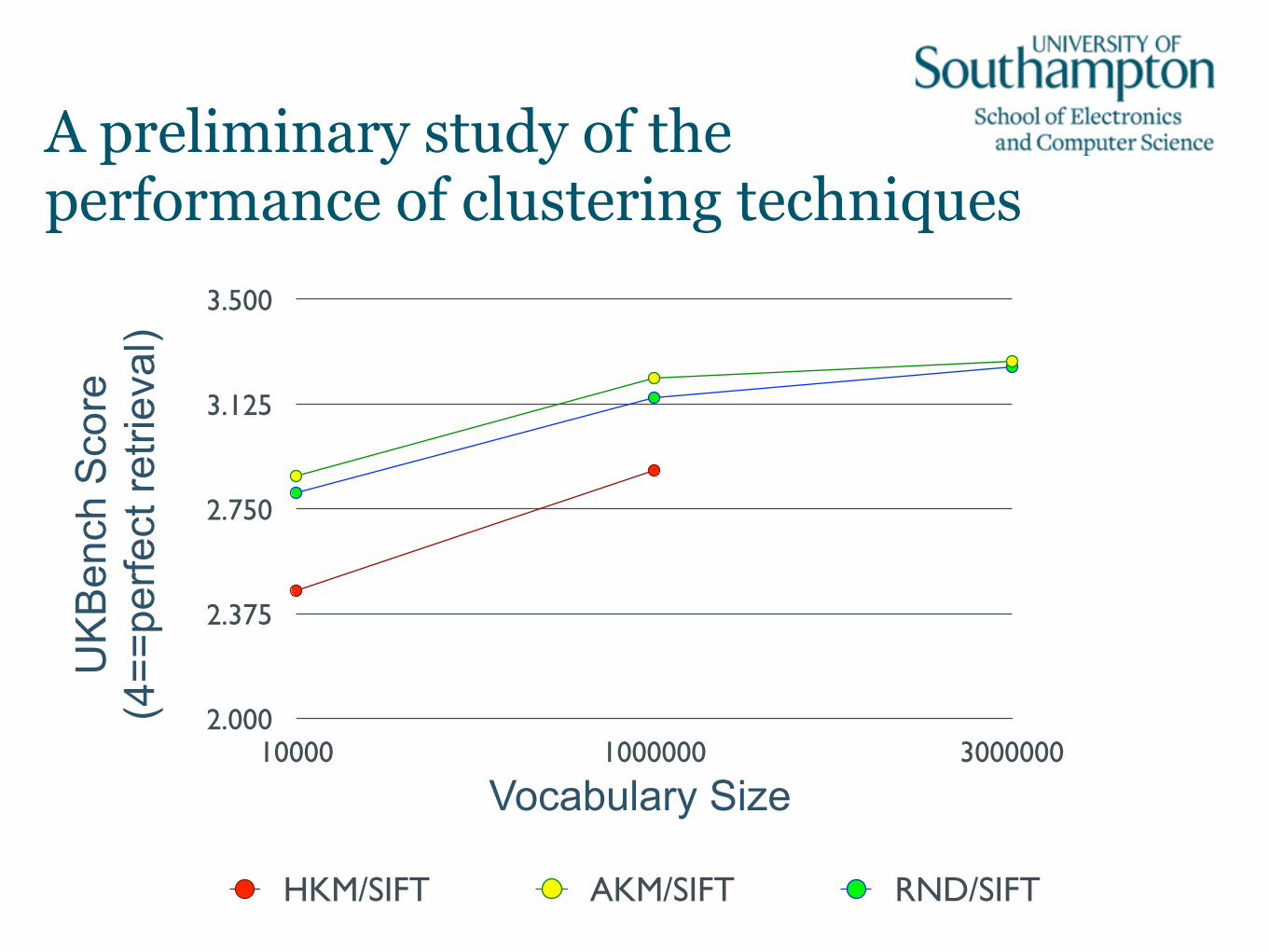
A preliminary study of the performance of clustering techniques

2.000

2.375

2.750

3.125

3.500

10000 1000000 3000000

HKM/SIFT AKM/SIFT RND/SIFT

UK

Ben

ch S

core

(4

==pe

rfect

retri

eval

)

Vocabulary Size

Highly scalable content-based

image search

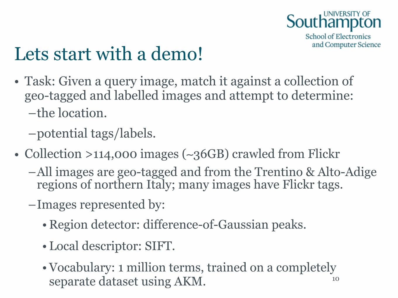
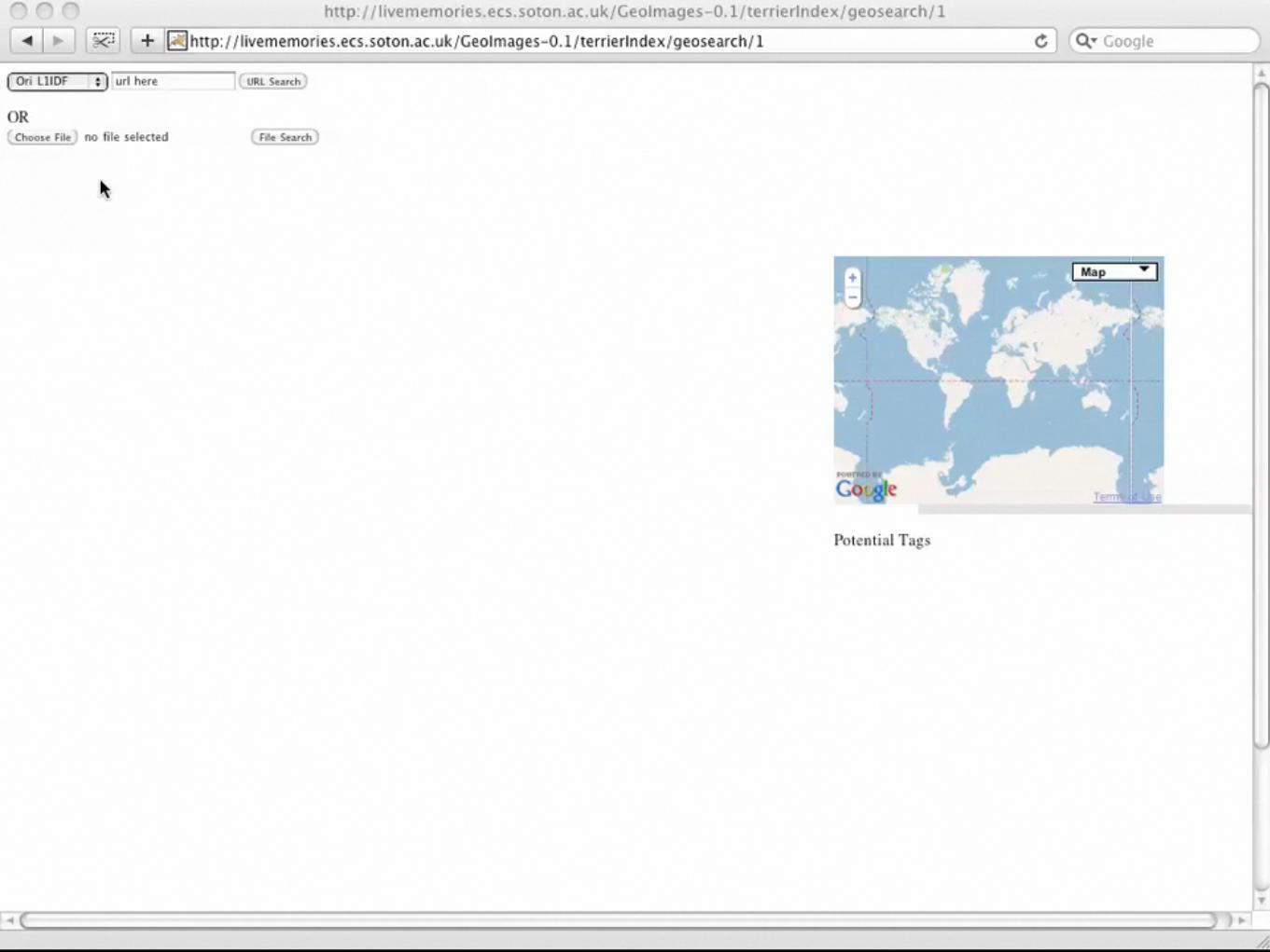
Lets start with a demo!• Task: Given a query image, match it against a collection of

geo-tagged and labelled images and attempt to determine: –the location. –potential tags/labels.

• Collection >114,000 images (∼36GB) crawled from Flickr –All images are geo-tagged and from the Trentino & Alto-Adige

regions of northern Italy; many images have Flickr tags. –Images represented by:

• Region detector: difference-of-Gaussian peaks.

• Local descriptor: SIFT.

• Vocabulary: 1 million terms, trained on a completely separate dataset using AKM. 10

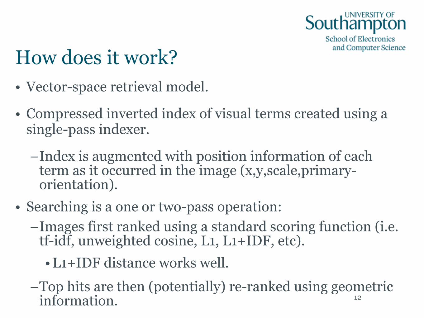
How does it work?• Vector-space retrieval model.

• Compressed inverted index of visual terms created using a single-pass indexer.

–Index is augmented with position information of each term as it occurred in the image (x,y,scale,primary-orientation).

• Searching is a one or two-pass operation: –Images first ranked using a standard scoring function (i.e.

tf-idf, unweighted cosine, L1, L1+IDF, etc). • L1+IDF distance works well.

–Top hits are then (potentially) re-ranked using geometric information. 12

Geometric re-ranking• A pair of images sharing a number of visual terms may or

may not be related.

–It can often be useful to ensure that the matching visual terms are spatially consistent between the images. • This is like the visual equivalent of phrase or proximity

searches in text. • Spatial/geometric constraints can be very strict;

–i.e. there must be an exact transform between the images (homography, affine, etc)

• Or quite loose; –i.e. all pairs of matching terms should have a similar

relative orientation or scale. 13

Introducing ImageTerrier!• It would take a considerable amount of effort to write a new search

engine from scratch.

–So, we’ve been building ours on top of Terrier ☺

–ImageTerrier is a set of classes that extend the Terrier core: • Collections and documents that read data produced from

image feature extractors.

• New indexers and supporting classes to make compressed augmented inverted indices for visual term data.

• New distance measures implemented as WeightingModels.

• Geometric re-ranking implemented as DocumentScoreModifiers.

• Command-line tools for indexing and searching. 14

Scalability: Using Map-Reduce• Indexing is an expensive operation, but compared to feature

extraction the cost is small.

–One solution to being able to deal with larger datasets is to distribute the workload across multiple machines.

–The Map-Reduce framework popularised by Google can let us do this in a way that minimises data transfer by distributing data and performing work only on the local portions.

• We have been experimenting with M-R implementations of our image processing tools that enable us to work on much bigger datasets.

15

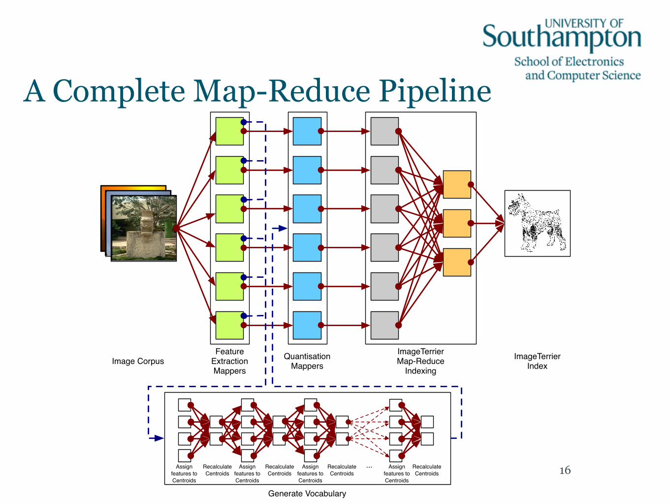
Feature Extraction Mappers

Quantisation Mappers

ImageTerrier Map-Reduce

IndexingImageTerrier

IndexImage Corpus

Assign features to Centroids

Recalculate Centroids

Assign features to Centroids

Recalculate Centroids

Assign features to Centroids

Recalculate Centroids

Assign features to Centroids

Recalculate Centroids

...

Generate Vocabulary

A Complete Map-Reduce Pipeline

16

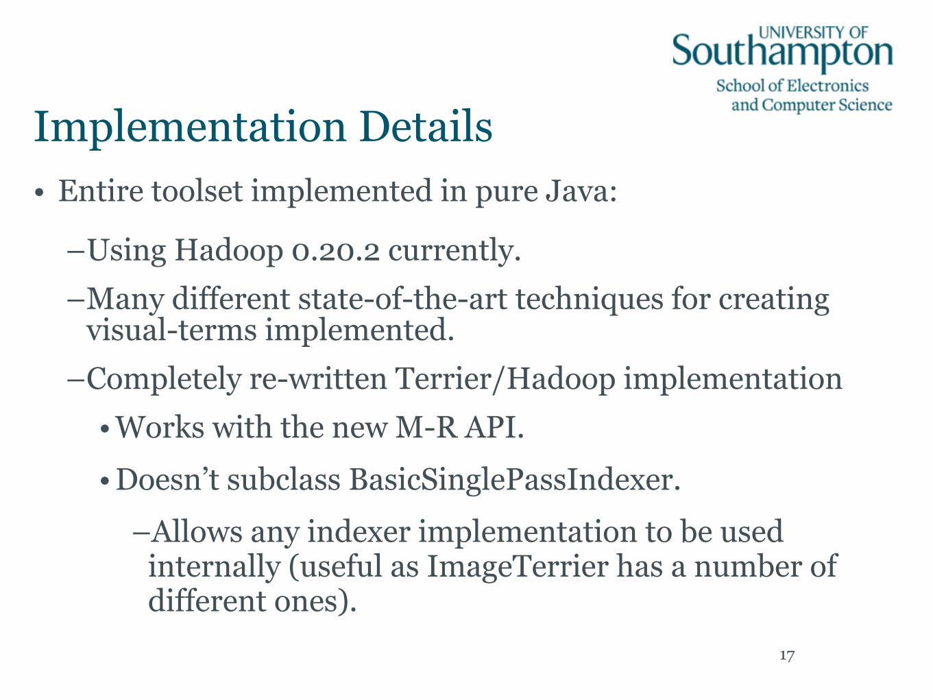
Implementation Details• Entire toolset implemented in pure Java:

–Using Hadoop 0.20.2 currently. –Many different state-of-the-art techniques for creating

visual-terms implemented. –Completely re-written Terrier/Hadoop implementation

• Works with the new M-R API. • Doesn’t subclass BasicSinglePassIndexer.

–Allows any indexer implementation to be used internally (useful as ImageTerrier has a number of different ones).

17

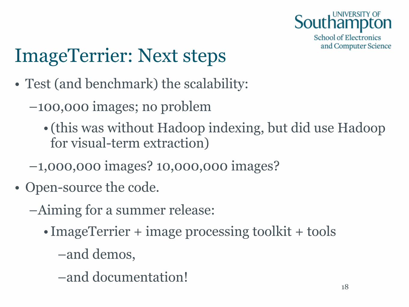
ImageTerrier: Next steps• Test (and benchmark) the scalability:

–100,000 images; no problem • (this was without Hadoop indexing, but did use Hadoop

for visual-term extraction) –1,000,000 images? 10,000,000 images?

• Open-source the code. –Aiming for a summer release:

• ImageTerrier + image processing toolkit + tools –and demos, –and documentation!

18

Diversity in search result ranking

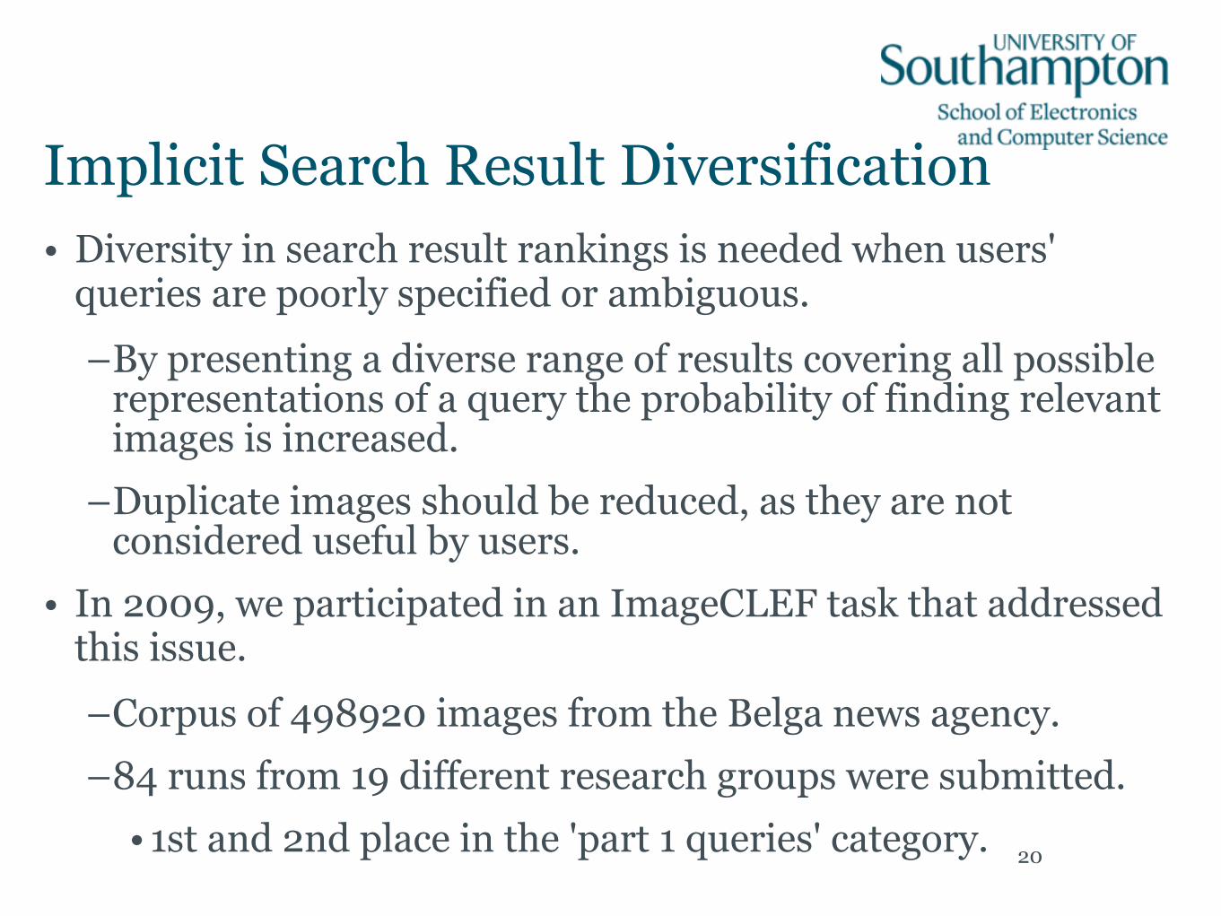
Implicit Search Result Diversification • Diversity in search result rankings is needed when users'

queries are poorly specified or ambiguous. –By presenting a diverse range of results covering all possible

representations of a query the probability of finding relevant images is increased.

–Duplicate images should be reduced, as they are not considered useful by users.

• In 2009, we participated in an ImageCLEF task that addressed this issue. –Corpus of 498920 images from the Belga news agency. –84 runs from 19 different research groups were submitted.

• 1st and 2nd place in the 'part 1 queries' category. 20

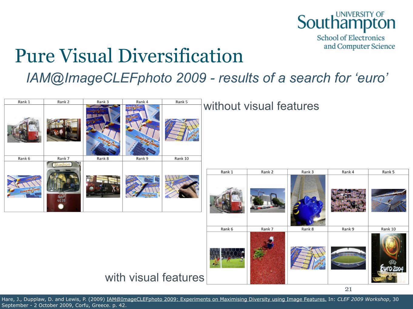
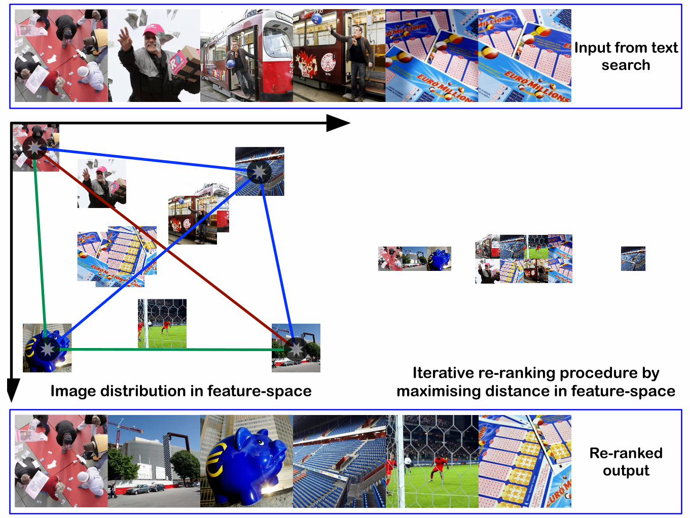
Pure Visual DiversificationIAM@ImageCLEFphoto 2009 - results of a search for ‘euro’

without visual features

with visual features21

Hare, J., Dupplaw, D. and Lewis, P. (2009) IAM@ImageCLEFphoto 2009: Experiments on Maximising Diversity using Image Features. In: CLEF 2009 Workshop, 30 September - 2 October 2009, Corfu, Greece. p. 42.

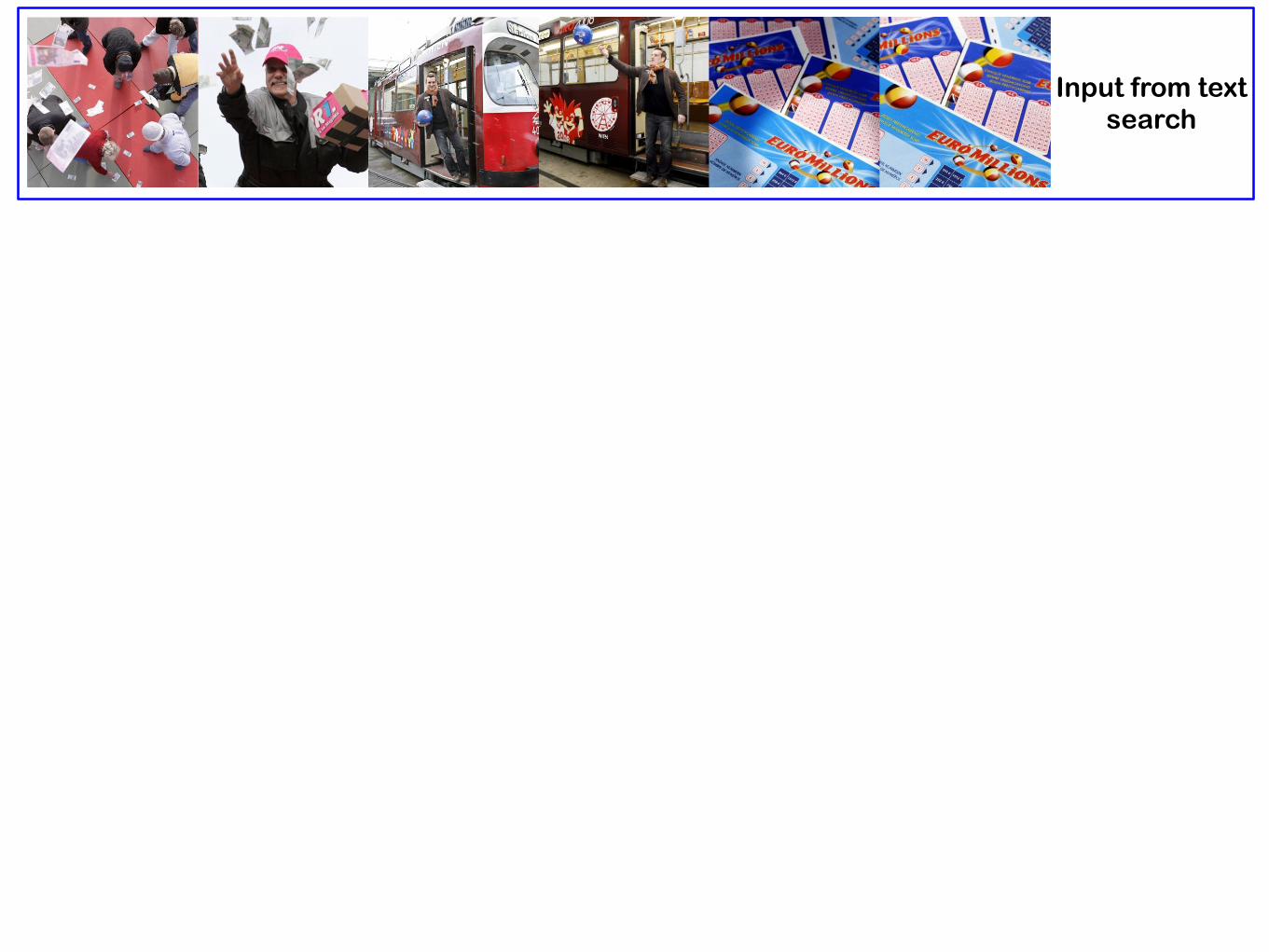
Input from text search

Input from text search

Local Feature Extraction

Input from text search

Local Feature Extraction

Feature Histograms/

Vectors

Input from text search

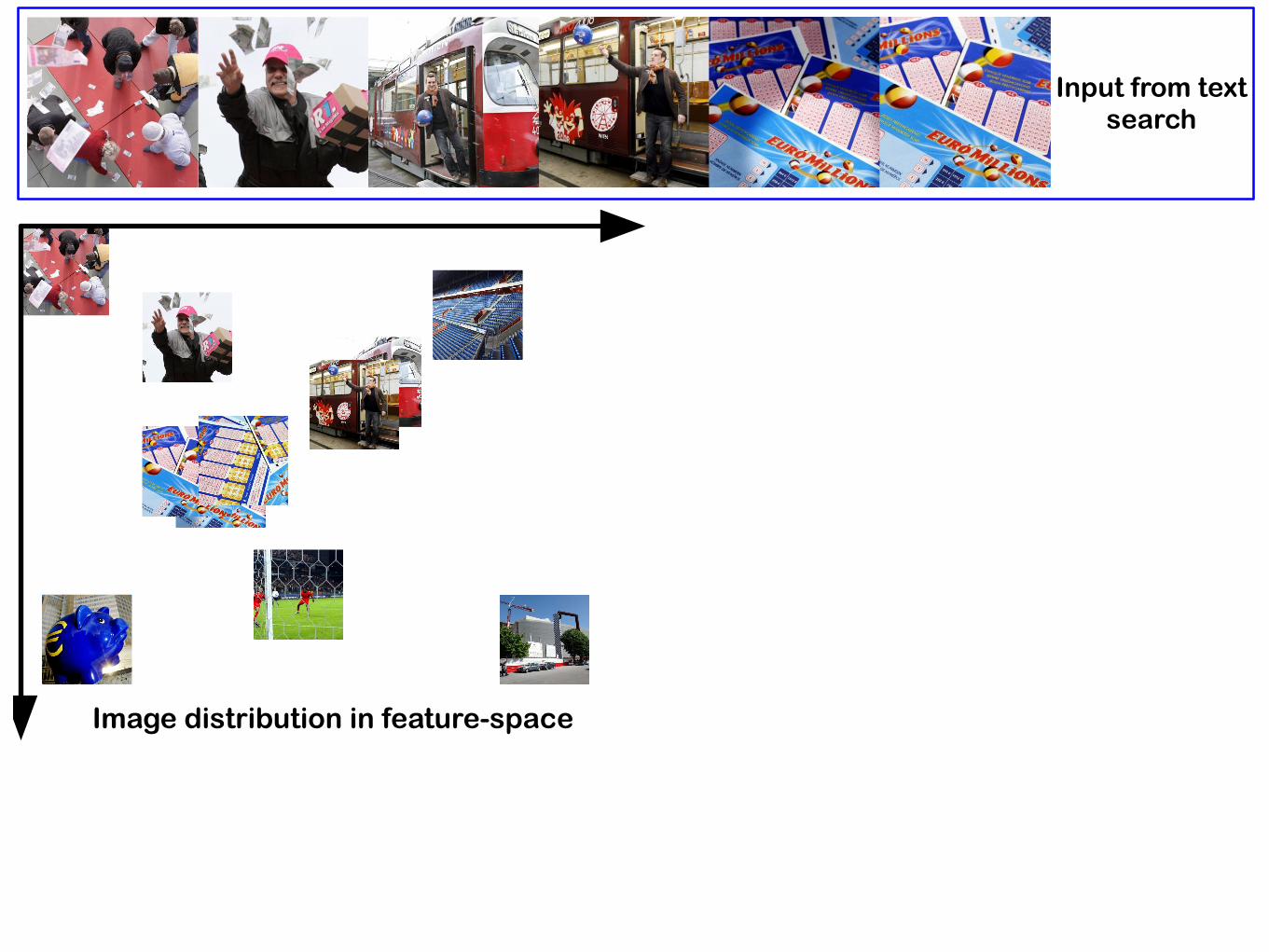
Image distribution in feature-space

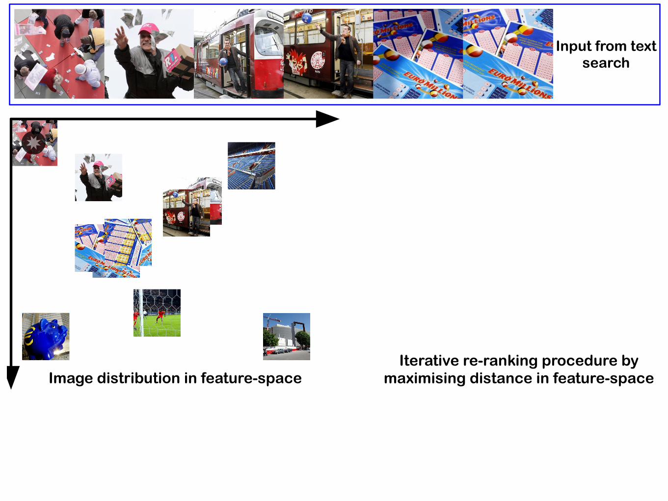
Input from text search

Image distribution in feature-spaceIterative re-ranking procedure by

maximising distance in feature-space

✸

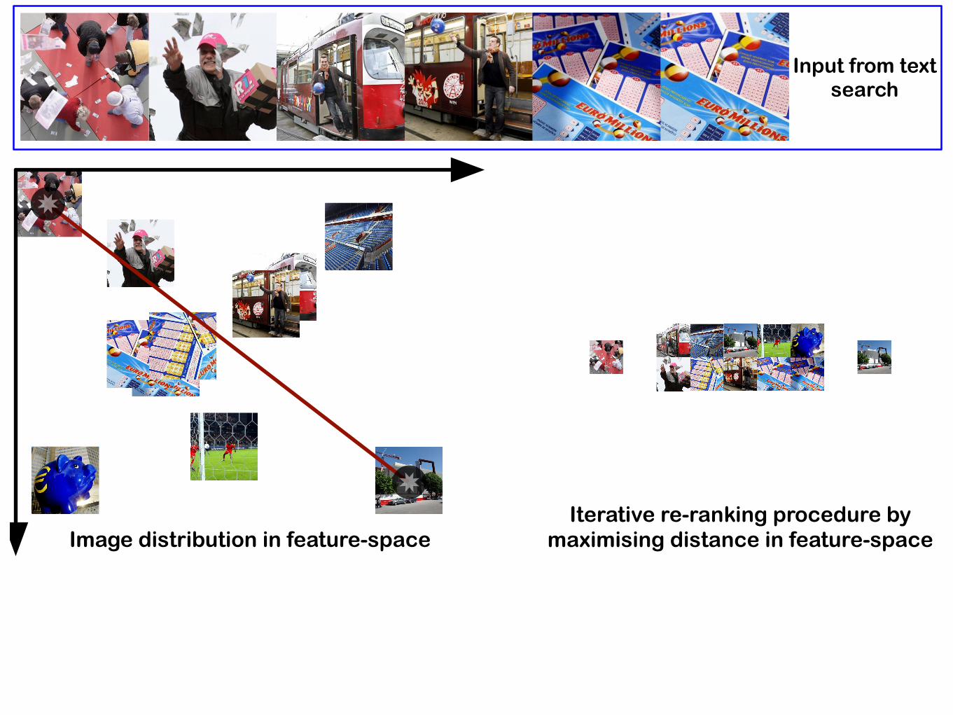
Input from text search

Image distribution in feature-spaceIterative re-ranking procedure by

maximising distance in feature-space

✸

✸

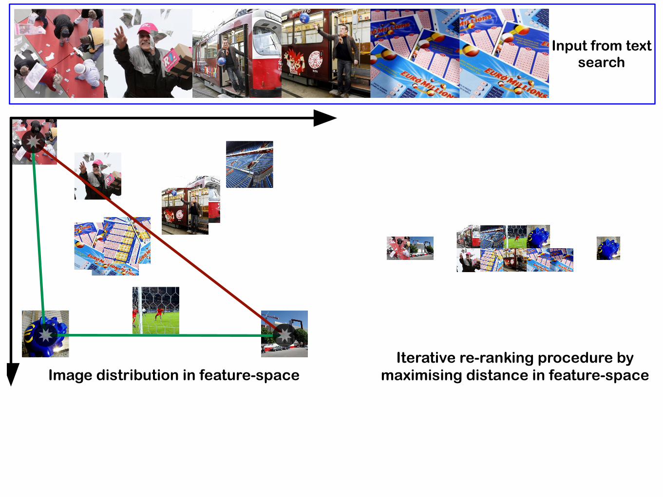
Input from text search

Image distribution in feature-spaceIterative re-ranking procedure by

maximising distance in feature-space

✸✸

✸

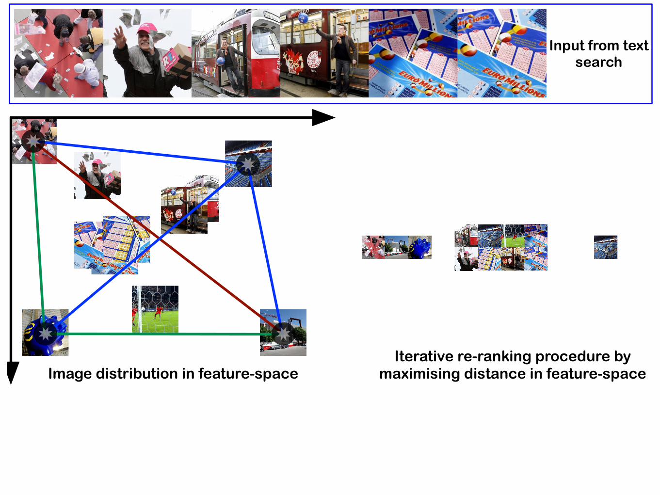
Input from text search

Image distribution in feature-spaceIterative re-ranking procedure by

maximising distance in feature-space

✸✸

✸✸

Input from text search

Re-ranked output

Image distribution in feature-spaceIterative re-ranking procedure by

maximising distance in feature-space

✸✸

✸✸

Explicit Search Result Diversification • Sometimes users have an idea about how they would like

their results to be diversified.

–For example; searching for images of Arnold Schwarzenegger diversified by the films he has starred in.

• Using a combination of different technologies we have built a prototype search engine that allows this kind of query.

23

http://www.diversity-search.info

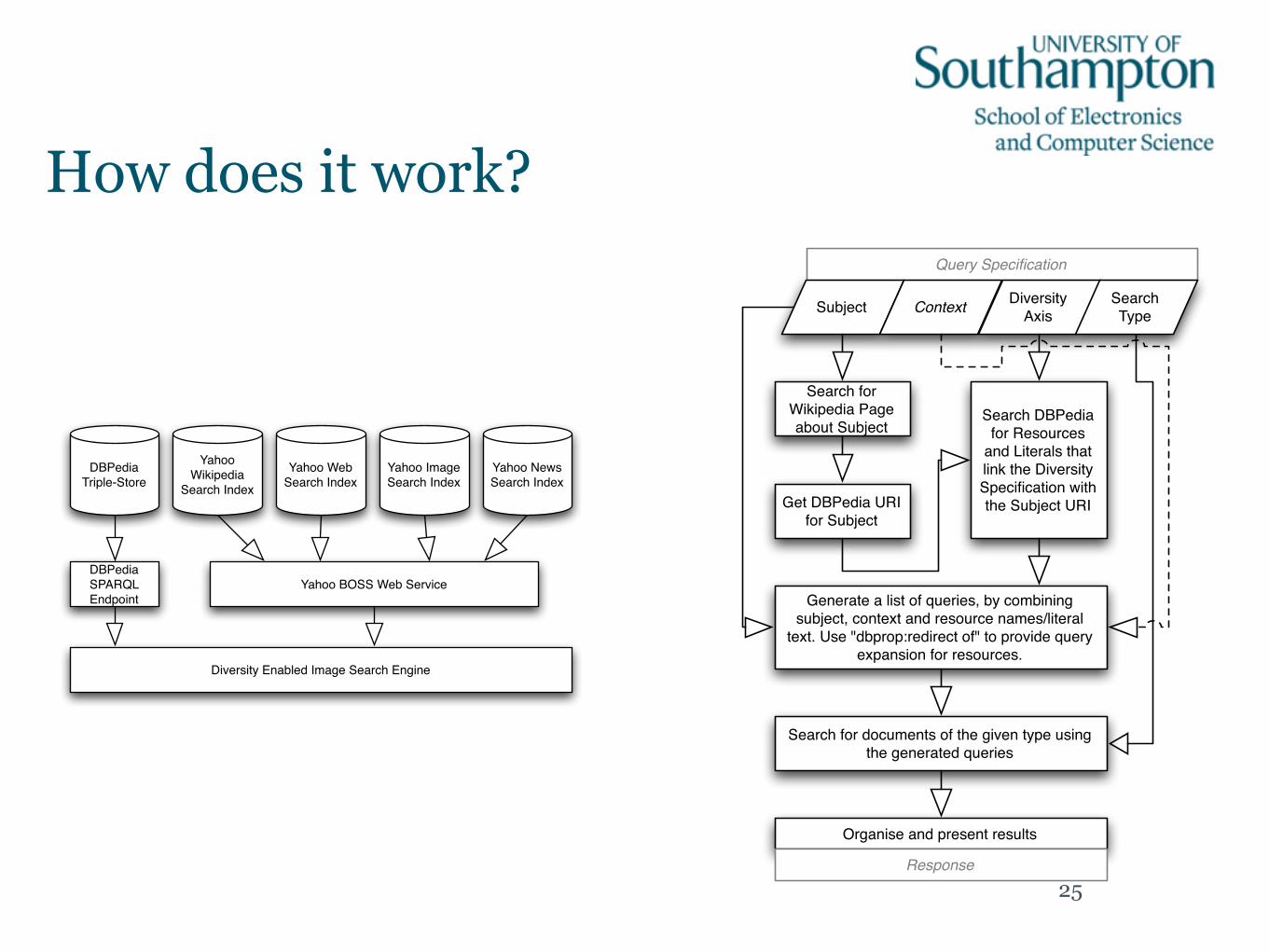
DBPediaTriple-Store

Yahoo Wikipedia

Search IndexYahoo Image Search Index

DBPediaSPARQL Endpoint

Yahoo BOSS Web Service

Diversity Enabled Image Search Engine

Yahoo Web Search Index

Yahoo News Search Index

Query Specification

Subject Context Diversity Axis

Search for Wikipedia Page about Subject

Get DBPedia URI for Subject

Search DBPedia for Resources

and Literals that link the Diversity Specification with the Subject URI

Generate a list of queries, by combining subject, context and resource names/literal

text. Use "dbprop:redirect of" to provide query expansion for resources.

Search for documents of the given type using the generated queries

Organise and present results

Response

Search Type

How does it work?

25

Classifying images to aid search and

diversification

Classifying sentiment

• Recently we’ve been investigating the possibility of estimating the sentiment of an image based on its visual characteristics. –Applications include search and diversification along a

sentiment axis.

Joint work with Stefan Siersdorfer, Enrico Minack and Fan Deng at the L3S Research Centre in Hannover

Siersdorfer, S., Hare, J., Minack, E. and Deng, F. (2010) Analyzing and Predicting Sentiment of Images on the Social Web. In: ACM Multimedia 2010, 25-29 October 2010, Firenze, Italy. pp. 715-718.

Zontone, P., Boato, G., Hare, J., Lewis, P., Siersdorfer, S. and Minack, E. (2010) Image and Collateral Text in Support of Auto-annotation and Sentiment Analysis. In: TextGraphs-5: Graph-based Methods for Natural Language Processing, 16th July 2010, Uppsala, Sweden. pp. 88-92.

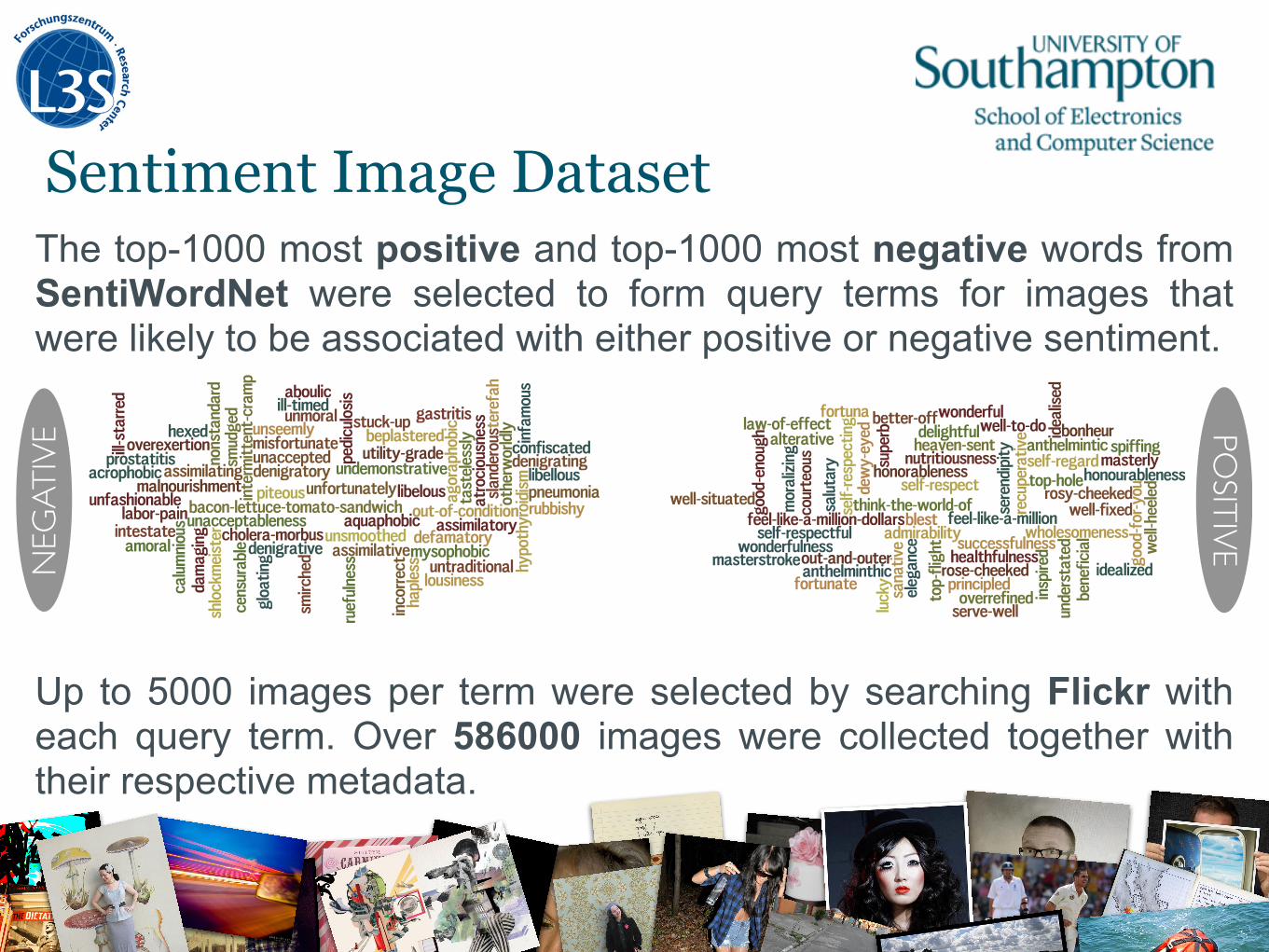
Sentiment Image DatasetThe top-1000 most positive and top-1000 most negative words from SentiWordNet were selected to form query terms for images that were likely to be associated with either positive or negative sentiment.

NEGATIVE POSITIVE

Up to 5000 images per term were selected by searching Flickr with each query term. Over 586000 images were collected together with their respective metadata.

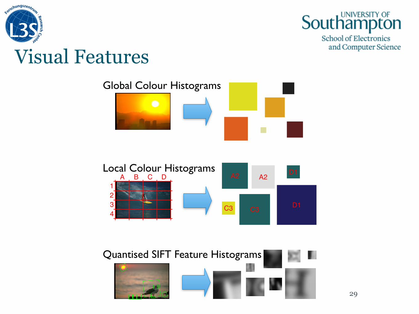
Visual Features

29

Global Colour Histograms

Local Colour HistogramsA B C D

1234

A2 A2

C3 C3 D1

D1

Quantised SIFT Feature Histograms

Pos

itiv

e

GC

H

Neg

ativ

ePos

itiv

e

LC

H

Neg

ativ

ePos

itiv

e

SIF

T

Neg

ativ

e

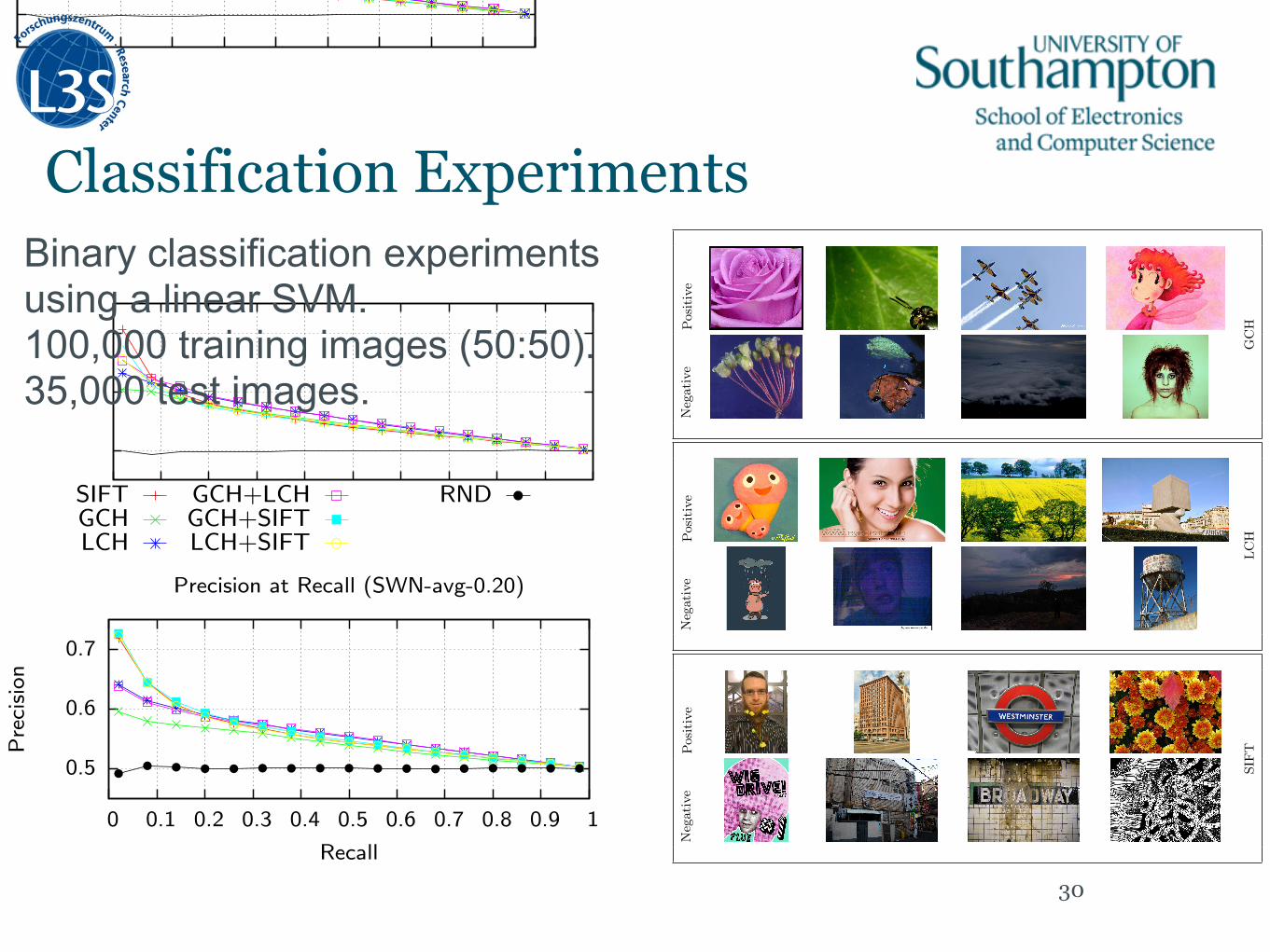
Figure 4: Images classified as positive and negative based on the three features: GCH, LCH, and SIFT

discover image features that are most correlated with sen-timents. For each feature, we computed the MI value withrespect to the both positive and negative sentiment cate-gory. Figure 3 illustrates the 16 most discriminative visualfeatures based on their MI value for the positive and nega-tive categories (in rank order; top-to-bottom). Overall, theselected features mirror the features we inferred for the sam-ple of classified images described in the previous section.

The GCH features for positive sentiment are dominatedby earthy colors and skin tones. Conversely, the features fornegative sentiment are dominated by blue and green tones.Interestingly, this association can intuitively be hypothe-sized because it mirrors human perception of warm (posi-tive) and cold (negative) colors. The LCH features showthe same trend as the GCH features — blue tones associ-ated with negative sentiment, and skin tones associated withpositive sentiment. In addition, the LCH features indicatethat there is no bias to the spatial location in which pixels ofthe respective colors occur for positive sentiment. Negative

features appear to be biased away from the far right of theimage plane.

As mentioned in the previous section, results based onSIFT visual terms are di⇥cult to interpret directly, but wecan make some general observations. Looking at the mostdiscriminative SIFT visual term features, the first obser-vation is that the features within the two classes are re-markably similar, but there is a clear di�erence between theclasses. The negative features seem dominated by a verylight central blob surrounded by a much darker background.The positive features are dominated by a dark blob on theside of the patch (the patches have been normalized for ro-tation, so the dark blob could occur in any orientation inthe image).

In order to explore the SIFT visual terms from a di�erentperspective, Figure 5 illustrates the top positive and nega-tive visual terms (from the MI analysis) in the context of twoimages (one classified as“positive”and the other“negative”).The first observation is that the positive image has more

From the three di�erent text representations tags, title,and description, we used only the tag annotations, becausethe others provided just a comparatively small collectionof images with strong sentiment values. For example, usingthe tag metadata, ⇥ 343,000 images with absolute sentimentvalue above 0.2 were available, whereas title and descriptiononly provided ⇥ 136,000 and ⇥ 52,000, respectively. Referto Figure 1 for more details. The upper diagram depictsthe number of images having an absolute sentiment valuewithin the respective interval, whereas the lower diagramillustrates the number of images with an absolute sentimentvalue above the respective value of � .

The distributions of sentiment values depicted in the his-tograms reflect the fact that many images did not contain adescription or title, or they quite often provided some kindof id (like IMG_1710). In contrast, the tags provided a muchricher basis for the sentiment value computation. We there-fore discarded textual image representations based on titleand description metadata, and focused on the tag-based tex-tual information.

Again, to crosscheck the correlation between the senti-ment values and the image features, we additionally gener-ated random sentiment values evenly distributed in [�1, 1](RND). Table 1 shows number of positive and negative im-ages for each sentiment value computation.

0

20000

40000

60000

80000

100000

120000

140000

0 0.1 0.2 0.3 0.4 0.5 0.6 0.7 0.8 0.9 1

no.

ofim

ages

sentiment value

SWN-avg Histogram

descriptiontagstitle

0

100000

200000

300000

400000

500000

600000

0 0.1 0.2 0.3 0.4 0.5 0.6 0.7 0.8 0.9 1

no.

ofim

ages

threshold � for sentiment value

SWN-avg Distribution

descriptiontagstitle

Figure 1: Histogram and distribution of sentimentvalues SWN-avg-� for di�erent types of textualmetadata

5.2 ClassificationWe performed di�erent series of binary classification ex-

periments of Flickr photos into the classes “positive senti-ment” and “negative sentiment”. From the labeled imagesand image features, we created training and test sets forclassification. We randomly picked 1,000, 10,000, and 50,000images for each category (positive and negative sentiment).

positive negative labeled

SW 294,559 199,370 493,929SWN-avg-0.00 316,089 238,388 554,477SWN-avg-0.10 260,225 190,012 450,237SWN-avg-0.20 194,700 149,096 343,796RND 293,456 292,812 586,268

Table 1: Statistics on labeled images in the dataset

0.5

0.6

0.7

0 0.1 0.2 0.3 0.4 0.5 0.6 0.7 0.8 0.9 1

Pre

cision

Recall

Precision at Recall (SW)

0.5

0.6

0.7

0 0.1 0.2 0.3 0.4 0.5 0.6 0.7 0.8 0.9 1

Pre

cision

Recall

Precision at Recall (SWN-avg-0.20)

SIFTGCHLCH

GCH+LCHGCH+SIFTLCH+SIFT

RND

Figure 2: Classification results for sentiment assign-ments SW and SWN-avg-� with � = 0.20 for trainingwith 50,000 photos per category

We trained an SVM model on these labeled data and testedon the remaining labeled data. For testing, we chose anequal number of positive and negative test images, with atleast 35,000 of each kind. We used the SVMlight [17] imple-mentation of linear support vector machines (SVMs) withstandard parameterization in our experiments, as this hasbeen shown to perform well for various classification tasks(see, e.g., [6, 16]).

Our quality measures are the precision-recall curves aswell as the precision-recall break-even points (BEP) for thesecurves (i.e. precision/recall at the point where precisionequals recall which is also equal to the F1 measure, theharmonic mean of precision and recall in that case). Somecharacteristic precision-recall curves are shown in Figure 2.To provide an overview of the performance of all featuresand sentiment value computation approaches, we extractedcharacteristic values for all configurations, namely the pre-cision values for recall at 5%, 10%, and 20%, and the BEPvalues (see Table 2).

We can observe that for small recall values, precision val-ues of up to 70% can be reached. Due to the challengingcharacter of this task, for high recall values, the precisiondegrades down to the random baseline. With increasing

From the three di�erent text representations tags, title,and description, we used only the tag annotations, becausethe others provided just a comparatively small collectionof images with strong sentiment values. For example, usingthe tag metadata, ⇥ 343,000 images with absolute sentimentvalue above 0.2 were available, whereas title and descriptiononly provided ⇥ 136,000 and ⇥ 52,000, respectively. Referto Figure 1 for more details. The upper diagram depictsthe number of images having an absolute sentiment valuewithin the respective interval, whereas the lower diagramillustrates the number of images with an absolute sentimentvalue above the respective value of � .

The distributions of sentiment values depicted in the his-tograms reflect the fact that many images did not contain adescription or title, or they quite often provided some kindof id (like IMG_1710). In contrast, the tags provided a muchricher basis for the sentiment value computation. We there-fore discarded textual image representations based on titleand description metadata, and focused on the tag-based tex-tual information.

Again, to crosscheck the correlation between the senti-ment values and the image features, we additionally gener-ated random sentiment values evenly distributed in [�1, 1](RND). Table 1 shows number of positive and negative im-ages for each sentiment value computation.

0

20000

40000

60000

80000

100000

120000

140000

0 0.1 0.2 0.3 0.4 0.5 0.6 0.7 0.8 0.9 1

no.

ofim

ages

sentiment value

SWN-avg Histogram

descriptiontagstitle

0

100000

200000

300000

400000

500000

600000

0 0.1 0.2 0.3 0.4 0.5 0.6 0.7 0.8 0.9 1

no.

ofim

ages

threshold � for sentiment value

SWN-avg Distribution

descriptiontagstitle

Figure 1: Histogram and distribution of sentimentvalues SWN-avg-� for di�erent types of textualmetadata

5.2 ClassificationWe performed di�erent series of binary classification ex-

periments of Flickr photos into the classes “positive senti-ment” and “negative sentiment”. From the labeled imagesand image features, we created training and test sets forclassification. We randomly picked 1,000, 10,000, and 50,000images for each category (positive and negative sentiment).

positive negative labeled

SW 294,559 199,370 493,929SWN-avg-0.00 316,089 238,388 554,477SWN-avg-0.10 260,225 190,012 450,237SWN-avg-0.20 194,700 149,096 343,796RND 293,456 292,812 586,268

Table 1: Statistics on labeled images in the dataset

0.5

0.6

0.7

0 0.1 0.2 0.3 0.4 0.5 0.6 0.7 0.8 0.9 1

Pre

cision

Recall

Precision at Recall (SW)

0.5

0.6

0.7

0 0.1 0.2 0.3 0.4 0.5 0.6 0.7 0.8 0.9 1

Pre

cision

Recall

Precision at Recall (SWN-avg-0.20)

SIFTGCHLCH

GCH+LCHGCH+SIFTLCH+SIFT

RND

Figure 2: Classification results for sentiment assign-ments SW and SWN-avg-� with � = 0.20 for trainingwith 50,000 photos per category

We trained an SVM model on these labeled data and testedon the remaining labeled data. For testing, we chose anequal number of positive and negative test images, with atleast 35,000 of each kind. We used the SVMlight [17] imple-mentation of linear support vector machines (SVMs) withstandard parameterization in our experiments, as this hasbeen shown to perform well for various classification tasks(see, e.g., [6, 16]).

Our quality measures are the precision-recall curves aswell as the precision-recall break-even points (BEP) for thesecurves (i.e. precision/recall at the point where precisionequals recall which is also equal to the F1 measure, theharmonic mean of precision and recall in that case). Somecharacteristic precision-recall curves are shown in Figure 2.To provide an overview of the performance of all featuresand sentiment value computation approaches, we extractedcharacteristic values for all configurations, namely the pre-cision values for recall at 5%, 10%, and 20%, and the BEPvalues (see Table 2).

We can observe that for small recall values, precision val-ues of up to 70% can be reached. Due to the challengingcharacter of this task, for high recall values, the precisiondegrades down to the random baseline. With increasing

Classification Experiments

30

Binary classification experiments using a linear SVM. 100,000 training images (50:50). 35,000 test images.

Sentiment Correlated Features

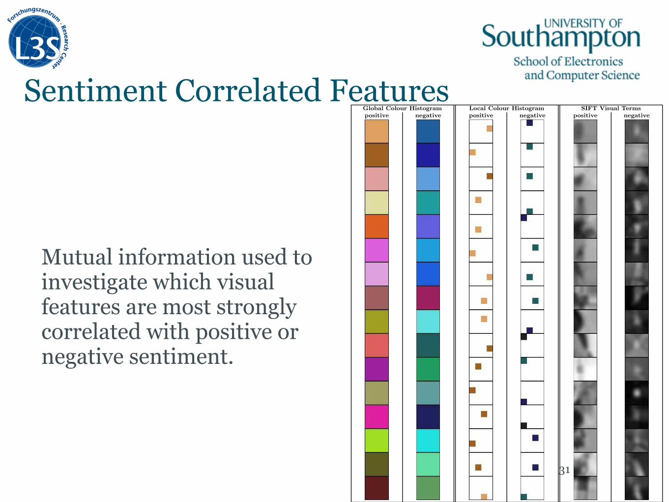
Mutual information used to investigate which visual features are most strongly correlated with positive or negative sentiment.

31

Global Colour Histogram Local Colour Histogram SIFT Visual Termspositive negative positive negative positive negative

Figure 1: The 16 most predictive visual features for positive and negative sentiment, calculated using mutualinformation. The visualisations are ranked by decreasing MI score, so the patches depicted at the top havemore predictive power than those further down. Global colour histogram features have been visualised byrendering patches showing the mean colour of the respective histogram bin. The visualisations of the localcolour histograms illustrate both the average colour of the histogram bin as well as its respective location inthe image plane. Depictions of the SIFT visual features have been extracted from interest regions of imagesin the dataset, and normalised for scale and rotation.

Thank You! Any Questions?