Scheduling Giovanni De Micheli - University of Texas at Austinusers.ece.utexas.edu/~gerstl/ee382v-ics_f09/lectures/lecture_12.pdf · 3 (c) Giovanni De Micheli 5 Taxonomy Unconstrained

1

SchedulingScheduling

Giovanni De MicheliIntegrated Systems Centre, EPF Lausanne

Additional sources:• Lecture notes by Kia Bazargan, U of M

• Source: http://www.ece.umn.edu/users/kia/Courses/EE5301

• Notes by Rajesh Gupta, UC San Diego• Original source: http://www.cecs.uci.edu/~rgupta/ics280.html

This presentation can be used for non-commercial purposes as long as this note and the copyright footers are not removed

© Giovanni De Micheli – All rights reserved

(c) Giovanni De Micheli 2

Module 1

Objectives:

The scheduling problem

Case analysis

Scheduling without constraints

Scheduling with timing constraints

2


Scheduling

Circuit model: Sequencing graph

Cycle-time is given

Operation delays expressed in cycles

Scheduling: Determine the start times for the operations

Satisfying all the sequencing (timing and resource) constraint

Goal: Determine area/latency trade-off


Example

* * + <

-

-

* * * * +

NOP

NOP

0

1 2

3

4

5

6

7

8

9

10

11

n

TIME 1

TIME 2

TIME 3

TIME 4

* * + <

-

-

* * * * +

NOP

NOP

0

1 2

3

4

5

6

7

8

9

10

11

n

3


Taxonomy

Unconstrained scheduling

Scheduling with timing constraints: Latency

Detailed timing constraints

Scheduling with resource constraints

Related problems: Chaining

Synchronization

Pipeline scheduling


Operation Scheduling

Input: Sequencing graph G(V, E), with n vertices

Cycle time . Operation delays D = {di: i=0..n}.

Output: Schedule determines start time ti of operation vi.

Latency = tn – t0.

Goal: determine area / latency tradeoff

Classes: Non-hierarchical and unconstrained

Latency constrained

Resource constrained

Hierarchical

© R. Gupta

4


Simplest method

All operations have bounded delays

All delays are in cycles:

Cycle-time is given

No constraints – no bounds on area

Goal:

Minimize latency


Min Latency Unconstrained Scheduling

Simplest case: no constraints, find min latency

Given set of vertices V, delays D and a partial order > on operations

E, find an integer labeling of operations : V Z+ Such that:

ti = (vi).

ti tj + dj (vj, vi) E.

= tn – t0 is minimum.

Solvable in polynomial time

Bounds on latency for resource constrained problems

ASAP algorithm used: topological order

© R. Gupta

5


ASAP Schedules

Schedule v0 at t0=0.

While (vn not scheduled) Select vi with all scheduled predecessors

Schedule vi at ti = max {tj+dj}, vj being a predecessor of vi.

Return tn.

+

NOP

+ <-

-NOP

1

23

4

© R. Gupta


ALAP Schedules

Schedule vn at tn=.

While (v0 not scheduled) Select vi with all scheduled successors

Schedule vi at ti = min {tj-dj}, vj being a succecessor of vi.

+

NOP

+ <-

-NOP

1

23

4

© R. Gupta

6


Remarks

ALAP solves a latency-constrained problem

Latency bound can be set to latency computed by ASAP

algorithm

Mobility:

Defined for each operation

Difference between ALAP and ASAP schedule

Slack on the start time


Example

Operations with zero mobility:

{ v1, v2, v3, v4, v5 }

Critical path

Operations with mobility one: { v6, v7 }

Operations with mobility two: { v8, v9, v10, v11 }

* * + <

-

-

* * * * +

NOP

NOP

0

1 2

3

4

5

6

7

8

9

10

11

n

TIME 1

TIME 2

TIME 3

TIME 4

*

*

+ <

-

-

* *

*

* +

NOP

NOP

0

1 2

3

4

5

6

7 8

9

10

11

n

7


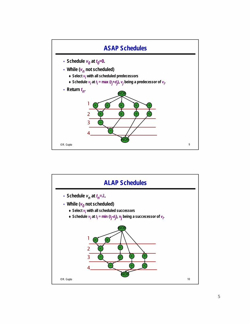
Scheduling under detailed timing constraints

Motivation:

Interface design

Control over operation start time

Constraints:

Upper/lower bounds on start-time difference of any operation pair

Feasibility of a solution


Constraint graph model

Start from sequencing graph Model delays as weights on edges

Add forward edges for minimum constraints: Edge ( vi , vj ) with weight lij → tj ≥ ti + lij

Add backward edges for maximum constraints: That is, for constraint from vi to vj

add backward edge ( vj , vi ) with weight: -uij because tj ≤ ti + uij→ ti ≥ tj - uij

8


Example

NOP

NOP

* *

+ +

0

1 3

2 4

n

NOP

NOP

* *

+ +

0

1 3

2 4

n

MAX TIME

3

MIN TIME

4

-3

4

0 0

22

2

11

6vn

5v4

1v3

3v2

1v1

1v0

Start timeVertex


Methods for scheduling under detailed timing constraints

Assumption:

All delays are fixed and known

Set of linear inequalities

Longest path problem

Algorithms:

Bellman-Ford, Liao-Wong

Extensions:

Unbounded delays, relative scheduling

9


Method for scheduling with unbounded-delay operations

Unbounded delays: Synchronization

Unbounded-delay operations (e.g. loops)

Anchors: Unbounded-delay operations

Relative scheduling: Schedule ops w.r. to the anchors

Combine schedules


Example

t3 = max { t1 + d1; ta + da }

NOP

NOP

* SYN

+ +

0

1 a

2 3

n

10


Relative scheduling method

For each vertex:

Determine relevant anchor set R (vi )

Anchors affecting start time

Determine time offsets from anchors

Start-time:

Expressed by : ti = max { ta + da + ti }

Computed only at run-time because delays of anchors are unknown


Relative scheduling under timing constraints

Problem definition:

Detailed timing constraints

Unbounded delay operations

Solution:

May or may not exist

Problem may be ill-specified

11


Relative scheduling under timing constraints

Feasible problem:

A solution exists when unknown delays are zero

Well-posed problem:

A solution exists for any value of the unknown delays

Theorem:

A constraint graph can be well-posed if there are no cycles with unbounded weights


Example

vi

vj

a

da

-uij

vjvi

a2a1

da1 da2

-uij

vjvi

a2a1

da1 da2

-uij

da2

(a) (b) (c)

12


Relative scheduling approach

Analyze graph: Detect anchors

Well-posedness test

Determine dependencies from anchors

Schedule ops with respect to relevant anchors: Bellman-Ford, Liao-Wong, Ku algorithms

Combine schedules to determine start times:ti = max { ta + da + ti }

a є R(vi)


Example

NOP

NOP

* SYN

+ +

0

1 a

2 3

N

2

2-3

1 1

3

da

3 0{v0 , a}v3

2 -{v0}v2

0 -{v0}v1

0 -{v0}a

Offsets

t0 ta

Relevant Anchor Set

R(vi)

Vertex

vi

13


Example of control-unit

1100

0000

0010

0001

counter

syncha 1 2

3

start Completion of (a)


Module 2

Objectives:

Scheduling with resource constraints

Exact formulation: ILP

Hu’s algorithm

Heuristic methods

List scheduling

Force-directed scheduling

14


Scheduling under resource constraints

Classical scheduling problem: Fix area bound – minimize latency (ML-RCS)

The amount of available resources affects the achievable latency

Dual problem: Fix latency bound – minimize resources (MR-LCS)

Assumption: All delays bounded and known


Given a set of ops V with integer delays D, a partial order on the operations E,and upper bounds { ak; k = 1, 2,…, nres } on resource usage:

Find an integer labeling of the operation φ : V → z+

such that :ti = φ( vi ),

ti ≥ tj + dj for all i,j s.t. (vj, vi) є E,

| {vi |T(vi) = k and ti ≤ l < tj + dj } | ≤ ak for all types k = 1,2,…,nres

and steps l

and tn is minimum

Minimum latency resource-constrained scheduling (ML-RCS)

15


Scheduling under resource constraints

Intractable problem

Algorithms:

Exact: Integer linear program

Hu (restrictive assumptions)

Approximate : List scheduling

Force-directed scheduling


Binary decision variables:

X = { xil, i = 1,2,…. n; l = 1,2,…, λ + 1}

xil is TRUE only when operation vi starts in step l of the schedule ( i.e. l = ti )

λ is an upper bound on latency

Start time of operation vi : Σl l . xil

ILP formulation

16


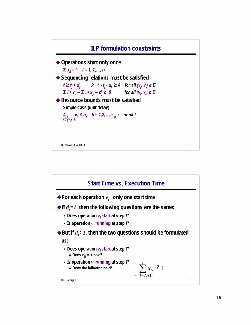
Operations start only onceΣ xil = 1 i = 1, 2,…, n

Sequencing relations must be satisfiedti ≥ tj + dj ti - tj - dj ≥ 0 for all (vj, vi) є E

Σ l • xil – Σ l • xjl – dj ≥ 0 for all (vj, vi) є E

Resource bounds must be satisfiedSimple case (unit delay)Σ l xil ≤ ak k = 1,2,…nres ; for all l

ILP formulation constraints

i:T(vi)=k


Start Time vs. Execution Time

For each operation vi , only one start time

If di=1, then the following questions are the same: Does operation vi start at step l?

Is operation vi running at step l?

But if di>1, then the two questions should be formulated as: Does operation vi start at step l?

Does xil = 1 hold?

Is operation vi running at step l? Does the following hold? 1

1

l

dlmim

i

x ?

© K. Bazargan

17


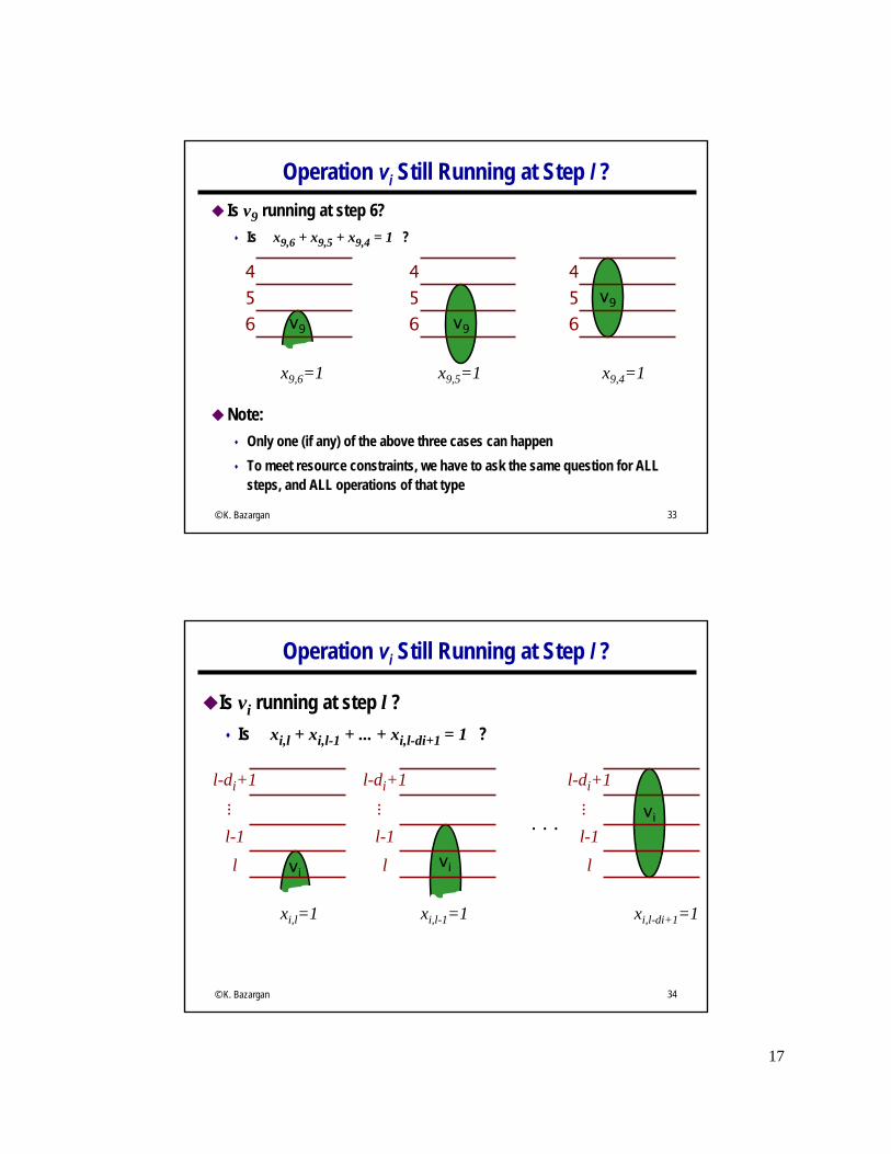
Operation vi Still Running at Step l ?

Is v9 running at step 6?

Is x9,6 + x9,5 + x9,4 = 1 ?

Note:

Only one (if any) of the above three cases can happen

To meet resource constraints, we have to ask the same question for ALL steps, and ALL operations of that type

v9

456

x9,4=1

v9

456

x9,5=1

v9

456

x9,6=1

© K. Bazargan


Operation vi Still Running at Step l ?

Is vi running at step l ?

Is xi,l + xi,l-1 + ... + xi,l-di+1 = 1 ?

vi

l

l-1

l-di+1

...

xi,l-di+1=1

vil

l-1

l-di+1

...

xi,l-1=1

vil

l-1

l-di+1

...

xi,l=1

. . .

© K. Bazargan

18


Constraints: Unique start times:

Sequencing (dependency) relations must be satisfied

Resource constraints

Objective: min cTt. t =start times vector, c =cost weight (e.g., [0 0 ... 1])

When c =[0 0 ... 1], cTt =

ILP Formulation of ML-RCS

l

il nix ,,1,0,1

jl

jll

ilijjji dxlxlEvvdtt ..),(

1,,1,,,1,)(: 1

lnkax reskkvTi

l

dlmim

i i

nll

xl .

© K. Bazargan


Example

Resource constraints: 2 ALUs; 2 Multipliers

a1 = 2; a2 = 2

Single-cycle operation di = 1 for all i

* * + <

-

-

* * * * +

NOP

NOP

0

1 2

3

4

5

6

7

8

9

10

11

n

19


ILP Example

Assume = 4

First, perform ASAP and ALAP

(we can write the ILP without ASAP and ALAP, but using ASAP and ALAP will simplify the inequalities)

+

NOP

+ <-

-NOP

1

23

4

+

NOP

+ <-

-NOP

1

23

4

v2v1

v3

v4

v5

vn

v6

v7

v8

v9

v10

v11

v2v1

v3

v4

v5

vn

v6

v7 v8

v9

v10

v11

© K. Bazargan


ILP Example: Unique Start Times Constraint

Without using ASAP and ALAP

values:

Using ASAP and ALAP:

1

...

...

...

1

1

4,113,112,111,11

4,23,22,21,2

4,13,12,11,1

xxxx

xxxx

xxxx

....

1

1

1

1

1

1

1

1

1

4,93,92,9

3,82,81,8

3,72,7

2,61,6

4,5

3,4

2,3

1,2

1,1

xxx

xxx

xx

xx

x

x

x

x

x

© K. Bazargan

20


ILP Example: Dependency Constraints

Using ASAP and ALAP, the non-trivial inequalities are:

(assuming unit delay for + and *)

01.4.3.2.5

01.4.3.2.5

01.3.2.4

01.3.2.4.3.2

01.3.2.4.3.2

01.2.3.2

4,113,112,115,

4,93,92,95,

3,72,74,5

3,102,101,104,113,112,11

3,82,81,84,93,92,9

2,61,63,72,7

xxxx

xxxx

xxx

xxxxxx

xxxxxx

xxxx

n

n

© K. Bazargan


ILP Example: Resource Constraints

Resource constraints (assuming 2 adders and 2

multipliers)

Objective:

Since =4 and sink has no mobility, any feasible solution is optimum, but we can use the following anyway:

2

2

2

2

2

2

2

4,114,94,5

3,113,103,93,4

2,112,102,9

1,10

3,83,7

2,82,72,62,3

1,81,61,21,1

xxx

xxxx

xxx

x

xx

xxxx

xxxx

4,3,2,1, .4.3.2 nnnn xxxxMin © K. Bazargan

21


Example

*

*

+

<

-

-

* *

*

*

+

NOP

NOP

0

1 2

3

4

5

6

78

9

10

11

n

TIME 1

TIME 2

TIME 3

TIME 4


Minimize resource usage under latency constraint

Additional constraint:

Latency bound must be satisfied

Σl l xnl ≤ λ + 1

Resource usage is unknown in the constraints

Resource usage is the objective to minimize

MR-LCS dual ILP formulation

22


Example

Multiplier area = 5 ALU area = 1. Objective function: 5a1 + a2

*

*

+

<

-

-

* *

*

*

+

NOP

NOP

0

1 2

3

4

5

6

78

9

10

11

n

TIME 1

TIME 2

TIME 3

TIME 4


ILP Solution

Use standard ILP packages

Transform into LP problem

Advantages:

Exact method

Others constraints can be incorporated

Disadvantages:

Works well up to few thousand variables

23


Hu’s Algorithm

Simple case of the scheduling problem Operations of unit delay

Operations (and resources) of the same type

Hu’s algorithm Greedy, polynomial AND optimal (exact)

Computes lower bound on number of resources for given latencyORComputes lower bound on latency subject to resource constraints

Basic idea: Label operations based on their distances from the sink

Try to schedule nodes with higher labels first(i.e., most “critical” operations have priority)

© R. Gupta


Hu’s algorithm with ā resources

Label operations with distance to sink

Set step l = 1

Repeat until all ops are scheduled: U = unscheduled vertices in V

predecessors have been scheduled (or no predecessors)

Select S U resources with |S| ā Maximal labels

Schedule the S operations at step l

Increment step l = l + 1

24


Example

Assumptions: One resource type only All operations have unit delay

Labels: Distance to sink

3 2 1 1

2

1

4 4 3 2 2

0

1 2

3

4

5

6

7

8

9

10

11

n


3 11

Example

Step 1: Op 1,2,6

Step 2: Op 3,7,8

Step 3: Op 4,9,10

Step 4: Op 5,11

2 1

2

4 4 3 2 2

0

1 2

3

4

5

6

7

8

9

10

11

n

_

a = 3

4 4 3 2

23

2

1

2

11

1

25


List scheduling algorithms

Heuristic method for: Min latency subject to resource bound (ML-RCS)

Min resource subject to latency bound (MR-LCS)

Greedy strategy (like Hu’s)

Does not guarantee optimality (unlike Hu’s)

General graphs (unlike Hu’s)

Resource constraints on different resource types

Operations of arbitrary delay

Priority list heuristics Priority decided by criticality (similar to Hu’s)

Longest path to sink, longest path to timing constraint

O(n) time complexity

© K. Bazargan


List scheduling algorithm for minimum latency

LIST_L( G(V, E), a) {

l = 1;

repeat {

for each resource type k = 1, 2, …, nres {

Determine ready operations Ul,k;

Determine unfinished operations Tl,k;

Select Sk Ul,k vertices, s.t. |Sk| + |Tl,k| ≤ ak;

Schedule the Sk operations at step l;

}

l = l + 1;

}

until (vn is scheduled) ;

return (t);

}

26


Example

* *

+

<

-

-

* * *

*

+

NOP

NOP

0

1 2

3

4

5

6

7 8

9

10

11

n

TIME 1

TIME 2

TIME 3

TIME 4

TIME 5

TIME 6

TIME 7

Resource bounds:

3 multipliers with delay 2

1 ALU with delay 1

* * + <

-

-

* * * * +

NOP

NOP

0

1 2

3

4

5

6

7

8

9

10

11

n


LIST_R( G(V, E), λ) {a = 1;Compute the latest possible start times tL by ALAP ( G(V, E), λ);if (t0 < 0)

return (Ø);l = 1;repeat {

for each resource type k = 1, 2, …, nres {Determine ready operations Ul,k;Compute the slacks { si = ti – l for all vi є Ulk};Schedule the candidate operations with zero slack and update a;Schedule the candidate operations not needing additional resources;}

l = l + 1;}until (vn is scheduled) ;return (t, a);

}

List scheduling algorithm for minimum resource usage

L

L

27


Example

TIME 1

TIME 2

TIME 3

TIME 4

*

*

+

<

-

-

* *

*

*

+

NOP

NOP

0

1 2

3

4

5

6

7 8

9

10

11

n

* * + <

-

-

* * * * +

NOP

NOP

0

1 2

3

4

5

6

7

8

9

10

11

n

AssumptionsUnit-delay resourcesMaximum latency = 4

Start with :a1 = 1 multipliera2 = 1 ALUs

Step 1Two multiplications on CPSet a1 = 2 Schedule Mult 1,2 Schedule ALU 10

Step 2Schedule Mult 3, 6Schedule ALU 11

Step 3Schedule Mult 7,8Schedule ALU 4

Step 4Set a2=2Schedule ALU 5, 9


Force-Directed Scheduling

Heuristic, similar to list scheduling Can handle ML-RCS and MR-LCS For ML-RCS, schedules step-by-step BUT, selection of the operations tries to find the globally best

set of operations

Idea [Paulin] Find the mobility i = ti

L – tiS of operations (ALAP-ASAP)

Look at the operation type probability distributions Try to flatten the operation type distributions

Definition: operation probability density pi ( l ) = Pr { vi executes in step l }

Assume uniform distribution: ],[1

1)( L

iSi

ii ttlforlp

© R. Gupta

28


Force-Directed Scheduling: Definitions

Operation-type distribution (sum of operation probabilities for each type)

Operation probabilities over control steps:

Distribution graph of type k over all steps:

qk ( l ) can be thought of as expected operator costfor implementing operations of type k at step l.

kvTi

ik

i

lplq)(:

)()(

)}(,),1(),0({ npppp iiii

)}(,),1(),0({ nqqq kkk

© K. Bazargan


Example

+

NOP

+ <-

-NOP

1

23

4

0)4(

83.03

1

2

1)3(

33.23

1

2

1

2

11)2(

83.23

1

2

111)1(

mult

mult

mult

mult

q

q

q

q

2.83

2.33

.83

66.13

1

3

11)4(

23

1

3

1

3

11)3(

13

1

3

1

3

1)2(

33.03

1)1(

add

add

add

add

q

q

q

q

0

1

2

1.66

0.33

© K. Bazargan

29


Force-Directed Scheduling Algorithm

Very similar to LIST_L(G(V,E), a)

Compute mobility of operations using ASAP and ALAP

Computer operation probabilities and type distributions

Select and schedule operations

Update operation probabilities and type distributions

Go to next control step

Difference with list scheduling in selecting operations

Select operations with least force

O(n2) time complexity due to pair-wise force computations

© R. Gupta


Force

Used as priority function

Force is related to concurrency:

Sort operations for least force

Mechanical analogy:

Force = constant x displacement Constant = operation-type distribution

Displacement = change in probability

30


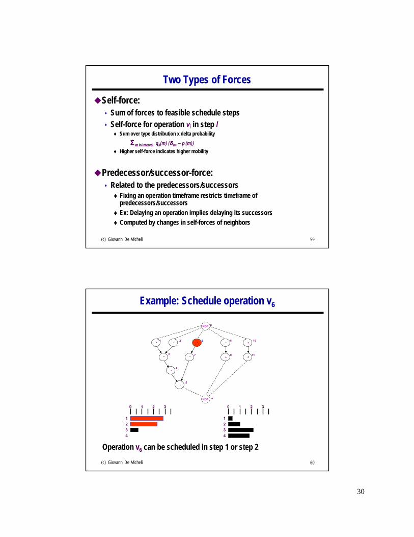
Self-force: Sum of forces to feasible schedule steps Self-force for operation vi in step l

Sum over type distribution x delta probability

Σ m in interval qk(m) (δlm – pi(m))

Higher self-force indicates higher mobility

Predecessor/successor-force: Related to the predecessors/successors

Fixing an operation timeframe restricts timeframe of predecessors/successors

Ex: Delaying an operation implies delaying its successors

Computed by changes in self-forces of neighbors

Two Types of Forces


Example: Schedule operation v6

Operation v6 can be scheduled in step 1 or step 2

* * + <

-

-

* * * * +

NOP

NOP

0

1 2

3

4

5

6

7

8

9

10

11

n

0 1 32

1

2

3

4

0 1 32

1

2

3

4

31


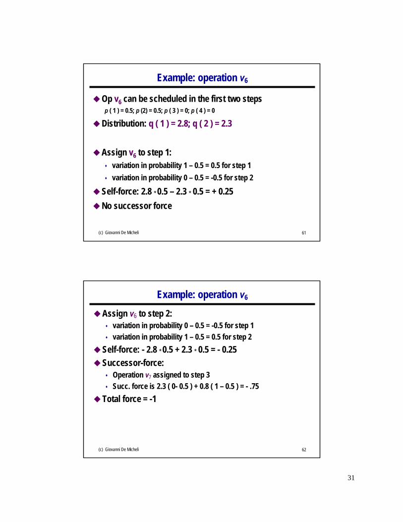
Example: operation v6

Op v6 can be scheduled in the first two stepsp ( 1 ) = 0.5; p (2) = 0.5; p ( 3 ) = 0; p ( 4 ) = 0

Distribution: q ( 1 ) = 2.8; q ( 2 ) = 2.3

Assign v6 to step 1: variation in probability 1 – 0.5 = 0.5 for step 1

variation in probability 0 – 0.5 = -0.5 for step 2

Self-force: 2.8 * 0.5 – 2.3 * 0.5 = + 0.25

No successor force



Assign v6 to step 2: variation in probability 0 – 0.5 = -0.5 for step 1

variation in probability 1 – 0.5 = 0.5 for step 2

Self-force: - 2.8 * 0.5 + 2.3 * 0.5 = - 0.25

Successor-force: Operation v7 assigned to step 3

Succ. force is 2.3 ( 0- 0.5 ) + 0.8 ( 1 – 0.5 ) = - .75

Total force = -1

32



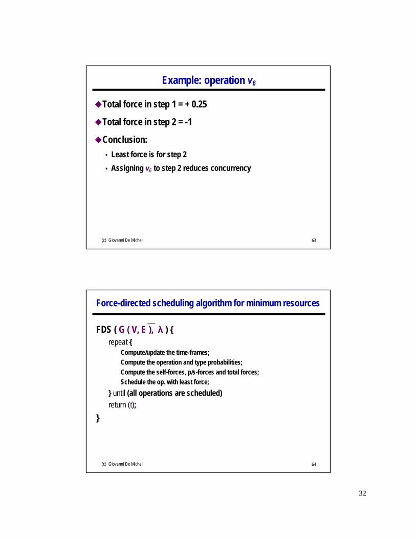
Total force in step 1 = + 0.25

Total force in step 2 = -1

Conclusion:

Least force is for step 2

Assigning v6 to step 2 reduces concurrency


Force-directed scheduling algorithm for minimum resources

FDS ( G ( V, E ), λ ) {repeat {

Compute/update the time-frames;

Compute the operation and type probabilities;

Compute the self-forces, p/s-forces and total forces;

Schedule the op. with least force;

} until (all operations are scheduled)

return (t);

}

33


Scheduling Generalizations

Conditional operations

Hierarchy

Resource generalizations

Multi-cycling and chaining

Pipelined resources

Model generalizations

Pipelining

Loops

© R. Gupta


Multi-Cycling and Chaining

Consider propagation delays of resources not in terms of cycles

Use scheduling to chain multiple operations in the same control step

Useful technique to explore effect of cycle-time on area/latency trade-off

Algorithms: ILP, ALAP/ASAP, list scheduling

34


Example

Cycle-time: 60

NOP

10

10 50

30 20

NOP

20 40

0

1 2

3 4

5

67

N

NOP

10

10 50

30 20

NOP

20 40

0

1 2

3 4

5

67

N

(a) (b)


Pipelining

Two levels of pipelining:

Structural pipelining Pipelined resources

Non-pipelined model

Functional pipelining Non-pipelined resources

Pipelined model

© R. Gupta

35


Structural Pipelining

Non-pipelined model using pipelined resources

Resources characterized by

Execution delay

Data introduction interval: DII

Implications

Operations sharing a pipelined resource are serialized (always)

Operations do not have data dependency

Solution using list scheduling

Relax criteria for selection of vertices

© R. Gupta


Structural Pipelining Example

3 multipliers w/ 2 cycle delay and DII = 1© R. Gupta

+ +

++

**** * * **+ + <<

< <**+

+

* * * * * *

--

--

-- -

-

** **

** **

36


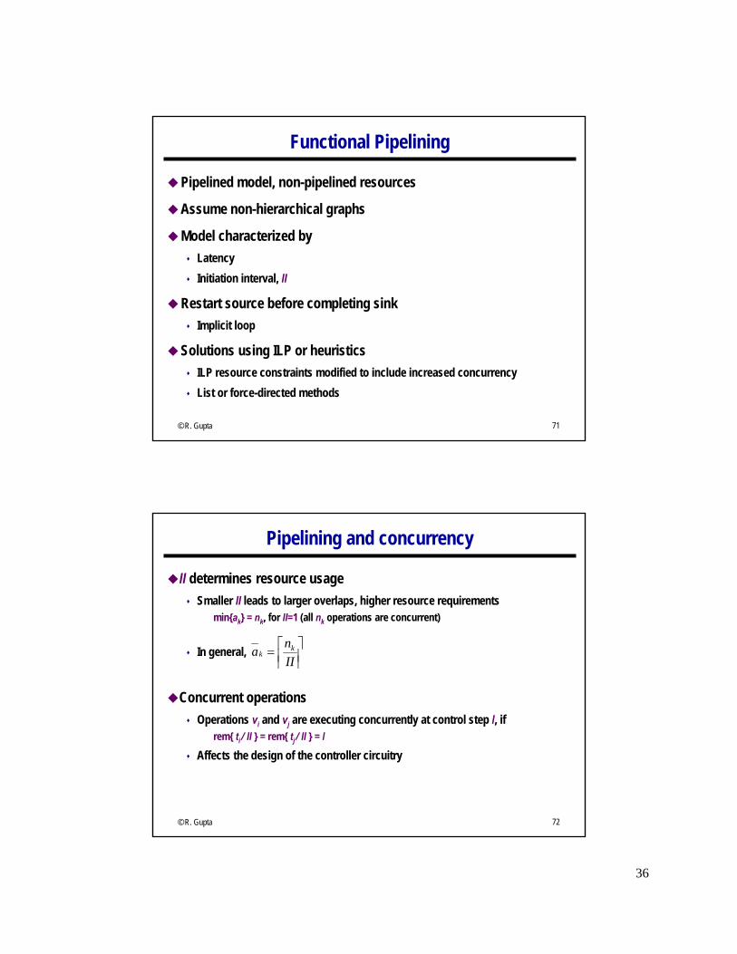
Functional Pipelining

Pipelined model, non-pipelined resources

Assume non-hierarchical graphs

Model characterized by

Latency

Initiation interval, II

Restart source before completing sink

Implicit loop

Solutions using ILP or heuristics

ILP resource constraints modified to include increased concurrency

List or force-directed methods

© R. Gupta


Pipelining and concurrency

II determines resource usage

Smaller II leads to larger overlaps, higher resource requirementsmin{ak} = nk, for II=1 (all nk operations are concurrent)

In general,

Concurrent operations

Operations vi and vj are executing concurrently at control step l, ifrem{ ti ⁄ II } = rem{ tj ⁄ II } = l

Affects the design of the controller circuitry

© R. Gupta

II

na k

k

37


Loop Scheduling

Potential parallelism across loop invocations

Single loop executions

Sequential execution

Loop unrolling (known iteration count) Merge multiple iterations into one to provide scheduling opportunities

Loop pipelining (iteration count might be unknown) Start next iteration while current one is still running

Depends on dependencies across iterations

Merging of multiple loops

Run different loops in parallel (no dependencies)

© R. Gupta


Loop Scheduling Example

Sequential

Unrolled

Pipelined

© R. Gupta

1 2 3 4 5 6 7 8

1,2,3 4,5,6 7,8,9

1

2

3

4

5

6

7

8

8

38


Loop Pipelining

Iteration count = N

Loop latency = N · λ

Pipeline loop iterations with II < λ

Latency of the pipelined loop = N · II + overhead

Overhead =

© R. Gupta

1II


Summary

Scheduling determines area/latency trade-off

Intractable problem in general:

Heuristic algorithms

ILP formulation (small-case problems)

Several heuristic formulations

List scheduling is the fastest and most used

Force-directed scheduling tends to yield good results

Several extensions

Chaining and multi-cycling

Pipelining

Scheduling Giovanni De Micheli - University of Texas at Austinusers.ece.utexas.edu/~gerstl/ee382v-ics_f09/lectures/lecture_12.pdf · 3 (c) Giovanni De Micheli 5 Taxonomy Unconstrained

Documents