Angus Deaton 1 Saving and Income Smoothing in Cote d'lvoire 1 Angus Deaton, Princeton University This paper is concerned with the extent to which farmers and other households in Cote d'lvoire save and dis-save in order to make their consumption smoother than their incomes. I attempt to test a strict form of inter-temporal smoothing, that consumption follows the permanent income hypothesis, by which consumption is equal to the annuity value of the sum of assets and the present discounted value of current and expected future labour income. The extent to which households in LDCs can and do smooth their incomes is still a matter of debate. Especially in rural areas, formal credit markets are imperfect or absent, and it has sometimes been argued that poor and ill-educated people find it inherently difficult to make good inter-temporal choices. Yet many important policy issues hang on the issue. 1. Introduction Much of the uncertainty in individual incomes depends on price and output variability in agriculture, and the value of government stabilization of commodity prices depends crucially on the extent to which rural households can stabilize their own consumption in the face of variable farm incomes, see Newbery and Stiglitz (1981) and Mirrlees (1988). Similarly, the extent to which public action is required to alleviate distress during periods of low incomes is determined by how well individuals themselves can provide for bad times. In much of Africa, and including C6te d'lvoire for most of its history, commodity prices paid to farmers have been held below world prices, and have not varied as much as world prices. Although such policies are perhaps necessary to supply the public purse in economies where there are limited other sources of revenue, they have also been justified on the grounds that governments 1 I am grateful to Kristin Butcher, John Campbell, and Franque Grimard for help during the preparation of this paper, and to the Lynde and Harry Bradley Foundation for support of my leave during which the research was done. This work is part of a larger project on saving in LDCs earned out for the World Bank. Valerie Kozel wrote most of the code for calculating incomes from the questionnaire, and this paper could not have been written without her preliminary work. I am grateful to Martha Ainsworth, Orley Ashenfelter, Surjit Bhalla, Paul Glewwe, Robert Moffitt, Philip Musgrove, Steve Pischke, Nicholas Stern, Duncan Thomas, and particularly Marjorie Flavin for comments on an earlier version. The views are those of the author, and should not be attributed to the World Bank or to any other organization.

Welcome message from author
This document is posted to help you gain knowledge. Please leave a comment to let me know what you think about it! Share it to your friends and learn new things together.
Transcript
Angus Deaton 1
Saving and Income Smoothing in Cote d'lvoire1
Angus Deaton, Princeton University
This paper is concerned with the extent to which farmers and other households inCote d'lvoire save and dis-save in order to make their consumption smoother thantheir incomes. I attempt to test a strict form of inter-temporal smoothing, thatconsumption follows the permanent income hypothesis, by which consumption is equalto the annuity value of the sum of assets and the present discounted value of currentand expected future labour income. The extent to which households in LDCs can anddo smooth their incomes is still a matter of debate. Especially in rural areas, formalcredit markets are imperfect or absent, and it has sometimes been argued that poorand ill-educated people find it inherently difficult to make good inter-temporalchoices. Yet many important policy issues hang on the issue.
1. Introduction
Much of the uncertainty in individual incomes depends on price and output variability inagriculture, and the value of government stabilization of commodity prices depends cruciallyon the extent to which rural households can stabilize their own consumption in the face ofvariable farm incomes, see Newbery and Stiglitz (1981) and Mirrlees (1988). Similarly, theextent to which public action is required to alleviate distress during periods of low incomesis determined by how well individuals themselves can provide for bad times. In much ofAfrica, and including C6te d'lvoire for most of its history, commodity prices paid to farmershave been held below world prices, and have not varied as much as world prices. Althoughsuch policies are perhaps necessary to supply the public purse in economies where there arelimited other sources of revenue, they have also been justified on the grounds that governments
1 I am grateful to Kristin Butcher, John Campbell, and Franque Grimard for help during the preparation of this paper,and to the Lynde and Harry Bradley Foundation for support of my leave during which the research was done. Thiswork is part of a larger project on saving in LDCs earned out for the World Bank. Valerie Kozel wrote most of thecode for calculating incomes from the questionnaire, and this paper could not have been written without herpreliminary work. I am grateful to Martha Ainsworth, Orley Ashenfelter, Surjit Bhalla, Paul Glewwe, Robert Moffitt,Philip Musgrove, Steve Pischke, Nicholas Stern, Duncan Thomas, and particularly Marjorie Flavin for comments onan earlier version. The views are those of the author, and should not be attributed to the World Bank or to any otherorganization.

2 JOURNAL OF AFRICAN ECONOMIES, VOLUME 1, NUMBER 1
are better able than producers to smooth income fluctuations. In practice, the swings ingovernment revenues engendered by fluctuations in world commodity prices have rarely beenadequately sterilized by African governments, but have rather been the source of much macro-economic instability, so that it is important to find out whether private producers might not dobetter if left to themselves.
There has been a good deal of previous work on the permanent income hypothesis inLDCs, reviewed, for example in Gersovitz (1988) and Deaton (1990). But it is clear fromBhalla's work on India (1979), (1980), Musgrove's work on Latin America (1979), and mostconvincingly of all, from Paxson's work on Thailand (1990), (1992), that smoothing takesplace, and that consumption is not equal to income, even among very poor households. Themain object of this paper is to add evidence for another country, Cdte d'lvoire, in a continentwhere there has been relatively little previous research on these issues. But I also test animplication of the permanent income hypothesis that has not been previously examined in adeveloping country. If agents look to the future when they are deciding how much to consume,they will save more when they have reason to expect that their incomes will fall. In particular,if agents have private information about their future incomes, we should be able to use theircurrent saving to predict their future income changes more accurately than would be possibleusing public information alone. C6te d'lvoire is a good country in which to test thisproposition. A substantial fraction of agricultural income derives from tree-crops, mainly cocoaand coffee, but also palm trees and bananas. If weather damages flowers, or if the farmer doesnot provide adequate weeding, the crop will suffer, and the farmer will know that his incomeis going to be low many months before he actually receives payment and income is realized.For many tree crops, yields are negatively correlated from one year to the next, so that abumper harvest in one year is a token that income is unlikely to be so high a year later. Ivorianfarmers are therefore likely to have a great deal of advance information about their incomes,and if they succeed in smoothing their consumption, we should be able to detect this advanceinformation in their saving behaviour.
My methodology is based on that pioneered by Campbell (1987), who used aggregate time-series data for the United States, and which here is adapted to the short panel data that areavailable for C6te d'lvoire. This methodology offers a number of advantages. As in thestandard "excess sensitivity" literature, that traces back to Hall (1978) and Flavin (1981), ittests whether or not changes in consumption are orthogonal to previous information, andparticularly whether consumption is sensitive to previously predictable changes in income.Moreover, the tests are carried out in such a way that if the null hypothesis is accepted, thenthe change in consumption will be exactly the amount that is warranted by the change inpermanent income calculated from a simultaneously estimated equation for income. Such amethodology reconciles "excess sensitivity" tests with tests for "excess smoothness" that checkwhether the volatility of consumption changes is consistent with the volatility of permanentincome changes calculated from fitted equations for income. (See Deaton (1987) for theoriginal statement of the excess smoothness puzzle, and Campbell and Deaton (1989) andDeaton (1992, Chapter 4) for an explanation of the relationship between the smoothness and
Angus Deaton 3
sensitivity issues.) There are real attractions to applying Campbell's tests to microeconomicbehaviour rather than to the macroeconomic aggregates of the original paper. It is easy to thinkof macroeconomic feedbacks that could generate a negative relationship between saving andfuture income growth, but these feedbacks are less likely to be an issue at the level of theindividual farmer.
The main difficulty in the work lies in the nature of the data. The C6te d'lvoire LivingStandards Survey collected information from around 1600 households in the country for theyears 1985, 1986, and 1987. Half of the households interviewed in 1985 were re-interviewedagain in 1986, while the new sample households in 1986 were carried through to a secondinterview in 1987. This rolling panel design means that for two distinct sets of 800 households,we have data on two consecutive years. For no household is there more than this; the data donot track households over a period of years, as is the case, for example, in the Panel Study ofIncome Dynamics in the United States. Data such as these cannot be used to test hypothesesabout inter-temporal behaviour without very strong supplementary assumptions. Permanentincome theory delivers propositions about time averages of individual behaviour, propositionsthat cannot be tested directly without time series data on individuals. Absent long panels, eitherwe can make aggregation assumptions that allow the theory to be tested on aggregate time-series data, or we can make assumptions that allow us to identify time-series properties fromcross-section data. The latter is the route followed here, and it must be admitted from theoutset that the assumptions are strong. In the empirical application, I shall require that eachagent's income process be stationary, and that once individual means have been subtracted out,each agent's time series process is identical, at least within geographical regions. Each farmeror worker receives his or her own income innovation, but even here, I need to assume that allincomes are affected equally by common regional macroeconomic shocks, shocks that arelikely to be of the greatest importance in an agricultural economy like that of C6te d'lvoire.I shall discuss these assumptions in more detail when I require them, and defend them as bestI am able.
Section 1 of the paper develops the basic theory, following the general principles ofCampbell's work, but adapting the model to the special requirements of C6te d'lvoire. Thesection lays the groundwork for interpreting the parameters that are estimated in the finalsection. I try to develop a link between the nature of agricultural income, particularly thedifferent time series properties that might be associated with different crops, and the jointstochastic behaviour of saving and income. The formulas that are developed can in principlerelate agro-climatic conditions to the bivariate time-series process describing saving andincome. Section 2 lays the econometric groundwork, makes the compromises that are requiredto use the Ivorian data, and explains how they affect the interpretation of the results. Section3 presents the estimates. The restrictions implied by the permanent income theory are notsupported by the data, although the nature of the failure does not suggest that consumptionresponds to predictable income changes, as has often been found in studies for the UnitedStates. However, I consistently find that saving predicts falls in income in the cross-sectiondata, so that farmers who are saving in one year are those who are most likely to have a fall
4 JOURNAL OF AFRICAN ECONOMIES, VOLUME 1, NUMBER 1
in income in the next. Although the interpretation of these findings is complicated byeconometric and data problems, they provide further support for the notion that farmers planahead, even if they do not do so according to the strict permanent income calculus forconsumption.
2. Saving, Income and Information
The hypothesis under consideration is that consumption is the annuity value of assets andexpected future labour income. Following Flavin (1981), I write this as
where c, is real consumption, y, is real labour income, A, is the real value of financial assets,r is the constant, known real rate of interest, and fi, is the information set available to the agentat time / and upon which expectations are based. The use of an infinite horizon model allowsme to abstract from life-cycle considerations, but perhaps the best literal interpretation is interms of a household that is a timeless dynasty or extended family, that will live for ever, andthat is large enough so that its demographic structure does not vary very much over time. Inthe analysis that follows, I shall require that the real interest rate r be strictly positive.However, it is possible to recast the model with a finite horizon and with r<0 with only aslight increase in the complexity of the algebra.
For my purposes, it is more convenient to write the PIH in a different but equivalent form,originally derived by Campbell. Define saving, s, as the difference between total income andconsumption, i.e.
Then substitution of (2) in (1) and rearrangement yields Campbell's "saving for a rainy day"equation, viz.
(3) st- -£(l+r)-'E(Aj>JQ,).i-i
where A denotes a backward first difference. Saving at / is the discounted present value of allfuture expected falls in income. Turning this equation into a testable proposition on the Ivoriandata is the main purpose of this section.
Start from the problem of observing expectations. The information set Q, is the informationset available to the agent, not the econometrician, and we should expect the agent to have all
Angus Deaton 5
sorts of advance notice of income changes that would be extremely difficult to detect in thedata. As argued in the introduction, this is particularly likely to be the case for fanners of treecrops, or for any farmer whose income is realized some time after the first informationbecomes available about the likely size of the harvest. Again we adopt a device first appliedin this context by Campbell (1987).
Suppose that the information available to the econometrician at time / is H, where H, c ft,so that everything known to the econometrician is known to the farmer, but not vice versa.Suppose also that H, contains (at the very least) both saving s, and income y. Then we can"project" (3) on to H, i.e. we take expectations of both sides conditional on H, Since 5, belongsto H, the projection of s, on to H, is just s,, while, for the right hand side, the law of iteratedexpectations simply results in the agent's information set Q, being replaced by theeconometrician's information set H, Hence, (3) becomes
(4) s, - -£(l+r)-'£l(Aj<J//,).
Equation (4), unlike (1) or (3), contains only observable quantities. Even so, the similaritybetween (3) and (4) is perhaps deceptive, and it might easily be supposed that the argumentabove serves only to provide a formal basis for what would have to be done in any case, whichis the substitution of observable for unobservable information. Note however that the argumentrequires that saving be in the econometrician's information set, so that (4) will not hold unlessexpectations about future income are conditioned on current saving. If income is modelled asa univariate time series process, which is then used to generate forecasts, current saving willnot satisfy equation (4) if the agent has private information. Under the permanent incomehypothesis, saving acts as a sufficient statistic for the agent's future income expectations, sothat using it to help predict income is necessary if we are to control for private information.
To go further, we need to specify a model for forecasting income, based on theeconometrician's observation set, Hn which can be used, together with (4), to generate testablerestrictions on the behaviour of saving. Campbell, in his work on savings in the United States,makes the assumption that the change in labour income is stationary, and shows that, in suchcircumstances, the PIH is consistent with a model in which saving and the change in labourincome are jointly stationary. For the C6te d'lvoire, I assume, in contrast, that incomes arestationary in levels. Over the last 15 years, there has been little growth in real living standardsin C6te d'lvoire; real per capita consumption in 1985 was the same as in 1970, and for the twoyears of the survey, 1985-86, average household income changed by less than a third of oneper cent. This apparent lack of change disguises the fact that, at the national level, there wasconsiderable growth in the first part of the period, followed by a marked decline later, asnational income followed fluctuations in cocoa and coffee prices. However, since procurementprices for these crops were held more or less constant in real terms, this national pattern wasnot passed through to the farmers who are our main concern, and whose income can perhapstherefore be treated as stationary. If so, the permanent income hypothesis implies that savings
6 JOURNAL OF AFRICAN ECONOMIES, VOLUME 1, NUMBER 1
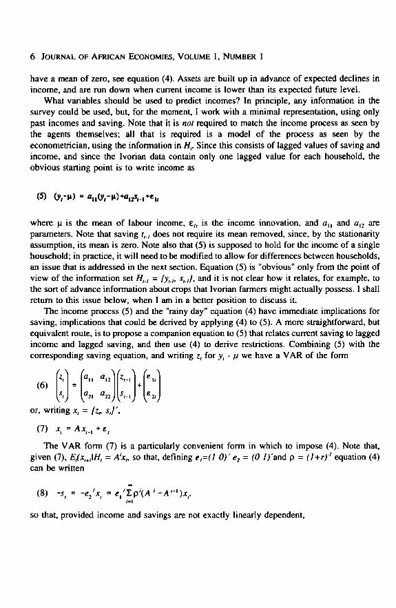
have a mean of zero, see equation (4). Assets are built up in advance of expected declines inincome, and are run down when current income is lower than its expected future level.
What variables should be used to predict incomes? In principle, any information in thesurvey could be used, but, for the moment, I work with a minimal representation, using onlypast incomes and saving. Note that it is not required to match the income process as seen bythe agents themselves; all that is required is a model of the process as seen by theeconometrician, using the information in //,. Since this consists of lagged values of saving andincome, and since the Ivorian data contain only one lagged value for each household, theobvious starting point is to write income as
(5) (yr-M) = fliiO
where u is the mean of labour income, e;, is the income innovation, and a,, and al2 areparameters. Note that saving r,.; does not require its mean removed, since, by the stationarityassumption, its mean is zero. Note also that (5) is supposed to hold for the income of a singlehousehold; in practice, it will need to be modified to allow for differences between households,an issue that is addressed in the next section. Equation (5) is "obvious" only from the point ofview of the information set //,., = {y,.,, s,.,/, and it is not clear how it relates, for example, tothe sort of advance information about crops that Ivorian farmers might actually possess. I shallreturn to this issue below, when I am in a better position to discuss it
The income process (5) and the "rainy day" equation (4) have immediate implications forsaving, implications that could be derived by applying (4) to (5). A more straightforward, butequivalent route, is to propose a companion equation to (5) that relates current saving to laggedincome and lagged saving, and then use (4) to derive restrictions. Combining (5) with thecorresponding saving equation, and writing z, for y, - n we have a VAR of the form
or, writing x, = fz* s,)\
(7) x,=Ax,_,+z,
The VAR form (7) is a particularly convenient form in which to impose (4). Note that,given (7), EJx,JH, = Axn so that, defining e,=(l 0)'e2 = (0 l)'md p = (1+r)' equation (4)can be written
(8) -5, = -e2'x, = e/ZpU'-A-^x,.
so that, provided income and savings are not exactly linearly dependent,
Angus Deaton 7
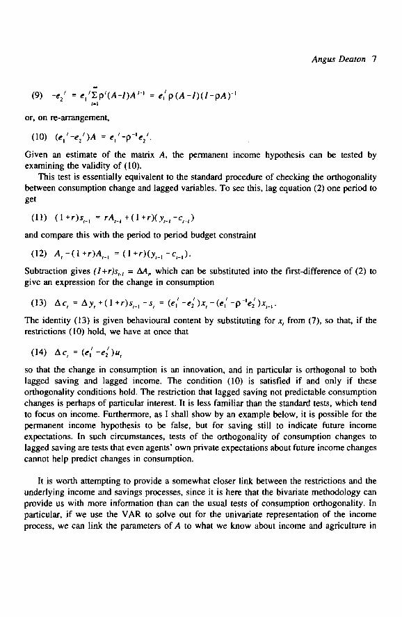
(9) -e2' =e , / Zp'(A-/M'- 1 =
or, on re-arrangement,
(10) (e/-e2')A = * , ' "P~V-
Given an estimate of the matrix A, the permanent income hypothesis can be tested byexamining the validity of (10).
This test is essentially equivalent to the standard procedure of checking the orthogonalitybetween consumption change and lagged variables. To see this, lag equation (2) one period toget
(11) ( l + r ) , , _, _ , , ,
and compare this with the period to period budget constraint
(12) i4r - (1
Subtraction gives (l+rjs,., = AAP which can be substituted into the first-difference of (2) togive an expression for the change in consumption
(13) Ac, = Ay,+(1+/•)*,_,-*, =(e, /-^':U /-(*, '-p- |e2 ' )*,_,-
The identity (13) is given behavioural content by substituting for x, from (7), so that, if therestrictions (10) hold, we have at once that
(14) Ac, =(*, /-e2/)W ,
so that the change in consumption is an innovation, and in particular is orthogonal to bothlagged saving and lagged income. The condition (10) is satisfied if and only if theseorthogonality conditions hold. The restriction that lagged saving not predictable consumptionchanges is perhaps of particular interest. It is less familiar than the standard tests, which tendto focus on income. Furthermore, as I shall show by an example below, it is possible for thepermanent income hypothesis to be false, but for saving still to indicate future incomeexpectations. In such circumstances, tests of the orthogonality of consumption changes tolagged saving are tests that even agents' own private expectations about future income changescannot help predict changes in consumption.
It is worth attempting to provide a somewhat closer link between the restrictions and theunderlying income and savings processes, since it is here that the bivariate methodology canprovide us with more information than can the usual tests of consumption orthogonality. Inparticular, if we use the VAR to solve out for the univariate representation of the incomeprocess, we can link the parameters of A to what we know about income and agriculture in
8 JOURNAL OF AFRICAN ECONOMIES, VOLUME 1, NUMBER 1
C6te d'lvoire. This provides an explicit link between the time-series process for income, asdetermined for example by the fanner's crop mix, and the joint stochastic behaviour of savingand income.
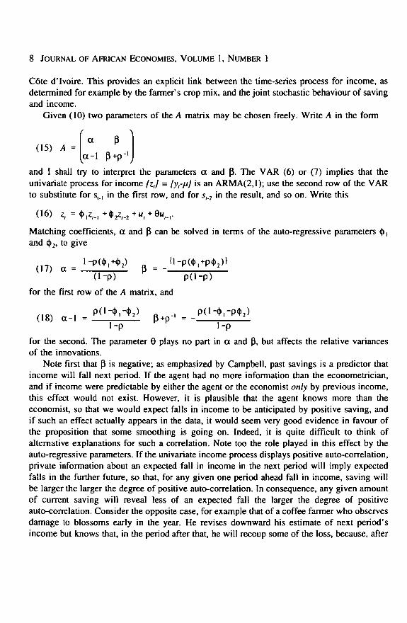
Given (10) two parameters of the A matrix may be chosen freely. Write A in the form
a p(15) A = '
and I shall try to interpret the parameters a and p. The VAR (6) or (7) implies that theunivariate process for income (zj = ty,-n) is an ARMA(2,1); use the second row of the VARto substitute for s,., in the first row, and for s,.2 in the result, and so on. Write this
Matching coefficients, a and P can be solved in terms of the auto-regressive parameters 4»,and <J>,, to give
(17) a - ' P ^ ' ^ ft - _d p )d - p ) P d - P )
for the first row of the A matrix, and
- - -( 18 ) a - 1 - P ( l * ^ p - p1-p 1-p
for the second. The parameter 8 plays no part in a and p, but affects the relative variancesof the innovations.
Note first that P is negative; as emphasized by Campbell, past savings is a predictor thatincome will fall next period. If the agent had no more information than the econometrician,and if income were predictable by either the agent or the economist only by previous income,this effect would not exist. However, it is plausible that the agent knows more than theeconomist, so that we would expect falls in income to be anticipated by positive saving, andif such an effect actually appears in the data, it would seem very good evidence in favour ofthe proposition that some smoothing is going on. Indeed, it is quite difficult to think ofalternative explanations for such a correlation. Note too the role played in this effect by theauto-regressive parameters. If the univariate income process displays positive auto-correlation,private information about an expected fall in income in the next period will imply expectedfalls in the further future, so that, for any given one period ahead fall in income, saving willbe larger the larger the degree of positive auto-correlation. In consequence, any given amountof current saving will reveal less of an expected fall the larger the degree of positiveauto-correlation. Consider the opposite case, for example that of a coffee fanner who observesdamage to blossoms early in the year. He revises downward his estimate of next period'sincome but knows that, in the period after that, he will recoup some of the loss, because, after
Angus Deaton 9
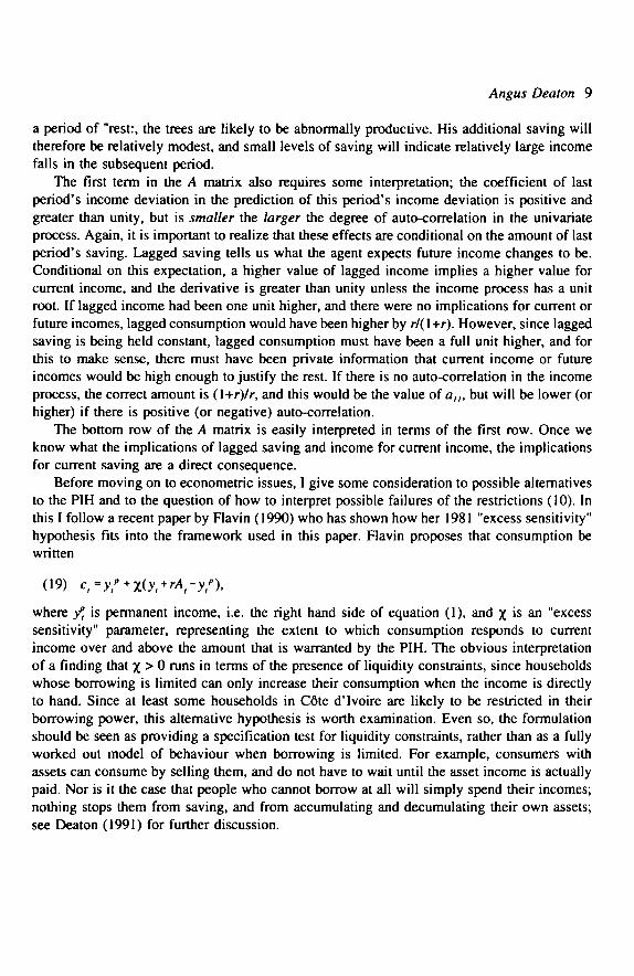
a period of "rest:, the trees are likely to be abnormally productive. His additional saving willtherefore be relatively modest, and small levels of saving will indicate relatively large incomefalls in the subsequent period.
The first term in the A matrix also requires some interpretation; the coefficient of lastperiod's income deviation in the prediction of this period's income deviation is positive andgreater than unity, but is smaller the larger the degree of auto-correlation in the univariateprocess. Again, it is important to realize that these effects are conditional on the amount of lastperiod's saving. Lagged saving tells us what the agent expects future income changes to be.Conditional on this expectation, a higher value of lagged income implies a higher value forcurrent income, and the derivative is greater than unity unless the income process has a unitroot. If lagged income had been one unit higher, and there were no implications for current orfuture incomes, lagged consumption would have been higher by r/(\+r). However, since laggedsaving is being held constant, lagged consumption must have been a full unit higher, and forthis to make sense, there must have been private information that current income or futureincomes would be high enough to justify the rest. If there is no auto-correlation in the incomeprocess, the correct amount is (l+r)/r, and this would be the value of a,,, but will be lower (orhigher) if there is positive (or negative) auto-correlation.
The bottom row of the A matrix is easily interpreted in terms of the first row. Once weknow what the implications of lagged saving and income for current income, the implicationsfor current saving are a direct consequence.
Before moving on to econometric issues, I give some consideration to possible alternativesto the PIH and to the question of how to interpret possible failures of the restrictions (10). Inthis I follow a recent paper by Flavin (1990) who has shown how her 1981 "excess sensitivity"hypothesis fits into the framework used in this paper. Flavin proposes that consumption bewritten
(19) cl=yl"*x(yl + rAi-yi"),
where yf, is permanent income, i.e. the right hand side of equation (1), and x is an "excesssensitivity" parameter, representing the extent to which consumption responds to currentincome over and above the amount that is warranted by the PIH. The obvious interpretationof a finding that X > 0 runs in terms of the presence of liquidity constraints, since householdswhose borrowing is limited can only increase their consumption when the income is directlyto hand. Since at least some households in C6te d'lvoire are likely to be restricted in theirborrowing power, this alternative hypothesis is worth examination. Even so, the formulationshould be seen as providing a specification test for liquidity constraints, rather than as a fullyworked out model of behaviour when borrowing is limited. For example, consumers withassets can consume by selling them, and do not have to wait until the asset income is actuallypaid. Nor is it the case that people who cannot borrow at all will simply spend their incomes;nothing stops them from saving, and from accumulating and decumulating their own assets;see Deaton (1991) for further discussion.
10 JOURNAL OF AFRICAN ECONOMIES, VOLUME 1, NUMBER 1
Even so, the excess sensitivity model (19) is very useful in the current context. Flavinshows that (19) implies that the rainy day equation (3) is modified to
(20) 5, = - ( l -x)£( l+r) - '£ (Ay M iq) .
so that current saving while no longer equal to the discounted present value of expected fallsin labour income, is proportional to it. In consequence, the switch of information sets, fromQ,to H, works exactly as it did before, and once again, there is a VAR representation in termsof income and saving. If the algebra is carried through as before, the restriction (10) takes thenew form
(21) Ul-x)et'-e2']A =
which, on elimination of x, gives the single non-linear restriction
(22) ( f l 2 2-p- ')( f l | 1-l) = f l | A | .
A failure of (10) when (22) is satisfied would suggest that the excess sensitivity model is a fairrepresentation of the data, and Flavin's own work (1990) suggests that this is the case for theaggregate data in the United States. Note finally that, as was the case with the permanentincome hypothesis, the restrictions of the excess sensitivity model have implications for theform of the consumption change equation. Follow the same procedure as before, and substitutefrom (7) for x, in the general consumption change equation (13), but now apply the excesssensitivity restriction (21). This gives
(23) Ac, = Xe,'( A-/)*,., +(«,/-e2')«/ = xE.-Ay. + ti-el)-,
so that, as is standard in the excess sensitivity literature, % measures the response ofconsumption change to anticipated changes in income.
3. Econometric Implementation
The theory developed in the previous section could be implemented without modificationif there were extensive time-series data for each household, so that a VAR could be estimatedand the restrictions tested for each individually. Instead, we have a large number of householdsbut only two consecutive observations for each. What is possible, and it is essentially all thatis possible, is to run cross-section regressions of income and saving on last period's incomeand saving, using the cross-sectional variances and covariances to estimate the parameters.However, these parameters cannot be regarded as estimates of the A matrix, except under veryimplausible assumptions. This section examines the problems, and shows how the data can stillbe used to test the theoretical restrictions.

Angus Deaton 11
The version of (5) that I shall work with is written
(24) y,,-u, = a,,(;>>„_,-u,) + a | 2 5, . , + y,, +eIft
with a corresponding saving equation
(25) s. = a21 (y,,., -M,) + a22s,,_, + Vj, + e a i .
According to these equations, and apart from the fixed effects //, and the idiosyncratic shockse(/, and e,2, the bivariate process describing income and saving is identical for all households,at least within a region or agro-climatic zone. The innovations in the original model are nowdecomposed into macroeconomic shocks, 4*,, and 4^, and idiosyncratic shocks, the formerentering additively and affecting all households equally. Equations (24) and (25) are perhapsthe simplest generalization of the original VAR that it is sensible to attempt to apply. Clearly,individual incomes must have different means, and just as clearly, there have to bemacroeconomic shocks, so that the aggregates of income and saving are not constant over time.However, there are many ways of incorporating these features, and the one I have chosen isvery special, and is guided as much by data availability as by realism. The assumption thatincome is stationary has already been discussed, as well as its implication that saving has meanzero for all the observations in the sample. Without this, the methods discussed below wouldnot work. The assumption that the macroeconomic shocks are additive is also required toobtain the results. As written, the two macroeconomic terms in (24) and (25) can be dealt withby including year dummies in the regression. However, if the macroeconomic shocks operatedin some other way, so that for example the effect on each household's income was different,then the cross-section estimates would not identify the parameters that I need. The fundamentalunderlying problem here is that of using short panel data to estimate time series parameters,something that cannot be done without strong maintained assumptions on the nature ofcommon shocks; for a review of this issue in the consumption context and a guide to some ofthe original literature, see Deaton (1992, Chapter 5).
It will also be useful to have the consumption change equation that corresponds to (24) and(25). If we apply equation (13) to (23) and (24), we reach
(26) Ac,, - &,(*,,-,-M,) + V H +(V.,-V2,) +( e , , , - e»,)
where, the coefficients are given by
(27) bx = f l n - f l 2 | - l b2 = fl|2-a22-(l+r)
so that, if the permanent income hypothesis is true, b ;=62 = 0. Clearly, it is a matter ofindifference which two of the three equations (24), (25), and (26) is estimated. However, mymain interest is first, the effect of lagged saving on income, and second, the orthogonality ofconsumption change to the lagged variables, so I shall work with the income and consumptionequations (24) and (26).
12 JOURNAL OF AFRICAN ECONOMIES, VOLUME l, NUMBER 1
Since the panel data for Cdte d'lvoire never have more than two years of data for eachhousehold, it is not possible to estimate any of the three equations with appropriate allowancefor the fixed effects. My procedure is to run the simplest regressions, ignoring the fixedeffects, and to examine the nature of the biases in the estimated coefficients. In general, it isclear that consistent estimates of the matrix A cannot be obtained by using two years of thecross-section to regress income and saving on lagged income and lagged saving. However,given the structure of the model, it is nevertheless the case that the estimates of the A matrixso obtained, although inconsistent, will still satisfy the theoretical restrictions (10) if thepermanent income hypothesis is true. I shall justify this statement formally below, but thesimplest way to see what is going on is to examine, not the income and saving equations (24)and (25), but the consumption change equation (26). Suppose that the consumption change isregressed on lagged income and lagged saving, ignoring the fixed effects. This regression canbe written
(29) A^V^H^A,^ ,
where the constant absorbs the macroeconomic shocks and the compound error term is givenby
(30) $„ = -*,M, • * „ - « * •
In general, ordinary least squares will not yield consistent estimates of (29), since the errorterm contains the fixed effect which is correlated with the lagged income variable. However,if the permanent income hypothesis is true, b, is zero, the fixed effect vanishes from the errorterm, and there is no bias. Hence, the PIH can be validly tested even if the fixed effects areignored. Another way of putting the same point is to note that non-zero estimates of theparameters cannot be attributed to the fixed effects, since they act as would measurement error,biasing the estimates towards zero. The same argument goes through for any instrumentalvariable estimator where the instruments are correlated with the omitted fixed effects. Onceagain, non-zero estimates cannot be explained by omitted fixed effects if the permanent incomehypothesis is true.
To see how the argument works for the VAR of saving and income, define the vector v,,by
so that the income and saving VAR can be written
(32) v,,=
where
Angus Deaton 13
(33) b, =(1 -a, ,)u+Hr,,
and u is the grand mean of the fixed effects. Although the b, vector contains quantities thatvary with /, there is only a single / in the analysis, 1987 or 1986 depending on which panelwe are using, and a single t-\, 1986 or 1985, so that b, is a constant in the cross-sectionregression.
Define the cross-sectional variance and covariance matrices
(34) C = cov(v./,v,'_l) M = vflr(v,M,v/_,) F = cov(//,v,,/.,)
which, from (32), satisfy °
(35) C = AM + F.
The ordinary least squares estimate of A from the cross-section has the probability limit CM~'so that we can write
(36) p\imA = CM' = A+FM']
which shows how the fixed effects render the OLS estimates inconsistent. However, supposethat the PIH is correct, and that the A matrix satisfies the restrictions in (10) and so can bewritten in the form (11). Hence, the truth of the PIH implies that the fixed effect vector/ in(33) has the form:
(37) /, = (l-a)(u,-u)
Hence, from (34) (e,' -e2') F = 0, so that from (36) and (10),
(38) {el-el)CM-1 =(e{-ei)A = e.'-p-'e/.
Under the null hypothesis of the PIH, we have the result that the probability limit of the OLSestimates satisfy exactly the same restrictions as does the matrix A, even though they do notprovide consistent estimates of it. For the purpose of testing the restrictions, it is unnecessaryto make any correction for differences between households in mean incomes.
It is also possible to use (36) to discover more about the properties of the OLS estimates,or at least of their probability limit CM' Again, under the null hypothesis of the PIH, (11) canbe used to evaluate (36) element by element. For the first row, which gives the parameterspredicting income,
14 JOURNAL OF AFRICAN ECONOMIES, VOLUME 1, NUMBER 1
(39) plima = (CA/"1),, = a
plimP = (CA/-')I2 = p
The stationarity of income implies that a is greater than unity, see (17), and (\f'),,>0, becauseM is positive definite, while (M~')i2<0 if saving and income are positively correlated in thecross section, as they are. Hence, if the permanent income hypothesis is true, the coefficientof lagged income on income is biased downwards, and that of lagged saving on income biasedup. Therefore if, conditional on previous values of income, saving does in fact predict incomefalls, the result is consistent with the hypothesis, provided the value of a is sufficiently closeto one. By contrast, if consumers are not looking ahead"in planning their consumption, it isquite hard to think of explanations of why, conditional on lagged income, lagged saving shouldhelp predict future income. In particular, there does not appear to be any mechanical reasonwhy we would expect the estimate of $(al2) to be negative. Consider, for example, a simplemechanical model in which each farmer's income is a first-order auto-regressive processaround its own individual mean, but in which there is no effect of lagged saving on income.This model is (26) with a,2 equal to zero, and with \a,,\ <, 1 and probably small in absolutevalue given the nature of agricultural income. To match the data, suppose also that for somereason unconnected with the theory, saving is positively correlated with the fixed effect inincome (richer farmers always save more), and thus with income itself, while remainingorthogonal to the innovations in income. A standard mis-specification analysis can then be usedto derive the probability limit of the coefficient on lagged saving in a cross-sectional regressionin which income is regressed on lagged income and lagged saving and no allowance is madefor fixed effects. As is easily shown, this limit is positive, so that such a model can yield noexplanation for a finding that farmers who save more will be those with the largest falls ofincome in the subsequent period.
If the permanent income hypothesis is false, but the data conform to Flavin's excesssensitivity model, the foregoing analysis can be modified in an appropriate way. It is stillpossible to start from the same VAR, and since the expected value of saving is still zero, therepresentation (32) still holds, and the OLS estimates will still converge to the right hand sideof (36), although the A matrix will be differenL If (21) holds instead of (10), the A matrixtakes the form
a p(40) A =
Given (40), the fixed effects /, in (33) can be written
Angus Deaton 15
H(41) / = (l-a)(p,-n)
[i-X)In consequence, [(1 ~x) e[ -e[\F = 0, so that, corresponding to (38), the excess sensitivity
hypothesis implies that(42) l(l-X)e! -eiKM'1 = [(l-X)e,' -ei\A = (l-X)e( -p"V2'.
As is the case for the pure permanent income hypothesis, when evaluating the test, we cantreat the OLS estimates as if they were estimates of A.
My statistical procedures can now be readily presented. The first stage is to estimate theVAR by ordinary least squares in the form
(43) A y f t = a o + ( a - l ) j , f t _ l + P V l + $ l f t
where b, and b2 are given by (27). The estimates of a and P are expected to be inconsistent,but, as argued above, a negative estimate for a can still be regarded as evidence that agentsare looking forward and saving in anticipation of bad times. If the full PIH is correct, b, andb2 should be zero, and this is straightforwardly tested using an F-test. The excess sensitivityhypothesis can be tested, for example, by applying a Wald test to the parameters of the VAR.However, the simplest way to obtain an estimate of the excess sensitivity parameter and to testthe hypothesis is to estimate (23) from the regression
(44) Ac,, = Y + X A v , , + ^ ,
using y,,., and s,,., as instruments. The first-stage of the appropriate two stage least squaresprocedure is simply the first of the two regressions in (43). The specification can be testedusing the over-identification test that comes from comparing the fit of (44) with theunrestricted model, which is the second regression in (43). I shall again present this as an F-statistic in order to facilitate comparison with the F-test for the unpredictability of consumptionchanges.
4. Results from Cote d'lvoire
I use data from the first three years, 1985, 1986, and 1987 of the Ivorian survey. Together,these give me two separate panels, which I shall work with separately. Although it would bepossible to pool the two data sets, three years' data are insufficient to average out any
16 JOURNAL OF AFRICAN ECONOMIES, VOLUME 1, NUMBER 1
macroeconomic shocks, and pooling will only blur any differences between the two panels thatwill result if the assumptions about the macroeconomic shocks are wildly incorrect. The sampledesign called for 800 households to be interviewed using essentially identical questionnairesin the three years, and a wide range of topics were covered, see Ainsworth and Mufioz (1986)for a description. For current purposes I need data on income, with labour income separatefrom capital income, and on saving, or equivalently, on consumption. The measurement ofconsumption is relatively straightforward. Households are asked to record purchases of a fairlydetailed list of foods and other goods, and separate sections of the questionnaire deal withhome produced food, and with regular charges, such as rent, water, and electricity for thosefew urban households who record such expenditures. The total of these amounts definesconsumption. I have done relatively little editing of the consumption data. Each of the hundredor so components were examined for gross outliers, and a few replacements were made, usu-ally by the mean (sometimes median) expenditure on that item in the village or sample clusterof the household. There were less than 100 such replacements in each year, out of a total of80,000 recorded expenditures.
The definition and measurement of income is a good deal more complex. It is clear thatit is useless to ask self-employed agricultural households in LDCs (and probably anywhereelse), "What was your income last year?" and the Living Standards Surveys make no attemptto do so. Instead, a measure of income is computed ex post, using the answers to severalhundred different questions. The most important of these cover wage employment in primaryand other jobs (significant only in urban areas), business income of various sorts, andagricultural income, which is itself computed by adding up sales of crops and deducting costs,an important element of which is in kind payment of crops to "share-croppers" who help withthe coffee and cocoa harvests in return for a fraction of the crop. The code that generates theincome figures is many hundreds of lines long, and embodies many difficult decisions, bothabout conceptual matters, and about likely measurement errors. An example of the formerprovides an illustration of the sort of problems that have to be faced. Ideally, some allowanceshould be made when computing farmers' incomes for depreciation to buildings andimplements, as well as for appreciation to various stocks of commodities and livestock. Thesurvey collects information on the value of capital and of stocks, including livestock, butessentially arbitrary conventions have to be employed, particularly to estimate depreciation.Such corrections can very easily generate income figures that look very low relative tomeasured consumption, and the estimates of savings may well be negative when, in fact, ona cash flow basis, the household's incomings are in excess of its outgoings. There is nothingconceptually wrong with such a situation, but questions arise as to whether the measuredsavings figures have much relationship to the concepts that the farmer actually thinks about.It is also far from clear that we can interpret a large number of negative values for saving asan indication that income is typically under-reported. Another problem that is specific to theIvorian data is the treatment of payments to share-croppers. The questionnaire was less thanperfectly designed to deal with the institution of mettayage as it exists in C6te d'lvoire andGhana, and while in kind payments to mettayeurs are theoretically recorded separately, the
Angus Deaton 17
relevant questions are open to misinterpretation. In addition, some farmers clearly reportedthese payments as payments to farm labour. Fairly elaborate precautions were taken to try tounscramble these problems, and many of the figures are undoubtedly correct. However, thepossibility remains both for double counting of costs, and for zero counting of costs.
A problem that is more specific to this paper is the separation of asset from labour income.This has always been a problem for empirical work on the permanent income hypothesis,particularly in the United States where the two magnitudes are reported separately neither onindividual tax returns nor in the national income and product accounts. For farmers in LDCs,the problem is a different one; if a farm family works land using tools, equipment, orchards,livestock, and buildings, and from that earns an income, how do we divide that incomebetween a return to capital and a return to labour? For C6te d'lvoire, it is possible to finessethis problem, at least to some extent. In spite of increasing scarcity in recent years, land is stillrelatively plentiful, so that it is possible to think of a family moving on to vacant land, onwhich they can earn a return to their labour by growing crops, and it seems reasonable to thinkof this return as labour income. Furthermore, many farmers have little in the way ofequipment, so that ignoring it altogether may not be too serious. Even so, cocoa and coffeefanners have substantial capital in the form of stands of trees, and farmers in the northernsavannah typically have herds of cattle. However, in a stationary environment there will belittle or no net investment in these assets, and most are not suitable as vehicles for short-termincome smoothing, which is the topic of this paper. Imagine therefore that there is a fixedcapital stock of all sorts, including land and trees, and that the application to these fixed assetsof labour generates labour income. This labour income is variable, because of weatherfluctuations, pests, and particularly in C6te d'lvoire, bush fires, and households use assets suchas money to smooth consumption, with net saving averaging zero over long enough timeperiods. The LSS data report show very little capital income, at least in the form of returns onliquid financial assets. This is presumably because a good deal of smoothing is done usingcurrency, but possibly also because there are a large number of loans between households, onlya fraction of which are actually reported. This paper therefore uses total income as if it werelabour income; any "corrections" would be small enough to be well within the (large) marginof error in the income estimates themselves.
Table 1 shows the means and standard deviations of income and saving for 1985, 1986, and1987 from the two panels for five separate regions of the country. Since the two panels overlapin 1986, there are two independent estimates for that year. Abidjan is the principal city, andalong with Other Urban comprise the areas where wage employment is common. East Forestand West Forest are in the south of the country, are rural areas, and much of income in bothregions comes from the cultivation of coffee and cocoa. The Savannah region is in the north,where agriculture is largely livestock and rain-fed crops, such as yams, maize, rice, and cotton.Note that the years are "survey years", rather than either calendar or crop years for any of themany crops grown in C6te d'lvoire. Different households are interviewed at different timesduring the year and are asked about their income and consumption during the previous twelvemonths. In consequence, most individuals will be interviewed at a point midway through their
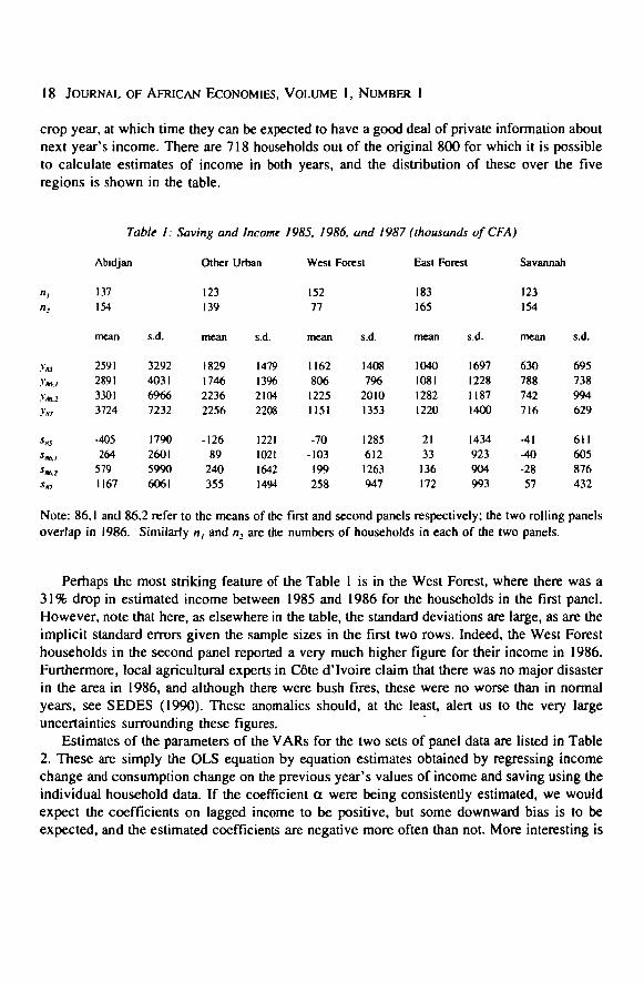
18 JOURNAL OF AFRICAN ECONOMIES, VOLUME 1, NUMBER 1
crop year, at which time they can be expected to have a good deal of private information aboutnext year's income. There are 718 households out of the original 800 for which it is possibleto calculate estimates of income in both years, and the distribution of these over the fiveregions is shown in the table.
Table 1: Saving and Income 1985, 1986, and 1987 (thousands of CFA)
Abidjan Other Urban West Forest East Forest Savannah
137154
mean
2591289133013724
-4052645791167
s.d.
3292403169667232
1790260159906061
123139
mean
1829174622362256
-12689240355
s.d.
1479139621042208
1221102116421494
15277
mean
116280612251151
-70-103199258
s.d.
140879620101353
12856121263947
183165
mean
1040108112821220
2133136172
s.d.
1697122811871400
1434923904993
123154
mean
630788742716
-41-40-2857
s.d.
695738994629
611605876432
Note: 86,1 and 86,2 refer to the means of the first and second panels respectively; the two rolling panelsoverlap in 1986. Similarly n, and n, are the numbers of households in each of the two panels.
Perhaps the most striking feature of the Table 1 is in the West Forest, where there was a31% drop in estimated income between 1985 and 1986 for the households in the first panel.However, note that here, as elsewhere in the table, the standard deviations are large, as are theimplicit standard errors given the sample sizes in the first two rows. Indeed, the West Foresthouseholds in the second panel reported a very much higher figure for their income in 1986.Furthermore, local agricultural experts in C6te d'lvoire claim that there was no major disasterin the area in 1986, and although there were bush fires, these were no worse than in normalyears, see SEDES (1990). These anomalies should, at the least, alert us to the very largeuncertainties surrounding these figures.
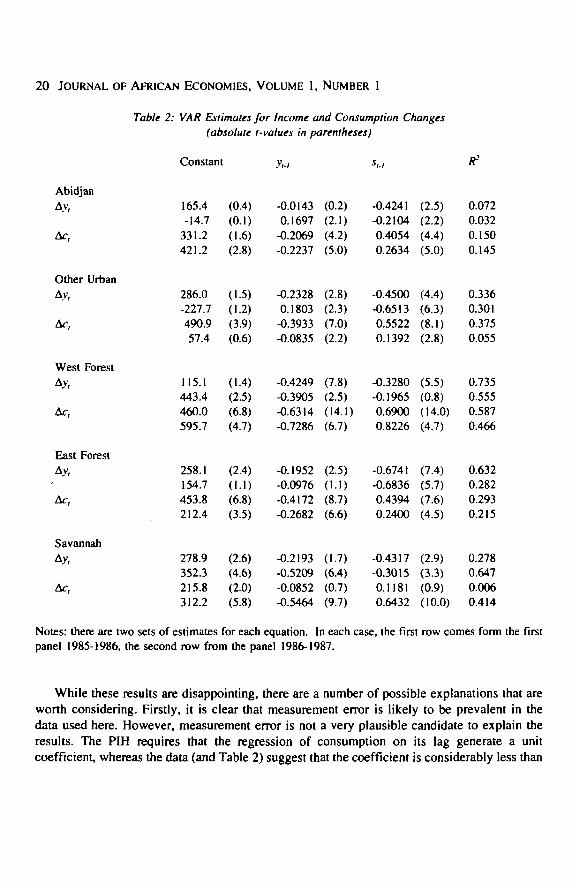
Estimates of the parameters of the VARs for the two sets of panel data are listed in Table2. These are simply the OLS equation by equation estimates obtained by regressing incomechange and consumption change on the previous year's values of income and saving using theindividual household data. If the coefficient a were being consistently estimated, we wouldexpect the coefficients on lagged income to be positive, but some downward bias is to beexpected, and the estimated coefficients are negative more often than not. More interesting is
Angus Deaton 19
the coefficient on lagged saving in the income equation, which is negative in all ten cases, andsignificantly so with one exception, the West Forest in the second panel. The size of the effectvaries somewhat from region to region, but is consistently strongest between the two panelsin the East Forest, which is the major cocoa growing area. Conditional on the previous year'sincome, 1000 CFA of additional saving predicts that income in the next year will be lower bybetween a third and two-thirds of that amount. This is exactly what the theory predicts, andunless some alternative explanation can be found, seems good evidence that these householdssave when they expect their incomes to fall.
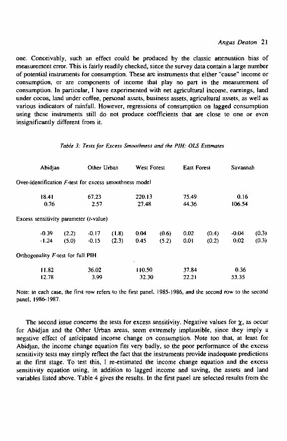
Of course, that consumers look ahead when deciding how much to save does not imply thatthey save exactly the amount that would be required by the permanent income hypothesis. Thetests for this are much more negative, and the consumption change regressions show thatconsumption changes are negatively related to lagged values of income and positively relatedto lagged values of saving. Note that, to a first approximation, the income and savingcoefficients are equal and opposite, so that the consumption regressions in Table 2 suggest that,in the cross-section, households with higher consumption in one year have a smallerconsumption change from that year to the next. These violations of the permanent incomehypothesis are sometimes quite large, particularly in the West Forest, and are statisticallysignificant, again with a single exception, the Savannah using the 1985-86 panel. The F-statistics for the hypothesis that lagged income and saving cannot predict consumption changeare given in the last row of Table 3, and with the one exception, strongly reject the hypothesis.
Somewhat surprisingly, the excess sensitivity model is not able to account for these results.While the formal tests are again in Table 3, the source of the problem can be seen in Table2. Saving predicts declines in income, which, if there is excess sensitivity, should predictdeclines in consumption, but the opposite is true in the data. Conditional on lagged income,lagged saving predicts consumption positively and (in all cases but one) significantly. As aresult, the excess sensitivity parameters listed in Table 3 are either negative (Abidjan and OtherUrban), or essentially zero. In only one case, the West Forest in the second panel, is there asensible estimate for x> and even here, the over-identification test in the first row rejects therestrictions implied by the model. Indeed, most of these F-tests reject the excess smoothnessmodel. Note further that the additional variance explained by the addition of the excesssensitivity parameter can be assessed by comparing the F-statistics in the first two rows withtwice the F-statistics in the last two rows. This comparison shows that, not only is the excesssmoothness model rejected, but it typically shows very little improvement over the strictpermanent income hypothesis. When this is not the case, as in the second panel for Abidjanand Other Urban (marginally), the estimates of x are not sensible, or, as in the Savannah inthe first panel, hold for a value of x of zero, because the PIH itself cannot be rejected. Theseresults seem to provide a strong rejection of the permanent income hypothesis, with no supportfor a weakening in the direction implied by the excess sensitivity formulation.
20 JOURNAL OF AFRICAN ECONOMIES, VOLUME 1, NUMBER 1
Table 2: VAR Estimates for Income and Consumption Changes(absolute t-values in parentheses)
Constant R2
Abidjan
Av,
Ac,
Other UrbanAv,
Ac,
West ForestAv,
Ac,
East Forest
Av,
Ac,
Savannah
Ac,
Notes: there are two sets of estimates for each equation. In each case, the first row comes form the firstpanel 1985-1986, the second row from the panel 1986-1987.
165.4-14.7
331.2421.2
286.0-227.7490.957.4
115.1443.4460.0595.7
258.1154.7453.8212.4
278.9352.3215.8312.2
(0.4)(0.1)(1.6)(2.8)
(1.5)(1.2)(3.9)(0.6)
(1.4)(2.5)(6.8)(4.7)
(2.4)(1.1)(6.8)(3.5)
(2.6)(4.6)(2.0)(5.8)
-0.01430.1697
-0.2069-0.2237
-0.23280.1803
-0.3933-0.0835
-0.4249-0.3905-0.6314-0.7286
-0.1952-0.0976-0.4172-0.2682
-0.2193-0.5209-0.0852-0.5464
(0.2)(2.1)(4.2)(5.0)
(2.8)(2.3)(7.0)(2.2)
(7.8)(2.5)(14.1)(6.7)
(2.5)(1.1)(8.7)(6.6)
(1.7)(6.4)(0.7)(9.7)
-0.4241-0.21040.40540.2634
-0.4500-0.65130.55220.1392
-0.3280-0.19650.69000.8226
-0.6741-0.68360.43940.2400
-0.4317-0.30150.11810.6432
(2.5)(2.2)(4.4)(5.0)
(4.4)(6.3)(8.1)(2.8)
(5.5)(0.8)(14.0)(4.7)
(7.4)(5.7)(7.6)(4.5)
(2.9)(3.3)(0.9)(10.0)
0.0720.0320.1500.145
0.3360.3010.3750.055
0.7350.5550.5870.466
0.6320.2820.2930.215
0.2780.6470.0060.414
While these results are disappointing, there are a number of possible explanations that areworth considering. Firstly, it is clear that measurement error is likely to be prevalent in thedata used here. However, measurement error is not a very plausible candidate to explain theresults. The PIH requires that the regression of consumption on its lag generate a unitcoefficient, whereas the data (and Table 2) suggest that the coefficient is considerably less than
Angus Deaton 21
one. Conceivably, such an effect could be produced by the classic attenuation bias ofmeasurement error. This is fairly readily checked, since the survey data contain a large numberof potential instruments for consumption. These are instruments that either "cause" income orconsumption, or are components of income that play no part in the measurement ofconsumption. In particular, I have experimented with net agricultural income, earnings, landunder cocoa, land under coffee, personal assets, business assets, agricultural assets, as well asvarious indicators of rainfall. However, regressions of consumption on lagged consumptionusing these instruments still do not produce coefficients that are close to one or eveninsignificantly different from it.
Table 3: Tests for Excess Smoothness and the PIH: OLS Estimates
Abidjan Other Urban West Forest East Forest Savannah
Over-identification F-test for excess smoothness model
18.41 67.23 220.13 75.49 0.16
0.76 2.57 27.48 44.36 106.54
Excess sensitivity parameter (r-value)
-0.39 (2.2) -0.17 (1.8) 0.04 (0.6) 0.02 (0.4) -0.04 (0.3)
-1.24 (5.0) -0.15 (2.3) 0.45 (5.2) 0.01 (0.2) 0.02 (0.3)
Orthogonality F-test for full PIH
11.82 36.02 110.50 37.84 0.3612.78 3.99 32.30 22.21 53.35
Note: in each case, the first row refers to the first panel, 1985-1986, and the second row to the secondpanel, 1986-1987.
The second issue concerns the tests for excess sensitivity. Negative values for x. as occurfor Abidjan and the Other Urban areas, seem extremely implausible, since they imply anegative effect of anticipated income change on consumption. Note too that, at least forAbidjan, the income change equation fits very badly, so the poor performance of the excesssensitivity tests may simply reflect the fact that the instruments provide inadequate predictionsat the first stage. To test this, I re-estimated the income change equation and the excesssensitivity equation using, in addition to lagged income and saving, the assets and landvariables listed above. Table 4 gives the results. In the first panel are selected results from the
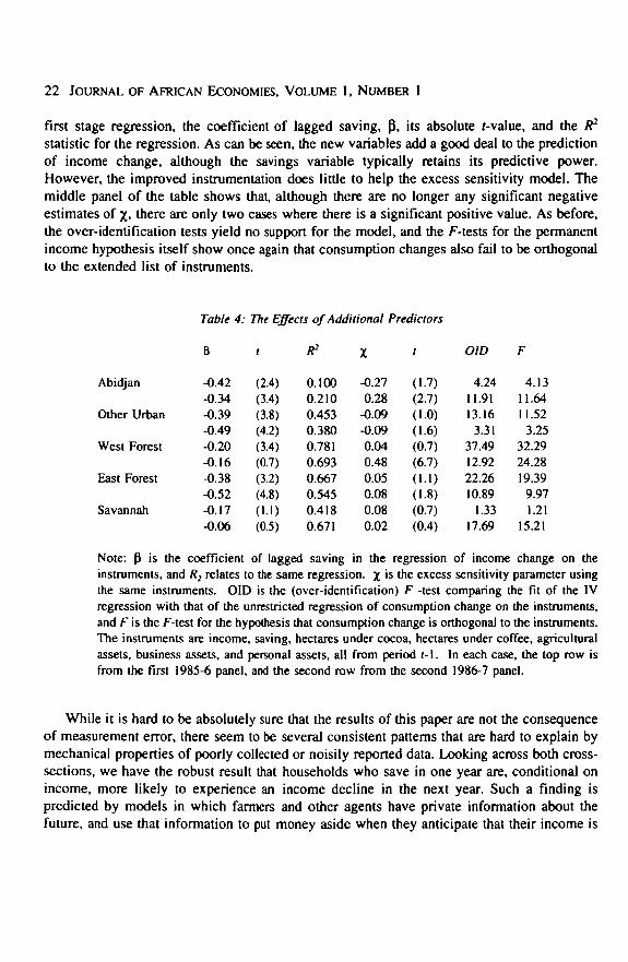
22 JOURNAL OF AFRICAN ECONOMIES, VOLUME 1, NUMBER 1
first stage regression, the coefficient of lagged saving, P, its absolute r-value, and the R2
statistic for the regression. As can be seen, the new variables add a good deal to the predictionof income change, although the savings variable typically retains its predictive power.However, the improved instrumentation does little to help the excess sensitivity model. Themiddle panel of the table shows that, although there are no longer any significant negativeestimates of x> there are only two cases where there is a significant positive value. As before,the over-identification tests yield no support for the model, and the F-tests for the permanentincome hypothesis itself show once again that consumption changes also fail to be orthogonalto the extended list of instruments.
Table 4: The Effects of Additional Predictors
B t ft2 Y / O1D
Abidjan
Other Urban
West Forest
East Forest
Savannah
-0.42-0.34-0.39-0.49-0.20-0.16-0.38-0.52-0.17-0.06
(2.4)(3.4)(3.8)(4.2)(3.4)(0.7)(3.2)(4.8)(I.I)(0.5)
0.1000.2100.4530.3800.7810.6930.6670.5450.4180.671
-0.270.28
-0.09-0.090.040.480.050.080.080.02
(1.7)(2.7)(1.0)(1.6)(0.7)(6.7)(1.1)(1.8)(0.7)(0.4)
4.2411.9113.16
3.3137.4912.9222.2610.89
1.3317.69
4.1311.6411.52
3.2532.2924.2819.39
9.971.21
15.21
Note: P is the coefficient of lagged saving in the regression of income change on theinstruments, and R2 relates to the same regression, x 's the excess sensitivity parameter usingthe same instruments. OID is the (over-identification) F -test comparing the fit of the IVregression with that of the unrestricted regression of consumption change on the instruments,and F is the F-test for the hypothesis that consumption change is orthogonal to the instruments.The instruments are income, saving, hectares under cocoa, hectares under coffee, agriculturalassets, business assets, and personal assets, all from period r-1. In each case, the top row isfrom the first 1985-6 panel, and the second row from the second 1986-7 panel.
While it is hard to be absolutely sure that the results of this paper are not the consequenceof measurement error, there seem to be several consistent patterns that are hard to explain bymechanical properties of poorly collected or noisily reported data. Looking across both cross-sections, we have the robust result that households who save in one year are, conditional onincome, more likely to experience an income decline in the next year. Such a finding ispredicted by models in which farmers and other agents have private information about thefuture, and use that information to put money aside when they anticipate that their income is
Angus Deaton 23
going to fall. Beyond that, the amount that people save is not well predicted by the permanentincome theory, nor, perhaps more surprisingly, by the supposition that consumption changesat least partly reflect anticipated income changes. Exactly what motivates the amount of savingmust remain a topic for future research, as must the possibility that the problems have moreto do with data problems than with reality.
References
Ainsworth, M. and J. Mufioz (1986) The Cdte d'lvoire living standards survey. Living StandardsMeasurement Study Working Paper No. 26, Washington, D.C. The World Bank.
Altonji, J. and A. Siow (1987) Testing the response of consumption to income change with (noisy) paneldata", Quarterly Journal of Economics, 16, 252-92.
Bhalla, S.S. (1979) "Measurement errors and the permanent income hypothesis: evidence from ruralIndia", American Economic Review, 69, 295-307.
- (1980) "The measurement of permanent income and its application to saving behaviour". Journal ofPolitical Economy, 88, 722^43.
Campbell, J.Y. (1987) "Does saving anticipate declining labour income? An alternative test of thepermanent income hypothesis", Econometrica, 55, 1249-73.
Campbell, J.Y., and A.S. Deaton (1989) "Why is consumption so smooth?". Review of Economic Studies,56, 357-374.
Deaton, A.S. (1987) "Life-cycle models of consumption: Is the evidence consistent with the theory?" inT.F. Bewley (ed.) Advances in Econometrics: 5th World Congress, 2, New York: CambridgeUniversity Press.
- (1990) "Saving in developing countries: theory and review". World Bank Economic Review(Proceedings of the World Bank Annual Conference on Development Economics 1989), 4, 6 1 - % .
- (1991) "Saving and liquidity constraints", Econometrica, 59, forthcoming.- (1992) Understanding consumption, Oxford and New York: Oxford University Press.Flavin, M. (1981) The adjustment of consumption to changing expectations about future income".
Journal of Political Economy, 89, 974-1009.- (1990) The excess smoothness of consumption: identification and interpretation", University of
Virginia, June, Processed.Gersovitz, M. (1988) "Saving and development", in H. Chenery and T.N. Srinivasan, Handbook of
Development Economics, 1, Amsterdam: Elsevier.Hall, R.E. (1978) "Stochastic implications of the life-cycle permanent income hypothesis", Journal of
Political Economy, 96, 339-57.Hall, R.E. and F.R. Mishkin (1982) The sensitivity of consumption to transitory income: estimates from
panel data on households", Econometrica, 50, 461-81.Mirrlees, J.A. (1988) "Optimal commodity price intervention", Nuffield College, Oxford, Processed.Musgrove, P.A. (1979) "Permanent household income and consumption in urban South America",
American Economic Review, 69, 355-68.Newbery, D.M.G. and J.E. Stiglitz (1981) The theory of commodity price stabilization: a study in the
economics of risk, Oxford: Oxford University Press.

24 JOURNAL OF AFRICAN ECONOMIES, VOLUME l, NUMBER 1
Paxson, C.H. (1990) "Consumption seasonally in Thailand", Research Program in Development Studies,Princeton University, Princeton, N.J., processed.
— (1992) "Using weather variability to estimate the response of savings to transitory income in Thai-land", American Economic Review, 82, 15-33.
SEDES, CIRAD (1990) "Bilan-diagnostic et programme de deuxieme phase du projet agricole du Centre-Ouest (PACO)", rapport reclige' par M. Pescay et F. Ruf, processed (January).
Related Documents