RooFit Users Manual 2.91-33

Document version 2.91-33 – October 14, 2008

RooFit Users Manual v2.91 W. Verkerke, D. Kirkby

2

Table of Contents

Table of Contents .................................................................................................................................... 2 What is RooFit? ....................................................................................................................................... 4 1. Installation and setup of RooFit .......................................................................................................... 6 2. Getting started ..................................................................................................................................... 7

Building a model .................................................................................................................................. 7 Visualizing a model .............................................................................................................................. 7 Importing data ...................................................................................................................................... 9 Fitting a model to data ....................................................................................................................... 10 Generating data from a model ........................................................................................................... 13 Parameters and observables ............................................................................................................ 13 Calculating integrals over models ..................................................................................................... 14 Tutorial macros .................................................................................................................................. 16

3. Signal and Background – Composite models ................................................................................... 17 Introduction ........................................................................................................................................ 17 Building composite models with fractions .......................................................................................... 17 Plotting composite models ................................................................................................................ 19 Using composite models ................................................................................................................... 20 Building extended composite models ................................................................................................ 21 Using extended composite models ................................................................................................... 23 Note on the interpretation of fraction coefficients and ranges ........................................................... 23 Navigation tools for dealing with composite objects .......................................................................... 25 Tutorial macros .................................................................................................................................. 28

4. Choosing, adjusting and creating basic shapes .............................................................................. 29 What p.d.f.s are provided? ................................................................................................................ 29 Reparameterizing existing basic p.d.f.s ............................................................................................. 30 Binding TFx, external C++ functions as RooFit functions ................................................................ 32 Writing a new p.d.f. class................................................................................................................... 33 Tutorial macros .................................................................................................................................. 36

5. Convolving a p.d.f. or function with another p.d.f. ............................................................................. 37 Introduction ........................................................................................................................................ 37 Numeric convolution with Fourier Transforms ................................................................................... 38 Plain numeric convolution.................................................................................................................. 43 Analytical convolution ........................................................................................................................ 44 Tutorial macros .................................................................................................................................. 48

6. Constructing multi-dimensional models ............................................................................................ 49 Introduction ........................................................................................................................................ 49 Using multi-dimensional models ........................................................................................................ 50 Modeling building strategy ................................................................................................................. 52 Multiplication ...................................................................................................................................... 53 Composition ....................................................................................................................................... 54 Conditional probability density functions ........................................................................................... 56 Products with conditional p.d.f.s ........................................................................................................ 58 Extending products to more than two dimensions ............................................................................ 61 Modeling data with per-event error observables. .............................................................................. 61 Tutorial macros .................................................................................................................................. 65

3

7. Working with projections and ranges ................................................................................................ 66 Using a N-dimensional model as a lower dimensional model ........................................................... 66 Visualization of multi-dimensional models ......................................................................................... 69 Definitions and basic use of rectangular ranges ............................................................................... 70 Fitting and plotting with rectangular regions ...................................................................................... 73 Ranges with parameterized boundaries ............................................................................................ 75 Regions defined by a Boolean selection function ............................................................................. 80 Tuning performance of projections through MC integration .............................................................. 83 Blending the properties of models with external distributions ........................................................... 84 Tutorial macros .................................................................................................................................. 87

8. Data modeling with discrete-valued variables .................................................................................. 88 Discrete variables .............................................................................................................................. 88 Models with discrete observables ..................................................................................................... 88 Plotting models in slices and ranges of discrete observables ........................................................... 91 Unbinned ML fits of efficiency functions using discrete observables ................................................ 93 Plotting asymmetries expressed in discrete observables ................................................................. 95 Tutorial macros .................................................................................................................................. 96

9. Dataset import and management ...................................................................................................... 97 Importing unbinned data from ROOT TTrees .................................................................................. 97 Importing unbinned data from ASCII files .......................................................................................... 98 Importing binned data from ROOT THx histograms .......................................................................... 98 Manual construction, filling and retrieving of datasets .................................................................... 100 Working with weighted events in unbinned data ............................................................................. 102 Plotting, tabulation and calculations of dataset contents ................................................................ 103 Calculation of moments and standardized moments ...................................................................... 105 Operations on unbinned datasets ................................................................................................... 106 Operations on binned datasets ....................................................................................................... 108 Tutorial macros ................................................................................................................................ 109

10. Organizational tools ...................................................................................................................... 110 Tutorial macros ................................................................................................................................ 110

11. Simultaneous fits ........................................................................................................................... 111 Tutorial macros ................................................................................................................................ 111

12. Likelihood calculation, minimization .............................................................................................. 112 Tutorial macros ................................................................................................................................ 112

13. Special models .............................................................................................................................. 113 Tutorial macros ................................................................................................................................ 113

14. Validation and testing of models ................................................................................................... 114 Tutorial macros ................................................................................................................................ 114

15. Programming guidelines ............................................................................................................... 115 Appendix A – Selected statistical topics ............................................................................................. 116 Appendix B – Pdf gallery ..................................................................................................................... 117 Appendix C – Decoration and tuning of RooPlots .............................................................................. 118

Tutorial macros ................................................................................................................................ 118 Appendix D – Integration and Normalization ...................................................................................... 119

Tutorial macros ................................................................................................................................ 119 Appendix E – Quick reference guide .................................................................................................. 120

Plotting ............................................................................................................................................. 120 Fitting and generating ...................................................................................................................... 127 Data manipulation ............................................................................................................................ 130 Automation tools .............................................................................................................................. 131

4

What is RooFit? Purpose The RooFit library provides a toolkit for modeling the expected distribution of events in a physics analysis. Models can be used to perform unbinned maximum likelihood fits, produce plots, and generate "toy Monte Carlo" samples for various studies. RooFit was originally developed for the BaBar collaboration, a particle physics experiment at the Stanford Linear Accelerator Center. The software is primarily designed as a particle physics data analysis tool, but its general nature and open architecture make it useful for other types of data analysis also.

Mathematical model The core functionality of RooFit is to enable the modeling of ‘event data’ distributions, where each event is a discrete occurrence in time, and has one or more measured observables associated with it. Experiments of this nature result in datasets obeying Poisson (or binomial) statistics. The natural modeling language for such distributions are probability density functions F(x;p) that describe the probability density the distribution of observables x in terms of function in parameter p. The defining properties of probability density functions, unit normalization with respect to all observables and positive definiteness, also provide important benefits for the design of a structured modeling language: p.d.f.s are easily added with intuitive interpretation of fraction coefficients, they allow construction of higher dimensional p.d.f.s out of lower dimensional building block with an intuitive language to introduce and describe correlations between observables, they allow the universal implementation of toy Monte Carlo sampling techniques, and are of course an prerequisite for the use of (unbinned) maximum likelihood parameter estimation technique.

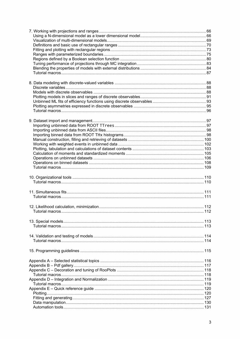
Design RooFit introduces a granular structure in its mapping of mathematical data models components to C++ objects: rather than aiming at a monolithic entity that describes a data model, each math symbol is presented by a separate object. A feature of this design philosophy is that all RooFit models always consist of multiple objects. For example a Gaussian probability density function consists typically of four objects, three objects representing the observable, the mean and the sigma parameters, and one object representing a Gaussian probability density function. Similarly, model building operations such as addition, multiplication, integration are represented by separate operator objects and make the modeling language scale well to models of arbitrary complexity.

Math concept Math symbol RooFit (base)class Variable RooRealVar Function RooAbsReal P.D.F. ; RooAbsPdf

Integral RooRealIntegral

Space point RooArgSet Addition 1 RooAddPdf

Convolution RooFFTConvPdf

Table 1 - Correspondence between selected math concepts and RooFit classes

Scope RooFit is strictly a data modeling language: It implements classes that represent variables, (probability density) functions, and operators to compose higher level functions, such as a class to construct a likelihood out of a dataset and a probability density function. All classes are instrumented to be fully functional: fitting, plotting and toy event generation works the same way for every p.d.f., regardless of its complexity. But important parts of the underlying functionality are delegated to standard ROOT

5

components where possible: For example, unbinned maximum likelihood fittings is implemented as minimization of a RooFit calculated likelihood function by the ROOT implementation of MINUIT.

Example Here is an example of a model defined in RooFit that is subsequently used for event generation, an unbinned maximum likelihood fit and plotting.

// --- Observable --- RooRealVar mes("mes","m_{ES} (GeV)",5.20,5.30) ; // --- Build Gaussian signal PDF --- RooRealVar sigmean("sigmean","B^{#pm} mass",5.28,5.20,5.30) ; RooRealVar sigwidth("sigwidth","B^{#pm} width",0.0027,0.001,1.) ; RooGaussian gauss("gauss","gaussian PDF",mes,sigmean,sigwidth) ; // --- Build Argus background PDF --- RooRealVar argpar("argpar","argus shape parameter",-20.0,-100.,-1.) ; RooArgusBG argus("argus","Argus PDF",mes,RooConst(5.291),argpar) ; // --- Construct signal+background PDF --- RooRealVar nsig("nsig","#signal events",200,0.,10000) ; RooRealVar nbkg("nbkg","#background events",800,0.,10000) ; RooAddPdf sum("sum","g+a",RooArgList(gauss,argus),RooArgList(nsig,nbkg)) ; // --- Generate a toyMC sample from composite PDF --- RooDataSet *data = sum.generate(mes,2000) ; // --- Perform extended ML fit of composite PDF to toy data --- sum.fitTo(*data,Extended()) ; // --- Plot toy data and composite PDF overlaid --- RooPlot* mesframe = mes.frame() ; data->plotOn(mesframe) ; sum.plotOn(mesframe) ; sum.plotOn(mesframe,Components(argus),LineStyle(kDashed)) ;

Example 1 – Example of extended unbinned maximum likelihood in RooFit

6

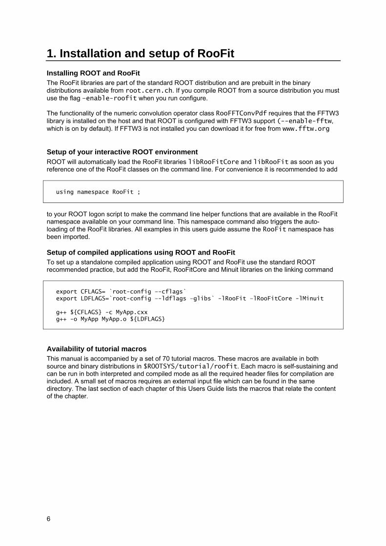
1. Installation and setup of RooFit Installing ROOT and RooFit The RooFit libraries are part of the standard ROOT distribution and are prebuilt in the binary distributions available from root.cern.ch. If you compile ROOT from a source distribution you must use the flag –enable-roofit when you run configure. The functionality of the numeric convolution operator class RooFFTConvPdf requires that the FFTW3 library is installed on the host and that ROOT is configured with FFTW3 support (--enable-fftw, which is on by default). If FFTW3 is not installed you can download it for free from www.fftw.org

Setup of your interactive ROOT environment ROOT will automatically load the RooFit libraries libRooFitCore and libRooFit as soon as you reference one of the RooFit classes on the command line. For convenience it is recommended to add

using namespace RooFit ; to your ROOT logon script to make the command line helper functions that are available in the RooFit namespace available on your command line. This namespace command also triggers the auto-loading of the RooFit libraries. All examples in this users guide assume the RooFit namespace has been imported.

Setup of compiled applications using ROOT and RooFit To set up a standalone compiled application using ROOT and RooFit use the standard ROOT recommended practice, but add the RooFit, RooFitCore and Minuit libraries on the linking command

export CFLAGS= `root-config –-cflags` export LDFLAGS=`root-config –-ldflags –glibs` -lRooFit –lRooFitCore -lMinuit g++ ${CFLAGS} -c MyApp.cxx g++ -o MyApp MyApp.o ${LDFLAGS}

Availability of tutorial macros This manual is accompanied by a set of 70 tutorial macros. These macros are available in both source and binary distributions in $ROOTSYS/tutorial/roofit. Each macro is self-sustaining and can be run in both interpreted and compiled mode as all the required header files for compilation are included. A small set of macros requires an external input file which can be found in the same directory. The last section of each chapter of this Users Guide lists the macros that relate the content of the chapter.

7

2. Getting started This section will guide you through an exercise of building a simple model and fitting it to data. The aim is to familiarize you with several basic concepts and get you to a point where you can do something useful yourself quickly. In subsequent sections we will explore several aspects of RooFit in more detail

Building a model A key concept in RooFit is that models are built in object-oriented fashion. Each RooFit class has a one-to-one correspondences to a mathematical object: there is a class to express a variable, RooRealVar, a base class to express a function, RooAbsReal, a base class to express a probability density function, RooAbsPdf, etc. As even the simplest mathematical functions consists of multiple objects – i.e. the function itself and its variables – all RooFit models also consist of multiple objects. The following example illustrates this

RooRealVar x(“x”,”x”,-10,10) ; RooRealVar mean(“mean”,”Mean of Gaussian”,0,-10,10) ; RooRealVar sigma(“sigma”,”Width of Gaussian”,3,-10,10) ; RooGaussian gauss(“gauss”,”gauss(x,mean,sigma)”,x,mean,sigma) ;

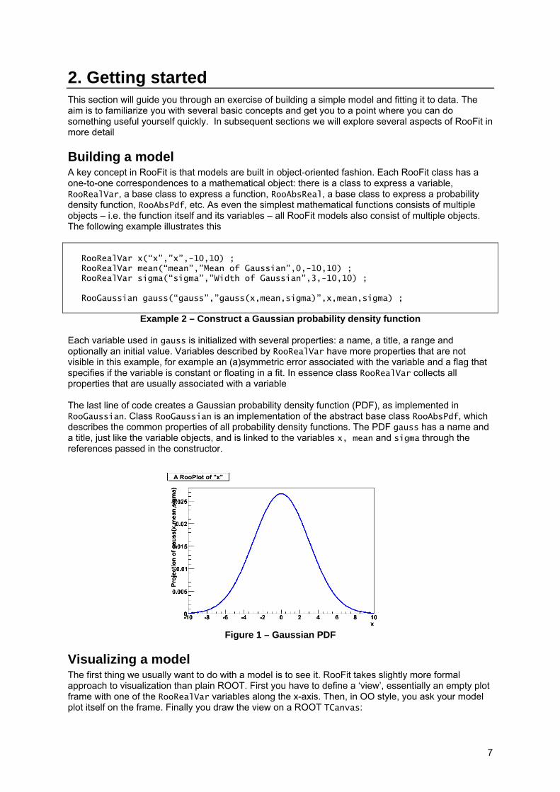
Example 2 – Construct a Gaussian probability density function Each variable used in gauss is initialized with several properties: a name, a title, a range and optionally an initial value. Variables described by RooRealVar have more properties that are not visible in this example, for example an (a)symmetric error associated with the variable and a flag that specifies if the variable is constant or floating in a fit. In essence class RooRealVar collects all properties that are usually associated with a variable The last line of code creates a Gaussian probability density function (PDF), as implemented in RooGaussian. Class RooGaussian is an implementation of the abstract base class RooAbsPdf, which describes the common properties of all probability density functions. The PDF gauss has a name and a title, just like the variable objects, and is linked to the variables x, mean and sigma through the references passed in the constructor.

Figure 1 – Gaussian PDF

Visualizing a model The first thing we usually want to do with a model is to see it. RooFit takes slightly more formal approach to visualization than plain ROOT. First you have to define a ‘view’, essentially an empty plot frame with one of the RooRealVar variables along the x-axis. Then, in OO style, you ask your model plot itself on the frame. Finally you draw the view on a ROOT TCanvas:

8

RooPlot* xframe = x.frame() ; gauss.plotOn(frame) ; frame->Draw()

The result of this example is shown in Figure 1. Note that in the creation of the view we do not have to specify a range, it is automatically taken from the range associated with the RooRealVar. It is possible to override this. Note also that when gauss draws itself on the frame, we don’t have to specify that we want to plot gauss as function of x, this information is retrieved from the frame. A frame can contain multiple objects (curves, histograms) to visualize. We can for example draw gauss twice with a different value of parameter sigma.

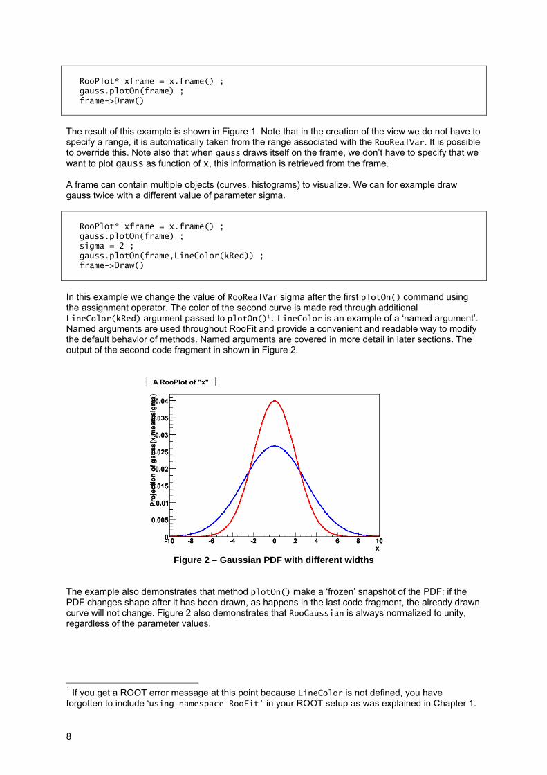
RooPlot* xframe = x.frame() ; gauss.plotOn(frame) ; sigma = 2 ; gauss.plotOn(frame,LineColor(kRed)) ; frame->Draw()

In this example we change the value of RooRealVar sigma after the first plotOn() command using the assignment operator. The color of the second curve is made red through additional LineColor(kRed) argument passed to plotOn()1. LineColor is an example of a ‘named argument’. Named arguments are used throughout RooFit and provide a convenient and readable way to modify the default behavior of methods. Named arguments are covered in more detail in later sections. The output of the second code fragment in shown in Figure 2.

Figure 2 – Gaussian PDF with different widths

The example also demonstrates that method plotOn() make a ‘frozen’ snapshot of the PDF: if the PDF changes shape after it has been drawn, as happens in the last code fragment, the already drawn curve will not change. Figure 2 also demonstrates that RooGaussian is always normalized to unity, regardless of the parameter values.

1 If you get a ROOT error message at this point because LineColor is not defined, you have forgotten to include ‘using namespace RooFit’ in your ROOT setup as was explained in Chapter 1.

9

Importing data Generally speaking, data comes in two flavors: unbinned data, represented in ROOT by class TTree and binned data, represented in ROOT by classes TH1,TH2 and TH3. RooFit can work with both.

Binned data (histograms) In RooFit, binned data is represented by the RooDataHist class. You can import the contents of any ROOT histogram into a RooDataHist object

TH1* hh = (TH1*) gDirectory->Get(“ahisto”) ;

RooRealVar x(“x”,”x”,-10,10) ; RooDataHist data(“data”,”dataset with x”,x,hh) ;

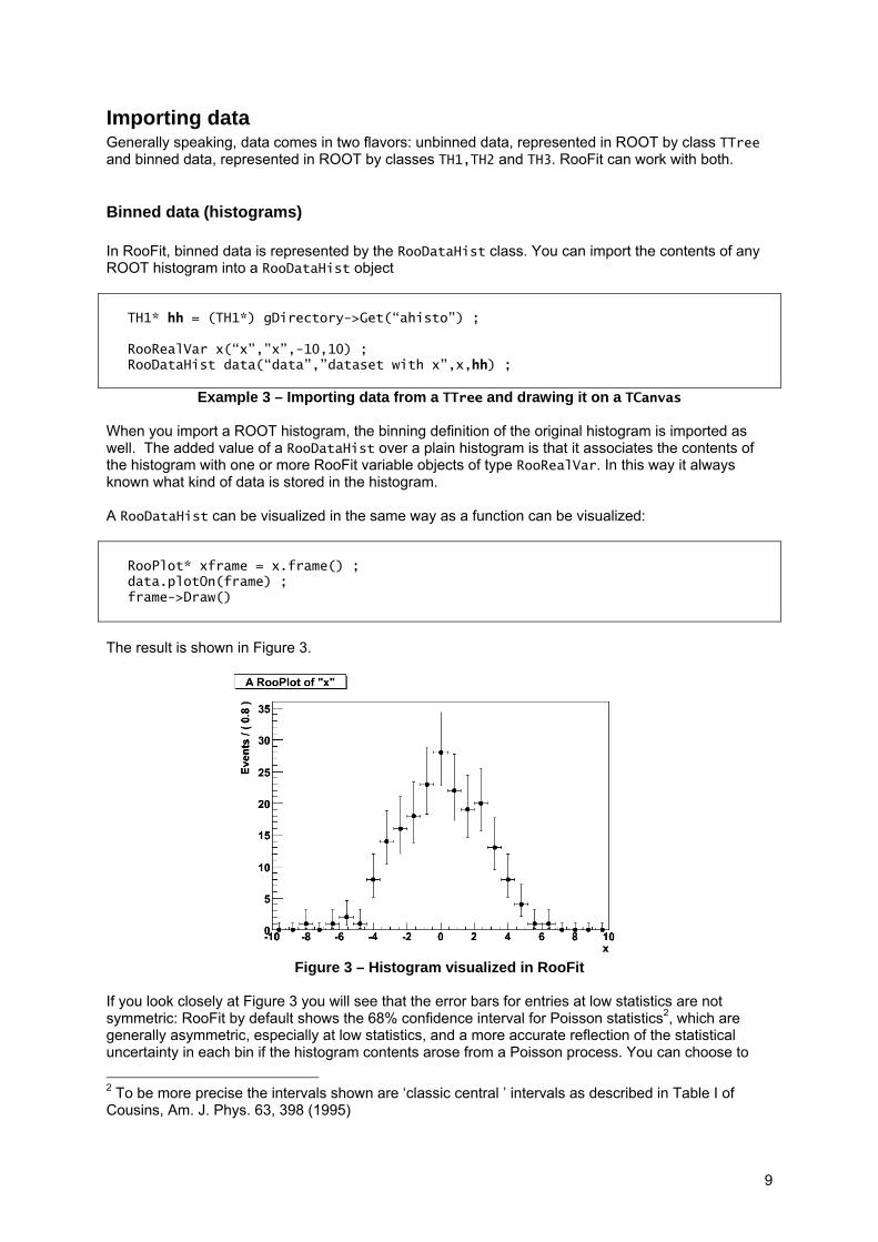
Example 3 – Importing data from a TTree and drawing it on a TCanvas When you import a ROOT histogram, the binning definition of the original histogram is imported as well. The added value of a RooDataHist over a plain histogram is that it associates the contents of the histogram with one or more RooFit variable objects of type RooRealVar. In this way it always known what kind of data is stored in the histogram. A RooDataHist can be visualized in the same way as a function can be visualized:

RooPlot* xframe = x.frame() ; data.plotOn(frame) ; frame->Draw()

The result is shown in Figure 3.

Figure 3 – Histogram visualized in RooFit

If you look closely at Figure 3 you will see that the error bars for entries at low statistics are not symmetric: RooFit by default shows the 68% confidence interval for Poisson statistics2, which are generally asymmetric, especially at low statistics, and a more accurate reflection of the statistical uncertainty in each bin if the histogram contents arose from a Poisson process. You can choose to 2 To be more precise the intervals shown are ‘classic central ’ intervals as described in Table I of Cousins, Am. J. Phys. 63, 398 (1995)

10

have the usual √N error shown by adding DataError(RooAbsData::SumW2) to the data.plotOn() line. This option only affects the visualization of the dataset.

Unbinned data (trees) Unbinned data can be imported in RooFit much along the same lines and is stored in class RooDataSet

TTree* tree = (TTree*) gDirectory->Get(“atree”) ;

RooRealVar x(“x”,”x”,-10,10) ; RooDataSet data(“data”,”dataset with x”,tree,x) ;

In this example tree is assumed to have a branch named “x” as the RooDataSet constructor will import data from the tree branch that has the same name as the RooRealVar that is passed as argument. A RooDataSet can import data from branches of type Double_t, Float_t, Int_t, UInt_t and Bool_t for a RooRealVar observable. If the branch is not of type Double_t, the data will converted to Double_t as that is the internal representation of a RooRealVar. It is not possible to import data from array branches such as Double_t[10]. It is possible to imported integer-type data as discrete valued observables in RooFit, this is explained in more detail in Chapter 8. Plotting unbinned data is similar to plotting binned data with the exception that you can now show it in any binning you like.

RooPlot* xframe = x.frame() ; data.plotOn(frame,Binning(25)) ; frame->Draw()

In this example we have overridden the default setting of 100 bins using the Binning() named argument.

Working with data In general working with binned and unbinned data is very similar in RooFit as both class RooDataSet (for unbinned data) and class RooDataHist (for binned data) inherit from a common base class, RooAbsData, which defines the interface for a generic abstract data sample. With few exceptions, all RooFit methods take abstract datasets as input arguments, making it easy to use binned and unbinned data interchangeably. The examples in this section have always dealt with one-dimensional datasets. Both RooDataSet and RooDataHist can however handle data with an arbitrary number of dimensions. In the next sections we will revisit datasets and explain how to work with multi-dimensional data.

Fitting a model to data Fitting a model to data involves the construction of a test statistic from the model and the data – the most common choices are χ2 and –log(likelihood) – and minimizing that test statistics with respect to all parameters that are not considered fixed3. The default fit method in RooFit is the unbinned maximum likelihood fit for unbinned data and the binned maximum likelihood fit for binned data.

3 This section assumes you are familiar with the basics of parameter estimation using likelihoods. If this is not the case, a short introduction is given in Appendix A.

11

In either case, the test statistic is calculated by RooFit and the minimization of the test statistic is performed by MINUIT through its TMinuit implementation in ROOT to perform the minimization and error analysis. An easy to use high-level interface to the entire fitting process is provided by the fitTo() method of class RooAbsPdf:

gauss.fitTo(data) ;

This command builds a –log(L) function from the gauss function and the given dataset, passes it to MINUIT, which minimizes it and estimate the errors on the parameters of gauss. The output of the fitTo() method produces the familiar MINUIT output on the screen:

********** ** 13 **MIGRAD 1000 1 ********** FIRST CALL TO USER FUNCTION AT NEW START POINT, WITH IFLAG=4. START MIGRAD MINIMIZATION. STRATEGY 1. CONVERGENCE WHEN EDM .LT. 1.00e-03 FCN=25139.4 FROM MIGRAD STATUS=INITIATE 10 CALLS 11 TOTAL EDM= unknown STRATEGY= 1 NO ERROR MATRIX EXT PARAMETER CURRENT GUESS STEP FIRST NO. NAME VALUE ERROR SIZE DERIVATIVE 1 mean -1.00000e+00 1.00000e+00 1.00000e+00 -6.53357e+01 2 sigma 3.00000e+00 1.00000e+00 1.00000e+00 -3.60009e+01 ERR DEF= 0.5 MIGRAD MINIMIZATION HAS CONVERGED. MIGRAD WILL VERIFY CONVERGENCE AND ERROR MATRIX. COVARIANCE MATRIX CALCULATED SUCCESSFULLY FCN=25137.2 FROM MIGRAD STATUS=CONVERGED 33 CALLS 34 TOTAL EDM=8.3048e-07 STRATEGY= 1 ERROR MATRIX ACCURATE EXT PARAMETER STEP FIRST NO. NAME VALUE ERROR SIZE DERIVATIVE 1 mean -9.40910e-01 3.03997e-02 3.32893e-03 -2.95416e-02 2 sigma 3.01575e+00 2.22446e-02 2.43807e-03 5.98751e-03 ERR DEF= 0.5 EXTERNAL ERROR MATRIX. NDIM= 25 NPAR= 2 ERR DEF=0.5 9.241e-04 -1.762e-05 -1.762e-05 4.948e-04 PARAMETER CORRELATION COEFFICIENTS NO. GLOBAL 1 2 1 0.02606 1.000 -0.026 2 0.02606 -0.026 1.000 ********** ** 18 **HESSE 1000 ********** COVARIANCE MATRIX CALCULATED SUCCESSFULLY FCN=25137.2 FROM HESSE STATUS=OK 10 CALLS 44 TOTAL EDM=8.30707e-07 STRATEGY= 1 ERROR MATRIX ACCURATE EXT PARAMETER INTERNAL INTERNAL NO. NAME VALUE ERROR STEP SIZE VALUE 1 mean -9.40910e-01 3.04002e-02 6.65786e-04 -9.40910e-01 2 sigma 3.01575e+00 2.22449e-02 9.75228e-05 3.01575e+00 ERR DEF= 0.5 EXTERNAL ERROR MATRIX. NDIM= 25 NPAR= 2 ERR DEF=0.5 9.242e-04 -1.807e-05 -1.807e-05 4.948e-04 PARAMETER CORRELATION COEFFICIENTS NO. GLOBAL 1 2 1 0.02672 1.000 -0.027 2 0.02672 -0.027 1.000

The result of the fit – the new parameter values and their errors – is propagated back to the RooRealVar objects that represent the parameters of gauss, as is demonstrated in the code fragment below:

mean.Print() ; RooRealVar::mean: -0.940910 +/- 0.030400 sigma.Print() ; RooRealVar::sigma: 3.0158 +/- 0.022245

A subsequent drawing of gauss will therefore reflect the new shape of the function after the fit. We now draw both the data and the fitted function on a frame,

12

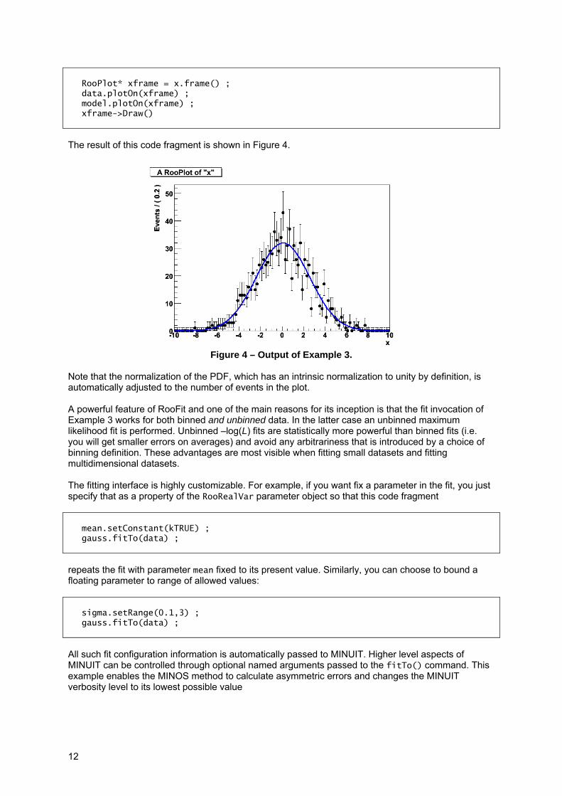
RooPlot* xframe = x.frame() ; data.plotOn(xframe) ; model.plotOn(xframe) ; xframe->Draw()

The result of this code fragment is shown in Figure 4.

Figure 4 – Output of Example 3.

Note that the normalization of the PDF, which has an intrinsic normalization to unity by definition, is automatically adjusted to the number of events in the plot. A powerful feature of RooFit and one of the main reasons for its inception is that the fit invocation of Example 3 works for both binned and unbinned data. In the latter case an unbinned maximum likelihood fit is performed. Unbinned –log(L) fits are statistically more powerful than binned fits (i.e. you will get smaller errors on averages) and avoid any arbitrariness that is introduced by a choice of binning definition. These advantages are most visible when fitting small datasets and fitting multidimensional datasets. The fitting interface is highly customizable. For example, if you want fix a parameter in the fit, you just specify that as a property of the RooRealVar parameter object so that this code fragment

mean.setConstant(kTRUE) ; gauss.fitTo(data) ;

repeats the fit with parameter mean fixed to its present value. Similarly, you can choose to bound a floating parameter to range of allowed values:

sigma.setRange(0.1,3) ; gauss.fitTo(data) ;

All such fit configuration information is automatically passed to MINUIT. Higher level aspects of MINUIT can be controlled through optional named arguments passed to the fitTo() command. This example enables the MINOS method to calculate asymmetric errors and changes the MINUIT verbosity level to its lowest possible value

13

gauss.fitTo(data, Minos(kTRUE), PrintLevel(-1)) ;

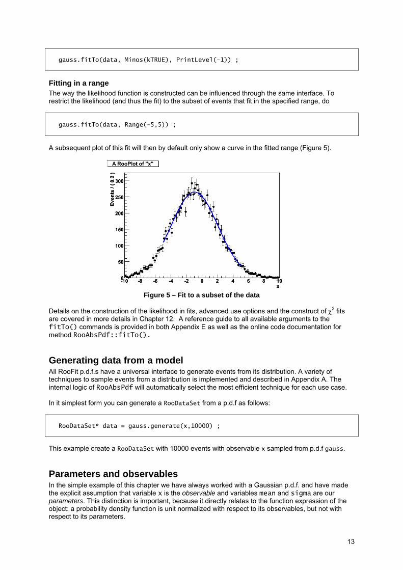
Fitting in a range The way the likelihood function is constructed can be influenced through the same interface. To restrict the likelihood (and thus the fit) to the subset of events that fit in the specified range, do

gauss.fitTo(data, Range(-5,5)) ; A subsequent plot of this fit will then by default only show a curve in the fitted range (Figure 5).

Figure 5 – Fit to a subset of the data

Details on the construction of the likelihood in fits, advanced use options and the construct of χ2 fits are covered in more details in Chapter 12. A reference guide to all available arguments to the fitTo() commands is provided in both Appendix E as well as the online code documentation for method RooAbsPdf::fitTo().

Generating data from a model All RooFit p.d.f.s have a universal interface to generate events from its distribution. A variety of techniques to sample events from a distribution is implemented and described in Appendix A. The internal logic of RooAbsPdf will automatically select the most efficient technique for each use case. In it simplest form you can generate a RooDataSet from a p.d.f as follows:

RooDataSet* data = gauss.generate(x,10000) ;

This example create a RooDataSet with 10000 events with observable x sampled from p.d.f gauss.

Parameters and observables In the simple example of this chapter we have always worked with a Gaussian p.d.f. and have made the explicit assumption that variable x is the observable and variables mean and sigma are our parameters. This distinction is important, because it directly relates to the function expression of the object: a probability density function is unit normalized with respect to its observables, but not with respect to its parameters.

14

Nevertheless RooFit p.d.f classes themselves have no intrinsic static notion of this distinction between parameters and observables. This may seem confusing at first, but provides essential flexibility that we will need later when building composite objects. The distinction between parameters and observables is always made, though, but it arises dynamically from each use context. The following example shows how gauss is used as a p.d.f for observable mean:

RooDataSet* data = gauss.generate(mean,1000) ; RooPlot* mframe = mean.frame() ; data->plotOn(mframe) ; gauss.plotOn(mframe) ;

Given that the mathematical expression for a Gaussian is symmetric under the interchange of x and m, this unsurprisingly yields a Gaussian distribution in (now) observable m in terms of parameters x and sigma. Along the same lines it is also possible to use gauss as a p.d.f in sigma with parameters x and mean. In many cases, it is not necessary to explicitly say which variables are observable, because its definition arises implicitly from the use context. Specifically, whenever a use context involves both a p.d.f and a dataset, the implicit and automatic definition observables are those variables that occur in both the dataset and p.d.f definition. This automatic definition works for example in fitting, which involves an explicit dataset, but also in plotting: the RooPlot frame variable is always considered the observable4. In all other contexts where the distinction is relevant, the definition of what variables are considered observables has to be manually supplied. This is why when you call generate() you have to specify what you consider to be the observable in each call.

RooDataSet* data = gauss.generate(x,10000) ;

However, in all three possible use cases of gauss, it is a properly normalized probability density function with respect to the (implicitly declared) observable. This highlights an important consequence of the ‘dynamic observable’ concept of RooFit: RooAbsPdf objects do not have a unique return value, it depends on the local definition of observables. This functionality is achieved through an explicit a posteriori normalization step in RooAbsPdf::getVal() that is different for each definition of observables.

Double_t gauss_raw = gauss.getVal() ; // raw unnormalized value Double_t gauss_pdfX = gauss.getVal(x) ; // value when used as p.d.f in x Double_t gauss_pdfM = gauss.getVal(mean) ; // value when used as p.d.f in mean Double_t gauss_pdfS = gauss.getVal(sigma) ; // value when used as p.d.f in sigma

Calculating integrals over models Integrals over p.d.f.s and functions are represented as separate objects in RooFit. Thus, rather than defining integration as an action, an integral is defined by object inheriting from RooAbsReal, of 4 This automatic concept also extends to multi-dimensional datasets and p.d.f.s that are projected on 1-dimensional plot frame. This explained in more detail in Chapter 7.

15

which the value is calculated through an integration action. Such objects are constructed through the createIntegral() method or RooAbsReal

RooAbsReal* intGaussX = gauss.createIntegral(x) ;

Any RooAbsReal function or RooAbsPdf pdf can be integrated this way. Note that for p.d.f.s the above configuration integrates the raw (unnormalized) value of gauss. In fact the normalized return value of gauss.getVal(x) is precisely gauss.getVal()/intGaussX->getVal(). Most integrals are represented by an object of class RooRealIntegral. Upon construction this class determines the most efficient way an integration request can be performed. If the integrated functions supports analytical integration over the requested observable(s) this analytical implementation will be used5, otherwise a numeric technique is selected. The actual integration is not performed at construction time, but is done on demand when RooRealIntegral::getVal() is called. Once calculated, the integral value is cached and remains valid until either one of the integrand parameters changes value, or if (one of ) the integrand observables changes its normalization range. You can inspect the chosen strategy for integration by printing the integral object

intGauss->Print("v") ... --- RooRealIntegral --- Integrates g[ x=x mean=m sigma=s ] operating mode is Analytic Summed discrete args are () Numerically integrated args are () Analytically integrated args using mode 1 are (x) Arguments included in Jacobian are () Factorized arguments are () Function normalization set <none>

Integrals over normalized p.d.f.s. It is also possible to construct integrals over normalized p.d.f.s:

RooAbsReal* intGaussX = gauss.createIntegral(x,NormSet(x)) ;

This example is not particularly useful, as it will always return 1, but with the same interface one can also integrate over a predefined sub-range of the observable

x.setRange(“signal”,-2,2) ; RooAbsReal* intGaussX = gauss.createIntegral(x,NormSet(x),Range(“signal”)) ;

to extract the fraction of a model in the “signal” range. The concept of named ranges like “signal” will be elaborated in Chapters 3 and 7. The return value of normalized p.d.f.s integrals is naturally in the range [0,1].

5 There are situations in which the internal analytical of an p.d.f. cannot be used, for example when the integrated observable is transformed through a function in the input declaration of the p.d.f which would give rise to a Jacobian term that is not included in the internal integral calculation. Such situations are automatically recognized and handled through numeric integration.

16

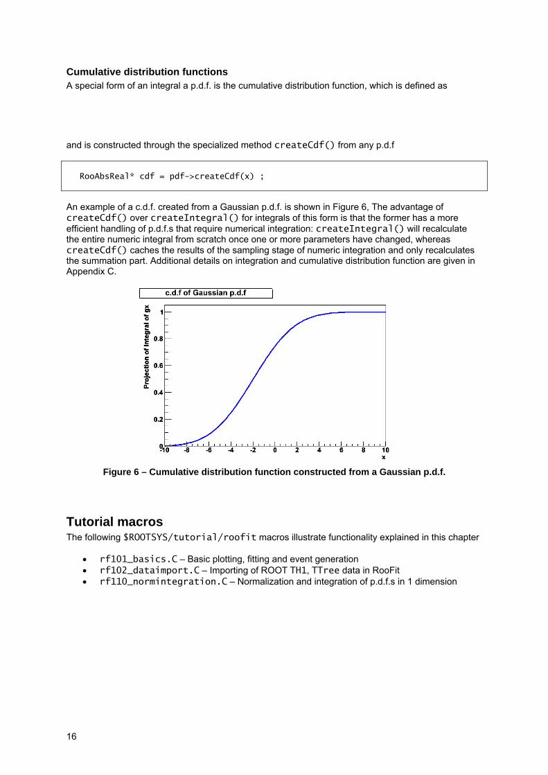
Cumulative distribution functions A special form of an integral a p.d.f. is the cumulative distribution function, which is defined as

and is constructed through the specialized method createCdf() from any p.d.f

RooAbsReal* cdf = pdf->createCdf(x) ;

An example of a c.d.f. created from a Gaussian p.d.f. is shown in Figure 6, The advantage of createCdf() over createIntegral() for integrals of this form is that the former has a more efficient handling of p.d.f.s that require numerical integration: createIntegral() will recalculate the entire numeric integral from scratch once one or more parameters have changed, whereas createCdf() caches the results of the sampling stage of numeric integration and only recalculates the summation part. Additional details on integration and cumulative distribution function are given in Appendix C.

Figure 6 – Cumulative distribution function constructed from a Gaussian p.d.f.

Tutorial macros The following $ROOTSYS/tutorial/roofit macros illustrate functionality explained in this chapter

• rf101_basics.C – Basic plotting, fitting and event generation • rf102_dataimport.C – Importing of ROOT TH1, TTree data in RooFit • rf110_normintegration.C – Normalization and integration of p.d.f.s in 1 dimension

17

3. Signal and Background – Composite models Introduction Data models are often used to describe samples that include multiple event hypotheses, e.g. signal and (one or more types of) background. To describe sample of such nature, a composite model can be constructed. For event hypotheses, ‘signal’ and ‘background’, a composite model M(x) is constructed from a model S(x) describing signal and B(x) describing background as

1 In this formula, f is the fraction of events in the sample that are signal-like. The generic expression for a sum of N hypotheses is

1

A elegant property of adding p.d.f.s in this way is that M(x) does not need to be explicitly normalized to one: if both S(x) and B(x) are normalized to one then M(x) is – by construction – also normalized. RooFit provide a special ‘addition operator’ p.d.f. in class RooAddPdf to simplify building and using such composite p.d.f.s.

The extended likelihood formalism As a final result of a measurement is often quoted as a number of events, rather than a fraction, it is often desirable to express a data model directly in terms of the number of signal and background events, rather than the fraction of signal events (and the total number of events), i.e.

In this expression ME(x) is not normalized to 1 but to NS+NB = N, the number of events in the data sample and is therefore not a proper probability density function, but rather a shorthand notation for two expressions: the shape of the distribution and the expected number of events

that can be jointly constrained in the extended likelihood formalism6:

log log log ,

In RooFit both regular sums (Ncoef=Npdf-1) and extended likelihood sum (Ncoef=Npdf) are represented by the operator pdf class RooAddPdf, that will automatically construct the extended likelihood term in the latter case.

Building composite models with fractions We start with a description of plain (non-extended) composite mode. Here is a simple example of a composite PDF constructed with RooAddPdf using fractional coefficients.

6 See Appendix A for details on the extended likelihood formalism

18

RooRealVar x(“x”,”x”,-10,10) ; RooRealVar mean(“mean”,”mean”,0,-10,10) ; RooRealVar sigma(“sigma,”sigma”,2,0.,10.) ; RooGaussian sig(“sig”,”signal p.d.f.”,x,mean,sigma) ; RooRealVar c0(“c0”,”coefficient #0”, 1.0,-1.,1.) ; RooRealVar c1(“c1”,”coefficient #1”, 0.1,-1.,1.) ; RooRealVar c2(“c2”,”coefficient #2”,-0.1,-1.,1.) ; RooChebychev bkg(“bkg”,”background p.d.f.”,x,RooArgList(c0,c1,c2)) ; RooRealVar fsig(“fsig”,”signal fraction”,0.5,0.,1.) ; // model(x) = fsig*sig(x) + (1-fsig)*bkg(x) RooAddPdf model(“model”,”model”,RooArgList(sig,bkg),fsig) ;

Example 4 – Adding two pdfs using a fraction coefficient In this example we first construct a Gaussian p.d.f sig and flat background p.d.f bkg and then add them together with a signal fraction fsig in model. Note the use the container class RooArgList to pass a list of objects as a single argument in a function. RooFit has two container classes: RooArgList and RooArgSet. Each can contain any number RooFit value objects, i.e. any object that derives from RooAbsArg such a RooRealVar, RooAbsPdf etc. The distinction is that a list is ordered, you can access the elements through a positional reference (2nd, 3rd,…), and can may contain multiple objects with the same name, while a set has no order but requires instead each member to have a unique name A RooAddPdf instance can sum together any number of components, to add three p.d.f.s with two coefficients, one would write

// model2(x) = fsig*sig(x) + fbkg1*bkg1(x) + (1-fsig-fbkg)*bkg2(x) RooAddPdf model2(“model2”,”model2”,RooArgList(sig,bkg1,bkg2), RooArgList(fsig,fbkg1)) ;

To construct a non-extended p.d.f. in which the coefficients are interpreted as fractions, the number of coefficients should always be one less than the number of p.d.f.s.

Using RooAddPdf recursively Note that the input p.d.f.s of RooAddPdf do not need to be basic p.d.f.s, they can be composite p.d.f.s themselves. Take a look at this example that uses sig and bkg from Example 7 as input:

// Construct a third pdf bkg_peak RooRealVar mean_bkg(“mean_bkg”,”mean”,0,-10,10) ; RooRealVar sigma_bkg(“sigma_bkg,”sigma”,2,0.,10.) ; RooGaussian bkg_peak(“bkg_peak”,”peaking bkg p.d.f.”,x,mean_bkg,sigma_bkg) ; // First add sig and peak together with fraction fpeak RooRealVar fpeak(“fpeak”,”peaking background fraction”,0.1,0.,1.) ; RooAddPdf sigpeak(“sigpeak”,”sig+peak”,RooArgList(bkg_peak,sig),fpeak) ; // Next add (sig+peak) to bkg with fraction fpeak RooRealVar fbkg(”fbkg”,”background fraction”,0.5,0.,1.) ; RooAddPdf model(“model”,”bkg+(sig+peak)”,RooArgList(bkg,sigpeak),fbkg) ;

Example 5 – Adding three p.d.f.s through recursive addition of two terms

19

The final p.d.f model represents the following expression

1 1 It is also possible to construct such a recursive addition formulation with a single RooAddPdf by telling the constructor that the fraction coefficients should be interpreted as recursive fractions. To construct the functional equivalent of the model object in the example above one can write

RooAddPdf model(“model”,”bkg+(sig+peak)”,RooArgList(bkg,peak,bkg),

RooArgList(fbkg,fpeak),kTRUE) ;

Example 6 – Adding three p.d.f.s recursively using the recursive mode of RooAddPdf In this constructor mode the interpretation of the fractions is as follows

1 1 1 1

Plotting composite models The modular structure of a composite p.d.f. allows you to address the individual components. One can for example plot the individual components of a composite model on top of that model to visualize its structure.

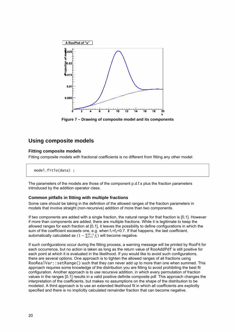
RooPlot* frame = x.frame() ; model.plotOn(frame) ; model.plotOn(frame, Components(bkg),LineStyle(kDashed)) ; frame->Draw() ;

The output of this code fragment is show in Figure 7. The component plot is drawn with a dashed line style. A complete overview of plot style options, see Appendix C. You can identify the components by object reference, as is done above, or by name:

model.plotOn(frame, Components(“bkg”),LineStyle(kDashed)) ; The latter is convenient when your plotting code has no access to the component objects, for example if your model is built in a separate function that only returns the top-level RooAddPdf object. If you want to draw the sum of multiple components you can do that in two ways as well:

model.plotOn(frame, Components(RooArgSet(bkg1,bkg2)),LineStyle(kDashed)) ; model.plotOn(frame, Components(“bkg1,bkg2”),LineStyle(kDashed)) ;

Note that in the latter form wildcards are allowed so that a well chosen component naming scheme allows you for example to do this:

model.plotOn(frame, Components(“bkg*”),LineStyle(kDashed)) ; If required multiple wildcard expressions can be specified in a comma separated list.

20

Figure 7 – Drawing of composite model and its components

Using composite models

Fitting composite models Fitting composite models with fractional coefficients is no different from fitting any other model:

model.fitTo(data) ;

The parameters of the models are those of the component p.d.f.s plus the fraction parameters introduced by the addition operator class.

Common pitfalls in fitting with multiple fractions Some care should be taking in the definition of the allowed ranges of the fraction parameters in models that involve straight (non-recursive) addition of more than two components. If two components are added with a single fraction, the natural range for that fraction is [0,1]. However if more than components are added, there are multiple fractions. While it is legitimate to keep the allowed ranges for each fraction at [0,1], it leaves the possibility to define configurations in which the sum of the coefficient exceeds one, e.g. when f1=f2=0.7. If that happens, the last coefficient, automatically calculated as 1 ∑ will become negative. If such configurations occur during the fitting process, a warning message will be printed by RooFit for each occurrence, but no action is taken as long as the return value of RooAddPdf is still positive for each point at which it is evaluated in the likelihood. If you would like to avoid such configurations, there are several options. One approach is to tighten the allowed ranges of all fractions using RooRealVar::setRange() such that they can never add up to more than one when summed. This approach requires some knowledge of the distribution you are fitting to avoid prohibiting the best fit configuration. Another approach is to use recursive addition, in which every permutation of fraction values in the ranges [0,1] results in a valid positive definite composite pdf. This approach changes the interpretation of the coefficients, but makes no assumptions on the shape of the distribution to be modeled. A third approach is to use an extended likelihood fit in which all coefficients are explicitly specified and there is no implicitly calculated remainder fraction that can become negative.

21

Generating data with composite models The interface to generate events from a composite model is identical to that of a basic model.

// Generate 10000 events RooDataSet* x = model.generate(x,10000) ;

Internally, RooFit will take advantage of the composite structure of the p.d.f. and delegate the generation of events to the component p.d.f.s methods, which is in general more efficient.

Building extended composite models To construct a composite p.d.f , that can be used with extended likelihood fits from plain component p.d.f.s specify an equal number of components and coefficients.

RooRealVar nsig(“nsig”,”signal fraction”,500,0.,10000.) ; RooRealVar nbkg(“nbkg”,”background fraction”,500,0.,10000.) ; RooAddPdf model(“model”,”model”,RooArgList(sig,bkg),RooArgList(nsig,nbkg)) ;

Example 7 – Adding two pdfs using two event count coefficients The allowed ranges of the coefficient parameters in this example have been adjusted to be able to accommodate event counts rather than fractions. In practical terms, the difference between the model constructed by Example 7 and Example 4 is that in the second form the RooAbsPdf object model is capable of predicting the expected number of data events (i.e. nsig+nbkg) through its member function expectedEvents(), while model in the first form cannot. The second form divides each coefficient with the sum of all coefficients to arrive at the component fractions. It is also possible to construct a sum of two or more component p.d.f.s that are already extended p.d.f.s themselves, in which case no coefficients need to be provided to construct an extended sum p.d.f:

RooAddPdf model(“model”,”model”,RooArgList(esig,ebkg)) ; Such inputs can be either previously constructed RooAddPdfs – using the extended mode option – or plain p.d.f.s that have been made extended using the RooExtendPdf utility p.d.f.

RooRealVar nsig(“nsig”,”nsignal”,500,0,10000.) ; RooExtendPdf esig(“esig”,”esig”,sig,nsig) ; RooRealVar nbkg(“nbkg”,”nbackground”,500,0,10000.) ; RooExtendPdf ebkg(“ebkg”,”ebkg”,bkg,nbkg) ; RooAddPdf model(“model”,”model”,RooArgList(esig,ebkg)) ;

The model constructed above is functionally completely equivalent to that of Example 7. It can be preferable to do this for logistical considerations as you associate the yield parameter with a shape p.d.f immediately rather than making the association at the point where the sum is constructed. However, class RooExtendPdf also offers extra functionality to interpret event counts in a different range:

22

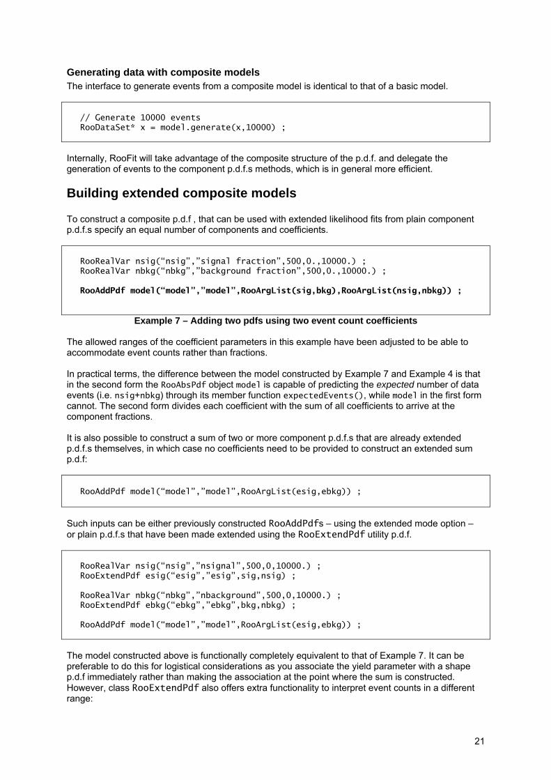
Figure 8 – Illustration of a composite extended p.d.f.

Suppose one is interested in the signal event yield in the range [4,6] of the model shown in Figure 8: you can calculate this from the total signal yield, multiplied by the fraction of the signal p.d.f shape that is in the range [4,6]

x.setRange(“window”,4,6) ; RooAbsReal* fracSigRange = sig.createIntegral(x,x,”window”) ; Double_t nsigWindow = nsig.getVal() * fracSigRange->getVal() ;

but one would still have to manually propagate the error on both the signal yield and the fraction integral of the shape to the final result. Class RooExtendPdf offers the possibility to apply the transformation immediately inside the calculation of the expected number of events so that the likelihood, and thus the fit result, is directly expressed in terms of nsigWindow, and all errors are automatically propagated correctly.

x.setRange(“window”,4,6”) ; RooRealVar nsigw(“nsigw”,”nsignal in window”,500,0,10000.) ; RooExtendPdf esig(“esig”,”esig”,sig,nsigw,”window”) ;

The effect of this modification is that the expected number of events returned by esig becomes

so that after minimizing the extended maximum likelihood nsigw equals the best estimate for the number of events in the signal window. Additional details on integration over ranges and normalization operations are covered in Appendix D.

23

Using extended composite models

Generating events from extended models Some extra features apply to composite models built for the extended likelihood formalism. Since these model predict a number events one can omit the requested number of events to be generated

RooDataSet* x = model.generate(x) ; In this case the number of events predicted by the p.d.f. is generated. You can optionally request to introduce a Poisson fluctuation in the number of generated events trough the Extended() argument:

RooDataSet* x = model.generate(x, Extended(kTRUE)) ; This is useful if you generate many samples as part of a study where you look at pull distributions. For pull distributions of event count parameters to be correct, a Poisson fluctuation on the total number of events generated should be present. Fit studies and pull distributions are covered in more detail in Chapter 14.

Fitting Composite extended p.d.f.s can only be successfully fit if the extended likelihood term is included in the minimization because they have one extra degree of freedom in their parameterization that is constrained by this extended term. If a p.d.f. is capable of calculating an extended term (i.e. any extended RooAddPdf object, the extended term is automatically included in the likelihood calculation. You can manually override this default behavior by adding the Extended() named argument in the fitTo() call.

model.fitTo(data,Extended(kTRUE)) ; // optional

Plotting The default procedure for visualization of extended likelihood models is the same as that of regular p.d.f.s: the event count used for normalization is that of the last dataset added to the plot frame. You have the option to override this behavior and use the expected event count of the pdf for its normalization as follows

model.plotOn(frame,Normalization(1.0,RooAbsReal::RelativeExtended)) ;

Note on the interpretation of fraction coefficients and ranges A closer look at the expression for composite p.d.f.s

1

shows that the fraction coefficients multiply normalized p.d.f.s. shapes, which has important consequences for the interpretation of these fraction coefficients: if the range of an observable is changed, the shape of the p.d.f. will change. This is illustrated in Figure 9(left,middle), which shows a

24

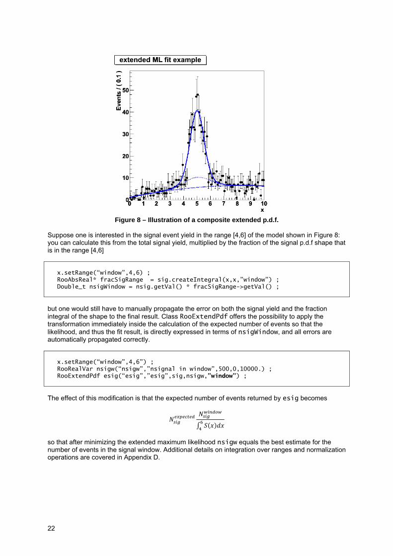
composite p.d.f consisting of a Gaussian plus a polynomial with a fraction of 0.5 in the range [-20,20] (left) and in the range [-5,5] (middle) that were created as follows:

RooPlot* frame1 = x.frame() ; model.plotOn(frame1) ; model.plotOn(frame1,Components(“bkg”),LineStyle(kDashed)) ; x.setRange(-5,5) ; RooPlot* frame2 = x.frame() ; model.plotOn(frame2) ; model.plotOn(frame2,Components(“bkg”),LineStyle(kDashed)) ;

Figure 9 – Composite p.d.f with fsig=0.5 in the range [-20,20] (left) and the range [-5,5] (middle)

and the range[-5,5] with [-20,20] as fraction interpretation range (right). However, there are cases, in which one would like to use the same object as a p.d.f with the same shape, but just defined in a narrower range (Figure 9-right). This decoupling of the shape from the domain can be accomplished with the introduction of a reference range that controls the shape independently of the domain on which the p.d.f. is used

Introducing an explicit reference range It is possible to fix the interpretation of RooAddPdf fraction coefficient to a frozen ‘reference’ range that is used to interpret the fraction, regardless of the actual range defined for the observables.

x.setRange(“ref”,-20,20) ; model.fixCoefRange(“ref”) ; RooPlot* frame3 = x.frame() ; model.plotOn(frame3) ; model.plotOn(frame3,Components(“bkg”),LineStyle(kDashed)) ;

In this mode of operation the shape is the same for each range of x in which model is used. The reference range can be both wider (as done above) and narrower than the original range.

Using the Range() command in fitTo() on composite models A reference range is introduced by default when you use the Range() specification mentioned in the preceding chapter in the fitTo() command to restrict the data to be fitted:

model.fitTo(data,Range(-5,5)) ; // fit only data in range[-5,5]

25

In this case, the interpretation range for the fractions of model will be set to a (temporary) named range “fit” that is created on the fly that is identical to the original range of the observables of the models. The fitted p.d.f shape thus resembles that Figure 9-right and not that of Figure 9-middle. This default behavior applies only to composite models without a preexisting reference range: if the fitted model already has a fixed reference range set, that range will continue to be used. It is also possible specify the reference range to be used by all RooAddPdf components during the fit with an extra named argument SumCoefRange()

// Declare “ref” range x.setRange(“ref”,-10,10) ; // Fit model to all data x[-20,20], interpret coefficients in range [-10,10] model.fitTo(data,SumCoefRange(“ref”)) ; // Fit model to data with x[-10,10], interpret coefficients same range model.fitTo(data,SumCoefRange(“ref”),Range(“ref”)) ; // Fit model to data with x[-10,10], interpret coefficients in range [-20,20] model.fitTo(data,Range(“ref”)) ;

Navigation tools for dealing with composite objects One of the added complications of using composite model versus using basic p.d.f.s is that you no longer know what the variables of your model are. RooFit provides several tools for dealing with composite objects when you only have direct access to the top-level node of the expression tree, i.e. the model object in the preceding examples.

What are the variables of my model? Given any composite RooFit value object, the getVariables() method returns you a RooArgSet with all parameters of your model:

RooArgSet* params = model->getVariables() ; params->Print(“v”) ;

This code fragment will output

RooArgSet::parameters: 1) RooRealVar::c0: "coefficient #0" 2) RooRealVar::c1: "coefficient #1" 3) RooRealVar::c2: "coefficient #2" 4) RooRealVar::mean: "mean" 5) RooRealVar::nbkg: "background fraction" 6) RooRealVar::nsig: "signal fraction" 7) RooRealVar::sigma: "sigma" 8) RooRealVar::x: "x"

If you know the name of a variable, you can retrieve a pointer to the object through the find() method of RooArgSet:

RooRealVar* c0 = (RooRealVar*) params->find(“c0”) ; c0->setVal(5.3) ;

26

If no object is found in the set with the given name, find() returns a null pointer. Although sets can contain any RooFit value type (any class derived from RooAbsArg) one deals in practice usually with sets of all RooRealVars. Therefore class RooArgSet is equipped with some special member functions to simplify operations on such sets. The above example can be shortened to

params->setRealValue(“c0”,5.3) ;

Similarly, there also exists a member function getRealValue().

What are the parameters and observable of my model? The concept of what variables are considered parameters versus observables is dynamic and depends on the use context, as explained in chapter 2. However, the following utility functions can be used to retrieve the set of parameters or observables from a given definition of what are observables

// Given a p.d.f model(x,m,s) and a dataset D(x,y) // Using (RooArgSet of) variables as given observable definition RooArgSet* params = model.getParameters(x) ; // Returns (m,s) RooArgSet* obs = model.getObservables(x) ; // Returns x // Using RooAbsData as definition of observables RooArgSet* params = model.getParameters(D) ; // Returns (m,s) RooArgSet* obs = model.getObservables(D) ; // Return x

What is the structure of my composite model? In addition to manipulation of the parameters one may also wonder what the structure of a given model is. For an easy visual inspection of the tree structure use the tree printing mode

model.Print(“t”) ;

The output will look like this:

0x9a76d58 RooAddPdf::model (model) [Auto] 0x9a6e698 RooGaussian::sig (signal p.d.f.) [Auto] 0x9a190a8 RooRealVar::x (x) 0x9a20ca0 RooRealVar::mean (mean) 0x9a3ce10 RooRealVar::sigma (sigma) 0x9a713c8 RooRealVar::nsig (signal fraction) 0x9a26cb0 RooChebychev::bkg (background p.d.f.) [Auto] 0x9a190a8 RooRealVar::x (x) 0x9a1c538 RooRealVar::c0 (coefficient #0) 0x9a774d8 RooRealVar::c1 (coefficient #1) 0x9a3b670 RooRealVar::c2 (coefficient #2) 0x9a66c00 RooRealVar::nbkg (background fraction)

For each lists object you will see the pointer to the object, following by the class name and object name and finally the object title in parentheses. A composite object tree is traversed top-down using a depth-first algorithm. With each node traversal the indentation of the printout is increased. This traversal method implies that the same object may

27

appear more than once in this printout if it is referenced in more than one place. See e.g. the multiple reference of observable x in the example above. The set of components of a p.d.f can also be accessed through the utility method getComponents(), which will return all the ‘branch’ nodes of its expression tree and is the complement of getVariables(), which returns the ‘leaf’ nodes. The example below illustrates the use of getComponents() to only print out the variables of model component “sig”:

RooArgSet* comps = model.getComponents() ; RooAbsArg* sig = comps->find(“sig”) ; RooArgSet* sigVars = sig->getVariables() ; sigVars->Print() ;

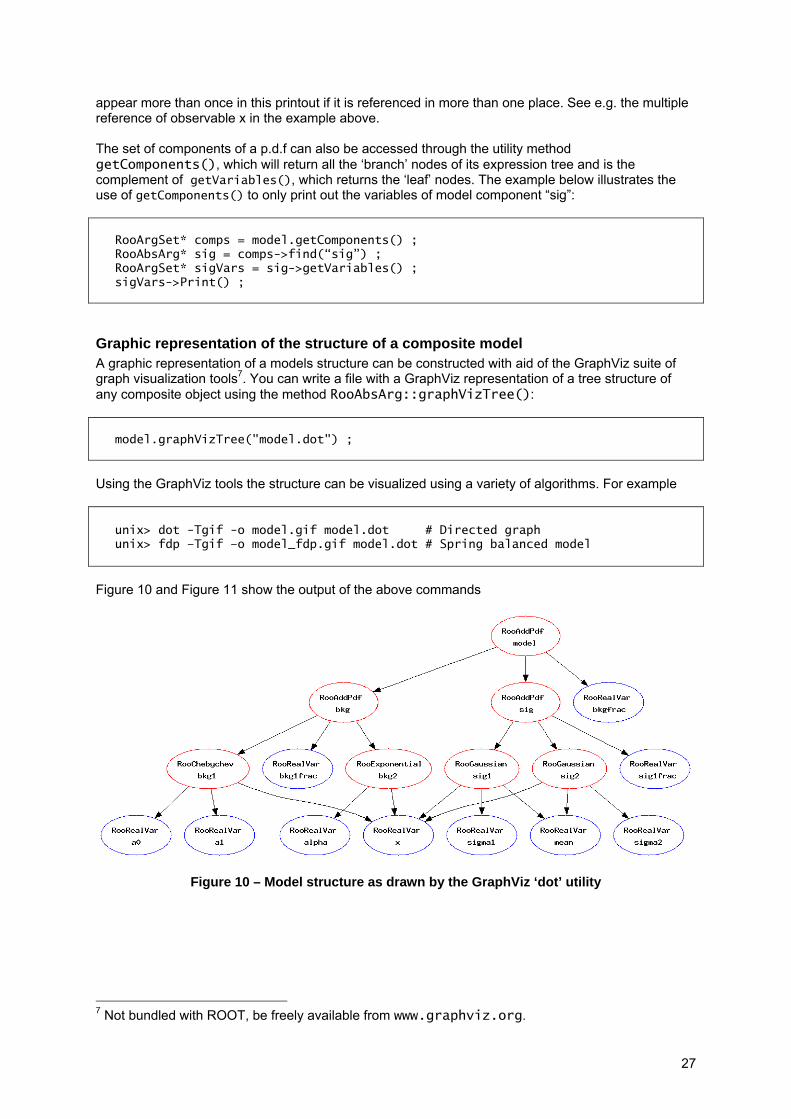
Graphic representation of the structure of a composite model A graphic representation of a models structure can be constructed with aid of the GraphViz suite of graph visualization tools7. You can write a file with a GraphViz representation of a tree structure of any composite object using the method RooAbsArg::graphVizTree():

model.graphVizTree("model.dot") ;

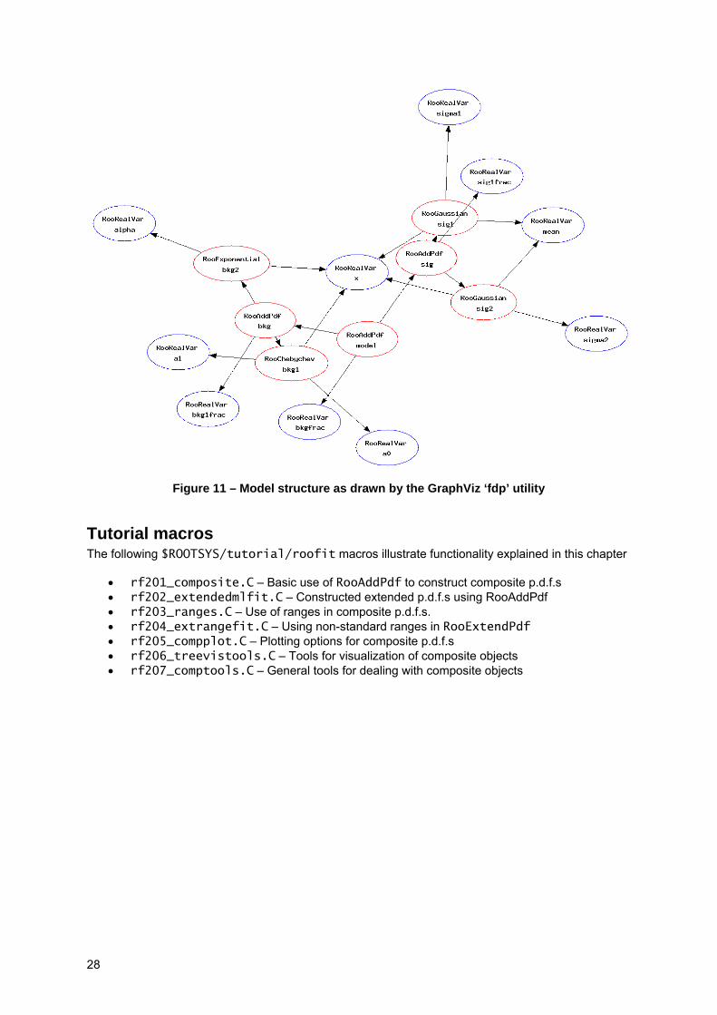
Using the GraphViz tools the structure can be visualized using a variety of algorithms. For example

unix> dot -Tgif -o model.gif model.dot # Directed graph unix> fdp –Tgif –o model_fdp.gif model.dot # Spring balanced model

Figure 10 and Figure 11 show the output of the above commands

Figure 10 – Model structure as drawn by the GraphViz ‘dot’ utility

7 Not bundled with ROOT, be freely available from www.graphviz.org.

28

Figure 11 – Model structure as drawn by the GraphViz ‘fdp’ utility


• rf201_composite.C – Basic use of RooAddPdf to construct composite p.d.f.s • rf202_extendedmlfit.C – Constructed extended p.d.f.s using RooAddPdf • rf203_ranges.C – Use of ranges in composite p.d.f.s. • rf204_extrangefit.C – Using non-standard ranges in RooExtendPdf • rf205_compplot.C – Plotting options for composite p.d.f.s • rf206_treevistools.C – Tools for visualization of composite objects • rf207_comptools.C – General tools for dealing with composite objects

29

4. Choosing, adjusting and creating basic shapes We will now have a closer look at what basic shapes are provided with RooFit, how you can tailor them to your specific problem and how you can write a new p.d.f.s in case none of the stock p.d.f.s. have the shape you need.

What p.d.f.s are provided? RooFit provides a library of about 20 probability density functions that can be used as building block for your model. These functions include basic functions, non-parametric functions, physics-inspired functions and specialized decay functions for B physics. A more detailed description of each of this p.d.f.s is provided in p.d.f. gallery in Appendix B

Basic functions The following basic shapes are provided as p.d.f.s

• Gaussian, class RooGaussian. The normal distribution shape

• A bifurcated Gaussian, class RooBifurGauss. A variation on the Gaussian where the width of the Gaussian on the low and high side of the mean can be set independently

• Exponential , class RooExponential. Standard exponential decay distribution

• Polynomial, class RooPolynomial. Standard polynomial shapes with coefficients for each power of xn.

• Chebychev polynomial, class RooChebychev. An implementation of Chebychev polynomials of the first kind.

• Poisson, class RooPoisson. The standard Poisson distribution. Note that each functional form has one parameter less than usual form, because the degree of freedom that controls the ‘vertical’ scale is eliminated by the constraint that the integral of the p.d.f. must always exactly 1.

Prac

tical

Tip

The use of Chebychev polynomials over regular polynomials is recommended because of their superior stability in fits. Chebychev polynomials and regular polynomials can describe the same shapes, but a clever reorganization of power terms in Chebychev polynomials results in much lower correlations between the coefficients ai in a fit, and thus to a more stable fit behavior. For a definition of the functions Ti and some background reading, look e.g. at http://mathworld.wolfram.com/ChebyshevPolynomialoftheFirstKind.html

Non-parametric functions RooFit offers two classes that can describe the shape of an external data distribution without explicit parameterization

• Histogram, class RooHisPdf. A p.d.f. that represents the shape of an external RooDataHist histogram, with optional interpolation to construct a smooth function

• Kernel estimation, class RooKeysPdf. A p.d.f. that represent the shape of an external unbinned dataset as a superposition of Gaussians with equal surface, but with varying width, depending on the local event density.

30

Physics inspired functions In addition to the basic shapes RooFit also implements a series of shapes that are commonly used to model physical ‘signal’ distributions.

• Landau, class RooLandau. This function parameterizes energy loss in material and has no analytical form. RooFit uses the parameterized implementation in TMath::Landau.

• Breit-Wigner, class RooBreitWigner. The non-relativistic Breit-Wigner shape models

resonance shapes and its cousin the Voigtian (class RooVoigtian)– a Breit-Wigner convolved with a Gaussian --- are commonly used to describe the shape of a resonance in the present of finite detector resolution.

• Crystal ball, class RooCBShape. The Crystal ball function is a Gaussian with a tail on the low

side that is traditionally used to describe the effect of radiative energy loss in an invariant mass.

• Novosibirsk, class RooNovosibirsk. A modified Gaussian with an extra tail parameter that

skews the Gaussian into an asymmetric shape with a long tail on one side and a short tail on the other.

• Argus, class RooArgusBG. The Argus function is an empirical formula to model the phase space of multi-body decays near threshold and is frequently used in B physics.

• D*±-D0 phase space, class RooDstD0BG. An empirical function with one parameter that can

model the background phase space in the D*±-D0 invariant mass difference distribution.

Specialized functions for B physics RooFit was originally development for BaBar, the B-factory experiment at SLAC, therefore it also provides a series of specialized p.d.f.s. describing the decay of B0 mesons including their physics effect.

• Decay distribution, class RooDecay. Single or double-sided exponential decay distribution.

• Decay distribution with mixing, class RooBMixDecay Single or double-sided exponential decay distribution with effect of B0-B0bar mixing

• Decay distribution with SM CP violation, class RooBCPEffDecay. Single or double-sided exponential decay distribution with effect Standard Model CP violation

• Decay distribution with generic CP violation, class RooBCPGenDecay. Single or double-sided exponential decay distribution with generic parameterization of CP violation effects

• Decay distribution with CP violation into non-CP eigenstates, class RooNonCPEigenDecay. Single or double-sided exponential decay distribution of decays into non-CP eigenstates with generic parameterization of CP violation effects

• Generic decay distribution, with mixing, CP, CPT violation, class RooBDecay. Most generic description of B decay with optional effects of mixing, CP violation and CPT violation.

Reparameterizing existing basic p.d.f.s In Chapter 2 it was explained that RooAbsPdf classes have no intrinsic notion of variables being parameters or observables. In fact, RooFit functions and p.d.f.s. even have no hard-wired assumption that the parameters of a function are variables (i.e. a RooRealVar), so you can modify the

31

parameterization of any existing p.d.f. by substituting a function for a parameter. The following example illustrates this:

// Observable RooRealVar x(“x”,”x”,-10,10) ; // Construct sig_left(x,mean,sigma) RooRealVar mean(“mean”,”mean”,0,-10,10) ; RooRealVar sigma(“sigma_core”,”sigma (core)”,1,0.,10.) ; RooGaussian sig_left(“sig_left”,”signal p.d.f.”,x,mean,sigma) ; // Construct function mean_shifted(mean,shift) RooRealVar shift(“shift”,”shift”,1.0) ; RooFormulaVar mean_shifted(“mean_shifte”,”mean+shift”,RooArgSet(mean,shift)); // Construct sig_right(x,mean_shifted(mean,shift),sigma) RooGaussian sig_right(“sig_right”,”signal p.d.f.”,x,mean_shifted,sigma) ; // Construct sig=sig_left+sig_right RooRealVar frac_left(“frac_left”,”fraction (left)”,0.7,0.,1.) ; RooAddPdf sig(“sig”,”signal”,RooArgList(sig_left,sig_right),frac_left) ;

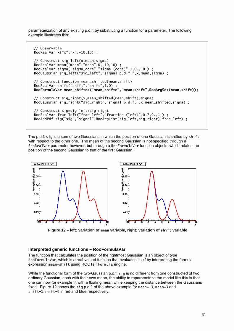
The p.d.f. sig is a sum of two Gaussians in which the position of one Gaussian is shifted by shift with respect to the other one. The mean of the second Gaussian is not specified through a RooRealVar parameter however, but through a RooFormulaVar function objects, which relates the position of the second Gaussian to that of the first Gaussian.

Figure 12 – left: variation of mean variable, right: variation of shift variable

Interpreted generic functions – RooFormulaVar The function that calculates the position of the rightmost Gaussian is an object of type RooFormulaVar, which is a real-valued function that evaluates itself by interpreting the formula expression mean+shift using ROOTs TFormula engine. While the functional form of the two-Gaussian p.d.f. sig is no different from one constructed of two ordinary Gaussian, each with their own mean, the ability to reparametrize the model like this is that one can now for example fit with a floating mean while keeping the distance between the Gaussians fixed. Figure 12 shows the sig p.d.f. of the above example for mean=-3, mean=3 and shift=3,shift=6 in red and blue respectively.

32

Class RooFormulaVar can handle any C++ expression that ROOT class TFormula can. This includes most math operators (+,-,/,*,…), nested parentheses and some basic math and trigonometry functions like sin, cos, log, abs etc…Consult the ROOT TFormula documentation for a complete overview of the functionality. The names of the variables in the formula expression are those of the variables given in the RooArgSet as 3rd parameter in the constructor. Alternatively, you can reference the variable through positional index if you pass the variables in a RooArgList:

RooFormulaVar mean_shifted(“mean_shifte”,”@0+@1”,RooArgList(mean,shift));

This form is usually easier if you follow a ‘factory-style’ approach in your own code where you don’t know (or don’t care to know) the names of the variables you intend to add in code that declares the RooFormulaVar. Class RooFormulaVar is explicitly intended for trivial transformations like the one shown above. If you need a more complex transformation you should write a compiled class. The final section of this Chapter cover the use of RooClassFactory to simplify the writing of classes that can be compiled.

Compiled generic functions – Addition, multiplication, polynomials For simple transformation, the utility classes RooPolyVar, RooAddition and RooProduct are available, that implement a polynomial function, a sum of N components and a product of N components respectively.

Binding TFx, external C++ functions as RooFit functions If you have an existing C(++) function from either ROOT or from a private library that is linked with your ROOT session or standalone application, you can trivially bind such a function as a RooFit function or p.d.f. object. For example, to bind the ROOT provided function double TMath::Erf(Double_t) as a RooFit function object you do

RooRealVar x(“x”,”x”,-10,10) ; RooAbsReal* erfFunc = bindFunction(TMath::Erf,x) ; RooPlot* frame = x.frame() ; erfFunc->plotOn(frame) ;

To bind an external function as p.d.f. rather than as a function use the bindPdf() method, as is illustrated here with the ROOT::Math::beta_pdf function

RooRealVar x("x","x",0,1) ; RooRealVar a("a","a",5,0,10) ; RooRealVar b("b","b",2,0,10) ; RooAbsPdf* beta = bindPdf("beta",ROOT::Math::beta_pdf,x,a,b) ; RooDataSet* data = beta.generate(x,10000) ; RooPlot* frame = x.frame() ; data->plotOn(frame) ; beta->plotOn(frame) ;

The bindFunction() and bindPdf() helper functions return a pointer to an matching instance of one of the templated classes RooCFunction[N]Binding or RooCFunction[N]PdfBinding,

33

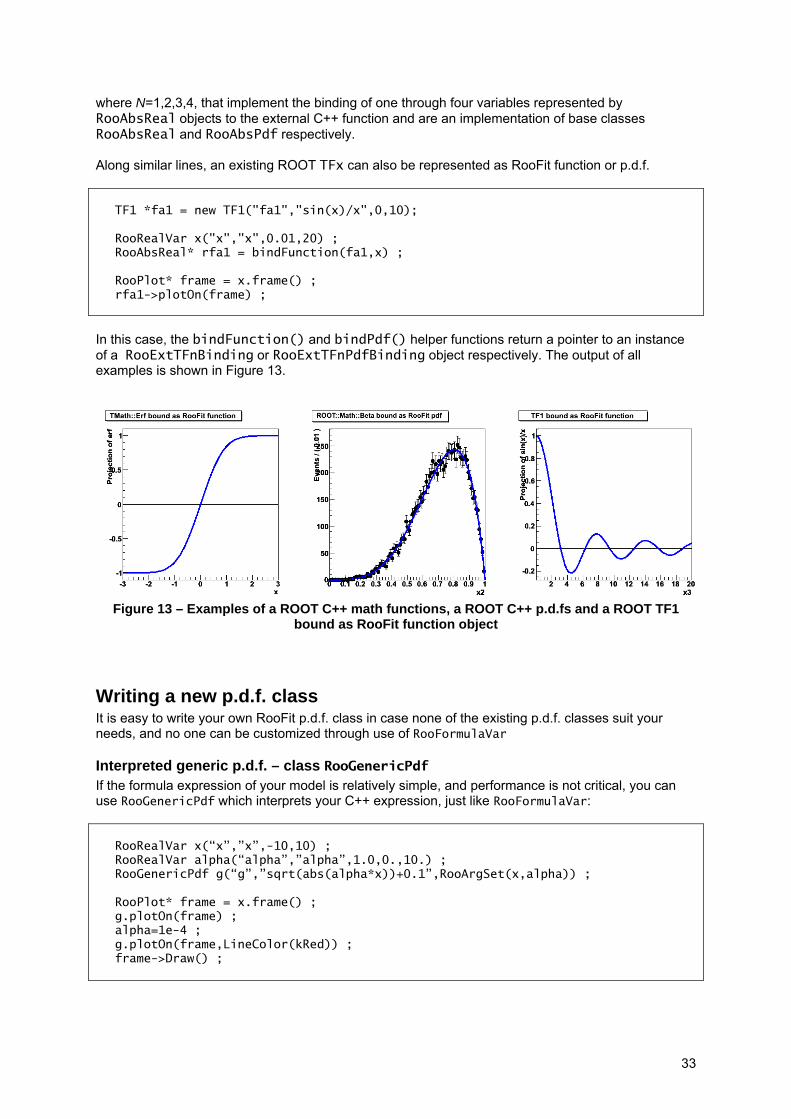
where N=1,2,3,4, that implement the binding of one through four variables represented by RooAbsReal objects to the external C++ function and are an implementation of base classes RooAbsReal and RooAbsPdf respectively. Along similar lines, an existing ROOT TFx can also be represented as RooFit function or p.d.f.

TF1 *fa1 = new TF1("fa1","sin(x)/x",0,10); RooRealVar x("x","x",0.01,20) ; RooAbsReal* rfa1 = bindFunction(fa1,x) ; RooPlot* frame = x.frame() ; rfa1->plotOn(frame) ;

In this case, the bindFunction() and bindPdf() helper functions return a pointer to an instance of a RooExtTFnBinding or RooExtTFnPdfBinding object respectively. The output of all examples is shown in Figure 13.

Figure 13 – Examples of a ROOT C++ math functions, a ROOT C++ p.d.fs and a ROOT TF1

bound as RooFit function object

Writing a new p.d.f. class It is easy to write your own RooFit p.d.f. class in case none of the existing p.d.f. classes suit your needs, and no one can be customized through use of RooFormulaVar

Interpreted generic p.d.f. – class RooGenericPdf If the formula expression of your model is relatively simple, and performance is not critical, you can use RooGenericPdf which interprets your C++ expression, just like RooFormulaVar:

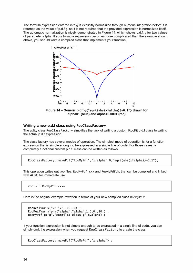
RooRealVar x(“x”,”x”,-10,10) ; RooRealVar alpha(“alpha”,”alpha”,1.0,0.,10.) ; RooGenericPdf g(“g”,”sqrt(abs(alpha*x))+0.1”,RooArgSet(x,alpha)) ; RooPlot* frame = x.frame() ; g.plotOn(frame) ; alpha=1e-4 ; g.plotOn(frame,LineColor(kRed)) ; frame->Draw() ;

34

The formula expression entered into g is explicitly normalized through numeric integration before it is returned as the value of p.d.f g, so it is not required that the provided expression is normalized itself. The automatic normalization is nicely demonstrated in Figure 14, which shows p.d.f. g for two values of parameter alpha. If your formula expression becomes more complicated than the example shown above, you should write a compiled class that implements your function.

Figure 14 – Generic p.d.f g(“sqrt(abs(x*alpha))+0.1”) drawn for

alpha=1 (blue) and alpha=0.0001 (red)

Writing a new p.d.f class using RooClassFactory The utility class RooClassFactory simplifies the task of writing a custom RooFit p.d.f class to writing the actual p.d.f expression. The class factory has several modes of operation. The simplest mode of operation is for a function expression that is simple enough to be expressed in a single line of code. For those cases, a completely functional custom p.d.f. class can be written as follows:

RooClassFactory::makePdf(“RooMyPdf”,”x,alpha”,0,“sqrt(abs(x*alpha))+0.1”); This operation writes out two files, RooMyPdf.cxx and RooMyPdf.h, that can be compiled and linked with ACliC for immediate use

root>.L RooMyPdf.cxx+

Here is the original example rewritten in terms of your new compiled class RooMyPdf:

RooRealVar x(“x”,”x”,-10,10) ; RooRealVar alpha(“alpha”,”alpha”,1.0,0.,10.) ; RooMyPdf g(“g”,”compiled class g”,x,alpha) ;

If your function expression is not simple enough to be expressed in a single line of code, you can simply omit the expression when you request RooClassFactory to create the class

RooClassFactory::makePdf(“RooMyPdf”,”x,alpha”) ;

35

This creates a fully functional class with a dummy implementation of RooAbsPdf::evaluate(). To make it a functional class, edit the file RooMyPdf.cxx and insert a function expression as return value in the evaluate() method of your class, using as many lines of code as you need.

Double_t RooMyPdf::evaluate() const { // ENTER EXPRESSION IN TERMS OF VARIABLE ARGUMENTS HERE return 1 ; }

You can use all symbols that you listed as function arguments in the makePdf() call as C++ double objects.8 Since RooAbsPdf have no fixed interpretation of variables being observables or parameters, there is no need, or point, in explicitly normalizing the expression in evaluate() with respect to a specific choice of observables: the return value of evaluate() is always divided a posteriori by a normalization integral before it is return through RooAbsPdf::getVal(). By default this normalization step is done using a numeric integrator, but if you know how to integrate your class over one (or more) choices of observables, you can advertise this capability in the p.d.f. and your analytical integral will be used instead of numeric integration whenever it is appropriate. You can invoke RooClassFactory::makePdf() with different options that will make skeleton code for the analytical integral interface. Details can be found in the RooClassFactory HTML class documentation. Additional information on how to write p.d.f. classes with optional support for analytical integration and internal event generation handling is given in Chapter 14.

Instantiating custom p.d.f objects using RooClassFactory Another mode of operation of RooClassFactory is that you request the factory to immediately perform the compilation and instantiation of an object in terms of a set of given variable objects:

RooAbsPdf* myPdf = RooClassFactory::makePdfInstance(“RooMyPdf”, “sqrt(abs(x*alpha))+0.1”, RooArgSet(x,alpha)) ;

Note that the functional form of this invocation is very similar to that of creating an object of type RooGenericPdf: you provide a string with a C++ function expression and a set of input variables and you get back an instance of a RooAbsPdf that implements that shape in terms of the given variables. The difference is in the way the code is generated: interpreted for and compiled for RooClassFactory. What is more appropriate depends on the use case: the RooClassFactory route will result in faster execution, but incurs a startup overhead of a few seconds to compiled and link the code each time macro is executed. The RooGenericPdf route has negligible startup overhead but will slow down the executing of plotting, event generation and fitting.

8 Note that in reality these objects are not doubles, but objects of type RooRealProxy that hold references to the RooRealVar variables (or more generically RooAbsReal functions) that were specified as inputs of the instance of the function object. These objects can be handled as doubles in function expressions because RooRealProxy implements operator double() that facilitates that functionality.

36

Writing a new function class using RooClassFactory The code factory class RooClassFactory cannot only write skeleton p.d.f.s, but also skeletons for generic real-valued functions. Generic real-valued function are all classes in RooFit that inherit from RooAbsReal. Class RooFormulaVar is a good example of a generic real-valued function. Unlike p.d.f.s, RooAbsReal are not normalized to unity and can also take negative values. Compilable custom real-valued functions are a good replacement for RooFormulaVar in cases where the formula expression is less than trivial, or in cases where performance is critical. Creating a skeleton for a generic function object is done with the makeFunction() method of RooClassFactory

RooClassFactory::makeFunction(“RooMyFunction”,”x,b”) ;


• rf103_interprfuncs.C – Creating interpreted functions and p.d.f.s. • rf104_classfactory.C – Using the class factory to make a custom p.d.f class • rf105_funcbinding.C – Binding external C++ functions and ROOT TFx objects

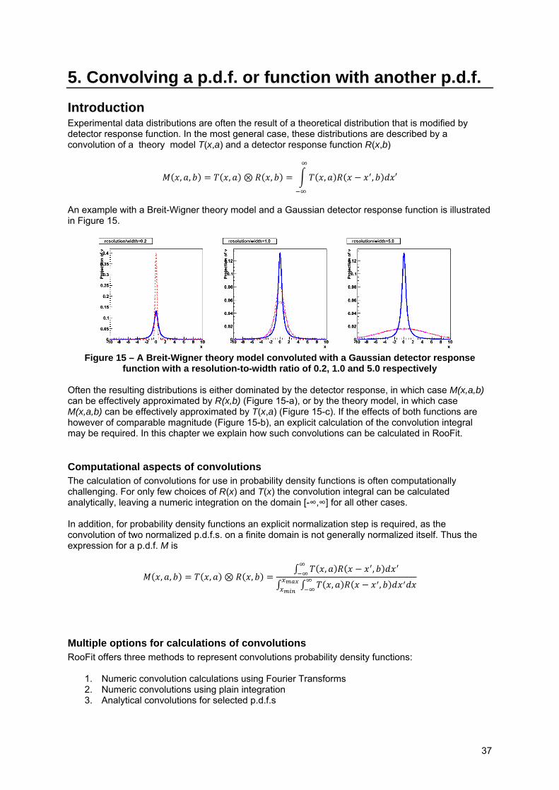
37

5. Convolving a p.d.f. or function with another p.d.f. Introduction Experimental data distributions are often the result of a theoretical distribution that is modified by detector response function. In the most general case, these distributions are described by a convolution of a theory model T(x,a) and a detector response function R(x,b)

, , , , , ,

An example with a Breit-Wigner theory model and a Gaussian detector response function is illustrated in Figure 15.

Figure 15 – A Breit-Wigner theory model convoluted with a Gaussian detector response function with a resolution-to-width ratio of 0.2, 1.0 and 5.0 respectively

Often the resulting distributions is either dominated by the detector response, in which case M(x,a,b) can be effectively approximated by R(x,b) (Figure 15-a), or by the theory model, in which case M(x,a,b) can be effectively approximated by T(x,a) (Figure 15-c). If the effects of both functions are however of comparable magnitude (Figure 15-b), an explicit calculation of the convolution integral may be required. In this chapter we explain how such convolutions can be calculated in RooFit.

Computational aspects of convolutions The calculation of convolutions for use in probability density functions is often computationally challenging. For only few choices of R(x) and T(x) the convolution integral can be calculated analytically, leaving a numeric integration on the domain [-∞,∞] for all other cases. In addition, for probability density functions an explicit normalization step is required, as the convolution of two normalized p.d.f.s. on a finite domain is not generally normalized itself. Thus the expression for a p.d.f. M is

, , , ,, ,

, ,

Multiple options for calculations of convolutions RooFit offers three methods to represent convolutions probability density functions:

1. Numeric convolution calculations using Fourier Transforms 2. Numeric convolutions using plain integration 3. Analytical convolutions for selected p.d.f.s

38

Numeric convolution with Fourier Transforms For most applications, numeric convolutions calculated in Fourier transformed space provide the best tradeoff between versatility, precision and computational intensity. To better understand the features of convolutions calculated with discrete Fourier transforms we start with a brief introduction on the underlying math.

The Circular Convolution Theorem and Discrete Fourier Transformations The circular convolution theorem states that the convolution of two series of coefficients xi and yi in the space domain9 can be calculated in the frequency domain as a simple multiplication of coefficients

· This theorem allows us to calculate convolutions without any explicit integral calculation. The drawback is that it requires Fourier transforms and discrete input data. However, in practice these problems that are more easily solved than numeric integration over an open domain. Another feature of the theorem is that for finite n the convolution observable is treated as cyclical, which may or may not be desirable depending on the application. We will get back to this. To be able to use discrete Fourier transforms all continuous input function must be sampled into a discrete distribution:

Any such discrete distribution xI, can be represented in the frequency domain by an equal number of coefficients Xi through the application of a Fourier transform:

Both the spatial domain coefficients xi and the frequency domain coefficients Xi are in general complex numbers. If the input coefficients xi are real, as is the case for sampling from probability density functions, the frequency domain coefficients Xi will exhibit the symmetry Xn-k=X*k. Conversely, a distribution in the frequency domain can be converted (back) to a distribution in the space domain using an inverse Fourier transform

1

The resulting spatial domain coefficients xi of the inverse transform are in general complex numbers, unless the coefficients Xi satisfied the symmetry Xn-k=X*k in which case all xi are real. The convolution operator class RooFFTConvPdf implements the following algorithm to compute circular convolutions of the type M(x) = T(x) R(x) as follows

1. Sample T(x) into an array ti and R(x) into ri 2. Fourier Transform arrays ti Ti and ri Ri into the frequency domain 3. Calculate the convolution in the frequency domain as Mi = Ti⋅Ri 4. Inverse Fourier Transform the array Mi mi into the space domain 5. Represent the array mi as a continuous function M(x) through interpolation.

The bulk of the computational effort of the approach is in the calculation of the (inverse) discrete Fourier transforms. Fast calculation of discrete Fourier transforms is a heavily researched topic in the field of signal processing and excellent algorithms exists to be able to calculate these transforms

9 A series of coefficients in the space domain is effectively a histogram

39

efficiently. RooFit uses the freely available package FFTW3, which is interfaced to ROOT through class TVirtualFFT, and provides one of the fastest available implementations of discrete Fourier transforms. This means that to be able to use RooFFTConvPdf, you must have FFTW installed with your ROOT installation10.

Performance of FFT based convolutions The speed of the FFTW calculations does not scale linearly with the number of sampling points. It is unproblematic to sample p.d.f.s at high resolutions like 1000 or 10000 evenly spaced points in the domain of the observable, so that sampling granularity is not an issue for most applications. As an indication of the performance, a convolution of a Landau p.d.f with a Gaussian resolution sampled on 10000 points each takes roughly 90 milliseconds per evaluation, resulting a typical fit times of a few seconds, (assuming 50-100 MINUIT steps for minimization and error analysis), making FFT-based convolution 10 to 100 times faster than convolution through plain numeric integration.

Limitations of FFT based convolutions You should be aware though of the specific features of this algorithm

• The resulting convolution is explicitly circular: any tail that goes ‘over the edge’ on the upper bound of the domain of the convolution observable side will show up on the lower bound and vice versa. This is effect is illustrated in Figure 16. In case this is unwanted, class RooFFTConvPdf has tools minimize these effects that are explained in the next sections. It is correct behavior for inherently circular observables such as azimuthal angles.

• A small but finite approximation is introduced by the sampling frequency. While unproblematic for most applications (at e.g. 10000 sampling points) you should exert some caution with models that fit very high frequency signal components (such as Bs meson oscillations)

• The shape of both the theory model and the resolution are truncated at the boundaries of the defined range of the observable. The effect of this is most obvious in the resolution p.d.f. and best illustrated with an extreme example: Given a observable with a defined range [-1,1]: if you would convolve you theory model with a Gaussian of infinite width you’re effectively convolving it with a block function of width 2.

Most of these possible adverse effects can be avoided by choosing parameters appropriately, i.e. choosing a sufficiently high sampling frequency, a sufficiently wide sampling range.

Figure 16 – Demonstration of cyclical nature of FFT based convolutions. Dashed line is theory model (Landau). Solid lines is theory model convoluted with a Gaussian. The overflow of the

convoluted p.d.f. at the xmax resurfaces at the xmin

10 See www.fftw.org for the installation of FFTW itself. In your ROOT installation, be sure to run configure with options –with-fftw-libdir=<path> and –with-fftw-incdir=<path> in case you have installed FFTW in a non-standard location.

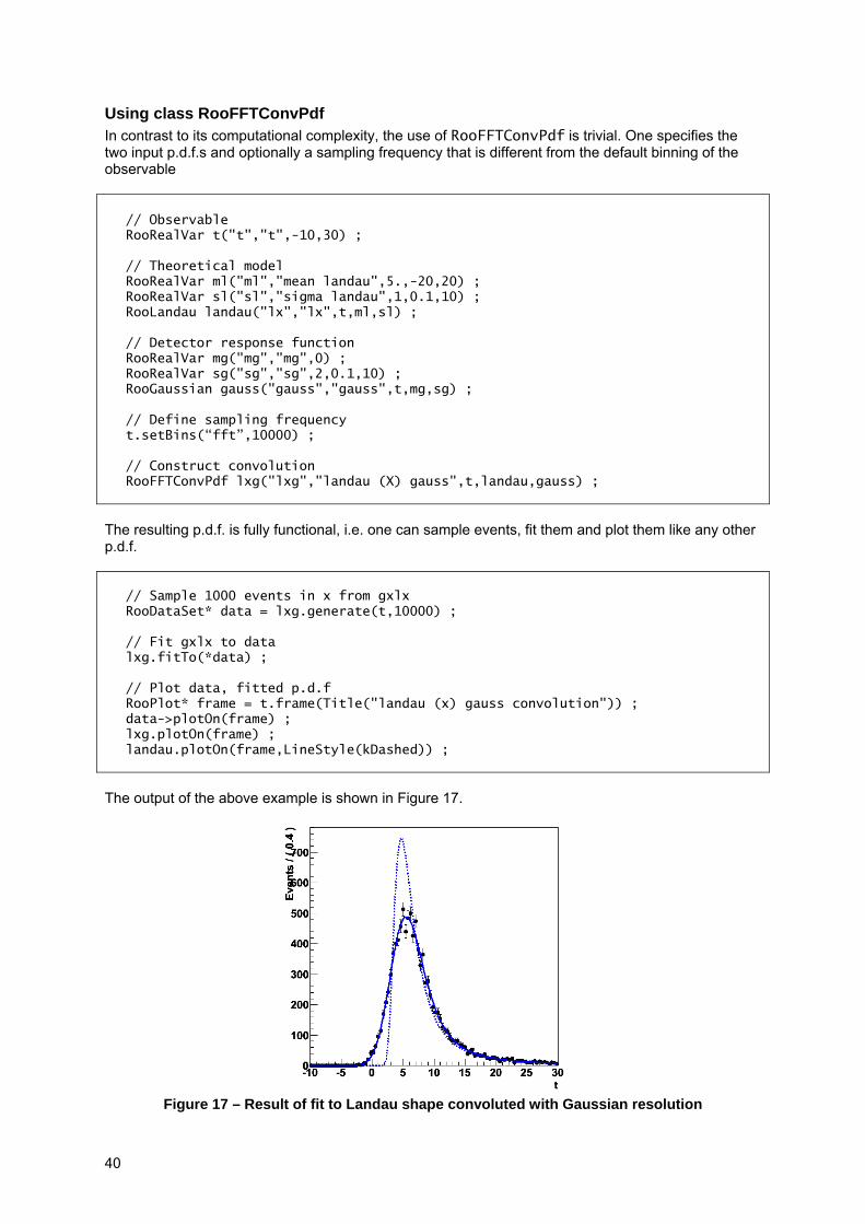
40

Using class RooFFTConvPdf In contrast to its computational complexity, the use of RooFFTConvPdf is trivial. One specifies the two input p.d.f.s and optionally a sampling frequency that is different from the default binning of the observable

// Observable RooRealVar t("t","t",-10,30) ; // Theoretical model RooRealVar ml("ml","mean landau",5.,-20,20) ; RooRealVar sl("sl","sigma landau",1,0.1,10) ; RooLandau landau("lx","lx",t,ml,sl) ; // Detector response function RooRealVar mg("mg","mg",0) ; RooRealVar sg("sg","sg",2,0.1,10) ; RooGaussian gauss("gauss","gauss",t,mg,sg) ; // Define sampling frequency t.setBins(“fft”,10000) ; // Construct convolution RooFFTConvPdf lxg("lxg","landau (X) gauss",t,landau,gauss) ;

The resulting p.d.f. is fully functional, i.e. one can sample events, fit them and plot them like any other p.d.f.

// Sample 1000 events in x from gxlx RooDataSet* data = lxg.generate(t,10000) ; // Fit gxlx to data lxg.fitTo(*data) ; // Plot data, fitted p.d.f RooPlot* frame = t.frame(Title("landau (x) gauss convolution")) ; data->plotOn(frame) ; lxg.plotOn(frame) ; landau.plotOn(frame,LineStyle(kDashed)) ;

The output of the above example is shown in Figure 17.

Figure 17 – Result of fit to Landau shape convoluted with Gaussian resolution

41

Tuning the sampling frequency The default sampling frequency that is used to sample both input p.d.f.s is the default binning specification of the convolution observable, as specified through RooRealVar::setBins(). Note that the default binning for a RooRealVar is 100 bins, which is usually insufficient resolution for a FFT convolution. To change this you can either increase the density of the default binning, e.g. x.setBins(1000), or specify an alternate binning with the name “fft” that is used for FFT convolution sampling only, i.e. x.setBins(“fft”,10000).

Sampling of multidimensional p.d.f.s Even though RooFFTConvPdf only supports convolution in one observable, it can convolve multidimensional p.d.f.s, e.g. one can do

, , In such cases the input p.d.f. T(x,y) is sampled in both observables x and y and the output histogram that caches the result of M(x,y) is also two-dimensional so that the value of M is precalculated for all values of x and y. The sampling density for FFT sampling of T in the observable y is controlled in the same way as that of x: in the absence of a alternate binning named “fft” defined in y, the default binning of y is used. The sampling density of x and y does not need to be the same

Interpolation of FFT output By default the output histogram of the FFT convolution is interpolated to second order to yield a smooth and continuously derivable p.d.f shape. You can change this default through the setInterpolationOrder() member function, or supply it as the optional argument in the constructor. At order zero, no interpolation is used. The highest order supported is 9. If the output histogram is multi-dimensional interpolation is applied to all real-valued dimensions.11

Adjustment of the sampling range Even though the FFT convolution formalism is completely symmetrical in the two input p.d.f.s, the role of both p.d.f.s in most applications is not. Class RooFFTConvPdf assumes that the first p.d.f. is the theory model and that the second p.d.f. is the resolution model. In this interpretation it is often convenient to define different sampling ranges for the theory model and the resolution mode. For example, if one fits a Z boson mass peak in the range 60-100 GeV one would like to sample the theory model in the range [60,100], but the resolution model in a range symmetrically around zero, e.g. [-20,20] as resolution models that do not (intentionally) introduce a bias are always centered around zero. To simplify these (theory model resolution model) use cases class RooFFTConvPdf has the following default sampling strategy

• The first p.d.f. is assumed to be the theory model and is sampled in the defined range of the observable (using either the fft or default binning density)

• The second p.d.f is assumed to be the resolution model and is sampled in a range that is symmetric around zero with the same width and sampling density as the theory model12

Without this shifting strategy one would in the example of the Z boson be forced to fit the range [-20,100] to include both theory and resolution in the range, which is usually undesirable as it requires

11 At present, the interpolation is limited to at most two real-valued dimensional due to an implementation limitation in RooDataHist. 12 The FFT formalism does not allow the sampling density or width of the range of the theory model and resolution model to be different.

42

you to model the theory distribution always to below zero, which may include areas in which it is not well known or undefined (i.e. [-20,60]). You can adjust the range shifting feature through a call

lxg.setShift(s1,s2) ;

where s1 and s2 are the amounts by which the sampling ranges for pdf1 and pdf2 are shifted respectively. A pair of values of (0,-(xmin+xmax)/2) replicates the default behavior and a pair of values of (0,0) disables the shifting feature altogether.

Reducing cyclical spill over – Adjusting the buffer fraction RooFFTConvPdf introduces a blank buffer in the FFT sampling array beyond the end of the sampling range of both p.d.f.s. The purpose of this buffer is to reduce the effect over cyclical overflows: any overflow will first spill into the buffer area, which is discarded when the FFT output buffer is interpreted as the output p.d.f. shape, before it leaks back into the observable range. The effect of such cyclical leaking is shown in Figure 16, which was created with the buffer feature disabled. If your convolution observable is a inherently cyclical observable, such spillover is in fact a desired feature and you should disable this feature by setting the buffer size to zero using

lxg.setBufferFraction(0) ; If your observable is not inherently cyclical, the default buffer fraction 10% of the size of sampling array is usually sufficient to suppress minor cyclical leakage. If you observe otherwise you can increase the buffer fraction to a large value using setBufferFraction(x) where x is a fraction of the sampling array size. Please note that computation time will go up if very large buffer fractions are chosen.

Generating events from a convolution p.d.f If both input p.d.f.s of a RooFFTConvPdf provide an internal event generator that supports generation of events in the convolution observable in the domain [-∞,∞], a special generator context is automatically selected to construct the distribution of the convolution. Rather than sampling the convoluted p.d.f. distribution with an accept/reject sampling technique, it samples values from the theory model and resolution model separately (using the internal generator method of each) and constructs the convoluted observable as

reflecting the ‘smearing’ nature of the convolution operation. Only events that pass the requirement

are returned as generated events. This method of event generation is typically more efficient that the default accept/reject sampling technique. If the smearing method cannot be applied, e.g. because one or both of the input p.d.f. lack an internal generator, the default sampling method on the convoluted distribution is automatically substituted.

43

Plain numeric convolution

Method and performance If you do not wish to use class RooFFTConvPdf because one of its algorithmic features are problematic you can try class RooNumConvPdf, which calculates the convolution integral

, , , ,, ,

, ,

and its normalization integral through straight numeric integration. By default RooNumConvPdf performs the numeric convolution integral on the domain [-∞,+∞] . This calculation is numerically difficult, and can suffer from stability problems. Class RooNumConvPdf should therefore be your option of last resort. In particular, if you intend to fit a RooNumConvPdf you should be aware that a precision of O(10-7) needs to be reached for the numeric noise not disturb MINUIT in its likelihood minimum finding. In practice this means O(100) evaluations of R and T to calculate M for each data point.

Using class RooNumConvPdf Class RooNumConvPdf has an almost identical constructor syntax as class RooFFTConvPdf, so one can switch easily between the two:

RooRealVar x(“x”,”x”,-10,10) ; RooRealVar meanl(“meanl”,”mean of Landau”,2) ; RooRealVar sigmal(“sigmal”,”sigma of Landau”,1) ; RooLandau landau(“landau”,”landau”,x,meanl,sigmal) ; RooRealVar meang(“meang”,”mean of Gaussian”,0) ; RooRealVar sigmag(“sigmag”,”sigma of Gaussian”,2) ; RooGaussian gauss(“gauss”,”gauss”,x,meang,sigmag) ; RooNumConvPdf model(“model”,”model”,x,landau,gauss) ; RooPlot* frame = x.frame() ; model.plotOn(frame) ; landau.plotOn(frame,LineStyle(kDashed)) ; frame->Draw() ;

Example 8 – Numeric convolution of a Landau with a Gaussian

Figure 18 show the result of Example 8.

Configuring the numeric convolution integration By default RooNumConvPdf performs the numeric convolution integral on the full domain of the convolution variable (i.e. from -∞ to +∞) using a x 1/x transformation to calculate the integrals of the tails extending to infinity. This calculation is difficult, can suffer from stability problems and may be avoided for certain choices of resolution models.

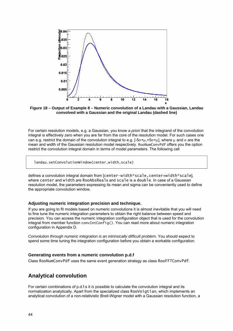
44

Figure 18 – Output of Example 8 – Numeric convolution of a Landau with a Gaussian, Landau

convolved with a Gaussian and the original Landau (dashed line) For certain resolution models, e.g. a Gaussian, you know a priori that the integrand of the convolution integral is effectively zero when you are far from the core of the resolution model. For such cases one can e.g. restrict the domain of the convolution integral to e.g. [-5σ+μ,+5σ+μ], where μ and σ are the mean and width of the Gaussian resolution model respectively. RooNumConvPdf offers you the option restrict the convolution integral domain in terms of model parameters. The following call

landau.setConvolutionWindow(center,width,scale)

defines a convolution integral domain from [center-width*scale,center+width*scale], where center and width are RooAbsReals and scale is a double. In case of a Gaussian resolution model, the parameters expressing its mean and sigma can be conveniently used to define the appropriate convolution window.

Adjusting numeric integration precision and technique. If you are going to fit models based on numeric convolutions it is almost inevitable that you will need to fine tune the numeric integration parameters to obtain the right balance between speed and precision. You can access the numeric integration configuration object that is used for the convolution integral from member function convIntConfig(). You can read more about numeric integration configuration in Appendix D. Convolution through numeric integration is an intrinsically difficult problem. You should expect to spend some time tuning the integration configuration before you obtain a workable configuration.

Generating events from a numeric convolution p.d.f Class RooNumConvPdf uses the same event generation strategy as class RooFFTConvPdf.

Analytical convolution For certain combinations of p.d.f.s it is possible to calculate the convolution integral and its normalization analytically. Apart from the specialized class RooVoigtian, which implements an analytical convolution of a non-relativistic Breit-Wigner model with a Gaussian resolution function, a

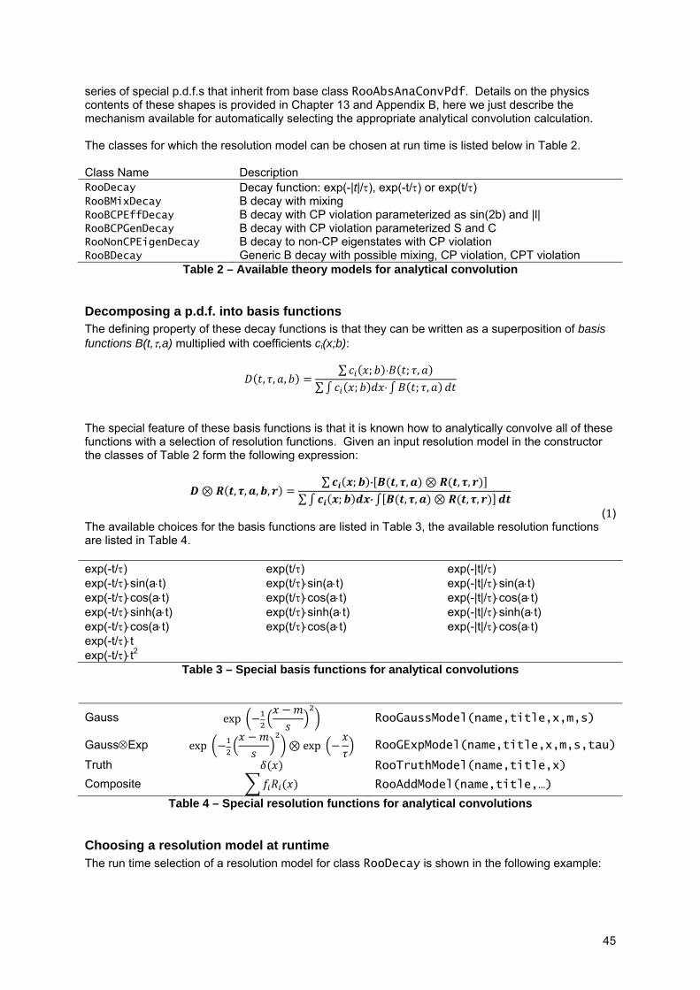
45

series of special p.d.f.s that inherit from base class RooAbsAnaConvPdf. Details on the physics contents of these shapes is provided in Chapter 13 and Appendix B, here we just describe the mechanism available for automatically selecting the appropriate analytical convolution calculation. The classes for which the resolution model can be chosen at run time is listed below in Table 2. Class Name Description RooDecay Decay function: exp(-|t|/τ), exp(-t/τ) or exp(t/τ) RooBMixDecay B decay with mixing RooBCPEffDecay B decay with CP violation parameterized as sin(2b) and |l| RooBCPGenDecay B decay with CP violation parameterized S and C RooNonCPEigenDecay B decay to non-CP eigenstates with CP violation RooBDecay Generic B decay with possible mixing, CP violation, CPT violation

Table 2 – Available theory models for analytical convolution

Decomposing a p.d.f. into basis functions The defining property of these decay functions is that they can be written as a superposition of basis functions B(t,τ,a) multiplied with coefficients ci(x;b):

, , ,∑ ; ⋅ ; ,

∑ ; ⋅ ; ,

The special feature of these basis functions is that it is known how to analytically convolve all of these functions with a selection of resolution functions. Given an input resolution model in the constructor the classes of Table 2 form the following expression:

, , , ,∑ ; ⋅ , , , ,

∑ ; ⋅ , , , ,

(1) The available choices for the basis functions are listed in Table 3, the available resolution functions are listed in Table 4. exp(-t/τ) exp(t/τ) exp(-|t|/τ) exp(-t/τ)⋅sin(a⋅t) exp(t/τ)⋅sin(a⋅t) exp(-|t|/τ)⋅sin(a⋅t) exp(-t/τ)⋅cos(a⋅t) exp(t/τ)⋅cos(a⋅t) exp(-|t|/τ)⋅cos(a⋅t) exp(-t/τ)⋅sinh(a⋅t) exp(t/τ)⋅sinh(a⋅t) exp(-|t|/τ)⋅sinh(a⋅t) exp(-t/τ)⋅cos(a⋅t) exp(t/τ)⋅cos(a⋅t) exp(-|t|/τ)⋅cos(a⋅t) exp(-t/τ)⋅t exp(-t/τ)⋅t2

Table 3 – Special basis functions for analytical convolutions

Gauss exp RooGaussModel(name,title,x,m,s)

Gauss⊗Exp exp exp RooGExpModel(name,title,x,m,s,tau)

Truth RooTruthModel(name,title,x)

Composite RooAddModel(name,title,…)

Table 4 – Special resolution functions for analytical convolutions

Choosing a resolution model at runtime The run time selection of a resolution model for class RooDecay is shown in the following example:

46

// Observable RooRealVar t(“t”,”t”,-10,10) ; // Gaussian Resolution model RooRealVar mean(“mean”,”mean”,0) ; RooRealVar sigma(“sigma”,”sigma”,1) ; RooGaussModel gaussm(“gaussm”,t,mean,sigma) ; // Decay p.d.f analytically convoluted with gaussm RooRealVar tau(“tau”,”lifetime”,1.54) ; RooDecay model(“model”,”decay (x) gauss”,t,tau,gaussm) ;

// --- Plot decay (x) gauss --- RooPlot* frame = x.frame() ; model.plotOn(frame) ; // --- Overlay with decay (x) truth --- RooTruthModel truthm("truthm","truth model",x) ; RooDecay modelt("modelt","decay (x) delta",x,tau,truthm) ; modelt.plotOn(frame,LineStyle(kDashed)) ; frame->Draw() ;

First we construct a decay function instance model convoluted with a Gaussian resolution model, then we create a decay function instance modelt, convoluted with a delta function. The resulting plot is shown in Figure 19.

Figure 19 – Decay p.d.f convolved with Gaussian and delta function (dashed)

Using composite resolution models A realistic detector resolution is often more complicated than a simple Gaussian. Class RooAddModel allows you to add multiple resolution models into a single composite resolution model that can be passed to any convolvable p.d.f. Here is an example using RooAddModel to construct a decay function convolved with a double Gaussian resolution.

RooRealVar x("x","x",-10,10) ;

47

RooRealVar mean("mean","mean",0) ; RooRealVar sigma_core("sigma_core","sigma core",1) ; RooGaussModel gaussm_core("gaussm_core","core gauss",x,mean,sigma_core) ; RooRealVar sigma_tail("sigma_tail","sigma tail",5) ; RooGaussModel gaussm_tail("gaussm_tail","tail gauss",x,mean,sigma_tail) ;

RooRealVar frac_core("frac_core","core fraction",0.9) ; RooAddModel gaussm("gaussm","core+tail gauss", RooArgList(gaussm_core,gaussm_tail),frac_core) ; RooRealVar tau("tau","lifetime",1.54) ; RooDecay model("model","decay (x) gauss",x,tau,gaussm);

Class RooAddModels functionality is very similar to that of class RooAddPdf, with the restriction that you can only specify fraction coefficients and no event yield coefficients as the extended likelihood formalism doesn’t apply to resolution models.

Writing your own analytically convoluted p.d.f. Instruction on how to write your own implementation of RooAbsAnaConvPdf or RooResolutionModel are found in Chapter 14.

Extracting a single convolution term Sometimes it is useful to be able to directly access the individual , , , , terms from Equation (1) to construct your own p.d.f or for debugging purposes. To do so you should first create the needed resolution model and the basis function expressed as a RooFormulaVar. The RooResolutionModel::convolution() method will then allow you to create a new object that represents the convolution of the basis function with the resolution function:

// Observables RooRealVar t(“t”,”t”,-10,10) ; RooRealVar tau(“tau”,”tau”,1.54) ; // Create Gaussian resolution model RooRealVar mean(“mean”,”mean”,0) ; RooRealVar sigma(“sigma”,”sigma”,1) ; RooGaussModel gaussm(“gaussm”,”gaussm”,t,mean,sigma) ; // Create basis function RooFormulaVar basis(“basis”,"exp(-@0/@1)",RooArgList(t,tau)) ; // Create basis (x) gauss RooAbsReal* decayConvGauss = gaussm.convolution(&basis) ; // Plot convolution RooPlot* frame = t.frame() ; decayConvGauss->plotOn(frame) ;

The output of the example is shown in Figure 20. Note that the calculation of the convolution does not use the interpreted formula expression of basis, the RooFormulaVar is mere used as an object to specify with basis function should be used (based on the expression string) and what the associated parameters are. It is therefore imperative that the exact string specifications are used that are implemented in the various resolution models. The exact expression associated with each basis function of Table 3 are listed in Chapter 14.

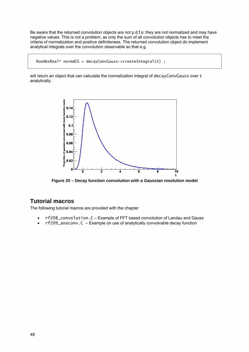
48

Be aware that the returned convolution objects are not p.d.f.s: they are not normalized and may have negative values. This is not a problem, as only the sum of all convolution objects has to meet the criteria of normalization and positive definiteness. The returned convolution object do implement analytical integrals over the convolution observable so that e.g.

RooAbsReal* normdCG = decayConvGauss->createIntegral(t) ; will return an object that can calculate the normalization integral of decayConvGauss over t analytically.

Figure 20 – Decay function convolution with a Gaussian resolution model

Tutorial macros The following tutorial macros are provided with the chapter

• rf208_convolution.C – Example of FFT based convolution of Landau and Gauss • rf209_anaconv.C – Example on use of analytically convolvable decay function

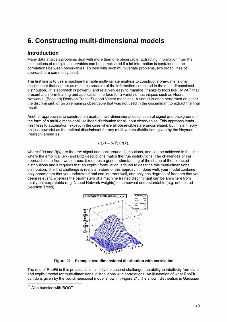
49

6. Constructing multi-dimensional models Introduction Many data analysis problems deal with more than one observable. Extracting information from the distributions of multiple observables can be complicated if a lot information is contained in the correlations between observables. To deal with such multi-variate problems, two broad lines of approach are commonly used. The first line is to use a machine trainable multi-variate analysis to construct a one-dimensional discriminant that capture as much as possible of the information contained in the multi-dimensional distribution. This approach is powerful and relatively easy to manage, thanks to tools like TMVA13 that present a uniform training and application interface for a variety of techniques such as Neural Networks, (Boosted) Decision Trees, Support Vector machines. A final fit is often performed on either the discriminant, or on a remaining observable that was not used in the discriminant to extract the final result. Another approach is to construct an explicit multi-dimensional description of signal and background in the form of a multi-dimensional likelihood distribution for all input observables. This approach lends itself less to automation, except in the case where all observables are uncorrelated, but it is in theory no less powerful as the optimal discriminant for any multi-variate distribution, given by the Neyman-Pearson lemma as

/ , where S(x) and B(x) are the true signal and background distributions, and can be achieved in the limit where the empirical S(x) and B(x) descriptions match the true distributions. The challenges of this approach stem from two sources: it requires a good understanding of the shape of the expected distributions and it requires that an explicit formulation is found to describe this multi-dimensional distribution. The first challenge is really a feature of this approach: if done well, your model contains only parameters that you understand and can interpret well, and only has degrees of freedom that you deem relevant, whereas the parameters of a machine trained discriminant can be anywhere from totally uninterpretable (e.g. Neural Network weights) to somewhat understandable (e.g. unboosted Decision Trees).

Figure 21 – Example two-dimensional distribution with correlation

The role of RooFit in this process is to simplify the second challenge, the ability to intuitively formulate and explicit model for multi-dimensional distributions with correlations. An illustration of what RooFit can do is given by the two-dimensional model shown in Figure 21. The shown distribution is Gaussian 13 Also bundled with ROOT

50

distribution in x for each value of y, where the mean of the Gaussian depends on y. In addition the distribution of y is a Gaussian as well. It can be challenging to formulate a two-dimensional p.d.f. H(x,y) that describe exactly this distribution and it correlation in plain C++. In RooFit you can write it exactly in the way the distribution was formulated here with four lines of code14: you first write a conditional p.d.f. F(x|y) that represents the distribution of x given a value of y, then you construct a p.d.f G(y) that describes the distribution in y and finally you combine these two pieces of information. RooFits ability to write multi-dimensional distributions with correlations is powered by its ability to be able to use any p.d.f. as a conditional p.d.f, which is made possible by its flexible p.d.f. normalization strategy. In the remainder of this section we will guide you to the basics of constructing multi-dimensional models in a variety of ways. Usage issues specific to multi-dimensional models are covered in Chapter 7.

Using multi-dimensional models Before we go into the details on how to best construct multidimensional models we start with a brief overview on how the RooFit plotting, fitting and event generation interface is extended to models with more than one observable. To illustrate all basic concepts we construct a two-dimensional RooGenericPdf in observables x and y. We choose this simplest possible formulation as the internal structure of multi-dimensional p.d.f.s is irrelevant in the plotting, fitting and generation interface: these work the same regardless of the structure of the model

RooRealVar x(“x”,”x”,-10,10) ; RooRealVar y(“y”,”y”,-10,10) ; RooRealVar a(“a”,”a”,5) ; RooRealVar b(“b”,”b”,2) ; RooGenericPdf f(“f”,”a*x*x+b*y*y-0.3*y*y*y”,RooArgSet(x,y,a,b)) ;

Example 9 – A simple two-dimensional p.d.f.

Evaluation In Chapter 2 it was explained that when you evaluate a RooFit p.d.f. you must always explicitly state which variables are the observables. In case there is more than observables, one can simply pass a RooArgSet with all observables instead of a single RooAbsArg:

f.getVal(RooArgSet(x,y)) ;

Generating and fitting Since both generation and fitting have a natural definition of observables, the extension of the interface to more than one observable is straightforward. In event generation you pass a RooArgSet with the observable instead of a single observable, and in fitting nothing changes in the interface as the definition of (in this case two) observables is taken automatically from the RooDataSet that is passed.

14 Excluding the lines needed to declare the model parameters. Actual code shown in Example 12.

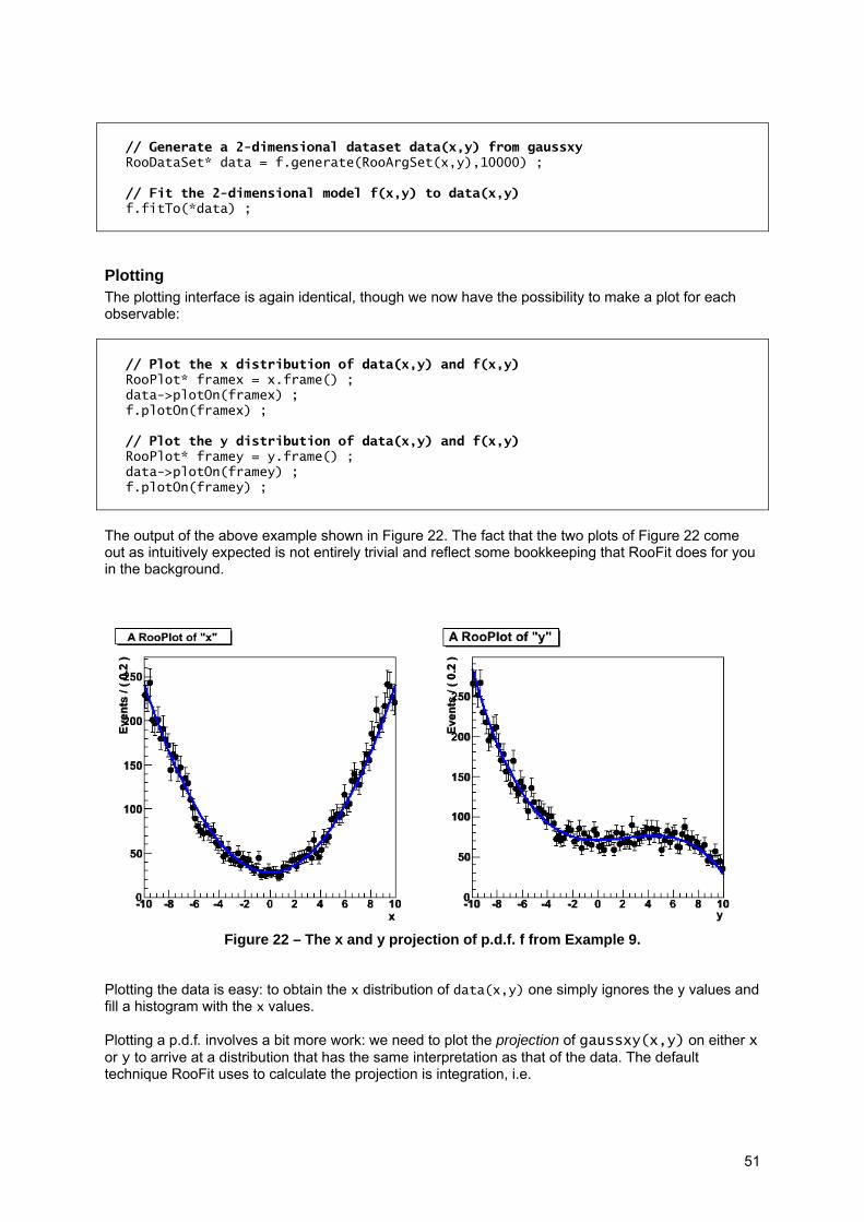
51

Plotting The plotting interface is again identical, though we now have the possibility to make a plot for each observable:

// Plot the x distribution of data(x,y) and f(x,y) RooPlot* framex = x.frame() ; data->plotOn(framex) ; f.plotOn(framex) ; // Plot the y distribution of data(x,y) and f(x,y) RooPlot* framey = y.frame() ; data->plotOn(framey) ; f.plotOn(framey) ;

The output of the above example shown in Figure 22. The fact that the two plots of Figure 22 come out as intuitively expected is not entirely trivial and reflect some bookkeeping that RooFit does for you in the background.

Figure 22 – The x and y projection of p.d.f. f from Example 9. Plotting the data is easy: to obtain the x distribution of data(x,y) one simply ignores the y values and fill a histogram with the x values. Plotting a p.d.f. involves a bit more work: we need to plot the projection of gaussxy(x,y) on either x or y to arrive at a distribution that has the same interpretation as that of the data. The default technique RooFit uses to calculate the projection is integration, i.e.

// Generate a 2-dimensional dataset data(x,y) from gaussxy RooDataSet* data = f.generate(RooArgSet(x,y),10000) ; // Fit the 2-dimensional model f(x,y) to data(x,y) f.fitTo(*data) ;

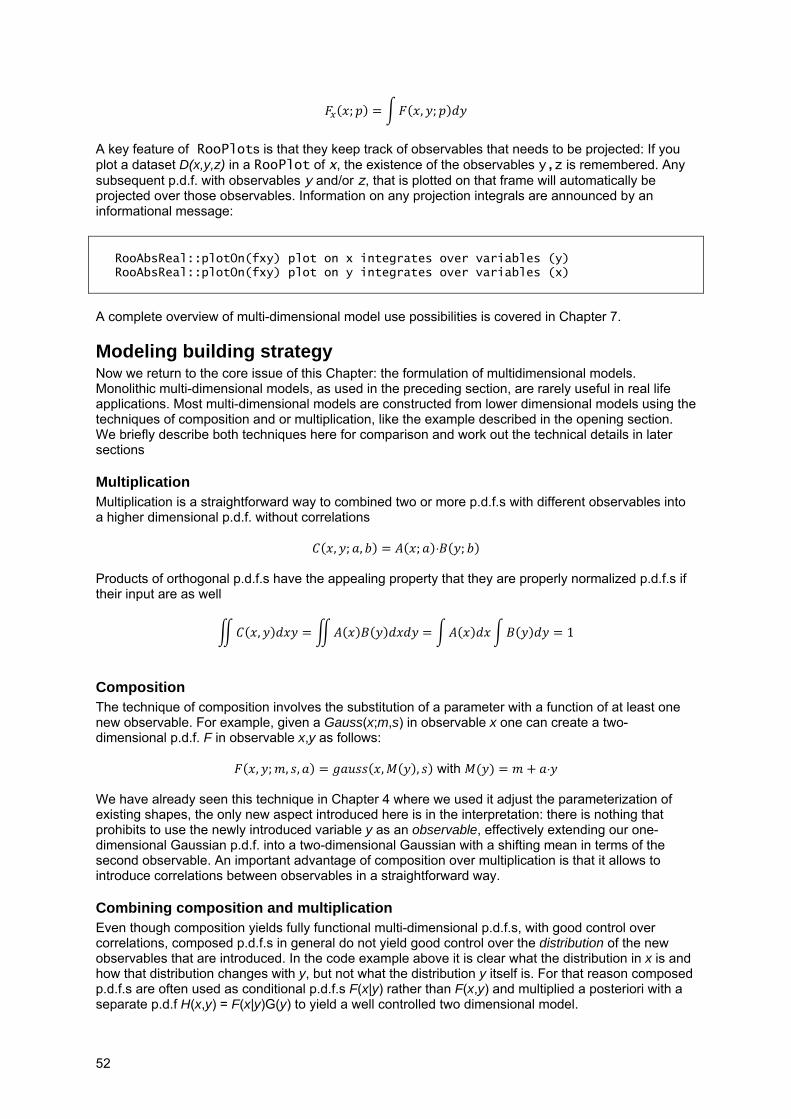
52

; , ;

A key feature of RooPlots is that they keep track of observables that needs to be projected: If you plot a dataset D(x,y,z) in a RooPlot of x, the existence of the observables y,z is remembered. Any subsequent p.d.f. with observables y and/or z, that is plotted on that frame will automatically be projected over those observables. Information on any projection integrals are announced by an informational message:

A complete overview of multi-dimensional model use possibilities is covered in Chapter 7.

Modeling building strategy Now we return to the core issue of this Chapter: the formulation of multidimensional models. Monolithic multi-dimensional models, as used in the preceding section, are rarely useful in real life applications. Most multi-dimensional models are constructed from lower dimensional models using the techniques of composition and or multiplication, like the example described in the opening section. We briefly describe both techniques here for comparison and work out the technical details in later sections

Multiplication Multiplication is a straightforward way to combined two or more p.d.f.s with different observables into a higher dimensional p.d.f. without correlations

, ; , ; ⋅ ; Products of orthogonal p.d.f.s have the appealing property that they are properly normalized p.d.f.s if their input are as well

, 1

Composition The technique of composition involves the substitution of a parameter with a function of at least one new observable. For example, given a Gauss(x;m,s) in observable x one can create a two-dimensional p.d.f. F in observable x,y as follows:

, ; , , , , with ⋅ We have already seen this technique in Chapter 4 where we used it adjust the parameterization of existing shapes, the only new aspect introduced here is in the interpretation: there is nothing that prohibits to use the newly introduced variable y as an observable, effectively extending our one-dimensional Gaussian p.d.f. into a two-dimensional Gaussian with a shifting mean in terms of the second observable. An important advantage of composition over multiplication is that it allows to introduce correlations between observables in a straightforward way.

Combining composition and multiplication Even though composition yields fully functional multi-dimensional p.d.f.s, with good control over correlations, composed p.d.f.s in general do not yield good control over the distribution of the new observables that are introduced. In the code example above it is clear what the distribution in x is and how that distribution changes with y, but not what the distribution y itself is. For that reason composed p.d.f.s are often used as conditional p.d.f.s F(x|y) rather than F(x,y) and multiplied a posteriori with a separate p.d.f H(x,y) = F(x|y)G(y) to yield a well controlled two dimensional model.

RooAbsReal::plotOn(fxy) plot on x integrates over variables (y) RooAbsReal::plotOn(fxy) plot on y integrates over variables (x)

53

Multiplication We first explain how construct multi-dimensional models through multiplication of p.d.f.s

Class RooProdPdf In RooFit the construction of any kind of product p.d.f. is done through class RooProdPdf. Here is a simple example:

RooRealVar x(“x”,”x”,-10,10) ; RooRealVar meanx(“meanx”,”meanx”,2,-10,10) ; RooRealVar sigmax(“sigmax”,”sigmax”,1,0.,10.) ; RooGaussian gaussx(“gaussx”,”gaussx”,x,meanx,sigmax) ; RooRealVar y(“y”,”y”,-10,10) ; RooRealVar meany(“meany”,”meany”,-2,-10,10) ; RooRealVar sigmay(“sigmay”,”sigmay”,5,0.,10.) ; RooGaussian gaussy(“gaussy”,”gaussy”,y,meany,sigmay) ; RooProdPdf gaussxy(“gaussxy”,”gaussxy”,RooArgSet(gaussx,gaussy)) ;

Example 10 – A 2-dimensional p.d.f. constructed as the product of two one-dimensional p.d.f.s The product p.d.f. gaussxy can be used for fitting and generating in exactly the same way as the monolithic p.d.f. f of Example 9.

RooDataSet* data = gaussxy.generate(RooArgSet(x,y),10000) ; gaussxy.fitTo(*data) ; RooPlot* framex = x.frame() ; data->plotOn(framex) ; gaussxy.plotOn(framex) ; RooPlot* framey = y.frame() ; data->plotOn(framey) ; gaussxy.plotOn(framey) ;

The operator class RooProdPdf can multiply any number of components, in this example we multiply two one-dimensional p.d.f.s, but you can equally well multiply e.g. 7 one-dimensional p.d.f.s or 2 five-dimensional p.d.f.s.

Figure 23 – Output from Example 10

54

Behind the scenes Even though the fitting, plotting and event generation interface looks the same, the implementation of these actions for products of uncorrelated p.d.f.s is considerably different. First, no explicit normalization is calculated for the product as the a product of orthogonal p.d.f.s is normalized by construction:

, 1

Projection integrals that occur in plotting can be simplified along similar lines

,

and these simplifications are applied through logical deduction on the structure of the input p.d.f of any RooProdPdf rather than through brute-force calculation. Event generation is also streamlined through exploitation of factorization properties. In the example of C(x,y) the distribution of x and y can be sampled independently from A(x) and B(y) and combined a posteriori, rather than through a sampling of the joint distribution. In addition to benefits gained from reducing the dimensionality of the problem, this approach allows to delegate the generation of observables to the component p.d.f.s which may implement an internal generator that is more efficient than the default accept/reject sampling technique. Figure 24 illustrates this distribution generation process.

Figure 24 – Illustration of distributed generation of uncorrelated products.

Composition No special operator class is required for the composition technique. The earlier example of a Gaussian distribution in observable x with a mean that depends on observable y,

, ; , , , , with ⋅

is coded this as follows:

// Create observables RooRealVar x("x","x",-5,5) ; RooRealVar y("y","y",-5,5) ;

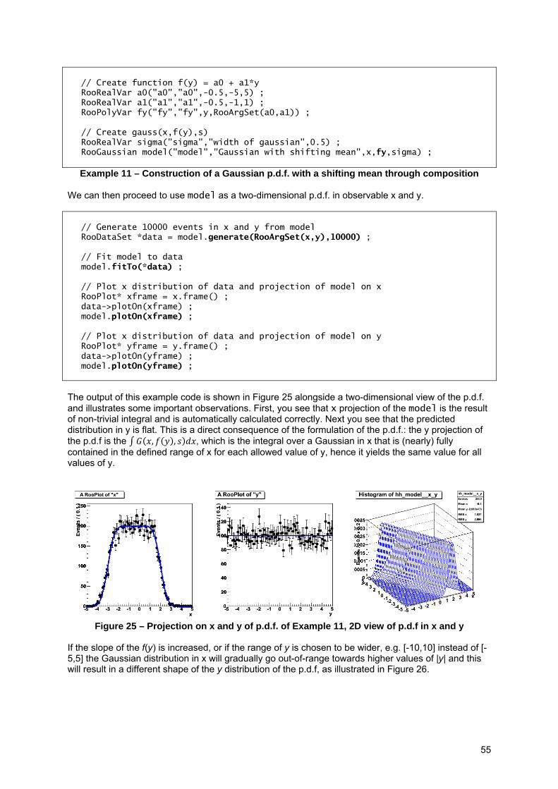
55

// Create function f(y) = a0 + a1*y RooRealVar a0("a0","a0",-0.5,-5,5) ; RooRealVar a1("a1","a1",-0.5,-1,1) ; RooPolyVar fy("fy","fy",y,RooArgSet(a0,a1)) ; // Create gauss(x,f(y),s) RooRealVar sigma("sigma","width of gaussian",0.5) ; RooGaussian model("model","Gaussian with shifting mean",x,fy,sigma) ;

Example 11 – Construction of a Gaussian p.d.f. with a shifting mean through composition

We can then proceed to use model as a two-dimensional p.d.f. in observable x and y.

// Generate 10000 events in x and y from model RooDataSet *data = model.generate(RooArgSet(x,y),10000) ; // Fit model to data model.fitTo(*data) ; // Plot x distribution of data and projection of model on x RooPlot* xframe = x.frame() ; data->plotOn(xframe) ; model.plotOn(xframe) ; // Plot x distribution of data and projection of model on y RooPlot* yframe = y.frame() ; data->plotOn(yframe) ; model.plotOn(yframe) ;

The output of this example code is shown in Figure 25 alongside a two-dimensional view of the p.d.f. and illustrates some important observations. First, you see that x projection of the model is the result of non-trivial integral and is automatically calculated correctly. Next you see that the predicted distribution in y is flat. This is a direct consequence of the formulation of the p.d.f.: the y projection of the p.d.f is the , , , which is the integral over a Gaussian in x that is (nearly) fully contained in the defined range of x for each allowed value of y, hence it yields the same value for all values of y.

Figure 25 – Projection on x and y of p.d.f. of Example 11, 2D view of p.d.f in x and y

If the slope of the f(y) is increased, or if the range of y is chosen to be wider, e.g. [-10,10] instead of [-5,5] the Gaussian distribution in x will gradually go out-of-range towards higher values of |y| and this will result in a different shape of the y distribution of the p.d.f, as illustrated in Figure 26.

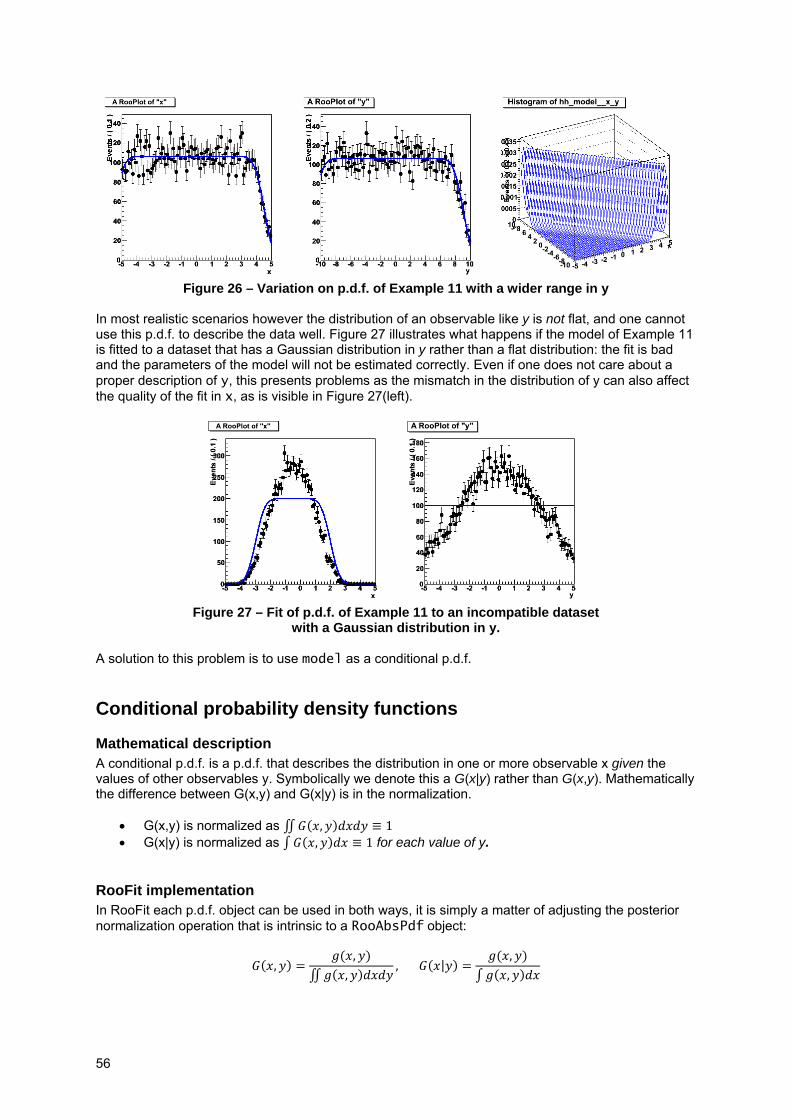
56

Figure 26 – Variation on p.d.f. of Example 11 with a wider range in y

In most realistic scenarios however the distribution of an observable like y is not flat, and one cannot use this p.d.f. to describe the data well. Figure 27 illustrates what happens if the model of Example 11 is fitted to a dataset that has a Gaussian distribution in y rather than a flat distribution: the fit is bad and the parameters of the model will not be estimated correctly. Even if one does not care about a proper description of y, this presents problems as the mismatch in the distribution of y can also affect the quality of the fit in x, as is visible in Figure 27(left).

Figure 27 – Fit of p.d.f. of Example 11 to an incompatible dataset

with a Gaussian distribution in y. A solution to this problem is to use model as a conditional p.d.f.

Conditional probability density functions

Mathematical description A conditional p.d.f. is a p.d.f. that describes the distribution in one or more observable x given the values of other observables y. Symbolically we denote this a G(x|y) rather than G(x,y). Mathematically the difference between G(x,y) and G(x|y) is in the normalization.

• G(x,y) is normalized as , 1 • G(x|y) is normalized as , 1 for each value of y.

RooFit implementation In RooFit each p.d.f. object can be used in both ways, it is simply a matter of adjusting the posterior normalization operation that is intrinsic to a RooAbsPdf object:

,,,

, |,,

57

where g(x) is the ‘raw’ unnormalized value returned by RooAbsPdf::evaluate(). Note that the normalization integral of G(x|y) can have a different value for each value of y, so the difference between G(x,y) and G(x|y) is not simply a constant overall normalization factor.

Fitting with conditional p.d.f.s To fit a p.d.f as a conditional p.d.f. rather than as a full p.d.f. use the ConditionalObservables() modifier to fitTo():

// Fit model as M(x|y) to D(x,y) model.fitTo(*data,ConditionalObservables(y)) ;

You may observe that using model as a conditional p.d.f.s is much slower than using it as a plain p.d.f. This happens because the normalization integral over x needs to be calculated separately for each event when used a conditional p.d.f., whereas the normalization integral of a plain p.d.f. is the same for all events in the likelihood and therefore only calculated when a parameter value changes. This effect is most notable if the normalization calculation requires a numeric integration step.

Plotting conditional p.d.f.s Plotting a conditional p.d.f. requires some extra work. Whereas a plain two-dimensional p.d.f. G(x,y) can be projected on x through integration

; , ; ,

this cannot be done G(x|y) because it contains – by construction – no information on the distribution of y. Thus we need an external source for the distribution of y to perform the projection. To that end we rewrite the projection integral as a Monte Carlo integral

; , ; 1

, ;

where the values yi are taken from a sampling of the p.d.f. G. Now, instead using those sampled values for yi, we substitute those from the dataset D(x,y) to which G was fitted to calculate the projection. The following code fragment shows how this is done

// Plot projection of D(x,y) and M(x|y) on x RooPlot* frame = x.frame() ; data->plotOn(frame) ; model.plotOn(frame,ProjWData(y,*data)) ;

The modified ProjWData() instructs plotOn() to use MC integration instead of plain integration for the projection of observable y and to use the value yi provided by dataset data to perform the projection. The modifier is only active when the resulting plot requires an actual integration over the indicated observable. If it is used, a messages will be printed with some details

[#1] INFO:Plotting -- RooAbsReal::plotOn(model) plot on x averages using data variables (y) [#1] INFO:Plotting -- RooDataWeightedAverage::ctor(modelDataWgtAvg) constructing data weighted average of function model_Norm[x] over 6850 data points of (y) with a total weight of 6850

58

The plot that results from the above example is shown in Figure 28. In general, projections calculated through Monte Carlo integration can be slow because each point of the curve is calculated as an average of potentially large number of samplings (>>1000). In Chapter 7 strategies are discussed to tune the performance/precision tradeoff of Monte Carlo projections.

Figure 28 – Projection of p.d.f of Example 11 used as conditional p.d.f. G(x|y) through Monte

Carlo projection technique using distribution of y values from data. Note that there is no corresponding projection on the y observable because the conditional p.d.f. G(x|y) predicts no distribution in y.

Generating events with conditional p.d.f.s The generation of events from a conditional p.d.f. G(x|y) requires – like plotting – an external input on the distribution of y. You can feed an input dataset with values of y in the generation step using the ProtoData() modifier of RooAbsPdf::generate():

RooDataSet *data = model.generate(x,ProtoData(externDataY)) ; where externDataY is a dataset with the values yi to be used for this generation. If a prototype dataset is specified, the number of events to generate defaults to the number of events in the prototype dataset, but it is still possible to specify a different number. If more events are requested than there are events, prototype events will be used multiple times. See Chapter 7 for additional details.

Warning on the use of composite models as conditional p.d.f.s From a technical point is it entirely unproblematic to use composite models (signal plus background) constructed with RooAddPdf as conditional p.d.f.s, you can substitute the example model of this section with a RooAddPdf composite model and everything will work the same. However be aware that when you do this you assume that all components (signal and background) have the same distribution in the conditional observable(s). This is not necessarily a trivial, or correct assumption15.

Products with conditional p.d.f.s A product of a conditional p.d.f. G(x|y) with a second p.d.f. F(y)

, | 15 See e.g. G. Punzi physics/0401045 on the potential pitfalls of such assumptions

59

offers a construction of all the benefits of a conditional p.d.f.s without its practical and interpretational drawbacks. In the form above, the conditional p.d.f G(x|y) provides the description of the distribution of x and how that description depends on y, and the plain p.d.f. F(y) provides the description of the overall distribution in y. The result is a full p.d.f. in both observables and it eliminates the need for extraneous datasets in plotting and event generation steps. A product of this form is automatically normalized if F and G are normalized:

| | 1⋅ 1

thus no additional normalization overhead is incurred.

Using conditional p.d.f.s with RooProdPdf The regular RooProdPdf operator class can be used to construct a product of p.d.f.s. that contain conditional terms: you need to indicate what input p.d.f.s are conditional through the Conditional() modifier. To complete the example of the opening section, we now write a Gaussian p.d.f in observable y and multiply that with the conditional p.d.f. G(x|y) from the preceding section.

// Create f(y) RooPolyVar fy("fy","fy",y,RooArgSet(a0,a1)) ; // Create gauss(x,f(y),s) RooGaussian model("model","Gaussian with shifting mean",x,fy,sigma) ; // Create gaussy(y,0,5) RooGaussian gy("gy","Model for y",y,RooConst(0),RooConst(3)) ; // Create gaussx(x,sx|y) * gaussy(y) RooProdPdf condprod("condprod","model(x|y)*gy(y)",gy,Conditional(model,x)) ;

Example 12 – Constructing a product of a conditional p.d.f. with a plain p.d.f to describe a two-dimensional distribution with correlations

The Conditional() argument instructs RooProdPdf to interpret model as a conditional p.d.f. G(x| ) where denotes all observables other than x16. We have repeated the definition of model here to visualize the claim in the opening section that the model shown in Figure 21 can be written in 4 lines of code excluding parameter declarations.

Plotting, fitting and generating with conditional product models Since a product of a conditional p.d.f. G(x|y) with a plain p.d.f. F(y) is a plain p.d.f itself, all operations related to plotting, fitting and event generation work as usual.

// Generate 1000 events in x and y from model RooDataSet *data = condprod.generate(RooArgSet(x,y),10000) ;

16 Since RooFit p.d.f. have no static notion of observables vs parameters, the value of depends on the use context of this object. If the observables are (x,y), G(x| ) evaluates to G(x|y). If the observables are (x), it evaluates to G(x). If x is not among the observables the G term is dropped entirely from the product, as happens to all RooProdPdf terms that don’t depend on any observable. Additional details on this issue are discussed in Chapter 7.

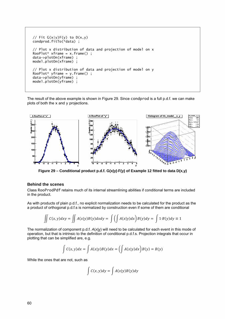
60

// Fit G(x|y)F(y) to D(x,y) condprod.fitTo(*data) ; // Plot x distribution of data and projection of model on x RooPlot* xframe = x.frame() ; data->plotOn(xframe) ; model.plotOn(xframe) ; // Plot x distribution of data and projection of model on y RooPlot* yframe = y.frame() ; data->plotOn(yframe) ; model.plotOn(yframe) ;

The result of the above example is shown in Figure 29. Since condprod is a full p.d.f. we can make plots of both the x and y projections.

Figure 29 – Conditional product p.d.f. G(x|y)⋅F(y) of Example 12 fitted to data D(x,y)

Behind the scenes Class RooProdPdf retains much of its internal streamlining abilities if conditional terms are included in the product. As with products of plain p.d.f., no explicit normalization needs to be calculated for the product as the a product of orthogonal p.d.f.s is normalized by construction even if some of them are conditional

, | | 1⋅ 1

The normalization of component p.d.f. A(x|y) will need to be calculated for each event in this mode of operation, but that is intrinsic to the definition of conditional p.d.f.s. Projection integrals that occur in plotting that can be simplified are, e.g.

, | |

While the ones that are not, such as

, |

61

are calculated through numeric integration. Note that compared to the Monte Carlo integration technique, used for the projection of conditional p.d.f. that are used standalone, this is usually faster can be calculated with an accurate numeric target precision17. Also event generation is still handled in a distribution mode. For products involving conditional terms, the order in which observables are generated is relevant and is determined automatically. For the example for the p.d.f. F(x|y)G(y), first the observable y is generated using the generator context of G(y). Then the observable x is generated from F(x|y). If F implements an internal generator, event generation for F(x|y)G(y) occurs at the same efficiency as for F(x)G(y). If accept/reject sampling is required for F, some performance loss occurs because the maximum value of F must now be found in the two-dimensional space (x,y) instead of in the one-dimensional space (x), which requires more trial samplings.

Extending products to more than two dimensions For illustrational clarity all examples in this section have been chosen to have two observables. All of the described functionality is available for an arbitrary number of dimensions. In any place where a RooArgSet of two observables is passed, a RooArgSet of N observables can be substituted

RooDataSet *data = condprod.generate(RooArgSet(x,y,z,t),10000) ; In any place where a single conditional observable was passed, a RooArgSet of conditional observables can be passed:

model.fitTo(*data,ConditionalObservables(RooArgSet(y,z))) ; model.plotOn(frame,ProjWData(RooArgSet(y,z),*data)) ;

A RooProdPdf can take arbitrary number of regular input p.d.f.s and up to eight18 conditional p.d.f.s specifications.

RooProdPdf condprod("condprod","A(x|y)*B(y|z)*C(z)*D(t,u)*E(k)", RooArgSet(C,D,E), Conditional(A,x),Conditional(B,y)) ;

It is explicitly allowed to ‘chain’ conditional p.d.f.s, i.e. A(x|y)⋅B(y|z)⋅C(z). You can also introduce cross-correlation terms of the type A(x|y)⋅B(y|x) but terms of this type are not automatically normalized if A and B are, and you incur the computational overhead of an explicit 2-dimensional numeric integration step. This feature should thus be used with some caution.

Modeling data with per-event error observables. We conclude this Chapter with a section that illustrates how the concept of conditional p.d.f.s can be used to describe a common type of multi-dimensional problem: The modeling of the distribution of an observable t that has associated uncertainty on that measurement for each event quantified in a second observable dt.

17 The adaptive Gauss-Kronrod numeric integration algorithm typically needs O(50) function evaluations to calculate the integral of a smooth function with a target precision of 10-7. 18 This limit is imposed by the constructor interface, is not fundamental, and can be extended on request.

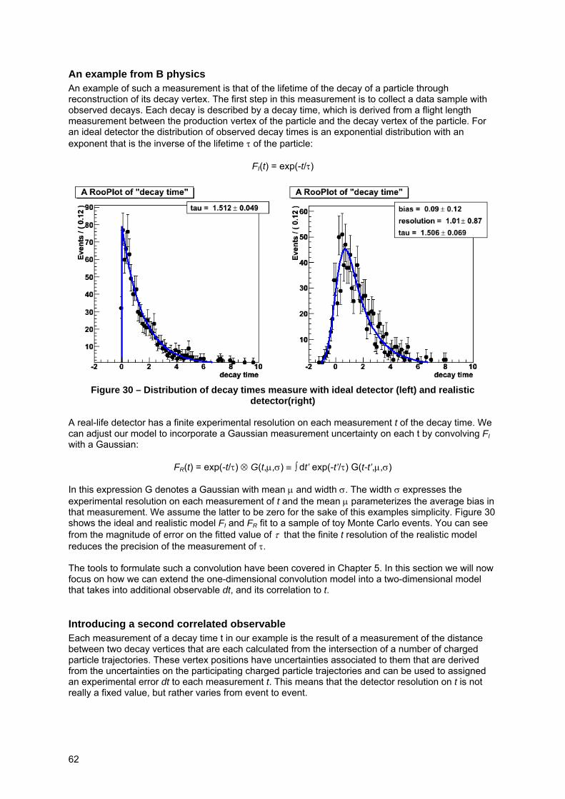
62

An example from B physics An example of such a measurement is that of the lifetime of the decay of a particle through reconstruction of its decay vertex. The first step in this measurement is to collect a data sample with observed decays. Each decay is described by a decay time, which is derived from a flight length measurement between the production vertex of the particle and the decay vertex of the particle. For an ideal detector the distribution of observed decay times is an exponential distribution with an exponent that is the inverse of the lifetime τ of the particle:

FI(t) = exp(-t/τ)

Figure 30 – Distribution of decay times measure with ideal detector (left) and realistic detector(right)

A real-life detector has a finite experimental resolution on each measurement t of the decay time. We can adjust our model to incorporate a Gaussian measurement uncertainty on each t by convolving FI with a Gaussian:

FR(t) = exp(-t/τ) ⊗ G(t,μ,σ) ≡ ∫ dt’ exp(-t’/τ) G(t-t’,μ,σ) In this expression G denotes a Gaussian with mean μ and width σ. The width σ expresses the experimental resolution on each measurement of t and the mean μ parameterizes the average bias in that measurement. We assume the latter to be zero for the sake of this examples simplicity. Figure 30 shows the ideal and realistic model FI and FR fit to a sample of toy Monte Carlo events. You can see from the magnitude of error on the fitted value of τ that the finite t resolution of the realistic model reduces the precision of the measurement of τ. The tools to formulate such a convolution have been covered in Chapter 5. In this section we will now focus on how we can extend the one-dimensional convolution model into a two-dimensional model that takes into additional observable dt, and its correlation to t.

Introducing a second correlated observable Each measurement of a decay time t in our example is the result of a measurement of the distance between two decay vertices that are each calculated from the intersection of a number of charged particle trajectories. These vertex positions have uncertainties associated to them that are derived from the uncertainties on the participating charged particle trajectories and can be used to assigned an experimental error dt to each measurement t. This means that the detector resolution on t is not really a fixed value, but rather varies from event to event.

63

This example of a decay time measurement represent a substantial class of measurements where an observable x is accompanied by an error estimate dx that can be treated as a second correlated observable in the model that describes the experimental results. Following the composition strategy, we first modify the model such that each event is characterized by a pair of values (t,dt) rather than a single number t and thereby we acknowledge that certain events – those with small dt – carry more information then others, and use this information to achieve a better measurement of τ with the same data. Here is the enhanced p.d.f:

FE(t,dt) = exp(-t/τ) ⊗ G(t,μ,dt) It is easy to see that this small modification – replacing the resolution estimate σ by the per-event error dt – realizes the intended effect. Given two events A and B with identical observed decay times tA=tB=t and uncertainties that differ by a factor of two dtA= dtB/2, the contribution of event A to the total likelihood will differ from the contribution of event B because exponential shape of the model for event A is convolved with a Gaussian that is twice as small as that for event B. A refit of the data sample of Figure 30 to such an enhanced model reflects the enhanced statistical power of this model, by reducing the measurement error of τ from 0.067 to 0.060, a 10% improvement of the measurement performed on the same data that is equivalent to having 20% more data available19.

Accounting for improper external error estimates An important caveat in the enhanced model FE is that it assumes that the provided error estimates dt are correct. If these estimates are too small on average, the error on the physics parameter τ will be too small as well. As this is usually undesirable, you should verify the correctness of the errors dt by looking at pull distributions, i.e. comparing the spread of the measured values (the external error) to the distribution of the given errors (the internal error). We can incorporate this check in the model FE through the following modification:

FE(t,dt) = exp(-t/τ) ⊗ G(t,μ,σ⋅dt) Now the model doesn’t make any absolute interpretation of the errors dt, it just assumes that the true uncertainty of each t measurement scales linearly with the provided error. The parameter σ serves as a global scale factor applied to the per-event errors dt. If you fit this model to the data and the uncertainty estimates dt turn out the be correct on average you will find that σ=1. If the error estimates are too high or too low on average, this is apparent from a mismatch in the distribution of values and errors in the data and the fit will steer σ to a value smaller or greater than 1. Effectively one could interpret G as a fit to the pull distribution associated with the vertexing procedure. Thanks to this built-in correction of the per-event errors the improved model FE has gained an important quality: the error on the physics parameter τ is to first order independent of the correctness of the error estimates dt. A second order dependency comes in when the pull distribution of the dt errors cannot be accurately described by a Gaussian. Also this can be mitigated, for example by replacing G by a sum of two or more Gaussians of different width and mean.

Coding the example model Here is an example that codes the life time measurement with per-event errors:

// Observables RooRealVar t("t","t",-2,10) ; RooRealVar dt("dt","per-event error on t",0.01,5) ;

19 The actual gain depends on the spread of the per-event errors. The shown example has a performance that is typical for BaBar experimental data.

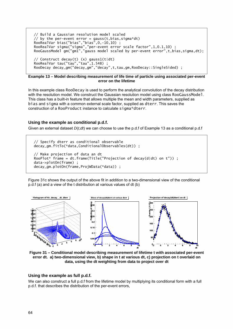
64

// Build a Gaussian resolution model scaled // by the per-event error = gauss(t,bias,sigma*dt) RooRealVar bias("bias","bias",0,-10,10) ; RooRealVar sigma("sigma","per-event error scale factor",1,0.1,10) ; RooGaussModel gm("gm1","gauss model scaled by per-event error",t,bias,sigma,dt); // Construct decay(t) (x) gauss1(t|dt) RooRealVar tau("tau","tau",1.548) ; RooDecay decay_gm("decay_gm","decay",t,tau,gm,RooDecay::SingleSided) ;

Example 13 – Model describing measurement of life time of particle using associated per-event

error on the lifetime In this example class RooDecay is used to perform the analytical convolution of the decay distribution with the resolution model. We construct the Gaussian resolution model using class RooGaussModel. This class has a built-in feature that allows multiple the mean and width parameters, supplied as bias and sigma with a common external scale factor, supplied as dterr. This saves the construction of a RooProduct instance to calculate sigma*dterr.

Using the example as conditional p.d.f. Given an external dataset D(t,dt) we can choose to use the p.d.f of Example 13 as a conditional p.d.f

// Specify dterr as conditional observable decay_gm.fitTo(*data,ConditionalObservables(dt)) ; // Make projection of data an dt RooPlot* frame = dt.frame(Title("Projection of decay(d|dt) on t")) ; data->plotOn(frame) ; decay_gm.plotOn(frame,ProjWData(*data)) ;

Figure 31c shows the output of the above fit in addition to a two-dimensional view of the conditional p.d.f (a) and a view of the t distribution at various values of dt (b)

Figure 31 – Conditional model describing measurement of lifetime t with associated per-event

error dt. a) two-dimensional view, b) shape in t at various dt, c) projection on t overlaid on data, using the dt weighting from data to project over dt

Using the example as full p.d.f. We can also construct a full p.d.f from the lifetime model by multiplying its conditional form with a full p.d.f. that describes the distribution of the per-event errors,

65

// Make empirical p.d.f describing dt shape in data RooDataHist* expHistDterr = expDataDterr->binnedClone() ; RooHistPdf pdfErr("pdfErr","pdfErr",dterr,*expHistDterr) ; // Construct production of decay_dm(dt|dterr) with empirical pdfErr(dterr) RooProdPdf model("model","model",pdfErr,Conditional(decay_gm,dt)) ;

Example 14 – Full two-dimensional model describing measurement of lifetime and its associated error on the lifetime

which can be used as a regular p.d.f.

model.fitTo(*data) ; RooPlot* frame = dt.frame() ; data->plotOn(frame) ; model.plotOn(frame) ;

Figure 32b shows the projection on the t observable of the fitted p.d.f in addition to the two-dimensional view (a),

Figure 32 – Full model describing measurement of lifetime t with associated per-event error dt.

a) two-dimensional view, b) projection on t (through integration) overlaid on data


• rf301_composition.C – Multi-dimensional p.d.f.s through composition • rf302_utilfuncs.C – Utility functions classes available for use in composition • rf303_conditional.C – Use of composed models as conditional p.d.f.s • rf304_uncorrprod.C – Simple uncorrelated multi-dimensional p.d.f.s • rf305_condcorrprod.C – Multi-dimensional p.d.f.s with conditional p.d.f.s in product • rf306_condpereventerrors.C – Complete example of cond/ p.d.f. with per-event errors • rf307_fullpereventerrors.C – Complete example of full p.d.f. with per-event errors • rf308_normintegration2d.C – Examples on normalization of p.d.f.s in >1 dimension

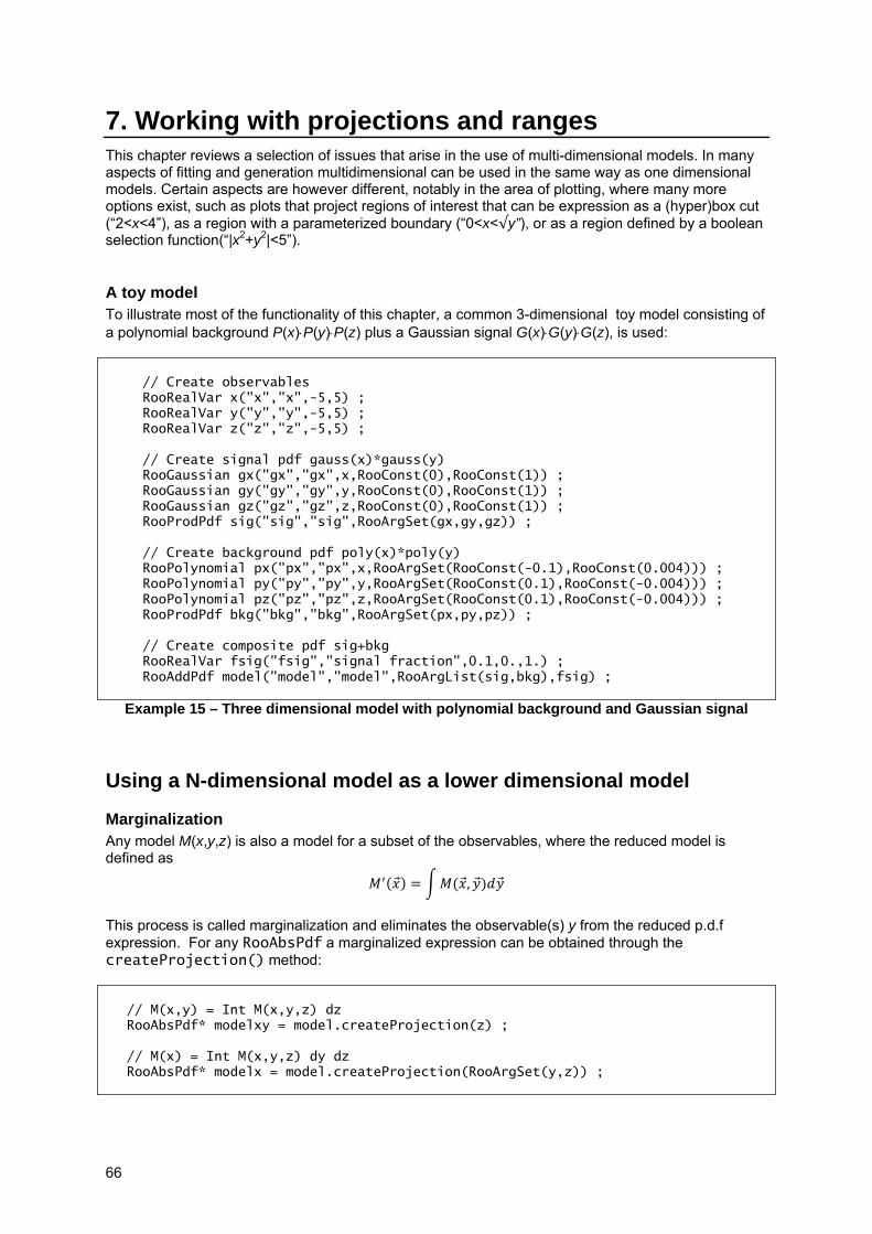
66

7. Working with projections and ranges This chapter reviews a selection of issues that arise in the use of multi-dimensional models. In many aspects of fitting and generation multidimensional can be used in the same way as one dimensional models. Certain aspects are however different, notably in the area of plotting, where many more options exist, such as plots that project regions of interest that can be expression as a (hyper)box cut (“2<x<4”), as a region with a parameterized boundary (“0<x<√y”), or as a region defined by a boolean selection function(“|x2+y2|<5”).

A toy model To illustrate most of the functionality of this chapter, a common 3-dimensional toy model consisting of a polynomial background P(x)⋅P(y)⋅P(z) plus a Gaussian signal G(x)⋅G(y)⋅G(z), is used:

// Create observables RooRealVar x("x","x",-5,5) ; RooRealVar y("y","y",-5,5) ; RooRealVar z("z","z",-5,5) ; // Create signal pdf gauss(x)*gauss(y) RooGaussian gx("gx","gx",x,RooConst(0),RooConst(1)) ; RooGaussian gy("gy","gy",y,RooConst(0),RooConst(1)) ; RooGaussian gz("gz","gz",z,RooConst(0),RooConst(1)) ; RooProdPdf sig("sig","sig",RooArgSet(gx,gy,gz)) ; // Create background pdf poly(x)*poly(y) RooPolynomial px("px","px",x,RooArgSet(RooConst(-0.1),RooConst(0.004))) ; RooPolynomial py("py","py",y,RooArgSet(RooConst(0.1),RooConst(-0.004))) ; RooPolynomial pz("pz","pz",z,RooArgSet(RooConst(0.1),RooConst(-0.004))) ; RooProdPdf bkg("bkg","bkg",RooArgSet(px,py,pz)) ; // Create composite pdf sig+bkg RooRealVar fsig("fsig","signal fraction",0.1,0.,1.) ; RooAddPdf model("model","model",RooArgList(sig,bkg),fsig) ;

Example 15 – Three dimensional model with polynomial background and Gaussian signal

Using a N-dimensional model as a lower dimensional model

Marginalization Any model M(x,y,z) is also a model for a subset of the observables, where the reduced model is defined as

,

This process is called marginalization and eliminates the observable(s) y from the reduced p.d.f expression. For any RooAbsPdf a marginalized expression can be obtained through the createProjection() method:

// M(x,y) = Int M(x,y,z) dz RooAbsPdf* modelxy = model.createProjection(z) ; // M(x) = Int M(x,y,z) dy dz RooAbsPdf* modelx = model.createProjection(RooArgSet(y,z)) ;

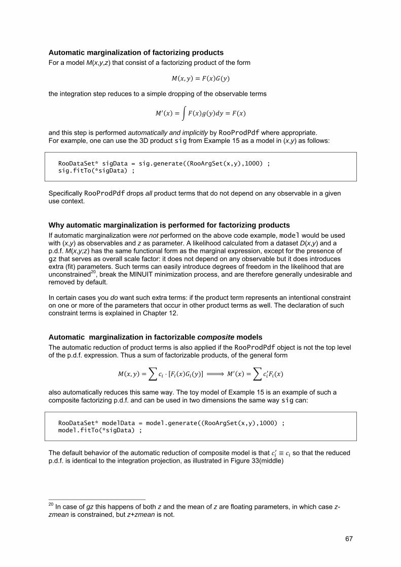
67

Automatic marginalization of factorizing products For a model M(x,y,z) that consist of a factorizing product of the form

, the integration step reduces to a simple dropping of the observable terms

and this step is performed automatically and implicitly by RooProdPdf where appropriate. For example, one can use the 3D product sig from Example 15 as a model in (x,y) as follows:

RooDataSet* sigData = sig.generate((RooArgSet(x,y),1000) ; sig.fitTo(*sigData) ;

Specifically RooProdPdf drops all product terms that do not depend on any observable in a given use context.

Why automatic marginalization is performed for factorizing products If automatic marginalization were not performed on the above code example, model would be used with (x,y) as observables and z as parameter. A likelihood calculated from a dataset D(x,y) and a p.d.f. M(x,y;z) has the same functional form as the marginal expression, except for the presence of gz that serves as overall scale factor: it does not depend on any observable but it does introduces extra (fit) parameters. Such terms can easily introduce degrees of freedom in the likelihood that are unconstrained20, break the MINUIT minimization process, and are therefore generally undesirable and removed by default. In certain cases you do want such extra terms: if the product term represents an intentional constraint on one or more of the parameters that occur in other product terms as well. The declaration of such constraint terms is explained in Chapter 12.

Automatic marginalization in factorizable composite models The automatic reduction of product terms is also applied if the RooProdPdf object is not the top level of the p.d.f. expression. Thus a sum of factorizable products, of the general form

, ⋅

also automatically reduces this same way. The toy model of Example 15 is an example of such a composite factorizing p.d.f. and can be used in two dimensions the same way sig can:

RooDataSet* modelData = model.generate((RooArgSet(x,y),1000) ; model.fitTo(*sigData) ;

The default behavior of the automatic reduction of composite model is that so that the reduced p.d.f. is identical to the integration projection, as illustrated in Figure 33(middle)

20 In case of gz this happens of both z and the mean of z are floating parameters, in which case z-zmean is constrained, but z+zmean is not.

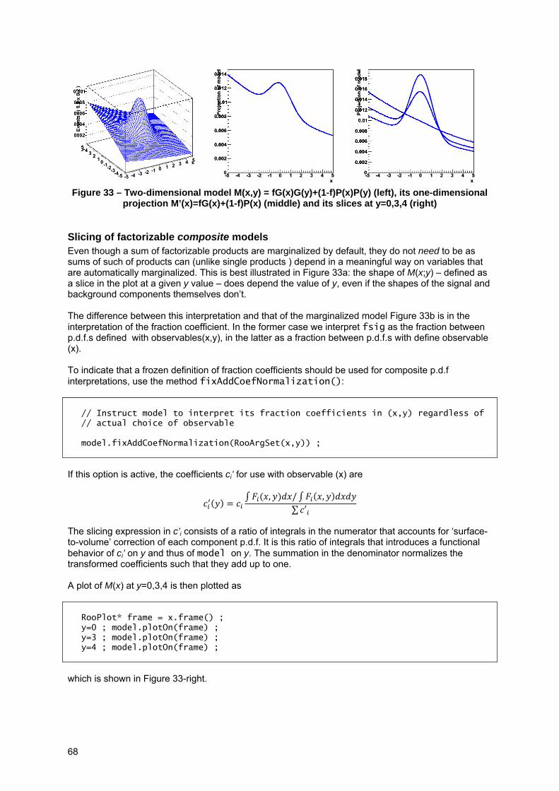
68

Figure 33 – Two-dimensional model M(x,y) = fG(x)G(y)+(1-f)P(x)P(y) (left), its one-dimensional

projection M’(x)=fG(x)+(1-f)P(x) (middle) and its slices at y=0,3,4 (right)

Slicing of factorizable composite models Even though a sum of factorizable products are marginalized by default, they do not need to be as sums of such of products can (unlike single products ) depend in a meaningful way on variables that are automatically marginalized. This is best illustrated in Figure 33a: the shape of M(x;y) – defined as a slice in the plot at a given y value – does depend the value of y, even if the shapes of the signal and background components themselves don’t. The difference between this interpretation and that of the marginalized model Figure 33b is in the interpretation of the fraction coefficient. In the former case we interpret fsig as the fraction between p.d.f.s defined with observables(x,y), in the latter as a fraction between p.d.f.s with define observable (x). To indicate that a frozen definition of fraction coefficients should be used for composite p.d.f interpretations, use the method fixAddCoefNormalization():

// Instruct model to interpret its fraction coefficients in (x,y) regardless of // actual choice of observable model.fixAddCoefNormalization(RooArgSet(x,y)) ;

If this option is active, the coefficients ci’ for use with observable (x) are

, / ,∑

The slicing expression in c’i consists of a ratio of integrals in the numerator that accounts for ‘surface-to-volume’ correction of each component p.d.f. It is this ratio of integrals that introduces a functional behavior of ci’ on y and thus of model on y. The summation in the denominator normalizes the transformed coefficients such that they add up to one. A plot of M(x) at y=0,3,4 is then plotted as

RooPlot* frame = x.frame() ; y=0 ; model.plotOn(frame) ; y=3 ; model.plotOn(frame) ; y=4 ; model.plotOn(frame) ;

which is shown in Figure 33-right.

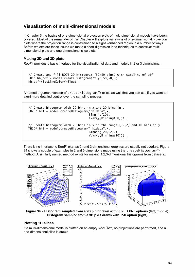
69

Visualization of multi-dimensional models In Chapter 6 the basics of one-dimensional projection plots of multi-dimensional models have been covered. Most of the remainder of this Chapter will explore variations of one-dimensional projection plots where the projection range is constrained to a signal-enhanced region in a number of ways. Before we explore those issues we make a short digression in to techniques to construct multi-dimensional plots and one-dimensional slice plots

Making 2D and 3D plots RooFit provides a basic interface for the visualization of data and models in 2 or 3 dimensions.

// Create and fill ROOT 2D histogram (50x50 bins) with sampling of pdf TH1* hh_pdf = model.createHistogram("x,y",50,50) ; hh_pdf->SetLineColor(kBlue) ;

A named argument version of createHistogram() exists as well that you can use if you want to exert more detailed control over the sampling process:

// Create histogram with 20 bins in x and 20 bins in y TH2D* hh1 = model.createHistogram("hh_data",x, Binning(20), YVar(y,Binning(20))) ; // Create histogram with 20 bins in x in the range [-2,2] and 10 bins in y TH2D* hh2 = model.createHistogram("hh_data",x, Binning(20,-2,2), YVar(y,Binning(10))) ;

There is no interface to RooPlots, as 2- and 3-dimensional graphics are usually not overlaid. Figure 34 shows a couple of examples in 2 and 3 dimensions made using the createHistogram() method. A similarly named method exists for making 1,2,3-dimensional histograms from datasets..

Figure 34 – Histogram sampled from a 2D p.d.f drawn with SURF, CONT options (left, middle).

Histogram sampled from a 3D p.d.f drawn with ISO option (right).

Plotting 1D slices If a multi-dimensional model is plotted on an empty RooPlot, no projections are performed, and a one-dimensional slice is drawn

70

// Plot model(x) at y=0,z=0 z=0 ; y=0 ; RooPlot* frame = x.frame() model.plotOn(frame) ; // Overlay model(x) at y=5,z=0 y=5 ; model.plotOn(frame,LineStyle(kDashed)) ;

If models involve RooAddPdf composite terms, it may be necessary to fix the interpretation of their coefficients to a fixed set using fixAddCoefNormalization() before making these slice plots as explained in the preceding section. For models with two or more observables, one can also choose to plot a projection over one or more observables, rather than a slice in all but one observable

// Overlay Int model(x) dy at z=0 z=0 ; model.plotOn(frame,Project(y)) ; // Overlay Int model(x) dz at y=3 y=3 ; model.plotOn(frame,Project(z)) ;

Definitions and basic use of rectangular ranges In Chapter 2 the Range(double,double) modifier was introduced to restrict the action of fitting and plotting to the specified range. Using p.d.f.s defined in Example 15, we can construct a simple one-dimensional p.d.f, and fit and plot it the range [-2,2] as follows

// Construct one-dimensionalGaussian+Polynomial model RooRealVar f("f","signal fraction",0.1,0.,1.) ; RooAddPdf pdf("pdf","pdf",RooArgList(gx,px),f) ; pdf.fitTo(data,Range(-2,2)) ; pdf.plotOn(frame,Range(-2,2)) ;

Named ranges An alternate way work with ranges is to create a named range associated with the observable that can subsequently be referenced by name through the Range(const char*) modifier

x.setRange(“signal”,-2,2) ;

pdf.fitTo(data,Range(“signal”)) ; pdf.plotOn(frame,Range(“signal”)) ;

Named range simplify the management of ranges in user analysis code as the definition of a range can be made in one place and be referenced everywhere. Most of the range functionality of RooFit works exclusively with named ranges and it is recommended to use named ranges for all but the most trivial use cases.

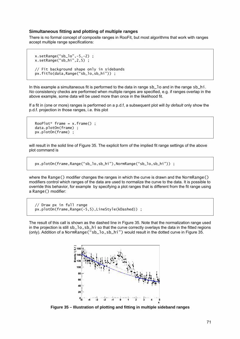
71

Simultaneous fitting and plotting of multiple ranges There is no formal concept of composite ranges in RooFit, but most algorithms that work with ranges accept multiple range specifications:

x.setRange(“sb_lo”,-5,-2) ; x.setRange(“sb_hi”,2,5) ;

// Fit background shape only in sidebands px.fitTo(data,Range(“sb_lo,sb_hi”)) ;

In this example a simultaneous fit is performed to the data in range sb_lo and in the range sb_hi. No consistency checks are performed when multiple ranges are specified, e.g. if ranges overlap in the above example, some data will be used more than once in the likelihood fit.

If a fit in (one or more) ranges is performed on a p.d.f, a subsequent plot will by default only show the p.d.f. projection in those ranges, i.e. this plot

RooPlot* frame = x.frame() ; data.plotOn(frame) ; px.plotOn(frame) ;

will result in the solid line of Figure 35. The explicit form of the implied fit range settings of the above plot command is

px.plotOn(frame,Range(“sb_lo,sb_hi”),NormRange(“sb_lo,sb_hi”)) ;

where the Range() modifier changes the ranges in which the curve is drawn and the NormRange() modifiers control which ranges of the data are used to normalize the curve to the data. It is possible to override this behavior, for example by specifying a plot ranges that is different from the fit range using a Range() modifier:

// Draw px in full range px.plotOn(frame,Range(-5,5),LineStyle(kDashed)) ;

The result of this call is shown as the dashed line in Figure 35. Note that the normalization range used in the projection is still sb_lo,sb_hi so that the curve correctly overlays the data in the fitted regions (only). Addition of a NormRange(“sb_lo,sb_hi”) would result in the dotted curve in Figure 35.

Figure 35 – Illustration of plotting and fitting in multiple sideband ranges

72

A

B

Semantics of range definitions in multiple observables If a range with a given name occurs in more than one observable, the range is defined as the logical and of the two regions, i.e.

RooRealVar y(“y”,”y”,-10,10) ; x.setRange(“signal”,-2,2) ; y.setRange(“signal”,-2,2) ;

defines the region in (x,y) space defined by (-2<x<2 && -2<y<2). If a named range has not been explicitly defined on an observable and it is referenced, it is automatically defined on the fly as a range equal to the full range

RooRealVar z(“z”,”z”,-10,10) ; z.getMin(“signal”) ; // returns -10

Technically, a range is special type of binning (class RooRangeBinning) with a single bin. A range can therefore also be retrieved though the binning definitions interface of RooRealVar:

RooAbsBinning& signalBinning = x.getBinning(“signal”) ;

A binning does not need to be of type RooRangeBinning to be functional as range, any type of binning object can serve as range

RooUniformBinning unibin(-2,2,100) ; z.setBinning(unibin,”signal”) ;

Using multiple ranges with more than observable All interfaces that accept the specification of multiple ranges also work with multi-dimensional ranges. In such cases the logical ‘and’ between the definitions of the same range in different observables takes precedence over the logical ‘or’ between ranges with different names, as illustrated below.

// Define range A x.setRange(“A”,0,2) ; y.setRange(“A”,0,2) ; // Define range B x.setRange(“B”,-2,0) ; y.setRange(“B”,-2,0) ; // Fit to (A||B) model.fitTo(data,Range(“A,B”)) ;

Example 16 – Constructing and using multiple ranges in more than one dimensions

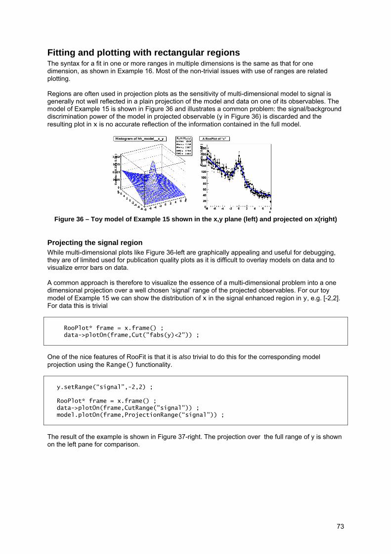
73

Fitting and plotting with rectangular regions The syntax for a fit in one or more ranges in multiple dimensions is the same as that for one dimension, as shown in Example 16. Most of the non-trivial issues with use of ranges are related plotting. Regions are often used in projection plots as the sensitivity of multi-dimensional model to signal is generally not well reflected in a plain projection of the model and data on one of its observables. The model of Example 15 is shown in Figure 36 and illustrates a common problem: the signal/background discrimination power of the model in projected observable (y in Figure 36) is discarded and the resulting plot in x is no accurate reflection of the information contained in the full model.

Figure 36 – Toy model of Example 15 shown in the x,y plane (left) and projected on x(right)

Projecting the signal region While multi-dimensional plots like Figure 36-left are graphically appealing and useful for debugging, they are of limited used for publication quality plots as it is difficult to overlay models on data and to visualize error bars on data. A common approach is therefore to visualize the essence of a multi-dimensional problem into a one dimensional projection over a well chosen ‘signal’ range of the projected observables. For our toy model of Example 15 we can show the distribution of x in the signal enhanced region in y, e.g. [-2,2]. For data this is trivial

RooPlot* frame = x.frame() ; data->plotOn(frame,Cut("fabs(y)<2")) ;

One of the nice features of RooFit is that it is also trivial to do this for the corresponding model projection using the Range() functionality.

y.setRange(“signal”,-2,2) ; RooPlot* frame = x.frame() ; data->plotOn(frame,CutRange("signal")) ; model.plotOn(frame,ProjectionRange(“signal”)) ;

The result of the example is shown in Figure 37-right. The projection over the full range of y is shown on the left pane for comparison.

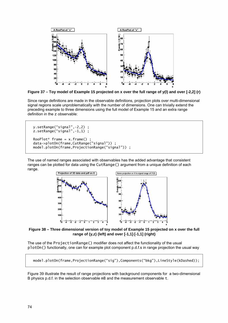
74

Figure 37 – Toy model of Example 15 projected on x over the full range of y(l) and over [-2,2] (r) Since range definitions are made in the observable definitions, projection plots over multi-dimensional signal regions scale unproblematically with the number of dimensions. One can trivially extend the preceding example to three dimensions using the full model of Example 15 and an extra range definition in the z observable:

y.setRange(“signal”,-2,2) ; z.setRange(“signal”,-1,1) ; RooPlot* frame = x.frame() ; data->plotOn(frame,CutRange("signal")) ; model.plotOn(frame,ProjectionRange(“signal”)) ;

The use of named ranges associated with observables has the added advantage that consistent ranges can be plotted for data using the CutRange() argument from a unique definition of each range.

Figure 38 – Three dimensional version of toy model of Example 15 projected on x over the full

range of (y,z) (left) and over [-1,1]⋅[-1,1] (right) The use of the ProjectionRange() modifier does not affect the functionality of the usual plotOn() functionally, one can for example plot component p.d.f.s in range projection the usual way

model.plotOn(frame,ProjectionRange(“sig”),Components(“bkg”),LineStyle(kDashed));

Figure 39 illustrate the result of range projections with background components for a two-dimensional B physics p.d.f. in the selection observable mB and the measurement observable t.

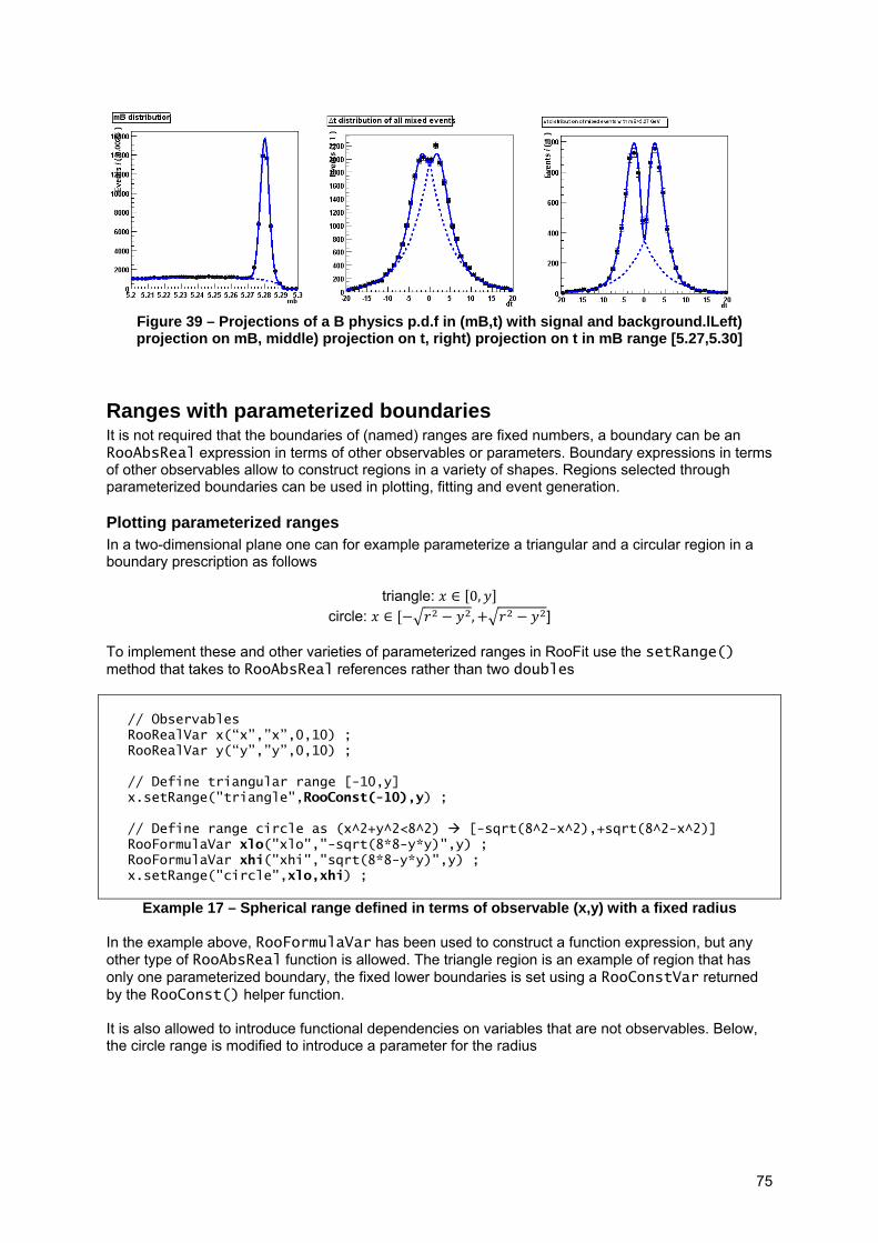
75

Figure 39 – Projections of a B physics p.d.f in (mB,t) with signal and background.lLeft) projection on mB, middle) projection on t, right) projection on t in mB range [5.27,5.30]

Ranges with parameterized boundaries It is not required that the boundaries of (named) ranges are fixed numbers, a boundary can be an RooAbsReal expression in terms of other observables or parameters. Boundary expressions in terms of other observables allow to construct regions in a variety of shapes. Regions selected through parameterized boundaries can be used in plotting, fitting and event generation.

Plotting parameterized ranges In a two-dimensional plane one can for example parameterize a triangular and a circular region in a boundary prescription as follows

triangle: 0, circle: , ]

To implement these and other varieties of parameterized ranges in RooFit use the setRange() method that takes to RooAbsReal references rather than two doubles

// Observables RooRealVar x(“x”,”x”,0,10) ; RooRealVar y(“y”,”y”,0,10) ; // Define triangular range [-10,y] x.setRange("triangle",RooConst(-10),y) ; // Define range circle as (x^2+y^2<8^2) [-sqrt(8^2-x^2),+sqrt(8^2-x^2)] RooFormulaVar xlo("xlo","-sqrt(8*8-y*y)",y) ; RooFormulaVar xhi("xhi","sqrt(8*8-y*y)",y) ; x.setRange("circle",xlo,xhi) ;

Example 17 – Spherical range defined in terms of observable (x,y) with a fixed radius In the example above, RooFormulaVar has been used to construct a function expression, but any other type of RooAbsReal function is allowed. The triangle region is an example of region that has only one parameterized boundary, the fixed lower boundaries is set using a RooConstVar returned by the RooConst() helper function. It is also allowed to introduce functional dependencies on variables that are not observables. Below, the circle range is modified to introduce a parameter for the radius

76

// Define range circle as (x^2+y^2<r^2) [-sqrt(r^2-x^2),+sqrt(r^2-x^2)] RooRealVar r(“r,”radius”,8,1,10) ; RooFormulaVar xlo("xlo","-sqrt(r*r-y*y)",RooArgSet(r,y)) ; RooFormulaVar xhi("xhi","sqrt(r*r-y*y)",RooArgSet(r,y)) ; x.setRange("circle",xlo,xhi) ;

Example 18 – Spherical range defined in terms of observables (x,y) and an extra range

parameter r that defines the radius For illustrational clarity we demonstrate the effect of these parameterized ranges on a flat p.d.f.

// Define a flat p.d.f in (x,y) RooPolynomial px(“px”,”px”,x) ; RooPolynomial py(“py”,”py”,y) ; RooProdPdf flat(“flat”,”flat”,RooArgSet(px,py)) ; // Generate flat distribution in (x,y) RooDataSet* data = flat.generate(RooArgSet(x,y),10000) ;

The plotting commands are identical to those of rectangular regions:

// Plot both data model in “signal” range RooPlot* frame = y.frame() ; data->plotOn(frame,CutRange(“triangle”)) ; flat.plotOn(frame,ProjectionRange(“triangle”)) ; // Plot both data model in “circle” range RooPlot* frame = y.frame() ; data->plotOn(frame,CutRange(“circle”)) ; flat.plotOn(frame,ProjectionRange(“circle”)) ;

The output of the above example is shown in Figure 40.

Figure 40 – Projection on x of a flat p.d.f and dataset in (x,y) of the region , (left) and

, (right) with r=8

Projecting a non-rectangular signal region Parameterized ranges can be used in the same way as rectangular regions. One can for example define a spherical signal region instead of rectangular signal region for the model of Example 15 and use that to construct a projection on the x observable.

77

RooFormulaVar ylo("ylo","-sqrt(1-z*z)",RooArgSet(z)) ; RooFormulaVar yhi("yhi","sqrt(1-z*z)",RooArgSet(z)) ; y.setRange("circle",ylo,yhi) ; z.setRange("circle",-1,1) ; RooPlot* frame = x.frame() ; d->plotOn(frame,Cut("y*y+z*z<1")) ; model.plotOn(frame,ProjectionRange("circle")) ;

Figure 41 – Projection of model of Example 15 on x in “circle” region in (y,z) defined by

1 The output of this projection is shown in Figure 41. In practice it is difficult construct an explicit parameterization for the boundaries of an optimal signal region. Another technique to construct projections of a signal region, a likelihood ratio plot, does not require an explicit parameterization and is discussed in the section “Working with implicitly defined sub-regions – Likelihood ratio plots”

Fitting parameterized regions Analogous to the plotting example it is also possible to fit data in non-rectangular regions. A likelihood constructed on a non-rectangular region implies two changes over the default likelihood construction: selecting the subset of events that fit in the selected region and adjusting the normalization of the p.d.f. such that it is normalized to unity of the selected region rather than over the full domain.

Figure 42 – Distribution of decay times of theoretical distribution (red points) and after an

acceptance cut (black points) that varies on an event-by-event bases

78

For certain classes of problems, it may be helpful to define such a likelihood for fitting on a non-rectangular region. A practical example of such a problem is a fit of a decay distribution with an acceptance that varies on an event-by-event basis, e.g. due to the implementation of the event trigger. An example decay distribution is shown in Figure 42: The red points show the istribution of an ordinary exponential decay, whereas the black points show the subset of events that fall within the trigger acceptance region. If the trigger acceptance windows is known from the data, expressed as separate observable tacc, it possible to account for the trigger acceptance in the model normalization by normalizing the decay model on the range [tacc,tmax] that is variable on an event-by-event basis, rather than on a fixed range [0,tmax].

// Declare observables RooRealVar t("t","t",0,5) ; RooRealVar tacc("tacc","tacc",0,0,5) ; // Make parameterized range in t : [tmin,5] t.setRange(tacc,RooConst(t.getMax())) ; // Make pdf RooRealVar tau("tau","tau",-1.54,-10,-0.1) ; RooExponential model("model","model",t,tau) ;

A fit of this model to a dataset D(t,tacc) will result in a correct lifetime measurement (provided the acceptance information in the dataset is correct) even though the data does not show the usual exponential distribution as is shown in the blue curve of Figure 42.

RooFitResult* r = model.fitTo(data) ; RooPlot* frame = t.frame() ; data->plotOn(frame) ; model.plotOn(frame,NormRange(1.5,5)) ;

For illustrational clarity the normalization of the projection of model In Figure 42 is chosen to be done on the range [1.5,5], which is mostly free of acceptance effects, to result in a curve normalization consistent with full decay distribution (red points). Note that in this example we have not used a named range into introduce a non-rectangular shape, but have substituted the default normalization range – which is used in the normalization of the minimized likelihood – with a parameterized range.

Integration over parameterized regions The basic semantics of constructing integrals over regions in p.d.f.s defined by simple ranges has been covered in Chapter two. The integrals that are required for the projection of and normalization of parameterized regions can be constructed in the same way as integrals over plain rectangular regions:

RooAbsReal* intCircle = flat.createIntegral(RooArgSet(x,y), NormSet(RooArgSet(x,y), Range(“circle”)) ;

Note again that for a integral over normalized p.d.f., the normalization observables must be explicitly and separately specified as RooAbsPdf objects have no internal notion of observables versus parameters. The above integral calculates the integral of flat(y,z) over (y,z) in the “circle” range and returns by definition a number between 0 and 1. The returned integral object depends on any

79

model parameters as well as any extra parameters that the range definition introduced, like the radius parameter of Example 18. The example below shows the dependence of the integral over the flat p.d.f of Example 17 on the radius

RooPlot* rframe = r.frame(0,10) ; intCircle->plotOn(rframe) ;

The output is shown in Figure 43.

Figure 43 – Fraction of flat p.d.f. in (x,y) over radius with circle r at (0,0)

Relation to cumulative distribution functions A special form of an integral over a parameterized range is the cumulative distribution function, which is defined as

and is constructed through the specialized method createCdf() from any p.d.f. This method can create a cumulative distribution function in any number of observables just like createIntegral():

RooAbsReal* cdf = pdf->createCdf(RooArgSet(x,y)) ;

Additional details on integration and cumulative distribution function are in Appendix B.

Figure 44 – Example of cumulative distribution function (right) defined from a two dimensional

probability density function (left)

80

Regions defined by a Boolean selection function Regions defined by parameterized boundaries can describe many, but not all shapes. In addition to any difficulties that may arise in the formulation of the boundary expression, shapes that result in more than two boundaries in any given observable (e.g. a ring-shaped region) cannot be described these way. Regions of arbitrary complexity can be described through the definition of a Boolean selection function that returns true or false to indicate if the given coordinate is in the region. While regions defined in this way are not supported for high-level operations in RooFit, it is possible to use them in a relatively straightforward way in event generation and plotting21.

Projecting regions defined by a Boolean selection function In Chapter 6 it was already shown that the integral used in projection plots can be substituted with the Monte Carlo approximation:

; , ;,

where D(y) is a set of points sampled from the p.d.f itself, and yi are the points in that dataset. In case illustrated in Chapter 6, D(y) was an external dataset, here we will work with a dataset that is sampled from the p.d.f. itself. The Monte Carlo approximation can be explicitly performed with a couple of lines of code

// Sample 10000 events in y from model RooDataSet* toyData = model.generate(y,10000) ;

// Project model over y using weighting over toy MC data model.plotOn(frame,ProjWData(*toyData)) ;

Projections calculated through Monte Carlo integration are generally more computationally intensive, so one does not normally use it for a problem like Figure 37, which features a simple rectangular cut that can be also be made through an (analytical) integration over a rectangular sub region. However MC integration offers the advantage that such projections are not restricted to shapes of which the boundary can be parameterized: you can select any region that you can define in terms of a selection expression on the projection data. The example below selects a spherical region in (y,z) with radius 2

// Select subset of events with |y2+z2|<2 RooDataSet* projData = toyData->reduce(“(y*y+z*z)<4”) ;

While that selection could also be constructed through a range with a parameterized boundary of y in terms of z, the following example cannot (easily):

// Select subset of events with 1<|y2+z2|<2 RooDataSet* projData = toyData->reduce(“(y*y+z*z)<4 && (y*y+z*z)>1”) ;

Using a likelihood ratio as Boolean selection function A particular application of selecting plot projection regions is the likelihood ratio technique. The concept is that instead of constructing an ad-hoc signal region, as was done for e.g. Figure 37, one uses the information in the likelihood in the projected observable(s) on the signal-to-(signal+background) ratio to construct a signal-enhanced region that should be plotted. Given a model

21 It is not possible to construct likelihoods in regions defined by a selection function in RooFit (yet) as there is no infrastructure to calculate p.d.f. normalizations over such regions.

81

, , , , 1 , ,

to be projected on x, the signal likelihood ratio in the projected observables (y,z) is defined as

,⋅ , ,

, ,,,

The quantity LR(y,z) expresses the probability that a given event (y,z) is signal-like, according to the information in M in the y and z observables. In the limit that S and B describe the true signal and background shapes, this likelihood ratio is the optimal discriminant. In this way we construct a likelihood ratio projection plot of M(x,y,z) on x that incorporates the model information on signal purity in all observables. For data, the procedure is trivial, one plots the subset of events that match the criterium LR(y,z)>α, where α is a value chosen been 0 and 1 depending on the desired purity of the plot. The corresponding p.d.f projection amounts to the following integral

, ,,

where α is again the minimum signal purity predicted by the projection of M on (y,z). The result is a plot of the distribution of data D(x,y,z) and model M(x,y,z) in x on the subset of events with have a signal probability greater than α% according to the model M in the observables (y,z).

Constructing the likelihood ratio A likelihood plot can be constructed in a fully automated procedure from a model, and has only one input parameter: the desired purity as quantified by the minimum required value of S/(S+B) in the projection quantified by α in the formula(s) above. The likelihood ratio formula needs to be constructed first

// Calculate signal and total likelihood projected over x RooAbsPdf* sigproj = sig.createProjection(x) ; RooAbsPdf* totproj = model.createProjection(x) ; // Construct the signal / signal+background probability RooFormulaVar llratio("llratio","(fsig*@0)/(@1)", RooArgList(*sigproj,*totproj,fsig)) ;

The createProjection() method of RooAbsPdf used in this example returns an integral of a p.d.f. over the listed observables as a new p.d.f. The signal model probability is multiplied with the signal fraction from the composite model to yield a number that is by construction in the range [0,1].22

Making the likelihood ratio projection plot A plot of the data with likelihood ratio cut is straightforward once the LR has been added as an observable to the dataset

// Extract the subset of data with large signal likelihood RooDataSet* dataSel = (RooDataSet*) data->reduce(Cut("llratio>0.5")) ; // Plot selected data RooPlot* frame = x.frame() ; dataSel->plotOn(frame) ;

22 This is not necessary for the formalism to work, but aids the interpretation of the LR value

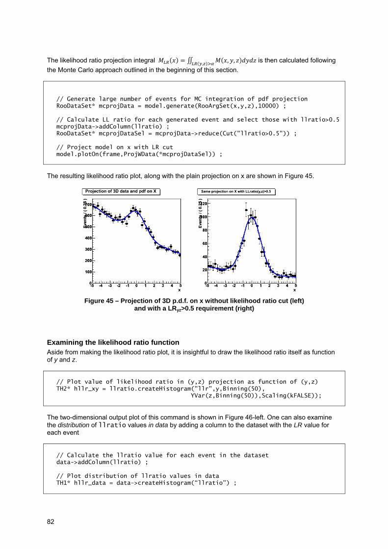
82

The likelihood ratio projection integral , ,, is then calculated following the Monte Carlo approach outlined in the beginning of this section.

// Generate large number of events for MC integration of pdf projection RooDataSet* mcprojData = model.generate(RooArgSet(x,y,z),10000) ; // Calculate LL ratio for each generated event and select those with llratio>0.5 mcprojData->addColumn(llratio) ; RooDataSet* mcprojDataSel = mcprojData->reduce(Cut("llratio>0.5")) ; // Project model on x with LR cut model.plotOn(frame,ProjWData(*mcprojDataSel)) ;

The resulting likelihood ratio plot, along with the plain projection on x are shown in Figure 45.

Figure 45 – Projection of 3D p.d.f. on x without likelihood ratio cut (left)

and with a LRyz>0.5 requirement (right)

Examining the likelihood ratio function Aside from making the likelihood ratio plot, it is insightful to draw the likelihood ratio itself as function of y and z.

// Plot value of likelihood ratio in (y,z) projection as function of (y,z) TH2* hllr_xy = llratio.createHistogram("llr",y,Binning(50), YVar(z,Binning(50)),Scaling(kFALSE));

The two-dimensional output plot of this command is shown in Figure 46-left. One can also examine the distribution of llratio values in data by adding a column to the dataset with the LR value for each event

// Calculate the llratio value for each event in the dataset data->addColumn(llratio) ; // Plot distribution of llratio values in data TH1* hllr_data = data->createHistogram(“llratio”) ;

83

The addColumn() method of a RooDataSet takes any function or p.d.f. as input arguments, calculates it value for the observable values of each event in the dataset and adds a column to the dataset with the calculated values. Te distribution of likelihood ratio values in data are shown in Figure 46-right. The maximum value of the likelihood ratio is about 0.6 and occurs in the region around (y,z)=(0,0) consistent with expectations from the signal model shape. Most events in data have a LR close to zero, about 5% of events have a LR>0.5.

Figure 46 – left) value pf LR=S(y,z)/[S+B](y,z) as function of (y,z),

right) distribution of LR(y,z) values in data

Tuning performance of projections through MC integration Projection of models through the Monte Carlo integration approach can be slow if the number of sampled events is large. This section describes two techniques that can be applied to speed up the calculation.

Binning projection data If the projection dataset has only one or two dimensions it can be advantageous to bin the projection data. You can do this manually

// Project with unbinned data model.plotOn(xframe,ProjWData(*data)) ; // Projected with data in default binning (100 bins) RooAbsData* binnedData = data->binnedClone() ; model.plotOn(xframe,ProjWData(*binnedData)) ; // Project with data in custom binning (5 bins) ((RooRealVar*)expDataY->get()->find("y"))->setBins(5) ; RooAbsData* binnedData2 = data->binnedClone() ; model.plotOn(xframe,ProjWData(*binnedData2),LineColor(kRed)) ;

or request it as an option in ProjWData()

// Projected with data in default binning (100 bins) model.plotOn(xframe,ProjWData(*binnedData,kTRUE));

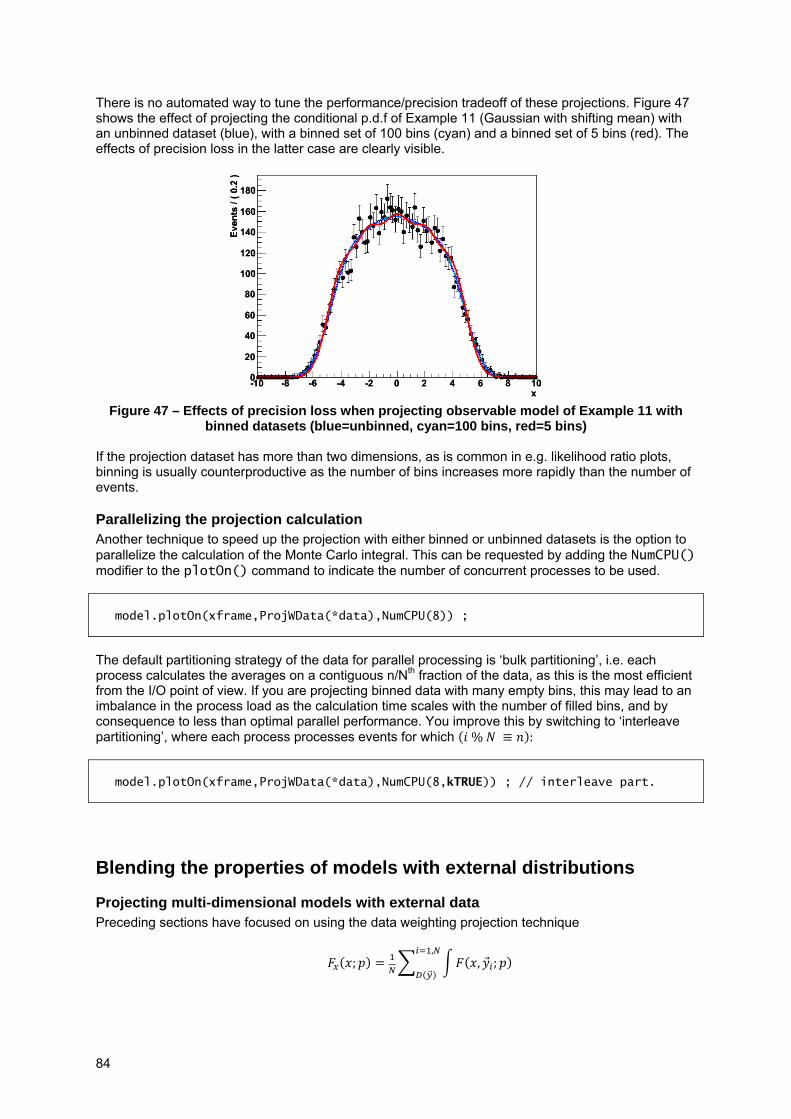
84

There is no automated way to tune the performance/precision tradeoff of these projections. Figure 47 shows the effect of projecting the conditional p.d.f of Example 11 (Gaussian with shifting mean) with an unbinned dataset (blue), with a binned set of 100 bins (cyan) and a binned set of 5 bins (red). The effects of precision loss in the latter case are clearly visible.

Figure 47 – Effects of precision loss when projecting observable model of Example 11 with

binned datasets (blue=unbinned, cyan=100 bins, red=5 bins) If the projection dataset has more than two dimensions, as is common in e.g. likelihood ratio plots, binning is usually counterproductive as the number of bins increases more rapidly than the number of events.

Parallelizing the projection calculation Another technique to speed up the projection with either binned or unbinned datasets is the option to parallelize the calculation of the Monte Carlo integral. This can be requested by adding the NumCPU() modifier to the plotOn() command to indicate the number of concurrent processes to be used.

model.plotOn(xframe,ProjWData(*data),NumCPU(8)) ;

The default partitioning strategy of the data for parallel processing is ‘bulk partitioning’, i.e. each process calculates the averages on a contiguous n/Nth fraction of the data, as this is the most efficient from the I/O point of view. If you are projecting binned data with many empty bins, this may lead to an imbalance in the process load as the calculation time scales with the number of filled bins, and by consequence to less than optimal parallel performance. You improve this by switching to ‘interleave partitioning’, where each process processes events for which % :

model.plotOn(xframe,ProjWData(*data),NumCPU(8,kTRUE)) ; // interleave part.

Blending the properties of models with external distributions

Projecting multi-dimensional models with external data Preceding sections have focused on using the data weighting projection technique

; , ;,

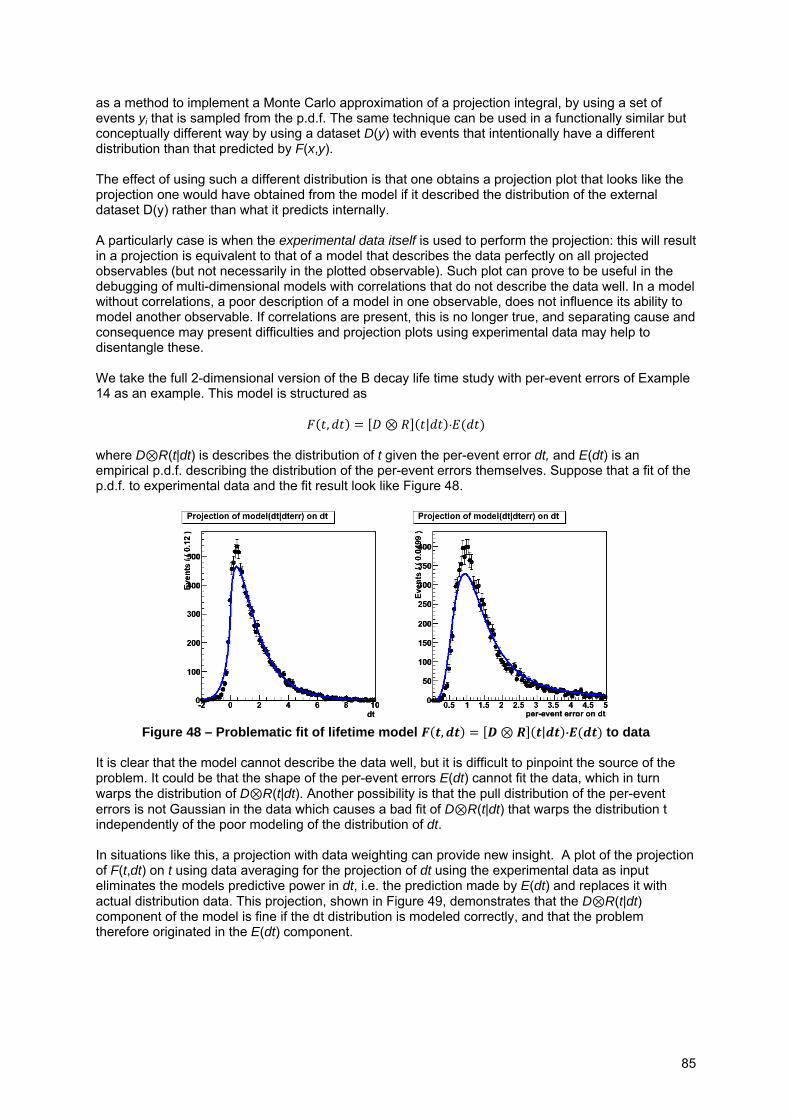
85

as a method to implement a Monte Carlo approximation of a projection integral, by using a set of events yi that is sampled from the p.d.f. The same technique can be used in a functionally similar but conceptually different way by using a dataset D(y) with events that intentionally have a different distribution than that predicted by F(x,y). The effect of using such a different distribution is that one obtains a projection plot that looks like the projection one would have obtained from the model if it described the distribution of the external dataset D(y) rather than what it predicts internally. A particularly case is when the experimental data itself is used to perform the projection: this will result in a projection is equivalent to that of a model that describes the data perfectly on all projected observables (but not necessarily in the plotted observable). Such plot can prove to be useful in the debugging of multi-dimensional models with correlations that do not describe the data well. In a model without correlations, a poor description of a model in one observable, does not influence its ability to model another observable. If correlations are present, this is no longer true, and separating cause and consequence may present difficulties and projection plots using experimental data may help to disentangle these. We take the full 2-dimensional version of the B decay life time study with per-event errors of Example 14 as an example. This model is structured as

, | ⋅ where D R(t|dt) is describes the distribution of t given the per-event error dt, and E(dt) is an empirical p.d.f. describing the distribution of the per-event errors themselves. Suppose that a fit of the p.d.f. to experimental data and the fit result look like Figure 48.

Figure 48 – Problematic fit of lifetime model , | ⋅ to data

It is clear that the model cannot describe the data well, but it is difficult to pinpoint the source of the problem. It could be that the shape of the per-event errors E(dt) cannot fit the data, which in turn warps the distribution of D R(t|dt). Another possibility is that the pull distribution of the per-event errors is not Gaussian in the data which causes a bad fit of D R(t|dt) that warps the distribution t independently of the poor modeling of the distribution of dt. In situations like this, a projection with data weighting can provide new insight. A plot of the projection of F(t,dt) on t using data averaging for the projection of dt using the experimental data as input eliminates the models predictive power in dt, i.e. the prediction made by E(dt) and replaces it with actual distribution data. This projection, shown in Figure 49, demonstrates that the D R(t|dt) component of the model is fine if the dt distribution is modeled correctly, and that the problem therefore originated in the E(dt) component.

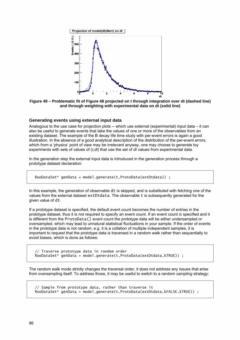
86

Figure 49 – Problematic fit of Figure 48 projected on t through integration over dt (dashed line)

and through weighting with experimental data on dt (solid line)

Generating events using external input data Analogous to the use case for projection plots -- which use external (experimental) input data – it can also be useful to generate events that take the values of one or more of the observables from an existing dataset. The example of the B decay life time study with per-event errors is again a good illustration. In the absence of a good analytical description of the distribution of the per-event errors, which from a ‘physics’ point of view may be irrelevant anyway, one may choose to generate toy experiments with sets of values of (t,dt) that use the set of dt values from experimental data. In the generation step the external input data is introduced in the generation process through a prototype dataset declaration:

RooDataSet* genData = model.generate(t,ProtoData(extDtdata)) ;

In this example, the generation of observable dt is skipped, and is substituted with fetching one of the values from the external dataset extDtdata. The observable t is subsequently generated for the given value of dt. If a prototype dataset is specified, the default event count becomes the number of entries in the prototype dataset, thus it is not required to specify an event count. If an event count is specified and it is different from the ProtoData() event count the prototype data will be either undersampled or oversampled, which may lead to unnatural statistical fluctuations in your sample. If the order of events in the prototype data is not random, e.g. it is a collation of multiple independent samples, it is important to request that the prototype data is traversed in a random walk rather than sequentially to avoid biases, which is done as follows:

// Traverse prototype data in random order RooDataSet* genData = model.generate(t,ProtoData(extDtdata,kTRUE)) ;

The random walk mode strictly changes the traversal order, it does not address any issues that arise from oversampling itself. To address those, it may be useful to switch to a random sampling strategy:

// Sample from prototype data, rather than traverse it RooDataSet* genData = model.generate(t,ProtoData(extDtdata,kFALSE,kTRUE)) ;

87

which samples events from the prototype dataset with uniform probability. This will result more frequent multiple use of the same events, i.e. even if Ngen<Nproto, but may result in more natural statistical fluctuations in certain applications The generator setup with prototype data works for any type of model: factorizing products of p.d.f.s, conditional p.d.f., products involving conditional p.d.f.s and non-factorizing multi-dimensional p.d.f.s. In case of factorizing products, a distribution sampled from a component p.d.f. is simply replaced with that of the external data. In case of conditional p.d.f.s in a product, the conditional observable is taken from the external dataset, instead of a value generated by another model in the product. For multi-dimensional non-factorizing terms, the specified observables are again loaded from the prototype dataset and then passed to an adapted generator context that only generates the remaining observables, treating the prototype data observables as parameters.


• rf309_ndimplot.C – Making 2 and 3 dimensional plots of p.d.f.s and datasets • rf311_rangeplot.C – Projecting p.d.f and data ranges in continuous observables • rf312_multirangefit.C – Performing fits in multiple (disjoint) ranges 1-,N-dimensions • rf313_paramranges.C – Using parameterized ranges to define non-rectangular regions • rf314_paramfitrange.C – Working with parameterized ranges in a fit. • rf315_projectpdf.C – Marginalization of multi-dimensional p.d.f.s through integration • rf316_llratioplot.C – Construction of a likelihood ratio plot

88

8. Data modeling with discrete-valued variables RooFit has a hierarchy of classes that represents variables and functions with discrete values. Discrete variables can be used to describe fundamentally discrete observables such as the electric charge of a particle but can also serve a role as ‘meta’-observable that divides a sample into a number of sub-samples (“run-1”, “run-2”) or be used to represent the decision of a selection algorithm (event is “accepted” or “rejected”). This Chapter focuses on the role of discrete variables in data modeling, how discrete observables can be used in standard fitting, plotting and event generation operations. Two common fitting problems involving discrete observables are explicitly worked out in the final two section: how do an unbinned maximum likelihood fit to an efficiency function and how to extract a (CP) asymmetry from data.

Discrete variables RooFit class RooCategory represent discrete-valued variables:

// Define discrete-valued observable RooCategory b0flav("b0flav","B0 flavor eigenstate") ; // Define allowed states with name and code b0flav.defineType("B0",-1) ; b0flav.defineType("B0bar",1) ;

Variables of class RooCategory can take a finite set of values declared through defineType(). Each value consists of a string label and integer numeric representation. The numeric representation can be explicitly chosen for each state, but it is not required

// Define discrete-valued observable RooCategory tagCat("tagCat","Tagging category") ; // Define a category with labels only tagCat.defineType("Lepton") ; tagCat.defineType("Kaon") ; tagCat.defineType("NetTagger-1") ; tagCat.defineType("NetTagger-2") ; Example 19 – Example of discrete observable with four valid states defined by name only

If no numeric representation is assigned, a code is automatically assigned.

Models with discrete observables Discrete variables represented by class RooCategory can be used as parameters or observables of functions and p.d.f. in the same way as continuous variables represented by RooRealVar.

Example model with discrete observables An example of a p.d.f. with discrete variables is class RooBMixDecay which describes the distribution of the decay time difference (t1-t2) for the decay 4 between the two B0 meson decays, which includes the physics effect of flavor oscillations. The final state of such decay is characterized by three observables

• t - The decay time difference (continuous) – RooRealVar

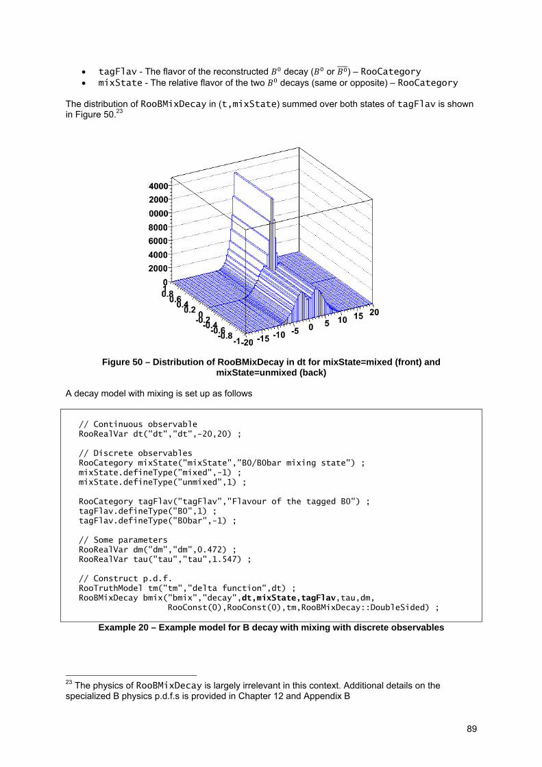
89

• tagFlav - The flavor of the reconstructed decay ( or ) – RooCategory • mixState - The relative flavor of the two decays (same or opposite) – RooCategory

The distribution of RooBMixDecay in (t,mixState) summed over both states of tagFlav is shown in Figure 50.23

Figure 50 – Distribution of RooBMixDecay in dt for mixState=mixed (front) and

mixState=unmixed (back) A decay model with mixing is set up as follows

// Continuous observable RooRealVar dt("dt","dt",-20,20) ; // Discrete observables RooCategory mixState("mixState","B0/B0bar mixing state") ; mixState.defineType("mixed",-1) ; mixState.defineType("unmixed",1) ; RooCategory tagFlav("tagFlav","Flavour of the tagged B0") ; tagFlav.defineType("B0",1) ; tagFlav.defineType("B0bar",-1) ; // Some parameters RooRealVar dm("dm","dm",0.472) ; RooRealVar tau("tau","tau",1.547) ; // Construct p.d.f. RooTruthModel tm("tm","delta function",dt) ; RooBMixDecay bmix("bmix","decay",dt,mixState,tagFlav,tau,dm, RooConst(0),RooConst(0),tm,RooBMixDecay::DoubleSided) ;

Example 20 – Example model for B decay with mixing with discrete observables

23 The physics of RooBMixDecay is largely irrelevant in this context. Additional details on the specialized B physics p.d.f.s is provided in Chapter 12 and Appendix B

90

For this particular p.d.f. explicit numeric assignments are made to the states of tagFlav and mixState as these have physical interpretations. We will use class RooBMixDecay in the above setup as an example to illustrate further features in data modeling with discrete observables.

Using models with discrete observables Fitting and event generation of models with discrete observables works in exactly the same way as for models with exclusively continuous observables

// Generate 10000 events in (dt,mixState,tagFlav) RooDataSet* data = bmix.generate(RooArgSet(dt,mixState,tagFlav),10000) ; // Print contents of dataset data->Print(“v”) ; Dataset bmixData (Generated From bmix) Contains 10000 entries Observables: RooArgSet::Dataset Variables: (Owning contents) 1) dt = -1.63478 L(-20 - 20) "dt" 2) mixState = unmixed "B0/B0bar mixing state" 3) tagFlav = B0bar "Flavour of the tagged B0" // Fit bmix to data bmix.fitTo(*data) ;

In general, any RooArgSet that serves as definition of the observables can contain a mix of RooRealVar and RooCategory objects. The continuous observable dt can be plotted as usual

// Plot distribution of dt RooPlot* frame = dt.frame() ; data->plotOn(frame) ; model.plotOn(frame) ;

When a projection is required over a discrete observables, as is the case in the above example, a summation over all states is substituted wherever an integration over continuous observables occurs. The above projection thus corresponds to

, ,

where T,M represent tagFlav and mixState respectively.

Using models with discrete parameters The use of discrete valued parameters (as opposed to observables) presents no special issues in RooFit, all functionality works as expected, with one important exception: MINUIT is not capable of handling discrete parameters in its minimization, thus one cannot have floating discrete parameters in models to be fitted. A fit with a constant discrete parameters presents no issues as constant parameters are not exported by default to MINUIT. For example one can choose to only fit the mixed decays of preceding example treating bmix as a p.d.f. B(dt,T;M,…)

// Construct a reduced dataset with mixed events only RooDataSet* dataMix= data->reduce(RooArgSet(dt,tagFlav)) ;

91

// Fit bmix to mixed data with mixed shape mixState.setLabel(“mixed”) ; mixState.setConstant(kTRUE) ; bmix.fitTo(*dataMix) ;

Plotting models in slices and ranges of discrete observables

Ranges in discrete observables The concept of named ranges also applies to discrete observables. The specification semantics are different and is illustrated on the tagging category of Example 20:

// Define range “good” to comprise states “Lepton” and “Kaon” tagCat.setRange(“good”,”Lepton,Kaon”) ; // Extend “good” to include “NetTagger-1” tagCat.addToRange(“good”,”NetTagger-1”) // Remove range “good” tagCat.clearRange(“good”)

But their use in fitting and plotting is the same

// Define range “good” tagCat.setRange(“good”,”Kaon,Lepton”) ; // Plot only projection of states of tagCat in “good” range mymodel.plotOn(frame,ProjectionRange(“good”)) ;

Ranges in continuous and discrete observables can be combined in the same way that ranges in multiple continuous observables are combined: whenever a range specification in more than observable occurs the range is automatically formed as the logical “and” of these definitions, e.g.

// Define range “good” x.setRange(“good”,-5,5) ; // Plot only projection in range tagCat[“Lepton”,”Kaon”] * x[-5,5] mymodel.plotOn(frame,ProjectionRange(“good”)) ;

Range plots in categories have the same data normalization properties as range plots in continuous observables.

Plotting continuous observables in slices of discrete observables Plotting a slice of a multidimensional p.d.f. in a discrete observable is similar to projecting a range consisting of a single state in a discrete observable, but has slightly different normalization properties that are reflected in the semantics of the operation. To project a slice that corresponds to a single state of discrete observable use the Slice() modifier of plotOn()

RooPlot* frame = dt.frame() ; data->plotOn(frame, Cut(“mixState==mixState::mixed”) ) ; model.plotOn(frame, Slice(mixState,”mixed”) ) ;

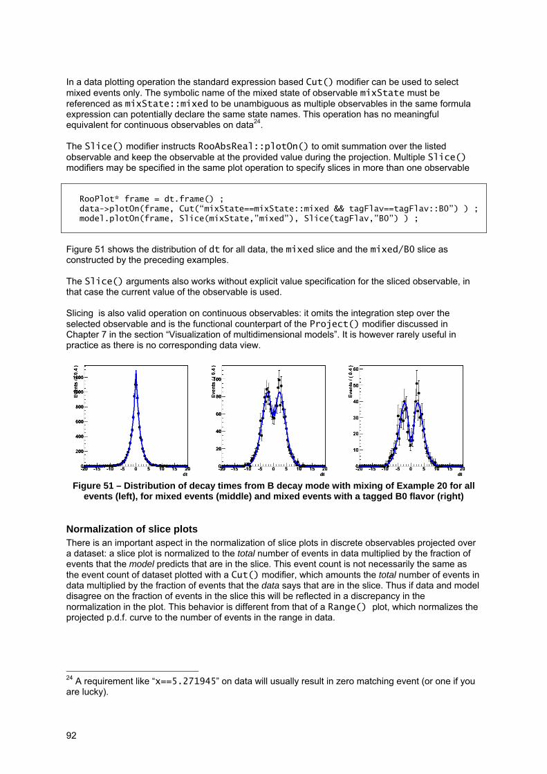
92

In a data plotting operation the standard expression based Cut() modifier can be used to select mixed events only. The symbolic name of the mixed state of observable mixState must be referenced as mixState::mixed to be unambiguous as multiple observables in the same formula expression can potentially declare the same state names. This operation has no meaningful equivalent for continuous observables on data24. The Slice() modifier instructs RooAbsReal::plotOn() to omit summation over the listed observable and keep the observable at the provided value during the projection. Multiple Slice() modifiers may be specified in the same plot operation to specify slices in more than one observable

RooPlot* frame = dt.frame() ; data->plotOn(frame, Cut(“mixState==mixState::mixed && tagFlav==tagFlav::B0”) ) ; model.plotOn(frame, Slice(mixState,”mixed”), Slice(tagFlav,”B0”) ) ;

Figure 51 shows the distribution of dt for all data, the mixed slice and the mixed/B0 slice as constructed by the preceding examples. The Slice() arguments also works without explicit value specification for the sliced observable, in that case the current value of the observable is used. Slicing is also valid operation on continuous observables: it omits the integration step over the selected observable and is the functional counterpart of the Project() modifier discussed in Chapter 7 in the section “Visualization of multidimensional models”. It is however rarely useful in practice as there is no corresponding data view.

Figure 51 – Distribution of decay times from B decay mode with mixing of Example 20 for all

events (left), for mixed events (middle) and mixed events with a tagged B0 flavor (right)

Normalization of slice plots There is an important aspect in the normalization of slice plots in discrete observables projected over a dataset: a slice plot is normalized to the total number of events in data multiplied by the fraction of events that the model predicts that are in the slice. This event count is not necessarily the same as the event count of dataset plotted with a Cut() modifier, which amounts the total number of events in data multiplied by the fraction of events that the data says that are in the slice. Thus if data and model disagree on the fraction of events in the slice this will be reflected in a discrepancy in the normalization in the plot. This behavior is different from that of a Range() plot, which normalizes the projected p.d.f. curve to the number of events in the range in data.

24 A requirement like “x==5.271945” on data will usually result in zero matching event (or one if you are lucky).

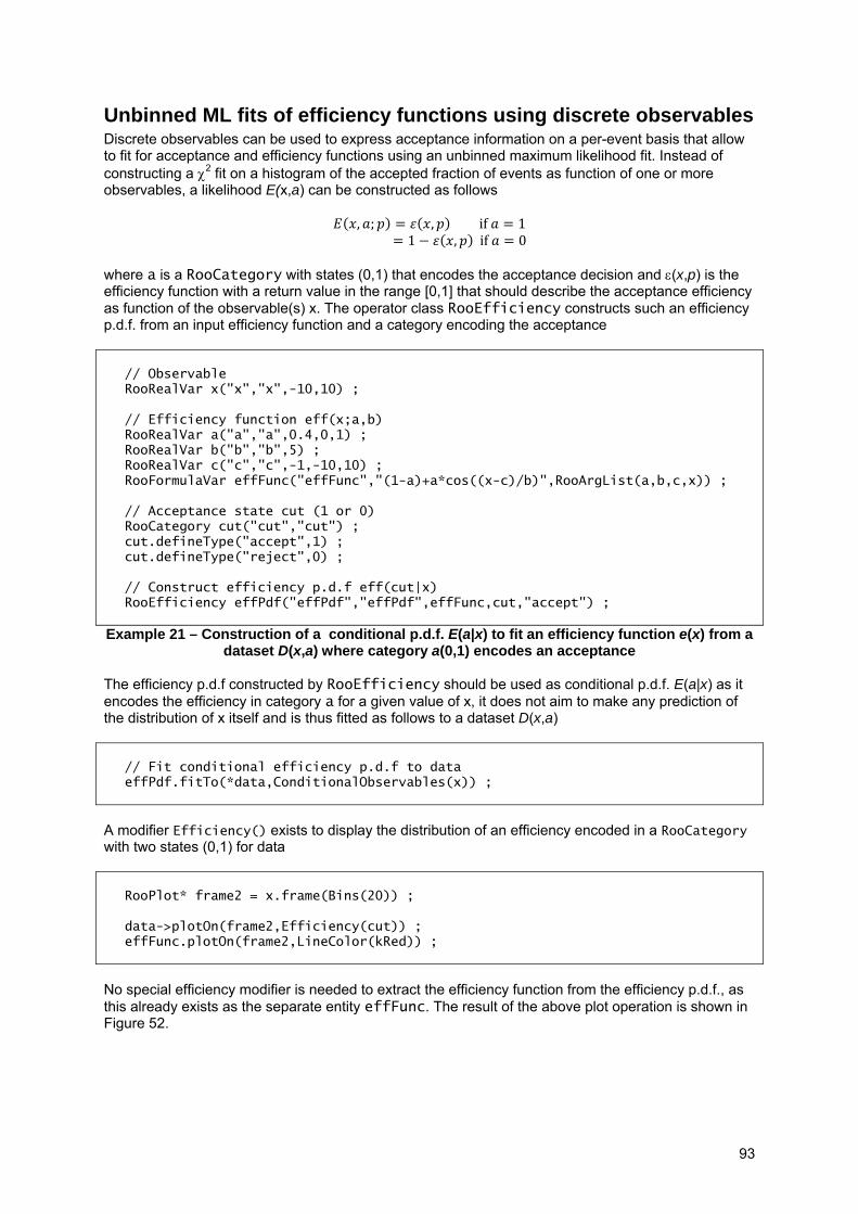
93

Unbinned ML fits of efficiency functions using discrete observables Discrete observables can be used to express acceptance information on a per-event basis that allow to fit for acceptance and efficiency functions using an unbinned maximum likelihood fit. Instead of constructing a χ2 fit on a histogram of the accepted fraction of events as function of one or more observables, a likelihood E(x,a) can be constructed as follows

, ; , if 1 1 , if 0

where a is a RooCategory with states (0,1) that encodes the acceptance decision and ε(x,p) is the efficiency function with a return value in the range [0,1] that should describe the acceptance efficiency as function of the observable(s) x. The operator class RooEfficiency constructs such an efficiency p.d.f. from an input efficiency function and a category encoding the acceptance

// Observable RooRealVar x("x","x",-10,10) ; // Efficiency function eff(x;a,b) RooRealVar a("a","a",0.4,0,1) ; RooRealVar b("b","b",5) ; RooRealVar c("c","c",-1,-10,10) ; RooFormulaVar effFunc("effFunc","(1-a)+a*cos((x-c)/b)",RooArgList(a,b,c,x)) ; // Acceptance state cut (1 or 0) RooCategory cut("cut","cut") ; cut.defineType("accept",1) ; cut.defineType("reject",0) ; // Construct efficiency p.d.f eff(cut|x) RooEfficiency effPdf("effPdf","effPdf",effFunc,cut,"accept") ;

Example 21 – Construction of a conditional p.d.f. E(a|x) to fit an efficiency function e(x) from a dataset D(x,a) where category a(0,1) encodes an acceptance

The efficiency p.d.f constructed by RooEfficiency should be used as conditional p.d.f. E(a|x) as it encodes the efficiency in category a for a given value of x, it does not aim to make any prediction of the distribution of x itself and is thus fitted as follows to a dataset D(x,a)

// Fit conditional efficiency p.d.f to data effPdf.fitTo(*data,ConditionalObservables(x)) ;

A modifier Efficiency() exists to display the distribution of an efficiency encoded in a RooCategory with two states (0,1) for data

RooPlot* frame2 = x.frame(Bins(20)) ; data->plotOn(frame2,Efficiency(cut)) ; effFunc.plotOn(frame2,LineColor(kRed)) ;

No special efficiency modifier is needed to extract the efficiency function from the efficiency p.d.f., as this already exists as the separate entity effFunc. The result of the above plot operation is shown in Figure 52.

94

Figure 52 – Visualization of a dataset D(x,a) with an category a that encoded as efficiency. Left:

all data (black) and data with a=1 (red). Right: Efficiency of a from data overlaid with fitted efficiency function of Example 21.

Efficiencies as function of multiple observables can be fitted the same way.

// Fit conditional efficiency p.d.f to data effPdf.fitTo(*data,ConditionalObservables(RooArgSet(x,y))) ;

For visualization of multidimensional efficiencies the multi-dimensional createHistogram() plotting tools – covered in Chapter 7 – can be used

// Sample histogram from 2D efficiency function TH1* hh_eff = effFunc.createHistogram("hh_eff",x,Binning(50), YVar(y,Binning(50)),Scaling(kFALSE)); // Sample histograms from all data, selected data TH1* hh_data_all = data->createHistogram("hh_data_all", x,Binning(8),YVar(y,Binning(8))) ; TH1* hh_data_sel = data>createHistogram("hh_data_sel", x,Binning(8),YVar(y,Binning(8)), Cut("cut==cut::accept")) ; // Construct data efficiency histogram using TH1 divisions TH1* hh_data_eff = hh_data_sel->Clone("hh_data_eff"); hh_data_eff->Divide(hh_data_all) ;

A fitted two-dimensional efficiency function and its input data are shown in Figure 53.

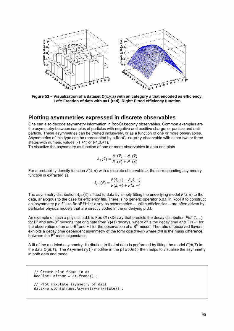
95

Figure 53 – Visualization of a dataset D(x,y,a) with an category a that encoded as efficiency.

Left: Fraction of data with a=1 (red). Right: Fitted efficiency function

Plotting asymmetries expressed in discrete observables One can also decode asymmetry information in RooCategory observables. Common examples are the asymmetry between samples of particles with negative and positive charge, or particle and anti-particle. These asymmetries can be treated inclusively, or as a function of one or more observables. Asymmetries of this type can be represented by a RooCategory observable with either two or three states with numeric values (-1,+1) or (-1,0,+1). To visualize the asymmetry as function of one or more observables in data one plots

For a probability density function , with a discrete observable a, the corresponding asymmetry function is extracted as

, ,, ,

The asymmetry distribution is fitted to data by simply fitting the underlying model , to the data, analogous to the case for efficiency fits. There is no generic operator p.d.f. in RooFit to construct an ‘asymmetry p.d.f.’ like RooEfficiency as asymmetries – unlike efficiencies – are often driven by particular physics models that are directly coded in the underlying p.d.f. An example of such a physics p.d.f. is RooBMixDecay that predicts the decay distribution F(dt,T,…) for B0 and anti-B0 mesons that originate from Y(4s) decays, where dt is the decay time and T is -1 for the observation of an anti-B0 and +1 for the observation of a B0 meson. The ratio of observed flavors exhibits a decay time dependent asymmetry of the form cos(dm·dt) where dm is the mass difference between the B0 mass eigenstates. A fit of the modeled asymmetry distribution to that of data is performed by fitting the model F(dt,T) to the data D(dt,T). The Asymmetry() modifier in the plotOn() then helps to visualize the asymmetry in both data and model

// Create plot frame in dt RooPlot* aframe = dt.frame() ; // Plot mixState asymmetry of data data->plotOn(aframe,Asymmetry(mixState)) ;

96

// Plot corresponding asymmetry predicted by p.d.f bmix.plotOn(aframe,Asymmetry(mixState)) ; // Adjust vertical range of plot to sensible values for an asymmetry aframe->SetMinimum(-1.1) ; aframe->SetMaximum(1.1) ;

When plotting asymmetries in data, binomial error bars are drawn, as is done for efficiencies. The resulting asymmetry plot is shown in Figure 54. The Asymmetry() argument is not limited to B physics p.d.f.s, it can be applied to any model that has a discrete observable with states (-1,+1) or (-1,0,+1).

Figure 54 – Asymmetry in mixState category of the model for B decay

with mixing defined in Example 20


• rf108_plotbinning.C – Plotting asymmetries in categories with custom binning • rf310_sliceplot.C -- Projecting p.d.f and data slices in discrete observables • rf404_categories.C -- Working with RooCategory objects to describe discrete variables • rf701_efficiencyfit.C – Unbinned ML fit of one-dimensional efficiency function • rf702_efficiencyfit_2D.C -- Unbinned ML fit of two-dimensional efficiency function • rf708_bphysics.C – Use examples of b physics p.d.f including RooBMixDecay

97

9. Dataset import and management

This chapter gives an overview on how data can be imported into RooFit from external sources. Details are given on the various operations that can be applied to datasets such as merger and addition.

Importing unbinned data from ROOT TTrees The basic import syntax of TTrees into one-dimensional RooDataSets has been covered in Chapter 2. These import rules extend naturally for multidimensional datasets, one can just add more observables to the dataset that is the target of the import.

TTree* tree = (TTree*) gDirectory->Get(“atree”) ;

RooRealVar x(“x”,”x”,-10,10) ; RooRealVar y(“y”,”y”,-10,10) ;

RooCategory c(“c”,”c”) ; c.defineType(“accept”,1) ; c.defineType(“reject”,0) ;

RooDataSet data(“data”,”data”,RooArgSet(x,y,c),Import(tree)) ;

Branch type conversion rules RooFit datasets are by design ‘flat’, i.e. each event is described a set of variables that are either discrete or continuous, but are each unstructured, they cannot be arrays or objects. A RooRealVar member of a dataset can import equally named branches an external tree of type Double_t, Float_t, Int_t, UInt_t and Bool_t. Upon import these are automatically converted to Double_t, the native representation of RooRealVar. A RooCategory member of a dataset can import equally named branches of an external tree of type Int_t, UInt_t and Bool_t. Upon import these are converted into two branches: one Int_t branch that holds the numeric representation of the type and one const char* branch that holds the string representation. The string representations are taken from the RooCategory state definitions at the time of lookup and stored in the internal tree representation as well to expedite the loading of dataset rows with categories. In the internal representation the integer branch takes a suffix “_idx” and the string branch takes a suffix “_lbl” with respect to the category name.

Application of range cuts Each variable that is imported from an external tree must match its default range specification. In the code example above this means that only tree entries with -10<x<10 are loaded. If a tree has multiple observables, an event is only imported if all observables meet their range requirements. For categories in-range requirement means that the integer entry must have been defined as a valid type.

Application of additional cuts on import Additional cuts to be applied during the importation step can be supplied with an Cut() argument

RooDataSet data(“data”,”data”,RooArgSet(x,y,c),Import(tree),Cut(“x+y<0”)) ;

98

Importing unbinned data from ASCII files A separate interface exists to construct a new RooDataSets from the contents of flat ASCII files.

RooDataSet* impData = RooDataSet::read(“ascii.txt”,RooArgList(x,y,c)) ;

The ASCII file is assumed to have one line for each event. On each line the values of the observables interpreted in the order in which the observables are listed in the RooArgList argument of read(), e.g.

# Comment lines are allowed and must start with a ‘#’ # X Y C 0.365 8.5689 accept 2.498 -4.763 reject

Lines that start with a ‘#’ are automatically ignored, facilitating comment lines in these files. For category observables, both the string representation and the integer representation can be used. As in the importing of data from TTrees, events where one or more observables contain a value outside the defined range of the corresponding RooRealVar/RooCategory are rejected.

Importing binned data from ROOT THx histograms

Importing a single THx The syntax for importing a single ROOT TH1 histogram into a RooDataHist was already covered in Chapter 2. As for unbinned data, the import rules extend naturally to higher dimensional histograms:

TH2* hh = (TH2*) gDirectory->Get(“ahisto”) ;

RooRealVar x(“x”,”x”,-10,10) ; RooRealVar x(“y”,”y”,-10,10) ; RooDataHist data(“data”,”dataset with (x,y)”,RooArgList(x,y),hh)

Note that the RooDataHist constructor in this form takes a RooArgList rather than a RooArgSet as the order of the observables is essential: it is used to map the x,y and z axis of the imported TH1/2/3.

Application of range cuts Since ROOT histograms have a intrinsic range definition on their observables, unlike TTree branches, the handling of ranges during data import is slightly different from that of unbinned data. What is the same is that all THx bins that are outside the range definition in the corresponding RooRealVar are rejected, thus one can selectively import a subset of a histogram by choosing a range definition in the RooRealVar that is narrower than the range of the corresponding axis in the histogram. This example

TH1* hh = new TH1D(“demo”,”demo histo”,100,-20,20) ; RooRealVar x(“x”,”x”,-10,10) ; RooDataHist data(“data”,”data”,x,hh) ;

99

will only the bins of hh that are in the range [-10,10]. What is different with respect to unbinned data import is that in case the range specification of a RooRealVar does not exactly match a bin boundary of the imported histogram, the bin that contains the range limit is fully imported and the range limit on the corresponding RooRealVar is adjusted outward to match the outer bin boundary. Observables associated with RooDataHists may thus have (slightly) different range definitions after a THx import operation.

Import of binning definition When a RooDataHist is constructed from a THx, the bin definition of the THx is copied in each imported observable. This also applies if the THx has a custom (variable) binning.

Importing a projection of a histogram If multi-dimensional THx is imported in a lower-dimensional RooDataHist its contents is automatically projected (i.e. integrated over the dimensional that are not imported)

Importing multiple histograms into a N+1 dimensional RooDataHist It is also possible to import a ‘stack’ of THx histograms into a single RooDataHist. In this case an extra RooCategory observables is introduced that labels source histograms

// Declare observable x RooRealVar x("x","x",-10,10) ; // Create category observable c that serves as index for the ROOT histograms RooCategory c("c","c") ; // Create a datahist that imports contents of all TH1 mapped by index category c RooDataHist* dh = new RooDataHist("dh","dh",x,Index(c), Import("SampleA",*hh_1), Import("SampleB",*hh_2), Import("SampleC",*hh_3)) ;

The Index() argument designates category c as the index category to label the source histograms. The Import() argument imports one histogram and sets the associated label of the index category c. If the index category does not have a state defined with the given label, it is defined on the fly, otherwise the preexisting state is used. All imported histogram must be of the same dimensions. The histogram stack import can also be done through an alternate constructor that takes and map<string,TH1*>, which lends itself better to embedded applications

// Alternative constructor form for importing multiple histograms map<string,TH1*> hmap ; hmap["SampleA"] = hh_1 ; hmap["SampleB"] = hh_2 ; hmap["SampleC"] = hh_3 ; // Construct RooDataHist using alternate ctor RooDataHist* dh2 = new RooDataHist("dh","dh",x,c,hmap) ;

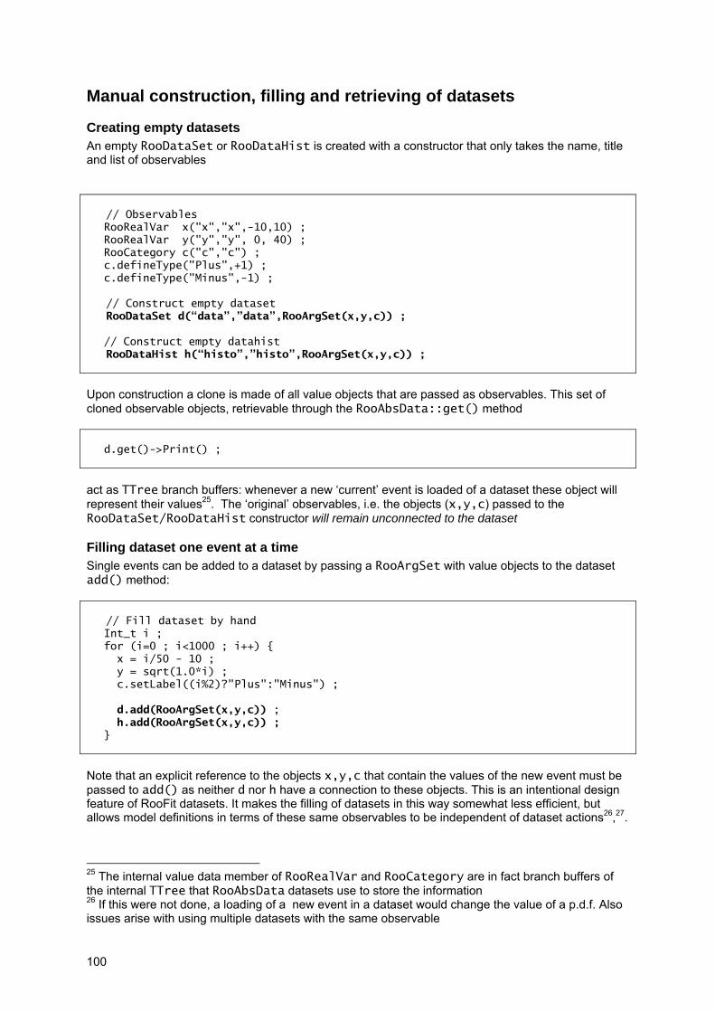
100

Manual construction, filling and retrieving of datasets

Creating empty datasets An empty RooDataSet or RooDataHist is created with a constructor that only takes the name, title and list of observables // Observables

RooRealVar x("x","x",-10,10) ; RooRealVar y("y","y", 0, 40) ; RooCategory c("c","c") ; c.defineType("Plus",+1) ; c.defineType("Minus",-1) ;

// Construct empty dataset RooDataSet d(“data”,”data”,RooArgSet(x,y,c)) ;

// Construct empty datahist RooDataHist h(“histo”,”histo”,RooArgSet(x,y,c)) ; Upon construction a clone is made of all value objects that are passed as observables. This set of cloned observable objects, retrievable through the RooAbsData::get() method

d.get()->Print() ;

act as TTree branch buffers: whenever a new ‘current’ event is loaded of a dataset these object will represent their values25. The ‘original’ observables, i.e. the objects (x,y,c) passed to the RooDataSet/RooDataHist constructor will remain unconnected to the dataset

Filling dataset one event at a time Single events can be added to a dataset by passing a RooArgSet with value objects to the dataset add() method:

// Fill dataset by hand

Int_t i ; for (i=0 ; i<1000 ; i++) { x = i/50 - 10 ; y = sqrt(1.0*i) ; c.setLabel((i%2)?"Plus":"Minus") ;

d.add(RooArgSet(x,y,c)) ; h.add(RooArgSet(x,y,c)) ; }

Note that an explicit reference to the objects x,y,c that contain the values of the new event must be passed to add() as neither d nor h have a connection to these objects. This is an intentional design feature of RooFit datasets. It makes the filling of datasets in this way somewhat less efficient, but allows model definitions in terms of these same observables to be independent of dataset actions26,27.

25 The internal value data member of RooRealVar and RooCategory are in fact branch buffers of the internal TTree that RooAbsData datasets use to store the information 26 If this were not done, a loading of a new event in a dataset would change the value of a p.d.f. Also issues arise with using multiple datasets with the same observable

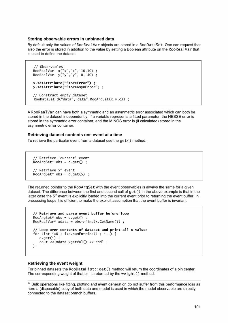
101

Storing observable errors in unbinned data By default only the values of RooRealVar objects are stored in a RooDataSet. One can request that also the error is stored in addition to the value by setting a Boolean attribute on the RooRealVar that is used to define the dataset

// Observables

RooRealVar x("x","x",-10,10) ; RooRealVar y("y","y", 0, 40) ; x.setAttribute(“StoreError”) ; y.setAttribute(“StoreAsymError”) ; // Construct empty dataset

RooDataSet d(“data”,”data”,RooArgSet(x,y,c)) ;

A RooRealVar can have both a symmetric and an asymmetric error associated which can both be stored in the dataset independently. If a variable represents a fitted parameter, the HESSE error is stored in the symmetric error container, and the MINOS error is (if calculated) stored in the asymmetric error container.

Retrieving dataset contents one event at a time To retrieve the particular event from a dataset use the get() method:

// Retrieve ‘current’ event RooArgSet* obs = d.get() ; // Retrieve 5th event RooArgSet* obs = d.get(5) ;

The returned pointer to the RooArgSet with the event observables is always the same for a given dataset. The difference between the first and second call of get() in the above example is that in the latter case the 5th event is explicitly loaded into the current event prior to returning the event buffer. In processing loops it is efficient to make the explicit assumption that the event buffer is invariant

// Retrieve and parse event buffer before loop RooArgSet* obs = d.get() ; RooRealVar* xdata = obs->find(x.GetName()) ; // Loop over contents of dataset and print all x values for (int i=0 ; i<d.numEntries() ; i++) { d.get(i) ; cout << xdata->getVal() << endl ; }

Retrieving the event weight For binned datasets the RooDataHist::get() method will return the coordinates of a bin center. The corresponding weight of that bin is returned by the weight() method: 27 Bulk operations like fitting, plotting and event generation do not suffer from this performance loss as here a (disposable) copy of both data and model is used in which the model observable are directly connected to the dataset branch buffers.

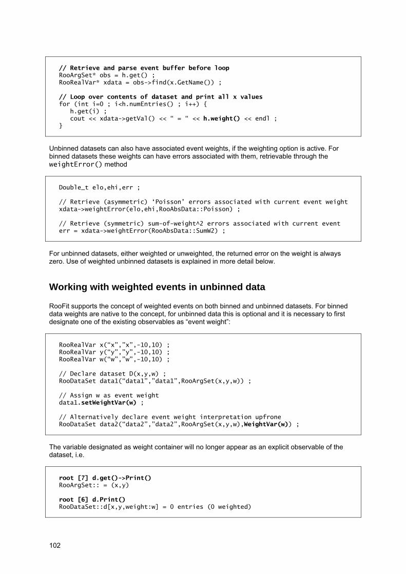
102

// Retrieve and parse event buffer before loop RooArgSet* obs = h.get() ; RooRealVar* xdata = obs->find(x.GetName()) ; // Loop over contents of dataset and print all x values for (int i=0 ; i<h.numEntries() ; i++) { h.get(i) ; cout << xdata->getVal() << “ = “ << h.weight() << endl ; }

Unbinned datasets can also have associated event weights, if the weighting option is active. For binned datasets these weights can have errors associated with them, retrievable through the weightError() method

Double_t elo,ehi,err ; // Retrieve (asymmetric) ‘Poisson’ errors associated with current event weight xdata->weightError(elo,ehi,RooAbsData::Poisson) ; // Retrieve (symmetric) sum-of-weight^2 errors associated with current event err = xdata->weightError(RooAbsData::SumW2) ;

For unbinned datasets, either weighted or unweighted, the returned error on the weight is always zero. Use of weighted unbinned datasets is explained in more detail below.

Working with weighted events in unbinned data RooFit supports the concept of weighted events on both binned and unbinned datasets. For binned data weights are native to the concept, for unbinned data this is optional and it is necessary to first designate one of the existing observables as “event weight”:

RooRealVar x(“x”,”x”,-10,10) ; RooRealVar y(“y”,”y”,-10,10) ; RooRealVar w(“w”,”w”,-10,10) ; // Declare dataset D(x,y,w) ; RooDataSet data1(“data1”,”data1”,RooArgSet(x,y,w)) ; // Assign w as event weight data1.setWeightVar(w) ; // Alternatively declare event weight interpretation upfrone RooDataSet data2(“data2”,”data2”,RooArgSet(x,y,w),WeightVar(w)) ;

The variable designated as weight container will no longer appear as an explicit observable of the dataset, i.e.

root [7] d.get()->Print() RooArgSet:: = (x,y) root [6] d.Print() RooDataSet::d[x,y,weight:w] = 0 entries (0 weighted)

103

Nevertheless, the name of the weight variable is relevant when data is imported from an external source, e.g.

// Alternatively declare event weight interpretation upfrone RooDataSet data3(“data2”,”data2”,RooArgSet(x,y,w),WeightVar(w),Import(myTree)) ;

imports the event weights from the tree branch named w. When filling an unbinned weighted dataset by hand one can simply add the weight to the add() method:

// Add weighted event to unbinned dataset Double_t wgt=0.5 ; data1.add(RooArgSet(x,y),wgt) ;

Use of weighted data presents some fundamental issues28 in maximum likelihood fits and should be used with due care. Chapter 12 has additional details on fitting of weighted datasets.

Plotting, tabulation and calculations of dataset contents

The RooPlot interface The preceding Chapters have already covered a variety of ways to make plots of continuous observables from datasets, either through the plotOn() method on 1-dimensional RooPlot frames

RooPlot* frame = x.frame() ; d.plotOn(frame) ;

and no further details are offered here. The THx interface The createHistogram() method that creates and fills 1-,2- or 3-dimensional ROOT histograms has also been covered in earlier Chapters and is not elaborated here.

TH1* hh = d.createHistogram(“x,y”,100,100) ;

The TTree Draw() and Scan() interface It is also possible to directly access the internal TTree representation of a RooDataSet through the tree() method, which gives access to methods like Draw() and Scan() that are useful for debugging and quick data exploration

d.tree().Draw(“x”) ; d.tree().Scan(“x”) ;

28 In the likelihood formalism the sum of the weights is interpreted as a number of events, thus the statistical error reported by a ML fit to weighted data will be proportional to the sum of the weights which is in general incorrect.

104

Tabulating discrete observables A separate interface is provided to tabulate the values of discrete RooCategory observables that occur in a dataset

Roo1DTable* btable = data->table(b0flav) ; btable->Print() ; Roo1DTable::b0flav = (B0=5050,B0bar=4950) btable->Print("v") ; Table b0flav : pData +-------+------+ | B0 | 5050 | | B0bar | 4950 | +-------+------+

The RooAbsData::table() method fills a Roo1DTable object with the information from the dataset. The default Print() implementation of the table summarizes the contents on a single line whereas the verbose (“v”) configuration produces an ASCII art table. It is possible to specify a cut to be applied prior to tabulation using the Cut() argument, similar to what can be done in plotOn():

// Create table for subset of events matching cut expression Roo1DTable* ttable = data->table(tagCat,"x>8.23") ; ttable->Print("v") ; Table tagCat : pData(x>8.23) +-------------+-----+ | Lepton | 439 | | Kaon | 442 | | NetTagger-1 | 446 | | NetTagger-2 | 425 | +-------------+-----+

The information contained in tables can be retrieved through the get() method to get the event count of a single state, or using the getFrac() method to return the fraction of events in a given state

// Retrieve number of events from table Double_t nb0 = btable->get("B0") ; // Retrieve fraction of events with "Lepton" tag Double_t fracLep = ttable->getFrac("Lepton") ;

All internal bookkeeping of tables, as well as the table interface methods, work with Double_t representations rather than Int_t for event counts as event counts for weighted datasets are generally not integers. To tabulate the event counts in permutations of states of multiple categories, pass a set of categories to table() instead of single category

105

// Create table for all (tagCat x b0flav) state combinations Roo1DTable* bttable = data->table(RooArgSet(tagCat,b0flav)) ; bttable->Print("v") ;

Table (tagCat x b0flav) : pData +---------------------+------+ | {Lepton;B0} | 1262 | | {Kaon;B0} | 1275 | | {NetTagger-1;B0} | 1253 | | {NetTagger-2;B0} | 1260 | | {Lepton;B0bar} | 1280 | | {Kaon;B0bar} | 1214 | | {NetTagger-1;B0bar} | 1236 | | {NetTagger-2;B0bar} | 1220 | +---------------------+------+

Tables can, like RooPlots be persisted in ROOT files

Calculation of ranges of observables The method getRange() returns information on the lowest and highest value of a given observable that occurs in the dataset. In it simplest form it reports the lowest and highest occurring value of a given continuous observable x:

Double_t xlo, xhi ; data->getRange(x,xlo,xhi) ;

But it can also account for some amount of margin, expressed as a fraction of actual xhi-xlo, by which the returned range is widened.

data->getRange(x,xlo,xhi,0.05) ;

This option can be useful to calculate ranges for of plots and is interfaced in the AutoRange() argument of RooRealVar::frame()

RooPlot* frame = x.frame(AutoRange(*data,0.05)) ;

Alternatively, the definition of the range can be widened such that mean of the distribution is at the center of the returned range, which is requested by a Boolean kTRUE argument in getRange() and is interfaced with the AutoSymRange() argument

RooPlot* frame = x.frame(AutoSymRange(*data,0.05)) ;

Calculation of moments and standardized moments For each continuous observable the (standardized) moments of a dataset, defined as

, ,

106

can be calculated as follows

// Any moment Double_t m5 = data.moment(x,5) ; // Any standardized moment Double_t m5s = data.standMoment(x,5) ;

For convenience the following synonyms have been defined

// Mean and sigma Double_t mean = data.mean(x) ; // 1st moment Double_t rms = data.sigma(x) ; // 2nd moment // Skewness and kurtosis Double_t skew = data.skewness(x) ; // 3rd standardized moment Double_t kurt = data.kurtosis(x) ; // 4th standardized moment

The value of the 1st and 2nd standardized moments are 0 and 1 respectively by construction. In any of the above methods, a cut expression string or cut range can be specified that is applied to the data prior to calculation of the requested moment

// Mean with cut expression Double_t mean_cut = data.mean(x,”y>5.27”) ; // Mean with range cut Double_t mean_ranfe = data.mean(x,””,”good”) ;

Operations on unbinned datasets Unbinned datasets support a variety of operations like merging, appending, splitting and reduction to alter their contents.

Counting events All datasets have two separate counting methods: numEvents() which returns the number of event records and sumEvents() which returns the sum of the weights in all event records. For unbinned datasets without weights both method return the same answer

Appending datasets Given two datasets with the same observables, one can append the contents of one dataset to the other through the append() method:

// The append() function adds // two datasets row-wise data1->append(*data2) ;

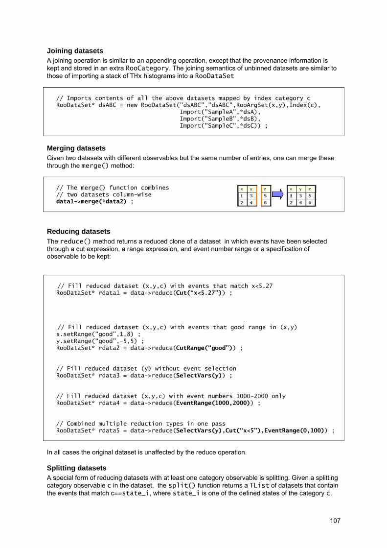
107

Joining datasets A joining operation is similar to an appending operation, except that the provenance information is kept and stored in an extra RooCategory. The joining semantics of unbinned datasets are similar to those of importing a stack of THx histograms into a RooDataSet

// Imports contents of all the above datasets mapped by index category c RooDataSet* dsABC = new RooDataSet("dsABC","dsABC",RooArgSet(x,y),Index(c), Import("SampleA",*dsA), Import("SampleB",*dsB), Import("SampleC",*dsC)) ;

Merging datasets Given two datasets with different observables but the same number of entries, one can merge these through the merge() method:

// The merge() function combines // two datasets column-wise data1->merge(*data2) ;

Reducing datasets The reduce() method returns a reduced clone of a dataset in which events have been selected through a cut expression, a range expression, and event number range or a specification of observable to be kept: // Fill reduced dataset (x,y,c) with events that match x<5.27

RooDataSet* rdata1 = data->reduce(Cut(“x<5.27”)) ;

// Fill reduced dataset (x,y,c) with events that good range in (x,y)

x.setRange(“good”,1,8) ; y.setRange(“good”,-5,5) ; RooDataSet* rdata2 = data->reduce(CutRange(“good”)) ; // Fill reduced dataset (y) without event selection RooDataSet* rdata3 = data->reduce(SelectVars(y)) ; // Fill reduced dataset (x,y,c) with event numbers 1000-2000 only RooDataSet* rdata4 = data->reduce(EventRange(1000,2000)) ; // Combined multiple reduction types in one pass RooDataSet* rdata5 = data->reduce(SelectVars(y),Cut(“x<5”),EventRange(0,100)) ;

In all cases the original dataset is unaffected by the reduce operation.

Splitting datasets A special form of reducing datasets with at least one category observable is splitting. Given a splitting category observable c in the dataset, the split() function returns a TList of datasets that contain the events that match c==state_i, where state_i is one of the defined states of the category c.

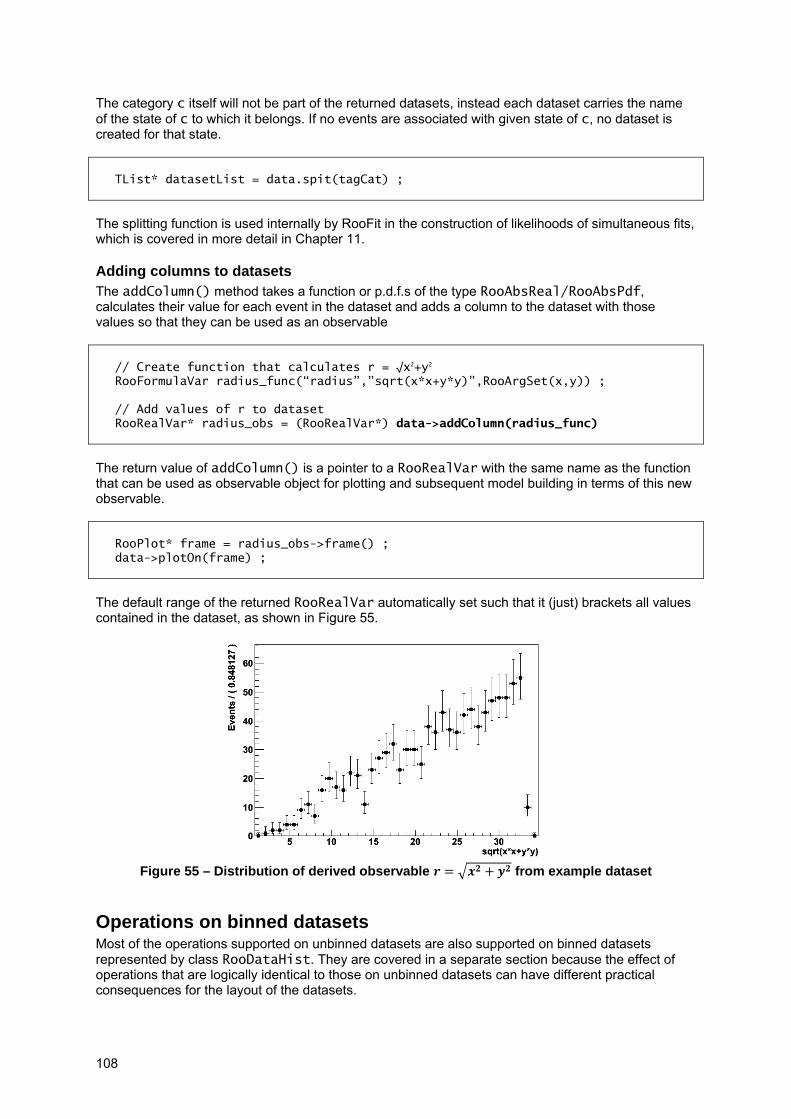
108

The category c itself will not be part of the returned datasets, instead each dataset carries the name of the state of c to which it belongs. If no events are associated with given state of c, no dataset is created for that state.

TList* datasetList = data.spit(tagCat) ;

The splitting function is used internally by RooFit in the construction of likelihoods of simultaneous fits, which is covered in more detail in Chapter 11.

Adding columns to datasets The addColumn() method takes a function or p.d.f.s of the type RooAbsReal/RooAbsPdf, calculates their value for each event in the dataset and adds a column to the dataset with those values so that they can be used as an observable

// Create function that calculates r = √x2+y2 RooFormulaVar radius_func(“radius”,”sqrt(x*x+y*y)”,RooArgSet(x,y)) ; // Add values of r to dataset RooRealVar* radius_obs = (RooRealVar*) data->addColumn(radius_func)

The return value of addColumn() is a pointer to a RooRealVar with the same name as the function that can be used as observable object for plotting and subsequent model building in terms of this new observable.

RooPlot* frame = radius_obs->frame() ; data->plotOn(frame) ;

The default range of the returned RooRealVar automatically set such that it (just) brackets all values contained in the dataset, as shown in Figure 55.

Figure 55 – Distribution of derived observable from example dataset

Operations on binned datasets Most of the operations supported on unbinned datasets are also supported on binned datasets represented by class RooDataHist. They are covered in a separate section because the effect of operations that are logically identical to those on unbinned datasets can have different practical consequences for the layout of the datasets.

109

Counting events The event record counted return by numEvents() on binned datasets is a fixed and reflects the number of bins defined in the dataset. The sumEvents() which returns the sum of the weights all bins.

Adding data The addition of two datasets that is performed in unbinned datasets with the append() operation is done with the add(const RooDataHist&) method for binned data. The different name reflect the different process by which datasets are combined. In unbinned datasets, a new event record is created for each newly added event, in binned datasets the weights of existing event records (at pre-determined coordinates) are merely updated.

// The add() function adds // two datasets data1->add(*data2) ;

Joining datasets A joining operation is similar to an addition operation, except that the provenance information is kept and stored in an extra RooCategory. The joining semantics of binned datasets are similar to those of importing a stack of THx histograms into a RooDataHist

// Imports contents of all the above datasets mapped by index category c RooDataSet* dsABC = new RooDataHist("dsABC","dsABC",RooArgSet(x,y),Index(c), Import("SampleA",*dsA), Import("SampleB",*dsB), Import("SampleC",*dsC)) ;

Merging datasets The merge operation is not defined on binned datasets

Reducing datasets The reduce() method returns a reduced clone of a binned dataset in which events have been selected through a cut expression, a range expression, and event number range or a specification of observable to be kept. The semantics are the same as that of unbinned datasets. The number of bins in each returned clone, as returned by numEvents(), is the same as the original for all reduction operations except SelectVars(). The EventRange() reduction technique is also implemented for binned datasets and operates as a ‘bin range’.

Splitting datasets The splitting of binned datasets works in exactly the same way as splitting of unbinned datasets.

Constructing an binned weighted dataset Binned datasets are by construction weighted, so every binned dataset is a weighted dataset.


• rf401_importttreethx.C – Importing data from TTrees and THx into RooFit datasets • rf402_datahandling.C – Demonstration of various dataset content operations • rf403_weightedevts.C – Example of handling of dataset with weighted events

110

10. Organizational tools The section is scheduled for the next update of the manual and will cover the use of the Workspace to organize analysis projects, give details on how to use ASCII configuration files in RooFit, how to tune and customize the RooFit message service and illustrate the use of various debugging tools that are available. The tutorial macros associated with this section already exist, are fully functional, and to a large extent self-documenting


• rf502_wspacewrite.C – Persisting pdfs and data into a ROOT file through the workspace • rf503_wspaceread.C – Reading persisted pdfs and data from a workspace in a ROOT file. • rf505_asciicfg.C – Reading and writing ASCII configuration files for p.d.f parameters • rf506_msgservice.C – Customizing the RooFit message service • rf507_debugtools.C – Demonstration of RooFit debugging and memory tracing tools • rf508_listsetmanip.C – Illustration of manipulations on RooArgSet and RooArgList

111

11. Simultaneous fits The section is scheduled for the next update of the manual and will cover all aspects of simultaneous fits including their use in a variety of analysis scenarios and how to use RooSimWSTool to automatically construct simultaneous p.d.f. from a prototype specification. The tutorial macros associated with this section already exist, are fully functional, and to a large extent self-documenting


• rf504_simwstool.C – How to use RooSimWSTool to construct simultaneous p.d.f.s

112

12. Likelihood calculation, minimization The section is scheduled for the next update of the manual and will cover construction and calculation of likelihood and χ2 functions in RooFit, the low level interface to the MINUIT minimizer, explain the various optimization and parallelization techniques that are available in likelihood calculations, describe how profile likelihoods can be constructed, how evaluation errors are handled in likelihood calculations and finally how constraints on parameter can be included in likelihood fits. The tutorial macros associated with this section already exist, are fully functional, and to a large extent self-documenting


• rf601_intminuit.C – Demonstration of interactive MINUIT minimization of a likelihood • rf602_chi2fit.C – Demonstration of a χ2 fit in RooFit • rf603_multicpu.C – Parallelization of likelihood calculation on a multi-core host • rf604_constraints.C – How to include constraints in a likelihood fit • rf605_profilell.C – Construction and use of a profile likelihood estimator • rf606_nllerrorhandling.C – Demonstration of likelihood error handling techniques • rf607_fitresult.C – Illustration of functionality of the RooFitResult class

113

13. Special models The section is scheduled for the next update of the manual and will cover a number of special p.d.f. implement in RooFit. These include RooEffProd, which multiplies a p.d.f. with an efficiency function, RooRealSumPdf, which construct a p.d.f. as the sum of a number of amplitude functions, RooHistPdf and RooKeysPdf that facilitate non-parametric representations of data as a p.d.f though histogramming and kernel estimation respectively, RooLinearMorph, which implement a linear transformation algorithm between two arbitrary input p.d.f. shapes. Finally a number of specialized B physics p.d.f.s is discussed. The tutorial macros associated with this section already exist, are fully functional, and to a large extent self-documenting


• rf703_effpdfprod.C – Operator p.d.f. multiplying efficiency with a p.d.f. • rf704_amplitudefit.C – Operator p.d.f. that sums a series of amplitude functions • rf705_linearmorph.C – Operator p.d.f. implanting linear shape interpolation between pdfs • rf706_histpdf.C – P.d.f. representing the shape of a histogram • rf707_kernelestimation.C – Kernel estimation p.d.f. based on unbinned dataset • rf708_bphysics.C – Illustration of various B physics p.d.f.s

114

14. Validation and testing of models The section is scheduled for the next update of the manual and will cover tools for automated toy MC validation studies using the RooMCStudy class and the various extension models that exist for these studies such as c2 calculation, significance calculation and parameter randomization. A separate section on the handling of parameter constraints on such studies will be included. The tutorial macros associated with this section already exist, are fully functional, and to a large extent self-documenting


• rf109_chi2residpull.C – Calculating χ2 and residual distributions in RooPlots • rf801_mcstudy.C – Basic toy MC validation study • rf802_mcstudy_addons.C – Toy MC study with χ2 calculation and separate fit model • rf803_mcstudy_addons2.C – Toy MC study with randomized params & significance calc. • rf804_mcstudy_constr.C – Toy MC Study with external parameter constraints

115

15. Programming guidelines The section is scheduled for the next update of the manual and will cover programming guidelines for RooFit functions and p.d.f.s and a variety of other classes.

116

Appendix A – Selected statistical topics The section is scheduled for the next update of the manual and will cover some basic statistical topics related to probability density functions, maximum likelihood and parameter estimation.

117

Appendix B – Pdf gallery The section is scheduled for the next update of the manual and will contain a gallery of available basic RooFit p.d.f.s

118

Appendix C – Decoration and tuning of RooPlots The section is scheduled for the next update of the manual and will contain details on how RooPlots can be decorated with arrows, text boxes and information on fit parameters and how the appearance of curves and histograms can be changed. The tutorial macros associated with this section already exist, are fully functional, and to a large extent self-documenting


• rf106_plotdecoration.C – How to add text, arrows, parameters to a RooPlot • rf107_plotstyles.C – How to change the appearance of curves and histograms • rf108_plotbinning.C – How to change the binning of data plotted on a RooPlot

119

Appendix D – Integration and Normalization The section is scheduled for the next update of the manual and will contain details on how normalization and integration is handled in RooFit. The tutorial macros associated with this section already exist, are fully functional, and to a large extent self-documenting


• rf110_normintegration.C – Normalization and integration in one dimension • rf308_normintegration2d.C – Normalization and integration in multiple dimensions • rf111_numintconfig.C – Configuring numeric integrators used in RooFit

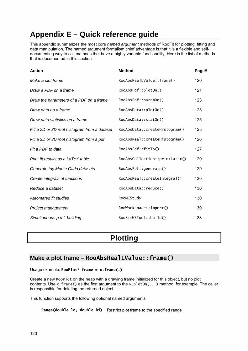
120

Appendix E – Quick reference guide This appendix summarizes the most core named argument methods of RooFit for plotting, fitting and data manipulation. The named argument formalism chief advantage is that it is a flexible and self-documenting way to call methods that have a highly variable functionality. Here is the list of methods that is documented in this section

Action Method Page#

Make a plot frame RooAbsRealLValue::frame() 120

Draw a PDF on a frame RooAbsPdf::plotOn() 121

Draw the parameters of a PDF on a frame RooAbsPdf::paramOn() 123

Draw data on a frame RooAbsData::plotOn() 123

Draw data statistics on a frame RooAbsData::statOn() 125

Fill a 2D or 3D root histogram from a dataset RooAbsData::createHistogram() 125

Fill a 2D or 3D root histogram from a pdf RooAbsReal::createHistogram() 126

Fit a PDF to data RooAbsPdf::fitTo() 127

Print fit results as a LaTeX table RooAbsCollection::printLatex() 129

Generate toy Monte Carlo datasets RooAbsPdf::generate() 129

Create integrals of functions RooAbsReal::createIntegral() 130

Reduce a dataset RooAbsData::reduce() 130

Automated fit studies RooMCStudy 130

Project management RooWorkspace::import() 130

Simultaneous p.d.f. building RooSimWSTool::build() 133

Plotting

Make a plot frame – RooAbsRealLValue::frame() Usage example: RooPlot* frame = x.frame(…) Create a new RooPlot on the heap with a drawing frame initialized for this object, but no plot contents. Use x.frame() as the first argument to the y.plotOn(...) method, for example. The caller is responsible for deleting the returned object. This function supports the following optional named arguments

Range(double lo, double hi) Restrict plot frame to the specified range

121

Range(const char* name) Restrict plot frame to range with the specified name

Bins(Int_t nbins) Set default binning for datasets to specified number of bins

AutoRange(const RooAbsData& data, double margin=0.1)

Choose plot range such that all points in given data set fit inside the range with given fractional margin.

AutoSymRange(const RooAbsData data, double margin=0.1)

Choose plot range such that all points in given data set fit inside the range and such that center of range coincides with mean of distribution in given dataset.

Name(const char* name) Give specified name to RooPlot object

Title(const char* title) Give specified title to RooPlot object

Some examples:

// Create frame with name “foo” and title “bar” x.frame(Name(“foo”),Title(“bar”)) ; // Create frame with range (-10,10) and default binning of 25 bins x.frame(Range(-10,10),Bins(25)) ; // Create frame with range that fits all events in data with 10% margin that // is centered around mean of data x.frame(AutoSymRange(data)) ;

Draw a PDF on a frame – RooAbsPdf::plotOn() Usage example: RooPlot* frame = pdf.plotOn(frame,…) ; Plots (projects) the PDF on a specified frame. If a PDF is plotted in an empty frame, it will show a unit normalized curve in the frame variable, taken at the present value of other observables defined for this PDF. If a PDF is plotted in a frame in which a dataset has already been plotted, it will show a projected curve integrated over all variables that were present in the shown dataset except for the one on the x-axis. The normalization of the curve will also be adjusted to the event count of the plotted dataset. An informational message will be printed for each projection step that is performed This function takes the following named arguments

Projection control

Slice(const RooArgSet& set) Override default projection behavior by omitting observables listed in set from the projection, resulting a 'slice' plot. Slicing is usually only sensible in discrete observables

Project(const RooArgSet& set) Override default projection behavior by projecting over observables given in set and complete ignoring the default projection behavior. Advanced use only.

122

ProjWData(const RooAbsData& d) Override default projection technique (integration by default). For observables present in given dataset projection of PDF is achieved by constructing a Monte-Carlo summation of the curve for all observable values in given set. Consult Chapter 7 for details

ProjWData(const RooArgSet& s, const RooAbsData& d)

As above but only consider subset 's' of observables in dataset 'd' for projection through data averaging

ProjectionRange(const char* rn) Override default range of projection integrals to a different range specified by given range name. This technique allows you to project a finite width slice in a real-valued observable

NormRange(const char* rn) Calculate curve normalization w.r.t. data only in specified ranges. Note that a Range(), which restricts the plotting range, by default implies a NormRange() on the same range, but this option allows to override the default, or specify a normalization ranges when the full curve is to be drawn

Miscellaneous content control

Normalization(Double_t scale, ScaleType code)

Adjust normalization by given scale factor. Interpretation of number depends on code: Relative: relative adjustment factor, NumEvent: scale to match given number of events.

Name(const chat* name) Give curve specified name in frame. Useful if curve is to be referenced later

Asymmetry(const RooCategory& c) Show the asymmetry of the PDF in given two-state category (A+-A-) / (A++A-) rather than the PDF projection. Category must have two states with indices -1 and +1 or three states with indices -1,0 and +1.

ShiftToZero(Bool_t flag) Shift entire curve such that lowest visible point is at exactly zero. Mostly useful when plotting -log(L) or χ2 distributions

AddTo(const char* name,Double_t wgtSelf, double_t wgtOther)

Add constructed projection to already existing curve with given name and relative weight factors

Plotting control

LineStyle(Int_t style) Select line style by ROOT line style code, default is solid

LineColor(Int_t color) Select line color by ROOT color code, default is blue

LineWidth(Int_t width) Select line with in pixels, default is 3

FillStyle(Int_t style) Select fill style, default is not filled. If a filled style is selected, also use VLines() to add vertical downward lines at end of curve to ensure proper closure

FillColor(Int_t color) Select fill color by ROOT color code

Range(const char* name) Only draw curve in range defined by given name

Range(double lo, double hi) Only draw curve in specified range

123

VLines() Add vertical lines to y=0 at end points of curve

Precision(Double_t eps) -- Control precision of drawn curve w.r.t to scale of plot, default is 1e-3. Higher precision will result in more and more densely spaced curve points

Invisble(Bool_t flag) Add curve to frame, but do not display. Useful in combination AddTo()

Draw parameters of a PDF on a frame – RooAbsPdf::paramOn() Usage example: pdf.paramOn(frame,…) Add a box with parameter values (and errors) to the specified frame The following named arguments are supported

Parameters(const RooArgSet& param)

Only the specified subset of parameters will be shown. By default all non-constant parameters are shown

ShowConstant(Bool_t flag) Also display constant parameters

Format(const char* optStr) Classic parameter formatting options, provided for backward compatibility

Format(const char* what,...) Parameter formatting options, details are given below

Label(const chat* label) Add header line with given label to parameter box

Layout(Double_t xmin, Double_t xmax, Double_t ymax)

Specify relative position of left, right side and top of box. Vertical size of box is calculated automatically from number lines in box

The Format(const char* what,...) has the following structure

const char* what Controls what is shown. "N" adds name, "E" adds error, "A" shows asymmetric error, "U" shows unit, "H" hides the value

FixedPrecision(int n) Controls precision, set fixed number of digits

AutoPrecision(int n) Controls precision. Number of shown digits is calculated from error + n specified additional digits (1 is sensible default)

Example use: pdf.paramOn(frame,Label("fit result"),Format("NEU",AutoPrecision(1)));

Draw data on a frame – RooAbsData::plotOn() Usage example: data.plotOn(frame,…) Plots the dataset on the specified frame. By default an unbinned dataset will use the default binning of the target frame. A binned dataset will by default retain its intrinsic binning.

124

The following optional named arguments can be used to modify the default behavior

Data representation options

Asymmetry(const RooCategory& c) Show the asymmetry of the data in given two-state category (A+-A-) / (A++A-). Category must have two states with indices -1 and +1 or three states with indices -1, 0 and +1.

Efficiency(const RooCategory& c) Show the efficiency encoded by a two-state category as (accept) / (accept+reject). Category must have two states with indices 0 and 1 that are interpreted as reject and accept respectively.

DataError(RooAbsData::EType) Select the type of error drawn: Poisson (default) draws asymmetric Poisson confidence intervals. SumW2 draws symmetric sum-of-weights error, None draws no errors

Binning(double xlo, double xhi, int nbins)

Use specified binning to draw dataset

Binning(const RooAbsBinning&) Use specified binning to draw dataset

Binning(const char* name) Use binning with specified name to draw dataset

RefreshNorm(Bool_t flag) Force refreshing for PDF normalization information in frame. If set, any subsequent PDF will normalize to this dataset, even if it is not the first one added to the frame. By default only the 1st dataset added to a frame will update the normalization information

Histogram drawing options

DrawOption(const char* opt) Select ROOT draw option for resulting TGraph object

LineStyle(Int_t style) Select line style by ROOT line style code, default is solid

LineColor(Int_t color) Select line color by ROOT color code, default is black

LineWidth(Int_t width) Select line with in pixels, default is 3

MarkerStyle(Int_t style) Select the ROOT marker style, default is 21

MarkerColor(Int_t color) Select the ROOT marker color, default is black

MarkerSize(Double_t size) Select the ROOT marker size

XErrorSize(Double_t frac) Select size of X error bar as fraction of the bin width, default is 1

Misc. other options

Name(const chat* name) Give curve specified name in frame. Useful if curve is to be referenced later

Invisble(Bool_t flag) Add curve to frame, but do not display. Useful in combination AddTo()

AddTo(const char* name, Double_t wgtSelf, Double_t

Add constructed histogram to already existing histogram

125

wgtOther) with given name and relative weight factors

Draw data statistics on a frame – RooAbsData::statOn() Usage example: data.statOn(frame,…) Add a box with statistics information to the specified frame. By default a box with the event count, mean and RMS of the plotted variable is added. The following optional named arguments are accepted

What(const char* whatstr) Controls what is printed: "N" = count, "M" is mean, "R" is RMS.

Format(const char* optStr) Classic parameter formatting options, provided for backward compatibility

Format(const char* what,...) Parameter formatting options, details given below

Label(const chat* label) Add header label to parameter box

Layout(Double_t xmin, Double_t xmax, Double_t ymax)

Specify relative position of left, right side of box and top of box. Vertical size of the box is calculated automatically from number lines in box

Cut(const char* expression) Apply given cut expression to data when calculating statistics.

CutRange(const char* rangeName)

Only consider events within given range when calculating statistics. Multiple CutRange() argument may be specified to combine ranges


const char* what

Controls what is shown. "N" adds name, "E" adds error, A" shows asymmetric error, "U" shows unit, "H" hides the value



VerbatimName(Bool_t flag) Put variable name in a \verb+ + clause.

Fill a 2D or 3D root histogram from a dataset – RooAbsData::createHistogram() Usage example: TH1* hist = data.createHistogram(name,xvar,…) Create and fill a ROOT histogram TH1,TH2 or TH3 with the values of this dataset.

126

This function accepts the following arguments

const char* name Name of the ROOT histogram

const RooAbsRealLValue& xvar Observable to be mapped on x axis of ROOT histogram

Binning(const char* name) Apply binning with given name to x axis of histogram

Binning(RooAbsBinning& binning) Apply specified binning to x axis of histogram

Binning(double lo, double hi, int nbins)

Apply specified binning to x axis of histogram

AutoBinning(Int_t nbins, Double_t margin)

Construct binning with nbins bins with a range that just fits that of the data with a given extra fractional margin.

AutoSymBinning(Int_t nbins, Double_t margin)

Construct binning with nbins bins with a range that just fits that of the data with a given extra fractional margin, but with the additional padding on one side to make the mean of the data distribution coincide with the center of the range.

YVar(const RooAbsRealLValue& var,...)

Observable to be mapped on y axis of ROOT histogram

ZVar(const RooAbsRealLValue& var,...)

Observable to be mapped on z axis of ROOT histogram

The YVar() and ZVar() arguments can be supplied with optional Binning() arguments to control the binning of the Y and Z axes, e.g. createHistogram("histo",x,Binning(-1,1,20), YVar(y,Binning(-1,1,30)), ZVar(z,Binning("zbinning"))) The caller takes ownership of the returned histogram

Fill a 2D or 3D root histogram from a PDF – RooAbsReal::createHistogram() Usage example: TH1* hist = pdf.createHistogram(name,xvar,…) Create and fill a ROOT histogram TH1, TH2 or TH3 with the values of this function. This function accepts the following arguments

const char* name Name of the ROOT histogram

const RooAbsRealLValue& xvar Observable to be mapped on x axis of ROOT histogram

Binning(const char* name) Apply binning with given name to x axis of histogram

127

Binning(RooAbsBinning& binning) Apply specified binning to x axis of histogram

Binning(double lo, double hi, int nbins)

Apply specified binning to x axis of histogram

ConditionalObservables(const RooArgSet& set)

Do not normalized PDF over following observables when projecting PDF into histogram

Scaling(Bool_t flag) Apply density-correction scaling (multiply by bin volume), default is kTRUE

YVar(const RooAbsRealLValue& var,...)

Observable to be mapped on y axis of ROOT histogram

ZVar(const RooAbsRealLValue& var,...)

Observable to be mapped on z axis of ROOT histogram

The YVar() and ZVar() arguments can be supplied with optional Binning() arguments to control the binning of the Y and Z axes, e.g. createHistogram("histo",x,Binning(-1,1,20), YVar(y,Binning(-1,1,30)), ZVar(z,Binning("zbinning"))) The caller takes ownership of the returned histogram.

Fitting and generating

Fit a PDF to data – RooAbsPdf::fitTo() Usage example: pdf.fitTo(data,…) Fit PDF to given dataset. If dataset is unbinned, an unbinned maximum likelihood is performed. If the dataset is binned, a binned maximum likelihood is performed. By default the fit is executed through the MINUIT commands MIGRAD, HESSE and MINOS in succession. The following named arguments are supported

Options to control construction of -log(L)


Do not normalize PDF over listed observables

Extended(Bool_t flag) Control addition of extended likelihood term, automatically determined by default

Range(const char* name) Fit only data inside range with given name

Range(Double_t lo, Double_t hi) Fit only data inside given range. A range named "fit" is created on the fly on all observables.

NumCPU(int num) Parallelize NLL calculation on num CPUs

Optimize(Bool_t flag) Activate constant term optimization (on by default)

128

SplitRange(Bool_t flag) Use separate fit ranges in a simultaneous fit. Actual range name for each subsample is assumed to by rangeName_{indexState} where indexState is the state of the master index category of the simultaneous fit

Constrain(const RooArgSet& pars) Include constraints to listed parameters in likelihood using internal constrains in p.d.f

ExternalConstraints(const RooArgSet& cpdfs)

Include given external constraint p.d.f.s to likelihood

Options to control flow of fit procedure

InitialHesse(Bool_t flag) Flag controls if HESSE before MIGRAD as well, off by default

Hesse(Bool_t flag) Flag controls if HESSE is run after MIGRAD, on by default

Minos(Bool_t flag) Flag controls if MINOS is run after HESSE, on by default

Minos(const RooArgSet& set) Only run MINOS on given subset of arguments

Save(Bool_t flag) Flag controls if RooFitResult object is produced and returned, off by default

Strategy(Int_t flag) Set MINUIT strategy (0 through 2, default is 1)

FitOptions(const char* optStr) Steer fit with classic options string (for backward compatibility). Use of this option excludes use of any of the new style steering options

EvalErrorWall(Bool_t flag) Activate ‘likelihood wall’ to force MIGRAD to retreat when evaluation errors occur in the likelihood expression. On by default.

Options to control informational output

Verbose(Bool_t flag) Flag controls if verbose output is printed (NLL, parameter changes during fit

Timer(Bool_t flag) Time CPU and wall clock consumption of fit steps, off by default

PrintLevel(Int_t level) Set MINUIT print level (1 through 3, default is 1). At 1 all RooFit informational messages are suppressed as well.

PrintEvalErrors(Int_t numErr) Control number of p.d.f evaluation errors printed per likelihood evaluation. A negative value suppress output completely, a zero value will only print the error count per p.d.f component, a positive value is will print details of each error up to numErr messages per p.d.f component.

129

Print fit results as a LaTeX table – RooAbsCollection::printLatex() Usage example: paramList.printLatex(…) ; Output content of collection as LaTex table. By default a table with two columns is created: the left column contains the name of each variable, the right column the value. The following optional named arguments can be used to modify the default behavior

Columns(Int_t ncol) Fold table into multiple columns, i.e. ncol=3 will result in 3 x 2 = 6 total columns

Sibling(const RooAbsCollection& other)

Define sibling list. The sibling list is assumed to have objects with the same name in the same order. If this is not the case warnings will be printed. If a single sibling list is specified, 3 columns will be output: the (common) name, the value of this list and the value in the sibling list. Multiple sibling lists can be specified by repeating the Sibling() command.

Format(const char* str) Classic format string, provided for backward compatibility

Format(...) Formatting arguments, details are given below

OutputFile(const char* fname) Send output to file with given name rather than standard output


const char* what Controls what is shown. "N" adds name, "E" adds error, "A" shows asymmetric error, "U" shows unit, "H" hides the value



VerbatimName(Bool_t flag) Put variable name in a \verb+ + clause.

Example use: list.printLatex(Columns(2), Format("NEU",AutoPrecision(1),VerbatimName()) ) ;

Generate toy Monte Carlo datasets – RooAbsPdf::generate() Usage example: RooDataSet* data = pdf.generate(x,…) ; Generate a new dataset containing the specified variables with events sampled from our distribution. Generate the specified number of events or expectedEvents() if not specified. Any variables of this PDF that are not in whatVars will use their current values and be treated as fixed parameters. Returns zero in case of an error. The caller takes ownership of the returned dataset.

130

The following named arguments are supported

Verbose(Bool_t flag) Print informational messages during event generation

NumEvent(int nevt) Generate specified number of events

Extended() The actual number of events generated will be sampled from a Poisson distribution with mu=nevt. For use with extended maximum likelihood fits

ProtoData(const RooDataSet& data, Bool_t randOrder, Bool_t

resample)

Use specified dataset as prototype dataset. If randOrder is set to true the order of the events in the dataset will be read in a random order the order of the events in the dataset will be read in a random order number of events in the prototype dataset. If resample is true events are taken from the prototype dataset through sampling rather than through traversal.

If ProtoData() is used, the specified existing dataset as a prototype: the new dataset will contain the same number of events as the prototype (unless otherwise specified), and any prototype variables not in whatVars will be copied into the new dataset for each generated event and also used to set our PDF parameters. The user can specify a number of events to generate that will override the default. The result is a copy of the prototype dataset with only variables in whatVars randomized. Variables in whatVars that are not in the prototype will be added as new columns to the generated dataset.

Create integrals of functions– RooAbsReal::createIntegral() Usage example: RooAbsReal* intOfFunc = func.createIntegral(x,…) ; Create an object that represents the integral of the function over one or more observables listed in iset The actual integration calculation is only performed when the return object is evaluated. The name of the integral object is automatically constructed from the name of the input function, the variables it integrates and the range integrates over The following named arguments are accepted

NormSet(const RooArgSet&) Specify normalization set, mostly useful when working with PDFS

NumIntConfig(const RooNumIntConfig&)

Use given configuration for any numeric integration, if necessary

Range(const char* name) Integrate only over given range. Multiple ranges may be specified by passing multiple Range() arguments

Data manipulation

Reduce a dataset – RooAbsData::reduce()

131

Usage example: RooAbsData* reducedData = data.reduce(…) ; Create a reduced copy of this dataset. The caller takes ownership of the returned dataset The following optional named arguments are accepted

SelectVars(const RooArgSet& vars)

Only retain the listed observables in the output dataset

Cut(const char* expression) Only retain event surviving the given cut expression

Cut(const RooFormulaVar& expr)

Only retain event surviving the given cut formula

CutRange(const char* name) Only retain events inside range with given name. Multiple CutRange arguments may be given to select multiple ranges

EventRange(int lo, int hi) Only retain events with given sequential event numbers

Name(const char* name) Give specified name to output dataset

Title(const char* name) Give specified title to output dataset

Automation tools

Automated fit studies – class RooMCStudy Usage example: RooMCStudy mgr(model,observables,…) ; Construct Monte Carlo Study Manager. This class automates generating data from a given PDF, fitting the PDF to that data and accumulating the fit statistics. The constructor accepts the following arguments

const RooAbsPdf& model The PDF to be studied

const RooArgSet& observables The variables of the PDF to be considered the observables

FitModel(const RooAbsPdf&) The PDF for fitting, if it is different from the PDF for generating


The set of observables that the PDF should not be normalized over

Binned(Bool_t flag) Bin the dataset before fitting it. Speeds up fitting of large data samples

FitOptions(const char*) Classic fit options, provided for backward compatibility

FitOptions(....) Options to be used for fitting. All named arguments inside FitOptions()are passed to RooAbsPdf::fitTo();

132

Verbose(Bool_t flag) Activate informational messages in event generation phase

Extended(Bool_t flag) Determine number of events for each sample anew from a Poisson distribution

ProtoData(const RooDataSet&, Bool_t randOrder)

Prototype data for the event generation. If the randOrder flag is set, the order of the dataset will be re-randomized for each generation cycle to protect against systematic biases if the number of generated events does not exactly match the number of events in the prototype dataset at the cost of reduced precision with mu equal to the specified number of events

Constrain(const RooArgSet& pars) Apply internal constraints on given parameters in fit and sample constrained parameter values from constraint p.d.f for each toy.

ExternalConstraints(const RooArgSet& cpdfs)

Apply given external constraints in likelihood and sample constrained parameter values from constraint p.d.f. for each toy.

The plotParam() method plots the distribution of the fitted value of the given parameter on a newly created frame. This function accepts the following optional arguments

FrameRange(double lo, double hi) Set range of frame to given specification

FrameBins(int bins) Set default number of bins of frame to given number

Frame(...) Pass supplied named arguments to RooAbsRealLValue::frame() function. See frame() function for list of allowed arguments

If no frame specifications are given, the AutoRange() feature will be used to set the range. Any other named argument is passed to the RooAbsData::plotOn() call. See that function for allowed options The plotPull() method plots the distribution of pull values for the specified parameter on a newly created frame. If asymmetric errors are calculated in the fit (by MINOS) those will be used in the pull calculation This function accepts the following optional arguments

FrameRange(double lo, double hi)

Set range of frame to given specification

FrameBins(int bins) Set default number of bins of frame to given number

Frame(...) Pass supplied named arguments to RooAbsRealLValue::frame() function. See frame() function for list of allowed arguments

FitGauss(Bool_t flag) Add a Gaussian fit to the frame

If no frame specifications are given, the AutoSymRange() feature will be used to set the range Any other named argument is passed to the RooAbsData::plotOn() call. See that function for allowed options

133

Project management – RooWorkspace::import() Usage example: ws.import(pdf,RenameConflictNodes(“_my”)) ; Import a RooAbsArg object, e.g. function, p.d.f or variable into the workspace. This import function clones the input argument and will own the clone. If a composite object is offered for import, e.g. a p.d.f with parameters and observables, the complete tree of objects is imported. If any of the -variables of a composite object (parameters/observables) are already in the workspace the imported p.d.f. is connected to the already existing variables. If any of the function objects (p.d.f, formulas) to be imported already exists in the workspace an error message is printed and the import of the entire tree of objects is cancelled. Several optional arguments can be provided to modify the import procedure. The import accepts the following arguments for importing value objects (functions & variables)

const RooAbsArg& inArg The imported function/p.d.f

RenameConflictNodes(const char* suffix)

Add suffix to branch node name if name conflicts with existing node in workspace

RenameNodes(const char* suffix) Add suffix to all branch node names including top level node

RenameVariable(const char* inputName, const char*

outputName)

Rename variable as specified upon import

RecycleConflictNodes() If any of the function objects to be imported already exist in the name space, connect the imported expression to the already existing nodes. WARNING: use with care! If function definitions do not match, this alters the definition of your function upon import

The import accepts the following arguments for importing data objects

const RooAbsData& inData The imported dataset.

RenameDataset(const char* suffix)

Rename dataset upon insertion

RenameVariable(const char* inputName, const char*

outputName)

Change names of observables in dataset upon insertion.

Simultaneous p.d.f building – RooSimWSTool::build() Usage example: wstool.build(“simPdf”,”protoPdf”,SplitParam(mean,runBlock)) ; Construct a simultaneous p.d.f. from a prototype p.d.f. with one or more parameter splitting specifications. The build function accepts the following arguments

const char* simPdfName Name of the output simultaneous p.d.f. that is built

134

const char* protoPdfName Name of the prototype p.d.f. in the workspace that is to be used as template for the build

SplitParam(const char* varName, const char* catName)

Split parameter with given name(s) in categories with given name(s). Each argument may contain wildcards and comma separated lists. All referenced variables and categories must exist in the associated workspace

SplitParam(const RooArgSet& vars, const RooArgSet& cats)

Split given parameter(s) in given categories. All referenced variables and categories must exist in the associated workspace

SplitParamConstrained(const char* varName, const char*

catName, const char* remainderStateName

Split parameter with given name(s) in categories with given name(s). The specialization for the category state name matching remainderState will be a formula object that evaluates to 1 minus the sum of all other specialization, thus effectively constructing a constrained split with fractions adding up to one over the split. Each argument may contain wildcards and comma separated lists. All referenced variables and categories must exist in the associated workspace

SplitParamConstrained(const RooArgSet& varSet, const

RooArgSet& catSet, const char* remainderStateName

Version of constrained split argument with references to variables and categories instead of name specifications.

Restrict(const char* catName, const char* stateNameList)

Restrict build to list of states given in stateNameList for given category.

RooFit Users Manual 2.91-33

Documents

building composite models

background composite

plotting composite models

composite objects

setup of roofit

generating data

tutorial macros

roofit users manual