Robust Principal Component Analysis on Graphs - arXiv · 2 TABLE I: A comparison of various PCA models and their properties. X2Rp nis the data matrix, U2Rp dand Q2Rd n are the principal

Page 1

1

Robust Principal Component Analysis on GraphsNauman Shahid∗, Vassilis Kalofolias∗, Xavier Bresson∗, Michael Bronstein†, Pierre Vandergheynst∗∗Signal Processing Laboratory (LTS2), EPFL, Switzerland, Email: [email protected]

† Universita della Svizzera Italiana, Switzerland, Email: [email protected]

Abstract

Principal Component Analysis (PCA) is the most widely used tool for linear dimensionality reduction and clustering. Still it ishighly sensitive to outliers and does not scale well with respect to the number of data samples. Robust PCA solves the first issuewith a sparse penalty term. The second issue can be handled with the matrix factorization model, which is however non-convex.Besides, PCA based clustering can also be enhanced by using a graph of data similarity. In this article, we introduce a new modelcalled ‘Robust PCA on Graphs’ which incorporates spectral graph regularization into the Robust PCA framework. Our proposedmodel benefits from 1) the robustness of principal components to occlusions and missing values, 2) enhanced low-rank recovery,3) improved clustering property due to the graph smoothness assumption on the low-rank matrix, and 4) convexity of the resultingoptimization problem. Extensive experiments on 8 benchmark, 3 video and 2 artificial datasets with corruptions clearly reveal thatour model outperforms 10 other state-of-the-art models in its clustering and low-rank recovery tasks.

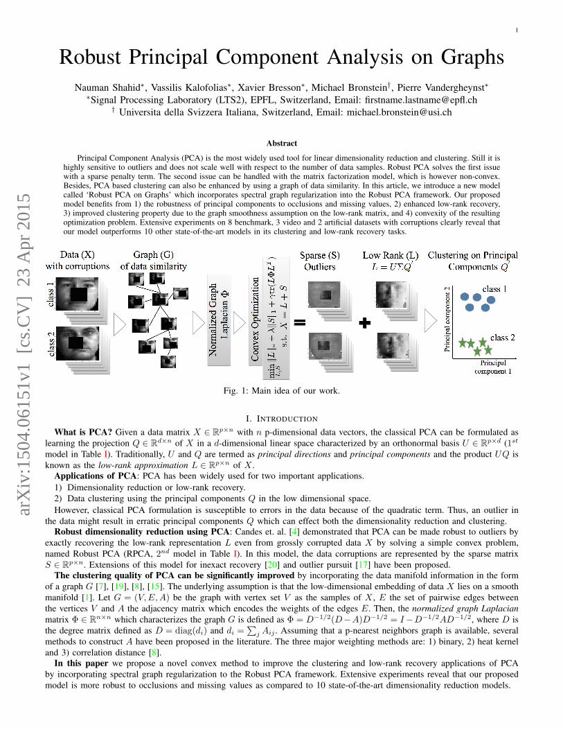
Fig. 1: Main idea of our work.

I. INTRODUCTION

What is PCA? Given a data matrix X ∈ Rp×n with n p-dimensional data vectors, the classical PCA can be formulated aslearning the projection Q ∈ Rd×n of X in a d-dimensional linear space characterized by an orthonormal basis U ∈ Rp×d (1st

model in Table I). Traditionally, U and Q are termed as principal directions and principal components and the product UQ isknown as the low-rank approximation L ∈ Rp×n of X .

Applications of PCA: PCA has been widely used for two important applications.1) Dimensionality reduction or low-rank recovery.2) Data clustering using the principal components Q in the low dimensional space.However, classical PCA formulation is susceptible to errors in the data because of the quadratic term. Thus, an outlier in

the data might result in erratic principal components Q which can effect both the dimensionality reduction and clustering.Robust dimensionality reduction using PCA: Candes et. al. [4] demonstrated that PCA can be made robust to outliers by

exactly recovering the low-rank representation L even from grossly corrupted data X by solving a simple convex problem,named Robust PCA (RPCA, 2nd model in Table I). In this model, the data corruptions are represented by the sparse matrixS ∈ Rp×n. Extensions of this model for inexact recovery [20] and outlier pursuit [17] have been proposed.

The clustering quality of PCA can be significantly improved by incorporating the data manifold information in the formof a graph G [7], [19], [8], [15]. The underlying assumption is that the low-dimensional embedding of data X lies on a smoothmanifold [1]. Let G = (V,E,A) be the graph with vertex set V as the samples of X , E the set of pairwise edges betweenthe vertices V and A the adjacency matrix which encodes the weights of the edges E. Then, the normalized graph Laplacianmatrix Φ ∈ Rn×n which characterizes the graph G is defined as Φ = D−1/2(D−A)D−1/2 = I−D−1/2AD−1/2, where D isthe degree matrix defined as D = diag(di) and di =

∑j Aij . Assuming that a p-nearest neighbors graph is available, several

methods to construct A have been proposed in the literature. The three major weighting methods are: 1) binary, 2) heat kerneland 3) correlation distance [8].

In this paper we propose a novel convex method to improve the clustering and low-rank recovery applications of PCAby incorporating spectral graph regularization to the Robust PCA framework. Extensive experiments reveal that our proposedmodel is more robust to occlusions and missing values as compared to 10 state-of-the-art dimensionality reduction models.

arX

iv:1

504.

0615

1v1

[cs

.CV

] 2

3 A

pr 2

015

Page 2

2

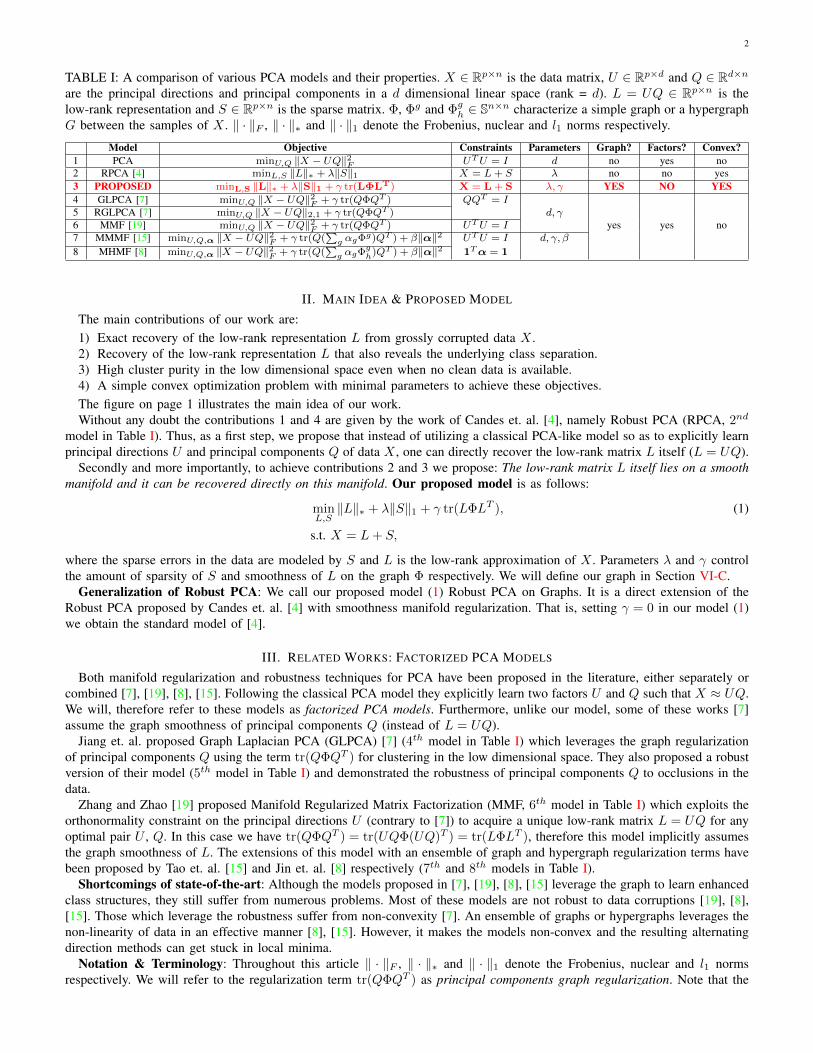
TABLE I: A comparison of various PCA models and their properties. X ∈ Rp×n is the data matrix, U ∈ Rp×d and Q ∈ Rd×nare the principal directions and principal components in a d dimensional linear space (rank = d). L = UQ ∈ Rp×n is thelow-rank representation and S ∈ Rp×n is the sparse matrix. Φ, Φg and Φgh ∈ Sn×n characterize a simple graph or a hypergraphG between the samples of X . ‖ · ‖F , ‖ · ‖∗ and ‖ · ‖1 denote the Frobenius, nuclear and l1 norms respectively.

Model Objective Constraints Parameters Graph? Factors? Convex?1 PCA minU,Q ‖X − UQ‖2F UTU = I d no yes no2 RPCA [4] minL,S ‖L‖∗ + λ‖S‖1 X = L+ S λ no no yes3 PROPOSED minL,S ‖L‖∗ + λ‖S‖1 + γ tr(LΦLT) X = L + S λ, γ YES NO YES4 GLPCA [7] minU,Q ‖X − UQ‖2F + γ tr(QΦQT ) QQT = I5 RGLPCA [7] minU,Q ‖X − UQ‖2,1 + γ tr(QΦQT ) d, γ6 MMF [19] minU,Q ‖X − UQ‖2F + γ tr(QΦQT ) UTU = I yes yes no7 MMMF [15] minU,Q,α ‖X − UQ‖2F + γ tr(Q(

∑g αgΦg)QT ) + β‖α‖2 UTU = I d, γ, β

8 MHMF [8] minU,Q,α ‖X − UQ‖2F + γ tr(Q(∑

g αgΦgh)QT ) + β‖α‖2 1Tα = 1

II. MAIN IDEA & PROPOSED MODEL

The main contributions of our work are:1) Exact recovery of the low-rank representation L from grossly corrupted data X .2) Recovery of the low-rank representation L that also reveals the underlying class separation.3) High cluster purity in the low dimensional space even when no clean data is available.4) A simple convex optimization problem with minimal parameters to achieve these objectives.The figure on page 1 illustrates the main idea of our work.Without any doubt the contributions 1 and 4 are given by the work of Candes et. al. [4], namely Robust PCA (RPCA, 2nd

model in Table I). Thus, as a first step, we propose that instead of utilizing a classical PCA-like model so as to explicitly learnprincipal directions U and principal components Q of data X , one can directly recover the low-rank matrix L itself (L = UQ).

Secondly and more importantly, to achieve contributions 2 and 3 we propose: The low-rank matrix L itself lies on a smoothmanifold and it can be recovered directly on this manifold. Our proposed model is as follows:

minL,S‖L‖∗ + λ‖S‖1 + γ tr(LΦLT ), (1)

s.t. X = L+ S,

where the sparse errors in the data are modeled by S and L is the low-rank approximation of X . Parameters λ and γ controlthe amount of sparsity of S and smoothness of L on the graph Φ respectively. We will define our graph in Section VI-C.

Generalization of Robust PCA: We call our proposed model (1) Robust PCA on Graphs. It is a direct extension of theRobust PCA proposed by Candes et. al. [4] with smoothness manifold regularization. That is, setting γ = 0 in our model (1)we obtain the standard model of [4].

III. RELATED WORKS: FACTORIZED PCA MODELS

Both manifold regularization and robustness techniques for PCA have been proposed in the literature, either separately orcombined [7], [19], [8], [15]. Following the classical PCA model they explicitly learn two factors U and Q such that X ≈ UQ.We will, therefore refer to these models as factorized PCA models. Furthermore, unlike our model, some of these works [7]assume the graph smoothness of principal components Q (instead of L = UQ).

Jiang et. al. proposed Graph Laplacian PCA (GLPCA) [7] (4th model in Table I) which leverages the graph regularizationof principal components Q using the term tr(QΦQT ) for clustering in the low dimensional space. They also proposed a robustversion of their model (5th model in Table I) and demonstrated the robustness of principal components Q to occlusions in thedata.

Zhang and Zhao [19] proposed Manifold Regularized Matrix Factorization (MMF, 6th model in Table I) which exploits theorthonormality constraint on the principal directions U (contrary to [7]) to acquire a unique low-rank matrix L = UQ for anyoptimal pair U , Q. In this case we have tr(QΦQT ) = tr(UQΦ(UQ)T ) = tr(LΦLT ), therefore this model implicitly assumesthe graph smoothness of L. The extensions of this model with an ensemble of graph and hypergraph regularization terms havebeen proposed by Tao et. al. [15] and Jin et. al. [8] respectively (7th and 8th models in Table I).

Shortcomings of state-of-the-art: Although the models proposed in [7], [19], [8], [15] leverage the graph to learn enhancedclass structures, they still suffer from numerous problems. Most of these models are not robust to data corruptions [19], [8],[15]. Those which leverage the robustness suffer from non-convexity [7]. An ensemble of graphs or hypergraphs leverages thenon-linearity of data in an effective manner [8], [15]. However, it makes the models non-convex and the resulting alternatingdirection methods can get stuck in local minima.

Notation & Terminology: Throughout this article ‖ · ‖F , ‖ · ‖∗ and ‖ · ‖1 denote the Frobenius, nuclear and l1 normsrespectively. We will refer to the regularization term tr(QΦQT ) as principal components graph regularization. Note that the

Page 3

3

graph regularization involves principal components Q, not principal directions U . We will also refer to the regularization termtr(LΦLT ) as low-rank graph regularization. RPCA and our proposed models (2nd and 3rd models in Table I) which performexact low-rank recovery by splitting X = L+ S will be referred to as non-factorized PCA models. A comparison of variousPCA models introduced so far is presented in Table I. Note that only RPCA and our proposed model leverage convexity andenjoy a unique global optimum with guaranteed convergence.

IV. COMPARISON WITH RELATED WORKS

The main differences between our model (1) and the various state-of-the-art factorized PCA models [7], [19], [12], [8], [15]are, as summarized in Table I, the following.

Non-factorized model: Instead of explicitly learning the principal directions U and principal components Q, it learns theirproduct, i.e. the low-rank matrix L. Hence, (1) is a non-factorized PCA model.

Exact low-rank recovery: Unlike factorized models we target the exact low-rank recovery by modeling the data matrix asthe sum of low-rank L and a sparse matrix S.

Different graph regularization term: Model (1) is based on the assumption that it is the low-rank matrix L that is smoothon the graph, and not just the principal components matrix Q. Therefore we replace the principal components graph termtr(QΦQ>) with the low-rank graph term tr(LΦL>). Note that as explained in Section III, the two terms are only equivalentif orthogonality of U is further assumed, as in [19], [12], [8], [15] and not in [7].

A. Advantages over Factorized PCA ModelsRobustness to gross corruptions for clustering & low-rank recovery: The low-rank graph tr(LΦLT ) can be more realistic

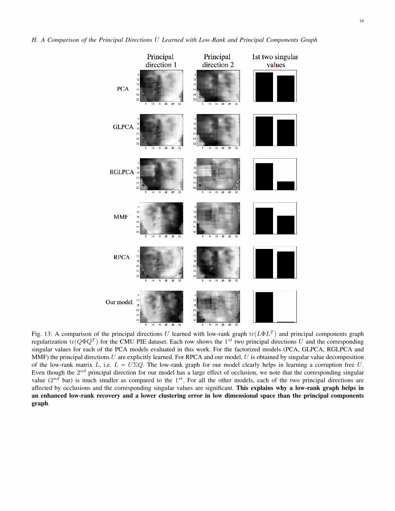
than the principal components graph tr(QΦQT ). It allows the principal directions U to benefit from the graph regularizationas well (recall that L = UQ). Thus, our model enjoys an enhanced low-rank recovery and class separation even from grosslycorrupted data. For details, please refer to Sections VII & VIII (also see Fig. 13 in supplementary material).

Convexity: It is a strictly convex problem and a unique global optimum can be obtained by using standard methods like anAlternating Direction Method of Multipliers (ADMM) [2].

One model parameter only: Our model does not require the rank of L to be specified up-front. The nuclear norm relaxationenables the automatic selection of an appropriate rank based on the parameters λ and γ. Furthermore, as illustrated in ourexperiments, the value λ = 1/

√max(n, p) proposed in [4] gives very good results. As a result, the only unknown parameter

to be selected is γ, and for this we can use methods such as cross validation (For additional details please see Figs. 16 & 17in the supplementary material).

V. OPTIMIZATION SOLUTION

We use an ADMM [2] to rewrite Problem (1):

minL,S,W

‖L‖∗ + λ‖S‖1 + γ tr(WΦWT )

s.t. X = L+ S, L = W.

Thus, the augmented Lagrangian and iterative scheme are:

(L, S,W )k+1 = argminL,S,W

‖L‖∗ + λ‖S‖1 + γ tr(WΦWT )

+ 〈Zk1 , X − L− S〉 +r12‖X − L− S‖2F

+ 〈Zk2 ,W − L〉+r22‖W − L‖2F ,

Zk+11 = Zk1 + r1(X − Lk+1 − Sk+1),

Zk+12 = Zk2 + r2(W k+1 − Lk+1),

where Z1 ∈ Rp×n and Z2 ∈ Rp×n are the lagrange multipliers and k is the iteration index. Let Hk1 = X − Sk + Zk1 /r1 and

Hk2 = W k + Zk2 /r2, then this reduces to the following updates for L, S and W as:

Lk+1 = prox 1(r1+r2)

‖L‖∗

(r1Hk1 + r2H

k2

r1 + r2

),

Sk+1 = prox λr1‖S‖1

(X − Lk+1 +

Zk1r1

),

W k+1 = r2(γΦ + r2I)−1(Lk+1 − Zk2

r2

),

where proxf is the proximity operator of the convex function f as defined in [5]. The details of this solution, algorithm,convergence and computational complexity are given in the supplementary material Sections A, B & C.

Page 4

4

VI. EXPERIMENTAL SETUP

We use the model (1) to solve two major PCA-based problems.1) Data clustering in low-dimensional space with corrupted and uncorrupted data (Section VII ).2) Low-rank recovery from corrupted data (Section VIII).Our extensive experimental setup is designed to test the robustness and generalization capability of our model to a wide

variety of datasets and corruptions for the above two applications. Precisely, we perform our experiments on 8 benchmark,3 video and 2 artificial datasets with 10 different types of corruptions and compare with 10 state-of-the-art dimensionalityreduction models as explained in sections VI-A & VI-B.

A. Setup for Clustering

1) Datasets: All the datasets are well-known benchmarks. The 6 image databases include CMU PIE1, ORL2, YALE3,COIL204, MNIST5 and USPS data sets. MFeat database 6 consists of features extracted from handwritten numerals and theBCI database7 comprises of features extracted from a Brain Computer Interface setup. Our choice of datasets is based ontheir various properties such as pose changes, rotation (for digits), data type and non-negativity, as presented in Table II in thesupplementary material.

2) Comparison with 10 models: We compare the clustering performance of our model with k-means on the original dataX and 9 other dimensionality reduction models. These models can be divided into two categories.

1. Models without graph: 1) classical Principal Component Analysis (PCA) 2) Non-negative Matrix Factorization (NMF)[10] and 4) Robust PCA (RPCA) [4].

2. Models with graph: These models can be further divided into two categories based on the graph type. a. Principalcomponents graph: 1) Normalized Cuts (NCuts) [14], 2) Laplacian Eigenmaps (LE) [1], 3) Graph Laplacian PCA (GLPCA)[7], 4) Robust Graph Laplacian PCA (RGLPCA) [7], 5) Manifold Regularized Matrix Factorization (MMF) [19], 6) GraphRegularized Non-negative Matrix Factorization (GNMF) [3], b. Low-rank graph: Our proposed model.

Table II and Fig. 9 in the supplementary material give a summary of all the models.3) Corruptions in datasets: Corruptions in image databases: We introduce three types of corruptions in each of the 6

image databases:1. No corruptions.2. Fully corrupted data. Two types of corruptions are introduced in all the images of each database: a) Block occlusions

ranging from 10 to 40% of the image size. b) Missing pixels ranging from 10% to 40% of the total pixels in the image. Thesecorruptions are modeled by placing zeros uniformly randomly in the images.

3. Sample specific corruptions. The above two types of corruptions (occlusions and missing pixels) are introduced in only25% of the images of each database.

Corruptions in non-image databases: We introduce only full and sample specific missing values in the non-image databasesbecause the block occlusions in non-image databases correspond to an unrealistic assumption. Example missing pixels andblock occlusions in the image are shown in Fig. 10 in the supplementary material.

Pre-processing: For NCuts, LE, PCA, GLPCA, RGLPCA, MMF, RPCA and our model we pre-process the datasets to zeromean and unit standard deviation along the features. Additionally for MMF all the samples are made unit norm as suggestedin [19]. For NMF and GNMF we only pre-process the non-negative datasets to unit norm along the samples. We performpre-processing after introducing the corruptions.

4) Clustering Metric: We use clustering error to evaluate the clustering performance of all the models considered in thiswork. The clustering error is E = ( 1

n

∑kr=1 nr) × 100, where nr is the number of misclassified samples in cluster r. We

report the minimum clustering error from 10 runs of k-means (k = number of classes) on the principal components Q. Thisprocedure reduces the bias introduced by the non-convex nature of k-means. For RPCA and our model we obtain principalcomponents Q

′via SVD of the low-rank matrix L = UΣQ

′during the nuclear proximal update in every iteration. For more

details of the clustering error evaluation and parameter selection scheme for each of the models, please refer to Fig. 11 andTable III of the supplementary material.

1http://vasc.ri.cmu.edu/idb/html/face/2http://www.cl.cam.ac.uk/research/dtg/attarchive/facedatabase.html3http://vision.ucsd.edu/content/yale-face-database4http://www.cs.columbia.edu/CAVE/software/softlib/coil-20.php5http://yann.lecun.com/exdb/mnist/6https://archive.ics.uci.edu/ml/datasets/Multiple+Features7http://olivier.chapelle.cc/ssl-book/benchmarks.html

Page 5

5

B. Setup for Low-Rank Recovery

Since the low-rank ground truth for the 8 benchmark datasets used for clustering is not available, we perform the followingtwo types of experiments.

1) Quantitative evaluation of the normalized low-rank reconstruction error using corrupted artificial datasets.2) Visualization of the recovered low-rank representations for 1) occluded images of the CMU PIE dataset and 2) static

background of 3 different videos8.

C. Normalized Graph Laplacian

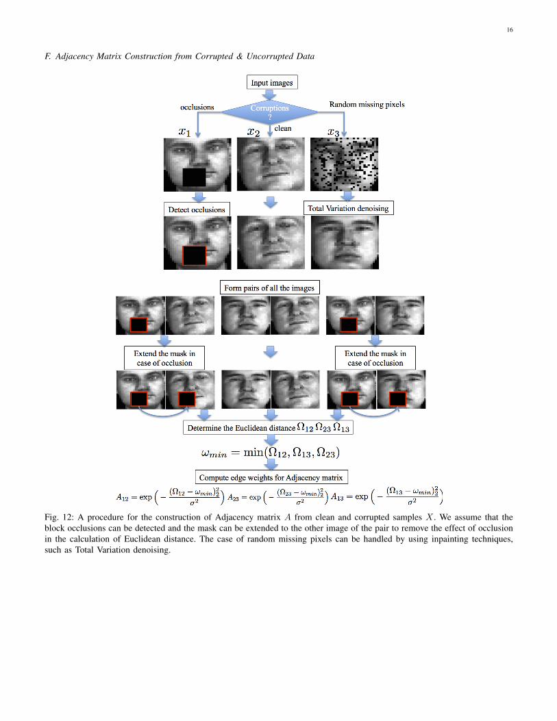
In order to construct the graph Laplacian Φ, the pairwise Euclidean distance is computed between each pair of the vectorizeddata samples (xi, xj). Let Ω be the matrix which contains all the pairwise distances, then Ωij , the Euclidean distance betweenxi and xj is given as:

Case I: Block Occlusions

Ωij =

√‖Mij (xi − xj)‖22

‖Mij‖1,

where Mij ∈ 0, 1p is the vector mask corresponding to the intersection of uncorrupted values in xi and xj . Thus

M lij =

1 if features xli & xlj observed,0 otherwise

Thus, we detect the block occlusions and consider only the observed pixels.Case II: Random Missing Values: We use a Total Variation denoising procedure and calculate Ωij using the cleaned

images.Let ωmin be the minimum of all the pairwise distances in Ω. Then the adjacency matrix A for the graph G is constructed

by using

Aij = exp(− (Ωij − ωmin)2

σ2

)Finally, the normalized graph Laplacian Φ = I − D−1/2AD−1/2 is calculated, where D is the degree matrix. Note that

different types of data might call for different distance metrics and values of σ2, however for all the experiments and datasetsused in this work the Euclidean distance metric and σ2 = 0.05 work well. To clarify further for the reader, we present adetailed example of graph construction with corrupted and uncorrupted images in Fig. 12 of supplementary material.

VII. CLUSTERING IN LOW DIMENSIONAL SPACE

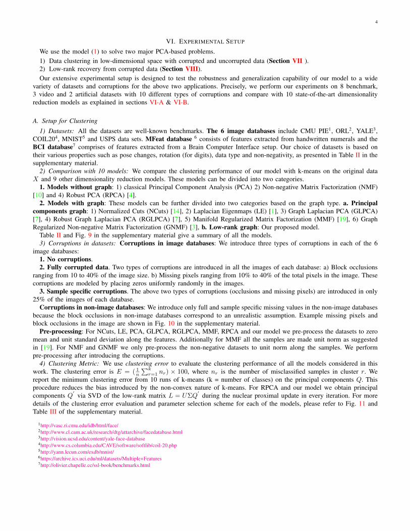
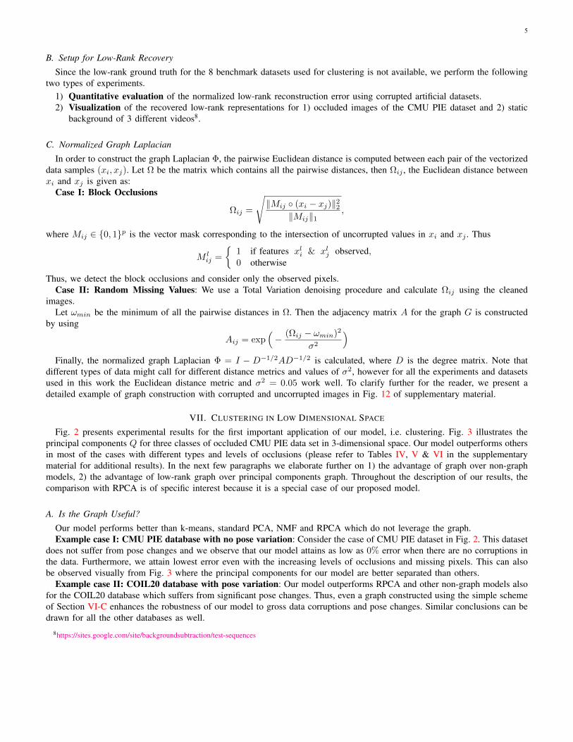
Fig. 2 presents experimental results for the first important application of our model, i.e. clustering. Fig. 3 illustrates theprincipal components Q for three classes of occluded CMU PIE data set in 3-dimensional space. Our model outperforms othersin most of the cases with different types and levels of occlusions (please refer to Tables IV, V & VI in the supplementarymaterial for additional results). In the next few paragraphs we elaborate further on 1) the advantage of graph over non-graphmodels, 2) the advantage of low-rank graph over principal components graph. Throughout the description of our results, thecomparison with RPCA is of specific interest because it is a special case of our proposed model.

A. Is the Graph Useful?

Our model performs better than k-means, standard PCA, NMF and RPCA which do not leverage the graph.Example case I: CMU PIE database with no pose variation: Consider the case of CMU PIE dataset in Fig. 2. This dataset

does not suffer from pose changes and we observe that our model attains as low as 0% error when there are no corruptions inthe data. Furthermore, we attain lowest error even with the increasing levels of occlusions and missing pixels. This can alsobe observed visually from Fig. 3 where the principal components for our model are better separated than others.

Example case II: COIL20 database with pose variation: Our model outperforms RPCA and other non-graph models alsofor the COIL20 database which suffers from significant pose changes. Thus, even a graph constructed using the simple schemeof Section VI-C enhances the robustness of our model to gross data corruptions and pose changes. Similar conclusions can bedrawn for all the other databases as well.

8https://sites.google.com/site/backgroundsubtraction/test-sequences

Page 6

6

Fig. 2: Clustering error of various dimensionality reduction models for CMU PIE, ORL, YALE & COIL20 datasets. Thecompared models are: 1) k-means without dimensionality reduction 2) Normalized Cuts (NCuts) [14] 3) Laplacian Eigenmaps(LE) [1] 4) classical Principal Component Analysis (PCA) 5) Graph Laplacian PCA (GLPCA) [7] 6) Robust Graph LaplacianPCA (RGLPCA) [7] 7) Manifold Regularized Matrix Factorization (MMF) [19] 8) Non-negative Matrix Factorization [10]9) Graph Regularized Non-negative Matrix Factorization (GNMF) [3], 10) Robust PCA (RPCA) [4] and 11) Robust PCA onGraphs (proposed model). Two types of full and partial corruptions are introduced in the data: 1) Block occlusions and 2)Random missing values. The numerical errors corresponding to this figure along with additional results on MNIST, USPS,MFeat and BCI datasets are presented in Tables IV, V & VI of the supplementary material.

Fig. 3: Principal components Q of three classes of CMU PIE data set in 3 dimensional space. Only ten instances of each classare used with block occlusions occupying 20% of the entire image. Our proposed model (on the lower right corner) giveswell-separated principal components without any clustering error.

Page 7

7

B. Low-Rank or Principal Components Graph?

We compare the performance of our model with NCuts, LE, GLPCA, RGLPCA, MMF & GNMF which use principalcomponents graph. It is obvious from Fig. 2 that our model outperforms the others even for the datasets with pose changes.Similar conclusions can be drawn for all the other databases with corruptions and by visually comparing the principalcomponents of these models in Fig. 3 as well.

Unlike factorized models, the principal directions U in the low-rank graph tr(LΦLT ) benefit from the graph regularizationas well and show robustness to corruptions. This leads to a better clustering in the low-dimensional space even when the graphis constructed from corrupted data (please refer to Fig. 13 of the supplementary material for further experimental explanation).

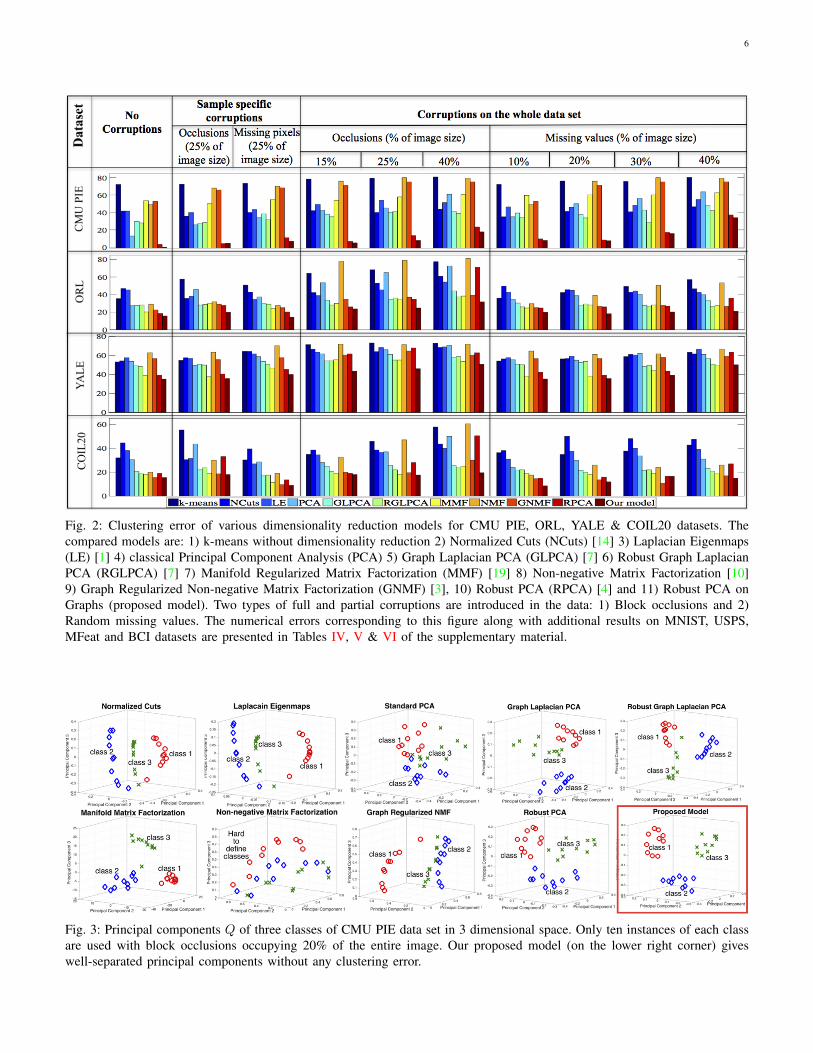
C. Robustness to Graph Quality

We perform an experiment on the YALE dataset with 35% random missing pixels. Fig. 4 shows the variation in clusteringerror of different PCA models by using a graph constructed with decreasing information about the mask. Our model stilloutperforms others even though the quality of graph deteriorates with corrupted data. It is essential to note that in the worstcase scenario when the mask is not known at all, our model performs equal to RPCA but still better than those which use aprincipal components graph.

Fig. 4: Effect of lack of information about the corruptions mask on the clustering error. YALE dataset with 35% randommissing pixels is used for this experiment. Our model (last bar in each group) outperforms the others.

VIII. LOW-RANK RECOVERY

A. Low-Rank Recovery from Artificial Datasets

To perform a quantitative comparison of exact low-rank recovery between RPCA and our model, we perform experimentson 2 artificial datasets as in [4]. Note that only RPCA and our model perform exact low-rank recovery so we do not presentresults for other PCA models. We generate low-rank square matrices L = ATB ∈ Rn×n (rank d = 0.02n to 0.3n) with A andB independently chosen d× n matrices with i.i.d. Gaussian entries of zero mean and variance 1/n. We introduce 6% to 30%errors ρ = ‖S‖0/n2 in these matrices from an i.i.d. Bernoulli distribution for support of S with two sign schemes.

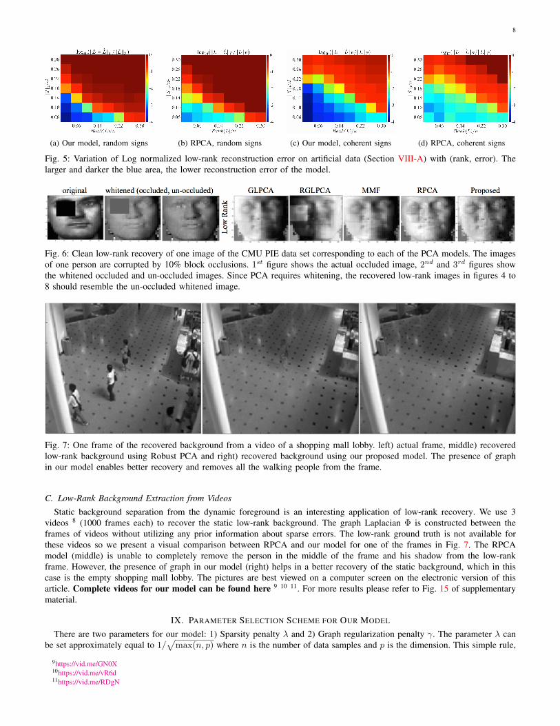
1) Random signs: Each corrupted entry takes a value ±1 with a probability ρ/2.2) Coherent signs: The sign for each corrupted entry is coherent with the sign of the corresponding entry in L.Fig. 5 compares the variation of log normalized low-rank reconstruction error log(‖L− L‖F /‖L‖F ) with rank (x-axis) and

error (y-axis) between RPCA (b and d) and our model (a and c). The larger and darker the blue region, the better is thereconstruction. The first two plots correspond to the random sign scheme and the next ones to coherent sign scheme. It canbe seen that for each (rank,error) pair the reconstruction error for our model is less than that for RPCA. Hence, the low-rankgraph helps in an enhanced low-rank recovery.

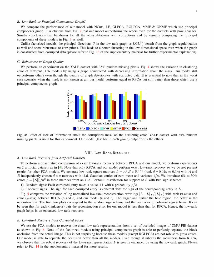
B. Low-Rank Recovery from Corrupted Faces

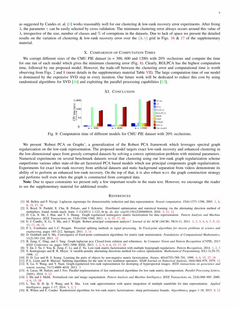
We use the PCA models to recover the clean low-rank representations from a set of occluded images of CMU PIE datasetas shown in Fig. 6. None of the factorized models using principal components graph is able to perfectly separate the blockocclusion from the actual image. This is not surprising because these models (except RGLPCA) are not robust to gross errors.Our model is able to separate the occlusion better than all the models. Even though it inherits the robustness from RPCA,we observe that the robust recovery of the low-rank representation L is greatly enhanced by using the low-rank graph. Pleaserefer to Fig. 14 in the supplementary material for more results.

Page 8

8

(a) Our model, random signs (b) RPCA, random signs (c) Our model, coherent signs (d) RPCA, coherent signs

Fig. 5: Variation of Log normalized low-rank reconstruction error on artificial data (Section VIII-A) with (rank, error). Thelarger and darker the blue area, the lower reconstruction error of the model.

Fig. 6: Clean low-rank recovery of one image of the CMU PIE data set corresponding to each of the PCA models. The imagesof one person are corrupted by 10% block occlusions. 1st figure shows the actual occluded image, 2nd and 3rd figures showthe whitened occluded and un-occluded images. Since PCA requires whitening, the recovered low-rank images in figures 4 to8 should resemble the un-occluded whitened image.

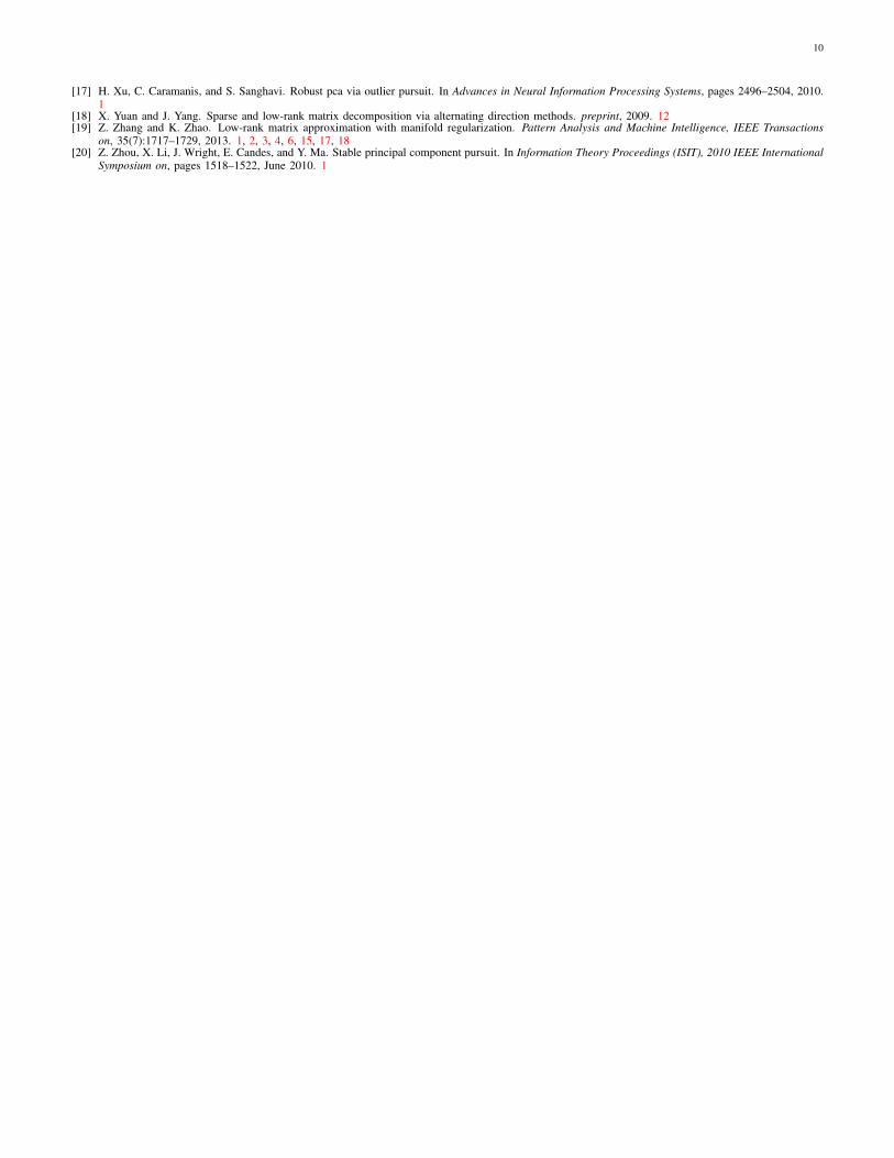
Fig. 7: One frame of the recovered background from a video of a shopping mall lobby. left) actual frame, middle) recoveredlow-rank background using Robust PCA and right) recovered background using our proposed model. The presence of graphin our model enables better recovery and removes all the walking people from the frame.

C. Low-Rank Background Extraction from Videos

Static background separation from the dynamic foreground is an interesting application of low-rank recovery. We use 3videos 8 (1000 frames each) to recover the static low-rank background. The graph Laplacian Φ is constructed between theframes of videos without utilizing any prior information about sparse errors. The low-rank ground truth is not available forthese videos so we present a visual comparison between RPCA and our model for one of the frames in Fig. 7. The RPCAmodel (middle) is unable to completely remove the person in the middle of the frame and his shadow from the low-rankframe. However, the presence of graph in our model (right) helps in a better recovery of the static background, which in thiscase is the empty shopping mall lobby. The pictures are best viewed on a computer screen on the electronic version of thisarticle. Complete videos for our model can be found here 9 10 11. For more results please refer to Fig. 15 of supplementarymaterial.

IX. PARAMETER SELECTION SCHEME FOR OUR MODEL

There are two parameters for our model: 1) Sparsity penalty λ and 2) Graph regularization penalty γ. The parameter λ canbe set approximately equal to 1/

√max(n, p) where n is the number of data samples and p is the dimension. This simple rule,

9https://vid.me/GN0X10https://vid.me/vR6d11https://vid.me/RDgN

Page 9

9

as suggested by Candes et. al. [4] works reasonably well for our clustering & low-rank recovery error experiments. After fixingλ, the parameter γ can be easily selected by cross-validation. The minimum clustering error always occurs around this value ofλ, irrespective of the size, number of classes and % of corruptions in the datasets. Due to lack of space we present the detailedresults on the variation of clustering & low-rank recovery error over the (λ, γ) grid in Figs. 16 & 17 of the supplementarymaterial.

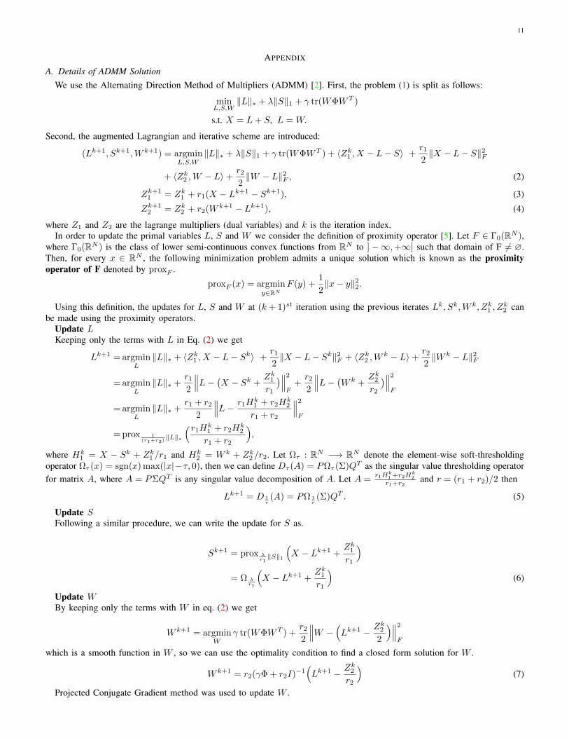
X. COMPARISON OF COMPUTATION TIMES

We corrupt different sizes of the CMU PIE dataset (n = 300, 600 and 1200) with 20% occlusions and compute the timefor one run of each model which gives the minimum clustering error (Fig. 8). Clearly, RGLPCA has the highest computationtime, followed by our proposed model. However, the trade-off between the clustering error and computational time is worthobserving from Figs. 2 and 8 (more details in the supplementary material Table VII). The large computation time of our modelis dominated by the expensive SVD step in every iteration. Our future work will be dedicated to reduce this cost by usingrandomized algorithms for SVD [16] and exploiting the parallel processing capabilities [13].

XI. CONCLUSION

Fig. 8: Computation time of different models for CMU PIE dataset with 20% occlusions.

We present ‘Robust PCA on Graphs’, a generalization of the Robust PCA framework which leverages spectral graphregularization on the low-rank representation. The proposed model targets exact low-rank recovery and enhanced clustering inthe low-dimensional space from grossly corrupted datasets by solving a convex optimization problem with minimal parameters.Numerical experiments on several benchmark datasets reveal that clustering using our low-rank graph regularization schemeoutperforms various other state-of-the-art factorized PCA based models which use principal components graph regularization.Experiments for exact low-rank recovery from artificial datasets and static background separation from videos demonstrate itsability of to perform an enhanced low-rank recovery. On the top of that, it is also robust w.r.t. the graph construction strategyand performs well even when the graph is constructed from corrupted data.

Note: Due to space constraints we present only a few important results in the main text. However, we encourage the readerto see the supplementary material for additional results.

REFERENCES

[1] M. Belkin and P. Niyogi. Laplacian eigenmaps for dimensionality reduction and data representation. Neural computation, 15(6):1373–1396, 2003. 1, 4,6, 15, 17, 18

[2] S. Boyd, N. Parikhl, E. Chu, B. Peleato, and J. Eckstein. Distributed optimization and statistical learning via the alternating direction method ofmultipliers, found. trends mach. learn. 3 (1)(2011) 1–122, ht tp. dx. doi. org/10.1561/2200000016, 2010. 3, 11, 12

[3] D. Cai, X. He, J. Han, and T. S. Huang. Graph regularized nonnegative matrix factorization for data representation. Pattern Analysis and MachineIntelligence, IEEE Transactions on, 33(8):1548–1560, 2011. 4, 6, 15, 17, 18

[4] E. J. Candes, X. Li, Y. Ma, and J. Wright. Robust principal component analysis? Journal of the ACM (JACM), 58(3):11, 2011. 1, 2, 3, 4, 6, 7, 9, 12,15, 17, 18, 21

[5] P. L. Combettes and J.-C. Pesquet. Proximal splitting methods in signal processing. In Fixed-point algorithms for inverse problems in science andengineering, pages 185–212. Springer, 2011. 3, 11

[6] D. Goldfarb and S. Ma. Convergence of fixed-point continuation algorithms for matrix rank minimization. Foundations of Computational Mathematics,11(2):183–210, 2011. 12

[7] B. Jiang, C. Ding, and J. Tang. Graph-laplacian pca: Closed-form solution and robustness. In Computer Vision and Pattern Recognition (CVPR), 2013IEEE Conference on, pages 3492–3498. IEEE, 2013. 1, 2, 3, 4, 6, 15, 17, 18

[8] T. Jin, J. Yu, J. You, K. Zeng, C. Li, and Z. Yu. Low-rank matrix factorization with multiple hypergraph regularizers. Pattern Recognition, 2014. 1, 2, 3[9] S. Kontogiorgis and R. R. Meyer. A variable-penalty alternating directions method for convex optimization. Mathematical Programming, 83(1-3):29–53,

1998. 12[10] D. D. Lee and H. S. Seung. Learning the parts of objects by non-negative matrix factorization. Nature, 401(6755):788–791, 1999. 4, 6, 15, 17, 18[11] P.-L. Lions and B. Mercier. Splitting algorithms for the sum of two nonlinear operators. SIAM Journal on Numerical Analysis, 16(6):964–979, 1979. 12[12] X. Lu, Y. Wang, and Y. Yuan. Graph-regularized low-rank representation for destriping of hyperspectral images. IEEE transactions on geoscience and

remote sensing, 51(7):4009–4018, 2013. 3[13] A. Lucas, M. Stalzer, and J. Feo. Parallel implementation of fast randomized algorithms for low rank matrix decomposition. Parallel Processing Letters,

24(01), 2014. 9, 12[14] J. Shi and J. Malik. Normalized cuts and image segmentation. Pattern Analysis and Machine Intelligence, IEEE Transactions on, 22(8):888–905, 2000.

4, 6, 15, 18[15] L. Tao, H. H. Ip, Y. Wang, and X. Shu. Low rank approximation with sparse integration of multiple manifolds for data representation. Applied

Intelligence, pages 1–17, 2014. 1, 2, 3[16] R. Witten and E. Candes. Randomized algorithms for low-rank matrix factorizations: sharp performance bounds. Algorithmica, pages 1–18, 2013. 9, 12

Page 10

10

[17] H. Xu, C. Caramanis, and S. Sanghavi. Robust pca via outlier pursuit. In Advances in Neural Information Processing Systems, pages 2496–2504, 2010.1

[18] X. Yuan and J. Yang. Sparse and low-rank matrix decomposition via alternating direction methods. preprint, 2009. 12[19] Z. Zhang and K. Zhao. Low-rank matrix approximation with manifold regularization. Pattern Analysis and Machine Intelligence, IEEE Transactions

on, 35(7):1717–1729, 2013. 1, 2, 3, 4, 6, 15, 17, 18[20] Z. Zhou, X. Li, J. Wright, E. Candes, and Y. Ma. Stable principal component pursuit. In Information Theory Proceedings (ISIT), 2010 IEEE International

Symposium on, pages 1518–1522, June 2010. 1

Page 11

11

APPENDIX

A. Details of ADMM SolutionWe use the Alternating Direction Method of Multipliers (ADMM) [2]. First, the problem (1) is split as follows:

minL,S,W

‖L‖∗ + λ‖S‖1 + γ tr(WΦWT )

s.t. X = L+ S, L = W.

Second, the augmented Lagrangian and iterative scheme are introduced:

(Lk+1, Sk+1,W k+1) = argminL,S,W

‖L‖∗ + λ‖S‖1 + γ tr(WΦWT ) + 〈Zk1 , X − L− S〉 +r12‖X − L− S‖2F

+ 〈Zk2 ,W − L〉+r22‖W − L‖2F , (2)

Zk+11 = Zk1 + r1(X − Lk+1 − Sk+1), (3)

Zk+12 = Zk2 + r2(W k+1 − Lk+1), (4)

where Z1 and Z2 are the lagrange multipliers (dual variables) and k is the iteration index.In order to update the primal variables L, S and W we consider the definition of proximity operator [5]. Let F ∈ Γ0(RN ),

where Γ0(RN ) is the class of lower semi-continuous convex functions from RN to ]−∞,+∞] such that domain of F 6= ∅.Then, for every x ∈ RN , the following minimization problem admits a unique solution which is known as the proximityoperator of F denoted by proxF .

proxF (x) = argminy∈RN

F (y) +1

2‖x− y‖22.

Using this definition, the updates for L, S and W at (k+ 1)st iteration using the previous iterates Lk, Sk,W k, Zk1 , Zk2 can

be made using the proximity operators.Update LKeeping only the terms with L in Eq. (2) we get

Lk+1 = argminL‖L‖∗ + 〈Zk1 , X − L− Sk〉 +

r12‖X − L− Sk‖2F + 〈Zk2 ,W k − L〉+

r22‖W k − L‖2F

= argminL‖L‖∗ +

r12

∥∥∥L− (X − Sk +Zk1r1

)∥∥∥2F

+r22

∥∥∥L− (W k +Zk2r2

)∥∥∥2F

= argminL‖L‖∗ +

r1 + r22

∥∥∥L− r1Hk1 + r2H

k2

r1 + r2

∥∥∥2F

= prox 1(r1+r2)

‖L‖∗

(r1Hk1 + r2H

k2

r1 + r2

),

where Hk1 = X − Sk + Zk1 /r1 and Hk

2 = W k + Zk2 /r2. Let Ωτ : RN −→ RN denote the element-wise soft-thresholdingoperator Ωτ (x) = sgn(x) max(|x|−τ, 0), then we can define Dτ (A) = PΩτ (Σ)QT as the singular value thresholding operatorfor matrix A, where A = PΣQT is any singular value decomposition of A. Let A =

r1Hk1 +r2H

k2

r1+r2and r = (r1 + r2)/2 then

Lk+1 = D 1r(A) = PΩ 1

r(Σ)QT . (5)

Update SFollowing a similar procedure, we can write the update for S as.

Sk+1 = prox λr1‖S‖1

(X − Lk+1 +

Zk1r1

)= Ω λ

r1

(X − Lk+1 +

Zk1r1

)(6)

Update WBy keeping only the terms with W in eq. (2) we get

W k+1 = argminW

γ tr(WΦWT ) +r22

∥∥∥W − (Lk+1 − Zk22

)∥∥∥2F

which is a smooth function in W , so we can use the optimality condition to find a closed form solution for W .

W k+1 = r2(γΦ + r2I)−1(Lk+1 − Zk2

r2

)(7)

Projected Conjugate Gradient method was used to update W .

Page 12

12

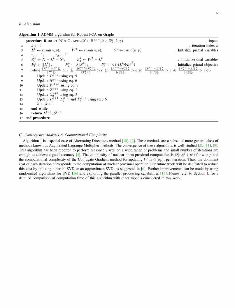
B. Algorithm

Algorithm 1 ADMM algorithm for Robust PCA on Graphs

1: procedure ROBUST PCA GRAPHS(X ∈ Rp×n,Φ ∈ Sn+, λ, γ) . inputs2: k ← 0 . iteration index k3: Lk ← rand(n, p), W k ← rand(n, p), Sk ← rand(n, p) . Initialize primal variables4: r1 ← 1, r2 ← 15: Zk1 ← X − Lk − Sk, Zk2 ←W k − Lk . Initialize dual variables6: P k1 ← ‖Lk‖∗, P k2 ← λ‖Sk‖1, P k3 ← γ tr(LkΦLk

T) . Initialize primal objective

7: while ‖Pk+11 −Pk1 ‖

2F

‖Pk1 ‖2F> ε &

‖Pk+12 −Pk2 ‖

2F

‖Pk2 ‖2F> ε &

‖Pk+13 −Pk3 ‖

2F

‖Pk3 ‖2F> ε &

‖Zk+11 −Zk1 ‖

2F

‖Zk1 ‖2F> ε &

‖Zk+12 −Zk2 ‖

2F

‖Zk2 ‖2F> ε do

8: Update Lk+1 using eq. 59: Update Sk+1 using eq. 6

10: Update W k+1 using eq. 711: Update Zk+1

1 using eq. 212: Update Zk+1

2 using eq. 313: Update P k+1

1 , P k+12 and P k+1

3 using step 6.14: k ← k + 115: end while16: return Lk+1, Sk+1

17: end procedure

C. Convergence Analysis & Computational Complexity

Algorithm 1 is a special case of Alternating Directions method [18], [2]. These methods are a subset of more general class ofmethods known as Augmented Lagrange Multiplier methods. The convergence of these algorithms is well-studied [2], [11], [9].This algorithm has been reported to perform reasonably well on a wide range of problems and small number of iterations areenough to achieve a good accuracy [4]. The complexity of nuclear norm proximal computation is O(np2 + p3) for n > p andthe computational complexity of the Conjugate Gradient method for updating W is O(np), per iteration. Thus, the dominantcost of each iteration corresponds to the computation of nuclear proximal operator. Our future work will be dedicated to reducethis cost by utilizing a partial SVD or an approximate SVD, as suggested in [6]. Further improvements can be made by usingrandomized algorithms for SVD [16] and exploiting the parallel processing capabilities [13]. Please refer to Section L for adetailed comparison of computation time of this algorithm with other models considered in this work.

Page 13

13

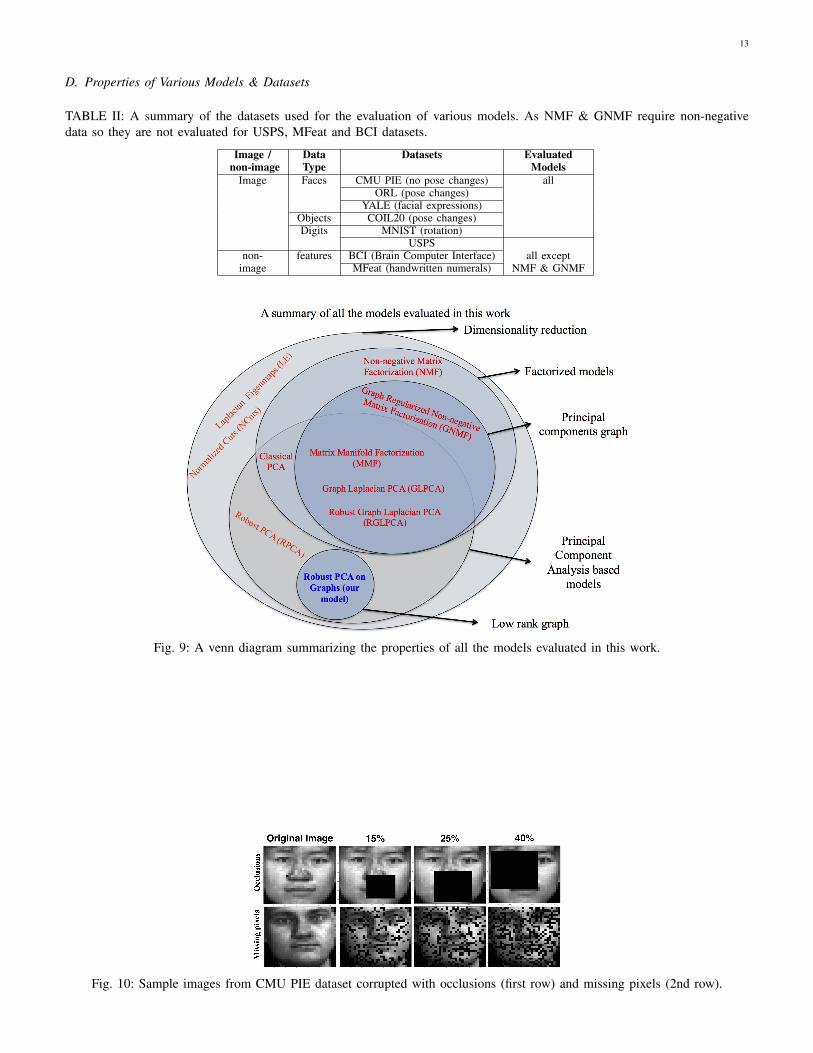
D. Properties of Various Models & Datasets

TABLE II: A summary of the datasets used for the evaluation of various models. As NMF & GNMF require non-negativedata so they are not evaluated for USPS, MFeat and BCI datasets.

Image / Data Datasets Evaluatednon-image Type Models

Image Faces CMU PIE (no pose changes) allORL (pose changes)

YALE (facial expressions)Objects COIL20 (pose changes)Digits MNIST (rotation)

USPSnon- features BCI (Brain Computer Interface) all except

image MFeat (handwritten numerals) NMF & GNMF

Fig. 9: A venn diagram summarizing the properties of all the models evaluated in this work.

Fig. 10: Sample images from CMU PIE dataset corrupted with occlusions (first row) and missing pixels (2nd row).

Page 14

14

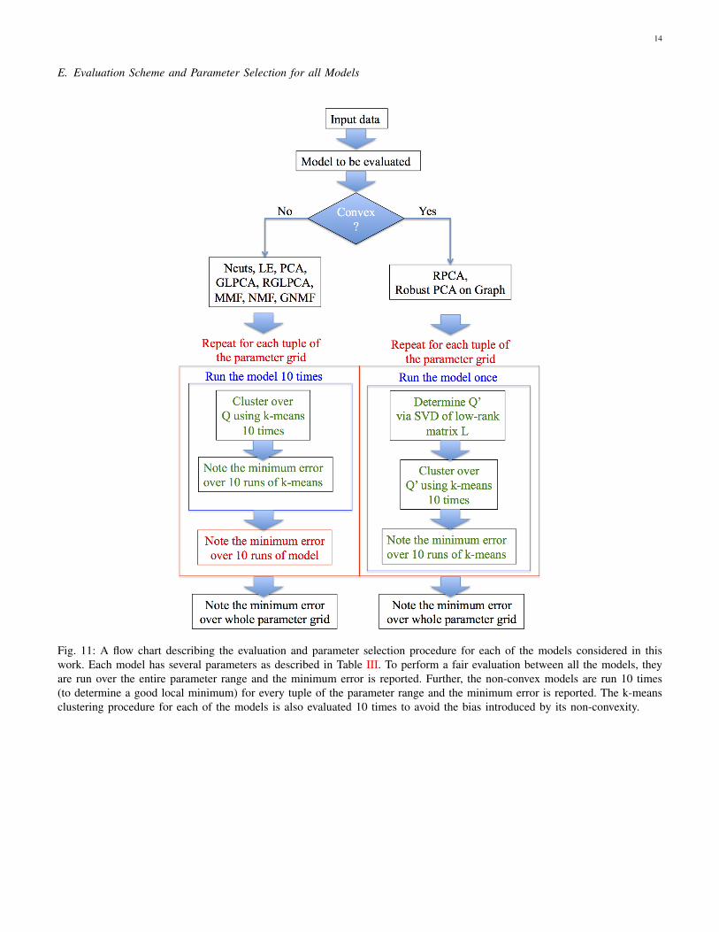
E. Evaluation Scheme and Parameter Selection for all Models

Fig. 11: A flow chart describing the evaluation and parameter selection procedure for each of the models considered in thiswork. Each model has several parameters as described in Table III. To perform a fair evaluation between all the models, theyare run over the entire parameter range and the minimum error is reported. Further, the non-convex models are run 10 times(to determine a good local minimum) for every tuple of the parameter range and the minimum error is reported. The k-meansclustering procedure for each of the models is also evaluated 10 times to avoid the bias introduced by its non-convexity.

Page 15

15

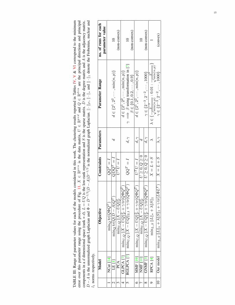
TAB

LE

III:

Ran

geof

para

met

erva

lues

for

each

ofth

em

odel

sco

nsid

ered

inth

isw

ork.

The

clus

teri

ngre

sults

repo

rted

inTa

bles

IV,V

&V

Ico

rres

pond

toth

em

inim

umer

ror

over

this

para

met

erra

nge

usin

gth

epr

oced

ure

ofFi

g.11

.X∈

Rp×n

isth

eda

tam

atri

x,U∈

Rp×d

andQ∈

Rd×n

are

the

prin

cipa

ldi

rect

ions

and

prin

cipa

lco

mpo

nent

sin

ad

dim

ensi

onal

spac

e(r

ank

=d

).L

=UQ

isth

elo

w-r

ank

repr

esen

tatio

nan

dS

isth

esp

arse

mat

rix.D

isth

ede

gree

mat

rix

andA

isth

ead

jace

ncy

mat

rix.

D−A

isth

eun

norm

aliz

edgr

aph

Lap

laci

anan

dΦ

=D−1/2(D−A

)D−1/2

isth

eno

rmal

ized

grap

hL

apla

cian

.‖·‖F

,‖·‖∗

and‖·‖

1de

note

the

Frob

eniu

s,nu

clea

ran

dl 1

norm

sre

spec

tivel

y.

Mod

elO

bjec

tive

Con

stra

ints

Para

met

ers

Para

met

erR

ange

no.o

fru

nsfo

rea

chpa

ram

eter

valu

e1

NC

ut[1

4]m

inQ

tr(Q

ΦQ

T)

QQ

T=I

2L

E[1

]m

inQ

tr(Q

(D−A

)QT

)QDQ

T=I

dd∈2

1,2

2,···,m

in(n,p

)10

3PC

Am

inU,Q‖X−UQ‖2 F

UTU

=I

(non

-con

vex)

4G

LPC

A[7

]m

inU,Q‖X−UQ‖2 F

+γ

tr(Q

ΦQ

T)

d∈2

1,2

2,···,m

in(n,p

)5

RG

LPC

A[7

]m

inU,Q‖X−UQ‖ 2

,1+γ

tr(Q

ΦQ

T)

QQ

T=I

d,γ

γ=⇒

βus

ing

tran

sfor

mat

ion

in[7

]10

β∈0.1,0.2,···,0.9

(non

-con

vex)

6M

MF

[19]

min

U,Q‖X−UQ‖2 F

+γ

tr(Q

ΦQ

T)

UTU

=I

d,γ

d∈2

1,2

2,···,m

in(n,p

)7

NM

F[1

0]m

inU,Q‖X−UQ‖2 F

U≥

0,Q≥

0d

108

GN

MF

[3]

min

U,Q‖X−UQ‖2 F

+γ

tr(Q

ΦQ

T)

U≥

0,Q≥

0d,γ

γ∈2

−3,2

−2,···,1

000

(non

-con

vex)

9R

PCA

[4]

min

L,S‖L‖ ∗

+λ‖S‖ 1

X=L

+S

λλ∈

2−

3√

min

(n,p

):0.0

1:

23

√m

in(n

,p)

1

10O

urm

odel

min

L,S‖L‖ ∗

+λ‖S‖ 1

+γ

tr(L

ΦLT

)X

=L

+S

λ,γ

γ∈2

−3,2

−2,···,1

000

(con

vex)

Page 16

16

F. Adjacency Matrix Construction from Corrupted & Uncorrupted Data

Fig. 12: A procedure for the construction of Adjacency matrix A from clean and corrupted samples X . We assume that theblock occlusions can be detected and the mask can be extended to the other image of the pair to remove the effect of occlusionin the calculation of Euclidean distance. The case of random missing pixels can be handled by using inpainting techniques,such as Total Variation denoising.

Page 17

17

G. Clustering Results on all Databases

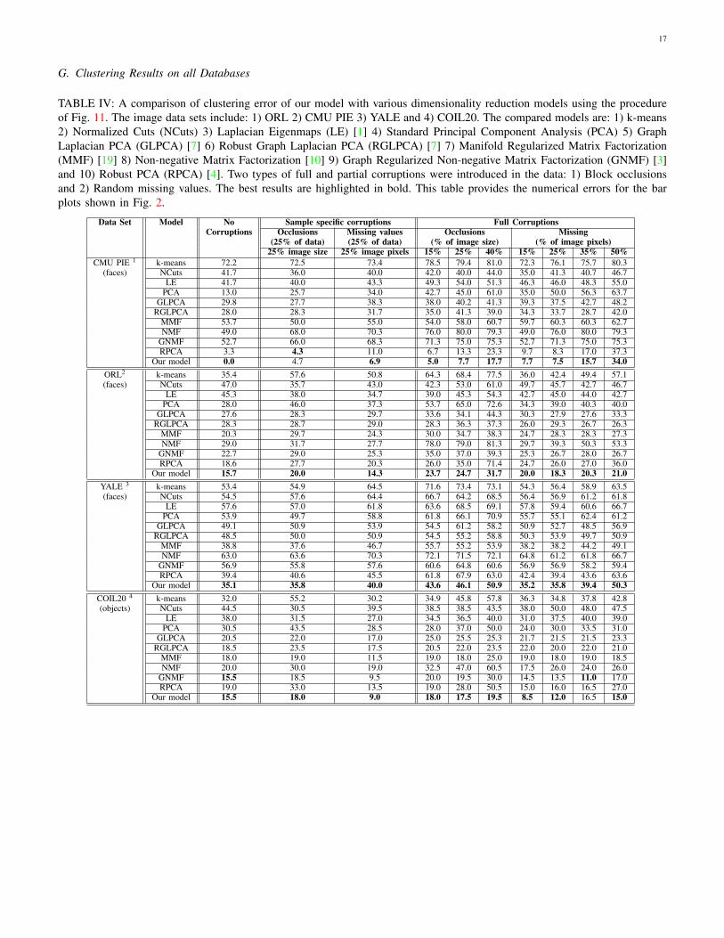
TABLE IV: A comparison of clustering error of our model with various dimensionality reduction models using the procedureof Fig. 11. The image data sets include: 1) ORL 2) CMU PIE 3) YALE and 4) COIL20. The compared models are: 1) k-means2) Normalized Cuts (NCuts) 3) Laplacian Eigenmaps (LE) [1] 4) Standard Principal Component Analysis (PCA) 5) GraphLaplacian PCA (GLPCA) [7] 6) Robust Graph Laplacian PCA (RGLPCA) [7] 7) Manifold Regularized Matrix Factorization(MMF) [19] 8) Non-negative Matrix Factorization [10] 9) Graph Regularized Non-negative Matrix Factorization (GNMF) [3]and 10) Robust PCA (RPCA) [4]. Two types of full and partial corruptions were introduced in the data: 1) Block occlusionsand 2) Random missing values. The best results are highlighted in bold. This table provides the numerical errors for the barplots shown in Fig. 2.

Data Set Model No Sample specific corruptions Full CorruptionsCorruptions Occlusions Missing values Occlusions Missing

(25% of data) (25% of data) (% of image size) (% of image pixels)25% image size 25% image pixels 15% 25% 40% 15% 25% 35% 50%

CMU PIE 1 k-means 72.2 72.5 73.4 78.5 79.4 81.0 72.3 76.1 75.7 80.3(faces) NCuts 41.7 36.0 40.0 42.0 40.0 44.0 35.0 41.3 40.7 46.7

LE 41.7 40.0 43.3 49.3 54.0 51.3 46.3 46.0 48.3 55.0PCA 13.0 25.7 34.0 42.7 45.0 61.0 35.0 50.0 56.3 63.7

GLPCA 29.8 27.7 38.3 38.0 40.2 41.3 39.3 37.5 42.7 48.2RGLPCA 28.0 28.3 31.7 35.0 41.3 39.0 34.3 33.7 28.7 42.0

MMF 53.7 50.0 55.0 54.0 58.0 60.7 59.7 60.3 60.3 62.7NMF 49.0 68.0 70.3 76.0 80.0 79.3 49.0 76.0 80.0 79.3

GNMF 52.7 66.0 68.3 71.3 75.0 75.3 52.7 71.3 75.0 75.3RPCA 3.3 4.3 11.0 6.7 13.3 23.3 9.7 8.3 17.0 37.3

Our model 0.0 4.7 6.9 5.0 7.7 17.7 7.7 7.5 15.7 34.0ORL2 k-means 35.4 57.6 50.8 64.3 68.4 77.5 36.0 42.4 49.4 57.1(faces) NCuts 47.0 35.7 43.0 42.3 53.0 61.0 49.7 45.7 42.7 46.7

LE 45.3 38.0 34.7 39.0 45.3 54.3 42.7 45.0 44.0 42.7PCA 28.0 46.0 37.3 53.7 65.0 72.6 34.3 39.0 40.3 40.0

GLPCA 27.6 28.3 29.7 33.6 34.1 44.3 30.3 27.9 27.6 33.3RGLPCA 28.3 28.7 29.0 28.3 36.3 37.3 26.0 29.3 26.7 26.3

MMF 20.3 29.7 24.3 30.0 34.7 38.3 24.7 28.3 28.3 27.3NMF 29.0 31.7 27.7 78.0 79.0 81.3 29.7 39.3 50.3 53.3

GNMF 22.7 29.0 25.3 35.0 37.0 39.3 25.3 26.7 28.0 26.7RPCA 18.6 27.7 20.3 26.0 35.0 71.4 24.7 26.0 27.0 36.0

Our model 15.7 20.0 14.3 23.7 24.7 31.7 20.0 18.3 20.3 21.0YALE 3 k-means 53.4 54.9 64.5 71.6 73.4 73.1 54.3 56.4 58.9 63.5(faces) NCuts 54.5 57.6 64.4 66.7 64.2 68.5 56.4 56.9 61.2 61.8

LE 57.6 57.0 61.8 63.6 68.5 69.1 57.8 59.4 60.6 66.7PCA 53.9 49.7 58.8 61.8 66.1 70.9 55.7 55.1 62.4 61.2

GLPCA 49.1 50.9 53.9 54.5 61.2 58.2 50.9 52.7 48.5 56.9RGLPCA 48.5 50.0 50.9 54.5 55.2 58.8 50.3 53.9 49.7 50.9

MMF 38.8 37.6 46.7 55.7 55.2 53.9 38.2 38.2 44.2 49.1NMF 63.0 63.6 70.3 72.1 71.5 72.1 64.8 61.2 61.8 66.7

GNMF 56.9 55.8 57.6 60.6 64.8 60.6 56.9 56.9 58.2 59.4RPCA 39.4 40.6 45.5 61.8 67.9 63.0 42.4 39.4 43.6 63.6

Our model 35.1 35.8 40.0 43.6 46.1 50.9 35.2 35.8 39.4 50.3COIL20 4 k-means 32.0 55.2 30.2 34.9 45.8 57.8 36.3 34.8 37.8 42.8(objects) NCuts 44.5 30.5 39.5 38.5 38.5 43.5 38.0 50.0 48.0 47.5

LE 38.0 31.5 27.0 34.5 36.5 40.0 31.0 37.5 40.0 39.0PCA 30.5 43.5 28.5 28.0 37.0 50.0 24.0 30.0 33.5 31.0

GLPCA 20.5 22.0 17.0 25.0 25.5 25.3 21.7 21.5 21.5 23.3RGLPCA 18.5 23.5 17.5 20.5 22.0 23.5 22.0 20.0 22.0 21.0

MMF 18.0 19.0 11.5 19.0 18.0 25.0 19.0 18.0 19.0 18.5NMF 20.0 30.0 19.0 32.5 47.0 60.5 17.5 26.0 24.0 26.0

GNMF 15.5 18.5 9.5 20.0 19.5 30.0 14.5 13.5 11.0 17.0RPCA 19.0 33.0 13.5 19.0 28.0 50.5 15.0 16.0 16.5 27.0

Our model 15.5 18.0 9.0 18.0 17.5 19.5 8.5 12.0 16.5 15.0

Page 18

18

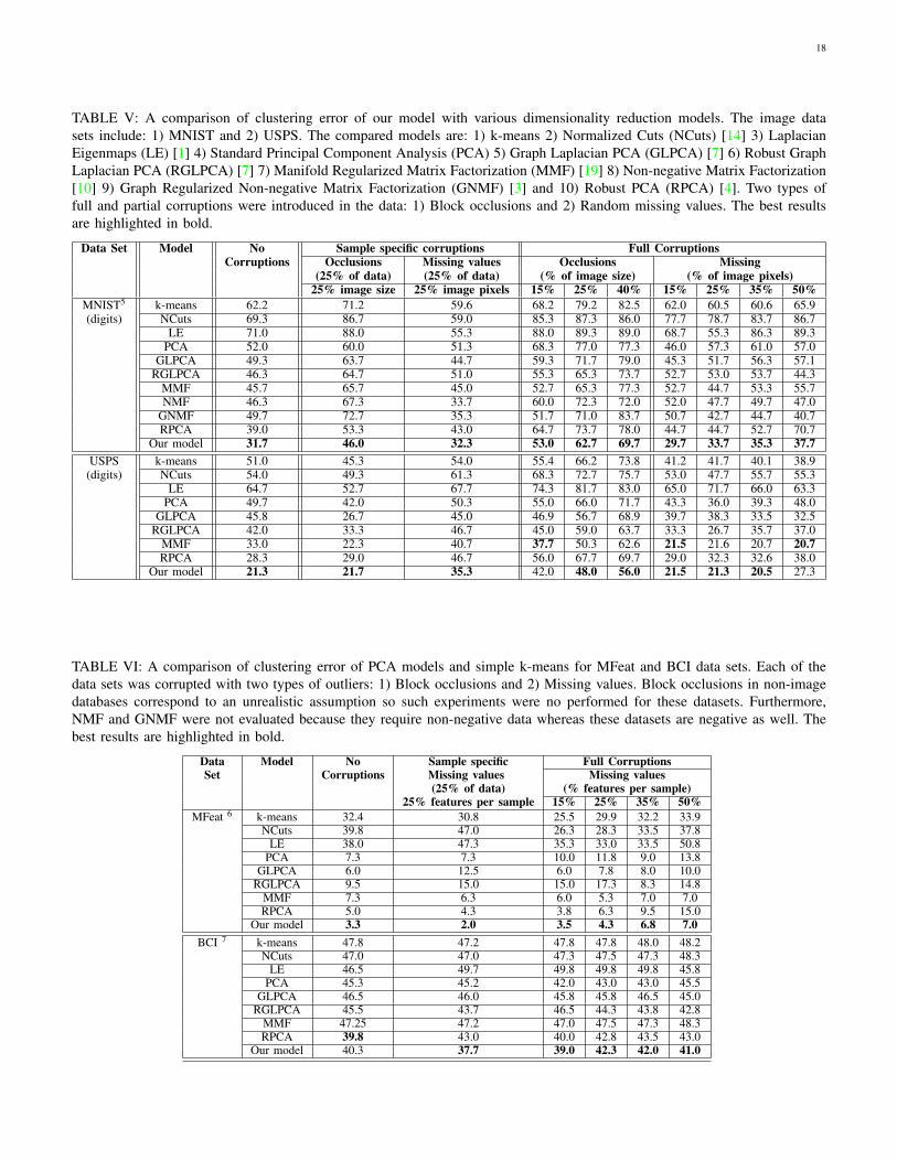
TABLE V: A comparison of clustering error of our model with various dimensionality reduction models. The image datasets include: 1) MNIST and 2) USPS. The compared models are: 1) k-means 2) Normalized Cuts (NCuts) [14] 3) LaplacianEigenmaps (LE) [1] 4) Standard Principal Component Analysis (PCA) 5) Graph Laplacian PCA (GLPCA) [7] 6) Robust GraphLaplacian PCA (RGLPCA) [7] 7) Manifold Regularized Matrix Factorization (MMF) [19] 8) Non-negative Matrix Factorization[10] 9) Graph Regularized Non-negative Matrix Factorization (GNMF) [3] and 10) Robust PCA (RPCA) [4]. Two types offull and partial corruptions were introduced in the data: 1) Block occlusions and 2) Random missing values. The best resultsare highlighted in bold.

Data Set Model No Sample specific corruptions Full CorruptionsCorruptions Occlusions Missing values Occlusions Missing

(25% of data) (25% of data) (% of image size) (% of image pixels)25% image size 25% image pixels 15% 25% 40% 15% 25% 35% 50%

MNIST5 k-means 62.2 71.2 59.6 68.2 79.2 82.5 62.0 60.5 60.6 65.9(digits) NCuts 69.3 86.7 59.0 85.3 87.3 86.0 77.7 78.7 83.7 86.7

LE 71.0 88.0 55.3 88.0 89.3 89.0 68.7 55.3 86.3 89.3PCA 52.0 60.0 51.3 68.3 77.0 77.3 46.0 57.3 61.0 57.0

GLPCA 49.3 63.7 44.7 59.3 71.7 79.0 45.3 51.7 56.3 57.1RGLPCA 46.3 64.7 51.0 55.3 65.3 73.7 52.7 53.0 53.7 44.3

MMF 45.7 65.7 45.0 52.7 65.3 77.3 52.7 44.7 53.3 55.7NMF 46.3 67.3 33.7 60.0 72.3 72.0 52.0 47.7 49.7 47.0

GNMF 49.7 72.7 35.3 51.7 71.0 83.7 50.7 42.7 44.7 40.7RPCA 39.0 53.3 43.0 64.7 73.7 78.0 44.7 44.7 52.7 70.7

Our model 31.7 46.0 32.3 53.0 62.7 69.7 29.7 33.7 35.3 37.7USPS k-means 51.0 45.3 54.0 55.4 66.2 73.8 41.2 41.7 40.1 38.9(digits) NCuts 54.0 49.3 61.3 68.3 72.7 75.7 53.0 47.7 55.7 55.3

LE 64.7 52.7 67.7 74.3 81.7 83.0 65.0 71.7 66.0 63.3PCA 49.7 42.0 50.3 55.0 66.0 71.7 43.3 36.0 39.3 48.0

GLPCA 45.8 26.7 45.0 46.9 56.7 68.9 39.7 38.3 33.5 32.5RGLPCA 42.0 33.3 46.7 45.0 59.0 63.7 33.3 26.7 35.7 37.0

MMF 33.0 22.3 40.7 37.7 50.3 62.6 21.5 21.6 20.7 20.7RPCA 28.3 29.0 46.7 56.0 67.7 69.7 29.0 32.3 32.6 38.0

Our model 21.3 21.7 35.3 42.0 48.0 56.0 21.5 21.3 20.5 27.3

TABLE VI: A comparison of clustering error of PCA models and simple k-means for MFeat and BCI data sets. Each of thedata sets was corrupted with two types of outliers: 1) Block occlusions and 2) Missing values. Block occlusions in non-imagedatabases correspond to an unrealistic assumption so such experiments were no performed for these datasets. Furthermore,NMF and GNMF were not evaluated because they require non-negative data whereas these datasets are negative as well. Thebest results are highlighted in bold.

Data Model No Sample specific Full CorruptionsSet Corruptions Missing values Missing values

(25% of data) (% features per sample)25% features per sample 15% 25% 35% 50%

MFeat 6 k-means 32.4 30.8 25.5 29.9 32.2 33.9NCuts 39.8 47.0 26.3 28.3 33.5 37.8

LE 38.0 47.3 35.3 33.0 33.5 50.8PCA 7.3 7.3 10.0 11.8 9.0 13.8

GLPCA 6.0 12.5 6.0 7.8 8.0 10.0RGLPCA 9.5 15.0 15.0 17.3 8.3 14.8

MMF 7.3 6.3 6.0 5.3 7.0 7.0RPCA 5.0 4.3 3.8 6.3 9.5 15.0

Our model 3.3 2.0 3.5 4.3 6.8 7.0BCI 7 k-means 47.8 47.2 47.8 47.8 48.0 48.2

NCuts 47.0 47.0 47.3 47.5 47.3 48.3LE 46.5 49.7 49.8 49.8 49.8 45.8

PCA 45.3 45.2 42.0 43.0 43.0 45.5GLPCA 46.5 46.0 45.8 45.8 46.5 45.0

RGLPCA 45.5 43.7 46.5 44.3 43.8 42.8MMF 47.25 47.2 47.0 47.5 47.3 48.3RPCA 39.8 43.0 40.0 42.8 43.5 43.0

Our model 40.3 37.7 39.0 42.3 42.0 41.0

Page 19

19

H. A Comparison of the Principal Directions U Learned with Low-Rank and Principal Components Graph

Fig. 13: A comparison of the principal directions U learned with low-rank graph tr(LΦLT ) and principal components graphregularization tr(QΦQT ) for the CMU PIE dataset. Each row shows the 1st two principal directions U and the correspondingsingular values for each of the PCA models evaluated in this work. For the factorized models (PCA, GLPCA, RGLPCA andMMF) the principal directions U are explicitly learned. For RPCA and our model, U is obtained by singular value decompositionof the low-rank matrix L, i.e. L = UΣQ. The low-rank graph for our model clearly helps in learning a corruption free U .Even though the 2nd principal direction for our model has a large effect of occlusion, we note that the corresponding singularvalue (2nd bar) is much smaller as compared to the 1st. For all the other models, each of the two principal directions areaffected by occlusions and the corresponding singular values are significant. This explains why a low-rank graph helps inan enhanced low-rank recovery and a lower clustering error in low dimensional space than the principal componentsgraph.

Page 20

20

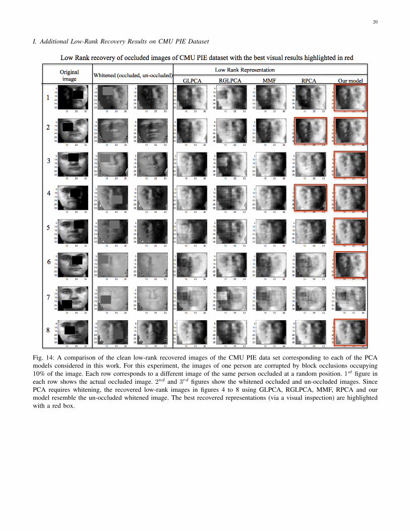
I. Additional Low-Rank Recovery Results on CMU PIE Dataset

Fig. 14: A comparison of the clean low-rank recovered images of the CMU PIE data set corresponding to each of the PCAmodels considered in this work. For this experiment, the images of one person are corrupted by block occlusions occupying10% of the image. Each row corresponds to a different image of the same person occluded at a random position. 1st figure ineach row shows the actual occluded image. 2nd and 3rd figures show the whitened occluded and un-occluded images. SincePCA requires whitening, the recovered low-rank images in figures 4 to 8 using GLPCA, RGLPCA, MMF, RPCA and ourmodel resemble the un-occluded whitened image. The best recovered representations (via a visual inspection) are highlightedwith a red box.

Page 21

21

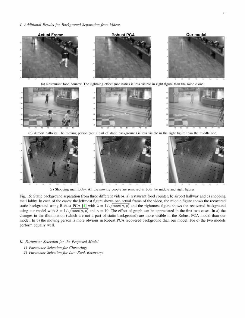
J. Additional Results for Background Separation from Videos

(a) Restaurant food counter. The lightning effect (not static) is less visible in right figure than the middle one.

(b) Airport hallway. The moving person (not a part of static background) is less visible in the right figure than the middle one.

(c) Shopping mall lobby. All the moving people are removed in both the middle and right figures.

Fig. 15: Static background separation from three different videos. a) restaurant food counter, b) airport hallway and c) shoppingmall lobby. In each of the cases: the leftmost figure shows one actual frame of the video, the middle figure shows the recoveredstatic background using Robust PCA [4] with λ = 1/

√max(n, p) and the rightmost figure shows the recovered background

using our model with λ = 1/√

max(n, p) and γ = 10. The effect of graph can be appreciated in the first two cases. In a) thechanges in the illumination (which are not a part of static background) are more visible in the Robust PCA model than ourmodel. In b) the moving person is more obvious in Robust PCA recovered background than our model. For c) the two modelsperform equally well.

K. Parameter Selection for the Proposed Model

1) Parameter Selection for Clustering:2) Parameter Selection for Low-Rank Recovery:

Page 22

22

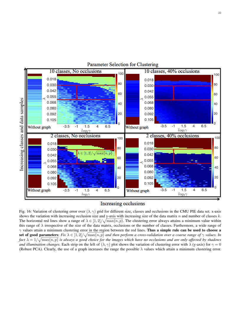
Fig. 16: Variation of clustering error over (λ, γ) grid for different size, classes and occlusions in the CMU PIE data set. x-axisshows the variation with increasing occlusion size and y-axis with increasing size of the data matrix n and number of classes k.The horizontal red lines show a range of λ ∈ [1, 2]/

√max(n, p). The clustering error always attains a minimum value within

this range of λ irrespective of the size of the data matrix, occlusions or the number of classes. Furthermore, a wide range ofγ values attain a minimum clustering error in the region between the red lines. Thus a simple rule can be used to choose aset of good parameters: Fix λ ∈ [1, 2]/

√max(n, p) and then perform a cross-validation over a coarse range of γ values. In

fact λ = 1/√

max(n, p) is always a good choice for the images which have no occlusions and are only affected by shadowsand illumination changes. Each strip on the left of (λ, γ) plot shows the variation of clustering error with λ (y-axis) for γ = 0(Robust PCA). Clearly, the use of a graph increases the range the possible λ values which attain a minimum clustering error.

Page 23

23

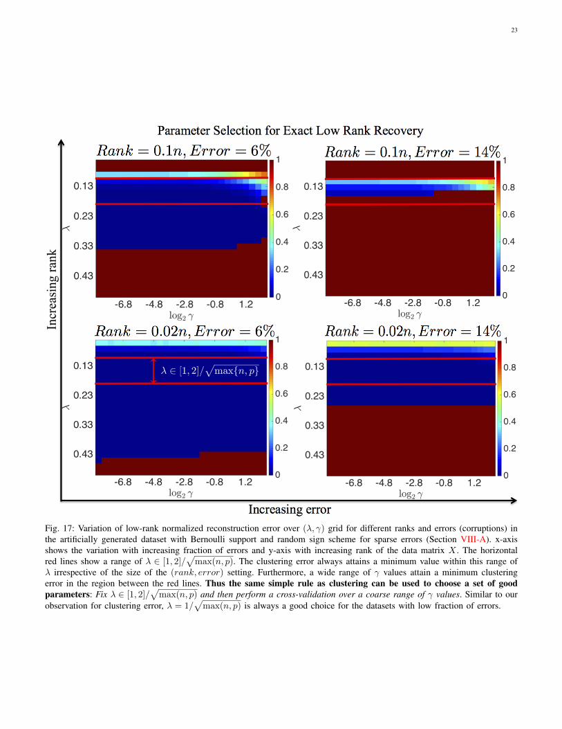
Fig. 17: Variation of low-rank normalized reconstruction error over (λ, γ) grid for different ranks and errors (corruptions) inthe artificially generated dataset with Bernoulli support and random sign scheme for sparse errors (Section VIII-A). x-axisshows the variation with increasing fraction of errors and y-axis with increasing rank of the data matrix X . The horizontalred lines show a range of λ ∈ [1, 2]/

√max(n, p). The clustering error always attains a minimum value within this range of

λ irrespective of the size of the (rank, error) setting. Furthermore, a wide range of γ values attain a minimum clusteringerror in the region between the red lines. Thus the same simple rule as clustering can be used to choose a set of goodparameters: Fix λ ∈ [1, 2]/

√max(n, p) and then perform a cross-validation over a coarse range of γ values. Similar to our

observation for clustering error, λ = 1/√

max(n, p) is always a good choice for the datasets with low fraction of errors.

Page 24

24

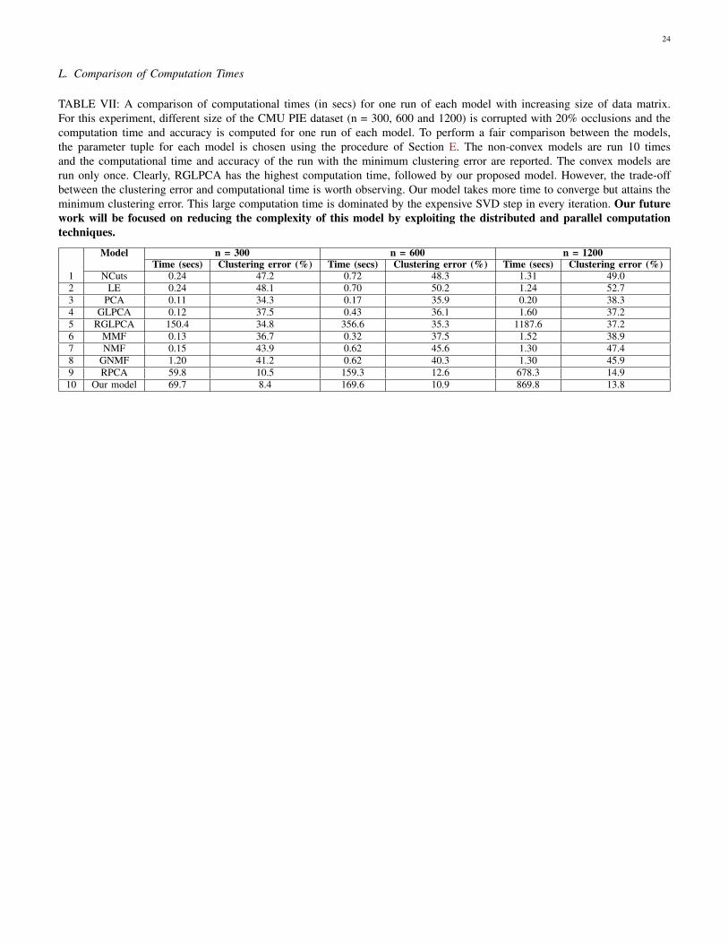
L. Comparison of Computation Times

TABLE VII: A comparison of computational times (in secs) for one run of each model with increasing size of data matrix.For this experiment, different size of the CMU PIE dataset (n = 300, 600 and 1200) is corrupted with 20% occlusions and thecomputation time and accuracy is computed for one run of each model. To perform a fair comparison between the models,the parameter tuple for each model is chosen using the procedure of Section E. The non-convex models are run 10 timesand the computational time and accuracy of the run with the minimum clustering error are reported. The convex models arerun only once. Clearly, RGLPCA has the highest computation time, followed by our proposed model. However, the trade-offbetween the clustering error and computational time is worth observing. Our model takes more time to converge but attains theminimum clustering error. This large computation time is dominated by the expensive SVD step in every iteration. Our futurework will be focused on reducing the complexity of this model by exploiting the distributed and parallel computationtechniques.

Model n = 300 n = 600 n = 1200Time (secs) Clustering error (%) Time (secs) Clustering error (%) Time (secs) Clustering error (%)

1 NCuts 0.24 47.2 0.72 48.3 1.31 49.02 LE 0.24 48.1 0.70 50.2 1.24 52.73 PCA 0.11 34.3 0.17 35.9 0.20 38.34 GLPCA 0.12 37.5 0.43 36.1 1.60 37.25 RGLPCA 150.4 34.8 356.6 35.3 1187.6 37.26 MMF 0.13 36.7 0.32 37.5 1.52 38.97 NMF 0.15 43.9 0.62 45.6 1.30 47.48 GNMF 1.20 41.2 0.62 40.3 1.30 45.99 RPCA 59.8 10.5 159.3 12.6 678.3 14.9

10 Our model 69.7 8.4 169.6 10.9 869.8 13.8