Robot Formation Control Methodology Based on Artificial Vector Fields Anh Duc Dang Hamburg 2017

Welcome message from author
This document is posted to help you gain knowledge. Please leave a comment to let me know what you think about it! Share it to your friends and learn new things together.
Transcript
Robot Formation Control Methodology Based on Artificial Vector Fields
Anh Duc Dang
Hamburg 2017
Robot Formation Control Methodology Based on
Artificial Vector Fields
To the Faculty of Electrical Engineering of
Helmut Schmidt University / University of the Federal Armed Forces Hamburg
for the attainment of the academic degree of
Doctor of Engineering
submitted
DISSERTATION
by
Anh Duc Dang
from Thai Nguyen, Vietnam
Hamburg 2017
II
First advisor: Prof. Dr.-Ing. Joachim Horn
Second advisor: Prof. Dr.-Ing. Gerd Scholl
Date of examination: August 15, 2017
III
Acknowledgments
Firstly, I would like to thank the Vietnamese Government, and specially thank the
MOET (Ministry of Education and Training) and the WUS (World University Service-
Deutsches Komitee e.V.), who supported me to implement this research.
I would like to express my deepest gratitude to my advisor, Prof. Dr.-Ing. Joachim
Horn, for his guidance, patience and continuous support in the completion of my Ph.D. I
would also like to thank Prof. Dr.-Ing. Gerd Scholl for his tutelage and the extra support
given during the research studies towards the completion of my Ph.D and Prof. Dr.-Ing.
Stefan Dickmann for serving as the chair of the Examination Commission.
I would like to thank all my colleagues for their valuable comments, discussions,
suggestions and for a pleasant working atmosphere created during my studies at the
Helmut-Schmidt-University. In addition, I would like to express my sincere thanks to Dr.-
Ing. Klaus Frick at the Helmut-Schmidt-University, who was always willing to help and
give best suggestions.
I would like to thank all my friends for their cheerful friendship, encouragements, as-
sistance, and their extramural support these past years.
Finally, I would like to specifically thank my family for always encouraging and sup-
porting me throughout my journey these past years. Last but not least, I would like to thank
my wife, Hoang Anh Phung, for her love and encouragement.
Hamburg, August 2017
Anh Duc Dang

IV
V
Abstract
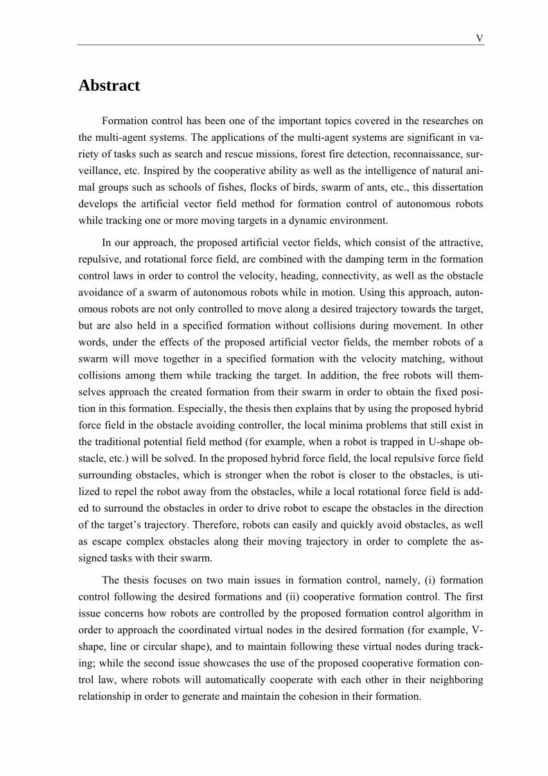
Formation control has been one of the important topics covered in the researches on the multi-agent systems. The applications of the multi-agent systems are significant in va-riety of tasks such as search and rescue missions, forest fire detection, reconnaissance, sur-veillance, etc. Inspired by the cooperative ability as well as the intelligence of natural ani-mal groups such as schools of fishes, flocks of birds, swarm of ants, etc., this dissertation develops the artificial vector field method for formation control of autonomous robots while tracking one or more moving targets in a dynamic environment.
In our approach, the proposed artificial vector fields, which consist of the attractive, repulsive, and rotational force field, are combined with the damping term in the formation control laws in order to control the velocity, heading, connectivity, as well as the obstacle avoidance of a swarm of autonomous robots while in motion. Using this approach, auton-omous robots are not only controlled to move along a desired trajectory towards the target, but are also held in a specified formation without collisions during movement. In other words, under the effects of the proposed artificial vector fields, the member robots of a swarm will move together in a specified formation with the velocity matching, without collisions among them while tracking the target. In addition, the free robots will them-selves approach the created formation from their swarm in order to obtain the fixed posi-tion in this formation. Especially, the thesis then explains that by using the proposed hybrid force field in the obstacle avoiding controller, the local minima problems that still exist in the traditional potential field method (for example, when a robot is trapped in U-shape ob-stacle, etc.) will be solved. In the proposed hybrid force field, the local repulsive force field surrounding obstacles, which is stronger when the robot is closer to the obstacles, is uti-lized to repel the robot away from the obstacles, while a local rotational force field is add-ed to surround the obstacles in order to drive robot to escape the obstacles in the direction of the target’s trajectory. Therefore, robots can easily and quickly avoid obstacles, as well as escape complex obstacles along their moving trajectory in order to complete the as-signed tasks with their swarm.
The thesis focuses on two main issues in formation control, namely, (i) formation control following the desired formations and (ii) cooperative formation control. The first issue concerns how robots are controlled by the proposed formation control algorithm in order to approach the coordinated virtual nodes in the desired formation (for example, V-shape, line or circular shape), and to maintain following these virtual nodes during track-ing; while the second issue showcases the use of the proposed cooperative formation con-trol law, where robots will automatically cooperate with each other in their neighboring relationship in order to generate and maintain the cohesion in their formation.
VI
Table of Contents
Acknowledgments .................................................................................................. III
Abstract .................................................................................................................. V
Symbols ............................................................................................................... VIII
1 Introduction ............................................................................................... 1 1.1 Motivation ............................................................................................................... 1 1.2 Problem statement ................................................................................................... 3 1.3 Method of approach ................................................................................................ 5 1.4 Research contributions ............................................................................................ 6 1.5 Literature review ..................................................................................................... 8 1.5.1 Specific geometric formation control ..................................................................... 8 1.5.2 Cooperative control ................................................................................................. 9 1.6 Organization of this dissertation ........................................................................... 12
2 Path Planning For a Single Robot ........................................................ 13 2.1 Introduction ........................................................................................................... 13 2.2 Background ........................................................................................................... 14 2.2.1 Idea of the artificial vector field method............................................................... 14 2.2.2 Potential field method ........................................................................................... 15 2.2.3 Conclusion ............................................................................................................ 19 2.3 Path planning algorithm for a mobile robot .......................................................... 19 2.3.1 Problem statement ................................................................................................. 19 2.3.2 Target tracking control algorithm ......................................................................... 20 2.3.3 Obstacle avoidance control ................................................................................... 22 2.4 Simulation results ................................................................................................. 29 2.4.1 The target tracking in a free environment ............................................................. 29 2.4.2 The target tracking under the influence of the obstacles ...................................... 31 2.5 Summary ............................................................................................................... 34
3 Formation Control Following Desired Formations ............................. 35 3.1 Introduction ........................................................................................................... 35 3.2 Problem formulation ............................................................................................. 38 3.3 Building desired formations .................................................................................. 40 3.3.1 Collinear desired formation .................................................................................. 41 3.3.2 V-shape desired formation .................................................................................... 43 3.3.3 Circular desired formation .................................................................................... 45 3.4 Formation adaptation while tracking a moving target .......................................... 47 3.4.1 Formation connection control algorithm .............................................................. 47 3.4.2 Collision avoidance control algorithm .................................................................. 54 3.4.3 Obstacle avoidance control algorithm .................................................................. 55
VII
3.4.4 Target tracking control algorithm ......................................................................... 56 3.4.5 Simulation Results ................................................................................................ 61 3.4.6 Conclusion ............................................................................................................ 69 3.5 Direction control for collinear formation .............................................................. 70 3.5.1 Target tracking control algorithm ......................................................................... 70 3.5.2 Simulation results ................................................................................................. 72 3.5.3 Conclusion ............................................................................................................ 75
4 Cooperative Control for Multi Robot Systems .......................................... 76 4.1 Introduction ........................................................................................................... 76 4.2 Problem statement ................................................................................................. 78 4.3 Connection between neighboring robots .............................................................. 79 4.4 Adaptive formation control in a dynamic environment ........................................ 83 4.4.1 Problem formulation ............................................................................................. 83 4.4.2 Adaptive formation control algorithm .................................................................. 84 4.4.3 Conclusion ............................................................................................................ 94 4.5 Cooperative formation control in a dynamic environment ................................... 94 4.5.1 Problem formulation ............................................................................................. 94 4.5.2 Formation control algorithm ................................................................................. 96 4.5.3 Simulation results ................................................................................................. 97 4.5.4 Conclusion .......................................................................................................... 101
5 Merging and Splitting in a Mobile Sensor Network .......................... 102 5.1 Introduction ......................................................................................................... 102 5.2 Sensor merging control ....................................................................................... 103 5.2.1 Problem statement ............................................................................................... 103 5.2.2 Sensor merging control algorithm ...................................................................... 106 5.3 Sensor splitting control ....................................................................................... 109 5.4 General controller ............................................................................................... 113 5.5 Simulation results ............................................................................................... 114 5.6 Conclusion .......................................................................................................... 122
6 Conclusion and Future Work ............................................................. 124 6.1 Conclusion .......................................................................................................... 124 6.2 Future work ......................................................................................................... 126
7 Appendix .............................................................................................. 127 7.1 Vector field ......................................................................................................... 127 7.2 Curl of a vector field ........................................................................................... 127 7.3 Gradient vector field ........................................................................................... 129 7.4 Proof of gravitational force field......................................................................... 131
8 Publications ......................................................................................... 132
9 References ............................................................................................. 133
VIII
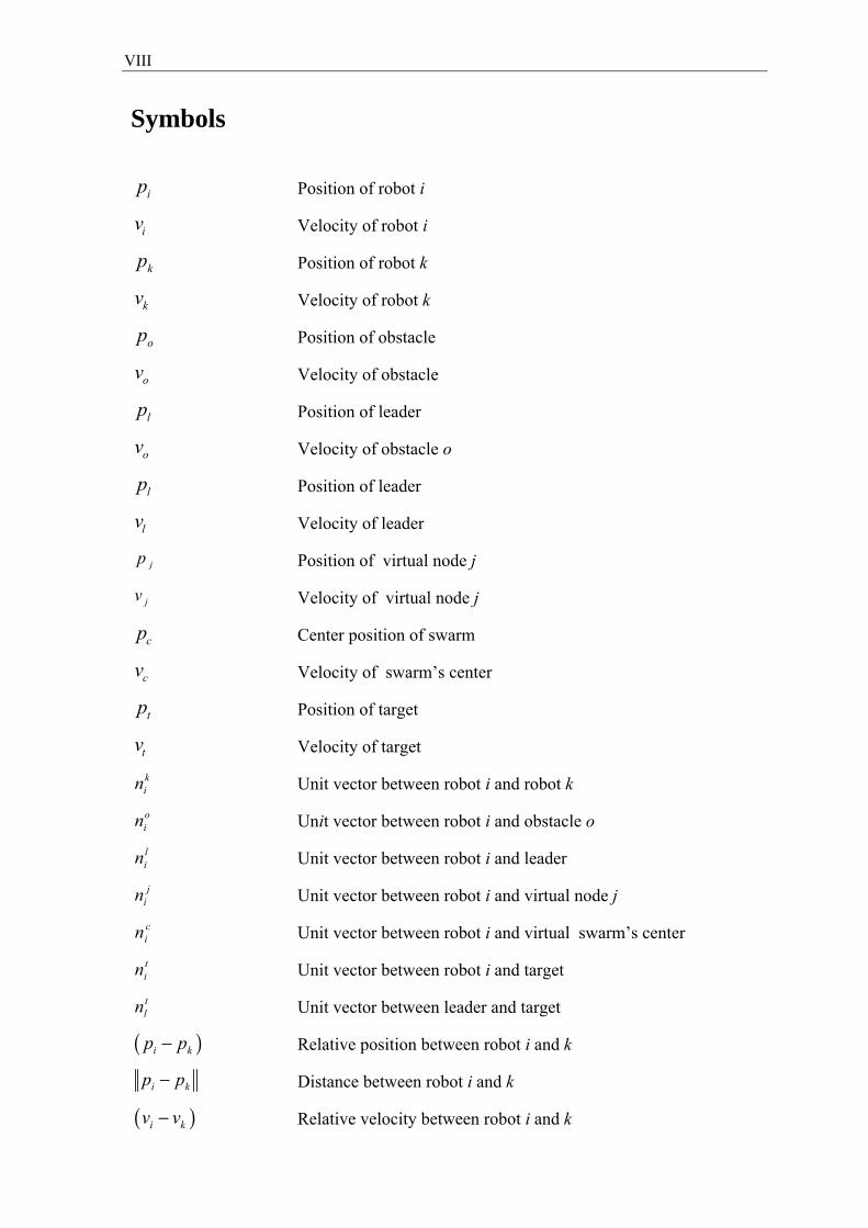
Symbols
ip Position of robot i
iv Velocity of robot i
kp Position of robot k
kv Velocity of robot k
op Position of obstacle
ov Velocity of obstacle
lp Position of leader
ov Velocity of obstacle o
lp Position of leader
lv Velocity of leader
jp Position of virtual node j
jv Velocity of virtual node j
cp Center position of swarm
cv Velocity of swarm’s center
tp Position of target
tv Velocity of target kin Unit vector between robot i and robot k oin Unit vector between robot i and obstacle o lin Unit vector between robot i and leader j
in Unit vector between robot i and virtual node j cin Unit vector between robot i and virtual swarm’s center tin Unit vector between robot i and target tln Unit vector between leader and target
( )i kp p− Relative position between robot i and k
i kp p− Distance between robot i and k
( )i kv v− Relative velocity between robot i and k
IX
( )i tp p− Relative position between robot i and target
i tp p− Distance between robot i and target
( )i tv v− Relative velocity between robot i and target
( )i op p− Relative position between robot i and obstacle i
i op p− Distance between robot i and obstacle i
( )i ov v− Relative velocity between robot i and obstacle i
( )i cp p− Relative position between robot i and swarm’s center
i cp p− Distance between robot i and swarm’s center
( )i cv v− Relative velocity between robot i and swarm’s center
( )i lp p− Relative position between robot i and leader
i lp p− Distance between robot i and leader
( )i lv v− Relative velocity between robot i and leader
( )i jp p− Relative position between robot i and virtual node j
i jp p− Distance between robot i and virtual node j
( )i jv v− Relative velocity between robot i and virtual node j
( )l tp p− Relative position between leader and target
l tp p− Distance between leader and target
( )l tv v− Relative velocity between leader and target
N Number of robots
M Number of obstacles
( )kiN t Set of robots in the neighborhood of robot i at time t
( )oiN t Set of obstacles in the neighborhood of robot i at

1
1 Introduction
1.1 Motivation
In recent years, researches on multi-agent systems have widely been conducted in
physic [6, 7, 8], chemistry [9, 10], biology [11], and especially in control and cybernetic
science [24]-[94] over the world. Formation control is one of the necessary and important
problems in the research field on the multi-agent systems. The formation control of auton-
omous robots, such as the formation of autonomous underwater vehicles [21, 84], un-
manned aerial vehicles [29, 30, 31, 83], flocking control [34]-[42], mobile sensor networks
[43]-[57], etc., and its potential applications into a variety of tasks including search and
rescue missions, forest fire detection, reconnaissance, and surveillance, etc., have attracted
a lot of attention from researchers worldwide.
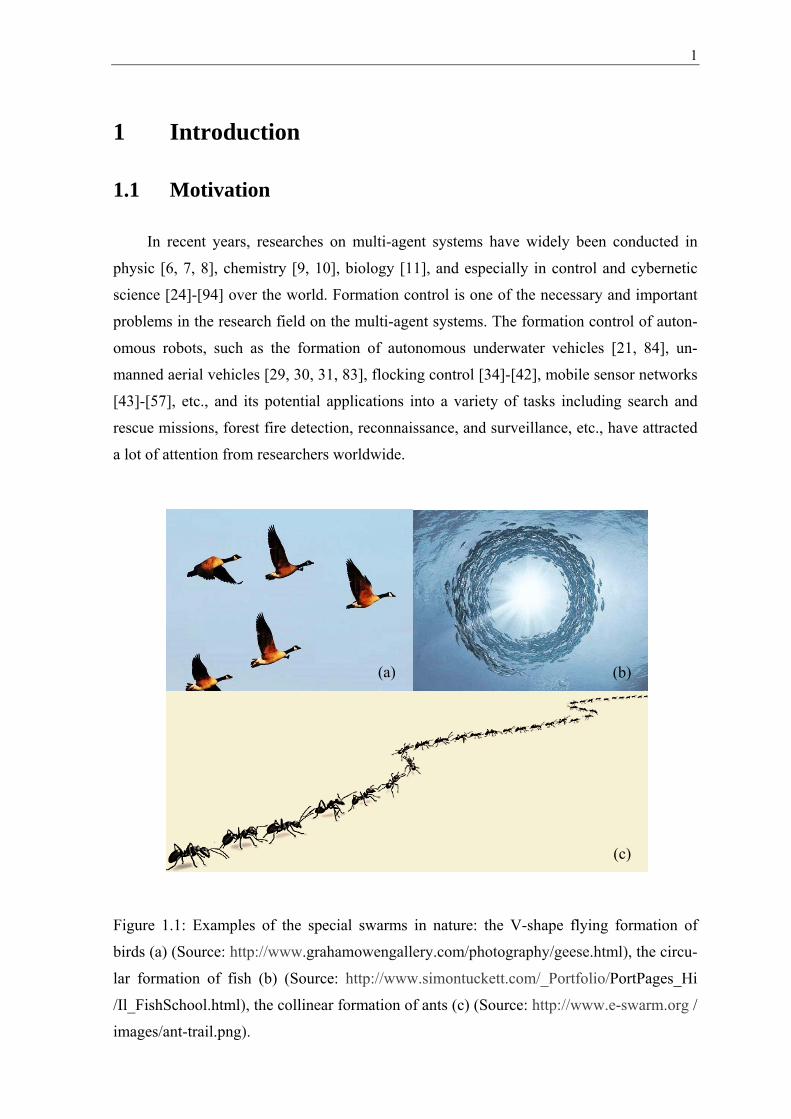
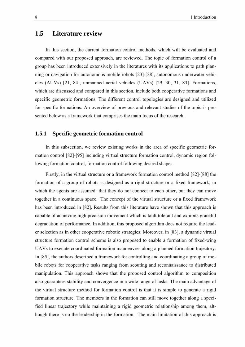
Figure 1.1: Examples of the special swarms in nature: the V-shape flying formation of
birds (a) (Source: http://www.grahamowengallery.com/photography/geese.html), the circu-
lar formation of fish (b) (Source: http://www.simontuckett.com/_Portfolio/PortPages_Hi
/Il_FishSchool.html), the collinear formation of ants (c) (Source: http://www.e-swarm.org /
images/ant-trail.png).
(a) (b)
(c)
2 1 Introduction
In observing the animal groups in nature, such as schools of fish, flocks of birds,
swarm of ants, etc., we can see the intelligences as well as the several interesting features
of these animal groups. Moreover, from the natural animal groups we can also find some
special formations that are organized into the particular shapes such as V-shape, line or
circle, etc., see figure 1.1. Natural features as well as the intelligences of a swarm [1]-[14]
that have suggested our designing the control laws for the multi-agent systems, are ex-
pressed as follows:
• A swarm can still search and track a source of food (a target) efficiently while avoid-
ing obstacles. This natural phenomenon helps us to design the target tracking control
algorithm for a swarm of autonomous robots in a dynamic environment.
• A swarm can also split into smaller sub-groups in order to search and approach mul-
tiple food sources (targets) and avoid obstacles simultaneously. If any food source
runs out, the individuals that are using this food source will continue to search and
approach other food sources. This situation directs us to the building of sensor merg-
ing and splitting in a mobile sensor network when the number of the targets changes.
This control law guarantees that all free sensors can easily and quickly approach their
swarm as well as some sensors will be split from a main group into a sub-group to
track a new target.
• A swarm has the ability to change its size to adapt to the environment. Based on this
feature, we can design the adaptive formation control algorithm for a swarm of au-
tonomous robots while escaping obstacles to track a moving target. Using this con-
trol law, the swarm’s size shrinks into the smaller size in order to adapt to the com-
plex environment while maintaining the formation connectivity.
• Each member in a swarm can communicate and interact with its neighbors within its
limited sensing range in order to avoid the collisions with its neighbors, and generate
the robust connectivity in its formation. Moreover, based on this organization, the in-
formation that each member obtains from the environment can be sent to all other
members in formation. Hence, in cases where only some members in the swarm de-
tect the obstacles or the food source, etc., but all other members in the swarm can still
avoid these obstacles, or approach this food source with their swarm. This natural fea-
ture motivates us as researchers to design the formation cooperative control algo-
rithm. This control algorithm guarantees that the formation of a swarm is maintained
without collisions among the members in the swarm while tracking the dynamic tar-
get.
1.2 Problem statement 3
• Each member in a swarm can still combine and move with its neighbors in the cohe-
sive formation, although it may not sense the position as well as the velocity of its
neighbors accurately. This natural feature has inspired the authors to think about the
formation control of a swarm of autonomous robots in the noisy environments.
• A swarm can move in the particular formations such as V-shape, line or circle, etc.,
see figure 1.1. This special ability encourages us to study the formation control of a
swarm of multiple autonomous robots following the desired formations. If successful,
this control law will ensure that multiple autonomous robots can uphold a specific
formation while traversing a trajectory and avoiding collisions among them simulta-
neously. The potential applications of this approach in the specific tasks or missions
such as search, observation, supervision or surrounding, etc., play the important roles
in reality.
Finally, motived by the features, the abilities, and the intelligences of the animal
groups in the nature with the potential applications from multi-agent systems in reality, this
thesis focuses on the research and the design of the control algorithms for multi-agent sys-
tems, such as: formation connection control; path planning for the formation of a swarm in
a dynamic environment; formation control of autonomous robots in a noisy environment;
adaptive and cooperative formation control in complex environments, etc.
1.2 Problem statement
Although there are many research directions on the multi-robot systems, but the main
issue is that the member robots in a group have to collaborate in order to achieve the de-
sired tasks, such as observing, tracking or encircular a moving target, etc. As presented in
the preceding passages, formation control of autonomous robots is observed in various
kinds of the animal groups in the nature, such as schools of fishes, flocks of birds, swarm
of ants, etc., [1]–[7]. This guarantees that the members in the formation of a group have to
move together in a desired organization under the velocity matching without collisions
among them. In addition, the free robots in a group, which still do not have the cohesion
with their formation, must themselves approach their formation in order to obtain the fixed
position in their formation. Moreover, the formation of a swarm must be maintained while
moving in a free environment as well as in a dynamic environment. All of these analyses
have identified our research concentration issues as follows:
• “Formation control following the desired formations”, the content of this issue is to
4 1 Introduction
control the formation of autonomous robots following the particular shapes such as
V-shape, line or circle, etc., while observing and tracking the dynamic target. In this
method, the desired formation, which consists of the coordinated virtual nodes, is first
generated. The shape of the desired formation is decided on its potential application
in the specific tasks or missions such as search, observation, supervision, tracking or
surrounding, etc. Then, the robots are controlled to approach the coordinated virtual
nodes in the desired formation and to maintain at these virtual nodes while moving
simultaneously. Using this method, robots can easily uphold a specific formation
while traversing a trajectory and avoiding collisions among them simultaneously.
Although this topic is very interesting and important in the field of the research on the
multi-robot systems, but the research results in this field are still very limited. There-
fore, this research direction will be developed in this thesis, such as the adaptive
shape-formation control while tracking a moving target under the influences of the
varying environments.
• “Cooperative formation control”, the content of this issue is to control the formation
of a group of autonomous robots based on the stable and robust connections among
neighboring members to complete the specific tasks or missions such as search, ob-
servation, supervision or tracking the dynamic targets. In this method, the neighbor-
ing robots are linked to each other by the attractive/repulsive force fields among them
to create a robust cohesion in a formation and avoid collisions among them simulta-
neously. The success of the cooperative formation control method based on the con-
nections among neighboring members in a swarm as an α-lattice configuration has
been published in some literature, such as flocking control [34]-[42]. The published
results show that this topic is very interesting, and has potential applications in mili-
tary areas as well as in civilian areas. However, there are some constraints on the ap-
proach, such as: when the cohesion in the formation of the swarm is broken while
avoiding obstacles, while we need the maintaining of the formation in order to per-
form a certain job. Moreover, the formation adaptation of a swarm in the complex
environments such as U-shape or the narrow space between obstacles, etc., is also an
important issue that needs attention. Additionally, the thesis addresses other arising
issues namely the swarm–finding of the free robots that have not been offered a fixed
position in a formation (for example: the robots that get lost, or are separated from
their formation for certain cause).
1.3 Method of approach 5
1.3 Method of approach
There are many methods to generate and control the formation of a swarm of auton-
omous mobile robots. One of the simple and effective methods utilized to control the coor-
dination, the motion, the formation connectivity, as well as the obstacle avoidance for a
swarm in order to track the dynamic targets is the artificial vector field tool. This vector
field tool is built on the relative positions and velocities among the targets, robots, and ob-
stacles in the environment.
In this thesis, the proposed solution for formation control of autonomous robots is
based on the improved vector fields that consist of the artificial potential fields and the
artificial rotational fields. The proposed potential fields, which include the attractive and
repulsive force fields and are generated by negative gradient of the corresponding potential
functions, are not only used to control autonomous robots moving on a desired trajectory
(path planning for a swarm), but are also used to hold these robots in a specified formation
without collisions during movement (formation connection control). The attractive force
field is generated surrounding the goals such as the target of the swarm, the virtual nodes
in the desired formation, etc., to drive robots towards these goals (for example the target
tracking control or the swarm-finding control, etc.,) with the velocity matching. Further-
more, surrounding the neighboring robots in a formation, the local attractive force field is
combined with the local repulsive force field in order to create and keep the formation
connectivity, as well as to avoid collisions among the members of the swarm. Moreover,
using the hybrid force field, which consists of the repulsive force field and the rotational
force field surrounding obstacles, robots can easily and quickly avoid and escape obstacles
along their moving trajectory while maintaining their formation. In this obstacle avoiding
control law, the repulsive force field that is stronger when the robot is closer to the obsta-
cles is utilized to repel the robot away from the obstacle, while a rotational force field is
added to drive the robot to escape the obstacles in the direction of the target’s trajectory.
Especially, this added rotational force field will solve the local minima problems in the
traditional potential field method such as when robots are trapped in the complex obstacles
(for example U-shape obstacle, etc.), [22], [24].
Finally, the proposed artificial vector fields combined with the damping term in the
formation controller will generate the desired velocities and headings, as well as the stable
formation connectivity for the robots of a swarm while tracking the dynamic targets.
Moreover our proposed formation controller also guarantees that the formation adaptation
in different tasks and missions, and in varied environments is performed.
6 1 Introduction
1.4 Research contributions
As presented above, “formation control following the desired formations” and “coop-
erative formation control” are the main contributions of our research in this dissertation. As
such, the research is expected to indicate:
• Formation control following the desired formations
The content of this contribution is to control the formation of autonomous robots fol-
lowing the desired shapes including V-shape, line and circle, while observing and
tracking a dynamic target under the influence of the dynamic environment. In this ap-
proach, the desired formations, which consists of the equidistant neighboring virtual
nodes, is first generated based on the relative position between the swarm’s virtual
leader and the target. The swarm’s virtual leader is randomly chosen from a swarm’s
member that is closest to the target. This leader plays an important role to create and
lead its formation moving towards the target in a stable direction. Hence, in many un-
desired cases, such as the leader is broken or trapped in the obstacles (for example U-
shape obstacle) one new leader is replaced in order to continue to lead the swarm
tracking the target. Further, the motion of the robots towards the desired positions in
the desired formation is controlled by the artificial force fields that consist of the local
and global potential fields surrounding the virtual nodes. Under the effect of these ar-
tificial force fields, robots will automatically find their desired position at the virtual
nodes in the desired formation. Additionally, the local repulsive force field surround-
ing each robot is used to avoid the collision with each other. Moreover, using the re-
pulsive vector field combined with the rotational vector field in the obstacle avoiding
controller, robots can easily escape the obstacles while tracking a moving target.
In summary, this main contribution is performed as follow: firstly, the desired for-
mation (V-shape, line or circular shape) of the virtual nodes, which are equally
spaced, is designed on the relative position between the swarm’s virtual leader and
the target. Secondly, the control algorithms, which are developed based on the artifi-
cial vector fields, guarantee that the motion of robots always converges to the created
virtual nodes in the desired formation under the effects of the dynamic environment
and avoid collisions simultaneously. Furthermore, the formation adaptation and the
target approaching direction are decided by the target’s position sense of the virtual
leader. Using our proposed control algorithms, all robots can easily approach the de-
1.4 Research contributions 7
sired formation and maintain their formation connectively while tracking a moving
target in a dynamic environment.
• Cooperative formation control
The content of this contribution is to control the formation of a group of autonomous
robots based on the stable and robust connections among the neighboring members in
order to track the dynamic targets in the various environments. In this approach, the
neighboring robots are first linked to each other by the artificial attractive/repulsive
force fields among them in order to create a robust cohesion in a formation and avoid
collisions among them simultaneously. Further, in order to adapt to the changing en-
vironments, for example in the case when a group of multi robots must pass through a
narrow space among obstacles, we propose the adaptive formation control algorithm.
Using this control algorithm, the members in a formation can cooperatively learn the
swarm’s parameters to decide the size of their formation so that the formation con-
nection and the target tracking performance can be improved. Furthermore, in order
to solve the local minima problems in the traditional potential field method as pre-
sented in [20, 21, 22], and help robots find a good way to approach the moving target
while maintaining their formation simultaneously, we propose the developed obstacle
avoiding controller. In this proposed obstacle avoiding controller we also utilize the
repulsive/ rotational force fields combined with the direction of the target’s trajectory
to drive the robot formation so as to escape the obstacle. Moreover, in order to solve
the problems of the robot contribution and distribution in the scenario of multiple dy-
namic target tracking, we use the robot splitting/merging control algorithm. Using our
control law, the free robots can easily approach their formation, as well as some
member robots from a main group can be split into smaller subgroup.
Finally, this main contribution is built as follows: the formation’s connectivity is first
developed on the local attractive and repulsive force fields among the neighboring
members of a group. Furthermore, the cooperation control algorithm for the for-
mation maintenance of a group while avoiding obstacles is built on the data that are
collected and updated by the sensing of each member about the environment around
it.
8 1 Introduction
1.5 Literature review
In this section, the current formation control methods, which will be evaluated and
compared with our proposed approach, are reviewed. The topic of formation control of a
group has been introduced extensively in the literatures with its applications to path plan-
ning or navigation for autonomous mobile robots [23]-[28], autonomous underwater vehi-
cles (AUVs) [21, 84], unmanned aerial vehicles (UAVs) [29, 30, 31, 83]. Formations,
which are discussed and compared in this section, include both cooperative formations and
specific geometric formations. The different control topologies are designed and utilized
for specific formations. An overview of previous and relevant studies of the topic is pre-
sented below as a framework that comprises the main focus of the research.
1.5.1 Specific geometric formation control
In this subsection, we review existing works in the area of specific geometric for-
mation control [82]-[95] including virtual structure formation control, dynamic region fol-
lowing formation control, formation control following desired shapes.
Firstly, in the virtual structure or a framework formation control method [82]-[88] the
formation of a group of robots is designed as a rigid structure or a fixed framework, in
which the agents are assumed that they do not connect to each other, but they can move
together in a continuous space. The concept of the virtual structure or a fixed framework
has been introduced in [82]. Results from this literature have shown that this approach is
capable of achieving high precision movement which is fault tolerant and exhibits graceful
degradation of performance. In addition, this proposed algorithm does not require the lead-
er selection as in other cooperative robotic strategies. Moreover, in [83], a dynamic virtual
structure formation control scheme is also proposed to enable a formation of fixed-wing
UAVs to execute coordinated formation manoeuvres along a planned formation trajectory.
In [85], the authors described a framework for controlling and coordinating a group of mo-
bile robots for cooperative tasks ranging from scouting and reconnaissance to distributed
manipulation. This approach shows that the proposed control algorithm to composition
also guarantees stability and convergence in a wide range of tasks. The main advantage of
the virtual structure method for formation control is that it is simple to generate a rigid
formation structure. The members in the formation can still move together along a speci-
fied linear trajectory while maintaining a rigid geometric relationship among them, alt-
hough there is no the leadership in the formation. The main limitation of this approach is
1.5 Literature review 9
that the rigidity of the virtual structure or a fixed framework affects the formation’s turning
performance when moving along a curvature trajectory.
Another approach for the specific geometric formation control is to use a dynamic re-
gion. In this method, all member robots of a group are controlled to move together in a
given dynamic region [89], [90]. The published results in this approach have shown that
robots stay within a moving region, and are able to adjust their formation by rotating and
scaling during movement together simultaneously. This method does not require specific
ordering or positioning of the robots inside the given dynamic region. The motion of each
robot in formation depends on the motion of its neighbors and the given dynamic region.
One positive approach, which has also attended the growing attention from research-
ers worldwide, for the specific geometric formation control is the formation control follow-
ing desired shapes [91]-[95]. In this approach, robots are independently controlled to move
towards the virtual nodes in the designed desired formation (V-shape, line, or circle) and
converge at these virtual nodes simultaneously during movement. Moreover, the designed
virtual nodes in the desired formation must guarantee that the robots that are occupying the
neighboring virtual nodes do not interact with each other.
1.5.2 Cooperative control
Cooperative control is also known as an interesting research direction in multi robot
systems. This research direction has received a lot of attention from researchers in recent
years [32]-[76]. It has been used for a variety of application fields, however, in this section
we only review the existing works that relate to our research in this thesis, including: coop-
erative control while tracking a moving target; cooperative control in the dynamic targets
tracking; adaptive flocking control in a dynamic environment.
Firstly, cooperative control of multi robot while tracking a moving target [32]-[63]
can be split into the different research sub-issues based on the knowledge of graph theory,
potential field, network communication, and system stability analysis.
In [32]-[37], the approach for the flocking control of multi agent with a virtual leader
is introduced. In this approach, the organization of a group and its motion depend on the
position, velocity, and trajectory of the leader. In [32, 33], the leader robot of a group
tracks a predefined trajectory, and the other member robots in the group will follow this
leader while maintaining a particular formation. Further, a method, which is built based on
the extension of the flocking control algorithm in [41], for flocking control of multi-agents
10 1 Introduction
with a virtual leader was also presented in [34]-[36]. In addition, in [37], the authors inves-
tigated the dynamic properties of the group for the case where the state of the virtual leader
may be time-varying and the topology of the neighboring relations among agents is dy-
namic. Although this approach is simple, but its main disadvantage is that the group’s mo-
tion is dependent on the leader, so any failures from the leader will influence on the motion
of the whole system.
In [38]-[62], the approach for the flocking control of multi agent without any leader is
presented. In this approach, all robots of a group are controlled together to achieve a target,
in other words, all these robots take a similar role while in motion. Each agent of a group
will connect with other agents in its communicating range while it moves towards the tar-
get position. Thus, the formation’s cohesion of a group will be automatically generated on
the local connectivity among the neighboring agents in group. Using this control method
the stability and robustness of a formation are attained [77]-[81], but the quick swarm-
approach of the free agents in the global workspace is still limited. In [39, 40, 41, 49, 50,
51], the algorithm for the quick swarm-approach of the free agents utilizes the parabolic
attractive potential function, so the corresponding attractive force will converge linearly
towards zero as the free agents will approach the target position with their decreasing ve-
locity. These have demonstrated that the cooperation among the free agents in the local
workspace has been well maintained. However, in the global workspace when the free
agents that are far from the target will be acted by a large attractive force from the target,
thus they will move with the very high speed to the target. In addition, in [50], a distributed
flocking algorithm for mobile sensor network to track a moving target is also presented. In
this literature, the author used an extension of a distributed Kalman filtering algorithm for
the sensors to estimate the target’s position. Moreover, the cooperative sensing and learn-
ing in a mobile sensor network have been studied by many researchers in recent years. The
cooperative sensing in a mobile sensor network can be applied in many different fields
such as target tracking, monitoring, observation, or environmental mapping, etc., and can
be found in [51, 56, 57, 58,]. The approaches to the cooperative learning in a mobile sensor
network including game theory, evolutionary computation or reinforcement learning, etc.,
are introduced in [54, 60, 86]. The published results around this topic show that the prob-
lems of the environment mapping as well as estimation based on the multi agent coopera-
tive sensing and learning are very interesting and still open research directions.
Secondly, cooperative control in the dynamic targets tracking is presented in [64]-
[70]. In [64], the problem of motion planning and sensor assignment strategies for tracking
multiple targets with a mobile sensor network is discussed. The authors focused on triangu-
1.5 Literature review 11
lation based tracking where two sensors merge their measurements in order to estimate the
position of a target. Further, in [66], robots equipped with sensors and communication de-
vices discover and track as many evasive targets as possible in an open region. Additional-
ly, a technique for multiple moving objects tracking with a mobile robot is discussed in
[68]. In this approach, the authors have introduced a sample-based variant of joint proba-
bilistic data association filters to track features originating from individual objects, and to
solve the correspondence problem between the detected features and the filters. Moreover,
the control algorithms for the dynamic targets tracking in a mobile sensor network are also
discussed in [69, 70].
Thirdly, adaptive flocking control in a dynamic environment [71]-[76] is also an in-
teresting issue in cooperative control. In [71], the authors presented a distributed approach
for adaptive flocking of the swarms of mobile robots that enables the robots to navigate
autonomously in complex environments populated with obstacles. In this approach, an
integrated algorithm that allows a swarm of robots to navigate in a coordinated manner,
split into multiple swarms, or merge with other swarms according to the environment con-
ditions is proposed. However, the problems for controlling the size of a group were not
considered in this literature. In [75], four novel collision avoidance processes for mobile
robots to generate effective collision‐free trajectories when forming and maintaining a
formation are discussed. In addition, robust adaptive flocking control of multi-agent sys-
tems with nonlinear dynamics is introduced in [76]. In this method, the coupling weights,
which are perturbed by asymmetric uncertain parameters, are dynamically updated while
the network topology for velocity is fixed.
12 1 Introduction
1.6 Organization of this dissertation
The rest of this dissertation is formed by separated chapters, in which:
Chapter 2 introduces the approach to path planning for a single mobile robot in a dy-
namic environment. This approach is based on the artificial vector fields that include the
developed potential force fields and the proposed rotational force field.
Chapter 3 presents the approach for formation control of the autonomous robots fol-
lowing the desired formations while tracking a moving target under the influence of the
dynamic environment.
Chapter 4 proposes the cooperative formation control algorithms for a group of multi
robots while avoiding obstacles as well as tracking a moving target.
Chapter 5 presents the sensor merging/spitting algorithm for a mobile sensor network
while tracking the moving targets in a dynamic environment.
Chapter 6 outlines the conclusion drawn from the findings, implications for practice
as well as recommendations for future researches.
13
2 Path Planning For a Single Robot
2.1 Introduction
The problem of path planning for an autonomous robot in a dynamic environment is
how to plan and control the robot to move towards the target position in a desired path
while avoiding obstacles in the environment. Therefore, navigation or path planning for the
autonomous mobile robot is one of the most important applications for robot control sys-
tems. This interesting topic has attracted the attention from researchers in recent years.
Obstacle avoidance is an important issue in path planning for autonomous robots
while reaching the target position. The artificial potential field as shown in [14]-[23] is
known as a positive method in order to solve this problem. Recently, the potential field
method has been widely studied and applied powerfully to path planning or navigation for
autonomous mobile robot to reach the position of the target in a simple environment, see
[14]-[20]. However, in a complex environment, in which the U-shaped obstacles or con-
nected walls exist, the application of the potential field method to path planning for the
autonomous robots is very difficult. Robot can be trapped in these obstacles before reach-
ing the target position.
This chapter presents a novel improved artificial vector field method (AVFM) for
path planning for a single robot to reach a target, which can be stationary or dynamic, in a
dynamic environment. This approach is developed based on the traditional potential field
method combined with the rotational field method. Using this approach, the robot can easi-
ly avoid and escape the obstacles in the environment without collision while reaching a
stationary target. Furthermore, when the target moves in an unknown environment, the
obstacle avoiding direction of the robot has a great influence on finding the fastest way
towards the target. Following approach, a global attractive force field, which is built sur-
rounding the target, is used to drive the robot towards the target. On the other hand, the
repulsive force field, which is stronger when the robot is closer to the obstacle, is also de-
signed surrounding the obstacles to repel the robot away from the obstacle. This repulsive
force helps the robot to avoid the collision with the obstacles. Moreover, the rotational vec-
tor field is added to control the robot to avoid and escape the obstacles in the direction of
the target’s trajectory. Under the effect of this blended vector field, the robot can easily
escape the obstacles to continue tracking the target. However, in order for the robot to
quickly exit the complex obstacles, the computed rotational force must be larger than the
14 2 Path Planning For a Single Robot
sum of the repulsive forces of the obstacles and the attractive force of the target. The direc-
tion of the target’s movement is determined on the relative position between the current
position and the future position of the target with the preselected time-step ∆t.
The rest of this chapter is organized as follows: The basic potential field method is
reviewed in section 2.2. Then, from the basic potential fields we propose the control algo-
rithms for path planning of a single robot while tracking a moving target under the effects
of the dynamic environment in section 2.3. The effectiveness of the proposed approach is
verified in simulations in section 2.4. Finally, section 2.5 summarizes this chapter.
2.2 Background
This subsection presents the background of the artificial vector field method that will
be extended, and applied to path planning for an autonomous robot in a dynamic environ-
ment. Firstly, the idea for this method is presented in subsection 2.2.1. Then, the tradition-
al potential fields are introduced as background for the artificial vector field method in
subsection 2.2.2.
2.2.1 Idea of the artificial vector field method
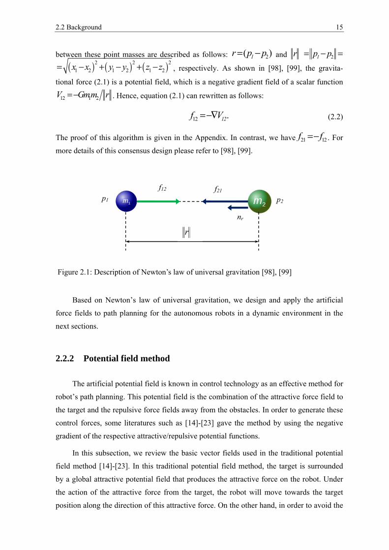
The idea of the artificial vector field method is based on Newton’s law of universal
gravitation [98], [99]. According to Newton’s law of universal gravitation, any two objects
in space exert gravitational forces on each other along the line connecting the centers of
these objects. These gravitational forces are attractive, equal in magnitude, and have oppo-
site directions. The magnitude of these gravitational forces is proportional to the product of
the masses of these objects and inversely proportional to the square of the distance between
them, see figure 2.1.
Consider the gravitational force of a point mass m2 located at the position ( )T
2 2 2 2p x ,y ,z= acting on a point mass m1 located at the position ( )T1 1 1 1p x ,y ,z= . As pre-
sented in [98], [99], this gravitational force is given by
1 2 1 212 2 2 .r
m m m mrf G G n
rr r
= − = −
(2.1)
Where G is the gravitational constant, and rn r r= is the unit vector along the direction
from the point mass m2 to the point mass m1. The relative position vector and the distance
2.2 Background 15
between these point masses are described as follows: 2( )1r p p= − and 2 1r p p= − =
( ) ( ) ( )2 2 21 2 1 2 1 2x x y y z z= − + − + − , respectively. As shown in [98], [99], the gravita-
tional force (2.1) is a potential field, which is a negative gradient field of a scalar function
12 1 2V Gmm r=− . Hence, equation (2.1) can rewritten as follows:
12 .12f V=−∇ (2.2)
The proof of this algorithm is given in the Appendix. In contrast, we have 21 12f f=− . For
more details of this consensus design please refer to [98], [99].
Figure 2.1: Description of Newton’s law of universal gravitation [98], [99]
Based on Newton’s law of universal gravitation, we design and apply the artificial
force fields to path planning for the autonomous robots in a dynamic environment in the
next sections.
2.2.2 Potential field method
The artificial potential field is known in control technology as an effective method for
robot’s path planning. This potential field is the combination of the attractive force field to
the target and the repulsive force fields away from the obstacles. In order to generate these
control forces, some literatures such as [14]-[23] gave the method by using the negative
gradient of the respective attractive/repulsive potential functions.
In this subsection, we review the basic vector fields used in the traditional potential
field method [14]-[23]. In this traditional potential field method, the target is surrounded
by a global attractive potential field that produces the attractive force on the robot. Under
the action of the attractive force from the target, the robot will move towards the target
position along the direction of this attractive force. On the other hand, in order to avoid the
f12 f21
p1 p2
nr
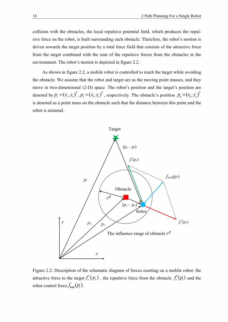
16 2 Path Planning For a Single Robot
collision with the obstacles, the local repulsive potential field, which produces the repul-
sive force on the robot, is built surrounding each obstacle. Therefore, the robot’s motion is
driven towards the target position by a total force field that consists of the attractive force
from the target combined with the sum of the repulsive forces from the obstacles in the
environment. The robot’s motion is depicted in figure 2.2.
As shown in figure 2.2, a mobile robot is controlled to reach the target while avoiding
the obstacle. We assume that the robot and target are as the moving point masses, and they
move in two-dimensional (2-D) space. The robot’s position and the target’s position are
denoted by ( )Tr r rp x ,y= , ( )T
t t tp x ,y= , respectively. The obstacle’s position ( )To o op x ,y=
is denoted as a point mass on the obstacle such that the distance between this point and the
robot is minimal.
Figure 2.2: Description of the schematic diagram of forces exerting on a mobile robot: the
attractive force to the target ( )rrtf p , the repulsive force from the obstacle ( )r
orf p and the
robot control force ( )total rf p .
Obstacle
x
y
Target
pr
pt
Robot
The influence range of obstacle
po
(pr - pt)
frt(pr)
(pr – po)
ftotal(pr)
fro(pr)
2.2 Background 17
A. Attractive potential field
As shown in [15]-[23], the most commonly used attractive potential function is given
as follows
1( ) ( , ).2
matt r
tr t kV p = p p ρ (2.3)
The corresponding attractive force field is given by the negative gradient of the potential
function (2.3) as follows
( ) ( )
( ) , if 1( , )
( ), if .
t
t
tr r att r
r t
r t
r t
f p = V p
k
p pm =
p p
k
=
p p m = 2
ρ
−∇
− −− −
(2.4)
Where kt is a positive scaling factor, and m=1 or 2. ( , )r t r tp p p pρ = − and ( )r tp p− are
the distance and the relative position vector between the robot and the target, respectively.
The equation (2.4) shows that: For m=1, the attractive potential is conic in shape, and the
corresponding attractive force has constant amplitude. For m=2, the attractive potential is
parabolic in shape, and the corresponding attractive force converges linearly towards zero
as the robot approaches the target.
B. Repulsive potential field
Similarly, one commonly used repulsive potential function is given in [15]-[23] as
21 1 1 , ( , )2 ( , )( )
otherwise. 0 ,
or o
r orep r
k p p rp p rV p
ββ ρ
ρ
− =
≤
(2.5)
Taking the negative gradient of the potential function (2.5), we obtain the corresponding
attractive force as follows
18 2 Path Planning For a Single Robot
2
( )
1 ( , )( , ) ( , )
,
( )
otherwise
r rep r
o or r o
r
o
o r
r
o
p V p
1 1k n , p p r
p p r p p
0
f
.
ββ ρ
ρ ρ
−∇
−
≤=
=
(2.6)
Where ko is a positive constant, 0rβ > is the influence range of the obstacle, and ( ) ( , )o
r r o r on p p p pρ= − is a unit vector along the direction from the obstacle to the robot.
The magnitude of the relative position vector ( )r op p− between the robot and the obstacle
is ( , ) or o rp p p pρ = − , which is the distance from the robot to the obstacle.
C. Total potential field
Finally, the total force, which is used to control a mobile robot to move towards the
target while avoiding an obstacle of the environment as depicted in figure 2.2, is the sum of
the attractive force from the target and the repulsive force from the obstacle as
( ) ( ) ( )tr r
otota r rl rf f fp p p+= . (2.7)
In general, the total force on the robot is given by
1( ) ( ) ( )r r
Mt oi
total r r ri
p p pf f f=
+= . (2.8)
Where M is the number of the obstacles in the environment, and ( )roi
rf p is the repulsive
force generated by the ith obstacle.
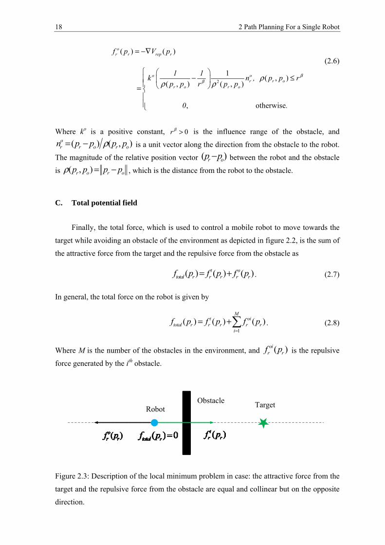
Figure 2.3: Description of the local minimum problem in case: the attractive force from the
target and the repulsive force from the obstacle are equal and collinear but on the opposite
direction.
Robot Target Obstacle
2.3 Path planning algorithm for a mobile robot 19
2.2.3 Conclusion
Although artificial potential field is known as a positive method for path planning of
mobile robots, but in several cases of local minimum problems this approach has demon-
strated limitations; for instance, when the attractive force of the target and the repulsive
force of the obstacles are equal in magnitude and collinear but on the opposite direction,
the total force on the robot is equal to zero, leading to a halt in the robot’s motion is
stopped. Moreover, in complex environments, such as U-shaped obstacles or long walls,
etc., the application of the traditional potential field method for path planning of autono-
mous robots is very difficult. Robots can be trapped in these obstacles before reaching the
target, as seen in figure 2.3.
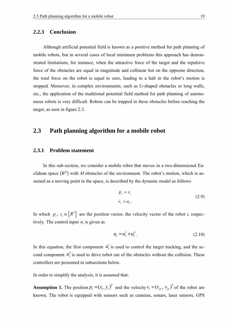
2.3 Path planning algorithm for a mobile robot
2.3.1 Problem statement
In this sub-section, we consider a mobile robot that moves in a two-dimensional Eu-
clidean space with M obstacles of the environment. The robot’s motion, which is as-
sumed as a moving point in the space, is described by the dynamic model as follows
.
rr
r r
p v
v u
=
=
(2.9)
In which { }2, r rp v R∈ are the position vector, the velocity vector of the robot i, respec-
tively. The control input ru is given as
t or r ru u u+= . (2.10)
In this equation, the first component tru is used to control the target tracking, and the se-
cond component oru is used to drive robot out of the obstacles without the collision. These
controllers are presented in subsections below.
In order to simplify the analysis, it is assumed that:
Assumption 1. The position ( )Tr r rp x , y= and the velocity ( , )T
r xr yrv v v= of the robot are
known. The robot is equipped with sensors such as cameras, sonars, laser sensors, GPS
20 2 Path Planning For a Single Robot
sensors, and associated algorithms, etc., to estimate the trajectory (position ( )Tt t tp x , y= ,
and velocity ( )Tt xt ytv v , v= ) of the target precisely.
Assumption 2. The velocity of the moving target is limited by the maximum velocity of
the robot rmaxtv v< .
Assumption 3. The robot can sense the position ( )To o op x , y= and the velocity
( )To xo yov v , v= of the obstacles in the environment precisely.
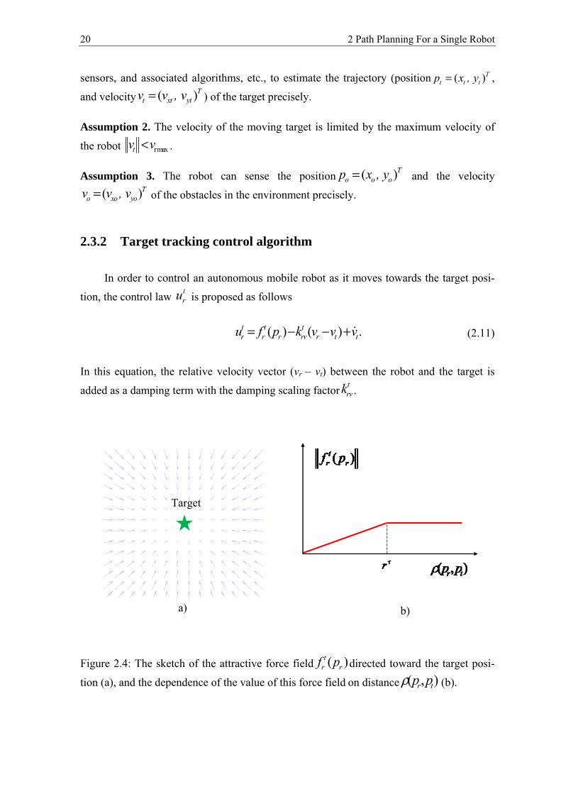
2.3.2 Target tracking control algorithm
In order to control an autonomous mobile robot as it moves towards the target posi-
tion, the control law tru is proposed as follows
( ) ( ) .r r rv rt t t
r ttf p k v v vu = −− + (2.11)
In this equation, the relative velocity vector (vr – vt) between the robot and the target is
added as a damping term with the damping scaling factor trvk .
Figure 2.4: The sketch of the attractive force field ( )rrtf p directed toward the target posi-
tion (a), and the dependence of the value of this force field on distance ( , )r tp pρ (b).
a)
b)
Target
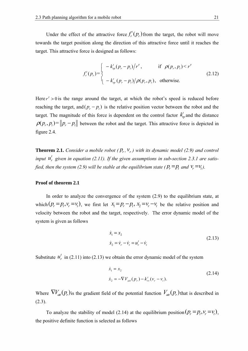
2.3 Path planning algorithm for a mobile robot 21
Under the effect of the attractive force ( )rrtf p from the target, the robot will move
towards the target position along the direction of this attractive force until it reaches the
target. This attractive force is designed as follows:
( ) , if ( , )( )
( ) ( , ) , otherwise.
trp r t r t
tr
trp r t r
r
t
k p p r p p < r
f p =
k p p p p
τ τρ
ρ
− − − −
(2.12)
Here 0rτ > is the range around the target, at which the robot’s speed is reduced before
reaching the target, and ( )r tp p− is the relative position vector between the robot and the
target. The magnitude of this force is dependent on the control factor trpk and the distance
( , )r t r tp p = p pρ − between the robot and the target. This attractive force is depicted in
figure 2.4.
Theorem 2.1. Consider a mobile robot ( rp , rv ) with its dynamic model (2.9) and control
input tru given in equation (2.11). If the given assumptions in sub-section 2.3.1 are satis-
fied, then the system (2.9) will be stable at the equilibrium state ( r tp p= and r tv v= ).
Proof of theorem 2.1
In order to analyze the convergence of the system (2.9) to the equilibrium state, at
which ( , )r tr tp p v v== , we first let 1 2, r t r tx p p x v v= − = − be the relative position and
velocity between the robot and the target, respectively. The error dynamic model of the
system is given as follows
1 2
2t
r t trv v
x
u v
x
x
=
= − = −
(2.13)
Substitute tru in (2.11) into (2.13) we obtain the error dynamic model of the system
1 2
2 ( ) .( )att r rvt
r tV p k
x
v
x
vx
=
= −∇ − −
(2.14)
Where ( )att rV p∇ is the gradient field of the potential function ( )att rV p that is described in
(2.3).
To analyze the stability of model (2.14) at the equilibrium position( , )r tr tp p v v== ,
the positive definite function is selected as follows
22 2 Path Planning For a Single Robot
2 2( ) 12
Tatt rV xV p x= + (2.15)
Consider the potential function (2.3) we have the relationship as follows ( )( )att
T
rrV p p∂ ∂
( )( ) ( )att r
T
r tpV p p= ∂ ∂ − . Taking the time derivative of (2.15) along the trajectory of the
system (2.14), we obtain:
( )
( )2
2
2
1 2 2
2
2
2
( ( )
( )
( ) )
( ) ( )
0.
att r
att r
att r att r r
T T
v
r
T t
tv
T
T
V p
V p
V
V t x x x
x x
p V p
k
x x
x x
k
= ∇ +
= ∇ +
∇ ∇
= − ≤
= − −
(2.16)
Equation (2.16) shows that the selected positive definite function V is a Lyapunov func-
tion [95], which guarantees that the system (2.14) is stable at the equilibrium point( , )r tr tp p v v== .
2.3.3 Obstacle avoidance control
A. Control algorithm
This sub-section presents the control algorithm for a mobile robot passing through M
obstacles to reach a target. As analyzed above, the obstacle avoidance control algorithm is
also proposed as follows
( )1
( ) ( ) ( )M
op or o or r rv rr
o
or r r op + f p c vu k vf
=
= + − . (2.17)
Where, the relative velocity vector (vr – vo) between the robot and its neighbor-obstacle o is
used as a damping term with the damping scaling factor orvk . Let ( )o
rN t be the set of the ob-
stacles in the neighborhood of the robot at time t, such that:
{ }{ }( ) ,: ( , ) .or or o rN o p p p p r o 1t ,..Mβρ= ∀ = − ≤ ∈ (2.18)
In (2.18), 0rβ > and ( , ) or o rp p p pρ = − are the influence range of obstacle and the Eu-
clidean distance between the robot and the obstacle o, respectively. The scalar cro is de-
fined as:
2.3 Path planning algorithm for a mobile robot 23
( ) 1 if
0 otherwise.or
oro N t
c ∈=
(2.19)
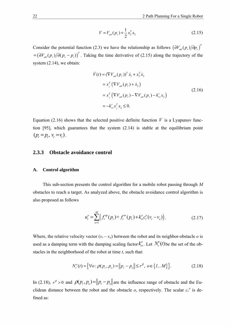
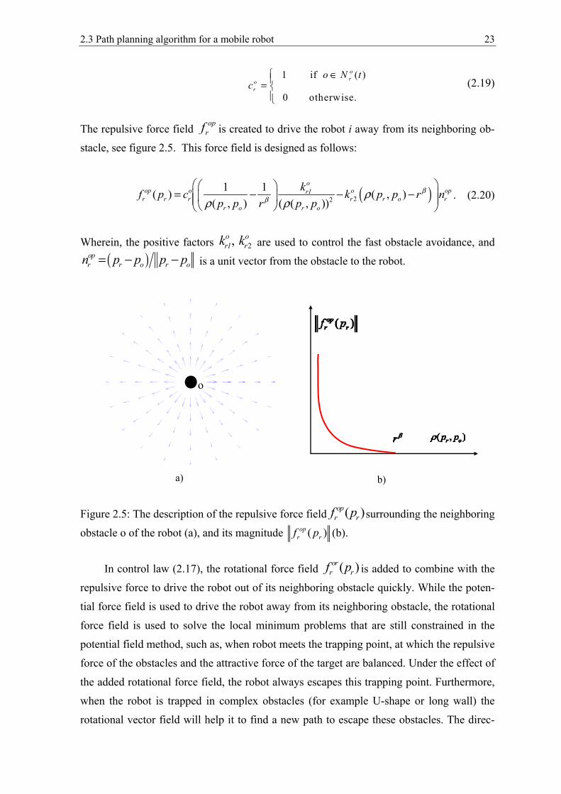
The repulsive force field prof is created to drive the robot i away from its neighboring ob-
stacle, see figure 2.5. This force field is designed as follows:
( )22
1 1( ) ( , )( , ) ( ( ), )
or1
r rop o o op
r r r o rr o r o
kp c k p p r
r pf n
p p pβ
β ρρ ρ
= − − −
. (2.20)
Wherein, the positive factors 2, or1
ork k are used to control the fast obstacle avoidance, and
( )ropr o r on p p p p− −=
is a unit vector from the obstacle to the robot.
Figure 2.5: The description of the repulsive force field ( )rropf p surrounding the neighboring
obstacle o of the robot (a), and its magnitude ( )rropf p (b).
In control law (2.17), the rotational force field ( )rrorf p is added to combine with the
repulsive force to drive the robot out of its neighboring obstacle quickly. While the poten-
tial force field is used to drive the robot away from its neighboring obstacle, the rotational
force field is used to solve the local minimum problems that are still constrained in the
potential field method, such as, when robot meets the trapping point, at which the repulsive
force of the obstacles and the attractive force of the target are balanced. Under the effect of
the added rotational force field, the robot always escapes this trapping point. Furthermore,
when the robot is trapped in complex obstacles (for example U-shape or long wall) the
rotational vector field will help it to find a new path to escape these obstacles. The direc-
a)
o
4
b)
24 2 Path Planning For a Single Robot
tion of the rotational force can be clockwise or counter-clockwise (see figure 2.6). Hence,
this rotational force is built as:
( )or or o orr rr r rw cf p n= . (2.21)
Wherein, the unit vector orrn is given as:
( )( ) ( , ) , ( ) ( , ) .Tor orr r r o r o r o r on c y y p p x x p pρ ρ= − − − (2.22)
In this equation, the scalar orrc is used to define the direction for the rotational force: the
rotational force is clockwise if ,orrc 1= and counter-clockwise if 1or
rc =− . Let be the an-
gle between the unit vector orrn and the vector ( )orp p− , we obtain a relationship as fol-
lows:
( ) ( )2cos ( )( ) ( )( ) ( , )
0.
orr r o r o r o r o r oc x x y y y y x x p pσ ρ= − − − − −
= (2.23)
Equation (2.23) shows that the unit vector orrn is always perpendicular with the vector
( )orp p− . The positive gain factor 0orrw > , which is the magnitude of the rotational force
( )rrorf p acting on the robot, is used as a control element to drive the robot to quickly es-
cape obstacles. Therefore, this control element is designed such that the total force on the
robot always has the direction in the selected rotational direction. Now, in order to deter-
mine this control element, we let ) ( )(tol tol tol Tr r rrf p x , y= be the total force on the robot. We
obtain the relationships as follows
( ) ( ) ( ), , ( , ) ( , )
Tor orTtol tol top or top orr r o r r o
r r r r r rr o r o
c y y c x xx y x w y w
p p p pρ ρ − −= + −
. (2.24)
Where top t opr r rx x x= + and top t op
r r ry y y= + are the coordinates of the force ( )toprrf p =
( )top top Tr rx , y= that is the sum of the attractive force ( ) ( )t t t T
rr r rf p x , y= from the target and
the repulsive force ( ) ( )op op op Tr r rr , yf p x= from the obstacle on the robot. or
nx =
( ) ( , )orr r o r oc y y p pρ= − and ( ) ( , )or or
n r r o r oy c x x p pρ=− − are the coordinates of the unit
vector orrn as proposed in (2.22).
2.3 Path planning algorithm for a mobile robot 25
Let (( ), )tor
l opd r rp nfα =∠ be the desired angle between the total force ( )tol
rrf p and the
unit vector ( ), Topo o
rpp
n nx yn = ( ) ( )( ), T
r o r o r o r ox yx p p y p p= − − − − , see figure 2.7,
we have the relationship as
( ) ( )2 2
( ) ( )( )op top or or op top or orn r r n n r r n
dtop or or top or orr r n r r n
x x w x y y w ycos
x w x y w yα + + +=
+ + +. (2.25)
This equation can be rewritten as follows
( )20or or
r ra w bw c+ + = , (2.26)
Here: 2 2 2( ( ) ) ( ( ) ) ( )or or or op or opd n d n n n n na cos x cos y x x y yα α= + − + ,
( ) ( ) ( )( )22 ( ) 2top or top or op or op or top op top opd r n r n n n n n r n r nb cos x x y y x x y y x x y yα= + − + + ,
( ) ( ) ( )2 2 2( ) ( )top op op top op top
d r d n n r n rc cos x cos x x x y yα α= + − + .
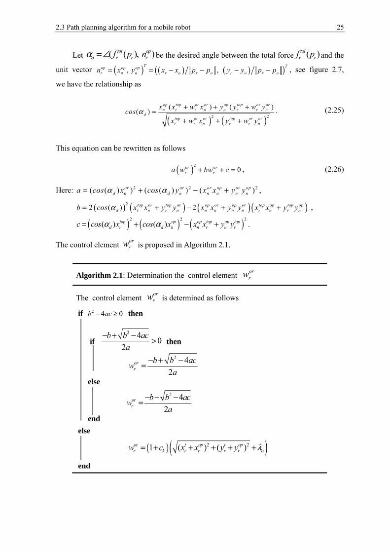
The control element orrw is proposed in Algorithm 2.1.
Algorithm 2.1: Determination the control element orrw
The control element orrw is determined as follows
if 2 4 0b ac− ≥ then
if 2 4 0
2b b ac
a
− + − > then
2 42
orr
b b acw
a
− + −=
else
2 42
orr
b b acw
a
− − −=
end
else
( )( )2 21 ( ) ( )or t op t opr k r r r r ow c x x y y λ= + + + + +
end
26 2 Path Planning For a Single Robot
In the Algorithm 2.1, the positive factor oλ guarantees that if the sum of the attrac-
tive force and the repulsive force on the robot is equal to zero, then the added rotational
force is large enough in order to drive the robot quickly escaping the trapped point as de-
scribed in figure 2.3. The scaling factor kc , which depends on the angle α between the
sum vector ( )toprif p and the unit vector or
rn (see figure 2.7), is described as follows:
1
2
, if 2
, otherwise.k
cc
c
α π<=
(2.27)
Where, two constants c1 and c2 can be chosen as follows: 11 ,c− < 20 c< , and 1 2c c< . Algo-
rithm (2.1) also shows that the robot is driven in the direction of the rotational force( )rr
orf p when it meets the obstacle. Hence, it can easily escape the obstacles in order to
continue to reach the target, see figure 2.7.
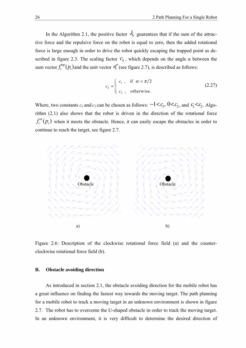
Figure 2.6: Description of the clockwise rotational force field (a) and the counter-
clockwise rotational force field (b).
B. Obstacle avoiding direction
As introduced in section 2.1, the obstacle avoiding direction for the mobile robot has
a great influence on finding the fastest way towards the moving target. The path planning
for a mobile robot to track a moving target in an unknown environment is shown in figure
2.7. The robot has to overcome the U-shaped obstacle in order to track the moving target.
In an unknown environment, it is very difficult to determine the desired direction of
-4-2
02
2
0
2
4
02
4
b) a)
Obstacle Obstacle
2.3 Path planning algorithm for a mobile robot 27
movement for the robot to easily escape obstacles and simultaneously reach the target
quickly. Hence, a positive method to solve this problem is to control the robot to escape
obstacles following the direction of the target’s trajectory. This method is built on the ge-
ometry, as depicted in figure 2.7 and figure 2.8.
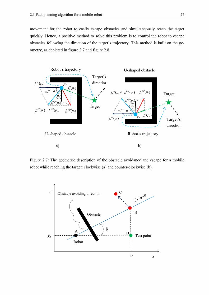
Figure 2.7: The geometric description of the obstacle avoidance and escape for a mobile
robot while reaching the target: clockwise (a) and counter-clockwise (b).
Robot´s trajectory
frt(pr)
Target fr
op(pr)
frtop(pr)
fror(pr)
nror
fror(pr)+ fr
top(pr)
pr
pr
Target
Target’s direction
Target’s direction
U-shaped obstacle
a)
αd
α
α
αd
Robot´s trajectory
frt(pr)
frop(pr)
frtop(pr)
fror(pr)
nror
fror(pr)+ fr
top(pr)
U-shaped obstacle
b)
Test point
y
x
A
B
C
D
xB
yA
Obstacle
Obstacle avoiding direction
β
Robot
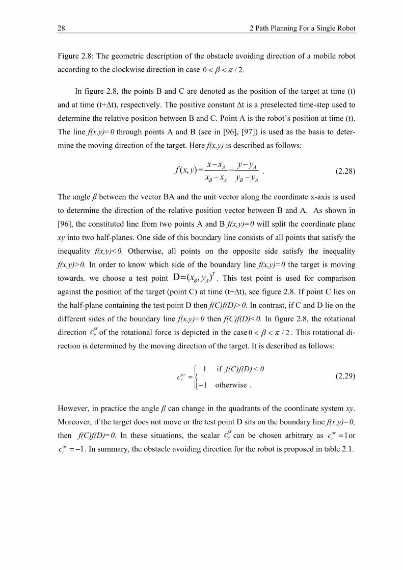
28 2 Path Planning For a Single Robot
Figure 2.8: The geometric description of the obstacle avoiding direction of a mobile robot
according to the clockwise direction in case 0 / 2.β π< <
In figure 2.8, the points B and C are denoted as the position of the target at time (t)
and at time (t+∆t), respectively. The positive constant ∆t is a preselected time-step used to
determine the relative position between B and C. Point A is the robot’s position at time (t).
The line f(x,y)=0 through points A and B (see in [96], [97]) is used as the basis to deter-
mine the moving direction of the target. Here f(x,y) is described as follows:
( , ) A A
B A B A
x x y yf x y
x x y y
− −= −− − . (2.28)
The angle β between the vector BA and the unit vector along the coordinate x-axis is used
to determine the direction of the relative position vector between B and A. As shown in
[96], the constituted line from two points A and B f(x,y)=0 will split the coordinate plane
xy into two half-planes. One side of this boundary line consists of all points that satisfy the
inequality f(x,y)<0. Otherwise, all points on the opposite side satisfy the inequality
f(x,y)>0. In order to know which side of the boundary line f(x,y)=0 the target is moving
towards, we choose a test point D ( )TB Ax , y= . This test point is used for comparison
against the position of the target (point C) at time (t+∆t), see figure 2.8. If point C lies on
the half-plane containing the test point D then f(C)f(D)>0. In contrast, if C and D lie on the
different sides of the boundary line f(x,y)=0 then f(C)f(D)<0. In figure 2.8, the rotational
direction orrc of the rotational force is depicted in the case 0 / 2β π< < . This rotational di-
rection is determined by the moving direction of the target. It is described as follows:
1 if
1 otherwise .orr
f(C)f(D) < 0c
= −
(2.29)
However, in practice the angle β can change in the quadrants of the coordinate system xy.
Moreover, if the target does not move or the test point D sits on the boundary line f(x,y)=0,
then f(C)f(D)=0. In these situations, the scalar orrc can be chosen arbitrary as 1or
rc = or
1orrc = − . In summary, the obstacle avoiding direction for the robot is proposed in table 2.1.

2.4 Simulation results 29
TABLE 2.1: DETERMINATION ROTATIONAL DIRECTION
2.4 Simulation results
In this section we test our proposed theoretical results for the target tracking of a mo-
bile robot. For the simulations, we assume that the initial velocities of the robot and the
target are set to zero, and the general parameters are listed as follows: 100rτ = , 20r β = ,3t
rpk = , 2,1trvk = , 80o
r1k = , 6or2k = , 1.6o
rvk = , 1 0.7c = , 2 3,8c = , 0 2λ = .
2.4.1 The target tracking in a free environment
In this sub-section, we test the control algorithms for a mobile robot tracking a mov-
ing target in a free environment, in which no obstacle exists. The parameters for this simu-
lation are given as follows: The initial position of the robot is set at the position
(50, 200)Trp = , and the target moves along the trajectory (0.7t 200, 0.5t 800)T
tp = + − + .
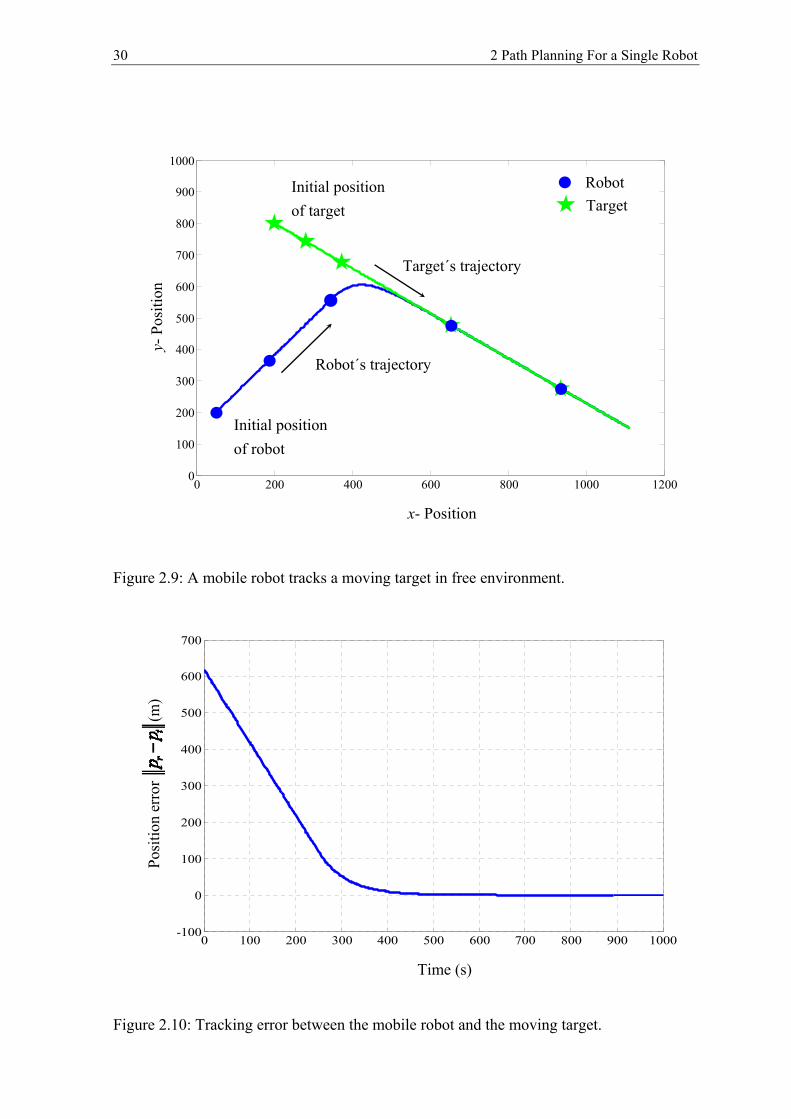
The results of the simulations in figure 2.9, figure 2.10 and figure 2.11 show that the
target tracking of a mobile robot is successful, the robot approaches the position of the tar-
get very well. At the initial time, the position of the robot is far from the target, but after a
period of circa 400s the robot can catch up the moving target and then continue to track
this moving target. The trajectory of the robot is always to follow up the trajectory of the
target with very small error (the position error between the robot and the target, see figure
2.10). Moreover, the state of the robot ( , )r rp v as described in (2.9) always converges to the
equilibrium state, at which r tp p= and r tv v= , see figure 2.10 and figure 2.11. These simu-
lation results confirm the theory stated in Theorem 2.1.
β f(C)f(D) cror
0 / 2β π≤ < ( ) ( ) 0f C f D ≤ 1 ( ) ( ) 0f C f D > -1
/ 2π β π≤ < ( ) ( ) 0f C f D ≥ 1 ( ) ( ) 0f C f D < -1
3 / 2π β π≤ < ( ) ( ) 0f C f D ≤ 1 ( ) ( ) 0f C f D > -1
3 / 2 2π β π≤ < ( ) ( ) 0f C f D ≥ 1 ( ) ( ) 0f C f D < -1
30 2 Path Planning For a Single Robot
0 200 400 600 800 1000 12000
100
200
300
400
500
600
700
800
900
1000
Target´s trajectory
Robot Target
Robot´s trajectory
Initial position of robot
Initial position of target
x- Position
y- P
ositi
on
Figure 2.9: A mobile robot tracks a moving target in free environment.
Figure 2.10: Tracking error between the mobile robot and the moving target.
0 100 200 300 400 500 600 700 800 900 1000-100
0
100
200
300
400
500
600
700
Time (s)
Posi
tion
erro
r (m
)
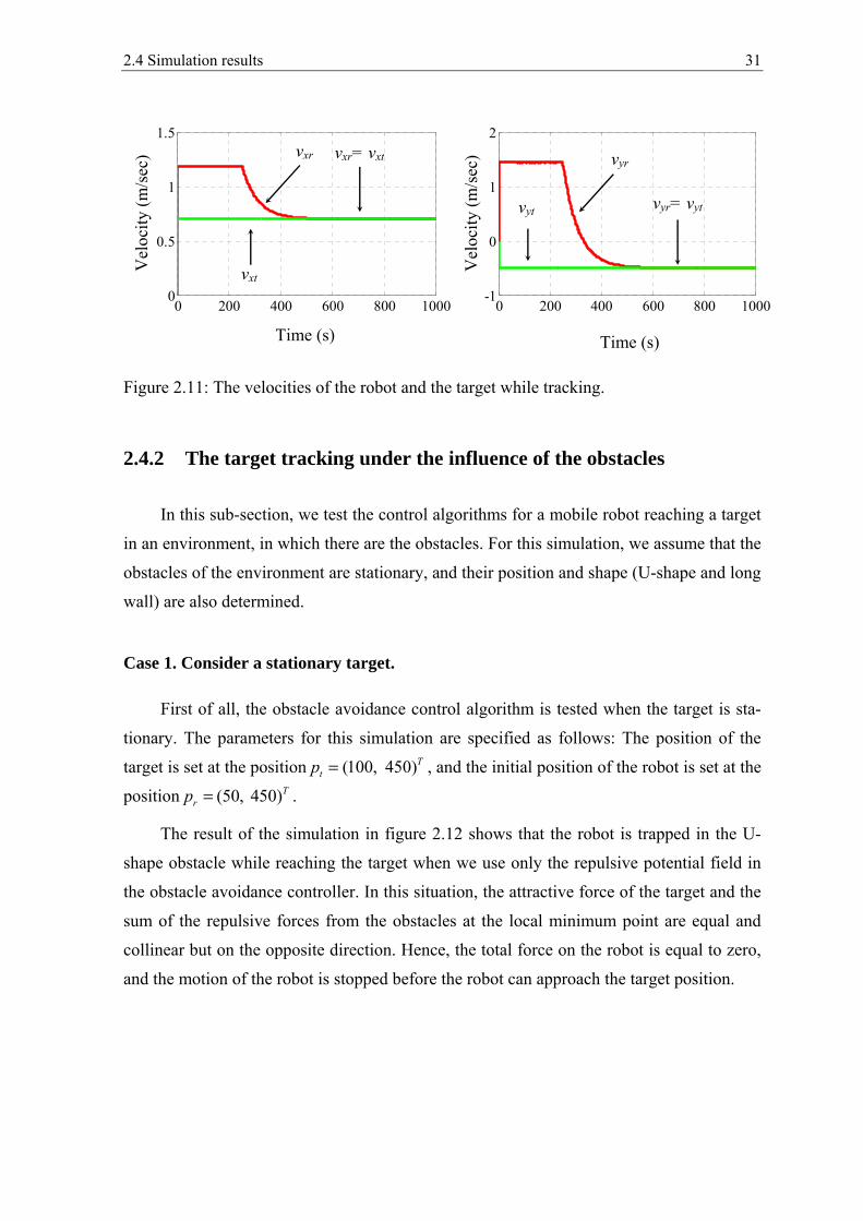
2.4 Simulation results 31
Figure 2.11: The velocities of the robot and the target while tracking.
2.4.2 The target tracking under the influence of the obstacles
In this sub-section, we test the control algorithms for a mobile robot reaching a target
in an environment, in which there are the obstacles. For this simulation, we assume that the
obstacles of the environment are stationary, and their position and shape (U-shape and long
wall) are also determined.
Case 1. Consider a stationary target.
First of all, the obstacle avoidance control algorithm is tested when the target is sta-
tionary. The parameters for this simulation are specified as follows: The position of the
target is set at the position (100, 450)Ttp = , and the initial position of the robot is set at the
position (50, 450)Trp = .
The result of the simulation in figure 2.12 shows that the robot is trapped in the U-
shape obstacle while reaching the target when we use only the repulsive potential field in
the obstacle avoidance controller. In this situation, the attractive force of the target and the
sum of the repulsive forces from the obstacles at the local minimum point are equal and
collinear but on the opposite direction. Hence, the total force on the robot is equal to zero,
and the motion of the robot is stopped before the robot can approach the target position.
0 200 400 600 800 1000-1
0
1
2
0 200 400 600 800 10000
0.5
1
1.5
Time (s)
vxr
Vel
ocity
(m/s
ec)
Vel
ocity
(m/s
ec) vyr
vxt
vyt
vxr= vxt
vyr= vyt
Time (s)
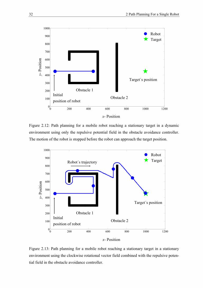
32 2 Path Planning For a Single Robot
Figure 2.12: Path planning for a mobile robot reaching a stationary target in a dynamic
environment using only the repulsive potential field in the obstacle avoidance controller.
The motion of the robot is stopped before the robot can approach the target position.
Figure 2.13: Path planning for a mobile robot reaching a stationary target in a stationary
environment using the clockwise rotational vector field combined with the repulsive poten-
tial field in the obstacle avoidance controller.
0 200 400 600 800 1000 12000
100
200
300
400
500
600
700
800
900
1000
Target´s position
Robot Target Robot´s trajectory
Initial position of robot
x- Position
y- P
ositi
on
Obstacle 1
Obstacle 2
0 200 400 600 800 1000 12000
100
200
300
400
500
600
700
800
900
1000
Robot Target
Target´s position
Initial position of robot
x- Position
y- P
ositi
on
Obstacle 1
Obstacle 2
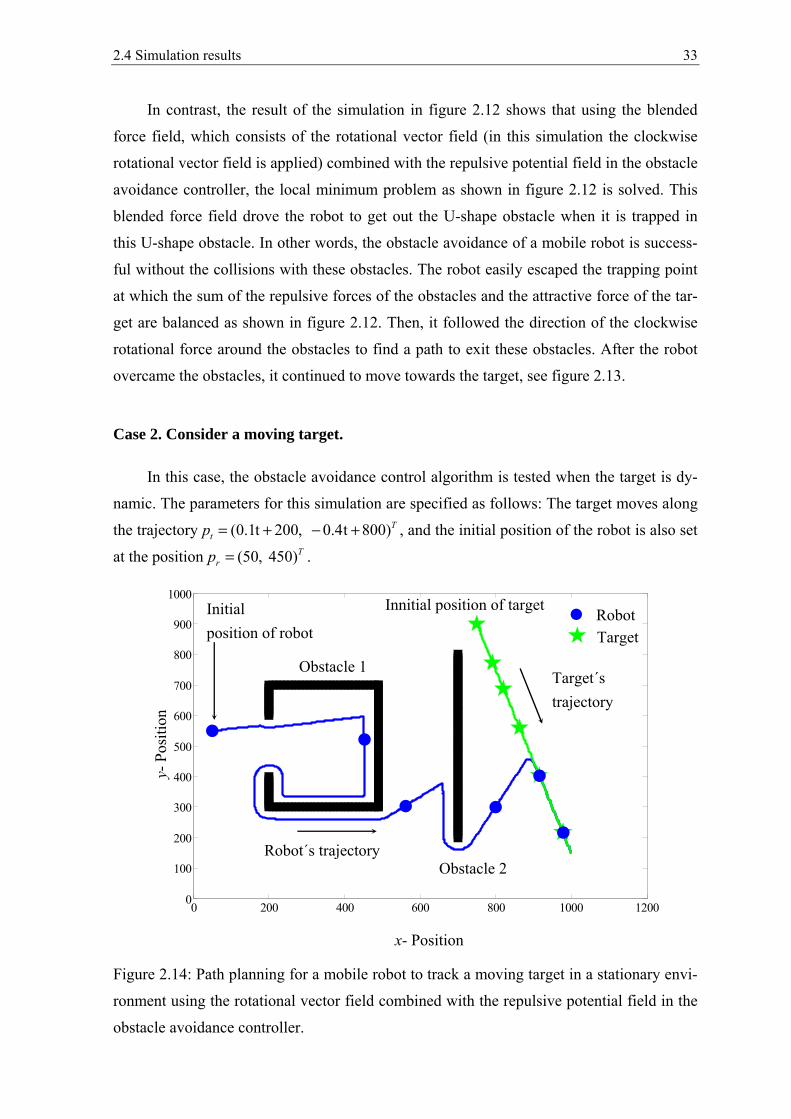
2.4 Simulation results 33
In contrast, the result of the simulation in figure 2.12 shows that using the blended
force field, which consists of the rotational vector field (in this simulation the clockwise
rotational vector field is applied) combined with the repulsive potential field in the obstacle
avoidance controller, the local minimum problem as shown in figure 2.12 is solved. This
blended force field drove the robot to get out the U-shape obstacle when it is trapped in
this U-shape obstacle. In other words, the obstacle avoidance of a mobile robot is success-
ful without the collisions with these obstacles. The robot easily escaped the trapping point
at which the sum of the repulsive forces of the obstacles and the attractive force of the tar-
get are balanced as shown in figure 2.12. Then, it followed the direction of the clockwise
rotational force around the obstacles to find a path to exit these obstacles. After the robot
overcame the obstacles, it continued to move towards the target, see figure 2.13.
Case 2. Consider a moving target.
In this case, the obstacle avoidance control algorithm is tested when the target is dy-
namic. The parameters for this simulation are specified as follows: The target moves along
the trajectory (0.1t 200, 0.4t 800)Ttp = + − + , and the initial position of the robot is also set
at the position (50, 450)Trp = .
Figure 2.14: Path planning for a mobile robot to track a moving target in a stationary envi-
ronment using the rotational vector field combined with the repulsive potential field in the
obstacle avoidance controller.
0 200 400 600 800 1000 12000
100
200
300
400
500
600
700
800
900
1000
Target´s trajectory
Robot Target
Robot´s trajectory
Initial position of robot
Innitial position of target
x- Position
y- P
ositi
on
Obstacle 1
Obstacle 2
34 2 Path Planning For a Single Robot
The result of the simulation in figure 2.14 shows the intelligence of a mobile robot
while pursuing a moving target. When this robot detects the obstacle it changes its moving
direction to avoid collision with this obstacle and searches the new path to chase the target
simultaneously. Figure 2.14 also shows that the obstacle avoidance of a mobile robot ac-
cording the moving direction of the target is successful. The movement direction of the
robot is driven towards the left of the U-shape and the wall-shape obstacles by the counter-
clockwise rotational force field from these obstacles. Hence, this mobile robot can easily
and quickly escape the U-shaped and the wall-shape obstacles in order to move towards the
target without collisions.
2.5 Summary
This chapter has presented an approach to path planning for a mobile to reach a target
in a dynamic environment based on the combination of the traditional potential fields and
the rotational vector field. In this approach, the artificial attractive force field from the tar-
get is used to drive the robot towards the target position. The repulsive force field sur-
rounding the obstacles is used to drive the robot away from the obstacles, while the rota-
tional force field is added surrounding the obstacles to help the robot to quickly escape the
balance point at which the sum of the attractive force from the target and the repulsive
forces from the obstacles is equal to zero. Especially, in case the robot is trapped in com-
plex obstacles, such as U-shaped obstacles, this added rotational vector field also plays an
important role in helping the robot to find a new path to escape these obstacles. The obsta-
cle avoiding direction for the mobile robot is designed to be in the moving direction of the
target, such that the robot can easily escape the obstacles and find the fastest path towards
the target. The results of the simulations have shown that, under the effect of the blended
force field, an autonomous robot can easily find a path to reach a target in a dynamic envi-
ronment.
The development of this proposed approach to path planning for the formation of a
swarm of multi robots to track a moving target in a dynamic environment, as an interesting
research topic, will be examined in the next chapters.
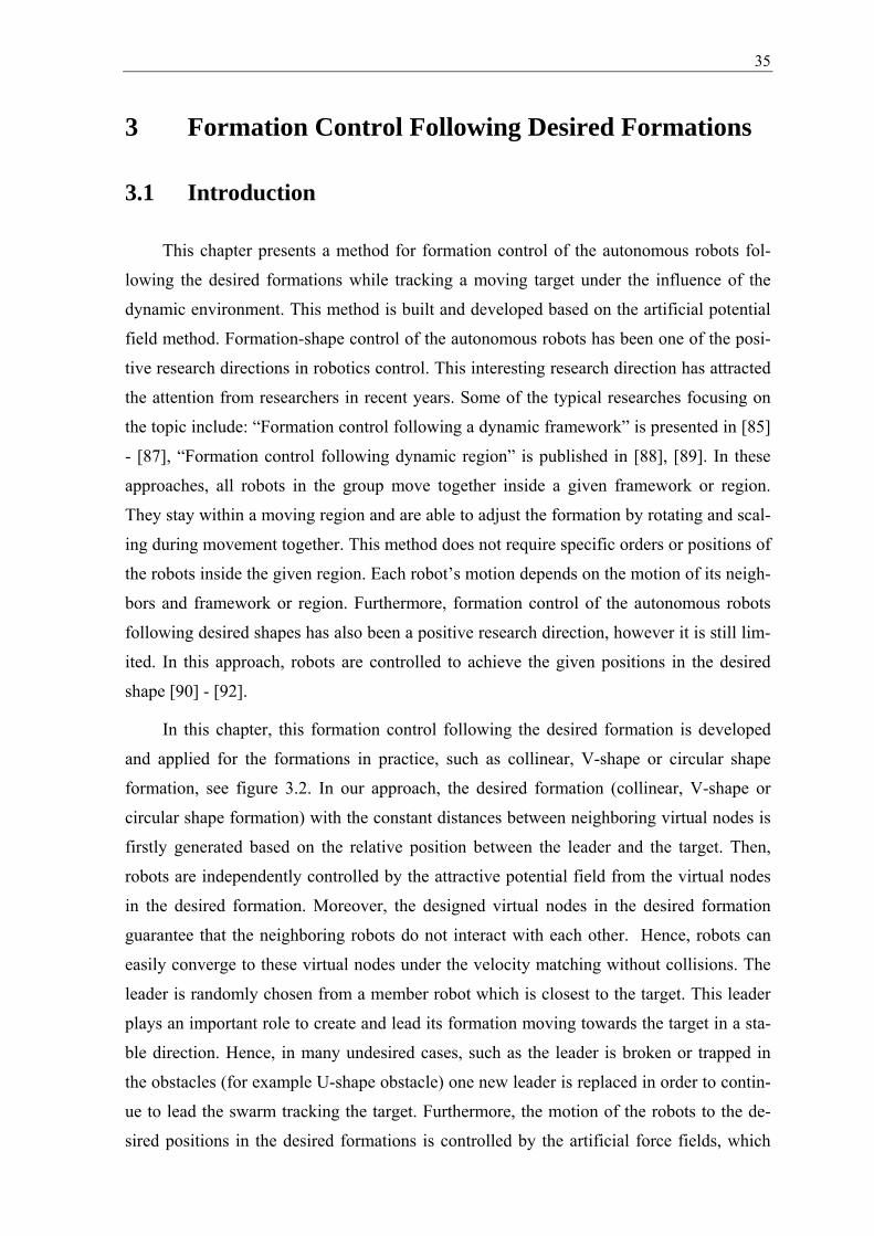
35
3 Formation Control Following Desired Formations
3.1 Introduction
This chapter presents a method for formation control of the autonomous robots fol-
lowing the desired formations while tracking a moving target under the influence of the
dynamic environment. This method is built and developed based on the artificial potential
field method. Formation-shape control of the autonomous robots has been one of the posi-
tive research directions in robotics control. This interesting research direction has attracted
the attention from researchers in recent years. Some of the typical researches focusing on
the topic include: “Formation control following a dynamic framework” is presented in [85]
- [87], “Formation control following dynamic region” is published in [88], [89]. In these
approaches, all robots in the group move together inside a given framework or region.
They stay within a moving region and are able to adjust the formation by rotating and scal-
ing during movement together. This method does not require specific orders or positions of
the robots inside the given region. Each robot’s motion depends on the motion of its neigh-
bors and framework or region. Furthermore, formation control of the autonomous robots
following desired shapes has also been a positive research direction, however it is still lim-
ited. In this approach, robots are controlled to achieve the given positions in the desired
shape [90] - [92].
In this chapter, this formation control following the desired formation is developed
and applied for the formations in practice, such as collinear, V-shape or circular shape
formation, see figure 3.2. In our approach, the desired formation (collinear, V-shape or
circular shape formation) with the constant distances between neighboring virtual nodes is
firstly generated based on the relative position between the leader and the target. Then,
robots are independently controlled by the attractive potential field from the virtual nodes
in the desired formation. Moreover, the designed virtual nodes in the desired formation
guarantee that the neighboring robots do not interact with each other. Hence, robots can
easily converge to these virtual nodes under the velocity matching without collisions. The
leader is randomly chosen from a member robot which is closest to the target. This leader
plays an important role to create and lead its formation moving towards the target in a sta-
ble direction. Hence, in many undesired cases, such as the leader is broken or trapped in
the obstacles (for example U-shape obstacle) one new leader is replaced in order to contin-
ue to lead the swarm tracking the target. Furthermore, the motion of the robots to the de-
sired positions in the desired formations is controlled by the artificial force fields, which
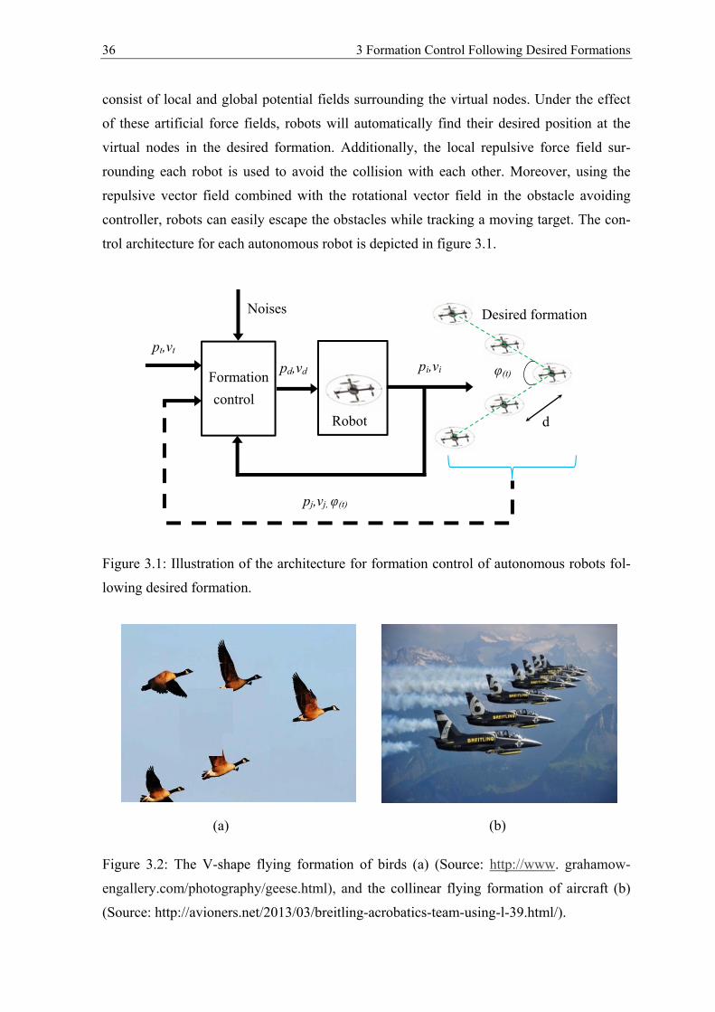
36 3 Formation Control Following Desired Formations
Robot
Desired formation Noises
Formation control
pj,vj, φ(t)
pt,vt
pd,vd pi,vi
d
φ(t)
consist of local and global potential fields surrounding the virtual nodes. Under the effect
of these artificial force fields, robots will automatically find their desired position at the
virtual nodes in the desired formation. Additionally, the local repulsive force field sur-
rounding each robot is used to avoid the collision with each other. Moreover, using the
repulsive vector field combined with the rotational vector field in the obstacle avoiding
controller, robots can easily escape the obstacles while tracking a moving target. The con-
trol architecture for each autonomous robot is depicted in figure 3.1.
Figure 3.1: Illustration of the architecture for formation control of autonomous robots fol-
lowing desired formation.
Figure 3.2: The V-shape flying formation of birds (a) (Source: http://www. grahamow-
engallery.com/photography/geese.html), and the collinear flying formation of aircraft (b)
(Source: http://avioners.net/2013/03/breitling-acrobatics-team-using-l-39.html/).
(a) (b)
3.1 Introduction 37
The main contributions of this chapter are as follows:
• “Formation adaptation while tracking a moving target” is presented in section 3.4. In
this content, we consider an approach for the adaptive formation control of autono-
mous robots following desired shapes under the influence of the environment, such as
noises, obstacles, etc. In this approach, the V-shape and circle-shape formation are
used as the desired formations. Firstly, the V-shape formation is used to track a mov-
ing target in the global potential field from the target. As analyzed in literatures [4]-
[7], the V-shape formation of birds (for example the formation flight of the Canada
geese during migration, see figure 3.2a) has a lot of advantages, such as energy sav-
ings during flight. The research results in these published literatures indicated that the
members in the V-shape formation realized up to 51% in energy savings over solo
flight. Moreover, by flying in V-shape formation the members in the formation can
easily communicate with each other, etc. Additionally, the circular shape formation
with its advantages, such as, the members in the formation can easily cooperate with
each other in tasks for example the encirclement, surveillance of the target [93], [94],
is used to approach the target in the local potential field surrounding the target.
• “Direction control for collinear formation” is presented in section 3.5. In this content, we consider an approach to control autonomous robots to achieve a de-sired collinear formation during movement towards the target position. As pre-sented in [91], the collinear formation has a lot of advantages, such as the members in the formation can easily cooperate to each other in tasks for exam-ple the observation, monitoring and tracking the targets, see figure 3.2b. In this approach, one robot, which has the closest distance to the target, is firstly se-lected as the leader of the swarm. The desired formation is built based on the relative position between this leader and the target. Secondly, the trajectory of the remaining robots towards the desired positions in the desired formation is driven by the artificial force fields. These force fields consist of the local and global attractive potential fields surrounding each virtual node in the desired formation. Furthermore, an orientation controller is added in order to guarantee that the desired formation is always headed in the invariant direction to the tar-get position. In addition, the local repulsive force fields around each robot and obstacle are employed in order to avoid collisions during movement. The stabil-ity of a swarm following a desired collinear formation in invariant direction to-wards the target position is verified in simulations.
38 3 Formation Control Following Desired Formations
The remaining sections of this chapter are organized as follows: the problem formula-
tion is presented in the section 3.2. Section 3.3 presents the method in order to build the
desired formations. In section 3.4, the formation adaptation control algorithm for a swarm
while tracking a moving target is presented. The direction control for a collinear formation
is discussed in section 3.5.
3.2 Problem formulation
In this section, we consider a swarm of N robots that has the mission to track, encircle
a moving target in two-dimensional space. Let ( ) ,Ti i ip x ,y= ( , )T
i ix iyv v v= be the position,
velocity vector of the robot i (i=1,2,..,N), respectively. The dynamic model of the robot i is
described as:
,
i i
i i
p v
v u i = 1,..,N.
=
=
(3.1)
As introduced above, the aim of this chapter is to control the formation of autono-
mous robots following desired formations that are generated based on the relative position
between the leader and the target. While tracking the moving target, robots must avoid the
collisions with each other, avoid the obstacles, and their formation must be maintained and
kept stable under the influence of the environment. Hence, in order to solve these condi-
tions we propose the control input ui for each robot as:
, if robot is the leader ; ,
+ , otherwise.
t oi i
ij o k
i i i
u u i l i l = 1,..,Nu
u u u
+= +
(3.2)
Where, the first controller jiu is used to control the formation connection. The second con-
troller oiu is used to drive robots avoiding obstacles. The controller k
iu is added to help ro-
bots avoid the collision during movement. Using the tracking controller tiu the leader can
easily drive its swarm towards the target. Now, in order to design these controllers, firstly,
we have some definitions and remarks as follows:
Definition 3.1. The desired collinear formation is the locus of all virtual nodes that lie on a
line and equidistant to each other.
3.2 Problem formulation 39
Definition 3.2. The desired V-shape formation is a formation that is linked by two linear
formations. These line formations are driven by a selected leader, and connected by a for-
mation angle φ. In each line formation, the virtual nodes are equidistant to each other.
Definition 3.3. The desired circular shape formation is the locus of all virtual nodes that
are equidistant to each other and equidistant from the target.
Definition 3.4. Robot i (i=1,2,..,N; pi=(xi, yi)T; vi=(vix, viy)T) is called an active robot at
time t if the distance from it to the virtual node j (j=1,2,..,N) of the desired formation is
smaller than the radius of the active circle surrounding each virtual node (dij < ra =d/2-λa,
λa is a positive constant), see figure 3.3. Otherwise, it is a free robot.
Definition 3.5. Virtual node j (j=1,2,..,N; qj=(xj, yj)T; vj=(vjx, vjy)T) of the desired formation
is active if there is a robot i (i=1,2,..,N) in the active circle of this virtual node. In contrast,
it is free.
Definition 3.6. Desired position for each robot i in the desired formation is a virtual node j
at which lim ( i jtp (t) q (t))= 0
→∞− , and the virtual node (j-1) is also active.
Remark 3.1. Consider a desired formation (V-shape or circular shape formation) of N vir-
tual nodes as shown in figure 3.3. Each Robot must find an desired position in this desired
formation. Firstly, each free robot i will pursue the closest free virtual node j in order to be
active at this virtual node. If the position of this active robot at the active node j is still not
desired (for example robot k (k=1,2,..,N, k≠l in figure 3.3), then this active robot will au-
tomatically move into the virtual nodes (j-1) until it achieves an desired position in the
desired formation.
Remark 3.2. The motion of the formation depends on the relative position between the
leader and the target. At initial time, one robot, which is closest to the target, is chosen as
the leader, and then it is saved to lead its formation towards the target. During the move-
ment, if this leader encounters any risk, such as it is broken or hindered by the environ-
ment, then a new leader is replaced. This new leader will reorganize the formation and
continue to lead the new formation tracking the target.
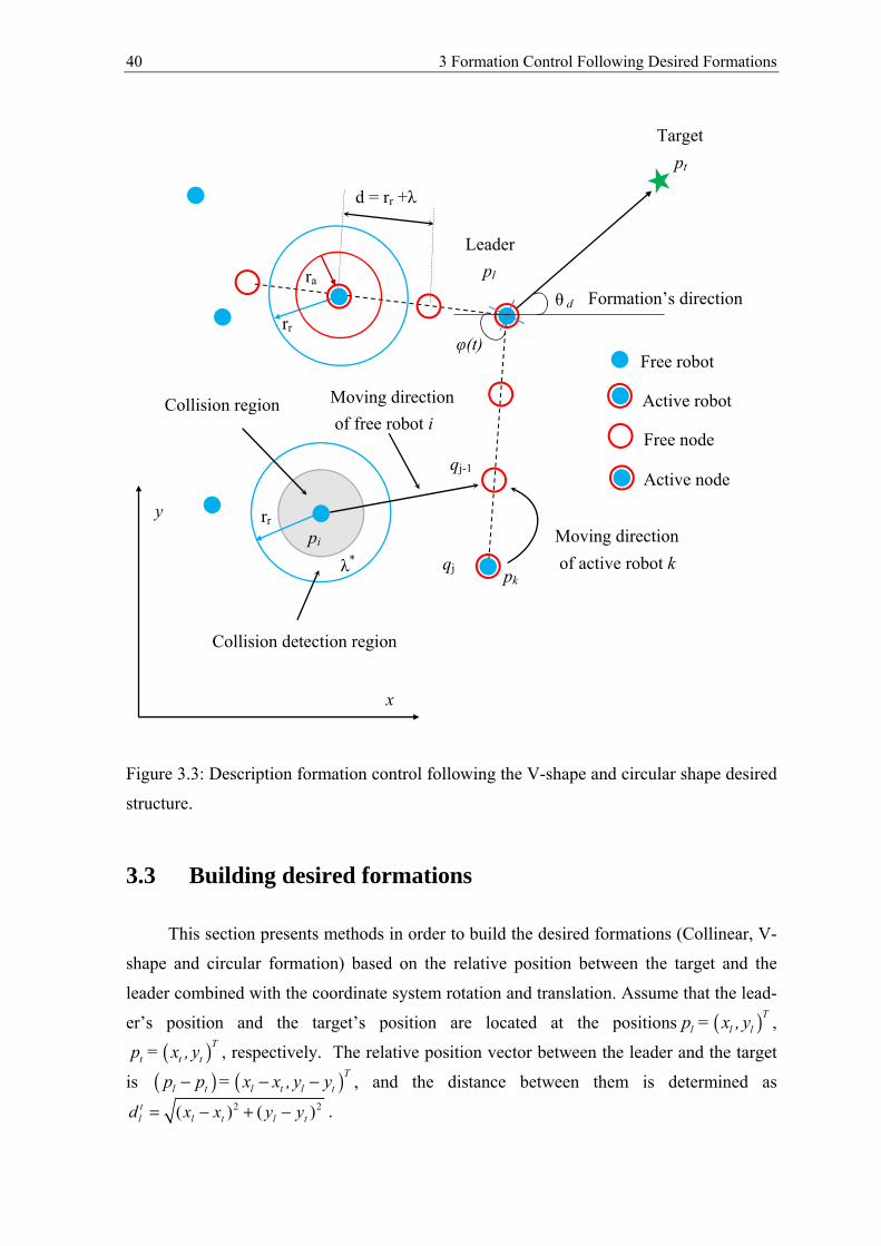
40 3 Formation Control Following Desired Formations
Figure 3.3: Description formation control following the V-shape and circular shape desired
structure.
3.3 Building desired formations
This section presents methods in order to build the desired formations (Collinear, V-
shape and circular formation) based on the relative position between the target and the
leader combined with the coordinate system rotation and translation. Assume that the lead-
er’s position and the target’s position are located at the positions ( )Tl l lxp = , y ,
( )t t
T
t= xp , y , respectively. The relative position vector between the leader and the target
is ( ) ( )t
T
l tl tlp p x= x , y y− − − , and the distance between them is determined as 2 2( ) ( )t
ll t tlx x yd y= − + − .
pk
rr
λ*
pi
φ(t)
Formation’s direction
d = rr +λ
Leader pl
Free robot
Active robot
Free node
Active node
Moving direction of active robot k
Moving direction of free robot i
Collision region
Collision detection region
rr
ra
Target pt
θ d
qj-1
qj
x
y
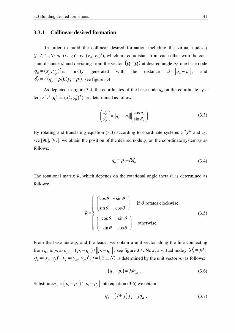
3.3 Building desired formations 41
3.3.1 Collinear desired formation
In order to build the collinear desired formation including the virtual nodes j
(j=1,2,..,N; qj=(xj, yj)T; vj=(vjx, vjy)T), which are equidistant from each other with the con-
stant distance d, and deviating from the vector ( )t lp p− at desired angle δd, one base node ( , )Tq x yμ μ μ= is firstly generated with the distance ld q pμ= − , and
( ),( )d l t lq p p pμδ =∠ − − , see figure 3.4.
As depicted in figure 3.4, the coordinates of the base node qμ on the coordinate sys-
tem ( = ( , ) ) are determined as follows:
cossin
dl
d
xq p
yμ
μμ
δδ
= −
′′
. (3.3)
By rotating and translating equation (3.3) according to coordinate systems and xy,
see [96], [97], we obtain the position of the desired node qμ on the coordinate system xy as
follows:
lq qp Rμ μ′= + . (3.4)
The rotational matrix R, which depends on the rotational angle theta θ, is determined as
follows:
cos sin if rotates clockwise,
sin cos
cos sin otherwise.
sin cos
R
θ θθ
θ θ
θ θ
θ θ
− = −
(3.5)
From the base node qμ and the leader we obtain a unit vector along the line connecting
from qμ to pl as ( ) /l lln p q p qμ μμ = − − , see figure 3.4. Now, a virtual node j ( ;ljd jd=
( , ;)Tj j jq x y= , 1,2,; ..( ,) )T
j jx jyv v v j N= = is determined by the unit vector nμl as follows:
( )j l lq p jdnμ− = .
(3.6)
Substitute ( ) /l lln p p p pμ μμ = − − into equation (3.6) we obtain:
( )j lq = 1+ j p jqμ− .
(3.7)
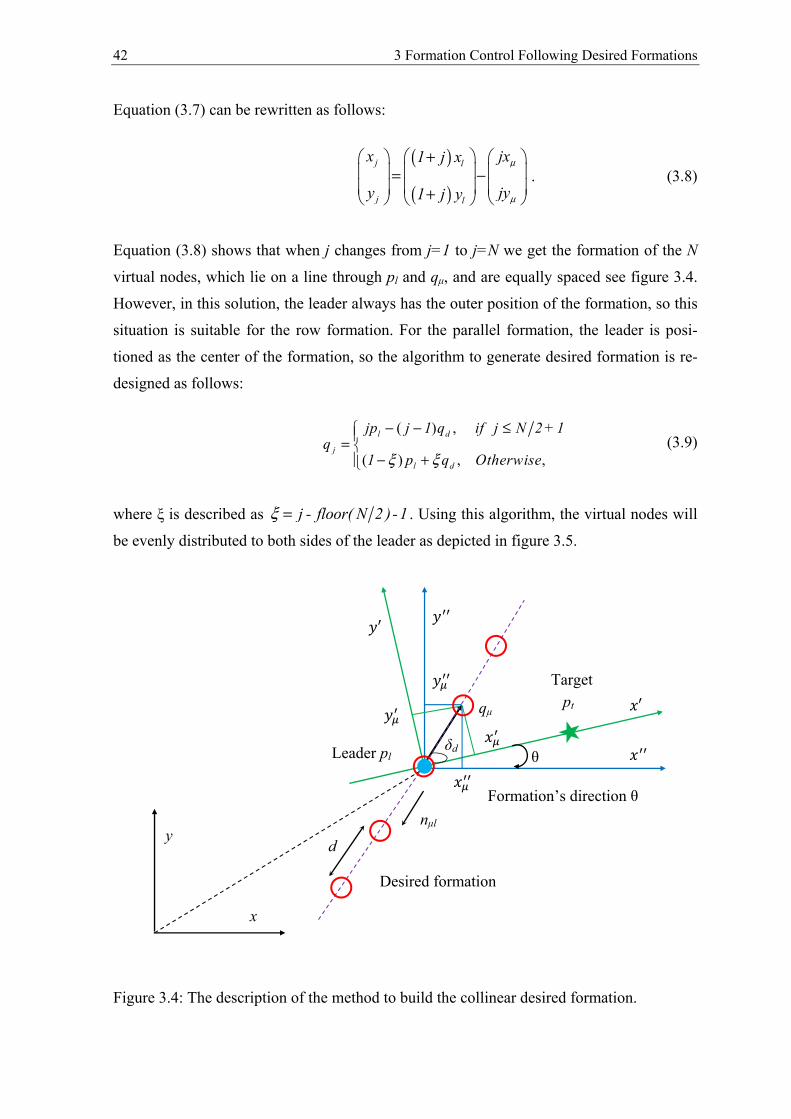
42 3 Formation Control Following Desired Formations
θ Leader pl
qμ
x
y
′ ′
d
nμl
δd
Target pt
Desired formation
Formation’s direction θ
Equation (3.7) can be rewritten as follows:
( )
( )
j l
j l
jx xx
y yy
1 j
j1 j
μ
μ
+ = − +
. (3.8)
Equation (3.8) shows that when j changes from j=1 to j=N we get the formation of the N
virtual nodes, which lie on a line through pl and qμ, and are equally spaced see figure 3.4.
However, in this solution, the leader always has the outer position of the formation, so this
situation is suitable for the row formation. For the parallel formation, the leader is posi-
tioned as the center of the formation, so the algorithm to generate desired formation is re-
designed as follows:
( ) ,
( ) , ,
l d
j
l d
jp j 1 q if j N 2 + 1q
1 p q Otherwiseξ ξ
− − ≤= − +
(3.9)
where ξ is described as j - floor( N 2 )-1ξ = . Using this algorithm, the virtual nodes will
be evenly distributed to both sides of the leader as depicted in figure 3.5.
Figure 3.4: The description of the method to build the collinear desired formation.
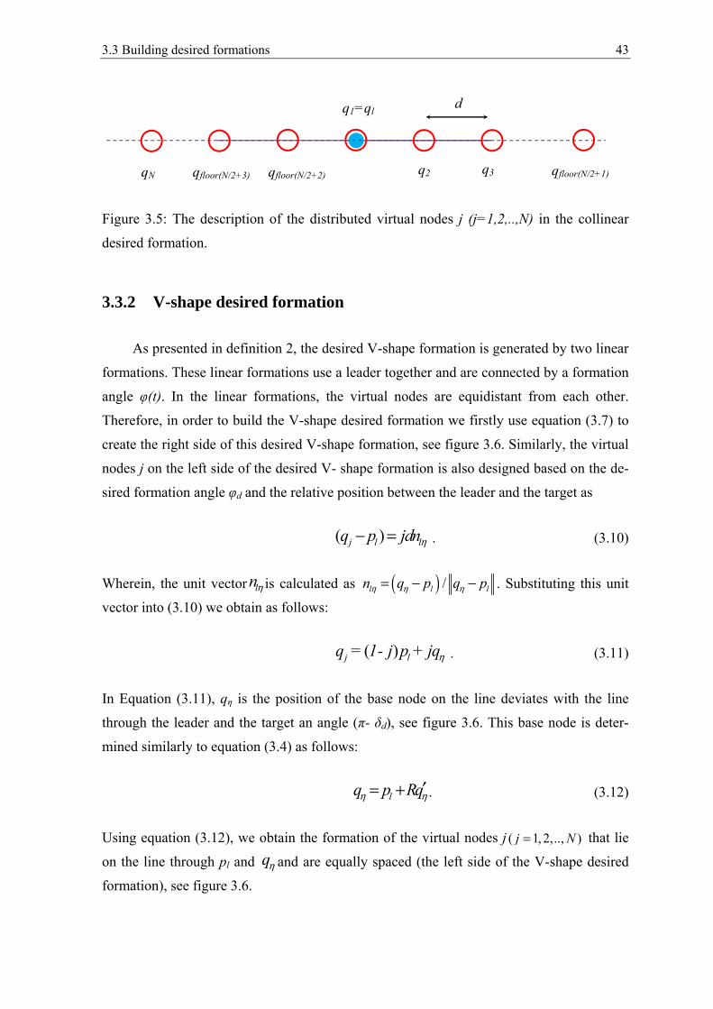
3.3 Building desired formations 43
Figure 3.5: The description of the distributed virtual nodes j (j=1,2,..,N) in the collinear
desired formation.
3.3.2 V-shape desired formation
As presented in definition 2, the desired V-shape formation is generated by two linear
formations. These linear formations use a leader together and are connected by a formation
angle φ(t). In the linear formations, the virtual nodes are equidistant from each other.
Therefore, in order to build the V-shape desired formation we firstly use equation (3.7) to
create the right side of this desired V-shape formation, see figure 3.6. Similarly, the virtual
nodes j on the left side of the desired V- shape formation is also designed based on the de-
sired formation angle φd and the relative position between the leader and the target as
( )j l lq p jdnη− = .
(3.10)
Wherein, the unit vector lnη is calculated as ( ) /ll ln pq q pηη η= − − . Substituting this unit
vector into (3.10) we obtain as follows:
( )j lq = 1- j p + jqη .
(3.11)
In Equation (3.11), qη is the position of the base node on the line deviates with the line
through the leader and the target an angle (π- δd), see figure 3.6. This base node is deter-
mined similarly to equation (3.4) as follows:
lq qp Rη η′= + . (3.12)
Using equation (3.12), we obtain the formation of the virtual nodes j ( 1, 2, )..,j N= that lie
on the line through pl and qη and are equally spaced (the left side of the V-shape desired
formation), see figure 3.6.
q2 q3 qfloor(N/2+1) qfloor(N/2+2) qfloor(N/2+3) qN
q1=ql d
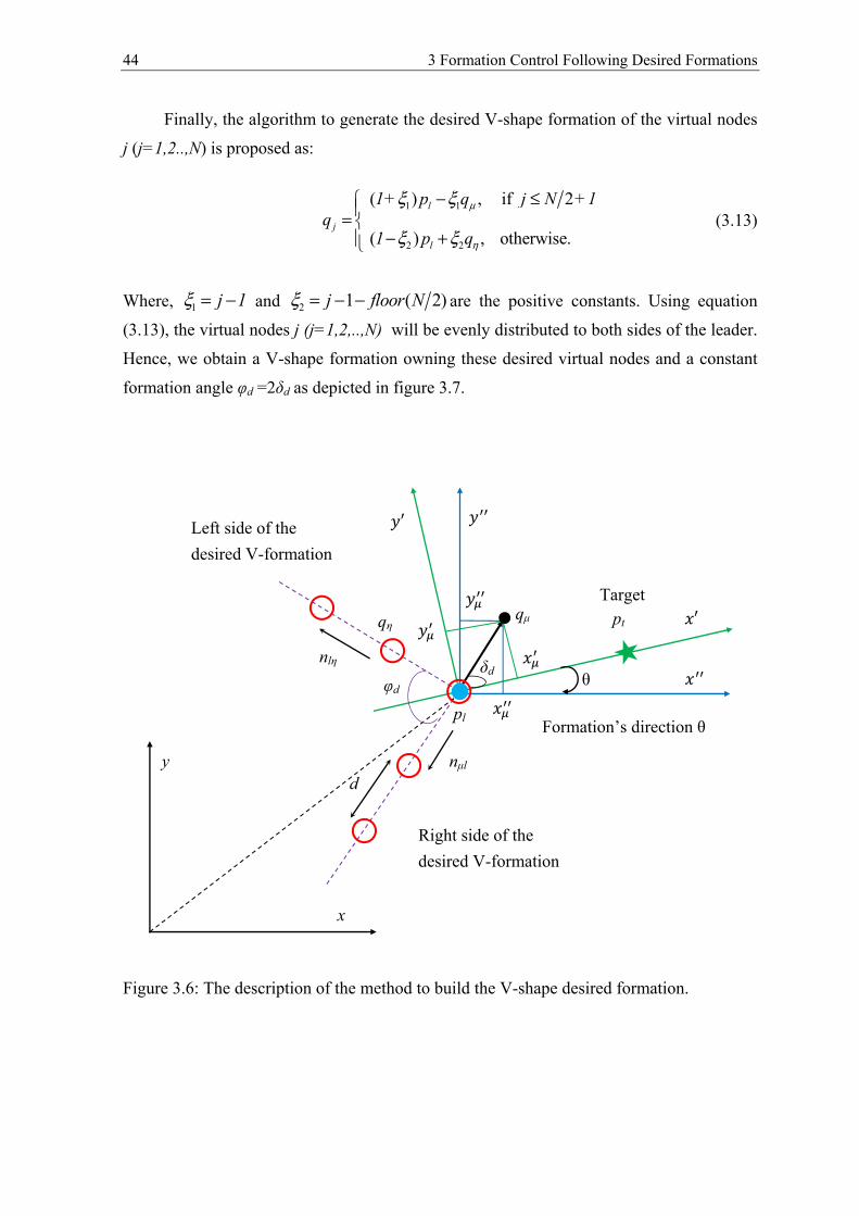
44 3 Formation Control Following Desired Formations
θ
pl
qμ
Left side of the desired V-formation
x
y
′ ′
φd
dnμl
δd
qη
nlη
Target pt
Right side of the desired V-formation
Formation’s direction θ
Finally, the algorithm to generate the desired V-shape formation of the virtual nodes
j (j=1,2..,N) is proposed as:
1 1
2 2
( ) , if
( ) , otherwi
2
se.
l
j
l
1+ p q q
1 p
j N +1
q
μ
η
ξ ξ
ξ ξ
−= − +
≤
(3.13)
Where, 1 j 1ξ = − and 2 1 ( 2)j floor Nξ = − − are the positive constants. Using equation
(3.13), the virtual nodes j (j=1,2,..,N) will be evenly distributed to both sides of the leader.
Hence, we obtain a V-shape formation owning these desired virtual nodes and a constant
formation angle φd =2δd as depicted in figure 3.7.
Figure 3.6: The description of the method to build the V-shape desired formation.
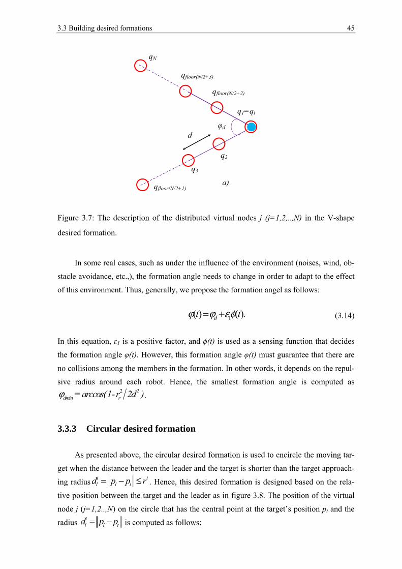
3.3 Building desired formations 45
Figure 3.7: The description of the distributed virtual nodes j (j=1,2,..,N) in the V-shape
desired formation.
In some real cases, such as under the influence of the environment (noises, wind, ob-
stacle avoidance, etc.,), the formation angle needs to change in order to adapt to the effect
of this environment. Thus, generally, we propose the formation angel as follows:
1( ) ( ).dt tϕ ϕ εφ= + (3.14)
In this equation, ε1 is a positive factor, and ϕ(t) is used as a sensing function that decides
the formation angle φ(t). However, this formation angle φ(t) must guarantee that there are
no collisions among the members in the formation. In other words, it depends on the repul-
sive radius around each robot. Hence, the smallest formation angle is computed as2 2
dmin r=arccos(1-r 2d )ϕ .
3.3.3 Circular desired formation
As presented above, the circular desired formation is used to encircle the moving tar-
get when the distance between the leader and the target is shorter than the target approach-
ing radius lt tl t rd p p= − ≤ . Hence, this desired formation is designed based on the rela-
tive position between the target and the leader as in figure 3.8. The position of the virtual
node j (j=1,2..,N) on the circle that has the central point at the target’s position pt and the
radius ltl td p p= − is computed as follows:
φd
q1=ql
q2
q3
qfloor(N/2+1)
qfloor(N/2+2)
qfloor(N/2+3)
qN
a)
d
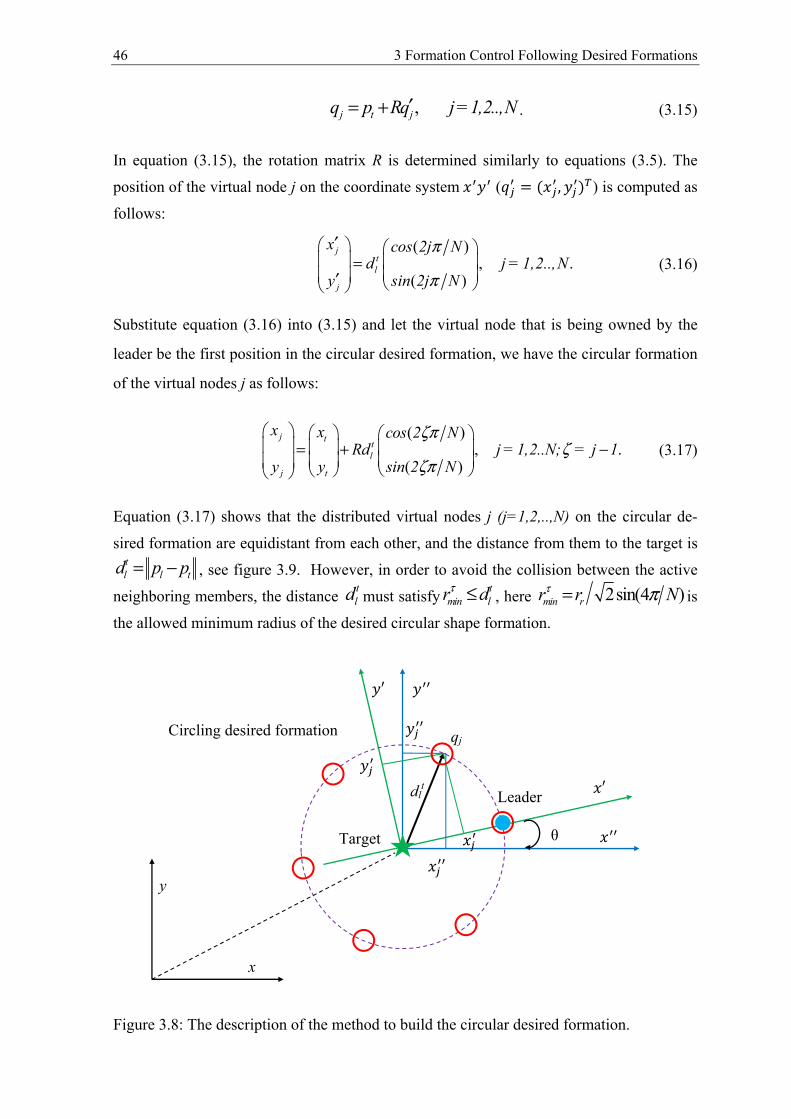
46 3 Formation Control Following Desired Formations
, j t jq p Rq =1,2 .,Nj .′= + . (3.15)
In equation (3.15), the rotation matrix R is determined similarly to equations (3.5). The
position of the virtual node j on the coordinate system ( = ( , ) ) is computed as
follows:
( ), .
( )
jtl
j
x cos 2j Nd j = 1,2..,N
y sin 2j N
π
π
′ =
′ (3.16)
Substitute equation (3.16) into (3.15) and let the virtual node that is being owned by the
leader be the first position in the circular desired formation, we have the circular formation
of the virtual nodes j as follows:
( ), .
( )
j ttl
j t
x x cos 2 NRd j = 1,2..N; = j 1
y y sin 2 N
ζπζ
ζπ
= + −
(3.17)
Equation (3.17) shows that the distributed virtual nodes j (j=1,2,..,N) on the circular de-
sired formation are equidistant from each other, and the distance from them to the target is
ltl td p p= − , see figure 3.9. However, in order to avoid the collision between the active
neighboring members, the distance tld must satisfy t
min lr dτ ≤ , here 2sin(4 )min rr r Nτ π= is
the allowed minimum radius of the desired circular shape formation.
Figure 3.8: The description of the method to build the circular desired formation.
θ
′ ′
qj
Target
Leader dl
t
x
y
Circling desired formation
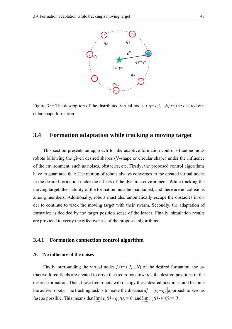
3.4 Formation adaptation while tracking a moving target 47
Figure 3.9: The description of the distributed virtual nodes j (j=1,2,..,N) in the desired cir-
cular shape formation.
3.4 Formation adaptation while tracking a moving target
This section presents an approach for the adaptive formation control of autonomous
robots following the given desired shapes (V-shape or circular shape) under the influence
of the environment, such as noises, obstacles, etc. Firstly, the proposed control algorithms
have to guarantee that: The motion of robots always converges to the created virtual nodes
in the desired formation under the effects of the dynamic environment. While tracking the
moving target, the stability of the formation must be maintained, and there are no collisions
among members. Additionally, robots must also automatically escape the obstacles in or-
der to continue to track the moving target with their swarm. Secondly, the adaptation of
formation is decided by the target position sense of the leader. Finally, simulation results
are provided to verify the effectiveness of the proposed algorithms.
3.4.1 Formation connection control algorithm
A. No influence of the noises
Firstly, surrounding the virtual nodes j (j=1,2,…N) of the desired formation, the at-
tractive force fields are created to drive the free robots towards the desired positions in the
desired formation. Then, these free robots will occupy these desired positions, and become
the active robots. The tracking task is to make the distance ji i jd p q= − approach to zero as
fast as possible. This means that lim( i jtp (t) q (t))= 0
→∞− and lim( i jt
v (t) - v (t))= 0→∞
.
Target
dlt
q3
qN
qN-1
q2
q4
q1=ql
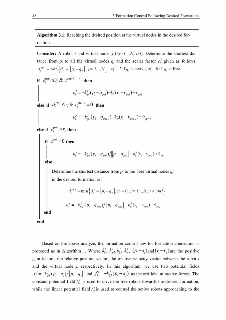
48 3 Formation Control Following Desired Formations
Based on the above analyze, the formation control law for formation connection is
proposed as in Algorithm 1. Where, j j jip1 ip
j2 ip3 ivk , k , k , k , ( )i jp q− and ( )i jv v− are the positive
gain factors, the relative position vector, the relative velocity vector between the robot i
and the virtual node j, respectively. In this algorithm, we use two potential fields
3 ( )jip i j i
j1i jk p q qf p= − − − and 12 ( )j
ipji i jk p qf =− − as the artificial attractive forces. The
constant potential field j1if is used to drive the free robots towards the desired formation,
while the linear potential field 2jif is used to control the active robots approaching to the
Algorithm 3.1: Reaching the desired position at the virtual nodes in the desired for-
mation.
Consider: A robot i and virtual nodes j (i,j=1,..,N, i≠l). Determine the shortest dis-
tance from pi to all the virtual nodes qj and the scalar factor cij given as follows:
{ }m1 min , ,j ji i i jd d p q j = 1,.. N−== , ci
j =1 if qj is active, cij =0 if qj is free.
if m 1m1 1& 1j j
i iad cr −≤ = then
( ) ( )j j
i jm1 i jm1j
ip1 i iv jm1k p q k v vu v=− − − − +
else if m 1m1 1& 0j j
i iad cr −≤ = then
(( ) )j ji jm1
jip2 i -1 iv jm1-1i jm1-1= k p q k v vu +v− −− −
else if m1j
i ad r> then
if m1 0i
jc = then
( ) ( )j j
i jm1 jj
ip3 i i iv jm1m1 i jm1= k p q p q k v v vu − +− − − −
else
Determine the shortest distance from pi to the free virtual nodes qj
in the desired formation as: { }2 min , 0, , ,i
jm j ji i i jd d p q c j = 1,.. N j jm1== − = ≠
3 ( ) ( )j j
i jm2 jj
ip i i iv jm2 i j mm 22k p q p q k v vu v+= − − − − −
end
end
3.4 Formation adaptation while tracking a moving target 49
virtual nodes of the desired formation. Additionally, the component ( )i jivjk v v− − is is also
utilized as the damping term. Therefore, using the desired position finding algorithm (Al-
gorithm 3.1) robots can quickly approach their desired position at the virtual nodes in the
desired formation.
Theorem 3.1. Consider the active robot i with its dynamic model (3.1) and control inputj
iu given in Algorithm 3.1 at the active node j in the desired formation. If the velocity of the
node j is smaller than the maximum velocity of the robot i, and the node j-1 is also active,
then the system (3.1) will be stable at the equilibrium point, at which jip q= and i jv v=
for all i and j.
Proof of theorem 3.1
In order to analyze the stability of the robot i at the active node j when the node j-1 is
also active, we rewrite the control law jiu as follow:
2 ( . ) ji iv j
j ji i ju k v v vf= +− −
(3.18)
Consider the vector field 2 , ,0j Tip1 i j i
ji ik (p q ) ( )f P Q=− − = , here )j
i ip1 i jP k (x x=− − , j
i ip1 i jQ k ( y y )=− − , and 0iZ = . According to [96], [97], we obtain:
( )2curl ( , , 0, 0) , 0 . i i i i i i
i i i i i i
ji
Z Q P Z Qf
P
y z z x x y
∂ ∂ ∂ ∂ ∂ ∂= − − − = ∂ ∂ ∂ ∂ ∂ ∂ (3.19)
Equation (3.19) shows that the vector field 2jif is irrotational. Now, we consider the scale
function as follows:
( ) ( )1 . 2
Tji i
ji ip j j1k p q pV q= − −
(3.20)
Taking the negative gradient of the function jiV we obtain:
( ) ( )
( ) ( )( )2 2
12
12
jip1
ji
Tji i j i j
i jp i j1
V
x
k p q p q
k x y y
−∇ = −∇
= −∇ − + −
−
−
(3.21)
50 3 Formation Control Following Desired Formations
( ) ( )( )( ) ( )( )
( )( )
2 2
2 2
2
12
12
( ) .
jip1
jip1
j
T
i j i ji
i j i ji
T
i j
i
ip1
jip1
jip1
j
jii j
x x y yx
x x y yy
x
k
k
k
k
k
x
p q
y y
f
∂ − − + − ∂ = ∂ − − + − ∂
− − =
− =
− −
−=
So, (3.19) and (3.21) show that the vector field 2jif is a potential field, and its potential
function is jiV .
Let 1 2, i j i jx p q x v v= − = − be the relative position and velocity of the robot i and
node j. We have the error dynamic model of the system as follows:
1 2
2 , .ji j
x x
u v i, j = 1,2 .x . N
=
= −
(3.22)
Substitute jiu in (3.18) into (3.22) we obtain the error dynamic model as:
1 2
2 ( ).jivj
i i jk
x
v v
x
x V
=
= − −∇ −
(3.23)
To analyze the stability of model (3.23) at the equilibrium position( 0,jip q− = 0)i jv v− = ,
the positive definite function is selected as follows:
2 21 . 2
j Tf iV V x x= + (3.24)
Consider the potential function (3.20) we have the relationship as follows ( )Tij
iV p∂ ∂ =
( )( ) .j T
ji iV p q= ∂ ∂ − Taking the time derivative of (3.24) along the trajectory of the sys-
tem (3.23), we obtain:
( )( )
2
2
2
1 2 2 2
2
2
(
( ) )
0.
iv
i
j T T T jf i i
T j j j
Tv
i i
j
V t V x x x x V x
x V V
x
k x
xk
= −
= ∇
−
+ = ∇ +
∇
= −
∇
≤
(3.25)
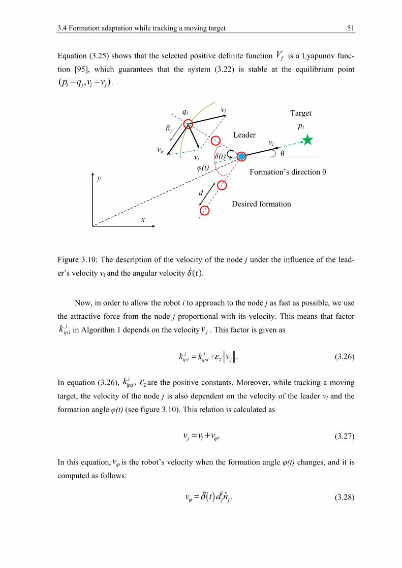
3.4 Formation adaptation while tracking a moving target 51
Target pt
vφ
Desired formation
x
y φ(t)
d
δ(t)
Formation’s direction θ
Leader
vl
vj
qj
vl
j
θ
Equation (3.25) shows that the selected positive definite function fV is a Lyapunov func-
tion [95], which guarantees that the system (3.22) is stable at the equilibrium point( , )j i jip q v v== .
Figure 3.10: The description of the velocity of the node j under the influence of the lead-
er’s velocity vl and the angular velocity ( ). Now, in order to allow the robot i to approach to the node j as fast as possible, we use
the attractive force from the node j proportional with its velocity. This means that factorj
ip1k in Algorithm 1 depends on the velocity jv . This factor is given as
2+ . j jip1 ipd jk k vε=
(3.26)
In equation (3.26), 2, jipdk ε are the positive constants. Moreover, while tracking a moving
target, the velocity of the node j is also dependent on the velocity of the leader vl and the
formation angle φ(t) (see figure 3.10). This relation is calculated as
. j lv v vϕ= +
(3.27)
In this equation, vϕ is the robot’s velocity when the formation angle φ(t) changes, and it is
computed as follows:
( ) ˆ . lj jv t d nϕ δ=
(3.28)
52 3 Formation Control Following Desired Formations
Where, the angular velocity of the formation angle φ(t)/2 is ( ) ( )( / 2)t t tδ ϕ=∂ ∂ . The dis-
tance between the leader and the node j is jlj ld q p= − . The unit vector ˆ jn , which is per-
pendicular with the vector ( )ljq p− , is given as:
( )( ) , (ˆ )ˆ .Tl l
j i j l j j l jn c y - y d x - x d= − (3.29)
Where, the scalar ˆic is dependent on the rotational direction of the formation angle. Con-
sider the robots on the left side of the V-shape formation (see Fig.7), the scalar ˆic is de-
fined as:
1 if
1 othe
( )ˆ
r se.wii
dtc
ϕ ϕ <= −
(3.30)
Similarly, for the robots on the right side of the V-shape formation the scalar ˆic is also
defined as:
1 if
1 othe
( )ˆ
r i .w sei
dtc
ϕ ϕ= −
>
(3.31)
B. Influence of the noises
To consider the stability of the formation under the influence of the noises, which
cause the position errors between the robot i and the virtual node j, we assume that the es-
timates of the position and the velocity of the robot i are: ˆi i pip p z= + and ˆ ii viv v z= + ,
where piz and viz are the position and velocity measurement errors of the robot i, respective-
ly. Similarly, the estimates of the position and the velocity of the virtual node j are also
defined as: ˆj j qjq q z= + and ˆj j vjv v z= + , where qjz and vjz are the position and velocity noises
of the node j, respectively. Now, we propose the new control law for the robot i at the ac-
tive node j in noisy environment as:
ˆ ˆˆ ˆ ˆ ˆ ) ) .( ( j jip1 i iv
ji vj ji j ijk p q ku v v v z+ −= − − − − (3.32)
Where 2ˆ ˆ+j jip1 ipd jk k vε= and ˆ j
ivk are the positive factors. Let 1 ˆ ˆi jx p q= − = i j pijp q z− + and
2ˆ ˆ ˆi j i ij v jx vv v v z= − += − be the relative position and velocity of the robot i and node j in
noisy environment, here vij vi vjz z z= − and pij pi qjz z z= − . We have the error dynamic of the
system as:
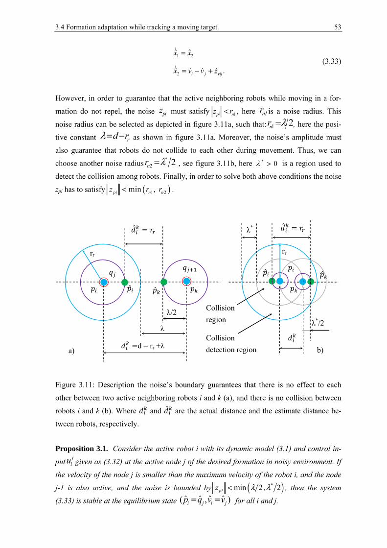
3.4 Formation adaptation while tracking a moving target 53
1 2
2 .ˆ
ˆˆ
vij jiv
x x
x zv=
=
− +
(3.33)
However, in order to guarantee that the active neighboring robots while moving in a for-
mation do not repel, the noise piz must satisfy 1pi nz r< , here n1r is a noise radius. This
noise radius can be selected as depicted in figure 3.11a, such that: 1 2nr λ= , here the posi-
tive constant rd rλ= − as shown in figure 3.11a. Moreover, the noise’s amplitude must
also guarantee that robots do not collide to each other during movement. Thus, we can
choose another noise radius *2 2nr λ= , see figure 3.11b, here * 0λ > is a region used to
detect the collision among robots. Finally, in order to solve both above conditions the noise
zpi has to satisfy ( )1 2min , pi n nz r r< .
Figure 3.11: Description the noise’s boundary guarantees that there is no effect to each
other between two active neighboring robots i and k (a), and there is no collision between
robots i and k (b). Where and are the actual distance and the estimate distance be-
tween robots, respectively.
Proposition 3.1. Consider the active robot i with its dynamic model (3.1) and control in-
putj
iu given as (3.32) at the active node j of the desired formation in noisy environment. If
the velocity of the node j is smaller than the maximum velocity of the robot i, and the node
j-1 is also active, and the noise is bounded by ( )*min 2, 2piz λ λ< , then the system
(3.33) is stable at the equilibrium state ˆ ˆ ˆ ˆ( , )j ii jp q v v== for all i and j.
rr
=d = rr +λ
λ
λ/2
=
a) b)
Collision detection region
Collision region
rr
λ*
λ*/2
=
54 3 Formation Control Following Desired Formations
Proof of proposition 3.1
Similar to the proof of theorem 1, to analyze the stability of the system (3.33) we
choose the Lyapunov function as:
1 1 2 21 1ˆ ˆ ˆ ˆ ˆ2 2
. j Tiz p
Tk x x x xV = + (3.34)
Taking the time derivative of equation (3.34) along the trajectory of the system (3.33), we
obtained as follows:
1 1 22221 ˆ ˆˆ ˆˆ ˆ ˆ ˆ( ) ( )j T j TT Tz ip ipV t k x x x x x k x x== ++ (3.35)
Substitute 2x in (3.33) into (3.35) we obtain:
22ˆ ˆ ˆ ( ) 0. iv
j Tz k xV xt =− ≤ (3.36)
So, equation (3.36) shows that the system (3.33) is stable with the control law (3). Howev-
er, this stability is limited by the boundary of the noise. If ( )*min 2, 2piz λ λ≥ , then the
active neighboring robots can repel to each other or the robots can collide, so the stability
is broken, see figure 3.11.
3.4.2 Collision avoidance control algorithm
This section presents a method for the collision avoidance among the robots during
movement based on the artificial repulsive potential field. Let ( )ikN t be the set of the robots
in the neighborhood of the robot i at time t, such that:
{ }{ }( ) : , . , .ki k
ki i rN k d p p r k 1,. Nt k i= ∀ = − ≤ ∈ ≠ (3.37)
Where, rr is the repulsive radius surrounding each robot, and kid is the Euclidean distance
between robot k and robot i. Now, in order to avoid the collision between robots i and k (i,
k=1,2,..,N; i≠k, i≠l), the local repulsive force field is created surrounding each robot within
the repulsive radius rr as:
( )21
21 1
).
(
kk k ki
i i i rk k
k i ii r i
kf
kk d r c n
d r d
= − − −
(3.38)
3.4 Formation adaptation while tracking a moving target 55
Where, the positive factors 1 2, k ki ik k are used to control the fast interaction. The unit vector
kin from robot k to robot i is given as ( ) .k
i i k i kn p p p p= − − The scalar cik is defined as
follows:
1 if
0 othe
( )
rwise.ki
kik N
ct ∈=
(3.39)
The algorithm for the collision avoidance is built based on the repulsive vector field (3.38)
combined with the relative velocity vector ( )kivk
ik v v− between robot k and robot i as fol-
lows:
( )( )N
ki i i iv
k=1, i
k k ki k
k
c k v vu f≠
= − − . (3.40)
The controller (3.40) shows that the neighboring robots are always driven to leave each
other. In other words, this controller guarantees that there are no collisions among robots in
the swarm.
3.4.3 Obstacle avoidance control algorithm
This sub-section presents the control algorithm for robots passing through M obsta-
cles to track a moving target. As analyzed in chapter 2, this obstacle avoidance control
algorithm is also proposed as follows:
( )1,
( )M
op or o oi iv i
o o
oi i o
ki + f k cf vu v
= ≠
= + − . (3.41)
Where, the linear repulsive force field piof and the rotational force field r
iof surrounding
obstacles are presented in chapter 2. The relative velocity vector (vi – vo) between the robot
i and its neighbor-obstacle o is used as a damping term with the damping scaling factor oivk .
Similar to definition (3.37), here we can also define the set of the obstacles in the neigh-
borhood of the robot i at time t as follows:
{ }{ }: ( ) , , .ooi iN o d r o 1,..M o kt β= ∀ ≤ ∈ ≠ (3.42)
In (3.42), 0r β > and i io
od p p= − are the obstacle detection range and the Euclidean
distance between the robot i and the obstacle o, respectively. The scalar cio is defined as:
56 3 Formation Control Following Desired Formations
( ) 1 if
0 otherwise.oi
oio N t
c ∈=
(3.43)
As presented in chapter 2, using the control law (3.41) robots can easily escape obstacles to
continue to track the target.
3.4.4 Target tracking control algorithm
A. Leader selection
Firstly, one robot, which is closest to the target, is selected as the leader in order to
generate the desired formation. Then, this leader is saved to lead its formation to track a
moving target. In case, the leader meets risk, such as it is broken or trapped in obstacles, it
must transfer its leadership to another, and becomes a free member as other free robots in
the swarm. The leader is selected as Algorithm 3.2.
Algorithm 3.2: Leader selection
Update data: The actual position of robots pi (i=1,..,N, i≠l), obstacle’s information,
the target’s position pt, the actual position of the leader (pξ=pl).
if time t=0 (at initial time) then
Compute the shortest distance from the robot pi to the target pt in order to
determine the leader as follows:
{ }1 min , ,itimi tnd p p i = 1,.. N= − ; l imin1p p=
else
if the actual leader meets obstacle or is broken then
Leadership is transferred to other member that is free and has the closest
distance to the target.
{ }2 min , , , , freen iim tt
id p p i = 1,. N i ξ= − ≠ ; l imin2p p=
else
Maintain the leadership of the actual leader.
lp pξ=
end
end
3.4 Formation adaptation while tracking a moving target 57
B. No influence of the noises
The target tracking controller, which is designed based on the relative position be-
tween the leader and the target, has to guarantee that the formation’s motion is always
driven towards the target. The tracking task is to make the distance between the leader and
the target tl l td p p= − approaching to the radius of the desired circular formation rr as fast
as possible. This means that lim( l ttv (t) v (t))= 0
→∞− and lim( (r t
l t l t ltp (t) p (t))= r p (t) p (t)) d
→∞− − .
Based on the above analysis, the control law for the target tracking is proposed as follows:
( ) .tl l lv l tt t
tu f k v v v= − +− (3.44)
Where, tlvk and tv are the positive factor and the acceleration of the target, respectively.
( )l tv v− is the relative velocity vector between the leader and the target. The potential fieldt
lf from the target is used to drive the leader moving towards the target, and it is given as:
22 ( ) , if
( ( )
, otherwise.
1 1)
t tt t tl l
tl1
ltt
t
lt tl l
l
tl1 i
k k d rn
fd r
d r d r r=
k n
τ
τ τ
−− − −
−
<
(3.45)
Where, 2, t
ltk r and t
mintrr rτ< < are the positive constant, the target approaching radius, and
the desired radius of the circular formation, respectively. 3+t tl1 l1d tk k vε= , here 3, t
l1dk ε
are the positive constants. The unit vector along the line connection from the target to the
leader is computed as ( ) /tl l t l tn p p p p= − − . In the equation (3.45), the constant attrac-
tive force 12lt t j
l ikf n−= is sued to track the target when tltd r> . On the other hand, the at-
tractive/repulsive force field 22 1( (1 1 ) )( ( ) ( ))t t t t t
lt t t
1 l llll lf k d r d k d r r r nτ τ τ− − −= − surround-
ing the equilibrium position, at which l tp p rτ− = , ( ) 0l tv v− = is used to encircle the
target when tltd r≤ . Hence, using this combined vector field the leader can easily ap-
proach to the target at the equilibrium position.
Theorem 3.2. Consider the leader l is described by the model (3.1) and controlled by the
control law (3.44) when t
ltd r≤ . If the velocity of the target is smaller than the maximum
velocity of the leader, then the system (3.1) will be stable at the equilibrium state, at which
l tv v= and ( ) ( ) /l t l t l tp p r p p p pτ− = − − .
Proof of theorem 3.2
58 3 Formation Control Following Desired Formations
Firstly, we consider the vector field ( )tl l t1l l t= K p p pf p − −
in (3.45). Let
2 2 12( ( ) ( ))) (t tt t t tt
l lll l l lK k d k r d k d r r rτ τ τ− − −= − , )l l l t l tP K (x x p p= − − , 0lZ = and)l l l t l tQ K (y y p p= − − , we have:
T
)curl ( , , 0.t l l l l l l
l l ll
l l1
l
Z Q P Z Q P
y z z x x yf
∂ ∂ ∂ ∂ ∂ ∂= − − − = ∂ ∂ ∂ ∂ ∂ ∂ (3.46)
Equation (3.46) shows that the vector field t1lf is not rotational.
Consider the scale function as follow:
2 21
2( )1 1 1 .
2 ( )
tt t l
l
tl
l ttl
k d r= k
d rV
r r
τ
τ τ
− − + − (3.47)
Taking the negative gradient of tiV we obtain:
2 22 1
2 2 1
2 2 12
( )1 12 2( )
( )1 1 ( )( )
( )1 ( ) (
)
t1l l
tl
tl
ttllt t
l l
tt tll lt t
l l
t
t tl l
t
t t tl l l
t
t t tl l l
t
k k d r
d r r r
k k k d rd r
d r d r r r
k k k d rd d
d r d r r
f V
τ
τ τ
ττ
τ τ τ
τ
τ τ
=
− − + −
−− − − − −
−= − − −
−∇
= −∇
= − ∇
∇
∇
∇
2 12
( )1 1 ( ( )
.)
ttl
t tl l
t lt tl l
k k d rd
d r d r r
τ
τ τ
−= − − ∇
−
(3.48)
Similar to equation (3.21), here we also obtain a gradient field ( ) /tl l t l td p p p p∇ − −= .
So, (3.46) and (3.48) show that the vector field t1lf is also a potential field, and its potential
function is tlV .
In order to analyze the stability of the leader at the equilibrium position, at whichr
l tp p r− = and ( ) 0l tv v− = , we let 1x
be the position error between the vector ( )l tp p−and the vector ( ) /r
l t l tr p p p p− − , and 2x
be the relative velocity between the leader and
the target. We get: 1 ( )tll tx p pλ −= and 2 ( )l tx v v= −
, here ( )1 /rl
tl tr p pλ = − − . The error
dynamic of the system is described as follows:
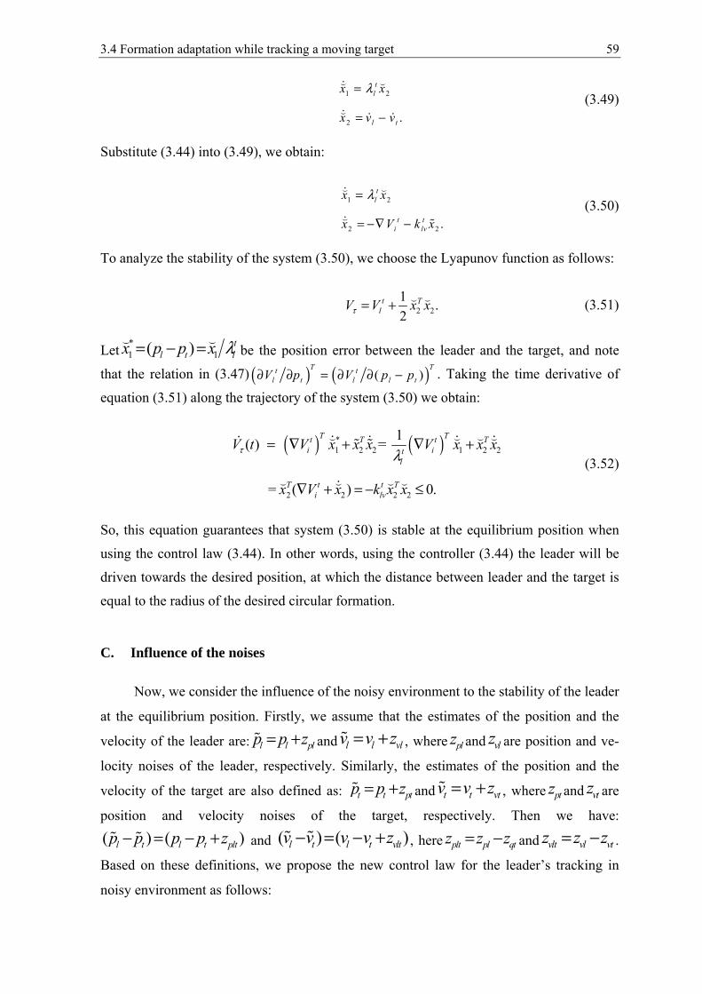
3.4 Formation adaptation while tracking a moving target 59
1 2
2 .l t
tl
v v
x x
x
λ
−
=
=
(3.49)
Substitute (3.44) into (3.49), we obtain:
1 2
2 2 .
tl
ti lv
t
x x
x V xk
λ=
= −∇ −
(3.50)
To analyze the stability of the system (3.50), we choose the Lyapunov function as follows:
2 21 . 2
t TlV V x xτ = + (3.51)
Let *1 1( ) t
l t lx p p x λ= − = be the position error between the leader and the target, and note
that the relation in (3.47) ( ) ( )( )T Tt t
l t l l tV p V p p∂ ∂ = ∂ ∂ − . Taking the time derivative of
equation (3.51) along the trajectory of the system (3.50) we obtain:
( ) ( )2 2 2 2
2 2 2
*1 1
2
( )
1
)
=
.= 0(
T Tt T t Ttl
l
i i
T t t Ti v
V t V x x V x x
x V x x x
x x
k
τ λ+ +
− ≤
= ∇ ∇
∇ + =
(3.52)
So, this equation guarantees that system (3.50) is stable at the equilibrium position when
using the control law (3.44). In other words, using the controller (3.44) the leader will be
driven towards the desired position, at which the distance between leader and the target is
equal to the radius of the desired circular formation.
C. Influence of the noises
Now, we consider the influence of the noisy environment to the stability of the leader
at the equilibrium position. Firstly, we assume that the estimates of the position and the
velocity of the leader are: l l plp p z= + and l l vlv zv= + , where plz and vlz are position and ve-
locity noises of the leader, respectively. Similarly, the estimates of the position and the
velocity of the target are also defined as: t t ptp p z= + and t t vtv zv= + , where ptz and vtz are
position and velocity noises of the target, respectively. Then we have:
( ) ( )l t l t pltp p p p z− = − + and ( ) ( )l t l t vltv v v v z− = − + , here plt pl qtz z z= − and vlt vl vtz z z= − .
Based on these definitions, we propose the new control law for the leader’s tracking in
noisy environment as follows:

60 3 Formation Control Following Desired Formations
( ) z .tl l lv lt t
vlt ttf v v vu k= − +− − (3.53)
Where, tlvk is a positive factor. The force field t
lf is given as:
2 1
1
2
( ) , if ( )
1(
)
.
1 t tt tl llt
t
t t
ttllt t
l ll
l i
k k rn r
r r r
k n , otherw
dd
d
s
df
i e
τ
τ τ
−− − − = −
<
(3.54)
In this equation, 1 3+t tl l1 tdk k vε= , 2
tlk , and l t
tl pd p= − are the positive factors, and
the Euclidean distance, respectively. The unit vector tln is computed as
( ) .tl l t l tn p p p p= − −
Let 1x be the position error between the vector ( )l tp p− and the vector
( ) /l t l tr p p p pτ − − , and 2x be the relative velocity between the leader and the target. We
get: 1 ( ) ( ) / z( ,)rl t l t l t l t plt
tlx p p r p p p p p pλ== − − − − − +
2 ( ) ( z )l t l t vltx v v v v= − = − +
,here 1 /=tl l tr p pτλ − − , and the error dynamic of the system is given as:
1 2
2 .zl t vl
t
t
l
v v
x x
x
λ=
= − +
(3.55)
Proposition 3.2. Consider the leader l is described by the model (3.1) and controlled by
the control law (3.53) in noisy environment whent
ltd r≤ . If the velocity of the target is
smaller than the maximum velocity of the leader, and the noise is bounded by a radius*( 2, 2)nr min λ λ= as given in theorem 2, then system (3.55) is stable at the equilibrium
state ( ) 0lv v− ≈ and ( ) ( ) /l t l t l tp p r p p p pτ− ≈ − − .
Proof of proposition 3.2
Similar to the proof of theorem 2, to analyze the stability of the system (3.55) we
choose the Lyapunov function as:
2 212
t TlV V x xξ = + , (3.56)
Where ( )t t ti l lV V d= with l t
tld p p= − . Let *
1 1z( )l t plttlx p p x λ= − + = be the position error
between the leader and the target, and note that the relation as follows: ( )Tti lV p∂ ∂ =
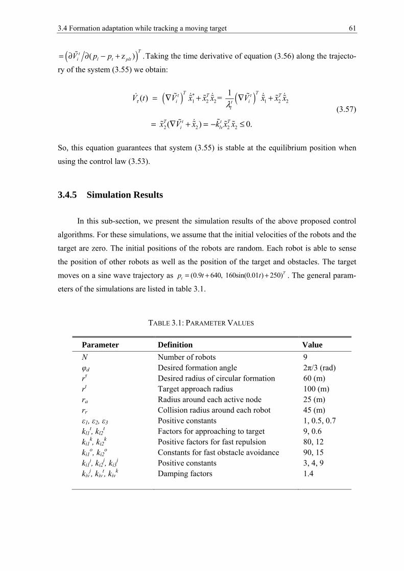
3.4 Formation adaptation while tracking a moving target 61
( )( ) .zl t p
Tti ltp pV − += ∂ ∂ Taking the time derivative of equation (3.56) along the trajecto-
ry of the system (3.55) we obtain:
( ) ( )*1 12 2 2 2
2 2 2 2
1=
( )
( ) 0.
T Tt T t Ti t
l
lv
i
T t t Ti
V t V x x V x x
x
x x
kV x x x
τ λ+ +
− ≤
= ∇ ∇
= ∇ + =
(3.57)
So, this equation guarantees that system (3.55) is stable at the equilibrium position when
using the control law (3.53).
3.4.5 Simulation Results
In this sub-section, we present the simulation results of the above proposed control
algorithms. For these simulations, we assume that the initial velocities of the robots and the
target are zero. The initial positions of the robots are random. Each robot is able to sense
the position of other robots as well as the position of the target and obstacles. The target
moves on a sine wave trajectory as (0.9 640, 160sin(0.01 ) 250)Ttp t t= + + . The general param-
eters of the simulations are listed in table 3.1.
TABLE 3.1: PARAMETER VALUES
Parameter Definition Value N Number of robots 9 φd Desired formation angle 2π/3 (rad) rτ Desired radius of circular formation 60 (m) rt Target approach radius 100 (m) ra Radius around each active node 25 (m) rr Collision radius around each robot 45 (m)
ε1, ε2, ε3 Positive constants 1, 0.5, 0.7 kl1
t, kl2t Factors for approaching to target 9, 0.6
ki1k, ki2
k Positive factors for fast repulsion 80, 12 ki1
o, ki2o Constants for fast obstacle avoidance 90, 15
ki1j, ki2
j, ki3j Positive constants 3, 4, 9
kivj, kiv
t, kivk Damping factors 1.4
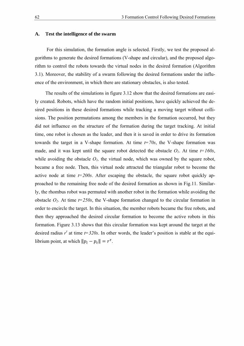
62 3 Formation Control Following Desired Formations
A. Test the intelligence of the swarm
For this simulation, the formation angle is selected. Firstly, we test the proposed al-
gorithms to generate the desired formations (V-shape and circular), and the proposed algo-
rithm to control the robots towards the virtual nodes in the desired formation (Algorithm
3.1). Moreover, the stability of a swarm following the desired formations under the influ-
ence of the environment, in which there are stationary obstacles, is also tested.
The results of the simulations in figure 3.12 show that the desired formations are easi-
ly created. Robots, which have the random initial positions, have quickly achieved the de-
sired positions in these desired formations while tracking a moving target without colli-
sions. The position permutations among the members in the formation occurred, but they
did not influence on the structure of the formation during the target tracking. At initial
time, one robot is chosen as the leader, and then it is saved in order to drive its formation
towards the target in a V-shape formation. At time t=70s, the V-shape formation was
made, and it was kept until the square robot detected the obstacle O1. At time t=160s,
while avoiding the obstacle O1, the virtual node, which was owned by the square robot, became a free node. Then, this virtual node attracted the triangular robot to become the
active node at time t=200s. After escaping the obstacle, the square robot quickly ap-
proached to the remaining free node of the desired formation as shown in Fig.11. Similar-
ly, the rhombus robot was permuted with another robot in the formation while avoiding the
obstacle O2. At time t=250s, the V-shape formation changed to the circular formation in
order to encircle the target. In this situation, the member robots became the free robots, and
then they approached the desired circular formation to become the active robots in this
formation. Figure 3.13 shows that this circular formation was kept around the target at the
desired radius rτ at time t=320s. In other words, the leader’s position is stable at the equi-
librium point, at which ‖ − ‖ = .
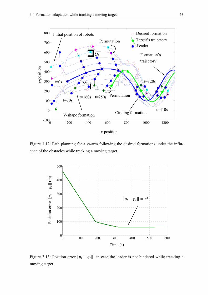
3.4 Formation adaptation while tracking a moving target 63
0 200 400 600 800 1000 1200-100
0
100
200
300
400
500
600
700
800 Desired formation
Leader
Circling formation V-shape formation
O2
Formation’s trajectory
Target’s trajectory Initial position of robots
Permutation
O1
Permutation t=70s
t=250s
t=320s t=0s
t=160s
t=410s
x-position
y-po
sitio
n
0 100 200 300 400 500 6000
100
200
300
400
500
Time (s)
Posi
tion
erro
r ‖ −‖ (m)
‖ − ‖ =
Figure 3.12: Path planning for a swarm following the desired formations under the influ-
ence of the obstacles while tracking a moving target.
Figure 3.13: Position error ‖ − ‖ in case the leader is not hindered while tracking a
moving target.
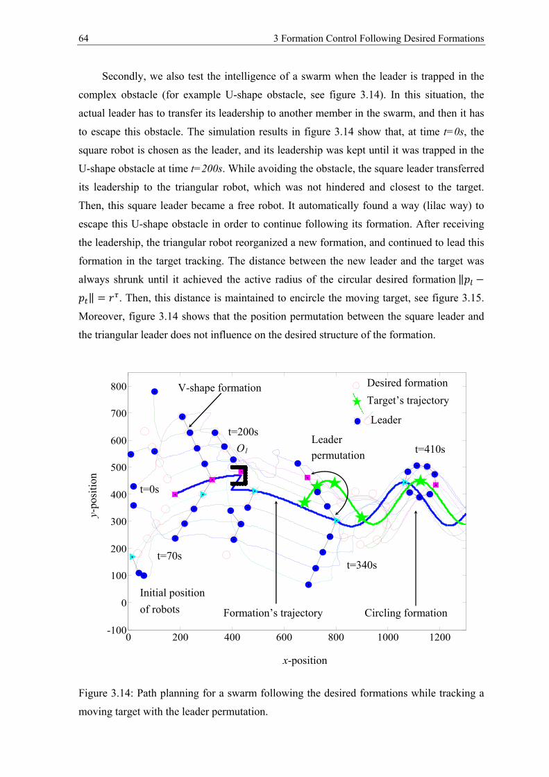
64 3 Formation Control Following Desired Formations
0 200 400 600 800 1000 1200-100
0
100
200
300
400
500
600
700
800
Leader
Circling formation
V-shape formation
O1
Formation’s trajectory
Target’s trajectory
Initial position of robots
Leader permutation
Desired formation
t=70s t=340s
t=410s
t=0s
t=200s
x-position
y-po
sitio
n
Secondly, we also test the intelligence of a swarm when the leader is trapped in the
complex obstacle (for example U-shape obstacle, see figure 3.14). In this situation, the
actual leader has to transfer its leadership to another member in the swarm, and then it has
to escape this obstacle. The simulation results in figure 3.14 show that, at time t=0s, the
square robot is chosen as the leader, and its leadership was kept until it was trapped in the
U-shape obstacle at time t=200s. While avoiding the obstacle, the square leader transferred
its leadership to the triangular robot, which was not hindered and closest to the target.
Then, this square leader became a free robot. It automatically found a way (lilac way) to
escape this U-shape obstacle in order to continue following its formation. After receiving
the leadership, the triangular robot reorganized a new formation, and continued to lead this
formation in the target tracking. The distance between the new leader and the target was
always shrunk until it achieved the active radius of the circular desired formation ‖ −‖ = . Then, this distance is maintained to encircle the moving target, see figure 3.15.
Moreover, figure 3.14 shows that the position permutation between the square leader and
the triangular leader does not influence on the desired structure of the formation.
Figure 3.14: Path planning for a swarm following the desired formations while tracking a
moving target with the leader permutation.
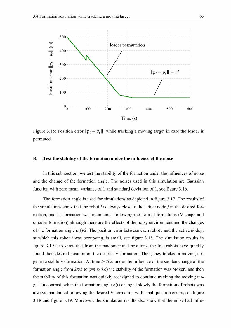
3.4 Formation adaptation while tracking a moving target 65
0 100 200 300 400 500 6000
100
200
300
400
500
Time (s)
Posi
tion
erro
r ‖ −‖ (m)
‖ − ‖ =
leader permutation
Figure 3.15: Position error ‖ − ‖ while tracking a moving target in case the leader is
permuted.
B. Test the stability of the formation under the influence of the noise
In this sub-section, we test the stability of the formation under the influences of noise
and the change of the formation angle. The noises used in this simulation are Gaussian
function with zero mean, variance of 1 and standard deviation of 1, see figure 3.16.
The formation angle is used for simulations as depicted in figure 3.17. The results of
the simulations show that the robot i is always close to the active node j in the desired for-
mation, and its formation was maintained following the desired formations (V-shape and
circular formation) although there are the effects of the noisy environment and the changes
of the formation angle φ(t)/2. The position error between each robot i and the active node j,
at which this robot i was occupying, is small, see figure 3.18. The simulation results in
figure 3.19 also show that from the random initial positions, the free robots have quickly
found their desired position on the desired V-formation. Then, they tracked a moving tar-
get in a stable V-formation. At time t=70s, under the influence of the sudden change of the
formation angle from 2π/3 to φ=( π-0.6) the stability of the formation was broken, and then
the stability of this formation was quickly redesigned to continue tracking the moving tar-
get. In contrast, when the formation angle φ(t) changed slowly the formation of robots was
always maintained following the desired V-formation with small position errors, see figure
3.18 and figure 3.19. Moreover, the simulation results also show that the noise had influ-
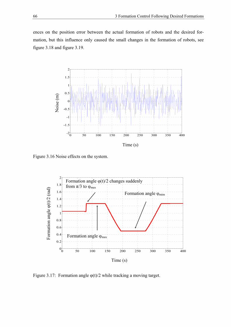
66 3 Formation Control Following Desired Formations
ences on the position error between the actual formation of robots and the desired for-
mation, but this influence only caused the small changes in the formation of robots, see
figure 3.18 and figure 3.19.
Figure 3.16 Noise effects on the system.
Figure 3.17: Formation angle φ(t)/2 while tracking a moving target.
0 50 100 150 200 250 300 350 4000
0.2
0.4
0.6
0.8
1
1.2
1.4
1.6
1.8
2
Time (s)
Form
atio
n an
gle φ
(t)/2
(rad
)
Formation angle φ(t)/2 changes suddenly from π/3 to φmax
Formation angle φmax
Formation angle φmim
0 50 100 150 200 250 300 350 400-2
-1.5
-1
-0.5
0
0.5
1
1.5
2
Time (s)
Noi
se (m
)
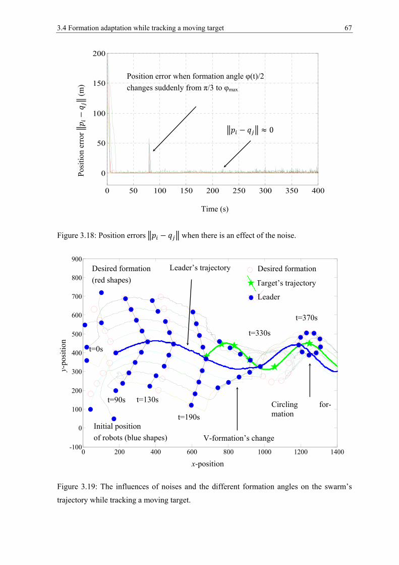
3.4 Formation adaptation while tracking a moving target 67
Figure 3.18: Position errors − when there is an effect of the noise.
Figure 3.19: The influences of noises and the different formation angles on the swarm’s
trajectory while tracking a moving target.
0 50 100 150 200 250 300 350 400
0
50
100
150
200
Time (s)
Posi
tion
erro
r − (
m)
− ≈ 0
Position error when formation angle φ(t)/2 changes suddenly from π/3 to φmax
0 200 400 600 800 1000 1200 1400-100
0
100
200
300
400
500
600
700
800
900Desired formation (red shapes)
V-formation’s change
Leader’s trajectory
Target’s trajectory
Initial position of robots (blue shapes)
Circling for-mation
Leader
t=90s
t=0s
t=130s
t=190s
t=330s
t=370s
x-position
y-po
sitio
n
Desired formation
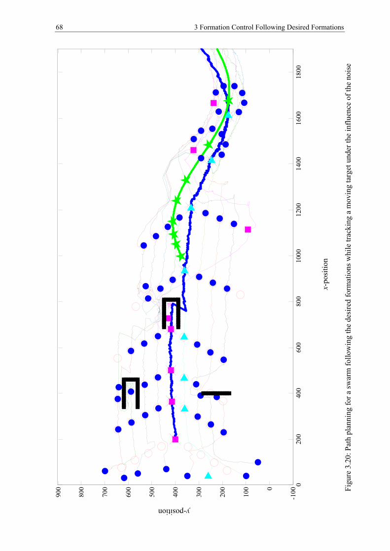
68 3 Formation Control Following Desired Formations
Des
ired
form
atio
n
(red
shap
es)
Lead
er’s
traj
ecto
ry Ta
rget
’s tr
ajec
tory
Initi
al p
ositi
on
of ro
bots
(blu
e sh
apes
)
Circ
ling
fo
rmat
ion
Obs
tacl
e
t=90
s t=0s
t=13
0s
t=22
0s
t=41
0s
t=53
0s
t=29
0s
x-po
sitio
n
y-position
Des
ired
form
atio
n
Lea
der
per
mut
atio
n
020
040
060
080
010
0012
0014
0016
0018
00-1
000
100
200
300
400
500
600
700
800
900 Fi
gure
3.2
0: P
ath
plan
ning
for a
swar
m fo
llow
ing
the
desi
red
form
atio
ns w
hile
trac
king
a m
ovin
g ta
rget
und
er th
e in
fluen
ce o
f the
noi
se
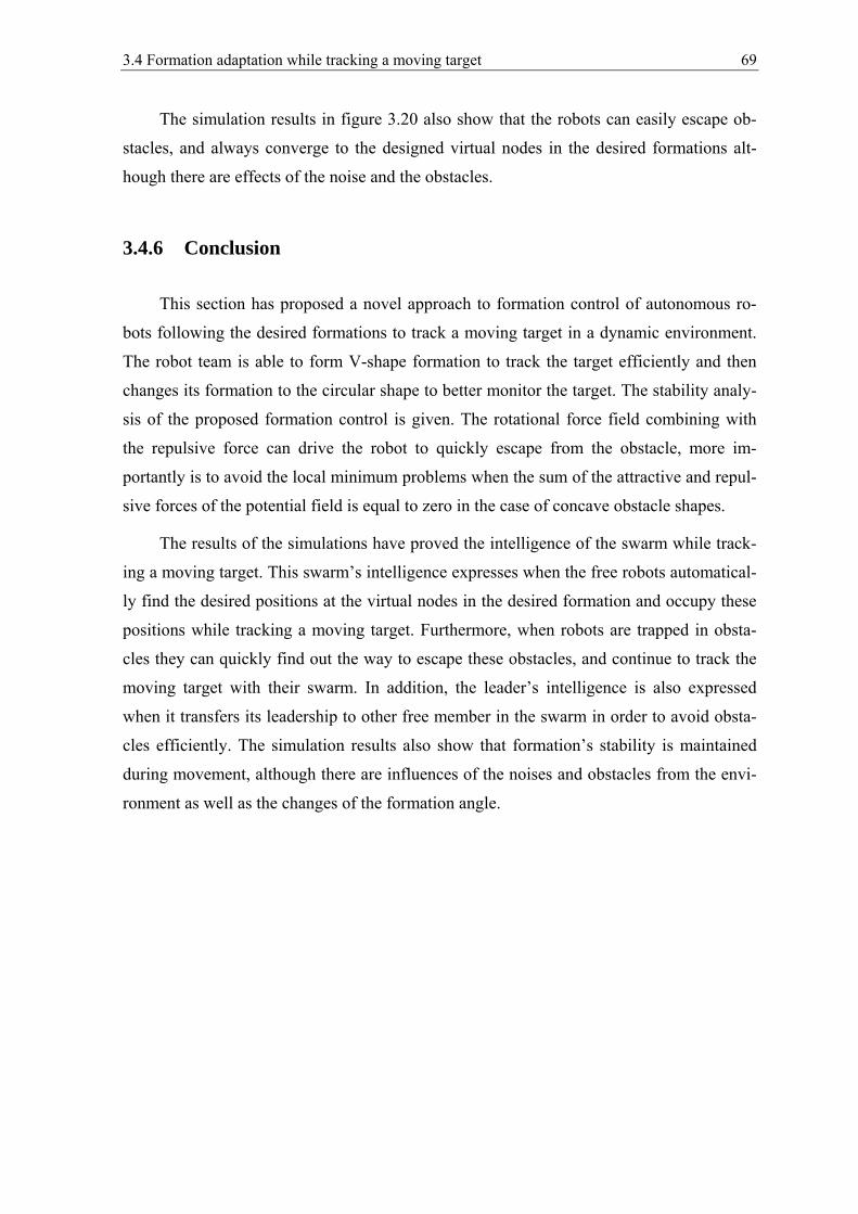
3.4 Formation adaptation while tracking a moving target 69
The simulation results in figure 3.20 also show that the robots can easily escape ob-
stacles, and always converge to the designed virtual nodes in the desired formations alt-
hough there are effects of the noise and the obstacles.
3.4.6 Conclusion
This section has proposed a novel approach to formation control of autonomous ro-
bots following the desired formations to track a moving target in a dynamic environment.
The robot team is able to form V-shape formation to track the target efficiently and then
changes its formation to the circular shape to better monitor the target. The stability analy-
sis of the proposed formation control is given. The rotational force field combining with
the repulsive force can drive the robot to quickly escape from the obstacle, more im-
portantly is to avoid the local minimum problems when the sum of the attractive and repul-
sive forces of the potential field is equal to zero in the case of concave obstacle shapes.
The results of the simulations have proved the intelligence of the swarm while track-
ing a moving target. This swarm’s intelligence expresses when the free robots automatical-
ly find the desired positions at the virtual nodes in the desired formation and occupy these
positions while tracking a moving target. Furthermore, when robots are trapped in obsta-
cles they can quickly find out the way to escape these obstacles, and continue to track the
moving target with their swarm. In addition, the leader’s intelligence is also expressed
when it transfers its leadership to other free member in the swarm in order to avoid obsta-
cles efficiently. The simulation results also show that formation’s stability is maintained
during movement, although there are influences of the noises and obstacles from the envi-
ronment as well as the changes of the formation angle.
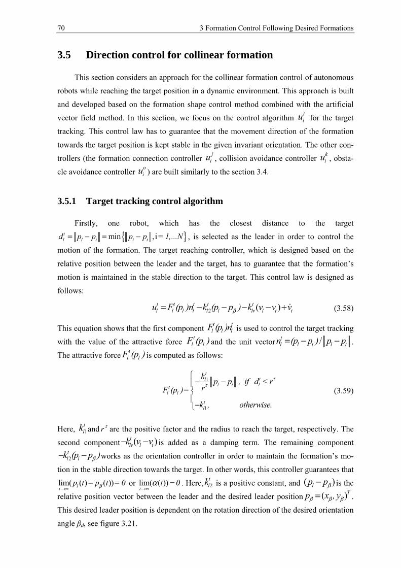
70 3 Formation Control Following Desired Formations
3.5 Direction control for collinear formation
This section considers an approach for the collinear formation control of autonomous
robots while reaching the target position in a dynamic environment. This approach is built
and developed based on the formation shape control method combined with the artificial
vector field method. In this section, we focus on the control algorithm tiu for the target
tracking. This control law has to guarantee that the movement direction of the formation
towards the target position is kept stable in the given invariant orientation. The other con-
trollers (the formation connection controller jiu , collision avoidance controller k
iu , obsta-
cle avoidance controller oiu ) are built similarly to the section 3.4.
3.5.1 Target tracking control algorithm
Firstly, one robot, which has the closest distance to the target
{ }min ,il t il ttd p p p p = 1,...N= − = − , is selected as the leader in order to control the
motion of the formation. The target reaching controller, which is designed based on the
relative position between the leader and the target, has to guarantee that the formation’s
motion is maintained in the stable direction to the target. This control law is designed as
follows:
2 ( ) t tl lt t
lt
l l lv l t tl(p ) k (p p ) k v v vu F n β= − − − − + (3.58)
This equation shows that the first component t tl l lF (p )n is used to control the target tracking
with the value of the attractive force tl lF (p )and the unit vector /t
l l t l tn (p p ) p p= − − .
The attractive force tl lF (p ) is computed as follows:
1
1 .
ttl
l ttl
tl
l
l
kp p , if d < r
r(p )=
k , otherwise
F
ττ
− −−
(3.59)
Here, 1tlk and r τ are the positive factor and the radius to reach the target, respectively. The
second component ( )lv l ttk v v−− is added as a damping term. The remaining component
2t
llk (p p )β− − works as the orientation controller in order to maintain the formation’s mo-
tion in the stable direction towards the target. In other words, this controller guarantees that
lim( ( ) ( ))ltp t p t = 0β→∞
− or lim( ( ))t
t 0α→∞
= . Here, 2tlk is a positive constant, and ( )lp pβ− is the
relative position vector between the leader and the desired leader position ( )Tp x , yβ β β= .
This desired leader position is dependent on the rotation direction of the desired orientation
angle βd, see figure 3.21.

3.5 Direction control for collinear formation 71
Figure 3.21: The desired leader position ( )Tp x , yβ β β= in case the positive desired angle.
Assume that the desired orientation angle rotates clockwise is positive, and rotates
counter-clockwise is negative. Consider the case that the desired orientation angle is posi-
tive, the desired leader position is calculated as follows: We build the coordinate
tem ′ ′ based on this positive desired orientation angle βd as depicted in figure 3.21. The
desired coordinates on the coordinate system ′ ′, at which the leader has to reach in order
to guarantee that the movement direction towards the target is stable, is determined as ( , ) = ( , 0) . On the coordinate system xy, the coordinates of this desired leader
position are determined as follows:
cos sins n cos 0i
t d d l
t d d
x x x
y yβ
β
β ββ β
− = +
′
. (3.60)
On the other hand, from figure 3.21 the coordinates of the leader is determined as follows:
cos sinsin co
s
l t d d l
l t d d l
x x x
y y y
β ββ β
− = +
′
′ . (3.61)
By equating (3.61), we obtainlx ′ as follows:
( ) cos ( ) sinl l t d l t dx x x y yβ β−′ += − . (3.62)
In case the desired angle is negative, we will findlx ′ as follows:
( ) cos ( ) sinl l t d l t dx x x y yβ β−′ −= − . (3.63)
Target pt
βd
Leader pl
(pβ - pl)
x
y
′ ′
=
α
pβ
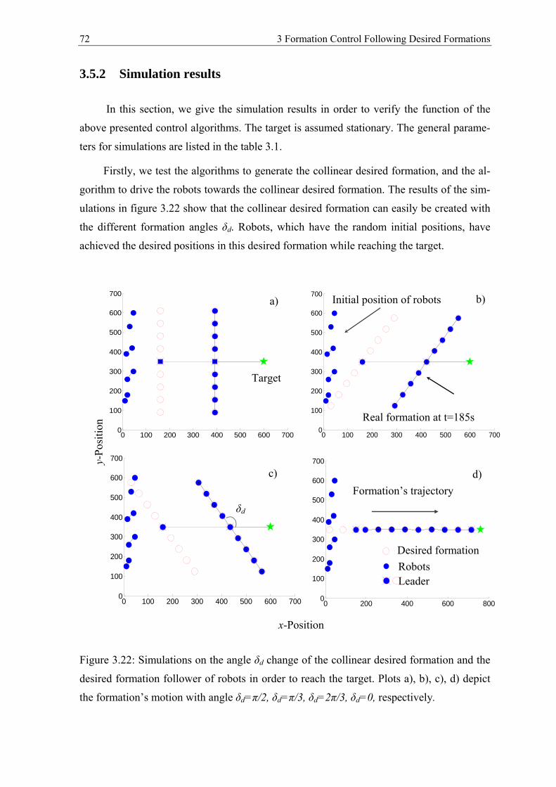
72 3 Formation Control Following Desired Formations
3.5.2 Simulation results
In this section, we give the simulation results in order to verify the function of the
above presented control algorithms. The target is assumed stationary. The general parame-
ters for simulations are listed in the table 3.1.
Firstly, we test the algorithms to generate the collinear desired formation, and the al-
gorithm to drive the robots towards the collinear desired formation. The results of the sim-
ulations in figure 3.22 show that the collinear desired formation can easily be created with
the different formation angles δd. Robots, which have the random initial positions, have
achieved the desired positions in this desired formation while reaching the target.
Figure 3.22: Simulations on the angle δd change of the collinear desired formation and the
desired formation follower of robots in order to reach the target. Plots a), b), c), d) depict
the formation’s motion with angle δd=π/2, δd=π/3, δd=2π/3, δd=0, respectively.
0 100 200 300 400 500 600 7000
100
200
300
400
500
600
700
0 100 200 300 400 500 600 7000
100
200
300
400
500
600
700
0 100 200 300 400 500 600 7000
100
200
300
400
500
600
700
0 200 400 600 8000
100
200
300
400
500
600
700
Initial position of robots
Desired formation
Target
δd
Real formation at t=185s
a) b)
d) c)
x-Position
y-Po
sitio
n
Formation’s trajectory
Robots Leader
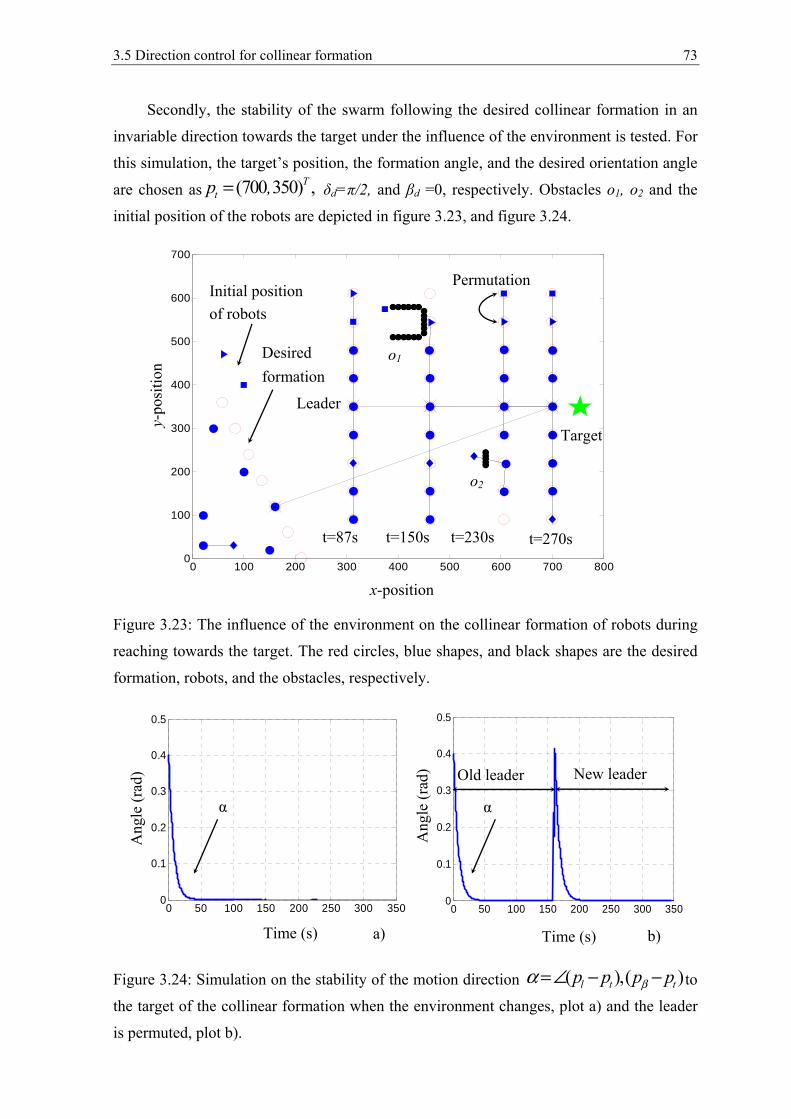
3.5 Direction control for collinear formation 73
Secondly, the stability of the swarm following the desired collinear formation in an
invariable direction towards the target under the influence of the environment is tested. For
this simulation, the target’s position, the formation angle, and the desired orientation angle
are chosen as (700 350) ,Ttp , = δd=π/2, and βd =0, respectively. Obstacles o1, o2 and the
initial position of the robots are depicted in figure 3.23, and figure 3.24.
Figure 3.23: The influence of the environment on the collinear formation of robots during
reaching towards the target. The red circles, blue shapes, and black shapes are the desired
formation, robots, and the obstacles, respectively.
Figure 3.24: Simulation on the stability of the motion direction ( ),( )l t tp p p pβα =∠ − − to
the target of the collinear formation when the environment changes, plot a) and the leader
is permuted, plot b).
0 50 100 150 200 250 300 3500
0.1
0.2
0.3
0.4
0.5
0 50 100 150 200 250 300 3500
0.1
0.2
0.3
0.4
0.5
Time (s)
Ang
le (r
ad)
Time (s)
Ang
le (r
ad)
a) b)
α α
Old leader New leader
0 100 200 300 400 500 600 700 8000
100
200
300
400
500
600
700
x-position
Initial position of robots
y-po
sitio
n o1 Desired
formation
o2
t=87s t=150s t=230s t=270s
Leader
Target
Permutation
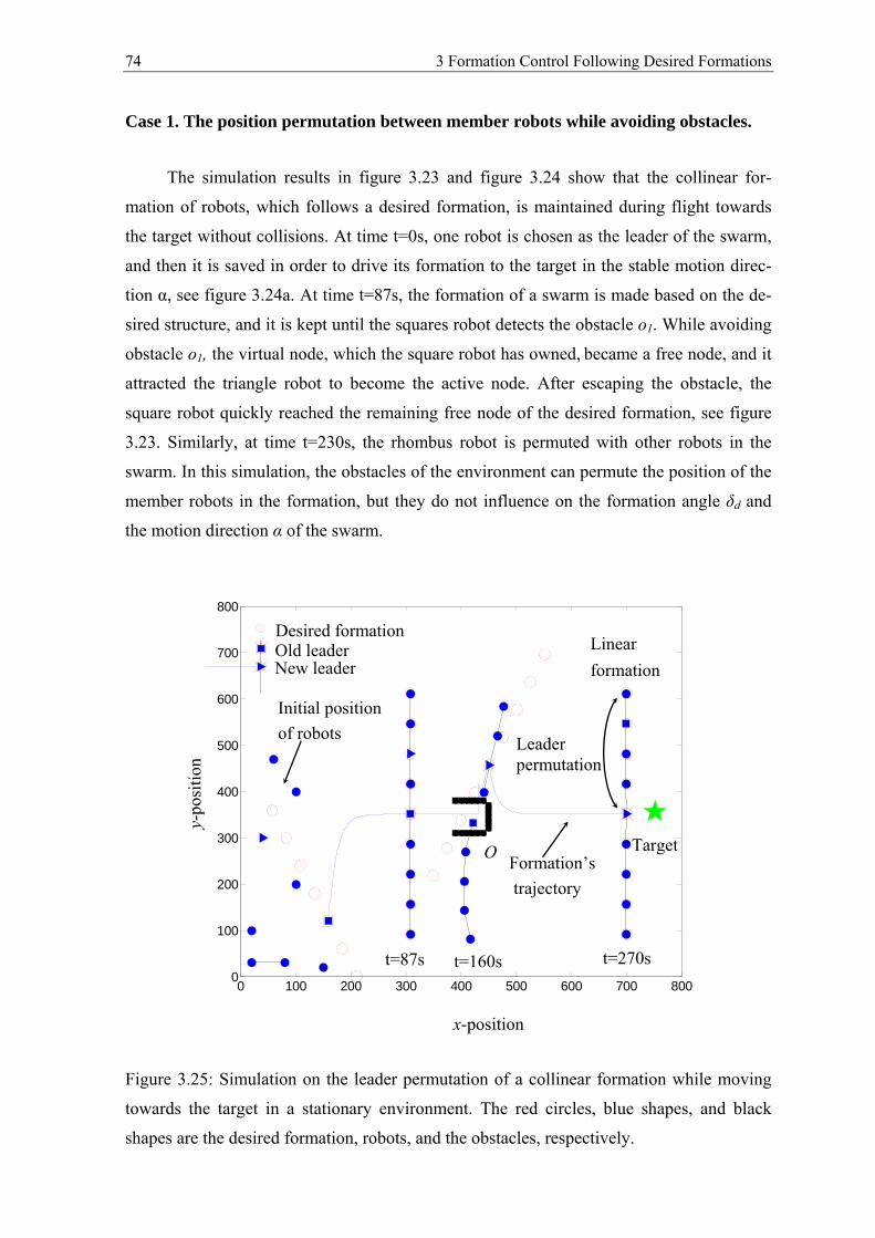
74 3 Formation Control Following Desired Formations
Case 1. The position permutation between member robots while avoiding obstacles.
The simulation results in figure 3.23 and figure 3.24 show that the collinear for-
mation of robots, which follows a desired formation, is maintained during flight towards
the target without collisions. At time t=0s, one robot is chosen as the leader of the swarm,
and then it is saved in order to drive its formation to the target in the stable motion direc-
tion α, see figure 3.24a. At time t=87s, the formation of a swarm is made based on the de-
sired structure, and it is kept until the squares robot detects the obstacle o1. While avoiding
obstacle o1, the virtual node, which the square robot has owned, became a free node, and it
attracted the triangle robot to become the active node. After escaping the obstacle, the
square robot quickly reached the remaining free node of the desired formation, see figure
3.23. Similarly, at time t=230s, the rhombus robot is permuted with other robots in the
swarm. In this simulation, the obstacles of the environment can permute the position of the
member robots in the formation, but they do not influence on the formation angle δd and
the motion direction α of the swarm.
Figure 3.25: Simulation on the leader permutation of a collinear formation while moving
towards the target in a stationary environment. The red circles, blue shapes, and black
shapes are the desired formation, robots, and the obstacles, respectively.
0 100 200 300 400 500 600 700 8000
100
200
300
400
500
600
700
800
y-po
sitio
n
x-position
Initial position of robots
Linear formation
t=87s t=160s t=270s
O
Old leader New leader
Target
Leader permutation
Desired formation
Formation’s trajectory
3.5 Direction control for collinear formation 75
Case 2. The leader permutation while avoiding obstacles.
The leader change influences on the organization of the formation during movement
towards the target. Figure 3.25 shows that, at time t=0, the square robot is chosen as the
leader and it also saved to lead the swarm to the target. Using the orientation controller
2t
llk (p p )β− − as given in (3.58), this leader quickly achieved the desired direction βd =0 to
the target (t=50s to t=150s), see figure 3.24b. The formation’s organization is changed
when the square leader (old leader) is trapped in the U-shape obstacle at time t=160s. In
this situation, the square leader lost the leader role. It became a free robot and automatical-
ly found a way to escape this obstacle and continued to track its formation. The triangle
robot, which is a free robot and closest to the target, is used as a new leader in order to con-
tinue to lead the swarm towards the target. Figure 3.24b shows the new leader has quickly
led its formation in the desired direction before reaching the target.
3.5.3 Conclusion
In this section, we have proposed a novel approach to formation control of autono-
mous robots following a desired collinear formation to reach a stationary target. The de-
sired formation with the different formation angles is built on the relative position between
the target and the leader of the swarm. The trajectory of member robots is driven by the
artificial force fields from the virtual attractive nodes of the desired formation. The mission
of the leader is to lead the formation towards the target in a desired direction. Furthermore,
the repulsive force fields between robots are used to guarantee that there are no collisions
in the swarm during movement. Moreover, in order to avoid obstacles of the environment,
the repulsive and rotating force fields are also added. The results of the simulations have
shown that using the proposed control algorithms the member robots have quickly
achieved the desired positions in the desired formation. In some cases, such as obstacle
avoidance, the position of some robots in formation can be permuted, but the structure and
the motion direction of the formation are kept.
76
4 Cooperative Control for Multi Robot Systems
4.1 Introduction
Formation control of multi-robot systems has been one of the interesting research top-
ics in the control community all over the world in recent years. Its potential applications in
many areas, such as search and rescue missions, forest fire detection and surveillance, is
the motivation and reason for this attraction. In the formation control of multi-robot sys-
tems, the moving trajectory determination of each member-robot and the control of its mo-
tion along this determined trajectory are crucial problems. One of the effective and inter-
esting methods to solve these problems is the artificial vector field method as presented in
chapter 2. In this method, the motion of the robots is controlled by the artificial force fields
that are built based on the relative positions of the robots, target and obstacles of the envi-
ronment.
In recent years, the artificial potential field method has been widely studied and used
to control the formation of multi-agent systems to reach the position of the goal in a dy-
namic environment, see [14]-[33]. One of the main issues in the formation control of multi-
agents to track a moving target is that all the member robots have to move together without
collisions among them in an ordered swarm. Moreover, the whole swarm must avoid ob-
stacles along its trajectory, which has a big influence on the target reaching. In order to
solve these problems, the motion of each member robot is controlled by a total force field
which includes the interactive forces between neighboring robots, the repulsive forces from
the environment obstacles, and the attractive force of the target. Under the effect of this
total force, the formation of the swarm is stably maintained while the swarm reaches the
target position in the free environment. In contrast, this stability is broken when the swarm
avoids the obstacles of the dynamic environment. In this situation, the agents of the swarm
are split, and each agent will itself determine its direction to avoid the obstacle. After the
swarm has overcome the obstacles, its organization is redesigned; however, its formation is
possibly changed, see [34]-[50]. This problem can be resolved, if the swarm maintains its
formation in a smaller size. This is an interesting topic that attracts the attention from re-
searchers in recent years. Some research results around this topic are presented in [74]-
[76]. In this approach, each agent can cooperatively learn the network’s parameters to de-
cide the size and the split of the network in a decentralized fashion so that the connectivity,
formation and tracking performance can be improved when avoiding obstacles.
4.1 Introduction 77
In this chapter, we present a control method for the cooperation among the members
of a swarm under the effect of the dynamic environment. The stability and robustness of
the formation of a swarm are maintained while avoiding obstacles and tracking a moving
target. Moreover, in a complex environment where the space among obstacles is narrow,
we suggest that the swarm’s size can change, so the swarm can easily pass through this
space. In addition, in order to avoid collisions and maintain the stability in the formation of
a swarm, the neighboring robots will be connected to each other by the attractive and re-
pulsive vector field between them. Information about obstacles in the environment will be
sent to all other member robots in the swarm. Therefore, the velocity of the robots in a
formation while avoiding obstacle is the same.
The main contributions of this chapter are as follows:
• “Connection between neighboring robots” is presented in section 4.3. In this content,
we propose an approach for the connection between neighboring robots in a swarm.
The main aim of this approach is to generate the stable and robust links among the
neighboring robots in the formation of a swarm. These connections are controlled by
the attractive/repulsive forces among them. Hence, using the attractive/repulsive forc-
es, the neighboring robots will quickly approach the equilibrium position, at which
the distances among them are constant (that is the sum of the attractive/repulsive
forces are equal to zero).
• “Adaptive formation control in a dynamic environment” is presented in section 4.4.
In this content, we consider an approach for the adaptive formation control of the au-
tonomous robots while tracking a moving target in a dynamic environment. The main
aim of this approach is to control the formation of a swarm that can easily and quick-
ly escape the obstacles of the environment without the collisions (especially, in an
environment, in which the space between the obstacles is narrow). While avoiding the
obstacles, the formation structure of the swarm can change, but it is not broken. In
order to perform this idea, an applied active method is to shrink the swarm’s size into
the smaller size. Hence, the adaptive formation control algorithm is designed such
that the swarm’s size is inversely proportional to the sum of the repulsive forces from
the obstacles acting on the swarm.
• “Cooperative formation control in a dynamic environment” is presented in section
4.5. In this content, we consider an approach for the cooperative formation control of
the autonomous robots while tracking a moving target in a dynamic environment. The
main aim of this approach is to control the formation of a swarm to quickly avoid and
78 4 Cooperative Control for Multi Robot Systems
overcome the obstacles of the environment following the direction of the target’s tra-
jectory while keeping the formation. This approach is built based on the repulsive
force combined with the rotational force surrounding the obstacles.
The rest of this chapter is organized as follows: The problem statement is given in the next section. Section 4.3 presents the cooperative control algorithm for two neighboring robots. In section 4.4, the adaptive control method for the formation of a swarm while avoiding obstacles to track a moving target is presented. Finally, section 4.5 presents the coopera-tive control algorithm for the neighboring robots in the formation of a swarm while track-ing a moving target in a dynamic environment.
4.2 Problem statement
In this section, we consider a swarm of N robots ( 2N ≥ ) that moves in a two-
dimensional Euclidean space { }2R with M obstacles of the environment. Each robot’s mo-
tion, which is assumed as a moving point in the space, is described by the dynamic model
as follows:
, i i
i i
p v
v u i = 1,..,N.
=
=
(4.1)
Where { }2( , , )i i ip v u R∈ are the position, the velocity, and the control input of the robot i,
respectively.
In the formation of a desired swarm, the neighboring robots have to link with each
other to generate the constant distances among them (example in figure 4.1). Let ( )iN tα be
the set of the robots in the neighborhood of the robot i at time (t), such that:
{ }{ }: , . , ) .( ji iN j d r j 1 j it , Nα α= ∀ ≤ ∈ ≠ . (4.2)
Where 0 0rα > , 0rα > , and ij
i jd p p−= are the collision range surrounding each robot, the
interaction range (radius of neighborhood circle, see figure 4.1), and the Euclidean distance
between the robot i and the robot j, respectively. For example, in figure 4.1, the robot R1
has three neighbors: R2, R3, R4.
Similarly, let ( )iN tβ be the set of the obstacles in the neighborhood of the robot i at
time (t), such that:
{ }{ }( ) : 1,.. , .,oiiN o d r o jt M oβ β= ∀ ≤ ∈ ≠ (4.3)
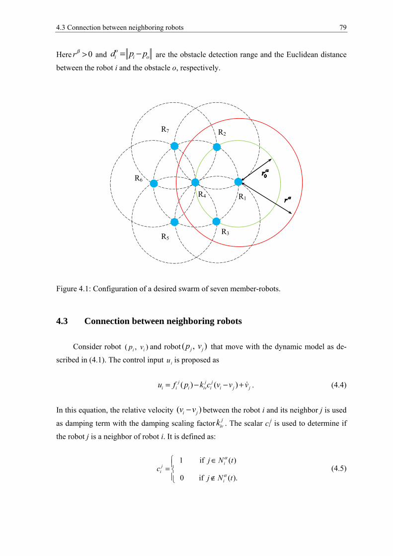
4.3 Connection between neighboring robots 79
Here 0rβ > and i io
od p p= − are the obstacle detection range and the Euclidean distance
between the robot i and the obstacle o, respectively.
Figure 4.1: Configuration of a desired swarm of seven member-robots.
4.3 Connection between neighboring robots
Consider robot ( , )i ip v and robot ( , )j jp v that move with the dynamic model as de-
scribed in (4.1). The control input iu is proposed as
( ( ))j j ji i iv i j jiiu f k c v v vp= − − + . (4.4)
In this equation, the relative velocity ( )i jv v− between the robot i and its neighbor j is used
as damping term with the damping scaling factor jivk . The scalar ci
j is used to determine if
the robot j is a neighbor of robot i. It is defined as:
1 if
0 if
( )
( ).
ij
i
i
j Nc
j
t
tN
α
α
∈= ∉
(4.5)
R1
R2
R3
R4
R5
R6
R7
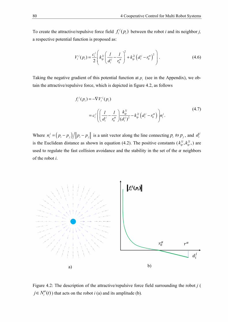
80 4 Cooperative Control for Multi Robot Systems
To create the attractive/repulsive force field ( )ij
if p between the robot i and its neighbor j,
a respective potential function is proposed as:
( )00
22
( )2
jj 1j 2j ji
i ipi ip iji
ck k d r
dV
r
1 1p α
α
= − + −
. (4.6)
Taking the negative gradient of this potential function at ip (see in the Appendix), we ob-
tain the attractive/repulsive force, which is depicted in figure 4.2, as follows
( )02
0
( ) ( )
.( )
j ji i
1jipj 2j j j
i ip i ij ji i
i if p V p
1 kc k d r n
d r
1
dα
α
=
− − −
−∇
= (4.7)
Where ( )ji i j i jn p p p p= − − is a unit vector along the line connecting i jp to p , and j
id
is the Euclidean distance as shown in equation (4.2). The positive constants ( , ,1j 2jip ipk k ) are
used to regulate the fast collision avoidance and the stability in the set of the neighbors
of the robot i.
Figure 4.2: The description of the attractive/repulsive force field surrounding the robot j (( )ij N tα∈ ) that acts on the robot i (a) and its amplitude (b).
4
b) a)
4.3 Connection between neighboring robots 81
The interacting ranges ( 0 , 0,r rα α > shown in figure 4.1) describe the influence of the
force ( )ij
if p on the robot i. When 0 ,0 jid rα< < then robots i and j repel each other to avoid
the collision between them. Otherwise, when 0 ,jir d rα α< ≤ they attract each other to
achieve the equilibrium position 0( )jid rα= in the set of neighbors of robot i. In case
jid rα> there is no interaction between these members. As depicted in figure 4.2, the ef-
fect of the attractive/repulsive force ( )ij
if p of the robot j ( ( )ij N tα∈ ) on the robot i is de-
pending on the relative position between robot j and robot i. Under the effect of this attrac-
tive/repulsive force, the neighboring robots will quickly approach the equilibrium position
0( )jid rα= , at which the force ( )i
jif p is equal to zero.
Theorem 4.1. Consider the robot i is described by the model (4.1), and controlled by the
control law (4.4). If the robot ( )ij N tα∈ , then robot i will approach to the equilibrium posi-
tion, at which i jv v= and 0i jp p rα− = .
Proof of theorem 4.1
Consider a point ijp lies on the line connecting ip to jp , and satisfies 0ij jp p rα− = ,
see figure 4.3. The position of this point ijp is calculated as follows:
0( ) ( ) /ij j i j i jp p r p p p pα− = − − . (4.8)
This equation can be rewritten as
(1 )j jij i i i jp p pλ λ= + − . (4.9)
Where 0 /ji i jr p pαλ = − . Now, in order to analyze the stability of the robot i at the equi-
librium position, at which i jv v= and 0i jp p rα− = , we let 1 (1 )( )ji ij i i jx p p p pλ= − = − −
and 2 i jx v v= − . The error dynamic of the system is described as follows:
1 2
2
(1 )
.
ji
i j
x x
x v v
λ= −
= −
(4.10)
Substitute (4.4) into (4.10) we obtain:
1 2
2 2
(1 )
.( )
ji
j ji ivi
x x
x V xp k
λ= −
= − −∇
(4.11)
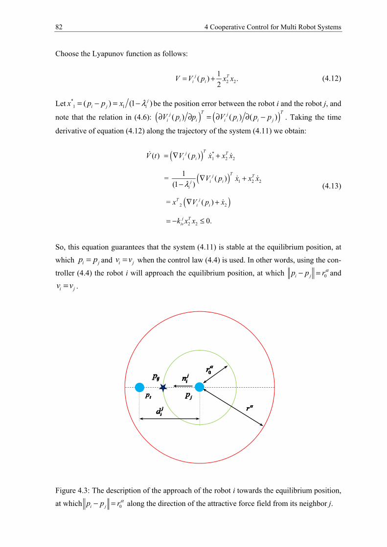
82 4 Cooperative Control for Multi Robot Systems
Choose the Lyapunov function as follows:
2 21( ) . 2
Ti
jiV V p x x= + (4.12)
Let *1 1( ) (1 )j
i j ix p p x λ= −− = be the position error between the robot i and the robot j, and
note that the relation in (4.6): ( ) ( )( ) ( ) ( )j ji i
T T
i i i i jV p p V p p p∂ ∂ = ∂ ∂ − . Taking the time
derivative of equation (4.12) along the trajectory of the system (4.11) we obtain:
( )
( )
( )
*1
1
2
2
2
2 2
2 2
2
( ) ( )
( )
= ( )
1= (1 )
0.
ji
jij
i
ji
j
T Ti
T T
Ti
i
i
Tv
V t V p x x
V p x x
x
x
V p x
x
x
k x
λ
= ∇
∇
∇ +
=
+
+−
− ≤
(4.13)
So, this equation guarantees that the system (4.11) is stable at the equilibrium position, at
which i jp p= and i jv v= when the control law (4.4) is used. In other words, using the con-
troller (4.4) the robot i will approach the equilibrium position, at which 0i jp p rα− = and
i jv v= .
Figure 4.3: The description of the approach of the robot i towards the equilibrium position,
at which 0i jp p rα− = along the direction of the attractive force field from its neighbor j.
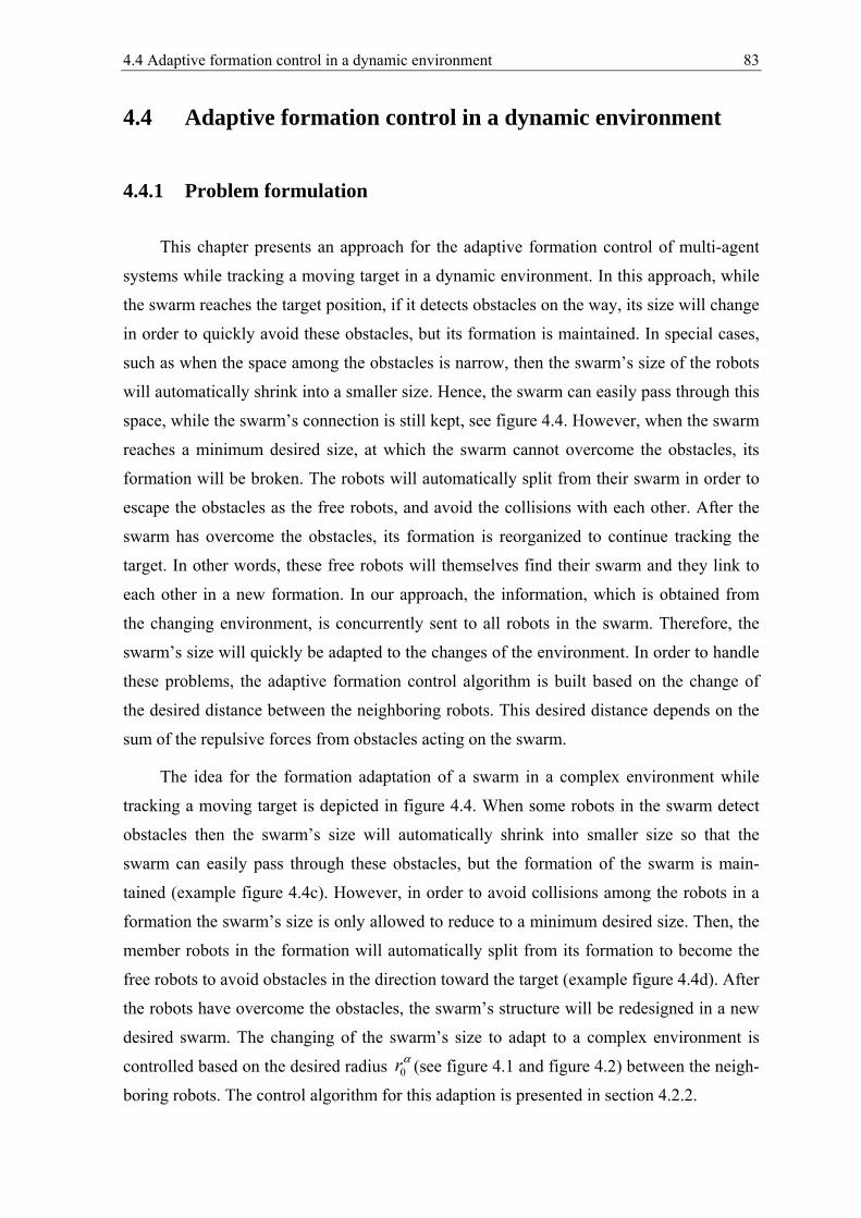
4.4 Adaptive formation control in a dynamic environment 83
4.4 Adaptive formation control in a dynamic environment
4.4.1 Problem formulation
This chapter presents an approach for the adaptive formation control of multi-agent
systems while tracking a moving target in a dynamic environment. In this approach, while
the swarm reaches the target position, if it detects obstacles on the way, its size will change
in order to quickly avoid these obstacles, but its formation is maintained. In special cases,
such as when the space among the obstacles is narrow, then the swarm’s size of the robots
will automatically shrink into a smaller size. Hence, the swarm can easily pass through this
space, while the swarm’s connection is still kept, see figure 4.4. However, when the swarm
reaches a minimum desired size, at which the swarm cannot overcome the obstacles, its
formation will be broken. The robots will automatically split from their swarm in order to
escape the obstacles as the free robots, and avoid the collisions with each other. After the
swarm has overcome the obstacles, its formation is reorganized to continue tracking the
target. In other words, these free robots will themselves find their swarm and they link to
each other in a new formation. In our approach, the information, which is obtained from
the changing environment, is concurrently sent to all robots in the swarm. Therefore, the
swarm’s size will quickly be adapted to the changes of the environment. In order to handle
these problems, the adaptive formation control algorithm is built based on the change of
the desired distance between the neighboring robots. This desired distance depends on the
sum of the repulsive forces from obstacles acting on the swarm.
The idea for the formation adaptation of a swarm in a complex environment while
tracking a moving target is depicted in figure 4.4. When some robots in the swarm detect
obstacles then the swarm’s size will automatically shrink into smaller size so that the
swarm can easily pass through these obstacles, but the formation of the swarm is main-
tained (example figure 4.4c). However, in order to avoid collisions among the robots in a
formation the swarm’s size is only allowed to reduce to a minimum desired size. Then, the
member robots in the formation will automatically split from its formation to become the
free robots to avoid obstacles in the direction toward the target (example figure 4.4d). After
the robots have overcome the obstacles, the swarm’s structure will be redesigned in a new
desired swarm. The changing of the swarm’s size to adapt to a complex environment is
controlled based on the desired radius 0rα (see figure 4.1 and figure 4.2) between the neigh-
boring robots. The control algorithm for this adaption is presented in section 4.2.2.
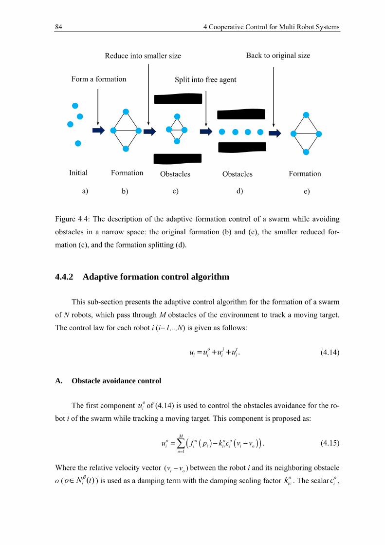
84 4 Cooperative Control for Multi Robot Systems
Figure 4.4: The description of the adaptive formation control of a swarm while avoiding
obstacles in a narrow space: the original formation (b) and (e), the smaller reduced for-
mation (c), and the formation splitting (d).
4.4.2 Adaptive formation control algorithm
This sub-section presents the adaptive control algorithm for the formation of a swarm
of N robots, which pass through M obstacles of the environment to track a moving target.
The control law for each robot i (i=1,..,N) is given as follows:
.i ito j
i iuu u u++= (4.14)
A. Obstacle avoidance control
The first component oiu of (4.14) is used to control the obstacles avoidance for the ro-
bot i of the swarm while tracking a moving target. This component is proposed as:
( ) ( )( )1
Mo o o
i i i iv io
i oo
k c v vu f p=
= − − . (4.15)
Where the relative velocity vector ( )i ov v− between the robot i and its neighboring obstacle
o ( ( )io N tβ∈ ) is used as a damping term with the damping scaling factor oivk . The scalar o
ic ,
Obstacles Formation Formation Initial
Form a formation
Reduce into smaller size
Split into free agent
Obstacles
Back to original size
a) b) c) d) e)
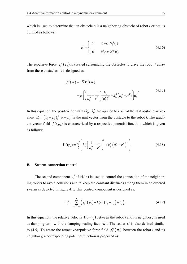
4.4 Adaptive formation control in a dynamic environment 85
which is used to determine that an obstacle o is a neighboring obstacle of robot i or not, is
defined as follows:
1 if
0 if
( )
(t).
ioi
i
o Nc
o N
tβ
β
∈= ∉
(4.16)
The repulsive force ( )oi if p is created surrounding the obstacles to drive the robot i away
from these obstacles. It is designed as:
( )2
1
( )
n
( )
1)(
o oi i
oo o oi i io o
i
i i
ipip
i
f
kc
p V
kr
p
d rd d
δ ββ
=
= − − −
−∇
. (4.17)
In this equation, the positive constants , poi ipk kδ are applied to control the fast obstacle avoid-
ance. ( )oi i o i on p p p p= − − is the unit vector from the obstacle to the robot i. The gradi-
ent vector field ( )io
if p is characterized by a respective potential function, which is given
as follows:
( )2
21 1(p )2
oo o oi
i ioi ip ipi
ck k d r
d rV δ β
β
= − + −
. (4.18)
B. Swarm-connection control
The second component jiu of (4.14) is used to control the connection of the neighbor-
ing robots to avoid collisions and to keep the constant distances among them in an ordered
swarm as depicted in figure 4.1. This control component is designed as:
( ) ( )( )N
j j j ji i iv i
j=1, j ii i j jk c vp vu vf
≠
= − − + . (4.19)
In this equation, the relative velocity ( )i jv v− between the robot i and its neighbor j is used
as damping term with the damping scaling factor jivk . The scalar j
ic is also defined similar
to (4.5). To create the attractive/repulsive force field ( )ijif p between the robot i and its
neighbor j, a corresponding potential function is proposed as:
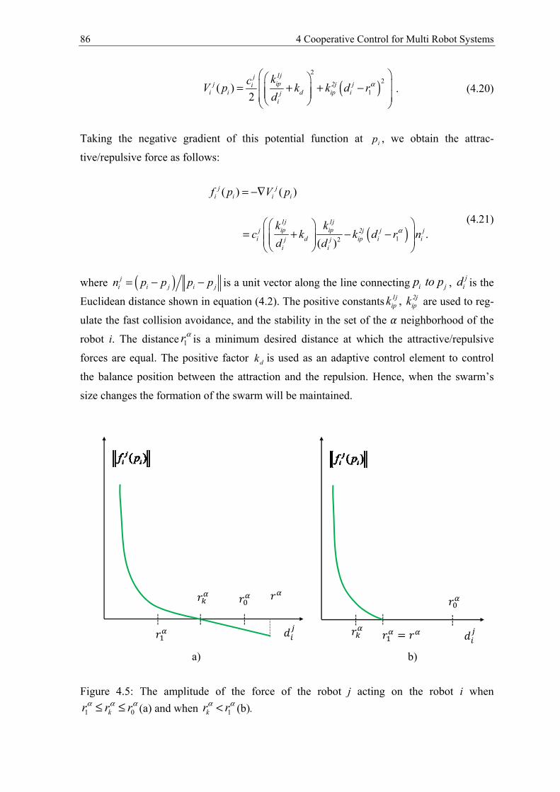
86 4 Cooperative Control for Multi Robot Systems
( )2
2
12( )
1jjipj 2j ji
i d ip iji
i
kckV r
dp k d α
= + + −
. (4.20)
Taking the negative gradient of this potential function at ip , we obtain the attrac-
tive/repulsive force as follows:
( )12
( ) ( )
.( )
j ji i
1j 1jip ipj 2j j j
i d ip i ij ji i
i i
k kc k k d r
f p
n
p
d d
V
α
=
= + − −
−∇
(4.21)
where ( )ji i j i jn p p p p= − − is a unit vector along the line connecting i jp to p , j
id is the
Euclidean distance shown in equation (4.2). The positive constants , 1j 2jip ipk k are used to reg-
ulate the fast collision avoidance, and the stability in the set of the neighborhood of the
robot i. The distance 1rα is a minimum desired distance at which the attractive/repulsive
forces are equal. The positive factor dk is used as an adaptive control element to control
the balance position between the attraction and the repulsion. Hence, when the swarm’s
size changes the formation of the swarm will be maintained.
Figure 4.5: The amplitude of the force of the robot j acting on the robot i when
1 0kr r rα α α≤ ≤ (a) and when 1kr rα α< (b).
4
=
b)
4
a)
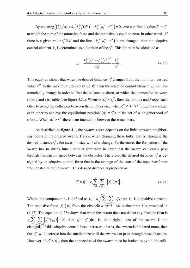
4.4 Adaptive formation control in a dynamic environment 87
By equating ( ) ( )( )12( 0)1j j 1j j 2j j
ip i d ip i ip ik d k k d k d rα+ − − = , one can find a value ji kd rα=
at which the sum of the attractive force and the repulsive is equal to zero. In other words, if
there is a given value 1kr rα α≥ and the line ( )12j jip ik d rα− − is not changed, then the adaptive
control element dk is determined as a function of the krα . This function is calculated as
( )( )2
12j 1jip k k ip
d 1jip k
k r r r kk
k r
α α α
α
−= − . (4.22)
This equation shows that when the desired distance krα changes from the minimum desired
value 1rα to the maximum desired value 0r
α then the adaptive control element dk will au-
tomatically change in order to find the balance position, at which the connection between
robot j and i is stable (see figure 4.5a). When 0 jkid rα< < , then the robots i and j repel each
other to avoid the collisions between them. Otherwise, when jikr d rα α< ≤ , then they attract
each other to achieve the equilibrium position ( )kj
id rα= in the set of neighborhood of
robot i. When jid rα> there is no interaction between these members.
As described in figure 4.1, the swarm’s size depends on the links between neighbor-
ing robots in the ordered swarm. Hence, when changing these links, that is, changing the
desired distance krα , the swarm’s size will also change. Furthermore, the formation of the
swarm has to shrink into a smaller formation in order that the swarm can easily pass
through the narrow space between the obstacles. Therefore, the desired distance krα is de-
signed by an adaptive control force that is the average of the sum of the repulsive forces
from obstacles to the swarm. This desired distance is proposed as:
( )01 ( )i
No
k o i ii o N t
r r pc fβ
α α
= ∈
= − . (4.23)
Where, the component co is defined as 1 ( )
,i
No
o c ii o N t
c k cβ= ∈
= here ck is a positive constant.
The repulsive force ( )oi if p from the obstacle o (o=1…M) to the robot i is presented in
(4.17). The equation (4.23) shows that when the swarm does not detect any obstacle (that is
( )1 ( )
0i
No
o i ii o N t
c f pβ= ∈
= ) then 0kr rα α= (that is, the original size of the swarm is not
changed). If this adaptive control force increases, that is, the swarm is hindered more, then
the krα will decrease into the smaller size until the swarm can pass through these obstacles.
However, if 0kr rα α< , then the connection of the swarm must be broken to avoid the colli-
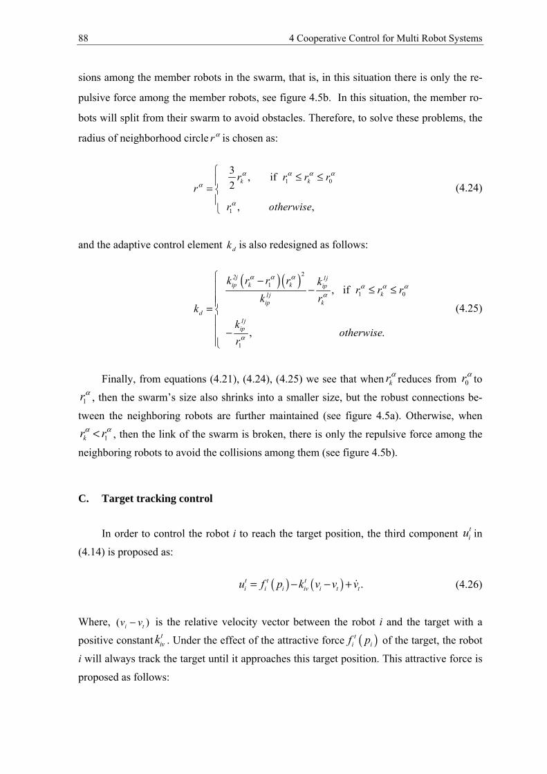
88 4 Cooperative Control for Multi Robot Systems
sions among the member robots in the swarm, that is, in this situation there is only the re-
pulsive force among the member robots, see figure 4.5b. In this situation, the member ro-
bots will split from their swarm to avoid obstacles. Therefore, to solve these problems, the
radius of neighborhood circle rα is chosen as:
1 0
1
3 , if 2
, ,
k kr r r rr
r otherwise
α α α α
α
α
≤ ≤=
(4.24)
and the adaptive control element dk is also redesigned as follows:
( )( )211 0
1
, if
, .
2j 1jip k k ip
k1jip k
d1jip
k r r r kr r r
k rk
kotherwise
r
α α αα α α
α
α
− − ≤ ≤= −
(4.25)
Finally, from equations (4.21), (4.24), (4.25) we see that when krα reduces from 0r
α to
1rα , then the swarm’s size also shrinks into a smaller size, but the robust connections be-
tween the neighboring robots are further maintained (see figure 4.5a). Otherwise, when
1kr rα α< , then the link of the swarm is broken, there is only the repulsive force among the
neighboring robots to avoid the collisions among them (see figure 4.5b).
C. Target tracking control
In order to control the robot i to reach the target position, the third component tiu in
(4.14) is proposed as:
( ) ( ) .i i i iv it t
tt
tf k vp v vu = −− + (4.26)
Where, ( )i tv v− is the relative velocity vector between the robot i and the target with a
positive constant tivk . Under the effect of the attractive force ( )i i
tf p of the target, the robot
i will always track the target until it approaches this target position. This attractive force is
proposed as follows:
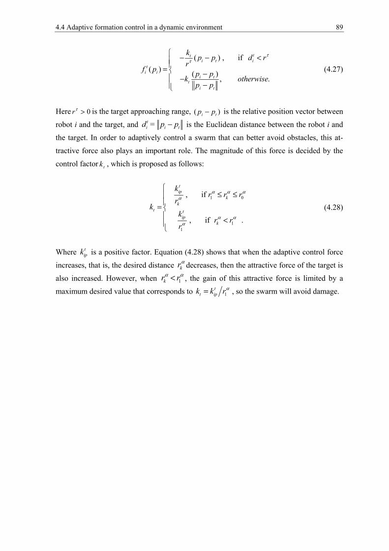
4.4 Adaptive formation control in a dynamic environment 89
( ) , if
( ) ( ) , .
ti t
ti
i t
i t
ti
i
t
kp p d r
rf p
p pk otherwise
p p
ττ
− − <= − −−
(4.27)
Here 0rτ > is the target approaching range, ( )i tp p− is the relative position vector between
robot i and the target, and ti i td = p p− is the Euclidean distance between the robot i and
the target. In order to adaptively control a swarm that can better avoid obstacles, this at-
tractive force also plays an important role. The magnitude of this force is decided by the
control factor tk , which is proposed as follows:
1 0
11
, if
, if .
ip
i
t
kk
t t
kp
kr r r
rk
kr r
r
α α αα
α αα
≤ ≤
= <
(4.28)
Where tipk is a positive factor. Equation (4.28) shows that when the adaptive control force
increases, that is, the desired distance krα decreases, then the attractive force of the target is
also increased. However, when 1kr rα α< , the gain of this attractive force is limited by a
maximum desired value that corresponds to 1ipt
tk k rα= , so the swarm will avoid damage.
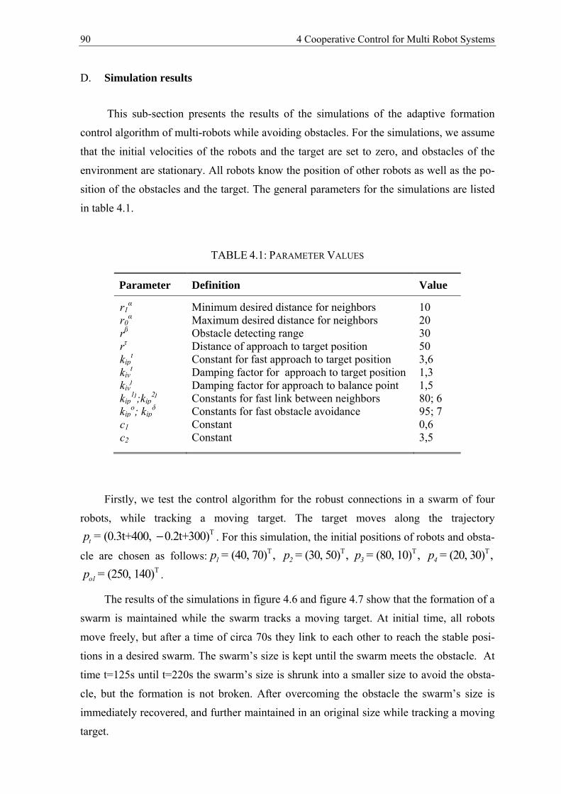
90 4 Cooperative Control for Multi Robot Systems
D. Simulation results
This sub-section presents the results of the simulations of the adaptive formation
control algorithm of multi-robots while avoiding obstacles. For the simulations, we assume
that the initial velocities of the robots and the target are set to zero, and obstacles of the
environment are stationary. All robots know the position of other robots as well as the po-
sition of the obstacles and the target. The general parameters for the simulations are listed
in table 4.1.
TABLE 4.1: PARAMETER VALUES
Parameter
Definition
Value
r1α
Minimum desired distance for neighbors
10 r0α Maximum desired distance for neighbors 20
rβ Obstacle detecting range 30 rτ Distance of approach to target position 50 kip
t Constant for fast approach to target position 3,6 kiv
t Damping factor for approach to target position 1,3 kiv
j Damping factor for approach to balance point 1,5 kip
1j;kip2j Constants for fast link between neighbors 80; 6
kipo; kip
δ Constants for fast obstacle avoidance 95; 7 c1 Constant 0,6 c2 Constant 3,5
Firstly, we test the control algorithm for the robust connections in a swarm of four
robots, while tracking a moving target. The target moves along the trajectoryT(0.3t+400, 0.2t+300)tp = − . For this simulation, the initial positions of robots and obsta-
cle are chosen as follows: T(40, 70) , 1p = T(30, 50) ,2p = T(80, 10) , 3p = T(20, 30) ,4p =T(250, 140)o1p = .
The results of the simulations in figure 4.6 and figure 4.7 show that the formation of a
swarm is maintained while the swarm tracks a moving target. At initial time, all robots
move freely, but after a time of circa 70s they link to each other to reach the stable posi-
tions in a desired swarm. The swarm’s size is kept until the swarm meets the obstacle. At
time t=125s until t=220s the swarm’s size is shrunk into a smaller size to avoid the obsta-
cle, but the formation is not broken. After overcoming the obstacle the swarm’s size is
immediately recovered, and further maintained in an original size while tracking a moving
target.
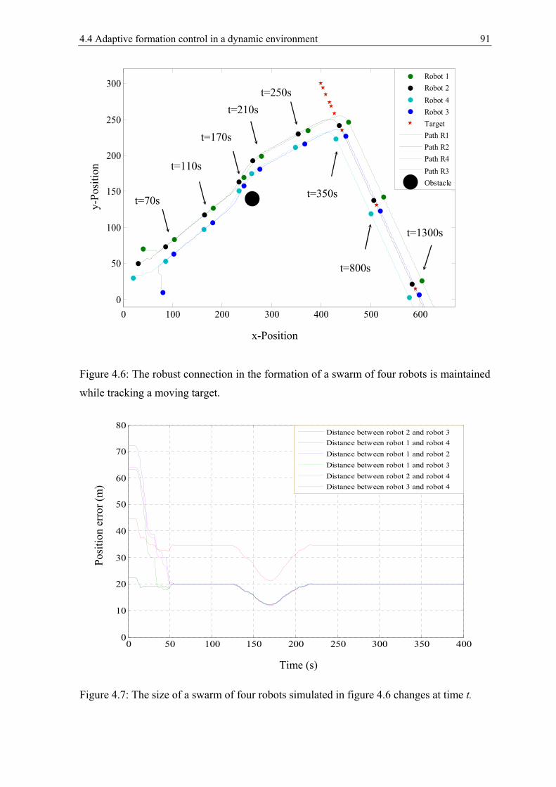
4.4 Adaptive formation control in a dynamic environment 91
Figure 4.6: The robust connection in the formation of a swarm of four robots is maintained
while tracking a moving target.
Figure 4.7: The size of a swarm of four robots simulated in figure 4.6 changes at time t.
0 50 100 150 200 250 300 350 4000
10
20
30
40
50
60
70
80
Distance between robot 2 and robot 3Distance between robot 1 and robot 4Distance between robot 1 and robot 2Distance between robot 1 and robot 3Distance between robot 2 and robot 4Distance between robot 3 and robot 4
Time (s)
Posi
tion
erro
r (m
)
0 100 200 300 400 500 6000
50
100
150
200
250
300
Robot 1Robot 2Robot 4Robot 3TargetPath R1Path R2Path R4Path R3Obstacle
x-Position
y-Po
sitio
n
t=1300s
t=800s
t=350s
t=250s t=210s
t=170s
t=110s
t=70s
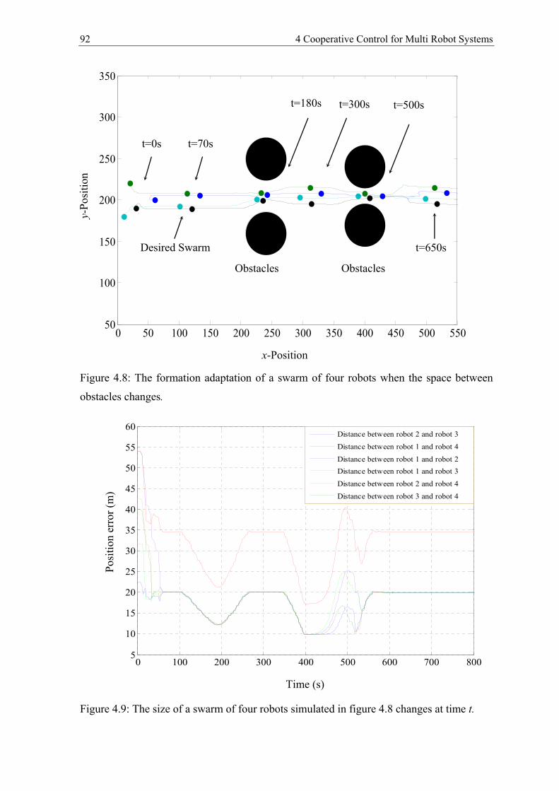
92 4 Cooperative Control for Multi Robot Systems
Figure 4.8: The formation adaptation of a swarm of four robots when the space between
obstacles changes.
Figure 4.9: The size of a swarm of four robots simulated in figure 4.8 changes at time t.
0 50 100 150 200 250 300 350 400 450 500 55050
100
150
200
250
300
350
t=0s t=70s
t=180s t=300s
t=650s
t=500s
x-Position
y-Po
sitio
n
Obstacles Obstacles
Desired Swarm
0 100 200 300 400 500 600 700 8005
10
15
20
25
30
35
40
45
50
55
60
Distance between robot 2 and robot 3Distance between robot 1 and robot 4Distance between robot 1 and robot 2Distance between robot 1 and robot 3Distance between robot 2 and robot 4Distance between robot 3 and robot 4
Time (s)
Posi
tion
erro
r (m
)
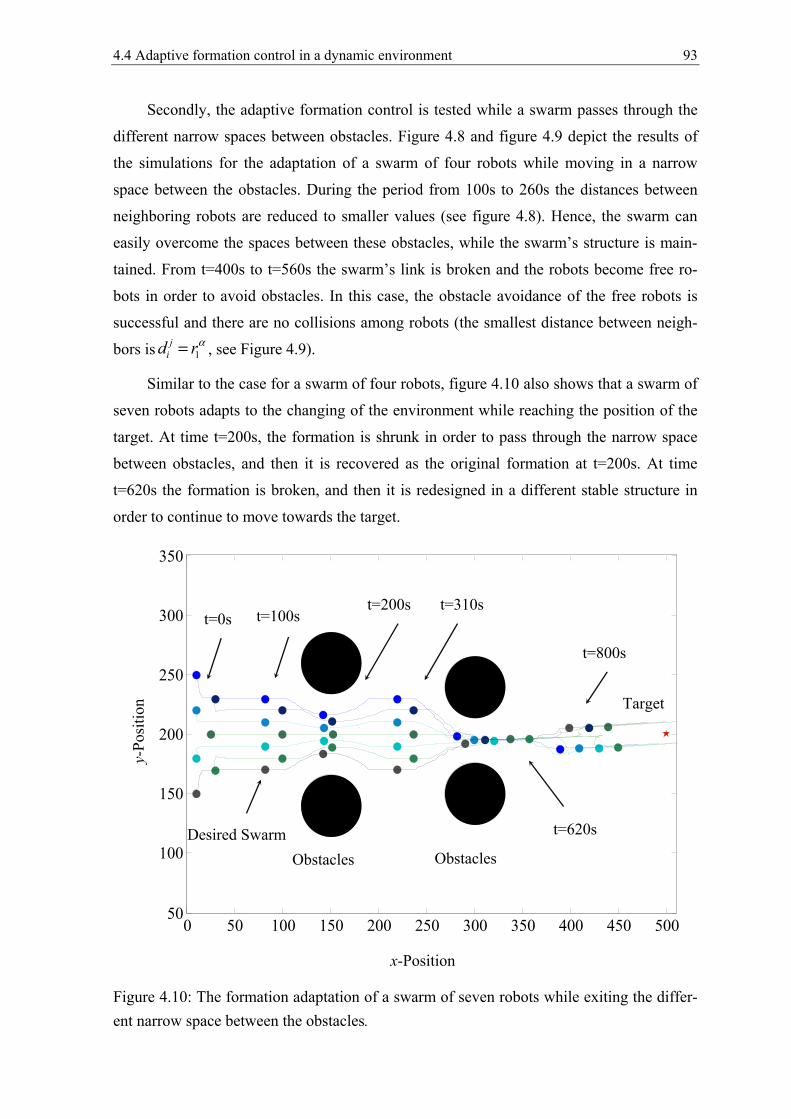
4.4 Adaptive formation control in a dynamic environment 93
Secondly, the adaptive formation control is tested while a swarm passes through the
different narrow spaces between obstacles. Figure 4.8 and figure 4.9 depict the results of
the simulations for the adaptation of a swarm of four robots while moving in a narrow
space between the obstacles. During the period from 100s to 260s the distances between
neighboring robots are reduced to smaller values (see figure 4.8). Hence, the swarm can
easily overcome the spaces between these obstacles, while the swarm’s structure is main-
tained. From t=400s to t=560s the swarm’s link is broken and the robots become free ro-
bots in order to avoid obstacles. In this case, the obstacle avoidance of the free robots is
successful and there are no collisions among robots (the smallest distance between neigh-
bors is 1j
id rα= , see Figure 4.9).
Similar to the case for a swarm of four robots, figure 4.10 also shows that a swarm of
seven robots adapts to the changing of the environment while reaching the position of the
target. At time t=200s, the formation is shrunk in order to pass through the narrow space
between obstacles, and then it is recovered as the original formation at t=200s. At time
t=620s the formation is broken, and then it is redesigned in a different stable structure in
order to continue to move towards the target.
Figure 4.10: The formation adaptation of a swarm of seven robots while exiting the differ-ent narrow space between the obstacles.
0 50 100 150 200 250 300 350 400 450 50050
100
150
200
250
300
350
t=0s
Obstacles Obstacles Desired Swarm
t=200s t=310s
t=620s
t=800s
x-Position
y-Po
sitio
n
t=100s
Target
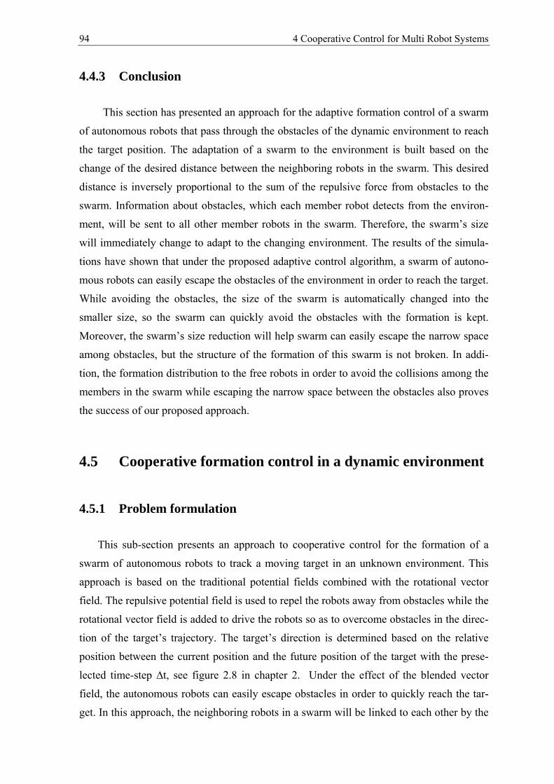
94 4 Cooperative Control for Multi Robot Systems
4.4.3 Conclusion
This section has presented an approach for the adaptive formation control of a swarm
of autonomous robots that pass through the obstacles of the dynamic environment to reach
the target position. The adaptation of a swarm to the environment is built based on the
change of the desired distance between the neighboring robots in the swarm. This desired
distance is inversely proportional to the sum of the repulsive force from obstacles to the
swarm. Information about obstacles, which each member robot detects from the environ-
ment, will be sent to all other member robots in the swarm. Therefore, the swarm’s size
will immediately change to adapt to the changing environment. The results of the simula-
tions have shown that under the proposed adaptive control algorithm, a swarm of autono-
mous robots can easily escape the obstacles of the environment in order to reach the target.
While avoiding the obstacles, the size of the swarm is automatically changed into the
smaller size, so the swarm can quickly avoid the obstacles with the formation is kept.
Moreover, the swarm’s size reduction will help swarm can easily escape the narrow space
among obstacles, but the structure of the formation of this swarm is not broken. In addi-
tion, the formation distribution to the free robots in order to avoid the collisions among the
members in the swarm while escaping the narrow space between the obstacles also proves
the success of our proposed approach.
4.5 Cooperative formation control in a dynamic environment
4.5.1 Problem formulation
This sub-section presents an approach to cooperative control for the formation of a
swarm of autonomous robots to track a moving target in an unknown environment. This
approach is based on the traditional potential fields combined with the rotational vector
field. The repulsive potential field is used to repel the robots away from obstacles while the
rotational vector field is added to drive the robots so as to overcome obstacles in the direc-
tion of the target’s trajectory. The target’s direction is determined based on the relative
position between the current position and the future position of the target with the prese-
lected time-step ∆t, see figure 2.8 in chapter 2. Under the effect of the blended vector
field, the autonomous robots can easily escape obstacles in order to quickly reach the tar-
get. In this approach, the neighboring robots in a swarm will be linked to each other by the
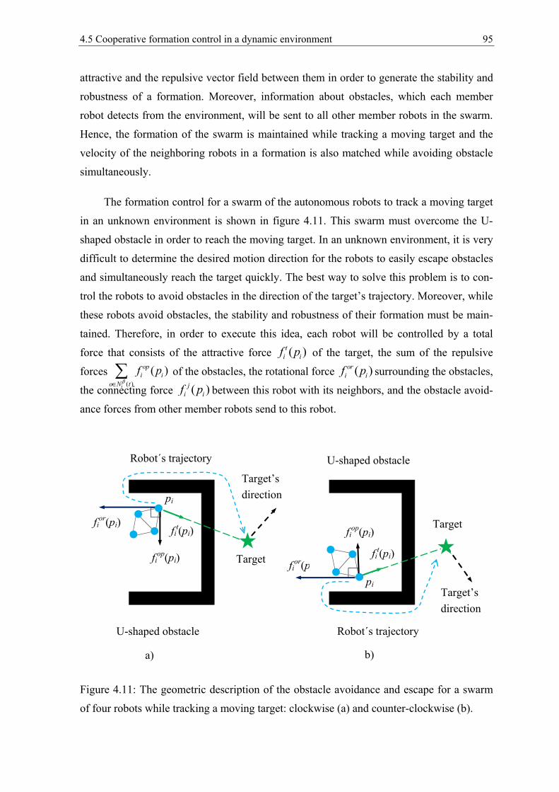
4.5 Cooperative formation control in a dynamic environment 95
attractive and the repulsive vector field between them in order to generate the stability and
robustness of a formation. Moreover, information about obstacles, which each member
robot detects from the environment, will be sent to all other member robots in the swarm.
Hence, the formation of the swarm is maintained while tracking a moving target and the
velocity of the neighboring robots in a formation is also matched while avoiding obstacle
simultaneously.
The formation control for a swarm of the autonomous robots to track a moving target
in an unknown environment is shown in figure 4.11. This swarm must overcome the U-
shaped obstacle in order to reach the moving target. In an unknown environment, it is very
difficult to determine the desired motion direction for the robots to easily escape obstacles
and simultaneously reach the target quickly. The best way to solve this problem is to con-
trol the robots to avoid obstacles in the direction of the target’s trajectory. Moreover, while
these robots avoid obstacles, the stability and robustness of their formation must be main-
tained. Therefore, in order to execute this idea, each robot will be controlled by a total
force that consists of the attractive force ( )iitf p of the target, the sum of the repulsive
forces( )
( )i
io t
oi
N
pf pβ∈ of the obstacles, the rotational force ( )i
orif p surrounding the obstacles,
the connecting force ( )ij
if p between this robot with its neighbors, and the obstacle avoid-
ance forces from other member robots send to this robot.
Figure 4.11: The geometric description of the obstacle avoidance and escape for a swarm
of four robots while tracking a moving target: clockwise (a) and counter-clockwise (b).
Robot´s trajectory
fit(pi)
Target fiop(pi)
fior(pi)
pi
Target
Target’s direction
Target’s direction
fiop(pi)
fior(pi)
pi
U-shaped obstacle
a)
Robot´s trajectory
fit(pi)
U-shaped obstacle
b)
96 4 Cooperative Control for Multi Robot Systems
4.5.2 Formation control algorithm
This section presents the formation control algorithm for a swarm of N robots, which
passes through M obstacles to track a moving target. As stated above, the final aim of the
member robots in a swarm is to escape obstacles of the environment to reach the target
while staying together. Accordingly, the control algorithm for each member robot i of a
swarm is also given as follows:
.i itj o
i iuu u u++= (4.29)
In this control law, the first component jiu is used to control the robust connection
between the neighboring robots in the formation. As shown in section 4.4, this connection
is controlled based on the combination of the attractive vector field and the repulsive vec-
tor field among the neighboring robots. Furthermore, in order to obtain the quick stability
at the balance point, at which the distance among the neighboring robots is constant, the
relative velocity vector (vi – vj) between them is added as a damping term with the scaling
factor jivk .
The second component oiu of (4.29) is used to control the obstacle avoidance for each
member robot of the swarm. As presented above, the final aim of this sub-section is to con-
trol the formation of a swarm to quickly escape the obstacles, but this formation is always
maintained while avoiding these obstacles. In order to solve this problem, information
about obstacles, which each member robot detects from the environment, will be sent to all
other member robots in the swarm. Therefore, the obstacle avoidance control law is pro-
jected for each robot i as follows:
( )1 ( )
( ) ( ) ( )k
Nop or o o
i k k kv ko
k k k ok o N t
p f p k c v vu fβ= ∈
= + − − . (4.30)
Where the relative velocity vector (vk – vo) between the robot k (k=1,2,..N) and its neigh-
bor-obstacle ( )ko N tβ∈ is used as a damping term with the damping scaling factor kkvo. The
local repulsive force surrounding the obstacle ( )kkopf p is used to drive the robot away
from this obstacle. The local rotational force surrounding the obstacle ( )kkorf p is used to
drive the robot to escape this obstacle in the direction of the target’s trajectory. As present-
ed in section 2.3, the combination of these forces will help that the robot can easily and
quickly exit the obstacles to continue tracking a moving target.
4.5 Cooperative formation control in a dynamic environment 97
The third component tiu of (4.29) is used to control the robot to reach the target posi-
tion as represented in section 4.4. However, in order to control the formation cooperation
of a swarm while avoiding obstacles better, the attractive force surrounding the target must
have the smaller magnitude. Hence, this attractive force is proposed as follows:
( ) , if ( ) ( ) , other i .w se
tti t
ti
i tt
i t
i
i
kp p d r
rf p
p pk
p p
ξτ
τ
ξ
− − <= − −
−
(4.31)
Where, the scaling factor tkξ is designed, such that:
1
2
( ) (empty set if
otherw
)
ise.
t
t
t
i tk Nk
k
βξ
ξ
ξ
=
= ∅
(4.32)
Here, the selected positive constants 1 tkξ and 2 tkξ satisfy that: 1 2 . t tk kξ ξ>
Finally, the control law for each member robot i of a swarm is summarized as follows
( ) ( )( )
( )
( ) ( )
( )
1 ( )
( ) ( ) ( )
i
k
i i i j j
k
j j ji iv i
j N t
Nop o
k k o
i
r o ok k kv k
k o
i iv i
N
tt t
t
t
k c v v v
p f p k c v v
f k v
p
v v
u f
f
p
α
β
∈
= ∈
= − − +
+ − −
+ − +
+
−
(4.33)
4.5.3 Simulation results
This sub-section presents the simulation results of the cooperative formation control
of the autonomous robots to track a moving target in a dynamic environment. The general
parameters for the simulations are listed in table 4.1.
Case 1: The keeping of the formation of a swarm of four robots while avoiding the
U-shaped obstacle to track a moving target is tested. For these simulations, the initial posi-
tions of the robots are chosen as follows: T T2(20, 180) , p =(30, 230) , 1p =
T(40, 170) , 3p = T(10, 210) .4p =
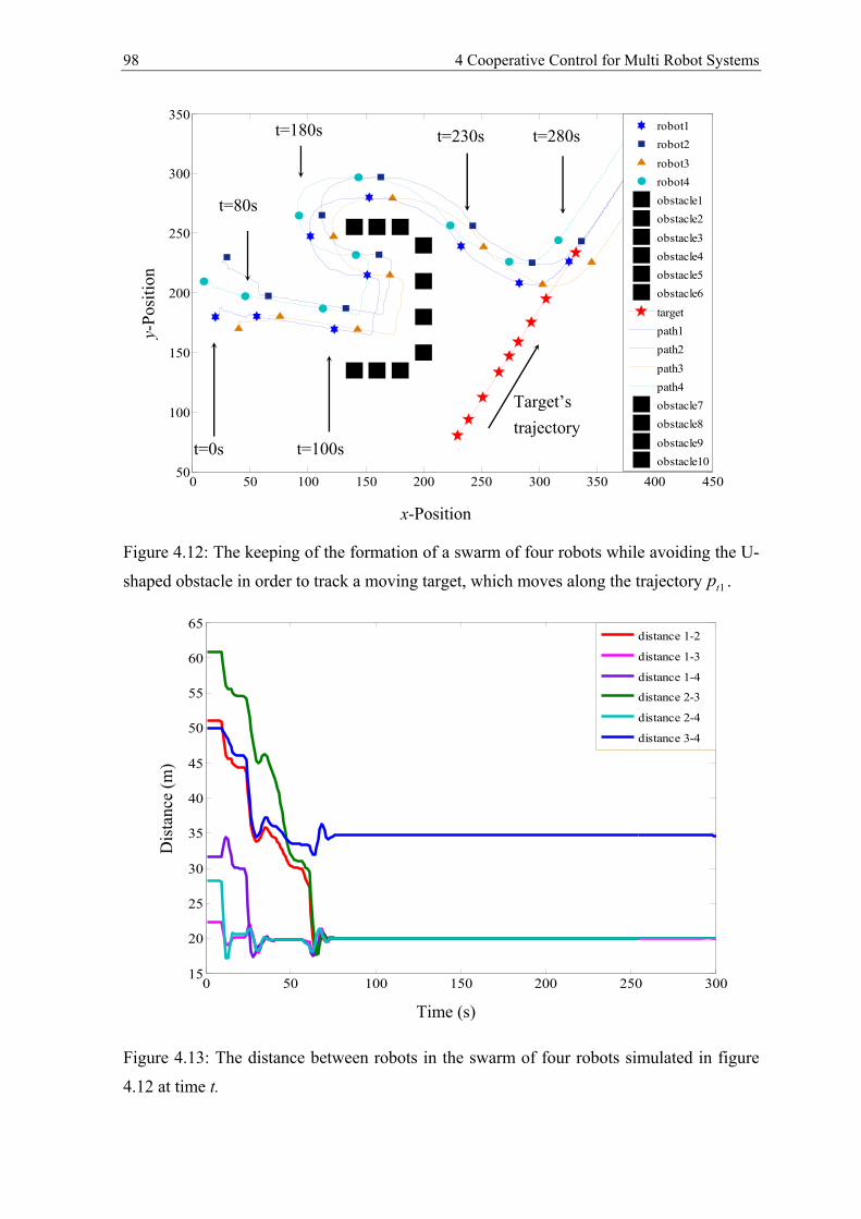
98 4 Cooperative Control for Multi Robot Systems
Figure 4.12: The keeping of the formation of a swarm of four robots while avoiding the U-
shaped obstacle in order to track a moving target, which moves along the trajectory 1tp .
Figure 4.13: The distance between robots in the swarm of four robots simulated in figure
4.12 at time t.
0 50 100 150 200 250 300 350 400 45050
100
150
200
250
300
350
robot1robot2robot3robot4obstacle1obstacle2obstacle3obstacle4obstacle5obstacle6targetpath1path2path3path4obstacle7obstacle8obstacle9obstacle10
x-Position
y-Po
sitio
n
t=0s
t=80s
t=100s
t=180s t=230s t=280s
Target’s trajectory
0 50 100 150 200 250 30015
20
25
30
35
40
45
50
55
60
65
distance 1-2
distance 1-3
distance 1-4
distance 2-3
distance 2-4
distance 3-4
Time (s)
Dis
tanc
e (m
)
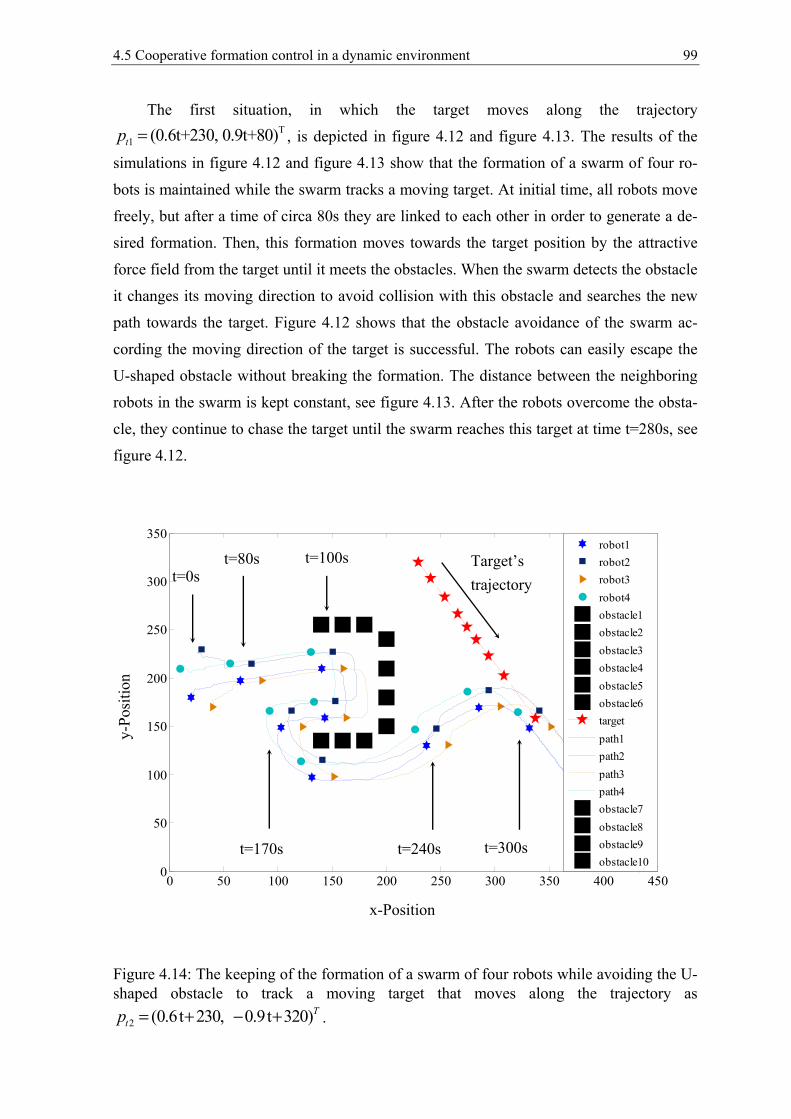
4.5 Cooperative formation control in a dynamic environment 99
The first situation, in which the target moves along the trajectoryT
1 (0.6t+230, 0.9t+80)tp = , is depicted in figure 4.12 and figure 4.13. The results of the
simulations in figure 4.12 and figure 4.13 show that the formation of a swarm of four ro-
bots is maintained while the swarm tracks a moving target. At initial time, all robots move
freely, but after a time of circa 80s they are linked to each other in order to generate a de-
sired formation. Then, this formation moves towards the target position by the attractive
force field from the target until it meets the obstacles. When the swarm detects the obstacle
it changes its moving direction to avoid collision with this obstacle and searches the new
path towards the target. Figure 4.12 shows that the obstacle avoidance of the swarm ac-
cording the moving direction of the target is successful. The robots can easily escape the
U-shaped obstacle without breaking the formation. The distance between the neighboring
robots in the swarm is kept constant, see figure 4.13. After the robots overcome the obsta-
cle, they continue to chase the target until the swarm reaches this target at time t=280s, see
figure 4.12.
Figure 4.14: The keeping of the formation of a swarm of four robots while avoiding the U-shaped obstacle to track a moving target that moves along the trajectory as
2 (0.6t 230, 0.9t 320)Ttp = + − + .
0 50 100 150 200 250 300 350 400 4500
50
100
150
200
250
300
350
robot1robot2robot3robot4obstacle1obstacle2obstacle3obstacle4obstacle5obstacle6targetpath1path2path3path4obstacle7obstacle8obstacle9obstacle10
Target’s trajectory t=0s
t=80s t=100s
t=170s t=240s t=300s
x-Position
y-Po
sitio
n
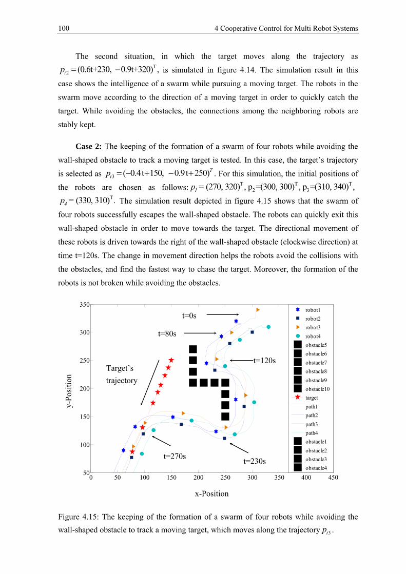
100 4 Cooperative Control for Multi Robot Systems
The second situation, in which the target moves along the trajectory asT
2 (0.6t+230, 0.9t+320) , tp = − is simulated in figure 4.14. The simulation result in this
case shows the intelligence of a swarm while pursuing a moving target. The robots in the
swarm move according to the direction of a moving target in order to quickly catch the
target. While avoiding the obstacles, the connections among the neighboring robots are
stably kept.
Case 2: The keeping of the formation of a swarm of four robots while avoiding the
wall-shaped obstacle to track a moving target is tested. In this case, the target’s trajectory
is selected as 3 ( 0.4t 150, 0.9t 250)Ttp = − + − + . For this simulation, the initial positions of
the robots are chosen as follows: T T T2 3(270, 320) , p =(300, 300) , p =(310, 340) , 1p =
T(330, 310) .4p = The simulation result depicted in figure 4.15 shows that the swarm of
four robots successfully escapes the wall-shaped obstacle. The robots can quickly exit this
wall-shaped obstacle in order to move towards the target. The directional movement of
these robots is driven towards the right of the wall-shaped obstacle (clockwise direction) at
time t=120s. The change in movement direction helps the robots avoid the collisions with
the obstacles, and find the fastest way to chase the target. Moreover, the formation of the
robots is not broken while avoiding the obstacles.
Figure 4.15: The keeping of the formation of a swarm of four robots while avoiding the wall-shaped obstacle to track a moving target, which moves along the trajectory 3tp .
0 50 100 150 200 250 300 350 400 45050
100
150
200
250
300
350
robot1robot2robot3robot4obstacle5obstacle6obstacle7obstacle8obstacle9obstacle10targetpath1path2path3path4obstacle1obstacle2obstacle3obstacle4
Target’s trajectory
t=0s
x-Position
y-Po
sitio
n
t=80s
t=120s
t=230s t=270s
4.5 Cooperative formation control in a dynamic environment 101
4.5.4 Conclusion
This section has presented an approach to the cooperative control for the formation of
a swarm of autonomous robots to track a moving target in a dynamic environment based
on the combination of the potential force fields and the rotational force field. The rotational
force field is added to help the robots to quickly escape obstacles. The movement direction
for the robots to avoid obstacles is designed to be in the moving direction of the target,
such that the robots can easily escape the obstacles and find the fastest path towards the
target. The results of the simulations have shown that, under the effect of the blended force
field, a swarm of autonomous robots can easily find a path to track a moving target in a
environment, in which there are the different obstacles. Using the added rotational force
field, the obstacle avoidance of this swarm is successfully achieved. Moreover, the robots
in a swarm are connected to each other and they obtain the information about the obstacles
of the environment from other member robots. Thus, the formation of a swarm is main-
tained while avoiding the obstacles in order to track a moving target.
102
5 Merging and Splitting in a Mobile Sensor Network
5.1 Introduction
In recent years, the mobile sensor network has been an interesting research topic in
the control community all over the world [39]-[59]. Its potential applications in many are-
as, such as search and rescue missions, and forest fire detection and surveillance, is the
motivation for this attraction.
One of the interesting issues in the mobile sensor network to reach the target position
is flocking control [34]-[38]. The sensors in the network have to link with each other in
order to avoid collision and maintain their velocity during tracking. Obstacle avoidance
[16, 17] is also an interesting topic in path planning for autonomous mobile sensors to
reach the target. The artificial potential field is known as a positive method in order to
solve these problems. Recently, the artificial vector field method has been widely studied
and powerfully applied to formation control of a swarm of multi-agents to reach a target in
a dynamic environment, see [23]-[50].
Furthermore, the control of a mobile sensor network is important and presents two
main issues: sensor splitting and sensor merging. Sensor splitting arises when the new
targets appear, automatically splitting from the main group of the moving sensors into the
subgroups in order to track the new targets. In contrast, sensor merging can occur when
targets disappear, forcing those subgroups to redistribute to the remaining sensor groups
still tracking their targets. Additionally, sensor merging is required at operation start time
due to initial sensor placements. Although this topic is very interesting, and has potential
applications in military area as well as in civilian area, but the research results in this field
are still very limited. The published literature has mainly focused on the control for the
mobile sensor network to reach a single target. Using the artificial attractive potential field,
which is generated from the target and has decreasing amplitude to the target’s position,
the free sensors will automatically meet and connect to each other during tracking [39]-
[50]. However, in practice, it is very difficult to execute this method, as the velocity of a
free sensor is very high when it is far from the target.
In this chapter, we propose a novel approach to control the sensor merging/spitting in
a mobile sensor network while tracking the moving targets in a dynamic environment. This
approach is developed based on the traditional potential field method [14]-[22] combined
5.2 Sensor merging control 103
with the geometry method and the energy level partitioning method. In this approach, the
invariable global attractive force field surrounding the target is used to drive all sensors in
a group towards their target. Simultaneously, a constant global attractive force field is also
generated from the virtual leader of a group in order to control the free-sensors to combine
into their group. In a group, a member-sensor, which has the shortest distance to the target
of this group, is chosen as the virtual leader. Under the effect of the total force field, which
contents the attractive force field of the target and the virtual leader, the free-sensors will
usually move towards their group during tracking because the attractive force of the virtual
leader is always designed larger than the global attractive force of the target. In contrast,
sensor splitting, wherein a sensor group is broken into subgroups in order to track the new
targets, is performed by the geometry method. In this method, when a new target appears, a
boundary line through the target position and the center of the main group is generated as
the basis for the sensor splitting. The sensors that lie together on one side of this boundary
line will form to a new subgroup with a new virtual leader
The rest of this chapter is organized as follows: The sensor merging control method based on the energy level partitioning surrounding the virtual leader is given in the next section. Section 5.3 presents the sensor splitting control method. In section 5.4, the general control-ler for each sensor in a mobile sensor network is given. The results of the simulations are given in section 5.5. Finally, section 5.6 concludes this chapter.
5.2 Sensor merging control
5.2.1 Problem statement
In this section we consider a network of N mobile sensors ( 2N ≥ ) that track a mov-
ing target in a two-dimensional Euclidean space with M obstacles in the environment.
The free-sensors have to merge into the formation of a group and become new members.
The member-sensors in a swarm will connect with their neighboring sensors in order to
generate a stable formation without collisions. Each sensor, which is assumed as a moving
point in the space, is also described by the dynamic model as:
,
i i
i i
p v
v u i = 1,..,N.
=
=
(5.1)
Where { }2( , , )i i ip v u R∈ are the position, the velocity, and the control input of the robot i,
respectively.

104 5 Merging and Splitting in a Mobile Sensor Network
Figure 5.1: The description of a group of the mobile sensors in the energy level partitioning
surrounding the virtual leader while tracking a moving target.
First of all, in order to simplify the analysis, we make the following remarks, defini-
tions, and assumptions:
Remark 5.1. In a mobile sensor network, each subgroup has the mission to track a respec-
tive moving target. In each subgroup, a sensor which has the shortest distance to the target
will be selected as the virtual leader of this group. This virtual leader has the mission to
attract free-sensors towards the formation of this group. Under the attractive force of this
leader, these free-sensors will quickly combine into the formation and become the new
members. Moreover, the formation of a group will be maintained by the connection be-
S1 S2
S3
S4 S5
S6
r0α
rα
S8
S9
S10
S11
S12
S13
Target
Level 2
Level 3
Level 4
S7
S14
dlt
r4
Level 1
Level 5
5.2 Sensor merging control 105
tween neighboring member-sensors in this formation during tracking without collisions. A
sensor is determined as a free-sensor or member-sensor in a group which depends on the
relative position between this sensor and the leader through energy levels as described on
figure 5.1.
Definition 5.1. A sensor j is the neighbor of the sensor i if it lies in the limited communica-
tion range rα of the sensor i (radius of neighborhood circle, shown in figure 5.1). During
the motion of the sensors in a group the relative position between them can change, hence
the neighbors of each sensor can also change. Therefore, in general we can define the set of
the sensors in the neighborhood of sensor i at time t as follows:
{ }{ }: , 1,..) ,( , ji iN j d r j N j itα α= ≤ ∈ ≠ . (5.2)
Where ij
i jd p p−= is the Euclidean distance between sensor i and sensor j in the space.
For example, in figure 5.1, the sensor S1 has three neighbors: S2, S6 and S7. As depicted in
figure 5.1, in order to generate a stable and robust formation each member sensor in a
group is only allowed to connect with its neighboring sensor. Thus, to perform this prob-
lem the radius rα of neighborhood circle can be chosen, such that: 0 03r r rαα α<< .
Definition 5.2. A sensor i (i=1,..,N) is the member of a group if it lies in the energy level 1
of the virtual leader. In other words, it is the neighbor of the leader (the distance from this
sensor to the leader is smaller than the radius of the neighboring circle rα). For example, in
figure 5.1, sensor S6 is selected as the virtual leader of a group, hence the sensors S1, S5, S6
and S7 are member-sensors of this group, because these sensors lie in the energy level 1 of
the virtual leader. In case, sensor i lies in the energy level n ( )n 1≠ , it will be a member-
sensor of a group if it has at least two neighbors which lie in the smaller energy level cor-
responding to (n-1), or it has at least one neighbor that lies in the energy level (n-1) and at
least two neighbors that have the same energy level n with sensor i. For example, in figure
5.1, sensor S2 (S2 lies in the energy level 2) is a member sensor, because it has two neigh-
bors (S1, S7) that lie in the energy level 1. Similarly, sensors S4 and S14 also are the member
sensors in the group of the virtual leader S6. Furthermore, sensor S3 (S3 lies in the energy
level 2) is a member sensor, because it has one neighbor that lies in the energy level 1 and
two neighbors (S2, S4) that lie in the energy level 2 . In other cases, sensor i is a free-
sensor, for example sensors S11, S12 and S13 in figure 5.1. Furthermore, sensors S8, S9 and
S10 also are free-sensors, although they are connected in a sub-formation.
106 5 Merging and Splitting in a Mobile Sensor Network
Assumption 5.1. The position ( )Ti i ip x , y= and the velocity ( , )T
i ix iyv v v= of the robot i are
known. The robot is equipped with sensors such as cameras, sonars, laser sensors, GPS
sensors, and associated algorithms, etc., to estimate the trajectory (position ( )Tt t tp x , y=
and velocity ( )Tt tx tyv v , v= ) of the target precisely.
Assumption 5.2. The velocity of the moving target is limited by the maximum velocity of
the robot rmaxtv v< .
Assumption 5.3. The robot can sense the position ( )To o op x , y= and the velocity
( )To ox oyv v , v= of the obstacles in the environment precisely.
5.2.2 Sensor merging control algorithm
This sub-section presents an approach for the free sensor merging control into a
group. This approach is based on the energy level partitioning method surrounding the vir-
tual leader. The main aim of this approach is to control all free robots that can quickly find
and reach a group in order to become the members in the formation of this group. Accord-
ing to the above analyses, the sensor merging control algorithm for a group of N sensors
while tracking a moving target is built by the following steps:
Step 1. Choose a sensor, which has the shortest distance to the target, as the virtual leader
of the group. The distance from the virtual leader to the target is computed as:
{ }mint tl i i td d p p ,i = 1 .= ,.. N= − . (5.3)
Step 2. Partition the energy levels from the selected virtual leader in order to determine
that the sensor i is a free-sensor or a member-sensor of the group. Let nr be the radius of
the energy level n from the virtual leader. Then, the magnitude of the energy level n,
(n={1,2,…}), is described as 1n nr r −− , and it satisfies the equation 10 n nrr rα−= − , see figure
5.1. Here, the positive constant 0rα is a minimum desired distance between the neighboring
sensors, at which the attractive and repulsive forces between these neighboring sensors
balance. In general, the radius of the energy level n is built as follows:
0n nrr αλ= + . (5.4)
In this equation, the positive constant λ is used to determine the radius of the neighborhood
circle rα ( 0r rα αλ= + ), see figure 5.1. Now, we consider a sensor i that has the relative
5.2 Sensor merging control 107
distance to the leader, such that: li i ld = p p− . In order to determine the energy level in ,
at which the sensor i is existing, we build an inequality as follows:
{ }0 , 1,2,3...li i id n r i = 1,..N and n =αλ≤ + . (5.5)
From this inequality, the energy level in is proposed as follows:
( )0( ) /li in ceil d rαλ= − . (5.6)
Let ce be the number of the sensors that lie in the energy level ( 1)in − and are the neigh-
bors of the sensor i at time t. This component is described as follows:
,
N
e jj 1 j i
c c= ≠
= . (5.7)
Here, the scaling factor cj is defined as:
aj i i
j
1 , if n = n 1 and j N (t) c =
0 , otherwise
− ∈
. (5.8)
Where, jn is the energy level, at which the sensor j ( , .. ; )j 1,2 N j i= ≠ is existing. Similar
to equation (5.7), the number of the sensors that lie in the energy level ni and are the
neighbors of the sensor i at time t, is described as follows:
,
N
m kk 1 k i
c c= ≠
= . (5.9)
Here, the scalar ck is also described as follows:
.
ak i i
k
1 , if n = n and k N (t) c =
0 , otherwise
∈
(5.10)
Where, kn is the energy level which the sensor k ( , .. ; )k 1,2 N k i= ≠ is owning.
Finally, a sensor that is determined to be a free-sensor or member-sensor of a group is pre-
sented on the flowing diagram in figure 5.2.
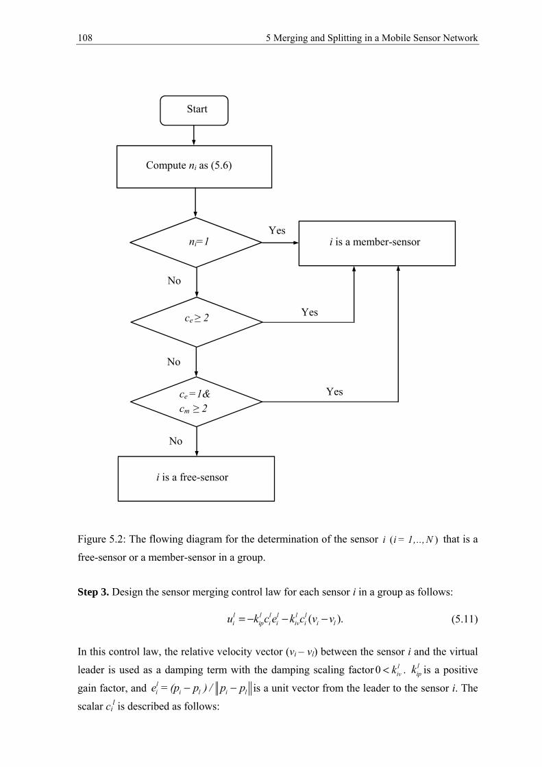
108 5 Merging and Splitting in a Mobile Sensor Network
Figure 5.2: The flowing diagram for the determination of the sensor ( )i i = 1,..,N that is a
free-sensor or a member-sensor in a group.
Step 3. Design the sensor merging control law for each sensor i in a group as follows:
( ).l l l lip i i
l li iv i i lk c e k c v vu −= − − (5.11)
In this control law, the relative velocity vector (vi – vl) between the sensor i and the virtual
leader is used as a damping term with the damping scaling factor 0 livk< . l
ipk is a positive
gain factor, and li i l i le = (p p ) / p p− − is a unit vector from the leader to the sensor i. The
scalar cil is described as follows:
Start
Compute ni as (5.6)
i is a member-sensor Yes
No
ce ≥ 2
ni=1
Yes
No
ce =1& cm ≥ 2
Yes
i is a free-sensor
No
5.3 Sensor splitting control 109
li
1 , if i is free sensor c =
0 , otherwise
−
. (5.12)
Equation (5.12) shows that only free-sensors are affected by the attractive force of the vir-
tual leader. In other words, using the attractive force from the virtual leader, all free sen-
sors will find and approach their group to become the new members in this group. Then,
these new members will combine with other members in the group to continue tracking
their target.
Remark 5.2. If a target disappears at time t, the sensors that are tracking this target will automatically combine with the nearest existing subgroups as the free-sensors of these subgroups.
5.3 Sensor splitting control
This sub-section presents the sensor splitting control method from a group, which is
tracking a moving target, into subgroups to track the new targets when these new targets
appear. The idea to design this method is depicted in figure 5.3.
As shown in figure 5.3 the line f(x,y)=0 through the center A of the main group and
the new target splits the main group, which is tracking the old target, into two sub-groups.
The first sub-group (subgroup 1) consists of the sensors that lie on the side that contains
the old target while the second subgroup (subgroup 2) consists of the sensors that lie on the
opposite side. Assume that in the main group there are N sensors ( 2N ≥ ), and each sensor
( )i i = 1,..,N is located at the position ( , )Ti i ip x y= . Then, the center of this main group
at time t is calculated, such that:
1
1( ) (t).N
ii
A t pN =
= (5.13)
Let 1 1 1( ) ( ( ), ( ) )T
t t tp t x t y t= , 2 2 2( ) ( ( ), ( ) )T
t t tp t x t y t= , and ( ) ( ( ), ( ))TA AA t x t y t= be the posi-
tion of the target 1 (old target), the position of the target 2 (new target), and the position of
the center of the main group at time t, respectively. According to [96], [97], the boundary
line f(x,y)=0 is given , such that:
( )
2 2
( ) ( ), .( ) ( ) ( ) ( )
A A
t A t A
x x t y y tf x y
x t x t y t y t
− −−− −
= (5.14)
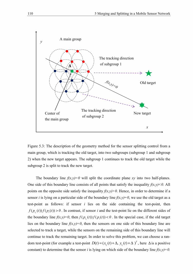
110 5 Merging and Splitting in a Mobile Sensor Network
Figure 5.3: The description of the geometry method for the sensor splitting control from a
main group, which is tracking the old target, into two subgroups (subgroup 1 and subgroup
2) when the new target appears. The subgroup 1 continues to track the old target while the
subgroup 2 is split to track the new target.
The boundary line f(x,y)=0 will split the coordinate plane xy into two half-planes.
One side of this boundary line consists of all points that satisfy the inequality f(x,y)<0. All
points on the opposite side satisfy the inequality f(x,y)>0. Hence, in order to determine if a
sensor i is lying on a particular side of the boundary line f(x,y)=0, we use the old target as a
test-point as follows: if sensor i lies on the side containing the test-point, then
( ( )) ( ( ))1t if p t f p t 0> . In contrast, if sensor i and the test-point lie on the different sides of
the boundary line f(x,y)=0, then ( ( )) ( ( ))1t if p t f p t 0< . In the special case, if the old target
lies on the boundary line f(x,y)=0, then the sensors on one side of this boundary line are
selected to track a target, while the sensors on the remaining side of this boundary line will
continue to track the remaining target. In order to solve this problem, we can choose a ran-
dom test-point (for example a test-point 1 1
( ) ( ( ) , ( ) )Tt tD t x t y t= +Δ +Δ , here Δ is a positive
constant) to determine that the sensor i is lying on which side of the boundary line f(x,y)=0.
Old target
y
x
The tracking direction of subgroup 1 A
New target The tracking direction of subgroup 2
Center of the main group
A main group
5.3 Sensor splitting control 111
If the sensors ( )i i = 1,..,N of the main group satisfy the inequality ( ( )) ( ( ))if D t f p t 0≥ ,
then they are selected as the members of a subgroup (for example subgroup 1) to track the
old target. The remaining sensors of the main group will be redesigned into a new group
(for example subgroup 1) to track the new target. Finally, after the sensor partitioning, the
mission of each sensor is to reach its target, and this mission is maintained until this target
disappears or some new targets appear.
Based on the above analysis, the control law for each sensor i to track its target is
proposed as follows:
( ) ( ) .m m
mi i iv t t
tt ti if p k v vu v−= − + (5.15)
Similar to equation (5.11), in this equation, the relative velocity vector ( )mi tv v− between
the sensor i and its target is added as a damping term with the positive factor tivk . The force
field ( )mii
tf p is designed as an attractive potential field surrounding each target tm with
m={1,2,3…}. Therefore, under the effect of this force field, each sensor i will always be
attracted towards its target until it reaches this target. This attractive force field is designed
as follows:
m m
m
m
tip t
i t itt
i
tip t
i
i
i
kp p e , if d < r
r(p )= f
k e , otherwise.
ττ
− −
−
(5.16)
Here 0rτ > is the close range surrounding the target, at which the sensor’s speed is reduced
before reaching the target, and /m m mit i t i te (p p ) p p= − − is the unit vector directing from
the target ( , )m mt tp v to the sensor ( , )i ip v . Equation (5.16) shows that the magnitude of the
attractive force ( )mii
tf p is depending on the positive control factor tipk and the distance
m
m
ti i td = p p− between sensor i and its target.
Example: The sensor splitting control algorithm from a main group into two sub-groups to
track two moving targets is presented in Algorithm 5.1.
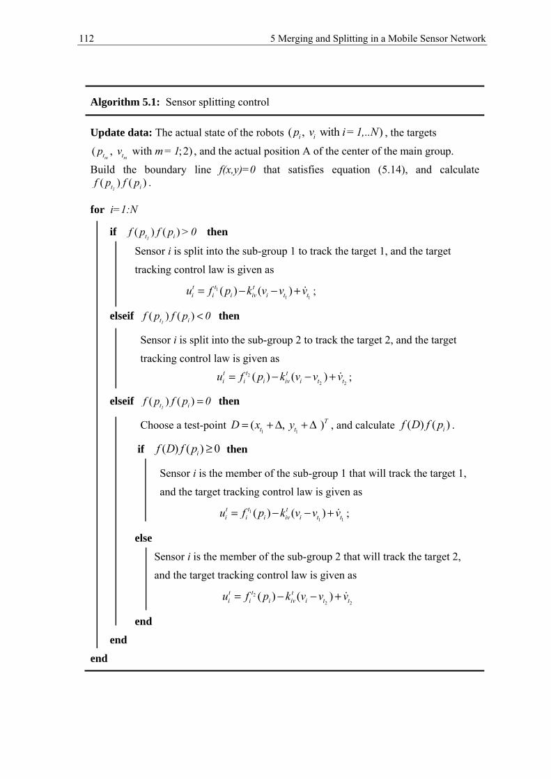
112 5 Merging and Splitting in a Mobile Sensor Network
Algorithm 5.1: Sensor splitting control
Update data: The actual state of the robots ( , with )i ip v i =1,..N , the targets
( , with ;2)m mt tp v m = 1 , and the actual position A of the center of the main group.
Build the boundary line f(x,y)=0 that satisfies equation (5.14), and calculate ( ) ( )
1t if p f p .
for i=1:N
if ( ) ( )1t if p f p > 0 then
Sensor i is split into the sub-group 1 to track the target 1, and the target
tracking control law is given as
1
1
1( ) ( )i i iv
tt ti t tif p k v v vu = −− + ;
elseif ( ) ( )1t if p f p 0< then
Sensor i is split into the sub-group 2 to track the target 2, and the target
tracking control law is given as
2
2
2( ) ( )i i iv
tt ti t tif p k v v vu = −− + ;
elseif ( ) ( )1t if p f p 0= then
Choose a test-point 1 1
( , )Tt tD x y= +Δ +Δ , and calculate ( ) ( )if D f p .
if ( ) ( ) 0if D f p ≥ then
Sensor i is the member of the sub-group 1 that will track the target 1,
and the target tracking control law is given as
1
1
1( ) ( )i i iv
tt ti t tif p k v v vu = −− + ;
else
Sensor i is the member of the sub-group 2 that will track the target 2,
and the target tracking control law is given as
2
2
2( ) ( )i i iv
tt ti t tif p k v v vu = −− +
end
end
end
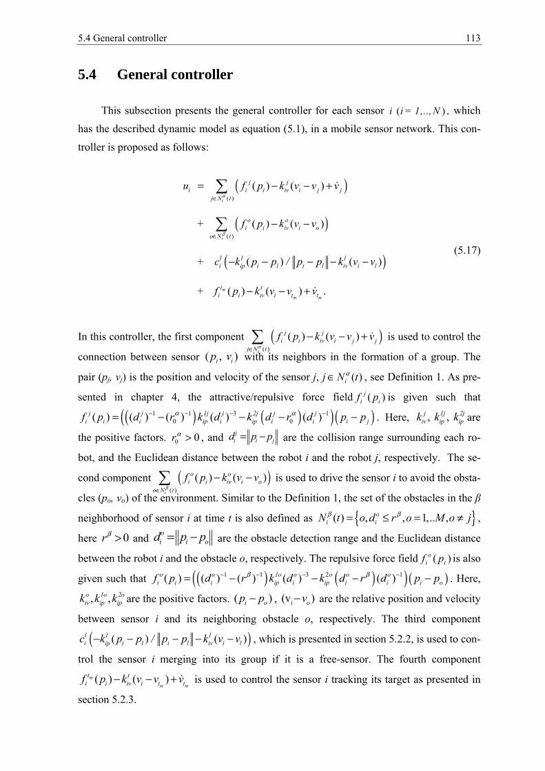
5.4 General controller 113
5.4 General controller
This subsection presents the general controller for each sensor ( )i i = 1,..,N , which
has the described dynamic model as equation (5.1), in a mobile sensor network. This con-
troller is proposed as follows:
( )
( )
( )
( )
( )
+
(
+ ( )
+
) ( )
( ) (
)
) ( ) .
( )
(m m
i
i
m
j ji iv
j N t
i ivo N t
l
i i i j j
o oi i o
li l i l iv i l
li ip
t tii iv i t t
k v v v
k v v
c k k v v
f p k
u f p
f p
p p
v v
p
v
/ p
α
β
∈
∈
= − −
− −
− −
− +
+
− − −
−
(5.17)
In this controller, the first component ( )( )
( ) ( )i
j ji iv
j N ti i j jk v vf p v
α∈
+− − is used to control the
connection between sensor ( , )i ip v with its neighbors in the formation of a group. The
pair (pj, vj) is the position and velocity of the sensor j, ( )ij N tα∈ , see Definition 1. As pre-
sented in chapter 4, the attractive/repulsive force field ( )ij
if p is given such that
( ) ( )( )( )1 1 3 10 0( ) )( ( ( () ) )j j 1j j 2j j j
i i ip ii i i i jp id r k d k d r df p p pα α− − − −= − − −− . Here, , , j 1j 2jiv ip ipk k k are
the positive factors. 0 0rα > , and ij
i jd p p−= are the collision range surrounding each ro-
bot, and the Euclidean distance between the robot i and the robot j, respectively. The se-
cond component ( )( )
( ) ( )i
o oi ii iv
o N top kf v v
β∈
− − is used to drive the sensor i to avoid the obsta-
cles (po, vo) of the environment. Similar to the Definition 1, the set of the obstacles in the β
neighborhood of sensor i at time t is also defined as { }( ) , 1,.. , ,oiiN o d r o jt M oβ β= ≤ = ≠ ,
here 0rβ > and i io
od p p= − are the obstacle detection range and the Euclidean distance
between the robot i and the obstacle o, respectively. The repulsive force field ( )iiof p is also
given such that ( ) ( )( )( )1 1 3 12( ) ) )( ) )( ( (o 1o o o o oi i ip i io
i i op i id r k d k d r df p p pβ β− − − −− − −= − . Here,
, ,1o 2oi i pov p ik k k are the positive factors. ( )i op p− , (v )i ov− are the relative position and velocity
between sensor i and its neighboring obstacle o, respectively. The third component
( )( ) ( )li l i l iv i l
l li ip p p / pc k k v vp− − −−− , which is presented in section 5.2.2, is used to con-
trol the sensor i merging into its group if it is a free-sensor. The fourth component
( ) ( )m
m
mi ivt t
i i t tf p k v v v+− − is used to control the sensor i tracking its target as presented in
section 5.2.3.
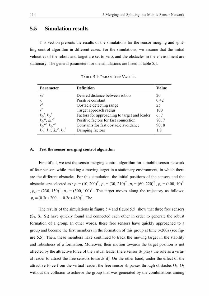
114 5 Merging and Splitting in a Mobile Sensor Network
5.5 Simulation results
This section presents the results of the simulations for the sensor merging and split-
ting control algorithm in different cases. For the simulations, we assume that the initial
velocities of the robots and target are set to zero, and the obstacles in the environment are
stationary. The general parameters for the simulations are listed in table 5.1.
TABLE 5.1: PARAMETER VALUES
Parameter
Definition
Value
r0α
λ
Desired distance between robots Positive constant
20 0.42
rβ Obstacle detecting range 25 rτ Target approach radius 100 kip
t, kipl Factors for approaching to target and leader 6; 7
kip1j, kip
2j Positive factors for fast connection 80; 7 kip
1o, kip2o Constants for fast obstacle avoidance 90; 8
kivj, kiv
t, kivo, kiv
l Damping factors 1,8
A. Test the sensor merging control algorithm
First of all, we test the sensor merging control algorithm for a mobile sensor network
of four sensors while tracking a moving target in a stationary environment, in which there
are the different obstacles. For this simulation, the initial positions of the sensors and the
obstacles are selected as : (10, 200)T1p = , T(30, 210)2p = , T(60, 220)3p = , T(400, 10)4p =
, T(230, 150)o1p = , T(300, 100)o2p = . The target moves along the trajectory as follows:
(0.3 200, 0.2 480) .Ttp t t= + − + The
The results of the simulations in figure 5.4 and figure 5.5 show that three free sensors
(S1, S2, S3) have quickly found and connected each other in order to generate the robust
formation of a group. In other words, these free sensors have quickly approached to a
group and become the first members in the formation of this group at time t=200s (see fig-
ure 5.5). Then, these members have continued to track the moving target in the stability
and robustness of a formation. Moreover, their motion towards the target position is not
affected by the attractive force of the virtual leader (here sensor S3 plays the role as a virtu-
al leader to attract the free sensors towards it). On the other hand, under the effect of the
attractive force from the virtual leader, the free sensor S4 passes through obstacles O1, O2
without the collision to achieve the group that was generated by the combinations among
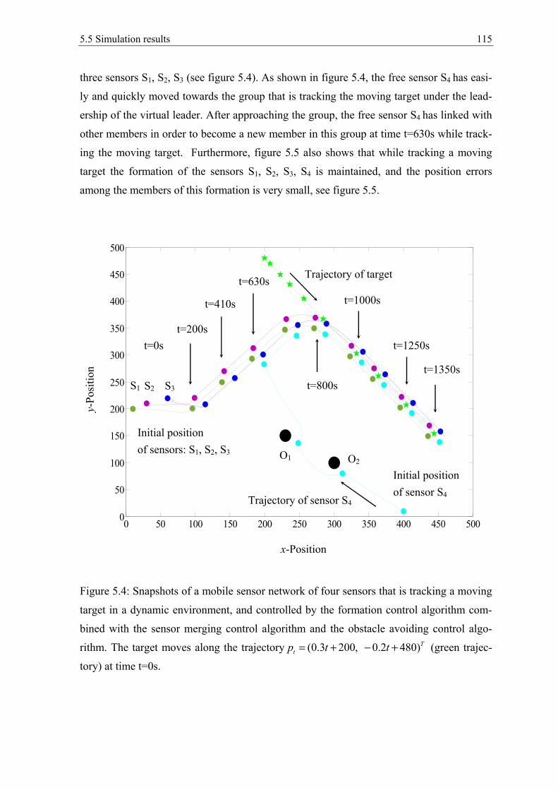
5.5 Simulation results 115
three sensors S1, S2, S3 (see figure 5.4). As shown in figure 5.4, the free sensor S4 has easi-
ly and quickly moved towards the group that is tracking the moving target under the lead-
ership of the virtual leader. After approaching the group, the free sensor S4 has linked with
other members in order to become a new member in this group at time t=630s while track-
ing the moving target. Furthermore, figure 5.5 also shows that while tracking a moving
target the formation of the sensors S1, S2, S3, S4 is maintained, and the position errors
among the members of this formation is very small, see figure 5.5.
Figure 5.4: Snapshots of a mobile sensor network of four sensors that is tracking a moving
target in a dynamic environment, and controlled by the formation control algorithm com-
bined with the sensor merging control algorithm and the obstacle avoiding control algo-
rithm. The target moves along the trajectory (0.3 200, 0.2 480)Ttp t t= + − + (green trajec-
tory) at time t=0s.
0 50 100 150 200 250 300 350 400 450 5000
50
100
150
200
250
300
350
400
450
500
x-Position
y-Po
sitio
n
t=0s t=200s
t=410s
t=630s
t=800s
t=1000s
t=1350s
t=1250s
O1
S1 S2 S3
Initial position of sensors: S1, S2, S3
O2
Initial position of sensor S4
Trajectory of sensor S4
Trajectory of target

116 5 Merging and Splitting in a Mobile Sensor Network
Figure 5.5: Position errors among the sensors in a mobile sensor network of four sensors at
time t while tracking a moving target as simulated in figure 5.4.
Secondly, we test the control algorithm for a mobile sensor network of seven sensors
while tracking a moving target in a stationary environment. For this simulation, the target
moves along the trajectory T(0.06t+200, 0.08t+480)tp = − . The initial positions of sensors
and obstacles are selected as: T(10, 20)1p = , T(20, 10)2p = , T(30, 20)3p = , T(40, 50)4p = ,T(5, 80)5p = , T(300, 10)6p = , T(450, 10)7p = , T(350, 100)o1p = , T(280, 200)o2p = .
The results of the simulations in figure 5.6 show that the swarm-finding of two sen-
sors (S6 and S7) is successfully achieved, and this swarm-finding does not change the gen-
eral trajectory of the swarm. As shown in figure 5.6, at beginning all sensors are directed to
the position of the virtual leader. The free-sensors S1,2…5 quickly find their neighbors, and
immediately they connect together to become the first member-sensors of a basic group.
The approach of the sensor S6 into this basic group is not difficult. Furthermore, the sensor
S7 also successfully reaches the basic group, although it is hindered by some obstacles of
the environment while tracking. The organization of the basic group is changed when the
free-sensors S6 and S7 become the new members of this basic group. The constant distanc-
es among member-sensors are maintained while these sensors track the moving target.
Posi
tion
erro
r (m
)
Time (s)
0 200 400 600 800 1000 1200 14000
50
100
150
200
250
300
350
400
450
Distance between robot 1and robot 2Distance between robot 1and robot 3Distance between robot 1and robot 4Distance between robot 2 and robot 3Distance between robot 2 and robot 4Distance between robot 3 and robot 4
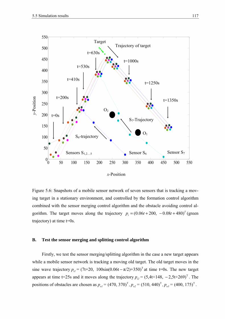
5.5 Simulation results 117
Figure 5.6: Snapshots of a mobile sensor network of seven sensors that is tracking a mov-
ing target in a stationary environment, and controlled by the formation control algorithm
combined with the sensor merging control algorithm and the obstacle avoiding control al-
gorithm. The target moves along the trajectory (0.06 200, 0.08 480)Ttp t t= + − + (green
trajectory) at time t=0s.
B. Test the sensor merging and splitting control algorithm
Firstly, we test the sensor merging/splitting algorithm in the case a new target appears
while a mobile sensor network is tracking a moving old target. The old target moves in the
sine wave trajectory T(7t+20, 100sin(0.06t π/2)+350)t1p = − at time t=0s. The new target
appears at time t=25s and it moves along the trajectory T(5,4t+148, 2,5t+269)t2p = − . The
positions of obstacles are chosen as T T T(470, 370) (510, 440) (400, 175)o1 o2 o3p = , p = , p = .
0 50 100 150 200 250 300 350 400 450 500 5500
50
100
150
200
250
300
350
400
450
500
550
x-Position
y-Po
sitio
n
t=0s
t=200s
t=410s
t=630s
t=1000s
t=1350s
t=1250s
O2
Sensors S1,2…5
O1
Sensor S6
S6-trajectory
Trajectory of target
t=530s
Sensor S7
S7-Trajectory
Target
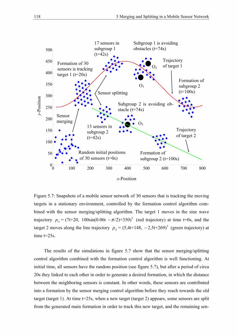
118 5 Merging and Splitting in a Mobile Sensor Network
Figure 5.7: Snapshots of a mobile sensor network of 30 sensors that is tracking the moving
targets in a stationary environment, controlled by the formation control algorithm com-
bined with the sensor merging/splitting algorithm. The target 1 moves in the sine wave
trajectory T(7t+20, 100sin(0.06t /2)+350)t1p = π− (red trajectory) at time t=0s, and the
target 2 moves along the line trajectory T(5,4t+148, 2,5t+269)t2p = − (green trajectory) at
time t=25s.
The results of the simulations in figure 5.7 show that the sensor merging/splitting
control algorithm combined with the formation control algorithm is well functioning. At
initial time, all sensors have the random position (see figure 5.7), but after a period of circa
20s they linked to each other in order to generate a desired formation, in which the distance
between the neighboring sensors is constant. In other words, these sensors are contributed
into a formation by the sensor merging control algorithm before they reach towards the old
target (target 1). At time t=25s, when a new target (target 2) appears, some sensors are split
from the generated main formation in order to track this new target, and the remaining sen-
0 100 200 300 400 500 600 700 8000
50
100
150
200
250
300
350
400
450
500
x-Position
y-Po
sitio
n
O1
Sensor merging
Random initial positions of 30 sensors (t=0s)
Formation of 30 sensors is tracking target 1 (t=20s)
Sensor splitting
Trajectory of target 2
Trajectory of target 1
17 sensors in subgroup 1 (t=42s)
Subgroup 1 is avoiding obstacles (t=74s)
Subgroup 2 is avoiding ob-stacle (t=74s)
Formation of subgroup 2 (t=100s)
Formation of subgroup 2 (t=100s)
13 sensors in subgroup 2 (t=42s)
O2
O3
5.5 Simulation results 119
sors continue to track the old target. In figure 5.7, we can see that after sensors are split
they have quickly combined to each other into a new formation. At time t=74s, the for-
mation of subgroups is broken while avoiding obstacles. Then, these formations are auto-
matically redesigned while tracking the moving targets at time t=100s, see figure 5.7.
As shown in figure 5.7, the sensor splitting from a main group into subgroups based
on the geometry method has been successful. However, the number of the sensors in sub-
groups is possibly unequal (for example, in figure 5.7 there are 17 sensors in the first sub-
group while in the second subgroup there are only 13 sensors). So, to solve this problem
the sensor splitting algorithm is developed as follows:
Step 1. Split sensors into subgroups when a new target appears as represented above.
Step 2. Determine the number of the sensors in each subgroup. Assume that the number of
the sensors in the first subgroup and the second subgroup are ξ and ζ (ζ+ξ=N), respective-
ly. Let δ be the necessary number of the sensors to add into a subgroup in that the number
of the sensors is unequal to N/2. If ξ< ζ, (ξ=N/2 –δ) and (ζ=N/2+ δ), then δ sensors of the
second subgroup that have the smallest distance to the first target will split into the first
subgroup. In contrast, if ξ>ζ, (ξ=N/2+δ) and (ζ=N/2–δ), then δ sensors of the first sub-
group that have the smallest distance to the second target will split into the second sub-
group.
The developed sensor splitting algorithm is tested in the second case: a new target
appears in the interval time from t=25s to t=95s while a main group is tracking a moving
old target. The results of the simulations in figure 5.8 show that the developed sensor split-
ting algorithm is well working, the sensors are split equally into subgroups ( as shown in
figure 5.8, each subgroup has 15 sensors) when the new target appears at time t=25s. In
contrast, when the second target disappears at time t=95s, the second subgroup, which is
tracking this target, merges into the first subgroup and continues to track the first target as
the members of this subgroup. This sensor merging is successful and without the colli-
sions. However, the structure of the formation of the whole group after merging can be
redesigned. Each member sensor quickly finds its neighbors, and they connect to each oth-
er in order to generate and maintain the stable and robust connections in their formation
during tracking.
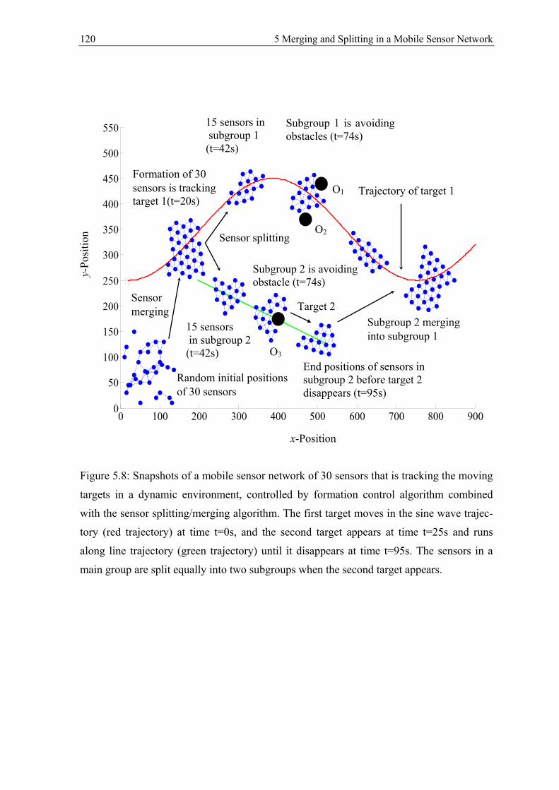
120 5 Merging and Splitting in a Mobile Sensor Network
Figure 5.8: Snapshots of a mobile sensor network of 30 sensors that is tracking the moving
targets in a dynamic environment, controlled by formation control algorithm combined
with the sensor splitting/merging algorithm. The first target moves in the sine wave trajec-
tory (red trajectory) at time t=0s, and the second target appears at time t=25s and runs
along line trajectory (green trajectory) until it disappears at time t=95s. The sensors in a
main group are split equally into two subgroups when the second target appears.
0 100 200 300 400 500 600 700 800 9000
50
100
150
200
250
300
350
400
450
500
550
O3
x-Position
y-Po
sitio
n
Random initial positions of 30 sensors
Sensor merging
O1
Sensor splitting
15 sensors in subgroup 2 (t=42s)
15 sensors in subgroup 1 (t=42s)
Subgroup 1 is avoiding obstacles (t=74s)
O2
Subgroup 2 is avoiding obstacle (t=74s)
Trajectory of target 1
Formation of 30 sensors is tracking target 1(t=20s)
End positions of sensors in subgroup 2 before target 2 disappears (t=95s)
Subgroup 2 merging into subgroup 1
Target 2
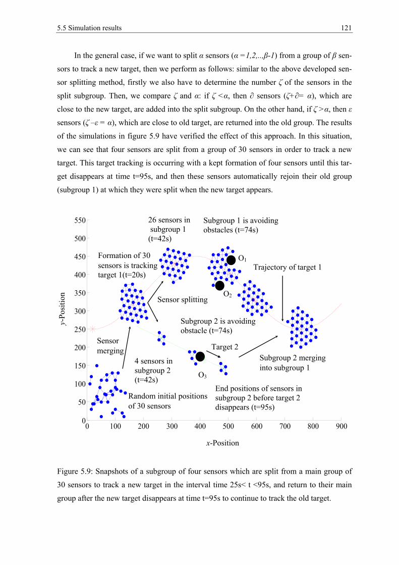
5.5 Simulation results 121
In the general case, if we want to split α sensors (α =1,2,..,β-1) from a group of β sen-
sors to track a new target, then we perform as follows: similar to the above developed sen-
sor splitting method, firstly we also have to determine the number ζ of the sensors in the
split subgroup. Then, we compare ζ and α: if ζ <α, then ∂ sensors (ζ+∂= α), which are
close to the new target, are added into the split subgroup. On the other hand, if ζ >α, then ε
sensors (ζ –ε = α), which are close to old target, are returned into the old group. The results
of the simulations in figure 5.9 have verified the effect of this approach. In this situation,
we can see that four sensors are split from a group of 30 sensors in order to track a new
target. This target tracking is occurring with a kept formation of four sensors until this tar-
get disappears at time t=95s, and then these sensors automatically rejoin their old group
(subgroup 1) at which they were split when the new target appears.
Figure 5.9: Snapshots of a subgroup of four sensors which are split from a main group of
30 sensors to track a new target in the interval time 25s< t <95s, and return to their main
group after the new target disappears at time t=95s to continue to track the old target.
0 100 200 300 400 500 600 700 800 9000
50
100
150
200
250
300
350
400
450
500
550
O3
x-Position
y-Po
sitio
n
Random initial positions of 30 sensors
Sensor merging
O1
Sensor splitting
4 sensors in subgroup 2 (t=42s)
26 sensors in subgroup 1 (t=42s)
Subgroup 1 is avoiding obstacles (t=74s)
O2
Subgroup 2 is avoiding obstacle (t=74s)
Trajectory of target 1
Formation of 30 sensors is tracking target 1(t=20s)
End positions of sensors in subgroup 2 before target 2 disappears (t=95s)
Subgroup 2 merging into subgroup 1
Target 2
122 5 Merging and Splitting in a Mobile Sensor Network
5.6 Conclusion
This paper has presented an approach to control a mobile sensor network to track the
moving targets in a dynamic environment. In this approach, we solve two main issues: the
sensor splitting and merging control when the number of the targets is changed. The free
sensor merging into a group is controlled by the invariable attractive force field from the
selected virtual leader in this group. In other words, under the effect of the attractive force
field from the selected virtual leader, the free-sensors can easily reach the main group and
become the new members in formation of this group. In contrast, subgroups will be split
from the existing groups to track new targets when these new targets appear. The sensor
splitting algorithm is built based on the geometry relationship between the targets and the
center of the group. The members in a split subgroup will connect with their neighbors in
order to generate a robust formation without collision while tracking their target. In addi-
tion, when a target disappears, the sensors that are tracking this target will automatically
contribute into the nearest existing subgroup. The effectiveness of this proposed approach
has been verified in simulations.
The results of the simulations have shown that this approach is one of the good con-
trol methods that can be applied to control the contribution and distribution of a mobile
sensor network while tracking the dynamic targets. The sensor merging algorithm, which is
built based on the energy level partitioning in the invariable attractive force field of the
virtual leader, works very well. Using this control algorithm, the free-sensors can easily
find and approach their group while reaching the target, and then these free-sensors will
become the new member-sensors in the formation of the group. Especially, this method
solves the speed problem that occurs when the free-sensors are away from their target. Fur-
thermore, the swarm-finding of the free sensors does not influence on the target tracking of
the swarm. On the other hand, the sensor splitting algorithm based on the geometry method
shows that this is an active method for the sensor distribution from a main group into sub-
groups to track the new targets. The sensor partitioning is quickly performed at the time
when a new target appears, and then the formation of these split sensors is maintained
while tracking their target in a free environment until this target disappears. However,
while avoiding the obstacles the formation connection of the groups are broken. In this
situation, the member-sensors of these groups are distributed to the free sensors in order to
easily escape the obstacles without the collision among them. After exiting the obstacles,
the formation of the distributed sensors is reorganized to continue tracking their target.
Moreover, the results of the simulations in figure 5.9 have also shown that the development
5.6 Conclusion 123
and application of the proposed approach for the exact sensor splitting from a main group
into subgroups, such as the splitting α sensors from a group of β sensors, ( 1, 2... 1α β= − ,
and Nβ ≤ ) into a subgroup, are successful.
124
6 Conclusion and Future Work
6.1 Conclusion
This work has presented a method for controlling the formation of autonomous robots
while tracking the dynamic targets under the influence of the dynamic environment. This
approach is based on the developed artificial vector fields. In this approach, the proposed
artificial vector fields, which consist of the attractive, repulsive, and rotational force field,
are combined with the damping term in the formation control laws in order to control the
velocity, heading, connectivity, as well as the obstacle avoidance for a swarm of autono-
mous robots during movement. In addition, using the added rotational force field in the
obstacle avoiding controller, robots can easily escape the obstacles while moving towards
the target. In the preceding chapters, focuses on two main issues of formation control fol-
lowing the desired formations and cooperative formation control have been given.
In the first approach (formation control following the desired formations), a desired
formation (for example V-shape, line or circular shape), which includes the coordinated
equidistant virtual nodes, is first generated based on the relative position between the
swarm’s virtual leader and the moving target. The virtual leader of the swarm is randomly
chosen from a member that is closest to the target. This virtual leader plays an important
role in creating and driving the formation towards the target in a stable trajectory. Hence,
in undesired cases, for example, when the leader is broken or trapped in the obstacles (U-
shape obstacle), a new leader is immediately chosen, so that the swarm will continue to
track the target. The selected virtual leader is controlled by a global attractive potential
field generated from the target in order to drive its formation on a specific trajectory to-
wards the target. Furthermore, the motion of each robot is controlled by the artificial force
fields, which include the local and global attractive potential fields surrounding the gener-
ated virtual nodes in the desired formation and the local repulsive potential field surround-
ing each robot. Hence, the robot always converges to a certain virtual node in the desired
formation and avoids collisions with other robots simultaneously. In addition, using the
repulsive vector field combined with the rotational vector field in the obstacle avoiding
controller, robots can easily escape the obstacles while tracking. Using the desired position
finding algorithm, robots can quickly find their desired position at the virtual nodes in the
desired formation. Moreover, the influence of the noisy environment on the stability of the
6.1 Conclusion 125
formation, as well as the formation adaptation of a swarm while reaching a moving target
are also studied in this topic. The results of the simulations have proved the success of the
approach. Results show that the robots quickly approached the coordinated virtual nodes in
the desired formation and maintained at these virtual nodes, although affected by a noisy
environment. Especially, upon the use of the desired position finding algorithm, the for-
mation of a swarm was not discrete. On overcoming the obstacle, the robots continued to
approach their formation and then they found the other desired positions in the formation.
In the second approach (cooperative formation control), robots are only allowed to
communicate within their neighboring relationship; however, the swarm’s cohesion must
be maintained coincidentally in tracking the moving target and as well as while avoiding
obstacle. Therefore, in order to perform the cooperative formation control for a swarm, the
neighboring robots are first linked to each other by the proposed formation connection con-
troller. These neighboring connections created the robust formation cohesion and avoided
collisions among robots in the swarm simultaneously. Further, for the formation adaptation
while passing through a narrow space among obstacles, the adaptive formation control
algorithm is built based on the size change of formation. Moreover, the splitting/merging
control algorithm is used to help the free robots to easily and quickly find their formation
as well as to split some roots from a main group into smaller subgroups when some new
targets appear. The simulations have shown that our proposed algorithms for controlling
the cooperative formation have well worked, namely: the free robots have easily merged
into the formation of their swarm; the formation connectivity was maintained while track-
ing; the formation’s size was shrunk into a smaller size while overcoming the narrow space
among obstacles to maintain formation.
Finally, our proposed control algorithms are not only to control autonomous robots
moving along a desired trajectory, but also to hold these robots in a specified formation
without collisions during movement. Especially, using the added rotational force field in
the obstacle avoiding controller, the local minima problems that still exist in the traditional
potential field method have been solved.
126 6 Conclusion and Future Work
6.2 Future work
Further studies and researches can be expanded to cooperative control in a hybrid sys-
tem, cooperative learning and sensing. The first research objective is to develop a method
for formation control of autonomous robots in three-dimensional space (3-D) to model
swarms and allow heterogeneous swarms of aerial, ground, and underwater vehicles to
combine formation together in a certain task while avoiding collisions; for example, the
cooperation of the unmanned aerial vehicles with autonomous mobile robots while pursu-
ing the moving objectives. In addition, learning and sensing can also be developed and
utilized in the environment where the connectivity, the size, as well as the structure of a
swarm can be improved by environmental parameters. In a multi robot network, members
can learn to avoid the moving obstacles, while maintaining network connectivity and to-
pology, aside to find a desired configuration of network. Moreover, members in a network
can also sense the environmental parameters in order to perform the task of the environ-
ment estimation and mapping.
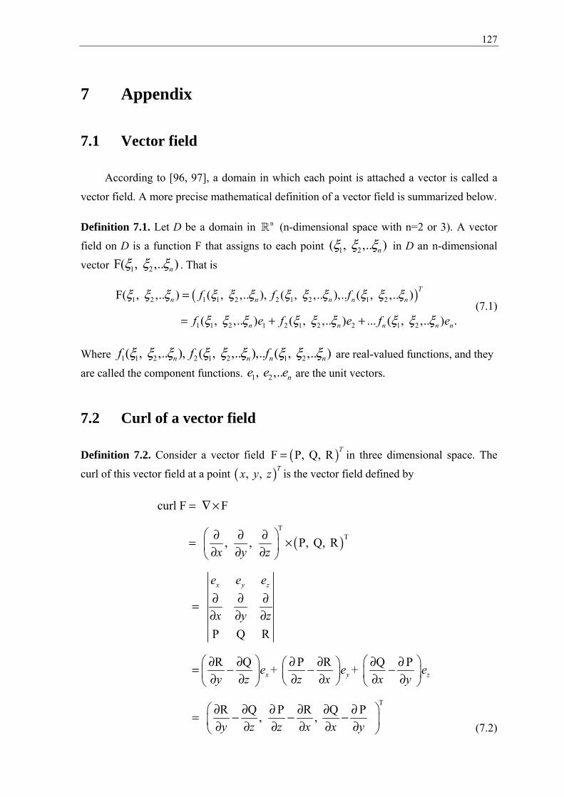
127
7 Appendix
7.1 Vector field
According to [96, 97], a domain in which each point is attached a vector is called a
vector field. A more precise mathematical definition of a vector field is summarized below.
Definition 7.1. Let D be a domain in n (n-dimensional space with n=2 or 3). A vector
field on D is a function F that assigns to each point 1 2( , ,.. )nξ ξ ξ in D an n-dimensional
vector 1 2F( , ,.. )nξ ξ ξ . That is
( )1 2 1 1 2 2 1 2 1 2
1 1 2 1 2 1 2 2 1 2
F( , ,.. ) ( , ,.. ), ( , ,.. ),.. ( , ,.. )
( , ,.. ) ( , ,.. ) ... ( , ,.. ) .
T
n n n n n
n n n n n
f f f
f e f e f e
ξ ξ ξ ξ ξ ξ ξ ξ ξ ξ ξ ξ
ξ ξ ξ ξ ξ ξ ξ ξ ξ
=
= + + (7.1)
Where 1 1 2 2 1 2 1 2( , ,.. ), ( , ,.. ),.. ( , ,.. )n n n nf f fξ ξ ξ ξ ξ ξ ξ ξ ξ are real-valued functions, and they
are called the component functions. 1 2, ,.. ne e e are the unit vectors.
7.2 Curl of a vector field
Definition 7.2. Consider a vector field ( )F P, Q, R T= in three dimensional space. The
curl of this vector field at a point ( ), , Tx y z is the vector field defined by
( )T
T
T
curl F F
, , P, Q, R
P Q R
R Q P R Q P + +
R Q P R Q P , ,
x y z
x y z
x y z
e e e
x y z
e e ey z z x x y
y z z x x y
= ∇×
∂ ∂ ∂= × ∂ ∂ ∂
∂ ∂ ∂=∂ ∂ ∂
∂ ∂ ∂ ∂ ∂ ∂ = − − − ∂ ∂ ∂ ∂ ∂ ∂
∂ ∂ ∂ ∂ ∂ ∂= − − − ∂ ∂ ∂ ∂ ∂ ∂ (7.2)
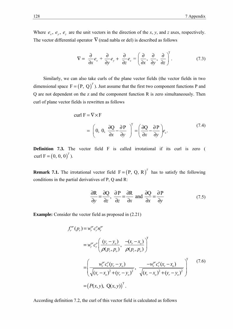
128 7 Appendix
Where , , x y ze e e are the unit vectors in the direction of the x, y, and z axes, respectively.
The vector differential operator ∇ (read nabla or del) is described as follows
T
+ = , , .x y ze e ex y z x y z
∂ ∂ ∂ ∂ ∂ ∂∇ = + ∂ ∂ ∂ ∂ ∂ ∂ (7.3)
Similarly, we can also take curls of the plane vector fields (the vector fields in two
dimensional space ( )F P, Q T= ). Just assume that the first two component functions P and
Q are not dependent on the z and the component function R is zero simultaneously. Then
curl of plane vector fields is rewritten as follows
T
curl F F
Q P Q P 0, 0, .zex y x y
= ∇×
∂ ∂ ∂ ∂= − = − ∂ ∂ ∂ ∂
(7.4)
Definition 7.3. The vector field F is called irrotational if its curl is zero (
( )curl F 0, 0, 0 T= ).
Remark 7.1. The irrotational vector field ( )F P, Q, R T= has to satisfy the following conditions in the partial derivatives of P, Q and R:
R Q P R Q P, and y z z x x y
∂ ∂ ∂ ∂ ∂ ∂= = =∂ ∂ ∂ ∂ ∂ ∂
(7.5)
Example: Consider the vector field as proposed in (2.21)
( )
T
T
2 2 2 2
T
( )
( ) ( ) , ( , ) ( , )
( ) ( ) , ( ) ( ) ( ) ( )
( , ), Q( , ) .
or or o orr r r r
or o r o r or r
r o r o
or o or or r r o r r r o
r o r o r o r o
r p w c n
y y x xw c
p p p p
w c y y w c x x
x x y y x x y y
P x y x
f
y
ρ ρ
=
− − −=
− − − = − + − − + −
=
(7.6)
According definition 7.2, the curl of this vector field is calculated as follows
7.3 Gradient vector field 129
( )
2 2 2 2
2
32 2
Qcurl 0 +0
( )
(
( )) ( )( ) ( ) ( )
( )
( )
( ) ( )
orr x y z
r r
or o or or r r o r r r o
zr rr o r o r o r o
or or r r o
r
r o r o
p
w c x x w c y y
yx x y y x x y y
w c y y
x x y
Pf e e e
x
ex
y
y
∂ ∂= ∂ ∂
∂ ∂ = − ∂ ∂
+ −
− − −− + − − + −
− − +− + −
=( )
2
32 2
2 2
( ) ( ) ( )
( ) ( ).
or or r r o
z
r o r o
or or r
z
r o r o
w c x x
x x y y
w c
x x ye
y
e− −
− + −
−− + −
=
(77)
Equation (7.7) shows that ( ) 0 (curl , ) ( , )orr r or r op x y x yf ≠ ∀ ≠ , hence ( )or
r rpf is a rota-tional vector field.
7.3 Gradient vector field
Definition 7.4. If the vector field F is defined differentiable everywhere and ( )curl F 0, 0, 0 T= , then F is a gradient vector field.
Remark 7.2. A gradient vector field F has some corresponding potential function f such that
T
T
, if ( )
F
, , if ( , ).
f ff f x, y
x yf
f f ff f x, y z
x y z
∂ ∂ = ∂ ∂ = ∇ = ∂ ∂ ∂ = ∂ ∂ ∂
(7.8)
In other words, the gradient of a differentiable scalar field nf ⊂ is a vector field. This vector field satisfies equation (7.8).
Example: Consider the scalar function ( )ij
iV p as proposed in (4.6). Taking the negative gradient of this scalar function at ip we obtain
130 7 Appendix
( )
( ) ( )
22
00
0 00 0
20
( )
1 1 1 1
1 1
2
1( )
jj 1j 2j ji
i ip ip iji
j 1j j 2j j ji ip i ip i ij j
i i
j 1ji ip ij j
i
i i
ck k d r
d r
c k c k d r d rd r
1 1
d r
c d
V
d r d
p
k
αα
α αα α
α
− + − −∇ = −∇
= − ∇
− − − − −
−
∇
= ∇ ( )
( )
0
2 00
1 1 1( )
j j 2j j ji ip i i
j 1j j 2j j ji ip i ip i ij j
i i
c k d r d
c k c k d r dd r d
α
αα
∇− −
− − −
∇
=
(7.9)
Where the distance between robots i and j is calculated as 2 2( ) ( )ji i j i jd x x y y= − + − .
Hence, we have
2 2
2 2 2 2
2 2 2 2
T
T
= ,
= ,
( ) ( )
( ) ( ) ( ) ( )
( ) ( )
( ) ( ) ( )
( = .
( )
)
ji i j i j
i j i j i j i ji i
i j i j
i j i j i j i j
i j
i j
d x x y y
x x y y x x y yx y
x x y y
x x y y x x y y
p p
p p
∇ =∇
∂ ∂ ∂ ∂
− + −
− + − − + −
− −
− + − − + −
−
−
(7.10)
Substitute (7.10) into (7.9), we obtain
( )020
( ) ( )
(
).
)(
j ji i
1jip i jj 2j j
i ip ij ji i
i i
i j
k p pc
f p V p
1 1k d r
d r d p pα
α
=
− − − − −
−∇
= (7.11)
Equation (7.11) shows that the scalar function ( )ij
iV p as proposed in (4.6) is the potential function of the force field ( )i
jif p as given in (4.7).
7.4 Proof of gravitational force field 131
7.4 Proof of gravitational force field
In this subsection, we first prove that the gravitational force field (2.1) is a gradient
vector field. In order to simplify the analysis, we assume that: the point mass m2 located at
the origin attracts the point mass m1 located at T 3 T1 ( , , ) (0, 0, 0)p x y z= ∈ with a
force of magnitude 212 1 2F Gm m r r= . Therefore, equation (2.1) can be rewrite as follows
( )
( ) ( ) ( )( )
T1 212 3
2 2 2
T
1 2 1 2 1 23 3 3
2 2 2 2 2 2 2 2 2
T
( , , )
, ,
( , , ), ( , , ), ( , , ) .
Gm mf x y z
x y z
Gm m x Gm m y Gm m z
x y z x y z x y z
P x y z Q x y z R x y z
−=+ +
− − −= + + + + + +
=
(7.12)
According to definition 7.2, the curl of this force field at T1 ( , , )p x y z= is calculated as
( )
T
12
T
R Q P R Q Pcurl , ,
0, 0, 0 .
fy z z x x y
∂ ∂ ∂ ∂ ∂ ∂= − − − ∂ ∂ ∂ ∂ ∂ ∂
=
(7.13)
Equation (7.13) shows that the force field (7.12) is a gradient vector field.
Now, in order to prove that the scalar function 12 1 2V Gmm r=− is the potential
function of the force field 12f , we take the negative gradient of 12V as follows
( ) ( ) ( )
( )
T
1 2 1 2 1 212 2 2 2 2 2 2 2 2 2
T
1 2 1 2 1 23 3 3
2 2 2 2 2 2 2 2 2
T1 2123
2 2 2
, ,
= , ,
( , , ) .
Gm m Gm m Gm mV
x y zx y z x y z x y z
Gm m x Gm m y Gm m z
x y z x y z x y z
Gm mx y z f
x y z
∂ ∂ ∂ −∇ = ∂ ∂ ∂+ + + + + +
− − − + + + + + +
−= =+ +
(7.14)
Equation (7.14) shows that the scalar function 12 1 2V Gmm r=− is the potential function of the force field 3
12 1 2f Gm m r r= − .
132
8 Publications
[1] Anh Duc Dang, Hung Manh La and Joachim Horn, “Distributed formation control for autonomous robots following desired shape in noisy environment”, IEEE Inter-national Conference on Multisensor Fusion and Integration for Intelligent Systems (MFI 2016), Badeb-Baden, Germany, pages 285-290, September 19-21, 2016.
[2] Anh Duc Dang, Hung Manh La and Joachim Horn, “Influence of formation angle on stability of V-formation while tracking a moving target”, Journal of Automation and Control Engineering, 2016, accepted.
[3] Anh Duc Dang and Joachim Horn, “Stability of V-formation while tracking a mov-ing target”, Proceedings of the Automatics- 2015 XXII International Conference on Automatic Control, Odessa, Ukraine, pages 154-156, September 10-11, 2015.
[4] Anh Duc Dang and Joachim Horn, “Formation control of autonomous robots fol-lowing desired formation during tracking a moving target”, Proceedings of the 2nd IEEE International Conference on Cybernetics, Gdynia, Poland, pages 160-165, June 24-26, 2015.
[5] Anh Duc Dang and Joachim Horn, “A mobile sensor network tracking moving tar-gets in a dynamic environment”, Proceedings of the 3rd IFAC Workshop on Multi-vehicle systems (MVS 2015), Genova, Italy, pages 1-6, May 18, 2015.
[6] Anh Duc Dang and Joachim Horn, “Collinear formation control of autonomous robots to move towards a target using artificial force fields”, Proceedings of the 2015 IEEE International Conference on Technologies for Practical Robot Applica-tions, Boston, USA, pages 1-6, May 11-12, 2015.
[7] Anh Duc Dang and Joachim Horn, “Formation adaptation control of autonomous robots in a dynamic environment”, Proceedings of the 2015 IEEE International Conference on Industrial Technology, Seville, Spain, pages 3190-3195, March 17-19, 2015.
[8] Anh Duc Dang and Joachim Horn, “Formation control of leader-following UAVs to track a moving target in dynamic environment”, Journal of Automation and Con-trol Engineering, Vol.3, No.1, pages 1-8, February 2015.
[9] Anh Duc Dang and Joachim Horn, “Formation control of autonomous robots to track a Moving target in an unknown Environment”, Proceedings of the 2014 IEEE International Conference on Robotics and Biomimetics, Bali, indonesia, pages 896-901, December 5-10, 2014.
[10] Anh Duc Dang and Joachim Horn, “Intelligent Swarm-Finding in Formation Con-trol of Multi-Robots to Track a Moving Target”, World Academy of Science, Engi-neering and Technology, International Journal of Computer, Information Science and Engineering, Vol.8, No.4, pages 12-18, 2014.
[11] Anh Duc Dang and Joachim Horn, “Path planning for a formation of autonomous robots in an unknown environment using artificial force fields”, Proceedings of the 18th IEEE International Conference on System Theory, Control and Computing, Si-naia, Romania, pages 773-778, October 17-19, 2014.
133
9 References
[1] C. Reynolds, “Flocks, birds, and schools: A distributed behavioral model,” Computer Graphics,ACM SIGGRAPH ’87 Conference Proceedings, Anaheim, California, vol. 21, no. 4, pp. 25–34, 1987.
[2] S. G. Reebs, “Can a minority of informed leaders determine the foraging movements of a fish shoal?,” Animal Behavior, vol. 59, pp. 403–409, 2000.
[3] A. Avitabile, R. A. Morse, and R. Boch, “Swarming honey bees guded by pheromones”, Annuals of the Entomological Society of America, 68(6):1079-1082, 1975.
[4] Lisa Lofland Gould and Frank Heppner, “The vee formation of canada geese”, the Auk 91, pages 494–506, July 1974.
[5] Timothy C. Williams, Thomas J. Klonoski and Philip Berkeley, “Angle of canada goose v flight formation measured by radar”, the Auk 93, pages 554–559, July 1976.
[6] Pete Seiler, aniruddha Pant, and Karl Hedrick, “Analysis of bird formations”, Proceed-ings of the 41st IEEE Conference on Decision and Control, pages 118–123, December 2002.
[7] John P. Badgerow, “An analysis of function in the formation flight of Canada geese”, the Auk 105, pages 749–755, October 1988.
[8] A. Mogilner, L. Edelstein-Keshet, L. Bent, and A. Spiros, “Mutual interactions, poten-tials, and individual distance in a social aggregation,” J. Math. Biol, vol. 47, pp. 353–389, 2003.
[9] S. Pang and J. A. Farrell, “Chemical plume source localization,” IEEE Transactions On Systems, Man, And Cybernetics, vol. 36, no. 5, pp. 1068–1080, 2006.
[10] J. A. Farrell, S. Pang, and W. Li, “Chemical plume tracing via an autonomous underwa-ter vehicle,” IEEE J. Oceanic Eng., vol. 30, no. 2, pp. 428–442, Apr. 2005.
[11] Simon Garnier, Jacques Gautrais, Guy Theraulaz,“The biological principles of swarm intelligence’’, Springer, Swarm Intell (2007) 1, pp: 3–31.
[12] Aleksandar Jevtic, Diego Andina, ‘Swarm Intelligence and Its Applications in Swarm Robotics’’, 6th WSEAS Int. Conference on Computational Intelligence, Man-Machine Systems and Cybernetics, Tenerife, Spain, pp. 41-46, December 2007.
[13] E. Bonabeau, M. Dorigo, and G, “Theraulaz. Swarm Intelligence: From Natural to Ar-tifcial Systems” , Oxford Univ. Press, NY, 1999.
[14] Shi and Yiwen Zhao, “An efficient path planning algorithm for mobile robot using im-proved potential field”, Proc. of the 2009 IEEE Intl. Conf. on Robotics and Biomimetics, pp. 1704-1708, December 2009.
[15] Simon János and István Matijevics, “Implementation of potential field method for mo-bile robot navigation in greenhouse environment with WSN support”, IEEE 8th Intl. Symp. on Intelligent Systems and Informatics, pp. 319-323, September 2010.
[16] O. Khatib, “Real-time obstacle avoidance for manipulators and mobile robots ”, Inter-national Journal of Robotics Research, Vol.o, No.1, pp. 90-98, 1986.
[17] Kim, J. O and Khosla, P. K, “Real-time obstacle avoidance for manipulators and mobile robotusing harmonic potentiel functions”, IEEE Trans. on Robotics and Automation, vol. 8, no. 3, pp. 338-349, 1992.
[18] L. Huang, “Velocity planning for a mobile robot to track amoving target – a potential field approach,” Robotics and Autonomous Systems, pp.1–9, 2008.
134 9 References
[19] Y. Koren and J. Borenstein, “Potential field methods and their inherent limitations for a mobile robot navigation,” Proceedings of the 46th IEEE Conference on Robotics and Automation, pp. 1398–1404, 1991.
[20] S. S. Ge and Y. J. Cui, “New potential functions for mobile robot path planning”, IEEE Trans. on Robotics and Automation, vol. 16, no.5, pp. 615-620, October 2000.
[21] Ding Fu-guang, Jiao Peng, Bian Xin-qian, Wang Hong-jian “AUV local path planning based on virtual potential field”, Proc. of the IEEE Intl. Conf. on Mechatronics and Au-tomation Niagara Falls, pp. 1711-1716, July 2005.
[22] Qing Li, Lijun Wang, Bo Chen, and Zhou Zhou, “An Improved Artificial Potential Field Method for Solving Local Minimum Problem”. IEEE the 2th Intl. Conf. on Intel-ligent control and Information Processing, pp. 420-424, 2011.
[23] Frank E. Schneider and Dennis Wildermuth, “A potential field based approach to multi robot formation navigation”, Proc. of the 2003 IEEE Intl. Conf. on Robotics, Intelligent System and Signal Processing, pp. 680-685, October 2003.
[24] Anh Duc Dang and Joachim Horn, “Intelligent swarm-finding in formation control of multi-robots to track a moving target”, Intl. Journal of Computer, Information Science and Engineering, Vol.8, No. 4, pp.12-18, 2014.
[25] Min Gyu Park and Min Cheol Lee “Artificial potential field based path planning for mobile robots using a virtual obstacle concept”, Proc. of the 2003 IEEE/ASME Intl. Conf. on Advanced Intelligent Mechatronics, pp. 735-740, 2003.
[26] Feilong Li, Yan Tan, Yujun Wang and Gengyu Ge “Mobile robots path planning based on evolutionary artificial potential fields approach”, Proc. of the the 2th Intl. Conf. on Computer Science and Electronics Engineering, pp. 1314-1317, 2013.
[27] Anh Duc Dang and Joachim Horn, “Formation control of autonomous robots to track a Moving target in an unknown Environment”, Proceedings of the 2014 IEEE Interna-tional Conference on Robotics and Biomimetics, Bali, indonesia, pp. 896-901, Decem-ber 5-10, 2014.
[28] Anh Duc Dang and Joachim Horn, “Path planning for a formation of autonomous robots in an unknown environment using artificial force fields”, Proceedings of the 18th IEEE International Conference on System Theory, Control and Computing, Sinaia, Romania, pages 773-778, October 17-19, 2014.
[29] A. Abdessameud and A. Tayebi, “Formation control of VTOL-UAVs”, Joint 48th IEEE Conf. on Decision and Control and 28th Chinese Control Conference , pp. 3454-3459,December 2009.
[30] Luis García- Delgado, Alejandro Dzul, Víctor Santibánez and Miguel Llama, “Quad-rotor formation control as an interconnected system”, Preprints of the 18th IFAC World Congress, pp. 13582-13587, August 2011.
[31] M. Alighanbari and J. P. How, “Decentralized task assignment for unmanned aerial ve-hicles,” Proceedings of the 44nd IEEE Conference on Decision and Control and Euro-pean Control Conference, pp. 5668–5673, 2005.
[32] Kishorekumar H Kowdiki, Ranjit Kumar Barai and Samar Bhattacharya, “Leader-follower formation control using artificial potential functions: A kinematic approach”, IEEE Intl. Conf. on Advances in Engineering, Science and Management, pp. 500-505, March 2012.
[33] Naomi Ehrich Leonard and Edward Fiorelli, “Virtual leader, artificial potential and co-ordinated control of groups”, Proc. of the 40th IEEE Conf. on Decision and Control, pp. 2968-2973, December 2001.
135
[34] H. Su, X. Wang, and Z. Lin, “Flocking of multi–agents with a virtual leader,” IEEE Transactions on Automatic Control, vol. 54, no. 2, pp. 293–307, 2009.
[35] H. Su, X. Wang, and Z. Lin, “Flocking of multi–agents with a virtual leader, part I: with a minority of informed agents,” Proceedings of the 46th IEEE Conference on Decision and Control, pp. 2937–2942, 2007.
[36] H. Su, X. Wang, and Z. Lin, “Flocking of multi–agents with a virtual leader, part II: with a virtual leader of varying velocity,” Proceedings of the 46th IEEE Conference on Decision and Control, pp. 1429–1434, 2007.
[37] H. Shi, L. Wang, T. Chu, F. Fu, and M. Xu, “Flocking of multi–agents with a virtual leader,” Proceedings of the 2007 IEEE Symposium on Artificial Life, pp. 287–29, 2007.
[38] J. Jennings, G.Whelan, andW. F. Evans, “Cooperative search and rescue with a team of mobile robots,” Proceedings of the 8th International Conference on Advanced robotics, Monterrey, CA, USA, 1997.
[39] H. M. La and W. Sheng, “Flocking control of a mobile sensor network to track and ob-serve a moving target,” Proceedings of the 2009 IEEE International Conference on Ro-botics and Automation (ICRA), Kobe, Japan, 2009.
[40] A. Regmi, R. Sandoval, R. Byrne, H. Taner, and C. T. Abdallah, “Experimental imple-mentation of flocking algorithms in wheeled mobile robots,” American Control Confer-ence, pp. 4917–4922, 2005.
[41] R. Olfati-Saber, “Flocking for multi-agent dynamic systems: Algorithms and theory”, IEEE Transactions on Automatic Control, 51(3):401–420, 2006.
[42] H. G. Tanner, A. Jadbabai, and G. J. Pappas, “Flocking in fixed and switching net-works,” IEEE Transactions on Automatic Control, vol. 52, pp. 863–868, May 2007.
[43] Michael M. Zavlanos and George J. Pappas, “Potential fields for maintaining connectiv-ity of mobile networks,” IEEE Transactions on Robotics, vol. 23, no. 4, pp. 812–816, August 2007.
[44] K. M. Lynch, P. Yang, and R. A. Freeman, “Decentralized environmental modeling by mobile sensor networks,” IEEE Transaction on Robotics, vol. 24, no. 3, pp. 710–724, 2008.
[45] D. Culler, D. Estrin, and M. Srivastava, “Overview of sensor networks,” IEEE Comput-er, vol. 37, no. 8, pp. 41–49, 2004.
[46] M. Tubaishat and S. Madria, “Sensor networks: An overview,” IEEE Potentials, pp. 20–23, May 2003.
[47] I. Akyildiz, W. Su, Y. Sankarasubramanian, and E. Cayirci, “A surve of sensor net-works,” IEEE Communications Magazine, pp. 102–114, 2002.
[48] V. Kumar, D. Rus, and S. Singh, “Robot and sensor networks for first responders,” IEEE Pervasive Computing, vol. 3, no. 4, pp. 24–33, 2004.
[49] Dong Eui Chang, Shawn C. Shadden, Jerrold E. Marsden and Reza Olfati-Saber, “ Col-lision avoidance for multiple agent systems”, Proc. of the 42nd IEEE Conf. on Decision and Control, pp. 539-543, December 2003.
[50] R. Olfati-Saber, “Distributed tracking for mobile sensor networks with information driven mobility”, Proceedings of the 2007 American Control Conference, pages 4606–4612, 2007.
[51] H. M. La and W. Sheng, “Distributed sensor fusion for scalar field mapping using mo-bile sensor networks”, IEEE Transactions on Cybernetics, pp. 766-778, Vol. 43, No. 2, April, 2013.

136 9 References
[52] B. Sinopoli, C. Sharp, L. Schenato, S. Schaffert, and S. S. Sastry, “Distributed control applications within sensor networks,” Proceedings of the IEEE, vol. 91, no. 8, pp. 1235–1246, 2003.
[53] J. Clark and R. Fierro, “Mobile robotic sensors for perimeter detection and tracking,” ISA transactions, vol. 46, pp. 3–13, 2007.
[54] J. Choi, S. Oh, and R. Horowitz, “Distributed learning and cooperative control for mul-ti-agent systems,” Automatica, vol. 45, no. 12, pp. 2802–2814, 2009.
[55] S. Kar and J. M. F. Moura, “Distributed consensus algorithms in sensor networks with imperfect communication: Link failures and channel noise,” IEEE Transactions on Sig-nal Processing, vol. 57, no. 1, pp. 355–369, 2009.
[56] T. H. Chung, J. W. Burdick, and R. M. Murray, “Decentralized motion control of mo-bile sensing agents in a network,” Proceedings of the 44th IEEE Conference on Deci-sion andControl, 2005.
[57] J. Cortes, S.Martinez, T. Karatas, and F. Bullo, “Coverage control for mobile sensing networks,” IEEE Transactions on Robotics and Automation, vol. 20, no. 2, pp. 243–255, 2004.
[58] P. Yang, R. A. Freeman, and K. M. Lynch, “Distributed cooperative active sensing us-ing consensus filters,” Proceedings of the 2009 IEEE International Conference on Ro-botics and Automation, pp. 405–410, 2007.
[59] K. M. Lynch, P. Yang, and R. A. Freeman, “Decentralized environmental modeling by mobile sensor networks,” IEEE Transaction on Robotics, vol. 24, no. 3, pp. 710–724, 2008.
[60] H. M. La, R. Lim and W. Sheng, “Multi-robot cooperative learning for predator avoid-ance”, IEEE Transactions on Control Systems Technology, April 2014.
[61] A. Jadbabaie, J. Lin, and A. S. Morse, “Coordination of groups of mobile autonomous agents using nearest neighbor rules,” IEEE Transactions on Automatic Control, vol. 48, no. 6, pp. 988–1001, 2003.
[62] Z. Lin, M. E. Broucke, and B. A. Francis, “Local control strategies for groups of mobile autonomous agents,” IEEE Transactions on Automatic Control, vol. 49, no. 4, pp. 622–629, 2004.
[63] B. Jung and G. S. Sukhatme, “Cooperative multi–robot target tracking,” The 8th Interna-tional Symposium on Distributed Autonomous Robotic Systems, pp. 81–90, 2006.
[64] S. Kamath, E. Meisner, and V. Isler. “Triangulation based multi target tracking with mobile sensor networks”. IEEE Intl. Conf. on Robotics and Automation, pages 3283–3288, 2007.
[65] B. Jung and G. S. Sukhatme, “Tracking targets using multiple robots: The effect of en-vironment occlusion,” Autonomous Robots Journal, vol. 13, no. 3, pp. 191–205, 2002.
[66] A. Kolling and S. Carpin, “Cooperative observation of multiple moving targets: an algo-rithm and its formalization,” The International Journal of Robotics Research, vol. 26, no. 9, pp. 935–953, 2007.
[67] J. Spletzer and C. Taylor, “Dynamic sensor planning and control for desiredly tracking targets,” International Journal of Robotics Research, 2003.
[68] D. Schulz, W. Burgard, D. Fox, and A. B. Cremers, “Tracking multiple moving targets with a mobile robot using particle filters and statistical data association,” Proc of IEEE International Conference on Robotics and Automation, ICRA2001, vol. 2, pp. 1665–1670, 2001.
137
[69] Anh Duc Dang and Joachim Horn, “A mobile sensor network tracking moving targets in a dynamic environment”, Proceedings of the 3rd IFAC Workshop on Multivehicle sys-tems MVS 2015, Genova, Italy, pages 1-6, May 18, 2015.
[70] H. M. La and W. Sheng, “Dynamic targets tracking and observing in a mobile sensor network”, the Elsevier journal on Robotics and Autonomous Systems, pp. 996–1009, Vol. 60, Issue 7, July 2012.
[71] G. Lee and N.Y. Chong , “Adaptive flocking of robot swarms: Algorithms and proper-ties”, IEICE Trans. on Communications, vol. E91-B, no.9, pp. 2848–2855, September 2008.
[72] P. Ogren, E. Fiorelli, and N. E. Leonard, “Cooperative control of mobile sensor net-works: Adaptive gradient climbing in a distributed environment,” IEEE Transactions on Automatic Control, vol. 49, no. 8, pp. 1292–1302, 2006.
[73] Y. Yang, N. Xiong, N. Y. Chong and X. Défago, “A decentralized and adaptive flock-ing algorithm for autonomous mobile robusts”, IEEE 3th Intl. Conf. on Grid and Perva-sive Computing-Workshops, pp. 262-268, 2008.
[74] Anh Duc Dang and Joachim Horn, “Formation adaptation control of autonomous robots in a dynamic environment”, Proceedings of the 2015 IEEE International Conference on Industrial Technology, Seville, Spain, pages 3190-3195, March 17-19, 2015.
[75] Y. Dai, K. S. Choi and S. G. Lee “Adaptive formation control and collision avoidance using a priority for nonholonomic mobile robots”, Intl. Jour. of Advanced Robotics Sys-tem, vol. 10, , pp. 1–14, 2013.
[76] Wenwu Yu and Guanrong Chen, “Robust adaptive flocking control of nonlinear multi-agent systems”, IEEE Intl. Sym. on Computer-Aided Control system Design, pp. 363-367, September 2010.
[77] H. G. Tanner, A. Jadbabai, and G. J. Pappas, “Stable flocking of mobile agents, part i: fixed topology”, Proceedings of the 42nd IEEE Conference on Decision and Control, pages 2010–2015, 2003.
[78] Y. Liu and K. M. Passino, “Stable social foraging swarms in a noisy environment,” IEEE Transactions on Automatic Control, vol. 49, no. 1, pp. 30–44, 2004.
[79] Saptarshi Bandyopadhyay, Chakravarthini M. Saaj and Bijnan Bandyopadhyay, “Stabil-ity analysis of small Satellite formation flying and reconfiguration missions in deep space ”, 12th IEEE Workshop on Variable Structure System, VSS’12, pp. 285-290, Janu-ary 2012.
[80] Veysel Gazi and Kevin M. Passino,“Stability analysis of swarms”, IEEE Transactions on Automatic Control, vol. 48, No. 4, pp. 692–697, April 2003.
[81] L. Moreau, “Stability of multiagent systems with time–dependent communication links,” IEEE Transactions on Automatic Control, vol. 50, no. 2, pp. 169–182, 2005.
[82] K.-H. Tan and M. A. Lewis, “Virtual structure for high-precision cooperative mobile robot control”, Proceedings of the IEEE/RSJ International Conference on Intelligent Robots and Systems, pp. 132-139, 1999.
[83] Chang Boon Low, “A dynamic virtual structure formation control for fixed-wing UAVs”, IEEE Intl. Conf. on control and Automation, pp. 627-632, December, 2011.
[84] Huizhen Yang and Fumin Zhang, “Geometric formation control for autonomous under-water vehicles”, IEEE Intl. Conf. on Robotics and Automation, pp. 4288-4293, May, 2010.
138 9 References
[85] Aveek Das, Rafael Fierro, Vijay Kumar, Jim Ostrowski, John Spletzer and Camillo Taylor, “A framework for vision based formation control”, IEEE Transactions on Ro-botics and Automation,Vol. XX, No. Y, Month, pp. 1-13, 2001.
[86] X. Sun, T.Mao, J. D. Kralik, and L. E. Ray, “Cooperative multi-robot reinforcement learning: A framework in hybrid state space,” Proceedings of the 2009 IEEE/RSJ Inter-national Conference on Intelligent Robots and Systems (IROS 2009), St. Louis, MO, USA, 2009.
[87] T. Eren, P. N. Belhumeur, B. D. O. Anderson, and A. S. Morse, “A framework for maintaining formations based on rigidity,” Proceedings of the IFAC World Congress, pp. 2752–2757, 2002.
[88] Tolga Eren, “Formation shape control based on bearing rigidity”, Intl Journal of con-trol, Vol. 85, No. 9, pp. 1361–1379, September, 2012.
[89] S. P. Hou, C. C. Cheahand J. J. E. Slotine, “Dynamic Region Following Formation Con-trol for a Swarm of Robots”, IEEE Intl. Conf. on Robotics and Automation, pp. 1929-1934, May, 2009.
[90] John R. Spletzer and Rafael Fierro. “Desired positioning strategies for shape changes in robot teams”, IEEE Intl. Conf. on Robotics and Automation, pp. 742-747, April, 2005.
[91] Anh Duc Dang and Joachim Horn, “Collinear formation control of autonomous robots to move towards a target using artificial force fields”, Proceedings of the 2015 IEEE In-ternational Conference on Technologies for Practical Robot Applications, Boston, USA, pages 1-6, May 11-12, 2015.
[92] Anh Duc Dang and Joachim Horn, “Formation control of autonomous robots following desired formation during tracking a moving target”, Proceedings of the 2nd IEEE Inter-national Conference on Cybernetics, Gdynia, Poland, pages 160-165, June 24-26, 2015.
[93] Geunho Lee, Seokhoon Yoon, Nak Young Chong and Henrik Christensen, “A mobile sensor network forming concentric circles through local interaction and consensus building”, Journal of Robotics and Mechatronics, vol.21, no. 4, pp.469-477,2009.
[94] Chen Wang, Guangming Xie and Ming Cao, “Forming circle formation of anonymous mobile agents with order preservation”, IEEE Transactions on Automatic Control, vol. 58, no.12, pp. 3248–3254, December 2012.
[95] Randy A. Freeman and Petar V. Kokotovíc, “Robust Nonlinear Control Design: State-Space and Lyapunov Techniques, Birkhäuser”, 1996.
[96] Lial and Hungerford, “Mathematics with applications”, 8th edition, Addison Wesley, 2003.
[97] Horst Stöcker, “Taschenbuch mathematischer Formeln und moderner Verfahren”, 4., korrigierte Auflage, Harri Deutsch, Frankfurt am Main, 1999.
[98] David Halliday and Robert Resnick, “Physik 1”, Walter de Gruyter, Berlin, New York, 1993.
[99] Steffen Bohrmann, Rudolf Pitka, Horst Stöcker, Georg Terlecki “Physik für Ingenieure ”, Harri Deutsch, Frankfurt am Main, Thun, 1993.
139
Curriculum Vitae
Personal Data
Name: Anh Duc Dang
Date of birth: 14.12.1977
Place of birth: Thai nguyen, Vietnam
Nationality: Vietnamese
E-Mail: [email protected]
Education
12/ 2005 Received the M.S. degree from Thai Nguyen University of Tech-nology, Thai Nguyen, Vietnam, in Major Electrical Engineering.
05/ 2001 Received the B.S. degree from Thai Nguyen University of Tech-nology, Thai Nguyen, Vietnam, in Major Electrical Engineering.
Experience
05/2010 – 02/2017 Research Assistant, Helmut Schmidt University / University of the Federal Armed Forces Hamburg, Germany.
05/2009 – 05/2010 Lecturer and researcher of the Electronics - Electrical Engineering Department, Hanoi University of Economic and Technical Indus-tries.
02/2006 – 07/2006 Internship in automation technology, HTW university and voca-tional training center in Sulzbach, Saarland, Germany.
04/2005 – 05/2009 Lecturer and researcher of the Electronics Engineering Depart-ment, Thai Nguyen University of Technology.
09/2001 – 04/2005 Lecturer and researcher of the Electrical Engineering Department, Thai Nguyen University of Technology.
Related Documents


![[ VIP ] Simplied Methodology for Obtaining the Dynamic Model of Robot Manipualtors](https://static.cupdf.com/doc/110x72/56d6bdca1a28ab30168f5b69/-vip-simplied-methodology-for-obtaining-the-dynamic-model-of-robot-manipualtors.jpg)