RGB-D SLAM in Dynamic Environments using Static Point ...

RGB-D SLAM in Dynamic Environments using Static Point Weighting

Shile Li1 and Dongheui Lee1

Abstract— We propose a real-time depth edge based RGB-DSLAM system for dynamic environment. Our visual odometrymethod is based on frame-to-keyframe registration, where onlydepth edge points are used. To reduce the influence of dynamicobjects, we propose a static weighting method for edge pointsin the keyframe. Static weight indicates the likelihood of onepoint being part of the static environment. This static weight isadded into the Intensity Assisted Iterative Closest Point (IAICP)method to perform the registration task. Furthermore, ourmethod is integrated into a SLAM (Simultaneous Localizationand Mapping) system, where an efficient loop closure detectionstrategy is used. Both our visual odometry method and SLAMsystem are evaluated with challenging dynamic sequences fromthe TUM RGB-D dataset. Compared to state-of-the-art methodsfor dynamic environment, our method reduces the trackingerror significantly.

I. INTRODUCTION

For navigation purposes, Simultaneous Localization andMapping (SLAM) system is required in many robotic appli-cations. In many SLAM systems, visual odometry estimationplays a key role. It estimates the camera’s ego-motion bycomparing consecutive frames of image. Especially RGB-D based visual odometry is extensively researched in lastyears due to the emergence of low cost depth camera such asKinect [12][21][20][8][16][27][22]. Using RGB-D data, 3Dego-motion of camera can be obtained, whereas conventionalencoder based wheel odometry can only provide 2D motion.

To simplify the problem formulation, most state-of-the-art visual odometry methods assume static environment.However, dynamic objects, such as human, exist in many reallife environments. While small portion of dynamic objectscan be handled by viewing them as noise, large proportion ofdynamic objects violate the static environment assumption,thus the usage of many existing visual odometry methods forreal applications is limited.

Current RGB-D visual odometry methods can be roughlycategorized into two groups. To handle dynamic objects,different strategies are used for these two groups. The firstgroup is dense visual odometry [13][12][25][19]. Thesemethods formulate the task as an energy minimizationproblem. The energy function is the sum over pixel-wiseintensity/depth difference between the target image andwarped source image. Then the camera’s 6 DOF motion isiteratively optimized over this energy function. This form ofenergy function strongly depends on the static environmentassumption. In a dynamic environment, even with the correctmotion, a dynamic object can cause large intensity/depth

1The authors are with the Chair of Automatic Control Engineering,Department of Electrical Engineering and Computer Engineering, TechnicalUniversity of Munich [email protected], [email protected]

difference between the warped source frame and the targetframe. Therefore the energy function does not have theminimum at the correct motion. To compensate dynamicobject, dynamic objects need to be found and excluded fromthe optimization process. Wang et al. calculate dense opticalflow from RGB images, and dynamic objects are foundby clustering the image based on point trajectories [26].The pixels of dynamic objects are then excluded for energyfunction minimization. Their method improves the robust-ness against dynamic object effectively, but the optical flowestimation and clustering cannot be performed in real-time.Sun et al. [24] use intensity difference image to identify theboundary of dynamic objects. Then dense dynamic points aresegmented using the quantized depth image. Their methodachieves stable performance for highly dynamic scenes, butsegmentation takes half second per frame, which hinders thereal-time applicability. Kim et al. [15] propose to use depthdifference to multiple warped previous frames to calculatea static background model. However, due to the apertureproblem, if the dynamic object moves parallel to the imageplane, only the boundary of dynamic object can be foundeffectively using depth difference. Therefore the influence ofdynamic object cannot be totally removed.

The second group is correspondence based method[21][10][9][6]. Correspondences are matched between thesource and target frames. Then the camera’s ego-motionis estimated using closed-form solution from the corre-spondences. The correspondence can be found by matchingkeypoints (such as SIFT, SURF) [9], or for Iterative Clos-est Point [2] based methods [21][11], correspondences aredensely established using a certain distance metric. Sincepoints from the static environment follow the same motion,RANSAC regression is usually used to filter out dynamicobjects [14][17]. However, if there are more dynamic featurepoints than static ones, RANSAC may result in a wrongestimate of static feature points.

To compensate dynamic objects, all above mentionedmethods require a correspondence matching step, whereeither dense or sparse correspondences are needed. Whileaccurate dense correspondences matching is time consuming[26], fast approximation [15] suffers from the aperture prob-lem. Accurate matching of 2D keypoints can be performedin real-time [14][17]. However sparse 2D keypoints can bedistributed unevenly in the environment. If a dynamic objecthas many texture, then the dynamic keypoints will outnumberstatic keypoints, which may results in failure in RANSACregression. Therefore additional IMU sensor data are oftenused to compensate this issue [14][17].

In this paper, we choose to use depth edges to find

correspondences. Depth edge contains the structure informa-tion of the environment. It was shown that accurate visualodometry can be estimated based on depth edge [3][4].Depth edge points are sparsely present, therefore they canbe efficiently matched. Furthermore, the amount of depthedge points is more balanced than 2D keypoints. We matchedge points between frames by using both geometric andintensity distances [18]. Upon matched edge points, a novelstatic weighting method is proposed to downweight dynamicpoints for the visual odometry method. Furthermore, usingan efficient loop closure detection procedure, the visualodometry method is fused into a pose graph based SLAMsystem, resulting in a fast RGB-D SLAM system suitable fordynamic environment.

The main contributions of this paper are:• A novel efficient static weighting method is proposed

to reduce the influence of dynamic objects on poseestimation. It calculates the likelihood of each keyframepoint being part of the static environment.

• The static weighting terms are integrated into the IAICPmethod. This leads to a real-time RGB-D visual odom-etry method for dynamic environment.

The effectiveness of our method against dynamic ob-jects is tested on dynamic sequences from TUM RGB-D dataset [23]. Our proposed RGB-D SLAM using staticpoint weighting outperforms previous methods [12][15][24]in most sequences.

II. PRELIMINARIES

Given a 3D point p = (x,y,z,1)T in homogeneous coor-dinate relative to the camera, the image pixel coordinatex = (u,v)T (u ∈ [0,height − 1],v ∈ [0,width− 1]) of p iscalculated with the camera projection function π:

x = π(p) = (x fx

z+ox,

y fy

z+oy)

T , (1)

where height and width are the pixel number in image’s x-and y- direction, fx, fy are the camera focal lengths and ox,oy are the camera center coordinates.

Due to the ego-motion of the camera, a 3D point p inthe keyframe coordinate is rigidly transformed in the currentframe with the transformation matrix Tt

k ∈ SE(3). The point’snew coordinate in the current camera coordinate frame isthen:

p′ = Ttkp =

[Rt

k ttk

0 1

]p (2)

At time step t, an intensity image It and an organized pointcloud Pt with the resolution width× height are obtained,where Pt(i) indicates the ith point in Pt . Intensity valueof pixel x is a gray scale value It(x) ∈ [0,255], whichis converted from RGB values (0.299red + 0.587green +0.114blue). The pixel x’s corresponding 3D point p isindicated as Pt(ind(x)), where ind() is the mapping from theimage coordinate to the point index in the organized pointcloud’s one-dimensional list:

ind(x) = ind((u,v)T ) = v×width+u, (3)

Keframe Edge Points

Current Frame

Keyframe Static Weights

Edge Points of Current Frame

IAICP Correspondence

matching

Correspondenceweighting

Incrementaltransformation

estimation

Static weightsestimation

Estimated Transformation

Update

Sec. III-D

Sec. III-C

Foreground depth edge extraction

Sec. III-B

Fig. 1. Overview of our visual odometry system.

To find out the image coordinate x of a point index i, theinverse mapping is:

x = ind−1(i) = (i−b iwidth

cwidth, b iwidth

c)T . (4)

III. FOREGROUND EDGE BASED VISUALODOMETRY

A. Overview

The overview of the proposed visual odometry method isillustrated in Fig 1. For each incoming frame, foregroundedge points are first extracted, where only extracted edgepoints are used for odometry estimation. Every Nth frame isselected as a keyframe1. For each keyframe, static weightsfor edge points are estimated. A static weight indicateshow likely one point belongs to the static environment.Then the relative transformation from the keyframe to thecurrent frame is estimated using IAICP algorithm [18], wherestatic weights are combined in order to reduce the effect ofdynamic moving objects on the transformation estimation.Finally, the static weights for the keyframe are updated basedon the estimated motion.

B. Foreground depth edge extraction

Depth edge points are points that have large depth dis-continuity in their neighourhood. Two types of depth edgepoints exist: foreground edge points and occluded edgepoints. Foreground edge points present boundaries of objects,which are in front of other objects. Occluded edge points arefrom objects behind some other objects, they are caused byocclusion of other objects infront of them. The foregroundedge points are stable to a moving camera, because theycapture the geometry of the objects. However occluded edgepoints are sensitive to a moving camera, therefore they needto be excluded for estimating camera trajectory.

1Alternatively one can consider to select keyframe based on cameramotion. In highly dynamic environment, however, the visual content changesdrastically even when the camera does not move. In this case, there mightnot be enough common visible points to estimate the relative pose, thus itcan fail to estimate camera motion.

Fig. 2. Foreground depth edge extraction and static weighting examples taken from ”fr3/walking” sequences. First row: the original RGB image. Secondrow: foreground depth edge. Third row: static weighting result, where green indicates static and red indicates dynamic.

Foreground depth edge points play an important role foriterative closest point method. As evidenced in [18] [3],using foreground depth edge points can improve the accuracyof registration result. Because by using depth edge points,the probability of finding correct correspondence is higherthan using uniformly sampled points. Moreover, correctcorrespondences are also needed for our static weightingprocess (Section III-C).

Given the point cloud Pt , a set Bt consisting of foregroundedge point indices is constructed. Firstly the depth differ-ences {hi}4

i=1 between each point and its four neighboursare computed:

hi = eTZ Pt(ind(x))− eT

Z Pt(ind(x+oi)), (5)

where eZ = (0,0,1,0)T is used to extract depth value ofone point and the four offset vectors < o1,o2,o3,o4 > are< (0,b)T ,(0,−b)T ,(b,0)T ,(−b,0)T >. An offset b > 1 isused here, because a lot of depth difference between directneighours (b = 1) cannot be computed due to a lot ofNaN (Not a Number) value pixels that exist near the depthdiscontinous area. On the other hand a larger b value causesmore points to be detected as depth edge, resulting in thickeredges. Balancing between the NaN value avoidance effectand the thickness of depth edge, we empirically set b = 4.Then a point is considered as foreground edge points andadded into the edge point set Bt = {Bt , ind−1(x)}, if it fulfillsthe following conditions:

max(h1,h2,h3,h4) < eTZ Pt(ind(x))τb,

max(abs(h1−h2),abs(h3−h4)) > eTZ Pt(ind(x))τ f .

(6)

The first condition rejects occluded edge points, becauseoccluded points have a much larger depth than their neigh-bours, where eT

Z Pt(ind(x))τb is the depth depended threshold.With a very large τb, no occluded point can be rejected. Ifτb is too small, a lot of actual foreground edge points canbe also rejected due to slightly larger depth than neigbouringpixels. The second condition checks whether a point can beconsidered as edge point by checking the depth discontinuitywith a threshold eT

Z Pt(ind(x))τ f . If τ f is too large, then noedge points can be detected and if τ f is too small, almostevery point is detected as edge. In our experiments, τb andτ f are set as 0.015m and 0.04m respectively. In the second

row of Figure 2, some examples of foreground depth edgeextraction are illustrated.

C. Static weight estimation

Two types of points exist in the environment: pointsfrom static object and points from dynamic moving object.Due to the ego-motion of the camera, observed points areconstantly moving in the camera’s coordinate. Comparingpoint clouds from two frames, static points are moved withsame rigid transformation, which is the inverse of camera’sego-motion, while dynamic points do not follow the samerigid transformation due to their own movements.

We estimate the static weights for a source point cloudPsrc by comparing it to a target point cloud Ptgt . The staticweight is only estimated for the foreground depth edge points{Psrc(i)}i∈Bsrc , where Bsrc is the set of edge point indices(Section III-B). The static weight of Psrc(i) is denoted aswsrc,tgt

i , and it is estimated based on the Euclidean distancebetween Psrc(i) and the corresponding point Ptgt(c(i)) in thetarget cloud: di =

∥∥TtgtsrcPsrc(i)−Ptgt(c(i))

∥∥, where c(i)∈ Btgtis the found correspondence point index in the target cloudand Ttgt

src is the estimated transformation that aligns the sourcecloud to the target cloud. In case that c(i) is not found inthe vicinity of Psrc(i), we set di to a large constant value D.

A static point Psrc(i) after transformation becomesTtgt

srcPsrc(i). Assuming that c(i) and Ttgtsrc are both correct,

TtgtsrcPsrc(i) should be aligned perfectly on its corresponding

point Ptgt(c(i)). Therefore for a static point, di should bezero or a small value due to sensor noises. Taking advantageof this characteristic, the static points can be distinguishedfrom the dynamic points based on the statistic over {di}i∈Bsrc .Following [12], the static weight wsrc,tgt

i is estimated basedon the Student’s t-distribution

wsrc,tgti = ν0+1

ν0+((di−µD)/σD)2 , (7)

σD = 1.4826Median{|di−µD|}di 6=D (8)

ν0 is the degree of freedom of t-distribution, where a largerν0 results in steeper decrease of wsrc,tgt

i with increasing di.Notice that points without a valid correspondence in the closeneighbourhood (Psrc(i)di=D) are not used for computing σD.In our experiments, ν0 is empirically set to 10. The mean

Distance to correspondence [m]

pro

babili

ty

Fig. 3. Histogram of correspondence distance and pdf of t-distribution.The pdf of t-distribution fits the actual data nicely.

value µD is manually set to zero, because smaller distanceindicates a more static point. The variance σD is estimatedusing the median absolute deviation.

Figure 3 shows an example of the histogram of correspon-dence distance and t-distribution. The chosen distributionfits the actual experimental data nicely. A zero valued diindicates highest static likelihood, a small di is caused bysensor noises or discrete sampling of the environment, and alarge di is caused by dynamic movement that differs from thecamera motion. The procedure to estimate the static weights{wsrc,tgt

i }i∈Bsrc is summarized in Algorithm 1.In our visual odometry method, the static weights are only

estimated for keyframes, where keyframes are always set assource frame. Assuming that the latest keyframe is Pk with kas the index of the keyframe, the static weight of keyframepoints are calculated by comparing the keyframe to two othertarget frames: one is the previous keyframe Pk−N , another oneis the latest frame at time step t: Pt . The static weight forthe point Pk(i) is defined as wS(i):

wS(i) = αwk,k−Ni +(1−α)wk,t

i , (9)

where wk,k−Ni is computed by setting last keyframe Pk−N

as the target cloud in Algorithm 1, and wk,ti is computed

by setting the current frame Pt as target cloud. In ourexperiments, α is empirically set as:

α =

{1 if t = k0.5N/(N + t− k) otherwise (10)

If the keyframe is the current frame, the static weights areinitialized with wk,k−N

i . With passage of time, more influencefrom current frame is considered where the initialization termwk,k−N

i and the update term wk,ti are complementary to each

other.The update term wk,t

i is used for two reasons. i) Previ-ously static object can start moving after the keyframe hasbeen defined, where previously static points can convert todynamic points. If only the initialization term is used, thenew dynamic points can only be detected by the time ofthe new keyframe k+N. This would result in drift problemin the time interval [k+ 1,k+N− 1]. ii) Due to occlusionof foreground objects, the visible part of the environmentalways changes. Newly occluded part from the keyframecannot find correct correspondences in the new frame Pt ,therefore newly occluded part should be avoided in the

transformation estimation process. Occluded points usuallyhave large distance to their falsely found correspondences,thus by using wk,t

i , they can be efficiently downweighted.The initialization term is important as well as the update

term. It is estimated by comparing the keyframe with lastkeyframe. If only the update term is used, dynamic objectswith small velocity cannot be distinguished effectively. Forthe time step k + 1, dynamic points with small velocity isnot moved too far within one frame, the distance betweencorrespondences might land in the ”small noise” range ofstatic points. On the contrary, the initialization term iscalculated with a relative larger time difference N, thus the difor small velocity objects is larger and more distinguishablefrom static points.

In the third row of Figure 2, some examples of estimatedstatic weights are illustrated. It shows that our method caneffectively downweight dynamic points for different cases,including one person moving, two persons moving and partof one person moving.

Algorithm 1 Static weighting for depth edge pointsInput: - a source cloud Psrc and edge point set Bsrc

- a target cloud Ptgt- corresponding point index for source cloud edge points {c(i)}i∈Bsrc- current transformation estimate Ttgt

srcOutput: - static weights: wsrc,tgt

i for i ∈ Bsrcfor i ∈ Bsrc do

Calculate distance di between warped source point TtgtsrcPsrc(i) and its corre-

sponding point Ptgt (c(i))end forCalculate variance σD of {di}i∈Bsrc (eq. (8))for i ∈ Bsrc do

Estimate static weight wsrc,tgti (eq. (7))

end for

D. Intensity Assisted Iterative Closest Point

The pair-wise point cloud registration is performed usingIntensity Assisted Iterative Closest Point (IAICP) method[18]. Compared to the conventional ICP method, the intensityinformation of each point is also used for correspondencematching and weighting.

Given a source frame < Psrc, Isrc > and a target frame<Ptgt , Itgt >, IAICP estimates the relative transformation thataligns the source cloud Psrc to the target cloud Ptgt . IAICPis an iterative method, where the transformation matrix T∗is usually initialized with identity matrix or with a motionprediction. In our experiments, T∗ is initialized with firstorder motion prediction. Then the optimal transformationvalue T∗ is searched iteratively, where the kth iteration canbe summarized as:

i) Search for each depth edge point Psrc(i)i∈Bsrc of thesource cloud a point in the target cloud as correspondence.For Psrc(i), the index of the corresponding point index in thetarget point cloud Ptgt is denoted as c(i) ∈ Btgt , where

c(i) = argminj‖T∗Psrc(i)−Ptgt( j)‖. (11)

ii) Compute the optimal incremental transformation Tkthat minimizes the sum of weighted Euclidean distancebetween the established correspondences:

Tk = argminT

∑i

W (i)‖TT∗Psrc(i)−Ptgt(c(i))‖, (12)

where W (i) is a weighting term that indicates the qualityof correspondence. The equation is usually solved with aclosed-form solution [5] such as Singular Value Decompo-sition [1]. In our method, not all edge points are used tocompute eq. (12), instead we randomly select 120 depth edgepoints for each ICP iteration.

iii) Update T∗ as: T∗← TkT∗.In the following, we explain how to compute the weighting

term W (i) and how to get the correspondence index c(i).1) Correspondence weighting: In practice, not every es-

tablished correspondence is determined correctly. The out-liers badly influences the transformation estimation. To com-pensate outliers, a weighting term W (i) for correspondingpair < Psrc(i),Ptgt(c(i)) >, is estimated. The weighting isbased on an intensity term wI(i), a geometric term wG(i)and also the static weighting term wS(i) (Section III-C):

W (i) = wI(i)wG(i)wS(i). (13)

The static weighting term wS(i) is estimated as described inSection III-C. The intensity term wI(i) is calculated basedon intensity residual r(I)i :

r(I)i = Is(ind−1(i))− It(ind−1(c(i))),

wI(i) =ν1 +1

ν1 +((r(I)i −µ(I))/σ (I))2,

(14)

where ν1, degree of freedom of t-distribution, is set to 5,µ(I) and σ (I) are the median and deviation value of allcorresponding pairs. We followed [13] to use Student’s t-distribution based weighting function2. The geometric termwG(i) is estimated similarly:

r(G)i = ‖T∗Ps(i)−Pt(c(i))‖,

wG(i) =ν1 +1

ν1 +((r(G)i −µ(G))/σ (G))2

(15)

Using the proposed weighting terms, outlying correspon-dences with large intensity difference or having large geo-metric distance are intuitively downweighted. Furthermore,the static weight is responsible to downweight the influenceof dynamic object.

2) Correspondence matching: Taking advantage of theorganized point cloud, the search of matching point isperformed in the image coordinate. By warping the sourceframe point Psrc(i) with the current estimate of T∗, the imagecoordinate of the warped point is x′ = π(T∗Psrc(i)). Thentarget depth edge points Psrc( j) j∈Bt in the neighbourhood ofx′ are considered as candidate of correspondence for Psrc(i),where neighbourhood N(x′) is defined as a square aroundimage coordinate x′.

Having a query pair < Psrc(i),Ptgt( j)> to check, a scorefunction for this pair is given as:

s(i, j) = wI(Isrc(ind−1(i))− Itgt(ind−1( j)))w(µ=0)

G (‖T∗Psrc(i)−Ptgt( j)‖).(16)

2According to [8], Student estimator achieves better result than Huberestimator and Turkey estimator.

wI(·) (eq. (14)) and w(µ=0)G (·) (eq. (15)) are weighting

functions derived from last ICP’s iteration, where w(µ=0)G sets

the mean value to zero, because more closer point is moreprobable to be true corresponding point.

Then the correspondence is taken as the point that maxi-mizes the score function:

c(i) = argmaxj∈(Btgt∩N(x′))

s(i, j). (17)

IV. LOOP CLOSURE DETECTION

A pure visual odometry system suffers from drift problem,because current absolute pose is obtained by accumulatingprevious ego-motion estimates, which also accumulates theestimation errors. To compensate the drift problem, weintegrated our method into a pose graph based SLAM system[7] . In the pose graph, consecutive keyframes are connectedwith a pose constraint, that is from the visual odometrymethod. In addition to that, if a keyframe detects previouslyseen environment, new constraints are added to previouskeyframes, thus the accumulated drift can be corrected usinggraph optimization considering all constraints. We refer to [7]for details about pose graph optimization. In the following,our procedure of loop closure detection will be presented.

As a new keyframe Pk is set, we check loop closure ofPk with 10 randomly selected previous keyframe Pr. A loopclosure is detected between Pk and Pr, when three conditionsare fulfilled.

i) Geometric proximity: The two keyframes should not betoo far away from each other:

‖transl(Trk)‖< τdistance (18)

where transl(T) extracts the translation vector from the trans-formation matrix T, and the threshold τdistance is set to 1.5min the experiments. This is because distanced keyframes havelower probability of viewing same part of the environment.

ii) Common visible part: The two keyframes should havecommon visible environment in view. A point from Pk, Pk(i)is also possibly visible in Pr, if the warped point is still insidethe image border:

π(TrkPk(i)) ∈ {[0,width−1]× [0,height−1]}. (19)

For checking, 100 edge points are randomly selected fromPk. If less than 30% of points are visible, no loop closurebetween Pk and Pr is defined.

iii) Forward backward consistency check: If the previoustwo conditions are satisfied, the pair-wise registration is thenperformed using above described IAICP method (SectionIII-D). The registration is performed twice by setting Pr assource frame in one time and as target frame in the othertime. Two registration results Tr

k and Tkr are compared for

consistency. The consistency check can be passed if:

‖transl(TrkTk

r))‖< τdistanceDi f f ,

‖rotation(TrkTk

r))‖< τangleDi f f ,(20)

where thresholds are set as τdistanceDi f f = 0.02m andτangleDi f f = 3◦.

If the keyframe pair < Pk,Pr > fulfills all three conditions,a new relative pose constraint Tr

k between them is added intothe pose graph, which means detection of a new loop closure.

V. EXPERIMENT

Our method is tested with TUM RGB-D dataset [23].Many previous papers [12][13][18][8][27] evaluated theirmethods on this dataset and achieved good results, howeverthe sequences containing dynamic objects were not oftenused for evaluation. In these sequences, people move in theenvironment, while the camera also moves with differentpatterns (static, xyz, rpy and halfsphere). These sequencesare challenging due to the large proportion of dynamic partsin the observation, where in extreme case more than half ofthe image is occupied with dynamic object. Figure 2 showssome example frames taken from the ”walking” sequences.To handle the high dynamic environment, previous meth-ods require non real-time method to segment dynamic part[24][26] or suffer from large drift [15].

For our experiments, the ”sitting”, ”walking” sequencesfrom the TUM dataset are used. The ”sitting” sequencesare considered as low dynamic sequences and the ”waling”sequences are considered as high dynamic sequences. Totest the performance of our method in a normal staticenvironment, sequences captured in static environment arealso used for evaluation.

In the following, our visual odometry method and SLAMsystem are evaluated and compared with previous methods[13][15][24]. All the experiments are performed on a desktopcomputer with Intel Core i7-4790K CPU (4GHz) and 16 GBRAM. The visual odometry method only uses one CPU core,and for SLAM system, another CPU core is used for loopclosure detection and map optimization.

A. Evaluation of visual odometry method

For the evaluation of visual odometry, Relative Pose Error(RPE) metric is used. We firstly investigate the effectivenessof our static weighting strategy and then compare our methodwith previous other methods.

1) Effect of static weighting: To verify the effectiveness ofthe proposed static weighting strategy, our visual odometry istested both with and without the static weight term wS(I) inthe IAICP part (eq. (13)). The comparison is shown in TableI, where ”Depth edge + IAICP” means our method withoutstatic weighting. In ”Depth edge + RANSAC + IAICP”, aRANSAC based outlier rejection procedure is used, wherethe RANSAC procedure uses 100 iterations and has a outlierthreshold of 1.5cm. The static weighting term improves thevisual odometry result in most of the sequences and worksbetter than the RANSAC based outlier rejection method. Theaverage improvement in terms of translational drift for low-dynamic sequences is 8%, and for high-dynamic sequences,the average improvement is 52%. This verifies that ourstatic weighting strategy effectively reduces the influence ofdynamic objects, especially for high-dynamic environments.

(a) without the initialization term (b) with the initialization term

0 0.5 1static weight

0

500

1000

1500

2000

2500

3000

3500

num

ber

of

poin

ts

(c) without the initialization term

0 0.5 1static weight

0

500

1000

1500

2000

2500

num

ber

of

poin

ts

(d) with the initialization term

Fig. 4. Static weight of 401th frame (keyframe) in ”fr3/walking xyz”sequence at time step t = 402. (a)(b) show the visualization of static weightsand (c)(d) show the histogram of static weights.

2) Effect of static weight initialization: The static weightinitialization with previous keyframe is important as ex-plained in Section III-C. To verify the importance of theinitialization, experiments are also performed by setting α

in eq. (9) to zero. An example case is illustrated in Figure4, where a person is walking to the right. In this example,static weights are estimated for the keyframe Pk (k = 401).At time step t = 402, the person’s movement is not thatlarge between consecutive frames. Therefore if the weightinitialization is not applied, then some parts of the humanbody are considered as a static part (green). If the initialvalue is considered, which are obtained by comparing thekeyframe with last keyframe (t = 396), then the human bodyis more distinguished as a dynamic object by leveraging alarger distance during the 5 frames.

3) Comparison with previous methods: We compared ourresult with Dense Visual Odometry (DVO) [13] method andmodel-based dense-visual-odometry (BaMVO) [15] method.DVO is a state-of-the-art RGB-D visual odometry methodfor static environment, which can only handle small amountdynamic objects. BaMVO is specially designed to handledynamic environment. The comparison results are shownin Table I, our result outperforms in almost all dynamicsequences. Even in the static environment sequences, ourvisual odometry method still outperformed DVO, whichtakes the static environment assumption. For the highly dy-namic sequences, our method outperforms significantly. Ourmethod improves the visual odometry performance by 74.6%compared to DVO, and by 58.2% compared to BaMVO.

The sources of improvements are twofold: firstly by usingsparse foreground depth edge points, correct correspondencescan be efficiently found, where a higher correct ratio resultsin a more accurate transformation estimation; secondly, usingthese correspondences, our static weighting strategy effec-tively reduces the influence of dynamic objects. Comparedto our method, DVO takes the static environment assumption

TABLE IVISUAL ODOMETRY RESULTS: TRANSLATIONAL DRIFT AND ROTATIONAL DRIFT ON TUM RGB-D DATASET

sequences RMSE of translational drift [m/s] RMSE of rotational drift [◦/s]

DVO[13]

BaMVO[15]

Depth edge+ IAICP

Depth edge+ RANSAC+ IAICP

Ourmethod

DVO[13]

BaMVO[15]

Our methodwithout

Depth edge+ RANSAC+ IAICP

Ourmethod

static fr2/desk 0.0296 0.0299 0.0174 0.0170 0.0173 1.3920 1.1167 0.7325 0.7145 0.7266fr3/long-office 0.0231 0.0332 0.0200 0.0193 0.0168 1.5689 2.1583 0.9001 1.0683 0.8012

lowdynamic

fr2/desk-person 0.0354 0.0352 0.0245 0.0189 0.0173 1.5368 1.2159 1.0389 0.8310 0.8213fr3/sitting-static 0.0157 0.0248 0.0198 0.0210 0.0231 0.6084 0.6977 0.5823 0.6220 0.7228fr3/sitting-xyz 0.0453 0.0482 0.0256 0.0254 0.0219 1.4980 1.3885 0.9152 0.9791 0.8466fr3/sitting-rpy 0.1735 0.1872 0.1058 0.1076 0.0843 6.0164 5.9834 5.2157 10.4392 5.6258fr3/sitting-halfsphere 0.1005 0.0589 0.0624 0.0583 0.0389 4.6490 2.8804 2.5247 2.7427 1.8836

highdynamic

fr3/walking-static 0.3818 0.1339 0.1192 0.0496 0.0327 6.3502 2.0833 2.9475 1.3791 0.8085fr3/walking-xyz 0.4360 0.2326 0.1802 0.1482 0.0651 7.6669 4.3911 3.4778 3.8904 1.6442fr3/walking-rpy 0.4038 0.3584 0.2855 0.3031 0.2252 7.0662 6.3398 5.5704 11.4640 5.6902fr3/walking-halfsphere 0.2628 0.1738 0.2016 0.0799 0.0527 5.2179 4.2863 4.5076 4.5912 2.4048

fr2/desk_with person fr3/walking_xyz fr3/walking_halfsphere

(a)

wit

h st

atic

wei

ght

fr2/desk_with person fr3/walking_xyz fr3/walking_halfsphere

(b)

w/o

sta

tic

wei

ght

Fig. 5. Examples of estimated trajectories from our SLAM system. (a) Estimated trajectories with the proposed static weighting term. (b) Estimatedtrajectories without the proposed static weighting term.

in their problem formulation and cannot perform normallyin highly dynamic sequences. In BaMVO, static weightsare calculated based on depth difference, where points onthe same image coordinate are simply approximated ascorrespondence. This approximation might cause the apertureproblem for parallel dynamic motion to the image plane.

Our visual odometry method is performed on VGA imageresolution (640× 480) and requires only one CPU thread.The average computation time per frame is 22ms. Comparedto our method, DVO requires 32ms per frame (320× 240resolution, i7-2600 CPU with 3.40GHz) and BaMVO re-quires 42ms per frame (320× 240 resolution, Intel i7 CPUwith 3.3GHz). The computation time of our method isless because no dense operation is needed as in DVO andBaMVO, both static weighting and transformation estimationare only performed on sparse depth edge points. The real-time performance makes our method suitable for on-lineapplications.

B. Evaluation of SLAM system

Finally we evaluated our SLAM system that includesloop closure detection and map optimization. For evaluatingSLAM system, Absolute Trajectory Error (ATE) [23] metric

is used. The estimated trajectories are compared to groundtruth, and some examples are shown in Figure 5. In thefirst row of Figure 5, the trajectories are estimated usingour proposed weighting term, and in the second row ofFigure 5, the trajectories are estimated without the proposedweighting term. It is notable that for the low-dynamic se-quence ”fr2desk with person” the improvement with staticweighting is small, and for high-dynamic sequences thetrajectory error is reduced greatly.

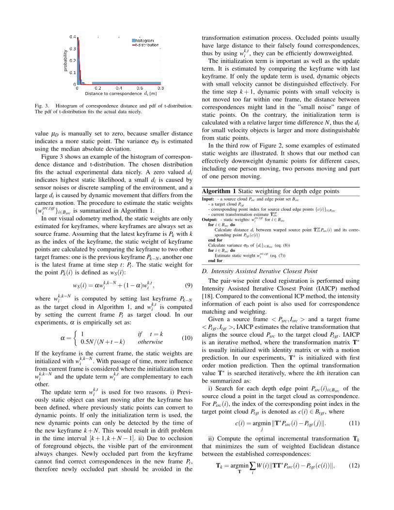
Our SLAM system is compared to a non real-time method[24], which is a recent state-of-the-art RGB-D SLAMmethod for dynamic environment. In [24], dense dynamicobject segmentation is performed for each frame, which takeshalf second per frame. The authors segment dynamic objectsfrom each frame, and directly use the segmented framesas input for DVO-SLAM system [12]. The comparison isshown in Table II. The first column shows the sequence namefrom the TUM Dataset, where both low-dynamic ”sitting”sequences and high-dynamic ”walking” sequences are usedfor comparison. Our SLAM system works better in most ofthe sequences. The improvement for low-dynamic sequencesis 15.2%, and the improvement for high-dynamic sequencesis more notable with 24.7%.

TABLE IISLAM RESULTS: RMSE OF ABSOLUTE TRAJECTORY ERROR [M]

sequence Motion Remvoal+DVO SLAM [24] Our SLAM system

RMSE standarddeviation RMSE standard

deviationfr3/walking halfsphere 0.1252 0.0903 0.0489 0.7266fr3/walking rpy 0.1333 0.0839 0.1791 0.1161fr3/walking static 0.0656 0.0536 0.0261 0.0122fr3/walking xyz 0.0932 0.0534 0.0601 0.0330fr3/sitting halfsphere 0.0470 0.0249 0.0432 0.0246fr3/sitting xyz 0.0482 0.0282 0.0397 0.0206fr2/desk with person 0.0596 0.0239 0.0484 0.0237

The average computation time for our SLAM systemtakes ca. 45ms per frame, including visual odometry esti-mation, loop closure detection and pose graph optimization.Compared to this, the method from [24] cannot be appliedfor real-time application, since their segmentation procedurealone already takes half second per frame.

VI. CONCLUSIONWe proposed a real-time RGB-D visual odometry method

that can handle highly dynamic environment such as the”walking” sequences from TUM Dataset [23]. The methoduses foreground depth edge point to compute pair-wisepoint cloud registration. A robust static weighting strategyis proposed based on depth edge correspondences distance.Fusing the static weighting strategy into the intensity assistedICP [18], our visual odometry system handles dynamic en-vironment robustly. Furthermore, loop closure detection andmap optimization are integrated, resulting a real-time SLAMsystem suitable for dynamic environment. Our method isevaluated on the dynamic sequences from TUM Dataset [23].Compared to state-of-the-art real-time method [15], in termsof translational drift per second, our method improves thevisual odometry accuracy by 58% in challenging ”walk-ing” sequences. The performance of our SLAM system isalso proven using the TUM Dataset, which shows betterperformance than recent non real-time method [24]. In ourmethod, the static weighting is only applied to foregrounddepth edges. Therefore our visual odometry method requiresgeometry rich environments, where a lot of depth edges exist.In future work, we want to investigate how to efficientlypropagate the sparsely estimated static weights to the entireimage, such that denser information can be used for regis-tration.

REFERENCES

[1] K. S. Arun, T. S. Huang, and S. D. Blostein. Least-squares fittingof two 3-D point sets. IEEE Transactions on Pattern Analysis andMachine Intelligence, (5):698–700, 1987.

[2] P. J. Besl and N. D. McKay. Method for registration of 3-D shapes. InRobotics-DL tentative, pages 586–606. International Society for Opticsand Photonics, 1992.

[3] L. Bose and A. Richards. Fast depth edge detection and edge basedRGB-D SLAM. In IEEE International Conference on Robotics andAutomation (ICRA), pages 1323–1330. IEEE, 2016.

[4] C. Choi, A. J. Trevor, and H. I. Christensen. RGB-D edge detectionand edge-based registration. In IEEE/RSJ International ConferenceonIntelligent Robots and Systems (IROS), pages 1568–1575, 2013.

[5] D. W. Eggert, A. Lorusso, and R. B. Fisher. Estimating 3-D rigidbody transformations: a comparison of four major algorithms. MachineVision and Applications, 9(5-6):272–290, 1997.

[6] F. Endres, J. Hess, J. Sturm, D. Cremers, and W. Burgard. 3-Dmapping with an RGB-D camera. IEEE Transactions on Robotics,30(1):177–187, 2014.

[7] G. Grisetti, R. Kummerle, C. Stachniss, and W. Burgard. A tutorial ongraph-based slam. IEEE Intelligent Transportation Systems Magazine,2(4):31–43, 2010.

[8] D. Gutierrez-Gomez, W. Mayol-Cuevas, and J. Guerrero. Inverse depthfor accurate photometric and geometric error minimisation in RGB-Ddense visual odometry. In IEEE International Conference on Roboticsand Automation (ICRA), pages 83–89, 2015.

[9] P. Henry, M. Krainin, E. Herbst, X. Ren, and D. Fox. RGB-Dmapping: Using kinect-style depth cameras for dense 3D modeling ofindoor environments. The International Journal of Robotics Research,31(5):647–663, 2012.

[10] P. Henry, M. Krainin, E. Herbst, X. Ren, and D. Fox. RGB-D mapping:Using depth cameras for dense 3D modeling of indoor environments.In Experimental robotics, pages 477–491. Springer, 2014.

[11] S. Izadi, D. Kim, O. Hilliges, D. Molyneaux, R. Newcombe, P. Kohli,J. Shotton, S. Hodges, D. Freeman, A. Davison, et al. Kinectfusion:real-time 3D reconstruction and interaction using a moving depthcamera. In Proceedings of the 24th annual ACM symposium on Userinterface software and technology, pages 559–568, 2011.

[12] C. Kerl, J. Sturm, and D. Cremers. Dense visual slam for RGB-Dcameras. In IEEE/RSJ International Conference on Intelligent Robotsand Systems (IROS), pages 2100–2106, 2013.

[13] C. Kerl, J. Sturm, and D. Cremers. Robust odometry estimation forRGB-D cameras. In IEEE International Conference onRobotics andAutomation (ICRA), pages 3748–3754, 2013.

[14] D.-H. Kim, S.-B. Han, and J.-H. Kim. Visual odometry algorithmusing an RGB-D sensor and IMU in a highly dynamic environment.In Robot Intelligence Technology and Applications 3, pages 11–26.Springer, 2015.

[15] D.-H. Kim and J.-H. Kim. Effective background model-based RGB-Ddense visual odometry in a dynamic environment. IEEE Transactionson Robotics, 32(6):1565–1573, 2016.

[16] S. Klose, P. Heise, and A. Knoll. Efficient compositional approachesfor real-time robust direct visual odometry from RGB-D data. InIEEE/RSJ International Conference on Intelligent Robots and Systems(IROS), pages 1100–1106, 2013.

[17] T.-S. Leung and G. Medioni. Visual navigation aid for the blind indynamic environments. In IEEE Conference on Computer Vision andPattern Recognition Workshops, pages 565–572, 2014.

[18] S. Li and D. Lee. Fast visual odometry using intensity-assisted iterativeclosest point. IEEE Robotics and Automation Letters, 1(2):992–999,2016.

[19] M. Meilland, A. Comport, P. Rives, et al. A spherical robot-centeredrepresentation for urban navigation. In IEEE/RSJ International Con-ference onIntelligent Robots and Systems (IROS), pages 5196–5201,2010.

[20] R. A. Newcombe and A. J. Davison. Live dense reconstruction with asingle moving camera. In IEEE Conference on Computer Vision andPattern Recognition (CVPR), pages 1498–1505, 2010.

[21] R. A. Newcombe, S. Izadi, O. Hilliges, D. Molyneaux, D. Kim,A. J. Davison, P. Kohi, J. Shotton, S. Hodges, and A. Fitzgibbon.Kinectfusion: Real-time dense surface mapping and tracking. In IEEEinternational symposium on Mixed and augmented reality (ISMAR),pages 127–136, 2011.

[22] J. Stuckler and S. Behnke. Multi-resolution surfel maps for efficientdense 3D modeling and tracking. Journal of Visual Communicationand Image Representation, 25(1):137–147, 2014.

[23] J. Sturm, N. Engelhard, F. Endres, W. Burgard, and D. Cremers. Abenchmark for the evaluation of RGB-D SLAM systems. In IEEE/RSJInternational Conference on Intelligent Robots and Systems (IROS),pages 573–580, 2012.

[24] Y. Sun, M. Liu, and M. Q.-H. Meng. Improving RGB-D SLAM indynamic environments: A motion removal approach. Robotics andAutonomous Systems, 89:110–122, 2017.

[25] T. Tykkala, C. Audras, A. Comport, et al. Direct iterative closest pointfor real-time visual odometry. In IEEE International Conference onComputer Vision Workshops, pages 2050–2056, 2011.

[26] Y. Wang and S. Huang. Towards dense moving object segmentationbased robust dense RGB-D SLAM in dynamic scenarios. In 13thInternational Conference on Control Automation Robotics & Vision(ICARCV), pages 1841–1846. IEEE, 2014.

[27] T. Whelan, H. Johannsson, M. Kaess, J. J. Leonard, and J. McDonald.Robust real-time visual odometry for dense RGB-D mapping. In IEEEInternational Conference on Robotics and Automation (ICRA), pages5724–5731, 2013.