report deep foundations.pdf

Final Report

FHWA/IN/JTRP-2004/21

Limits States Design of Deep Foundations

by

Kevin Foye Graduate Research Assistant

Grace Abou Jaoude

Graduate Research Assistant

Rodrigo Salgado Professor

School of Civil Engineering

Purdue University

Joint Transportation Research Program Project No. C-36-36HH

File No. 6-14-34 SPR-2406

Conducted in Cooperation with the Indiana Department of Transportation

and the U.S. Department of Transportation Federal Highway Administration

The contents of this report reflect the views of the authors who are responsible for the facts and accuracy of the data presented herein. The contents do not necessarily reflect the official views or policies of the Federal Highway Administration or the Indiana Department of Transportation. This report does not constitute a standard, specification, or regulation.

Purdue University West Lafayette, Indiana

December 2004

62-1 12/04 JTRP-2004/21 INDOT Division of Research West Lafayette, IN 47906

INDOT Research

TECHNICAL Summary Technology Transfer and Project Implementation Information

TRB Subject Code: 62-1 Foundation Soils December 2004 Publication No.: FHWA/IN/JTRP-2004/21, SPR-2406 Final Report

Limit States Design of Deep Foundation Introduction

Foundation design consists of selecting and proportioning foundations in such a way that limit states are prevented. Limit states are of two types: Ultimate Limit States (ULS) and Serviceability Limit States (SLS). ULSs are associated with danger, involving such outcomes as structural collapse. SLSs are associated with impaired functionality, and in foundation design are often caused by excessive settlement. Reliability-based design (RBD) is a design philosophy that aims at keeping the probability of reaching limit states lower than some limiting value. Thus, a direct assessment of risk is possible with RBD. This evaluation is not possible with traditional working stress design. The use of RBD directly in projects is not straightforward and is cumbersome to designers, except in large-budget projects. Load and Resistance Factor Design (LRFD) shares most of the benefits of RBD while being much simpler to apply. LRFD has traditionally been used for ULS checks, but SLS's have been brought into the LRFD framework recently (AASHTO 1998). Load and Resistance Factor Design (LRFD) is a design method in which design loads are increased and design resistances are reduced through multiplication by factors that are greater than one and less than one, respectively. In this method, foundations are proportioned so that the factored loads are not greater than the factored resistances. In order for foundation design to be consistent with current structural design practice, the use of the same loads, load factors and load combinations would be required. In this study, we review the load factors presented in various LRFD Codes from the US, Canada and Europe. A simple first-order second moment (FOSM) reliability analysis is presented to determine appropriate

ranges for the values of the load factors. These values are compared with those proposed in the Codes. For LRFD to gain acceptance in geotechnical engineering, a framework for the objective assessment of resistance factors is needed. Such a framework, based on reliability analysis is proposed in this study. Probability Density Functions (PDFs), representing design variable uncertainties, are required for analysis. A systematic approach to the selection of PDFs is presented. Such a procedure is a critical prerequisite to a rational probabilistic analysis in the development of LRFD methods in geotechnical engineering. Additionally, in order for LRFD to fulfill its promise for designs with more consistent reliability, the methods used to execute a design must be consistent with the methods assumed in the development of the LRFD factors. In this study, a methodology for the estimation of soil parameters for use in design equations is proposed that should allow for more statistical consistency in design inputs than is possible in traditional methods.

The primary objective of this study is to propose a Limit States Design method for shallow and deep foundations that is based on a rational, probability-based investigation of design methods. In particular, Load and Resistance Factor Design is used to facilitate the Limit States Design methodology. Specifically, the objectives of the study are to 1) provide guidance on the choice of values for load factors; 2) develop recommendations on how to determine characteristic soil resistances under various design settings; 3) develop resistance factors compatible with the load factors and the method of determining characteristic resistance.


Findings This research was able to develop a

systematic framework for the assessment of resistance factors for geotechnical LRFD. Several steps comprise this framework: a) the design equations are identified; b) all variables showing in the design equation are decomposed to identify all component quantities; c) probabilistic models for the uncertain quantities are developed using all available data; d) reliability analysis is used to determine the limit state values corresponding to a set of nominal design values at a specified reliability index; e) resistance factors are determined algebraically from the corresponding nominal and limit state values. In order for LRFD to fulfill its promise for designs with more consistent reliability, the methods used to execute a design must be consistent with the methods assumed in the development of the LRFD factors. In this study, a methodology for the estimation of soil parameters for use in design equations is proposed to allow for more statistical consistency in design inputs than is possible in traditional methods. This methodology, called the conservatively assessed mean (CAM) method, is defined so that 80% of the measured values of a specific property are likely to fall above the CAM value. We were able

to show that the CAM procedure tends to stabilize the reliability of design checks completed using particular RF values even when the uncertainty of the soil at a site is different from that assumed in the analysis. The primary objective of this study is to propose a LRFD method for shallow and deep foundations that is based on a rational, probability-based investigation of design methods. Since resistance factor values are dependent upon the values of load factors used, a method to adjust the resistance factors to account for code-specified load factors is presented. Resistance factors for ultimate bearing capacity are then computed using reliability analysis for shallow and deep foundations both in sand and in clay, for use with both ASCE-7 (1996) and AASHTO (1998) load factors. The various considered methods obtain their input parameters from the CPT, the SPT, or laboratory testing.

Finally, designers may wish to use design methods that are not considered in this study. As such, the designer needs the capability to select resistance factors that reflect the uncertainty of the design method chosen. A methodology is proposed in this study to accomplish this task, in a way that is consistent with the framework.

Implementation The resistance factor results of this study could be used to develop future LRFD codes for geotechnical design. As a first step towards implementation, Purdue University and INDOT are organizing a workshop to educate designers on the principles and application of the resistance factors and their associated design methods. This workshop will form the basis for INDOT designers to explore the use of these methods in support of code development. It is important to note that in order for LRFD to fulfill its promise for designs with more consistent reliability, the soil investigation forming the basis of a geotechnical design must be consistent with the interpretation methods assumed in the development of the LRFD factors. Thus, the concept of the CAM method must be implemented as the first component of the LRFD methodology. The implementation of

the CAM method would not require additional efforts than those already common in soil investigations. It is easily applied and is demonstrated in the design examples in this study report. In summary, the key areas of implementation are

• to hold a workshop on LRFD to introduce geotechnical engineers to the application of LRFD to foundations

• the use of the Conservatively Assessed Mean procedure to improve the repeatability of soil property assessments

the shift to the use of factored loads and resistance factors in the assessment of design resistances for foundations.


Contacts For more information: Prof. Rodrigo Salgado Principal Investigator School of Civil Engineering Purdue University West Lafayette IN 47907 Phone: (765) 494-5030 Fax: (765) 496-1364 E-mail: [email protected]

Indiana Department of Transportation Division of Research 1205 Montgomery Street P.O. Box 2279 West Lafayette, IN 47906 Phone: (765) 463-1521 Fax: (765) 497-1665 Purdue University Joint Transportation Research Program School of Civil Engineering West Lafayette, IN 47907-1284 Phone: (765) 494-9310 Fax: (765) 496-7996

TECHNICAL REPORT STANDARD TITLE PAGE 1. Report No.

2. Government Accession No.

3. Recipient's Catalog No.

FHWA/IN/JTRP-2004/21

4. Title and Subtitle Limit States Design of Deep Foundations

5. Report Date December 2004

6. Performing Organization Code 7. Author(s) Kevin Foye, Grace Abou Jaoude, and Rodrigo Salgado

8. Performing Organization Report No. FHWA/IN/JTRP-2004/21

9. Performing Organization Name and Address Joint Transportation Research Program 550 Stadium Mall Drive Purdue University West Lafayette, IN 47907-2051

10. Work Unit No.

11. Contract or Grant No.

SPR-2406 12. Sponsoring Agency Name and Address Indiana Department of Transportation State Office Building 100 North Senate Avenue Indianapolis, IN 46204

13. Type of Report and Period Covered

Final Report

14. Sponsoring Agency Code

15. Supplementary Notes Prepared in cooperation with the Indiana Department of Transportation and Federal Highway Administration. 16. Abstract Load and Resistance Factor Design (LRFD) shows promise as a viable alternative to the present working stress design (WSD) approach to foundation design. The key improvements of LRFD over the traditional Working Stress Design (WSD) are the ability to provide a more consistent level of reliability and the possibility of accounting for load and resistance uncertainties separately. In order for foundation design to be consistent with current structural design practice, the use of the same loads, load factors and load combinations would be required. In this study, we review the load factors presented in various LRFD Codes from the US, Canada and Europe. A simple first-order second moment (FOSM) reliability analysis is presented to determine appropriate ranges for the values of the load factors. These values are compared with those proposed in the Codes. The comparisons between the analysis and the Codes show that the values of load factors given in the Codes generally fall within ranges consistent with the results of the FOSM analysis. For LRFD to gain acceptance in geotechnical engineering, a framework for the objective assessment of resistance factors is needed. Such a framework, based on reliability analysis is proposed in this study. Probability Density Functions (PDFs), representing design variable uncertainties, are required for analysis. A systematic approach to the selection of PDFs is presented. Such a procedure is a critical prerequisite to a rational probabilistic analysis in the development of LRFD methods in geotechnical engineering. Additionally, in order for LRFD to fulfill its promise for designs with more consistent reliability, the methods used to execute a design must be consistent with the methods assumed in the development of the LRFD factors. In this study, a methodology for the estimation of soil parameters for use in design equations is proposed that should allow for more statistical consistency in design inputs than is possible in traditional methods. Resistance factor values are dependent upon the values of load factors used. Thus, a method to adjust the resistance factors to account for code-specified load factors is also presented. Resistance factors for ultimate bearing capacity are computed using reliability analysis for shallow and deep foundations both in sand and in clay, for use with both ASCE-7 (1996) and AASHTO (1998) load factors. The various considered methods obtain their input parameters from the CPT, the SPT, or laboratory testing. Designers may wish to use design methods that are not considered in this study. As such, the designer needs the capability to select resistance factors that reflect the uncertainty of the design method chosen. A methodology is proposed in this study to accomplish this task, in a way that is consistent with the framework. 17. Key Words Load and Resistance Factor Design (LRFD); Geotechnical Engineering; Foundation Design; in-situ testing; Reliability-Based Design (RBD); Probability.

18. Distribution Statement No restrictions. This document is available to the public through the National Technical Information Service, Springfield, VA 22161

19. Security Classif. (of this report)

Unclassified

20. Security Classif. (of this page)

Unclassified

21. No. of Pages 234

22. Price

Form DOT F 1700.7 (8-69)

i

i

ACKNOWLEDGEMENTS

Bryan Scott and Bumjoo Kim, former Purdue Graduate students, were responsible

for writing the material on load factors. Bryan Scott also made significant contributions

to the assessment of shallow foundation uncertainty and resistance factors. Their work is

greatly appreciated as it is a significant contribution to this final report.

ii

TABLE OF CONTENTS

Page

LIST OF TABLES ........................................................................................................... iv

LIST OF FIGURES ....................................................................................................... viii

CHAPTER 1. Introduction ................................................................................................. 1

1.1 Background ............................................................................................................ 1

1.2 Study Objectives .................................................................................................... 3

1.3 Report Organization ............................................................................................... 4

CHAPTER 2. Assessment of Current Load Factors .......................................................... 5

2.1 Introduction ............................................................................................................ 5

2.2 Load And Resistance Factor Design (LRFD) and Limit States ............................. 6

2.3 Load Factors Proposed By LRFD Codes in the US, Canada, And Europe ........... 7

2.4 Simple Reliability Analysis ................................................................................. 13

2.5 Selection of Parameters Used in the Analysis ..................................................... 20

2.6 Comparison Between Results and Load Factors in the Codes ............................ 22

2.7 Future Development of Geotechnical LRFD Design ........................................... 24

2.8 Summary and Conclusions .................................................................................. 25

2.9 Notation ................................................................................................................ 27

CHAPTER 3. Methodology to Determine Resistance Factors ........................................ 39

3.1 A Rational Framework for Evaluating Resistance Factors .................................. 40

3.2 Tools to Assess Uncertainty ................................................................................. 41

3.3 Tools to Assess Resistance Factors ...................................................................... 49

iii

3.4 Summary .............................................................................................................. 55

CHAPTER 4. Assessment of Variable Uncertainties for Shallow Foundations ............. 57

4.1 Assessment of Uncertainty in Bearing Capacity of Footings on Sand ................ 57

4.2 Assessment of Uncertainty in Bearing Capacity of Footings on Clay ................. 70

4.3 Summary .............................................................................................................. 74

CHAPTER 5. Assessment of Resistance Factors for Shallow Foundations .................... 75

5.1 Calculation of Resistance Factors ........................................................................ 75

5.2 Characteristic Resistance ..................................................................................... 85

CHAPTER 6. Design Examples for Shallow Foundations .............................................. 91

CHAPTER 7. Assessment of Design Methods for Deep Foundations .......................... 103

7.1 LRFD Design of Piles ........................................................................................ 103

7.2 Design of Piles in Sand ...................................................................................... 106

7.3 Design of Piles in Clay ...................................................................................... 114

CHAPTER 8. Resistance Factors for Deep Foundations on Sand ................................. 121

8.1 Assessment of Variable Uncertainties for Deep Foundations on Sand .............. 121

8.2 Assessment of Resistance Factors ..................................................................... 161

CHAPTER 9. Resistance Factors for Deep Foundations on Clay ................................. 175

9.1 Assessment of Variable Uncertainties for Deep Foundations on Clay .............. 175

9.2 Assessment of Resistance Factors ..................................................................... 185

CHAPTER 10. Design Examples for Deep Foundations .............................................. 195

CHAPTER 11. Summary and Conclusions ................................................................... 209

LIST OF REFERENCES ............................................................................................... 217

viii

LIST OF TABLES

Table Page Table 2.3.1 Load Factors ..................................................................................................29

Table 2.3.2 Load Factors and Gravity Load Combinations..............................................30

Table 2.3.3 Load Factors for SLS.....................................................................................31

Table 2.5.1 Ratio of Mean to Nominal Load and Coefficient of Variation......................32

Table 2.5.2 Values of Ratio of Mean to Nominal Load and Coefficient of Variation used

for the analysis ...................................................................................................................33

Table 2.6.1 Comparison of the Values of Load Factors ...................................................34

Table 3.2.1 Values of Number of Standard Deviations (Nσ) (after Tippett 1925) ..........44

Table 4.1.1 COVs, Bias Factors and Distribution Types for use in a Probabilistic

Analysis of Bearing Capacity on Sand and Clay ...............................................................60

Table 4.1.2 COVs, bias factors and distribution types for bearing capacity factors for use

in reliability analysis of footings on sand using the CPT ..................................................69

Table 4.1.3 COVs, bias factors and distribution types for bearing capacity factors for use

in reliability analysis of footings on sand using the SPT...................................................69

Table 4.2.1 Uniform Distribution Bounds on Ncscdc for varying embedment ratios for use

in a Probabilistic Analysis of Bearing Capacity on Clay (Salgado et al. 2004) ................74

Table 5.1.1 Recommended RFs for Bearing Capacity on Sand and Clay ........................81

Table 6.1 CPT qc log statistics ..........................................................................................94

Table 6.2 Bearing Capacity Factors in Sand Example .....................................................95

Table 6.3 Results of CPT Design Example on Sand and Clay .........................................98

Table 7.2.1 Summary of Selected Design Methods for Reliability Analysis in Sands ...113

ix

Table 7.3.1 Values of α and K for use with Aoki and Velloso (1975) direct design

method..............................................................................................................................117

Table 7.3.2 Values of F1 and F2 for use with Aoki and de Alencar Velloso (1975) direct

design method ..................................................................................................................117

Table 7.3.3 Summary of Selected Design Methods for Reliability Analysis in Clays...119

Table 8.1.1 Summary Statistics for Composite Uncertainty of Modulus G ..................157

Table 8.2.1 Summary Table for the Design of Deep Foundations in Sand. . ................162

Table 8.2.2 Results of Resistance Factor Evaluation for Property-Based Shaft Capacity

of Closed Ended Piles in Sand for ASCE-7 Load Factors...............................................165

Table 8.2.3 Results of Resistance Factor Evaluation for Property-Based Base Capacity of

Closed Ended Piles in Sand for ASCE-7 Load Factors ...................................................167

Table 8.2.4 Results of Resistance Factor Evaluation for Direct Base Capacity of Closed

Ended Piles in Sand for ASCE-7 Load Factors ...............................................................169

Table 8.2.5 Results of Resistance Factor Evaluation for Property-Based Shaft Capacity

of Open Ended Piles in Sand for ASCE-7 Load Factors .................................................170


Open Ended Piles in Sand for ASCE-7 Load Factors......................................................171

Table 8.2.7 Results of Resistance Factor Evaluation for Direct Shaft Capacity of Open-

Ended Pipe Piles in Sand for ASCE-7 Load Factors .......................................................171

Table 8.2.8 Results of Resistance Factor Evaluation for Direct Base Capacity of Open

Ended Piles in Sand for ASCE-7 Load Factors ...............................................................172


Drilled Shafts in Sand for ASCE-7 Load Factors............................................................173

x

Table 8.2.10 Results of Resistance Factor Evaluation for Direct Base Capacity of Drilled

Shafts in Sand for ASCE-7 Load Factors ........................................................................174

Table 9.2.1 – Summary Table for the Design of Deep Foundations in Clay...................186

Table 9.2.2 – Results of Resistance Factor Evaluation for Property-Based Shaft Capacity

of Driven Piles in Clay.....................................................................................................191

Table 9.2.3 – Results of Resistance Factor Evaluation for Property-Based Base Capacity

of Driven Piles in Clay.....................................................................................................192

Table 9.2.4 – Results of Resistance Factor Evaluation for Aoki and de Velloso (1975)

Direct SPT Design Method..............................................................................................192

Table 10.1. CPT qc log statistics to find CAM line in sand layers in Figure 10.1..........199

Table 10.2 Summary of Design Trial for Shaft Resistance in Sand ...............................200

Table 10.3 Hypothetical Load Test Database .................................................................205

iv

LIST OF FIGURES

Figure Page

Figure 2.4.1 Load Effects, Resistance and Reliability ................................................. 35

Figure 2.5.1 Variation of Separation Coefficient, α .................................................... 36

Figure 2.6.1 Comparison of Analysis and the Codes ................................................... 37

Figure 3.2.1 Mean Trend (power regression) and Bounds of CPT Tip Resistance Data

for Sand .....................................................................................................43

Figure 3.2.2 The Mean, Nominal, and Limit State Values of a Normally Distributed

Design Parameter ..................................................................................... 48

Figure 3.3.1 Depiction of Reliability Index ................................................................. 52

Figure 4.1.1 Sources of Uncertainty with Coefficients of Variation (COVs) for Bearing

Capacity in Sand ...................................................................................... 59

Figure 4.1.2 The Mean, Nominal, and Limit State Values of a Normally Distributed

Design Parameter ..................................................................................... 62

Figure 4.1.3 Mean Trend (Power Regression) and Bounds of Cpt Tip Resistance Data

for Sand .................................................................................................... 64

Figure 4.1.4 SPT – CPT Correlation (after Robertson et. al.,1983 and Ismael and Jeragh,

1986) ........................................................................................................ 65

Figure 4.1.5 Example Histograms of Monte Carlo Simulation (MC) and Numerical

Integration (NI) Results for φp, Nq, Nγ, and sq .......................................... 70

Figure 5.1.1 Adjusted Resistance Factors for Footings on Sand using CPT ................ 77

Figure 5.1.2 Adjusted Resistance Factors for Footings on Sand using SPT ................ 78

v

Figure 5.1.3 Two-Dimensional Explanation (similar to Figure 3.2.1c) of RF Curve

Shapes in Figure 5.1.1(a-c) and Figure 5.1.2(a-b) ................................... 79

Figure 5.1.4 Adjusted Resistance Factors for Footings on Clay using CPT ................ 84

Figure 5.1.5 Adjusted Resistance Factors for a Square Footing, LL/DL = 1.0, varying

β .............................................................................................................. 85

Figure 5.2.1 Visual Approximation of CAM Function for a CPT Profile ................... 87

Figure 5.2.2 Adjusted Resistance Factors Computed Using CPT Profiles with Different

Variabilities .............................................................................................. 90

Figure 6.1 General design flow for geotechnical engineering .................................. 91

Figure 6.2 LRFD flow chart for ULS checks for foundation design ........................ 92

Figure 6.3 CPT logs with Best Fit Lines and Range Lines ....................................... 93

Figure 7.3.1 Measured vs. Calculated Total Pile Resistance in Study by Aoki and

Velloso (1975) for Franki, Cased Franki, Precast, and Steel piles ........ 119

Figure 8.1.1 K/K0 Relationship by Paik and Salgado (2003) for closed-ended piles

(PLR = 0) and fully unplugged open-ended piles (PLR = 1) ................. 126

Figure 8.1.2 δc/φc Values Based on Results from High Quality, Direct Interface Shear

Tests ....................................................................................................... 127

Figure 8.1.3 Histogram of δc/φc Values for Ra > 2µm, Based on Results from High

Quality, Direct Interface Shear Tests .................................................... 128

Figure 8.1.4 qb,10%/qc Values Based on Results from High Quality, Instrumented Pile

Load Tests .............................................................................................. 131

Figure 8.1.5 Histogram of errorqb,10%/qc (detrended qb,10%/qc values) for Closed-Ended

Piles in Sand ........................................................................................... 132

vi

Figure 8.1.6 Histogram of qbL for DR = 80% for Closed-Ended Piles in Sand ........... 134

Figure 8.1.7 Average Ks/K0 Values from Paik and Salgado (2003) for Open-Ended

Piles in Sand ........................................................................................... 139

Figure 8.1.8 Histogram of errorKs/Ko (detrended Ks/K0 values) for Open-Ended Piles in

Sand ........................................................................................................ 141

Figure 8.1.9 Histogram of errorqb,10%/σ’h (detrended qb,10%/σ’h values) for Open-Ended

Piles in Sand ........................................................................................... 144

Figure 8.1.10 Histogram Representing the Composite Uncertainty for qb,10%/σ’h ....... 146

Figure 8.1.11 qb,10%/qc vs. IFR(%) from Paik and Salgado (2003) with Trend Line

Proposed by Lee et al. (2003) ................................................................ 150

Figure 8.1.12 Histogram of errorqb,10%/qc (detrended qb,10%/qc values) for Open-Ended

Piles in Sand ........................................................................................... 151

Figure 8.1.13 Uncertainty Propagation for Modeling Drilled Shaft Base Movement,

from CONPOINT Estimates of DR to Modulus Es ................................. 154

Figure 8.1.14 Variation of Curve Fitting Parameters f and g with DR (Lee and Salgado

1999) ...................................................................................................... 158

Figure 9.1.1 Measured Values of α Compared to Equations Proposed by Randolph and

Murphy (1985) (Flemming et al. 1992) ................................................. 177

Figure 9.1.2 Histogram of the α Data Points Detrended by Equation (9.1.2) ............ 178

Figure 9.1.3 Measured vs. Calculated Total Pile Resistance in Study by Aoki and

Velloso (1975) for Franki, Cased Franki, Precast, and Steel piles ........ 181

Figure 9.1.4 Histogram of the ( )bs RR + Measured Data Points Detrended by the

Calculated Datapoints from Figure 9.1.3 ............................................... 183

vii

Figure 9.2.1 Plot of Adjusted Resistance Factor RF Varying with Total Resistance

COV and Target Reliability Index β (ASCE-7 LFs) ............................. 189

Figure 9.2.2 Plot of Adjusted Resistance Factor RF Varying with Total Resistance

COV and Target Reliability Index β (AASHTO LFs) ........................... 190

Figure 10.1 LRFD flow chart for ULS checks for foundation design ...................... 196

Figure 10.2 Results from 7 CPT logs in sand with mean trend (“best fit”) lines and

Range Lines (BCP Committee 1971) .................................................... 198

Figure 10.3 Normalized IFR Plot from Lee et al. (2003) .......................................... 201

Figure 10.4 Plot of Adjusted Resistance Factor RF Varying with Total Resistance

COV and Target Reliability Index β (ASCE-7 LFs) ............................. 206

1

CHAPTER 1. INTRODUCTION

1.1 Background

Foundation design consists of selecting and proportioning foundations in such a

way that limit states are prevented. Limit states are of two types: Ultimate Limit States

(ULS) and Serviceability Limit States (SLS). ULSs are associated with danger, involving

such outcomes as structural collapse. SLSs are associated with impaired functionality,

and in foundation design are often caused by excessive settlement. Reliability-based

design (RBD) is a design philosophy that aims at keeping the probability of reaching

limit states lower than some limiting value. In other words, the goal of design is to

produce structures that have probabilities of failure less than a prescribed acceptable

value. Thus, a direct assessment of risk is possible with RBD. This evaluation is not

possible with traditional working stress design. The use of RBD directly in projects is

not straightforward and is cumbersome to designers, except in large-budget projects.

Load and Resistance Factor Design (LRFD) is a design methodology that is similar to

existing practice, but can be developed using RBD concepts. LRFD shares most of the

benefits of RBD while being much simpler to apply. LRFD has traditionally been used

for ULS checks in structures, but SLS have been brought into the LRFD framework

recently (AASHTO 1998).

Load and Resistance Factor Design (LRFD) is a design method in which design

loads are increased and design resistances are reduced through multiplication by factors

that are greater than one and less than one, respectively. In this method, foundations are

proportioned so that the factored loads are not greater than the factored resistances:

2

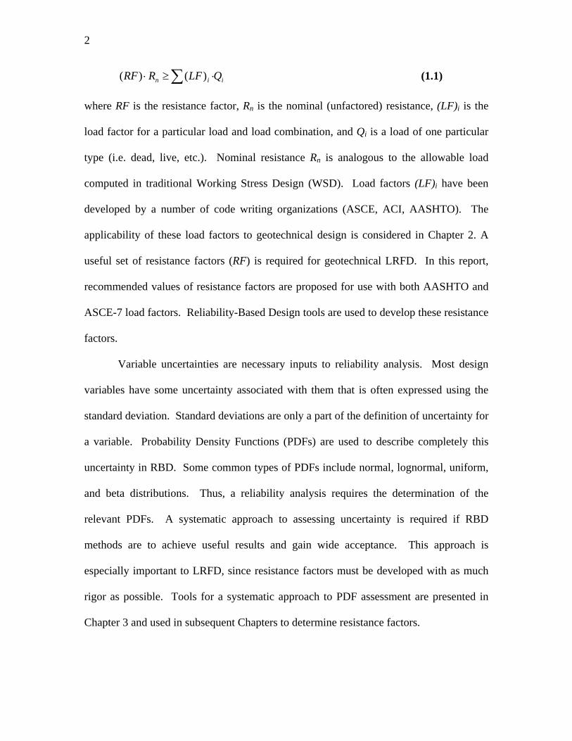
iin QLFRRF ∑ ⋅≥⋅ )()( (1.1)

where RF is the resistance factor, Rn is the nominal (unfactored) resistance, (LF)i is the

load factor for a particular load and load combination, and Qi is a load of one particular

type (i.e. dead, live, etc.). Nominal resistance Rn is analogous to the allowable load

computed in traditional Working Stress Design (WSD). Load factors (LF)i have been

developed by a number of code writing organizations (ASCE, ACI, AASHTO). The

applicability of these load factors to geotechnical design is considered in Chapter 2. A

useful set of resistance factors (RF) is required for geotechnical LRFD. In this report,

recommended values of resistance factors are proposed for use with both AASHTO and

ASCE-7 load factors. Reliability-Based Design tools are used to develop these resistance

factors.

Variable uncertainties are necessary inputs to reliability analysis. Most design

variables have some uncertainty associated with them that is often expressed using the

standard deviation. Standard deviations are only a part of the definition of uncertainty for

a variable. Probability Density Functions (PDFs) are used to describe completely this

uncertainty in RBD. Some common types of PDFs include normal, lognormal, uniform,

and beta distributions. Thus, a reliability analysis requires the determination of the

relevant PDFs. A systematic approach to assessing uncertainty is required if RBD

methods are to achieve useful results and gain wide acceptance. This approach is

especially important to LRFD, since resistance factors must be developed with as much

rigor as possible. Tools for a systematic approach to PDF assessment are presented in

Chapter 3 and used in subsequent Chapters to determine resistance factors.

3

As a first step in design, geotechnical engineers interpret tests and other data to

assess soil parameters. Soil parameters for use in a design equation must be determined

in a reproducible way that is consistent with the resistance factor. This is a crucial issue

among several that must be addressed before reliability-based design methods, such as

LRFD, reach their full potential in geotechnical design (Becker 1996, Kulhawy and

Phoon 2002). The cone penetration test (CPT) is used to illustrate a method to estimate

soil parameters in a statistically consistent manner in Chapter 5.

1.2 Study Objectives

The primary objective of this study is to propose a Limit States Design method for

shallow and deep foundations that is based on a rational, probability-based investigation

of design methods. In particular, Load and Resistance Factor Design is used to facilitate

the Limit States Design methodology. Specifically, the objectives of the study are to

• provide guidance on the choice of values for load factors for permanent and

temporary loads of different types and under various combinations;

• Develop recommendations on how to determine characteristic soil resistances

under various design settings (including type of soil, type of soil investigation,

type of analysis, etc.);

• Develop resistance factors compatible with the load factors and the method of

determining characteristic resistance.

4

1.3 Report Organization

• Chapter 2 is a discussion of available code prescribed load factors and the

results of an investigation into their applicability to geotechnical design.

• In Chapter 3 we propose a framework for LRFD factor development. We also

present probability tools to assess the variable uncertainty and resistance

factors.

• In Chapters 4 and 5 we apply the framework from Chapter 3 to shallow

foundations. Section 5.2 describes a method to determine characteristic

resistance that is compatible with the resistance factors proposed in this report.

• In Chapter 6 we demonstrate shallow foundation design using the

characteristic resistance method and the LRFD factors.

• Chapter 7 is an introduction to the deep foundation design methods that we

aim to integrate into the LRFD framework.

• In Chapter 8 and 9 we present the resistance factors for deep foundations in

sand and clay, respectively. Section 9.2.1 describes a method for designers to

select resistance factors for design methods other than those discussed in this

report.

• In Chapter 10 we demonstrate deep foundation design using the characteristic

resistance method and the LRFD factors.

• In Chapter 11 we summarize the study, highlight its contributions and

identify potential future directions for research.

5

CHAPTER 2. ASSESSMENT OF CURRENT LOAD FACTORS

2.1 Introduction

Over the past 4 decades, a load and resistance factor design (LRFD) method was

brought into practice in the United States with the adoption of the American Concrete

Institute Building Design Code (ACI) in 1963 (Goble 1999). In structural design practice,

LRFD is currently accepted worldwide along with a traditional design method, allowable

stress design (ASD), or as it is also known, working stress design (WSD). With the trend

toward the increased use of LRFD, new LRFD Codes in the US, Canada and Europe

(AASHTO 1994, API 1993, MOT 1992, NRC 1995, and ECS 1994) have included the

implementation of LRFD for geotechnical design over the past several years.

Additionally, an ACI document in preparation also advocates LRFD design of shallow

foundations. The AASHTO (1994, 1998) Code proposes the use of the same loads, load

factors and load combinations for foundation design as those used in structural design.

The resistance factors in the AASHTO Code were calibrated for the same load factors

used in the design of structural members. Since the load and resistance factors for

structural design have been calibrated and adjusted through their use in practice over

many years, it would be appropriate to use the same loads, load factors and load

combinations in foundation design to be consistent with current structural practice.

Through the use of the same load factors, not only can a consistent design between

superstructures and substructures be attained, but also the design process itself may be

significantly simplified (Withiam, et al. 1997).

The successful unification of the structural and geotechnical design processes may

be achieved through the use of appropriate resistance factors in foundation LRFD, such

6

that for the given set of load factors and load combinations, LRFD produces a design

consistent with current practice, or even a more economic design for a desired reliability

level. Compared with structural design, however, LRFD in foundation design is still

new. To facilitate its general use in practice, continuous calibration efforts to determine

the appropriate resistance factors, as was done for structural design codes, are desirable.

While attempting to develop the resistance factors, a general understanding of the load

factors proposed in current LRFD Codes may provide a means to easily compare and

evaluate resistance factors proposed recently or in the future. In this chapter, load factors

presented in various LRFD Codes from the US, Canada and Europe are reviewed, and the

similarities and differences between the values of load factors are assessed. A simple

reliability analysis is conducted to determine an appropriate range for the values of load

factors. The results of this analysis are then compared with the values presented in the

reviewed Codes. We conclude with recommendations on how to best develop LRFD for

acceptance in geotechnical practice.

2.2 Load And Resistance Factor Design (LRFD) and Limit States

The basic design inequality for LRFD can be given as:

nnii RRFSLF ⋅≤⋅∑ (2.2.1)

Where: LF, Sn, RF, and Rn = load factor, nominal load, resistance factor, and nominal

resistance, respectively. The resistance is set such that the factored load effects do not

exceed the factored resistance for pre-defined possible limit states. Here, the term “limit

state” refers to any set of conditions that may produce unsatisfactory performance of the

7

structural or geotechnical system. The limit states would be associated with the various

loads and load combinations considered in the design. In general, limit states are grouped

into two categories, ultimate limit states (ULS) and serviceability limit states (SLS).

Ultimate limit states are associated with the concepts of danger (or lack of safety),

usually involving structural damage that may lead to instability or collapse of the

structure. An ULS may involve, for example, the rupture of critical parts of the structure,

progressive collapse of a structural member, or instability due to deformations of the

structure (MacGregor 1997). For foundations, the classical notion of a bearing capacity

failure is clearly an ULS.

Serviceability limit states are defined as conditions that may undermine the

function or service requirements (performance) of the structure under expected service or

working loads (Becker 1996). Examples of serviceability limit states include cracking of

architectural finishings or walls, excessive deformation (differential movement) of the

superstructure, rupture of utility lines, or pavement cracking or undulation (which would

lead to a “rough ride” on a bridge).

2.3 Load Factors Proposed By LRFD Codes in the US, Canada, And Europe

To review the load factors proposed by various LRFD Codes, a total of eight

bridge, building and on- and offshore foundation LRFD Codes from the US, Canada and

Europe were collected. These were the following: “AASHTO LRFD Bridge Design

Specifications (AASHTO 1998)”, “Building Code Requirements for Structural Concrete

(ACI 1999)”, “LRFD Specification for Structural Steel Buildings (AISC 1994)”,

“Recommended Practice for Planning, Designing, and Constructing Fixed Offshore

8

Platforms-LRFD (API 1993)”, “Ontario Highway Bridge Design Code (MOT 1992)”,

“National Building Code of Canada (NRC 1995)”, “Code of Practice for Foundation

Engineering (DGI 1985)” and “Eurocode 1 (ECS 1994)”. The load factors in the above

Codes have been determined through calibration processes either before or after the

Codes adopted LRFD for implementation in design practice. Code calibration may be

done in several ways: using judgment and experience, fitting with traditional design

Codes (i.e. ASD), using reliability analysis based on rational probability theory, or using

a combination of these approaches (Barker, et al. 1991). The load and resistance factors

in the LRFD Codes of the US and Canada have been primarily calibrated using

probability theory, which has provided a theoretical basis for LRFD since the late 1960s

in the US. In Denmark and other European countries, the load and resistance factors in

the Codes have been mainly derived from fitting with previous Codes and adjusted

through their use in practice. In Denmark, LSD has been used for geotechnical

applications since the 1960s.

There are many differences in the types of limit states considered for design and in

the load types and load combinations defined for each limit state when comparing the

bridge and offshore Codes to the building Codes. Usually a greater number of limit states

and load types apply to the design of special structures such as bridges and offshore

foundations. However, certain types of loads appear in most design situations for all

types of structures. These are dead loads, live loads, wind loads and earthquake loads. In

this study, load factors for these four major load types are considered. Some load types

that are not considered include collision loads, snow and ice loads, and earth pressure

loads.

9

Load factors for Ultimate Limit States (ULS)

Table 2.3.1 shows the ranges of values of load factors for ultimate limit states

(ULS) in the Codes discussed earlier. In general, for the bridge Codes (AASHTO 1998,

MOT 1992) and offshore foundation Code (API 1993), the range of load factor values is

rather wide compared with that for building or onshore foundation Codes. For example,

the range of values of load factors for dead loads in AASHTO and MOT extends from

1.25 to 1.95 and 1.1 to 1.5, respectively, whereas the range for the building Codes, except

ECS (1995), is 1.2 to 1.4. The values of live load factors in the bridge and offshore

foundation Codes lie between 1.1 and 1.75. The values of live load factors for the

building Codes, except ACI (1999), are in the range of 1.3 to 1.5.

Many different dead load types are considered in AASHTO (1998) and MOT

(1992). These include the weight of the structural members, the weight of wearing

surfaces such as asphalt, and earth pressure loads. A different value of load factor is

applied to each of these load types. For example, in AASHTO (1998), while the value of

load factor for structural components is 1.25, the load factor values for the weight of

wearing surfaces and the vertical earth pressure applied to flexible buried structures are

1.5 and 1.95, respectively. The relatively high values of the load factors for the wearing

surface weight and the earth pressure applied to buried structures reflect high variability

in estimating the magnitude of the corresponding loads. On the other hand, the dead

loads in the building Codes such as ACI (1999) and NRC (1995) consist mostly of the

weight of structural components, partitions and all other materials incorporated into the

building to be supported permanently by the structural components. The same load factor

10

is used for all of these loads as they are all treated simply as dead loads. The rather wide

ranges for the dead load factors in the bridge Codes, therefore, are associated with the

various types of dead loads accounted for in the design of bridges.

For the live loads in Table 2.3.1, the values for the load factors that are less than 1.0

apply when the load is used together with other transient loads (i.e. live, wind, or

earthquake loads) in a load combination. This is based on the assumption that the

simultaneous occurrence of the maximum value of each load is not likely, and some loads

may counteract other loads when they occur together. To account for this, most Codes,

except the bridge Codes (AASHTO, MOT), apply a load combination factor less than 1.0

when more than two different transient loads are used in a load combination. As an

example, NRC (1995) proposes a value of 0.7 for the load combination factor when both

a live and a wind load are present. In that case, therefore, 70% of each factored load

effect for both the live and the wind loads are considered in design. That is:

))()((7.0)( WWLLDD SLFSLFSLFS ++= (2.3.1)

The load combination factor usually varies with the number of transient loads that are

present. That is, in the case where only one transient load applies, the value of the load

combination factor is unity.

In the bridge Codes (AASHTO and MOT), different values of the load factors are

defined in different load combinations, instead of multiplying the proposed load factors

for each load by the load combination factor. As an example, AASHTO defines one load

combination when live load is present, but wind load is not:

LD SSS 75.125.1 += (2.3.2)

but defines another load combination when both live load and wind load are present:

11

WLD SSSS 4.035.125.1 ++= (2.3.4)

To make comparisons between the values easier, the values of load factors for a

representative load combination will be used. The load combination will be a gravity

load combination (i.e., dead load plus live load). Table 2.3.2 shows a comparison of the

gravity load combinations for the different Codes. From Table 2.3.2, it can be seen that

the variations among the Codes for the values of load factors for dead and live loads fall

into a relatively narrow range, 1.0 to 1.4 and 1.3 to 1.75, respectively. Excluding the

values in the Danish foundation Code (DGI 1985) from the comparison, the range of

values for dead loads becomes even narrower (i.e. 1.2 to 1.4).

For wind and earthquake loads, the values of load factors for the different Codes

show comparatively better agreement than for gravity loads. The values of wind load

factors vary from 1.2 to 1.5. For earthquake loads, the values of the load factors are 1.0

in most Codes. Earthquake loads are site-dependent loads, which means that there may

exist regional variations for design loads. Therefore, most Codes state that nominal

earthquake loads should be determined relatively conservatively and a value of 1.0

should be used for the earthquake load factor. This is done in order to avoid a load factor

value that varies from site to site.

In summary, the comparisons show that the values of load factors for ULS are

generally consistent for all the Codes reviewed. A major difference appears in dead load

factors between the building Codes and bridge Codes. Compared with the building

Codes, the bridge Codes subdivide dead loads into more specific load types (e.g., vertical

earth pressure applied to flexible buried structures), for which different values of load

factor are used, resulting in wide ranges of load factor values. However, when

12

considering a gravity load combination, the values fall within rather narrow ranges for all

the Codes.

Load factors for Serviceability Limit States (SLS)

Though ULSs are the focus of the current research, serviceability limit states (SLS)

must be considered as well. Table 2.3.3 shows the values of load factors for

serviceability limit states in the Codes reviewed. SLSs are treated differently from ULSs.

Load factors are applied in both cases, but resistance factors are not used for SLS checks.

Instead, the settlements resulting from the factored loads must not exceed the allowable

settlements. Load factors of unity are typically prescribed for SLS checks. The bridge

Codes, such as AASHTO (1998) and MOT (1991), use load factor values less than 1.0

for wind and live loads. In MOT, values of 0.7 and 0.75 apply to wind and live loads,

respectively, while AASHTO uses a value of 0.3 for wind load factor.

The use of values less than 1.0 is derived from the reasoning that the time-

dependent loads such as live and wind loads are not likely to remain at their maximum

value for significant periods of time and therefore, factored loads for SLS checks will be

less than the design loads. Furthermore, live loads considered in bridge designs are

traffic loads that may be highly dependent on time compared with live loads in buildings

that are mostly occupancy loads. Using a live load factor of 0.75, the MOT Code

accounts for the time-dependent characteristic of the traffic loads. However, the use of a

load factor value of 1.0 may be more appropriate for SLS checks for foundations on

granular soils, as the settlement of granular soils is immediate. This is not a problem for

13

most codes, as load factors of 1.0 are used for SLS checks in all of the Codes, except the

two bridge Codes. Earthquake loads are not considered for SLS in the Codes.

2.4 Simple Reliability Analysis

A simple reliability analysis was conducted to determine the appropriate ranges of

the load factor values in ULS for the four different types of loads considered in this study.

The method employed was the first-order second-moment (FOSM) method, assuming

lognormal distributions for the design variables (i.e. load and resistance). This method

was developed largely by Cornell (1969) and Lind (1971).

Loads may not be distributed lognormally; in fact, the exact distribution

characteristics of loads are never known. The distribution used to model the loads should

be the least biased distribution, using the given information. This given information is

typically the mean and the variance (or coefficient of variation) of the loads. In order to

determine which distribution is in fact the least biased, the principle of maximum entropy

may be employed. This principle states that the least biased distribution is the

distribution that maximizes entropy subject to the constraints imposed by the given

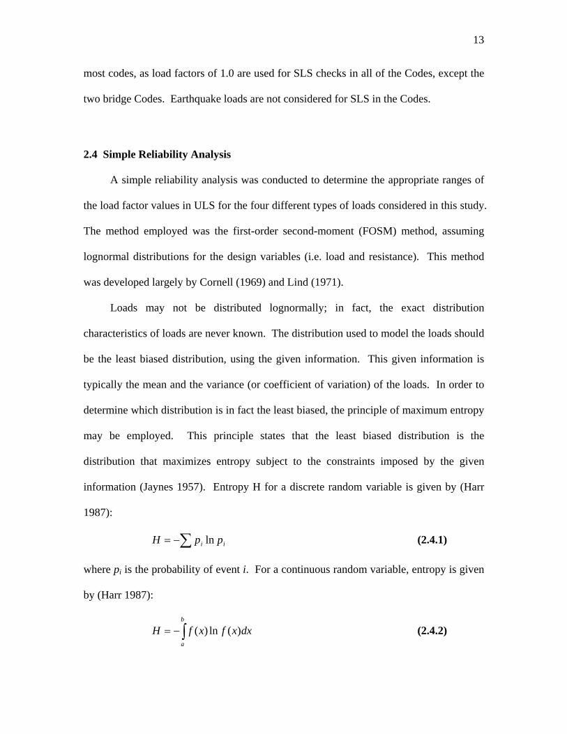
information (Jaynes 1957). Entropy H for a discrete random variable is given by (Harr

1987):

ii ppH ln∑−= (2.4.1)

where pi is the probability of event i. For a continuous random variable, entropy is given

by (Harr 1987):

dxxfxfHb

a

)(ln)(∫−= (2.4.2)

14

where a and b are the lower and upper limits, respectively, of the variable. The negative

sign in each of these equations makes entropy positive. If the only data available about a

variable are the values of the upper and lower limit, the principle of maximum entropy

states that the uniform distribution (the distribution such that all values within the range

of possible values are equally likely) is the least biased distribution (Harr 1987).

In geotechnical engineering, information about the mean and variance of a load or

resistance is typically available, even though the exact distribution may not be known.

The lower and upper limits of the load or resistance may be unknown. In this case the

principle of maximum entropy states that the normal distribution is the least biased

distribution. However, the magnitudes of load and resistance found in geotechnical

problems cannot take negative values. This firmly establishes a lower limit for both

loads and resistances. The upper limit of the load or resistance is typically unknown.

This is especially true for transient loads (i.e., live loads, wind loads, and earthquake

loads), which can assume values that are extremely large, though quite improbable. These

transient loads are typically modeled by load specification committees using more precise

distributions, namely, the Type I or Type II extreme-value distributions (Ellingwood et al.

1980), but these distributions require more knowledge of the variable than simply the

mean, variance, and minimum value. Therefore, these distributions do not represent the

least biased distribution for the loads for the information generally available. Accordingly,

the lognormal distribution better models transient loads, as it is fully characterized by its

first two moments, allowing easier implementation in FOSM analysis. This leads to a

distribution that is not only relatively simple to implement, but also gives reasonable

results (MacGregor 1976). Moreover, the lognormal distribution better represents the

15

product of several positive random variables, even if these variables are not themselves

lognormally distributed. In load modeling, the nominal load itself may be modeled as the

product of several components, each of which may also be modeled as a random variable.

For example, wind loads are usually modeled as the product of wind speed and other

empirical or experimental parameters that are treated as random variables (ASCE 7-95).

Occasionally, an engineer on a project will have detailed load information specific to that

project. In this case, specific load factors could be developed or a more complex analysis

could be used, if the effort is justified by the economics of the project.

An overall resistance is frequently modeled as the product of nominal resistance

and several parameters to account for the different sources of uncertainty. In the design

of a bridge structure, the overall resistance of a structural member is commonly modeled

as the product of nominal resistance and a material factor, a fabrication factor, and an

analysis factor, which are used to account for the uncertainties for the material strengths,

component dimensions, and analytical models, respectively (Nowak and Grouni 1994).

This can be expressed mathematically as:

afmnRR ηηη= (2.4.3)

where: ηm is a material factor that accounts for the uncertainty of the strength of the

material, ηf is a fabrication factor that accounts for the uncertainty of the size of the

fabricated member (e.g. the variability of the size of formwork for cast in place concrete),

and ηa is an analysis factor that accounts for the uncertainty of the analytical model used

to calculate resistance. Soil resistance for foundation design may also be modeled in

several cases as the product of nominal resistance and several components that account

for the uncertainties of inherent soil variability, measurement (testing), and analytical

16

methods. Perhaps this is best illustrated by considering the general bearing capacity

equation for clays,

( ) ccccccbL cNgbidsq = (2.4.4)

which uses a series of multiplicative correction factors to model the bearing capacity of a

shallow foundation. Measurement uncertainty would be seen in c, as cohesion is a soil

strength parameter that must be measured using in-situ testing, lab tests, or correlations

with other measured parameters. Additional variability due to the inherent uncertainty of

the bearing capacity equation itself would result in the analysis uncertainty.

In this context, the lognormal assumption for both loads and resistances appears

to be reasonable, as both can be treated as the product of several random variables. The

load effects and resistances of a structural or geotechnical system may then be expressed

as shown in Figure 2.4.1. Let the load effect S and the resistance R be random variables;

then, failure (the attainment of an ULS) occurs when 0lnln <− SR (represented by the

shaded area in Figure 2.4.1). The probability of failure Pf can be written as:

[ ]0)ln(ln <−= SRPPf (2.4.5)

Assuming that the random variables, ln R and ln S, are statistically independent,

the mean U and standard deviation σU of U = SR lnln − are given by:

SRU lnln −= (2.4.6)

2ln

2ln SRU σσσ += (2.4.7)

The safety index or reliability index β, which is a relative measure of safety for a

given system, can be expressed as a function of the mean and standard deviation of U

(Figure 2.4.1):

17

2ln

2ln

lnln

SR

SRσσ

β+

−= (2.4.8)

For a lognormal distribution:

)1ln( 22ln SS V+=σ , )1ln( 22

ln RR V+=σ (2.4.9)

where: VS and VR = the coefficients of variation of S and R, respectively, defined as the

ratio of the standard deviation to the mean. For small VS or VR, (say, less than 0.6), the

following expressions are acceptable approximations (MacGregor 1976):

2ln

2SSV σ≅ , 2

ln2

RRV σ≅ (2.4.10)

According to MacGregor (1976), the error in (2.4.10) is less than 2% for VR = 0.3,

increasing to about 10% for VR = 0.6. For comparison, the reported values of VR for

various geotechnical properties and resistances lie in a wide range of about 0.05 to 0.85

(Becker 1996). Considering the mean values of the reported values, the range varies

from about 0.1 to 0.5. The assumption of (2.4.10) overestimates the uncertainty of the

resistance, and is therefore slightly conservative. Based on (2.4.9) and (2.4.10), (2.4.8)

can be rewritten as follows:

22lnln RS VVSR +≥− β (2.4.11)

Lind (1971) has shown that:

RSRS VVVV αα +≅+ 22 (2.4.12)

where: α = separation coefficient having values between 0.707 and 1.0 (depending on the

value of the ratio sR VV / ), and MacGregor (1976) has shown that:

⎟⎟⎠

⎞⎜⎜⎝

⎛≅−

SRSR lnlnln (2.4.13)

18

which can be used to approximate (2.4.11). Taking (2.4.12) and (2.4.13) into (2.4.11):

RS VVSR βαβα +≥)/ln( (2.4.14)

or

)(/ RS VVeSR βαβα +≥ (2.4.15)

Rearranging (2.4.15) gives:

)()( SR VV eSeR βαβα ≥− (2.4.16)

The mean load effect S and resistance R can be defined as:

SnkSS = , RnkRR = (2.4.17)

where: Sn, Rn, kS, and kR are the nominal load, the nominal resistance, and the bias factors

(i.e. the ratio of mean to nominal) for load and resistance, respectively. Using (2.4.17),

(2.4.16) can be rewritten in a form analogous to the LRFD fundamental equation:

)()( SR VSn

VRn ekSekR βαβα ≥− (2.4.18)

or

nn SLFRRF ⋅≥⋅ (2.4.19)

where: LF and RF = load factor and resistance factor, respectively. From (2.4.18) and

(2.4.19), the value of the load factor and the resistance factor can be calculated by:

SVS ekLF βα= (2.4.20)

RVRekRF βα−= (2.4.21)

With (2.4.20), if appropriate values of the parameters α, β, kS, and VS are known,

the value of the load factor for each load type can be obtained in a simple manner. In

most cases, however, the estimation of these parameters is difficult. This is so not only

19

because α is a function of both the load effects and the resistance, but also because the

values of kS and VS are not well known due to limited statistical data.

A similar derivation can be employed for determining load and resistance factors

if the underlying distributions are normal. This will be useful for determining the load

factor for dead load, as dead loads are typically modeled as having a normal distribution

(Ellingwood, et. al. 1980). For normally distributed variables, the probability of failure is

given by (Haldar and Mahadevan 2000):

[ ]0)( <−= SRPPf (2.4.22)

The reliability index β is given by:

22SR

SRσσ

β+

−= (2.4.23)

Using the separation coefficient α, (2.4.23) can be written as:

( )SR

SRσσα

β+

−= (2.4.24)

Rearranging (2.4.24) gives:

SR SR αβσαβσ −=− (2.4.25)

Noting that RV RR /σ= and SV SS /σ= ,

( ) ( )SR SR αβσαβσ −=− 11 (2.4.26)

With SnkSS = and RnkRR = ,

( )SS VkLF αβ+= 1 (2.4.27)

( )RR VkRF αβ−= 1 (2.4.28)

20

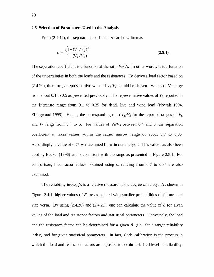
2.5 Selection of Parameters Used in the Analysis

From (2.4.12), the separation coefficient α can be written as:

)/(1)/(1 2

SR

SR

VVVV

++

=α (2.5.1)

The separation coefficient is a function of the ratio VR/VS. In other words, it is a function

of the uncertainties in both the loads and the resistances. To derive a load factor based on

(2.4.20), therefore, a representative value of VR/VS should be chosen. Values of VR range

from about 0.1 to 0.5 as presented previously. The representative values of VS reported in

the literature range from 0.1 to 0.25 for dead, live and wind load (Nowak 1994,

Ellingwood 1999). Hence, the corresponding ratio VR/VS for the reported ranges of VR

and VS range from 0.4 to 5. For values of VR/VS between 0.4 and 5, the separation

coefficient α takes values within the rather narrow range of about 0.7 to 0.85.

Accordingly, a value of 0.75 was assumed for α in our analysis. This value has also been

used by Becker (1996) and is consistent with the range as presented in Figure 2.5.1. For

comparison, load factor values obtained using α ranging from 0.7 to 0.85 are also

examined.

The reliability index, β, is a relative measure of the degree of safety. As shown in

Figure 2.4.1, higher values of β are associated with smaller probabilities of failure, and

vice versa. By using (2.4.20) and (2.4.21), one can calculate the value of β for given

values of the load and resistance factors and statistical parameters. Conversely, the load

and the resistance factor can be determined for a given β (i.e., for a target reliability

index) and for given statistical parameters. In fact, Code calibration is the process in

which the load and resistance factors are adjusted to obtain a desired level of reliability.

21

The load effects S in Figure 2.4.1 are usually the combination of load effects for several

different load types according to the load combinations used. For instance, in a gravity

load combination, a load effect S will be the combination of dead load effects and live

load effects. In this case, the reliability index β is commonly calculated using the

reliability equations, where statistical parameters, such as VS and VR, are the statistical

parameters representative of the combined load effects (i.e. dead load and live load) and

the overall resistance. Based on this approach, Ellingwood et. al. (1980), after careful

examination of β for common structural members, such as concrete, steel, and timber,

reported that the representative values of reliability index β tend to fall within the range

of 2.5 to 3.0 for both the gravity load and the gravity plus wind load combinations. These

values for β are representative of the reliability associated with existing designs. He also

suggested that, for gravity load, gravity plus wind load, and gravity plus earthquake load

combinations, the representative target reliability indices βT are 3.0, 2.5, and 1.75,

respectively. These target reliability indices have been established after consideration of

the reliability associated with current designs. Establishing target reliability indices

based on current designs will lead to load factors that produce designs that are similar to

current designs. This is desirable because the reliability indices can be refined later, if

there is a need to refine them at all, in a cautious manner as the Codes evolve. To derive

the load factor for a particular load type using (2.4.20), therefore, the selection of

different values of β for each load type would be required. In this analysis, based on

Ellingwood’s work, the values of β equal to 3.0 for dead load, 2.75 for live load, 2.5 for

wind load, and 1.75 for earthquake loads were assumed.

22

For the evaluation of the values of kS and VS, extensive research has been

performed over several decades of use of LRFD in structural design. For the time-variant

loads such as live, wind, and earthquake loads, the values of kS and VS are normally

obtained from time-stochastic modeling processes based on available recorded data (e.g.

traffic survey data, wind speed data or seismic acceleration coefficient). Table 2.5.1

shows the values of kS and VS reported by several researchers. As expected, the biases for

gravity loads (i.e. dead load and live load) are relatively small. This means that gravity

loads tend to be estimated rather accurately. Also note that the coefficient of variation for

dead loads is quite low. On the other hand, VS for earthquake loads are significantly

higher than for other loads. Based on the data presented in Table 2.5.1, ranges of values

for kS and VS are determined for each load type for use in the analysis of the present

chapter. The ranges of values used are presented in Table 2.5.2.

2.6 Comparison Between Results and Load Factors in the Codes

Table 2.6.1 and Figure 2.6.1 show the comparisons of the values of the load factors

between the analysis and the Codes. The load factors for beneficial dead loads were

obtained using equations similar in form to equations (2.4.21) and (2.4.28), namely:

SVS ekLF αβ−= (2.6.1)

for the lognormal distribution, and

( )SS VkLF αβ−= 1 (2.6.2)

for the normal distribution, based on the reasoning that beneficial dead loads resist failure.

These equations are similar to the resistance factor equations, except the bias factor and

coefficient of variation are for the beneficial load effects, not the resistances. These

23

equations also differ from the standard load factor equations, (2.4.20) and (2.4.27), in that

they are expressed in terms of -αβVS instead of αβVS. This accounts for the beneficial

nature of these loads. The values for load factors given in the Codes are found to be

reasonably consistent for all loads considered. A relatively wide range in earthquake load

factors is mainly due to the values of VS used in the analysis, which lie within a wide

range. In the same table, for comparisons, average values for the ranges of each load are

shown. For dead and live load, the values by the analysis are somewhat higher than those

in all the Codes. It is interesting to note, however, that when a comparison is made with

the US Codes (i.e. AASHTO, ACI, and AISC), the average values from the analysis

show relatively good agreement with the values from the Codes, although the ranges

given in the analysis are rather large (Table 2.6.1). For α varying from 0.7 to 0.85, the

ranges become somewhat larger, but the only load factors affected significantly are those

for earthquake loads. In some cases, the analysis supports the use of load factors that are

higher than the load factors currently used in the Codes. This can be seen in Figure 2.6.1

for earthquake loads especially. This apparent unconservatism in the current Codes is

due to the underlying probability distribution for the loads. The current research is using

the least biased distribution considering only the mean and variance of the loads along

with the fact that the loads cannot be negative. The Codes are based on more precise, and

therefore more biased, distributions of the loads, using more information about the

particular loads being considered. Upon considering this extra information, the code

developers can arrive at a more precise load factor for a particular case. As can be seen

from Figure 2.6.1, these values always lie within the range determined by the current

research.

24

2.7 Future Development of Geotechnical LRFD Design

As demonstrated by equations (2.4.19), (2.4.20), (2.4.21), and (2.5.1), load and

resistance factors are inexorably linked through the values of β, VR, and VS. This means

that each Code will assign different values to resistance factors, because of the different

load factor values adopted. This adds to the complexity of LRFD compared with

Allowable Stress Design (ASD). In ASD, engineers need only to understand the concept

of the global factor of safety, which has been in use for at least a century. The safety

factor for a footing, for example, typically would be in the range of 2 to 4, and the

engineer selects the value to use in design based on general guidelines. In LRFD, it is

essential to use the values of LF and RF prescribed in the Code, as well as a nominal

resistance consistent with the LF and RF values. This requires understanding of more

complex concepts.

Acceptance of the LRFD approach hinges on making the method understandable

to and usable by geotechnical engineers. The large array of different load factors

currently in existence, which leads to a large number of different resistance factors, adds

to the overall complexity of LRFD for the practicing engineer and ultimately discourages

the use of this design method. Our analysis shows that, in general, the load factors

proposed by different codes are all acceptable from a theoretical standpoint. Ideally, in

order to facilitate the use of LRFD in routine practice, the leadership of the organizations

responsible for each code would join in adopting a single set of load factors, at least for

the primary loads, such as the four load types discussed in this chapter (i.e. dead, live,

wind, and earthquake loads). We recognize this is difficult to accomplish, as it involves

25

overcoming non-technical, political hurdles. The alternative is for engineers to become

used to using different load and resistance factors when designing the same type of

foundation element depending on the Code controlling design.

2.8 Summary and Conclusions

The load factors proposed by various current structural and foundation LRFD

Codes were reviewed. Usually, a larger number of limit states, load types and load

combinations are considered in the bridge and offshore foundation design codes,

compared with building and onshore foundation design codes. In this study, the load

factors for four major load types (i.e. dead, live, wind and earthquake loads) that control

most design cases were examined and compared between the Codes.

For ULSs, the load factor values fall within rather consistent ranges for most load

types considered. Differences appear in the dead and the live load factors between the

building and the bridge Codes. For the bridge Codes, the values of dead load factors lie

within a relatively wide range. This is because, for bridge design, more types of loads are

usually defined as dead loads, for which different values of load factors are used to

account for the different degrees of uncertainty inherent in each load. While the use of a

large number of different load factors adds to the complexity of a Code, it also adds to the

utility of the Code. When a greater number of load factors are used, the uncertainties due

to each load type are better separated. This separation of uncertainties is the ultimate

goal of LRFD. The bridge Codes also define different values of live load factors for

different load combinations (i.e. different limit states) instead of using load combination

factors to account for the reduced probability of simultaneous occurrence of maximum

26

values of several transient loads. When considering a gravity load combination, however,

the values for the dead and the live load factors are reduced to a rather narrow range for

all of the Codes, resulting in ranges consistent with other load types examined.

For SLSs, some differences appear again between the bridge and building Codes.

While most Codes prescribe the use of unfactored loads, AASHTO (1998) and MOT

(1991) use values less than 1.0 for wind and both wind and live load factors, respectively.

This reflects the differences in how each Code prescribes the determination of the

characteristic wind load, as well as the transient nature of the live load for bridges.

However, an argument can be made against using load factors less than one, except when

the foundation soil is clay.

A simple FOSM reliability analysis was implemented to find appropriate ranges of

the load factor values for each load considered in this study. The analysis produced

results consistent with all the Codes reviewed, although the values produced lie in rather

wide ranges due to the relatively wide range of the input parameters. The analysis shows

even better agreement with the Codes when considering only the US Codes (AASHTO,

ACI, and AISC). The values presented in the US Codes lie in the middle of the

acceptable range determined by the analysis, as summarized by Figure 2.6.1. As the

analysis uses the least biased distribution to model the loads, load factors for use in

geotechnical LRFD should not lie outside the range determined by the current research

unless that load factor applies to a specific type of load that is not considered in this

research.

27

2.9 Notation

H = entropy

kR = bias factor of resistance

kS = bias factor of load effect

LF = load factor

(LF)D= dead load factor

(LF)L= live load factor

(LF)W= wind load factor

pi = probability of event i

Pf = probability of failure

R = resistance

RF = resistance factor

Rn= nominal resistance

R = mean resistance

S = load effects

SD= nominal dead load effect

SL= nominal live load effect

Sn= nominal load effect

SW= nominal wind load effect

S = mean load effect

VR = coefficient of variation of resistance

28

VS = coefficient of variation of load effect

α = separation coefficient

β = reliability index

βT= target reliability index

ηm= material factor

ηf= fabrication factor

ηa= analysis factor

σ = standard deviation

29

Table 2.3.1. Load factors

US Canada Europe

Loads AASHTO (1998)

ACI (1999)

AISC (1994)

API (1993)

MOT (1992)

NRC (1995)

DGI (1985)

ECS (1995)

Dead

Live

Wind

Seismic

1.25-1.95 (0.65-0.9)

1.35-1.75

1.4

1.0

1.4 (0.9)

1.7

1.3

1.4

1.2-1.4 (0.9)

1.6

1.3

1.0

1.1-1.3 (0.9)

1.1-1.5 (0.8)

1.2-1.35

0.9

1.1-1.5 (0.65-0.95)

1.15-1.4

1.3

1.3

1.25 (0.85)

1.5

1.5

1.0

1.0 (0.85)

1.3

1.3

1.0

1.0-1.35 (0.95)

1.3-1.5

1.3-1.5

1.0 Note: Values in parentheses apply when the load effects tend to resist failure for a given load combination.

30

Table 2.3.2. Load factors and gravity load combinations

Code Representative gravity load combination AASHTO (1998) 1.25D+1.75L ACI (1999) 1.4D+1.7L AISC (1994) 1.2D+1.6L API (1993) 1.3D+1.5L MOT (1992) 1.2D+1.4L NRC (1995) 1.25D+1.5L DGI (1985) 1.0D+1.3L ECS (1995) 1.35D+1.5L

31

Table 2.3.3. Load factors for SLS

US Canada Europe Loads AASHTO

(1998) ACI

(1999) AISC (1994)

MOT (1991)

NRC (1995)

DGI (1985)

ECS (1995)

Dead

Live

Wind

1.0

1.0

0.3

1.0

1.0

1.0

1.0

1.0

1.0

1.0

0.75

0.7

1.0

1.0

1.0

1.0

N/Aa

N/Aa

1.0

1.0

1.0 aThe values for transient loads are given in the structural Code.

32

Table 2.5.1. Ratio of mean to nominal load, kS, and coefficient of variation, VS

Loads kS References VS References

Dead 1.03-1.05 Nowak 1994;

Ellingwood 1999

0.08-0.15 Nowak 1994; Ellingwood

1999

Live 1.0 Ellingwood 1999 0.25 Ellingwood 1999

Wind 0.875 Nowak 1994 0.20 Nowak 1994

Earthquake 0.3 Nowak 1994 0.7 < Ellingwood, et al. 1980;

Nowak 1994

Note: kS and VS in transient loads (i.e. live, wind and earthquake loads) are maximum 50-year values

33

Table 2.5.2. Values of kS and VS assumed for the analysis

Loads kS VS

Dead 1.0-1.05 0.07–0.16

Live 0.95-1.05 0.2–0.3

Wind 0.85-0.9 0.15–0.25

Earthquake 0.25-0.35 0.9-1.1

34

Table 2.6.1. Comparison of the values of load factors from the analysis and from the

Codes

Dead load Live load Wind load Earthquake

load

Analysis

(0.7<α<0.85)

1.16 - 1.58 (1.34)

0.66 - 0.91a

(0.79)

1.40 - 2.12

(1.71)

1.11 - 1.53

(1.29)

0.75 - 1.80

(1.17)

Analysis

(α=0.75)

1.17 - 1.50 (1.33)

0.70 - 0.90a

(0.79)

1.44 - 1.95

(1.68)

1.13 - 1.44

(1.28)

0.81 - 1.48

(1.12)

All Codes

1.0 - 1.4b (1.24)

0.65 - 0.95a

(0.80)

1.3 - 1.75b

(1.53) 1.2 - 1.5 (1.36) 0.9 - 1.4 (1.08)

AASHTO,

ACI and AISC

only

1.2 - 1.4b (1.28)

0.65 - 0.9a (0.86)

1.6 - 1.75b

(1.68) 1.3 - 1.4 (1.33) 1.0 - 1.4 (1.13)

Note: Values in parentheses represent average values

a Beneficial dead loads bThe range for a representative gravity load combination, as presented in Table 2.3.2

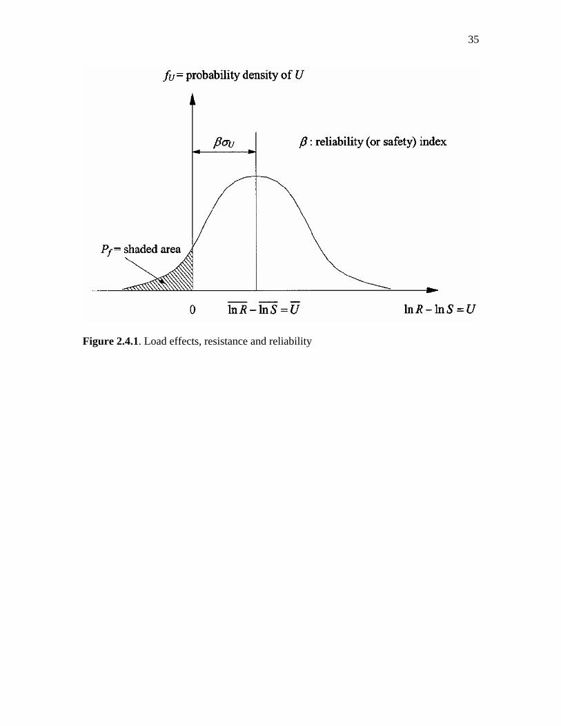
35

Figure 2.4.1. Load effects, resistance and reliability

36

VR/VS

1 2 3 4 5

α

0.60

0.65

0.70

0.75

0.80

0.85

0.90

0.95

1.00

Figure 2.5.1. Variation of separation coefficient, α

37

654

3

21

6

54

3

21

65

4

3

21

65

43

21

65

4321

EarthquakeWindLiveDeadBeneficial Dead

1: Normal (α: 0.7 - 0.85)2: Normal (α: 0.75)3: Log-Normal (α: 0.7 - 0.85)4: Log-Normal (α: 0.75)5: All Codes6: AASHTO, ACI, AISC

0.4

1.0

1.6

2.2

Load Factor

Figure 2.6.1. Comparison of analysis and the Codes

38

39

CHAPTER 3. METHODOLOGY TO DETERMINE RESISTANCE FACTORS

Many possible techniques exist to select Resistance Factors (RFs) for use in

geotechnical LRFD. One very common technique is to “calibrate” RFs using existing

factors of safety and code-specified Load Factors as input. In this way, RFs may be

specified to allow the equivalent correction to resistance as results from existing factors

of safety. This technique is acceptable as a first step in the adoption of LRFD, but better

methods are available. The most rational method available to determine RFs is reliability

analysis.

Many studies have been published that advocate the use of reliability analysis for

LRFD development. However, our study differs significantly in the methods used to

assess the uncertainty of design variables input into the reliability analysis. The most

widely used techniques involve statistics performed on large databases of

indiscriminately combined data. An example of this technique applied to load test

databases is the recent NCHRP Report 507 (Paikowsky 2004). An example of this

technique applied to soil properties is Phoon and Kulhawy (1999). These methods have

the advantage that they are readily applied in the short term. However, they have the

disadvantage that there is virtually no control over the quality or applicability of the data

collected. In contrast, this study uses very carefully selected data that targets very

precisely the uncertainties in design we need to quantify. To ensure the completeness of

our uncertainty assessment, we have proposed the following rational framework for

evaluating resistance factors. This work is presented as a model for research into the

development of complete LRFD methodologies for geotechnical design.

40

3.1 A Rational Framework for Evaluating Resistance Factors

A consistent framework for evaluating resistance factors is key to successful

LRFD implementation. A number of possible approaches exist, such as scaling factors to

existing factors of safety; using simple probabilistic analyses considering a select set of

uncertainties; and performing more rigorous probabilistic analyses considering all

quantifiable uncertainties. Results of a method conforming to this last approach would be

highly credible. After the model framework for determining resistance factors for

structural design set forth by Ellingwood et al. (1980), the following set of steps is

proposed as a geotechnical framework for such a method:

1. identify the equations used to compute foundation resistance;

2. identify the component variables of the resistance equations;

3. identify the measurable quantities (geotechnical tests) associated with each of

the input variables;

4. identify all component uncertainties for each variable, including transformations;

5. evaluate the composite uncertainties using available statistics (literature,

tests/analysis, current research);

6. use uncertainties to select PDFs for reliability analysis;

7. select representative design variables (dimensions, strengths, loads);

8. execute reliability analysis to obtain resistance factors;

9. adjust resistance factors for governing load factors;

10. repeat reliability analysis to cover a range of representative design conditions.

41

Steps 1-6 of these guidelines are demonstrated in Chapter 4 for the development

of PDFs for shallow foundation bearing capacity in sands and in clays. Steps 7-10 are

demonstrated in Chapter 5 for the development of resistance factors for shallow

foundation bearing capacity. Steps 1-10 are applied to deep foundations in Chapter 8 for

sands and Chapter 9 for clays.

3.2 Tools to Assess Uncertainty

Steps 1-3 of the framework will be explained as they are demonstrated in

Chapters 4, 7, 8, and 9. In each of steps 4-6 in these guidelines, operations will be

performed on the data describing the uncertainty of geotechnical measurements and

transformations. The following tools are used to accomplish these operations.

Standard Deviation and Coefficient of Variation

The scatter or uncertainty in measurements and correlations can be quantified

using the standard deviation. The standard deviation (σ) of a random variable X can be

estimated using the sample standard deviation (S) when n occurrences of value xi are

known,

( )

)1(1

2

−

−=

∑=

n

xS

n

ixi

X

µ (3.2.1)

where SX is the sample standard deviation of X and µX is the mean of X. According to

probability theory, SX has expected value (mean) σx, hence it is used to find σX. For

many random variables in engineering, it is more convenient to express standard

deviation using a Coefficient of Variation (COV):

42

X

XCOVµσ

= (3.2.2)

It is especially useful in case where the standard deviation varies with the mean value.

In the assessment of variable uncertainties in the following chapters, there are

many instances where a particular relationship between two variables can be determined

from data. Suppose we have data indicating a relationship between variables X and Y. A

function y = f(x) can be defined that represents a mean trendline through this data. This

task is routinely accomplished using least squares regression. It is necessary to describe

the uncertainty of this correlation f(x). The first step is to detrend the data by subtracting

f(xi) from each value yi. A standard deviation quantifying the uncertainty of this

correlation can then be found by applying equation (3.2.1) to all the values of (yi – f(xi)).

Alternatively, if it is observed that the scatter of the data about the mean trend line is

proportional to the value of f(x), then a representative COV expressing the uncertainty of

the correlation can be found by applying equation (3.2.1) to all values of (yi – f(xi))/f(xi).

6σ and modified 6σ method

The scatter in measurements tends to conform to normal distributions. A normal

distribution is a type of PDF that can be described completely using its mean and

standard deviation. Many geotechnical data such as Standard Penetration Test (SPT)

blow count (N) and Cone Penetration Resistance (CPT) tip resistance (qc) have trends

with depth. The 6σ method can expedite assessments of the standard deviation of these

trended data1. The first step is to observe the bounds and mean trend of the data. An

1 This six standard deviation (6σ) procedure is also recommended for determining the uncertainty of variables by the FHWA (Withiam et. al. 1997).

43

example mean trend and data bounds are illustrated in Figure 3.2.1 for qc. For a

particular depth, the value of the mean and the range (difference between minimum and

maximum bound values) can be computed. The standard deviation is then found using

σ=6

Range (3.2.3)

where σ is the standard deviation. An implication of Equation (3.2.3) is that the range is

taken to represent six standard deviations of the normal distribution – encompassing

99.74% of the possible values of qc for this measurement. In geotechnical engineering,

the standard deviation is frequently expressed using the Coefficient of Variation (COV),

µσ

=COV (3.2.4)

where µ is the mean. The value of using the COV instead of σ is that, in many cases, the

COV is independent of µ. It is possible that for some geotechnical quantities, the COV

varies with the mean value or with depth. In these circumstances, it is conservative to

select the greatest computed COV value for use in reliability analysis.

8 12 16 20 24 28qc (MPa)

8

7

6

5

4

3

Dep

th (m

)

8 12 16 20 24 28

8

7

6

5

4

3

lower bound on data (µ - 3σ)

upper bound on data (µ + 3σ)

mean trend (from regression

Figure 3.2.1. Mean Trend (power regression) and Bounds of CPT Tip Resistance Data for Sand. The mean and bounds can be used to calculate the COV for qc using the 6σ procedure.

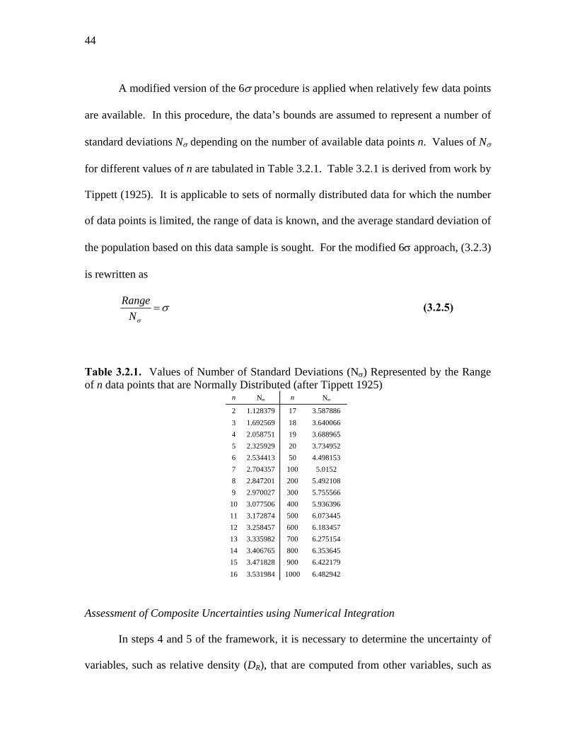
44

A modified version of the 6σ procedure is applied when relatively few data points

are available. In this procedure, the data’s bounds are assumed to represent a number of

standard deviations Nσ depending on the number of available data points n. Values of Nσ

for different values of n are tabulated in Table 3.2.1. Table 3.2.1 is derived from work by

Tippett (1925). It is applicable to sets of normally distributed data for which the number

of data points is limited, the range of data is known, and the average standard deviation of

the population based on this data sample is sought. For the modified 6σ approach, (3.2.3)

is rewritten as

σσ

=N

Range (3.2.5)

Table 3.2.1. Values of Number of Standard Deviations (Nσ) Represented by the Range of n data points that are Normally Distributed (after Tippett 1925)

n Nσ n Nσ

2 1.128379 17 3.587886 3 1.692569 18 3.640066 4 2.058751 19 3.688965 5 2.325929 20 3.734952 6 2.534413 50 4.498153 7 2.704357 100 5.0152 8 2.847201 200 5.492108 9 2.970027 300 5.755566

10 3.077506 400 5.936396 11 3.172874 500 6.073445 12 3.258457 600 6.183457 13 3.335982 700 6.275154 14 3.406765 800 6.353645 15 3.471828 900 6.422179 16 3.531984 1000 6.482942

Assessment of Composite Uncertainties using Numerical Integration

In steps 4 and 5 of the framework, it is necessary to determine the uncertainty of

variables, such as relative density (DR), that are computed from other variables, such as

45

CPT qc. An equation (transformation) is used to compute qc from DR. Just as for qc and

DR, the transformation also has uncertainty (Phoon and Kulhawy 1999). Numerical

Integration is a technique that allows us to combine the uncertainties of the original

variable X and the transformation to determine the uncertainty of the final (transformed)

variable Y. The result of this numerical integration technique is a histogram depicting the

uncertainty of the final variable.

The PDF of a random variable Y that is a function f of a random variable X can be

expressed as (Ang and Tang 1975)

( )dy

ydfyfpyp XY)()()(

11

−−= (3.2.6)

where ( )xpX is the PDF of X and )(1 yf − is the inverse of the transformation function

from X to Y. In a numerical scheme, (3.2.6) can be approximated by assuming dy = ∆y

and multiplying both sides of the equation by ∆y, yielding

( ) )()()( 11 yfyfpyyp XY−− ∆=∆ (3.2.7)

Since transformation f(x) has uncertainty, Eq. (3.2.7) needs to be modified to incorporate

a PDF representing the transformation uncertainty. The concept of conditional

probability is used for that. The conditional PDF of variable Y for a given value x is

written )|(| xyp XY . The conditional PDF represents the uncertainty of Y when the value

of X is known exactly. Thus, PDF )|(| xyp XY represents the transformation uncertainty,

the uncertainty of f(x). By this definition, PDF )|(| xyp XY has expected value y=f(x),

46

meaning this PDF is also a function of x. According to probability theory, the

independent PDF2 of Y can be found by

∫∞

∞−= dxxpxypyp XXYY )()|()( | (3.2.8)

Multiplying both sides by dy yields

∫∞

∞−= dxxpxypdydyyp XXYY )()|()( | (3.2.9)

Finally, to facilitate numerical evaluation, as in (3.2.7), an iterative scheme is adopted.

The probability of random variable Y taking a value y contained in the finite range ∆y is

expressed as yypY ∆)( . To find yypY ∆)( , the integral of (3.2.9) is approximated by a

summation where dxxpX )( and dyxyp XY )|(| are approximated by integrals over small

intervals ∆x and ∆y, respectively, to yield

∑ ∫∫=

∆+

∆−

∆+

∆− ⎥⎦⎤

⎢⎣⎡ ⋅=∆

b

a

yy

yy XY

x

x XY dyxypdxxpyypξ

ξ

ξ

21

21

21

21

)|()()( | (3.2.10)

where the successive integration limits in x are ∆x apart, and a and b are chosen such that

∑∫=

∆+

∆−≈

b

a

x

x X dxxpξ

ξ

ξ1)(2

1

21

(3.2.11)

This means we are evaluating yypY ∆)( in essence for all values of x, given that we have

very closely approximated 100% probability of x being between a and b. The evaluation

of (3.2.10) is repeated across a range of y values, always ∆y apart. The final result is a

complete description of PDF )(ypY in terms of a histogram with intervals of width ∆y.

Assessment of Composite Uncertainties using Monte Carlo Simulation

2 according to probability theory, the independent PDF of a random variable Y that is jointly distributed with another variable X is the PDF of Y over all possible values of x.

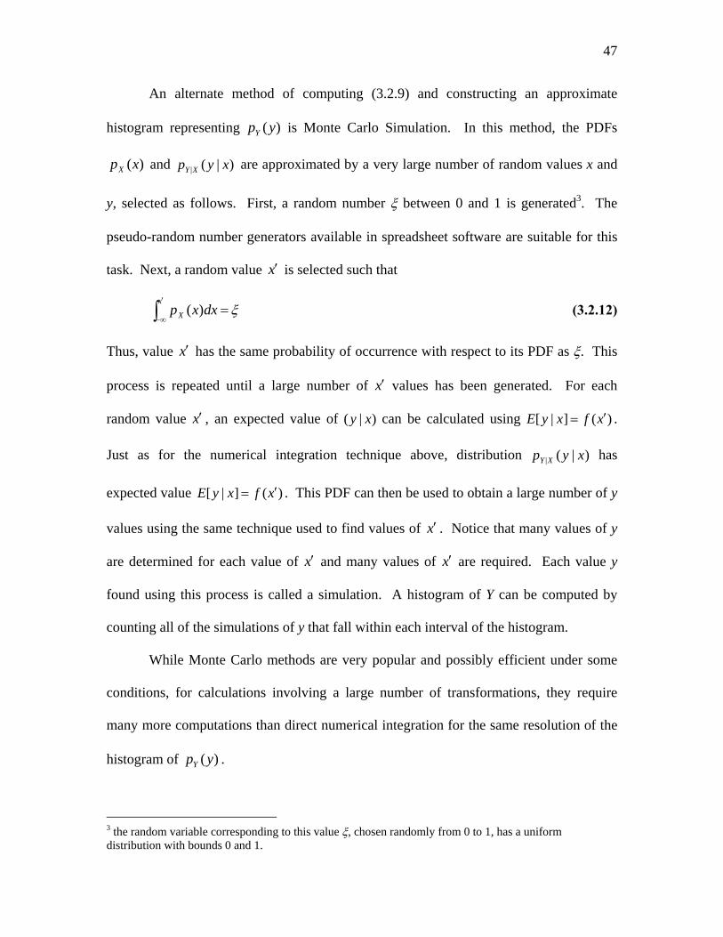
47

An alternate method of computing (3.2.9) and constructing an approximate

histogram representing )(ypY is Monte Carlo Simulation. In this method, the PDFs

)(xpX and )|(| xyp XY are approximated by a very large number of random values x and

y, selected as follows. First, a random number ξ between 0 and 1 is generated3. The

pseudo-random number generators available in spreadsheet software are suitable for this

task. Next, a random value x′ is selected such that

ξ=∫′

∞−

x

X dxxp )( (3.2.12)

Thus, value x′ has the same probability of occurrence with respect to its PDF as ξ. This

process is repeated until a large number of x′ values has been generated. For each

random value x′ , an expected value of )|( xy can be calculated using )(]|[ xfxyE ′= .

Just as for the numerical integration technique above, distribution )|(| xyp XY has

expected value )(]|[ xfxyE ′= . This PDF can then be used to obtain a large number of y

values using the same technique used to find values of x′ . Notice that many values of y

are determined for each value of x′ and many values of x′ are required. Each value y

found using this process is called a simulation. A histogram of Y can be computed by

counting all of the simulations of y that fall within each interval of the histogram.

While Monte Carlo methods are very popular and possibly efficient under some

conditions, for calculations involving a large number of transformations, they require

many more computations than direct numerical integration for the same resolution of the

histogram of )(ypY .

3 the random variable corresponding to this value ξ, chosen randomly from 0 to 1, has a uniform distribution with bounds 0 and 1.

48

Nominal Values, Mean Values, and Bias Factors

Figure 3.2.2 illustrates the PDF for an idealized design parameter that is normally

distributed. The mean value corresponds to the expected value (or mean) of the

distribution. For measurements, this value is determined by taking the mean of the data,

or by finding a mean trend for trended data such as qc. For transformed variables Y, such

as DR, the mean value µY is taken as the expected value of Y according to PDF )(ypY or

the histogram representing PDF )(ypY . In many cases in geotechnical design, the value

of the parameter used in design, the “nominal” value, may be different from the mean

value. In these cases, a bias factor is used to express the difference. The bias factor is

defined as

nominal

factor biasy

Yµ= (3.2.13)

Parameter Value

limit s

tate valu

e

Prob

abili

ty D

ensi

ty

nominal valu

e

mean valu

e

Figure 3.2.2. The mean, nominal, and limit state values of a normally distributed design parameter. Here, limit state value corresponds to the value at which a limit state such as bearing capacity failure is reached. Mean value is the mean of the distribution under consideration. Nominal value is the parameter value used in design. The mean can be calculated from the nominal by (nominal) * (bias factor).

The mean value of a design parameter can be different from the nominal value for one of

two reasons. First, some equations used in design are known to be biased. In these cases,

49

the bias factor is used to correct the value determined using the design equation for the

known bias so that the statistical mean of the design parameter reflects our best

knowledge of what that parameter should be. Second, nonlinear transformations y=f(x)

result in transformed PDFs )(ypY with shapes that differ from those of the input PDFs

)(xpX . The change in shape also shifts the mean value such that ( )][][ XEfYE ≠ . Bias

factors are useful for defining the PDFs for normally and lognormally distributed

variables. These PDFs can be described completely with the mean and the COV.

The third value identified in Figure 3.2.2 is the limit state value. This value is the

value of the design parameter required for a design to reach a particular limit state. The

optimization required to find this value is presented in the following section.

3.3 Tools to Assess Resistance Factors

In the previous section we presented the methodology to develop Probability

Density Functions (PDFs) describing the uncertainties of the variables for any limit state

design check. In this section, we will present the methodology to perform the reliability

analysis and compute resistance factors (steps 7-10 of the framework) for these design

checks.

Design, Mean, and Limit State Values and the Reliability Index

For a certain limit state, the limit state equation (the function that separates

satisfactory from unsatisfactory performance) can be given as a function of several

variables. For example, the limit state equation for the ultimate bearing capacity of

rectangular footings on sand under vertical load is

50

021

=⎟⎠⎞

⎜⎝⎛ ⋅⋅⋅+⋅⋅⋅⋅−

⋅+

γγγγ sNBdsNDLBLLDL

qqq (3.3.1)

In (3.3.1), if the resistance is greater than the load effect, there is some margin of safety.

This margin of safety can be expressed through the concept of the reliability index (β)

(Cornell 1969, Hasofer and Lind 1974, Low and Tang 1997). The reliability index is

dependent on the mean and variance of each of the variables and also on the limit state

under consideration. A visual depiction of the reliability index is shown in Figure 3.3.1.

In part (a) of Figure 3.3.1, β is expressed for a problem with one normally distributed

random variable. In this case, the probability of failure can be simply calculated as the

area under the probability density function (PDF) of X to the left of the limit state (LS)

value. The reliability index can be seen as the ratio of the distance between the expected

value of X (the mean µ) and the limit state value, xLS, to the variable standard deviation σ

of X. Thus, β is directly related to the probability of failure. The Hasofer and Lind (1974)

definition of the reliability index retains this property of β for multi-variable problems.

In part (b) of Figure 3.3.1, a two-variable problem is expressed. A simpler, two-

dimensional illustration of Fig. 3.3.1(b) appears in Fig. 3.3.1(c). Here the probability

density is indicated by contours. Now the reliability index can be expressed as

22

⎟⎟⎠

⎞⎜⎜⎝

⎛ −+⎟⎟

⎠

⎞⎜⎜⎝

⎛ −=

Y

YLS

X

XLS yxσ

µσ

µβ (3.3.2)

For multiple random variables Xi, with i = 1, 2, . . ., n, with corresponding means and

standard deviations µi and σi, a generalization of (3.3.2) is possible,

51

( ) [ ] ( )mxσmx 2T −−=⎟⎟⎠

⎞⎜⎜⎝

⎛ −++⎟

⎟⎠

⎞⎜⎜⎝

⎛ −+⎟

⎟⎠

⎞⎜⎜⎝

⎛ −=

−12

,

2

,2

2

,1

2

2

1

1

n

n

X

XLSn

X

XLS

X

XLS xxxσ

µσ

µσ

µβ Λ

(3.3.3)

where x is a vector of limit state values of Xi, m is a vector of mean (µ) values of Xi, and

[σ2] is a diagonal matrix of the variance (σ2) values of Xi. Equation (3.3.3) holds for

uncorrelated normal random variables. A more general expression, considering the

possibility that the normal random variables are correlated, was given by Low and Tang

(1997):

)()( 1 mxCmx −−= −Tβ (3.3.4)

where C is the covariance matrix of the random variables considered where Ckl =

covariance(Xk,Xl). Note that covariance(Xk,Xk) is equal to the variance of Xk. When

random variables Xi are uncorrelated, non-diagonal terms Ckl are equal to zero, thus C is

equal to [σ2] and (3.3.4) reduces to (3.3.3). Since the minimum β for a given set of mean

values is sought, an optimization of x that satisfies the limit state equation is required.

52

x

limit s

tate valu

ePr

obab

ility

Den

sity

((

))p

xX

nominal valu

e

mean valu

e

failu

re sp

ace

µX LS - x

X

LSX xσ

µβ

−=

PDF of , X pX( )x

(a)

x

y

Prob

abili

ty D

ensit

y (

())

px,

yXY

(b)

x

y

mean values

failure space

limit state surface

optimized minimum distancebetween limit state and mean values

PDF contours

(c)

Figure 3.3.1. Depiction of Reliability Index: (a) one normally distributed random variable – here reliability index (β) is defined as the distance from the mean parameter value to its limit state value, normalized with respect to its standard deviation; (b) two normally distributed random variables; (c) a two-dimensional projection of (b) illustrating the concept of “distance” to the limit state surface.

53

In LRFD, the goal is to have a set of load and resistance factors that will allow the

engineer to produce designs with a consistent reliability index. Therefore, in the

determination of load and resistance factors, the reliability index must be set equal to a

certain value in order to attain uniform reliability throughout a structural and geotechnical

system. Ellingwood et al. (1980) argued that this target reliability index should be 3.0 for

gravity loading situations. Some structural elements, such as steel connections have

target reliability indices greater than 3.0 (Fisher et al., 1978). In these cases, a major

driving concern is to provide for a plastic, gradual failure of the overall structure rather

than a brittle, sudden one. Vesic (1973) argued that foundations are loaded in a load-

controlled mode and that, under some conditions, sudden bearing capacity failures could

occur. However, most footings are members of a larger system of redundant footings,

with the possibility of settlements and load transfer between footings prior to any

structural collapse. Therefore, considering each footing as a component of a structural

system, a reliability index of 3.0 is consistent with existing structural practice, even in the

relatively few cases where “brittle” foundation failure would be possible.

Computation of resistance values using a target reliability index can be

accomplished with an iterative scheme. First, initial mean values of the variables

governing a foundation design are selected, defining a point in multi-variable space. The

reliability index for this initial trial is computed by finding x in (3.3.4) with the

requirement that x be on the limit state surface and minimize β. These computations can

be efficiently executed using the spreadsheet formulation of Low and Tang (1997). In

this formulation, non-normal PDFs are substituted by normal distributions such that the

cumulative probability at the limit state value is equal to that for the non-normal PDF.

54

Once a value of β is obtained, it is compared with the target value. Trial mean values are

adjusted and reliability indices computed iteratively until the target β is satisfied. The

output of this optimization for one design case is a set of limit state and nominal design

values for which the minimum β is equal to the target reliability index.

Computing Load and Resistance Factors

With the nominal and limit state points known, load and resistance factors can be

determined. The value of resistance is calculated for the point on the limit state surface

defined by (3.3.1) as

( ) ⎟⎠⎞

⎜⎝⎛ ⋅⋅⋅⋅+⋅⋅⋅⋅⋅=

LSLSLSLSLSLS qqqfLSLSLSLSLSLS dsNDsNBLBR γγ γγ21

(3.3.5)

where R is the resistance and the subscript LS denotes values on the limit state surface.

Next, the value of resistance for the design values is found using

( ) ⎟⎠⎞

⎜⎝⎛ ⋅⋅⋅⋅+⋅⋅⋅⋅⋅=

nnnnnn qqqfnnnnnn dsNDsNBLBR γγ γγ21 (3.3.6)

where n denotes the nominal resistance values (the values used for design). The

resistance reduction factor (RF)* can then be calculated as

n

LS

RRRF =*)( (3.3.7)

Here, the asterisk is used to denote an optimum RF value determined in analysis.

Optimum load factors (LF)* are also determined as

( )i

LSii Q

QLF ,* = (3.3.8)

55

where Qi is the design value of the load and Qi,LS is the value of a load for the

corresponding point on the limit state surface. The optimum RF is only applicable when

considered in conjunction with these load factors.

The resistance reduction factor must be modified to be applicable to load factors –

(LF)DL and (LF)LL – developed by code-writing authorities. Prevention of an ultimate

limit state requires that the factored resistance must be greater than or equal to the

factored load,

( ) ( ) LLLFDLLFRRF LLDLn ⋅+⋅≥⋅ *** (3.3.9)

Inequality (3.3.9) can be maintained when using load factors other than the optimum load

factors by multiplying both sides by the least of ( ) ( ) DLDL LFLF */ or ( ) ( ) LLLL LFLF */ .

This operation yields

( )( )

( )( ) ⎭

⎬⎫

⎩⎨⎧

⋅=LL

LL

DL

DL

LFLF

LFLFRFRF **

* ,min (3.3.10)

Note that this correction is conservative for any value of the LL/DL ratio.

3.4 Summary

In this chapter, we proposed a framework for the rational assessment of resistance

factors for use in geotechnical LRFD. We presented tools to assess the uncertainty of

random variables appearing in design equations. Finally, we presented a methodology to

compute resistance factors within the framework. In the next chapter, we demonstrate

steps 1-6 of the framework to determine variable uncertainties for shallow foundation

design.

56

57

CHAPTER 4. ASSESSMENT OF VARIABLE UNCERTAINTY FOR SHALLOW

FOUNDATIONS

4.1 Assessment of Uncertainty in Bearing Capacity of Footings on Sand

In this section, each of steps 1-6 of the rational framework for evaluating

resistance factors discussed in Chapter 3 is demonstrated for shallow foundations on sand.

Step 1. Identify limit state equation

The equation for fully drained conditions for sand is considered. For rectangular

footings on sand, the bearing capacity limit state equation is

021

=⎟⎠⎞

⎜⎝⎛ ⋅⋅⋅+⋅⋅⋅⋅−

⋅+


qqq (4.1.1)

where DL is the dead load, LL is the live load, B and L are the footing plan dimensions, γ

is the design soil unit weight, D is the footing base depth, Nq and Nγ are bearing capacity

factors, and sq, sγ and dq are correction factors for footing shape and depth of embedment

of the footing. Equation (4.1.1) represents a design check against the possibility that the

foundation will experience a classical bearing capacity failure. A reliability analysis

relevant to this design check must consider the probability that the bearing capacity is

evaluated to be less than required to support the load placed on the foundation.

Step 2. Identify the component variables

Of the variables in Equation (4.1.1), B, L, and D are selected by the designer; DL

and LL are outputs of the design of the superstructure; γ is estimated or measured; and

58

factors Nq, Nγ, sq, sγ and dq are determined using transformations from friction angle φp

and B, L and D. Friction angle φp can be computed from Bolton (1986):

⎥⎥⎥⎥⎥

⎦

⎤

⎢⎢⎢⎢⎢

⎣

⎡

−

⎟⎟⎟⎟⎟

⎠

⎞

⎜⎜⎜⎜⎜

⎝

⎛

⎟⎟⎟⎟⎟

⎠

⎞

⎜⎜⎜⎜⎜

⎝

⎛

⋅

+−

+

−⋅+= Qhp

p

Rcp RQD '

3

2sin1sin1

ln100

σφφ

ξφφ (4.1.2)

where Q and RQ are constants (typically 10 and 1) and φc is the critical state friction angle,

an intrinsic property for a sand. Coefficient ξ in (4.1.2) is equal to 5 for plane strain and

3 for triaxial compression conditions. Horizontal effective stress σ'h is a representative

value estimated by the designer for a depth approximately 0.5B below the footing base.

Relative density DR can be determined by using correlations with the CPT or SPT.

Step 3. Identify the geotechnical tests associated with each variable

Two geotechnical tests have been identified, the CPT and the SPT. Because of

the transformations identified in Step 2, the uncertainties in CPT tip resistance qc and

SPT blow count N influence the uncertainty of factors Nq, Nγ, sq, and dq in Equation

(4.1.1). The influence of qc is illustrated in Figure 4.1.1.

Figure 4.1.1 is a schematic representation of the variabilities in Equation (4.1.1),

including the component COVs. A number appears immediately under each variable in

Figure 4.1.1. This number represents the COV associated with that variable. The

reference (a number in a circle) for this value is presented when the variable is an input

variable, not a calculated variable. An arrow between two variables in Figure 4.1.1

represents a transformation. The number inside the arrow represents the COV of that

particular transformation, calculated with respect to its output. The COV of a

59

transformed variable (the output) is a reflection of both the COV of the original variable

and of the transformation. Thus, moving from transformation to transformation in

sequence, the COVs presented are composites of the variabilities introduced by the

original variables and the preceding transformations. Details of how these COVs have

been determined appear in the following subsections.

021 =⎟

⎠⎞⎜

⎝⎛ ⋅⋅⋅+⋅⋅⋅⋅−

⋅+


qqq

0.045

0.15 0.25

0.03

0.045

0.24 0.23 0.02 0.03

0.045

0.33 0.19

0

φ

0.043

DRqc

0.070.13

0.160.020

0.23

0.02

0.12

1 2

3 4

56 7

8 9 10 4 11 12

3 3

3

0.045

0.020.020

φφc

0.017

7

No. Source Use of Source 1 Nowak(1994) and Ellingwood(1999) Reported COV – dead load 2 Ellingwood(1999) Reported COV – live load 3 ACI (1990) Standard tolerances – variability of footing dimensions 4 Hammitt (1966) Reported COV – unit weight 5 Withiam et. al. (1997), Purdue University Reported COV and CPT logs – variability of qc 6 Salgado and Mitchell(2003) Data on qc predictions from Dr – variability of Dr 7 Bolton(1986) Equation to calculate φp from Dr 8 Reissner (1924) Deterministic relationship for Nq 9 DeBeer (1970) Data on bearing capcity – variability of sq 10 Bandini (2003) Limit analysis results – variability of dq 11 Sloan and Yu (1994) Limit analysis results – variability of Nγ 12 DeBeer (1970) Data on bearing capcity – variability of sγ

Figure 4.1.1. Sources of Uncertainty with Coefficients of Variation (COVs) for Bearing Capacity in Sand. Numbers below variable symbols represent variable COVs. Numbers in arrows indicate transformation COVs (in terms of result). Numbers in circles indicate references.

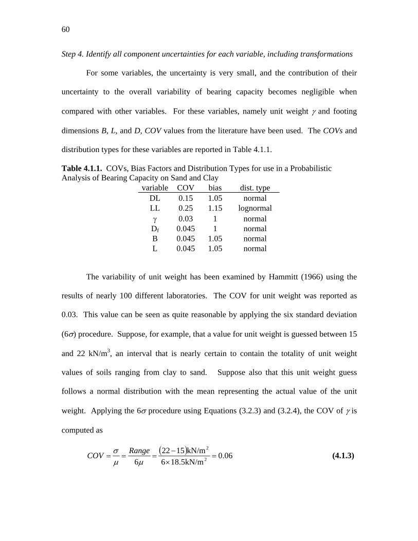
60

Step 4. Identify all component uncertainties for each variable, including transformations

For some variables, the uncertainty is very small, and the contribution of their

uncertainty to the overall variability of bearing capacity becomes negligible when

compared with other variables. For these variables, namely unit weight γ and footing

dimensions B, L, and D, COV values from the literature have been used. The COVs and

distribution types for these variables are reported in Table 4.1.1.

Table 4.1.1. COVs, Bias Factors and Distribution Types for use in a Probabilistic Analysis of Bearing Capacity on Sand and Clay

variable COV bias dist. type DL 0.15 1.05 normal LL 0.25 1.15 lognormal γ 0.03 1 normal

Df 0.045 1 normal B 0.045 1.05 normal L 0.045 1.05 normal

The variability of unit weight has been examined by Hammitt (1966) using the

results of nearly 100 different laboratories. The COV for unit weight was reported as

0.03. This value can be seen as quite reasonable by applying the six standard deviation

(6σ) procedure. Suppose, for example, that a value for unit weight is guessed between 15

and 22 kN/m3, an interval that is nearly certain to contain the totality of unit weight

values of soils ranging from clay to sand. Suppose also that this unit weight guess

follows a normal distribution with the mean representing the actual value of the unit

weight. Applying the 6σ procedure using Equations (3.2.3) and (3.2.4), the COV of γ is

computed as

( ) 06.0

kN/m5.186kN/m1522

6 2

2

=×

−===

µµσ RangeCOV (4.1.3)

61

It is likely that even a simple measurement will be more accurate than such a guess,

validating a COV of 0.03.

ACI 117 (ACI 1990) sets the tolerance for horizontal dimensions (B, L) of

unformed footings with widths between 2ft and 6ft at –1/2 in to +6 in. A conservative

estimate of the COV for footing dimensions is desired. Thus, according to (3.2.4), the

smallest applicable value for µ should be used (2 ft., in this case). Applying the 6σ

procedure and using 2ft as the mean, the COV for footing dimensions is 0.045. This

value is also conservatively applied to formed footings since the small uncertainty in B

and L has minimal effect on the reliability analysis.

For a tolerance of this nature specified by ACI – where the upper bound is

substantially further from the design value than the lower bound – it is reasonable to

assume builders will tend to err on the high side of design values. It is appropriate to

apply a bias factor (Equation 3.2.13) to account for this tendency. According to equation

(3.2.13), footing dimensions which are built, on average, larger than design(nominal) will

have a bias factor greater than 1, as is the case in Figure 4.1.2. Using ACI 117, a

conservative estimate of the bias factor for footing dimensions is 1.05. The bias factors

for B and L is also presented with their COVs in Table 4.1.1.

62

Parameter Value

limit s

tate valu

ePr

obab

ility

Den

sity

nominal valu

e

mean valu

e

Figure 4.1.2. The mean, nominal, and limit state values of a normally distributed design parameter. Here, limit state value corresponds to the value at which a limit state such as bearing capacity failure is reached. Mean value is the mean of the distribution under consideration. Nominal value is the parameter value used in design. The mean can be calculated from the nominal by (nominal) * (bias factor).

Live Load LL and Dead Load DL variability has significant impact on the final

uncertainty in bearing capacity. It has been examined thoroughly in Chapter 2. Nowak

(1994) and Ellingwood (1999) report a COV and bias factor for dead load of 0.15 and

1.05, respectively. Ellingwood (1999) reports a COV and bias factor for live load of 0.25

and 1.15, respectively. These COVs and bias factors appear in Table 4.1.1.

As we will show later in Step 5, the uncertainty of capacity factors Nq, Nγ, sq, and

dq will be determined from the uncertainties of measurement qc or N and of the

transformations from qc to DR, DR to φp, and φp to the bearing capacity factors. This

progression is illustrated by the arrows in Figure 4.1.1. Thus, in Step 4, it is necessary to

find the uncertainty of qc and of each of these transformations.

First, the assessment of the uncertainty in qc is presented. The estimation of soil

properties from in-situ test data involves uncertainties introduced by the inherent soil

variability, the measurement uncertainty, and the transformation model uncertainty

63

(Phoon and Kulhawy 1999). Tip resistance qc inherits uncertainty from the variability of

the CPT measurements themselves as well as the variability of the soil profile. The

variability of the test equipment is difficult to discern since very little human or random

error is possible in the test (Kulhawy and Trautmann 1996). However, the variability of

the overall measurement is readily observed by examining CPT logs. The value of the

coefficient of variation of qc presented in Withiam et. al. (1997) is 0.07. Values may be

expected to be slightly higher for coarser sand and slightly lower for finer sand, but 0.07

was confirmed as reasonable in the current research by considering tip resistance versus

depth profiles for various CPT tests in sand. One of these profiles, for a reasonably

uniform sand layer (same DR), is presented in Figure 4.1.3. A power regression was

performed on the data, conforming to the relationship expressed by Salgado and Mitchell

(2003), according to which qc varies with a power function of horizontal effective stress.

This power function describes the mean line in Figure 4.1.3. The bounds in Figure 4.1.3,

also varying with depth, were fit to the actual data points around the mean line. Using

the 6σ procedure, the COV can be calculated using (3.2.3) and (3.2.4) as described earlier

in the paper.

64

8 12 16 20 24 28qc (MPa)

8

7

6

5

4

3

Dep

th (m

)

8 12 16 20 24 28

8

7

6

5

4

3

lower bound on data (µ - 3σ)

upper bound on data (µ + 3σ)

mean trend (from regression

Figure 4.1.3. Mean Trend (power regression) and Bounds of CPT Tip Resistance Data for Sand. The mean and bounds can be used to calculate the COV for qc using the 6σ procedure.

The SPT is subject to greater test uncertainty than the CPT (Kulhawy and

Trautmann 1996). The additional uncertainty introduced by this test can be assessed by

considering a transformation from N values to qc values. The relationship between SPT

blow count N and CPT tip resistance qc in sand has been studied by Robertson et. al.

(1983), Ismael and Jeragh (1986), and the geotechnical engineering group at Purdue

University. Using their combined data (Figure 4.1.4), the modified 6σ procedure can be

applied to compute the COV of the transformation from N to qc using equations (3.2.5)

and (3.2.4). The modified 6σ procedure is used since relatively few data points are

available. The resulting COV is 0.16. The purpose of finding this transformation

uncertainty is so that the cone tip resistance estimated by the SPT, qc,SPT, may be used in

place of N for the remaining transformations illustrated in Figure 4.1.1. Thus,

uncertainties representing SPT- and CPT-based designs will be developed within the

same framework. What is required, then, is a PDF describing the uncertainty of qc,SPT.

Note that the results of the side-by-side field CPTs and SPTs performed by Robertson et.

65

al. (1983) and Ismael and Jeragh (1986) reflect both the uncertainty of the in-situ sand

and of the individual tests. Thus, the inherent soil variability and the SPT measurement

uncertainty are fully accounted for. Thus, a normal distribution is selected for qc,SPT with

a COV of 0.16.

0.1 1mean grain size (mm)

2

4

6

8

10q c

/ N

55 (1

00 k

Pa)

0.1 1

2

4

6

8

10

Figure 4.1.4. SPT – CPT correlation (after Robertson et. al.1983, Ismael and Jeragh 1986, and Purdue University)

The transformation from qc to DR is that proposed by Salgado and Mitchell (2003)

based on the results of the most recent version of the CONPOINT program (Salgado et al.

1997, Salgado 2003),

⎥⎥⎦

⎤

⎢⎢⎣

⎡⎟⎟⎠

⎞⎜⎜⎝

⎛⋅⋅=

2

'1ln1

13

c

h

A

A

cR

ppq

ccD

σ (4.1.4)

where pA is a reference stress, σ’h is the horizontal effective stress, and constants c1, c2

and c3 are related to intrinsic properties of sands. The predictive capability of an equation

like (4.1.4) to determine values of qc from a known DR in the lab was examined by

Salgado, Mitchell and Jamiolkowski (1997). Experimental values of qc were found to fall

66

within a ± 30% band of predicted values. The 6σ procedure was applied to find the COV

of this predicted qc, yielding a value of 0.10. Taking qc as normally distributed with a

COV of 0.10, Equation (3.2.7) can be used to find the PDF of DR. This PDF, representing

the transformation uncertainty from qc to DR, was found to be normally distributed with a

standard deviation between 3% and 6% depending on the specific value of relative

density. The COV in Figure 4.1.1 representing the uncertainty of this transformation is

that of a representative case.

The transformation from DR to φp (Equation 4.1.2) was calibrated against lab-

measured values of DR (Bolton, 1986). With respect to the accuracy of (4.1.2), Bolton

reported a ±1º band encompassing all measurements of φc and a ±2º band capturing all

measured values of φp – φc about predicted values. First, the 6σ procedure was applied to

find the COV of φc and φp – φc. Then, numerical integration of Equation (3.2.9) was used

to find the PDF of the DR to φp transformation, just as was done for the N to qc correlation.

The resulting transformation PDF was found to be a normal distribution with a COV of

0.020. The same COV found using Monte Carlo simulation was 0.015.

The bearing capacity factors Nγ, sq, and dq have uncertainties due to the

transformations required to compute them. The uncertainty of these transformations has

been examined using tools such as limit analysis and test data. Factor Nq is calculated

from the exact relationship given by Reissner (1924):

⎟⎠⎞

⎜⎝⎛ +⋅=

245tan2tan φφπeNq (4.1.5)

Since it is exact, the arrow representing the φp to Nq transformation in Figure 4.1.1 reports

a COV of zero.

67

Factor Nγ is found using Brinch Hansen (1970) expression:

φφφπγ tan1

245tan5.1 2tan ⋅⎟⎟

⎠

⎞⎜⎜⎝

⎛−⎟

⎠⎞

⎜⎝⎛ +⋅⋅= eN (4.1.6)

The results of numerical limit analysis by Sloan and Yu (1996) were used to determine

the possible range of the values of Nγ with respect to φp. Since the true value of Nγ is in

fact guaranteed by limit analysis to be within the limit bounds for a given friction angle,

the probability of Nγ being so bound is 100%, not the 99.7% associated with the 6σ

procedure. However, for practical purposes, the 6σ deviation procedure can be used

effectively. Using the 6σ procedure, the COV of the φp to Nγ transformation was found

to be 0.12.

Limit analysis was again used to determine the possible range of the values of dq

with respect to D/B ratio based on results by Bandini (2003). Using the 6σ procedure, the

COV of the φp to dq transformation was found to be 0.02.

The COVs for the shape factors sq and sγ can be determined by making reference

to more than fifty tests performed by DeBeer (1970). The modified 6σ procedure

(Equation 3.2.5) is used since relatively few data points are available. The resulting

COVs are 0.23 and 0.19 for the φp to sq transformation and factor sγ, respectively.

At this point, the uncertainties for all of the relevant geotechnical tests,

transformations and other design variables have been described. The next step will be to

combine these uncertainties to describe the PDFs for each of the variables that appear in

Equation (4.1.1).

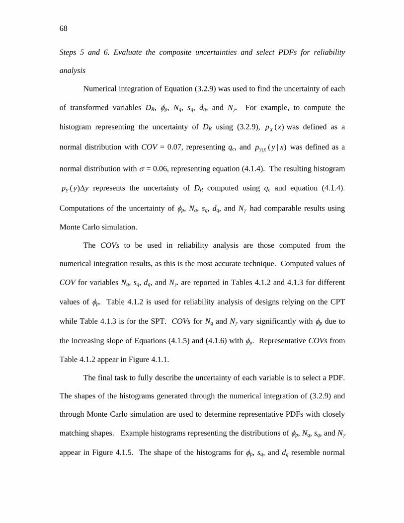
68

Steps 5 and 6. Evaluate the composite uncertainties and select PDFs for reliability

analysis

Numerical integration of Equation (3.2.9) was used to find the uncertainty of each

of transformed variables DR, φp, Nq, sq, dq, and Nγ. For example, to compute the

histogram representing the uncertainty of DR using (3.2.9), )(xpX was defined as a

normal distribution with COV = 0.07, representing qc, and )|(| xyp XY was defined as a

normal distribution with σ = 0.06, representing equation (4.1.4). The resulting histogram

yypY ∆)( represents the uncertainty of DR computed using qc and equation (4.1.4).

Computations of the uncertainty of φp, Nq, sq, dq, and Nγ had comparable results using

Monte Carlo simulation.

The COVs to be used in reliability analysis are those computed from the

numerical integration results, as this is the most accurate technique. Computed values of

COV for variables Nq, sq, dq, and Nγ. are reported in Tables 4.1.2 and 4.1.3 for different

values of φp. Table 4.1.2 is used for reliability analysis of designs relying on the CPT

while Table 4.1.3 is for the SPT. COVs for Nq and Nγ vary significantly with φp due to

the increasing slope of Equations (4.1.5) and (4.1.6) with φp. Representative COVs from

Table 4.1.2 appear in Figure 4.1.1.

The final task to fully describe the uncertainty of each variable is to select a PDF.

The shapes of the histograms generated through the numerical integration of (3.2.9) and

through Monte Carlo simulation are used to determine representative PDFs with closely

matching shapes. Example histograms representing the distributions of φp, Nq, sq, and Nγ

appear in Figure 4.1.5. The shape of the histograms for φp, sq, and dq resemble normal

69

distributions. Thus, normal distributions are used to represent these variables. The shape

of the histograms for Nq and Nγ suggests the use of lognormal distributions. The

distribution type selected for each variable also appears in Tables 4.1.2 and 4.1.3.

Table 4.1.2. COVs, bias factors and distribution types for bearing capacity factors for use in reliability analysis of footings on sand using the CPT

Nq - lognormal Nγ - lognormal dq - normal sq - normal Footing type φp COV bias COV bias COV bias COV bias

36.5 0.21 1.12 0.30 1.17 0.02 1.00 0.23 1.00 39.5 0.24 1.14 0.33 1.19 0.02 1.00 0.23 1.00 Square 42.8 0.31 1.16 0.41 1.22 0.03 1.00 0.23 1.00 38.7 0.34 1.24 0.46 1.34 0.03 1.00 43.5 0.41 1.28 0.54 1.38 0.03 1.00 strip 48.5 0.47 1.30 0.63 1.49 0.03 1.00

Table 4.1.3. COVs, bias factors and distribution types for bearing capacity factors for use in reliability analysis of footings on sand using the SPT

Nq - lognormal Nγ - lognormal dq – normal sq - normal Footing type φp COV bias COV bias COV bias COV bias

39.5 0.32 1.13 0.42 1.19 0.08 1.00 0.24 1.00 square 42.8 0.34 1.16 0.45 1.21 0.04 1.00 0.23 1.00 43.5 0.55 1.33 0.70 1.47 0.06 1.00 strip 48.5 0.61 1.38 0.72 1.50 0.04 1.00

Each of these PDFs is not fully described without considering if a bias factor is

required. As mentioned in the bias factor subsection, bias factors for Nq and Nγ are

needed due to the effect of the non-linear transformations in (4.1.5) and (4.1.6). As seen

in Figure 4.1.1, values of the bearing capacity factors ultimately depend on values of qc.

In Chapter 5, we suggest that the designer conservatively select a value of qc that is 0.84

standard deviations less than the mean. Thus, bias is introduced to every design

parameter that is a transformation of qc. As a result, the means of the bearing capacity

factors are different from the biased values used in design (Figure 4.1.2). Thus, bias

factors are computed using (3.2.13). Inputs to (3.2.13) are the means, computed from the

70

histograms found using numerical integration of (3.2.9), and nominal values, determined

using the design equations presented earlier with the conservative qc value. These bias

factors are also reported in Tables 4.1.2 and 4.1.3.

30 35 40 45 50 55 60

φp

0

500

1000

1500

2000

2500

sim

ulat

ions

(MC

)

0

0.002

0.004

0.006

0.008

inte

rval

pro

babi

lity

(NI)

0 100 200 300 400

Nq

0

2000

4000

6000

sim

ulat

ions

(MC

)

0

0.002

0.004

0.006

0.008

inte

rval

pro

babi

lity

(NI)

(a) (b)

0 100 200 300 400 500

Nγ

0

2000

4000

6000

8000

sim

ulat

ions

(MC

)

0

0.004

0.008

0.012

0.016

0.02in

terv

al p

roba

bilit

y (N

I)

0 1 2 3 4

sq

0

1000

2000

3000

4000

5000

sim

ulat

ions

(MC

)

0

0.002

0.004

0.006

0.008

inte

rval

pro

babi

lity

(NI)

(c) (d)

MC

NI MC NI

MC NI MC

NI

Figure 4.1.5. Example Histograms of Monte Carlo Simulation (MC) and Numerical Integration (NI) Results for φp, Nq, Nγ, and sq

4.2 Assessment of Uncertainty in Bearing Capacity of Footings on Clay


The equation for fully undrained conditions for clay is considered. The bearing

capacity limit state equation is

( ) 0=⋅+⋅⋅⋅−⋅+ DsdNs

LBLLDL

cccu γ (4.2.1)

where su is the undrained shear strength.

71


Of the variables in Equation (4.2.1), DL, LL, B, L, D, and γ have already been

treated in the sand section (see Table 4.1.1). Nc, dc, and sc are factors depending on the

problem geometry (described by B, L, and D). The equations defining sc and dc for use in

design are taken from Salgado et al. (2004),

BDdc ⋅+= 27.01 (4.2.2)

and

BD

LBsc ⋅+⋅+= 17.012.01 (4.2.3)

Undrained shear strength su can be determined from lab and in-situ test correlations.


The CPT or laboratory testing (such as the unconfined compression test) can be

used to find values of su. Thus, qc or su is the measured test value associated with

Equation (4.2.1), depending on the test performed.


The variability of qc in clay was estimated using CPT logs from the literature in

known uniform clay deposits. By selecting this group of data, the variability of qc in clay

only, not an aggregate profile of clay and other materials, can be assessed. Ten logs from

two papers were analyzed – Jacobs and Coutts (1992) and Baligh et. al. (1980) – using

the 6σ procedure exactly as performed on the sand qc data (Figure 4.1.3). As before, only

logs or portions of logs for one reasonably uniform layer were considered. From this data,

the COV for qc in clay was found to be 0.06.

72

From tip resistance qc, su can be determined from

k

vcu N

qs

σ−= (4.2.4)

where σv is the vertical stress and Nk is the cone factor. Limit analysis of circular

foundations in clay by Salgado et al. (2004) is used to analyze the expected value of the

cone factor and its uncertainty. The value of Nk according to Salgado et al. (2004) is

between 11.0 and 13.7. Unlike Nγ, no other information concerning the mean value of Nk

is used here. Thus, the least biased estimate (Harr 1987) of the PDF of Nk, representing

the uncertainty of transformation (4.2.4), is a uniform distribution between 11.0 and 13.7.

The uncertainty of su as determined in the lab can be estimated by considering the

extreme case of the unconfined compression test, which should be more uncertain than

most other lab tests, such as triaxial testing, in common use. Phoon (1995) reports a

number of papers addressing the uncertainty of this test. A representative value given by

the author is a COV of 0.30. This value is confirmed by a paper on undrained testing by

Matsuo and Asaoka (1977). Matsuo and Asaoka (1977) examined the uncertainty and

spatial variability of undrained laboratory tests on marine clays. They attribute the

uncertainty of su to inherent soil variability and sample disturbance. Hence, it is natural

that the uncertainty found for laboratory testing for su is higher than that for in-situ CPT

testing since the scatter in qc measurements is largely controlled by local soil variability.

Since the COV of undrained shear strength from laboratory tests is much higher

than that found for CPT determinations, continued use of the normal distribution for su is

not likely to be realistic. A better suited PDF for strength would include the bounded

distributions, such as the beta or lognormal distributions. Lognormal distributions are in

73

common use for this parameter in the literature. Therefore a lognormal distribution is

used to represent the uncertainty of su in reliability analysis.

The value of Nc is known exactly as 2 + π ≈ 5.14 and therefore has no uncertainty

(Prandtl 1920). However, factors sc and dc are not known exactly. The uncertainties of

these factors can be accounted for using the results of limit analysis. Salgado et al. (2004)

report upper and lower bounds on a lumped bearing capacity factor Ncscdc at different

embedment ratios for strip and square footings. Applying the same least biased principle

as for Nk, these results can be used directly to define a set of uniform distributions for

Ncscdc. For this type of PDF, the upper and lower bounds define the distribution

completely. The distribution bounds are given in Table 4.2.1.


analysis

Numerical integration of Equation (3.2.9) was used to find the uncertainty of su

determined from qc. To compute the histogram representing the uncertainty of su using

(3.2.9), )(xpX was defined as a normal distribution with COV = 0.06, representing qc,

and )|(| xyp XY was defined as a uniform distribution with bounds 11.0 and 13.7,

representing factor Nk from equation (4.2.4). The resulting histogram yypY ∆)(

represents the uncertainty of su computed using qc and equation (4.2.4). From this

histogram, su was found to be normally distributed with COV = 0.09.

74

Table 4.2.1. Uniform Distribution Bounds on Ncscdc for varying embedment ratios for use in a Probabilistic Analysis of Bearing Capacity on Clay (Salgado et al. 2004)

D/B Strip footing Square footing 0.00 5.132 5.203 5.523 6.221 0.01 5.164 5.271 5.610 6.498 0.05 5.293 5.396 5.886 6.830 0.10 5.448 5.536 6.171 7.129 0.20 5.696 5.802 6.590 7.516 0.40 6.029 6.137 7.194 8.092 0.60 6.240 6.341 7.671 8.577 0.80 6.411 6.508 8.068 9.004 1.00 6.562 6.656 8.429 9.355 2.00 7.130 7.229 9.752 10.861 3.00 7.547 7.655 10.532 12.000 4.00 7.885 7.997 10.941 12.879 5.00 8.168 8.286 11.206 13.603

The PDF representing Ncscdc was defined completely in step 4. The bounds of the

uniform distribution desribing the uncertainty of Ncscdc appear in Table 4.2.1. The PDFs

for DL, LL, B, L, D, and γ have been defined in the sand section and are reported in Table

4.1.1.

4.3 Summary

In this chapter, steps 1-6 of the framework were demonstrated to determine the

variable uncertainties for ultimate limit state design checks of shallow foundation on sand

and clay. The next steps, 7-10, to determine resistance factors for shallow foundation

ULS design are demonstrated in the next chapter.

75

CHAPTER 5. ASSESSMENT OF RESISTANCE FACTORS FOR SHALLOW

FOUNDATIONS

5.1 Calculation of Resistance Factors

Input Variables

Before any calculations can take place, the governing limit state equation must be

defined and the COVs and bias factors must be established for each variable of the

equation. This procedure was demonstrated in Chapter 4. With the variable COVs,

target β, and reliability analysis method defined, RFs can be computed.

A large number of possible design parameters exist in foundation design. There

are also many design and test methods. Each of these will lead to different uncertainties

in the overall problem. Therefore, a complete analysis of the problem will consider a

range of design parameters. Eight sets of design conditions are considered – strip and

square footings on sand using the CPT and SPT, and strip and square footings on clay

using the Salgado et al. (2004) and the Meyerhof (1951) shape and depth factors.

Resistance factors are computed for different values of the live- to dead-load ratio

(LL/DL), strength parameter (expressed as either friction angle φ or undrained shear

strength su), and relative embedment (D/B).

Live load is more uncertain than dead load. Trends observed by Galambos et al.

(1982), Milford (1987), and Tabsh (1997) indicate that the influence of the additional

uncertainty introduced by live load is greatest for small values of LL/DL and decreases

for greater values of LL/DL. This influence becomes negligible for LL/DL ≥ 4. Also,

results in Ellingwood et al. (1982) indicate that, in calibration, resistance factors also

76

effectively cease to change for LL/DL ≥ 4. This upper boundary will therefore allow

both a thorough analysis and safe RF values for design. A lower bound is taken as

LL/DL = 0.5.

For footings on sand, values of friction angle φ were considered from 35º to 42º

and from 37º to 48º for square and strip footings, respectively. For clay, values of

undrained shear strength considered were su = 150kPa and su = 800kPa. Embedment

ratios were considered from D/B = 0 to D/B = 1 since shallow foundations are usually

defined for D/B ≤ 1.

Structural design codes using the ASCE-7 (1996) load factors include ACI 318-02

(ACI, 2002) and AISC 3rd ed. (AISC 2001). For the dead- and live- load combination,

these load factors are (LF)DL = 1.2 and (LF)LL = 1.6. AASHTO (1998) load factors are

(LF)DL = 1.25 and (LF)LL = 1.75.

Sand

The results of the resistance factor computations for footings on sand are shown

in Figure 5.1.1 (CPT) and Figure 5.1.2 (SPT) for ASCE-7 load factors. One trend is

immediately apparent in all five square footing plots: a sharp increase in resistance factor

from D/B = 0 to D/B = 0.1. This trend is due mostly to the difference in COV between

Nq and Nγ. At D/B = 0, the ‘γ’ term of the bearing capacity equation is the only term

contributing to resistance. At higher values of D/B, the ‘q’ term (which has lower

uncertainty than the ‘γ’ term) contributes more to resistance. Hence, for these higher

values of D/B, the uncertainty of the overall equation is less than at D/B = 0, causing the

RF to increase.

77

0 0.2 0.4 0.6 0.8 1Depth-to-Width (D/B)

0.3

0.4

0.5

0.6

0.7

0.8

0.9A

djus

ted

Res

ista

nce

Fact

or (R

F)

0.3

0.4

0.5

0.6

0.7

0.8

0.9LL/DL = 0.5LL/DL = 1.0LL/DL = 2.0LL/DL = 4.0

0 0.2 0.4 0.6 0.8 1

0 0.2 0.4 0.6 0.8 1Depth-to-Width (D/B)

0.3

0.4

0.5

0.6

0.7

0.8

0.9

Adj

uste

d R

esis

tanc

e Fa

ctor

(RF)

0.3

0.4

0.5

0.6

0.7

0.8


0 0.2 0.4 0.6 0.8 1

(a) (b)

0 0.2 0.4 0.6 0.8 1Depth-to-Width (D/B)

0.3

0.4

0.5

0.6

0.7

0.8

0.9

Adj

uste

d R

esis

tanc

e Fa

ctor

(RF)

0.3

0.4

0.5

0.6

0.7

0.8


0 0.2 0.4 0.6 0.8 1

0 0.2 0.4 0.6 0.8 1Depth-to-Width (D/B)

0.3

0.4

0.5

0.6

0.7

0.8

0.9

Adj

uste

d R

esis

tanc

e Fa

ctor

(RF)

0.3

0.4

0.5

0.6

0.7

0.8


0 0.2 0.4 0.6 0.8 1

(c) (d)

0 0.2 0.4 0.6 0.8 1Depth-to-Width (D/B)

0.3

0.4

0.5

0.6

0.7

0.8

0.9

Adj

uste

d R

esis

tanc

e Fa

ctor

(RF)

0.3

0.4

0.5

0.6

0.7

0.8


0 0.2 0.4 0.6 0.8 1

0 0.2 0.4 0.6 0.8 1Depth-to-Width (D/B)

0.3

0.4

0.5

0.6

0.7

0.8

0.9

Adj

uste

d R

esis

tanc

e Fa

ctor

(RF)

0.3

0.4

0.5

0.6

0.7

0.8


0 0.2 0.4 0.6 0.8 1

(e) (f)

Figure 5.1.1. Adjusted Resistance Factors for Footings on Sand using CPT: Square: (a)φp = 35.8º, (b)φp = 38.8º, (c) φp = 42.2º; Strip: (d)φp = 37.5º, (e) φp = 42.4º, (f) φp = 47.6º

square, φp = 35.8º square, φp = 38.8º

square, φp = 42.2º strip, φp = 37.5º

strip, φp = 42.4º strip, φp = 47.6º

78

0 0.2 0.4 0.6 0.8 1Depth-to-Width (D/B)

0

0.1

0.2

0.3

0.4

0.5

0.6

0.7

Adj

uste

d R

esis

tanc

e Fa

ctor

(RF)

0

0.1

0.2

0.3

0.4

0.5

0.6

0.7

LL/DL = 0.5LL/DL = 1.0LL/DL = 2.0LL/DL = 4.0

0 0.2 0.4 0.6 0.8 1

0 0.2 0.4 0.6 0.8 1Depth-to-Width (D/B)

0

0.1

0.2

0.3

0.4

0.5

0.6

0.7

Adj

uste

d R

esis

tanc

e Fa

ctor

(RF)

0

0.1

0.2

0.3

0.4

0.5

0.6

0.7


0 0.2 0.4 0.6 0.8 1

(a) (b)

0 0.2 0.4 0.6 0.8 1Depth-to-Width (D/B)

0

0.1

0.2

0.3

0.4

0.5

0.6

0.7

Adj

uste

d R

esis

tanc

e Fa

ctor

(RF)

0

0.1

0.2

0.3

0.4

0.5

0.6

0.7


0 0.2 0.4 0.6 0.8 1

0 0.2 0.4 0.6 0.8 1Depth-to-Width (D/B)

0

0.1

0.2

0.3

0.4

0.5

0.6

0.7

Adj

uste

d R

esis

tanc

e Fa

ctor

(RF)

0

0.1

0.2

0.3

0.4

0.5

0.6

0.7


0 0.2 0.4 0.6 0.8 1

(c) (d)

Figure 5.1.2. Adjusted Resistance Factors for Footings on Sand using SPT: Square: (a)φp = 38.8º, (b) φp = 42.2º; Strip: (c) φp = 42.4º, (d) φp = 47.6º

For square footings, a distinct trend of decreasing RF after approximately D/B =

0.5 illustrates another influence on RF computations. The optimization of (3.3.4) will

yield a point on the limit state surface tangent to some contour of probability density

about the mean values. Figure 5.1.3 illustrates a two-variable example where a change in

the slope of the limit state curve will affect the calculated resistance factor. Considering

the relationship between load capacity and bearing capacity factor Nq, a slope can be

square, φp = 38.8º square, φp = 42.2º

strip, φp = 42.4º strip, φp = 47.6º

79

defined for the relationship between Nq and load for a given design condition (values of

D, B, sq, dq, sγ). As D/B increases, values of D and dq increase for a given value of B,

indicating an increase in the slope of the limit state surface in Nq-load space. Note that

σdq and σD will also increase, but µsq and σsq will remain constant, which affects the

optimization of (3.3.4). This change in the Nq vs. load slope will move the location of the

point of tangency between the limit state surface and the probabilistic distribution about

the mean of Nq. As shown in Figure 5.1.3, this increase in slope will cause an increase in

the separation between mean and limit state values of Nq, and therefore, a decrease in RF.

Load

limit

state

line

(P )LS 1

Pn

(P )LS 2

limit s

tate lin

e

for depth D 1

for d

epth

D2

Nq(N )q,LS 2 (N )q,LS 1 Nq,n

D > D2 1

Figure 5.1.3. Two-Dimensional Explanation (similar to Figure 3.2.1c) of RF Curve Shapes in Figure 5.1.1(a-c) and Figure 5.1.2(a-b) – when the other bearing capacity variables change, the slope of the limit state surface at the point of consideration from depth 1 to depth 2 also changes – the optimum relative distance between nominal and limit state values is affected.

A very important result presented in Figures 5.1.1 and 5.1.2 is the effect of

different friction angles φ on the computed value of RF. Since values of the bearing

capacity factors increase exponentially with increasing φ, an overestimate of φ will

significantly overestimate the nominal resistance of the footing. This possibility is

80

correctly accounted for in the reliability analyses, showing as decreasing values of RF for

higher nominal values of φ.

Also of interest in Figures 5.1.1 and 5.1.2 are the curves for different LL/DL

ratios. Due to the high uncertainty of live load relative to dead load, the plots could

naively be expected to present a sequence of high to low RFs for low to high LL/DLs.

However, this is not the case. The answer lies in the fact that the RFs cannot be

considered in isolation, but always combined with load factors. Since different LL/DL

ratios are presented, an assessment of the overall adjustment must consider the LL/DL,

LFs, and RFs together. These quantities can be grouped as a factor of safety:

( ) ( )

( )RFDLLL

DLLLLFLF

FSLLDL

⎟⎠⎞

⎜⎝⎛ +

⎟⎠⎞

⎜⎝⎛+

=1

(5.1.1)

Referring, for instance, to Figure 5.1.2(a), with a D/B of 0.5, the curves report a RF of

0.49 for LL/DL = 0.5 and 0.53 for LL/DL = 4.0. Considering also the LF values (LFDL =

1.2 and LFDL = 1.6) and LL/DL, Equation (5.1.1) yields values of factor of safety of 2.72

and 2.87, respectively. This result indicates that the factor of safety is greater for the

LL/DL = 4.0 case despite the higher RF, and thus the greater load uncertainty is

accounted for properly.

Two last observations are made. First, due to the uncertainty introduced by the

SPT test procedure, RFs for designs using the SPT are lower than those using the CPT.

Finally, in all cases for square footings, the change in resistance factor with embedment is

greatest from D/B = 0 to D/B = 0.10. For this reason, recommended values of RF for

81

footings on sand are broken into two categories: D/B < 0.10 and D/B ≥ 0.10. The

recommended RF values appear in Table 5.1.1.

Table 5.1.1. Recommended Resistance Factors for Bearing Capacity on Sand and Clay, applicable for D/B ≤ 1

ASCE-7 LFs AASHTO (1998) LFs Design Case D/B < 0.10 D/B ≥ 0.10 D/B < 0.10 D/B ≥ 0.10

Footings on Sand

φ ≤ 38º 0.40 0.42 Strip Footings using CPT

φ > 38º 0.25 0.26

Strip Footings using SPT 0.20 0.21

φ ≤ 39º 0.40 0.45 0.42 0.47 Rectangular Footings using CPT

φ > 39º 0.30 0.35 0.31 0.36

Rectangular Footings using SPT 0.30 0.35 0.31 0.36

Footings on Clay

Strip Footings using Salgado et al. (2003) Factors (CPT) 0.70 0.73

Strip Footings using Meyerhof (1951) Factors (CPT) 0.72 0.75 0.75 0.78

Rectangular Footings using Salgado et al. (2003) Factors (CPT) 0.73 0.76

Rectangular Footings using Meyerhof (1951) Factors (CPT) 0.70 0.78 0.73 0.81

Strip Footings using Salgado et al. (2003) Factors (lab) 0.52 0.54

Strip Footings using Meyerhof (1951) Factors (lab) 0.52 0.55 0.54 0.57

Rectangular Footings using Salgado et al. (2003) Factors (lab) 0.52 0.54

Rectangular Footings using Meyerhof (1951) Factors (lab) 0.48 0.54 0.50 0.56

Clay

The results of the resistance factor computations for footings on clay designed

using the CPT are shown in Figure 5.1.4. In Chapter 3 the concept of bias and the bias

factor were presented. One use of the bias factor mentioned was to correct design

equations so that they yield values equal to the mean values observed in analysis and

testing. The bias introduced by the Meyerhof (1951) shape and depth factors, and the

resulting effect on RFs is notable in Figure 5.1.4. A difference appears between the RFs

computed using the Salgado et al. (2004) and by the Meyerhof (1951) factors. The

82

probability density functions (PDFs) of the composite bearing capacity factor (Ncscdc) for

clay presented in Chapter 4 were developed on the basis of the limit analysis results by

Salgado et al. (2004). Thus the mean value of Ncscdc can be quite different from the

nominal design value suggested by the Meyerhof (1951) design factor equations. The end

result is that the resistance factors presented here behave partially as adjustment factors.

In this study, bias factors have been applied to designs both on sand and on clay, but their

use has particularly prominent effect in this example.

Three other noteworthy observations are made. First, RF decreases with

increasing LL/DL. Second, unlike sands, the RF plots for clays do not show any

pronounced change in RF over a particular D/B range (excluding the Meyerhof (1951)

shape and depth factor correction mentioned above). Finally, in striking contrast to sand,

the effect of different strength (su) values is negligible, as seen from the comparison of

Figures 5.1.4(a) and 5.1.4(c).

Effect of Target Reliability Index

An important consideration in the selection of RF values for use in design is the

appropriate target value of the reliability index to use. A target β of 3.0 was argued

earlier as the most appropriate for shallow foundation ULS design. Figure 5.1.5 presents

the results of the RF computations described above with varying target β values. In both

sand and clay, the effect of changing β is quite significant, as expected. Charts such as

these can act as valuable tool to assess the acceptable probability of classical ULS failure

when compared with established design methodologies and factors. Also of note in

83

Figure 5.1.5(c) is the possibility of a RF greater than 1.0. This condition is due to the

reasons discussed in the following section.

84

0 0.2 0.4 0.6 0.8 1Depth-to-Width (D/B)

0.4

0.5

0.6

0.7

0.8

0.9

1

1.1

Adj

uste

d R

esis

tanc

e Fa

ctor

(RF)

0.4

0.5

0.6

0.7

0.8

0.9

1

1.1


0 0.2 0.4 0.6 0.8 1

0 0.2 0.4 0.6 0.8 1Depth-to-Width (D/B)

0.4

0.5

0.6

0.7

0.8

0.9

1

1.1

Adj

uste

d R

esis

tanc

e Fa

ctor

(RF)

0.4

0.5

0.6

0.7

0.8

0.9

1

1.1


0 0.2 0.4 0.6 0.8 1

(a) (b)

0 0.2 0.4 0.6 0.8 1Depth-to-Width (D/B)

0.4

0.5

0.6

0.7

0.8

0.9

1

1.1

Adj

uste

d R

esis

tanc

e Fa

ctor

(RF)

0.4

0.5

0.6

0.7

0.8

0.9

1

1.1


0 0.2 0.4 0.6 0.8 1

0 0.2 0.4 0.6 0.8 1Depth-to-Width (D/B)

0.4

0.5

0.6

0.7

0.8

0.9

1

1.1

Adj

uste

d R

esis

tanc

e Fa

ctor

(RF)

0.4

0.5

0.6

0.7

0.8

0.9

1

1.1


0 0.2 0.4 0.6 0.8 1

(c) (d)

0 0.2 0.4 0.6 0.8 1Depth-to-Width (D/B)

0.4

0.5

0.6

0.7

0.8

0.9

1

1.1

Adj

uste

d R

esis

tanc

e Fa

ctor

(RF)

0.4

0.5

0.6

0.7

0.8

0.9

1

1.1


0 0.2 0.4 0.6 0.8 1

(e) Figure 5.1.4. Adjusted Resistance Factors for Footings on Clay using CPT: Salgado et al. (2003) shape and depth Factors: (a) Square, su = 150 kPa, (b) Strip, su = 150 kPa, (c) Square, su = 800 kPa; Meyerhof (1951) Factors: (d) Square, su = 150 kPa, (e) Strip, su = 150 kPa

Salgado et al. (2003) factors



Meyerhof (1951) factors square, su = 150 kPa

Meyerhof (1951) factors strip, su = 150 kPa

85

0 0.2 0.4 0.6 0.8 1Depth-to-Width (D/B)

0.3

0.4

0.5

0.6

0.7

0.8

0.9A

djus

ted

Res

ista

nce

Fact

or (R

F)

0.3

0.4

0.5

0.6

0.7

0.8

0.9β = 2.0β = 2.5β = 3.0β = 3.5

0 0.2 0.4 0.6 0.8 1

0 0.2 0.4 0.6 0.8 1

Depth-to-Width (D/B)

0.1

0.2

0.3

0.4

0.5

0.6

0.7

Adj

uste

d R

esis

tanc

e Fa

ctor

(RF)

0.1

0.2

0.3

0.4

0.5

0.6

0.7

β = 2.0β = 2.5β = 3.0β = 3.5

0 0.2 0.4 0.6 0.8 1

(a) (b)

0 0.2 0.4 0.6 0.8 1Depth-to-Width (D/B)

0.4

0.5

0.6

0.7

0.8

0.9

1

1.1

Adj

uste

d R

esis

tanc

e Fa

ctor

(RF)

0.4

0.5

0.6

0.7

0.8

0.9

1

1.1

β = 2.0β = 2.5β = 3.0β = 3.5

0 0.2 0.4 0.6 0.8 1

(c)

Figure 5.1.5. Adjusted Resistance Factors for a Square Footing, LL/DL = 1.0, varying β: (a) sand using CPT, φp = 35.8º, (b) sand using SPT, φp = 38.8º, (c) clay using Salgado et al. (2003) Factors, su = 150 kPa

5.2 Characteristic Resistance

In-situ tests, such as the CPT or SPT, are used in sands to evaluate the friction

angle. To estimate undrained shear strength in clays, the CPT or laboratory tests can be

used. Following the collection of soil strength data, the engineer’s task becomes

selecting an appropriate value of strength for design. This value of strength is referred to

sand, CPT, φp = 35.8º

sand, SPT, φp = 38.8º

clay, su = 150 kPa

86

as characteristic strength. The characteristic strength, in turn, is used to determine the

characteristic (design) resistance in bearing capacity analysis.

The uncertainties in test correlations are quantifiable. To take advantage of

LRFD, a statistically consistent approach to design is necessary. Determination of the

characteristic shear strength as a conservatively assessed mean (CAM) is helpful in this

regard. The first step in determining the CAM is to determine the mean value of the data.

Since shear strength tends to increase with depth because of the higher effective

confining stress, a mean trend of the data with depth is found. Once this mean function is

determined, it must be reduced by some amount to conservatively assess the mean. One

reduction method is a percent exceedance criterion (Becker 1996), in which the value

above which 80% of the data lay is determined.

Characteristic Values in Sand

Characteristic values for friction angle in sand can be determined using both the

CPT and SPT. For each CPT performed, the individual layers of soil are first identified.

A layer in this context is defined as a volume of soil with approximately the same relative

density. For each soil that is of interest, the values of qc are normalized using the

following relationship from Salgado and Mitchell (2003):

2

3'

1

c

A

hDc

A

c

pce

pq

R

⎟⎟⎠

⎞⎜⎜⎝

⎛⋅=

σ (5.2.1)

where pA is a reference stress of 100kPa, DR is relative density, σ’h is the lateral effective

stress, and c1, c2, and c3 are coefficients related to intrinsic sand properties. The equation

87

can also be rewritten with depth in place of σ’h. Using a power regression, the resulting

equation will be consistent with (5.2.1), where qc is a function of depth raised to a power.

Unless a very large number of data points is available, the sample (data) set is

relatively small compared to the size of the population (all possible values). Thus, the

modified 6σ procedure (Chapter 3) is an applicable statistical tool to determine the

standard deviation. Taking the mean of the sample (a regression line with depth) as a

close representation of the population mean, the 80% exceedance value line can be

determined as a value 0.84 standard deviations below the regression line. This value can

be determined by operating on detrended data. When a large number of data points is

available, the procedure can also be approximated visually. Figure 5.2.1 illustrates an

example where the CAM line for an approximately linear qc profile can be drawn visually

such that 80% of the data points lie above the CAM line.

8 12 16 20 24qc (MPa)

8

7

6

5

4

3

Dep

th (m

)

8

7

6

5

4

3

8 12 16 20 24

Figure 5.2.1. Visual Approximation of CAM Function for a CPT Profile – The trend line is drawn so that 80% of the data points occur to the right of the line.

CAM trendline

88

An assessment of the validity of the 80% exceedance criterion is in order.

Considering equation (1.1.1), it is necessary that the evaluation of (RF)Rn correspond to a

consistent level of reliability regardless of the value of qc COV existing in the field. Thus,

either RF or Rn must vary with COVqc so that the target reliability index β is always

achieved. In this chapter, it has already been shown that for a given target reliability

index and qc uncertainty, an optimum RF can be found. Thus, it is necessary that, if Rn is

to be a function of COVqc,

[ ][ ] [ ][ ])()( ,, qcCAMnmeannqc COVRRFRCOVRF = (5.2.2)

where RF(COVqc) is the optimum resistance factor that varies with COVqc and is

multiplied with a nominal resistance Rn,mean found using the mean trend of qc with depth;

and Rn,CAM(COVqc) is a nominal resistance Rn that varies with COVqc. In the approach

followed in this report, the variation of Rn with the COVqc is captured by defining Rn as a

CAM of the resistance. This nominal resistance is then multiplied by a constant RF value

(the value determined using reliability analysis).

Geotechnical designers routinely determine representative values of Rn in practice.

Thus, the determination of Rn,CAM adds no burden to the engineer. Values of RF are

usually selected according to design codes or established practice. Detailed reliability

analyses may be used to determine RF values at the time of code development or in other

RF studies. However, detailed reliability analyses are highly uncommon for specific

projects. Thus, it is more reasonable to establish one value of RF for a type of design

than to specify the use of RF(COVqc).

Note that the reinforced concrete code (ACI 1999) makes use of Rn,CAM(COV)

rather than RF(COV) for concrete design. In this code, ACI specifies 95% exceedance as

89

a criterion for evaluating concrete compressive strength. However, given the values of

COV encountered in geotechnical design, this criterion would yield physically unrealistic

values when applied to qc. Thus, an 80% criterion has been selected.

To assess the ability of this 80% criterion-based resistance Rn,CAM to satisfy

equation (5.2.2), values of RF(COVqc) and RF for a square foundation on sand and on

clay were determined for different values of COVqc. The results of this assessment

appear in Figure 5.2.2. These plots are presented in the same relative RF scale as Figures

5.1.1, 5.1.2 and 5.1.4 to highlight the relative influence of the COV of qc. Of note in

Figure 5.2.2(b) is the negligible change in RF with COV. Thus, in this case, the

application of Rn,CAM(COVqc) is successful since a constant RF is desired. The application

of this CAM method to sands is less successful. Referring to Figure 5.2.2(a), although

the decrease in RF (based on the CAM qc) with increasing qc COV is less than the

decrease in RF(COVqc) (based on the mean qc), the decrease is still significant. Thus, the

CAM method proposed only partly accounts for a higher uncertainty than that assumed in

the development of the proposed RF values in the case of sands.

Taking the CAM value after normalizing sounding data accounts for the deviation

of the data from the mean trend with depth – the spatial variability of the soil in the

vertical direction. To account for the lateral variability of the soil, the traditional

approach of using the worst applicable sounding appears to be the best solution. A

statistical treatment of the soil variability in the lateral direction is far too complicated

and in most cases not feasible, given the information available.

In summary, the conservatively assessed mean (CAM) procedure is a valuable

tool in selecting design values for two reasons: first, and most importantly, it provides a

90

statistically consistent method to analyze data from a particular soil layer, replacing

arbitrary selection with a consistent procedure; second, the CAM procedure tends to

stabilize the reliability of design checks completed using particular RF values. This

method does not replace the engineer’s responsibility to determine which data are

relevant to the design problem, but rather supplements the tools available to analyze

them.

0.06 0.07 0.08 0.09 0.1qc COV

0.2

0.3

0.4

0.5

0.6

0.7

0.8

Adj

uste

d R

esis

tanc

e Fa

ctor

(RF)

0.2

0.3

0.4

0.5

0.6

0.7

0.8using CAM procedureusing mean

0.06 0.07 0.08 0.09 0.1

0.05 0.06 0.07 0.08 0.09 0.1

qc COV

0.2

0.3

0.4

0.5

0.6

0.7

0.8

Adj

uste

d R

esis

tanc

e Fa

ctor

(RF)

0.2

0.3

0.4

0.5

0.6

0.7

0.8

using CAM procedureusing mean

0.05 0.06 0.07 0.08 0.09 0.1

(a) (b)

Figure 5.2.2. Adjusted Resistance Factors Computed Using CPT Profiles with Different Variabilities, with and without the CAM procedure, LL/DL = 1.0: (a) strip on sand surface, φp = 42.4º, (b) Square Footing on Clay using Salgado et al. (2003) Factors, su = 150 kPa, D/B = 0.4

91

CHAPTER 6. DESIGN EXAMPLES FOR SHALLOW FOUNDATIONS

Design Philosophy

In general, all geotechnical designs follow the flow of design tasks outlined in

Figure 6.1.

interpret & filterdata

select stiffnessparameters

select strengthparameters

size to preventED SLS / ULS

size to prevent BC ULS

final designselection

in-situ / lab testmeasurements

Figure 6.1. General design flow for geotechnical engineering. ULS = ultimate limit states, BC = bearing capacity, SLS = serviceability limit states, ED = excessive deformation.

In the LRFD method advocated in this report, the selection of the CAM value of

strength parameters starts with the interpretation of geotechnical tests. For example, after

the relevant CPT soundings have been selected, a CAM value of qc is determined by

finding the trend of the data with depth and adjusting the trend according to the CAM

procedure. This process is illustrated in the examples below.

Since we are addressing ULS design checks specifically here, the following flow

chart (Figure 6.2) illustrates the process in more detail.

92

select foundation system and design

method

resize foundation

group available test data by soil layer

use CAM procedure to select design values from data

compute resistance using trial

foundation design

check resistance using LRFD

equation

fails check

passes check compare alternative foundation systems

select Resistance factor for design method (tables)

Figure 6.2. LRFD flow chart for ULS checks for foundation design. Dashed line boxes indicate steps specific to a particular design method, solid line boxes indicate steps common to all foundation types.

Notice in Figure 6.2 that the selection of CAM values for in-situ and laboratory

tests only needs to be done once. These values can subsequently be used in any of the

design methods available for a particular foundation element. The designer must take

care to make sure that the Resistance Factor used to check a design matches the particular

design method used. Tables of suggested resistance factors have been developed. The

design example below illustrates their use.

93

Example Design Case

Two sites are considered. One is a primarily sand soil profile. The other is a clay

site. A number of CPT soundings were taken at each site and the measured tip resistance

(qc) profiles are presented in Figure 6.3. For each site, a square column footing with 440

kN (99 kip) live load and 600 kN (135 kip) dead load will be designed against ultimate

limit states. Using live load and dead load factors of 1.6 and 1.2 (ASCE-7 factors),

respectively, the design load is 1,420 kN (319 kip). The basement is to extend to a depth

of 1 m (3.3 ft). The water table is very deep. Based on the available logs, a reasonable

foundation should be possible at a depth of 2.0 m (6.6 ft) (1 m below basement

elevation).

Three CPT Logs in Sand

0

1

2

3

4

5

6

7

8

9

0 10 20 30 40

qc (MPa)

Dep

th (m

)

0

1

2

3

4

5

6

7

8

90 10 20 30 40

Two CPT Logs in Clay

0

1

2

3

4

5

6

0 1 2 3 4 5

qc (MPa)

Dep

th (m

)

0

1

2

3

4

5

60 1 2 3 4 5

Figure 6.3. CPT logs with Best Fit Lines and Range Lines

The first step to design the foundations is to establish trial footing dimensions and

use these to find applicable soil strength parameters from the CPT logs. A CAM method

using an 80% exceedence criterion is illustrated using linear regression – a tool readily

94

available to engineers in spreadsheet applications. These lines represent the mean

function of a soil parameter with depth for the soils. Lines can also be drawn bounding

the qc data points, representing the entire range of qc data for those depths. Both sets of

lines are included in Figure 6.3. Table 6.1 presents the statistics used to find the 80%

exceedance criterion CAM line using the modified 6σ procedure, effectively shifting the

mean line to the left on the plots. In the sand layer, the CAM line is given by the

equation

)(6151.1)/(7497.2, MPazmMPaq CAMc −⋅= , 2m < z < 7m (6.1)

For the clay layer,

)(23656.0)/(049042.0, MPazmMPaq CAMc +⋅= , 0.2m < z < 3.8m (6.2)

Table 6.1. CPT qc log statistics

Sand Profile Clay Profile

Range (MPa) (R) 11.7 1.2 Data Points in Range (n) 294 142

Standard Deviations Represented (from Tippett 1925) (Rσ=1)

5.743 5.261

One Standard Deviation (MPa) (σ = R / Rσ=1) 2.037 0.2281 Number of Standard Deviations for 80%

Exceedance 0.84 0.84

Adjustment for 80% Exceedance (MPa) 1.71 0.192

Design in Sand using CPT

Considering the base depth of 2 m and trial footing width of 1.5 m (4.9 ft), a depth

of interest to soil strength evaluation will be at 2.75 m (9.0 ft) (0.5B below the footing

base). Using (6.1), the CAM qc at 2.75 m is 5.9 MPa (123 ksf). To use the Salgado and

95

Mitchell (2003) charts to interpret qc, a value for horizontal effective stress (σh’) must be

found. Assuming a unit weight and lateral earth pressure coefficient at rest (K0) of 20

kN/m3 (127 pcf) and 0.45, respectively, a depth of 2.75 m gives a σh’ of 25 kPa (522 psf).

Assuming a critical state friction angle of 33°, the Salgado and Mitchell (2003) charts

yield a relative density and peak friction angle (φp) of 40% and 37°, respectively. Table

6.2 presents the equations used to compute the bearing capacity factors.

Table 6.2. Bearing capacity factors in sand example Factor Equation Overburdena

φπ

φφ tan

sin1sin1 eNq −

+=

Unit Weightb

φγ tan)1(5.1 −= qNN

Shapeb φsin1

LBsq +=

Shapeb LBs 4.01−=γ

Depthb B

Dd f

q2)sin1(tan21 φφ −+=

Depthb 1=γd aafter Reissner (1924) bafter Brinch Hansen (1970)

The factored bearing capacity in sand for this example can be expressed as

⎥⎦

⎤⎢⎣

⎡⎟⎠⎞

⎜⎝⎛ += γγγγγ dsBNdsDNBRFRRF qqqn 2

1)( 2 (6.3)

where RF is the resistance reduction factor; Rn is the nominal resistance (a force); B is the

foundation width; γ is the soil unit weight; D is the foundation depth; Nq, Nγ are bearing

capacity factors, sq, sγ are shape factors; and dq, dγ are depth factors. Since the footing is

located 1m below basement elevation, 1m depth of soil is available to resist bearing

96

capacity failure. Since D/B = 1/1.5 > 0.10, Table 5.1.1 yields a recommended resistance

factor of 0.45. Using the RF = 0.45, the value of (RF)Rn is 1,840 kN (414 kip).

Considering the calculated design load of 1,420 kN (319 kip) and the requirement to

satisfy inequality (1.1.1), this is an acceptable design. However, another design iteration

is attempted.

For the next iteration, a trial footing width of 1.4m is used. This B yields a

(RF)Rn of 1,590 kN (357 kip), an optimized design. If a highly optimized design is

desired, Figure 5.1.1(a & b) can be used instead of Table 5.1.1 to obtain a value of RF for

the specific design situation. In this case, the optimal RF for this D/B and LL/DL ratio

obtained from Figure 5.1.1 is still 0.45, so no further optimization is possible.

Design in Sand Using SPT

The same design procedure can be applied to the problem using SPT data. The

only difference in this approach is the interpretation of the test data. The available data

for this example are corrected SPT blow counts (N60) of 8, 6, 9, 7, 10, and 9 at depths of

2, 2.5, 3, 3.5, 4, and 4.5 m, respectively. The depth of influence considered earlier,

2.75m, falls within these measurements. Using the Liao and Whitman (1986) stress-

normalization, blow counts can be corrected to stress-normalized values (N1)60,

( )v

ApNN'60601 σ

= (6.4)

where pA is the reference stress 100 kPa (2089 psf) and σ’v is the vertical effective stress.

This stress-normalization essentially accounts for the trend of N60 with depth. Thus, the

mean of the data can be found by taking the mean of the normalized blow count values

97

(N1)60. The mean and range of the resulting (N1)60 values is 10.3 and 4.3, respectively.

Only 6 data points are available, so the modified 6σ procedure is applied, yielding a

standard deviation σΝ of 1.7 blow counts. To determine the 80% exceedance CAM

(N1)60 value, 0.84 standard deviations are subtracted from the mean. The resulting CAM

(N1)60 value is 8.9.

The transformation from N60 to DR can be expressed as (Skempton 1986):

A

vR

pBCA

ND '60

σ+

= (6.5)

where A, B and C are coefficients related to overconsolidation, taken here as 30, 27 and 1,

respectively. Since the CAM (N1)60 value represents data normalized for σ’v = 100 kPa

(2089 psf), (6.5) becomes

( )BCA

NDR +

= 601 (6.6)

For an (N1)60 value of 8.9, (6.5) yields DR = 40%. The design process can then proceed as

described for the CPT example – finding the φp value using DR and calculating (RF)Rn

using (6.3). For this case φ = 37º, and RF = 0.30 (Table 5.1.1, D/B > 0.10). An

optimized design occurs for a footing width B of 1.7m having a (RF)Rn = 1,600kN (360

kip). The additional uncertainty associated with the SPT led to a larger footing (B = 1.7

vs. 1.4m) in comparison with the CPT design.

98

Design in Clay using CPT

In clay, the first step is to find the undrained shear strength. A depth of interest to

determine a representative value of shear strength is 2.75m (0.25B below the footing).

This depth appears conservative since the slip surface (extending to approximately 1B

below the footing) will pass into a stronger layer. Using (6.2), the CAM value of qc is

371 kPa (7750 psf). Undrained shear strength can be calculated from

k

vcu N

qs

σ−= (6.7)

where Nk is the cone factor – taken here as 10 (Yu et al., 2000). Assuming a soil unit

weight of 16 kN/m3 (102 psf), (6.7) yields an su of 33 kPa (690 psf). For B = 3.0m,

factors sc and dc can be found using Salgado et al. (2004),

BDdc ⋅+= 27.01 (6.8)

BD

LBsc ⋅+⋅+= 17.012.01 (6.9)

The bearing capacity equation is

( ) ( )[ ]DdsNsBRFRRF cccun γ+= 2)( (6.10)

Using the recommended resistance reduction factor of 0.73 and substituting the values

found above, (6.10) yields a factored resistance of 1,670 kN (375 psf) – a conservative

design. For the next iteration, the trial footing width, B, is set to 2.8 m, giving a (RF)Rn

of 1,470 kN (330 kip) – an optimized design. Results of the two trial designs are

presented in Table 6.3.

99

Table 6.3. Results of CPT Design Example on Sand and Clay Β φp Nq sq dq Nγ sγ RF (RF)Rn Rn F.S.

1.5m 37° 42.9 1.60 1.16 47.4 0.6 0.45 1,840kN 4,090kN 3.93 Sa

nd

1.4m 37° 42.9 1.60 1.16 47.4 0.6 0.45 1,590kN 3,540kN 3.41 B su sc dc RF (RF)Rn Rn F.S.

3.0m 33kPa 1.22 1.16 0.73 1,670kN 2,290kN 2.21 Cla

y

2.8m 33kPa 1.23 1.16 0.73 1,470kN 2,010kN 1.94

Design in Clay using Unconfined Compression Test

In clay, the first step is to find the undrained shear strength. To determine a CAM

value of su from laboratory tests, a group of relevant tests must be selected first. Relevant

tests are those that were performed on soil samples taken from the same soil layer that is

being designed against. If several soil layers are involved, separate CAM values can be

determined for each layer. If samples are taken from different depths and the soil

properties are expected to vary with depth, then measures to normalize the data before

applying CAM statistics are necessary.

In this example, several soil samples from the same depth were tested to estimate

su for use in design. The available data for this example are unconfined compression test

measurements of su of 30, 37, 40, 45, and 52 kPa (627, 773, 835, 940, and 1090 psf).

Now, we determine the standard deviation of the data. Only 5 data points are available,

so the modified 6σ procedure is applied (equation 3.2.5), yielding a standard deviation

σsu of 9.46 kPa. To determine the 80% exceedance CAM su value, 0.84 standard

deviations are subtracted from the mean. The resulting CAM su value is 32.9 kPa (687

psf).

Design of shallow foundations on clay proceeds as before for ULS design checks

using in-situ test data, taking care to use the correct value of RF from Table 5.1.1 (0.52

for the present example since we are designing a square footing using the Salgado et al.

2004 factors).

100

Comparison with Working Stress Design

Since comparison of these results with traditional Working Stress Design methods

is of interest, values of the factor of safety are also given in Table 6.3. Factor of safety is

defined here as

DLLLRSF n

+=.. (6.11)

It should be noted that, for design on clay using the CPT, the optimized designs have

values of factor of safety less than 2.5. This result would suggest that use of FS values

greater than 3 (a practice often seen) is overly conservative with respect to an ULS

calculation. Within the Limit States Design (LSD) framework, the Ultimate Limit State

and serviceability limit states are treated separately. The traditional practice of using

factors of safety greater than 2.5 in stability calculations may have served a purpose in

avoiding serviceability limit states, but, as pointed out by Becker (1996), this is not an

appropriate use of safety factors. Safety factors in WSD or load and resistance factors in

LRFD must be used only to prevent a specific ULS. The practice of inflating FS values

to account for anything else should be discouraged.

The factors of safety found for sand (in excess of 3) were quite high. This result

is expected since the uncertainties associated with the transformations from qc

measurements to design factor values are much larger than for clay. This comparison

between traditional factors of safety and reliability-based factors offers an opportunity to

examine acceptable risk in current practice. Reference to Figure 5.1.5 facilitates this

discussion. In this figure, adjusted resistance factors for footing designs on sand and clay

are presented for different target reliability indices. For a given resistance factor and

value of D/B, a corresponding value of β can be obtained from Figure 5.1.5. Higher

101

reliability indices are related to lower probabilities of failure. For different resistance

factors, equivalent factors of safety can be computed using either equation (6.11) or

(5.1.1). These factors of safety can then be compared to existing practices.

102

103

CHAPTER 7. ASSESSMENT OF DESIGN METHODS FOR DEEP FOUNDATIONS

In this chapter, an appraisal of some available design methods is made and design

equations are selected for reliability analysis and resistance factor calculation. In the

course of the literature review, it was often discovered that the experimental and

theoretical support for many design methods is incomplete. Bustamante and Gianeselli

(1982) addressed this issue by stating that “the discrepancies observed between real and

theoretical bearing capacities are explained by the fact that present design methods have

been developed on the basis of questionable and often insufficient experimental data.”

Thus, many design methods can be expected to produce unpredictable deviations between

measured and predicted load capacities. This means that we are unable to rationally

assess the uncertainty for some design methods within the framework established in

Chapter 3. In the following development, only design equations with strong experimental

support and thorough theoretical development are considered.

7.1 LRFD Design of Piles

In terms of limit states design (LSD), pile foundations are typically designed

against an ultimate limit state (ULS). For shaft resistance, the full load capacity of the

shaft is often mobilized at relatively small pile displacements. Franke (1993) states that

side resistance is fully mobilized well before maximum base resistance is reached. Thus,

an ULS is clearly the most pertinent check for shaft resistance. For base resistance, it is

possible to have very large relative settlements before the pile enters a plunging mode.

The unit base load at plunging is qbL. However, to consistently define an ultimate limit

104

bearing pressure, a settlement-based criterion for limit bearing capacity is often adopted.

Most of the methods considered in this section use the settlement-to-pile diameter ratio of

10% (s/B = 10%) definition of ultimate limit bearing capacity, qb,10%. Thus, although an

ULS is defined, there is an implied serviceability limit state (SLS) check in these design

methods that should be sufficient in the majority of projects. For foundations of

particularly sensitive buildings, a more strict tolerable settlement criterion may need to be

imposed to ensure serviceability.

The basic Load and Resistance Factor design (LRFD) equation is

( ) ( )∑≥ iin QLFRRF (7.1.1)

In pile design, both base and shaft resistance contribute to the overall load-carrying

capacity of the pile. There are two possible approaches to implementing an axial load

limit state design check in LRFD:

( )( ) ( )∑≥+ iibs QLFRRRF (7.1.2)

or

( ) ( ) ( )∑≥+ iibbss QLFRRFRRF (7.1.3)

where Rs and Rb are the shaft and base resistances, respectively, and (RF)s and (RF)b are

the shaft and base resistance factors, respectively. In reality, the shaft and base

resistances are not independent. However, given that in practice we do calculate them

separately, it must be recognized that the uncertainties in their prediction are very

different. Therefore the likelihood of overestimating shaft resistance by a certain factor is

very different than it is for base resistance. Thus, it is more accurate to apply (RF)s and

(RF)b as separate resistance factors, as in (7.1.3), since the uncertainty of shaft and base

resistance estimates is so different. However, in the case of some direct design methods,

105

it may not be possible to calibrate separate resistance factors for base and shaft resistance

depending on the available data to validate the method. Therefore, (7.1.2) is applicable to

some circumstances, but (7.1.3) offers better control over design reliability.

Reliability analysis is used to find suitable resistance factors for use with (7.1.2)

and (7.1.3). In the case of (7.1.3), the reliabilities for shaft and base resistance are

computed separately. By doing so, we assume that the two are independent and, as a

consequence, the likelihood of the designer overestimating one resistance is not affected

by the likelihood of the designer overestimating the other. This approach is in a way

similar to reinforced concrete design, where separate design checks are used for both

shear and bending limit states even though both design checks depend on the strength

properties of the concrete.

Pile design methods can be broadly classified as either direct or property-based.

Direct design methods rely on direct correlations between in-situ tests and measured pile

capacity. Property-based design methods compute pile capacity using various soil

parameters as input. These parameters are computed from in-situ and/or laboratory tests.

A major difference between property-based methods and direct methods is that property-

based methods tend to have higher uncertainty (lower RF), but apply to general cases,

while direct methods tend to have lower uncertainty (higher RF) but apply only to cases

resembling the specific piles and soils they were developed for. One implication of this

difference is that it may be riskier to apply a direct method to a design situation that is

different from the pile load test database supporting the method, even though the method

may show excellent agreement with measured values in the database.

106

In Chapters 8 and 9 we will assess the uncertainty of the design methods selected

in this Chapter for use in reliability analysis. Resistance factors will be determined in this

analysis.

7.2 Design of Piles in Sand

Fundamental Load Response Mechanisms and Property-Based Design

First, studies of shaft capacity design are discussed. Perhaps the most well-known

issue in shaft capacity design is the notion of a limiting value of shaft friction at some

limit depth. The literature on the subject reveals the following:

• Vesic (1964, 1970, 1977), Meyerhof (1964, 1976) and Kerisel (1964) discussed

for the first time the critical depth concept;

• Kulhawy (1984) states that limiting unit shaft capacity is a fallacy;

• Kraft (1991), Randolph (1994), and Kulhawy (1984) explain the factors that

caused the concept of critical depth as follows:

a. For side resistance: the apparent limiting value of shaft resistance is

caused by the simultaneous decrease in lateral earth pressure coefficient

at-rest (K0) with depth and decrease in φp with increase in σ'v.

b. For tip resistance: the apparent limiting value of base resistance is caused

by decreasing values of φp and rigidity index with increasing σ'v (Rigidity

index = stiffness/strength)

• Fellenius and Altaee (1995) claim that the critical depth concept resulted from a

misinterpretation of pile load tests where residual load effects were neglected;

107

• Salgado (1995) shows that there is no critical depth, but rather a decreasing rate of

increase of bearing capacity with depth.

The literature search revealed a few notable attempts to account for this

knowledge of the causes of an apparent limiting shaft and base resistance:

• Fleming et al. (1992) attempted to incorporate in their design the effect of

decreasing φ as σ increases. They defined K = 0.02 Nq with δ = φc. This method

overestimates shaft friction for long piles but compares well with the method

presented by Vesic (1970);

• To allow for the degradation of friction due to pile length, Toolan et al. (1990)

presented a new method. Their aim was to account for the well-established

observation that local shaft friction at any fixed level varies with pile penetration,

as discussed by Vesic (1970), Hanna and Tan (1973), Lehane et al. (1993). They

proposed an exponential decay function of shaft friction with length of pile in

terms of local value;

• Randolph (1994), Kulhawy (1984), Toolan et al. (1990), Vesic (1967), Hettler

(1982) and Kraft (1991) explained the trend of limiting values by K0 depth

profiles, friction fatigue processes, local shear-stress distributions and sand

dilation;

• Salgado (1995) shows that the limit unit base resistance qbL increases non-linearly,

at decreasing rates, with increasing σ'v. The limit base resistance qbL is

108

approximately equal to the cone penetration resistance qc (Salgado 2004),

( )3

21 expC

A

hR

A

bL

pDCC

pq

⎟⎟⎠

⎞⎜⎜⎝

⎛ ′=

σ (7.2.1)

where pA is reference stress (100 kPa), C1, C2 and C3 are constants, DR is relative

density, and hσ ′ is the horizontal effective stress.

In their study of open ended pile shaft capacity, Paik and Salgado (2003) where

able to show very clearly the dependency of shaft capacity on K0 for driven piles.

Therefore, it is important that the designer account for K0 in the property-based methods.

In the uncertainty evaluation in the following section, limit state equations are expressed

in terms of K0 for this reason.

The literature search revealed a number of observations concerning the pile

design method recommended by the American Petroleum Institute (API). The API

guidelines are in wide use and are supported by considerable research, so assessments of

these guidelines allow some insight into the quality of pile design in sand. We are using

these results to identify key issues in pile design in sand when considering other design

equations. Note the following observations regarding the API method:

• Toolan et al. (1990) reveal a number of limitations of the API codes (several

supporting tests are unreliable, the method overpredicts capacity, the method

cannot account for loose and very dense sites);

• Randolph (1994) states that API guidelines limit values of shaft and toe

resistances at an absolute stress level or depth independently of pile diameter. He

109

explains that limiting values on end-bearing and shaft capacities are an

idealization;

• Randolph (1994) concludes that “There is a need for new, high-quality field data

on pile driveability and axial capacity in sand, particularly from piles in field scale,

in order to help resolve uncertainties regarding limiting values of shaft friction

and end-bearing, the treatment of partial displacement piles, and potential

differences in tensile and compressive shaft capacity.”;

• With respect to “partial displacement piles,” design of open ended piles has

traditionally been accomplished through the use of general recommendations for

the lateral earth pressure coefficient of the shaft Ks (e.g. Kraft 1990) that do not

take the degree of plugging into account. However, it has been shown by Paik

and Salgado (2003) that open ended pile resistance depends on degree of plugging

during driving, as measured by the incremental filling ratio (IFR). IFR is defined

as:

pdLIFR

dL= (7.2.2)

where Lp is the plug length and L is the pile penetration length.

From these observations, it can be seen that much progress is still needed in pile

design in sand with respect to accuracy and number and quality of data used to support

design methods. The assessment of design equation uncertainty in the following section

exposes some areas where pile design can benefit from targeted investigation and better

data.

The available knowledge concerning shaft interface friction is much better than

that for overall pile design in sand. A large amount of research has been conducted on

110

the subject of the interface friction between steel and sand, including recent contributions

by Kishida and Uesugi (1987), Jardine et al. (1993), Rao et al. (1998), and Jardine and

Chow (1998).

Surface roughness is an important factor in interface friction. Two different

measures of the surface roughness are commonly encountered in the literature: average

roughness (Ra) and maximum roughness (Rmax). Average, or “center-line average”

roughness is an industry standard in the United States and also a very common measure.

Average roughness (expressed in µm) is defined as (Outokumpu Stainless, 2004)

( )∫=l

a dxxzl

R0

1 (7.2.3)

where l is the evaluation length of the measurement (typically 8mm) and z(x) is the

measured surface profile. The surface profile z(x) is expressed such that the area under

the profile above the mean line is equal to that below. Maximum roughness is the

maximum difference in height between a “peak” and a “trough” for a surface profile over

a certain gauge length. Thus Rmax is always expressed for a certain gauge length. Rmax (L

= 2.5mm) is a common measure according to the Japanese Standards Association

(Kishida and Uesugi, 1987). However, Ra is a more common measure of surface

roughness, and the results by Rao et al. (1998), which are reported with reference to Ra,

are used to support the reliability analysis in this chapter.

Rao et al. (1998) and Kishida and Uesugi (1987) have shown that both Rmax (L =

D50) and Ra/Davg. are useful measures of roughness for finding correlations between

interface friction angle δ and roughness for different pile materials. Davg is the total area

beneath the particle size distribution curve divided by 100%, where particle size is plotted

on a linear scale. Values of Davg are approximately equal to D50 for sands tested by Rao

111

et al. Values of Ra for steel piles and D50 for sands are easily obtained in practice. For

steel piles, Ra is typically 8-10 µm.

Sand sheared along the sides of a pile reaches large strains such that critical state

is achieved. Thus, critical state friction angle φc and the corresponding interface friction

angle δc are relevant friction angle values to use in design. Interface friction tests results

by Jardine et al. (1993), Rao et al. (1998), and Jardine and Chow (1998) are used in the

next section to evaluate the uncertainty of δc / φc.

Direct Design Methods

Most of the direct design methods are based on either the standard penetration test

(SPT) or the cone penetration test (CPT). The SPT does not relate well to the quasi-static

pile loading process. In contrast, the CPT resembles a scaled-down pile load test (Lee

and Salgado 1999). The main difference between the CPT and a larger diameter pile base

is the size of the zone of soil influencing the base capacity. Thus, spatial variability of

soil parameters is the main source of uncertainty in comparisons between CPT tip

resistance qc and pile load tests. White (2003) shows that qbL , on average, tends to qc.

Direct design methods have been developed for most pile types. Load settlement

curves are different depending on pile installation procedure (in general terms, on

whether the pile is a displacement or non-displacement pile. However, qbL is mobilized

at large settlement levels and is identical for displacement and non-displacement piles.

Lee and Salgado (1999) developed a design method based on analysis of non-

displacement piles. They observed that there is a good agreement between load tests

performed on steel H-piles, precast concrete piles, and drilled shafts and the predicted

112

values using their proposed design method. They suggest their design method to be

considered a direct method to determine base resistance for displacement piles (H-piles

and close-ended piles) and non-displacement piles (drilled shafts). Lehane and Randolph

(2002) recommend that the base capacity of displacement piles be estimated,

conservatively, using the values of Lee and Salgado (1999) for non-displacement piles.

The design methods we chose for reliability analysis are summarized in Table

7.2.1. These methods were chosen for the completeness of their supporting data. Various

sources were used to develop the design methods for closed-ended piles and the complete

list of references will be provided in Chapter 8.

113

Table 7.2.1 – Summary of selected design methods for reliability analysis in sands

Driven Closed-Ended Pipe Piles Base Shaft

Property-Based Methods (%)0051.002.1%10,

RbL

b Dq

q−=

(Various sources)

vcc

css K

KKf σφ

φδ ′⎟⎟

⎠

⎞⎜⎜⎝

⎛= tan0

0

(Various sources)

Direct Methods (%)0051.002.1%10,

Rc

b Dq

q−=

(Various sources)

ccc

ss qq

qff 002.0=⎟⎟

⎠

⎞⎜⎜⎝

⎛=

(Various sources)

Driven Open-Ended Pipe Piles Base Shaft

Property-Based Methods ⎟⎠⎞

⎜⎝⎛ −=

′ 100IFR(%)295326%10, α

σ h

bq

(Paik and Salgado 2003)

vcc

css K

KKf σφ

φδ ′⎟⎟

⎠

⎞⎜⎜⎝

⎛= tan0

0


Direct Methods 557.0(%)00443.0%10, +−= IFR

qq

c

b


ccc

ss qq

qff 002.0=⎟⎟

⎠

⎞⎜⎜⎝

⎛=


Drilled Shafts Base Shaft

Property-Based Methods (%)0011.0225.0%10,

RbL

b Dq

q−=⎟⎟

⎠

⎞⎜⎜⎝

⎛

(Lee and Salgado 1999)

Direct Methods (%)0011.0225.0%10,

Rc

b Dq

q−=⎟⎟

⎠

⎞⎜⎜⎝

⎛

(Lee and Salgado 1999)

Note that precast concrete piles are the same as closed ended pipe piles in terms of base

capacity and shaft resistance since they are both displacement piles. The only difference

is the possibility of a greater value for δc/φc due to the higher surface roughness of

concrete.

114

7.3 Design of Piles in Clays

In this section, we present and explain the selected methods and equations for

design of driven closed-ended piles in clay soils that are used for reliability analysis and

resistance factor calculation. We did not assess the uncertainty for design methods of

open-ended pipe piles because we had insufficient data to complete a satisfactory analysis.

However, the use of open-ended piles in clay is not as common as in sands.

As for sands, it is important to have a specific definition for the ultimate base

bearing capacity in clays. This is often accomplished using the qb,10% definition (s/B =

10%). For soft to medium stiff clays, qbL is nearly equal to qb,10% since the bearing

capacity of piles in these clays is fully mobilized at small settlements, less than 0.10B in

most cases. We did not assess the uncertainty of design methods in stiff clays since there

are not enough load testing data.

The base resistance of drilled shafts could be compared with driven closed-ended

piles since the load-settlement curves will also lead to qbL at small settlements. This is a

consequence of the undrained load-settlement behavior of clay. So for both driven piles

and drilled shafts in clay, the base resistance is qbL, which is determined using the same

equations for both pile types. Thus the same uncertainty will be applied to the base

resistance of drilled shafts. We did not assess the uncertainty for design methods of shaft

capacity for drilled shafts since instrumented pile load tests are relatively new, and few

load test databases have been presented in the literature.

The base bearing capacity of piles in clay has traditionally been taken as the

plunging bearing capacity:

115

uucbL ssNq 9== (7.3.1)

where su is the undrained shear strength of the clay near the pile base. Stark and Juhrend

(1989) have shown that the bearing capacity factor Nc is likely to be greater than 9 based

on a comparison of results from several different studies. Limit analysis of circular

foundations in clay by Salgado et al. (2004) is used to analyze the expected value of

factor Nc and its uncertainty. The value of Nc according to Salgado et al. (2004) is

between 11.0 and 13.7. An average Nc value of 12 is used for the proposed resistance

factor.

The American Petroleum Institute API (1991) recommends the following

equation for unit shaft resistance using the α method for clays,

us sf α= (7.3.2)

where α is an empirical factor which can be related to clay properties. Values of α are

determined using the recommendations by Randolph and Murphy (1985), written as a

relationship with strength ratio:

0.5 0.5

0.5 0.25

, for 1

, for 1

u u u

v v vNC

u u u

v v vNC

s s s

s s s

σ σ σα

σ σ σ

−

−

⎧⎛ ⎞ ⎛ ⎞⎪ ≤⎜ ⎟ ⎜ ⎟′ ′ ′⎪⎝ ⎠ ⎝ ⎠

= ⎨⎛ ⎞ ⎛ ⎞⎪

>⎜ ⎟ ⎜ ⎟⎪ ′ ′ ′⎝ ⎠ ⎝ ⎠⎩

(7.3.3)

Discussing this method, Randolph and Murphy (1985) state that “the strength ratio may

be related both to the value of OCR for a given soil, and also the value of K0. However,

α is a more fundamental (and directly measurable) quantity than either of the other two,

and also reflects the full stress history of the soil.” Knowing that the API α method is in

116

wide use and accounts for the factors that affect shaft resistance, we considered it for

LRFD.

For direct methods, we considered the method proposed by Aoki and de Alencar

Velloso (1975) based on SPT for piles in a variety of soils ranging from sands to clays.

In this method, base capacity is computed as:

SPTbb Nnq = (7.3.4a)

1F

Knb = (7.3.4b)

where empirical factors K and F1 are found in Tables 7.3.1 and 7.3.2. These factors are

based on the results of 63 pile load tests performed on Franki, Cased Franki, Precast, and

Steel piles. At their bases, these piles can all be expected to behave as large-

displacement, driven close-ended piles due to their method of installation.

Shaft capacity is computed as:

SPTsis Nnf = (7.3.5a)

2

1

FKnsi

α= (7.3.5b)

where empirical factors K, α1 and F2 are found in Tables 7.3.1 and 7.3.2.

117

Table 7.3.1 – Values of α1 and K for use with Aoki and Velloso (1975) direct design method

Table 7.3.2 – Values of F1 and F2 for use with Aoki and de Alencar Velloso (1975) direct design method Pile Type F1 F2 Drilled Shafts 3.5 7.0 Franki 2.5 5.0 Steel 1.75 3.5 Precast concrete 1.75 3.5

118

A comparison of the measured total capacities with those computed using (7.3.4) and

(7.3.5) appears in Figure 7.3.1 as given by Aoki and de Alencar Velloso (1975). Like

most direct methods, this data set is the same data set used to calibrate the method.

Examples of such other methods include Chow (1997) and Eslami and Fellenius (1997).

The fact that such design methods were developed for specific design situations limits

their wide applicability. This is a limitation of all direct design methods and not only the

method we considered in our reliability analysis. Accordingly, these methods can only

be used under the same testing circumstances. Later in Section 9.2.1 we will demonstrate

how to select different resistance factors for different design methods based on data

similar to Figure 7.3.1.

119

0 200 400 600calculated capacity

0

100

200

300

400

500m

easu

red

capa

city

0 200 400 600

0

100

200

300

400

500

Pile TypeFrankiCased FrankiPrecastSteel

Figure 7.3.1 – Measured vs. calculated total pile resistance in study by Aoki and Velloso

(1975) for Franki, Cased Franki, Precast, and Steel piles.

Table 7.3.3 is a summary of the selected design equations for clays.

Table 7.3.3 – Summary of selected design methods for reliability analysis in clays

Base Shaft

Property-Based Methods ucbL sNq = (Salgado et al. 2004)

us sf α= (Randolph and Murphy 1985)

Direct Methods SPTbb Nnq =

(Aoki and de Alencar Velloso 1975)

SPTsis Nnf = (Aoki and de Alencar Velloso

1975)

120

121

CHAPTER 8. RESISTANCE FACTORS FOR DEEP FOUNDATIONS ON SAND

8.1 Assessment of Variable Uncertainties for Deep Foundations on Sand

Many design methods are available for consideration. In this section, a few

design equations are selected from the literature, or inferred from a database of available

instrumented pile load tests. In every case, a limit state equation, quantifying an ULS

design check, is expressed in terms of the applied load and design variables. Each limit

state equation contains the expression for design resistance, and thus reflects directly the

design equation to be used.

Piles are often designed on the basis of in-situ tests prior to any pile driving

activity. Occasionally, a pile design may be verified for a particular project by

performing dynamic or static load testing on an installed pile. In these cases, a measure

is being made of pile capacity for those specific design circumstances: pile length, pile

cross-section, and soil profile. From this measurement, the designer has better

knowledge of the actual pile capacity, hence reducing the uncertainty of production pile

capacity. Thus, it is possible to consider two cases: 1) the uncertainty of a pile’s predicted

capacity in the absence of any confirming measurements, and 2) the uncertainty of a

pile’s predicted capacity after a similar pile at the same site has been tested. In the

following development, the first case is considered. Thus, the resistance factors

developed in this chapter are applicable to the routine design of piles, where the designer

will not be able to revise the design on the basis of a verification test program. The data

used to support this assessment consists of paired sets of in-situ test or soil property data

122

and pile load capacity data. By considering this data set, the relationship between soil

test measurements and likely outcomes of pile capacity is sought.

8.1.1 Design of Closed-Ended Driven Piles in Sand

Property-Based Design of Shaft Capacity


The limit state equation for shaft capacity is written

0tan00

=−−⎥⎦

⎤⎢⎣

⎡′⎟⎟

⎠

⎞⎜⎜⎝

⎛LLDLdLaK

KK

svcc

cs σφφδ (8.1.1)

where (Ks/K0) is the ratio of earth pressure coefficient acting on the driven pile to the

assumed at-rest coefficient K0, (δc/φc) is the ratio of skin interface friction angle to

measured critical-state friction angle φc for the soil, vσ ′ is the effective overburden

pressure at the depth where unit skin friction is estimated, as is the shaft area per unit pile

length, dL is a unit length of pile, DL is the dead load acting on the unit length of pile,

and LL is the live load acting on the unit length of pile.


Of the variables in Equation (8.1.1), K0, vσ ′ , and as are selected by the designer;

DL and LL are outputs of the design of the superstructure; φc is estimated or measured;

and the ratios (Ks/K0) and (δc/φc) are based on published results (i.e., values

recommended for design).

123


Of the identified variables, only φc can be measured in routine practice. Variable

K0 cannot be measured independently of DR or φp in the field, and thus no systematic

uncertainty in its determination can be defined. This means that the designer must have

some other information, such as geologic history, from which to make an estimate of K0.

Since no measurement is made, any uncertainty assigned to this variable is arbitrary and

does not reflect the specific design circumstance.


The uncertainty for variables φc, DL, and LL have been identified previously

(refer to Table 4.1.1). Variable as is specified by the designer and has negligible

uncertainty since driven pile sections are fabricated at relatively small tolerances.

Variable dL is used only for design purposes and has no effect on the final design

prediction. Variable K0 is estimated by the designer, but no systematic uncertainty can be

determined for it.

We select the relationship from Paik and Salgado (2003) to choose values of ratio

(Ks/K0) for use in design. One strength of this relationship is the fact that it is supported

by a focused calibration chamber study where most variables are strictly controlled. Thus,

the nature of the relationship is not obscured by testing errors or other erroneous

inferences about the stress states or soil properties around the pile shaft – errors that are

redundant to those already accounted for in other aspects of the design. This relationship

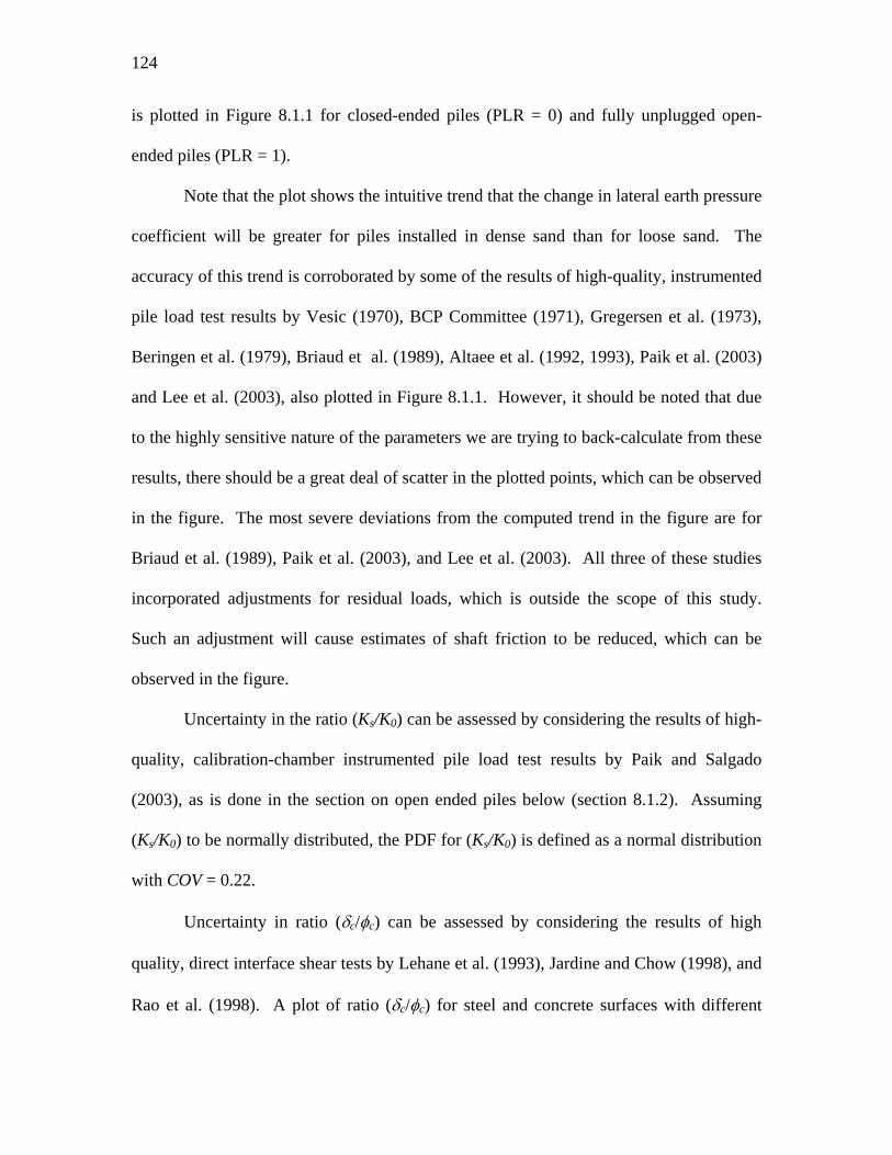
124

is plotted in Figure 8.1.1 for closed-ended piles (PLR = 0) and fully unplugged open-

ended piles (PLR = 1).

Note that the plot shows the intuitive trend that the change in lateral earth pressure

coefficient will be greater for piles installed in dense sand than for loose sand. The

accuracy of this trend is corroborated by some of the results of high-quality, instrumented

pile load test results by Vesic (1970), BCP Committee (1971), Gregersen et al. (1973),

Beringen et al. (1979), Briaud et al. (1989), Altaee et al. (1992, 1993), Paik et al. (2003)

and Lee et al. (2003), also plotted in Figure 8.1.1. However, it should be noted that due

to the highly sensitive nature of the parameters we are trying to back-calculate from these

results, there should be a great deal of scatter in the plotted points, which can be observed

in the figure. The most severe deviations from the computed trend in the figure are for

Briaud et al. (1989), Paik et al. (2003), and Lee et al. (2003). All three of these studies

incorporated adjustments for residual loads, which is outside the scope of this study.

Such an adjustment will cause estimates of shaft friction to be reduced, which can be

observed in the figure.

Uncertainty in the ratio (Ks/K0) can be assessed by considering the results of high-

quality, calibration-chamber instrumented pile load test results by Paik and Salgado

(2003), as is done in the section on open ended piles below (section 8.1.2). Assuming

(Ks/K0) to be normally distributed, the PDF for (Ks/K0) is defined as a normal distribution

with COV = 0.22.

Uncertainty in ratio (δc/φc) can be assessed by considering the results of high

quality, direct interface shear tests by Lehane et al. (1993), Jardine and Chow (1998), and

Rao et al. (1998). A plot of ratio (δc/φc) for steel and concrete surfaces with different

125

average roughnesses Ra in contact with different sands appears in Figure 8.1.2. Note that

at values of Ra greater than 4µm, there is no appreciable change in (δc/φc). Typical values

of Ra for steel piles are greater than 8µm. Figure 8.1.3 is a histogram of the data in

Figure 8.1.2 for values of Ra greater than 2µm. Based on these results, a normal

distribution with mean 0.9 and COV 0.10 represents the uncertainty in (δc/φc).


analysis

Equation (8.1.1) does not include variables that are computed from other variables.

Hence, there is no transformation uncertainty to integrate into a composite uncertainty.

The PDFs for (Ks/K0) and (δc/φc) are selected in Step 4 and the PDF of φc is found in

Section 4.1. These PDFs can be used directly with Equation (8.1.1) in reliability analysis.

126

0

1

2

3

4

5

6

7

8

0 20 40 60 80 100

DR (%)

K /

K0

PLR = 0

PLR = 1

Briaud et al. (1989)

Altaee et al. (1992 &1993)BCP Committee (1971)

Gregersen et al. (1973)

Beringen et al. (1979)

Paik et al (2003)

Vesic (1970)

Lee et al. (2003)

Figure 8.1.1. Relationship by Paik and Salgado (2003) for closed-ended piles (PLR = 0) and fully unplugged open-ended piles (PLR = 1). The results of several high-quality instrumented pile load tests on closed-ended piles are plotted for comparison.

127

0 4 8 12 16 20Ra (µm)

0.2

0.4

0.6

0.8

1

1.2δ c

/ φ c

0 4 8 12 16 20

0.2

0.4

0.6

0.8

1

1.2

SteelConcrete

Figure 8.1.2 – δc/φc values based on results from high quality, direct interface shear tests.

128

Property-Based Design of Base Capacity


The limit state equation for base capacity is written

0%10, =−−⎟⎟⎠

⎞⎜⎜⎝

⎛LLDLAq

qq

bbLbL

b (8.1.2)

where (qb,10%/qbL) is the ratio of the base pressure at s/B = 10% to plunging base

resistance qbL, Ab is the pile base area, DL is the dead load acting on the base of the pile,

and LL is the live load acting on the base of the pile.

Sand Interface Friction (at critical state)

0

5

10

15

20

25

30

0.69 0.75 0.81 0.87 0.93 0.99 1.05

range max, δc / φc

freq

uenc

y

DATA normal distribution

Ra > 2 µmData fromRao et al. (1998)Lehane et al. (1993)Jardine and Chow (1998)

µ = 0.88COV = 0.098

Figure 8.1.3 – Histogram of δc/φc values for Ra > 2µm, based on results from high quality, direct interface shear tests

129


Of the variables in Equation (8.1.2), Ab is selected by the designer; DL and LL are

outputs of the design of the superstructure; qbL is computed from relative density DR; and

ratio (qb,10%/qc) is based on published results.


Of the identified variables, qbL is computed from DR, and DR can be estimated

using the CPT, the SPT, or field sampling (although special sampling procedures would

be required to obtain a reliable estimate of DR). Limit bearing pressure qbL is computed

from DR using Salgado and Mitchell (2003):

( )3

21 expC

A

hR

A

bL

pDCC

pq

⎟⎟⎠

⎞⎜⎜⎝

⎛ ′=

σ (8.1.3)

where pA is reference stress (100 kPa), C1, C2 and C3 are constants, DR is relative density,

and hσ ′ is the horizontal effective stress.


The uncertainty for variables DL, and LL have been identified previously (refer to

Table 4.1.1). Variable Ab is specified by the designer and has negligible uncertainty since

driven pile sections are fabricated at relatively small tolerances. Uncertainty in ratio

(qb,10%/qbL) can be assessed by considering the results of high quality, instrumented pile

load test results by Vesic (1970), BCP Committee (1971), Gregersen et al. (1973),

Beringen et al. (1979), Briaud et al. (1989), Altaee et al. (1992, 1993), Paik et al. (2003)

and Lee et al. (2003). A plot of ratio (qb,10%/qc) for sand layers with different relative

130

densities appears in Figure 8.1.4. The uncertainty of ratio (qb,10%/qbL) can be inferred

from Figure 8.1.4 because, on average, the plunging load qbL is equal to the cone tip

resistance qc (see discussion is Chapter 7). A significant trend of decreasing (qb,10%/qc)

with increasing DR is noted from these results. The following trend for ratio (qb,10%/qc)

has been found and is plotted with the data in Figure 8.1.4.

(%)0051.002.1%10,R

c

b Dq

q−= (8.1.4)

The scatter in ratio (qb,10%/qc) can be assessed by considering the data after it has been

detrended and normalized with respect to Equation (8.1.4). This detrending is

accomplished by

( )

( )R

Rdatac

b

qq

D

Dq

q

errorcb

c

b,10%

c

b,10%%10,

/

qq

qq

%10,

−⎟⎟⎠

⎞⎜⎜⎝

⎛

= (8.1.5)

where errorqb,10%/qc expresses the relative position of a particular data point around the

trend line and function qb,10%/qc(DR) represents the trend line (8.1.4) evaluated for DR

equal to that for the qb,10%/qc data point. When errorqb,10%/qc is computed for all data

points, the distribution of the data points around the trendline can be depicted using the

histogram in Figure 8.1.5. Since we divide by the mean trend value in (8.1.5), the

standard deviation of errorqb,10%/qc is equal to the COV of qb,10%/qc . Assuming (qb,10%/qc)

to be normally distributed, the data in Figure 8.1.4 indicate a COV of 0.17 when equation

(3.2.1) is applied to the detrended data. This normal distribution is also depicted using a

histogram in Figure 8.1.5. Since Equation (8.1.4) defines a mean value for (qb,10%/qbL) a

PDF representing the uncertainty of (qb,10%/qbL) is a normal distribution with COV of 0.17.

131

0 20 40 60 80 100DR (%)

0

0.2

0.4

0.6

0.8

1

q b,1

0% /

q c

0 20 40 60 80 100

0

0.2

0.4

0.6

0.8

1

Briaud et al. (1989)Altaee et al. (1992 & 1993)BCP Committee (1971)Gregersen et al. (1973)Beringen et al. (1979)Paik et al (2003)Vesic (1970)

Figure 8.1.4 – qb,10%/qc values based on results from high quality, instrumented pile load tests on driven, full scale piles in sand. qc values were measured using the CPT; qb,10%was determined from load settlement curves from compression testing; qb was measure directly from strain gauges in the pile; all piles were closed-ended steel piles or precast concrete; the trendline shown is qb,10%/qc = -0.0051DR(%) + 1.02

132

The predictive capability of an equation like (8.1.3) to determine values of qbL

from a known DR in the lab was examined by Salgado et al. (1997). Experimental values

of qbL were found to fall within a ± 30% band of predicted values. The 6σ procedure was

applied to find the COV of this predicted qbL, yielding a value of 0.10. In the absence of

other data, we consider the uncertainty of DR measurements using the uncertainty of DR

determined from the CPT. In Section 4.1, the standard deviation of DR was found to be

8% or less.

qb10%/qc error histogram

0

1

2

3

4

-0.23 -0.116 -0.002 0.112 0.226 0.34

normalized error greater than

freq

uenc

y

Data Normal distribution

NOTES:- error = (ydata - f(x)) / f(x)- distribution found: norm. dist., COV = 0.17

Figure 8.1.5 – Histogram of errorqb,10%/qc (detrended qb,10%/qc values) for closed-ended piles in sand

133


analysis

Numerical integration of Equation (3.2.7) was used to find the uncertainty of

transformed variable qbL. To compute the histogram representing the uncertainty of qbL

using (3.2.7), )(xpX was defined as a normal distribution with σ = 8%, representing

DR(%), and transformation y=f(x) is Equation (8.1.3). Note that numerical integration of

(3.2.9) is not used here, and thus the uncertainty of transformation (8.1.3) is only

included once, since it has already been accounted for in the uncertainty of DR. The

alternative would have been to integrate the uncertainty of (8.1.3) twice, which is not

sensible because the same model is being used and thus no additional uncertainty is

introduced through its use to find qbL. The resulting histogram of qbL is closely matched

by a normal distribution with COV = 0.16. This histogram appears in Figure 8.1.6 for the

case where DR = 80%. A bias factor is needed for qbL because it depends on the CAM

method used to find DR. For example, if the CPT is used to find DR the bias factor on qbL

will be 1.06.

134

0.000E+00

1.000E-03

2.000E-03

3.000E-03

4.000E-03

5.000E-03

6.000E-03

7.000E-03

0 5 10 15 20 25 30 35 40

qbL

¬DR

*f(D

R)

Figure 8.1.6 – Histogram of qbL for DR = 80% for closed-ended piles in sand

135

Direct Design of Shaft Capacity

We did not assess the uncertainty for direct design of shaft capacity because we

had insufficient data to complete a satisfactory analysis. In Section 8.2, resistance factors

for property-based shaft capacity are conservatively adopted for direct design.

Direct Design of Base Capacity



0%10, =−−⎟⎟⎠

⎞⎜⎜⎝

⎛LLDLAq

qq

bcc

b (8.1.6)

where (qb,10%/qc) is the ratio of the base pressure at s/B = 10% to cone tip resistance qc,

Ab is the pile base area, DL is the dead load acting on the base of the pile, and LL is the

live load acting on the base of the pile.


Of the variables in Equation (8.1.6), Ab is selected by the designer; DL and LL are

outputs of the design of the superstructure; qc is measured directly; and the ratio (qb,10%/qc)

is based on published results.


Of the identified variables, qc can be measured in routine practice. The

uncertainty of qc has been examined in Section 4.1.

136


The uncertainty for variables qc, DL, and LL have been identified previously

(refer to Table 4.1.1). Variable Ab is specified by the designer and has negligible


Uncertainty in ratio (qb,10%/qc) was assessed for property-based design of closed-ended

piles and was found to be normally distributed, with a COV of 0.14 and mean equal to

Equation (8.1.4).


analysis

Equation (8.1.6) does not include variables that are computed from other variables,

with the exception of (qb,10%/qc) because DR appears in Equation (8.1.4). Figure 8.1.4

inherently includes the uncertainty of DR since these values were estimated from the field.


PDFs for (qb,10%/qc) and qc are selected in Step 4 and Section 4.1, respectively, and can be

used directly with Equation (8.1.6) in reliability analysis.

8.1.2 Design of Open-Ended Driven Piles in Sand




137

0tan00

=−−⎥⎦

⎤⎢⎣

⎡′⎟⎟

⎠

⎞⎜⎜⎝

⎛LLDLdLaK

KK

svcc

cs σφφδ (8.1.7)

where (Ks/K0) is the ratio of earth pressure coefficient acting on the driven pile to the

assumed at-rest coefficient K0, (δc/φc) is the ratio of skin interface friction angle to

measured critical-state friction angle φc for the soil, vσ ′ is the effective overburden

pressure at the depth where unit skin friction is estimated, as is the shaft area per unit pile

length, dL is a unit length of pile, DL is the dead load acting on the unit length of pile,

and LL is the live load acting on the unit length of pile.


Of the variables in Equation (8.1.7), K0, vσ ′ , and as are selected by the designer;

DL and LL are outputs of the design of the superstructure; φc is estimated or measured;

and ratios (Ks/K0) and (δc/φc) are based on published results. The value of (Ks/K0) to use

in design is found using Paik and Salgado (2003):

( )PLR8.42.70

−= βKK (8.1.8a)

90%(%)20% ,329.00089.0(%)0002.0 2 <<+−= RRR DDDβ (8.1.8b)

where PLR is the plug length ratio, which can be measured or estimated.


Of the identified variables, only φc and PLR can be measured in routine practice.

Variable K0 cannot be measured independently of DR or φp in the field, and thus no

systematic uncertainty in its determination can be defined. This means that the designer

138

must have some other information, such as geologic history, from which to make an

estimate of K0. However, since no measurement is made, any uncertainty assigned to this

variable is arbitrary and does not reflect the specific design circumstance. Plug length

ratio PLR can be measured for a test pile before production piling starts or can be

estimated from charts presented by Lee et al. (2003).


The uncertainty for variables φc, DL, and LL have been identified previously

(refer to Table 4.1.1). Variable as is specified by the designer and has negligible


Variable dL is used only for design purposes and has no affect on the final design

prediction. Variable K0 is estimated by the designer, but no systematic uncertainty can be

determined for it.

Uncertainty in ratio (Ks/K0) can be assessed by considering the results of high-

quality, calibration chamber, instrumented pile load test results by Paik and Salgado

(2003). A plot of ratio (Ks/K0) for sand with different relative densities appears in Figure

8.1.7. Note that, in contrast to closed-ended piles, there is a trend of increasing Ks/K0

with increasing DR. This is due to the effect of plugging. Denser sands exhibit more

plugging, increasing the displacement of the surrounding soil during driving. Increased

displacement caused by pile driving increases the stress against the pile shaft, hence

higher values of Ks/K0 are observed. Closed-ended piles behave as a fully plugged open-

ended pile for any relative density. Thus, there is no variation in displacement with

relative density for closed-ended piles. The scatter in ratio (Ks/K0) can be assessed by

139

considering the data after it has been detrended and normalized with respect to equation

(8.1.8). This detrending is accomplished by

( )

( )Rs

Rs

data

s

KK

DPLRKK

DPLRKK

KK

errors

,

,

0

00/ 0

−⎟⎟⎠

⎞⎜⎜⎝

⎛

= (8.1.9)

where errorKs/Ko expresses the relative position of a particular data point around the trend

line and function Ks/K0(PLR,DR) represents the trend line (8.1.8) evaluated for PLR and

20 40 60 80 100DR(%)

0

1

2

3

4

Ks /

K0

20 40 60 80 100

0

1

2

3

4

measuredcalculated

Figure 8.1.7 – Average Ks/K0 values from Paik and Salgado (2003) for open-ended piles in sand; calculated points indicate values computed using (8.1.8).

140

DR equal to that for the Ks/K0 data point. When errorKs/Ko is computed for all data points,

the distribution of the data points around the trendline can be depicted using the

histogram in Figure 8.1.8. Since we divide by the mean trend value in (8.1.9), the

standard deviation of errorKs/Ko is equal to the COV of Ks/K0. Assuming (Ks/K0) to be

normally distributed, the data in Figure 8.1.7 indicate a COV of 0.22 when equation

(3.2.1) is applied to the detrended data. This normal distribution is also depicted using a

histogram in Figure 8.1.8.

The uncertainty of (δc/φc) has been determined in Section 8.1.1.

141


analysis

Equation (8.1.7) does not include variables that are computed from other variables.


The PDFs for (Ks/K0) and (δc/φc) are selected in Step 4 and the PDF of φc is found in

Section 4.1. These PDFs can be used directly with Equation (8.1.7) in reliability analysis.




Ks/K0 error histogram - OE Piles

0

1

2

3

4

5

6

-0.241 -0.1 0.041 0.182 0.323 0.464


freq

uenc

y

data nrom. dist.


Figure 8.1.8 – Histogram of errorKs/Ko (detrended Ks/K0 values) for open-ended piles in sand

142

0%10, =−−′⎟⎟⎠

⎞⎜⎜⎝

⎛′

LLDLAq

bhh

b σσ

(8.1.10)

where (qb,10%/σ’h) is the ratio of the base pressure at s/B = 10% to horizontal effective

stress σ’h, Ab is the pile base area, DL is the dead load acting on the base of the pile, and

LL is the live load acting on the base of the pile.


Of the variables in Equation (8.1.10), DL and LL are outputs of the design of the

superstructure; hσ ′ is estimated by the designer, Ab is calculated using the outside pile

diameter do,

( ) 4/2ob dA π= (8.1.11)

and the ratio (qb,10%/σ’h) is based on published results by Paik and Salgado (2003) as

follows:

⎟⎠⎞

⎜⎝⎛ −=

′ 100IFR(%)295326%10, α

σ h

bq (8.1.12a)

90%(%)20% ,0141.0(%)0112.0 <<−= RR DDα (8.1.12b)

where IFR(%) is the incremental filling ratio, which can be measured or estimated.


Values of (qb,10%/σ’h) depend on DR, which can be estimated using the CPT, the

SPT, or field sampling. Incremental filling ratio IFR(%) can be measured or estimated

from charts presented by Lee et al. (2003).

143


The uncertainty for variables DL and LL have been identified previously (refer to


driven pile sections are fabricated at relatively small tolerances.

Uncertainty in ratio (qb,10%/ hσ ′ ) can be assessed by considering the results of high


(2003). The scatter in ratio (qb,10%/ hσ ′ ) can be assessed by considering this data after it

has been detrended and normalized with respect to equation (8.1.12). This detrending is

accomplished by

( )

( )Rh

Rhdatah

b

q

DIFR

DIFRq

errorhb

,q

,q

%10b,

%10b,%10,

/%10,

σ

σσσ

′

′−⎟⎟

⎠

⎞⎜⎜⎝

⎛′

=′ (8.1.13)

where error qb,10%/σ’h expresses the relative position of a particular data point around the

trend line and function qb,10%/ hσ ′ (IFR,DR) represents the trend line (8.1.12) evaluated for

IFR(%) and DR equal to that for the qb,10%/ hσ ′ data point. When error qb,10%/σ’h is

computed for all data points, the distribution of the data points around the trendline can

be depicted using the histogram in Figure 8.1.9. Since we divide by the mean trend value

in (8.1.12), the standard deviation of errorqb,10%/σ’h is equal to the COV of qb,10%/ hσ ′ .

Assuming transformation (qb,10%/ hσ ′ ) to be normally distributed, the data indicate a COV

of 0.11 when equation (3.2.1) is applied to the detrended data. This PDF represents the

variability of corrected values of qb,10% for a given value of hσ ′ . This normal distribution

is also depicted using a histogram in Figure 8.1.9.

144

Due to chamber-to-field size effects, qb,10% was corrected by Paik and Salgado

(2003) based on the results of Salgado et al. (1998). This work is based on penetration

resistance analysis described by Salgado et al. (1997). Salgado et al. (1997) examined

the predictive capability of this analysis to determine values of qc from a known DR in the

lab. Experimental values of qc were found to fall within a ± 30% band of predicted values.

The 6σ procedure was applied to find the COV of this predicted qc, yielding a value of

0.10. Thus, a normal distribution with COV = 0.10 represents the uncertainty of

corrected values of qb,10% since the same theoretical model was used to make the

correction as was assessed in the study by Salgado et al. (1997).

qb,10%/σ'h error histogram - OE Piles

0

1

2

3

4

5

6

7

-0.224 -0.166 -0.108 -0.05 0.008 0.066


freq

uenc

y

data norm dist.


Figure 8.1.9 – Histogram of errorqb,10%/σ’h (detrended qb,10%/σ’h values) for open-ended piles in sand

145


analysis

The composite uncertainty of (qb,10%/ hσ ′ ) due to transformation uncertainty and

the uncertainty of the correction to field values of qb,10% must be assessed. Numerical

integration of (3.2.9) is used to accomplish this task. To compute the histogram

representing the composite uncertainty of (qb,10%/ hσ ′ ), )(xpX was defined as a normal

distribution with COV = 0.10, representing qb,10%, and )|(| xyp XY was defined as a

normal distribution with COV = 0.11, representing the transformation uncertainty

(qb,10%/ hσ ′ ). The resulting histogram yypY ∆)( represents the uncertainty of (qb,10%/ hσ ′ )

assessed by Paik and Salgado (2003) using calibration chamber tests. This histogram

appears in Figure 8.1.10. A matching PDF is a normal distribution with COV = 0.15.

Note that the uncertainty of DR introduced by in-situ test correlation to (qb,10%/ hσ ′ )

through the use of Equation (8.1.12) is accounted for by this PDF. This is because the

model used to assess the field correction for qb,10% is the same model used to correlate

CPT qc values to DR. Thus, any variation in the prediction of the model for a specific

case will have been accounted for. For example, suppose that for a given DR, the Salgado

et al. (1998) model predicts a field value of qb,10% that is too high. In the same instance, it

will also predict a DR that is too low when applied to a qc measurement. Thus, the

variability of this model should only be integrated once into the composite uncertainty of

(qb,10%/ hσ ′ ). Redundant integration of its uncertainty will overestimate the uncertainty of

(qb,10%/ hσ ′ ).

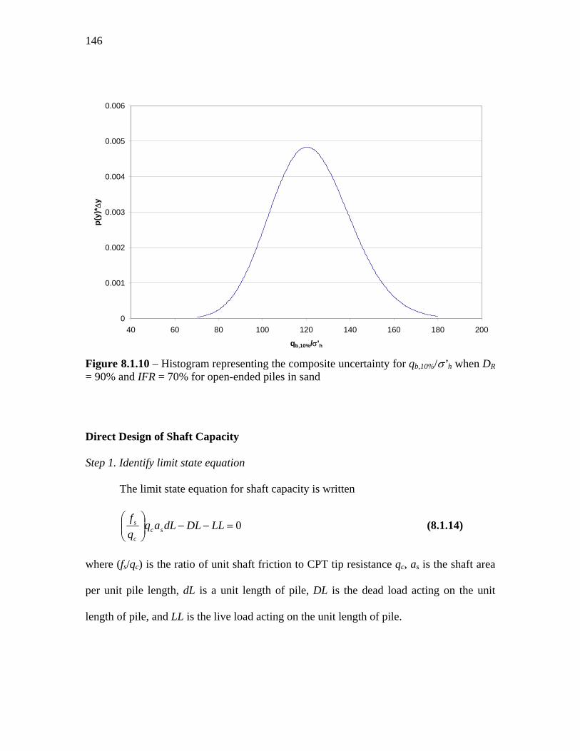
146




0=−−⎟⎟⎠

⎞⎜⎜⎝

⎛LLDLdLaq

qf

scc

s (8.1.14)

where (fs/qc) is the ratio of unit shaft friction to CPT tip resistance qc, as is the shaft area

per unit pile length, dL is a unit length of pile, DL is the dead load acting on the unit

length of pile, and LL is the live load acting on the unit length of pile.

0

0.001

0.002

0.003

0.004

0.005

0.006

40 60 80 100 120 140 160 180 200

qb,10%/σ'h

p(y)

* ∆y

Figure 8.1.10 – Histogram representing the composite uncertainty for qb,10%/σ’h when DR= 90% and IFR = 70% for open-ended piles in sand

147


Of the variables in Equation (8.1.14), as is selected by the designer; DL and LL

are outputs of the design of the superstructure; qc is measured; and ratio (fs/qc) is based on

published results. Lee et al. (2003) recommend a value between 0.0015 and 0.004 for

(fs/qc). Analysis of the data from Paik and Salgado (2003) indicates a mean value of

0.002.



uncertainty of qc has been examined in Section 4.1.



Table 4.1.1). Variable as is specified by the designer and has negligible uncertainty since

driven pile sections are fabricated at relatively small tolerances. Variable dL is used only

for design purposes and has no affect on the final design prediction.

Uncertainty in ratio (fs/qc) can be assessed by considering the results of high


(2003). Assuming (Ks/K0) to be normally distributed, the data from Paik and Salgado

(2003) indicate a mean of 0.002 and a COV of 0.23 when equation (3.2.1) is applied.

148


analysis

Equation (8.1.14) does not include variables that are computed from other

variables. Hence, there is no transformation uncertainty to integrate into a composite

uncertainty. The PDFs for (fs/qc) and qc are selected in Step 4 and Section 4.1,

respectively, and can be used directly with Equation (8.1.14) in reliability analysis.




0%10, =−−⎟⎟⎠

⎞⎜⎜⎝

⎛LLDLAq

qq

bcc

b (8.1.15)

where (qb,10%/qc) is the ratio of the base pressure at s/B = 10% to CPT tip resistance qc, Ab

is the pile base area, DL is the dead load acting on the base of the pile, and LL is the live

load acting on the base of the pile.


Of the variables in Equation (8.1.15), DL and LL are outputs of the design of the

superstructure; qc is measured directly, Ab is calculated using the outside pile diameter

(8.1.11), and the ratio (qb,10%/qc) is based on published results by Paik and Salgado (2003)

and Lee et al. (2003). The value of qb,10%/qc to use in design is found using Lee et al.

(2003):

557.0(%)00443.0 +−= IFRqq

c

b (8.1.16)

149

where IFR(%) is the incremental filling ratio, which can be measured or estimated.



uncertainty of qc has been examined in Section 4.1. Incremental filling ratio IFR(%) can

be measured or estimated from charts presented by Lee et al. (2003).




driven pile sections are fabricated at relatively small tolerances.

Uncertainty in ratio (qb,10%/qc) can be assessed by considering the results of high


(2003). A plot of ratio (qb,10%/qc) for different values of incremental filling ratio IFR(%)

appears in Figure 8.1.11. A significant trend of decreasing (qb,10%/qc) with increasing

IFR(%) is noted from these results. The trendline defined by (8.1.16) is plotted with the

data in Figure 8.1.11. The scatter in ratio (qb,10%/qc) can be assessed by considering the

data after it has been detrended and normalized with respect to equation (8.1.16). This

detrending is accomplished by

( )

( )IFR

IFRq

q

error datac

b

qq cb

c

b,10%

c

b,10%%10,

/

qq

qq

%10,

−⎟⎟⎠

⎞⎜⎜⎝

⎛

= (8.1.17)

150

where errorqb,10%/qc expresses the relative position of a particular data point around the

trend line and function qb,10%/qc(IFR) represents the trend line (8.1.16) evaluated for

IFR(%) equal to that for the qb,10%/qc data point. When errorqb,10%/qc is computed for all

data points, the distribution of the data points around the trendline can be depicted using

the histogram in Figure 8.1.12. Since we divide by the mean trend value in (8.1.17), the

standard deviation of errorqb,10%/qc is equal to the COV of qb,10%/qc. Assuming (qb,10%/qc)

to be normally distributed, the data in Figure 8.1.11 indicate a COV of 0.10 when

equation (3.2.1) is applied to the detrended data. This normal distribution is also depicted

using a histogram in Figure 8.1.12.

40 50 60 70 80 90IFR(%)

0

0.1

0.2

0.3

0.4

q b,1

0% /

q c

measuredequation

40 50 60 70 80 90

0

0.1

0.2

0.3

0.4

Figure 8.1.11 – qb,10%/qc vs. IFR(%) for Open-Ended piles from Paik and Salgado (2003) with trend line proposed by Lee et al. (2003)

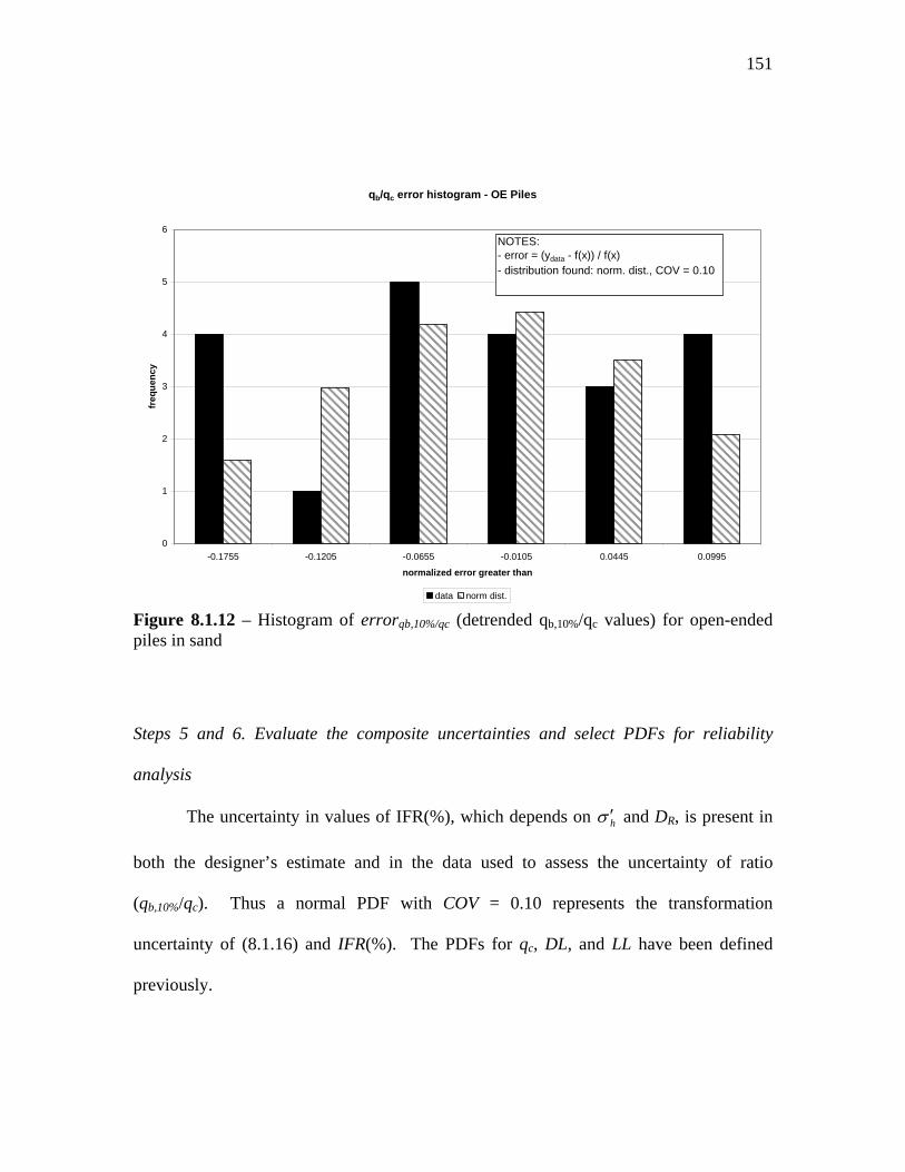
151


analysis

The uncertainty in values of IFR(%), which depends on hσ ′ and DR, is present in

both the designer’s estimate and in the data used to assess the uncertainty of ratio

(qb,10%/qc). Thus a normal PDF with COV = 0.10 represents the transformation

uncertainty of (8.1.16) and IFR(%). The PDFs for qc, DL, and LL have been defined

previously.

qb/qc error histogram - OE Piles

0

1

2

3

4

5

6

-0.1755 -0.1205 -0.0655 -0.0105 0.0445 0.0995


freq

uenc

y

data norm dist.


Figure 8.1.12 – Histogram of errorqb,10%/qc (detrended qb,10%/qc values) for open-ended piles in sand

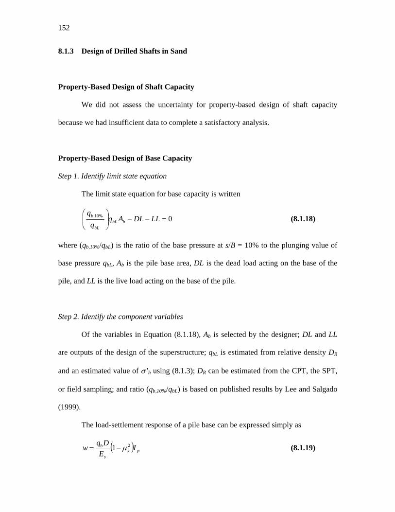
152

8.1.3 Design of Drilled Shafts in Sand


We did not assess the uncertainty for property-based design of shaft capacity

because we had insufficient data to complete a satisfactory analysis.




0%10, =−−⎟⎟⎠

⎞⎜⎜⎝

⎛LLDLAq

qq

bbLbL

b (8.1.18)

where (qb,10%/qbL) is the ratio of the base pressure at s/B = 10% to the plunging value of

base pressure qbL, Ab is the pile base area, DL is the dead load acting on the base of the

pile, and LL is the live load acting on the base of the pile.


Of the variables in Equation (8.1.18), Ab is selected by the designer; DL and LL

are outputs of the design of the superstructure; qbL is estimated from relative density DR

and an estimated value of σ’h using (8.1.3); DR can be estimated from the CPT, the SPT,

or field sampling; and ratio (qb,10%/qbL) is based on published results by Lee and Salgado

(1999).

The load-settlement response of a pile base can be expressed simply as

( ) pss

b IE

Dqw 21 µ−= (8.1.19)

153

where w is the settlement, qb is the unit base load, Es and µs are the soil Young’s modulus

and Poissons’s ratio, respectively, and Ip is an influence factor. Even though the soil

response cannot be expected to be linear elastic as is implied by (8.1.19), if the modulus

is adjusted for the strain level, this is an acceptable approximation. For use in design

circumstances, Es in Equation (8.1.19) can be calibrated with the results from ABAQUS

as was done by Lee and Salgado (1999, 2002). If sufficient convergence checks are

performed, the calibration performed using ABAQUS introduces little uncertainty

beyond that of the material model. Thus, if the uncertainty for Es in (8.1.19) can be found,

the uncertainty of qb is found. Rewriting (8.1.19) with the assessment of uncertainty in

mind, the following expression for qb results:

ss

b cD

wEq = (8.1.20)

where cs is a constant accounting for the problem mechanics and geometry. Equation

(8.1.20) clearly shows that qb is directly proportional to Es. Thus the uncertainty in qb is

directly proportional to that of Es.

Lee and Salgado (1999) developed a non-linear elastic constitutive model to

investigate the load-settlement response at the base of a drilled shaft. With this load-

settlement model, Equation (8.1.20) can be used to estimate Es using DR as an input

parameter. Thus, the uncertainty of the constitutive model used by Lee and Salgado

(1999) must be considered to evaluate the uncertainty of Es. Figure 8.1.13 illustrates the

complete series of transformations required to move from relative density to modulus Es.

The numbers beneath each variable represent the COV for that variable. The numbers in

each arrow represent the uncertainty for that transformation in terms of the resulting

variable.

154

The work of Hardin and Black (1966) led to the following empirical relationship

for G0,

gg nm

na

gg P

eee

CG )'(1

)( )1(

0

20

0 σ−

+

−= (8.1.21)

where Cg, ng, and eg are intrinsic material variables; eo is the initial void ratio; Pa is a

reference pressure of (100 kPa); and σ’m is the initial mean effective stress in the same

units as Pa. The initial void ratio can be determined from relative density using the

fundamental equation

minmax

max

eeeeDR −

−= (8.1.22)

The modulus degradation with stress level is modeled with the expression

DRqc

0.00.13

0.13

0.14

f0.004

g0

G0

G 0

0.01

0.15

0.084

0

0.12 0.12

e 0.0460.083

0

emax,min0.012

0

Es

Figure 8.1.13 – Uncertainty propagation for modeling drilled shaft base movement, fromCONPOINT estimates of DR to modulus Es

155

gn

o

g

omax

o

II

JJJJ

fGG

⎟⎟⎠

⎞⎜⎜⎝

⎛⎥⎥

⎦

⎤

⎢⎢

⎣

⎡

⎟⎟⎠

⎞⎜⎜⎝

⎛

−

−−=

1

1

22

22

0

1 (8.1.23)

where J2 = second invariant of the deviatoric stress tensor, f and g are curve fitting

parameters, and I1 and I1o are the first variants of the stress tensor at the current and initial

states, respectively.


Of the identified variables, DR can be estimated using the CPT, the SPT, or unit

weight from field sampling. The CPT, SPT, or unit weight can be measured in routine

practice. The uncertainty of qc and NSPT has been examined in Section 4.1.


The first consideration is the uncertainty in ratio (qb,10%/qbL). The uncertainty of

this ratio is due to the uncertainties in the numerical model used to represent the soil.

Starting at the left side of Figure 8.1.13, the influence of DR uncertainty is considered.

Since the curves presented by Lee and Salgado (1999) for base resistance use cone

penetration as the input concerning the state of the soil, the ability of CONPOINT to

predict qc from DR is a pertinent measure of the variability of DR in the analysis. Values

of qc at this point are not measured, but computed by CONPOINT, so the inherent soil

variability measured by the CPT is not introduced at this stage.

To find values of G0 for use in the analysis, e0 is found using (8.1.22) from DR,

emin, and emax. The uncertainty of void ratios emin and emax can be approximated from

ASTM standard tolerances. The uncertainty of the transformation represented by

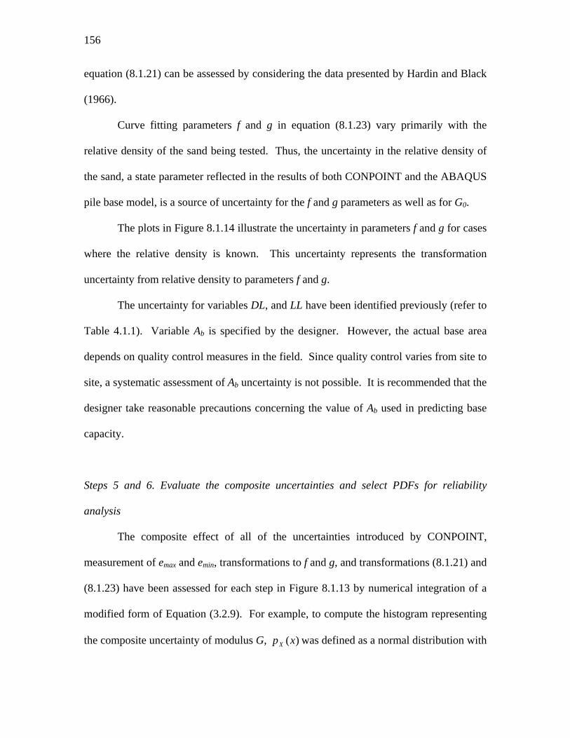
156

equation (8.1.21) can be assessed by considering the data presented by Hardin and Black

(1966).

Curve fitting parameters f and g in equation (8.1.23) vary primarily with the

relative density of the sand being tested. Thus, the uncertainty in the relative density of

the sand, a state parameter reflected in the results of both CONPOINT and the ABAQUS

pile base model, is a source of uncertainty for the f and g parameters as well as for G0.

The plots in Figure 8.1.14 illustrate the uncertainty in parameters f and g for cases

where the relative density is known. This uncertainty represents the transformation

uncertainty from relative density to parameters f and g.


Table 4.1.1). Variable Ab is specified by the designer. However, the actual base area

depends on quality control measures in the field. Since quality control varies from site to

site, a systematic assessment of Ab uncertainty is not possible. It is recommended that the

designer take reasonable precautions concerning the value of Ab used in predicting base

capacity.


analysis

The composite effect of all of the uncertainties introduced by CONPOINT,

measurement of emax and emin, transformations to f and g, and transformations (8.1.21) and

(8.1.23) have been assessed for each step in Figure 8.1.13 by numerical integration of a

modified form of Equation (3.2.9). For example, to compute the histogram representing

the composite uncertainty of modulus G, )(xpX was defined as a normal distribution with

157

COV = 0.084, representing G0, )( ypY was defined as a normal distribution with COV =

0.15, representing f, and )(zpZ was defined as a normal distribution with COV = 0.01,

representing g. Conditional PDF )( xyzwp XYZW was not used since any inaccuracy in

Equation (8.1.23) depends completely on fitting parameters f and g. The histogram

representing the uncertainty of G was produced for a series of different vertical strain

values and relative densities. Based on this survey of uncertainties for G, a COV of 0.12

was taken as representative. The results of this survey are summarized in Table 8.1.1.

Thus, according to the relationship in Equation (8.1.20) the COV for qb is 0.12. Lee and

Salgado (1999) calculated values of qb,10% using this model and then normalized the

results to obtain qb,10%/qbL. Values of qbL were determined using CONPOINT and soil

properties used for the model. Note that the uncertainty of CONPOINT was incorporated

at the beginning of Figure 8.1.13. Thus, the uncertainty of qb,10%/qbL is the same as for

model determined values of qb.

The uncertainty of qbL was examined in Section 8.1.1. The resulting PDF is a

Table 8.1.1 – summary statistics for the evaluation of the composite uncertainty of modulus G in the Lee and Salgado (1999) model for different values of relative density and vertical strain at a point in the soil model.

DR vertical strain mean (µG) Std. dev. (σG) COVG 50 0.1% 21.63364 2.695234 0.124585 60 0.1% 22.95865 2.79628 0.121796 80 0.1% 25.47008 2.93825 0.115361 50 0.5% 9.182838 1.122245 0.122211 60 0.5% 9.687383 1.073985 0.110864 80 0.5% 10.62515 1.092017 0.102777 50 1.0% 6.039453 0.859287 0.142279 60 1.0% 6.361194 0.774608 0.121771 80 1.0% 6.94989 0.771959 0.111075

158

normal distribution with COV = 0.16 and bias factor = 1.06.

y = -0.0005x + 0.9947R2 = 0.7428

0.9250.93

0.9350.94

0.9450.95

0.9550.96

0.9650.97

0.9750.98

0 20 40 60 80 100 120

relative density

f

y = 0.0016x + 0.0971R2 = 0.5114

0

0.05

0.1

0.15

0.2

0.25

0.3

0.35

0 20 40 60 80 100 120

relative density

g

Figure 8.1.14 – Variation of curve fitting parameters f and g with DR (Lee and Salgado 1999)

159


We did not assess the uncertainty for direct design of shaft capacity because we

had insufficient data to complete a satisfactory analysis.




0%10, =−−⎟⎟⎠

⎞⎜⎜⎝

⎛LLDLAq

qq

bcc

b (8.1.24)

where (qb,10%/qc) is the ratio of s/B = 10% limit base pressure to CPT tip resistance qc, Ab

is the pile base area, DL is the dead load acting on the base of the pile, and LL is the live

load acting on the base of the pile.


Of the variables in Equation (8.1.24), Ab is selected by the designer; DL and LL

are outputs of the design of the superstructure; qc is measured directly; and ratio (qb,10%/qc)

is based on published results by Lee and Salgado (1999).


Of the identified variables in equation (8.1.24), qc can be measured in routine

practice. The uncertainty of qc has been examined in Section 4.1.

160


The uncertainty of (qb,10%/qc) has been examined for property-based design of

drilled shafts. The resulting PDF is a normal distribution with COV = 0.12. The

uncertainty of qc was examined in Section 4.1. The resulting PDF is a normal distribution

with COV = 0.07 and bias factor = 1.06.


analysis

PDFs for (qb,10%/qc) and qc are selected in Step 4 and Section 4.1, respectively,

and can be used directly with Equation (8.1.24) in reliability analysis.

161

8.2 Assessment of Resistance Factors

In this section, we will assess the resistance factors for the property-based and

direct design methods for the different pile types we discussed in Section 8.1. To

facilitate discussion, we summarize all design equations in Table 8.2.1. Table 8.2.1 also

includes the resistance factors (RF) that would be used in design with ASCE-7 and

AASHTO load factors. For reference purposes, we calculated an equivalent factor of

safety (FS) that would be used in Working Stress Design (WSD). FS is taken as the ratio

of a representative load factor over the resistance factor.

For design methods that are not mentioned in this Chapter, the designer has the

option to assess the resistance factor for the total capacity from direct design methods.

This procedure is discussed in detail in Section 9.2.1.

For every computation of RF, we check different ratios of LL/DL since live load

is more uncertain than dead load and different ratios of LL/DL will yield different RFs.

As seen in Chapter 5, depending on the relative uncertainty of resistance and load, lower

LL/DL ratios will occasionally yield lower resistance factors. Therefore, both high and

low ratios of LL/DL are checked.

As we noted in Chapter 5, resistance factors vary with design variable values. For

this reason, we also examine the effect of different design variable values on the design

equations for the different pile types we considered. In general, for the equations we

selected, the specific value of design variables has little influence on the final resistance

factor.

162

Table 8.2.1 – Summary table for the design of deep foundations in sand. Resistance Factors (RF) are given for use with ASCE-7 and AASHTO load factors. FS indicates an approximate value of WSD safety factor corresponding to the resistance factor given. Property-Based Design of Driven, Closed-Ended Piles ( ) ( ) ( )∑≥+ iibbss QLFRRFRRF

Shaft Capacity:

∫=L

sss dLafR

vcc

css K

KKf σφ

φδ ′⎟⎟

⎠

⎞⎜⎜⎝

⎛= tan0

0

( )0

7.2 0.0112 (%) 0.0141 , 20% (%) 90%sR R

KD D

K= − < <

0.85c

c

δφ

=

(RF)s = 0.37 (ASCE-7) (RF)s = 0.40 (AASHTO) FS = 3.9

Base Capacity: bbb AqR %10,=

bLbL

bb q

qq

q ⎟⎟⎠

⎞⎜⎜⎝

⎛= %10,

%10,

(%)0051.002.1%10,R

bL

b Dq

q−=

( )3

21 expC

A

hR

A

bL

pDCC

pq

⎟⎟⎠

⎞⎜⎜⎝

⎛ ′=

σ

(RF)b = 0.50 (ASCE-7) (RF)b = 0.52 (AASHTO) FS = 3.0

Direct (CPT) Design of Driven, Closed-Ended Piles ( ) ( ) ( )∑≥+ iibbss QLFRRFRRF

Shaft Capacity:

∫=L

sss dLafR

ccc

ss qq

qff 002.0=⎟⎟

⎠

⎞⎜⎜⎝

⎛=



cc

bb q

qq

q ⎟⎟⎠

⎞⎜⎜⎝

⎛= %10,

%10,

(%)0051.002.1%10,R

c

b Dq

q−=

(RF)b = 0.56 (ASCE-7) (RF)b= 0.59 (AASHTO) FS = 2.6

163

Property-Based Design of Driven, Open-Ended Piles ( ) ( ) ( )∑≥+ iibbss QLFRRFRRF

Shaft Capacity:

∫=L

sss dLafR

vcc

css K

KKf σφ

φδ ′⎟⎟

⎠

⎞⎜⎜⎝

⎛= tan0

0

( )PLR8.42.70

−= βKK

0.85c

c

δφ

=

90%(%)20% ,0141.0(%)0112.0 <<−= RR DDβ



hh

bb

qq σ

σ′⎟⎟

⎠

⎞⎜⎜⎝

⎛′

= %10,%10,

⎟⎠⎞

⎜⎝⎛ −=

′ 100IFR(%)295326%10, α

σ h

bq

90%(%)20% ,0141.0(%)0112.0 <<−= RR DDα 2

2⎟⎠⎞

⎜⎝⎛= o

bd

A π


Direct (CPT) Design of Driven, Open-Ended Piles ( ) ( ) ( )∑≥+ iibbss QLFRRFRRF

Shaft Capacity:

∫=L

sss dLafR

ccc

ss qq

qff 002.0=⎟⎟

⎠

⎞⎜⎜⎝

⎛=



cc

bb q

qq

q ⎟⎟⎠

⎞⎜⎜⎝

⎛= %10,

%10,

557.0(%)00443.0%10, +−= IFRq

q

c

b

2

2⎟⎠

⎞⎜⎝

⎛= ob

dA π


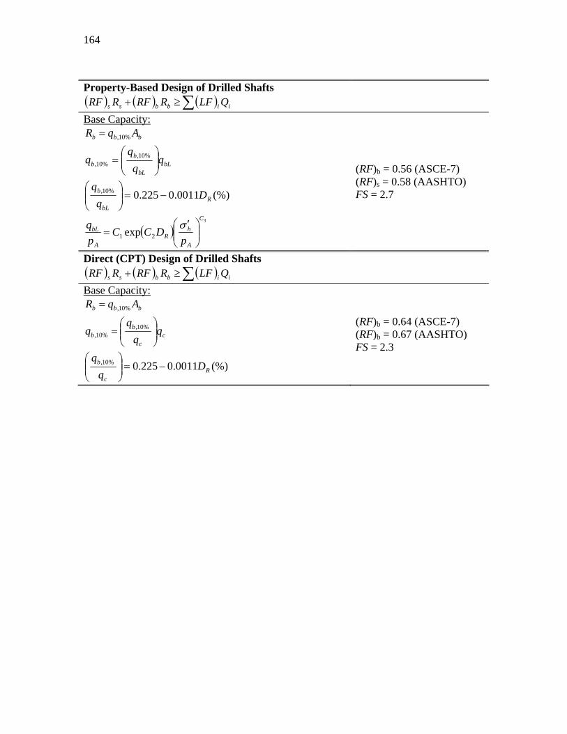
164

Property-Based Design of Drilled Shafts ( ) ( ) ( )∑≥+ iibbss QLFRRFRRF


bLbL

bb q

qq

q ⎟⎟⎠

⎞⎜⎜⎝

⎛= %10,

%10,

(%)0011.0225.0%10,R

bL

b Dq

q−=⎟⎟

⎠

⎞⎜⎜⎝

⎛

( )3

21 expC

A

hR

A

bL

pDCC

pq

⎟⎟⎠

⎞⎜⎜⎝

⎛ ′=

σ

(RF)b = 0.56 (ASCE-7) (RF)s = 0.58 (AASHTO) FS = 2.7

Direct (CPT) Design of Drilled Shafts ( ) ( ) ( )∑≥+ iibbss QLFRRFRRF


cc

bb q

qq

q ⎟⎟⎠

⎞⎜⎜⎝

⎛= %10,

%10,

(%)0011.0225.0%10,R

c

b Dq

q−=⎟⎟

⎠

⎞⎜⎜⎝

⎛


165

8.2.1 Closed-Ended Driven Piles in Sand


Table 8.2.2 shows a summary of the relevant PDFs and their COVs for the

property-based design method of shaft capacity that were determined in Section 8.1.

Adjusted resistance factors RF were computed using a target reliability index β of 3.0. A

summary of the results appears in Table 8.2.2. Note that values of RF do not depend on

values of K0 and φc. Note that the value of K0 to be used in design was taken as

deterministic, as explained in Section 8.1. However, had some uncertainty for K0 been

introduced, the RF would have been less. Also note that the PDFs and design equations

assessed for the design of closed-ended piles is the same as for open-ended piles.

Accordingly, the resistance factor found match that of the open-ended pile case. Since

Table 8.2.2 – Results of Resistance Factor Evaluation for Property-Based Shaft Capacity of Closed Ended Piles in Sand for ASCE-7 Load Factors Principal Random Variables and Associated PDFs Variable PDF COV K/K0 normal, bias factor = 1.0 0.22 δc/φc normal, µ = 0.9 0.10 φc normal, bias factor = 1.0 0.01 Resistance Factor Results, β = 3.0 K0 φc LL/DL RF 0.4 33 1 0.37 0.4 33 4 0.41 1.0 33 1 0.38 1.0 33 4 0.41 1.0 30 1 0.38 1.0 30 4 0.41

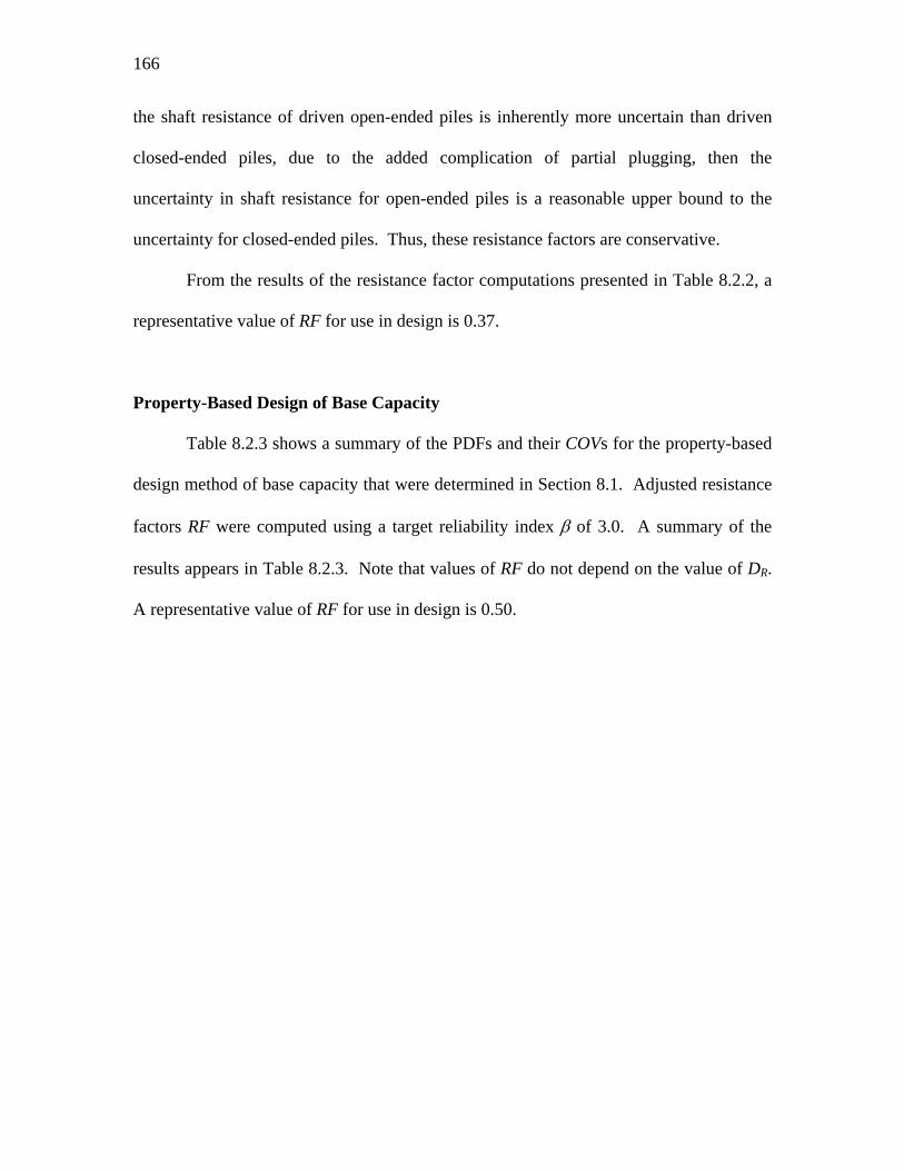
166

the shaft resistance of driven open-ended piles is inherently more uncertain than driven

closed-ended piles, due to the added complication of partial plugging, then the

uncertainty in shaft resistance for open-ended piles is a reasonable upper bound to the

uncertainty for closed-ended piles. Thus, these resistance factors are conservative.

From the results of the resistance factor computations presented in Table 8.2.2, a

representative value of RF for use in design is 0.37.


Table 8.2.3 shows a summary of the PDFs and their COVs for the property-based

design method of base capacity that were determined in Section 8.1. Adjusted resistance

factors RF were computed using a target reliability index β of 3.0. A summary of the

results appears in Table 8.2.3. Note that values of RF do not depend on the value of DR.

A representative value of RF for use in design is 0.50.

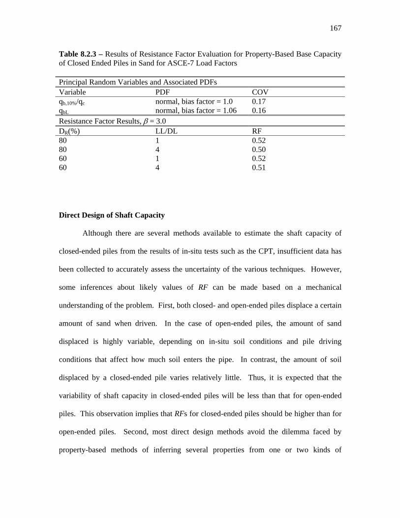
167


Although there are several methods available to estimate the shaft capacity of

closed-ended piles from the results of in-situ tests such as the CPT, insufficient data has

been collected to accurately assess the uncertainty of the various techniques. However,

some inferences about likely values of RF can be made based on a mechanical

understanding of the problem. First, both closed- and open-ended piles displace a certain

amount of sand when driven. In the case of open-ended piles, the amount of sand

displaced is highly variable, depending on in-situ soil conditions and pile driving

conditions that affect how much soil enters the pipe. In contrast, the amount of soil

displaced by a closed-ended pile varies relatively little. Thus, it is expected that the

variability of shaft capacity in closed-ended piles will be less than that for open-ended

piles. This observation implies that RFs for closed-ended piles should be higher than for

open-ended piles. Second, most direct design methods avoid the dilemma faced by

property-based methods of inferring several properties from one or two kinds of

Table 8.2.3 – Results of Resistance Factor Evaluation for Property-Based Base Capacity of Closed Ended Piles in Sand for ASCE-7 Load Factors Principal Random Variables and Associated PDFs Variable PDF COV qb,10%/qc normal, bias factor = 1.0 0.17 qbL normal, bias factor = 1.06 0.16 Resistance Factor Results, β = 3.0 DR(%) LL/DL RF 80 1 0.52 80 4 0.50 60 1 0.52 60 4 0.51

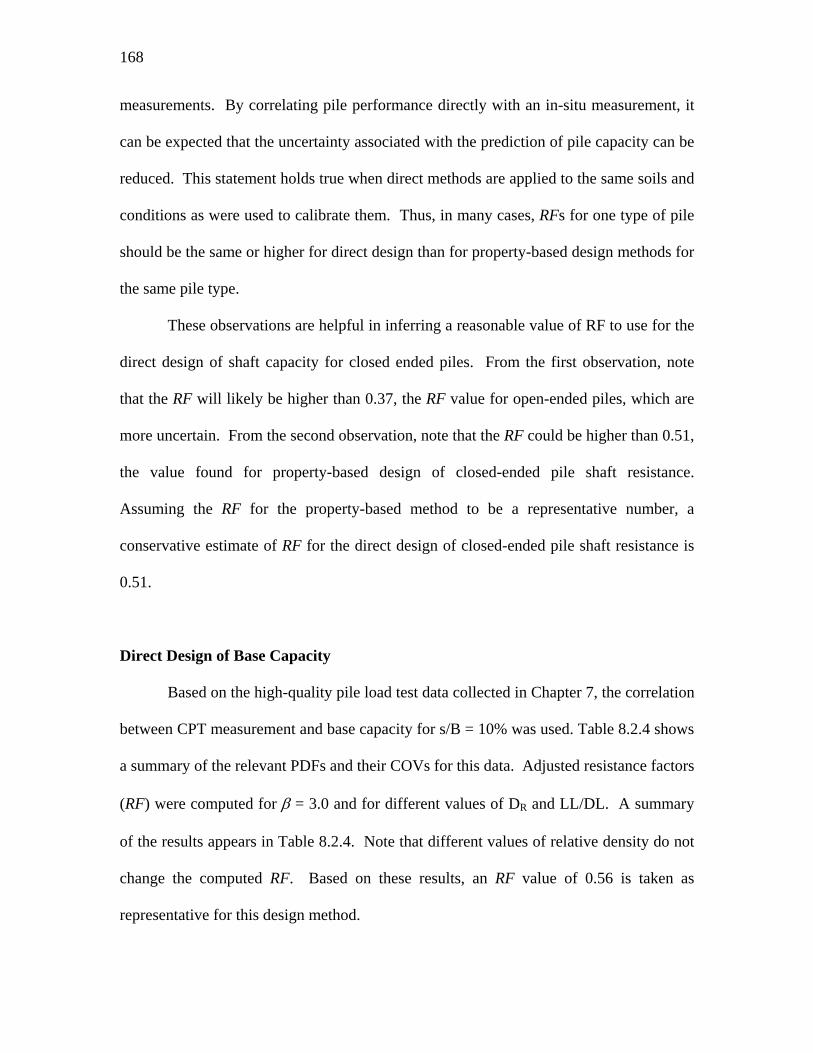
168

measurements. By correlating pile performance directly with an in-situ measurement, it

can be expected that the uncertainty associated with the prediction of pile capacity can be

reduced. This statement holds true when direct methods are applied to the same soils and

conditions as were used to calibrate them. Thus, in many cases, RFs for one type of pile

should be the same or higher for direct design than for property-based design methods for

the same pile type.

These observations are helpful in inferring a reasonable value of RF to use for the

direct design of shaft capacity for closed ended piles. From the first observation, note

that the RF will likely be higher than 0.37, the RF value for open-ended piles, which are

more uncertain. From the second observation, note that the RF could be higher than 0.51,

the value found for property-based design of closed-ended pile shaft resistance.

Assuming the RF for the property-based method to be a representative number, a

conservative estimate of RF for the direct design of closed-ended pile shaft resistance is

0.51.


Based on the high-quality pile load test data collected in Chapter 7, the correlation

between CPT measurement and base capacity for s/B = 10% was used. Table 8.2.4 shows

a summary of the relevant PDFs and their COVs for this data. Adjusted resistance factors

(RF) were computed for β = 3.0 and for different values of DR and LL/DL. A summary

of the results appears in Table 8.2.4. Note that different values of relative density do not

change the computed RF. Based on these results, an RF value of 0.56 is taken as

representative for this design method.

169

8.2.2 Open-Ended Driven Piles in Sand


Table 8.2.5 shows a summary of the PDFs and their COVs determined for the

relevant design variables of the property-based design method of shaft capacity.

Adjusted RF values were found using a target reliability index β of 3.0. A summary of

the results appears in Table 8.2.5. Note that varying K0 and φc practically does not affect

the value of RF obtained. A representative value of RF for use in design is 0.37. Note

that the value of K0 to be used in design was taken as deterministic as explained in

Section 8.1. However, had some uncertainty for K0 been introduced, the RF would have

been less.

Table 8.2.4 – Results of Resistance Factor Evaluation for Direct Base Capacity of Closed Ended Piles in Sand for ASCE-7 Load Factors Principal Random Variables and Associated PDFs Variable PDF COV qb,10%/qc normal, bias factor = 1.0 0.17 qc normal, bias factor = 1.06 0.07 Resistance Factor Results, β = 3.0 DR(%) LL/DL RF 80 1 0.59 80 4 0.57 60 1 0.59 60 4 0.56

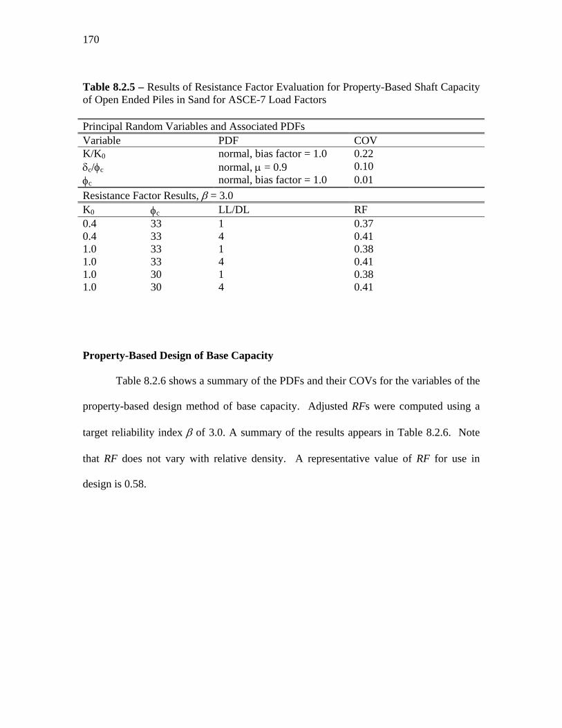
170


Table 8.2.6 shows a summary of the PDFs and their COVs for the variables of the

property-based design method of base capacity. Adjusted RFs were computed using a

target reliability index β of 3.0. A summary of the results appears in Table 8.2.6. Note

that RF does not vary with relative density. A representative value of RF for use in

design is 0.58.

Table 8.2.5 – Results of Resistance Factor Evaluation for Property-Based Shaft Capacity of Open Ended Piles in Sand for ASCE-7 Load Factors Principal Random Variables and Associated PDFs Variable PDF COV K/K0 normal, bias factor = 1.0 0.22 δc/φc normal, µ = 0.9 0.10 φc normal, bias factor = 1.0 0.01 Resistance Factor Results, β = 3.0 K0 φc LL/DL RF 0.4 33 1 0.37 0.4 33 4 0.41 1.0 33 1 0.38 1.0 33 4 0.41 1.0 30 1 0.38 1.0 30 4 0.41

171


Table 8.2.7 shows a summary of the PDFs and their COVs for the direct design

method of shaft capacity as determined in Section 8.1. Adjusted resistance factors RF

were determined for a target reliability index (β) of 3.0. A summary of the results

appears in Table 8.2.7. Based on this analysis, a reasonable RF for use in design is 0.37.

Note that the RF obtained for the property-based prediction of pile capacity does not

differ from that found for direct design. Considering the source of the data, this is likely

Table 8.2.6 – Results of Resistance Factor Evaluation for Property-Based Base Capacity of Open Ended Piles in Sand for ASCE-7 Load Factors Principal Random Variables and Associated PDFs Variable PDF COV qb,10%/σ’h normal, bias factor = 1.0 0.15 Resistance Factor Results, β = 3.0 DR(%) LL/DL RF 90 1 0.61 90 4 0.58 60 1 0.61 60 4 0.58

Table 8.2.7 – Results of Resistance Factor Evaluation for Direct Shaft Capacity of Open-Ended Pipe Piles in Sand for ASCE-7 Load Factors Principal Random Variables and Associated PDFs Variable PDF COV fs/qc normal, µ = 0.002 0.23 qc Normal, bias factor = 1.06 0.07 Resistance Factor Results, β = 3.0 LL/DL RF 1 0.37 4 0.40

172

caused by the fact that the primary source of uncertainty for open-ended piles is the

degree of plugging during driving. Thus, the effect of additional uncertainties introduced

by attempting to estimate soil properties is minimized.


Table 8.2.8 shows a summary of the PDFs and their COVs selected to model the

uncertainty of (qb,10%/qc) and (qc) discussed in Section 8.1. Adjusted resistance factors

were computed using a target reliability index (β) of 3.0. A summary of the results also

appears in Table 8.2.8. Note that although different input values of IFR(%) were used to

compute RF, there is no effect on the resulting value. There is an effect of different

values of LL/DL ratio which has been accounted for by trying two different values of

live-to-dead load ratio. A reasonable value of RF for use in design is 0.66.

Table 8.2.8 – Results of Resistance Factor Evaluation for Direct Base Capacity of Open Ended Piles in Sand for ASCE-7 Load Factors Principal Random Variables and Associated PDFs Variable PDF COV qb,10%/qc normal, bias factor = 1.0 0.10 qc normal, bias factor = 1.06 0.07 Resistance Factor Results, β = 3.0 IFR(%) LL/DL RF 60 1 0.66 60 4 0.69 20 1 0.66 20 4 0.69

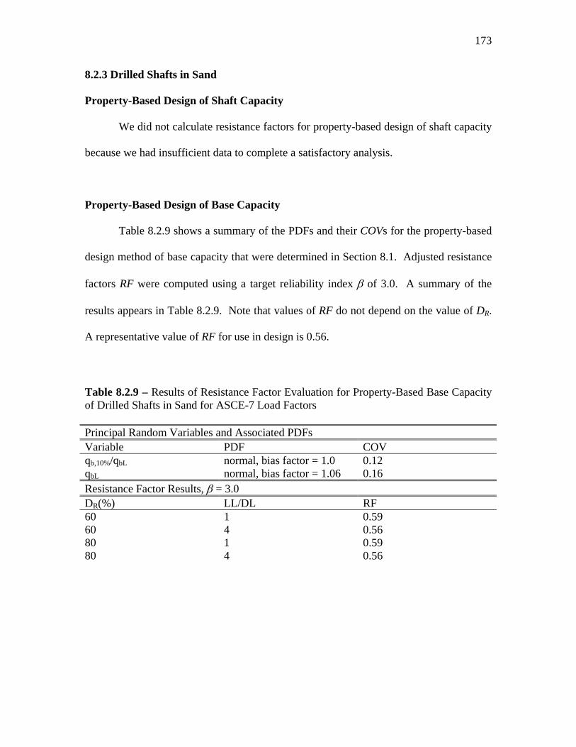
173

8.2.3 Drilled Shafts in Sand


We did not calculate resistance factors for property-based design of shaft capacity



Table 8.2.9 shows a summary of the PDFs and their COVs for the property-based

design method of base capacity that were determined in Section 8.1. Adjusted resistance

factors RF were computed using a target reliability index β of 3.0. A summary of the

results appears in Table 8.2.9. Note that values of RF do not depend on the value of DR.

A representative value of RF for use in design is 0.56.

Table 8.2.9 – Results of Resistance Factor Evaluation for Property-Based Base Capacity of Drilled Shafts in Sand for ASCE-7 Load Factors Principal Random Variables and Associated PDFs Variable PDF COV qb,10%/qbL normal, bias factor = 1.0 0.12 qbL normal, bias factor = 1.06 0.16 Resistance Factor Results, β = 3.0 DR(%) LL/DL RF 60 1 0.59 60 4 0.56 80 1 0.59 80 4 0.56

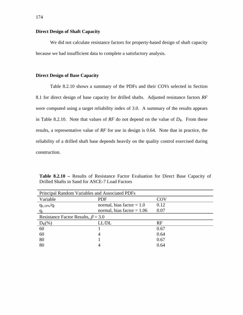
174





Table 8.2.10 shows a summary of the PDFs and their COVs selected in Section

8.1 for direct design of base capacity for drilled shafts. Adjusted resistance factors RF

were computed using a target reliability index of 3.0. A summary of the results appears

in Table 8.2.10. Note that values of RF do not depend on the value of DR. From these

results, a representative value of RF for use in design is 0.64. Note that in practice, the

reliability of a drilled shaft base depends heavily on the quality control exercised during

construction.

Table 8.2.10 – Results of Resistance Factor Evaluation for Direct Base Capacity of Drilled Shafts in Sand for ASCE-7 Load Factors Principal Random Variables and Associated PDFs Variable PDF COV qb,10%/qc normal, bias factor = 1.0 0.12 qc normal, bias factor = 1.06 0.07 Resistance Factor Results, β = 3.0 DR(%) LL/DL RF 60 1 0.67 60 4 0.64 80 1 0.67 80 4 0.64

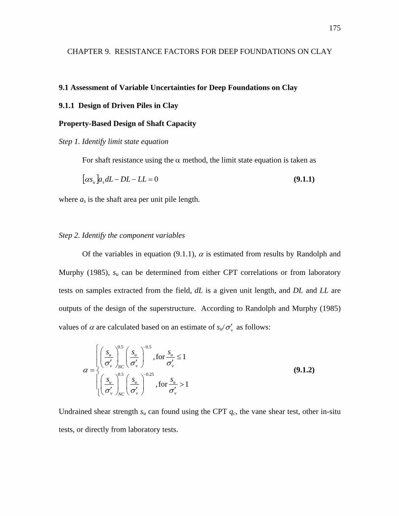
175

CHAPTER 9. RESISTANCE FACTORS FOR DEEP FOUNDATIONS ON CLAY

9.1 Assessment of Variable Uncertainties for Deep Foundations on Clay

9.1.1 Design of Driven Piles in Clay



For shaft resistance using the α method, the limit state equation is taken as

[ ] 0=−− LLDLdLas suα (9.1.1)

where as is the shaft area per unit pile length.


Of the variables in equation (9.1.1), α is estimated from results by Randolph and

Murphy (1985), su can be determined from either CPT correlations or from laboratory

tests on samples extracted from the field, dL is a given unit length, and DL and LL are

outputs of the design of the superstructure. According to Randolph and Murphy (1985)

values of α are calculated based on an estimate of su/ vσ ′ as follows:

0.5 0.5

0.5 0.25

, for 1

, for 1

u u u

v v vNC

u u u

v v vNC

s s s

s s s

σ σ σα

σ σ σ

−

−

⎧⎛ ⎞ ⎛ ⎞⎪ ≤⎜ ⎟ ⎜ ⎟′ ′ ′⎪⎝ ⎠ ⎝ ⎠

= ⎨⎛ ⎞ ⎛ ⎞⎪

>⎜ ⎟ ⎜ ⎟⎪ ′ ′ ′⎝ ⎠ ⎝ ⎠⎩

(9.1.2)

Undrained shear strength su can found using the CPT qc, the vane shear test, other in-situ

tests, or directly from laboratory tests.

176


There are several possible tests that can be used to estimate su. For the purpose of

this report, we assess the uncertainty of su from CPT measurements as determined using

the following equation:

k

vcu N

qs σ−= (9.1.3)

Values of su/ vσ ′ can also be deduced from these measurements.



Table 4.1.1). Variable as is specified by the designer and has negligible uncertainty since

driven pile sections are fabricated at relatively small tolerances. Variable dL is used only

for design purposes and has no affect on the final design prediction.

The data in Figure 9.1.1 obtained from Flemming et al. (1992) can be detrended

by subtracting the mean trend given by (9.1.2) as follows:

( ) ,

,

u udata

v vNC

u u

v vNC

s s

errors s

α

α ασ σ

ασ σ

⎛ ⎞⎛ ⎞ ⎛ ⎞⎜ ⎟− ⎜ ⎟ ⎜ ⎟⎜ ⎟′ ′⎝ ⎠ ⎝ ⎠⎝ ⎠=

⎛ ⎞⎛ ⎞ ⎛ ⎞⎜ ⎟⎜ ⎟ ⎜ ⎟⎜ ⎟′ ′⎝ ⎠ ⎝ ⎠⎝ ⎠

(9.1.4)

Since we divide by the mean trend value in (9.1.4), the standard deviation of errorα is

equal to the COV of α. Using Equation (3.2.1), we get a COV of 0.21 for α. This value

is the uncertainty of Equation (9.1.2). Figure 9.1.2 is a histogram of the α datapoints

177

detrended by Equation (9.1.2). A PDF representing the uncertainty in α is a normal

distribution with COV = 0.21 and mean determined by (9.1.2).

The undrained shear strength su of clay, determined using the CPT, was found in

Chapter 4 to be normally distributed with COV = 0.09 and a bias factor of 1.05. This

PDF represents both the testing and transformation uncertainty in the determination of su.

The uncertainty for lab determined values of su will be higher due to varying disturbance

effects.

Figure 9.1.1 – Measured values of α compared to equations proposed by Randolph and

Murphy (1985) (Flemming et al. 1992)

178

0

5

10

15

20

25

-0.41 -0.231 -0.052 0.127 0.306 0.485 0.664

norm. error

freq

uenc

y

data norm. dist.


Figure 9.1.2 – Histogram of the α data points detrended by Equation (9.1.2).


analysis

The PDFs of α and su are selected in Step 4 and can be used directly with

Equation 9.1.1 in reliability analysis.



The limit state equation for base resistance is taken as

[ ] 0=−− LLDLAsN buc (9.1.5)

where Nc is a bearing capacity factor and Ab is the pile base area. An s/B = 10% criterion

is desired for the base resistance of piles in clay. For soft to medium clays, piles reach a

179

plunging mode at relatively small settlements. Thus, values of Nc may be used directly

for these soils. We do not comment on qb,10% for stiff clays since there is not enough load

testing results in the literature to compare qbL to qb,10%.


As stated earlier, there are different methods to estimate su. Values of Nc come

from Salgado et al. (2004). DL and LL are outputs of the design of the superstructure.


For the purpose of this report, we assume that su can be found using the CPT qc

and equation (9.1.3).


Limit analysis of circular foundations in clay by Salgado et al. (2004) is used to

analyze the expected value of Nc and its uncertainty. The value of Nc according to

Salgado et al. (2004) is between 11.0 and 13.7. If no assumptions about the mean value

of Nc are made, the least biased estimate of the PDF of Nc is a uniform distribution

between 11.0 and 13.7.

The PDF for su was found in Chapter 4 to be a normal distribution with a COV of

0.09 and a bias factor of 1.05.

180


analysis

The PDFs of Nc and su are selected in Step 4 and can be used directly with

Equation 9.1.5 in reliability analysis.

Direct Design of Total Capacity

Unlike for sands, we do not have a satisfactory database to support separate

resistance factors on shaft and base resistance for direct design methods in clay.

Therefore, we propose using the total capacity form (7.1.2) of the LRFD equation so that

total load pile test data can be used to estimate a reasonable resistance factor. Note that

this decision will result in designs with less consistent reliabilities between different pile

lengths. However, the method used to determine RF described in this section will allow

practitioners to select RFs based on available load test data.

In the following development, we demonstrate how to obtain the RF for the Aoki

and de Alencar Velloso (1975) design method since they present a useful load test

database. Values of measured vs. predicted total pile capacity from Aokoi and de Alencar

Velloso (1975) are presented in Figure 9.1.3.

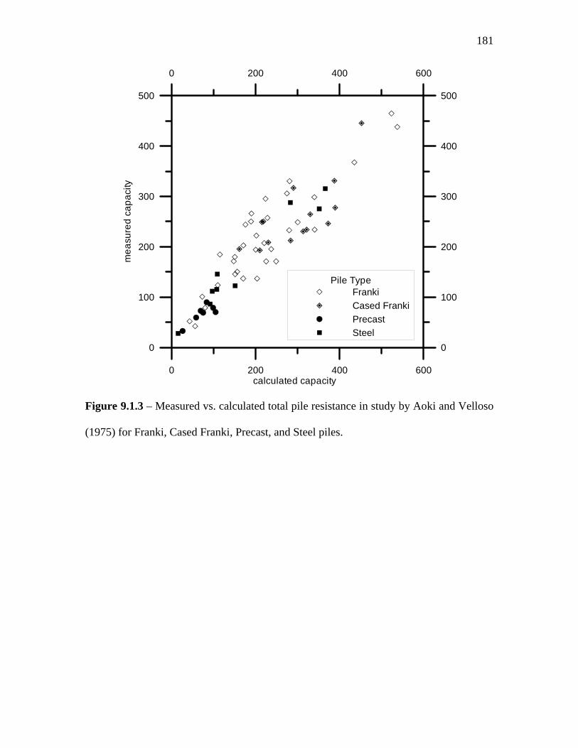
181

0 200 400 600calculated capacity

0

100

200

300

400

500

mea

sure

d ca

paci

ty

0 200 400 600

0

100

200

300

400

500

Pile TypeFrankiCased FrankiPrecastSteel

Figure 9.1.3 – Measured vs. calculated total pile resistance in study by Aoki and Velloso

(1975) for Franki, Cased Franki, Precast, and Steel piles.

182


The limit state equation for total pile resistance is taken as

( ) 0=−−+ LLDLRR bs (9.1.6)

where ( )bs RR + is the total resistance of the pile.


There are no component variables for this limit state equation since the shaft and

base resistances are lumped in the data available for reliability analysis.


The uncertainty of the SPT contributes to the uncertainty of ( )bs RR + but cannot

be extracted from the available data. This uncertainty is integral in the scatter of the

datapoints in Figure 9.1.3


Plots of measured vs. predicted capacity are one tool to assess the uncertainty of a

direct design method. In the absence of instrumented pile load tests, these plots are the

only available tool. Briaud and Tucker (1988) and Eslami and Fellenius (1997) are

examples from the literature where this technique has been applied. It has the advantage

of allowing a direct assessment of the likely deviation of pile capacity measurements

from predictions, but has the disadvantage of limited applicability, as discussed earlier.

For instance, if the designer has a particular method and a sufficient amount of

calibration data where testing is done on the same type of pile and soil, a PDF can be

183

estimated to represent the uncertainty of total capacity. For the Aoki and de Alencar

Velloso method, the first step is to detrend the data using the following equation:

( )

( ) ( )( )s b

s b s bmeasured predictedR R

s b measured

R R R Rerror

R R+

+ − +=

+ (9.1.7)

Note that the predicted value obtained from this design method is the mean trend since

we need to assess the deviation of actual values from this predicted value. Since we

divide by the mean trend value in (9.1.7), the standard deviation of error(Rs+Rb) is equal to

the COV of ( )bs RR + . Using Equation (3.2.1), we get a COV of 0.27 for ( )bs RR + . This

value is the uncertainty of predicted values of pile capacity using the Aoki and de

Alencar Velloso (1975) design method. A histogram showing the detrended data is

presented in Figure 9.1.4.

0

1

2

3

4

5

6

7

8

-0.329 -0.104 0.121 0.346 0.571


freq

uenc

y

data norm dist

NOTES:- error = (ydata - f(x)) / f(x)- COV = 0.27

Figure 9.1.4 – Histogram of the ( )bs RR + measured data points detrended by the

calculated datapoints from Figure 9.1.3.

184


analysis

Based on recommendations of Briaud and Tucker (1988) and from the shape of

the histogram in Figure 9.1.4, we selected a log-normal distribution to represent the

uncertainty of ( )bs RR + . The PDF selected is log-normal with mean equal to the design

equation values presented in Chapter 7 for the Aoki and de Alencar Velloso (1975)

method and COV equal to 0.27.

9.1.2 Design of Drilled Shafts in Clay


We did not assess the uncertainty for property-based design of shaft capacity



As explained in Chapter 7, the ultimate limit state base load for soft and medium

stiff clays is the plunging limit bearing capacity. As a result, plunging limit bearing

capacity qbL is applied to the design of both drilled shafts and driven piles. Thus the

uncertainties are the same as determined in Section 9.1.1.


Similar to the case of driven piles in clays, we do not have a satisfactory database

to support separate resistance factors on shaft and base capacity for drilled shafts.

Accordingly, the only available tool is to assess the uncertainty of total capacity based on

185

the same procedure presented in Section 9.1.1. We recommend that the designer take

advantage of available pile load tests on drilled shafts to support the selection of

resistance factor for design using the method outlined in the following Section.

9.2 Assessment of Resistance Factors

In this section, we will assess the resistance factors for the property-based and

direct design methods for the different pile types we discussed in Section 9.1. To

facilitate discussion, we summarize all design equations in Table 9.2.1 and we refer to it

hereinafter. Table 9.2.1 also includes the resistance factors (RF) that would be used in

design with ASCE-7 and AASHTO load factors. For reference purposes, we calculated

an equivalent factor of safety (FS) that would be used in Working Stress Design (WSD).

FS is taken as the ratio of a representative load factor over the resistance factor.

For every computation of RF we check different ratios of LL/DL since live load is

more uncertain than dead load and different ratios of LL/DL will yield different RFs. As

seen in Chapter 5, depending on the relative uncertainty of resistance and load, lower

LL/DL ratios will occasionally yield lower resistance factors. Therefore, both high and

low ratios of LL/DL are checked.

As we noted in Chapter 5, resistance factors vary with design variable values. For

this reason, we also examine the effect of different design variable values on the design

equations for the different pile types we considered. In general, for the equations we

selected, the specific value of design variables has little influence on the final resistance

factor.

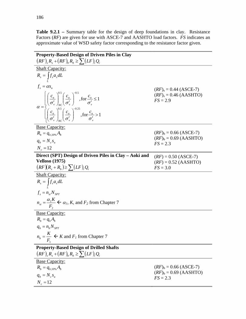
186

Table 9.2.1 – Summary table for the design of deep foundations in clay. Resistance Factors (RF) are given for use with ASCE-7 and AASHTO load factors. FS indicates an approximate value of WSD safety factor corresponding to the resistance factor given. Property-Based Design of Driven Piles in Clay ( ) ( ) ( )∑≥+ iibbss QLFRRFRRF

Shaft Capacity:

∫=L

sss dLafR

us sf α=

⎪⎪

⎩

⎪⎪

⎨

⎧

>′⎟⎟

⎠

⎞⎜⎜⎝

⎛′⎟⎟

⎠

⎞⎜⎜⎝

⎛′

≤′⎟⎟

⎠

⎞⎜⎜⎝

⎛′⎟⎟

⎠

⎞⎜⎜⎝

⎛′

= −

−

1for,

1for,

25.05.0

5.05.0

v

u

v

u

NCv

u

v

u

v

u

NCv

u

ccc

ccc

σσσ

σσσα



ucb sNq = 12=cN


Direct (SPT) Design of Driven Piles in Clay – Aoki and Velloso (1975) ( )( ) ( )∑≥+ iibs QLFRRRF

(RF) = 0.50 (ASCE-7) (RF) = 0.52 (AASHTO) FS = 3.0

Shaft Capacity:

∫=L

sss dLafR

SPTsis Nnf =

2

1

FKnsi

α= α1, K, and F2 from Chapter 7

Base Capacity: bbb AqR =

SPTbb Nnq =

1FKnb = K and F1 from Chapter 7

Property-Based Design of Drilled Shafts ( ) ( ) ( )∑≥+ iibbss QLFRRFRRF


ucb sNq = 12=cN


187

9.2.1 Designer Assessed Resistance Factors for Direct Methods

The main goal of this report was to present resistance factors for use with shallow

and deep foundations. These resistance factors were specifically developed based on the

uncertainty that we could quantify for the different design variables in each of the design

equations we considered. However, this is insufficient to cover all the cases that could

arise in practice knowing that there are many direct design methods that are developed

for specific design situations. As such, the designer needs the capability to select

resistance factors that reflect the uncertainty of the design method used. A suitable

technique is to assess the uncertainty of total capacity from predicted vs. measured load

test data. It is important to note that the load test database used with the specific methods

the designer chooses should contain numerous cases of similar soil conditions and pile

type. This is necessary to ensure the applicability the design method and its uncertainty.

We are considering the case when the designer has predicted vs. measured total

load data for a given design method. The LRFD equation used in this case would be:

( )( ) ( )∑≥+ iibs QLFRRRF (9.2.1)

where (Rs + Rb) is the total load capacity of the pile. Thus, we are finding a single RF

value to be applied to the total pile capacity. To allow the designer to readily find a value

of RF for a specific method, we computed different RF values for a range of COV values

for (Rs + Rb) and different target reliability indices β. Figures 9.2.1 and 9.2.2 present the

charts of RFs for use with ASCE-7 and AASHTO load factors, respectively. To use

these figures, one must have an input value of COV and reliability index β.

As was explained in Chapter 3, the reliability index is an expression of the

likelihood of failure. Higher values of β indicate a lower probability of failure for the

188

design. All of the recommended resistance factors presented in this report were for a

reliability index of 3.0, the conventional value for structural design.

The COV must be determined from the load test database. The first step is to

calculate the “error” for each load test as follows:

( )

( ) ( )( )s b

s b s bmeasured predictedR R

s b measured

R R R Rerror

R R+

+ − +=

+ (9.2.2)

The predicted capacity is calculated for each load test case using the chosen design

method and the available in-situ test data. The measured capacity is the total capacity

obtained from the result of each load test. Note that we consider the predicted capacity to

be the mean of the data since we need to assess the deviation of actual values from this

predicted value. To compute the COV of (Rs + Rb), we apply Equations (3.2.1) and (3.2.2)

to the “error” values for the entire load database.

The final step to assess a RF for the chosen design method is to enter either Figure

9.2.1 or 9.2.2 with the calculated COV and β.

189

0.2 0.24 0.28 0.32 0.36Total Resistance (Rs+Rb) COV

0.2

0.4

0.6

0.8

Adju

sted

Res

ista

nce

Fact

or (R

F)

β = 2.0β = 2.5β = 3.0β = 3.5

0.2 0.24 0.28 0.32 0.36

0.2

0.4

0.6

0.8

Figure 9.2.1 – Plot of Adjusted Resistance Factor RF varying with total resistance COV and target reliability index β, to be applied to total load capacity in the design of piles using ASCE-7 load factors. A bias factor of 1.06 for a lognormally distributed total resistance is assumed, implying that the resistance is assessed conservatively according to the CAM procedure.

190

0.2 0.24 0.28 0.32 0.36Total Resistance (Rs+Rb) COV

0.2

0.4

0.6

0.8

Adju

sted

Res

ista

nce

Fact

or (R

F)

β = 2.0β = 2.5β = 3.0β = 3.5

0.2 0.24 0.28 0.32 0.36

0.2

0.4

0.6

0.8

Figure 9.2.2 – Plot of Adjusted Resistance Factor RF varying with total resistance COV and target reliability index β, to be applied to total load capacity in the design of piles using AASHTO load factors. A bias factor of 1.06 for a lognormally distributed total resistance is assumed, implying that the resistance is assessed conservatively according to the CAM procedure.

191

9.2.2 Driven Piles in Clay

Property-Based Shaft Capacity


property-based design method of shaft capacity that were determined in Section 9.1.

Adjusted resistance factors were computed using a target reliability index (β) of 3.0. A

summary of the results also appears in Table 9.2.2. Note that, although different input

values of (su/σ’v) were used to compute RF, there is no effect on the resulting value. A

reasonable value of RF for use in design is 0.44.

Table 9.2.2 – Results of Resistance Factor Evaluation for Property-Based Shaft Capacity of Driven Piles in Clay Principal Random Variables and Associated PDFs Variable PDF COV α normal, bias factor = 1.0 0.21 su normal, bias factor = 1.05 0.09 Resistance Factor Results (su/σ’v) LL/DL RF 0.3 1 0.44 0.3 4 0.46 1.0 1 0.44 1.0 4 0.46 5.0 1 0.44 5.0 4 0.46

Property-Based Base Capacity


property-based design method of base capacity that were determined in Section 9.1.

Adjusted resistance factors were computed using a target reliability index (β) of 3.0. A

192

summary of the results also appears in Table 9.2.3. A reasonable value of RF for use in

design is 0.66.

Table 9.2.3 – Results of Resistance Factor Evaluation for Property-Based Base Capacity of Driven Piles in Clay Principal Random Variables and Associated PDFs Variable PDF COV Nc uniform: [11.0, 13.7] 0.28 su normal, bias factor = 1.05 0.09 Resistance Factor Results LL/DL RF 1 0.68 4 0.66


Table 9.2.4 shows a summary of the relevant PDFs and their COVs for the direct

design method of total capacity that were determined in Section 9.1. Adjusted resistance

factors were computed using a target reliability index (β) of 3.0. A summary of the

results also appears in Table 9.2.4. A reasonable value of RF for use in design is 0.50.

Table 9.2.4 – Results of Resistance Factor Evaluation for Aoki and de Velloso (1975) Direct SPT Design Method Principal Random Variables and Associated PDFs Variable PDF COV Qtotal lognormal, bias factor = 1.06 0.27 Resistance Factor Results LL/DL RF 1 0.52 4 0.50

193

9.2.3 Design of Drilled Shafts in Clay





As explained in Chapter 7, the ultimate limit state base load for soft and medium

stiff clays is the plunging limit bearing capacity. As a result, plunging limit bearing

capacity qbL is applied to the design of both drilled shafts and driven piles. Thus the

uncertainties are the same as determined in Section 9.1.1. An appropriate resistance

factor for use in property-based design of base capacity of drilled shafts is the same as

that proposed for driven piles. A reasonable value of RF for use in design is 0.66.


We did not calculate resistance factors for direct design of total capacity because

we had insufficient data to complete a satisfactory analysis. However, in Section 9.2.1

we discussed a way for designers to select values of resistance factors for different design

methods. We recommend the use of this technique for direct design of drilled shafts

provided sufficient load test data is available.

194

195

CHAPTER 10. DESIGN EXAMPLES FOR DEEP FOUNDATIONS

Design Using LRFD

As in Chapter 6 for shallow foundations, this chapter explains how to use the

resistance factors found in the previous chapters to design. Two design examples are

considered. In the first example, we design a pile in a primarily medium dense sand soil

profile. The second example demonstrates how to select a resistance factor (RF) for use

with a direct design method not presented in this report.

In both examples the basic process of LRFD design is illustrated according to the

flow chart in Figure 10.1.

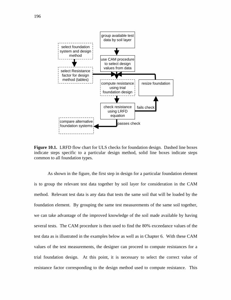
196

select foundation system and design

method

resize foundation

group available test data by soil layer

use CAM procedure to select design values from data

compute resistance using trial

foundation design

check resistance using LRFD

equation

fails check

passes check compare alternative foundation systems

select Resistance factor for design method (tables)

Figure 10.1. LRFD flow chart for ULS checks for foundation design. Dashed line boxes indicate steps specific to a particular design method, solid line boxes indicate steps common to all foundation types.

As shown in the figure, the first step in design for a particular foundation element

is to group the relevant test data together by soil layer for consideration in the CAM

method. Relevant test data is any data that tests the same soil that will be loaded by the

foundation element. By grouping the same test measurements of the same soil together,

we can take advantage of the improved knowledge of the soil made available by having

several tests. The CAM procedure is then used to find the 80% exceedance values of the

test data as is illustrated in the examples below as well as in Chapter 6. With these CAM

values of the test measurements, the designer can proceed to compute resistances for a

trial foundation design. At this point, it is necessary to select the correct value of

resistance factor corresponding to the design method used to compute resistance. This

197

dependency is illustrated using the dashed line borders in Figure 10.1. After finding a

resistance value for a particular design, its suitability can be checked using the basic

LRFD equation. Factored design resistances that are greater than factored loads represent

trial designs that have passed the check while factored design resistances that are less

than the design load have failed the check. It is possible with several trial designs to

compare design alternatives. In the following examples, the process of selecting a CAM

value, selecting a resistance factor, and performing an LRFD check is illustrated.

Design of Open Ended Pipe Pile in Sand Using Direct Method

A number of CPT soundings were taken at the site and the measured tip resistance

(qc) profile is presented in Figure 10.2. A pile with 150 kN (34 kip) live load and 350 kN

(79 kip) dead load will be designed against ultimate limit states. The pile cap base

elevation is to be located at a depth of 2.0 m (6.6 ft). An open-ended pipe pile will be

driven to 9 m (29.5 ft) at the sand site to take advantage of the relatively dense sand layer

overlying the looser layer below 10m. Using live load and dead load factors of 1.6 and

1.2 (ASCE-7 factors), respectively, the design load is 660 kN (148 kip). The water table

is at depth.

198

mean trend line

Figure 10.2. Results from 7 CPT logs in sand with mean trend (“best fit”) lines and Range Lines (BCP Committee 1971)

The first step to design the foundation is to establish the CAM trend line for the

combined CPT logs. A CAM method using an 80% exceedance criterion is illustrated

using linear regression – a tool readily available to engineers in spreadsheet applications.

These lines represent the mean function of a soil parameter with depth for the soils.

Lines can also be drawn bounding the qc data points, representing the entire range of qc

data for those depths. Both sets of lines are included in Figure 10.2. Table 10.1 presents

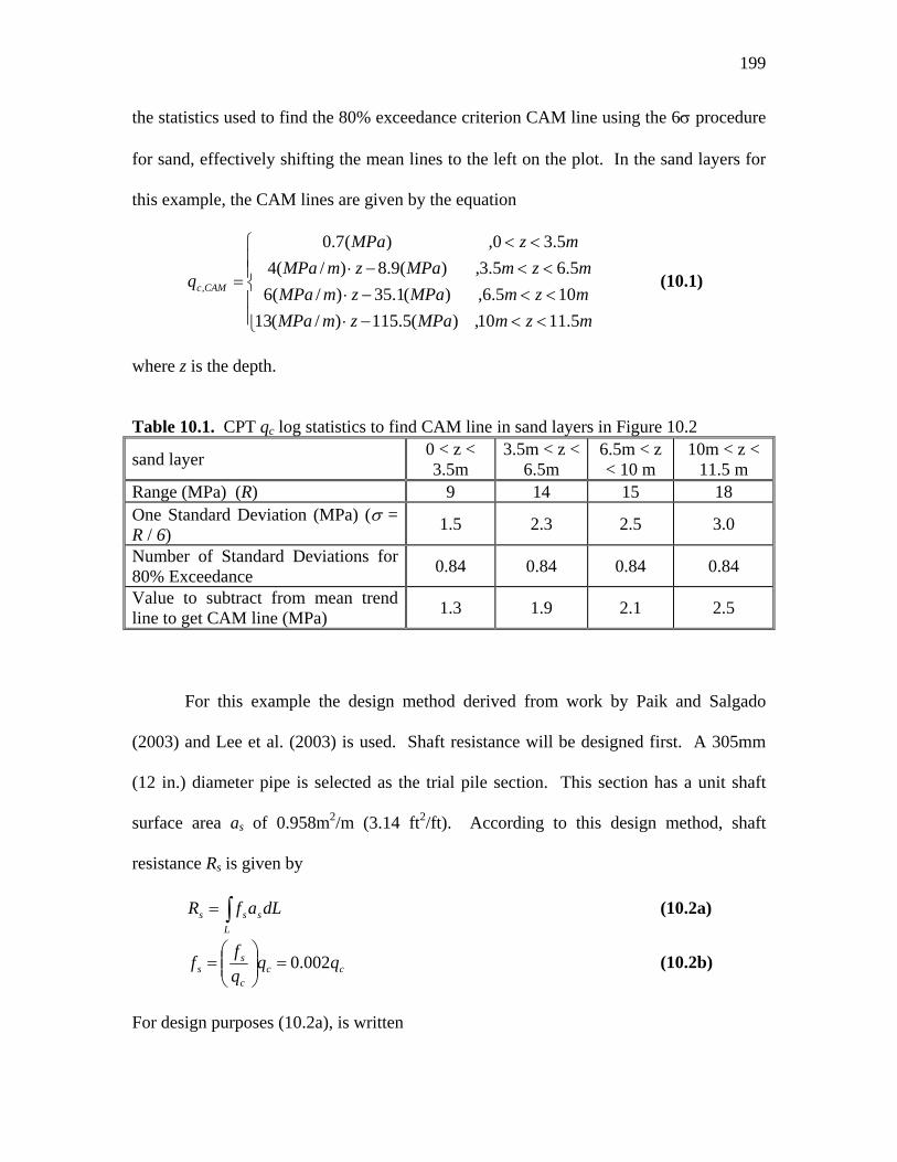
199

the statistics used to find the 80% exceedance criterion CAM line using the 6σ procedure

for sand, effectively shifting the mean lines to the left on the plot. In the sand layers for

this example, the CAM lines are given by the equation

⎪⎪⎩

⎪⎪⎨

⎧

<<−⋅<<−⋅<<−⋅

<<

=

mzmMPazmMPamzmMPazmMPamzmMPazmMPa

mzMPa

q CAMc

5.1110,)(5.115)/(13105.6,)(1.35)/(6

5.65.3,)(9.8)/(45.30,)(7.0

, (10.1)

where z is the depth.

Table 10.1. CPT qc log statistics to find CAM line in sand layers in Figure 10.2

sand layer 0 < z < 3.5m

3.5m < z < 6.5m

6.5m < z < 10 m

10m < z < 11.5 m

Range (MPa) (R) 9 14 15 18 One Standard Deviation (MPa) (σ = R / 6) 1.5 2.3 2.5 3.0

Number of Standard Deviations for 80% Exceedance 0.84 0.84 0.84 0.84

Value to subtract from mean trend line to get CAM line (MPa) 1.3 1.9 2.1 2.5

For this example the design method derived from work by Paik and Salgado

(2003) and Lee et al. (2003) is used. Shaft resistance will be designed first. A 305mm

(12 in.) diameter pipe is selected as the trial pile section. This section has a unit shaft

surface area as of 0.958m2/m (3.14 ft2/ft). According to this design method, shaft

resistance Rs is given by

∫=L

sss dLafR (10.2a)

ccc

ss qq

qff 002.0=⎟⎟⎠

⎞⎜⎜⎝

⎛= (10.2b)

For design purposes (10.2a), is written

200

iisiss dLafR ∑= ,, (10.3)

where subscript i denotes a section of some length along the pile. By summing the

resistance contribution from all sections, we arrive at the total shaft capacity for the pile.

In this example, a few sections will need to be considered for an accurate design in each

sand layer. For example purposes, one section is considered in the first layer and 3

sections are considered in the second and third. Table 10.2 summarizes the analysis of

shaft resistance.

Table 10.2 – summary of design trial for shaft resistance in sand

section no.#

starting depth (m)

ending depth (m)

mid depth (m) dL (m)

qc,CAM (MPa)* fs (kPa)

fsasdL (kN)

1 2 3.5 2.75 1.5 0.7 1.4 2.0 2 3.5 4 3.75 0.5 6.1 12.2 5.8 3 4 5 4.5 1 9.1 18.2 17.4 4 5 6 5.5 1 13.1 26.2 25.1 5 6 7 6.5 1 3.9 7.8 7.5 6 7 8 7.5 1 9.9 19.8 19.0 7 8 9 8.5 1 15.9 31.8 30.5

*qc,CAM computed at mid depth using (10.1)

The total unfactored shaft capacity is computed by summing the “fsasdL” column in Table

10.2, yielding a value of 107 kN (24 kip).

According to this design method, base resistance Rb is given by

bbb AqR %10,= (10.4a)

cc

bb q

qq

q ⎟⎟⎠

⎞⎜⎜⎝

⎛= %10,

%10, (10.4b)

557.0(%)00443.0 +−= IFRqq

c

b (10.4c)

To estimate qb,10%, an estimate of IFR(%) must be made first. Figure 10.3 is a plot from

Lee et al. (2003) that can be used to estimate IFR before driving.

201

Figure 10.3 – Normalized IFR plot from Lee et al. (2003), used to estimate IFR.

Normalized IFR (NIFR) is

nD

IFRNIFR = (10.5)

where Dn is

i

dn d

zD = (10.6)

where zd is the driving depth and di is the inner pile diameter. For this case, with zd = 9 m

(29.5 ft) and di ≈ 0.305m (1 ft), equation (10.6) yields a Dn of 30. Figure 10.3 indicates a

NIFR of about 2% if we assume a DR of 65% for the medium dense sand. From equation

(10.5), IFR(%) is computed as 59%. Thus, from equation (10.4c), (qb,10%/qc) is estimated

as 0.30. From CAM trendline (10.1), a conservative average qc in the region of soil near

the pile base is 18.9 MPa (395 ksf). Using (10.4b), we get a value of 5,580 kPa (117 ksf)

for qb,10%.

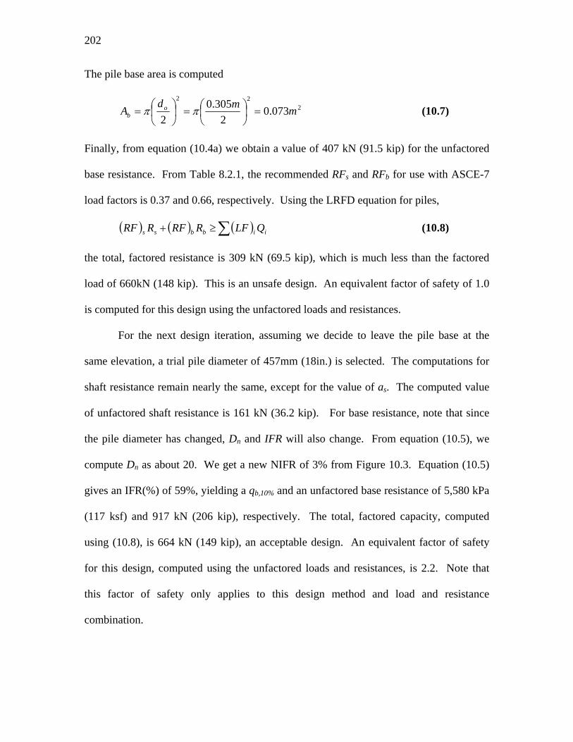
202

The pile base area is computed

222

073.02

305.02

mmdA o

b =⎟⎠⎞

⎜⎝⎛=⎟

⎠⎞

⎜⎝⎛= ππ (10.7)

Finally, from equation (10.4a) we obtain a value of 407 kN (91.5 kip) for the unfactored

base resistance. From Table 8.2.1, the recommended RFs and RFb for use with ASCE-7

load factors is 0.37 and 0.66, respectively. Using the LRFD equation for piles,

( ) ( ) ( )∑≥+ iibbss QLFRRFRRF (10.8)

the total, factored resistance is 309 kN (69.5 kip), which is much less than the factored

load of 660kN (148 kip). This is an unsafe design. An equivalent factor of safety of 1.0

is computed for this design using the unfactored loads and resistances.

For the next design iteration, assuming we decide to leave the pile base at the

same elevation, a trial pile diameter of 457mm (18in.) is selected. The computations for

shaft resistance remain nearly the same, except for the value of as. The computed value

of unfactored shaft resistance is 161 kN (36.2 kip). For base resistance, note that since

the pile diameter has changed, Dn and IFR will also change. From equation (10.5), we

compute Dn as about 20. We get a new NIFR of 3% from Figure 10.3. Equation (10.5)

gives an IFR(%) of 59%, yielding a qb,10% and an unfactored base resistance of 5,580 kPa

(117 ksf) and 917 kN (206 kip), respectively. The total, factored capacity, computed

using (10.8), is 664 kN (149 kip), an acceptable design. An equivalent factor of safety

for this design, computed using the unfactored loads and resistances, is 2.2. Note that

this factor of safety only applies to this design method and load and resistance

combination.

203

Finding an RF for use in Design of Piles Using Direct Method

In Chapter 9, we presented the Aoki and de Alencar Velloso (1975) method as a

general direct design method. We will use this design example to demonstrate how other

direct methods can be used to develop resistance factors based on available load test data.

It is important to note that the load test database used for such design methods should

contain numerous cases of similar soil conditions and pile type. This is necessary to

ensure the applicability the design method and its uncertainty.

The Bustamante and Gianeselli (1982) method is selected for design since our

hypothetical design firm (performing these example calculations) has pile load test data

to support use of the method for similar soils and pile type. Table10.3 is the pile load test

database for the hypothetical company.

The task in this example will be to determine what value of resistance factor to

use in design. Note from the discussion in Chapters 7, 8, and 9, when load test data of

this type is available (measured vs. predicted total capacity), the following LRFD

equation must be used,

( )( ) ( )∑≥+ iibs QLFRRRF (10.9)

where (Rs + Rb) is the total load capacity of the pile. Thus, we are finding a single RF

value to be applied to the total pile capacity. Since we are using ASCE-7 load factors for

the example, Figure 10.3 must be used to estimate RF. To use this figure, we must have

an input value of COV and reliability index β. The reliability index for this example will

be set at 3.0, the conventional value for structural design. The COV must be determined

from the load test database in Table 10.3. The first step to find the COV is to calculate

204

the “error” for each load test. The predicted capacity is calculated using the Bustamante

and Gianeselli (1982) method. Note that we assume the predicted capacity to be the

mean of the data since we need to assess the deviation of actual values from this

predicted value. To compute the COV of (Rs + Rb), we apply Equations (3.2.1) and

(3.2.2) to column (4) in Table 10.3. The resulting COV is 0.23. The final step to assess a

RF for this design is to enter Figure 10.4 with a COV of 0.23 and a β of 3.0. The

resulting RF is 0.55.

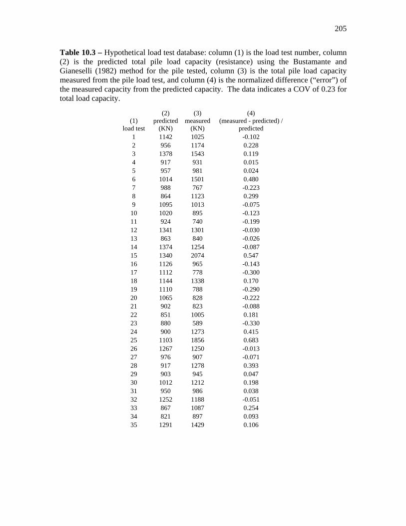
205

Table 10.3 – Hypothetical load test database: column (1) is the load test number, column (2) is the predicted total pile load capacity (resistance) using the Bustamante and Gianeselli (1982) method for the pile tested, column (3) is the total pile load capacity measured from the pile load test, and column (4) is the normalized difference (“error”) of the measured capacity from the predicted capacity. The data indicates a COV of 0.23 for total load capacity.

(1) load test

(2) predicted

(KN)

(3) measured

(KN)

(4) (measured - predicted) /

predicted 1 1142 1025 -0.102 2 956 1174 0.228 3 1378 1543 0.119 4 917 931 0.015 5 957 981 0.024 6 1014 1501 0.480 7 988 767 -0.223 8 864 1123 0.299 9 1095 1013 -0.075

10 1020 895 -0.123 11 924 740 -0.199 12 1341 1301 -0.030 13 863 840 -0.026 14 1374 1254 -0.087 15 1340 2074 0.547 16 1126 965 -0.143 17 1112 778 -0.300 18 1144 1338 0.170 19 1110 788 -0.290 20 1065 828 -0.222 21 902 823 -0.088 22 851 1005 0.181 23 880 589 -0.330 24 900 1273 0.415 25 1103 1856 0.683 26 1267 1250 -0.013 27 976 907 -0.071 28 917 1278 0.393 29 903 945 0.047 30 1012 1212 0.198 31 950 986 0.038 32 1252 1188 -0.051 33 867 1087 0.254 34 821 897 0.093 35 1291 1429 0.106

206

0.2 0.24 0.28 0.32 0.36Total Resistance (Rs + Rb) COV

0.2

0.4

0.6

0.8Ad

just

ed R

esis

tanc

e Fa

ctor

(RF)

β = 2.0β = 2.5β = 3.0β = 3.5

0.2 0.24 0.28 0.32 0.36

0.2

0.4

0.6

0.8

Figure 10.4 – Plot of Adjusted Resistance Factor RF varying with total resistance COV and target reliability index β, to be applied to total load capacity in the design of piles using ASCE-7 load factors. A bias factor of 1.06 for a lognormally distributed total resistance is assumed, implying that the resistance is assessed conservatively according to the CAM procedure.

The RF found in this example could then be applied with the Bustamante and

Gianeselli (1982) method to perform design checks on pile designs using Equation (10.9).

Bandini and Salgado (1998) have summaries of several direct pile design methods,

including the Bustamante and Gianeselli (1982) method.

207

Example Conclusion

From the first design example, observe that pile design methods can be applied in

nearly the same way as for WSD. Now, resistance factors are applied instead of safety

factors and factored loads are used instead of unfactored loads. In the sand example, a

design method for open ended piles was demonstrated that takes advantage of recent

research results by Paik and Salgado (2003) and Lee and Salgado (2003). In the second

example, a technique was demonstrated where practitioners can estimate resistance

factors for use in design based on pile load test data in similar soils with the same type of

pile. In this way, the uncertainty likely to be encountered for a particular design can be

addressed specifically. From this technique, it should be possible to expand the use of

LRFD to design methods other than those mentioned in this report.

208

209

CHAPTER 11. SUMMARY AND CONCLUSIONS

The first step in the present research was to assess the suitability of available load

factors for use in geotechnical Load and Resistance Factor Design (LRFD). The load

factors proposed by various current structural and foundation LRFD Codes were

reviewed. Usually, a larger number of limit states, load types and load combinations are

considered in the bridge and offshore foundation design codes, compared with building

and onshore foundation design codes. In this study, the load factors for four major load

types (i.e. dead, live, wind and earthquake loads) that control most design cases were

examined and compared between the Codes.

A simple FOSM reliability analysis was implemented to find appropriate ranges

of the load factor values for each load considered in this study. The analysis produced

results consistent with all the Codes reviewed, although the values produced lie in rather

wide ranges due to the relatively wide range of the input parameters. The analysis shows

even better agreement with the Codes when considering only the US Codes (AASHTO,

ACI, and AISC). The values presented in the US Codes lie in the middle of the

acceptable range determined by the analysis, as summarized by Figure 2.6.1. Both the

present ACI and AISC codes use the ASCE-7 recommended load factors. Therefore, the

present load factors prescribed by ASCE-7 and AASHTO are acceptable for use in

geotechnical LRFD.

Once we established that the code load factors can be used with confidence, the

next step was to investigate a method to evaluate resistance factors in the most

theoretically sound manner possible. We proposed a framework for the objective

210

development of resistance factors. Several steps comprise this framework. First, identify

the design equation. Second, identify all component quantities. Define probabilistic

models for the uncertain quantities using available data. Next, use reliability analysis to

determine the limit state values corresponding to a set of nominal design values at a

specified reliability index. Resistance factors can be determined algebraically from the

corresponding nominal and limit state values.

Using probabilistic models, optimum load and resistance factors are developed.

To make the results of this work compatible with established code load factors, an

adjustment must be made to the resistance factors. We presented a method in Section 3.3

that will satisfactorily accomplish this task.

Table 5.1.1 presents recommended resistance factors for use with ASCE-7 (1996)

or AASHTO (1998) live- and dead-load factors for shallow foundations. These tables

contain simplified guidelines based on the more thorough results of Figures 5.1.1, 5.1.2

and 5.1.4 for ASCE-7 load factors.

Serviceability and ultimate limit states should be treated separately. Results of

the present analysis suggest traditional WSD factors of safety may be overly conservative

for shallow foundations in clay. However, addressing safety factors alone will not offer

any improvement to present practice. The design process of interpreting data and using

transformation models to develop design resistance values must be examined. Without

the availability of consistent criteria for defining design resistance values, the safety

margin of a design is unknown and cannot be compared to other designs. The

development of statistically consistent methods to select design values, such as the CAM

211

method in Section 5.2, is quite feasible and will pave the way for the benefits of

reliability-based design to be fully realized.

LRFD of foundations will yield designs with consistent reliabilities if a

statistically consistent approach is used. The method proposed for establishing a

conservative mean for use in design is readily reproducible in practice. Resistance

factors have been determined that are compatible with this procedure. Three advantages

are offered by this method. First, since the method uses statistical tools to determine

values, the need for arbitrary judgment calls within a given soil layer is reduced. Second,

as a statistically consistent tool for evaluating design inputs, the method can be expected

to yield designs with much more consistent reliabilities than is possible otherwise.

Finally, the method has been shown to be a useful tool for maintaining consistent

reliability with respect to soil profiles with variabilities that differ from those used to

determine the resistance factors. This result is highly significant to the practical

implementation of LRFD methods in geotechnical engineering, since soil deposits vary

significantly from site to site.

In order to develop a complete set of LRFD factors for use in the ultimate limit

state design of shallow footings, uncertainties associated with different test methods, load

inclination factors, footing base inclination factors, and ground inclination must be

incorporated into future reliability analyses.

For the design of deep foundations, two major classes of design methods are

available: direct methods, which use in-situ tests to directly determine a resistance; and

property-based methods, which use soil properties determined from a variety of tests to

compute resistance. A major difference between property-based methods and direct

212

methods is that property-based methods tend to have higher uncertainty (lower RF), but

apply to general cases, while direct methods tend to have lower uncertainty (higher RF)

and only apply to specific cases resembling the specific piles and soils they were

developed for. One implication of this difference is that it may be riskier to apply a direct

method to a design situation that is different from the pile load test database supporting

the method, even though the method may show excellent agreement with measured

values in the database.

In the course of the literature review, it was often discovered that the experimental

and theoretical support for many design methods is incomplete. Thus, many design

methods can be expected to produce unpredictable deviations between measured and

predicted load capacities. This means that we are unable to rationally assess the

uncertainty for some design methods within the framework established in Chapter 3. The

available data to support existing design methods for drilled shafts and piles in clay, in

particular, were found to be limited.

Tables 8.2.1 and 9.2.1 present recommended resistance factors for use with

ASCE-7 (1996) or AASHTO (1998) live- and dead-load factors for deep foundations on

sand and clay, respectively. These tables also contain summaries of the design equations

to be used with each resistance factor.

In the course of this study, we attempted to investigate the most promising design

methods for deep foundations. However, any effort will be insufficient to cover all the

cases that could arise in practice knowing that there are many direct design methods that

are developed for specific design situations. As such, the designer needs the capability to

select resistance factors that reflect the uncertainty of the design method used. A suitable

213

technique is to assess the uncertainty of total capacity from predicted vs. measured load

test data. A methodology to apply this technique was presented in Section 9.2.1 and

demonstrated in Chapter 10.

Recommendations Reached in the Study

In this section, we summarize the various conclusions reached in the study

concerning how to implement LRFD properly for geotechnical design. These

recommendations are grouped according to their area of application.

• Selecting Load factors for use in Geotechnical LRFD

o Designers should use load factors in geotechnical LRFD that are

consistent with structural LRFD.

• Selecting Resistance Factors for use in Geotechnical LRFD

o Reliability analysis is the most rational technique available to assess

resistance factors.

o The process of specifying resistance factors in the code that yield the same

design proportions as previously used factors of safety is known as factor

calibration. Factor calibration is useful as a first step to implementing

LRFD and is the most common method currently in use.

o For shallow foundations, the single, “lumped” resistance factor approach

should be used.

o Better control over the uncertainty of a pile design is offered by the

multiple factor approach. However, some designs will not have enough

data to support this approach and the lumped factor must be used.

214

o There is a significant difference between designs supported by a pile load

test verification program and those without. Reliability analysis was

performed to support recommended values of RFs for cases without load

verification. RFs for verified pile designs are necessarily higher.

o For direct pile design methods not covered in the report, designers can

determine their own resistance factor using the figures provided. This is

possible when they have access to load test data supporting a design

method that is sufficiently similar to the design circumstances considered.

Thus, the results of this report can be extended beyond the cases

considered.

• Developing Resistance Factors Using Reliability Analysis

o Reliability analysis is the most rational technique available to assess

resistance factors.

o It is important to use a systematic approach to evaluate the uncertainty of

design variables.

o The proposed framework in Section 3.1 should be used to develop

resistance factors since it is a rational, systematic, and credible approach.

o For thorough investigations of design variable uncertainty, numerical

integration of the fundamental PDF equations is recommended to handle

the transformation to dependent PDFs in favor of Monte Carlo simulation

or first-order approximations.

215

o It is useful to develop target reliability indices based on current acceptable

practice, to allow the cautious, gradual adjustment of safety levels

(reliability indices and the resulting design proportions) over time.

o To assess currently acceptable reliability indices, reliability indices can be

back calculated from existing factors of safety.

o RFs have been produced in this report for a target reliability index of 3.0.

Existing practice or acceptable risk may vary and alternative target

reliability indices may be used. For piles, tools have been provided to do

this on a limited basis. More complete reliability analyses are required for

more thorough adjustments.

o The process of specifying resistance factors in the code that yield the same

design proportions as previously used factors of safety is known as factor

calibration. Factor calibration is useful as a first step to implementing

LRFD and is the most common method currently in use.

• Selecting Characteristic Values of Strength for Design

o It is critical to realizing the full potential of reliability-based design

methods to determine characteristic resistance in a reproducible way.

o Use of the Conservatively Assessed Mean (CAM) procedure outlined in

Chapter 5 is necessary to achieve more uniform inputs to design and take

advantage of the benefits offered by using LRFD. The CAM procedure is

also demonstrated in Chapters 6 and 10.

o In-situ test soundings and other soil tests should be grouped together for

analysis when they are known to be measurements of the same soil or soil

216

layer. Tests of different materials or in-situ soundings revealing different

features at a site are necessarily kept separate.

o Spatial variability in the vertical direction can be readily taken into

account using some in-situ tests. However, spatial variability in the

horizontal direction is impossible to determine routinely and the best

treatment of the problem is to use the “worst” applicable sounding, or

group of soundings.

• Engineering Education about LRFD

o Engineers will have to be educated about the rationale behind matching

proper and consistent values of RFs, LFs and characteristic resistance

within LRFD.

o Engineers will have to become familiar with the number of different

factors to adjust to and accept LRFD.

• General Recommendations Concerning the Design of Deep Foundations

o A number of deep foundation design methods were selected for this study

on the basis of the completeness of their supporting data. These should be

used in design since the methods have such good support.

o Several aspects of pile design require further investigation as data is

incomplete.

o For property-based design of piles, the value of K0 selected for use in shaft

design is very important – it is a highly relevant parameter and should be

selected with care.

217

LIST OF REFERENCES

Aas, G., Lacasse, S., Lunne, T. and Hoeg, K. (1986) “Use of In Situ Tests for

Foundation Design on Clay.” In Situ ’86: Use of In Situ Tests in Geotechnical

Engineering. Samuel Clemence, ed. ASCE. 1-30.

AASHTO (1994). LRFD Bridge Design Specifications, 1st ed. American Association of

State Highway and Transportation Officials, Washington D.C.

AASHTO (1998). LRFD Bridge Design Specifications, 2nd ed. American Association of

State Highway and Transportation Officials, Washington D.C.

ACI (1990). Standard Specifications for Tolerances for Concrete Construction and

Materials (117-90). American Concrete Institute, Detroit.

ACI (1999). Building Code Requirements for Structural Concrete (318-99) and

Commentary (318R-99). American Concrete Institute, Detroit.

ACI (2002). Building Code Requirements for Structural Concrete (318-02) and

Commentary (318R-02). American Concrete Institute, Detroit.

AISC (1994). Load and Resistance Factor Design Specification for Structural Steel

Buildings, 2nd ed. American Institute of Steel Construction, Inc., Chicago, Illinois.

AISC (2001). Manual of Steel Construction: Load and Resistance Factor Design. 3rd ed.

American Institute of Steel Construction, Chicago.

Allen, D. E. (1975). “Limit states design-probabilistic study.” Can. J. Civ. Engrg., 2, 36-

49.

Altaee et al. (1992). “Axial load transfer for piles in sand: I. Tests on an instrumented

precast pile.” Canadian Geotechnical Journal. 29. 11-20.

218

Altaee et al. (1993). “Load transfer for piles in sand and the critical depth.” Canadian

Geotechnical Journal. 30. 455-463.

American Petroleum Institute (API) (1993). Recommended practice for planning,

designing and constructing fixed offshore platforms-load and resistance factor

design. American Petroleum Institute, Washington D.C.

American Society of Civil Engineers (ASCE). (1996). ‘‘Minimum design loads for

buildings and other structures.’’ ASCE 7-95, ASCE, Reston,Va.

Ang, A. H-S., and W-H. Tang (1975). Probability Concepts in Engineering Planning and

Design, Volume I: Basic Principles. Wiley.

Aoki, N. and D. de Alencar (1975). “An Approximate Method to Estimate the Bearing

Capacity of Piles.” Proc. 5th Pan-American Conference of Soil Mechanics and

Foundation Engineering, Buenos Aires. 1. 367-376.

Baligh, M. M., V. Vivatrat, and C. C. Ladd (1980). “Cone Penetration in Soil Profiling.”

Journal of the Geotechnical Engineering Division, ASCE. 106:4. 447-461.

Bandini, P. (2003) PhD Thesis. Purdue University.

Bandini, P. and R. Salgado (1998). “Methods of Pile Design Based on CPT and SPT

Results.” Geotechnical Site Characterization. Robertson and Mayne, eds. 967-

976.

Barker, R. M., Duncan, J. M., Rojiani, K. B., Ooi, P. S. K., Tan, C. K., and Kim, S. G.

(1991). Manuals for the design of bridge foundations. Transportation Research

Board, NCHRP report 343.

BCP Committee (1971). “Field tests on piles in sand.” Soils and Foundations. 11:2. 29-

49.

219

Becker, D. E. (1996). “Eighteenth Canadian Geotechnical Colloquium: Limit States

Design for Foundations. Part II. Development for the National Building Code of

Canada.” Can. Geotech. J., 33, 984-1007.

Becker, D. E. (1996). “Eighteenth Canadian Geotechnical Colloquium: Limit States

Design for Foundations. Part I. An overview of the foundation design process.”

Canadian Geotechnical Journal. 33:6. 956-983.

Beringen F.L., Windle D. & Van Hooydonk W.R. (1979). “Results of loading tests on

driven piles in sand.” Proc. Conference on Recent Developments in the Design

and Construction of Piles. ICE, London. 213-225.

Bolton, M. D. (1986). “The Strength and Dilatancy of Sands.” Geotechnique. 36. 65-78.

Briaud, J.-L. and L. M. Tucker (1988). “Measured and Predicted Axial Load Response

of 98 Piles.” Journal of Geotechnical Engineering, ASCE. 114:9. 984-1001.

Briaud, J.-L., L. M. Tucker, and E. Ng. (1989). “Axially Loaded 5 Pile Group and a

Single Pile in Sand.” Proc. 12th Int. Conf. Soil Mechanics and Foundation

Engineering, Rio de Janeiro. 2. 1121-1124.

Brinch Hansen, J. (1970). “A Revised and Extended Formula for Bearing Capacity.”

The Danish Geotechnical Institute, Bulletin No. 28.

Brinch Hansen, J. (1970). “A Revised and Extended Formula for Bearing Capacity.”

The Danish Geotechnical Institute, Bulletin No. 28.

Bustamante, M. and L. Gianeselli (1982). “Pile Bearing Capacity Prediction by Means of

Static Penetrometer CPT.” Proc. 2nd European Symposium on Penetration

Testing, Amsterdam. 2. 493-500.

220

Chow, F.C. (1997). Investigations into the Behaviour of Displacement Piles for Offshore

Foundations. PhD dissertation, University of London (Imperial College).

Cornell, C. A. (1969). “A Probability-Based Structural Code.” ACI Journal. 974-985.

Cornell, C. A. (1969). “Structural safety specifications based on second-moment

reliability.” Symp. Int. Assn. Brid. and Struct. Engrg., London.

Darrag, A. A. (1987). Capacity of Driven Piles in Cohesionless Soils Including Residual

Stresses. PhD Thesis, Purdue University.

DeBeer, E. E. (1970) “Experimental Determination of the Shape Factors and the

Bearing Capacity Factors of Sand.” Geotechnique, 20, 387-411.

DGI (1985). Code of practice for foundation engineering. Danish Geotechnical Institute,

Copenhagen, Denmark.

ECS (1994). Eurocode 7:Geotechnical Design-Part I: General Rules. European

Committee for Standardization, Central Secretariat, Brussels.

ECS (1995). Eurocode 1:Basis of Design and Actions on Structures-Part I: Basis of

Design. European Committee for Standardization, Central Secretariat, Brussels.

Ellingwood, B. R. (1999). “Wind Load Statistics for Probability-Based Structural

Design.” Journal of Structural Engineering, ASCE. 125:4. 453-463.

Ellingwood, B., Galambos, T. V., MacGregor, J. G., and Cornell C. A. (1980).

Development of a probability based load criterion for American National

Standard A58 - Building Code Requirements for Minimum Design Loads in

Buildings and other Structures. National Bureau of Standards, Washington, D.C.

221

Ellingwood, Bruce, James G. MacGregor, Theodore V. Galambos, and C. Allin Cornell.

(1982). “Probability Based Load Criteria: Load Factors and Load

Combinations.” Journal of the Structural Division, ASCE. 108:5. 978-997.

Eslami, A. and B. H. Fellenius (1997). “Pile Capacity by Direct CPT and CPTu Methods

Applied to 102 Case Histories.” Canadian Geotechnical Journal. 34. 886-904.

Fellenius, B. H. and A. A. Altaee (1995). “Critical Depth: How it Came into Being and

Ehy it Does not Exist.” Proceedings, ICE, Geotehcnical Engineering. 113. 107-

111.

Fisher, John W., Theodore V. Galambos, Geoffrey L. Kulak, Mayasandra K. Ravindra

(1978). “Load and Resistance Factor Design Criteria for Connectors.” Journal of

the Structural Division, ASCE. 104:9. New York: ASCE. pp. 1427-1441.

Fleming, W. G. K., A. J. Weltman, M. F. Randolph, and W. K. Elson (1992). Piling

Engineering. Halsted Press, New York.

Foye, K. C., R. Salgado and B. Scott (2004). “Assessment of Variable Uncertainties for

Reliability-Based Design of Foundations.” Journal of Geotechnical and

Geoenvironmental Engineering. ASCE. In press.

Foye, K. C., R. Salgado and B. Scott (2004). “Resistance Factors for Use in Shallow

Foundation LRFD.” Journal of Geotechnical and Geoenvironmental Engineering.

ASCE. In press.

Franke, E. (1993). “EUROCODE Safety Approach as Applied to Single Piles.” 4th

International DFI Conference. 13-18.

222

Galambos, Theodore V., Bruce Ellingwood, James G. MacGregor, and C. Allin Cornell.

(1982). “Probability Based Load Criteria: Assessment of Current Design

Practice.” Journal of the Structural Division, ASCE. 108:5. 959-977.

Goble, G. (1999). Geotechnical Related Development and Implementation of Load and

Resistance Factor Design (LRFD) Methods. Transportation Research Board,

NCHRP synthesis 276.

Gregersen O.S., G. Aas, and E. Dibiagio (1973). “Load tests on friction piles in loose

sand.” Proc. 8th Int. Conf. Soil Mechanics & Foundation Engineering, Moscow.

2. 109-117.

Haldar, A. and Mahadevan, S. (2000). Probability, Reliability, and Statistical Methods in

Engineering Design. John Wiley and Sons, Inc. New York.

Hammitt, G. M. (1966). “Statistical Analysis of Data from a Comparative Laboratory

Test Program Sponsored by ACIL.” Miscellaneous Paper 4-785. U. S. Army

Engineering Waterways Experiment Station, Corps of Engineers.

Hanna, T.H. and R.H.S. Tan (1973). “The Behavior of Long Piles under Compressive

Loads in Sand.” Canadian Geotechnical Journal. 10:2. 311-340.

Hardin, B. O., and Black, W. L. (1966). ‘‘Sand Stiffness Under Various Triaxial

Stresses.’’ J. Soil Mech. and Found. Div., ASCE. 92:2. 27–42.

Harr, M. E. (1987). Reliability Based Design in Civil Engineering. Dover, Mineola, NY.

Hasofer, A. M. and N. C. Lind (1974). “Exact and Invariant Second-Moment Code

Format.” Journal of the Engineering Mechanics Division. ASCE. 100:1. 111-

121.

223

Hettler, A. (1982). "Approximation Formula for Piles Under Tension." Proc., IUTAM,

Conf. on Deformation and Failure of Granular Materials. 603–608.

Ismael, N. F. and Jeragh, A. M. (1986) “Static Cone Tests and Settlement of Calcareous

Desert Sands.” Can. Geotech. J., 23, 297-303.

Jacobs, P. A., and J. S. Coutts (1992). “A Comparison of Electric Piezocone Tips at the

Bothkennar Test Site.” Géotechnique. 42:2. 369-375.

Jardine, R., Chow, F.C., (1998). Research into the Behaviour of Displacement Piles for

Offshore Foundations. OTO 98 833. Health and Safety Executive.

Jaynes, E. T. (1957). “Information Theory and Statistical Mechanics, II,” Phys. Rev., 108.

Journal of Geotechnical Engineering, ASCE. 102:3. 197-228.

Kerisel, J. (1964). “Deep Foundations, Basic Experimental Facts.” Proc. North

American Conf. Deep Foundations, Mexican Society of Soil Mechanics. 1. 5-44.

Kishida, H., and M. Uesugi (1987). “Tests of the interface between sand and

Kraft, L. M. (1990). “Computing Axial Capacity in Sands for Offshore Conditions.”

Marine Geotechnology. 9. 61-92.

Kraft, L.M. (1991) “Performance of Axially Loaded Pipe Piles in Sand.” Journal of

Geotechnical Engineering, ASCE. 117:2. 272-296.

Kulhawy, F. H, and K. K. Phoon (2002). “Observations on Geotechnical Reliability-

Based Design Development in North America.” Proceedings. International

Workshop on Foundation Design Codes and Soil Investigation in view of

International Harmonization and Performance Based Design, Hayama, Japan. 31-

48.

224

Kulhawy, F. H., and C. H. Trautmann (1996). “Estimation of In-Situ Test Uncertainty.”

Uncertainty in the Geologic Environment: From Theory to Practice. C. D.

Shackelford, P. P. Nelson, M. J. S. Roth, eds. ASCE. 269-286.

Kulhawy, F.H. (1984) “Limiting Tip and Side Resistance: Fact or Fallacy?” Proceed. of

the symposium on the Analysis and Design of pile Foundations. American Society

of Civil Engineers, San Francisco, Calif. 80-98.

Lee, J. and R. Salgado (1999). “Determination of Pile Base Resistance in Sands.” Journal

of Geotechnical and Geoenvironmental Engineering, ASCE. 125:8. 673-683.

Lee, J., R. Salgado, and K. Paik (2003). “Estimation of Load Capacity of Pipe Piles in

Sand Based on Cone Penetration Test Results.” Journal of Geotechnical and

Geoenvironmental Engineering, ASCE. 129:6. 391-403.

Lehane, B.M., and Randolph, M. F. (2002). “Evaluation of a minimum base resistance

for driven pipe piles in siliceous sand.“ Journal of Geotechnical and

Geoenvironmental Engineering, ASCE, 128(3), 198-205.

Lehane, B.M., Jardine, R.J., Bond, A.J., and Frank, R. (1993). “Mechanisms of Shaft

Friction in Sand from Instrumented Pile Tests.” Journal of Geotechnical

Engineering, ASCE. 119:1. 19-35.

Liao, S. C. and R. V. Whitman (1986). “Overburden Correction Factors for SPT in

Sand.” Journal of Geotechnical Engineering, ASCE. 112:3. 373-377.

Lind, N. C. (1971). “Consistent partial safety factors.” J. Struct. Engrg. Div., ASCE,

97(ST6), 1651-1670.

225

Low, B. K., and W. H. Tang. (1997). “Efficient Reliability Evaluation Using

Spreadsheet.” Journal of Geotechnical and Geoenvironmental Engineering.

123:7. 749-752.

Lunne, T. and Eide, O. (1976). “Correlations between cone resistance and vane shear

strength in some Scandinavian soft to medium stiff clays.” Can. Geotech. J., 13,

430-441.

MacGregor, J. G. (1976). “Safety and limit states design for reinforced concrete.” Can. J.

Civ. Engrg., 3, 484-513.

MacGregor, J. G. (1997). Reinforced Concrete Mechanics and Design, 3rd ed. Prentice

Hall.

Meyerhof, G. G. (1951). "The Ultimate Bearing Capacity of Foundations." Geotechnique.

2:4. 301-332.

Meyerhof, G.G. (1976). “Bearing Capacity and Settlement of Pile Foundations.”

Milford, R. V. (1987). “Load Factors for Limit Sates Codes.” Journal of Structural


MOT (1992). Ontario highway bridge design code. Ministry of Transportation Ontario,

Downsview.

Nowak, A. S. (1994). “Load model for bridge design code.” Can. J. Civ. Engrg., 21, 36-

49.

Nowak, A. S. and Grouni, H. N. (1994). “Calibration of the Ontario highway bridge

design code 1991 edition.” Can. J. Civ. Engrg., 21, 25-35.

Nowak, A.S. (1994). "Load Model for Bridge Design Code." Canadian Journal of Civil

Engineering. 21. 36-49.

226

NRC (1995). National building code of Canada. National Research Council of Canada,

Ottawa.

Outokumpu Stainless (2004). “Definition of Surface Roughness.”

http://www.outokumpu.com/template/Page____5852.asp

Paik, K. and R. Salgado (2003). “Determination of Bearing Capacity of Open-Ended

Piles in Sand.” Journal of Geotechnical and Geoenvironmental Engineering,

ASCE. 129:1. 46-57.

Paik, K., R. Salgado, J. Lee, and B. Kim (2003). “Behavior of Open- and Closed-Ended

Piles Driven Into Sands.” Journal of Geotechnical and Geoenvironmental


Paikowsky, Samuel G. 2004. Load and Resistance Factor Design for Deep Foundations.

NCHRP Report 507. Washington, D.C.: Transportation Research Board.

Phoon, K. K., and F. H. Kulhawy (1999). “Characterization of Geotechnical Variability.”

Canadian Geotechnical Journal. 36. 612-624.

Prandtl, L. (1920). “Über die Härte Plasticher Körper.” Nachr. Ges. Wiss. Gött., Math-

Phys. Kl., 12, 74-85.

Randolph, M. F. and B. J. Murphy (1985). “Shaft Capacity of Driven Piles in Clay.”

Proc. 17th Offshore Technology Conf., Houston. 1. 371-378.

Randolph, M.F., Dolwin, J., and Beck, R. (1994). “Design of Driven Piles in Sand”.

Géotechnique. 44:3. 427-448.

Rao, K. S., M. M. Allam, and R. G. Robinson (1998). “Interfacial Friction Between

Sands and Solid Surfaces.” Proc. ICE, Geotechnical Engineering. 131. 75-82.

227

Reissner, H. (1924). "Zum Erddruckproblem." Proceedings of the First International

Congress forf Applied Mechanics. C. B. Biezeno and J. M. Burgers, eds. Delft.

295-311.

Robertson, P. K., Campanella, R. G., and Wightman, A. (1983). “SPT-CPT

Correlations.” Journal of Geotechnical and Geoenvironmental Engineering,

ASCE, 109, 1449-1459.

Rosenblueth, E. (1975). “Point Estimates for Probability Moments.” Proceedings of the

National Academy of Sciences of the United States of America. 72:10. 3812-

3814.

Salgado, R. (2003). CONPOINT User Manual.

Salgado, R. (2004). The Engineering of Foundations. McGraw-Hill, app. 1500 pages

w/figures (in preparation).

Salgado, R. and J. K. Mitchell (2003). “Computation of Penetration Resistance in

Sands.” Geotechnical Report Number 2003-2. School of Civil Engineering, 550

Stadium Mall Drive, Purdue University. West Lafayette, Indiana.

Salgado, R. and J. K. Mitchell (2003). “Computation of Penetration Resistance in

Sands.” Geotechnical Report Number 2003-2. School of Civil Engineering, 550

Stadium Mall Drive, Purdue University. West Lafayette, Indiana.

Salgado, R., A. V. Lyamin, S. W. Sloan, and H. S. Yu (2004). “Two- and Three-

Dimensional Bearing Capacity of Foundations in Clay.” Géotechnique. accepted

for publication.

228

Salgado, R., J. K. Mitchell, and M. Jamiolkowski (1997). “Cavity Expansion and

Penetration Resistance in Sand.” Journal of Geotechnical and Geoenvironmental

Engineering, ASCE, 123:4, 344-354.

Scott, B. (2002) “Development of Load and Resistance Factor Design Method for

Shallow Foundations.” PhD thesis, Purdue University, West Lafayette, Indiana.

Scott, B., B. J. Kim and R. Salgado (2003). “Assessment of Current Load Factors for

Use in Geotechnical LRFD.” Journal of Geotechnical and Geoenvironmental


Shooman, M. L. (1968). Probabilistic Reliability: An Engineering Approach. McGraw-

Hill. New York.

Skempton, A. W. (1986). “Standard Penetration Test Procedures and the Effects in Sand

of Overburden Pressure, Relative Density, Particle Size, Ageing and

Overconsolidation.” Geotechnique. 36:3. 425-337.

Sloan, S. W. and Yu, H. S. (1996). “Rigorous Plasticity Solutions for the Bearing

Capacity Factor Nγ.” Proceedings of the 7th Australia-New Zealand Conference

on Geomechanics, Adelaide. 544-550.

Stark, T. D. and J. E. Juhrend (1989). “Undrained Shear Strength from Cone Penetration

Tests.” Proc. 12th Int. Conf. Soil Mechanics and Foundation Engineering. 327-

330.

steel in the simple shear apparatus,” Géotechnique. 37:1. 45-52.

Tabsh, Sami W. (1997). “Safety of Reinforced Concrete Members Designed Following

ACI 318 Building Code.” Engineering Structures. 19:10. 843-850.

229

Tippett, L. H. C. (1925). “On the Extreme Individuals and the Range of Samples Taken

from a Normal Population.” Biometrika. 17:3/4. New York : Macmillan. 364-

387.

Toolan, F. E., M. L. Lings, and U. A. Mirza (1990). “An Appraisal of API RP2A

Recommendations for Determining Skin Friction of Piles in Sand.” Proc. 22nd

Offshore Technology Conf., Houston. OTC 6422. 4. 33-42.

Vesic, A. S. (1964). “Model Testing of Deep Foundations in Sand and Scaling Laws.”

Proc. Conf. Deep Foundations, Mexican Society of Soil Mechanics and

Geotechnical Engineering. Mexico City. 2. 525-533.

Vesic, A. S. (1967). “A Study of Bearing Capacity of Deep Foundations.” Final rep.,

Project B-189, Georgia Institute of Technology. Atlanta, GA.

Vesic, A. S. (1970). “Tests on Instrumented Piles, Ogeechee River Site.” J. Soil Mech.

Found. Div., ASCE. 96:2. 561–504.

Vesic, A. S. (1973). “Analysis of Ultimate Loads of Shallow Foundations.” Journal of

the Soil Mechanics and Foundations Division, ASCE. 99:1. 45-73.

White, D. J. (2003). “Field Measurements of CPT and Pile Base Resistance in Sand.”

CUED/D-SOILS/TR327. University of Cambridge.

Withiam, J. L., Voytko, E. P., Barker, R. M., Duncan, J. M., Kelly, B. C., Musser, S. C.,

and Elias, V. (1997). Load and resistance design (LRFD) for highway bridge

substructures. Federal Highway Administration, Washington, D.C.

Yu, H. S., L. R. Herrmann, and R. W. Boulanger (2000). “Analysis of Steady Cone

Penetration Resistance in Clay.” Journal of Geotechnical and Geoenvironmental


report deep foundations.pdf

Documents

design loads

design resistances

design method

design philosophy

load factors

reliabilitybased design

limit states lower

ultimate limit states