Relationships Among Exceedances of Chemical Criteria or

EPA/600/R-06/078

February 2007

Relationships AmongExceedances of ChemicalCriteria or Guidelines, the

Results of Ambient ToxicityTests, and Community Metrics in

Aquatic Ecosystems

National Center for Environmental AssessmentOffice of Research and Development

U.S. Environmental Protection AgencyCincinnati, OH 45268

NOTICE

The U.S. Environmental Protection Agency through its Office of Research and Development funded and managed the research described here. It has been subjected to the Agency’s peer and administrative review and has been approved for publication as an EPA document. Mention of trade names or commercial products does not constitute endorsement or recommendation for use.

ABSTRACT

In order to use bioassessments to help to diagnose or identify the specific environmental stressors affecting aquatic or marine ecosystems, a better understanding is needed of the relationships among community metrics, ambient chemical criteria or guidelines and ambient toxicity tests. However, these relationships are not necessarily simple, because metrics generally assess measurement endpoints at the community level of biological organization, while ambient criteria or guidelines and ambient toxicity tests assess measurement endpoints at the organism level. Although a basic hierarchical relationship exists between the levels of biological organization used as measurement endpoints by these methods, quantification of this relationship may be further complicated by the influence of other differences among these methods that affect their sensitivity and specificity to the stressors present at individual sites.

Since 1990, the U.S. Environmental Protection Agency has conducted Environmental Monitoring and Assessment Program surveys of both wadeable stream and estuarine sites. These surveys have collected data on biotic assemblages, physical and chemical habitat characteristics and, in some cases, water and sediment chemistry and toxicity. Among these studies is a survey of wadeable streams in the Southern Rockies ecoregion of Colorado in 1994 and 1995 and a survey of estuaries in the Virginian Province of the eastern United States from 1990 to 1993. Streams in the Southern Rockies ecoregion are affected by contamination from hardrock metal mining, while the estuarine sites may be affected by sediment contamination by polyaromatic hydrocarbons and metals. We characterized streams as metals-affected based on exceedance of hardness-adjusted metals criteria for Cd, Cu, Pb and Zn in surface water; on water column toxicity tests (48-hour Pimephales promelas and Ceriodaphnia dubia survival); on exceedance of sediment threshold effect levels; or on sediment toxicity tests (7-day Hyalella azteca survival and growth). Estuarine sites were characterized as affected by sediment contamination based on exceedance of sediment guidelines or on sediment toxicity tests (i.e., 10-day Ampelisca abdita survival). The results of these classifications were contrasted by use of contingency tables and a measure of association, (. Then, assemblage metrics were compared statistically among affected and unaffected sites to identify metrics sensitive to the contamination. In streams, a number of macroinvertebrate metrics, particularly richness metrics, were less in groups of sites identified as affected by metals with the criteria or

ii

ambient toxicity tests, while other metrics were not. Fish metrics were less sensitive to the metal contamination, but this lack of sensitivity is likely because of the low diversity of fish assemblages in these Rocky Mountain streams. Similarly at the estuarine sites, a number of benthic metrics differed between the groups of sites segregated using the organism-level measure, while other metrics did not. These same metrics also exhibited relationships with contaminant concentrations in regression analyses. This variation among metrics depends on the sensitivity of the individual metrics to the stressor gradients of interest as many metrics may not measure the community responses characteristic of a specific stressor. The differences between groups for the more sensitive metrics imply that a relationship exists between the organism-level effects assessed by ambient chemistry or ambient toxicity tests and the community-level effects assessed by community metrics. However, the organism-level effects are only predictive to a limited extent of the community-level effects at individual sites.

Beyond the differences in the levels of biological organization represented by their measurement endpoints, these methods differ in their specificity and sensitivity to different stressors. Criteria or guidelines are specific to the contaminants being measured and assessed and cannot assess contaminants or stressors that are not measured or that lack guidelines for comparison. Ambient toxicity tests should detect effects of any toxicants present and bioavailable, but cannot assess other characteristics of a site that can affect the biotic community. Community metrics are the least specific of the three methods, because they measure directly community-level effects in the native assemblages. Metrics may be selected that are sensitive to a specific stressor, but they also will be sensitive to other stressors, such as alterations in physical habitat that are not addressed by the other methods.

Other factors also affect the relative sensitivity and predictiveness of these different methods. Toxicity tests and chemical criteria or benchmarks based on measurement endpoints that are chronic in duration would be more predictive of community-level effects. Toxicity tests often use one or two standard species, which can be more tolerant of specific contaminants than other indigenous species and would be less predictive of community-level effects than a chemical criterion or benchmark based on a species sensitivity distribution composed of many species.

Preferred citation:

U.S. EPA. 2006. Relationships Among Exceedances of Chemical Criteria or Guidelines, the Results of

Ambient Toxicity Tests, and Community Metrics in Aquatic Ecosystems. U.S. Environmental Protection

Agency, National Center for Environmental Assessment, Cincinnati, OH. EPA/600/R-06/078.

iii

TABLE OF CONTENTS

Page

TABLE OF CONTENTS . . . . . . . . . . . . . . . . . . . . . . . . . . . . . . . . . . . . . . . . . . . . . . . . ivLIST OF TABLES . . . . . . . . . . . . . . . . . . . . . . . . . . . . . . . . . . . . . . . . . . . . . . . . . . . . . viLIST OF FIGURES . . . . . . . . . . . . . . . . . . . . . . . . . . . . . . . . . . . . . . . . . . . . . . . . . . . viiLIST OF ABBREVIATIONS . . . . . . . . . . . . . . . . . . . . . . . . . . . . . . . . . . . . . . . . . . . . viiiPREFACE . . . . . . . . . . . . . . . . . . . . . . . . . . . . . . . . . . . . . . . . . . . . . . . . . . . . . . . . . . . ixAUTHORS, CONTRIBUTORS AND REVIEWERS . . . . . . . . . . . . . . . . . . . . . . . . . . . x

1. INTRODUCTION . . . . . . . . . . . . . . . . . . . . . . . . . . . . . . . . . . . . . . . . . . . . . . . . 1

1.1. DATA SETS USED . . . . . . . . . . . . . . . . . . . . . . . . . . . . . . . . . . . . . . . . . 5

2. WADEABLE STREAMS IN THE SOUTHERN ROCKIES ECOREGION OF COLORADO . . . . . . . . . . . . . . . . . . . . . . . . . . . . . . . . . . . . . . . . . . . . . . . . 8

2.1. INTRODUCTION . . . . . . . . . . . . . . . . . . . . . . . . . . . . . . . . . . . . . . . . . . . 82.2. MATERIALS AND METHODS . . . . . . . . . . . . . . . . . . . . . . . . . . . . . . . . 8

2.2.1. Study Area and Survey Design . . . . . . . . . . . . . . . . . . . . . . . . . . 82.2.2. Water and Sediment Chemistry . . . . . . . . . . . . . . . . . . . . . . . . . 102.2.3. Invertebrate and Fish Toxicity Tests . . . . . . . . . . . . . . . . . . . . . 102.2.4. Macroinvertebrate Collection and Identification . . . . . . . . . . . . . 112.2.5. Fish Collection and Identification . . . . . . . . . . . . . . . . . . . . . . . . 112.2.6. Calculation of Community Metrics . . . . . . . . . . . . . . . . . . . . . . . 122.2.7. Data Handling and Analysis . . . . . . . . . . . . . . . . . . . . . . . . . . . . 16

2.3. RESULTS AND DISCUSSION . . . . . . . . . . . . . . . . . . . . . . . . . . . . . . . 19

2.3.1. Organism-level Measures . . . . . . . . . . . . . . . . . . . . . . . . . . . . . 192.3.2. Organism-level Measures versus Community Metrics . . . . . . . . 232.3.3. Piecewise Regression Analyses . . . . . . . . . . . . . . . . . . . . . . . . 29

3. ESTUARINE SYSTEMS IN THE VIRGINIAN PROVINCE OF THE ATLANTIC COAST . . . . . . . . . . . . . . . . . . . . . . . . . . . . . . . . . . . . . . . . . . . . . 34

3.1. INTRODUCTION . . . . . . . . . . . . . . . . . . . . . . . . . . . . . . . . . . . . . . . . . . 343.2. MATERIALS AND METHODS . . . . . . . . . . . . . . . . . . . . . . . . . . . . . . . 34

iv

TABLE OF CONTENTS cont.

Page

3.2.1. Study Area and Survey Design . . . . . . . . . . . . . . . . . . . . . . . . . 343.2.2. Field and Laboratory Methods . . . . . . . . . . . . . . . . . . . . . . . . . . 353.2.3. Sediment Contaminant Concentrations . . . . . . . . . . . . . . . . . . . 353.2.4. Ambient Toxicity Tests . . . . . . . . . . . . . . . . . . . . . . . . . . . . . . . . 353.2.5. Calculation of Community Metrics . . . . . . . . . . . . . . . . . . . . . . . 363.2.6. Data Handling and Analysis . . . . . . . . . . . . . . . . . . . . . . . . . . . . 40

3.3. RESULTS AND DISCUSSION . . . . . . . . . . . . . . . . . . . . . . . . . . . . . . . 43

3.3.1. Organism-level Measures . . . . . . . . . . . . . . . . . . . . . . . . . . . . . 433.3.2. Organism-level Measures versus Community Metrics . . . . . . . . 47

4. CONCLUSIONS . . . . . . . . . . . . . . . . . . . . . . . . . . . . . . . . . . . . . . . . . . . . . . . . 57

5. REFERENCES . . . . . . . . . . . . . . . . . . . . . . . . . . . . . . . . . . . . . . . . . . . . . . . . 60

v

LIST OF TABLES

No. Title Page

1 Macroinvertebrate and Fish Metrics that Exhibited Differences Between the Two Groups Segregated Using at Least One of the Measurement Endpoints . . . . . . . . . . . . . . . . . . . . . . . . . . . . . . . . . . . . . . . . . . . . . . . . . . . . . 13

2 Metrics that Did Not Exhibit Differences among the Groups . . . . . . . . . . . . . . 15

3 Criteria Used to Divide Sites into the Impacted or Unimpacted Groups . . . . . 17

4 Correspondence of Conclusions of Assessments for Surface Water andSediment for Sampling Events . . . . . . . . . . . . . . . . . . . . . . . . . . . . . . . . . . . . . 20

5 Correspondence of Conclusions of Assessments Based on Chemical Criteria and Ambient toxicity tests for Sampling Events . . . . . . . . . . . . . . . . . . 21

6 Enumeration of Sampling Events in Wadeable Streams in the Southern Rockies Ecoregion of Colorado Where Classification Based on the Organism-level Measures and that Based on the Community Metric Disagree . . . . . . . . . . . . . . . . . . . . . . . . . . . . . . . . . . . . . . . . . . . . . . . . . . . . . . 27

7 Benthic Metrics that Exhibited Differences Between the Two Groups Segregated Using at Least One of the Following Measurement Endpoints . . . 37

8 Benthic Metrics that Did Not Exhibit Differences among the Two GroupsSegregated Using at Least One of the Measurement Endpoints . . . . . . . . . . . 39

9 Criteria Used to Divide Sites into the Impacted or Unimpacted Groups . . . . . 41

10 Criteria Used to Classify Metrics as Different than Expected . . . . . . . . . . . . . . 44

11 Correspondence of Conclusions of Assessments Based on Chemical Criteria and Ambient Toxicity Tests for Sampling Events . . . . . . . . . . . . . . . . 45

12 Comparison of Sites where Maximum p from the Logistic Regression>0.50 for Metals versus for PAHs . . . . . . . . . . . . . . . . . . . . . . . . . . . . . . . . . . 48

13 Enumeration of Sampling Events in Estuarine Systems of the Virginian Province of the Atlantic Coast where Classification Based on the Organism-level Effects Measures and that Based on the Community Metric Disagree . . . . . . . . . . . . . . . . . . . . . . . . . . . . . . . . . . . . . . . . . . . . . . . . 54

vi

LIST OF FIGURES

No. Title Page

1 Map of Colorado, USA, with the Mineralized Region of the Southern Rockies Ecoregion and Locations of the 1994-1995 Regional Environmental Monitoring Assessment Program Reaches . . . . . . . . . . . . . . . . 9

2 Comparison of Metals Concentrations in Water and in Sediment Between Groups Identified as Potentially Affected or Unaffected by the Ambient Toxicity Test of Water and Sediment, Respectively . . . . . . . . . . 22

3 Comparison of Macroinvertebrate Metrics Between Groups Identified asPotentially Affected or Unaffected by Each of the Organism-level Endpoints . 24

4 Comparison of Macroinvertebrate and Fish Metrics Between Groups Identified as Potentially Affected or Unaffected by Each of the Organism-level Endpoints . . . . . . . . . . . . . . . . . . . . . . . . . . . . . . . . . . . . . . . . 25

5 Piecewise Regressions of Taxa Richness Metrics on the Summed Ratios of the Dissolved Concentrations of Cd, Cu, Pb and Zn to their Chronic AWQC . . . . . . . . . . . . . . . . . . . . . . . . . . . . . . . . . . . . . . . . . . . . . . . . 31

6 Piecewise Regressions of Taxa Richness Metrics on the Summed Ratios of the Sediment Concentrations of Cd, Cu, Pb and Zn to their TELs . . . . . . . . . . . . . . . . . . . . . . . . . . . . . . . . . . . . . . . . . . . . . . . . . . . . 32

7 Comparison of Percent Survival of A. abdita Between Sites where Maximum p < 0.50 from the Logistic Regressions and those where Maximum p > 0.50 . . . . . . . . . . . . . . . . . . . . . . . . . . . . . . . . . . . . . . . . . . . . . . 46

8 Regressions of Residuals of Benthic Metrics (Richness and Composition) on Maximum p from the Logistic Regressions . . . . . . . . . . . . . . 49

9 Regressions of Residuals of Benthic Metrics (Pollution-Indicator and Abundance) on Maximum p from the Logistic Regressions . . . . . . . . . . . 50

10 Regressions of Residuals of Benthic Metrics on Percent Survival for the Sediment Toxicity Tests with A. ampelisca . . . . . . . . . . . . . . . . . . . . . . 51

vii

LIST OF ABBREVIATIONS

ANCOVA Analysis of Co-variance

ANOVA Analysis of Variance

APHA American Public Health Association

AVS Acid Volitile Sulfide

AWQC Ambient Water Quality Criteria

EMAP Environmental Monitoring and Assessment Program

EPT Ephemeroptera, Plecoptera, and Trichoptera

ER-M Effects Range - Median

LCL Lower Confidence Limit

PAHs Polyaromatic hydrocarbons

PEL Potential Effects Level

R-EMAP Regional Environmental Monitoring and Assessment Program

SEM Simultaneously-Extracted Metals

TEL Threshold-effect Level

UCL Upper Confidence Limit

USGS United States Geological Survey

viii

PREFACE

U.S. EPA’s Office of Water, Regional Offices, and other program offices use

three general approaches for the ecological assessment of contaminant exposure and

effects in surface waters or sediments: (1) comparisons of chemical concentration data

in water or sediments to chemical criteria or other guidelines, (2) ambient toxicity

assessments of sediment or water, and (3) bioassessments of biotic assemblages,

such as fish, invertebrates, or periphyton. In practice, these methods are used

independently to assess the attainment of aquatic life use in various water bodies.

Chemical criteria and ambient toxicity assessments are indirect approaches, because

they evaluate the suitability of a water body to support a healthy biotic community,

whereas bioassessments directly assess the existing biotic community. Moreover,

these different methods measure effects using differing measurement endpoints that

assess different levels of biological organization. Chemical criteria and ambient toxicity

assessments are based on measures of the responses of organisms and are generally

indicative of organism- or possibly population-level effects. Bioassessments, while

usually working with selected biotic assemblages, are generally indicative of the

community level effects. In addition, chemical criteria and ambient toxicity assessments

differ, because chemical criteria or guidelines can be based on bioassay data from a

broad range of taxa, whereas ambient toxicity assessments use a few standard

bioassay species.

It is not clear whether these three approaches provide similar levels of protection

to aquatic organisms, populations and communities. The two studies presented in this

report begin to address that question. Results of the first study suggest that, for metals

in Colorado streams, chemical criteria combined in a concentration additivity model

approximate the threshold for effects on aquatic communities observed in

bioassessments. Results of the second study are not as clear but suggest that biotic

metrics can be more protective then chemical thresholds or ambient toxicity

assessments.

This report is intended for ecological risk assessors and field biologists in the

Office of Water, Regional Offices, other program offices, and the States interested in

the application of these methods for evaluating the attainment of aquatic life use in

streams and estuaries and for assessing the causes of impairment in affected systems.

This report may also be of interest to research scientists interested in the further

development of these methods.

ix

AUTHORS, CONTRIBUTORS AND REVIEWERS

AUTHORS

Michael B. Griffith U.S. Environmental Protection Agency National Center for Environmental Assessment Cincinnati, OH 45268

Chapter 2

Alan T. Herlihy Department of Fisheries and Wildlife Oregon State University Corvallis, OR 97333

James M. Lazorchak U.S. Environmental Protection Agency National Exposure Research Laboratory Cincinnati, OH 45268

Chapter 3

Michael Kravitz U.S. Environmental Protection Agency National Center for Environmental Assessment Cincinnati, OH 45268

EXTERNAL PEER REVIEWERS

Jerome Diamond, Ph.D., Director Tetra Tech, Inc. Owings Mills, MD 21117

Thomas W. La Point, Ph.D., Professor and Director Institute of Applied Sciences University of North Texas Denton, TX 76203

Gary M. Rand, Ph.D., Professor Southeast Environmental Research Center (SERC) Department of Environmental Studies Florida International University North Miami, FL 33181

x

ACKNOWLEDGMENTS

For the Colorado R-EMAP study in Chapter 2, field sampling design and data collection were funded by U.S. EPA’s Office of Research and Development as part of its Regional Environmental Monitoring and Assessment Programs. P. Johnson (U.S. EPA, Region VIII, Denver, Colorado) helped coordinate the field work and analysis of the chemistry and macroinvertebrate samples and, along with W. Schroeder (U.S. EPA, Region VIII, Denver, Colorado), provided details on the sampling and analyses for water and sediment chemistry. Comments by M. Kravitz, F. McCormick, G. Suter and two anonymous reviewers greatly improved the quality of the manuscript on which Chapter 2 is based. Also, preparation of that manuscript was supported in part by a U.S. EPA cooperative agreement (CR824682) with Oregon State University.

For the Virginian Estuarine Province EMAP study in Chapter 3, field sampling design and data collection were funded by U.S. EPA’s Office of Research and Development as part of its Environmental Monitoring and Assessment Program ­Estuaries and managed by D. Keith, C.J. Strobel, J. Martinson, J.B. Frithsen, K.J. Scott, J. Paul, A.F. Holland, R.W. Latimer and S.C. Schimmel. Comments by J. Paul improved the quality of Chapter 3.

xi

1. INTRODUCTION

In general, the U.S. EPA has used three different methods for the ecological

assessment of contaminant exposure and effects in surface waters or sediments.

These methods are (1) comparisons of chemical concentration data in water or

sediments to chemical criteria or other guidelines, (2) ambient toxicity assessments of

sediment or water and (3) bioassessments of selected biotic assemblages, such as

fish, invertebrates or periphyton.

Chemical criteria or other guidelines are generally concentrations of specific

contaminants of interest that are associated with some threshold for biological effects.

These guidelines are derived using numerical methods from compilations of laboratory

bioassay or other effects data, such as species sensitivity distributions (Suter et al.,

2001). The most commonly-used chemical criteria are the national ambient water

quality criteria for the protection of aquatic life that have been derived from laboratory

bioassay data following U.S. EPA guidelines (1985). Procedures have been proposed

for deriving sediment guidelines for non-ionic organic chemicals or metals by applying

the theory of equilibrium-partitioning to water quality criteria to estimate threshold

concentrations of these contaminants in sediment pore water (U.S. EPA, 2003a;

Hansen et al., 1996). This approach has been extended to assess mixtures of

polyaromatic hydrocarbons (PAHs) and divalent metals (Swartz et al., 1995; U.S. EPA,

2003b,c). Other paired chemistry and effects data sets, usually for natural sediments

containing mixtures of contaminants, have been used to derive sediment-effects

concentrations such as Effects Range - Median (ER-M), and Potential Effects Level

(PEL, MacDonald et al., 1996). An ER-M is defined as a sediment chemical

concentration above which effects were frequently observed or predicted for most

species (Long et al., 1995). A PEL is defined as a sediment chemical concentration

above which adverse effects were frequently observed. Paired chemistry and sediment

toxicity test data have been used to derive sediment effect concentrations (U.S. EPA,

1996) or logistic regressions that estimate the probability that a sediment is toxic (Field

et al., 2002). Quantitative chemical data for water or sediments are compared with

these chemical criteria, guidelines or sediment-effects concentrations to determine

whether a contaminant of interest is at a concentration that may have adverse effects

on aquatic organisms.

1

In ambient toxicity assessments, samples of sediments or water are tested

directly in laboratory bioassays with standard organisms and protocols. These standard

organisms include Pimephales promelas Rafinesque (fathead minnow) and

Ceriodaphnia dubia (Jurine) (a cladoceran) for testing freshwater (U.S. EPA, 1993),

Hyalella azteca Saussure (an amphipod) and Chironomus tentans Fabricius (a midge)

for testing freshwater sediments (U.S. EPA, 2000a), Mysidopsis bahia (M.) (mysid

shrimp) or Cyprinodon variegatus Lacepède (sheepshead minnow) for testing estuarine

water (U.S. EPA, 1993) or Ampelisca abdita Mills (an amphiod) and Rhepoxynius

abronius (J.L. Barnard) (an amphipod) for testing estuarine sediments (U.S. EPA,

1994a). Acute tests for water are conducted for 24 to 96 hours, while those for

sediments are conducted for 7 to 10 days, and the measurement endpoints are survival

and sometimes growth. Chronic tests may be conducted for 7 to 42 days, and the

measurement endpoints are survival, growth, and usually some measure of

reproductive success. A sample is identified as having adverse effects on aquatic

organisms if a measurement endpoint is significantly reduced compared with

concurrently-run controls.

In bioassessments, samples of a selected biotic assemblage, such as fish or

benthic invertebrates, are collected, and the organisms are identified, counted, and

sometimes weighed. These data are then used to calculate and score metrics that

describe the assemblage. The metric scores are then summed to produce an index of

biotic integrity (Barbour et al., 1999). A broad range of metrics can be calculated

depending on the diversity of the selected biotic assemblage. General classes of

metrics include richness metrics (i.e., counts of the number of specified taxa in the

assemblage), evenness metrics, composition metrics, trophic or habitat guild metrics.

Whether a metric is indicative of adverse effects at a site can be determined by

comparison with its value at sites determined to represent reference conditions

(Barbour et al., 1999). Variation in a metric relative to a known stressor gradient,

particularly in relation to a threshold in a stressor gradient, can also show adverse

effects (Karr and Chu, 1998). We use this second definition in this report.

These different methods assess effects using differing assessment and

measurement endpoints at different levels of biological organization (U.S. EPA, 2003d).

Moreover, assumptions exist about the relationships among the levels of protection

associated with each of these assessment tools. Chemical criteria, guidelines, or

effects-concentrations that are based on laboratory bioassay data and ambient toxicity

assessments that use laboratory bioassays are based on measures of the responses of

2

organisms, such as survival, growth and fecundity, and, therefore, are show organism-

level effects. Bioassessments, because they quantify characteristics of selected biotic

assemblages, show community-level effects. In addition, chemical and ambient toxicity

assessments differ, because chemical assessments can be based on laboratory

bioassay or other data from a broad range of taxa, whereas ambient toxicity

assessments use a few standard, bioassay species to test environmental samples.

A premise about the relationships among the measurement endpoints of each

of these assessment tools and the protection for higher levels of biological organization

is that these levels of biological organization are hierarchical (O’Neill et al., 1986).

Laboratory bioassays measure survival, growth, and fecundity, but these organism-level

effects may be extrapolated to population-level effects because rates of mortality and

reproduction affect the number of individuals in a population (Kuhn et al., 2000).

Chemical water quality criteria, as derived by U.S. EPA (1985), are assumed to be

protective of at least 95% of the taxa in aquatic communities because the thresholds

are set at the fifth percentile of the genera sensitivity distribution for a chemical. Other

methods for deriving chemical guidelines may use different thresholds. The level of

protection at the community level for ambient toxicity assessments may be variable

because of variable sensitivity of the bioassay species to different chemicals compared

with the indigenous taxa in communities.

Some of these premises have been previously addressed in studies intended to

validate whole effluent and ambient toxicity tests (Mount et al., 1984, 1985, 1986a,b,c;

Mount and Norberg-King, 1985, 1986; Norberg-King and Mount, 1986; Birge et al.,

1989; Eagleson et al., 1990; Dickson et al., 1992; Clements and Kiffney, 1994;

Diamond and Daley, 2000), but many of those studies predate the full development of

standardized bioassessment protocols and the use of many community-level metrics.

Moreover, these studies were mostly conducted at relatively few individual sites on

single stream systems upstream and downstream of known point-sources.

Mount et al. (1984) and related studies compared the results of chronic 7-day

tests with Ceriodaphnia spp. and P. promelas of serial dilutions of effluents and of

ambient water and the results of community surveys of fish or macroinvertebrates.

Their study reaches included from one to more than ten point sources, which included

publically-owned treatment plants (POTWs), industrial plants, and chemical plants.

Community measurements included the total number of taxa, total density, Shannon-

Weaver species diversity, a community-loss index, and the density and percentage

3

composition of individual species and of major taxa, such as Ephemeroptera,

Trichoptera, Chironomidae, and Mollusca.

Birge et al. (1989) compared the results of 8-day embryo-larval tests with P.

promelas of ambient water and the results of community surveys of macroinvertebrates

and fish. Their study reaches were upstream and downstream from a POTW, and

community measurements included Shannon-Weaver species diversity, a coefficient of

dominance, species richness, total density, the percent composition of

macroinvertebrate functional groups, and the presence or absence of fish species.

Eagleson et al. (1990) compared the results of chronic, 7-day tests with C. dubia

of effluents taking into account the site-specific dilution of the effluent in the receiving

stream and the results of community surveys of macroinvertebrates conducted

upstream and downstream of the effluent discharge. The sources of the effluents were

classified as either municipal or industrial. Community measurements were total taxa

richness and the taxa richness of major taxa groups, such as Ephemeroptera,

Plecoptera, Trichoptera, Chironomidae, Oligochaeta, and Crustacea.

Dickson et al. (1992) reanalyzed data from several of the above studies along

with data from the Trinity River collected upstream and downstream six major POTWs.

The Trinity River study compared short-term, chronic tests with C. dubia and P.

promelas of ambient water with the results of community surveys of macroinvertebrates

and fish. Community measurements were fish or macroinvertebrate richness and

evenness, and a fish index of biotic integrity.

Clements and Kiffney (1994) compared the results of chronic, 7-day tests with C.

dubia of ambient water collected along a metals contamination gradient upstream and

downstream of California Gulch, a point source of mine drainage to the Arkansas River,

with the results of community surveys of macroinvertebrates. Community

measurements were taxa richness, total abundance, and the percent abundance of

Ephemeroptera and Orthocladiinae.

Use of these methods in ecological assessment and management of

environmental contaminants can benefit from greater understanding of the relationships

among these levels of biological organization and their protection by the measurement

endpoints assessed by these methods. Although the Office of Water follows a policy of

independent applicability (U.S. EPA, 1991), this policy has been questioned because of

misunderstandings about the relationships among these methods and their relative

limitations.

4

The following described research tested the assumptions about the relationships

between the measurement endpoints at the organism level used by chemical criteria or

guidelines and other bioassay-based regulatory tools with assemblage metrics, which

are measurement endpoints at the community level of biological organization. The

objectives of this project were to

(1) assess the availability of data sets from studies that have used two or all three of the methods to assess sediment or surface water quality at a number of sites,

(2) compare and contrast statistically the results produced by the different methods at different sites to determine the relationships among the measurement endpoints assessed by each method,

(3) assess the extent to which the methods that are based on measurement of organism-level effects are predictive and protective of effects at the assemblage or community level as measured by assemblage metrics.

1.1. DATA SETS USED

A limitation to this approach is the availability of data sets from studies that have

used two or all three of the methods to assess sediment or surface water quality at a

number of sites. Several regional data sets were identified from the U.S. EPA’s

Environmental Monitoring and Assessment Program (EMAP), and these data sets

encompass studies of both wadeable streams and estuaries. However, these EMAP

data sets have limitations. First, many EMAP studies have not analyzed potentially

toxic contaminants in surface water, either in streams or estuaries. Because of the

random-selection approach of EMAP, only a small proportion of sites are likely to have

surface water concentrations of these contaminants above detectable limits, unless

widespread sources for a contaminant exist across a region. In 1994 and 1995, a

Regional EMAP (R-EMAP) survey of the Southern Rocky Mountains ecoregion

(Omernik, 1987) of Colorado had widespread sources. These sources consisted of

historical and active hard rock, metals mining sites (Lyon et al., 1993), and these

streams were sampled for total and dissolved metals in surface water. For the same

reasons, ambient toxicity tests of surface water have not been conducted in many

EMAP studies, but ambient toxicity tests using Pimephales promelas and Ceriodaphnia

dubia were conducted in this Colorado R-EMAP study. Also for these reasons,

sampling of sediments for chemical analyses or ambient toxicity tests has been

uncommon in EMAP wadeable stream studies. However, again this Colorado R-EMAP

study collected sediment samples that were analyzed for metals and tested with

5

ambient toxicity tests using Hyalella azteca. EMAP - Estuaries has routinely collected

sediment samples for chemical analyses and for ambient toxicity tests, often using

Ampelisca abdita. These studies have been conducted in cooperation with the National

Oceanographic and Atmospheric Administration’s National Status and Trends Program,

which has routinely collected sediments and bivalves for chemical analysis (O’Connor,

1994). An EMAP - Estuaries study of the Virginian Estuarine Province (Strobel et al.,

1999) conducted from 1990 to 1993 was selected for analysis.

A common thread of most EMAP studies has been the sampling and analysis of

biotic assemblages, particularly benthic invertebrates and fish. Both the Colorado

R-EMAP study and the Virginian Province EMAP study collected benthic invertebrates

and fish. However, because only sediment chemistry and ambient toxicity test data

were available for the Virginian Province EMAP study, we used only the benthic

invertebrate data from that study.

Several limitations are imposed on our assessment by use of these data sets

and by technical aspects of the three methods used for the ecological assessment of

contaminant exposure and effects. These data sets are secondary data, because they

were collected for purposes that were different from those for which they are used in

this report. As a result, some aspects of their study design are not optimal for our

purposes. For example, the ambient toxicity tests conducted in both studies were acute

in duration (U.S. EPA, 1993, 1994a,b), whereas the results of chronic toxicity tests

would have been more comparable to the community metrics, which generally reflect

longer-term effects (Karr and Chu, 1998). Moreover, EMAP generally uses a random-

selection approach to identifying sampling sites (Strobel et al., 1999; Herlihy et al.,

2000), although both studies included some sites where contamination was known or

suspected to occur. While both studies were conducted in regions (i.e., the historical

mining region of the Southern Rockies in Colorado and estuaries of the Virginian

estuarine province of the eastern United States), where widespread contamination of

surface water or sediments is known to occur, the number of sites classified into the

unaffected or affected groups was unbalanced (i.e., the number of sites in the

unaffected groups was larger than the number in the affected group). Many sites were

also potentially affected by other stressors that may not be identifiable by comparisons

of chemistry to available criteria or guidelines or by the ambient toxicity tests but may

affect community metrics.

Also, technical differences among the three methods go beyond the methods’

differences in the levels of biological organization used as their measurement

6

endpoints. For example, differences are related to laboratory testing versus field

sampling and the selection of test species that are amenable to their use in a laboratory

setting. The intent of this report is to address the relationships among the

measurement endpoints used by the three methods. However, these aspects of study

design and technical differences among the methods are discussed in the following

chapters to clarify how they affect the observed relationships among the measurement

endpoints.

The following chapters outline our comparisons of the results of the three

methods for assessment of contaminant exposure and effects at sites sampled by

(1) the R-EMAP study conducted in 1994 and 1995 of wadeable streams in the Southern Rockies ecoregion of Colorado and

(2) the EMAP study conducted from 1990 to 1993 of poly-euhaline estuarine sites in the Virginian Province of the eastern United States.

The chapter on the R-EMAP study of wadeable streams in the Southern Rockies

ecoregion of Colorado has already been published in a slightly different form in the

journal, Environmental Toxicology and Chemistry (Griffith et al., 2004). Similarly, the

chapter on the EMAP study of poly-euhaline estuarine sites in the Virginian Province

was written to be published soon in a scientific journal. The final chapter summarizes

our conclusions based on these two comparisons.

7

2. WADEABLE STREAMS IN THE SOUTHERN ROCKIES ECOREGION OF COLORADO

2.1. INTRODUCTION

In this chapter, we compare and contrast statistically the results of three different

methods used by the U.S. EPA for the ecological assessment of contaminant exposure

and effects in surface water and sediments of freshwater ecosystems: (1) chemical

criteria for the protection of aquatic life such as ambient water quality criteria (AWQC)

or sediment-effects concentrations, (2) ambient toxicity assessments of water or

sediments, and (3) bioassessments of fish or macroinvertebrate assemblages to

determine the relationships among the levels of biological organization assessed by

each method. We also assess the extent to which organism-level effects predict effects

at the community level. This approach is applied to the effects of metals contamination

in streams associated with hard rock, metal mining in the mineralized belt of the

Southern Rockies ecoregion of Colorado. This region is characterized by historical and

active mining for base metals, and discharges from approximately 23,000 abandoned

mines affect more than 2000 km of streams in Colorado (Lyon et al., 1993; Colorado

Division of Minerals and Geology, 2003).

2.2. MATERIALS AND METHODS

2.2.1. Study Area and Survey Design. The mineralized belt of the Southern Rockies

ecoregion includes headwater drainages of the South Platte, Arkansas, Rio Grande,

and Colorado Rivers (Figure 1). We present data compiled from R-EMAP surveys

conducted in 1994 and 1995. As part of these surveys, 73 sampling sites were

selected using a randomization method with a spatial systematic component (Herlihy et

al., 2000). The stream network on the digitized version of the 1:100,000 scale USGS nd rdtopographic map was used as the sample frame. The surveys were restricted to 2 , 3

and 4th order (Strahler, 1957) on the 1:100,000 scale map. Sample probabilities were nd rd thset so that roughly equal numbers of 2 -, 3 - and 4 -order streams appeared in the

sample. Besides the 73 random sites, 13 other sites were selected that were variable

distances either upstream (i.e., six sites) or downstream (i.e., seven sites) of known

mining sites. Subsets of sites were revisited either within a year or during the second

year to assess variability between visits, but data from only the first visit to a site were

considered in these analyses. Nevertheless, some sites lacked data for one or more of

the measurements, such as chemistry, toxicity tests, macroinvertebrates or fish.

8

----- mineralized region

! random-selection reaches

� upstream reaches

O downstream reaches

FIGURE 1

Map of Colorado, USA, with the Mineralized Region of the Southern Rockies Ecoregion and Locations of the 1994-1995 Regional Environmental Monitoring Assessment Program (R-EMAP) Reaches

9

Streams were sampled from late July to late September each year. This period

of the water year is when stable base flows occur in these Rocky Mountain streams.

Sampling was conducted to avoid episodic events when biological and chemical

conditions were likely different from those during baseflow (Herlihy et al., 2000). A

length of stream equal to 40 times the mean low-flow, wetted width (minimum of 150 m

and maximum of 500 m) was delineated around each randomly chosen sampling point.

The reach length was based on EMAP pilot studies that suggested this reach length

was necessary to characterize the physical habitats in the stream (Herlihy et al., 2000).

Eleven cross-section transects were established at equal intervals along the length of

the reach.

2.2.2. Water and Sediment Chemistry. Stream water samples were collected in a

flowing portion near the middle of each stream reach in low-density polyethylene

containers (Lazorchak et al., 1998). Samples for dissolved cations and metals were

filtered (0.45-:m filter) in the field, and samples for dissolved and total metals were

preserved with 2 mL of concentrated HNO (U.S. EPA, 1987). All samples were placed 3

on ice and sent to the analytical laboratory (Lazorchak et al., 1998). Base cations and

metals were determined by atomic absorption (U.S. EPA, 1987). Hardness was

calculated from dissolved Ca and Mg (APHA, 1995). The detection limits achieved for

Cd, Cu, Pb, and Zn were 0.3, 0.5, 2.0, and 2.0 :g/L, respectively.

Sediments for metal analysis were collected from depositional areas near each

of the nine interior cross-section transects along a reach and placed in resealable

plastic bags, placed on ice and sent to the analytical laboratory (Lazorchak et al., 1998).

Samples were digested with HNO and HCl, and metals were measured by atomic 3

absorption (U.S. EPA, 1994b). The detection limits achieved for Cd and Pb were 0.025

and 1.08 mg/kg dry weight of sediment, respectively. Cu and Zn were detected in all

tested samples.

2.2.3. Invertebrate and Fish Toxicity Tests. Subsamples of the water and sediments

were also used in ambient toxicity tests. Water toxicity tests were conducted with <24­

hour-old Ceriodaphnia dubia and 3- to 7-day-old Pimephales promelas using standard

water column toxicity testing procedures (U.S. EPA, 1993). The bioassays were 48­

hour, static-renewal tests, conducted at 20°C. Moderately-hard reconstituted water was

used for the control water. Negative controls with moderately-hard reconstituted water

were run with each set of field samples, and 90% survival in the negative control was

required for a test to be valid. Also, tests with a reference toxicant, KCl, were used to

evaluate the condition of the C. dubia and P. promelas. The measurement endpoint for

10

these bioassays was percent survival. Preliminary comparisons showed that survival in

the test bioassays where survival was 80% or less was significantly less than survival in

the control bioassays.

Sediment toxicity tests were conducted with 7-day-old Hyalella azteca using

sediment toxicity testing procedures (U.S. EPA, 1994b). The tests were conducted in

several sets, with 10 to 14 sediments tested in each set. The bioassays were 7-day,

static-renewal tests, conducted at 25°C. Reformulated, moderately-hard, reconstituted

water was used as the overlying water (Smith et al., 1997), and potting soil sediment

was used as the control sediment. Animals were fed and the temperature of the

overlying water was recorded daily. At the end of the test, the sediments were sieved

through a U.S. standard #60 screen (250-:m mesh), and the live animals were

collected and counted. Animals were euthanized with 70% ethanol, dried for 2 hours at

100°C, and placed in a desiccator until weighed. Negative controls with a potting soil

sediment were run with each set of field samples, and 80% survival in the negative

control was required for a test to be valid. Also, a water-only test with a reference

toxicant, KCl, was used to evaluate the condition of the amphipods. The measurement

endpoints for this bioassay were percent survival and percent growth. Preliminary

comparisons indicated that survival and growth in the test bioassays where survival was

85% or less (Minimum significant difference [MSD] = 4.93%, Thursby et al., 1997) or

growth was 90% or less (MSD = 8.93%), were significantly less than survival and

growth in the control bioassays.

2.2.4. Macroinvertebrate Collection and Identification. Semi-quantitative

macroinvertebrate samples were collected from riffles or pools at each of the nine

interior cross-section transects along a reach with a kick net (Lazorchak et al., 1998).

The samples from each transect were combined into separate composite riffle and pool

samples for each reach. Because of the preponderance of riffle habitats at all sites

(i.e., a pool composite sample was collected at only 11 of 86 sites), only data from

composite riffle samples were used in these analyses. A 300-organism subsample was

counted for each composite sample. Abundance per m2 was estimated based on the

number of grids sorted, subsamples and transects in a composite sample.

2.2.5. Fish Collection and Identification. Fish were collected from the entire stream

reach according to time and distance criteria using pulsed direct-current backpack

electrofishing equipment supplemented by seining (Lazorchak et al., 1998). Total

collection time was not less than 45 minutes and not longer than 3 hours within the

defined sampling reach and was divided in proportion to the area of the stream reach

11

within each of the ten intervals between the eleven cross-section transects. Seining

was used in conjunction with electrofishing to ensure sampling of species that may

otherwise have been under-represented by an electrofishing survey alone or when a

stream was too deep for electrofishing to be conducted safely. The objective was to

collect a representative sample of the fish assemblage by methods designed to collect

all except very rare species, and provide a robust measure of proportional abundances

of species. Sport fish and easily recognized species were identified and released.

Voucher specimens (up to 25) of smaller individuals of each species and unidentified

specimens were retained for museum verification.

2.2.6. Calculation of Community Metrics. We used the macroinvertebrate data to

calculate various community metrics (Tables 1 and 2) proposed in the literature

(Barbour et al., 1999). Richness metrics are the number of taxa identified in a sample

within the specified group (e.g., total taxa richness, Plecoptera taxa richness).

Abundances metrics are the number of individuals found in a sample within the

specified group (e.g., total abundance). Composition metrics are the abundance of

individuals in the specified taxonomic group divided by total abundance or by the

specified larger group (e.g., Chironomidae) and expressed as a percentage (%

individuals that were Ephemeroptera, % Tanytarsini of Chironomidae). Evenness

metrics are either total abundance divided by total taxa richness (e.g., abundance per

taxon) or the abundance of the most common taxon or five most common taxa divided

by total abundance and expressed as a percentage (e.g., % individuals that were the

most common taxon) Trophic or habitat guild metrics can quantify taxa richness of a

particular trophic or habitat guild (e.g., collector-gatherer taxa richness), or the

abundance of individuals in the trophic or habitat guild divided by total abundance and

expressed as a percentage (e.g., % individuals that were collector-gatherers).

Pollution-indicator metrics can quantify taxa richness of a group of indicator taxa (e.g.,

intolerant taxa richness), or the abundance of individuals in the group of indicator taxa

divided by total abundance and expressed as a percentage (e.g., % individuals that

were tolerant taxa). Similarly, we calculated community metrics for fish (Tables 1 and

2), but these were limited by the low natural diversity of fish assemblages in these

coldwater systems (McCormick et al., 1994). The maximum total fish species or

subspecies richness observed was six, while maximum native fish species or

subspecies richness observed was four. Of those sites with fish, the mean proportion

of fish that were trout was 82.7%, and a mean 97.4% of the trout were not native.

12

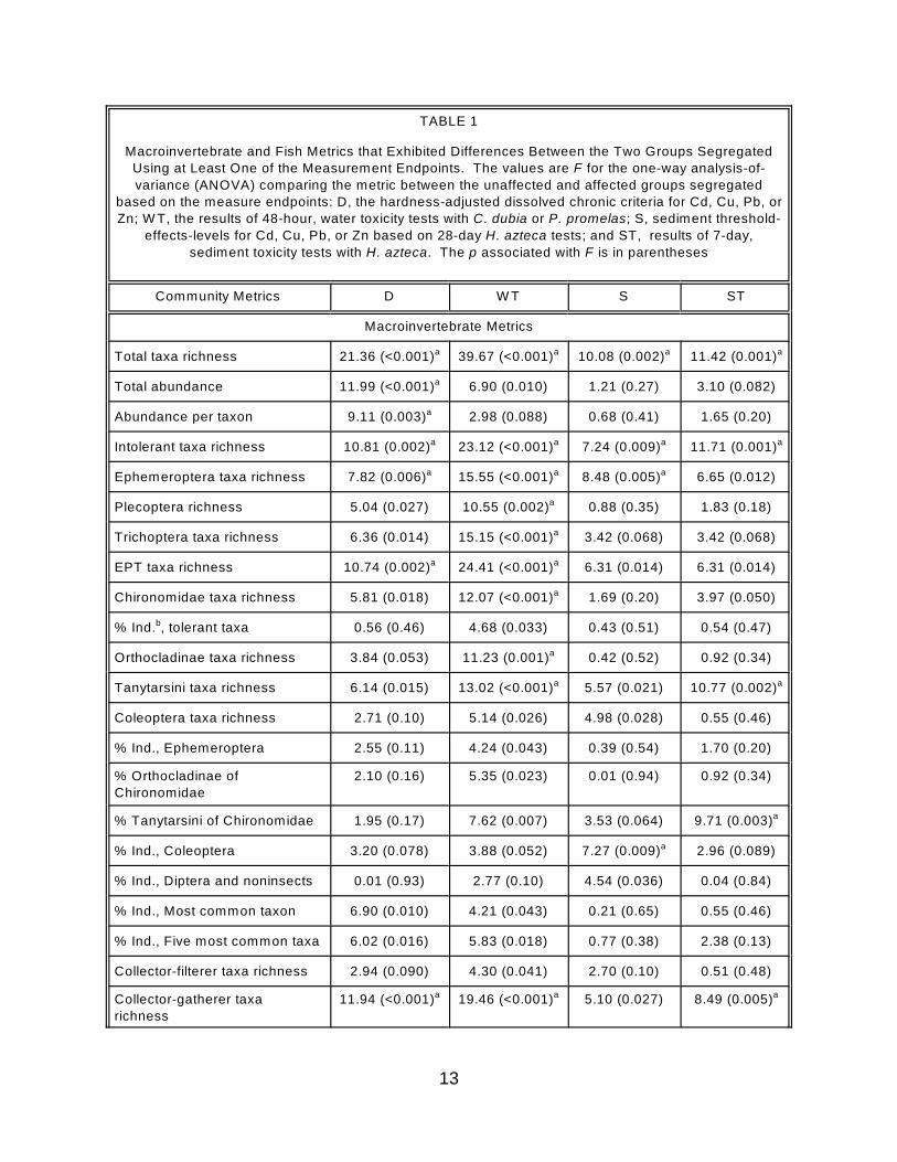
TABLE 1

Macroinvertebrate and Fish Metrics that Exhibited Differences Between the Two Groups Segregated

Using at Least One of the Measurement Endpoints. The values are F for the one-way analysis-of­

variance (ANOVA) comparing the metric between the unaffected and affected groups segregated

based on the measure endpoints: D, the hardness-adjusted dissolved chronic criteria for Cd, Cu, Pb, or

Zn; W T, the results of 48-hour, water toxicity tests with C. dubia or P. promelas; S, sediment threshold-

effects-levels for Cd, Cu, Pb, or Zn based on 28-day H. azteca tests; and ST, results of 7-day,

sediment toxicity tests with H. azteca. The p associated with F is in parentheses

Community Metrics D W T S ST

Macroinvertebrate Metrics

Total taxa richness 21.36 (<0.001) a 39.67 (<0.001) a 10.08 (0.002) a 11.42 (0.001) a

Total abundance 11.99 (<0.001) a 6.90 (0.010) 1.21 (0.27) 3.10 (0.082)

Abundance per taxon 9.11 (0.003) a 2.98 (0.088) 0.68 (0.41) 1.65 (0.20)

Intolerant taxa richness 10.81 (0.002) a 23.12 (<0.001) a 7.24 (0.009) a 11.71 (0.001) a

Ephemeroptera taxa richness 7.82 (0.006) a 15.55 (<0.001) a 8.48 (0.005) a 6.65 (0.012)

Plecoptera richness 5.04 (0.027) 10.55 (0.002) a 0.88 (0.35) 1.83 (0.18)

Trichoptera taxa richness 6.36 (0.014) 15.15 (<0.001) a 3.42 (0.068) 3.42 (0.068)

EPT taxa richness 10.74 (0.002) a 24.41 (<0.001) a 6.31 (0.014) 6.31 (0.014)

Chironomidae taxa richness 5.81 (0.018) 12.07 (<0.001) a 1.69 (0.20) 3.97 (0.050)

% Ind. , tolerant taxa b 0.56 (0.46) 4.68 (0.033) 0.43 (0.51) 0.54 (0.47)

Orthocladinae taxa richness 3.84 (0.053) 11.23 (0.001) a 0.42 (0.52) 0.92 (0.34)

Tanytarsini taxa richness 6.14 (0.015) 13.02 (<0.001) a 5.57 (0.021) 10.77 (0.002) a

Coleoptera taxa richness 2.71 (0.10) 5.14 (0.026) 4.98 (0.028) 0.55 (0.46)

% Ind., Ephemeroptera 2.55 (0.11) 4.24 (0.043) 0.39 (0.54) 1.70 (0.20)

% Orthocladinae of

Chironomidae

2.10 (0.16) 5.35 (0.023) 0.01 (0.94) 0.92 (0.34)

% Tanytarsini of Chironomidae 1.95 (0.17) 7.62 (0.007) 3.53 (0.064) 9.71 (0.003)a

% Ind., Coleoptera 3.20 (0.078) 3.88 (0.052) 7.27 (0.009) a 2.96 (0.089)

% Ind., Diptera and noninsects 0.01 (0.93) 2.77 (0.10) 4.54 (0.036) 0.04 (0.84)

% Ind., Most common taxon 6.90 (0.010) 4.21 (0.043) 0.21 (0.65) 0.55 (0.46)

% Ind., Five most common taxa 6.02 (0.016) 5.83 (0.018) 0.77 (0.38) 2.38 (0.13)

Collector-filterer taxa richness 2.94 (0.090) 4.30 (0.041) 2.70 (0.10) 0.51 (0.48)

Collector-gatherer taxa

richness

11.94 (<0.001) a 19.46 (<0.001) a 5.10 (0.027) 8.49 (0.005) a

13

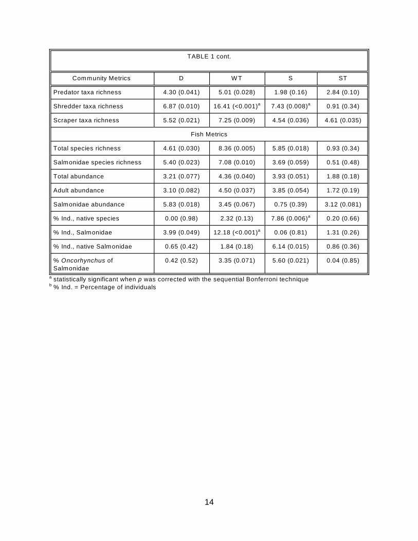
TABLE 1 cont.

Community Metrics D W T S ST

Predator taxa richness 4.30 (0.041) 5.01 (0.028) 1.98 (0.16) 2.84 (0.10)

Shredder taxa richness 6.87 (0.010) 16.41 (<0.001) a 7.43 (0.008) a 0.91 (0.34)

Scraper taxa richness 5.52 (0.021) 7.25 (0.009) 4.54 (0.036) 4.61 (0.035)

Fish Metrics

Total species richness 4.61 (0.030) 8.36 (0.005) 5.85 (0.018) 0.93 (0.34)

Salmonidae species richness 5.40 (0.023) 7.08 (0.010) 3.69 (0.059) 0.51 (0.48)

Total abundance 3.21 (0.077) 4.36 (0.040) 3.93 (0.051) 1.88 (0.18)

Adult abundance 3.10 (0.082) 4.50 (0.037) 3.85 (0.054) 1.72 (0.19)

Salmonidae abundance 5.83 (0.018) 3.45 (0.067) 0.75 (0.39) 3.12 (0.081)

% Ind., native species 0.00 (0.98) 2.32 (0.13) 7.86 (0.006) a 0.20 (0.66)

% Ind., Salmonidae 3.99 (0.049) 12.18 (<0.001) a 0.06 (0.81) 1.31 (0.26)

% Ind., native Salmonidae 0.65 (0.42) 1.84 (0.18) 6.14 (0.015) 0.86 (0.36)

% Oncorhynchus of

Salmonidae

0.42 (0.52) 3.35 (0.071) 5.60 (0.021) 0.04 (0.85)

a statistically significant when p was corrected with the sequential Bonferroni technique b % Ind. = Percentage of individuals

14

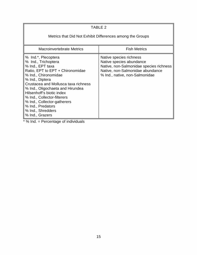
TABLE 2

Metrics that Did Not Exhibit Differences among the Groups

Macroinvertebrate Metrics Fish Metrics

% Ind.*, Plecoptera % Ind., Trichoptera % Ind., EPT taxa Ratio, EPT to EPT + Chironomidae % Ind., Chironomidae % Ind., Diptera Crustacea and Mollusca taxa richness % Ind., Oligochaeta and Hirundea Hilsenhoff’s biotic index % Ind., Collector-filterers % Ind., Collector-gatherers % Ind., Predators % Ind., Shredders % Ind., Grazers

Native species richness Native species abundance Native, non-Salmonidae species richness Native, non-Salmonidae abundance % Ind., native, non-Salmonidae

* % Ind. = Percentage of individuals

15

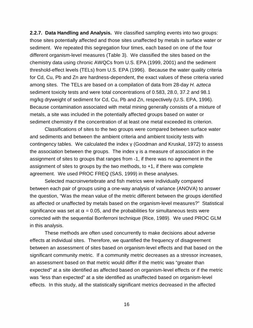
2.2.7. Data Handling and Analysis. We classified sampling events into two groups:

those sites potentially affected and those sites unaffected by metals in surface water or

sediment. We repeated this segregation four times, each based on one of the four

different organism-level measures (Table 3). We classified the sites based on the

chemistry data using chronic AWQCs from U.S. EPA (1999, 2001) and the sediment

threshold-effect levels (TELs) from U.S. EPA (1996). Because the water quality criteria

for Cd, Cu, Pb and Zn are hardness-dependent, the exact values of these criteria varied

among sites. The TELs are based on a compilation of data from 28-day H. azteca

sediment toxicity tests and were total concentrations of 0.583, 28.0, 37.2 and 98.1

mg/kg dryweight of sediment for Cd, Cu, Pb and Zn, respectively (U.S. EPA, 1996).

Because contamination associated with metal mining generally consists of a mixture of

metals, a site was included in the potentially affected groups based on water or

sediment chemistry if the concentration of at least one metal exceeded its criterion.

Classifications of sites to the two groups were compared between surface water

and sediments and between the ambient criteria and ambient toxicity tests with

contingency tables. We calculated the index ( (Goodman and Kruskal, 1972) to assess

the association between the groups. The index ( is a measure of association in the

assignment of sites to groups that ranges from -1, if there was no agreement in the

assignment of sites to groups by the two methods, to +1, if there was complete

agreement. We used PROC FREQ (SAS, 1999) in these analyses.

Selected macroinvertebrate and fish metrics were individually compared

between each pair of groups using a one-way analysis of variance (ANOVA) to answer

the question, “Was the mean value of the metric different between the groups identified

as affected or unaffected by metals based on the organism-level measures?” Statistical

significance was set at " = 0.05, and the probabilities for simultaneous tests were

corrected with the sequential Bonferroni technique (Rice, 1989). We used PROC GLM

in this analysis.

These methods are often used concurrently to make decisions about adverse

effects at individual sites. Therefore, we quantified the frequency of disagreement

between an assessment of sites based on organism-level effects and that based on the

significant community metric. If a community metric decreases as a stressor increases,

an assessment based on that metric would differ if the metric was “greater than

expected” at a site identified as affected based on organism-level effects or if the metric

was “less than expected” at a site identified as unaffected based on organism-level

effects. In this study, all the statistically significant metrics decreased in the affected

16

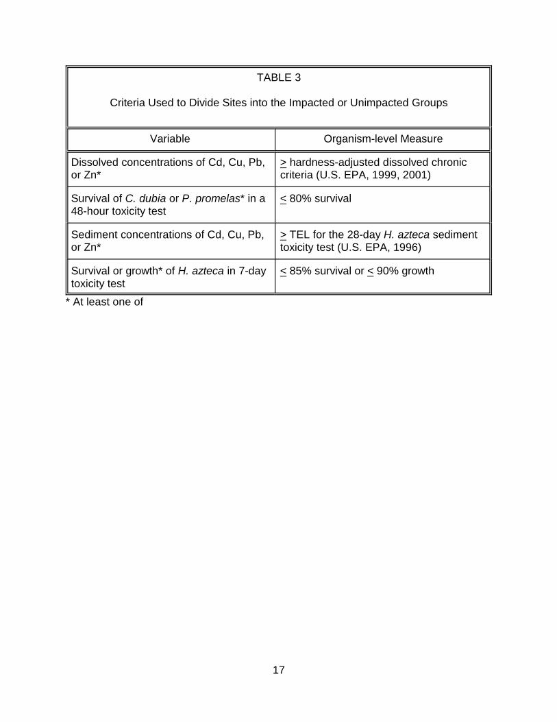
TABLE 3

Criteria Used to Divide Sites into the Impacted or Unimpacted Groups

Variable Organism-level Measure

Dissolved concentrations of Cd, Cu, Pb, or Zn*

> hardness-adjusted dissolved chronic criteria (U.S. EPA, 1999, 2001)

Survival of C. dubia or P. promelas* in a 48-hour toxicity test

< 80% survival

Sediment concentrations of Cd, Cu, Pb, or Zn*

> TEL for the 28-day H. azteca sediment toxicity test (U.S. EPA, 1996)

Survival or growth* of H. azteca in 7-day toxicity test

< 85% survival or < 90% growth

* At least one of

17

group, and we defined community metrics as “greater than expected” when the metrics

were greater than the 95% upper confidence limit (UCL) of an affected group and as

“less than expected” when the metrics were less than the 95% lower confidence limit

(LCL) of the unaffected group as calculated in the one-way ANOVA. We used PROC

MEANS (SAS, 1999) to calculate the 95% UCL and LCL.

We used piecewise or segmented regression (Toms and Lesperance, 2003)

further to explore the relationships between the significant metrics and the

concentrations of Cd, Cu, Pb and Zn in surface water or sediments relative to the

organism-level-based criteria. Piecewise regression is an approach to modeling data

where the regression changes at one or more points, called join points, along the range

of the independent variable (Bellman and Roth, 1969). If the criteria or effects-level

values (i.e., the chronic AWQC for surface water or the TEL for sediments) represent

threshold concentrations for effects at the community level as measured by the metrics,

then "1 or $1 should be significantly less than 0 in the piecewise regression model,

(Eq. 1)

where:

x1 = a dummy variable with a value of 1 if at least one metal exceeded its criterion or sediment-effects concentration and a value of 0 otherwise

x2 = the summation of the ratios of the concentration of each metal to its criterion or sediment-effects concentration

y = the metric value.

By designing the analysis in this way, the model is reduced to

(Eq. 2)

when no metals exceed their criteria or sediment-effects concentration because "1 x1 =

0 and $1 x1 loge x2 = 0. The coefficients, "1 and $1, then are the changes in the intercept

and slope of the regression when at least one metal exceeds its criterion or sediment-

effects concentration. We used PROC GLM (SAS, 1999) in these regression analyses.

This approach, using the summed ratios of the concentration of each metal to its

criterion or sediment-effects concentration as the continuous independent variable,

assumed that the effects of the four metals were concentration additive and that the

criteria or sediment-effects concentrations represent their common mechanism and

threshold level of effect. The criteria do not account for possible synergistic or

antagonistic effects among these metals (U.S. EPA, 2000b).

18

2.3. RESULTS AND DISCUSSION

Because data were not complete for some sites (i.e., some sites lacked fish

data, chemistry data or toxicity data), macroinvertebrate metrics could be compared for

83 to 85 sites depending on the organism-level measurement endpoint. Fish metrics

could be compared for 76 to 78 sites.

2.3.1. Organism-level Measures. Using either metal concentrations or ambient

toxicity tests, we identified more sites as affected by sediment contamination than by

surface water contamination because there were more sites where metal

concentrations or ambient toxicity tests indicated sediments were toxic whereas surface

water was not than sites showing the reverse (Table 4). The association among

groups, (, was +0.89 between assessments based on water or sediment metal

concentrations and +0.83 for those based on water or sediment toxicity tests.

As described in the literature on the hydrogeochemistry of the mine drainage that

results in this metal contamination (Chapman et al., 1983; Filipek et al., 1987), metal

concentrations in water are greatest closer to the mine source, but decrease as metal

solubility changes in relation to pH and other factors. Metal concentrations in

sediments increase downstream of the mine source within the zone where the metals

are deposited. Although pH data for these sites were considered invalid, dissolved

organic carbon ranged from less than a detection limit of 1.0 mg/L to 10.8 mg/L.

Therefore, we would expect some sites to have elevated concentrations of these metals

in sediment but not water. Also, the tests of sediment measure incrementally more

sensitive endpoints than those for water (i.e., survival and growth versus just survival).

Comparing metal concentrations versus ambient toxicity tests, more sites were

identified as affected based on metal concentrations than on ambient toxicity tests

(Table 5), because metal concentrations indicated surface water or sediments were

toxic whereas ambient toxicity tests did not indicate toxicity at more sites than in the

reverse where ambient toxicity tests indicated toxicity although criteria did not. The

association among groups, (, was greater for the assessments based on water (( =

+0.98) than those based on sediment (( = +0.73). The mean summed ratios of the

dissolved concentrations of the four metals to their chronic AWQCs and the mean

summed ratios of the sediment concentrations of the four metals to their TELs were

greater at sites classified as affected by the ambient toxicity tests for water and

sediment, respectively (Figure 2). However, these two measures agreed in their

classification of a site at only 53% of the 19 sites identified as affected by at least one

19

TABLE 4

Correspondence of Conclusions of Assessments for Surface Water and Sediment for Sampling Events

Were water criteria exceeded? Criteria (( = +0.89)

No Yes Total

No 53 3 56

Were sediment TELs exceeded? Yes 15 15 30

Total 68 18 n = 86

Did water ambient toxicity tests show effects? Ambient toxicity tests (( = +0.83)

No Yes Total

No 63 4 67

Did sediment ambient toxicity tests Yes 10 7 17

show effects?

Total 73 11 n = 84

20

TABLE 5

Correspondence of Conclusions of Assessments Based on Chemical Criteria and Ambient Toxicity Tests for Sampling Events

Were metal AWQC exceeded? Water (( = +0.98)

No Yes Total

No 65 8 73

Did water toxicity tests show effects?

Yes 1 10 11

Total 66 18 n = 84

Were metal sediment TELs exceeded? Sediment (( = +0.73)

No Yes Totals

No 49 18 67

Did sediment toxicity tests show Yes 5 12 17

effects?

Totals 54 30 n = 84

21

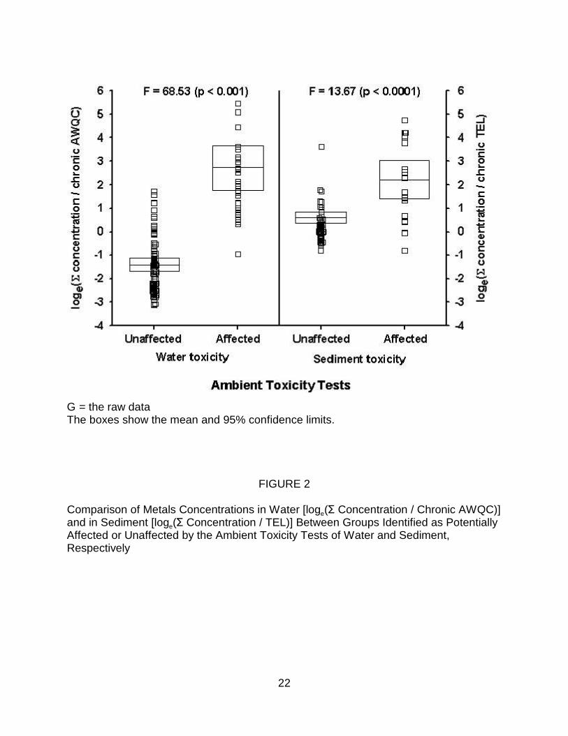
G = the raw dataThe boxes show the mean and 95% confidence limits.

FIGURE 2

Comparison of Metals Concentrations in Water [log (E Concentration / Chronic AWQC)] e

and in Sediment [log (E Concentration / TEL)] Between Groups Identified as Potentially e

Affected or Unaffected by the Ambient Toxicity Tests of Water and Sediment, Respectively

22

measure for water and only 34% of the 35 sites identified as affected by at least one

measure for sediment.

2.3.2. Organism-level Measures versus Community Metrics. When each metric

was compared between pairs of groups segregated using the organism-level measures

using a one-way ANOVA, a number of macroinvertebrate metrics exhibited significant

differences between at least one pair of groups segregated using the organism-level

measures (Table 1), whereas other metrics did not exhibit significant differences

between any pairs of groups (Table 2). To be conservative, we will concentrate on

those metrics for which F was statistically significant when p was corrected with the

sequential Bonferroni technique. The metrics listed in Table 1 with the greatest F

values from the one-way ANOVA are generally richness metrics: total taxa richness

[AWQC - F = 21.36 (p<0.001 < adjusted p=0.050), water toxicity test - F = 39.67

(p<0.001 < adjusted p=0.050), sediment TEL - F = 10.08 ( p=0.002 < adjusted

p=0.050), sediment toxicity test - F = 11.42 (p=0.001 < adjusted p=0.050)],

Ephemeroptera, Plecoptera and Trichoptera (EPT) taxa richness [AWQC - F = 10.74

(p=0.002 < adjusted p=0.010), water toxicity test - F = 24.41 (p<0.001 < adjusted

p=0.025)], Tanytarsini taxa richness [water toxicity tests - F = 13.02 (p<0.001 < adjusted

p=0.006), sediment toxicity tests - F = 10.77 (p=0.002 < adjusted p=0.017)], intolerant

taxa richness [AWQC - F = 10.81 (p=0.002 < adjusted p=0.013), water toxicity test - F =

23.12 (p<0.001 < adjusted p=0.016), sediment toxicity test - F = 11.71 (p=0.001 <

adjusted p=0.050)], and collector-gatherer richness [AWQC - F = 11.94 (p<0.001 <

adjusted p=0.017), water toxicity test - F = 19.46 (p<0.001 < adjusted p=0.013),

sediment toxicity test - F = 8.49 (p=0.005 < adjusted p=0.010)], for macroinvertebrates

(Figures 3 and 4). An exception is the total number of individuals [AWQC - F = 11.99

(p=0.001 < adjusted p = 0.025)] for macroinvertebrates (Figure 4), which is an

abundance metric. The metrics that exhibited significant differences between pairs of

groups and are listed in Table 1 are relatively sensitive to the stressor gradient

represented by metals contamination, whereas the metrics listed in Table 2 are

insensitive to this gradient. Similar metrics were identified for being sensitive to this

gradient by multivariate analyses in Griffith et al. (2001).

This sensitivity of richness metrics to metal contamination is consistent with an

assumption that effects at the organism and population levels are the basis of effects

observed at the community level. Persistent toxicants, such as metals, increase

mortality and decrease growth and reproduction of individuals within an exposed

population. These are organism-level effects that result in reduced abundances at the

23

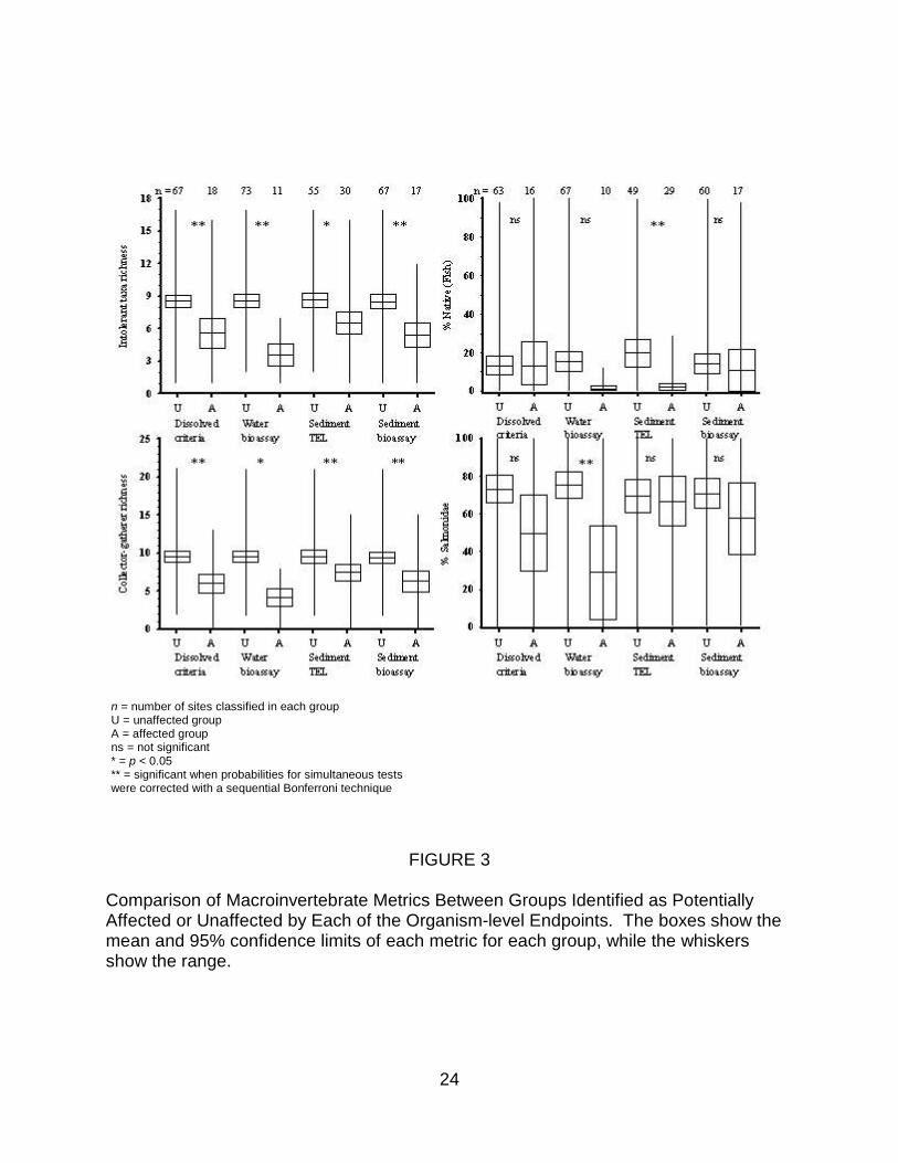
n = number of sites classified in each groupU = unaffected groupA = affected groupns = not significant* = p < 0.05** = significant when probabilities for simultaneous testswere corrected with a sequential Bonferroni technique

FIGURE 3

Comparison of Macroinvertebrate Metrics Between Groups Identified as Potentially Affected or Unaffected by Each of the Organism-level Endpoints. The boxes show the mean and 95% confidence limits of each metric for each group, while the whiskers show the range.

24

n = number of sites classified in each group U = unaffected group A = affected group ns = not significant * = p < 0.05 ** = significant when probabilities for simultaneous tests were corrected with a sequential Bonferroni technique

FIGURE 4

Comparison of Macroinvertebrate and Fish Metrics Between Groups Identified as Potentially Affected or Unaffected by Each of the Organism-level Endpoints. The boxes show the mean and 95% confidence limits of each metric for each group, while the whiskers show the range.

25

population level (Kuhn et al., 2000). At some threshold, population recruitment fails,

and more sensitive species will be eliminated from the community (Sheehan, 1984).

Because the threshold concentrations at which different species are affected vary, more

of the species in a community would be affected with increasing toxicant

concentrations, and taxa richness would decrease (Barnthouse et al., 1986). The

insensitivity of various composition metrics suggests no concomitant increase in more

tolerant species, which could adapt or acclimatize themselves to these toxicants,

occurred in compensation for the eliminated species (Vinebrooke et al., 2003). Such

population effects would also be the basis of the observed decrease in the total number

of individuals collected. We did not test other abundance metrics for

macroinvertebrates because such metrics are not normally used in bioassessments.

Abundance metrics require quantitative samples, and many states and other entities

collect only qualitative samples as part of bioassessments (Barbour et al., 1999).

However, this R-EMAP study collected semi-quantitative samples.

Fish metrics were less sensitive to the metal contamination. Only two

composition metrics were significantly different between one pair of groups (Table 1,

Figure 4): % individuals that were native species [sediment TEL - F = 7.86 (p=0.006 <

adjusted p=0.017) and % individuals that were Salmonidae [water toxicity test - F =

12.18 (p<0.001 < adjusted p=0.006)]. However, this lack of sensitivity by the fish

metrics might be a result of the low diversity of the fish assemblage in these cold-water

streams. Maximum total fish species or subspecies richness in these streams was six,

and maximum native fish species or subspecies richness was four. In streams with

fish, a mean of 83% of the fish were Salmonidae, and a mean of 97% of the

Salmonidae were not native species or subspecies.

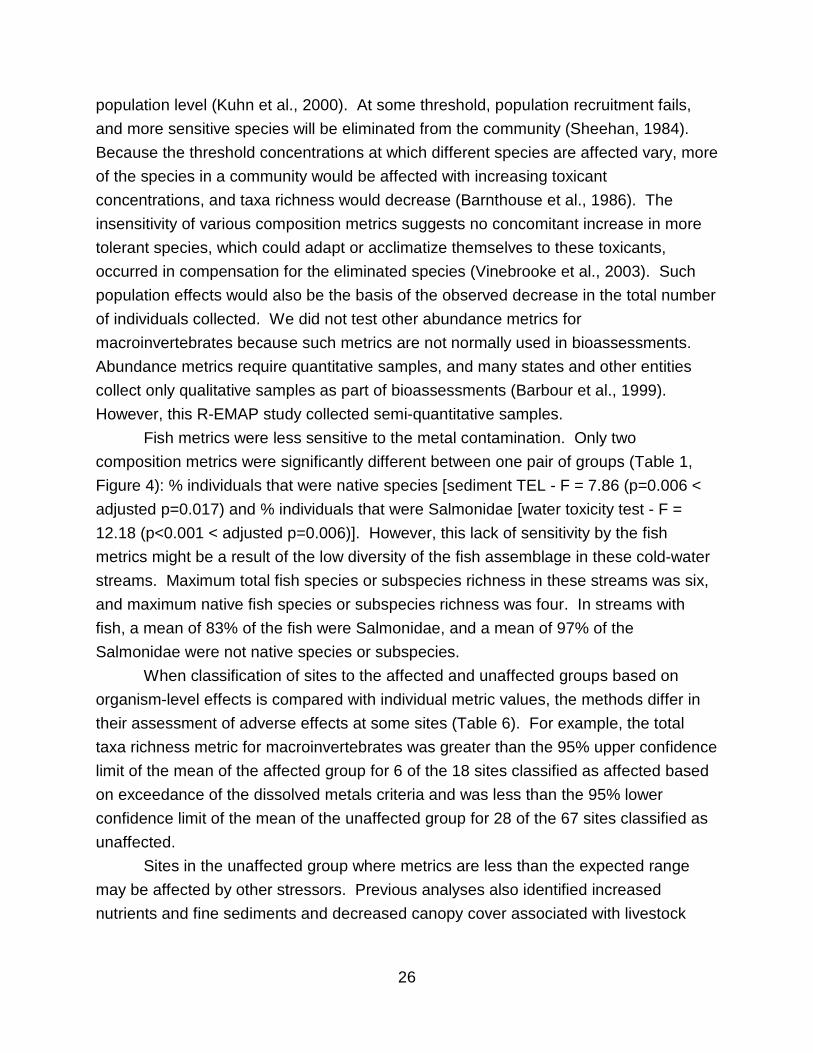
When classification of sites to the affected and unaffected groups based on

organism-level effects is compared with individual metric values, the methods differ in

their assessment of adverse effects at some sites (Table 6). For example, the total

taxa richness metric for macroinvertebrates was greater than the 95% upper confidence

limit of the mean of the affected group for 6 of the 18 sites classified as affected based

on exceedance of the dissolved metals criteria and was less than the 95% lower

confidence limit of the mean of the unaffected group for 28 of the 67 sites classified as

unaffected.

Sites in the unaffected group where metrics are less than the expected range

may be affected by other stressors. Previous analyses also identified increased

nutrients and fine sediments and decreased canopy cover associated with livestock

26

TABLE 6

Enumeration of Sampling Events in Wadeable Streams in the Southern Rockies Ecoregion of Colorado Where Classification Based on the Organism-level Measures

and that Based on the Community Metric Disagree

Metric

Number of Sampling Events*

Classified as

Unaffected

Metric <95% LCL for

Unaffected Group

Classified as

Affected

Metric >95% UCL for Affected

Group

Dissolved Chronic Criteria

Total taxa richness (macroinvertebrates)

67 28 18 6

Total number of individuals 67 36 18 1

Number, Individuals per taxon 67 32 18 3

Intolerant taxa richness 67 23 18 5

Ephemeroptera taxa richness 67 22 18 7

EPT taxa richness 67 20 18 4

Collector-gatherer taxa richness 67 30 18 6

Water Toxicity Tests

Total taxa richness (macroinvertebrates)

73 29 11 3

Intolerant taxa richness 73 25 11 2

Ephemeroptera taxa richness 73 24 11 2

Plecoptera taxa richness 73 28 11 3

Trichoptera taxa richness 73 29 11 4

EPT taxa richness 73 25 11 4

Chironomidae taxa richness 73 32 11 3

Orthocladinae taxa richness 73 31 11 3

27

TABLE 6 cont.

Metric

Number of Sampling Events

Classified as

Unaffected

Metric <95% LCL for

Unaffected Group

Classified as

Affected

Metric >95% UCL for Affected

Group

Tanytarsini taxa richness 73 27 11 3

Collector-gatherer taxa richness 73 33 11 4

Shredder taxa richness 73 40 11 1

% Individuals, Salmonidae 67 25 11 3

Sediment Threshold Effects Levels

Total taxa richness (macroinvertebrates)

55 21 30 13

Ephemeroptera taxa richness 55 25 30 9

% Coleoptera 55 28 30 9

Shredder taxa richness 55 30 30 8

% Individuals, native species 49 39 29 0

Sediment Toxicity Tests

Total taxa richness (macroinvertebrates)

67 26 17 7

Intolerant taxa richness 67 22 17 6

Tanytarsini taxa richness 67 23 17 4

% Tanytarsini of Chironomidae 67 33 17 2

Collector-gatherer taxa richness 67 33 17 5

* The total number sampling events is the sum of the columns labeled “Classified as unaffected” and “Classified as affected.”

28

grazing in riparian zones as another stressor gradient in these Rocky Mountain streams

(Griffith et al., 2001). Also, because most sites were only sampled once, we do not

know the temporal variability of metal concentrations in these streams, and these single

measurements may underestimate exposure of fish or macroinvertebrates to metals in

some streams.

At sites in the affected group where metrics were greater than the expected

range, exposure to metals in surface water and sediments may differ from that

measured, in part because of unaccounted for effects on metal bioavailability. In

surface water, factors, such as dissolved organic carbon, pH, or other cations besides

water hardness, may also affect metal bioavailability (Di Toro et al., 2001), but U.S.

EPA water quality criteria are currently only adjusted for water hardness. The TELs

were derived from analyses of laboratory bioassay data (U.S. EPA, 1996) that did not

consider possible factors affecting metal bioavailability in sediments (Chapman et al.,

1999). Acid volatile sulfide (AVS) can affect the bioavailability of metals in sediments

(Liber et al., 1997). However, AVS was not measured in this study, and significant

concentrations of AVS are unlikely to occur in the coarse, well-aerated sediments of

these shallow, high-gradient streams. Including these additional factors that affect

metal bioavailability in models used to adjust the criteria or other guidelines may be

appropriate.

The differences in assignment of sites to affected and unaffected groups based

on criteria or sediment-effects concentrations versus ambient toxicity tests likely also

result from the direct assessment of bioavailability by the ambient toxicity tests.

However, there is also a difference in duration between the organism-level endpoints

for the chemical criteria and ambient toxicity tests. The criteria we used for surface

water are chronic criteria, whereas the ambient toxicity tests would be considered acute

in duration. Chronic effects are expected at lower concentrations of toxicants than

acute effects, and chronic effects would be reflected by the community metrics.

2.3.3. Piecewise Regression Analyses. Metal contamination associated with hard-

rock metal mining is a complex impact on streams. In the mineralized zone of the

Southern Rockies Ecoregion, the contamination is a mixture of primarily four metals,

Cd, Cu, Pb and Zn, that changes as surface water chemistry changes downstream from

the mine source (Chapman et al., 1983). To simplify our analyses, we assumed a

potential impact if one or more of the concentrations of these four metals in surface

water exceeded their hardness-adjusted criteria or in sediments exceeded their TEL.

Therefore, the affected group includes a continuum of sites from those in which one

29

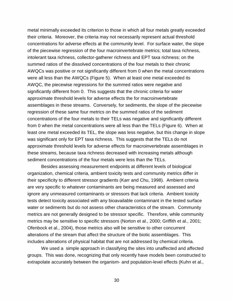
metal minimally exceeded its criterion to those in which all four metals greatly exceeded

their criteria. Moreover, the criteria may not necessarily represent actual threshold

concentrations for adverse effects at the community level. For surface water, the slope

of the piecewise regression of the four macroinvertebrate metrics; total taxa richness,

intolerant taxa richness, collector-gatherer richness and EPT taxa richness; on the

summed ratios of the dissolved concentrations of the four metals to their chronic

AWQCs was positive or not significantly different from 0 when the metal concentrations

were all less than the AWQCs (Figure 5). When at least one metal exceeded its

AWQC, the piecewise regressions for the summed ratios were negative and

significantly different from 0. This suggests that the chronic criteria for water

approximate threshold levels for adverse effects the for macroinvertebrate

assemblages in these streams. Conversely, for sediments, the slope of the piecewise

regression of these same four metrics on the summed ratios of the sediment

concentrations of the four metals to their TELs was negative and significantly different

from 0 when the metal concentrations were all less than the TELs (Figure 6). When at

least one metal exceeded its TEL, the slope was less negative, but this change in slope

was significant only for EPT taxa richness. This suggests that the TELs do not

approximate threshold levels for adverse effects for macroinvertebrate assemblages in

these streams, because taxa richness decreased with increasing metals although

sediment concentrations of the four metals were less than the TELs.

Besides assessing measurement endpoints at different levels of biological

organization, chemical criteria, ambient toxicity tests and community metrics differ in

their specificity to different stressor gradients (Karr and Chu, 1998). Ambient criteria

are very specific to whatever contaminants are being measured and assessed and

ignore any unmeasured contaminants or stressors that lack criteria. Ambient toxicity

tests detect toxicity associated with any bioavailable contaminant in the tested surface

water or sediments but do not assess other characteristics of the stream. Community

metrics are not generally designed to be stressor specific. Therefore, while community

metrics may be sensitive to specific stressors (Norton et al., 2000; Griffith et al., 2001;

Ofenbock et al., 2004), those metrics also will be sensitive to other concurrent

alterations of the stream that affect the structure of the biotic assemblages. This

includes alterations of physical habitat that are not addressed by chemical criteria.

We used a simple approach in classifying the sites into unaffected and affected

groups. This was done, recognizing that only recently have models been constructed to

extrapolate accurately between the organism- and population-level effects (Kuhn et al.,

30

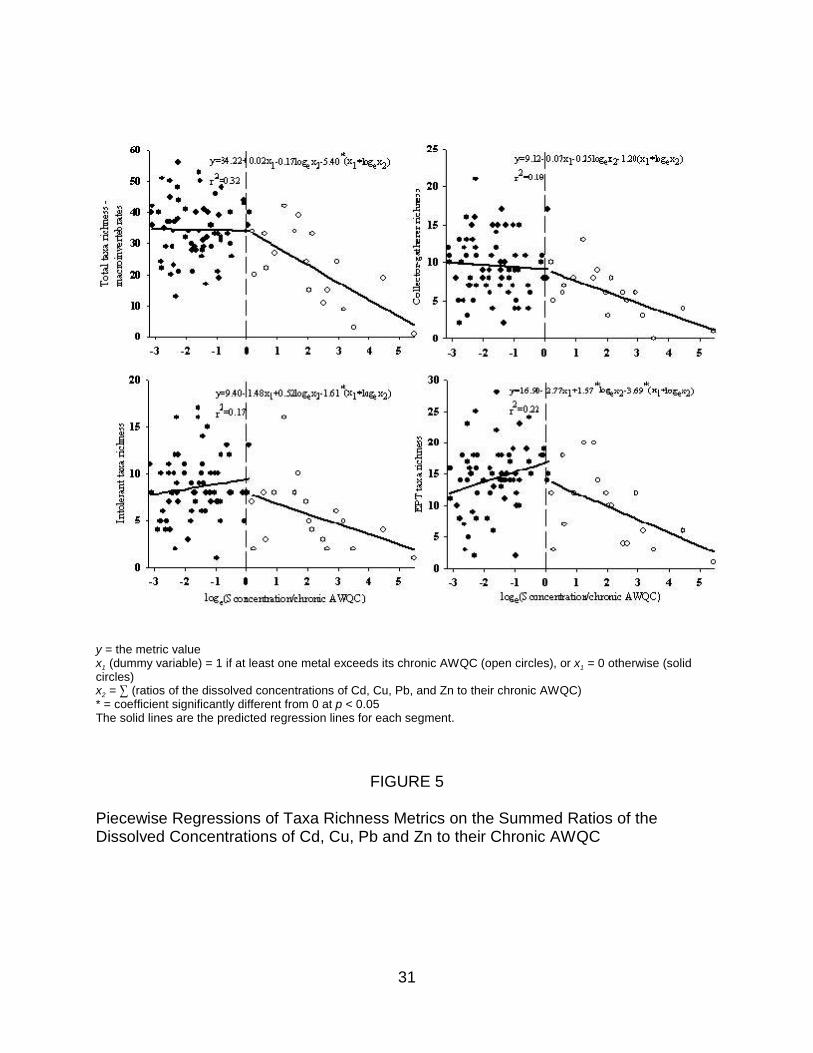
y = the metric valuex1 (dummy variable) = 1 if at least one metal exceeds its chronic AWQC (open circles), or x1 = 0 otherwise (solidcircles)x2 = 3 (ratios of the dissolved concentrations of Cd, Cu, Pb, and Zn to their chronic AWQC)* = coefficient significantly different from 0 at p < 0.05The solid lines are the predicted regression lines for each segment.

FIGURE 5

Piecewise Regressions of Taxa Richness Metrics on the Summed Ratios of the Dissolved Concentrations of Cd, Cu, Pb and Zn to their Chronic AWQC

31

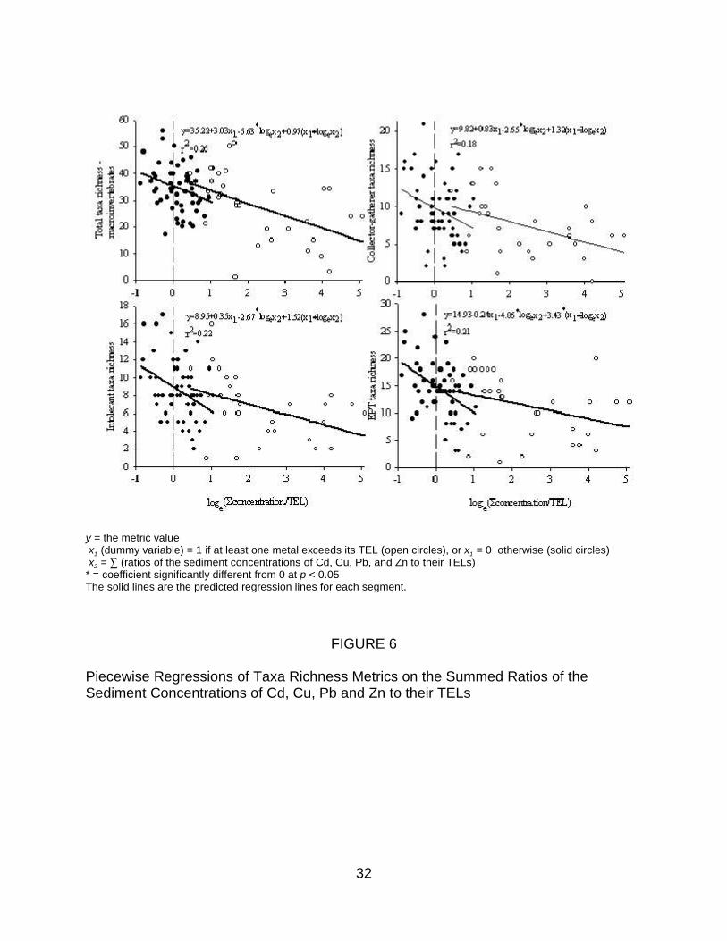
y = the metric value x1 (dummy variable) = 1 if at least one metal exceeds its TEL (open circles), or x1 = 0 otherwise (solid circles) x2 = 3 (ratios of the sediment concentrations of Cd, Cu, Pb, and Zn to their TELs)

* = coefficient significantly different from 0 at p < 0.05The solid lines are the predicted regression lines for each segment.

FIGURE 6

Piecewise Regressions of Taxa Richness Metrics on the Summed Ratios of the Sediment Concentrations of Cd, Cu, Pb and Zn to their TELs

32

2000), and we still cannot accurately model or extrapolate between population and

community effects because of the difficulties of incorporating variation in exposure and

response across the hierarchical levels of time, space and organization (de Kruijf, 1991;

Karr and Chu, 1998). Considering this simple classification, one might expect few, if

any, of the metrics would have exhibited differences in their means between the two

groups. However, a number of metrics, particularly richness metrics, exhibited

differences between the groups although the conclusions based on the organism-level

measures and on community metrics disagreed at some sites. This would suggest that

a relationship exists between the organism-level effects assessed by ambient criteria or

guidelines or ambient toxicity tests and the community-level effects assessed by

community metrics. However, the organism-level effects are only predictive to a limited

extent of the community-level effects at individual sites, because this predictability is

affected by differences among the methods that go beyond the hierarchical levels of

biological organization used as their measurement endpoints. We need to assess the

generality of these relationships for other contaminants besides metals.

33

3. ESTUARINE SYSTEMS IN THE VIRGINIAN PROVINCE OF THE ATLANTIC COAST

3.1. INTRODUCTION

In this chapter, we compare and contrast statistically the results of three different

methods used by the U.S. EPA for the ecological assessment of contaminant exposure

and effects in sediments in estuarine ecosystems: (1) chemical guidelines, (2) ambient

toxicity assessments, and (3) bioassessments of benthic invertebrates to determine the

relationships among the levels of biological organization assessed by each method.

We also assess the extent to which organism-level effects predict effects at the

community level. Through these comparisons, we expected to assess the relationships

among the levels of biological organization protected by the different methods and

assess the extent to which organism-level effects are predictive of effects at the

community level. In this paper, this approach is applied to the effects of sediment

contamination in estuaries of the Virginian Province of the Atlantic coast of the United

States. Contaminants in these sediments were expected to be metals, polyaromatic

hydrocarbons (PAHs), some pesticides and polychlorinated biphenyl (PCB) congeners.

3.2. MATERIALS AND METHODS

3.2.1. Study Area and Survey Design. The Virginian Province of the United States

includes estuarine habitats along the Atlantic coast extending from Cape Henry, Virginia

to Cape Cod, Massachusetts. In the following tables, we present data compiled from

U.S. EPA’s EMAP surveys conducted from 1990 to 1993. As part of these surveys,

sampling sites were selected in a stratified, random manner within each of three

classes of estuaries based on size: large estuaries, large tidal rivers and small estuaries

or tidal rivers (Strobel et al., 1999). In the Virginian Province, this sampling approach

identified 12 large estuaries, five large tidal rivers and 144 small estuaries or tidal rivers.

Additional sites were selected non-randomly in areas for which there was prior

knowledge of ambient environmental conditions that represent areas with likely

anthropogenic disturbance. Some sites were revisited during a subsequent year to

assess variability among years, but data from only one visit to a site were considered in

these analyses. Nevertheless, some sites lacked data for one or more of the

measurements, such as chemistry, toxicity tests or benthic invertebrates.

Sites were sampled from July to September each year. This index period was

selected as the period of the year when biotic responses to potential anthropogenic and

natural stressors were anticipated to be most pronounced (Strobel et al., 1995).

34

3.2.2. Field and Laboratory Methods. Field methods for the Virginian Province

surveys are fully documented in Reifsteck et al. (1993), and laboratory methods are

documented in U.S. EPA (1995). These methods are summarized briefly below.

At each station, salinity (‰), temperature (°C), and dissolved oxygen (DO, mg/L)

were recorded with a model SBE-25 Sealogger conductivity-temperature-depth profiler

(Sea-Bird Electronics, Inc., Bellevue, WA).

At each station, generally three replicate grab samples were collected with a

0.044-m2 Young-modified Van Veen grab (Theodore E. Young, Sandwich, MA) and

processed for benthos (i.e., at two sites, only two replicate grab samples were collected

and processed). Samples were sieved in the field with a 0.5-mm mesh screen.

Material retained on the screen was preserved in 10% buffered formalin with rose

bengal. In the laboratory, samples were sorted. Organisms were counted, weighed,

and identified to the lowest possible taxonomic level, usually species (Strobel et al.,

1995).

Additional grab samples were collected at each site, and the top two cm of

sediment was composited for analysis of percent silt-clay, contaminant concentrations

and sediment toxicity (Strobel et al., 1995). Percent silt-clay was the portion of

sediment passing through a 63-:m screen.

3.2.3. Sediment Contaminant Concentrations. Subsamples of the composited

sediments were analyzed for organic and metal contaminants. Analysis of organics

involved Soxhlet extraction and extract drying with NaSO , concentration with a 4

Kuderna-Danish apparatus and cleanup with activated Cu for elemental S and gel

permeation chromatograph or alumina for organic interferents (Paul et al., 1999). PAHs

were analyzed with gas chromatography/mass spectrometry. Pesticides and PCB

congeners were analyzed with gas chromatography/electron capture detection

confirmed by a second column. For Ag, Al, Cr, Cu, Fe, Mn, Ni, Pb and Zn, sediments

were digested with HF and HNO3 on a hot plate followed by analysis with inductively-

coupled plasma, atomic emission spectrometry. For As, Cd, Sb, Se and Sn, sediments

were digested with HNO and HCl in a microwave oven followed by analysis with a 3

Zeeman-corrected, stabilized-temperature graphite furnace atomic absorption

spectrometry (Paul et al., 1999). Hg was analyzed by cold-vapor atomic absorption

spectrometry.

3.2.4. Ambient Toxicity Tests. Other subsamples of the composited sediments were

used in ambient toxicity tests. Standard, acute, 10-day static tests (U.S. EPA, 1995;

Strobel et al., 1999) were conducted with juvenile Ampelisca abdita. Prior to testing,

35

the amphipods were acclimated at 20°C for at least 48 hours. During testing, the

amphipods were not fed. For each sediment tested, five glass test chambers were

filled with 200 mL of sediment and 600 mL of seawater with salinity of 30 ‰. The

chambers were illuminated constantly to inhibit amphipod emergence from the

sediment and maximize exposure. The water was aerated to maintain dissolved

oxygen concentrations >90% saturation. Temperature of the overlying water was

maintained at 20+1°C. Dead animals were counted and removed daily, and at the end

of the test, the sediments were sieved through a 0.5-mm screen and live amphipods

were collected and counted. Any amphipods, which were not accounted for, were

presumed to have died during the test. Negative controls with an uncontaminated

sediment were run with each set of field samples, and 85% survival in the negative

control was required for a test to be valid. Also, a water-only test with a reference

toxicant, CdCl or C H SO Na (sodium dodecyl sulfate), was used to evaluate the 2 12 25 4

condition of the amphipods. The measurement endpoint for these bioassays was

percent survival. These test bioassays indicated toxicity if survival was statistically

different from (" = 0.05) and <80% of survival the corresponding negative control

bioassays (Thursby et al., 1997; Strobel et al., 1999).

3.2.5. Calculation of Community Metrics. We used the benthos data to calculate

various community metrics (Tables 7 and 8), identified as indicative of community

integrity in the literature (Fauchald and Jumars, 1979; Engle et al., 1994; Weisberg et

al., 1997; van Dolah et al., 1999; Olsgard et al., 2003). Richness metrics are the

number of taxa identified in a sample within the specified group (e.g., total taxa

richness, Polychaeta species richness). Abundance metrics are the number of

individuals found in a sample within the specified group (e.g., total abundance, Spionida

abundance), while total biomass in the dry weight of organisms in a sample.

Composition metrics are the abundance of individuals in the specified taxonomic group

divided by total abundance or by the specified larger group (e.g., Polychaeta) and

expressed as a percentage (e.g., % individuals that were Mollusca, % Polychaeta that

were Spionida). Evenness metrics are either total abundance, the abundance of the

specified group, or biomass divided by total taxa richness (e.g., abundance per taxon,

biomass per taxon) or the abundance of the two most common taxa divided by total

abundance and expressed as a percentage (e.g., % individuals in the two most

common taxa). Trophic or habitat guild metrics can quantify taxa richness of a

particular trophic or habitat guild (e.g., Polychaeta omnivore species richness, Infaunal

taxa richness)or the abundance of individuals in the trophic or habitat guild divided by

36

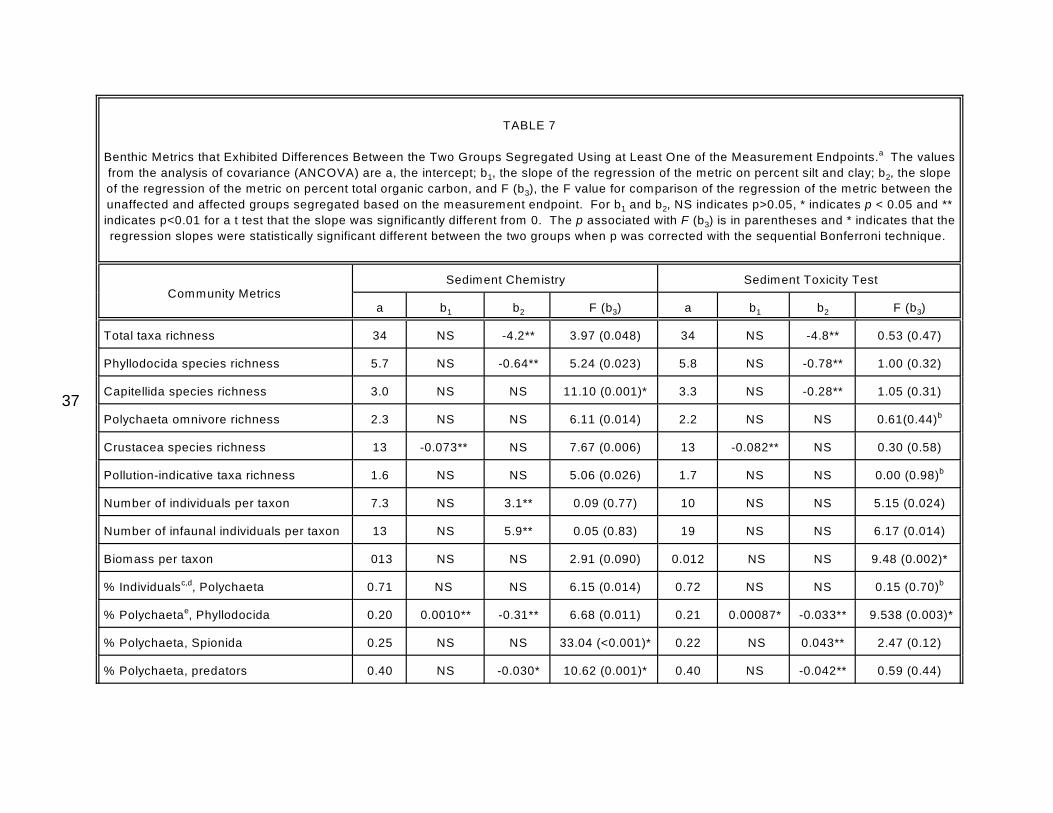
37

TABLE 7

Benthic Metrics that Exhibited Differences Between the Two Groups Segregated Using at Least One of the Measurement Endpoints. The values a

1 2from the analysis of covariance (ANCOVA) are a, the intercept; b , the slope of the regression of the metric on percent silt and clay; b , the slope

3of the regression of the metric on percent total organic carbon, and F (b ), the F value for comparison of the regression of the metric between the

1 2unaffected and affected groups segregated based on the measurement endpoint. For b and b , NS indicates p>0.05, * indicates p < 0.05 and **

3indicates p<0.01 for a t test that the slope was significantly different from 0. The p associated with F (b ) is in parentheses and * indicates that the

regression slopes were statistically significant different between the two groups when p was corrected with the sequential Bonferroni technique.

Community Metrics Sediment Chemistry Sediment Toxicity Test

a 1b 2b 3F (b ) a 1b 2b 3F (b )

Total taxa richness 34 NS -4.2** 3.97 (0.048) 34 NS -4.8** 0.53 (0.47)

Phyllodocida species richness 5.7 NS -0.64** 5.24 (0.023) 5.8 NS -0.78** 1.00 (0.32)

Capitellida species richness 3.0 NS NS 11.10 (0.001)* 3.3 NS -0.28** 1.05 (0.31)

Polychaeta omnivore richness 2.3 NS NS 6.11 (0.014) 2.2 NS NS 0.61(0.44)b

Crustacea species richness 13 -0.073** NS 7.67 (0.006) 13 -0.082** NS 0.30 (0.58)

Pollution-indicative taxa richness 1.6 NS NS 5.06 (0.026) 1.7 NS NS 0.00 (0.98)b

Number of individuals per taxon 7.3 NS 3.1** 0.09 (0.77) 10 NS NS 5.15 (0.024)

Number of infaunal individuals per taxon 13 NS 5.9** 0.05 (0.83) 19 NS NS 6.17 (0.014)

Biomass per taxon 013 NS NS 2.91 (0.090) 0.012 NS NS 9.48 (0.002)*

% Individuals , Polychaeta c,d 0.71 NS NS 6.15 (0.014) 0.72 NS NS 0.15 (0.70) b

% Polychaeta , Phyllodocida e 0.20 0.0010** -0.31** 6.68 (0.011) 0.21 0.00087* -0.033** 9.538 (0.003)*

% Polychaeta, Spionida 0.25 NS NS 33.04 (<0.001)* 0.22 NS 0.043** 2.47 (0.12)

% Polychaeta, predators 0.40 NS -0.030* 10.62 (0.001)* 0.40 NS -0.042** 0.59 (0.44)

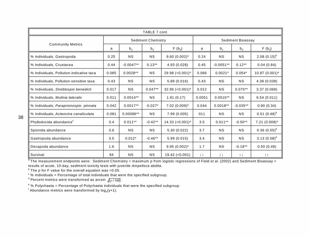
38

TABLE 7 cont.

Community Metrics Sediment Chemistry Sediment Bioassay

a 1b 2b 3F (b ) a 1b 2b 3F (b )

% Individuals, Gastropoda 0.25 NS NS 9.60 (0.002)* 0.24 NS NS 2.08 (0.15)b

% Individuals, Crustacea 0.44 -0.0047** 0.13** 4.93 (0.028) 0.45 -0.0051** 0.12** 0.04 (0.84)

% Individuals, Pollution-indicative taxa 0.085 0.0028** NS 29.98 (<0.001)* 0.066 0.0021* 0.054* 10.87 (0.001)*

% individuals, Pollution-sensitive taxa 0.43 NS NS 5.89 (0.016) 0.43 NS NS 4.38 (0.038)

% Individuals, Streblospio benedicti 0.017 NS 0.047** 32.95 (<0.001)* 0.012 NS 0.075** 3.37 (0.068)

% Individuals, Mulinia lateralis 0.011 0.0014** NS 1.91 (0.17) 0.0051 0.0015** NS 6.54 (0.011)

% Individuals, Paraprionospio pinnata 0.042 0.0017** -0.027* 7.02 (0.009)* 0.044 0.0018** -0.035** 0.90 (0.34)

% Individuals, Acteocina canaliculata 0.081 0.00086** NS 7.99 (0.005) 011 NS NS 0.51 (0.48)b

Phyllodocida abundance f 3.4 0.011** -0.42** 14.33 (<0.001)* 3.5 0.011** -0.50** 7.21 (0.008)*

Spionida abundance 3.6 NS NS 5.30 (0.022) 3.7 NS NS 0.36 (0.55)b

Gastropoda abundance 3.5 0.012* -0.46** 5.99 (0.015) 3.4 NS NS 3.13 (0.08)b

Decapoda abundance 1.6 NS NS 9.95 (0.002)* 1.7 NS -0.18** 0.50 (0.48)

Survival 94 NS NS 19.42 (<0.001) )) )) )) ))

a The measurement endpoints were: Sediment Chemistry = maximum p from logistic regressions of Field et al. (2002) and Sediment Bioassay =

results of acute, 10-day, sediment toxicity tests with juvenile Ampelisca abdita. b The p for F value for the overall equation was >0.05. c % Individuals = Percentage of total individuals that were the specified subgroup.d Percent metrics were transformed as arcsin

e % Polychaeta = Percentage of Polychaeta individuals that were the specified subgroup. f Abundance metrics were transformed by log (y+1). e

.

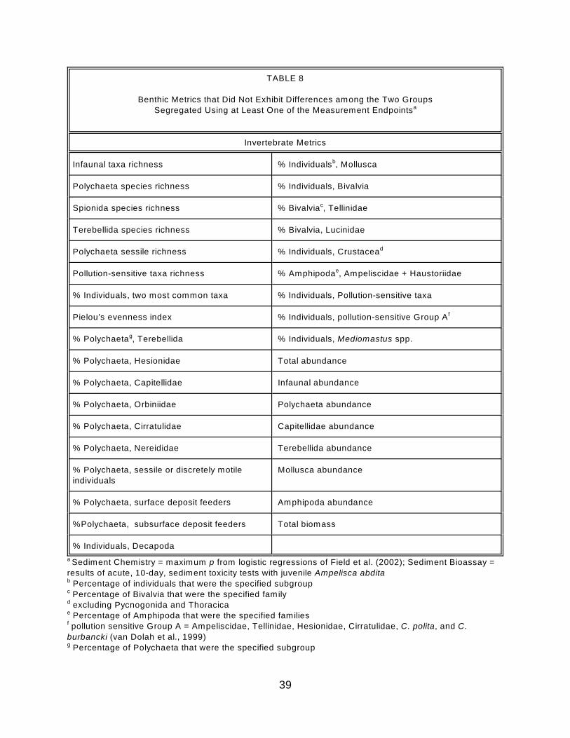
TABLE 8

Benthic Metrics that Did Not Exhibit Differences among the Two Groups

Segregated Using at Least One of the Measurement Endpointsa

Invertebrate Metrics

Infaunal taxa richness % Individuals , Molluscab

Polychaeta species richness % Individuals, Bivalvia

Spionida species richness % Bivalvia , Tellinidaec

Terebellida species richness % Bivalvia, Lucinidae

Polychaeta sessile richness % Individuals, Crustacead

Pollution-sensitive taxa richness % Amphipoda , Ampeliscidae + Haustoriidaee

% Individuals, two most common taxa % Individuals, Pollution-sensitive taxa

Pielou’s evenness index % Individuals, pollution-sensitive Group Af

% Polychaeta , Terebellida g % Individuals, Mediomastus spp.

% Polychaeta, Hesionidae Total abundance

% Polychaeta, Capitellidae Infaunal abundance

% Polychaeta, Orbiniidae Polychaeta abundance

% Polychaeta, Cirratulidae Capitellidae abundance

% Polychaeta, Nereididae Terebellida abundance

% Polychaeta, sessile or discretely motile

individuals

Mollusca abundance

% Polychaeta, surface deposit feeders Amphipoda abundance

%Polychaeta, subsurface deposit feeders Total biomass

% Individuals, Decapoda

a Sediment Chemistry = maximum p from logistic regressions of Field et al. (2002); Sediment Bioassay =

results of acute, 10-day, sediment toxicity tests with juvenile Ampelisca abdita b Percentage of individuals that were the specified subgroup c Percentage of Bivalvia that were the specified family d excluding Pycnogonida and Thoracica e Percentage of Amphipoda that were the specified familiesf pollution sensitive Group A = Ampeliscidae, Tellinidae, Hesionidae, Cirratulidae, C. polita, and C.

burbancki (van Dolah et al., 1999) g Percentage of Polychaeta that were the specified subgroup

39

total abundance or abundance of the specified larger group and expressed as a

percentage (% Polychaeta that were predators). Pollution-indicator metrics are the

abundance of one or more pollution-indicator taxa divided by total abundance or by the

abundance of a larger taxonomic group (e.g., % individuals that were pollution-

indicative taxa, % individuals that Streblospio benedicti ).

3.2.6. Data Handling and Analysis. The sites ranged in salinity from freshwater tidal

(<0.5 ‰) to poly-euhaline (>18 ‰), and many community metrics were correlated with

this gradient, particularly because some metrics were often 0 either at the freshwater

tidal or poly-euhaline sites. Therefore, to reduce this source of variation, we only used

data from the poly-euhaline sites. To focus on effects associated with contaminants in

sediments, we also excluded sites where the measured concentration of dissolved

oxygen was less than 2.0 mg/L. As a result, data from 201 sites were used in these

analyses.

We classified sampling events into two groups, those sites potentially affected

and those sites unaffected by contaminants in sediment. This segregation was

performed twice using the two different organism-level measures (Table 9). We used

the logistic regression models from Field et al. (2002) to classify the chemistry data.

The logistic regression models are for 10 metals, 22 PAHs, total PCBs and 4

organochlorine pesticides and are based on a compilation of matching data for

sediment chemistry and 10-day sediment toxicity tests with the amphipods, R. abronius

or A. abdita from a wide-range of estuarine habitats on the Atlantic, Gulf and Pacific

coasts of North America. It should be noted that a subset of the data used by Field et

al. (2002) was taken from these Virginian Province surveys. The logistic regression

models estimate the probability that sediments from a site will exhibit toxicity based on

individual chemical concentrations, though sediments may be contaminated with a

mixture of chemicals. Field et al. (2002) warn that these logistic regression models are

not dose-response relationships but can be considered indicators of toxicity. A site was

included in the potentially affected group based on sediment chemistry if the predicted

probability that the sediment was toxic exceeded 0.5 for at least one chemical (Field et

al., 2002).

Classifications of sites to groups was compared between sediment chemistry

and ambient toxicity tests with contingency tables, and the index ( (Goodman and

Kruskal, 1972) was calculated to assess the association between the groups. The

index ( is a measure of association in the assignment of sites to groups that ranges

from -1, if there was no agreement in the assignment of sites to groups by the two

40

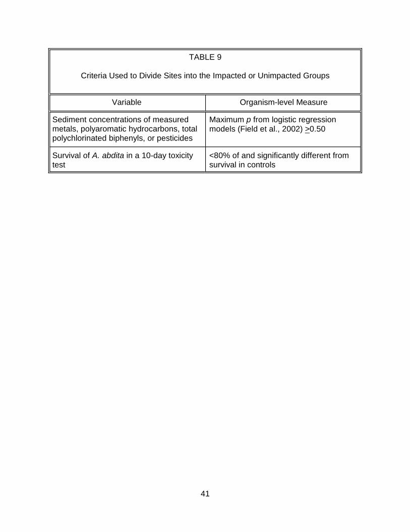
TABLE 9

Criteria Used to Divide Sites into the Impacted or Unimpacted Groups

Variable Organism-level Measure

Sediment concentrations of measured metals, polyaromatic hydrocarbons, total polychlorinated biphenyls, or pesticides

Maximum p from logistic regression models (Field et al., 2002) >0.50

Survival of A. abdita in a 10-day toxicity test

<80% of and significantly different from survival in controls

41

methods, to +1, if there was complete agreement. We used PROC FREQ (SAS, 1999)

in these analyses. As the focus of this research is the relationships between

classifications of sites with these two methods, sediment chemistry and ambient toxicity

tests, and community metrics, this analysis was done to contrast how these two

methods classify the sites.

Because many benthic metrics also varied with the silt and clay content or the

organic carbon content of the sediment, we compared each benthic invertebrate metric

between each pair of groups using analysis of covariance (ANCOVA). The question

answered was, “Was the regression of the metric on percent silt and clay and percent

organic carbon in the sediments different between the groups identified as affected or

unaffected by contaminants based on the organism-level measures?” The data were

fitted to the model:

(Eq. 3)

where:

x3 = a dummy variable with a value of 1 if at least one metal exceeded its criterion or sediment-effects concentration and a value of 0 otherwise

x1 = % silt and clay content of the sediment

x2 = % organic carbon content of the sediment

y = the metric value.

By designing the analysis in this way, the model reduces to a two-way ANCOVA, if

either b or b is not significantly different from 0, and reduces to a one-way ANOVA, if 1 2

both b and b2 are not significantly different from 0. To homogenize the variance, 1

abundance metrics were transformed by log (y+1) and percentage metrics were e

transformed by arcsine. Statistical significance was set at " = 0.05, and the

probabilities for simultaneous tests were corrected with the sequential Bonferroni

technique (Rice, 1989). We used PROC GLM (SAS, 1999) in this ANCOVA.

To explore further the relationships between the significant metrics and the

organism-level measures, we examined the residual of each metric,

(Eq. 4)

where a, b , and b2 are the estimated intercept and significant slopes from the 1

regression in Equation 3 (Draper and Smith, 1981).

42

This approach removes the variation in the metric variables resulting from the silt

and clay content and the organic carbon content of the sediments. Then, we regressed

the residuals of the significant metrics either against maximum p from the logistic

regressions or percent survival of A. abdita in the ambient toxicity tests.

These methods may be used concurrently to make decisions about whether

adverse effects are occurring or are likely at individual sites. Therefore, we quantified

the frequency of disagreement between assessments of sites based on organism-level

effects and those based on the significant community metrics. An assessment based

on a community metric would differ if the metric was “different from expected” at sites

identified as affected or unaffected based on organism-level effects. However, whether

a metric was “different from expected” changed depending on whether a metric

increased or decreased at affected sites. We defined community metrics as “different

from expected” using the 95% confidence limits as outlined in Table 10. We used

PROC REG, PROC UNIVARIATE, and PROC GLM to calculate the parameters

necessary to estimate the 95% confidence limits.

3.3. RESULTS AND DISCUSSION

Because data were not complete for some sites (i.e., some sites lacked

invertebrate data, chemistry data particularly for PCBs or pesticides, or ambient toxicity

test data), comparisons were made for 152 to 201 sites depending on the variables

being compared.

3.3.1. Organism-level Measures. A few more sites were identified as affected based

on chemistry than on ambient toxicity tests (Table 11) because chemistry indicated

sediments were toxic whereas the ambient toxicity tests did not at more sites than did

the reverse where ambient toxicity tests indicated toxicity whereas chemistry did not.

The association between groups, (, was +0.724 for the assessments using ambient

toxicity tests versus chemistry, and mean percent survival of A. abdita in the toxicity

tests was less among the sites where maximum p was greater than 0.5 (Figure 7).

However, these two measures agreed in their classification of a site at only 25% of the

43 sites where sediments were identified as affected by least one measure.

This inconsistency in classification of sediments as affected between ambient

toxicity tests and chemistry has been identified previously (O'Connnor and Paul, 2000;

O'Connor et al., 1998) for other benchmarks. Although A. abdita has been a standard

species for testing of estuarine sediments (U.S. EPA, 1994a), it may be more tolerant of

many contaminants compared with other indigenous estuarine species (Hyland et al.,

1996). The logistic equations we used were based on an analysis of compiled data on

43

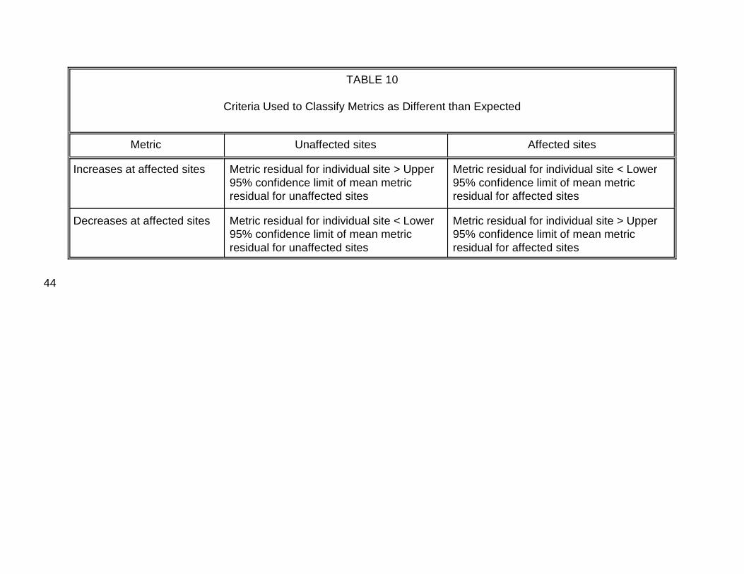
44

TABLE 10

Criteria Used to Classify Metrics as Different than Expected

Metric Unaffected sites Affected sites

Increases at affected sites Metric residual for individual site > Upper 95% confidence limit of mean metric residual for unaffected sites

Metric residual for individual site < Lower 95% confidence limit of mean metric residual for affected sites

Decreases at affected sites Metric residual for individual site < Lower 95% confidence limit of mean metric residual for unaffected sites

Metric residual for individual site > Upper 95% confidence limit of mean metric residual for affected sites

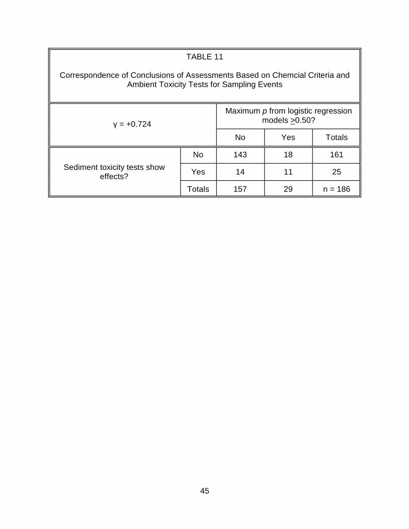
TABLE 11

Correspondence of Conclusions of Assessments Based on Chemcial Criteria and Ambient Toxicity Tests for Sampling Events

( = +0.724

Maximum p from logistic regression models >0.50?

No Yes Totals

No 143 18 161

Sediment toxicity tests showeffects?

Yes 14 11 25

Totals 157 29 n = 186

45

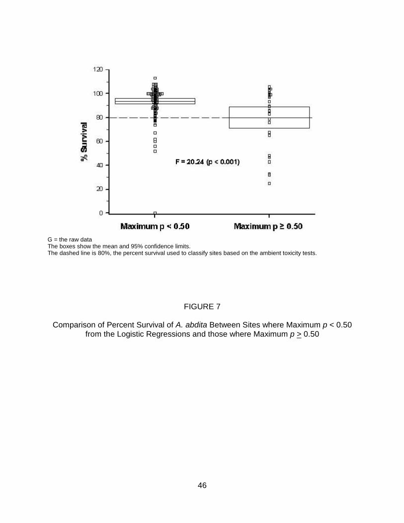
G = the raw dataThe boxes show the mean and 95% confidence limits.The dashed line is 80%, the percent survival used to classify sites based on the ambient toxicity tests.

FIGURE 7

Comparison of Percent Survival of A. abdita Between Sites where Maximum p < 0.50 from the Logistic Regressions and those where Maximum p > 0.50

46

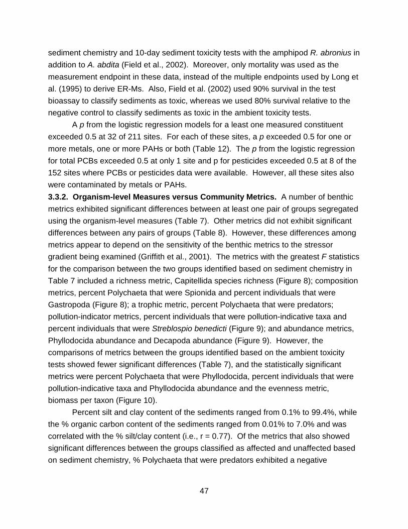
sediment chemistry and 10-day sediment toxicity tests with the amphipod R. abronius in

addition to A. abdita (Field et al., 2002). Moreover, only mortality was used as the

measurement endpoint in these data, instead of the multiple endpoints used by Long et

al. (1995) to derive ER-Ms. Also, Field et al. (2002) used 90% survival in the test

bioassay to classify sediments as toxic, whereas we used 80% survival relative to the

negative control to classify sediments as toxic in the ambient toxicity tests.

A p from the logistic regression models for a least one measured constituent

exceeded 0.5 at 32 of 211 sites. For each of these sites, a p exceeded 0.5 for one or

more metals, one or more PAHs or both (Table 12). The p from the logistic regression

for total PCBs exceeded 0.5 at only 1 site and p for pesticides exceeded 0.5 at 8 of the

152 sites where PCBs or pesticides data were available. However, all these sites also

were contaminated by metals or PAHs.

3.3.2. Organism-level Measures versus Community Metrics. A number of benthic

metrics exhibited significant differences between at least one pair of groups segregated

using the organism-level measures (Table 7). Other metrics did not exhibit significant

differences between any pairs of groups (Table 8). However, these differences among

metrics appear to depend on the sensitivity of the benthic metrics to the stressor

gradient being examined (Griffith et al., 2001). The metrics with the greatest F statistics

for the comparison between the two groups identified based on sediment chemistry in

Table 7 included a richness metric, Capitellida species richness (Figure 8); composition

metrics, percent Polychaeta that were Spionida and percent individuals that were

Gastropoda (Figure 8); a trophic metric, percent Polychaeta that were predators;

pollution-indicator metrics, percent individuals that were pollution-indicative taxa and

percent individuals that were Streblospio benedicti (Figure 9); and abundance metrics,

Phyllodocida abundance and Decapoda abundance (Figure 9). However, the

comparisons of metrics between the groups identified based on the ambient toxicity

tests showed fewer significant differences (Table 7), and the statistically significant

metrics were percent Polychaeta that were Phyllodocida, percent individuals that were

pollution-indicative taxa and Phyllodocida abundance and the evenness metric,

biomass per taxon (Figure 10).

Percent silt and clay content of the sediments ranged from 0.1% to 99.4%, while

the % organic carbon content of the sediments ranged from 0.01% to 7.0% and was

correlated with the % silt/clay content (i.e., r = 0.77). Of the metrics that also showed

significant differences between the groups classified as affected and unaffected based

on sediment chemistry, % Polychaeta that were predators exhibited a negative

47

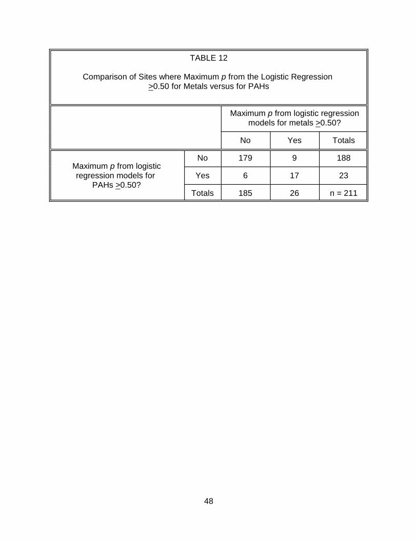
TABLE 12

Comparison of Sites where Maximum p from the Logistic Regression>0.50 for Metals versus for PAHs

Maximum p from logistic regression models for metals >0.50?

No Yes Totals

Maximum p from logisticregression models for

PAHs >0.50?

No 179 9 188

Yes 6 17 23

Totals 185 26 n = 211

48

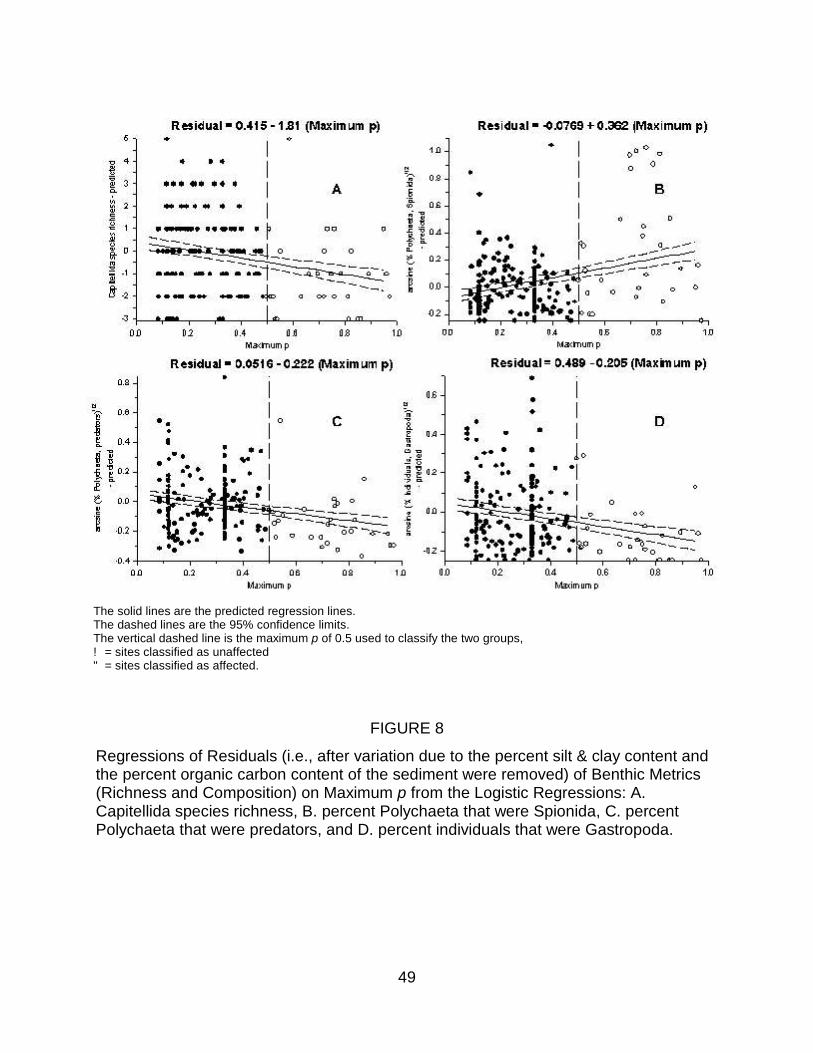
The solid lines are the predicted regression lines.The dashed lines are the 95% confidence limits.The vertical dashed line is the maximum p of 0.5 used to classify the two groups,! = sites classified as unaffected" = sites classified as affected.

FIGURE 8

Regressions of Residuals (i.e., after variation due to the percent silt & clay content and the percent organic carbon content of the sediment were removed) of Benthic Metrics (Richness and Composition) on Maximum p from the Logistic Regressions: A. Capitellida species richness, B. percent Polychaeta that were Spionida, C. percent Polychaeta that were predators, and D. percent individuals that were Gastropoda.

49

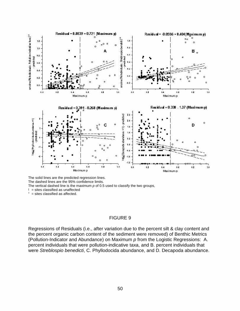
The solid lines are the predicted regression lines.The dashed lines are the 95% confidence limits.The vertical dashed line is the maximum p of 0.5 used to classify the two groups,! = sites classified as unaffected" = sites classified as affected.

FIGURE 9

Regressions of Residuals (i.e., after variation due to the percent silt & clay content and the percent organic carbon content of the sediment were removed) of Benthic Metrics (Pollution-Indicator and Abundance) on Maximum p from the Logistic Regressions: A. percent individuals that were pollution-indicative taxa, and B. percent individuals that were Streblospio benedicti, C. Phyllodocida abundance, and D. Decapoda abundance.

50

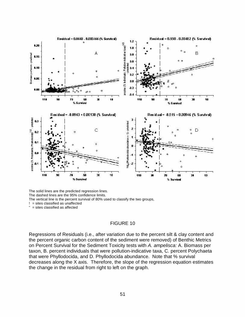
The solid lines are the predicted regression lines.The dashed lines are the 95% confidence limits.The vertical line is the percent survival of 80% used to classify the two groups,! = sites classified as unaffected" = sites classified as affected

FIGURE 10

Regressions of Residuals (i.e., after variation due to the percent silt & clay content and the percent organic carbon content of the sediment were removed) of Benthic Metrics on Percent Survival for the Sediment Toxicity tests with A. ampelisca: A. Biomass per taxon, B. percent individuals that were pollution-indicative taxa, C. percent Polychaeta that were Phyllodocida, and D. Phyllodocida abundance. Note that % survival decreases along the X axis. Therefore, the slope of the regression equation estimates the change in the residual from right to left on the graph.

51

relationship with % organic carbon, % individuals that were Streblospio bendicti

exhibited a positive relationship with % organic carbon, % individuals that were

pollution-indicative taxa exhibited a positive relation with % silt and clay, and

Phyllodocida abundance exhibited a positive relationship with % silt and clay and a

negative relationship with % organic carbon (Table 7). Of the metrics that also showed

significant differences between the groups classified as affected and unaffected based

on the sediment toxicity tests, % individuals that were pollution-indicative taxa showed

positive relationships with both % silt and clay and % organic carbon, and both %

Polychaeta that were Phyllodocida and Phyllodocida abundance showed a positive

relationship with % silt and clay and a negative relationship with % organic carbon.

The sensitivity of these richness, composition, trophic guild, pollution-indicator

and abundance metrics to the identified sediment contamination is consistent with an

assumption that effects at the organism and population levels are the basis of effects

observed at the community level. Toxicants, such as PAHs and metals, may increase

mortality and decrease reproduction of organisms within exposed populations that are

less tolerant to the toxicants. In turn, more tolerant organisms in exposed populations

may experience less of an increase in mortality and less of a decrease in reproduction,

and these populations may increase, in part, because of reduced species interactions

(Vinebrooke et al., 2003). These are organism-level effects that result in altered

relative abundances at the population level (Kuhn et al., 2000). Such population effects

would also be the basis of the observed changes in the absolute abundances of

different taxa. If at some threshold population recruitment fails, less tolerant species

will be eliminated from the community (Sheehan, 1984). Because the threshold

concentrations at which different species are affected vary, more of the species in a

community would be affected with increasing toxicant concentrations, and taxa richness

would decrease (Barnthouse et al., 1986). However, single species toxicity tests may

not be a very sensitive indicator for such community changes if the test organism is

more tolerant than other indigenous taxa. This sensitivity may be further reduced

because of the acute duration of the toxicity tests. The metrics measure chronic

effects, which occur at lower concentrations of toxicants than acute effects. This may

explain the fewer metrics that distinguished between sites classified based on the

ambient toxicity tests.

While the assessments using toxicity tests and biotic metrics may have been

more comparable if the duration of the toxicity tests were chronic, this is a limitation of

our use of secondary data, which was collected for another purpose. We used EMAP

data, and because of decisions made by the EMAP researchers, only data from toxicity

52

tests of acute duration were available. Moreover, the random site-selection approach

of EMAP results in sampling of uncontaminated and contaminated sites in proportion to

their occurance across a region. This resulted in the unbalanced distribution of sites

between the unaffected and affected groups as identified by sediment chemistry or the

ambient bioassays. The advantage of this data set is includes data from a large

number of sites that do not exhibit spacial correlations.

When classification of sites to the affected and unaffected groups based on

organism-level effects is compared with individual metric values, the methods differ in

their assessment of adverse effects at some sites (Table 13). For example,

Phyllodocida species richness was less than the 95% lower confidence limit of the

mean of the unaffected group for 88 (51.5%) of the 171 the sites classified as

unaffected. Moreover, Phyllodocida species richness was greater than the 95% upper

confidence limit of the mean of the affected group for 8 (26.7%) of the 30 sites

classified as affected by metals or PAHs based on the logistic equations. Sites in the

unaffected group where metrics are different from expected are probably affected by

other stressors. Previous analyses have identified other contaminants in sediments,

such as some pesticides, butyltins, or selenium (Kiddon et al., 2003), that could not be

assessed with the logistic equations (Field et al., 2002). Other stressors may include

excess nutrients, with their effect on light penetration, on dissolved oxygen in the water

column and on total organic carbon in the sediments; the presence of marine debris or

other habitat alterations (Strobel et al., 1999; Kiddon et al., 2003). We only excluded

sites where low dissolved oxygen was an obvious additional stressor.

At sites in the affected group where metrics were different from expected,

exposure to contaminants in sediments may differ from that measured, in part because

of unaccounted for effects on bioavailability. The logistic regressions were derived from

analyses of bioassay data that did not consider possible site-specific factors affecting

the bioavailability of the contaminants in sediments (Field et al., 2002). Alternate

approaches to assessing sediment chemistry have measured AVS or the fraction of

organic carbon, which may affect the bioavailability of metals and organics such as

PAHs, respectively (Liber et al., 1997; U.S. EPA, 2003b). While these methods attempt

to assess the bioavailability of these contaminants, there are limitations to these

approaches, particularly with the assumption that equilibrium conditions exist within the

sediments for metals and AVS or PAHs and organic carbon (O’Connor and Paul, 2000).

In preliminary analyses, sediments from only 9 of 201 sites could be classified as

potentially toxic based on the equilibrium partitioning model for chronic PAH effects

(U.S. EPA, 2003b). Five of those sites had a maximum p > 0.5 and five sites exhibited

53

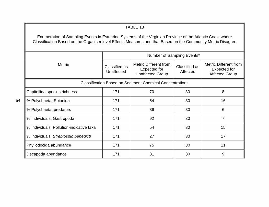
54

TABLE 13

Enumeration of Sampling Events in Estuarine Systems of the Virginian Province of the Atlantic Coast where Classification Based on the Organism-level Effects Measures and that Based on the Community Metric Disagree

Metric

Number of Sampling Events*

Classified as Unaffected

Metric Different from Expected for

Unaffected Group

Classified as Affected

Metric Different from Expected for

Affected Group

Classification Based on Sediment Chemical Concentrations

Capitellida species richness 171 70 30 8

% Polychaeta, Spionida 171 54 30 16

% Polychaeta, predators 171 86 30 6

% Individuals, Gastropoda 171 92 30 7

% Individuals, Pollution-indicative taxa 171 54 30 15

% Individuals, Streblospio benedicti 171 27 30 17

Phyllodocida abundance 171 75 30 11

Decapoda abundance 171 81 30 9

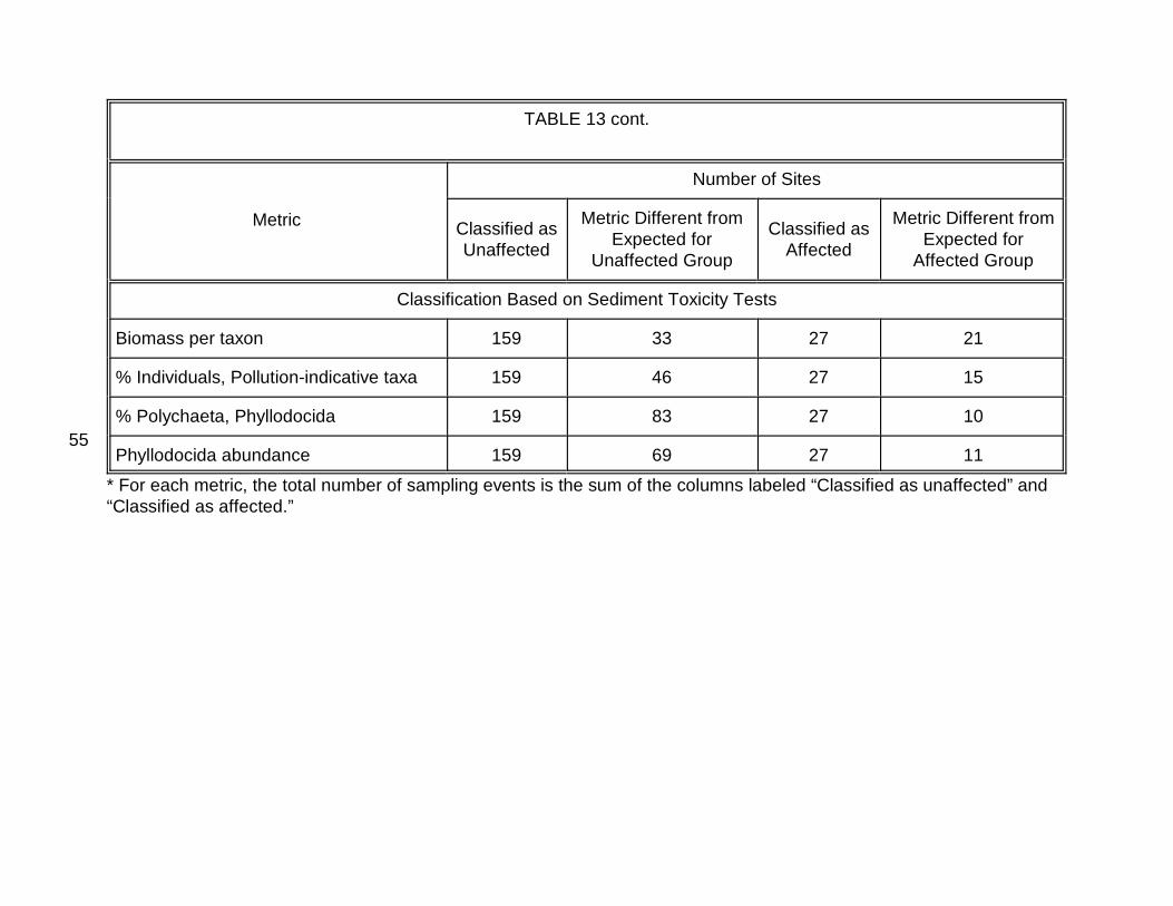
55

TABLE 13 cont.

Metric

Number of Sites

Classified as Unaffected

Metric Different from Expected for

Unaffected Group

Classified as Affected

Metric Different from Expected for

Affected Group

Classification Based on Sediment Toxicity Tests

Biomass per taxon 159 33 27 21

% Individuals, Pollution-indicative taxa 159 46 27 15

% Polychaeta, Phyllodocida 159 83 27 10

Phyllodocida abundance 159 69 27 11

* For each metric, the total number of sampling events is the sum of the columns labeled “Classified as unaffected” and “Classified as affected.”

toxicity in the ambient toxicity tests. The Simultaneously Extracted Metals/Acid Volatile

Sulfide (SEM/AVS) ratio exceeded one for sediments from 27 of the 133 sites where

AVS data were available. However, this means only that the metals may be

bioavailable and not that their bioavailable concentrations are sufficient to cause toxicity

(Hansen et al., 1996). This may be why only four of those sites exhibited toxicity in the

ambient toxicity tests, and only three sites had a maximum p > 0.5.

Besides assessing measurement endpoints at different levels of biological

organization, chemical guidelines, ambient toxicity tests and community metrics differ in

their specificity to different stressor gradients (Karr and Chu, 1998). Chemical

guidelines are very specific to the contaminants being measured and assessed and

ignore any unmeasured contaminants or stressors that lack guidelines for comparison.

Ambient toxicity tests detect toxicity associated with the entire milieu of bioavailable

contaminants in the tested sediments but do not assess other characteristics of the

estuarine site. Community metrics are not generally stressor specific. Therefore, while

community metrics may be sensitive to specific stressors (Griffith et al., 2001), they also

will be sensitive to other concurrent alterations of the ecosystem that affect the

structure of the biotic assemblages, including alterations of physical habitat that are not

addressed by chemical benchmarks.

We used a simple approach in classifying the sites into the unaffected and

affected groups. This was done, recognizing that only recently have models been

constructed to extrapolate accurately between the organism- and population-level

effects (Kuhn et al., 2000), and we still cannot accurately model or extrapolate between

population and community effects because of the difficulties of incorporating variation in

exposure and response across the hierarchical levels of time, space and organization

(de Kruijf, 1991; Landis, 2002). Considering this simple classification, one might expect

few, if any, of the metrics would have exhibited differences in their means between the

two groups. However, a number of metrics exhibited differences between the groups

although the conclusions based on the organism-level measures and on community

metrics disagreed at some sites. This would suggest that a relationship exists between

the organism-level effects assessed by chemistry or ambient toxicity tests and the

community-level effects assessed by community metrics. However, organism-level

effects are only predictive to a limited extent of the community-level effects at individual

sites. This also suggests benthic metrics may be used to confirm adverse effects at

sites identified for further analysis based on chemical data as has been done with

ambient toxicity tests (O’Connor et al., 1998). However, care is needed in the selection

of appropriate metrics because metrics differ in their sensitivity to different stressors.

56

4. CONCLUSIONS

At least for the stressors identified, metals in stream water and sediments or

metals and PAHs in estuarine sediments, these two studies show relationships between

effects at the organism level, as identified by criteria or other benchmarks for surface

water or sediments, or by ambient toxicity tests of surface water or sediments and

effects at the community level, as assessed with community metrics for

macroinvertebrates or fish that are sensitive to the effects of these toxicants. Although

effects at the organism level observed in toxicity tests can be linked conceptually to the

effects measured by community metrics at the community level, these relationships are

not necessarily simple. Furthermore, these relationships are obscured by technical

differences among the methods beyond the differences in the levels of biological

organization represented by their measurement endpoints. These technical differences

affect the methods’ specificity and sensitivity to the stressors being assessed. This is

why the organism-level effects are only predictive to a limited extent of the community-

level effects at individual sites and why these methods frequently differ in their

assessment of individual sites. The value of our assessment is that we were able to

use much larger data sets to show the statistical relationships among these methods,

as opposed to the comparisons of relatively few individual sites in previous studies.

Criteria or guidelines are specific to the contaminants of interest in each

ecosystem and environmental medium. However, criteria or guidelines cannot assess

contaminants or stressors that are not measured or that lack guidelines for comparison.

Ambient toxicity tests are less specific to individual contaminants because they should

detect effects of any toxicants present and bioavailable in either surface water and

sediments. However, ambient toxicity tests do not assess other characteristics of a site

that can affect the biotic community.

Community metrics are the least specific of the three methods, because they

directly measure community-level effects in the native assemblages. Although metrics

may be selected that are sensitive to a specific stressor (Norton et al., 2000; Ofenbock

et al., 2004), those metrics will not be necessarily sensitive only to that stressor and will

respond to other stressors, such as alterations in physical habitat. Other community

metrics will be insensitive to the specific stressors of interest, because they may not

measure alterations in assemblage structure characteristic of the stressor of interest.

Therefore, metrics alone probably cannot be used to establish stressor-specific

causality but might be used to indicate likely stressors at particular sites. Moreover,

data sets similar to those analyzed in this study that include both measurements of

57

biological assemblages and of stressors might be used to assess stressor-specific,

response relationships and identify thresholds for effects associated with specific

stressors. The segmented regression technique used in the analysis of the Colorado

REMAP data could be used to identify such thresholds for effects.

Other factors also affect the relative sensitivity of these different methods.

Toxicity tests that are designed to measure endpoints that are chronic in duration and

chemical criteria or benchmarks that are based on chronic measurement endpoints

should be more predictive of community-level effects than those based on acute

measurement endpoints, because community metrics reflect longer-term changes in

communities (Karr and Chu, 1998). Toxicity tests often use one or two standard

species, which can be more tolerant of specific contaminants than other indigenous

species. In such cases, toxicity tests would be less predictive of community-level

effects. A chemical benchmark based on a species sensitivity distribution composed of

many species is likely to be more predictive of community-level effects. Because of

these limitations and because these methods are complementary, the policy of

independent application remains appropriate.

These differences in specificity that make these methods complementary might

be used in a strength of evidence analysis (U.S. EPA, 2000c). Low values of metrics

known to be sensitive to particular stressors could be used to suggest that those

stressors have influenced the community at a site. Subsequently, ambient toxicity tests

of site media may be used to verify whether these stressors are toxic contaminants

present water or sediments. Chemical analyses would verify whether such media

contained toxic concentrations of the contaminants.

Because of the technical differences between these methods, their relative

protectiveness, even when considering specific contaminants, such as metals in

freshwater or sediments or metals and persistent organics in estuarine sediments, is

variable and difficult to quantify with certainty. In some cases, such as the AWQCs for

metals in freshwater and the thresholds identified by piecewise regression for various

metrics, the protectiveness may be similar. However, in other cases, such as the TELs

for metals in freshwater sediments, the guidelines may not estimate values that are

related to distinct changes in the biotic assemblages as quantified by the metrics.

Moreover, this protectiveness is dependent on how the point where adverse effects are

considered significant is estimated. This point can be based on acute effects or chronic

effects. A point can also be based on a statistically significant change relative to control

tests or reference conditions or based on a specified percent change relative to a

control tests or reference conditions. Field et al. (2002) state that maximum p from their

58

logistic regressions may be selected by a user to "match the level of protectiveness

appropriate for the objectives of their assessment." Techniques, like piecewise

regression, may be used to identify true thresholds, which represent levels of

contaminants or other stressors above which biotic assemblages exhibit significant

changes. However, a threshold model may not be appropriate in cases where both the

contaminant and response change in a more linear fashion.

59

5. REFERENCES

APHA (American Public Health Association). 1995. Standard Methods for the Examination of Water and Wastewater, 19th ed, A.D. Eaton, L.S. Clescer, A.E. Greenberg, Ed. American Water Works Association, Water Environment Federation, Washington, DC.

Barbour, M.T., J. Gerritsen, B.D. Snyder and J.B. Stribling. 1999. Rapid Bioassessment Protocols for Use in Wadeable Streams and Rivers: Periphyton, Benthic Macroinvertebrates, and Fish, 2nd ed. U.S. Environmental Protection Agency, Office of Water, Washington, DC. EPA/841/B-99/002.

Barnthouse, L.W., R.V. O'Neill, S.M. Bartell and G.W. Suter II. 1986. Population and ecosystem theory in ecological risk assessment. In: Aquatic Toxicology and Environmental Fate, Vol. 9, T.M. Poston and R. Purdy, Ed. ASTM STP 921. American Society for Testing and Materials, Philadelphia, PA. p. 82-96.

Bellman, R. and R. Roth. 1969. Curve fitting by segmented straight lines. J. Am. Stat. Assoc. 64:1079-1084.

Birge, W.J., J.A. Black, T.M. Short and A.G. Westerman. 1989. A comparative ecological and toxicological investigation of a secondary wastewater treatment plant effluent and its receiving stream. Environ. Toxicol. Chem. 8:437-450.

Chapman, B.M., D.R. Jones and R.F. Jung. 1983. Processes controlling metal ion attenuation in acid mine drainage streams. Geochim. Cosmoschim. Acta. 47:1957-1973.

Chapman, P.M., F. Wang, W.J. Adams and A. Green. 1999. Appropriate applications of sediment quality values for metals and metalloids. Environ. Sci. Technol. 33(2):3937-3941.

Clements, W.H. and P.M. Kiffney. 1994. Integrated laboratory and field approach for assessing impact s of heavy metals at the Arkansas River, Colorado. Environ. Toxicol. Chem. 13:397-404.

Colorado Division of Minerals and Geology. 2003. Inactive mine reclamation program. Available at http://mining.state.co.us/AbanondonedMines/inactivemine.pdf.

de Kruijf, H.A.M. 1991. Extrapolation through hierarchical levels. Comp. Biochem. Physiol. 100C(½):291-299.

Diamond, J. and C. Daley. 2000. What is the relationship between whole effluent toxicity and instream biological condition? Environ. Toxicol. Chem. 19:158-168.

60

Dickson, K.L., W.T. Waller, J.H. Kennedy and L.P. Ammann. 1992. Assessing the relationship between ambient toxicity and instream biological response. Environ. Toxicol. Chem. 11:1307-1322.

Di Toro, D.M., H.E. Allen, H.L. Bergman, J.S. Meyer, P.R. Paquin and R.C. Santore. 2001. Biotic ligand model of the acute toxicity of metals. 1. Technical basis. Environ. Toxicol. Chem. 20(10):2383-2396.

Draper, N. and H. Smith. 1981. Applied Regression Analysis, 2nd ed. John Wiley & Sons, New York, NY.

Eagleson, K.W., D.L. Lenat, L.W. Ausley and F.B. Winborne. 1990. Comparison of measured instream biological responses with responses predicted using the Ceriodaphnia dubia chronic toxicity test. Environ. Toxicol. Chem. 9:1019-1028.

Engle, V.D., J.K. Summers and G.R. Gaston. 1994. A benthic index of environmental condition of Gulf of Mexico estuaries. Estuaries. 17(2):372-384.

Fauchald, K. and P.A. Jumars. 1979. The diet of worms: A study of polycahete feeding guilds. Oceanogr. Mar. Biol. Ann. Rev. 17:193-284.

Field, L.J., D.D. MacDonald, S.B. Norton et al. 2002. Predicting amphipod toxicity from sediment chemistry using logistic regression models. Environ. Toxicol. Chem. 21(9):1993-2005.

Filipek, L.H., D.K. Nordstrom and W.H. Ficklin. 1987. Interaction of acid mine drainage with waters and sediments of West Squaw Creek in the West Shasta Mining District, California. Environ. Sci. Technol. 21:388-396.

Goodman, L.A. and W.H. Kruskal. 1972. Measures of association for cross classifications. IV: Simplification of asymptotic variances. J. Am. Stat. Assoc. 67(338):415-421.

Griffith, M.B., P.R. Kaufmann, A.T. Herlihy and B.H. Hill. 2001. Analysis of macroinvertebrate assemblages in relation to environmental gradients in Rocky Mountain streams. Ecol. Appl. 11:489-505.

Griffith, M.B., J.M. Lazorchak and A.T. Herlihy. 2004. Relationships among exceedences of metals criteria, the results of ambient bioassays, and community metrics in mining-impacted streams. Environ. Toxicol. Chem. 23:1786-1795.

Hansen, D.J., W.J. Berry, J.D. Mahony et al. 1996. Predicting the toxicity of metal-contaminated field sediments using interstitial concentration of metals and acid-volatile sulfide normalizations. Environ. Toxicol. Chem. 15:2080–2094.

61

Herlihy, A.T., D.P. Larsen, S.G. Paulsen, N.S. Urguhart and B.J. Rosenbaum. 2000. Designing a spatially balanced, randomized site selection process for regional stream surveys: the EMAP mid-Atlantic pilot study. Environ. Monit. Assess. 63:95-113.

Hyland, J.L., T.J. Herrlinger, T.R. Snoots et al. 1996. Environmental quality of estuaries of the Carolinian Province: 1994. NOAA Technical Memorandum NOS ORCA 97. National Oceanic and Atmospheric Administration, National Ocean Service, Office of Ocean Resources Conservation and Assessment, Silver Spring, MD.

Karr, J.R. and E.W. Chu. 1998. Restoring Life in Running Waters: Better Biological Monitoring. Island Press, Washington, DC.

Kiddon, J.A., J.F. Paul, H.W. Buffum et al. 2003. Ecological condition of U.S. mid-Atlantic estuaries, 1997-1998. Mar. Poll. Bull. 46:1224-1244.

Kuhn, A., W.R. Munns Jr., S. Poucher, D. Champlin and S. Lussier. 2000. Prediction of population-level response from mysid toxicity test data using population modeling techniques. Environ. Toxicol. Chem. 19:2364-2371.

Landis, W.G. 2002. Uncertainty in the extrapolation from individual effects to impacts upon landscapes. Human Ecol. Risk Assess. 8(1):193-204.

Lazorchak, J.M., D.J. Klemm and D.V. Peck, Ed. 1998. Environmental Monitoring and Assessment Program - Surface Waters: Field Operations and Methods for Measuring the Ecological Condition of Wadeable Streams. U.S. Environmental Protection Agency, Office of Research and Development, Washington, DC. EPA/620/R-94/004F.

Liber, K., D.J. Call, T.P. Markee et al. 1997. Effects of acid-volatile sulfide on zinc bioavailability and toxicity to benthic macroinvertebrates: A spiked-sediment field experiment. Environ. Toxicol. Chem. 15(12):2113-2125.

Long, E.R., D.D. MacDonald, S.L. Smith and F.D. Calder. 1995. Incidence of adverse biological effects within ranges of chemical concentrations in marine and estuarine sediments. Environ. Manage. 19:81-97.

Lyon, J.S., T.J. Hilliard and T.N. Bethell. 1993. Burden of Gilt, Mineral Policy Center, Washington, DC.

MacDonald, D.D., R.S. Carr, F.D. Calder, E.R. Long and C.G. Ingersoll. 1996. Development and evaluation of sediment quality guidelines for Florida coastal waters. Ecotoxicology. 5:253-278.

McCormick, F.H., B.H. Hill, L.P. Parrish and W.T. Willingham. 1994. Mining impacts on fish assemblages in the Eagle and Arkansas Rivers, Colorado. J. Freshwater Ecol. 9(3):145-179.

62

Mount, D.I. and T.J. Norberg-King. 1985. Validity of Effluent and Ambient Toxicity Tests for Predicting Biological Impact, Scippo Creek, Circleville, Ohio. U.S. Environmental Protection Agency, Office of Research and Development, Environmental Research Laboratory, Duluth, MN. EPA/600/3-85/044.

Mount, D.I. and T.J. Norberg-King. 1986. Validity of Effluent and Ambient Toxicity Tests for Predicting Biological Impact, Kanawha River, Charleston, West Virginia. Environmental Protection Agency, Office of Research and Development, Environmental Research Laboratory, Duluth, MN. EPA/600/3-86/006.

Mount, D.I., N.A. Thomas, T.J. Norberg, M.T. Barbour, T.H. Roush and W.F. Brandes. 1984. Effluent and Ambient Toxicity Testing and Instream Community Response on the Ottawa River, Lima, Ohio. Environmental Protection Agency, Office of Research and Development, Environmental Research Laboratory, Duluth, MN. EPA/600/3-84/080.

Mount, D.I., A.E. Steen and T.J.Norberg-King. 1985. Validity of Effluent and Ambient Toxicity Tests for Predicting Biological Impact on Five Mile Creek, Birmingham, Alabama. Environmental Protection Agency, Office of Research and Development, Environmental Research Laboratory, Duluth, MN. EPA/600/8-85/015.

Mount, D.I., T.J. Norberg-King and A.E. Steen. 1986a. Validity of Effluent and Ambient Toxicity Tests for Predicting Biological Impact, Naugatuck River, Waterbury, Connecticut. Environmental Protection Agency, Office of Research and Development, Environmental Research Laboratory, Duluth, MN. EPA/600/8-86/005.

Mount, D.I., T.J. Norberg-King and A.E. Steen. 1986b. Validity of Ambient Toxicity Tests for Predicting Biological Impact, Ohio River, near Wheeling, West Virginia. Environmental Protection Agency, Office of Research and Development, Environmental Research Laboratory, Duluth, MN. EPA/600/3-85/071.

Mount, D.I., A.E. Steen and T.J. Norberg-King. 1986c. Validity of Effluent and Ambient Toxicity Tests for Predicting Biological Impact, Back River, Baltimore Harbor, Maryland. Environmental Protection Agency, Office of Research and Development, Environmental Research Laboratory, Duluth, MN. EPA/600/8-86/001.

Norberg-King, T.J. and D.I. Mount. 1986. Validity of Effluent and Ambient Toxicity Tests for Predicting Biological Impact, Skeleton Creek, Enid, Oklahoma. Environmental Protection Agency, Office of Research and Development, Environmental Research Laboratory, Duluth, MN. EPA/600/8-86/002.

Norton, S.B., S.M. Cormier, M. Smith, and R.C. Jones. 2000. Can biological assessments discriminate among types of stress? A case study from the Eastern Corn Belt Plains ecoregion. Environ. Toxicol. Chem. 19(4):1113-1119.

63

O’Connor, T.P. 1994. The NOAA national status and trends, mussel watch program: National monitoring of chemical contamination in the coastal United States. In: Environmental Statistics, Assessment and Forcasting, C.R. Cothern and N.P. Ross, Ed. Lewis Publishers, Boca Raton, FL. p. 331-349.

O’Connor, T.P. and J.F. Paul. 2000. Misfit between sediment toxicity and chemistry. Mar. Poll. Bull. 40:59-64.

O’Connor, T.P., K.D. Daskalakis, J.L. Hyland, J.F. Paul, and J.K. Summers. 1998. Comparisons of sediment toxicity with predictions based chemical guidelines. Environ. Toxicol. Chem. 17(3):468-471.

Ofenbock, T., O. Moog, J. Gerritsen and M. Barbour. 2004. A stressor specific multimetric approach for monitoring running waters in Austria using benthic macroinvertebrates. Hydrobiologia. 516:251-268.

Olsgard, F., T. Brattegard and T. Holthe. 2003. Polychaetes as surrogates for marine biodiveristy: Lower taxonomic resolution and indicator groups. Biodivers. Conserv. 12:1033-1049.

Omernik, J.M. 1987. Ecoregions of the conterminous United States map (scale 1:7,500,000). Ann. Assoc. Am. Geogr. 77:118-125.

O’Neill, R.V., D.L. DeAngelis, J.B. Wade and T.F.H. Allen. 1986. A Hierarchical Concept of Ecosystems. Princeton University Press, Princeton, NJ.

Paul, J.F., J.H. Gentile, K.J. Scott, S.C. Schimmel, D.E. Campbell and R.W. Latimer. 1999. EMAP-Virginia Province Four-Year Assessment (1990-93). U.S. Environmental Protection Agency, Atlantic Ecology Division, Narragansett, RI. EPA/600/R-99/004.

Reifsteck, D.M., C.J. Strobel and D.J. Keith. 1993. EMAP-Estuaries 1993 Virginian Province Field Operations and Safety Manual. U.S. Environmental Protection Agency, Office of Research and Development, Narragansett, RI. June 1993.

Rice, W.R. 1989. Analyzing tables of statistical tests. Evolution. 43:223-225.

SAS (Statistical Analysis System). 1999. SAS/STAT© User’s Guide, Version 8. SAS Institute, Inc., Cary, NC.

Sheehan, P.J. 1984. Effects on individuals and populations. In: Effects of Pollutants at the Ecosystem Level, P.J. Sheehan, D.R. Mill, G.C. Butler and P. Bourdeau, Ed. John Wiley and Sons, Chichester, England. p. 23-50.

Smith M.E., J.M. Lazorchak, L.E. Herrin, S. Brewer-Swartz and W.T. Thoeny. 1997. A reformulated, reconstituted water for testing the freshwater amphipod, Hyalella azteca. Environ. Toxicol. Chem. 16(6):1229-1233.

64

Strahler, A.N. 1957. Quantitative analysis of watershed geomorphology. Trans. Am. Geophys. Union. 38:913-920.

Strobel, C.J., H.W. Buffum, S.J. Benyi, E.A. Petrocelli, D.R. Reifsteck and D.J. Keith. 1995. Statistical Summary: Environmental Monitoring and Assessment Program ­Estuaries, Virginian Province - 1990 to 1993. U.S. Environmental Protection Agency, Office of Research and Development, Narragansett, RI. EPA/620/R-94/026.

Strobel, C.J., H.W. Buffum, S.J. Benyi, and J.F. Paul. 1999. Environmental Monitoring and Assessment Program: Current status of Virginian Province (U.S.) estuaries. Environ. Monit. Assess. 56:1-25.

Suter, G.W. II, T.P. Traas and L. Posthuma. 2001. Issues and practices in the derivation and use of species sensitivity distributions. In: Species Sensitivity Distributions in Ecotoxicology, L. Posthuma, G.W. Suter II and T.P. Traas, Ed. Lewis Publishers, Boca Raton, FL. p. 437-474.

Swartz, R.C., D.W. Schultz, R.J. Ozretich et al. 1995. 3PAH: A model to predict the toxicity of polynuclear aromatic hydrocarbon mixtures in field-collected sediments. Environ. Toxicol. Chem. 14(11):1977-1987.

Thursby, G.B., J. Heltshe and K.J. Scott. 1997. Revised approach to toxicity test acceptability criteria using a statistical performance assessment. Environ. Toxicol. Chem. 16(6):1322-1329.

Toms, J.D. and M.L. Lesperance. 2003. Piecewise regression: A tool for identifying ecological thresholds. Ecology. 84(8):2034-2041.

U.S. EPA. 1985. Guidelines for Deriving Numerical National Water Quality Criteria for the Protection of Aquatic Organisms and Their Uses. U.S. Environmental Protection Agency, Office of Research and Development, Washington, DC. NTIS PB85-227049. EPA/822/R-85/100.

U.S. EPA. 1987. Handbook of Methods for Acid Deposition Studies: Laboratory Analyses for Surface Water Chemistry. U.S. Environmental Protection Agency, Office of Research and Development, Washington, DC. EPA/600/4-87/026.

U.S. EPA. 1991. Policy on the Use of Biological Assessments and Criteria in the Water Quality Program. U.S. Environmental Protection Agency, Office of Water, Washington, DC.

U.S. EPA. 1993. Methods for Measuring the Acute Toxicity of Effluents and Receiving Waters to Freshwater and Marine Organisms, 4th ed. U.S. Environmental Protection Agency, Office of Research and Development, Cincinnati, OH. EPA/600/4-90/027F.

65

U.S. EPA. 1994a. Methods for Assessing the Toxicity of Sediment-associated Contaminants with Estuarine and Marine Amphipods. U.S. Environmental Protection Agency, Office of Research and Development, Narragansett, RI. EPA/600/R-94/025.

U.S. EPA. 1994b. Methods for Measuring the Toxicity and Bioaccumulation of Sediment-associated Contaminants with Freshwater Invertebrates. U.S. Environmental Protection Agency, Office of Research and Development, Washington, DC. EPA/600/R-94/024.

U.S. EPA. 1995. Environmental Monitoring and Assessment Program (EMAP): Laboratory Methods Manual - Estuaries, Volume 1: Biological and Physical Analyses. U.S. Environmental Protection Agency, Office of Research and Development, Narragansett, RI. EPA/620/R-95/008.

U.S. EPA. 1996. Calculation and Evaluation of Sediment Effect Concentrations for the Amphipod Hyalella azteca and the Midge Chironomus riparius. Great Lakes National Program Office, Assessment and Remediation of Contaminated Sediments (ARCS) Program, Chicago, IL. EPA/905/R-96/008.

U.S. EPA. 1999. National Recommended Water Quality Criteria – Correction. U.S. Environmental Protection Agency, Office of Water, Washington, DC. EPA/822/Z-99/001.

U.S. EPA. 2000a. Methods for Measuring the Toxicity and Bioaccumulation of Sediment-associated Contaminants with Freshwater Invertebrates, 2nd ed. U.S. Environmental Protection Agency, Office of Water, Office of Science and Technology, Washington, DC. EPA/600/R-99/064.

U.S. EPA. 2000b. Supplementary Guidance for Conducting Health Risk Assessment of Chemical Mixtures. U.S. Environmental Protection Agency, Risk Assessment Forum, Washington, DC. EPA/630/R-00/002.

U.S. EPA. 2000c. Stressor Identification Guidance Document. U.S. Environmental Protection Agency, Office of Water, Washington, DC. EPA/822/B-00/025.

U.S. EPA. 2001. 2001 Update of Ambient Aquatic Water Quality Criteria for Cadmium. U.S. Environmental Protection Agency, Office of Water, Washington, DC. EPA/822/R-01/001.

U.S. EPA. 2003a. Technical Basis for the Derivation of Equilibrium Partitioning Sediment Benchmarks (ESBs) for the Protection of Benthic Organisms: Nonionic Organics. U.S. Environmental Protection Agency, Office of Research and Development, Washington, DC. EPA/600/R-02/014.

66

U.S. EPA. 2003b. Procedures for the Derivation of Equilibrium Partitioning Sediment Benchmarks (ESBs) for the Protection of Benthic Organisms: PAH Mixtures. U.S. Environmental Protection Agency, Office of Research and Development, Washington, DC. EPA/600/R-02/013.

U.S. EPA. 2003c. Procedures for the Derivation of Equilibrium Partitioning Sediment Benchmarks (ESBs) for the Protection of Benthic Organisms: Metals Mixtures (cadmium, copper, lead, nickel, silver, and zinc). U.S. Environmental Protection Agency, Office of Research and Development, Washington, DC. EPA/600/R-02/011.

U.S. EPA. 2003d. Generic Ecological Assessment Endpoints (GEAEs) for Ecological Risk Assessment. U.S. Environmental Protection Agency, Risk Assessment Forum, Washington, DC. EPA/630/P-02/004F.

van Dolah, R.F., J.L. Hyland, A.F. Holland, J.S. Rosen and T.R. Snoots. 1999. A benthic index of biological integrity for assessing habitat quality in estuaries of the southeastern USA. Mar. Environ. Res. 48:269-283.

Vinebrooke, R.D., D.W. Schindler, D.L. Findlay, M.A. Turner, M. Paterson and K.H. Mills. 2003. Trophic dependence of ecosystem resistance and species compensation in experimentally acidified Lake 302S (Canada). Ecosystems. 6:101-113.

Weisberg, S.B., J.A. Ranasinghe, D.M. Dauer, L.C. Schaffner, R.J. Diaz and J.B. Frithsen. 1997. An estuarine benthic index of biotic integrity (B-IBI) for Chesapeake Bay. Estuaries. 20(1):149-158.

67