RELATIONSHIP BETWEEN VOLATILITY...Implied volatility is thus a forward-looking measure of likely future volatility conditions. On the other hand, historical volatility is a hackward-looking

ASSESSING THE INTRADAY

RELATIONSHIP BETWEEN

IMPLIED AND HISTORICAL

VOLATILITY

IRA G. KAWALLERPAUL D. KOCHJOHN E. PETERSON

INTRODUCTION

Historical volatility of the price of an asset or security is typicallycomputed as the standard deviation of daily returns over some recentperiod (for example, the past 20-60 days). An option's price, however,reflects expected volatility yet to he realized, over the life of the option.If an instrument's return is perceived to he more volatile, the optionon that instrument should he worth more, and vice versa. Given avalue for this perceived volatility and the other parameters in an optionpricing model, the theoretical price of the option can he determined.On the other hand, given the current price of a specific option contractalong with the model's other parameters, the model can he solvedhackwards for the value of the volatility parameter implied hy the

We wish to acknowledge the helpful comments of two anonymous referees. Financial support fromthe Theis foundation is gratefully acknowledged. These views do not necessarily reflect those ofthe Chicago Mercantile Exchange.

• Ira G. Kawaller is Vice President-Director, New York Office of the ChicagoMercantile Exchange.

m Paul D. Koch is an Associate Professor at the University of Kansas.

• John E. Peterson is an Instructor at Northem State University in South Dakota.

The Journal of Futures Markets, Vol. 14, No. 3, 323-346 (1994)© 1994 by John Wiley & Sons, Inc. CCC 0270-7314/94/030323-24

324 Kawaller, Koch, and Peterson

current price of the option. This outcome is called "implied volatility"of the option.

A market's perception of future volatility conditions can changeinstantaneously. Such changes in the market's mood about an underlyinginstrument should he reflected in option prices and, therefore, in impliedvolatility. Implied volatility is thus a forward-looking measure of likelyfuture volatility conditions. On the other hand, historical volatility is ahackward-looking measure of recent volatility conditions. Furthermore,since the traditional measure of historical volatility incorporates returnhehavior over the past 20-60 days, such a measure displays suhstantialinertia. That is, as volatility conditions change from day to dayj tradi-tional measures of historical volatility are sluggish to respond hecausecurrent conditions are diluted by the market's hehavior over this pasthorizon. These characteristics of traditional volatility measures suggest arelationship in which implied volatility might offer predictive informationregarding suhsequent historical volatility hehavior.

Previous work investigates the relationship between implied volatil-ity of option prices and historical volatility of the underlying asset.' Somestudies question the hypothesis that option prices offer substantial infor-mation content regarding expected volatility conditions in the underlyingmarket [Beckers (1981); Wilson and Fung (1990)]. However, other worksuggests that implied volatility may he useful in predicting subsequentmovements in historical volatility of the underlying instrument's return[Heaton (1986); Latane and Rendleman (1976)].

Throughout this literature little attention has heen given to whether,over a shorter time frame, some measure of historical volatility of-fers any predictive information regarding suhsequent option prices.Intuition suggests that option traders may very well react to changesin short-term volatility hy adjusting their volatility expectation up-ward or downward, to provide timely inputs to their option pricingmodels. With this in mind, this study investigates whether such aprocess can be measured objectively, by using measures of historicalvolatility computed over shorter time intervals. Also tests are used todetermine whether implied volatility serves as a useful predictor ofhistorical volatility.

Time intervals of two different lengths are used to measure impliedand historical volatility: one interval per day and ten intervals per day.

'See, for example, Ball and Torous (1986); Beckers (1981); Brenner, Courtadon, and Subrah-manyam (1985); Chiras and Manaster (1978); Franks and Schwartz (1988); Han and Misra (1990);Heaton (1986); Latane and Rendleman (1976); Manaster and Rendleman (1982); Park and Sears(1985); Poterba and Summers (1986); and Wilson and Fung (1990).

Implied and Historical Volatility 325

The measures of historical volatility used here employ transactions datathroughout the course of a single trading day, rather than aggregatingdaily data across the 20- to 60-day time frame traditionally used byother researchers and market participants. Moreover, the time seriesof intraday volatility measures are computed over non-overlapping timeintervals, so that price information during one interval is not carriedover to the next. Options on the following four futures contracts areexamined: (i) the S&P 500 index; (ii) deutsche marks; (iii) Eurodollars;and (iv) live cattle.

Any such investigation must take into account the well-documentedassociation hetween volume and volatility in futures markets [Ek-man (1992); Kawaller, Koch, and Koch (1990); Merrick (1987)].This relationship is controlled for hy incorporating the volume ofhoth the underlying futures market and the option market intothe model.

For all contracts and time intervals investigated, historical volatilityis found to he strongly associated with movements in futures volume.After accounting for the relationship with volume. Granger test resultsare mixed across these contracts and time intervals. For the two timeintervals investigated, the analysis often suggests no suhstantive lead/lagrelationship in either direction. When significant relationships do ap-pear, however, the market involved and the nature of the relationshipdepend upon the time interval of measurement used.

DATA AND METHODOLOGY

Data

Transactions data are from the Chicago Mercantile Exchange for thefour futures contracts listed ahove, for the fourth quarter, 1988, nearbycontract period.^ These data include all quotes when the price isdifferent from the previous trade. In addition, all price quotes for at-the-money call and put options on each contract are ohtained for thesame period:^ ^

2 For each market the time series hegins on the day the futures contract becomes nearby, andends one week prior to expiration. The sample periods follow: (i) S&P 500 futures, Sept. 16-Dec.8, 1988; (ii) deutsche mark futures, Sept. 20-Dec. 9, 1988; (iii) Eurodollar futures, Sept. 20-Dec. 12, 1988; and (iv) live cattle futures, Sept. 1-Nov. 17, 1988.'The Black (1976a) and the Black/Scholes (1972 and 1973) models have a tendency to misspriceoptions that are further out-of-the-money. Hence, the at-the-money option is selected here as theoption vnth a strike price closest to the actual price on the underlying contract throughout eachday. Within the day it is not unusual to have a change in the designated at-the-money instrument.


i. Fir = price of S&P 500 stock index futures contract at time T,ciT = price of call option on S&P 500 stock index futures at time T,PIT = price of put option on S&P 500 stock index futures at time T;

ii. F2T = price of deutsche mark futures contract at time T,C2T = price of call option on deutsche mark futures at time T,P2T = price of put option on deutsche mark futures at time T;

iii. FsT = price of Eurodollar futures contract at time T,CiT = price of call option on Eurodollar futures at time T,P3T = price of put option on Eurodollar futures at time T;

iv. F4T = price of live cattle futures at time T,C4T = price of call option on live cattle futures at time T,P4T = price of put option on live cattle futures at time T,

where T indexes the intraday price quotes on each futures and option.These transactions price data are used to construct time series reflectingintraday movements in historical volatility of the underlying returns (cr t̂),to be matched with implied volatility in option prices (o-jj).

Constructing Measures of Historical Volatility

The computation of historical volatility for each futures contract iscomplicated by the fact that the frequency of trading in each underlyingcontract varies throughout any trading day. To measure intraday histor-ical volatility for each futures contract, one must first have a time seriesin each futures price itself, taken at equispaced time intervals. Therefore,the last price quote every minute on each underlying futures contractis used to generate four minute-to-minute price series {F.-j; j = 1 —4}. Then the natural log of the price relative is computed betweensuccessive prices to generate a series of minute-to-minute returns[rjT = ln(FjT/FjT-i); j = 1 - 4]. Thus, over the course of a tradingday (e.g., 6 hours and 40 minutes for S&P 500 futures), the sam-ple includes as many as 400 minute-to-minute observations on theinstrument's return.

Movements in intraday historical volatility (aht) are measuredusing each underlying contract's minute-to-minute return during non-overlapping time intervals of two different lengths. First daily volatilitymeasures are constructed using all return observations throughout each

''If no price quote appears during one or more minutes for any underlying contract, the most recentquote is retained as the relevant price. The absence of a futures trade is reflective of a period ofzero volatility. By retaining the most recent futures quote for all minutes when no quote appears,a futures price series is generated which displays no variation across all such minutes.

Implied and Historical Voiatility 327

day. Second, the trading day is divided into ten equal time intervals foreach underlying futures contract.'

Over each time interval, t (whether the day-long interval or the1/10th day interval), the sample standard deviation of each return seriesis recorded as that interval's observation on historical volatility

(rT-r)T^ (1)T = l

where N = the number of minute-to-minute returns available withineach interval (e.g., N = 400 for each 6-hour and 40-minute daily timeinterval, or N = 40 For each 40-minute interval within that day); 7equals the sample mean for rr in each interval; T indexes the minute-to-minute observations on r j within each interval; and t indexes the timeintervals chosen to measure historical volatility.

Constructing Measures of Implied Volatility

For each instrument, every time interval's observation on historicalvolatility {(Tht) is matched with the average implied volatility of all at-the-money call and put option quotes within that same time interval:

o-it = X (Tic + S îp ^Lc=i p=\ J

et + NpO (2)

where au = denotes the measure of implied volatility during interval t;o-jc refers to the implied volatility of the cth call quote during intervalt; aip refers to the implied volatility of the pth put quote duringinterval t; and Net and Np are the number of call and put quotes,respectively, during interval t.^ This procedure yields the matched time

'Traditional measures of historical volatility reflect variation in daily returns over the previous20-60 days [e.g., Latane and Rendleman (1976)]. Since the intraday measures used here revealchanges in intraday volatility over much shorter nonoverlapping time intervals, the measures may heperceived as containing more "noise" than traditional measures. An alternative view would regardthese measures as containing more timely "information" that might be germane to options pricing.*The Black (1976a) model is used to compute implied volatility for options on the four futurescontracts. It should be noted that the reliability of these implied volatility measures rests on thevalidity of this option pricing model. For each implied volatility computation, this model requiresdata on the fraction of a year to expiration, the risk-free rate, the strike price, and the actual pricequote of the option. The annualized return on the Treasury Bill maturing nearest the expirationof each option contract investigated is used as a proxy for the risk free rate. This relationship isinvestigated also using the average implied of calls and puts separately in the analysis. Results aregenerally robust and available upon request.

Numerous diagnostic checks and robustness checks are used throughout the analysis. To conservespace they are not presented here. These diagnostics uniformly point to robust results, and theyare available upon request.


= inti

= int2

+

+

M,

fe=lfet-fe +

ht-k +

M2

1k=l

M,

I

series, ((Tht,(ru), over both daily and 40-minute time intervals that arenecessary to investigate any predictive relationships between intradaymovements in implied and historical volatility.

Methodology

Granger tests [Granger (1969)] are used to investigate the potentialpredictive relationships between each pair of matched time series onhistorical and implied volatility. In this approach, each volatility measureis hypothesized to depend potentially upon its own past movements andpast movements in the other volatility measure:

-u-k + en (3)

-u-k + e-^ (4)

where eu and e^t are disturbances that reflect variation in each volatilitymeasure over time, beyond that attributable to past movements in bothvolatility measures/ This two-equation model can be rewritten using thelag operator, L (L'̂ XJ = X(-fe), as follows:

KV) BiL) iro-fet] p i t ]C{L) DiL)\[au\ "^[eaj ^̂^

where the intercepts are inherent; where each distributed lag fromeqs. (3) and (4) appears as a polynomial in the lag operator; andwhere the disturbances are assumed to be normally distributed andnot autocorrelated, but may be contemporaneously correlated acrossequations.^

In tbe context of tbis model, tbe null hypothesis tbat impliedvolatility does not lead (or "Granger-cause") historical volatility can

Ân expanded version of this model in which each volatility measure depends on its ownpast and current and past movements in the other volatility measure is estimated also. Theaddition of these contemporaneous effects transforms the model in (3) and (4) into a systemof two simultaneous equations. When this expanded model is estimated using Three StageLeast Squares, the contemporaneous coefficients are almost always statistically insignificant.Furthermore, the remaining results on the lead/lag relationships are robust. This analysis providesempirical justification for the Granger test specification in eqs. (3) and (4).^Theoretically, if enough lagged values of the left-hand side variable are included in each equation,the residuals will be reduced to white noise [Geweke (1978); Granger (1969)]. This assumptionof no autocorrelation in each disturbance is important for the validity of the F tests on Granger-causality, and is tested formally with the Ljung-Box (1978) test on the autocorrelation functionof the residuals of each equation. Results indicate that the residuals are white noise in all cases.


be tested with zero-restrictions on tbe lagged coefficients of impliedvolatility in tbe first equation of (5):

Hv.o-it - h a-ht[B{L) = 0]Likewise, tbe null bypotbesis of no Granger-causality in tbe oppositedirection can be tested witb zero-restrictions in tbe second equationof (5):

H2: (Tht - h (Tit [C(L) = 0]Results will reveal wbetber implied volatility contains statistically sig-nificant predictive information regarding subsequent movements inbistorical volatility, and/or vice versa. It is notewortby tbat the notionof Granger-causal priority merely reflects tbe predictive information inone variable regarding anotber. Tbis notion bas little to do witb tbepbilosopbical concept of causality.

Nonprice Factors that May Affect Volatility

Botb equations in (5) are expanded to include tbe following five vari-ables tbat may also influence bistorical and/or implied volatility. Eacbpotential influence is tben discussed in turn.

Trend = time trend;FVOL = trading volume in tbe underlying futures market;OVOL = trading volume in tbe options market;Return = lagged return in tbe underlying futures market;Dk = dummy variables to reflect different days of tbe week or

different intraday time intervals.

First, tbe argument bas been made tbat tbe variance of returnson eacb futures contract sbould be expected to increase systematicallytoward tbe end of tbe nearby contract period [Samuelson (1965)].If futures prices are unbiased estimates of subsequent spot prices,and if spot prices follow a stationary first-order autoregressive process,tbe impact of new information on futures prices will be greater nearexpiration [Anderson and Dantbine (1983)]. Since market informationtbus becomes more important over time, tbe variance could rise. Tbispossibility is addressed by including a time trend in eacb equation ofsystem (5). Lack of a robust positive coefficient for tbis variable maycreate some doubt regarding eitber tbe assumptions above or tbe processbypotbesized in Samuelson (1965).

Second, trading volume in tbe futures contract may affect volatilityin tbe underlying futures prices [Ekman (1992); Kawaller, Kocb, and


Kocb (1990); Merrick (1987)]. If futures volume affects futures volatil-ity, it may also affect implied volatility in option prices on tbe futurescontract. Third, a similar argument can be made to suggest tbat totalvolume on all call and put options may affect both implied and historicalvolatility for a given contract. Therefore, when daily time intervals areanalyzed, daily volume on the underlying futures contract and dailyvolume on all call and put options are included as additional explanatoryvariables in each equation of (5). For these four futures contracts andtheir related options, volume data are generally unavailable for timeintervals shorter than one day. Thus, when analyzing 10 intervals perday, the following proxies are used for volume on futures and optionsduring the tth intraday time interval:^

FVOL = Nft = number of futures quotes during interval t;

OVOL = Net + Npt = total number of call and put quotes in inter-val t.

Fourtb, market volatility may vary consistently witb general marketmovements. For example. Black (1976b) demonstrates tbat stock marketvolatility tends to increase as stock prices fall, and decrease as stockprices rise. In this model, general market movements are captured byincluding lagged returns in tbe underlying futures market. Specifically,this market return is measured as the natural log of the ratio of thelast futures quote to the first futures quote in each time interval. Inthis analysis, one lagged return is included in each equation of (5). Ifmarket volatility consistently rises when futures prices fall and falls whenfutures prices rise, negative coefficients for these lagged returns shouldbe observed. Tbe model including several lagged values of tbe return ineacb equation is also estimated witb generally robust results.

Finally, it is also possible tbat implied and bistorical volatility varysystematically across different days of tbe week, or across differentintraday intervals. Hence, when daily intervals are analyzed, five day-of-the-week dummy variables are added to eacb equation of (5). Tbese fivedummies replace tbe intercept term in each equation. Then, for eachequation a test is conducted of the joint hypothesis that the Mondayintercept is identical to that on the other four days of the week. Whenanalyzing ten intervals per day, a separate dummy variable is added for

'Harris (1987) suggests that the number of transactions should be closely related to actual tradingvolume throughout any trading day. For NYSE data, Harris shows that the number of transactionsis highly correlated with volume throughout the trading day. For futures data, Ekman (1992) usesthe number of recorded transactions to approximate trading volume on a contract.


each intraday interval. Again, these ten dummies replace the interceptin each equation of (5), and the joint hypothesis that the intercept ofthe day's first interval is identical to that of the other intraday intervalsis tested. The coefficients of these intraday dummies will display anysystematic intraday pattern in au or au inherent in the data, and thejoint test will reveal whether such a pattern is statistically significant.

Econometric Considerations

Note that system (5) is specified in terms of the levels of volatility.Consistent with the relationships analyzed hy Wiggins (1987) andKawaller, Koch, and Koch (1990), a natural log transformation of ahtand ait is employed in the regression analysis. Tbis corrects for possiblebeteroskedasticity in tbe error terms. ̂ *̂

Before tbe system can be estimated, a finite lag parameterizationmust be selected. While longer lag lengths lessen the chance of mis-

'"Kawaller, Koch, and Koch (1990, p. 384) point out that the sample variance has the followingasymptotic distribution, if the underlying futures price series is normally distributed:

d-l"-NWl,2<Tt,nN - 1)}

where N is the sample size, and (7 ,̂ is the true volatility within the time interval t. This distributiondemonstrates that the precision (variance) of each observation on the measure of historical volatilitydepends upon the true a^, during that interval. Thus, the precision of the data on &),, varies asthe true volatility does. This phenomenon may translate into heteroskedasticity in the error termof the first equation in the model, which determines historical volatility. Given the normalityassumption underlying the futures price series, this heteroskedasticity disappears with the naturallog transformation:

ln(*^,) • N{\n{(Tl),2/N]

The practice of applying the natural log transformation follows the rule provided in Judge et al.(1985, p. 160, eq. 5.3.20), which suggests that one consider functions of the volatility measuresthat will stabilize the error variances. The natural log transformation is such a function to correctfor heteroskedasticity that might be transferred to the regression error terms.

The error term (e2() for the second equation in the model, which determines implied volatility,may exhibit further heteroskedasticity due to the effect of grouping [Theil (1971, p. 249)]. Eachobservation on implied volatility is the average implied of all option quotes during that time interval(that day or that 40-minute period). The precision of this sample mean depends on the number ofoption quotes during each interval. As a result, for example, the sample mean from a time intervalthat experiences ten option quotes would have a smaller variance than the sample mean from atime interval vdth one quote.

To resolve this heteroskedasticity problem, the following weighted least squares transformationcan be applied to all variables in the implied volatility equation, (4): let transformed o-j, =O"ii * (Net + Npi)"'. After applying this weighted least squares scheme to all variables in eq. (4),generally robust results are obtained. However, only the results without this transformation of thesecond equation are used in the presented model, because while this procedure results in an errorvariance for e2t that is homoskedastic, it may also introduce spurious correlation into the model.This problem is due to the fact that the variable, (Nc + Np), already appears on the right-handside of the model as a proxy for options volume, when ten intervals per day are analyzed.


specification, they also consume more degrees of freedom. Hence oneshould choose the minimum lag length that specifies the relationshipsaccurately. Geweke (1978) argues that, for each equation, the numher oflags on the dependent variahle (Mi) should he kept generous to minimizethe chance of serially correlated errors, while the numher of lags on theother variahles (M2) should he set lower to retain power in the hypothesistests. With this in mind. Mi = 10 lags and M2 = 5 lags when employingdaily time intervals, and Mi = 15 lags and M2 = 5 lags when using thehigher frequency intervals of ten per day. The model is also estimatedusing several other sets of lag lengths, vdth generally rohust results.

The system of seemingly unrelated regressions in (5) is estimatedusing the standard Zellner-Aitken technique [Johnston (1984,pp. 337-341)]. If the information embodied in each error termaffects both volatility measures, this would imply contemporaneouscorrelation between the errors, and Ordinary Least Squares will yieldinefficient estimates.

EMPIRICAL RESULTS

Data Characteristics

Table I presents the sample means of all variables for each futurescontract investigated, along with the average frequencies of optionquotes in each market. The average market return is negative forEurodollar futures, and positive for the other three markets. This resultindicates that the fourth quarter 1988 nearby contract period representsa time of generally falling futures prices in the Eurodollar market, andgenerally rising prices in the other three markets.

The last three columns of Table I indicate reasonable liquidityfor these four futures markets during the sample period. The optionmarkets also appear to be fairly liquid. The only possible exception is foroptions on Eurodollar futures, which experience an average of 18 optionquotes per day (eight calls and ten puts). While this average liquidityvaries substantially across markets, these averages appear to representconsistent activity on most days, as there are very few intraday intervalswhich experience no futures and/or option trades.

Daily Time Intervals

Initially consider the influence of the five nonprice factors onhistorical and implied volatility. Coefficient estimates for three of thesefive nonprice factors (futures volume, options volume, and lagged


I!

I

E

;^-0

CO

CO

D

I

CO

CO

u

^

111

CMooCM

inCM

CO

in ^ r ~ — C M

CO t ^ 05 Ot^ c» en t^

oooTCO

00O)co"CM

CO

co"

oCM

00 O> " "^ GO ' 1 -

isiio

Q.CO

g8

oopoI

gooCJ

in <D -^T- 1 - Oo o o o

UJ p

t op

o

8

1 - CO

° 5CD d

<D T - COr^ o ••-y- y- tDd d CD

• t1- p

r in^- CMp T -

d d

CO

d

in oT - CMp

III I I

T3

^ JO

(0 as

1 E cr̂ O) - t ou -^

g in o in o0. II -S II 2

S O) ^ r*- ^ ojg in o U5 o ind) o c5 o 5 o.c r^ ^ CJ) 5 in

o8 -» 0) >CO S . Q &.

o2 03

a

•li- "D (0 — .=

0) c o m •" •"m Q. g in .!" c

£ 3

f- 03 2 ,o g aSi £

€ £s a 3.

•2 TB" o I ^ e

a

"" ffi S - £ "

£ « S

£ .E


TABLE IIInfluence of Futures Volume, Options Volume, and

Lagged Market Returns One Interval Per

Dependent Variable

S&P 500 futuresFutures volume (std err)*"Options volume (std err)''Lagged mkt return (std err)

Deutsche mark futuresFutures volume (std err)*"Options volume (std err)*"Lagged mkt return (std err)

Eurodollar futuresFutures volume (std err)*"Options volume (std err)"Lagged mkt return (std err)

Live cattle futuresFutures volume (std err)*"Options volume (std err)''Lagged mkt return (std err)

Historical Vol.

1,51-6,52-0.88

2,680,0020,05

0,781,05

15.1

2,968,48

-1,86

(0.23)"=(7,42)(3,28)

(0.57)<=(1,68)(8,22)

(0.14)'=

(1,80)

(31.27)

(1,74)"(9,86)(5,11)

Implied Vol.

0,05-0,92-1,99

0,20-0,46

0.15

-0,08-0,21-5.4

0,24-0,38-0.01

(0,09)(2,72)(1,10)"

(0.14)(0,43)(1,93)

(0,05)(0,61)

(11,55)

(0,35)(1,91)(1,03)

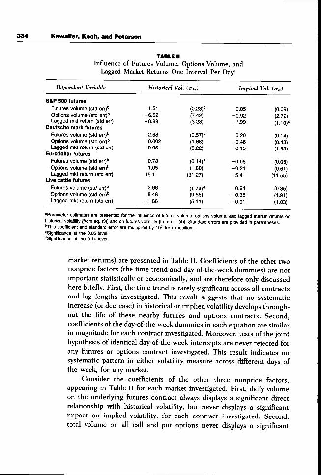
^Parameter estimates are presented for the influence of futures volume, options volume, and lagged market returns onhistorical volatility [from eq, (3)] and on futures voiatiiity [from eq, (4)], Standard errors are provided in parentheses,"This coefficient and standard error are muitipiied by 10^ for exposition,^Significance at the 0,05 levei,"Significance at the 0,10 level,

market returns) are presented in Table II. Coefficients of the other twononprice factors (the time trend and day-of-the-week dummies) are notimportant statistically or economically, and are therefore only discussedhere briefly. First, the time trend is rarely significant across all contractsand lag lengths investigated. This result suggests that no systematicincrease (or decrease) in historical or implied volatility develops through-out the life of these nearby futures and options contracts. Second,coefficients of the day-of-the-week dummies in each equation are similarin magnitude for each contract investigated. Moreover, tests of the jointhypothesis of identical day-of-the-week intercepts are never rejected forany futures or options contract investigated. This result indicates nosystematic pattern in either volatility measure across different days ofthe week, for any market.

Consider the coefficients of the other three nonprice factors,appearing in Table II for each market investigated. First, daily volumeon the underlying futures contract always displays a significant directrelationship with historical volatility, but never displays a significantimpact on implied volatility, for each contract investigated. Second,total volume on all call and put options never displays a significant

Implied and Historical Voiatiiity 335

relationship with either implied or historical volatility. Finally, the laggedmarket return is significantly negative (at the 0.10 level) only for impliedvolatility in the S&P 500 market. This result suggests that marketdeclines (increases) tend to be followed by increases (declines) in impliedvolatility for this market.

Granger test results are presented in Table III for each contractinvestigated. The first hypothesis, H\{ait-h au), is rejected at the0.05 level for the Eurodollar and live cattle futures markets, but isnot rejected for the other two markets. The second hypothesis, H2{o'ht -h(Tit), is also rejected at the 0.05 level for the Eurodollar and livecattle futures markets, indicating a bidirectional lead/lag relationshipbetween implied and historical volatility for these two markets. The sec-ond hypothesis is also rejected at the 0.10 level for the S&P 500 futuresmarket. No lead/lag relationship is indicated for deutsche mark futures.

Ten Intervals Per Day

Before discussing the Granger test results over these shorter time in-tervals, consider the nonprice factors influencing historical and impliedvolatility. The time trend is not presented here but it reveals a significantpositive coefficient for the S&P 500 and Eurodollar futures and optionsmarkets. On the other hand, a significant negative trend appears for

TABLE IIIGranger Tests: Relationship between Implied

and Historical Volatility One Interval per

S&P 500 futures

Deutsche mark futures

Eurodollar futures

Live cattle futures

DF^

(5,50)

(5,48)

(5,50)

(5,42)

0,42

(0,833)1,00

(0,426)3,35®

(0,011)2,67®(0,035)

H2: o-fc, -A a-i,"

2,14"(0.076)

1,46(0,222)2,42®

(0,049)3,06®(0,019)

=ln each case. Granger tests are conducted by estimating eqs, (3) and (4) as a system of seemingly unrelated regressions,using ten daiiy iags on the dependent variable and five daily lags on the right-hand side variable in each equation. Resultsare generally robust when other sets of lag lengths are used, and when OLS estimation is employed,"•DF provides the degrees of freedom for each asymptotic F statistic,''Hi and H2 test the hypotheses of no Granger causality in each direction, between historical volatility in the underlyingfutures contract and implied volatility in options on that futures contract. Approximate marginal significance levels areprovided in parentheses,"Significance at the 0,10 level,"Significance at the 0,05 level.


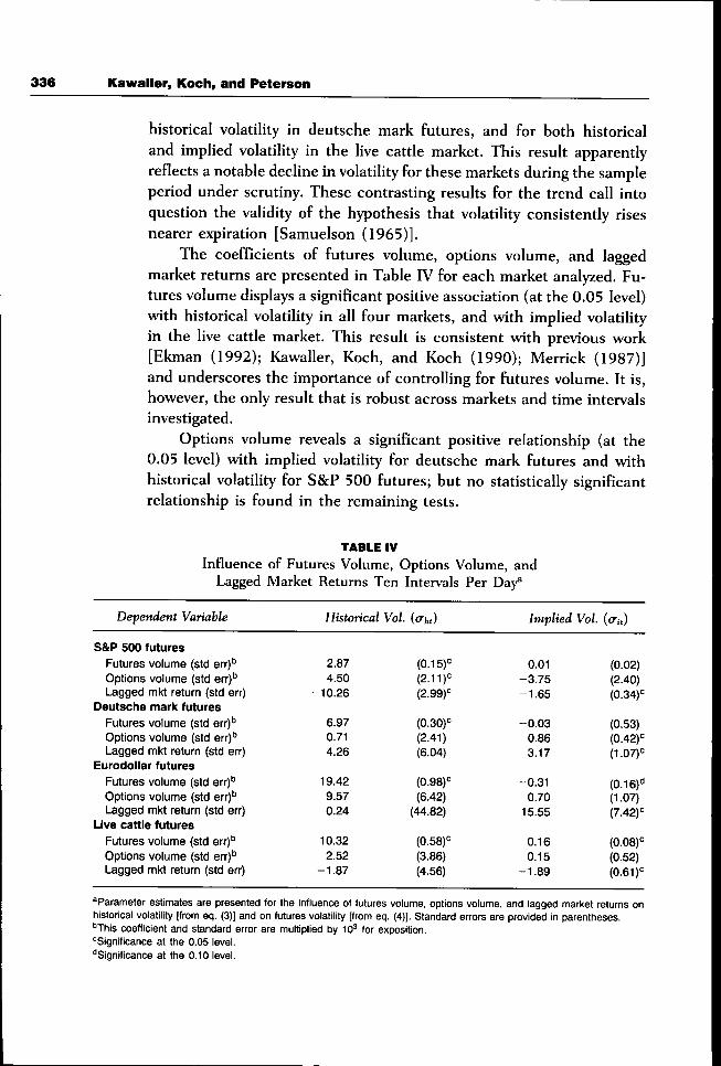
historical volatility in deutsche mark futures, and for both historicaland implied volatility in the live cattle market. This result apparentlyreflects a notable decline in volatility for these markets during the sampleperiod under scrutiny. These contrasting results for the trend call intoquestion the validity of the hypothesis that volatility consistently risesnearer expiration [Samuelson (1965)].

The coefficients of futures volume, options volume, and laggedmarket returns are presented in Table IV for each market analyzed. Fu-tures volume displays a significant positive association (at the 0.05 level)with historical volatility in all four markets, and with implied volatilityin the live cattle market. This result is consistent with previous work[Ekman (1992); Kawaller, Koch, and Koch (1990); Merrick (1987)]and underscores the importance of controlling for futures volume. It is,however, the only result that is robust across markets and time intervalsinvestigated.

Options volume reveals a significant positive relationship (at the0.05 level) with implied volatility for deutsche mark futures and wdthhistorical volatility for S&P 500 futures; but no statistically significantrelationship is found in the remaining tests.

TABLE IV

Influence of Futures Volume, Options Volume, andLagged Market Returns Ten Intervals Per

Dependent Variable

S&P 500 futuresFutures volume (std err)''Options volume (std err)''Lagged mkt return (std err)

Deutsche mark futuresFutures volume (std err)''Options volume (std err)''Lagged mkt return (std err)

Eurodollar futuresFutures volume (std err)''Options volume (std err)''Lagged mkt return (std err)

Live cattle futuresFutures volume (std err)"Options volume (std err)''Lagged mkt return (std err)

Historical Vol.

2,874,50

-10.26

6.970,714,26

19,429,570,24

10,322,52

-1,87

(2,11)'̂(2,99)"=

(0,30)"=(2,41)(6,04)

(0.98)"=(6,42)

(44,82)

(3,86)(4,56)

Implied Vol.

0,01-3,75-1,65

-0,030,863,17

-0,310,70

15,55

0,160,15

-1,89

(0,02)(2,40)(0,34)<=

(0,53)(0,42)"=(1,07)"=

(0,16)"(1,07)(7,42)"=

(0,08)"=(0,52)(0,61)"=

^Parameter estimates are presented for the influence of futures volume, options volume, and lagged market returns onhistorical volatility [from eq, (3)] and on futures volatility [from eq, (4)], Standard errors are provided in parentheses,''This coefficient and standard error are multiplied by 10^ for exposition,"^Significance at the 0,05 level,""Significance at the 0,10 level.


Similarly, lagged returns display a significant negative associationwith both historical and implied volatility in the S&P 500 market, aswell as with implied volatility in the live cattle market. At the same time,significant positive coefficients appear for implied volatility in hoth thedeutsche mark and Eurodollar options markets.

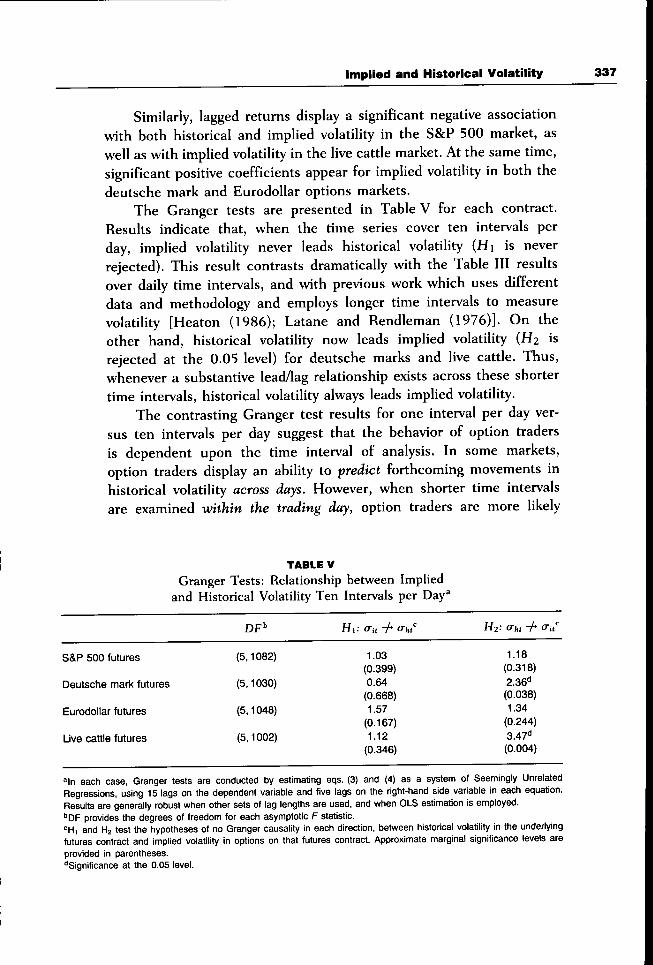
The Granger tests are presented in Tahle V for each contract.Results indicate that, when the time series cover ten intervals perday, implied volatility never leads historical volatility (Hi is neverrejected). This result contrasts dramatically vWth the Tahle III resultsover daily time intervals, and with previous work which uses differentdata and methodology and employs longer time intervals to measurevolatility [Heaton (1986); Latane and Rendleman (1976)]. On theother hand, historical volatility now leads implied volatility (H2 isrejected at the 0.05 level) for deutsche marks and live cattle. Thus,whenever a substantive lead/lag relationship exists across these shortertime intervals, historical volatility always leads implied volatility.

The contrasting Granger test results for one interval per day ver-sus ten intervals per day suggest that the hehavior of option tradersis dependent upon the time interval of analysis. In some markets,option traders display an ahility to predict forthcoming movements inhistorical volatility across days. However, when shorter time intervalsare examined within the trading day, option traders are more likely

TABLE VGranger Tests: Relationship between Implied

and Historical Volatility Ten Intervals per

S&P 500 futures

Deutsche mark futures

Eurodollar futures

Live cattle futures

(5,1082)

(5,1030)

(5,1048)

(5,1002)

H i : o-j, -/» at,,"

1.03(0.399)0.64

(0.668)1.57

(0.167)1.12

(0.346)

H2: o-fci -A a-i,"

1.18

(0.318)

2.36"(0.038)

1.34(0.244)

3.47"(0.004)

=ln each case. Granger tests are conducted by estimating eqs. (3) and (4) as a system of Seemingiy UnrelatedRegressions, using 15 iags on the dependent variable and five iags on the right-hand side variable in each equation.Results are generally robust when other sets of lag lengths are used, and when OLS estimation is employed."DF provides the degrees of freedom for each asymptotic F statistic.•̂ Hi and H2 test the hypotheses of no Granger causality in each direction, between historical volatility in the underlyingfutures contract and implied volatility in options on that futures contract. Approximate marginal significance levels areprovided in parentheses."Significance at the 0.05 level.


to respond to previous intraday short-term volatility conditions in theunderlying market.

Intraday Patterns in o'ht and

When analyzing ten intervals per day, larger volatility is anticipatedduring the first and last intervals each day. Although trading in thesemarkets is closed overnight during the sample period, new informationcontinuously accumulates and may he expected to influence tradingmore heavily at the market's open and close [Ahimud and Mendel-son (1987); Ekman (1992); Kawaller, Koch, and Koch (1990); Wood,Mclnish, and Ord (1985)].

A preliminary investigation of this possibility is conducted forall four markets, hy estimating an ordinary least squares regressionof each volatility measure on a time trend and ten intraday dummyvariahles. Results are presented in Panel A of Figures 1 -4 , for thefour markets examined. These results represent the systematic intradaypatterns in historical and implied volatility inherent in each market,before accounting for the intraday variation in each volatility measuredue to the other influences in the model.

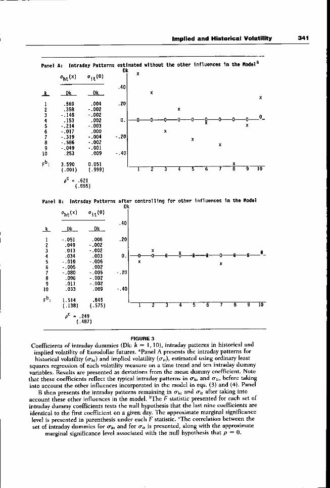
Scrutiny of Panel A in Figures 1, 3, and 4 reveals a distinct"U"-shaped pattern in historical volatility for these three markets andsignificant F-tests indicating that this pattern is statistically profound.This pattern is consistent with previous work [Ahimud and Mendelson(1987); Ekman (1992); Kawaller, Koch, and Koch (1990); and Wood,Mclnish, and Ord (1985)] and reflects significantly greater volatility atthe open and close of each day for these three markets. The intradaypattern for historical volatility of deutsche mark futures, in Panel A ofFigure 2, deviates somewhat from this "U" shape. This market revealssignificantly greater volatility at the beginning and middle of the typicaltrading day, followed hy declining volatility toward the day's close. Thispattern likely reflects the importance of trading out of London, whichtends to "close" between 11:00 AM and 12:00 noon, Chicago time. Also,note that for Eurodollars (in Fig. 3) some of the "London effect" still isapparent, although the effect seems less prominent here. On the otherhand, for live cattle and S&P markets (Figs. 1 and 4), London is muchless important and the London effect is not in evidence.

Scrutiny of the results for implied volatility in Panel A ofFigures 1-4 indicates no detectable patterns in this volatility measurefor any market. This result supports the intuition that options traders


Panel A: Intraday Patterns estimated without the other Influences In the Hodel*Dk

.25

.20

.15

.10

.05

0.

-.05

-.10

-.15

A.12345678910

pb.

Panel

PK.235.028

-.119-.121-.164-.104-.062.034.125.150

16.879(.001)

pC =

PK

-.

-.0.(.

.119

.724)

B: Intraday

004000000003002001001004002001

058999)

Patt

t(0)

9 10

Intraday Patterns after controlling for other Influences In the ModelDk

.25

_ k .

123456789

10

.106

.108

.105

.060

.028

.054

.071

.058

.093

.075

.915

.001)

Dk

.006-.003-.001

.002-.004

.003

.000-.004

.000

.000

1.672(.091)

.20

.15

.10

.05

0.

- .05

- .10

-.15

-0 0-

10

- . 2 3 5( .513)

FIGURE 1Coefficients of intraday dummies (Dk: fe = 1, 10), intraday patterns in historical and

implied volatility of S&P 500 futures. "Panel A presents the intraday patterns forhistorical volatility {a-t,t) and implied volatility (o-j,), estimated using ordinary least

squares regression of each volatility measure on a time trend and ten intraday dummyvariables. Results are presented as deviations from the mean dummy coefficient. Notethat these coefficients reflect the typical intraday patterns in o"),, and CTJ,, before takinginto account the other influences incorporated in the model in eqs. (3) and (4). Panel

B then presents the intraday patterns remaining in crj,, and an after taking intoaccount these other influences in the model. ""The F statistic presented for each set ofintraday dummy coefficients tests the null hypothesis that the last nine coefficients areidentical to the first coefficient on a given day. The approximate marginal significancelevel is presented in parenthesis under each F statistic. "̂ The correlation between theset of intraday dummies for aht and for au is presented, along with the approximate

marginal significance level associated with the null hypothesis that p = 0.


Panel A: Intraday Patterns estimated without the other Influences In theDk

X

.10JL Dk Dk

12345678910

pb.

.134

.040

.024

.058

.128

.035-.030-.153-.103-.133

4.763(.001)

pC ̂

(

.006

.001

.000

.000

.004

.004

.005-.002-.005-.013

0.238(.989)

.755

.012)

.05

0.

- .05

-.10

"1 T IT

Panel 8; Intraday Patterns after controlling for other Influences In the Model

Dk

"ufO)

_k-

12345678910

F":

Dk

-.119-.067-.006.029.081.032.041.003.020

-.015

4.183(.001)

p' =(

Ok

.004-.006.001.002.000.001.003

-.004-.002.000

.449(.908)

.056

.878)

.10

.05

0.

-.05

-.10

1 2 3 4 5 6 7 8 9

FIGURE 2Coefficients of intraday dummies (Dk: k = 1,10), intraday patterns in historical and

implied volatility of Deutsche mark futures. "Panel A presents the intraday patterns forhistorical volatility (aht) and implied volatility ((T;,), estimated using ordinary least

squares regression of each volatility measure on a time trend and ten intraday dummyvariables. Results are presented as deviations from the mean dummy coefficient. Notethat these coefficients reflect the typical intraday patterns in <7(,, and au, before takinginto account the other influences incorporated in the model in eqs. (3) and (4). Panel

B then presents the intraday patterns remaining in cr/,, and au after taking intoaccount these other influences in the model. ""The F statistic presented for each set ofintraday dummy coefficients tests the null hypothesis that the last nine coefficients areidentical to the first coefficient on a given day. The approximate marginal significancelevel is presented in parenthesis under each F statistic. "̂ The correlation between theset of intraday dummies for aht and for au is presented, along with the approximate



Panel A: Intraday Patterns estimated without the other Influences In the

X.123456789

10

pb.

Dk

.569

.358-.148

.153-.214-.017-.319-.586-.049

.253

3.590(.001)

(

Dk

--

-

---

0(

.621

.055)

.004

.002

.002

.002

.003

.000

.004

.002

.001

.009

.051

.999)

.40

.20

0.

-.20

-.40

1 2 5 4 5 6 7 8 9 l O "

Panel B: Intraday Patterns after controlling for other Influences In the ModelDk

A.123456789

10

-.051.049.013.034

- . 0 1 0- . 0 0 5- .080

.006

.011

.033

1.514(.138)

.006-.002-.002

.003-.006

.002-.005-.002-.002

.009

.845(.575)

= .249(.487)

.40

.20

0.

- .20

- .40

6 7 9 10

FIGURE 3

Coefficients of intraday dummies (Dk: fe = 1,10), intraday patterns in historical andimplied volatility of Eurodollar futures. °Panel A presents the intraday patterns forhistorical volatility (o-fc,) and implied volatility (o-j,), estimated using ordinary least

squares regression of each volatility measure on a time trend and ten intraday dummyvariables. Results are presented as deviations from the mean dummy coefficient. Notethat these coefficients reflect the typical intraday patterns in aht and au, before takinginto account the other influences incorporated in the model in eqs. (3) and (4). Panel

B then presents the intraday patterns remaining in aht and au after taking intoaccount these other influences in the model. ''The F statistic presented for each set ofintraday dummy coefficients tests the null hypothesis that the last nine coefficients areidentical to the first coefficient on a given day. The approximate marginal significancelevel is presented in parenthesis under each F statistic. "The correlation between theset of intraday dummies for aht and for CTU is presented, along with the approximate



Panel

Jc.

12345678910

F :

A: Intraday Patterns

Dk

.397

.050-.010-.051-.060-.138-.182-.156-.081.230

21.707(.001)

p<= = -

(

oî(0)

Dk

.001-.006.002

-.003.002

-.005.004.003.001.000

-0.204(.994)

.127

.726)

estimatedDk

.40

.20

11\. lU

0.

.10

.20

X

—0-

1

without the

X

—n Q0 X

2 3

other Influences In the Model^

X

-0 0 n 0 0 0 0-u

X XX

" XX

4 5 6 7 8 9 lo

Panel 8: Intraday Patterns af ter control l ing for other Influences In the ModelDk

o.AO) .40

.20

.10

0.

.10

.20

_k_

12345678910

F":

Dk

-.096-.028.000.022.023

-.011.000.030.053.007

1.002(.437)

/ =(

Dk

-.010-.011.003.001.012

-.005.012.004.000

-.007

2.938(.002)

.557

.095)

10

FIGURE 4Coefficients of intraday dummies (Dk: k = 1,10), intraday patterns in historical and

implied volatility of live cattle futures. "Panel A presents the intraday patterns forhistorical volatility (akt) and implied volatility (au), estimated using ordinary least

squares regression of each volatility measure on a time trend and ten intraday dummyvariahles. Results are presented as deviations from the mean dummy coefficient. Notethat these coefficients reflect the typical intraday patterns in aht and au, hefore takinginto account the other influences incorporated in the model in eqs. (3) and (4). Panel

B then presents the intraday patterns remaining in aht and au after taking intoaccount these other influences in the model. "The F statistic presented for each set ofintraday dummy coefficients tests the null hypothesis that the last nine coefficients areidentical to the Brst coefficient on a given day. The approximate marginal significancelevel is presented in parenthesis under each F statistic. '̂ The correlation hetween theset of intraday dummies for ay and for au is presented, along with the approximate



do not price the intraday patterns inherent in historical volatility forthese four futures markets.

The systematic daily patterns for historical volatility indicated inPanel A of Figures 1—4 reflect hehavior in each underlying market thatmust he accounted for in this model. For example, if futures volume isgreater at the heginning and close of the typical trading day, inclusionof futures volume in the historical volatility equation may explain asuhstantial portion of the "U"-shaped pattern appearing in three of thesemarkets. On the other hand, the right-hand side variahles included inthis model may not account for all of this intraday pattern.

This evidence points to the need for employing separate dummyvariahles for each intraday interval in hoth equations of the model in(5). The joint hypothesis that each equation's intercept for the first timeinterval is identical to that for the other nine intervals on a given dayis tested also. The coefficients of these dummy variahles should displayany intraday patterns remaining in the data, after accounting for theintraday variation in aht and a^ due to the other influences in themodel. The joint F-test should then reveal the statistical significance ofany such intraday patterns remaining after the inclusion of the model'sother parameters. It is crucial to use this dummy variahle approach toaccount for any such potential intraday patterns remaining in aht or au,so that one can sensihly estimate potential leadlag relationships acrossdays in the model. This prohlem is analogous to the need to "seasonallyadjust" when analyzing any data that display seasonality.

A priori, the dummy coefficients of the model in (5) are expected todisplay a much less distinct pattern than the patterns presented in PanelA of Figures 1—4. This is horn out in scrutiny of Panel B in Figures 3and 4, which reveal no distinct pattern in historical volatility aftercontrolling for the other influences in the model. Panel B of Figures 1and 2 similarly reveals a less notahle pattern in historical volatility giventhe model's other parameters. However, the plots and joint F testsindicate that the patterns for these two markets are still distinct. Forhoth S&P 500 futures and deutsche mark futures, this pattern suggestsa relatively low level of historical volatility at the heginning of the typicaltrading day, which increases throughout the day, after accounting forvolume changes and other intraday influences in the model.

CONCLUSIONS /;

This study addresses the question of whether intraday movements inimplied volatility lead or follow movements in historical volatility of the

344 Kawaiier, Koch, and Peterson

underlying instrument's return, after accounting for changes in tradingvolume. Put another way, the analysis is designed to assess: (a) whetheroption traders are ahle to make reliahle predictions ahout forthcomingmovements in the volatility of underlying returns; and/or (h) whetheroption traders respond to recent changes in historical volatility andadjust option prices accordingly. Futures contracts on the S&P 500index, deutsche mark. Eurodollars, and live cattle are examined alongwith their associated options. Matched time series in historical andimplied volatility are constructed from transactions data, using timeintervals of two different lengths: one interval per day and ten intervalsper day.

Results reveal a strong association hetween trading volume in eachfutures contract and historical volatility in the futures return, for hothtime intervals investigated. This result is consistent with previous work[Ekman (1992); Kawaller, Koch, and Koch (1990); Merrick (1987)],and it underscores the need to control for changes in volume whenattempting to uncover the lead/lag relationship hetween historical andimplied volatility. No stahle analogous relationship is evidenced hetweenvolume and implied volatility in option prices. This result may heattrihutahle to the forward-looking nature of implied volatility versusthe hackward-looking nature of historical volatility, or the possihility ofmore noise inherent in implied volatilities.

Concerning the issue of leads and lags hetween implied and histori-cal volatility, the analysis shows one area of consistency. When usingdata measured over ten intervals per day, implied volatility never leadshistorical volatility. Thus, on a very short-term hasis (within the courseof the day), option traders seem unahle to forecast impending volatilitychanges with any degree of reliahility. This conclusion, however, doesnot generally hold when the time interval is expanded to one-day periods,where an improved forecasting capahility for option traders is found insome markets.

When considering the possihility that historical volatility leadsimplied volatility, the results are inconsistent across markets. In thiscase, however, mixed results are shown for hoth time intervals. Thus,option traders may respond to recent changes in historical volatility; hutif they do so, the mechanism hy which they respond does not appear tohe systematic across all markets.

The inconsistencies shown in this study suggest it may he inap-propriate to generalize ahout these phenomena across markets; andthat conclusions hased on time intervals of one length may not applyfor alternative intervals hased on different lengths of time. It is also


important to emphasize that findings in this study may he reflective ofconditions pertaining to the fourth quarter of 1988 that may not herohust over time.

The final contrihution of the analysis deals with intraday patternsin volatility. Significant intraday patterns of historical volatility areohserved, hut no analogous rohust patterns are detected with impliedvolatility. Moreover, the pattern associated with historical volatilityreveals some variation across markets. While opening and closing timesare consistently associated with higher historical volatility, it should henoted that a midday (Chicago time) historical volatility "spike" occursin markets where suhstantial trading volume emanates from London.

BIBLIOGRAPHY

Ahimud, Y., and Mendelson, H. (1987, July): "Trading Mechanisms and StockReturns: An Empirical Investigation," Jowrmjl of Finance, 42:533—553.

Anderson, R. W., and Danthine, J.-P. (1983): "The Time Pattern of Hedging andthe Volatility of Futures Prices," Review of Economic Studies, 249—266.

Ball, C.A., and Torous, W. N. (1986): "Futures Options and the Volatility ofFutures Prices," Jowrmil of Finance, 41:857-870.

Beckers, S. (1981): "Standard Deviations Implied in Option Prices as Predic-tors of Future Stock Price Variability," Journal of Banking and Finance,5:363-381.

Black, F. (1976a, March): "The Pricing of Commodity Contracts," Jowmal ofFinancial Economics, 3:167—179.

Black, F. (1976b): "Studies of Stock Price Volatility Changes," Proceedings ofthe 1976 Meetings of the American Statistical Association, Business andEconomics Section, pp. 177—181.

Black, F., and Scholes, M. (1972, May): "The Valuation of Options Contractsand a Test of Market Efficiency," Jowmai of Finance, 27:399-418.

Black, F., and Scholes, M. (1973, May-June): "The Pricing of Options andCorporate Liabilities," JowrwaZ of Political Economy, 637-659.

Brenner, M., Courtadon, G., and Subrahmanyam, M. (1985): "Options on theSpot and Options on the Future," JowmaZ of Finance, 40:1303—1317.

Chiras, D., and Manaster, S. (1978): "The Information Content of OptionPrices and a Test of Market Efficiency," Journal of Financial Economics,6:213-234.

Ekman, P. (1992, August): "Intraday Patterns in the S&P 500 Index FuturesMarket," The Journal of Futures Markets, 12:365-381.

Franks, J.R., and Schwartz, E.S. (1988): "The Stochastic Behavior of MarketVariance Implied in the Prices of Index Options: Evidence on Leverage,Volume, and Other Effects," U.C.L.A. Working Paper #10-88, pp. 1-27.

Geweke, J. (1978, April): "Testing the Exogeneity Specification in the Com-plete Dynamic Simultaneous Equations Model," Journal of Econometrics,7:163-185.


Granger, C.W. (1969, July): "Investigating Causal Relations by EconometricModels and Cross-Spectral Methods," Econometrica, 37:424-438.

Han, L.M., and Misra, L. (1990): "The Relationship Between the Volatilitiesof the S&P 500 Index and Futures Contracts Implicit in Their Call OptionPrices," The Journal of Futures Markets, 10:273-285.

Harris, L. (1987): "Transaction Data Tests of the Mixture of DistributionsHypothesis," Jowrmii of Financial and Quantitative Analysis, 22:127-141.

Heaton, H. (1986): "Volatilities Implied by Options Premium: A Test of MarketEfficiency," Financial Review, 21:37—49.

Johnston, J. (1984): Econometric Methods (3rd ed.). New York: McGraw-Hill.Judge, G., et al. (1985): The Theory and Practice of Econometrics. New York:

Wiley.Kawaller, I.G., Koch, P. D., and Koch, T.W. (1990, July): "Intraday Relation-

ships Between Volatility in S&P 500 Futures Prices and the S&P 500Index," JoMmai of Banking and Finance, 14:373—397.

Latane, H., and Rendleman, Jr., R.J. (1976, May): "Standard Deviationsof Stock Price Ratios Implied in Options Prices," Journal of Finance,31:369-382.

Ljung, G. M., and Box, G. E. P. (1978): "On a Measure of Lack of Fit in TimeSeries Models," Biometrika, 65:297-303.

Manaster, S., and Rendleman, R. (1982): "Option Prices as Predictors ofEquilibrium Stock Prices," Jowrwai of Finance, 37:1043-1058.

Merrick, J. (1987, January): "Volume Determination in Stock and Stock IndexFutures Markets: An Analysis of Arbitrage and Volatility Effects," FederalReserve Bank of Philadelphia Working Paper No. 87-2, pp. 1 -24.

Park, H. Y., and Sears, R. S. (1985): "Estimating Stock Index Futures VolatilityThrough the Prices of Their Options," The Journal of Futures Markets,5:223-238.

Poterba, J. M., and Summers, L. H. (1986): "The Persistence of Volatility inStock Market Fluctuations," American Economic Review, 76:1142—1151.

Samuelson, P. (1965, August): "Proof tbat Properly Anticipated Prices Fluctu-ate Randomly," Industrial Management Review, 6:41-49.

Theil, H. (1971): Principles of Econometrics. New York: Wiley.Wiggins, J. (1987, December): "Option Values Under Stochastic Volatility:

Theory and Empirical Estimates," Journal of Financial Economics,19:351-372.

Wilson, W.W., and Fung, H.G. (1990, February): "Information Content ofVolatilities Implied by Option Premiums in Grain Futures Markets," TheJournal of Futures Markets, 10:13-28.

Wood, R., Mclnish, T., and Ord, J.K. (1985, July): "An Investigation ofTransactions Data for NYSE Stocks," JowmaZ of Finance, 40:723-739.

RELATIONSHIP BETWEEN VOLATILITY...Implied volatility is thus a forward-looking measure of likely future volatility conditions. On the other hand, historical volatility is a hackward-looking

Documents