REGRESSION LINES IN STATA THOMAS ELLIOTT 1. Introduction to Regression Regression analysis is about exploring linear relationships between a dependent variable and one or more independent variables. Regression models can be represented by graphing a line on a cartesian plane. Think back on your high school geometry to get you through this next part. Suppose we have the following points on a line: x y -1 -5 0 -3 1 -1 2 1 3 3 What is the equation of the line? y = α + βx β = Δy Δx = 3 - 1 3 - 2 =2 α = y - βx =3 - 2(3) = -3 y = -3+2x If we input the data into STATA, we can generate the coefficients automatically. The com- mand for finding a regression line is regress. The STATA output looks like: Date : January 30, 2013. 1

Welcome message from author
This document is posted to help you gain knowledge. Please leave a comment to let me know what you think about it! Share it to your friends and learn new things together.
Transcript
REGRESSION LINES IN STATA
THOMAS ELLIOTT
1. Introduction to Regression
Regression analysis is about exploring linear relationships between a dependent variable andone or more independent variables. Regression models can be represented by graphing a lineon a cartesian plane. Think back on your high school geometry to get you through this nextpart.
Suppose we have the following points on a line:
x y-1 -50 -31 -12 13 3
What is the equation of the line?
y = α + βx
β =∆y
∆x=
3 − 1
3 − 2= 2
α = y − βx = 3 − 2(3) = −3
y = −3 + 2x
If we input the data into STATA, we can generate the coefficients automatically. The com-mand for finding a regression line is regress. The STATA output looks like:
Date: January 30, 2013.1
2 THOMAS ELLIOTT
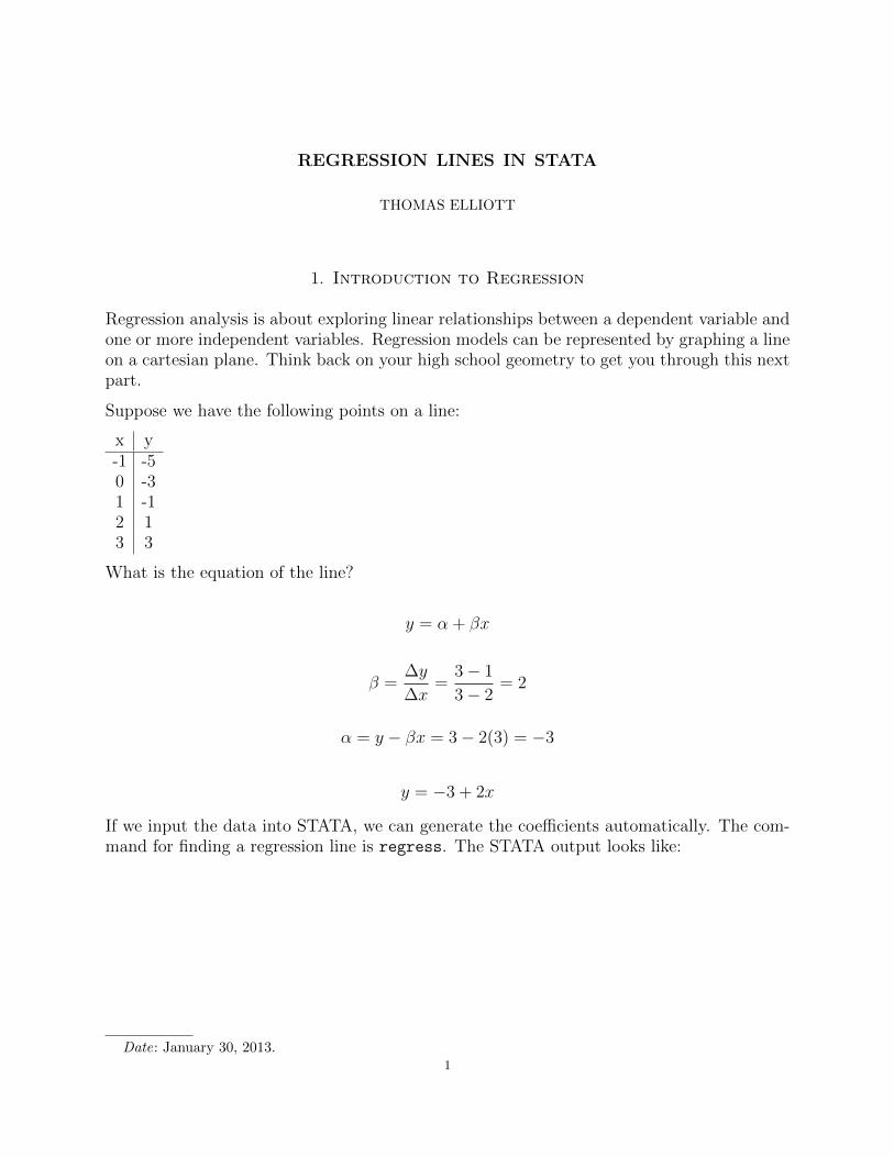
. regress y x
Source | SS df MS Number of obs = 5
-------------+------------------------------ F( 1, 3) = .
Model | 40 1 40 Prob > F = .
Residual | 0 3 0 R-squared = 1.0000
-------------+------------------------------ Adj R-squared = 1.0000
Total | 40 4 10 Root MSE = 0
------------------------------------------------------------------------------
y | Coef. Std. Err. t P>|t| [95% Conf. Interval]
-------------+----------------------------------------------------------------
x | 2 . . . . .
_cons | -3 . . . . .
------------------------------------------------------------------------------
The first table shows the various sum of squares, degrees of freedom, and such used tocalculate the other statistics. In the top table on the right lists some summary statistics ofthe model including number of observations, R2 and such. However, the table we will focusmost of our attention on is the bottom table. Here we find the coefficients for the variablesin the model, as well as standard errors, p-values, and confidence intervals.
In this particular regression model, we find the x coefficient (β) is equal to 2 and the constant(α) is -3. This matches the equation we calculated earlier. Notice that no standard errorsare reported. This is because the data fall exactly on the line so there is zero error. Alsonotice that the R2 term is exactly equal to 1.0, indicating a perfect fit.
Now, let’s work with some data that are not quite so neat. We’ll use the hire771.dta
data.
use hire771
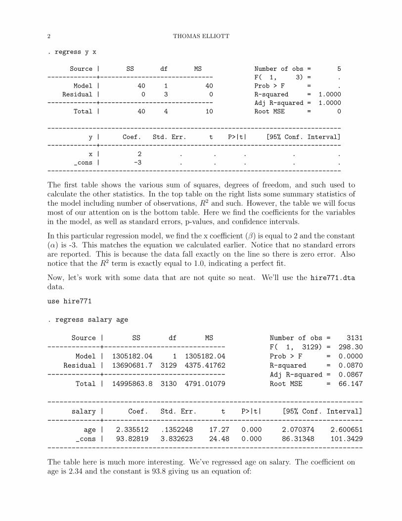
. regress salary age
Source | SS df MS Number of obs = 3131
-------------+------------------------------ F( 1, 3129) = 298.30
Model | 1305182.04 1 1305182.04 Prob > F = 0.0000
Residual | 13690681.7 3129 4375.41762 R-squared = 0.0870
-------------+------------------------------ Adj R-squared = 0.0867
Total | 14995863.8 3130 4791.01079 Root MSE = 66.147
------------------------------------------------------------------------------
salary | Coef. Std. Err. t P>|t| [95% Conf. Interval]
-------------+----------------------------------------------------------------
age | 2.335512 .1352248 17.27 0.000 2.070374 2.600651
_cons | 93.82819 3.832623 24.48 0.000 86.31348 101.3429
------------------------------------------------------------------------------
The table here is much more interesting. We’ve regressed age on salary. The coefficient onage is 2.34 and the constant is 93.8 giving us an equation of:
REGRESSION LINES IN STATA 3
salary = 93.8 + 2.34age
How do we interpret this? For every year older someone is, they are expected to receiveanother $2.34 a week. A person with age zero is expected to make $93.8 a week. We canfind the salary of someone given their age by just plugging in the numbers into the aboveequation. So a 25 year old is expected to make:
salary = 93.8 + 2.34(25) = 152.3
Looking back at the results tables, we find more interesting things. We have standard errorsfor the coefficient and constant because the data are messy, they do not fall exactly on theline, generating some error. If we look at the R2 term, 0.087, we find that this line is not avery good fit for the data.
4 THOMAS ELLIOTT
2. Testing Assumptions
The OLS regression model requires a few assumptions to work. These are primarily concernedwith the residuals of the model. The residuals are the same as the error - the vertical distanceof each data point from the regression line. The assumptions are:
• Homoscedasticity - the probability distribution of the errors has constant variance
• Independence of errors - the error values are statistically independent of eachother
• Normality of error - error values are normally distributed for any given value of x
The easiest way to test these assumptions are simply graphing the residuals on x and seewhat patterns emerge. You can have STATA create a new variable containing the residualfor each case after running a regression using the predict command with the residual
option. Again, you must first run a regression before running the predict command.
regress y x1 x2 x3
predict res1, r
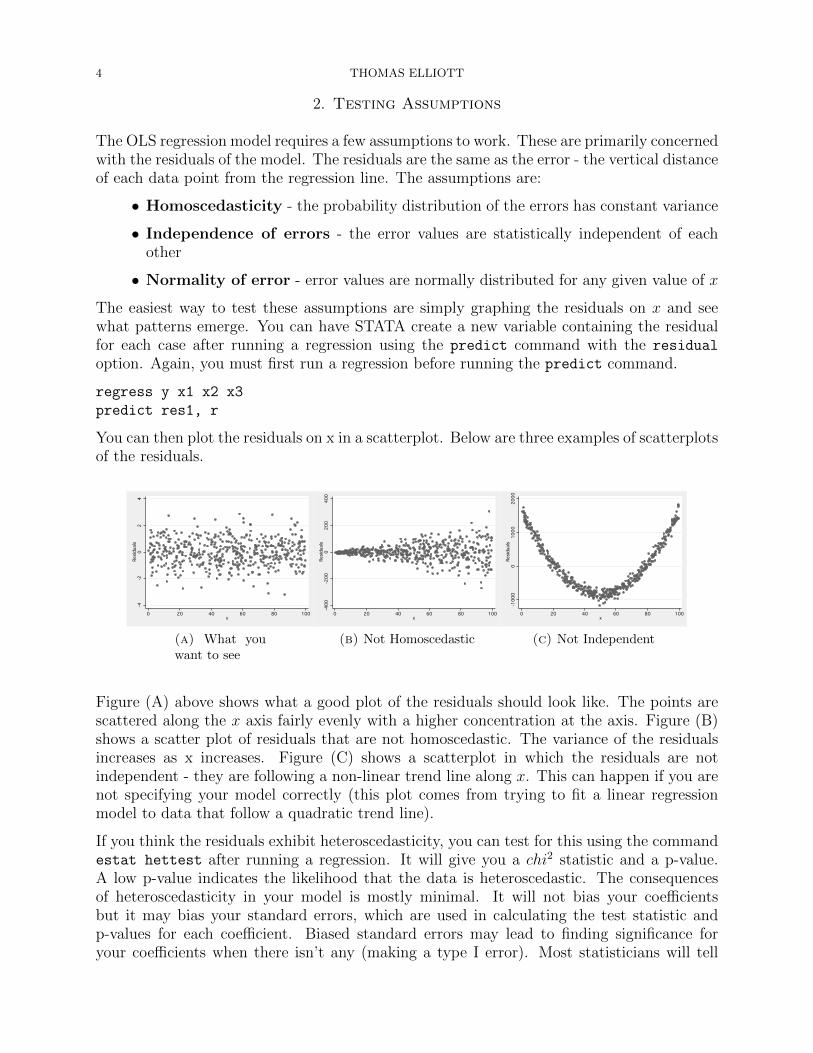
You can then plot the residuals on x in a scatterplot. Below are three examples of scatterplotsof the residuals.
-4
-4
-4-2
-2
-20
0
02
2
24
4
4Residuals
Resid
uals
Residuals0
0
020
20
2040
40
4060
60
6080
80
80100
100
100x
x
x
(a) What youwant to see
-400
-400
-400-200
-200
-2000
0
0200
200
200400
400
400Residuals
Resid
uals
Residuals0
0
020
20
2040
40
4060
60
6080
80
80100
100
100x
x
x
(b) Not Homoscedastic
-1000
-100
0
-10000
0
01000
1000
10002000
2000
2000Residuals
Resid
uals
Residuals0
0
020
20
2040
40
4060
60
6080
80
80100
100
100x
x
x
(c) Not Independent
Figure (A) above shows what a good plot of the residuals should look like. The points arescattered along the x axis fairly evenly with a higher concentration at the axis. Figure (B)shows a scatter plot of residuals that are not homoscedastic. The variance of the residualsincreases as x increases. Figure (C) shows a scatterplot in which the residuals are notindependent - they are following a non-linear trend line along x. This can happen if you arenot specifying your model correctly (this plot comes from trying to fit a linear regressionmodel to data that follow a quadratic trend line).
If you think the residuals exhibit heteroscedasticity, you can test for this using the commandestat hettest after running a regression. It will give you a chi2 statistic and a p-value.A low p-value indicates the likelihood that the data is heteroscedastic. The consequencesof heteroscedasticity in your model is mostly minimal. It will not bias your coefficientsbut it may bias your standard errors, which are used in calculating the test statistic andp-values for each coefficient. Biased standard errors may lead to finding significance foryour coefficients when there isn’t any (making a type I error). Most statisticians will tell
REGRESSION LINES IN STATA 5
you that you should only worry about heteroscedasticity if it is pretty severe in your data.There are a variaty of fixes (most of them complicated) but one of the easiest is specifyingvce(robust) as an option in your regression command. This uses a more robust methodto calculate standard errors that is less likely to be biased by a number of things, includingheteroscedasticity.
If you find a pattern in the residual plot, then you’ve probably misspecified your regressionmodel. This can happen when you try to fit a linear model to non-linear data. Take anotherlook at the scatterplots for your dependent and independent variables to see if any non-linearrelationships emerge. We’ll spend some time in future labs going over how to fit non-linearrelationships with a regression model.
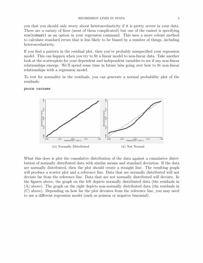
To test for normality in the residuals, you can generate a normal probability plot of theresiduals:
pnorm varname
0.00
0.00
0.000.25
0.25
0.250.50
0.50
0.500.75
0.75
0.751.00
1.00
1.00Normal F[(res1-m)/s]
Norm
al F
[(re
s1-m
)/s]
Normal F[(res1-m)/s]0.00
0.00
0.000.25
0.25
0.250.50
0.50
0.500.75
0.75
0.751.00
1.00
1.00Empirical P[i] = i/(N+1)
Empirical P[i] = i/(N+1)
Empirical P[i] = i/(N+1)
(d) Normally Distributed
0.00
0.00
0.000.25
0.25
0.250.50
0.50
0.500.75
0.75
0.751.00
1.00
1.00Normal F[(res4-m)/s]
Norm
al F
[(re
s4-m
)/s]
Normal F[(res4-m)/s]0.00
0.00
0.000.25
0.25
0.250.50
0.50
0.500.75
0.75
0.751.00
1.00
1.00Empirical P[i] = i/(N+1)
Empirical P[i] = i/(N+1)
Empirical P[i] = i/(N+1)
(e) Not Normal
What this does is plot the cumulative distribution of the data against a cumulative distri-bution of normally distributed data with similar means and standard deviation. If the dataare normally distributed, then the plot should create a straight line. The resulting graphwill produce a scatter plot and a reference line. Data that are normally distributed will notdeviate far from the reference line. Data that are not normally distributed will deviate. Inthe figures above, the graph on the left depicts normally distributed data (the residuals in(A) above). The graph on the right depicts non-normally distributed data (the residuals in(C) above). Depending on how far the plot deviates from the reference line, you may needto use a different regression model (such as poisson or negative binomial).
6 THOMAS ELLIOTT
3. Interpreting Coefficients
Using the hire771 dataset, the average salary for men and women is:
Table 1. Average Salary
Avg. SalaryMale 218.39Female 145.56Total 156.80
We can run a regression of salary on sex with the following equation:
Salary = α + βSex
Salary = 218.39 − 72.83Sex
Remember that regression is a method of averages, predicting the average salary given valuesof x. So from this equation, we can calculate what the predicted average salary for men andwomen would be from this equation:
Table 2. Predicted Salary
equation predicted salaryMale x = 0 α 218.39Female x = 1 α + β 146.56
How might we interpret these coefficients? We can see that α is equal to the average salaryfor men. α is always the predicted average salary when all x values are equal to zero. βis the effect that x has on y. In the above equation, x is only ever zero or one so we caninterpret the β as the effect on predicted average salary when x is one. So the predictedaverage salary when x is zero, or for men, is $218.39 a week. When x is one, or for women,the average predicted salary decreases by $72.83 a week (remember that β is negative). Sowomen are, on average, making $72.83 less per week than men.
Remember: this only works for single regression with a dummy variable. Using a continuousvariable or including other independent variables will not yield cell averages. Quickly, let’ssee what happens when we include a second dummy variable:
Salary = α + βsexxsex + βHOxHO
Salary = 199.51 − 59.75xsex + 47.25xHO
REGRESSION LINES IN STATA 7
Table 3. Average Salaries
Male FemaleField Office 211.46 138.27Home Office 228.80 197.68
Table 4. Predicted Salaries
Male Female
Field Officeα α + βsex
199.51 139.76
Home Officeα + βHO α + βsex + βHO
246.76 187.01
We can see that the average salaries are not given using the regression method. As we learnedin lecture, this is because we only have three coefficients to find four average salaries. Moreintuitively, the regression is assuming equal slopes for the four different groups. In otherwords, the effect of sex on salary is the same for people in the field office and in the homeoffice. Additionally, the effect of office location is the same for both men and women. If wewant the regression to accurately reflect the cell averages, we should allow the slope of onevariable to vary for the categories of the other variables by including an interaction term(see interaction handout). Including an interacting term between sex and home office willreproduce the cell averages accurately.
8 THOMAS ELLIOTT
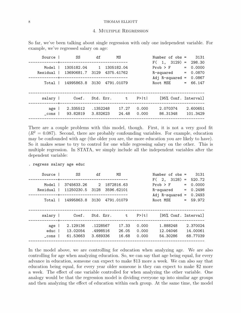
4. Multiple Regression
So far, we’ve been talking about single regression with only one independent variable. Forexample, we’ve regressed salary on age:
Source | SS df MS Number of obs = 3131
-------------+------------------------------ F( 1, 3129) = 298.30
Model | 1305182.04 1 1305182.04 Prob > F = 0.0000
Residual | 13690681.7 3129 4375.41762 R-squared = 0.0870
-------------+------------------------------ Adj R-squared = 0.0867
Total | 14995863.8 3130 4791.01079 Root MSE = 66.147
------------------------------------------------------------------------------
salary | Coef. Std. Err. t P>|t| [95% Conf. Interval]
-------------+----------------------------------------------------------------
age | 2.335512 .1352248 17.27 0.000 2.070374 2.600651
_cons | 93.82819 3.832623 24.48 0.000 86.31348 101.3429
------------------------------------------------------------------------------
There are a couple problems with this model, though. First, it is not a very good fit(R2 = 0.087). Second, there are probably confounding variables. For example, educationmay be confounded with age (the older you are, the more education you are likely to have).So it makes sense to try to control for one while regressing salary on the other. This ismultiple regression. In STATA, we simply include all the independent variables after thedependent variable:
. regress salary age educ
Source | SS df MS Number of obs = 3131
-------------+------------------------------ F( 2, 3128) = 520.72
Model | 3745633.26 2 1872816.63 Prob > F = 0.0000
Residual | 11250230.5 3128 3596.62101 R-squared = 0.2498
-------------+------------------------------ Adj R-squared = 0.2493
Total | 14995863.8 3130 4791.01079 Root MSE = 59.972
------------------------------------------------------------------------------
salary | Coef. Std. Err. t P>|t| [95% Conf. Interval]
-------------+----------------------------------------------------------------
age | 2.129136 .1228567 17.33 0.000 1.888248 2.370024
educ | 13.02054 .4998516 26.05 0.000 12.04046 14.00061
_cons | 61.53663 3.689336 16.68 0.000 54.30286 68.77039
------------------------------------------------------------------------------
In the model above, we are controlling for education when analyzing age. We are alsocontrolling for age when analyzing education. So, we can say that age being equal, for everyadvance in education, someone can expect to make $13 more a week. We can also say thateducation being equal, for every year older someone is they can expect to make $2 morea week. The effect of one variable controlled for when analyzing the other variable. Oneanalogy would be that the regression model is dividing everyone up into similar age groupsand then analyzing the effect of education within each group. At the same time, the model
REGRESSION LINES IN STATA 9
is dividing everyone into groups of similar education and then analyzing the effect of agewithin each group. This isn’t a perfect analogy, but it helps to visualize what it means whenwe say the regression model is finding the effect of age on salary controlling for educationand vice versa.
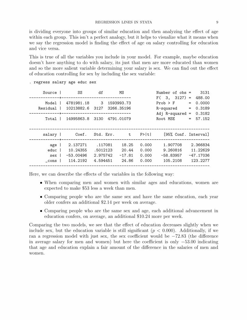
This is true of all the variables you include in your model. For example, maybe educationdoesn’t have anything to do with salary, its just that men are more educated than womenand so the more salient variable determining your salary is sex. We can find out the effectof education controlling for sex by including the sex variable:
. regress salary age educ sex
Source | SS df MS Number of obs = 3131
-------------+------------------------------ F( 3, 3127) = 488.00
Model | 4781981.18 3 1593993.73 Prob > F = 0.0000
Residual | 10213882.6 3127 3266.35196 R-squared = 0.3189
-------------+------------------------------ Adj R-squared = 0.3182
Total | 14995863.8 3130 4791.01079 Root MSE = 57.152
------------------------------------------------------------------------------
salary | Coef. Std. Err. t P>|t| [95% Conf. Interval]
-------------+----------------------------------------------------------------
age | 2.137271 .117081 18.25 0.000 1.907708 2.366834
educ | 10.24355 .5012123 20.44 0.000 9.260816 11.22629
sex | -53.00496 2.975742 -17.81 0.000 -58.83957 -47.17036
_cons | 114.2192 4.594451 24.86 0.000 105.2108 123.2277
------------------------------------------------------------------------------
Here, we can describe the effects of the variables in the following way:
• When comparing men and women with similar ages and educations, women areexpected to make $53 less a week than men.
• Comparing people who are the same sex and have the same education, each yearolder confers an additional $2.14 per week on average.
• Comparing people who are the same sex and age, each additional advancement ineducation confers, on average, an additional $10.24 more per week.
Comparing the two models, we see that the effect of education decreases slightly when weinclude sex, but the education variable is still significant (p < 0.000). Additionally, if weran a regression model with just sex, the sex coefficient would be −72.83 (the differencein average salary for men and women) but here the coefficient is only −53.00 indicatingthat age and education explain a fair amount of the difference in the salaries of men andwomen.
10 THOMAS ELLIOTT
5. Quadratic Terms
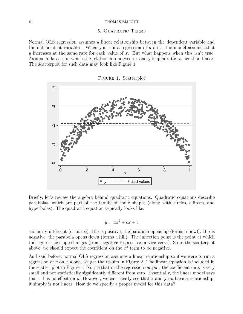
Normal OLS regression assumes a linear relationship between the dependent variable andthe independent variables. When you run a regression of y on x, the model assumes thaty increases at the same rate for each value of x. But what happens when this isn’t true.Assume a dataset in which the relationship between x and y is quadratic rather than linear.The scatterplot for such data may look like Figure 1.
Figure 1. Scatterplot0
0
0.1
.1
.1.2
.2
.2.3
.3
.3.4
.4
.40
0
0.2
.2
.2.4
.4
.4.6
.6
.6.8
.8
.81
1
1x
x
xy
y
yFitted values
Fitted values
Fitted values
Briefly, let’s review the algebra behind quadratic equations. Quadratic equations describeparabolas, which are part of the family of conic shapes (along with circles, ellipses, andhyperbolas). The quadratic equation typically looks like:
y = ax2 + bx+ c
c is our y-intercept (or our α). If a is positive, the parabola opens up (forms a bowl). If a isnegative, the parabola opens down (forms a hill). The inflection point is the point at whichthe sign of the slope changes (from negative to positive or vice versa). So in the scatterplotabove, we should expect the coefficient on the x2 term to be negative.
As I said before, normal OLS regression assumes a linear relationship so if we were to run aregression of y on x alone, we get the results in Figure 2. The linear equation is included inthe scatter plot in Figure 1. Notice that in the regression output, the coefficient on x is verysmall and not statistically significantly different from zero. Essentially, the linear model saysthat x has no effect on y. However, we can clearly see that x and y do have a relationship,it simply is not linear. How do we specify a proper model for this data?
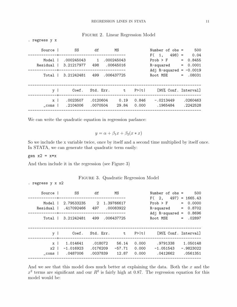
REGRESSION LINES IN STATA 11
Figure 2. Linear Regression Model. regress y x
Source | SS df MS Number of obs = 500
-------------+------------------------------ F( 1, 498) = 0.04
Model | .000245043 1 .000245043 Prob > F = 0.8455
Residual | 3.21217977 498 .00645016 R-squared = 0.0001
-------------+------------------------------ Adj R-squared = -0.0019
Total | 3.21242481 499 .006437725 Root MSE = .08031
------------------------------------------------------------------------------
y | Coef. Std. Err. t P>|t| [95% Conf. Interval]
-------------+----------------------------------------------------------------
x | .0023507 .0120604 0.19 0.846 -.0213449 .0260463
_cons | .2104006 .0070504 29.84 0.000 .1965484 .2242528
------------------------------------------------------------------------------
We can write the quadratic equation in regression parlance:
y = α + β1x+ β2(x ∗ x)
So we include the x variable twice, once by itself and a second time multiplied by itself once.In STATA, we can generate that quadratic term easily:
gen x2 = x*x
And then include it in the regression (see Figure 3)
Figure 3. Quadratic Regression Model. regress y x x2
Source | SS df MS Number of obs = 500
-------------+------------------------------ F( 2, 497) = 1665.43
Model | 2.79533235 2 1.39766617 Prob > F = 0.0000
Residual | .417092466 497 .00083922 R-squared = 0.8702
-------------+------------------------------ Adj R-squared = 0.8696
Total | 3.21242481 499 .006437725 Root MSE = .02897
------------------------------------------------------------------------------
y | Coef. Std. Err. t P>|t| [95% Conf. Interval]
-------------+----------------------------------------------------------------
x | 1.014641 .018072 56.14 0.000 .9791338 1.050148
x2 | -1.016923 .0176209 -57.71 0.000 -1.051543 -.9823022
_cons | .0487006 .0037839 12.87 0.000 .0412662 .0561351
------------------------------------------------------------------------------
And we see that this model does much better at explaining the data. Both the x and thex2 terms are significant and our R2 is fairly high at 0.87. The regression equation for thismodel would be:
12 THOMAS ELLIOTT
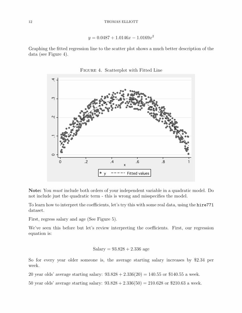
y = 0.0487 + 1.0146x− 1.0169x2
Graphing the fitted regression line to the scatter plot shows a much better description of thedata (see Figure 4).
Figure 4. Scatterplot with Fitted Line0
0
0.1
.1
.1.2
.2
.2.3
.3
.3.4
.4
.40
0
0.2
.2
.2.4
.4
.4.6
.6
.6.8
.8
.81
1
1x
x
xy
y
yFitted values
Fitted values
Fitted values
Note: You must include both orders of your independent variable in a quadratic model. Donot include just the quadratic term - this is wrong and misspecifies the model.
To learn how to interpret the coefficients, let’s try this with some real data, using the hire771dataset.
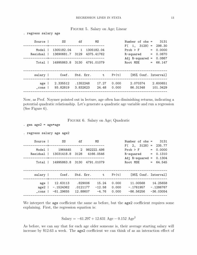
First, regress salary and age (See Figure 5).
We’ve seen this before but let’s review interpreting the coefficients. First, our regressionequation is:
Salary = 93.828 + 2.336 age
So for every year older someone is, the average starting salary increases by $2.34 perweek.
20 year olds’ average starting salary: 93.828 + 2.336(20) = 140.55 or $140.55 a week.
50 year olds’ average starting salary: 93.828 + 2.336(50) = 210.628 or $210.63 a week.
REGRESSION LINES IN STATA 13
Figure 5. Salary on Age; Linear. regress salary age
Source | SS df MS Number of obs = 3131
-------------+------------------------------ F( 1, 3129) = 298.30
Model | 1305182.04 1 1305182.04 Prob > F = 0.0000
Residual | 13690681.7 3129 4375.41762 R-squared = 0.0870
-------------+------------------------------ Adj R-squared = 0.0867
Total | 14995863.8 3130 4791.01079 Root MSE = 66.147
------------------------------------------------------------------------------
salary | Coef. Std. Err. t P>|t| [95% Conf. Interval]
-------------+----------------------------------------------------------------
age | 2.335512 .1352248 17.27 0.000 2.070374 2.600651
_cons | 93.82819 3.832623 24.48 0.000 86.31348 101.3429
------------------------------------------------------------------------------
Now, as Prof. Noymer pointed out in lecture, age often has diminishing returns, indicating apotential quadratic relationship. Let’s generate a quadratic age variable and run a regression(See Figure 6).
Figure 6. Salary on Age; Quadratic. gen age2 = age*age
. regress salary age age2
Source | SS df MS Number of obs = 3131
-------------+------------------------------ F( 2, 3128) = 235.77
Model | 1964445 2 982222.498 Prob > F = 0.0000
Residual | 13031418.8 3128 4166.0546 R-squared = 0.1310
-------------+------------------------------ Adj R-squared = 0.1304
Total | 14995863.8 3130 4791.01079 Root MSE = 64.545
------------------------------------------------------------------------------
salary | Coef. Std. Err. t P>|t| [95% Conf. Interval]
-------------+----------------------------------------------------------------
age | 12.63113 .829006 15.24 0.000 11.00568 14.25658
age2 | -.1524362 .0121177 -12.58 0.000 -.1761957 -.1286767
_cons | -61.29655 12.88607 -4.76 0.000 -86.56256 -36.03054
------------------------------------------------------------------------------
We interpret the age coefficient the same as before, but the age2 coefficient requires someexplaining. First, the regression equation is:
Salary = −61.297 + 12.631 Age − 0.152 Age2
As before, we can say that for each age older someone is, their average starting salary willincrease by $12.63 a week. The age2 coefficient we can think of as an interaction effect of
14 THOMAS ELLIOTT
age on itself. For each year older someone is, the effect of age decreases by 0.152 so thedifference in average starting salary for 21 year olds over 20 year olds is bigger than thedifference between 51 and 50.
Average starting salary for 20 year olds is: −61.297+12.631(20)−0.152(202) = 130.523
Average starting salary for 50 year olds is: −61.297+12.631(50)−0.152(502) = 190.253
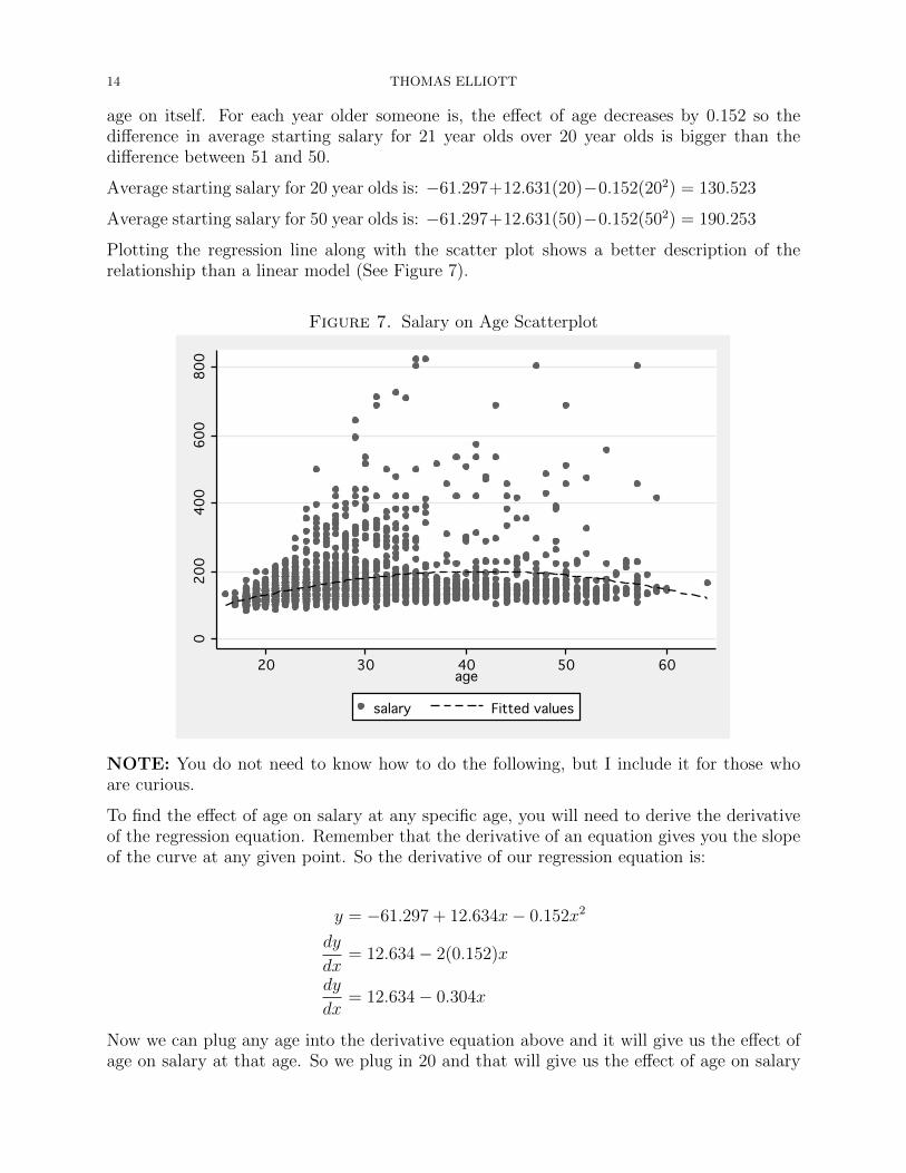
Plotting the regression line along with the scatter plot shows a better description of therelationship than a linear model (See Figure 7).
Figure 7. Salary on Age Scatterplot0
0
0200
200
200400
400
400600
600
600800
800
80020
20
2030
30
3040
40
4050
50
5060
60
60age
age
agesalary
salary
salaryFitted values
Fitted values
Fitted values
NOTE: You do not need to know how to do the following, but I include it for those whoare curious.
To find the effect of age on salary at any specific age, you will need to derive the derivativeof the regression equation. Remember that the derivative of an equation gives you the slopeof the curve at any given point. So the derivative of our regression equation is:
y = −61.297 + 12.634x− 0.152x2
dy
dx= 12.634 − 2(0.152)x
dy
dx= 12.634 − 0.304x
Now we can plug any age into the derivative equation above and it will give us the effect ofage on salary at that age. So we plug in 20 and that will give us the effect of age on salary

REGRESSION LINES IN STATA 15
when one moves from 20 to 21 (more or less). Similarly, plugging in 50 will give us the effectof age on salary when one moves from 50 to 51:
dy
dx= 12.634 − 0.304(20) = 6.554
dy
dx= 12.634 − .304(50) = −2.566
So according to the results above, moving from 20 to 21 is expected to add $6.55 per weekto one’s salary on average. However, moving from 50 to 51 is expected to subtract $2.57per week from one’s salary on average. So age is beneficial to salary until some age between20 and 50, after which increases in age will decrease salary. The point at which the effectof age switches from positive to negative is the inflection point (the very top of the curve).The effect of age at this point will be zero as it transitions from positive to negative. Wecan find the age at which this happens by substituting in zero for the slope:
0 = 12.634 − 0.304x
x =12.634
0.304= 41.55
So increases in age adds to one’s salary until 41 years, after which age subtracts from salary.Remember: this data is starting salary for 3000 new employees at the firm so people are notgetting pay cuts when they get older. Rather, the firm is offering lower starting salaries topeople who are older than 41 years than people who are around 41 years old.
Related Documents


![[Bruderl] Applied Regression Analysis Using Stata](https://static.cupdf.com/doc/110x72/55cf96a7550346d0338ce88d/bruderl-applied-regression-analysis-using-stata.jpg)