Quantum Electrodynamics - CAS · Quantum Electrodynamics Ling-Fong Li (Institute) Slide_06 QED 1 / 35. Quantum Electrodynamics Lagrangian density for QED , L= y(x)gm i ...

Quantum Electrodynamics

Ling-Fong Li

(Institute) Slide_06 QED 1 / 35

Quantum ElectrodynamicsLagrangian density for QED ,

L = ψ (x ) γµ(i∂µ − eAµ

)ψ (x )−mψ (x )ψ (x )− 1

4FµνF µν

Equations of motion are(iγµ∂µ −m

)ψ (x ) = eAµγµψ non-linear coupled equations

∂υF µν = eψγµψ

QuantizationWrite L= L0 + Lint

L0 = ψ(iγµ∂µ −m

)ψ− 1

4FµνF µν

Lint = −eψγµψAµ

where L0 ,free field Lagrangian, Lint is interaction part.Conjugate momenta for fermion

∂L∂ (∂0ψα)

= iψ†α (x )

For em fields choose the gauge−→∇ · −→A = 0

Conjugate mometa


πi =∂L

∂ (∂0Ai )= −F 0i = E i

From equation of motion

∂νF 0ν = eψ†ψ =⇒ −∇2A0 = eψ†ψ

A0 is not an independent field ,

A0 = e∫d 3x

′ ψ† (x ′, t)ψ (x ′, t)

4π|−→x ′ −−→x |

= e∫ d 3x

′ρ (x ′, t)

|−→x −−→x ′ |

Commutation relations

ψα (−→x , t) ,ψ†

β

(−→x ′ , t

) = δαβδ3

(−→x −−→x ′ ) ψα (−→x , t) ,ψβ

(−→x ′ , t

) = ... = 0[

Ai (−→x , t) ,Aj

(−→x ′ , t

)]= iδtrij

(−→x −−→x ′ )where

δtrij (~x −~y ) =∫ d 3k(2π)3

e i~k ·(~x−~y )(δij −ki kjk 2)

Commutators involving A0

[A0 (−→x , t) ,ψα

(−→x ′ , t

)]= e

∫ d 3x′′

4π|−→x −−→x ′′ |

[ψ†(−→x ′′ , t

)ψ(−→x ′′ , t

),ψα

(−→x ′ , t

)]= − e

4π

ψα

(−→x ′ , t

)|−→x −

−→x ′ |

Hamiltonian density


H =∂L

∂ (∂0ψα)ψα +

∂L∂ (∂0Ak )

Ak −L

= ψ†(−i−→α · −→∇ + βm

)ψ+

12

(−→E 2 +

−→B 2)+−→E · −→∇A0 + eψγµψAµ

and

H =∫d 3xH =

∫d 3xψ†

[−→α · (−i−→∇ − e−→A ) + βm]

ψ+12

(−→E 2 +

−→B 2)

A0 does not appear in the interaction,But if we write

−→E =

−→El +

−→Et where

−→El = −

−→∇A0 ,−→Et = −

∂−→A

∂t

Then

12

∫d 3x

(−→E 2 +

−→B 2)=12

∫d 3x−→El 2 +

∫d 3x

(−→Et 2 +

−→B 2)

longitudinal part is

12

∫d 3x−→El 2 =

e4π

∫d 3xd 3y

ρ (−→x , t) ρ (−→y , t)|−→x −−→y | Coulomb interaction

Without classical solutions, can not do mode expansion to get creation and annihilation operators We can onlydo perturbation theory.


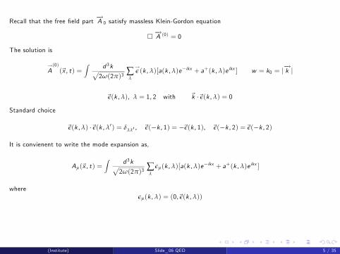
Recall that the free field part−→A 0 satisfy massless Klein-Gordon equation

−→A (0) = 0

The solution is

→A(0)(~x , t) =

∫ d 3k√2ω(2π)3

∑λ

→ε (k ,λ)[a(k ,λ)e−ikx + a+(k ,λ)e ikx ] w = k0 = |

−→k |

~ε(k ,λ), λ = 1, 2 with ~k ·~ε(k ,λ) = 0

Standard choice

~ε(k ,λ) ·~ε(k ,λ′) = δλλ′ , ~ε(−k , 1) = −~ε(k , 1), ~ε(−k , 2) =~ε(−k , 2)

It is convienent to write the mode expansion as,

Aµ(~x , t) =∫ d 3k√

2ω(2π)3∑λ

εµ(k ,λ)[a(k ,λ)e−ikx + a+(k ,λ)e ikx ]

whereεµ(k ,λ) = (0,~ε(k ,λ))


Photon PropagatorFeynman propagatpr for photon is

iDµν (x , x ′) =⟨0∣∣T (Aµ (x )Aν (x ′)

)∣∣ 0⟩= θ (t − t ′)

⟨0∣∣Aµ (x )Aν (x ′)

∣∣ 0⟩+ θ (t ′ − t)⟨0∣∣Aν (x ′)Aµ (x )

∣∣ 0⟩From mode expansion,

⟨0∣∣Aµ (x )Aν (x ′)

∣∣ 0⟩ =∫ d 3kd 3k ′

(2π)3√2ωk 2ωk ′

∑λ,λ′

εµ(k ,λ)εν(k ′,λ′)⟨0∣∣∣[a(k ,λ)e−ikx ]a+(k ′,λ′)e ik ′x ′ ∣∣∣ 0⟩

=∫ d 3kd 3k ′

(2π)32ωk∑λ,λ′

εµ(k ,λ)εν(k ′,λ′) δ3 (k − k ′) e−ikx+ik ′x ′

=∫ d 3k(2π)32ωk

∑λ,λ′

εµ(k ,λ)εν(k ,λ′)e−ik (x−x

′ )

Note that12π

∫ dk0k 20 −ω2 + i ε

e−ik0(t−t′) =

−i 12ω e

−iω(t−t ′) for t > t ′

−i 12ω eiω(t−t ′) for t ′ > t

We then get

∫ d 4k

(2π)4e−ik ·(x

′−x)

k 2 + i ε= −i

∫ d 3k(2π)32ωk

[θ(t − t ′)e−ik (x−x ′ ) + θ(t − t ′)e ik (x−x ′ )

]


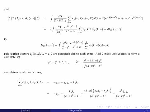
and

⟨0∣∣T (Aµ (x )Aν (x ′)

)∣∣ 0⟩ =∫ d 3k(2π)32ωk

∑λ,λ′

εµ(k ,λ)εν(k ,λ′)[θ(t − t ′)e−ik (x−x ′ ) + θ(t − t ′)e ik (x−x ′ ) ]

= i∫ d 4k

(2π)4e−ik ·(x

′−x)

k 2 + i ε

2

∑λ=1

εν(k ,λ)εµ(k ,λ) = iDµν (x , x ′)

Or

Dµν (x , x ′) =∫ d 4k

(2π)4e−ik ·(x

′−x)

k 2 + i ε

2

∑λ=1

εν(k ,λ)εµ(k ,λ)

polarization vectors εµ(k ,λ), λ = 1, 2 are perpendicular to each other. Add 2 more unit vectors to form acomplete set

ηµ = (1, 0, 0, 0) , kµ =kµ − (k · η) ηµ√(k · η)2 − k 2

completeness relation is then,

2

∑λ=1

εν(k ,λ)εµ(k ,λ) = −gµν − ηµην − kµ kν

= −gµν −kµkν

(k · η)2 − k 2+(k · η)

(kµην + ηµkν

)(k · η)2 − k 2

−k 2ηµην

(k · η)2 − k 2


If we define propagator in momentum space as

Dµν (x , x ′) =∫ d 4k

(2π)4e−ik ·(x

′−x)Dµν (k )

then

Dµν (k ) =1

k 2 + i ε

−gµν −kµkν

(k · η)2 − k 2+(k · η)

(kµην + ηµkν

)(k · η)2 − k 2

−k 2ηµην

(k · η)2 − k 2

terms proportional to kµ will not contribute to physical processes and the last term is of the form δµ0 δν0 willbe cancelled by the Coulom interaction..


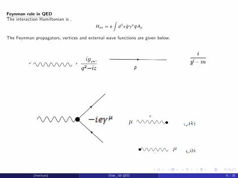
Feynman rule in QEDThe interaction Hamiltonian is ,

Hint = e∫d 3x

_ψγµψAµ

The Feynman propagators, vertices and external wave functions are given below.


p

p p

p


e+e−→ µ+µ−

Total Cross Sectionmomenta for this reaction

e+ (p ′) + e− (p)→ µ+ (k ′) + µ− (k )

Use Feynman rule to write the matrix element as

M (e+e− → µ+µ−) =_v (p ′, s ′) (−ieγµ) u (p, s)

(−igµν

q2

)_u(k ′, r ′) (−ieγν) v (k , r )

=ie2

q2_v (p ′, s ′)γµu (p, s)

_u(k ′, r ′)γµv (k , r )

where q = p + p ′. Notet that electron vertex have property,

qµ

_v (p ′)γµu (p) = (p + p ′)µ

_v (p ′)γµu (p) =

_v (p ′)

(/p + /p ′

)u (p) = 0


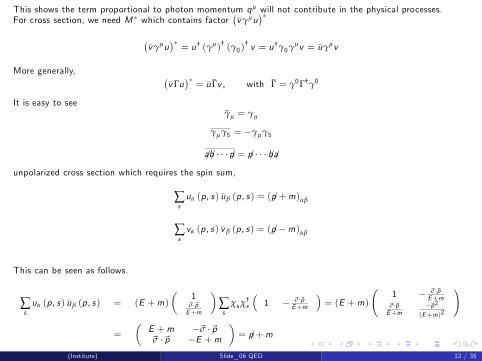
This shows the term proportional to photon momentum qµ will not contribute in the physical processes.For cross section, we need M ∗ which contains factor

(_vγµu

)∗(_vγµu

)∗= u† (γµ)† (γ0)

† v = u†γ0γµv =_uγµv

More generally, (_vΓu

)∗=

_u_Γv , with

_Γ = γ0Γ†γ0

It is easy to see _γµ = γµ

γµγ5 = −γµγ5

/a /b · · · /p = /p · · · /b /a

unpolarized cross section which requires the spin sum,

∑suα (p, s)

_uβ (p, s) = ( /p +m)αβ

∑svα (p, s)

_v β (p, s) = ( /p −m)αβ

This can be seen as follows.

∑suα (p, s)

_uβ (p, s) = (E +m)

(1~σ·~pE+m

)∑s

χsχ†s

(1 − ~σ·~p

E+m

)= (E +m)

(1 − ~σ·~p

E+m~σ·~pE+m

−~p2(E+m)2

)

=

(E +m −~σ ·~p~σ ·~p −E +m

)= /p +m


Similarly for the v−spinor,

∑svα (p, s)

_v β (p, s) = (E +m)

(~σ·~pE+m1

)χsχ

†s

(~σ·~pE+m −1

)= (E +m)

(~p2

(E+m)2− ~σ·~pE+m

~σ·~pE+m −1

)

=

(E −m −~σ ·~p~σ ·~p − (E +m)

)= /p −m


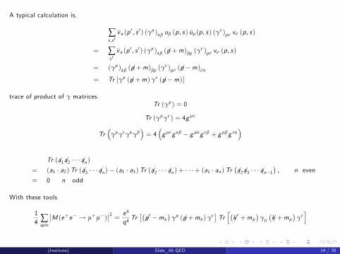
A typical calculation is,

∑s ,s ′

_v α(p ′, s ′) (γµ)αβ uβ (p, s)

_uρ(p, s) (γν)ρσ vσ (p, s)

= ∑s ′

_v α(p ′, s ′) (γµ)αβ ( /p +m)βρ (γ

ν)ρσ vσ (p, s)

= (γµ)αβ ( /p +m)βρ (γν)ρσ ( /p −m)σα

= Tr [γµ ( /p +m) γν ( /p −m)]

trace of product of γ matrices.Tr (γµ) = 0

Tr (γµγν) = 4g µν

Tr(

γµγνγαγβ)= 4

(g µνg αβ − g µαg νβ + g µβg να

)

Tr ( /a1 /a2 · · · /an)= (a1 · a2)Tr ( /a3 · · · /an)− (a1 · a3)Tr ( /a2 · · · /an) + · · ·+ (a1 · an)Tr

(/a2 /a3 · · · /an−1

), n even

= 0 n odd

With these tools

14 ∑spin

∣∣M (e+e− → µ+µ−)∣∣2 = e4

q4Tr[(/p ′ −me

)γµ ( /p +me ) γν

]Tr[(/k ′ +mµ

)γµ

(/k +mµ

)γν]


for energies mµ.

14 ∑spin′

∣∣M (e+e− → µ+µ−)∣∣2 = 8 e4

q4

[(p · k )

(p ′ · k ′

)+ (p ′ · k )

(p · k ′

)]

In center of mass,pµ = (E , 0, 0,E ) , p ′µ = (E , 0, 0,−E )

kµ =

(E ,→k), k ′µ =

(E ,−

→k), with

→k · z = E cos θ

If we set mµ = 0, E =

∣∣∣∣→k ∣∣∣∣ andq2 = (p + p ′)2 = 4E 2 , p · k = p ′ · k ′ = E 2 (1− cos θ) ,

p ′ · k = p · k ′ = E 2 (1+ cos θ)

Then

14 ∑spin′|M |2 =

8e4

16E 4

[E 4 (1− cos θ)2 + E 4 (1+ cos θ)2

]= e4

(1+ cos2 θ

)Note that under the parity θ → π − θ. this matrix element conserves the parity


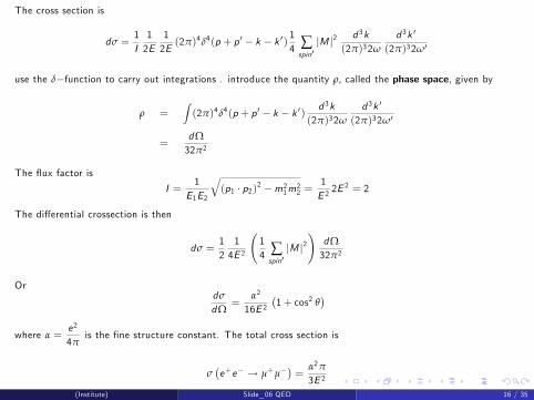
The cross section is

dσ =1I12E

12E(2π)4δ4(p + p ′ − k − k ′) 1

4 ∑spin′|M |2 d 3k

(2π)32ω

d 3k ′

(2π)32ω′

use the δ−function to carry out integrations . introduce the quantity ρ, called the phase space, given by

ρ =∫(2π)4δ4(p + p ′ − k − k ′) d 3k

(2π)32ω

d 3k ′

(2π)32ω′

=dΩ32π2

The flux factor is

I =1

E1E2

√(p1 · p2)2 −m2

1m22 =

1E 22E 2 = 2

The differential crossection is then

dσ =1214E 2

(14 ∑spin′|M |2

)dΩ32π2

Ordσ

dΩ=

α2

16E 2(1+ cos2 θ

)where α =

e2

4πis the fine structure constant. The total cross section is

σ(e+e− → µ+µ−

)=

α2π

3E 2


Or

σ(e+e− → µ+µ−

)=4α2π

3swith s = (p1 + p2)

2 = 4E 2


e+e−→ hadronsOne of the interesting procesess in e+e− collider is the reaction

e+e− → hadrons

According to QCD, theory of strong interaciton, this processes will go through

e+e− → q_q

and then q_q trun into hadrons. Since coupling of γ to q

_q differs from the coupling to µ+µ− only in their

charges cross section for q_q as

σ(e+e− → q

_q)= 3

(Q 2q

) 4α2π

3s= 3

(Q 2q

)σ(e+e− → µ+µ−

)Qq is electric charge of quark q. The factor of 3 because each quark has 3 colors. Then

σ (e+e− → hadrons)σ (e+e− → µ+µ−)

= 3

(∑i

Q 2i

)

Summation is over quarks which are allowed by the avaliable energies. e. g., for energy below the the charmquark only u, d , and s quarks should be included,

σ (e+e− → hadrons)σ (e+e− → µ+µ−)

= 3

[(23

)2+

(13

)2+

(13

)2]= 2

which is not far from the reality.



ep → ep,e (k ) + p (p) −→ e (k ′) + p (p ′)

Proton has strong interaction. First consider proton has no strong interaction and include strong interactionlater. The lowest order contribution is ,

M (e + p → e + p) =_u(p ′, s ′) (−ieγµ) u (p, s)

(−igµν

q2

)_u(k ′, r ′) (−ieγν) u (k , r )

=ie2

q2_u(p ′, s ′)γµu (p, s)

_u(k ′, r ′)γµu (k , r )


where q = k − k ′. For unploarized cross section, sum over the spins ,

14 ∑spin|M (e + p → e + p)|2 = e4

q4Tr[(/p ′ +M

)γµ ( /p +M ) γν

]Tr[(/k ′ +me

)γµ ( /k +me ) γν

]

Again neglect me . Compute the traces

Tr[/k ′γµ /kγν

]= 4 [k ′µk ν − g µν (k · k ′) + kµk ′ν ]

Tr[(/p ′ +M

)γµ ( /p +M ) γν

]= 4 [p ′µpν − g µν (p · p ′) + pµp ′ν ] + 4M 2g µν

Then14 ∑spin|M (e + p → e + p)|2 = e4

q4

8[(p · k )

(p ′ · k ′

)+ (p ′ · k )

(p · k ′

)]− 8M 2 (k · k ′)


Use laboratoy frame

pµ = (M , 0, 0, 0) , kµ =

(E ,→k), k ′µ =

(E ′,

→k ′)

Thenp · k = ME , p.k ′ = ME ′, k · k ′ = EE ′ (1− cos θ)

p ′ · k ′ = (p + k − k ′) .k ′ = p.k ′ + k · k ′, p ′ · k = (p + k − k ′) .k = p.k − k · k ′

q2 = (k − k ′)2 = −2k · k ′ = −2EE ′ (1− cos θ)

Differential cross section is

dσ =1I12p0

12k0

(2π)4δ4(p + k − p ′ − k ′) 14 ∑spin′|M |2 d 3p ′

(2π)32p ′0

d 3k ′

(2π)32k ′0

The phase space is

ρ =∫(2π)4δ4(p + k − p ′ − k ′) d 3p ′

(2π)32p ′0

d 3k ′

(2π)32k ′0(1)

=14π2

∫δ (p0 + k0 − p ′0 − k ′0)

d 3k ′

2p ′02k′0

where

p ′0 =

√M 2 +

(→p +

→k −

→k ′)2=

√M 2 +

(→k −

→k ′)2


Use the momenta in lab frame,

ρ =14π2

∫δ (M + E − p ′0 − E ′)

k ′2dk ′dΩ2p ′02E ′

=14π2

∫δ (M + E − p ′0 − E ′)

dΩE ′dE ′

p ′0

Letx = −E + p ′0 + E ′

Then

dx = dE ′(1+dp ′0dE ′

) = dE ′(p ′0 + E

′ − E cos θ

p ′0

)and

ρ =14π2

∫δ (x −M ) dΩE ′dx

(p ′0 + E ′ − E cos θ)=

14π2

dΩE ′

M + E (1− cos θ)

From the argument of the δ−function we get the relation, M = x = −E + p ′0 + E ′From momentum conservation

p ′20 = M2 +

(→k −

→k ′)2= M 2 + E 2 + E ′2 − 2EE ′ cos θ

and from energy conservation

p ′20 = (M + E − E ′)2 = M 2 + E 2 + E ′2 − 2EE ′ + 2ME − 2ME ′


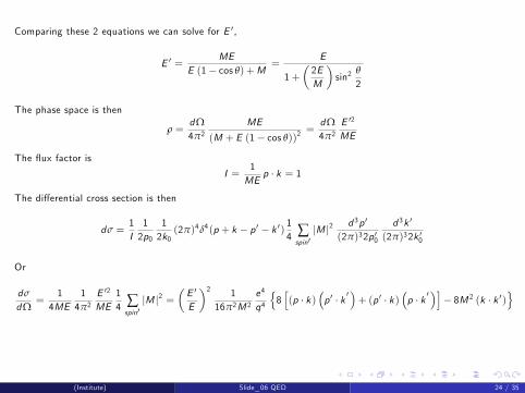
Comparing these 2 equations we can solve for E ′,

E ′ =ME

E (1− cos θ) +M=

E

1+(2EM

)sin2

θ

2

The phase space is then

ρ =dΩ4π2

ME

(M + E (1− cos θ))2=dΩ4π2

E ′2

ME

The flux factor is

I =1ME

p · k = 1

The differential cross section is then

dσ =1I12p0

12k0

(2π)4δ4(p + k − p ′ − k ′) 14 ∑spin′|M |2 d 3p ′

(2π)32p ′0

d 3k ′

(2π)32k ′0

Or

dσ

dΩ=

14ME

14π2

E ′2

ME14 ∑spin′|M |2 =

(E ′

E

)2 116π2M 2

e4

q4

8[(p · k )

(p ′ · k ′

)+ (p ′ · k )

(p · k ′

)]− 8M 2 (k · k ′)


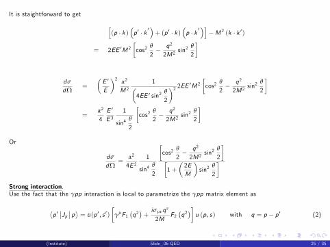
It is staightforward to get [(p · k )

(p ′ · k ′

)+ (p ′ · k )

(p · k ′

)]−M 2 (k · k ′)

= 2EE ′M 2[cos2

θ

2− q2

2M 2 sin2 θ

2

]

dσ

dΩ=

(E ′

E

)2 α2

M 2

1(4EE ′ sin2

θ

2

)2 2EE ′M 2[cos2

θ

2− q2

2M 2 sin2 θ

2

]

=α2

4E ′

E 31

sin4θ

2

[cos2

θ

2− q2

2M 2 sin2 θ

2

]

Or

dσ

dΩ=

α2

4E 21

sin4θ

2

[cos2

θ

2− q2

2M 2 sin2 θ

2

][1+

(2EM

)sin2

θ

2

]Strong interaction.Use the fact that the γpp interaction is local to parametrize the γpp matrix element as

⟨p ′∣∣Jµ

∣∣ p⟩ = _u(p ′, s ′)

[γµF1

(q2)+iσµνqν

2MF2(q2)]u (p, s) with q = p − p ′ (2)


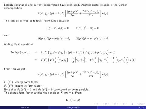
Lorentz covariance and current conservation have been used. Another useful relation is the Gordondecomposition

_u(p ′)γµu (p) =

_u(p ′)

[(p + p ′)µ

2m+iσµν (p ′ − p)ν

2m

]u (p)

This can be derived as follows. From Dirac equation

( /p −m)u(p) = 0,_u(p ′)( /p ′ −m) = 0

and _u(p ′)γµ( /p −m)u(p) = 0,

_u(p ′)( /p ′ −m)γµu(p) = 0

Adding these equations,

2m_u(p ′)γµu (p) =

_u(p ′)

(γµ /p + /p ′γµ

)u (p) =

_u(p ′)

(pνγµγν + p

′νγνγµ

)u (p)

=_u(p ′)

(pν(

12

γµ,γν

+12

[γµ,γν

]) + p ′ν(

12

γµ,γν

− 12

[γµ,γν

])

)u (p)

From this we get_u(p ′)γµu (p) =

_u(p ′)

[(p + p ′)µ

2m+iσµν (p ′ − p)ν

2m

]u (p)

F1(q2), charge form factor

F2(q2), magnetic form factor .

Note that F1(q2)= 1 and F2

(q2)= 0 correspond to point particle.

The charge form factor satifies the condition F1 (0) = 1. From

Q |p〉 = |p〉


we get ⟨p ′ |Q | p

⟩=⟨p ′ |p

⟩= 2E (2π)3 δ3

(→p −→p

′)


On the other hand from Eq(2) we see that

⟨p ′ |Q | p

⟩=

∫d 3x

⟨p ′ |J0 (x )| p

⟩=∫d 3x

⟨p ′ |J0 (0)| p

⟩e i(p

′−p)·x

= (2π)3 δ3(→p −→p

′) _u(p ′, s ′)γ0u (p, s) F1 (0)

= 2E (2π)3 δ3(→p −→p

′)F1 (0)

compare two equations =⇒ F1 (0) = 1. To gain more insight, write Q in terms of charge density

Q =∫d 3xρ (x ) =

∫d 3xJ0 (x )

Then ⟨p ′ |J0 (x )| p

⟩= e iq·x

⟨p ′ |J0 (0)| p

⟩= e iq·xF1

(q2) _u(p ′, s ′)γ0u (p, s)

F1(q2)is the Fourier transform of charge density distribution i.e.

F1(q2)∼∫d 3xρ (x ) e−i

→q ·→x

Expand F1(q2)in powers of q2 ,

F1(q2)= F1 (0) + q2F ′1 (0) + · · ·

F1 (0) is total charge and F ′1 (0) is related to the charge radius.Calulate cross section as before,

dσ

dΩ=

α2

4E 2

[cos2

θ

2

(1

1− q2/4M 2

) [G 2E −

(q2/4M 2

)G 2M]− q2

2M 2 sin2 θ

2G 2M

]sin4

θ

2

[1+

(2EM

)sin2

θ

2

](Institute) Slide_06 QED 28 / 35

where

GE = F1 +q2

4M 2 F2

GM = F1 + F2

Experimentally, GE and GM have the form,

GE(q2)≈GM

(q2)

κp≈ 1

(1− q2/0.7Gev 2)2(3)

where κp = 2.79 magnetic moment of the proton. If proton were point like, we would have GE(q2)

=GM(q2)= 1

Dependence of q2 in Eq(3) =⇒ proton has a structure. For large q2 the elastic cross section falls off rapidlyas GE ≈ GM ∼ q−4 .


Compton Scattering

γ (k ) + e (p) −→ γ (k ′) + e (p ′)

Two diagrams contribute,

The amplitude is given by

M (γe −→ γe) =_u(p ′)(−ieγµ)ε′µ (k

′)i

/p + /k −m (−ieγν) εν (k ) u (p)

+_u(p ′)(−ieγµ)εµ (k )

i

/p − /k ′ −m(−ieγν) ε′ν (k

′) u (p)

Note that if write the amplitude asM = ε′µ (k

′)M µ


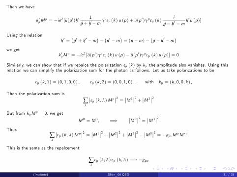
Then we have

k ′µMµ = −ie2 [

_u(p ′) /k ′

1/p + /k −m γνεν (k ) u (p) +

_u(p ′)γµεµ (k )

i

/p − /k ′ −m/k ′u (p)]

Using the relation/k ′ =

(/p ′ + /k ′ −m

)−(/p ′ −m

)= ( /p −m)−

(/p − /k ′ −m

)we get

k ′µMµ = −ie2 [

_u(p ′)γνεν (k ) u (p)−

_u(p ′)γµεµ (k ) u (p)] = 0

Similarly, we can show that if we repalce the polarization εµ (k ) by kµ the amplitude also vanishes. Using thisrelation we can simplify the polarization sum for the photon as follows. Let us take polarizations to be

εµ (k , 1) = (0, 1, 0, 0) , εµ (k , 2) = (0, 0, 1, 0) , with kµ = (k , 0, 0, k ) ,

Then the polarization sum is

∑λ

∣∣εµ (k ,λ)M µ∣∣2 = ∣∣M 1

∣∣2 + ∣∣M 2∣∣2

But from kµM µ = 0, we get

M 0 = M 3 , =⇒∣∣M 0

∣∣2 = ∣∣M 3∣∣2

Thus∑λ

∣∣εµ (k ,λ)M µ∣∣2 = ∣∣M 1

∣∣2 + ∣∣M 2∣∣2 + ∣∣M 3

∣∣2 − ∣∣M 0∣∣2 = −gµνM µM ∗ν

This is the same as the repalcement

∑λ

εµ (k ,λ) εµ (k ,λ) −→ −gµν


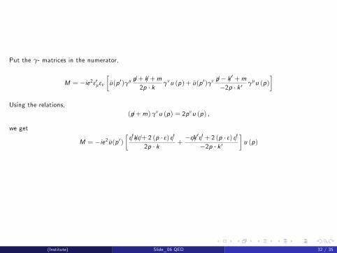
Put the γ- matrices in the numerator,

M = −ie2ε′µεν

[_u(p ′)γµ /p + /k +m

2p · k γνu (p) +_u(p ′)γν /p − /k ′ +m

−2p · k ′ γµu (p)]

Using the relations,( /p +m) γνu (p) = 2pνu (p) ,

we get

M = −ie2_u(p ′)

[/ε′ /k /ε+ 2 (p · ε) /ε′

2p · k +− /ε /k ′ /ε′ + 2 (p · ε) /ε′

−2p · k ′]u (p)


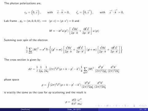
The photon polarizations are,

εµ =(0,→ε), with

→ε ·→k = 0, ε′µ =

(0,→ε′), with

→ε′·→k′= 0,

Lab frame , pµ = (m, 0, 0, 0), =⇒ (p · ε) = (p · ε′) = 0 and

M = −ie2_u(p ′)

[/ε′ /k /ε2p · k +

/ε /k ′ /ε′

2p · k ′]u (p)

Summing over spin of the electron

12 ∑spin|M |2 = e4Tr

(/p ′ +m

) [ /ε′ /k /ε2p · k +

/ε /k ′ /ε′

2p · k ′]( /p +m)

[/ε′ /k /ε2p · k +

/ε /k ′ /ε′

2p · k ′]

The cross section is given by

dσ =1I12p0

12k0

(2π)4δ4(p + k − p ′ − k ′) 14 ∑spin′|M |2 d 3p ′

(2π)32p ′0

d 3k ′

(2π)32k ′0

phase space

ρ =∫(2π)4δ4(p + k − p ′ − k ′) d 3p ′

(2π)32p ′0

d 3k ′

(2π)32k ′0

is exactly the same as the case for ep scattering and the result is

ρ =dΩ4π2

ω′2

mω


It is straightforward to compute the trace with result,

dσ

dΩ=

α2

4m2

(ω′

ω

)2 [ω′

ω+

ω

ω′+ 4 (ε · ε′)2 − 2

]

This is Klein-Nishima relation. In the limit ω → 0,

dσ

dΩ=

α2

m2 (ε · ε′)2

hereα

mis classical electron radius.


For unpolarized cross section, sum over polarization of photon,

∑λλ′

[ε (k ,λ) · ε′

(k ′,λ′

)]2= ∑

λλ′

[→ε (k ,λ) ·→ε

′ (k ′,λ′

)]2

Since→ε (k , 1) ,

→ε (k , 2) and

→k form basis in 3-dimension, completeness relation is

∑λ

εi (k ,λ) εj (k ,λ) = δij − ki kj

Then

∑λλ′

[→ε (k ,λ) ·→ε

′ (k ′,λ′

)]2=(δij − ki kj

) (δij − k ′i k ′j

)= 1+ cos2 θ

where k · k ′ = cos θ. The cross section is

dσ

dΩ=

α2

2m2

(ω′

ω

)2 [ω′

ω+

ω

ω′− sin2 θ

]The total cross section,

σ =πα2

m2

∫ 1

−1dz 1[

1+ω

m(1− z )

]3 + 1[1+

ω

m(1− z )

] − 1− z 2[1+

ω

m(1− z )

]2 At low energies, ω → 0, we

σ =8πα2

3m2

and at high energies

σ =πα2

ωm

[ln2ω

m+12+O

(mωlnmω

)](Institute) Slide_06 QED 35 / 35

Quantum Electrodynamics - CAS · Quantum Electrodynamics Ling-Fong Li (Institute) Slide_06 QED 1 / 35. Quantum Electrodynamics Lagrangian density for QED , L= y(x)gm i ...

Documents