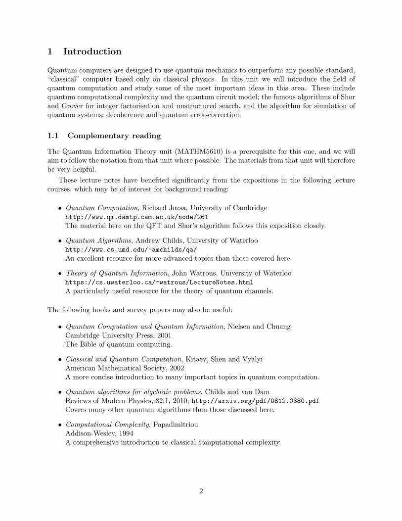
School of Mathematics Spring 2017 QUANTUM COMPUTATION Lecture notes Ashley Montanaro, University of Bristol [email protected] Contents 1 Introduction 2 2 Classical and quantum computational complexity 4 3 Grover’s algorithm 11 4 The Quantum Fourier Transform and periodicity 18 5 Integer factorisation 23 6 Phase estimation 29 7 Hamiltonian simulation 32 8 Noise and the framework of quantum channels 36 9 Quantum error-correction 41 For updates and further materials, see https://people.maths.bris.ac.uk/ ~ csxam/teaching/ qc2017/. Version 1.41 (April 7, 2017). 1

Welcome message from author
This document is posted to help you gain knowledge. Please leave a comment to let me know what you think about it! Share it to your friends and learn new things together.
Transcript
School of Mathematics Spring 2017
QUANTUM COMPUTATION
Lecture notes
Ashley Montanaro, University of [email protected]
Contents
1 Introduction 2
2 Classical and quantum computational complexity 4
3 Grover’s algorithm 11
4 The Quantum Fourier Transform and periodicity 18
5 Integer factorisation 23
6 Phase estimation 29
7 Hamiltonian simulation 32
8 Noise and the framework of quantum channels 36
9 Quantum error-correction 41
For updates and further materials, see https://people.maths.bris.ac.uk/~csxam/teaching/
qc2017/.
Version 1.41 (April 7, 2017).
1
1 Introduction
Quantum computers are designed to use quantum mechanics to outperform any possible standard,“classical” computer based only on classical physics. In this unit we will introduce the field ofquantum computation and study some of the most important ideas in this area. These includequantum computational complexity and the quantum circuit model; the famous algorithms of Shorand Grover for integer factorisation and unstructured search, and the algorithm for simulation ofquantum systems; decoherence and quantum error-correction.
1.1 Complementary reading
The Quantum Information Theory unit (MATHM5610) is a prerequisite for this one, and we willaim to follow the notation from that unit where possible. The materials from that unit will thereforebe very helpful.
These lecture notes have benefited significantly from the expositions in the following lecturecourses, which may be of interest for background reading:
• Quantum Computation, Richard Jozsa, University of Cambridgehttp://www.qi.damtp.cam.ac.uk/node/261
The material here on the QFT and Shor’s algorithm follows this exposition closely.
• Quantum Algorithms, Andrew Childs, University of Waterloohttp://www.cs.umd.edu/~amchilds/qa/
An excellent resource for more advanced topics than those covered here.
• Theory of Quantum Information, John Watrous, University of Waterloohttps://cs.uwaterloo.ca/~watrous/LectureNotes.html
A particularly useful resource for the theory of quantum channels.
The following books and survey papers may also be useful:
• Quantum Computation and Quantum Information, Nielsen and ChuangCambridge University Press, 2001The Bible of quantum computing.
• Classical and Quantum Computation, Kitaev, Shen and VyalyiAmerican Mathematical Society, 2002A more concise introduction to many important topics in quantum computation.
• Quantum algorithms for algebraic problems, Childs and van DamReviews of Modern Physics, 82:1, 2010; http://arxiv.org/pdf/0812.0380.pdfCovers many other quantum algorithms than those discussed here.
• Computational Complexity, PapadimitriouAddison-Wesley, 1994A comprehensive introduction to classical computational complexity.
2
1.2 Notation
We write [n] := 1, . . . , n for the integers between 1 and n, and Zn for the group of integers modulon, often just identified with the set 0, . . . , n− 1. dxe, bxc and bxe denote the smallest integer ysuch that y ≥ x, the largest integer z such that z ≤ x, and the closest integer to x, respectively. Weuse
(nk
)for the binomial coefficient “n choose k”, n!/(k!(n−k)!). We say a randomised or quantum
algorithm is “bounded-error” if its failure probability is upper-bounded by some constant below1/2.
We use standard “computer science style” notation relating to asymptotic complexity:
• f(n) = O(g(n)) if there exist real c > 0 and integer n0 ≥ 0 such that for all n ≥ n0,f(n) ≤ c g(n).
• f(n) = Ω(g(n)) if there exist real c > 0 and integer n0 ≥ 0 such that for all n ≥ n0,f(n) ≥ c g(n). Clearly, f(n) = O(g(n)) if and only if g(n) = Ω(f(n)).
• f(n) = Θ(g(n)) if f(n) = O(g(n)) and f(n) = Ω(g(n)).
O, Ω and Θ can be viewed as asymptotic, approximate versions of ≤, ≥ and =.
1.3 Change log
• v1.0: first version covering first part of the unit.
• v1.01: minor typo corrections.
• v1.1: addition of lecture notes on Grover’s algorithm.
• v1.2: addition of lecture notes on Shor’s algorithm, and minor clarifications about Grover’salgorithm.
• v1.21: minor typo corrections about the QFT.
• v1.3: addition of lecture notes on phase estimation and Hamiltonian simulation.
• v1.4: addition of lecture notes on quantum channels and quantum error-correction.
• v1.41: fix typo in section on QFT.
3
2 Classical and quantum computational complexity
Computational complexity theory aims to classify different problems in terms of their difficulty, orin other words the resources required in order to solve them. Two of the most important types ofresources one might study are time (the number of computational steps used by an algorithm solvinga problem) and space (the amount of additional work space used by the algorithm). Classically,the formal model underpinning the notion of an “algorithm” is the Turing machine. We will notgo into details about this here, instead taking the informal approach that the number of steps usedby an algorithm corresponds to the number of lines of code executed when running the algorithm,and the space usage is the amount of memory (RAM) used by the algorithm. For much more onthe topic, see the book Computational Complexity by Papadimitriou, for example.
Rather than looking at the complexity of algorithms for solving one particular instance of aproblem, the theory considers asymptotics: given a family of problems, parametrised by an instancesize (usually denoted n), we study the resources used by the best possible algorithm for solvingthat family of problems. Thus the term “problem” is used henceforth as shorthand for “family ofproblems”. A dividing line between efficient and inefficient algorithms is provided by the notion ofpolynomial-time computation, where an algorithm running in time polynomial in n, i.e. O(nc) forsome fixed c, is considered efficient. For example, consider the following two problems:
• Primality testing: given an integer M expressed as n binary digits, is it a prime number?
• Factorisation: given an integer M expressed as n binary digits, output the prime factors ofM .
As the input is of size n, we would like to solve these problems using an algorithm which runs intime poly(n) (not poly(M)!). No such classical algorithm is known for the factorisation problem;as we will see later, the situation is different for quantum algorithms. However, surprisingly, thereis a polynomial-time classical algorithm for the tantalisingly similar problem of primality testing.
An important class of problems is known as decision problems; these are problems that have ayes-no answer. The first of the above problems is a decision problem, while the second is not. Butit can be made into a decision problem without changing its underlying complexity significantly:
• Factorisation (decision variant): given integers M and K expressed as n binary digits each,does M have a prime factor smaller than K?
It is clear that, if we can solve the usual “search” variant of the factorisation problem, solving thedecision variant is easy. Further, solving the decision variant allows us to solve the search variantof the problem using binary search. Given an integer M whose prime factors we would like todetermine, and an algorithm which solves the decision variant of the factorisation problem, we canuse O(logM) = O(n) evaluations of this algorithm with different values of K to find the smallestprime factor F of M . (First we try K = dM/2e, then either K = dM/4e or K = d3M/4e, etc.)The other factors can be found by dividing M by F and repeating. This is a simple example of areduction: conversion of one problem into another.
A natural way to compare the complexity of problems is via the notion of complexity classes,where a complexity class is simply a set of problems. Some important classical complexity classesare:
• P: the class of decision problems which can be solved in polynomial time by a classicalcomputer.
4
• NP: the class of decision problems such that, if the answer is “yes”, there is a proof of thisfact which can be verified in polynomial time by a classical computer.
• PSPACE: the class of decision problems which can be solved in polynomial space by a classicalcomputer.
Primality testing is in P, although this was shown for the first time only in 2002. The decisionvariant of factorisation is in NP, because given a claimed prime factor of M smaller than K, it canbe easily checked whether the claim is correct. However, factorisation is not known to be in P. Everyproblem in P is automatically in NP, because the verifier can simply ignore any claimed proof andsolve the problem directly. In addition, any problem in NP is automatically in PSPACE, becauseone can loop over all polynomial-length proofs in polynomial space in order to determine whetherthe answer to a problem instance should be “yes” or “no”. Thus we have P⊆NP⊆PSPACE.
A problem is said to be NP-complete if it is in NP, and every other problem in NP reduces to itin polynomial time. So NP-complete problems are, informally, the “hardest” problems in NP. Theseinclude many problems of practical importance in areas such as timetabling, resource allocation,and optimisation. One simple example is the Subset Sum problem. An instance of this problem isa sequence of integers x1, . . . , xn; our task, given such a sequence, is to determine whether there isa subset of the integers which sums to 0. Given such a subset, we can easily check that it sums to0; however, finding such a subset seems to require checking exponentially many subsets.
NP stands for “nondeterministic polynomial-time”, not “non-polynomial time”. In fact, it iscurrently unknown whether every problem in NP can be solved in polynomial time, i.e. whetherP=NP. This is the famous P vs. NP question; resolving it would win you a prize of $1M from theClay Mathematics Institute.
2.1 Quantum computational complexity
How are we to measure resource usage by a quantum algorithm running on a quantum computer?One framework within which to do this is the quantum circuit model. Recall that in quantummechanics, evolutions of a quantum system are described by unitary operators. But not all unitaryoperators are equally easy to implement physically. We might imagine that, in a real quantumcomputing experiment, the operations that we can actually perform in the lab are small, “local”ones on just a few qubits at a time. We can build up more complicated unitary operators asproducts of these small, elementary operations.
Intuitively, a quantum computation running for T steps and using space S corresponds toa unitary operation on S qubits (i.e. acting on C2S ) expressed as a product of T elementaryoperations picked from some family F . Each elementary operation is assumed to take time O(1)and act nontrivially on O(1) qubits. That is, if U is one such elementary operation, we assumethat it can be written as U = U ′⊗ I, where U ′ acts on k qubits, for some small constant k (usually,k ≤ 3). The nontrivial parts U ′ of such operations are called quantum gates, by analogy withlogic gates in classical electronic circuits. The set of allowed quantum gates will depend on ourphysical architecture. However, it turns out that most “reasonable” sets of gates on O(1) qubits areuniversal, in the sense that any unitary operation on S qubits can be approximately decomposedas a product of these basic operations, acting on different qubits. A sequence of quantum gates isknown as a quantum circuit.
A quantum circuit can be drawn as a diagram by associating each qubit with a horizontal“wire”, and drawing each gate as a box across the wires corresponding to the qubits on which it
5
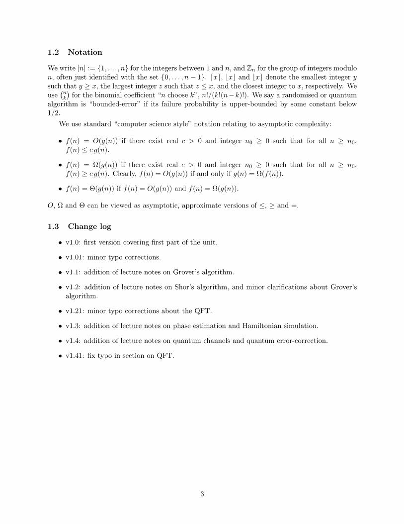
acts. This is easiest to illustrate with an example: the circuit
HU
VX
corresponds to the unitary operator (I ⊗ V )(U ⊗ I)(H ⊗ I ⊗X) on 3 qubits. Beware that a circuitis read left to right, with the starting input state on the far left, but the corresponding unitaryoperators act right to left! For convenience, in the diagram we have drawn multi-qubit gates asonly acting on nearest-neighbour qubits, but this is not an essential restriction of the model.
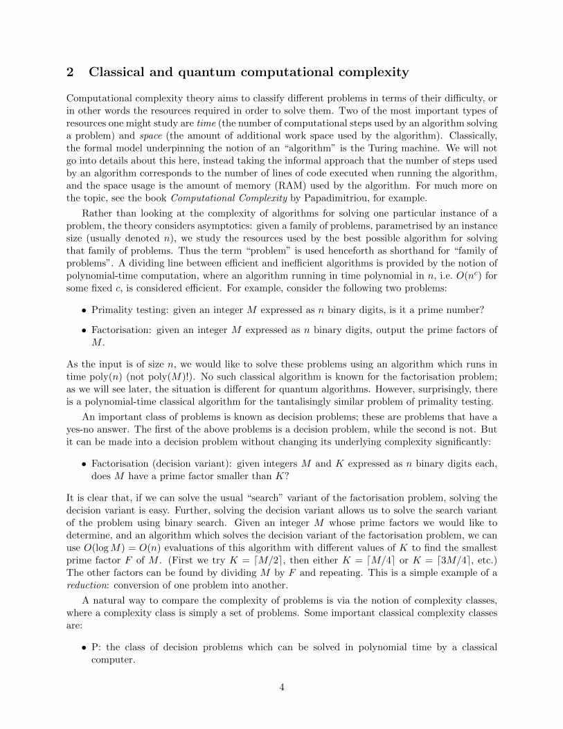
The quantum circuit picture also allows us to represent initial state preparation, and finalmeasurement of the qubits in the computational basis, as shown in this more complicated example:
|0〉 HU
Z
W
H
|0〉U
Y H
|0〉V
HU
|0〉 X H
We usually assume that the initial state of the quantum computer is |0〉⊗S and the computationfinishes with a measurement of some of the qubits in the computational basis, which gives the outputof the computation. If we prefer, we can allow intermediate measurements during the circuit; thisturns out not to change the power of the model.
Some special gates turn out to be particularly useful. You are already familiar with theHadamard gate H = 1√
2
(1 11 −1
)(with respect to the standard, aka “computational” basis), and
the gates X, Y , Z corresponding to the Pauli operators. We can think of the X gate as imple-menting a NOT operation, as X|0〉 = |1〉, X|1〉 = |0〉. Another useful type of gate will be the“controlled-G” gates. For any gate G, the corresponding controlled-G gate CG uses an extra qubitto control whether the gate is applied or not. That is,
CG|0〉|ψ〉 = |0〉|ψ〉, CG|1〉|ψ〉 = |1〉G|ψ〉.
In a circuit diagram, this is denoted using a filled circle on the control line:
•G
A particularly useful such gate is controlled-NOT (CNOT), denoted•
. Written as a matrix
with respect to the computational basis,
CNOT =
1 0 0 00 1 0 00 0 0 10 0 1 0
.
For any fixed gate set F , some large unitary matrices cannot be decomposed efficiently in termsof gates from F , in the sense that to write them as a product of gates from F requires expo-nentially many such gates. For a rough way of seeing this, consider the problem of producing
6
an arbitrary quantum state of n qubits∑
x∈0,1n αx|x〉, in the special case where each coefficient
αx ∈ ±1/2n/2. There are 22n such states. Any circuit on n qubits made up of T gates, eachacting on k qubits, picked from a gate set of size G can be described by one of(
G
(n
k
))T= O
((Gnk)T
)= O
(2T log(Gnk)
)different sequences of gates, so for k,G = O(1) we need T log n = Ω(2n) to be able to produce2Ω(2n) different unitary operators, and hence 22n different states. A similar argument still works ifwe allow approximate computation or continuous gate sets.
In general, just as in the classical world, we look for efficient quantum circuits which use poly(n)qubits and poly(n) gates to solve a problem on an input of size n. The class of decision problemswhich can be solved by a quantum computer, in time polynomial in the input size, with probabilityof failure at most 1/3, is known as BQP (“bounded-error quantum polynomial-time”). This classencapsulates the notion of efficient quantum computation. The failure probability bound of 1/3 isessentially arbitrary; it can be reduced to an arbitrarily small constant by repetition and takingthe majority vote.
Observe that in the quantum circuit picture we can perform multiple operations in parallel, sowe in fact have two possible ways to measure “time” complexity: circuit size (number of gates) andcircuit depth (number of time steps to execute all the gates). But these can only differ by a factorof O(S), where S is the number of qubits.
2.2 Classical and reversible circuits
Any classical computation which maps a bit-string (element of 0, 1n) to another bit-string (ele-ment of 0, 1m) can be broken down into a sequence of logical operations, each of which acts on asmall number of bits (e.g. AND, OR and NOT gates). Such a sequence is called a (classical) circuit.As a first step in understanding the power of quantum computers, we would like to show that anyclassical circuit can be implemented as a quantum circuit, implying that quantum computation isat least as powerful as classical computation.
But there is a difficulty: in quantum mechanics, if we wish the state of our system to remainpure, the evolution that we apply has to be unitary, and hence reversible. Some classical logicaloperations (such as AND, written ∧) are not reversible. However, reversible variants of these canbe developed using the following trick. If we wish to compute an arbitrary classical operationf : 0, 1n → 0, 1m reversibly, we attach a so-called “ancilla” register of m bits, each orignallyset to 0, and modify f to give a new operation f ′ : 0, 1n × 0, 1m → 0, 1n × 0, 1m whichperforms the map
f ′(x, y) = (x, y ⊕ f(x)),
where ⊕ is bitwise XOR, i.e. addition modulo 2 (so each bit of y ⊕ f(x) is the sum mod 2 of thecorresponding bits of y and f(x)). Then if we input y = 0m, we get (x, f(x)), from which we canextract our desired output f(x). If we perform f ′ twice, we get (x, y ⊕ f(x) ⊕ f(x)) = (x, y). Sof is reversible. And any reversible function that maps bit-strings to bit-strings corresponds to apermutation matrix, which is unitary, so can be implemented as a sequence of quantum gates. If wecombine many gates of this form to compute a function f : 0, 1n → 0, 1, say, we will finish withan output of the form (junk, x, f(x)). If we wish to remove the junk, we can simply copy the outputf(x) onto a fresh ancilla bit in state 0 by applying a CNOT gate, and then repeat all the previousgates in reverse. As each is its own inverse, the final state of the computation is (0, x, f(x)).
7
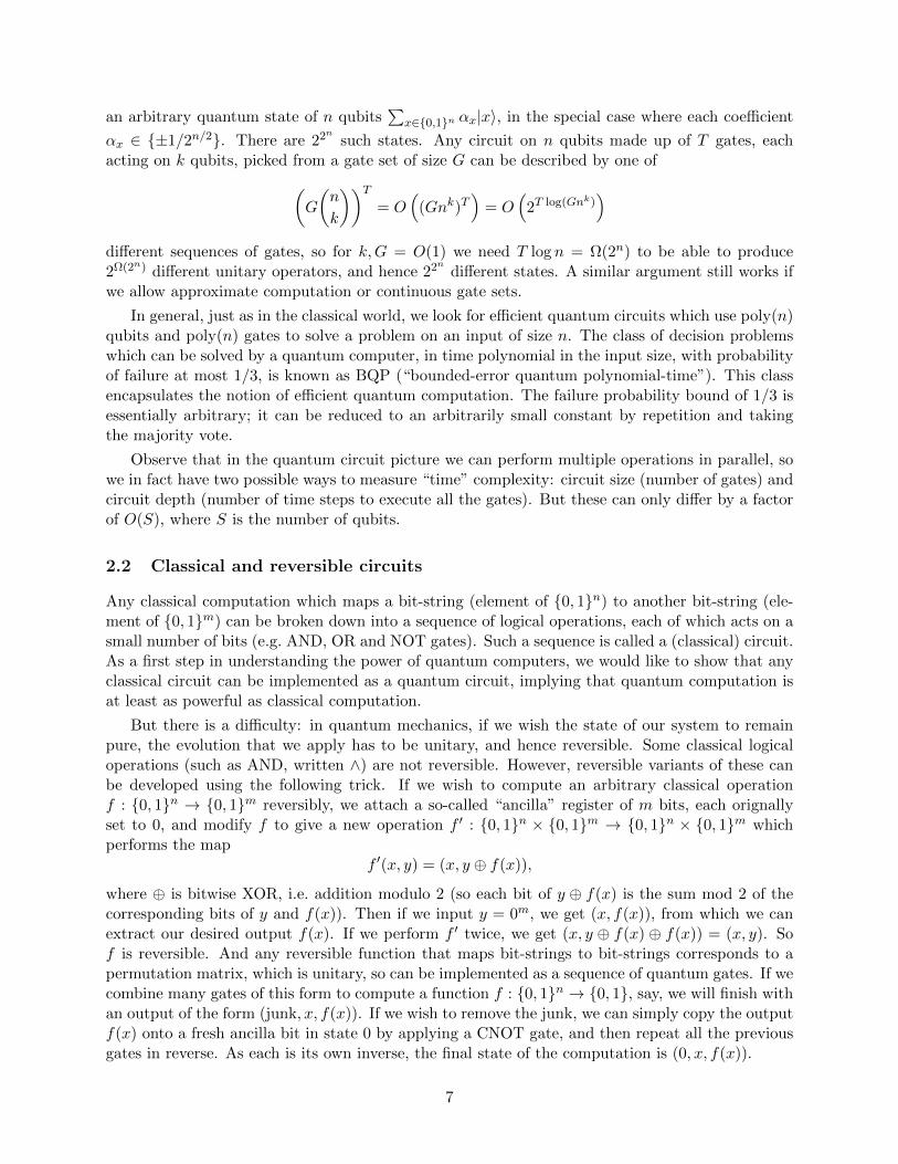
To obtain universal deterministic classical computation, it is sufficient to be able to implementthe NOT and AND gates. The NOT gate is immediately reversible. Applying the above construc-tion to AND we get the map (x1, x2, y) 7→ (x1, x2, y ⊕ (x1 ∧ x2)) for x1, x2, y ∈ 0, 1. The unitaryoperator which implements this is then simply the map
|x1〉|x2〉|y〉 7→ |x1〉|x2〉|y ⊕ (x1 ∧ x2)〉.
Written as a matrix with respect to the computational basis this is
1 0 0 0 0 0 0 00 1 0 0 0 0 0 00 0 1 0 0 0 0 00 0 0 1 0 0 0 00 0 0 0 1 0 0 00 0 0 0 0 1 0 00 0 0 0 0 0 0 10 0 0 0 0 0 1 0
,
an operation known as the Toffoli gate. In a circuit diagram, the Toffoli gate is written as“controlled-controlled-NOT”, i.e.
••
Randomised classical computation can also be embedded in a quantum circuit. Imagine we havea classical computation which makes use of some random bits, each of which is 0 or 1 with equalprobability. We can simulate this by applying a Hadamard gate to |0〉 to produce the state 1√
2(|0〉+
|1〉). Then we can either measure this qubit immediately to obtain a uniformly random bit, or ifwe prefer, apply classical gates to it and then measure it at the end of the computation; the resultis the same either way.
It is known that the Toffoli gate, together with the Hadamard gate, are even sufficient for univer-sal quantum computation. That is, any quantum computation whatsoever can be approximatelyrepresented as a circuit of Toffoli and Hadamard gates. Another representative universal set ofquantum gates is H,X,CNOT, T, where T =
(1 00 eiπ/4
). It turns out that almost any non-trivial
set of gates is universal in this sense; therefore, we generally do not worry about the details of thegate set being used.
2.3 Query complexity
While time complexity is a practically important measure of the complexity of algorithms, it suffersfrom the difficulty that it is very hard to prove lower bounds on it, and that technical details cansometimes obscure the key features of an algorithm. One way to sidestep this is to use a model whichis less realistic, but cleaner and more mathematically tractable: the model of query complexity.
In this model, we assume we have access to an oracle, or “black box”, to which we can passqueries, and which returns answers to our queries. Our goal is to determine some property of theoracle using the minimal number of queries. On a classical computer, we can think of the oracle asa function f : 0, 1n → 0, 1m. We pass in inputs x ∈ 0, 1n, and receive outputs f(x) ∈ 0, 1m.How does this fit into physical reality? We imagine we are given access to the oracle either as aphysical device which we cannot open and look inside, or as a circuit which we can see, but for
8
which it might be difficult to compute some property of the circuit. For example, even given adescription of a circuit computing some function f : 0, 1n → 0, 1, it might be hard to find aninput x such that f(x) = 1. Sometimes it is more natural to think of an oracle function f as amemory storing n strings of m bits each, where we can retrieve an arbitrary string at the cost ofone query.
We can give a quantum computer access to a oracle using the generic reversible computationconstruction discussed in the previous section. That is, instead of having a function f : 0, 1n →0, 1m, we produce a unitary operator Of which performs the map1
Of |x〉|y〉 = |x〉|y ⊕ f(x)〉.
Of is sometimes known as the bit oracle. If m = 1, so f returns one bit, it would also make senseto consider an oracle Uf which does not use an ancilla, but instead flips the phase of an input state|x〉 by applying the map
Uf |x〉 = (−1)f(x)|x〉.
This variant is thus sometimes known as the phase oracle. Given access to a bit oracle, we cansimulate a phase oracle by attaching an ancilla qubit in the state 1√
2(|0〉 − |1〉):
Of |x〉1√2
(|0〉 − |1〉) =1√2
(|x〉|f(x)〉 − |x〉|f(x)⊕ 1〉) = (−1)f(x)|x〉 1√2
(|0〉 − |1〉).
Note that the ancilla qubit is left unchanged by this operation, which is called the phase kickbacktrick. Also note that the effect of the phase oracle is not observable if we apply it to just onecomputational basis state |x〉, but only if we apply it to a superposition:∑
x∈0,1nαx|x〉 7→
∑x∈0,1n
(−1)f(x)αx|x〉.
Importantly, note that to implement the oracles Of and Uf we do not need to understand anymore about the inner workings of f than we do classically. That is, if we are given a classicalcircuit computing f , we can follow a purely mechanical construction to create quantum circuitsimplementing Of and Uf . This is useful because f itself may have quite complicated behaviour,even if it is expressible as a small circuit, and we may not be able to understand its behaviourcompletely.
2.4 The Deutsch-Jozsa algorithm as a quantum circuit
Recall that the Deutsch-Jozsa algorithm can distinguish between balanced and constant functionsf : 0, 1n → 0, 1 with one use of the oracle Uf , whereas an exact classical algorithm for solvingthe same problem would require exponentially many (in n) queries to f . That is, if we are promisedeither that f is constant or that |x : f(x) = 0| = |x : f(x) = 1| = 2n−1, we can determinewhich is the case with one quantum query.
We now verify that this algorithm can be implemented as an efficient quantum circuit on n
1Note that the notation used here is different to Quantum Information Theory.
9
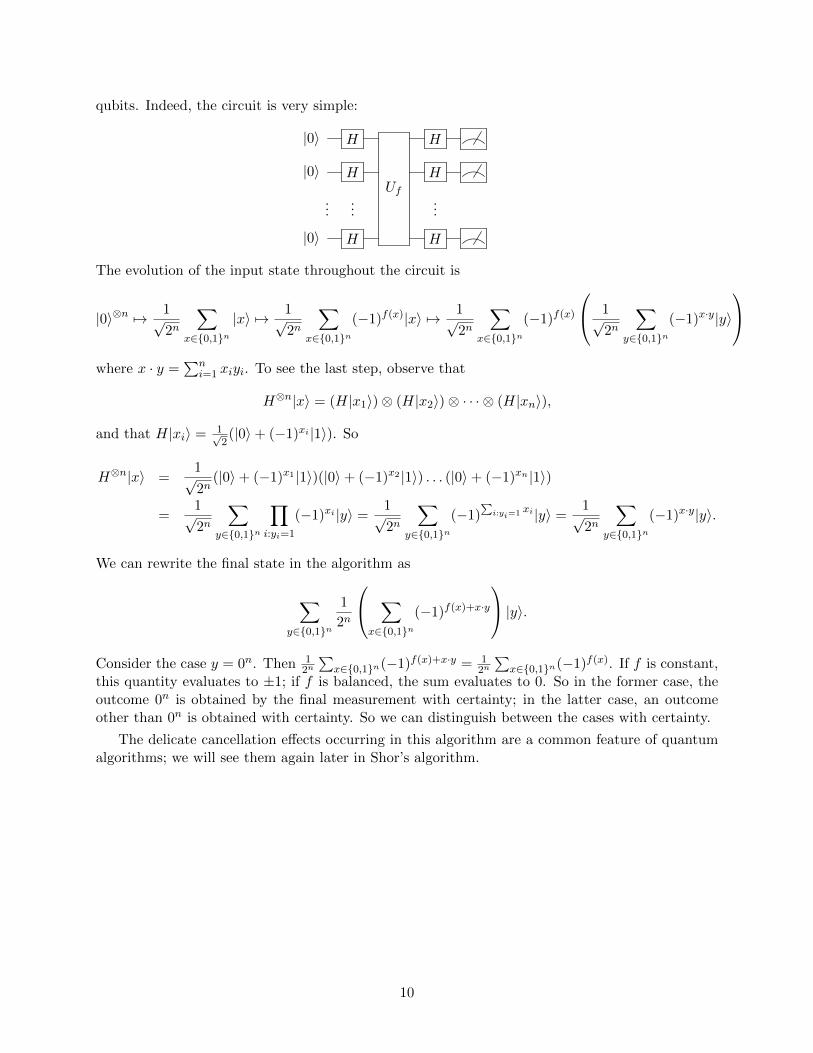
qubits. Indeed, the circuit is very simple:
|0〉 H
Uf
H
|0〉 H H
......
...
|0〉 H H
The evolution of the input state throughout the circuit is
|0〉⊗n 7→ 1√2n
∑x∈0,1n
|x〉 7→ 1√2n
∑x∈0,1n
(−1)f(x)|x〉 7→ 1√2n
∑x∈0,1n
(−1)f(x)
1√2n
∑y∈0,1n
(−1)x·y|y〉
where x · y =
∑ni=1 xiyi. To see the last step, observe that
H⊗n|x〉 = (H|x1〉)⊗ (H|x2〉)⊗ · · · ⊗ (H|xn〉),
and that H|xi〉 = 1√2(|0〉+ (−1)xi |1〉). So
H⊗n|x〉 =1√2n
(|0〉+ (−1)x1 |1〉)(|0〉+ (−1)x2 |1〉) . . . (|0〉+ (−1)xn |1〉)
=1√2n
∑y∈0,1n
∏i:yi=1
(−1)xi |y〉 =1√2n
∑y∈0,1n
(−1)∑i:yi=1 xi |y〉 =
1√2n
∑y∈0,1n
(−1)x·y|y〉.
We can rewrite the final state in the algorithm as
∑y∈0,1n
1
2n
∑x∈0,1n
(−1)f(x)+x·y
|y〉.Consider the case y = 0n. Then 1
2n∑
x∈0,1n(−1)f(x)+x·y = 12n∑
x∈0,1n(−1)f(x). If f is constant,this quantity evaluates to ±1; if f is balanced, the sum evaluates to 0. So in the former case, theoutcome 0n is obtained by the final measurement with certainty; in the latter case, an outcomeother than 0n is obtained with certainty. So we can distinguish between the cases with certainty.
The delicate cancellation effects occurring in this algorithm are a common feature of quantumalgorithms; we will see them again later in Shor’s algorithm.
10
3 Grover’s algorithm
A simple example of a problem that fits into the query complexity model is unstructured search ona set of N elements for a unique marked element. In this problem we are given access to a functionf : [N ] → 0, 1 with the promise that f(x0) = 1 for a unique “marked” element x0. Our task isto output x0.
It is intuitively clear that the unstructured search problem should require about N queries tobe solved (classically!). We can formalise this as the following proposition:
Proposition 3.1. Let A be a classical algorithm which solves the unstructured search problem on aset of N elements with failure probability δ < 1/2. Then A makes Ω(N) queries in the worst case.
Proof sketch. We can think of any classical algorithm A as choosing in advance, either determinis-tically or randomly, a sequence S of distinct indices x1, . . . , xN to query, and then querying themone by one until the marked element x0 is found. Imagine an adversary chooses x0 uniformly atrandom. Then, on average, x0 will appear at position about N/2 in the sequence S. As for arandom choice of x0 the algorithm makes Ω(N) queries on average, the average number of queriesmade in the worst case must also be Ω(N).
In the quantum setting, we will see that the unstructured search problem can be solved withsignificantly fewer queries.
Theorem 3.2 (Grover ’97). There is a quantum algorithm which solves the unstructured searchproblem using O(
√N) queries.
For simplicity, assume that N = 2n for some integer n (this is not an essential restriction). Inthis case, we can associate each element of [N ] with an n-bit string. Then Grover’s algorithm isdescribed in Box 1.
We are given access to f : 0, 1n → 0, 1 with the promise that f(x0) = 1 for a uniqueelement x0. We use a quantum circuit on n qubits with initial state |0〉⊗n. Let H denotethe Hadamard gate, and let U0 denote the n-qubit operation which inverts the phase of|0n〉: U0|0n〉 = −|0n〉, U0|x〉 = |x〉 for x 6= 0n.
1. Apply H⊗n.
2. Repeat the following operations T times, where T = bπ4√Nc:
(a) Apply Uf .
(b) Apply D := −H⊗nU0H⊗n.
3. Measure all the qubits and output the result.
Box 1: Grover’s algorithm
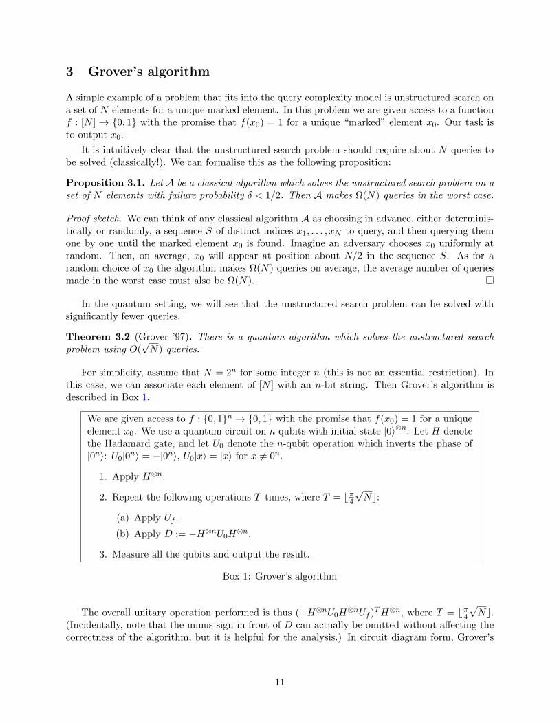
The overall unitary operation performed is thus (−H⊗nU0H⊗nUf )TH⊗n, where T = bπ4
√Nc.
(Incidentally, note that the minus sign in front of D can actually be omitted without affecting thecorrectness of the algorithm, but it is helpful for the analysis.) In circuit diagram form, Grover’s
11
algorithm looks like this:
|0〉 H
Uf D Uf
. . .
D|0〉 H . . .
......
|0〉 H . . .
It may be far from clear initially why this algorithm works, or indeed whether it does work. Todescribe the algorithm, we introduce unitary operators I|ψ〉 and R|ψ〉, where |ψ〉 is an arbitrarystate. These are defined as follows:
I|ψ〉 := I − 2|ψ〉〈ψ|, R|ψ〉 := −I|ψ〉 = 2|ψ〉〈ψ| − I,
where I is the identity. I|ψ〉 can be seen as an “inversion about |ψ〉” operation, while R|ψ〉 can beseen as a “reflection about |ψ〉” operation. An arbitrary state |φ〉 can be expanded as
|φ〉 = α|ψ〉+ β|ψ⊥〉
for some α and β, and some state |ψ⊥〉 such that 〈ψ|ψ⊥〉 = 0. Then
I|ψ〉|φ〉 = −α|ψ〉+ β|ψ⊥〉,
so I|ψ〉 has flipped the phase of the component corresponding to |ψ〉, and left the componentorthogonal to |ψ〉 unchanged. R|ψ〉 has the opposite effect. Observe that, in the unstructuredsearch problem with marked element x0, Uf = I|x0〉. Further observe that
H⊗nU0H⊗n = H⊗n(I − 2|0n〉〈0n|)H⊗n = I − 2|+〉〈+| = I|+〉,
where |+〉 = 1√2n
∑x∈0,1n |x〉, so D = −I|+〉. By moving the minus sign, the algorithm can equally
well be thought of as alternating the operations −I|x0〉 and I|+〉, or equivalently R|x0〉 and −R|+〉.We have the following claims:
1. For any states |ψ〉, |φ〉, and any state |ξ〉 in the 2d plane spanned by |ψ〉 and |φ〉, the statesR|ψ〉|ξ〉 and R|φ〉|ξ〉 remain in this 2d plane.
This is immediate from geometric arguments, but one can also calculate explicitly:
R|ψ〉(α|ψ〉+ β|φ〉) = R|ψ〉(α|ψ〉+ β(γ|ψ〉+ δ|ψ⊥〉)) = (α+ βγ)|ψ〉 − βδ|ψ⊥〉= (α+ 2βγ)|ψ〉 − β(γ|ψ〉+ δ|ψ⊥〉) = (α+ 2βγ)|ψ〉 − β|φ〉.
2. Within the 2d plane spanned by orthogonal states |ψ〉, |ψ⊥〉, I|ψ〉 = −R|ψ〉 = R|ψ⊥〉 .
Again, one can calculate explicitly that
−R|ψ〉(α|ψ〉+ β|ψ⊥〉) = −α|ψ〉+ β|ψ⊥〉 = R|ψ⊥〉(α|ψ〉+ β|ψ⊥〉).
3. If |ξ〉 is within the 2d plane spanned by |ψ〉, |ψ⊥〉,
R|ψ〉|ξ〉 = 〈ψ|ξ〉|ψ〉 − 〈ψ⊥|ξ〉|ψ⊥〉.
This is just a straightforward calculation.
12
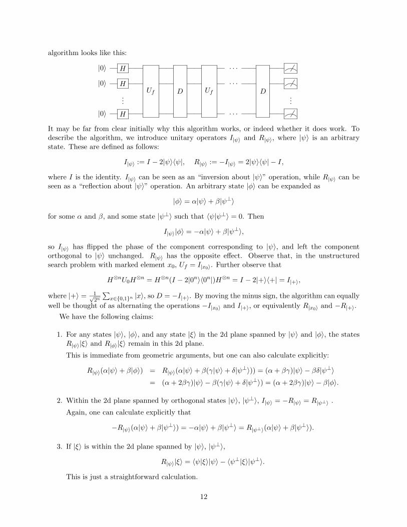
Combining these claims, we see that each step of Grover’s algorithm consists of two reflectionsin the plane spanned by |+〉, |x0〉: a reflection about |x0〉 followed by a reflection about |+⊥〉,a state orthogonal to |+〉 within this plane. We can illustrate this with the following diagram,demonstrating the effect of these operations on an arbitrary state |ξ〉 within this 2d plane:
|+〉
|x0〉|+⊥〉|ξ〉 R|x0〉 R|+⊥〉
|+〉
|x0〉|+⊥〉
|ξ〉
|+〉
|x0〉|+⊥〉|ξ〉
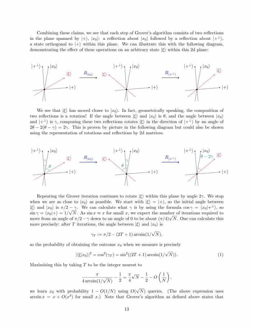
We see that |ξ〉 has moved closer to |x0〉. In fact, geometrically speaking, the composition oftwo reflections is a rotation! If the angle between |ξ〉 and |x0〉 is θ, and the angle between |x0〉and |+⊥〉 is γ, composing these two reflections rotates |ξ〉 in the direction of |+⊥〉 by an angle of2θ − 2(θ − γ) = 2γ. This is proven by picture in the following diagram but could also be shownusing the representation of rotations and reflections by 2d matrices.
|+〉
|x0〉|+⊥〉|ξ〉
θ
γR|x0〉 R|+⊥〉
|+〉
|x0〉|+⊥〉
|ξ〉θγ
|+〉
|x0〉|+⊥〉|ξ〉θ − 2γ
Repeating the Grover iteration continues to rotate |ξ〉 within this plane by angle 2γ. We stopwhen we are as close to |x0〉 as possible. We start with |ξ〉 = |+〉, so the initial angle between|ξ〉 and |x0〉 is π/2 − γ. We can calculate what γ is by using the formula cos γ = 〈x0|+⊥〉, sosin γ = 〈x0|+〉 = 1/
√N . As sinx ≈ x for small x, we expect the number of iterations required to
move from an angle of π/2−γ down to an angle of 0 to be about (π/4)√N . One can calculate this
more precisely: after T iterations, the angle between |ξ〉 and |x0〉 is
γT := π/2− (2T + 1) arcsin(1/√N),
so the probability of obtaining the outcome x0 when we measure is precisely
|〈ξ|x0〉|2 = cos2(γT ) = sin2((2T + 1) arcsin(1/√N)). (1)
Maximising this by taking T to be the integer nearest to
π
4 arcsin(1/√N)− 1
2=π
4
√N − 1
2−O
(1
N
),
we learn x0 with probability 1 − O(1/N) using O(√N) queries. (The above expression uses
arcsinx = x + O(x3) for small x.) Note that Grover’s algorithm as defined above states that
13
T
Success probability
1
10 20 30 40 50
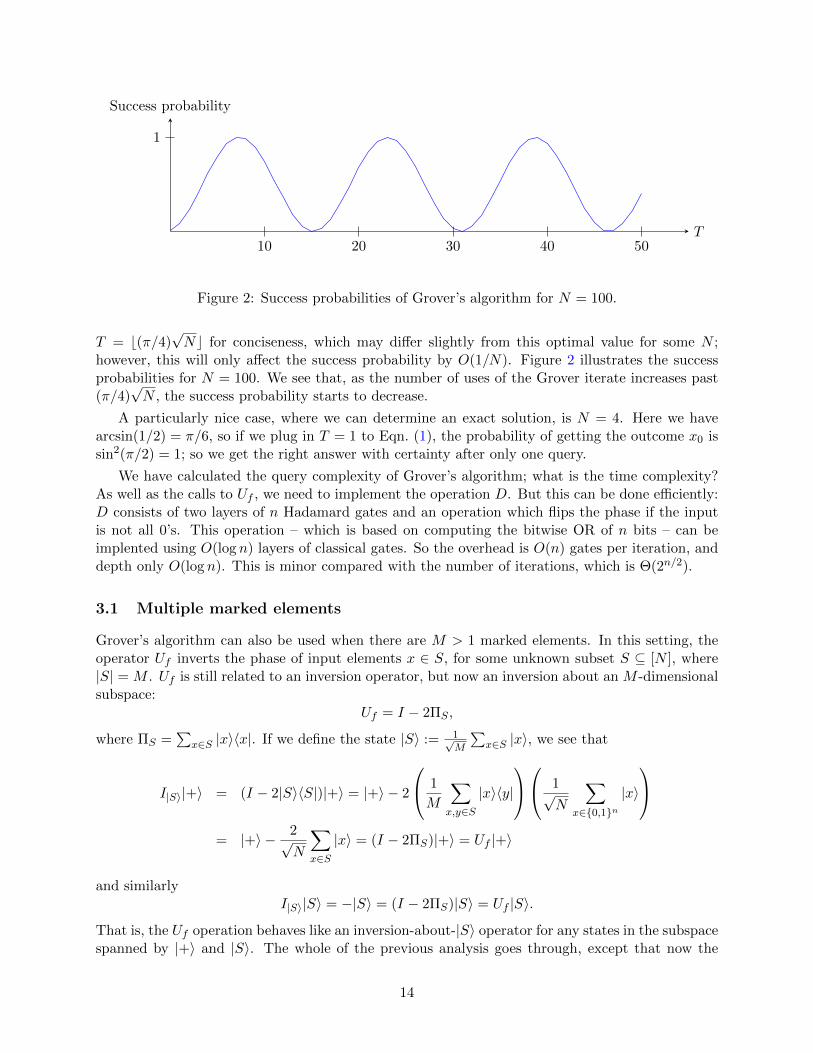
Figure 2: Success probabilities of Grover’s algorithm for N = 100.
T = b(π/4)√Nc for conciseness, which may differ slightly from this optimal value for some N ;
however, this will only affect the success probability by O(1/N). Figure 2 illustrates the successprobabilities for N = 100. We see that, as the number of uses of the Grover iterate increases past(π/4)
√N , the success probability starts to decrease.
A particularly nice case, where we can determine an exact solution, is N = 4. Here we havearcsin(1/2) = π/6, so if we plug in T = 1 to Eqn. (1), the probability of getting the outcome x0 issin2(π/2) = 1; so we get the right answer with certainty after only one query.
We have calculated the query complexity of Grover’s algorithm; what is the time complexity?As well as the calls to Uf , we need to implement the operation D. But this can be done efficiently:D consists of two layers of n Hadamard gates and an operation which flips the phase if the inputis not all 0’s. This operation – which is based on computing the bitwise OR of n bits – can beimplented using O(log n) layers of classical gates. So the overhead is O(n) gates per iteration, anddepth only O(log n). This is minor compared with the number of iterations, which is Θ(2n/2).
3.1 Multiple marked elements
Grover’s algorithm can also be used when there are M > 1 marked elements. In this setting, theoperator Uf inverts the phase of input elements x ∈ S, for some unknown subset S ⊆ [N ], where|S| = M . Uf is still related to an inversion operator, but now an inversion about an M -dimensionalsubspace:
Uf = I − 2ΠS ,
where ΠS =∑
x∈S |x〉〈x|. If we define the state |S〉 := 1√M
∑x∈S |x〉, we see that
I|S〉|+〉 = (I − 2|S〉〈S|)|+〉 = |+〉 − 2
1
M
∑x,y∈S
|x〉〈y|
1√N
∑x∈0,1n
|x〉
= |+〉 − 2√
N
∑x∈S|x〉 = (I − 2ΠS)|+〉 = Uf |+〉
and similarlyI|S〉|S〉 = −|S〉 = (I − 2ΠS)|S〉 = Uf |S〉.
That is, the Uf operation behaves like an inversion-about-|S〉 operator for any states in the subspacespanned by |+〉 and |S〉. The whole of the previous analysis goes through, except that now the
14
angle γ moved at each step satisfies sin γ = 〈S|+〉 =√M/N . Thus after T iterations we have
|〈ξ|S〉|2 = cos2(γT ) = sin2((2T + 1) arcsin(√M/N)).
By a similar argument to before we can pick T ≈ (π/4)√N/M to obtain overlap with |S〉 close
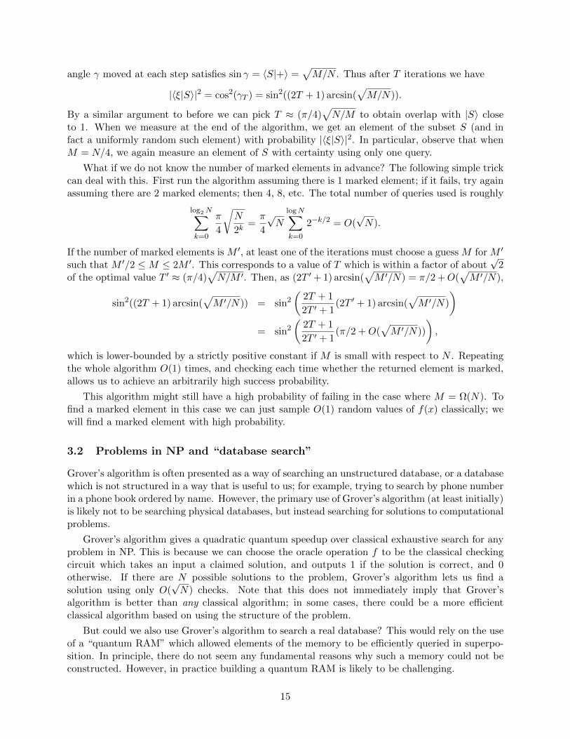
to 1. When we measure at the end of the algorithm, we get an element of the subset S (and infact a uniformly random such element) with probability |〈ξ|S〉|2. In particular, observe that whenM = N/4, we again measure an element of S with certainty using only one query.
What if we do not know the number of marked elements in advance? The following simple trickcan deal with this. First run the algorithm assuming there is 1 marked element; if it fails, try againassuming there are 2 marked elements; then 4, 8, etc. The total number of queries used is roughly
log2N∑k=0
π
4
√N
2k=π
4
√N
logN∑k=0
2−k/2 = O(√N).
If the number of marked elements is M ′, at least one of the iterations must choose a guess M for M ′
such that M ′/2 ≤M ≤ 2M ′. This corresponds to a value of T which is within a factor of about√
2of the optimal value T ′ ≈ (π/4)
√N/M ′. Then, as (2T ′ + 1) arcsin(
√M ′/N) = π/2 +O(
√M ′/N),
sin2((2T + 1) arcsin(√M ′/N)) = sin2
(2T + 1
2T ′ + 1(2T ′ + 1) arcsin(
√M ′/N)
)= sin2
(2T + 1
2T ′ + 1(π/2 +O(
√M ′/N))
),
which is lower-bounded by a strictly positive constant if M is small with respect to N . Repeatingthe whole algorithm O(1) times, and checking each time whether the returned element is marked,allows us to achieve an arbitrarily high success probability.
This algorithm might still have a high probability of failing in the case where M = Ω(N). Tofind a marked element in this case we can just sample O(1) random values of f(x) classically; wewill find a marked element with high probability.
3.2 Problems in NP and “database search”
Grover’s algorithm is often presented as a way of searching an unstructured database, or a databasewhich is not structured in a way that is useful to us; for example, trying to search by phone numberin a phone book ordered by name. However, the primary use of Grover’s algorithm (at least initially)is likely not to be searching physical databases, but instead searching for solutions to computationalproblems.
Grover’s algorithm gives a quadratic quantum speedup over classical exhaustive search for anyproblem in NP. This is because we can choose the oracle operation f to be the classical checkingcircuit which takes an input a claimed solution, and outputs 1 if the solution is correct, and 0otherwise. If there are N possible solutions to the problem, Grover’s algorithm lets us find asolution using only O(
√N) checks. Note that this does not immediately imply that Grover’s
algorithm is better than any classical algorithm; in some cases, there could be a more efficientclassical algorithm based on using the structure of the problem.
But could we also use Grover’s algorithm to search a real database? This would rely on the useof a “quantum RAM” which allowed elements of the memory to be efficiently queried in superpo-sition. In principle, there do not seem any fundamental reasons why such a memory could not beconstructed. However, in practice building a quantum RAM is likely to be challenging.
15
3.3 Amplitude amplification
The basic idea behind Grover’s algorithm can be generalised remarkably far, to an algorithmfor finding solutions to any problem using a heuristic. This algorithm is known as amplitudeamplification.
Imagine we have N = 2n possible solutions, of which a subset S are “good”, and we wouldlike to find a good solution. As well as having access to a “checking” algorithm f as before, wheref(x) = 1 if and only if x is marked, we now have access to a “guessing” algorithm A, which hasthe job of producing potential solutions to the problem. It performs the map
A|0n〉 =∑
x∈0,1nαx|x〉
for some coefficients αx. So, if we were to apply A and then measure, the probability that wewould obtain a good solution is
p :=∑x∈S|αx|2;
we think of A as a heuristic which tries to output a good solution. We can use f to check whethera claimed solution is actually good. If we repeated Algorithm A until we got a good solution, theexpected number of trials we would need is Θ(1/p).
We now describe the amplitude amplification algorithm.
We are given access to A and Uf as above.
1. Apply A to the starting state |0〉⊗n.
2. Repeat the following operations T times, for some T to be determined:
(a) Apply Uf .
(b) Apply −AU0A−1.
3. Measure all the qubits and output the result.
Box 3: Amplitude amplification
Note that this is exactly the same as Grover’s algorithm, except that we have replaced the H⊗n
operations with A or A−1. Write
|ψ〉 = A|0n〉, |G〉 =ΠS |ψ〉‖ΠS |ψ〉‖
,
where again ΠS =∑
x∈S |x〉〈x|. We now repeat the analysis of the previous section, except thatwe replace |+〉 with |ψ〉 and |S〉 with |G〉. We observe that everything goes through just as before!The first operation applied is equivalent to I|G〉, and the second is equivalent to −I|ψ〉. We startwith the state |ψ〉 and rotate towards |G〉. The angle γ moved at each step now satisfies
sin γ = 〈ψ|G〉 = ‖ΠS |ψ〉‖ =√p,
so the number of iterations required to move from |ψ〉 to |G〉 is O(1/√p) – a quadratic improvement.
16
Finally observe that we can generalise one step further, by replacing the algorithm Uf withinversion about an arbitrary subspace, rather than a subspace defined in terms of computationalbasis vectors. This allows us to use amplitude amplification to drive amplitude towards an arbitrarysubspace, or indeed to create an arbitrary quantum state, given the ability to reflect about thatstate.
17
7 3 4 2 9 7 3 4 2 9 7 3 4 2 9 7 3 4 2 9
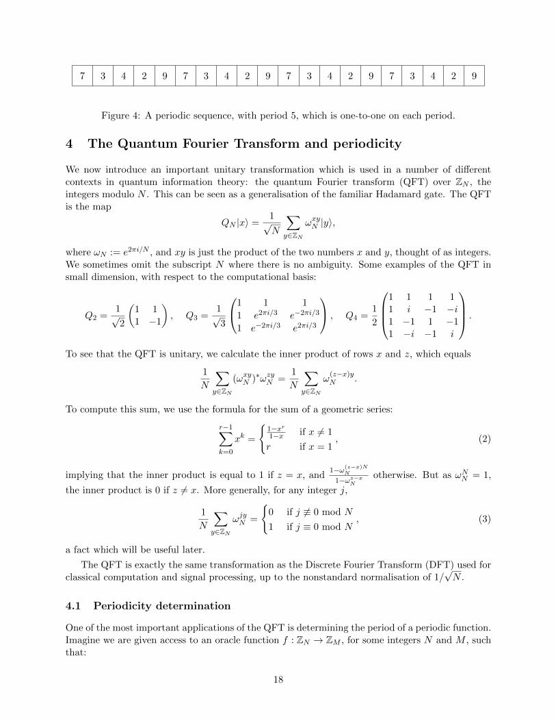
Figure 4: A periodic sequence, with period 5, which is one-to-one on each period.
4 The Quantum Fourier Transform and periodicity
We now introduce an important unitary transformation which is used in a number of differentcontexts in quantum information theory: the quantum Fourier transform (QFT) over ZN , theintegers modulo N . This can be seen as a generalisation of the familiar Hadamard gate. The QFTis the map
QN |x〉 =1√N
∑y∈ZN
ωxyN |y〉,
where ωN := e2πi/N , and xy is just the product of the two numbers x and y, thought of as integers.We sometimes omit the subscript N where there is no ambiguity. Some examples of the QFT insmall dimension, with respect to the computational basis:
Q2 =1√2
(1 11 −1
), Q3 =
1√3
1 1 1
1 e2πi/3 e−2πi/3
1 e−2πi/3 e2πi/3
, Q4 =1
2
1 1 1 11 i −1 −i1 −1 1 −11 −i −1 i
.
To see that the QFT is unitary, we calculate the inner product of rows x and z, which equals
1
N
∑y∈ZN
(ωxyN )∗ωzyN =1
N
∑y∈ZN
ω(z−x)yN .
To compute this sum, we use the formula for the sum of a geometric series:
r−1∑k=0
xk =
1−xr1−x if x 6= 1
r if x = 1, (2)
implying that the inner product is equal to 1 if z = x, and1−ω(z−x)N
N
1−ωz−xN
otherwise. But as ωNN = 1,
the inner product is 0 if z 6= x. More generally, for any integer j,
1
N
∑y∈ZN
ωjyN =
0 if j 6≡ 0 mod N
1 if j ≡ 0 mod N, (3)
a fact which will be useful later.
The QFT is exactly the same transformation as the Discrete Fourier Transform (DFT) used forclassical computation and signal processing, up to the nonstandard normalisation of 1/
√N .
4.1 Periodicity determination
One of the most important applications of the QFT is determining the period of a periodic function.Imagine we are given access to an oracle function f : ZN → ZM , for some integers N and M , suchthat:
18
• f is periodic: there exists r such that r divides N and f(x+ r) = f(x) for all x ∈ ZN ;
• f is one-to-one on each period: for all pairs (x, y) such that |x− y| < r, f(x) 6= f(y).
Our task is to determine r.
The periodicity determination algorithm is presented in Box 5.
We are given access to a periodic function f with period r, which is one-to-one on eachperiod. We start with the state |0〉|0〉, where the first register is dimension N , and thesecond dimension M .
1. Apply QN to the first register.
2. Apply Of to the two registers.
3. Measure the second register.
4. Apply QN to the first register.
5. Measure the first register; let the answer be k.
6. Simplify the fraction k/N as far as possible and return the denominator.
Box 5: Periodicity determination
The initial sequence of operations which occur during the algorithm is:
|0〉|0〉 17→ 1√N
∑x∈ZN
|x〉|0〉 27→ 1√N
∑x∈ZN
|x〉|f(x)〉.
When the second register is measured, we receive an answer, say z. By the periodic and one-to-oneproperties of f , all input values x ∈ ZN for which f(x) = z are of the form x0 + jr for some x0 andinteger j. The state therefore collapses to something of the form√
r
N
N/r−1∑j=0
|x0 + jr〉.
After we apply the QFT, we get the state
√r
N
N/r−1∑j=0
∑y∈ZN
ωy(x0+jr)N |y〉
=
√r
N
∑y∈ZN
ωyx0N
N/r−1∑j=0
ωjryN
|y〉.Observe that, as r divides N , ωrN = e2πi(r/N) = ωN/r. This state is thus equivalent to
√r
N
∑y∈ZN
ωyx0N
N/r−1∑j=0
ωjyN/r
|y〉.By Eqn. (3), the sum over j is 0 unless y ≡ 0 mod N/r, or in other words if y = `N/r for someinteger `. So we can rewrite this state as
1√r
r−1∑`=0
ω`x0N/rN |`N/r〉.
19
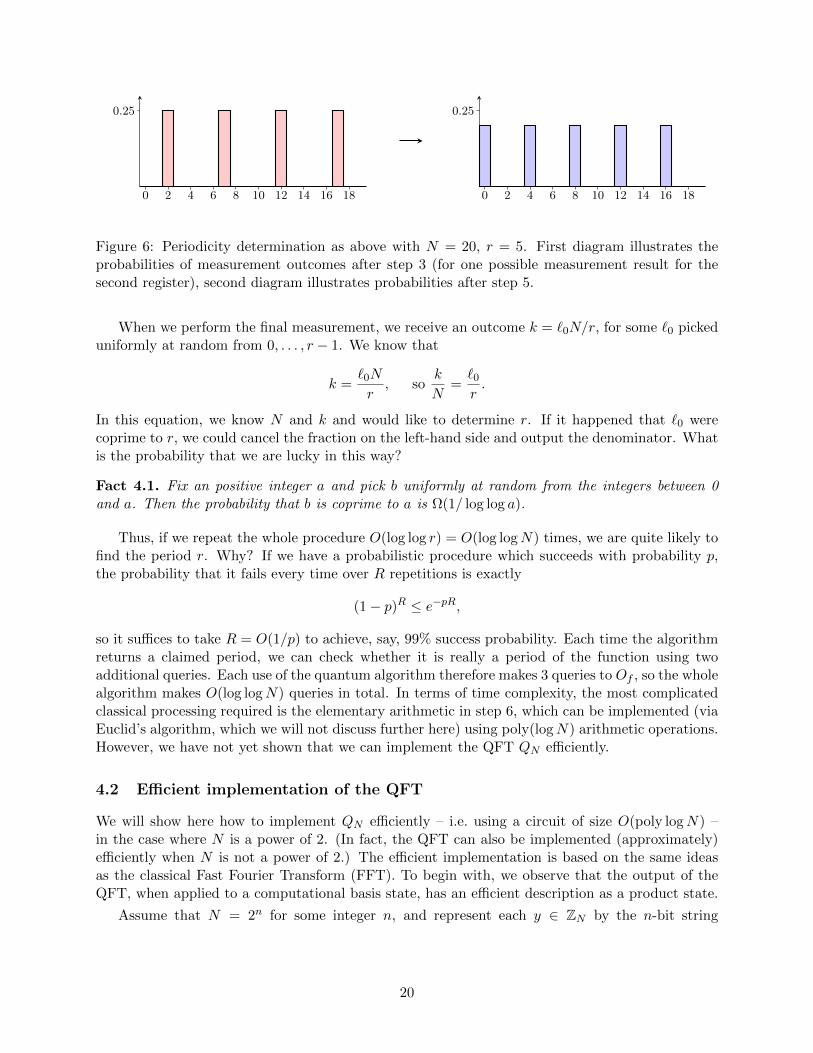
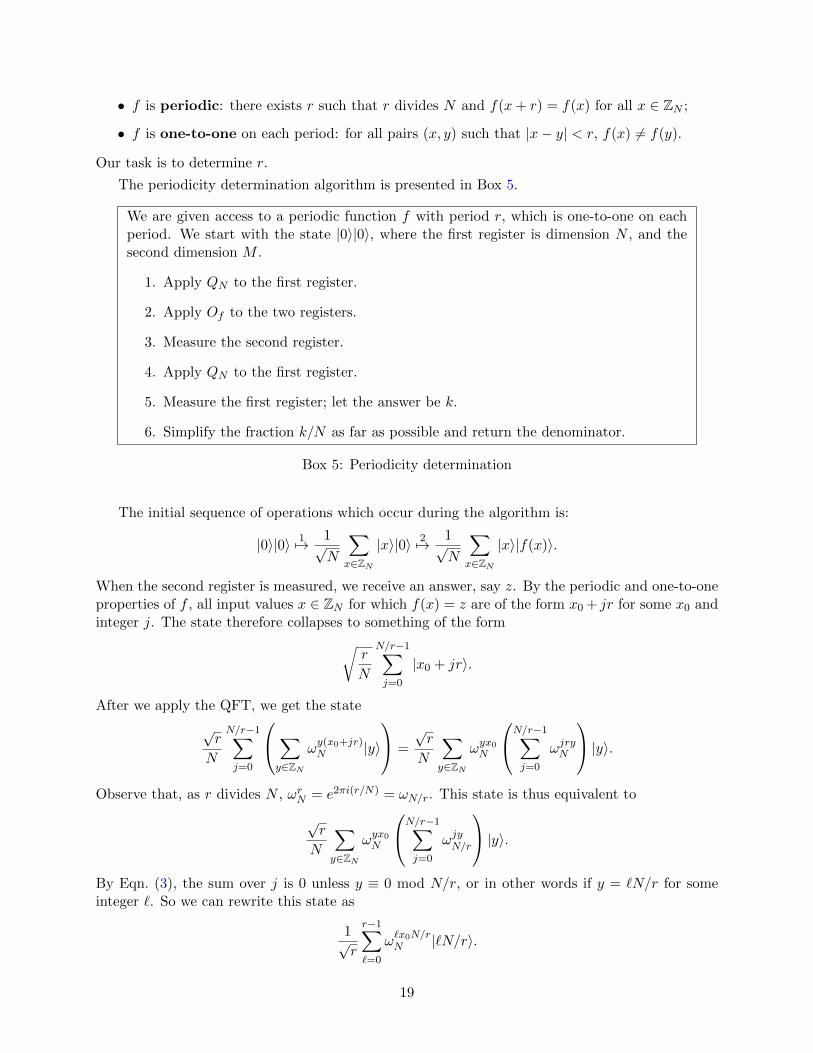
0 2 4 6 8 10 12 14 16 18
0.25
0 2 4 6 8 10 12 14 16 18
0.25
Figure 6: Periodicity determination as above with N = 20, r = 5. First diagram illustrates theprobabilities of measurement outcomes after step 3 (for one possible measurement result for thesecond register), second diagram illustrates probabilities after step 5.
When we perform the final measurement, we receive an outcome k = `0N/r, for some `0 pickeduniformly at random from 0, . . . , r − 1. We know that
k =`0N
r, so
k
N=`0r.
In this equation, we know N and k and would like to determine r. If it happened that `0 werecoprime to r, we could cancel the fraction on the left-hand side and output the denominator. Whatis the probability that we are lucky in this way?
Fact 4.1. Fix an positive integer a and pick b uniformly at random from the integers between 0and a. Then the probability that b is coprime to a is Ω(1/ log log a).
Thus, if we repeat the whole procedure O(log log r) = O(log logN) times, we are quite likely tofind the period r. Why? If we have a probabilistic procedure which succeeds with probability p,the probability that it fails every time over R repetitions is exactly
(1− p)R ≤ e−pR,
so it suffices to take R = O(1/p) to achieve, say, 99% success probability. Each time the algorithmreturns a claimed period, we can check whether it is really a period of the function using twoadditional queries. Each use of the quantum algorithm therefore makes 3 queries to Of , so the wholealgorithm makes O(log logN) queries in total. In terms of time complexity, the most complicatedclassical processing required is the elementary arithmetic in step 6, which can be implemented (viaEuclid’s algorithm, which we will not discuss further here) using poly(logN) arithmetic operations.However, we have not yet shown that we can implement the QFT QN efficiently.
4.2 Efficient implementation of the QFT
We will show here how to implement QN efficiently – i.e. using a circuit of size O(poly logN) –in the case where N is a power of 2. (In fact, the QFT can also be implemented (approximately)efficiently when N is not a power of 2.) The efficient implementation is based on the same ideasas the classical Fast Fourier Transform (FFT). To begin with, we observe that the output of theQFT, when applied to a computational basis state, has an efficient description as a product state.
Assume that N = 2n for some integer n, and represent each y ∈ ZN by the n-bit string
20
(y0, y1, . . . , yn−1), where y = y0 + 2y1 + 4y2 + · · ·+ 2n−1yn−1. Then
QN |x〉 =1
2n/2
∑y∈Z2n
ωxy2n |y〉
=1
2n/2
∑y∈0,1n
ωx(
∑n−1j=0 2jyj)
2n |yn−1〉|yn−2〉 . . . |y0〉
=
1√2
∑yn−1∈0,1
ω2n−1xyn−1
2n |yn−1〉
1√2
∑yn−2∈0,1
ω2n−2xyn−2
2n |yn−2〉
. . .
1√2
∑y0∈0,1
ωxy02n |y0〉
=
n⊗j=1
1√2
∑yn−j∈0,1
ωxyn−j2j
|yn−j〉
.
Because xyn−j ≡ 0 mod 2j when x is an integer multiple of 2j , we see that the j’th qubit of theoutput only depends on the j bits x0, . . . , xj−1. We can write this another way, as
QN |x〉 =1
2n/2
(|0〉+ e2πi(.x0)|1〉
)(|0〉+ e2πi(.x1x0)|1〉
). . .(|0〉+ e2πi(.xn−1...x0)|1〉
),
where the notation (.xj−1 . . . x0) is used for the binary fraction
xj−1
2+xj−2
4+ . . .
x0
2j.
So we see that the first qubit of the output depends on only the last qubit of the input, the secondqubit depends on the last two, etc. We can utilise this structure by building up the output statein reverse order. The last stage of the circuit creates the correct state for the first qubit, which isthen not used again; the last but one stage creates the correct state for the second qubit, etc. Toproduce the correct state for each qubit, we can use the gates H and Rd, where
H =1√2
(1 11 −1
), Rd =
(1 0
0 eπi/2d
).
Here we are assuming that we have access to Rd gates for arbitrary d; as briefly discussed in Section2, this is not essential as any universal gate set will allow us to approximately implement thesegates. Observe that the Hadamard gate can be written as the map
H|x〉 =1√2
(|0〉+ e2πi(.x)|1〉
)for x ∈ 0, 1. We can use this to start building up a binary fraction in the phase of the basisstate |1〉. Applying a Rd gate to this state will add 1/2d+1 to this binary fraction. To apply Rdconditional on the bits of x, we will use controlled-Rd gates.
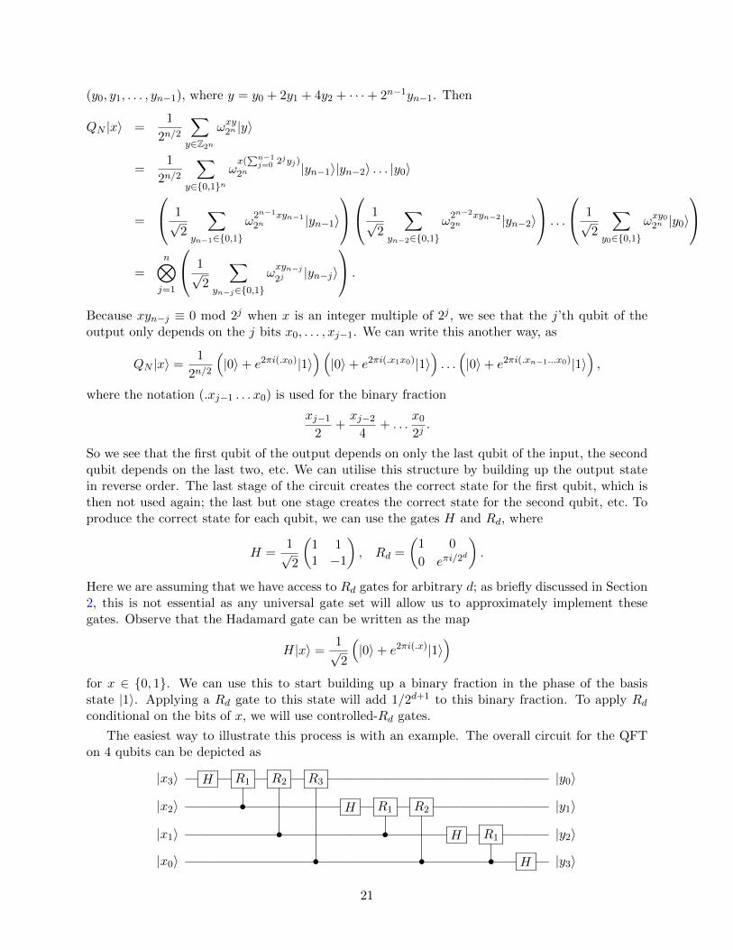
The easiest way to illustrate this process is with an example. The overall circuit for the QFTon 4 qubits can be depicted as
|x3〉 H R1 R2 R3 |y0〉
|x2〉 • H R1 R2 |y1〉
|x1〉 • • H R1 |y2〉
|x0〉 • • • H |y3〉
21
Observe that the output state is backwards, i.e. the qubits appear in reverse order. They can bereturned to the original order, if desired, using swap gates. How many gates in total are used inthe circuit? The j’th stage of the circuit, for j = 1, . . . , n, uses one Hadamard gate and n − j Rdgates. Thus the overall number of gates used is O(n2); n(n−1)/2 Rd gates and n Hadamard gates,then n additional swap gates, if used. This is O(log2N), so we have indeed obtained an efficientcircuit.
This complexity can be improved further, to O(n log n), if we are content with an approximateversion of the QFT. The observation which implies this is that many of the operations in the circuitare Rd gates for large values of d, which do not affect the output significantly. Indeed, it turns outthat there is a constant C such that if we omit the gates Rd with d ≥ C log n, for any input state|x〉 the output is close to the input up to an error of at most 1/poly(n). The modified circuit usesO(log n) gates at each stage, so O(n log n) in total.
22
5 Integer factorisation
The main application of periodicity determination is Shor’s quantum algorithm for integer factori-sation. Given an n-digit integer N as input, this algorithm outputs a non-trivial factor of N (or thatN is prime, if this is the case) with success probability 1− ε, for any ε > 0, in time O(n3). The best
classical algorithm known (the general number field sieve) runs in time eO(n1/3 log2/3 n). In fact, thisis a heuristic bound and this algorithm’s worst-case runtime has not been rigorously determined;the best proven bound is somewhat higher. Shor’s algorithm thus achieves a super-polynomialimprovement. This result might appear only of mathematical interest, were it not for the fact thatthe very widely-used RSA public-key cryptosystem relies on the hardness of integer factorisation.Shor’s efficient factorisation algorithm implies that this cryptosystem is insecure against attack bya large quantum computer. Although no large-scale quantum computer yet exists, this result hasalready had major implications for cryptography, as national security agencies start to move awayfrom the RSA cryptosystem.
Unfortunately (?), proving correctness of Shor’s algorithm requires going through a number oftechnical details. First we need to show that factoring reduces to a periodicity problem – though inthis case an approximate periodicity problem. This part uses only classical number theory. Then weneed to show that periodicity can still be determined even in the setting where the input functionis only approximately periodic. This part uses the theory of continued fractions.
5.1 From factoring to periodicity
The basic skeleton of the quantum factorisation algorithm is given in Box 7. It is based on two“magic” subroutines. The first is a classical algorithm for computing the greatest common divisor(gcd) of two integers. This can be achieved efficiently using Euclid’s algorithm. The second ingre-dient is an algorithm for computing the order of an integer a modulo N , i.e. the smallest integer rsuch that ar ≡ 1 mod N ; this is where we will use periodicity determination. As long as a and Nare coprime, such an integer p exists:
Fact 5.1 (Euler’s theorem). If a and N are coprime then there exists p such that ar ≡ 1 mod N .
Let N denote the integer to be factorised. Assume that N is not even or a power of aprime.
1. Choose 1 < a < N uniformly at random.
2. Compute b = gcd(a,N). If b > 1 output b and stop.
3. Determine the order r of a modulo N . If r is odd, the algorithm has failed; termi-nate.
4. Compute s = gcd(ar/2 − 1, N). If s = 1, the algorithm has failed; terminate.
5. Output s.
Box 7: Integer factorisation algorithm (overview)
We start by showing that this algorithm does work, assuming that the subroutines used allwork correctly. If a is coprime to N , there exists r such that ar ≡ 1 mod N . If, further, such an r
23
is even, we can factorar − 1 = (ar/2 + 1)(ar/2 − 1) ≡ 0 mod N.
So N divides the product (ar/2 + 1)(ar/2 − 1). If neither term in the product is a multiple of Nitself, N must divide partly into each of them, so if we computed gcd(ar/2±1, N), we would obtaina factor of N . Because r is the smallest integer x such that ax ≡ 1 mod N , we know that ar/2 − 1is not divisible by N . We also need that ar/2 + 1 is not divisible by N . This, and r being even,turn out to occur with quite high probability:
Fact 5.2. Let N be odd and not a power of a prime. If 1 < a < N is chosen uniformly at randomwith gcd(a,N) = 1, then Pr[r is even and ar/2 6≡ −1 mod N ] ≥ 1/2.
The algorithm thus succeeds with probability at least 1/2. If it fails, we simply repeat thewhole process. After K repetitions, we achieve a failure probability of at most 1/2K . Even if theorder-finding procedure has some small probability of error (which will turn out to be the case),we can check whether the algorithm’s output s is correct by attempting to divide N by s.
We assumed throughout that N is not even or a power of a prime. If N is even, we simplyoutput 2 as a factor. To deal with the case that N = p` for some prime p and some integer ` > 0,we observe that we can efficiently compute the roots N1/k, for k = 2, . . . , log2N . If any of these isan integer, we have found a factor of N . Finally, what about if N is itself prime? In this case thealgorithm will fail every time. We can therefore output “prime” after a suitable number of failures.
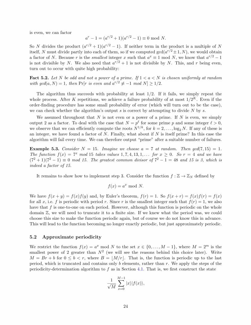
Example 5.3. Consider N = 15. Imagine we choose a = 7 at random. Then gcd(7, 15) = 1.The function f(x) = 7x mod 15 takes values 1, 7, 4, 13, 1, . . . for x ≥ 0. So r = 4 and we have(72 + 1)(72 − 1) ≡ 0 mod 15. The greatest common divisor of 72 − 1 = 48 and 15 is 3, which isindeed a factor of 15.
It remains to show how to implement step 3. Consider the function f : Z→ ZN defined by
f(x) = ax mod N.
We have f(x + y) = f(x)f(y) and, by Euler’s theorem, f(r) = 1. So f(x + r) = f(x)f(r) = f(x)for all x, i.e. f is periodic with period r. Since r is the smallest integer such that f(r) = 1, we alsohave that f is one-to-one on each period. However, although this function is periodic on the wholedomain Z, we will need to truncate it to a finite size. If we knew what the period was, we couldchoose this size to make the function periodic again, but of course we do not know this in advance.This will lead to the function becoming no longer exactly periodic, but just approximately periodic.
5.2 Approximate periodicity
We restrict the function f(x) = ax mod N to the set x ∈ 0, . . . ,M − 1, where M = 2m is thesmallest power of 2 greater than N2 (we will see the reasons behind this choice later). WriteM = Br + b for 0 ≤ b < r, where B = bM/rc. That is, the function is periodic up to the lastperiod, which is truncated and contains only b elements, rather than r. We apply the steps of theperiodicity-determination algorithm to f as in Section 4.1. That is, we first construct the state
1√M
M−1∑x=0
|x〉|f(x)〉,
24
0 2 4 6 8 10 12 14 16 18 20 22 24 26 28 30
0.2
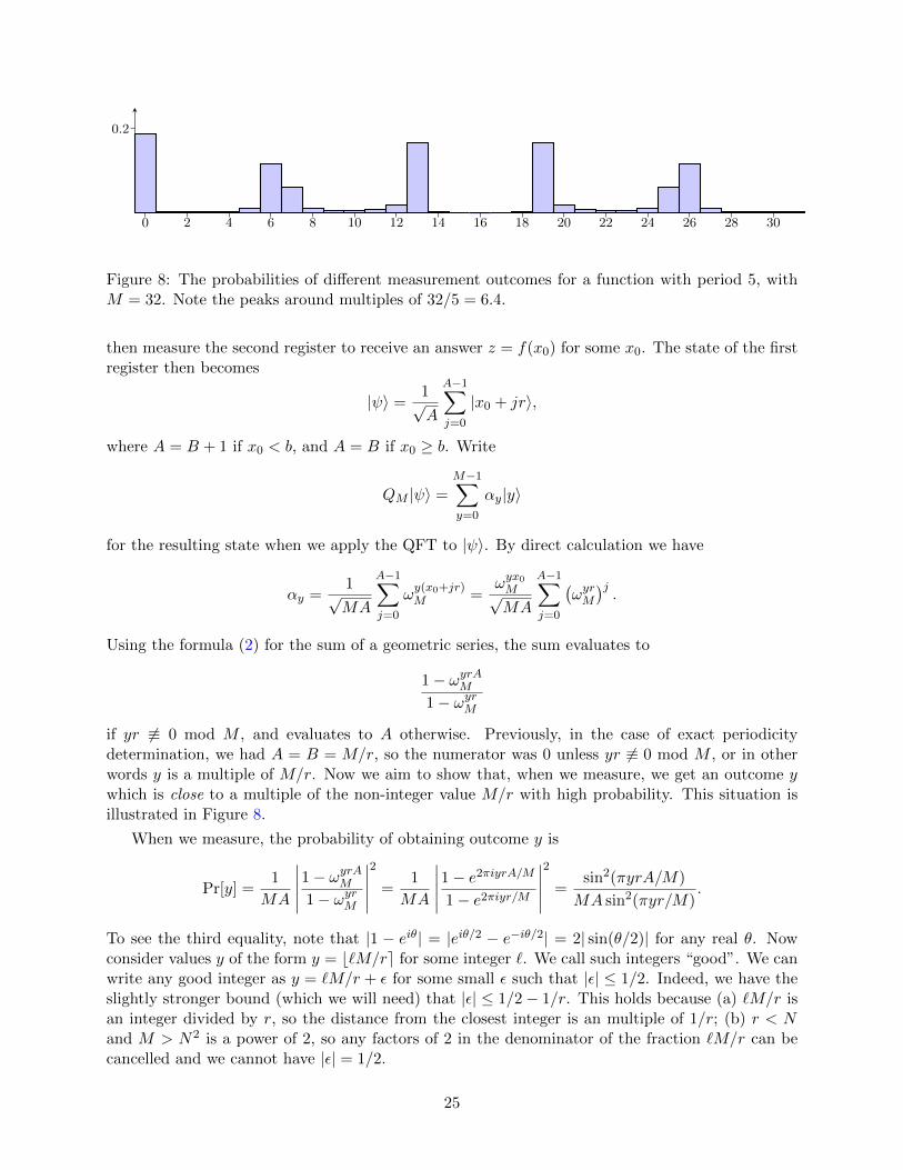
Figure 8: The probabilities of different measurement outcomes for a function with period 5, withM = 32. Note the peaks around multiples of 32/5 = 6.4.
then measure the second register to receive an answer z = f(x0) for some x0. The state of the firstregister then becomes
|ψ〉 =1√A
A−1∑j=0
|x0 + jr〉,
where A = B + 1 if x0 < b, and A = B if x0 ≥ b. Write
QM |ψ〉 =M−1∑y=0
αy|y〉
for the resulting state when we apply the QFT to |ψ〉. By direct calculation we have
αy =1√MA
A−1∑j=0
ωy(x0+jr)M =
ωyx0M√MA
A−1∑j=0
(ωyrM)j.
Using the formula (2) for the sum of a geometric series, the sum evaluates to
1− ωyrAM
1− ωyrMif yr 6≡ 0 mod M , and evaluates to A otherwise. Previously, in the case of exact periodicitydetermination, we had A = B = M/r, so the numerator was 0 unless yr 6≡ 0 mod M , or in otherwords y is a multiple of M/r. Now we aim to show that, when we measure, we get an outcome ywhich is close to a multiple of the non-integer value M/r with high probability. This situation isillustrated in Figure 8.
When we measure, the probability of obtaining outcome y is
Pr[y] =1
MA
∣∣∣∣∣1− ωyrAM
1− ωyrM
∣∣∣∣∣2
=1
MA
∣∣∣∣∣1− e2πiyrA/M
1− e2πiyr/M
∣∣∣∣∣2
=sin2(πyrA/M)
MA sin2(πyr/M).
To see the third equality, note that |1 − eiθ| = |eiθ/2 − e−iθ/2| = 2| sin(θ/2)| for any real θ. Nowconsider values y of the form y = b`M/re for some integer `. We call such integers “good”. We canwrite any good integer as y = `M/r + ε for some small ε such that |ε| ≤ 1/2. Indeed, we have theslightly stronger bound (which we will need) that |ε| ≤ 1/2− 1/r. This holds because (a) `M/r isan integer divided by r, so the distance from the closest integer is an multiple of 1/r; (b) r < Nand M > N2 is a power of 2, so any factors of 2 in the denominator of the fraction `M/r can becancelled and we cannot have |ε| = 1/2.
25
Then
Pr[y] =sin2(π(`M/r + ε)rA/M)
MA sin2(π(`M/r + ε)r/M)=
sin2(`Aπ + εrAπ/M)
MA sin2(`π + εrπ/M)=
sin2(εrAπ/M)
MA sin2(εrπ/M)
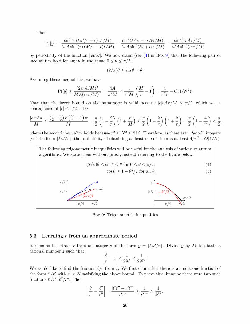
by periodicity of the function | sin θ|. We now claim (see (4) in Box 9) that the following pair ofinequalities hold for any θ in the range 0 ≤ θ ≤ π/2:
(2/π)θ ≤ sin θ ≤ θ.
Assuming these inequalities, we have
Pr[y] ≥ (2εrA/M)2
MA(εrπ/M)2=
4A
π2M≥ 4
π2M
(M
r− 1
)=
4
π2r−O(1/N2).
Note that the lower bound on the numerator is valid because |ε|rAπ/M ≤ π/2, which was aconsequence of |ε| ≤ 1/2− 1/r:
|ε|rAπM
≤(
12 −
1r
)r(Mr + 1
)π
M=π
2
(1− 2
r
)(1 +
r
M
)≤ π
2
(1− 2
r
)(1 +
2
r
)=π
2
(1− 4
r2
)<π
2,
where the second inequality holds because r2 ≤ N2 ≤ 2M . Therefore, as there are r “good” integersy of the form b`M/re, the probability of obtaining at least one of them is at least 4/π2 −O(1/N).
The following trigonometric inequalities will be useful for the analysis of various quantumalgorithms. We state them without proof, instead referring to the figure below.
(2/π)θ ≤ sin θ ≤ θ for 0 ≤ θ ≤ π/2; (4)
cos θ ≥ 1− θ2/2 for all θ. (5)
sin θ
(2/π)θ
θπ/2
π/4
π/2π/4
cos θ
1 − θ2/2
1
0.5
π/2π/4
Box 9: Trigonometric inequalities
5.3 Learning r from an approximate period
It remains to extract r from an integer y of the form y = b`M/re. Divide y by M to obtain arational number z such that ∣∣∣∣ `r − z
∣∣∣∣ < 1
2M<
1
2N2.
We would like to find the fraction `/r from z. We first claim that there is at most one fraction ofthe form `′/r′ with r′ < N satisfying the above bound. To prove this, imagine there were two suchfractions `′/r′, `′′/r′′. Then ∣∣∣∣ `′r′ − `′′
r′′
∣∣∣∣ =|`′r′′ − r′`′′|
r′r′′≥ 1
r′r′′>
1
N2.
26
But, as `′/r′, `′′/r′′ are each within 1/(2N2) of z, they must be at most distance 1/N2 apart, sowe have a contradiction.
We have seen that it suffices to find any fraction `′/r′ such that r′ < N to learn `/r. To dothis, we use the theory of continued fractions. The continued fraction expansion (CFE) of z is anexpression of the form
z =1
a1 + 1a2+ 1
a3+...
,
where the ai are positive integers. To find the integers ai, we start by writing
z =1
z′,
where z′ = a1 + b for some integer a1 and some b < 1; then repeating this process on b. Notethat, for any rational z, this expansion must terminate after some number of iterations C. One canshow that in fact, for any rational z = s/t where s and t are m-bit integers, C = O(m). Once wehave calculated this expansion, if we truncate it after some smaller number of steps, we obtain anapproximation to z. These approximations are called convergents of the CFE.
Example 5.4. The continued fraction expansion of z = 31/64 is
31
64=
1
2 + 115+ 1
2
.
The convergents are1
2,
1
2 + 115
=15
31.
Fact 5.5. Any fraction p/q with |p/q − z| < 1/(2q2) will appear as one of the convergents of theCFE of z.
Therefore, if we carry out the continued fraction expansion of z, we are guaranteed to find `/r,as the unique fraction close enough to z.
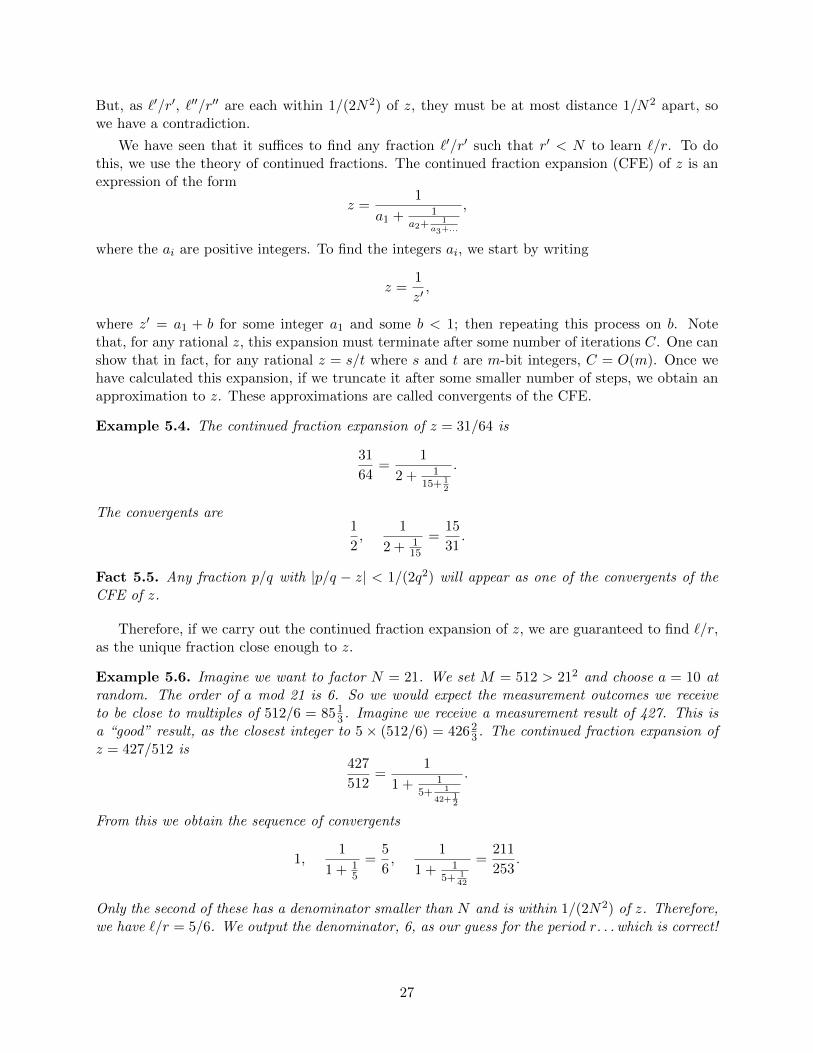
Example 5.6. Imagine we want to factor N = 21. We set M = 512 > 212 and choose a = 10 atrandom. The order of a mod 21 is 6. So we would expect the measurement outcomes we receiveto be close to multiples of 512/6 = 851
3 . Imagine we receive a measurement result of 427. This isa “good” result, as the closest integer to 5× (512/6) = 4262
3 . The continued fraction expansion ofz = 427/512 is
427
512=
1
1 + 15+ 1
42+12
.
From this we obtain the sequence of convergents
1,1
1 + 15
=5
6,
1
1 + 15+ 1
42
=211
253.
Only the second of these has a denominator smaller than N and is within 1/(2N2) of z. Therefore,we have `/r = 5/6. We output the denominator, 6, as our guess for the period r. . . which is correct!
27
5.4 Complexity analysis
How complex is the final, overall algorithm? Recall that N is n bits in length. We have seen thatthe QFT on ZM can be implemented in time O(log2M) = O(n2). To implement the modularexponentiation operation f(x) = ax mod N efficiently, we can use repeated squaring to producef(2k) for any integer k in k squaring operations. Multiplying the different values f(2k) togetherfor each k such that the k’th bit of a is nonzero produces f(x). So we require O(n) multiplicationsof n-bit integers to compute f(x). Multiplying two n-bit numbers can be achieved classically usingstandard long multiplication in time O(n2), so we get an overall complexity of O(n3).
It turns out (though we will not show it here) that the classical processing of the measurementresults based on Euclid’s algorithm and the continued fractions algorithm can also be done in timeO(n3). Thus the overall time complexity of the whole algorithm is O(n3), whereas the best knownclassical algorithm runs in time exponential in n1/3. The asymptotic quantum complexity can infact be improved a bit further, to O(n2 poly log n), by using more advanced multiplication anddivision algorithms with runtime O(n poly log n). However, these algorithms only become moreefficient in practice for very large values of n.
28
6 Phase estimation
We now discuss an important primitive used in quantum algorithms called phase estimation, whichprovides a different and unifying perspective on the quantum algorithms which you have just seen.Phase estimation is once again based on the QFT over ZN , where N = 2n.
Imagine we are given a unitary operator U . U may either be written down as a quantum circuit,or we may be given access to a black box which allows us to apply a controlled-U j operation forinteger values of j. We are also given a state |ψ〉 which is an eigenvector of U : U |ψ〉 = e2πiφ|ψ〉 forsome real φ such that 0 ≤ φ < 1. We would like to determine φ to n bits of precision, for somearbitrary n.
To do so, we prepend an n qubit register to |ψ〉, initially in the state |0〉, and create the state
1√N
N−1∑x=0
|x〉|ψ〉
by applying a Hadamard gate to each qubit in the first register. We then apply the unitary operator
U ′ =N−1∑x=0
|x〉〈x| ⊗ Ux.
This operator can be thought of as performing the map where if the first register contains x, weapply U x times to the second register. By expressing x in binary we can implement U ′ usingcontrolled-U2j gates for different integers j, controlled on different qubits in the first register. Afterapplying U ′, we are left with the state
1√N
N−1∑x=0
e2πiφx|x〉|ψ〉;
note that the second register is left unchanged. We now apply the operator Q−1 to the first registerand then measure it, receiving outcome y (say). We output the binary fraction
0.y1y2 . . . yn =y1
2+y2
4+ · · ·+ yn
2n
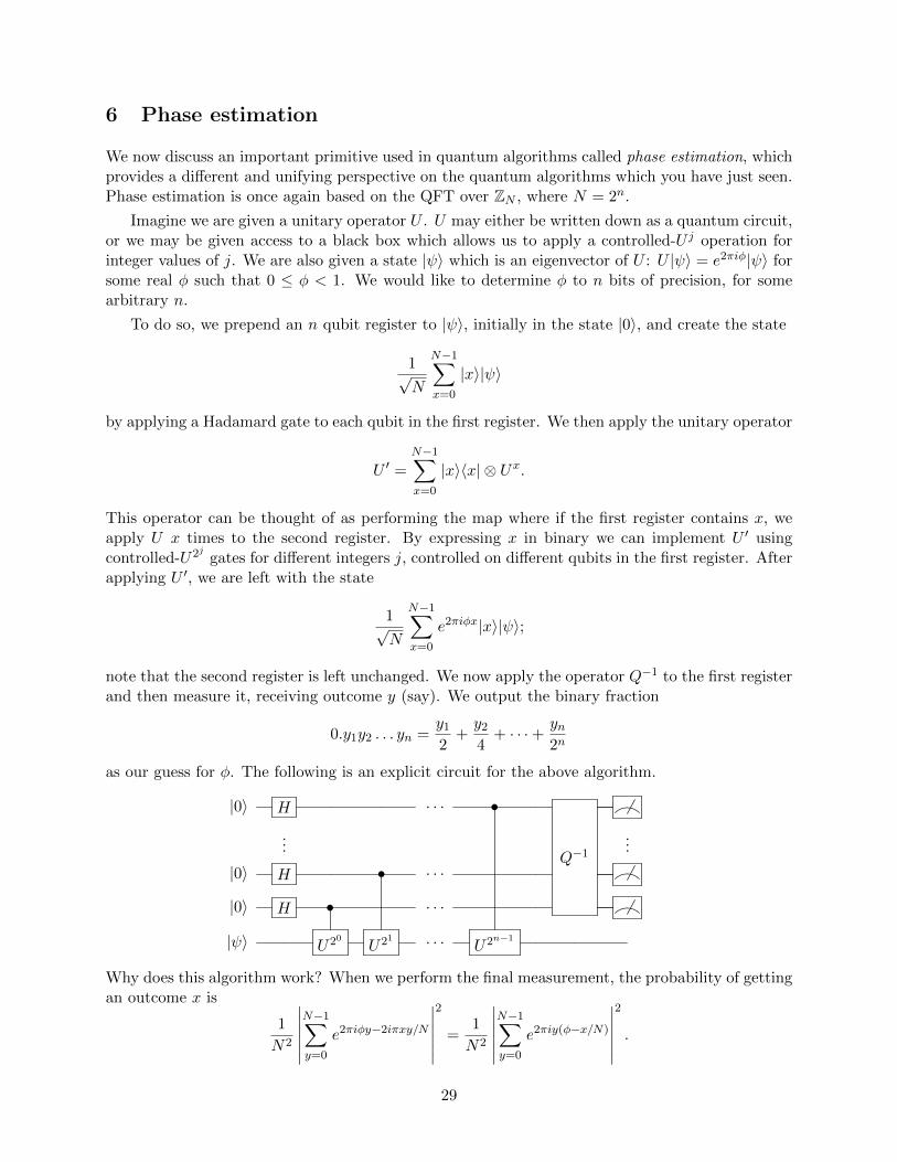
as our guess for φ. The following is an explicit circuit for the above algorithm.
|0〉 H . . . •
Q−1
......
|0〉 H • . . .
|0〉 H • . . .
|ψ〉 U20 U21 . . . U2n−1
Why does this algorithm work? When we perform the final measurement, the probability of gettingan outcome x is
1
N2
∣∣∣∣∣∣N−1∑y=0
e2πiφy−2iπxy/N
∣∣∣∣∣∣2
=1
N2
∣∣∣∣∣∣N−1∑y=0
e2πiy(φ−x/N)
∣∣∣∣∣∣2
.
29
First imagine that the binary expansion of φ is at most n bits long, or in other words φ = z/N forsome 0 ≤ z ≤ N − 1. In this case we have
1
N2
∣∣∣∣∣∣N−1∑y=0
e2πiy(φ−x/N)
∣∣∣∣∣∣2
=1
N2
∣∣∣∣∣∣N−1∑y=0
e2πiy(z−x)/N
∣∣∣∣∣∣2
= δxz
by the unitarity of the QFT, so the measurement outcome is guaranteed to be z, implying thatthe algorithm outputs φ with certainty. If the binary expansion of φ is longer than n bits, we nowshow that we still get the best possible answer with probability Ω(1), and indeed are very likelyto get an answer close to φ. The proof turns out to be very similar to that of correctness of theperiodicity determination algorithm in the approximate case.
Theorem 6.1. The probability that the above algorithm outputs the real number with n binarydigits which is closest to φ is at least 4/π2. Further, the probability that the algorithm outputs θsuch that |θ − φ| ≥ ε is at most O(1/(Nε)).
Proof. If the binary expansion of φ has n binary digits or fewer, we are done by the argumentabove. So, assuming it does not, let φ be the closest approximation to φ that has n binary digits,and write φ = a/N for some integer 0 ≤ a ≤ N−1. For any z, define δ(z) := φ−z/N and note that0 < |δ(a)| ≤ 1/(2N). For any φ, the probability of getting outcome z from the final measurementis
Pr[z] =1
N2
∣∣∣∣∣∣N−1∑y=0
e2πiy(φ−z/N)
∣∣∣∣∣∣2
=1
N2
∣∣∣∣∣∣N−1∑y=0
e2πiyδ(z)
∣∣∣∣∣∣2
=1
N2
∣∣∣∣∣1− e2πiNδ(z)
1− e2πiδ(z)
∣∣∣∣∣2
=sin2(πNδ(z))
N2 sin2(πδ(z)),
(6)where we evaluate the sum using the formula for a geometric series. This quantity should befamiliar from the proof of correctness of the periodicity determination algorithm.
We first lower bound this expression for z = a to prove the first part of the lemma. As|δ(a)| ≤ 1/(2N), we have Nπδ(a) ≤ π/2. Then
Pr[a] =sin2(πNδ(a))
N2 sin2(πδ(a))≥ (2Nδ(a))2
N2(πδ(a))2=
4
π2
using the trigonometric inequalities (4).
In order to prove the second part of the theorem, we now find an upper bound on expression(6). First, it is clear that sin2(πNδ(z)) ≤ 1 always. For the denominator, by the same argumentto above we have sin(πδ(z)) ≥ 2δ(z) and hence, for all z,
Pr[get outcome z] ≤ 1
N2
(1
2δ(z)
)2
=1
4N2δ(z)2.
We now sum this expression over all z such that |δ(z)| ≥ ε. The sum is symmetric about δ(z) = 0,and as z is an integer, the terms in this sum corresponding to δ(z) > 0 are δ0, δ0 + 1/N, . . . , forsome δ0 ≥ ε. The sum will be maximised when δ0 = ε, when we obtain
Pr[get outcome z with |δ(z)| ≥ ε] ≤ 1
4N2
∞∑k=0
1
(ε+ k/N)2≤ 1
4
∫ ∞0
1
(Nε+ k)2dk
=1
4
∫ ∞Nε
1
k2dk = O
(1
Nε
).
30
We observe the following points regarding the behaviour of this algorithm.
• What happens if we do not know an eigenvector of U? If we input an arbitrary state |ϕ〉to the phase estimation algorithm, we can write it as a superposition |ϕ〉 =
∑j αj |ψj〉 over
eigenvectors |ψj〉. Therefore, the algorithm will output an estimate of each correspondingeigenvalue φj with probability |αj |2. This may or may not allow us to infer anything useful,depending on what we know about U in advance.
• In order to approximate φ to n bits of precision, we needed to apply the operator U2m , forall 0 ≤ m ≤ n− 1. If we are given U as a black box, this may be prohibitively expensive aswe need to use the black box exponentially many times in n. However, if we have an explicitcircuit for U , we may be able to find a more efficient way of computing U2m . An example ofthis is modular exponentiation, where we can efficiently perform repeated squaring.
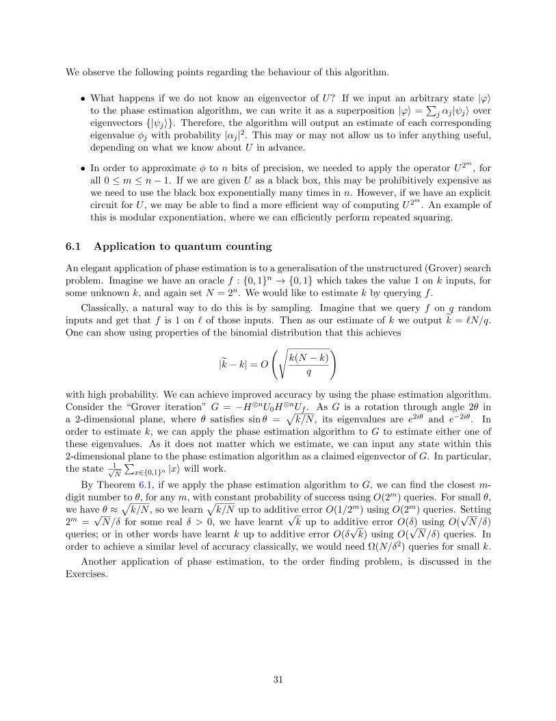
6.1 Application to quantum counting
An elegant application of phase estimation is to a generalisation of the unstructured (Grover) searchproblem. Imagine we have an oracle f : 0, 1n → 0, 1 which takes the value 1 on k inputs, forsome unknown k, and again set N = 2n. We would like to estimate k by querying f .
Classically, a natural way to do this is by sampling. Imagine that we query f on q randominputs and get that f is 1 on ` of those inputs. Then as our estimate of k we output k = `N/q.One can show using properties of the binomial distribution that this achieves
|k − k| = O
(√k(N − k)
q
)
with high probability. We can achieve improved accuracy by using the phase estimation algorithm.Consider the “Grover iteration” G = −H⊗nU0H
⊗nUf . As G is a rotation through angle 2θ ina 2-dimensional plane, where θ satisfies sin θ =
√k/N , its eigenvalues are e2iθ and e−2iθ. In
order to estimate k, we can apply the phase estimation algorithm to G to estimate either one ofthese eigenvalues. As it does not matter which we estimate, we can input any state within this2-dimensional plane to the phase estimation algorithm as a claimed eigenvector of G. In particular,the state 1√
N
∑x∈0,1n |x〉 will work.
By Theorem 6.1, if we apply the phase estimation algorithm to G, we can find the closest m-digit number to θ, for any m, with constant probability of success using O(2m) queries. For small θ,we have θ ≈
√k/N , so we learn
√k/N up to additive error O(1/2m) using O(2m) queries. Setting
2m =√N/δ for some real δ > 0, we have learnt
√k up to additive error O(δ) using O(
√N/δ)
queries; or in other words have learnt k up to additive error O(δ√k) using O(
√N/δ) queries. In
order to achieve a similar level of accuracy classically, we would need Ω(N/δ2) queries for small k.
Another application of phase estimation, to the order finding problem, is discussed in theExercises.
31
7 Hamiltonian simulation
One of the earliest – and most important – applications of a quantum computer is likely to bethe simulation of quantum mechanical systems. There are quantum systems for which no efficientclassical simulation is known, but which we can simulate on a universal quantum computer. Whatdoes it mean to “simulate” a physical system? According to the OED, simulation is “the techniqueof imitating the behaviour of some situation or process (whether economic, military, mechanical,etc.) by means of a suitably analogous situation or apparatus”. What we will take simulation tomean here is approximating the dynamics of a physical system. Rather than tailoring our simulatorto simulate only one type of physical system (which is sometimes called analogue simulation), weseek a general simulation algorithm which can simulate many different types of system (sometimescalled digital simulation).
According to quantum mechanics, physical systems are specified by Hamiltonians. For thepurposes of this unit, a Hamiltonian H is a Hermitian operator acting on n qubits (i.e. H = H†),which corresponds physically to a system made up of n 2-level subsystems. The time evolution ofthe state |ψ〉 of a quantum system is governed by Schrodinger’s equation:
i~d
dt|ψ(t)〉 = H(t)|ψ(t)〉,
where H(t) is the Hamiltonian of the system (for convenience, we will henceforth absorb ~ intoH(t)). An important special case on which we will focus is the time-independent setting whereH(t) = H is constant. In this case the solution of this equation is
|ψ(t)〉 = e−iHt|ψ(0)〉.
Given a physical system specified by some Hamiltonian H, we would like to simulate the evolutionof the system on an arbitrary initial state for a certain amount of time t. In other words, given H,we would like to implement a unitary operator which approximates
U(t) = e−iHt.
What does it mean to approximate a unitary? The “gold standard” of approximation is approxi-mation in the operator norm (aka spectral norm)
‖A‖ := max|ψ〉6=0
‖A|ψ〉‖‖|ψ〉‖
,
where ‖|ψ〉‖ =√〈ψ|ψ〉 is the usual Euclidean norm of |ψ〉. Note that this is indeed a norm, and
in particular satisfies the triangle inequality ‖A+ B‖ ≤ ‖A‖+ ‖B‖. We say that U approximatesU to within ε if
‖U − U‖ ≤ ε.
This is a natural definition of approximation because it implies that, for any state |ψ〉, U |ψ〉 andU |ψ〉 are only distance at most ε apart.
7.1 Simulation of k-local Hamiltonians
In order for our quantum simulation of a Hamiltonian H to be efficient, we need U = e−iHt tobe approximable by a quantum circuit containing poly(n) gates. A fairly straightforward counting
32
argument shows that not all Hamiltonians H can be simulated efficiently. However, it turns outthat several important physically motivated classes can indeed be simulated. Perhaps the mostimportant of these is k-local Hamiltonians.
A Hamiltonian H of n qubits is said to be k-local if it can be written as a sum
H =m∑j=1
Hj
for some m, where each Hj is a Hermitian matrix which acts non-trivially on at most k qubits. Thatis, Hj is the tensor product of a matrix H ′j on k qubits, and the identity matrix on the remainingn− k qubits. For example, the Hamiltonian H on 3 qubits defined by
H = X ⊗ I ⊗ I − 2I ⊗ Z ⊗ Y
is 2-local. Many interesting physical systems are k-local for small k (say k ≤ 3), some of which youmay be familiar with. Simple examples include the two-dimensional Ising model on a n× n squarelattice,
H = J
n∑i,j=1
Z(i,j)Z(i,j+1) + Z(i,j)Z(i+1,j)
and the Heisenberg model on a line,
H =n∑i=1
JxX(i)X(i+1) + JyY
(i)Y (i+1) + JzZ(i)Z(i+1),
both of which are used in the study of magnetism and many other areas of physics (in the equationsabove, M (j) denotes a single-qubit operator acting on the j’th qubit, and J, Jx, Jy, Jz are constants).
Note that, if H is k-local for k = O(1), we can assume that m ≤(nk
)= O(nk), so m is polynomial
in n. We first show that each of the individual Hj operators can be simulated efficiently, which isimmediate from the following theorem, formalising a claim made at the start of the unit.
Theorem 7.1 (Solovay-Kitaev theorem). Let U be a unitary operator which acts non-triviallyon k = O(1) qubits, and let S be an arbitrary universal set of quantum gates. Then U can beapproximated in the operator norm to within ε using O(logc(1/ε)) gates from S, for some c < 4.
Proof. Sadly beyond the scope of this course. For a readable explanation, see Andrew Childs’lecture notes.
As each e−iHjt acts non-trivially on only at most k qubits, it follows from the Solovay-Kitaev the-orem that we can approximate each of these operators individually to within ε in timeO(polylog(1/ε)).In the special case where all of the Hj operators commute, we have
e−iHt = e−i(∑mj=1Hj)t =
m∏j=1
e−iHjt.
Thus a natural way to find a unitary operator approximating e−iHt is to take the product of ourapproximations of e−iH1t, . . . , e−iHmt. Although each of these approximates e−iHjt to within ε, thisdoes not imply that their product approximates e−iHt to within ε. However, we now show that theapproximation error only scales linearly.
33
Lemma 7.2. Let (Ui), (Vi) be sequences of m unitary operators satisfying ‖Ui − Vi‖ ≤ ε for all1 ≤ i ≤ m. Then ‖Um . . . U1 − Vm . . . V1‖ ≤ mε.
Proof. The proof is by induction on m. The claim trivially holds for m = 1. Assuming that itholds for a given m, we have
‖Um+1Um . . . U1 − Vm+1Vm . . . V1‖= ‖Um+1Um . . . U1 − Um+1Vm . . . V1 + Um+1Vm . . . V1 − Vm+1Vm . . . V1‖≤ ‖Um+1Um . . . U1 − Um+1Vm . . . V1‖+ ‖Um+1Vm . . . V1 − Vm+1Vm . . . V1‖= ‖Um+1(Um . . . U1 − Vm . . . V1)‖+ ‖(Um+1 − Vm+1)Vm . . . V1‖= ‖Um . . . U1 − Vm . . . V1‖+ ‖Um+1 − Vm+1‖≤ (m+ 1)ε.
Thus, in order to approximate∏mj=1 e
−iHjt to within ε, it suffices to approximate each of theHj to within ε/m. We formalise this as the following proposition.
Proposition 7.3. Let H be a Hamiltonian which can be written as the sum of m commuting termsHj, each acting non-trivially on k = O(1) qubits. Then, for any t, there exists a quantum circuitwhich approximates the operator e−iHt to within ε in time O(m polylog(m/ε)).
7.2 The non-commuting case
Unfortunately, this simulation technique does not necessarily work for non-commuting Hj . The rea-son is that if A and B are non-commuting operators, it need not hold that e−i(A+B)t = e−iAte−iBt.However, we can simulate non-commuting Hamiltonians via an observation known as the Lie-Trotterproduct formula.
In what follows, the notation X +O(ε), for a matrix X, is used as shorthand for X +E, whereE is a matrix satisfying ‖E‖ ≤ Cε, for some universal constant C (not depending on X or ε).
Lemma 7.4 (Lie-Trotter product formula). Let A and B be Hermitian matrices such that ‖A‖ ≤ δand ‖B‖ ≤ δ, for some real δ ≤ 1. Then
e−iAe−iB = e−i(A+B) +O(δ2).
Proof. From the Taylor series for ex, for any matrix A such that ‖A‖ = δ ≤ 1, we have
e−iA = I − iA+∞∑k=2
(−iA)k
k!= I − iA+ (−iA)2
∞∑k=0
(−iA)k
(k + 2)!= I − iA+O(δ2),
where the last equality follows from∥∥∥∥∥∞∑k=0
(−iA)k
(k + 2)!
∥∥∥∥∥ ≤∞∑k=0
δk
(k + 2)!≤ eδ = O(1).
Hence
e−iAe−iB =(I − iA+O(δ2)
) (I − iB +O(δ2)
)= I − iA− iB +O(δ2) = e−i(A+B) +O(δ2).
34
Applying this formula multiple times, for any Hermitian matrices H1, . . . ,Hm satisfying ‖Hj‖ ≤δ ≤ 1 for all j,
e−iH1e−iH2 . . . e−iHm =(e−i(H1+H2) +O(δ2)
)e−iH3 . . . e−iHm
=(e−i(H1+H2+H3) +O((2δ)2)
)e−iH4 . . . e−iHm +O(δ2)
= e−i(H1+···+Hm) +O(δ2) +O((2δ)2) + · · ·+O(((m− 1)δ)2)
= e−i(H1+···+Hm) +O(m3δ2).
Applying this claim to the matrices Hjt/p for arbitrary t and some large integer p, we have
∥∥∥e−iH1t/pe−iH2t/p . . . e−iHmt/p − e−i(H1+···+Hm)t/p∥∥∥ = O
(m3
(tδ
p
)2).
So there is a universal constant C such that if p ≥ Cm3(tδ)2/ε,∥∥∥e−iH1t/pe−iH2t/p . . . e−iHmt/p − e−i(H1+···+Hm)t/p∥∥∥ ≤ ε/p.
By Lemma 7.2, for any such p,∥∥∥(e−iH1t/pe−iH2t/p . . . e−iHmt/p)p− e−i(H1+···+Hm)t
∥∥∥ ≤ ε.Given this result, we can simulate a k-local Hamiltonian simply by simulating the evolution ofeach term for time t/p to high enough accuracy and concatenating the individual simulations. Wesummarise this as the following theorem.
Theorem 7.5. Let H be a Hamiltonian which can be written as the sum of m terms Hj, each actingnon-trivially on k = O(1) qubits and satisfying ‖Hj‖ ≤ 1. Then, for any t, there exists a quantumcircuit which approximates the operator e−iHt to within ε in time O(m4t2/ε), up to polylogarithmicfactors.
It seems somewhat undesirable that, in order to simulate a Hamiltonian for time t, this algorithmhas dependence on t which is O(t2). In fact, using more complicated simulation techniques, theoverall complexity in Theorem 7.5 can be improved to time O(mt), up to polylogarithmic factors.
35
8 Noise and the framework of quantum channels
Not all processes which occur in quantum mechanics are reversible. As a very simple example,consider the operation of throwing away the input state and replacing it with the state |0〉:
|ψ〉 7→ |0〉
for all |ψ〉. This clearly cannot be implemented as a unitary operator. Just as mixed statesgeneralise pure states, we can generalise unitary operations to so-called completely positive trace-preserving (CPTP) maps, also known as quantum channels. These occur throughout quantuminformation theory and are particularly useful for describing noisy operations and decoherence, thebane of quantum computers.
Recall that a mixed state ρ of n qubits, which describes a probabilistic mixture of pure states|ψ〉, is a Hermitian 2n×2n matrix which is positive semidefinite (all its eigenvalues are non-negative;we write ρ ≥ 0 to denote this) and has trace 1. What axioms would we like a physically reasonablemap (“superoperator”) E , which takes mixed states to mixed states, to satisfy?
1. E should be linear: E(pρ+ qσ) = p E(ρ) + q E(σ) for all real p, q.
2. E should be trace-preserving: tr E(ρ) = tr ρ.
3. E should preserve positivity: if ρ ≥ 0, then E(ρ) ≥ 0. But there is a further constraint: ifwe apply E to part of an entangled quantum state, the whole state should remain positivesemidefinite. That is, (E ⊗ I)(ρ) ≥ 0 for ρ ≥ 0, where I is the identity map on an arbitrarilylarge ancilla system. This constraint is called complete positivity.
A completely positive, trace-preserving linear map is called a quantum channel.
8.1 Representations of quantum channels
There are a number of ways in which quantum channels can be represented. We describe two here.
We first consider the Kraus (aka “operator-sum”) representation. Here a channel E with inputdimension din and output dimension dout is described by a sequence of dout × din matrices Ek suchthat ∑
k
E†kEk = I.
The effect of E on a state ρ is then
E(ρ) =∑k
EkρE†k.
A trivial example of a channel in Kraus form is the identity channel I(ρ) = ρ, which has one Krausoperator E1 = I. For a product channel E = E1 ⊗ E2, where
E1(ρ) =∑k
E(1)k ρ(E
(1)k )†, E2(σ) =
∑k
E(2)k σ(E
(2)k )†
we have
E(ρ⊗ σ) = E1(ρ)⊗ E2(σ) =
(∑k
E(1)k ρ(E
(1)k )†
)⊗
(∑`
E(2)` σ(E
(2)` )†
)=
∑k,`
(E(1)k ⊗ E
(2)` )(ρ⊗ σ)((E
(1)k )† ⊗ (E
(2)` )†),
36
so E must have Kraus operators which are tensor products of each pair of those of E1 and E2.
We claim that any superoperator in Kraus form obeys our three axioms:
1. E is linear: for any X and Y ,
E(X + Y ) =∑k
Ek(X + Y )E†k =∑k
EkXE†k +
∑k
EkY E†k = E(X) + E(Y ).
2. E is trace-preserving:
tr E(ρ) = tr
(∑k
EkρE†k
)=∑k
tr(EkρE
†k
)=∑k
tr(ρE†kEk
)= tr
(ρ∑k
E†kEk
)= tr ρ,
where in the second and fourth equalities we use linearity of trace, and in the third we useits invariance under cyclic shifts.
3. E is completely positive. Here it is sufficient to show that E ⊗ I maps positive operatorsto positive operators. Let ρ be an arbitrary positive operator on the extended system (withancilla). Then
(E ⊗ I)(ρ) =∑k
(Ek ⊗ I)ρ(E†k ⊗ I).
For this to be positive semidefinite, it is sufficient that for any positive semidefinite ρ and anymatrix M , MρM † is positive semidefinite. This holds because we can expand ρ as a convexcombination of pure states |ψi〉, and
M |ψi〉〈ψi|M † = |ψ′i〉〈ψ′i|
for some (unnormalised) vector |ψ′i〉, which is positive semidefinite.
In fact, it turns out that the equivalence goes the other way too: every quantum channel can bewritten in Kraus form. We omit the proof (see Nielsen & Chuang, Theorem 8.1).
The Kraus representation is not unique. For example, the channels described by pairs of Krausoperators (with respect to the standard basis)
E1 =1√2
(1 00 1
), E2 =
1√2
(1 00 −1
), and F1 =
(1 00 0
), F2 =
(0 00 1
)have different representations, but are actually the same channel. This can be seen by writingF1 = (E1 + E2)/
√2, F2 = (E1 − E2)/
√2, and calculating
F1ρF†1 + F2ρF
†2 =
(E1 + E2)ρ(E†1 + E†2) + (E1 − E2)ρ(E†1 − E†2)
2= E1ρE
†1 + E2ρE
†2.
Second, we describe the Stinespring representation. In this representation, a channel E fromsystem A to system B, E : B(CdA) → B(CdB ), is described by an isometry from A to the pair ofsystems B and E, V : CdA → CdB ⊗ CdE , such that
E(ρ) = trE(V ρV †).
(We say that V is an isometry if V †V = I; this is equivalent to V preserving inner productsbetween states.) That is, the channel consists of applying an isometry to ρ, mapping it into a
37
larger-dimensional space, then tracing out (discarding) part of the space. We can think of thispicture as modelling the dynamics of an open quantum system, where ρ interacts with the outsideenvironment E, then to calculate the final state of the system we discard the environment.
Given a Kraus representation of a channel with operators Ek, we can write down a Stinespringrepresentation in a straightforward way:
V =∑k
Ek ⊗ |k〉. (7)
ThenV †V =
∑k,`
E†kE`〈k|`〉 =∑k
E†kEk = I,
so V is indeed an isometry. Further, for any ρ,
trE(V ρV †) =∑k,`
trE [(Ek ⊗ |k〉)ρ(E†` ⊗ 〈`|)] =∑k,`
trE [(Ekρ⊗ |k〉)(E†` ⊗ 〈`|)]
=∑k,`
(EkρE†` )〈`|k〉 =
∑k
EkρE†k,
so this faithfully represents the original channel. Also observe that any isometry V can be decom-posed as in Eqn. (7), so the equivalence goes both ways. As we can think of any isometry as aunitary operator on a larger space, this correspondence implies that any quantum channel can bethought of as unitary evolution of a larger system, followed by tracing out a subsystem.
8.2 Examples of quantum channels
• Unitary evolution is a quantum channel described by one Kraus operator: ρ 7→ UρU †.
• Discarding ρ and replacing it with some state |ψ〉 is a quantum channel. If ρ is d-dimensional,we have d Kraus operators |ψ〉〈k|, k = 1, . . . , d. Then, for any state ρ,
d∑k=1
|ψ〉〈k|ρ|k〉〈ψ| = |ψ〉
(d∑
k=1
〈k|ρ|k〉
)〈ψ| = (tr ρ)|ψ〉〈ψ| = |ψ〉〈ψ|.
• The qubit depolarising channel replaces the input state ρ with the maximally mixed stateI/2, with probability p; with probability 1− p, the input state is unchanged. That is,
ED(ρ) = pI
2+ (1− p)ρ.
This represents a simple form of noise: with probability p, our knowledge of the qubit is com-pletely randomised, and with probability 1−p the qubit is unharmed. The qubit depolarisingchannel has Kraus operators
E1 =√
1− 3p/4I, E2 = (√p/2)X, E3 = (
√p/2)Y, E4 = (
√p/2)Z.
This can be generalised to d dimensions, where we have
ED(ρ) = pI
d+ (1− p)ρ.
38
• The amplitude damping channel models a scenario in quantum optics where a photon maybe lost, with some probability. We imagine that we have a basis |0〉, |1〉 where 0 represents“no photon” and 1 represents “photon”. Then the Kraus operators of the amplitude dampingchannel EAD are (with respect to the standard basis)
E0 =
(1 00√
1− γ
), E1 =
(0√γ
0 0
)for some γ, which corresponds to the probability of losing a photon. So
EAD(|0〉〈0|) = |0〉〈0|, EAD(|1〉〈1|) = γ|0〉〈0|+ (1− γ)|1〉〈1|
as expected.
• Every measurement is a quantum channel. Imagine we have a projective measurement, i.e.a set of orthogonal projectors Pk such that
∑k Pk = I. Then the probability that we get
outcome k when we perform this measurement on state ρ is trPkρ, and the resulting state ifthis occurs is
ρ′k :=PkρPktr(Pkρ)
.
The Kraus operators of this channel are just the projectors Pk. This is correct because∑k
PkρPk =∑k
tr(Pkρ)PkρPktr(Pkρ)
;
the output state is a probabilistic mixture of the states ρ′k with the correct probabilities.
8.3 Quantum channels and the Bloch sphere
We next discuss an intuitive geometric interpretation of quantum channels. Recall the notion ofthe Bloch sphere from Quantum Information Theory: that mixed states ρ of one qubit can beidentified with points (called “Bloch vectors”) (αx, αy, αz) within the unit sphere in R3 via thecorrespondence
ρ =1
2(I + αxX + αyY + αzZ) .
Then it turns out that any quantum channel E mapping a qubit to a qubit can be thought of asan affine map on the interior of the Bloch sphere. That is, if we write v = (αx, αy, αz)
T , then anysingle-qubit channel can be associated with the map
v 7→ Av + b
for some 3 × 3 matrix A and 3-dimensional vector b. To see this, first observe that as quantumchannels are linear and trace-preserving, and all of the Pauli matrices have trace 0, any operator ofthe form αxX+αyY +αzZ must be mapped by E to another operator of the form α′xX+α′yY +α′zZ.Applying this to a basis of 3 vectors (αx, αy, αz) for R3 and using linearity uniquely determines A.Then, as A maps the vector (0, 0, 0) to (0, 0, 0), b must be the vector of coefficients correspondingto the state E(I/2).
So, to find A and b, we can apply E to I/2 and the Pauli matrices, and write down the Blochvectors corresponding to the result. For example, consider the depolarising channel ED. ThenED(I/2) = I/2, so b = (0, 0, 0)T . On the other hand,
ED(X) = (1− p)X, ED(Y ) = (1− p)Y, ED(Z) = (1− p)Z,
39
so A maps the vector (1, 0, 0) to the vector (1 − p, 0, 0), and similarly for (0, 1, 0) and (0, 0, 1).Writing A as a matrix with respect to the standard basis,
A =
1− p 0 00 1− p 00 0 1− p
.
Thus we see that, geometrically, A shrinks the Bloch sphere by a factor of 1− p in every direction.
40
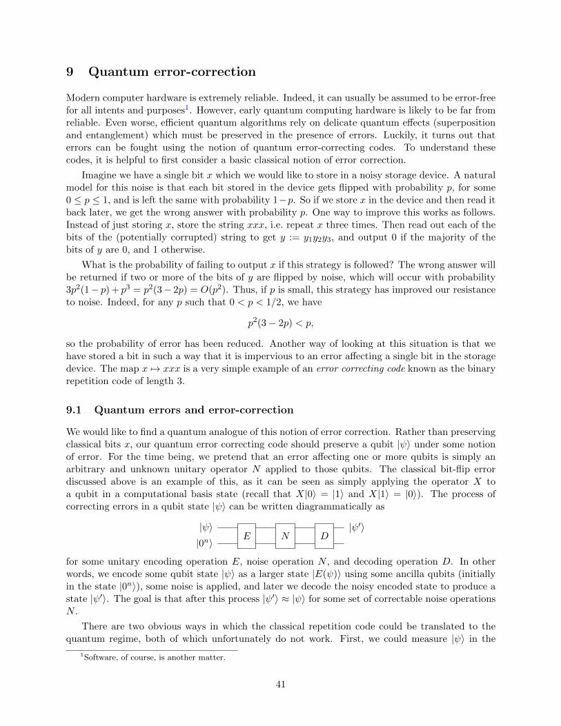
9 Quantum error-correction
Modern computer hardware is extremely reliable. Indeed, it can usually be assumed to be error-freefor all intents and purposes1. However, early quantum computing hardware is likely to be far fromreliable. Even worse, efficient quantum algorithms rely on delicate quantum effects (superpositionand entanglement) which must be preserved in the presence of errors. Luckily, it turns out thaterrors can be fought using the notion of quantum error-correcting codes. To understand thesecodes, it is helpful to first consider a basic classical notion of error correction.
Imagine we have a single bit x which we would like to store in a noisy storage device. A naturalmodel for this noise is that each bit stored in the device gets flipped with probability p, for some0 ≤ p ≤ 1, and is left the same with probability 1−p. So if we store x in the device and then read itback later, we get the wrong answer with probability p. One way to improve this works as follows.Instead of just storing x, store the string xxx, i.e. repeat x three times. Then read out each of thebits of the (potentially corrupted) string to get y := y1y2y3, and output 0 if the majority of thebits of y are 0, and 1 otherwise.
What is the probability of failing to output x if this strategy is followed? The wrong answer willbe returned if two or more of the bits of y are flipped by noise, which will occur with probability3p2(1− p) + p3 = p2(3− 2p) = O(p2). Thus, if p is small, this strategy has improved our resistanceto noise. Indeed, for any p such that 0 < p < 1/2, we have
p2(3− 2p) < p,
so the probability of error has been reduced. Another way of looking at this situation is that wehave stored a bit in such a way that it is impervious to an error affecting a single bit in the storagedevice. The map x 7→ xxx is a very simple example of an error correcting code known as the binaryrepetition code of length 3.
9.1 Quantum errors and error-correction
We would like to find a quantum analogue of this notion of error correction. Rather than preservingclassical bits x, our quantum error correcting code should preserve a qubit |ψ〉 under some notionof error. For the time being, we pretend that an error affecting one or more qubits is simply anarbitrary and unknown unitary operator N applied to those qubits. The classical bit-flip errordiscussed above is an example of this, as it can be seen as simply applying the operator X toa qubit in a computational basis state (recall that X|0〉 = |1〉 and X|1〉 = |0〉). The process ofcorrecting errors in a qubit state |ψ〉 can be written diagrammatically as
|ψ〉E N D
|ψ′〉|0n〉
for some unitary encoding operation E, noise operation N , and decoding operation D. In otherwords, we encode some qubit state |ψ〉 as a larger state |E(ψ)〉 using some ancilla qubits (initiallyin the state |0n〉), some noise is applied, and later we decode the noisy encoded state to produce astate |ψ′〉. The goal is that after this process |ψ′〉 ≈ |ψ〉 for some set of correctable noise operationsN .
There are two obvious ways in which the classical repetition code could be translated to thequantum regime, both of which unfortunately do not work. First, we could measure |ψ〉 in the
1Software, of course, is another matter.
41
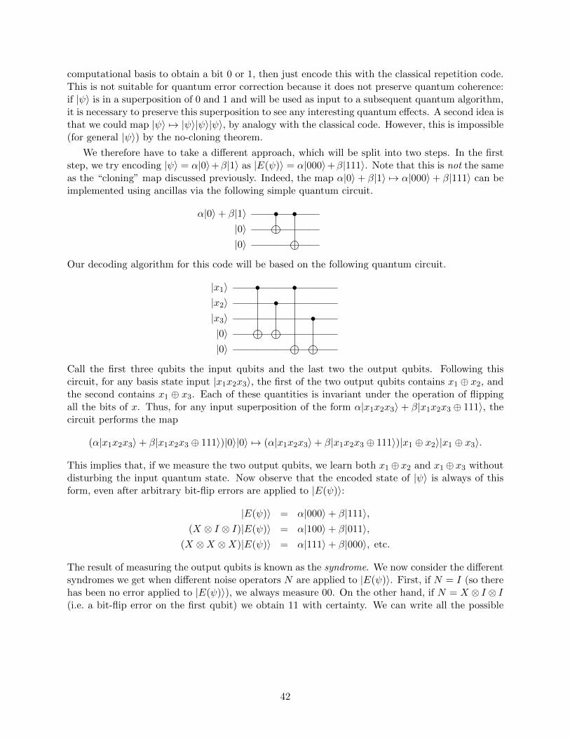
computational basis to obtain a bit 0 or 1, then just encode this with the classical repetition code.This is not suitable for quantum error correction because it does not preserve quantum coherence:if |ψ〉 is in a superposition of 0 and 1 and will be used as input to a subsequent quantum algorithm,it is necessary to preserve this superposition to see any interesting quantum effects. A second idea isthat we could map |ψ〉 7→ |ψ〉|ψ〉|ψ〉, by analogy with the classical code. However, this is impossible(for general |ψ〉) by the no-cloning theorem.
We therefore have to take a different approach, which will be split into two steps. In the firststep, we try encoding |ψ〉 = α|0〉+β|1〉 as |E(ψ)〉 = α|000〉+β|111〉. Note that this is not the sameas the “cloning” map discussed previously. Indeed, the map α|0〉+ β|1〉 7→ α|000〉+ β|111〉 can beimplemented using ancillas via the following simple quantum circuit.
α|0〉+ β|1〉 • •|0〉|0〉
Our decoding algorithm for this code will be based on the following quantum circuit.
|x1〉 • •|x2〉 •|x3〉 •|0〉|0〉
Call the first three qubits the input qubits and the last two the output qubits. Following thiscircuit, for any basis state input |x1x2x3〉, the first of the two output qubits contains x1 ⊕ x2, andthe second contains x1 ⊕ x3. Each of these quantities is invariant under the operation of flippingall the bits of x. Thus, for any input superposition of the form α|x1x2x3〉 + β|x1x2x3 ⊕ 111〉, thecircuit performs the map
(α|x1x2x3〉+ β|x1x2x3 ⊕ 111〉)|0〉|0〉 7→ (α|x1x2x3〉+ β|x1x2x3 ⊕ 111〉)|x1 ⊕ x2〉|x1 ⊕ x3〉.
This implies that, if we measure the two output qubits, we learn both x1⊕ x2 and x1⊕ x3 withoutdisturbing the input quantum state. Now observe that the encoded state of |ψ〉 is always of thisform, even after arbitrary bit-flip errors are applied to |E(ψ)〉:
|E(ψ)〉 = α|000〉+ β|111〉,(X ⊗ I ⊗ I)|E(ψ)〉 = α|100〉+ β|011〉,
(X ⊗X ⊗X)|E(ψ)〉 = α|111〉+ β|000〉, etc.
The result of measuring the output qubits is known as the syndrome. We now consider the differentsyndromes we get when different noise operators N are applied to |E(ψ)〉. First, if N = I (so therehas been no error applied to |E(ψ)〉), we always measure 00. On the other hand, if N = X ⊗ I ⊗ I(i.e. a bit-flip error on the first qubit) we obtain 11 with certainty. We can write all the possible
42
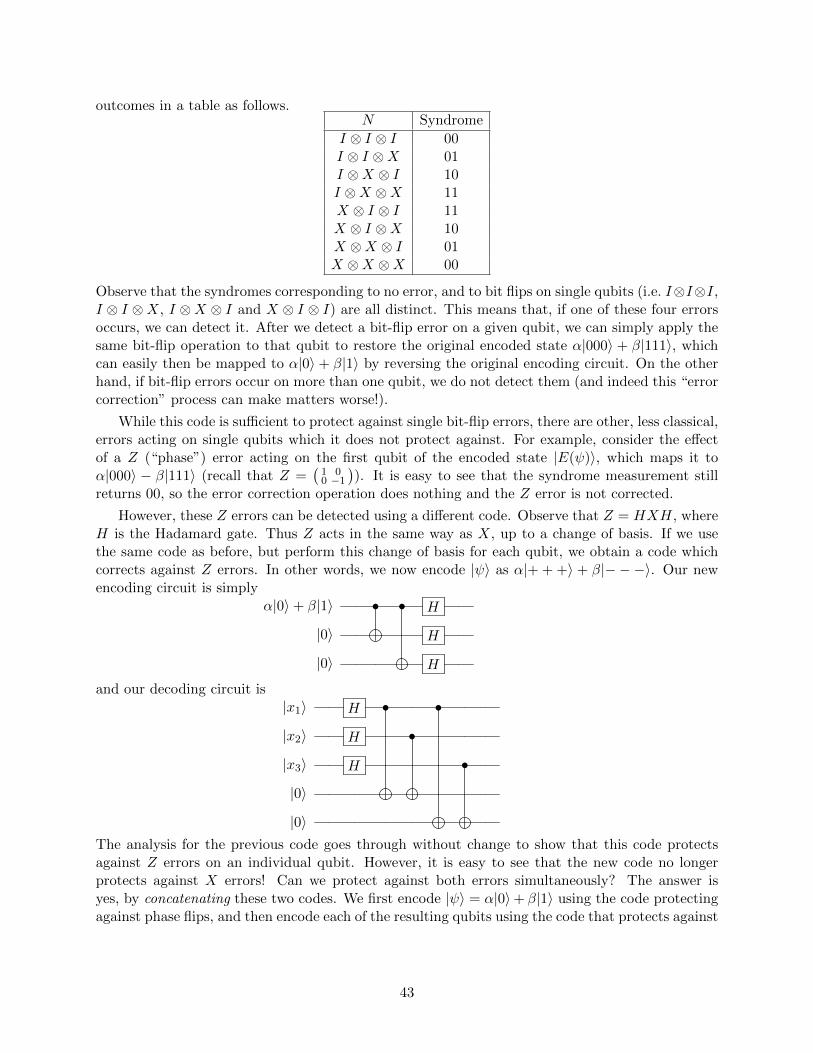
outcomes in a table as follows.N Syndrome
I ⊗ I ⊗ I 00I ⊗ I ⊗X 01I ⊗X ⊗ I 10I ⊗X ⊗X 11X ⊗ I ⊗ I 11X ⊗ I ⊗X 10X ⊗X ⊗ I 01X ⊗X ⊗X 00
Observe that the syndromes corresponding to no error, and to bit flips on single qubits (i.e. I⊗I⊗I,I ⊗ I ⊗X, I ⊗X ⊗ I and X ⊗ I ⊗ I) are all distinct. This means that, if one of these four errorsoccurs, we can detect it. After we detect a bit-flip error on a given qubit, we can simply apply thesame bit-flip operation to that qubit to restore the original encoded state α|000〉 + β|111〉, whichcan easily then be mapped to α|0〉+ β|1〉 by reversing the original encoding circuit. On the otherhand, if bit-flip errors occur on more than one qubit, we do not detect them (and indeed this “errorcorrection” process can make matters worse!).
While this code is sufficient to protect against single bit-flip errors, there are other, less classical,errors acting on single qubits which it does not protect against. For example, consider the effectof a Z (“phase”) error acting on the first qubit of the encoded state |E(ψ)〉, which maps it toα|000〉 − β|111〉 (recall that Z =
(1 00 −1
)). It is easy to see that the syndrome measurement still
returns 00, so the error correction operation does nothing and the Z error is not corrected.
However, these Z errors can be detected using a different code. Observe that Z = HXH, whereH is the Hadamard gate. Thus Z acts in the same way as X, up to a change of basis. If we usethe same code as before, but perform this change of basis for each qubit, we obtain a code whichcorrects against Z errors. In other words, we now encode |ψ〉 as α|+ + +〉 + β|− − −〉. Our newencoding circuit is simply
α|0〉+ β|1〉 • • H
|0〉 H
|0〉 H
and our decoding circuit is|x1〉 H • •
|x2〉 H •
|x3〉 H •
|0〉
|0〉The analysis for the previous code goes through without change to show that this code protectsagainst Z errors on an individual qubit. However, it is easy to see that the new code no longerprotects against X errors! Can we protect against both errors simultaneously? The answer isyes, by concatenating these two codes. We first encode |ψ〉 = α|0〉+ β|1〉 using the code protectingagainst phase flips, and then encode each of the resulting qubits using the code that protects against
43
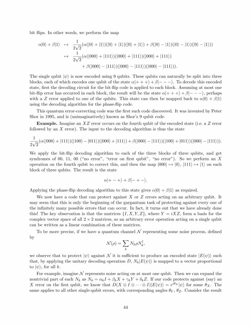
bit flips. In other words, we perform the map
α|0〉+ β|1〉 7→ 1
2√
2(α(|0〉+ |1〉)(|0〉+ |1〉)(|0〉+ |1〉) + β(|0〉 − |1〉)(|0〉 − |1〉)(|0〉 − |1〉))
7→ 1
2√
2(α(|000〉+ |111〉)(|000〉+ |111〉)(|000〉+ |111〉)
+ β(|000〉 − |111〉)(|000〉 − |111〉)(|000〉 − |111〉)).
The single qubit |ψ〉 is now encoded using 9 qubits. These qubits can naturally be split into threeblocks, each of which encodes one qubit of the state α|+ + +〉+β|− − −〉. To decode this encodedstate, first the decoding circuit for the bit-flip code is applied to each block. Assuming at most onebit-flip error has occurred in each block, the result will be the state α|+ + +〉+ β|− − −〉, perhapswith a Z error applied to one of the qubits. This state can then be mapped back to α|0〉 + β|1〉using the decoding algorithm for the phase-flip code.
This quantum error-correcting code was the first such code discovered. It was invented by PeterShor in 1995, and is (unimaginatively) known as Shor’s 9 qubit code.
Example. Imagine an XZ error occurs on the fourth qubit of the encoded state (i.e. a Z errorfollowed by an X error). The input to the decoding algorithm is thus the state
1
2√
2(α(|000〉+ |111〉)(|100〉− |011〉)(|000〉+ |111〉) + β(|000〉− |111〉)(|100〉+ |011〉)(|000〉− |111〉)).
We apply the bit-flip decoding algorithm to each of the three blocks of three qubits, and getsyndromes of 00, 11, 00 (“no error”, “error on first qubit”, “no error”). So we perform an Xoperation on the fourth qubit to correct this, and then the map |000〉 7→ |0〉, |111〉 7→ |1〉 on eachblock of three qubits. The result is the state
α|+−+〉+ β|−+−〉.
Applying the phase-flip decoding algorithm to this state gives α|0〉+ β|1〉 as required.
We now have a code that can protect against X or Z errors acting on an arbitrary qubit. Itmay seem that this is only the beginning of the gargantuan task of protecting against every one ofthe infinitely many possible errors that can occur. In fact, it turns out that we have already donethis! The key observation is that the matrices I,X, Y, Z, where Y = iXZ, form a basis for thecomplex vector space of all 2× 2 matrices, so an arbitrary error operation acting on a single qubitcan be written as a linear combination of these matrices.
To be more precise, if we have a quantum channel N representing some noise process, definedby
N (ρ) =∑k
NkρN†k ,
we observe that to protect |ψ〉 against N it is sufficient to produce an encoded state |E(ψ)〉 suchthat, by applying the unitary decoding operation D, Nk|E(ψ)〉 is mapped to a vector proportionalto |ψ〉, for all k.
For example, imagine N represents noise acting on at most one qubit. Then we can expand thenontrivial part of each Nk as Nk = αkI + βkX + γkY + δkZ. If our code protects against (say) anX error on the first qubit, we know that D(X ⊗ I ⊗ · · · ⊗ I)|E(ψ)〉 = eiθX |ψ〉 for some θX . Thesame applies to all other single-qubit errors, with corresponding angles θY , θZ . Consider the result
44
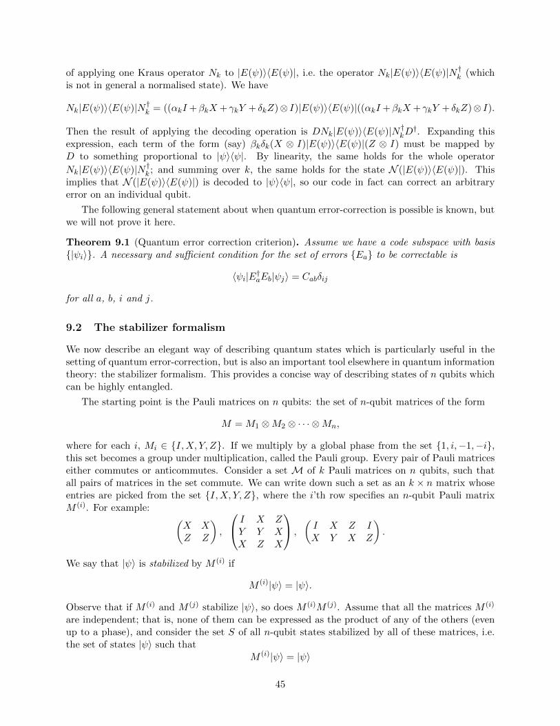
of applying one Kraus operator Nk to |E(ψ)〉〈E(ψ)|, i.e. the operator Nk|E(ψ)〉〈E(ψ)|N †k (whichis not in general a normalised state). We have
Nk|E(ψ)〉〈E(ψ)|N †k = ((αkI +βkX + γkY + δkZ)⊗ I)|E(ψ)〉〈E(ψ)|((αkI +βkX + γkY + δkZ)⊗ I).
Then the result of applying the decoding operation is DNk|E(ψ)〉〈E(ψ)|N †kD†. Expanding this
expression, each term of the form (say) βkδk(X ⊗ I)|E(ψ)〉〈E(ψ)|(Z ⊗ I) must be mapped byD to something proportional to |ψ〉〈ψ|. By linearity, the same holds for the whole operator
Nk|E(ψ)〉〈E(ψ)|N †k ; and summing over k, the same holds for the state N (|E(ψ)〉〈E(ψ)|). Thisimplies that N (|E(ψ)〉〈E(ψ)|) is decoded to |ψ〉〈ψ|, so our code in fact can correct an arbitraryerror on an individual qubit.
The following general statement about when quantum error-correction is possible is known, butwe will not prove it here.
Theorem 9.1 (Quantum error correction criterion). Assume we have a code subspace with basis|ψi〉. A necessary and sufficient condition for the set of errors Ea to be correctable is
〈ψi|E†aEb|ψj〉 = Cabδij
for all a, b, i and j.
9.2 The stabilizer formalism
We now describe an elegant way of describing quantum states which is particularly useful in thesetting of quantum error-correction, but is also an important tool elsewhere in quantum informationtheory: the stabilizer formalism. This provides a concise way of describing states of n qubits whichcan be highly entangled.
The starting point is the Pauli matrices on n qubits: the set of n-qubit matrices of the form
M = M1 ⊗M2 ⊗ · · · ⊗Mn,
where for each i, Mi ∈ I,X, Y, Z. If we multiply by a global phase from the set 1, i,−1,−i,this set becomes a group under multiplication, called the Pauli group. Every pair of Pauli matriceseither commutes or anticommutes. Consider a set M of k Pauli matrices on n qubits, such thatall pairs of matrices in the set commute. We can write down such a set as an k × n matrix whoseentries are picked from the set I,X, Y, Z, where the i’th row specifies an n-qubit Pauli matrixM (i). For example: (
X XZ Z
),
I X ZY Y XX Z X
,
(I X Z IX Y X Z
).
We say that |ψ〉 is stabilized by M (i) if
M (i)|ψ〉 = |ψ〉.
Observe that if M (i) and M (j) stabilize |ψ〉, so does M (i)M (j). Assume that all the matrices M (i)
are independent; that is, none of them can be expressed as the product of any of the others (evenup to a phase), and consider the set S of all n-qubit states stabilized by all of these matrices, i.e.the set of states |ψ〉 such that
M (i)|ψ〉 = |ψ〉
45
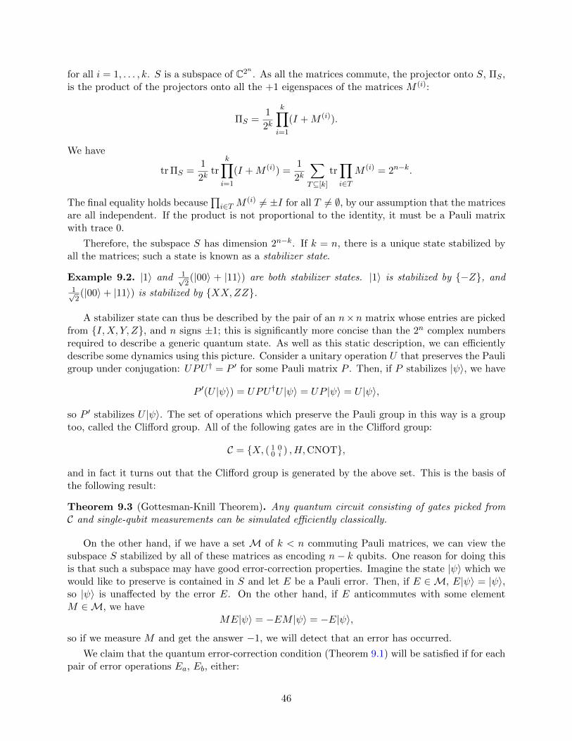
for all i = 1, . . . , k. S is a subspace of C2n . As all the matrices commute, the projector onto S, ΠS ,is the product of the projectors onto all the +1 eigenspaces of the matrices M (i):
ΠS =1
2k
k∏i=1
(I +M (i)).
We have
tr ΠS =1
2ktr
k∏i=1
(I +M (i)) =1
2k
∑T⊆[k]
tr∏i∈T
M (i) = 2n−k.
The final equality holds because∏i∈T M
(i) 6= ±I for all T 6= ∅, by our assumption that the matricesare all independent. If the product is not proportional to the identity, it must be a Pauli matrixwith trace 0.
Therefore, the subspace S has dimension 2n−k. If k = n, there is a unique state stabilized byall the matrices; such a state is known as a stabilizer state.
Example 9.2. |1〉 and 1√2(|00〉 + |11〉) are both stabilizer states. |1〉 is stabilized by −Z, and
1√2(|00〉+ |11〉) is stabilized by XX,ZZ.
A stabilizer state can thus be described by the pair of an n×n matrix whose entries are pickedfrom I,X, Y, Z, and n signs ±1; this is significantly more concise than the 2n complex numbersrequired to describe a generic quantum state. As well as this static description, we can efficientlydescribe some dynamics using this picture. Consider a unitary operation U that preserves the Pauligroup under conjugation: UPU † = P ′ for some Pauli matrix P . Then, if P stabilizes |ψ〉, we have
P ′(U |ψ〉) = UPU †U |ψ〉 = UP |ψ〉 = U |ψ〉,
so P ′ stabilizes U |ψ〉. The set of operations which preserve the Pauli group in this way is a grouptoo, called the Clifford group. All of the following gates are in the Clifford group:
C = X, ( 1 00 i ) , H,CNOT,
and in fact it turns out that the Clifford group is generated by the above set. This is the basis ofthe following result:
Theorem 9.3 (Gottesman-Knill Theorem). Any quantum circuit consisting of gates picked fromC and single-qubit measurements can be simulated efficiently classically.
On the other hand, if we have a set M of k < n commuting Pauli matrices, we can view thesubspace S stabilized by all of these matrices as encoding n− k qubits. One reason for doing thisis that such a subspace may have good error-correction properties. Imagine the state |ψ〉 which wewould like to preserve is contained in S and let E be a Pauli error. Then, if E ∈ M, E|ψ〉 = |ψ〉,so |ψ〉 is unaffected by the error E. On the other hand, if E anticommutes with some elementM ∈M, we have
ME|ψ〉 = −EM |ψ〉 = −E|ψ〉,
so if we measure M and get the answer −1, we will detect that an error has occurred.
We claim that the quantum error-correction condition (Theorem 9.1) will be satisfied if for eachpair of error operations Ea, Eb, either:
46
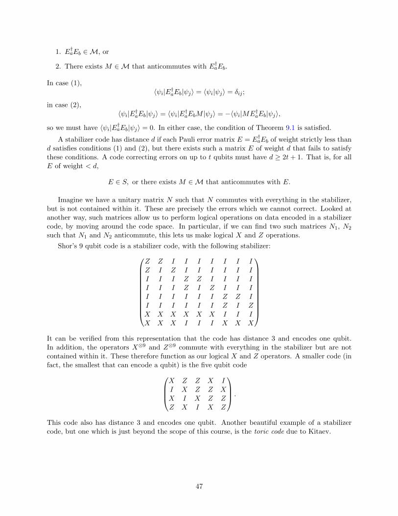
1. E†aEb ∈M, or
2. There exists M ∈M that anticommutes with E†aEb.
In case (1),〈ψi|E†aEb|ψj〉 = 〈ψi|ψj〉 = δij ;
in case (2),〈ψi|E†aEb|ψj〉 = 〈ψi|E†aEbM |ψj〉 = −〈ψi|ME†aEb|ψj〉,
so we must have 〈ψi|E†aEb|ψj〉 = 0. In either case, the condition of Theorem 9.1 is satisfied.
A stabilizer code has distance d if each Pauli error matrix E = E†aEb of weight strictly less thand satisfies conditions (1) and (2), but there exists such a matrix E of weight d that fails to satisfythese conditions. A code correcting errors on up to t qubits must have d ≥ 2t+ 1. That is, for allE of weight < d,
E ∈ S, or there exists M ∈M that anticommutes with E.
Imagine we have a unitary matrix N such that N commutes with everything in the stabilizer,but is not contained within it. These are precisely the errors which we cannot correct. Looked atanother way, such matrices allow us to perform logical operations on data encoded in a stabilizercode, by moving around the code space. In particular, if we can find two such matrices N1, N2
such that N1 and N2 anticommute, this lets us make logical X and Z operations.
Shor’s 9 qubit code is a stabilizer code, with the following stabilizer:
Z Z I I I I I I IZ I Z I I I I I II I I Z Z I I I II I I Z I Z I I II I I I I I Z Z II I I I I I Z I ZX X X X X X I I IX X X I I I X X X
It can be verified from this representation that the code has distance 3 and encodes one qubit.In addition, the operators X⊗9 and Z⊗9 commute with everything in the stabilizer but are notcontained within it. These therefore function as our logical X and Z operators. A smaller code (infact, the smallest that can encode a qubit) is the five qubit code
X Z Z X II X Z Z XX I X Z ZZ X I X Z
.
This code also has distance 3 and encodes one qubit. Another beautiful example of a stabilizercode, but one which is just beyond the scope of this course, is the toric code due to Kitaev.
47
Related Documents