Proximal Gradient Algorithms: Applications in Signal ... · Signal Processing Niccolo Antonello ... KU Leuven C2-16-00449 “Distributed Digital Signal Processing for Ad-hoc Wireless

1

Proximal Gradient Algorithms: Applications in

Signal ProcessingNiccolo Antonello,Lorenzo Stella, Panagiotis Patrinos,and Toon van Waterschoot

Abstract

Advances in numerical optimization have supported breakthroughs in several areas of signal processing. This paper

focuses on the recent enhanced variants of the proximal gradient numerical optimization algorithm, which combine

quasi-Newton methods with forward-adjoint oracles to tackle large-scale problems and reduce the computational

burden of many applications. These proximal gradient algorithms are here described in an easy-to-understand way,

illustrating how they are able to address a wide variety of problems arising in signal processing. A new high-level

modeling language is presented which is used to demonstrate the versatility of the presented algorithms in a series

of signal processing application examples such as sparse deconvolution, total variation denoising, audio de-clipping

and others.

Index Terms

Numerical optimization, Proximal gradient algorithm, Large-scale optimization

I. INTRODUCTION

Signal processing and numerical optimization are independent scientific fields that have always been mutually

influencing each other. Perhaps the most convincing example where the two fields have met is compressed sensing

(CS) [1]. CS originally treated the classic signal processing problem of reconstructing a continuous signal from its

digital counterparts using a sub-Nyquist sampling rate. The reconstruction is achieved by solving an optimization

problem known as the least absolute shrinkage and selection operator (LASSO) problem. Stemming from the

visibility given by CS, LASSO gained popularity within the signal processing community. Indeed, LASSO is a

N. Antonello, P. Patrinos and T. van Waterschoot are with KU Leuven, ESAT–STADIUS, Stadius Center for Dynamical Systems, SignalProcessing and Data Analytics, Kasteelpark Arenberg 10, 3001 Leuven, Belgium.

L. Stella is with Amazon Development Center Germany, Krausenstraße 38, 10117 Berlin, Germany.

N. Antonello and T. van Waterschoot are also with KU Leuven, ESAT–ETC, e-Media Research Lab, Andreas Vesaliusstraat 13, 1000 Leuven,Belgium.

This research work was carried out at the ESAT Laboratory of KU Leuven, the frame of the FP7-PEOPLE Marie Curie Initial TrainingNetwork “Dereverberation and Reverberation of Audio, Music, and Speech (DREAMS)”, funded by the European Commission under GrantAgreement no. 316969, KU Leuven Research Council CoE PFV/10/002 (OPTEC), KU Leuven Impulsfonds IMP/14/037, KU Leuven InternalFunds VES/16/032 and StG/15/043, KU Leuven C2-16-00449 “Distributed Digital Signal Processing for Ad-hoc Wireless Local Area AudioNetworking”, FWO projects G086318N and G086518N, and Fonds de la Recherche Scientifique – FNRS and the Fonds WetenschappelijkOnderzoek – Vlaanderen under EOS Project no 30468160 (SeLMA). The scientific responsibility is assumed by its authors.

arX

iv:1

803.

0162

1v2

[ee

ss.S

P] 8

May

201

8

2

specific case of a structured nonsmooth optimization problem, and so representative of a more generic class of

problems encompassing constrained and nonconvex optimization.

Developing efficient algorithms capable of solving structured nonsmooth optimization problems has been the

focus of recent research efforts in the field of numerical optimization, because classical methods (e.g., Newton-

type) do not directly apply. In the context of convex optimization, such problems can be conveniently transformed

into conic form and solved in a robust and efficient way using interior point methods. These methods became

very popular as they are applicable to a vast range of optimization problems [2]. Unfortunately, they do not scale

well with the problem size as they heavily rely on matrix factorizations and are therefore efficient for medium-size

problems only [3].

More recently, there has been a renewed interest towards splitting algorithms [4]–[6]. These are first-order

algorithms that minimize nonsmooth cost functions with minimal memory requirements allowing to tackle large-

scale problems. The main disadvantage of splitting algorithms is their low speed of convergence, and hence a

significant research effort has been devoted to their tuning and acceleration. Notable splitting algorithms are the

proximal gradient (PG) algorithm [7], also known as forward-backward splitting (FBS) algorithm, the alternating

direction method of multipliers (ADMM) [8], the Douglas-Rachford (DR) and the Pock-Chambolle algorithm (PC)

[9]. The first acceleration of PG can be traced back to [10] and is known as the fast proximal gradient (FPG)

algorithm or as fast iterative shrinkage-thresholding algorithm (FISTA) [11]. More recent acceleration approaches

of PG include the variable metric forward-backward (VMFB) algorithm [12]–[15] and the application of quasi-

Newton methods [16]–[19].

Several surveys dedicated to these algorithms and their applications in signal processing have appeared [3],

[5], [6], [20], mainly focusing on convex problems only. In fact, only recently some extensions and analysis for

nonconvex problems have started to emerge [21], [22]. In convex problems there is no distinction between local

and global minima. For this reason, they are in general easier to solve than their nonconvex counterpart which

are characterized by cost functions with multiple local minima. Despite this, it was recently shown that nonconvex

formulations might either give solutions that exhibit better performance for the specific signal processing application

[23], or lead to computationally tractable problems [24], for which the presence of spurious local minima is less

pronounced or absent, and thus local optimization coupled with a proper initialization often leads to global minima

[22].

This paper will focus on the PG algorithm and its accelerated variants, with the aim of introducing the latest

trends of this numerical optimization framework to the signal processing community. The recent advances in the

acceleration of the PG algorithm combined with matrix-free operations provide a novel flexible framework: in

many signal processing applications such improvements allow tackling previously intractable problems and real-

time processing. This framework will be presented in an effective and timely manner, summarizing the concepts

3

that have led to these recent advances and providing easily accessible and user-friendly software tools. In particular,

the paper will focus on the following topics:

• Accelerated variants of PG: FISTA has received significant attention in the signal processing community.

However, more recently, the PG algorithm has been accelerated using different techniques: it has been shown

that Quasi-Newton methods [18], [19] can significantly improve the algorithm performance and make it more

robust to ill-conditioning.

• Non-convex optimization: proximal gradient algorithms can treat both convex and nonconvex optimization

problems. While many convex relaxations increase dimensionality [25] and may result in computationally

intractable problems, proximal gradient algorithms are directly applicable to the original nonconvex problem

thus avoiding scalability issues. It is indeed of equal importance to have modeling tools and robust, rapidly

converging algorithms for both nonconvex and convex nonsmooth problems. This allows to quickly test different

problem formulations independently of their smoothness and convexity.

• Forward-adjoint oracles and matrix-free optimization: one important feature of proximal gradient algorithms is

that they usually only require direct and adjoint applications of the linear mappings involved in the problem: in

particular, no matrix factorization is required and these algorithms can be implemented using forward-adjoint

oracles (FAOs), yielding matrix-free optimization algorithms [26], [27]. Many signal processing applications

can readily make use of FAOs yielding a substantial decrease of the memory requirements.

• A versatile, high-level modeling language: many optimization frameworks owe part of their success to easily

accessible software packages, e.g., [28], [29]. These software packages usually provide intuitive interfaces

where optimization problems can be described using mathematical notation. In this paper a new, open-

source, high-level modeling language implemented in Julia [30] called StructuredOptimization will be

presented. This combines efficient implementations of proximal gradient algorithms with a collection of FAOs

and functions often used in signal processing, allowing the user to easily formulate and solve optimization

problems.

A series of signal processing application examples will be presented throughout the paper in separate frames to

support the explanations of various concepts. Additionally, these examples will include code snippets illustrating

how easily problems are formulated in the proposed high-level modeling language.

The paper is organized as follows: in Section II models and their usage in optimization are displayed through the

description of inverse problems and the main differences between convex and nonconvex optimization. In Section III

the classical proximal gradient algorithms and their accelerated variants are described. In Section IV the concepts of

FAOs and matrix-free optimization are introduced. Section V describes the types of problems that proximal gradient

algorithms can tackle. Finally, in Section VI the proposed high-modeling language is described and conclusions are

given in Section VII.

4

II. MODELING

Models allow not only to describe physical phenomena, but also to transform signals and access hidden infor-

mation that these often carry. Models may be physical models, obeying the laws of physics and describing e.g.,

mechanical systems, electrical circuits or chemical reactions or parametric models, which are not necessarily linked

to physical phenomena, and are purely defined by mathematical relations and numerical parameters. In general, both

categories of models consist of defining an associated mapping that links an input signal x(t) to an output signal

y(t). Here t may stand for time, but signals could be also N -dimensional e.g., x(t1, . . . , tN ), and be functions of

many quantities: position, temperature or the index of a pixel of a digital image. For computational convenience if

the models are continuous, they must be discretized: the continuous signals involved are sampled and their samples

stored either in vectors x = [x(t1), . . . , x(tn)]ᵀ ∈ Rn, in matrices X ∈ Rn1×n2 or in tensors X ∈ Rn1×···×nN

depending on their dimensionality. In the following these vectors, matrices and tensors will be referred to as signals

as well. The mapping A : D→ C associated with a model therefore links two (perhaps complex) finite-dimensional

spaces D and C like, for example, A : Cn → Cm. Notice that in this work a (complex) finite-dimensional space

D induces a Hilbert space with real inner product i.e., 〈x,y〉 = Re(xHy), where H is the conjugate-transpose

operation, and with norm ‖x‖ =√〈x,x〉. Mappings can also be defined between the Cartesian product of m and

n finite-dimensional spaces: A : D1 × · · · × Dm → C1 × · · · × Cn for example when dealing with multiple-input

multiple-output models.

Depending on the nature of the models, mappings can be either linear or nonlinear. Such distinction often carries

differences on the algorithms where these mappings are employed: as it will be described later, in optimization this

often draws the line between convex and nonconvex optimization. For this reason, here the nonlinear mappings are

indicated with the notation A : D → C while the linear mappings with the notation A ∈ L (D, C), where L is the

set of all linear mappings between D and C.

A. Inverse problems

Models are often used to make predictions. For example it is possible to predict how a model behaves under

the excitation of an input signal x. The output signal y = Ax can be computed by evaluating the mapping A

associated with the model using a specific algorithm. Notice that here the notation Ax does not necessarily stand

for the matrix-vector product. In many signal processing applications, however, one is interested in the opposite

problem: an output signal y is at disposal, and the input signal x is to be found. Such problems are known as

inverse problems and involve many signal processing applications some of which will be treated in this paper

like denoising, source separation, channel equalization and system identification. Inverse problems are in general

ill-posed problems and this makes it difficult to solve them. Three main challenges create this difficulty. Firstly

the inverse of the mapping is needed. This is rarely available, it must be computed numerically and it may be

5

Example 1 Sparse Deconvolution

0 5 · 10−2 0.1 0.15 0.2 0.25 0.3 0.35 0.4 0.45 0.5

−2

0

2

4

Time (s)

ground truth xgt; x?, λ = 10−2; x?, λ = 0

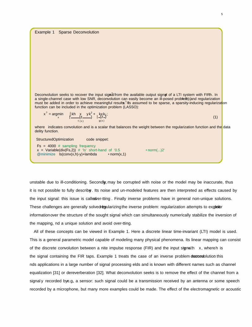
Deconvolution seeks to recover the input signal x? from the available output signal y of a LTI system with FIR h. Ina single-channel case with low SNR, deconvolution can easily become an ill-posed problem (λ = 0) and regularizationmust be added in order to achieve meaningful results. If x? is assumed to be sparse, a sparsity-inducing regularizationfunction can be included in the optimization problem (LASSO):

x? = argminx

12‖h ∗ x− y‖2︸ ︷︷ ︸

f(x)

+λ‖x‖1︸ ︷︷ ︸g(x)

,(1)

where ∗ indicates convolution and λ is a scalar that balances the weight between the regularization function and the datafidelity function.

StructuredOptimization code snippet:

Fs = 4000 # sampling frequencyx = Variable(div(Fs,2)) # ‘ls‘ short-hand of ‘0.5*norm(...)ˆ2‘@minimize ls(conv(x,h)-y)+lambda*norm(x,1)

unstable due to ill-conditioning. Secondly, y may be corrupted with noise or the model may be inaccurate, thus

it is not possible to fully describe y. Its noise and un-modeled features are then interpreted as effects caused by

the input signal: this issue is called over-fitting. Finally inverse problems have in general non-unique solutions.

These challenges are generally solved by regularizing the inverse problem: regularization attempts to exploit prior

information over the structure of the sought signal which can simultaneously numerically stabilize the inversion of

the mapping, find a unique solution and avoid over-fitting.

All of these concepts can be viewed in Example 1. Here a discrete linear time-invariant (LTI) model is used.

This is a general parametric model capable of modeling many physical phenomena. Its linear mapping can consist

of the discrete convolution between a finite impulse response (FIR) and the input signal: y = h ∗ x, where h is

the signal containing the FIR taps. Example 1 treats the case of an inverse problem named deconvolution: this

finds applications in a large number of signal processing fields and is known with different names such as channel

equalization [31] or dereverberation [32]. What deconvolution seeks is to remove the effect of the channel from a

signal y recorded by e.g., a sensor: such signal could be a transmission received by an antenna or some speech

recorded by a microphone, but many more examples could be made. The effect of the electromagnetic or acoustic

6

channel corrupts either the sequence of bits of the transmission or the intelligibility of speech and should be therefore

removed. This can be achieved by fitting the recorded signal y with the LTI model. Equation (1) shows the type of

optimization problem that can bring such result. This consists of the minimization of a cost function, here consisting

of the sum of two functions f and g. These are functions of x which in this context indicates the optimization

variables. When the optimization variables minimize the cost function the optimal solution x? is obtained. Typically,

solving (1) analytically is not possible and the optimal solution is reached numerically through the usage of specific

iterative algorithms starting from an initial guess of the optimization variables x0. Here the functions f and g,

associated with a lower case letter, are always assumed to be proper and closed. These always map an element of

a finite-dimensional space to a single number belonging to the extended real line R = R ∪ {−∞,+∞}.

In Example 1 function f is a data fidelity term, representing the error between the model and the signal y in the

least squares sense. The smaller this term is, the closer the output of the linear mapping, driven by the solution x?,

is to y. On the other hand, g is a l1-norm regularization term: this is a convex relaxation of the l0-norm, i.e., the

norm counting the number of non-zero elements of x, and promotes sparsity in the solution x?. The coefficient λ

balances the relative weight of the data fidelity and sparsity inducing terms in the cost function. Here, the signal y

is corrupted using white noise as if it was recorded in a noisy environment or by a faulty sensor.

The figure of Example 1 shows what would happen if λ = 0, i.e., the case of an un-regularized inverse problem.

This solution has low-frequency oscillations, a sign of the numerical instability of the inverted linear mapping.

Additionally, it is populated by white noise indicating over-fitting. On the other hand, if λ→∞ the prior knowledge

would dominate the cost function leading to the sparsest solution possible, that is a null solution. Generally, λ needs

careful tuning, a procedure that can be automatized by means of different strategies which may involve a sequence of

similar optimization problems. Here, with a properly tuned λ the ground truth signal is recovered almost perfectly.

B. Convex and nonconvex problems

As it is important to choose the proper model to describe the available data, so it is to select the most

convenient problem formulation. Different problem formulations can in fact yield optimization problems with

different properties and one should be able to carefully choose the one that is best suited for the application

of interest.

Perhaps the most fundamental distinction is between convex and nonconvex optimization problems. This distinction

is in fact crucial as, in general, nonconvex problems are more difficult to solve than the convex ones. The main

advantage of convex problems lies in the fact that every local minimum is a global one. On the contrary, the

cost functions of nonconvex problems are characterized by the presence of local minima. These are identified as

solutions but they are typically sub-optimal, since it is usually not possible to determine whether there exist other

solutions that further minimize the cost function. As a consequence of this, the initialization of the algorithms used

7

in nonconvex optimization becomes crucial as it can lead to distinct local minima with solutions that can greatly

differ from each other.

In order to avoid this issue, many nonconvex problems can be re-formulated or approximated by convex ones:

it is often possible to relax the nonconvex functions by substituting them with convex ones that have similar

properties. The LASSO is a good example of such a strategy: the original problem involves an l0-norm, which is a

nonconvex function. Despite very different mathematically, the l1-norm behaves similarly by inducing sparsity over

the optimization variables it is being applied to. Such relaxation however can have consequences on the solution and

Example 2 displays such situation. Here the problem of line spectral estimation is treated: this has many applications

like source localization [33], de-noising [34], and many others. A signal y ∈ Rn is given and is modeled as a

mixture of sinusoidal components. These lie on a fine grid of frequencies belonging to a discrete Fourier transform

(DFT) and hence corresponding to the elements of a complex-valued signal x? ∈ Csn which must be estimated.

The optimization problem seeks for a sparse solution as these components are assumed to be only few.

Looking at the figure of Example 2 it is clear that the solution of the nonconvex problem outperforms the one

obtained through the LASSO. The solution of LASSO has in fact many small spurious frequency components. These

are not present in the solution of the nonconvex problem which also exhibits amplitudes that are much closer to

the ones of the ground truth. This shows that convex relaxations may lead to poorer results than the ones obtained

by solving the original nonconvex problem. However, as stated earlier, the presence of local minima requires

the problem to be initialized carefully. Indeed, the improved performance of the solution obtained by solving the

nonconvex problem in Example 2 would have been very hard to accomplish with a random initialization: most likely

a “bad” local minimum would have been reached corresponding to a solution with completely wrong amplitudes

and frequencies. Instead, by warm-starting the nonconvex problem with the solution of the LASSO, a “good” local

minimum is found.

There are very few nonconvex problems that are not particularly affected by the initialization issue. A lucky

case, under appropriate assumptions, is the one of robust principal component analysis (PCA) [35] (Example 4).

In general, however, what is typically done is to come up with a good strategy for the initialization. Obviously,

the path adopted in Example 2, i.e., initializing the nonconvex problem with the solution of a convex relaxation, is

not always accessible. In fact a general rule for initialization does not exist and this is usually problem-dependent:

different strategies may involve random initialization using distributions that are obtained by analyzing the available

data [36] (Example 3) or by solving multiple times the optimization problems while modifying parameters that

govern the nonconvexity (Example 6).

Despite these disadvantages, nonconvex optimization is becoming more and more popular for multiple reasons.

Firstly, as Example 2 has just shown, sometimes the quality of the solution of a convex relaxation is not satisfactory.

Secondly, convex relaxations may come at the cost of a larger optimization problem with respect to the original

8

nonconvex one [23], [25], [37] and may be prohibitive in terms of both memory and computational power. Finally,

sometimes convex relaxations are simply not possible, for example when nonlinear mappings are involved in the

optimization problems. These nonlinear mappings are typically derived from complex models which have shown to

produce outstanding results and are becoming very common for example in machine learning and model predictive

control. For these reasons, having algorithms that are convergent both for convex and nonconvex problems is quite

important.

Example 2 Line spectral estimation

f1 f2 f3 f4f5 f6,7,8f9 f10f11 f12 f13 f140

0.2

0.4

0.6

0.8

Frequency (kHz)

Mag

nitu

de

xgt

xzp

x?1

x?0

Line spectral estimation seeks to accurately recover the frequencies and amplitudes of a signal y ∈ Rn which consistsof a mixture of N sinusoids. A simple solution is take the zero-padded DFT of y: xzp = F[y, 0, . . . 0] ∈ Csn where s isthe super-resolution factor and F ∈ L (Rsn,Csn) the DFT mapping. However, looking at xzp, spectral leakage causescomponents at close frequencies to merge. This issue is not present if the following optimization problems are used forline spectral estimation:

(a) x?1 = argminx

1

2‖SFix− y‖2 + λ‖x‖1, (b) x?0 = argmin

x

1

2‖SFix− y‖2 s.t. ‖x‖0 ≤ N, (2)

here x ∈ Csn consists of the candidate sparse sinusoidal components, Fi ∈ L (Csn,Rsn) is the inverse DFT andS ∈ L (Rsn,Rn) is a mapping that simply selects the first n elements. Problem (b) is nonconvex which means that ithas several local minima and its convex relaxation (a) is typically solved instead (LASSO). Nevertheless, PG methodscan solve (a) as well as (b): if a good initialization is given, e.g., the solution of (a), improved results can be achieved.

StructuredOptimization code snippet:

x = Variable(s*n) # n = 2ˆ8; s = 6;@minimize ls(ifft(x)[1:n]-y)+lambda*norm(x,1) # (a)@minimize ls(ifft(x)[1:n]-y) st norm(x,0) <= N # (b)

III. PROXIMAL GRADIENT ALGORITHMS

All of the problems this paper treats, including the ones of Examples 1 and 2, can be formulated as

minimizex

ϕ(x) = f(x) + g(x) (3)

where f is a smooth function (i.e., it is differentiable, and its gradient ∇f is Lipschitz-continuous), while g is

possibly nonsmooth. Despite its simplicity, problem (3) encompasses a large variety of applications. For example,

constrained optimization can be formulated as (3): for a (nonempty) set S , by setting g to be the indicator function

9

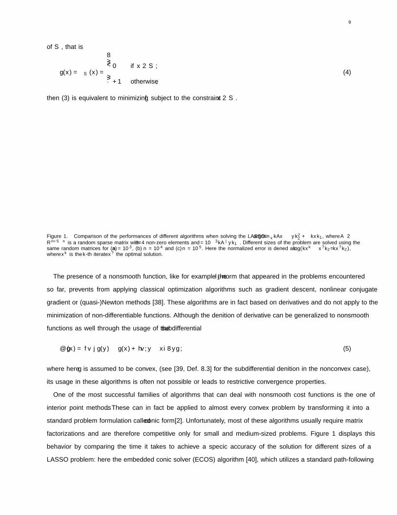
of S , that is

g(x) = δS (x) =

0 if x ∈ S ,

+∞ otherwise,(4)

then (3) is equivalent to minimizing f subject to the constraint x ∈ S .

1 2 3 4 5 6 7 8 9 10

·10−2

−8

−6

−4

−2

0

(a)

Time (s)

Nor

mal

ized

Err

or

1 2 3 4 5 6 7 8 9 10

−8

−6

−4

−2

0

(b)

Time (s)

ECOS SCS PG FPG PANOC

1 2 3 4 5 6 7 8 9 10

·102

−8

−6

−4

−2

0

(c)

Time (s)

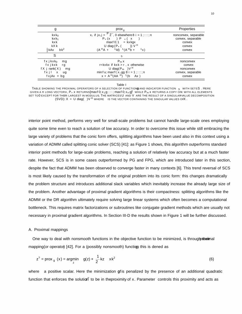
Figure 1. Comparison of the performances of different algorithms when solving the LASSO: argminx‖Ax − y‖22 + λ‖x‖1, where A ∈Rn/5×n is a random sparse matrix with n/4 non-zero elements and λ = 10−3‖Aᵀy‖∞. Different sizes of the problem are solved using thesame random matrices for (a) n = 103, (b) n = 104 and (c) n = 105. Here the normalized error is defined as: log(‖xk − x?‖2/‖x?‖2),where xk is the k-th iterate x? the optimal solution.

The presence of a nonsmooth function, like for example the l1-norm that appeared in the problems encountered

so far, prevents from applying classical optimization algorithms such as gradient descent, nonlinear conjugate

gradient or (quasi-)Newton methods [38]. These algorithms are in fact based on derivatives and do not apply to the

minimization of non-differentiable functions. Although the definition of derivative can be generalized to nonsmooth

functions as well through the usage of the subdifferential

∂g(x) = {v | g(y) ≥ g(x) + 〈v,y − x〉 ∀y} , (5)

where here g is assumed to be convex, (see [39, Def. 8.3] for the subdifferential definition in the nonconvex case),

its usage in these algorithms is often not possible or leads to restrictive convergence properties.

One of the most successful families of algorithms that can deal with nonsmooth cost functions is the one of

interior point methods. These can in fact be applied to almost every convex problem by transforming it into a

standard problem formulation called conic form [2]. Unfortunately, most of these algorithms usually require matrix

factorizations and are therefore competitive only for small and medium-sized problems. Figure 1 displays this

behavior by comparing the time it takes to achieve a specific accuracy of the solution for different sizes of a

LASSO problem: here the embedded conic solver (ECOS) algorithm [40], which utilizes a standard path-following

10

g proxγg Properties

‖x‖0 xi if |xi| >√2γ, 0 elsewhere ∀ i = 1, . . . , n nonconvex, separable

‖x‖1 P+(x− γ)− P+(−x− γ) convex, separable‖x‖ max{0, 1− γ/‖x‖}x convex‖X‖∗ U diag (P+(σ − γ))VH convex

12‖Ax− b‖2 (AHA+ γ−1Id)−1(AHb+ γ−1x) convex

S ΠS

{x | ‖x‖0 ≤ m} Pmx nonconvex{x | ‖x‖ ≤ r} r/‖x‖x if ‖x‖ > r, x otherwise convex

{X | rank(X) ≤ m} U diag(Pmσ)VH nonconvex{x | l ≤ x ≤ u} min{u,max{l, xi}} ∀ i = 1, . . . , n convex, separable{x|Ax = b} x+AH(AAH)−1(b−Ax) convex

Table ITABLE SHOWING THE PROXIMAL OPERATORS OF A SELECTION OF FUNCTIONS g AND INDICATOR FUNCTION δS WITH SETS S . HERE

GIVEN A n LONG VECTOR x, P+x RETURNS [max{0, x1}, . . . ,max{0, xn}]ᵀ WHILE Pmx RETURNS A COPY OF x WITH ALL ELEMENTSSET TO 0 EXCEPT FOR THE m LARGEST IN MODULUS. THE MATRICES U AND V ARE THE RESULT OF A SINGULAR-VALUE DECOMPOSITION

(SVD): X = U diag(σ)VH WHERE σ IS THE VECTOR CONTAINING THE SINGULAR VALUES OF X.

interior point method, performs very well for small-scale problems but cannot handle large-scale ones employing

quite some time even to reach a solution of low accuracy. In order to overcome this issue while still embracing the

large variety of problems that the conic form offers, splitting algorithms have been used also in this context using a

variation of ADMM called splitting conic solver (SCS) [41]: as Figure 1 shows, this algorithm outperforms standard

interior point methods for large-scale problems, reaching a solution of relatively low accuracy but at a much faster

rate. However, SCS is in some cases outperformed by PG and FPG, which are introduced later in this section,

despite the fact that ADMM has been observed to converge faster in many contexts [6]. This trend reversal of SCS

is most likely caused by the transformation of the original problem into its conic form: this changes dramatically

the problem structure and introduces additional slack variables which inevitably increase the already large size of

the problem. Another advantage of proximal gradient algorithms is their compactness: splitting algorithms like the

ADMM or the DR algorithm ultimately require solving large linear systems which often becomes a computational

bottleneck. This requires matrix factorizations or subroutines like conjugate gradient methods which are usually not

necessary in proximal gradient algorithms. In Section III-D the results shown in Figure 1 will be further discussed.

A. Proximal mappings

One way to deal with nonsmooth functions in the objective function to be minimized, is through their proximal

mapping (or operator) [42]. For a (possibly nonsmooth) function g, this is defined as

z? = proxγg(x) = argminz

{g(z) +

1

2γ‖z− x‖2

}(6)

where γ a positive scalar. Here the minimization of g is penalized by the presence of an additional quadratic

function that enforces the solution z? to be in the proximity of x. Parameter γ controls this proximity and acts as

11

g(x) proxγg(x) Requirements

Separable sum h1(x1) + h2(x2) [proxγh1 (x1)ᵀ, proxγh2 (x2)ᵀ]ᵀ x = [xᵀ1 ,x

ᵀ2 ]

ᵀ

Translation h(x+ b) proxγh(x+ b)− b

Affine addition h(x) + 〈a,x〉 proxγh(x− γa)Postcomposition ah(x) + b proxaγh(x) a > 0

Precomposition h(Ax) x+ µ−1A∗(proxµγh(Ax)− Ax

)AA∗ = µId, µ ≥ 0

Regularization h(x) + ρ2‖x− b‖2 proxγh(γ(1/γx+ ρb)) γ = γ/(1 + γρ), ρ ≥ 0

Convex Conjugate supx{〈x,u〉 − h(x)} u− γ prox(1/γ)h(u/γ) h convex

Table IITABLE SHOWING DIFFERENT PROPERTIES OF PROXIMAL MAPPINGS.

a stepsize: small values of γ will result in z? being very close to x, while large ones will yield a solution close to

the minimum of g.

For many functions the correspondent proximal mappings have closed-form solutions and can be computed very

efficiently. Table I shows some examples for functions which are commonly used in applications. For example, the

proximal mapping of g(·) = λ‖ · ‖1, consists of a “soft-thresholding” operation of x, while for l0-norm it is the

so-called “hard-thresholding” operation. When g is the indicator function of a set S , cf. (4), then proxγg = ΠS ,

the projection onto S . As Table I shows, many of these projections are also cheaply computable like in the case

of boxes, norm balls, affine subspaces.

However, an analytical solution to (6) is not always available. For example, given two functions h1 and h2, the

fact that proxγh1and proxγh2

can be efficiently computed does not necessarily imply that proxγ(h1+h2) is efficient

as well. Additionally, the proximal mapping of the composition g ◦ A of a function g with a linear operator A, is

also not efficient in general. An exception to this is linear least squares: if g(·) = 12‖· − b‖2 is composed with

matrix A, the proximal mapping of function g(Ax) = 12‖Ax − b‖2 has in fact a closed-form solution, which

however requires solving a linear system as Table I shows. When this linear system is large (i.e., A has a large

number of columns) such inversion may be infeasible to tackle with direct methods (such as QR decomposition

or Cholesky factorization), and one may need to resort to iterative algorithms, e.g., using conjugate gradient. In

general, composition by a linear mapping results in an efficient closed-form proximal mapping only when A satisfies

AA∗ = µId where µ ≥ 0, Id is the identity mapping and A∗ is the adjoint mapping of A (see Section IV for the

definition of adjoint mapping). Linear mappings with such properties are called tight frames, and include orthogonal

mappings like the discrete Fourier transform (DFT) and discrete cosine transform (DCT).

Many properties can be exploited to derive closed-form expressions for proximal operators: Table II summarizes

some of the most important ones [4]. Among these, the separable sum is particularly useful: if h1 and h2 have

efficiently computable proximal mappings, then so does function g(x1,x2) = h1(x1) +h2(x2). For example, using

12

the properties in Table II, it is very easy to compute the proximal mapping of g(x) = ‖diag(d)x‖1 =∑ |dixi|.

If function g is convex then proxγg is everywhere well defined: (6) consists of the minimization of a strongly

convex objective, and as such has a unique solution for any x. When g is nonconvex, however, this condition fails to

hold. Existence of solutions to (6) in this case is guaranteed (possibily for small enough γ) under prox-boundedness

assumptions on g: this is a rather technical assumption which roughly speaking amounts to g being bounded below

by a (possibly nonconvex) quadratic function. The interested reader can refer to [39, Def. 1.23] for its formal

definition.

In general, for nonconvex g the operator proxγg is set-valued, i.e., problem (6) may have multiple solutions. As

an example of this, consider set B0,m = {x | ‖x‖0 ≤ m}, i.e., the `0 pseudo-norm ball. Projecting a point x ∈ Rn

onto B0,m amounts to setting to zero its n−m smallest coefficients in magnitude. However consider n = 5, m = 3,

and point x = [5.7,−2.4, 1.2, 1.2, 1.2]ᵀ. In this case there are three points in B0,3 which are closest to x. In fact:

ΠB0,3(x) = {[5.7,−2.4, 1.2, 0, 0]ᵀ, [5.7,−2.4, 0, 1.2, 0]ᵀ, [5.7,−2.4, 0, 0, 1.2]ᵀ} . (7)

In practice, proximal mappings of nonconvex functions are evaluated by choosing a single element out of its set.

B. Proximal gradient method

A very popular algorithm to solve (3), when ϕ is the sum of a smooth function f and a (possibly) nonsmooth

function g with efficient proximal mapping, is the proximal gradient (PG) algorithm: this combines the gradient

descent, a well known first-order method, with the proximal mapping described in Section III-A.

Algorithm 1 Proximal Gradient Algorithm (PG)Set x0 ∈ RnSet γ ∈ (0, 2L−1f ]for k = 0, 1, . . . do

xk+1 = proxγg(xk − γ∇f(xk))

The PG algorithm is illustrated in Algorithm 1: here x0 is the initial guess, γ represents a stepsize and ∇f is

the gradient of the smooth function f . The algorithm consists of alternating gradient (or forward) steps on f and

proximal (or backward) steps on g, and is a particular case of the forward-backward splitting (FBS) algorithm for

finding a zero of the sum of two monotone operators [43], [44]. The reason behind this terminology is apparent

from the optimality condition of the problem defining the proximal operator (6): if z = proxγg(x), then necessarily

z = x− γv, with v ∈ ∂g(x), i.e., z is obtained by an implicit (backward) subgradient step over g, as opposed to

the explicit (forward) step over f .

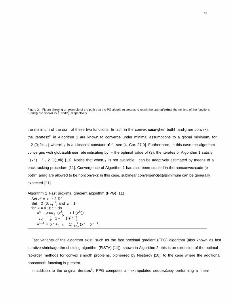
The steps of the algorithm are visualized in Figure 2: the gradient step moves the iterate xk towards the minimum

of f , while the proximal step makes progress towards the minimum of g. This alternation will ultimately lead to

13

x0

x1

f + g f

g

x1

x2

x?f x?g x?

xk − γ∇f(xk) proxγ,g xk+1

Figure 2. Figure showing an example of the path that the PG algorithm creates to reach the optimal value x?. Here the minima of the functionsf and g are shown in x?f and x?g respectively.

the minimum of the sum of these two functions. In fact, in the convex case (i.e., when both f and g are convex),

the iterates xk in Algorithm 1 are known to converge under minimal assumptions to a global minimum, for

γ ∈ (0, 2/Lf ) where Lf is a Lipschitz constant of ∇f , see [4, Cor. 27.9]. Furthermore, in this case the algorithm

converges with global sublinear rate: indicating by ϕ? the optimal value of (3), the iterates of Algorithm 1 satisfy

ϕ(xk) − ϕ? ∈ O(1/k) [11]. Notice that when Lf is not available, γ can be adaptively estimated by means of a

backtracking procedure [11]. Convergence of Algorithm 1 has also been studied in the nonconvex case (i.e., where

both f and g are allowed to be nonconvex): in this case, sublinear convergence to a local minimum can be generally

expected [21].

Algorithm 2 Fast proximal gradient algorithm (FPG) [11]Set v0 = x−1 ∈ RnSet γ ∈ (0, L−1f ] and θ0 = 1for k = 0, 1, . . . do

xk = proxγg(vk − γ∇f(vk))

θk+1 = 12

(1 +

√1 + 4θ2k

)

vk+1 = xk + (θk − 1)θ−1k+1(xk − xk−1)

Fast variants of the algorithm exist, such as the fast proximal gradient (FPG) algorithm (also known as fast

iterative shrinkage-thresholding algorithm (FISTA) [11]), shown in Algorithm 2: this is an extension of the optimal

first-order methods for convex smooth problems, pioneered by Nesterov [10], to the case where the additional

nonsmooth function g is present.

In addition to the original iterates xk, FPG computes an extrapolated sequence vk by performing a linear

14

combination of previous two iterates. Intuitively, this provides intertia to the computed sequence, which improves

the convergence speed over PG: in fact, the particular choice of the coefficients of such inertial step ensure that in the

convex case the iterates of Algorithm 2 satisfy ϕ(xk)−ϕ? ∈ O(1/k2) [11], [45], [46]. This method is particularly

appealing since the extrapolated sequence vk only requires O(n) floating point operations to be computed. However,

the convergence of FPG has only been proven when both f and g are convex.

C. Forward-backward envelope

Recently, new algorithms based on the PG algorithm have emerged: these rely on the concept of the forward-

backward envelope (FBE) which was first introduced in [47]. In order to explain what the FBE is, one should look

at the PG algorithm from a different perspective. Using the definition of proxγg, with elementary manipulations

the iterations of Algorithm 1 can be equivalently rewritten as,

xk+1 = argminz

{qγ(z,x

k)︷ ︸︸ ︷f(xk) + 〈z− xk,∇f(xk)〉+ 1

2γ ‖z− xk‖2 +g(z)}, (8)

that is, the minimization of g plus a quadratic model qγ(z,xk) of f around the current iterate xk. When ∇f is

Lipschitz continuous and γ ≤ L−1f , then for all x

ϕ(z) = f(z) + g(z) ≤ qγ(z,x) + g(z). (9)

In this case the steps (8) of the PG algorithm are a majorization-minimization procedure. This is visualized, in the

one-dimensional case, in Figure 3. The minimum value of (8) is the forward-backward envelope associated with

problem (3), indicated by ϕγ :

ϕγ(x) = minz

{f(x) + 〈z− x,∇f(x)〉+ 1

2γ ‖z− x‖2 + g(z)}. (10)

The FBE has many noticeable properties: these are described in detail in [19] for the case where g is convex,

and extended in [18] to the case where g is allowed to be nonconvex. First, ϕγ is a lower bound to ϕ, and the

two functions share the same local minimizers. In particular, inf ϕ = inf ϕγ and argminϕ = argminϕγ , hence

minimizing ϕγ is equivalent to minimizing ϕ. Additionally, ϕγ is real-valued as opposed to ϕ which is extended

real-valued: as Figure 3 shows, even at points where ϕ is +∞, ϕγ has a finite value instead. Furthermore, when

f is twice differentiable and g is convex, then ϕγ is continuously differentiable.

Finally, it is worth noticing that evaluating the FBE (10) essentially requires computing one proximal gradient

step, i.e., one step of Algorithm 1. This is an important feature from the algorithmic perspective: any algorithm that

solves (3) by minimizing ϕγ (and thus needs its evaluation) requires exactly the same operations as Algorithm 1.

In the next section one of such algorithms is illustrated.

15

xk xk+1

ϕ(x) ϕγ(x)

qγ(z, xk) + g(z) qγ(z, xk+1) + g(z)

xk xk+1

Figure 3. One step of PG amounts to a majorization-minimization over ϕ, when stepsizes γ is sufficiently small. The minimum value of suchmajorization is the forward-backward envelope ϕγ . Left: in the convex case, ϕγ is a smooth lower bound to the original objective ϕ. Right: inthe nonconvex case ϕγ is not everywhere smooth.

D. Newton-type proximal gradient methods

In Section III-C it was shown that minimizing the FBE is equivalent to solving problem (3). Algorithm 3 is a

generalization of the standard PG algorithm that minimizes the FBE using a backtracking line search.

Algorithm 3 Proximal Averaged Newton-type algorithm for Optimality Conditions (PANOC)Set x0 ∈ RnSet γ ∈ (0, L−1f ] and σ ∈ (0, 1

2γ (1− γLf ))for k = 0, 1, . . . do

vk = proxγg(xk − γ∇f(xk))

dk = −Hk(xk − vk) for some nonsingular Hkxk+1 = (1− τk)vk + τk(xk + dk),where τk is the largest value in

{( 12 )i | i ∈ N

}such that

ϕγ(xk+1) ≤ ϕγ(xk)− σ‖vk − xk‖2

The Proximal Averaged Newton-type algorithm for Optimality Conditions (PANOC) was proposed in [48], and

the idea behind it is very simple: the PG algorithm is a fixed-point iteration for solving the system of nonsmooth,

nonlinear equations Rγ(x) = 0, where

Rγ(x) = x− proxγg(x− γ∇f(x)), (11)

is the fixed-point residual mapping. In fact, it is immediate to verify that the iterates in Algorithm 1 satisfy

xk+1 = xk −Rγ(xk). (12)

16

It is very natural to think of applying a Newton-type method, analogously to what is done for smooth, nonlinear

equations [38, Chap. 11]:

xk+1 = xk − HkRγ(xk), (13)

where (Hk) is an appropriate sequence of nonsingular linear transformations. The update rule of Algorithm 3 is a

convex combination of (12) and (13), dictated by the stepsize τk which is determined by backtracking line-search

over the FBE. When τk = 1 then (13) is performed; as τk → 0 then the update gets closer and closer to (12).

Note that Algorithm 3 reduces to Algorithm 1 for the choice Hk = Id: in this case the stepsize τk is always

equal to 1. However, by carefully choosing Hk one can greatly improve convergence of the iterations. In [48] the

case of quasi-Newton methods is considered: start with H0 = Id, and update it so as to satisfy the (inverse) secant

condition

xk+1 − xk = Hk+1

[Rγ(xk+1)−Rγ(xk)

]. (14)

This can be achieved via the (modified) Broyden method in which case the resulting sequence of Hk can be proven

to satisfy the so called Dennis-More condition which ensures superlinear convergence of the iterates xk. A detailed

convergence proof of PANOC can be found in [48].

Algorithm 4 L-BFGS two-loop recursion with memory M

Set for i = k −M, . . . , k − 1

si = xi+1 − xi

wi = Rγ(xi+1)−Rγ(xi)

ρi = 〈si,wi〉Set H = ρk−1/〈wk−1,wk−1〉, dk = −Rγ(xk)for i = k − 1, . . . , k −M do

αi ← 〈si,dk〉/ρidk ← dk − αiwi

dk ← Hdk

for i = k −M,k −M + 1, . . . , k − 1 doβi ← 〈wi,dk〉/ρidk ← dk + (αi − βi)si

Using full quasi-Newton updates requires computing and storing n2 coefficients at every iteration of Algorithm 3,

where n is the problem dimension. This is of course impractical for n larger than a few hundreds. Therefore, limited-

memory methods such as L-BFGS can be used: this computes directions dk using O(n) operations [38], and is thus

well suited for large-scale problems. Algorithm 4 illustrates how the L-BFGS method can be used in the context

of Algorithm 3 to compute directions: at each iteration, the M most recent pairs of vectors si = xi+1 − xi and

wi = Rγ(xi+1)−Rγ(xi) are collected, and are used to compute the product HkRγ(xk) implicitly (i.e., without

ever storing the full operator Hk in memory) for an operator Hk that approximately satisfies (14).

17

PG FPG PANOC

DNN classifier (Ex. 3)n = 73, ε = 10−4

nonconvex

t 131.8 n/a 7.6

k 50000 n/a 1370

Robust PCA (Ex. 4)n = 3225600, ε = 10−4

nonconvex

t 92.8 n/a 38.5

k 697 n/a 81

Total variation (Ex. 5)n = 524288, ε = 10−3

convex

t 8.2 4.3 11.2

k 582 278 259

Audio de-clipping (Ex. 6)n = 2048, ε = 10−5

nonconvex

t 368.5 n/a 66.2

k 8908 n/a 732

Table IIITABLE COMPARING THE TIME t (IN s) AND THE NUMBER OF ITERATIONS k (MEAN PER FRAME FOR EXAMPLE 6) NEEDED TO SOLVE THE

DIFFERENT EXAMPLES USING PROXIMAL GRADIENT ALGORITHMS. THE VALUE n INDICATES THE NUMBER OF OPTIMIZATION VARIABLESOF EACH PROBLEM AND ε = ‖Rγ(xk)‖∞/γ THE STOPPING CRITERIA TOLERANCE.

In Tables III and IV comparisons between the different proximal gradient algorithms are shown. In most of

the cases, the PANOC algorithm outperforms the other proximal gradient algorithms. It is worth noticing that its

performance is sometimes comparable to the one of the FPG algorithm: Example 5 is a case when this is particularly

evident. Although PANOC requires less iterations than FPG, as Table III shows, these are more expensive as they

perform the additional backtracking line-search procedure. Example 5, which treats the an application of image

processing, actually requires a low tolerance to achieve a satisfactory solution. It is in these particular cases, that

(fast) PG becomes very competitive with PANOC: this is quite evident also in Figure 1 as it can be seen that for

low accuracies of the solution the performance of FPG and PANOC is very similar. Of course, these observations

are problem-dependent, and one should always verify empirically which algorithm better performs in the specific

application.

IV. MATRIX-FREE OPTIMIZATION

In all of the algorithms described in Section III the gradient of f must be computed at every iteration. This

operation is therefore fundamental as it can dramatically affect the overall performance of proximal gradient

algorithms. Consider the cost functions of Examples 1 and 2: in both cases the data fidelity function f consists of the

composition of the squared norm with a linear mapping A. These linear mappings need to be evaluated numerically

by means of a specified algorithm. A simple and very versatile algorithm that works for both examples, consists

of performing a matrix-vector product. The function f can then be written as

f(x) =1

2‖Ax− y‖2, (15)

i.e., the cost function of a linear least squares problem. In Example 1, A ∈ Rm×n would be a Toeplitz matrix whose

columns contain shifted versions of the FIR h. Instead, in Example 2, A would correspond to a complex-valued

18

matrix containing complex exponentials resulting from the inverse DFT. By applying the chain rule the gradient

of (15) at the iterate xk reads:

∇f(xk) = AH(Axk − y

), (16)

where H indicates the conjugate-transpose operation. If A is a dense matrix, evaluating (16) then takes two matrix-

vector products each one having a complexity O (mn). Moreover A must be stored and this occupies O(mn) bytes

despite the redundancy of the information it carries.

Using a matrix-vector product as an algorithm to perform discrete convolution or an inverse DFT is actually

not the best choice: it is well known that there exist a variety of algorithms capable of outperforming the matrix-

vector product algorithm. For example, discrete convolution can be performed with a complexity of O (n log n)

by transforming the signals h and xk into the frequency domain, multiplying them and transforming the result

back into the time domain. The memory requirements are also lower since now only the O(n) bytes of the FIR

need to be stored. When A represents convolution, its conjugate-transpose matrix-vector product appearing in (16),

corresponds to a cross-correlation: this operation can also be evaluated with the very same complexity and memory

requirements as the convolution. Cross-correlation is in fact the adjoint mapping of convolution [49].

In general, given a linear mapping A ∈ L (D, C) the adjoint mapping is its uniquely associated linear mapping

A∗ ∈ L (C, D). In this context A is often called forward mapping. Formally, the adjoint mapping is defined by the

equivalence of these inner products

〈Ax,y〉C = 〈x,A∗y〉D ∀ x ∈ D, ∀ y ∈ C. (17)

The adjoint mapping A∗ generalizes the conjugate-transpose operation and like A, it can be evaluated using different

algorithms. It is now possible to define the forward-adjoint oracles (FAOs) of a linear mapping A: these oracles

consist of two specific black-box algorithms that are used to compute the forward mapping A and its associated

adjoint mapping A∗ respectively. Avoiding the use of matrices in favor of FAOs for the evaluation of the linear

mappings leads to matrix-free optimization. Table IV shows the improvements in terms of computational time with

respect to using matrices: clearly, for the aforementioned reasons, solving the optimization problems of Examples 1

and 2 using matrix-free optimization is substantially faster.

A. Directed acyclic graphs

Being generalizations of matrices, linear mappings share many features with them. For example it is possible to

horizontally or vertically concatenate linear mappings that share their codomain or domain respectively. Additionally,

it is possible to compose linear mappings, e.g., A ∈ L (K, C) can be composed with B ∈ L (D, K) to construct

AB ∈ L (D, C). Although conceptually equivalent, these and other calculus rules are implemented in a substantially

19

Example 3 Deep Neural Network Classifier

−2 0 2

−2

0

2

A B StructuredOptimization code snippet:

# W1, W2, W3, b1, b2, b3 are variables# S1, S2, S3 are sigmoid operators

L1 = S1*(W1* D.+b1) # input layerL2 = S2*(W2*L1.+b2) # inner layery = S3*(W3*L2.+b3) # output layer

reg = lambda1*norm(W1,1)+ # regularizationlambda2*norm(W2,1)+lambda3*norm(W3,1)

@minimize crossentropy(y,yt)+reg

A deep neural network is a relatively simple model that, by composing multiple linear transformations and nonlinearactivation functions, allows obtaining highly nonlinear mappings that can be used for classification or regression tasks[36]. This is achieved by training the network, i.e., by finding the optimal parameters (the coefficients of the lineartransformations) with respect to a loss function and some training data, and amounts to solving a highly nonconvexoptimization problem. In this example, three layers are combined to perform classification of data points into two setsA and B depicted in the figure above. The following optimization problem is solved to train the network:

minimizeW1,W2,W3,b1,b2,b3

−N∑n=1

f︷ ︸︸ ︷(yn log(yn) + (1− yn) log(1− yn)) +

3∑k=1

g︷ ︸︸ ︷λk‖vec(Wk)‖1

subject to y = S3(W3L2 + b3), L2 = S2(W2L1 + b2), L1 = S1(W1D + b1).

(18)

Here D ∈ RN×2 are the training data points with binary labels (0 for A and 1 for B) stored in y. Wi and bi arethe weights and biases of the i-th layer which combination outputs y ∈ RN . This output is fitted through the usageof a cross-entropy loss function f [36] to the labels y. The nonlinear mappings Si are sigmoid functions modeling theactivations of the neurons. A regularization function g is added to simultaneously prevent over-fitting while enforcing theweights to be sparse matrices. Contour lines show the classifier obtained after the training.

Using Matrices Matrix-FreePG FPG PANOC PG FPG PANOC

Sparse Deconvolution (Ex. 1) 1174 520 360 253 127 89Line Spectral Estimation (Ex. 2) 2773 1089 237 1215 489 108

Table IVTABLE COMPARING THE TIME (IN ms) THAT DIFFERENT PG ALGORITHMS EMPLOY TO SOLVE THE OPTIMIZATION PROBLEMS OF

EXAMPLES 1 AND 2 USING MATRICES OR MATRIX-FREE OPTIMIZATION.

different fashion to what is typically done with matrices. With matrices the application of a calculus rule results in

a new and independent matrix which is then used to evaluate the forward and adjoint mappings through matrix-

vector products. On the contrary, combinations of linear mappings that are evaluated through FAOs constitute a

directed acyclic graph (DAG) which preserves the structure of the calculus rules involved. Each node of these

20

graphs is associated with a particular mapping and the calculus rules are applied according to the way these nodes

are connected. It is actually convenient to use these DAGs to evaluate the cost function together with its gradient,

a strategy that is known as automatic differentiation in numerical analysis [50] and back-propagation in machine

learning [36].

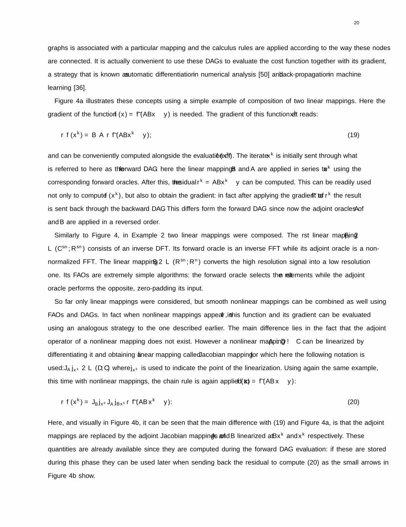
Figure 4a illustrates these concepts using a simple example of composition of two linear mappings. Here the

gradient of the function f(x) = f(ABx− y) is needed. The gradient of this function at xk reads:

∇f(xk) = B∗A∗∇f(ABxk − y), (19)

and can be conveniently computed alongside the evaluation of f(xk). The iterate xk is initially “sent” through what

is referred to here as the forward DAG: here the linear mappings B and A are applied in series to xk using the

corresponding forward oracles. After this, the residual rk = ABxk − y can be computed. This can be readily used

not only to compute f(xk), but also to obtain the gradient: in fact after applying the gradient of f to rk the result

is “sent back” through the backward DAG. This differs form the forward DAG since now the adjoint oracles of A

and B are applied in a reversed order.

Similarly to Figure 4, in Example 2 two linear mappings were composed. The first linear mapping Fi ∈

L (Csn,Rsn) consists of an inverse DFT. Its forward oracle is an inverse FFT while its adjoint oracle is a non-

normalized FFT. The linear mapping S ∈ L (Rsn,Rn) converts the high resolution signal into a low resolution

one. Its FAOs are extremely simple algorithms: the forward oracle selects the first n elements while the adjoint

oracle performs the opposite, zero-padding its input.

So far only linear mappings were considered, but smooth nonlinear mappings can be combined as well using

FAOs and DAGs. In fact when nonlinear mappings appear in f , this function and its gradient can be evaluated

using an analogous strategy to the one described earlier. The main difference lies in the fact that the adjoint

operator of a nonlinear mapping does not exist. However a nonlinear mapping A : D → C can be linearized by

differentiating it and obtaining a linear mapping called Jacobian mapping for which here the following notation is

used: JA|xk ∈ L (D, C) where |xk is used to indicate the point of the linearization. Using again the same example,

this time with nonlinear mappings, the chain rule is again applied to f(x) = f(ABx− y):

∇f(xk) = J∗B|xkJ∗A|Bxk∇f(ABxk − y). (20)

Here, and visually in Figure 4b, it can be seen that the main difference with (19) and Figure 4a, is that the adjoint

mappings are replaced by the adjoint Jacobian mappings of A and B linearized at Bxk and xk respectively. These

quantities are already available since they are computed during the forward DAG evaluation: if these are stored

during this phase they can be used later when sending back the residual to compute (20) as the small arrows in

Figure 4b show.

21

xk B ABxk

−ABxk

y

f

rk︷ ︸︸ ︷ABxk − y

f(ABxk − y)

∇f

A∗B∗

A∗∇f(rk)

B∗A∗∇f(rk)

−−→DAG

←−−DAG

(a)

xk B ABxk

−ABxk

y

f

rk︷ ︸︸ ︷ABxk − y

f(ABxk − y)

∇f

J∗A|BxkJ∗B|xk

J∗A|Bxk∇f(rk)

J∗B|xkJ∗A|Bxk∇f(rk)

−−→DAG

←−−DAG

(b)

Figure 4. Forward and backward DAGs used to evaluate the gradient of a function composed with (a) linear mappings or (b) nonlinearmappings.

These intuitive examples represent only one of the various calculus rules that can be use to combine mappings.

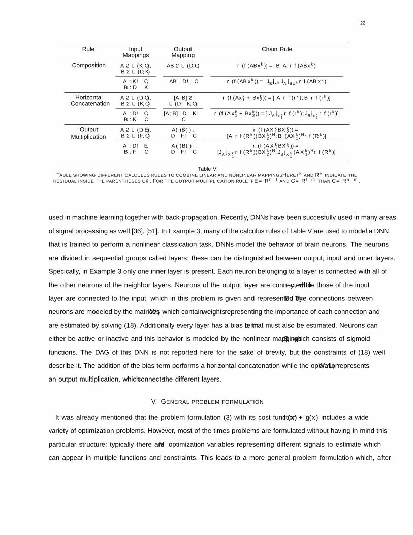
Many other calculus rules can be applied to construct models with much more complex DAGs. Table V shows the

most important calculus rules used to create models. As it can be seen, the horizontal concatenation rule is very

similar to the horizontal concatenation of two matrices. However this creates a forward DAG that has two inputs

xk1 and xk2 that are processed in parallel using two forward oracles whose result is then summed. This rule can also

be used to simply add up different optimization variables by setting the mappings to be identity, like in the least

squares function of Example 4. By inspecting the chain rule it is possible to see how its backward DAG would

look: this would be a reversed version of the forward DAG, having a single input ∇f(rk) and two outputs where

the respective adjoint (Jacobian) mappings would be applied.

The final calculus rule of Table V, called output multiplication has a similar forward DAG to the horizontal

concatenation, with the summation being substituted with a multiplication. The resulting mapping, even when

linear mappings are used, is always nonlinear. Due to this nonlinear behavior its backward DAG is more difficult

to picture but still the very same concepts are applied.

Example 3 shows an example of a deep neural network (DNN), a type of nonlinear model which is extensively

22

Rule InputMappings

OutputMapping

Chain Rule

Composition

B A

A ∈ L (K, C),B ∈ L (D, K)

AB ∈ L (D, C) ∇(f(ABxk)) = B∗A∗∇f(ABxk)

A : K→ C,B : D→ K

AB : D→ C ∇(f(ABxk)) = J∗B|xkJ∗A|Bxk∇f(ABxk)

HorizontalConcatenation

A B

+

A ∈ L (D, C),B ∈ L (K, C)

[A,B] ∈L (D× K, C)

∇(f(Axk1 + Bxk2)) = [A∗∇f(rk),B∗∇f(rk)]

A : D→ C,B : K→ C

[A,B] : D× K→C

∇(f(Axk1 + Bxk2)) = [J∗A|xk1∇f(rk), J∗B|xk2∇f(r

k)]

OutputMultiplication

A B

×

A ∈ L (D, E),B ∈ L (F, G)

A(·)B(·) :D× F→ C

∇(f(AXk1BX

k2)) =

[A∗∇f(Rk)(BXk2)

H,B∗(AXk1)

H∇f(Rk)]

A : D→ E,B : F→ G

A(·)B(·) :D× F→ C

∇(f(AXk1BXk

2)) =[J∗A|Xk1∇f(R

k)(BXk2)

H, J∗B|Xk2 (AXk1)

H∇f(Rk)]

Table VTABLE SHOWING DIFFERENT CALCULUS RULES TO COMBINE LINEAR AND NONLINEAR MAPPINGS. HERE rk AND Rk INDICATE THE

RESIDUAL INSIDE THE PARENTHESES OF f . FOR THE OUTPUT MULTIPLICATION RULE IF E = Rn×l AND G = Rl×m THAN C = Rn×m .

used in machine learning together with back-propagation. Recently, DNNs have been succesfully used in many areas

of signal processing as well [36], [51]. In Example 3, many of the calculus rules of Table V are used to model a DNN

that is trained to perform a nonlinear classification task. DNNs model the behavior of brain neurons. The neurons

are divided in sequential groups called layers: these can be distinguished between output, input and inner layers.

Specifically, in Example 3 only one inner layer is present. Each neuron belonging to a layer is connected with all of

the other neurons of the neighbor layers. Neurons of the output layer are connected to y, while those of the input

layer are connected to the input, which in this problem is given and represented by D. The connections between

neurons are modeled by the matrices Wi which contain weights representing the importance of each connection and

are estimated by solving (18). Additionally every layer has a bias term bi that must also be estimated. Neurons can

either be active or inactive and this behavior is modeled by the nonlinear mappings Si which consists of sigmoid

functions. The DAG of this DNN is not reported here for the sake of brevity, but the constraints of (18) well

describe it. The addition of the bias term performs a horizontal concatenation while the operation WiLi represents

an output multiplication, which connects the different layers.

V. GENERAL PROBLEM FORMULATION

It was already mentioned that the problem formulation (3) with its cost function f(x) + g(x) includes a wide

variety of optimization problems. However, most of the times problems are formulated without having in mind this

particular structure: typically there are M optimization variables representing different signals to estimate which

can appear in multiple functions and constraints. This leads to a more general problem formulation which, after

23

Example 4 Video background removalFr

ames

Fore

grou

ndB

ackg

roun

d

The frames of a video can be viewed as a superposition of a moving foreground to a steady background. Splitting thebackground form the foreground can be a difficult task due to the continuous changes happening in different areas of theframes. The following optimization problem can be posed to deal with such task:

minimizeL,S

1

2‖L + S−Y‖2 + λ‖vec(S)‖1

subject to rank(L) ≤ 1.

StructuredOptimization code snippet:

@minimize ls(L+S-Y)+lambda*norm(S,1)st rank(L) <= 1

Here Y ∈ Rnm×l consists of a matrix in which the l-th column contains the pixel values of the vectorized l-th framewith dimensions n ×m. The optimization problem, also known as robust PCA, decomposes Y into a sparse matrix S,representing the foreground changes and a rank-1 matrix L consisting of the constant background, whose columns arelinearly dependent.

converting the constraints into indicator functions, can be summarized as follows [52], [53]:

minimizex1,...,xM

N∑

i=1

hi

M∑

j=1

Ai,jxj

, (21)

where the N functions hi : C1 × · · · × CM → R are composed with linear mappings Ai,j : Dj → Ci. Notice that

here the eventual presence of nonlinear mappings is included in hi.

In order to apply the framework described in the previous sections, (21) must be re-structured into (3) by splitting

the different hi into two groups: this means, one must appropriately partition the set of indexes {1, . . . , N} into

two subsets If , Ig , such that {1, . . . , N} = If ∪ Ig and If ∩ Ig = ∅, and set

f(x1, . . . ,xM ) =∑

i∈If

hi

M∑

j=1

Ai,jxj

, (22)

24

g(x1, . . . ,xM ) =∑

i∈Ig

hi

M∑

j=1

Ai,jxj

. (23)

In order for f in (22) to be smooth, clearly one must have that hi is smooth for all i ∈ If . When this is the

case, denoting ri =∑Mj=1 Ai,jxj , one has that

∇f(x1, . . . ,xM ) =

∑

i∈If

A∗i,1∇hi(ri)

ᵀ

, . . . ,

∑

i∈If

A∗i,M∇hi(ri)

ᵀᵀ

. (24)

On the other hand, g in (23) should have an efficiently computable proximal mapping. This happens, for example,

if all of the following conditions are met [53]:

• for all i ∈ Ig , function hi has an efficient proximal mapping;

• for all i ∈ Ig and j ∈ {1, . . . ,M}, mapping Ai,j satisfies Ai,jA∗i,j = µi,j Id, where µi,j ≥ 0.

• for all j ∈ {1, . . . ,M}, the cardinality card {i | Ai,j 6= 0} = 1.

These rules ensure that the separable sum and precomposition properties of proximal mappings, cf. Table II, are

applicable yielding an efficient proximal mapping for g.

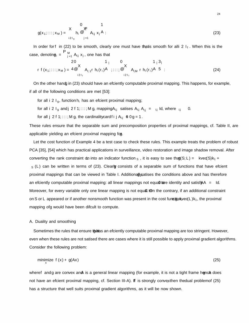
Let the cost function of Example 4 be a test case to check these rules. This example treats the problem of robust

PCA [35], [54] which has practical applications in surveillance, video restoration and image shadow removal. After

converting the rank constraint on L into an indicator function δS , it is easy to see that g(S,L) = λ‖vec(S)‖1 +

δS (L) can be written in terms of (23). Clearly g consists of a separable sum of functions that have efficient

proximal mappings that can be viewed in Table I. Additionally, g satisfies the conditions above and has therefore

an efficiently computable proximal mapping: all linear mappings not equal to 0 are identity and satisfy AA∗ = µId.

Moreover, for every variable only one linear mapping is not equal to 0. On the contrary, if an additional constraint

on S or L appeared or if another nonsmooth function was present in the cost function, e.g., ‖vec(L)‖1, the proximal

mapping of g would have been difficult to compute.

A. Duality and smoothing

Sometimes the rules that ensure that g has an efficiently computable proximal mapping are too stringent. However,

even when these rules are not satisfied there are cases where it is still possible to apply proximal gradient algorithms.

Consider the following problem:

minimizex

f(x) + g(Ax) (25)

where f and g are convex and A is a general linear mapping (for example, it is not a tight frame hence g ◦A does

not have an efficient proximal mapping, cf. Section III-A). If f is strongly convex, then the dual problem of (25)

has a structure that well suits proximal gradient algorithms, as it will be now shown.

25

Example 5 Total variation de-noising

ground truth Xgt noisy Y denoised X?

StructuredOptimizationcode snippet:

V = Variation(size(Y))U = Variable(size(V,1)...)

@minimize ls(-V’*U+Y)+conj(lambda*norm(U,2,1,2))

X = Y-V’*(∼U)

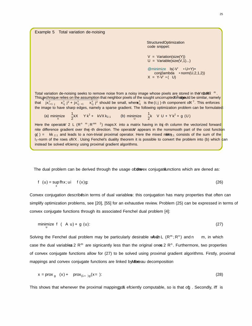
Total variation de-noising seeks to remove noise from a noisy image whose pixels are stored in the matrix Y ∈ Rn×m.This technique relies on the assumption that neighbor pixels of the sought uncorrupted image X? should be similar, namelythat

√|x?i+1,j − x?i,j |2 + |x?i,j+1 − x?i,j |2 should be small, where x?i,j is the (i, j)-th component of X?. This enforces

the image to have sharp edges, namely a sparse gradient. The following optimization problem can be formulated:

(a) minimizeX

1

2‖X−Y‖2 + λ‖VX‖2,1 (b) minimize

U

1

2‖ − V∗U + Y‖2 + g∗(U)

Here the operator V ∈ L (Rn×m,Rnm×2) maps X into a matrix having in its j-th column the vectorized forwardfinite difference gradient over the j-th direction. The operator V appears in the nonsmooth part of the cost functiong(·) = λ‖·‖2,1 and leads to a non-trivial proximal operator. Here the mixed norm ‖·‖2,1 consists of the sum of thel2-norm of the rows of VX. Using Fenchel’s duality theorem it is possible to convert the problem into (b) which caninstead be solved efficiency using proximal gradient algorithms.

The dual problem can be derived through the usage of the convex conjugate functions which are defined as:

f∗(u) = supx{〈x,u〉 − f(x)}. (26)

Convex conjugation describes f in terms of dual variables u: this conjugation has many properties that often can

simplify optimization problems, see [20], [55] for an exhaustive review. Problem (25) can be expressed in terms of

convex conjugate functions through its associated Fenchel dual problem [4]:

minimizeu

f∗(−A∗u) + g∗(u). (27)

Solving the Fenchel dual problem may be particularly desirable when A ∈ L (Rm,Rn) and n � m, in which

case the dual variables u ∈ Rm are significantly less than the original ones x ∈ Rn. Furthermore, two properties

of convex conjugate functions allow for (27) to be solved using proximal gradient algorithms. Firstly, proximal

mappings and convex conjugate functions are linked by the Moreau decomposition:

x = proxγg∗(x) + γ prox(1/γ)g(x/γ). (28)

This shows that whenever the proximal mapping of g is efficiently computable, so is that of g∗. Secondly, if f is

26

strongly convex then its convex conjugate f∗ has a Lipschitz gradient [56, Lemma 3.2]. This also implies that any

solution of (27) can be converted back to the one of the original problem through [20]:

x? = ∇f∗(−A∗u?). (29)

Therefore, under these assumptions it is possible to solve (27) using proximal gradient algorithms of Section III-B.

When this is done, the (fast) PG algorithm results in what is also known as (fast) alternating minimization algorithm

(AMA) [56], [57].

Example 5 treats the classical image processing application of de-noising a digital image. Here in the original

problem a linear operator appears in a nonsmooth function preventing its proximal mapping to be efficient. Function

f here is the squared norm which is self-dual i.e., f(·) = 12‖·‖2 = f∗(·). Hence it is possible to solve the dual

problem instead, using proximal gradient algorithms: in the Fenchel dual problem the linear mapping is transferred

into the smooth function f∗ in terms of its adjoint allowing the usage of an efficient proximal mapping for the

nonsmooth function g through (28). Once the dual solution U? is obtained, this can be easily converted back to

the one of the original problem through the usage of (29): ∇f(X?) = X? −Y = −V∗U?.

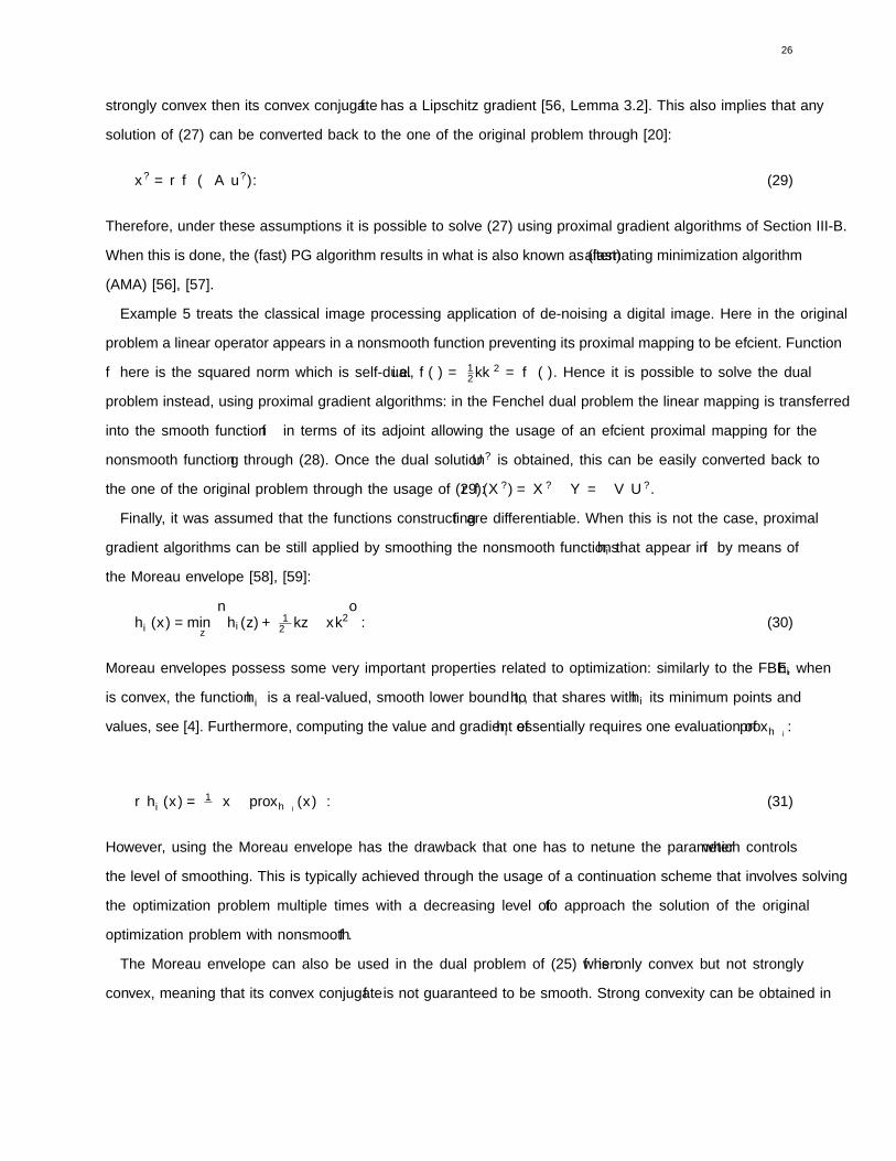
Finally, it was assumed that the functions constructing f are differentiable. When this is not the case, proximal

gradient algorithms can be still applied by “smoothing” the nonsmooth functions hi that appear in f by means of

the Moreau envelope [58], [59]:

hβi (x) = minz

{hi(z) + 1

2β ‖z− x‖2}. (30)

Moreau envelopes possess some very important properties related to optimization: similarly to the FBE, when hi

is convex, the function hβi is a real-valued, smooth lower bound to hi, that shares with hi its minimum points and

values, see [4]. Furthermore, computing the value and gradient of hβi essentially requires one evaluation of proxβhi :

∇hβi (x) = 1β

(x− proxβhi(x)

). (31)

However, using the Moreau envelope has the drawback that one has to finetune the parameter β which controls

the level of smoothing. This is typically achieved through the usage of a continuation scheme that involves solving

the optimization problem multiple times with a decreasing level of β to approach the solution of the original

optimization problem with nonsmooth f .

The Moreau envelope can also be used in the dual problem of (25) when f is only convex but not strongly

convex, meaning that its convex conjugate f∗ is not guaranteed to be smooth. Strong convexity can be obtained in

27

f by adding to it a regularization term:

fβ(x) = f(x) + β2 ‖x‖2. (32)

Then, the convex conjugate of fβ becomes the Moreau envelope of the convex conjugate of f , i.e., (f∗β) = (f∗)β

[4, Prop. 14.1], which is now differentiable and allows to solve the dual problem (27) using proximal gradient

algorithms.

VI. A HIGH-LEVEL MODELING LANGUAGE: StructuredOptimization

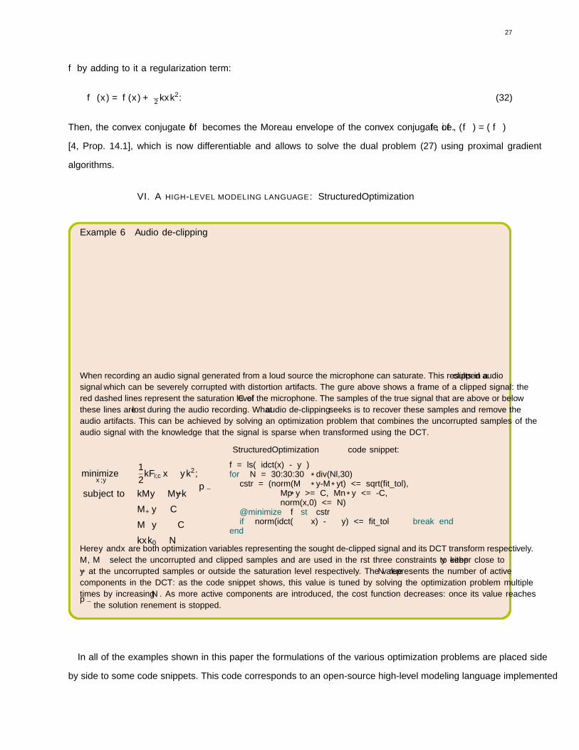
Example 6 Audio de-clipping

0 0.1 0.2 0.3 0.4 0.5 0.6 0.7 0.8 0.9 1

−0.4

−0.2

0

0.2

0.4

Time (ms)

ygt; y; y?;

When recording an audio signal generated from a loud source the microphone can saturate. This results in a clipped audiosignal which can be severely corrupted with distortion artifacts. The figure above shows a frame of a clipped signal: thered dashed lines represent the saturation level C of the microphone. The samples of the true signal that are above or belowthese lines are lost during the audio recording. What audio de-clipping seeks is to recover these samples and remove theaudio artifacts. This can be achieved by solving an optimization problem that combines the uncorrupted samples of theaudio signal with the knowledge that the signal is sparse when transformed using the DCT.

minimizex,y

1

2‖Fi,cx− y‖2,

subject to ‖My −My‖ ≤ √εM+y ≥ CM−y ≤ −C‖x‖0 ≤ N

StructuredOptimization code snippet:

f = ls( idct(x) - y )for N = 30:30:30*div(Nl,30)cstr = (norm(M*y-M*yt) <= sqrt(fit_tol),

Mp*y >= C, Mn*y <= -C,norm(x,0) <= N)

@minimize f st cstrif norm(idct(∼x) - ∼y) <= fit_tol break end

end

Here y and x are both optimization variables representing the sought de-clipped signal and its DCT transform respectively.M, M± select the uncorrupted and clipped samples and are used in the first three constraints to keep y either close toy at the uncorrupted samples or outside the saturation level respectively. The value N represents the number of activecomponents in the DCT: as the code snippet shows, this value is tuned by solving the optimization problem multipletimes by increasing N . As more active components are introduced, the cost function decreases: once its value reaches√ε the solution refinement is stopped.

In all of the examples shown in this paper the formulations of the various optimization problems are placed side

by side to some code snippets. This code corresponds to an open-source high-level modeling language implemented

28

in Julia.

Julia is a relatively new open-source programming language which was specifically designed for scientific

computing and offers high performance often comparable to low-level languages like C. Despite being a young

programming language it has a rapidly growing community and already offers many packages in various fields

[30].

The proposed high-level modeling language is provided in the software package StructuredOptimization

[60]: this utilizes a syntax that is very close to the mathematical formulation of an optimization problem. This user-

friendly interface acts as a parser to utilize three different packages that implement many of the concepts described

in this paper:

• ProximalOperators is a library of proximal mappings of functions that are frequently used in signal

processing and optimization. These can be transformed and manipulated using the properties described in

Section III-A.

• AbstractOperators provides a library of FAOs that can be used to create and evaluate DAGs of linear

and nonlinear mappings as described in Section IV. This package also offers a syntax analogue to the one that

is typically used with matrices.

• ProximalAlgorithms is a library of optimization algorithms that includes the PG algorithm and its

enhanced variants described in Sections III-B and III-D.

When a problem is provided to StructuredOptimization this is automatically analyzed to check whether

it falls within the sets of problems described in Section V. Firstly, the various functions and constraints, which are

conveniently converted into indicator functions, need to be split into the functions f and g. As it was described

in Section V sometimes multiple splitting configurations are possible: StructuredOptimization adopts the

simplest strategy possible, splitting the smooth functions form the nonsmooth ones. The nonsmooth functions are

then analyzed to verify if the rules described in Section V are fulfilled to ensure an efficient proximal mapping of

g exists. If this is the case, StructuredOptimization then provides the necessary inputs to the algorithms

of ProximalAlgorithms to efficiently solve the problem.

Example 6 can be used as a showcase of the proposed high-level modeling language. This example treats the

recovery of an audio signal corrupted by clipping [61], [62]. This recovery is performed using a weighted overlap-

add method, i.e., by splitting the audio signal into overlapping frames of length n = 210 and processing them

serially, using an initialization strategy analogue to the one proposed in [63].

The high-level modeling language that StructuredOptimization provides is designed to be as much

natural as possible. Firstly the optimization variables can be defined, e.g., x ∈ Rn is constructed by typing x

= Variable(n). By default the variables are initialized by vectors of zeros but it is possible to set different

initializations e.g., Variable([0;1]) will be a variable of two elements initialized by the vector [0, 1]ᵀ. The

29

user can also utilize different equivalent notations: for example in the first line of the code snippet of Example 6 the

function f could be defined equivalently with f = 0.5*norm(F*x-y)ˆ2, by firstly constructing the mapping

Fi,c using the notation F = IDCT(n). Similarly, the selection mappings applied to y, i.e., Mp*y, could be replaced

equivalently by y[idp] where idp is an array of indexes corresponding to the ones of the selection mapping

M+.

Once the cost function f and the constraints cstr are defined, the problem can be solved by typing @minimize

f st cstr. If an efficient proximal mapping is found, the problem is solved using a proximal gradient algorithm.

As it can be seen, here this condition is fulfilled despite the fact that multiple constraints over the variable y are

present: these still lead to an efficient proximal mapping since they are applied to non-overlapping slices of the

variable y and are therefore separable.

The standard algorithm, PANOC, is then used to solve the problem, but if a specific one is to be used e.g.,

the FPG algorithm, one can specify that: @minimize cf st cstr with FPG(). As the code snippet of

Example 6 shows, the series of problems is set inside a loop: here every problem is automatically warm-started by

the previous one, as the variables x and y are always linked to their respective data vectors which can be accessed

by typing ∼x. More details about the software can be found in the documentation online. Finally, in line with the

philosophy of reproducible research all the code that was used to create the examples and the various comparison

of the algorithms is publicly available online [60].

Many other software packages based on proximal gradient algorithms have been recently developed. There are

different MATLAB toolboxes: FOM provides several proximal gradient algorithms [64] and ForBES implements

Newton-type accelerated proximal gradient algorithms [65]. TFOCS offers different splitting algorithms that can be

used in combination with FAOs through the usage of the toolbox Spot [66]. ProxImaL [67], also implements

different matrix-free splitting algorithms in the Python language with a particular focus to image processing

applications.

VII. CONCLUSIONS

The proximal gradient algorithms described in this paper can be applied to a wide variety of signal processing

applications. Many examples were presented here to show this versatility with a particular focus on inverse problems

of large-scale that naturally arises in many audio, communication, image and video processing applications. Recent

enhancements of the PG algorithm have improved significantly its convergence speed. These offer the possibility

of using quasi-Newton methods reaching solutions of high accuracy with a speed that was previously beyond the

reach of most first-order methods. Additionally these algorithms can be easily combined with fast forward-adjoint

oracles to compute the mappings involved leading to matrix-free optimization.

The applications illustrated in this paper are only a small portion of what these algorithms can tackle and it is

envisaged that many others will benefit their properties. In fact, proximal gradient algorithms are relatively simple

30

and they result in very compact implementations, which most of the time do not require additional subroutines,

unlike other splitting algorithms e.g., ADMM. This makes them particularly well suited for embedded systems

and real-time applications. Additionally, many of the operations involved in this framework are parallel by nature:

not only proximal mappings, which in many contexts are separable, but also matrix-free optimization, that utilizes

graphs of forward-adjoint oracles, naturally lead to parallelism. This makes these algorithms also particularly fit for

wireless sensor networks and many Internet-of-Things applications.

Finally, these algorithms can tackle nonconvex problems: machine learning showed how nonlinear models can

reach outstanding results. It is envisaged that these algorithms with their flexibility can be used to create novel

nonlinear filters by easily testing the effectiveness of new nonlinear models.

REFERENCES

[1] E. J. Candes and M. B. Wakin, “An introduction to compressive sampling,” IEEE Signal Process. Mag., vol. 25, no. 2, pp. 21–30, 2008.

[2] M. Grant, S. Boyd, and Y. Ye, “Disciplined convex programming,” in Global Optimization: From Theory to Implementation. Springer,

2006, pp. 155–210.

[3] V. Cevher, S. Becker, and M. Schmidt, “Convex optimization for big data: Scalable, randomized, and parallel algorithms for big data

analytics,” IEEE Signal Process. Mag., vol. 31, no. 5, pp. 32–43, 2014.

[4] H. H. Bauschke and P. L. Combettes, Convex analysis and monotone operator theory in Hilbert spaces. Springer, 2011.

[5] P. L. Combettes and J.-C. Pesquet, “Proximal splitting methods in signal processing,” in Fixed-point algorithms for inverse problems in

science and engineering. Springer, 2011, pp. 185–212.

[6] N. Parikh and S. P. Boyd, “Proximal algorithms,” Foundations and Trends in Optimization, vol. 1, no. 3, pp. 127–239, 2014.

[7] P. L. Combettes and V. R. Wajs, “Signal recovery by proximal forward-backward splitting,” Multiscale Modeling & Simulation, vol. 4,

no. 4, pp. 1168–1200, 2005.

[8] S. Boyd, N. Parikh, E. Chu, B. Peleato, and J. Eckstein, “Distributed optimization and statistical learning via the alternating direction

method of multipliers,” Foundations and Trends in Machine Learning, vol. 3, no. 1, pp. 1–122, 2011.

[9] A. Chambolle and T. Pock, “A first-order primal-dual algorithm for convex problems with applications to imaging,” Journal of Mathematical

Imaging and Vision, vol. 40, no. 1, pp. 120–145, 2011.

[10] Y. Nesterov, “A method of solving a convex programming problem with convergence rate O(1/k2),” Soviet Mathematics Doklady, vol. 27,

no. 2, pp. 372–376, 1983.

[11] A. Beck and M. Teboulle, “A fast iterative shrinkage-thresholding algorithm for linear inverse problems,” SIAM Journal on Imaging

Sciences, vol. 2, no. 1, pp. 183–202, 2009.

[12] J. F. Bonnans, J. C. Gilbert, C. Lemarechal, and C. A. Sagastizabal, “A family of variable metric proximal methods,” Math. Programming,

vol. 68, no. 1-3, pp. 15–47, 1995.

[13] E. Chouzenoux, J.-C. Pesquet, and A. Repetti, “Variable metric forward–backward algorithm for minimizing the sum of a differentiable

function and a convex function,” J. Optimiz. Theory App., vol. 162, no. 1, pp. 107–132, 2014.

[14] P. Frankel, G. Garrigos, and J. Peypouquet, “Splitting methods with variable metric for kurdyka–łojasiewicz functions and general

convergence rates,” J. Optimiz. Theory App., vol. 165, no. 3, pp. 874–900, Jun 2015.

[15] E. Chouzenoux, J.-C. Pesquet, and A. Repetti, “A block coordinate variable metric forward–backward algorithm,” J. Global Optimiz.,

vol. 66, no. 3, pp. 457–485, 2016.

[16] S. Becker and J. Fadili, “A quasi-newton proximal splitting method,” in Adv. Neural Inf. Process. Syst., 2012, pp. 2618–2626.

[17] J. D. Lee, Y. Sun, and M. A. Saunders, “Proximal newton-type methods for minimizing composite functions,” SIAM J. Optimiz., vol. 24,

no. 3, pp. 1420–1443, 2014.

31

[18] A. Themelis, L. Stella, and P. Patrinos, “Forward-backward envelope for the sum of two nonconvex functions: Further properties and

nonmonotone line-search algorithms,” arXiv:1606.06256, 2016.

[19] L. Stella, A. Themelis, and P. Patrinos, “Forward-backward quasi-Newton methods for nonsmooth optimization problems,” Computational

Optimization and Applications, vol. 67, no. 3, pp. 443–487, 2017.

[20] N. Komodakis and J.-C. Pesquet, “Playing with duality: An overview of recent primal-dual approaches for solving large-scale optimization

problems,” IEEE Signal Process. Mag., vol. 32, no. 6, pp. 31–54, 2015.

[21] H. Attouch, J. Bolte, and B. F. Svaiter, “Convergence of descent methods for semi-algebraic and tame problems: proximal algorithms,

forward–backward splitting, and regularized Gauss–Seidel methods,” Mathematical Programming, vol. 137, no. 1, pp. 91–129, 2013.

[22] P. Jain and P. Kar, “Non-convex optimization for machine learning,” Foundations and Trends in Machine Learning, vol. 10, no. 3-4, pp.

142–336, 2017.

[23] E. J. Candes, Y. C. Eldar, T. Strohmer, and V. Voroninski, “Phase retrieval via matrix completion,” SIAM Review, vol. 57, no. 2, pp.

225–251, 2015.

[24] N. Boumal, V. Voroninski, and A. Bandeira, “The non-convex Burer-Monteiro approach works on smooth semidefinite programs,” Advances

in Neural Information Processing Systems, pp. 2757–2765, 2016.

[25] Z.-Q. Luo, W.-K. Ma, A. M.-C. So, Y. Ye, and S. Zhang, “Semidefinite relaxation of quadratic optimization problems,” IEEE Signal

Process. Mag., vol. 27, no. 3, pp. 20–34, 2010.

[26] S. Diamond and S. Boyd, “Matrix-free convex optimization modeling,” in Optimization and its Applications in Control and Data Sciences.

Springer, 2016, pp. 221–264.

[27] J. Folberth and S. Becker, “Efficient adjoint computation for wavelet and convolution operators [lecture notes],” IEEE Signal Process.

Mag., vol. 33, no. 6, pp. 135–147, 2016.

[28] M. Grant, S. Boyd, and Y. Ye. (2008) CVX: Matlab software for disciplined convex programming. [Online]. Available: http://cvxr.com/cvx/

[29] S. Becker, E. Candes, and M. Grant. (2012) TFOCS: Templates for first-order conic solvers. [Online]. Available: http://cvxr.com/tfocs/

[30] J. Bezanson, A. Edelman, S. Karpinski, and V. B. Shah, “Julia: A fresh approach to numerical computing,” SIAM Review, vol. 59, no. 1,

pp. 65–98, 2017.

[31] C. R. Berger, Z. Wang, J. Huang, and S. Zhou, “Application of compressive sensing to sparse channel estimation,” IEEE Commun. Mag.,

vol. 48, no. 11, 2010.

[32] I. Kodrasi and S. Doclo, “Joint dereverberation and noise reduction based on acoustic multi-channel equalization,” IEEE/ACM Trans. Audio

Speech Lang. Process., vol. 24, no. 4, pp. 680–693, 2016.

[33] S. I. Adalbjornsson, T. Kronvall, S. Burgess, K. Astrom, and A. Jakobsson, “Sparse localization of harmonic audio sources,” IEEE/ACM

Trans. Audio Speech Lang. Process., vol. 24, no. 1, pp. 117–129, 2016.

[34] B. N. Bhaskar, G. Tang, and B. Recht, “Atomic norm denoising with applications to line spectral estimation,” IEEE Trans. Signal Process.,

vol. 61, no. 23, pp. 5987–5999, 2013.

[35] P. Netrapalli, U. Niranjan, S. Sanghavi, A. Anandkumar, and P. Jain, “Non-convex robust PCA,” Advances in Neural Information Processing

Systems, pp. 1107–1115, 2014.

[36] S. Theodoridis, Machine learning: a Bayesian and optimization perspective. Academic Press, 2015.

[37] S. Ling and T. Strohmer, “Self-calibration and biconvex compressive sensing,” Inverse Problems, vol. 31, no. 11, 2015.

[38] J. Nocedal and S. Wright, Numerical Optimization, 2nd ed. New York: Springer, 2006.

[39] R. T. Rockafellar and R. J. Wets, Variational analysis. Springer, 2011.

[40] A. Domahidi, E. Chu, and S. Boyd, “ECOS: An SOCP solver for embedded systems,” in Proc. European Control Conf. (ECC), 2013, pp.

3071–3076.

[41] B. O’Donoghue, E. Chu, N. Parikh, and S. Boyd, “Conic optimization via operator splitting and homogeneous self-dual embedding,”

Journal of Optimization Theory and Applications, vol. 169, no. 3, pp. 1042–1068, June 2016.

[42] J.-J. Moreau, “Proximite et dualite dans un espace Hilbertien,” Bulletin de la Societe mathematique de France, vol. 93, pp. 273–299, 1965.

32

[43] R. E. Bruck, “An iterative solution of a variational inequality for certain monotone operators in Hilbert space,” Bulletin of the American

Mathematical Society, vol. 81, no. 5, pp. 890–893, 1975.

[44] P.-L. Lions and B. Mercier, “Splitting algorithms for the sum of two nonlinear operators,” SIAM Journal on Numerical Analysis, vol. 16,

no. 6, pp. 964–979, 1979.

[45] P. Tseng, “On accelerated proximal gradient methods for convex-concave optimization,” Department of Mathematics, University of

Washington, Tech. Rep., 2008.

[46] Y. Nesterov, “Gradient methods for minimizing composite functions,” Mathematical Programming, vol. 140, no. 1, pp. 125–161, 2013.

[47] P. Patrinos and A. Bemporad, “Proximal Newton methods for convex composite optimization,” in Proc. 52nd IEEE Conf. Decision Control

(CDC), 2013, pp. 2358–2363.

[48] L. Stella, A. Themelis, P. Sopasakis, and P. Patrinos, “A simple and efficient algorithm for nonlinear model predictive control,” in Proc.

56th IEEE Conf. Decision Control (CDC), 2017, pp. 1939–1944.

[49] J. F. Claerbout, Earth soundings analysis: Processing versus inversion. Blackwell Scientific Publications Cambridge, Massachusetts,

USA, 1992, vol. 6.

[50] A. Griewank and A. Walther, Evaluating derivatives: principles and techniques of algorithmic differentiation. Siam, 2008.

[51] Y. LeCun, Y. Bengio, and G. Hinton, “Deep learning,” Nature, vol. 521, no. 7553, pp. 436–444, 2015.

[52] L. M. Briceno-Arias and P. L. Combettes, “Convex variational formulation with smooth coupling for multicomponent signal decomposition

and recovery,” Numer. Math. Theory Methods Appl., vol. 2, pp. 485–508, 2009.

[53] L. M. Briceno-Arias, P. L. Combettes, J.-C. Pesquet, and N. Pustelnik, “Proximal algorithms for multicomponent image recovery problems,”

J. Math. Imaging and Vision, vol. 41, no. 1-2, pp. 3–22, 2011.

[54] E. J. Candes, X. Li, Y. Ma, and J. Wright, “Robust principal component analysis?” Journal of the ACM (JACM), vol. 58, no. 3, p. 11,

2011.

[55] P. L. Combettes, D. Dung, and B. C. Vu, “Dualization of signal recovery problems,” Set-Valued and Variational Analysis, vol. 18, no. 3-4,

pp. 373–404, 2010.

[56] A. Beck and M. Teboulle, “A fast dual proximal gradient algorithm for convex minimization and applications,” Operations Research

Letters, vol. 42, no. 1, pp. 1–6, 2014.

[57] P. Tseng, “Applications of a splitting algorithm to decomposition in convex programming and variational inequalities,” SIAM Journal on

Control and Optimization, vol. 29, no. 1, pp. 119–138, 1991.

[58] Y. Nesterov, “Smoothing technique and its applications in semidefinite optimization,” Mathematical Programming, vol. 110, no. 2, pp.

245–259, 2007.

[59] A. Beck and M. Teboulle, “Smoothing and first order methods: A unified framework,” SIAM Journal on Optimization, vol. 22, no. 2, pp.

557–580, 2012.

[60] L. Stella and N. Antonello. (2017) StructuredOptimization.jl. [Online]. Available: https://github.com/kul-forbes/StructuredOptimization.jl

[61] A. Adler, V. Emiya, M. G. Jafari, M. Elad, R. Gribonval, and M. D. Plumbley, “Audio inpainting,” IEEE Trans. Audio Speech Lang.

Process., vol. 20, no. 3, pp. 922–932, 2012.

[62] B. Defraene, N. Mansour, S. De Hertogh, T. van Waterschoot, M. Diehl, and M. Moonen, “Declipping of audio signals using perceptual

compressed sensing,” in Proc. 2014 IEEE Global Conf. Signal Inf. Process. (GlobalSIP ’14), Atlanta, GA, USA, Dec. 2014, pp. 114–125.

[63] S. Kitic, N. Bertin, and R. Gribonval, “Sparsity and cosparsity for audio declipping: a flexible non-convex approach,” in Proc. Int. Conf.

Latent Variable Analysis and Signal Separation. Springer, 2015, pp. 243–250.

[64] A. Beck and N. Guttmann-Beck, “FOM–a MATLAB toolbox of first order methods for solving convex optimization problems,” 2017.

[Online]. Available: https://sites.google.com/site/fomsolver/

[65] L. Stella and P. Patrinos. (2016) ForBES. [Online]. Available: https://github.com/kul-forbes/ForBES

[66] E. van den Berg and M. P. Friedlander. (2014) SPOT - A Linear-Operator Toolbox. [Online]. Available: http://www.cs.ubc.ca/labs/scl/spot/

[67] F. Heide, S. Diamond, M. Nießner, J. Ragan-Kelley, W. Heidrich, and G. Wetzstein, “ProxImaL: Efficient image optimization using

proximal algorithms,” ACM Transactions on Graphics (TOG), vol. 35, no. 4, 2016.