U.S. Department of the Interior U.S. Geological Survey Techniques and Methods 6–B5 In Cooperation With the Cuyahoga County Board of Health, Northeast Ohio Regional Sewer District, Ohio Water Development Authority, and Ohio Lake Erie Office Procedures for Developing Models To Predict Exceedances of Recreational Water-Quality Standards at Coastal Beaches

Welcome message from author
This document is posted to help you gain knowledge. Please leave a comment to let me know what you think about it! Share it to your friends and learn new things together.
Transcript
U.S. Department of the InteriorU.S. Geological Survey
Techniques and Methods 6–B5
In Cooperation With the Cuyahoga County Board of Health, Northeast Ohio Regional Sewer District, Ohio Water Development Authority, and Ohio Lake Erie Office
Procedures for Developing Models To Predict Exceedances of Recreational Water-Quality Standards at Coastal Beaches

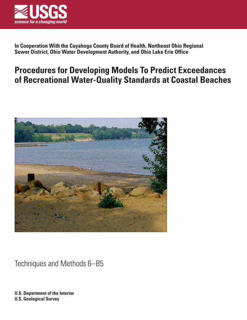
Cover photo: View of Edgewater Park beach, Cleveland, Ohio, looking west from the breakwater. (Photograph by Kenneth Frame, U.S. Geological Survey.)
Procedures for Developing Models To Predict Exceedances of Recreational Water-Quality Standards at Coastal Beaches
By Donna S. Francy and Robert A. Darner
In Cooperation with the Cuyahoga County Board of Health, Northeast Ohio Regional Sewer District, Ohio Water Development Authority, and Ohio Lake Erie Office
Techniques and Methods 6–B5
U.S. Department of the InteriorU.S. Geological Survey
U.S. Department of the InteriorDIRK KEMPTHORNE, Secretary
U.S. Geological SurveyMark D. Myers, Director
U.S. Geological Survey, Reston, Virginia: 2006
For product and ordering information: World Wide Web: http://www.usgs.gov/pubprod Telephone: 1-888-ASK-USGS
For more information on the USGS--the Federal source for science about the Earth, its natural and living resources, natural hazards, and the environment: World Wide Web: http://www.usgs.gov Telephone: 1-888-ASK-USGS
Any use of trade, product, or firm names is for descriptive purposes only and does not imply endorsement by the U.S. Government.
Although this report is in the public domain, permission must be secured from the individual copyright owners to reproduce any copyrighted materials contained within this report.
Suggested citation:Francy, D.S., and Darner, R.A., 2006, Procedures for developing models to predict exceedances of recreational water-quality standards at coastal beaches: U.S. Geological Survey Techniques and Methods 6–B5, 34 p.
iii
ContentsAbstract ...........................................................................................................................................................1Introduction.....................................................................................................................................................1Procedures for Developing Predictive Models ........................................................................................3
Data Collection ......................................................................................................................................3Exploratory Data Analysis ...................................................................................................................4Model Development .............................................................................................................................5Model Diagnostics and Selection ......................................................................................................5Model Output and Validation ..............................................................................................................6
The Future of Predictive Modeling .............................................................................................................7Summary..........................................................................................................................................................7Acknowledgments .........................................................................................................................................8References Cited............................................................................................................................................8Examples From Beach Studies at Huntington Reservation, Bay Village, Ohio ..................................10Appendix 1— SAS commands to determine the best 50 models and to obtain individual
model parameters and Fortran program to determine the probability of exceeding the single-sample maximum bathing-water standard .............................................................28
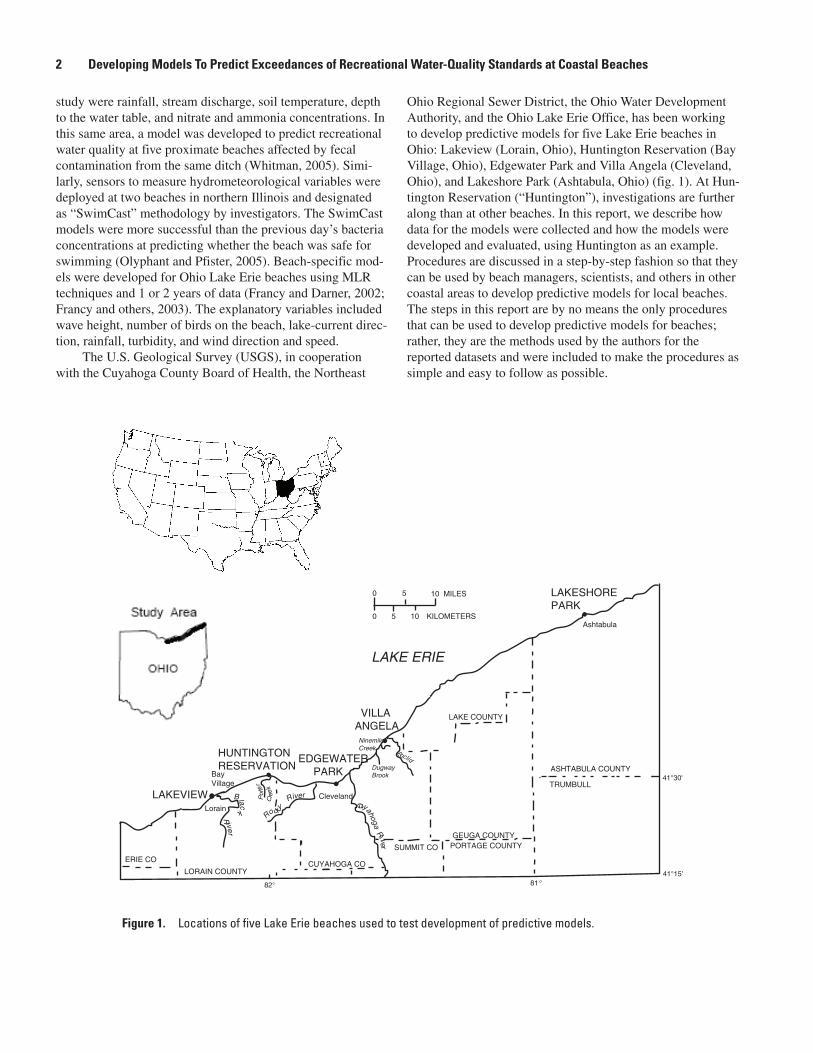
Figures1. Map showing locations of five Lake Erie beaches used to test development of predictive
models ............................................................................................................................................22–8. Graphs showing—
2. Huntington, 2000–2004, relations between Escherichia coli concentrations and turbidity and day of the year. ....................................................................................................................16
3. Huntington, 2000–2004, Escherichia coli concentrations in water, by wave height and 24-hour wind direction ...............................................................................................................16
4. Partial residual plots of explanatory variables for the Huntington 2000–2004 model: weighted 48-hour rainfall, wave height, and log10 turbidity ................................................21
5. Predicted Escherichia coli concentrations and residuals for the Huntington 2000–2004 model ............................................................................................................................................22
6. Measured and predicted Escherichia coli concentrations for the Huntington 2000–2004 model ............................................................................................................................................22
7. Establishment of the threshold probability for the Huntington 2000–2004 model .....................238. Huntington 2005, performance in assessing recreational water-quality of Huntington
2000–2004 model: probability output and predicted Escherichia coli output compared to the current method .....................................................................................................................26
iv
Tables1. Example of computing “wind direction 24” by vector addition of hourly wind directions and
wind speeds for the 24-hour period preceding sampling for Huntington .........................142. Summary statistics of Escherichia coli concentrations at Huntington, 2000–2005 ......................153. Pearson’s r correlations between log10 Escherichia coli concentrations and
explanatory variables for Huntington, 2000–2005 ..................................................................174. Pearson’s r correlations among explanatory variables for Huntington, 2000–2004......................185. List of possible models and the Mallows’ Cp test for Huntington 2000–2004 ................................196. Huntington 2000–2004 model, statistics and parameter estimates .................................................207. Huntington, numbers of correct responses and the sensitivities and specificities of model
responses with indicated thresholds and predicted Escherichia coli (E. coli) concentrations compared to previous day’s E. coli concentrations ..................................24
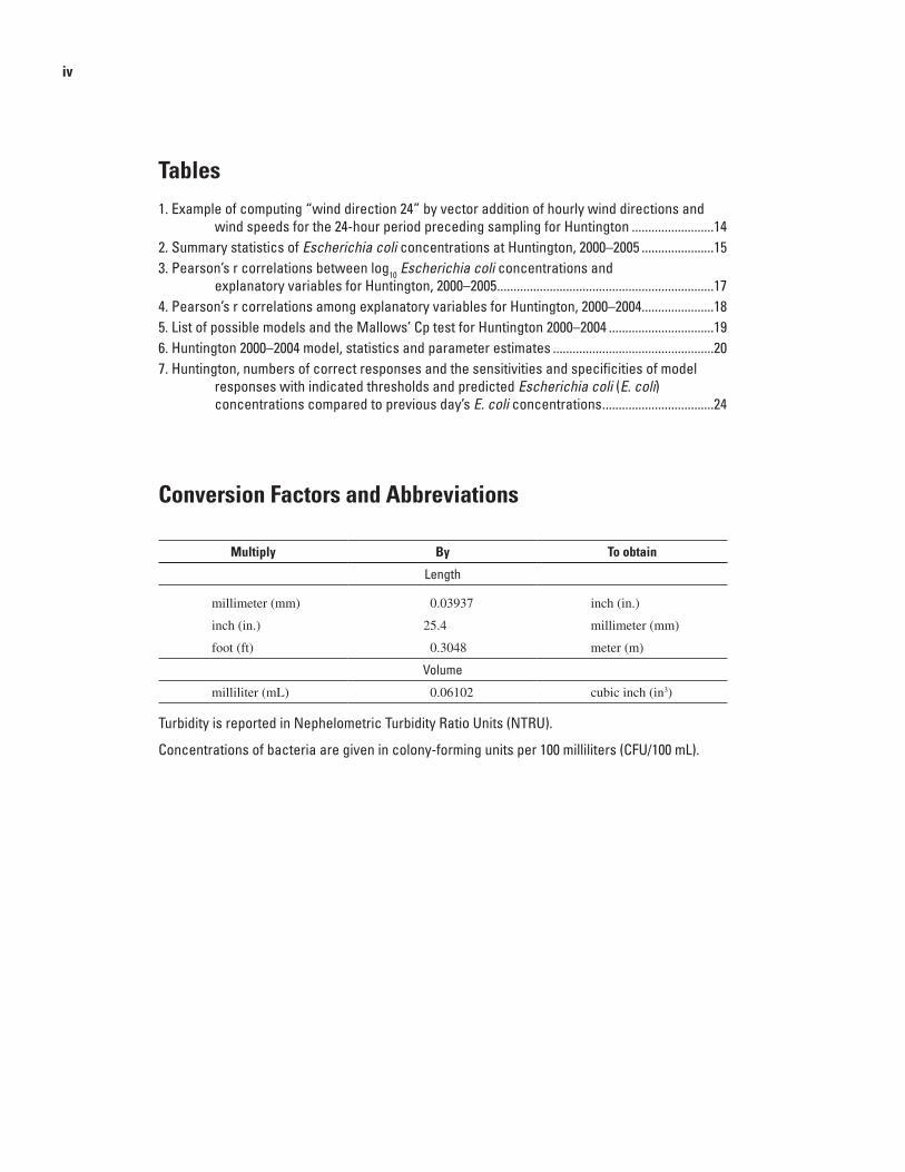
Conversion Factors and Abbreviations
Multiply By To obtain
Length
millimeter (mm) 0.03937 inch (in.)
inch (in.) 25.4 millimeter (mm)
foot (ft) 0.3048 meter (m)
Volume
milliliter (mL) 0.06102 cubic inch (in3)
Turbidity is reported in Nephelometric Turbidity Ratio Units (NTRU).
Concentrations of bacteria are given in colony-forming units per 100 milliliters (CFU/100 mL).
AbstractState recreational water-quality standards are based on
concentrations of indicator organisms, such as Escherchia coli (E. coli). Because the analytical methods for enumerating E. coli take at least 18–24 hours to complete, some agencies have turned to predictive modeling to obtain near-real-time estimates of recreational water quality. The USGS has been working with local agencies to develop empirical predic-tive models for five Lake Erie beaches in Ohio. One beach, Huntington, is used as example in this report to describe in a step-by-step fashion how data for models were collected and how models were developed and evaluated. These steps are not the only procedures that can be used to develop predictive models for beaches; rather, they are the methods used by the authors for the reported datasets.
The steps to develop predictive models are data collec-tion; exploratory data analysis; model development, selection, and diagnosis; determination of model output values; and model validation and refinement. For Huntington, the predic-tive model was based on data collected during the recreational seasons of 2000–2004. The explanatory variables were wave height, weighted rainfall in the past 48 hours, and log
10 turbid-
ity; the model explained 38 percent of the variability in E. coli concentrations. Two outputs from the model were calculated: (1) the predicted E. coli concentration and (2) the probability that the E. coli single-sample maximum bathing-water stan-dard of 235 colony-forming units per 100 milliliters (CFU/100 mL) will be exceeded. A threshold probability of 29 percent was established for the Huntington 2000–2004 model. The threshold probability is the probability associated with too great a risk to allow swimming and is established by examining historical data. The model was validated in 2005 and yielded more correct responses and better predicted exceedance of the bathing-water standard than did the cur-rent method for assessing recreational water quality (using the previous day’s E. coli concentration).
The procedures described in this report can be used to develop and test predictive models at other beaches. Predic-tive modeling is a dynamic process meant to augment exist-ing beach-monitoring programs, not to replace them. Models should be continuously validated and refined to improve
predictions and better protect public health. If validation tests are successful, a beach manager may decide to develop an Internet-based system that provides model predictions to the beach-going public. This type of system, called “nowcasting,” was implemented at Huntington on May 30, 2006.
IntroductionAs the result of the Beaches Environmental Assess-
ment and Coastal Health (BEACH) Act of 2000, states have adopted U.S. Environmental Protection Agency criteria into state recreational water-quality standards (U.S. Environmental Protection Agency, 1986, 1998, 1999). These include concen-trations of bacterial indicators—Escherichia coli (E. coli) or enterococci for freshwaters and enterococci for marine waters. The analytical methods for these organisms, however, take at least 18–24 hours to complete. Recreational water-quality conditions may change during this time, leading to erroneous assessments of public-health risk. As a result, some agencies have turned to predictive modeling to obtain near-real-time estimates of recreational water quality. In situations where nonpoint or unidentified sources dominate, empirical model-ing is most appropriate. Empirical models, developed through statistical techniques such as multiple linear regression (MLR), use easily measured environmental and water-quality variables to estimate bacterial-indicator concentrations or the probability of exceeding target concentrations.
Researchers have worked to study the use of environmen-tal and water-quality variables and to develop empirical mod-els for assessments of recreational water quality for coastal waters. Ackerman and Weisberg (2003) confirmed the use of a rainfall advisory system in southern California and found that rainfall amounts greater than 6 mm consistently led to beach water-quality degradation. At recreational estuaries in Austra-lia, rainfall alone accounted for 15–66 percent of the vari-ability in bacterial-indicator densities (Hose and others, 2005). In a study in Indiana, several variables measured with onsite sensors were used to develop equations that accounted for 60–90 percent of the variability in E. coli concentrations at the outlets of two ditches draining into Lake Michigan (Olyphant and others, 2003). Explanatory variables used in the Indiana
Procedures for Developing Models To Predict Exceedances of Recreational Water-Quality Standards at Coastal Beaches
By Donna S. Francy and Robert A. Darner
study were rainfall, stream discharge, soil temperature, depth to the water table, and nitrate and ammonia concentrations. In this same area, a model was developed to predict recreational water quality at five proximate beaches affected by fecal contamination from the same ditch (Whitman, 2005). Simi-larly, sensors to measure hydrometeorological variables were deployed at two beaches in northern Illinois and designated as “SwimCast” methodology by investigators. The SwimCast models were more successful than the previous day’s bacteria concentrations at predicting whether the beach was safe for swimming (Olyphant and Pfister, 2005). Beach-specific mod-els were developed for Ohio Lake Erie beaches using MLR techniques and 1 or 2 years of data (Francy and Darner, 2002; Francy and others, 2003). The explanatory variables included wave height, number of birds on the beach, lake-current direc-tion, rainfall, turbidity, and wind direction and speed.
The U.S. Geological Survey (USGS), in cooperation with the Cuyahoga County Board of Health, the Northeast
Ohio Regional Sewer District, the Ohio Water Development Authority, and the Ohio Lake Erie Office, has been working to develop predictive models for five Lake Erie beaches in Ohio: Lakeview (Lorain, Ohio), Huntington Reservation (Bay Village, Ohio), Edgewater Park and Villa Angela (Cleveland, Ohio), and Lakeshore Park (Ashtabula, Ohio) (fig. 1). At Hun-tington Reservation (“Huntington”), investigations are further along than at other beaches. In this report, we describe how data for the models were collected and how the models were developed and evaluated, using Huntington as an example. Procedures are discussed in a step-by-step fashion so that they can be used by beach managers, scientists, and others in other coastal areas to develop predictive models for local beaches. The steps in this report are by no means the only procedures that can be used to develop predictive models for beaches; rather, they are the methods used by the authors for the reported datasets and were included to make the procedures as simple and easy to follow as possible.
RockyRiver
C
uyahogaR
i ver
Black
R iver
Cre
ekP
orte
r
Euclid
NinemileCreek
DugwayBrook
LAKESHORE PARK
VILLA ANGELA
EDGEWATER PARK
HUNTINGTONRESERVATION
LAKEVIEW
ERIE CO
LORAIN COUNTYCUYAHOGA CO
SUMMIT CO
LAKE COUNTY
ASHTABULA COUNTY
TRUMBULL
GEUGA COUNTYPORTAGE COUNTY
LAKE ERIE
41°15'81°
41°30'
82°
Ashtabula
Cleveland
Lorain
BayVillage
10 MILES0 5
0 5 10 KILOMETERS
Figure 1. Locations of five Lake Erie beaches used to test development of predictive models.
� Developing Models To Predict Exceedances of Recreational Water-Quality Standards at Coastal Beaches
Procedures for Developing Predictive Models
Procedures for developing predictive models involve data collection, exploratory data analysis, model development, model diagnostics and selection, and model output and valida-tion. (Use the “go to “ links to jump to illustrative examples.)
Data Collection
The most important step in any monitoring program is to collect a high-quality data set. At least two seasons of data should be collected for predictive-model development, and data from a third season should be used for model validation. Weather conditions, recreational use, and lake levels can differ from year to year, so collecting only one season of data may lead to development of predictive models that are calibrated on a small subset of possible environmental conditions. Ideally, data for predictive-model development should be collected 7 days a week; however, economic considerations often preclude such an intensive data-collection effort. At the very least, four consecutive days of data are needed each week. In order to present water-quality information to the public before they head to the beach, samples are preferably collected in the morning.
Collect samples for E. coli and turbidity in the area used for swimming; at some beaches more than one sample may be needed to represent water-quality conditions at the beach. Collect samples in knee- to waist-deep water, consistently from the same depth each day. Be sure to leave about 1 to 2 in. of headspace in each bottle to allow adequate mixing. Place samples on ice immediately after collection and analyze them within 6 hours. Detailed information about establishing beach sites, designing a monitoring program, and collecting samples is available in U.S. Environmental Protection Agency (2002a, chap. 4 and Appendix J).
Go to example 1
Samples should be analyzed for E. coli and enterococci by use of a USEPA-recommended method (U.S. Environmen-tal Protection Agency, 2002a, p. 4–17 to 4–19). Membrane filtration (MF) and most probable number (MPN) are the two types of methods that are currently used for enumerating bacterial indicators in ambient waters (U.S. Environmental Protection Agency, 2002a, p. 4-17).
If more than one sample is collected at each beach (mul-tiple-point samples), the sample can be analyzed separately or composited. If multiple-point samples are analyzed separately, calculate the daily average indicator concentration. (Average concentrations are used instead of median concentrations so as not to downweight the influence of extreme values.) To form a
composite, shake each point sample to ensure homogeneity of the sample. Immediately after shaking, combine 100-mL aliquots from each point sample into a sterile bottle to form the composite sample. In a recent study of Lake Erie beaches, E. coli concentrations from averaged multiple-point samples and from composite samples were not significantly different and yielded similar measures of recreational water quality (Erin E. Bertke, U.S. Geological Survey, written commun., 2006).
Ideally, turbidity should be measured onsite by use of a field turbidimeter or in situ by use of a water-quality meter. If the sample is transported to a laboratory for turbidity analysis, be sure to keep the sample on ice at all times. Because turbid-ity instruments of different designs may not yield equiva-lent results, use the same instrument throughout the project (Anderson, 2005).
Go to example �
Because models are only as good as the data used to develop them, strict quality-assurance and quality-control (QA/QC) practices are essential. Distribute field and labora-tory protocols to all personnel to ensure that procedures are followed correctly and consistently. Do onsite QA/QC checks of procedures performed by field and laboratory personnel throughout the recreational season. Procedures for QA/QC laboratory practices are described in Francy and others (2005).
Quality-control samples are collected to measure sam-pling and analytical variability or contamination potential. At least 10 percent of E. coli samples should be QC samples including split replicates, field blanks, and positive-control reference cultures. Split replicates consist of two bottles col-lected by the same person at the sampling point, each bottle being analyzed twice. Field blanks measure contamination potential during sample collection and handling. To collect a field blank, pour 200–500 mL of sterile buffer into the bottle under actual field conditions. Positive-control reference cul-tures are pure cultures of E. coli obtained from a commercial supplier or prepared in house. Carefully monitor results from QC samples, and retest and (or) take corrective measures when needed. For turbidity, measure duplicate aliquots from the same bottle, and repeat measurements that do not agree within established control limits. Send turbidity reference standards periodically to field or laboratory personnel analyzing the samples so that instruments and techniques can be checked for accuracy.
Go to example 3 Obtain information from recently conducted sanitary
surveys, talk to local water-resource managers, and (or) visit the beach several times to compile a list of possible variables that may be affecting bacterial-indicator concentrations at the beach. These are the variables that are used to develop predic-tive models.
Procedures for Developing Predictive Models 3
Obtain wave-height data of some kind, because wave height is an important variable at most Great Lakes beaches (Francy and others, 2003: Olyphant and Pfis-ter, 2005). Wave heights can be estimated visually and placed into categories, measured by use of a graduated stick, or measured by use of in situ equipment; more precise measurements may lead to better predictive models.
Count or carefully estimate the number of birds on the beach from a remote location so as not to disturb them.
Obtain weather (rainfall and wind direction) and lake-level data from the nearest reliable source; in most cases, weather data are available from a nearby airport. If local weather data are not available, consider install-ing a rain gage or weather station near the beach or within the watershed.
Obtain any other reliable data that may be available, such as streamflow from nearby tributaries (U.S. Geo-logical Survey, 2006) and effluent discharge informa-tion from wastewater-treatment plants or combined-sewer overflows.
Go to example 4
Exploratory Data Analysis
For each beach, daily data are compiled into spreadsheets and reviewed at least weekly throughout the recreational sea-son so that any errors can be quickly addressed. Equations and spreadsheet entries are checked by a second person. Because of the wide range of expected values, bacterial concentra-tions are generally log
10 transformed before exploratory data
analysis. A good way to start is to examine summary statistics by
year and for multiple years of data combined, including the median, minimum, and maximum bacterial-indicator concen-trations and the number of the days the standard was exceeded. This will provide general water-quality information and may help to explain between-year differences in important explana-tory variables.
Go to example 5
After examining the yearly summary statistics, construct graphs of the bacterial-indicator concentrations and pos-sible explanatory variables. Scatterplots are used to examine the relation between a continuous variable, such as rainfall, and bacterial-indicator concentrations and to ensure that the relation is linear. Plot each explanatory variable on the x-axis and average concentrations of E. coli or enterococci on the y-axis. Plots may indicate relations that are nonlinear. In those cases, options are to find a linearizing transformation, con-
•
•
•
•
sider expressing the variable in categories, or omit the variable for inclusion in the linear model. Consider using boxplots to understand the distribution of indicator concentrations as a function of variables that are not continuous but rather are grouped by categories, such as wave height and wind direc-tion. Analyze plots by year and for all years combined.
Go to example 6
After graphs have been constructed and analyzed, statistics are calculated to quantify the strength of the associa-tions between bacterial-indicator concentrations and possible explanatory variables and to understand the relations among explanatory variables. A significance level of α < 0.05 is a default value generally used in traditional statistics, but there is no reason why other values should not be used (Helsel and Hirsch, 2002, chap. 4, p. 106–107). The significance level is the risk deemed acceptable by the decision maker of rejecting the null hypothesis when it is in fact true.
Pearson’s r may be used to determine the linear associa-tion between bacterial-indicator concentrations and continu-ous variables (Helsel and Hirsch, 2002, chap. 8, p. 209); the null hypothesis, in this case, is that the correlation coefficient is zero. The Pearson’s r correlation coefficient helps identify which variables are possible important predictors of bacterial-indicator concentrations. Pearson’s r correlation coefficients may also be used to determine the relations among explana-tory variables; explanatory variables that are strongly related are “collinear” and may reduce the strength of a model.
Analysis of variance (ANOVA) may be used to determine the relations between categorical variables and bacterial-indi-cator concentrations; indicator data are placed into groups on the basis of variable categories. If bacterial-indicator data are not normally distributed, they are combined and ranked from lowest to highest and an ANOVA is computed on the ranks; this is a nonparametric ANOVA (Helsel and Hirsch, 2002, chap. 7, p. 157–163). If the ANOVA indicates differences between groups, the Tukey-Kramer multiple comparison test can be used to determine which groups differ from each other (Helsel and Hirsch, 2002, chap. 7, p. 195–200). In ANOVA, the null hypothesis is that an explanatory variable is not related to the bacterial-indicator concentration. Results from ANOVA show which variables are important and serve as guidelines in grouping categorical data for model development.
Go to example 7
Graphs, correlations, and results from ANOVA and Tukey’s test are then examined together to determine the fol-lowing:
Which explanatory variables had strong associations with bacterial-indicator concentrations? These include continuous or categorical variables with significant correlations to indicator concentrations or significant
•
4 Developing Models To Predict Exceedances of Recreational Water-Quality Standards at Coastal Beaches
differences in bacterial-indicator concentrations among groups, respectively. These are the variables that should be given a higher priority for inclusion in the model.
Was the relation consistent from year to year? These include variables with significant statistics from year to year and similar graphical relations. A consistent relation indicates that the model likely will do bet-ter in predicting bacterial-indicator concentrations in subsequent years than models employing explanatory variables that do not show consistent relations.
Was the relation influenced by one or two extreme values? If so, were these extreme values valid measure-ments? After examining graphs for outliers, determine whether an outlier resulted from sampling and (or) ana-lytical errors. If an outlier value was erroneous, omit it from the model. If the outlier appears to be a valid measurement, it should remain in the dataset; data collected in subsequent years may verify the validity of the outlier.
Is the relation between the explanatory variable and E. coli linear? A linear relation can be identified by examining graphs of continuous data. If the data do not appear to lie along the straight line and some other pattern is evident, consider doing a data transformation of the explanatory variable that results in a linear rela-tion, or omit the variable altogether (Helsel and Hirsch, 2002, chap. 9, p. 228–229).
Were two explanatory variables strongly correlated to each other (collinear)? These include continuous variables with significant relations to each other, such as two rainfall variables. It can also be two different variables that are correlated, such as lake level and day of the year. Consider using only one of the strongly correlated variables in the model.
Model Development
Explanatory variables that show significant relations to bacterial indicator concentrations are used to produce a list of possible MLR models. A means of doing this is the Mal-lows’ Cp test (Mallows, 1973), by which the MLR models are ordered so that R2 is maximized and Mallows’ Cp statistic is minimized. The R2 of each model (coefficient of determina-tion) is the fraction of the variation in E. coli concentrations that can be explained by the given combination of explanatory variables. The Cp statistic is a measure of the error in a model with a subset of explanatory variables relative to the error in a model that incorporates all potential explanatory variables. The steps in model development using the Mallows’ Cp test are as follows:
•
•
•
•
Include all variables with significant relations to indicator concentrations as potential variables in the model.
Produce an ordered list of models based on R2 and Mal-lows’ Cp values. An example of commands used in a sta-tistical package to determine the best 50 models is shown in Appendix 1, Example 1.1.
Models are then selected for further examination on the basis of the Mallows’ Cp ranking and a subjective component by considering the following:
Does the model include explanatory variables that are strongly related to each other (collinear)? Collinear-ity may destabilize the MLR equation. If so, consider eliminating these types of variable combinations from the model, especially if no additional information is gained from including related variables.
Does the model include variables that are difficult or not practical to measure? If so, include those variables only if they significantly improve the model.
Does the model include an explanatory variable that was shown to be important in exploratory data analy-sis? Among similar Mallows’ Cp statistics, select the model that includes the variable or variables you feel are important at a particular beach.
Go to example 8
Model Diagnostics and Selection
Model statistics are examined and diagnostic tests are done to identify the model(s) for each beach that provide the best linear, unbiased estimator of bacterial-indicator con-centrations (Helsel and Hirsch, 2002, chap. 9, p. 228–237). These include determination of parameter estimates, Cook’s D values, partial residual plots, and residual plots. An example of commands used in a statistical package to determine these model parameters is shown in Appendix 1, Example 1.2; an example of the output is shown in Example 1.3. Performing well on model diagnostic tests and having a set of explana-tory variables that seems reasonable and are relatively easy to collect are the criteria for choosing the “best” model for each beach. To determine the best model, consider the following:
Are the parameter estimates reasonable in magnitude and significant for each explanatory variable? Sign and magnitude of the parameter estimate should be in keeping with the expected effect of the explanatory variable on the predicted variable. The t-values and p-values provide information on the significance of each parameter estimate and indicate whether or not the parameter is different from zero (Helsel and Hirsch, 2002, chap. 9, p. 237–238). Variables with parameter estimates that are not significant should be considered for elimination.
1.
2.
•
•
•
•
Procedures for Developing Predictive Models 5
Do any observations have high influence on the regres-sion? Cook’s D is used as a measure of influence and leverage. The critical Cook’s D is calculated from the number of explanatory variables and observations. An MLR with several explanatory variables and more than 30 observations would have a critical Cook’s D value in the range of 1.6 to 2.0 (Helsel and Hirsch, 2002, chap. 9, p. 248). A value higher than the critical range indicates that the observation has high influence on the regression. If this occurs, examine the value for possible errors or special conditions that may preclude its inclusion in the dataset. For example, if the observa-tion forces a best-fit line away from a large portion of the data, consider omitting it from the dataset; this can be seen through a plot of measured versus predicted indicator concentrations.
Do the partial residual plots indicate each variable is influencing the regression? In a partial residual plot, the bacterial-indicator concentration is regressed against all explanatory variables except for one, and the residuals are plotted against the omitted explana-tory variable. These plots show how much influence the omitted variable has on the regression by eliminat-ing the effects from other variables. If the partial plot for any variable does not show an expected pattern (lin-ear for continuous variables, increasing or decreasing for categorical variables), consider a transformation for the explanatory variable or using an alternative model.
Is the relation linear? Plot measured versus predicted indicator concentrations to ensure the relation is linear. Examine any outliers from the graph for data errors or commonalties. For example, if the outliers occurred on days when wave height was elevated, and wave height is not an explanatory variable in the model, consider using a model that includes wave height.
Are the residuals evenly distributed around the zero-residual line over the range of observations? Regres-sion residuals are plotted against predicted bacte-rial-indicator concentrations to determine whether residuals are similar in range and evenly distributed above and below the zero line over the entire range of observations. If they were not, consider transforming a variable, adding an additional variable, or selecting an alternative model. Examine the relation between regression residuals and date to look for autocor-relation; tests and remedies for autocorrelation are described in Montgomery and Peck (1982).
Go to example 9
•
•
•
•
Model Output and Validation
Two types of output may be produced by the MLR mod-els. The first and obvious output is the predicted bacterial-indi-cator concentration. Because prediction intervals have been shown to be fairly wide in earlier studies (Francy and Darner, 1998; Francy and others, 2003), a second output variable may be used in the hope of getting a more accurate prediction—the probability of exceeding an appropriate target value. For the USGS studies in Ohio to date, the target has been exceed-ance of the single-sample maximum bathing-water standard. The probability that the predicted value is greater than 235 CFU/100 mL is computed as the probability of Student’s t being greater than x, with the degrees of freedom equaling the number of observations used in the regression minus the num-ber of regression coefficients in the regression equation.
x = (log(235) –y / sep
where y is the regression estimate of the log10
E. coli andsep is the standard error of prediction of y.
For each selected model, a probability associated with too great a risk to allow swimming is determined retrospectively—this is called the threshold probability. Threshold probabili-ties are determined by taking the dataset used to develop the model and finding the probability that is a reasonable balance between achieving a high number of correct responses and a low number of false negative responses. Computed probabili-ties that are less than the threshold indicate that bacterial water quality is most likely acceptable for swimming. Computed probabilities equal to or greater than the threshold probability indicate that the water quality is most likely not acceptable and that a water-quality advisory may be needed. Model specifici-ties and sensitivities for the threshold-probability technique are reported and compared to specificities and sensitivities associ-ated with the current method used to assess recreational water quality. The sensitivity is the proportion of actual exceedances (concentrations > 235 CFU/100 mL) that are predicted cor-rectly (by the model or the current method) as being above the standard. The specificity is the proportion of nonexceedances that are correctly predicted as being below the standard.
Go to example 10
Models perform fairly well when predicting responses to data used to develop them. A better test of a model is to predict responses for an independent period. For model valida-tion, data are collected during an independent year (a year whose data were not used for model development) to compare the model’s performance with the current method for assessing recreational water-quality. After validation tests, the additional year of data can be added to the model-development process, and a new model with another year of data is developed for use in subsequent years.
Go to example 11
6 Developing Models To Predict Exceedances of Recreational Water-Quality Standards at Coastal Beaches
^
^
The Future of Predictive ModelingThe procedures described in this report can be used to
develop predictive models at local beaches; all that is needed is an existing monitoring program, a basic knowledge of statis-tics, and computer software. Equipment costs for data collec-tion are minimal, because most of the data required for predic-tive models are available from other agencies or are easily measured by field technicians at the beach. As a model proves to be a useful tool at a particular beach, beach managers may decide to invest in more expensive equipment to measure environmental conditions in real time. Also, if validation tests are successful, beach managers may also decide to develop an Internet-based system that provides model predictions to the beachgoing public. An Internet-based system enables a beach manager to provide reliable estimates of recreational water quality on weekends. Currently, weekend estimates are not commonly available because of the time and cost of laboratory analysis.
Predictive modeling is a dynamic process meant to augment existing beach-monitoring programs, not to replace them. Models should be continuously validated and refined to improve predictions and better protect public health.
Go to example 1�
SummaryState recreational water-quality standards are based on
concentrations of indicator organisms, such as E. coli. Because the analytical methods for enumerating these organisms take at least 18–24 hours to complete, some agencies have turned to predictive modeling to obtain near-real-time estimates of recreational water quality. Empirical predictive models, devel-oped through statistical techniques such as multiple linear regression, use easily measured environmental and water-qual-ity variables to estimate bacterial-indicator concentrations or the probability of exceeding target concentrations.
The USGS has been working with local agencies to develop empirical predictive models for five Lake Erie beaches in Ohio. At Huntington Reservation, Bay Village, Ohio, investigations are further along than at other beaches; six years of data have been collected and a model has been validated during an independent year. In this report, Huntington is used as example to describe how data for models were collected and how models were developed and evaluated. Procedures are discussed in a step-by-step fashion so that they can be used by beach managers, scientists, and others in other coastal areas to develop predictive models for local beaches. The steps in this report are by no means the only procedures that can be used to develop predictive models for beaches; rather, they are the methods used by the authors for the reported datasets.
The steps to develop predictive models include data col-lection, exploratory data analysis; model development, selec-tion, and diagnosis; determination of model output values; and model validation and refinement. At Huntington, data were collected or compiled during the recreational seasons of 2000–2005 to determine E. coli concentrations, turbid-ity, bird counts, water temperature, categorical wave heights, lake levels, rainfall amounts, and wind directions. A predic-tive model was developed for the 2000–2004 data; this model was validated in 2005, and a new model was developed from 2000–2005 data.
During exploratory data analysis at Huntington, correla-tions between E. coli concentrations and explanatory variables showed that the strength and significance of correaltions can differ from year to year for some variables, whereas other variables were consistently and significantly related to E. coli. At Huntington, R
d-1, turbidity, and log
10 turbidity were positively
and significantly related to E. coli for all years tested. Combin-ing two days of rainfall data (Rw48) improved the correlations to E. coli over single-day rainfall variables. Categorical data were examined by use of boxplots and analysis of variance. E. coli concentrations increased with increasing wave height but were not significantly related to wind direction.
A list of possible models, along with their Mallows’ Cp statistic and R2 values were developed for the Hunting-ton 2000–2004 data. The best model contained the variables wave height, Rw48, and log
10 turbidity and explained 38
percent of the variability of E. coli concentrations (Hun-tington 2000–2004 model). The Huntington 2000–2004 model passed regression diagnostic and hypothesis tests. Two outputs from the model were calculated: (1) the predicted E. coli concentration and (2) the probability that the single-sample maximum bathing-water standard of 235 CFU/100 mL E. coli will be exceeded. A threshold probabil-ity of 29 percent was established for Huntington 2000–2004 model. The model was validated in 2005 and yielded more correct responses and better predicted exceedance of the bath-ing-water standard than the current method for assessing recre-ational water quality (use of the previous day’s E. coli concen-tration). In fact, the current method failed to accurately predict any of the eight exceedances, whereas the model accurately predicted four of them. A new model based on 2000–2005 data was developed that explained 42 percent of the vari-ability of E. coli concentrations and included the same three variables plus day of the year (Huntington 2000–2005 model). Predictions based on the Huntington 2000–2005 model and the threshold probability have been presented to the public through an Internet-based “nowcasting” system since May 30, 2006; the model will continue to be validated and refined.
Predictive modeling is a dynamic process meant to augment existing beach-monitoring programs, not to replace them. Models should be continuously validated and refined to improve predictions and better protect public health. The procedures described in this report can be used to develop predictive models at other local beaches.
Summary 7
AcknowledgmentsIndividuals from many agencies helped to ensure the
successful completion of this study. The authors thank Lester Stumpe, Mark Citriglia, and Eva Hatvani of the Northeast Ohio Regional Sewer District; Jill Lis of the Cuyahoga County Board of Health; Jack Kurowski of the Lorain City Health Deptartment; Brenda Stephens of the Ashtabula Township Park Commission; and students Lena Kavaliauskas, Timothy Roberts, and Paula Carver. Special thanks go to Greg Koltun and Tammy Zimmerman for their statistical expertise and helpful reviews of this report.
References Cited[Online references active at the time of publication are linked to those Web sites in this document.]
Ackerman, D., and Weisberg, S.B., 2003, Relationship between rainfall and beach bacterial concentrations on Santa Monica Bay beaches: Journal of Water and Health, v. 1, no. 2, p. 85–89.
Anderson, C.W., 2005, Turbidity: U.S. Geological Survey Techniques of Water-Resources Investigations, book 9, chap. A6., section 6.7, accessed June 2006 at http://pubs.water.usgs.gov/twri9A6/
Finney, R.L., and Thomas, G.B., 1989, Calculus: Reading, Mass., Addison-Wesley Publishing Company, chaps. 1.5 and 11.
Francy, D.S., and Darner, R.A., 1998, Factors affecting Escherichia coli concentrations at Lake Erie public bathing beaches: U.S. Geological Survey Water-Resources Investi-gations Report 98–4241, 41 p.
Francy, D.S., and Darner, R.A., 2002, Forecasting bacteria levels at bathing beaches in Ohio: U.S. Geological Survey Fact Sheet FS–132–02, 4 p.
Francy, D.S., Gifford, A.M., and Darner, R.A., 2003, Esch-erichia coli at Ohio bathing beaches—Distribution, sources, wastewater indicators, and predictive modeling: U.S. Geo-logical Survey Water-Resources Investigations Report 02–4285, 120 p.
Francy, D.S., Bushon, R.N., Brady, A.M.G., Kephart, C.M., and Stoeckel, D.M., 2005, Quality assurance/quality control manual for the Ohio Water Microbiology Laboratory, accessed at http://oh.water.usgs.gov/micro/lab.html#qcm
Helsel, D.R., and Hirsch, R.M., 2002, Statistical methods in water resources: U.S. Geological Survey Techniques of Water-Resource Investigations, book 4, chap. A3, accessed March 2006 at http://pubs.er.usgs.gov/pubs/twri/twri04A3
Hose, G.C., Gordon, G., McCullough, F.E., Pulver, N., and Murray, B.R., 2005, Spatial and rainfall related patterns of bacterial contamination in Sydney Harbour estuary: Journal of Water and Health, v. 3, no. 5, p. 349–358.
Mallows, C.L., 1973, Some comments on Cp: Technometrics, v. 15, p. 661–675.
Montgomery, D.C., and Peck, E.A., 1982, Introduction to lin-ear regression analysis: New York, John Wiley & Sons, p. 347–360.
Myers, D.N., and Wilde, F.D., eds., 2003, Biological indi-cators (3d ed.): U.S. Geological Survey Techniques of Water-Resources Investigations, book 9, chap. A7, accessed March 2006 at http://pubs.water.usgs.gov/twri9A7/
National Oceanic and Atmospheric Administration, 2005a, International Great Lakes Datum: Center for Operational Oceanographic Products and Services, accessed Octo-ber 2005 at http://www.co-ops.nos.noaa.gov/
National Oceanic and Atmospheric Administration, 2005b, National Virtual Data System—National Climatic Data Center: Asheville, N.C., accessed October 2004 and 2005 at
Oh
Ol
Ol
SA
U.
U.
8 Developing Models To Predict Exceedances of Recreational Water-Quality Standards at Coastal Beaches
nndc.noaa.gov/
io Environmental Protection Agency, 2003, Water use definitions and statewide criteria: Ohio Administrative Code, chap. 3745-1-07, p. 7 and 26, accessed April 2006 at http://www.epa.state.oh.us/dsw/rules/3745-1.html
yphant, G.A., and Pfister, M., 2005, SwimCast—Its physi-cal and statistical basis, in Proceedings of the Joint Con-ference—Lake Michigan State of the Lake and the Great Lakes Beach Association, Green Bay, Wis., November 2–3, 2005: p. 56, accessed at http://www.great-lakes.net/glba/2005conference.html
yphant, G.A., Thomas, J., Whitman, R.L., and Harper, D., 2003, Characterization and statistical modeling of bacterial (Escherichia coli) outflows from watersheds that discharge into southern Lake Michigan: Environmental Monitoring and Assessment, v. 81, p. 289–300.
S Institute, Inc., 1990, SAS/STAT user’s guide, version 6 (4th ed.): Cary, N.C. [multiple volumes].
S. Environmental Protection Agency, 1986, Ambient water quality criteria for bacteria—1986: Washington, D.C., Office of Research and Development, EPA–440/5–84–002, 18 p.
S. Environmental Protection Agency, 1998, Bacterial water quality standards for recreational waters—Status report: Washington, D.C., Office of Water, EPA–823–R–98–003.
U.S. Environmental Protection Agency, 1999, EPA action plan for beaches and recreational waters: Washington, D.C., Office of Water, EPA–600–R–98–079.
U.S. Environmental Protection Agency, 2000, Improved enu-meration methods for the recreational water quality indica-tors—Enterococci and Escherichia coli: Washington, D.C., Office of Science and Technology, EPA/821/R–97–004, 49 p.
U.S. Environmental Protection Agency, 2002a, National beach guidance and required performance criteria for grants: Washington, D.C., EPA 823–B–02–004 [variously pagi-nated].
U.S. Environmental Protection Agency, 2002b, Method 1603—Escherichia coli in water by membrane filtration using modified membrane-thermotolerant Escherichia coli agar: Washington, D.C., Office of Water, EPA 821–R–02–23, 9 p.
References Cited 9
U.S. Environmental Protection Agency, 2004, Water quality standards for coastal and Great Lakes recreational waters—Final rule: Federal Register 40 CFR Part 131, v. 69, no. 220, p. 67,217–67,226.
U.S. Geological Survey, 2006, Real-time water data for the nation, accessed June 2006 at http://waterdata.usgs.gov/nwis/rt
Whitman, Richard, 2005, Project S.A.F.E., accessed August 2006 at http://www.glsc.usgs.gov/projectSAFE.php

Examples From Beach Studies at Huntington Reservation, Bay Village, Ohio
Example 1
Data were collected at Huntington, Bay Village, Ohio, during the recreational seasons (May through September) of 2000–2005. Data from 2000–2004 were used to develop a predictive model, and data from 2005 were used to validate the model. Samples were collected by the Cuyahoga County Board of Health (CCBH), Monday through Thursday mornings at two sampling points in the swimming area in thigh-deep water using a grab-sampling technique (Myers and Wilde, 2003). Samples were collected in 500-mL autoclaved polypropylene bottles, with 1 to 2 in. of headspace in each bottle for proper mixing. The bottles were placed on ice within 10 minutes of sample collection.
Back to page 3
Central sampling location, Huntington Reservation, Bay Village, Ohio. (Photo by Donna Francy, U.S. Geological Survey.)
Samples are collected in a 500-mL autoclaved polypropylene bottle using a grab-sampling technique. (Photo by Donna Francy, U.S. Geological Survey.)
10 Developing Models To Predict Exceedances of Recreational Water-Quality Standards at Coastal Beaches
Example �
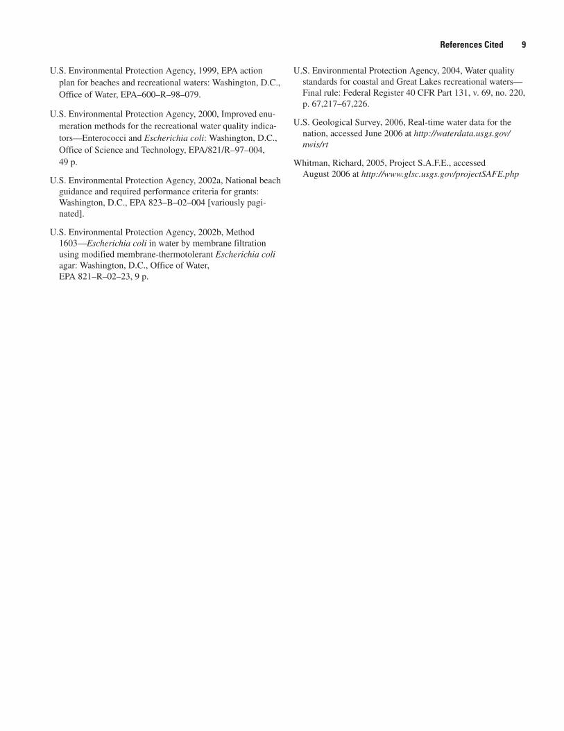
At Huntington, water samples were transported to the Cuyahoga County Sanitary Engineers laboratory and analyzed for E. coli and turbidity within 3 hours of collection. In Ohio, E. coli concentrations are used to monitor recreational water qual-ity. Each point sample was analyzed for concentrations of E. coli by use of the mTEC (U.S. Environmental Protection Agency, 2000) or modified mTEC (U.S. Environmental Protection Agency, 2002b) membrane-filtration methods. A daily E. coli con-centration was calculated by averaging results from two sampling points. An aliquot of water was removed from the bottle to measure turbidity in the laboratory by use of a turbidimeter.
Filter being applied to suction device during membrane-filtration procedure. (Photo by Donna Myers, U.S. Geological Survey.)
Differing densities of bacteria colonies resulting from various plated sample volumes , modified mTEC method. Magenta colonies are counted as presumptive E. coli. (Photo by Donna Francy, U.S. Geological Survey.)
Back to page 3
Examples From Beach Studies at Huntington Reservation, Bay Village, Ohio 11
Example 3
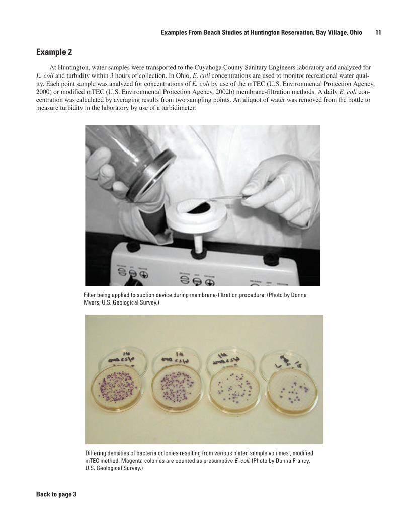
For Huntington, field and laboratory protocols were distributed by the USGS to all personnel. The USGS did several onsite field and laboratory QA/QC checks each year, and corrective actions were taken as needed. Quality-control samples were rou-tinely analyzed during 2004 and 2005, including field blanks and replicate samples for E. coli. The laboratory analyzed positive-control reference cultures that were pure cultures of E. coli ATCC 10798 (American Type Culture Collection, Rockville, Md.) prepared by the USGS and distributed to field personnel by overnight mail. At the same time, personnel in the USGS laboratory plated the pure culture, and results were compared. For duplicate turbidity measurements, those measurements >10 NTRU that did not agree within 10 percent or <10 NTRU that did not agree within 1 NTRU were repeated. Turbidity reference standards were sent once in 2004 and twice in 2005 to the analyst; corrective actions were taken if results were greater than 25 percent dif-ferent from standard values.
Back to page 3
Turbidimeter and water samples. Turbidities, in nephelometric turbidity ratio units (NTRU), are below the samples. For most samples at Huntington Reservation, turbidity was less than 100 NTRU. (Photos provided by Stephen Lawrence, U.S. Geological Survey.)
1� Developing Models To Predict Exceedances of Recreational Water-Quality Standards at Coastal Beaches
Example 4
Environmental and water-quality data for predictive model development at Huntington were collected by field techni-cians or compiled from other sources. Field technicians counted the number of birds on the beach upon arrival and estimated wave-height categories at the time of sample collection. Wave heights were placed into four categories based on minimum and maximum heights in each wave train: (1) 0 to 2 ft, (2) 1 to 3 ft, (3) 2 to 4 ft, and (4) > 3 to 5 ft. Wave heights in 2005 were also measured using a second, more accurate method: A survey rod was placed in the water at the sampling location for 1 minute, during which field crews noted the minimum and maximum heights. Lake-level data were obtained from the National Oce-anic and Atmospheric Administration (NOAA) station in Cleveland (NOAA ID 9063053) (National Oceanic and Atmospheric Administration, 2005a).
Rainfall and wind-direction data were compiled from the National Weather Service local climatology data station at Hop-kins International Airport (National Oceanic and Atmospheric Administration, 2005b). “R
d-1” was the amount of rain, in inches,
that fell in the 24-hour period (9 a.m. to 9 a.m.) preceding the morning sampling. Similarly, “Rd-2
” and “Rd-3
” were amounts of rain that fell in 24-hour periods 2 days and 3 days, respectively, preceding the morning sampling. Weighted rainfall variables were calculated so that the most recent rainfall received the highest weight, as follows:
Rw72= (3* Rd-1
+2* Rd-2
+ Rd-3
)
Rw48= (2* Rd-1
+ Rd-2
)
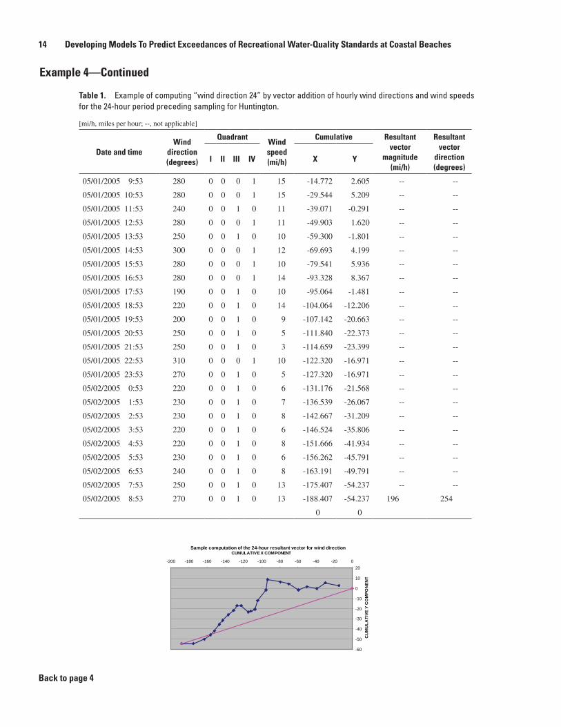
“Wind direction 24” was calculated by vector addition of hourly wind directions and wind speeds for the 24-hour period preceding sampling (table 1). A vector is a quantity that has both magnitude and direction. A discussion of trigonometric functions and vector math is beyond the scope of this report; a detailed description is provided in Finney and Thomas (1989). Wind directions were then placed into categories by examining patterns in graphs of E. coli concentrations and wind direction 24; processes affecting E. coli were also considered to ensure the wind direction 24 categories could be explained and seemed reasonable. For example, if one suspected a source of fecal contamination was west of the beach, higher E. coli concentrations associated with easterly wind directions would seem reasonable.
(Continued on next page)
Examples From Beach Studies at Huntington Reservation, Bay Village, Ohio 13
Example 4—Continued
Table 1. Example of computing “wind direction 24” by vector addition of hourly wind directions and wind speeds for the 24-hour period preceding sampling for Huntington.
[mi/h, miles per hour; --, not applicable]
Date and time
Wind direction (degrees)
QuadrantWind speed(mi/h)
Cumulative Resultant vector
magnitude(mi/h)
Resultant vector
direction(degrees)
I II III IV X Y
05/01/2005 9:53 280 0 0 0 1 15 -14.772 2.605 -- --
05/01/2005 10:53 280 0 0 0 1 15 -29.544 5.209 -- --
05/01/2005 11:53 240 0 0 1 0 11 -39.071 -0.291 -- --
05/01/2005 12:53 280 0 0 0 1 11 -49.903 1.620 -- --
05/01/2005 13:53 250 0 0 1 0 10 -59.300 -1.801 -- --
05/01/2005 14:53 300 0 0 0 1 12 -69.693 4.199 -- --
05/01/2005 15:53 280 0 0 0 1 10 -79.541 5.936 -- --
05/01/2005 16:53 280 0 0 0 1 14 -93.328 8.367 -- --
05/01/2005 17:53 190 0 0 1 0 10 -95.064 -1.481 -- --
05/01/2005 18:53 220 0 0 1 0 14 -104.064 -12.206 -- --
05/01/2005 19:53 200 0 0 1 0 9 -107.142 -20.663 -- --
05/01/2005 20:53 250 0 0 1 0 5 -111.840 -22.373 -- --
05/01/2005 21:53 250 0 0 1 0 3 -114.659 -23.399 -- --
05/01/2005 22:53 310 0 0 0 1 10 -122.320 -16.971 -- --
05/01/2005 23:53 270 0 0 1 0 5 -127.320 -16.971 -- --
05/02/2005 0:53 220 0 0 1 0 6 -131.176 -21.568 -- --
05/02/2005 1:53 230 0 0 1 0 7 -136.539 -26.067 -- --
05/02/2005 2:53 230 0 0 1 0 8 -142.667 -31.209 -- --
05/02/2005 3:53 220 0 0 1 0 6 -146.524 -35.806 -- --
05/02/2005 4:53 220 0 0 1 0 8 -151.666 -41.934 -- --
05/02/2005 5:53 230 0 0 1 0 6 -156.262 -45.791 -- --
05/02/2005 6:53 240 0 0 1 0 8 -163.191 -49.791 -- --
05/02/2005 7:53 250 0 0 1 0 13 -175.407 -54.237 -- --
05/02/2005 8:53 270 0 0 1 0 13 -188.407 -54.237 196 254
0 0
Sample computation of the 24-hour resultant vector for wind direction
-60
-50
-40
-30
-20
-10
0
10
20-200 -180 -160 -140 -120 -100 -80 -60 -40 -20 0
CUMULATIVE X COMPONENT
CU
MU
LATI
VEY
CO
MPO
NEN
T
Back to page 4
14 Developing Models To Predict Exceedances of Recreational Water-Quality Standards at Coastal Beaches
Example 5
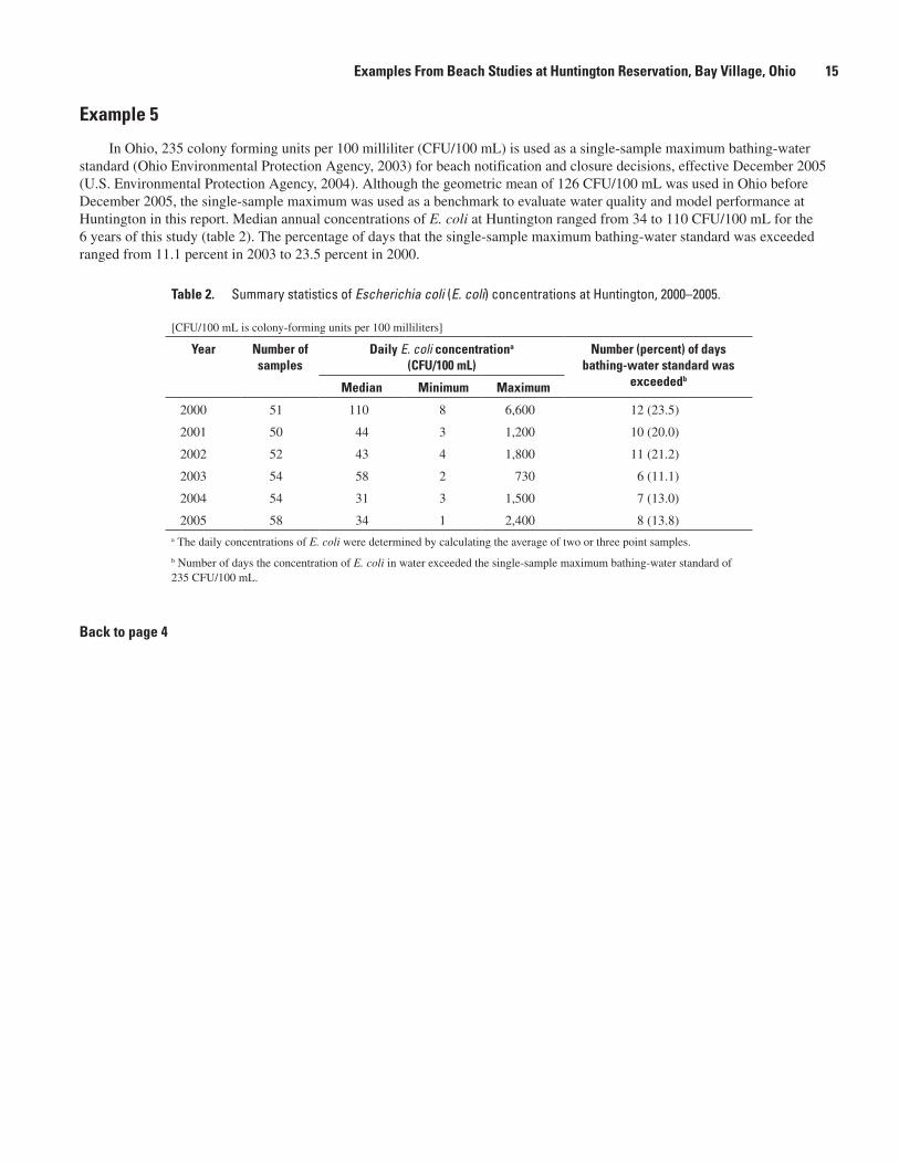
In Ohio, 235 colony forming units per 100 milliliter (CFU/100 mL) is used as a single-sample maximum bathing-water standard (Ohio Environmental Protection Agency, 2003) for beach notification and closure decisions, effective December 2005 (U.S. Environmental Protection Agency, 2004). Although the geometric mean of 126 CFU/100 mL was used in Ohio before December 2005, the single-sample maximum was used as a benchmark to evaluate water quality and model performance at Huntington in this report. Median annual concentrations of E. coli at Huntington ranged from 34 to 110 CFU/100 mL for the 6 years of this study (table 2). The percentage of days that the single-sample maximum bathing-water standard was exceeded ranged from 11.1 percent in 2003 to 23.5 percent in 2000.
Table �. Summary statistics of Escherichia coli (E. coli) concentrations at Huntington, 2000–2005.
[CFU/100 mL is colony-forming units per 100 milliliters]
Year Number of samples
Daily E. coli concentrationa (CFU/100 mL)
Number (percent) of days bathing-water standard was
exceededbMedian Minimum Maximum
2000 51 110 8 6,600 12 (23.5)
2001 50 44 3 1,200 10 (20.0)
2002 52 43 4 1,800 11 (21.2)
2003 54 58 2 730 6 (11.1)
2004 54 31 3 1,500 7 (13.0)
2005 58 34 1 2,400 8 (13.8)a The daily concentrations of E. coli were determined by calculating the average of two or three point samples.
b Number of days the concentration of E. coli in water exceeded the single-sample maximum bathing-water standard of 235 CFU/100 mL.
Back to page 4
Examples From Beach Studies at Huntington Reservation, Bay Village, Ohio 15
Example 6
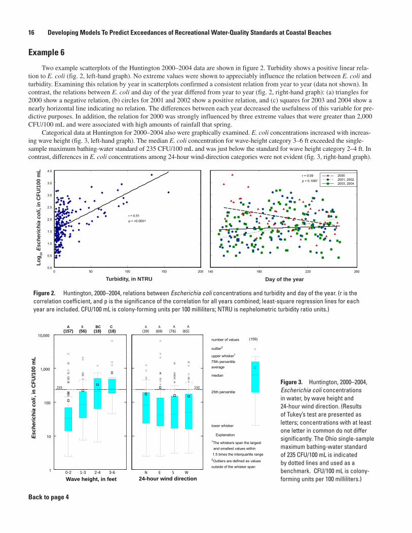
Two example scatterplots of the Huntington 2000–2004 data are shown in figure 2. Turbidity shows a positive linear rela-tion to E. coli (fig. 2, left-hand graph). No extreme values were shown to appreciably influence the relation between E. coli and turbidity. Examining this relation by year in scatterplots confirmed a consistent relation from year to year (data not shown). In contrast, the relations between E. coli and day of the year differed from year to year (fig. 2, right-hand graph): (a) triangles for 2000 show a negative relation, (b) circles for 2001 and 2002 show a positive relation, and (c) squares for 2003 and 2004 show a nearly horizontal line indicating no relation. The differences between each year decreased the usefulness of this variable for pre-dictive purposes. In addition, the relation for 2000 was strongly influenced by three extreme values that were greater than 2,000 CFU/100 mL and were associated with high amounts of rainfall that spring.
Categorical data at Huntington for 2000–2004 also were graphically examined. E. coli concentrations increased with increas-ing wave height (fig. 3, left-hand graph). The median E. coli concentration for wave-height category 3–6 ft exceeded the single-sample maximum bathing-water standard of 235 CFU/100 mL and was just below the standard for wave height category 2–4 ft. In contrast, differences in E. coli concentrations among 24-hour wind-direction categories were not evident (fig. 3, right-hand graph).
Figure �. Huntington, 2000–2004, relations between Escherichia coli concentrations and turbidity and day of the year. (r is the correlation coefficient, and p is the significance of the correlation for all years combined; least-square regression lines for each year are included. CFU/100 mL is colony-forming units per 100 milliliters; NTRU is nephelometric turbidity ratio units.)
Figure 3. Huntington, 2000–2004, Escherichia coli concentrations in water, by wave height and 24-hour wind direction. (Results of Tukey’s test are presented as letters; concentrations with at least one letter in common do not differ significantly. The Ohio single-sample maximum bathing-water standard of 235 CFU/100 mL is indicated by dotted lines and used as a benchmark. CFU/100 mL is colony-forming units per 100 milliliters.)
Back to page 4
16 Developing Models To Predict Exceedances of Recreational Water-Quality Standards at Coastal Beaches
0-2 1-3 2-4 3-6
(157) (56) (18) (18)
Wave height, in feet1
10
100
1,000
10,000
Esch
eric
hia
coli,
in C
FU/1
00 m
L
235
A BCB C
N E S W
(39) (69) (76) (65)
24-hour wind direction1
10
100
1,000
10,000
235
A A A A
(159)number of values
outlier2
upper whisker1
75th percentileaverage
median
25th percentile
lower whisker
Explanation
1The whiskers span the largest and smallest values within 1.5 times the interquartile range2Outliers are defined as values outside of the whisker span
0 50 100 150 200Turbidity, in NTRU
0.0
0.5
1.0
1.5
2.0
2.5
3.0
3.5
4.0
Log 10
Esc
heric
hia
coli,
in C
FU/1
00 m
L
A
r = 0.51p = <0.0001
140 180 220 260Day of the year
0.0
0.5
1.0
1.5
2.0
2.5
3.0
3.5
4.0
Log 10
Esc
heric
hia
coli,
in C
FU/1
00 m
L
B
r = 0.09p = 0.1087
20002001, 20022003, 2004
Log 10
Esc
heric
hia
coli,
in C
FU/1
00 m
L
Turbidity, in NTRU Day of the year
Example 7
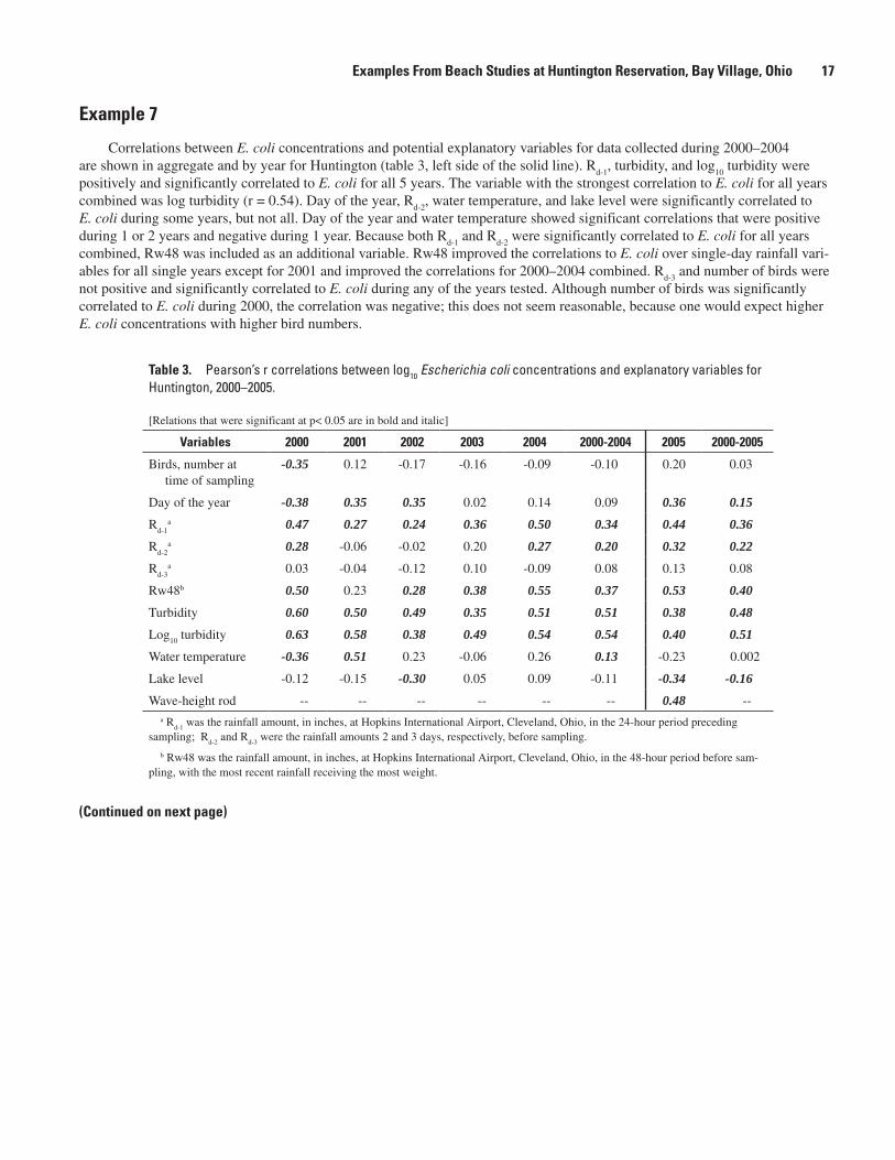
Correlations between E. coli concentrations and potential explanatory variables for data collected during 2000–2004 are shown in aggregate and by year for Huntington (table 3, left side of the solid line). R
d-1, turbidity, and log
10 turbidity were
positively and significantly correlated to E. coli for all 5 years. The variable with the strongest correlation to E. coli for all years combined was log turbidity (r = 0.54). Day of the year, R
d-2, water temperature, and lake level were significantly correlated to
E. coli during some years, but not all. Day of the year and water temperature showed significant correlations that were positive during 1 or 2 years and negative during 1 year. Because both R
d-1 and R
d-2 were significantly correlated to E. coli for all years
combined, Rw48 was included as an additional variable. Rw48 improved the correlations to E. coli over single-day rainfall vari-ables for all single years except for 2001 and improved the correlations for 2000–2004 combined. R
d-3 and number of birds were
not positive and significantly correlated to E. coli during any of the years tested. Although number of birds was significantly correlated to E. coli during 2000, the correlation was negative; this does not seem reasonable, because one would expect higher E. coli concentrations with higher bird numbers.
Table 3. Pearson’s r correlations between log10 Escherichia coli concentrations and explanatory variables for Huntington, 2000–2005.
[Relations that were significant at p< 0.05 are in bold and italic]
Variables �000 �001 �00� �003 �004 �000-�004 �005 �000-�005
Birds, number at time of sampling
-0.35 0.12 -0.17 -0.16 -0.09 -0.10 0.20 0.03
Day of the year -0.38 0.35 0.35 0.02 0.14 0.09 0.36 0.15
Rd-1
a 0.47 0.27 0.24 0.36 0.50 0.34 0.44 0.36
Rd-2
a 0.28 -0.06 -0.02 0.20 0.27 0.20 0.32 0.22
Rd-3
a 0.03 -0.04 -0.12 0.10 -0.09 0.08 0.13 0.08
Rw48b 0.50 0.23 0.28 0.38 0.55 0.37 0.53 0.40
Turbidity 0.60 0.50 0.49 0.35 0.51 0.51 0.38 0.48
Log10
turbidity 0.63 0.58 0.38 0.49 0.54 0.54 0.40 0.51
Water temperature -0.36 0.51 0.23 -0.06 0.26 0.13 -0.23 0.002
Lake level -0.12 -0.15 -0.30 0.05 0.09 -0.11 -0.34 -0.16
Wave-height rod -- -- -- -- -- -- 0.48 --a R
d-1 was the rainfall amount, in inches, at Hopkins International Airport, Cleveland, Ohio, in the 24-hour period preceding
sampling; Rd-2
and Rd-3
were the rainfall amounts 2 and 3 days, respectively, before sampling.
b Rw48 was the rainfall amount, in inches, at Hopkins International Airport, Cleveland, Ohio, in the 48-hour period before sam-pling, with the most recent rainfall receiving the most weight.
(Continued on next page)
Examples From Beach Studies at Huntington Reservation, Bay Village, Ohio 17
Example 7—Continued
The relations among explanatory variables at Huntington for 2000–2004 data were also examined (table 4). Strong signifi-cant correlations were found for Rw48 and the two single-day rainfall variables; this is not surprising because R
d-1 and R
d-2 are
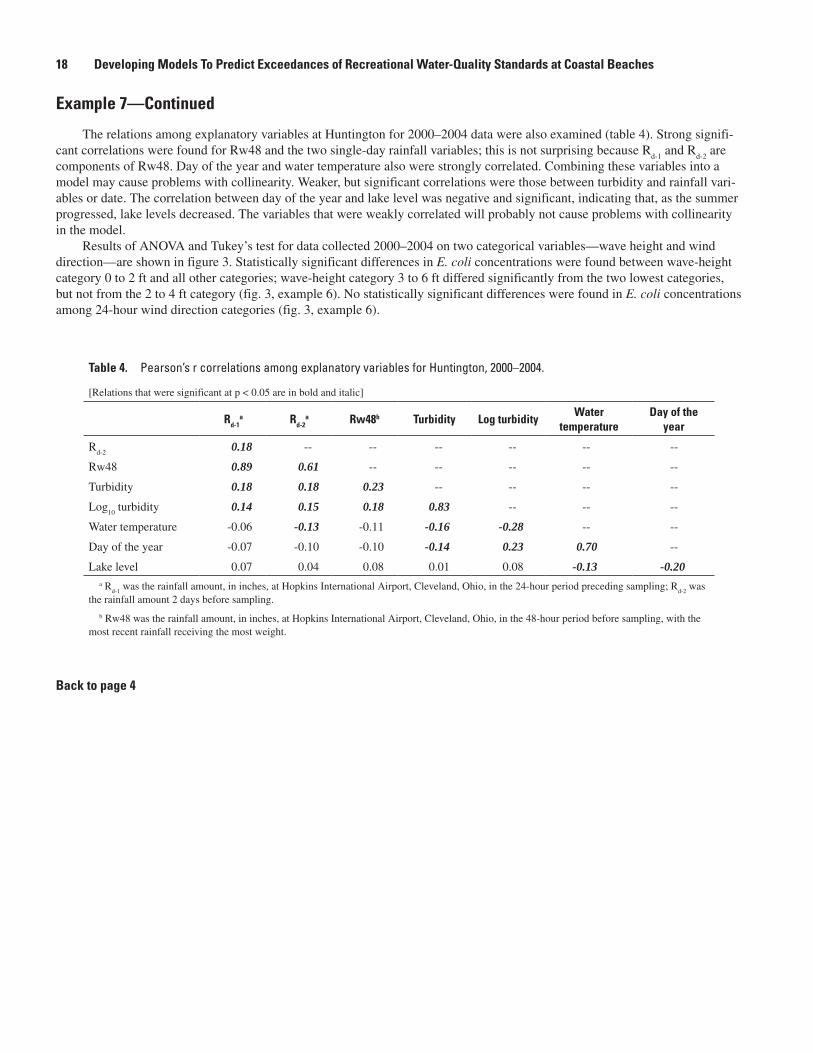
components of Rw48. Day of the year and water temperature also were strongly correlated. Combining these variables into a model may cause problems with collinearity. Weaker, but significant correlations were those between turbidity and rainfall vari-ables or date. The correlation between day of the year and lake level was negative and significant, indicating that, as the summer progressed, lake levels decreased. The variables that were weakly correlated will probably not cause problems with collinearity in the model.
Results of ANOVA and Tukey’s test for data collected 2000–2004 on two categorical variables—wave height and wind direction—are shown in figure 3. Statistically significant differences in E. coli concentrations were found between wave-height category 0 to 2 ft and all other categories; wave-height category 3 to 6 ft differed significantly from the two lowest categories, but not from the 2 to 4 ft category (fig. 3, example 6). No statistically significant differences were found in E. coli concentrations among 24-hour wind direction categories (fig. 3, example 6).
Table 4. Pearson’s r correlations among explanatory variables for Huntington, 2000–2004.
[Relations that were significant at p < 0.05 are in bold and italic]
Rd-1a Rd-�
a Rw48b Turbidity Log turbidityWater
temperatureDay of the
year
Rd-2
0.18 -- -- -- -- -- --
Rw48 0.89 0.61 -- -- -- -- --
Turbidity 0.18 0.18 0.23 -- -- -- --
Log10
turbidity 0.14 0.15 0.18 0.83 -- -- --
Water temperature -0.06 -0.13 -0.11 -0.16 -0.28 -- --
Day of the year -0.07 -0.10 -0.10 -0.14 0.23 0.70 --
Lake level 0.07 0.04 0.08 0.01 0.08 -0.13 -0.20a R
d-1 was the rainfall amount, in inches, at Hopkins International Airport, Cleveland, Ohio, in the 24-hour period preceding sampling; R
d-2 was
the rainfall amount 2 days before sampling.
b Rw48 was the rainfall amount, in inches, at Hopkins International Airport, Cleveland, Ohio, in the 48-hour period before sampling, with the most recent rainfall receiving the most weight.
Back to page 4
18 Developing Models To Predict Exceedances of Recreational Water-Quality Standards at Coastal Beaches
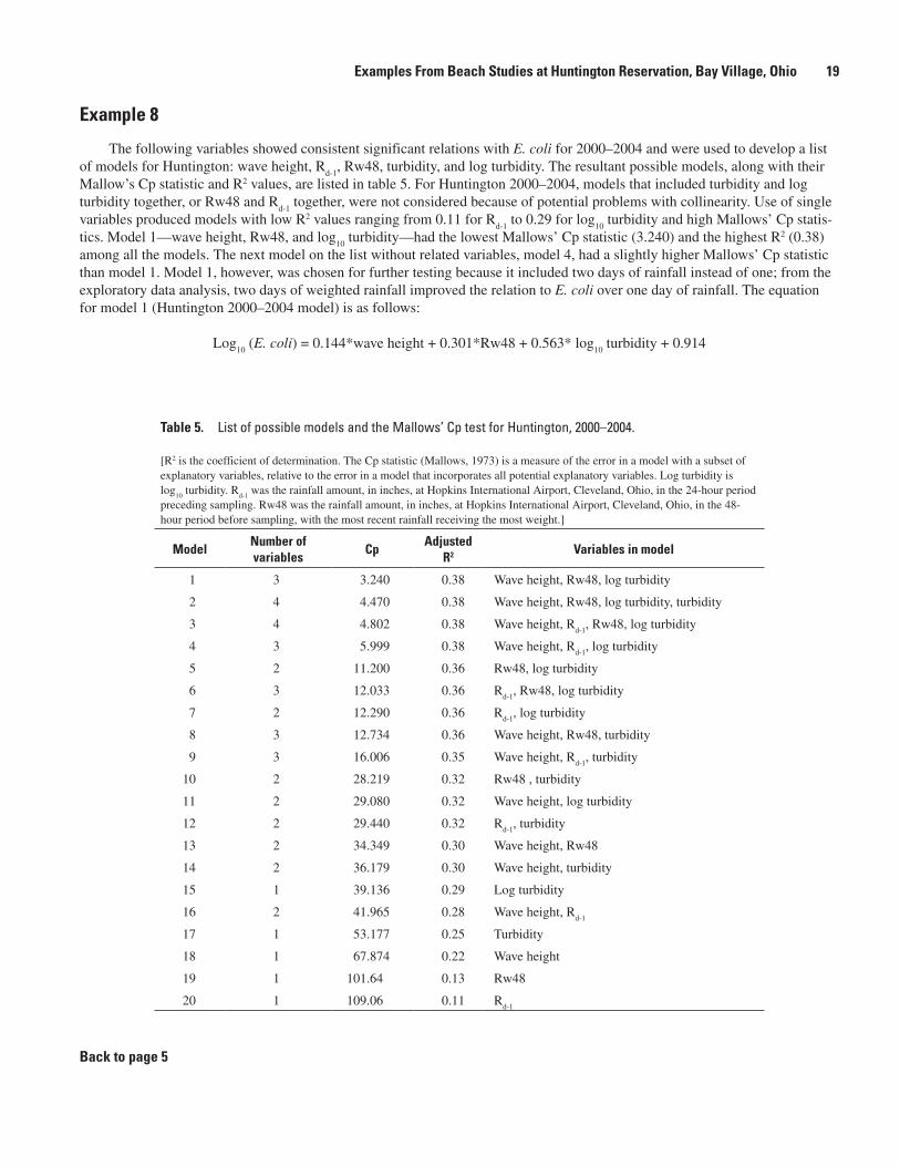
Example 8
The following variables showed consistent significant relations with E. coli for 2000–2004 and were used to develop a list of models for Huntington: wave height, R
d-1, Rw48, turbidity, and log turbidity. The resultant possible models, along with their
Mallow’s Cp statistic and R2 values, are listed in table 5. For Huntington 2000–2004, models that included turbidity and log turbidity together, or Rw48 and R
d-1 together, were not considered because of potential problems with collinearity. Use of single
variables produced models with low R2 values ranging from 0.11 for Rd-1
to 0.29 for log10
turbidity and high Mallows’ Cp statis-tics. Model 1—wave height, Rw48, and log
10 turbidity—had the lowest Mallows’ Cp statistic (3.240) and the highest R2 (0.38)
among all the models. The next model on the list without related variables, model 4, had a slightly higher Mallows’ Cp statistic than model 1. Model 1, however, was chosen for further testing because it included two days of rainfall instead of one; from the exploratory data analysis, two days of weighted rainfall improved the relation to E. coli over one day of rainfall. The equation for model 1 (Huntington 2000–2004 model) is as follows:
Log10
(E. coli) = 0.144*wave height + 0.301*Rw48 + 0.563* log10
turbidity + 0.914
Table 5. List of possible models and the Mallows’ Cp test for Huntington, 2000–2004.
[R2 is the coefficient of determination. The Cp statistic (Mallows, 1973) is a measure of the error in a model with a subset of explanatory variables, relative to the error in a model that incorporates all potential explanatory variables. Log turbidity is log
10 turbidity. R
d-1 was the rainfall amount, in inches, at Hopkins International Airport, Cleveland, Ohio, in the 24-hour period
preceding sampling. Rw48 was the rainfall amount, in inches, at Hopkins International Airport, Cleveland, Ohio, in the 48-hour period before sampling, with the most recent rainfall receiving the most weight.]
ModelNumber of variables
CpAdjusted
R� Variables in model
1 3 3.240 0.38 Wave height, Rw48, log turbidity
2 4 4.470 0.38 Wave height, Rw48, log turbidity, turbidity
3 4 4.802 0.38 Wave height, Rd-1
, Rw48, log turbidity
4 3 5.999 0.38 Wave height, Rd-1
, log turbidity
5 2 11.200 0.36 Rw48, log turbidity
6 3 12.033 0.36 Rd-1
, Rw48, log turbidity
7 2 12.290 0.36 Rd-1
, log turbidity
8 3 12.734 0.36 Wave height, Rw48, turbidity
9 3 16.006 0.35 Wave height, Rd-1
, turbidity
10 2 28.219 0.32 Rw48 , turbidity
11 2 29.080 0.32 Wave height, log turbidity
12 2 29.440 0.32 Rd-1
, turbidity
13 2 34.349 0.30 Wave height, Rw48
14 2 36.179 0.30 Wave height, turbidity
15 1 39.136 0.29 Log turbidity
16 2 41.965 0.28 Wave height, Rd-1
17 1 53.177 0.25 Turbidity
18 1 67.874 0.22 Wave height
19 1 101.64 0.13 Rw48
20 1 109.06 0.11 Rd-1
Back to page 5
Examples From Beach Studies at Huntington Reservation, Bay Village, Ohio 19
Example 9
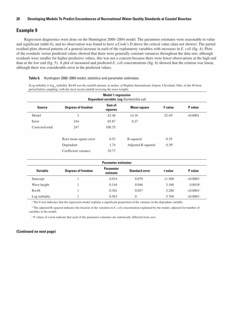
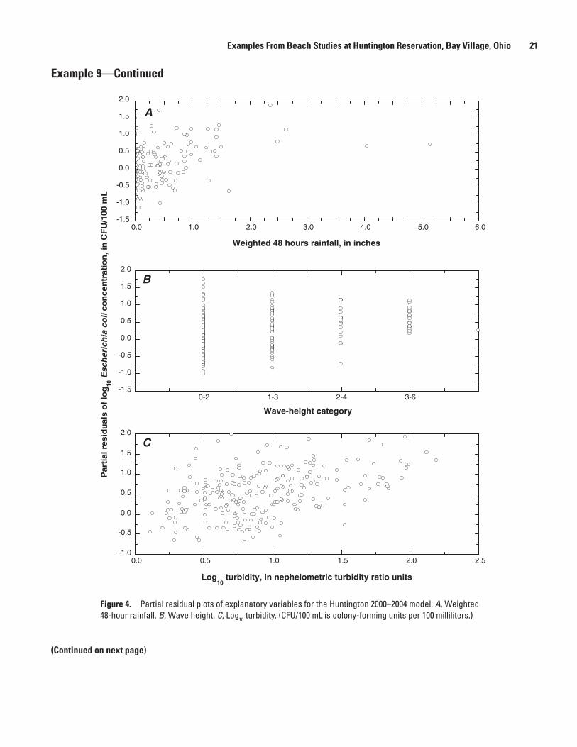
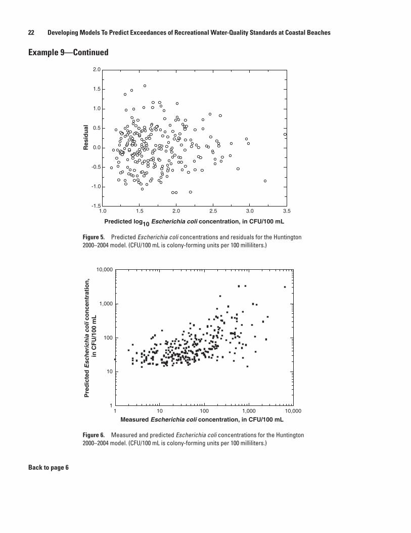
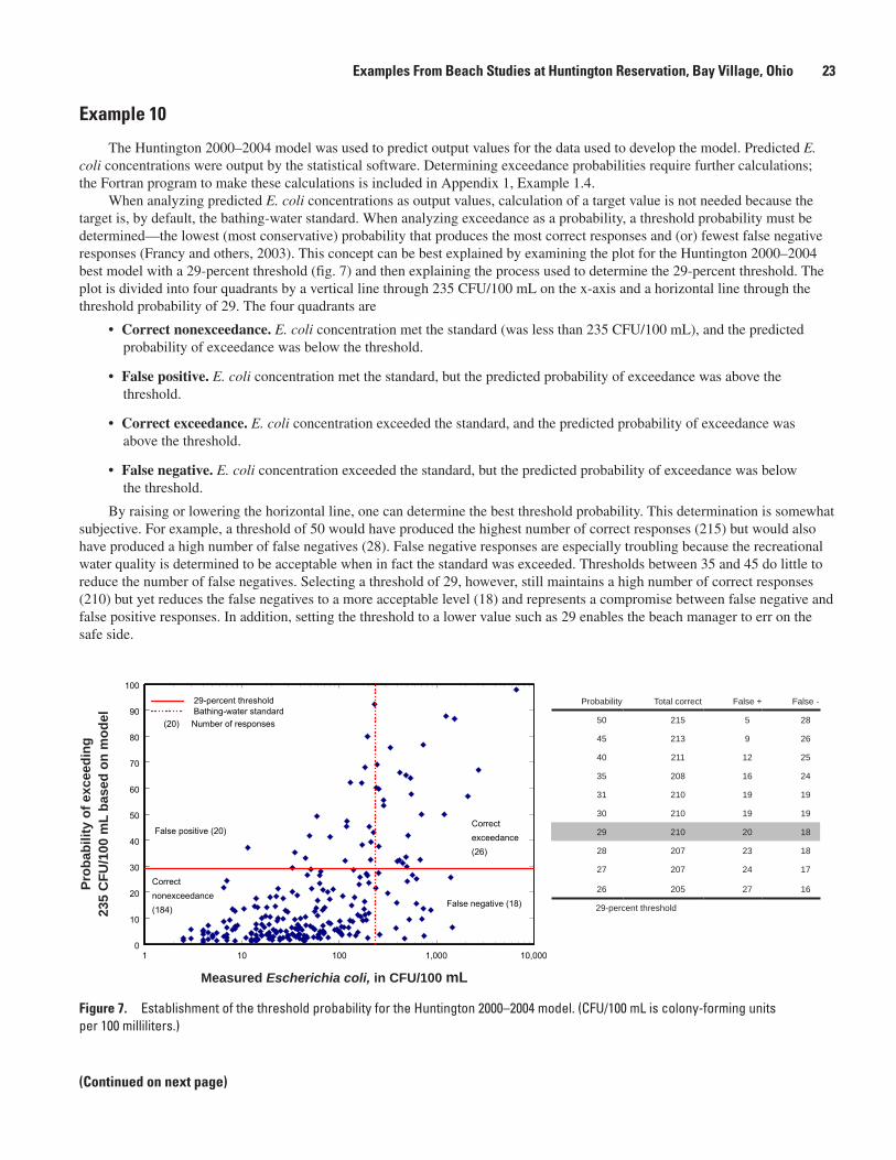
Regression diagnostics were done on the Huntington 2000–2004 model. The parameter estimates were reasonable in value and significant (table 6), and no observation was found to have a Cook’s D above the critical value (data not shown). The partial residual plots showed patterns of a general increase in each of the explanatory variables with increases in E. coli (fig. 4). Plots of the residuals versus predicted values showed that there were generally constant variances throughout the data sets; although residuals were smaller for higher predictive values, this was not a concern because there were fewer observations at the high end than at the low end (fig. 5). A plot of measured and predicted E. coli concentrations (fig. 6) showed that the relation was linear, although there was considerable error in the predicted values.
Table 6. Huntington 2000–2004 model, statistics and parameter estimates.
[Log turbidity is log10
turbidity. Rw48 was the rainfall amount, in inches, at Hopkins International Airport, Cleveland, Ohio, in the 48-hour period before sampling, with the most recent rainfall receiving the most weight]
Model 1 regressionDependent variable: Log Escherichia coli
Source Degrees of freedomSum of squares
Mean square F value P value
Model 3 42.48 14.16 52.45a <0.0001
Error 244 65.87 0.27
Corrected total 247 108.35
Root mean square error 0.52 R-squared 0.39
Dependent 1.74 Adjusted R-squared 0.38b
Coefficient variance 29.77
Parameter estimates
Variable Degrees of freedomParameter estimate
Standard error t value P value
Intercept 1 0.914 0.079 11.560 <0.0001c
Wave height 1 0.144 0.046 3.160 0.0018c
Rw48 1 0.301 0.057 5.280 <0.0001c
Log turbidity 1 0.563 0 5.760 <0.0001c
a The F-test indicates that the regression model explains a significant proportion of the variance in the dependant variable.
b The adjusted R-squared indicates the fraction of the variation in E. coli concentration explained by the model, adjusted for number of variables in the model.
c P values of t-tests indicate that each of the parameter estimates are statistically different from zero.
(Continued on next page)
�0 Developing Models To Predict Exceedances of Recreational Water-Quality Standards at Coastal Beaches
Example 9—Continued
Figure 4. Partial residual plots of explanatory variables for the Huntington 2000-2004 model:(A) weighted 48 hour rainfall, (B) wave height, and (C) log10 turbidity. (CFU/100 mL is colony-forming units per 100 milliliters.)
0.0 0.5 1.0 1.5 2.0 2.5-1.0
-0.5
0.0
0.5
1.0
1.5
2.0
0-2 1-3 2-4 3-6-1.5
-1.0
-0.5
0.0
0.5
1.0
1.5
2.0
0.0 1.0 2.0 3.0 4.0 5.0 6.0
Par
tial r
esid
uals
of l
og10
Esc
heri
chia
col
i con
cent
ratio
n, in
CFU
/100
mL
-1.5
-1.0
-0.5
0.0
0.5
1.0
1.5
2.0
Weighted 48 hours rainfall, in inches
Wave-height category
Log10
turbidity, in nephelometric turbidity ratio units
A
B
C
(Continued on next page)
Figure 4. Partial residual plots of explanatory variables for the Huntington 2000–2004 model. A, Weighted 48-hour rainfall. B, Wave height. C, Log10 turbidity. (CFU/100 mL is colony-forming units per 100 milliliters.)
Examples From Beach Studies at Huntington Reservation, Bay Village, Ohio �1
Example 9—Continued
Back to page 6
Figure 6. Measured and predicted Escherichia coli concentrations for the Huntington 2000–2004 model. (CFU/100 mL is colony-forming units per 100 milliliters.)
Figure 5. Predicted Escherichia coli concentrations and residuals for the Huntington 2000–2004 model. (CFU/100 mL is colony-forming units per 100 milliliters.)
Predicted log10 Escherichia coli concentration, in CFU/100 mL
Res
idua
l
1.0 1.5 2.0 2.5 3.0 3.5-1.5
-1.0
-0.5
0.0
0.5
1.0
1.5
2.0
1 10 100 1,000 10,0001
10
100
1,000
10,000
Pre
dict
edE
sche
rich
ia c
oli c
once
ntra
tion,
in
CFU
/100
mL
Measured Escherichia coli concentration, in CFU/100 mL
�� Developing Models To Predict Exceedances of Recreational Water-Quality Standards at Coastal Beaches
Example 10
The Huntington 2000–2004 model was used to predict output values for the data used to develop the model. Predicted E. coli concentrations were output by the statistical software. Determining exceedance probabilities require further calculations; the Fortran program to make these calculations is included in Appendix 1, Example 1.4.
When analyzing predicted E. coli concentrations as output values, calculation of a target value is not needed because the target is, by default, the bathing-water standard. When analyzing exceedance as a probability, a threshold probability must be determined—the lowest (most conservative) probability that produces the most correct responses and (or) fewest false negative responses (Francy and others, 2003). This concept can be best explained by examining the plot for the Huntington 2000–2004 best model with a 29-percent threshold (fig. 7) and then explaining the process used to determine the 29-percent threshold. The plot is divided into four quadrants by a vertical line through 235 CFU/100 mL on the x-axis and a horizontal line through the threshold probability of 29. The four quadrants are
Correct nonexceedance. E. coli concentration met the standard (was less than 235 CFU/100 mL), and the predicted probability of exceedance was below the threshold.
False positive. E. coli concentration met the standard, but the predicted probability of exceedance was above the threshold.
Correct exceedance. E. coli concentration exceeded the standard, and the predicted probability of exceedance was above the threshold.
False negative. E. coli concentration exceeded the standard, but the predicted probability of exceedance was below the threshold.
By raising or lowering the horizontal line, one can determine the best threshold probability. This determination is somewhat subjective. For example, a threshold of 50 would have produced the highest number of correct responses (215) but would also have produced a high number of false negatives (28). False negative responses are especially troubling because the recreational water quality is determined to be acceptable when in fact the standard was exceeded. Thresholds between 35 and 45 do little to reduce the number of false negatives. Selecting a threshold of 29, however, still maintains a high number of correct responses (210) but yet reduces the false negatives to a more acceptable level (18) and represents a compromise between false negative and false positive responses. In addition, setting the threshold to a lower value such as 29 enables the beach manager to err on the safe side.
•
•
•
•
(Continued on next page)
Figure 7. Establishment of the threshold probability for the Huntington 2000–2004 model. (CFU/100 mL is colony-forming units per 100 milliliters.)
1 10 100 1,000 10,000Measured Escherichia coli, in CFU/100 mL
0
10
20
30
40
50
60
70
80
90
100
Pro
babi
lity
of e
xcee
ding
235
CFU
/100
mL
base
d on
mod
el
False positive (20)
Correct nonexceedance(184)
False negative (18)
Correct exceedance(26)
29-percent thresholdBathing-water standard
(20) Number of responses
Measured Escherichia coli, in CFU/100 mL
Prob
abili
ty o
f exc
eedi
ng
235
CFU
/100
mL
base
d on
mod
el
Probability Total correct False + False -
50 215 5 28
45 213 9 26
40 211 12 25
35 208 16 24
31 210 19 19
30 210 19 19
29 210 20 18
28 207 23 18
27 207 24 17
26 205 27 16
29-percent threshold
Examples From Beach Studies at Huntington Reservation, Bay Village, Ohio �3
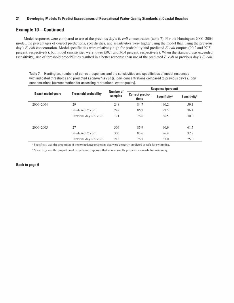
Example 10—Continued
Model responses were compared to use of the previous day’s E. coli concentration (table 7). For the Huntington 2000–2004 model, the percentages of correct predictions, specificities, and sensitivities were higher using the model than using the previous day’s E. coli concentration. Model specificities were relatively high for probability and predicted E. coli outputs (90.2 and 97.5 percent, respectively), but model sensitivities were lower (59.1 and 36.4 percent, respectively). When the standard was exceeded (sensitivity), use of threshold probabilities resulted in a better response than use of the predicted E. coli or previous day’s E. coli.
Table 7. Huntington, numbers of correct responses and the sensitivities and specificities of model responses with indicated thresholds and predicted Escherichia coli (E. coli) concentrations compared to previous day’s E. coli concentrations (current method for assessing recreational water quality).
Beach model years Threshold probabilityNumber of samples
Response (percent)
Correct predic-tions
Specificitya Sensitivityb
2000–2004 29 248 84.7 90.2 59.1
Predicted E. coli 248 86.7 97.5 36.4
Previous day’s E. coli 171 76.6 86.5 30.0
2000–2005 27 306 85.9 90.9 61.5
Predicted E. coli 306 85.6 96.4 32.7
Previous day’s E. coli 213 76.5 87.0 25.0a Specificity was the proportion of nonexceedance responses that were correctly predicted as safe for swimming.
b Sensitivity was the proportion of exceedance responses that were correctly predicted as unsafe for swimming.
Back to page 6
�4 Developing Models To Predict Exceedances of Recreational Water-Quality Standards at Coastal Beaches
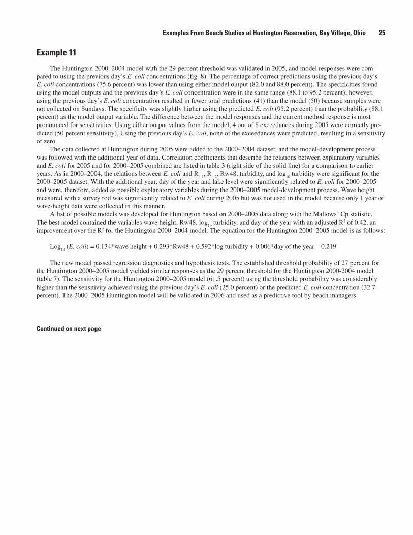
Example 11
The Huntington 2000–2004 model with the 29-percent threshold was validated in 2005, and model responses were com-pared to using the previous day’s E. coli concentrations (fig. 8). The percentage of correct predictions using the previous day’s E. coli concentrations (75.6 percent) was lower than using either model output (82.0 and 88.0 percent). The specificities found using the model outputs and the previous day’s E. coli concentration were in the same range (88.1 to 95.2 percent); however, using the previous day’s E. coli concentration resulted in fewer total predictions (41) than the model (50) because samples were not collected on Sundays. The specificity was slightly higher using the predicted E. coli (95.2 percent) than the probability (88.1 percent) as the model output variable. The difference between the model responses and the current method response is most pronounced for sensitivities. Using either output values from the model, 4 out of 8 exceedances during 2005 were correctly pre-dicted (50 percent sensitivity). Using the previous day’s E. coli, none of the exceedances were predicted, resulting in a sensitivity of zero.
The data collected at Huntington during 2005 were added to the 2000–2004 dataset, and the model-development process was followed with the additional year of data. Correlation coefficients that describe the relations between explanatory variables and E. coli for 2005 and for 2000–2005 combined are listed in table 3 (right side of the solid line) for a comparison to earlier years. As in 2000–2004, the relations between E. coli and R
d-1, R
d-2, Rw48, turbidity, and log
10 turbidity were significant for the
2000–2005 dataset. With the additional year, day of the year and lake level were significantly related to E. coli for 2000–2005 and were, therefore, added as possible explanatory variables during the 2000–2005 model-development process. Wave height measured with a survey rod was significantly related to E. coli during 2005 but was not used in the model because only 1 year of wave-height data were collected in this manner.
A list of possible models was developed for Huntington based on 2000–2005 data along with the Mallows’ Cp statistic. The best model contained the variables wave height, Rw48, log
10 turbidity, and day of the year with an adjusted R2 of 0.42, an
improvement over the R2 for the Huntington 2000–2004 model. The equation for the Huntington 2000–2005 model is as follows:
Log10
(E. coli) = 0.134*wave height + 0.293*Rw48 + 0.592*log turbidity + 0.006*day of the year – 0.219
The new model passed regression diagnostics and hypothesis tests. The established threshold probability of 27 percent for the Huntington 2000–2005 model yielded similar responses as the 29 percent threshold for the Huntington 2000-2004 model (table 7). The sensitivity for the Huntington 2000–2005 model (61.5 percent) using the threshold probability was considerably higher than the sensitivity achieved using the previous day’s E. coli (25.0 percent) or the predicted E. coli concentration (32.7 percent). The 2000–2005 Huntington model will be validated in 2006 and used as a predictive tool by beach managers.
Continued on next page
Examples From Beach Studies at Huntington Reservation, Bay Village, Ohio �5
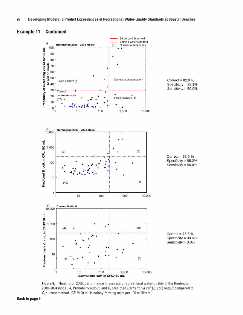
Back to page 6
Figure 8. Huntington 2005, performance in assessing recreational water-quality of the Huntington 2000–2004 model. A, Probability output, and B, predicted Escherichia coli (E. coli) output compared to C, current method. (CFU/100 mL is colony-forming units per 100 milliliters.)
Example 11—Continued
Correct = 82.0 %Specificity = 88.1%Sensitivity = 50.0%
Correct = 88.0 %Specificity = 95.2%Sensitivity = 50.0%
Correct = 75.6 %Specificity = 88.6%Sensitivity = 0.0%
1 10 100 1,000 10,0000
10
20
30
40
50
60
70
80
90
100Pr
obab
ility
of e
xcee
ding
235
CFU
/100
mL
bas
ed o
n m
odel
False positive (5)
Correct nonexceedance(37) False negative (4)
Correct exceedance (4)
29-percent thresholdBathing-water standard
(5) Number of responsesHuntington 2000 - 2004 ModelA
1 10 100 1,000 10,0001
10
100
1,000
10,000
Pred
icte
d E.
col
i, in
CFU
/100
mL
(2)
(40) (4)
(4)
Huntington 2000 - 2004 ModelB
1 10 100 1,000 10,000Escherichia coli, in CFU/100 mL
1
10
100
1,000
10,000
Prev
ious
day
's E
. col
i, in
CFU
/100
mL
(4)
(31) (6)
(0)
Current MethodC
�6 Developing Models To Predict Exceedances of Recreational Water-Quality Standards at Coastal Beaches
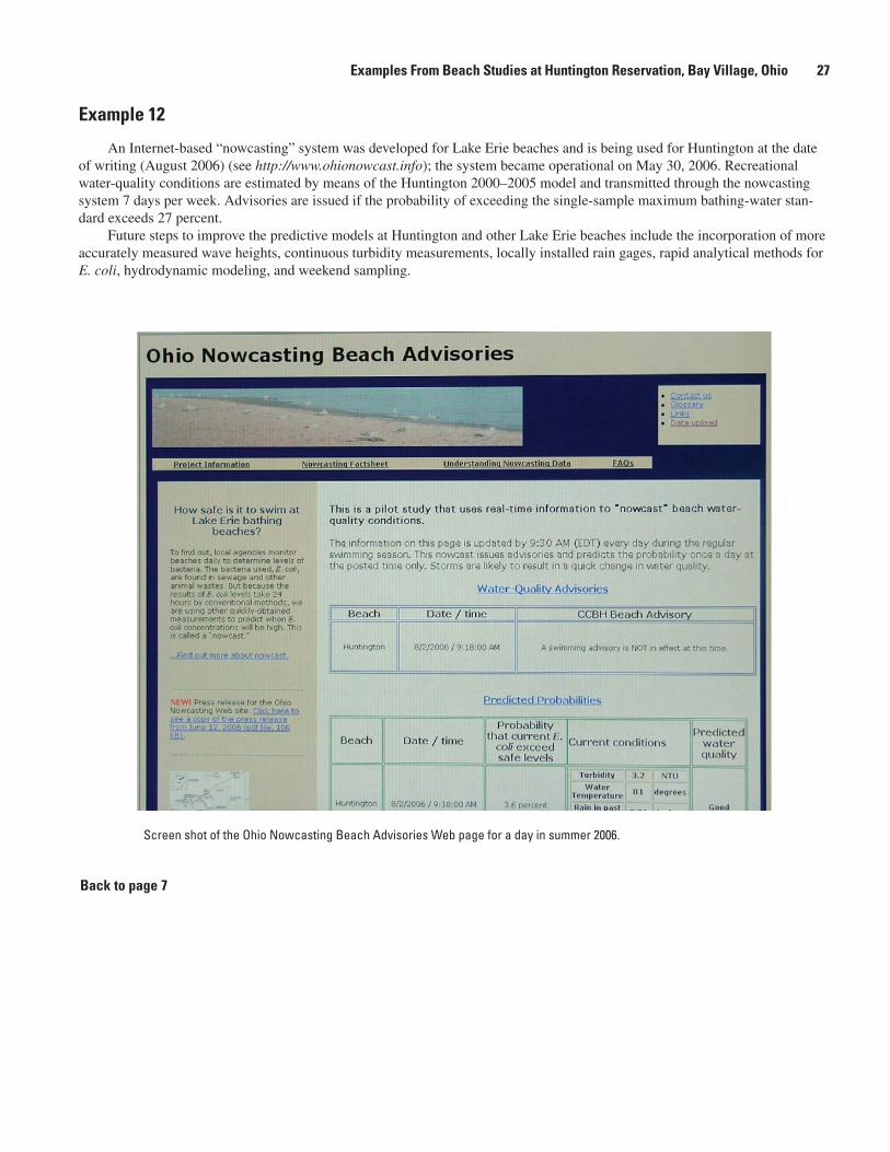
Screen shot of the Ohio Nowcasting Beach Advisories Web page for a day in summer 2006.
Example 1�
An Internet-based “nowcasting” system was developed for Lake Erie beaches and is being used for Huntington at the date of writing (August 2006) (see http://www.ohionowcast.info); the system became operational on May 30, 2006. Recreational water-quality conditions are estimated by means of the Huntington 2000–2005 model and transmitted through the nowcasting system 7 days per week. Advisories are issued if the probability of exceeding the single-sample maximum bathing-water stan-dard exceeds 27 percent.
Future steps to improve the predictive models at Huntington and other Lake Erie beaches include the incorporation of more accurately measured wave heights, continuous turbidity measurements, locally installed rain gages, rapid analytical methods for E. coli, hydrodynamic modeling, and weekend sampling.
Examples From Beach Studies at Huntington Reservation, Bay Village, Ohio �7
Back to page 7
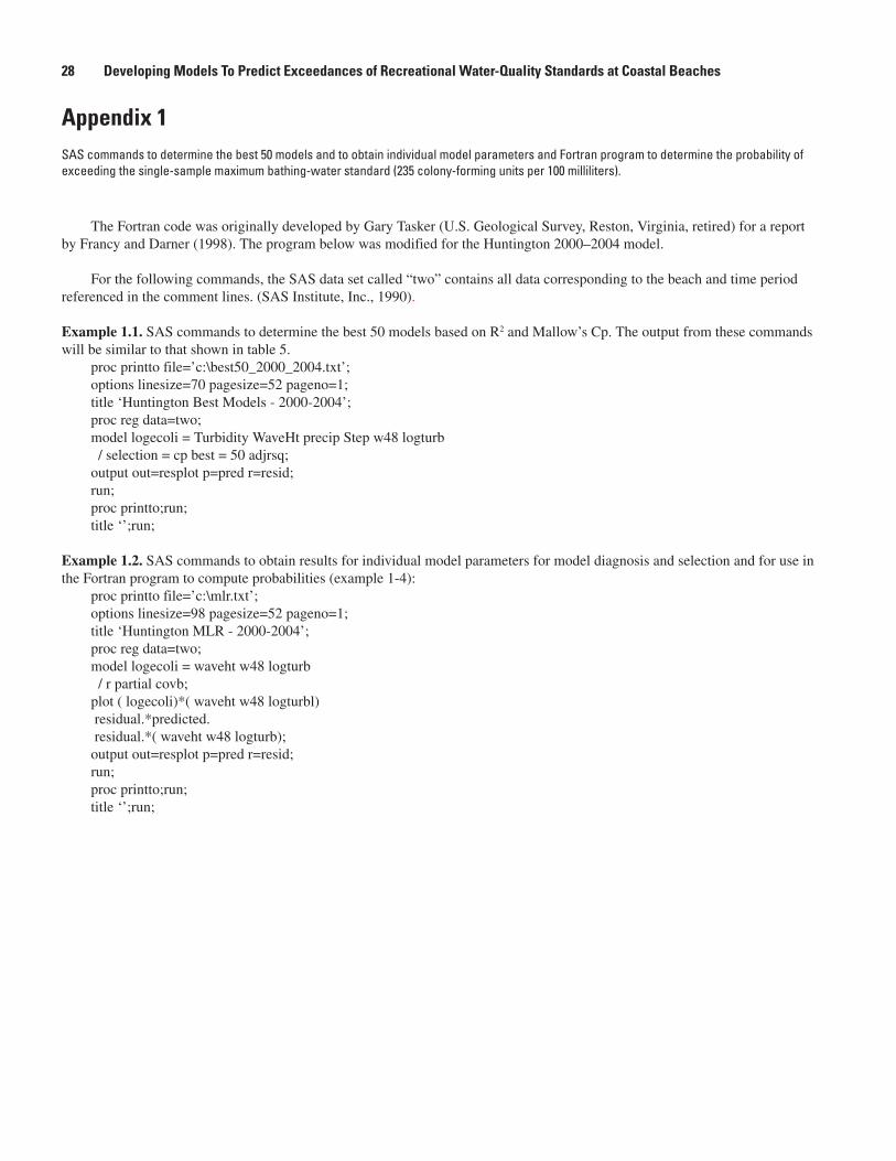
Appendix 1SAS commands to determine the best 50 models and to obtain individual model parameters and Fortran program to determine the probability of exceeding the single-sample maximum bathing-water standard (235 colony-forming units per 100 milliliters).
The Fortran code was originally developed by Gary Tasker (U.S. Geological Survey, Reston, Virginia, retired) for a report by Francy and Darner (1998). The program below was modified for the Huntington 2000–2004 model.
For the following commands, the SAS data set called “two” contains all data corresponding to the beach and time period referenced in the comment lines. (SAS Institute, Inc., 1990).
Example 1.1. SAS commands to determine the best 50 models based on R2 and Mallow’s Cp. The output from these commands will be similar to that shown in table 5.
proc printto file=’c:\best50_2000_2004.txt’;options linesize=70 pagesize=52 pageno=1;title ‘Huntington Best Models - 2000-2004’;proc reg data=two;model logecoli = Turbidity WaveHt precip Step w48 logturb / selection = cp best = 50 adjrsq;output out=resplot p=pred r=resid;run;proc printto;run;title ‘’;run;
Example 1.2. SAS commands to obtain results for individual model parameters for model diagnosis and selection and for use in the Fortran program to compute probabilities (example 1-4):
proc printto file=’c:\mlr.txt’;options linesize=98 pagesize=52 pageno=1;title ‘Huntington MLR - 2000-2004’;proc reg data=two;model logecoli = waveht w48 logturb / r partial covb;plot ( logecoli)*( waveht w48 logturbl) residual.*predicted. residual.*( waveht w48 logturb);output out=resplot p=pred r=resid;run;proc printto;run;title ‘’;run;
�8 Developing Models To Predict Exceedances of Recreational Water-Quality Standards at Coastal Beaches
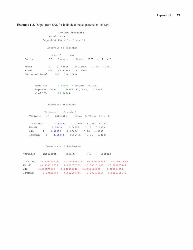
Example 1-3. Output from SAS for individual model parameters (mlr.txt).
The REG Procedure Model: MODEL1
Dependent Variable: logecoli
Analysis of Variance
Sum of Mean
Source DF Squares Square F Value Pr > F
Model 3 42.48015 14.16005 52.45 <.0001
Error 244 65.87395 0.26998
Corrected Total 247 108.35410
Root MSE 0.51959 R-Square 0.3920
Dependent Mean 1.74555 Adj R-Sq 0.3846
Coeff Var 29.76664
Parameter Estimates
Parameter Standard
Variable DF Estimate Error t Value Pr > |t|
Intercept 1 0.91432 0.07906 11.56 <.0001
WaveHt 1 0.14416 0.04556 3.16 0.0018
w48 1 0.30089 0.05694 5.28 <.0001
logturb 1 0.56274 0.09765 5.76 <.0001
Covariance of Estimates
Variable Intercept WaveHt w48 logturb
Intercept 0.0062507263 -0.000810778 -0.000171345 -0.00420649
WaveHt -0.000810778 0.002076132 -0.000151048 -0.002687444
w48 -0.000171345 -0.000151048 0.0032421405 -0.000624654
logturb -0.00420649 -0.002687444 -0.000624654 0.0095355972
Appendix 1 �9
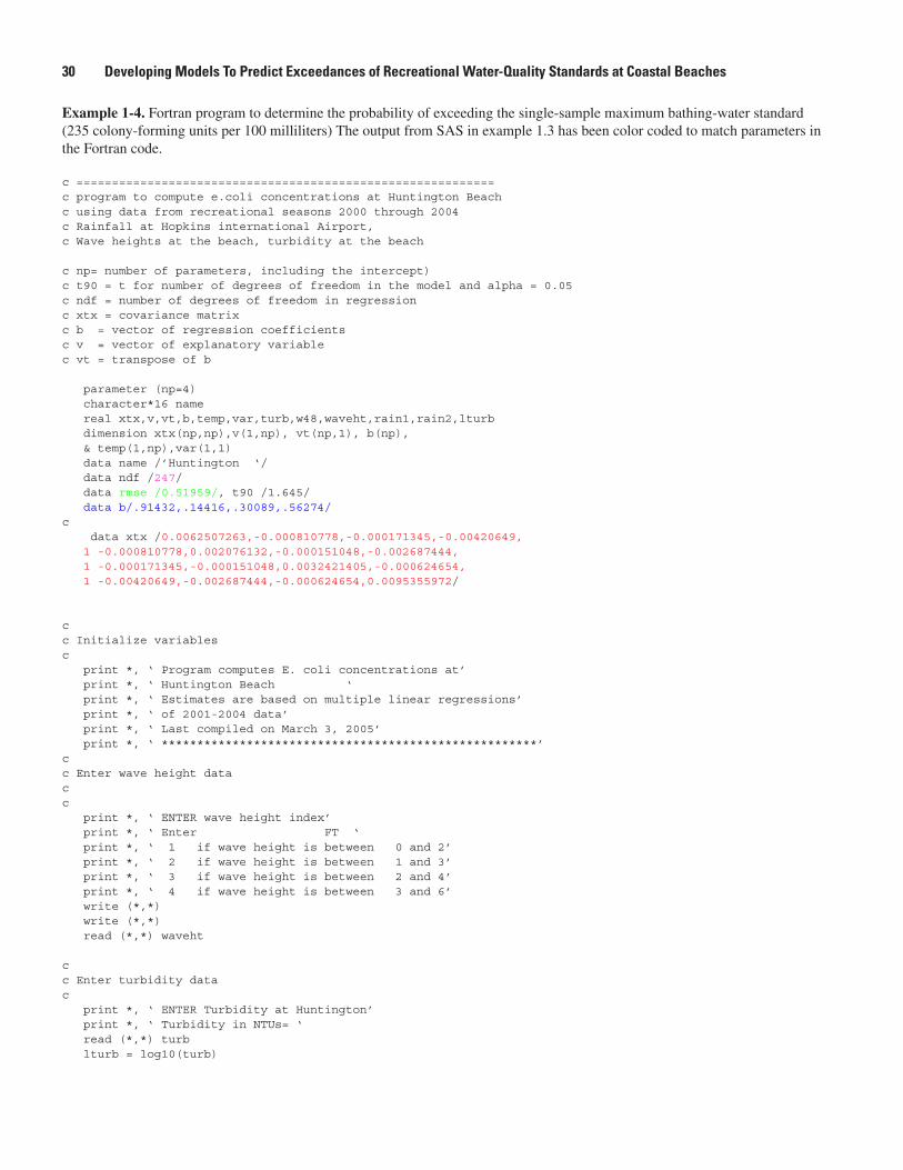
Example 1-4. Fortran program to determine the probability of exceeding the single-sample maximum bathing-water standard (235 colony-forming units per 100 milliliters) The output from SAS in example 1.3 has been color coded to match parameters in the Fortran code.
c ===========================================================c program to compute e.coli concentrations at Huntington Beach c using data from recreational seasons 2000 through 2004c Rainfall at Hopkins international Airport,c Wave heights at the beach, turbidity at the beach
c np= number of parameters, including the intercept)c t90 = t for number of degrees of freedom in the model and alpha = 0.05c ndf = number of degrees of freedom in regressionc xtx = covariance matrixc b = vector of regression coefficientsc v = vector of explanatory variablec vt = transpose of b
parameter (np=4) character*16 name real xtx,v,vt,b,temp,var,turb,w48,waveht,rain1,rain2,lturb dimension xtx(np,np),v(1,np), vt(np,1), b(np), & temp(1,np),var(1,1) data name /’Huntington ‘/ data ndf /247/ data rmse /0.51959/, t90 /1.645/ data b/.91432,.14416,.30089,.56274/ c data xtx /0.0062507263,-0.000810778,-0.000171345,-0.00420649, 1 -0.000810778,0.002076132,-0.000151048,-0.002687444, 1 -0.000171345,-0.000151048,0.0032421405,-0.000624654, 1 -0.00420649,-0.002687444,-0.000624654,0.0095355972/
cc Initialize variablesc print *, ‘ Program computes E. coli concentrations at’ print *, ‘ Huntington Beach ‘ print *, ‘ Estimates are based on multiple linear regressions’ print *, ‘ of 2001-2004 data’ print *, ‘ Last compiled on March 3, 2005’ print *, ‘ *****************************************************’cc Enter wave height datacc print *, ‘ ENTER wave height index’ print *, ‘ Enter FT ‘ print *, ‘ 1 if wave height is between 0 and 2’ print *, ‘ 2 if wave height is between 1 and 3’ print *, ‘ 3 if wave height is between 2 and 4’ print *, ‘ 4 if wave height is between 3 and 6’ write (*,*) write (*,*) read (*,*) waveht
cc Enter turbidity datac print *, ‘ ENTER Turbidity at Huntington’ print *, ‘ Turbidity in NTUs= ‘ read (*,*) turb lturb = log10(turb)
30 Developing Models To Predict Exceedances of Recreational Water-Quality Standards at Coastal Beaches
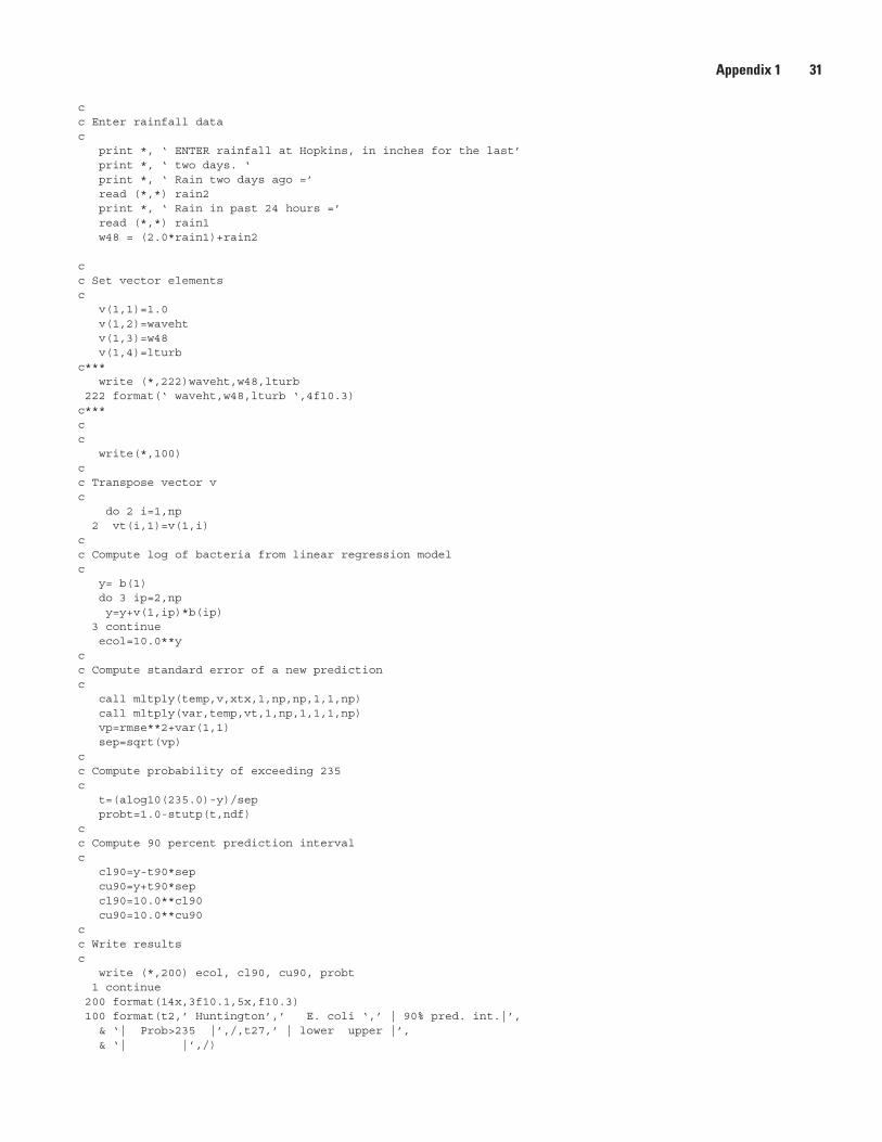
cc Enter rainfall datac print *, ‘ ENTER rainfall at Hopkins, in inches for the last’ print *, ‘ two days. ‘ print *, ‘ Rain two days ago =’ read (*,*) rain2 print *, ‘ Rain in past 24 hours =’ read (*,*) rain1 w48 = (2.0*rain1)+rain2
cc Set vector elements c v(1,1)=1.0 v(1,2)=waveht v(1,3)=w48 v(1,4)=lturbc*** write (*,222)waveht,w48,lturb 222 format(‘ waveht,w48,lturb ‘,4f10.3)c***cc write(*,100)cc Transpose vector vc do 2 i=1,np 2 vt(i,1)=v(1,i)cc Compute log of bacteria from linear regression modelc y= b(1) do 3 ip=2,np y=y+v(1,ip)*b(ip) 3 continue ecol=10.0**ycc Compute standard error of a new predictionc call mltply(temp,v,xtx,1,np,np,1,1,np) call mltply(var,temp,vt,1,np,1,1,1,np) vp=rmse**2+var(1,1) sep=sqrt(vp)cc Compute probability of exceeding 235c t=(alog10(235.0)-y)/sep probt=1.0-stutp(t,ndf)cc Compute 90 percent prediction intervalc cl90=y-t90*sep cu90=y+t90*sep cl90=10.0**cl90 cu90=10.0**cu90cc Write resultsc write (*,200) ecol, cl90, cu90, probt 1 continue 200 format(14x,3f10.1,5x,f10.3) 100 format(t2,’ Huntington’,’ E. coli ‘,’ | 90% pred. int.|’, & ‘| Prob>235 |’,/,t27,’ | lower upper |’, & ‘| |’,/)
Appendix 1 31
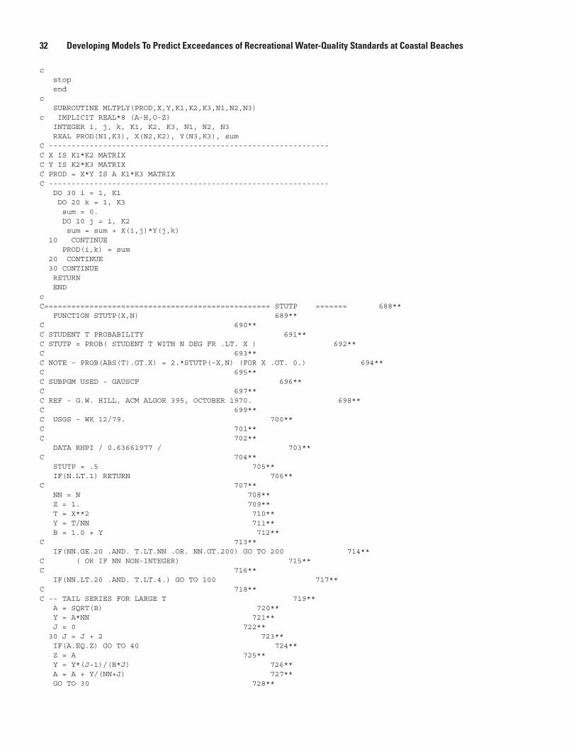
c stop endc SUBROUTINE MLTPLY(PROD,X,Y,K1,K2,K3,N1,N2,N3)c IMPLICIT REAL*8 (A-H,O-Z) INTEGER i, j, k, K1, K2, K3, N1, N2, N3 REAL PROD(N1,K3), X(N2,K2), Y(N3,K3), sumC --------------------------------------------------------------C X IS K1*K2 MATRIXC Y IS K2*K3 MATRIXC PROD = X*Y IS A K1*K3 MATRIXC -------------------------------------------------------------- DO 30 i = 1, K1 DO 20 k = 1, K3 sum = 0. DO 10 j = 1, K2 sum = sum + X(i,j)*Y(j,k) 10 CONTINUE PROD(i,k) = sum 20 CONTINUE 30 CONTINUE RETURN ENDcC================================================== STUTP ======= 688** FUNCTION STUTP(X,N) 689**C 690**C STUDENT T PROBABILITY 691**C STUTP = PROB( STUDENT T WITH N DEG FR .LT. X ) 692**C 693**C NOTE - PROB(ABS(T).GT.X) = 2.*STUTP(-X,N) (FOR X .GT. 0.) 694**C 695**C SUBPGM USED - GAUSCF 696**C 697**C REF - G.W. HILL, ACM ALGOR 395, OCTOBER 1970. 698**C 699**C USGS - WK 12/79. 700**C 701**C 702** DATA RHPI / 0.63661977 / 703**C 704** STUTP = .5 705** IF(N.LT.1) RETURN 706**C 707** NN = N 708** Z = 1. 709** T = X**2 710** Y = T/NN 711** B = 1.0 + Y 712**C 713** IF(NN.GE.20 .AND. T.LT.NN .OR. NN.GT.200) GO TO 200 714**C ( OR IF NN NON-INTEGER) 715**C 716** IF(NN.LT.20 .AND. T.LT.4.) GO TO 100 717**C 718**C -- TAIL SERIES FOR LARGE T 719** A = SQRT(B) 720** Y = A*NN 721** J = 0 722** 30 J = J + 2 723** IF(A.EQ.Z) GO TO 40 724** Z = A 725** Y = Y*(J-1)/(B*J) 726** A = A + Y/(NN+J) 727** GO TO 30 728**
3� Developing Models To Predict Exceedances of Recreational Water-Quality Standards at Coastal Beaches
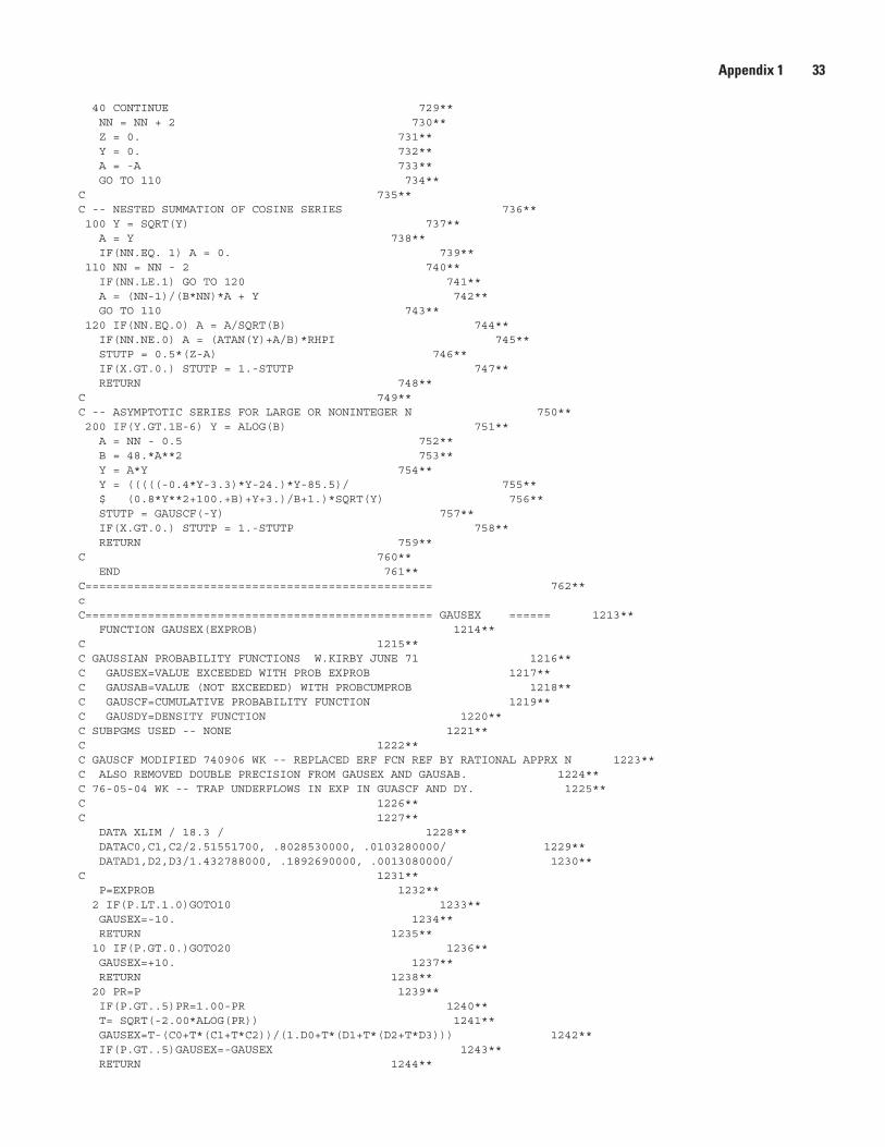
40 CONTINUE 729** NN = NN + 2 730** Z = 0. 731** Y = 0. 732** A = -A 733** GO TO 110 734**C 735**C -- NESTED SUMMATION OF COSINE SERIES 736** 100 Y = SQRT(Y) 737** A = Y 738** IF(NN.EQ. 1) A = 0. 739** 110 NN = NN - 2 740** IF(NN.LE.1) GO TO 120 741** A = (NN-1)/(B*NN)*A + Y 742** GO TO 110 743** 120 IF(NN.EQ.0) A = A/SQRT(B) 744** IF(NN.NE.0) A = (ATAN(Y)+A/B)*RHPI 745** STUTP = 0.5*(Z-A) 746** IF(X.GT.0.) STUTP = 1.-STUTP 747** RETURN 748**C 749**C -- ASYMPTOTIC SERIES FOR LARGE OR NONINTEGER N 750** 200 IF(Y.GT.1E-6) Y = ALOG(B) 751** A = NN - 0.5 752** B = 48.*A**2 753** Y = A*Y 754** Y = (((((-0.4*Y-3.3)*Y-24.)*Y-85.5)/ 755** $ (0.8*Y**2+100.+B)+Y+3.)/B+1.)*SQRT(Y) 756** STUTP = GAUSCF(-Y) 757** IF(X.GT.0.) STUTP = 1.-STUTP 758** RETURN 759**C 760** END 761**C================================================== 762**cC================================================== GAUSEX ====== 1213** FUNCTION GAUSEX(EXPROB) 1214**C 1215**C GAUSSIAN PROBABILITY FUNCTIONS W.KIRBY JUNE 71 1216**C GAUSEX=VALUE EXCEEDED WITH PROB EXPROB 1217**C GAUSAB=VALUE (NOT EXCEEDED) WITH PROBCUMPROB 1218**C GAUSCF=CUMULATIVE PROBABILITY FUNCTION 1219**C GAUSDY=DENSITY FUNCTION 1220**C SUBPGMS USED -- NONE 1221**C 1222**C GAUSCF MODIFIED 740906 WK -- REPLACED ERF FCN REF BY RATIONAL APPRX N 1223**C ALSO REMOVED DOUBLE PRECISION FROM GAUSEX AND GAUSAB. 1224**C 76-05-04 WK -- TRAP UNDERFLOWS IN EXP IN GUASCF AND DY. 1225**C 1226**C 1227** DATA XLIM / 18.3 / 1228** DATAC0,C1,C2/2.51551700, .8028530000, .0103280000/ 1229** DATAD1,D2,D3/1.432788000, .1892690000, .0013080000/ 1230**C 1231** P=EXPROB 1232** 2 IF(P.LT.1.0)GOTO10 1233** GAUSEX=-10. 1234** RETURN 1235** 10 IF(P.GT.0.)GOTO20 1236** GAUSEX=+10. 1237** RETURN 1238** 20 PR=P 1239** IF(P.GT..5)PR=1.00-PR 1240** T= SQRT(-2.00*ALOG(PR)) 1241** GAUSEX=T-(C0+T*(C1+T*C2))/(1.D0+T*(D1+T*(D2+T*D3))) 1242** IF(P.GT..5)GAUSEX=-GAUSEX 1243** RETURN 1244**
Appendix 1 33
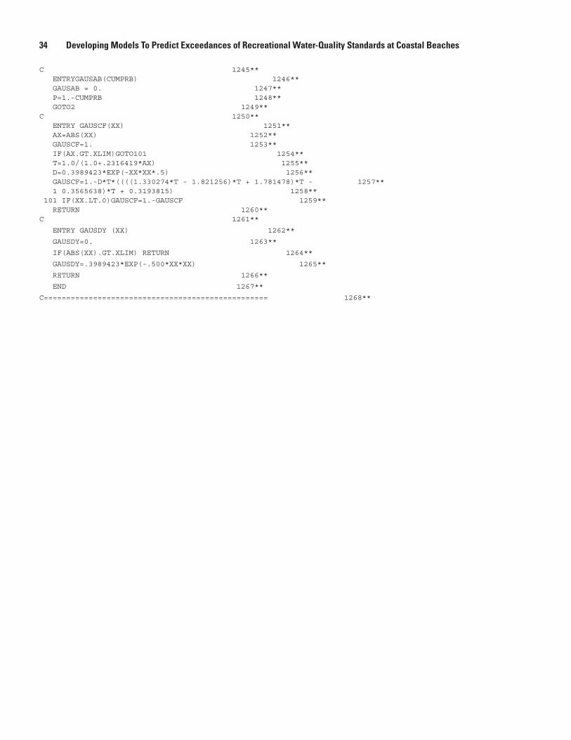
C 1245** ENTRYGAUSAB(CUMPRB) 1246** GAUSAB = 0. 1247** P=1.-CUMPRB 1248** GOTO2 1249**C 1250** ENTRY GAUSCF(XX) 1251** AX=ABS(XX) 1252** GAUSCF=1. 1253** IF(AX.GT.XLIM)GOTO101 1254** T=1.0/(1.0+.2316419*AX) 1255** D=0.3989423*EXP(-XX*XX*.5) 1256** GAUSCF=1.-D*T*((((1.330274*T - 1.821256)*T + 1.781478)*T - 1257** 1 0.3565638)*T + 0.3193815) 1258** 101 IF(XX.LT.0)GAUSCF=1.-GAUSCF 1259** RETURN 1260**C 1261**
ENTRY GAUSDY (XX) 1262**
GAUSDY=0. 1263**
IF(ABS(XX).GT.XLIM) RETURN 1264**
GAUSDY=.3989423*EXP(-.500*XX*XX) 1265**
RETURN 1266**
END 1267**
C================================================== 1268**
34 Developing Models To Predict Exceedances of Recreational Water-Quality Standards at Coastal Beaches
Related Documents