______________________________ Département TECHNIQUES DE COMMERCIALISATION Online lessons : ENT, section « outils pédagogiques », platform Claroline, category TC, Course « MATHS3 ». ________ MATHEMATICS ________ Semester 3 Probability distributions Statistical inference IUT of Saint-Etienne - TC - J.F.Ferraris - Math - S3 - InferStats - CoursEx - Rev2014n - page 1 / 44

Welcome message from author
This document is posted to help you gain knowledge. Please leave a comment to let me know what you think about it! Share it to your friends and learn new things together.
Transcript
______________________________Département TECHNIQUES DE COMMERCIALISATION
Online lessons : ENT, section « outils pédagogiques », platform Claroline, category TC, Course « MATHS3 ».
________ MATHEMATICS ________
Semester 3
Probability distributions
Statistical inference
IUT of Saint-Etienne - TC - J.F.Ferraris - Math - S3 - InferStats - CoursEx - Rev2014n - page 1 / 44
Introduction and history 3
Lessons and tutorials 5
I Discrete probability laws 5
I-1 Generalities : remainder 5
I-2 Hypergeometric law 6
I-3 Binomial law 8
I-4 Poisson's law 10
II A continuous probability law : the normal law 12
II-1 Convergence of discrete laws 12
II-2 Continuous random variable 13
II-3 Normal law (or Laplace's law) 16
II-4 Approximation of other laws by a normal law 21
III Sampling distributions 23
III-1 Introduction 23
III-2 Sampling distribution of means 23
III-3 Sampling distribution of proportions 24
IV Estimation 26
IV-1 Point estimates 26
IV-2 Estimate of µ by a confidence interval 27
IV-3 Estimate of π by a confidence interval 28
V Statistical hypothesis testing 30
V-1 Adequacy Khi-2 (χ²) tests 31
V-2 Conformance tests 33
Exercises 36
Form 45
TABLE OF CONTENTS
IUT of Saint-Etienne - TC - J.F.Ferraris - Math - S3 - InferStats - CoursEx - Rev2014n - page 2 / 44
INTRODUCTION AND HISTORY
A quick story of normal law
On late XVIIth century, Jacques Bernoulli shows the way to binomial law, calculating the chances of
success while performing several times a given experiment. His manual calculatations become
horribly complicated when numbers grow, due to the length of factorial calculus.
In the first half of XVIIIth century, Abraham de Moivre works on chance calculus and discovers a formula
that gives (approximately) the factorial of a natural number n :
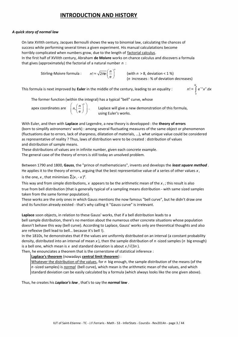
Stirling-Moivre formula : (with n > 8, deviation < 1 %)
(n increases : % of deviation decreases)
This formula is next improved by Euler in the middle of the century, leading to an equality :
The former function (within the integral) has a typical "bell" curve, whose
apex coordinates are . Laplace will give a new demonstration of this formula,
using Euler's works.
With Euler, and then with Laplace and Legendre, a new theory is developped : the theory of errors
(born to simplify astronomers' work) : among several fluctuating measures of the same object or phenomenon
(fluctuations due to errors, lack of sharpness, dilatation of materials, …), what unique value could be considered
as representative of reality ? Thus, laws of distribution were to be created : distribution of values
and distribution of sample means.
These distributions of values are in infinite number, given each concrete example.
The general case of the theory of errors is still today an unsolved problem.
Between 1790 and 1800, Gauss, the "prince of mathematicians", invents and develops the least square method .
He applies it to the theory of errors, arguing that the best representative value of a series of other values x i
is the one, x , that minimises Σ(x i - x )².
This way and from simple distributions, x appears to be the arithmetic mean of the x i ; this result is also
true from bell distribution (that is generally typical of a sampling means distribution - with same sized samples
taken from the same former population).
These works are the only ones in which Gauss mentions the now famous "bell curve", but he didn't draw one
and its function already existed - that's why calling it "Gauss curve" is irrelevant.
Laplace soon objects, in relation to these Gauss' works, that if a bell distribution leads to a
bell sample distribution, there's no mention about the numerous other concrete situations whose population
doesn't behave this way (bell curve). According to Laplace, Gauss' works only are theoretical thoughts and also
are reflexive (bell lead to bell… because it's bell !).
In the 1810s, he demonstrates that if the values are uniformly distributed on an interval (a constant probability
density, distributed into an interval of mean x ), then the sample distribution of n -sized samples (n big enough)
is a bell one, which mean is x and standard deviation is about x /√(3n ).
Then, he enounciates a theorem that is the cornerstone of statistical inference :
Laplace's theorem (nowadays central limit theorem) :
Whatever the distribution of the values, for n big enough, the sample distribution of the means (of the
n -sized samples) is normal (bell curve), which mean is the arithmetic mean of the values, and which
standard deviation can be easily calculated by a formula (which always looks like the one given above).
Thus, he creates his Laplace's law , that's to say the normal law .
!n
nn n
≈ π
2e
! .0
e dx nn x x
+∞−= ∫
,e
nn
n
IUT of Saint-Etienne - TC - J.F.Ferraris - Math - S3 - InferStats - CoursEx - Rev2014n - page 3 / 44
In the XIXth century appears the profession of statistician (in any field, people need to know how a
population behaves). The most famous and prolific at this time was the french Adolphe Quételet,
wo published an analysis of Laplace's philosophy, numerous concrete data series showing bell-shaped
distributions (for instance, the "chest sizes of 4000 scottish soldiers", whose distribution perfectly fits in
the kind of theoretical normal curve. Indeed, the chest size of a man is the result of the sum of
several, random and independant factors - genetics, education, feeding, activity, … - and Laplace's theorem
assesses that the distribution of a sum, like the one of a mean, is normal !)
It has also to be reported that Quételet was the first who drew one of these famous normal bell curves !
(neither Gauss, nor Laplace, felt the need to draw one while thinking about theory)
Everything isn't necessarily normal
During the second half of XIXth century, statisticians show that everything isn't normally distributed
(the symmetry of normal law isn't representative of what happen in the whole world). Consequently, other
continuous or discrete laws are created in order to model several concrete situations. For instance :
* Poisson's law, quite asymmetrical, in case of rare events,
* Pareto's law for incomes distributions, asymmetrical too,
* Exponential law and others based on the same model, for life lengths, asymmetrical again, …
Other laws were created before the normal law exists :
* Uniform law, where the probability of any value is the same (throw of a die),
* Binomial law (from Bernoulli),
* Geometric law, dealing whith the number of tries you need to get your first success (binomial cases),
* Hypergeometric law, similar to binomial law, but in which repetition isn't allowed, ...
In the early XXst century, laws of superior orders are built, dealing with more than one variable, or involving
degrees of freedom :
* Student's law (sample distribution of means, built with two variables : mean and standard deviation)
* χχχχ² law - "Khi-squared" - (to evaluate the differences between a theoretical law and a real distribution)
At this time, english statisticians like Pearson, Student (William Sealy Gosset) or Fisher begin to develop
a true actual methodology in statistics, that's to say a well-formalized theory of inference (drawing conclusions
about a population, only knowing one of its samples), by the mean of creating new probability laws to describe
phenomenons :
They have dictated, between 1900 and 1950, an "objectivist" or "frequencist" interpretation for the concept of
probability. From the 1950s has expressed an argument known as the "neo-Bayesian" school telling that
statistical inference shouldn't be based on the collected data alone, but also need the knowledge and use
of underlying probabilistic models. It's the "subjectivist" school.
Calculation tools are increasingly powerful
With data processing (computering), a new performance took off : the "multidimensional data analysis".
It consists in describing, sort and simplify large recordings of collected data (e.g. : a survey on 3000 persons
on wich it has been collected 80 informations each).
Observed and crossed results may suggest laws (already existing or not), models or explainations that may
avoid statisticians to consider data relatively to arbitrary laws, formerly created, to wich they would be forced
to do a comparison.
IUT of Saint-Etienne - TC - J.F.Ferraris - Math - S3 - InferStats - CoursEx - Rev2014n - page 4 / 44
I. Discrete probability distributions
I.1 General case : remainder What you must have remembered from last chapter…
Let's consider an object or a set of objects and conceive a random experiment on it, which
outcomes form a sample space partitioned into a certain number of events.
e.g. :
objects : two dice
experiment : roll them, then calculate their sum
sample space : Ω = 2, 3, 4, 5, 6, 7, 8, 9, 10, 11, 12 (non equally likely outcomes)
partition of Ω : E1 : "less than 7" ; E2 : "from 7 to 10" ; E3 : "11 or 12"
Each event Ei can be associated with a real value x i : a gain.
These gains are randomly reached, like each outcome - unpredictable - of the experiment ;
Onto this game, thus, "gain" is called a random variable , written X .
e.g. :
events :
gain X (€) :
For each value of the gain, we have to be able to calculate the probability of the associated event.
That's called "getting the probability law of X ".
e.g. :
gain X (€) : (former chapter,
pi or p(X = x i) : tutorial 6)
Interpretation and purpose of those probabilities :
If you play this game many times, you will lose or win approximately according in the proportions
announced by these probabilities.
With our example : every 36 games, you will have on average 15 losses of 3 €, 18 gains of 1 €
and 3 gains of 5 € ; thus, by combining them : a global loss of 12 €, on average, every 36 games.
This global result can be expressed for one game : 12/36 ≈ 0.33.
Playing it long-term, you'll have an average loss of 33 cents per try.
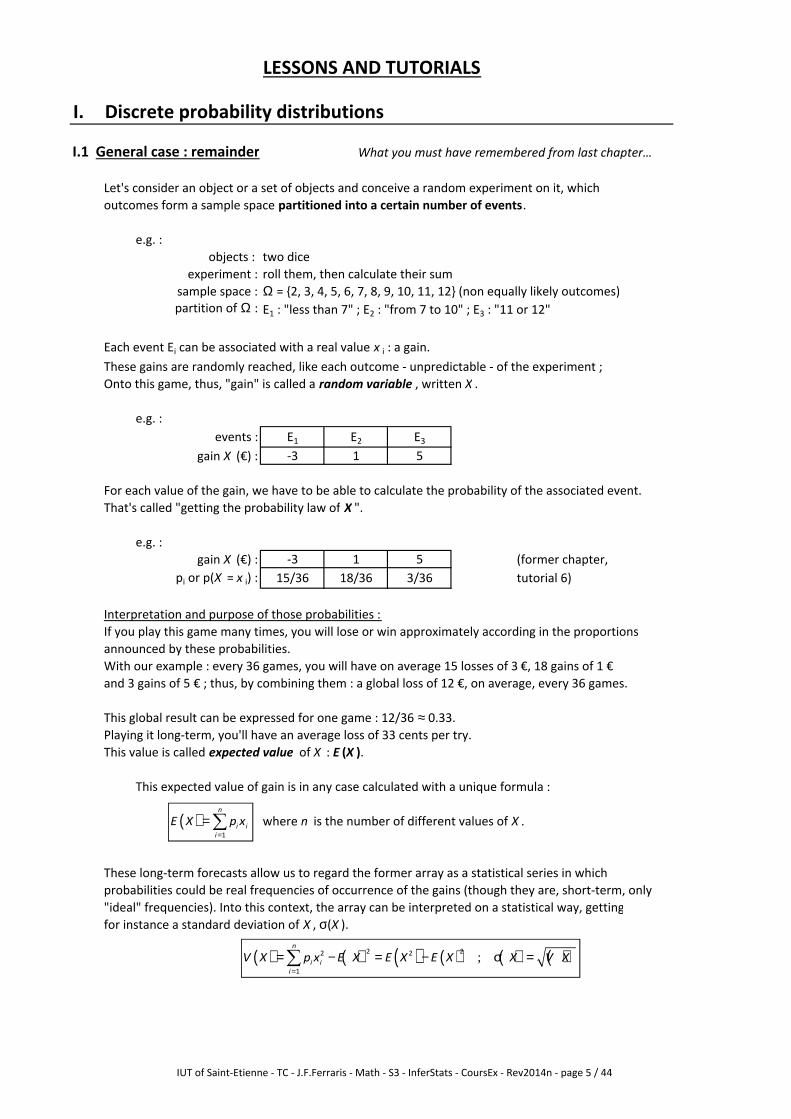
This value is called expected value of X : E (X ).
This expected value of gain is in any case calculated with a unique formula :
where n is the number of different values of X .
These long-term forecasts allow us to regard the former array as a statistical series in which
probabilities could be real frequencies of occurrence of the gains (though they are, short-term, only
"ideal" frequencies). Into this context, the array can be interpreted on a statistical way, getting
for instance a standard deviation of X , σ(X ).
15/36
E2 E3
-3 1
18/36 3/36
E1
5
-3 1 5
LESSONS AND TUTORIALS
( )1
n
i i
i
E X p x=
=∑
( ) ( ) ( ) ( ) ( ) ( );2 22 2
1
n
i i
i
V X p x E X E X E X X V X=
= − = − σ =∑
IUT of Saint-Etienne - TC - J.F.Ferraris - Math - S3 - InferStats - CoursEx - Rev2014n - page 5 / 44
IUT of Saint-Etienne – TC –J.F.Ferraris – Math – S3 – InferStats – CoursEx – Rev2014n – page 6 / 44
I.2 Hypergeometric law
Its study will be restricted to a simple partition of Ω in two subsets (one event and its contrary).
I.2.1 Definition and implementation
The distribution of a random variable X is hypergeometric iff :
* an experiment is performed n times with no repetition of an outcome,
leading to combinations.
* X is defined as the number of success that may be obtained after n attempts.
Given a sample space Ω containing N outcomes, partitioned in two events :
A, containing a outcomes, called “success”
and A , containing the N - a remaining outcomes, called “failure”.
An experiment is performed n times, with no possibility of repetition of an outcome each
new time (hence, n ≤ N). Once finished, we will have obtained :
k success, random, smaller than n (number of attempts), and smaller than a (total
number of available success outcomes),
and n - k failures, smaller than N - a (total number of available failure outcomes).
Defining X as the random variable « number of success after n attempts »,
the probability distribution of X is hypergeometric, with the parameters n, a and N.
We can write it : HHHH (n , a , N).
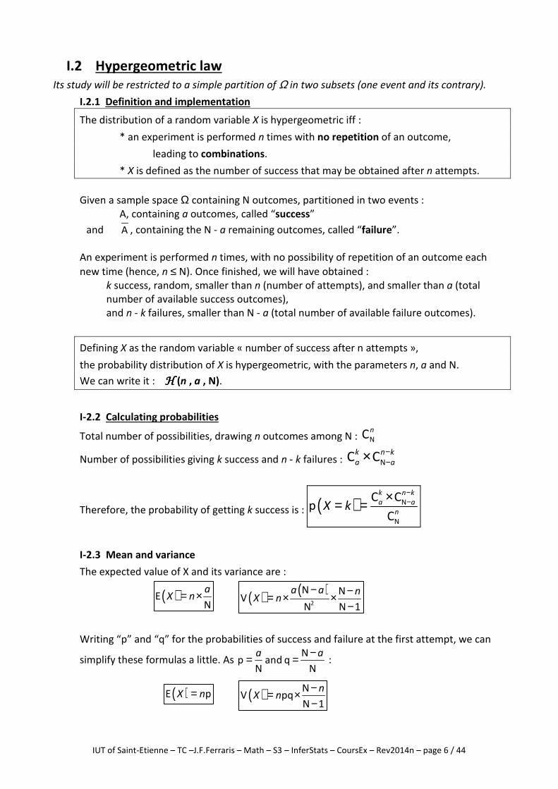
I-2.2 Calculating probabilities
Total number of possibilities, drawing n outcomes among N : NCn
Number of possibilities giving k success and n - k failures : NC Ck n k
a a
−−×
Therefore, the probability of getting k success is : ( ) N
N
C Cp
C
k n k
a a
nX k
−−×= =
I-2.3 Mean and variance
The expected value of X and its variance are :
Writing “p” and “q” for the probabilities of success and failure at the first attempt, we can
simplify these formulas a little. As N
p and qN N
a a−= = :
( )EN
aX n= × ( ) ( )
2
N NV
N N 1
a a nX n
− −= × ×−
( )E pX n= ( ) NV pq
N 1
nX n
−= ×−
IUT of Saint-Etienne – TC –J.F.Ferraris – Math – S3 – InferStats – CoursEx – Rev2014n – page 7 / 44
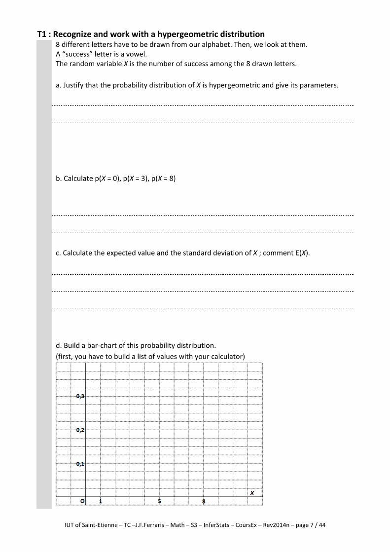
T1 : Recognize and work with a hypergeometric distribution 8 different letters have to be drawn from our alphabet. Then, we look at them.
A “success” letter is a vowel.
The random variable X is the number of success among the 8 drawn letters.
a. Justify that the probability distribution of X is hypergeometric and give its parameters.
b. Calculate p(X = 0), p(X = 3), p(X = 8)
c. Calculate the expected value and the standard deviation of X ; comment E(X).
d. Build a bar-chart of this probability distribution.
(first, you have to build a list of values with your calculator)
I.3 Binomial law
I.3.1 Definition and implementation
The distribution of a random variable X is binomial iff :
* the experiment was conducted n times with possible repetition of an outcome,
through a partition of Ω into one event (success) and its contrary (failure).
* X counts the number of success reached after n attempts.
a. Bernoulli's scheme
Let be a random experiment leading to a sample space Ω.
The event A, called success , has a probability to occur, p(A), written p .
Its contrary, called failure , has a probability q = 1 - p .
The choice tree we can draw from this situation is called Bernoulli scheme .
b. Binomial law
Let be an experiment following a Bernoulli scheme, and let process it n times,
under identical conditions, i.e. : p is constant.
X will be the random variable that counts the number k of success at the end of the n tries.
The probability law of X is a binomial law, with parameters n and p . BBBB (n ; p ).
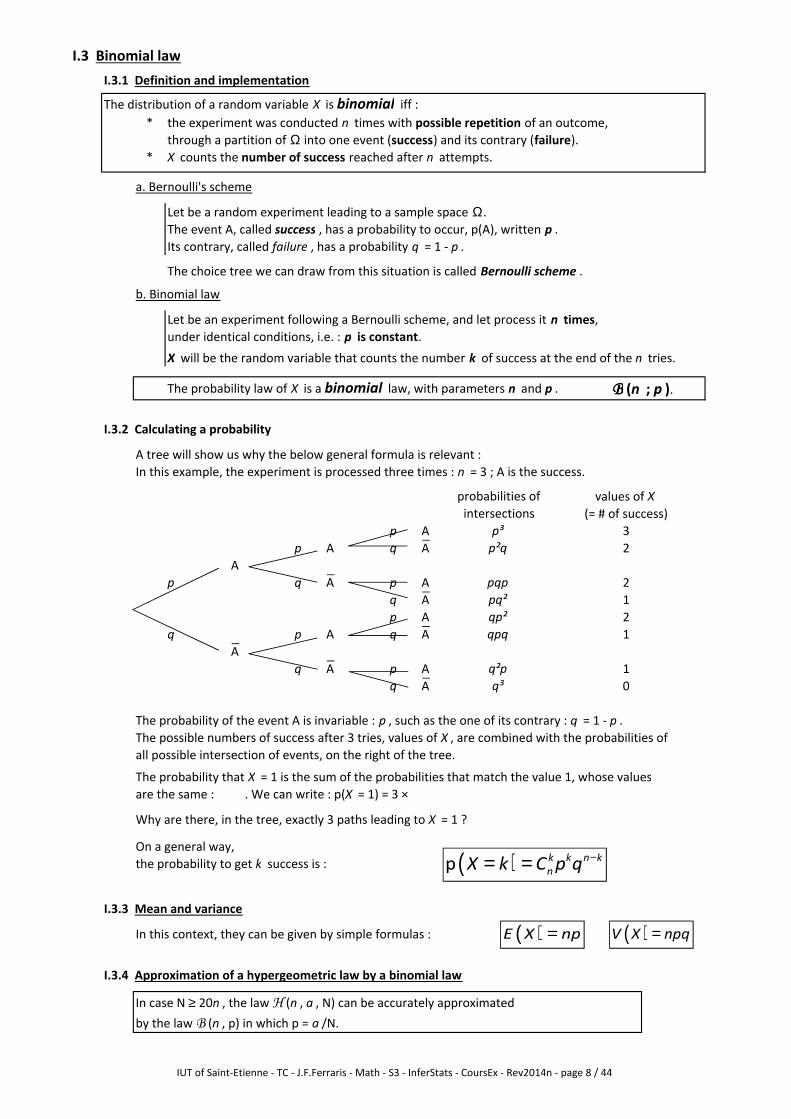
I.3.2 Calculating a probability
A tree will show us why the below general formula is relevant :
In this example, the experiment is processed three times : n = 3 ; A is the success.
values of X
(= # of success)
p A 3
p A q A 2
A
p q A p A 2
q A 1
p A 2
q p A q A 1
A
q A p A 1
q A 0
The probability of the event A is invariable : p , such as the one of its contrary : q = 1 - p .
The possible numbers of success after 3 tries, values of X , are combined with the probabilities of
all possible intersection of events, on the right of the tree.
The probability that X = 1 is the sum of the probabilities that match the value 1, whose values
are the same : . We can write : p(X = 1) = 3 ×
Why are there, in the tree, exactly 3 paths leading to X = 1 ?
On a general way,
the probability to get k success is :
I.3.3 Mean and variance
In this context, they can be given by simple formulas :
I.3.4 Approximation of a hypergeometric law by a binomial law
In case N ≥ 20n , the law H (n , a , N) can be accurately approximated
by the law B (n , p) in which p = a /N.
q²p
q³
probabilities of
intersections
p³
p²q
pqp
pq²
qp²
qpq
( )p k k n k
nX k C p q −= =
( )E X np= ( )V X npq=
IUT of Saint-Etienne - TC - J.F.Ferraris - Math - S3 - InferStats - CoursEx - Rev2014n - page 8 / 44
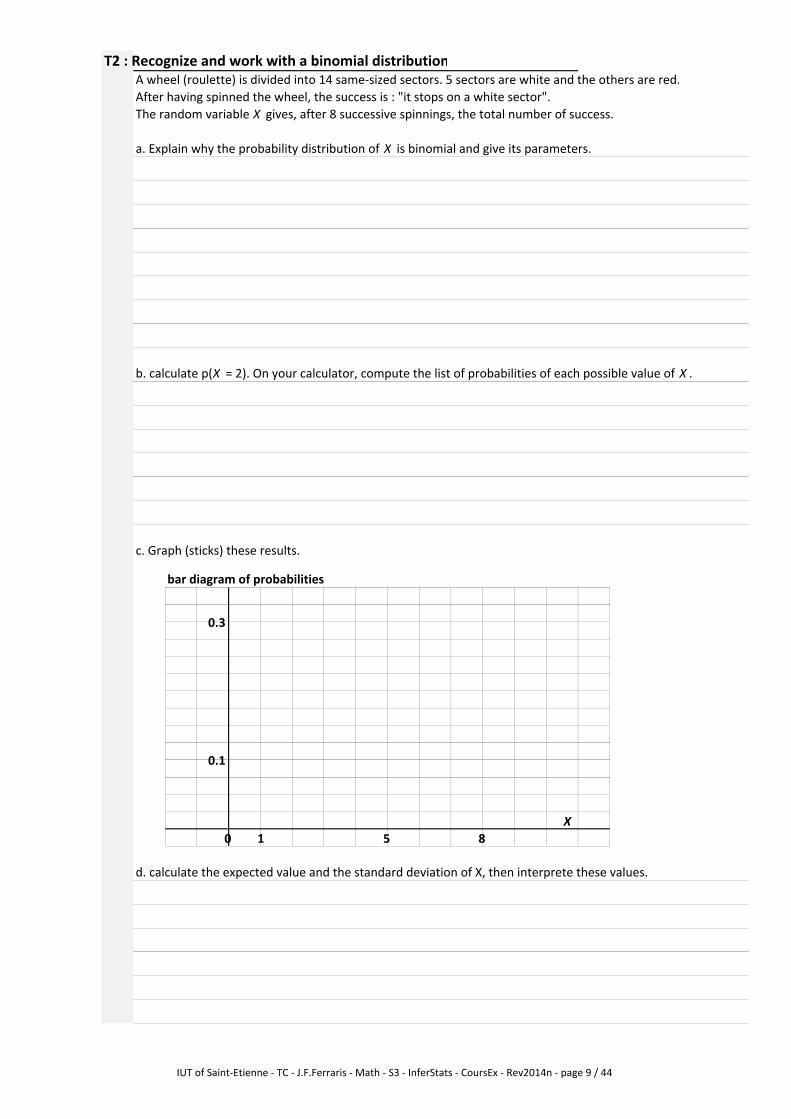
T2 : Recognize and work with a binomial distribution
A wheel (roulette) is divided into 14 same-sized sectors. 5 sectors are white and the others are red.
After having spinned the wheel, the success is : "it stops on a white sector".
The random variable X gives, after 8 successive spinnings, the total number of success.
a. Explain why the probability distribution of X is binomial and give its parameters.
b. calculate p(X = 2). On your calculator, compute the list of probabilities of each possible value of X .
c. Graph (sticks) these results.
bar diagram of probabilities
d. calculate the expected value and the standard deviation of X, then interprete these values.
1 5
0.1
0.3
0 8
X
IUT of Saint-Etienne - TC - J.F.Ferraris - Math - S3 - InferStats - CoursEx - Rev2014n - page 9 / 44
I.4 Poisson's law
I.4.1 Why it has been created
In many cases, the number of different values that a variable X can reach is very big.
So, calculating a probability may involve very large number of combinations (and also include
large powers if the law is binomial), that even a calculater might not be able to calculate.
Moreover, in case a success is a rare event, every result isn't useful, like calculating the
extremely low probabilities of many non-realistic situations implying a large number of success
(non-realistic because very far from the weak mean number of expected success).
In the context of a binomial law, with a weak value of p , an other formula will be used (instead of
the binomial one) based on a Poisson's law , whose results will appear to be close enough to reality.
Concrete examples of use :
* examining a sample taken from a large quantity of products, or a large harvest, in case
the probability p that an element is shoddy (wrong) is low :
Here, the n elements of the sample are taken among N elements without possible repetition -
which gives a hypergeometric law, but n is very little compared to N , so we can simplify
the situation considering it as if repetition were allowed. So, this case can be treated by a
binomial law, whose results will be reliable. Moreover, the low value of p allows us to use a
Poisson's law instead of a binomial law.
* problems of length of a queue
* predicting a maximum number of accidents or failures, or other rare events concerning
a large population (for insurance companies, or study of rare diseases, for instance).
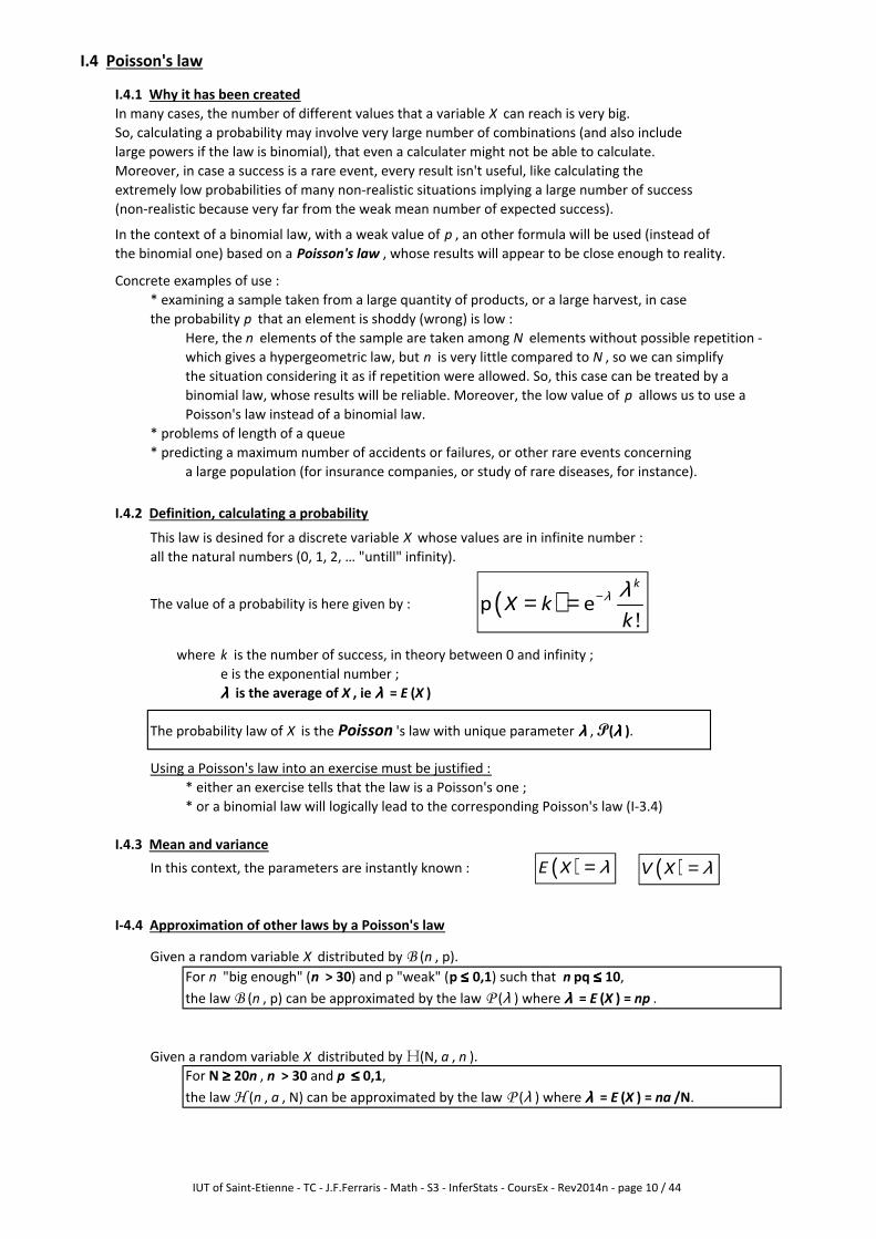
I.4.2 Definition, calculating a probability
This law is desined for a discrete variable X whose values are in infinite number :
all the natural numbers (0, 1, 2, … "untill" infinity).
The value of a probability is here given by :
where k is the number of success, in theory between 0 and infinity ;
e is the exponential number ;
λλλλ is the average of X , ie λλλλ = E (X )
The probability law of X is the Poisson 's law with unique parameter λλλλ , P(λλλλ ).
Using a Poisson's law into an exercise must be justified :
* either an exercise tells that the law is a Poisson's one ;
* or a binomial law will logically lead to the corresponding Poisson's law (I-3.4)
I.4.3 Mean and variance
In this context, the parameters are instantly known :
I-4.4 Approximation of other laws by a Poisson's law
Given a random variable X distributed by B (n , p).
For n "big enough" (n > 30) and p "weak" (p ≤≤≤≤ 0,1) such that n pq ≤≤≤≤ 10,
the law B (n , p) can be approximated by the law P (λ ) where λλλλ = E (X ) = np .
Given a random variable X distributed by H(N, a , n ).
For N ≥≥≥≥ 20n , n > 30 and p ≤≤≤≤ 0,1,
the law H (n , a , N) can be approximated by the law P (λ ) where λλλλ = E (X ) = na /N.
( )!
p ek
X kk
λ λ−= =
( )E X λ= ( )V X λ=
IUT of Saint-Etienne - TC - J.F.Ferraris - Math - S3 - InferStats - CoursEx - Rev2014n - page 10 / 44

T3 : Using a Poisson's law
The variable X is distributed by the binomial law [n = 50 and p = 0.06].
a. Obtain (calculator list) p(X = i ) for each integer i from 0 to 7.
b. Justify the approximation of this law by a Poisson's whose parameter has to be given.
c. Give, by using Poisson's law table, the probabilities asked above.
Compare them to the ones obtained with the binomial law.
d. Using the formula given on page 10, display those probabilities on a new list of your calculator.
IUT of Saint-Etienne - TC - J.F.Ferraris - Math - S3 - InferStats - CoursEx - Rev2014n - page 11 / 44
II. A continuous probability law : the Normal law
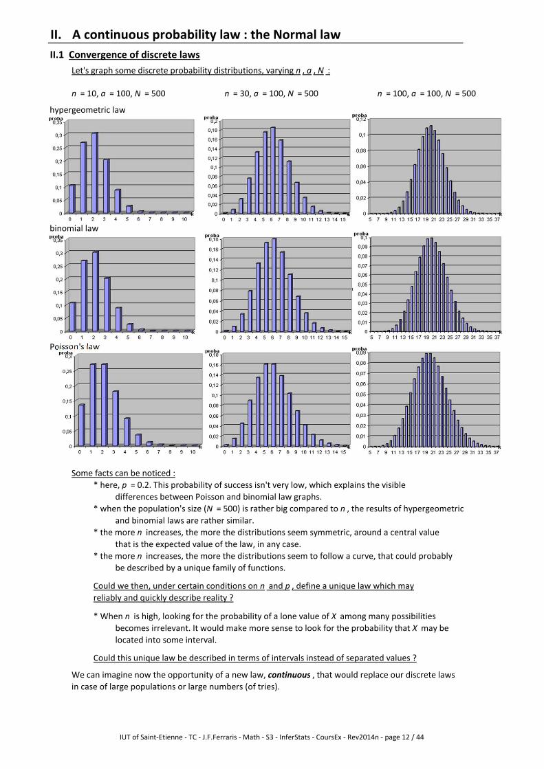
II.1 Convergence of discrete laws
Let's graph some discrete probability distributions, varying n , a , N :
n = 10, a = 100, N = 500 n = 30, a = 100, N = 500 n = 100, a = 100, N = 500
hypergeometric law
binomial law
Poisson's law
Some facts can be noticed :
* here, p = 0.2. This probability of success isn't very low, which explains the visible
differences between Poisson and binomial law graphs.
* when the population's size (N = 500) is rather big compared to n , the results of hypergeometric
and binomial laws are rather similar.
* the more n increases, the more the distributions seem symmetric, around a central value
that is the expected value of the law, in any case.
* the more n increases, the more the distributions seem to follow a curve, that could probably
be described by a unique family of functions.
Could we then, under certain conditions on n and p , define a unique law which may
reliably and quickly describe reality ?
* When n is high, looking for the probability of a lone value of X among many possibilities
becomes irrelevant. It would make more sense to look for the probability that X may be
located into some interval.
Could this unique law be described in terms of intervals instead of separated values ?
We can imagine now the opportunity of a new law, continuous , that would replace our discrete laws
in case of large populations or large numbers (of tries).
IUT of Saint-Etienne - TC - J.F.Ferraris - Math - S3 - InferStats - CoursEx - Rev2014n - page 12 / 44
II.2 Continuous random variable
II.2.1 Statistical notion of "continuous" distribution
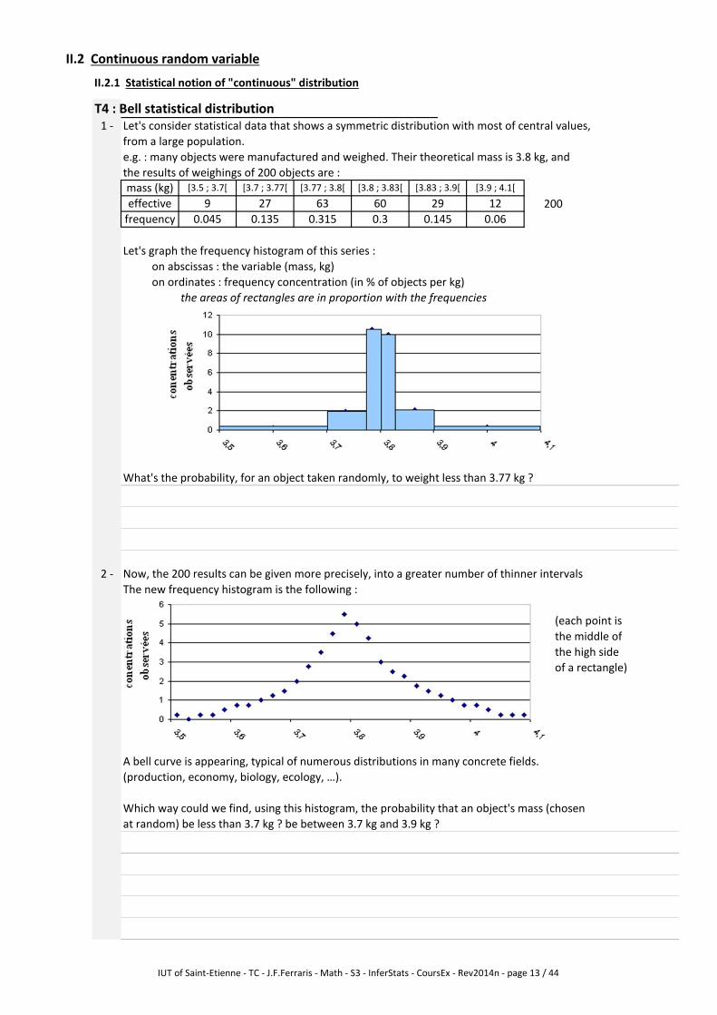
T4 : Bell statistical distribution
1 - Let's consider statistical data that shows a symmetric distribution with most of central values,
from a large population.
e.g. : many objects were manufactured and weighed. Their theoretical mass is 3.8 kg, and
the results of weighings of 200 objects are :
Let's graph the frequency histogram of this series :
on abscissas : the variable (mass, kg)
on ordinates : frequency concentration (in % of objects per kg)
the areas of rectangles are in proportion with the frequencies
What's the probability, for an object taken randomly, to weight less than 3.77 kg ?
2 - Now, the 200 results can be given more precisely, into a greater number of thinner intervals
The new frequency histogram is the following :
(each point is
the middle of
the high side
of a rectangle)
A bell curve is appearing, typical of numerous distributions in many concrete fields.
(production, economy, biology, ecology, …).
Which way could we find, using this histogram, the probability that an object's mass (chosen
at random) be less than 3.7 kg ? be between 3.7 kg and 3.9 kg ?
[3.83 ; 3.9[ [3.9 ; 4.1[
effective 9 27 20029 12
[3.7 ; 3.77[ [3.77 ; 3.8[ [3.8 ; 3.83[
0.135 0.315
63 60
[3.5 ; 3.7[
0.3 0.145 0.06frequency 0.045
mass (kg)
IUT of Saint-Etienne - TC - J.F.Ferraris - Math - S3 - InferStats - CoursEx - Rev2014n - page 13 / 44

3 - We could consider weighing far more than 200 pieces, and with far more accurate results.
The histogram could contain a large number of rectangles and would become difficult to draw
and to read ! The only useful graph would contain only a points cloud, that would actually follow
a bell-shaped curve, that could be modeled by a function f .
In this context, how would we calculate the probabilities asked above ?
Notice : many concrete distributions aren't symmetric (incomes, …), but they won't be studied here
IUT of Saint-Etienne - TC - J.F.Ferraris - Math - S3 - InferStats - CoursEx - Rev2014n - page 14 / 44
II.2.2 Continuous random variable
Let's take place into an ideal case where the random variable X can take any value
among real numbers, from an infinite population.
def We say that a random variable is continuous if the set of its possible values
is an interval I of R (maybe R itself).
Thus, the "frequency concentration" is now a "probability density".
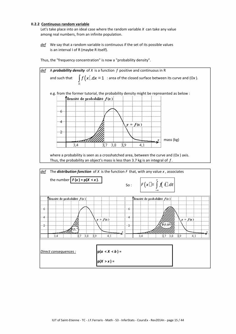
def A probability density of X is a function f positive and continuous in R
and such that : area of the closed surface between its curve and (Ox ).
e.g. from the former tutorial, the probability density might be represented as below :
mass (kg)
where a probability is seen as a crosshatched area, between the curve and (Ox ) axis.
Thus, the probability an object's mass is less than 3.7 kg is an integral of f .
def The distribution fonction of X is the function F that, with any value x , associates
the number F (x ) = p(X < x ).
So :
Direct consequences : p(a < X < b ) =
p(X > x ) =
( ).d 1f x x =∫ℝ
( ) ( ).dx
F x f t t−∞
= ∫
IUT of Saint-Etienne - TC - J.F.Ferraris - Math - S3 - InferStats - CoursEx - Rev2014n - page 15 / 44
II.3 Normal law (or Laplace's law)
As seen before, with a large population and a large number of measures on it (or of drawings),
many concrete phenomenons, and many discrete probability laws, can be modeled by typically
shaped probability densities.
These functions f have a general expression : with a > 0.
Their curves are "bell curves".
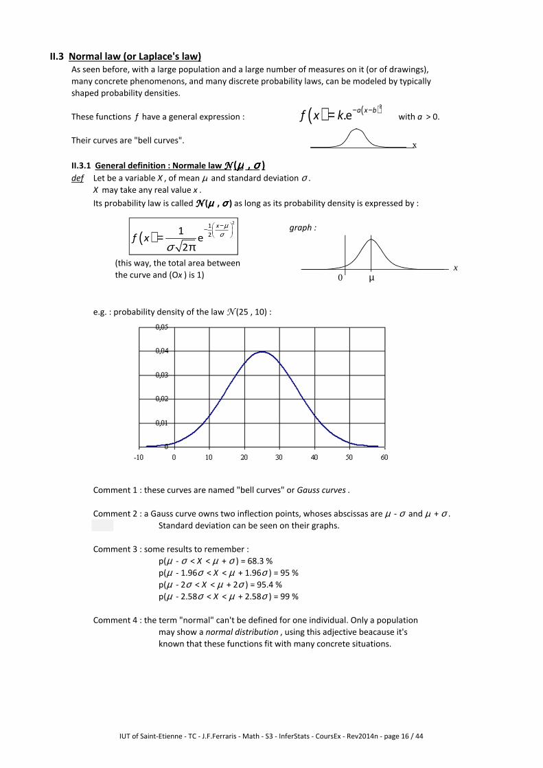
II.3.1 General definition : Normale law NNNN (µµµµ , σσσσ )
def Let be a variable X , of mean µ and standard deviation σ .
X may take any real value x .
Its probability law is called NNNN (µµµµ , σσσσ ) as long as its probability density is expressed by :
graph :
(this way, the total area between
the curve and (Ox ) is 1)
e.g. : probability density of the law N (25 , 10) :
Comment 1 : these curves are named "bell curves" or Gauss curves .
Comment 2 : a Gauss curve owns two inflection points, whoses abscissas are µ - σ and µ + σ .
Standard deviation can be seen on their graphs.
Comment 3 : some results to remember :
p(µ - σ < X < µ + σ ) = 68.3 %
p(µ - 1.96σ < X < µ + 1.96σ ) = 95 %
p(µ - 2σ < X < µ + 2σ ) = 95.4 %
p(µ - 2.58σ < X < µ + 2.58σ ) = 99 %
Comment 4 : the term "normal" can't be defined for one individual. Only a population
may show a normal distribution , using this adjective beacause it's
known that these functions fit with many concrete situations.
x
xµ0
( ) ( ).2
ea x b
f x k− −=
( )2
1
21e
2
x
f x
µσ
σ
− − =
π
IUT of Saint-Etienne - TC - J.F.Ferraris - Math - S3 - InferStats - CoursEx - Rev2014n - page 16 / 44
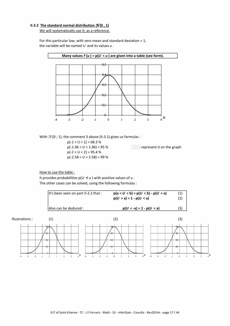
II.3.2 The standard normal distribution NNNN (0 , 1)
We will systematically use it, as a reference.
For this particular law, with zero mean and standard deviation = 1,
the variable will be named U and its values u .
With N (0 ; 1), the comment 3 above (II-3.1) gives us formulas :
p(-1 < U < 1) = 68.3 %
p(-1.96 < U < 1.96) = 95 % represent it on the graph
p(-2 < U < 2) = 95.4 %
p(-2.58 < U < 2.58) = 99 %
How to use the table :
It provides probabilities p(U < u ) with positive values of u .
The other cases can be solved, using the following formulas :
It's been seen on part II-2.2 that : p(a < U < b) = p(U < b) - p(U < a) (1)
p(U > a) = 1 - p(U < a) (2)
Also can be deduced : p(U < -a) = 1 - p(U < a) (3)
Illustrations : (1) (2) (3)
Many values F (u ) = p(U < u ) are given into a table (see form).
IUT of Saint-Etienne - TC - J.F.Ferraris - Math - S3 - InferStats - CoursEx - Rev2014n - page 17 / 44
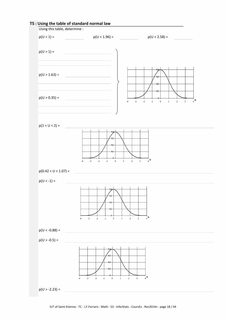
T5 : Using the table of standard normal law
Using this table, determine :
p(U < 1) = p(U < 1.96) = p(U < 2.58) =
p(U > 1) =
p(U > 1.63) =
p(U > 0.35) =
p(1 < U < 2) =
p(0.42 < U < 1.07) =
p(U < -1) =
p(U < -0.88) =
p(U > -0.5) =
p(U > -2.23) =
IUT of Saint-Etienne - TC - J.F.Ferraris - Math - S3 - InferStats - CoursEx - Rev2014n - page 18 / 44

p(-1.85 < U < -1.07) =
p(-1.12 < U < 0.6) =
II.3.3 Variable change : transition from NNNN (µµµµ , σσσσ ) to NNNN (0 , 1)
The standard normal law, with its table, is our only tool to get probabilities values.
In any case then, we'll have to translate our normal law into the law N (0 , 1).
prop Let be a random variable X , with mean µ and standard deviation σ, whose law is N (µ , σ ).
Then, the variable U = has a N (0 , 1) distribution.
Thus :
Whatever the variable (X ou U), the probability to be got is the crosshatched area.
e.g., the abscissa µ +2σ on X axis corresponds to the abscissa 2 on U axis (according to
the variable change) and then p(X < µ +2σ ) = p(U < 2).
X - µσ
xµ µ +σ µ +2σµ -σµ -2σ
( )p pX
X x Uµ
σ− < = <
IUT of Saint-Etienne - TC - J.F.Ferraris - Math - S3 - InferStats - CoursEx - Rev2014n - page 19 / 44
T6 : Calculate probabilities in a general case
Determine the asked probabilities, using the given normal distributions :
1 - law of X : N (50 , 10). Calculate p(X < 60), p(X < 43), p(45 < X < 55)
2 - law of X : N (3 , 0.45). Calculate p(X > 4), p(X < 2.55), p(3.2 < X < 3.7)
IUT of Saint-Etienne - TC - J.F.Ferraris - Math - S3 - InferStats - CoursEx - Rev2014n - page 20 / 44
II.4 Normal approximation of other laws
On part II-1, it's been stated that when n becomes a large number, the discrete laws become
close to the normal law.
So, we're allowed to use the normal law instead of one other, under the following conditions :
Approximation criterions for the replacement of a binomial law :
Starting with B (n , p ), if n > 30 and npq > 5,
then we can use N (µ , σ ) with µ = np and σ = √(npq )
Approximation criterions for the replacement of a Poisson's law :
Starting with P (λ ), if λ > 20,
then we can use N (µ , σ ) with µ = λ and σ = √λ
Probability of a single value :
Having a discrete case, in which variable X may only take natural values, for instance,
we could wish to calculate p(X = k).
However, the normal law is only able to calculate probabilities of inequalities.
In this case, the rule is :
Or : you can use a binomial
or a Poisson's law…
T7 : Approximations from other laws to normal law
Justify you can use a normal law, then calculate the probabilities :
1 - In a land, 30 % of the companies do exports. If we choose 80 companies at random,
what's the probability that more than 30 do exports ?
p(X = k ) = p(k - 0.5 < X < k + 0.5)
IUT of Saint-Etienne - TC - J.F.Ferraris - Math - S3 - InferStats - CoursEx - Rev2014n - page 21 / 44

What's the probability that exactly 30 companies do exports ?
2 - The number of items sold each day is distributed following a Poisson's law whose parameter is 25.
What's the probability that, one day, that less than 20 items would be sold ?
IUT of Saint-Etienne - TC - J.F.Ferraris - Math - S3 - InferStats - CoursEx - Rev2014n - page 22 / 44
III. Sampling distributions
III.1 Introduction
Do you know an operation where the entire population is surveyed ?
…to get several informations ?
Means deployed are huge. It takes more than a year to collect and analyse the whole
data set, and also an impressive number of surveyors to walk through the whole country.
Of course, this work can't be carried out for any survey…
By selecting a part of the population, you can get a pretty good representation of reality.
This selection, more or less "representative" to reality, is called sample.
Survey methods do exist, to build a sample as representative to the population as possible.
Our aim is, in this section, given an completely known population, to be able to tell how
its set of samples will surely behave.
Naming conventions :
Population's parameters will be written using greek alphabet :
mean : µ ; standard deviation : σ ; proportion : π
Sample's parameters will be written using our alphabet :
mean : x ; standard deviation : s ; proportion : p
III.2 Sampling distribution of means
Taking individuals from a population, we aim to study a random variable X .
Once chosen a natural number n , we can theoretically extract every n -sized sample.
we are able to calculate the mean of sample # k.
def We name mean random variable of n-sized samples the variable whose values
are the different means of n -sized samples.
def We name sampling distribution of means the distribution of the list of values ,
i.e. the probability law of variable .
theorem
Let consider a big population, on which is studied a quantitative variable X ,
normally distributed, whose mean is µ and standard deviation σ .
So, the law of is N (on EAS*)
* see next page
or N (on exhaustive sampling*)
Comment 1 : in case N > 20n (little sample compared to the population),
we can approximate the coefficient as if it were equal to 1, and so erase it.
Comment 2 : in an exercice, if no comparison between N and n is possible, then we will consider
that we have an EAS case.
Comment 3 : consequence of the "central limit" theorem
When N tends to infinity (concretely : when the population is very big), the probability law
of is normal, whatever the probability law of X .
kx
kx
X
Xk
x
X ;n
σµ
;1
N n
Nn
σµ − −
1
N n
N
−−
X
IUT of Saint-Etienne - TC - J.F.Ferraris - Math - S3 - InferStats - CoursEx - Rev2014n - page 23 / 44
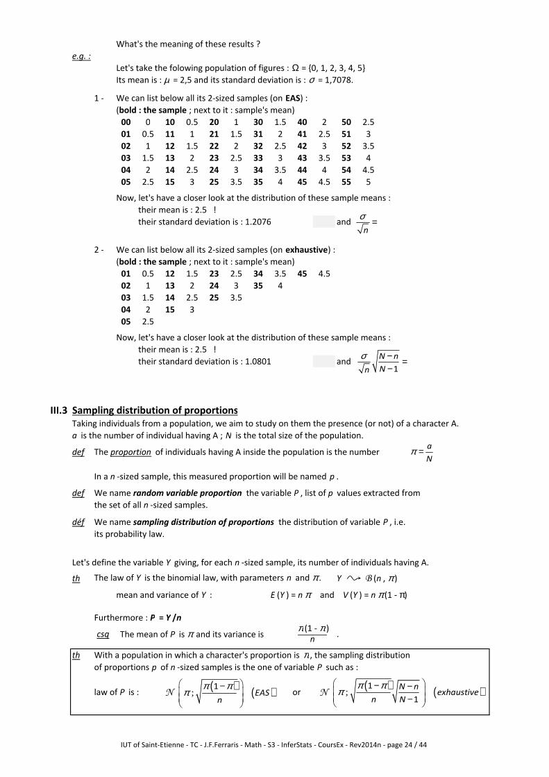
What's the meaning of these results ?
e.g. :
Let's take the folowing population of figures : Ω = 0, 1, 2, 3, 4, 5
Its mean is : µ = 2,5 and its standard deviation is : σ = 1,7078.
1 - We can list below all its 2-sized samples (on EAS) :
(bold : the sample ; next to it : sample's mean)
00 0 10 0.5 20 1 30 1.5 40 2 50 2.5
01 0.5 11 1 21 1.5 31 2 41 2.5 51 3
02 1 12 1.5 22 2 32 2.5 42 3 52 3.5
03 1.5 13 2 23 2.5 33 3 43 3.5 53 4
04 2 14 2.5 24 3 34 3.5 44 4 54 4.5
05 2.5 15 3 25 3.5 35 4 45 4.5 55 5
Now, let's have a closer look at the distribution of these sample means :
their mean is : 2.5 !
their standard deviation is : 1.2076 and
2 - We can list below all its 2-sized samples (on exhaustive) :
(bold : the sample ; next to it : sample's mean)
01 0.5 12 1.5 23 2.5 34 3.5 45 4.5
02 1 13 2 24 3 35 4
03 1.5 14 2.5 25 3.5
04 2 15 3
05 2.5
Now, let's have a closer look at the distribution of these sample means :
their mean is : 2.5 !
their standard deviation is : 1.0801 and
III.3 Sampling distribution of proportions
Taking individuals from a population, we aim to study on them the presence (or not) of a character A.
a is the number of individual having A ; N is the total size of the population.
def The proportion of individuals having A inside the population is the number
In a n -sized sample, this measured proportion will be named p .
def We name random variable proportion the variable P , list of p values extracted from
the set of all n -sized samples.
déf We name sampling distribution of proportions the distribution of variable P , i.e.
its probability law.
Let's define the variable Y giving, for each n -sized sample, its number of individuals having A.
th The law of Y is the binomial law, with parameters n and π . Y B (n , π )
mean and variance of Y : E (Y ) = n π and V (Y ) = n π (1 - π)
Furthermore : P = Y /n
th With a population in which a character's proportion is π , the sampling distribution
of proportions p of n -sized samples is the one of variable P such as :
law of P is : N or N
csq The mean of P is π and its variance isπ (1 - π )
.n
n
σ =
1
N n
Nn
σ − =−
a
Nπ =
( ) ( );1
EASn
π ππ −
( ) ( );1
1
N nexhaustive
n N
π ππ − − −
IUT of Saint-Etienne - TC - J.F.Ferraris - Math - S3 - InferStats - CoursEx - Rev2014n - page 24 / 44
T8 : Sampling distributions
1 - From a normal population - mean 120, standard deviation 40 - are taken every EAS of sizes
n = 10 and n = 50.
a. What are the laws of sampling distributions of means of 10-sized samples ? 50 ?
b. Quickly draw these two distributions on the same graph.
c. What's the probability that the mean of a random 10-sized sample would be more than 130 ?
d. Same question for a 50-sized sample.
2 - In the world's population, severa years ago, were 3.38 billion women and 3.12 billion men.
P is the variable giving the proportion of women in every sample of 100 persons.
a. What is the probability law of P ?
b. What is the probability that, in a sample, there would be more men than women ?
IUT of Saint-Etienne - TC - J.F.Ferraris - Math - S3 - InferStats - CoursEx - Rev2014n - page 25 / 44
IUT of Saint-Etienne – TC –J.F.Ferraris – Math – S3 – InferStats – CoursEx – Rev2014n – page 26 / 44
IV. Estimation Problematic
A large population is to be studied. It’s partially or totally unknown. A unique n-sized sample is
taken from it. To what extent does this sample represent the whole population ? The available
informations taken from this sample are they reliable in order to estimate the reality of the
unknown population ?
As it’s a large population, we will systematically consider SRS samples.
IV.1 Point estimates
A ^ will be placed upon an unknown parameter to express an estimation of it.
IV.1.1 Estimate of a mean, of a proportion
th x is a point estimate of µ. ˆ xµ =
1
1 n
i
i
X Xn =
= ∑ is an unbiased estimator of µ, i.e. : its expected value is µ.
(indeed, we noticed on part III that the mean of the means of samples was µ)
th p is a point estimate of π. ˆ pπ =
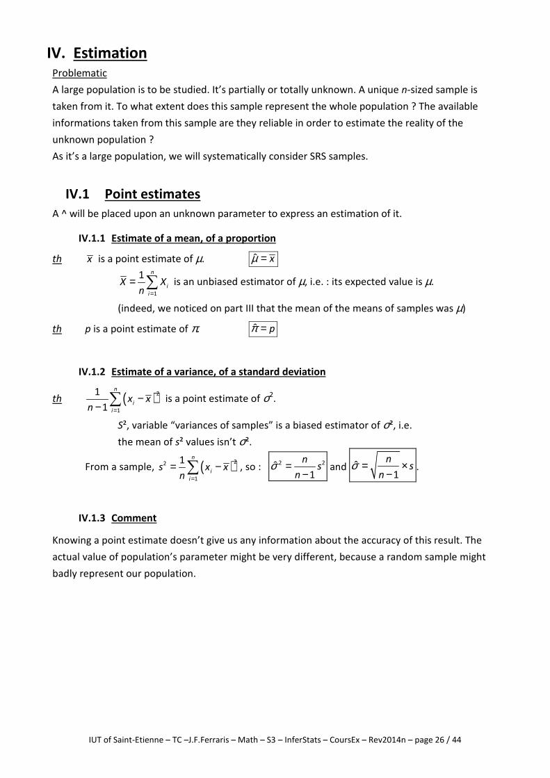
IV.1.2 Estimate of a variance, of a standard deviation
th ( )2
1
1
1
n
i
i
x xn =
−− ∑ is a point estimate of σ2
.
S², variable “variances of samples” is a biased estimator of σ², i.e.
the mean of s² values isn’t σ².
From a sample, ( )22
1
1 n
i
i
s x xn =
= −∑ , so : ˆ 2 2
1
ns
nσ =
− and ˆ
1
ns
nσ = ×
−.
IV.1.3 Comment
Knowing a point estimate doesn’t give us any information about the accuracy of this result. The
actual value of population’s parameter might be very different, because a random sample might
badly represent our population.
IUT of Saint-Etienne – TC –J.F.Ferraris – Math – S3 – InferStats – CoursEx – Rev2014n – page 27 / 44
IV.2 Estimation of µµµµ by a confidence interval
Confidence intervals were created to give an answer to the question raised in the former
comment. For instance, around a sample’s mean we’ll build an interval “having 95% chances to
include µ ”. The building method of this interval actually depends on the knowledge of σ.
def We name significance level, αααα, the probability that the interval does not include µ.
We name confidence level, 1 - αααα, the probability that the interval includes µ.
Two values of α are commonly used : 5% and 1%, which means a 95% or a 99% confidence level.
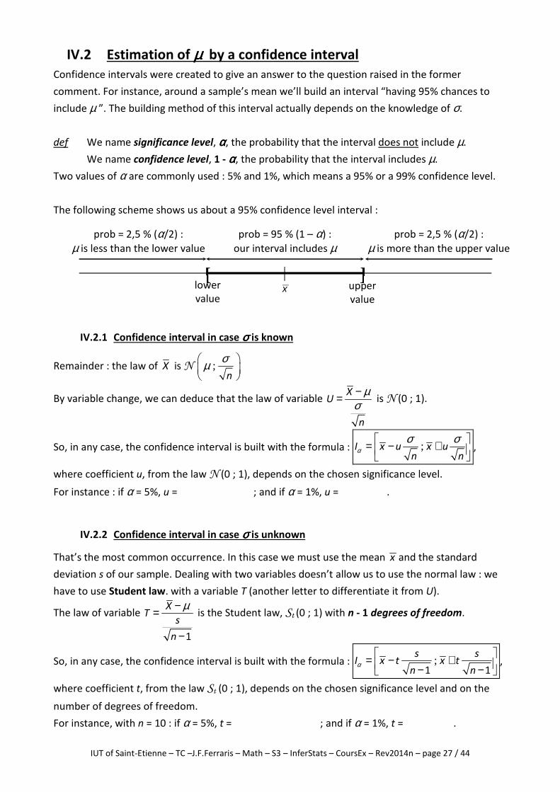
The following scheme shows us about a 95% confidence level interval :
IV.2.1 Confidence interval in case σσσσ is known
Remainder : the law of X is N ;n
σµ
By variable change, we can deduce that the law of variable X
U
n
µσ−= is N (0 ; 1).
So, in any case, the confidence interval is built with the formula : ;I x u x un n
ασ σ = − +
,
where coefficient u, from the law N (0 ; 1), depends on the chosen significance level.
For instance : if α = 5%, u = ; and if α = 1%, u = .
IV.2.2 Confidence interval in case σσσσ is unknown
That’s the most common occurrence. In this case we must use the mean x and the standard
deviation s of our sample. Dealing with two variables doesn’t allow us to use the normal law : we
have to use Student law. with a variable T (another letter to differentiate it from U).
The law of variable
1
XT
s
n
µ−=
−
is the Student law, St (0 ; 1) with n - 1 degrees of freedom.
So, in any case, the confidence interval is built with the formula : ;1 1
s sI x t x t
n nα
= − + − − ,
where coefficient t, from the law St (0 ; 1), depends on the chosen significance level and on the
number of degrees of freedom.
For instance, with n = 10 : if α = 5%, t = ; and if α = 1%, t = .
[ ]
prob = 95 % (1 – α) :
our interval includes µ
prob = 2,5 % (α/2) :
µ is less than the lower value
lower
value
upper
value
prob = 2,5 % (α/2) :
µ is more than the upper value
IUT of Saint-Etienne – TC –J.F.Ferraris – Math – S3 – InferStats – CoursEx – Rev2014n – page 28 / 44
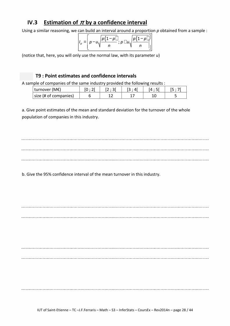
IV.3 Estimation of ππππ by a confidence interval
Using a similar reasoning, we can build an interval around a proportion p obtained from a sample :
( ) ( );
1 1p p p pI p u p u
n nα
− −= − +
(notice that, here, you will only use the normal law, with its parameter u)
T9 : Point estimates and confidence intervals
A sample of companies of the same industry provided the following results :
turnover (M€) [0 ; 2[ [2 ; 3[ [3 ; 4[ [4 ; 5[ [5 ; 7[
size (# of companies) 6 12 17 10 5
a. Give point estimates of the mean and standard deviation for the turnover of the whole
population of companies in this industry.
b. Give the 95% confidence interval of the mean turnover in this industry.

IUT of Saint-Etienne – TC –J.F.Ferraris – Math – S3 – InferStats – CoursEx – Rev2014n – page 29 / 44
c. Give a point estimate of the proportion of companies whose turnover is more than 4.5 M€.
b. Give the 99% confidence interval of this proportion in this industry.
IUT of Saint-Etienne – TC –J.F.Ferraris – Math – S3 – InferStats – CoursEx – Rev2014n – page 30 / 44
V. Statistical hypothesis testing On knowing one sample from an unknown population, we can word a hypothesis : an assumption
that we want to test. A suitable statistical test will, or won’t, permit us to reject the tested
hypothesis, named null hypothesis, H0.
In many tests, an alternative hypothesis, H1, has to be worded too.
We name significance level of a test the chance, α, we would be wrong on rejecting H0.
The value 1 – α is then the confidence level of the test.
Here, we’ll only deal with two kinds of tests :
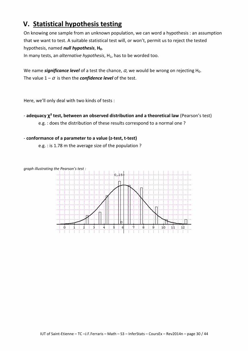
- adequacy χχχχ² test, between an observed distribution and a theoretical law (Pearson’s test)
e.g. : does the distribution of these results correspond to a normal one ?
- conformance of a parameter to a value (z-test, t-test)
e.g. : is 1.78 m the average size of the population ?
graph illustrating the Pearson’s test :
IUT of Saint-Etienne – TC –J.F.Ferraris – Math – S3 – InferStats – CoursEx – Rev2014n – page 31 / 44
V.1 χχχχ² test of adequacy between a distribution and a law
The null hypothesis H0 has to be : “there’s a perfect adequacy between them”.
Our aim is to know if it’s risky or not to reject H0. (this risk α – to be wrong rejecting it - will be
chosen ; on the other side, the risk (β) to be wrong accepting H0 can’t be known).
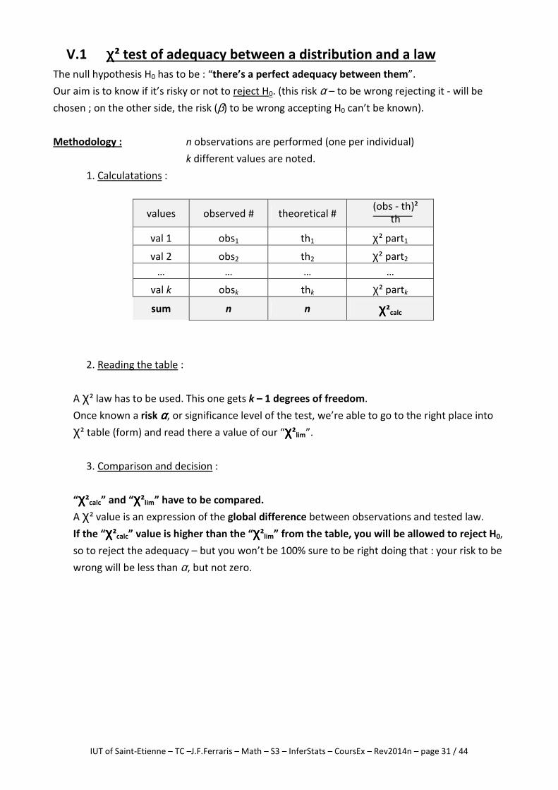
Methodology : n observations are performed (one per individual)
k different values are noted.
1. Calculatations :
values observed # theoretical #
val 1 obs1 th1 χ² part1
val 2 obs2 th2 χ² part2
… … … …
val k obsk thk χ² partk
sum n n χχχχ²calc
2. Reading the table :
A χ² law has to be used. This one gets k – 1 degrees of freedom.
Once known a risk αααα, or significance level of the test, we’re able to go to the right place into
χ² table (form) and read there a value of our “χχχχ²lim”.
3. Comparison and decision :
“χχχχ²calc” and “χχχχ²lim” have to be compared.
A χ² value is an expression of the global difference between observations and tested law.
If the “χχχχ²calc” value is higher than the “χχχχ²lim” from the table, you will be allowed to reject H0,
so to reject the adequacy – but you won’t be 100% sure to be right doing that : your risk to be
wrong will be less than α, but not zero.
(obs - th)² th

IUT of Saint-Etienne – TC –J.F.Ferraris – Math – S3 – InferStats – CoursEx – Rev2014n – page 32 / 44
T10 : adequacy χχχχ² test
120 throws of a same die have been performed. The table below shows the results.
Considering this sample of results, can we say this die is not a fake one, with a 2%
significance level ?
result 1 2 3 4 5 6
observed # of throws 26 15 14 24 25 16
theor. # of throws
(obs - th)²
th
IUT of Saint-Etienne – TC –J.F.Ferraris – Math – S3 – InferStats – CoursEx – Rev2014n – page 33 / 44
V.2 Conformance testing of a mean, of a proportion
V.2.1 Principle
Given a data set of n observations, from a sample, we have to decide wether a value µ0 can, or
can’t, correspond to the mean of the population (same expectations for a value π0 representing a
proportion).
Thus, the null hypothesis is H0 : µ = µ0 (or π = π0)
Following the situation, the alternative hypothesis can be :
H1 : µ ≠ µ0 (two-sided test)
H1 : µ < µ0 (one-sided test) or H1 : µ > µ0 (another one-sided test)
H0 will be rejected if the sample’s mean x (or the sample’s proportion p) is far enough from the
tested value µ0 (or π0).
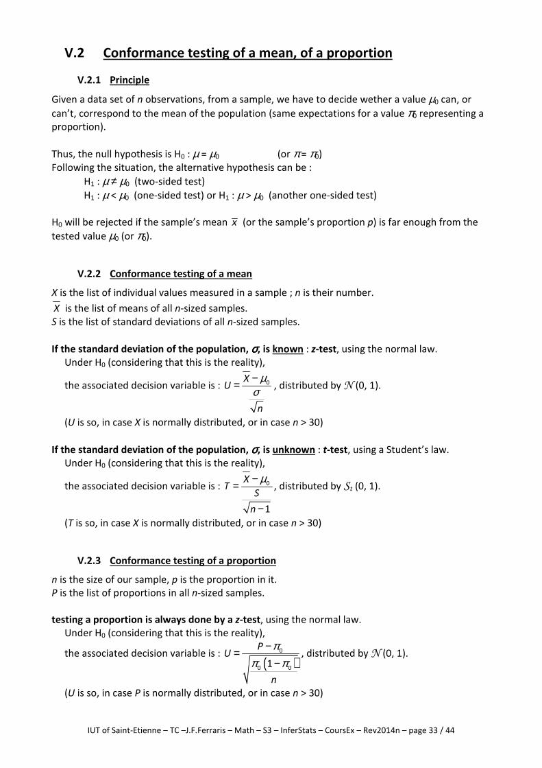
V.2.2 Conformance testing of a mean
X is the list of individual values measured in a sample ; n is their number.
X is the list of means of all n-sized samples.
S is the list of standard deviations of all n-sized samples.
If the standard deviation of the population, σσσσ, is known : z-test, using the normal law.
Under H0 (considering that this is the reality),
the associated decision variable is : 0XU
n
µσ−= , distributed by N (0, 1).
(U is so, in case X is normally distributed, or in case n > 30)
If the standard deviation of the population, σσσσ, is unknown : t-test, using a Student’s law.
Under H0 (considering that this is the reality),
the associated decision variable is : 0
1
XT
S
n
µ−=
−
, distributed by St (0, 1).
(T is so, in case X is normally distributed, or in case n > 30)
V.2.3 Conformance testing of a proportion
n is the size of our sample, p is the proportion in it.
P is the list of proportions in all n-sized samples.
testing a proportion is always done by a z-test, using the normal law.
Under H0 (considering that this is the reality),
the associated decision variable is : ( )
0
0 01
PU
n
ππ π
−=−
, distributed by N (0, 1).
(U is so, in case P is normally distributed, or in case n > 30)
IUT of Saint-Etienne – TC –J.F.Ferraris – Math – S3 – InferStats – CoursEx – Rev2014n – page 34 / 44
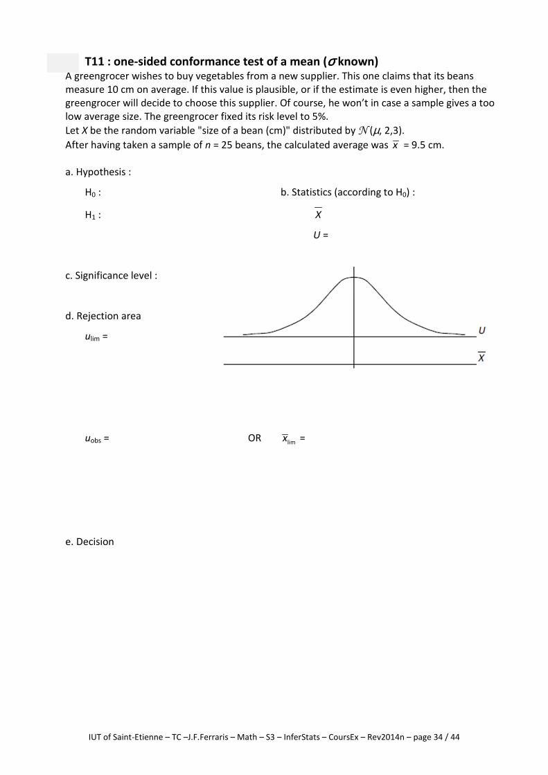
T11 : one-sided conformance test of a mean (σσσσ known) A greengrocer wishes to buy vegetables from a new supplier. This one claims that its beans
measure 10 cm on average. If this value is plausible, or if the estimate is even higher, then the
greengrocer will decide to choose this supplier. Of course, he won’t in case a sample gives a too
low average size. The greengrocer fixed its risk level to 5%.
Let X be the random variable "size of a bean (cm)" distributed by N (µ, 2,3).
After having taken a sample of n = 25 beans, the calculated average was x = 9.5 cm.
a. Hypothesis :
H0 : b. Statistics (according to H0) :
H1 : X
U =
c. Significance level :
d. Rejection area
ulim =
uobs = OR limx =
e. Decision
IUT of Saint-Etienne – TC –J.F.Ferraris – Math – S3 – InferStats – CoursEx – Rev2014n – page 35 / 44
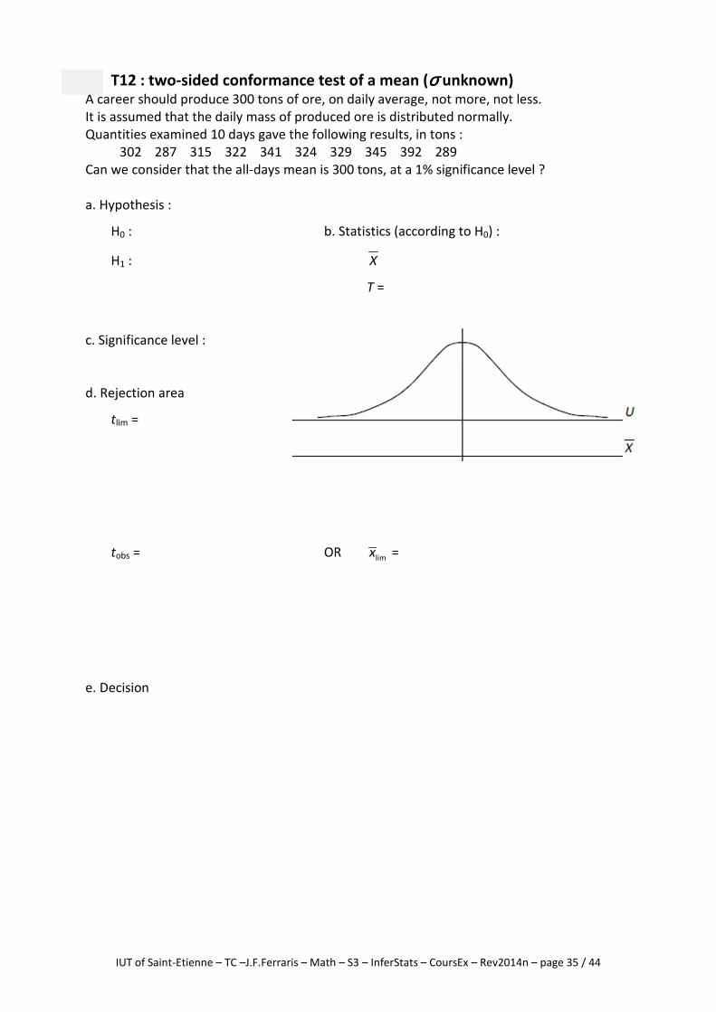
T12 : two-sided conformance test of a mean (σσσσ unknown) A career should produce 300 tons of ore, on daily average, not more, not less.
It is assumed that the daily mass of produced ore is distributed normally.
Quantities examined 10 days gave the following results, in tons :
302 287 315 322 341 324 329 345 392 289
Can we consider that the all-days mean is 300 tons, at a 1% significance level ?
a. Hypothesis :
H0 : b. Statistics (according to H0) :
H1 : X
T =
c. Significance level :
d. Rejection area
tlim =
tobs = OR limx =
e. Decision
IUT of Saint-Etienne – TC –J.F.Ferraris – Math – S3 – InferStats – CoursEx – Rev2014n – page 36 / 44
EXERCISES
I. DISCRETE LAWS
Exercise 1
A supermarket sells 24 fruit species, counting 8 “bio” label. A blind control consists in choosing 10
fruits of different species. The variable X gives the number of “bio” species among these 10.
1. Give, with explanations, the probability law of X.
2. Calculate its expected value and standard deviation.
3. What is the probability that less than two “bio” species would be chosen ?
Exercise 2
A car driver meets five signal lights on his way. They share the same duration of red and green
lightening : 40 seconds green and 20 seconds red. Unfortunately, they are not synchronized, so
that the color of one light is independent of the color of another one.
1. When approaching the first light, what’s the probability it will be green ?
2. What’s the probability that the lights will all be green ?
3. What’s the probability that at least two lights will be red ?
4. What’s the mean expected number of green lights driving this way ?
Exercise 3
The germination capacity of a seed is 0.8 (probability to germinate).
1. 8 seeds are sown. Calculate the probabilities of the following events :
a. exactly 5 seeds will germinate.
b. At least 7 seeds will germinate.
2. When a seed has germinated, the probability that a slug eats the young plant is 0.4.
a. Calculate the probability that a seed will finally become a grown plant.
b. How many seeds must be sown to get more than 99% chances of getting at least
one grown plant ?
Exercise 4
According to a survey, 80% of the customers of a product “A” are satisfied.
Choosing randomly 10 customers of this product, what’s the probability that…
a. they’re all satisfied ?
b. 80% of them are satisfied ?
c. at least 80% are satisfied ?
Exercise 5
6% of French people are clients of the mobile phoning operator “Yellow”.
A survey consists in asking to 50 randomly chosen French people which is their mobile phoning
operator. The variable X gives the number of “Yellow” clients among these 50 people.
IUT of Saint-Etienne – TC –J.F.Ferraris – Math – S3 – InferStats – CoursEx – Rev2014n – page 37 / 44
1. a. Justify and give the probability law of X.
b. What are the chances that the population proportion of clients would be the same
into the sample ?
c. What is special with this former probability ?
d. What’s the probability that none of the 50 people would be a “Yellow” client ?
e. What’s the probability that there would be at least 4 “Yellow” clients ?
2. In this part, the number of persons to call is still unknown. How many people would have
to be called, to get more than 99% chances finding at least one “Yellow” client ?
Exercise 6
The shop “HighTech” sells computers. The variable number of daily sales is distributed like a
Poisson’s law whose parameter is 4. Calculate the probability that the next day…
a. No computer would be sold
b. At least one computer would be sold
c. Exactly 2 computers would be sold.
Exercise 7 (determine X, n, p and justify the use of a Poisson’s law)
On a survey implying a large number of persons, only 2% of them accept to give their name.
Given that one of the investigators has to interview 250 people, calculate the probability that…
a. All these people won’t give their name.
b. At least 5 people will give their name.
Exercise 8
A box contains 250 matches. It has been exposed to moisture, so that 20% of matches won’t
lighten. Taking at random 10 matches, the variable X gives the number of matches that will
lighten.
1. Demonstrate that the law of X is binomial and give its parameters and expected value.
2. Calculate the following probabilities :
a. No match will lighten
b. They will all lighten
c. At least 3 won’t lighten
3. a. Look again for the above probabilities, this time using a Poisson’s law.
b. Explain the differences of your answers between questions 2 and 3.
Exercise 9
In a large population are met on average 0.4% of blind people.
1. Into a sample of 100 people, what’s the probability there’s no blind people ? at least 2 ?
2. Answer these questions using the correct Poisson’s law (justify its use).
IUT of Saint-Etienne – TC –J.F.Ferraris – Math – S3 – InferStats – CoursEx – Rev2014n – page 38 / 44
II. NORMAL LAW
Exercise 10 (with solutions)
It’s been stated that the variable X “mass (kg) of a newborn baby” is distributed by the law
N (3.1 ; 0.5).
1. What’s the probability that a newborn baby weights more than 4 kg ?
variable change : U = (X – 3.1)/0.5 is distributed by the standard normal law N (0 ; 1).
our U value : u = (4 – 3.1)/0.5 = 1.8 ; from the table : F(1.8) = p(U < 1.8) = 0.9641.
our answer : p(X > 4 kg) = p(U > 1.8) = 1 – 0.9641 = 0.0359.
2. What’s the probability that a newborn baby weights less than 3 kg ?
variable change : U = (X – 3.1)/0.5 is distributed by the standard normal law N (0 ; 1).
our U value : u = (3 – 3.1)/0.5 = -0.2 ; from the table : F(0.2) = p(U < 0.2) = 0,5793.
our answer : p(X < 3 kg) = p(U < -0.2) = 1 - p(U < 0.2) = 1 - 0.5793 = 0.4207.
3. What’s the probability that a newborn baby’s weight is between 3 and 4 kg ?
interval formula : p(a < X < b) = p(X < b) – p(X < a).
our answer : p(3 < X < 4) = p(X < 4) – p(X < 3) = 0.9641 – 0.4207 = 0.5434.
Exercise 11
1. The variable U is distributed by the standard normal law N (0 ; 1).
a. Calculate : * p(U < 0.86) * p(U > 1.96) * p(U > -1.39) * p(-0.63 < U < 0.63)
b. Give the value u0 such that : * p(U < u0) = 0.8944 * p(-u0 < U < u0) = 0.98
2. The variable X is distributed by the normal law N (25 ; 7).
a. Calculate : * p(X > 35.5) * p(X < 18)
b. Give the value x0 such that : p(X > x0) = 0.0516
Exercise 12
A company manufactures beacons (flashing lights) for all types of machines, in large quantities.
The probability that a beacon is defective is p = 0.04.
A random sample of 600 beacons is taken from the production. X is the random variable that gives
the number of defective beacons among the 600.
1. Show that the random variable X is a binomial distribution whose parameters are to be
specified.
2. Show that we can approximate the distribution of X by a normal distribution.
3. Determine µ and σ, mean and standard deviation of the variable X for the normal
distribution.
4. Then calculate with precision allowed by the tables, the probability of having at least 27
defective flashing lights in the drawing of 600 beacons.
IUT of Saint-Etienne – TC –J.F.Ferraris – Math – S3 – InferStats – CoursEx – Rev2014n – page 39 / 44
Exercise 13
A commercial agent is assigned to telephone solicitations. On average, one in five (phone calls)
leads to appeal an order.
1. We name X the random variable “number of past commands after 60 calls”.
a. Give the name and the parameters of the probability distribution of X.
b. Justify that the law can be approximated by a normal distribution, giving its
parameters.
c. Using the normal distribution, calculate the following probabilities :
* p(X > 15) * p(X < 10) * p(X = 12)
2. Find out the minimum number of phone calls that must be passed by the sales agent so
that his chances to get at least 15 orders are more than 75%.
Exercise 14
It is assumed that on average you’re checked once in 20 in the bus by a controller. M.A makes 800
trips a year on the line.
1. What is the probability that M.A. would be checked between 30 and 50 times a year?
2. M.A always travels without a ticket. An annual subscription would be 320 € / year.
At what height must the company fix the fine, so that at least 75% of cheaters would better
take an annual subscription ? 99% ?
III. SAMPLING
Exercise 15
In a production of light bulbs, it is assumed that the lifetime of a bulb is a normal random variable
in which mean is 900 hours and standard deviation 80 hours. Calculate the probability that in a
random sample of 100 bulbs (SRS), the average lifetime of bulbs exceeds 910 hours.
Exercise 16
A candidate obtained 55% of votes cast in an election.
1. What is the probability that, in a sample of 100 people, his result be less than 50% ?
2. Same question for a sample of 2000 people.
3. How many people do we have to take so as the probability that less than 50% of them
voted for him drops below 1% ?
IUT of Saint-Etienne – TC –J.F.Ferraris – Math – S3 – InferStats – CoursEx – Rev2014n – page 40 / 44
Exercise 17
In one region, during the summer period, it is assumed that the number of tourists present in a
day follows a normal distribution witch mean is 50,000 and standard deviation 8,000.
1. The prefecture estimated that tourism is "manageable" (reception, environment,
pollution, ...) when the probability to receive less than 55,000 people in a day exceeds 70%.
Is this the case?
2. Officials want to base their thinking on using samples of 10 vacation days.
a. What is the law of X : "Average daily number of vacationers in a sample of 10 days" ?
b. What is the probability that, in such a sample, the average daily number of tourists
is less than 55,000 ?
Exercise 18 (with solutions)
An elevator can carry a load of 580 kg. It is assumed that the mass - of a person chosen at random
among the users of the elevator, expressed in kilograms - is a random variable following a normal
distribution N(µ, σ) with µ = 70 kg and σ = 16 kg.
What is the maximum number of persons that may be permitted to be together in the elevator if
you want the risk of overload does not exceed 0.01 ?
Consider a sample of n (unknown) people in this elevator. There is an overload if the total
mass (variable X) exceeds 580 kg. The average mass of the sample is distributed following
N (70 ; 16/√n) and the total mass is the product of the average mass by n.
Hence, the distribution of the total mass is N (70n ; 16√n).
Variable change : U = (X - 70n)/16√n follows N (0 ; 1).
We aim that p(X > 580) = 0.01, and on the other side, we know that p(U > 2.33) = 0.01.
So, we must have .580 70
2 3316
n
n
− = (and even > 2.33), and then .70 37 28 580 0n n+ − = .
We can solve this equation as a quadratic one (∆, …) or we can test several values of n :
the conclusion is n < 7. For this elevator will be displayed : “6 people maximum”.
Exercise 19
A large population took an IQ test. The results are normally distributed with µ = 102 and σ = 15.
1. What’s the proportion of people whose IQ is less than 100 ?
2. We want to analyze the results of a few samples of this population. For this, we form
groups of 20 individuals selected by simple random sampling (SRS), and the average IQ of
each group will be calculated.
a. Give the parameters of the normal distribution of IQ means of all 20-sized samples.
b. What is the probability that our selected group has an average IQ below 100 ?
c. Instead of 20, how many people would we have to choose to be less than 5% chance
that the average IQ of this new group is below 100 ?
3. Using the answer of question 1, what is the probability that in a group of 20 people, the
proportion (of individuals whose IQ is less than 100) is more than 50 % ?
IUT of Saint-Etienne – TC –J.F.Ferraris – Math – S3 – InferStats – CoursEx – Rev2014n – page 41 / 44
IV. ESTIMATION
Exercise 20
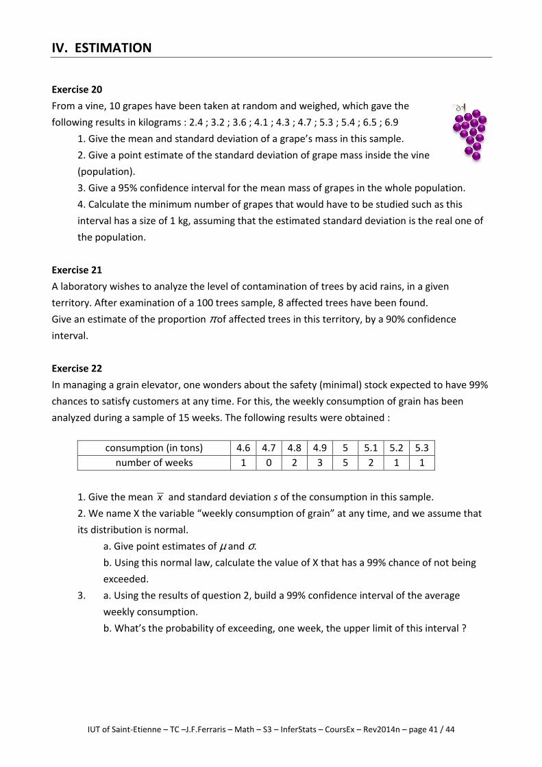
From a vine, 10 grapes have been taken at random and weighed, which gave the
following results in kilograms : 2.4 ; 3.2 ; 3.6 ; 4.1 ; 4.3 ; 4.7 ; 5.3 ; 5.4 ; 6.5 ; 6.9
1. Give the mean and standard deviation of a grape’s mass in this sample.
2. Give a point estimate of the standard deviation of grape mass inside the vine
(population).
3. Give a 95% confidence interval for the mean mass of grapes in the whole population.
4. Calculate the minimum number of grapes that would have to be studied such as this
interval has a size of 1 kg, assuming that the estimated standard deviation is the real one of
the population.
Exercise 21
A laboratory wishes to analyze the level of contamination of trees by acid rains, in a given
territory. After examination of a 100 trees sample, 8 affected trees have been found.
Give an estimate of the proportion π of affected trees in this territory, by a 90% confidence
interval.
Exercise 22
In managing a grain elevator, one wonders about the safety (minimal) stock expected to have 99%
chances to satisfy customers at any time. For this, the weekly consumption of grain has been
analyzed during a sample of 15 weeks. The following results were obtained :
consumption (in tons) 4.6 4.7 4.8 4.9 5 5.1 5.2 5.3
number of weeks 1 0 2 3 5 2 1 1
1. Give the mean x and standard deviation s of the consumption in this sample.
2. We name X the variable “weekly consumption of grain” at any time, and we assume that
its distribution is normal.
a. Give point estimates of µ and σ.
b. Using this normal law, calculate the value of X that has a 99% chance of not being
exceeded.
3. a. Using the results of question 2, build a 99% confidence interval of the average
weekly consumption.
b. What’s the probability of exceeding, one week, the upper limit of this interval ?
IUT of Saint-Etienne – TC –J.F.Ferraris – Math – S3 – InferStats – CoursEx – Rev2014n – page 42 / 44
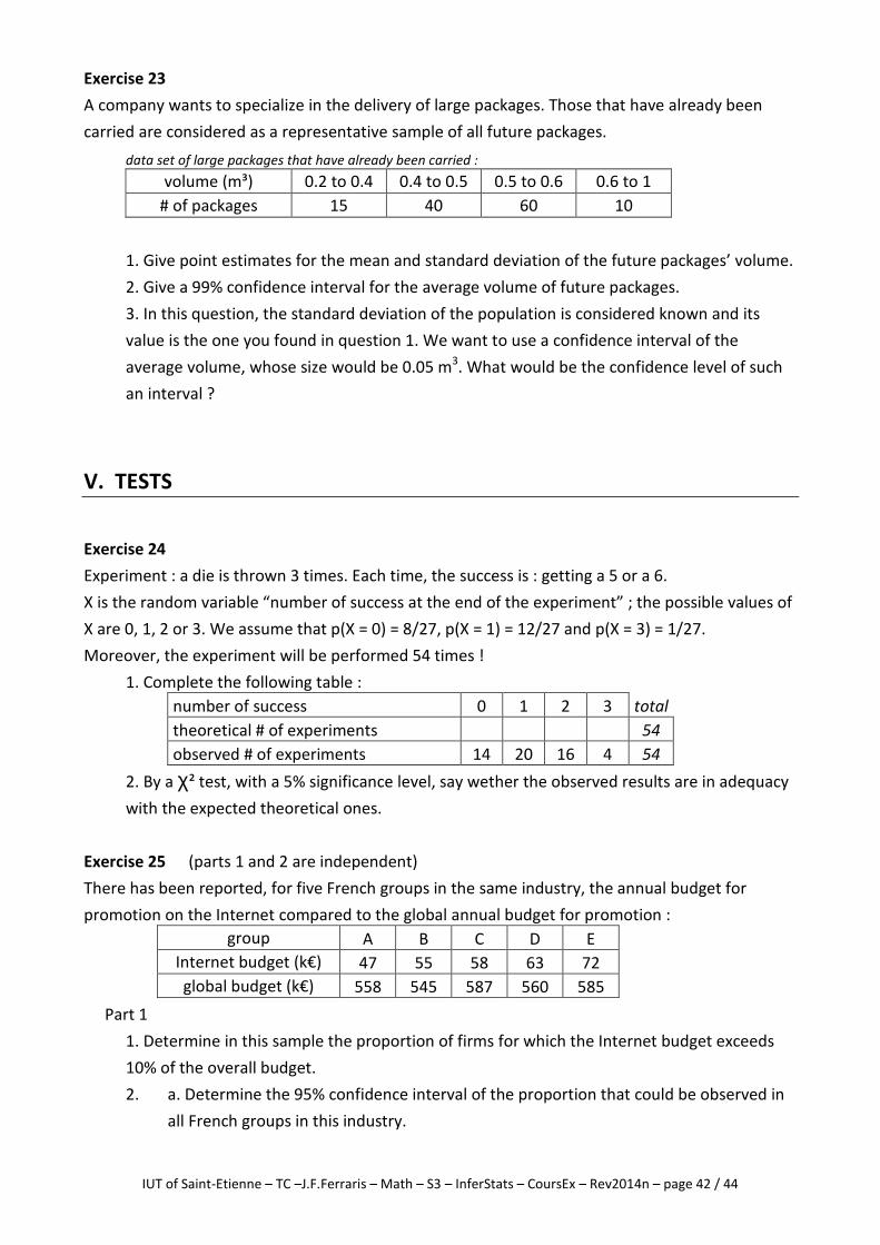
Exercise 23
A company wants to specialize in the delivery of large packages. Those that have already been
carried are considered as a representative sample of all future packages.
data set of large packages that have already been carried :
volume (m³) 0.2 to 0.4 0.4 to 0.5 0.5 to 0.6 0.6 to 1
# of packages 15 40 60 10
1. Give point estimates for the mean and standard deviation of the future packages’ volume.
2. Give a 99% confidence interval for the average volume of future packages.
3. In this question, the standard deviation of the population is considered known and its
value is the one you found in question 1. We want to use a confidence interval of the
average volume, whose size would be 0.05 m3. What would be the confidence level of such
an interval ?
V. TESTS
Exercise 24
Experiment : a die is thrown 3 times. Each time, the success is : getting a 5 or a 6.
X is the random variable “number of success at the end of the experiment” ; the possible values of
X are 0, 1, 2 or 3. We assume that p(X = 0) = 8/27, p(X = 1) = 12/27 and p(X = 3) = 1/27.
Moreover, the experiment will be performed 54 times !
1. Complete the following table :
number of success 0 1 2 3 total
theoretical # of experiments 54
observed # of experiments 14 20 16 4 54
2. By a χ² test, with a 5% significance level, say wether the observed results are in adequacy
with the expected theoretical ones.
Exercise 25 (parts 1 and 2 are independent)
There has been reported, for five French groups in the same industry, the annual budget for
promotion on the Internet compared to the global annual budget for promotion :
group A B C D E
Internet budget (k€) 47 55 58 63 72
global budget (k€) 558 545 587 560 585
Part 1
1. Determine in this sample the proportion of firms for which the Internet budget exceeds
10% of the overall budget.
2. a. Determine the 95% confidence interval of the proportion that could be observed in
all French groups in this industry.
IUT of Saint-Etienne – TC –J.F.Ferraris – Math – S3 – InferStats – CoursEx – Rev2014n – page 43 / 44
b. This industry actually consists of 58 groups in France. What is the minimal number,
that can be assumed with a confidence level of 80%, of groups whose internet budget
exceeds 10% of their overall budget?
Part 2
Perform a Khi-squared test to tell, with a significance level of 5%, if the data observed for
these five companies are in adequacy with the following assertion : “in France, Internet
budget worths 10% of overall budget”.
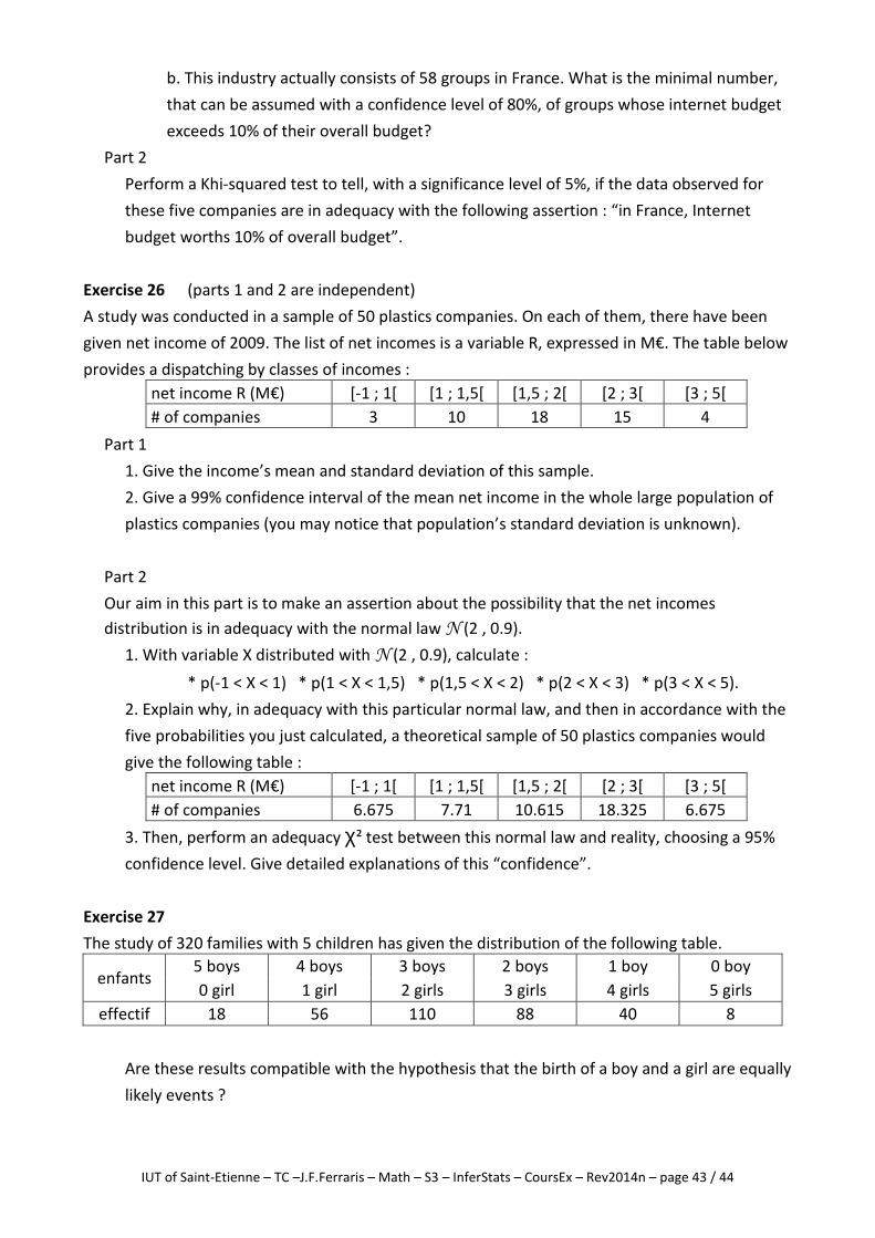
Exercise 26 (parts 1 and 2 are independent)
A study was conducted in a sample of 50 plastics companies. On each of them, there have been
given net income of 2009. The list of net incomes is a variable R, expressed in M€. The table below
provides a dispatching by classes of incomes :
net income R (M€) [-1 ; 1[ [1 ; 1,5[ [1,5 ; 2[ [2 ; 3[ [3 ; 5[
# of companies 3 10 18 15 4
Part 1
1. Give the income’s mean and standard deviation of this sample.
2. Give a 99% confidence interval of the mean net income in the whole large population of
plastics companies (you may notice that population’s standard deviation is unknown).
Part 2
Our aim in this part is to make an assertion about the possibility that the net incomes
distribution is in adequacy with the normal law N (2 , 0.9).
1. With variable X distributed with N (2 , 0.9), calculate :
* p(-1 < X < 1) * p(1 < X < 1,5) * p(1,5 < X < 2) * p(2 < X < 3) * p(3 < X < 5).
2. Explain why, in adequacy with this particular normal law, and then in accordance with the
five probabilities you just calculated, a theoretical sample of 50 plastics companies would
give the following table :
net income R (M€) [-1 ; 1[ [1 ; 1,5[ [1,5 ; 2[ [2 ; 3[ [3 ; 5[
# of companies 6.675 7.71 10.615 18.325 6.675
3. Then, perform an adequacy χ² test between this normal law and reality, choosing a 95%
confidence level. Give detailed explanations of this “confidence”.
Exercise 27
The study of 320 families with 5 children has given the distribution of the following table.
enfants 5 boys 4 boys 3 boys 2 boys 1 boy 0 boy
0 girl 1 girl 2 girls 3 girls 4 girls 5 girls
effectif 18 56 110 88 40 8
Are these results compatible with the hypothesis that the birth of a boy and a girl are equally
likely events ?
IUT of Saint-Etienne – TC –J.F.Ferraris – Math – S3 – InferStats – CoursEx – Rev2014n – page 44 / 44
Exercise 28
A string manufacturer states that the objects it produces have an average tensile strength of 300
kg (with a standard deviation of 30 kg). It is assumed that the variable “strength of a string” is
normally distributed. Experiments on 10 strings revealed the following breakdown tensions :
251 277 255 305 341 324 329 314 272 289
Can we consider, analyzing this sample, that the average tensile strength of the population
of strings is equal to 300 kg? (significance level : 10%)
Exercise 29
For 1000 French baccalaureate candidates chosen at random, 675 were successful. Test at a 10%
significance level the assumption that the success rate in France is 70%.
Exercise 30
In several countries, the weather forecast is given as a probability.
Forecasting "the probability of rain tomorrow is 0.4" was made 50 times during the past year and
when it’s been done, it rained 26 times the day after. Test the accuracy of the prediction, with a
5% α-level.
IUT TC Formulaire global du Semestre 3 MATHEMATIQUES
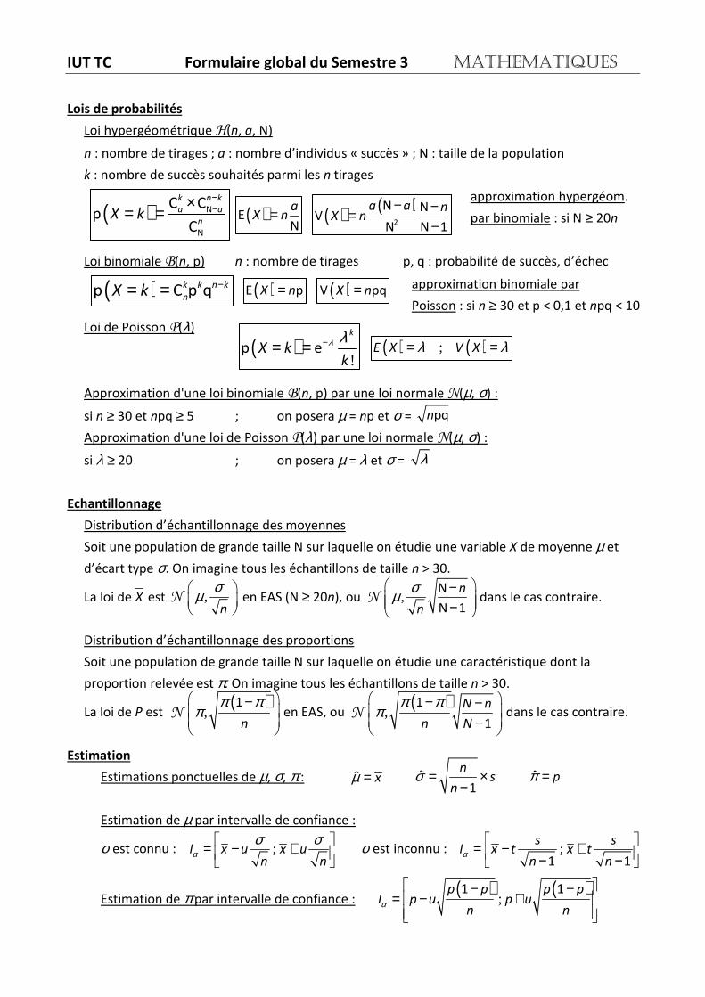
Lois de probabilités
Loi hypergéométrique H(n, a, N)
n : nombre de tirages ; a : nombre d’individus « succès » ; N : taille de la population
k : nombre de succès souhaités parmi les n tirages
approximation hypergéom.
par binomiale : si N ≥ 20n
Loi binomiale B(n, p) n : nombre de tirages p, q : probabilité de succès, d’échec
approximation binomiale par
Poisson : si n ≥ 30 et p < 0,1 et npq < 10
Loi de Poisson P(λ)
Approximation d'une loi binomiale B(n, p) par une loi normale N(µ, σ) :
si n ≥ 30 et npq ≥ 5 ; on posera µ = np et σ =
Approximation d'une loi de Poisson P(λ) par une loi normale N(µ, σ) :
si λ ≥ 20 ; on posera µ = λ et σ =
Echantillonnage
Distribution d’échantillonnage des moyennes
Soit une population de grande taille N sur laquelle on étudie une variable X de moyenne µ et
d’écart type σ. On imagine tous les échantillons de taille n > 30.
La loi de est en EAS (N ≥ 20n), ou dans le cas contraire.
Distribution d’échantillonnage des proportions
Soit une population de grande taille N sur laquelle on étudie une caractéristique dont la
proportion relevée est π. On imagine tous les échantillons de taille n > 30.
La loi de P est en EAS, ou dans le cas contraire.
Estimation
Estimations ponctuelles de µ, σ, π :
Estimation de µ par intervalle de confiance :
σ est connu : σ est inconnu :
Estimation de π par intervalle de confiance :
( ) k k n k
nX k
−= =p C p q ( )X n=E p
( ) ( )a a nX n
− −=−2
N NV
N N 1
( )!
p ek
X kk
λ λ−= = ( ) ( );E X V Xλ λ= =
,n
σµ
N ,N
N 1
n
n
σµ − −
N
( ),
1
n
π ππ −
N( )
,1
1
N n
n N
π ππ − − −
N
ˆ xµ = ˆ1
ns
nσ = ×
−ˆ pπ =
;I x u x un n
ασ σ = − +
;
1 1
s sI x t x t
n nα
= − + − −
( ) ( );
1 1p p p pI p u p u
n nα
− −= − +
( )k n k
a a
nX k
−−×= = N
N
C Cp
C( ) a
X n=EN
( )X n=V pq
pqn
λ
X
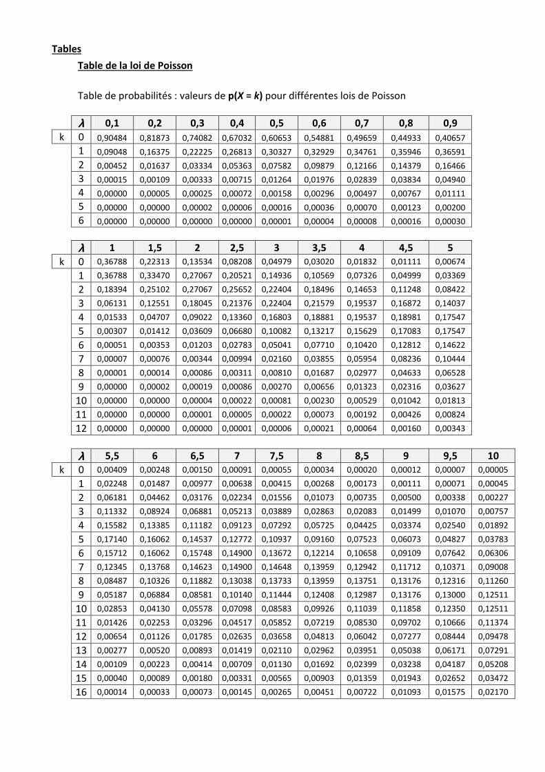
Tables
Table de la loi de Poisson
Table de probabilités : valeurs de p(X = k) pour différentes lois de Poisson
λλλλ 0,1 0,2 0,3 0,4 0,5 0,6 0,7 0,8 0,9
k 0 0,90484 0,81873 0,74082 0,67032 0,60653 0,54881 0,49659 0,44933 0,40657
1 0,09048 0,16375 0,22225 0,26813 0,30327 0,32929 0,34761 0,35946 0,36591
2 0,00452 0,01637 0,03334 0,05363 0,07582 0,09879 0,12166 0,14379 0,16466
3 0,00015 0,00109 0,00333 0,00715 0,01264 0,01976 0,02839 0,03834 0,04940
4 0,00000 0,00005 0,00025 0,00072 0,00158 0,00296 0,00497 0,00767 0,01111
5 0,00000 0,00000 0,00002 0,00006 0,00016 0,00036 0,00070 0,00123 0,00200
6 0,00000 0,00000 0,00000 0,00000 0,00001 0,00004 0,00008 0,00016 0,00030
λλλλ 1 1,5 2 2,5 3 3,5 4 4,5 5
k 0 0,36788 0,22313 0,13534 0,08208 0,04979 0,03020 0,01832 0,01111 0,00674
1 0,36788 0,33470 0,27067 0,20521 0,14936 0,10569 0,07326 0,04999 0,03369
2 0,18394 0,25102 0,27067 0,25652 0,22404 0,18496 0,14653 0,11248 0,08422
3 0,06131 0,12551 0,18045 0,21376 0,22404 0,21579 0,19537 0,16872 0,14037
4 0,01533 0,04707 0,09022 0,13360 0,16803 0,18881 0,19537 0,18981 0,17547
5 0,00307 0,01412 0,03609 0,06680 0,10082 0,13217 0,15629 0,17083 0,17547
6 0,00051 0,00353 0,01203 0,02783 0,05041 0,07710 0,10420 0,12812 0,14622
7 0,00007 0,00076 0,00344 0,00994 0,02160 0,03855 0,05954 0,08236 0,10444
8 0,00001 0,00014 0,00086 0,00311 0,00810 0,01687 0,02977 0,04633 0,06528
9 0,00000 0,00002 0,00019 0,00086 0,00270 0,00656 0,01323 0,02316 0,03627
10 0,00000 0,00000 0,00004 0,00022 0,00081 0,00230 0,00529 0,01042 0,01813
11 0,00000 0,00000 0,00001 0,00005 0,00022 0,00073 0,00192 0,00426 0,00824
12 0,00000 0,00000 0,00000 0,00001 0,00006 0,00021 0,00064 0,00160 0,00343
λλλλ 5,5 6 6,5 7 7,5 8 8,5 9 9,5 10
k 0 0,00409 0,00248 0,00150 0,00091 0,00055 0,00034 0,00020 0,00012 0,00007 0,00005
1 0,02248 0,01487 0,00977 0,00638 0,00415 0,00268 0,00173 0,00111 0,00071 0,00045
2 0,06181 0,04462 0,03176 0,02234 0,01556 0,01073 0,00735 0,00500 0,00338 0,00227
3 0,11332 0,08924 0,06881 0,05213 0,03889 0,02863 0,02083 0,01499 0,01070 0,00757
4 0,15582 0,13385 0,11182 0,09123 0,07292 0,05725 0,04425 0,03374 0,02540 0,01892
5 0,17140 0,16062 0,14537 0,12772 0,10937 0,09160 0,07523 0,06073 0,04827 0,03783
6 0,15712 0,16062 0,15748 0,14900 0,13672 0,12214 0,10658 0,09109 0,07642 0,06306
7 0,12345 0,13768 0,14623 0,14900 0,14648 0,13959 0,12942 0,11712 0,10371 0,09008
8 0,08487 0,10326 0,11882 0,13038 0,13733 0,13959 0,13751 0,13176 0,12316 0,11260
9 0,05187 0,06884 0,08581 0,10140 0,11444 0,12408 0,12987 0,13176 0,13000 0,12511
10 0,02853 0,04130 0,05578 0,07098 0,08583 0,09926 0,11039 0,11858 0,12350 0,12511
11 0,01426 0,02253 0,03296 0,04517 0,05852 0,07219 0,08530 0,09702 0,10666 0,11374
12 0,00654 0,01126 0,01785 0,02635 0,03658 0,04813 0,06042 0,07277 0,08444 0,09478
13 0,00277 0,00520 0,00893 0,01419 0,02110 0,02962 0,03951 0,05038 0,06171 0,07291
14 0,00109 0,00223 0,00414 0,00709 0,01130 0,01692 0,02399 0,03238 0,04187 0,05208
15 0,00040 0,00089 0,00180 0,00331 0,00565 0,00903 0,01359 0,01943 0,02652 0,03472
16 0,00014 0,00033 0,00073 0,00145 0,00265 0,00451 0,00722 0,01093 0,01575 0,02170
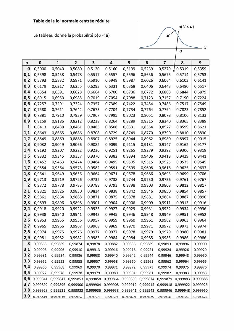
Table de la loi normale centrée réduite
Le tableau donne la probabilité p(U < u)
u 0 1 2 3 4 5 6 7 8 9
0 0,5000 0,5040 0,5080 0,5120 0,5160 0,5199 0,5239 0,5279 0,5319 0,5359
0,1 0,5398 0,5438 0,5478 0,5517 0,5557 0,5596 0,5636 0,5675 0,5714 0,5753
0,2 0,5793 0,5832 0,5871 0,5910 0,5948 0,5987 0,6026 0,6064 0,6103 0,6141
0,3 0,6179 0,6217 0,6255 0,6293 0,6331 0,6368 0,6406 0,6443 0,6480 0,6517
0,4 0,6554 0,6591 0,6628 0,6664 0,6700 0,6736 0,6772 0,6808 0,6844 0,6879
0,5 0,6915 0,6950 0,6985 0,7019 0,7054 0,7088 0,7123 0,7157 0,7190 0,7224
0,6 0,7257 0,7291 0,7324 0,7357 0,7389 0,7422 0,7454 0,7486 0,7517 0,7549
0,7 0,7580 0,7611 0,7642 0,7673 0,7704 0,7734 0,7764 0,7794 0,7823 0,7852
0,8 0,7881 0,7910 0,7939 0,7967 0,7995 0,8023 0,8051 0,8078 0,8106 0,8133
0,9 0,8159 0,8186 0,8212 0,8238 0,8264 0,8289 0,8315 0,8340 0,8365 0,8389
1 0,8413 0,8438 0,8461 0,8485 0,8508 0,8531 0,8554 0,8577 0,8599 0,8621
1,1 0,8643 0,8665 0,8686 0,8708 0,8729 0,8749 0,8770 0,8790 0,8810 0,8830
1,2 0,8849 0,8869 0,8888 0,8907 0,8925 0,8944 0,8962 0,8980 0,8997 0,9015
1,3 0,9032 0,9049 0,9066 0,9082 0,9099 0,9115 0,9131 0,9147 0,9162 0,9177
1,4 0,9192 0,9207 0,9222 0,9236 0,9251 0,9265 0,9279 0,9292 0,9306 0,9319
1,5 0,9332 0,9345 0,9357 0,9370 0,9382 0,9394 0,9406 0,9418 0,9429 0,9441
1,6 0,9452 0,9463 0,9474 0,9484 0,9495 0,9505 0,9515 0,9525 0,9535 0,9545
1,7 0,9554 0,9564 0,9573 0,9582 0,9591 0,9599 0,9608 0,9616 0,9625 0,9633
1,8 0,9641 0,9649 0,9656 0,9664 0,9671 0,9678 0,9686 0,9693 0,9699 0,9706
1,9 0,9713 0,9719 0,9726 0,9732 0,9738 0,9744 0,9750 0,9756 0,9761 0,9767
2 0,9772 0,9778 0,9783 0,9788 0,9793 0,9798 0,9803 0,9808 0,9812 0,9817
2,1 0,9821 0,9826 0,9830 0,9834 0,9838 0,9842 0,9846 0,9850 0,9854 0,9857
2,2 0,9861 0,9864 0,9868 0,9871 0,9875 0,9878 0,9881 0,9884 0,9887 0,9890
2,3 0,9893 0,9896 0,9898 0,9901 0,9904 0,9906 0,9909 0,9911 0,9913 0,9916
2,4 0,9918 0,9920 0,9922 0,9925 0,9927 0,9929 0,9931 0,9932 0,9934 0,9936
2,5 0,9938 0,9940 0,9941 0,9943 0,9945 0,9946 0,9948 0,9949 0,9951 0,9952
2,6 0,9953 0,9955 0,9956 0,9957 0,9959 0,9960 0,9961 0,9962 0,9963 0,9964
2,7 0,9965 0,9966 0,9967 0,9968 0,9969 0,9970 0,9971 0,9972 0,9973 0,9974
2,8 0,9974 0,9975 0,9976 0,9977 0,9977 0,9978 0,9979 0,9979 0,9980 0,9981
2,9 0,9981 0,9982 0,9982 0,9983 0,9984 0,9984 0,9985 0,9985 0,9986 0,9986
3 0,99865 0,99869 0,99874 0,99878 0,99882 0,99886 0,99889 0,99893 0,99896 0,99900
3,1 0,99903 0,99906 0,99910 0,99913 0,99916 0,99918 0,99921 0,99924 0,99926 0,99929
3,2 0,99931 0,99934 0,99936 0,99938 0,99940 0,99942 0,99944 0,99946 0,99948 0,99950
3,3 0,99952 0,99953 0,99955 0,99957 0,99958 0,99960 0,99961 0,99962 0,99964 0,99965
3,4 0,99966 0,99968 0,99969 0,99970 0,99971 0,99972 0,99973 0,99974 0,99975 0,99976
3,5 0,99977 0,99978 0,99978 0,99979 0,99980 0,99981 0,99981 0,99982 0,99983 0,99983
3,6 0,999841 0,999847 0,999853 0,999858 0,999864 0,999869 0,999874 0,999879 0,999883 0,999888
3,7 0,999892 0,999896 0,999900 0,999904 0,999908 0,999912 0,999915 0,999918 0,999922 0,999925
3,8 0,999928 0,999931 0,999933 0,999936 0,999938 0,999941 0,999943 0,999946 0,999948 0,999950
3,9 0,9999519 0,9999539 0,9999557 0,9999575 0,9999593 0,9999609 0,9999625 0,9999641 0,9999655 0,9999670
U
u
p(U < u)
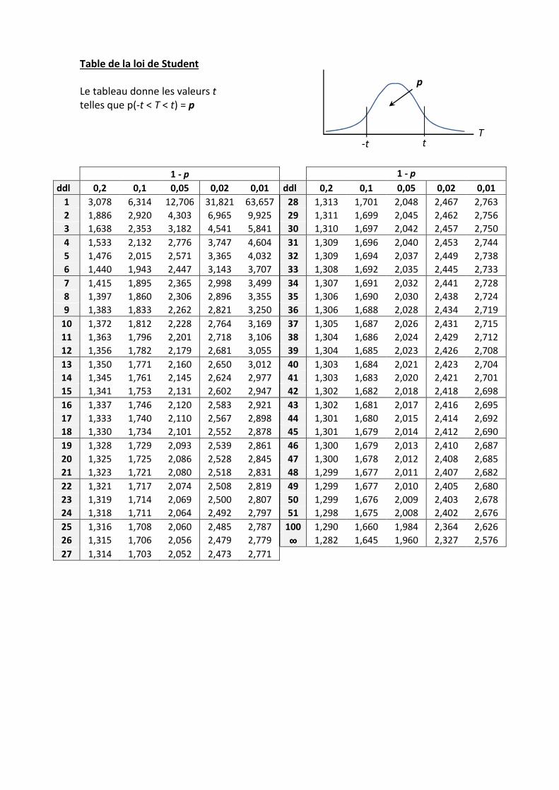
Table de la loi de Student
Le tableau donne les valeurs t
telles que p(-t < T < t) = p
1 - p 1 - p
ddl 0,2 0,1 0,05 0,02 0,01 ddl 0,2 0,1 0,05 0,02 0,01
1 3,078 6,314 12,706 31,821 63,657 28 1,313 1,701 2,048 2,467 2,763
2 1,886 2,920 4,303 6,965 9,925 29 1,311 1,699 2,045 2,462 2,756
3 1,638 2,353 3,182 4,541 5,841 30 1,310 1,697 2,042 2,457 2,750
4 1,533 2,132 2,776 3,747 4,604 31 1,309 1,696 2,040 2,453 2,744
5 1,476 2,015 2,571 3,365 4,032 32 1,309 1,694 2,037 2,449 2,738
6 1,440 1,943 2,447 3,143 3,707 33 1,308 1,692 2,035 2,445 2,733
7 1,415 1,895 2,365 2,998 3,499 34 1,307 1,691 2,032 2,441 2,728
8 1,397 1,860 2,306 2,896 3,355 35 1,306 1,690 2,030 2,438 2,724
9 1,383 1,833 2,262 2,821 3,250 36 1,306 1,688 2,028 2,434 2,719
10 1,372 1,812 2,228 2,764 3,169 37 1,305 1,687 2,026 2,431 2,715
11 1,363 1,796 2,201 2,718 3,106 38 1,304 1,686 2,024 2,429 2,712
12 1,356 1,782 2,179 2,681 3,055 39 1,304 1,685 2,023 2,426 2,708
13 1,350 1,771 2,160 2,650 3,012 40 1,303 1,684 2,021 2,423 2,704
14 1,345 1,761 2,145 2,624 2,977 41 1,303 1,683 2,020 2,421 2,701
15 1,341 1,753 2,131 2,602 2,947 42 1,302 1,682 2,018 2,418 2,698
16 1,337 1,746 2,120 2,583 2,921 43 1,302 1,681 2,017 2,416 2,695
17 1,333 1,740 2,110 2,567 2,898 44 1,301 1,680 2,015 2,414 2,692
18 1,330 1,734 2,101 2,552 2,878 45 1,301 1,679 2,014 2,412 2,690
19 1,328 1,729 2,093 2,539 2,861 46 1,300 1,679 2,013 2,410 2,687
20 1,325 1,725 2,086 2,528 2,845 47 1,300 1,678 2,012 2,408 2,685
21 1,323 1,721 2,080 2,518 2,831 48 1,299 1,677 2,011 2,407 2,682
22 1,321 1,717 2,074 2,508 2,819 49 1,299 1,677 2,010 2,405 2,680
23 1,319 1,714 2,069 2,500 2,807 50 1,299 1,676 2,009 2,403 2,678
24 1,318 1,711 2,064 2,492 2,797 51 1,298 1,675 2,008 2,402 2,676
25 1,316 1,708 2,060 2,485 2,787 100 1,290 1,660 1,984 2,364 2,626
26 1,315 1,706 2,056 2,479 2,779 ∞∞∞∞ 1,282 1,645 1,960 2,327 2,576
27 1,314 1,703 2,052 2,473 2,771
p
-t t T
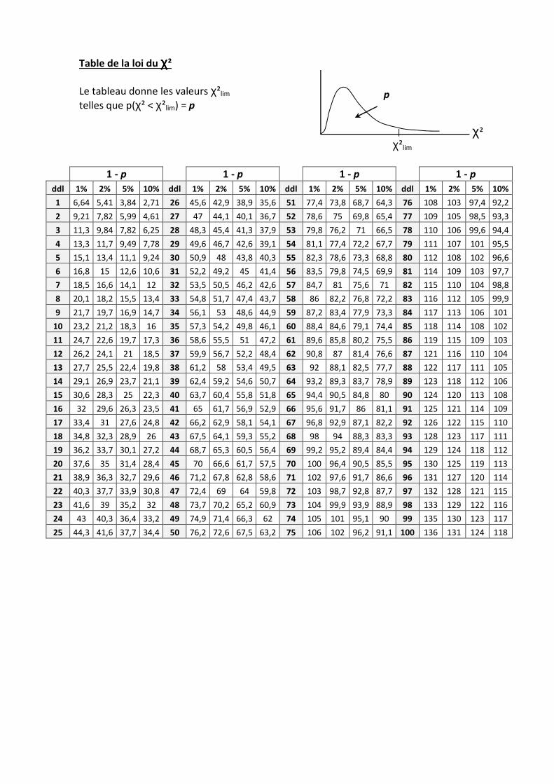
Table de la loi du χχχχ²
Le tableau donne les valeurs χ²lim
telles que p(χ² < χ²lim) = p
1 - p 1 - p 1 - p 1 - p
ddl 1% 2% 5% 10% ddl 1% 2% 5% 10% ddl 1% 2% 5% 10% ddl 1% 2% 5% 10%
1 6,64 5,41 3,84 2,71 26 45,6 42,9 38,9 35,6 51 77,4 73,8 68,7 64,3 76 108 103 97,4 92,2
2 9,21 7,82 5,99 4,61 27 47 44,1 40,1 36,7 52 78,6 75 69,8 65,4 77 109 105 98,5 93,3
3 11,3 9,84 7,82 6,25 28 48,3 45,4 41,3 37,9 53 79,8 76,2 71 66,5 78 110 106 99,6 94,4
4 13,3 11,7 9,49 7,78 29 49,6 46,7 42,6 39,1 54 81,1 77,4 72,2 67,7 79 111 107 101 95,5
5 15,1 13,4 11,1 9,24 30 50,9 48 43,8 40,3 55 82,3 78,6 73,3 68,8 80 112 108 102 96,6
6 16,8 15 12,6 10,6 31 52,2 49,2 45 41,4 56 83,5 79,8 74,5 69,9 81 114 109 103 97,7
7 18,5 16,6 14,1 12 32 53,5 50,5 46,2 42,6 57 84,7 81 75,6 71 82 115 110 104 98,8
8 20,1 18,2 15,5 13,4 33 54,8 51,7 47,4 43,7 58 86 82,2 76,8 72,2 83 116 112 105 99,9
9 21,7 19,7 16,9 14,7 34 56,1 53 48,6 44,9 59 87,2 83,4 77,9 73,3 84 117 113 106 101
10 23,2 21,2 18,3 16 35 57,3 54,2 49,8 46,1 60 88,4 84,6 79,1 74,4 85 118 114 108 102
11 24,7 22,6 19,7 17,3 36 58,6 55,5 51 47,2 61 89,6 85,8 80,2 75,5 86 119 115 109 103
12 26,2 24,1 21 18,5 37 59,9 56,7 52,2 48,4 62 90,8 87 81,4 76,6 87 121 116 110 104
13 27,7 25,5 22,4 19,8 38 61,2 58 53,4 49,5 63 92 88,1 82,5 77,7 88 122 117 111 105
14 29,1 26,9 23,7 21,1 39 62,4 59,2 54,6 50,7 64 93,2 89,3 83,7 78,9 89 123 118 112 106
15 30,6 28,3 25 22,3 40 63,7 60,4 55,8 51,8 65 94,4 90,5 84,8 80 90 124 120 113 108
16 32 29,6 26,3 23,5 41 65 61,7 56,9 52,9 66 95,6 91,7 86 81,1 91 125 121 114 109
17 33,4 31 27,6 24,8 42 66,2 62,9 58,1 54,1 67 96,8 92,9 87,1 82,2 92 126 122 115 110
18 34,8 32,3 28,9 26 43 67,5 64,1 59,3 55,2 68 98 94 88,3 83,3 93 128 123 117 111
19 36,2 33,7 30,1 27,2 44 68,7 65,3 60,5 56,4 69 99,2 95,2 89,4 84,4 94 129 124 118 112
20 37,6 35 31,4 28,4 45 70 66,6 61,7 57,5 70 100 96,4 90,5 85,5 95 130 125 119 113
21 38,9 36,3 32,7 29,6 46 71,2 67,8 62,8 58,6 71 102 97,6 91,7 86,6 96 131 127 120 114
22 40,3 37,7 33,9 30,8 47 72,4 69 64 59,8 72 103 98,7 92,8 87,7 97 132 128 121 115
23 41,6 39 35,2 32 48 73,7 70,2 65,2 60,9 73 104 99,9 93,9 88,9 98 133 129 122 116
24 43 40,3 36,4 33,2 49 74,9 71,4 66,3 62 74 105 101 95,1 90 99 135 130 123 117
25 44,3 41,6 37,7 34,4 50 76,2 72,6 67,5 63,2 75 106 102 96,2 91,1 100 136 131 124 118
χ²lim χ²
p
Related Documents