FINAL REPORT Predicting the Effects of Fuel Composition and Flame Structure on Soot Generation in Turbulent Non-Premixed Flames SERDP Project WP-1578 MARCH 2011 Christopher R. Shaddix Sandia National Laboratories Hai Wang University of Southern California Robert W. Schefer Joseph C. Oefelein Lyle M. Pickett Sandia National Laboratories

Welcome message from author
This document is posted to help you gain knowledge. Please leave a comment to let me know what you think about it! Share it to your friends and learn new things together.
Transcript
FINAL REPORT Predicting the Effects of Fuel Composition and Flame Structure
on Soot Generation in Turbulent Non-Premixed Flames
SERDP Project WP-1578
MARCH 2011 Christopher R. Shaddix Sandia National Laboratories Hai Wang University of Southern California Robert W. Schefer Joseph C. Oefelein Lyle M. Pickett Sandia National Laboratories

This report was prepared under contract to the Department of Defense Strategic Environmental Research and Development Program (SERDP). The publication of this report does not indicate endorsement by the Department of Defense, nor should the contents be construed as reflecting the official policy or position of the Department of Defense. Reference herein to any specific commercial product, process, or service by trade name, trademark, manufacturer, or otherwise, does not necessarily constitute or imply its endorsement, recommendation, or favoring by the Department of Defense.
REPORT DOCUMENTATION PAGE Form Approved
OMB No. 0704-0188 Public reporting burden for this collection of information is estimated to average 1 hour per response, including the time for reviewing instructions, searching existing data sources, gathering and maintaining the data needed, and completing and reviewing this collection of information. Send comments regarding this burden estimate or any other aspect of this collection of information, including suggestions for reducing this burden to Department of Defense, Washington Headquarters Services, Directorate for Information Operations and Reports (0704-0188), 1215 Jefferson Davis Highway, Suite 1204, Arlington, VA 22202-4302. Respondents should be aware that notwithstanding any other provision of law, no person shall be subject to any penalty for failing to comply with a collection of information if it does not display a currently valid OMB control number. PLEASE DO NOT RETURN YOUR FORM TO THE ABOVE ADDRESS.
1. REPORT DATE (DD-MM-YYYY) 28-03-2011
2. REPORT TYPE Final
3. DATES COVERED (From - To) Mar 2007 – Mar 2011
4. TITLE AND SUBTITLE
Predicting the Effects of Fuel Composition and Flame Structure
5a. CONTRACT NUMBER
on Soot Generation in Turbulent Non-Premixed Flames: SERDP
WP-1578
5b. GRANT NUMBER
5c. PROGRAM ELEMENT NUMBER
6. AUTHOR(S)
Christopher R. Shaddix, Hai Wang, Robert W. Schefer,
5d. PROJECT NUMBER
WP-1578
Joseph C. Oefelein, Lyle M. Pickett
5e. TASK NUMBER
5f. WORK UNIT NUMBER 7. PERFORMING ORGANIZATION NAME(S) AND ADDRESS(ES)
AND ADDRESS(ES)
8. PERFORMING ORGANIZATION REPORT NUMBER
Sandia National Laboratories
7011 East Avenue
Livermore, CA 94550
University of Southern
California
Los Angeles, CA 90089
9. SPONSORING / MONITORING AGENCY NAME(S) AND ADDRESS(ES) 10. SPONSOR/MONITOR’S ACRONYM(S) Strategic Environmental SERDP
Research and Development
Program 11. SPONSOR/MONITOR’S REPORT
NUMBER(S)
Arlington, VA
12. DISTRIBUTION / AVAILABILITY STATEMENT
13. SUPPLEMENTARY NOTES
14. ABSTRACT
This project aimed to develop a reduced chemistry and soot model for making accurate predictions of soot emissions from military gas
turbine engines. Measurements of soot formation were performed in laminar flat premixed flames and turbulent non-premixed jet flames at
1 atm pressure and in turbulent liquid spray flames under representative conditions for takeoff in a gas turbine engine. Fuels investigated
included ethylene and a JP-8 surrogate consisting of n-dodecane and m-xylene. The pressurized turbulent jet flame measurements
demonstrated that the surrogate fuel was representative of actual JP-8. The premixed flame measurements revealed that flame temperature
has a strong impact on the rate of soot nucleation and particle coagulation. Mean and rms soot concentrations were measured throughout
the turbulent non-premixed jet flames, together with soot concentration-temperature data, as well as spatially resolved radiant emission. A
detailed chemical kinetic mechanism for ethylene combustion, including fuel-rich chemistry and benzene formation steps, was compiled,
validated, and reduced. The reduced ethylene mechanism was incorporated into a high-fidelity large eddy simulation (LES) code, together
with a moment-based soot model and different models for thermal radiation. The LES results highlight the importance of including an
optically-thick radiation model to accurately predict gas temperatures and thus soot formation rates. When including such a radiation
model, the LES model predicts mean soot concentrations within 30% in the ethylene jet flame. 15. SUBJECT TERMS Gas turbine, soot formation, jet flames, JP-8, ethylene, premixed flat flame, radiation, LES
16. SECURITY CLASSIFICATION OF:
17. LIMITATION OF ABSTRACT
18. NUMBER OF PAGES
19a. NAME OF RESPONSIBLE PERSON Christopher Shaddix
a. REPORT
b. ABSTRACT
c. THIS PAGE
19b. TELEPHONE NUMBER (include area
code) 925-294-3840
Standard Form 298 (Rev. 8-98) Prescribed by ANSI Std. Z39.18
ii
Table of Contents Page
Table of Contents ...................................................................................................................... ii
List of Acronyms ..................................................................................................................... iv
List of Figures .......................................................................................................................... vi
List of Tables ........................................................................................................................... xi
Acknowledgements ................................................................................................................. xii
1.0 Abstract ...............................................................................................................................1
2.0 Objective .............................................................................................................................3
3.0 Background .........................................................................................................................4
4.0 Materials and Methods ........................................................................................................8
4.1 Soot Chemistry Model ..............................................................................................9
4.2 Soot Chemistry Model Reduction .............................................................................9
4.3 Flat Flame Measurements .......................................................................................10
4.4 Turbulent Non-Premixed Flame Measurements .....................................................11
4.5 Pressurized Spray Combustion ...............................................................................13
4.6 Large Eddy Simulation ...........................................................................................14
5.0 Results and Accomplishments ..........................................................................................17
5.1 Soot Chemistry Model ............................................................................................17
5.1.1 Development and Validation of Ethylene Chemical Kinetic Mechanism ...17
5.1.2 Development of a Detailed Chemical Kinetic Mechanism for the SERDP
JP-8 Surrogate .............................................................................................19
5.2 Reduction of Ethylene Chemical Kinetic Mechanism ............................................20
5.3 Flat Flame Measurements .......................................................................................20
5.3.1 Measurement of Soot PSDFs for Different Flame Temperatures ................20
5.3.2 Measurement of Soot PSDFs for Benzene-Doped Ethylene Flames ...........22
5.3.3 Development of an Improved Soot Probe Technique for Premixed Flat
Flames .........................................................................................................23
5.3.4 Measurement of Soot PSDFs for n-Dodecane Flames ................................23
5.3.5 Measurement of Aliphatic Compounds in Flat Flame Soot.........................24
iii
5.4 Turbulent Non-Premixed Flame Measurements .....................................................25
5.4.1 Ethylene TNF Burner Development ............................................................25
5.4.2 Surrogate JP-8 Fuel Vaporization and TNF Burner Development ..............27
5.4.3 Simultaneous OH• PLIF and Planar LII ......................................................30
5.4.4 Simultaneous PAH PLIF and Planar LII .....................................................32
5.4.5 Soot Volume Fraction ..................................................................................34
5.4.6 Laser Extinction and Correction for Signal Trapping ..................................36
5.4.7 Joint Statistics of Soot Temperature and Volume Fraction .........................42
5.4.8 Thermal Radiation .......................................................................................44
5.4.9 Velocity Field...............................................................................................48
5.5 Pressurized Spray Combustion of JP-8 and JP-8 Surrogate ...................................48
5.5.1 Lift-off Length .............................................................................................50
5.5.2 Soot Measurements ......................................................................................51
5.5.3 Influence of Ambient Conditions.................................................................54
5.5.4 Influence of Injection Pressure ....................................................................56
5.6 Large Eddy Simulation ...........................................................................................57
5.6.1 Coupled Treatment of Soot and Radiation Models in LES Simulations .....57
5.6.2 Soot model ...................................................................................................61
5.6.3 Radiation model ...........................................................................................62
5.6.4 Sensitivity Analysis .....................................................................................64
5.6.5 LES of the ethylene-air diffusion flame .......................................................65
6.0 Conclusions and Implications for Future Research ..........................................................70
7.0 Literature Cited .................................................................................................................72
8.0 List of Technical Publications ..........................................................................................77
iv
List of Acronyms
AFM atomic force microscopy
AFRL Air Force Research Lab
ALS Advanced Light Source
Ar argon
ASTM American Society for Testing and
Materials
BSSF burner-stabilized stagnation-flow
C2H2 acetylene
C2H4 ethylene
C12H26 dodecane
CaF2 calcium fluoride
CFD computational fluid dynamic
CH methylidyne
CH4 methane
CH2O formaldehyde
CMC conditional moment closure
CO carbon monoxide
CO2 carbon dioxide
CPC condensation particle counter
cw continuous wave (i.e. non-pulsed)
DOE Department of Energy
DMA differential mobility analyzer
DNS direct numerical simulation
DRO Direct Reduction-Optimization
EGR exhaust gas recirculation
EPA Environmental Protection Agency
FSK full-spectrum k-distribution
FT Fischer-Tropsch
FTIR fourier transform infrared
GE General Electric
GEAE General Electric Aircraft Engines
H atomic hydrogen
H2 molecular hydrogen
H2O water
H/C ratio of fuel hydrogen to carbon
HACA hydrogen-abstraction-carbon-
addition
HeNe helium-neon
IBM International Business Machines
ID internal diameter
JP-8 jet propulsion 8 (U.S. military jet
fuel)
Ke dimensionless extinction coefficient
LES large eddy simulation
LII laser-induced incandescence
LOI Level of Importance
MPI Message Passing Interface
MURI Multi-University Research Initiative
N2 molecular nitrogen
NERSC National Energy Research Scientific
Computing Center
NIST National Institute of Standards and
Technology
NO nitric oxide
NO2 nitrogen dioxide
O atomic oxygen
O2 molecular oxygen
OH hydroxyl radical
P&W Pratt & Whitney
PAH polycyclic aromatic hydrocarbons
PDF probability density function
PIV particle-image velocimetry
PLIF planar laser-induced fluorescence
PLII planar laser-induced incandescence
PM particulate matter
PM2.5 particulate matter with an
aerodynamic diameter less than 2.5
micrometers
PSDF particle size distribution function
PSR perfectly stirred reactor
QSST quasi-steady state

v
RANS Reynolds-averaged Navier Stokes
Re Reynolds number
RRKM Rice, Ramsperger, Kassel, and
Marcus
SERDP Strategic Environmental Research
and Development Program
SGS subgrid-scale
SMPS Scanning Mobility Particle Sizer
SPMD Single-Program—Multiple-Data
TCL Turbulent Combustion Laboratory
TEM transmission electron microscopy
TNF turbulent nonpremixed flame
UIC University of Illinois at Chicago
U.S. United States
USC University of Southern California
UTRC United Technologies Research
Center
UV ultraviolet
YAG yttrium aluminium garnet
vi
List of Figures Page
Figure 1. Graphical representation of major activities in this research project,
leading to the production of a validated reduced soot chemistry model
for predictions of soot emissions from gas turbine engines ...........................................8
Figure 2. Photograph of typical sooting ethylene premixed flat flame, stabilized
on a McKenna burner...................................................................................................10
Figure 3. Schematic diagram of flat flame soot sampling and analysis by SMPS
or thermal desorption chemical ionization mobility mass spectrometry,
which was not used in this study..................................................................................11
Figure 4. Calculated visible flame length of n-decane (vapor) fueled turbulent jet
flame for different fuel tube diameters ........................................................................12
Figure 5. Schematic of the constant-volume combustion vessel and the optical
setup for soot measurements ........................................................................................13
Figure 6. Experimental (symbols) and computed (lines) ignition delay times
behind reflected shock waves. Experimental data are taken from ref.
80. The ignition is measured by the onset of CH* chemiluminescent
emission .......................................................................................................................17
Figure 7. Experimental (symbols) and computed (lines) species profiles during
ethylene oxidation in a flow reactor at a pressure of 5 atm and
temperature of 950 K. Computed profiles are time-shifted (SERDP
v0.1: -40 msec; WF97: -0.5 sec; NIST: -1.1 sec; Utah: -1.2 sec) to
match experimental data ..............................................................................................18
Figure 8. Comparison of experimental n-dodecane-air flame speed
measurements [39] (left) and ignition delay measurements [82] (right)
with predictions from the detailed chemical kinetic model for SERDP
JP-8 surrogate ...............................................................................................................19
Figure 9. Comparison of experimental m-xylene-air flame speed measurements
[83] (left) and ignition delay measurements [40] (right) with
predictions from the detailed chemical kinetic model for SERDP JP-8
surrogate .......................................................................................................................19
Figure 10. Test of skeletal models in adiabatic PSR. The error bars are the
uncertainty of the detailed model and were determined by a spectral
expansion method [81] .................................................................................................21
Figure 11. Evolution of PSDFs measured for ethylene flat flame with a maximum
temperature of 1900 K. Symbols are experimental data and lines are
fits to data using a bi-lognormal distribution function .................................................21
Figure 12. Evolution of PSDFs measured for ethylene flat flame with a maximum
temperature of 1660 K. Symbols are experimental data and lines are
fits to data using a bi-lognormal distribution function .................................................22
vii
Figure 13. AFM images of soot collected from an ethylene flat flame with a
maximum temperature of 1740 K ................................................................................22
Figure 14. Comparison of measured and radiation corrected gas temperature
(symbols) and calculated temperature profiles in an ethylene flame as a
function of distance from the burner surface. The sampling plate
position relative to the burner surface is marked by the dashed lines.
The computation assumes a stagnation flow field .......................................................24
Figure 15. Repeat measurements of the evolution of PSDFs in an n-dodecane flat
flame with a maximum temperature of 1660 K ...........................................................25
Figure 16. Photographs of the pilot flames for the ―½-scale Sydney burner,‖ on
the left, and the actual full-scale Sydney burner, on the right .....................................26
Figure 17. PLIF images of OH• over heights of x/D from 2.3 to 15.6 (i.e. from x
= 8.7 mm to x = 58.8 mm) for four different ethylene jet flow
velocities, corresponding to Re = 10,000 to 25,000, on the ½-scale
Sydney burner. The light blue inner structures evident in interior
regions of the flame arise from PAH PLIF ..................................................................26
Figure 18. Photographs of the complete ethylene burner assembly (top) and
burner face (left). The pilot plate design with three concentric rows of
pilot flames that provide uniform heating is shown to the right ..................................27
Figure 19. Fast-shutter (1/1600 s) photographs of ethylene jet flames stabilized on
the new jet flame burner ..............................................................................................28
Figure 20. Sample Rayleigh scattering image (top) and derived temperature field
(bottom), up to the flame boundary, 5 mm downstream from the
burner lip. The anomalous profile for Re = 10,000 results from the
nonlinear response of a mass flow controller for the pilot flame when
used near its lower flow limit.......................................................................................28
Figure 21. Schematic of liquid fuel handling and vaporization system ........................................29
Figure 22. Design drawing of finned aluminum heat exchanger for rapid
vaporization of fuel spray ............................................................................................29
Figure 23. Photograph of liquid fuel vaporizer, with externally clamped electrical
heaters. The side port tubing is for nitrogen purging of the system ............................30
Figure 24. Photograph of the flame base of SERDP JP-8 surrogate TNF flame ..........................30
Figure 25. Instantaneous distribution of soot and OH• in a turbulent non-premixed
ethylene jet flame, as revealed by simultaneous LII and OH PLIF
imaging. False-color structures are from the LII images, on which have
been overlaid OH• structures, in an inverted grayscale. z and r
designate the axial and radial coordinates ...................................................................31
Figure 26. Evolution of OH• and soot structures within a Re = 20000 turbulent
non-premixed ethylene jet flame, as revealed by simultaneous LII and
OH PLIF imaging ........................................................................................................32
viii
Figure 27. Evolution of OH• and soot within a Re = 20,000 turbulent non-
premixed JP-8 surrogate jet flame, as revealed by simultaneous LII
and OH• PLIF. Images on the left show LIF from OH• and PAH (in
interior regions, particularly low in flame), whereas images on the
right show soot LII, with boundaries of OH• in white .................................................33
Figure 28. Evolution of PAH and soot structures within a Re = 20,000 turbulent
non-premixed ethylene jet flame, as revealed by simultaneous LII and
PAH PLIF imaging. The images show soot LII, with boundaries of
PAH denoted in magenta .............................................................................................33
Figure 29. Radial distribution of soot volume fraction at a height of 41.5 mm in a
laminar ethylene jet flame as measured by laser extinction and LII.
Measurements from extinction are de-convoluted with three
algorithms: Abel three-point inversion (Abel 3), Abel two-point
inversion (Abel 2), and onion peeling ..........................................................................34
Figure 30. Axial profile of soot volume fraction integrated across the canonical
ethylene jet flame measured by laser extinction and LII. A and B
indicate results from LII images obtained at two different heights .............................35
Figure 31. Instantaneous, mean, and rms soot volume fractions measured by LII
imaging in a Re = 20,000 turbulent non-premixed ethylene jet flame.
The mean and rms statistics are computed from 500 instantaneous
images taken at each height .........................................................................................36
Figure 32. PDFs of soot volume fraction at six axial locations along the jet
centerline in a Re = 20,000 turbulent non-premixed ethylene jet flame.
The statistics are computed from 1000 instantaneous images .....................................37
Figure 33. PDFs of soot volume fractions at four radial locations of the same
height of 475 mm in a Re = 20,000 turbulent non-premixed ethylene
jet flame. These statistics are computed from 1000 instantaneous
images ..........................................................................................................................37
Figure 34. Soot intermittency in the ethylene jet flame (a) as a function of axial
position along the flame centerline (left) and (b) as a function of radial
position at the height of minimum centerline intermittency ........................................38
Figure 35. Instantaneous, mean, and rms soot volume fractions measured by LII
imaging in a Re = 20,000 turbulent non-premixed JP-8 surrogate jet
flame. The mean and rms statistics are computed from 1000
instantaneous images taken at each height...................................................................39
Figure 36. Experimentally measured laser fluence dependence of LII signals
measured on the laser-incident side of a laminar ethylene flame ................................40
Figure 37. Schematic of experimental setup for performing laser extinction
measurements across a turbulent jet flame ―PD‖ stands for silicon
photodiode detector ......................................................................................................40
ix
Figure 38. Map of extinction measurement chord locations at a mid-height region
of the turbulent jet flames ............................................................................................41
Figure 39. A sample time record of measured soot optical thickness for the
ethylene flame at z/d = 135, r/d = 0 .............................................................................41
Figure 40. Power spectral densities (PSDs) of soot optical thickness for the
centerline of the ethylene flame at five different heights ............................................42
Figure 41. Derived mean LII signal transmittance at mid-height of the ethylene jet
flame ............................................................................................................................42
Figure 42. Original (top) and signal-trapping-corrected (bottom) LII data at mid-
height of the ethylene jet flame ....................................................................................43
Figure 43. Schematic of diagnostic configuration used to perform 3-line
measurements of soot temperature/concentration statistics in the
turbulent jet flame ........................................................................................................43
Figure 44. Optical probe for performing 3-line measurements of soot temperature/
concentration statistics in the turbulent jet flame. Aluminum optical
housing (left) is water-cooled and provides N2 purge gas. Refractory
probe ends (right) are uncooled ...................................................................................44
Figure 45. Sample time record for laser transmittance, two-color emission, and
derived soot volume fraction and soot temperature at mid-height of the
ethylene jet flame .........................................................................................................45
Figure 46. Photograph of radiometer, with water-cooled light pipe attached,
positioned at exit of a blackbody source, to calibrate the radiometer
output ...........................................................................................................................46
Figure 47. A sample time record of measured radiant intensity for the ethylene
flame at z/d = 135, r/d = 0 ............................................................................................46
Figure 48. Axial profiles of mean and rms radiant intensity measured within the
ethylene and JP-8 surrogate flames. To avoid data cluttering, error
bars are only drawn at selected positions .....................................................................47
Figure 49. Radial distributions of mean radiant intensity at several different
heights within the ethylene (left) and JP-8 surrogate (right) jet flames.
To avoid data cluttering, error bars are only drawn at selected positions ....................47
Figure 50. Photograph of the base of the ethylene jet flame when applying PIV to
the seeded flow within the fuel jet and in the surrounding coflow air .........................48
Figure 51. OH chemiluminescence and lift-off lengths for a quasi-steady fuel jet.
Operating conditions: 15% O2, 22.8 kg/m3 ambient density and 150
MPa injection pressure .................................................................................................51
Figure 52. Optical thickness (KL) data as a function of the axial distance from the
nozzle. Operating conditions as in Fig. 51 ...................................................................52
x
Figure 53. Planar laser-induced incandescence measurement. Operating
conditions as in Fig. 51 ................................................................................................53
Figure 54. Soot volume fraction distribution. Operating conditions as in Fig. 51 ........................53
Figure 55. Soot volume fractions distribution for a gas turbine combustor
condition. Ambient conditions: 1200 K, 40 bar, 11.8 kg/m3, and 15%
O2. Injector conditions: SR fuel, 150 MPa injection pressure .....................................54
Figure 56. OH chemiluminescence and lift-off lengths for a quasi-steady fuel jet.
Operating conditions: 11.8 kg/m3 ambient density, SR fuel, and 150
MPa injection pressure .................................................................................................55
Figure 57. Soot optical thickness (KL) versus ambient temperature for 15% O2
and 21% O2 gases. Operating conditions as in Fig. 56 ................................................56
Figure 58. Soot optical thickness (KL) versus injection velocity (injection
pressure). Ambient conditions: 15% O2, 11.8 kg/m3, 1200 K. SR fuel .......................57
Figure 59. OH Chemiluminescence and lift-off lengths for the conditions of Fig.
58..................................................................................................................................58
Figure 60. Comparison of CHEMKIN SENKIN results for an ethylene/air
mixture when using the full USC ethylene mechanism and the new
reduced ethylene mechanism .......................................................................................59
Figure 61. Comparison between CHEMKIN PREMIX calculations using the
reduced ethylene chemical kinetic mechanism and experimental
measurements above a flat flame burner [107]: p=20 Torr,
C2H4/O2/50% Ar, φ=1.9) .............................................................................................59
Figure 62. Comparison of premixed experiment from Appel et al. [108].....................................60
Figure 63. Comparison of diffusion flame experiment from Wang et al. [109] ...........................60
Figure 64. Unsteady, unstrained ethylene-air diffusion flame showing soot
volume fraction which compares the optically thin radiation model, P1
gray radiation model and no radiation model ..............................................................65
Figure 65. The calculated error of soot volume fraction between the optically thin
radiation model to the P1 gray model, where P1 gray model is assumed
to be the correct solution ..............................................................................................66
Figure 66. LES of the CRF piloted ethylene diffusion flame showing the
computational domain, flow conditions and instantaneous soot volume
fraction with a qualitative comparison to the experiment ............................................68
Figure 67. Soot volume fraction versus axial distance along the centerline of the
burner ...........................................................................................................................69

xi
List of Tables Page
Table 1. Fuel Properties .............................................................................................................49
Table 2. Experimental Operating Conditions ............................................................................50
Table 3. Operating conditions for piloted ethylene jet flame ....................................................68

xii
Acknowledgements
Allen Salmi of Sandia National Laboratories assisted with the design, mounting, and alignment
of the open jet flame burners and with the design of the liquid fuel vaporization system. Bob
Harmon of Sandia National Laboratories assisted with burner mounting, gas flow control, and
coflow air conditioning. Dennis Morrison of Sandia assisted with purchasing and construction of
the liquid fuel vaporization system. Rob Barlow of Sandia provided recommendations for
turbulent non-premixed burner design and operation.
Post-doctoral researchers Yao Zhang, Hoon Kook, and Jeff Doom have provided essential
contributions to the research at Sandia National Laboratories. Graduate students Aamir Abid,
Joaquin Camacho, and David Sheen have provided essential contributions to the research at
USC.
The financial support of the Strategic Environmental Research and Development Program is
acknowledged.
1
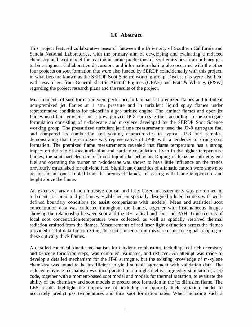
1.0 Abstract
This project featured collaborative research between the University of Southern California and
Sandia National Laboratories, with the primary aim of developing and evaluating a reduced
chemistry and soot model for making accurate predictions of soot emissions from military gas
turbine engines. Collaborative discussions and information sharing also occurred with the other
four projects on soot formation that were also funded by SERDP coincidentally with this project,
in what became known as the SERDP Soot Science working group. Discussions were also held
with researchers from General Electric Aircraft Engines (GEAE) and Pratt & Whitney (P&W)
regarding the project research plans and the results of the project.
Measurements of soot formation were performed in laminar flat premixed flames and turbulent
non-premixed jet flames at 1 atm pressure and in turbulent liquid spray flames under
representative conditions for takeoff in a gas turbine engine. The laminar flames and open jet
flames used both ethylene and a prevaporized JP-8 surrogate fuel, according to the surrogate
formulation consisting of n-dodecane and m-xylene developed by the SERDP Soot Science
working group. The pressurized turbulent jet flame measurements used the JP-8 surrogate fuel
and compared its combustion and sooting characteristics to typical JP-8 fuel samples,
demonstrating that the surrogate was representative of JP-8, with a tendency to strong soot
formation. The premixed flame measurements revealed that flame temperature has a strong
impact on the rate of soot nucleation and particle coagulation. Even in the higher temperature
flames, the soot particles demonstrated liquid-like behavior. Doping of benzene into ethylene
fuel and operating the burner on n-dodecane was shown to have little influence on the trends
previously established for ethylene fuel. Significant quantities of aliphatic carbon were shown to
be present in soot sampled from the premixed flames, increasing with flame temperature and
height above the flame.
An extensive array of non-intrusive optical and laser-based measurements was performed in
turbulent non-premixed jet flames established on specially designed piloted burners with well-
defined boundary conditions (to assist comparisons with models). Mean and statistical soot
concentration data was collected throughout the flames, together with instantaneous images
showing the relationship between soot and the OH radical and soot and PAH. Time-records of
local soot concentration-temperature were collected, as well as spatially resolved thermal
radiation emitted from the flames. Measurements of red laser light extinction across the flames
provided useful data for correcting the soot concentration measurements for signal trapping in
these optically thick flames.
A detailed chemical kinetic mechanism for ethylene combustion, including fuel-rich chemistry
and benzene formation steps, was compiled, validated, and reduced. An attempt was made to
develop a detailed mechanism for the JP-8 surrogate, but the existing knowledge of m-xylene
chemistry was found to be insufficient to yield suitable agreement with validation data. The
reduced ethylene mechanism was incorporated into a high-fidelity large eddy simulation (LES)
code, together with a moment-based soot model and models for thermal radiation, to evaluate the
ability of the chemistry and soot models to predict soot formation in the jet diffusion flame. The
LES results highlight the importance of including an optically-thick radiation model to
accurately predict gas temperatures and thus soot formation rates. When including such a
2
radiation model, the LES model predicts mean soot concentrations within 30% in the ethylene jet
flame.
The results of this project suggest that LES modeling, when incorporating suitably reduced
chemical kinetics with fuel-rich chemistry and a suitable, optically-thick radiation model, can
predict soot formation with good accuracy in an ethylene nonpremixed jet flame (at 1 atm) when
using a fairly simple soot model (developed explicitly for application to ethylene flames).
Extension of this predictive ability to more complex fuels representative of JP-8 requires
improvements in the understanding of aromatic oxidation and pyrolysis chemistry and may
require further improvements to the soot model itself.
3
2.0 Objective
The goal of this project was to develop a reduced chemical model and associated experimental
data that permit accurate predictions by combustor models of engine-out fine particulate matter
(PM) emissions, dominated by soot, from military gas turbine engines. By combining laminar, 1-
D flame measurements and modeling of particle size distributions and chemistry, detailed flow
field and soot measurements in open jet flames, and high-fidelity turbulent flame modeling, an
accurate reduced-chemistry model for soot formation and oxidation was generated that is
available for use by engine designers to reduce soot emissions in future engines and to evaluate
the effects of fuel composition and the use of fuel additives on soot emissions.
Several secondary objectives included the following: (1) improving the understanding of the
evolution of soot optical properties and particle size distribution function (PSDF) during the soot
mass growth process; (2) improving the understanding of soot formation and oxidation as a
function of turbulence mixing, fuel composition, and pressure; and (3) improving the ability to
predict soot formation and oxidation using large eddy simulation (LES) methods.
4
3.0 Background
The health effects of fine particulate matter in ambient air are becoming increasingly evident.
These particles are able to deeply penetrate lung tissue and have been shown to have a number of
deleterious effects associated with the pulmonary and cardiovascular systems, leading to
increased human morbidity and mortality [1-8]. As a consequence, the U.S. Environmental
Protection Agency (EPA) has been setting increasingly strict ambient air quality standards for
particulate matter with an aerodynamic diameter less than 2.5 micrometers (PM2.5).
Furthermore, local regulatory agencies are working to minimize emissions of fine particulates or
of gaseous compounds (such as sulfur and ammonia) that generate fine particulates in the
atmosphere. Airports and military bases are receiving increased attention in this regard, as they
can be significant point sources for emissions of these pollutants. Gas turbine engines are
important sources of PM2.5 emissions at these locations. In addition, in-flight emission of fine
particulates from gas turbine engines has effects on contrail/cloud formation and climate forcing
[9].
In light of these considerations, in addition to considerations of infrared signatures and excessive
heating of the gas turbine liner, there is a strong interest in reducing the emission of particulate
matter (dominated by soot particles) from military gas turbine engines. In particular, it is
desirable to have a truly predictive modeling capability for soot emission, considering the
influence of changes in the fuel chemical composition (either bulk composition or with the
inclusion of additives) and in the engine design and operation.
The traditional approach to predicting soot emissions from gas turbine engines is to use one of a
large number of empirical correlation formulas that have been developed relating soot emission
to bulk fuel composition and/or the laminar smoke point of the particular fuel. These correlations
have been based on fuel hydrogen content, H/C ratio, aromatic content, and naphthalene content,
among other variables [10]. However, soot emissions vary considerably with combustor
operating conditions (i.e. idle, cruise, and takeoff settings), as would be expected with the
resultant variations in combustor inlet temperature and pressure [11,12]. Therefore, the most
advanced empirical correlations attempt to take into account the effects of operating conditions,
for example as they relate to the characteristic residence times in the fuel-rich primary zone and
the oxidating secondary zone [13]. Even with this degree of sophistication, however, empirical
correlations generally do not offer predictability better than a mean standard deviation of 40%
for a range of fuels and operating conditions, for a given engine design [13]. Furthermore, the
range of applicability of a given correlation is usually very narrow and the use of the correlation
is generally limited to the gas turbine combustor in which the correlation is developed.
Consequently, the empirical approach has not yielded effective predictability of soot emissions.
In the last 10-15 years, several computational fluid dynamic (CFD) modeling approaches have
been attempted for prediction of soot emissions from gas turbine combustors, using standard k-
models to describe mean turbulence properties [14-19]. The soot formation and oxidation rates
have been based on laminar flamelet approaches for non-premixed flames, assuming that the
presence of soot does not affect the structure of the laminar flamelets (i.e., low soot limit). Most
of the calculations to-date have used various simplifying assumptions: (a) soot oxidation by O2
only, (b) soot formation constants taken from studies using propane or ethylene, and/or (c)
5
calculations performed for steady laminar flamelets. Furthermore, in all case radiant heat transfer
from soot was ignored. These modeling attempts largely failed to accurately predict engine-out
soot emission (usually the only soot measurement available), even with some partially tuned
parameters and often when only making comparisons against a single engine/operating
condition. In some cases, the predicted soot masses were exceedingly high (by orders of
magnitude), while in others they were low. All of the simulations have shown that the soot
concentrations in the primary combustion zone are several orders of magnitude higher than the
exhaust soot concentrations, demonstrating that accurate predictions of soot oxidation rates are
as important as predictions of soot inception and mass growth rates for determining engine-out
soot emissions.
Recent efforts at improving the accuracy of CFD modeling of gas turbine combustors have
focused on the development of large eddy simulation (LES) approaches [20-24]. LES, in contrast
to the traditional CFD approach known as Reynolds-averaged Navier Stokes (RANS), accurately
tracks large unsteady vortical motions and properly accounts for their effect on mean flow
quantities. In gas turbine combustor flows, fluid mixing is driven by such vortices, so LES is
expected to give superior results in comparison to RANS approaches. The long timescales
associated with soot formation make it especially sensitive to large-scale vortex mixing
processes [25,26], and therefore make its accurate prediction much more likely with LES.
However, the computational demands for LES are much greater than for RANS, so currently
only relatively crude LES models have been employed to simulate actual gas turbine combustor
operation. In the future, as LES is further developed and computational capabilities improve, it is
expected that LES models with the capability of calculating soot concentrations will be
employed for simulating gas turbine combustors.
Currently, LES modeling is being used to further the understanding of chemistry-turbulence
interactions in simpler, idealized flame geometries such as open jet flames [27-33]. Much of this
work has been coordinated as part of a collaborative international research effort associated with
the International Workshop on Measurement and Computation of Turbulent Nonpremixed
Flames (www.ca.sandia.gov/TNF), led by researchers at the Combustion Research Facility of
Sandia National Labs. Under funding from the U.S. DOE Basic Energy Sciences program,
several canonical flame systems have been investigated in Sandia’s Turbulent Combustion
Laboratory (TCL) using an array of laser diagnostic techniques to provide an extensive
experimental database for comparison with model predictions. Flames studied in the TCL have
been selected to address a progression in chemical-kinetic and flow-field complexity, starting
with simple hydrogen jet flames. Specific experiments, as well as the overall progression of
flames, have been designed to allow separate physical processes and individual submodels to be
isolated. For example, a series of H2 flames with helium dilution allowed a detailed evaluation of
NO predictions, independent of uncertainties in the radiation model [34]. Jet flames of CO/H2/N2
[35] and CH4/N2/H2 [36] have added kinetic complexity, while maintaining the simple, attached
jet-flame geometry. The series of piloted CH4/air jet flames [37] includes increasing degrees of
localized extinction that tests the ability of models to treat strong interactions of turbulence and
chemistry. This systematic progression is essential to the development of robust, predictive,
integrated models that have a solid basis in fundamental combustion science.
In this project, we built on this established hierarchy of canonical turbulent non-premixed flames
and focused on flames that include soot and the relevant fuel chemistry for military gas turbines
6
(i.e. a JP-8 surrogate). As with the previous flames investigated in the TCL, a variety of laser
diagnostic methods were employed to provide the best-possible experimental database for
detailed comparisons with model predictions. For the sooty flames investigated in this project,
several of the laser diagnostic approaches that have been routinely employed in the nonsooting
TNF workshop flames (such as Raman scattering and Rayleigh scattering) cannot be effectively
employed. However, previous research at Sandia has demonstrated that several different
techniques that give important information about the flow field, flame structure, soot field, and
radiation field can be effectively employed in unsteady sooty non-premixed flames, and these
techniques were employed in this investigation. In addition, the geometric, boundary and flow
conditions associated with the flame system were carefully controlled and recorded, allowing
modelers to identically match these conditions. In contrast, other existing experimental databases
for sooty turbulent non-premixed flames involve a scarcity of measured parameters (typically
only soot concentrations and mean temperature) and usually involve poorly defined boundary
conditions. Consequently, flame modelers have insufficient data available with which to validate
proposed models of soot formation and oxidation.
Pressure and ambient temperature are known to have strong influences on soot formation in non-
premixed flames. Over the past ten years, the effects of the liquid fuel injection process and
ambient pressure and temperature conditions on flame ignition and soot formation under diesel
combustion conditions have been systematically investigated in Sandia’s Engine Combustion
Simulation Lab. Recently, interest in the Single-Fuel Concept for the U.S. military has led to
research on JP-8 jet flame properties under simulated diesel combustion conditions. In this
project we capitalized on this existing dataset with world-average JP-8 and a natural gas Fischer-
Tropsch (FT) JP-8 fuel to compare the combustion performance of the JP-8 surrogate chosen by
the SERDP Soot Science research group against these fuel standards. Furthermore, we performed
measurements under appropriate takeoff conditions for military gas turbines to provide insight
into the important parameters for soot formation and for validation data for future modeling
predictions of soot formation.
Finally, to incorporate a realistic chemical kinetic model of the soot formation and oxidation
processes into a high-fidelity LES code, a significant effort of this project has been to generate
appropriate detailed and reduced chemical kinetic mechanisms for the combustion and pyrolysis
reactions of the investigated fuels. Clearly, use of a full, detailed chemical kinetic mechanism for
JP-8 (or even for a JP-8 surrogate), with at least 200 chemical species and over 1000 reactions is
not computationally feasible for all but the simplest CFD solver, unless this information is
conveyed in laminar flamelet lookup tables. Rather, for a high-fidelity LES model of a turbulent
jet flame no more than approximately 20 reactive scalars can currently be carried in the
calculation. Therefore, only the essential chemical species to describe the primary combustion
reactions and to describe the primary steps of soot formation, growth, and oxidation can be
incorporated into the model. Determining these species and the associated reduced chemical
steps and rate constants is a key part of development of an effective LES architecture for
predicting soot concentrations.
Another key ingredient of successful soot modeling in non-premixed flames, not fully
recognized at the beginning of this project, is the incorporation of a suitable radiation model. The
incorporation of radiation effects is important to yield accurate flame temperature predictions,
which in turn control soot formation and oxidation rates. There are many different approaches to

7
radiation modeling, with vastly differing computational requirements and overall accuracy,
depending on the optical thickness of the flame in question. To keep computational costs
reasonable, we investigated the influence of the simplest type of radiation model (assuming an
optically thin environment with no radiant absorption) and a reasonably accurate model for
flames with some optical thickness (i.e. with radiant absorption).
8
4.0 Materials and Methods
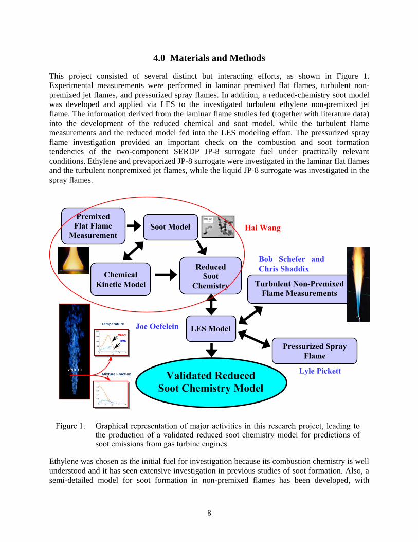
This project consisted of several distinct but interacting efforts, as shown in Figure 1.
Experimental measurements were performed in laminar premixed flat flames, turbulent non-
premixed jet flames, and pressurized spray flames. In addition, a reduced-chemistry soot model
was developed and applied via LES to the investigated turbulent ethylene non-premixed jet
flame. The information derived from the laminar flame studies fed (together with literature data)
into the development of the reduced chemical and soot model, while the turbulent flame
measurements and the reduced model fed into the LES modeling effort. The pressurized spray
flame investigation provided an important check on the combustion and soot formation
tendencies of the two-component SERDP JP-8 surrogate fuel under practically relevant
conditions. Ethylene and prevaporized JP-8 surrogate were investigated in the laminar flat flames
and the turbulent nonpremixed jet flames, while the liquid JP-8 surrogate was investigated in the
spray flames.
Figure 1. Graphical representation of major activities in this research project, leading to the production of a validated reduced soot chemistry model for predictions of soot emissions from gas turbine engines.
Ethylene was chosen as the initial fuel for investigation because its combustion chemistry is well
understood and it has seen extensive investigation in previous studies of soot formation. Also, a
semi-detailed model for soot formation in non-premixed flames has been developed, with
100 nm Premixed
Flat Flame
Measurement
s
Chemical
Kinetic Model
Soot Model
Reduced
Soot
Chemistry
Model
LES Model
Validated Reduced
Soot Chemistry Model
Turbulent Non-Premixed
Flame Measurements
Pressurized Spray
Flame
Measurements
Hai Wang
Joe Oefelein
Bob Schefer and
Chris Shaddix
Lyle Pickett x/d = 10 Mixture Fraction
Temperature
MEAN
RMS
9
specific application to laminar ethylene flames [38] and served well as a test case for
predictiveness in the LES computations of the non-premixed turbulent jet flames. JP-8, in the
form of a simplified chemical surrogate mixture, was also chosen for investigation in this project,
to provide direct relevance to aviation-fueled engines.
4.1 Soot Chemistry Model
A predictive model of soot formation includes three logical parts: (i) a gas-phase chemistry
model describing the rate of heat release and fuel ignition; (ii) a gas-phase model predicting the
production and destruction of relevant precursor species for soot nucleation, namely polycyclic
aromatic hydrocarbons (PAH); and (iii) a gas-surface and aerosol dynamics model for soot
nucleation and mass growth. In this project, an updated detailed gas-phase chemistry model for
ethylene combustion was compiled and combined with a PAH model. This model was then
validated against experimental measurements of laminar flame speed, ignition delay (shock
tube), and individual species concentrations in flat flames and flow reactor experiments.
Participants from the current set of SERDP soot program projects chose to use a common JP-8
surrogate, with consideration of the recommendations from the Surrogate Working Group and
the MURI projects that were recently initiated on this topic. This surrogate composition was
chosen to be a blend of 77 vol-% n-dodecane and 23 vol-% m-xylene. A detailed chemical
kinetic model for this surrogate was constructed, based on a mechanism for n-dodecane
combustion derived from the JetSuRF alkane combustion mechanism developed at USC [39] and
an m-xylene reaction mechanism developed by the Nancy research group in France [40].
Although many fundamental soot models have been proposed over the last 15 years, the physical
and chemical processes in these models are fundamentally the same as those proposed in the
early 1990’s [41-43]. The formation and mass growth of polycyclic aromatic hydrocarbons
include the hydrogen-abstraction-carbon-addition mechanism (HACA) [41] and the more
recently recognized kinetic processes involving resonantly stabilized species [44,45]. Though the
exact mechanism of soot inception remains somewhat empirical, this obstacle does not seem to
notably affect soot mass predictions [46]. The formation and growth of soot particles are
described by collision-induced coalescence, surface reaction/oxidation, and surface
condensation, and, when particles exceed a certain size, by particle-particle agglomeration,
leading to fractal-like aggregates. Several methods of solution of aerosol dynamics have been
proposed, including the moment [41,42], sectional [47],
Galerkin [48], and stochastic methods
[46,49,50]. Because of limitations on the number of species and variables high-fidelity LES
models are able to handle, the moment method remains the most promising near-term solution to
soot aerosol dynamics and was used in this project.
4.2 Soot Chemistry Model Reduction
Current computational capabilities place an upper limit of approximately 20 reactive scalars for
high-fidelity LES simulations of jet flames with sufficient spatial resolution. Though the
permissible number of scalars is likely to increase in the next several years, simulations using a
full, or even skeletal, soot chemistry model are probably not feasible for many years to come.
Because of the wide ranges of timescales involved in soot chemistry, the problem of model
reduction was approached using an array of suitable techniques. The detailed reaction model was
10
first reduced to a skeletal model that could account for fuel ignition and heat release as well as
the formation of the first aromatic ring. Subsequently, the skeletal reaction mechanism was
reduced to 20 species using the Level of Importance (LOI) approach [51]. The PAH chemistry
was reduced using a neural network approach. In the neural network approach, the production
rate of a soot-precursor PAH (e.g., pyrene) was mapped as a function of the local concentrations
of the hydrogen atom, acetylene, and molecular oxygen, residence time, and temperature in a
piecewise fashion over the entire space of the independent variables. This procedure ensured the
PAH production rates to be continuous in the entire independent-variable space. Lastly, the soot
number density and mean particle diameter was modeled with a 2-moment method. In this way,
the total number of reactive scalars was limited to 20 chemical species, plus the concentration of
a characteristic PAH and two variables to describe soot chemistry. Development and validation
of the reduced model was based on the detailed-chemistry model previously discussed.
4.3 Flat Flame Measurements
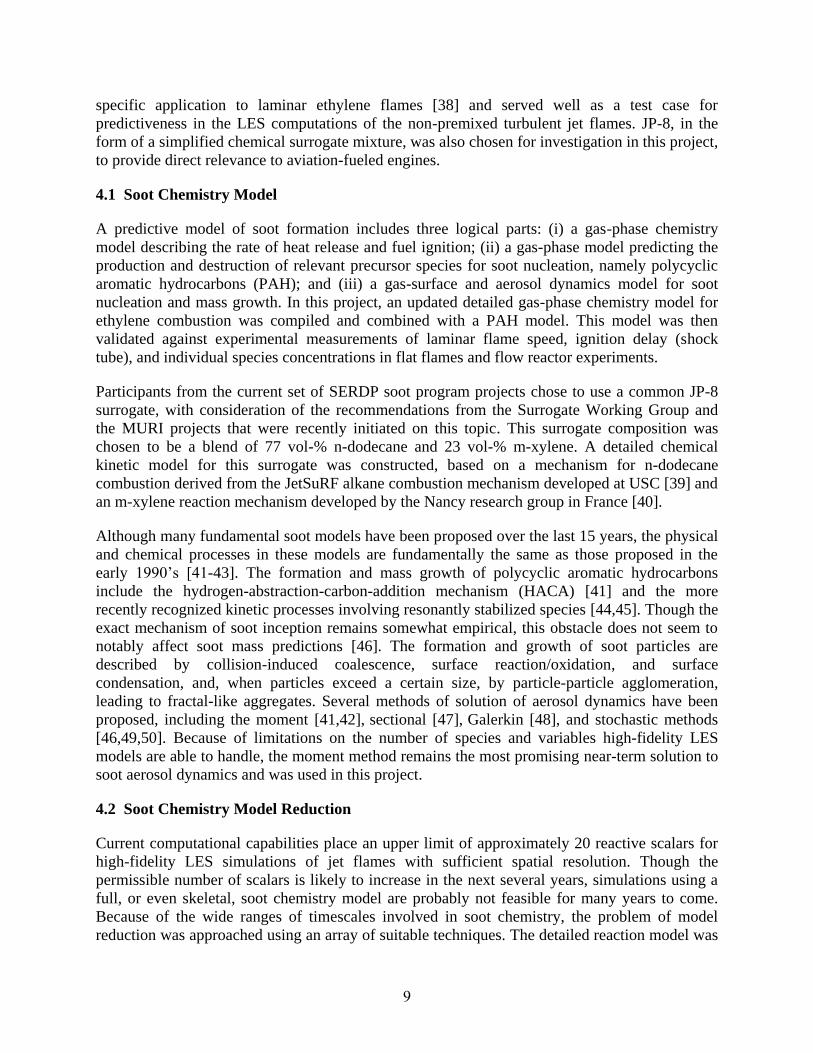
Scanning Mobility Particle Sizer (SMPS) characterization of soot PSDFs was performed in
premixed, burner-stabilized C2H4 flames (see Fig. 2) over a range of flame temperature and C/O
ratios, using previously established experimental methods and procedures [46,52,53]. The SMPS
device consists of a differential mobility analyzer (DMA), which uses an electron mobility
classifier to sort particles according to size, followed by a condensation particle counter (CPC),
which increases the size of the sorted particles through condensation and then optically counts
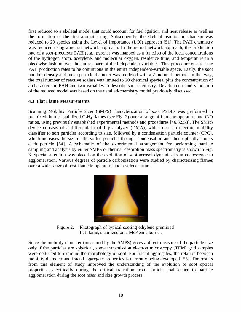
each particle [54]. A schematic of the experimental arrangement for performing particle
sampling and analysis by either SMPS or thermal desorption mass spectrometry is shown in Fig.
3. Special attention was placed on the evolution of soot aerosol dynamics from coalescence to
agglomeration. Various degrees of particle carbonization were studied by characterizing flames
over a wide range of post-flame temperature and residence time.
Figure 2. Photograph of typical sooting ethylene premixed flat flame, stabilized on a McKenna burner.
Since the mobility diameter (measured by the SMPS) gives a direct measure of the particle size
only if the particles are spherical, some transmission electron microscopy (TEM) grid samples
were collected to examine the morphology of soot. For fractal aggregates, the relation between
mobility diameter and fractal aggregate properties is currently being developed [55]. The results
from this element of study improved the understanding of the evolution of soot optical
properties, specifically during the critical transition from particle coalescence to particle
agglomeration during the soot mass and size growth process.
11
Figure 3. Schematic diagram of flat flame soot sampling and analysis by SMPS or thermal desorption chemical ionization mobility mass spectrometry, which was not used in this study.
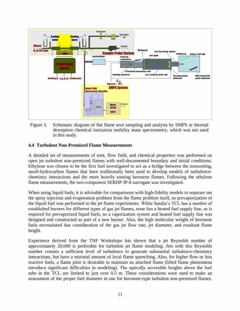
4.4 Turbulent Non-Premixed Flame Measurements
A detailed set of measurements of soot, flow field, and chemical properties was performed on
open jet turbulent non-premixed flames with well-documented boundary and initial conditions.
Ethylene was chosen to be the first fuel investigated to act as a bridge between the nonsooting,
small-hydrocarbon flames that have traditionally been used to develop models of turbulence-
chemistry interactions and the more heavily sooting kerosene flames. Following the ethylene
flame measurements, the two-component SERDP JP-8 surrogate was investigated.
When using liquid fuels, it is advisable for comparisons with high-fidelity models to separate out
the spray injection and evaporation problem from the flame problem itself, so prevaporization of
the liquid fuel was performed in the jet flame experiments. While Sandia’s TCL has a number of
established burners for different types of gas jet flames, none has a heated fuel supply line, as is
required for prevaporized liquid fuels, so a vaporization system and heated fuel supply line was
designed and constructed as part of a new burner. Also, the high molecular weight of kerosene
fuels necessitated due consideration of the gas jet flow rate, jet diameter, and resultant flame
height.
Experience derived from the TNF Workshops has shown that a jet Reynolds number of
approximately 20,000 is preferable for turbulent jet flame modeling. Jets with this Reynolds
number contain a sufficient level of turbulence to generate substantial turbulence-chemistry
interactions, but have a minimal amount of local flame quenching. Also, for higher flow or less
reactive fuels, a flame pilot is desirable to maintain an attached flame (lifted flame phenomena
introduce significant difficulties in modeling). The optically accessible heights above the fuel
tube in the TCL are limited to just over 0.5 m. These considerations were used to make an
assessment of the proper fuel diameter to use for kerosene-type turbulent non-premixed flames.
Po210
neutralizerAerosol in
Heating element
Am241
Chemical ionization cell
Ion gate
Ion mobility drift cell
ExhaustIon focusing optics
Faraday plate
detector
Ortho-TOF MS
Microchannel
plate detector
Reflector
Particle
collection
Diluent
(N2)
Po210
neutralizerAerosol in
Heating element
Am241
Chemical ionization cell
Ion gate
Ion mobility drift cell
ExhaustIon focusing optics
Faraday plate
detector
Ortho-TOF MS
Microchannel
plate detector
Reflector
Particle
collection
Diluent
(N2)
Porous plug
burner
Porous plug
burner
Shielding Ar C2H4/O2/Ar Cooling water
Secondary
airP1
Diluent
N2 at 29.5 lpm
P2
Exhaust
Flow meter
Filter
orifice
Cooling
water
Cooling
water
Sample Probe System
Kr
85
NDMA
P
Model 3080
Electrostatic Classifier
Model
3025A
UCPC
Exhaust
SMPS System
Kr
85
NDMA
P
Model 3080
Electrostatic Classifier
Model
3025A
UCPC
Exhaust
SMPS System
12
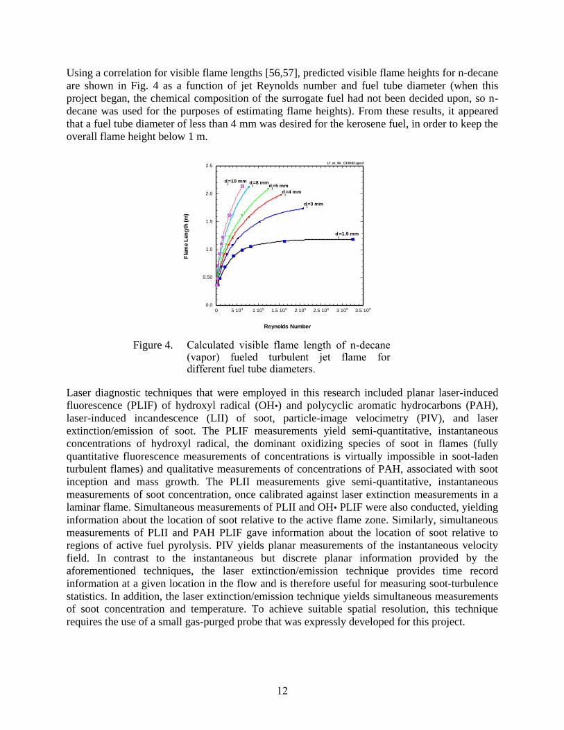
Using a correlation for visible flame lengths [56,57], predicted visible flame heights for n-decane
are shown in Fig. 4 as a function of jet Reynolds number and fuel tube diameter (when this
project began, the chemical composition of the surrogate fuel had not been decided upon, so n-
decane was used for the purposes of estimating flame heights). From these results, it appeared
that a fuel tube diameter of less than 4 mm was desired for the kerosene fuel, in order to keep the
overall flame height below 1 m.
Figure 4. Calculated visible flame length of n-decane (vapor) fueled turbulent jet flame for different fuel tube diameters.
Laser diagnostic techniques that were employed in this research included planar laser-induced
fluorescence (PLIF) of hydroxyl radical (OH•) and polycyclic aromatic hydrocarbons (PAH),
laser-induced incandescence (LII) of soot, particle-image velocimetry (PIV), and laser
extinction/emission of soot. The PLIF measurements yield semi-quantitative, instantaneous
concentrations of hydroxyl radical, the dominant oxidizing species of soot in flames (fully
quantitative fluorescence measurements of concentrations is virtually impossible in soot-laden
turbulent flames) and qualitative measurements of concentrations of PAH, associated with soot
inception and mass growth. The PLII measurements give semi-quantitative, instantaneous
measurements of soot concentration, once calibrated against laser extinction measurements in a
laminar flame. Simultaneous measurements of PLII and OH• PLIF were also conducted, yielding
information about the location of soot relative to the active flame zone. Similarly, simultaneous
measurements of PLII and PAH PLIF gave information about the location of soot relative to
regions of active fuel pyrolysis. PIV yields planar measurements of the instantaneous velocity
field. In contrast to the instantaneous but discrete planar information provided by the
aforementioned techniques, the laser extinction/emission technique provides time record
information at a given location in the flow and is therefore useful for measuring soot-turbulence
statistics. In addition, the laser extinction/emission technique yields simultaneous measurements
of soot concentration and temperature. To achieve suitable spatial resolution, this technique
requires the use of a small gas-purged probe that was expressly developed for this project.
0.0
0.50
1.0
1.5
2.0
2.5
0 5 104 1 105 1.5 105 2 105 2.5 105 3 105 3.5 105
Lf_vs_Re_C10H22.qpa2
Fla
me L
en
gth
(m
)
Reynolds Number
dj=1.9 mm
dj=3 mm
dj=4 mm
dj=5 mm
dj=10 mm d
j=8 mm
13
In addition to the aforementioned measurements, Rayleigh scattering measurements were
performed along a horizontal line, just above the burner lip, to define the thermal boundary
conditions for modeling of these flames.
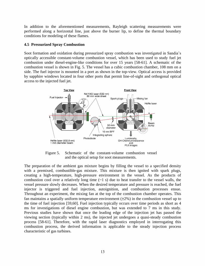
4.5 Pressurized Spray Combustion
Soot formation and oxidation during pressurized spray combustion was investigated in Sandia’s
optically accessible constant-volume combustion vessel, which has been used to study fuel jet
combustion under diesel-engine-like conditions for over 15 years [58-61]. A schematic of the
combustion vessel is shown in Fig. 5. The vessel has a cubic combustion chamber, 108 mm on a
side. The fuel injector is mounted in a port as shown in the top-view. Optical access is provided
by sapphire windows located in four other ports that permit line-of-sight and orthogonal optical
access to the injected fuel jet.
Figure 5. Schematic of the constant-volume combustion vessel and the optical setup for soot measurements.
The preparation of the ambient gas mixture begins by filling the vessel to a specified density
with a premixed, combustible-gas mixture. This mixture is then ignited with spark plugs,
creating a high-temperature, high-pressure environment in the vessel. As the products of
combustion cool over a relatively long time (~1 s) due to heat transfer to the vessel walls, the
vessel pressure slowly decreases. When the desired temperature and pressure is reached, the fuel
injector is triggered and fuel injection, autoignition, and combustion processes ensue.
Throughout an experiment, the mixing fan at the top of the combustion chamber operates. This
fan maintains a spatially uniform temperature environment ( 2%) in the combustion vessel up to
the time of fuel injection [59,60]. Fuel injection typically occurs over time periods as short as 4
ms for investigations of diesel engine combustion, but was extended to 7 ms in this study.
Previous studies have shown that once the leading edge of the injection jet has passed the
viewing section (typically within 2 ms), the injected jet undergoes a quasi-steady combustion
process [58-61]. Therefore, with the rapid laser diagnostics employed in interrogating this
combustion process, the derived information is applicable to the steady injection process
characteristic of gas turbines.
14
The temperature, density, and composition of the ambient gas in the vessel at the time of fuel
injection can be widely varied with this simulation procedure. The ambient gas temperature and
pressure at injection are determined from the ambient gas pressure at the time the fuel injector is
triggered and the mass of gas initially transferred into the vessel (a constant up to the time of the
injection event). The ambient temperature can be varied from 1300 K down to 500 K, and the
ambient pressure can be varied up to 35 MPa. For most experiments, a combustible-gas mixture
of 68.1% N2, 28.4% O2, 3.0% C2H2, and 0.5% H2 (by volume) is used. The product composition
of this combustible mixture simulates air, having a composition of 21.0% O2, 69.3% N2, 6.1%
CO2, and 3.6% H2O (by volume) and a molecular weight of 29.5. The JP-8 surrogate fuel was
investigated in this study. Two combustion conditions were investigated: a pressure of 2.7 MPa
and initial temperatures of 800–900 K, representative of jet engine takeoff conditions, and a
pressure of 6.7 MPa and initial temperatures of 900–1000 K, representative of diesel engine
conditions. The takeoff pressure and temperature ranges that were investigated were based on
recommendations from our project monitors at Pratt & Whitney and GE Aircraft Engines. The
SERDP JP-8 surrogate was investigated under the diesel engine conditions for the purpose of
comparing its combustion and soot formation tendencies with those that have been previously
determined in this experimental device for a range of JP-8 fuels. As the SERDP surrogate only
involves two species and had not been previously investigated before this work, there was
substantial interest among all of the SERDP Soot Science program members to compare its
performance against actual JP-8 fuels under practically relevant combustion conditions.
Several different optical diagnostics were employed in the constant-volume combustion vessel
experiments, as indicated in Fig. 5. These included line-of-sight laser extinction, PLII imaging,
natural soot luminosity imaging, and OH• chemiluminescence imaging. The laser extinction
technique is used for measuring the soot optical thickness across a fuel jet, while the PLII
imaging is used for visualizing the spatial location of soot in a fuel jet. The spatial soot profiles,
provided by PLII, and quantitative optical thickness from laser extinction are then combined to
obtain soot volume fraction distributions throughout the jet. OH• chemiluminescence images
were used for determining the ignition delay after the start of spray injection and the lift-off
length of the combusting region of the fuel jet during its quasi-steady combustion phase. The lift-
off length measurement is used to estimate the amount of air entrained into the fuel jet, and
therefore the extent of partial premixing at the flame stabilization point, using a relationship
developed for a 1-D model fuel jet [59,62]. This information is important for interpreting the
measured amounts of soot formation, because partial premixing of the jet reduces its tendency to
form soot.
4.6 Large Eddy Simulation
The baseline theoretical-numerical framework combines a general treatment of the governing
conservation and state equations with state-of-the-art numerical algorithms and massively-
parallel programming paradigms [63-67]. The numerical formulation treats the fully-coupled
compressible form of the conservation equations, but can be evaluated in the incompressible
limit. The theoretical framework handles both multicomponent and mixture-averaged systems,
with a generalized treatment of the equation of state, thermodynamics, and transport processes. It
can accommodate high-pressure real-gas/liquid phenomena, multiple-scalar mixing processes,
finite-rate chemical kinetics and multiphase phenomena in a fully coupled manner. For LES
applications, the instantaneous conservation equations are filtered and models are applied to
15
account for the subgrid-scale (SGS) mass, momentum and energy transport processes. The
baseline SGS closure is obtained using the mixed dynamic Smagorinsky model by combining the
models of Erlebacher et al. [68] and Speziale
[69] with the dynamic modeling procedure [70-72]
and the Smagorinsky eddy viscosity model [73]. There are no tuned constants employed
anywhere in the closure. The property evaluation scheme is derived using the extended
corresponding states model [74,75] and designed to handle multicomponent systems. The scheme
has been optimized to account for thermodynamic nonidealities and transport anomalies over a
wide range of pressures and temperatures.
The numerical framework provides a fully-implicit all-Mach-number time-advancement using a
fully explicit multistage scheme. A unique dual-time approach is employed with a generalized
(pseudo-time) preconditioning methodology that treats convective, diffusive, geometric, and
source term anomalies in an optimal manner. The implicit formulation allows one to set the
physical-time step based solely on accuracy considerations. The spatial differencing scheme is
optimized for LES using a staggered grid arrangement in generalized curvilinear coordinates.
This provides non-dissipative spectrally clean damping characteristics and discrete conservation
of mass, momentum and total-energy. The scheme can handle arbitrary geometric features,
which inherently dominate the evolution of turbulence. A Lagrangian-Eulerian formulation is
employed to accommodate particulates, sprays, or Lagrangian based combustion models, with
full coupling applied between the two systems. The algorithm is massively-parallel and has been
optimized to provide excellent parallel scalability attributes using a distributed multiblock
domain decomposition with a generalized connectivity scheme. Distributed-memory message-
passing is performed using Message Passing Interface (MPI) and the Single-Program—Multiple-
Data (SPMD) model. It accommodates complex geometric features and time varying meshes
with generalized hexahedral cells while maintaining the high accuracy attributes required for
LES. The numerical framework has been ported to all major platforms and provides highly
efficient fine-grain scalability attributes. Sustained parallel efficiencies above 90-percent have
been achieved with jobs as large as 4096 processors on the National Energy Research Scientific
Computing Center (NERSC) IBM SP platform (Seaborg). The code is fully vectorized and has
been optimized for both vector and commodity architectures.
Our combustion modeling approach for the high-fidelity LES facilitates direct treatment of
turbulence-chemistry interactions and multiple-scalar mixing processes without the use of tuned
model constants. The systematic development and validation of this approach is currently a
major focal point. Unlike conventional models, chemistry (and the associated mechanisms
developed under this grant) is treated directly within the LES formalism. The filtered energy and
chemical source terms are closed by employing a moment-based reconstruction methodology
that provides a modeled representation of the local instantaneous scalar field. Model coefficients
are evaluated locally in closed form as a function of time and space using the dynamic modeling
procedure. In the limit as the grid resolution and time-step approach the smallest relevant scales,
contributions from the subgrid-scale models approach zero and the limit of a direct numerical
simulation (DNS) is achieved.
All of the subgrid-scale models for combustion developed to-date are relatively simple due to
past computational limitations and the long-standing requirement of fast turnaround times for
calculations. Approaches aimed at obtaining accurate closure schemes include the assumption of
fast chemistry, the assumption of laminar flamelets, the conditional moment closure (CMC), and
16
PDF transport models. Klimenko has established the relation between CMC and unsteady
flamelets [76]. There are several limitations associated with each of these approaches, and each
exhibit clear trade-offs between model accuracy and the validity of the modeling assumptions.
More recently, a new class of reconstruction subgrid-scale models has been proposed that
combine the purely mathematical approximate deconvolution procedure with physical
information from an assumed scalar spectrum to match specific scalar moments [77,78].
Approximate reconstruction using moments provides an alternative approach that avoids the
intermediate step of modeling the joint-PDF associated with subgrid-scale fluctuations. The
instantaneous scalar field is estimated using an approximate deconvolution operation that
requires the filtered moments of respective scalars to match to a specified order. The estimated
scalar field is then used as a surrogate for the exact scalar field to calculate the subgrid-scale
contribution and the additional set of derived coefficients can be obtained in a consistent manner
using the dynamic procedure. Research to-date suggests that this method cannot be reliably used
to close the filtered chemical source terms directly. It has been shown, however, that it can be
used to obtain highly accurate representations of polynomial nonlinearities associated with terms
such as subgrid-scale scalar variances.
Here, we extend the approach described above by using the highly accurate representations of
the subgrid-scalar scalar variances and coupling this to a stochastic reconstruction methodology
to obtain a modeled representation of the instantaneous scalar field. This, in turn, is used to
obtain accurate representations of the filtered chemical source terms. The approach allows one to
track the evolution of multiple scalars in both time and space and accounts for finite-rate
chemistry in a time-accurate manner.
A focal point of our effort under this grant is to incorporate a suitable radiation model closure
and to incorporate a method-of-moments soot model into the LES framework. Soot particulates
are treated both directly in the Eulerian frame and also using a Lagrangian particle model to
simulate a statistically relevant sample of soot ―parcels‖. This model is directly coupled to an
appropriately reduced chemical mechanism that accounts for the instantaneous production soot
particles, subject to nucleation from the gas phase and coagulation in the free molecular regime.
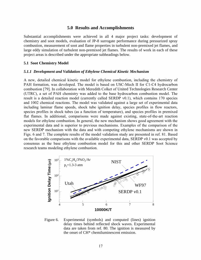
17
5.0 Results and Accomplishments
Substantial accomplishments were achieved in all 4 major project tasks: development of
chemistry and soot models, evaluation of JP-8 surrogate performance during pressurized spray
combustion, measurement of soot and flame properties in turbulent non-premixed jet flames, and
large eddy simulation of turbulent non-premixed jet flames. The results of work in each of these
project areas is described under the appropriate subheadings below.
5.1 Soot Chemistry Model
5.1.1 Development and Validation of Ethylene Chemical Kinetic Mechanism
A new, detailed chemical kinetic model for ethylene combustion, including the chemistry of
PAH formation, was developed. The model is based on USC-Mech II for C1-C4 hydrocarbon
combustion [79]. In collaboration with Meredith Colket of United Technologies Research Center
(UTRC), a set of PAH chemistry was added to the base hydrocarbon combustion model. The
result is a detailed reaction model (currently called SERDP v0.1), which contains 170 species
and 1002 chemical reactions. The model was validated against a large set of experimental data
including laminar flame speeds, shock tube ignition delay, species profiles in flow reactors,
species profiles in shock tubes (as a function of temperature), and species profiles in premixed
flat flames. In additional, comparisons were made against existing, state-of-the-art reaction
models for ethylene combustion. In general, the new mechanism shows good agreement with the
experimental data and is superior to previous mechanisms. Examples of the comparison of the
new SERDP mechanism with the data and with competing ethylene mechanisms are shown in
Figs. 6 and 7. The complete results of the model validation study are presented in ref. 81. Based
on the favorable comparisons with the available experimental data, SERDP v0.1 was accepted by
consensus as the base ethylene combustion model for this and other SERDP Soot Science
research teams modeling ethylene combustion.
101
102
103
4 5 6 7 8
1%C2H
4/3%O
2/Ar
p5=1.3-3 atm
10000K/T
Ign
itio
n D
ela
y T
ime (
s) NIST
Utah WF97
SERDP v0.1
Figure 6. Experimental (symbols) and computed (lines) ignition delay times behind reflected shock waves. Experimental data are taken from ref. 80. The ignition is measured by the onset of CH* chemiluminescent emission.
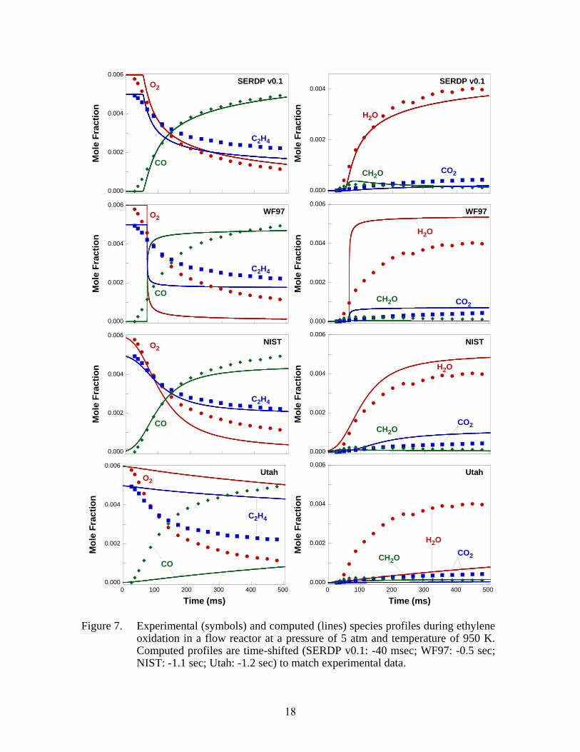
18
0.000
0.002
0.004
0.006
Mo
le F
rac
tio
n
SERDP v0.1O2
C2H4
CO
0.000
0.002
0.004
Mo
le F
rac
tio
n
SERDP v0.1
H2O
CO2CH2O
0.000
0.002
0.004
0.006
Mo
le F
rac
tio
n
O2
C2H4
CO
WF97
0.000
0.002
0.004
0.006
Mo
le F
rac
tio
n
WF97
CO2CH2O
H2O
0.000
0.002
0.004
0.006
Mo
le F
rac
tio
n
O2
C2H4
CO
NIST
0.000
0.002
0.004
0.006
Mo
le F
rac
tio
n
NIST
CO2CH2O
H2O
0.000
0.002
0.004
0.006
0 100 200 300 400 500
Mo
le F
rac
tio
n
Time (ms)
O2
Utah
CO
C2H4
0.000
0.002
0.004
0.006
0 100 200 300 400 500
Mo
le F
rac
tio
n
Time (ms)
Utah
CO2CH2O
H2O
Figure 7. Experimental (symbols) and computed (lines) species profiles during ethylene oxidation in a flow reactor at a pressure of 5 atm and temperature of 950 K. Computed profiles are time-shifted (SERDP v0.1: -40 msec; WF97: -0.5 sec; NIST: -1.1 sec; Utah: -1.2 sec) to match experimental data.
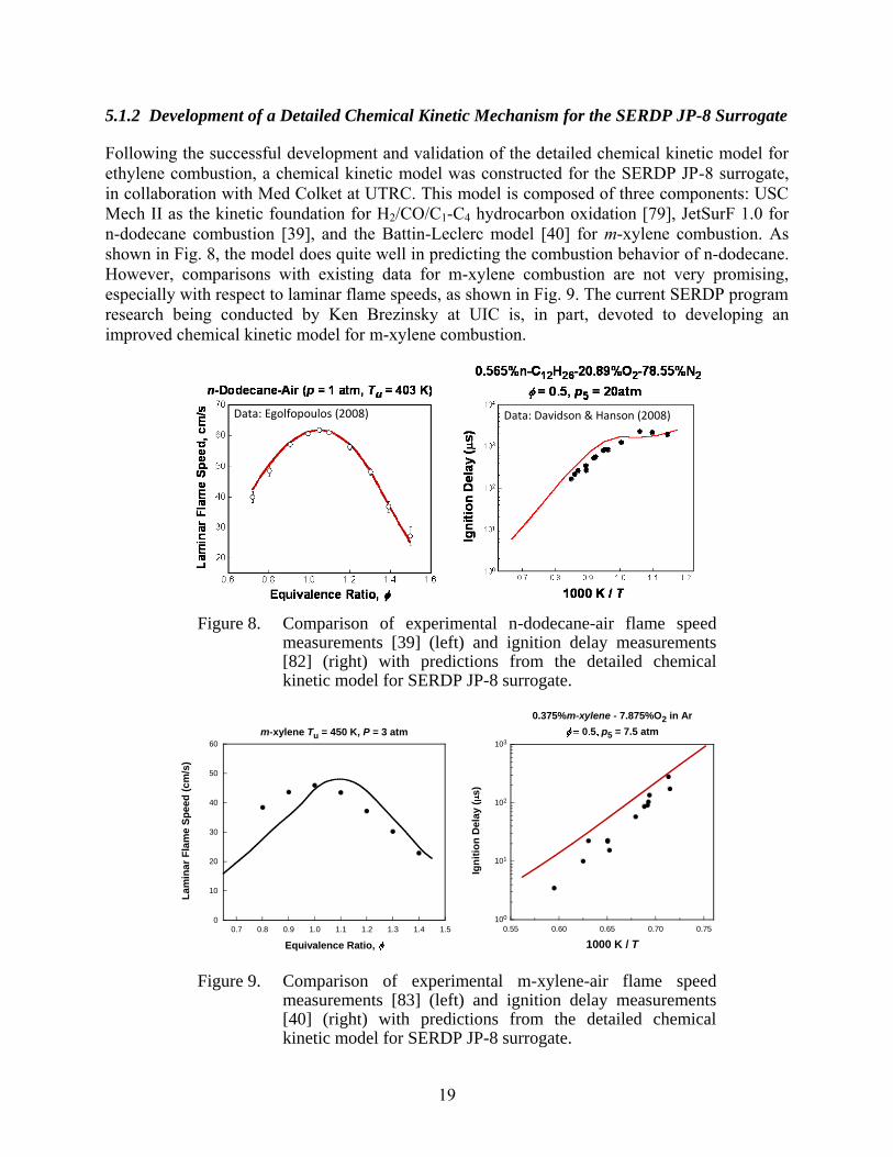
19
5.1.2 Development of a Detailed Chemical Kinetic Mechanism for the SERDP JP-8 Surrogate
Following the successful development and validation of the detailed chemical kinetic model for
ethylene combustion, a chemical kinetic model was constructed for the SERDP JP-8 surrogate,
in collaboration with Med Colket at UTRC. This model is composed of three components: USC
Mech II as the kinetic foundation for H2/CO/C1-C4 hydrocarbon oxidation [79], JetSurF 1.0 for
n-dodecane combustion [39], and the Battin-Leclerc model [40] for m-xylene combustion. As
shown in Fig. 8, the model does quite well in predicting the combustion behavior of n-dodecane.
However, comparisons with existing data for m-xylene combustion are not very promising,
especially with respect to laminar flame speeds, as shown in Fig. 9. The current SERDP program
research being conducted by Ken Brezinsky at UIC is, in part, devoted to developing an
improved chemical kinetic model for m-xylene combustion.
Figure 8. Comparison of experimental n-dodecane-air flame speed measurements [39] (left) and ignition delay measurements [82] (right) with predictions from the detailed chemical kinetic model for SERDP JP-8 surrogate.
Figure 9. Comparison of experimental m-xylene-air flame speed measurements [83] (left) and ignition delay measurements [40] (right) with predictions from the detailed chemical kinetic model for SERDP JP-8 surrogate.
Data: Egolfopoulos (2008)Data: Egolfopoulos (2008) Data: Davidson & Hanson (2008)Data: Davidson & Hanson (2008)
0
10
20
30
40
50
60
0.7 0.8 0.9 1.0 1.1 1.2 1.3 1.4 1.5
m-xylene Tu = 450 K, P = 3 atm
Equivalence Ratio,
La
min
ar
Fla
me
Sp
ee
d (
cm
/s)
100
101
102
103
0.55 0.60 0.65 0.70 0.75
0.375%m-xylene - 7.875%O2 in Ar
0 5 p5 = 7.5 atm
Ign
itio
n D
ela
y (
s)
1000 K / T
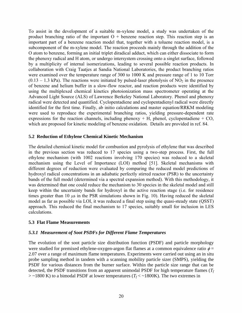
20
To assist in the development of a suitable m-xylene model, a study was undertaken of the
product branching ratio of the important O + benzene reaction step. This reaction step is an
important part of a benzene reaction model that, together with a toluene reaction model, is a
subcomponent of the m-xylene model. The reaction proceeds mainly through the addition of the
O atom to benzene, forming an initial triplet diradical adduct, which can either dissociate to form
the phenoxy radical and H atom, or undergo intersystem crossing onto a singlet surface, followed
by a multiplicity of internal isomerizations, leading to several possible reaction products. In
collaboration with Craig Taatjes at Sandia National Laboratories, the product branching ratios
were examined over the temperature range of 300 to 1000 K and pressure range of 1 to 10 Torr
(0.13 – 1.3 kPa). The reactions were initiated by pulsed-laser photolysis of NO2 in the presence
of benzene and helium buffer in a slow-flow reactor, and reaction products were identified by
using the multiplexed chemical kinetics photoionization mass spectrometer operating at the
Advanced Light Source (ALS) of Lawrence Berkeley National Laboratory. Phenol and phenoxy
radical were detected and quantified. Cyclopentadiene and cyclopentadienyl radical were directly
identified for the first time. Finally, ab initio calculations and master equation/RRKM modeling
were used to reproduce the experimental branching ratios, yielding pressure-dependent rate
expressions for the reaction channels, including phenoxy + H, phenol, cyclopentadiene + CO,
which are proposed for kinetic modeling of benzene oxidation. Details are provided in ref. 84.
5.2 Reduction of Ethylene Chemical Kinetic Mechanism
The detailed chemical kinetic model for combustion and pyrolysis of ethylene that was described
in the previous section was reduced to 17 species using a two-step process. First, the full
ethylene mechanism (with 1002 reactions involving 170 species) was reduced to a skeletal
mechanism using the Level of Importance (LOI) method [51]. Skeletal mechanisms with
different degrees of reduction were evaluated by comparing the reduced model predictions of
hydroxyl radical concentrations in an adiabatic perfectly stirred reactor (PSR) to the uncertainty
bands of the full model (determined via a spectral expansion method). With this methodology, it
was determined that one could reduce the mechanism to 30 species in the skeletal model and still
keep within the uncertainty bands for hydroxyl in the active reaction stage (i.e. for residence
times greater than 10 s in the PSR simulations shown in Fig. 10). Having reduced the skeletal
model as far as possible via LOI, it was reduced a final step using the quasi-steady state (QSST)
approach. This reduced the final mechanism to 17 species, suitably small for inclusion in LES
calculations.
5.3 Flat Flame Measurements
5.3.1 Measurement of Soot PSDFs for Different Flame Temperatures
The evolution of the soot particle size distribution function (PSDF) and particle morphology
were studied for premixed ethylene-oxygen-argon flat flames at a common equivalence ratio =
2.07 over a range of maximum flame temperatures. Experiments were carried out using an in situ
probe sampling method in tandem with a scanning mobility particle sizer (SMPS), yielding the
PSDF for various distances from the burner surface. Within the particle size range that can be
detected, the PSDF transitions from an apparent unimodal PSDF for high temperature flames (Tf
> ~1800 K) to a bimodal PSDF at lower temperatures (Tf < ~1800K). The two extremes in
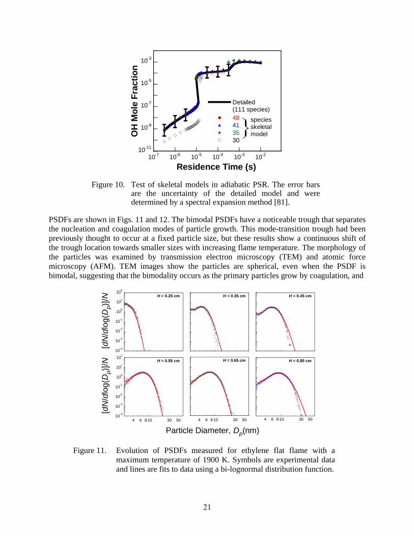
21
Figure 10. Test of skeletal models in adiabatic PSR. The error bars are the uncertainty of the detailed model and were determined by a spectral expansion method [81].
PSDFs are shown in Figs. 11 and 12. The bimodal PSDFs have a noticeable trough that separates
the nucleation and coagulation modes of particle growth. This mode-transition trough had been
previously thought to occur at a fixed particle size, but these results show a continuous shift of
the trough location towards smaller sizes with increasing flame temperature. The morphology of
the particles was examined by transmission electron microscopy (TEM) and atomic force
microscopy (AFM). TEM images show the particles are spherical, even when the PSDF is
bimodal, suggesting that the bimodality occurs as the primary particles grow by coagulation, and
Figure 11. Evolution of PSDFs measured for ethylene flat flame with a
maximum temperature of 1900 K. Symbols are experimental data
and lines are fits to data using a bi-lognormal distribution function.
10-11
10-9
10-7
10-5
10-3
10-7
10-6
10-5
10-4
10-3
10-2
Detailed (111 species)
48
30
35
41
OH
Mo
le F
racti
on
Residence Time (s)
speciesskeletalmodel
Particle Diameter, Dp(nm)
[dN
/dlo
g(D
p)]
/N
10-4
10-3
10-2
10-1
100
101
102
H = 0.25 cm H = 0.35 cm H = 0.45 cm
10-4
10-3
10-2
10-1
100
101
102
4 6 8 10 30 50
H = 0.55 cm
4 6 8 10 30 50
H = 0.65 cm
4 6 8 10 30 50
H = 0.85 cm
[dN
/dlo
g(D
p)]
/N
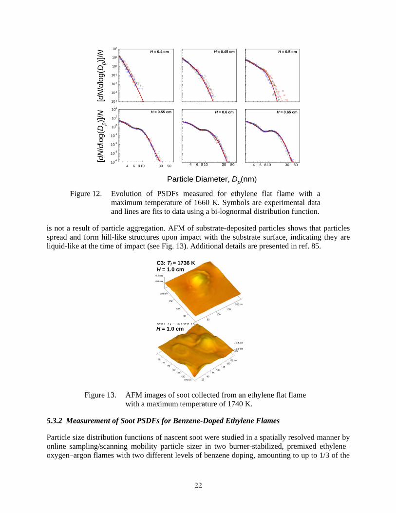
22
Figure 12. Evolution of PSDFs measured for ethylene flat flame with a
maximum temperature of 1660 K. Symbols are experimental data
and lines are fits to data using a bi-lognormal distribution function.
is not a result of particle aggregation. AFM of substrate-deposited particles shows that particles
spread and form hill-like structures upon impact with the substrate surface, indicating they are
liquid-like at the time of impact (see Fig. 13). Additional details are presented in ref. 85.
Figure 13. AFM images of soot collected from an ethylene flat flame
with a maximum temperature of 1740 K.
5.3.2 Measurement of Soot PSDFs for Benzene-Doped Ethylene Flames
Particle size distribution functions of nascent soot were studied in a spatially resolved manner by
online sampling/scanning mobility particle sizer in two burner-stabilized, premixed ethylene–
oxygen–argon flames with two different levels of benzene doping, amounting to up to 1/3 of the
Particle Diameter, Dp(nm)
[dN
/dlo
g(D
p)]
/N10-4
10-3
10-2
10-1
100
101
102
H = 0.4 cm H = 0.45 cm H = 0.5 cm
10-4
10-3
10-2
10-1
100
101
102
4 6 810 30 50
H = 0.55 cm
4 6 810 30 50
H = 0.6 cm
4 6 810 30 50
H = 0.65 cm
[dN
/dlo
g(D
p)]
/N
C3: Tf = 1736 K
H = 1.0 cm
C3: Tf = 1736 K H = 1.0 cm
C3: Tf = 1736 K
H = 1.0 cm
C3: Tf = 1736 K H = 1.0 cm
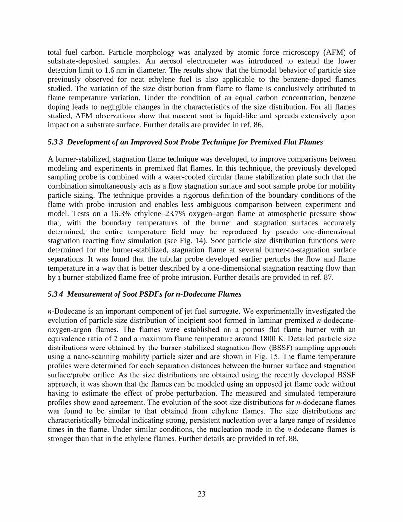
23
total fuel carbon. Particle morphology was analyzed by atomic force microscopy (AFM) of
substrate-deposited samples. An aerosol electrometer was introduced to extend the lower
detection limit to 1.6 nm in diameter. The results show that the bimodal behavior of particle size
previously observed for neat ethylene fuel is also applicable to the benzene-doped flames
studied. The variation of the size distribution from flame to flame is conclusively attributed to
flame temperature variation. Under the condition of an equal carbon concentration, benzene
doping leads to negligible changes in the characteristics of the size distribution. For all flames
studied, AFM observations show that nascent soot is liquid-like and spreads extensively upon
impact on a substrate surface. Further details are provided in ref. 86.
5.3.3 Development of an Improved Soot Probe Technique for Premixed Flat Flames
A burner-stabilized, stagnation flame technique was developed, to improve comparisons between
modeling and experiments in premixed flat flames. In this technique, the previously developed
sampling probe is combined with a water-cooled circular flame stabilization plate such that the
combination simultaneously acts as a flow stagnation surface and soot sample probe for mobility
particle sizing. The technique provides a rigorous definition of the boundary conditions of the
flame with probe intrusion and enables less ambiguous comparison between experiment and
model. Tests on a 16.3% ethylene–23.7% oxygen–argon flame at atmospheric pressure show
that, with the boundary temperatures of the burner and stagnation surfaces accurately
determined, the entire temperature field may be reproduced by pseudo one-dimensional
stagnation reacting flow simulation (see Fig. 14). Soot particle size distribution functions were
determined for the burner-stabilized, stagnation flame at several burner-to-stagnation surface
separations. It was found that the tubular probe developed earlier perturbs the flow and flame
temperature in a way that is better described by a one-dimensional stagnation reacting flow than
by a burner-stabilized flame free of probe intrusion. Further details are provided in ref. 87.
5.3.4 Measurement of Soot PSDFs for n-Dodecane Flames
n-Dodecane is an important component of jet fuel surrogate. We experimentally investigated the
evolution of particle size distribution of incipient soot formed in laminar premixed n-dodecane-
oxygen-argon flames. The flames were established on a porous flat flame burner with an
equivalence ratio of 2 and a maximum flame temperature around 1800 K. Detailed particle size
distributions were obtained by the burner-stabilized stagnation-flow (BSSF) sampling approach
using a nano-scanning mobility particle sizer and are shown in Fig. 15. The flame temperature
profiles were determined for each separation distances between the burner surface and stagnation
surface/probe orifice. As the size distributions are obtained using the recently developed BSSF
approach, it was shown that the flames can be modeled using an opposed jet flame code without
having to estimate the effect of probe perturbation. The measured and simulated temperature
profiles show good agreement. The evolution of the soot size distributions for n-dodecane flames
was found to be similar to that obtained from ethylene flames. The size distributions are
characteristically bimodal indicating strong, persistent nucleation over a large range of residence
times in the flame. Under similar conditions, the nucleation mode in the n-dodecane flames is
stronger than that in the ethylene flames. Further details are provided in ref. 88.
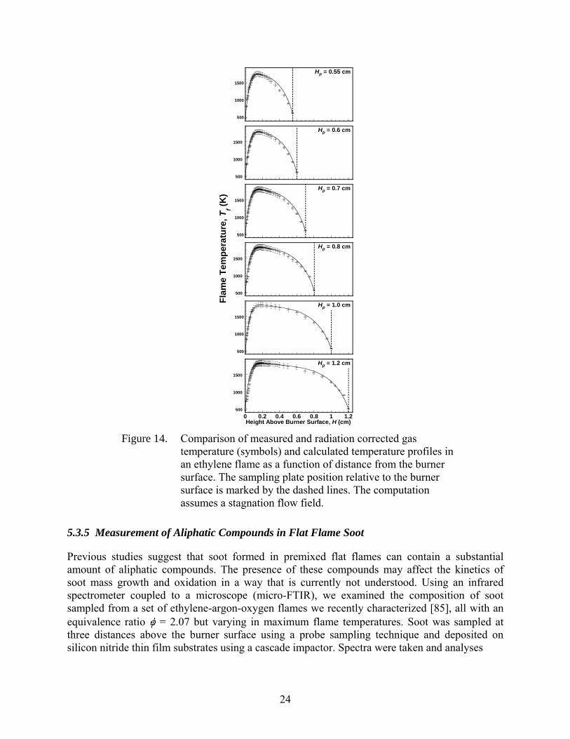
24
Figure 14. Comparison of measured and radiation corrected gas
temperature (symbols) and calculated temperature profiles in
an ethylene flame as a function of distance from the burner
surface. The sampling plate position relative to the burner
surface is marked by the dashed lines. The computation
assumes a stagnation flow field.
5.3.5 Measurement of Aliphatic Compounds in Flat Flame Soot
Previous studies suggest that soot formed in premixed flat flames can contain a substantial
amount of aliphatic compounds. The presence of these compounds may affect the kinetics of
soot mass growth and oxidation in a way that is currently not understood. Using an infrared
spectrometer coupled to a microscope (micro-FTIR), we examined the composition of soot
sampled from a set of ethylene-argon-oxygen flames we recently characterized [85], all with an
equivalence ratio = 2.07 but varying in maximum flame temperatures. Soot was sampled at
three distances above the burner surface using a probe sampling technique and deposited on
silicon nitride thin film substrates using a cascade impactor. Spectra were taken and analyses
500
1000
1500
Hp = 0.7 cm
0 0.2 0.4 0.6 0.8 1 1.2
500
1000
1500
Hp = 1.2 cm
Height Above Burner Surface, H (cm)
500
1000
1500
Hp = 0.55 cm
500
1000
1500
Hp = 0.6 cm
500
1000
1500
Hp = 1.0 cm
500
1000
1500
Hp = 0.8 cm
Fla
me
Te
mp
era
ture
, T
f (K
)
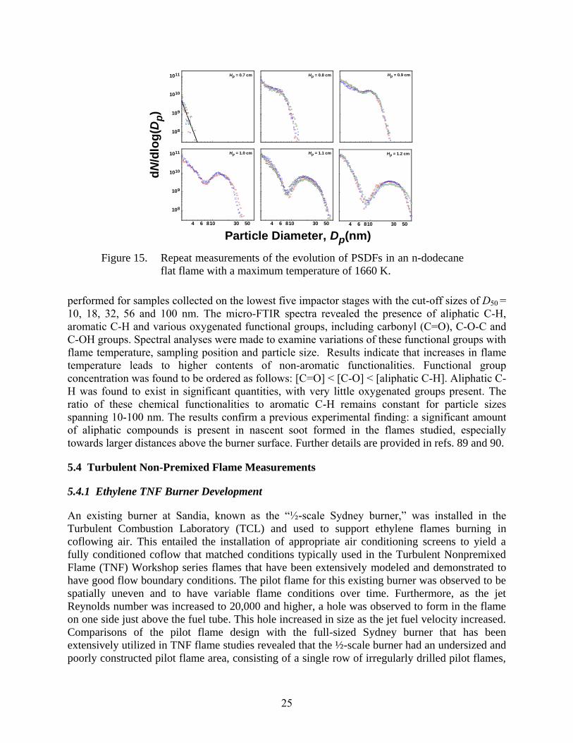
25
Figure 15. Repeat measurements of the evolution of PSDFs in an n-dodecane
flat flame with a maximum temperature of 1660 K.
performed for samples collected on the lowest five impactor stages with the cut-off sizes of D50 =
10, 18, 32, 56 and 100 nm. The micro-FTIR spectra revealed the presence of aliphatic C-H,
aromatic C-H and various oxygenated functional groups, including carbonyl (C=O), C-O-C and
C-OH groups. Spectral analyses were made to examine variations of these functional groups with
flame temperature, sampling position and particle size. Results indicate that increases in flame
temperature leads to higher contents of non-aromatic functionalities. Functional group
concentration was found to be ordered as follows: [C=O] < [C-O] < [aliphatic C-H]. Aliphatic C-
H was found to exist in significant quantities, with very little oxygenated groups present. The
ratio of these chemical functionalities to aromatic C-H remains constant for particle sizes
spanning 10-100 nm. The results confirm a previous experimental finding: a significant amount
of aliphatic compounds is present in nascent soot formed in the flames studied, especially
towards larger distances above the burner surface. Further details are provided in refs. 89 and 90.
5.4 Turbulent Non-Premixed Flame Measurements
5.4.1 Ethylene TNF Burner Development
An existing burner at Sandia, known as the ―½-scale Sydney burner,‖ was installed in the
Turbulent Combustion Laboratory (TCL) and used to support ethylene flames burning in
coflowing air. This entailed the installation of appropriate air conditioning screens to yield a
fully conditioned coflow that matched conditions typically used in the Turbulent Nonpremixed
Flame (TNF) Workshop series flames that have been extensively modeled and demonstrated to
have good flow boundary conditions. The pilot flame for this existing burner was observed to be
spatially uneven and to have variable flame conditions over time. Furthermore, as the jet
Reynolds number was increased to 20,000 and higher, a hole was observed to form in the flame
on one side just above the fuel tube. This hole increased in size as the jet fuel velocity increased.
Comparisons of the pilot flame design with the full-sized Sydney burner that has been
extensively utilized in TNF flame studies revealed that the ½-scale burner had an undersized and
poorly constructed pilot flame area, consisting of a single row of irregularly drilled pilot flames,
4 6 810 30 50
Hp = 1.1 cm
108
109
1010
1011 Hp = 0.7 cm Hp = 0.8 cm Hp = 0.9 cm
108
109
1010
1011
4 6 810 30 50
Hp = 1.0 cm
4 6 810 30 50
Hp = 1.2 cm
Particle Diameter, Dp(nm)
dN
/dlo
g(D
p)
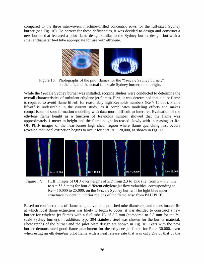
26
compared to the three interwoven, machine-drilled concentric rows for the full-sized Sydney
burner (see Fig. 16). To correct for these deficiencies, it was decided to design and construct a
new burner that featured a pilot flame design similar to the Sydney burner design, but with a
smaller diameter fuel tube appropriate for use with ethylene.
Figure 16. Photographs of the pilot flames for the ―½-scale Sydney burner,‖ on the left, and the actual full-scale Sydney burner, on the right.
While the ½-scale Sydney burner was installed, scoping studies were conducted to determine the
overall characteristics of turbulent ethylene jet flames. First, it was determined that a pilot flame
is required to avoid flame lift-off for reasonably high Reynolds numbers (Re ≥ 15,000). Flame
lift-off is undesirable in the current study, as it complicates modeling efforts and makes
comparisons of soot formation modeling with data more difficult to interpret. Evaluation of the
ethylene flame height as a function of Reynolds number showed that the flame was
approximately 1 meter in height and the flame height increased slowly with increasing jet Re.
OH PLIF images of the near-burner high shear region where flame quenching first occurs
revealed that local extinction begins to occur for a jet Re ~ 20,000, as shown in Fig. 17.
Figure 17. PLIF images of OH• over heights of x/D from 2.3 to 15.6 (i.e. from x = 8.7 mm
to x = 58.8 mm) for four different ethylene jet flow velocities, corresponding to
Re = 10,000 to 25,000, on the ½-scale Sydney burner. The light blue inner
structures evident in interior regions of the flame arise from PAH PLIF.
Based on considerations of flame height, available polished tube diameters, and the estimated Re
at which local flame extinction was likely to begin to occur, it was decided to construct a new
burner for ethylene jet flames with a fuel tube ID of 3.2 mm (compared to 3.8 mm for the ½-
scale Sydney burner). In addition, type 304 stainless steel was chosen for the burner material.
Photographs of the burner and the pilot plate design are shown in Fig. 18. Tests with the new
burner demonstrated good flame attachment for the ethylene jet flame for Re > 30,000, even
when using an ethylene/air pilot flame with a heat release rate that was only 2% of that of the
Re = 10,000 Re = 15,000 Re = 20,000 Re = 25,000
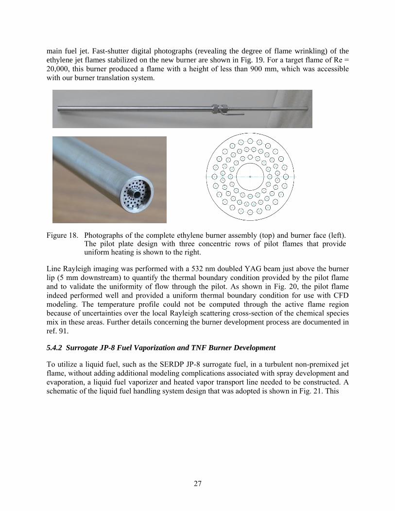
27
main fuel jet. Fast-shutter digital photographs (revealing the degree of flame wrinkling) of the
ethylene jet flames stabilized on the new burner are shown in Fig. 19. For a target flame of Re =
20,000, this burner produced a flame with a height of less than 900 mm, which was accessible
with our burner translation system.
Figure 18. Photographs of the complete ethylene burner assembly (top) and burner face (left). The pilot plate design with three concentric rows of pilot flames that provide uniform heating is shown to the right.
Line Rayleigh imaging was performed with a 532 nm doubled YAG beam just above the burner
lip (5 mm downstream) to quantify the thermal boundary condition provided by the pilot flame
and to validate the uniformity of flow through the pilot. As shown in Fig. 20, the pilot flame
indeed performed well and provided a uniform thermal boundary condition for use with CFD
modeling. The temperature profile could not be computed through the active flame region
because of uncertainties over the local Rayleigh scattering cross-section of the chemical species
mix in these areas. Further details concerning the burner development process are documented in
ref. 91.
5.4.2 Surrogate JP-8 Fuel Vaporization and TNF Burner Development
To utilize a liquid fuel, such as the SERDP JP-8 surrogate fuel, in a turbulent non-premixed jet
flame, without adding additional modeling complications associated with spray development and
evaporation, a liquid fuel vaporizer and heated vapor transport line needed to be constructed. A
schematic of the liquid fuel handling system design that was adopted is shown in Fig. 21. This
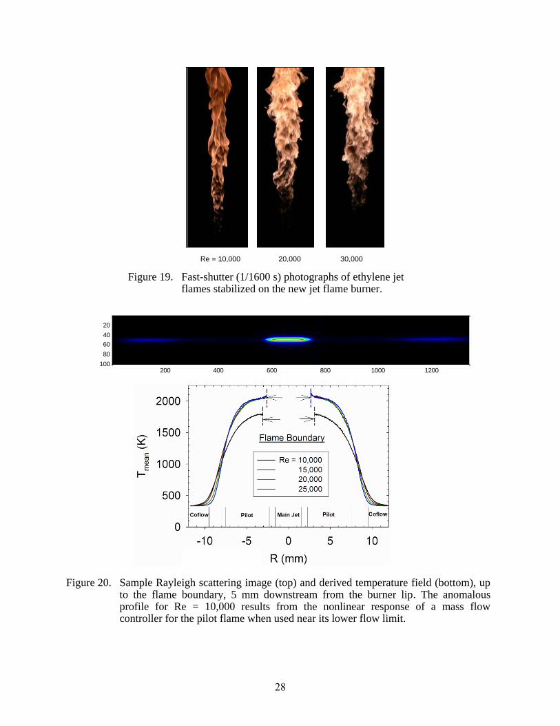
28
Figure 19. Fast-shutter (1/1600 s) photographs of ethylene jet flames stabilized on the new jet flame burner.
Figure 20. Sample Rayleigh scattering image (top) and derived temperature field (bottom), up to the flame boundary, 5 mm downstream from the burner lip. The anomalous profile for Re = 10,000 results from the nonlinear response of a mass flow controller for the pilot flame when used near its lower flow limit.
200 400 600 800 1000 1200
20
40
60
80
100
Re = 10,000 20,000 30,000
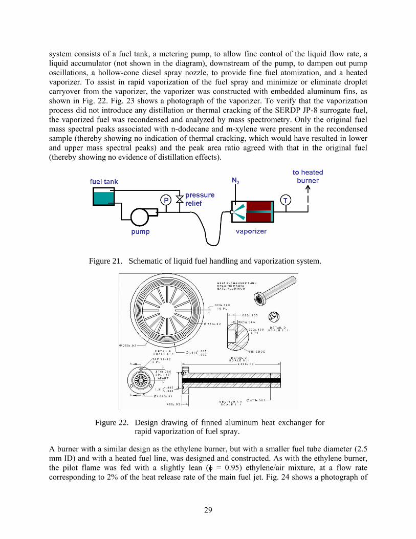
29
system consists of a fuel tank, a metering pump, to allow fine control of the liquid flow rate, a
liquid accumulator (not shown in the diagram), downstream of the pump, to dampen out pump
oscillations, a hollow-cone diesel spray nozzle, to provide fine fuel atomization, and a heated
vaporizer. To assist in rapid vaporization of the fuel spray and minimize or eliminate droplet
carryover from the vaporizer, the vaporizer was constructed with embedded aluminum fins, as
shown in Fig. 22. Fig. 23 shows a photograph of the vaporizer. To verify that the vaporization
process did not introduce any distillation or thermal cracking of the SERDP JP-8 surrogate fuel,
the vaporized fuel was recondensed and analyzed by mass spectrometry. Only the original fuel
mass spectral peaks associated with n-dodecane and m-xylene were present in the recondensed
sample (thereby showing no indication of thermal cracking, which would have resulted in lower
and upper mass spectral peaks) and the peak area ratio agreed with that in the original fuel
(thereby showing no evidence of distillation effects).
Figure 21. Schematic of liquid fuel handling and vaporization system.
Figure 22. Design drawing of finned aluminum heat exchanger for rapid vaporization of fuel spray.
A burner with a similar design as the ethylene burner, but with a smaller fuel tube diameter (2.5
mm ID) and with a heated fuel line, was designed and constructed. As with the ethylene burner,
the pilot flame was fed with a slightly lean ( = 0.95) ethylene/air mixture, at a flow rate
corresponding to 2% of the heat release rate of the main fuel jet. Fig. 24 shows a photograph of
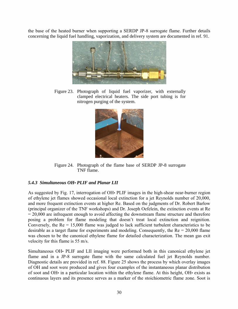
30
the base of the heated burner when supporting a SERDP JP-8 surrogate flame. Further details
concerning the liquid fuel handling, vaporization, and delivery system are documented in ref. 91.
Figure 23. Photograph of liquid fuel vaporizer, with externally clamped electrical heaters. The side port tubing is for nitrogen purging of the system.
Figure 24. Photograph of the flame base of SERDP JP-8 surrogate TNF flame.
5.4.3 Simultaneous OH• PLIF and Planar LII
As suggested by Fig. 17, interrogation of OH• PLIF images in the high-shear near-burner region
of ethylene jet flames showed occasional local extinction for a jet Reynolds number of 20,000,
and more frequent extinction events at higher Re. Based on the judgments of Dr. Robert Barlow
(principal organizer of the TNF workshops) and Dr. Joseph Oefelein, the extinction events at Re
= 20,000 are infrequent enough to avoid affecting the downstream flame structure and therefore
posing a problem for flame modeling that doesn‘t treat local extinction and reignition.
Conversely, the Re = 15,000 flame was judged to lack sufficient turbulent characteristics to be
desirable as a target flame for experiments and modeling. Consequently, the Re = 20,000 flame
was chosen to be the canonical ethylene flame for detailed characterization. The mean gas exit
velocity for this flame is 55 m/s.
Simultaneous OH• PLIF and LII imaging were performed both in this canonical ethylene jet
flame and in a JP-8 surrogate flame with the same calculated fuel jet Reynolds number.
Diagnostic details are provided in ref. 88. Figure 25 shows the process by which overlay images
of OH and soot were produced and gives four examples of the instantaneous planar distribution
of soot and OH• in a particular location within the ethylene flame. At this height, OH• exists as
continuous layers and its presence serves as a marker of the stoichiometric flame zone. Soot is
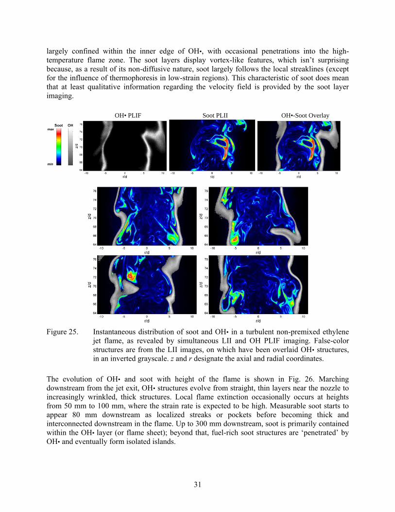
31
largely confined within the inner edge of OH•, with occasional penetrations into the high-
temperature flame zone. The soot layers display vortex-like features, which isn‘t surprising
because, as a result of its non-diffusive nature, soot largely follows the local streaklines (except
for the influence of thermophoresis in low-strain regions). This characteristic of soot does mean
that at least qualitative information regarding the velocity field is provided by the soot layer
imaging.
OH• PLIF Soot PLII OH•-Soot Overlay
Figure 25. Instantaneous distribution of soot and OH• in a turbulent non-premixed ethylene
jet flame, as revealed by simultaneous LII and OH PLIF imaging. False-color
structures are from the LII images, on which have been overlaid OH• structures,
in an inverted grayscale. z and r designate the axial and radial coordinates.
The evolution of OH• and soot with height of the flame is shown in Fig. 26. Marching
downstream from the jet exit, OH• structures evolve from straight, thin layers near the nozzle to
increasingly wrinkled, thick structures. Local flame extinction occasionally occurs at heights
from 50 mm to 100 mm, where the strain rate is expected to be high. Measurable soot starts to
appear 80 mm downstream as localized streaks or pockets before becoming thick and
interconnected downstream in the flame. Up to 300 mm downstream, soot is primarily contained
within the OH• layer (or flame sheet); beyond that, fuel-rich soot structures are ‗penetrated‘ by
OH• and eventually form isolated islands.
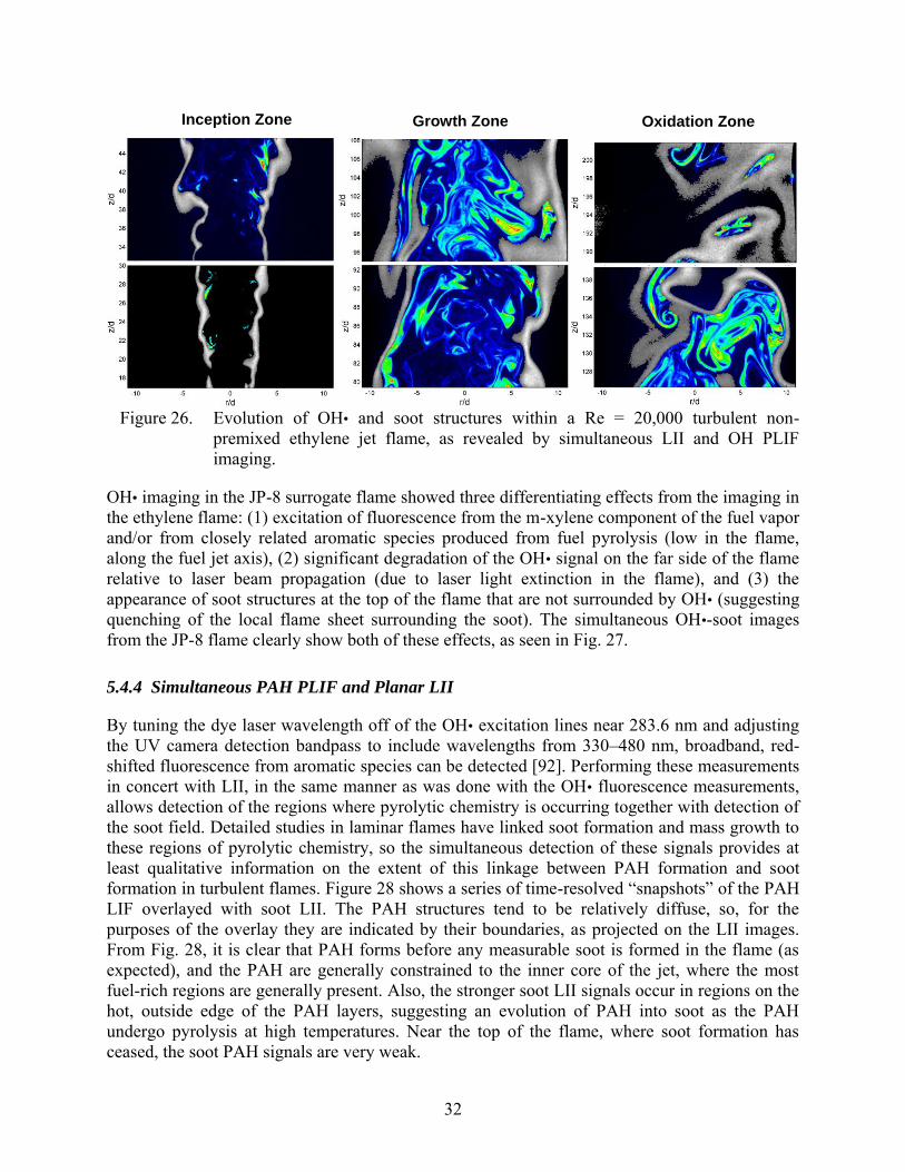
32
Figure 26. Evolution of OH• and soot structures within a Re = 20,000 turbulent non-
premixed ethylene jet flame, as revealed by simultaneous LII and OH PLIF
imaging.
OH• imaging in the JP-8 surrogate flame showed three differentiating effects from the imaging in
the ethylene flame: (1) excitation of fluorescence from the m-xylene component of the fuel vapor
and/or from closely related aromatic species produced from fuel pyrolysis (low in the flame,
along the fuel jet axis), (2) significant degradation of the OH• signal on the far side of the flame
relative to laser beam propagation (due to laser light extinction in the flame), and (3) the
appearance of soot structures at the top of the flame that are not surrounded by OH• (suggesting
quenching of the local flame sheet surrounding the soot). The simultaneous OH•-soot images
from the JP-8 flame clearly show both of these effects, as seen in Fig. 27.
5.4.4 Simultaneous PAH PLIF and Planar LII
By tuning the dye laser wavelength off of the OH• excitation lines near 283.6 nm and adjusting
the UV camera detection bandpass to include wavelengths from 330–480 nm, broadband, red-
shifted fluorescence from aromatic species can be detected [92]. Performing these measurements
in concert with LII, in the same manner as was done with the OH• fluorescence measurements,
allows detection of the regions where pyrolytic chemistry is occurring together with detection of
the soot field. Detailed studies in laminar flames have linked soot formation and mass growth to
these regions of pyrolytic chemistry, so the simultaneous detection of these signals provides at
least qualitative information on the extent of this linkage between PAH formation and soot
formation in turbulent flames. Figure 28 shows a series of time-resolved ―snapshots‖ of the PAH
LIF overlayed with soot LII. The PAH structures tend to be relatively diffuse, so, for the
purposes of the overlay they are indicated by their boundaries, as projected on the LII images.
From Fig. 28, it is clear that PAH forms before any measurable soot is formed in the flame (as
expected), and the PAH are generally constrained to the inner core of the jet, where the most
fuel-rich regions are generally present. Also, the stronger soot LII signals occur in regions on the
hot, outside edge of the PAH layers, suggesting an evolution of PAH into soot as the PAH
undergo pyrolysis at high temperatures. Near the top of the flame, where soot formation has
ceased, the soot PAH signals are very weak.
Inception Zone Growth Zone Oxidation Zone
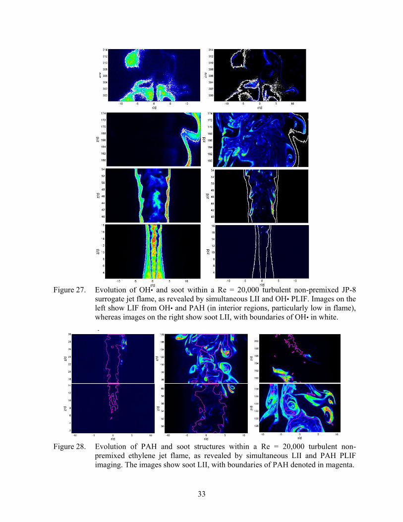
33
Figure 27. Evolution of OH• and soot within a Re = 20,000 turbulent non-premixed JP-8
surrogate jet flame, as revealed by simultaneous LII and OH• PLIF. Images on the
left show LIF from OH• and PAH (in interior regions, particularly low in flame),
whereas images on the right show soot LII, with boundaries of OH• in white.
Figure 28. Evolution of PAH and soot structures within a Re = 20,000 turbulent non-
premixed ethylene jet flame, as revealed by simultaneous LII and PAH PLIF
imaging. The images show soot LII, with boundaries of PAH denoted in magenta.
Inception Zone Growth Zone Oxidation ZoneInception Zone Growth Zone Oxidation Zone
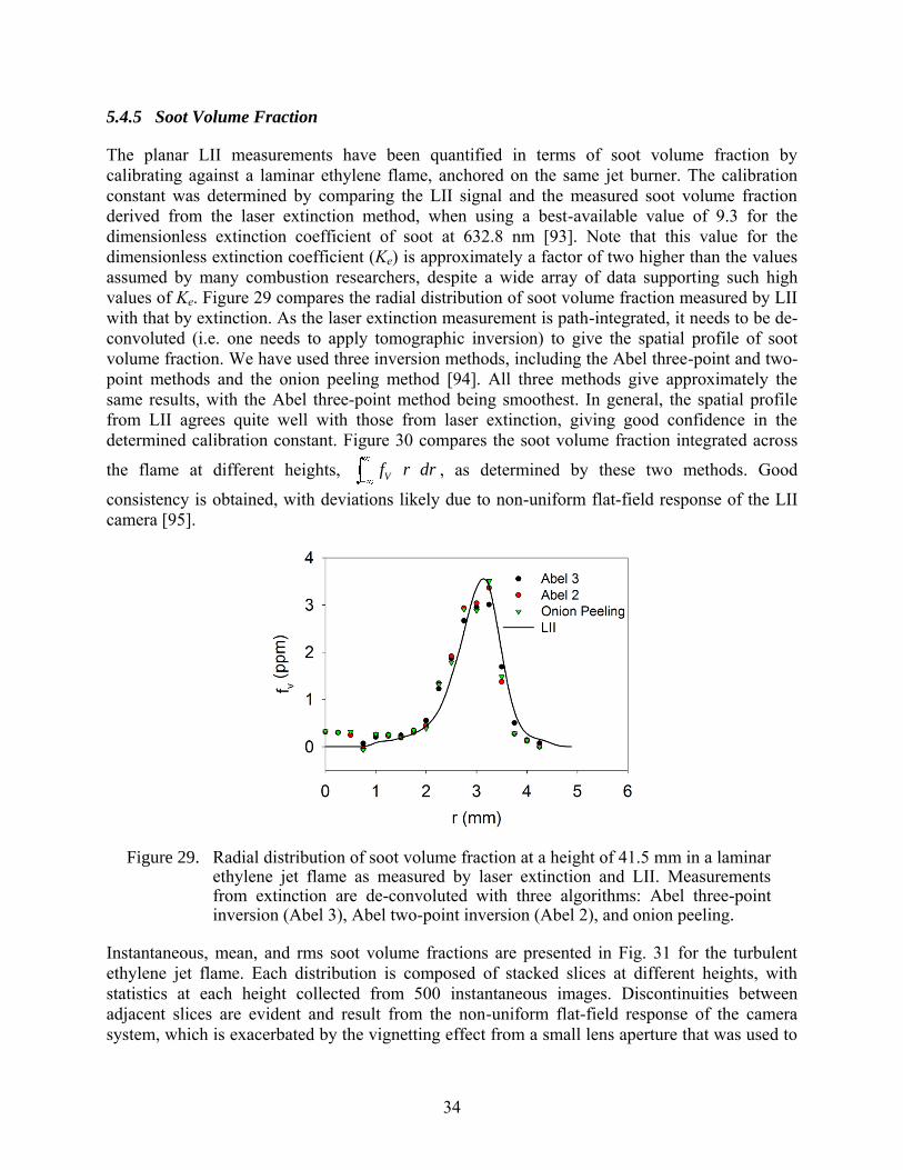
34
5.4.5 Soot Volume Fraction
The planar LII measurements have been quantified in terms of soot volume fraction by
calibrating against a laminar ethylene flame, anchored on the same jet burner. The calibration
constant was determined by comparing the LII signal and the measured soot volume fraction
derived from the laser extinction method, when using a best-available value of 9.3 for the
dimensionless extinction coefficient of soot at 632.8 nm [93]. Note that this value for the
dimensionless extinction coefficient (Ke) is approximately a factor of two higher than the values
assumed by many combustion researchers, despite a wide array of data supporting such high
values of Ke. Figure 29 compares the radial distribution of soot volume fraction measured by LII
with that by extinction. As the laser extinction measurement is path-integrated, it needs to be de-
convoluted (i.e. one needs to apply tomographic inversion) to give the spatial profile of soot
volume fraction. We have used three inversion methods, including the Abel three-point and two-
point methods and the onion peeling method [94]. All three methods give approximately the
same results, with the Abel three-point method being smoothest. In general, the spatial profile
from LII agrees quite well with those from laser extinction, giving good confidence in the
determined calibration constant. Figure 30 compares the soot volume fraction integrated across
the flame at different heights, Vf r dr , as determined by these two methods. Good
consistency is obtained, with deviations likely due to non-uniform flat-field response of the LII
camera [95].
Figure 29. Radial distribution of soot volume fraction at a height of 41.5 mm in a laminar ethylene jet flame as measured by laser extinction and LII. Measurements from extinction are de-convoluted with three algorithms: Abel three-point inversion (Abel 3), Abel two-point inversion (Abel 2), and onion peeling.
Instantaneous, mean, and rms soot volume fractions are presented in Fig. 31 for the turbulent
ethylene jet flame. Each distribution is composed of stacked slices at different heights, with
statistics at each height collected from 500 instantaneous images. Discontinuities between
adjacent slices are evident and result from the non-uniform flat-field response of the camera
system, which is exacerbated by the vignetting effect from a small lens aperture that was used to
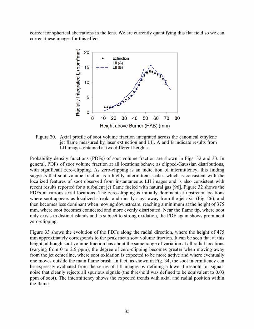
35
correct for spherical aberrations in the lens. We are currently quantifying this flat field so we can
correct these images for this effect.
Figure 30. Axial profile of soot volume fraction integrated across the canonical ethylene jet flame measured by laser extinction and LII. A and B indicate results from LII images obtained at two different heights.
Probability density functions (PDFs) of soot volume fraction are shown in Figs. 32 and 33. In
general, PDFs of soot volume fraction at all locations behave as clipped-Gaussian distributions,
with significant zero-clipping. As zero-clipping is an indication of intermittency, this finding
suggests that soot volume fraction is a highly intermittent scalar, which is consistent with the
localized features of soot observed from instantaneous LII images and is also consistent with
recent results reported for a turbulent jet flame fueled with natural gas [96]. Figure 32 shows the
PDFs at various axial locations. The zero-clipping is initially dominant at upstream locations
where soot appears as localized streaks and mostly stays away from the jet axis (Fig. 26), and
then becomes less dominant when moving downstream, reaching a minimum at the height of 375
mm, where soot becomes connected and more evenly distributed. Near the flame tip, where soot
only exists in distinct islands and is subject to strong oxidation, the PDF again shows prominent
zero-clipping.
Figure 33 shows the evolution of the PDFs along the radial direction, where the height of 475
mm approximately corresponds to the peak mean soot volume fraction. It can be seen that at this
height, although soot volume fraction has about the same range of variation at all radial locations
(varying from 0 to 2.5 ppm), the degree of zero-clipping becomes greater when moving away
from the jet centerline, where soot oxidation is expected to be more active and where eventually
one moves outside the main flame brush. In fact, as shown in Fig. 34, the soot intermittency can
be expressly evaluated from the series of LII images by defining a lower threshold for signal-
noise that cleanly rejects all spurious signals (the threshold was defined to be equivalent to 0.03
ppm of soot). The intermittency shows the expected trends with axial and radial position within
the flame.
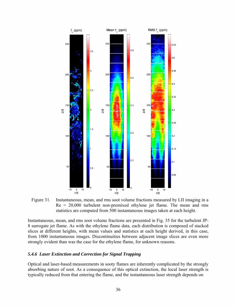
36
Figure 31. Instantaneous, mean, and rms soot volume fractions measured by LII imaging in a
Re = 20,000 turbulent non-premixed ethylene jet flame. The mean and rms
statistics are computed from 500 instantaneous images taken at each height.
Instantaneous, mean, and rms soot volume fractions are presented in Fig. 35 for the turbulent JP-
8 surrogate jet flame. As with the ethylene flame data, each distribution is composed of stacked
slices at different heights, with mean values and statistics at each height derived, in this case,
from 1000 instantaneous images. Discontinuities between adjacent image slices are even more
strongly evident than was the case for the ethylene flame, for unknown reasons.
5.4.6 Laser Extinction and Correction for Signal Trapping
Optical and laser-based measurements in sooty flames are inherently complicated by the strongly
absorbing nature of soot. As a consequence of this optical extinction, the local laser strength is
typically reduced from that entering the flame, and the instantaneous laser strength depends on
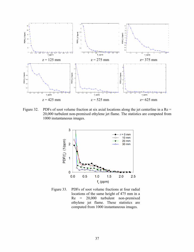
37
z = 125 mm z = 275 mm z= 375 mm
z = 425 mm z = 525 mm z= 625 mm
Figure 32. PDFs of soot volume fraction at six axial locations along the jet centerline in a Re =
20,000 turbulent non-premixed ethylene jet flame. The statistics are computed from
1000 instantaneous images.
Figure 33. PDFs of soot volume fractions at four radial
locations of the same height of 475 mm in a
Re = 20,000 turbulent non-premixed
ethylene jet flame. These statistics are
computed from 1000 instantaneous images.
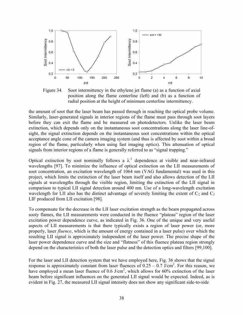
38
Figure 34. Soot intermittency in the ethylene jet flame (a) as a function of axial
position along the flame centerline (left) and (b) as a function of
radial position at the height of minimum centerline intermittency.
the amount of soot that the laser beam has passed through in reaching the optical probe volume.
Similarly, laser-generated signals in interior regions of the flame must pass through soot layers
before they can exit the flame and be measured on photodetectors. Unlike the laser beam
extinction, which depends only on the instantaneous soot concentrations along the laser line-of-
sight, the signal extinction depends on the instantaneous soot concentrations within the optical
acceptance angle cone of the camera imaging system (and thus is affected by soot within a broad
region of the flame, particularly when using fast imaging optics). This attenuation of optical
signals from interior regions of a flame is generally referred to as ―signal trapping.‖
Optical extinction by soot nominally follows a -1
dependence at visible and near-infrared
wavelengths [97]. To minimize the influence of optical extinction on the LII measurements of
soot concentration, an excitation wavelength of 1064 nm (YAG fundamental) was used in this
project, which limits the extinction of the laser beam itself and also allows detection of the LII
signals at wavelengths through the visible region, limiting the extinction of the LII signal in
comparison to typical LII signal detection around 400 nm. Use of a long-wavelength excitation
wavelength for LII also has the distinct advantage of severely limiting the extent of C2 and C3
LIF produced from LII excitation [98].
To compensate for the decrease in the LII laser excitation strength as the beam propagated across
sooty flames, the LII measurements were conducted in the fluence ―plateau‖ region of the laser
excitation power dependence curve, as indicated in Fig. 36. One of the unique and very useful
aspects of LII measurements is that there typically exists a region of laser power (or, more
properly, laser fluence, which is the amount of energy contained in a laser pulse) over which the
resulting LII signal is approximately independent of the laser power. The precise shape of the
laser power dependence curve and the size and ―flatness‖ of this fluence plateau region strongly
depend on the characteristics of both the laser pulse and the detection optics and filters [99,100].
For the laser and LII detection system that we have employed here, Fig. 36 shows that the signal
response is approximately constant from laser fluences of 0.25 – 0.7 J/cm2. For this reason, we
have employed a mean laser fluence of 0.6 J/cm2, which allows for 60% extinction of the laser
beam before significant influences on the generated LII signal would be expected. Indeed, as is
evident in Fig. 27, the measured LII signal intensity does not show any significant side-to-side
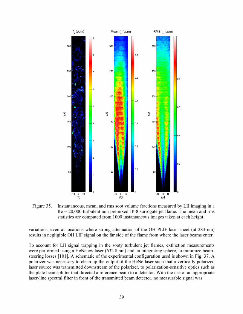
39
Figure 35. Instantaneous, mean, and rms soot volume fractions measured by LII imaging in a
Re = 20,000 turbulent non-premixed JP-8 surrogate jet flame. The mean and rms
statistics are computed from 1000 instantaneous images taken at each height.
variations, even at locations where strong attenuation of the OH PLIF laser sheet (at 283 nm)
results in negligible OH LIF signal on the far side of the flame from where the laser beams enter.
To account for LII signal trapping in the sooty turbulent jet flames, extinction measurements
were performed using a HeNe cw laser (632.8 nm) and an integrating sphere, to minimize beam-
steering losses [101]. A schematic of the experimental configuration used is shown in Fig. 37. A
polarizer was necessary to clean up the output of the HeNe laser such that a vertically polarized
laser source was transmitted downstream of the polarizer, to polarization-sensitive optics such as
the plate beamsplitter that directed a reference beam to a detector. With the use of an appropriate
laser-line spectral filter in front of the transmitted beam detector, no measurable signal was
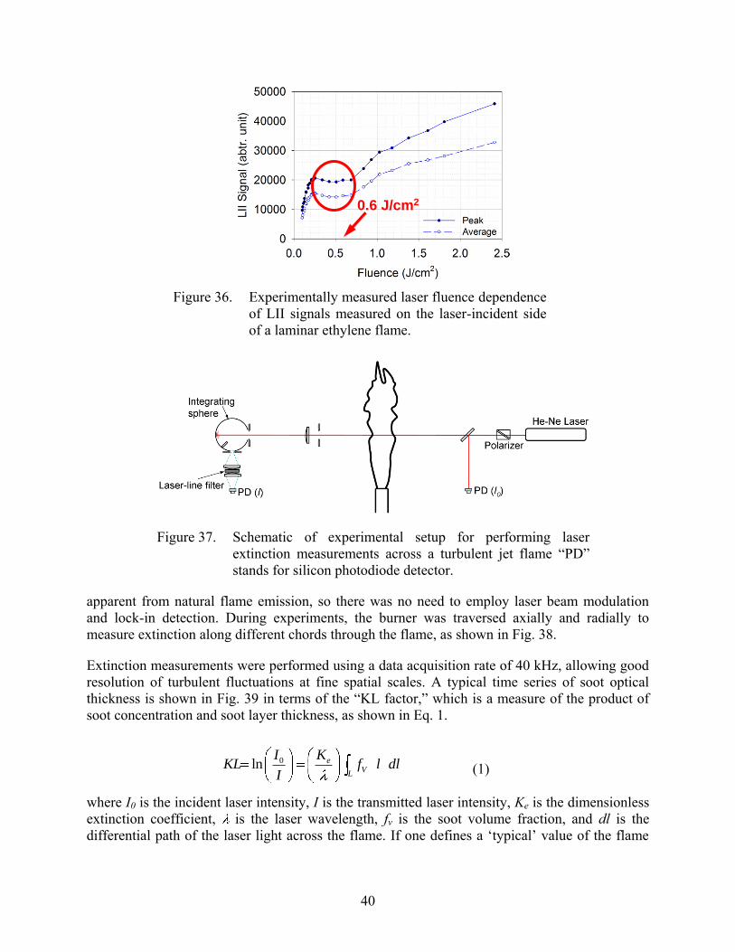
40
Figure 36. Experimentally measured laser fluence dependence
of LII signals measured on the laser-incident side
of a laminar ethylene flame.
Figure 37. Schematic of experimental setup for performing laser
extinction measurements across a turbulent jet flame ―PD‖
stands for silicon photodiode detector.
apparent from natural flame emission, so there was no need to employ laser beam modulation
and lock-in detection. During experiments, the burner was traversed axially and radially to
measure extinction along different chords through the flame, as shown in Fig. 38.
Extinction measurements were performed using a data acquisition rate of 40 kHz, allowing good
resolution of turbulent fluctuations at fine spatial scales. A typical time series of soot optical
thickness is shown in Fig. 39 in terms of the ―KL factor,‖ which is a measure of the product of
soot concentration and soot layer thickness, as shown in Eq. 1.
0ln eV
L
I KKL f l dl
I (1)
where I0 is the incident laser intensity, I is the transmitted laser intensity, Ke is the dimensionless
extinction coefficient, is the laser wavelength, fv is the soot volume fraction, and dl is the
differential path of the laser light across the flame. If one defines a ‗typical‘ value of the flame
0.6 J/cm20.6 J/cm2
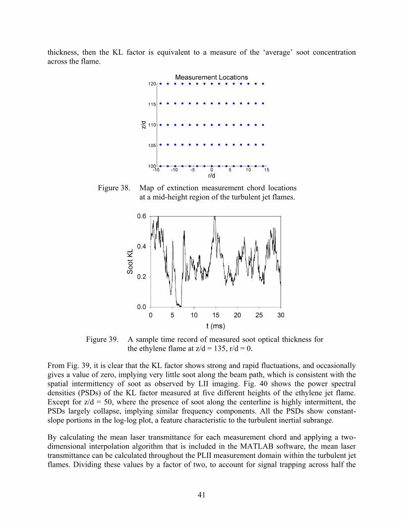
41
thickness, then the KL factor is equivalent to a measure of the ‗average‘ soot concentration
across the flame.
Figure 38. Map of extinction measurement chord locations
at a mid-height region of the turbulent jet flames.
Figure 39. A sample time record of measured soot optical thickness for
the ethylene flame at z/d = 135, r/d = 0.
From Fig. 39, it is clear that the KL factor shows strong and rapid fluctuations, and occasionally
gives a value of zero, implying very little soot along the beam path, which is consistent with the
spatial intermittency of soot as observed by LII imaging. Fig. 40 shows the power spectral
densities (PSDs) of the KL factor measured at five different heights of the ethylene jet flame.
Except for z/d = 50, where the presence of soot along the centerline is highly intermittent, the
PSDs largely collapse, implying similar frequency components. All the PSDs show constant-
slope portions in the log-log plot, a feature characteristic to the turbulent inertial subrange.
By calculating the mean laser transmittance for each measurement chord and applying a two-
dimensional interpolation algorithm that is included in the MATLAB software, the mean laser
transmittance can be calculated throughout the PLII measurement domain within the turbulent jet
flames. Dividing these values by a factor of two, to account for signal trapping across half the
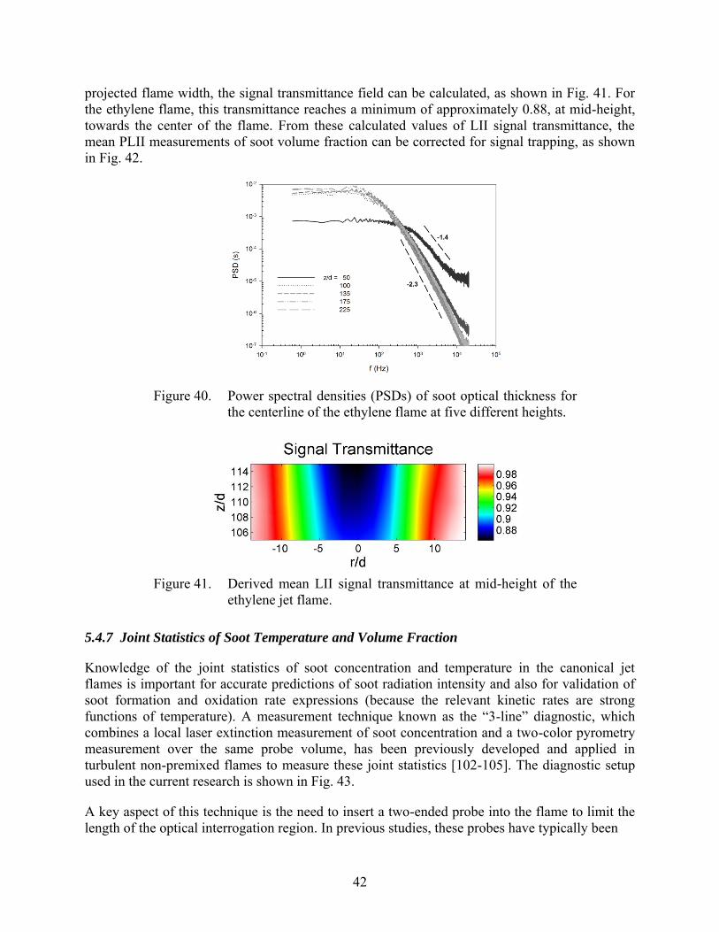
42
projected flame width, the signal transmittance field can be calculated, as shown in Fig. 41. For
the ethylene flame, this transmittance reaches a minimum of approximately 0.88, at mid-height,
towards the center of the flame. From these calculated values of LII signal transmittance, the
mean PLII measurements of soot volume fraction can be corrected for signal trapping, as shown
in Fig. 42.
Figure 40. Power spectral densities (PSDs) of soot optical thickness for
the centerline of the ethylene flame at five different heights.
Figure 41. Derived mean LII signal transmittance at mid-height of the
ethylene jet flame.
5.4.7 Joint Statistics of Soot Temperature and Volume Fraction
Knowledge of the joint statistics of soot concentration and temperature in the canonical jet
flames is important for accurate predictions of soot radiation intensity and also for validation of
soot formation and oxidation rate expressions (because the relevant kinetic rates are strong
functions of temperature). A measurement technique known as the ―3-line‖ diagnostic, which
combines a local laser extinction measurement of soot concentration and a two-color pyrometry
measurement over the same probe volume, has been previously developed and applied in
turbulent non-premixed flames to measure these joint statistics [102-105]. The diagnostic setup
used in the current research is shown in Fig. 43.
A key aspect of this technique is the need to insert a two-ended probe into the flame to limit the
length of the optical interrogation region. In previous studies, these probes have typically been
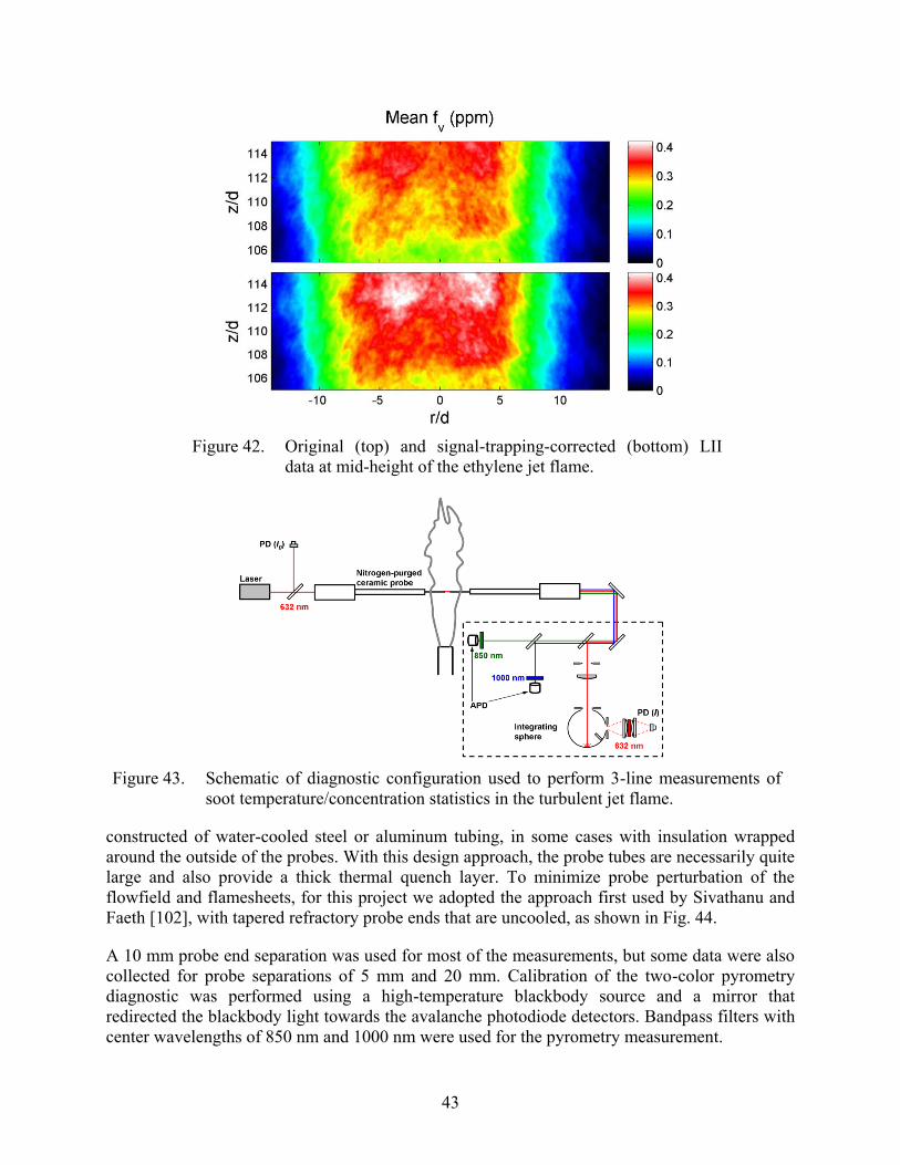
43
Figure 42. Original (top) and signal-trapping-corrected (bottom) LII
data at mid-height of the ethylene jet flame.
Figure 43. Schematic of diagnostic configuration used to perform 3-line measurements of
soot temperature/concentration statistics in the turbulent jet flame.
constructed of water-cooled steel or aluminum tubing, in some cases with insulation wrapped
around the outside of the probes. With this design approach, the probe tubes are necessarily quite
large and also provide a thick thermal quench layer. To minimize probe perturbation of the
flowfield and flamesheets, for this project we adopted the approach first used by Sivathanu and
Faeth [102], with tapered refractory probe ends that are uncooled, as shown in Fig. 44.
A 10 mm probe end separation was used for most of the measurements, but some data were also
collected for probe separations of 5 mm and 20 mm. Calibration of the two-color pyrometry
diagnostic was performed using a high-temperature blackbody source and a mirror that
redirected the blackbody light towards the avalanche photodiode detectors. Bandpass filters with
center wavelengths of 850 nm and 1000 nm were used for the pyrometry measurement.

44
Figure 44. Optical probe for performing 3-line measurements of soot temperature/
concentration statistics in the turbulent jet flame. Aluminum optical housing
(left) is water-cooled and provides N2 purge gas. Refractory probe ends (right)
are uncooled.
Extinction of a 632.8 nm HeNe laser beam was used to determine soot volume fraction, by
employing Eq. 1 with an assumed value for Ke of 9.3, based on the measurements of Williams et
al. [93]. Fig. 45 shows a sample data record of transmission and emission signals from the
ethylene flame at a mid-height position, along with the deduced soot volume fraction and
temperature variation. Note that the apparent mean soot volume fraction of ~ 0.5 ppm compares
favorably with the mean fv deduced from LII measurements in this region of this flame (Fig. 31).
The pyrometry measurements show that the soot temperature is typically within the region of
1350 – 1650 K.
5.4.8 Thermal Radiation
Turbulent non-premixed flames using higher molecular weight fuels typically have substantial
thermal radiation loss, on account of strong contributions from radiating soot. This radiant loss
reduces the peak flame temperature and also acts to moderate both soot formation and oxidation,
because of the high characteristic activation energies of these two processes. As will be
demonstrated in a successive section on flame modeling, accurate modeling of soot formation
and oxidation requires that soot radiation also be modeled accurately, because a model that
predicts the correct soot concentrations within a flame or emitted from a flame but erroneously
calculates the soot temperature will not be extendable to other flames. For this reason,
measurements of thermal radiation from model flame systems are important components of
model validation. As with other experimental measurements, the better the temporal and spatial
resolution of the measurement, the more useful the data are for model validation. For this reason,
a radiometer was constructed using a thin-film thermopile with a CaF2 window. The use of the
CaF2 window material makes the radiometer equally sensitive to radiant emission from 0.13–11
m, encompassing nearly all of the energy-containing radiation from the flame. The thermopile
that was chosen for this measurement is 1 mm in diameter and has a characteristic response time
of 12.8 ms (corresponding to a -3 dB cut-off frequency of 12.4 Hz). A black-anodized, 250 mm
long water-cooled steel tube with an ID of 2 mm minimizes light reflections within the probe and
restricts incident radiation to a small solid angle (Ω) of 41.065 10 sr. The detector sensor is
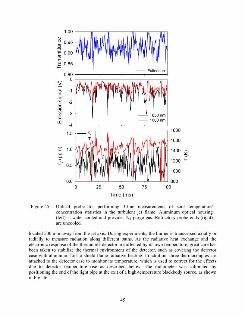
45
Figure 45. Optical probe for performing 3-line measurements of soot temperature/
concentration statistics in the turbulent jet flame. Aluminum optical housing
(left) is water-cooled and provides N2 purge gas. Refractory probe ends (right)
are uncooled.
located 500 mm away from the jet axis. During experiments, the burner is transversed axially or
radially to measure radiation along different paths. As the radiative heat exchange and the
electronic response of the thermopile detector are affected by its own temperature, great care has
been taken to stabilize the thermal environment of the detector, such as covering the detector
case with aluminum foil to shield flame radiative heating. In addition, three thermocouples are
attached to the detector case to monitor its temperature, which is used to correct for the effects
due to detector temperature rise as described below. The radiometer was calibrated by
positioning the end of the light pipe at the exit of a high-temperature blackbody source, as shown
in Fig. 46.
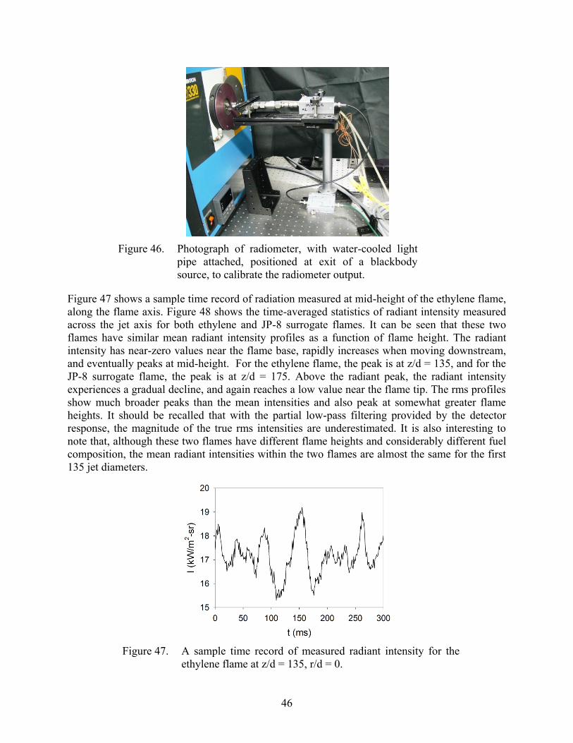
46
Figure 46. Photograph of radiometer, with water-cooled light
pipe attached, positioned at exit of a blackbody
source, to calibrate the radiometer output.
Figure 47 shows a sample time record of radiation measured at mid-height of the ethylene flame,
along the flame axis. Figure 48 shows the time-averaged statistics of radiant intensity measured
across the jet axis for both ethylene and JP-8 surrogate flames. It can be seen that these two
flames have similar mean radiant intensity profiles as a function of flame height. The radiant
intensity has near-zero values near the flame base, rapidly increases when moving downstream,
and eventually peaks at mid-height. For the ethylene flame, the peak is at z/d = 135, and for the
JP-8 surrogate flame, the peak is at z/d = 175. Above the radiant peak, the radiant intensity
experiences a gradual decline, and again reaches a low value near the flame tip. The rms profiles
show much broader peaks than the mean intensities and also peak at somewhat greater flame
heights. It should be recalled that with the partial low-pass filtering provided by the detector
response, the magnitude of the true rms intensities are underestimated. It is also interesting to
note that, although these two flames have different flame heights and considerably different fuel
composition, the mean radiant intensities within the two flames are almost the same for the first
135 jet diameters.
Figure 47. A sample time record of measured radiant intensity for the
ethylene flame at z/d = 135, r/d = 0.
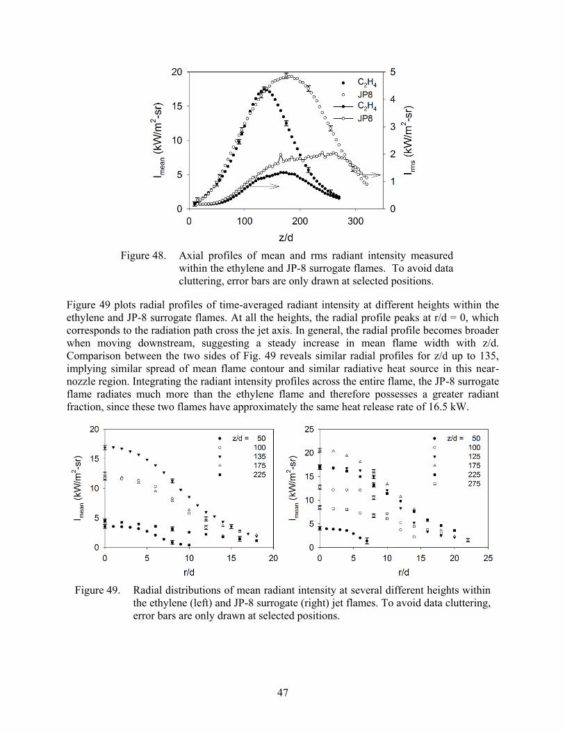
47
Figure 48. Axial profiles of mean and rms radiant intensity measured
within the ethylene and JP-8 surrogate flames. To avoid data
cluttering, error bars are only drawn at selected positions.
Figure 49 plots radial profiles of time-averaged radiant intensity at different heights within the
ethylene and JP-8 surrogate flames. At all the heights, the radial profile peaks at r/d = 0, which
corresponds to the radiation path cross the jet axis. In general, the radial profile becomes broader
when moving downstream, suggesting a steady increase in mean flame width with z/d.
Comparison between the two sides of Fig. 49 reveals similar radial profiles for z/d up to 135,
implying similar spread of mean flame contour and similar radiative heat source in this near-
nozzle region. Integrating the radiant intensity profiles across the entire flame, the JP-8 surrogate
flame radiates much more than the ethylene flame and therefore possesses a greater radiant
fraction, since these two flames have approximately the same heat release rate of 16.5 kW.
Figure 49. Radial distributions of mean radiant intensity at several different heights within
the ethylene (left) and JP-8 surrogate (right) jet flames. To avoid data cluttering,
error bars are only drawn at selected positions.
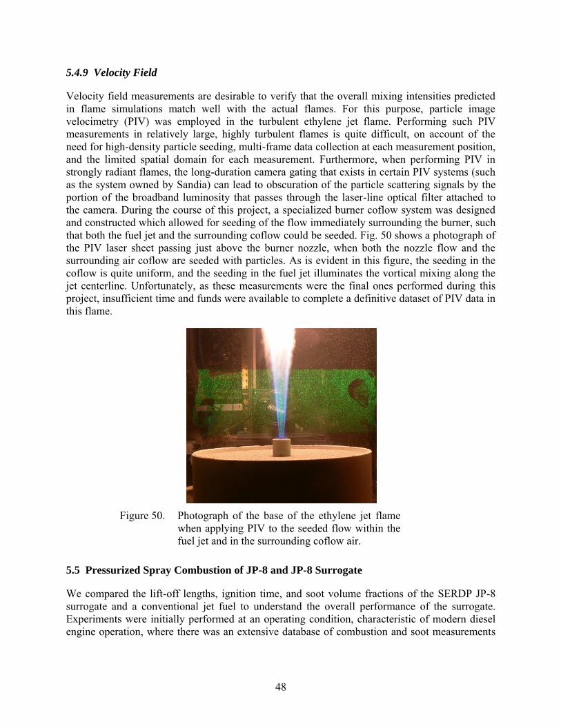
48
5.4.9 Velocity Field
Velocity field measurements are desirable to verify that the overall mixing intensities predicted
in flame simulations match well with the actual flames. For this purpose, particle image
velocimetry (PIV) was employed in the turbulent ethylene jet flame. Performing such PIV
measurements in relatively large, highly turbulent flames is quite difficult, on account of the
need for high-density particle seeding, multi-frame data collection at each measurement position,
and the limited spatial domain for each measurement. Furthermore, when performing PIV in
strongly radiant flames, the long-duration camera gating that exists in certain PIV systems (such
as the system owned by Sandia) can lead to obscuration of the particle scattering signals by the
portion of the broadband luminosity that passes through the laser-line optical filter attached to
the camera. During the course of this project, a specialized burner coflow system was designed
and constructed which allowed for seeding of the flow immediately surrounding the burner, such
that both the fuel jet and the surrounding coflow could be seeded. Fig. 50 shows a photograph of
the PIV laser sheet passing just above the burner nozzle, when both the nozzle flow and the
surrounding air coflow are seeded with particles. As is evident in this figure, the seeding in the
coflow is quite uniform, and the seeding in the fuel jet illuminates the vortical mixing along the
jet centerline. Unfortunately, as these measurements were the final ones performed during this
project, insufficient time and funds were available to complete a definitive dataset of PIV data in
this flame.
Figure 50. Photograph of the base of the ethylene jet flame
when applying PIV to the seeded flow within the
fuel jet and in the surrounding coflow air.
5.5 Pressurized Spray Combustion of JP-8 and JP-8 Surrogate
We compared the lift-off lengths, ignition time, and soot volume fractions of the SERDP JP-8
surrogate and a conventional jet fuel to understand the overall performance of the surrogate.
Experiments were initially performed at an operating condition, characteristic of modern diesel
engine operation, where there was an extensive database of combustion and soot measurements
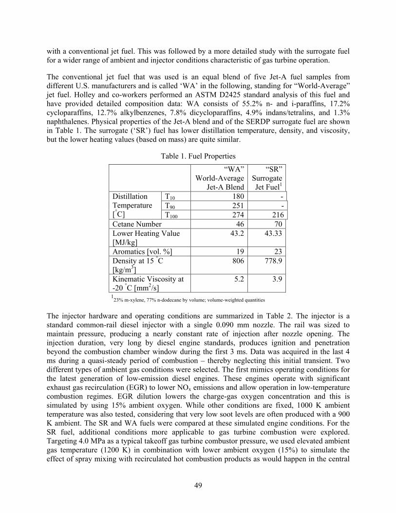
49
with a conventional jet fuel. This was followed by a more detailed study with the surrogate fuel
for a wider range of ambient and injector conditions characteristic of gas turbine operation.
The conventional jet fuel that was used is an equal blend of five Jet-A fuel samples from
different U.S. manufacturers and is called ‗WA‘ in the following, standing for ―World-Average‖
jet fuel. Holley and co-workers performed an ASTM D2425 standard analysis of this fuel and
have provided detailed composition data: WA consists of 55.2% n- and i-paraffins, 17.2%
cycloparaffins, 12.7% alkylbenzenes, 7.8% dicycloparaffins, 4.9% indans/tetralins, and 1.3%
naphthalenes. Physical properties of the Jet-A blend and of the SERDP surrogate fuel are shown
in Table 1. The surrogate (‗SR‘) fuel has lower distillation temperature, density, and viscosity,
but the lower heating values (based on mass) are quite similar.
Table 1. Fuel Properties
―WA‖
World-Average
Jet-A Blend
―SR‖
Surrogate
Jet Fuel1
Distillation
Temperature
[°C]
T10 180 -
T90 251 -
T100 274 216
Cetane Number 46 70
Lower Heating Value
[MJ/kg]
43.2 43.33
Aromatics [vol. %] 19 23
Density at 15 °C
[kg/m3]
806 778.9
Kinematic Viscosity at
-20 °C [mm
2/s]
5.2 3.9
123% m-xylene, 77% n-dodecane by volume; volume-weighted quantities
The injector hardware and operating conditions are summarized in Table 2. The injector is a
standard common-rail diesel injector with a single 0.090 mm nozzle. The rail was sized to
maintain pressure, producing a nearly constant rate of injection after nozzle opening. The
injection duration, very long by diesel engine standards, produces ignition and penetration
beyond the combustion chamber window during the first 3 ms. Data was acquired in the last 4
ms during a quasi-steady period of combustion – thereby neglecting this initial transient. Two
different types of ambient gas conditions were selected. The first mimics operating conditions for
the latest generation of low-emission diesel engines. These engines operate with significant
exhaust gas recirculation (EGR) to lower NOx emissions and allow operation in low-temperature
combustion regimes. EGR dilution lowers the charge-gas oxygen concentration and this is
simulated by using 15% ambient oxygen. While other conditions are fixed, 1000 K ambient
temperature was also tested, considering that very low soot levels are often produced with a 900
K ambient. The SR and WA fuels were compared at these simulated engine conditions. For the
SR fuel, additional conditions more applicable to gas turbine combustion were explored.
Targeting 4.0 MPa as a typical takeoff gas turbine combustor pressure, we used elevated ambient
gas temperature (1200 K) in combination with lower ambient oxygen (15%) to simulate the
effect of spray mixing with recirculated hot combustion products as would happen in the central
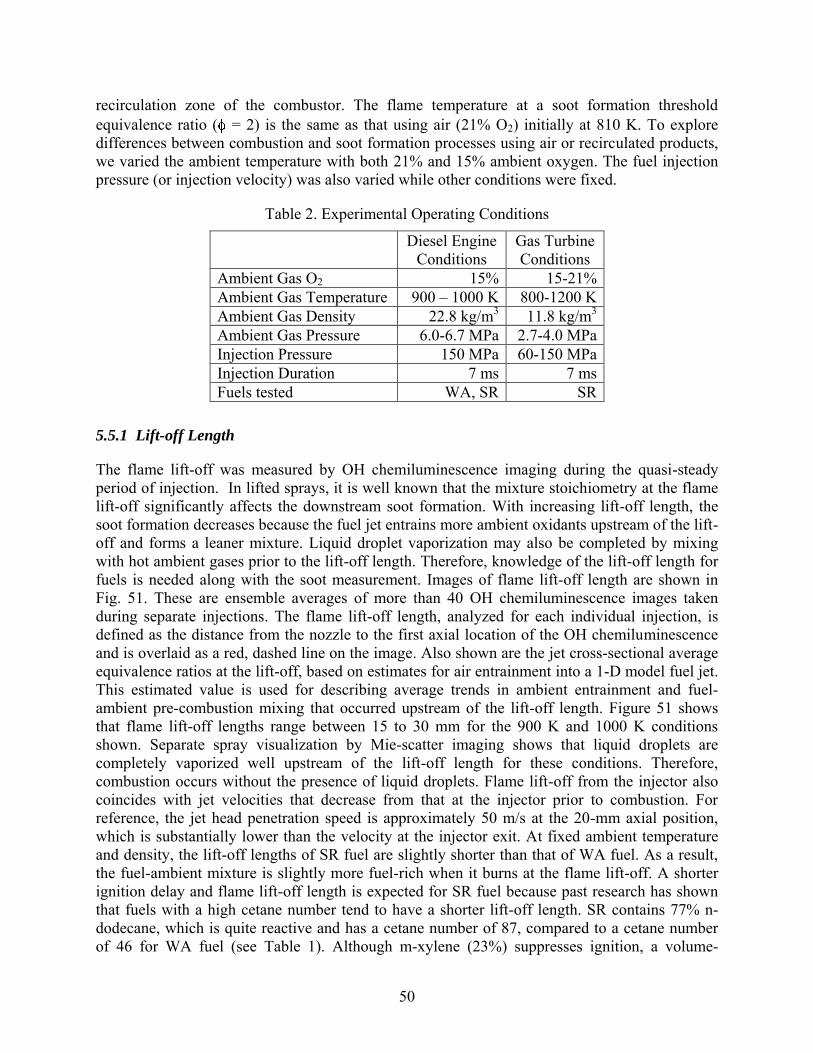
50
recirculation zone of the combustor. The flame temperature at a soot formation threshold
equivalence ratio ( = 2) is the same as that using air (21% O2) initially at 810 K. To explore
differences between combustion and soot formation processes using air or recirculated products,
we varied the ambient temperature with both 21% and 15% ambient oxygen. The fuel injection
pressure (or injection velocity) was also varied while other conditions were fixed.
Table 2. Experimental Operating Conditions
Diesel Engine
Conditions
Gas Turbine
Conditions
Ambient Gas O2 15% 15-21%
Ambient Gas Temperature 900 – 1000 K 800-1200 K
Ambient Gas Density 22.8 kg/m3 11.8 kg/m
3
Ambient Gas Pressure 6.0-6.7 MPa 2.7-4.0 MPa
Injection Pressure 150 MPa 60-150 MPa
Injection Duration 7 ms 7 ms
Fuels tested WA, SR SR
5.5.1 Lift-off Length
The flame lift-off was measured by OH chemiluminescence imaging during the quasi-steady
period of injection. In lifted sprays, it is well known that the mixture stoichiometry at the flame
lift-off significantly affects the downstream soot formation. With increasing lift-off length, the
soot formation decreases because the fuel jet entrains more ambient oxidants upstream of the lift-
off and forms a leaner mixture. Liquid droplet vaporization may also be completed by mixing
with hot ambient gases prior to the lift-off length. Therefore, knowledge of the lift-off length for
fuels is needed along with the soot measurement. Images of flame lift-off length are shown in
Fig. 51. These are ensemble averages of more than 40 OH chemiluminescence images taken
during separate injections. The flame lift-off length, analyzed for each individual injection, is
defined as the distance from the nozzle to the first axial location of the OH chemiluminescence
and is overlaid as a red, dashed line on the image. Also shown are the jet cross-sectional average
equivalence ratios at the lift-off, based on estimates for air entrainment into a 1-D model fuel jet.
This estimated value is used for describing average trends in ambient entrainment and fuel-
ambient pre-combustion mixing that occurred upstream of the lift-off length. Figure 51 shows
that flame lift-off lengths range between 15 to 30 mm for the 900 K and 1000 K conditions
shown. Separate spray visualization by Mie-scatter imaging shows that liquid droplets are
completely vaporized well upstream of the lift-off length for these conditions. Therefore,
combustion occurs without the presence of liquid droplets. Flame lift-off from the injector also
coincides with jet velocities that decrease from that at the injector prior to combustion. For
reference, the jet head penetration speed is approximately 50 m/s at the 20-mm axial position,
which is substantially lower than the velocity at the injector exit. At fixed ambient temperature
and density, the lift-off lengths of SR fuel are slightly shorter than that of WA fuel. As a result,
the fuel-ambient mixture is slightly more fuel-rich when it burns at the flame lift-off. A shorter
ignition delay and flame lift-off length is expected for SR fuel because past research has shown
that fuels with a high cetane number tend to have a shorter lift-off length. SR contains 77% n-
dodecane, which is quite reactive and has a cetane number of 87, compared to a cetane number
of 46 for WA fuel (see Table 1). Although m-xylene (23%) suppresses ignition, a volume-
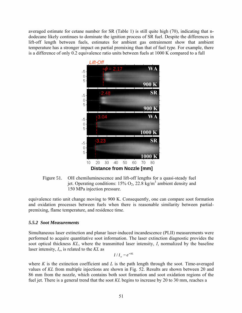
51
averaged estimate for cetane number for SR (Table 1) is still quite high (70), indicating that n-
dodecane likely continues to dominate the ignition process of SR fuel. Despite the differences in
lift-off length between fuels, estimates for ambient gas entrainment show that ambient
temperature has a stronger impact on partial premixing than that of fuel type. For example, there
is a difference of only 0.2 equivalence ratio units between fuels at 1000 K compared to a full
Figure 51. OH chemiluminescence and lift-off lengths for a quasi-steady fuel
jet. Operating conditions: 15% O2, 22.8 kg/m3 ambient density and
150 MPa injection pressure.
equivalence ratio unit change moving to 900 K. Consequently, one can compare soot formation
and oxidation processes between fuels when there is reasonable similarity between partial-
premixing, flame temperature, and residence time.
5.5.2 Soot Measurements
Simultaneous laser extinction and planar laser-induced incandescence (PLII) measurements were
performed to acquire quantitative soot information. The laser extinction diagnostic provides the
soot optical thickness KL, where the transmitted laser intensity, I, normalized by the baseline
laser intensity, Io, is related to the KL as KL
o eII /
where K is the extinction coefficient and L is the path length through the soot. Time-averaged
values of KL from multiple injections are shown in Fig. 52. Results are shown between 20 and
86 mm from the nozzle, which contains both soot formation and soot oxidation regions of the
fuel jet. There is a general trend that the soot KL begins to increase by 20 to 30 mm, reaches a
Distance from Nozzle [mm]
Lift-Off
SR
WA
900 K
900 K
SR
WA
1000 K
1000 K
= 2.17
2.48
3.04
3.23
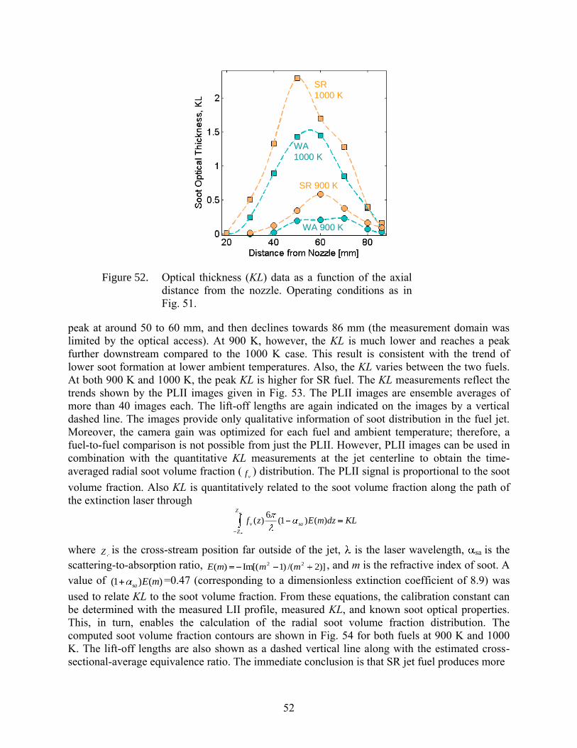
52
Figure 52. Optical thickness (KL) data as a function of the axial
distance from the nozzle. Operating conditions as in
Fig. 51.
peak at around 50 to 60 mm, and then declines towards 86 mm (the measurement domain was
limited by the optical access). At 900 K, however, the KL is much lower and reaches a peak
further downstream compared to the 1000 K case. This result is consistent with the trend of
lower soot formation at lower ambient temperatures. Also, the KL varies between the two fuels.
At both 900 K and 1000 K, the peak KL is higher for SR fuel. The KL measurements reflect the
trends shown by the PLII images given in Fig. 53. The PLII images are ensemble averages of
more than 40 images each. The lift-off lengths are again indicated on the images by a vertical
dashed line. The images provide only qualitative information of soot distribution in the fuel jet.
Moreover, the camera gain was optimized for each fuel and ambient temperature; therefore, a
fuel-to-fuel comparison is not possible from just the PLII. However, PLII images can be used in
combination with the quantitative KL measurements at the jet centerline to obtain the time-
averaged radial soot volume fraction (vf ) distribution. The PLII signal is proportional to the soot
volume fraction. Also KL is quantitatively related to the soot volume fraction along the path of
the extinction laser through
KLdzmEzf
Z
Z
sav )()1(6
)(
where Z is the cross-stream position far outside of the jet, is the laser wavelength, sa is the
scattering-to-absorption ratio, )]2/()1Im[()( 22 mmmE , and m is the refractive index of soot. A
value of )()1( mEsa=0.47 (corresponding to a dimensionless extinction coefficient of 8.9) was
used to relate KL to the soot volume fraction. From these equations, the calibration constant can
be determined with the measured LII profile, measured KL, and known soot optical properties.
This, in turn, enables the calculation of the radial soot volume fraction distribution. The
computed soot volume fraction contours are shown in Fig. 54 for both fuels at 900 K and 1000
K. The lift-off lengths are also shown as a dashed vertical line along with the estimated cross-
sectional-average equivalence ratio. The immediate conclusion is that SR jet fuel produces more
SR
1000 K
SR 900 K
WA
1000 K
WA 900 K
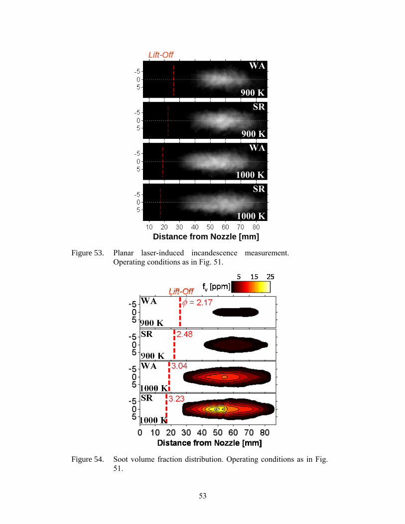
53
Figure 53. Planar laser-induced incandescence measurement.
Operating conditions as in Fig. 51.
Figure 54. Soot volume fraction distribution. Operating conditions as in Fig.
51.
Distance from Nozzle [mm]
Lift-Off
SR
WA
900 K
900 K
SR
WA
1000 K
1000 K
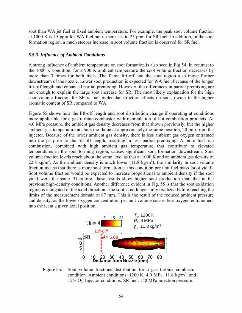
54
soot than WA jet fuel at fixed ambient temperature. For example, the peak soot volume fraction
at 1000 K is 15 ppm for WA fuel but it increases to 25 ppm for SR fuel. In addition, in the soot
formation region, a much steeper increase in soot volume fraction is observed for SR fuel.
5.5.3 Influence of Ambient Conditions
A strong influence of ambient temperature on soot formation is also seen in Fig 54. In contrast to
the 1000 K condition, for a 900 K ambient temperature the soot volume fraction decreases by
more than 3 times for both fuels. The flame lift-off and the soot region also move further
downstream of the nozzle. Lower soot production is expected for WA fuel, because of the longer
lift-off length and enhanced partial premixing. However, the differences in partial premixing are
not enough to explain the large soot increase for SR. The most likely explanation for the high
soot volume fraction for SR is fuel molecular structure effects on soot, owing to the higher
aromatic content of SR compared to WA.
Figure 55 shows how the lift-off length and soot distribution change if operating at conditions
more applicable for a gas turbine combustor with recirculation of hot combustion products. At
4.0 MPa pressure, the ambient gas density decreases from that shown previously, but the higher
ambient gas temperature anchors the flame at approximately the same position, 20 mm from the
injector. Because of the lower ambient gas density, there is less ambient gas oxygen entrained
into the jet prior to the lift-off length, resulting in less partial premixing. A more fuel-rich
combustion, combined with high ambient gas temperature that contribute to elevated
temperatures in the soot forming region, causes significant soot formation downstream. Soot
volume fraction levels reach about the same level as that at 1000 K and an ambient gas density of
22.8 kg/m3. As the ambient density is much lower (11.8 kg/m
3), the similarity in soot volume
fraction means that there is more soot formation at this condition per unit fuel mass (soot yield).
Soot volume fraction would be expected to increase proportional to ambient density if the soot
yield were the same. Therefore, these results show higher soot production than that at the
previous high-density conditions. Another difference evident in Fig. 55 is that the soot oxidation
region is elongated in the axial direction. The soot is no longer fully oxidized before reaching the
limits of the measurement domain at 87 mm. This is the result of the reduced ambient pressure
and density, as the lower oxygen concentration per unit volume causes less oxygen entrainment
into the jet at a given axial position.
Figure 55. Soot volume fractions distribution for a gas turbine combustor
condition. Ambient conditions: 1200 K, 4.0 MPa, 11.8 kg/m3, and
15% O2. Injector conditions: SR fuel, 150 MPa injection pressure.
Distance from Nozzle [mm]
Ta: 1200 K
Pa: 4 MPa
a: 11.8 kg/m3
SR = 5.08
Lift-Off
25155
fv [ppm]
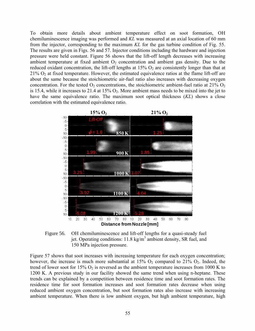
55
To obtain more details about ambient temperature effect on soot formation, OH
chemiluminescence imaging was performed and KL was measured at an axial location of 60 mm
from the injector, corresponding to the maximum KL for the gas turbine condition of Fig. 55.
The results are given in Figs. 56 and 57. Injector conditions including the hardware and injection
pressure were held constant. Figure 56 shows that the lift-off length decreases with increasing
ambient temperature at fixed ambient O2 concentration and ambient gas density. Due to the
reduced oxidant concentration, the lift-off lengths at 15% O2 are consistently longer than that at
21% O2 at fixed temperature. However, the estimated equivalence ratios at the flame lift-off are
about the same because the stoichiometric air-fuel ratio also increases with decreasing oxygen
concentration. For the tested O2 concentrations, the stoichiometric ambient-fuel ratio at 21% O2
is 15.4, while it increases to 21.4 at 15% O2. More ambient mass needs to be mixed into the jet to
have the same equivalence ratio. The maximum soot optical thickness (KL) shows a close
correlation with the estimated equivalence ratio.
Figure 56. OH chemiluminescence and lift-off lengths for a quasi-steady fuel
jet. Operating conditions: 11.8 kg/m3 ambient density, SR fuel, and
150 MPa injection pressure.
Figure 57 shows that soot increases with increasing temperature for each oxygen concentration;
however, the increase is much more substantial at 15% O2 compared to 21% O2. Indeed, the
trend of lower soot for 15% O2 is reversed as the ambient temperature increases from 1000 K to
1200 K. A previous study in our facility showed the same trend when using n-heptane. These
trends can be explained by a competition between residence time and soot formation rates. The
residence time for soot formation increases and soot formation rates decrease when using
reduced ambient oxygen concentration, but soot formation rates also increase with increasing
ambient temperature. When there is low ambient oxygen, but high ambient temperature, high
Distance from Nozzle [mm]
Lift-Off
= 1.6
1.99
15% O2 21% O2
3.25
3.92
5.08
1.25
1.85
3.07
4.04
5.28
850 K
900 K
1000 K
1100 K
1200 K
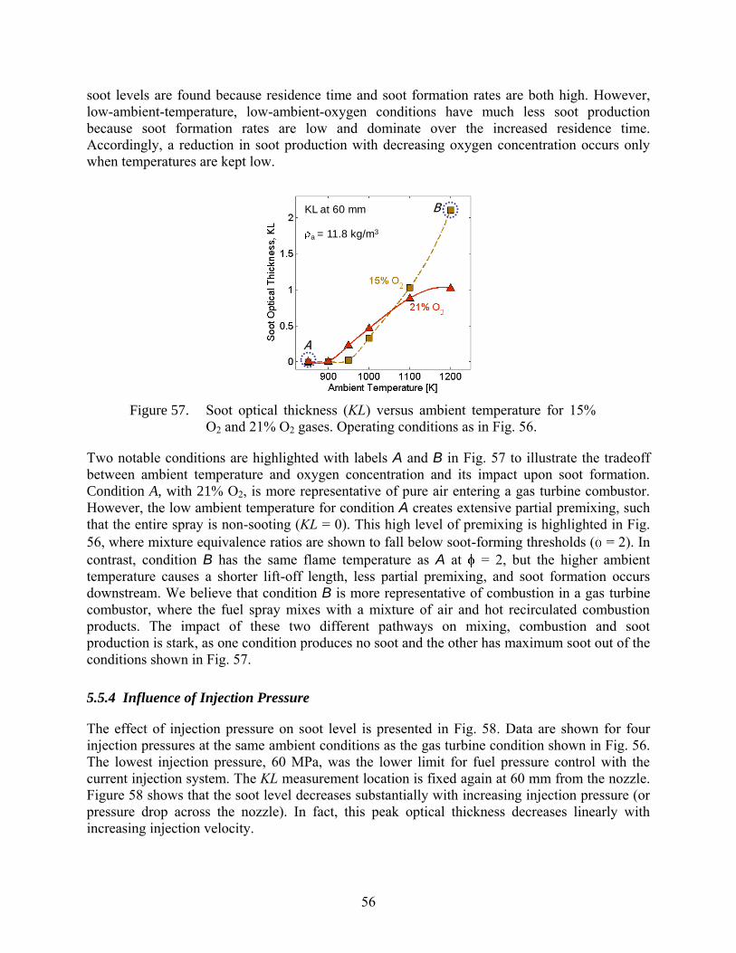
56
soot levels are found because residence time and soot formation rates are both high. However,
low-ambient-temperature, low-ambient-oxygen conditions have much less soot production
because soot formation rates are low and dominate over the increased residence time.
Accordingly, a reduction in soot production with decreasing oxygen concentration occurs only
when temperatures are kept low.
Figure 57. Soot optical thickness (KL) versus ambient temperature for 15%
O2 and 21% O2 gases. Operating conditions as in Fig. 56.
Two notable conditions are highlighted with labels A and B in Fig. 57 to illustrate the tradeoff
between ambient temperature and oxygen concentration and its impact upon soot formation.
Condition A, with 21% O2, is more representative of pure air entering a gas turbine combustor.
However, the low ambient temperature for condition A creates extensive partial premixing, such
that the entire spray is non-sooting (KL = 0). This high level of premixing is highlighted in Fig.
56, where mixture equivalence ratios are shown to fall below soot-forming thresholds ( = 2). In
contrast, condition B has the same flame temperature as A at = 2, but the higher ambient
temperature causes a shorter lift-off length, less partial premixing, and soot formation occurs
downstream. We believe that condition B is more representative of combustion in a gas turbine
combustor, where the fuel spray mixes with a mixture of air and hot recirculated combustion
products. The impact of these two different pathways on mixing, combustion and soot
production is stark, as one condition produces no soot and the other has maximum soot out of the
conditions shown in Fig. 57.
5.5.4 Influence of Injection Pressure
The effect of injection pressure on soot level is presented in Fig. 58. Data are shown for four
injection pressures at the same ambient conditions as the gas turbine condition shown in Fig. 56.
The lowest injection pressure, 60 MPa, was the lower limit for fuel pressure control with the
current injection system. The KL measurement location is fixed again at 60 mm from the nozzle.
Figure 58 shows that the soot level decreases substantially with increasing injection pressure (or
pressure drop across the nozzle). In fact, this peak optical thickness decreases linearly with
increasing injection velocity.
KL at 60 mm B
A
a = 11.8 kg/m3
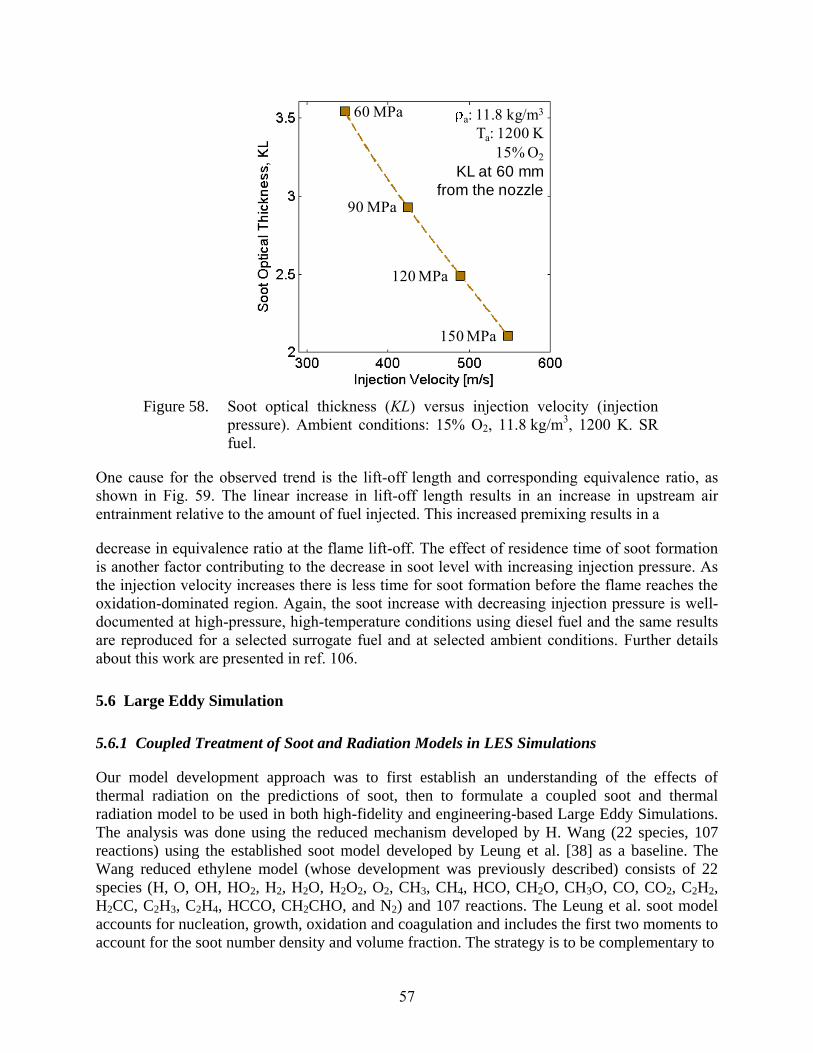
57
Figure 58. Soot optical thickness (KL) versus injection velocity (injection
pressure). Ambient conditions: 15% O2, 11.8 kg/m3, 1200 K. SR
fuel.
One cause for the observed trend is the lift-off length and corresponding equivalence ratio, as
shown in Fig. 59. The linear increase in lift-off length results in an increase in upstream air
entrainment relative to the amount of fuel injected. This increased premixing results in a
decrease in equivalence ratio at the flame lift-off. The effect of residence time of soot formation
is another factor contributing to the decrease in soot level with increasing injection pressure. As
the injection velocity increases there is less time for soot formation before the flame reaches the
oxidation-dominated region. Again, the soot increase with decreasing injection pressure is well-
documented at high-pressure, high-temperature conditions using diesel fuel and the same results
are reproduced for a selected surrogate fuel and at selected ambient conditions. Further details
about this work are presented in ref. 106.
5.6 Large Eddy Simulation
5.6.1 Coupled Treatment of Soot and Radiation Models in LES Simulations
Our model development approach was to first establish an understanding of the effects of
thermal radiation on the predictions of soot, then to formulate a coupled soot and thermal
radiation model to be used in both high-fidelity and engineering-based Large Eddy Simulations.
The analysis was done using the reduced mechanism developed by H. Wang (22 species, 107
reactions) using the established soot model developed by Leung et al. [38] as a baseline. The
Wang reduced ethylene model (whose development was previously described) consists of 22
species (H, O, OH, HO2, H2, H2O, H2O2, O2, CH3, CH4, HCO, CH2O, CH3O, CO, CO2, C2H2,
H2CC, C2H3, C2H4, HCCO, CH2CHO, and N2) and 107 reactions. The Leung et al. soot model
accounts for nucleation, growth, oxidation and coagulation and includes the first two moments to
account for the soot number density and volume fraction. The strategy is to be complementary to
a: 11.8 kg/m3
Ta: 1200 K
15% O2
KL at 60 mm
from the nozzle
60 MPa
90 MPa
120 MPa
150 MPa
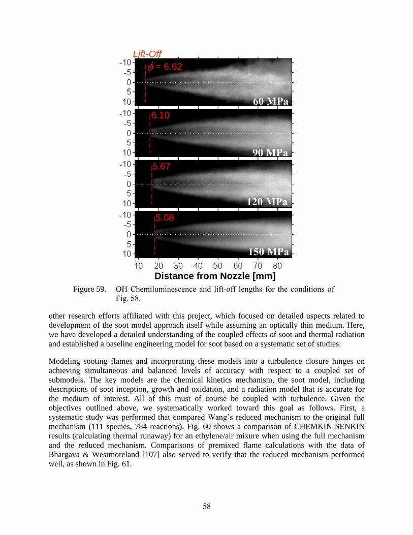
58
Figure 59. OH Chemiluminescence and lift-off lengths for the conditions of
Fig. 58.
other research efforts affiliated with this project, which focused on detailed aspects related to
development of the soot model approach itself while assuming an optically thin medium. Here,
we have developed a detailed understanding of the coupled effects of soot and thermal radiation
and established a baseline engineering model for soot based on a systematic set of studies.
Modeling sooting flames and incorporating these models into a turbulence closure hinges on
achieving simultaneous and balanced levels of accuracy with respect to a coupled set of
submodels. The key models are the chemical kinetics mechanism, the soot model, including
descriptions of soot inception, growth and oxidation, and a radiation model that is accurate for
the medium of interest. All of this must of course be coupled with turbulence. Given the
objectives outlined above, we systematically worked toward this goal as follows. First, a
systematic study was performed that compared Wang’s reduced mechanism to the original full
mechanism (111 species, 784 reactions). Fig. 60 shows a comparison of CHEMKIN SENKIN
results (calculating thermal runaway) for an ethylene/air mixure when using the full mechanism
and the reduced mechanism. Comparisons of premixed flame calculations with the data of
Bhargava & Westmoreland [107] also served to verify that the reduced mechanism performed
well, as shown in Fig. 61.
Distance from Nozzle [mm]
Lift - Off
60 MPa
= 6.62
6.10
5.08
90 MPa
120 MPa
150 MPa
5.67
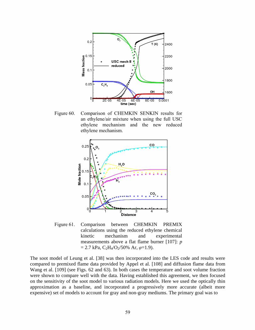
59
Figure 60. Comparison of CHEMKIN SENKIN results for
an ethylene/air mixture when using the full USC
ethylene mechanism and the new reduced
ethylene mechanism.
Figure 61. Comparison between CHEMKIN PREMIX
calculations using the reduced ethylene chemical
kinetic mechanism and experimental
measurements above a flat flame burner [107]: p
= 2.7 kPa, C2H4/O2/50% Ar, φ=1.9).
The soot model of Leung et al. [38] was then incorporated into the LES code and results were
compared to premixed flame data provided by Appel et al. [108] and diffusion flame data from
Wang et al. [109] (see Figs. 62 and 63). In both cases the temperature and soot volume fraction
were shown to compare well with the data. Having established this agreement, we then focused
on the sensitivity of the soot model to various radiation models. Here we used the optically thin
approximation as a baseline, and incorporated a progressively more accurate (albeit more
expensive) set of models to account for gray and non-gray mediums. The primary goal was to
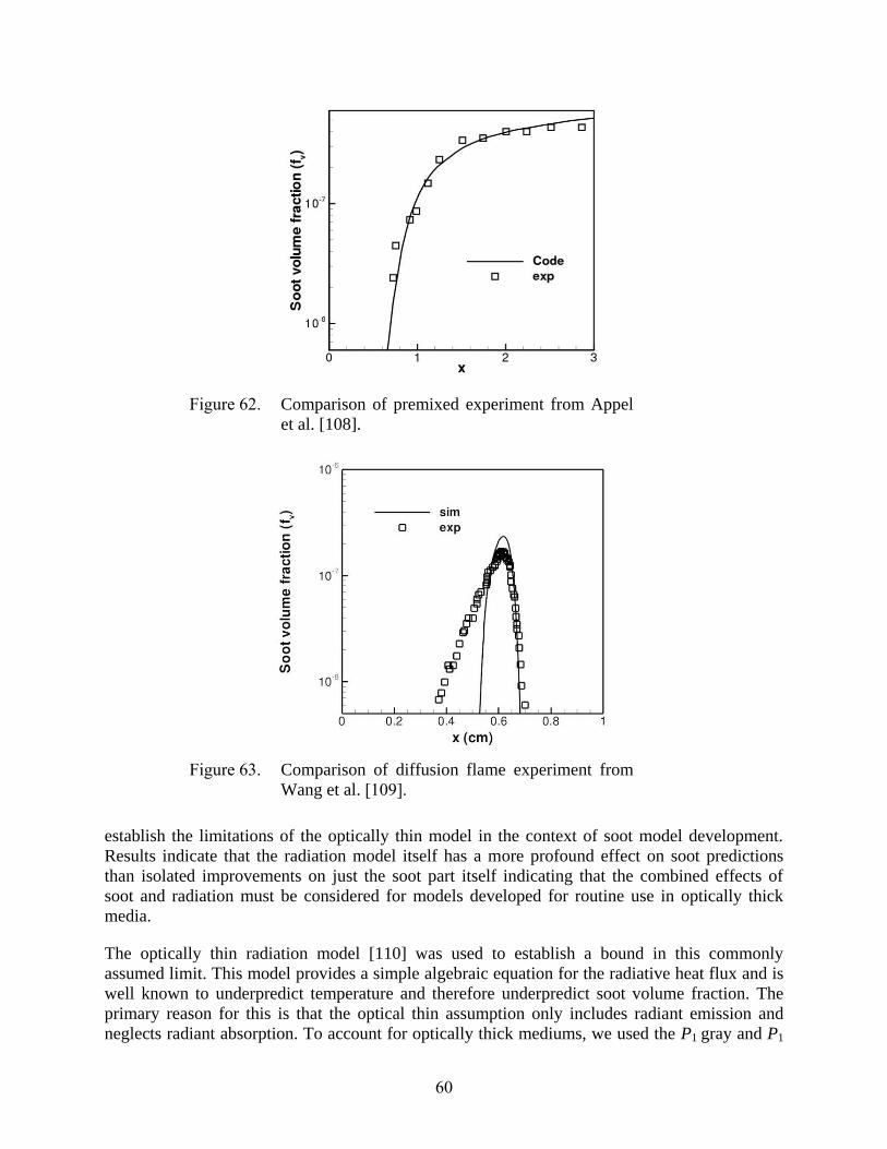
60
Figure 62. Comparison of premixed experiment from Appel
et al. [108].
Figure 63. Comparison of diffusion flame experiment from
Wang et al. [109].
establish the limitations of the optically thin model in the context of soot model development.
Results indicate that the radiation model itself has a more profound effect on soot predictions
than isolated improvements on just the soot part itself indicating that the combined effects of
soot and radiation must be considered for models developed for routine use in optically thick
media.
The optically thin radiation model [110] was used to establish a bound in this commonly
assumed limit. This model provides a simple algebraic equation for the radiative heat flux and is
well known to underpredict temperature and therefore underpredict soot volume fraction. The
primary reason for this is that the optical thin assumption only includes radiant emission and
neglects radiant absorption. To account for optically thick mediums, we used the P1 gray and P1
61
FSK (non-gray) model from Wang et al. [111], which accounts for both emission and absorption
with various levels of fidelity. The P1 gray model is a Helmholtz equation with variable
coefficients and a source term. The model also accounts for gas and soot radiation through the
absorption coefficient and the evaluation of the Planck–mean absorption coefficients. The
database for the gas phase is based on HITEMP from Modest [110]. The P1 nongray model
employs a Helmholtz equation and needs to be solved as a function of spectral location. We
employ a Gaussian quadrature technique for its solution. Generally, around ten Helmholtz
equations are required to solve the radiative heat flux. The absorption coefficient is a function of
normalized spectral space. Each models described above provides a better prediction of
temperature in optically thick mediums but includes additional complexity and cost. Thus, it is
important to quantify the compounding effect of inaccurate temperature predictions on the soot
model itself.
5.6.2 Soot model
The semi-empirical soot model from Leung et al. [38] uses the following soot chemistry
mechanism
.1
,2
1
,2
,2
2
222
222
nn
COOsC
HsCnHCasnC
HsCHC
This mechanism includes nucleation, growth, oxidation, and coagulation and is coupled through
source terms as a function of C2H2, CO, O2 and H2. The first two moments are considered to
account for the number density and soot mass per volume. The soot mass fraction and particle
number density are
s
s
Y
j
Y
j
jss
n
j
n
j
j
x
v
x
uY
t
Y
x
v
x
nu
t
n
,
respectively. The soot diffusion term is
esisThermophorDiffusion Browniam
1 556.01
jMj
pMx
T
T
M
LexDv
where M is either n or . The Lewis number for soot particles is in general large and the
Brownian diffusion term is neglected. The source terms for the species, soot mass fraction and
particle density are
62
,
,
,2
,
,22
,2
3
21
3
21
321
4
min
22
22
2222
RW
RRW
RW
RRW
RRRWS
RC
NS
COCO
HH
OO
HCHC
cY
a
n
s
and the reaction rates are (kmol/m3/s)
.6
,66
2
,19680
exp51.0
,12100
exp46.0
,21000
exp51.0
3/1
3/2
6/11
6/12/16/1
4
2
2/1
3
222
221
nY
A
nW
YTWCR
AOT
TER
AHCT
ER
HCT
ER
s
s
s
C
s
ss
C
a
s
s
Note that the total density including soot and the internal energy is .e Y + e Y = e ssgg The soot
volume faction is Y_s
= fS
v where 3
S / 1850= mkg which is defined as the soot density and
Cmin=100. The constants Ca = 9.0, κ = 1.38E-23 (J/K), and Na = 6.022E26 (particles/kmol) are
the agglomeration rate constant, incipient carbon particle Boltzmann constant, and Avogadro's
number, respectively.
5.6.3 Radiation model
Thermal radiation is represented by rQ and gives the rate of radiation heat loss per unit volume.
This term enters into the energy equation as the divergence of the radiative heat flux and
quantifies the loss or gain of thermal energy due to both emission and absorption as
63
0
0 4
4
4
dIG
dIdIqQ
b
brr
Here, η is the wave-number, Ω is the solid angle, κη is the spectral absorption coefficient and Iη is
the spectral radiative intensity, Gη the spectral incident radiation and b denotes a black-body
property.
From Wang and Modest [111,112], the P1 non-gray radiation model is
.4
1
0
dgGIkuQ gbr
Where k is the reordered local mixture absorption coefficient and is a function of the spectral g
variable weighted by the Planck function. The quantity u is a scaling function that incorporates
the spatial variations of the absorption coefficient, and a is a nongray stretching factor
accounting for varying local temperatures in the Planck function. Term Gg is the spectral incident
radiation in g-space. The P1 approximation is given by
1
kuGg 3ku Gg 4 aIb (1)
The boundary conditions for equation (1) are
bgg kuaIkuGGn 4ˆ3
22
where is the surface emittance. If the wall emittances is zero ( 0 ), then .0gG The
incident radiation Gg is calculated at spectral locations as a function of g. To compute Qr for the
non-gray radiation, the integration is performed by numerical quadrature. If Gaussian quadrature
is used, then equation (1) is approximated by
M
j
gbjjjjr GIaukQ1
.4
A simpler method is to assume that medium is gray, which yields
GIQ pbpr 4
64
where 4TI b . Here, G is the spectral incident radiation and p is the Planck mean absorption
coefficient. The incident radiation G is solved by the spherical harmonic P1 method with self-
absorption term which is defined as
(2) .431
bpgp
p
IGG
The boundary conditions for equation (2) are
.4ˆ3
22bpp IGGn
The model accounts for gas and soot radiation through the absorption coefficient and the
evaluation of the Planck--mean absorption coefficients are from Zhang and Modest [29]. The
database is based on HITRAN96 and HITEMP using curve-fitting for CO2, H2O, CH4, and CO.
The absorption coefficient for soot is from Kent and Honnery [113] which is modeled as
asoot 18.62 fvT . Therefore, the absorption coefficient is p p p,i T asooti [113-115]. For
optically thin radiation, G is zero. Therefore, .4 4TQ pr
5.6.4 Sensitivity Analysis
To understand the sensitivity of the coupled system of soot and radiation models, we compare
results to the premixed flame from Appel et al. [108] and a diffusion flame from Wang et al.
[109]. Figure 62 is a comparison of a premixed flame from Appel et al. and Figure 63 is a
comparison of a diffusion flame from Wang et al. The symbols denote the experiment and the
simulation is the solid line. Note that reasonable agreement is obtained for the premixed flame.
As for the diffusion flame, Leung et al. soot model over-predicts the peak soot volume fraction
and under-predicts the soot away from the peak value. The under-prediction is also observed
from Wang et al. using a method of moments with interpolative closure.
Figures 64 illustrates the sensitivity of the soot predictions to minor changes in temperature from
radiation effects, particularly the effect of including both absorption and emission. We applied
the P1 gray radiation model to an unsteady, unstrained diffusion flame that mimics the conditions
of our piloted ethylene jet flame. This problem is a good canonical case to study the effects of
radiation as a function of time at conditions analogous to those observed in the jet flame.
Relatively small effects of radiation on temperature predictions have a significant effect on the
soot volume fraction predictions. The maximum temperature with no radiation model, optically
thin radiation, and P1 gray model are 2240 K, 2170 K and 2155 K, respectfully. The maximum
soot volume fraction with no radiation, optically thin radiation, and P1 gray model are 1.62 ppm,
0.75 ppm and 0.68 ppm, respectfully. This simulation illustrates that a small change in
temperature (~85 K) can induce an order of magnitude change in soot production. Figure 65
shows the calculated soot volume fraction error between the optically thin radiation model and
the P1 gray model, where P1 gray model is assumed to be the correct solution. Errors as great as
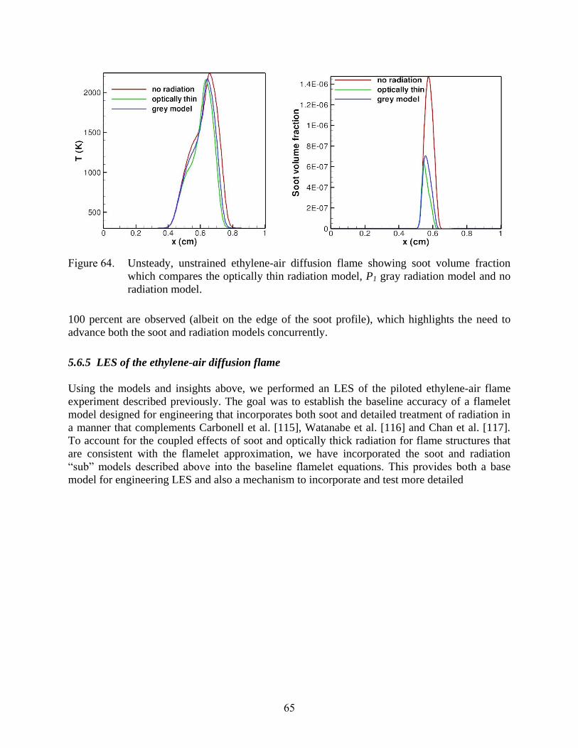
65
Figure 64. Unsteady, unstrained ethylene-air diffusion flame showing soot volume fraction
which compares the optically thin radiation model, P1 gray radiation model and no
radiation model.
100 percent are observed (albeit on the edge of the soot profile), which highlights the need to
advance both the soot and radiation models concurrently.
5.6.5 LES of the ethylene-air diffusion flame
Using the models and insights above, we performed an LES of the piloted ethylene-air flame
experiment described previously. The goal was to establish the baseline accuracy of a flamelet
model designed for engineering that incorporates both soot and detailed treatment of radiation in
a manner that complements Carbonell et al. [115], Watanabe et al. [116] and Chan et al. [117].
To account for the coupled effects of soot and optically thick radiation for flame structures that
are consistent with the flamelet approximation, we have incorporated the soot and radiation
―sub‖ models described above into the baseline flamelet equations. This provides both a base
model for engineering LES and also a mechanism to incorporate and test more detailed
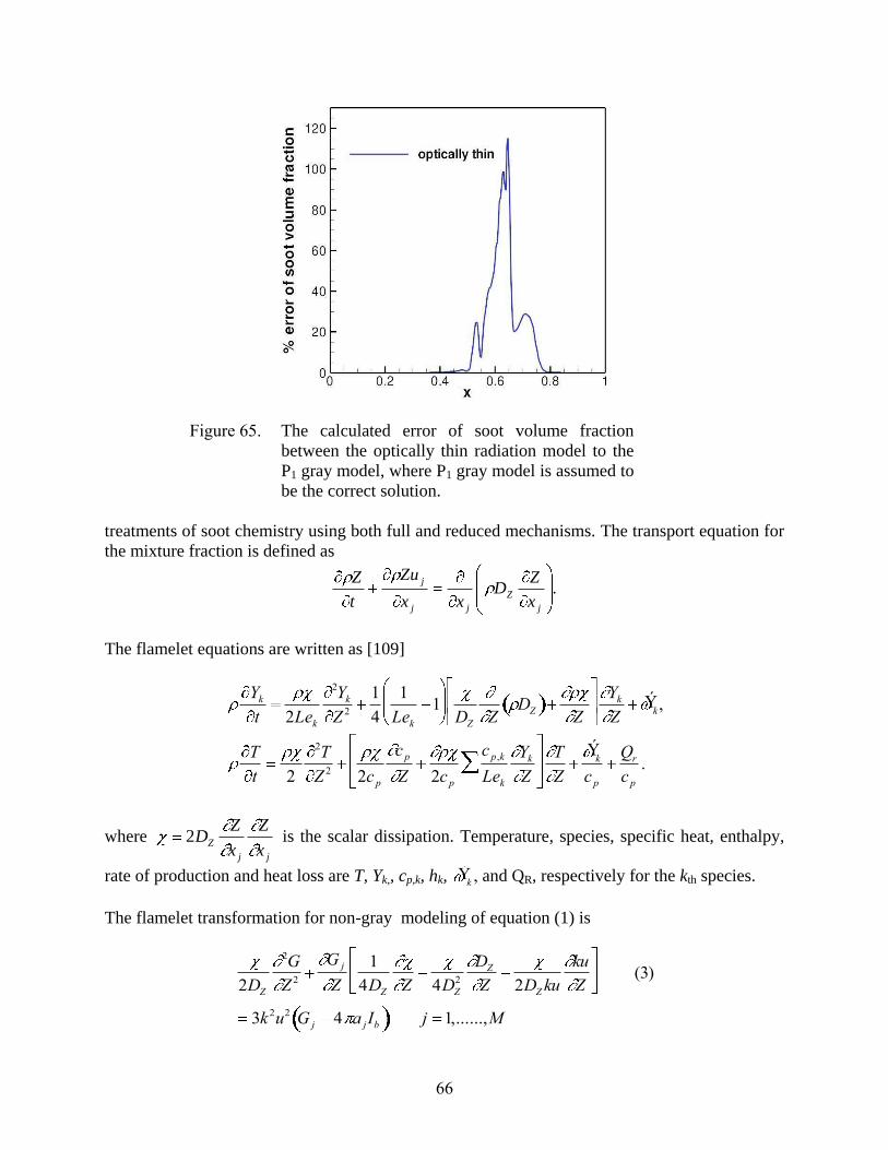
66
Figure 65. The calculated error of soot volume fraction
between the optically thin radiation model to the
P1 gray model, where P1 gray model is assumed to
be the correct solution.
treatments of soot chemistry using both full and reduced mechanisms. The transport equation for
the mixture fraction is defined as
.j
Z
jj
j
x
ZD
xx
Zu
t
Z
The flamelet equations are written as [109]
Yk
t 2Lek
2Yk
Z 2
1
4
1
Lek1DZ Z
DZZ
Yk
ZÝ k ,
T
t 2
2T
Z 2 2c p
c p
Z 2c p
c p,k
Lek
Yk
Z
T
Z
Ý k
c p
Qr
c p.
where jj
Zx
Z
x
ZD2 is the scalar dissipation. Temperature, species, specific heat, enthalpy,
rate of production and heat loss are T, Yk,, cp,k, hk, Ý k , and QR, respectively for the kth species.
The flamelet transformation for non-gray modeling of equation (1) is
2DZ
2G
Z 2
G j
Z
1
4DZ Z 4DZ2
DZ
Z 2DZku
ku
Z (3)
3k 2u2 G j 4 a jIb , j 1,......,M
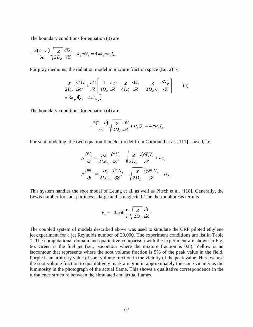
67
The boundary conditions for equation (3) are
2 2
3 2DZ
G j
Zk juG j 4 k jua jIb .
For gray mediums, the radiation model in mixture fraction space (Eq. 2) is
.43
(4) 244
1
2 22
2
bjp
p
pZ
Z
ZZZ
IG
ZDZ
D
DZDZ
G
Z
G
D
The boundary conditions for equation (4) are
2 2
3 2DZ
G
ZpG j 4 pIb .
For soot modeling, the two-equation flamelet model from Carbonell et al. [111] is used, i.e,
.22
22
2
2
2
2
s
s
s
s
N
ss
Z
s
N
s
Y
ss
Z
s
Y
s
Z
VN
DZ
N
Let
N
Z
VY
DZ
Y
Let
Y
This system handles the soot model of Leung et al. as well as Pitsch et al. [118]. Generally, the
Lewis number for soot particles is large and is neglected. The thermophoresis term is
.2
556.0Z
T
DTV
Z
s
The coupled system of models described above was used to simulate the CRF piloted ethylene
jet experiment for a jet Reynolds number of 20,000. The experiment conditions are list in Table
1. The computational domain and qualitative comparison with the experiment are shown in Fig.
66. Green is the fuel jet (i.e., isocontour where the mixture fraction is 0.8). Yellow is an
isocontour that represents where the soot volume fraction is 5% of the peak value in the field.
Purple is an arbitrary value of soot volume fraction in the vicinity of the peak value. Here we use
the soot volume fraction to qualitatively mark a region in approximately the same vicinity as the
luminosity in the photograph of the actual flame. This shows a qualitative correspondence in the
turbulence structure between the simulated and actual flames.
68
Figure 66. LES of the CRF piloted ethylene diffusion flame showing the computational
domain, flow conditions and instantaneous soot volume fraction with a
qualitative comparison to the experiment.
Table 3: Operating conditions for piloted ethylene jet flame
Jet Diameter Outer
Diameter
Pilot Jet Reynolds
number
Jet velocity Coflow
velocity
3.2 mm 19.1 mm φ=0.9 20,000 54.7 m/s 0.6 m/s
Figure 67 shows the computed and measured soot volume fraction versus axial distance along
the centerline of the burner. The blue curve is the time-averaged prediction from LES. The red is
the experimental LII data. For the LES, the error bars indicate the effect that a 20 K change in
mean local temperature has on the performance of the soot model. For the experiment, the error
bars represent an uncertainty of 20 percent in accuracy. Surprisingly good agreement is achieved
to within the uncertainties over the complete interval between x/d of 0 to 300. The LES
computations with the Leung et al. soot model and the P1 non-gray radiation model tends to
overpredict the experimental soot concentrations. However, the experimental concentrations are
known to be underpredicted by ~ 10% because of the effects of signal trapping, as previously
discussed, so the actual disparity between the simulations and the measurements is smaller than
suggested by Fig. 67.
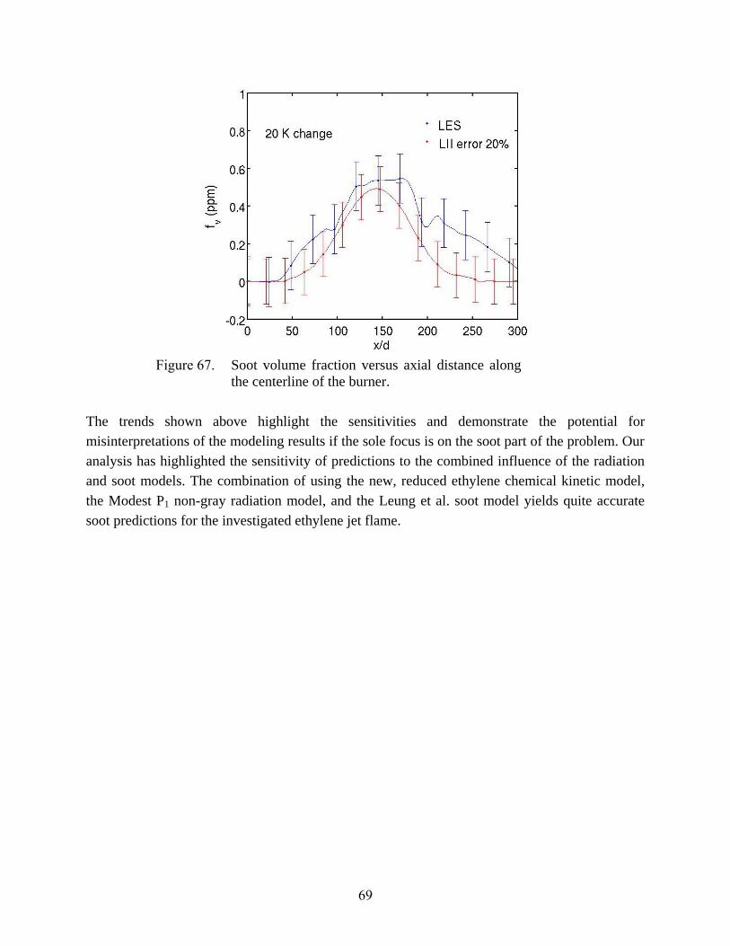
69
Figure 67. Soot volume fraction versus axial distance along
the centerline of the burner.
The trends shown above highlight the sensitivities and demonstrate the potential for
misinterpretations of the modeling results if the sole focus is on the soot part of the problem. Our
analysis has highlighted the sensitivity of predictions to the combined influence of the radiation
and soot models. The combination of using the new, reduced ethylene chemical kinetic model,
the Modest P1 non-gray radiation model, and the Leung et al. soot model yields quite accurate
soot predictions for the investigated ethylene jet flame.
70
6.0 Conclusions and Implications for Future Research
Measurements of soot formation were performed in laminar flat premixed flames and turbulent
non-premixed jet flames at 1 atm pressure and in turbulent liquid spray flames under
representative conditions for takeoff in a gas turbine engine. The laminar flames and open jet
flames used both ethylene and a prevaporized JP-8 surrogate fuel composed of n-dodecane and
m-xylene. The pressurized turbulent jet flame measurements used the JP-8 surrogate fuel and
compared its combustion and sooting characteristics to a world-average JP-8 fuel sample. The
pressurized jet flame measurements demonstrated that the surrogate was representative of JP-8,
with a somewhat higher tendency to soot formation. The premixed flame measurements revealed
that flame temperature has a strong impact on the rate of soot nucleation and particle
coagulation, but little sensitivity in the overall trends was found with different fuels. Even in the
higher temperature flames, the soot particles demonstrated liquid-like behavior. Significant
quantities of aliphatic carbon were found in soot sampled from the premixed flames. An
extensive array of non-intrusive optical and laser-based measurements was performed in
turbulent non-premixed jet flames established on specially designed piloted burners. Soot
concentration data was collected throughout the flames, together with instantaneous images
showing the relationship between soot and the OH radical and soot and PAH. Time-records of
local soot concentration-temperature were collected, as well as spatially resolved thermal
radiation emitted from the flames. Measurements of red laser light extinction across the flames
provided useful data for correcting the soot concentration measurements for signal trapping.
A detailed chemical kinetic mechanism for ethylene combustion, including fuel-rich chemistry
and benzene formation steps, was compiled, validated, and reduced. Difficulties in existing m-
xylene chemical kinetic mechanisms prevented the development of a reduced mechanism for the
JP-8 surrogate. The reduced ethylene mechanism was incorporated into a high-fidelity LES code,
together with a moment-based soot model and models for thermal radiation, to evaluate the
ability of the chemistry and soot models to predict soot formation in the jet diffusion flame. The
LES results highlight the importance of including an optically-thick radiation model to
accurately predict gas temperatures and thus soot formation rates. When including such a
radiation model, the LES model predicts mean soot concentrations within 30% in the ethylene jet
flame.
The results of this project suggest that LES modeling, when incorporating suitably reduced
chemical kinetics with fuel-rich chemistry and a suitable, optically-thick radiation model, can
predict soot formation with good accuracy in an ethylene nonpremixed jet flame (at 1 atm) when
using a fairly simple soot model (developed explicitly for application to ethylene flames).
Extension of this predictive ability to more complex fuels representative of JP-8 requires
improvements in the understanding of aromatic oxidation and pyrolysis chemistry and may
require further improvements to the soot model itself. The single most important insight that was
gained from this project was that it is essential for a suitable radiation model, generally meaning
one designed for at least moderately optically thick environments, to be directly incorporated
into the turbulent flame model, together with a soot model. Simply incorporating a soot model in
post-processing mode, as has generally been done to-date in predicting soot formation and
emission from gas turbine engines, is not a meaningful test of the soot model, because the
predicted flow field temperatures will be in significant error, and the soot formation chemistry is
71
characterized by a high activation energy. Incorporating soot models with increasing complexity
while neglecting the influence of radiation does not guarantee any more accurate results than
using the simplest soot model.
In the three years that we have worked on this problem, we have made significant strides, in
keeping with the original project plan. To generate a soot and radiation model that is truly
predictive for gas turbine combustion engines, (a) more work needs to be done to clarify
aromatics reaction chemistry, particularly under fuel-rich conditions, (b) a suitable reduced
chemical kinetic mechanism needs to be generated for the JP-8 surrogate for which we made
experimental measurements in this project, and (c) detailed comparisons need to be made
between LES model predictions (using a suitable radiation and soot model) and the experimental
measurements. To account for variations in JP-8 composition, measurements should be
performed in a piloted turbulent jet flame burner (such as developed here) for different fuel
compositions, reduced chemical kinetic mechanisms should be developed, and then comparisons
should be made with LES simulations and measurements. If these comparisons prove to not be
favorable, adjustments should be made to either the form or the constants in the soot model to
give better agreement. Having validated the soot/radiation model for applications at 1 atm
pressure, LES simulations should be performed of a pressurized experiment using the same fuel.
72
7.0 Literature Cited
[1] F. Laden, L.M. Neas, D.W. Dockery, J. Schwartz, ―Association of fine particulate matter from different sources
with daily mortality in six US cities,‖ Envir. Health Persp. 108:941-947 (2000).
[2] J.A. Sarnat, J. Schwartz, P.J. Catalon, H.H. Suh, ―Gaseous pollutants in particulate matter epidemiology:
Confounders or surrogates?‖ Envir. Health Persp. 109:1053-1061 (2001).
[3] C.A. Pope, R.T. Burnett, M.J. Thun, E.E. Calle, D. Krewski, K. Ito, G.D. Thurston, ―Lung cancer,
cardiopulmonary mortality, and long-term exposure to fine particulate air pollution,‖ JAMA 287:1132-1141
(2002).
[4] A.J. Ghio, Y.C.T. Huang, ―Exposure to concentrated ambient particles (CAPs): A review,‖ Inhalation Toxic.
16:53-59 (2004).
[5] EPA Report No. EPA 600/6-04/058, ―Particulate Matter Research Program: Five years of progress,‖ July 2004,
available at www.epa.gov.
[6] R.J. Delfino, C. Sioutas, S. Malik, ―Potential role of ultrafine particles in associations between airborne particle
mass and cardiovascular health,‖ Envir. Health Persp. 113:934-946 (2005).
[7] C. de Haar, I. Hassing, M. Bol, R. Bleumink, R. Pieters, ―Ultrafine carbon black particles cause early airway
inflammation and have adjuvant activity in a mouse allergic airway disease model,‖ Toxic. Sciences 87:409-418
(2005).
[8] R.B. Schlesinger, N. Kunzli, G.M. Hidy, T. Gotschi, M. Jerrett, ―The health relevance of ambient particulate
matter characteristics: Coherence of toxicological and epidemiological inferences,‖ Inhalation Toxic. 18:95-125
(2006).
[9] R. Watson, J. Houghton, D. Yihui, B. Metz, O. Davidson, N. Sundararaman, D. Griggs, D. Dokken, Aviation
and the Global Atmosphere, a special report of the Intergovernmental Panel on Climate Change (IPCC), 1999,
available from http://www.grida.no/climate/ipcc/aviation/.
[10] L.G. Blevins, ―Particulate matter emitted from aircraft engines,‖ AIAA Paper 2003-0666, presented at the
AIAA/ICAS International Air and Space Symposium and Exposition: The Next 100 Years, Dayton OH, 2003.
[11] L.H. Linden, J.B. Heywood, ―Soot emission from jet engines,‖ Combust. Sci. Tech. 2:401-411 (1971).
[12] P. Sampath, M. Gratton, D. Kretschmer, J. Odgers, ―Fuel property effects upon exhaust smoke and the weak
extinction characteristics of the Pratt & Whitney PT6A-65 engine,‖ J. Eng. Gas Turb. Power 108:175-181
(1986).
[13] A. De Champlain, D. Kretschmer, J. Tsogo, G.F. Pearce, ―Prediction of soot emissions in gas-turbine
combustors,‖ J. Prop. Power 13:117-122 (1997).
[14] E.M. Amin, G.E. Andrews, M. Pourkashnian, A. Williams, R.A. Yetter, ―A computational study of pressure
effects on pollutant generation in gas turbine combustors,‖ Trans. ASME 119:76-83 (1997).
[15] A.K. Tolpadi, A.M. Danis, H.C. Mongia, R.P. Lindstedt, ―Soot modeling in gas turbine combustors,‖ ASME
97-GT-149, 1997.
[16] H.T. Brocklehurst, C.H. Priddin, J.B. Moss, ―Soot predictions within an aero gas turbine combustion chamber,‖
ASME 97-GT-148, 1997.
[17] H. Barths, N. Peters, N. Brehm, A. Mack, M. Pfitzner, V. Smiljanovski, ―Simulation of pollutant formation in a
gas-turbine combustor using unsteady flamelets,‖ Proc. Combust. Inst. 27:1841-1847 (1998).
[18] M. Balthasar, F. Mauss, M. Pfitzner, A. Mack, ―Implementation and validation of a new soot model and
application to aeroengine combustors,‖ Trans. ASME 124:66-74 (2002).
[19] E. Riesmeier, S. Honnet, N. Peters, ―Flamelet modeling of pollutant formation in a gas turbine combustion
chamber using detailed chemistry for a kerosene model fuel,‖ J. Eng. Gas Turb. Power 126:899-905 (2004).
[20] W.-W. Kim, S. Menon, H.C. Mongia, ―Large-eddy simulation of a gas turbine combustor flow,‖ Combust. Sci.
and Tech. 143:25-62 (1999).
[21] F. di Mare, W.P. Jones, K.R. Menzies, ―Large eddy simulation of a model gas turbine combustor,‖ Combust.
Flame 137:278-294 (2004).
[22] P. Moin, S. Apte, ―Large-eddy simulation of realistic gas turbine combustors,‖ AIAA Paper 2004-330, 2004.
73
[23] W.-W. Kim, S. Syed, ―Large-eddy simulation needs for gas turbine combustor design,‖ AIAA Paper 2004-331,
2004.
[24] S. James, J. Zhu, M.S. Anand, ―Large-eddy simulations of gas turbine combustors,‖ AIAA Paper 2005-552,
2005.
[25] C.R. Shaddix, J.E. Harrington, K.C. Smyth, ―Quantitative measurements of enhanced soot production in a
flickering methane/air diffusion flame,‖ Combust. Flame 99:723-732 (1994).
[26] C.R. Kaplan, C.R. Shaddix, K.C. Smyth, ―Computations of enhanced soot production in time-varying CH4/air
diffusion flames,‖ Combust. Flame 106:392-405 (1996).
[27] H. Pitsch, H. Steiner, ―Large-eddy simulation of a turbulent piloted methane/air diffusion flame (Sandia flame
D),‖ Phys. Fluids 12:2541-2554 (2000).
[28] A. Kempf, A. Sadiki, J. Janicka, ―Prediction of finite chemistry effects using large eddy simulation,‖ Proc.
Combust. Inst. 29:1979-1985 (2002).
[29] H. Pitsch, ―Improved pollutant predictions in large-eddy simulations of turbulent non-premixed combustion by
considering scalar dissipation rate fluctuations,‖ Proc. Combust. Inst. 29:1971-1978 (2002).
[30] C.D. Pierce, P. Moin, ―Progress-variable approach for large-eddy simulation of non-premixed turbulent
combustion,‖ J. Fluid Mech. 504:73-97 (2004).
[31] A. Kempf, F. Flemming, J. Janicka, ―Investigation of lengthscales, scalar dissipation, and flame orientation in a
piloted diffusion flame by LES,‖ Proc. Combust. Inst. 30:557-565 (2005).
[32] M.R.H. Sheikhim, T.G. Drozda, P. Givi, F.A. Jaberi, S.B. Pope, ―Large eddy simulation of a turbulent
nonpremixed piloted methane jet flame,‖ Proc. Combust. Inst. 30:549-556 (2005).
[33] S. Navarro-Martinez, A. Kronenburg, F. di Mare, ―Conditional moment closure for large eddy simulations,‖
Flow Turbulence Combust. 75:245-274 (2005).
[34] R.S. Barlow, N.S.A. Smith, J.-Y. Chen, R.W. Bilger, ―Nitric oxide formation in dilute hydrogen jet flames:
Isolation of the effects of radiation and turbulence-chemistry submodels,‖ Combust. Flame 117:4-31 (1999).
[35] R.S. Barlow, G.J. Fiechtner, C.D. Carter, J.-Y. Chen, ―Experiments on the structure of turbulent CO/H2/N2 jet
flames,‖ Combust. Flame 120:549-569 (2000).
[36] W. Meier, R.S. Barlow, Y.-L. Chen, J.-Y. Chen, ―Raman/Rayleigh/LIF measurements in a turbulent
CH4/H2/N2 jet diffusion flame: Experimental techniques and turbulence chemistry interaction,‖ Combust.
Flame 120:326-343 (2000).
[37] R.S. Barlow, J.H. Frank, ―Effects of turbulence on species mass fractions in methane/air jet flames,‖ Proc.
Combust. Inst. 27:1087-1095 (1998).
[38] K.M. Leung, R.P. Lindstedt, W.P. Jones, ―A simplified reaction mechanism for soot formation in non-premixed
flames,‖ Combust. Flame 87:289-305 (1991).
[39] X. You, F.N. Egolfopoulos, H. Wang, ―Detailed and simplified kinetic models of n-dodecane oxidation: The
role of fuel cracking in aliphatic hydrocarbon combustion,‖ Proc. Combust. Inst. 32:403-410 (2009).
[40] F. Battin-Leclerc, R. Bounaceur, N. Belmekki, P.A. Glaude, ―Experimental and modeling study of the oxidation
of xylenes,‖ Int. J. Chem. Kinet. 38:284-302 (2006).
[41] M. Frenklach, H. Wang, ―Detailed modeling of soot particle nucleation and growth,‖ Proc. Combust. Inst.
23:1559-1566 (1991).
[42] M. Frenklach, H. Wang, ―Detailed mechanism and modeling of soot particle formation,‖ in Soot Formation in
Combustion: Mechanisms and Models of Soot Formation, (Bockhorn, H., ed.), Springer Series in Chemical
Physics, vol. 59, Springer-Verlag, Berlin, 1994, pp.162-190.
[43] H. Wang, M. Frenklach, ―A detailed kinetic modeling study of aromatics formation, growth and oxidation in
laminar premixed ethylene and acetylene flames,‖ Combust. Flame 110: 173-221 (1997).
[44] H. Richter, J.B. Howard, ―Formation of polycyclic aromatic hydrocarbons and their growth to soot—a review
of chemical reaction pathways,‖ Prog. Energy Combust. Sci. 26:565-608 (2000).
[45] J.A. Miller, S.J. Klippenstein, "The recombination of propargyl radical: solving the master equation," J. Phys.
Chem. A 105:7254-7266, (2001).
74
[46] B. Zhao, Z. Yang, M.V. Johnston, H. Wang, A. S. Wexler, M. Balthasar, M. Kraft, ―Measurement and
numerical simulation of soot particle size distribution functions in a laminar premixed ethylene-oxygen-argon
flame,‖ Combust. Flame 133: 173-188 (2003).
[47] M.B. Colket, R.J. Hall, in Soot Formation in Combustion: Mechanisms and Models of Soot Formation,
(Bockhorn, H., ed.), Springer Series in Chemical Physics, vol. 59, Springer-Verlag, Berlin, 1994, 442-468.
[48] J. Appel, H. Bockhorn, M. Wulkow, ―Numerical simulation of soot particle size distributions with a discrete
galerkin method,‖ In Scientific Computing in Chemical Engineering II, Simulation, Image Processing,
Optimization, and Control, F. Keil, W. Mackens, H. Voß, J. Werther (ed.), Berlin Heidelberg, 1999, p. 94.
[49] J. Singh, M. Balthasar, M. Kraft, W. Wagner, ―Stochastic modeling of soot particle size and age distributions in
laminar premixed flames,‖ Proc. Combust. Inst. 30:1457-1465 (2005).
[50] J. Singh, R.I.A. Patterson, M. Kraft, H. Wang, ―Numerical simulation and sensitivity analysis of detailed soot
particle size distribution in laminar premixed ethylene flames,‖ Combust. Flame 145:117-127 (2006).
[51] T. Løvås, D. Nilsson, F. Mauss, ―Automatic reduction procedure for chemical mechanisms applied to premixed
methane/air flames,‖ Proc. Combust. Inst. 28:1809–1815 (2000).
[52] B. Zhao, Z. Yang, J. Wang, M. V. Johnston, H. Wang, ―Analysis of soot nanoparticles in a laminar premixed
ethylene flame by scanning mobility particle sizer,‖ Aerosol Sci. Technol. 37:611-620 (2003).
[53] B. Zhao, Z. Yang, Z. Li, M. V. Johnston, H. Wang, ―Particles size distribution function of incipient soot in
laminar premixed ethylene flames: effect of flame temperature,‖ Proc. Combust. Inst. 30: 1441-1448 (2005).
[54] S.C. Wang, R.C. Flagan, ―Scanning electrical mobility spectrometer,‖ Aer. Sci. Technol. 13: 230-240 (1990).
[55] C. M. Sorensen, ―The mobility of fractal aggregates: a review,‖ Aer. Sci. Technol. 45: 755-769 (2011).
[56] M.A. Delichatsios, ―Transition from momentum to buoyancy-controlled turbulent jet diffusion flames and
flame height relationships,‖ Combust. Flame 92:349–364 (1993).
[57] R.W. Schefer, W.G. Houf, B. Bourne, J. Colton, ―Spatial and radiative properties of an open-flame hydrogen
plume,‖ in press, Int. J. Hydrogen Energy.
[58] L.M. Pickett, D.L. Siebers, ―Soot in diesel fuel jets: effects of ambient temperature, ambient density, and
injection pressure,‖ Combust. Flame 138:114–135 (2004).
[59] J.D. Naber, D.L. Siebers, ―Effects of gas density and vaporization on penetration and dispersion of diesel
sprays,‖ SAE Paper 960034, 1996.
[60] D.L. Siebers, ―Liquid phase fuel penetration in diesel sprays,‖ SAE Paper 980809, 1998.
[61] D.L. Siebers, B. Higgins, L.M. Pickett, ―Flame liftoff on direct-injection diesel fuel jets: Oxygen concentration
effects,‖ SAE Paper 2002-01-0890, 2002.
[62] D.L. Siebers, ―Scaling liquid phase fuel penetration in diesel sprays based on mixing-limited vaporization,‖ SAE
Paper 1999-01-0528, 1999.
[63] J.C. Oefelein, ―Thermophysical characteristics of LOX-H2 flames at supercritical pressure,‖ Proc. Combust.
Inst. 30: 2929-2937 (2005).
[64] J.C. Oefelein, ―Mixing and combustion of cryogenic oxygen-hydrogen shear-coaxial jet flames at supercritical
pressure,‖ Combust. Sci. and Tech. 178:229-252 (2006).
[65] J.C. Oefelein, V. Sankaran, T.G. Drozda, ―Large eddy simulation of swirling particle-laden flow in a model
axisymmetric combustor,‖ Proc. Combust. Inst. 31:2291-2299 (2007).
[66] J.C. Oefelein, ―Large eddy simulation of turbulent combustion processes in power and propulsion systems,‖
Prog. Aerosp. Sci. 42:2-37 (2006).
[67] J.C. Oefelein, R.W. Schefer, R.W. Barlow, ―Toward validation of large-eddy simulation for turbulent
combustion ,‖ AIAA J. 44:418-433 (2006).
[68] G. Erlebacher, M.Y. Hussaini, C.G. Speziale, T.A. Zang, ―Toward the large eddy simulation of compressible
turbulent flows,‖ J. Fluid Mech. 238:155-185 (1992).
[69] C.G. Speziale, ―Galilean invariance of subgrid-scale stress models in the large eddy simulation of turbulence,‖
J. Fluid Mech. 156:55-62 (1985).
[70] M. Germano, U. Piomelli, P. Moin, W.H. Cabot, ―A dynamic subgrid-scale eddy viscosity model,‖ Phys. Fluids
3:1760-1765 (1991).
75
[71] P. Moin, K. Squires, W. Cabot, S. Lee, ―A dynamic subgrid-scale model for compressible turbulence and scalar
transport,‖ Phys. Fluids 3:2746-2757 (1991).
[72] D.K. Lilly, ―A proposed modification of the Germano subgrid-scale closure method, Phys. Fluids 3:633-635
(1992).
[73] J. Smagorinsky, ―General circulation experiments with the primitive equations. I. The basic experiment,‖
Monthly Weather Rev. 9:99-164 (1963).
[74] T.W. Leland, P.S. Chappelear, ―The corresponding states principle. A review of current theory and practice,‖
Ind. Eng. Chem. Fund. 60:15-43 (1968).
[75] J.S. Rowlinson, I.D.Watson, ―The prediction of the thermodynamic properties of fluids and fluid mixtures-I.
The principle of corresponding states and its extensions,‖ Chem. Eng. Science 24:1565-1574 (1969).
[76] A.Y. Klimenko, R.W. Bilger, ―Conditional moment closure for turbulent combustion,‖ Prog. Energy Combust.
Sci. 25:595-687(1999).
[77] C. Pantano, S. Sarkar, ―A subgrid model for nonlinear functions of a scalar,‖ Phys. Fluids 13:3803-3819 (2001).
[78] J. P. Mellado, S. Sarkar, C. Pantano, ―Reconstruction subgrid models for nonpremixed combustion,‖ Phys.
Fluids 15:3280-3307 (2003).
[79] H. Wang, X. You, A.V. Joshi, S.G. Davis, A. Laskin, F. Egolfopoulos, C.K. Law, USC Mech Version II. High-
Temperature Combustion Reaction Model of H2/CO/C1-C4 Compounds.
http://ignis.usc.edu/USC_Mech_II.htm , May 2007.
[80] C.J. Brown, G.O. Thomas, Combust. Flame 117:861-870 (1999).
[81] D.A. Sheen, X. You, H. Wang, T. Løvås, ―Spectral uncertainty quantification, propagation and optimization of
a detailed kinetic model for ethylene combustion,‖ Proc. Combust. Inst. 32:535-542 (2009).
[82] S.S. Vasu, D.F. Davidson, Z. Hong, V. Vasudevan, R.K. Hanson, ―n-Dodecane oxidation at high-pressures:
Measurements of ignition delay times and OH concentration time-histories,‖ Proc. Combust. Inst. 32:173-180
(2009).
[83] T.J. Farrell, R.J. Johnston, I.P. Androulakis, ―Molecular structure effects on laminar burning velocities at
elevated temperature and pressure,‖ SAE Paper 2004-01-2936, 2004.
[84] C.A. Taatjes, D.L. Osborn, T.M. Selby, G. Meloni, A.J. Trevitt, E. Epifanivskii, A.I. Krylov, B. Sirjean, E.
Dames, H. Wang, ―Products of the benzene + O(3P) reaction,‖ J. Phys. Chem. A 114:3355-3370 (2010).
[85] A.D. Abid, N. Heinz, E.D. Tolmachoff, D.J. Phares, C.S. Campbell, H. Wang, ―On the evolution of particle size
distribution functions of soot in premixed ethylene-oxygen-argon flames,‖ Combust. Flame 154:775-788
(2008).
[86] A.D. Abid, E.D. Tolmachoff, D.J. Phares, H. Wang, Y. Liu, A. Laskin, ―Size distribution and morphology of
nascent soot in premixed ethylene flames with and without benzene doping,‖ Proc. Combust. Inst. 32:681-688
(2009).
[87] A.D. Abid, J. Camacho, D.A. Sheen, H. Wang, ―Quantitative measurement of soot particle size distribution in
premixed flames–the burner-stabilized stagnation flame approach,‖ Combust. Flame 156:1862–1870 (2009).
[88] A.D. Abid, J. Camacho, D.A. Sheen, H. Wang, ―Evolution of soot particle size distribution function in burner-
stabilized stagnation n-dodecane-oxygen-argon flames,‖ Energy & Fuels 23:4286-4298 (2009).
[89] J.P. Cain, P.L. Gassman, H. Wang, A. Laskin, ―Micro-FTIR study of soot chemical composition – evidence of
aliphatic hydrocarbons on nascent soot surfaces,‖ (feature article), Physical Chemistry Chemical Physics
12:5206-5218 (2010).
[90] J.P. Cain, J. Camacho, D.J. Phares, H. Wang, A. Laskin, ―Evidence of aliphatics in nascent soot particles
formed in premixed ethylene flames,‖ Proc. Combust. Inst. 33:533-540 (2011).
[91] J. Zhang, C.R. Shaddix, R.W. Schefer, ―Design of ‗model-friendly‘ turbulent non-premixed jet burners for C2+
hydrocarbon fuels.‖ submitted to Rev. Sci. Instr.
[92] K.C. Smyth, C.R. Shaddix, D.A. Everest, Combust. Flame 111:185–207 (1997).
[93] T.C. Williams, C.R. Shaddix, K.A. Jensen, and J.M. Suo-Anttila, ―Measurement of the dimensionless extinction
coefficient of soot within laminar diffusion flames,‖ Int. J. Heat and Mass Transfer 50:1616-1630 (2007).
[94] C.J. Dasch, ―One-dimensional tomography: a comparison of Abel, onion-peeling, and filtered backprojection
methods,‖ Appl. Optics 31:1146-1152 (1992).
76
[95] T.C. Williams, C.R. Shaddix, ―Simultaneous correction of flat field and nonlinearity response of intensified
charge-coupled devices,‖ Rev. Sci. Instr. 78, 123702 (2007).
[96] N.H. Qamar, Z.T. Alwahabi, Q.N. Chan, G.J. Nathan, D. Roekaerts, K.D. King, ―Soot volume fraction in a
piloted turbulent jet non-premixed flame of natural gas,‖ Combust. Flame 156:1339–1347 (2009).
[97] S.S. Krishnan, K.-C. Lin, G.M. Faeth, ―Extinction and scattering properties of soot emitted from buoyant
turbulent diffusion flames,‖ J. Heat Trans. 123:331-339 (2001).
[98] F. Goulay, P.A. Schrader, L. Nemes, M. Dansson, H.A. Michelsen, ―Photochemical interferences for laser-
induced incandescence of flame-generated soot,‖Proc. Combust. Inst. 32:963-970 (2009).
[99] R.J. Santoro, C.R. Shaddix, ―Laser-induced incandescence,‖ in: K. Kohse-Höinghaus, J.B. Jeffries (Eds.),
Applied Combustion Diagnostics, Taylor & Francis, New York, NY, 2002, pp. 252–286.
[100] H.A. Michelsen, P.O. Witze, D. Kayes, S. Hochgreb, ―Time-resolved laser-induced incandescence of soot: the
influence of experimental factors and microphysical mechanisms,‖ Appl. Optics 42:5577-5590 (2003).
[101] M.P. Musculus, L.M. Pickett, "Diagnostic considerations for optical laser-extinction measurements of soot in
high-pressure transient combustion environments," Combust. Flame 141:371-391 (2005).
[102] Y.R. Sivathanu, G.M. Faeth, ―Temperature/soot volume fraction correlations in the fuel-rich region of buoyant
turbulent diffusion flames,‖ Combust. Flame 81:150-165 (1990).
[103] A. Coppalle, D. Joyeux, ―Temperature and soot volume fraction in turbulent diffusion flames: measurements of
mean and fluctuating values,‖ Combust. Flame 96:275-284 (1994).
[104] L.A. Gritzo, Y.R. Sivathanu, W. Gill, ―Transient measurements of radiative properties, soot volume fraction
and soot temperature in a large pool fire,‖ Combust. Sci. and Tech. 139:113–136 (1998).
[105] J.J. Murphy, C.R. Shaddix, ―Soot property measurements in a two-meter diameter JP-8 pool fire,‖ Combust. Sci.
and Tech. 178:865–894 (2006).
[106] S. Kook, L.M. Pickett, ―Soot volume fraction and morphology of conventional and surrogate jet fuel sprays at
1000-K and 6.7-MPa ambient conditions,‖ Proc. Combust. Inst. 33:2911-2918 (2011).
[107] A. Bhargava, P.R. Westmoreland, ―Measured flame structure and kinetics in a fuel-rich ethylene flame,‖
Combust. Flame 113:333–347 (1998).
[108] J. Appel, H. Bockhorn, M. Frenklach, ―Kinetic modeling of soot formation with detailed chemistry and physics:
laminar premixed flames of C2 hydrocarbons,‖ Combust. Flame 121:122–136 (2000).
[109] H. Wang, D.X. Du, C.J. Sung, C.K. Law, ―Experiments and numerical simulation on soot formation in
opposed–jet ethylene diffusion flames,‖ Proc. Combust. Inst. 26:2359–2368 (1996).
[110] M.F. Modest, Radiative Heat Transfer, 2nd ed., Academic Press, San Diego, 2003.
[111] L.Wang, D. Haworth, S. Turns, M. Modest, ―Interactions among, thermal radiation, and NOx emissions in
oxygen–enriched turbulent non–premixed flames: a computational fluid dynamics modeling study,‖ Combust.
Flame 141:170–179 (2005).
[112] L. Wang, M.F. Modest, D. C. Haworth and S. R. Turns, ―Modeling nongray gas-phase and soot radiation in
luminous turbulent nonpremixed jet flames,‖ Combust. Theory and Modeling 9:479-498 (2005).
[113] J.H. Kent, D.R. Honnery, ―Soot formation rates in diffusion flames – a unifying trend,‖ Combust. Sci. and Tech.
75:287-298 (1991).
[114] H. Zhang, M. F. Modest, ―Evaluation of the Planck-mean absorption coefficients from HITRAN and HITEMP
databases,‖ J. Quant. Spectroscopy Radiative Transf. 73:649-653 (2002).
[115] D. Carbonell, A. Oliva, C. Perez-Segarra, ―Implementation of two-equation soot flamelet models of laminar
diffusion flames,‖ Combust. Flame 156:621-632 (2009).
[116] H. Watanabe, R. Kurose, S. Komori, H. Pitsch, ―Effects of radiation on spray flame characteristics and soot
formation,‖ Combust. Flame 152:2-13 (2008).
[117] S. H. Chan, X. C. Pan, M. M. M. Abou-Ellail, ―Flamelet structure of radiating CH4/air flames,‖ Combust.
Flame 102:438-446 (1995).
[118] H. Pistch, E. Riesmeier, N. Peters, ―Unsteady flamelet modeling of soot formation in turbulent diffusion flame,‖
Combust. Sci. and Tech. 158:389-406 (2000).
77
8.0 List of Technical Publications
Peer-Reviewed Journal Publications
[1] J. Zhang, C.R. Shaddix, R.W. Schefer, ―Simultaneous 2-D imaging of OH/soot and PAH/soot in a
turbulent nonpremixed jet flame,‖ to be submitted to Applied Physics B.
[2] J. Zhang, C.R. Shaddix, R.W. Schefer, ―Quantitative measurements of soot volume fraction in a
turbulent nonpremixed ethylene jet flame,‖ to be submitted to Combustion and Flame.
[3] J. Zhang, C.R. Shaddix, R.W. Schefer, ―Design of ‗model-friendly‘ turbulent non-premixed jet
burners for C2+ hydrocarbon fuels.‖ submitted to Rev. Sci. Instr.
[4] H. Wang, ―Formation of nascent soot and other condensed-phase materials in flames,‖ (Invited) Proc.
Combust. Inst. 33:41-67 (2011).
[5] J.P. Cain, J. Camacho, D.J. Phares, H. Wang, A. Laskin, ―Evidence of aliphatics in nascent soot
particles formed in premixed ethylene flames,‖ Proc. Combust. Inst. 33:533-540 (2011).
[6] S. Kook, L.M. Pickett, ―Soot volume fraction and morphology of conventional and surrogate jet fuel
sprays at 1000-K and 6.7-MPa ambient conditions,‖ Proc. Combust. Inst. 33:2911-2918 (2011).
[7] S. Kook, L.M. Pickett, ―Effect of Fuel Volatility and Ignition Quality on Combustion and Soot
Formation at Fixed Premixing Conditions‖, SAE International Journal of Engines 2(2):11-23 (SAE
Paper 2009-01-2643), 2010.
[8] J.P. Cain, P.L. Gassman, H. Wang, A. Laskin, ―Micro-FTIR study of soot chemical composition –
evidence of aliphatic hydrocarbons on nascent soot surfaces,‖ (feature article), Physical Chemistry
Chemical Physics 12:5206-5218 (2010).
[9] C.A. Taatjes, D.L. Osborn, T.M. Selby, G. Meloni, A.J. Trevitt, E. Epifanivskii, A.I. Krylov, B.
Sirjean, E. Dames, H. Wang, ―Products of the benzene + O(3P) reaction,‖ Journal of Physical
Chemistry A 114:3355-3370 (2010).
[10] A.D. Abid, J. Camacho, D.A. Sheen, H. Wang, ―Evolution of soot particle size distribution function
in burner-stabilized stagnation n-dodecane-oxygen-argon flames,‖ Energy & Fuels 23:4286-4298
(2009).
[11] A.D. Abid, J. Camacho, D.A. Sheen, H. Wang, ―Quantitative measurement of soot particle size
distribution in premixed flames–the burner-stabilized stagnation flame approach,‖ (Feature article)
Combustion and Flame, 156, 1862–1870 (2009).
[12] A.D. Abid, E.D. Tolmachoff, D.J. Phares, H. Wang, Y. Liu, A. Laskin, ―Size distribution and
morphology of nascent soot in premixed ethylene flames with and without benzene doping,‖
Proceedings of the Combustion Institute, 32, pp. 681-688 (2009).
[13] D.A. Sheen, X. You, H. Wang, T. Løvås, ―Spectral uncertainty quantification, propagation and
optimization of a detailed kinetic model for ethylene combustion,‖ Proceedings of the Combustion
Institute, 32, pp. 535-542 (2009).
[14] A.D. Abid, N. Heinz, E.D. Tolmachoff, D.J. Phares, C.S. Campbell, H. Wang, ―On the evolution of
particle size distribution functions of soot in premixed ethylene-oxygen-argon flames,‖ Combustion
and Flame, 154, pp. 775-788 (2008).
Book Chapter
[15] H. Wang, A.D. Abid, ―Size distribution and chemical composition measurements of nascent soot
formed in premixed ethylene flames,‖ in Bockhorn, H., D’Anna, A., Sarofim, A. F., Wang, H. eds.,
Combustion Generated Fine Carbonaceous Particles, Karlsruhe University Press, 2009, Chapter 23,
pp. 367-384.
78
Technical Reports
[16] C. Shaddix, H. Wang, R. Schefer, J. Oefelein, L. Pickett, ―Predicting the Effects of Fuel Composition
and Flame Structure on Soot Generation in Turbulent Non-Premixed Flames,‖ 2009 SERDP Interim
Project Report, Feb. 28., 2009.
[17] C. Shaddix, H. Wang, R. Schefer, J. Oefelein, L. Pickett, ―Predicting the Effects of Fuel Composition
and Flame Structure on Soot Generation in Turbulent Non-Premixed Flames,‖ 2007 SERDP Annual
Project Report, Dec. 14, 2007.
Conference Proceedings
[18] S. Kook, L.M. Pickett, ―Quantitative Soot Measurement for Fuels with Different Cetane Number at
Low-Temperature-Combustion Diesel Conditions,‖ Proceedings of the Australian Combustion
Symposium, pp. 207-210, Brisbane, Australia, Dec. 2-4, 2009.
[19] J. Zhang, C.R. Shaddix, R.W. Schefer, ―Soot Formation in a Turbulent JP-8 Jet Flame Investigated by
2D Laser-induced Incandescence and Planar Laser-induced Fluorescence,‖ Proceedings of Fall 2009
Meeting of the Western States Section of the Combustion Institute, paper 09F-57, Irvine, CA, Oct.
26–27, 2009.
[20] S. Kook, L.M. Pickett, ―Combustion and Soot Processes of World-Average and Surrogate Jet Fuels at
High Temperature and High-Pressure Conditions,‖ Proceedings of 6th U.S. National Combustion
Meeting, Ann Arbor, MI, May 17–20, 2009.
[21] A.D. Abid, J. Camacho, D.A. Sheen, H. Wang, ―Burner-Stabilized Stagnation Flow Flame Approach
to Probe Soot Size Distributions,‖ Proceedings of 6th U.S. National Combustion Meeting, Ann Arbor,
MI, May 17–20, 2009.
[22] A.D. Abid, H. Wang, ―Particle Size Distribution Functions of Soot Formed in Laminar Premixed n-
Dodecane-Oxygen-Argon Flames,‖ Proceedings of 6th U.S. National Combustion Meeting, Ann
Arbor, MI, May 17–20, 2009.
[23] D.A. Sheen, T. Lovas, H. Wang, ―Reduction of Detailed Chemical Models with Controlled
Uncertainty,‖ Proceedings of 6th U.S. National Combustion Meeting, Ann Arbor, MI, May 17–20,
2009.
[24] J. Zhang, C.R. Shaddix, R.W. Schefer, ―Investigation of Soot Formation in Turbulent Nonpremixed
Ethylene Jet Flames by 2D Laser-Induced Incandescence and Planar Laser-Induced Fluorescence,‖
Proceedings of 6th U.S. National Combustion Meeting, Ann Arbor, MI, May 17–20, 2009.
[25] A.D. Abid, H. Wang, ―Study on the Presence of Nanoparticles in Near-Sooting Premixed Ethylene-
Air Flat Flames,‖ Proceedings of Spring 2008 Meeting of the Western States Section of the
Combustion Institute, paper 08S-69, Los Angeles, CA, Mar. 16–18, 2008.
[26] J. Zhang, T.C. Williams, C.R. Shaddix R.W. Schefer, ―Application of Planar LIF and LII Imaging to
a Turbulent Nonpremixed Sooty Ethylene Jet Flame,‖ Proceedings of Spring 2008 Meeting of the
Western States Section of the Combustion Institute, paper 08S-30, Los Angeles, CA, Mar. 16–18,
2008.
[27] A.D. Abid, H. Wang, ―Detailed Soot Particle Size Distributions and Modeling Study of
Ethylene/Oxygen/Argon Flames Doped with Benzene,‖ Proceedings of Fall 2007 Meeting of the
Western States Section of the Combustion Institute, paper 07F-68, Livermore, CA, Oct. 16–17, 2007.
[28] A.D. Abid, N. Heinz, E.D. Tolmachoff, D.J. Phares, C.S. Campbell, H. Wang, ―Evolution of Particle
Size Distribution Function of Nascent Soot in Premixed Ethylene Flames,‖ AAAR 2007 Annual
Conference, Reno, NV, Sept. 24–28, 2007.
79
Conference Abstracts
[29] C.R. Shaddix, J. Zhang, R.W. Schefer, ―Towards Quantitative Measurements of Soot Concentration
in Strongly Sooting Turbulent Jet Diffusion Flames,‖ OSA LACSEA Conference, San Diego, CA,
Feb. 1-3, 2010.
[30] C.R. Shaddix, J. Zhang, R.W. Schefer, L.M. Pickett, S. Kook, J. Doom, J.C. Oefelein, A. Abid, J.
Camacho, H. Wang, ―Predicting the Effects of Fuel Composition and Flame Structure on Soot
Generation in Turbulent Non-Premixed Flames,‖ Partners in Environmental Technology Technical
Symposium & Workshop, Washington, DC, December 1-3, 2009.
[31] J. Doom, J.C. Oefelein, ―Simulation of an ethylene-air jet flame with soot and radiation modeling,‖
62nd Annual American Physical Society DFD Meeting, Minneapolis, MN, Nov. 22-24, 2009.
[32] J. Zhang, C.R. Shaddix, R.W. Schefer, ―Application of 2D laser-induced incandescence and planar
laser-induced fluorescence to a highly sooty turbulent jet flame‖ Gordon Research Conference on
Laser Diagnostics in Combustion, Waterville Valley, NH, Aug. 16–21, 2009.
[33] C. Shaddix, J. Zhang, R. Schefer, L. Pickett, S. Kook, J. Oefelein, A. Abid, J. Camacho, H. Wang
―Predicting the Effects of Fuel Composition and Flame Structure on Soot Generation in Turbulent
Non-Premixed Flames,‖ Partners in Environmental Technology Technical Symposium & Workshop,
Washington, DC, T-160, December 2-4, 2008.
[34] J. Zhang, C.R. Shaddix, R.W. Schefer, ―Soot Volume Fraction Imaging in a Turbulent Nonpremixed
Ethylene Jet Flame‖ 32nd International Combustion Symposium, Montreal, Canada, Aug. 3–8, 2008.
[35] J. Zhang, T.C. Williams, C.R. Shaddix, R.W. Schefer, ―Soot Volume Fraction Imaging in a Turbulent
Nonpremixed Ethylene Jet Flame by Quantitative 2D Laser-Induced Incandescence,‖ Ninth
International Workshop on Measurement and Computation of Turbulent Nonpremixed Flames,
Montreal, Canada, July 31–Aug. 2, 2008.
[36] T. Litzinger ―Combustion Science to Reduce PM Emissions from Military Engines: An Overview of
Five New SERDP Projects,‖ Partners in Environmental Technology Technical Symposium &
Workshop, Washington, DC, December 4-6, 2007.
Related Documents