Practical Robotics (PRAC)

Practical Robotics (PRAC)A Mobile Robot Navigation System

(1) - Sensor and Kinematic Modelling

Nick Pears

University of York, Department of Computer Science

December 17, 2014

nep (UoY CS) PRAC Practical Robotics December 17, 2014 1 / 31

Practical Robotics (PRAC): Module outline- first half, Nick Pears and Alan Millard (labs)

Lecture 1: A Mobile Robot Navigation System (1) - Sensor andKinematic Modelling (Nick Pears, week 2)

Lab 1a (week 2): Calibrating and characterising IR range sensors.Lab 1b (week 3): Calibrating and characterising the odometry system.

Lecture 2: A Mobile Robot Navigation System (2) - Steering Controland Integrated Navigation System (Nick Pears, week 3)

Lab 2a (week 4): A steering control system for wall following.Lab 2b (week 5): An integrated robot navigation system (timepermitting!)


Practical Robotics (PRAC): Module Outline- second half, Alan Millard and Adrian Bors

Lecture 3 (Alan Millard, week 4): ROS and SLAM.

Lab 3a (week 6): The Robot Operating System (ROS)Lab 3b (week 7): Swarm PI robot lab ALab 3c (week 8): Swarm PI robot lab B

Lecture 4 (Adrian Bors, week 5): Computer Vision (CV) for MobileRobots (Optical Flow).

Lab 4a (week 9): CV lab ALab 4b (week 10): CV lab B


Outline of this lecture

The first part of this lecture will overview modelling in general and thendiscuss the kinematic modelling on the Pololu m3pi robot.

1 An overview of modelling in robotics.

2 Kinematic modelling of the robot.

The second part of this lecture will look at each of the two main sensorsystems that we will use

1 Calibrating, characterising and using the IR distance sensors in thenavigation system (extereoceptive sensors).

2 Calibrating, characterising and using the odometry sensors in thenavigation system (proprioceptive sensors).


Lecture 1, part 1: What is robot modelling?

1 Kinematics modelling: mathematical representation of (i) thegeometric layout of sensors and actuators, and the overall physicalrobot structure connecting these together and (ii) movement of therobot across all possible degrees of freedom.

2 Dynamics modelling: mathematical representation of how drivingforces and torques in robot’s actuators result in robot motion; again,over all possible degrees of freedom.

3 Sensor modelling: mathematical representation of the operation andcharacteristics of the robot’s sensors.

4 Environment modelling: mathematical representation of theenvironment that the robot(s) operate in.

5 Multi-agent modelling: mathematical representation of other robotsand other dynamic agents (eg. humans, pets).


Why do we model? (1)

If we model everything (robot, environment, other agents), we have arobot simulation. In terms of research: cheaper, easier, unsupervised,and (with enough compute power) possible to run faster thanreal-time, which is important for certain types of highly iterativealgorithms (eg genetic algorithms).

Beware of the gap between simulation and reality, due to unmodelledeffects and inaccuracies in modelling: the reality gap.

Modelling of the robot’s kinematics and dynamics allows us to designcontrol systems for smooth, efficient, accurate robot motion andactions (real or simulated).

Often, direct manual measurement of model parameters to sufficientaccuracy is difficult, and hence some form of model calibrationprocedures are required.



Sensor modelling allows us to characterise the behaviour of a sensorsystem, including operating range and measurement uncertainties dueto various types of noise.

Again, sensor parameters usually need to be determined by acalibration procedure.

If calibration is possible through the normal operation of the robot, itis often called self calibration (eg cross referencing across severalsensor systems).

One aspect of autonomy is for a robot to learn its own models, atleast parameters, sometimes even the overall model structure.



Environment modelling is essential for the autonomy of mobileplatforms, as witnessed by the mapping aspect of SLAM algorithms(Simultaneous Localisation and Mapping).

For a robot to behave intelligently in a space shared with multipleagents (other robots and humans), the robot must have a means ofpredicting the effect of its own behaviour within a dynamicenvironment, which may rapidly change over time, thereforemulti-agent modelling is necessary.

Look-ahead simulation can be used to implement short-term tacticalbehaviours.


Kinematic modelling and steering control used in this study

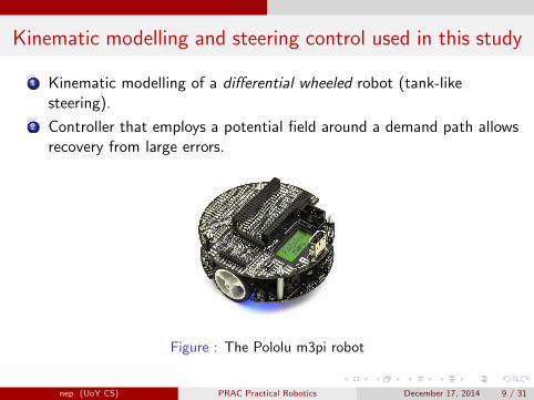
1 Kinematic modelling of a differential wheeled robot (tank-likesteering).

2 Controller that employs a potential field around a demand path allowsrecovery from large errors.

Figure : The Pololu m3pi robot


The robot frame and kinematic model parameters

Differential drive is very simple to implement and three wheels do notrequire a suspension system.Kinematic model parameters: let a be the radius of the drive wheelsand b be the wheelbase. i.e the distance between the wheels.Note also that there are potentially 4x3 sensor position parameters(discussed later).

xR

θR

b

ωR

ωL

yx s θs( )s, ,

distance sensorInfra red − sensor coordinates

in robot centred frame

a, drive wheel radius

, wheelbase

R R R

yR

Figure : The robot frame and kinematic parameters


The robot frame and kinematic model parameters

1 Origin of the robot’s coordinate system can be anywhere, naturalchoice is the midpoint of the drive wheels - why?

2 Note that the superscript R indicates a robot centred coorinate frame.3 In this navigation system, there are three different coordinate frames:

R - the robot centred frame (one frame).L - a local frame describing robot position relative to the start of somestraight line path segment (nseg frames for nseg path segments).G - a global frame in which to describe path segments, targets (walls),and accumulated position via odometry (one frame).

4 Make sure you use the correct frame and know how to switchbetween frames using a rigid Euclidean transformation (rotation and2D translation, reviewed later).


Kinematic modelling of a differential drive

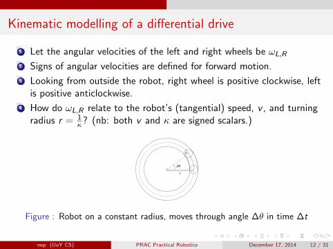
1 Let the angular velocities of the left and right wheels be ωL,R

2 Signs of angular velocities are defined for forward motion.

3 Looking from outside the robot, right wheel is positive clockwise, leftis positive anticlockwise.

4 How do ωL,R relate to the robot’s (tangential) speed, v , and turningradius r = 1

κ? (nb: both v and κ are signed scalars.)

∆θ

r

v

Figure : Robot on a constant radius, moves through angle ∆θ in time ∆t



(r − b

2)∆θ = aωL∆t (1)

(r +b

2)∆θ = aωR∆t (2)

Dividing the first equation (blue line, previous fig) by the second equation(red line, previous fig) gives

2r − b

2r + b=ωL

ωR(3)

Rearranging this equation (do it yourself later)

r =b(ωR + ωL)

2(ωR − ωL)= b

ωmean

ωdiff(4)



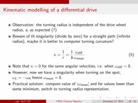
Observation: the turning radius is independent of the drive wheelradius, a, as expected (?)

Beware of th singularity (divide by zero) for a straight path (infiniteradius), maybe it is better to computer turning curvature?

κ =1

r=

1

b

ωdiff

ωmean(5)

Note that κ = 0 for the same angular velocities, i.e. when ωdiff = 0.

However, now we have a singularity when turning on the spot,ωL = −ωR hence ωmean = 0.

Practical solution: compute value of |ωmean| and for values lower thansome minimum, switch to turning radius representation.



1 We note that v = θ̇r is linear in r and that the robot’s origin is themidpoint between the two drive wheels.

2 This implies that the tangential speed, v , of the robot’s origin alongits curved path must be the average of the two tangential wheelspeeds, as follows:

v =vR + vL

2=

a(ωR + ωL)

2= aωmean (6)

Thus the transformation (ωL, ωR)→ (v , κ) from angular wheel speeds totangential speed and turning curvature is

v =a(ωR + ωL)

2= aωmean, κ =

2(ωR − ωL)

b(ωR + ωL)=

ωdiff

bωmean. (7)



1 However, in our robot system, we want to specify the (signed scalars)robot speed (v) and steering curvature (κ), using software routinesfor velocity and steering control respectively.

2 Thus we need to invert the relation on the previous slide, in order toget the required mapping (v , κ)→ (ωR , ωL)

3 To make v and κ independent of each other, we need to increase thespeed of the right wheel by ∆ω and decrease the left wheel speed bythe same amount, relative to the mean angular wheel speed definedby the desired velocity, v .



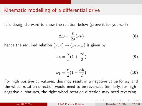
It is straightforward to show the relation below (prove it for yourself)

∆ω =b

2a(κv) (8)

hence the required relation (v , κ)→ (ωL, ωR) is given by

ωR =v

a(1 +

κb

2) (9)

ωL =v

a(1− κb

2) (10)

For high positive curvatures, this may result in a negative value for ωL andthe wheel rotation direction would need to be reversed. Similarly, for highnegative curvatures, the right wheel rotation direction may need reversing.


Lecture 1, part 2: Sensors used in this study

1 Infra-red (IR) distance sensors: extereoceptive

not always available due to limited operating rangeerrors fairly predictable and do not grow over time

2 Optical odometry: proprioceptive

always available,errors much less predictable, not independent (x, y dependent on θerror) and grow with time

3 Note the complementary nature of these two sensor systems : theycan be used to implement a predict-correct (odometry prediction, IRcorrection) localisation system.

4 Both systems require modelling : parameters to be found via directmeasurement or calibration.


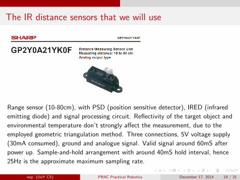
The IR distance sensors that we will use

Range sensor (10-80cm), with PSD (position sensitive detector), IRED (infrared

emitting diode) and signal processing circuit. Reflectivity of the target object and

environmental temperature don’t strongly affect the measurement, due to the

employed geometric triangulation method. Three connections, 5V voltage supply

(30mA consumed), ground and analogue signal. Valid signal around 60mS after

power up. Sample-and-hold arrangement with around 40mS hold interval, hence

25Hz is the approximate maximum sampling rate.


IR distance sensor characteristics

Output voltage is roughly in proportion to the position of the imagedIR spot on the PSD.

This PSD position is roughly proportional to the inverse of thetarget’s distance (a property of triangulation geometry).


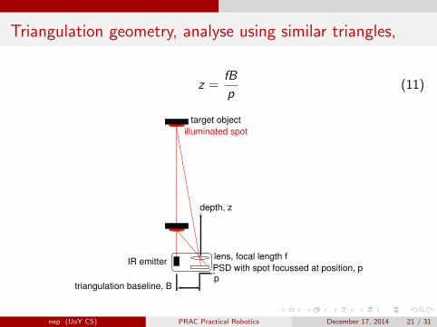
Triangulation geometry, analyse using similar triangles,

z =fB

p(11)

IR emitter

target object

illuminated spot

PSD with spot focussed at position, p

triangulation baseline, Bp

depth, z

lens, focal length f


Triangulation geometry

Image position, p and sensor range z are inversely proportional.

For a small change in p (eg, due to sensor noise), what is the changein z?

∂z

∂p= − fB

p2= − z2

fB(12)

If random noise level on p was constant over all distances (z),measurement repeatability would drop as square of distance, just dueto triangulation geometry.

However, the signal drops as square of distance which, for a PSD,causes random noise on p to also increase with the square of distance.

Combining both the geometric effect in (1) with the photometriceffect in (2) results a ranging RMS error that increases with thefourth power of distance!


IR sensor calibration

How do we convert a raw voltage reading (via ADC) to a distancemeasurement? Choosing a method and finding that method’s values orparameters is called sensor calibration. Possible methods:

1 Look up table

‘voltage - distance’ with linear interpolation (piecewise linear sensormodel).Look up table ‘voltage - reciprocal distance’ with linear interpolation(more accurate?)

2 Fit a parametric function using least-squares model fitting

Can use either the characteristic in (1) or (2) above using, for example,a polynomial (what order? linear, quadratic?)


Local pose estimation with IR sensors

1 For local pose estimation, measure distance and orientation relative totarget (wall).

2 This may be used to correct any errors in global position estimation(from odometry).

3 Need the position and orientation of the IR sensors in the robot’scoordinate frame, (xR

s , yRs , θ

Rs )i for i = 1 . . . 4.

4 Assuming good sensor orientation alignment, and accuratesymmetrical sensor distribution we may reduce from 12 to 2parameters (α, β), see next slide.

5 In the practical labs, decide for yourself whether or not this ’regularrectangle’ simplifying assumption is acceptable in terms of accuracy inlocal pose estimation.


Local pose estimation with IR sensors

yLt

Lθ

yL

yLt yL

dLF

d LR

xR

θR

yR

yx s θs( )s, , − sensor coordinates

in robot centred frame

Infra red distance sensor

α

β

xL

Ly

−

Note that y L is positive here

θ L is negative here

θL

local (path) frame

R R R

θL = tan−1

(dLR − dLF

2β

), y L = y L

t −dLR + α

cos θL(13)

where y Lt is the distance between the demand path and the target (wall).


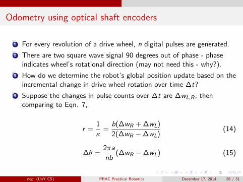
Odometry using optical shaft encoders

1 For every revolution of a drive wheel, n digital pulses are generated.

2 There are two square wave signal 90 degrees out of phase - phaseindicates wheel’s rotational direction (may not need this - why?).

3 How do we determine the robot’s global position update based on theincremental change in drive wheel rotation over time ∆t?

4 Suppose the changes in pulse counts over ∆t are ∆wL,R , thencomparing to Eqn. 7,

r =1

κ=

b(∆wR + ∆wL)

2(∆wR −∆wL)(14)

∆θ =2πa

nb(∆wR −∆wL) (15)


Odometry using optical shaft encoders

Odometry software function should consider two cases

1 When the (signed) returned count from each wheel is different.

2 When the (signed) return count from each wheel is the same, straightline, no rotation, hence r =∞.

The first case is described overleaf, the second (simpler case) is left as anexercise.


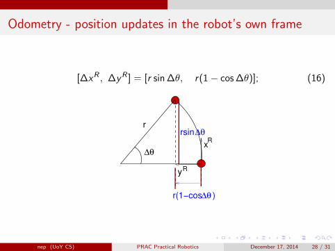
Odometry - position updates in the robot’s own frame

[∆xR , ∆y R ] = [r sin ∆θ, r(1− cos ∆θ)]; (16)

xR

yR

rrsin∆θ

∆θ

r(1−cos∆θ )


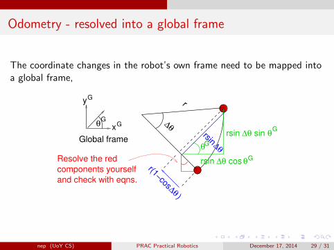
Odometry - resolved into a global frame

The coordinate changes in the robot’s own frame need to be mapped intoa global frame,

∆θrsin cos θ

∆θrsin θsinx

y

θ

Global frame

G

G

G

Resolve the red

components yourself

and check with eqns.

r(1−cos∆θ )

r

rsin∆θ

∆θ

θ

G

G

G


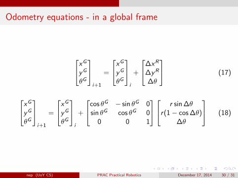
Odometry equations - in a global frame

xG

y G

θG

i+1

=

xG

y G

θG

i

+

∆xR

∆y R

∆θ

(17)

xG

y G

θG

i+1

=

xG

y G

θG

i

+

cos θG − sin θG 0sin θG cos θG 0

0 0 1

r sin ∆θr(1− cos ∆θ)

∆θ

(18)


Closing slide

This lecture will help you with the first two practical classes:

Lab 1a (week 2): Calibrating, characterising and using the IR rangesensors.

Lab 1b (week 3): Calibrating, characterising and using the odometrysensors.

Any questions?nep (UoY CS) PRAC Practical Robotics December 17, 2014 31 / 31

Practical Robotics (PRAC)

Documents