13-11-2014 Challenge the future Delft University of Technology Peter van Oosterom, joint work with Oscar Martinez Rubi (NLeSc), Theo Tijssen (TUD), Martin Kodde (Fugro), Mike Horhammer (Oracle) and Milena Ivanova (NLeSc) National eScience Symposium - Enabling Scientific Breakthroughs Stadsschouwburg Almere, 6 November 2014 Point cloud data management

Welcome message from author
This document is posted to help you gain knowledge. Please leave a comment to let me know what you think about it! Share it to your friends and learn new things together.
Transcript
13-11-2014
Challenge the future
DelftUniversity ofTechnology
Peter van Oosterom, joint work with Oscar Martinez Rubi (NLeSc), Theo Tijssen (TUD),
Martin Kodde (Fugro), Mike Horhammer (Oracle) and Milena Ivanova (NLeSc)
National eScience Symposium - Enabling Scientific Breakthroughs
Stadsschouwburg Almere, 6 November 2014
Point cloud data management
2MPC @ NL eScience Symp, 6 Nov’14
3MPC @ NL eScience Symp, 6 Nov’14
Content overview
0. Background1. Conceptual benchmark2. Executable benchmark3. Data organization4. Conclusion
4MPC @ NL eScience Symp, 6 Nov’14
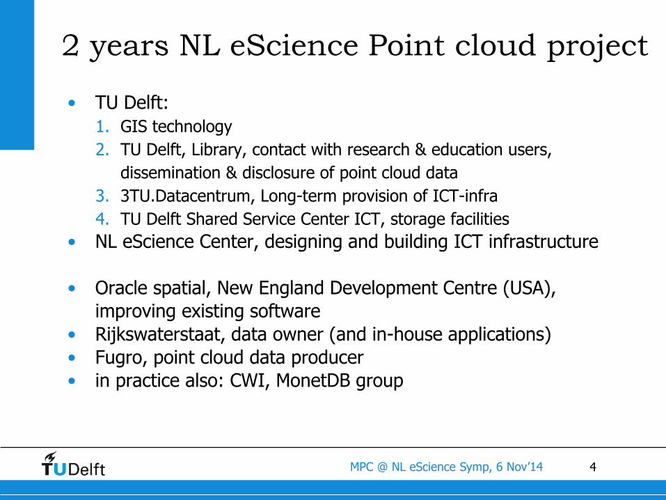
2 years NL eScience Point cloud project
• TU Delft:
1. GIS technology
2. TU Delft, Library, contact with research & education users,
dissemination & disclosure of point cloud data
3. 3TU.Datacentrum, Long-term provision of ICT-infra
4. TU Delft Shared Service Center ICT, storage facilities
• NL eScience Center, designing and building ICT infrastructure
• Oracle spatial, New England Development Centre (USA),
improving existing software
• Rijkswaterstaat, data owner (and in-house applications)
• Fugro, point cloud data producer
• in practice also: CWI, MonetDB group
5MPC @ NL eScience Symp, 6 Nov’14
User requirements
• report user requirements, based on structured interviews
conducted last year with
• Government community: RWS (Ministry)
• Commercial community: Fugro (company)
• Scientific community: TU Delft Library
• report at MPC public website http://pointclouds.nl
• basis for conceptual benchmark, with tests for functionality,
classified by importance (based on user requirements and
Oracle experience)
6MPC @ NL eScience Symp, 6 Nov’14
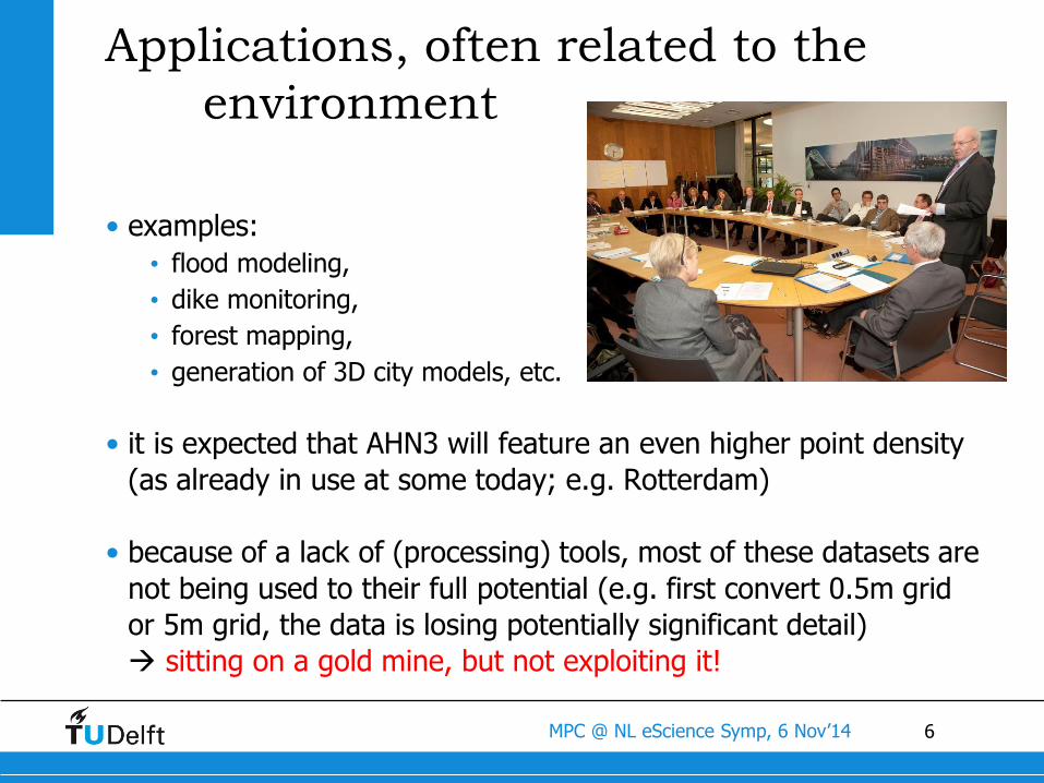
Applications, often related to the
environment
• examples:
• flood modeling,
• dike monitoring,
• forest mapping,
• generation of 3D city models, etc.
• it is expected that AHN3 will feature an even higher point density
(as already in use at some today; e.g. Rotterdam)
• because of a lack of (processing) tools, most of these datasets are
not being used to their full potential (e.g. first convert 0.5m grid
or 5m grid, the data is losing potentially significant detail)
sitting on a gold mine, but not exploiting it!
7MPC @ NL eScience Symp, 6 Nov’14
Approach
• develop infrastructure for the storage, the management, …
of massive point clouds (note: no object reconstruction)
• support range of hardware platforms: normal/ department servers
(HP), cloud-based solution (MS Azure), EXADATA (Oracle)
• scalable solution: if data sets becomes 100 times larger and/or if
we get 1000 times more users (queries), it should be possible to
configure based on same architecture
• generic, i.e. also support other (geo-)data and standards based, if
non-existent, then propose new standard to ISO (TC211/OGC):
Web Point Cloud Service (WPCS)
• also standardization at SQL level (SQL/SFS, SQL/raster, SQL/PC)?
8MPC @ NL eScience Symp, 6 Nov’14
Why a DBMS approach?
• today’s common practice: specific file format (LAS, LAZ, ZLAS,…)
with specific tools (libraries) for that format
• point clouds are a bit similar to raster data:
sampling nature, huge volumes, relatively static
• specific files are sub-optimal data management:
• multi-user (access and some update)
• scalability (not nice to process 60.000 AHN2 files)
• integrate data (types: vector, raster, admin)
• ‘work around’ could be developed, but that’s building own DBMS
• no reason why point cloud can not be supported efficient in DBMS
• perhaps ‘mix’ of both: use file (or GPU) format for the PC blocks
9MPC @ NL eScience Symp, 6 Nov’14
Content overview
0. Background1. Conceptual benchmark2. Executable benchmark3. Data organization4. Conclusion
10MPC @ NL eScience Symp, 6 Nov’14
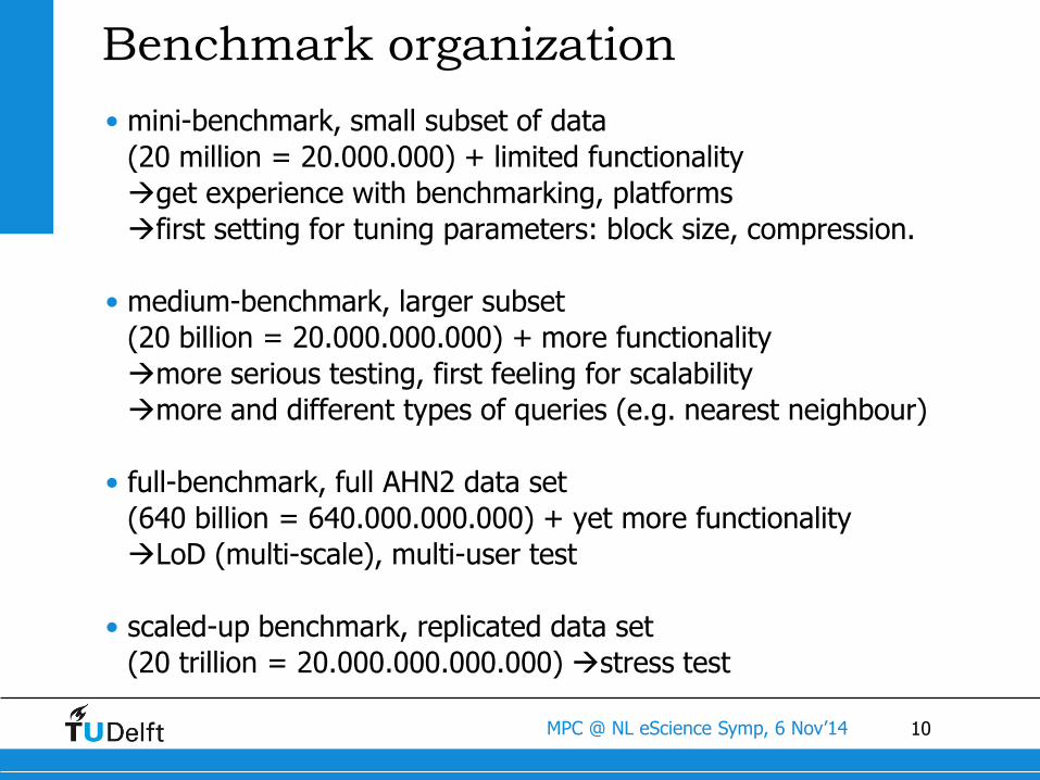
Benchmark organization
• mini-benchmark, small subset of data
(20 million = 20.000.000) + limited functionality
get experience with benchmarking, platforms
first setting for tuning parameters: block size, compression.
• medium-benchmark, larger subset
(20 billion = 20.000.000.000) + more functionality
more serious testing, first feeling for scalability
more and different types of queries (e.g. nearest neighbour)
• full-benchmark, full AHN2 data set
(640 billion = 640.000.000.000) + yet more functionality
LoD (multi-scale), multi-user test
• scaled-up benchmark, replicated data set
(20 trillion = 20.000.000.000.000) stress test
11MPC @ NL eScience Symp, 6 Nov’14
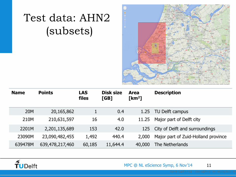
Test data: AHN2
(subsets)
Oracle Confidential – Internal/Restricted/Highly Restricted11
Name Points LAS files
Disk size [GB]
Area [km2]
Description
20M 20,165,862 1 0.4 1.25 TU Delft campus
210M 210,631,597 16 4.0 11.25 Major part of Delft city
2201M 2,201,135,689 153 42.0 125 City of Delft and surroundings
23090M 23,090,482,455 1,492 440.4 2,000 Major part of Zuid-Holland province
639478M 639,478,217,460 60,185 11,644.4 40,000 The Netherlands
12MPC @ NL eScience Symp, 6 Nov’14
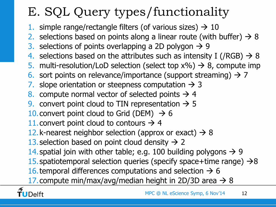
E. SQL Query types/functionality1. simple range/rectangle filters (of various sizes) 10
2. selections based on points along a linear route (with buffer) 8
3. selections of points overlapping a 2D polygon 9
4. selections based on the attributes such as intensity I (/RGB) 8
5. multi-resolution/LoD selection (select top x%) 8, compute imp
6. sort points on relevance/importance (support streaming) 7
7. slope orientation or steepness computation 3
8. compute normal vector of selected points 4
9. convert point cloud to TIN representation 5
10.convert point cloud to Grid (DEM) 6
11.convert point cloud to contours 4
12.k-nearest neighbor selection (approx or exact) 8
13.selection based on point cloud density 2
14.spatial join with other table; e.g. 100 building polygons 9
15.spatiotemporal selection queries (specify space+time range) 8
16.temporal differences computations and selection 6
17.compute min/max/avg/median height in 2D/3D area 8
13MPC @ NL eScience Symp, 6 Nov’14
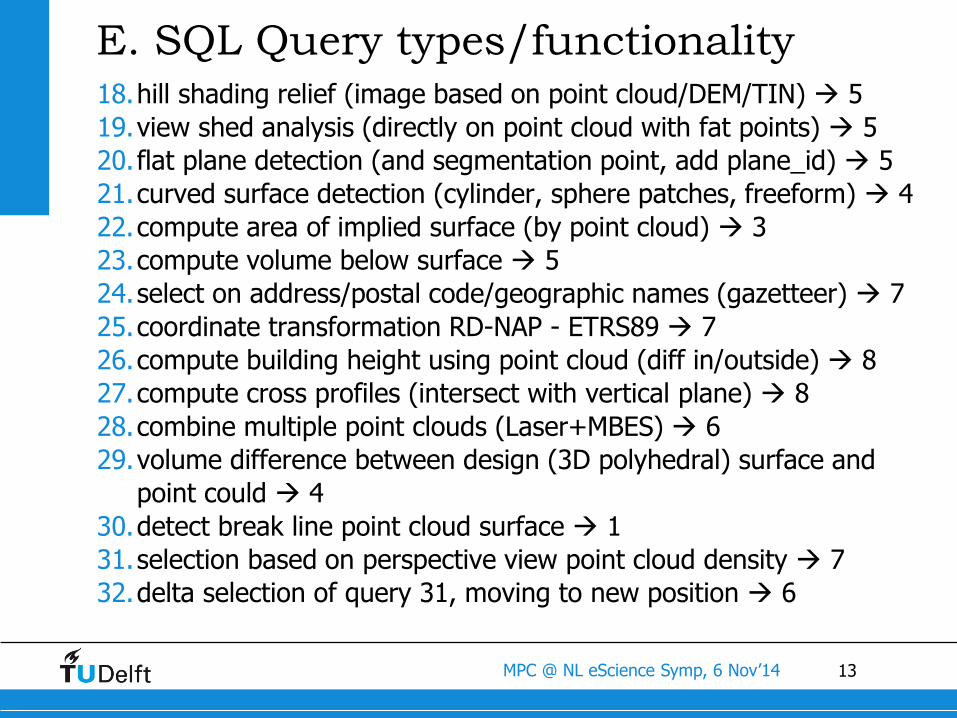
E. SQL Query types/functionality18.hill shading relief (image based on point cloud/DEM/TIN) 5
19.view shed analysis (directly on point cloud with fat points) 5
20.flat plane detection (and segmentation point, add plane_id) 5
21.curved surface detection (cylinder, sphere patches, freeform) 4
22.compute area of implied surface (by point cloud) 3
23.compute volume below surface 5
24.select on address/postal code/geographic names (gazetteer) 7
25.coordinate transformation RD-NAP - ETRS89 7
26.compute building height using point cloud (diff in/outside) 8
27.compute cross profiles (intersect with vertical plane) 8
28.combine multiple point clouds (Laser+MBES) 6
29.volume difference between design (3D polyhedral) surface and
point could 4
30.detect break line point cloud surface 1
31.selection based on perspective view point cloud density 7
32.delta selection of query 31, moving to new position 6
14MPC @ NL eScience Symp, 6 Nov’14
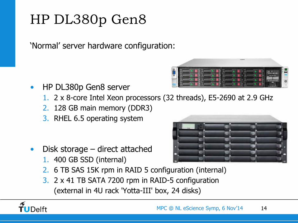
HP DL380p Gen8
‘Normal’ server hardware configuration:
• HP DL380p Gen8 server
1. 2 x 8-core Intel Xeon processors (32 threads), E5-2690 at 2.9 GHz
2. 128 GB main memory (DDR3)
3. RHEL 6.5 operating system
• Disk storage – direct attached
1. 400 GB SSD (internal)
2. 6 TB SAS 15K rpm in RAID 5 configuration (internal)
3. 2 x 41 TB SATA 7200 rpm in RAID-5 configuration
(external in 4U rack 'Yotta-III' box, 24 disks)
15MPC @ NL eScience Symp, 6 Nov’14
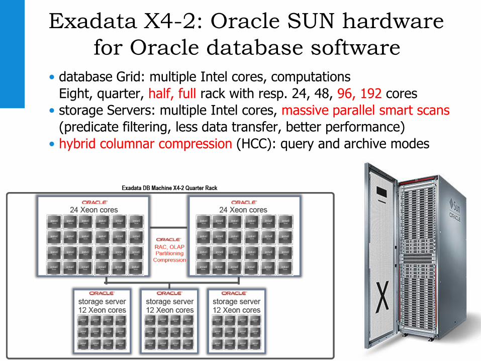
Exadata X4-2: Oracle SUN hardware
for Oracle database software
• database Grid: multiple Intel cores, computations
Eight, quarter, half, full rack with resp. 24, 48, 96, 192 cores
• storage Servers: multiple Intel cores, massive parallel smart scans
(predicate filtering, less data transfer, better performance)
• hybrid columnar compression (HCC): query and archive modes
16MPC @ NL eScience Symp, 6 Nov’14
Content overview
0. Background1. Conceptual benchmark2. Executable benchmark3. Data organization4. Conclusion
17MPC @ NL eScience Symp, 6 Nov’14
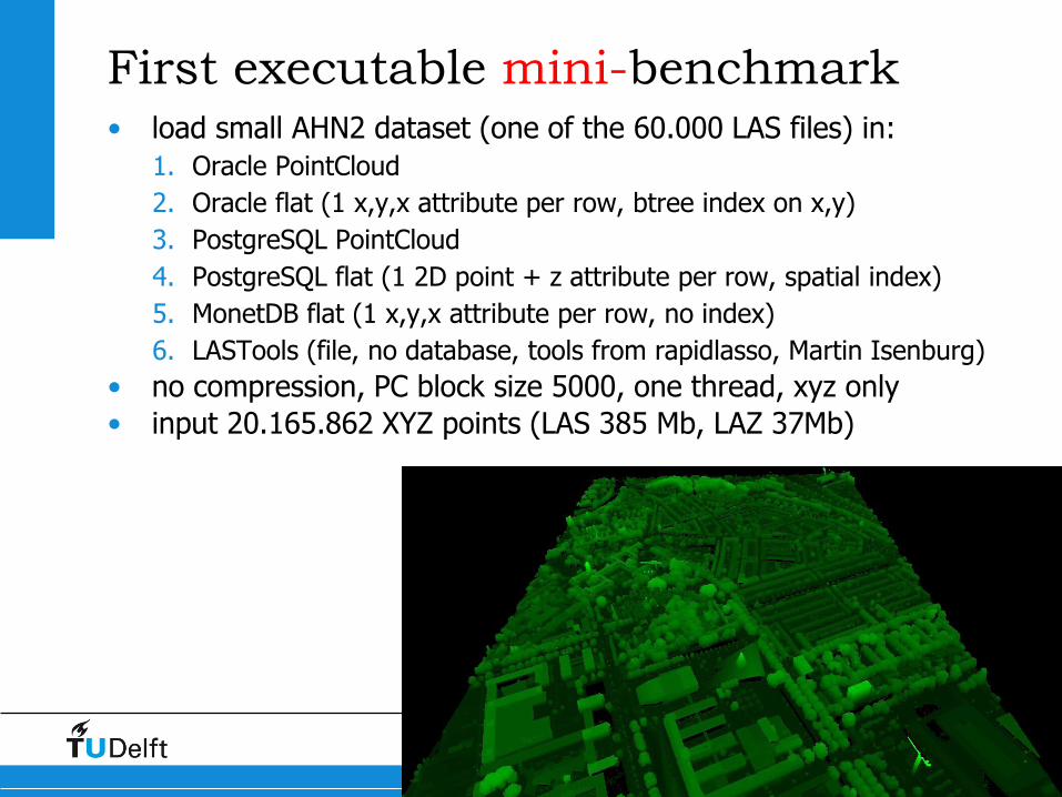
First executable mini-benchmark• load small AHN2 dataset (one of the 60.000 LAS files) in:
1. Oracle PointCloud
2. Oracle flat (1 x,y,x attribute per row, btree index on x,y)
3. PostgreSQL PointCloud
4. PostgreSQL flat (1 2D point + z attribute per row, spatial index)
5. MonetDB flat (1 x,y,x attribute per row, no index)
6. LASTools (file, no database, tools from rapidlasso, Martin Isenburg)
• no compression, PC block size 5000, one thread, xyz only
• input 20.165.862 XYZ points (LAS 385 Mb, LAZ 37Mb)
18MPC @ NL eScience Symp, 6 Nov’14
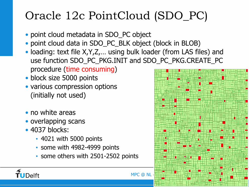
Oracle 12c PointCloud (SDO_PC)
• point cloud metadata in SDO_PC object
• point cloud data in SDO_PC_BLK object (block in BLOB)
• loading: text file X,Y,Z,… using bulk loader (from LAS files) and
use function SDO_PC_PKG.INIT and SDO_PC_PKG.CREATE_PC
procedure (time consuming)
• block size 5000 points
• various compression options
(initially not used)
• no white areas
• overlapping scans
• 4037 blocks:
• 4021 with 5000 points
• some with 4982-4999 points
• some others with 2501-2502 points
19MPC @ NL eScience Symp, 6 Nov’14
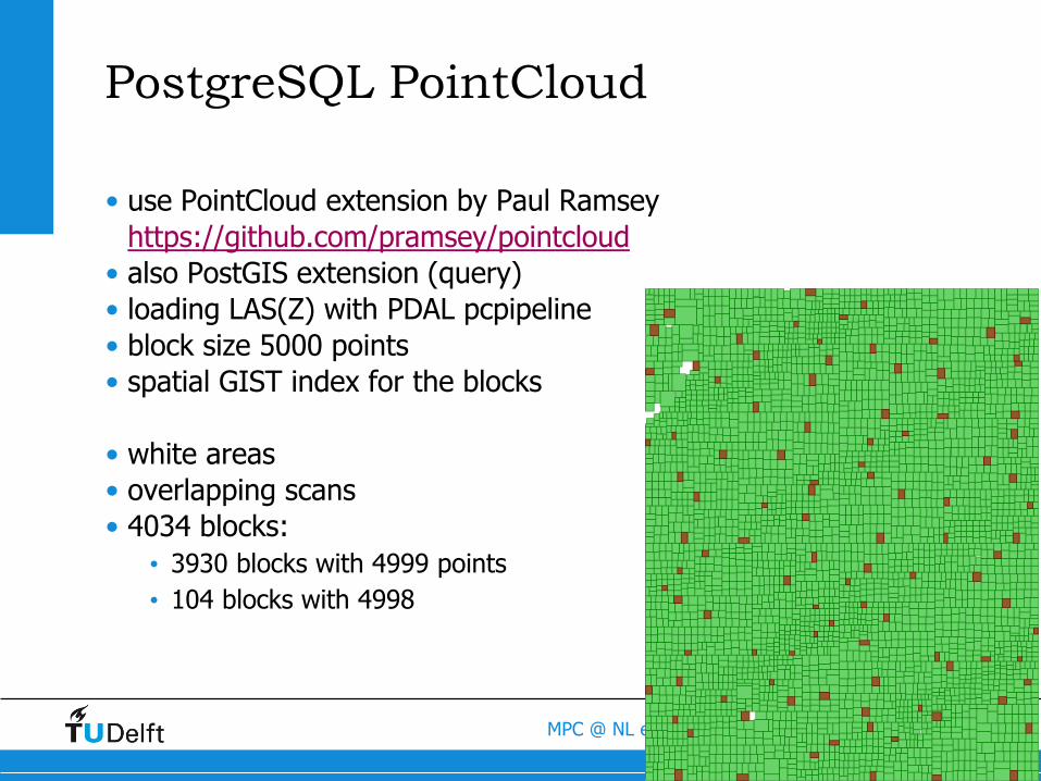
PostgreSQL PointCloud
• use PointCloud extension by Paul Ramsey
https://github.com/pramsey/pointcloud
• also PostGIS extension (query)
• loading LAS(Z) with PDAL pcpipeline
• block size 5000 points
• spatial GIST index for the blocks
• white areas
• overlapping scans
• 4034 blocks:
• 3930 blocks with 4999 points
• 104 blocks with 4998
20MPC @ NL eScience Symp, 6 Nov’14
MonetDB
• MonetDB: open source column-oriented DBMS developed by
Centrum Wiskunde & Informatica (CWI), the Netherlands
• MonetDB/GIS: OGC simple feature extension to MonetDB/SQL
• MonetDB has plans for support point cloud data (and nD array’s)
• for comparing with Oracle and PostgreSQL only simple rectangle
and circle queries Q1-Q4 (without conversion to spatial)
• no need to specify index (will be created
invisibly when needed by first query…)
21MPC @ NL eScience Symp, 6 Nov’14
LASTools
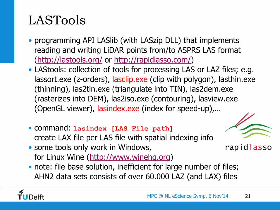
• programming API LASlib (with LASzip DLL) that implements
reading and writing LiDAR points from/to ASPRS LAS format
(http://lastools.org/ or http://rapidlasso.com/)
• LAStools: collection of tools for processing LAS or LAZ files; e.g.
lassort.exe (z-orders), lasclip.exe (clip with polygon), lasthin.exe
(thinning), las2tin.exe (triangulate into TIN), las2dem.exe
(rasterizes into DEM), las2iso.exe (contouring), lasview.exe
(OpenGL viewer), lasindex.exe (index for speed-up),…
• command: lasindex [LAS File path]
create LAX file per LAS file with spatial indexing info
• some tools only work in Windows,
for Linux Wine (http://www.winehq.org)
• note: file base solution, inefficient for large number of files;
AHN2 data sets consists of over 60.000 LAZ (and LAX) files
22MPC @ NL eScience Symp, 6 Nov’14
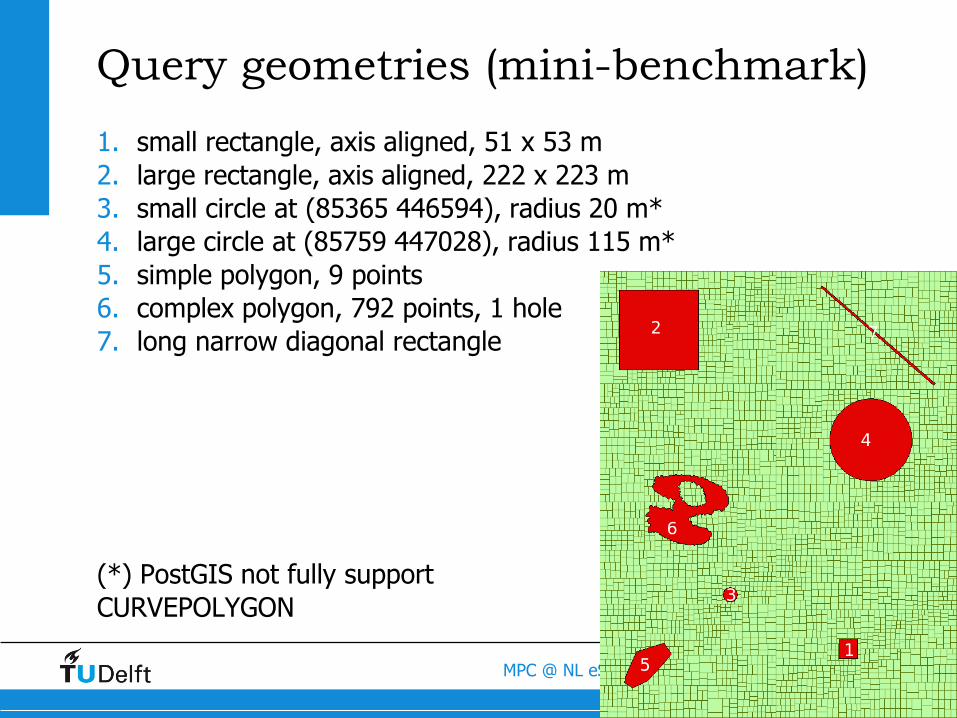
Query geometries (mini-benchmark)
1. small rectangle, axis aligned, 51 x 53 m
2. large rectangle, axis aligned, 222 x 223 m
3. small circle at (85365 446594), radius 20 m*
4. large circle at (85759 447028), radius 115 m*
5. simple polygon, 9 points
6. complex polygon, 792 points, 1 hole
7. long narrow diagonal rectangle
(*) PostGIS not fully support
CURVEPOLYGON
23MPC @ NL eScience Symp, 6 Nov’14
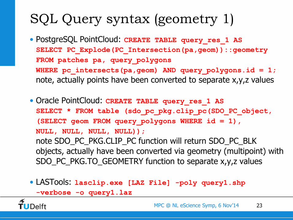
SQL Query syntax (geometry 1)
• PostgreSQL PointCloud: CREATE TABLE query_res_1 ASSELECT PC_Explode(PC_Intersection(pa,geom))::geometry
FROM patches pa, query_polygons
WHERE pc_intersects(pa,geom) AND query_polygons.id = 1;
note, actually points have been converted to separate x,y,z values
• Oracle PointCloud: CREATE TABLE query_res_1 AS SELECT * FROM table (sdo_pc_pkg.clip_pc(SDO_PC_object,
(SELECT geom FROM query_polygons WHERE id = 1),
NULL, NULL, NULL, NULL));
note SDO_PC_PKG.CLIP_PC function will return SDO_PC_BLK
objects, actually have been converted via geometry (multipoint) with
SDO_PC_PKG.TO_GEOMETRY function to separate x,y,z values
• LASTools: lasclip.exe [LAZ File] -poly query1.shp -verbose -o query1.laz
24MPC @ NL eScience Symp, 6 Nov’14
PC Block size and compression
• block size: 300, 500, 1000, 3000 and 5000 points
• compression:
• Oracle PC: none, medium and high
• PostGIS PC: none, dimensional
• conclusions (most the same for PostGIS, Oracle):
• Compression about factor 2 to 3 (not as good as LAZ/ZLAS: 10)
• Load time and storage size are linear to size datasets
• Query time not much different: data size / compression (max 10%)
• Oracle medium and high compression score equal
• Oracle load gets slow for small block size 300-500
• see graphs next slides: PostGIS (Oracle very similar)
25MPC @ NL eScience Symp, 6 Nov’14
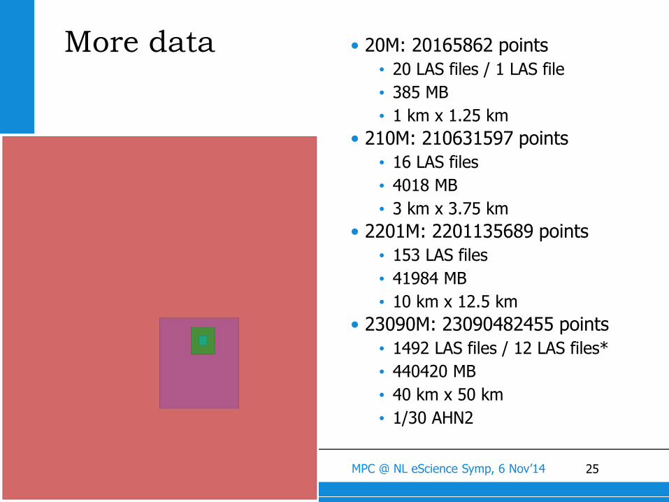
More data • 20M: 20165862 points
• 20 LAS files / 1 LAS file
• 385 MB
• 1 km x 1.25 km
• 210M: 210631597 points
• 16 LAS files
• 4018 MB
• 3 km x 3.75 km
• 2201M: 2201135689 points
• 153 LAS files
• 41984 MB
• 10 km x 12.5 km
• 23090M: 23090482455 points
• 1492 LAS files / 12 LAS files*
• 440420 MB
• 40 km x 50 km
• 1/30 AHN2
26MPC @ NL eScience Symp, 6 Nov’14
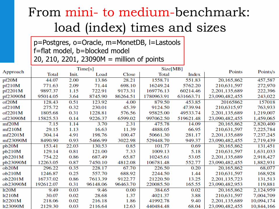
From mini- to medium-benchmark:
load (index) times and sizesp=Postgres, o=Oracle, m=MonetDB, l=Lastoolsf=flat model, b=blocked model20, 210, 2201, 23090M = million of points
27MPC @ NL eScience Symp, 6 Nov’14
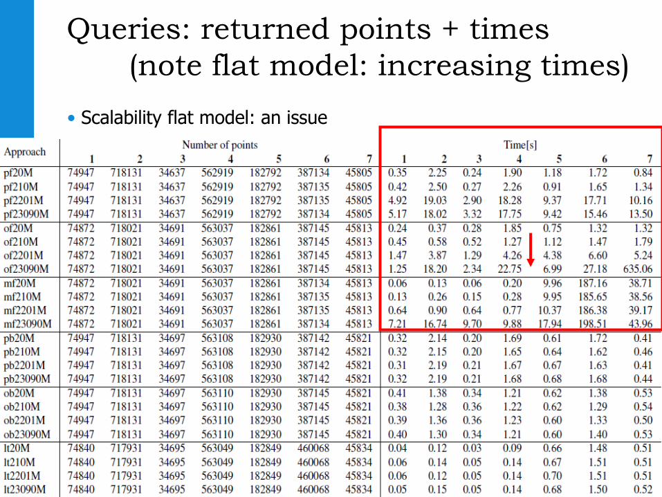
Queries: returned points + times
(note flat model: increasing times)
• Scalability flat model: an issue
28MPC @ NL eScience Symp, 6 Nov’14
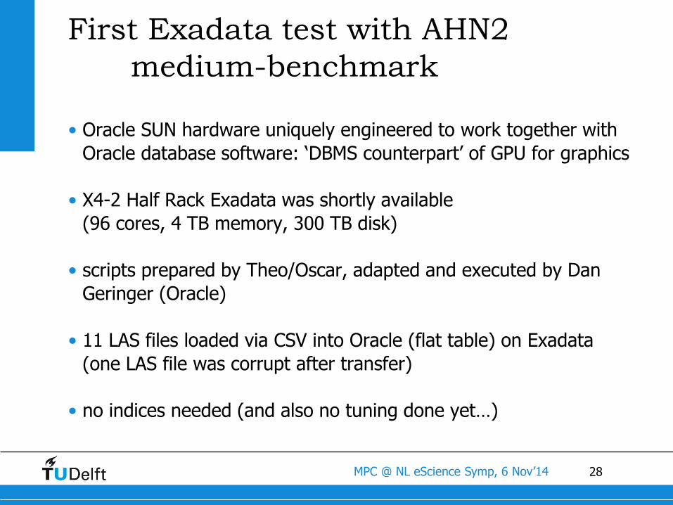
First Exadata test with AHN2
medium-benchmark
• Oracle SUN hardware uniquely engineered to work together with
Oracle database software: ‘DBMS counterpart’ of GPU for graphics
• X4-2 Half Rack Exadata was shortly available
(96 cores, 4 TB memory, 300 TB disk)
• scripts prepared by Theo/Oscar, adapted and executed by Dan
Geringer (Oracle)
• 11 LAS files loaded via CSV into Oracle (flat table) on Exadata
(one LAS file was corrupt after transfer)
• no indices needed (and also no tuning done yet…)
29MPC @ NL eScience Symp, 6 Nov’14
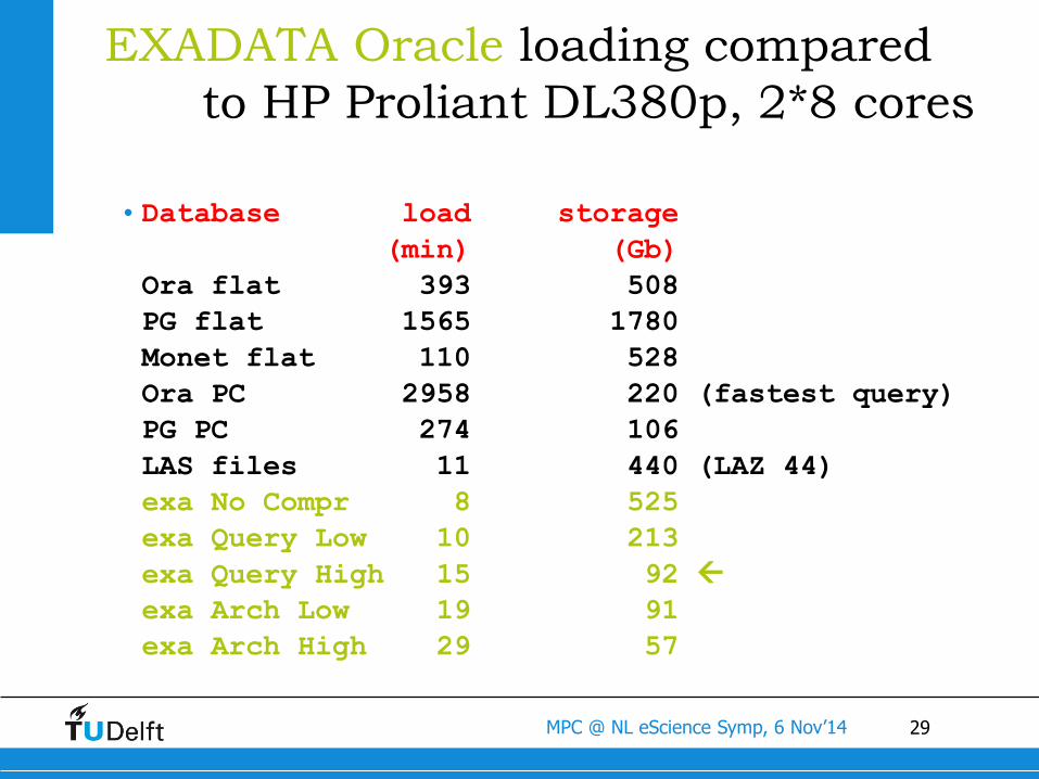
EXADATA Oracle loading compared
to HP Proliant DL380p, 2*8 cores
•Database load storage
(min) (Gb)
Ora flat 393 508
PG flat 1565 1780
Monet flat 110 528
Ora PC 2958 220 (fastest query)
PG PC 274 106
LAS files 11 440 (LAZ 44)
exa No Compr 8 525
exa Query Low 10 213
exa Query High 15 92
exa Arch Low 19 91
exa Arch High 29 57
30MPC @ NL eScience Symp, 6 Nov’14
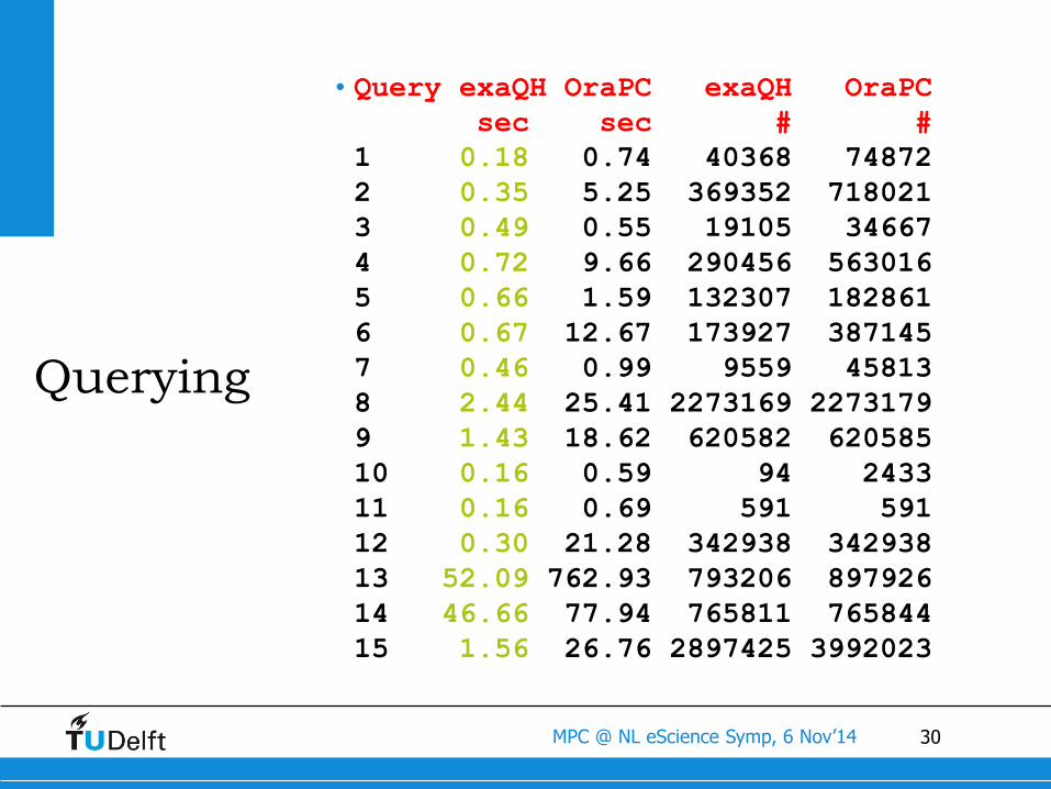
Querying
•Query exaQH OraPC exaQH OraPC
sec sec # #
1 0.18 0.74 40368 74872
2 0.35 5.25 369352 718021
3 0.49 0.55 19105 34667
4 0.72 9.66 290456 563016
5 0.66 1.59 132307 182861
6 0.67 12.67 173927 387145
7 0.46 0.99 9559 45813
8 2.44 25.41 2273169 2273179
9 1.43 18.62 620582 620585
10 0.16 0.59 94 2433
11 0.16 0.69 591 591
12 0.30 21.28 342938 342938
13 52.09 762.93 793206 897926
14 46.66 77.94 765811 765844
15 1.56 26.76 2897425 3992023
31MPC @ NL eScience Symp, 6 Nov’14
Oracle Confidential – Internal/Restricted/Highly Restricted31
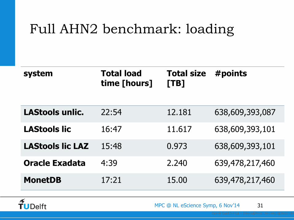
Full AHN2 benchmark: loading
system Total load time [hours]
Total size [TB]
#points
LAStools unlic. 22:54 12.181 638,609,393,087
LAStools lic 16:47 11.617 638,609,393,101
LAStools lic LAZ 15:48 0.973 638,609,393,101
Oracle Exadata 4:39 2.240 639,478,217,460
MonetDB 17:21 15.00 639,478,217,460
32MPC @ NL eScience Symp, 6 Nov’14
Content overview
0. Background1. Conceptual benchmark2. Executable benchmark3. Data organization4. Conclusion
33MPC @ NL eScience Symp, 6 Nov’14
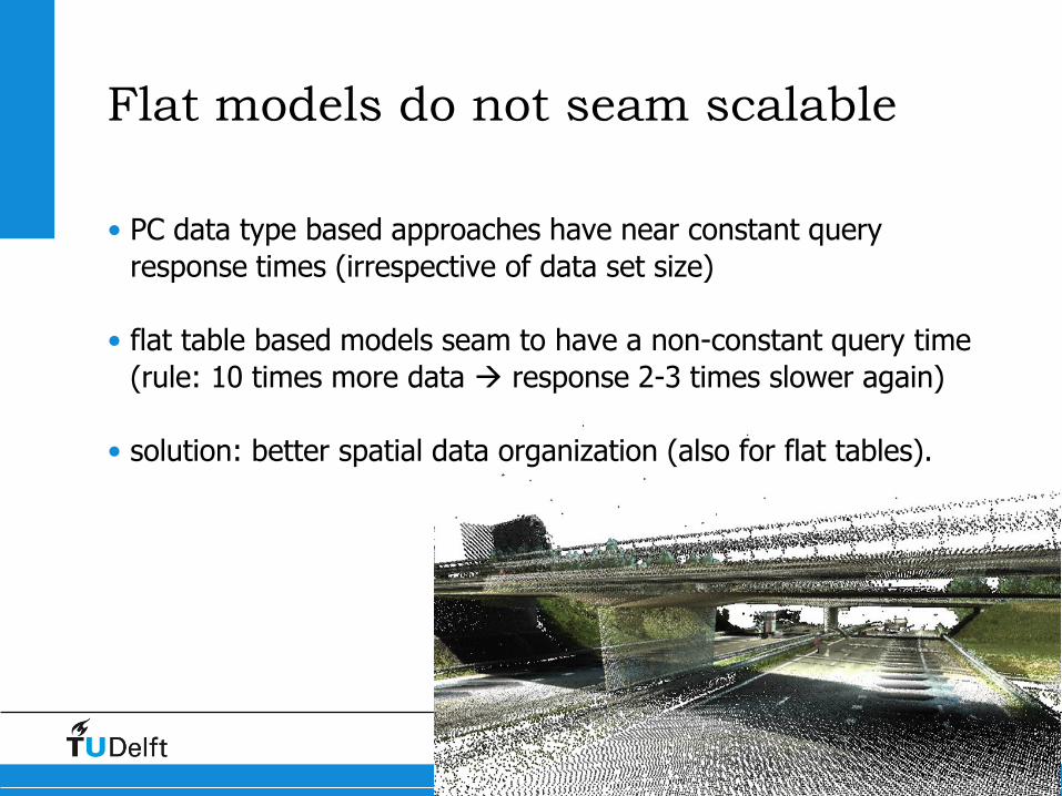
Flat models do not seam scalable
• PC data type based approaches have near constant query
response times (irrespective of data set size)
• flat table based models seam to have a non-constant query time
(rule: 10 times more data response 2-3 times slower again)
• solution: better spatial data organization (also for flat tables).
34MPC @ NL eScience Symp, 6 Nov’14
Data organization
• how can a flat table be organized efficiently?
• how can the point cloud blocks be created efficiently?
(with no assumption on data organization in input)
• answer: spatial clustering/coherence, e.g. quadtree/octree
(as obtained by Morton or Hilbert space filling curves)
35MPC @ NL eScience Symp, 6 Nov’14
Some Space Filling Curves
0 1 2 3 col
row
3
2
1
00
15
0 1 2 3 col
row
3
2
1
00
15
0 1 2 3 col
0 15
row
3
2
1
0
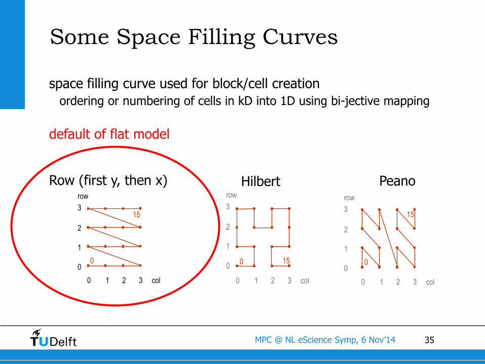
Row (first y, then x) PeanoHilbert
space filling curve used for block/cell creation
ordering or numbering of cells in kD into 1D using bi-jective mapping
default of flat model
36MPC @ NL eScience Symp, 6 Nov’14
0
00 01
row
01
00
3
0 1 2 3 col
row
3
2
1
00
15
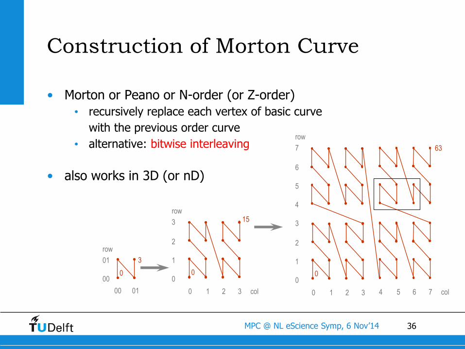
Construction of Morton Curve
• Morton or Peano or N-order (or Z-order)
• recursively replace each vertex of basic curve
with the previous order curve
• alternative: bitwise interleaving
• also works in 3D (or nD)
0 1 2 3
3
2
1
00
4 5 6 7 col
row
7
6
5
4
63
37MPC @ NL eScience Symp, 6 Nov’14
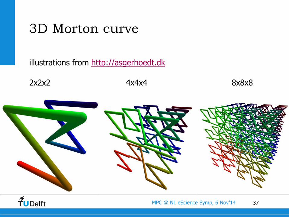
3D Morton curve
illustrations from http://asgerhoedt.dk
2x2x2 4x4x4 8x8x8
38MPC @ NL eScience Symp, 6 Nov’14
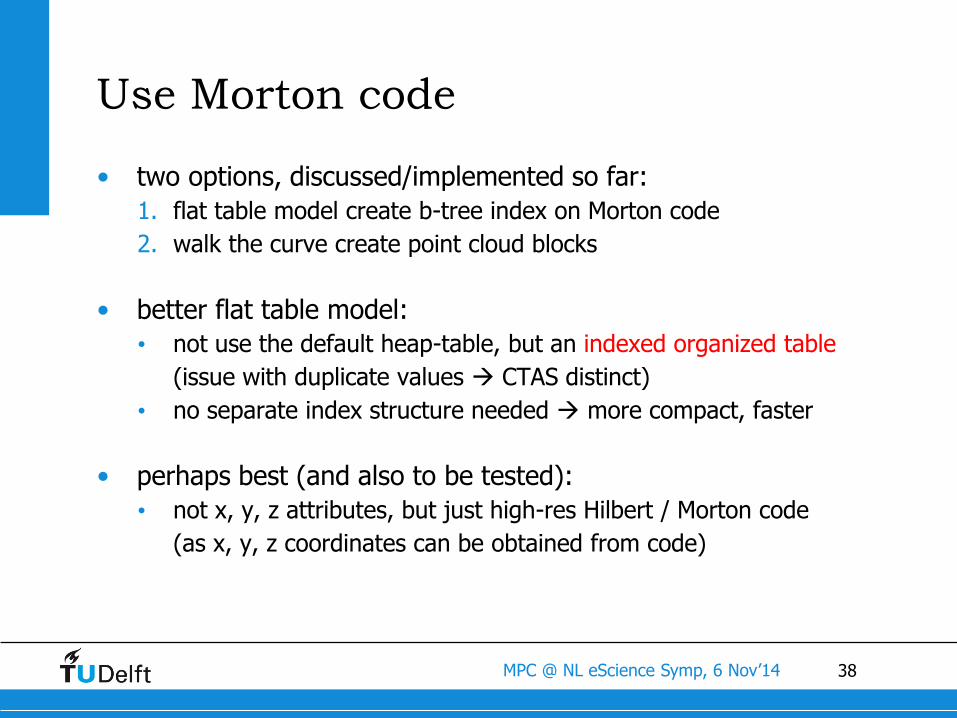
Use Morton code
• two options, discussed/implemented so far:
1. flat table model create b-tree index on Morton code
2. walk the curve create point cloud blocks
• better flat table model:
• not use the default heap-table, but an indexed organized table
(issue with duplicate values CTAS distinct)
• no separate index structure needed more compact, faster
• perhaps best (and also to be tested):
• not x, y, z attributes, but just high-res Hilbert / Morton code
(as x, y, z coordinates can be obtained from code)
39MPC @ NL eScience Symp, 6 Nov’14
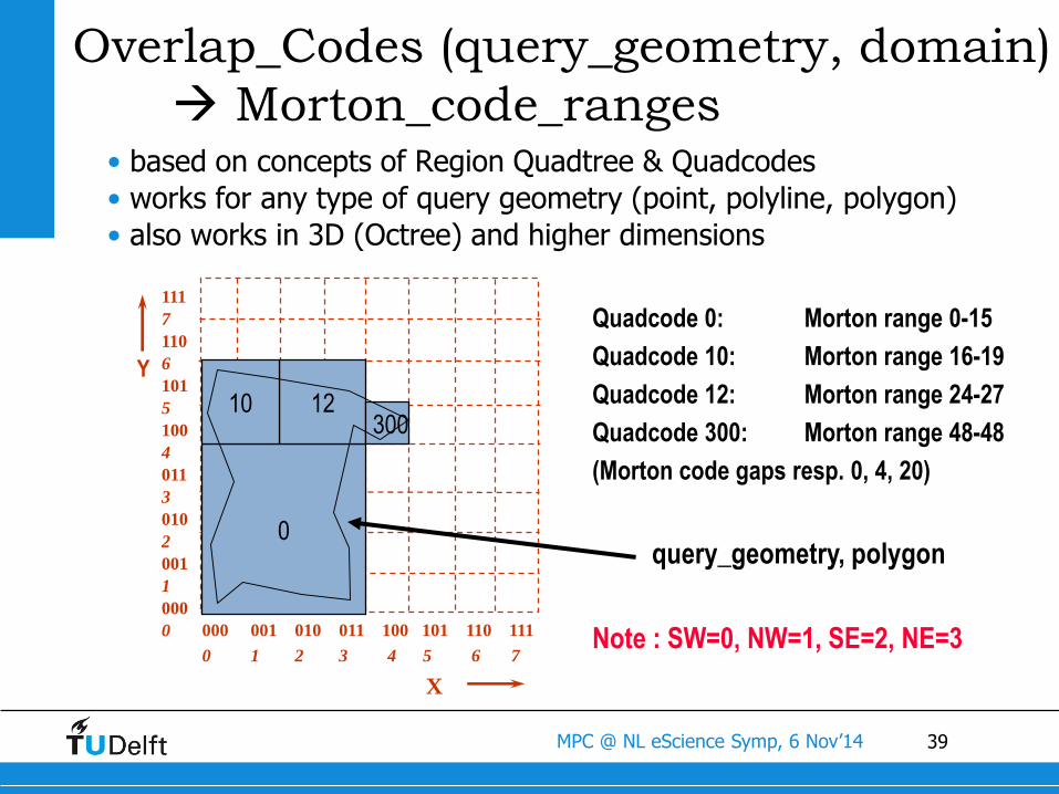
Quadcode 0: Morton range 0-15
Quadcode 10: Morton range 16-19
Quadcode 12: Morton range 24-27
Quadcode 300: Morton range 48-48
(Morton code gaps resp. 0, 4, 20)
query_geometry, polygon
Note : SW=0, NW=1, SE=2, NE=3
Overlap_Codes (query_geometry, domain)
Morton_code_ranges• based on concepts of Region Quadtree & Quadcodes
• works for any type of query geometry (point, polyline, polygon)
• also works in 3D (Octree) and higher dimensions
111
7
110
6
101
5
100
4
011
3
010
2
001
1
000
0
Y
0
12300
10
000 001 010 011 100 101 110 111
0 1 2 3 4 5 6 7
X
40MPC @ NL eScience Symp, 6 Nov’14
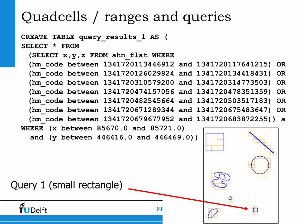
Quadcells / ranges and queries
CREATE TABLE query_results_1 AS (
SELECT * FROM
(SELECT x,y,z FROM ahn_flat WHERE
(hm_code between 1341720113446912 and 1341720117641215) OR
(hm_code between 1341720126029824 and 1341720134418431) OR
(hm_code between 1341720310579200 and 1341720314773503) OR
(hm_code between 1341720474157056 and 1341720478351359) OR
(hm_code between 1341720482545664 and 1341720503517183) OR
(hm_code between 1341720671289344 and 1341720675483647) OR
(hm_code between 1341720679677952 and 1341720683872255)) a
WHERE (x between 85670.0 and 85721.0)
and (y between 446416.0 and 446469.0))
Query 1 (small rectangle)

41MPC @ NL eScience Symp, 6 Nov’14
Use of Morton codes/ranges
(PostgreSQL flat model example)
Q1 Q4 Q7 response in seconds
rect circle line (of hot/second query
20M 0.16 0.85 2.32 first query exact
210M 0.38 1.80 3.65 same pattern, but
2201M 0.93 4.18 7.11 3-10 times slower
23090M 3.14 14.54 21.44 both for normal flat
model and for Morton
with Q1 Q4 Q7 flat model)
Morton rect circle line
20M 0.15 0.56 0.82
210M 0.15 0.56 0.42
2201M 0.13 0.64 0.41
23090M 0.15 0.70 0.60
42MPC @ NL eScience Symp, 6 Nov’14
Content overview
0. Background1. Conceptual benchmark2. Executable benchmark3. Data organization4. Conclusion
43MPC @ NL eScience Symp, 6 Nov’14
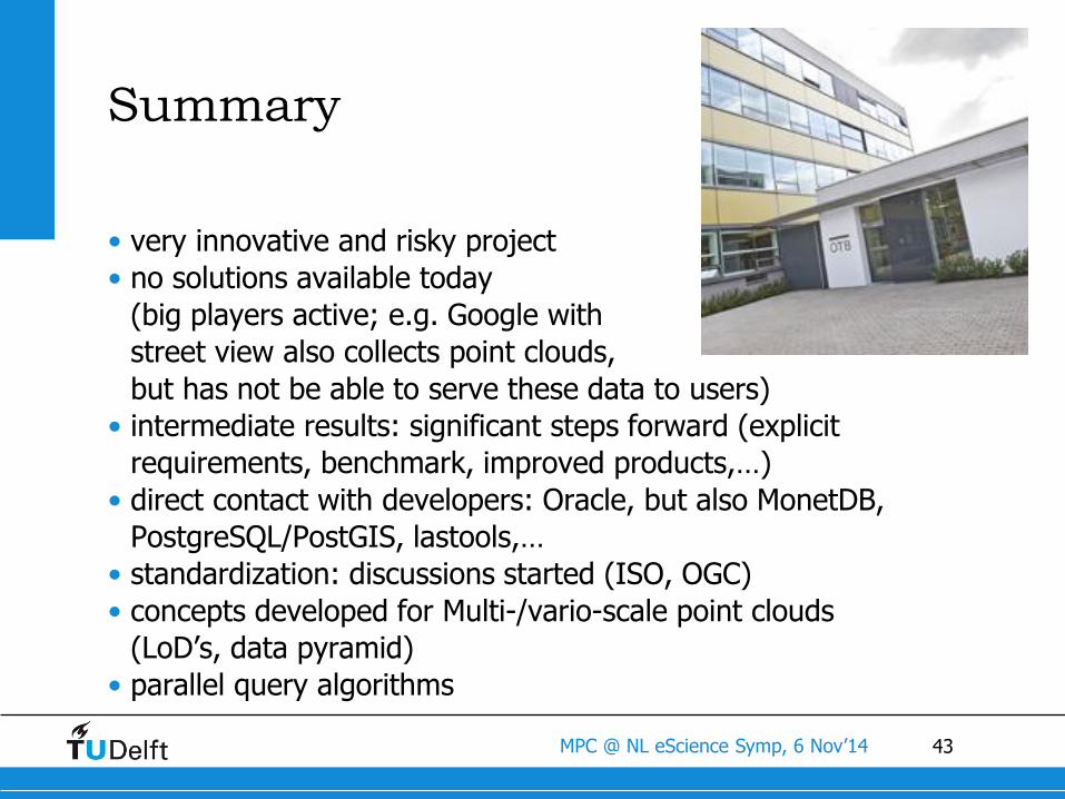
Summary
• very innovative and risky project
• no solutions available today
(big players active; e.g. Google with
street view also collects point clouds,
but has not be able to serve these data to users)
• intermediate results: significant steps forward (explicit
requirements, benchmark, improved products,…)
• direct contact with developers: Oracle, but also MonetDB,
PostgreSQL/PostGIS, lastools,…
• standardization: discussions started (ISO, OGC)
• concepts developed for Multi-/vario-scale point clouds
(LoD’s, data pyramid)
• parallel query algorithms
44MPC @ NL eScience Symp, 6 Nov’14
Next Phase of project
• full and scaled-up benchmarking
• web-based viewer (WebGL, LoD-tiles, Fugro prototype)
• model for operational service (for University users)
• ambitious project plan, further increased:
• MonetDB
• Lastools (and Esri’s ZLAS format)
• Patty project
• Via Apia project
• more data management platforms (optional):
• SpatialHadoop
• MS Azure data intensive cloud (announced last week)/MS SQL server
• GeolinQ (layered solution with bathymetric/hydrographics roots
• more data?
• Cyclomedia images / areal photographs
• very high density, prediction 35 trillion points for NL
• more attributes (r,g,b) 100 times more data than full AHN2
45MPC @ NL eScience Symp, 6 Nov’14
Future topics (beyond project)
• possible topics:
• different types of hardware/software solutions for point cloud data
management (e.g. SpatialHadoop, or lastools/Esri format tools)
• next to multiple-LoD's (data pyramid), explore true vario-scale LoD's
• advanced functionality (outside our current scope): surface/ volume
reconstruction, temporal difference queries, etc.
• higher dimensional point clouds, storing, structuring point clouds as
4D, 5D, 6D, etc points (instead of 3D point with a number of
attributes), explore advantages and disadvantages
• partners (Fugro, RWS or Oracle) most likely interested
• also interest form others (Cyclomedia, MonetDB)
46MPC @ NL eScience Symp, 6 Nov’14
Data pyramid (LoD/multi-scale)
• besides spatial clustering (blocks, space filling curves:
Hilbert/Morton), another required technique to obtain sufficient
performance is using data pyramids (Level of Detail/ Multi-scale)
• option is after every 4 points in cell move 5th point to parent cell
(for 2D organization and every 9th point in case of 3D),
recursively bottom-up filling the cell/blocks
• results in data pyramid (depending on input data distribution,
some areas my reach higher levels than others
discrete number of levels (multi-scale)
47MPC @ NL eScience Symp, 6 Nov’14
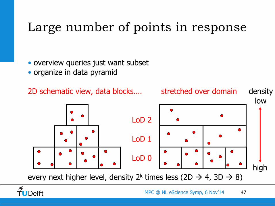
• overview queries just want subset
• organize in data pyramid
2D schematic view, data blocks…. stretched over domain density
low
LoD 2
LoD 1
LoD 0
high
every next higher level, density 2k times less (2D 4, 3D 8)
Large number of points in response
48MPC @ NL eScience Symp, 6 Nov’14
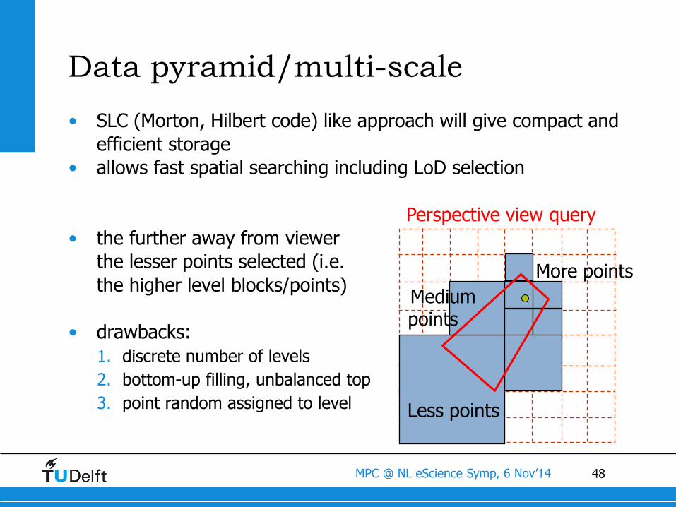
Data pyramid/multi-scale
• SLC (Morton, Hilbert code) like approach will give compact and
efficient storage
• allows fast spatial searching including LoD selection
• the further away from viewer
the lesser points selected (i.e.
the higher level blocks/points)
• drawbacks:
1. discrete number of levels
2. bottom-up filling, unbalanced top
3. point random assigned to level
More points
Medium points
Less points
Perspective view query
49MPC @ NL eScience Symp, 6 Nov’14
Data pyramid alternatives
• not random points, but more characteristic points move up
(more important), some analysis needed; e.g.:
1. compute local data density more dense less important
2. compute local surface shape more flat less important
3. other criteria, data collection/application dependent (intensity)
(combine into) one imp_value of point better than random
• not bottom-up, but top-down population, make sure that top
levels are always filled across complete domain (lower levels
may not be completely filled)
50MPC @ NL eScience Symp, 6 Nov’14
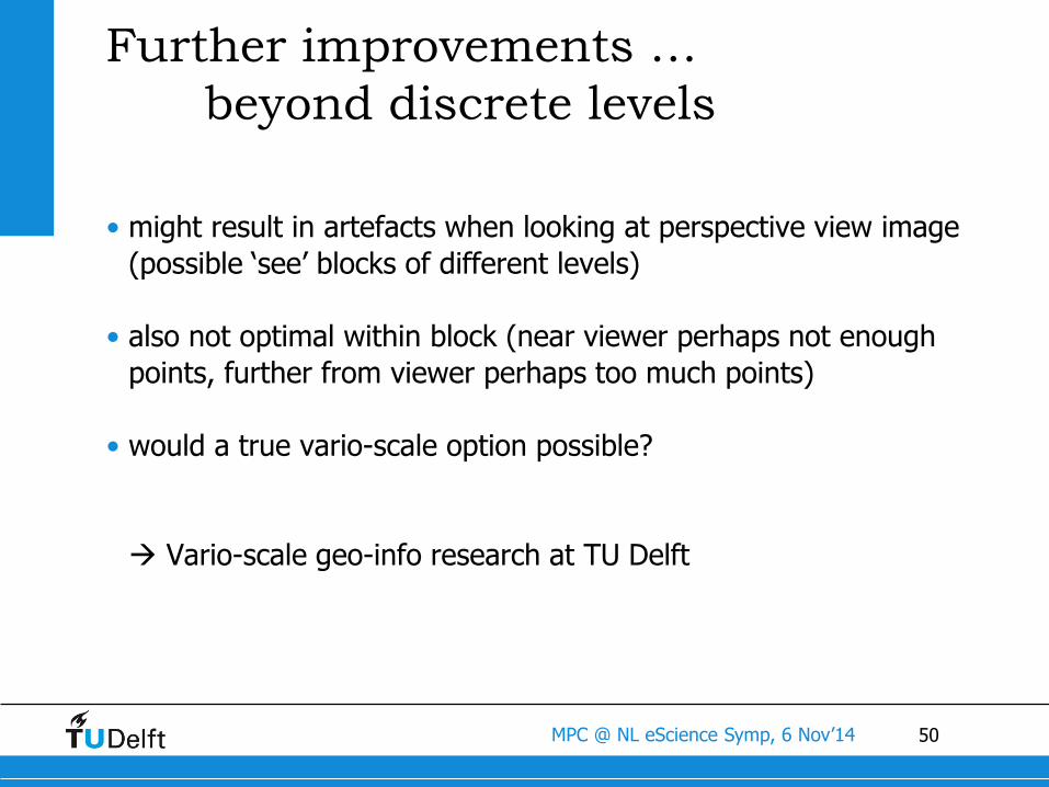
Further improvements …
beyond discrete levels
• might result in artefacts when looking at perspective view image
(possible ‘see’ blocks of different levels)
• also not optimal within block (near viewer perhaps not enough
points, further from viewer perhaps too much points)
• would a true vario-scale option possible?
Vario-scale geo-info research at TU Delft
51MPC @ NL eScience Symp, 6 Nov’14
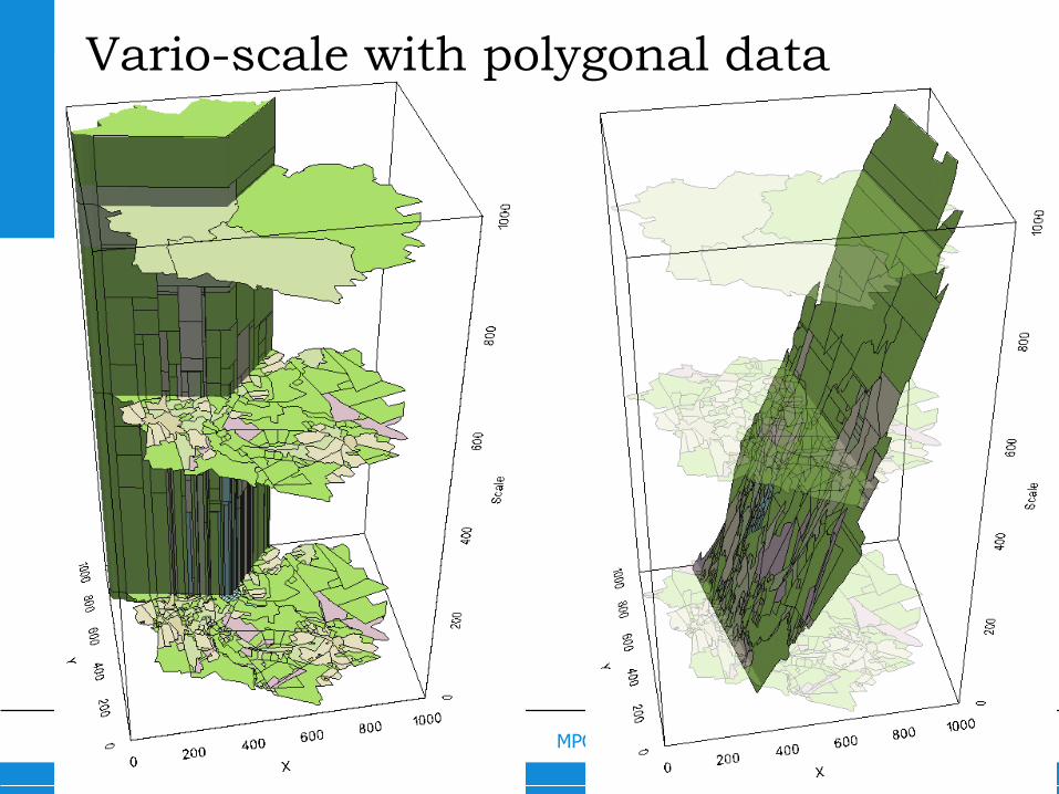
Vario-scale with polygonal data
52MPC @ NL eScience Symp, 6 Nov’14
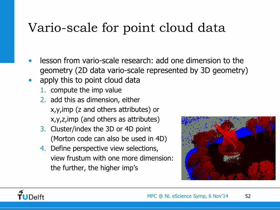
Vario-scale for point cloud data
• lesson from vario-scale research: add one dimension to the
geometry (2D data vario-scale represented by 3D geometry)
• apply this to point cloud data
1. compute the imp value
2. add this as dimension, either
x,y,imp (z and others attributes) or
x,y,z,imp (and others as attributes)
3. Cluster/index the 3D or 4D point
(Morton code can also be used in 4D)
4. Define perspective view selections,
view frustum with one more dimension:
the further, the higher imp’s
53MPC @ NL eScience Symp, 6 Nov’14
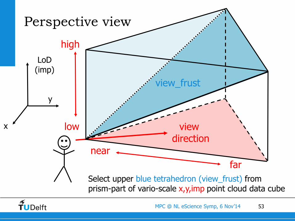
Perspective view
near
low
Select upper blue tetrahedron (view_frust) from prism-part of vario-scale x,y,imp point cloud data cube
x
y
LoD(imp)
far
high
view direction
view_frust
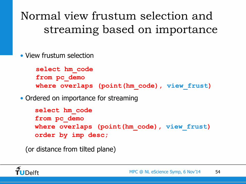
54MPC @ NL eScience Symp, 6 Nov’14
Normal view frustum selection and
streaming based on importance
• View frustum selection
• Ordered on importance for streaming
(or distance from tilted plane)
select hm_code
from pc_demo
where overlaps (point(hm_code), view_frust)
order by imp desc;
select hm_code
from pc_demo
where overlaps (point(hm_code), view_frust)
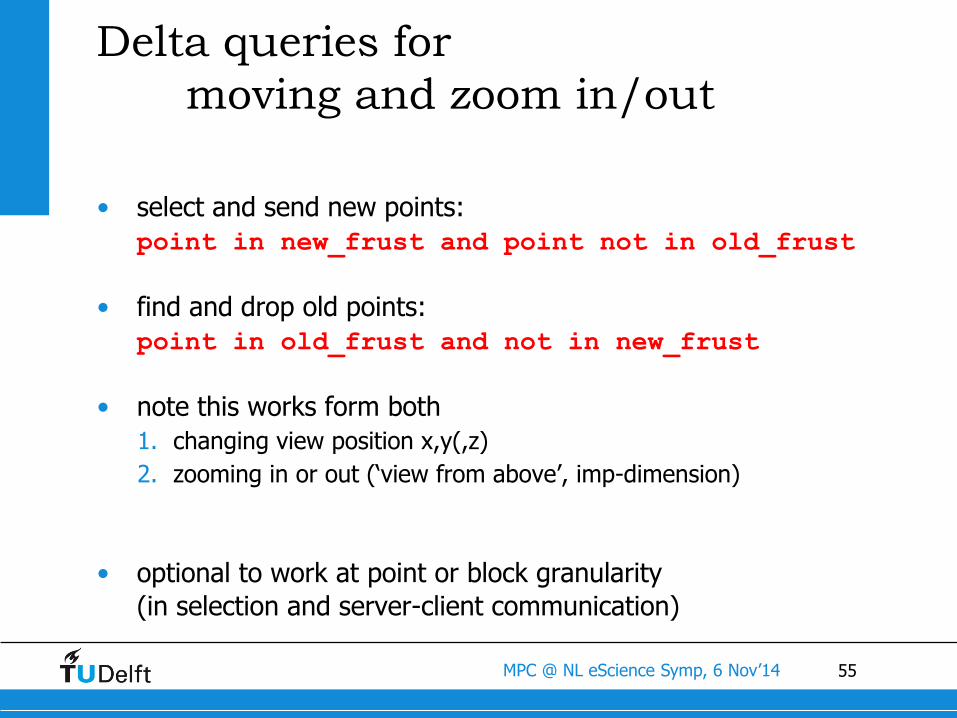
55MPC @ NL eScience Symp, 6 Nov’14
Delta queries for
moving and zoom in/out
• select and send new points:
point in new_frust and point not in old_frust
• find and drop old points:
point in old_frust and not in new_frust
• note this works form both
1. changing view position x,y(,z)
2. zooming in or out (‘view from above’, imp-dimension)
• optional to work at point or block granularity
(in selection and server-client communication)
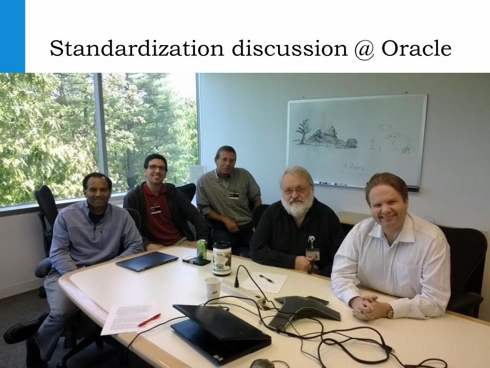
56MPC @ NL eScience Symp, 6 Nov’14
Standardization discussion @ Oracle
57MPC @ NL eScience Symp, 6 Nov’14
Standardization of point clouds?
• ISO/OGC spatial data:
• at abstract/generic level, 2 types of spatial representations: features
and coverages
• at next level (ADT level), 2 types: vector and raster, but perhaps
points clouds should be added
• at implementation/ encoding level, many different formats
(for all three data types)
• nD point cloud:
• points in nD space and not per se limited to x,y,z
(n ordinates of point which may also have m attributes)
• make fit in future ISO 19107 (as ISO 19107 is under revision).
• note: nD point clouds are very generic;
e.g. also cover moving object point data: x,y,z,t (id) series.
58MPC @ NL eScience Symp, 6 Nov’14
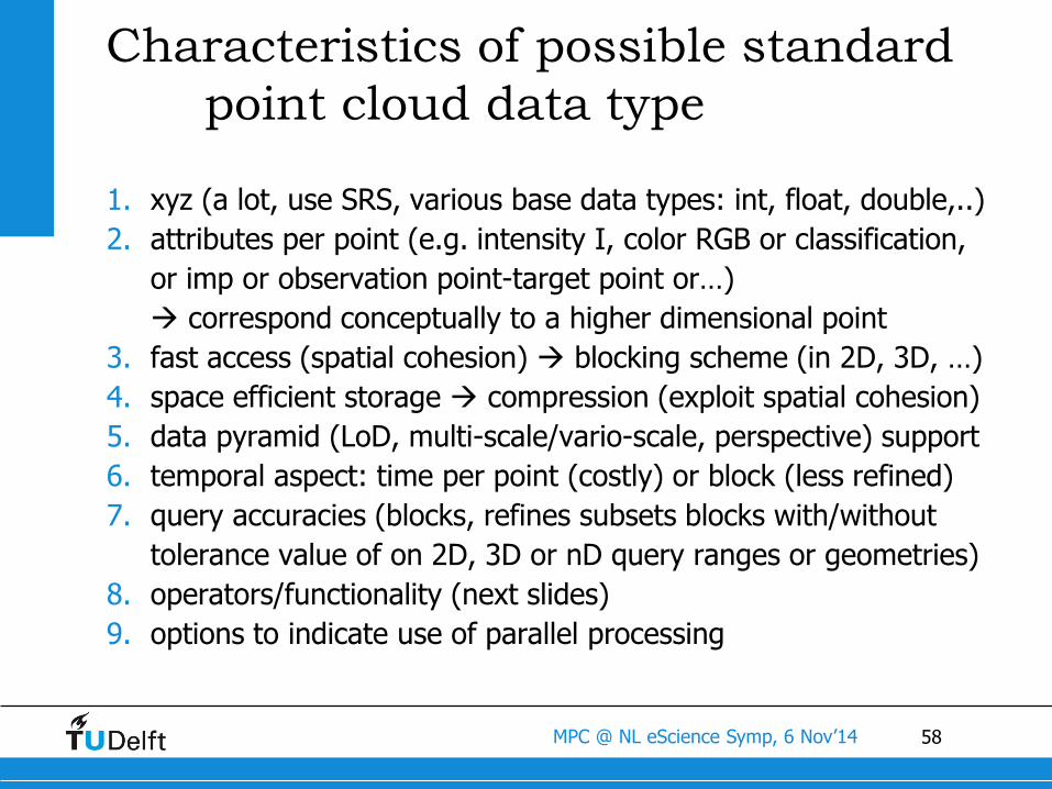
Characteristics of possible standard
point cloud data type
1. xyz (a lot, use SRS, various base data types: int, float, double,..)
2. attributes per point (e.g. intensity I, color RGB or classification,
or imp or observation point-target point or…)
correspond conceptually to a higher dimensional point
3. fast access (spatial cohesion) blocking scheme (in 2D, 3D, …)
4. space efficient storage compression (exploit spatial cohesion)
5. data pyramid (LoD, multi-scale/vario-scale, perspective) support
6. temporal aspect: time per point (costly) or block (less refined)
7. query accuracies (blocks, refines subsets blocks with/without
tolerance value of on 2D, 3D or nD query ranges or geometries)
8. operators/functionality (next slides)
9. options to indicate use of parallel processing
59MPC @ NL eScience Symp, 6 Nov’14
8. Operators/functionality
a. loading, specify
b. selections
c. analysis I (not assuming 2D surface in 3D space)
d. conversions (some assuming 2D surface in 3D space)
e. towards reconstruction
f. analysis II (some assuming a 2D surface in 3D space)
g. LoD use/access
h. Updates
(grouping of functionalities from user requirements)
60MPC @ NL eScience Symp, 6 Nov’14
8a. Loading, specify
• input format
• storage blocks based on which dimensions (2, 3, 4,…)
• data pyramid, block dimensions (level: discrete or continuous)
• compression option (none, lossless, lossy)
• spatial clustering (morton, hilbert,…) within and between blocks
• spatial indexing (rtree, quadtree) within and between blocks
• validation (more format, e.g. no attributes omitted, than any
geometry or topological validation; perhaps outlier detection)?
61MPC @ NL eScience Symp, 6 Nov’14
8b. Selections
• simple 2D range/rectangle filters (of various sizes)
• selections based on points along a 2D polyline (with buffer)
• selections of points overlapping a 2D polygon
• spatial joint with other table; e.g. overlap point with polygons
• select on address, postal code or on other textual geographic
names (gazetteer)
• selections based on the attributes such as intensity I (RGB, class)
• spatiotemporal selections (space and time range),
• combine multiple point clouds (Laser + MBES, classified +
unclassified)
(and so on for the other categories of operators/functionality)
62MPC @ NL eScience Symp, 6 Nov’14
Standardization actions
• participate in ISO 19107 (spatial schema) revision-team
make sure nD point clouds are covered
• within OGC make proposal for point cloud DWG
• probably focus on webservices level
more support/ partners expected
63MPC @ NL eScience Symp, 6 Nov’14
Webservices
• there is a lot of overlap between WMS, WFS and WCS...
• proposed OGC point cloud DWG should explore if WCS is good
start for point cloud services:
• If so, then analyse if it needs extension
• If not good starting point, consider a specific WPCS, web point cloud
service standards (and perhaps further increase the overlapping
family of WMS, WFS, WCS,... )
Related Documents