Place-Based Drivers of Mortality: Evidence from Migration

NBER WORKING PAPER SERIES

PLACE-BASED DRIVERS OF MORTALITY:EVIDENCE FROM MIGRATION

Amy FinkelsteinMatthew GentzkowHeidi L. Williams

Working Paper 25975http://www.nber.org/papers/w25975

NATIONAL BUREAU OF ECONOMIC RESEARCH1050 Massachusetts Avenue

Cambridge, MA 02138June 2019

We are grateful to the National Institute on Aging (Finkelstein, R01-AG032449), the National Science Foundation (Williams, 1151497) and the Stanford Institute for Economic Policy Research (Gentzkow) for financial support. The views expressed herein are those of the authors and do not necessarily reflect the views of the National Bureau of Economic Research.

At least one co-author has disclosed a financial relationship of potential relevance for this research. Further information is available online at http://www.nber.org/papers/w25975.ack

NBER working papers are circulated for discussion and comment purposes. They have not been peer-reviewed or been subject to the review by the NBER Board of Directors that accompanies official NBER publications.

© 2019 by Amy Finkelstein, Matthew Gentzkow, and Heidi L. Williams. All rights reserved. Short sections of text, not to exceed two paragraphs, may be quoted without explicit permission provided that full credit, including © notice, is given to the source.

Place-Based Drivers of Mortality: Evidence from MigrationAmy Finkelstein, Matthew Gentzkow, and Heidi L. WilliamsNBER Working Paper No. 25975June 2019JEL No. H51,I1,I11

ABSTRACT

We estimate the effect of current location on elderly mortality by analyzing outcomes of movers in the Medicare population. We control for movers' origin locations as well as a rich vector of pre-move health measures. We also develop a novel strategy to adjust for remaining unobservables, based on the assumption that the relative importance of observables and unobservables correlated with movers' destinations is the same as the relative importance of those correlated with movers' origins. We estimate substantial effects of current location. Moving from a 10th to a 90th percentile location would increase life expectancy at age 65 by 1.1 years, and equalizing location effects would reduce cross-sectional variation in life expectancy by 15 percent. Places with favorable life expectancy effects tend to have higher quality and quantity of health care, less extreme climates, lower crime rates, and higher socioeconomic status

Amy FinkelsteinDepartment of Economics, E52-442MIT50 Memorial DriveCambridge, MA 02142and [email protected]

Matthew GentzkowDepartment of EconomicsStanford University579 Serra MallStanford, CA 94305and [email protected]

Heidi L. WilliamsDepartment of Economics, E52-440MIT50 Memorial DriveCambridge, MA 02142and [email protected]

1 Introduction

Mortality rates vary substantially across the US. Focusing on the 100 most populous commuting

zones, Chetty et al. (2016b) estimate that life expectancy at age 40 ranges from a high of 85 in San

Jose, California to a low of 81 in Las Vegas, Nevada, with a standard deviation across commuting

zones of 1.2 years.1 Murray et al. (2006) estimate that county-level life expectancy at birth in

1999 ranged from 66.6 years in Bennett County, South Dakota to 81.3 years in Summit County,

Colorado. Currie and Schwandt (2016) likewise document substantial disparities across county

groups in life expectancy at birth as well as in mortality at older ages.

Why do people in some parts of the US live longer than others? The long list of possible

causes can be divided into two broad categories: differences in residents’ stocks of health capital

(Grossman 1972), and differences in the environment associated with their current location. Health

capital includes genetic endowments, as well as the persistent effects of prior health behaviors

(e.g., smoking, diet, exercise), prior medical care, and other past experiences that impact current

mortality. Potentially mortality-relevant aspects of residents’ current locations include the quality

and quantity of available medical care, local climate and pollution, and risk factors such as crime

and traffic accidents. Chetty et al. (2016b) find that the main correlates of area mortality in the

cross section are health capital factors such as smoking, obesity, and exercise, and that correlations

with place factors such as health care spending or local environmental conditions are weak. Neither

they nor other past work, however, isolate the causal impact of place effects.

In this paper, we use mortality outcomes of migrants in the elderly Medicare population to sep-

arately identify the causal role of health capital and current location on mortality in the U.S. We

will refer to the impact of current location by the shorthand “place effects.” Our strategy proceeds

in two steps. First, we analyze mortality differences among movers to different destinations, con-

trolling for both their origin locations and a rich vector of pre-move observable health measures in

Medicare claims data. The idea behind our approach is to take two patients from the same origin

(say, Boston), one of whom moves to a low-mortality area (say, Minneapolis), and the other of

whom moves to a high-mortality area (say, Houston), and to compare their mortality outcomes

1Authors’ calculations based on the publicly reported data provided by Chetty et al. (2016b) on life expectancyfor each commuting zone reported separately by gender, which we use to calculate overall life expectancy assumingequal shares of men and women in each commuting zone. Note that these data include only individuals with non-zeroreported household income.

1

after they move. If origin location plus pre-move health measures capture all differences in health

capital potentially correlated with choice of destination, this would provide a valid estimate of the

place effects.

Second, we apply a novel strategy to correct for any remaining selection on unobserved health

capital. Our strategy builds on prior work (Murphy and Topel 1990; Altonji et al. 2005; Oster

2016) in using variation in observable characteristics to adjust for variation in unobservables. In

our context, this amounts to using the correlation between movers’ choice of destination and their

observed health capital to adjust for potential correlation between choice of destination and unob-

served health capital.

What distinguishes our strategy from prior work is that we do not need to specify a priori

the overall importance of the unobservables. As Oster (2016) emphasizes, the standard approach

requires the researcher to specify this importance in the form of an assumption on the R2 of a

hypothetical regression including both the observables and the unobservables. We weaken this

assumption by exploiting an additional moment of our data: the extent to which the origin location

from which individuals move is predictive of their mortality after controlling for observed health.

If our observable measures capture all relevant dimensions of health capital, movers’ origins would

have no further predictive power. The key assumption that we make is that the relative importance

of observables and unobservables correlated with movers’ origins is the same as the relative impor-

tance of observables and unobservables correlated with movers’ destinations. We present several

pieces of evidence consistent with this assumption, and also show that it is implied by a natural

class of models of migration decisions.

We use data on all Medicare beneficiaries aged 65 and older from 1999 through 2014. The

enrollee-level panel data contain information on zip code of residence and date of death (if any),

along with demographic variables such as age, race, sex, and enrollment in Medicaid (a proxy

for low income). The claims data provide us with detailed annual measures of health conditions

based on recorded diagnoses, as well as measures of health care utilization. Our geographic unit

of analysis is a Commuting Zone (CZ), a standard aggregation of counties that partitions the US

and is designed to approximate labor markets.

The main outcome we focus on is life expectancy at age 65. We estimate the average of this

life expectancy in each location by fitting a standard Gompertz mortality model using observed

2

age-mortality gradients (Olshansky and Carnes 1997; Chetty et al. 2016b). In our analysis sample,

mean life expectancy at age 65 is 83.3 years, with an across-area standard deviation of 0.84 years.

We find that current location has a large causal impact on mortality. Our results imply that mov-

ing from an area at the 10th percentile of estimated place effects to an area at the 90th percentile

would increase life expectancy at age 65 by 1.1 years, or about half of the 90-10 cross-sectional

difference. We estimate that equalizing place effects across areas would reduce the cross-sectional

variation in life expectancy at age 65 by 15 percent. By comparison, equalizing health capital

across areas would reduce the cross-sectional variation by about 75 percent. Our analyses assume

that current location has no direct impact on health capital. While in principle location may in-

fluence health behaviors and hence health capital, we think it is a reasonable assumption that the

elderly’s health capital is fixed in the short run; consistent with this assumption, we provide evi-

dence that the impacts of place show up immediately and do not appear to increase with time spent

in the new location.

Our findings suggest that policies which affect short-run determinants of mortality such as

medical care or environmental factors can potentially produce large and immediate changes in

outcomes, as can policies such as the Moving to Opportunity Project (Ludwig et al. 2012; Chetty

et al. 2016a) that relocate vulnerable populations to areas with more favorable conditions. At

the same time, our findings suggest that health capital also plays an important role. While our

estimated place effects are positively correlated with average area life expectancy, this correlation

is far from perfect. Our place-by-place estimates of these components identify areas such as Santa

Fe, New Mexico; Denver, Colorado; and El Paso, Texas as having negative causal effects despite

relatively high average life expectancy, and other areas such as Charleston, West Virginia as having

positive causal effects despite relatively low average life expectancy.

Finally, we present evidence on the observable area-level correlates of our estimated place

effects. The results are intuitive. Areas with positive place effects tend to have higher-quality

hospitals, more primary care physicians and specialists per capita, and higher health care utiliza-

tion. The positive correlation between an area’s healthcare utilization and its causal impact on life

expectancy contrasts with the lack of correlation between utilization and average health outcomes

which has been emphasized in the Dartmouth Atlas literature and which we replicate here (Fisher

et al. 2003a,b; Skinner 2011). Areas with favorable place effects also tend to have less extreme

3

climates, less pollution, fewer homicides, fewer automobile fatalities, and are more urban. They

also tend to have higher socioeconomic status (SES) as measured by income and education, as well

as better health behaviors, which may reflect higher willingness to pay for healthcare quality and

other favorable place characteristics among such individuals.

Our work contributes to the large literature on the determinants of mortality. McGovern et al.’s

(2014) recent review of studies on health determinants concludes that this literature tends to at-

tribute the largest importance for mortality to health capital — specifically to behaviors (35-50%)

and to genetics (20-30%). Among potential place effects, it attributes between 5-20% of the de-

terminants of mortality to environment and around 10% to medical care. While the methodologies

of the studies underlying these estimates vary, they generally all rely on correlational analyses to

quantify the relative importance of these different factors.2 Our analysis advances this body of

descriptive work with a research design that more convincingly isolates causal effects.

Our work is particularly related to prior work on the drivers of geographic variation in mortality.

This work has also tended to highlight the importance of health capital, particularly health behav-

iors. Fuchs (2011) famously attributes the lower mortality rates of clean-living, predominantly

Mormon residents of Utah to better health behaviors than their neighbors in the more dissolute

state of Nevada.3 Chetty et al. (2016b) show that geographic variation in life expectancy for low-

income individuals is significantly correlated with health behaviors such as smoking, obesity and

exercise, but not significantly correlated with measures of health care quality or quantity. This is

consistent with the large Dartmouth Atlas literature which has found health care utilization to be

uncorrelated with mortality (Fisher et al. 2003a,b; Skinner 2011).4

Summarizing the state of knowledge on both the determinants of mortality and the determi-

nants of geographic variation in mortality, Cutler (2018) concludes, “Behavior is the key. When

we compare geographic regions, the dominant factor driving health differences is how Americans

behave. Unhealthy areas smoke more, drink more and eat to excess; healthier areas avoid these be-

2The underlying studies included in their review are DHH (1980), McGinnis and Foege (1993), Lantz et al. (1998),McGinnis et al. (2002), Mokdad et al. (2004), Danaei et al. (2009), WHO (2009), Booske et al. (2010), Stringhini et al.(2010), and Thoits (2010).

3See also Fuchs (1965) on geographic variation in mortality within the US.4In addition to geographic variation in medical care, a number of studies have examined the correlates of another

natural component of place effects — current environmental factors such as air pollution — with regional variation inmortality rates (e.g. Dockery et al. 1993; Samet et al. 2000). For example, Dockery et al. (1993) estimate that across-city variation in air pollution is positively associated with deaths from lung cancer and cardiopulmonary disease.

4

haviors.” The large role we estimate for health capital is consistent with this conventional wisdom.

However, our results also show that there is a substantial causal impact of place-based factors that

this conventional wisdom may understate.

Finally, our work is related to two recent papers that isolate causal impacts of place factors.

Doyle (2011) uses health emergencies of visitors to different areas of Florida to show that hospitals

in high-spending areas produce better outcomes than hospitals in low-spending areas. Deryug-

ina and Molitor (2018) document that Medicare survivors of Hurricane Katrina who move to

lower-mortality regions experience subsequently lower mortality than those who move to higher-

mortality regions.

Our empirical strategy for correcting for selection on unobservables may have applications in

other contexts. Oster (2016) emphasizes the sensitivity of the standard approach to assumptions

about the overall explanatory power of the observables, and notes that direct information to guide

such assumptions is often limited. We propose weaker assumptions under which this decision

can be guided by the data. Our approach is most obviously relevant to other contexts in which

individuals move across geographies, firms, or other units of analysis, and in which selection on

unobserved individual characteristics is a potential confound; this could arise due to data limi-

tations (e.g. Bronnenberg et al. 2012) or because an outcome cannot be measured repeatedly in

individual panel-level data (such as mortality in our case or inter-generational mobility in Chetty

and Hendren 2016). It may also be applied to other settings where there are auxiliary variables

whose relative correlation with observables and unobservables is plausibly similar to that of the

treatment of interest.

The rest of the paper proceeds as follow. Sections 2 and 3 describe our model and empirical

strategy, and Section 4 presents our data and summary statistics. Section 5 presents evidence on

the selection of movers across origins and destinations and describes how our empirical strategy

addresses this selection. Section 6 presents our main results on the impact of current environment

on life expectancy, and explores some observable correlates of the place effects. Section 7 provides

additional support for some of our key assumptions and shows robustness of our main results to

alternative specifications. The last section concludes.

5

2 Model

We consider a set of individuals indexed by i and a set J of locations indexed by j. The individuals

are either (i) movers who live in an origin location o∈J in years t < t∗i , move in year t∗i from o to

j ∈J , and then live in destination location j thereafter; or (ii) non-movers who live in the same

location j ∈J throughout the sample, and to whom we assign a reference year t∗i as discussed

below. We abuse notation slightly in using j to denote a generic location and also letting j (i) denote

the observed location of individual i (permanent location if i is a non-mover, and destination if i is

a mover). Similarly, we use o to denote a generic origin location and o(i) to denote the observed

origin of mover i.

We analyze a continuous-time survival model in which the mortality rate of person i at age a

depends on her location and her stock of health capital. We follow Chetty et al. (2016b) in adopting

a Gompertz specification in which the log of the mortality hazard rate mi j (a) that individual i would

experience at age a if she lived in location j is linear in age:

log(mi j (a)

)= βa+ γ j +θi. (1)

Here, θi is i’s health capital, which we assume is fixed over the horizon of ages observed in our

data, but may be endogenous to experiences earlier in life. The term γ j is a fixed effect capturing

the causal effect of living in location j, which we will refer to as the place effect.5 We let θ j denote

the average health capital of non-movers in j. In order to mirror the literature, which focuses on

race and sex adjusted mortality rates as the object of interest, in computing θ j we assign each area

j the national average racial and gender composition. We define the mortality rate of an average

non-mover in j at age a to be m j (a) = exp[βa+ γ j +θ j

]. We refer to the sum

(γ j +θi

)as the

mortality index of individual i, and to(γ j +θ j

)as the average mortality index in area j.

Our main outcome of interest is life expectancy at age 65, hereafter, life expectancy. Given

a generic continuous mortality hazard rate m(a), the probability the individual survives to age a

conditional to surviving to age 65 is given by the survival function S(a) = e−∫ a

65 m(v)dv. The life

expectancy of an individual who survives until age 65 is 65 +∫

∞

65 S(a)da.6 We define the life

5More precisely, γ j− γk is the causal effect of living in place j rather than place k.6Let F (a) and f (a) denote the distribution and density of age at death conditional on living to age 65, which

6

expectancy at 65 of an average non-mover in j by substituting m j (a) into these expressions. We

will denote this L j, and refer to it simply as average life expectancy in area j.

Our ultimate goal is to estimate the causal effect on life expectancy of living in area j. We

define this by considering a thought experiment in which an individual with average health capital

is assigned to live counterfactually in each location j beginning at age 65. Letting θ denote the

average health capital over the full population of non-movers, this defines a set of counterfactual

mortality rates m∗j (a) = exp[βa+ γ j +θ

]that differ across j only because of the place effects γ j.

Substituting m∗j (a) into the expression for life expectancy yields the counterfactual life expectancy

L∗j . Letting γ denote the population-weighted average of the γ j, and letting L denote the life ex-

pectancy associated with mortality hazard exp[βa+ γ +θ

], we define the treatment effect of area

j to be L∗j −L.

We assume that health capital θi can be further decomposed into a component that depends

on demographics Xi, a component that depends on observed health Hi, a series of terms capturing

unobserved health capital orthogonal to Xi and Hi but correlated with locations, and an orthogonal

residual:

θi = Xiψ +Hiλ +ηnmj(i)+η

origo(i) +η

destj(i) + ηi. (2)

Here, both Xi and Hi are measured as of year t∗i − 1. We define ηnmj(i), η

origo(i) , and ηdest

j(i) to be the

fixed effects from a hypothetical regression of θi on Xi, Hi, and fixed effects for non-movers’

locations, movers’ origins, and movers’ destinations respectively. (We fix ηnmj(i) = 0 for movers

and ηorigo(i) = ηdest

j(i) = 0 for non-movers.) We define ηi to be the residual from this regression.

We thus have E(ηi|Xi,Hi,o(i) , j (i)) = 0 for movers and E(ηi|Xi,Hi, j (i)) = 0 for non-movers by

construction.

Our definition of ηi as a residual that is orthogonal by construction mirrors Altonji et al. (2005)

and Oster (2016). It means that the coefficients ψ and λ capture both the causal effects of Xi

and Hi and the effects of any unobservables that may be correlated with Xi and Hi. It is natural

to assume that such correlations will exist, as unobserved determinants of health capital such as

smoking will generally be correlated with observed measures of health capital such as diagnoses

we assume is a continuous random variable. We have S (a) = 1− F (a). The hazard function is m(a) = f (a)S(a) =

− dda logS (a). Integrating both sides of this equation yields logS(a) = −

∫ a65 m(v)dv. Life expectancy at age 65 is∫

∞

65 a f (a)da. Integrating by parts, and assuming a finite end time, shows this is equal to 65+∫

∞

65 S(a)da.

7

of hypertension. This means that equation (2) does not define a structural relationship, and the η

terms include only the components of the unobservables orthogonal to Xi and Hi.

A key assumption in our model is the additive separability of health capital and the place ef-

fects in equation (1) for log mortality. Analogous assumptions are standard in the literature using

changes in residence or employment to separate effects of individual characteristics from geo-

graphic or institutional factors (e.g. Card et al. 2013; Chetty and Hendren 2018, 2016; Finkelstein

et al. 2016).

This is a strong assumption, but we see it as a reasonable one in our setting. It has the intuitive

implication that health capital and current location affect the level of mortality multiplicatively,

and, thus, that the level of mortality of individuals with poor health capital (high θi) will vary

more across areas than that of individuals who have better health capital (low θi); this has indeed

been documented by Chetty et al. (2016b). More concretely, suppose that there are two possible

levels of health capital, such that in an average location, individuals have either a 0.1% annual

mortality hazard or a 10% annual mortality hazard. The additive separability assumption implies

that anything about the current environment that reduces mortality — such as the quality of health

care or the air quality — will reduce mortality by a constant proportion for all individuals, with

a larger percentage point effect on individuals with worse health capital. Our specification rules

out place effects that cause the same level shift in mortality for all patients regardless of their

health capital. For example, if some places have a higher risk of death from auto accidents and

this probability is independent of health capital, our assumption would be violated. We present

empirical support for additive separability in Section 7 below.

3 Empirical Strategy

3.1 Estimation and Identification

Our main goal in estimation is to identify the place effects γ j. This will in turn allow us to recover

the average health capital θi of movers and non-movers in each location. Combining equations (1)

8

and (2) yields the following estimating equation for the realized mortality rate mi (a):

log(mi (a)) = βa+Xiψ +Hiλ + τorigo(i) + τ

destj(i) + τ

nmj(i)+ ηi. (3)

where τorigo(i) , τdest

j(i) , and τnmj(i) are fixed effects for movers’ origins, movers’ destinations, and non-

movers’ locations respectively, and we have τorigo(i) = η

origo(i) , τnm

j(i) = γ j(i)+ηnmj(i), and τdest

j(i) = γ j(i)+

ηdestj(i) .

We estimate this model by maximum likelihood. Given the estimated parameters, we can

consistently estimate the area j mortality rate m j (a) by m j (a) = exp[βa+X jψ +H jλ + τnm

j

],

where X j and H j are the averages of Xi and Hi over non-movers in j.7 Consistent with the definition

of θ j above, when we compute X j we set the elements of the vector associated with race and sex to

their national rather than their area averages. We compute estimates L j of average life expectancy

L j in area j by substituting m j (a) for m j (a) in the derivation of L j in Section 2. All of our reported

estimates of average life expectancy in area j are therefore race- and sex-adjusted.

The central challenge is identification of γ j. Simply comparing average mortality rates across

areas in the cross-section does not recover γ j, because locations may differ in their average health

capital E(θi| j (i) = j). An optimistic assumption would be that Xi and Hi absorb all such differ-

ences. In this case, ηnmj , η

origo , and ηdest

j would be equal to zero for all j,o ∈J , and we would

not need to use movers at all; we could simply estimate equation (3) using non-movers and the τnmj

would be consistent estimators of γ j.

A more plausible assumption would be that Xi and Hi do not absorb all area differences in health

capital, but that the remaining differences for movers are absorbed by the origin fixed effects ηorigo ,

so that ηdestj = 0 for all j. In this case, the estimated destination fixed effects τdest

j from equation

(3) would be consistent estimators of γ j. This assumption would follow from a model in which

the locations where people are born and live up to age 65 or older may be related to their genetic

endowments, health behaviors, and other determinants of health capital, but in which late-life

moving decisions are driven by idiosyncratic factors.

Our findings below are qualitatively consistent with this intuition, in the sense that conditioning

on movers’ origins eliminates a significant amount of non-random selection on observables. How-

7Note that θ j = X jψ +H jλ +ηnmj(i), and so X jψ +H jλ + τnm

j converges in probability to γ j +θ j.

9

ever, our results also suggest that some non-random selection may remain, implying that ηdestj 6= 0

and thus that τdestj may not exactly recover γ j. The selection correction strategy we develop in the

next sub-section is designed to deal with any such remaining selection.

Given consistent estimates γ j of γ j, we can estimate the treatment effects L∗j−L of each area j.

To do so, we estimate θ as the mean across all non-movers of Xiψ +Hiλ + τnmj − γ j, a consistent

estimator of θi. We estimate γ by the non-mover population-weighted mean of the γ j. We then

substitute these estimates in place of their population counterparts in the definitions of L∗j and L in

Section 2.

We will at various points form estimates of variances of CZ-level terms such as γ j. Unless

otherwise noted, all such estimates Var(z) for CZ-level variables z are based on a split sample

approach in which we randomly partition our sample into two parts, form separate estimates z1

and z2 using the two samples, and then define Var(z) = Cov(z1, z2). We compute confidence

intervals via 200 iterations of the Bayesian bootstrap procedure (Rubin 1981).8

When we report individual values of the place effects γ j or the life expectancy treatment effects

that depend on them, we adjust the γ j estimates for sampling error using a standard Empirical

Bayes’ procedure, producing adjusted estimates we denote γEBj . This closely follows the approach

of Chetty and Hendren (2016) and Finkelstein et al. (2017). Appendix A.1 provides more detail on

this procedure.

3.2 Adjusting for Selection on Unobservables

In this section, we introduce our strategy to allow for the possibility that movers’ destinations are

correlated with their unobserved health—i.e., that ηdestj 6= 0. Our approach builds on the now-

standard methodology developed by Murphy and Topel (1990) and Altonji et al. (2005), and ex-

panded on by Oster (2016), which uses variation in observables to make inferences about the likely

bias due to unobservables.

The standard approach relies on two key assumptions. The first is that the relationship between

the treatment of interest and the index of observables is similar to the relationship between the

treatment of interest and the index of unobservables. Altonji et al. (2005) and Oster (2016) refer

8The Bayesian bootstrap smooths bootstrap samples by reweighting rather than resampling observations. For arecent application see Angrist et al. (2017); their on-line Appendix provides implementation details that we follow.

10

to this as the equal selection assumption. Intuitively, it allows us to learn about the direction of

bias induced by the unobservables from the bias induced when we omit the observables. In a

standard labor economics context where we would attempt to measure returns to education, equal

selection would imply that if education is increasing in observed proxies for worker skill, it will be

increasing in unobserved skill as well. In our context, equal selection implies that if movers to a

particular destination tend to have unusually good observed health capital they will probably have

unusually good unobserved health capital as well.

The second assumption pins down the overall importance of the unobservables relative to the

observables. Oster (2016) operationalizes this as an assumed value for the R2 of a hypothetical

regression of the outcome on the treatment, the observables, and all the relevant unobservables.9

We will refer to this as the R2 assumption. Intuitively, specifying this value allows us to determine

the magnitude of the bias induced by the unobservables. In the labor economics example, the

bias would be small if there is very little variation in unobserved skill conditional on the observed

proxies, or large if this variation is large. In our context, the bias would be small if observed

proxies captured most of the variation in health capital, and so the variance of the unobserved

components was small. Oster (2016) emphasizes that the choice of the R2 value is by necessity

arbitrary in typical applications, and suggests some benchmark values researchers could use to

obtain conservative bounds.

The main innovation in our approach is to suggest an additional moment of the data that al-

lows us to weaken the R2 assumption. That moment is the variance of the origin component of

unobserved health—ηorigo in equation (2), which we recall is consistently estimated by the origin

fixed effect τorigj from equation (3). If our observable measures Hi captured all relevant dimen-

sions of health capital, movers’ origins would have no further predictive power, and we would

have ηorigj = 0. The extent to which origins remain predictive of mortality after we control for Hi

is a gauge of the extent to which important unobserved components remain.

To apply this logic formally, we first introduce some new constructs and notation. First, define

a “treatment” indicator Ti j = 1( j (i) = j) for movers equal to one if i’s destination is j. Second, as

an input to our selection correction strategy, we will need to estimate the components of observed

health capital related to movers’ origins and destinations respectively. Let hi = Hiλ (where λ

9Altonji et al. (2005) do not name this assumption, but they implicitly assume that the relevant R2 is one.

11

is defined in equation (3)) be the index of observed health capital for individual i; we refer to it

throughout as “observed health” for short. Define the following regression in the sample of movers:

hi = βha+Xiψ

h +horigo(i) +hdest

j(i) + hi, (4)

where horigo(i) and hdest

j(i) are origin and destination fixed effects respectively and hi is a residual. We

refer to horigo(i) and hdest

j(i) as the origin and destination components of observed health respectively.

These are by construction the residual components of observed health after partialing out age and

demographics. We normalize horigo(i) so the population mean of hdest

j(i) is zero. To estimate these

terms, we first form hi = Hiλ using the estimates λ from equation (3). We then estimate equation

(4) replacing hi with hi.

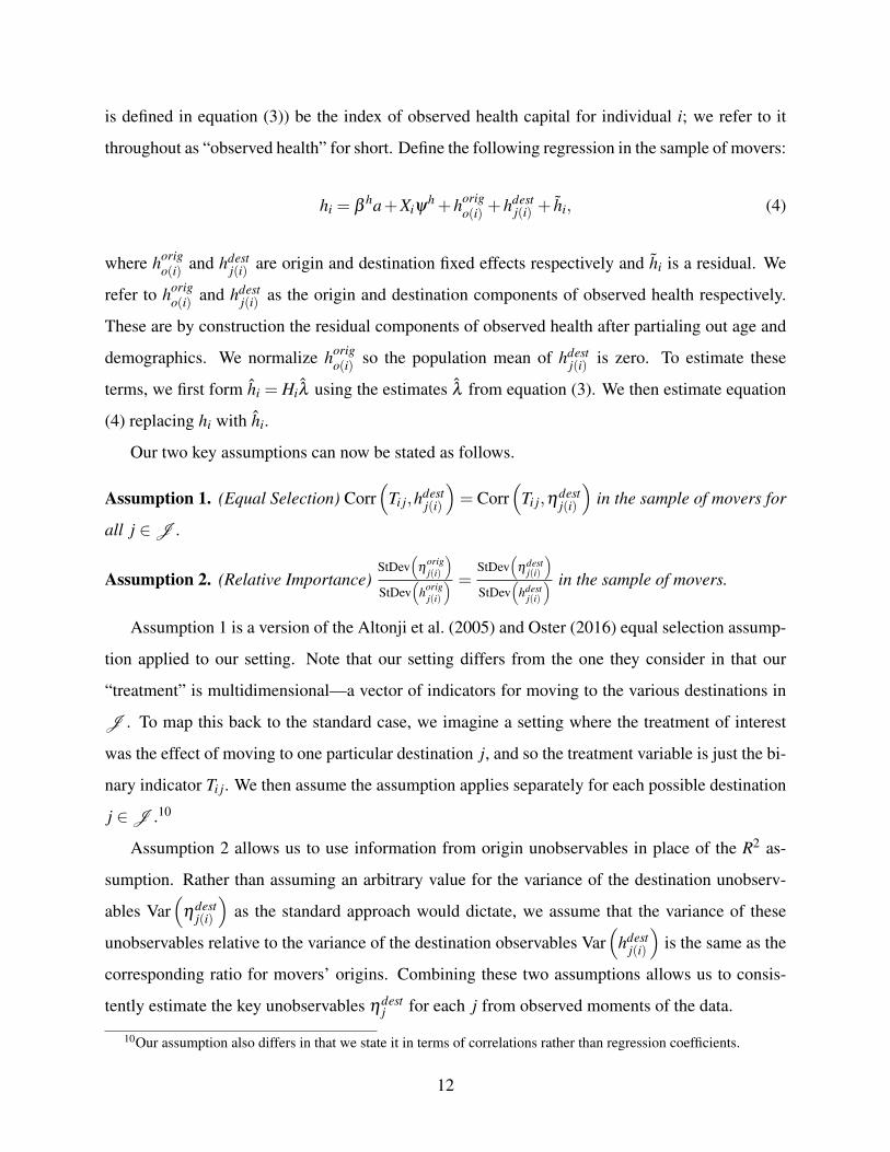
Our two key assumptions can now be stated as follows.

Assumption 1. (Equal Selection) Corr(

Ti j,hdestj(i)

)= Corr

(Ti j,η

destj(i)

)in the sample of movers for

all j ∈J .

Assumption 2. (Relative Importance)StDev

(η

origj(i)

)StDev

(horig

j(i)

) =StDev

(ηdest

j(i)

)StDev

(hdest

j(i)

) in the sample of movers.

Assumption 1 is a version of the Altonji et al. (2005) and Oster (2016) equal selection assump-

tion applied to our setting. Note that our setting differs from the one they consider in that our

“treatment” is multidimensional—a vector of indicators for moving to the various destinations in

J . To map this back to the standard case, we imagine a setting where the treatment of interest

was the effect of moving to one particular destination j, and so the treatment variable is just the bi-

nary indicator Ti j. We then assume the assumption applies separately for each possible destination

j ∈J .10

Assumption 2 allows us to use information from origin unobservables in place of the R2 as-

sumption. Rather than assuming an arbitrary value for the variance of the destination unobserv-

ables Var(

ηdestj(i)

)as the standard approach would dictate, we assume that the variance of these

unobservables relative to the variance of the destination observables Var(

hdestj(i)

)is the same as the

corresponding ratio for movers’ origins. Combining these two assumptions allows us to consis-

tently estimate the key unobservables ηdestj for each j from observed moments of the data.

10Our assumption also differs in that we state it in terms of correlations rather than regression coefficients.

12

These assumptions are strong, but they follow naturally from economic primitives. They will

hold in a broad class of models of selective migration so long as selection of locations is related to

overall health capital but not differentially to the observed and unobserved components. We show

this formally in Appendix A.2. Under some additional structure on the distributions of observables

and unobservables, we show that Assumptions 1 and 2 are both implied by the assumption that

selection of origins and destinations may depend on the single index θi = hi + ηi, where ηi =

ηorigo(i) +ηdest

j(i) + ηi, but that origins and destinations are independent of hi and ηi conditional on θi.

If the dimensions of health capital relevant to selection are not captured by a single index, our

assumption requires that the relative importance of unobservable to observable health in determin-

ing origin must be the same as the relative importance of unobservable to observable health in

determining destination. This could be violated if, for example, observed dimensions of health

capital such as diabetes are more strongly related to people’s choice of where to live when young,

while unobserved dimensions such as physical mobility are more strongly related to their migra-

tion decisions when they are elderly. We provide empirical support for the assumptions behind our

selection correction approach in Section 7.2 below.

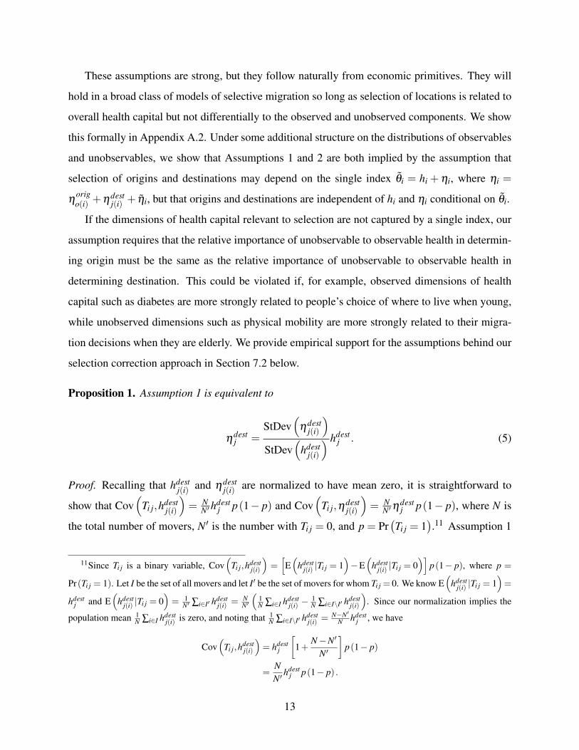
Proposition 1. Assumption 1 is equivalent to

ηdestj =

StDev(

ηdestj(i)

)StDev

(hdest

j(i)

) hdestj . (5)

Proof. Recalling that hdestj(i) and ηdest

j(i) are normalized to have mean zero, it is straightforward to

show that Cov(

Ti j,hdestj(i)

)= N

N′hdestj p(1− p) and Cov

(Ti j,η

destj(i)

)= N

N′ηdestj p(1− p), where N is

the total number of movers, N′ is the number with Ti j = 0, and p = Pr(Ti j = 1

).11 Assumption 1

11Since Ti j is a binary variable, Cov(

Ti j,hdestj(i)

)=[E(

hdestj(i) |Ti j = 1

)−E

(hdest

j(i) |Ti j = 0)]

p(1− p), where p =

Pr(Ti j = 1). Let I be the set of all movers and let I′ be the set of movers for whom Ti j = 0. We know E(

hdestj(i) |Ti j = 1

)=

hdestj and E

(hdest

j(i) |Ti j = 0)= 1

N′ ∑i∈I′ hdestj(i) = N

N′

(1N ∑i∈I hdest

j(i) −1N ∑i∈I\I′ hdest

j(i)

). Since our normalization implies the

population mean 1N ∑i∈I hdest

j(i) is zero, and noting that 1N ∑i∈I\I′ hdest

j(i) =N−N′

N hdestj , we have

Cov(

Ti j,hdestj(i)

)= hdest

j

[1+

N−N′

N′

]p(1− p)

=NN′

hdestj p(1− p) .

13

is then equivalent to

NN′h

destj p(1− p)

StDev(Ti j)

StDev(

hdestj(i)

) =NN′η

destj p(1− p)

StDev(Ti j)

StDev(

ηdestj(i)

) .Canceling terms yields the desired result.

This proposition is intuitive. It says that under our equal selection assumption, the destination

component ηdestj —i.e., the average unobserved, residual health in destination j—is equal to the

observed term hdestj scaled by a constant. The value of that constant is the ratio of the standard

deviations of ηdestj(i) and hdest

j(i) , and it can be interpreted as the relative importance of the unobserved

and observed components of health capital correlated with destinations. Assumption 2 then allows

us to estimate this ratio using the analogous ratio for movers’ origins.

Corollary 1. Under Assumptions 1 and 2,

ηdestj =

ˆStDev(

τorigj(i)

)ˆStDev(

horigj(i)

) hdestj (6)

is a consistent estimator of ηdestj , and γ j = τdest

j − ηdestj is a consistent estimator of γ j (where

ˆStDev(

τorigj(i)

)and ˆStDev

(horig

j(i)

)are consistent estimators of the standard deviations of τ

origj(i) and

horigj(i) ).

4 Data and Summary Statistics

4.1 Data and Variable Definitions

We use administrative data on Medicare enrollees for a 100% panel of Medicare beneficiaries —

both Traditional Medicare and Medicare Advantage — from 1999 to 2014.12

The steps for ηdestj(i) are analogous.

12About one-third of Medicare beneficiaries are enrolled in Medicare Advantage, a program in which privateinsurers receive capitated payments from the government in return for providing Medicare beneficiaries with healthinsurance. Because insurance claims (and hence healthcare utilization measures) for enrollees in Medicare Advantageare not available, the literature on geographic variation in healthcare spending and health outcomes for Medicareenrollees has focused primarily on Traditional Medicare. However, the Medicare data do contain demographic, healthand mortality information for both Traditional Medicare and Medicare Advantage enrollees.

14

We observe each enrollee’s zip code of residence each year. We define a year t for the purposes

of our analysis to run from April 1 of calendar year t to March 31 of calendar year t +1 since, for

most years, we observe residence as of March 31st of that year.

For each enrollee, we observe time-invariant indicators for race and gender. We observe time-

varying indicators for age, as well as enrollment in Medicaid (the supplemental public health in-

surance program for low income elderly), Medicare Parts A and B, and Medicare Advantage. We

observe all claims for inpatient and outpatient care for enrollee-years in Traditional Medicare. For

individuals who die during our sample, we observe the date of death.

Our primary analysis focuses on a sample of movers and non-movers defined below. We restrict

attention to movers whose CZ of residence changes exactly once. For each mover, we define year

t∗i (an individual’s “move year”) to be the year in which their location changes and t∗i +1 to be their

first full year in the new location. For non-movers, we define t∗i to be the second year we observe

them in the data without any missing covariates, so that we can measure their characteristics in the

prior year.

We use the Chronic Conditions segment of the Master Beneficiary Summary File from 1999 to

2014 to define 27 health status indicators for each person-year, with each indicator capturing the

presence of a specific chronic condition. Examples include lung cancer, diabetes, and depression;

the share of patients with each of these conditions and the estimated coefficients for each from

the Gompertz mortality hazard model (equation (3)) can be seen in Appendix Table A.1. The

algorithms defining these measures are publicly available13 and are based on definitions used in the

medical literature.14 Importantly, because we measure observed health Hi pre-move, and equation

(3) controls for origin fixed effects, we are not concerned about bias arising in our estimation

from the type of place-specific measurement error of health in claims data that prior work has

highlighted (Song et al. 2010; Finkelstein et al. 2016, 2017).

We measure total health care utilization for each person-year in Traditional Medicare, defined

to be total inpatient and outpatient spending, adjusted for price differences following the procedure

of Gottlieb et al. (2010).15 As discussed below, we restrict our analysis to beneficiaries enrolled in

13See https://www.ccwdata.org/documents/10280/19139421/original-ccw-chronic-condition-algorithms.pdf.

14See https://www.ccwdata.org/documents/10280/19139421/original-ccw-chronic-condition-algorithms-reference-list.pdf.

15Specifically, we follow the approach from Finkelstein, Gentzkow, and Williams (2016), except that we exclude

15

Traditional Medicare during year t∗i −1. This restriction implies that total health care utilization is

observed in year t∗i −1 for all individuals in our analysis sample, even if those individuals may be

enrolled in Medicare Advantage (and hence have unobserved health care utilization) during years

other than t∗i −1.

We define areas j to be Commuting Zones (CZs). Specifically, we use the 709 CZs defined by

the Census Bureau in 2000 as an aggregation of counties; CZs are designed to approximate local

labor markets and have been used previously to analyze geographic variation in life expectancy

(e.g. Chetty et al. 2016b).16

All of the enrollee-level covariates in our analysis (i.e. Hi and Xi) are measured as of year t∗i −1.

In our baseline specification, observable health (Hi) is a series of indicator variables for each of the

27 chronic conditions in the Chronic Conditions segment of the Master Beneficiary Summary file

and log(utilization + 1). Xi is a set of indicators for race (white or non-white), gender, and their

interaction; we also include an indicator variable for Medicaid status (as a proxy for low income),

a series of indicator variables for the calendar year corresponding to t∗i , and a constant.

4.2 Sample Restrictions and Summary Statistics

Our data contain approximately 81 million people and over 665 million person-years. We drop

from this sample person-years in which the enrollee is younger than 65 or older than 99.17 This

leaves us with a core sample of about 69 million beneficiaries; we exclude a few hundred thousand

beneficiaries with incomplete data.

To define our non-mover sample, we begin with the 62 million enrollees whose CZ of residence

does not change over the years we observe them. We need to assign each non-mover a valid

reference year t∗i such that we are able to see observable health characteristics in year t∗i − 1. We

therefore eliminate all non-movers who do not have a pre-2012 year t∗i such that they are 99 or

younger and alive until the end of that year, and also on Traditional Medicare during year t∗i − 1.

We take a random 10% sample of the remaining 43 million non-movers and define their t∗i to be

physician services (“carrier files”) because these files are only available for a 20 percent subsample.16See https://www.ers.usda.gov/data-products/commuting-zones-and-labor-market-areas/ for

more details.17Individuals younger than 65 appear in our data if they are disability-eligible (through Social Security disability

benefits) rather than age-eligible for Medicare.

16

the second year they are in the sample. When we estimate equation (3) using the pooled sample of

movers and non-movers, we upweight the non-movers by ten.

To define our mover sample, we begin with the 7 million enrollees whose CZ of residence

changes at least once during our sample period. To ensure changes in address reflect real changes

in location, we define a mover’s “claim share” in a particular year to be the ratio of the number of

claims located in their destination to the number located in either their origin or their destination.

We then follow Finkelstein, Gentzkow, and Williams (2016) in excluding those for whom the claim

share does not increase by at least 0.75 in their post-move years relative to their pre-move years.

Appendix A.3 provides more detail.

We further restrict the sample to movers who are not on Medicare Advantage in the year im-

mediately prior to or immediately after the move (since we need to measure claim shares in those

years) and who moved in years 2000-2012 (so that we can observe pre-move characteristics and

post-move mortality). We also exclude those who move at age 99 or later or do not survive through

the end of their move year (t∗i ). Our final sample contains 6.3 million individuals, of whom 2 mil-

lion are movers. Appendix A.3 provides more detail on the sample restrictions. By construction,

we are able to observe mortality for all beneficiaries for at least one year following t∗i . We are able

to observe mortality at least 7 years after t∗i for 63 percent of movers and at least 10 years after t∗i

for 35 percent of movers.

Because our strategy for estimating place effects requires that we observe a significant number

of movers to each area, we aggregate CZs that receive small numbers of movers to form larger areas

within states. Specifically, we first collect the bottom quartile of CZs by the number of incoming

movers. Then, in any case where a state contains two or more such CZs, we consolidate those CZs

into a single area. Appendix Figure A.1 shows the locations of the bottom quartile of CZs; they

are predominantly in the Great Plains. The number of movers to these CZs ranges from 2 to 359,

with a median of 155. Our final sample has 528 CZs and 35 aggregated CZs; these are the areas

corresponding to the j index in our model and we refer to these simply as “CZs” in what follows.18

Appendix Table A.2 shows summary statistics on the number of movers to each CZ; the minimum

number of movers to a CZ is 48, and the median is about 1,500.

18Note that 11 of these bottom quartile CZs are within a single state and therefore remain disaggregated. Thisprocedure causes us to omit roughly 3,000 movers who move across small CZs within the same state.

17

Table 1 reports summary statistics for comparable samples of movers and non-movers. The

first row shows our full sample, which consists of roughly 2 million movers and 4.3 million non-

movers. The remainder of the table shows characteristics of a sub-sample of movers and non-

movers with reference year t∗i = 2006. We focus on this subset to facilitate comparison of movers’

and non-movers’ characteristics.19 Movers tend to be older than non-movers, are slightly more

likely to be female and white, and slightly less likely to be on Medicaid. Not surprisingly given

the age differences, movers are also less healthy as measured by their count of chronic conditions

and their one and four year mortality.

5 Preliminary Evidence

5.1 Patterns of Mortality and Migration

Figure 1 shows our estimates L j of average non-mover life expectancy by area, constructed from

the estimated model of equation (3) as described in Section 3.1. The average life expectancy across

areas is 83.3 years, with a standard deviation of 0.84 years. Our life expectancy estimates are highly

correlated with the life expectancy estimates at age 40 by Chetty et al. (2016b), as shown for the

100 largest CZs in Appendix Figure A.2.

Since moves will be key to identifying place effects, we briefly discuss the characteristics

of moves in our sample. There is substantial variation across moves in the destination-origin

difference in non-mover life expectancy (L j). The standard deviation of this gap is roughly one

year, and the share of movers to higher life expectancy destinations (48 percent) is similar to the

share of moves to lower life expectancy destinations (52 percent); Appendix Figure A.3 shows

more detail on the destination-origin differences in average life expectancy. Conditional on origin,

the average standard deviation of destination life expectancy across CZs is 0.74, quite close to the

19For completeness Appendix Table A.3 reports the same summary statistics on the full set of 2 million moversand 4 million non-movers used to estimate equation (3), but the two sets of statistics are not directly comparable giventhe differences in how the two samples are defined.

18

cross sectional standard deviation of 0.84.20

We next examine the extent to which the observed health of movers differs systematically ac-

cording to their destinations. In Panel A of Figure 2, we compare the average observed health of

movers to different destinations adjusted for age and demographics (Xi). For each area j, we com-

pute the mean across movers to j of the residuals from a regression of our observed health index

hi = Hiλ on age in year t∗i − 1 and demographics Xi. The left-hand figure shows the distribution

of these average values across destinations. If movers were randomly assigned to destinations,

these averages should vary little; this is not the case. The right-hand figure is a binned scatterplot

showing how these average observed health values for movers to different destinations are corre-

lated with the average estimated mortality index γ j + θi of non-movers in each destination. The

relationship is significant and positive, suggesting that low-mortality destinations tend to attract

healthier movers.

In Panel B of Figure 2, we partial out fixed effects for movers’ origins (in addition to the age

and demographics that were already partialed out in Panel A). These values capture the extent

to which healthier movers from a given origin select systematically different destinations. The

results indicate that conditional on origin, mover observed health is still correlated with destination

mortality, but conditioning on origin lowers the slope from 0.24 to 0.15. While the selection on

observed health shown here will be accounted for by the explicit Hi controls in our model, it

suggests that there may be remaining selection on unobserved health which we will need to address

with our selection correction strategy.

5.2 Inputs to Selection Correction

Table 2 shows the standard deviations of the components of health capital that enter our selection

correction. For each component, we report the standard deviation across CZs, estimated using our

split-sample strategy, as well as 95-percent confidence intervals based on our Bayesian bootstrap.

The magnitudes are not easily interpretable, as they are in units of the log mortality rate log(mi),

20Appendix Table A.4 shows the full transition matrix of movers by decile of life expectancy in the origin anddecile of life expectancy in the destination. While moves are more common between closer deciles and from higherlife expectancy origins, we find that all the cells contain a significant number of observations. There are at least severalthousand people in each cell of the transition matrix, including moves from the highest life expectancy decile to thelowest, and vice versa. Appendix A.3 provides additional information on migration patterns.

19

but to get a sense, note that a 65-year old with average health capital θ and sample-wide average

place effect γ (which is 0 by construction) has an annual mortality rate of m= 0.013, and increasing

her health capital by one standard deviation (among 65-year-olds) would increase her mortality rate

by 0.005.

The first two rows report the estimated standard deviations of the components horigj(i) and η

origj(i)

correlated with movers’ origins. Recall that our estimators of these terms are the origin fixed effects

from equations (3) and (4) respectively. We find that the standard deviation of the unobservable

component ηorigj(i) is 0.061, and the standard deviation of the observable component horig

j(i) is 0.037.

This suggests that, despite the richness of our observable health measures, the remaining systematic

variation in health capital correlated with locations is substantial. The ratio of these terms 0.0610.037 =

1.65 is the key conversion factor that is used in Corollary 1 to pin down the relative importance of

unobservables and observables.

The last two rows report the estimated standard deviations of the components hdestj(i) and ηdest

j(i)

correlated with movers’ destinations. The hdestj(i) components are estimated by the destination fixed

effects in equation (4); we find that their standard deviation is 0.024. The ηdestj(i) components cannot

be directly estimated, and are the key objects our selection correction is designed to infer. Applying

Corollary 1, we estimate that the standard deviation of ηdestj(i) is 0.024× 0.061

0.037 = 0.040.

6 Main Results

6.1 Place Effects

Table 3 reports our decomposition of the area average mortality index γ j + θ j. As shown in the

first row, the standard deviation across CZs of this index is 0.105.

The following three rows report the decomposition of this index when we do not apply our

selection correction—i.e., when we assume ηdestj = 0 for all j. In this case, our estimate of the

place effects γ j is simply the destination fixed effects τdestj from equation (3), and average health

capital θ j is given by the average value of the remaining terms in that equation (excluding the

age term aiβ , and taking the national average of race and sex as discussed in Section 3.1). In this

case, we estimate that the standard deviation of the place effects is 0.077, or three-quarters of the

20

standard deviation of the overall index. The standard deviation of average health capital is 0.080,

and the correlation between the two components is slightly negative.

The bottom three rows report our preferred estimates applying the selection correction. Here,

our estimate of the place effects γ j is the difference τdestj − ηdest

j , where the unobservable compo-

nent ηdestj is inferred following the steps broken out in Table 2. Average health capital θ j is again

given by the average value of the remaining terms in equation (3) (excluding the age term aiβ , and

taking the national average of race and sex as discussed in Section 3.1). The standard deviation of

the selection-corrected place effects is 0.054, about one-third smaller than the uncorrected version,

and roughly half the standard deviation of the overall index. The standard deviation of average

health capital is 0.094, and the correlation between the two components is now positive.

Figure 3 shows a map of our estimated treatment effects (L∗j−L). These are defined in Section

2 and capture the impact of moving to an area on life expectancy for a mover with average health

capital. The most favorable effects are found in the Northeast and along the eastern seaboard,

down through parts of Florida. The most adverse effects, meanwhile, are concentrated in the deep

south (Alabama, Arkansas, Georgia, Louisiana, and parts of Florida) and in the Southwest (Texas,

Oklahoma, New Mexico, and Arizona).

Figure 4 shows a scatterplot of these treatment effects against estimated average life expectancy

L j in each place. The two are positively correlated: a one unit increase in average life expectancy is

associated with a 0.23 year increase in the treatment effect. Interestingly, for Medicare survivors of

Hurricane Katrina, Deryugina and Molitor (2018) estimate somewhat larger effects. They find that

moving to a place with a 1 percentage point higher mortality rate is associated with an increase in

migrant mortality of approximately 1 percentage point. The fact that they find larger effects could

reflect the fact that our estimates are adjusted for selection, as well as the specific sub-sample of

destinations that their migrants move to.

Figure 4 also shows a number of examples that highlight how average life expectancy and

treatment effects can diverge. For example, Charleston, West Virginia is a place that in the cross-

section has low average life expectancy, despite a relatively favorable treatment effect. The gap

reflects Charleston’s unusually poor average health capital. At the other extreme, Sante Fe is an

example of a place with relatively high average life expectancy despite a negative treatment effect.

The gap reflects the unusually good health capital of Sante Fe residents.

21

Table 4 reports the CZs with the ten most favorable and ten most adverse treatment effects. For

comparison, we also report average life expectancy in each place. The treatment effects of the ten

most favorable places range from 0.85 to 1.26 years, with the five best CZs all in New York and

Florida. The treatment effects of the ten least favorable places range from -0.75 to -0.70 years; the

two worst CZs are Lake Charles, LA and Beaumont, TX.

Table 5 summarizes our estimated treatment effects. The top panel reports the standard devia-

tion across CZs of average life expectancy, which is 0.84 years. The second row shows the standard

deviation of our estimated treatment effects, which is 0.44, or roughly half of the cross-sectional

variation in life expectancy.

To translate these estimates into the impact on life expectancy from moving from a place at

one part of the distribution of treatment effects to another, we assume the treatment effects are

normally distributed with a standard deviation equal to our preferred estimate in row (2) of the

table. This provides a simple summary that is not sensitive to adjusting individual estimates for

sampling error. This exercise suggests that moving from a 25th percentile area to a 75th percentile

area would increase life expectancy by 0.60 years; moving from a 10th to a 90th percentile area

would increase life expectancy by 1.1 years, or half the cross sectional 90-10 gap in life expectancy.

The final rows of the table show how much of the cross-sectional variation in life expectancy

can be explained by our treatment effects. We find that about 15 percent of the cross-CZ variance

in life expectancy would be eliminated if place effects were made equal across areas (with the

observed variation in health capital remaining the same). Conversely, we find that about 75 percent

of the variation would be eliminated if health capital were equalized (with the observed variation

in the causal effects of place remaining the same).21

6.2 Heterogeneity

Previous work has found that geographic variation in life expectancy is higher for lower-income

individuals (Chetty et al. 2016b). We replicate this result here, and examine to what extent it results

from different variances of place effects and health capital respectively. We restrict attention to the

100 largest CZs (which constitute about half of the non-mover population) to ensure sufficient

21Note that these shares need not sum to 1, both because of the non-zero correlation between average health capitaland place effects and because of the non-linear translation into life expectancy.

22

sample sizes to estimate treatment effects for each subgroup.

Table 6 summarizes the results. The first column shows that our main results are similar in

this restricted sample. The remaining columns re-estimate the model separately by race and by

Medicaid enrollment (an indicator of low socio-economic status), partitioning both movers and

non-movers. Row (2) is consistent with the prior Chetty et al. (2016b) finding: the standard devi-

ation of life expectancy is larger for individuals on Medicaid compared to those not on Medicaid,

and larger for non-white individuals compared to white individuals. We estimate that the standard

deviation of health capital effects is larger for Medicaid enrollees compared to non-Medicaid (see

row 4), while the standard deviation of treatment effects is quite similar (row 3). Similar patterns

also are apparent for non-whites compared to whites, although the results are less precise.

These estimates suggest that the greater geographic variation in life expectancy for low-income

populations may be primarily driven by greater variation in their health capital, rather than by

greater variation in treatment effects of place. This is consistent with evidence in Chetty et al.

(2016b) suggesting that variation in area life expectancy for low-income individuals is strongly

correlated with health behaviors such as smoking and exercise.

6.3 Dynamics

We consider an alternative binary Logit model of mortality, in which the outcome is mortality

within a fixed window of n years. This allows us to estimate effects separately for different window

lengths n, providing insight into the path of mortality effects in the years following moves. It also

provides a check on the robustness of our results to the Gompertz functional form assumed in our

main model.

We replace estimating equation (3) with a binary Logit model of n-year mortality. All covari-

ates are the same as in equation (3) except that we include in the Xi a fully interacted set of five

year age bins, race, and sex, rather than including age linearly and interacting race and gender. We

estimate the Logit model for 1-year, 2-year, 3-year, and 4-year mortality.

Table 7 reports the results. The first row reports our baseline estimates of the standard deviation

of the mortality index (γ j +θ j) and the standard deviation of the selection-corrected place effects

γ j from Table 3. In our baseline, the standard deviation of γ j is about half the standard deviation

23

of γ j +θ j. The last four rows show the results of the Logit model for different horizons.

There is no evidence that the impact of place attenuates with time. These results are consistent

with our interpretation of γ j as the on-impact effect of current location. While it is possible that

location may influence health behaviors and other determinants of health capital over longer time

horizons, the sharp on-impact effect of place we observe suggests such a channel is unlikely to

be a source of substantial bias in our results. It also suggests that the way that place affects life

expectancy for the elderly is primarily by affecting the arrival rate of health shocks (e.g. via

temperature or pollution) or the response to those shocks (e.g. via healthcare).

6.4 Correlates of Treatment Effects

To provide some suggestive evidence on what may drive the treatment effects we estimate, we

explore their correlation with various observable place characteristics. In keeping with the exist-

ing literature, we focus primarily on observables that proxy for the environment and for medical

care. We present detailed definitions, data sources, and summary statistics for these measures in

Appendix A.4.

Figure 5 reports bivariate correlations of both average life expectancy and our estimated treat-

ment effects with various area level characteristics. Each place characteristic has been normalized

to have mean zero and standard deviation one. We emphasize that these are simply correlations

and need not reflect causal effects. Still, most of the results follow intuitive patterns.

The top panel shows that places with favorable treatment effects tend to have higher quality

and quantity of health care. Treatment effects are significantly positively correlated with hospital

quality (as measured by the Hospital Compare score), primary care physicians per capita, and

specialists per capita. Areas with favorable treatment effects have fewer hospital beds per capita.

Measures of utilization – including utilization itself, along with imaging tests and diagnostic

tests – are also positively correlated with our treatment effects, though the magnitudes are smaller

than they are for hospital quality or physician quantity. Our finding of a positive correlation be-

tween an area’s health care utilization and its estimated impact on life expectancy is intriguing in

light of the well-documented finding that places with higher healthcare utilization do not have bet-

ter average health outcomes (Fisher et al. 2003a,b; Skinner 2011). Figure 5 shows that we replicate

24

this finding, with the correlation between utilization and average life expectancy estimated to be

precisely zero.

The bottom panel examines correlates with various non-healthcare area characteristics. Areas

with favorable place effects on life expectancy tend to have less pollution, less extreme summer

and winter temperatures, fewer homicides, and fewer automobile fatalities. They also tend to have

higher income and education, which could reflect either greater demand for quality health care and

amenities that reduce mortality or sorting of people with higher incomes and more education to

high-treatment-effect areas. These areas also tend to exhibit better health behaviors (more exercise,

less smoking, and lower obesity), which may similarly reflect either demand or sorting. Places

with higher shares of urban populations tend to have more favorable treatment effects. The share

of people over the age of 60 is uncorrelated with our treatment effects.

In general, the correlation of the characteristic with the estimated place component of life ex-

pectancy is smaller (in absolute value) than the correlation with the cross-sectional life expectancy.

This difference is particularly pronounced for health behaviors and demographics, consistent with

the raw correlations reflecting not only the causal effects but also the direct impacts of these vari-

ables on health capital.

7 Validation and Robustness

7.1 Additive Separability

Equation (1) assumes that health capital and current place have additively separable effects on

log mortality. As discussed above, we consider this a strong assumption but one that is attractive

economically since it has the intuitive implication that health capital and current location affect

the level of mortality multiplicatively. Thus, the level of mortality of individuals with poor health

capital (high θi) will vary more across areas than that of individuals who have better health capital.

One way to assess the validity of the assumption that place effects are separable from health

capital is to test whether these place effects differ across subsets of enrollees. We construct four

partitions of our mover sample based on move year, gender, age at move, and individual health at

move. Each partition results in two groups with approximately the same number of movers; we

25

estimate the model separately for movers in each group. For each partition, we use two summary

statistics to evaluate the stability of place effects across the two groups. Appendix Table A.5 shows

the results.

First, we analyze the standard deviation of place effects for each group. For five of the eight

groups the estimated standard deviations fall within the confidence interval [0.038,0.067] of our

baseline estimates. The three exceptions are “young movers” (standard deviation = 0.075), movers

in “good health” (standard deviation = 0.101), and male movers (standard deviation = 0.068).

Second, we examine the correlation of place effects between the two groups. The correlation

of the place effects between the two subsamples ranges from 0.16 (when we partition by individual

health) to about 0.24 (when we partition by gender or move year). To assess these correlations,

we need to adjust for the role of sampling error, as it reduces the correlation between any two in-

dependent subsamples even if the true place effects are the same. Appendix Figure A.4 compares

the estimated correlations to the distribution of correlation coefficients produced by randomly par-

titioning the mover sample into two equally sized groups and re-estimating the model 200 times.

The median correlation of place effects between two random partitions is 0.29. For partitions based

on age, move year, and gender, the correlation coefficients are within the 95% confidence interval

formed from the distribution of correlation coefficients from the random partitions. Only the cor-

relation coefficient for the partition based on individual health is outside of this interval. Overall,

this evidence supports the view that any deviations from additive separability may be modest.

7.2 Selection Correction Assumptions

The key novel assumption in our selection correction strategy is Assumption 2: that the relative

importance of the unobserved and observed components of health capital correlated with movers’

destinations is the same as the relative importance of the components correlated with movers’

origins.

One way to provide support for this assumption is to ask whether the analogous condition

would hold if some of our observed health measures had in fact been unobserved. That is, suppose

we divide Hi into K subsets Hki . For each subset, we imagine a hypothetical world where the

elements of Hki are the unobservables and the elements of H−k

i = Hi \Hki are the observables, so

26

the analogues of hi and ηi would be hi = H−ki λ−k and ηi = Hk

i λ k (where λ−k and λ k are the

appropriate sub-vectors of λ ). Denote the associated origin and destination components by hdestj,k ,

horigj,k , ηdest

j,k , ηorigj,k . We would like to confirm that

StDev(

ηorigj(i),k

)StDev

(horig

j(i),k

) ≈ StDev(

ηdestj(i),k

)StDev

(hdest

j(i),k

)∀k.To implement this test, we define 10 different subsets Hk

i , each of which is a random draw of

13 of the 27 total conditions. In each case we include log utilization in H−ki . For each subset, we

estimate Equation (3) and compute ηorigj,k = τ

origj,k , hi = H−k

i λ−k, and ηi = Hki λ k. We then compute

the implied hdestj,k and horig

j,k by re-estimating equation (4), and compute and ηdestj from equation (6).

Panel (a) of Figure 6 shows the results. This figure plotsStDev

(η

origj(i),k

)StDev

(horig

j(i),k

) on the x axis and

StDev(

ηdestj(i),k

)StDev

(hdest

j(i),k

) on the y axis. If these ratios vary proportionately for any subset of health measures k,

they should lie on a line that goes through the origin. The results support this; the points have a

clear monotonic relationship and we estimate an intercept of -0.01.

Panel (b) of Figure 6 directly examines how our key estimates vary if we re-estimate the entire

model using the different subsets of observables Hi in panel (a). It plots the distribution of these

ten estimates for the standard deviation of treatment effects (left hand panel) and the correlation of

the estimated treatment effects with our baseline estimates (right hand panel). The results indicate

that the standard deviation of treatment effects is lowest in our baseline model, suggesting it is

conservative, and that the correlation of treatment effects with the baseline is high.

Relaxing the assumptions

These results provide broad support for our key assumption, while suggesting that the true constant

of proportionality in Assumption 2 may be somewhat larger than one. Our baseline assumption

is that the ratiosStDev

(η

origj(i),k

)StDev

(horig

j(i),k

) andStDev

(ηdest

j(i),k

)StDev

(hdest

j(i),k

) are not just proportional, but in fact are equal. This

would imply that the points in panel (a) of Figure 6 should have a slope of one. The observed

slope of 1.72 is larger, but given the large standard error we cannot reject that it is equal to one. To

look at this another way, Appendix Figure A.5 shows the distribution of the ratio ofStDev

(ηdest

j(i),k

)StDev

(hdest

j(i),k

) to

27

StDev(

ηorigj(i),k

)StDev

(horig

j(i),k

) across the 10 draws. This ratio is always larger than one with a median value of 1.58.

To assess robustness to such deviations, we can consider relaxing both Assumptions 1 and 2 as

follows.

Assumption 3. (Relaxed Equal Selection) Corr(

Ti j,ηdestj(i)

)=C1 Corr

(Ti j,hdest

j(i)

)in the sample of

movers for all j ∈J , where C1 is a constant.

Assumption 4. (Relaxed Relative Importance)StDev

(ηdest

j(i)

)StDev

(hdest

j(i)

) =C2StDev

(η

origj(i)

)StDev

(horig

j(i)

) in the sample of movers,

where C2 is a constant.

Under these relaxed assumptions, the consistent estimator of ηdestj is now scaled by the factor

C1C2.

Corollary 2. Under Assumptions 3 and 4,

ηdestj =C1C2

ˆStDev(

τorigj(i)

)ˆStDev(

horigj(i)

) hdestj (7)

is a consistent estimator of ηdestj , and γ j = τdest

j − ηdestj is a consistent estimator of γ j (where

ˆStDev(

τorigj(i)

)and ˆStDev

(horig

j(i)

)are consistent estimators of the standard deviations of τ

origj(i) and

horigj(i) ).

We consider the sensitivity of our results to values of C = C1C2 not equal to one. We focus

on the implied variability of the place effects γ j and of the treatment effects L∗j −L as summary

outcomes in this exercise.

The implied StDev(γ j)

will not be monotonic in C. In fact, it is straightforward to show

that StDev(γ j)

is minimized when C =Cov(τdest

j ,ηbaselinej )

Var(ηbaselinej )

, where ηbaselinej =

StDev(

τorigj(i)

)StDev

(horig

j(i)

)hdestj is the

population value of our baseline estimator of ηdestj in Corollary 1.22 In our data

Cov(τdestj ,ηbaseline

j )Var(ηbaseline

j )=

22Since ηdestj =Cηbaseline

j , we have γ j = τdestj −C ·ηbaseline

j and thus

Var(γ j) = Var(

τdestj

)+Var

(C ·ηbaseline

j

)−2 ·Cov

(τ

destj ,C ·ηbaseline

j

).

Minimizing with respect to C yields the desired result.

28

1.26, suggesting that assuming C = 1 will imply conservative estimate of the importance of place

effects relative to alternatives C < 1 or C > 1.26.

Our baseline estimate of the standard deviation of life expectancy treatment effects is 0.44. Ap-

pendix Table A.6 reports this estimate for other values of C. If we choose the variance-minimizing

value C = 1.26, the implied standard deviation falls to 0.43. If we set C equal to the median value

1.58 from Figure A.5, the implied standard deviation is 0.45. If we set C equal to 2, the implied

standard deviation is 0.53. We conclude that our results are not sensitive to modest deviations from

our baseline assumption C = 1, and that this assumption is if anything conservative in the sense

that the alternatives imply even larger causal effects of place.

Furthermore, it turns out that we can derive both lower and upper bounds on the StDev(γ j)

without imposing the Equal Selection Assumption (Assumption 1) at all. These bounds turn out to

be fairly tight. Our point estimate (see Table 3) is 0.054 for StDev(γ j). As we derive in Appendix

A.5, without the Equal Selection assumption we can still derive a lower bound for the StDev(γ j)

of 0.041 (and an upper bound of 0.113).

7.3 Panel vs. Cross-Section Comparison

Another way to assess validity of our method is to apply it to outcomes which, unlike mortality,

are observed repeatedly for the same individual. For such outcomes, we can follow Finkelstein

et al. (2016) and adjust for selection directly by including individual fixed effects. We can then

compare the estimates we obtain for these outcomes using the cross-sectional selection correction

of the current paper to the “gold standard” estimates obtained from the panel.

The panel regression of Finkelstein et al. (2016) is:

yi jt = αi + γ j +ωt + xitβ + εi jt (8)

where yi jt is an outcome observed in a panel, such as a particular measure of health care utilization;

αi, γ j, and ωt are individual, CZ, and calendar year fixed effects; and xit consists of dummies for

five-year age bins as well as fixed effects for relative year for movers.

We consider three panel outcomes yi jt that we can construct using the inpatient and outpatient

claims data: an indicator for any hospital admission, an indicator for any emergency room visit,

29

and an indicator for any outpatient visit. For each of these outcomes, we first assume that we

only observe the outcome once post-move (as we do for mortality), and estimate equation (3) for

the binary outcome measured one year post-move. We report results both with and without the

selection correction. We then estimate equation (8) and compare.

The results are shown in Appendix Table A.7. In all cases, the selection correction moves the

estimates closer to the panel estimates. For both any hospital admission and any emergency room

visit, this is a substantial change, closing more than half the gap between the naive uncorrected

estimates and the panel estimates. For any outpatient visit, the effect of the selection correction is

smaller, though in the right direction. These results provide independent variation that our selection

correction succeeds in reducing bias due to unobservables.

7.4 Robustness

Appendix Table A.8 reports a suite of additional robustness checks. For each, we report a number

of key results: the standard deviation of average life expectancy(L j), the standard deviation of

area treatment effects(

L∗j −L)

, the correlation between the treatment effects estimated in that row

and the baseline treatment effects, and the correlation between average life expectancy and the

treatment effects (Corr(

L j,L∗j)). The first row repeats our baseline estimates for reference; once

again, we focus on the 100 largest CZs.

In row (2), we estimate a variant of our baseline model that allows the coefficients on age,

demographics, and health (β , ψ , and λ , respectively in equation (3)) to differ for movers and

nonmovers.

In row (3), we interact the components of observed health Hi with an enrollee’s age in the

year prior to their reference year t∗i . Since we define Hi as of t∗i −1 for all enrollees, our baseline

specification assumes that the coefficients that relate specific chronic conditions to log mortality

are independent of age. This robustness check relaxes that assumption in a limited way.

In row (4), we add average race- and sex-adjusted mortality rates in a mover’s origin county as

a control variable. This adjusts for selection of movers across different areas within origin CZs.

In row (5), we restrict the sample of moves to those of more than 100 miles, as measured

between the centroids of the mover’s origin and destination zip codes.

30

In rows (6) and (7), we focus on moves in which the gap between life expectancy in the mover’s

origin and in her destination is either above or below median respectively.

In row (8), we exclude any moves in which the origin CZ is geographically adjacent to the

destination CZ.

In row (9), we exclude moves to Florida, Arizona, and California. This provides a check that

patterns of selection specific to these popular retirement destinations are not biasing our results.

Rows (10) and (11) restrict the sample to moves occurring in 1999-2003 or to moves occurring

in 2004-2012 respectively. In the latter case we define the reference year t∗i for non-movers to be

the second year they appear in the data in the 2004-2012 period.

In all of these cases, the results are qualitatively unchanged. The correlation between the

estimated treatment effects and our baseline treatment effects is above 0.9 in all but two cases, and

above 0.8 in all cases.

8 Conclusion

This paper documents a substantial causal impact of current locations on mortality. We estimate

that moving from a 10th percentile area in terms of impact on life expectancy to the 90th percentile

area would increase life expectancy at 65 by 1.1 years, or about 5 percent of average remaining

life expectancy at 65. Equalizing place effects would reduce the cross-sectional variation in life

expectancy at 65 by 15 percent.

The findings have two key implications for further work. First, it is important to better un-

derstand what aspects of current environments are important for life expectancy. We presented

suggestive, cross-sectional evidence that places that are more favorable for life expectancy tend

to have higher quantity and better quality of health care; they also have lower pollution and less

extreme temperatures. More work is needed to understand the causal mechanisms.

Second, although place matters, our results also suggest an important role for heath capital in

affecting life expectancy. We estimate that equalizing health capital across places would reduce

the cross-sectional variation in life expectancy by three-quarters. Once again, more work is needed

to understand what aspects of health capital are important causal determinants of life expectancy.

Relatedly, understanding the determinants of mortality from an earlier vantage point could yield

31

further insights; it might well be that current environment in childhood or adulthood affects health

capital (via e.g. medical investments) which in turn affects elderly mortality.

32

ReferencesTen Leading Causes of Death in the United States, 1977. Technical report, Center for Disease

Control, July 1980. URL https://stacks.cdc.gov/view/cdc/7655/cdc_7655_DS1.pdf.

Joseph Altonji, Todd Elder, and Christopher Taber. Selection on observed and unobserved vari-ables: Assessing the effectiveness of Catholic schools. Journal of Political Economy, 2005.

Joshua D. Angrist, Peter D. Hull, Parag A. Pathak, and Christopher R. Walters. Leveraging lotteriesfor school value-added: Testing and estimation. The Quarterly Journal of Economics, 132(2):871–919, 2017.

Bridget C. Booske, Jessica K. Athens, David A. Kindig, Hyojun Park, and Patrick L. Reming-ton. Different perspectives for assigning weights to determinants of health. Technical report,University of Wisconsin: Population Health Institute, 2010.

Bart J. Bronnenberg, Jean-Pierre H. Dube, and Matthew Gentzkow. The evolution of brand pref-erences: Evidence from consumer migration. American Economic Review, 102(6):2472–2508,2012.

David Card, Joerg Heining, and Patrick M. Kline. Workplace heterogeneity and the rise of WestGerman wage inequality. Quarterly Journal of Economics, 128(3):967–1015, 2013.

Raj Chetty and Nathaniel Hendren. The impacts of neighborhoods on intergenerational mobility II:County-level estimates. Working Paper 23002, National Bureau of Economics Research, 2016.

Raj Chetty and Nathaniel Hendren. The impacts of neighborhoods on intergenerational mobility I:Childhood exposure effects. The Quarterly Journal of Economics, 133(3):1107–1162, 2018.

Raj Chetty, Nathaniel Hendren, and Lawrence F. Katz. The effects of exposure to better neigh-borhoods on children: New evidence from the Moving to Opportunity experiment. AmericanEconomic Review, 106(4):855–902, 2016a. doi: 10.1257/aer.20150572.

Raj Chetty, Michael Stepner, Sarah Abraham, Shelby Lin, Benjamin Scuderi, Nicholas Turner,Augustin Bergeron, and David Cutler. The association between income and life expectancy inthe United States, 2001-2014. Journal of the American Medical Association, 315(16):1750–1766, 2016b. doi: 10.1001/jama.2016.4226.

Janet Currie and Hannes Schwandt. Mortality inequality: the good news from a county-levelapproach. Journal of Economic Perspectives, 30(2):29–52, 2016.

David M Cutler. The school-first solution. Politico, Jan 2018. URL https://www.politico.com/agenda/story/2018/01/10/cost-effective-health-care-education-000607.

Goodarz Danaei, Eric L. Ding, Dariush Mozaffarian, Ben Taylor, Jurgen Rehm, Christopher J. L.Murray, and Majid Ezzati. The preventable causes of death in the United States: Comparativerisk assessment of dietary, lifestyle, and metabolic risk factors. PLoS Medicine, 6(4):e1000058,2009. doi: 10.1371/journal.pmed.1000058.

33

Tatyana Deryugina and David Molitor. Does when you die depend on where you live? Evidencefrom Hurricane Katrina. Working paper 24822, National Bureau of Economics Research, 2018.

Douglas W. Dockery, C. Arden Pope, Xiping Xu, John D. Spengler, James H. Ware, Martha E. Fay,Benjamin G. Ferris, and Frank E. Speizer. An association between air pollution and mortalityin six U.S. cities. New England Journal of Medicine, 329(24):1753–1759, 1993. doi: 10.1056/NEJM199312093292401.

Joseph J. Doyle. Returns to local-area health care spending: Evidence from health shocks topatients far from home. American Economic Journal: Applied Economics, 3(3):221–43, 2011.

Amy Finkelstein, Matthew Gentzkow, and Heidi Williams. Sources of geographic variation inhealth care: Evidence from patient migration*. The Quarterly Journal of Economics, 131(4):1681, 2016. doi: 10.1093/qje/qjw023.

Amy Finkelstein, Matthew Gentzkow, Peter Hull, and Heidi Williams. Adjusting risk adjustment–accounting for variation in diagnostic intensity. The New England journal of medicine, 376(7):608, 2017.

Elliott S. Fisher, David E. Wennberg, Therese A. Stukel, Daniel J. Gottlieb, F. L. Lucas, andEtoile L. Pinder. The implications of regional variations in medicare spending. Part 1: thecontent, quality, and accessibility of care. Annals of Internal Medicine, 138(4):273–287, 2003a.

Elliott S. Fisher, David E. Wennberg, Therese A. Stukel, Daniel J. Gottlieb, F. L. Lucas, andEtoile L. Pinder. The implications of regional variations in medicare spending. Part 2: thecontent, quality, and accessibility of care. Annals of Internal Medicine, 138(4):288–299, 2003b.

Victor R. Fuchs. Some economic aspects of mortality in the United States. Draft of Study Paper,National Bureau of Economic Research, 1965.

Victor R. Fuchs. Who Shall Live? Health, Economics and Social Choice. World Scientific Pub-lishing Company, 2011.

Daniel J. Gottlieb, Weiping Zhou, Yunjie Song, Kathryn G. Andrews, Jonathan S. Skinner, andJason M. Sutherland. Prices don’t drive regional Medicare spending variations. Health Affairs,29(3):537–543, 2010.

Michael Grossman. On the concept of health capital and the demand for health. Journal of PoliticalEconomy, 80(2):223–255, 1972. doi: 10.1086/259880.

Paula M. Lantz, James S. House, James M. Lepkowski, David R. Williams, Richard P. Mero, andJieming Chen. Socioeconomic factors, health behaviors, and mortality: Results from a nation-ally representative prospective study of US adults. Journal of the American Medical Association,279(21):1703–1708, 1998. doi: 10.1001/jama.279.21.1703.

Jens Ludwig, Greg J. Duncan, Lisa A. Gennetian, Lawrence F. Katz, Ronald C. Kessler, Jeffrey R.Kling, and Lisa Sanbonmatsu. Neighborhood effects on the long-term well-being of low-incomeadults. Science, 337(6101):1505, September 2012. doi: 10.1126/science.1224648.

34

J. Michael McGinnis and Williams H. Foege. Actual causes of death in the United States. Jour-nal of the American Medical Association, 270(18):2207–2212, 1993. doi: 10.1001/jama.1993.03510180077038.

J. Michael McGinnis, Pamela Williams-Russo, and James R. Knickman. The case for more activepolicy attention to health promotion. Health Affairs, 21(2):78–93, 2002. doi: 10.1377/hlthaff.21.2.78.

Laura McGovern, George Miller, and Paul Hughes-Cromwick. The relative contribution of multi-ple determinants to health outcomes. Health Affairs, August:1–9, 2014.

Ali H. Mokdad, James S. Marks, and Donna F. Stroup. Actual causes of death in the UnitedStates, 2000. Journal of the American Medical Association, 291(10):1238–1245, 2004. doi:10.1001/jama.291.10.1238.

Kevin M Murphy and Robert H Topel. Efficiency wages reconsidered: Theory and evidence. InAdvances in the Theory and Measurement of Unemployment, pages 204–240. Springer, 1990.

Christopher Murray, Sandeep Kulkami, Catherine Michaud, Niels Tomijima, Maria Bulzacchelli,Terrell Iandiorio, and Majid Ezzati. Eight Americas: Investigating mortality disparities acrossraces, counties, and race-counties in the United States. PLoS Medicine, 3(9):1513–1524, 2006.

S. Jay Olshansky and Bruce A. Carnes. Ever since Gompertz. Demography, 34(1):1–15, Feb 1997.doi: 10.2307/2061656.

Emily Oster. Unobservable selection and coefficient stability: Theory and evidence. WorkingPaper 19054, National Bureau of Economics Research, 2016.

Donald B Rubin. The Bayesian bootstrap. The Annals of Statistics, 9(1):130–134, 1981.

Jonathan M. Samet, Francesca Dominici, Frank C. Curriero, Ivan Coursac, and Scott L. Zeger.Fine particulate air pollution and mortality in 20 U.S. cities, 1987–1994. New England Journalof Medicine, 343(24):1742–1749, 2000. doi: 10.1056/NEJM200012143432401.

Jonathan Skinner. Causes and consequences of regional variations in health care. In ThomasG. McGuire Mark V. Pauly and Pedro P. Barros, editors, Handbook of Health Economics, vol-ume 2, pages 45–93. Elsevier, 2011.

Yunjie Song, Jonathan Skinner, Julie Bynam, Jason Sutherland, and Elliott Fisher. Regional vari-ations in diagnostic practices. New England Journal of Medicine, 363(1):45–53, 2010.

Silvia Stringhini, Severine Sabia, and Martin Shipley. Association of socioeconomic position withhealth behaviors and mortality. Journal of the American Medical Association, 303(12):1159–1166, 2010. doi: 10.1001/jama.2010.297.

Peggy A. Thoits. Stress and health: Major findings and policy implications. Journal of Healthand Social Behavior, 51(1_suppl):S41–S53, 2010. doi: 10.1177/0022146510383499. PMID:20943582.

35

WHO. Global health risks: Mortality and burden of disease attributable to selected majorrisks. Technical report, World Health Organization, 2009. URL https://www.who.int/healthinfo/global_burden_disease/GlobalHealthRisks_report_full.pdf?ua=1.

36

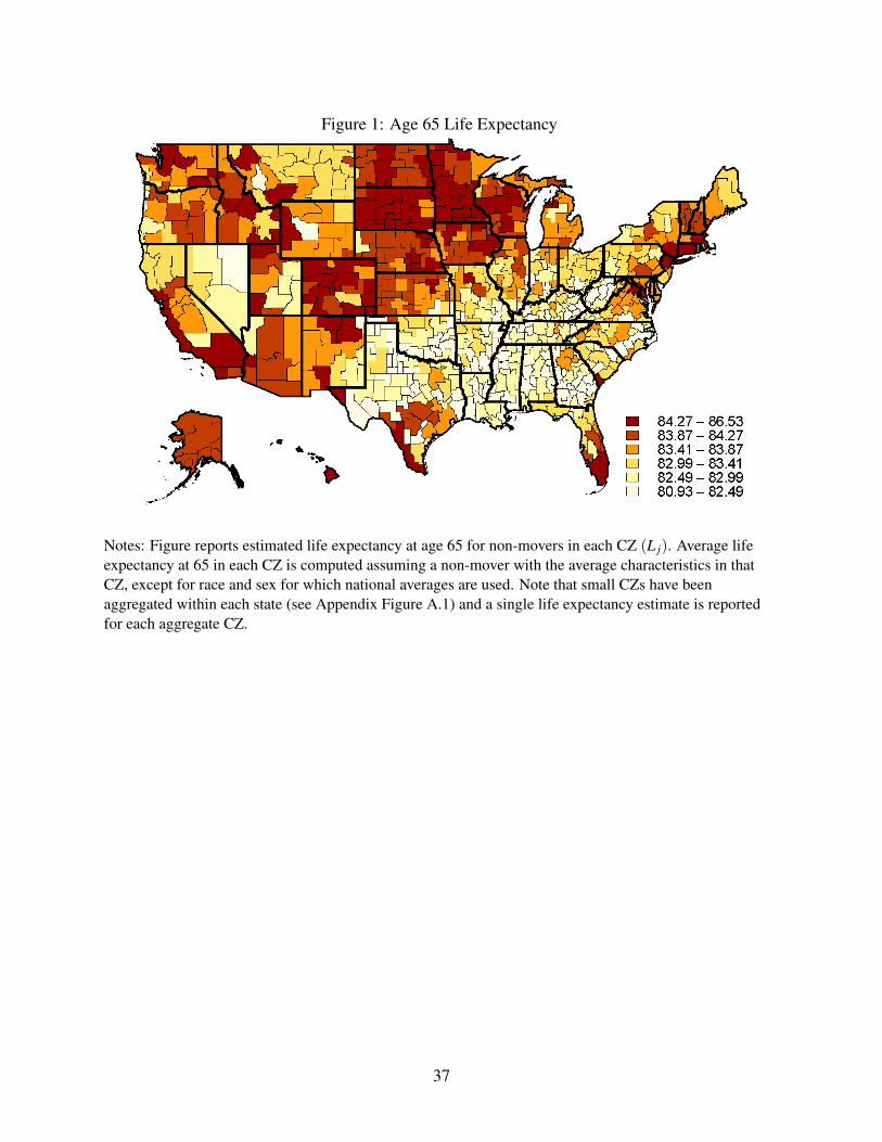
Figure 1: Age 65 Life Expectancy

Notes: Figure reports estimated life expectancy at age 65 for non-movers in each CZ (L j). Average lifeexpectancy at 65 in each CZ is computed assuming a non-mover with the average characteristics in thatCZ, except for race and sex for which national averages are used. Note that small CZs have beenaggregated within each state (see Appendix Figure A.1) and a single life expectancy estimate is reportedfor each aggregate CZ.

37

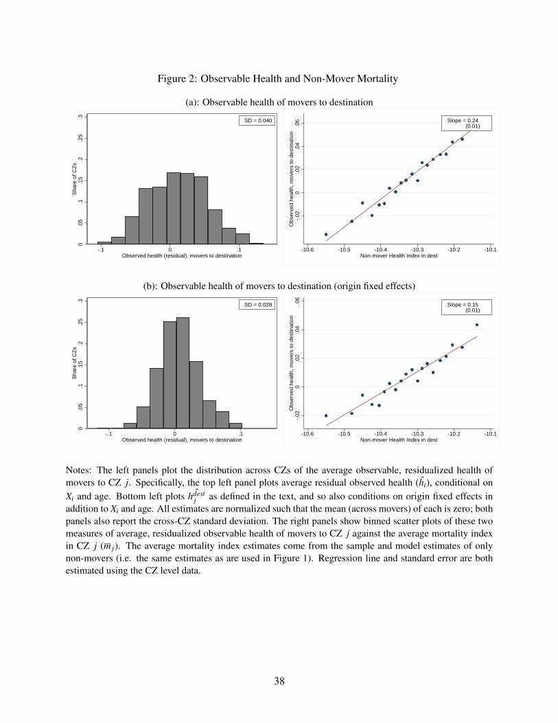
Figure 2: Observable Health and Non-Mover Mortality

(a): Observable health of movers to destination

0.0

5.1

.15

.2.2

5.3

Sha

re o

f CZ

s

-.1 0 .1Observed health (residual), movers to destination

SD = 0.040

-.02

0.0

2.0

4.0

6O

bser

ved

heal

th, m

over

s to

des

tinat

ion

-10.6 -10.5 -10.4 -10.3 -10.2 -10.1Non-mover Health Index in dest

Slope = 0.24 (0.01)

(b): Observable health of movers to destination (origin fixed effects)

0.0

5.1

.15

.2.2

5.3

Sha

re o

f CZ

s

-.1 0 .1Observed health (residual), movers to destination

SD = 0.028-.

020

.02

.04

.06

Obs

erve

d he

alth

, mov

ers

to d

estin

atio

n

-10.6 -10.5 -10.4 -10.3 -10.2 -10.1Non-mover Health Index in dest

Slope = 0.15 (0.01)

Notes: The left panels plot the distribution across CZs of the average observable, residualized health ofmovers to CZ j. Specifically, the top left panel plots average residual observed health (hi), conditional onXi and age. Bottom left plots ˆhdest

j as defined in the text, and so also conditions on origin fixed effects inaddition to Xi and age. All estimates are normalized such that the mean (across movers) of each is zero; bothpanels also report the cross-CZ standard deviation. The right panels show binned scatter plots of these twomeasures of average, residualized observable health of movers to CZ j against the average mortality indexin CZ j (m j). The average mortality index estimates come from the sample and model estimates of onlynon-movers (i.e. the same estimates as are used in Figure 1). Regression line and standard error are bothestimated using the CZ level data.

38

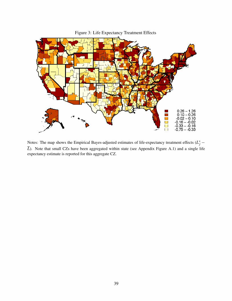
Figure 3: Life Expectancy Treatment Effects

Notes: The map shows the Empirical Bayes-adjusted estimates of life-expectancy treatment effects (L∗j −L). Note that small CZs have been aggregated within state (see Appendix Figure A.1) and a single lifeexpectancy estimate is reported for this aggregate CZ.

39

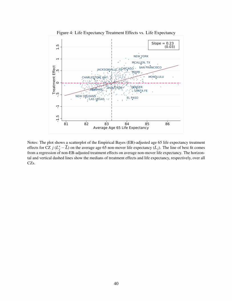
Figure 4: Life Expectancy Treatment Effects vs. Life Expectancy

DENVER

NEW ORLEANS

CHICAGO

CHARLESTON, WV

JACKSONVILLE, FL

NEW YORK

SANTA FE

EL PASO

HONOLULU

MCALLEN, TX

LAS VEGAS

MIAMI

MEMPHIS HOUSTON

SAN FRANCISCO

-1.5

-1-.5

0.5

11.

5Tr

eatm

ent E

ffect

81 82 83 84 85 86Average Age 65 Life Expectancy

Slope = 0.23 (0.03)

Notes: The plot shows a scatterplot of the Empirical Bayes (EB)-adjusted age 65 life expectancy treatmenteffects for CZ j (L∗j −L) on the average age 65 non-mover life expectancy (L j). The line of best fit comesfrom a regression of non-EB-adjusted treatment effects on average non-mover life expectancy. The horizon-tal and vertical dashed lines show the medians of treatment effects and life expectancy, respectively, over allCZs.

40

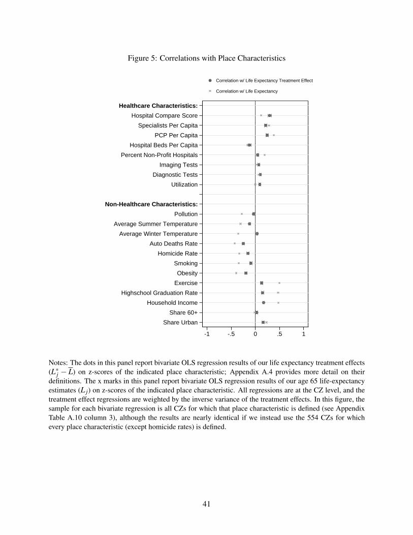
Figure 5: Correlations with Place Characteristics

Share Urban

Share 60+

Household Income

Highschool Graduation Rate

Exercise

Obesity

Smoking

Homicide Rate

Auto Deaths Rate

Average Winter Temperature

Average Summer Temperature

Pollution

Non-Healthcare Characteristics:

Utilization

Diagnostic Tests

Imaging Tests

Percent Non-Profit Hospitals

Hospital Beds Per Capita

PCP Per Capita

Specialists Per Capita

Hospital Compare Score

Healthcare Characteristics:

-1 -.5 0 .5 1

Correlation w/ Life Expectancy Treatment Effect

Correlation w/ Life Expectancy

Notes: The dots in this panel report bivariate OLS regression results of our life expectancy treatment effects(L∗j − L) on z-scores of the indicated place characteristic; Appendix A.4 provides more detail on theirdefinitions. The x marks in this panel report bivariate OLS regression results of our age 65 life-expectancyestimates (L j) on z-scores of the indicated place characteristic. All regressions are at the CZ level, and thetreatment effect regressions are weighted by the inverse variance of the treatment effects. In this figure, thesample for each bivariate regression is all CZs for which that place characteristic is defined (see AppendixTable A.10 column 3), although the results are nearly identical if we instead use the 554 CZs for whichevery place characteristic (except homicide rates) is defined.

41

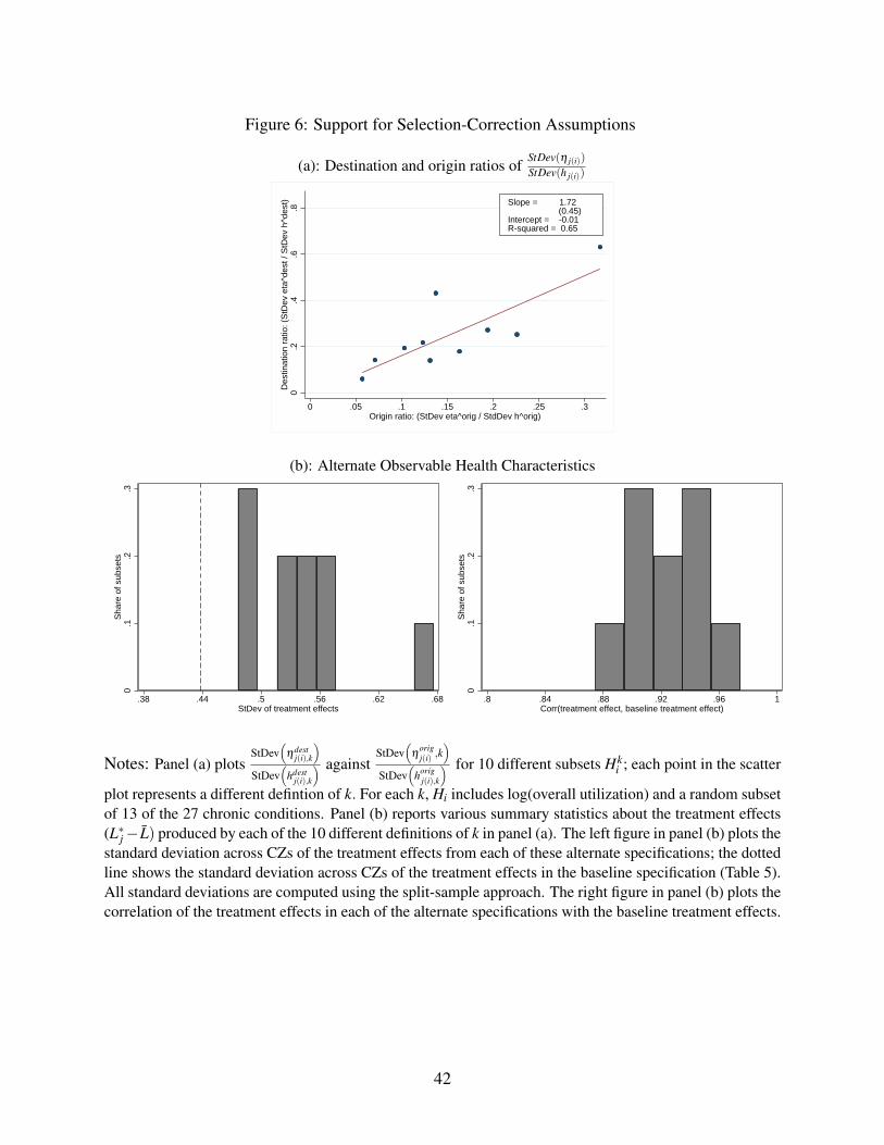
Figure 6: Support for Selection-Correction Assumptions

(a): Destination and origin ratios ofStDev(η j(i))

StDev(h j(i))

0.2

.4.6

.8D

estin

atio

n ra

tio: (

StD

ev e

ta^d

est /

StD

ev h

^des

t)

0 .05 .1 .15 .2 .25 .3Origin ratio: (StDev eta^orig / StdDev h^orig)

Slope = 1.72 (0.45)Intercept = -0.01R-squared = 0.65

(b): Alternate Observable Health Characteristics

0.1

.2.3

Sha

re o

f sub

sets

.38 .44 .5 .56 .62 .68StDev of treatment effects

0.1

.2.3

Sha

re o

f sub

sets

.8 .84 .88 .92 .96 1Corr(treatment effect, baseline treatment effect)

Notes: Panel (a) plotsStDev

(ηdest

j(i),k

)StDev

(hdest

j(i),k

) againstStDev

(η

origj(i) ,k

)StDev

(horig

j(i),k

) for 10 different subsets Hki ; each point in the scatter

plot represents a different defintion of k. For each k, Hi includes log(overall utilization) and a random subsetof 13 of the 27 chronic conditions. Panel (b) reports various summary statistics about the treatment effects(L∗j− L) produced by each of the 10 different definitions of k in panel (a). The left figure in panel (b) plots thestandard deviation across CZs of the treatment effects from each of these alternate specifications; the dottedline shows the standard deviation across CZs of the treatment effects in the baseline specification (Table 5).All standard deviations are computed using the split-sample approach. The right figure in panel (b) plots thecorrelation of the treatment effects in each of the alternate specifications with the baseline treatment effects.

42

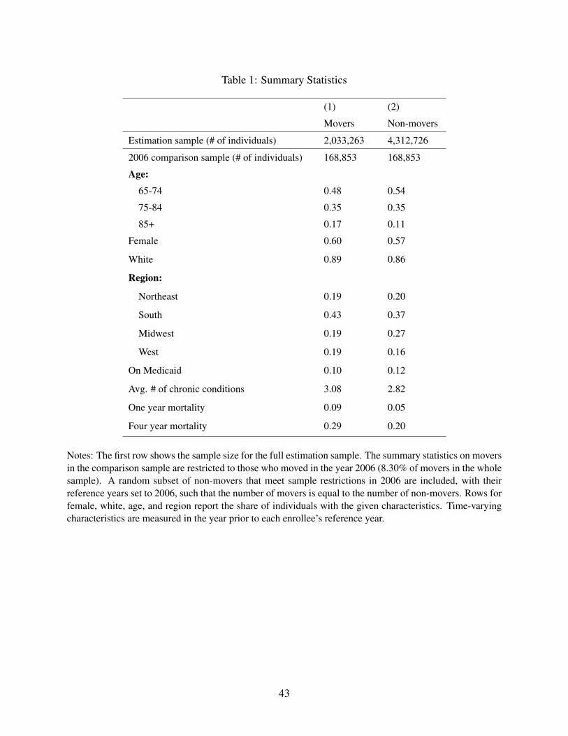
Table 1: Summary Statistics

(1) (2)

Movers Non-movers

Estimation sample (# of individuals) 2,033,263 4,312,726

2006 comparison sample (# of individuals) 168,853 168,853

Age:

65-74 0.48 0.54

75-84 0.35 0.35

85+ 0.17 0.11

Female 0.60 0.57

White 0.89 0.86

Region:

Northeast 0.19 0.20

South 0.43 0.37

Midwest 0.19 0.27

West 0.19 0.16

On Medicaid 0.10 0.12

Avg. # of chronic conditions 3.08 2.82

One year mortality 0.09 0.05

Four year mortality 0.29 0.20

Notes: The first row shows the sample size for the full estimation sample. The summary statistics on moversin the comparison sample are restricted to those who moved in the year 2006 (8.30% of movers in the wholesample). A random subset of non-movers that meet sample restrictions in 2006 are included, with theirreference years set to 2006, such that the number of movers is equal to the number of non-movers. Rows forfemale, white, age, and region report the share of individuals with the given characteristics. Time-varyingcharacteristics are measured in the year prior to each enrollee’s reference year.

43

Table 2: Inputs to Selection Correction

Standard Deviation

Origin Components:

Observed health (horigj(i) ) 0.037

[0.036, 0.037]

Unobserved health (ηorigj(i) ) 0.061

[0.058, 0.064]

Destination Components:

Observed health (hdestj(i) ) 0.024

[0.024, 0.025]

Unobserved health (ηdestj(i) ),

inferred based on Corollary 1

0.040[0.038, 0.043]

Notes: Standard deviations are computed using the split-sample approach, and are weighted by the numberof movers with each CZ as their destination. Confidence intervals are computed using 200 replications ofthe Bayesian bootstrap.

44

Table 3: Mortality Components

Standard Deviation

Mortality Index(γ j +θ j

)0.105

Unadjusted:

Place Effects (γ j) 0.077[0.068, 0.086]

Health Capital(θ j)

0.080[0.069, 0.088]

Correlation of γ j and θ j -0.008[-0.090, 0.074]

Selection Corrected:

Place Effects (γ j) 0.054[0.038, 0.067]

Health Capital(θ j)

0.094[0.083, 0.103]

Correlation of γ j and θ j 0.020[-0.082, 0.106]

Notes: These standard deviations across CZ give equal weight to each CZ and use the split-sample ap-proach. 95% confidence intervals are computed using 200 replications of the Bayesian bootstrap. For the“unadjusted” results in the top panel, γ j is defined as the destination fixed effects τdest

j from equation (3), andaverage health capital θ j is given by the average value of the remaining terms in that equation (excludingthe age term aiβ ). For the “selection corrected” results in the bottom panel, γ j is defined as the differenceτdest

j − ηdestj , where τdest

j is the destination fixed effect from equation (3) and the unobservable componentηdest

j is inferred following the steps broken out in Table 2; average health capital θ j is then calculated usingthe same approach as in the unadjusted results.

45

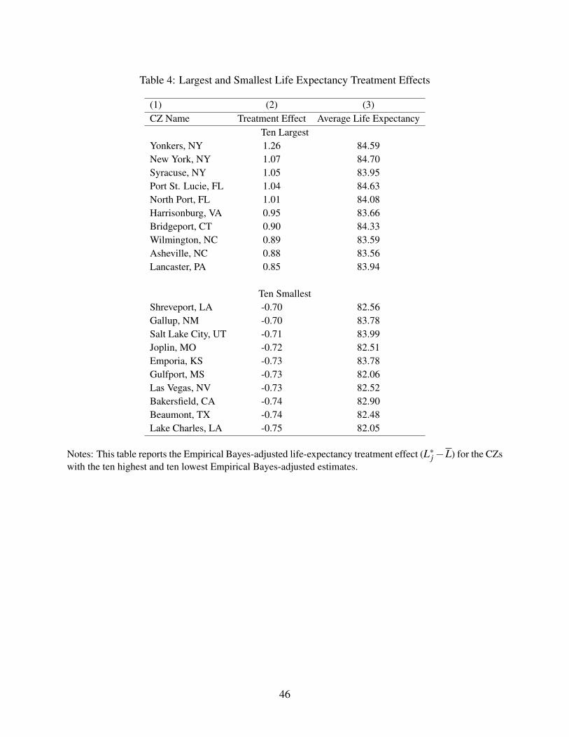
Table 4: Largest and Smallest Life Expectancy Treatment Effects

(1) (2) (3)CZ Name Treatment Effect Average Life Expectancy

Ten LargestYonkers, NY 1.26 84.59New York, NY 1.07 84.70Syracuse, NY 1.05 83.95Port St. Lucie, FL 1.04 84.63North Port, FL 1.01 84.08Harrisonburg, VA 0.95 83.66Bridgeport, CT 0.90 84.33Wilmington, NC 0.89 83.59Asheville, NC 0.88 83.56Lancaster, PA 0.85 83.94

Ten SmallestShreveport, LA -0.70 82.56Gallup, NM -0.70 83.78Salt Lake City, UT -0.71 83.99Joplin, MO -0.72 82.51Emporia, KS -0.73 83.78Gulfport, MS -0.73 82.06Las Vegas, NV -0.73 82.52Bakersfield, CA -0.74 82.90Beaumont, TX -0.74 82.48Lake Charles, LA -0.75 82.05

Notes: This table reports the Empirical Bayes-adjusted life-expectancy treatment effect (L∗j−L) for the CZswith the ten highest and ten lowest Empirical Bayes-adjusted estimates.

46

Table 5: Life Expectancy Decompositions

Cross-CZ standard deviation of:

(1) Age 65 Life Expectancy (L j) 0.84

(2) Treatment Effects (L∗j −L) 0.44[0.30, 0.54]

(3) Health Capital Effects 0.78[0.70, 0.85]

(4) Correlation of Treatment and Health Capital Effects -0.04[-0.13, 0.08]

Share variance would be reduced if:

(5) Place Effects were Made Equal 0.13[-0.02, 0.31]

(6) Health Capital was Made Equal 0.73[0.59, 0.87]

Notes: All objects are computed at the CZ level using the split-sample approach described in Section 3.1 andgive equal weight to each CZ; 95% confidence intervals are computed via 200 replications of the Bayesianbootstrap. In row (2), we compute the standard deviation of life expectancy if health capital were heldconstant; specifically, for each CZ j, we compute the counterfactual age 65 life expectancy if each CZ hadits own γ j but the nationally representative health capital θ as defined in the text. In row (3), we computethe standard deviation in life expectancy if the place effects were held constant; specifically, we definethe nationally representative place effect as the median of γ j among matched non-movers, and for eachCZ j, compute the counterfactual age 65 life expectancy where the CZ has its own θ j, but a nationallyrepresentative place effect. Row (4) reports the correlation between the health capital component of lifeexpectancy (whose standard deviation is shown in row 3) and the place component of life expectancy (whosestandard deviation is shown in row 2). In row (5) we show the share of the variance that would be reducedif place effects were made equal; this is computed by calculating the variance of life expectancy with placeeffects held constant (i.e. the square of row 3) and the variance in life expectancy (i.e. the square of row 1),and taking 1 minus the ratio of these numbers. Row (6) is computed in an analogous fashion.

47

Table 6: Heterogeneity by Medicaid Status and Race

Medicaid Status Race

Baseline Non-Medicaid Medicaid White Non-White

(1) Number of movers 710,990 650,246 60,744 629,126 81,864

(2) StDev of life expectancy (L j) 0.67 0.64 1.57 0.57 1.44

Cross-CZ standard deviation of:

(3) Treatment effects (L∗j − L) 0.47[0.40, 0.53]

0.46[0.38, 0.54]

0.72[0.37, 1.00]

0.48[0.41, 0.54]

0.73[0.00, 1.17]

(4) Health capital effects 0.55[0.47, 0.61]

0.49[0.40, 0.56]

1.55[1.31, 1.83]

0.46[0.38, 0.53]

1.01[0.47, 1.35]

Notes: This table summarizes the decompositions for the largest 100 CZs by population in 2000, estimated separatelyby race and Medicaid status during the year prior to the reference year. Both non-mover and mover samples arepartitioned by race or Medicaid satus. Sample sizes in row (1) exclude movers to or from any CZ outside of the 100largest CZs; this leaves us with about one-third of the baseline mover sample. Row (2) shows the cross-CZ standarddeviation of life expectancy at 65 among non-movers in the indicated sample. The standard deviations of treatmenteffects and health capital effects in rows (3) and (4) are computed using the split-sample approach, giving equal weightto each CZ. Brackets show the 95% confidence intervals computed via 100 iterations of the Bayesian bootstrap. Sincestandard deviations cannot be negative, any split-sample approach that produces a negative result we set to 0.00.

48

Table 7: Logistic Model

(1) (2)Standard Deviation ofMortality Index

(γ j + θ j

) Standard Deviation ofPlace Effects (γ j)

Baseline 0.105 0.054[0.038, 0.067]

Logistic Model:

1-year mortality 0.063 0.081[0.072, 0.091]

2-year mortality 0.069 0.073[0.061, 0.079]

3-year mortality 0.078 0.083[0.078, 0.088]

4-year mortality 0.088 0.082[0.075, 0.089]

Notes: Column (1) reports the cross-CZ standard deviation of our mortality index. Row (1) reports resultsfor the baseline Gompertz specification (See Table 3). For the baseline specification, the mortality indexis age, race, and sex adjusted; for the logit specifications it is not. Furthermore, in the logit specifications,rather than a β · t term, five-year age bins are fully interacted with race and sex. Column (2) reports thecross-CZ standard deviation of our place effects. 95% confidence intervals are reported underneath thepoint estimate in Column (2), and are computed with 20 replications of the Bayesian bootstrap. All standarddeviations of γ j are computed using the split-sample approach, and all standard deviations in both columnsgive equal weight to each CZ.

49

A Appendix

A.1 Empirical Bayes AdjustmentOur Empirical Bayes adjustment follows Chetty and Hendren (2016). This appendix describes theapproach in more detail.

Let γ j be the true life expectancy treatment effects with mean 0. Let M be the average causalplace effect which, by construction, is also 0. There is no measurement error in M. We assumethat γ j is a normally distributed random variable, so that

γ j = M+η j (9)

with η j ∼ N(0,χ2).

Further, assume that the unbiased estimates of γ j are subject to idiosyncratic measurementerror:

γ j = γ j +υ j (10)

where the estimation error υ j ∼ N(

0,s2j

)and s j is the standard error of γ j from the bootstrap.

Combining equations (9) and (10) implies:

γ j = M+η j +υ j (11)

and using OLS we are able to estimate Var(η j +υ j

)as Var

(η j +υ j

). Note that in our setting,

Var(η j +υ j

)= Var

(γ j).

With these assumptions, we are able to compute:

χ2 = Var

(η j)= Var

(η j +υ j

)−E

[s2

j]

(12)

Optimal linear predictions We compute forecasts γEBj of each CZ’s true causal effect γ j that

minimize the mean squared prediction error:

J

∑j=1

(γ

EBj − γ j

)2(13)

Note that the (unobserved) true causal effect of moving to j can be written as:

γ j = β1, j ·M+β2, j · γ j (14)

A hypothetical OLS regression across the 563 CZs to estimate the 563 β1, j coefficients and the563 β2, j coefficients allows us to form predictions of the true causal effects, γ j, using M and γ j,which we call γEB

j .

γEBj = β1, j ·M+ β2, j · γ j (15)

Note that these predictions, γEBj , would minimize the objective function in equation (13). Given

a way to estimate these coefficients, we can directly compute the optimal forecasts. However,

50

because γ j is unobserved, we cannot simply estimate the coefficients in an OLS regression. Instead,we use the derivation of these coefficients as in Chetty and Hendren (2016):

γEBj =

χ2

χ2 + s2j· γ j +

s2j

χ2 + s2jM (16)

Because in our setting M = 0 , this simplifies to:

γEBj =

χ2

χ2 + s2j· γ j (17)

A.2 Microfoundation for Assumptions 1 and 2In this section, we show a natural set of assumptions on the selection process under which As-sumptions 1 and 2 are guaranteed to hold. The key condition is that selection works only throughthe single index of overall health capital.

We begin with an underlying population of movers with health capital θi = hi +ηi, where hiand ηi are observed and unobserved components respectively. For simplicity, we ignore the roleof demographics and set Xiβ = 0. Following the approach of Section 2, we define ηi to be aresidual orthogonal to hi, so that any unobserved determinants of health capital correlated withthe observed measures are absorbed in hi, and ηi only includes the components not predictablefrom observables. We go beyond the structure imposed above to assume hi and ηi are indepen-dently normally distributed in the population, with hi ∼ N (0,σh) and ηi ∼ N (0,ση). We assumeE(ηi|o(i) , j (i)) = η

origo(i) +ηdest

j(i) and E(hi|o(i) , j (i)) = horigo(i) +hdest

j(i) .There is an unmodeled selection process under which each mover i is assigned an origin

o(i) ∈J and a destination d (i) ∈J . These assignments are potentially correlated with healthcapital. Such correlation could arise because health capital changes the relative appeal of living indifferent locations, because determinants of location choices are correlated with determinants ofhealth capital, and/or because origin locations exert a causal effect on health capital as of the timeof move.

The key assumption we impose on the selection process is that all such correlation operatesonly through overall health capital index θi = hi +ηi and not differentially through hi or ηi ontheir own. Formally, we assume that once we condition on overall health capital θi, origin anddestination locations provide no further information about the values of hi and ηi.

Assumption 5. (Single index) E(hi|θi,o(i) , j (i)) = E(hi|θi)

Note that since ηi = θi−hi, Assumption 5 implies E(ηi|θi,o(i) , j (i)) = E(ηi|θi). This singleindex assumption naturally constrains the selection on hi to be tightly related to selection on ηi, andwe show in the following proposition that it actually implies both of the key assumptions requiredfor our selection correction above.

Proposition 2. Assumption 5 implies Assumptions 1 and 2.

Proof. Normality of hi and ηi as well as the fact that θi = hi +ηi imply

θi|hi ∼ N (hi,ση) .

51

Standard conjugate prior results for the normal distribution with known variance imply

E(hi|θi) =

1σh

1σh

+ 1ση

·0+1

ση

1σh

+ 1ση

·θi

=σh

σh +ση

θi.

It then follows that for any o(i) and j (i),

horigo(i) +hdest

j(i) = E(hi|o(i) , j (i))

= Eθi [E(hi|θi,o(i) , j (i)) |o(i) , j (i)]= Eθi [E(hi|θi) |o(i) , j (i)]

= Eθi

[σh

ση +σhθi|o(i) , j (i)

]=

σh

ση +σh

(horig

o(i) +hdestj(i) +η

origo(i) +η

destj(i)

),

where the third line uses Assumption 5. We therefore have horigo(i) +hdest

j(i) =σhση

(η

origo(i) +ηdest

j(i)

). The

fact that this must hold for all o(i) and j (i) implies

horigo(i) =

σh

ση

ηorigo(i)

hdestj(i) =

σh

ση

ηdestj(i) .

We therefore haveStDev

(horig

o(i)

)StDev

(η

origo(i)

) =StDev

(hdest

j(i)

)StDev

(ηdest

j(i)

) = σhση

, which implies Assumption 2. We also have

StDev(

hdestj(i)

)StDev

(ηdest

j(i)

) = σhση

=hdest

j(i)

ηdestj(i)

, so Assumption 1 follows by Proposition 1.

52

A.3 Sample Restrictions, Mover Definition, and Characteristics of MovesAppendix Table A.9 details the number of observations excluded by each of our sample criteria.Our analysis sample consists of almost 69 million Medicare enrollees whom we observe betweenthe ages of 65 and 99. Of these, almost 62 million are non-movers; their zip code of residence doesnot change at any point over the years we observe them. The remaining 7 million are “potentialmovers,” in that their zip code of residence changes at least once. To the extent possible, we imposea parallel set of restrictions to the non-mover and mover samples.

Non-mover sample

To define our non-mover sample, we begin with the 62 million enrollees whose CZ of residencedoes not change over the years we observe them. We make several further restrictions that bringthe non-mover sample down to just over 43 million. For each non-mover, we need to be able todefine a year t∗i as a counterfactual move year. Most importantly, this requires that they have a yeart∗i −1 in which the non-mover was enrolled in Traditional Medicare, so that we can measure theirhealthcare utilization in year t∗i −1. We also exclude non-movers who do not have a t∗i −1 in whichthey are younger than 98 and that is before 2012. These restrictions decrease the number of eligiblenon-movers from 62 million to 52 million. We exclude non-movers who do not have a year t∗i −1such that they survive through the end of year t∗i , so that we are able to observe their mortality inyear t∗i +1. This eliminates another 9 million non-movers. Finally, we exclude the small numberof non-movers who do not have a remaining year t∗i −1 with data on controls of health utilizationand chronic conditions. For the remaining, non-movers, t∗i is defined as their second year in thesample. In all of our analyses we work with a random 10% sample of these remaining 43 millionnon-movers.

Mover sample

To define our mover sample, we begin with the 7 million “potential movers” - i.e. individualswhose zip code of residence changes at least once. We make several further restrictions to themover sample that brings the number of movers down to just over 2 million. First, we exclude in-dividuals whose CZ residence changes more than once; this brings the 7 million potential moversdown to 5.6 million. Second, we exclude movers who are enrolled in Medicare Advantage the yearbefore move (t∗i −1) or the year after move (t∗i +1) since, as discussed, we cannot observe health-care claims for Medicare Advantage enrollees and we need to observe the location of healthcareclaims to define movers. Following the approach of Finkelstein et al. (2016), we exclude “movers”for whom the ratio of the number of claims located in their destination to the number located ineither their origin or their destination does not increase by at least 0.75 in their post-move yearsrelative to their pre-move years; these are individuals who, despite having a change of officialaddress on file, do not appear to have really changed CZs based on their claims pattern.23

The exclusion of movers who are on MA in (t∗i − 1) or (t∗i + 1) brings the number of moversdown from 5.6 million to 4.2 million. The exclusion of “false” movers (i.e. those whose claims

23The change in claim share is not defined for movers who do not have at least one claim both pre- and post-move.Following Finkelstein et al. (2016), we exclude these cases if: (i) they have no post-move claims and a pre-movedestination claim share greater than 0.05; (ii) they have no pre-move claims and a post-move destination claim shareless than 0.95.

53

share does not increase by at least 0.75), further reduces the number of movers to 2.6 million. Afew other exclusions for data reasons bring our final mover sample down to 2 million movers. Ofthe 2 million movers in our final sample, about 18% of them are on MA in at least one year. Giventhe number of total enrollee-years we observe, we estimate an average annual cross-CZ move ratefor Medicare enrollees of about 0.5 percent.

Appendix Figure A.6 shows a mover’s claims in her destination CZ, as a share of those in eitherher origin or her destination, by relative year. There is a sharp change in the year of the move, andonly a very small share of claims in the destination pre-move or in the origin post-move. The shareof claims in the destination in the year of the move (relative year 0) is close to 0.5, suggesting thatmoves are made roughly uniformly throughout the year.

Characteristics of moves

We examined some of the characteristics of moves. The average distance between origin anddestination zip code centroids of movers in our sample is 547 miles, with a median of 305 milesand a standard deviation of 601 miles. Roughly 66 percent of moves cross state boundaries, and 48percent cross census division boundaries. Moves to Florida account for 12 percent of all moves,and moves to Arizona or California account for an additional 10 percent.

In our previous work (Finkelstein et al. 2016), we also used data from the Health and Re-tirement Survey to explore some of the time-varying correlates of moving in the Medicare pop-ulation; widowhood and retirement were significant predictors of moving, and the most commonself-reported rationale for moving was to be near one’s children

A.4 Data and Definitions for Place CharacteristicsHere we describe the data and definitions used for the place characteristic measures that we corre-late with treatment effects in Figure 5. Summary statistics for all of these measures can be foundin Appendix Table A.10.

A.4.1 Healthcare Utilization

We follow Finkelstein et al. (2016) to construct our health care utilization measures. The utilizationmeasure we use as a pre-period control in our estimation is created by aggregating care provided toMedicare beneficiaries as recorded in the inpatient and outpatient claims data. For the healthcareplace characteristics in Figure 5, we use a 20% random sample of data from the inpatient, outpa-tient, and carrier files from Medicare year 2010. See Finkelstein et al. (2016) Online Appendix formore details on how utilization is computed. Our definitions of diagnostic tests and imaging testsalso follow directly from Finkelstein et al. (2016) and detailed definitions of these variables canalso be found in that paper’s Online Appendix.

A.4.2 Other Healthcare Characteristics

Share of hospitals that are non-profit and Hospital beds per capita are defined as in Finkelsteinet al. (2016) using the 1998-2008 American Hospital Association’s annual survey of hospitals.

54

Specialists per thousand residents and PCPs per thousand residents are also defined as inFinkelstein et al. (2016) using counts of physicians from the 2011 AMA Physician Masterfile.CZ populations are computed by first aggregating county-level populations from the 2000 Censusand 2007-2011 ACS, and then taking the simple average across the two.

Hospital Compare Score, a measure that reports the quality of hospitals, is derived from “pro-cess of care” measures that are publicly reported by CMS and uses quarterly data from 2005 to2011. For a given measure (e.g., share of heart attack patients given aspirin at arrival or shareof pneumonia patients given oxygenation assessment), we standardize the score by first taking asimple average across the quarterly measures within a year for a given hospital to get an annualmeasure. We then construct z-scores for each measure across hospitals in a given year. Lastly, foreach hospital we take the simple average of the z-scores across measures within a year and thenthe simple average over years.

A.4.3 Non-healthcare Characteristics

Measures derived from Centers for Disease Control (CDC) data Many of our CZ-level mea-sures of non-healthcare characteristics are derived from data downloaded from the CDC (https://wonder.cdc.gov/) and cover the years 2001-2011 (except pollution, for which records are onlyavailable beginning in 2003).

• Homicides and Auto Deaths are defined by the National Center for Health Statistics usingICD-9 and ICD-10 mortality codes and are reported per 100,000 people from 2001-2011 at thecounty level. We take the simple average across counties to aggregate to the CZ level.

• Pollution is a measure of fine particulate matter and is reported in micrograms per cubic meter.For each county we have the daily average across all days from 2003-2011. We aggregate thesesingle county-level measures to the CZ level by taking the simple average across counties withineach CZ.

• Average Winter Temperature is defined as the average daily minimum air temperature duringthe months of January, February, and March for each county. For each county we take a simpleaverage across all winter months from 2001-2011, and then aggregate these single county-levelmeasures to the CZ level by taking the simple average across counties within each CZ.

• Average Summer Temperature is defined similarly to Average Winter Temperature, but usesthe average daily maximum air temperature during the months of June, July, and August.

Measures derived from Chetty et al. (2016b) data Our health behavior measures are derivedfrom the health behavior data posted by Chetty et al. (2016b) (https://healthinequality.org/data), as originally drawn from the Behavioral Risk Factor Surveillance Survey (BRFSS).The data cover 1996-2008 and are reported at the CZ level separately for each income quartile. Wetake the simple average of the four quartiles to get the average measure in each CZ.

• Smoking is the fraction of respondents who report currently smoking in each CZ of the pooledBRFSS sample over years 1996-2008.

• Obesity is the fraction of respondents who are obese (BMI≥30) in each CZ of the pooledBRFSS sample over years 1996-2008.

• Exercise is the fraction of respondents who have exercised in the past 30 days in each CZ ofthe pooled BRFSS sample over years 1996-2008.

55

Measures derived from Census data Our other CZ level measures of non-healthcare character-istics are derived from Census data.

• Share Urban is derived from the 2000 and 2010 Census data. Urban and total populations areavailable at the county level, and we aggregate these values within each CZ and compute the shareof that population that is urban. We then take the simple average of these values across the twocensus surveys.

• Share over 60, Median household income, and High school graduation rate are computedsimilarly using the 2000 Census survey and 2007-2011 American Community Survey. Medianhousehold income and high school graduation rates are computed for people 25 and older.

56

A.5 Bounding StDev(γ j)

without Equal SelectionAs formulated, Assumption 1 requires that equal selection holds for each individual location (allj ∈ J). This assumption is necessary to compute η j, and therefore to compute each γ j = τdest

j −ηdest

j . However, even in the absence of this equal selection assumption, we are able to recover asubset of our main results. Importantly, we can estimate bounds on the standard deviation of γ j. Allthat is required is to restate the Relative Importance Assumption with j rather than j (i) indexingin order to estimate the standard deviation, though not the actual quantities, of ηdest

j . That is:

Modified Assumption 2:StDev

(η

origj

)StDev

(horig

j

) =StDev(ηdest

j )StDev(hdest

j )

Recall that Var(γ j)= Var

(τdest

j

)−Var

(ηdest

j

)−2 ·Cov

(γ j,η

destj

). Because correlations are

bounded on [-1,1], we know

Cov(

γ j,ηdestj

)≤√

Var(γ j)·Var

(ηdest

j

)(18)

and

Cov(

γ j,ηdestj

)≥−

√Var(γ j)·Var

(ηdest

j

)(19)

Therefore,

Var(γ j)≥ Var

(τ

destj

)−Var

(η

destj

)−2 ·

√Var(γ j)·Var

(ηdest

j

)(20)

With some algebraic manipulations we see:

Var(γ j)+Var

(η

destj

)+2 ·

√Var(γ j)·Var

(ηdest

j

)≥ Var

(τ

destj

)(√

Var(γ j)+

√Var(

ηdestj

))2

≥ Var(

τdestj

)√

Var(γ j)+

√Var(

ηdestj

)≥

√Var(

τdestj

)√

Var(γ j)≥

√Var(

τdestj

)−√

Var(

ηdestj

)StDev

(γ j)≥ StDev

(τ

destj

)−StDev

(η

destj

)The upper bound follows from symmetry:

StDev(γ j)≤ StDev

(τ

destj

)+StDev

(η

destj

)In our data, we have StDev

(τdest

j

)= 0.077 and, from Modified Assumption 2, StDev

(ηdest

j

)=

57

0.036. Therefore, we estimate the lower and upper bounds on the standard deviation of γ j withoutthe equal selection assumption as 0.041 and 0.113.

58

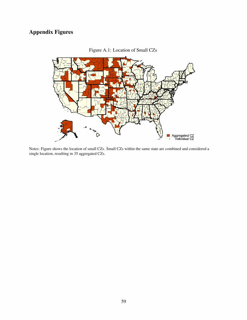
Appendix Figures

Figure A.1: Location of Small CZs

Notes: Figure shows the location of small CZs. Small CZs within the same state are combined and considered asingle location, resulting in 35 aggregated CZs.

59

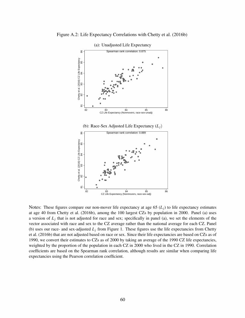
Figure A.2: Life Expectancy Correlations with Chetty et al. (2016b)

(a): Unadjusted Life Expectancy

8182

8384

8586

Che

tty e

t al.

(201

6) C

Z L

ife E

xpec

tanc

y

82 83 84 85 86CZ Life Expectancy (Nonmovers, race-sex-unadj)

Spearman rank correlation: 0.875

(b): Race-Sex Adjusted Life Expectancy (L j)

8182

8384

8586

Che

tty e

t al.

(201

6) C

Z L

ife E

xpec

tanc

y

82 83 84 85 86CZ Life Expectancy (Nonmovers, race-sex-adj)

Spearman rank correlation: 0.889

Notes: These figures compare our non-mover life expectancy at age 65 (L j) to life expectancy estimatesat age 40 from Chetty et al. (2016b), among the 100 largest CZs by population in 2000. Panel (a) usesa version of L j that is not adjusted for race and sex; specifically in panel (a), we set the elements of thevector associated with race and sex to the CZ average rather than the national average for each CZ. Panel(b) uses our race- and sex-adjusted L j from Figure 1. These figures use the life expectancies from Chettyet al. (2016b) that are not adjusted based on race or sex. Since their life expectancies are based on CZs as of1990, we convert their estimates to CZs as of 2000 by taking an average of the 1990 CZ life expectancies,weighted by the proportion of the population in each CZ in 2000 who lived in the CZ in 1990. Correlationcoefficients are based on the Spearman rank correlation, although results are similar when comparing lifeexpectancies using the Pearson correlation coefficient.

60

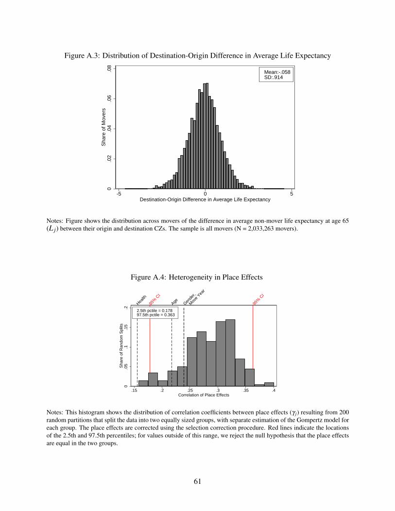
Figure A.3: Distribution of Destination-Origin Difference in Average Life Expectancy

0.0

2.0

4.0

6.0

8S

hare

of M

over

s

-5 0 5Destination-Origin Difference in Average Life Expectancy

Mean:-.058SD:.914

Notes: Figure shows the distribution across movers of the difference in average non-mover life expectancy at age 65(L j) between their origin and destination CZs. The sample is all movers (N = 2,033,263 movers).

Figure A.4: Heterogeneity in Place Effects

0.0

5.1

.15

.2S

hare

of R

ando

m S

plits

Gende

r,

Mov

e Yea

r

AgeHealth

95%

CI

95%

CI

.15 .2 .25 .3 .35 .4Correlation of Place Effects

2.5th pctile = 0.17897.5th pctile = 0.363

Notes: This histogram shows the distribution of correlation coefficients between place effects (γ j) resulting from 200random partitions that split the data into two equally sized groups, with separate estimation of the Gompertz model foreach group. The place effects are corrected using the selection correction procedure. Red lines indicate the locationsof the 2.5th and 97.5th percentiles; for values outside of this range, we reject the null hypothesis that the place effectsare equal in the two groups.

61

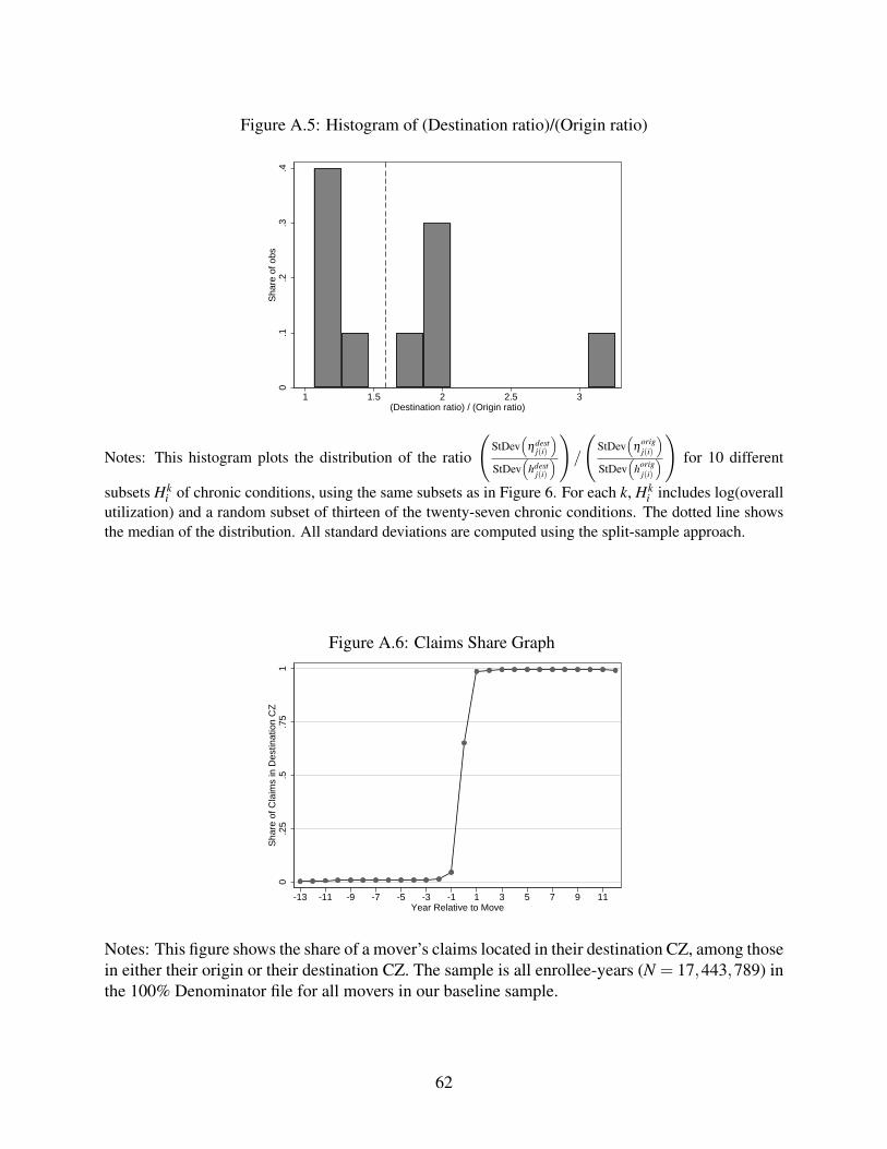
Figure A.5: Histogram of (Destination ratio)/(Origin ratio)

0.1

.2.3

.4S

hare

of o

bs

1 1.5 2 2.5 3(Destination ratio) / (Origin ratio)

Notes: This histogram plots the distribution of the ratio

(StDev

(ηdest

j(i)

)StDev

(hdest

j(i)

))/

(StDev

(η

origj(i)

)StDev

(horig

j(i)

))

for 10 different

subsets Hki of chronic conditions, using the same subsets as in Figure 6. For each k, Hk

i includes log(overallutilization) and a random subset of thirteen of the twenty-seven chronic conditions. The dotted line showsthe median of the distribution. All standard deviations are computed using the split-sample approach.

Figure A.6: Claims Share Graph

0.2

5.5

.75

1S

hare

of C

laim

s in

Des

tinat

ion

CZ

-13 -11 -9 -7 -5 -3 -1 1 3 5 7 9 11Year Relative to Move

Notes: This figure shows the share of a mover’s claims located in their destination CZ, among thosein either their origin or their destination CZ. The sample is all enrollee-years (N = 17,443,789) inthe 100% Denominator file for all movers in our baseline sample.

62

Appendix Tables

Table A.1: Predicting Mortality from Observables

(1) (2) (3)Coefficient (s.e.) Average

Log(Utilization + 1) 0.028 (0.000) 3.67Chronic Conditions:

Acquired Hypothyroidism -0.008 (0.003) 0.03Acute Myocardial Infarction -0.069 (0.009) 0.00Alzheimer’s 0.214 (0.009) 0.01Alzheimer’s and Related Disorders or Senile Dementia 0.474 (0.006) 0.03Anemia 0.152 (0.002) 0.09Asthma -0.054 (0.005) 0.02Atrial Fibrillation 0.222 (0.003) 0.03Benign Prostatic Hyperplasia -0.214 (0.004) 0.03Breast Cancer 0.087 (0.005) 0.01Cataract -0.095 (0.002) 0.15Chronic Kidney Disease 0.413 (0.006) 0.02Chronic Obstructive Pulmonary Disease 0.484 (0.003) 0.05Colorectal Cancer 0.048 (0.008) 0.01Depression 0.188 (0.004) 0.04Diabetes 0.342 (0.002) 0.08Endometrial Cancer 0.115 (0.014) 0.00Glaucoma -0.063 (0.003) 0.05Heart Failure 0.327 (0.003) 0.06Hyperlipidemia -0.221 (0.002) 0.15Hypertension 0.042 (0.002) 0.25Hip/Pelvic Fracture 0.042 (0.008) 0.00Ischemic Heart Disease 0.099 (0.003) 0.13Lung Cancer 0.772 (0.015) 0.00Osteoporosis 0.032 (0.004) 0.03Prostate Cancer 0.035 (0.003) 0.02Rheumatoid Arthritis -0.066 (0.003) 0.08Stroke / Transient Ischemic Attack 0.205 (0.005) 0.02

N 6,345,989

Notes: This table reports the coefficients of the components of Hi in our main estimating equation,equation (3). Standard errors are computed with 20 replications of the bootstrap. Column (3) reports thesample mean of log(Utilization + 1) in row (1) and, for all other rows, the share of beneficiaries with theindicated chronic condition in year t∗i −1. Utilization excludes physician services (“carrier files”) becausethese files are only available for a 20 percent subsample. As in the estimation, when computing thesample-wide shares, non-movers are upweighted by ten to account for our sampling procedure.

63

Table A.2: Number of Movers Received by CZ or Aggregate CZ

Statistics # Movers to CZ

Minimum 48

10th Percentile 468

25th Percentile 781

Median 1,522

75th Percentile 3,534

90th Percentile 9,241

Maximum 45,360

Notes: This table summarizes the number of movers received by each of the 563 CZs or aggregated CZs.

64

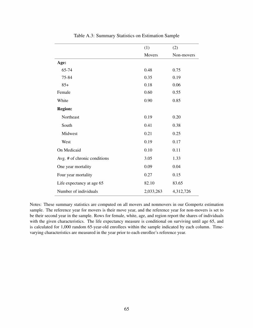
Table A.3: Summary Statistics on Estimation Sample

(1) (2)

Movers Non-movers

Age:

65-74 0.48 0.75

75-84 0.35 0.19

85+ 0.18 0.06

Female 0.60 0.55

White 0.90 0.85

Region:

Northeast 0.19 0.20

South 0.41 0.38

Midwest 0.21 0.25

West 0.19 0.17

On Medicaid 0.10 0.11

Avg. # of chronic conditions 3.05 1.33

One year mortality 0.09 0.04

Four year mortality 0.27 0.15

Life expectancy at age 65 82.10 83.65

Number of individuals 2,033,263 4,312,726

Notes: These summary statistics are computed on all movers and nonmovers in our Gompertz estimationsample. The reference year for movers is their move year, and the reference year for non-movers is set tobe their second year in the sample. Rows for female, white, age, and region report the shares of individualswith the given characteristics. The life expectancy measure is conditional on surviving until age 65, andis calculated for 1,000 random 65-year-old enrollees within the sample indicated by each column. Time-varying characteristics are measured in the year prior to each enrollee’s reference year.

65

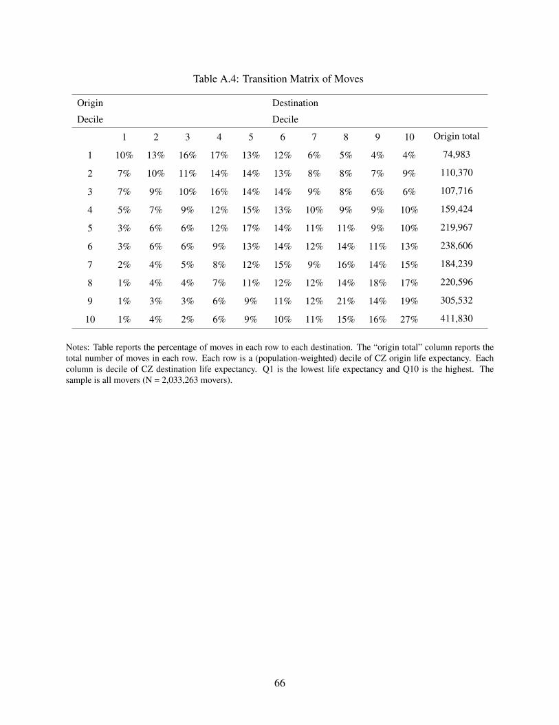
Table A.4: Transition Matrix of Moves

Origin

Decile

Destination

Decile

1 2 3 4 5 6 7 8 9 10 Origin total

1 10% 13% 16% 17% 13% 12% 6% 5% 4% 4% 74,983

2 7% 10% 11% 14% 14% 13% 8% 8% 7% 9% 110,370

3 7% 9% 10% 16% 14% 14% 9% 8% 6% 6% 107,716

4 5% 7% 9% 12% 15% 13% 10% 9% 9% 10% 159,424

5 3% 6% 6% 12% 17% 14% 11% 11% 9% 10% 219,967

6 3% 6% 6% 9% 13% 14% 12% 14% 11% 13% 238,606

7 2% 4% 5% 8% 12% 15% 9% 16% 14% 15% 184,239

8 1% 4% 4% 7% 11% 12% 12% 14% 18% 17% 220,596

9 1% 3% 3% 6% 9% 11% 12% 21% 14% 19% 305,532

10 1% 4% 2% 6% 9% 10% 11% 15% 16% 27% 411,830

Notes: Table reports the percentage of moves in each row to each destination. The “origin total” column reports thetotal number of moves in each row. Each row is a (population-weighted) decile of CZ origin life expectancy. Eachcolumn is decile of CZ destination life expectancy. Q1 is the lowest life expectancy and Q10 is the highest. Thesample is all movers (N = 2,033,263 movers).

66

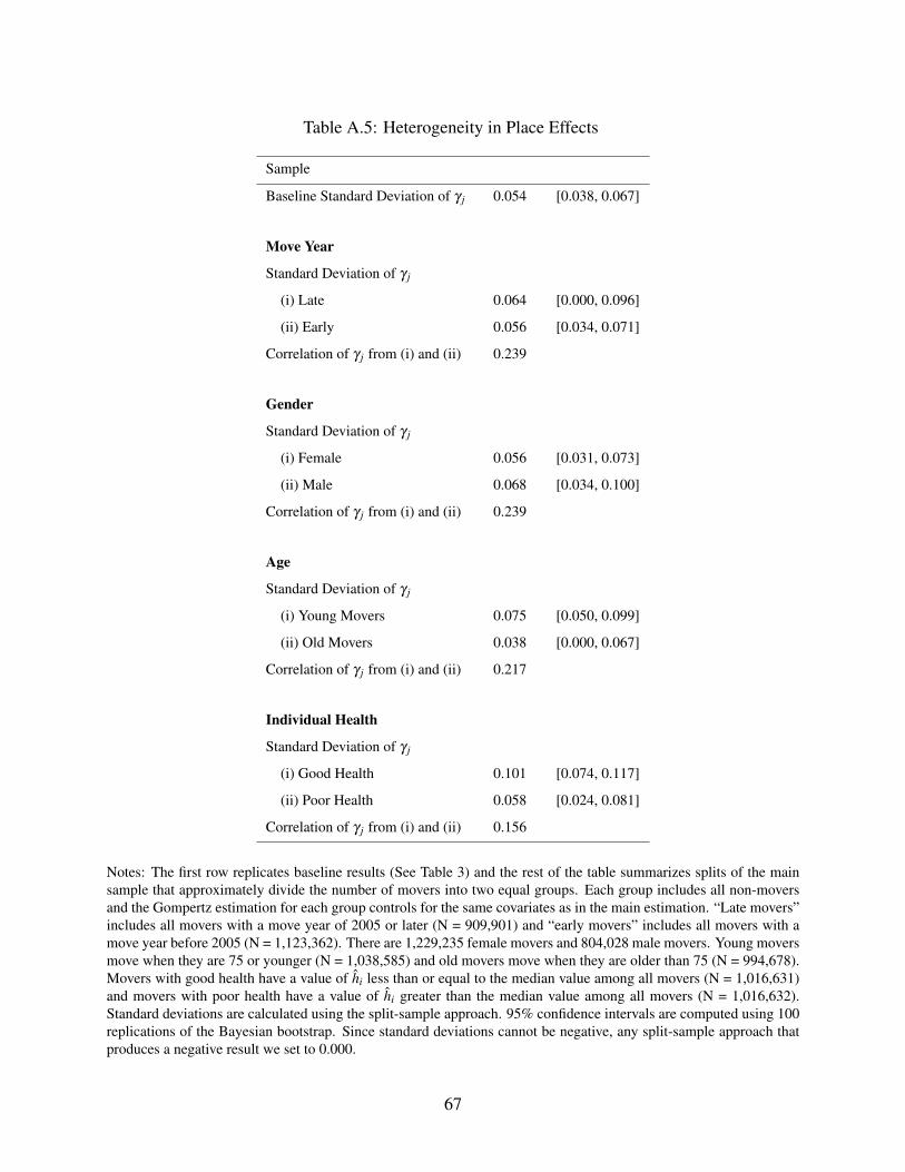
Table A.5: Heterogeneity in Place Effects

Sample

Baseline Standard Deviation of γ j 0.054 [0.038, 0.067]

Move Year

Standard Deviation of γ j

(i) Late 0.064 [0.000, 0.096]

(ii) Early 0.056 [0.034, 0.071]

Correlation of γ j from (i) and (ii) 0.239

Gender

Standard Deviation of γ j

(i) Female 0.056 [0.031, 0.073]

(ii) Male 0.068 [0.034, 0.100]

Correlation of γ j from (i) and (ii) 0.239

Age

Standard Deviation of γ j

(i) Young Movers 0.075 [0.050, 0.099]

(ii) Old Movers 0.038 [0.000, 0.067]

Correlation of γ j from (i) and (ii) 0.217

Individual Health

Standard Deviation of γ j

(i) Good Health 0.101 [0.074, 0.117]

(ii) Poor Health 0.058 [0.024, 0.081]

Correlation of γ j from (i) and (ii) 0.156

Notes: The first row replicates baseline results (See Table 3) and the rest of the table summarizes splits of the mainsample that approximately divide the number of movers into two equal groups. Each group includes all non-moversand the Gompertz estimation for each group controls for the same covariates as in the main estimation. “Late movers”includes all movers with a move year of 2005 or later (N = 909,901) and “early movers” includes all movers with amove year before 2005 (N = 1,123,362). There are 1,229,235 female movers and 804,028 male movers. Young moversmove when they are 75 or younger (N = 1,038,585) and old movers move when they are older than 75 (N = 994,678).Movers with good health have a value of hi less than or equal to the median value among all movers (N = 1,016,631)and movers with poor health have a value of hi greater than the median value among all movers (N = 1,016,632).Standard deviations are calculated using the split-sample approach. 95% confidence intervals are computed using 100replications of the Bayesian bootstrap. Since standard deviations cannot be negative, any split-sample approach thatproduces a negative result we set to 0.000.

67

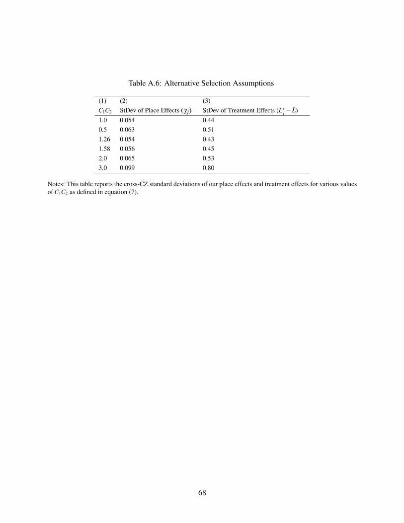
Table A.6: Alternative Selection Assumptions

(1) (2) (3)C1C2 StDev of Place Effects (γ j) StDev of Treatment Effects (L∗j − L)1.0 0.054 0.440.5 0.063 0.511.26 0.054 0.431.58 0.056 0.452.0 0.065 0.533.0 0.099 0.80

Notes: This table reports the cross-CZ standard deviations of our place effects and treatment effects for various valuesof C1C2 as defined in equation (7).

68

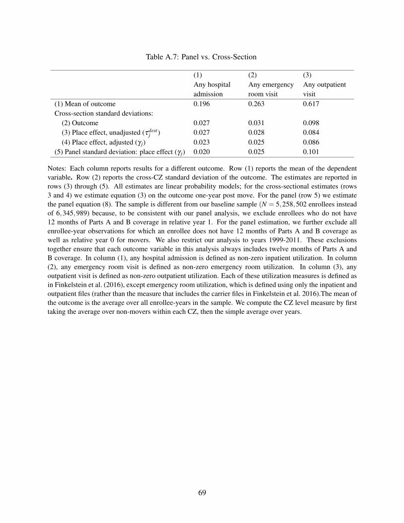
Table A.7: Panel vs. Cross-Section

(1) (2) (3)Any hospitaladmission

Any emergencyroom visit

Any outpatientvisit

(1) Mean of outcome 0.196 0.263 0.617Cross-section standard deviations:

(2) Outcome 0.027 0.031 0.098(3) Place effect, unadjusted (τdest

j ) 0.027 0.028 0.084(4) Place effect, adjusted (γ j) 0.023 0.025 0.086

(5) Panel standard deviation: place effect (γ j) 0.020 0.025 0.101

Notes: Each column reports results for a different outcome. Row (1) reports the mean of the dependentvariable. Row (2) reports the cross-CZ standard deviation of the outcome. The estimates are reported inrows (3) through (5). All estimates are linear probability models; for the cross-sectional estimates (rows3 and 4) we estimate equation (3) on the outcome one-year post move. For the panel (row 5) we estimatethe panel equation (8). The sample is different from our baseline sample (N = 5,258,502 enrollees insteadof 6,345,989) because, to be consistent with our panel analysis, we exclude enrollees who do not have12 months of Parts A and B coverage in relative year 1. For the panel estimation, we further exclude allenrollee-year observations for which an enrollee does not have 12 months of Parts A and B coverage aswell as relative year 0 for movers. We also restrict our analysis to years 1999-2011. These exclusionstogether ensure that each outcome variable in this analysis always includes twelve months of Parts A andB coverage. In column (1), any hospital admission is defined as non-zero inpatient utilization. In column(2), any emergency room visit is defined as non-zero emergency room utilization. In column (3), anyoutpatient visit is defined as non-zero outpatient utilization. Each of these utilization measures is defined asin Finkelstein et al. (2016), except emergency room utilization, which is defined using only the inpatient andoutpatient files (rather than the measure that includes the carrier files in Finkelstein et al. 2016).The mean ofthe outcome is the average over all enrollee-years in the sample. We compute the CZ level measure by firsttaking the average over non-movers within each CZ, then the simple average over years.

69

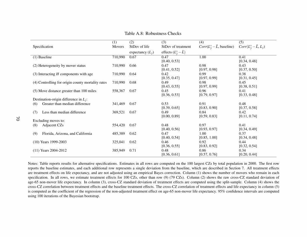
Table A.8: Robustness Checks

(1) (2) (3) (4) (5)Specification Movers StDev of life

expectancy (L j)StDev of treatmenteffects (L∗j − L)

Corr(L∗j − L, baseline) Corr(L∗j − L, L j)

(1) Baseline 710,990 0.67 0.47[0.40, 0.53]

1.00 0.41[0.34, 0.48]

(2) Heterogeneity by mover status 710,990 0.66 0.47[0.41, 0.52]

0.98[0.97, 0.98]

0.43[0.37, 0.50]

(3) Interacting H components with age 710,990 0.64 0.42[0.35, 0.47]

0.99[0.97, 0.99]

0.38[0.31, 0.45]

(4) Controlling for origin county mortality rates 710,990 0.68 0.49[0.43, 0.55]

0.98[0.97, 0.99]

0.45[0.38, 0.51]

(5) Move distance greater than 100 miles 558,367 0.67 0.45[0.36, 0.53]

0.96[0.79, 0.97]

0.41[0.33, 0.48]

Destination-origin difference in L j:(6) Greater than median difference 341,469 0.67 0.53

[0.39, 0.65]0.91[0.83, 0.90]

0.48[0.37, 0.58]

(7) Less than median difference 369,521 0.67 0.49[0.00, 0.89]

0.84[0.59, 0.83]

0.42[0.11, 0.74]

Excluding moves to:(8) Adjacent CZs 554,420 0.67 0.48

[0.40, 0.56]0.97[0.93, 0.97]

0.41[0.34, 0.49]

(9) Florida, Arizona, and California 485,389 0.62 0.47[0.40, 0.54]

1.00[0.85, 1.00]

0.37[0.34, 0.48]

(10) Years 1999-2003 325,041 0.62 0.46[0.36, 0.55]

0.92[0.83, 0.92]

0.44[0.32, 0.54]

(11) Years 2004-2012 385,949 0.71 0.48[0.36, 0.61]

0.86[0.57, 0.76]

0.34[0.20, 0.44]

Notes: Table reports results for alternative specifications. Estimates in all rows are computed on the 100 largest CZs by total population in 2000. The first rowreports the baseline estimates, and each additional row represents a single deviation from the baseline, which are described in Section 7. All treatment effectsare treatment effects on life expectancy, and are not adjusted using an empirical Bayes correction. Column (1) shows the number of movers who remain in eachspecification. In all rows, we estimate treatment effects for 100 CZs, other than row (9) (79 CZs). Column (2) shows the raw cross-CZ standard deviation ofage-65 non-mover life expectancy. In column (3), cross-CZ standard deviation of treatment effects are computed using the split-sample. Column (4) shows thecross-CZ correlation between treatment effects and the baseline treatment effects. The cross-CZ correlation of treatment effects and life expectancy in column (5)is computed as the coefficient of the regression of the non-adjusted treatment effect on age-65 non-mover life expectancy. 95% confidence intervals are computedusing 100 iterations of the Bayesian bootstrap.

70

Table A.9: Sample Restrictions

(1) (2)Enrollees Enrollee-years

Original sample 80,708,181 665,131,064Excluding enrollee-years with age < 65 or age > 99 69,330,956 560,057,853Excluding enrollee-years with incomplete data1 68,935,110 556,340,988

Number of non-movers after sample-wide drops 61,899,201Excluding non-movers without a valid relative year -1 with Traditional Medicare 52,448,582Excluding non-movers without a relative year -1 with 1-year mortality observed 43,147,931Excluding non-movers without a relative year -1 with pre-period controls2 43,145,670

Number of movers after sample-wide drops 7,035,909Excluding movers with more than one move 5,609,064Excluding movers on MA during relative years -1 or 1 4,204,679Excluding “false” movers2 2,564,376Excluding movers for whom we cannot observe one-year mortality 2,033,333Excluding movers with missing pre-period controls 2,033,263

Notes: (1) Data is incomplete if the CZ is missing for an enrollee-year, or an enrollee has gaps in the yearsthey are observed. (2) Pre-period controls consist of health utilization and chronic conditions. (3) Falsemovers are those movers for whom the ratio of the number of claims located in their destination to thenumber located in either their origin or their destination does not increase by at least 0.75 in their post-moveyears relative to their pre-move years.

71

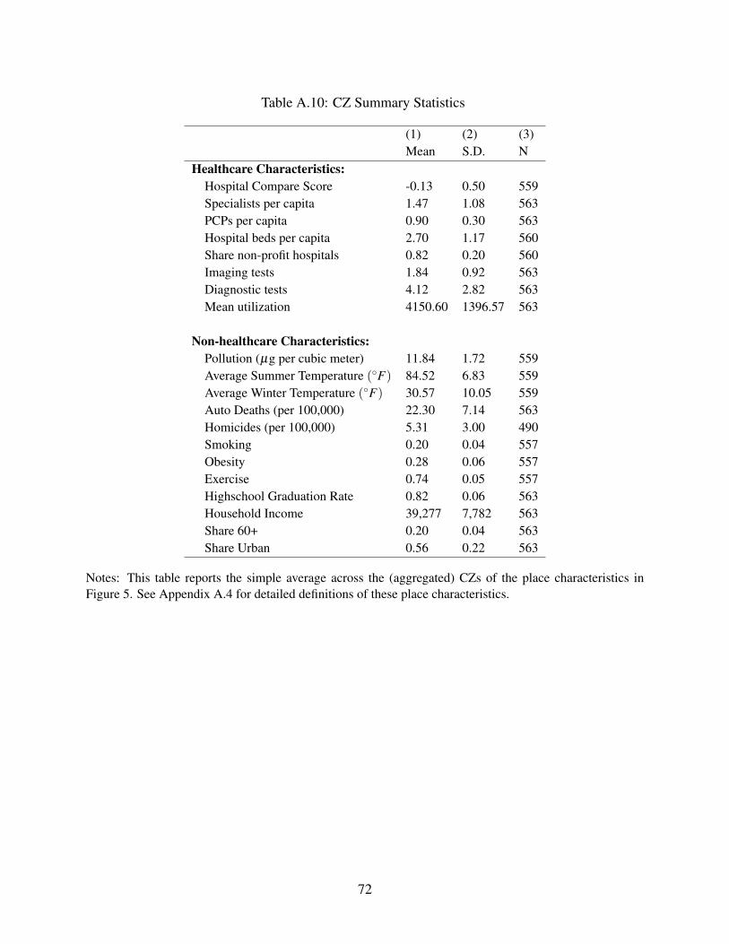
Table A.10: CZ Summary Statistics

(1) (2) (3)Mean S.D. N

Healthcare Characteristics:Hospital Compare Score -0.13 0.50 559Specialists per capita 1.47 1.08 563PCPs per capita 0.90 0.30 563Hospital beds per capita 2.70 1.17 560Share non-profit hospitals 0.82 0.20 560Imaging tests 1.84 0.92 563Diagnostic tests 4.12 2.82 563Mean utilization 4150.60 1396.57 563

Non-healthcare Characteristics:Pollution (µg per cubic meter) 11.84 1.72 559Average Summer Temperature (◦F) 84.52 6.83 559Average Winter Temperature (◦F) 30.57 10.05 559Auto Deaths (per 100,000) 22.30 7.14 563Homicides (per 100,000) 5.31 3.00 490Smoking 0.20 0.04 557Obesity 0.28 0.06 557Exercise 0.74 0.05 557Highschool Graduation Rate 0.82 0.06 563Household Income 39,277 7,782 563Share 60+ 0.20 0.04 563Share Urban 0.56 0.22 563

Notes: This table reports the simple average across the (aggregated) CZs of the place characteristics inFigure 5. See Appendix A.4 for detailed definitions of these place characteristics.

72