PIPE FLOW

Welcome message from author
This document is posted to help you gain knowledge. Please leave a comment to let me know what you think about it! Share it to your friends and learn new things together.
Transcript

PIPE FLOW
PIPE FLOW
A Practical and Comprehensive Guide
DONALD C. RENNELSGeneral Electric Company (ret.)
HOBART M. HUDSONAerojet General Corporation (ret.)
A JOHN WILEY & SONS, INC., PUBLICATION
®
Copyright © 2012 by John Wiley & Sons, Inc. All rights reserved
Published by John Wiley & Sons, Inc., Hoboken, New JerseyPublished simultaneously in Canada
No part of this publication may be reproduced, stored in a retrieval system, or transmitted in any form or by any means, electronic, mechanical, photocopying, recording, scanning, or otherwise, except as permitted under Section 107 or 108 of the 1976 United States Copyright Act, without either the prior written permission of the Publisher, or authorization through payment of the appropriate per-copy fee to the CopyrightClearance Center, Inc., 222 Rosewood Drive, Danvers, MA 01923, (978) 750-8400, fax (978) 750-4470, or on the web at www.copyright.com. Requests to the Publisher for permission should be addressed to the Permissions Department, John Wiley & Sons, Inc., 111 River Street, Hoboken, NJ 07030, (201) 748-6011, fax (201) 748-6008, or online at http://www.wiley.com/go/permissions.
Limit of Liability/Disclaimer of Warranty: While the publisher and author have used their best efforts in preparing this book, they make no representations or warranties with respect to the accuracy or completeness of the contents of this book and specifi cally disclaim any implied warranties of merchantability or fi tness for a particular purpose. No warranty may be created or extended by sales representatives or written sales materials. The advice and strategies contained herein may not be suitable for your situation. You should consult with a professional where appropriate. Neither the publisher nor author shall be liable for any loss of profi t or any other commercial damages, including but not limited to special, incidental, consequential, or other damages.
For general information on our other products and services or for technical support, please contact our Customer Care Department within the United States at (800) 762-2974, outside the United States at (317) 572-3993 or fax (317) 572-4002.
Wiley also publishes its books in a variety of electronic formats. Some content that appears in print may not be available in electronic formats. For more information about Wiley products, visit our web site at www.wiley.com.
Library of Congress Cataloging-in-Publication Data:
Rennels, Donald C., 1937– Pipe fl ow : a practical and comprehensive guide / Donald C Rennels, Hobart M Hudson. p. cm. Includes bibliographical references and index. ISBN 978-0-470-90102-1 (cloth) 1. Pipe–Fluid dynamics. 2. Water-pipes–Hydrodynamics. 3. Fluid mechanics. I. Hudson, Hobart M., 1931– II. Title. TJ935.R46 2012 620.1'064–dc23 2011043325
Printed in the United States of America
9780470901021
10 9 8 7 6 5 4 3 2 1

Knowledge shared is everything.
Knowledge kept is nothing. — Richard Beere,
Abbot of Glastonbury (1493 – 1524)
CONTENTS
v
PREFACE xv
NOMENCLATURE xvii
Abbreviation and Defi nition xix
PART I METHODOLOGY 1
Prologue 1
1 FUNDAMENTALS 3
1.1 Systems of Units 31.2 Fluid Properties 4
1.2.1 Pressure 41.2.2 Density 51.2.3 Velocity 51.2.4 Energy 51.2.5 Viscosity 51.2.6 Temperature 51.2.7 Heat 6
1.3 Important Dimensionless Ratios 61.3.1 Reynolds Number 61.3.2 Relative Roughness 61.3.3 Loss Coeffi cient 71.3.4 Mach Number 71.3.5 Froude Number 71.3.6 Reduced Pressure 71.3.7 Reduced Temperature 7
1.4 Equations of State 71.4.1 Equation of State of Liquids 71.4.2 Equation of State of Gases 8
1.5 Fluid Velocity 81.6 Flow Regimes 8References 12Further Reading 12
vi CONTENTS
2 CONSERVATION EQUATIONS 13
2.1 Conservation of Mass 132.2 Conservation of Momentum 132.3 The Momentum Flux Correction Factor 142.4 Conservation of Energy 16
2.4.1 Potential Energy 162.4.2 Pressure Energy 172.4.3 Kinetic Energy 172.4.4 Heat Energy 172.4.5 Mechanical Work Energy 18
2.5 General Energy Equation 182.6 Head Loss 182.7 The Kinetic Energy Correction Factor 192.8 Conventional Head Loss 202.9 Grade Lines 20References 21Further Reading 21
3 INCOMPRESSIBLE FLOW 23
3.1 Conventional Head Loss 233.2 Sources of Head Loss 23
3.2.1 Surface Friction Loss 243.2.1.1 Laminar Flow 243.2.1.2 Turbulent Flow 243.2.1.3 Reynolds Number 253.2.1.4 Friction Factors 25
3.2.2 Induced Turbulence 283.2.3 Summing Loss Coeffi cients 29
References 29Further Reading 30
4 COMPRESSIBLE FLOW 31
4.1 Problem Solution Methods 314.2 Approximate Compressible Flow Using Incompressible
Flow Equations 324.2.1 Using Inlet or Outlet Properties 324.2.2 Using Average of Inlet and Outlet Properties 33
4.2.2.1 Simple Average Properties 334.2.2.2 Comprehensive Average Properties 34
4.2.3 Using Expansion Factors 344.3 Adiabatic Compressible Flow with Friction: Ideal Equation 37
4.3.1 Using Mach Number as a Parameter 374.3.1.1 Solution when Static Pressure and Static
Temperature Are Known 384.3.1.2 Solution when Static Pressure and Total
Temperature Are Known 394.3.1.3 Solution when Total Pressure and Total
Temperature Are Known 404.3.1.4 Solution when Total Pressure and Static
Temperature Are Known 404.3.1.5 Treating Changes in Area 40
4.3.2 Using Static Pressure and Temperature as Parameters 414.4 Isothermal Compressible Flow with Friction: Ideal Equation 42
CONTENTS vii
4.5 Example Problem: Compressible Flow through Pipe 43References 47Further Reading 47
5 NETWORK ANALYSIS 49
5.1 Coupling Effects 495.2 Series Flow 505.3 Parallel Flow 505.4 Branching Flow 515.5 Example Problem: Ring Sparger 51
5.5.1 Ground Rules and Assumptions 525.5.2 Input Parameters 525.5.3 Initial Calculations 535.5.4 Network Equations 53
5.5.4.1 Continuity Equations 535.5.4.2 Energy Equations 53
5.5.5 Solution 545.6 Example Problem: Core Spray System 54
5.6.1 New, Clean Steel Pipe 555.6.1.1 Ground Rules and Assumptions 555.6.1.2 Input Parameters 565.6.1.3 Initial Calculations 575.6.1.4 Adjusted Parameters 575.6.1.5 Network Flow Equations 575.6.1.6 Solution 58
5.6.2 Moderately Corroded Steel Pipe 585.6.2.1 Ground Rules and Assumptions 585.6.2.2 Input Parameters 585.6.2.3 Adjusted Parameters 595.6.2.4 Network Flow Equations 595.6.2.5 Solution 59
References 60Further Reading 60
6 TRANSIENT ANALYSIS 61
6.1 Methodology 616.2 Example Problem: Vessel Drain Times 62
6.2.1 Upright Cylindrical Vessel 626.2.2 Spherical Vessel 636.2.3 Upright Cylindrical Vessel with Elliptical Heads 64
6.3 Example Problem: Positive Displacement Pump 656.3.1 No Heat Transfer 656.3.2 Heat Transfer 66
6.4 Example Problem: Time-Step Integration 676.4.1 Upright Cylindrical Vessel Drain Problem 676.4.2 Direct Solution 676.4.3 Time-Step Solution 67
References 68Further Reading 68
7 UNCERTAINTY 69
7.1 Error Sources 697.2 Pressure Drop Uncertainty 69
viii CONTENTS
7.3 Flow Rate Uncertainty 717.4 Example Problem: Pressure Drop 71
7.4.1 Input Data 717.4.2 Solution 72
7.5 Example Problem: Flow Rate 727.5.1 Input Data 727.5.2 Solution 73
PART II LOSS COEFFICIENTS 75
Prologue 75
8 SURFACE FRICTION 77
8.1 Friction Factor 778.1.1 Laminar Flow Region 778.1.2 Critical Zone 778.1.3 Turbulent Flow Region 78
8.1.3.1 Smooth Pipes 788.1.3.2 Rough Pipes 78
8.2 The Colebrook–White Equation 788.3 The Moody Chart 798.4 Explicit Friction Factor Formulations 79
8.4.1 Moody’s Approximate Formula 798.4.2 Wood’s Approximate Formula 798.4.3 The Churchill 1973 and Swamee and Jain Formulas 798.4.4 Chen’s Formula 798.4.5 Shacham’s Formula 808.4.6 Barr’s Formula 808.4.7 Haaland’s Formulas 808.4.8 Manadilli’s Formula 808.4.9 Romeo’s Formula 808.4.10 Evaluation of Explicit Alternatives to the
Colebrook–White Equation 808.5 All-Regime Friction Factor Formulas 81
8.5.1 Churchill’s 1977 Formula 818.5.2 Modifi cations to Churchill’s 1977 Formula 81
8.6 Surface Roughness 828.6.1 New, Clean Pipe 828.6.2 The Relationship between Absolute Roughness and
Friction Factor 828.6.3 Inherent Margin 848.6.4 Loss of Flow Area 848.6.5 Machined Surfaces 84
8.7 Noncircular Passages 85References 87Further Reading 87
9 ENTRANCES 89
9.1 Sharp-Edged Entrance 899.1.1 Flush Mounted 899.1.2 Mounted at a Distance 909.1.3 Mounted at an Angle 90
CONTENTS ix
9.2 Rounded Entrance 919.3 Beveled Entrance 919.4 Entrance through an Orifi ce 92
9.4.1 Sharp-Edged Orifi ce 929.4.2 Round-Edged Orifi ce 939.4.3 Thick-Edged Orifi ce 939.4.4 Beveled Orifi ce 93
References 99Further Reading 99
10 CONTRACTIONS 101
10.1 Flow Model 10110.2 Sharp-Edged Contraction 10210.3 Rounded Contraction 10310.4 Conical Contraction 104
10.4.1 Surface Friction Loss 10510.4.2 Local Loss 105
10.5 Beveled Contraction 10610.6 Smooth Contraction 10710.7 Pipe Reducer: Contracting 107References 112Further Reading 112
11 EXPANSIONS 113
11.1 Sudden Expansion 11311.2 Straight Conical Diffuser 11411.3 Multistage Conical Diffusers 117
11.3.1 Stepped Conical Diffuser 11711.3.2 Two-Stage Conical Diffuser 118
11.4 Curved Wall Diffuser 12011.5 Pipe Reducer: Expanding 121References 128Further Reading 128
12 EXITS 131
12.1 Discharge from a Straight Pipe 13112.2 Discharge from a Conical Diffuser 13212.3 Discharge from an Orifi ce 132
12.3.1 Sharp-Edged Orifi ce 13212.3.2 Round-Edged Orifi ce 13312.3.3 Thick-Edged Orifi ce 13312.3.4 Bevel-Edged Orifi ce 133
12.4 Discharge from a Smooth Nozzle 134
13 ORIFICES 139
13.1 Generalized Flow Model 13913.2 Sharp-Edged Orifi ce 140
13.2.1 In a Straight Pipe 14013.2.2 In a Transition Section 14113.2.3 In a Wall 141
x CONTENTS
13.3 Round-Edged Orifi ce 14213.3.1 In a Straight Pipe 14313.3.2 In a Transition Section 14313.3.3 In a Wall 144
13.4 Bevel-Edged Orifi ce 14513.4.1 In a Straight Pipe 14513.4.2 In a Transition Section 14513.4.3 In a Wall 146
13.5 Thick-Edged Orifi ce 14613.5.1 In a Straight Pipe 14613.5.2 In a Transition Section 14813.5.3 In a Wall 148
13.6 Multihole Orifi ces 14913.7 Noncircular Orifi ces 149References 154Further Reading 154
14 FLOW METERS 157
14.1 Flow Nozzle 15714.2 Venturi Tube 15814.3 Nozzle/Venturi 159References 161Further Reading 161
15 BENDS 163
15.1 Elbows and Pipe Bends 16315.2 Coils 166
15.2.1 Constant Pitch Helix 16715.2.2 Constant Pitch Spiral 167
15.3 Miter Bends 16815.4 Coupled Bends 16915.5 Bend Economy 169References 174Further Reading 174
16 TEES 177
16.1 Diverging Tees 17816.1.1 Flow through Run 17816.1.2 Flow through Branch 17916.1.3 Flow from Branch 182
16.2 Converging Tees 18216.2.1 Flow through Run 18216.2.2 Flow through Branch 18416.2.3 Flow into Branch 185
References 200Further Reading 200
17 PIPE JOINTS 201
17.1 Weld Protrusion 20117.2 Backing Rings 20217.3 Misalignment 203
17.3.1 Misaligned Pipe Joint 20317.3.2 Misaligned Gasket 203
CONTENTS xi
18 VALVES 205
18.1 Multiturn Valves 20518.1.1 Diaphragm Valve 20518.1.2 Gate Valve 20618.1.3 Globe Valve 20618.1.4 Pinch Valve 20718.1.5 Needle Valve 207
18.2 Quarter-Turn Valves 20718.2.1 Ball Valve 20818.2.2 Butterfl y Valve 20818.2.3 Plug Valve 208
18.3 Self-Actuated Valves 20918.3.1 Check Valve 20918.3.2 Relief Valve 210
18.4 Control Valves 21018.5 Valve Loss Coeffi cients 211References 211Further Reading 212
19 THREADED FITTINGS 213
19.1 Reducers: Contracting 21319.2 Reducers: Expanding 21319.3 Elbows 21419.4 Tees 21419.5 Couplings 21419.6 Valves 215Reference 215
PART III FLOW PHENOMENA 217
Prologue 217
20 CAVITATION 219
20.1 The Nature of Cavitation 21920.2 Pipeline Design 22020.3 Net Positive Suction Head 22020.4 Example Problem: Core Spray Pump 221
20.4.1 New, Clean Steel Pipe 22220.4.1.1 Input Parameters 22220.4.1.2 Solution 22220.4.1.3 Results 222
20.4.2 Moderately Corroded Steel Pipe 22220.4.2.1 Input Parameters 22320.4.2.2 Solution 22320.4.2.3 Results 224
Reference 224Further Reading 224
21 FLOW-INDUCED VIBRATION 225
21.1 Steady Internal Flow 22521.2 Steady External Flow 22521.3 Water Hammer 226
xii CONTENTS
21.4 Column Separation 227References 228Further Reading 228
22 TEMPERATURE RISE 231
22.1 Reactor Heat Balance 23222.2 Vessel Heat Up 23222.3 Pumping System Temperature 232References 233
23 FLOW TO RUN FULL 235
23.1 Open Flow 23523.2 Full Flow 23723.3 Submerged Flow 23723.4 Reactor Application 239Further Reading 240
APPENDIX A PHYSICAL PROPERTIES OF WATER AT 1 ATMOSPHERE 241
APPENDIX B PIPE SIZE DATA 245
B.1 Commercial Pipe Data 246
APPENDIX C PHYSICAL CONSTANTS AND UNIT CONVERSIONS 253
C.1 Important Physical Constants 253C.2 Unit Conversions 254
APPENDIX D COMPRESSIBILITY FACTOR EQUATIONS 263
D.1 The Redlich–Kwong Equation 263D.2 The Lee–Kesler Equation 264D.3 Important Constants for Selected Gases 266
APPENDIX E ADIABATIC COMPRESSIBLE FLOW WITH FRICTION, USING MACH NUMBER AS A PARAMETER 269
E.1 Solution when Static Pressure and Static Temperature Are Known 269E.2 Solution when Static Pressure and Total Temperature Are Known 272E.3 Solution when Total Pressure and Total Temperature Are Known 272E.4 Solution when Total Pressure and Static Temperature Are Known 273References 274
APPENDIX F VELOCITY PROFILE EQUATIONS 275
F.1 Benedict Velocity Profi le Derivation 275F.2 Street, Watters, and Vennard Velocity Profi le Derivation 277References 278
INDEX 279
PREFACE
xv
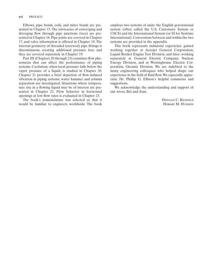
This book provides practical and comprehensive infor-mation on the subject of pressure drop and other phenomena in fl uid fl ow in pipes. The importance of piping systems in distribution systems, in industrial operations, and in modern power plants justifi es a book devoted exclusively to this subject. The emphasis is on fl ow in piping components and piping systems where greatest benefi t will derive from accurate prediction of pressure loss.
A great deal of experimental and theoretical research on fl uid fl ow in pipes and their components has been reported over the years. However, the basic methodol-ogy in fl uid fl ow textbooks is usually fragmented, scat-tered throughout several chapters and paragraphs; and useful, practical information is diffi cult to sort out. Moreover, textbooks present very little loss coeffi cient data, and those that are given are desperately out of date. Elsewhere, experimental data and published for-mulas for loss coeffi cients have provided results that are in considerable disagreement. Into the bargain, researchers have not accounted for all possible fl ow confi gurations and their results are not always presented in a readily useful form. This book addresses and fi xes these defi ciencies.
Instead of having to search and read through various sources, this book provides the user with virtually all the information required to design and analyze piping systems. Example problems, their setups, and solutions are provided throughout the book. Most parts of the book will be easily understood by those who are not experts in the fi eld.
Part I (Chapters 1 through 7 ) contains the essential methodology required to solve accurately pipe fl ow problems. Chapter 1 provides knowledge of the physical properties of fl uids and the nature of fl uid fl ow. Chapter
2 presents the basic principles of conservation of mass, momentum, and energy, and introduces the concepts of head loss and energy grade line. Chapter 3 presents the conventional head loss equation and characterizes the two sources of head loss — surface friction and induced turbulence. Several compressible fl ow calcula-tion methods are presented in Chapter 4 . The straight-forward setup of series, parallel, and branching fl ow networks, including sample problems, is presented in Chapter 5 . Chapter 6 introduces the basic methodology for solving transient fl ow problems, with specifi c exam-ples. A method to assess the uncertainty associated with pipe fl ow calculations is presented in Chapter 7 .
Part II (Chapters 8 through 19 ) presents consistent and reliable loss coeffi cient data on fl ow confi gurations most common to piping systems. Experimental test data and published formulas from worldwide sources are examined, integrated, and arranged into widely appli-cable equations — a valuable resource in this computer age. The results are also presented in straightforward tables and diagrams. The processes used to select and develop loss coeffi cient data for the various fl ow con-fi gurations are presented so the user can judge the merits of the results and the researcher can identify areas where further research is needed.
Friction factor, the main element of surface friction loss, is presented in Chapter 8 as an adjunct to quantify-ing the various features that contribute to head loss.
The fl ow confi gurations presented in Chapters 9 through 14 (entrances, contractions, expansions, exits, orifi ces, and fl ow meters) all exhibit some degree of fl ow contraction and/or expansion. As such, they have been treated as a family; where suffi cient data for any one particular confi guration were lacking, they were aug-mented by suffi cient data in another.
xvi PREFACE
Elbows, pipe bends, coils, and miter bends are pre-sented in Chapter 15 . The intricacies of converging and diverging fl ow through pipe junctions (tees) are pre-sented in Chapter 16 . Pipe joints are covered in Chapter 17 , and valve information is offered in Chapter 18 . The internal geometry of threaded (screwed) pipe fi ttings is discontinuous, creating additional pressure loss; and they are covered separately in Chapter 19 .
Part III (Chapters 20 through 23 ) examines fl ow phe-nomena that can affect the performance of piping systems. Cavitation, when local pressure falls below the vapor pressure of a liquid, is studied in Chapter 20 . Chapter 21 provides a brief depiction of fl ow - induced vibration in piping systems; water hammer and column separation are investigated. Situations where tempera-ture rise in a fl owing liquid may be of interest are pre-sented in Chapter 22 . Flow behavior in horizontal openings at low fl ow rates is evaluated in Chapter 23 .
The book ’ s nomenclature was selected so that it would be familiar to engineers worldwide. The book
employs two systems of units: the English gravitational system (often called the U.S. Customary System or USCS) and the International System (or SI for Syst è me International). Conversions between and within the two systems are provided in the appendix.
This book represents industrial experience gained working together at Aerojet General Corporation, Liquid Rocket Engine Test Division, and later, working separately at General Electric Company, Nuclear Energy Division, and at Westinghouse Electric Cor-poration, Oceanic Division. We are indebted to the many engineering colleagues who helped shape our experience in the fi eld of fl uid fl ow. We especially appre-ciate Dr. Phillip G. Ellison ’ s helpful comments and suggestions.
We acknowledge the understanding and support of our wives, Bel and Joan.
D onald C. R ennels H obart M. H udson
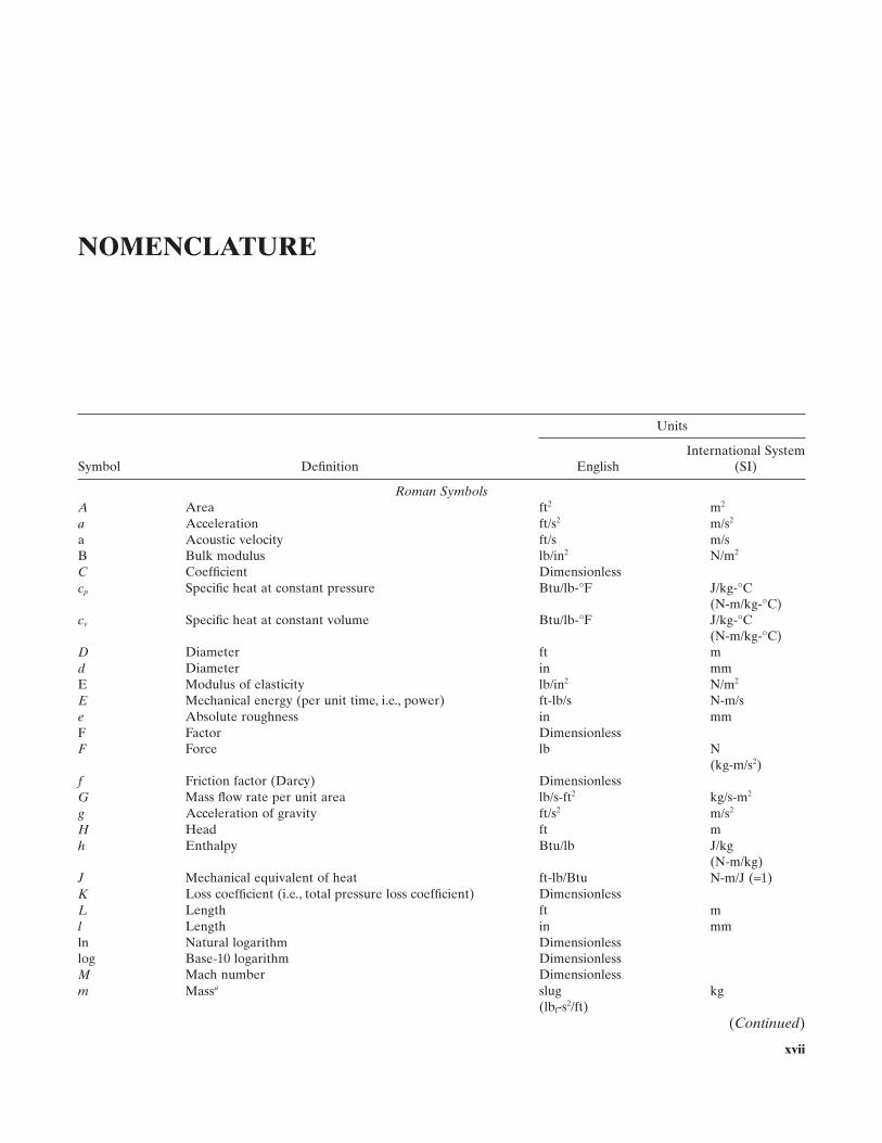
NOMENCLATURE
xvii
Symbol Defi nition
Units
English International System
(SI)
Roman SymbolsA Area ft 2 m 2
a Acceleration ft/s 2 m/s 2
a Acoustic velocity ft/s m/s B Bulk modulus lb/in 2 N/m 2
C Coeffi cient Dimensionless cp Specifi c heat at constant pressure Btu/lb - ° F J/kg - ° C
(N - m/kg - ° C) cv Specifi c heat at constant volume Btu/lb - ° F J/kg - ° C
(N - m/kg - ° C) D Diameter ft m d Diameter in mm E Modulus of elasticity lb/in 2 N/m 2
E Mechanical energy (per unit time, i.e., power) ft - lb/s N - m/s e Absolute roughness in mm F Factor Dimensionless F Force lb N
(kg - m/s 2 ) f Friction factor (Darcy) Dimensionless G Mass fl ow rate per unit area lb/s - ft 2 kg/s - m 2
g Acceleration of gravity ft/s 2 m/s 2
H Head ft m h Enthalpy Btu/lb J/kg
(N - m/kg) J Mechanical equivalent of heat ft - lb/Btu N - m/J ( = 1) K Loss coeffi cient (i.e., total pressure loss coeffi cient) Dimensionless L Length ft m l Length in mm ln Natural logarithm Dimensionless log Base - 10 logarithm Dimensionless M Mach number Dimensionless m Mass a slug kg
(lb f - s 2 /ft) (Continued)
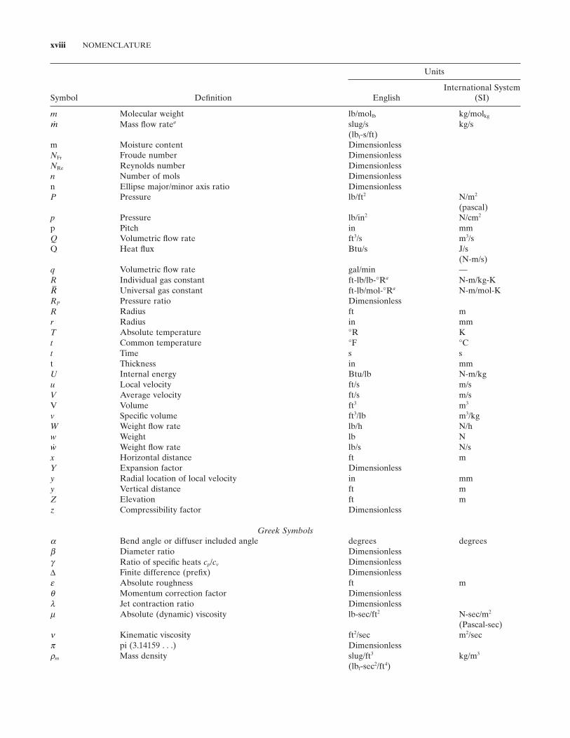
xviii NOMENCLATURE
Symbol Defi nition
Units
English International System
(SI)
m Molecular weight lb/mol lb kg/mol kg
m Mass fl ow rate a slug/s kg/s (lb f - s/ft)
m Moisture content Dimensionless NFr Froude number Dimensionless NRe Reynolds number Dimensionless n Number of mols Dimensionless n Ellipse major/minor axis ratio Dimensionless P Pressure lb/ft 2 N/m 2
(pascal) p Pressure lb/in 2 N/cm 2
p Pitch in mm Q Volumetric fl ow rate ft 3 /s m 3 /s Q Heat fl ux Btu/s J/s
(N - m/s) q Volumetric fl ow rate gal/min — R Individual gas constant ft - lb/lb - ° R a N - m/kg - K R Universal gas constant ft - lb/mol - ° R a N - m/mol - K RP Pressure ratio Dimensionless R Radius ft m r Radius in mm T Absolute temperature ° R K t Common temperature ° F ° C t Time s s t Thickness in mm U Internal energy Btu/lb N - m/kg u Local velocity ft/s m/s V Average velocity ft/s m/s V Volume ft 3 m 3
v Specifi c volume ft 3 /lb m 3 /kg W Weight fl ow rate lb/h N/h w Weight lb N w Weight fl ow rate lb/s N/s x Horizontal distance ft m Y Expansion factor Dimensionless y Radial location of local velocity in mm y Vertical distance ft m Z Elevation ft m z Compressibility factor Dimensionless
Greek Symbolsα Bend angle or diffuser included angle degrees degrees β Diameter ratio Dimensionless γ Ratio of specifi c heats cp / cv Dimensionless Δ Finite difference (prefi x) Dimensionless ε Absolute roughness ft m θ Momentum correction factor Dimensionless λ Jet contraction ratio Dimensionless µ Absolute (dynamic) viscosity lb - sec/ft 2 N - sec/m 2
(Pascal - sec) ν Kinematic viscosity ft 2 /sec m 2 /sec π pi (3.14159 . . . ) Dimensionless ρm Mass density slug/ft 3 kg/m 3
(lb f - sec 2 /ft 4 )
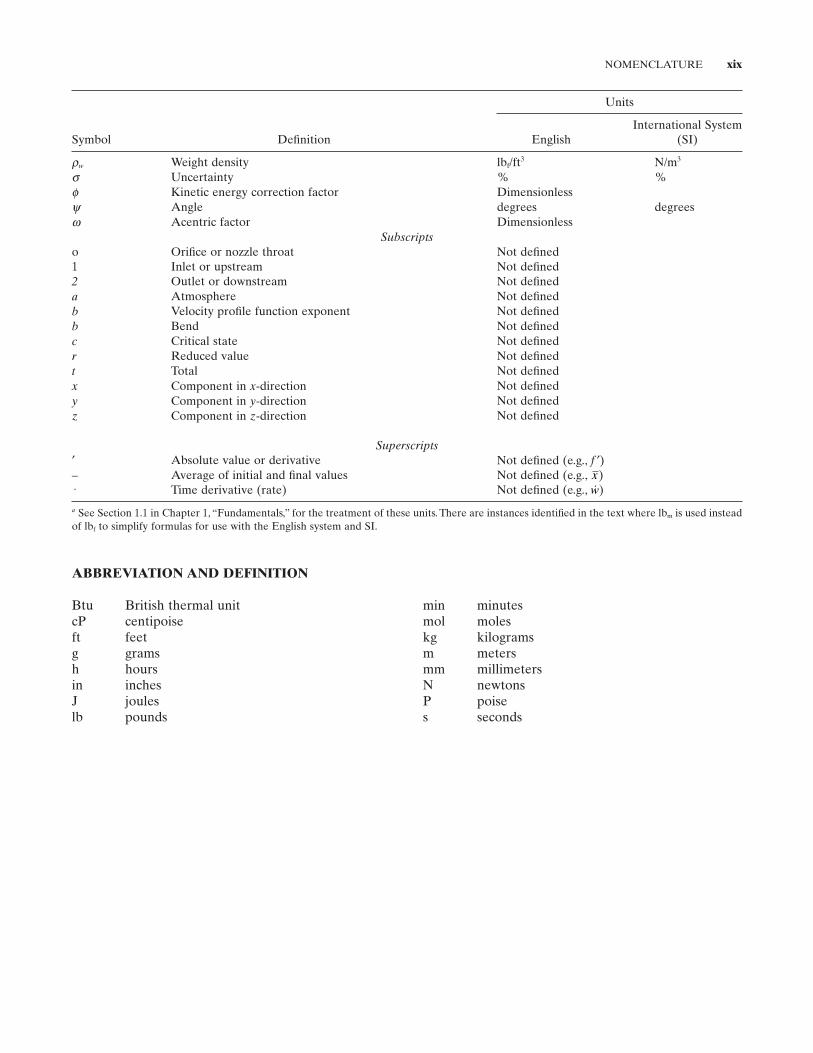
NOMENCLATURE xix
Symbol Defi nition
Units
English International System
(SI)
ρw Weight density lb f /ft 3 N/m 3
σ Uncertainty % % ϕ Kinetic energy correction factor Dimensionless ψ Angle degrees degrees ω Acentric factor Dimensionless
Subscripts o Orifi ce or nozzle throat Not defi ned 1 Inlet or upstream Not defi ned 2 Outlet or downstream Not defi ned a Atmosphere Not defi ned b Velocity profi le function exponent Not defi ned b Bend Not defi ned c Critical state Not defi ned r Reduced value Not defi ned t Total Not defi ned x Component in x - direction Not defi ned y Component in y - direction Not defi ned z Component in z - direction Not defi ned
Superscripts′ Absolute value or derivative Not defi ned (e.g., f ′ ) – Average of initial and fi nal values Not defi ned (e.g., x)⋅ Time derivative (rate) Not defi ned (e.g., w)
a See Section 1.1 in Chapter 1 , “ Fundamentals, ” for the treatment of these units. There are instances identifi ed in the text where lb m is used instead of lb f to simplify formulas for use with the English system and SI.
ABBREVIATION AND DEFINITION
Btu British thermal unit min minutes cP centipoise mol moles ft feet kg kilograms g grams m meters h hours mm millimeters in inches N newtons J joules P poise lb pounds s seconds
PART I
METHODOLOGY
to fl esh out Prandtl ’ s smooth pipe friction factor formula and Theodor von K á rm á n ’ s complete turbulence formula (1930). Discrepancies between Nikuradse ’ s artifi cially roughened pipe data and data on commercial pipe were resolved by Cyril F. Colebrook and Cedric M. White (1937). Colebrook published a semiration- al formula for random roughness (1939) that is still used today.
Chapter 4 , “ Compressible Flow, ” gives several ways to calculate head loss in compressible fl ow in pipes using approximate formulas derived from incompressible fl ow formulas. It culminates in giving theoretical formu-las for compressible fl ow using either the Mach number or absolute pressure. While the formulas are compli-cated enough to resist explicit solution, ways are given to solve them by trial - and - error methods.
Chapter 5 , “ Network Analysis, ” gives methods to solve distribution of fl ow in networks. Chapter 6 , “ Tran-sient Analysis, ” provides methods for solving fl ow problems whose fl ow rates are not constant. Chapter 7 , “ Uncertainty Analysis, ” gives methods for estimating the probable error or uncertainty in predicting pressure drop and fl ow rate.
PROLOGUE
Part I of this work consists of Chapters 1 through 7 . These chapters, with the exception of Chapters 5 – 7 , establish the basic “ rules of the road, ” so to speak.
Chapter 1 , “ Fundamentals, ” discloses the systems of units that are used throughout the book, nomenclature and meanings of fl uid properties, important dimension-less ratios, equations of state, and expositions of fl ow velocity and fl ow regimes.
Chapter 2 , “ Conservation Equations, ” elaborates on the conservation equations, that is, conservation of mass, of momentum and of energy. The general energy equa-tion, head loss, and grade lines are treated under con-servation of energy.
Chapter 3 , “ Incompressible Flow, ” expounds on how the particulars of incompressible fl ow (i.e., fl ow of liquids) became known through the breakthroughs of Julius Weisbach (head loss formula, 1845), Osborne Reynolds (the Reynolds number, 1883), and Ludwig Prandtl (boundary layers and the smooth pipe friction factor formula, 1904 – 1929). Johann Nikuradse ’ s artifi -cially roughened pipe experiments provided data (1933)
1
Pipe Flow: A Practical and Comprehensive Guide, First Edition. Donald C. Rennels and Hobart M. Hudson.© 2012 John Wiley & Sons, Inc. Published 2012 by John Wiley & Sons, Inc.
3
1 FUNDAMENTALS
In this chapter we consider the fundamentals concern-ing fl uid fl ow systems, such as the systems of units employed in this work, the physical properties of fl uids, and the nature of fl uid fl ow.
1.1 SYSTEMS OF UNITS
This book employs two systems of units: the U.S. Cus-tomary System (or USCS) and the International System (or SI, for Syst è me International). The latter is based on the metric system, a system devised in France during the French Revolution in the late 1700s, but uses interna-tionally standardized physical constants. Conversions between the systems may be found in Appendix C .
The USCS is virtually indistinguishable from the English gravitational system. There is some confusion in regard to the differences. Some authors imply that in USCS the slug is basic and the pound is derived, while others hold that the pound is basic and the slug is derived. In the English gravitational system the latter is assumed. For general engineering use it does not matter which is basic, because both systems agree that there is the slug for mass, the pound for force, the foot for length, and the second for time. This is all that need concern us in this work. The SI, derived from the metric system and having a much shorter pedigree, is consequently much more standardized.
Much confusion has resulted from the use in both English and metric systems of the same terms for the units of force and mass. To help eliminate the ambiguity
owing to this double use the following treatment has been adopted.
The equation relating force, mass, and acceleration is
F ma= , (1.1)
where F , m , and a are defi ned in the nomenclature. In SI the unit of mass, the kilogram, is basic. The unit of force is derived by means of the equation above and is given a unique name, the newton. Mass is never referred to by force units and vice versa. In the English gravita-tional system (which predates the USCS) and the USCS, a similar set of units is available and familiar to engi-neers, but it is not uniformly used. The unit of force, the pound, can be considered to be basic and the unit of mass derived by means of the relation above. It is often called the slug. While the slug is not often used, its inser-tion here need not pose any inconvenience. Where mass units are called for they may be easily obtained from the pound - force unit by the use of Equation 1.1 . By use of these conventions any fundamental equation given in this book may be used with either SI or English units.
It should be noted that Equation 1.1 returns, in the English gravitational system, a mass with units of lb f - s 2 /ft. This is not easily recognizable, so the engineering community has somewhat arbitrarily chosen the term “ slug ” to name the mass instead of lb f - s 2 /ft. Similarly, in SI, the force that comes out of the equation has units of kg - m/s 2 , and this force has been given the name “ newton. ” The equation does not contain a factor that transforms lb f - s 2 /ft to “ slugs ” or kg - m/s 2 to “ newtons. ”
Pipe Flow: A Practical and Comprehensive Guide, First Edition. Donald C. Rennels and Hobart M. Hudson.© 2012 John Wiley & Sons, Inc. Published 2012 by John Wiley & Sons, Inc.
4 FUNDAMENTALS
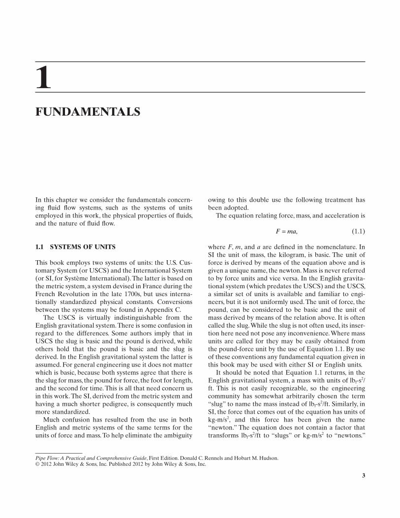
Atmospheric Pressure : The absolute pressure of the local atmosphere.
Standard Atmospheric Pressure : The absolute pres-sure of the standard atmosphere at mean sea level. Standard atmospheric pressure, or one atmosphere, is 14.696 lb/in 2 , 760.0 mm of mercury, 1.01325 × 10 5 N/m 2 (pascals), or 1.01325 bar.
Barometric Pressure : A barometer is an instrument used to measure atmospheric pressure by using water, air, or mercury. Thus atmospheric pressure is often called barometric pressure.
Critical Pressure : The pressure of a pure substance at its critical state ; where the density of the satu-rated liquid is the same as the density of the satu-rated vapor. At pressures higher than the critical, a liquid may be heated from a low temperature to a very high one without any discontinuity indicat-ing a change from the liquid to vapor phase. Values of critical pressure for selected gases are given in Appendix D .3.
Differential Pressure : The calculated or measured difference in pressure between any two points of interest. ‡
Gauge Pressure : The pressure measured with respect to local atmospheric pressure. This is the pres-sure read by the common pressure gauge whose detecting element is a coil of fl attened tube. (Sometimes this pressure is relative to standard atmospheric pressure. The reader is advised to determine which datum is used in other works or information sources.) §
We knowingly or unknowingly assume that there is an implicit conversion factor that changes the names of these units. This factor for SI is N/(kg - m/s 2 )/(kg), and in the English gravitational system it is lb f /slug - ft/s 2 . If you call these conversion factors “ Cg , ” Equation 1.1 becomes:
F C m agnewtons N/ kg-m/s kg m/s= ×[ , ( )][ ] [ ( )],2 2
or
F C m aglb lb/ slug-ft/s slug ft/sf = ⋅ ×[ , ( )][ ] [ ( )].2 2
The numeric value of the conversion factor is 1.000, so it does not change the number obtained, but only the name of the number. This may be the reason many writers subscript the g with a c to obtain gc , when a is the acceleration of gravity.
Unfortunately the modern engineer must deal with mixed units and nomenclature used in some current practice and remaining from past practice. Conversions are offered in Appendix C that can help the user to work with mixed units. (Some secondary equations are given in which the units are mixed for the convenience of users of the English gravitational system. These equa-tions and the units they require will be clearly indicated in the text.) Appendix C gives the important base units and derived units used here as well as the most fre-quently used conversions between systems.
1.2 FLUID PROPERTIES
Understanding the subject of pressure loss in fl uid fl ow requires an understanding of the fl uid properties that cause it. The principal concepts of interest in pressure loss due to fl ow are pressure, density, velocity, energy, and viscosity. Of secondary interest are temperature and heat.
1.2.1 Pressure
Pressure: The force per unit area exerted by a fl uid on an arbitrarily defi ned boundary or surface, usually the walls of the conduit in which the fl uid is fl owing, or its cross section. Pressures are mea-sured and quoted in different ways. A picture of pressure relationships can be gained from a diagram such as that of Figure 1.1 , in which are shown two typical pressures, one above, and the other below, atmospheric pressure. *
Absolute Pressure : The pressure measured with respect to a datum of absolute zero pressure in which there are no fl uid forces imposed on the boundary. †
FIGURE 1.1. Pressure relationships.
Atmospheric Pressure
AbsolutePressure
GaugePressure
(Perfect Vacuum)
Absolute Zero Pressure
BarometricPressure
AbsolutePressure(Gauge +
Barometric)
below Atmosphere
Any Pressure
(Varies with Weather and Altitude)
Vacuum
above Atmosphere
Any Pressure
* In the English system of units, pressure p is expressed in pounds per square inch, or psi. † Absolute pressure is often expressed as psia in the English system.
‡ Differential pressure is often expressed as psid in the English system. § Gauge pressure is often expressed as psig in the English system.
FLUID PROPERTIES 5
Average Velocity : A derived speed of a moving fl uid whose various regions are not moving at the same speed but which accounts for the mass fl ux over the cross section of interest through which the fl uid is moving.
Local Velocity : The actual speed of a moving fl uid at a particular point of interest.
1.2.4 Energy
Energy (Work Energy) : A measure of the ability of a substance to do or absorb work. It is usually measured in foot - pounds or newton - meters. (Newton - meters is also known as joules in SI.) Energy may exist in fi ve forms: (1) potential, owing to a substance ’ s elevation above an arbitrary datum; (2) pressure, which is a measure of a fl uid ’ s ability to lift some of itself to a level above an arbitrary datum or propel some of itself to a velocity; (3) kinetic, which resides in a sub-stance ’ s speed or velocity; (4) heat, which ultimately is a measure of the kinetic energy of the molecules of a substance; and (5) work. Work, in the case of fl uid fl ow, is actually an effect of pressure moving some resistance. The work may be added to or subtracted from a fl uid to change the status of the other four forms of energy. Pressure energy is sometimes called fl ow work because of its role in transferring work from one end of a conduit to another. Heat is considered sepa-rately below.
1.2.5 Viscosity
Viscosity : The resistance offered by a fl uid to relative motion, or shearing, between its parts.
Absolute Viscosity : The frictional or shearing force per unit area of relatively moving surfaces per unit velocity for a unit separation of the surfaces. It is also called coeffi cient of viscosity and dynamic viscosity.
Kinematic Viscosity : Absolute viscosity per unit mass per unit volume of the fl owing fl uid. (A fl uid ’ s kinematic viscosity is its absolute viscosity divided by its mass density.)
1.2.6 Temperature
Temperature : In most fl uid fl ow problems, tempera-ture will refer simply to warmth (or lack of it), such as is perceived by our sense of touch and will be used to establish other fl uid properties such as density and viscosity. It is usually measured on a somewhat arbitrary scale. The English system commonly uses the Fahrenheit scale, devised by
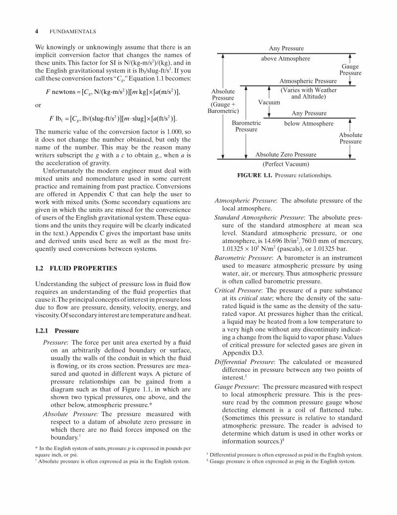
Total Pressure : The pressure resulting from a moving fl uid being brought to rest isentropically (without loss), as, for example, against a blunt object. (The kinetic energy of motion is converted to pressure when the fl uid is brought to rest.) Total pressure is also known as stagnation pressure and pitot pressure (see Fig. 1.2 ).
Static Pressure : The pressure in a moving fl uid before it is brought to rest. A pipe wall tap samples static pressure (see Fig. 1.2 ).
Vacuum : A pressure below local atmospheric pres-sure; often expressed as a negative pressure with respect to standard atmospheric pressure.
Vapor Pressure : The absolute pressure of a pure vapor in equilibrium with its liquid phase.
1.2.2 Density
Mass Density : The amount of material contained in a unit volume, measured in terms of its mass.
Weight Density : The amount of material contained in a unit volume, measured in terms of the force (weight) standard gravity exerts on the con-tained mass.
Specifi c Volume : The volume occupied by a unit mass or weight of material. (Which means it must be inferred from the units used. In the English system they will be ft 3 /lb[force]; in SI they will be m3 /kg[mass].)
1.2.3 Velocity
Velocity : The speed of motion of a fl uid with respect to a uniform datum. In pressure drop consider-ations it is usually used loosely with no direction implied. However, in impulse - momentum con-siderations, direction is an essential part of the measurement.
FIGURE 1.2. Total and static pressure.
Flow
Total
PressureStatic
Pressure
Pitot
Tube
6 FUNDAMENTALS
obvious to the sense of touch or yielding a change in temperature) is of interest. It can be measured in the same units as work energy and indeed is interchangeable with energy. Usually heat is mea-sured in units related to the heat – temperature relationship of water. In the English system the unit is the British thermal unit (usually abbrevi-ated Btu). In SI it is the kilocalorie. The conversion to mechanical energy is the mechanical equivalent of heat. Its value is given in Appendix C .1.
Specifi c Heat : The measure of the change of heat capacity of a unit weight or mass of a substance for a unit change of temperature. It is almost always expressed in heat units, that is, Btu or kilocalories. The units of specifi c heat are thus Btu/lb - R (or Btu/lb - F) and kcal/kg - K (or kcal/kg - C).
1.3 IMPORTANT DIMENSIONLESS RATIOS
Researchers have devised many dimensionless ratios in order to describe the behavior of physical processes. The most important to us in analyzing pressure drop in fl uid systems are described in the succeeding sections.
1.3.1 Reynolds Number
Named for the British engineer Osborne Reynolds (1842 – 1912), the Reynolds number is the ratio of momentum forces to viscous forces. It is extremely important in quantifying pressure drop in fl uids fl owing in closed conduits. It is given by:
NVD
gwDgA
wRe = =
ρµ µ
(English), (1.2a)
NVD mD
Am
Re = =ρµµ
(SI). (1.2b)
1.3.2 Relative Roughness
This quantity, as with the Reynolds number above, is extremely important in fi nding pressure drop in fl uids fl owing in pipes. It is rarely, if ever, assigned a symbol; but for illustration here let it be called RR . It is defi ned as:
RD
R ,=ε
where ε is the absolute roughness of the pipe inner wall and D is the pipe inside diameter. (In practice it is usually just called ε / D .)
the fi fteenth - century German physicist Gabriel Fahrenheit [1] . It is based on the lowest tempera-ture he could attain with a salt and ice mixture (assigned a value of 0 ° F) and human body tem-perature (to which he tried to assign a value of 96 ° F). This did not work out well and he ended up assigning 32 ° F to the melting point of ice and 212 ° F to the boiling point of water. The SI tem-perature scale (the Kelvin scale) is an absolute scale using the centigrade degree. The centigrade scale was devised by Swedish astronomer Anders Celsius in 1742 and incorporated into the metric system adopted in France at the close of the French Revolution [1] . On this scale — offi cially called Celsius since 1948 — the melting point and boiling point of water at standard atmospheric pressure were assigned values of 0 and 100 ° C respectively.
Absolute Temperature : Temperature measured from absolute zero. It was noted in the late 1700s by the French physicist Jacques Charles (1746 – 1823) that gases expand and contract in direct propor-tion to their temperature changes. On a suitably chosen scale their volumes are thus directly pro-portional to their temperatures. The extrapolated temperature of zero volume according to the kinetic theory of gases is also the point at which molecular activity — and hence heat content — vanishes. No lower temperature is possible and so this temperature is called absolute zero. Two tem-perature scales based on this zero point are in common use. One, utilizing the Fahrenheit degree, is called the Rankine scale; temperatures on this scale are marked ° R. The other, utilizing the Celsius degree, is called the Kelvin scale and its temperatures are marked K. The temperature 0 ° F corresponds to 459.67 ° R, and 0 ° C is identical to 273.15 K. Absolute zero is thus − 459.67 ° F or − 273.15 ° C.
Critical Temperature : The temperature of a pure substance at its critical state , above which its gas phase cannot be liquefi ed by the application of pressure, because at the critical temperature the latent heat of vaporization vanishes and the liquid cannot be distinguished from the gas. Values of critical temperature for selected gases are given in Appendix D .3.
1.2.7 Heat
Heat (Heat Energy) : Heat is the measure of thermal energy contained in a substance. In fl uid fl ow problems generally only sensible heat (i.e., heat
EQUATIONS OF STATE 7
1.3.6 Reduced Pressure
Reduced pressure, along with reduced temperature (described below), is useful in quantifying departures from the ideal state in gases. Reduced pressure is given by:
PPP
rc
= ,
where P is the pressure of interest and Pc is critical pressure.
1.3.7 Reduced Temperature
As with reduced pressure described above, reduced temperature helps to reduce the state point of most gases to a common base, making it possible to quantify departures of most gases from the ideal equation describing the relationship between pressure, tempera-ture, volume, and quantity of substance (the equation of state, described below). Reduced temperature is given by:
TTT
rc
= ,
where T is the temperature of interest and Tc is critical temperature.
1.4 EQUATIONS OF STATE
This section presents various equations which describe the physical properties of fl uids — principally the fl uid ’ s density as a function of pressure and temperature.
1.4.1 Equation of State of Liquids
An “ equation of state of liquids ” is not commonly expressed. This is because in usual engineering fl uid - fl ow problems, the volume properties of the liquid are scarcely affected by changes in temperature or pressure in the fl ow path. Where their properties are signifi cantly affected it is customary (because it is easiest and suffi -ciently accurate) to break the problem into small enough segments wherein the properties may be considered to be constant. Where this approach is not satisfactory, as, for instance, when dealing with liquids at pressures above the critical pressure, equations of state of liquids are available in the literature. Attention is directed to the works by Reid et al. [2] and Poling et al. [3] , pro-duced a quarter - century apart, which refl ect the growth in information available in the literature on this subject.
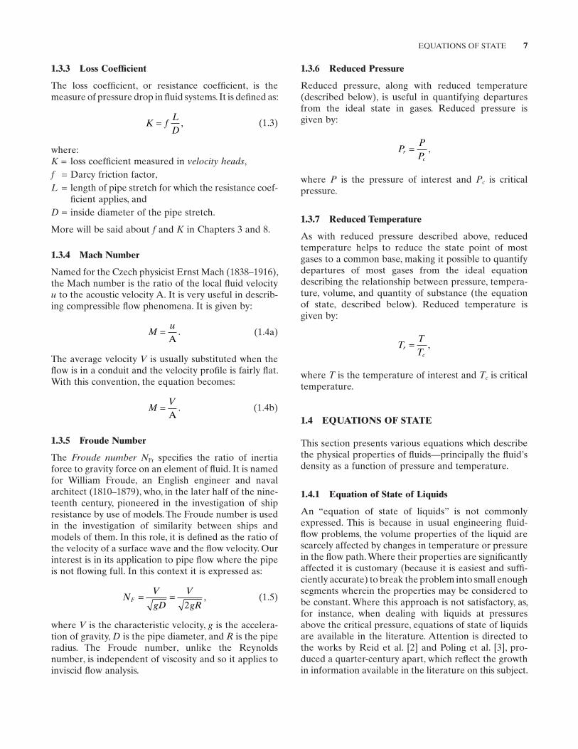
1.3.3 Loss Coeffi cient
The loss coeffi cient, or resistance coeffi cient, is the measure of pressure drop in fl uid systems. It is defi ned as:
K fLD
= , (1.3)
where:K = loss coeffi cient measured in velocity heads , f = Darcy friction factor, L = length of pipe stretch for which the resistance coef-
fi cient applies, and D = inside diameter of the pipe stretch.
More will be said about f and K in Chapters 3 and 8 .
1.3.4 Mach Number
Named for the Czech physicist Ernst Mach (1838 – 1916), the Mach number is the ratio of the local fl uid velocity u to the acoustic velocity A. It is very useful in describ-ing compressible fl ow phenomena. It is given by:
Mu
=A
. (1.4a)
The average velocity V is usually substituted when the fl ow is in a conduit and the velocity profi le is fairly fl at. With this convention, the equation becomes:
MV
=A
. (1.4b)
1.3.5 Froude Number
The Froude number NFr specifi es the ratio of inertia force to gravity force on an element of fl uid. It is named for William Froude, an English engineer and naval architect (1810 – 1879), who, in the later half of the nine-teenth century, pioneered in the investigation of ship resistance by use of models. The Froude number is used in the investigation of similarity between ships and models of them. In this role, it is defi ned as the ratio of the velocity of a surface wave and the fl ow velocity. Our interest is in its application to pipe fl ow where the pipe is not fl owing full. In this context it is expressed as:
NV
gD
V
gRF = =
2, (1.5)
where V is the characteristic velocity, g is the accelera-tion of gravity, D is the pipe diameter, and R is the pipe radius. The Froude number, unlike the Reynolds number, is independent of viscosity and so it applies to inviscid fl ow analysis.
8 FUNDAMENTALS
function, an equation of state, to describe this behavior, with varying success. Most of these “ real gas ” equations of state are limited in range of applicability. Two particu-larly attractive equations (solutions for z ), suitable for wide ranges of pressure and temperature, the Redlich – Kwong equation and the Lee – Kesler equation, are described in Appendix D . Scores more are described by Poling et al. [3] . The utility of these equations is illus-trated in Chapter 4 , “ Compressible Flow. ”
1.5 FLUID VELOCITY
As stated in Section 1.2 , velocity (so called; more accu-rately it would be called speed) is usually considered to be uniform over the cross section of fl ow. In reality, it is not. The fl uid in contact with the conduit wall must be at zero velocity, and velocity ordinarily increases toward the center. The assumption of uniform velocity immensely simplifi es fl uid fl ow calculations. There is an inaccuracy introduced by this assumption, but, fortunately, it usually does not affect the confi dence level of fl uid fl ow computations. The inaccuracies can be quantifi ed and will be considered in the follow-ing chapter.
Another assumption that is usually made is that the velocity is one - dimensional, that is, that radial compo-nents of fl ow velocities are inconsequential. Inaccura-cies introduced by this assumption are small and are absorbed by the loss coeffi cients.
1.6 FLOW REGIMES
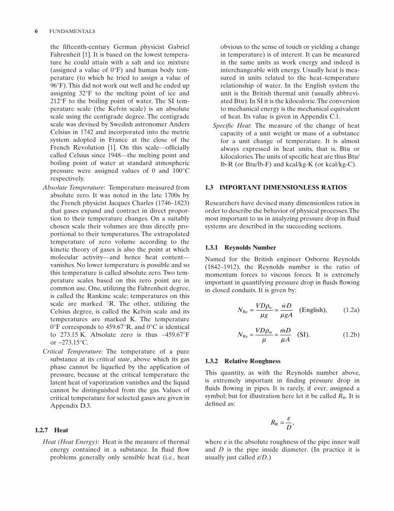
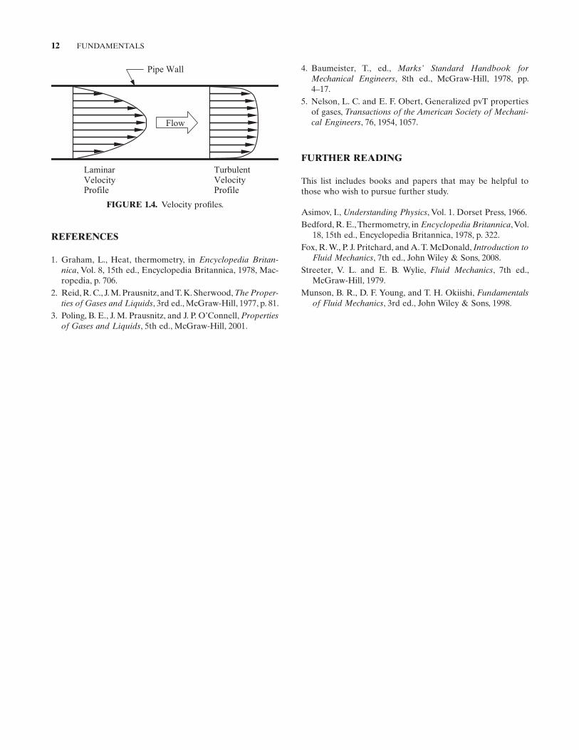
In the study of fl uid fl ow it has long been recognized that there are two distinct kinds of fl ow or fl ow regimes. The fi rst is characterized by preservation of layers or laminae in the fl ow stream. This kind of fl ow is called laminar or streamline fl ow. In cylindrical conduits the layers are cylindrical, the local velocities are strictly par-allel to the conduit axis, and they vary parabolically in velocity from zero at the wall to a maximum at the center. The second is characterized by destruction and mixing of the layers seen in laminar fl ow, and the local motions in the fl uid are chaotic or turbulent. This kind of fl ow is thus appropriately called turbulent fl ow. In circular conduits the axial velocity distribution is more nearly uniform than it is in laminar fl ow, although local velocity at the pipe wall is still zero. Laminar and turbulent fl ow velocity profi les are illustrated in Figure 1.4 . Because their effects will be treated in the following chapter you need to know that these two types of fl ow exist.
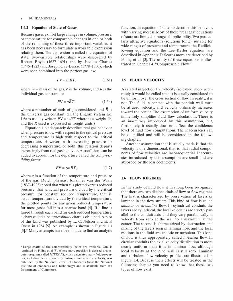
1.4.2 Equation of State of Gases
Because gases exhibit large changes in volume, pressure, or temperature for comparable changes in one or both of the remaining of these three important variables, it has been necessary to formulate a workable expression relating them. The expression is called the equation of state. Two - variable relationships were discovered by Robert Boyle (1627 – 1691) and by Jacques Charles (1746 – 1823) and Joseph Gay - Lussac (1778 – 1850), which were soon combined into the perfect gas law:
P mRTV ,= (1.6a)
where m = mass of the gas, V is the volume, and R is the individual gas constant; or
P nRTV ,= (1.6b)
where n = number of mols of gas considered and R is the universal gas constant. (In the English system Eq. 1.6a is usually written P V = wRT , where w = weight, lb, and the R used is expressed in weight units.)
Equation 1.6 adequately describes real gas behavior when pressure is low with respect to the critical pressure and temperature is high with respect to the critical temperature. However, with increasing pressure or decreasing temperature, or both, this relation departs increasingly from real gas behavior. A coeffi cient can be added to account for the departure, called the compress-ibility factor :
P zmRTV ,= (1.7)
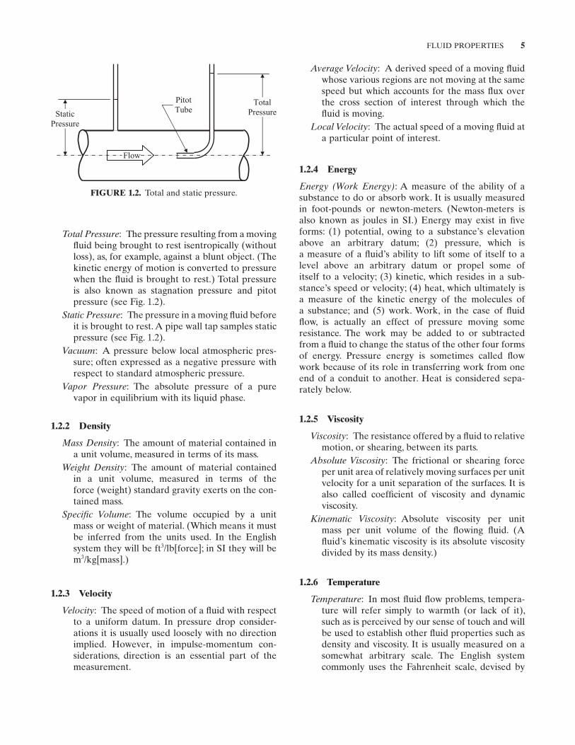
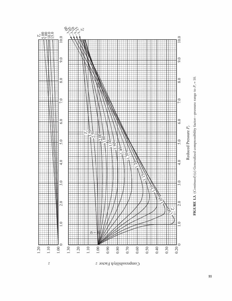
where z is a function of the temperature and pressure of the gas. Dutch physicist Johannes van der Waals (1837 – 1923) noted that when z is plotted versus reduced pressure, that is, actual pressure divided by the critical pressure, for constant reduced temperature, that is, actual temperature divided by the critical temperature, the plotted points for any given reduced temperature for most gases fall into a narrow band [4] . If a line is faired through each band for each reduced temperature, a chart called a compressibility chart is obtained. A plot of this kind was published by L. C. Nelson and E. F. Obert in 1954 [5] . An example is shown in Figure 1.3 [3] . * Many attempts have been made to fi nd an analytic
* Large charts of the compressibility factor are available. One is reprinted by Poling et al [3] . Where more precision is desired, a com-puter program, called MIPROPS , which calculates many fl uid proper-ties, including density, viscosity, entropy, and acoustic velocity, was published by the National Bureau of Standards (now the National Institute of Standards and Technology) and is available from the Department of Commerce.
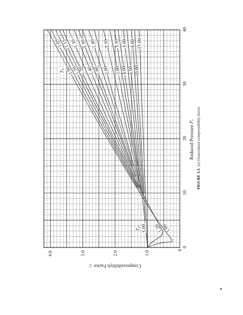
FIG
UR
E 1
.3.
(a)
Gen
eral
ized
com
pres
sibi
lity
fact
or.
00.1
0.2
0.3
0.4
001
0203
04
1.00
1.10
1.20
1.40
1.60
2.00
3.00
4.00
6.00
10.0
0
1.05
1.15
1.30
1.50
1.80
2.50
3.50
5.00
8.00
15.0
0
Tr
5.00 1.20
1.00r
T
Compressibilityh Factorz
Red
uced
Pre
ssur
e P
r
9
10
Compressibilityh Factorz
Red
uced
Pre
ssur
e P
r
1.02.0
3.04.0
5.06.0
7.08.0
9.00.1
03.0
04.0
05.0
06.0
07.0
08.0
09.0
00.1
0.600.65
0.700.75
0.80
0.85
0.90
0.95
1.00
00.300.5
00.2
06.1
04.1
03.1
02.1
51.1
01.1
50.1
Satu
ratio
n Li
ne
Tr
rT
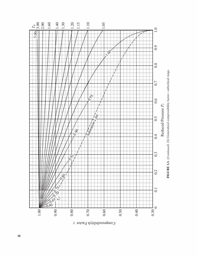
0
FIG
UR
E 1
.3.
(Con
tinue
d)(b
) G
ener
aliz
ed c
ompr
essi
bilit
y fa
ctor
— su
bcri
tica
l ran
ge.
11
002.0
0.10.2
0.30.4
0.50.6
0.70.8
0.90.01
03.0
04.0
05.0
06.0
07.0
08.0
09.0
00.1
01.1
02.1
03.1
00.1
01.1
02.1
1.00
1.05
1.10
5.00
7.00
10.0
15.0
1.00
1.05
1.10
1.15
Pr = 10
3.50
2.50
2.00
1.80
1.60
1.50
1.40
1.30
1.20
1.15
T r
rTrT
rT
0.10
0.20.5
0.30.4
0.60.7
0.90.8
0.01
Compressibilityh Factorz
Red
uced
Pre
ssur
e P
r
z
FIG
UR
E 1
.3.
(Con
tinue
d)(c
) G
ener
aliz
ed c
ompr
essi
bilit
y fa
ctor
— pr
essu
re r
ange
to
Pr =
10.
12 FUNDAMENTALS
4. Baumeister , T. , ed., Marks ’ Standard Handbook for Mechanical Engineers , 8th ed. , McGraw - Hill , 1978 , pp. 4 – 17 .
5. Nelson , L. C. and E. F. Obert , Generalized pvT properties of gases , Transactions of the American Society of Mechani-cal Engineers , 76 , 1954 , 1057 .
FURTHER READING
This list includes books and papers that may be helpful to those who wish to pursue further study.
Asimov , I. , Understanding Physics , Vol. 1 . Dorset Press , 1966 . Bedford , R. E. , Thermometry , in Encyclopedia Britannica , Vol.
18 , 15th ed. , Encyclopedia Britannica , 1978 , p. 322 . Fox , R. W. , P. J. Pritchard , and A. T. McDonald , Introduction to
Fluid Mechanics , 7th ed. , John Wiley & Sons , 2008 . Streeter , V. L. and E. B. Wylie , Fluid Mechanics , 7th ed. ,
McGraw - Hill , 1979 . Munson , B. R. , D. F. Young , and T. H. Okiishi , Fundamentals
of Fluid Mechanics , 3rd ed. , John Wiley & Sons , 1998 .
REFERENCES
1. Graham , L. , Heat, thermometry , in Encyclopedia Britan-nica , Vol. 8 , 15th ed. , Encyclopedia Britannica , 1978 , Mac-ropedia, p. 706 .
2. Reid , R. C. , J. M. Prausnitz , and T. K . Sherwood , The Proper-ties of Gases and Liquids , 3rd ed. , McGraw - Hill , 1977 , p. 81 .
3. Poling , B. E. , J. M. Prausnitz , and J. P. O ’ Connell , Propertiesof Gases and Liquids , 5th ed. , McGraw - Hill , 2001 .
FIGURE 1.4. Velocity profi les.
Pipe Wall
Flow
LaminarVelocityProfile
TurbulentVelocityProfile
13
2 CONSERVATION EQUATIONS
This chapter will consider the equations for conserva-tion of mass, energy and momentum, velocity profi les, and correction factors for momentum and energy. In general, the English gravitational system uses weight fl ow rate ( w), and the International System of Units (SI) uses mass fl ow rate ( m).
2.1 CONSERVATION OF MASS
The continuity equation is simply a statement that there is as much fl uid fl owing out of a system under consider-ation as there is fl owing into it. It assumes that mass is conserved and that fl uid is not being stored or released from storage within the system. The equations for weight rate of fl ow and mass rate of fl ow are:
w AV w= ρ , (2.1a)
m AV m= ρ . (2.1b)
When the continuity equation holds, the inlet fl ow rate is equal to the outlet fl ow rate, so that
A V A Vw w1 1 1 2 2 2( ) ( ) ,ρ ρ= (2.2a)
A V A Vm m1 1 1 2 2 2( ) ( ) .ρ ρ= (2.2b)
These equations are expressions of the continuityequation .
In these equations it is customary to assume that the velocity profi le is fl at, that is, the velocity in the fl uid
fl owing in a conduit is the same everywhere in the cross section. The velocity that accounts for all the weight fl ux (or mass fl ux) across the cross section of the conduit is the average velocity .
The velocity profi le is, of course, not fl at across the cross section! Does this assumption therefore cause an error in the continuity equation? No, because we use the same relation to defi ne the average velocity as to determine the weight fl ux through the cross section. The same cannot be said, however, for the momentum fl ux or the energy fl ux as we shall discover in the next sections.
2.2 CONSERVATION OF MOMENTUM
The momentum equation is a statement that a fl uid stream, as it relates to fl uid fl ow when acted upon by external forces whose sum is not zero, must acquire a change in velocity. The amount of this force may be found by use of the momentum equation. It is thus an application of Newton ’ s second law of motion (Eq. 1.1 ).
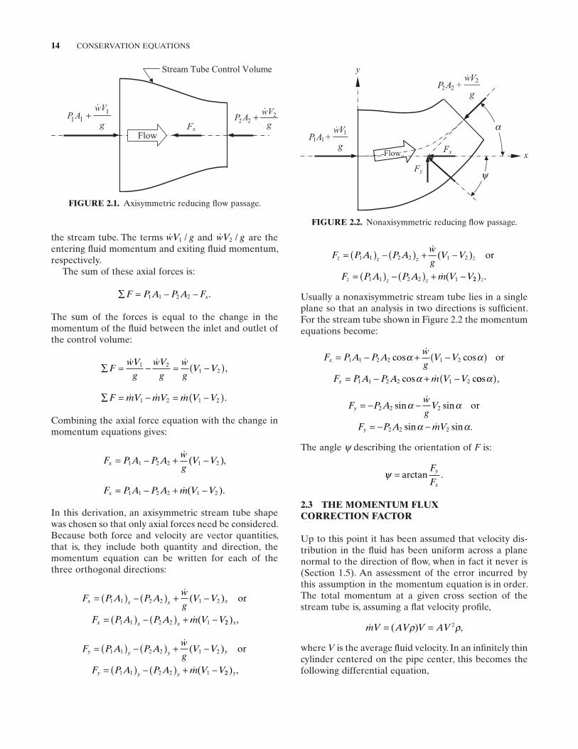
Consider an axisymmetric reducing fl ow passage as illustrated in Figure 2.1 . Assume that velocity distribu-tion is uniform at any cross section of the stream tube. P1A1 is the axial force acting on the fl uid in the control volume owing to absolute pressure P1 acting over area A1 ; P2A2 is the axial force owing to absolute pressure P2
acting over area A2 ; and F is the apparent residual force owing to the diminishing stream pressure acting over the axial projection of the outer control volume bound-ary and to the frictional resistance on the surface of
Pipe Flow: A Practical and Comprehensive Guide, First Edition. Donald C. Rennels and Hobart M. Hudson.© 2012 John Wiley & Sons, Inc. Published 2012 by John Wiley & Sons, Inc.
14 CONSERVATION EQUATIONS
F P A P Awg
V V
F P A P A m V V
z z z z
z z z
= ( ) − ( ) + −
= ( ) − ( ) + −
1 1 2 2 1 2
1 1 2 2 1
( )
(
or
22 )z.
Usually a nonaxisymmetric stream tube lies in a single plane so that an analysis in two directions is suffi cient. For the stream tube shown in Figure 2.2 the momentum equations become:
F P A P Awg
V V
F P A P A m V V
x
x
= − + −( )
= − + −
1 1 2 2 1 2
1 1 2 2 1 2
cos cos
cos c
α α
α
or
oosα( ),
F P Awg
V
F P A mV
y
y
= − −
= − −
2 2 2
2 2 2
sin sin
sin sin
α α
α α
or
.
The angle ψ describing the orientation of F is:
ψ = arctanF
Fy
x
.
2.3 THE MOMENTUM FLUX CORRECTION FACTOR
Up to this point it has been assumed that velocity dis-tribution in the fl uid has been uniform across a plane normal to the direction of fl ow, when in fact it never is (Section 1.5 ). An assessment of the error incurred by this assumption in the momentum equa tion is in order. The total momentum at a given cross section of the stream tube is, assuming a fl at velocity profi le,
mV AV V AV= =( )ρ ρ2 ,
where V is the average fl uid velocity. In an infi nitely thin cylinder centered on the pipe center, this becomes the following differential equation,
the stream tube. The terms wV g1 / and wV g2 / are the entering fl uid momentum and exiting fl uid momentum, respectively.
The sum of these axial forces is:
∑ = − −F P A P A Fx1 1 2 2 .
The sum of the forces is equal to the change in the momentum of the fl uid between the inlet and outlet of the control volume:
∑ = − = −( )FwV
gwV
gwg
V V 1 2
1 2 ,
∑ = − = −( )F mV mV m V V 1 2 1 2 .
Combining the axial force equation with the change in momentum equations gives:
F P A P Awg
V Vx = − + −1 1 2 2 1 2
( ),
F P A P A m V Vx = − + −1 1 2 2 1 2 ( ).
In this derivation, an axisymmetric stream tube shape was chosen so that only axial forces need be considered. Because both force and velocity are vector quantities, that is, they include both quantity and direction, the momentum equation can be written for each of the three orthogonal directions:
F P A P Awg
V V
F P A P A m V V
x x x x
x x x
= ( ) − ( ) + −
= ( ) − ( ) + −
1 1 2 2 1 2
1 1 2 2 1
( )
(
or
22 ) ,x
F P A P Awg
V V
F P A P A m V V
y y y y
y y y
= ( ) − ( ) + −
= ( ) − ( ) + −
1 1 2 2 1 2
1 1 2 2 1
( )
(
or
22 )y,
FIGURE 2.1. Axisymmetric reducing fl ow passage.
g
VwAP
111 +
g
VwAP 2
22 +Fx
Stream Tube Control Volume
Flow
FIGURE 2.2. Nonaxisymmetric reducing fl ow passage.
Fy
g
VAP
222
g
VAP
111
y
xFxFlow
w+
w+
y
a
THE MOMENTUM FLUX CORRECTION FACTOR 15
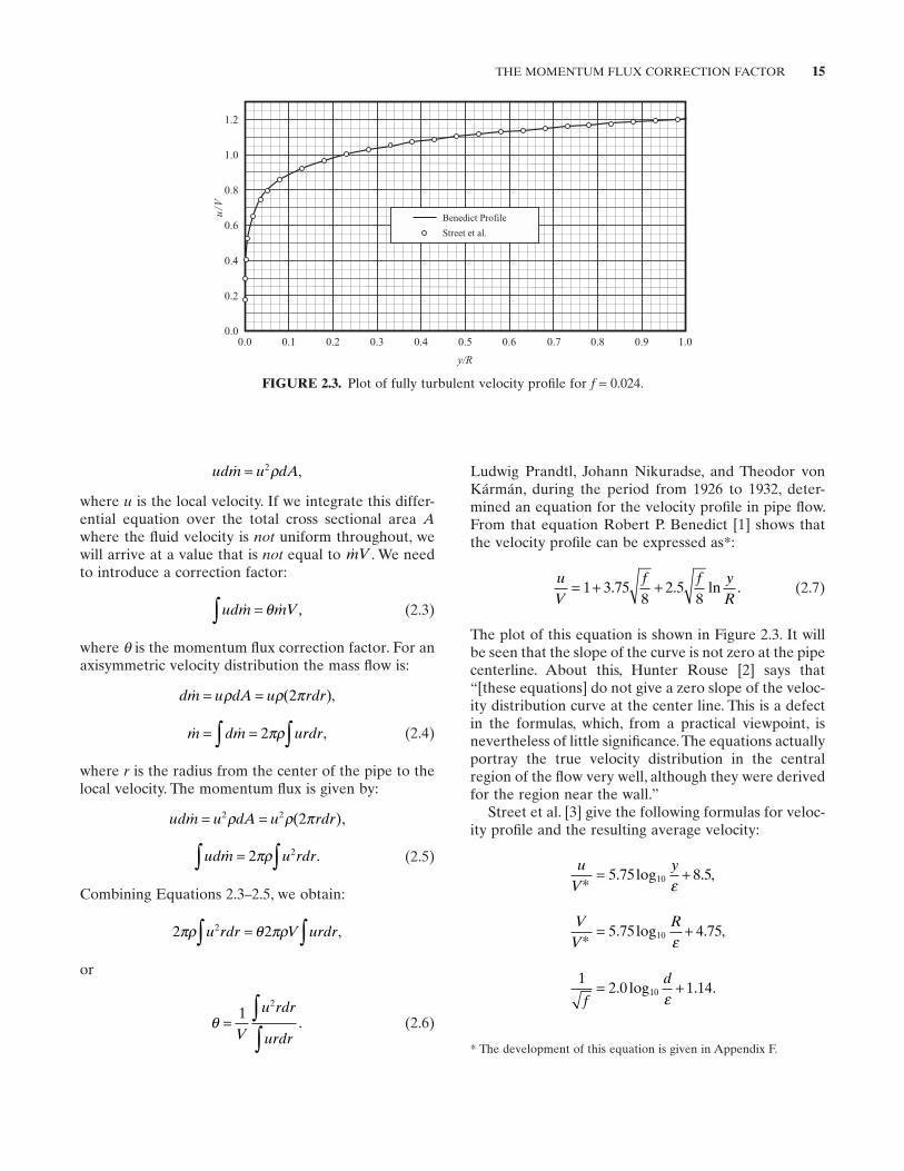
Ludwig Prandtl, Johann Nikuradse, and Theodor von K á rm á n, during the period from 1926 to 1932, deter-mined an equation for the velocity profi le in pipe fl ow. From that equation Robert P. Benedict [1] shows that the velocity profi le can be expressed as * :
uV
f f yR
= + +1 3 758
2 58
. . ln . (2.7)
The plot of this equation is shown in Figure 2.3 . It will be seen that the slope of the curve is not zero at the pipe centerline. About this, Hunter Rouse [2] says that “ [these equations] do not give a zero slope of the veloc-ity distribution curve at the center line. This is a defect in the formulas, which, from a practical viewpoint, is nevertheless of little signifi cance. The equations actually portray the true velocity distribution in the central region of the fl ow very well, although they were derived for the region near the wall. ”
Street et al. [3] give the following formulas for veloc-ity profi le and the resulting average velocity:
uV
y∗ = +5 75 8 510. log . ,
ε
VV
R∗ = +5 75 4 7510. log . ,
ε
12 0 1 1410
f
d= +. log . .
ε
udm u dA = 2ρ ,
where u is the local velocity. If we integrate this differ-ential equation over the total cross sectional area Awhere the fl uid velocity is not uniform throughout, we will arrive at a value that is not equal to mV . We need to introduce a correction factor:
udm mV ∫ = θ , (2.3)
where θ is the momentum fl ux correction factor. For an axisymmetric velocity distribution the mass fl ow is:
dm u dA u rdr = =ρ ρ π( )2 ,
m dm urdr= =∫ ∫2πρ , (2.4)
where r is the radius from the center of the pipe to the local velocity. The momentum fl ux is given by:
udm u dA u rdr = =2 2 2ρ ρ( ),π
udm u rdr∫ ∫= 2 2πρ . (2.5)
Combining Equations 2.3 – 2.5, we obtain:
2 22πρ θ πρu rdr V urdr∫ ∫= ,
or
θ = ∫∫
12
V
u rdr
urdr. (2.6)
FIGURE 2.3. Plot of fully turbulent velocity profi le for f = 0.024.
1.2
1.0
0.8
0.0
0.2
0.4
0.6u/V
Benedict Profile
Street et al.
0.0 0.1 0.2 0.8 0.90.3 0.4 0.5 0.6 0.7 1.0
y/R
* The development of this equation is given in Appendix F .
16 CONSERVATION EQUATIONS
2.4 CONSERVATION OF ENERGY
The energy equation is of paramount importance in our mathematical model of fl uid fl ow losses. It accounts for the various energy changes within a fl ow system, or a portion of interest, and enables us to formulate a math-ematical relationship that will provide consistently accurate predictions of pressure drop within it. The energy equation presents few diffi culties once these energies have been identifi ed.
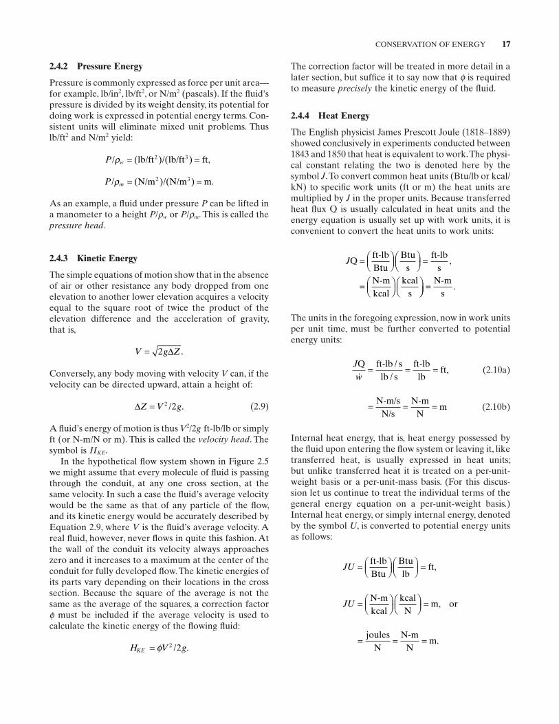
As its name implies, the energy equation rests on the law of conservation of energy. This law, when applied to the steady fl ow of any real fl uid, states that the rate of fl ow of energy entering a system is equal to that leaving the system. Figure 2.5 shows a hypothetical fl ow system with the fl uid properties and circumstances and the energy fl uxes affecting the energy balance.
In order to relate the energy infl ows and outfl ows in a system it is necessary to put them in common units. It is convenient for this discussion to express energy in work units such as foot - pounds or newton - meters, and unit energies in terms of foot - pounds per pound of fl uid, or newton - meters per newton. From Figure 2.5 it is seen that fi ve kinds of energy fl ux must be considered: poten-tial, pressure, kinetic, heat, and work.
2.4.1 Potential Energy
Every unit of fl uid lifted above an arbitrary datum required a certain amount of work to lift it there. If the unit of fl uid quantity is pounds (or newtons), the work required (in a uniform gravity fi eld) is its weight times the height it was lifted, ft - lb (or N - m). Thus the unit energy is ft - lb/lb or ft (or N - m/N or m), equal numerically and dimensionally to its elevation Zabove the datum. This is called the elevation or poten-tial head .
V * is the “ friction velocity, ” V m* /= τ ρ0 , where τ0 is the wall shear stress and ρm is the mass density (in either the English gravitational system or SI). By combining these three equations the following equation is obtained* :
uV
yR f
f
=+ +
−
log .
..
101
20 607231
1
20 044943
(2.8)
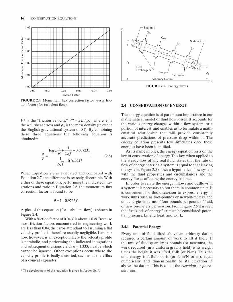
When Equation 2.8 is evaluated and compared with Equation 2.7 , the difference is scarcely discernible. With either of these equations, performing the indicated inte-grations and ratio in Equation 2.6 , the momentum fl ux correction factor is found to be:
θ = +1 0 9765. .f
A plot of this equation (for turbulent fl ow) is shown in Figure 2.4 .
With a friction factor of 0.04, θ is about 1.038. Because most friction factors encountered in engineering work are less than 0.04, the error attendant to assuming a fl at velocity profi le is therefore usually negligible. Laminar fl ow, however, is an exception. Here the velocity profi le is parabolic, and performing the indicated integrations and subsequent divisions yields θ = 1.333, a value which cannot be ignored. Other exceptions occur where the velocity profi le is badly distorted, such as at the effl ux of a conical expander.
FIGURE 2.4. Momentum fl ux correction factor versus fric-tion factor (for turbulent fl ow).
1.05
1.04
1.03
1.02
1.01
1.00
Mom
entu
m F
lux
Cor
rect
ion
Fac
tor
0.00 0.01 0.02 0.03 0.04 0.05
Friction Factor
FIGURE 2.5. Energy fl uxes.
2w
1V1
U1
P1
P1
U2
Z1
Z2
z
x
HeatExchangers
PumpTurbine
Station 1
Station 2
QIn
QOut
EP
ET
Arbitrary Datum
V2
w
* The development of this equation is given in Appendix F .
CONSERVATION OF ENERGY 17
The correction factor will be treated in more detail in a later section, but suffi ce it to say now that ϕ is required to measure precisely the kinetic energy of the fl uid.
2.4.4 Heat Energy
The English physicist James Prescott Joule (1818 – 1889) showed conclusively in experiments conducted between 1843 and 1850 that heat is equivalent to work. The physi-cal constant relating the two is denoted here by the symbol J . To convert common heat units (Btu/lb or kcal/kN) to specifi c work units (ft or m) the heat units are multiplied by J in the proper units. Because transferred heat fl ux Q is usually calculated in heat units and the energy equation is usually set up with work units, it is convenient to convert the heat units to work units:
JQft-lbBtu
Btus
ft-lbs
N-mkcal
kcals
=
=
=
,
=N-m
s.
The units in the foregoing expression, now in work units per unit time, must be further converted to potential energy units:
JwQ ft-lb
lbft-lblb
ft
= = =/ s
/ s, (2.10a)
= = =N-m/s
N/sN-m
Nm (2.10b)
Internal heat energy, that is, heat energy possessed by the fl uid upon entering the fl ow system or leaving it, like transferred heat, is usually expressed in heat units; but unlike transferred heat it is treated on a per - unit - weight basis or a per - unit - mass basis. (For this discus-sion let us continue to treat the individual terms of the general energy equation on a per - unit - weight basis.) Internal heat energy, or simply internal energy, denoted by the symbol U , is converted to potential energy units as follows:
JU =
=
ft-lbBtu
Btulb
ft,
JU =
=
N-mkcal
kcalN
m or,
= = =joules
NN-m
Nm.
2.4.2 Pressure Energy
Pressure is commonly expressed as force per unit area — for example, lb/in 2 , lb/ft 2 , or N/m 2 (pascals). If the fl uid ’ s pressure is divided by its weight density, its potential for doing work is expressed in potential energy terms. Con-sistent units will eliminate mixed unit problems. Thus lb/ft2 and N/m 2 yield:
P w/ lb/ft / lb/ft ftρ = =( ) ( ) ,2 3
P m/ N/m / N/m mρ = =( ) ( ) .2 3
As an example, a fl uid under pressure P can be lifted in a manometer to a height P / ρw or P / ρm . This is called the pressure head .
2.4.3 Kinetic Energy
The simple equations of motion show that in the absence of air or other resistance any body dropped from one elevation to another lower elevation acquires a velocity equal to the square root of twice the product of the elevation difference and the acceleration of gravity, that is,
V g Z= 2 ∆ .
Conversely, any body moving with velocity V can, if the velocity can be directed upward, attain a height of:
∆Z V g= 2 2/ . (2.9)
A fl uid ’ s energy of motion is thus V2 /2 g ft - lb/lb or simply ft (or N - m/N or m). This is called the velocity head . The symbol is HKE .
In the hypothetical fl ow system shown in Figure 2.5 we might assume that every molecule of fl uid is passing through the conduit, at any one cross section, at the same velocity. In such a case the fl uid ’ s average velocity would be the same as that of any particle of the fl ow, and its kinetic energy would be accurately described by Equation 2.9 , where V is the fl uid ’ s average velocity. A real fl uid, however, never fl ows in quite this fashion. At the wall of the conduit its velocity always approaches zero and it increases to a maximum at the center of the conduit for fully developed fl ow. The kinetic energies of its parts vary depending on their locations in the cross section. Because the square of the average is not the same as the average of the squares, a correction factor ϕ must be included if the average velocity is used to calculate the kinetic energy of the fl owing fl uid:
H V gKE = φ 2 2/ .
18 CONSERVATION EQUATIONS
With this convention, each term in the SI General Energy Equation has the units of meters.
Other forms of energy, such as chemical, electric, or atomic, may need reckoning in a particular fl ow problem. Their inclusion should present no diffi culties if they are treated as the fi ve forms shown here have been.
The fi rst three terms on each side of Equation 2.11a and 2.11b are called the Bernoulli terms, after Swiss mathematician Daniel Bernoulli (1700 – 1782), and are referred to as heads — P / ρ is called the pressure head, ϕ V2 /2 g is called the velocity head, and Z is called the elevation or potential head.
2.6 HEAD LOSS
The general energy equation as given above (Eq. 2.11a and 2.11b ) is valid for any real fl uid. There is, however, an observation that should be made here. Consider the most elementary fl ow system: a horizontal pipe of con-stant cross section, without pump or turbine, and without external heat transfer, carrying a fl uid from one end to the other. Let us also assume that changes of fl uid pres-sure or temperature do not affect the fl uid density during its passage through the fl ow system. (This kind of fl ow is called incompressible fl ow and it is very closely approximated by the fl ow of most liquids.) By the con-tinuity equation (Eq. 2.2a and 2.2b ), the average veloc-ity does not change; therefore the ϕ V2 /2 g terms are equal on both sides of Equation 2.11 and may be dropped. The elevation does not change from one side of the equation to the other, so the Z terms may be dropped. Without pump or turbine work the E w/ terms may be dropped. Without external transferred heat the JQ w/ terms may be dropped. This leaves only the P / ρ terms and the JU terms. Collect the JU terms and lump them into one term called ΔJU ; the resulting equation is:
P PJU1
1
2
2ρ ρ− = ∆ .
Again, as in Equation 2.11 , ρ is either ρw or ρm , depend-ing on the units chosen. The pressure head change is equal to the thermal energy term, ΔJU ! In this illustra-tion, we could have included the other Bernoulli or head terms and shown that ΔJU is equal to the change in total head. Appropriately enough, the change is called head loss , or HL . In the general energy equation, where there is external heat transfer, only a portion of ΔJU is owing to head loss. But since we have observed that in incompressible fl ow the thermal terms usually do not affect the fl uid density appreciably, we may drop the thermal terms altogether except for the portion that
2.4.5 Mechanical Work Energy
The mechanical work done on the fl uid in the fl ow system by a pump and, as in the case of heat fl ux, the work done by the fl uid in a turbine must be expressed in power units, or work per unit time, to maintain dimen-sional homogeneity in the energy equation. These units may be converted to potential energy units as they were in the case of heat fl ux (Eq. 2.10a and 2.10b):
E
wp
= = =
= = =
ft-lb slb/s
ft-lblb
ft
N-m/sN/s
N-mN
m
/
.
The same conversion also applies to turbine work, ET . The mechanical work energy is often called “ fl ow
work, ” because without fl ow there is no work performed. In the case of the pump, fl ow work is added to the fl ow, and in the case of the turbine, fl ow work is subtracted from the fl ow.
2.5 GENERAL ENERGY EQUATION
Having defi ned the energy fl uxes in the hypothetical fl ow system in common units, we may now write the energy balance:
P Vg
Z JUJw
Ew
P Vg
Z JUJ
w
P
w
1
1
1 12
1 11
2
2
2 22
2 2
2
2
( )
( )
ρφ
ρφ
+ + + + +
= + + + +
Q
QQ.2
wEw
T+ (2.11a)
Equation 2.11a is set up for weight units in either the English gravitational system (where lb f is basic) or SI (where the kilogram mass is basic) but using newtons as the force unit. For SI in mass units, the equation is:
Pg
Vg
ZJU
gJmg
Emg
Pg
Vg
Z
m
P
m
1
1
1 12
11 1
2
2
2 22
2
2
2
( )
( )
ρφ
ρφ
+ + + + +
= + + +
Q
JJUg
JQmg
Emg
T2 2+ +
. (2.11b)
As shown in Chapter 1 , the units of ρm , m , and m are changed to force units when multiplied by g , and this entity may not be easily recognized by the user. For this reason a conversion factor called Cg may be inserted into the conversion to change the name of the entity. This factor for SI is N/(m/s 2 )/(kg), and if you call it “ Cg , ” Equation 1.1 becomes:
F C m agNewtons N/ m/s /kg kg m/s2 2= ×[ ( )[ ( )].
THE KINETIC ENERGY CORRECTION FACTOR 19
The local kinetic energy fl ux is:
u dm u u dA u rdr2 2 3 2 = =( ) .ρ ρ π
The total kinetic energy fl ux may be found by integrat-ing along the radius:
u dm u rdr2 32∫ ∫= πρ . (2.14)
Combining Equations 2.13 , 2.4 , and 2.14 yields:
2 213 2
2
3
πρ φ πρu rdr V urdrV
u rdr
urdr∫ ∫ ∫
∫= =, φ . (2.15)
Robert P. Benedict [1] gives the following equation for velocity profi le:
uV
f f yR
= + +1 3 758
2 58
. . ln . (2.7, repeated)
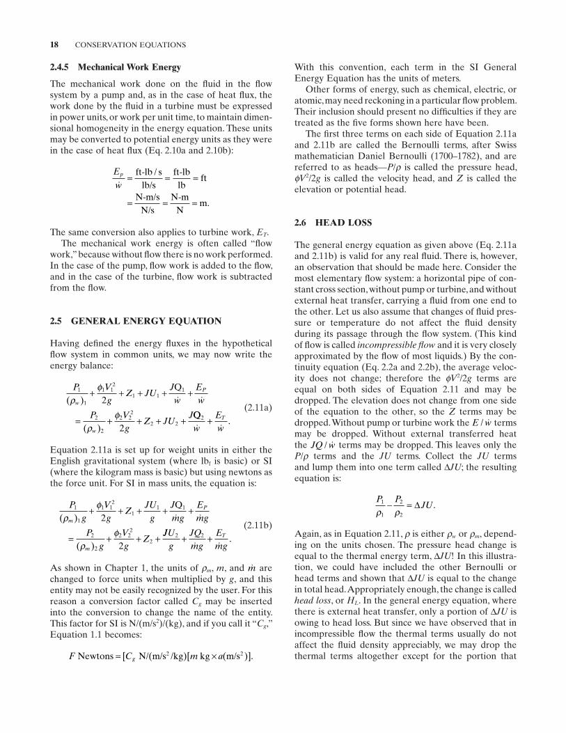
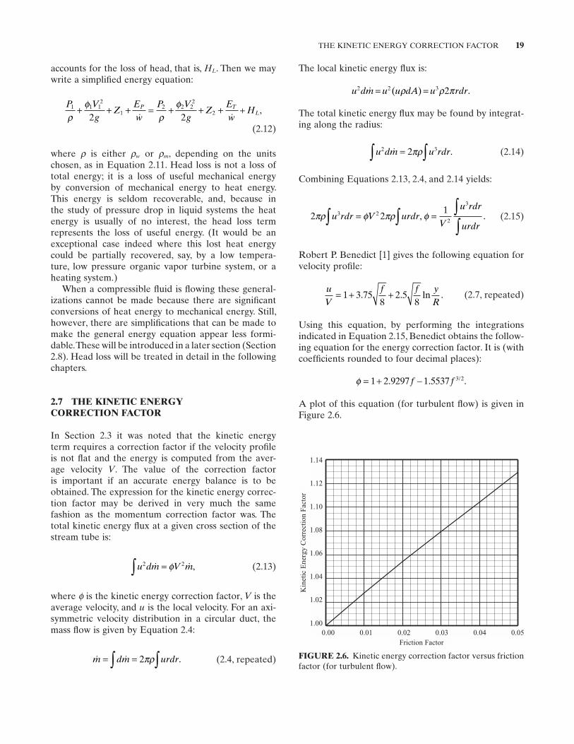
Using this equation, by performing the integrations indicated in Equation 2.15 , Benedict obtains the follow-ing equation for the energy correction factor. It is (with coeffi cients rounded to four decimal places):
φ = + −1 2 9297 1 5537 3 2. . ./f f
A plot of this equation (for turbulent fl ow) is given in Figure 2.6 .
accounts for the loss of head, that is, HL . Then we may write a simplifi ed energy equation:
P Vg
ZEw
P Vg
ZEw
+ HP TL
1 1 12
12 2 2
2
22 2ρ
φρ
φ+ + + = + + +
,
(2.12)
where ρ is either ρw or ρm , depending on the units chosen, as in Equation 2.11 . Head loss is not a loss of total energy; it is a loss of useful mechanical energy by conversion of mechanical energy to heat energy. This energy is seldom recoverable, and, because in the study of pressure drop in liquid systems the heat energy is usually of no interest, the head loss term represents the loss of useful energy. (It would be an exceptional case indeed where this lost heat energy could be partially recovered, say, by a low tempera-ture, low pressure organic vapor turbine system, or a heating system.)
When a compressible fl uid is fl owing these general-izations cannot be made because there are signifi cant conversions of heat energy to mechanical energy. Still, however, there are simplifi cations that can be made to make the general energy equation appear less formi-dable. These will be introduced in a later section (Section 2.8 ). Head loss will be treated in detail in the following chapters.
2.7 THE KINETIC ENERGY CORRECTION FACTOR
In Section 2.3 it was noted that the kinetic energy term requires a correction factor if the velocity profi le is not fl at and the energy is computed from the aver-age velocity V . The value of the correction factor is important if an accurate energy balance is to be obtained. The expression for the kinetic energy correc-tion factor may be derived in very much the same fashion as the momentum correction factor was. The total kinetic energy fl ux at a given cross section of the stream tube is:
u dm V m2 2 ∫ = φ , (2.13)
where ϕ is the kinetic energy correction factor, V is the average velocity, and u is the local velocity. For an axi-symmetric velocity distribution in a circular duct, the mass fl ow is given by Equation 2.4 :
m dm urdr= =∫ ∫2πρ . (2.4, repeated) FIGURE 2.6. Kinetic energy correction factor versus friction factor (for turbulent fl ow).
1.14
1.12
1.10
1.08
1.06
1.04
1.02
1.00
Kin
etic
Ene
rgy
Cor
rect
ion
Fac
tor
0.00 0.01 0.02 0.03 0.04 0.05Friction Factor
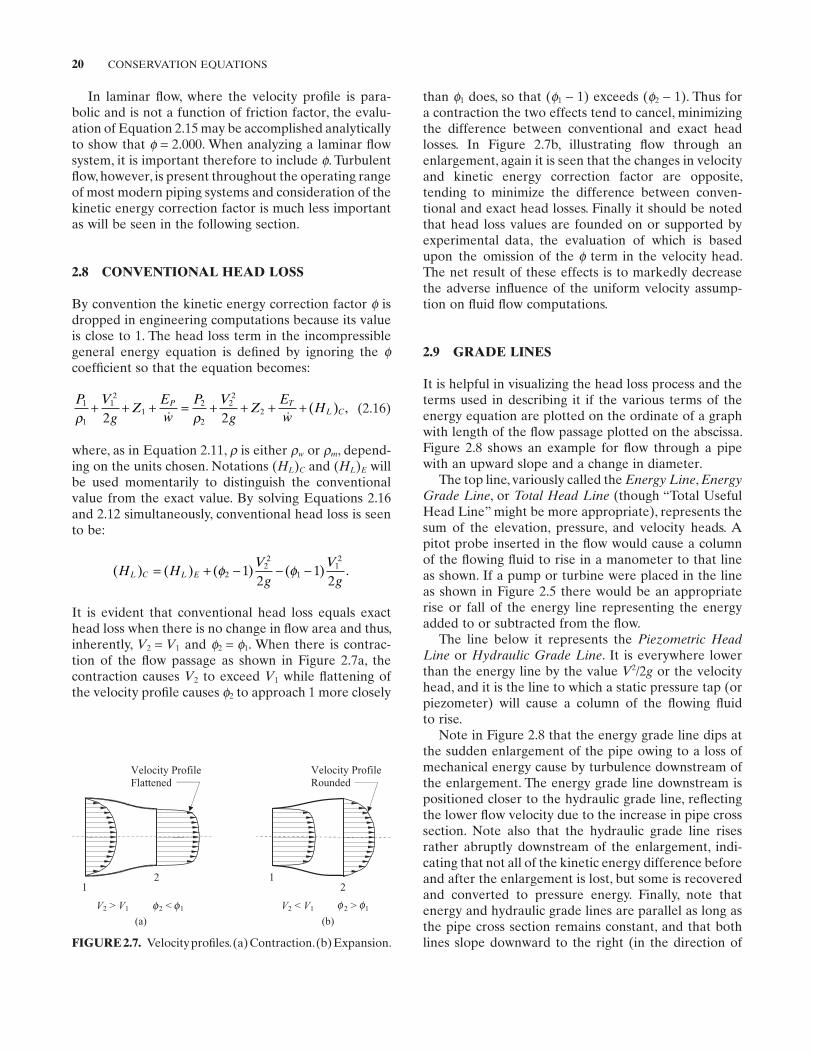
20 CONSERVATION EQUATIONS
than ϕ1 does, so that ( ϕ1 − 1) exceeds ( ϕ2 − 1). Thus for a contraction the two effects tend to cancel, minimizing the difference between conventional and exact head losses. In Figure 2.7 b, illustrating fl ow through an enlargement, again it is seen that the changes in velocity and kinetic energy correction factor are opposite, tending to minimize the difference between conven-tional and exact head losses. Finally it should be noted that head loss values are founded on or supported by experimental data, the evaluation of which is based upon the omis sion of the ϕ term in the velocity head. The net result of these effects is to markedly decrease the adverse infl uence of the uniform velocity assump-tion on fl uid fl ow computations.
2.9 GRADE LINES
It is helpful in visualizing the head loss process and the terms used in describing it if the various terms of the energy equation are plotted on the ordinate of a graph with length of the fl ow passage plotted on the abscissa. Figure 2.8 shows an example for fl ow through a pipe with an upward slope and a change in diameter.
The top line, variously called the Energy Line , EnergyGrade Line , or Total Head Line (though “ Total Useful Head Line ” might be more appropriate), represents the sum of the elevation, pressure, and velocity heads. A pitot probe inserted in the fl ow would cause a column of the fl owing fl uid to rise in a manometer to that line as shown. If a pump or turbine were placed in the line as shown in Figure 2.5 there would be an appropriate rise or fall of the energy line representing the energy added to or subtracted from the fl ow.
The line below it represents the Piezometric Head Line or Hydraulic Grade Line . It is everywhere lower than the energy line by the value V2 /2 g or the velocity head, and it is the line to which a static pressure tap (or piezometer) will cause a column of the fl owing fl uid to rise.
Note in Figure 2.8 that the energy grade line dips at the sudden enlargement of the pipe owing to a loss of mechanical energy cause by turbulence downstream of the enlargement. The energy grade line downstream is positioned closer to the hydraulic grade line, refl ecting the lower fl ow velocity due to the increase in pipe cross section. Note also that the hydraulic grade line rises rather abruptly downstream of the enlargement, indi-cating that not all of the kinetic energy difference before and after the enlargement is lost, but some is recovered and converted to pressure energy. Finally, note that energy and hydraulic grade lines are parallel as long as the pipe cross section remains constant, and that both lines slope downward to the right (in the direction of
In laminar fl ow, where the velocity profi le is para-bolic and is not a function of friction factor, the evalu-ation of Equation 2.15 may be accomplished analytically to show that ϕ = 2.000. When analyzing a laminar fl ow system, it is important therefore to include ϕ . Turbulent fl ow, however, is present throughout the operating range of most modern piping systems and consideration of the kinetic energy correction factor is much less important as will be seen in the following section.
2.8 CONVENTIONAL HEAD LOSS
By convention the kinetic energy correction factor ϕ is dropped in engineering computations because its value is close to 1. The head loss term in the incompressible general energy equation is defi ned by ignoring the ϕcoeffi cient so that the equation becomes:
P Vg
ZEw
P Vg
ZEw
HP TL C
1
1
12
12
2
22
22 2ρ ρ
+ + + = + + + +
( ) , (2.16)
where, as in Equation 2.11 , ρ is either ρw or ρm , depend-ing on the units chosen. Notations ( HL ) C and ( HL ) E will be used momentarily to distinguish the conventional value from the exact value. By solving Equations 2.16 and 2.12 simultaneously, conventional head loss is seen to be:
( ) ( ) ( ) ( ) .H HV
gV
gL C L E= + − − −φ φ2
22
112
12
12
It is evident that conventional head loss equals exact head loss when there is no change in fl ow area and thus, inherently, V2 = V1 and ϕ2 = ϕ1 . When there is contrac-tion of the fl ow passage as shown in Figure 2.7 a, the contraction causes V2 to exceed V1 while fl attening of the velocity profi le causes ϕ2 to approach 1 more closely
FIGURE 2.7. Velocity profi les. (a) Contraction. (b) Expansion.
(a) (b)
12
Velocity Profile Flattened
V ff f f2 > V1 2 < 1
21
Velocity Profile Rounded
V2 < V1 2 > 1
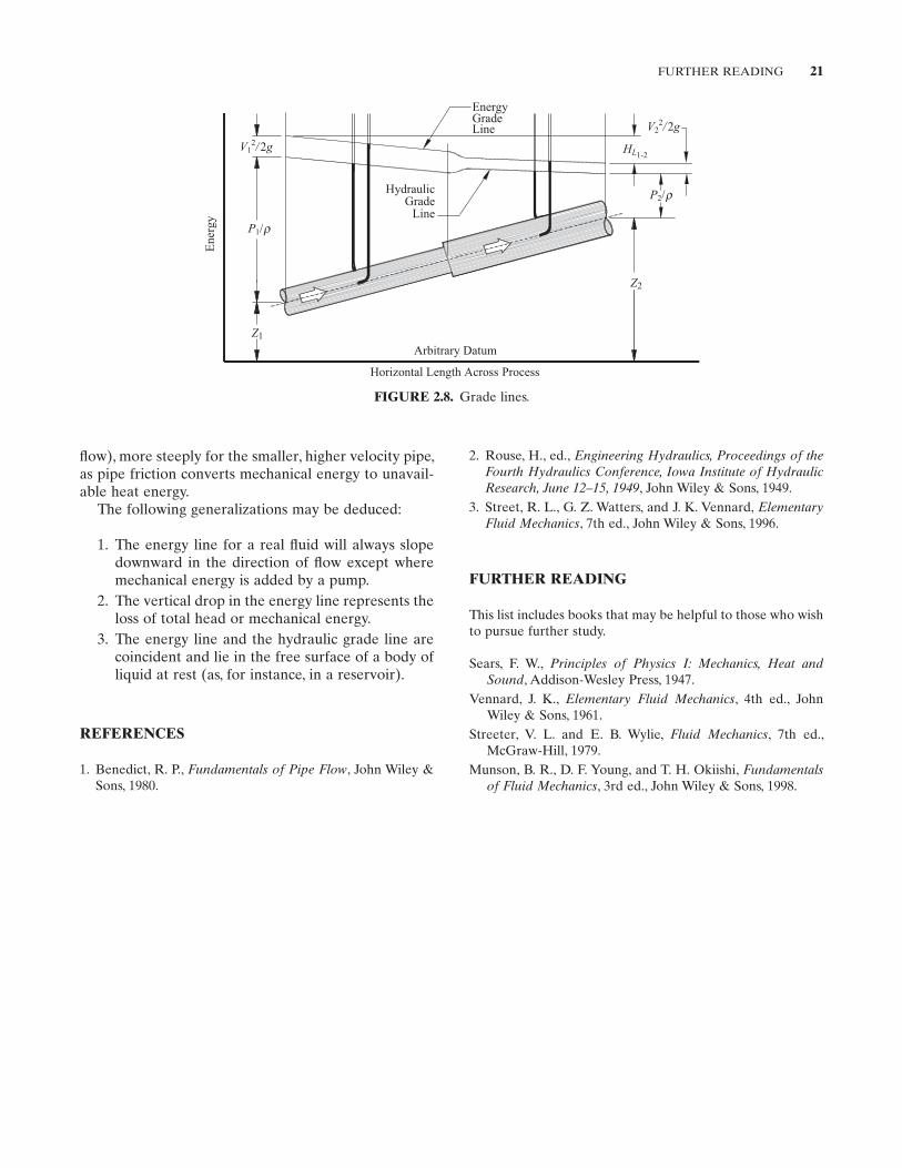
FURTHER READING 21
2. Rouse , H. , ed., Engineering Hydraulics, Proceedings of the Fourth Hydraulics Conference, Iowa Institute of Hydraulic Research, June 12 – 15, 1949 , John Wiley & Sons , 1949 .
3. Street , R. L. , G. Z. Watters , and J. K. Vennard , ElementaryFluid Mechanics , 7th ed. , John Wiley & Sons , 1996 .
FURTHER READING
This list includes books that may be helpful to those who wish to pursue further study.
Sears , F. W. , Principles of Physics I: Mechanics, Heat and Sound , Addison - Wesley Press , 1947 .
Vennard , J. K. , Elementary Fluid Mechanics , 4th ed. , John Wiley & Sons , 1961 .
Streeter , V. L. and E. B. Wylie , Fluid Mechanics , 7th ed. , McGraw - Hill , 1979 .
Munson , B. R. , D. F. Young , and T. H. Okiishi , Fundamentalsof Fluid Mechanics , 3rd ed. , John Wiley & Sons , 1998 .
fl ow), more steeply for the smaller, higher velocity pipe, as pipe friction converts mechanical energy to unavail-able heat energy.
The following generalizations may be deduced:
1. The energy line for a real fl uid will always slope downward in the direction of fl ow except where mechanical energy is added by a pump.
2. The vertical drop in the energy line represents the loss of total head or mechanical energy.
3. The energy line and the hydraulic grade line are coincident and lie in the free surface of a body of liquid at rest (as, for instance, in a reservoir).
REFERENCES
1. Benedict , R. P. , Fundamentals of Pipe Flow , John Wiley & Sons , 1980 .
FIGURE 2.8. Grade lines.
Horizontal Length Across Process
Ener
gy
HL
Z2
Z1
P1/
P2/
V22/2g
EnergyGradeLine
1-2
Arbitrary Datum
Hydraulic Grade
Line
V12/2g
r
r
23
3 INCOMPRESSIBLE FLOW
This chapter will explore kinds of fl ow, such as laminar and turbulent, the development of understanding of pressure losses in incompressible fl ow and the equations to describe them, and sources of pressure loss.
3.1 CONVENTIONAL HEAD LOSS
As was established in the previous chapter, if the fl uid pressure and temperature do not appreciably affect the fl uid density, the thermal terms of the gen-eral energy equation may be dropped, excepting one term called head loss ( HL ). The head loss term designates the mechanical energy (embodied in the Bernoulli terms P/ρ , ϕ V2 /2 g , and Z ) that is converted to thermal energy due to frictional resistance to fl ow. The resulting equation very closely describes the fl ow of most liquids. Further, when we neglect the kinetic energy correction factor, we obtain the conventional general energy equation:
P Vg
ZEw
P Vg
ZEw
Hw
P
w
TL
1
1
12
12
2
22
22 2ρ ρ( )
+ + + =( )
+ + + +
.
Now, for convenience and simplicity, assume that the fl ow line is level so that Z1 equals Z2 , and that there is no pump or turbine. Then the energy equation is simpli-fi ed to:
P Vg
P Vg
Hw w
L1
1
12
2
2
22
2 2( ) ( )ρ ρ+ = + +
or
HP P V V
gL
w w
= − + −1
1
2
2
12
22
2( ) ( ).
ρ ρ
For ordinary liquids under ordinary conditions, as indicated above, change of specifi c weight is so modest for fl ow - induced temperature and pressure changes that ( ρw ) 1 may be equated to ( ρw ) 2 . Making this simplifi cation,
HP P V V
gL
w
= − + −1 2 12
22
2ρ. (3.1)
Remember that HL is a loss in the general energy equa-tion; therefore, it represents a drop in the Energy Grade Line . Because there is no change in fl ow velocity when there is no change in fl ow area, this equation shows that pressure loss is directly proportional to head loss in a level constant area fl ow duct.
3.2 SOURCES OF HEAD LOSS
As was seen in Chapter 2 , head loss amounts to a con-version of available mechanical energy to unavailable heat energy. Two principal sources of this conversion may be identifi ed: (1) surface friction and (2) induced turbulence due to fi ttings and other changes in the fl ow path, such as valves.
Pipe Flow: A Practical and Comprehensive Guide, First Edition. Donald C. Rennels and Hobart M. Hudson.© 2012 John Wiley & Sons, Inc. Published 2012 by John Wiley & Sons, Inc.
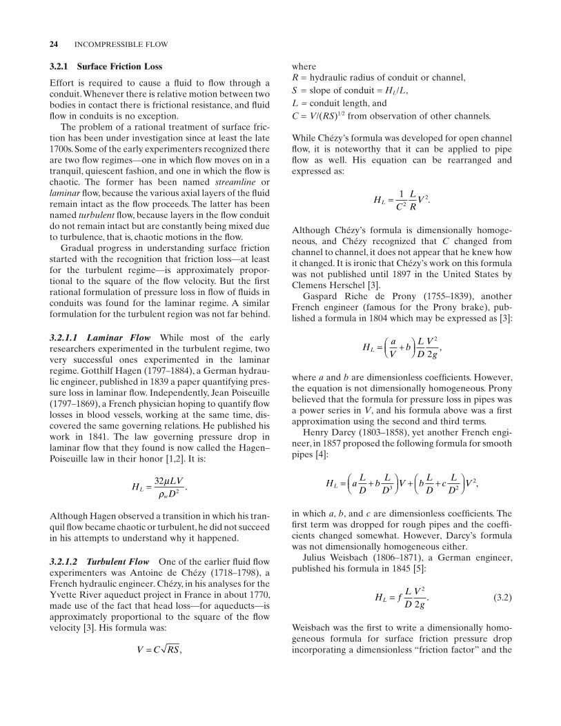
24 INCOMPRESSIBLE FLOW
whereR = hydraulic radius of conduit or channel, S = slope of conduit = HL / L , L = conduit length, and C = V /( RS ) 1/2 from observation of other channels.
While Ch é zy ’ s formula was developed for open channel fl ow, it is noteworthy that it can be applied to pipe fl ow as well. His equation can be rearranged and expressed as:
HC
LR
VL = 12
2.
Although Ch é zy ’ s formula is dimensionally homoge-neous, and Ch é zy recognized that C changed from channel to channel, it does not appear that he knew how it changed. It is ironic that Ch é zy ’ s work on this formula was not published until 1897 in the United States by Clemens Herschel [3] .
Gaspard Riche de Prony (1755 – 1839), another French engineer (famous for the Prony brake), pub-lished a formula in 1804 which may be expressed as [3] :
HaV
bLD
Vg
L = +
2
2,
where a and b are dimensionless coeffi cients. However, the equation is not dimensionally homogeneous. Prony believed that the formula for pressure loss in pipes was a power series in V , and his formula above was a fi rst approximation using the second and third terms.
Henry Darcy (1803 – 1858), yet another French engi-neer, in 1857 proposed the following formula for smooth pipes [4] :
H aLD
bLD
V bLD
cL
DVL = +
+ +
3 2
2,
in which a , b , and c are dimensionless coeffi cients. The fi rst term was dropped for rough pipes and the coeffi -cients changed somewhat. However, Darcy ’ s formula was not dimensionally homogeneous either.
Julius Weisbach (1806 – 1871), a German engineer, published his formula in 1845 [5] :
H fLD
Vg
L =2
2. (3.2)
Weisbach was the fi rst to write a dimensionally homo-geneous formula for surface friction pressure drop incorporating a dimensionless “ friction factor ” and the
3.2.1 Surface Friction Loss
Effort is required to cause a fl uid to fl ow through a conduit. Whenever there is relative motion between two bodies in contact there is frictional resistance, and fl uid fl ow in conduits is no exception.
The problem of a rational treatment of surface fric-tion has been under investigation since at least the late 1700s. Some of the early experimenters recognized there are two fl ow regimes — one in which fl ow moves on in a tranquil, quiescent fashion, and one in which the fl ow is chaotic. The former has been named streamline or laminar fl ow, because the various axial layers of the fl uid remain intact as the fl ow proceeds. The latter has been named turbulent fl ow, because layers in the fl ow conduit do not remain intact but are constantly being mixed due to turbulence, that is, chaotic motions in the fl ow.
Gradual progress in understanding surface friction started with the recognition that friction loss — at least for the turbulent regime — is approximately propor-tional to the square of the fl ow velocity. But the fi rst rational formulation of pressure loss in fl ow of fl uids in conduits was found for the laminar regime. A similar formulation for the turbulent region was not far behind.
3.2.1.1 Laminar Flow While most of the early researchers experimented in the turbulent regime, two very successful ones experimented in the laminar regime. Gotthilf Hagen (1797 – 1884), a German hydrau-lic engineer, published in 1839 a paper quantifying pres-sure loss in laminar fl ow. Independently, Jean Poiseuille (1797 – 1869), a French physician hoping to quantify fl ow losses in blood vessels, working at the same time, dis-covered the same governing relations. He published his work in 1841. The law governing pressure drop in laminar fl ow that they found is now called the Hagen – Poiseuille law in their honor [1,2] . It is:
HLVD
Lw
= 322
µρ
.
Although Hagen observed a transition in which his tran-quil fl ow became chaotic or turbulent, he did not succeed in his attempts to understand why it happened.
3.2.1.2 Turbulent Flow One of the earlier fl uid fl ow experimenters was Antoine de Ch é zy (1718 – 1798), a French hydraulic engineer. Ch é zy, in his analyses for the Yvette River aqueduct project in France in about 1770, made use of the fact that head loss — for aqueducts — is approximately proportional to the square of the fl ow velocity [3] . His formula was:
V C RS= ,
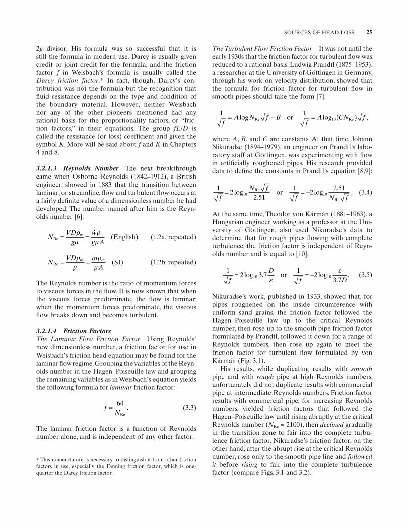
SOURCES OF HEAD LOSS 25
* This nomenclature is necessary to distinguish it from other friction factors in use, especially the Fanning friction factor, which is one - quarter the Darcy friction factor.
2g divisor. His formula was so successful that it is still the formula in modern use. Darcy is usually given credit or joint credit for the formula, and the friction factor f in Weisbach ’ s formula is usually called the Darcy friction factor . * In fact, though, Darcy ’ s con-tribution was not the formula but the recognition that fl uid resistance depends on the type and condition of the boundary material. However, neither Weisbach nor any of the other pioneers mentioned had any rational basis for the proportionality factors, or “ fric-tion factors, ” in their equations. The group fL / D is called the resistance (or loss) coeffi cient and given the symbol K . More will be said about f and K in Chapters 4 and 8 .
3.2.1.3 Reynolds Number The next breakthrough came when Osborne Reynolds (1842 – 1912), a British engineer, showed in 1883 that the transition between laminar, or streamline, fl ow and turbulent fl ow occurs at a fairly defi nite value of a dimensionless number he had developed. The number named after him is the Reyn-olds number [6] :
NVD
gwg A
w wRe ( )= =ρ
µρµ
English (1.2a, repeated)
NVD m
Am m
Re SI= =ρµ
ρµ
( ). (1.2b, repeated)
The Reynolds number is the ratio of momentum forces to viscous forces in the fl ow. It is now known that when the viscous forces predominate, the fl ow is laminar; when the momentum forces predominate, the viscous fl ow breaks down and becomes turbulent.
3.2.1.4 Friction Factors The Laminar Flow Friction Factor Using Reynolds ’ new dimensionless number, a friction factor for use in Weisbach ’ s friction head equation may be found for the laminar fl ow regime. Grouping the variables of the Reyn-olds number in the Hagen – Poiseuille law and grouping the remaining variables as in Weisbach ’ s equation yields the following formula for laminar friction factor:
fN
= 64
Re
. (3.3)
The laminar friction factor is a function of Reynolds number alone, and is independent of any other factor.
The Turbulent Flow Friction Factor It was not until the early 1930s that the friction factor for turbulent fl ow was reduced to a rational basis. Ludwig Prandtl (1875 – 1953), a researcher at the University of G ö ttingen in Germany, through his work on velocity distribution, showed that the formula for friction factor for turbulent fl ow in smooth pipes should take the form [7] :
1 110
fA N f B
fA CN f= − = ( )log log ,Re Reor
where A , B , and C are constants. At that time, Johann Nikuradse (1894 – 1979), an engineer on Prandtl ’ s labo-ratory staff at G ö ttingen, was experimenting with fl ow in artifi cially roughened pipes. His research provided data to defi ne the constants in Prandtl ’ s equation [8,9] :
12
2 511
22 51
10 10f
N f
f N f= = −log
.log
..Re
Re
or (3.4)
At the same time, Theodor von K á rm á n (1881 – 1963), a Hungarian engineer working as a professor at the Uni-versity of G ö ttingen, also used Nikuradse ’ s data to determine that for rough pipes fl owing with complete turbulence, the friction factor is independent of Reyn-olds number and is equal to [10] :
1
2 3 71
23 7
10 10f
D
f D= = −log . log
..
εε
or (3.5)
Nikuradse ’ s work, published in 1933, showed that, for pipes roughened on the inside circumference with uniform sand grains, the friction factor followed the Hagen – Poiseuille law up to the critical Reynolds number, then rose up to the smooth pipe friction factor formulated by Prandtl, followed it down for a range of Reynolds numbers, then rose up again to meet the friction factor for turbulent fl ow formulated by von K á rm á n (Fig. 3.1 ).
His results, while duplicating results with smoothpipe and with rough pipe at high Reynolds numbers, unfortunately did not duplicate results with commercial pipe at intermediate Reynolds numbers. Friction factor results with commercial pipe, for increasing Reynolds numbers, yielded friction factors that followed the Hagen – Poiseuille law until rising abruptly at the critical Reynolds number ( NRe ≈ 2100), then declined gradually in the transition zone to fair into the complete turbu-lence friction factor. Nikuradse ’ s friction factor, on the other hand, after the abrupt rise at the critical Reynolds number, rose only to the smooth pipe line and followed it before rising to fair into the complete turbulence factor (compare Figs. 3.1 and 3.2 ).
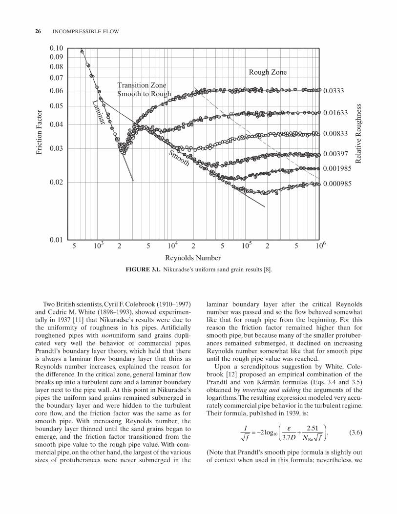
26 INCOMPRESSIBLE FLOW
FIGURE 3.1. Nikuradse ’ s uniform sand grain results [8] .
Reynolds Number
Smooth
rotcaF
noitcirF
100.01
5
0.02
53 2 104 2
Lam
inar
0.03
0.04
0.05
0.06
0.10
0.08
0.07
0.09
Transition ZoneSmooth to Rough
ssenhguoR
evitaleR
0.00397
55 10 2 5 106
0.000985
0.001985
Rough Zone
0.00833
0.01633
0.0333
Two British scientists, Cyril F. Colebrook (1910 – 1997) and Cedric M. White (1898 – 1993), showed experimen-tally in 1937 [11] that Nikuradse ’ s results were due to the uniformity of roughness in his pipes. Artifi cially roughened pipes with non uniform sand grains dupli-cated very well the behavior of commercial pipes. Prandtl ’ s boundary layer theory, which held that there is always a laminar fl ow boundary layer that thins as Reynolds number increases, explained the reason for the difference. In the critical zone, general laminar fl ow breaks up into a turbulent core and a laminar boundary layer next to the pipe wall. At this point in Nikuradse ’ s pipes the uniform sand grains remained submerged in the boundary layer and were hidden to the turbulent core fl ow, and the friction factor was the same as for smooth pipe. With increasing Reynolds number, the boundary layer thinned until the sand grains began to emerge, and the friction factor transitioned from the smooth pipe value to the rough pipe value. With com-mercial pipe, on the other hand, the largest of the various sizes of protuberances were never submerged in the
laminar boundary layer after the critical Reynolds number was passed and so the fl ow behaved somewhat like that for rough pipe from the beginning. For this reason the friction factor remained higher than for smooth pipe, but because many of the smaller protuber-ances remained submerged, it declined on increasing Reynolds number somewhat like that for smooth pipe until the rough pipe value was reached.
Upon a serendipitous suggestion by White, Cole-brook [12] proposed an empirical combination of the Prandtl and von K á rm á n formulas (Eqs. 3.4 and 3.5 ) obtained by inverting and adding the arguments of the logarithms. The resulting expression modeled very accu-rately commercial pipe behavior in the turbulent regime. Their formula, published in 1939, is:
1
f D N f= − +
23.7
2.51log .
Re10
ε (3.6)
(Note that Prandtl ’ s smooth pipe formula is slightly out of context when used in this formula; nevertheless, we
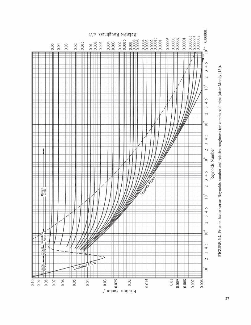
FIG
UR
E 3
.2.
Fric
tion
fac
tor
vers
us R
eyno
lds
num
ber
and
rela
tive
rou
ghne
ss f
or c
omm
erci
al p
ipe
(aft
er M
oody
[13
] ).
0.0
08
0.0
1
0.0
15
0.0
2
0.0
25
0.0
3
0.0
4
0.0
5
0.0
6
0.0
7
0.0
8
0.0
9
0.1
0FrictionFactor
10
32
34
5
Rey
nold
s N
um
ber
0.0
5
0.0
4
0.0
3
0.0
2
0.0
15
0.0
10
.00
8
0.0
06
0.0
04
0.0
02
0.0
01
0.0
00
60
.00
08
0.0
00
4
0.0
00
2
0.0
001
0.0
00
05
0.0
0001
RelativeRoughness/
0.0
00
00
5
Smoo
th P
ipes
10
410
510
610
71
08
52
34
52
34
52
34
52
34
52
34
91
00
.00
6
0.0
07
0.0
09
0.0
00
3
0.0
00
15
0.0
0002
0.0
0003
0.0
00003
0.0
00002
0.0
00001
0.0
01
5
0.0
03
Laminar Flow
f
Lam
inar
Zon
eC
riti
cal
Zone
Tra
nsi
tion
Zone
Ro
ug
hZ
one
D
27
28 INCOMPRESSIBLE FLOW
K fLD
= . (1.3, repeated)
Equation 3.1 may be rearranged as:
P PH
V Vgw
L1 2 1
222
2− = − −ρ
.
Using the identity A1V1 = A2V2 we may write:
P PH
Vg
AAw
L1 2 1
21
2
2
21
− = − −
ρ.
This is valid when there is a change in the fl ow area. Substituting Equation 3.7 for HL and rearranging gives:
P PV
gK
AA
w1 2
12
11
2
2
21− = − +
ρ. (3.8)
The loss coeffi cient for induced turbulence — “ local losses ” — is ordinarily based on the inlet size, which controls the inlet velocity. With that convention, the loss coeffi cient is subscripted with a 1, denoting the inlet, and the velocity in the equation must also be the inlet velocity, as shown. If it is desired to base the loss coeffi cient on the outlet velocity, then the last three steps yield:
P PV
gK
AA
w1 2
22
22
1
2
21− = −
+
ρ.
Using the identity w AV w= ρ , we can write:
Vw
A w
22
2 2=ρ
.
Substituting this into Equation 3.8 yields:
P Pw
gAK
AAw
1 2
2
12 1
1
2
2
21− = − +
ρ
.
If the loss coeffi cient is based on the outlet size, the pressure drop equation becomes:
P Pw
gAK
AAw
1 2
2
22 2
2
1
2
21− = + −
ρ
.
If the inlet and outlet areas are the same ( A1 = A2 ), the formula reduces to:
P P Kw
gA w1 2
2
22− =
ρ
.
will call it the “ Prandtl term ” because of its origin.) Soon afterwards (1944), Lewis F. Moody [13] published a design chart based on the Colebrook – White formula. The formula and chart (Fig. 3.2 ) have been so successful that they are still in use today. The chart is popularly known as the “ Moody Chart. ” See also the diagram in Part II, Chapter 8 .
3.2.2 Induced Turbulence
The second source of pressure losses in pipe fl ow, in contrast to pipe friction, is induced turbulence . These losses are often referred to as local losses or sometimes as minor losses , although they are usually far from minor. When turbulence in excess of that normally present in the fl ow is caused by the fl ow passage shape, the energy resident in the turbulence is not usually recovered as mechanical energy and is consequently converted to heat. As shown in Chapter 2 , mechanical energy converted to heat is described in the energy equation by the head loss term, HL .
A particular solution to the local loss problem ante-dates the Darcy – Weisbach equation; this is the Borda sudden expansion loss. Jean - Charles de Borda, by rea-soning, predicted in 1766 the head loss due to a sudden expansion. In modern terms his prediction may be written as:
HV
gAA
L = −
12
1
2
2
21 .
This equation is often called the Borda – Carnot equa-tion. Experiments proved Borda to be correct for the turbulent fl ow case.
Note that the head loss in Borda ’ s equation is proportional to V g1
2 2/ times a geometry - dependent constant . This arrangement has been found to be generally true in subsequent pressure loss work. If we denote the geometry - dependent constant as K , the general case of induced turbulence head loss may be written as:
H KV
gL =
2
2. (3.7)
K is known as the resistance coeffi cient or loss coeffi cient . As shown in Chapter 2 , V 2 /2 g is the velocity head , so that K is the head loss measured in velocity heads.
Making use of the fact that V 2 /2 g is the velocity head, the Weisbach equation (Eq. 3.2 ) may also be written using the loss coeffi cient K . Factoring the V.2 /2 g term from the equation shows that Equation 3.7 may be used to describe pipe friction when:
REFERENCES 29
Usually the “ standardized ” area is the area of the most important feature, usually pipe, in the stretch being considered.*
REFERENCES
1. Hagen , G. H. L. , Ueber die Bewegung des Wassers in agen cylindrischen Rohren , Poggendorfs Ann. Phys. Chem. , 46 , 1839 , 423 . (Translated as “ On the fl ow of water in narrow cylindrical pipes. ” )
2. Poiseille , J. L. M. , Recherches experimentales sur le mou-vement des liquids dans les tubes tres petits diameters , C. R. Acad. Sci. , 1841 . (Translated as “ Experimental research on the fl ow of liquids through pipes of very small diameters. ” )
3. Rouse , H. and S. Ince , History of Hydraulics, Iowa Institute of Hydraulic Research , State University of Iowa , 1957 .
4. Darcy , H. P. G. , Recherches experimentales relatives aux mouvement del ’ eau dans les tuyaux , Mem. Acad. Inst. Imp. Fr. , 15 , 1858 , 141 . (Translated as “ Experimental research on the fl ow of water in pipes. ” )
5. Weisbach , J. , Lehbuch der Ingenieur — und Maschinen - Mechanik , Braunschwieg, 1845 .
6. Reynolds , O. , An experimental investigation of the cir-cumstances which determine whether the motion of water will be direct of sinuous, and the laws of resistance in parallel channels , Philos. Trans. R. Soc. Lond. , 1883 .
7. Prandl , L. , Ergeb. Aerodyn. Versuchanst. Gottingen . Series 3, 1927 . (Translated as “ Reports of the Aerodynamic Research Institute at Gottingen. ” ).
8. Nikuradse , J. , Laws of fl ow in rough pipes (in German), Forsch. - Arb Ing. - Wesen , 361 , 1933 .
9. Prandl , L. , Neuere ergebnisse der turbulenzforschung , Z. VDI , 77 , 1933 , 105 . (Translated as “ Recent results of tur-bulence research. ” ).
10. Von K á rm á n , T. , Mechanische Ä hnlichkeit und Turbulenz , Nachrichten von der Gesellschaft der Wissenschofen zu Gő ttingen , 1930 , Fachgruppe 1, Mathematik, no. 5, pp. 58 – 76 . ( “ Mechanical similitude and turbulence, ” Tech. Mem. N.A.C.A., no. 611, 1931.).
11. Colebrook , C. F. and C. M. White , Experiments with fl uid friction in roughened pipes , Proc. R. Soc. Lond. , 161 , 1937 , 367 – 381 .
12. Colebrook , C. F. , Turbulent fl ow in pipes, with particular reference to the transition region between the smooth and rough pipe laws , J. Inst. Civ. Eng. , 11 , 1938 – 1939 , 133 – 156 .
13. Moody , L. F. , Friction factors for pipe fl ow , Trans. Am. Soc. Mech. Eng. , 66 , 1944 , 671 – 684 .
Unfortunately, this form is often used in practice even if the inlet and outlet areas are different.
While the head loss for induced turbulence is slightly dependent on the surface roughness, usually — unlike pipe friction — the feature geometry is by far the most important, and, after that, the Reynolds number. Part II gives K for a number of important pipe fi ttings and arrangements.
3.2.3 Summing Loss Coeffi cients
Pressure losses in incompressible fl ow are additive. If a piping stretch has various contributors to the overall pressure loss with different areas, it will be convenient to have a formula for the overall pressure loss in terms of the characteristics of the individual pressure loss con-tributors. We may write:
∆ ∆ ∆ ∆ ∆P P P P POA a b c n= + + + +… .
Substituting for the individual ΔP s results in:
∆P Kw
gAK
wgA
Kw
gAOA
w a w b w c
=
+
+
2
2
2
2
2
22 2 2ρ ρ ρ++
+
... .Kw
gA w n
2
22 ρ
The K s themselves are based on different areas, so we cannot add them. However, if we factor out w gA w
2 2/ ρwe get:
∆Pw
gA wK
AA
KAA
KAA
KAA
OA aa
bb
cc
nn
= + + + +
…
2
2
2
2
2
2
2
2
2
22.
Each K , as modifi ed by the ratio of the square of the ratio of the “ standardized ” area ( A ) to the actual area (Aa, A b, A c , or An ), can be added. We say that the resis-tance coeffi cients are referred to the standardized area (that is, A ). The general form is:
K KAA
K Kdd
aa
aa
= =2
2
4
4or , (3.9)
whereK = standardized K (usable in the ΔP formula with
A1 ), K a = actual K (usable with Aa in the ΔP formula), A = standardized area, Aa = actual area, d = standardized diameter, and da = actual diameter.
* The summing of loss coeffi cients is restated in Section 5.1 as series fl ow.
30 INCOMPRESSIBLE FLOW
Guislain , S. J. , How to make sense of friction factors in fl uid fl ow through pipe , Plant Engineering , June 12, 1980 , pp. 134 – 140 .
Lamont , P. A. , Pipe fl ow formulas compared with the theory of roughness , Am. Water Works Assoc. J. , 73 ( 5 ), 1981 .
Oluji ć , Ž . , Compute friction factors fast for fl ow in pipes , Chemical Engineering , December 14, 1981 , pp. 91 – 93 .
Roberson , J. A. and C. T. Crowe , Engineering Fluid Mechanics , 3rd ed. , Houghton Miffl in Company , 1985 .
Munson , B. R. , D. F. Young , and T. H. Okiishi , Fundamentalsof Fluid Mechanics , 3rd ed. , John Wiley & Sons , 1998 .
FURTHER READING
This list includes books and papers that may be helpful to those who wish to pursue further study.
Vennard , J. K. , Elementary Fluid Mechanics , 4th ed. , John Wiley & Sons , 1961 .
Booth , R. and N. Epstein , Kinetic energy and momentum factors for rough pipes , Can. J. Chem. Eng. , 47 , 1969 , 515 – 517 .
Streeter , V. L. and E. B. Wylie , Fluid Mechanics , 7th ed. , McGraw - Hill , 1979 .
Benedict , R. P. , Fundamentals of Pipe Flow , John Wiley & Sons , 1980 .
31
4 COMPRESSIBLE FLOW
This chapter deals with fi nding the pressure drop in ducts fl owing a compressible fl uid. Six methods of fi nding the pressure drop are offered, ranging from approximate methods of varying accuracy to analytical methods with absolute accuracy within the assumptions made. Units used are mainly English gravitational units, but International System (SI) units can be substituted if dimensional homogeneity is maintained. (English gravitational units use lb f , ft, and s as basic. This system is very nearly the same as the United States customary system (USCS) units, which use slug, ft, and s as basic. In either the USCS system or the English gravitational system, lb f = slugs × g , where g is the acceleration of gravity in ft/s 2 .)
4.1 PROBLEM SOLUTION METHODS
As pointed out in Chapter 2 , in incompressible fl ow without heat exchanger input or output the thermal terms may be equated to head loss. In compressible fl ow, however, such is not the case because there are signifi -cant conversions of heat energy to mechanical energy. Some methods for fi nding the pressure loss for a com-pressible fl uid fl owing in a duct are given below. Hori-zontal ducts are considered because the density of the fl owing compressible fl uid is usually low enough to neglect its effect on static pressure with modest changes in elevation.
It should be noted that each of the methods outlined below require the fl ow path to have a constant cross -
sectional area . Procedures are given in Section 4.3.1.5 or at the end of Section 4.3.2 on how to handle changes in cross - sectional area.
Compressible fl ow may be treated in six principal fashions:
1. If the pressure drop is small compared to the system pressure, variation in fl owing fl uid density with changing system pressure may be ignored and the pressure drop found by incompressible fl ow formulas. This technique works well for pres-sure drops below about 10% of the inlet pressure, and it works for either isothermal fl ow or adiabatic fl ow. The formula is given in Section 4.2.1 below.
2. For pressure drops up to about 40% of the inlet pressure, and for resistance coeffi cient K = 10 or greater (or for smaller drops if K is smaller), incompressible fl ow formulas work fairly well if the fl uid properties are determined at the average of inlet and outlet conditions. This also works with isothermal or adiabatic fl ow. The formula for this method is given early in Section 4.2.2 below, with an error chart for the adiabatic case.
3. For pressure drops up to about 40% of the inlet pressure, and for resistance coeffi cient K = 6 or greater, incompressible formulas work fairly well if the inlet and outlet pressures and their average are used in determining the pressure drop. This method is similar to the average properties method described above but takes more into account to
Pipe Flow: A Practical and Comprehensive Guide, First Edition. Donald C. Rennels and Hobart M. Hudson.© 2012 John Wiley & Sons, Inc. Published 2012 by John Wiley & Sons, Inc.
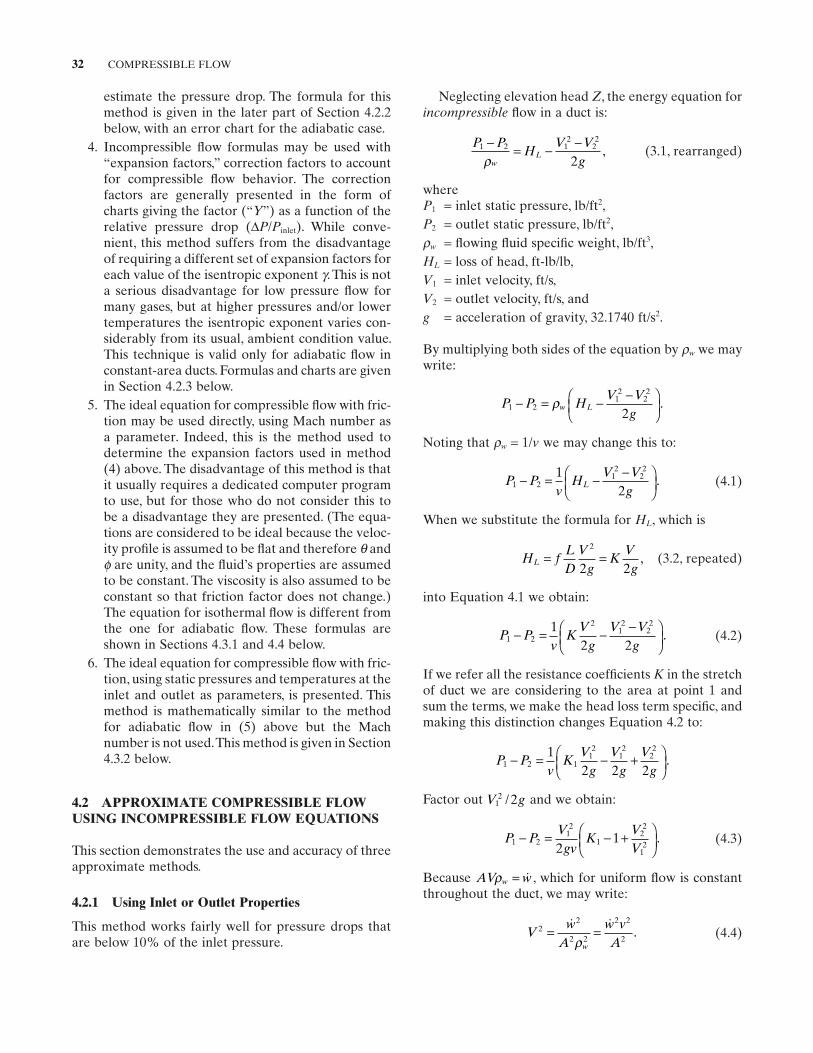
32 COMPRESSIBLE FLOW
Neglecting elevation head Z , the energy equation for incompressible fl ow in a duct is:
P P
HV V
gwL
1 2 12
22
2− = − −ρ
, (3.1, rearranged)
whereP1 = inlet static pressure, lb/ft 2 , P2 = outlet static pressure, lb/ft 2 , ρw = fl owing fl uid specifi c weight, lb/ft 3 , HL = loss of head, ft - lb/lb, V1 = inlet velocity, ft/s, V2 = outlet velocity, ft/s, and g = acceleration of gravity, 32.1740 ft/s 2 .
By multiplying both sides of the equation by ρw we may write:
P P H V V
gw L1 2
12
22
2− = − −
ρ .
Noting that ρw = 1/ v we may change this to:
P P v
HV V
gL1 2
12
221
2− = − −
. (4.1)
When we substitute the formula for HL , which is
H fLD
Vg
KVg
L = =2
2 2, (3.2, repeated)
into Equation 4.1 we obtain:
P Pv
KV
gV V
g1 2
212
221
2 2− = − −
. (4.2)
If we refer all the resistance coeffi cients K in the stretch of duct we are considering to the area at point 1 and sum the terms, we make the head loss term specifi c, and making this distinction changes Equation 4.2 to:
P Pv
KV
gV
gV
g1 2 1
12
12
221
2 2 2− = − +
.
Factor out V g12 2/ and we obtain:
P PVgv
KVV
1 212
122
122
1− = − +
. (4.3)
Because AV wwρ = , which for uniform fl ow is constant throughout the duct, we may write:
Vw
Aw vAw
22
2 2
2 2
2= = ρ
. (4.4)
estimate the pressure drop. The formula for this method is given in the later part of Section 4.2.2 below, with an error chart for the adiabatic case.
4. Incompressible fl ow formulas may be used with “ expansion factors, ” correction factors to account for compressible fl ow behavior. The correction factors are generally presented in the form of charts giving the factor ( “ Y ” ) as a function of the relative pressure drop ( ΔP / Pinlet ). While conve-nient, this method suffers from the disadvantage of requiring a different set of expansion factors for each value of the isentropic exponent γ . This is not a serious disadvantage for low pressure fl ow for many gases, but at higher pressures and/or lower temperatures the isentropic exponent varies con-siderably from its usual, ambient condition value. This technique is valid only for adiabatic fl ow in constant - area ducts. Formulas and charts are given in Section 4.2.3 below.
5. The ideal equation for compressible fl ow with fric-tion may be used directly, using Mach number as a parameter. Indeed, this is the method used to determine the expansion factors used in method (4) above. The disadvantage of this method is that it usually requires a dedicated computer program to use, but for those who do not consider this to be a disadvantage they are presented. (The equa-tions are considered to be ideal because the veloc-ity profi le is assumed to be fl at and therefore θ and ϕ are unity, and the fl uid ’ s properties are assumed to be constant. The viscosity is also assumed to be constant so that friction factor does not change.) The equation for isothermal fl ow is different from the one for adiabatic fl ow. These formulas are shown in Sections 4.3.1 and 4.4 below.
6. The ideal equation for compressible fl ow with fric-tion, using static pressures and temperatures at the inlet and outlet as parameters, is presented. This method is mathematically similar to the method for adiabatic fl ow in (5) above but the Mach number is not used. This method is given in Section 4.3.2 below.
4.2 APPROXIMATE COMPRESSIBLE FLOW USING INCOMPRESSIBLE FLOW EQUATIONS
This section demonstrates the use and accuracy of three approximate methods.
4.2.1 Using Inlet or Outlet Properties
This method works fairly well for pressure drops that are below 10% of the inlet pressure.
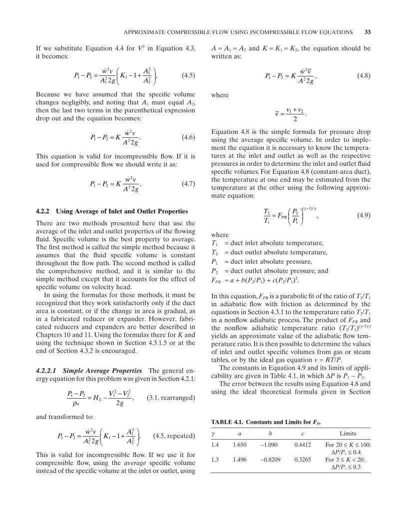
APPROXIMATE COMPRESSIBLE FLOW USING INCOMPRESSIBLE FLOW EQUATIONS 33
A = A1 = A2 and K = K1 = K2 , the equation should be written as:
P P Kw v
A g1 2
2
2 2− ≈
, (4.8)
where
vv v
=+1 2
2.
Equation 4.8 is the simple formula for pressure drop using the average specifi c volume. In order to imple-ment the equation it is necessary to know the tempera-tures at the inlet and outlet as well as the respective pressures in order to determine the inlet and outlet fl uid specifi c volumes. For Equation 4.8 (constant - area duct), the temperature at one end may be estimated from the temperature at the other using the following approxi-mate equation:
TT
FPP
PR2
1
2
1
1
≈
−( )/
,γ γ
(4.9)
whereT1 = duct inlet absolute temperature, T2 = duct outlet absolute temperature, P1 = duct inlet absolute pressure, P2 = duct outlet absolute pressure, and FPR ≈ a + b ( P2 / P1 ) + c ( P2 / P1 ) 2 .
In this equation, FPR is a parabolic fi t of the ratio of T2 / T1
in adiabatic fl ow with friction as determined by the equations in Section 4.3.1 to the temperature ratio T2 / T1
in a nonfl ow adiabatic process. The product of FPR and the nonfl ow adiabatic temperature ratio ( T2 / T1 ) (γ− 1)/γ
yields an approximate value of the adiabatic fl ow tem-perature ratio. It is then possible to determine the values of inlet and outlet specifi c volumes from gas or steam tables, or by the ideal gas equation v = RT / P .
The constants in Equation 4.9 and its limits of appli-cability are given in Table 4.1 , in which ΔP is P1 − P2 .
The error between the results using Equation 4.8 and using the ideal theoretical formula given in Section
If we substitute Equation 4.4 for V2 in Equation 4.3 , it becomes:
P Pw v
A gK
AA
1 2
2
12 1
12
222
1− = − +
. (4.5)
Because we have assumed that the specifi c volume changes negligibly, and noting that A1 must equal A2 , then the last two terms in the parenthetical expression drop out and the equation becomes:
P P Kw v
A g1 2
2
2 2− =
. (4.6)
This equation is valid for incompressible fl ow. If it is used for compressible fl ow we should write it as:
P P Kw v
A g1 2
2
2 2− ≈
. (4.7)
4.2.2 Using Average of Inlet and Outlet Properties
There are two methods presented here that use the average of the inlet and outlet properties of the fl owing fl uid. Specifi c volume is the best property to average. The fi rst method is called the simple method because it assumes that the fl uid specifi c volume is constant throughout the fl ow path. The second method is called the comprehensive method, and it is similar to the simple method except that it accounts for the effect of specifi c volume on velocity head.
In using the formulas for these methods, it must be recognized that they work satisfactorily only if the duct area is constant, or if the change in area is gradual, as in a fabricated reducer or expander. However, fabri-cated reducers and expanders are better described in Chapters 10 and 11 . Using the formulas there for K and using the technique shown in Section 4.3.1.5 or at the end of Section 4.3.2 is encouraged.
4.2.2.1 Simple Average Properties The general en -ergy equation for this problem was given in Section 4.2.1 :
P P
HV V
gwL
1 2 12
22
2− = − −ρ
, (3.1, rearranged)
and transformed to:
P Pw v
A gK
AA
1 2
2
12 1
12
222
1− = − +
. (4.5, repeated)
This is valid for incompressible fl ow. If we use it for compressible fl ow, using the average specifi c volume instead of the specifi c volume at the inlet or outlet, using
TABLE 4.1. Constants and Limits for FPr
γ a b c Limits
1.4 1.650 − 1.090 0.4412 For 20 ≤ K ≤ 100: ΔP / P1 ≤ 0.4
1.3 1.496 − 0.8209 0.3265 For 3 ≤ K < 20: ΔP / P1 ≤ 0.3
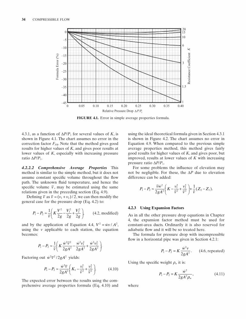
34 COMPRESSIBLE FLOW
using the ideal theoretical formula given in Section 4.3.1 is shown in Figure 4.2 . The chart assumes no error in Equation 4.9 . When compared to the previous simple average properties method, this method gives fairly good results for higher values of K , and gives poor, but improved, results at lower values of K with increasing pressure ratio ΔP/P1 .
For some problems the infl uence of elevation may not be negligible. For these, the ΔP due to elevation difference can be added:
P PvwgA
Kvv
vv v
Z Z1 2
2
212
222
2 2 12
1− ≈ − +
+ −( ).
4.2.3 Using Expansion Factors
As in all the other pressure drop equations in Chapter 4 , the expansion factor method must be used for constant - area ducts. Ordinarily it is also reserved for adiabatic fl ow and it will be so treated here.
The formula for pressure drop with incompressible fl ow in a horizontal pipe was given in Section 4.2.1 :
P P Kw vgA
1 2
2
22− =
. (4.6, repeated)
Using the specifi c weight ρw it is:
P P Kw
gA w1 2
2
22− =
ρ
, (4.11)
where
4.3.1 , as a function of ΔP/P1 for several values of K , is shown in Figure 4.1 . The chart assumes no error in the correction factor FPR . Note that the method gives good results for higher values of K , and gives poor results at lower values of K , especially with increasing pressure ratio ΔP/P1 .
4.2.2.2 Comprehensive Average Properties This method is similar to the simple method, but it does not assume constant specifi c volume throughout the fl ow path. The unknown fl uid temperature, and hence the specifi c volume v , may be estimated using the same relations given in the preceding section (Eq. 4.9 ).
Defi ning v as v v v= +( ) /1 2 2, we can then modify the general case for the pressure drop (Eq. 4.2 ) to:
P Pv
KV
gV
gV
g1 2
212
221
2 2 2− ≈ − +
, (4.2, modifi ed)
and by the application of Equation 4.4 , V wv A2 2= / ,using the v applicable to each station, the equation becomes:
P Pv
Kw v
gAw vgA
w vgA
1 2
2 2
2
212
2
222
2
12 2 2
− ≈ − +
.
Factoring out w v gA2 2 22/ yields:
P Pw vgA
Kvv
vv
1 2
2
2 112
222
22− ≈ − +
. (4.10)
The expected error between the results using the com-prehensive average properties formula (Eq. 4.10 ) and
FIGURE 4.1. Error in simple average properties formula.
0–45
0.05 0.10 0.15 0.20 0.25 0.30 0.35 0.40
–40
–35
–30
–25
–20
–15
–10
–5
0
Relative Pressure Drop P/P1
For
mul
a E
rror
(%
)
1
1.5
3
6
101520
Ktneiciffeo
Cecnatsise
R
∆
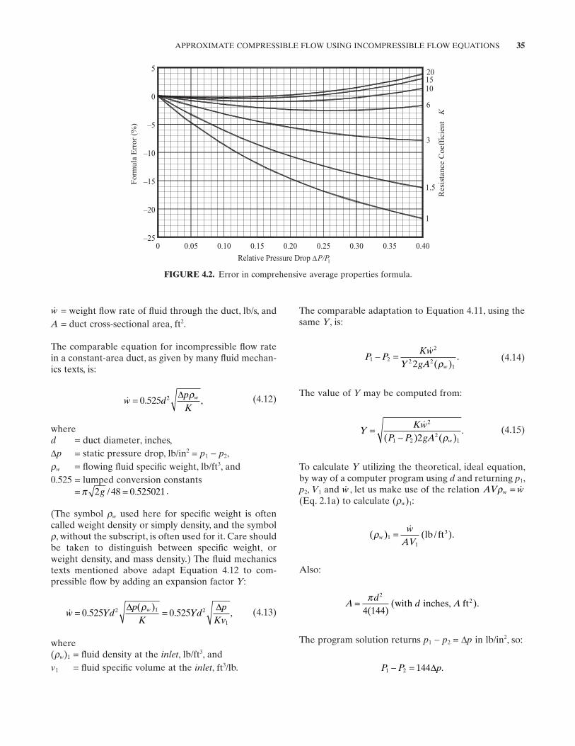
APPROXIMATE COMPRESSIBLE FLOW USING INCOMPRESSIBLE FLOW EQUATIONS 35
The comparable adaptation to Equation 4.11 , using the same Y , is:
P PKw
Y gA w1 2
2
2 212
− =
( ).
ρ (4.14)
The value of Y may be computed from:
YKw
P P gA w
=−
2
1 22
12( ) ( ).
ρ (4.15)
To calculate Y utilizing the theoretical, ideal equation, by way of a computer program using d and returning p1 , p2 , V1 and w , let us make use of the relation AV wwρ = (Eq. 2.1a ) to calculate ( ρw ) 1 :
( ) ( / ).ρww
AV1
1
3=
lb ft
Also:
Ad
d A= π 22
4 144( )( , ).with inches ft
The program solution returns p1 − p2 = Δp in lb/in 2 , so:
P P p1 2 144− = ∆ .
w = weight fl ow rate of fl uid through the duct, lb/s, and A = duct cross - sectional area, ft 2 .
The comparable equation for incompressible fl ow rate in a constant - area duct, as given by many fl uid mechan-ics texts, is:
w dpK
w= 0 525 2. ,∆ ρ (4.12)
whered = duct diameter, inches, Δp = static pressure drop, lb/in 2 = p1 − p2 , ρw = fl owing fl uid specifi c weight, lb/ft 3 , and 0.525 = lumped conversion constants
= =π 2 48 0 525021g / . .
(The symbol ρw used here for specifi c weight is often called weight density or simply density, and the symbol ρ , without the subscript, is often used for it. Care should be taken to distinguish between specifi c weight, or weight density, and mass density.) The fl uid mechanics texts mentioned above adapt Equation 4.12 to com-pressible fl ow by adding an expansion factor Y :
w Ydp
KYd
pKv
w= =0 525 0 5252 1 2
1
.( )
. ,∆ ∆ρ (4.13)
where ( ρw ) 1 = fl uid density at the inlet , lb/ft 3 , and v1 = fl uid specifi c volume at the inlet , ft 3 /lb.
FIGURE 4.2. Error in comprehensive average properties formula.
P/P1
–25
–20
–15
–10
–5
0
5
Relative Pressure Drop ∆04.051.001.050.00 0.20 0.25 0.350.30
1
tneiciffeoC
ecnatsiseR
3
1.5
K
6
201510
For
mul
a E
rror
(%
)
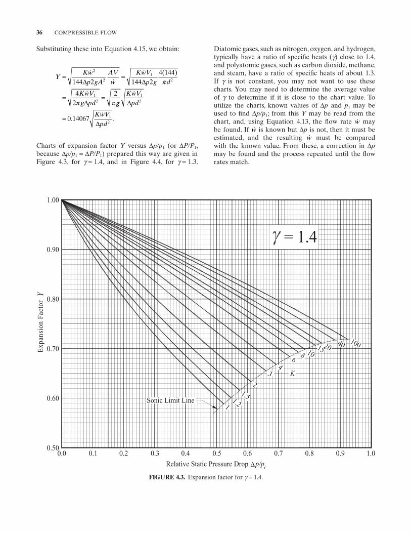
36 COMPRESSIBLE FLOW
FIGURE 4.3. Expansion factor for γ = 1.4.
0.00.50
Relative Static Pressure Drop p/p1
Exp
a nsi
onF
acto
rY
0.1
0.60
0.70
0.80
0.90
1.00
0.2 0.3 0.4 0.5 0.6 0.7 0.8 0.9 1.0
K
= 1.4
Sonic Limit Line
1004020151086
43
21.51.21
∆
Substituting these into Equation 4.15 , we obtain:
YKw
p gAAVw
KwVp g d
KwVg pd
= =
= =
2
21
2
12
144 2 144 24 144
42
2
∆ ∆
∆
( )π
π π ggKwV
pd
KwVpd
12
12
0 14067
∆
∆= . .
Charts of expansion factor Y versus Δp/p1 (or ΔP/P1 , because Δp/p1 = ΔP/P1 ) prepared this way are given in Figure 4.3 , for γ = 1.4, and in Figure 4.4 , for γ = 1.3.
Diatomic gases, such as nitrogen, oxygen, and hydrogen, typically have a ratio of specifi c heats ( γ ) close to 1.4, and polyatomic gases, such as carbon dioxide, methane, and steam, have a ratio of specifi c heats of about 1.3. If γ is not constant, you may not want to use these charts. You may need to determine the average value of γ to determine if it is close to the chart value. To utilize the charts, known values of Δp and p1 may be used to fi nd Δp/p1 ; from this Y may be read from the chart, and, using Equation 4.13 , the fl ow rate w may be found. If w is known but Δp is not, then it must be estimated, and the resulting w must be compared with the known value. From these, a correction in Δpmay be found and the process repeated until the fl ow rates match.
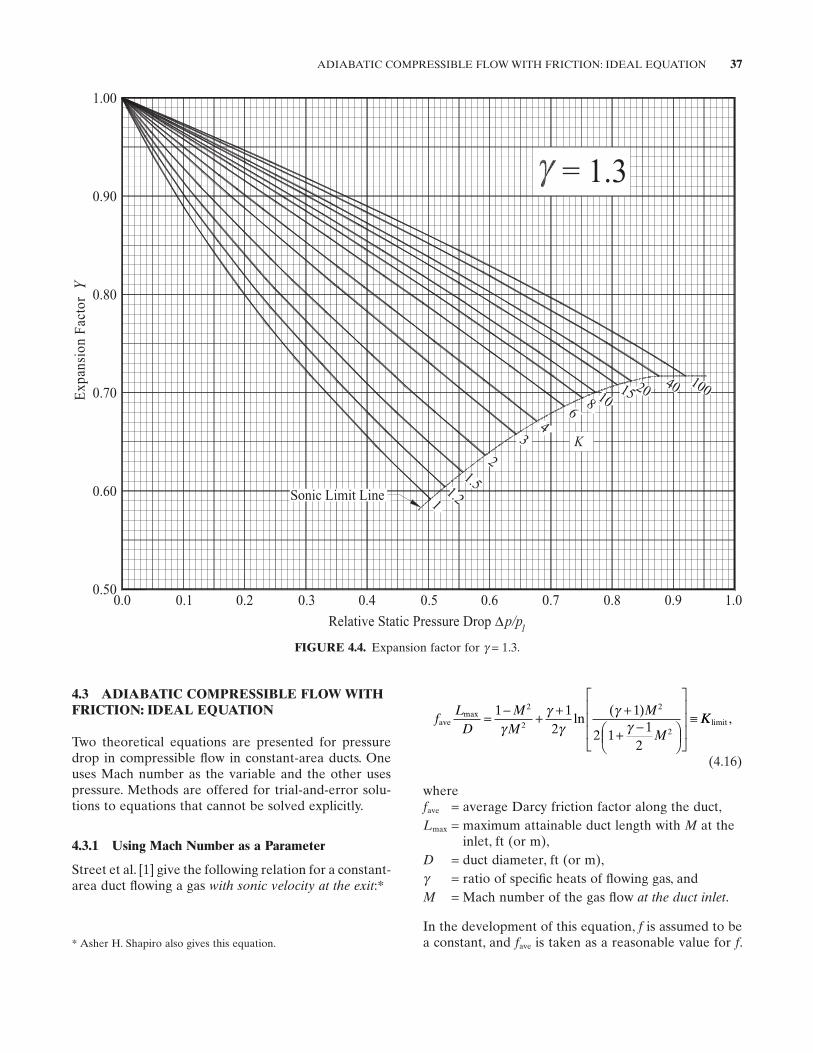
ADIABATIC COMPRESSIBLE FLOW WITH FRICTION: IDEAL EQUATION 37
* Asher H. Shapiro also gives this equation.
4.3 ADIABATIC COMPRESSIBLE FLOW WITH FRICTION: IDEAL EQUATION
Two theoretical equations are presented for pressure drop in compressible fl ow in constant - area ducts. One uses Mach number as the variable and the other uses pressure. Methods are offered for trial - and - error solu-tions to equations that cannot be solved explicitly.
4.3.1 Using Mach Number as a Parameter
Street et al. [1] give the following relation for a constant - area duct fl owing a gas with sonic velocity at the exit : *
fL
DM
MM
Mave
max ln( )= − + + +
+ −
≡1 12
1
2 11
2
2
2
2
2γγ
γγ
γ KKlimit ,
(4.16)
wherefave = average Darcy friction factor along the duct, Lmax = maximum attainable duct length with M at the
inlet, ft (or m), D = duct diameter, ft (or m), γ = ratio of specifi c heats of fl owing gas, and M = Mach number of the gas fl ow at the duct inlet .
In the development of this equation, f is assumed to be a constant, and fave is taken as a reasonable value for f .
FIGURE 4.4. Expansion factor for γ = 1.3.
0.00.50
Relative Static Pressure Drop p/p1
Exp
a nsi
onF
acto
rY
0.1
0.60
0.70
0.80
0.90
1.00
0.2 0.3 0.4 0.5 0.6 0.7 0.8 0.9 1.0
2
34
68 10
15 20 40 100
11.2
1.5
K
= 1.3
Sonic Limit Line
∆
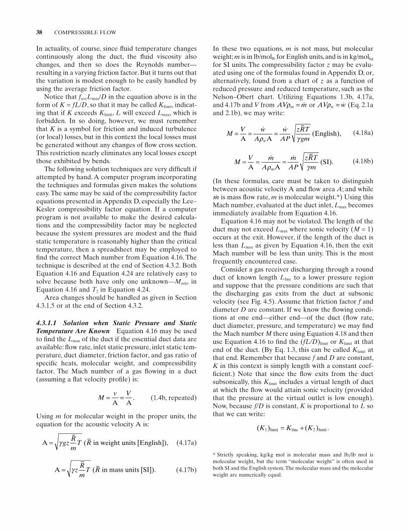
38 COMPRESSIBLE FLOW
In these two equations, m is not mass, but molecular weight; m is in lb/mol lb for English units, and is in kg/mol kg
for SI units. The compressibility factor z may be evalu-ated using one of the formulas found in Appendix D , or, alternatively, found from a chart of z as a function of reduced pressure and reduced temperature, such as the Nelson – Obert chart. Utilizing Equations 1.3b , 4.17a , and 4.17b and V from AV mmρ = or AV wwρ = (Eq. 2.1a and 2.1b ), we may write:
MV w
Aw
APzRT
gmw
= = =A A
English
ρ γ( ), (4.18a)
MV m
Am
APzRT
mm
= = =A A
SI
ρ γ( ). (4.18b)
(In these formulas, care must be taken to distinguish between acoustic velocity A and fl ow area A ; and while m is mass fl ow rate, m is molecular weight. * ) Using this
Mach number, evaluated at the duct inlet, Lmax becomes immediately available from Equation 4.16 .
Equation 4.16 may not be violated. The length of the duct may not exceed Lmax where sonic velocity ( M = 1) occurs at the exit. However, if the length of the duct is less than Lmax as given by Equation 4.16 , then the exit Mach number will be less than unity. This is the most frequently encountered case.
Consider a gas receiver discharging through a round duct of known length Lline to a lower pressure region and suppose that the pressure conditions are such that the discharging gas exits from the duct at subsonic velocity (see Fig. 4.5 ). Assume that friction factor f and diameter D are constant. If we know the fl owing condi-tions at one end — either end — of the duct (fl ow rate, duct diameter, pressure, and temperature) we may fi nd the Mach number M there using Equation 4.18 and then use Equation 4.16 to fi nd the ( fL/D ) limit or Klimit at that end of the duct. (By Eq. 1.3 , this can be called Klimit at that end. Remember that because f and D are constant, K in this context is simply length with a constant coef-fi cient.) Note that since the fl ow exits from the duct subsonically, this Klimit includes a virtual length of duct at which the fl ow would attain sonic velocity (provided that the pressure at the virtual outlet is low enough). Now, because f/D is constant, K is proportional to L so that we can write:
( ) ( ) .K K K1 2limit line limit= +
In actuality, of course, since fl uid temperature changes continuously along the duct, the fl uid viscosity also changes, and then so does the Reynolds number — resulting in a varying friction factor. But it turns out that the variation is modest enough to be easily handled by using the average friction factor.
Notice that faveLmax / D in the equation above is in the form of K = fL / D , so that it may be called Klimit , indicat-ing that if K exceeds Klimit , L will exceed Lmax , which is forbidden. In so doing, however, we must remember that K is a symbol for friction and induced turbulence (or local) losses, but in this context the local losses must be generated without any changes of fl ow cross section. This restriction nearly eliminates any local losses except those exhibited by bends.
The following solution techniques are very diffi cult if attempted by hand. A computer program incorporating the techniques and formulas given makes the solutions easy. The same may be said of the compressibility factor equations presented in Appendix D , especially the Lee – Kesler compressibility factor equation. If a computer program is not available to make the desired calcula-tions and the compressibility factor may be neglected because the system pressures are modest and the fl uid static temperature is reasonably higher than the critical temperature, then a spreadsheet may be employed to fi nd the correct Mach number from Equation 4.16 . The technique is described at the end of Section 4.3.2 . Both Equation 4.16 and Equation 4.24 are relatively easy to solve because both have only one unknown — Minlet in Equation 4.16 and T2 in Equation 4.24 .
Area changes should be handled as given in Section 4.3.1.5 or at the end of Section 4.3.2 .
4.3.1.1 Solution when Static Pressure and Static Temperature Are Known Equation 4.16 may be used to fi nd the Lmax of the duct if the essential duct data are available: fl ow rate, inlet static pressure, inlet static tem-perature, duct diameter, friction factor, and gas ratio of specifi c heats, molecular weight, and compressibility factor. The Mach number of a gas fl owing in a duct (assuming a fl at velocity profi le) is:
Mv V
= =A A
. (1.4b, repeated)
Using m for molecular weight in the proper units, the equation for the acoustic velocity A is:
A in weight units English= γ gzRm
T R( [ ]), (4.17a)
A in mass units SI= γ zRm
T R( [ ]). (4.17b)
* Strictly speaking, kg/kg mol is molecular mass and lb f /lb mol is molecular weight, but the term “ molecular weight ” is often used in both SI and the English system. The molecular mass and the molecular weight are numerically equal.
ADIABATIC COMPRESSIBLE FLOW WITH FRICTION: IDEAL EQUATION 39
T * is the static temperature when the accompanying Mach number is unity. The ratio of the inlet and outlet static temperatures is thus:
TT
MM
1
2
22
12
1 1 21 1 2
= + −+ −
( ) /( ) /
,γγ
(4.22)
from which the desired temperature is easily found. The foregoing relationships are useful if the static
pressure and static temperature at one end of the duct are known. If one or the other of the static values is not known, but the corresponding total value is known (and this is often, if not usually, the case) these equations may still be solved, but account must be made for the diver-gence between total and static values. For instance, if a gas in a pressurized vessel is allowed to escape to atmo-sphere through a duct and it attains sonic velocity at the end of the conduit, the static pressure at the outlet end of the duct may be as low as half its total pressure and static temperature may be as low as 80% of its total temperature.
There are three cases in which the required static values are not all known: (1) static pressure and total temperature are known; (2) total pressure and total tem-perature are known; and (3) total pressure and static temperature are known. These will be consid ered in order. We must make use of the following relationships:
TT
Mt=
+ −1 1 22( ) /,
γ
PP
Mt=
+ −[ ] −1 1 22 1
( ) //( )γ γ γ ,
where T , P , Tt , P t , and M are local values, T and P are static values, and Tt and Pt are total values.
Now, in order to simplify the equations, let us recast the equations for Mach number (Eq. 4.18a and 4.18b ) in the following form:
M B T P= / , (4.23)
where
BmA
zRm
=
γ( ),for SI
BwA
zRgm
=
γ( ).for English
4.3.1.2 Solution when Static Pressure and Total Temperature Are Known Now, if static pressure and
In Figure 4.5 , ( K1 ) limit corresponds to L1 , and ( K2 ) limit
corresponds to L2 , the virtual portion of the duct. Knowing the line resistance coeffi cient Kline and limit resistance coeffi cient ( K ) limit at one end of the duct enables us to fi nd the limit resistance coeffi cient at the other end of the duct. Then, since Klimit is associated with M at that end by Equation 4.16 , we may fi nd M at that end by solving the equation.
It must be noted that Equation 4.16 cannot be solved explicitly. A satisfactory solution can, however, be obtained using a trial - and - error method. Such a solution is undesirably tedious by hand, but it is easy using a programmable calculator or a computer. A solution technique is shown in Appendix E , Section E.2 , suitable for implementation in a computer program. A tech-nique using a spreadsheet is given in Section 4.5 for another explicitly unsolvable equation with one vari-able which is also applicable to Equation 4.16 .
Once the unknown Mach number is found, the accom-panying pressure and temperature may be found. The static pressure, in terms of the local Mach number and the static pressure P * at the location where Mach number is unity (that is, where velocity is sonic), is given by:
PP M M∗
= +
+ −
1 1
2 11
22
γγ . (4.19)
Taking the ratio of the expression evaluated for M = M1
to that for M = M2 yields:
PP
MM
MM
1
2
2
1
22
12
1 1 21 1 2
= + −+ −
( ) /( ) /
,γγ
(4.20)
from which the desired pressure is easily found. The static temperature is available similarly from:
TT M∗
= +
+ −
γγ
1
2 11
22
. (4.21)
FIGURE 4.5. Subsonic constant - area gas fl ow duct.
L L
L1
2line
MM M<< 1 < 1 = 11 2
Actual Duct Virtual Duct
GasReceiver
40 COMPRESSIBLE FLOW
computer. In this case, however, the solution is a little more complicated than that for Equation 4.16 . There are some added constraints that must be observed, but within these constraints the solution for M2 is easily found, and having found it the unknown pressures and temperatures can be found by applying Equations 4.16 through 4.22 in Section 4.3.1.1 . A trial - and - error solu-tion technique applicable to the equation above is described in Section 4.3.2 using a spreadsheet. A com-puter program solution technique is also shown in Appendix E , Section E.3 .
4.3.1.4 Solution when Total Pressure and Static Temperature Are Known If total pressure and statictemperature are known at one end of the duct, the expression for static pressure in terms of total pressure may be substituted into Equation 4.23 to obtain:
M M M2 2 2 11 1 2= + −[ ] −
core2 ,( ) /
/( )γ γ γ
where Mcore is again defi ned as the result of evaluating Equation 4.18 with the available temperature and pres-sure (total pressure and static temperature in this case) instead of with strictly the static values.
The detailed derivation and solution technique are given in Appendix E , Section E.4 . The derivation is very similar to that for the total pressure / total tem-perature case in Section 4.3.1.3 above, and the solution technique and caveats are identical. A solution tech-nique using a spreadsheet is also described in Section 4.5 below.
4.3.1.5 Treating Changes in Area While Street et al. ’ s adiabatic fl ow with friction equation is valid only for constant - area ducts, transitions between pipe sizes are as easy to handle as they are in incompressible fl ow calculations. For an expansion or contraction, it may be assumed that the change of area is negotiated isentropically (that is, without losses) so that the total pressure at the inlet and outlet of the fi tting are the same. (Total temperature will always be the same in adiabatic fl ow.) Then another calculation may be made on the new size of pipe, using the total conditions at the adjacent end of the previous run of pipe. To account for the local loss in the fi tting, the equivalent length of the fi tting ’ s resistance coeffi cient in the smaller pipeshould be determined, whether it is upstream or down-stream, and added to that stretch ’ s length. It is recom-mended that the smaller pipe be used for determining the energy loss because loss coeffi cients of contractions and expansions found in Part II are based on the veloc-ity in (or diameter of) the smaller pipe.
For calculating pressure drop in valves, it is recom-mended that a commercial valve sizing program be
total temperature are known, substitute the expression for static temperature T , in terms of total temperature Tt , in place of T ; then:
MBP
TM
t=+ −1 1 22 ( ) /γ
.
This equation is a quadratic in M 2 whose solution is:
MB T Pt2
21 2 1 11
= + − −−
( )( / ).
γγ
Note the similarity of the expression B T Pt / in this equation to that for Mach number M in Equation 4.23 . They are identical except that the one above contains Tt while Equation 4.23 contains simply T . Let us therefore call the expression (and similar expressions utilizing the available temperature and pressure, whether they be static or total) “ core Mach number, ” Mcore , because of its similarity to the simple expres-sion for Mach number based on static values, and because it is the “ core ” of the expression for Mach number when values other than static values are uti-lized. Then, for the static pressure and total temperaturecase, we may write:
MM2 1 2 1 1
1=
+ − −−
( )γγ
core2
.
This M 2 may now be substituted into Equation 4.16 to fi nd the faveLmax / D or Klimit , and from thence to fi nd the Mach number at the other end of the duct. Using Equa-tions 4.19 through 4.22 in the preceding section, the unknown pressures and temperatures may be found at both ends of the pipe.
4.3.1.3 Solution when Total Pressure and Total Temperature Are Known If total pressure and totaltemperature are known at one end of the duct, the expressions for static pressure in terms of total pressure and static temperature in terms of total temperature may be substituted into Equation 4.23 to obtain:
M M M2 2 1 11 1 2= + −[ ] + −
core2 ( ) / ,
( )/( )γ γ γ
where Mcore is again defi ned as the result of evaluating Equation 4.23 with the available temperature and pres-sure (total pressure and total temperature in this case) instead of with strictly the static values.
The foregoing formula presents a problem — it is another of those equations that cannot be solved explic-itly. As described in Section 4.3.1.1 regarding Equation 4.16 , a satisfactory solution can be obtained using a trial - and - error method with a programmable calculator or
ADIABATIC COMPRESSIBLE FLOW WITH FRICTION: IDEAL EQUATION 41
and T is static absolute temperature. A consistent set of units must be used, either USCS or SI . The gas fl ow cannot be choked unless it is at the end of the duct.
The friction factor in Equation 4.24 is assumed to be constant along the length of the pipe, which is tanta-mount to assuming fully developed turbulent fl ow throughout, and constant fl uid viscosity. Because of these assumptions, the average f should be used. Solu-tion of these equations may be accomplished provided suffi cient input data are available.
The most likely potential variables are P1 and T1 , P2
and T2 , G , and f . Length and diameter of the duct could be variables, but probably will be specifi ed in the design problem. A typical problem might be solved by estimat-ing f , solving Equation 4.24 for the unknown value (usually T2 ), then solving Equation 4.25 for fl ow rate G . (The weight or mass fl ow rate may be found by multi-plying G by the duct area.) Then the estimate of f can be checked; if it is different from the assumed f , the procedure should be repeated. Since the dependence of f on G is usually quite weak, the iterative procedure will converge rapidly.
Because Equation 4.24 cannot be solved explicitly, it must be solved using a trial - and - error method. (See Street et al. ’ s Mach number - based equation [Section 4.3 ]). The solution, however, can be consider-ably more diffi cult than that for Equation 4.16 . While Equation 4.16 ordinarily has one unknown variable, Equation 4.24 can have two — for instance, P2 and T2 if P1 and T1 are known (or P1 and T1 if P2 and T2
are known). However, the equation is given for the situation where P1 and P2 are known, so that the only unknown variable is T2 . (You may refer to Appendix E , Section E.1.2 for a solution technique using a computer program for a similar problem that can be adapted to this one.) Because Turton ’ s equation and Street et al. ’ s equation can be equated, and both accu-rately model the same phenomenon, with the same input data, the results must be the same (and are). The same warnings are valid: for instance, Mach number at the outlet cannot exceed unity, and there may be no solution because the chosen variables result in a super-sonic velocity at the outlet. If the inlet and outlet static values of pressure and/or temperature are not known in every instance while the total values are, the equations given for the relationships between static and total values can be used in the trial - and - error solution process. For solution by spreadsheet, see the suggested method in Section 4.5 below. When two unknowns exist, multiple solutions can be plotted to help solve the fi nal variable.
Where the adiabatic compressible fl ow negotiates a change in area, the formulas above do not apply. This eventuality may be treated as discussed in Section
used, which will check for choking in the valve. If the equations given above are used to write a computer program running under the Microsoft Windows operat-ing system, that program and the valve program may be run concurrently. The user may switch back and forth between both programs by pressing Alt + Tab, thereby avoiding having to reenter much of the same data in the compressible fl ow pressure drop program when switch-ing back to it.
If such a program is unavailable to the user, it is very important to consider area reductions and increases within the valve where choking may occur. Such choking can have a profound effect on the energy losses within the valve.
4.3.2 Using Static Pressure and Temperature as Parameters
Richard Turton [2] gives the following equations:
fLD
P T P TT T P T P T
= − −−
−
− +γγ
γγ
12
1 1 112
22
22
12
2 1 12
2 22
1
lnn ,PTP T
1 2
2 1
(4.24)
GgP P m
zRT T
P T P T=
−−−
21
12
22
2 1
22
12
12
22
γγ
, (4.25)
wheref = Darcy friction factor, L = duct length, ft or m, D = duct diameter, ft or m, γ = gas ratio of specifi c heats, dimensionless, P1 = duct stretch inlet static pressure, lb/ft 2 or N/m 2 , P2 = duct stretch outlet static pressure, lb/ft 2 or N/m 2 , T1 = duct stretch inlet static temperature, ° R or ° K, T2 = duct stretch outlet static temperature, ° R or ° K, m = molecular weight of fl owing gas, lb/mol lb or kg/
molkg , G = gas weight velocity, lb/s - ft 2 or gas mass velocity
kg/s - m 2 , g = acceleration of gravity, ft/sec 2 , used for English
units only , z = gas compressibility factor, dimensionless, and R = universal gas constant, ft - lb/mol lb - ° R or N - m/
molkg - ° K.
(As in Eq. 4.16 , fL/D may be called K . The equation for G in the reference lacks g and z . The g is added to obtain dimensional homogeneity when using English units , and the z is added to account for real gas density.)
In Turton ’ s equations, it is imperative to observe that area is constant, and that P is static absolute pressure,
42 COMPRESSIBLE FLOW
trial evaluation of the group on the right side of the equation. Separate evaluation of ( A2 / A1 ) 2 , 2/ γ and (γ + 1)/ γ will also aid in the solution. Using a spread-sheet, the right - hand group may be easily evaluated and the value of the left - hand group subtracted from it. Evaluation with a complete range of possible pressure ratios is recommended, as 0.1 ≤ P2 / P1 ≤ 1.0. The calcu-lated difference will in all probability bracket the fi nal solution, which is when the calculated difference is zero. Another set of solutions with a very restricted range about zero may then be evaluated, which will show a good approximation of the correct value of P2 / P1 . A chart may be constructed in the spreadsheet to help visualize this value. Then an additional single line of calculation may be used to try, by experimental adjust-ment of P2 / P1 , to get a difference in the two sides of the equation as close to zero as possible, say 1 × 10 − 4 or less. When this is attained, a very nearly correct solution of P2 / P1 will be revealed — closer than the precision of the calculated values. Knowing this will allow proceeding with solution of the pressure drop in the next section of pipe with the different area. If the value of P2 / P1 is close to 1 then the value of K2 of the area change fi tting may be calculated from:
K KAA
2 12
1
2
≈
.
4.4 ISOTHERMAL COMPRESSIBLE FLOW WITH FRICTION: IDEAL EQUATION
To obtain isothermal fl ow in a pipe the heat transferred out of the fl uid through the pipe walls and the energy converted into heat by the friction process must be adjusted so that the temperature remains constant. Such an adjustment is approximated naturally in uninsulated pipes where velocities are low (well below the sonic) and where temperatures inside and outside the pipe are of the same order. Often the fl ow of gases in long pipe-lines may be treated isothermally.
Street et al. [1] give the following equation for iso-thermal compressible fl ow in a constant - area duct:
P Pwg
RTA
PP
fLD
12
22
2
21
2
2− = +
ln ( ),for English
(4.26a)
P Pm RT
APP
fLD
12
22
2
21
2
2− = +
ln ( ),for SI (4.26b)
and
4.3.1.5 , “ Treating Changes in Area. ” For those wishing to work with static pressures as in Turton ’ s formula above, a formula relating area change with pressure change for isentropic fl ow (reversible adiabatic fl ow) in terms of static pressures follows:
w Ag P P P P P
v A A P= −
− −
+
21 2 1
22 1
1
1 2 12
2
21 1
γγ
γ γ γ[( / ) ( / ) ]( )[ ( / ) (
/ ( )/
// ) ],
/P12 γ for English( )
m AP P P P P
A A P= −
− −
+
21 2 1
22 1
1
1 2 12
2
21 1
γγ
γ γ γ[( / ) ( / ) ]( )[ ( / ) ( /
/ ( )/
v PP12) ]
( ),/γ for SI
wherew = weight fl ow rate, lb/s, for English units , m = mass fl ow rate, kg/s, for SI units ,
A1 = inlet area, ft 2 or m 2 , A2 = outlet area, ft 2 or m 2 , g = acceleration of gravity, ft/s 2 , used for English units
only , P1 = inlet static pressure, lb/ft 2 or N/m 2 , P2 = outlet static pressure lb/ft 2 or N/m 2 , γ = ratio of specifi c heats (dimensionless), and v1 = inlet specifi c volume, ft 3 /lb or m 3 /kg.
This formula will give the pressure change across an area change for isentropic fl ow — that is, with no fl ow losses. This is equivalent to assuming that the total pres-sure downstream of the area change is the same as that upstream. To account for the head loss in the area change, add a length of pipe to the upstream or down-stream pipe (preferably the smaller pipe), which has a K (i.e., fL/D ) equal to the K of the fi tting with the head loss.
It may be noted that the equation given above cannot be solved explicitly. However, if a computer program is not available to execute the recommendations given in Section 4.3.1.5 above, the equation can be solved by a trial - and - error technique described below.
Rearrange the equation by squaring and factoring out the known constants:
w vg P A
P P P PA A
21
1 22
2 12
2 11
2 12
12 1
( ) [( / ) ( / ) ][ ( / ) (
/ ( )/γγ
γ γ γ− = −−
+
PP P2 12/ ) ]
,/γ for English( )
m vP A
P P P PA A P
21
1 22
2 12
2 11
2 12
12 1
( ) [( / ) ( / ) ][ ( / ) (
/ ( )/γγ
− = −−
+γ γ γ
22 12/ ) ]
)./P γ (for SI
The group of known constants on the left side of the equation must be evaluated for comparison with the
EXAMPLE PROBLEM: COMPRESSIBLE FLOW THROUGH PIPE 43
Equations 4.26 , 4.27 , and 4.28 are therefore applicable only where M M1 2 1< ≤ /γ .
4.5 EXAMPLE PROBLEM: COMPRESSIBLE FLOW THROUGH PIPE
Using Richard Turton ’ s Equations 4.24 and 4.25 and a spreadsheet, determine the fl ow of nitrogen gas through a 4 ″ schedule 40 pipe. In his original paper Turton states:
This paper introduces two previously unpublished rela-tionships for adiabatic frictional fl ow in pipes. These equations allow the direct evaluation of the fl ow rate for the situation when upstream conditions and down-stream pressure are known.
Let us assume that the pipe is 100 ft long and its upstream pressure and temperature are 100 psia (14,400 lb/ft 2 ) and 530 ° R, respectively. The downstream pressure is 84.056 psia (12,104 lb/ft 2 ). The inside diam-eter of 4 ″ Sch 40 pipe is 4.026 in, and its cross - sectional fl ow area is 12.730 in 2 or 0.088405 ft 2 . The molecular weight of nitrogen is 28.013 lb/mol lb , and its ratio of specifi c heats is 1.400. The universal gas constant R is 1545.31 ft - lb/mol lb ° R. The equations are:
fLD
P T P TT T P T P T
= − −−
−
− +γγ
γγ
12
1 1 112
22
22
12
2 1 12
2 22
1
lnn ,PTP T
1 2
2 1
(4.24, repeated)
GgP P m
zRT T
P T P T=
−−−
21
12
22
2 1
22
12
12
22
γγ
, (4.25, repeated)
wheref = Darcy friction factor, *L = duct length, ft, D = duct diameter, ft γ = gas ratio of specifi c heats P1 = duct inlet static pressure, lb/ft 2
P2 = duct outlet static pressure, lb/ft 2
T1 = duct inlet static temperature, ° R T2 = duct outlet static temperature, ° R, m = molecular weight of fl owing gas, lb/mol lb , G = gas weight velocity, lb/s - ft 2
g = acceleration of gravity, ft/s 2
z = gas compressibility factor, dimensionless, and R = universal gas constant, ft - lb/mol lb - ° R.
w AgP P
RTPP
fLD
= −
+
12
22
1
2
2 ln( ),for English (4.27a)
m AP P
RTPP
fLD
= −
+
12
22
1
2
2 ln),(for SI (4.27b)
where P1 and P2 are the inlet and outlet absolute static pressures, respectively.
Generally the solution of these equations must be accomplished by trial and error. Frequently the fi rst term (2ln[ P1 / P2 ]) of the parenthesis quantity is so small in comparison with fl /d that it may be neglected, thus allowing a preliminary direct solution. It is then much easier to obtain a value of P2 and use it to approximate the fi rst term of the parenthesis, shortening the trial - and - error process as a result. (A spreadsheet method similar to that given in Section 4.5 may be employed to make the solution relatively easy.)
Because the weight fl ow rate, w , through the pipe line is constant and given by w AV w= ρ at all sections, the Reynolds number, which is given by
NVD wD
Aw
Re = =ρµ µ
, (1.2, repeated)
is also constant inasmuch as µ varies hardly at all if there is no temperature change. In English units µ is in lb m /ft - s. (The viscosity does change with pressure, but the change is very small if the pressure change is small.) Therefore, with isothermal fl ow, the friction factor is virtually constant in the duct even though the velocity of the gas will increase and its density decrease as the pressure drops along the fl ow path.
An important limitation to these equations occurs for large pressure drops ( P2 << P1 ). There is a point beyond which a reduction of fl /d (or K ) is required for further reduction of P2 ; therefore, if K is held constant, the pres-sure cannot drop below this point and thus the equation is applicable only between the pressure P1 and the limit-ing value of P2 .
Equation 4.26 may be written in terms of Mach number, M :
MM
MMM
fLD
12
22 1
2 2
1
1 2= − +
γ ln . (4.28)
Per Street et al., the limiting value of M2 may be found by differentiating Equation 4.28 with respect to l and setting dP2 / dl equal to infi nity. The result is:
M2 1= / .γ * Having worked this problem before, we can “ guess ” that f = 0.016466.
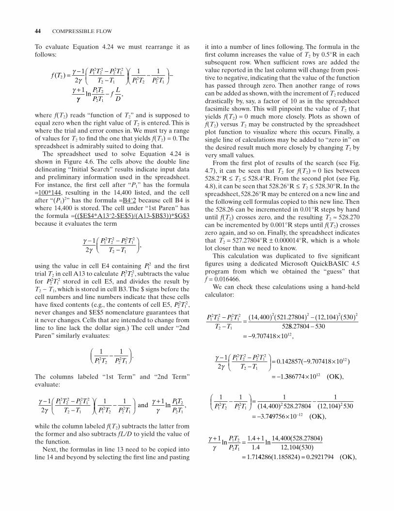
44 COMPRESSIBLE FLOW
To evaluate Equation 4.24 we must rearrange it as follows:
f TP T P T
T T P T P T( )2
12
22
22
12
2 1 12
2 22
1
12
1 1
1
= − −−
−
−
+
γγ
γγγ
ln ,PTP T
fLD
1 2
2 1
−
where f ( T2 ) reads “ function of T2 ” and is supposed to equal zero when the right value of T2 is entered. This is where the trial and error comes in. We must try a range of values for T2 to fi nd the one that yields f ( T2 ) = 0. The spreadsheet is admirably suited to doing that.
The spreadsheet used to solve Equation 4.24 is shown in Figure 4.6 . The cells above the double line delineating “ Initial Search ” results indicate input data and preliminary information used in the spreadsheet. For instance, the fi rst cell after “ P1 ” has the formula = 100 * 144 , resulting in the 14,400 listed, and the cell after “ ( P1 ) 2 ” has the formula = B4 ∧ 2 because cell B4 is where 14,400 is stored. The cell under “ 1st Paren ” has the formula = (($E$4 * A13 ∧ 2 - $E$5)/(A13 - $B$3)) * $G$3 because it evaluates the term
γγ− −
−
12
12
22
22
12
2 1
P T P TT T
,
using the value in cell E4 containing P12 and the fi rst
trial T2 in cell A13 to calculate P T12
22, subtracts the value
for P T22
12 stored in cell E5, and divides the result by
T2 − T1 , which is stored in cell B3. The $ signs before the cell numbers and line numbers indicate that these cells have fi xed contents (e.g., the contents of cell E5, P T2
212 ,
never changes and $E$5 nomenclature guarantees that it never changes. Cells that are intended to change from line to line lack the dollar sign.) The cell under “ 2nd Paren ” similarly evaluates:
1 1
12
2 22
1P T P T−
.
The columns labeled “ 1st Term ” and “ 2nd Term ” evaluate:
γγ
γγ
− −−
−
+12
1 1 112
22
22
12
2 1 12
2 22
1
P T P TT T P T P T
Pand ln 11 2
2 1
TP T
,
while the column labeled f ( T2 ) subtracts the latter from the former and also subtracts fL/D to yield the value of the function.
Next, the formulas in line 13 need to be copied into line 14 and beyond by selecting the fi rst line and pasting
it into a number of lines following. The formula in the fi rst column increases the value of T2 by 0.5 ° R in each subsequent row. When suffi cient rows are added the value reported in the last column will change from posi-tive to negative, indicating that the value of the function has passed through zero. Then another range of rows can be added as shown, with the increment of T2 reduced drastically by, say, a factor of 10 as in the spreadsheet facsimile shown. This will pinpoint the value of T2 that yields f ( T2 ) = 0 much more closely. Plots as shown of f ( T2 ) versus T2 may be constructed by the spreadsheet plot function to visualize where this occurs. Finally, a single line of calculations may be added to “ zero in ” on the desired result much more closely by changing T2 by very small values.
From the fi rst plot of results of the search (see Fig. 4.7 ), it can be seen that T2 for f ( T2 ) = 0 lies between 528.2 ° R ≤ T2 ≤ 528.4 ° R. From the second plot (see Fig. 4.8 ), it can be seen that 528.26 ° R ≤ T2 ≤ 528.30 ° R. In the spreadsheet, 528.26 ° R may be entered on a new line and the following cell formulas copied to this new line. Then the 528.26 can be incremented in 0.01 ° R steps by hand until f ( T2 ) crosses zero, and the resulting T2 ≈ 528.270 can be incremented by 0.001 ° R steps until f ( T2 ) crosses zero again, and so on. Finally, the spreadsheet indicates that T2 = 527.27804 ° R ± 0.000014 ° R, which is a whole lot closer than we need to know.
This calculation was duplicated to fi ve signifi cant fi gures using a dedicated Microsoft QuickBASIC 4.5 program from which we obtained the “ guess ” that f = 0.016466.
We can check these calculations using a hand - held calculator:
P T P TT T
12
22
22
12
2 1
2 2 2 214 400 521 27804 12 104 53052
−−
= ( ) ( ) − ( ) ( ), . ,88 27804 530
9 707418 1012
.
. ,
−= − ×
γγ− −
−
= − ×
= −
12
0 142857
1
12
22
22
12
2 1
P T P TT T
. ( )
.
9.707418 1012
3386774 1012× ( ),OK
1 1 114 400 528 27804
112 104 530
3 712
2 22
12 2P T P T
−
= −
= −( , ) . ( , )
. 449756 10 12× − ( ),OK
γγ+ = +
=
1 1 4 11 4
14 400 528 2780412 104 530
1 71
1 2
2 1
ln.
.ln
, ( . ), ( )
.
PTP T
44286 1 185824 0 2921794( . ) . ( ),= OK
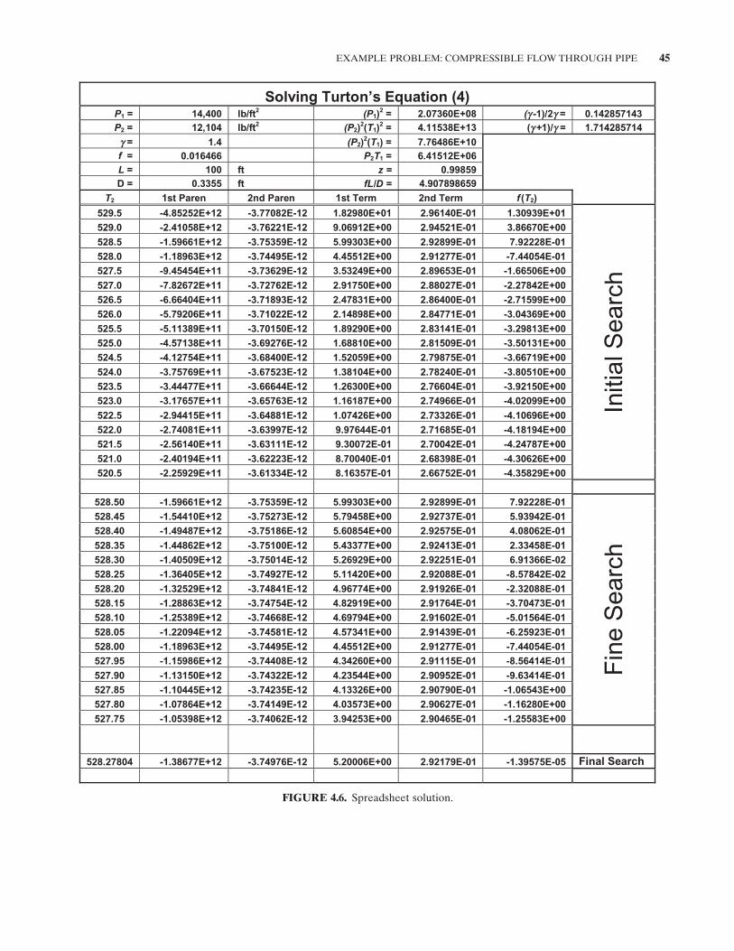
EXAMPLE PROBLEM: COMPRESSIBLE FLOW THROUGH PIPE 45
FIGURE 4.6. Spreadsheet solution.
Solving Turton’s Equation (4)P1 = 14,400 lb/ft2 (P1)
2 = 2.07360E+08 (g -1)/2g = 0.142857143P2 = 12,104 lb/ft2 (P2)
2(T1)2 = 4.11538E+13 (g+1)/g = 1.714285714
g = 1.4 (P2)2(T1) = 7.76486E+10
f = 0.016466 P2T1 = 6.41512E+06L = 100 ft z = 0.99859D = 0.3355 ft fL/D = 4.907898659
T2 1st Paren 2nd Paren 1st Term 2nd Term f (T2)
529.5 -4.85252E+12 -3.77082E-12 1.82980E+01 2.96140E-01 1.30939E+01
Initi
al S
earc
h
529.0 -2.41058E+12 -3.76221E-12 9.06912E+00 2.94521E-01 3.86670E+00
528.5 -1.59661E+12 -3.75359E-12 5.99303E+00 2.92899E-01 7.92228E-01
528.0 -1.18963E+12 -3.74495E-12 4.45512E+00 2.91277E-01 -7.44054E-01
527.5 -9.45454E+11 -3.73629E-12 3.53249E+00 2.89653E-01 -1.66506E+00
527.0 -7.82672E+11 -3.72762E-12 2.91750E+00 2.88027E-01 -2.27842E+00
526.5 -6.66404E+11 -3.71893E-12 2.47831E+00 2.86400E-01 -2.71599E+00
526.0 -5.79206E+11 -3.71022E-12 2.14898E+00 2.84771E-01 -3.04369E+00
525.5 -5.11389E+11 -3.70150E-12 1.89290E+00 2.83141E-01 -3.29813E+00
525.0 -4.57138E+11 -3.69276E-12 1.68810E+00 2.81509E-01 -3.50131E+00
524.5 -4.12754E+11 -3.68400E-12 1.52059E+00 2.79875E-01 -3.66719E+00
524.0 -3.75769E+11 -3.67523E-12 1.38104E+00 2.78240E-01 -3.80510E+00
523.5 -3.44477E+11 -3.66644E-12 1.26300E+00 2.76604E-01 -3.92150E+00
523.0 -3.17657E+11 -3.65763E-12 1.16187E+00 2.74966E-01 -4.02099E+00
522.5 -2.94415E+11 -3.64881E-12 1.07426E+00 2.73326E-01 -4.10696E+00
522.0 -2.74081E+11 -3.63997E-12 9.97644E-01 2.71685E-01 -4.18194E+00
521.5 -2.56140E+11 -3.63111E-12 9.30072E-01 2.70042E-01 -4.24787E+00
521.0 -2.40194E+11 -3.62223E-12 8.70040E-01 2.68398E-01 -4.30626E+00
520.5 -2.25929E+11 -3.61334E-12 8.16357E-01 2.66752E-01 -4.35829E+00
528.50 -1.59661E+12 -3.75359E-12 5.99303E+00 2.92899E-01 7.92228E-01
Fin
e S
earc
h
528.45 -1.54410E+12 -3.75273E-12 5.79458E+00 2.92737E-01 5.93942E-01
528.40 -1.49487E+12 -3.75186E-12 5.60854E+00 2.92575E-01 4.08062E-01
528.35 -1.44862E+12 -3.75100E-12 5.43377E+00 2.92413E-01 2.33458E-01
528.30 -1.40509E+12 -3.75014E-12 5.26929E+00 2.92251E-01 6.91366E-02
528.25 -1.36405E+12 -3.74927E-12 5.11420E+00 2.92088E-01 -8.57842E-02
528.20 -1.32529E+12 -3.74841E-12 4.96774E+00 2.91926E-01 -2.32088E-01
528.15 -1.28863E+12 -3.74754E-12 4.82919E+00 2.91764E-01 -3.70473E-01
528.10 -1.25389E+12 -3.74668E-12 4.69794E+00 2.91602E-01 -5.01564E-01
528.05 -1.22094E+12 -3.74581E-12 4.57341E+00 2.91439E-01 -6.25923E-01
528.00 -1.18963E+12 -3.74495E-12 4.45512E+00 2.91277E-01 -7.44054E-01
527.95 -1.15986E+12 -3.74408E-12 4.34260E+00 2.91115E-01 -8.56414E-01
527.90 -1.13150E+12 -3.74322E-12 4.23544E+00 2.90952E-01 -9.63414E-01
527.85 -1.10445E+12 -3.74235E-12 4.13326E+00 2.90790E-01 -1.06543E+00
527.80 -1.07864E+12 -3.74149E-12 4.03573E+00 2.90627E-01 -1.16280E+00
527.75 -1.05398E+12 -3.74062E-12 3.94253E+00 2.90465E-01 -1.25583E+00
528.27804 -1.38677E+12 -3.74976E-12 5.20006E+00 2.92179E-01 -1.39575E-05 Final Search
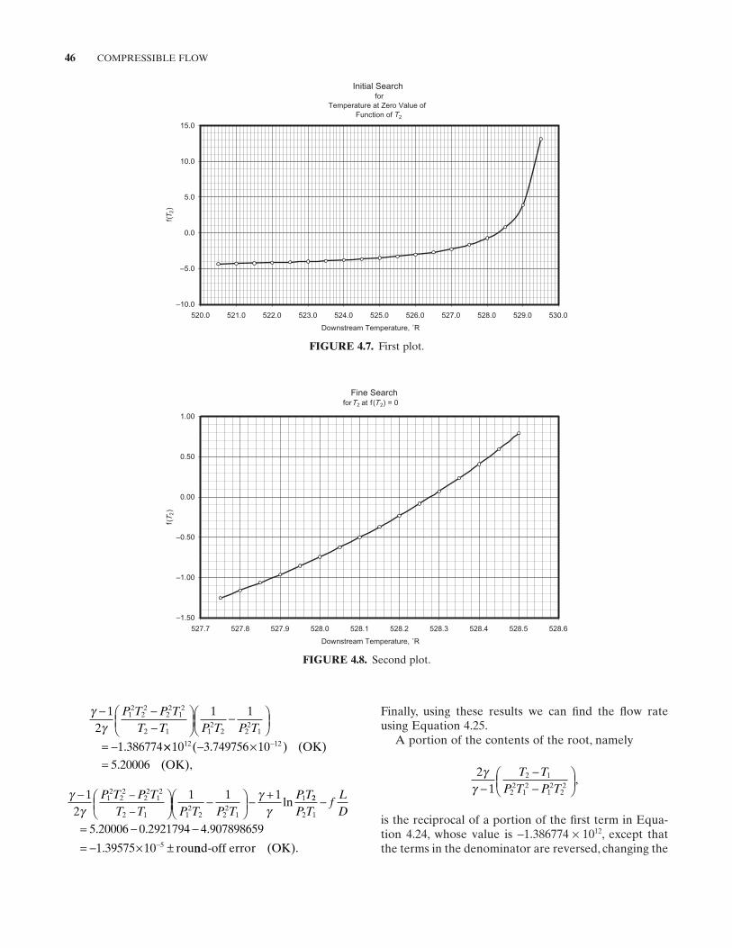
46 COMPRESSIBLE FLOW
Finally, using these results we can fi nd the fl ow rate using Equation 4.25 .
A portion of the contents of the root, namely
21
2 1
22
12
12
22
γγ −
−−
T TP T P T
,
is the reciprocal of a portion of the fi rst term in Equa-tion 4.24 , whose value is − 1.386774 × 10 12 , except that the terms in the denominator are reversed, changing the
γγ− −
−
−
= −
12
1 1
1 386774
12
22
22
12
2 1 12
2 22
1
P T P TT T P T P T
. ×× − ×=
−10 3 749756 1012 12( . ) ( )
( ),
OK
5.20006 OK
γγ
γγ
−
−
− +−−
12
1 1 112
22
22
12
2 1 12
2 22
1
1P T P TT T P T P T
PTln 22
2 1
0 4
P Tf
LD
−
= − −= − × ±−
5.20006 .2921794 .907898659
1.39575 10 rou5 nnd-off error OK( ).
FIGURE 4.7. First plot.
Initial Searchfor
Temperature at Zero Value ofFunction of T2
–10.0
–5.0
0.0
5.0
10.0
15.0
520.0 521.0 522.0 523.0 524.0 525.0 526.0 527.0 528.0 529.0 530.0
Downstream Temperature, ˚R
f( T2)
FIGURE 4.8. Second plot.
Fine SearchforT2 at f(T 2) = 0
–1.50
–1.00
–0.50
0.00
0.50
1.00
527.7 527.8 527.9 528.0 528.1 528.2 528.3 528.4 528.5 528.6
Downstream Temperature, ˚R
f(T
2)
FURTHER READING 47
program (whose output values are rounded to fi ve sig-nifi cant fi gure precision).
REFERENCES
1. Street , R. L. , G. Z. Watters , and J. K. Vennard , ElementaryFluid Mechanics , John Wiley & Sons , 1996 , pp. 608 – 609 , 611 – 612 .
2. Turton , R. , A new approach to non - choking adiabatic com-pressible fl ow of an ideal gas in pipes with friction , TheChemical Engineering Journal , 30 , 1985 , 159 – 160 .
FURTHER READING
This list includes books and papers that may be helpful to those who wish to pursue further study.
Shapiro , A. H. , The Dynamics and Thermodynamics of Com-pressible Flow , Vol. 1 , John Wiley & Sons , 1953 .
Spotts , M. F. , Numerical solution of complex equations , DesignNews , October 6, 1975 , pp. 88 – 90 .
Benedict , R. P. , Fundamentals of Pipe Flow , John Wiley & Sons , 1980 . (Chapters 3 and 8.)
Anderson , J. , Modern Compressible Flow, with Historical Per-spective , McGraw - Hill , 2003 .
Bernard , P. S. and J. W. Wallace , Turbulent Flow: Analysis, Mea-surement and Prediction , John Wiley & Sons , 2003 .
sign; the value is thus + 1.386774 × 10 12 . If we invert this we get + 7.210980 − 13 . The remaining part of the root is:
gP P mzR12
22
,
whose value is (including the compressibility factor of 0.99859 reported by the QuickBASIC program):
gP P mzR12
22 2 232 1740 14 400 12 104 28 0134
1545 31 0 99859= . ( , ) ( , ) .
. ( . ))
. .= ×1 77440 1016
Now we can evaluate Equation 4.25 :
GgP P m
zRT T
P T P T=
−−−
21
12
22
2 1
22
12
12
22
γγ
,
GgP P m
zRT T
P T P T=
−−−
= + × −
21
12
22
2 1
22
12
12
22
γγ
7.210980 10 13(11 77440 10
1 27952 10 113 116 1
16
4 2 2
. )
. . / / .
×
= × = ≈lb s-ft 13.12 lb s-ft
The weight fl ow rate is the product of this weight veloc-ity and the pipe cross - sectional area, which is 0.088405 ft 2 :
w = =113 116 0 088405 10. ( . ) . / .00002 lb s
This weight velocity for a 4 ″ Sch 40 pipe is functionally identical to the 10.000 lb/s input into the QuickBASIC
49
5 NETWORK ANALYSIS
A piping system is regularly made up of a number of piping elements that may be arranged in series fl ow , in parallel fl ow , or in branching fl ow . Series fl ow, where only one fl ow rate is involved, is rather straightforward. In parallel fl ow, two or more series combinations of piping elements diverge and then come together again downstream. In branching fl ow, a number of piping ele-ments are combined in various series and parallel fl ow arrangements that, unlike parallel fl ow, do not necessar-ily come together again. Branching fl ow can be extremely complicated to analyze. The three types of fl ow network arrangements are examined in this chapter. Two example problems are presented to illustrate the setup and solu-tion of pipe fl ow network arrangements.
Friction factor depends on pipe size, surface rough-ness, and Reynolds number, and can vary from pipe section to pipe section in parallel and branching fl ow networks. Differences in friction factor are usually large enough to justify extra computation. A simple approach is to fi rst assign a common friction factor, say 0.020 or 0.030 to each pipe section. After initial network solu-tion, compute Reynolds numbers and reassign friction factor in each pipe section using the Colebrook – White equation (Eq. 8.3 ). One or two iterations may then be needed to obtain a satisfactory solution. Another approach is to assume fully turbulent fl ow friction factors (Eq. 8.2 ) as a fi rst approximation for each pipe section, followed by network solution and, perhaps, further iterations as described above.
Note that there is essentially one fundamental com-position of fl uid fl ow equations. It is suggested that each
problem be worked out using the fundamental fl ow relationships presented in this book. The blind use of special formulae is not recommended. Calculated results can be converted to other units as appropriate after the fl ow network equations are solved. Unit conversions are available in Appendix C.2 .
5.1 COUPLING EFFECTS
Calculation procedures for fl ow losses in piping systems are normally based on simple one - dimensional fl ow concepts using loss coeffi cients realized by experiment. The basic loss coeffi cients are for isolated components having suffi ciently long inlet and outlet lengths of straight pipe to ensure that fully developed fl ow exists at the inlet to the component and redevelops again downstream of the component. However, when piping components are close coupled, interaction effects, or coupling effects , may appreciably affect their perfor-mance. Coupling effects may not completely disappear unless the components are separated by a spacer (a straight pipe section) of 30 pipe diameters or more. In practice, 4 or 5 pipe diameters may be suffi cient to reduce coupling effects to a negligible level.
One method adopted to account for the close cou-pling of two pipe components is to multiply the sum of their loss coeffi cients by a correction factor. The correc-tion factors are frequently less than unity; ignoring them often leads to an overestimation of pressure loss. An exception to this rule is a bend located upstream of a
Pipe Flow: A Practical and Comprehensive Guide, First Edition. Donald C. Rennels and Hobart M. Hudson.© 2012 John Wiley & Sons, Inc. Published 2012 by John Wiley & Sons, Inc.
50 NETWORK ANALYSIS
ΔP K K Kw
g AwOverall N= + + +[ ]1 2
2
22…
ρ
. (5.2)
5.3 PARALLEL FLOW
In parallel fl ow, two or more fl ow streams diverge and then converge downstream so that the fl ow divides among the pipe sections. The head loss is the same in every pipe section, and the individual fl ow rates are accumulative. * Overall resistance for a number N of piping sections connected in parallel is not a simple additive process.
To begin, the sum of the fl ow rates through each pipe section must equal the total fl ow into and out of the parallel network (the continuity principle):
… w w w wTotal N= + + +1 2 . (5.3)
The pressure loss equation, or its equivalent, must be satisfi ed for each pipe section (the energy principle):
ΔPKA
wg w
OverallOverall
Total= ⎛⎝⎜
⎞⎠⎟2
2
2
ρ
, (5.4)
ΔPKA
wg w
1 21
12
2= ⎛
⎝⎜⎞⎠⎟ρ
, (5.5)
ΔPKA
wg w
2 22
22
2= ⎛
⎝⎜⎞⎠⎟ρ
, (5.6)
and
ΔPKA
wg w
NN
N= ⎛⎝⎜
⎞⎠⎟2
2
2
ρ
, (5.7)
where K in this case represents the sum of the indi-vidual fl ow elements within each pipe section. The alge-braic sum of the head loss across each pipe section is the equal:
Δ Δ Δ ΔP P P POverall N= = = =1 2 … . (5.8)
Substitution of Equations 5.4 , 5.5 , 5.6 and 5.7 into Equa-tion 5.3 and taking into account Equation 5.8 gives:
A K A K A K A K/ / / / .( ) = ( ) + ( ) + + ( )Overall N1 2
…
diffuser where the nonuniform fl ow pattern at the dif-fuser entrance prevents normal pressure recovery. Like-wise, a bend located downstream of a diffuser can cause premature fl ow separation from the diffuser wall and affect the symmetry of pressure recovery. Another exception is two or more elbows or bends in different planes (a twisted S - form).
Data for a number of close - coupled piping compo-nents are available in the literature; see Corp and Hart-well [1] , Idel ’ chik [2] , Murikami, et al. [3] , and Miller [4] .
5.2 SERIES FLOW
In series fl ow two or more piping elements are con-nected so that the fl uid fl ows through one element and then another. Only one fl ow rate is involved. By reason, overall head loss for a number of piping elements con-nected in series is additive:
H KV
gK
Vg
KV
gL( ) = + + +Overall N
N1
12
222 2
2 2 2… ,
where the subscript N denotes the Nth pipe element. Letting the subscript R denote a reference location that may or may not be an actual geometric location in the piping arrangement, the continuity relationships are:
A V A V A V A V1 1 2 2= = = =… N N R R.
When each term is expressed in terms of a common reference area and a common reference velocity, there results:
H KAA
KAA
KAA
L( ) = ⎛⎝⎜
⎞⎠⎟ + ⎛
⎝⎜⎞⎠⎟ + + ⎛
⎝⎜⎞⎠⎟
⎡
⎣⎢Overall
R RN
R
N1
1
2
22
2 2
…⎤⎤
⎦⎥
VgR .2
2
By use of the continuity equations, the equation for head loss of a number of piping elements connected in series is:
H K A K A K Awg
Lw
( ) = + + +[ ]Overall N N1 12
22 2
2
22/ / / ,2 …
ρ
and the pressure loss equation is simply:
ΔP K A K A K Awg w
Overall N N= + + +[ ]1 12
2 22 2
2
2/ / / .…
ρ
(5.1)
Equation 5.1 is the broad - spectrum equation for pres-sure loss of piping elements in series. When the resis-tance of all piping elements is based on the same reference area A the loss coeffi cients are directly addi-tive and the pressure loss is given by Equation 5.2 :
* Vessels, reservoirs, or fl ow manifolds may be required at the diver-gent and convergent points to truly make the head loss the same in every pipe section when there are more than two parallel fl ow sections.
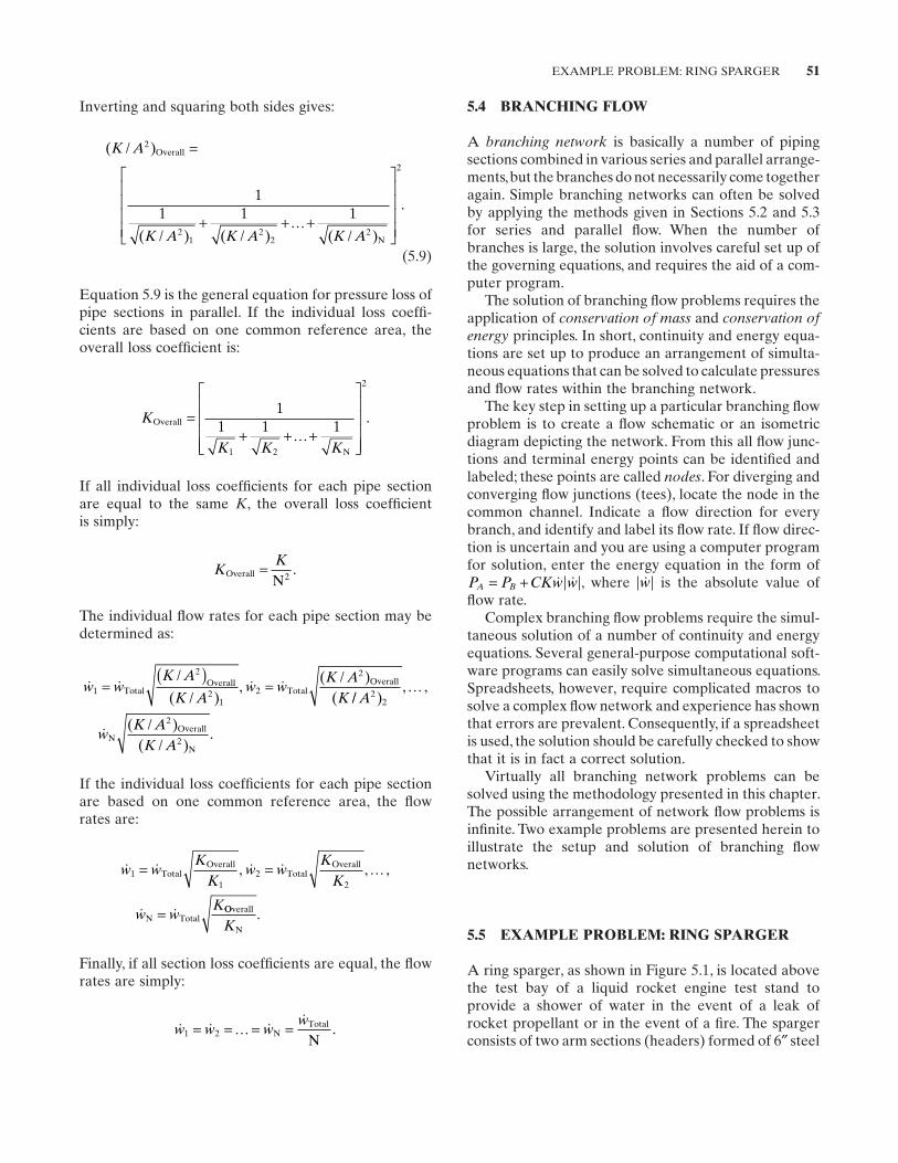
EXAMPLE PROBLEM: RING SPARGER 51
Inverting and squaring both sides gives:
( / )
( / ) / /
.
K A
K A K A K A
2
21
2 2
2
11 1 1
Overall
2 N( ) ( )
=
+ + +
⎡
⎣
⎢⎢⎢⎢
⎤
⎦
⎥⎥⎥⎥…
(5.9)
Equation 5.9 is the general equation for pressure loss of pipe sections in parallel. If the individual loss coeffi -cients are based on one common reference area, the overall loss coeffi cient is:
K
K K K
Overall
N
=+ + +
⎡
⎣
⎢⎢⎢⎢
⎤
⎦
⎥⎥⎥⎥
11 1 1
1 2
2
….
If all individual loss coeffi cients for each pipe section are equal to the same K , the overall loss coeffi cient is simply:
KK
OverallN
=2
.
The individual fl ow rates for each pipe section may be determined as:
w wK A
K Aw w
K AK
1
2
21
2
2
=( )
=TotalOverall
TotalOverall/
( / ),
( / )( // )
, ,
( / )( / )
.
A
wK A
K A
22
2
2
…
NOverall
N
If the individual loss coeffi cients for each pipe section are based on one common reference area, the fl ow rates are:
…
w wK
Kw w
KK
w wK
11
22
= =
=
TotalOverall
TotalOverall
N Total
, , ,
OOverall
NK.
Finally, if all section loss coeffi cients are equal, the fl ow rates are simply:
…
w w ww
1 2= = = =NTotal
N.
5.4 BRANCHING FLOW
A branching network is basically a number of piping sections combined in various series and parallel arrange-ments, but the branches do not necessarily come together again. Simple branching networks can often be solved by applying the methods given in Sections 5.2 and 5.3 for series and parallel fl ow. When the number of branches is large, the solution involves careful set up of the governing equations, and requires the aid of a com-puter program.
The solution of branching fl ow problems requires the application of conservation of mass and conservation of energy principles. In short, continuity and energy equa-tions are set up to produce an arrangement of simulta-neous equations that can be solved to calculate pressures and fl ow rates within the branching network.
The key step in setting up a particular branching fl ow problem is to create a fl ow schematic or an isometric diagram depicting the network. From this all fl ow junc-tions and terminal energy points can be identifi ed and labeled; these points are called nodes . For diverging and converging fl ow junctions (tees), locate the node in the common channel. Indicate a fl ow direction for every branch, and identify and label its fl ow rate. If fl ow direc-tion is uncertain and you are using a computer program for solution, enter the energy equation in the form of P P CKw wA B= + , where w is the absolute value of fl ow rate.
Complex branching fl ow problems require the simul-taneous solution of a number of continuity and energy equations. Several general - purpose computational soft-ware programs can easily solve simultaneous equations. Spreadsheets, however, require complicated macros to solve a complex fl ow network and experience has shown that errors are prevalent. Consequently, if a spreadsheet is used, the solution should be carefully checked to show that it is in fact a correct solution.
Virtually all branching network problems can be solved using the methodology presented in this chapter. The possible arrangement of network fl ow problems is infi nite. Two example problems are presented herein to illustrate the setup and solution of branching fl ow networks.
5.5 EXAMPLE PROBLEM: RING SPARGER
A ring sparger, as shown in Figure 5.1 , is located above the test bay of a liquid rocket engine test stand to provide a shower of water in the event of a leak of rocket propellant or in the event of a fi re. The sparger consists of two arm sections (headers) formed of 6 ″ steel
52 NETWORK ANALYSIS
• Use Equation 16.15 to model pressure loss due to diverging fl ow through branch at Nodes 1 through 6. Assume that the branch edge is sharp (radius ratio r / d equals zero).
5.5.2 Input Parameters
ρ w = 62.31 lb/ft 3 Weight density of 70 ° F water α ′ = 30 ° Angular separation of spray nozzles d 3 = 3.068 in Inside diameter of 3 ″ schedule 40
pipe d 6 = 6.065 in Inside diameter of 6 ″ schedule 40
pipe f 3 = 0.0173 Friction factor for fully turbulent
fl ow in 3 ″ elbow f 6 = 0.0149 Friction factor for fully turbulent
fl ow in 6 ″ pipe g = 32.174 ft/s 2 Acceleration of gravity K Noz = 10 Loss coeffi cient of spray nozzles in
terms of velocity in 3 ″ pipe K ′ = 0.57 Coeffi cient for sharp - edged opening
into 90 ° long radius (LR) elbow in terms of velocity in 3 ″ pipe
p 7 = 0 psig Gage pressure within test bay q Spray = 6000 gpm Total water fl ow rate to ring sparger r Ring = 60 in Centerline radius of ring sparger rd ffb = 0.20 Rounding radius r / d of branch edge
of inlet tee
pipe. Each header contains six equally spaced spray nozzles mounted atop 3 ″ 90 ° elbows.
A network fl ow model of the ring sparger is devel-oped in order to evaluate the uniformity of fl ow among the individual spray nozzles, to determine the pressure distribution within the header, and to determine the pressure at the inlet tee. As shown in Figure 5.2 , only one arm is modeled because of fl ow symmetry about the inlet tee. The nodes are shown in Figure 5.2 as heavy dots and are numbered from 0 to 7.
5.5.1 Ground Rules and Assumptions
• The water temperature is 70 ° F. • The total fl ow rate to the sparger is 6000 gpm. • According to the manufacturer, the loss coeffi cient
K Noz of the fl ow nozzles is 10 in terms of velocity head in 3 ″ schedule 40 pipe.
• Node 0 is located at the inlet to the sparger. Nodes 1 – 6 are located within the sparger arm just upstream of the diverging branches (i.e., in the common channel). Node 7 is located inside the test bay outside the sparger and is at atmospheric pressure.
• Ignore coupling effects. • Use Equation 16.18 to model pressure loss through
the inlet tee. Assume that the radius ratio r / d of the branch edge equals 0.20.
• Use Equation 16.7 to model pressure loss due to diverging fl ow through run at Nodes 1 through 6.
FIGURE 5.1. Ring sparger.
View A - A
Spray Nozzle (may be tilted downward)
3″ Sch 4090° LR
6″ Sch 40 PipeA
6″ × 6″Sch 40 90°Tee
A
30°Typical
60″ Radius
Symmetrical about
Centerline
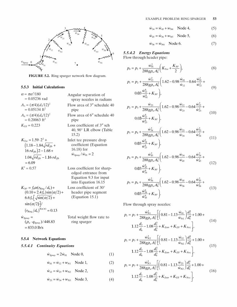
EXAMPLE PROBLEM: RING SPARGER 53
Flow area of 6 ″ schedule 40 pipe
K Ell = 0.223 Loss coeffi cient of 3 ″ sch 40, 90 ° LR elbow (Table 15.2 )
KTee = ⋅ +1 59 22. Inlet tee pressure drop coeffi cient (Equation 16.18 ) for w wSpray / 01 2=
K ′ = 0.57 Loss coeffi cient for sharp - edged entrance from Equation 9.3 for input into Equation 16.15
K f r dRing30 6 6° = +α( / ) Loss coeffi cient of 30 ° header pipe segment (Equation 15.1 )
wSpray = Total weight fl ow rate to ring sparger
5.5.4 Network Equations
5.5.4.1 Continuity Equations
w wSpray = 2 001 Node , (1)
w w w01 12 1 1= + N Node , (2)
w w w12 23 2= + N2 Node , (3)
w w w23 34 3= + N3 Node , (4)
w w w34 45 4= + N4 Node , (5)
w w w45 56 5= + N5 Node , (6)
w w56 6 6= N Node . (7)
5.5.4.2 Energy Equations Flow through header pipe:
p pwg A
KK
wTee0 1
012
62
30
288 2= + +⎛
⎝⎜⎞⎠⎟
°ρ
, (8)
p pwg A
ww
www
1 2122
62
01
12
012
122288
1 62 0 98 0 64
0
= + − − +⎛⎝⎜
ρ
. . .
.003 126
016 30
ww
K+ ⎞⎠⎟° ,
(9)
p pwg A
ww
www
2 323
62
12
23
122
232288
1 62 0 98 0 64
0 0
= + − − +⎛⎝⎜
ρ
. . .
. 33 126
236 30ww
K+ ⎞⎠⎟° ,
(10)
p pwg A
ww
www
3 4342
62
23
34
232
342288
1 62 0 98 0 64
0
= + − − +⎛⎝⎜
ρ
. . .
.003 346
236 30
ww
K+ ⎞⎠⎟° ,
(11)
p pwg A
ww
www
4 5452
62
34
45
342
452288
1 62 0 98 0 64
0
= + − − +⎛⎝⎜
ρ
. . .
.003 456
346 30ww
K+ ⎞⎠⎟° ,
(12)
p pwg A
ww
www
5 6562
62
45
56
452
562288
1 62 0 98 0 64
0
= + − − +⎛⎝⎜
ρ
. . .
.003 566
456 30
ww
K+ ⎞⎠⎟° .
(13)
Flow through spray nozzles:
p pwg A
ww
ddw
1 71
2
32
01
1
34
64288
0 81 1 13 1 00= + −⎛⎝⎜
⎞⎠⎟ + +⎡
⎣⎢
N
Nρ. . .
11 12 1 083
6
33
63
. . ,dd
dd
K K KEntr Ell Noz− + + + ⎤⎦⎥
(14)
p pwg A
ww
ddw
1 72
2
32
12 34
64288
0 81 1 13 1 00= + −⎛⎝⎜
⎞⎠⎟ + +⎡
⎣⎢
N
N2ρ. . .
11 12 1 083
6
33
63
. . ,dd
dd
K K KEntr Ell Noz− + + + ⎤⎦⎥
(15)
p pwg A
ww
ddw
1 73
2
32
23 34
64288
0 81 1 13 1 00= + −⎛⎝⎜
⎞⎠⎟ + +⎡
⎣⎢
N
N3ρ. . .
11 12 1 083
6
33
63
. . ,dd
dd
K K KEntr Ell Noz− + + + ⎤⎦⎥
(16)
5.5.3 Initial Calculations
α = π α ′ /180 = 0.05236 rad
Angular separation of spray nozzles in radians
A 3 = ( π /4)( d 3 /12) 2 = 0.05134 ft 2
FIGURE 5.2. Ring sparger network fl ow diagram.
Spray
56
45
34
23
12
N3
7
6
5
4
0 N6
N5
N4
N2
01
N1
1
2
3
ww
w
ww
w
w
w
w
w
w w
w
rdffb− +(1 18 1 84. .rdffb ) − +16 2 1 68.
rdffb −1 04 1. .116 rdffb
6 09= .
Flow area of 3 ″ schedule 40 pipe
A 6 = ( π /4)( d 6 /12) 2 = 0.20063 ft 2
f60 10 2 4 2+( ) ( ) +α. . sinf66 6 2 +α. sin( )⎡⎣
2(sin α ))⎤⎦ /
( ) =( ) .r dRing 64 0 13α π
qw Spray⋅( )/ .ρ 448 83
= .833 0 lb/s
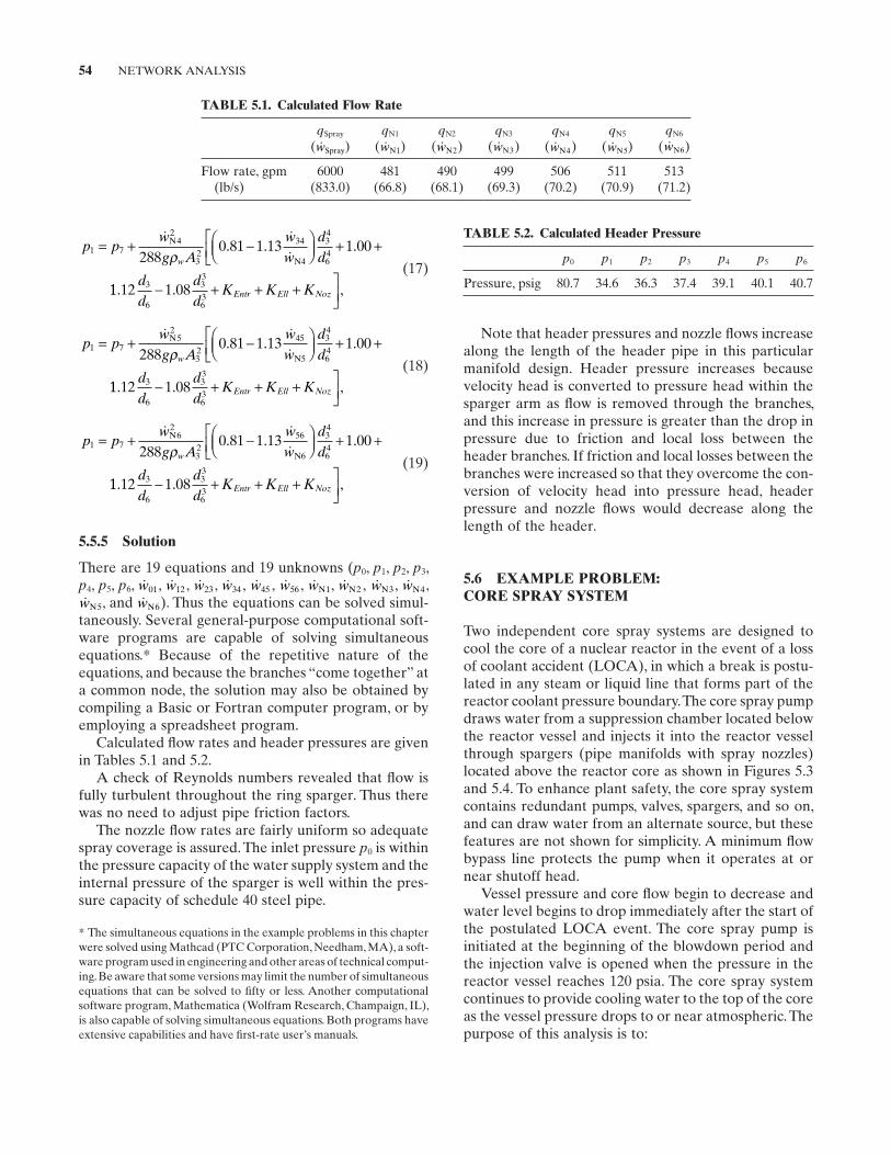
54 NETWORK ANALYSIS
Note that header pressures and nozzle fl ows increase along the length of the header pipe in this particular manifold design. Header pressure increases because velocity head is converted to pressure head within the sparger arm as fl ow is removed through the branches, and this increase in pressure is greater than the drop in pressure due to friction and local loss between the header branches. If friction and local losses between the branches were increased so that they overcome the con-version of velocity head into pressure head, header pressure and nozzle fl ows would decrease along the length of the header.
5.6 EXAMPLE PROBLEM: CORE SPRAY SYSTEM
Two independent core spray systems are designed to cool the core of a nuclear reactor in the event of a loss of coolant accident ( LOCA ), in which a break is postu-lated in any steam or liquid line that forms part of the reactor coolant pressure boundary. The core spray pump draws water from a suppression chamber located below the reactor vessel and injects it into the reactor vessel through spargers (pipe manifolds with spray nozzles) located above the reactor core as shown in Figures 5.3 and 5.4 . To enhance plant safety, the core spray system contains redundant pumps, valves, spargers, and so on, and can draw water from an alternate source, but these features are not shown for simplicity. A minimum fl ow bypass line protects the pump when it operates at or near shutoff head.
Vessel pressure and core fl ow begin to decrease and water level begins to drop immediately after the start of the postulated LOCA event. The core spray pump is initiated at the beginning of the blowdown period and the injection valve is opened when the pressure in the reactor vessel reaches 120 psia. The core spray system continues to provide cooling water to the top of the core as the vessel pressure drops to or near atmospheric. The purpose of this analysis is to:
p pwg A
ww
ddw
1 74
2
32
34 34
64288
0 81 1 13 1 00= + −⎛⎝⎜
⎞⎠⎟ + +⎡
⎣⎢
N
N4ρ. . .
11 12 1 083
6
33
63
. .dd
dd
K K KEntr Ell Noz− + + + ⎤⎦⎥,
(17)
p pwg A
ww
ddw
1 75
2
32
45 34
64288
0 81 1 13 1 00= + −⎛⎝⎜
⎞⎠⎟ + +⎡
⎣⎢
N
N5ρ. . .
11 12 1 083
6
33
63
. . ,dd
dd
K K KEntr Ell Noz− + + + ⎤⎦⎥
(18)
p pwg A
ww
ddw
1 76
2
32
56 34
64288
0 81 1 13 1 00= + −⎛⎝⎜
⎞⎠⎟ + +⎡
⎣⎢
N
N6ρ. . .
11 12 1 083
6
33
63
. . ,dd
dd
K K KEntr Ell Noz− + + + ⎤⎦⎥
(19)
5.5.5 Solution
There are 19 equations and 19 unknowns ( p 0 , p 1 , p 2 , p 3 , p 4 , p 5 , p 6 , w01, w12, w23 , w34 , w45 , w56 , wN1, wN2 , wN3, wN4, wN5, and wN6). Thus the equations can be solved simul-taneously. Several general - purpose computational soft-ware programs are capable of solving simultaneous equations. * Because of the repetitive nature of the equations, and because the branches “ come together ” at a common node, the solution may also be obtained by compiling a Basic or Fortran computer program, or by employing a spreadsheet program.
Calculated fl ow rates and header pressures are given in Tables 5.1 and 5.2 .
A check of Reynolds numbers revealed that fl ow is fully turbulent throughout the ring sparger. Thus there was no need to adjust pipe friction factors.
The nozzle fl ow rates are fairly uniform so adequate spray coverage is assured. The inlet pressure p 0 is within the pressure capacity of the water supply system and the internal pressure of the sparger is well within the pres-sure capacity of schedule 40 steel pipe.
TABLE 5.1. Calculated Flow Rate
q Spray
( wSpray) q N1
( wN1) q N2
( wN2) q N3
( wN3) q N4
( wN4) q N5
( wN5) q N6
( wN6)
Flow rate, gpm (lb/s)
6000 (833.0)
481 (66.8)
490 (68.1)
499 (69.3)
506 (70.2)
511 (70.9)
513 (71.2)
TABLE 5.2. Calculated Header Pressure
p 0 p 1 p 2 p 3 p 4 p 5 p 6
Pressure, psig 80.7 34.6 36.3 37.4 39.1 40.1 40.7
* The simultaneous equations in the example problems in this chapter were solved using Mathcad (PTC Corporation, Needham, MA), a soft-ware program used in engineering and other areas of technical comput-ing. Be aware that some versions may limit the number of simultaneous equations that can be solved to fi fty or less. Another computational software program, Mathematica (Wolfram Research, Champaign, IL), is also capable of solving simultaneous equations. Both programs have extensive capabilities and have fi rst - rate user ’ s manuals.
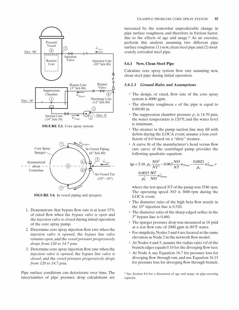
EXAMPLE PROBLEM: CORE SPRAY SYSTEM 55
increased by the somewhat unpredictable change in pipe surface roughness, and therefore in friction factor, due to the effects of age and usage. * As an exercise, perform this analysis assuming two different pipe surface roughness: (1) new, clean steel pipe and (2) mod-erately corroded steel pipe.
5.6.1 New, Clean Steel Pipe
Calculate core spray system fl ow rate assuming new, clean steel pipe during initial operation.
5.6.1.1 Ground Rules and Assumptions
• The design, or rated, fl ow rate of the core spray system is 4000 gpm.
• The absolute roughness e of the pipe is equal to 0.00180 in.
• The suppression chamber pressure p 1 is 14.70 psia, the water temperature is 120 ° F, and the water level is minimum.
• The strainer in the pump suction line may fi ll with debris during the LOCA event; assume a loss coef-fi cient of 6.0 based on a “ dirty ” strainer.
• A curve fi t of the manufacturer ’ s head versus fl ow rate curve of the centrifugal pump provides the following quadratic equation:
ΔpNONT
NONT
w ww Pumpw
Pump
w
= ⋅ − − +5 16 0 0630 0021
0 0015
2
22
2
. ..
.
ρρ
ρ
NNTNO
wPump 3 ,
where the test speed NT of the pump was 3540 rpm. The operating speed NO is 3600 rpm during the LOCA event.
• The diameter ratio of the high beta fl ow nozzle in the 10 ″ injection line is 0.520.
• The diameter ratio of the sharp - edged orifi ce in the 3 ″ bypass line is 0.460.
• The sparger pressure drop was measured as 16 psid at a test fl ow rate of 2000 gpm in 80 ° F water.
• For simplicity, Nodes 3 and 4 are located at the same elevation as Node 2 in the network fl ow model.
• At Nodes 4 and 5, assume the radius ratio r / d of the branch edges equals 0.10 for the diverging fl ow tees.
• At Node 4, use Equation 16.7 for pressure loss for diverging fl ow through run, and use Equation 16.15 for pressure loss for diverging fl ow through branch.
FIGURE 5.3. Core spray system.
Injectw
3
Pumpw
Elev. 98'
Elev. 18′
Elev. 0′
Bypass Line (3′′ Sch 80)
Discharge Line (12′′ Sch 80)
Suction Line (14′′ Sch 10)
BypasswSuppression
Chamber
Reactor Core
Injection Line (10′′ Sch 80)
5
4
2
1
8
Pressure Vessel
Injection Valve
Bypass Valve
•
•
•
FIGURE 5.4. In - vessel piping and spargers.
pS rew arg
Injectw
In-Vessel Tee(10″ 10″)
In-Vessel Piping (6″ Sch 40)
7Core SpraySparger
7
Symmetrical about
Centerline 8
65
6
•
•
×
1. Demonstrate that bypass fl ow rate is at least 15% of rated fl ow when the bypass valve is open and the injection valve is closed during initial operation of the core spray pump.
2. Determine core spray injection fl ow rate when the injection valve is opened , the bypass line valve remains open , and the vessel pressure progressively drops from 120 to 14.7 psia
3. Determine core spray injection fl ow rate when the injection valve is opened , the bypass line valve is closed , and the vessel pressure progressively drops from 120 to 14.7 psia .
Pipe surface conditions can deteriorate over time. The uncertainties of pipe pressure drop calculations are
* See Section 8.6 for a discussion of age and usage on pipe - carrying capacity.
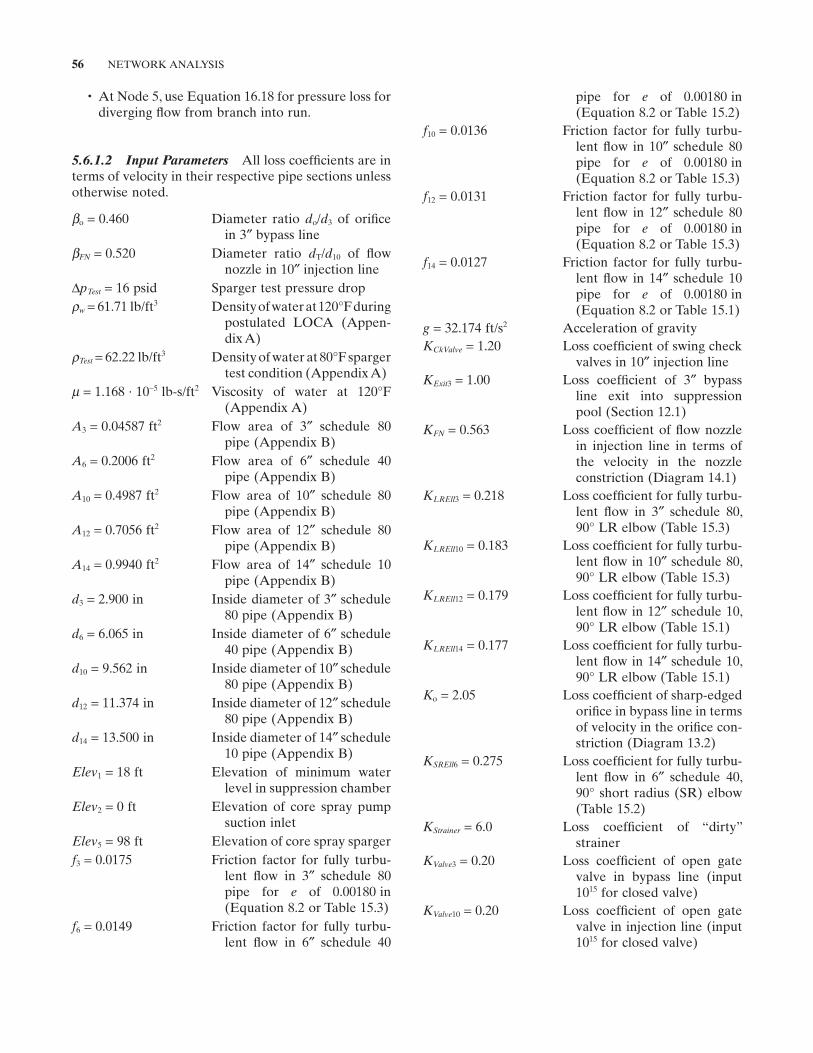
56 NETWORK ANALYSIS
pipe for e of 0.00180 in (Equation 8.2 or Table 15.2 )
f 10 = 0.0136 Friction factor for fully turbu-lent fl ow in 10 ″ schedule 80 pipe for e of 0.00180 in (Equation 8.2 or Table 15.3 )
f 12 = 0.0131 Friction factor for fully turbu-lent fl ow in 12 ″ schedule 80 pipe for e of 0.00180 in (Equation 8.2 or Table 15.3 )
f 14 = 0.0127 Friction factor for fully turbu-lent fl ow in 14 ″ schedule 10 pipe for e of 0.00180 in (Equation 8.2 or Table 15.1 )
g = 32.174 ft/s 2 Acceleration of gravity K CkValve = 1.20 Loss coeffi cient of swing check
valves in 10 ″ injection line K Exit 3 = 1.00 Loss coeffi cient of 3 ″ bypass
line exit into suppression pool (Section 12.1 )
K FN = 0.563 Loss coeffi cient of fl ow nozzle in injection line in terms of the velocity in the nozzle constriction (Diagram 14.1)
K LREll 3 = 0.218 Loss coeffi cient for fully turbu-lent fl ow in 3 ″ schedule 80, 90 ° LR elbow (Table 15.3 )
K LREll 10 = 0.183 Loss coeffi cient for fully turbu-lent fl ow in 10 ″ schedule 80, 90 ° LR elbow (Table 15.3 )
K LREll 12 = 0.179 Loss coeffi cient for fully turbu-lent fl ow in 12 ″ schedule 10, 90 ° LR elbow (Table 15.1 )
K LREll 14 = 0.177 Loss coeffi cient for fully turbu-lent fl ow in 14 ″ schedule 10, 90 ° LR elbow (Table 15.1 )
K o = 2.05 Loss coeffi cient of sharp - edged orifi ce in bypass line in terms of velocity in the orifi ce con-striction (Diagram 13.2)
K SREll 6 = 0.275 Loss coeffi cient for fully turbu-lent fl ow in 6 ″ schedule 40, 90 ° short radius (SR) elbow (Table 15.2 )
K Strainer = 6.0 Loss coeffi cient of “ dirty ” strainer
K Valve 3 = 0.20 Loss coeffi cient of open gate valve in bypass line (input 10 15 for closed valve)
K Valve 10 = 0.20 Loss coeffi cient of open gate valve in injection line (input 10 15 for closed valve)
• At Node 5, use Equation 16.18 for pressure loss for diverging fl ow from branch into run.
5.6.1.2 Input Parameters All loss coeffi cients are in terms of velocity in their respective pipe sections unless otherwise noted.
β o = 0.460 Diameter ratio d o / d 3 of orifi ce in 3 ″ bypass line
β FN = 0.520 Diameter ratio d T / d 10 of fl ow nozzle in 10 ″ injection line
Δ p Test = 16 psid Sparger test pressure drop ρ w = 61.71 lb/ft 3 Density of water at 120 ° F during
postulated LOCA (Appen-dix A )
ρ Test = 62.22 lb/ft 3 Density of water at 80 ° F sparger test condition (Appendix A )
μ = 1.168 · 10 − 5 lb - s/ft 2 Viscosity of water at 120 ° F (Appendix A )
A 3 = 0.04587 ft 2 Flow area of 3 ″ schedule 80 pipe (Appendix B )
A 6 = 0.2006 ft 2 Flow area of 6 ″ schedule 40 pipe (Appendix B )
A 10 = 0.4987 ft 2 Flow area of 10 ″ schedule 80 pipe (Appendix B )
A 12 = 0.7056 ft 2 Flow area of 12 ″ schedule 80 pipe (Appendix B )
A 14 = 0.9940 ft 2 Flow area of 14 ″ schedule 10 pipe (Appendix B )
d 3 = 2.900 in Inside diameter of 3 ″ schedule 80 pipe (Appendix B )
d 6 = 6.065 in Inside diameter of 6 ″ schedule 40 pipe (Appendix B )
d 10 = 9.562 in Inside diameter of 10 ″ schedule 80 pipe (Appendix B )
d 12 = 11.374 in Inside diameter of 12 ″ schedule 80 pipe (Appendix B )
d 14 = 13.500 in Inside diameter of 14 ″ schedule 10 pipe (Appendix B )
Elev 1 = 18 ft Elevation of minimum water level in suppression chamber
Elev 2 = 0 ft Elevation of core spray pump suction inlet
Elev 5 = 98 ft Elevation of core spray sparger f 3 = 0.0175 Friction factor for fully turbu-
lent fl ow in 3 ″ schedule 80 pipe for e of 0.00180 in (Equation 8.2 or Table 15.3 )
f 6 = 0.0149 Friction factor for fully turbu-lent fl ow in 6 ″ schedule 40
EXAMPLE PROBLEM: CORE SPRAY SYSTEM 57
5.6.1.4 Adjusted Parameters * After initial solution of the simultaneous equations, a check of Reynolds number revealed that fl ow is not fully turbulent through-out the system. Accordingly, pipe friction factors were adjusted upward using the Colebrook – White formula (Equation 8.3 ):
f 3 = 0.0180 Adjusted friction factor in 3 ″ schedule 80 pipe
f 6 = 0.0153 Adjusted friction factor in 6 ″ schedule 40 pipe
f 10 = 0.0140 Adjusted friction factor in 10 ″ schedule 80 pipe
f 12 = 0.0137 Adjusted friction factor in 12 ″ schedule 80 pipe
f 14 = 0.0134 Adjusted friction factor in 14 ″ schedule 10 pipe
Also, elbow loss coeffi cients were adjusted upward in direct proportion to friction factor increase per Equa-tion 15.2 :
K LREll 3 = 0.225 3 ″ schedule 80, 90 ° LR elbow K SREll 6 = 0.282 6 ″ schedule 40, 90 ° SR elbow K LREll 10 = 0.189 10 ″ schedule 80, 90 ° LR elbow K LREll 12 = 0.187 12 ″ schedule 80, 90 ° LR elbow K LREll 14 = 0.187 14 ″ schedule 10, 90 ° LR elbow
5.6.1.5 Network Flow Equations Continuity equa-tions:
w w wPump Inject Bypass= + Node 4, (1)
w wSparger Inject= 2 5Node . (2)
Energy equations:
p pK K K f
Ld
g
Strainer Valve LREll
w1 2
14 14 141 2
14
412
1
288= +
+ + ⋅ + +
⋅ ⋅
,
ρ ⋅⋅
+ −( )
A
w Elev ElevPumpw
142
22 1
144 ρ
,
(3)
p pNONT
NONT
w ww Pumpw
Pump2 3
2
225 16 0 063
0 0021
0 0015
= − ⋅ + − +. ..
.
ρρ
ρρwPump
NTNO
w2
3 ,
(4)
K Valve 14 = 0.20 Loss coeffi cient of open gate valve in pump suction line
L 1,2 = 40 ft Pump suction line straight pipe length
L 3,4 = 9 ft Pump discharge line straight pipe length
L 4,5 = 145 ft Injection line straight pipe length
L 6,7 = 12 ft In - vessel line straight pipe length
L 4,1 = 60 ft Bypass line straight pipe length NO = 3600 rpm Operating speed of pump
during LOCA NT = 3540 rpm Test speed of pump p 1 = 14.7 psia Suppression chamber pressure p 8 = 120 to 14.7 psia Reactor vessel pressure —
progressively decreasing to atmospheric pressure during LOCA
q Test = 2000 gpm Sparger test fl ow rate rd = 0.10 Radius ratio r / d of branch edge
of diverging tees at Nodes 4 and 5
5.6.1.3 Initial Calculations Loss coeffi cient of bypass line orifi ce in terms of velocity in 3 ″ pipe:
KK
Orifice = = =o
oβ4 4
2 050 460
45 78.
.. .
Loss coeffi cient of injection line fl ow nozzle in terms of velocity in 10 ″ pipe:
KK
FlowNozFN
FN
= = =β4 4
0 5630 520
7 694..
. .
Calculate K ′ for input into Equation 16.15 :
′ = − − + − +
=K rd rd rd rd
rdT T T T
T
0 57 1 07 2 13 8 24 8 84
2 90
1 2 3 2 2
5 2
. . . . .
.
/ /
/ 00 204. .
Calculate loss coeffi cient of sparger based on test data:
wq
TestTest Test= = × =ρ448 83
62 22 2000448 83
277 25.
..
. ,lb/s
K
g A pw
SpargerTest Test
Test
=
= × × ×
288
288 32 174 62 31 0 2006
62
2
ρ Δ
. . . 22
2
16277 25
4 83× =
.. .
* Friction factors and elbow loss coeffi cients will vary slightly as a function of valve lineup and vessel pressure from the representative values shown here.
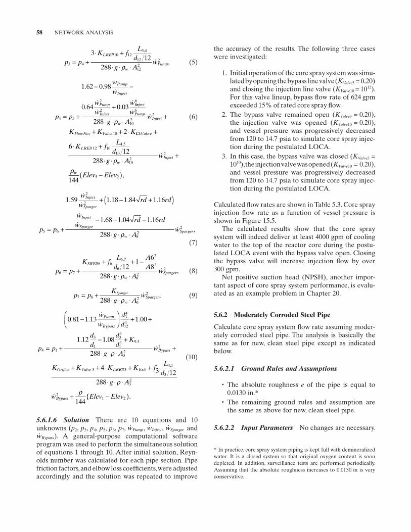
58 NETWORK ANALYSIS
the accuracy of the results. The following three cases were investigated:
1. Initial operation of the core spray system was simu-lated by opening the bypass line valve ( K Valve 3 = 0.20) and closing the injection line valve ( K Valve 10 = 10 12 ). For this valve lineup, bypass fl ow rate of 624 gpm exceeded 15% of rated core spray fl ow.
2. The bypass valve remained open ( K Valve 3 = 0.20), the injection valve was opened ( K Valve 10 = 0.20), and vessel pressure was progressively decreased from 120 to 14.7 psia to simulate core spray injec-tion during the postulated LOCA.
3. In this case, the bypass valve was closed ( K Valve 3 = 10 10 ), the injection valve was opened ( K Valve 10 = 0.20), and vessel pressure was progressively decreased from 120 to 14.7 psia to simulate core spray injec-tion during the postulated LOCA.
Calculated fl ow rates are shown in Table 5.3 . Core spray injection fl ow rate as a function of vessel pressure is shown in Figure 15.5 .
The calculated results show that the core spray system will indeed deliver at least 4000 gpm of cooling water to the top of the reactor core during the postu-lated LOCA event with the bypass valve open. Closing the bypass valve will increase injection fl ow by over 300 gpm.
Net positive suction head ( NPSH ), another impor-tant aspect of core spray system performance, is evalu-ated as an example problem in Chapter 20 .
5.6.2 Moderately Corroded Steel Pipe
Calculate core spray system fl ow rate assuming moder-ately corroded steel pipe. The analysis is basically the same as for new, clean steel pipe except as indicated below.
5.6.2.1 Ground Rules and Assumptions
• The absolute roughness e of the pipe is equal to 0.0130 in. *
• The remaining ground rules and assumption are the same as above for new, clean steel pipe.
5.6.2.2 Input Parameters No changes are necessary.
p pK f
Ld
g Aw
LREll
wPump3 4
10 123 4
12
122
2
312
288= +
⋅ +
⋅ ⋅ ⋅
,
,ρ
(5)
p p
ww
ww
w
Pump
Inject
Pump
Inject
I
4 5
2
2
1 62 0 98
0 64 0 03= +
− −
+
. .
. .
nnject
Pump
wInject
FlowNoz Valve
wg A
w
K K K
6
6
102
2
10
288
2
⋅ ⋅ ⋅+
+ + ⋅ρ
CCkVakve
LREll
wInject
w
K fL
dg A
w
+
⋅ +
⋅ ⋅ ⋅+
612
288
1
12 104 5
10
102
2
,
ρρ
4445 2Elev Elev−( ),
(6)
p p
ww
rd rd
w
Inject
Sparger
Inject
5 6
2
21 59 1 18 1 84 1 16
= +
+ − +( ). . . .
wrd rd
g AwSparger
wSparger
− + −
⋅ ⋅ ⋅
1 68 1 04 1 16
288 82
2
. . .,
ρ (7)
p pK f
Ld
AA
g Aw
SREll
wSparger6 7
6 66 7
6
2
2
62
2121
68
288= +
+ + −
⋅ ⋅ ⋅
,
,ρ
(8)
p pKg A
wSparger
wSparger7 8
62
2
288= +
⋅ ⋅ ⋅ρ , (9)
p p
ww
dd
dd
Pump
Bypass
4 1
34
124
3
1
0 81 1 13 1 00
1 12 1= +
−⎛⎝⎜
⎞⎠⎟
+ +
−
. . .
.
.. .08
288
4
33
13 9 3
32
2
3
dd
K
g Aw
K K K
Bypass
Orifice Valve LR
+
⋅ ⋅ ⋅+
+ + ⋅
ρ
EEll Exit
Bypass
K fL
dg A
w Elev Elev
34 1
3
32
21 2
3 12288
144
+ +
⋅ ⋅ ⋅
+ −
,
ρρ (( ).
(10)
5.6.1.6 Solution There are 10 equations and 10 unknowns ( p 2 , p 3 , p 4 , p 5 , p 6 , p 7 , wPump, wInject , wSparger and wBypass). A general - purpose computational software program was used to perform the simultaneous solution of equations 1 through 10. After initial solution, Reyn-olds number was calculated for each pipe section. Pipe friction factors, and elbow loss coeffi cients, were adjusted accordingly and the solution was repeated to improve
* In practice, core spray system piping is kept full with demineralized water. It is a closed system so that original oxygen content is soon depleted. In addition, surveillance tests are performed periodically. Assuming that the absolute roughness increases to 0.0130 in is very conservative.
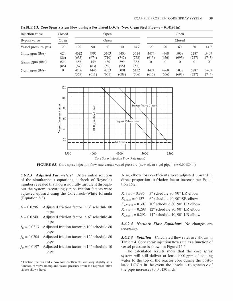
EXAMPLE PROBLEM: CORE SPRAY SYSTEM 59
Also, elbow loss coeffi cients were adjusted upward in direct proportion to friction factor increase per Equa-tion 15.2 .
K LREll 3 = 0.396 3 ″ schedule 80, 90 ° LR elbow K SREll 6 = 0.437 6 ″ schedule 40, 90 ° SR elbow K LREll 10 = 0.307 10 ″ schedule 80, 90 ° LR elbow K LREll 12 = 0.298 12 ″ schedule 80, 90 ° LR elbow K LREll 14 = 0.292 14 ″ schedule 10, 90 ° LR elbow
5.6.2.4 Network Flow Equations No changes are necessary.
5.6.2.5 Solution Calculated fl ow rates are shown in Table 5.4 . Core spray injection fl ow rate as a function of vessel pressure is shown in Figure 15.6 .
The calculated results show that the core spray system will still deliver at least 4000 gpm of cooling water to the top of the reactor core during the postu-lated LOCA in the event the absolute roughness e of the pipe increases to 0.0130 inch.
5.6.2.3 Adjusted Parameters * After initial solution of the simultaneous equations, a check of Reynolds number revealed that fl ow is not fully turbulent through-out the system. Accordingly, pipe friction factors were adjusted upward using the Colebrook – White formula (Equation 8.3 ).
f 3 = 0.0296 Adjusted friction factor in 3 ″ schedule 80 pipe
f 6 = 0.0240 Adjusted friction factor in 6 ″ schedule 40 pipe
f 10 = 0.0213 Adjusted friction factor in 10 ″ schedule 80 pipe
f 12 = 0.0204 Adjusted friction factor in 12 ″ schedule 80 pipe
f 14 = 0.0197 Adjusted friction factor in 14 ″ schedule 10 pipe
FIGURE 5.5. Core spray injection fl ow rate versus vessel pressure (new, clean steel pipe — e = 0.00180 in).
120
100
80
60
40
20
0
Ves
sel P
ress
ure
(psi
a)
3500 4000 4500 5000 5500
4000
gpm
Rat
ed F
low
14.7 psia
Bypass Valve Closed
Bypass Valve Open
Core Spray Injection Flow Rate (gpm)
TABLE 5.3. Core Spray System Flow during a Postulated LOCA (New, Clean Steel Pipe — e = 0.00180 in)
Injection valve Closed Open Open
Bypass valve Open Open Closed
Vessel pressure, psia 120 120 90 60 30 14.7 120 90 60 30 14.7
Q Pump , gpm (lb/s) 624 (86)
4622 (635)
4905 (674)
5163 (710)
5400 (742)
5514 (758)
4474 (615)
4768 (656)
5038 (693)
5287 (727)
5407 (743)
Q Bypass , gpm (lb/s) 624 (86)
486 (67)
459 (63)
430 (59)
399 (55)
382 (53)
0 0 0 0 0
Q Inject , gpm (lb/s) 0 4136 (569)
4446 (611)
4733 (651)
5001 (688)
5132 (706)
4474 (615)
4768 (656)
5038 (693)
5287 (727)
5407 (744)
* Friction factors and elbow loss coeffi cients will vary slightly as a function of valve lineup and vessel pressure from the representative values shown here.
60 NETWORK ANALYSIS
4. Miller , D. S. , Internal Flow, a Guide to Losses in Pipe and Duct Systems , The British Hydromechanics Research Asso-ciation , 1971 .
FURTHER READING
This list includes books and papers that may be helpful to those who wish to pursue further study.
Ito , T. , H. Fukawa , H. Okamoto , and H. Hoshino , Analysis of Hydraulic Pipe Line Network Using and Electronic Com-puter , Mitsubishi Technical Bulletin 46 , 1967 .
Streeter , V. L. , Fluid Mechanics , 6th ed. , McGraw - Hill , 1975 , pp. 556 – 568 .
Vennard , J. K. and R. L. Street , Elementary Fluid Mechanics , 5th ed. , John Wiley & Sons , 1975 , pp. 424 – 439 .
Ahuja , R. K. , T. L. Magnanti , and J. Orlin , Network Flows: Theory, Algorithms, and Applications , Prentice Hall , 1993 .
Jones , G. F. , Gravity - Driven Water Flow in Networks , John Wiley & Sons , 2011 .
NPSH, another important aspect of core spray system performance, is evaluated as an example problem in Chapter 20 .
REFERENCES
1. Corp , C. I. and H. T. Hartwell , Experiments on Loss of Head in U, S, and Twisted S Pipe Bends , Bulletin of the University of Wisconsin, Engineering Experiment Station Series No. 66, 1927 , pp. 1 – 181 .
2. Idel ’ chik , I. E. , Handbook of Hydraulic Resistance — Coeffi cients of Local Resistance and of Friction , Gosudarst-vennoe Energeticheskoe Izdatel ’ stvo , Moskva - Leningrad , 1960 . (Translated from Russian; published for the U.S. Atomic Energy Commission and the National Science Foundation, Washington, D. C. by the Israel Program for Scientifi c Translations, Jerusalem, 1966.).
3. Murikami , M. , Y. Shimuzu , and H. Shiragami , Studies on fl uid fl ow in three - dimensional bend conduits , Bulletin of Japan Society of Mechanical Engineers , 12 ( 54 ), 1969 , 1369 – 1379 .
FIGURE 5.6. Core spray injection fl ow rate versus vessel pressure (moderately corroded steel pipe — e = 0.0130 in).
120
100
80
60
40
20
0
Ves
sel P
ress
ure
(psi
a)
3500 4000 4500 5000 5500
4000
gpm
Rat
ed F
low
14.7 psia
Bypass Valve Closed
Bypass Valve Open
Core Spray Injection Flow Rate (gpm)
TABLE 5.4. Core Spray System Flow during a Postulated LOCA (Moderately Corroded Pipe — e = 0.0130 in)
Injection valve Closed Open Open
Bypass valve Open Open Closed
Vessel pressure, psia 120 120 90 60 30 14.7 120 90 60 30 14.7
Q Pump , gpm (lb/s) 605 (83)
4550 (625)
4831 (664)
5088 (699)
5323 (732)
5436 (747)
4393 (604)
4687 (644)
4955 (681)
5202 (715)
5322 (732)
Q Bypass , gpm (lb/s) 605 (83)
475 (65)
450 (62)
424 (58)
395 (54)
380 (52)
0 0 0 0 0
Q Inject , gpm (lb/s) 0 4075 (560)
4381 (602)
4664 (641)
4928 (678)
5056 (695)
4393 (604)
4687 (644)
4955 (681)
5202 (715)
5322 (732)
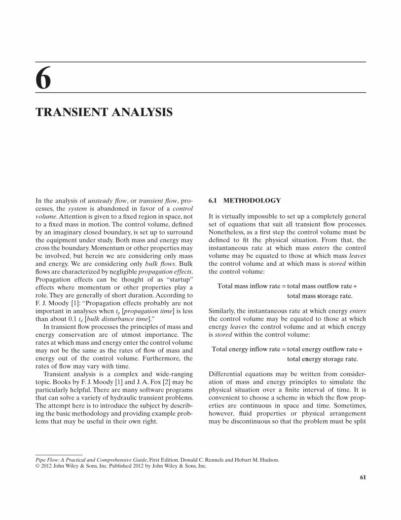
6 TRANSIENT ANALYSIS
In the analysis of unsteady fl ow , or transient fl ow , pro-cesses, the system is abandoned in favor of a controlvolume . Attention is given to a fi xed region in space, not to a fi xed mass in motion. The control volume, defi ned by an imaginary closed boundary, is set up to surround the equipment under study. Both mass and energy may cross the boundary. Momentum or other properties may be involved, but herein we are considering only mass and energy. We are considering only bulk fl ows . Bulk fl ows are characterized by negligible propagation effects . Propagation effects can be thought of as “ startup ” effects where momentum or other properties play a role. They are generally of short duration. According to F. J. Moody [1] : “ Propagation effects probably are not important in analyses when tp [ propagation time ] is less than about 0.1 td [ bulk disturbance time ]. ”
In transient fl ow processes the principles of mass and energy conservation are of utmost importance. The rates at which mass and energy enter the control volume may not be the same as the rates of fl ow of mass and energy out of the control volume. Furthermore, the rates of fl ow may vary with time.
Transient analysis is a complex and wide - ranging topic. Books by F. J. Moody [1] and J. A. Fox [2] may be particularly helpful. There are many software programs that can solve a variety of hydraulic transient problems. The attempt here is to introduce the subject by describ-ing the basic methodology and providing example prob-lems that may be useful in their own right.
6.1 METHODOLOGY
It is virtually impossible to set up a completely general set of equations that suit all transient fl ow processes. Nonetheless, as a fi rst step the control volume must be defi ned to fi t the physical situation. From that, the instantaneous rate at which mass enters the control volume may be equated to those at which mass leavesthe control volume and at which mass is stored within the control volume:
Total mass inflow rate total mass outflow rate
total mass
= +sstorage rate.
Similarly, the instantaneous rate at which energy entersthe control volume may be equated to those at which energy leaves the control volume and at which energy is stored within the control volume:
Total energy inflow rate total energy outflow rate
total e
= +nnergy storage rate.
Differential equations may be written from consider-ation of mass and energy principles to simulate the physical situation over a fi nite interval of time. It is convenient to choose a scheme in which the fl ow prop-erties are continuous in space and time. Sometimes, however, fl uid properties or physical arrangement may be discontinuous so that the problem must be split
Pipe Flow: A Practical and Comprehensive Guide, First Edition. Donald C. Rennels and Hobart M. Hudson.© 2012 John Wiley & Sons, Inc. Published 2012 by John Wiley & Sons, Inc.
61
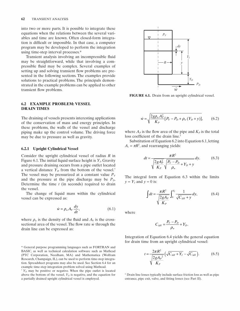
62 TRANSIENT ANALYSIS
wg AK
P P Y yw P
PV D w D= − + +( )[ ]2 2ρ ρ , (6.2)
where AP is the fl ow area of the pipe and KP is the total loss coeffi cient of the drain line. ‡
Substitution of Equation 6.2 into Equation 6.1 , letting Av = π R2 , and rearranging yields:
dtR
gAK
P PY y
dyP
P
V D
wD
=− + +
π
ρ
2
22. (6.3)
The integral form of Equation 6.3 within the limits y = YI and y = 0 is:
dtR
gAK
C ydy
P
P
H
YI
∫ ∫=+
π 2
02
1
∆
, (6.4)
where
CP P
YHV D
wD∆ = − +
ρ.
Integration of Equation 6.4 yields the general equation for drain time from an upright cylindrical vessel:
tR
gAK
C Y CP
P
H I H= + −( )2
2
2
2
π∆ ∆ . (6.5)
into two or more parts. It is possible to integrate these equations when the relations between the several vari-ables and time are known. Often closed - form integra-tion is diffi cult or impossible. In that case, a computer program may be developed to perform the integration using time - step interval processes. *
Transient analysis involving an incompressible fl uid may be straightforward, while that involving a com-pressible fl uid may be complex. Several examples of setting up and solving transient fl ow problems are pre-sented in the following sections. The examples provide solutions to practical problems. The principals demon-strated in the example problems can be applied to other transient fl ow problems.
6.2 EXAMPLE PROBLEM: VESSEL DRAIN TIMES
The draining of vessels presents interesting applications of the conservation of mass and energy principles. In these problems, the walls of the vessel and discharge piping make up the control volume. The driving force may be due to pressure as well as gravity.
6.2.1 Upright Cylindrical Vessel
Consider the upright cylindrical vessel of radius R in Figure 6.1 . The initial liquid surface height is YI . Gravity and pressure draining occurs from a pipe outlet located a vertical distance YD from the bottom of the vessel. †
The vessel may be pressurized at a constant value PV
and the pressure at the pipe discharge may be PD . Determine the time t (in seconds) required to drain the vessel.
The change of liquid mass within the cylindrical vessel can be expressed as:
w Adydt
w V= ρ , (6.1)
where ρw is the density of the fl uid and AV is the cross - sectional area of the vessel. The fl ow rate w through the drain line can be expressed as:
FIGURE 6.1. Drain from an upright cylindrical vessel.
YD
y
dy
YI
R
PD
PV
w
‡ Drain line losses typically include surface friction loss as well as pipe entrance, pipe exit, valve, and fi tting losses (see Part II ).
† YD may be positive or negative. When the pipe outlet is located above the bottom of the vessel, YD is negative, and the equation for a partially drained upright cylindrical vessel is employed.
* General purpose programming languages such as FORTRAN and BASIC, as well as technical calculation software such as Mathcad (PTC Corporation, Needham, MA) and Mathematica (Wolfram Research, Champaign, IL), can be used to perform time - step integra-tion. Spreadsheet programs may also be used. See Section 6.4 for an example time - step integration problem solved using Mathcad.
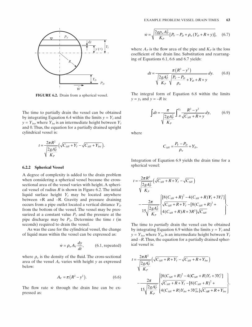
EXAMPLE PROBLEM: VESSEL DRAIN TIMES 63
wg AK
P P Y R yw P
PV D w D= − + + +( )[ ]2 2ρ ρ , (6.7)
where AP is the fl ow area of the pipe and KP is the loss coeffi cient of the drain line. Substitution and rearrang-ing of Equations 6.1 , 6.6 and 6.7 yields:
dtR y
gAK
P PY R y
dyP
P
V D
wD
=−( )
− + + +
π
ρ
2 2
22. (6.8)
The integral form of Equation 6.8 within the limits y = yI and y = – R is:
dtgAK
R y
C R ydy
P
P
HR
YI
∫ ∫= −+ +−
π2 2
2 2
∆
, (6.9)
where
CP P
YHV D
wD∆ = − +
ρ.
Integration of Equation 6.9 yields the drain time for a spherical vessel:
tR
gAK
C R Y C
gAK
C R C R
P
P
H I H
P
P
H H
= + + −( )
−
+( ) − +( )
2
2
2
152
8 4
2
2
2
2
π
π
∆ ∆
∆ ∆[ YY Y
C R Y C R
C R R R C
I I
H I H
H H
+
+ + − +( ) +
+( ) +
3
8
4 3
2
2
2
]
[
]
∆ ∆
∆ ∆
.
The time to partially drain the vessel can be obtained by integrating Equation 6.9 within the limits y = YI and y = YInt , where YInt is an intermediate height between YI
and – R . Thus, the equation for a partially drained spher-ical vessel is:
tR
gAK
C R Y C R Y
gAK
C R
P
P
H I H Int
P
P
H
= + + − + +( )
−
+( ) −
2
2
2
152
8 4
2
2
2
2
π
π
∆ ∆
∆[ CC R Y Y
C R Y C R
C R Y Y C
H I I
H I H
H Int Int
∆
∆ ∆
∆ ∆
+( ) +
+ + − +( ) +
+( ) +
3
8
4 3
2
2
2
]
[
] HH IntR Y+ +
.
The time to partially drain the vessel can be obtained by integrating Equation 6.4 within the limits y = YI and y = YInt , where YInt is an intermediate height between YI
and 0. Thus, the equation for a partially drained upright cylindrical vessel is:
tR
gAK
C Y C YP
P
H I H Int= + − +( )2
2
2
2
π∆ ∆ .
6.2.2 Spherical Vessel
A degree of complexity is added to the drain problem when considering a spherical vessel because the cross - sectional area of the vessel varies with height. A spheri-cal vessel of radius R is shown in Figure 6.2 . The initial liquid surface height YI may be located anywhere between + R and – R. Gravity and pressure draining occurs from a pipe outlet located a vertical distance YD
from the bottom of the vessel. The vessel may be pres-surized at a constant value PV and the pressure at the pipe discharge may be PD . Determine the time t (in seconds) required to drain the vessel.
As was the case for the cylindrical vessel, the change of liquid mass within the vessel can be expressed as:
w Adydt
w V= ρ , (6.1, repeated)
where ρw is the density of the fl uid. The cross - sectional area of the vessel AV varies with height y as expressed below:
A R yV = −( )π 2 2 . (6.6)
The fl ow rate w through the drain line can be ex -pressed as:
FIGURE 6.2. Drain from a spherical vessel.
YD
PV
dy
R
y (+)
PD
YI
w
64 TRANSIENT ANALYSIS
where AP is the fl ow area of the pipe and KP is the loss coeffi cient of the drain line. Substitution and rear-ranging of Equations 6.1 and 6.10 and letting AV = π R2
yields:
dtR
gAK
P PY
Ry
dyP
P
V D
wD
=− + + +
π
ρ
2
22n
. (6.11)
To determine drain time for the cylindrical region of the vessel, we employ the integral form of Equation 6.11 within the limits y = YI and y = 0:
dtR
gAK
CR
y
dyP
PH
YI
∫ ∫=+ +
π 2
2 02
1
∆n
, (6.12)
where
Cp p
YHV D
wD∆ = − +
ρ.
Integration of Equation 6.12 yields the time tCyl to drain the cylindrical region of the vessel:
tR
gAK
CR
Y CR
Cyl
P
P
H I H= + + − +
2
2
2
2
π∆ ∆
n n. (6.13)
In the case of the elliptical bottom head region of the vessel, the cross - sectional area varies with height y as expressed below:
A R yV = −( )π 2 2 2n . (6.14)
In this case, the fl ow rate through the drain line can be expressed as:
wg AK
P P YR
yw P
PV D w D= − + + +
2 ρ ρn
. (6.15)
Substitution and rearrangement of Equations 6.1 , 6.14 and 6.15 yields:
dtR y
gAK
p pY
Ry
dyP
P
V D
wD
=−( )
− + + +
π
ρ
2 2 2
22
n
n
. (6.16)
To determine drain time tBHd of the elliptical bottom head region of the vessel we employ the integral form of Equation 6.16 within the limits y = 0 and y = – R /n:
6.2.3 Upright Cylindrical Vessel with Elliptical Heads
Consider the cylindrical vessel with elliptical heads in Figure 6.3 . The ratio of the major axis to the minor axis of the elliptical head is denoted by n. Note that n = 1 represents a hemispherical head. Assume that the initial liquid surface height YI is located within the cylindrical region of the vessel. Draining occurs from a pipe outlet located a vertical distance YD from the bottom of the vessel. The vessel may be pressurized at a constant value PV and the pressure at the pipe dis-charge may be PD . Determine the time t required to drain the vessel.
The preceding drain problems for cylindrical and spherical vessels are revisited in order to obtain solu-tions. As before, the change of liquid mass within the vessel can be expressed as:
w Adydt
w V= ρ , (6.1, repeated)
where ρw is the weight density of the fl uid. Because of discontinuity in geometry at the interface between the cylinder and the elliptical head, the problem is split into two parts. Accordingly, the total time t is the sum of the time tCyl to drain the cylindrical section, and the time tBHd
to drain the bottom head:
t t tCyl BH= + .
In the case of the cylindrical region of the vessel, the cross - sectional area AV remains constant with height. The fl ow rate w through the drain line can be expressed as:
wg AK
P P YR
yw P
PV D w D= − + + +
2 2ρ ρn
, (6.10)
FIGURE 6.3. Drain from a cylindrical vessel with elliptical heads.
YD
y
dy
YI
R
PD
PV
R/n
w
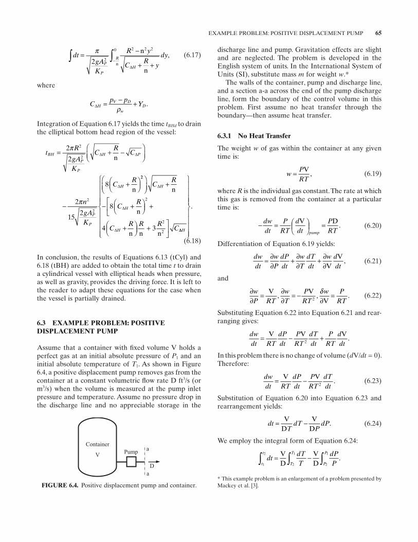
EXAMPLE PROBLEM: POSITIVE DISPLACEMENT PUMP 65
discharge line and pump. Gravitation effects are slight and are neglected. The problem is developed in the English system of units. In the International System of Units (SI), substitute mass m for weight w . *
The walls of the container, pump and discharge line, and a section a - a across the end of the pump discharge line, form the boundary of the control volume in this problem. First assume no heat transfer through the boundary — then assume heat transfer.
6.3.1 No Heat Transfer
The weight w of gas within the container at any given time is:
wPRT
= V, (6.19)
where R is the individual gas constant. The rate at which this gas is removed from the container at a particular time is:
− =
=dwdt
PRT
ddt
PRTpump
V D. (6.20)
Differentiation of Equation 6.19 yields:
dwdt
wP
dPdt
wT
dTdt
w ddt
= ∂∂
+ ∂∂
+ ∂∂V
V, (6.21)
and
∂∂
= ∂∂
= −∂
=wP RT
wT
PRT
w PRT
V,
V,
V2
δ. (6.22)
Substituting Equation 6.22 into Equation 6.21 and rear-ranging gives:
dwdt RT
dPdt
PRT
dTdt
PRT
ddt
= − +V V V2
.
In this problem there is no change of volume ( d V/ dt = 0). Therefore:
dwdt RT
dPdt
PRT
dTdt
= −V V.
2 (6.23)
Substitution of Equation 6.20 into Equation 6.23 and rearrangement yields:
dtT
dTP
dP= −VD
VD
. (6.24)
We employ the integral form of Equation 6.24 :
dtdTT
dPPt
t
T
T
P
P
1
2
2
1
2
1
∫ ∫ ∫= −VD
VD
.
dtgAK
R y
CR
y
dyP
PH
R∫ ∫= −
+ +−
π2 2
2 2 20 n
nn
∆
, (6.17)
where
Cp p
YHV D
wD∆ = − +
ρ.
Integration of Equation 6.17 yields the time tBHd to drain the elliptical bottom head region of the vessel:
tR
gAK
CR
C
n
gAK
CR
BH
P
P
H P
P
P
H
= + −
−
+
2
2
2
152
8
2
2
2
2
π
π
∆ ∆
∆
n
n
22
2
2
2
8
4 3
+
− +
+
+
+
CR
CR
CR R R
C
H
H
H
∆
∆
∆
n
n
n n n∆∆H
.
(6.18)
In conclusion, the results of Equations 6.13 (tCyl) and 6.18 (tBH) are added to obtain the total time t to drain a cylindrical vessel with elliptical heads when pressure, as well as gravity, provides the driving force. It is left to the reader to adapt these equations for the case when the vessel is partially drained.
6.3 EXAMPLE PROBLEM: POSITIVE DISPLACEMENT PUMP
Assume that a container with fi xed volume V holds a perfect gas at an initial absolute pressure of P1 and an initial absolute temperature of T1 . As shown in Figure 6.4 , a positive displacement pump removes gas from the container at a constant volumetric fl ow rate D ft 3 /s (or m3 /s) when the volume is measured at the pump inlet pressure and temperature. Assume no pressure drop in the discharge line and no appreciable storage in the
FIGURE 6.4. Positive displacement pump and container.
D
PumpV
Containera
a* This example problem is an enlargement of a problem presented by Mackey et al. [3] .
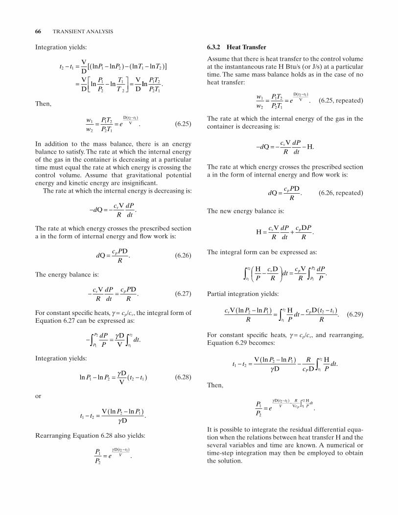
66 TRANSIENT ANALYSIS
6.3.2 Heat Transfer
Assume that there is heat transfer to the control volume at the instantaneous rate H Btu/s (or J/s) at a particular time. The same mass balance holds as in the case of no heat transfer:
ww
PTP T
et t
1
2
1 2
2 1
2 1
= =−( )D
V . (6.25, repeated)
The rate at which the internal energy of the gas in the container is decreasing is:
− = − −dcR
dPdt
vQV
H.
The rate at which energy crosses the prescribed section a in the form of internal energy and fl ow work is:
dc P
RpQ
D.= (6.26, repeated)
The new energy balance is:
HV D
= +cR
dPdt
c PR
v p .
The integral form can be expressed as:
H D VP
cR
dtcR
dPP
v
t
tp
P
P
−
=∫ ∫1
2
1
2
.
Partial integration yields:
c P P
R Pdt
c t tR
v p
t
tV H D.
ln ln2 1 2 1
1
2−( ) = −−( )∫ (6.29)
For constant specifi c heats, γ = cp / cv , and rearranging, Equation 6.29 becomes:
t tP P R
c Pdt
P t
t
1 22 1
1
2
− = −( ) − ∫VD D
Hln ln.
γ
Then,
PP
et tV
Rc P
dtp t
t
1
2
2 1
1
2
=∫−( )−γ D
VH
.
It is possible to integrate the residual differential equa-tion when the relations between heat transfer H and the several variables and time are known. A numerical or time - step integration may then be employed to obtain the solution.
Integration yields:
t t P P T T
PP
TT
2 1 1 2 1 2
1
2
1
2
− = −( ) − −( )[ ]
= −
=
VD
ln ln ln ln
VD
ln lnVD
llnPTP T
1 2
2 1
.
Then,
ww
PTP T
et t
1
2
1 2
2 1
2 1
= =−( )D
V . (6.25)
In addition to the mass balance, there is an energy balance to satisfy. The rate at which the internal energy of the gas in the container is decreasing at a particular time must equal the rate at which energy is crossing the control volume. Assume that gravitational potential energy and kinetic energy are insignifi cant.
The rate at which the internal energy is decreasing is:
− = −dcR
dPdt
vQV
.
The rate at which energy crosses the prescribed section a in the form of internal energy and fl ow work is:
dc P
RpQ
D.= (6.26)
The energy balance is:
− =cR
dPdt
c PR
v pV D. (6.27)
For constant specifi c heats, γ = cp / cv , the integral form of Equation 6.27 can be expressed as:
− =∫ ∫dPP
dtP
P
t
t
1
2
1
2γ DV
.
Integration yields:
ln lnP P t t1 2 2 1− = −( )γ DV
(6.28)
or
t tP P
1 22 1− = −( )VD
ln ln.
γ
Rearranging Equation 6.28 also yields:
PP
et tV1
2
2 1
=−( )γ D
.
EXAMPLE PROBLEM: TIME-STEP INTEGRATION 67
6.4.2 Direct Solution
Equation 6.5 can be employed to directly solve for the drain time.
t = × ×× ×
− + + − −
2 6
2 32 174 0 20065
14400 211762 31
4 2014400 2117
62
2
2
π. .
. ..
. .
314
216 38
+
= s
6.4.3 Time - Step Solution
Now calculate the drain time t using Equation 6.3 , the integral form of Equation 6.5 , assuming progressively smaller time steps Δt . *
Several programs are available to perform step - by - step integration. They are all similar in that they form a loop to repeatedly execute a calculation until a certain condition is met. The one shown below, uses a “ while ” loop, a programming feature found in Mathcad † as well as in other computational programs.
y = YI Sets initial water level t = 0 Sets transient start time
at zero Δt = 10 s ( = 1 s) ( = 0.1 s) Sets time - step interval
(three intervals will be used)
while y > 0 Sets condition to be met dy gA K
P P Y y
R t
P P
V D w D
=
−( ) + +
(( /
( ) / )
/ )
2
2
ρπ ∆
Repeatedly calculates Equation 6.3 (rearranged)
t = t + Δt Resets time y = y − dy Resets water level;
continues execution while y > 0
t = 220 s ( = 217 s) ( = 216.4 s) The condition is met when y ≤ 0 (three solutions for three time step intervals)
6.4 EXAMPLE PROBLEM: TIME - STEP INTEGRATION
Numerical integration is the approximate computation of an integral using numerical techniques. The term is sometimes used to describe the numerical solution of differential equations using a time- step integrationprocess. Herein the time - step process will be demon-strated by obtaining particular solutions to the differen-tial equation developed in Section 6.2.1 representing drain time from an upright cylindrical vessel.
6.4.1 Upright Cylindrical Vessel Drain Problem
Consider the upright cylindrical vessel shown in Figure 6.5 . The radius of the vessel is 6 ft. The vessel contains 70 ° F water at an initial height of 20 ft. The vessel pres-sure is constantly maintained at 100 lb/in 2 . The drain line discharges to atmosphere from an outlet located a distance of 4 ft below the bottom of the vessel. The loss coeffi cient of the drain line is based on velocity in the 6″ schedule 40 drain pipe.
The input parameters are:R = 6 ft Vessel radius YI = 20 ft Initial height of water YD = 4 ft Vertical distance of drain line
exit from bottom of vessel PV ( = 100 lb/in 2 )
= 14,400 lb/ft 2 Vessel pressure
PD ( = 14.7 lb/in 2 ) = 2117 lb/ft 2
Atmospheric pressure
AP = 0.20063 ft 2 Drain line fl ow area (6″ schedule 40 pipe)
K = 5 Drain line loss coeffi cient ρw = 62.31 lb/ft 3 Density of 70 ° F water
FIGURE 6.5. Drain from an upright cylindrical vessel (repeated).
YD
y
dy
YI
R
PD
PV
† Mathcad is a computational software program used in engineering and other areas of technical computing. The Mathcad Professional version may be needed to provide the programming tools required to solve time - step problems.
* In this application, Δt is substituted for dt . When Δt is small, Δt ≈ dt , and the closer the time - step interval is to zero the better the results are, provided the precision of the arithmetic (as in signifi cant fi gures) does not start providing inaccurate answers.
68 TRANSIENT ANALYSIS
Streeter , V. L. and E. B. Wylie , Hydraulic Transients , McGraw - Hill , 1967 .
Webb , S. W. and J. L. Caves , Fluid transient analysis in pipelines with nonuniform liquid density , Journal of Fluids Engineer-ing, Transactions of American Society of Mechanical Engi-neers , 105 , 1983 , 423 – 428 .
Blevins , R. D. , Applied Fluid Dynamics Handbook , Van Nos-trand Reinhold Company , 1984 .
Nanayakkara , S. and N. D. Perrieira , Wave propagation and attenuation in piping systems , Journal of Vibration, Acous-tics, Stress, and Reliability in Design , 108 , 1986 , 441 – 446 .
Pejovic , S. , A. P. Boldy , and D. Obradovic , Guidelines to Hydraulic Transient Analysis , Gower Technical Press , 1987 .
Thorley , R. D. and C. H. Tiley , Unsteady and transient fl ow of compressible fl uids in pipelines — A review of theoretical and some experimental studies , Heat and Fluid Flow , 8 , 1987 , 3 – 15 .
Ellis , J. , Pressure Transients in Water Engineering: A Guide to Analysis and Interpretation of Behavior , Thomas Telford Ltd. , 2008 .
Setting the time step at 10 seconds would likely provide a suffi ciently accurate answer for this simple computa-tion. Other computations, such as a transient analysis program that simulates a loss of coolant accident ( LOCA ) in a nuclear power plant, would use small time steps, and would simultaneously track pressure, tem-perature, phase change, fl uid density, fl ow rate, and so on, in addition to water level.
REFERENCES
1. Moody , F. J. , Unsteady Thermofl uid Mechanics , John Wiley & Sons , 1990 .
2. Fox , J. A. , Hydraulic Analysis of Unsteady Flow in Pipe Networks , The MacMillan Press Ltd , 1984 .
3. Mackay , C. O. , W. N. Barnard , and F. O. Ellenwood , Engi-neering Thermodynamics , John Wiley & Sons , 1957 .
FURTHER READING
This list includes books and papers that may be helpful to those who wish to pursue further study.
69
7 UNCERTAINTY
Uncertainty is the probable range of error. The uncer-tainty associated with hydraulic analysis may be defi ned as the statistical difference between calculated pressure drop and true pressure drop. It may also be defi ned as the statistical difference between calculated fl ow rate and true fl ow rate. *
There is uncertainty associated with practically every variable involved in calculating pressure drop or fl ow rate. In the uncertainty analysis, it is assumed that the individual errors have an equal probability of being posi-tive or negative; and further, that the probability density function describing the uncertainty is normally distrib-uted. This is done for three reasons: fi rst, these assump-tions simplify the mathematical manipulations required; second, the existing knowledge regarding the uncertainty of the various errors does not allow a more sophisticated treatment; and fi nally, this allows convenient expression of the results. With these assumptions, the combined value of the various errors can be determined and expressed as ± 1 (or 2 or 3) standard deviation(s) of the mean (or calculated) pressure drop or fl ow rate.
7.1 ERROR SOURCES
The predominant source of error in the calculation of pressure drop or fl ow rate is associated with the loss coeffi cients of the various elements within the fl ow system. The accuracy of loss coeffi cients is subject to
dimensional and surface roughness differences, experi-mental and theoretical variations, and to uncertainties associated with modeling the loss coeffi cient over a wide range of variables.
Suggested 3 - sigma values of uncertainty associated with the loss coeffi cients documented in Part II are given in Table 7.1 . † The uncertainty values are expressed as percentage. They refl ect the authors ’ judgment based on selecting, developing, and formulating the loss coef-fi cients for the various fl ow elements.
The suggested uncertainty values for tees are for normal ranges of fl ow and diameter ratio. Higher values may be appropriate outside of these ranges. It should be noted that some loss coeffi cient values in junctions pass through zero so that uncertainty values on a per-centage basis are unrealistic. Fixed uncertainty values may be appropriate under these conditions.
7.2 PRESSURE DROP UNCERTAINTY
The basic pressure drop equation for a pipe section can be expressed as:
P P KAA
wg A
Z Zw
w1 2 112
22
2
12 2 11
2− = − +
+ −( )ρ
ρ . (7.1)
In pressure drop analysis the values of fl ow rate, density, and fl ow area are established so that they contain little or no uncertainty. Assuming a normal distribution of error, the percentage uncertainty of calculated pressure
Pipe Flow: A Practical and Comprehensive Guide, First Edition. Donald C. Rennels and Hobart M. Hudson.© 2012 John Wiley & Sons, Inc. Published 2012 by John Wiley & Sons, Inc.
† If a data distribution is approximately normal, then 3 sigma (or three standard deviations) accounts for 99.73% of the data set.
* There is somewhat of a diffi culty here because we also have uncer-tainty associated with determining the true value. Perhaps we should say that the uncertainty is the difference between the calculated value and the measured value. Then that could encompass errors not only in calculating but also in measuring.
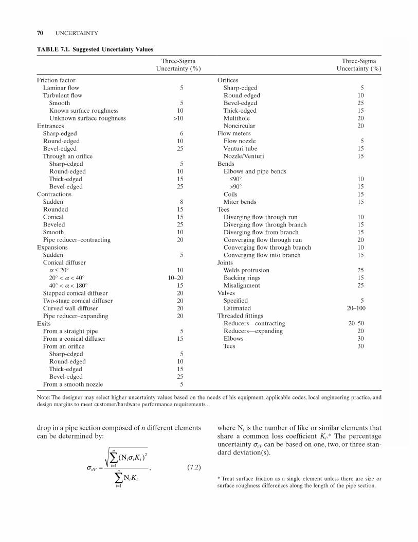
70 UNCERTAINTY
* Treat surface friction as a single element unless there are size or surface roughness differences along the length of the pipe section.
TABLE 7.1. Suggested Uncertainty Values
Three - Sigma Uncertainty (%)
Friction factor Laminar fl ow 5 Turbulent fl ow Smooth 5 Known surface roughness 10 Unknown surface roughness > 10 Entrances Sharp - edged 6 Round - edged 10 Bevel - edged 25 Through an orifi ce Sharp - edged 5 Round - edged 10 Thick - edged 15 Bevel - edged 25 Contractions Sudden 8 Rounded 15 Conical 15 Beveled 25 Smooth 10 Pipe reducer – contracting 20 Expansions Sudden 5 Conical diffuser α ≤ 20 ° 10 20 ° < α < 40 ° 10 – 20 40 ° < α < 180 ° 15 Stepped conical diffuser 20 Two - stage conical diffuser 20 Curved wall diffuser 20 Pipe reducer – expanding 20 Exits From a straight pipe 5 From a conical diffuser 15 From an orifi ce Sharp - edged 5 Round - edged 10 Thick - edged 15 Bevel - edged 25 From a smooth nozzle 5
Three - Sigma Uncertainty (%)
Orifi ces Sharp - edged 5 Round - edged 10 Bevel - edged 25 Thick - edged 15 Multihole 20 Noncircular 20 Flow meters Flow nozzle 5 Venturi tube 15 Nozzle/Venturi 15 Bends Elbows and pipe bends ≤ 90 ° 10 > 90 ° 15 Coils 15 Miter bends 15 Tees Diverging fl ow through run 10 Diverging fl ow through branch 15 Diverging fl ow from branch 15 Converging fl ow through run 20 Converging fl ow through branch 10 Converging fl ow into branch 15 Joints Welds protrusion 25 Backing rings 15 Misalignment 25 Valves Specifi ed 5 Estimated 20 – 100 Threaded fi ttings Reducers — contracting 20 – 50 Reducers — expanding 20 Elbows 30 Tees 30
drop in a pipe section composed of n different elements can be determined by:
σ dP
i i i
i
n
i i
i
n
K
K
=( )
=
=
∑
∑
N
N
,σ 2
1
1
(7.2)
where N i is the number of like or similar elements that share a common loss coeffi cient Ki . * The percentage uncertainty σdP can be based on one, two, or three stan-dard deviation(s).
Note: The designer may select higher uncertainty values based on the needs of his equipment, applicable codes, local engineering practice, and design margins to meet customer/hardware performance requirements..
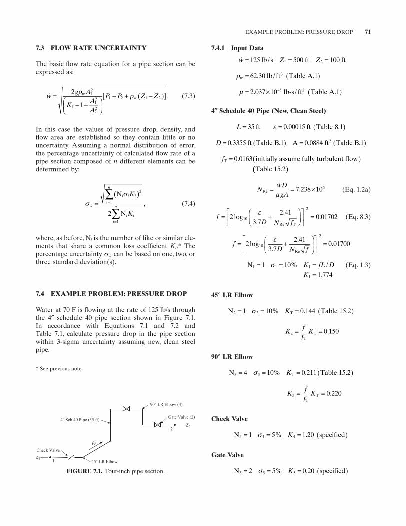
EXAMPLE PROBLEM: PRESSURE DROP 71
7.4.1 Input Data
w Z Z= = =125 500 1001 2lb s ft ft/
ρw = ( )62 30 13. / .lb ft Table A
µ = × ( )−2 037 10 15 2. / .lb-s ft Table A
4″ Schedule 40 Pipe (New, Clean Steel)
L = = ( )35 0 00015 8 1ft ft Table ε . .
D = ( ) = ( )0 3355 1 0 0884 12. . . .ft Table B A ft Table B
fT initially assume fully turbulent flow
Table 15.2
= ( )0 0163.
(( )
NwDgA
Re .= = ×
µ7 238 105 (Eq. 1.2a)
fD N f
= +
=
−
23 7
2 410 0170210
2
log.
..
Re
ε
T
(Eq. 8.3)
fD N f
= +
=
−
23 7
2 410 0170010
2
log.
..
Re
ε
N1 1 1
1
1 10
1 774
= = ==
σ % /
.
K fL D
K
(Eq. 1.3)
45 ° LR Elbow
N Table T2 21 10 0 144 15 2= = = ( )σ % . .K
Kff
K2 0 150= =T
T .
90 ° LR Elbow
N Table T3 34 10 0 211 15 2= = = ( )σ % . .K
Kff
K3 0 220= =T
T .
Check Valve
N specified44 41 5 1 20= = = ( )σ % .K
Gate Valve
N specified5 5 52 5 0 20= = = ( )σ % .K
7.3 FLOW RATE UNCERTAINTY
The basic fl ow rate equation for a pipe section can be expressed as:
wg A
KAA
P P Z Zww=
− +
− + −( )[ ]2
1
12
112
22
1 2 1 2ρ ρ . (7.3)
In this case the values of pressure drop, density, and fl ow area are established so they contain little or no uncertainty. Assuming a normal distribution of error, the percentage uncertainty of calculated fl ow rate of a pipe section composed of n different elements can be determined by:
σ w
i i i
i
n
i i
i
n
K
K
=( )
=
=
∑
∑
N
N
,σ 2
1
1
2
(7.4)
where, as before, N i is the number of like or similar ele-ments that share a common loss coeffi cient Ki . * The percentage uncertainty σ w can be based on one, two, or three standard deviation(s).
7.4 EXAMPLE PROBLEM: PRESSURE DROP
Water at 70 F is fl owing at the rate of 125 lb/s through the 4 ″ schedule 40 pipe section shown in Figure 7.1 . In accordance with Equations 7.1 and 7.2 and Table 7.1 , calculate pressure drop in the pipe section within 3 - sigma uncertainty assuming new, clean steel pipe.
FIGURE 7.1. Four - inch pipe section.
w
90˚ LR Elbow (4)
45˚ LR Elbow
Check Valve
Gate Valve (2)4'' Sch 40 Pipe (35 ft)
Z 22
Z 11
•
* See previous note.
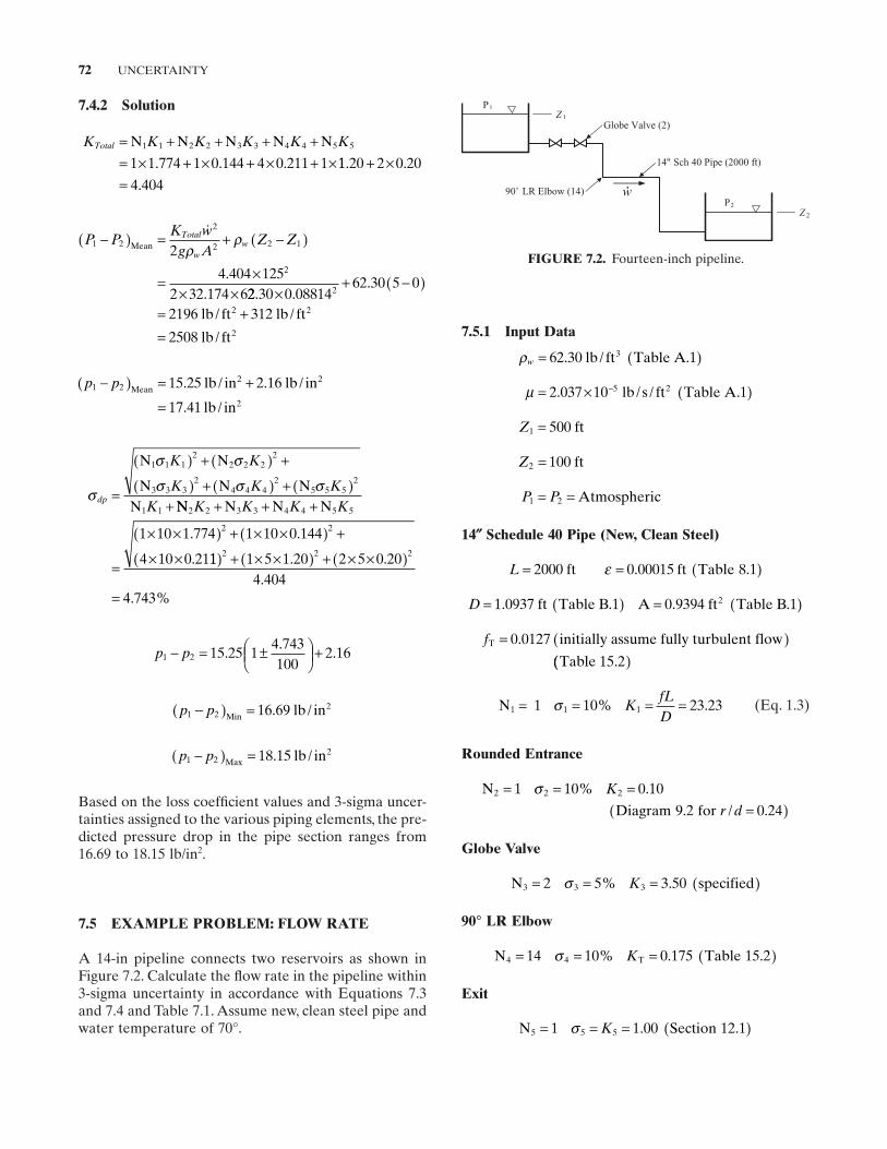
72 UNCERTAINTY
7.5.1 Input Data
ρw = ( )62 30 1. / .lb ft Table A3
µ = × ( )−2 037 10 5. / /lb s ft Table A.12
Z1 500= ft
Z2 100= ft
P P1 2= = Atmospheric
14″ Schedule 40 Pipe (New, Clean Steel)
L = = ( )2000 0 00015 8 1ft ft Table ε . .
D = ( ) = ( )1 0937 1 0 9394 12. . . .ft Table B A ft Table B
fT initially assume fully turbulent flow
Table 15.2
= ( )0 0127.
(( )
N 1 11 110 23 23 = = = =σ % .KfLD
(Eq. 1.3)
Rounded Entrance
N
Diagram for 2 2 21 10 0 10
9 2 0 24
= = ==( )
σ % .
. / .
K
r d
Globe Valve
N specified3 3 32 5 3 50= = = ( )σ % .K
90 ° LR Elbow
N Table T4 414 10 0 175 15 2= = = ( )σ % . .K
Exit
N Section 5 5 51 1 00 12 1= = = ( )σ K . .
7.4.2 Solution
K K K K K KTotal = + + + += × + × + × + ×
N N N N N1 1 2 2 3 3 4 4 5 5
1 1 774 1 0 144 4 0 211 1. . . 11 20 2 0 20
4 404
. .
.
+ ×=
P PK w
g AZ ZTotal
ww1 2
2
2 2 1
2
2
4 404 1252 32 174 6
−( ) = + −( )
= ×× ×
Mean
ρ
ρ
.. 22 30 0 08814
62 30 5 0
2196 312
2508
2
2 2
2
. ..
/ /
/
×+ −( )
= +=
lb ft lb ft
lb ft
p p1 22 2
2
15 25 2 16
17 41
−( ) = +
=Mean lb in lb in
lb in
. / . /
. /
σ dp
K K
K K KK
=
( ) + ( ) +
( ) + ( ) + ( )+
N N
N N NN
1 1 12
2 2 22
3 3 32
4 4 42
5 5 52
1 1
σ σ
σ σ σNN N N N2 2 3 3 4 4 5 5
2 21 10 1 774 1 10 0 144
4 10 0 21
K K K K+ + +
=
× ×( ) + × ×( ) +
× ×
. .
. 11 1 5 1 20 2 5 0 204 404
4 743
2 2 2( ) + × ×( ) + × ×( )
=
. ..
. %
p p1 2 15 25 14 743100
2 16− = ±
+..
.
p p1 2216 69−( ) =Min lb in. /
p p1 2218 15−( ) =Max lb in. /
Based on the loss coeffi cient values and 3 - sigma uncer-tainties assigned to the various piping elements, the pre-dicted pressure drop in the pipe section ranges from 16.69 to 18.15 lb/in 2 .
7.5 EXAMPLE PROBLEM: FLOW RATE
A 14 - in pipeline connects two reservoirs as shown in Figure 7.2 . Calculate the fl ow rate in the pipeline within 3 - sigma uncertainty in accordance with Equations 7.3 and 7.4 and Table 7.1 . Assume new, clean steel pipe and water temperature of 70 ° .
FIGURE 7.2. Fourteen - inch pipeline.
w
14'' Sch 40 Pipe (2000 ft)
90˚ LR Elbow (14)
Globe Valve (2)Z 1
P1
P2Z 2
•
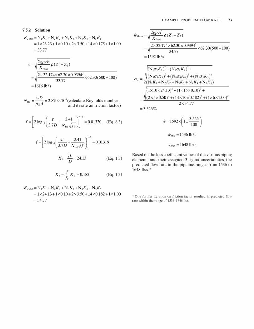
EXAMPLE PROBLEM: FLOW RATE 73
wg AK
Z ZTotal
Mean = −( )
= × × × ×
2
2 32 174 62 30 0 939434 77
62
2
1 2
2
ρ ρ
. . ..
.330 500 100
1592
−( )
= lb s/
σ
σ σ
σ σ σw
K K
K K KK
=
( ) + ( ) +
( ) + ( ) + ( )N N
N N NN
1 1 12
2 2 22
3 3 32
4 4 42
5 5 52
1 12 ++ + + +( )
=
× ×( ) + × ×( ) +
× ×
N N N N2 2 3 3 4 4 5 5
2 21 10 24 13 1 15 0 10
2 5 3 5
K K K K
. .
. 00 14 10 0 182 1 6 1 002 34 77
3 526
2 2 2( ) + × ×( ) + × ×( )×
=
. ..
. %
w = × ±
1592 13 526100.
wMin = 1536 lb s/
wMax = 1648 lb s/
Based on the loss coeffi cient values of the various piping elements and their assigned 3 - sigma uncertainties, the predicted fl ow rate in the pipeline ranges from 1536 to 1648 lb/s. *
7.5.2 Solution
K K K K K KTotal = + + + += × + × + × + ×
N N N N N1 1 2 2 3 3 4 4 5 5
1 23 23 1 0 10 2 3 50 14 0. . . .. .
.
175 1 1 00
33 77
+ ×=
wg AK
Z ZTotal
= −( )
= × × × ×
2
2 32 174 62 30 0 939433 77
62 30 50
2
1 2
2
ρ ρ
. . ..
. 00 100
1616
−( )
= lb s/
NwDgA
Re .= = ×
µ2 870 106 (calculate Reynolds number
and iterate oon friction factor)
fD N f
= +
=
−
23 7
2 410 0132010
2
log.
..
Re
ε
T
(Eq. 8.3)
fD N f
= +
=
−
23 7
2 410 0131910
2
log.
..
Re
ε
KfLD
1 24 13= = . (Eq. 1.3)
Kff
K4 0 182= =T
T . (Eq. 1.3)
K K K K K KTotal = + + + += × + × + × + ×
N N N N N1 1 2 2 3 3 4 4 5 5
1 24 13 1 0 10 2 3 50 14 0. . . .. .
.
182 1 1 00
34 77
+ ×=
* One further iteration on friction factor resulted in predicted fl ow rate within the range of 1534 – 1646 lb/s.
PART II
LOSS COEFFICIENTS
hibit some degree of fl ow contraction and/or expansion. As such, they were treated as a family; they share semiem-pirical formulas that were rationally tailored to meet the specifi cs of the various fl ow confi gurations. Where suffi cient data for a particular fl ow confi guration were lacking, they were augmented by ample data in a related confi guration.
Bends, tees, joints, and valves are treated in Chapters 15 through 18 , respectively. The loss coeffi cient data in Part II are on the whole applicable to pipe components with butt weld, socket weld, fl anged, or otherwise smooth - walled end connections. However, the internal geometry of threaded fi ttings is discontinuous, creating additional pressure loss, and they are covered separately in Chapter 19 .
The loss coeffi cient data are independent of the kind of fl uid as long as it is homogeneous and incompressible. The data are valid for turbulent fl ow conditions com-monly encountered throughout the operating range of most industrial piping systems. The effect of Reynolds number on loss coeffi cients is mainly evident at its small values. The loss coeffi cient values are generally appli-cable to Reynolds numbers greater than 10 5 , but they can be used with some loss of accuracy at lower Reyn-olds numbers in the turbulent fl ow regime.
In the case of laminar fl ow, the data can be used for rough estimates and only when the Reynolds number is greater than 100. In the case of compressible fl ow, they can be applied at Mach numbers up to approxi-mately 0.3 with little or no loss of accuracy. They may be used at higher subsonic velocities up to about
PROLOGUE
As explained in Chapter 2 , head loss represents a con-version of available mechanical energy to unavailable heat energy. The two principal sources of this conver-sion are: (1) surface friction and (2) induced turbulence due to pipe fi ttings and other changes in the fl ow path, such as fl ow meters and valves. The gradual process leading to understanding and quantifying surface fric-tion was presented in Chapter 3 . Its basic feature, fric-tion factor, is presented in Chapter 8 as an adjunct to quantifying the various features that contribute to head loss. Induced turbulence, in the form of loss coeffi cients (or resistance coeffi cients), is dealt with in the remain-ing chapters of Part II .
Chapters 9 through 19 present rational and compre-hensive investigations of pipe fl ow confi gurations com-monly encountered by the professional engineer. Experimental test data and formulas for loss coeffi -cients from worldwide sources are evaluated, integrated, and developed into widely applicable equations. The processes used to select and develop loss coeffi cient data for the various fl ow confi gurations are described so the reader can judge their merit and understand their limitations. The end results are presented in straightfor-ward tables and diagrams located at the end of each chapter, where a user familiar with the work can quickly fi nd them.
The fl ow confi gurations presented in Chapters 9 through 14 — “ Entrances, ” “ Contractions, ” “ Expan-sions, ” “ Exits, ” “ Orifi ces, ” and “ Flow Meters ” — all ex -
75
Pipe Flow: A Practical and Comprehensive Guide, First Edition. Donald C. Rennels and Hobart M. Hudson.© 2012 John Wiley & Sons, Inc. Published 2012 by John Wiley & Sons, Inc.
76 LOSS COEFFICIENTS
Mach number 0.8 with decreased accuracy. In addition, the data can be applied to square passages or to rectan-gular passages of low aspect ratio with moderate loss of accuracy.
The loss coeffi cient always represents the number of velocity heads, V2 /2 g , lost. The numerical value of any loss coeffi cient is intimately related to the inherent velocity in the associated pressure drop equation. In many cases the relationship is self - evident and the loss coeffi cient is simply labeled as K . In cases where there
is a change in fl ow area a subscript is used to denote the relationship. For example, in the case of a contraction, K2 indicates that the loss coeffi cient is related to the velocity at point 2, the downstream velocity. In the case of fl ow through tees, a subscript — two numbers separated by a comma — defi nes the fl ow path, and a sub - subscript defi nes the related velocity. For instance, K1 22, indicates that pressure loss is from point 1 to point 2 and the loss coeffi cient is related to the velocity at point 2.
77
8 SURFACE FRICTION
The gradual process leading to understanding and quan-tifying surface friction was presented in Chapter 3 . Surface friction and its main element, friction factor, are further considered in this chapter as an adjunct to quan-tifying the various features that contribute to head loss.
The loss coeffi cient due to surface friction (analogous to the loss coeffi cient due to local loss) is expressed as:
K fLD
= . (1.3, repeated)
Thus the product of the friction factor f and the geomet-ric factor L / D (or l/d ) represents the number of velocity heads lost due to surface friction. The friction factor under discussion here is that corresponding to fully developed velocity profi les that are encountered only after 20 or more pipe diameters downstream of a pipe inlet or other major disturbance. In practice, this condi-tion is rarely met. However, satisfactory results are gen-erally obtained ignoring this limitation.
8.1 FRICTION FACTOR
The relationship of friction factor to the Reynolds number and surface roughness has three distinct differ-ing regions of application.
8.1.1 Laminar Flow Region
As identifi ed in Chapter 3 , an expression for laminar fl ow friction factor was developed by the mid - 1800s:
fN
=64
.Re
(3.3, repeated)
Note that f is a function of the pipe Reynolds number only. Protrusions on the pipe surface do not cause tur-bulence in laminar fl ow. For laminar fl ow, pipes of dif-ferent surface roughness have the same friction factor for the same Reynolds number.
The upper range of Reynolds number for laminar fl ow is somewhat indefi nite, being dependent upon several incidental conditions, and may be as high as 4000. However, such high values are of little practical interest, and the engineer may take the upper limit of laminar fl ow to be defi ned by a Reynolds number of 2100.
8.1.2 Critical Zone
For pipe Reynolds numbers between 2100 and 3000 to 4000, the friction factor can have large uncertainties and is highly indeterminate. Hence this region is called the critical zone . The fl ow in this zone may be laminar or turbulent (or an unsteady mix of both) depending on the pipe entrance, initial disturbances, and pipe rough-ness. This transition region from laminar to turbulent fl ow is accompanied by a considerable increase in fric-tion factor, and thereby in pressure drop in the pipe. As a rule, however, pipes fl owing signifi cant amounts of fl uid, and which have measurable pressure loss, have a Reynolds number much greater than 3000 or 4000. Not-withstanding, the engineer may on occasion have to
Pipe Flow: A Practical and Comprehensive Guide, First Edition. Donald C. Rennels and Hobart M. Hudson.© 2012 John Wiley & Sons, Inc. Published 2012 by John Wiley & Sons, Inc.
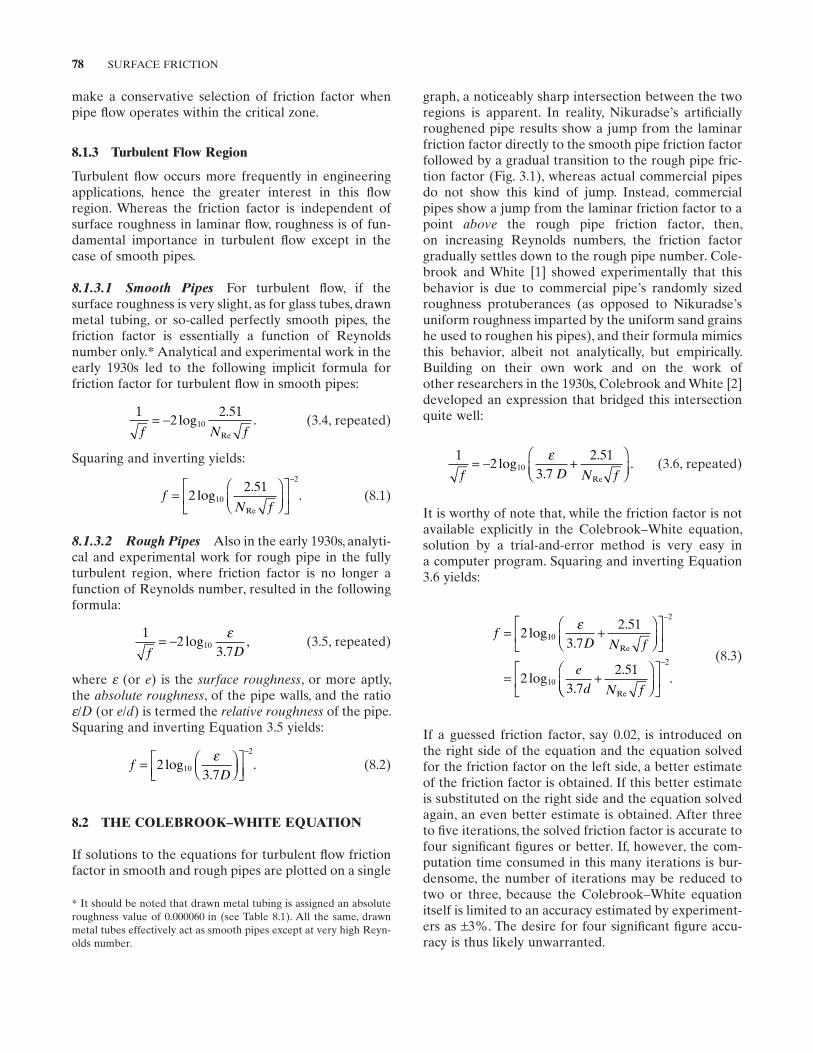
78 SURFACE FRICTION
graph, a noticeably sharp intersection between the two regions is apparent. In reality, Nikuradse ’ s artifi cially roughened pipe results show a jump from the laminar friction factor directly to the smooth pipe friction factor followed by a gradual transition to the rough pipe fric-tion factor (Fig. 3.1 ), whereas actual commercial pipes do not show this kind of jump. Instead, commercial pipes show a jump from the laminar friction factor to a point above the rough pipe friction factor, then, on increasing Reynolds numbers, the friction factor gradually settles down to the rough pipe number. Cole-brook and White [1] showed experimentally that this behavior is due to commercial pipe ’ s randomly sized roughness protuberances (as opposed to Nikuradse ’ s uniform roughness imparted by the uniform sand grains he used to roughen his pipes), and their formula mimics this behavior, albeit not analytically, but empirically. Building on their own work and on the work of other researchers in the 1930s, Colebrook and White [2] developed an expression that bridged this intersection quite well:
1
23 7
2 5110
f D N f= − +
⎛⎝⎜
⎞⎠⎟
log.
..
Re
ε (3.6, repeated)
It is worthy of note that, while the friction factor is not available explicitly in the Colebrook – White equation, solution by a trial - and - error method is very easy in a computer program. Squaring and inverting Equation 3.6 yields:
fD N f
ed N f
= +⎛⎝⎜
⎞⎠⎟
⎡
⎣⎢
⎤
⎦⎥
= +⎛
−
23 7
2 51
23 7
2 51
10
2
10
log.
.
log.
.
Re
Re
ε
⎝⎝⎜⎞⎠⎟
⎡
⎣⎢
⎤
⎦⎥
−2
.
(8.3)
If a guessed friction factor, say 0.02, is introduced on the right side of the equation and the equation solved for the friction factor on the left side, a better estimate of the friction factor is obtained. If this better estimate is substituted on the right side and the equation solved again, an even better estimate is obtained. After three to fi ve iterations, the solved friction factor is accurate to four signifi cant fi gures or better. If, however, the com-putation time consumed in this many iterations is bur-densome, the number of iterations may be reduced to two or three, because the Colebrook – White equation itself is limited to an accuracy estimated by experiment-ers as ± 3%. The desire for four signifi cant fi gure accu-racy is thus likely unwarranted.
make a conservative selection of friction factor when pipe fl ow operates within the critical zone.
8.1.3 Turbulent Flow Region
Turbulent fl ow occurs more frequently in engineering applications, hence the greater interest in this fl ow region. Whereas the friction factor is independent of surface roughness in laminar fl ow, roughness is of fun-damental importance in turbulent fl ow except in the case of smooth pipes.
8.1.3.1 Smooth Pipes For turbulent fl ow, if the surface roughness is very slight, as for glass tubes, drawn metal tubing, or so - called perfectly smooth pipes, the friction factor is essentially a function of Reynolds number only. * Analytical and experimental work in the early 1930s led to the following implicit formula for friction factor for turbulent fl ow in smooth pipes:
1
22 51
10f N f
= − log.
.Re
(3.4, repeated)
Squaring and inverting yields:
fN f
=⎛⎝⎜
⎞⎠⎟
⎡
⎣⎢
⎤
⎦⎥
−
22 51
10
2
log.
.Re
(8.1)
8.1.3.2 Rough Pipes Also in the early 1930s, analyti-cal and experimental work for rough pipe in the fully turbulent region, where friction factor is no longer a function of Reynolds number, resulted in the following formula:
1
23 7
10f D
= − log.
,ε
(3.5, repeated)
where ε (or e ) is the surface roughness , or more aptly, the absolute roughness , of the pipe walls, and the ratio ε / D (or e / d ) is termed the relative roughness of the pipe. Squaring and inverting Equation 3.5 yields:
fD
= ⎛⎝⎜
⎞⎠⎟
⎡⎣⎢
⎤⎦⎥
−
23 7
10
2
log.
.ε
(8.2)
8.2 THE COLEBROOK – WHITE EQUATION
If solutions to the equations for turbulent fl ow friction factor in smooth and rough pipes are plotted on a single
* It should be noted that drawn metal tubing is assigned an absolute roughness value of 0.000060 in (see Table 8.1 ). All the same, drawn metal tubes effectively act as smooth pipes except at very high Reyn-olds number.
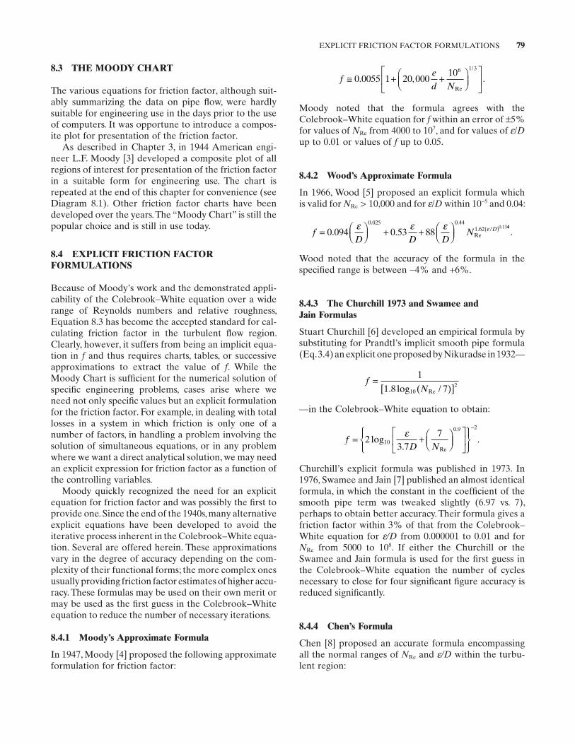
EXPLICIT FRICTION FACTOR FORMULATIONS 79
fed N
≅ + +
0 0055 1 20 000
106 1 3
. , .Re
/
Moody noted that the formula agrees with the Colebrook – White equation for f within an error of ± 5% for values of NRe from 4000 to 10 7 , and for values of ε / Dup to 0.01 or values of f up to 0.05.
8.4.2 Wood ’ s Approximate Formula
In 1966, Wood [5] proposed an explicit formula which is valid for NRe > 10,000 and for ε / D within 10 − 5 and 0.04:
fD D D
N D=
+ +
( )0 094 0 53 880 025 0 44
1 62 0 13. .
. .
Re. / .ε ε ε ε 44
.
Wood noted that the accuracy of the formula in the specifi ed range is between − 4% and + 6%.
8.4.3 The Churchill 1973 and Swamee and Jain Formulas
Stuart Churchill [6] developed an empirical formula by substituting for Prandtl ’ s implicit smooth pipe formula (Eq. 3.4 ) an explicit one proposed by Nikuradse in 1932 —
fN
=[ ]
1
1 8 7102. log ( / )Re
— in the Colebrook – White equation to obtain:
fD N
= +
−
23 7
710
0 9 2
log. Re
.ε.
Churchill ’ s explicit formula was published in 1973. In 1976, Swamee and Jain [7] published an almost identical formula, in which the constant in the coeffi cient of the smooth pipe term was tweaked slightly (6.97 vs. 7), perhaps to obtain better accuracy. Their formula gives a friction factor within 3% of that from the Colebrook – White equation for ε/D from 0.000001 to 0.01 and for NRe from 5000 to 10 8 . If either the Churchill or the Swamee and Jain formula is used for the fi rst guess in the Colebrook – White equation the number of cycles necessary to close for four signifi cant fi gure accuracy is reduced signifi cantly.
8.4.4 Chen ’ s Formula
Chen [8] proposed an accurate formula encompassing all the normal ranges of NRe and ε/D within the turbu-lent region:
8.3 THE MOODY CHART
The various equations for friction factor, although suit-ably summarizing the data on pipe fl ow, were hardly suitable for engineering use in the days prior to the use of computers. It was opportune to introduce a compos-ite plot for presentation of the friction factor.
As described in Chapter 3 , in 1944 American engi-neer L.F. Moody [3] developed a composite plot of all regions of interest for presentation of the friction factor in a suitable form for engineering use. The chart is repeated at the end of this chapter for convenience (see Diagram 8.1 ). Other friction factor charts have been developed over the years. The “ Moody Chart ” is still the popular choice and is still in use today.
8.4 EXPLICIT FRICTION FACTOR FORMULATIONS
Because of Moody ’ s work and the demonstrated appli-cability of the Colebrook – White equation over a wide range of Reynolds numbers and relative roughness, Equation 8.3 has become the accepted standard for cal-culating friction factor in the turbulent fl ow region. Clearly, however, it suffers from being an implicit equa-tion in f and thus requires charts, tables, or successive approximations to extract the value of f . While the Moody Chart is suffi cient for the numerical solution of specifi c engineering problems, cases arise where we need not only specifi c values but an explicit formulation for the friction factor. For example, in dealing with total losses in a system in which friction is only one of a number of factors, in handling a problem involving the solution of simultaneous equations, or in any problem where we want a direct analytical solution, we may need an explicit expression for friction factor as a function of the controlling variables.
Moody quickly recognized the need for an explicit equation for friction factor and was possibly the fi rst to provide one. Since the end of the 1940s, many alternative explicit equations have been developed to avoid the iterative process inherent in the Colebrook – White equa-tion. Several are offered herein. These approximations vary in the degree of accuracy depending on the com-plexity of their functional forms; the more complex ones usually providing friction factor estimates of higher accu-racy. These formulas may be used on their own merit or may be used as the fi rst guess in the Colebrook – White equation to reduce the number of necessary iterations.
8.4.1 Moody ’ s Approximate Formula
In 1947, Moody [4] proposed the following approximate formulation for friction factor:
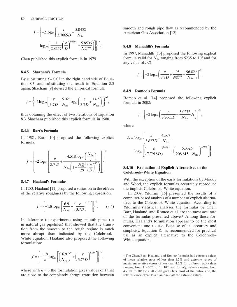
80 SURFACE FRICTION
smooth and rough pipe fl ow as recommended by the American Gas Association [12] .
8.4.8 Manadilli ’ s Formula
In 1997, Manadilli [13] proposed the following explicit formula valid for NRe ranging from 5235 to 10 8 and for any value of ε/D :
fD N N
= − + −
−
23 7
95 96 8210 0 983
2
log.
..
.
εRe Re
8.4.9 Romeo ’ s Formula
Romeo et al. [14] proposed the following explicit formula in 2002:
fD N
= − −
−
23 7065
5 027210
2
log.
.
Re
εA ,
where
A = −
+
log.
.
log.
.
Re
.
10
10
0 9924
3 8274 567
7 79185 33
εD N
Dε 226
208 815
0 9345
..
Re
.
+
N
8.4.10 Evaluation of Explicit Alternatives to the Colebrook – White Equation
With the exception of the early formulations by Moody and Wood, the explicit formulas accurately reproduce the implicit Colebrook – White equation.
In 2009, Yildirim [15] presented the results of a computer - based analysis of a number of explicit alterna-tives to the Colebrook – White equation. According to Yildirim ’ s statistical analyses, the formulas by Chen, Barr, Haaland, and Romeo et al. are the most accurate of the formulas presented above. * Among these for-mulas, Haaland ’ s formulation appears to be the most convenient one to use. Because of its accuracy and simplicity, Equation 8.4 is recommended for practical use as an explicit alternative to the Colebrook – White equation.
fD N
D
= − −
23 7065
5 0452
12 8257
10
10
1 1
log.
.
log.
Re
/
ε
ε 0098
0 8981
25 8506
+
−.
Re.N
.
Chen published this explicit formula in 1979.
8.4.5 Shacham ’ s Formula
By substituting f = 0.03 in the right hand side of Equa-tion 8.3 , and substituting the result in Equation 8.3 again, Shacham [9] devised the empirical formula
fD N D N
= − − +
23 7
5 023 7
14 510 10log
..
log.
.
Re Re
ε ε −−2
,
thus obtaining the effect of two iterations of Equation 8.3 . Shacham published this explicit formula in 1980.
8.4.6 Barr ’ s Formula
In 1981, Barr [10] proposed the following explicit formula:
fD
N
NN
D
= − +
+
23 7
4 5187
129
10
10
0 52 0 7log.
. log Re
ReRe
. .
εε
−2
.
8.4.7 Haaland ’ s Formulas
In 1983, Haaland [11] proposed a variation in the effects of the relative roughness by the following expression:
fN D
= − +
−
1 86 9
3 710
1 11 2
. log.
.Re
.ε. (8.4)
In deference to experiments using smooth pipes (as in natural gas pipelines) that showed that the transi-tion from the smooth to the rough regime is much more abrupt than indicated by the Colebrook – White equation, Haaland also proposed the following formulation:
fn N D
n n
= −
+
1 8 6 93 75
10
1 11.log
..Re
.ε
−2
,
where with n = 3 the formulation gives values of f that are close to the completely abrupt transition between
* The Chen, Barr, Haaland, and Romeo formulas had extreme values of mean relative error of less than 1.2% and extreme values of maximum relative errors of less than 4.7% for different ε / D values ranging from 1 × 10 − 6 to 5 × 10 − 2 and for NRe values ranging from 4 × 10 3 to 10 8 for a 20 × 500 grid. Over most of the entire grid, the relative errors were less than one - half the extreme values.
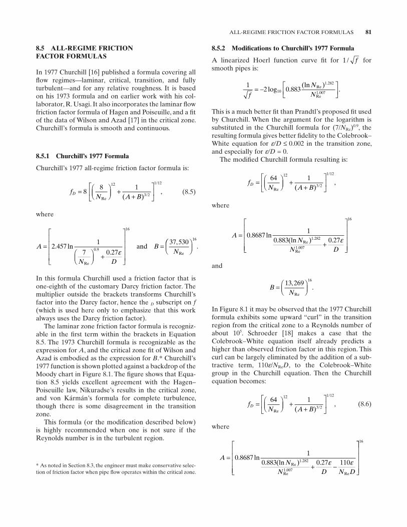
ALL-REGIME FRICTION FACTOR FORMULAS 81
8.5.2 Modifi cations to Churchill ’ s 1977 Formula
A linearized Hoerl function curve fi t for 1 / f for smooth pipes is:
12 0 88310
1 282
1 007f
NN
= −
log .(ln )Re
.
Re.
.
This is a much better fi t than Prandtl ’ s proposed fi t used by Churchill. When the argument for the logarithm is substituted in the Churchill formula for (7/ NRe ) 0.9 , the resulting formula gives better fi delity to the Colebrook – White equation for ε/D ≤ 0.002 in the transition zone, and especially for ε/D = 0.
The modifi ed Churchill formula resulting is:
fN A B
D =
+
+
64 112
3 2
1 12
Re/
/
( ),
where
AN
N D
=+
0 86871
0 883 0 271 282
1 007
16
. ln. (ln ) .Re
.
Re.
ε
and
BN
=
13 269 16,.
Re
In Figure 8.1 it may be observed that the 1977 Churchill formula exhibits some upward “ curl ” in the transition region from the critical zone to a Reynolds number of about 10 5 . Schroeder [18] makes a case that the Colebrook – White equation itself already predicts a higher than observed friction factor in this region. This curl can be largely eliminated by the addition of a sub-tractive term, 110 ε / NReD , to the Colebrook – White group in the Churchill equation. Then the Churchill equation becomes:
fN A B
D =
+
+
64 112
3 2
1 12
Re/
/
( ), (8.6)
where
AN
N D N D
=+ −
0 86871
0 883 0 27 1101 282
1 007
. ln. (ln ) .Re
.
Re.
Re
ε ε
16
8.5 ALL - REGIME FRICTION FACTOR FORMULAS
In 1977 Churchill [16] published a formula covering all fl ow regimes — laminar, critical, transition, and fully turbulent — and for any relative roughness. It is based on his 1973 formula and on earlier work with his col-laborator, R. Usagi. It also incorporates the laminar fl ow friction factor formula of Hagen and Poiseuille, and a fi t of the data of Wilson and Azad [17] in the critical zone. Churchill ’ s formula is smooth and continuous.
8.5.1 Churchill ’ s 1977 Formula
Churchill ’ s 1977 all - regime friction factor formula is:
fN A B
D =
+
+
8
8 112
3 2
1 12
Re/
/
( ),
(8.5)
where
A
N D
BN
=
+
=2 4571
7 0 27
37 5300 9
16
. ln.
,
Re
.Reε
and
16
.
In this formula Churchill used a friction factor that is one - eighth of the customary Darcy friction factor. The multiplier outside the brackets transforms Churchill ’ s factor into the Darcy factor, hence the D subscript on f(which is used here only to emphasize that this work always uses the Darcy friction factor).
The laminar zone friction factor formula is recogniz-able in the fi rst term within the brackets in Equation 8.5 . The 1973 Churchill formula is recognizable as the expression for A , and the critical zone fi t of Wilson and Azad is embodied as the expression for B . * Churchill ’ s 1977 function is shown plotted against a backdrop of the Moody chart in Figure 8.1 . The fi gure shows that Equa-tion 8.5 yields excellent agreement with the Hagen – Poiseuille law, Nikuradse ’ s results in the critical zone, and von K á rm á n ’ s formula for complete turbulence, though there is some disagreement in the transition zone.
This formula (or the modifi cation described below) is highly recommended when one is not sure if the Reynolds number is in the turbulent region.
* As noted in Section 8.3 , the engineer must make conservative selec-tion of friction factor when pipe fl ow operates within the critical zone.
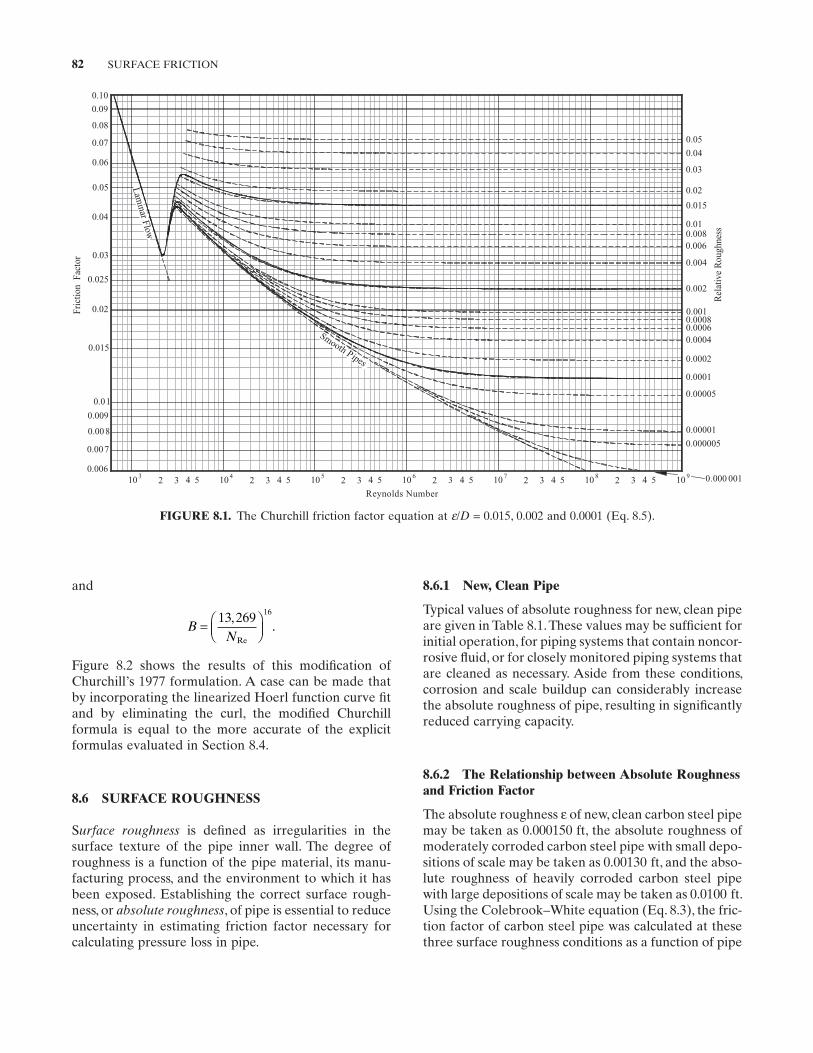
82 SURFACE FRICTION
FIGURE 8.1. The Churchill friction factor equation at ε / D = 0.015, 0.002 and 0.0001 (Eq. 8.5 ).
0.008
0.01
0.015
0.02
0.025
0.03
0.04
0.05
0.06
0.07
0.08
0.09
0.10
Fric
tion
Fac
tor
10 32 3 4 5
rebmuN sdlonyeR
0.05
0.04
0.03
0.02
0.015
0.010.0080.006
0.004
0.002
0.001
0.00060.0008
0.0004
0.0002
0.0001
0.00005
0.00001
Rel
ativ
e R
ough
ness
0.000005
0.000 001
Smooth Pipes
10 4 10 5 10 6 10 7 10 852 3 4 52 3 4 52 3 4 52 3 4 52 3 4 9100.006
0.007
0.009
Lam
inar Flow
and
BN
= ⎛⎝⎜
⎞⎠⎟
13 269 16,.
Re
Figure 8.2 shows the results of this modifi cation of Churchill ’ s 1977 formulation. A case can be made that by incorporating the linearized Hoerl function curve fi t and by eliminating the curl, the modifi ed Churchill formula is equal to the more accurate of the explicit formulas evaluated in Section 8.4 .
8.6 SURFACE ROUGHNESS
S urface roughness is defi ned as irregularities in the surface texture of the pipe inner wall. The degree of roughness is a function of the pipe material, its manu-facturing process, and the environment to which it has been exposed. Establishing the correct surface rough-ness, or absolute roughness , of pipe is essential to reduce uncertainty in estimating friction factor necessary for calculating pressure loss in pipe.
8.6.1 New, Clean Pipe
Typical values of absolute roughness for new, clean pipe are given in Table 8.1 . These values may be suffi cient for initial operation, for piping systems that contain noncor-rosive fl uid, or for closely monitored piping systems that are cleaned as necessary. Aside from these conditions, corrosion and scale buildup can considerably increase the absolute roughness of pipe, resulting in signifi cantly reduced carrying capacity.
8.6.2 The Relationship between Absolute Roughness and Friction Factor
The absolute roughness ε of new, clean carbon steel pipe may be taken as 0.000150 ft, the absolute roughness of moderately corroded carbon steel pipe with small depo-sitions of scale may be taken as 0.00130 ft, and the abso-lute roughness of heavily corroded carbon steel pipe with large depositions of scale may be taken as 0.0100 ft. Using the Colebrook – White equation (Eq. 8.3 ), the fric-tion factor of carbon steel pipe was calculated at these three surface roughness conditions as a function of pipe
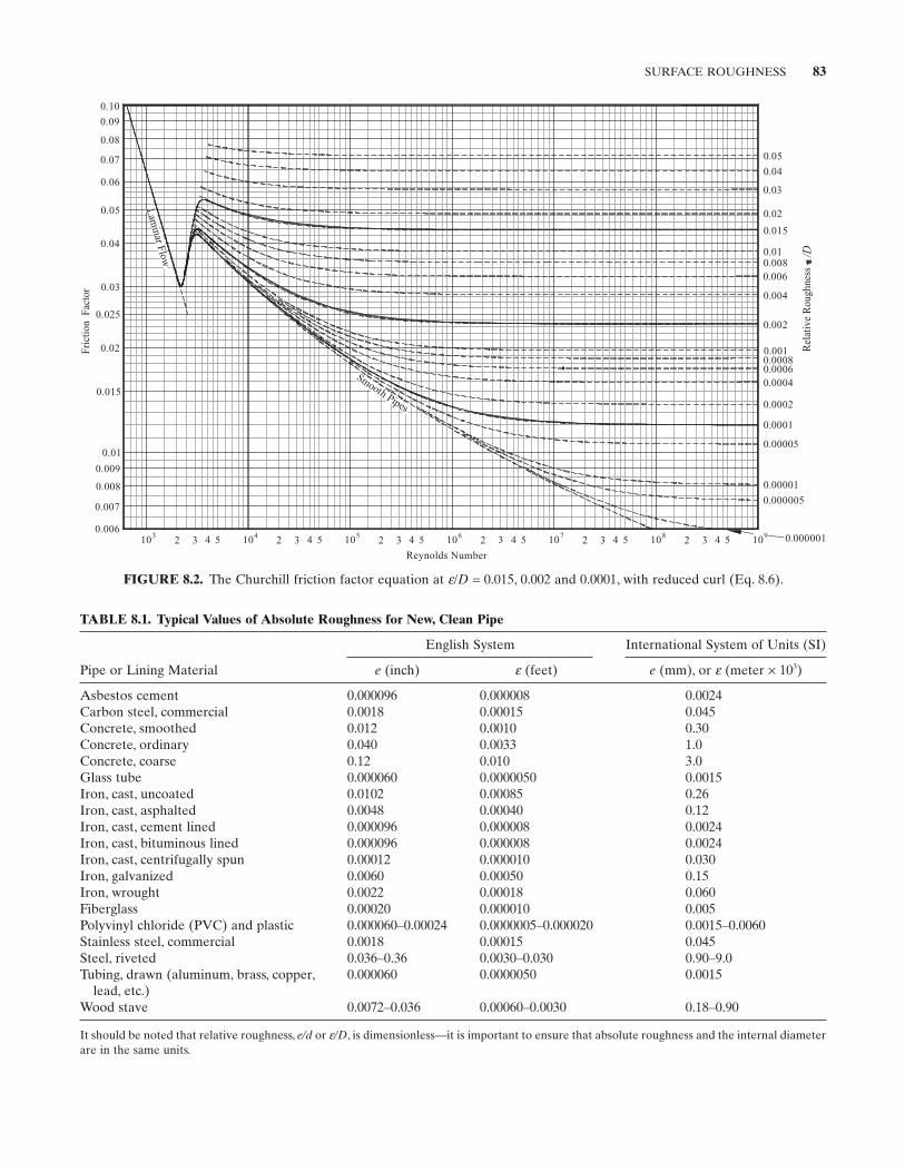
SURFACE ROUGHNESS 83
FIGURE 8.2. The Churchill friction factor equation at ε / D = 0.015, 0.002 and 0.0001, with reduced curl (Eq. 8.6 ).
8000.
100.
5100.
200.
5200.
300.
400.
500.
600.
700.
800.
900.
010.
Fric
tion
Fac
tor
01 3 2 3 4 5
rebmuNsdlonyeR
500.
400.
300.
200.
5100.
100.8000.6000.
4000.
2000.
1000.
60000.80000.
40000.
20000.
10000.
500000.
100000.
Rel
ativ
e R
ough
ness
5000000.
1000000.
Smooth Pipes
01 4 01 5 01 6 01 7 01 852 3 4 52 3 4 52 3 4 52 3 4 52 3 4 9016000.
7000.
9000.
Lam
inar Flow /D
TABLE 8.1. Typical Values of Absolute Roughness for New, Clean Pipe
Pipe or Lining Material
English System International System of Units (SI)
e (inch) ε (feet) e (mm), or ε (meter × 10 3 )
Asbestos cement 0.000096 0.000008 0.0024 Carbon steel, commercial 0.0018 0.00015 0.045 Concrete, smoothed 0.012 0.0010 0.30 Concrete, ordinary 0.040 0.0033 1.0 Concrete, coarse 0.12 0.010 3.0 Glass tube 0.000060 0.0000050 0.0015 Iron, cast, uncoated 0.0102 0.00085 0.26 Iron, cast, asphalted 0.0048 0.00040 0.12 Iron, cast, cement lined 0.000096 0.000008 0.0024 Iron, cast, bituminous lined 0.000096 0.000008 0.0024 Iron, cast, centrifugally spun 0.00012 0.000010 0.030 Iron, galvanized 0.0060 0.00050 0.15 Iron, wrought 0.0022 0.00018 0.060 Fiberglass 0.00020 0.000010 0.005 Polyvinyl chloride (PVC) and plastic 0.000060 – 0.00024 0.0000005 – 0.000020 0.0015 – 0.0060 Stainless steel, commercial 0.0018 0.00015 0.045 Steel, riveted 0.036 – 0.36 0.0030 – 0.030 0.90 – 9.0 Tubing, drawn (aluminum, brass, copper,
lead, etc.) 0.000060 0.0000050 0.0015
Wood stave 0.0072 – 0.036 0.00060 – 0.0030 0.18 – 0.90
It should be noted that relative roughness, e/d or ε /D , is dimensionless — it is important to ensure that absolute roughness and the internal diameter are in the same units.
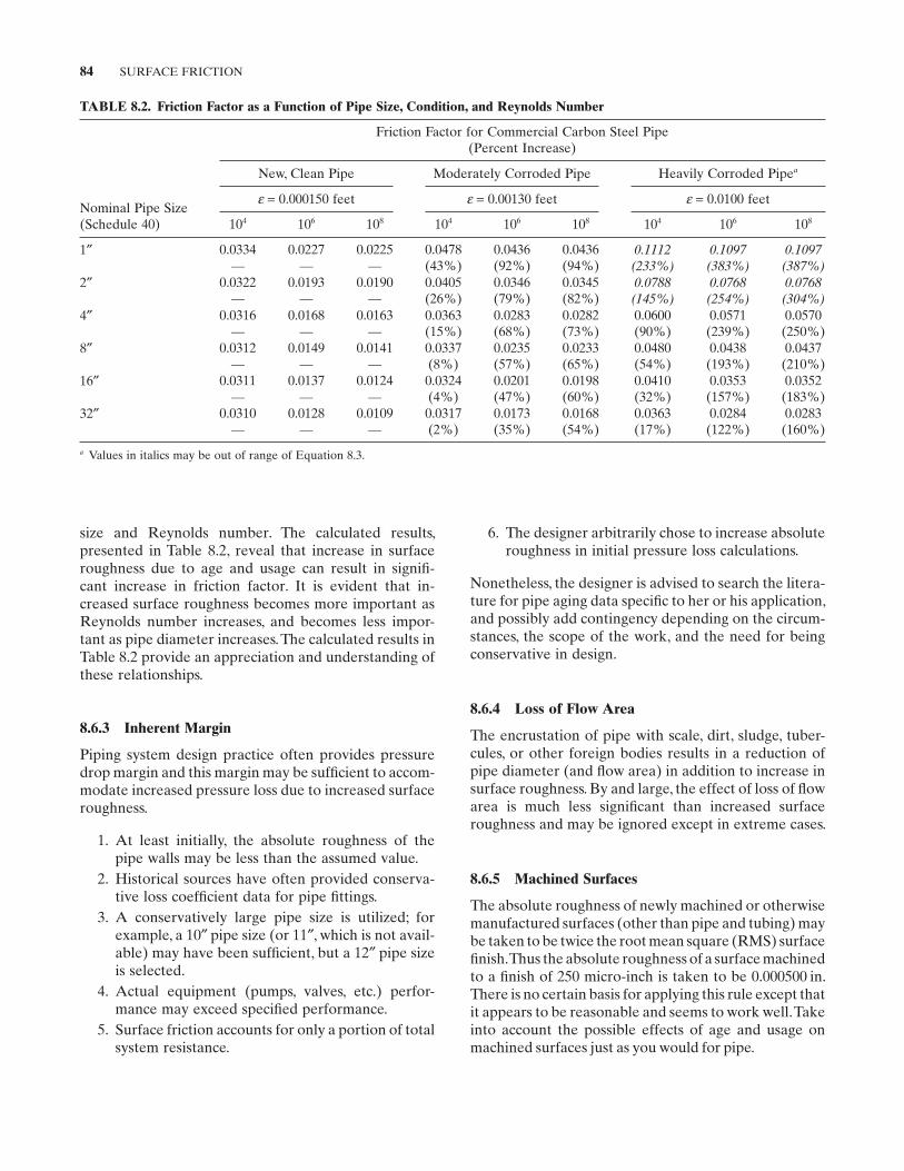
84 SURFACE FRICTION
TABLE 8.2. Friction Factor as a Function of Pipe Size, Condition, and Reynolds Number
Nominal Pipe Size (Schedule 40)
Friction Factor for Commercial Carbon Steel Pipe (Percent Increase)
New, Clean Pipe Moderately Corroded Pipe Heavily Corroded Pipe a
ε = 0.000150 feet ε = 0.00130 feet ε = 0.0100 feet
10 4 10 6 10 8 10 4 10 6 10 8 10 4 10 6 10 8
1 ″ 0.0334 —
0.0227 —
0.0225 —
0.0478 (43%)
0.0436 (92%)
0.0436 (94%)
0.1112(233%)
0.1097(383%)
0.1097(387%)
2 ″ 0.0322 —
0.0193 —
0.0190 —
0.0405 (26%)
0.0346 (79%)
0.0345 (82%)
0.0788(145%)
0.0768(254%)
0.0768(304%)
4 ″ 0.0316 —
0.0168 —
0.0163 —
0.0363 (15%)
0.0283 (68%)
0.0282 (73%)
0.0600 (90%)
0.0571 (239%)
0.0570 (250%)
8 ″ 0.0312 —
0.0149 —
0.0141 —
0.0337 (8%)
0.0235 (57%)
0.0233 (65%)
0.0480 (54%)
0.0438 (193%)
0.0437 (210%)
16 ″ 0.0311 —
0.0137 —
0.0124 —
0.0324 (4%)
0.0201 (47%)
0.0198 (60%)
0.0410 (32%)
0.0353 (157%)
0.0352 (183%)
32 ″ 0.0310 —
0.0128 —
0.0109 —
0.0317 (2%)
0.0173 (35%)
0.0168 (54%)
0.0363 (17%)
0.0284 (122%)
0.0283 (160%)
a Values in italics may be out of range of Equation 8.3 .
size and Reynolds number. The calculated results, presented in Table 8.2 , reveal that increase in surface roughness due to age and usage can result in signifi -cant increase in friction factor. It is evident that in -creased surface roughness becomes more important as Reynolds number increases, and becomes less impor-tant as pipe diameter increases. The calculated results in Table 8.2 provide an appreciation and understanding of these relationships.
8.6.3 Inherent Margin
Piping system design practice often provides pressure drop margin and this margin may be suffi cient to accom-modate increased pressure loss due to increased surface roughness.
1. At least initially, the absolute roughness of the pipe walls may be less than the assumed value.
2. Historical sources have often provided conserva-tive loss coeffi cient data for pipe fi ttings.
3. A conservatively large pipe size is utilized; for example, a 10 ″ pipe size (or 11 ″ , which is not avail-able) may have been suffi cient, but a 12 ″ pipe size is selected.
4. Actual equipment (pumps, valves, etc.) perfor-mance may exceed specifi ed performance.
5. Surface friction accounts for only a portion of total system resistance.
6. The designer arbitrarily chose to increase absolute roughness in initial pressure loss calculations.
Nonetheless, the designer is advised to search the litera-ture for pipe aging data specifi c to her or his application, and possibly add contingency depending on the circum-stances, the scope of the work, and the need for being conservative in design.
8.6.4 Loss of Flow Area
The encrustation of pipe with scale, dirt, sludge, tuber-cules, or other foreign bodies results in a reduction of pipe diameter (and fl ow area) in addition to increase in surface roughness. By and large, the effect of loss of fl ow area is much less signifi cant than increased surface roughness and may be ignored except in extreme cases.
8.6.5 Machined Surfaces
The absolute roughness of newly machined or otherwise manufactured surfaces (other than pipe and tubing) may be taken to be twice the root mean square ( RMS ) surface fi nish. Thus the absolute roughness of a surface machined to a fi nish of 250 micro - inch is taken to be 0.000500 in. There is no certain basis for applying this rule except that it appears to be reasonable and seems to work well. Take into account the possible effects of age and usage on machined surfaces just as you would for pipe.
NONCIRCULAR PASSAGES 85
8.7 NONCIRCULAR PASSAGES
The foregoing friction factor equations for circular pipes may be adapted to noncircular passages through the use of the hydraulic diameter . The hydraulic diam-eter, dh , is an arbitrary defi nition of a value calculated so that the ratio of pressure forces acting over the fl ow area to the frictional forces acting along the wetted perimeter* is the same for circular and noncircular pas-sages. It turns out that a multiplier of 4 is necessary to satisfy this defi nition. For example, applying the defi ni-tion to a circular passage produces:
d
d
ddh = =
44
2π
π,
as should be the case. The calculated hydraulic diameter of several noncircular fl ow passages follow.
For a square passage of width w ,
dww
wh = =44
2
.
† Additional correction factors are required to accurately calculate friction factor for fl ow through an annulus. These correction factors, available in the literature, differentiate between concentric and eccentric alignment of the annulus, and between laminar versus turbulent fl ow.
* The wetted perimeter is the perimeter of the fl ow passage in contact with the fl uid. The hydraulic diameter concept is particularly impor-tant in open channel fl ow calculations.
For a rectangular passage of width w and length l ,
dwl
w lwl
w lh =
+( )=
+4
22
.
For a slit of width w and (infi nite) length l ,
dwll
wh ≈ =42
2 .
For an annulus of outer diameter do and inner diameter di , †
dd d
d dd dh =
−( )+( )
= −4
42 2π
π
o i
o io i.
The hydraulic diameter dh is substituted for d in Equa-tion 1.3 (loss coeffi cient due to surface friction), as well as in the various friction factor equations and the “ Moody Chart. ” The hydraulic diameter is also used when com-puting Reynolds number for noncircular fl ow passages.
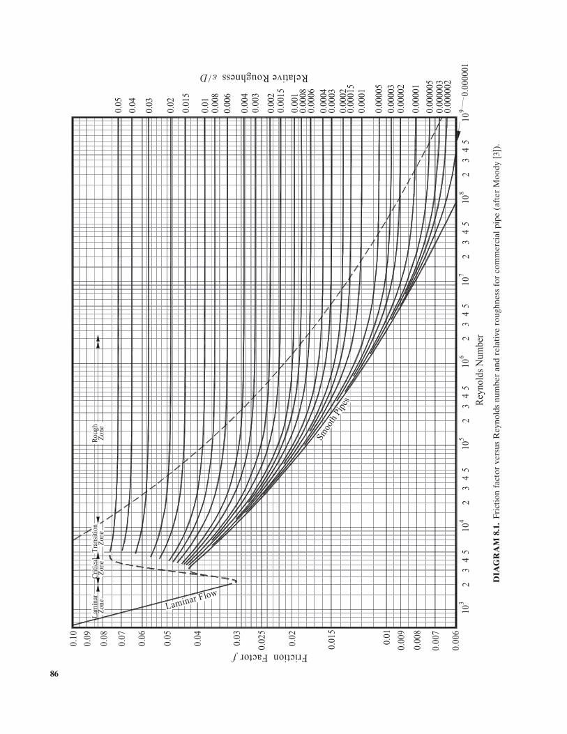
DIA
GR
AM
8.1
. Fr
icti
on f
acto
r ve
rsus
Rey
nold
s nu
mbe
r an
d re
lati
ve r
ough
ness
for
com
mer
cial
pip
e (a
fter
Moo
dy [
3]).
0.0
08
0.0
1
0.0
15
0.0
2
0.0
25
0.0
3
0.0
4
0.0
5
0.0
6
0.0
7
0.0
8
0.0
9
0.1
0FrictionFactor
10
32
34
5
Rey
no
lds
Nu
mb
er
0.0
5
0.0
4
0.0
3
0.0
2
0.0
15
0.0
10.0
08
0.0
06
0.0
04
0.0
02
0.0
01
0.0
006
0.0
008
0.0
004
0.0
002
0.0
001
0.0
0005
0.0
0001
RelativeRoughness/
0.0
00005
Smoo
th P
ipes
10
410
510
610
710
85
23
45
23
45
23
45
23
45
23
49
10
0.0
06
0.0
07
0.0
09
0.0
003
0.0
0015
0.0
0002
0.0
0003
0.0
00003
0.0
00002
0.0
00001
0.0
015
0.0
03
Laminar Flow
f
Lam
inar
Zo
ne
Cri
tica
lZ
on
eT
ransi
tion
Zo
ne
Ro
ug
hZ
on
e
D
86
FURTHER READING 87
REFERENCES
1. Colebrook , C. F. and C. M. White , Experiments with fl uid friction in roughened pipes , Proceedings of the Royal Society of London , 161 , 1937 , 367 – 381 .
2. Colebrook , C. F. , Turbulent fl ow in pipes, with particular reference to the transition region between the smooth and rough pipe laws , Journal of the Institution of Civil Engi-neers , 11 , 1938 – 1939 , 133 – 156 .
3. Moody , L. F. , Friction factors for pipe fl ow , Transactions of the American Society of Mechanical Engineers , 66 , 1944 , 671 – 684 .
4. Moody , L. F. , An approximate formula for pipe friction factors , Transactions of the American Society of Mechani-cal Engineers , 69 , 1947 , 1005 – 1006 .
5. Wood , D. J. , An explicit friction factor relationship , CivilEngineering- ASCE , 36 ( 12 ), 1966 , 60 – 61 .
6. Churchill , S. W. , Empirical expressions for the shear stress in turbulent fl ow in commercial pipe , American Institute of Chemical Engineering Journal , 19 ( 2 ), 1973 , 375 – 376 .
7. Swamee , P. K. and A. K. Jain , Explicit equations for pipe - fl ow problems , Journal of the Hydraulics Division, Ameri-can Society of Civil Engineers , 102 ( HY5 ), 1976 , 657 – 664 .
8. Chen , N. H. , An explicit equation for friction factor , Amer-ican Institute of Chemical Engineering Journal , 19 ( 2 ), 1980 , 229 – 230 .
9. Shacham , M. , An explicit equation for friction factor in pipe , Industrial & Engineering Chemistry Fundamentals , 19 ( 2 ), 1980 , 228 – 229 .
10. Barr , D. I. H. , Solutions to the Colebrook - White functions for resistance to uniform turbulent fl ow , Proceeding of the Institute of Civil Engineers , Part 2, 71 , 1981 , 529 .
11. Haaland , S. E. , Simple and explicit formulas for the friction factor in turbulent pipe fl ow , Transactions of the ASME, Journal of Fluids Engineering , 105 , 1983 , 89 – 90 .
12. Uhl , A. E. et al., Steady Flow in Gas Pipelines , Institute of Gas Technology Report No. 10, American Gas Association , New York, 1956 .
13. Manadilli , G. , Replace implicit equations with sigmoidal functions , Chemical Engineering , 104 ( 8 ), 1997 , 187 .
14. Romeo , E. , C. Royo , and A. Monzon , Improved explicit equations for estimation of friction factor in rough and smooth pipes , Chemical Engineering , 86 , 2002 , 369 – 374 .
15. Yildirim , G. , Computer - based analysis of explicit approxi-mations to the implicit Colebrook - White equation in tur-bulent fl ow friction factor calculation , Advances in Engineering Software , 40 , 2009 , 1183 – 1190 .
16. Churchill , S. W. , Friction - factor equation spans all fl uid - fl ow regimes , Chemical Engineering , 84 , 1977 , 91 – 92 .
17. Wilson , N. W. and R. S. Azad , A continuous prediction method for fully developed laminar, transitional and tur-bulent fl ows in pipes , Journal of Applied Mechanics , 42 , 1975 , 51 – 54 .
18. Schroeder , D. W. , A Tutorial on Pipe Flow Equations , Stoner Associates, Inc., Carlisle, Pennsylvania, August 16, 2001 .
FURTHER READING
This list includes books and papers that may be helpful to those who wish to pursue further study.
Kemler , E. , A study of the data on the fl ow of fl uids in pipes , Transactions of ASME , 55 , 1933 , 7 – 32 .
Colebrook , C. F. and C. M. White , The reduction of carrying capacity of pipes with age , Journal of the Institution of Civil Engineers , 10 , 1937 – 1938 , 99 – 118 .
Freeman , J. R. , Experiments on the Flow of Water in Pipes and Pipe Fittings, 1889 to 1893 . (Published by the ASME in a special volume in 1941 .).
Tao , L. N. and W. F. Donovan , Through - fl ow in concentric and eccentric annuli of fi ne clearance with and without relative motion of the boundaries , Transactions of the ASME , 77 , 1955 , 1291 – 1301 .
Rouse , H. and S. Ince , History of Hydraulics , Iowa Institute of Hydraulic Research, State University of Iowa , Iowa City, IA , 1957 .
Lohrenz , J. and F. Kurata , A friction factor plot … for smooth circular conduits, concentric annuli, and parallel plates , Industrial & Engineering Chemistry , 52 ( 8 ), 1960 , 703 – 706 .
U.S. Bureau of Reclamation , Friction Factors for Large Conduit Flowing Full , Engineering Monograph, No. 7, U.S. Department of the Interior, Washington, D.C., 1965 .
Selander , W. N. , Explicit Formulas for the Computation of Fric-tion Factors in Turbulent Pipe Flow , Atomic Energy of Canada Limited , Chalk River, Ontario, Canada , 1978 (AECL - 6354).
Guislain , S. J. , How to Make Sense of Friction Factors in Fluid Flow Through Pipe , Plant Engineering , June 12, 1980 , pp. 134 – 140 .
Lamont , P. A. , Pipe fl ow formulas compared with the theory of roughness , American Water Works Association Journal , 73 ( 5 ), 1981 .
Oluji ć , Ž . , Compute Friction Factors Fast for Flow in Pipes , Chemical Engineering , December 14, 1981 , pp. 91 – 93 .
Obot , N. T. , Determination of incompressible fl ow friction factor in smooth circular and noncircular passages: A gen-eralized approach including validation of the nearly century old hydraulic diameter concept , Transactions of the ASME, Journal of Fluids Engineering , 110 , 1988 , 431 – 440 .
Scaggs , W. F. , R. P. Taylor , and H. W. Coleman , Measurement and prediction of rough wall effects on friction factor — Uniform roughness results , Transactions of the ASME, Journal of Fluids Engineering , 110 , 1988 , 385 – 391 .
Taylor , R. P. , W. F. Scaggs , and H. W. Coleman , Measurement and prediction of the effects of nonuniform surface rough-ness on turbulent fl ow friction coeffi cients , Transactions of the ASME, Journal of Fluids Engineering , 110 , 1988 , 380 – 383 .
Farshad , F. F. and H. H. Rieke , Surface - roughness design values for modern pipes , Society of Petroleum Engineers, Drilling & Completion , SPE 89040 , 2006 , 212 – 215 .
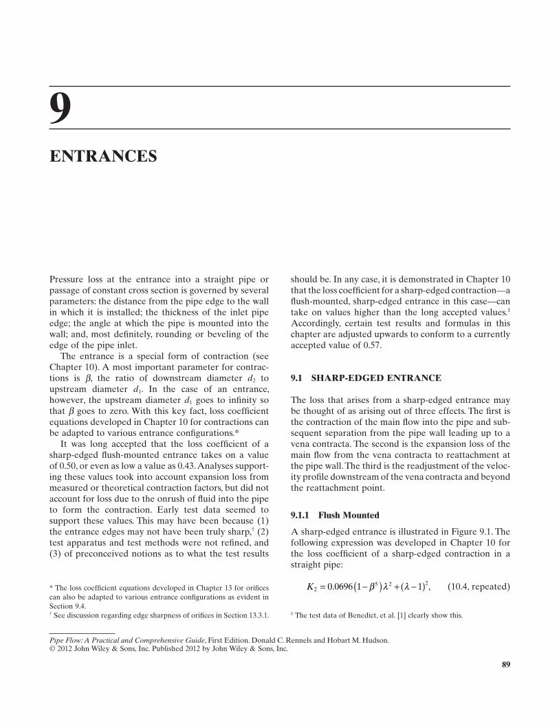
89
9 ENTRANCES
Pressure loss at the entrance into a straight pipe or passage of constant cross section is governed by several parameters: the distance from the pipe edge to the wall in which it is installed; the thickness of the inlet pipe edge; the angle at which the pipe is mounted into the wall; and, most defi nitely, rounding or beveling of the edge of the pipe inlet.
The entrance is a special form of contraction (see Chapter 10 ). A most important parameter for contrac-tions is β , the ratio of downstream diameter d 2 to upstream diameter d 1 . In the case of an entrance, however, the upstream diameter d 1 goes to infi nity so that β goes to zero. With this key fact, loss coeffi cient equations developed in Chapter 10 for contractions can be adapted to various entrance confi gurations. *
It was long accepted that the loss coeffi cient of a sharp - edged fl ush - mounted entrance takes on a value of 0.50, or even as low a value as 0.43. Analyses support-ing these values took into account expansion loss from measured or theoretical contraction factors, but did not account for loss due to the onrush of fl uid into the pipe to form the contraction. Early test data seemed to support these values. This may have been because (1) the entrance edges may not have been truly sharp, † (2) test apparatus and test methods were not refi ned, and (3) of preconceived notions as to what the test results
should be. In any case, it is demonstrated in Chapter 10 that the loss coeffi cient for a sharp - edged contraction — a fl ush - mounted, sharp - edged entrance in this case — can take on values higher than the long accepted values. ‡ Accordingly, certain test results and formulas in this chapter are adjusted upwards to conform to a currently accepted value of 0.57.
9.1 SHARP - EDGED ENTRANCE
The loss that arises from a sharp - edged entrance may be thought of as arising out of three effects. The fi rst is the contraction of the main fl ow into the pipe and sub-sequent separation from the pipe wall leading up to a vena contracta. The second is the expansion loss of the main fl ow from the vena contracta to reattachment at the pipe wall. The third is the readjustment of the veloc-ity profi le downstream of the vena contracta and beyond the reattachment point.
9.1.1 Flush Mounted
A sharp - edged entrance is illustrated in Figure 9.1 . The following expression was developed in Chapter 10 for the loss coeffi cient of a sharp - edged contraction in a straight pipe:
K25 2 20 0696 1 1= −( ) + −( ). ,β λ λ (10.4, repeated)
Pipe Flow: A Practical and Comprehensive Guide, First Edition. Donald C. Rennels and Hobart M. Hudson.© 2012 John Wiley & Sons, Inc. Published 2012 by John Wiley & Sons, Inc.
‡ The test data of Benedict, et al. [1] clearly show this. † See discussion regarding edge sharpness of orifi ces in Section 13.3.1.
* The loss coeffi cient equations developed in Chapter 13 for orifi ces can also be adapted to various entrance confi gurations as evident in Section 9.4 .
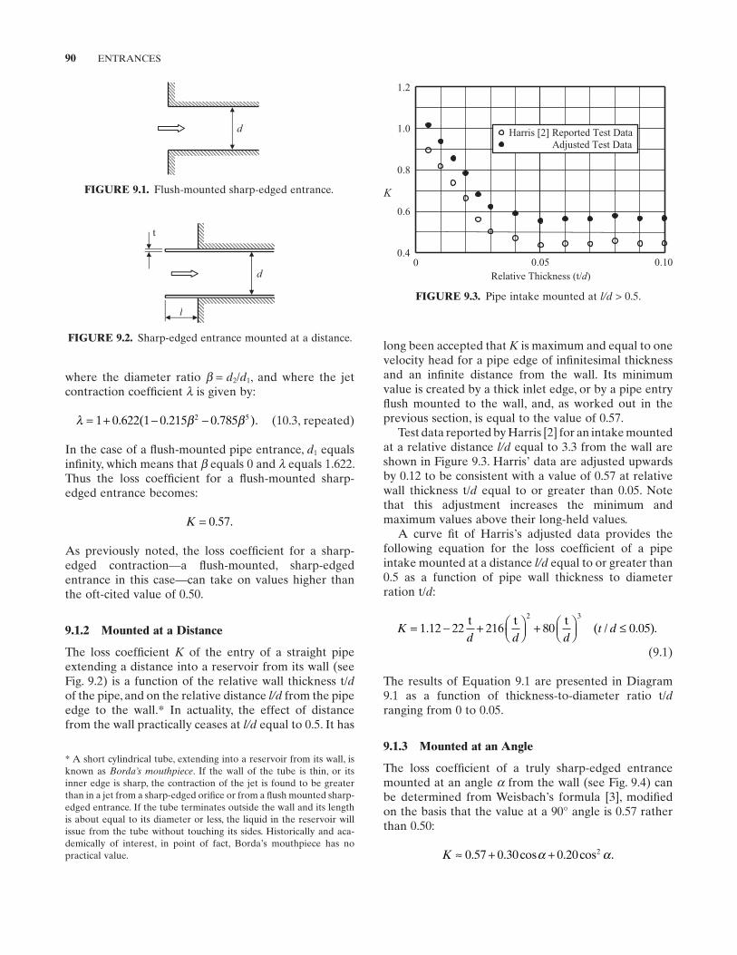
90 ENTRANCES
long been accepted that K is maximum and equal to one velocity head for a pipe edge of infi nitesimal thickness and an infi nite distance from the wall. Its minimum value is created by a thick inlet edge, or by a pipe entry fl ush mounted to the wall, and, as worked out in the previous section, is equal to the value of 0.57.
Test data reported by Harris [2] for an intake mounted at a relative distance l/d equal to 3.3 from the wall are shown in Figure 9.3 . Harris ’ data are adjusted upwards by 0.12 to be consistent with a value of 0.57 at relative wall thickness t/ d equal to or greater than 0.05. Note that this adjustment increases the minimum and maximum values above their long - held values.
A curve fi t of Harris ’ s adjusted data provides the following equation for the loss coeffi cient of a pipe intake mounted at a distance l/d equal to or greater than 0.5 as a function of pipe wall thickness to diameter ration t/ d :
K
d d dt d= − + ⎛
⎝⎜⎞⎠⎟ + ⎛
⎝⎜⎞⎠⎟ ≤1 12 22 216 80 0 05
2 3
. ( / . )t t t
.
(9.1)
The results of Equation 9.1 are presented in Diagram 9.1 as a function of thickness - to - diameter ratio t/ d ranging from 0 to 0.05.
9.1.3 Mounted at an Angle
The loss coeffi cient of a truly sharp - edged entrance mounted at an angle α from the wall (see Fig. 9.4 ) can be determined from Weisbach ’ s formula [3] , modifi ed on the basis that the value at a 90 ° angle is 0.57 rather than 0.50:
K ≈ + +0 57 0 30 0 20 2. . cos . cos .α α
FIGURE 9.1. Flush - mounted sharp - edged entrance.
d
FIGURE 9.2. Sharp - edged entrance mounted at a distance.
d
l
t
FIGURE 9.3. Pipe intake mounted at l/d > 0.5.
0.4
Relative Thickness (t/d)
1.0
0.8
K
0.6
0.100.050
Harris [2] Reported Test DataAdjusted Test Data
1.2
* A short cylindrical tube, extending into a reservoir from its wall, is known as Borda ’ s mouthpiece . If the wall of the tube is thin, or its inner edge is sharp, the contraction of the jet is found to be greater than in a jet from a sharp - edged orifi ce or from a fl ush mounted sharp - edged entrance. If the tube terminates outside the wall and its length is about equal to its diameter or less, the liquid in the reservoir will issue from the tube without touching its sides. Historically and aca-demically of interest, in point of fact, Borda ’ s mouthpiece has no practical value.
where the diameter ratio β = d 2 / d 1 , and where the jet contraction coeffi cient λ is given by:
λ β β= + − −1 0 622 1 0 215 0 7852 5. ( . . ). (10.3, repeated)
In the case of a fl ush - mounted pipe entrance, d 1 equals infi nity, which means that β equals 0 and λ equals 1.622. Thus the loss coeffi cient for a fl ush - mounted sharp - edged entrance becomes:
K = 0 57. .
As previously noted, the loss coeffi cient for a sharp - edged contraction — a fl ush - mounted, sharp - edged entrance in this case — can take on values higher than the oft - cited value of 0.50.
9.1.2 Mounted at a Distance
The loss coeffi cient K of the entry of a straight pipe extending a distance into a reservoir from its wall (see Fig. 9.2 ) is a function of the relative wall thickness t/ d of the pipe, and on the relative distance l/d from the pipe edge to the wall. * In actuality, the effect of distance from the wall practically ceases at l/d equal to 0.5. It has
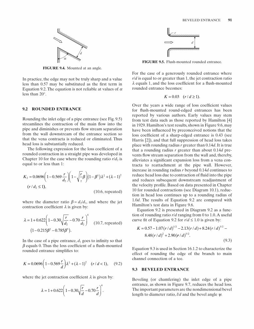
BEVELED ENTRANCE 91
FIGURE 9.4. Mounted at an angle.
d
a
In practice, the edge may not be truly sharp and a value less than 0.57 may be substituted as the fi rst term in Equation 9.2 . The equation is not reliable at values of α less than 20 ° .
9.2 ROUNDED ENTRANCE
Rounding the inlet edge of a pipe entrance (see Fig. 9.5 ) streamlines the contraction of the main fl ow into the pipe and diminishes or prevents fl ow stream separation from the wall downstream of the entrance section so that the vena contracta is reduced or eliminated. Thus head loss is substantially reduced.
The following expression for the loss coeffi cient of a rounded contraction in a straight pipe was developed in Chapter 10 for the case where the rounding ratio r / d 2 is equal to or less than 1:
Kr
dr
r d
22 2
5 2 2
2
0 0696 1 0 569 1 1 1
1
= −⎛⎝⎜
⎞⎠⎟ −
⎛⎝⎜
⎞⎠⎟
−( ) + −( )
≤
. .
( /
β β λ λ
)), (10.6, repeated)
where the diameter ratio β = d 2 / d 1 , and where the jet contraction coeffi cient λ is given by:
λ = + − −⎛⎝⎜
⎞⎠⎟
− −( )
1 0 622 1 0 30 0 70
1 0 215 0 785
2 2
4
2 5
. . .
. . .
rd
rd
β β
(10.7, repeated)
In the case of a pipe entrance, d 1 goes to infi nity so that β equals 0. Thus the loss coeffi cient of a fl ush - mounted rounded entrance simplifi es to:
Krd
r d= −⎛⎝⎜
⎞⎠⎟ + −( ) <0 0696 1 0 569 1 12 2. . ( / ),λ λ (9.2)
where the jet contraction coeffi cient λ is given by:
λ = + − −⎛⎝⎜
⎞⎠⎟
1 0 622 1 0 30 0 704
. . . .rd
rd
FIGURE 9.5. Flush - mounted rounded entrance.
d
r
For the case of a generously rounded entrance where r / d is equal to or greater than 1, the jet contraction ratio λ equals 1, and the loss coeffi cient for a fl ush - mounted rounded entrance becomes:
K r d= ≥0 03 1. ( / ).
Over the years a wide range of loss coeffi cient values for fl ush - mounted round - edged entrances has been reported by various authors. Early values may stem from test data such as those reported by Hamilton [4] in 1929. Hamilton ’ s test results, shown in Figure 9.6 , may have been infl uenced by preconceived notions that the loss coeffi cient of a sharp - edged entrance is 0.43 (see Harris [2] ), and that full suppression of head loss takes place with rounding radius r greater than 0.14 d . It is true that a rounding radius r greater than about 0.14 d pre-vents fl ow stream separation from the wall and, thereby, alleviates a signifi cant expansion loss from a vena con-tracta to reattachment at the pipe wall. However, increase in rounding radius r beyond 0.14 d continues to reduce head loss due to contraction of fl uid into the pipe and reduces subsequent downstream readjustment of the velocity profi le. Based on data presented in Chapter 10 for rounded contractions (see Diagram 10.1 ), reduc-tion in head loss continues up to a rounding radius of 1.0 d . The results of Equation 9.2 are compared with Hamilton ’ s test data in Figure 9.6 .
Equation 9.2 is presented in Diagram 9.2 as a func-tion of rounding ratio r / d ranging from 0 to 1.0. A useful curve fi t of Equation 9.2 for r / d ≤ 1.0 is given by:
K r d r d r d
r d
= − ( ) − ( ) + ( ) −
( ) +
0 57 1 07 2 13 8 24
8 48 2 90
1 2 3 2
2
. . / . / . /
. / .
/ /
rr d/ /( )5 2. (9.3)
Equation 9.3 is used in Section 16.1.2 to characterize the effect of rounding the edge of the branch to main channel connection of a tee.
9.3 BEVELED ENTRANCE
Beveling (or chamfering) the inlet edge of a pipe entrance, as shown in Figure 9.7 , reduces the head loss. The important parameters are the nondimensional bevel length to diameter ratio, l / d and the bevel angle ψ .
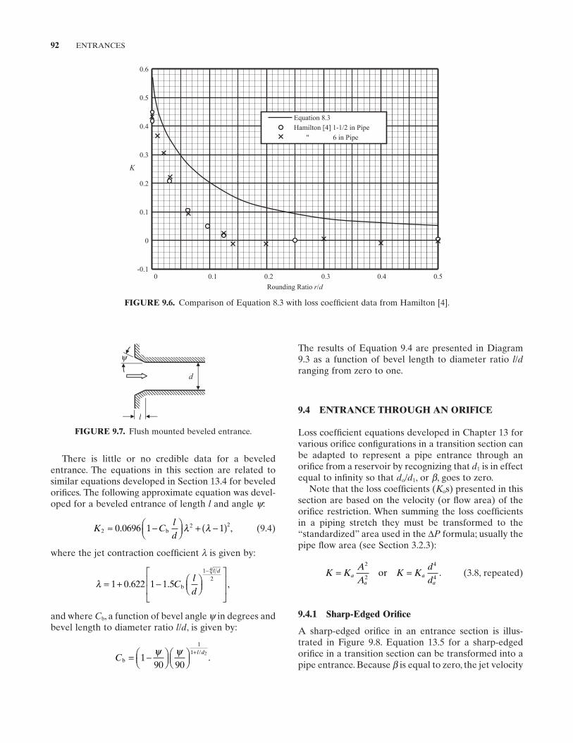
92 ENTRANCES
The results of Equation 9.4 are presented in Diagram 9.3 as a function of bevel length to diameter ratio l / d ranging from zero to one.
9.4 ENTRANCE THROUGH AN ORIFICE
Loss coeffi cient equations developed in Chapter 13 for various orifi ce confi gurations in a transition section can be adapted to represent a pipe entrance through an orifi ce from a reservoir by recognizing that d 1 is in effect equal to infi nity so that d o / d 1 , or β , goes to zero.
Note that the loss coeffi cients ( K o s) presented in this section are based on the velocity (or fl ow area) of the orifi ce restriction. When summing the loss coeffi cients in a piping stretch they must be transformed to the “ standardized ” area used in the Δ P formula; usually the pipe fl ow area (see Section 3.2.3):
K KAA
K Kdd
aa
aa
= =2
2
4
4or . (3.8, repeated)
9.4.1 Sharp - Edged Orifi ce
A sharp - edged orifi ce in an entrance section is illus-trated in Figure 9.8 . Equation 13.5 for a sharp - edged orifi ce in a transition section can be transformed into a pipe entrance. Because β is equal to zero, the jet velocity
There is little or no credible data for a beveled entrance. The equations in this section are related to similar equations developed in Section 13.4 for beveled orifi ces. The following approximate equation was devel-oped for a beveled entrance of length l and angle ψ :
K Cld
22 20 0696 1 1≈ −⎛
⎝⎜⎞⎠⎟ + −( ). ,b λ λ (9.4)
where the jet contraction coeffi cient λ is given by:
λ = + − ⎛⎝⎜
⎞⎠⎟
⎡
⎣
⎢⎢
⎤
⎦
⎥⎥
−
1 0 622 1 1 5
12
4
. . Cld
l d
b ,
and where C b , a function of bevel angle ψ in degrees and bevel length to diameter ratio l / d , is given by:
Cl d
b .= −⎛⎝⎜
⎞⎠⎟
⎛⎝⎜
⎞⎠⎟
+1
90 90
11 2ψ ψ /
FIGURE 9.6. Comparison of Equation 8.3 with loss coeffi cient data from Hamilton [4] .
0.6
0.5
0.4
0.3
0.2
0.1
0
-0.10 0.1 0.2 0.3 0.4 0.5
K
Rounding Ratio r/d
Equation 8.3 Hamilton [4] 1-1/2 in Pipe '' 6 in Pipe
FIGURE 9.7. Flush mounted beveled entrance.
d
l
y
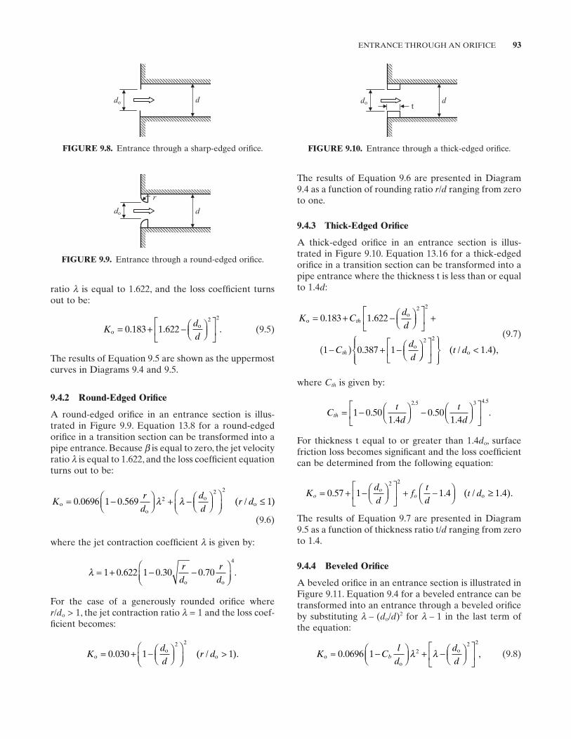
ENTRANCE THROUGH AN ORIFICE 93
The results of Equation 9.6 are presented in Diagram 9.4 as a function of rounding ratio r / d ranging from zero to one.
9.4.3 Thick - Edged Orifi ce
A thick - edged orifi ce in an entrance section is illus-trated in Figure 9.10 . Equation 13.16 for a thick - edged orifi ce in a transition section can be transformed into a pipe entrance where the thickness t is less than or equal to 1.4 d :
K Cdd
Cdd
th
th
oo
o
= + − ⎛⎝⎜
⎞⎠⎟
⎡
⎣⎢
⎤
⎦⎥ +
−( ) + − ⎛⎝⎜
⎞
0 183 1 622
1 0 387 1
2 2
. .
. ⎠⎠⎟⎡
⎣⎢
⎤
⎦⎥
⎧⎨⎪
⎩⎪
⎫⎬⎪
⎭⎪<
2 2
1 4( / . ),t do
(9.7)
where C th is given by:
Ctd
td
th = − ⎛⎝⎜
⎞⎠⎟ − ⎛
⎝⎜⎞⎠⎟
⎡
⎣⎢
⎤
⎦⎥1 0 50
1 40 50
1 4
2 5 3 4 5
..
..
.. .
For thickness t equal to or greater than 1.4 d o , surface friction loss becomes signifi cant and the loss coeffi cient can be determined from the following equation:
Kdd
ftd
t doo
o= + − ⎛⎝⎜
⎞⎠⎟
⎡
⎣⎢
⎤
⎦⎥ + −⎛
⎝⎜⎞⎠⎟ ≥0 57 1 1 4 1 4
2 2
. . ( / . ).o
The results of Equation 9.7 are presented in Diagram 9.5 as a function of thickness ratio t/ d ranging from zero to 1.4.
9.4.4 Beveled Orifi ce
A beveled orifi ce in an entrance section is illustrated in Figure 9.11 . Equation 9.4 for a beveled entrance can be transformed into an entrance through a beveled orifi ce by substituting λ – ( d o / d ) 2 for λ – 1 in the last term of the equation:
K Cl
ddd
boo
o ,≈ −⎛⎝⎜
⎞⎠⎟ + − ⎛
⎝⎜⎞⎠⎟
⎡
⎣⎢
⎤
⎦⎥0 0696 1 2
2 2
. λ λ (9.8)
ratio λ is equal to 1.622, and the loss coeffi cient turns out to be:
Kdd
oo= + − ⎛
⎝⎜⎞⎠⎟
⎡
⎣⎢
⎤
⎦⎥0 183 1 622
2 2
. . . (9.5)
The results of Equation 9.5 are shown as the uppermost curves in Diagrams 9.4 and 9.5 .
9.4.2 Round - Edged Orifi ce
A round - edged orifi ce in an entrance section is illus-trated in Figure 9.9 . Equation 13.8 for a round - edged orifi ce in a transition section can be transformed into a pipe entrance. Because β is equal to zero, the jet velocity ratio λ is equal to 1.622, and the loss coeffi cient equation turns out to be:
K
rd
dd
r doo
oo= −⎛
⎝⎜⎞⎠⎟ + − ⎛
⎝⎜⎞⎠⎟
⎛⎝⎜
⎞⎠⎟
≤0 0696 1 0 569 122 2
. . ( / )λ λ
(9.6)
where the jet contraction coeffi cient λ is given by:
λ = + − −⎛⎝⎜
⎞⎠⎟
1 0 622 1 0 30 0 704
. . . .r
dr
do o
For the case of a generously rounded orifi ce where r / d o > 1, the jet contraction ratio λ = 1 and the loss coef-fi cient becomes:
Kdd
r doo
o= + − ⎛⎝⎜
⎞⎠⎟
⎛⎝⎜
⎞⎠⎟
>0 030 1 12 2
. ( / ).
FIGURE 9.8. Entrance through a sharp - edged orifi ce.
ddo
FIGURE 9.9. Entrance through a round - edged orifi ce.
do d
r
FIGURE 9.10. Entrance through a thick - edged orifi ce.
ddo t
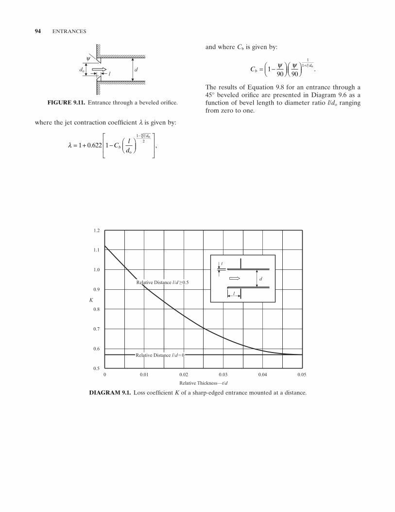
94 ENTRANCES
and where C b is given by:
Cbl d
= −⎛⎝⎜
⎞⎠⎟
⎛⎝⎜
⎞⎠⎟
+1
90 90
11ψ ψ o
.
The results of Equation 9.8 for an entrance through a 45 ° beveled orifi ce are presented in Diagram 9.6 as a function of bevel length to diameter ratio l / d o ranging from zero to one.
where the jet contraction coeffi cient λ is given by:
λ = + − ⎛⎝⎜
⎞⎠⎟
⎡
⎣
⎢⎢
⎤
⎦
⎥⎥
−
1 0 622 1
12
4
. Cl
db
l d
o
o
,
DIAGRAM 9.1. Loss coeffi cient K of a sharp - edged entrance mounted at a distance.
Relative Thickness—t/d
1.1
0.9
0.7
0 0.05
K
0.040.030.01 0.020.5
1.0
0.8
0.6
Relative Distance l/d ≥0.5
1.2
Relative Distance l/d = 0
d
l
t
FIGURE 9.11. Entrance through a beveled orifi ce.
ddo l
y
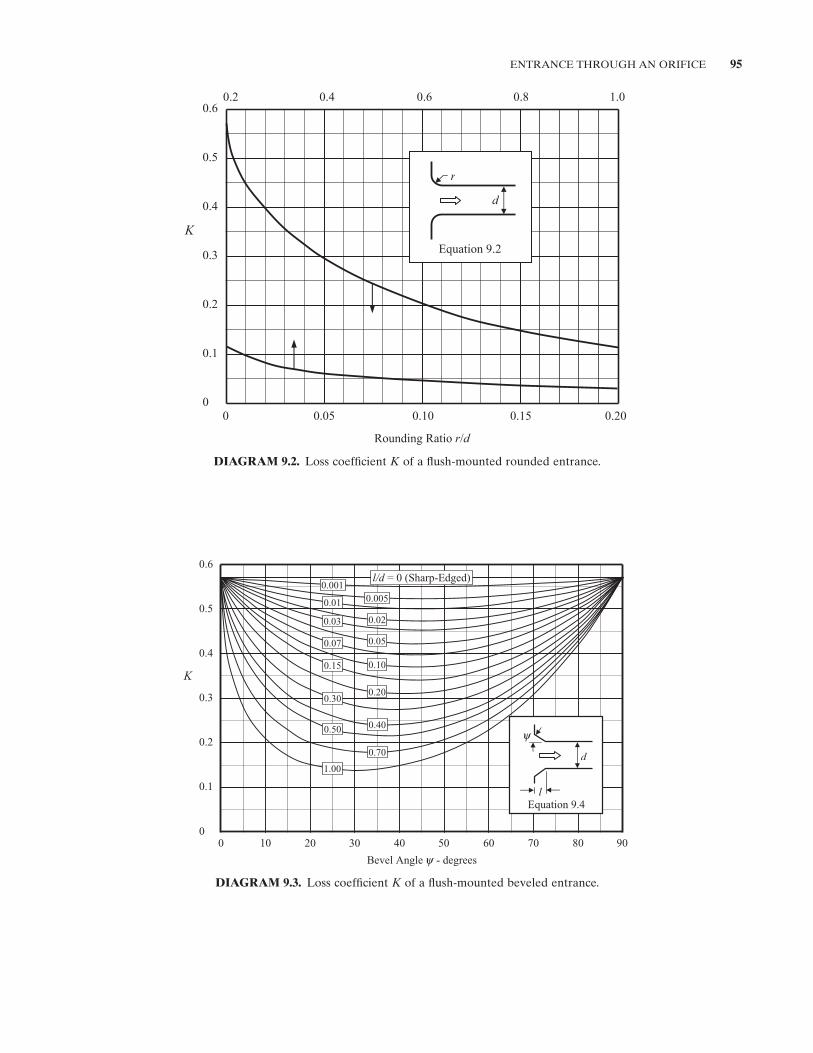
ENTRANCE THROUGH AN ORIFICE 95
DIAGRAM 9.2. Loss coeffi cient K of a fl ush - mounted rounded entrance.
Rounding Ratio r/d
0.6
0.5
0.4
0.3
0.2
0.1
0
0.2 0.4 0.6 0.8 1.0
K
0 0.05 0.10 0.15 0.20
r
d
Equation 9.2
DIAGRAM 9.3. Loss coeffi cient K of a fl ush - mounted beveled entrance.
K
0 20 40 60 80
Bevel Angle - degrees
0.6
0.5
0.4
0.3
0.2
0.1
0 90 70503010
0.001
0.01
0.020.03
0.050.07
0.10
0.20
0.15
0.50
0.70
1.00
l/d = 0 (Sharp-Edged)
0.005
0.40
0.30
d
Equation 9.4 l
y
y
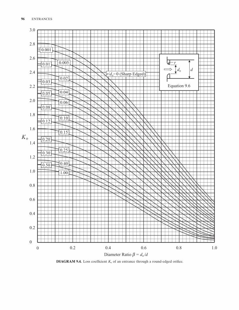
96 ENTRANCES
DIAGRAM 9.4. Loss coeffi cient K o of an entrance through a round - edged orifi ce.
3.0
2.8
2.6
2.4
2.2
2.0
1.8
1.6
1.4
1.2
1.0
0.8
0.6
0.4
0.2
0
0 0.4 0.6 0.8 1.0 0.2
Diameter Ratio = do /d
Ko
r/do=0 (Sharp Edged)
0.005 0.01
0.02 0.03
0.15
0.20
0.04
0.06
0.50
1.00
0.30 0.25
0.08
0.10 0.12
0.05
0.001
0.40
Equation 9.6
r
ddo
b
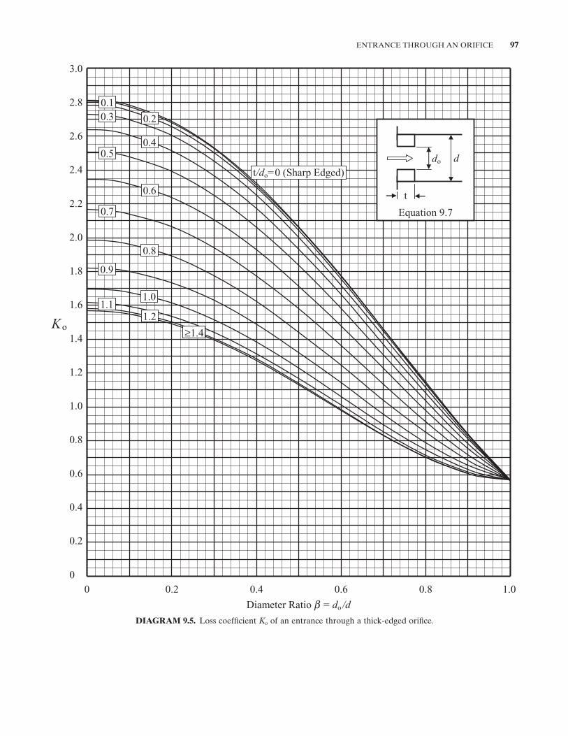
ENTRANCE THROUGH AN ORIFICE 97
DIAGRAM 9.5. Loss coeffi cient K o of an entrance through a thick - edged orifi ce.
3.0
2.8
2.6
2.4
2.2
2.0
1.8
1.6
1.4
1.2
1.0
0.8
0.6
0.4
0.2
0
0 0.4 0.6 0.8 1.0 0.2
Diameter Ratio = do /d
Ko
0.3
0.4 0.5
0.6
0.8
0.9
1.0 1.1
0.7
t/do=0 (Sharp Edged)
0.1
0.2
1.2
≥1.4
Equation 9.7
ddo
t
b
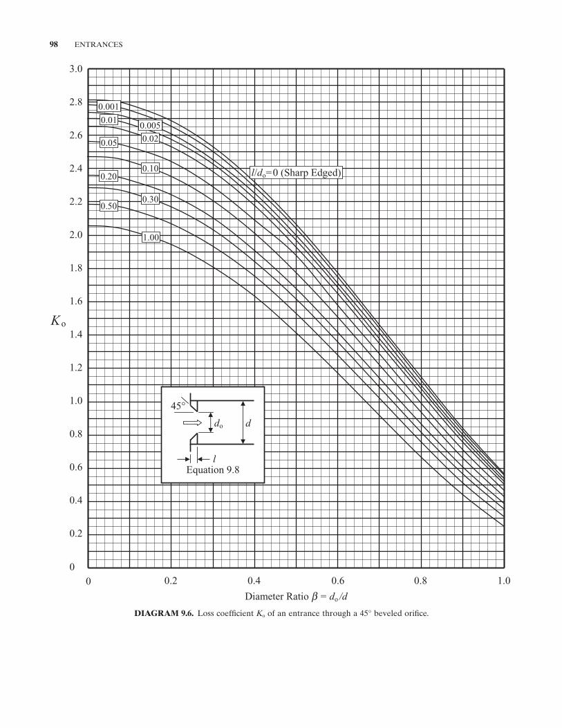
98 ENTRANCES
DIAGRAM 9.6. Loss coeffi cient K o of an entrance through a 45 ° beveled orifi ce.
3.0
2.8
2.6
2.4
2.2
2.0
1.8
1.6
1.4
1.2
1.0
0.8
0.6
0.4
0.2
0
0 0.4 0.6 0.8 1.0 0.2
Diameter Ratio = do /d
Ko
l/do=0 (Sharp Edged)
0.005 0.01
0.02
0.50
1.00
0.10 0.20
0.30
0.05
0.001
Equation 9.8
45°
ddo
l
b
FURTHER READING 99
Ross , D. , Turbulent fl ow in the entrance region of a pipe , Transactions of the American Society of Mechanical Engi-neers , 78 , 1956 , 915 – 923 .
Campbell , W. D. and J. C. Slattery , Flow in the entrance of a tube , Transactions of the American Society of Mechanical Engineers, Journal of Basic Engineering , 88 , 1963 , 41 – 46 .
Barbin , A. R. and J. B. Jones , Turbulent fl ow in the inlet region of a smooth pipe , Transactions of the American Society of Mechanical Engineers, Journal of Basic Engineering , 85 , 1974 , 29 – 34 .
Wang , J. - S. and J. P. Tullis , Turbulent fl ow in the entry region of a rough pipe , Transactions of the American Society of Mechanical Engineers, Journal of Fluids Engineering , 96 , 1974 , 62 – 68 .
Dong , W. and J. H. Lienhard , Contraction coeffi cients for Borda mouthpieces , Transactions of the American Society of Mechanical Engineers, Journal of Fluids Engineering , 108 , 1986 , 377 – 379 .
Bullen , P. R. , D. J. Cheeseman , L. A. Hussain , and A. E. Ruffell , The determination of pipe contraction pressure loss coef-fi cients for incompressible turbulent fl ow , International Journal of Heat and Fluid Flow , 8 ( 2 ), 1987 , 111 .
Bullen , P. R. , D. J. Cheeseman , and L. A. Hussain , The effects of inlet sharpness on the pipe contraction loss coeffi cient , International Journal of Heat and Fluid Flow , 9 ( 4 ), 1988 , 431 .
REFERENCES
1. Benedict , R. P. , N. A. Carlucci , and S. D. Swetz , Flow losses in abrupt enlargements and contractions , Transactions of the American Society of Mechanical Engineers, Journal of Engineering for Power , 88 , 1966 , 73 – 81 .
2. Harris , C. W. , The Infl uence of Pipe Thickness on Re - Entrant Intake Losses , University of Washington Engineer-ing. Experiment Station , Bulletin No. 48, November 1, 1928 .
3. Weisbach , J. , Mechanics of Engineering , translated by, E. B. Coxe, Van Nostrand Book Co. , 1872 .
4. Hamilton , J. B. , Suppression of Pipe Intake Losses by Various Degrees of Rounding , University of Washington Engineering Experiment Station , Bulletin No. 51, November 15, 1929 .
FURTHER READING
This list includes works that may be helpful to those who wish to pursue further study.
Rouse , H. and M. M. Hassan , Cavitation - Free Inlets and Contractions , Mechanical Engineering , 1933 , pp. 213 – 216 .
Deissler , R. G. , Turbulent heat transfer and friction factor in the entrance region of smooth passages , Transactions of the American Society of Mechanical Engineers , 76 , 1955 , 1221 – 1233 .
101
10 CONTRACTIONS
Flow through a sudden or sharp - edged contraction is shown in Figure 10.1 . The fl ow accelerates as it approaches the contraction and the outer fi laments adjacent to the wall achieve a high inward radial velocity of about the same order as the axial velocity. The high radially inward velocity causes the jet to contract and the fl ow stream to separate from the wall. The point of minimum cross - sectional fl ow area in the separated region is called the vena contracta . The jet subsequently decelerates and expands to fi ll the passage. Rounding, tapering, or bevel-ing the entrance section reduces the high radially inward velocity and substantially reduces the head loss.
10.1 FLOW MODEL
Taking the total head loss H2 of a contraction as the sum of the losses in the acceleration and deceleration regions, and treating them as a gradual contraction and a sudden expansion respectively, * gives:
H KV
gK
Vg
V Vg
2 222
22
2 2 2= = + −( )
accC2
C , (10.1)
where VC is the local velocity at the vena contracta and V2 is the velocity in the downstream pipe. The fi rst term on the right represents the gradual acceleration of the fl uid to the vena contracta and Kacc is the loss coeffi cient for the acceleration portion of the fl ow. The second term
represents the sudden expansion of the fl uid stream downstream of the vena contracta. †
Re - arrangement of Equation 10.1 gives:
K KVV
VV
2
2
22
2
2
1= + −
acc
C C .
The ratio VC /V2 can be expressed as the jet velocity ratio λ and the equation becomes:
K K22 21= + −( )accλ λ . (10.2)
Undoubtedly, the universal velocity profi le exists at the vena contracta as well as in the fully developed fl ow regions in the upstream and downstream pipes. None-theless, the simple assumption is made that the velocity profi le is uniform at the vena contracta and in the pipes. Successful correlation with test data in the following sections and chapters validates this simplifi cation.
Equation 10.2 allows for expressing the loss coeffi -cient of various types of contractions (sharp edged, rounded, conical, etc.) by the use of suitable terms for λ and Kacc based on available data. Additionally, the jet velocity ratio λ can be used to determine the local veloc-ity and, thereby, to estimate the local pressure at the vena contracta.
A term, the so - called beta ratio β , is used to describe contractions and expansions. For a pipe (or circular)
Pipe Flow: A Practical and Comprehensive Guide, First Edition. Donald C. Rennels and Hobart M. Hudson.© 2012 John Wiley & Sons, Inc. Published 2012 by John Wiley & Sons, Inc.
† The sudden expansion term derives from Equation 11.5 , the Borda – Carnot equation. * This treatment was suggested by Vennard [1] .
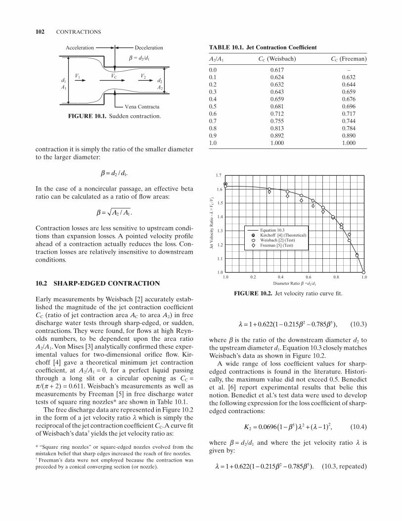
102 CONTRACTIONS
λ β β= + − −1 0 622 1 0 215 0 7852 5. ( . . ), (10.3)
where β is the ratio of the downstream diameter d2 to the upstream diameter d1 . Equation 10.3 closely matches Weisbach ’ s data as shown in Figure 10.2 .
A wide range of loss coeffi cient values for sharp - edged contractions is found in the literature. Histori-cally, the maximum value did not exceed 0.5. Benedict et al. [6] report experimental results that belie this notion. Benedict et al. ’ s test data were used to develop the following expression for the loss coeffi cient of sharp - edged contractions:
K25 2 20 0696 1 1= −( ) + −( ). ,β λ λ (10.4)
where β = d2 / d1 and where the jet velocity ratio λ is given by:
λ β β= + − −1 0 622 1 0 215 0 7852 5. ( . . ). (10.3, repeated)
contraction it is simply the ratio of the smaller diameter to the larger diameter:
β = d d2 1/ .
In the case of a noncircular passage, an effective beta ratio can be calculated as a ratio of fl ow areas:
β = A A2 1/ .
Contraction losses are less sensitive to upstream condi-tions than expansion losses. A pointed velocity profi le ahead of a contraction actually reduces the loss. Con-traction losses are relatively insensitive to downstream conditions.
10.2 SHARP - EDGED CONTRACTION
Early measurements by Weisbach [2] accurately estab-lished the magnitude of the jet contraction coeffi cient CC (ratio of jet contraction area AC to area A2 ) in free discharge water tests through sharp - edged, or sudden, contractions. They were found, for fl ows at high Reyn-olds numbers, to be dependent upon the area ratio A2 / A1 . Von Mises [3] analytically confi rmed these exper-imental values for two - dimensional orifi ce fl ow. Kir-choff [4] gave a theoretical minimum jet contraction coeffi cient, at A2 / A1 = 0, for a perfect liquid passing through a long slit or a circular opening as CC = π / ( π + 2) = 0.611. Weisbach ’ s measurements as well as measurements by Freeman [5] in free discharge water tests of square ring nozzles * are shown in Table 10.1 .
The free discharge data are represented in Figure 10.2 in the form of a jet velocity ratio λ which is simply the reciprocal of the jet contraction coeffi cient CC . A curve fi t of Weisbach ’ s data † yields the jet velocity ratio as:
FIGURE 10.1. Sudden contraction.
A2
d1
DecelerationAcceleration
Vena Contracta
V2V1 VCd2
= db 2/d1
A1
TABLE 10.1. Jet Contraction Coeffi cient
A2 / A1 CC (Weisbach) CC (Freeman)
0.0 0.617 – 0.1 0.624 0.632 0.2 0.632 0.644 0.3 0.643 0.659 0.4 0.659 0.676 0.5 0.681 0.696 0.6 0.712 0.717 0.7 0.755 0.744 0.8 0.813 0.784 0.9 0.892 0.890 1.0 1.000 1.000
FIGURE 10.2. Jet velocity ratio curve fi t.
1.0
1.6
1.5
1.4
1.3
1.2
1.1
1.7
0.2 0.4 0.6 0.81.0 1.0
Jet V
eloc
ity
Rat
io -
l=
VC
/V2
Diameter Ratio b =d2/d1
Equation 10.3 Kirchoff [4] (Theoretical) Weisbach [2] (Test) Freeman [5] (Test)
† Freeman ’ s data were not employed because the contraction was preceded by a conical converging section (or nozzle).
* “ Square ring nozzles ” or square - edged nozzles evolved from the mistaken belief that sharp edges increased the reach of fi re nozzles.
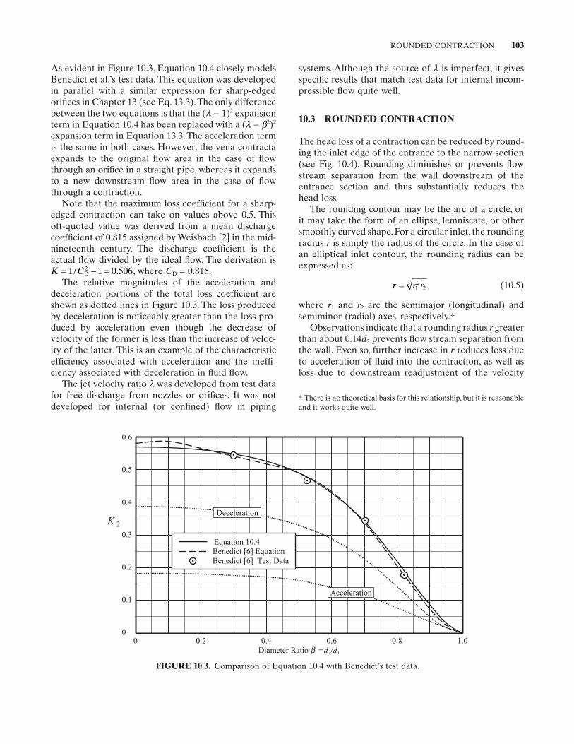
ROUNDED CONTRACTION 103
systems. Although the source of λ is imperfect, it gives specifi c results that match test data for internal incom-pressible fl ow quite well.
10.3 ROUNDED CONTRACTION
The head loss of a contraction can be reduced by round-ing the inlet edge of the entrance to the narrow section (see Fig. 10.4 ). Rounding diminishes or prevents fl ow stream separation from the wall downstream of the entrance section and thus substantially reduces the head loss.
The rounding contour may be the arc of a circle, or it may take the form of an ellipse, lemniscate, or other smoothly curved shape. For a circular inlet, the rounding radius r is simply the radius of the circle. In the case of an elliptical inlet contour, the rounding radius can be expressed as:
r r r= 12
23 , (10.5)
where r1 and r2 are the semimajor (longitudinal) and semiminor (radial) axes, respectively. *
Observations indicate that a rounding radius r greater than about 0.14 d2 prevents fl ow stream separation from the wall. Even so, further increase in r reduces loss due to acceleration of fl uid into the contraction, as well as loss due to downstream readjustment of the velocity
As evident in Figure 10.3 , Equation 10.4 closely models Benedict et al. ’ s test data. This equation was developed in parallel with a similar expression for sharp - edged orifi ces in Chapter 13 (see Eq. 13.3 ). The only difference between the two equations is that the ( λ − 1) 2 expansion term in Equation 10.4 has been replaced with a ( λ − β2 ) 2
expansion term in Equation 13.3 . The acceleration term is the same in both cases. However, the vena contracta expands to the original fl ow area in the case of fl ow through an orifi ce in a straight pipe, whereas it expands to a new downstream fl ow area in the case of fl ow through a contraction.
Note that the maximum loss coeffi cient for a sharp - edged contraction can take on values above 0.5. This oft - quoted value was derived from a mean discharge coeffi cient of 0.815 assigned by Weisbach [2] in the mid - nineteenth century. The discharge coeffi cient is the actual fl ow divided by the ideal fl ow. The derivation is K C= − =1 1 0 5062/ .D , where CD = 0.815.
The relative magnitudes of the acceleration and deceleration portions of the total loss coeffi cient are shown as dotted lines in Figure 10.3 . The loss produced by deceleration is noticeably greater than the loss pro-duced by acceleration even though the decrease of velocity of the former is less than the increase of veloc-ity of the latter. This is an example of the characteristic effi ciency associated with acceleration and the ineffi -ciency associated with deceleration in fl uid fl ow.
The jet velocity ratio λ was developed from test data for free discharge from nozzles or orifi ces. It was not developed for internal (or confi ned) fl ow in piping
* There is no theoretical basis for this relationship, but it is reasonable and it works quite well.
FIGURE 10.3. Comparison of Equation 10.4 with Benedict ’ s test data.
0 0.2 0.4 0.6 0.8 1.0Diameter Ratio b =d2/d1
0.6
0.5
0.4
0.3
0.2
0.1
0
Acceleration
Deceleration
Equation 10.4 Benedict [6] Equation Benedict [6] Test Data
K 2
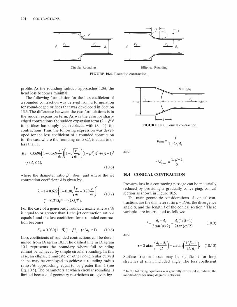
104 CONTRACTIONS
FIGURE 10.4. Rounded contraction.
d1
V2V1d2
r
V2d1
V1d2
r1 r2
Circular Rounding Elliptical Rounding
βlimit =+
11 2 2r d
and
r d//
.21 1
2limit = −β
10.4 CONICAL CONTRACTION
Pressure loss in a contracting passage can be materially reduced by providing a gradually converging, conical section as shown in Figure 10.5 .
The main geometric considerations of conical con-tractions are the diameter ratio β = d2 / d1 , the divergence angle α , and the length l of the conical section. * These variables are interrelated as follows:
ld d d= −
( )= −( )
( )1 2 2
2 21 1
2 2tan //
tan /α αβ
(10.9)
and
α β= −
= −
2
22
1 12
1 2
2
atan atand d
l l d/
/. (10.10)
Surface friction losses may be signifi cant for long stretches at small included angle. The loss coeffi cient
profi le. As the rounding radius r approaches 1.0 d2 the head loss becomes minimal.
The following formulation for the loss coeffi cient of a rounded contraction was derived from a formulation for round - edged orifi ces that was developed in Section 13.3 . The difference between the two formulations is in the sudden expansion term. As was the case for sharp - edged contractions, the sudden expansion term ( λ − β2 ) 2
for orifi ces has simply been replaced with ( λ − 1) 2 for contractions. Thus, the following expression was devel-oped for the loss coeffi cient of a rounded contraction for the case where the rounding ratio r / d2 is equal to or less than 1:
Krd
rd
r d
22 2
5 2 2
2
0 0696 1 0 569 1 1 1= −
−
−( ) + −( )
≤
. .
( /
β β λ λ
11), (10.6)
where the diameter ratio β = d2 / d1 , and where the jet contraction coeffi cient λ is given by:
λ
β β
= + − −
− −( )
1 0 622 1 0 30 0 70
1 0 215 0 785
2 2
4
2 5
. . .
. . .
rd
rd (10.7)
For the case of a generously rounded nozzle where r / d2
is equal to or greater than 1, the jet contraction ratio λequals 1 and the loss coeffi cient for a rounded contrac-tion becomes:
K r d24
20 030 1 1 1= −( ) −( ) ≥. ( / ).β β (10.8)
Loss coeffi cients of rounded contractions can be deter-mined from Diagram 10.1 . The dashed line in Diagram 10.1 represents the boundary where full rounding cannot be achieved by simple circular rounding. In this case, an ellipse, lemniscate, or other noncircular curved shape may be employed to achieve a rounding radius ratio r / d2 approaching, equal to, or greater than 1 (see Eq. 10.5 ). The parameters at which circular rounding is limited because of geometry restrictions are given by:
* In the following equations α is generally expressed in radians; the modifi cations for using degrees is obvious.
FIGURE 10.5. Conical contraction.
V2V1d2
= db 2/d1
l
d1 a
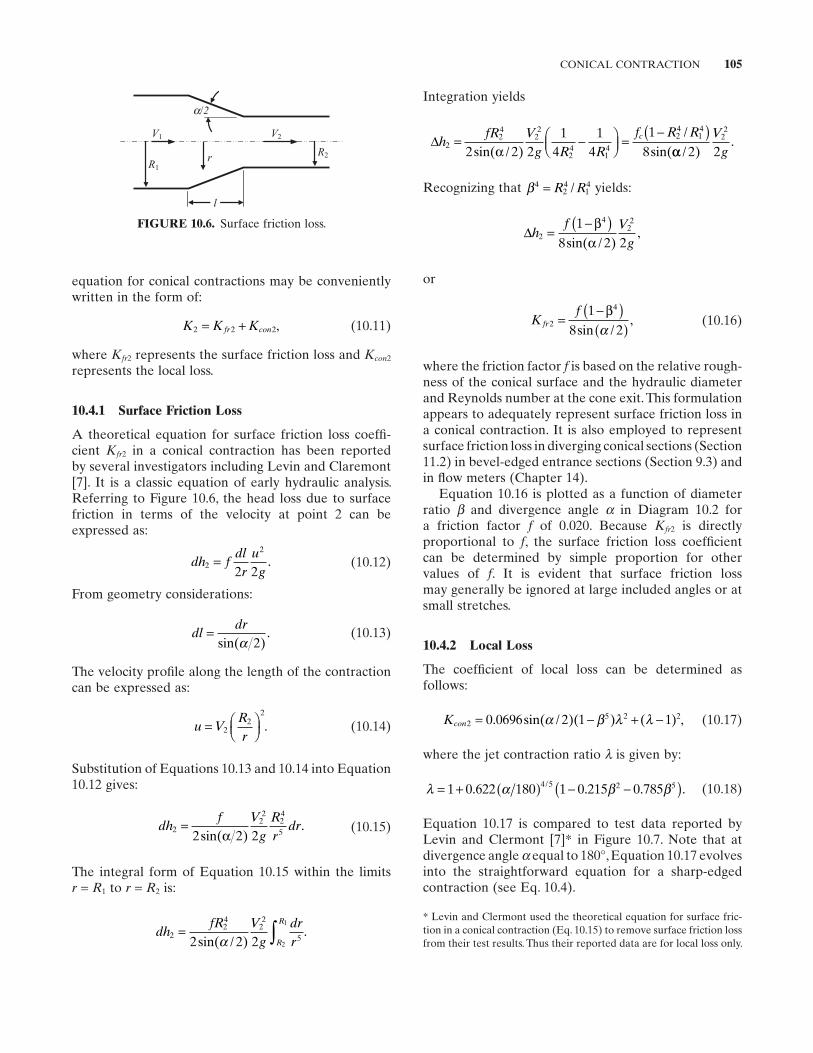
CONICAL CONTRACTION 105
equation for conical contractions may be conveniently written in the form of:
K K Kfr con2 2 2= + , (10.11)
where Kfr2 represents the surface friction loss and Kcon2
represents the local loss.
10.4.1 Surface Friction Loss
A theoretical equation for surface friction loss coeffi -cient Kfr2 in a conical contraction has been reported by several investigators including Levin and Claremont [7] . It is a classic equation of early hydraulic analysis. Referring to Figure 10.6 , the head loss due to surface friction in terms of the velocity at point 2 can be expressed as:
dh fdlr
ug
2
2
2 2= . (10.12)
From geometry considerations:
dldr=
sin( ).
α 2 (10.13)
The velocity profi le along the length of the contraction can be expressed as:
u VRr
=
2
22
. (10.14)
Substitution of Equations 10.13 and 10.14 into Equation 10.12 gives:
dhf V
gRr
dr222
24
52 2 2=
sin( ).
α (10.15)
The integral form of Equation 10.15 within the limits r = R1 to r = R2 is:
dhfR V
gdrrR
R
224
22
52 2 2 2
1
= ∫sin( / ).
α
FIGURE 10.6. Surface friction loss.
a/2
V2V1
l
R2
R1r
Integration yields
∆hfR V
g R R
f R Rc2
24
22
24
14
24
14
2 2 21
41
4
1
8= −
=
−( )sin( / )
/
sin(α αα / ).
2 222Vg
Recognizing that β424
14= R R/ yields:
∆hf V
g2
4221
8 2 2=
−( )βαsin( / )
,
or
Kf
fr 2
41
8 2=
−( )( )
βsin /
,α
(10.16)
where the friction factor f is based on the relative rough-ness of the conical surface and the hydraulic diameter and Reynolds number at the cone exit. This formulation appears to adequately represent surface friction loss in a conical contraction. It is also employed to represent surface friction loss in diverging conical sections (Section 11.2 ) in bevel - edged entrance sections (Section 9.3 ) and in fl ow meters (Chapter 14 ).
Equation 10.16 is plotted as a function of diameter ratio β and divergence angle α in Diagram 10.2 for a friction factor f of 0.020. Because Kfr2 is directly proportional to f , the surface friction loss coeffi cient can be determined by simple proportion for other values of f . It is evident that surface friction loss may generally be ignored at large included angles or at small stretches.
10.4.2 Local Loss
The coeffi cient of local loss can be determined as follows:
Kcon25 2 20 0696 2 1 1= − + −. sin( / )( ) ( ) ,α β λ λ (10.17)
where the jet contraction ratio λ is given by:
λ α β β= + ( ) − −( )1 0 622 180 1 0 215 0 7854 5 2 5. . . ./ (10.18)
Equation 10.17 is compared to test data reported by Levin and Clermont [7] * in Figure 10.7 . Note that at divergence angle α equal to 180 ° , Equation 10.17 evolves into the straightforward equation for a sharp - edged contraction (see Eq. 10.4 ).
* Levin and Clermont used the theoretical equation for surface fric-tion in a conical contraction (Eq. 10.15 ) to remove surface friction loss from their test results. Thus their reported data are for local loss only.
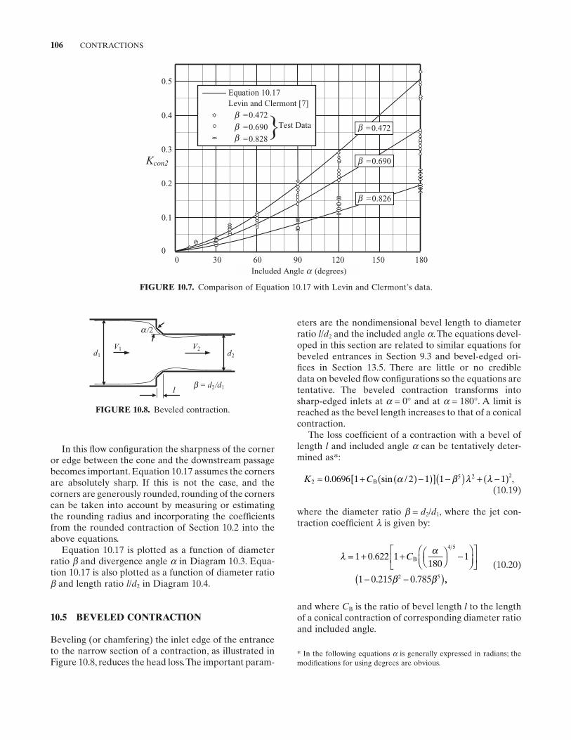
106 CONTRACTIONS
In this fl ow confi guration the sharpness of the corner or edge between the cone and the downstream passage becomes important. Equation 10.17 assumes the corners are absolutely sharp. If this is not the case, and the corners are generously rounded, rounding of the corners can be taken into account by measuring or estimating the rounding radius and incorporating the coeffi cients from the rounded contraction of Section 10.2 into the above equations.
Equation 10.17 is plotted as a function of diameter ratio β and divergence angle α in Diagram 10.3 . Equa-tion 10.17 is also plotted as a function of diameter ratio β and length ratio l / d2 in Diagram 10.4 .
10.5 BEVELED CONTRACTION
Beveling (or chamfering) the inlet edge of the entrance to the narrow section of a contraction, as illustrated in Figure 10.8 , reduces the head loss. The important param-
* In the following equations α is generally expressed in radians; the modifi cations for using degrees are obvious.
FIGURE 10.8. Beveled contraction.
d1
V2V1d2
l
/2a
= db 2/d1
FIGURE 10.7. Comparison of Equation 10.17 with Levin and Clermont ’ s data.
Included Angle a (degrees)
0.5
0.4
0.3
0.2
0.1
00 30 60 90 120 150 180
=0.826
=0.690
=0.472
Equation 10.17 Levin and Clermont [7]
=bbb
0.472
=0.690
=0.828 Test Data
Kcon2
b
b
b
eters are the nondimensional bevel length to diameter ratio l / d2 and the included angle α . The equations devel-oped in this section are related to similar equations for beveled entrances in Section 9.3 and bevel - edged ori-fi ces in Section 13.5 . There are little or no credible data on beveled fl ow confi gurations so the equations are tentative. The beveled contraction transforms into sharp - edged inlets at α = 0 ° and at α = 180 ° . A limit is reached as the bevel length increases to that of a conical contraction.
The loss coeffi cient of a contraction with a bevel of length l and included angle α can be tentatively deter-mined as * :
K C2 B≈ + ( ) −( )[ ] −( ) + −( )0 0696 1 2 1 1 15 2 2. sin / ,α β λ λ (10.19)
where the diameter ratio β = d2 / d1 , where the jet con-traction coeffi cient λ is given by:
λ α
β β
= + +
−
− −( )
1 0 622 1180
1
1 0 215 0 785
4 5
2 5
.
. .
CB
,,
(10.20)
and where CB is the ratio of bevel length l to the length of a conical contraction of corresponding diameter ratio and included angle.
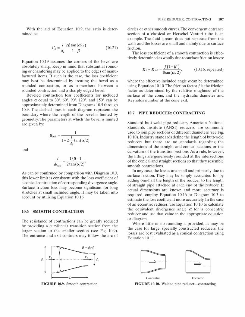
PIPE REDUCER: CONTRACTING 107
With the aid of Equation 10.9 , the ratio is deter-mined as:
Cl
dB = ( )
−2
2 21
β αβ
tan. (10.21)
Equation 10.19 assumes the corners of the bevel are absolutely sharp. Keep in mind that substantial round-ing or chamfering may be applied to the edges of manu-factured items. If such is the case, the loss coeffi cient may best be determined by treating the bevel as a rounded contraction, or as somewhere between a rounded contraction and a sharply edged bevel.
Beveled contraction loss coeffi cients for included angles α equal to 30 ° , 60 ° , 90 ° , 120 ° , and 150 ° can be approximately determined from Diagrams 10.5 through 10.9 . The dashed lines in each diagram represent the boundary where the length of the bevel is limited by geometry. The parameters at which the bevel is limited are given by:
βα
limit =+ ( )
1
1 2 22
ld
tan
and
ld2
1 12 2limit
= −( )
/tan
.β
α
As can be confi rmed by comparison with Diagram 10.3 , this lower limit is consistent with the loss coeffi cient of a conical contraction of corresponding divergence angle. Surface friction loss may become signifi cant for long stretches at small included angle. It may be taken into account by utilizing Equation 10.16 .
10.6 SMOOTH CONTRACTION
The resistance of contractions can be greatly reduced by providing a curvilinear transition section from the larger section to the smaller section (see Fig. 10.9 ). The entrance and exit contours may follow the arc of
FIGURE 10.9. Smooth contraction.
d1 d2V1 V2
= db
a
2/d1
lt
circles or other smooth curves. The convergent entrance section of a classical or Herschel Venturi tube is an example. The fl uid stream does not separate from the walls and the losses are small and mainly due to surface friction.
The loss coeffi cient of a smooth contraction is effec-tively determined as wholly due to surface friction losses:
K Kf
fr2 2
41
8 2≈ =
−( )( )
βαsin /
, (10.16, repeated)
where the effective included angle α can be determined using Equation 10.10 . The friction factor f is the friction factor as determined by the relative roughness of the surface of the cone, and the hydraulic diameter and Reynolds number at the cone exit.
10.7 PIPE REDUCER: CONTRACTING
Standard butt - weld pipe reducers, American National Standards Institute (ANSI) reducers, are commonly used to join pipe sections of different diameters (see Fig. 10.10 ). Industry standards defi ne the length of butt - weld reducers but there are no standards regarding the dimensions of the straight and conical sections, or the curvature of the transition sections. As a rule, however, the fi ttings are generously rounded at the intersections of the conical and straight sections so that they resemble smooth contractions.
In any case, the losses are small and primarily due to surface friction. They may be simply accounted for by adding one - half the length of the reducer to the length of straight pipe attached at each end of the reducer. If actual dimensions are known and more accuracy is required, employ Equation 10.16 or Diagram 10.3 to estimate the loss coeffi cient more accurately. In the case of an eccentric reducer, use Equation 10.10 to calculate the equivalent divergence angle α for a concentric reducer and use that value in the appropriate equation or diagram.
Where little or no rounding is provided, as may be the case for large, specially constructed reducers, the losses are best evaluated as a conical contraction using Equation 10.11 .
FIGURE 10.10. Welded pipe reducer — contracting.
EccentricConcentric

DIAGRAM 10.1. Loss coeffi cient K2 of a rounded contraction.
K
0 0.2 0.4 0.6 0.8 1.0
Diameter Ratio =d2/d1
0.6
0.5
0.4
0.3
0.2
0.1
0
r/d2 = 0 (Sharp-Edged)0.001
0.005 0.01
0.03
0.02
0.04
0.10
0.05
0.06
0.20
1.00 0.50
0.30
0.08
0.12
0.15
d1 d2
r
Equation 10.6
Circular Rounding Limit
b
DIAGRAM 10.2. Surface friction loss coeffi cient Kfr2 of a conical contraction.
2 3 4 5 6 7 8 9 10 15 20 30 40 50 60
0.15
0.10
0.05
0
Kfr2
Convergence Angle - degrees
= 0
0.50.6
0.70.8
0.850.9
0.95
Equation 10.16 (f = 0.020)
a
b

DIAGRAM 10.3. Local loss coeffi cient Kcon2 of a conical contraction as a function of included angle α .
0 0.2 0.4 0.6 0.8 1.0
Diameter Ratio =d2/d1
0.6
0.5
0.4
0.3
0.2
0.1
0
= 180˚ (Sharp-Edged)170˚
80˚
20˚
40˚
90˚
70˚60˚
50˚
30˚10˚
d1 d2
Equation 10.17
160˚150˚
140˚130˚
120˚110˚
110˚
Kcon2
b
a
a
0 0.2 0.4 0.6 0.8 1.0
Diameter Ratio =d2/d1
0.6
0.5
0.4
0.3
0.2
0.1
0
Kcon2
0.02 0.05
0.10
0.15
0.2
0.3
0.5
1.0
0.4
1.52
0.7
35
102040
d1 d2
Equation 10.17
l
l/d2 = 0 (Sharp-Edged)
bDIAGRAM 10.4. Local loss coeffi cient Kcon2 of a conical contraction as a function of length ratio l/d2 .
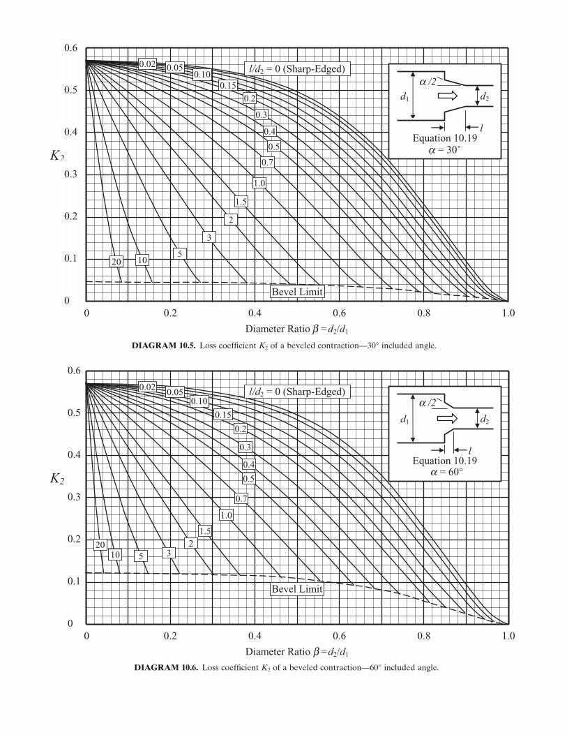
DIAGRAM 10.5. Loss coeffi cient K2 of a beveled contraction — 30 ° included angle.
0 0.2 0.4 0.6 0.8 1.0
Diameter Ratio =d2/d1
0.6
0.5
0.4
0.3
0.2
0.1
0
K20.5
1.0
0.4
1.5
2
0.7
3
5
l/d2 = 0 (Sharp-Edged)0.05 0.10
0.02
0.15
0.3
0.2
10
Bevel Limit
d1 d2
lEquation 10.19
= 30˚
/2
20
b
a
a
DIAGRAM 10.6. Loss coeffi cient K2 of a beveled contraction — 60 ° included angle.
0 0.2 0.4 0.6 0.8 1.0
Diameter Ratio =d2/d1
0.6
0.5
0.4
0.3
0.2
0.1
0
K2 0.5
1.0
0.4
1.52
0.7
35
l/d2 = 0 (Sharp-Edged)0.05 0.10
0.02
0.15
0.3
0.2
10 20
d1 d2
l
Equation 10.19
/2
Bevel Limit
b
= 60°a
a
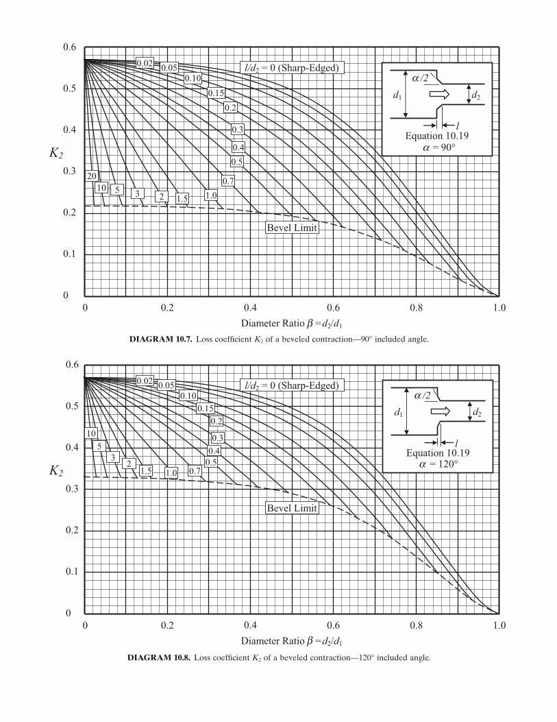
DIAGRAM 10.7. Loss coeffi cient K2 of a beveled contraction — 90 ° included angle.
0 0.2 0.4 0.6 0.8 1.0
Diameter Ratio =d2/d1
0.6
0.5
0.4
0.3
0.2
0.1
0
K20.5
1.0
0.4
1.52
0.7
35
l/d2 = 0 (Sharp-Edged)0.05 0.10
0.02
0.15
0.3
0.2
10 20
d1 d2
lEquation 10.19
/2
Bevel Limit
b
= 90°a
a
0 0.2 0.4 0.6 0.8 1.0
Diameter Ratio =d2/d1
0.6
0.5
0.4
0.3
0.2
0.1
0
K2
0.5
1.0
0.4
1.52
0.7
3
5
l/d2 = 0 (Sharp-Edged)0.050.10
0.02
0.15
0.3
0.2
10
Bevel Limit
d1 d2
l
Equation 10.19
/2
b
= 120°a
a
DIAGRAM 10.8. Loss coeffi cient K2 of a beveled contraction — 120 ° included angle.
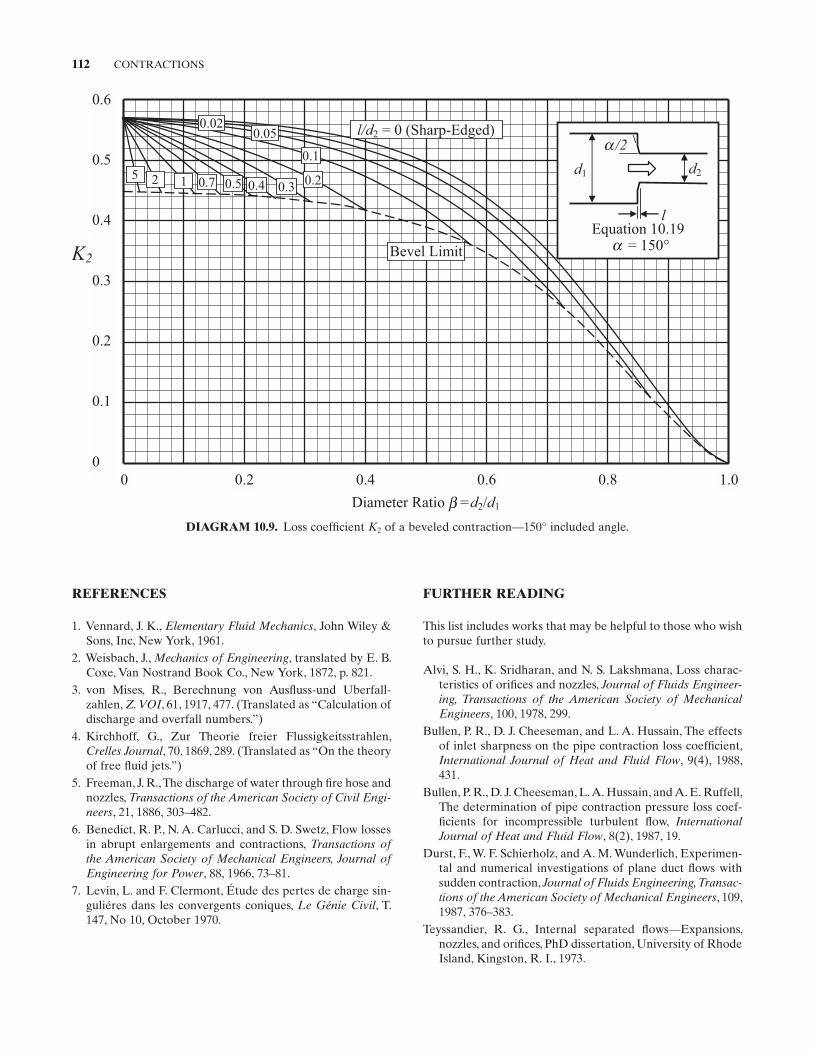
112 CONTRACTIONS
DIAGRAM 10.9. Loss coeffi cient K2 of a beveled contraction — 150 ° included angle.
0 0.2 0.4 0.6 0.8 1.0
Diameter Ratio =d2/d1
0.6
0.5
0.4
0.3
0.2
0.1
0
K2
0.51 0.42 0.75
l/d2 = 0 (Sharp-Edged)0.05
0.1
0.02
0.30.2
Bevel Limit
d1 d2
lEquation 10.19
/2
b
= 150°a
a
FURTHER READING
This list includes works that may be helpful to those who wish to pursue further study.
Alvi , S. H. , K. Sridharan , and N. S. Lakshmana , Loss charac-teristics of orifi ces and nozzles , Journal of Fluids Engineer-ing, Transactions of the American Society of Mechanical Engineers , 100 , 1978 , 299 .
Bullen , P. R. , D. J. Cheeseman , and L. A. Hussain , The effects of inlet sharpness on the pipe contraction loss coeffi cient , International Journal of Heat and Fluid Flow , 9 ( 4 ), 1988 , 431 .
Bullen , P. R. , D. J. Cheeseman , L. A. Hussain , and A. E. Ruffell , The determination of pipe contraction pressure loss coef-fi cients for incompressible turbulent fl ow , InternationalJournal of Heat and Fluid Flow , 8 ( 2 ), 1987 , 19 .
Durst , F. , W. F. Schierholz , and A. M. Wunderlich , Experimen-tal and numerical investigations of plane duct fl ows with sudden contraction , Journal of Fluids Engineering, Transac-tions of the American Society of Mechanical Engineers , 109 , 1987 , 376 – 383 .
Teyssandier , R. G. , Internal separated fl ows — Expansions, nozzles, and orifi ces , PhD dissertation, University of Rhode Island, Kingston, R. I., 1973 .
REFERENCES
1. Vennard , J. K. , Elementary Fluid Mechanics , John Wiley & Sons, Inc , New York , 1961 .
2. Weisbach , J. , Mechanics of Engineering , translated by E. B. Coxe, Van Nostrand Book Co. , New York , 1872 , p. 821 .
3. von Mises , R. , Berechnung von Ausfl uss - und Uberfall-zahlen, Z. VOI , 61 , 1917 , 477 . (Translated as “ Calculation of discharge and overfall numbers. ” )
4. Kirchhoff , G. , Zur Theorie freier Flussigkeitsstrahlen , Crelles Journal , 70 , 1869 , 289 . (Translated as “ On the theory of free fl uid jets. ” )
5. Freeman , J. R. , The discharge of water through fi re hose and nozzles , Transactions of the American Society of Civil Engi-neers , 21 , 1886 , 303 – 482 .
6. Benedict , R. P. , N. A. Carlucci , and S. D. Swetz , Flow losses in abrupt enlargements and contractions , Transactions of the American Society of Mechanical Engineers, Journal of Engineering for Power , 88 , 1966 , 73 – 81 .
7. Levin , L. and F. Clermont , É tude des pertes de charge sin-guli é res dans les convergents coniques , Le G é nie Civil , T. 147, No 10, October 1970 .
113
11 EXPANSIONS
Flow through a sudden or abrupt expansion in a piping system (see Fig. 11.1 ) gives rise to an increase in static pressure at the expense of a drop in kinetic energy. A “ potential ” core forms in the expanded section. Initially the core has a relatively fl at velocity profi le. This core spreads out and is separated from the remaining fl uid by a surface of separation which disintegrates into pow-erful eddies in a recirculation or free - mixing stall region. The eddies develop and gradually disappear, and the core expands radially over the section until reattach-ment to the wall occurs.
Many experimental investigations have been con-ducted for confi ned fl ow in sudden expansions (some-times referred to as backward facing steps). Test results show that for incompressible, fully developed turbulent fl ow in circular ducts the reattachment length - to - step height ratio, L/S , ranges from 6 to 9. Many authors assume that complete pressure recovery takes place at the reattachment point. However, beyond the reattach-ment point, the velocity profi le continues to change until a moderately developed turbulent fl ow profi le is achieved at distance ratios L / S on the order of 12 – 16.
Using a divergent connecting passage, or diffuser to make the transition from a passage of smaller cross section to a passage of larger cross section can substan-tially reduce expansion losses. The primary purpose of a diffuser is to convert kinetic energy of fl ow (or dynamic head) into static pressure (or static head) with minimum loss of total pressure. Much data, intimately related to the presence or absence of fl ow separation, or stall, are
available in the literature on the performance and design of straight, two - , and three - dimensional diffusers. Herein, we are simply concerned with loss of total pres-sure, or the loss coeffi cient, of three - dimensional diffus-ers, with or without appreciable stall.
The information presented in this chapter is based on incompressible fl ow. The information is based on symmetrical inlet conditions between the extremes of uniform velocity and of fully developed turbulent fl ow at the inlet to the expansion, and assumes a reasonable length of downstream straight pipe. Data on a number of inlet and outlet fl ow conditions may be found in the literature (see the section “ Further Reading ” at the end of this chapter).
11.1 SUDDEN EXPANSION
A sudden axisymmetric expansion is shown in Figure 11.2 . The energy, momentum, and continuity equations are applied to predict losses through the sudden expan-sion. While focus is directed to a single circular passage, this treatment is general and applies to both single and multiple passage expansions. The passage may actually be of any cross - sectional shape.
In the constant density fl uid case, the continuity rela-tionship for fl ow rate w through the control volume abcd is given by:
w A V A Vw w= =ρ ρ1 1 2 2. (11.1)
Pipe Flow: A Practical and Comprehensive Guide, First Edition. Donald C. Rennels and Hobart M. Hudson.© 2012 John Wiley & Sons, Inc. Published 2012 by John Wiley & Sons, Inc.
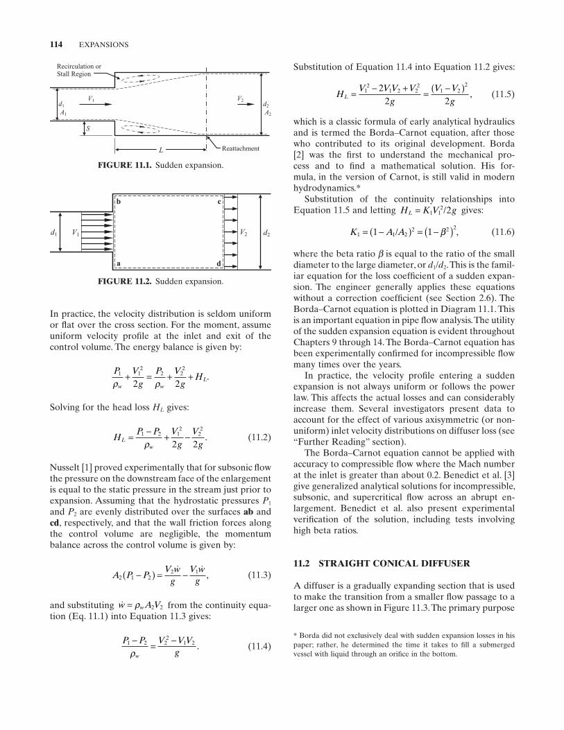
114 EXPANSIONS
Substitution of Equation 11.4 into Equation 11.2 gives:
HV V V V
gV V
gL = − + = −( )1
21 2 2
21 2
222 2
, (11.5)
which is a classic formula of early analytical hydraulics and is termed the Borda – Carnot equation, after those who contributed to its original development. Borda [2] was the fi rst to understand the mechanical pro-cess and to fi nd a mathematical solution. His for-mula, in the version of Carnot, is still valid in modern hydrodynamics. *
Substitution of the continuity relationships into Equation 11.5 and letting H K V gL = 1 1
2 2/ gives:
K A A1 /= −( ) = −( )1 11 22 2 2β , (11.6)
where the beta ratio β is equal to the ratio of the small diameter to the large diameter, or d1 / d2 . This is the famil-iar equation for the loss coeffi cient of a sudden expan-sion. The engineer generally applies these equations without a correction coeffi cient (see Section 2.6 ). The Borda – Carnot equation is plotted in Diagram 11.1 . This is an important equation in pipe fl ow analysis. The utility of the sudden expansion equation is evident throughout Chapters 9 through 14 . The Borda – Carnot equation has been experimentally confi rmed for incompressible fl ow many times over the years.
In practice, the velocity profi le entering a sudden expansion is not always uniform or follows the power law. This affects the actual losses and can considerably increase them. Several investigators present data to account for the effect of various axisymmetric (or non-uniform) inlet velocity distributions on diffuser loss (see “ Further Reading ” section).
The Borda – Carnot equation cannot be applied with accuracy to compressible fl ow where the Mach number at the inlet is greater than about 0.2. Benedict et al. [3] give generalized analytical solutions for incompressible, subsonic, and supercritical fl ow across an abrupt en -largement. Benedict et al. also present experimental verifi cation of the solution, including tests involving high beta ratios.
11.2 STRAIGHT CONICAL DIFFUSER
A diffuser is a gradually expanding section that is used to make the transition from a smaller fl ow passage to a larger one as shown in Figure 11.3 . The primary purpose
In practice, the velocity distribution is seldom uniform or fl at over the cross section. For the moment, assume uniform velocity profi le at the inlet and exit of the control volume. The energy balance is given by:
P Vg
P Vg
Hw w
L1 1
22 2
2
2 2ρ ρ+ = + + .
Solving for the head loss HL gives:
HP P V
gV
gL
w
= − + −1 2 12
22
2 2ρ. (11.2)
Nusselt [1] proved experimentally that for subsonic fl ow the pressure on the downstream face of the enlargement is equal to the static pressure in the stream just prior to expansion. Assuming that the hydrostatic pressures P1
and P2 are evenly distributed over the surfaces ab and cd , respectively, and that the wall friction forces along the control volume are negligible, the momentum balance across the control volume is given by:
A P PV w
gV w
g2 1 22 1−( ) = −
, (11.3)
and substituting w A Vw= ρ 2 2 from the continuity equa-tion (Eq. 11.1 ) into Equation 11.3 gives:
P P V V V
gw
1 2 22
1 2− = −ρ
. (11.4)
FIGURE 11.1. Sudden expansion.
S
V1 V2
Reattachment
Recirculation or Stall Region
L
d2
A2
d1
A1
FIGURE 11.2. Sudden expansion.
V1 V2d1 d2
a
cb
d
* Borda did not exclusively deal with sudden expansion losses in his paper; rather, he determined the time it takes to fi ll a submerged vessel with liquid through an orifi ce in the bottom.
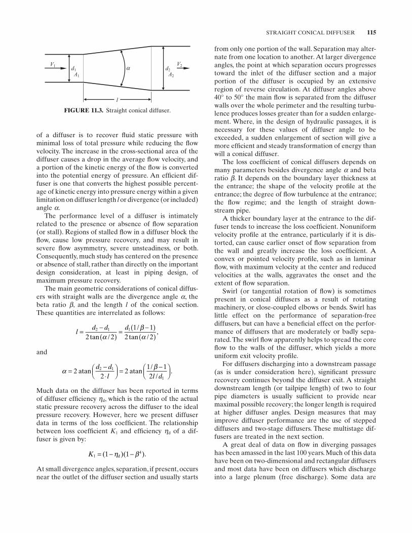
STRAIGHT CONICAL DIFFUSER 115
from only one portion of the wall. Separation may alter-nate from one location to another. At larger divergence angles, the point at which separation occurs progresses toward the inlet of the diffuser section and a major portion of the diffuser is occupied by an extensive region of reverse circulation. At diffuser angles above 40 ° to 50 ° the main fl ow is separated from the diffuser walls over the whole perimeter and the resulting turbu-lence produces losses greater than for a sudden enlarge-ment. Where, in the design of hydraulic passages, it is necessary for these values of diffuser angle to be exceeded, a sudden enlargement of section will give a more effi cient and steady transformation of energy than will a conical diffuser.
The loss coeffi cient of conical diffusers depends on many parameters besides divergence angle α and beta ratio β . It depends on the boundary layer thickness at the entrance; the shape of the velocity profi le at the entrance; the degree of fl ow turbulence at the entrance; the fl ow regime; and the length of straight down-stream pipe.
A thicker boundary layer at the entrance to the dif-fuser tends to increase the loss coeffi cient. Nonuniform velocity profi le at the entrance, particularly if it is dis-torted, can cause earlier onset of fl ow separation from the wall and greatly increase the loss coeffi cient. A convex or pointed velocity profi le, such as in laminar fl ow, with maximum velocity at the center and reduced velocities at the walls, aggravates the onset and the extent of fl ow separation.
Swirl (or tangential rotation of fl ow) is sometimes present in conical diffusers as a result of rotating machinery, or close - coupled elbows or bends. Swirl has little effect on the performance of separation - free diffusers, but can have a benefi cial effect on the perfor-mance of diffusers that are moderately or badly sepa-rated. The swirl fl ow apparently helps to spread the core fl ow to the walls of the diffuser, which yields a more uniform exit velocity profi le.
For diffusers discharging into a downstream passage (as is under consideration here), signifi cant pressure recovery continues beyond the diffuser exit. A straight downstream length (or tailpipe length) of two to four pipe diameters is usually suffi cient to provide near maximal possible recovery; the longer length is required at higher diffuser angles. Design measures that may improve diffuser performance are the use of stepped diffusers and two - stage diffusers. These multistage dif-fusers are treated in the next section.
A great deal of data on fl ow in diverging passages has been amassed in the last 100 years. Much of this data have been on two - dimensional and rectangular diffusers and most data have been on diffusers which discharge into a large plenum (free discharge). Some data are
of a diffuser is to recover fl uid static pressure with minimal loss of total pressure while reducing the fl ow velocity. The increase in the cross - sectional area of the diffuser causes a drop in the average fl ow velocity, and a portion of the kinetic energy of the fl ow is converted into the potential energy of pressure. An effi cient dif-fuser is one that converts the highest possible percent-age of kinetic energy into pressure energy within a given limitation on diffuser length l or divergence (or included) angle α .
The performance level of a diffuser is intimately related to the presence or absence of fl ow separation (or stall). Regions of stalled fl ow in a diffuser block the fl ow, cause low pressure recovery, and may result in severe fl ow asymmetry, severe unsteadiness, or both. Consequently, much study has centered on the presence or absence of stall, rather than directly on the important design consideration, at least in piping design, of maximum pressure recovery.
The main geometric considerations of conical diffus-ers with straight walls are the divergence angle α , the beta ratio β , and the length l of the conical section. These quantities are interrelated as follows:
ld d d= −
( )= −( )
( )2 1 1
2 21 1
2 2tan //
tan /,
αβα
and
α β= −⋅
= −
2
22
1 12
2 1
1
atan atand d
l l d/
/.
Much data on the diffuser has been reported in terms of diffuser effi ciency ηd , which is the ratio of the actual static pressure recovery across the diffuser to the ideal pressure recovery. However, here we present diffuser data in terms of the loss coeffi cient. The relationship between loss coeffi cient K1 and effi ciency ηd of a dif-fuser is given by:
K141 1= − −( )( ).η βd
At small divergence angles, separation, if present, occurs near the outlet of the diffuser section and usually starts
FIGURE 11.3. Straight conical diffuser.
A1
Va1 V2
d1 d2A2
l
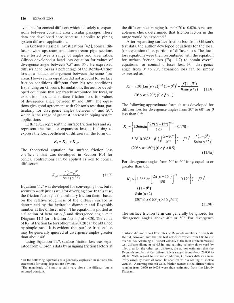
116 EXPANSIONS
the diffuser inlets ranging from 0.020 to 0.026. A reason-ableness check determined that friction factors in this range would be expected. ‡
After separating surface friction loss from Gibson ’ s test data, the author developed equations for the local (or expansion) loss portion of diffuser loss. The local loss equations were then recombined with the equation for surface friction loss (Eq. 11.7 ) to obtain overall equations for conical diffuser loss. For divergence angle from 0 ° to 20 ° , expansion loss can be simply expressed as:
Kf
11 75 2 2
4
8 30 2 11
8 2
0 20 0
= ( )[ ] −( ) +−( )( )
° ≤ ≤ ° ≥
. /sin /
( ) (
.tan α ββ
αα ββ ≤ 1).
(11.8)
The following approximate formula was developed for diffuser loss for divergence angles from 20 ° to 60 ° for βless than 0.5:
K1
1 2
4
1 3662 15
1800 170
3 28 0 0625
≈ − °( )
− −
−( )
. sin .
. .
/π α
β α −− °°
−( ) +−( )( )
° ≤ ≤ ° ≥ <
2040
11
8 2
20 60 0 0 5
2 24
ββ
αα β
f
sin /,
( ) ( . ). (11.9a)
For divergence angles from 20 ° to 60 ° for β equal to or greater than 0.5:
K
f
1
1 22 2
4
1 3662 15
1800 170 1
1
≈ − °( )
−
−( ) +
−(
. sin ./π α β
β ))( )
° ≤ ≤ ° ≥ ≤8 2
20 60 0 5 1
sin /
( ) ( . ).
αα β
(11.9b)
The surface friction term can generally be ignored for divergence angles above 40 ° or 50 ° . For divergence
available for conical diffusers which act solely as expan-sions between constant area circular passages. These data are developed here because it applies to piping system diffuser applications.
In Gibson ’ s classical investigations [4,5] , conical dif-fusers with upstream and downstream pipe sections were tested over a range of angles and area ratios. Gibson developed a head loss equation for values of divergence angle between 7.5 ° and 35 ° . He expressed diffuser head loss as a percentage of the Borda – Carnot loss at a sudden enlargement between the same fl ow areas. However, his equation did not account for surface friction conditions different from his test conditions. Expanding on Gibson ’ s formulations, the author devel-oped equations that separately accounted for local, or expansion, loss, and surface friction loss for values of divergence angle between 0 ° and 180 ° . The equa-tions give good agreement with Gibson ’ s test data, par-ticularly for divergence angles between 0 ° and 20 ° , which is the range of greatest interest in piping system applications.
Letting Kfr1 represent the surface friction loss and KL1
represent the local or expansion loss, it is fi tting to express the loss coeffi cient of diffusers in the form of:
K K Kfr1 1 1= + L .
The theoretical equation for surface friction loss coeffi cient that was developed in Section 10.4 for conical contractions can be applied as well to conical diffusers* :
Kf
fr1
41
8 2=
−( )( )
βαsin /
. (11.7)
Equation 11.7 was developed for converging fl ow, but it seems to work just as well for diverging fl ow. In this case, the friction factor f is the ordinary friction factor based on the relative roughness of the diffuser surface as determined by the hydraulic diameter and Reynolds number at the diffuser inlet. † The equation is plotted as a function of beta ratio β and divergence angle α in Diagram 11.2 for a friction factor f of 0.020. The value of K fr1 at friction factors other than 0.020 can be obtained by simple ratio. It is evident that surface friction loss may be generally ignored at divergence angles greater than about 40 ° .
Using Equation 11.7 , surface friction loss was sepa-rated from Gibson ’ s data by assigning friction factors at
‡ Gibson did not report fl ow rates or Reynolds numbers for his tests. He did, however, note that his test velocities varied from 1.83 to just over 21 ft/s. Assuming 21 ft/s test velocity at the inlet of the narrowest test diffuser diameter of 0.5 in, and ratioing velocity downward by inlet area for the other test diffusers, the author estimates that the Reynolds number at the diffuser inlets ranged from about 20,000 to 70,000. With regard to surface conditions, Gibson ’ s diffusers were “ very carefully made of wood, fi nished off with a coating of shellac varnish. ” Assuming smooth walls, friction factors at the diffuser inlets ranging from 0.020 to 0.026 were then estimated from the Moody Diagram.
† The magnitude of f may actually vary along the diffuser, but is assumed constant.
* In the following equations α is generally expressed in radians; the exceptions for using degrees are obvious.
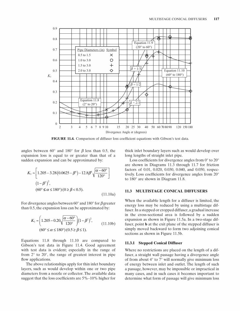
MULTISTAGE CONICAL DIFFUSERS 117
thick inlet boundary layers such as would develop over long lengths of straight inlet pipe.
Loss coeffi cients for divergence angles from 0 ° to 20 ° are shown in Diagrams 11.3 through 11.7 for friction factors of 0.01, 0.020, 0.030, 0.040, and 0.050, respec-tively. Loss coeffi cients for divergence angles from 20 ° to 180 ° are shown in Diagram 11.8 .
11.3 MULTISTAGE CONICAL DIFFUSERS
When the available length for a diffuser is limited, the energy loss may be reduced by using a multistage dif-fuser. In a stepped or cropped diffuser, a gradual increase in the cross - sectional area is followed by a sudden expansion as shown in Figure 11.5 a. In a two - stage dif-fuser, point b at the exit plane of the stepped diffuser is simply moved backward to form two adjoining conical sections as shown in Figure 11.5 b.
11.3.1 Stepped Conical Diffuser
Where no restrictions are placed on the length of a dif-fuser, a straight wall passage having a divergence angle of from about 4 ° to 7 ° will normally give minimum loss of energy between inlet and outlet. The length of such a passage, however, may be impossible or impractical in many cases, and in such cases it becomes important to determine what form of passage will give minimum loss
angles between 60 ° and 180 ° for β less than 0.5, the expansion loss is equal to or greater than that of a sudden expansion and can be approximated by:
K14 6
2 2
1 205 3 28 0 0625 12 860
120
1
60
≈ − −( ) − − °°
−( )°
. . . .
,
(
β β α
β≤≤ ≤ ° ≥ <α β180 0 0 5) ( . ).
(11.10a)
For divergence angles between 60 ° and 180 ° for β greater than 0.5, the expansion loss can be approximated by:
K1
2 21 205 0 20
60120
1
60 180 0 5 1
≈ − − °°
−( )
° ≤ ≤ ° ≥ ≤
. . ,
( ) ( . ).
α β
α β (11.10b)
Equations 11.8 through 11.10 are compared to Gibson ’ s test data in Figure 11.4 . Good agreement with test data is evident; especially in the range of from 2 ° to 20 ° , the range of greatest interest in pipe fl ow applications.
The above relationships apply for thin inlet boundary layers, such as would develop within one or two pipe diameters from a nozzle or collector. The available data suggest that the loss coeffi cients are 5% – 10% higher for
FIGURE 11.4. Comparison of diffuser loss coeffi cient equations with Gibson ’ s test data.
Divergence Angle a (degrees)
2 3 4 5 6 7 8 9 10 15 20 25 30 40 50 60 70 80 90 120 150 180
0.9
0.8
0.7
0.6
0.5
0.4
0.3
0.2
0.1
0
K1
Equation 11.8(2° to 20°)
Equation 11.10(60° to 180°)
Equation 11.9(20° to 60°)
= 1/3
= 1/2
Pipe Diameters (in) Symbol
0.5 to 1.5
1.0 to 3.0
1.5 to 3.0
2.0 to 3.0
= 2/3b
b
b
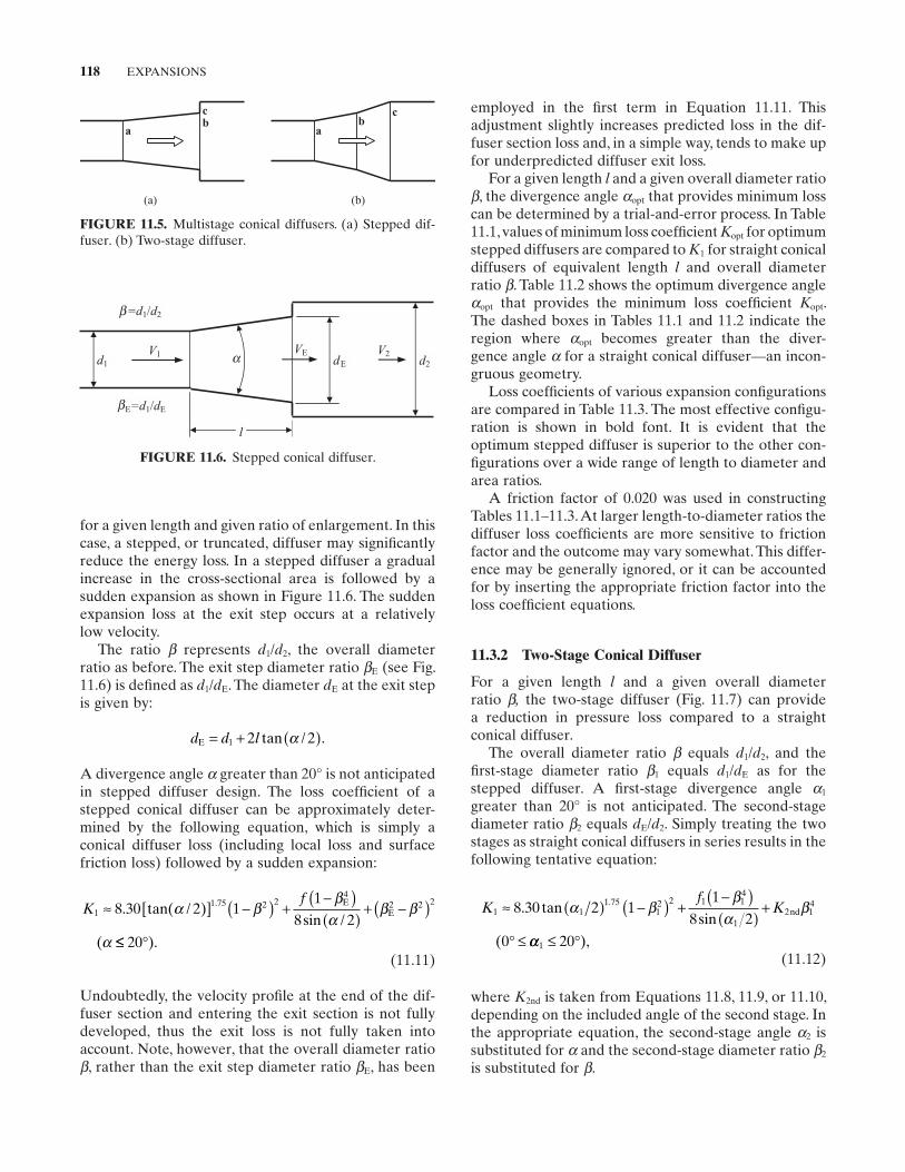
118 EXPANSIONS
FIGURE 11.5. Multistage conical diffusers. (a) Stepped dif-fuser. (b) Two - stage diffuser.
(a) (b)
c
ab b
a
c
FIGURE 11.6. Stepped conical diffuser.
VEd1 d2dE
V1 V2
l
E=d1/dE
=d1/d2b
b
a
for a given length and given ratio of enlargement. In this case, a stepped, or truncated, diffuser may signifi cantly reduce the energy loss. In a stepped diffuser a gradual increase in the cross - sectional area is followed by a sudden expansion as shown in Figure 11.6 . The sudden expansion loss at the exit step occurs at a relatively low velocity.
The ratio β represents d1 / d2 , the overall diameter ratio as before. The exit step diameter ratio βE (see Fig. 11.6 ) is defi ned as d1 / dE . The diameter dE at the exit step is given by:
d d lE = + ( )1 2 2tan / .α
A divergence angle α greater than 20 ° is not anticipated in stepped diffuser design. The loss coeffi cient of a stepped conical diffuser can be approximately deter-mined by the following equation, which is simply a conical diffuser loss (including local loss and surface friction loss) followed by a sudden expansion:
Kf
11 75 2 2
42 2 2
8 30 2 11
8 2≈ [ ] −( ) +
−( )( )
+ −( ). /sin /
(
.tan( ) EEα β
βα
β β
α ≤≤ °20 ). (11.11)
Undoubtedly, the velocity profi le at the end of the dif-fuser section and entering the exit section is not fully developed, thus the exit loss is not fully taken into account. Note, however, that the overall diameter ratio β , rather than the exit step diameter ratio βE , has been
employed in the fi rst term in Equation 11.11 . This adjustment slightly increases predicted loss in the dif-fuser section loss and, in a simple way, tends to make up for underpredicted diffuser exit loss.
For a given length l and a given overall diameter ratio β , the divergence angle αopt that provides minimum loss can be determined by a trial - and - error process. In Table 11.1 , values of minimum loss coeffi cient Kopt for optimum stepped diffusers are compared to K1 for straight conical diffusers of equivalent length l and overall diameter ratio β . Table 11.2 shows the optimum divergence angle αopt that provides the minimum loss coeffi cient Kopt . The dashed boxes in Tables 11.1 and 11.2 indicate the region where αopt becomes greater than the diver-gence angle α for a straight conical diffuser — an incon-gruous geometry.
Loss coeffi cients of various expansion confi gurations are compared in Table 11.3 . The most effective confi gu-ration is shown in bold font. It is evident that the optimum stepped diffuser is superior to the other con-fi gurations over a wide range of length to diameter and area ratios.
A friction factor of 0.020 was used in constructing Tables 11.1 – 11.3 . At larger length - to - diameter ratios the diffuser loss coeffi cients are more sensitive to friction factor and the outcome may vary somewhat. This differ-ence may be generally ignored, or it can be accounted for by inserting the appropriate friction factor into the loss coeffi cient equations.
11.3.2 Two - Stage Conical Diffuser
For a given length l and a given overall diameter ratio β , the two - stage diffuser (Fig. 11.7 ) can provide a reduction in pressure loss compared to a straight conical diffuser.
The overall diameter ratio β equals d1 / d2 , and the fi rst - stage diameter ratio β1 equals d1 / dE as for the stepped diffuser. A fi rst - stage divergence angle α1
greater than 20 ° is not anticipated. The second - stage diameter ratio β2 equals dE / d2 . Simply treating the two stages as straight conical diffusers in series results in the following tentative equation:
Kf
K1 11 75
12 2 1 1
4
12 1
48 30 2 11
8 2
0
≈ ( ) −( ) +−( )( )
+
° ≤
. tansin
(
.α ββ
αβnd
αα1 20≤ °), (11.12)
where K2nd is taken from Equations 11.8 , 11.9 , or 11.10 , depending on the included angle of the second stage. In the appropriate equation, the second - stage angle α2 is substituted for α and the second - stage diameter ratio β2
is substituted for β .
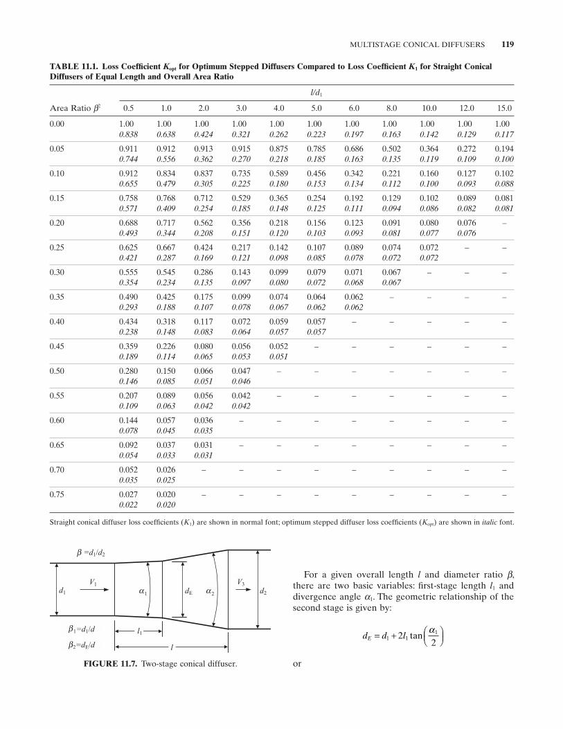
MULTISTAGE CONICAL DIFFUSERS 119
TABLE 11.1. Loss Coeffi cient Kopt for Optimum Stepped Diffusers Compared to Loss Coeffi cient K1 for Straight Conical Diffusers of Equal Length and Overall Area Ratio
Area Ratio β2
l/d1
0.5 1.0 2.0 3.0 4.0 5.0 6.0 8.0 10.0 12.0 15.0
0.00 1.00 1.00 1.00 1.00 1.00 1.00 1.00 1.00 1.00 1.00 1.00 0.838 0.638 0.424 0.321 0.262 0.223 0.197 0.163 0.142 0.129 0.117
0.05 0.911 0.912 0.913 0.915 0.875 0.785 0.686 0.502 0.364 0.272 0.194 0.744 0.556 0.362 0.270 0.218 0.185 0.163 0.135 0.119 0.109 0.100
0.10 0.912 0.834 0.837 0.735 0.589 0.456 0.342 0.221 0.160 0.127 0.102 0.655 0 .479 0.305 0.225 0.180 0.153 0.134 0.112 0.100 0.093 0.088
0.15 0.758 0.768 0.712 0.529 0.365 0.254 0.192 0.129 0.102 0.089 0.081 0.571 0.409 0.254 0.185 0.148 0.125 0.111 0.094 0.086 0.082 0.081
0.20 0.688 0.717 0.562 0.356 0.218 0.156 0.123 0.091 0.080 0.076 – 0.493 0.344 0.208 0.151 0.120 0.103 0.093 0.081 0.077 0.076
0.25 0.625 0.667 0.424 0.217 0.142 0.107 0.089 0.074 0.072 – – 0.421 0.287 0.169 0.121 0.098 0.085 0.078 0.072 0.072
0.30 0.555 0.545 0.286 0.143 0.099 0.079 0.071 0.067 – – – 0.354 0.234 0.135 0.097 0.080 0.072 0.068 0.067
0.35 0.490 0.425 0.175 0.099 0.074 0.064 0.062 – – – – 0.293 0.188 0.107 0.078 0.067 0.062 0.062
0.40 0.434 0.318 0.117 0.072 0.059 0.057 – – – – – 0.238 0.148 0.083 0.064 0.057 0.057
0.45 0.359 0.226 0.080 0.056 0.052 – – – – – – 0.189 0.114 0.065 0.053 0.051
0.50 0.280 0.150 0.066 0.047 – – – – – – – 0.146 0.085 0.051 0.046
0.55 0.207 0.089 0.056 0.042 – – – – – – – 0.109 0.063 0.042 0.042
0.60 0.144 0.057 0.036 – – – – – – – – 0.078 0.045 0.035
0.65 0.092 0.037 0.031 – – – – – – – – 0.054 0.033 0.031
0.70 0.052 0.026 – – – – – – – – – 0.035 0.025
0.75 0.027 0.020 – – – – – – – – – 0.022 0.020
Straight conical diffuser loss coeffi cients ( K1 ) are shown in normal font; optimum stepped diffuser loss coeffi cients ( Kopt ) are shown in italic font.
For a given overall length l and diameter ratio β , there are two basic variables: fi rst - stage length l1 and divergence angle α1 . The geometric relationship of the second stage is given by:
d d lE = +
1 1
122
tanα
orFIGURE 11.7. Two - stage conical diffuser.
d1 d2
V1
1
V3
dE
l
l1
=db
a 2a
1/d2
1=d1/d
2=dE/d
b
b
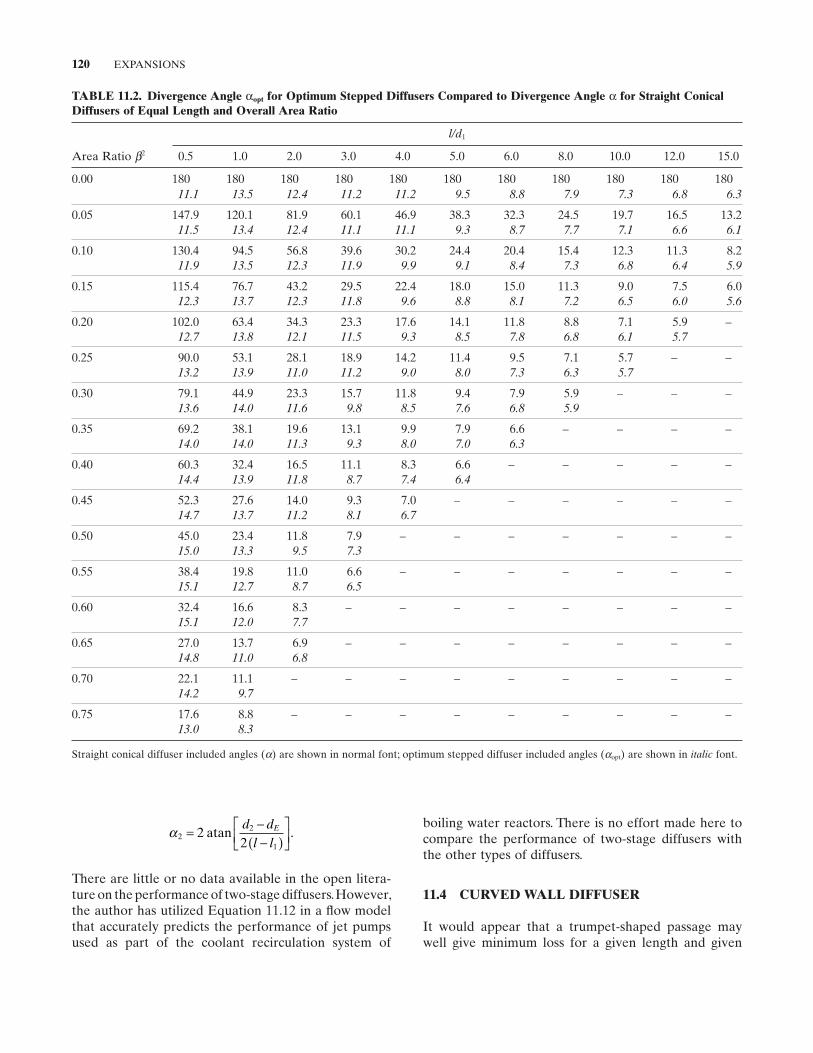
120 EXPANSIONS
TABLE 11.2. Divergence Angle αopt for Optimum Stepped Diffusers Compared to Divergence Angle α for Straight Conical Diffusers of Equal Length and Overall Area Ratio
Area Ratio β2
l/d1
0.5 1.0 2.0 3.0 4.0 5.0 6.0 8.0 10.0 12.0 15.0
0.00 180 180 180 180 180 180 180 180 180 180 180 11.1 13.5 12.4 11.2 11.2 9.5 8.8 7.9 7.3 6.8 6.3
0.05 147.9 120.1 81.9 60.1 46.9 38.3 32.3 24.5 19.7 16.5 13.2 11.5 13.4 12.4 11.1 11.1 9.3 8.7 7.7 7.1 6.6 6.1
0.10 130.4 94.5 56.8 39.6 30.2 24.4 20.4 15.4 12.3 11.3 8.2 11.9 13.5 12.3 11.9 9.9 9.1 8.4 7.3 6.8 6.4 5.9
0.15 115.4 76.7 43.2 29.5 22.4 18.0 15.0 11.3 9.0 7.5 6.0 12.3 13.7 12.3 11.8 9.6 8.8 8.1 7.2 6.5 6.0 5.6
0.20 102.0 63.4 34.3 23.3 17.6 14.1 11.8 8.8 7.1 5.9 – 12.7 13.8 12.1 11.5 9.3 8.5 7.8 6.8 6.1 5.7
0.25 90.0 53.1 28.1 18.9 14.2 11.4 9.5 7.1 5.7 – – 13.2 13.9 11.0 11.2 9.0 8.0 7.3 6.3 5.7
0.30 79.1 44.9 23.3 15.7 11.8 9.4 7.9 5.9 – – – 13.6 14.0 11.6 9.8 8.5 7.6 6.8 5.9
0.35 69.2 38.1 19.6 13.1 9.9 7.9 6.6 – – – – 14.0 14.0 11.3 9.3 8.0 7.0 6.3
0.40 60.3 32.4 16.5 11.1 8.3 6.6 – – – – – 14.4 13.9 11.8 8.7 7.4 6.4
0.45 52.3 27.6 14.0 9.3 7.0 – – – – – – 14.7 13.7 11.2 8.1 6.7
0.50 45.0 23.4 11.8 7.9 – – – – – – – 15.0 13.3 9.5 7.3
0.55 38.4 19.8 11.0 6.6 – – – – – – – 15.1 12.7 8.7 6.5
0.60 32.4 16.6 8.3 – – – – – – – – 15.1 12.0 7.7
0.65 27.0 13.7 6.9 – – – – – – – – 14.8 11.0 6.8
0.70 22.1 11.1 – – – – – – – – – 14.2 9.7
0.75 17.6 8.8 – – – – – – – – – 13.0 8.3
Straight conical diffuser included angles ( α ) are shown in normal font; optimum stepped diffuser included angles ( αopt ) are shown in italic font.
α22
1
22
= −−( )
atand d
l lE .
There are little or no data available in the open litera-ture on the performance of two - stage diffusers. However, the author has utilized Equation 11.12 in a fl ow model that accurately predicts the performance of jet pumps used as part of the coolant recirculation system of
boiling water reactors. There is no effort made here to compare the performance of two - stage diffusers with the other types of diffusers.
11.4 CURVED WALL DIFFUSER
It would appear that a trumpet - shaped passage may well give minimum loss for a given length and given
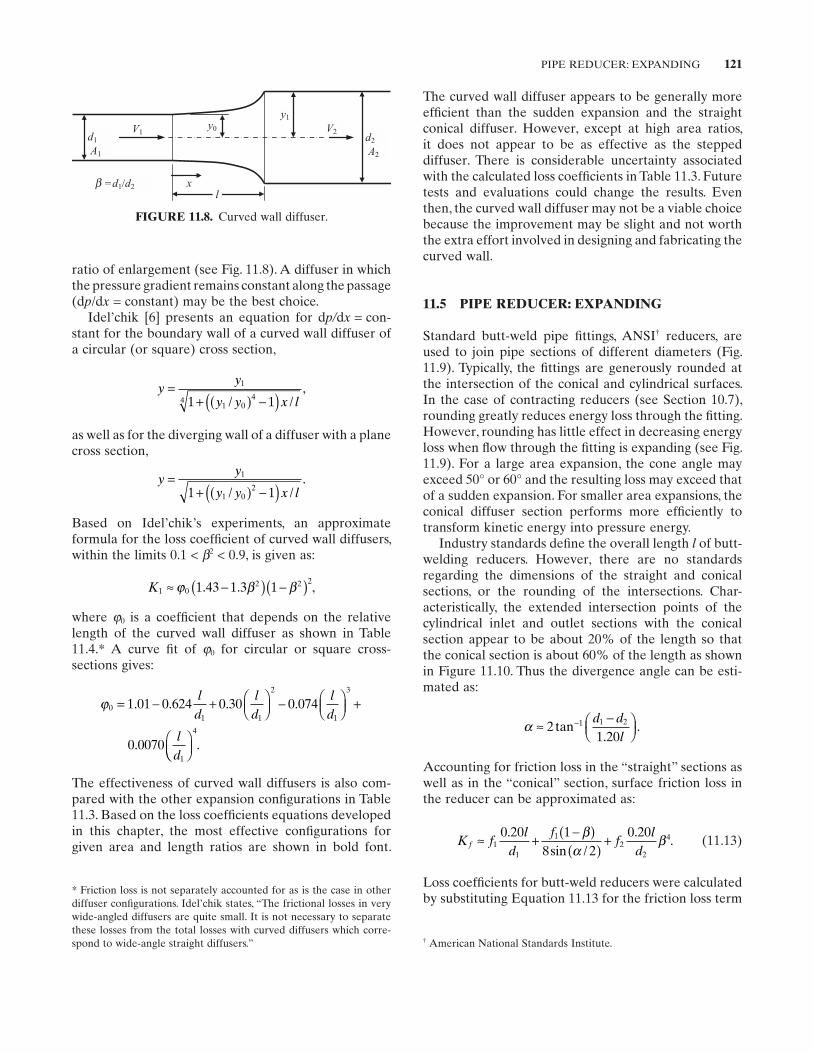
PIPE REDUCER: EXPANDING 121
FIGURE 11.8. Curved wall diffuser.
d1
A1
d2
A2
V1 V2
l=d1/d2
y0
y1
xb
ratio of enlargement (see Fig. 11.8 ). A diffuser in which the pressure gradient remains constant along the passage (dp /d x = constant) may be the best choice.
Idel ’ chik [6] presents an equation for d p/ d x = con-stant for the boundary wall of a curved wall diffuser of a circular (or square) cross section,
yy
y y x l=
+ ( ) −( )1
1 044 1 1/ /
,
as well as for the diverging wall of a diffuser with a plane cross section,
yy
y y x l=
+ ( ) −( )1
1 021 1/ /
.
Based on Idel ’ chik ’ s experiments, an approximate formula for the loss coeffi cient of curved wall diffusers, within the limits 0.1 < β2 < 0.9, is given as:
K1 02 2 2
1 43 1 3 1≈ −( ) −( )ϕ β β. . ,
where φ0 is a coeffi cient that depends on the relative length of the curved wall diffuser as shown in Table 11.4 . * A curve fi t of φ0 for circular or square cross - sections gives:
ϕ01 1
2
1
3
1
1 01 0 624 0 30 0 074
0 0070
= − +
−
+
. . . .
.
ld
ld
ld
ld
4
.
The effectiveness of curved wall diffusers is also com-pared with the other expansion confi gurations in Table 11.3 . Based on the loss coeffi cients equations developed in this chapter, the most effective confi gurations for given area and length ratios are shown in bold font.
The curved wall diffuser appears to be generally more effi cient than the sudden expansion and the straight conical diffuser. However, except at high area ratios, it does not appear to be as effective as the stepped diffuser. There is considerable uncertainty associated with the calculated loss coeffi cients in Table 11.3 . Future tests and evaluations could change the results. Even then, the curved wall diffuser may not be a viable choice because the improvement may be slight and not worth the extra effort involved in designing and fabricating the curved wall.
11.5 PIPE REDUCER: EXPANDING
Standard butt - weld pipe fi ttings, ANSI † reducers, are used to join pipe sections of different diameters (Fig. 11.9 ). Typically, the fi ttings are generously rounded at the intersection of the conical and cylindrical surfaces. In the case of contracting reducers (see Section 10.7 ), rounding greatly reduces energy loss through the fi tting. However, rounding has little effect in decreasing energy loss when fl ow through the fi tting is expanding (see Fig. 11.9 ). For a large area expansion, the cone angle may exceed 50 ° or 60 ° and the resulting loss may exceed that of a sudden expansion. For smaller area expansions, the conical diffuser section performs more effi ciently to transform kinetic energy into pressure energy.
Industry standards defi ne the overall length l of butt - welding reducers. However, there are no standards regarding the dimensions of the straight and conical sections, or the rounding of the intersections. Char-acteristically, the extended intersection points of the cylindrical inlet and outlet sections with the conical section appear to be about 20% of the length so that the conical section is about 60% of the length as shown in Figure 11.10 . Thus the divergence angle can be esti-mated as:
α ≈ −
−21 20
1 1 2tan.
.d d
l
Accounting for friction loss in the “ straight ” sections as well as in the “ conical ” section, surface friction loss in the reducer can be approximated as:
K fl
df
fl
df ≈ + −( )
( )+1
1
12
2
40 20 18 2
0 20.sin /
..
βα
β (11.13)
Loss coeffi cients for butt - weld reducers were calculated by substituting Equation 11.13 for the friction loss term
* Friction loss is not separately accounted for as is the case in other diffuser confi gurations. Idel ’ chik states, “ The frictional losses in very wide - angled diffusers are quite small. It is not necessary to separate these losses from the total losses with curved diffusers which corre-spond to wide - angle straight diffusers. ” † American National Standards Institute.
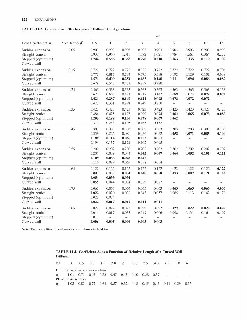
122 EXPANSIONS
TABLE 11.3. Comparative Effectiveness of Diffuser Confi gurations
Loss Coeffi cient K1 Area Ratio β2
l/d1
0.5 1 2 3 4 6 8 10 12
Sudden expansion 0.05 0.903 0.903 0.903 0.903 0.903 0.903 0.903 0.903 0.903 Straight conical 0.933 0.960 1.010 1.082 1.021 0.784 0.561 0.364 0.272 Stepped (optimum) 0.744 0.556 0.362 0.270 0.218 0.163 0.135 0.119 0.109 Curved wall – – – – – – – – –
Sudden expansion 0.15 0.722 0.722 0.722 0.722 0.722 0.722 0.722 0.722 0.706 Straight conical 0.772 0.817 0.784 0.575 0.388 0.192 0.129 0.102 0.089 Stepped (optimum) 0.571 0.409 0.254 0.185 0.148 0.111 0.094 0.086 0.082 Curved wall 0.679 0.547 0.423 0.357 0.330 – – – –
Sudden expansion 0.25 0.563 0.563 0.563 0.563 0.563 0.563 0.563 0.563 0.563 Straight conical 0.622 0.667 0.424 0.217 0.142 0.089 0.074 0.072 0.074 Stepped (optimum) 0.421 0.287 0.169 0.121 0.098 0.078 0.072 0.072 – Curved wall 0.473 0.381 0.294 0.249 0.230 – – – –
Sudden expansion 0.35 0.423 0.423 0.423 0.423 0.423 0.423 0.423 0.423 0.423 Straight conical 0.486 0.425 0.175 0.099 0.074 0.062 0.065 0.073 0.083 Stepped (optimum) 0.293 0.188 0.106 0.078 0.067 0.062 – – – Curved wall 0.313 0.253 0.195 0.165 0.152 – – – –
Sudden expansion 0.45 0.303 0.303 0.303 0.303 0.303 0.303 0.303 0.303 0.303 Straight conical 0.359 0.226 0.080 0.056 0.052 0.058 0.071 0.085 0.100 Stepped (optimum) 0.189 0.114 0.065 0.053 0.051 – – – – Curved wall 0.194 0.157 0.121 0.102 0.095 – – – –
Sudden expansion 0.55 0.202 0.202 0.202 0.202 0.202 0.202 0.202 0.202 0.202 Straight conical 0.207 0.089 0.044 0.042 0.047 0.064 0.082 0.102 0.121 Stepped (optimum) 0.109 0.063 0.042 0.042 – – – – – Curved wall 0.110 0.089 0.069 0.058 0.054 – – – –
Sudden expansion 0.65 0.122 0.122 0.122 0.122 0.122 0.122 0.122 0.122 0.122 Straight conical 0.092 0.037 0.031 0.040 0.050 0.073 0.097 0.121 0.144 Stepped (optimum) 0.054 0.033 0.031 – – – – – – Curved wall 0.055 0.044 0.034 0.029 0.027 – – – –
Sudden expansion 0.75 0.063 0.063 0.063 0.063 0.063 0.063 0.063 0.063 0.063 Straight conical 0.022 0.020 0.030 0.043 0.057 0.085 0.113 0.142 0.170 Stepped (optimum) 0.023 0.024 – – – – – – – Curved wall 0.022 0.017 0.017 0.011 0.011 – – – –
Sudden expansion 0.85 0.022 0.022 0.022 0.022 0.022 0.022 0.022 0.022 0.022 Straight conical 0.011 0.017 0.033 0.049 0.066 0.098 0.131 0.164 0.197 Stepped (optimum) 0.011 – – – – – – – – Curved wall 0.006 0.005 0.004 0.003 0.003 – – – –
Note: The most effi cient confi gurations are shown in bold font.
TABLE 11.4. Coeffi cient ϕ 0 as a Function of Relative Length of a Curved Wall Diffuser
l / d1 0 0.5 1.0 1.5 2.0 2.5 3.0 3.5 4.0 4.5 5.0 6.0
Circular or square cross section φ0 1.01 0.75 0.62 0.53 0.47 0.43 0.40 0.38 0.37 – – – Plane cross section φ0 1.02 0.83 0.72 0.64 0.57 0.52 0.48 0.45 0.43 0.41 0.39 0.37
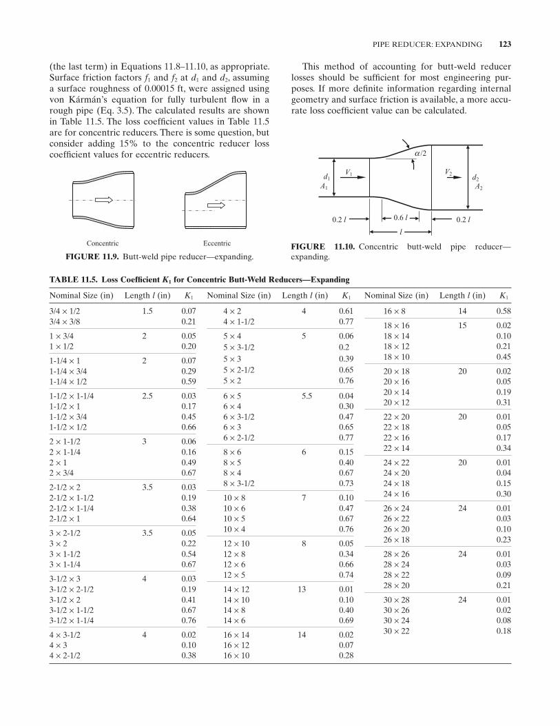
PIPE REDUCER: EXPANDING 123
(the last term) in Equations 11.8 – 11.10 , as appropriate. Surface friction factors f1 and f2 at d1 and d2 , assuming a surface roughness of 0.00015 ft, were assigned using von K á rm á n ’ s equation for fully turbulent fl ow in a rough pipe (Eq. 3.5 ). The calculated results are shown in Table 11.5 . The loss coeffi cient values in Table 11.5 are for concentric reducers. There is some question, but consider adding 15% to the concentric reducer loss coeffi cient values for eccentric reducers.
FIGURE 11.9. Butt - weld pipe reducer — expanding.
Concentric Eccentric FIGURE 11.10. Concentric butt - weld pipe reducer — expanding.
V1 V2d1 d2
A1 A2
/2a
0.2 l0.2 l 0.6 l
l
TABLE 11.5. Loss Coeffi cient K1 for Concentric Butt - Weld Reducers — Expanding
Nominal Size (in) Length l (in) K1 Nominal Size (in) Length l (in) K1 Nominal Size (in) Length l (in) K1
3/4 × 1/2 1.5 0.07 4 × 2 4 0.61 16 × 8 14 0.58 3/4 × 3/8 0.21 4 × 1 - 1/2 0.77 18 × 16 15 0.02 1 × 3/4 2 0.05 5 × 4 5 0.06 18 × 14 0.10 1 × 1/2 0.20 5 × 3 - 1/2 0.2 18 × 12 0.21
1 - 1/4 × 1 2 0.07 5 × 3 0.39 18 × 10 0.45
1 - 1/4 × 3/4 0.29 5 × 2 - 1/2 0.65 20 × 18 20 0.02 1 - 1/4 × 1/2 0.59 5 × 2 0.76 20 × 16 0.05
1 - 1/2 × 1 - 1/4 2.5 0.03 6 × 5 5.5 0.04 20 × 14 0.19
1 - 1/2 × 1 0.17 6 × 4 0.30 20 × 12 0.31
1 - 1/2 × 3/4 0.45 6 × 3 - 1/2 0.47 22 × 20 20 0.01 1 - 1/2 × 1/2 0.66 6 × 3 0.65 22 × 18 0.05
2 × 1 - 1/2 3 0.06 6 × 2 - 1/2 0.77 22 × 16 0.17
2 × 1 - 1/4 0.16 8 × 6 6 0.15 22 × 14 0.34
2 × 1 0.49 8 × 5 0.40 24 × 22 20 0.01 2 × 3/4 0.67 8 × 4 0.67 24 × 20 0.04
2 - 1/2 × 2 3.5 0.03 8 × 3 - 1/2 0.73 24 × 18 0.15
2 - 1/2 × 1 - 1/2 0.19 10 × 8 7 0.10 24 × 16 0.30
2 - 1/2 × 1 - 1/4 0.38 10 × 6 0.47 26 × 24 24 0.01 2 - 1/2 × 1 0.64 10 × 5 0.67 26 × 22 0.03
3 × 2 - 1/2 3.5 0.05 10 × 4 0.76 26 × 20 0.10
3 × 2 0.22 12 × 10 8 0.05 26 × 18 0.23
3 × 1 - 1/2 0.54 12 × 8 0.34 28 × 26 24 0.01 3 × 1 - 1/4 0.67 12 × 6 0.66 28 × 24 0.03
3 - 1/2 × 3 4 0.03 12 × 5 0.74 28 × 22 0.09
3 - 1/2 × 2 - 1/2 0.19 14 × 12 13 0.01 28 × 20 0.21
3 - 1/2 × 2 0.41 14 × 10 0.10 30 × 28 24 0.01 3 - 1/2 × 1 - 1/2 0.67 14 × 8 0.40 30 × 26 0.02 3 - 1/2 × 1 - 1/4 0.76 14 × 6 0.69 30 × 24 0.08
4 × 3 - 1/2 4 0.02 16 × 14 14 0.02 30 × 22 0.18
4 × 3 0.10 16 × 12 0.07 4 × 2 - 1/2 0.38 16 × 10 0.28
This method of accounting for butt - weld reducer losses should be suffi cient for most engineering pur-poses. If more defi nite information regarding internal geometry and surface friction is available, a more accu-rate loss coeffi cient value can be calculated.
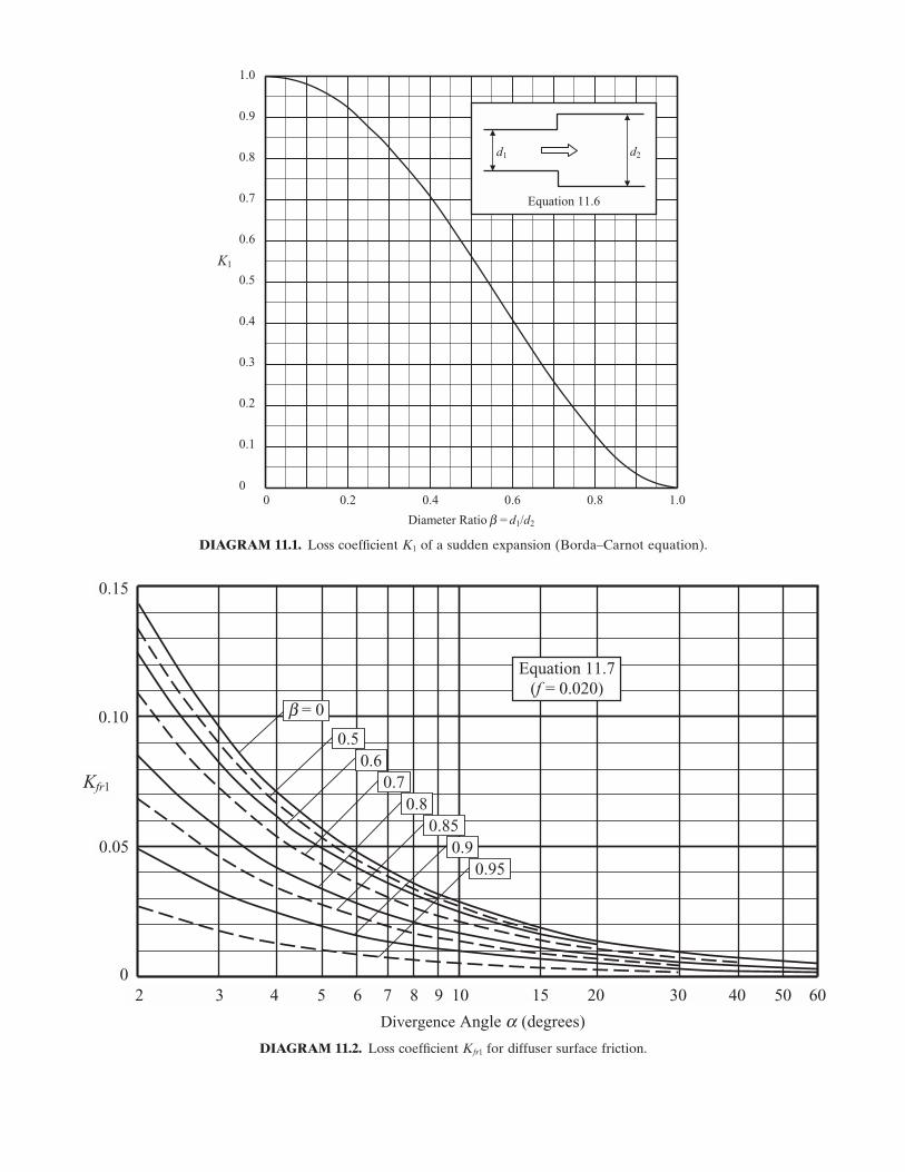
DIAGRAM 11.2. Loss coeffi cient Kfr1 for diffuser surface friction.
2 3 4 5 6 7 8 9 10 15 20 30 40 50 60
0.15
0.10
0.05
0
Kfr1
Divergence Angle (degrees)
= 0
0.50.6
0.70.8
0.850.9
0.95
Equation 11.7 (f = 0.020)
a
b
DIAGRAM 11.1. Loss coeffi cient K1 of a sudden expansion (Borda – Carnot equation).
Diameter Ratio = d1/d2
K1
0 0.2 0.4 0.6 0.8 1.0
1.0
0.9
0.8
0.7
0.6
0.5
0.4
0.3
0.2
0.1
0
d1 d2
Equation 11.6
b
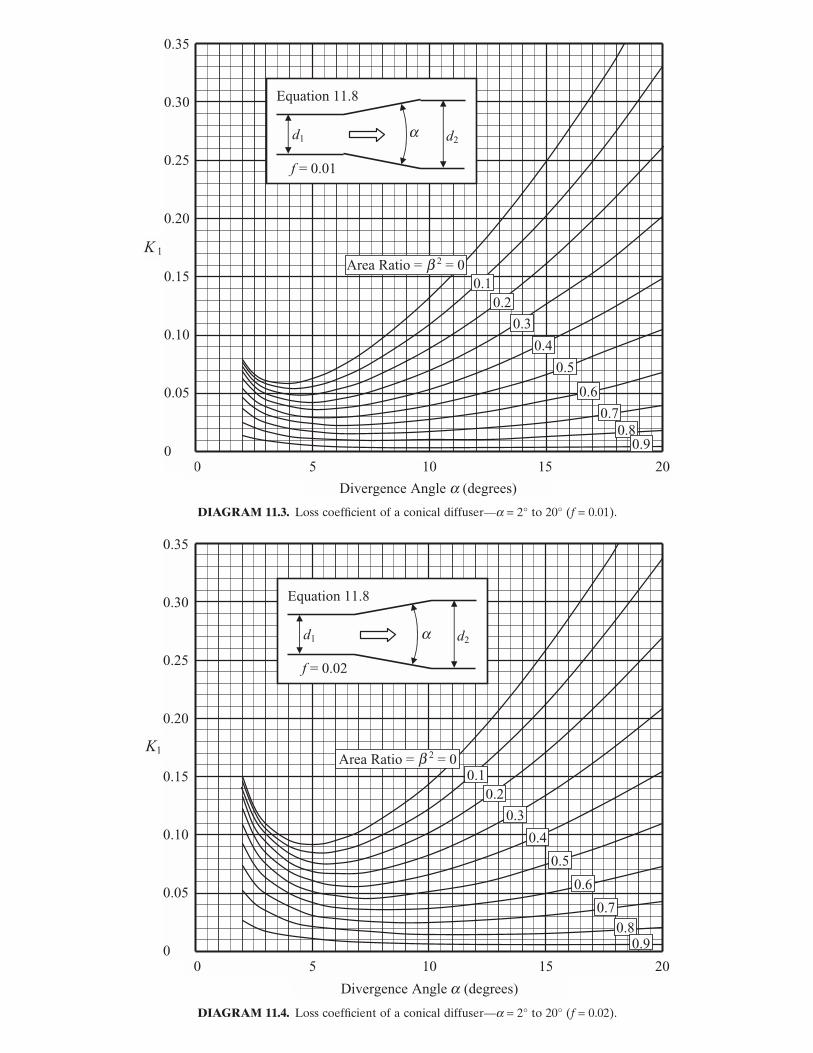
DIAGRAM 11.3. Loss coeffi cient of a conical diffuser — α = 2 ° to 20 ° ( f = 0.01).
Divergence Angle (degrees)
0 5 10 15 20
0.35
0.30
0.25
0.20
0.15
0.10
0.05
0
K 1
Area Ratio = 2 = 00.1
0.2
0.3
0.4
0.5
0.6
0.7 0.8
0.9
d1 d2
f = 0.01
Equation 11.8
a
a
b
DIAGRAM 11.4. Loss coeffi cient of a conical diffuser — α = 2 ° to 20 ° ( f = 0.02).
Divergence Angle (degrees)
0 5 10 15 20
0.35
0.30
0.25
0.20
0.15
0.10
0.05
0
K1Area Ratio = 2 = 0
0.10.2
0.3
0.4
0.5
0.6
0.7
0.8 0.9
d1 d2
f = 0.02
Equation 11.8
a
a
b
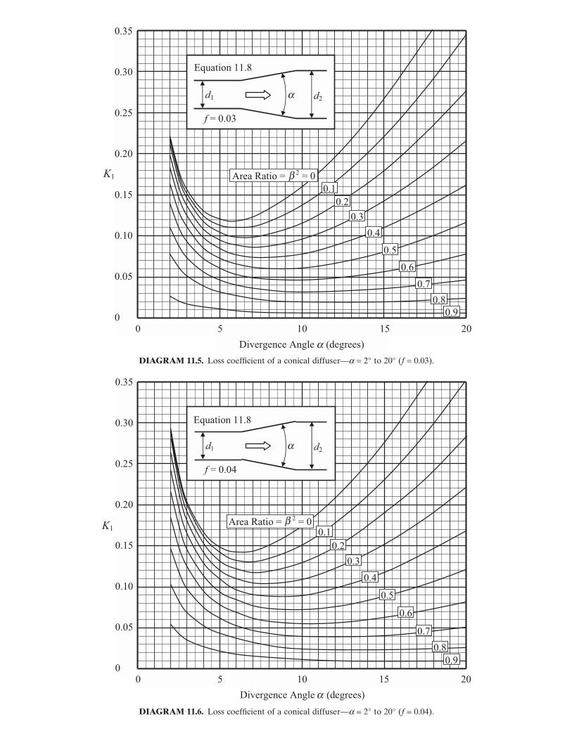
DIAGRAM 11.6. Loss coeffi cient of a conical diffuser — α = 2 ° to 20 ° ( f = 0.04).
Divergence Angle (degrees)
0 5 10 15 20
0.35
0.30
0.25
0.20
0.15
0.10
0.05
0
K1Area Ratio = 2 = 0
0.1
0.2
0.3
0.4
0.5
0.6
0.7
0.8
0.9
d1 d2
f = 0.04
Equation 11.8
a
a
b
DIAGRAM 11.5. Loss coeffi cient of a conical diffuser — α = 2 ° to 20 ° ( f = 0.03).
0 5 10 15 20
0.35
0.30
0.25
0.20
0.15
0.10
0.05
0
K1 Area Ratio = 2 = 0
0.1
0.2
0.3
0.4
0.5
0.6
0.7
0.8
0.9
Divergence Angle (degrees)
d1 d2
f = 0.03
Equation 11.8
a
a
b
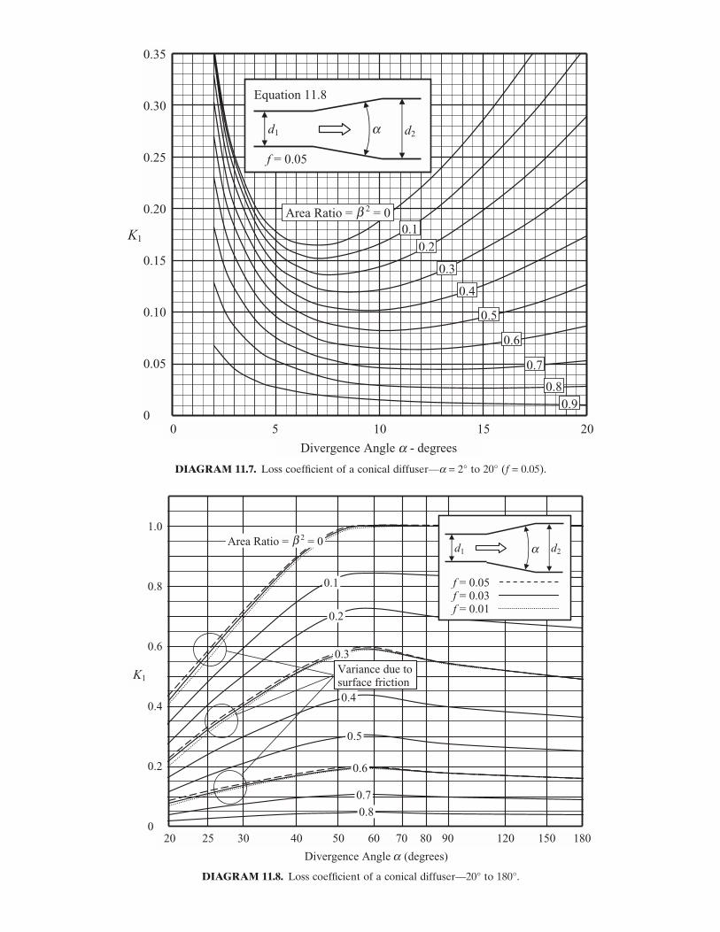
DIAGRAM 11.7. Loss coeffi cient of a conical diffuser — α = 2 ° to 20 ° ( f = 0.05).
Divergence Angle - degrees
0 5 10 15 20
0.35
0.30
0.25
0.20
0.15
0.10
0.05
0
K1
Area Ratio = 2 = 0
0.4
0.5
0.6
0.7
0.8 0.9
d1 d2
f = 0.05
Equation 11.8
a
a
b0.1
0.2
0.3
DIAGRAM 11.8. Loss coeffi cient of a conical diffuser — 20 ° to 180 ° .
Divergence Angle (degrees)
20 25 30 40 50 60 70 80 90 120 150 180
1.0
0.8
0.6
0.4
0.2
0
K1
d1 d2
f = 0.05 f = 0.03 f = 0.01
0.1
0.2
0.4
0.5
0.7
0.8
0.6
0.3
Area Ratio = 2 = 0
Variance due to surface friction
a
a
b
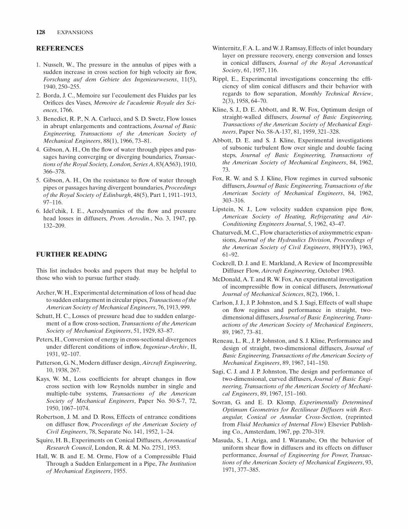
128 EXPANSIONS
Winternitz , F. A. L. and W. J. Ramsay , Effects of inlet boundary layer on pressure recovery, energy conversion and losses in conical diffusers , Journal of the Royal Aeronautical Society , 61 , 1957 , 116 .
Rippl , E. , Experimental investigations concerning the effi -ciency of slim conical diffusers and their behavior with regards to fl ow separation , Monthly Technical Review , 2 ( 3 ), 1958 , 64 – 70 .
Kline , S. J. , D. E. Abbott , and R. W. Fox , Optimum design of straight - walled diffusers , Journal of Basic Engineering, Transactions of the American Society of Mechanical Engi-neers , Paper No. 58 - A - 137, 81 , 1959 , 321 – 328 .
Abbott , D. E. and S. J. Kline , Experimental investigations of subsonic turbulent fl ow over single and double facing steps , Journal of Basic Engineering, Transactions of the American Society of Mechanical Engineers , 84 , 1962 , 73 .
Fox , R. W. and S. J. Kline , Flow regimes in curved subsonic diffusers , Journal of Basic Engineering, Transactions of the American Society of Mechanical Engineers , 84 , 1962 , 303 – 316 .
Lipstein , N. J. , Low velocity sudden expansion pipe fl ow , American Society of Heating, Refrigerating and Air - Conditioning Engineers Journal , 5 , 1962 , 43 – 47 .
Chaturvedi , M. C. , Flow characteristics of axisymmetric expan-sions , Journal of the Hydraulics Division, Proceedings of the American Society of Civil Engineers , 89 ( HY3 ), 1963 , 61 – 92 .
Cockrell , D. J. and E. Markland , A Review of Incompressible Diffuser Flow , Aircraft Engineering , October 1963 .
McDonald , A. T. and R. W. Fox , An experimental investigation of incompressible fl ow in conical diffusers , InternationalJournal of Mechanical Sciences , 8 ( 2 ), 1966 , 1 .
Carlson , J. J. , J. P. Johnston , and S. J. Sagi , Effects of wall shape on fl ow regimes and performance in straight, two - dimensional diffusers , Journal of Basic Engineering, Trans-actions of the American Society of Mechanical Engineers , 89 , 1967 , 73 – 81 .
Reneau , L. R. , J. P. Johnston , and S. J. Kline , Performance and design of straight, two - dimensional diffusers , Journal of Basic Engineering, Transactions of the American Society of Mechanical Engineers , 89 , 1967 , 141 – 150 .
Sagi , C. J. and J. P. Johnston , The design and performance of two - dimensional, curved diffusers , Journal of Basic Engi-neering, Transactions of the American Society of Mechani-cal Engineers , 89 , 1967 , 151 – 160 .
Sovran , G. and E. D. Klomp , Experimentally Determined Optimum Geometries for Rectilinear Diffusers with Rect-angular, Conical or Annular Cross - Section , (reprinted from Fluid Mechanics of Internal Flow ) Elsevier Publish-ing Co. , Amsterdam , 1967 , pp. 270 – 319 .
Masuda , S. , I. Ariga , and I. Waranabe , On the behavior of uniform shear fl ow in diffusers and its effects on diffuser performance , Journal of Engineering for Power, Transac-tions of the American Society of Mechanical Engineers , 93 , 1971 , 377 – 385 .
REFERENCES
1. Nusselt , W. , The pressure in the annulus of pipes with a sudden increase in cross section for high velocity air fl ow , Forschung auf dem Gebiete des Ingenieurwesens , 11 ( 5 ), 1940 , 250 – 255 .
2. Borda , J. C. , Memoire sur l ’ ecoulement des Fluides par les Orifi ces des Vases , Memoire de l ’ academie Royale des Sci-ences , 1766 .
3. Benedict , R. P. , N. A. Carlucci , and S. D. Swetz , Flow losses in abrupt enlargements and contractions , Journal of Basic Engineering, Transactions of the American Society of Mechanical Engineers , 88 ( 1 ), 1966 , 73 – 81 .
4. Gibson , A. H. , On the fl ow of water through pipes and pas-sages having converging or diverging boundaries , Transac-tions of the Royal Society, London, Series A , 83 ( A563 ), 1910 , 366 – 378 .
5. Gibson , A. H. , On the resistance to fl ow of water through pipes or passages having divergent boundaries , Proceedingsof the Royal Society of Edinburgh , 48 ( 5 ), Part 1, 1911 – 1913 , 97 – 116 .
6. Idel ’ chik , I. E. , Aerodynamics of the fl ow and pressure head losses in diffusers , Prom. Aerodin. , No. 3, 1947 , pp. 132 – 209 .
FURTHER READING
This list includes books and papers that may be helpful to those who wish to pursue further study.
Archer , W. H. , Experimental determination of loss of head due to sudden enlargement in circular pipes , Transactions of the American Society of Mechanical Engineers , 76 , 1913 , 999 .
Schutt , H. C. , Losses of pressure head due to sudden enlarge-ment of a fl ow cross - section , Transactions of the American Society of Mechanical Engineers , 51 , 1929 , 83 – 87 .
Peters , H. , Conversion of energy in cross - sectional divergences under different conditions of infl ow , Ingenieur - Archiv , II , 1931 , 92 – 107 .
Patterson , G. N. , Modern diffuser design , Aircraft Engineering , 10 , 1938 , 267 .
Kays , W. M. , Loss coeffi cients for abrupt changes in fl ow cross section with low Reynolds number in single and multiple - tube systems , Transactions of the American Society of Mechanical Engineers , Paper No. 50 - S - 7, 72 , 1950 , 1067 – 1074 .
Robertson , J. M. and D. Ross , Effects of entrance conditions on diffuser fl ow , Proceedings of the American Society of Civil Engineers , 78 , Separate No. 141, 1952 , 1 – 24 .
Squire , H. B. , Experiments on Conical Diffusers , AeronauticalResearch Council , London, R. & M. No. 2751, 1953 .
Hall , W. B. and E. M. Orme , Flow of a Compressible Fluid Through a Sudden Enlargement in a Pipe , The Institution of Mechanical Engineers , 1955 .
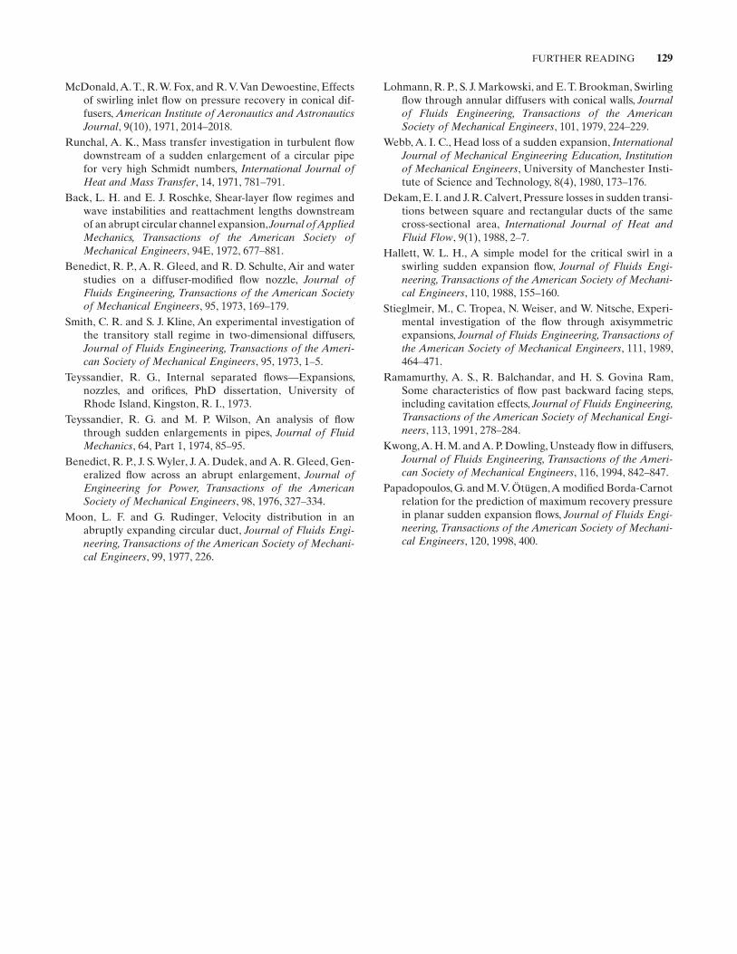
FURTHER READING 129
McDonald , A. T. , R. W. Fox , and R. V. Van Dewoestine , Effects of swirling inlet fl ow on pressure recovery in conical dif-fusers , American Institute of Aeronautics and Astronautics Journal , 9 ( 10 ), 1971 , 2014 – 2018 .
Runchal , A. K. , Mass transfer investigation in turbulent fl ow downstream of a sudden enlargement of a circular pipe for very high Schmidt numbers , International Journal of Heat and Mass Transfer , 14 , 1971 , 781 – 791 .
Back , L. H. and E. J. Roschke , Shear - layer fl ow regimes and wave instabilities and reattachment lengths downstream of an abrupt circular channel expansion , Journal of Applied Mechanics, Transactions of the American Society of Mechanical Engineers , 94E , 1972 , 677 – 881 .
Benedict , R. P. , A. R. Gleed , and R. D. Schulte , Air and water studies on a diffuser - modifi ed fl ow nozzle , Journal of Fluids Engineering, Transactions of the American Society of Mechanical Engineers , 95 , 1973 , 169 – 179 .
Smith , C. R. and S. J. Kline , An experimental investigation of the transitory stall regime in two - dimensional diffusers , Journal of Fluids Engineering, Transactions of the Ameri-can Society of Mechanical Engineers , 95 , 1973 , 1 – 5 .
Teyssandier , R. G. , Internal separated fl ows — Expansions, nozzles, and orifi ces , PhD dissertation, University of Rhode Island, Kingston, R. I., 1973 .
Teyssandier , R. G. and M. P. Wilson , An analysis of fl ow through sudden enlargements in pipes , Journal of Fluid Mechanics , 64 , Part 1, 1974 , 85 – 95 .
Benedict , R. P. , J. S. Wyler , J. A. Dudek , and A. R. Gleed , Gen-eralized fl ow across an abrupt enlargement , Journal of Engineering for Power, Transactions of the American Society of Mechanical Engineers , 98 , 1976 , 327 – 334 .
Moon , L. F. and G. Rudinger , Velocity distribution in an abruptly expanding circular duct , Journal of Fluids Engi-neering, Transactions of the American Society of Mechani-cal Engineers , 99 , 1977 , 226 .
Lohmann , R. P. , S. J. Markowski , and E. T. Brookman , Swirling fl ow through annular diffusers with conical walls , Journal of Fluids Engineering, Transactions of the American Society of Mechanical Engineers , 101 , 1979 , 224 – 229 .
Webb , A. I. C. , Head loss of a sudden expansion , InternationalJournal of Mechanical Engineering Education, Institution of Mechanical Engineers , University of Manchester Insti-tute of Science and Technology, 8 ( 4 ), 1980 , 173 – 176 .
Dekam , E. I. and J. R. Calvert , Pressure losses in sudden transi-tions between square and rectangular ducts of the same cross - sectional area , International Journal of Heat and Fluid Flow , 9 ( 1 ), 1988 , 2 – 7 .
Hallett , W. L. H. , A simple model for the critical swirl in a swirling sudden expansion fl ow , Journal of Fluids Engi-neering, Transactions of the American Society of Mechani-cal Engineers , 110 , 1988 , 155 – 160 .
Stieglmeir , M. , C. Tropea , N. Weiser , and W. Nitsche , Experi-mental investigation of the fl ow through axisymmetric expansions , Journal of Fluids Engineering, Transactions of the American Society of Mechanical Engineers , 111 , 1989 , 464 – 471 .
Ramamurthy , A. S. , R. Balchandar , and H. S. Govina Ram , Some characteristics of fl ow past backward facing steps, including cavitation effects , Journal of Fluids Engineering, Transactions of the American Society of Mechanical Engi-neers , 113 , 1991 , 278 – 284 .
Kwong , A. H. M. and A. P. Dowling , Unsteady fl ow in diffusers , Journal of Fluids Engineering, Transactions of the Ameri-can Society of Mechanical Engineers , 116 , 1994 , 842 – 847 .
Papadopoulos , G. and M. V. Ö t ü gen , A modifi ed Borda - Carnot relation for the prediction of maximum recovery pressure in planar sudden expansion fl ows , Journal of Fluids Engi-neering, Transactions of the American Society of Mechani-cal Engineers , 120 , 1998 , 400 .
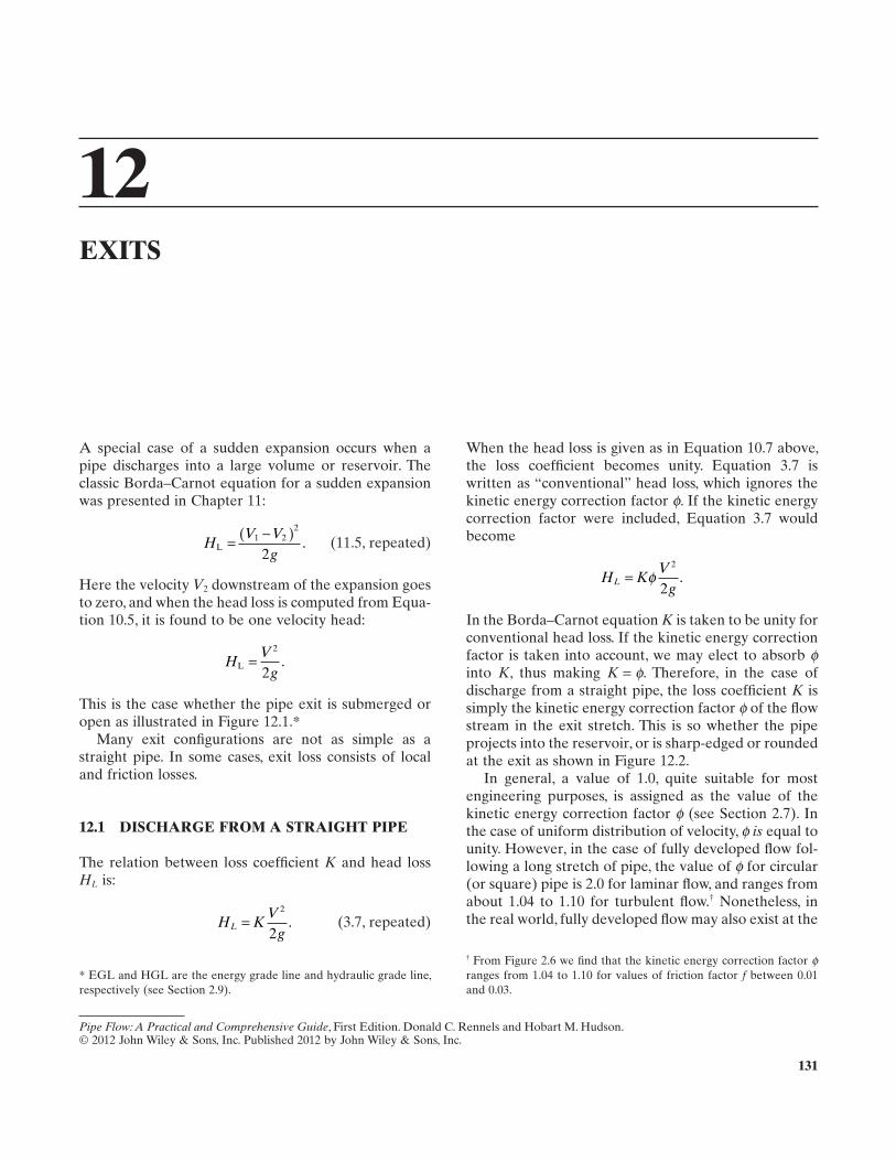
131
12 EXITS
A special case of a sudden expansion occurs when a pipe discharges into a large volume or reservoir. The classic Borda – Carnot equation for a sudden expansion was presented in Chapter 11 :
HV V
gL = −( )1 2
2
2. (11.5, repeated)
Here the velocity V 2 downstream of the expansion goes to zero, and when the head loss is computed from Equa-tion 10.5 , it is found to be one velocity head:
HV
gL .=
2
2
This is the case whether the pipe exit is submerged or open as illustrated in Figure 12.1 . *
Many exit confi gurations are not as simple as a straight pipe. In some cases, exit loss consists of local and friction losses.
12.1 DISCHARGE FROM A STRAIGHT PIPE
The relation between loss coeffi cient K and head loss H L is:
H KV
gL =
2
2. (3.7, repeated)
When the head loss is given as in Equation 10.7 above, the loss coeffi cient becomes unity. Equation 3.7 is written as “ conventional ” head loss, which ignores the kinetic energy correction factor ϕ . If the kinetic energy correction factor were included, Equation 3.7 would become
H KV
gL = φ
2
2.
In the Borda – Carnot equation K is taken to be unity for conventional head loss. If the kinetic energy correction factor is taken into account, we may elect to absorb ϕ into K , thus making K = ϕ . Therefore, in the case of discharge from a straight pipe, the loss coeffi cient K is simply the kinetic energy correction factor ϕ of the fl ow stream in the exit stretch. This is so whether the pipe projects into the reservoir, or is sharp - edged or rounded at the exit as shown in Figure 12.2 .
In general, a value of 1.0, quite suitable for most engineering purposes, is assigned as the value of the kinetic energy correction factor ϕ (see Section 2.7 ). In the case of uniform distribution of velocity, ϕ is equal to unity. However, in the case of fully developed fl ow fol-lowing a long stretch of pipe, the value of ϕ for circular (or square) pipe is 2.0 for laminar fl ow, and ranges from about 1.04 to 1.10 for turbulent fl ow. † Nonetheless, in the real world, fully developed fl ow may also exist at the
Pipe Flow: A Practical and Comprehensive Guide, First Edition. Donald C. Rennels and Hobart M. Hudson.© 2012 John Wiley & Sons, Inc. Published 2012 by John Wiley & Sons, Inc.
* EGL and HGL are the energy grade line and hydraulic grade line, respectively (see Section 2.9 ).
† From Figure 2.6 we fi nd that the kinetic energy correction factor ϕ ranges from 1.04 to 1.10 for values of friction factor f between 0.01 and 0.03.
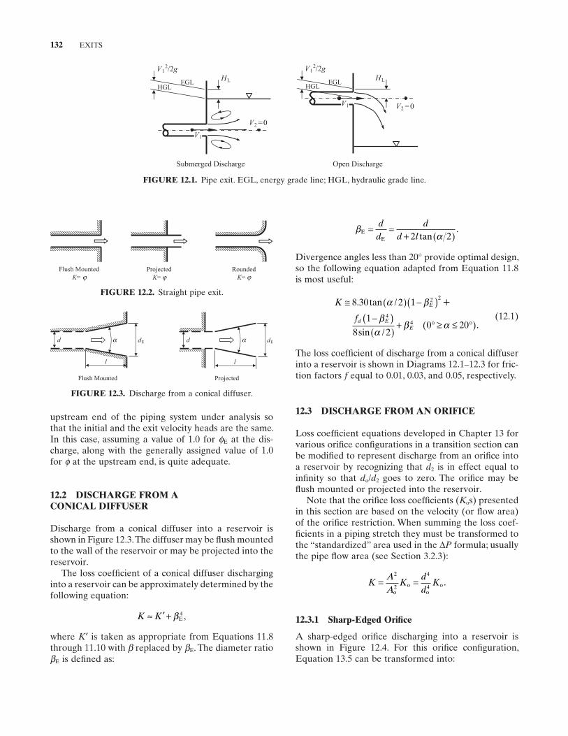
132 EXITS
βEE
.= =+ ( )
dd
dd l2 2tan α
Divergence angles less than 20 ° provide optimal design, so the following equation adapted from Equation 11.8 is most useful:
K
f
E
d EE
≅ ( ) −( )−( )( )
+ ° ≥ ≤ °( )
+8 30 2 1
1
8 20 20
2 2
44
. tan /
sin /.
α
α
β
ββ α
(12.1)
The loss coeffi cient of discharge from a conical diffuser into a reservoir is shown in Diagrams 12.1 – 12.3 for fric-tion factors f equal to 0.01, 0.03, and 0.05, respectively.
12.3 DISCHARGE FROM AN ORIFICE
Loss coeffi cient equations developed in Chapter 13 for various orifi ce confi gurations in a transition section can be modifi ed to represent discharge from an orifi ce into a reservoir by recognizing that d 2 is in effect equal to infi nity so that d o / d 2 goes to zero. The orifi ce may be fl ush mounted or projected into the reservoir.
Note that the orifi ce loss coeffi cients ( K o s) presented in this section are based on the velocity (or fl ow area) of the orifi ce restriction. When summing the loss coef-fi cients in a piping stretch they must be transformed to the “ standardized ” area used in the Δ P formula; usually the pipe fl ow area (see Section 3.2.3 ):
KAA
Kdd
K= =2 4
o2 o
o4 o.
12.3.1 Sharp - Edged Orifi ce
A sharp - edged orifi ce discharging into a reservoir is shown in Figure 12.4 . For this orifi ce confi guration, Equation 13.5 can be transformed into:
upstream end of the piping system under analysis so that the initial and the exit velocity heads are the same. In this case, assuming a value of 1.0 for ϕ E at the dis-charge, along with the generally assigned value of 1.0 for ϕ at the upstream end, is quite adequate.
12.2 DISCHARGE FROM A CONICAL DIFFUSER
Discharge from a conical diffuser into a reservoir is shown in Figure 12.3 . The diffuser may be fl ush mounted to the wall of the reservoir or may be projected into the reservoir.
The loss coeffi cient of a conical diffuser discharging into a reservoir can be approximately determined by the following equation:
K K≈ ′ + βE4 ,
where K ′ is taken as appropriate from Equations 11.8 through 11.10 with β replaced by β E . The diameter ratio β E is defi ned as:
FIGURE 12.1. Pipe exit. EGL, energy grade line; HGL, hydraulic grade line.
HGL
V1
V2 =0
HLEGL
V12/2g
Submerged Discharge
HGL EGL
V1 V2 =0
2V /2g1HL
Open Discharge
FIGURE 12.2. Straight pipe exit.
RoundedK=
Projected K=
Flush Mounted K= j jj
FIGURE 12.3. Discharge from a conical diffuser.
d
l
dEd
l
dE
Flush Mounted Projected
a a
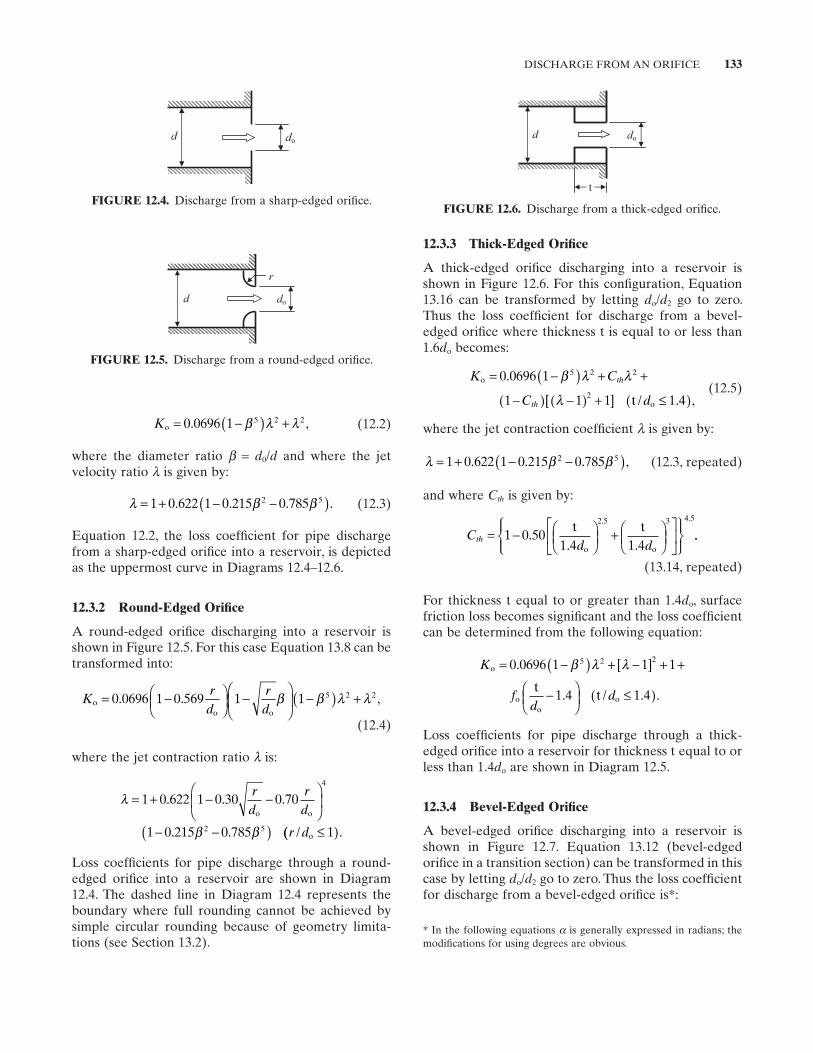
DISCHARGE FROM AN ORIFICE 133
Ko = −( ) +0 0696 1 5 2 2. ,β λ λ (12.2)
where the diameter ratio β = d 0 / d and where the jet velocity ratio λ is given by:
λ β β= + − −( )1 0 622 1 0 215 0 7852 5. . . . (12.3)
Equation 12.2 , the loss coeffi cient for pipe discharge from a sharp - edged orifi ce into a reservoir, is depicted as the uppermost curve in Diagrams 12.4 – 12.6 .
12.3.2 Round - Edged Orifi ce
A round - edged orifi ce discharging into a reservoir is shown in Figure 12.5 . For this case Equation 13.8 can be transformed into:
K
rd
rd
oo o
= −⎛⎝⎜
⎞⎠⎟
−⎛
⎝⎜
⎞
⎠⎟ −( ) +0 0696 1 0 569 1 1 5 2 2. . ,β β λ λ
(12.4)
where the jet contraction ratio λ is:
λ = + − −
⎛
⎝⎜
⎞
⎠⎟
− −( ) ≤
1 0 622 1 0 30 0 70
1 0 215 0 785 1
4
2 5
. . .
. . /
rd
rd
r d
o o
oβ β (( ).
Loss coeffi cients for pipe discharge through a round - edged orifi ce into a reservoir are shown in Diagram 12.4 . The dashed line in Diagram 12.4 represents the boundary where full rounding cannot be achieved by simple circular rounding because of geometry limita-tions (see Section 13.2 ).
FIGURE 12.4. Discharge from a sharp - edged orifi ce.
d do
12.3.3 Thick - Edged Orifi ce
A thick - edged orifi ce discharging into a reservoir is shown in Figure 12.6 . For this confi guration, Equation 13.16 can be transformed by letting d o / d 2 go to zero. Thus the loss coeffi cient for discharge from a bevel - edged orifi ce where thickness t is equal to or less than 1.6 d o becomes:
K C
C d
th
th
o
o[ ] t 1.4 ,
= −( ) + +
−( ) −( ) + ≤( )
0 0696 1
1 1 1
5 2 2
2
.
/
β λ
λ
λ (12.5)
where the jet contraction coeffi cient λ is given by:
λ β β= + − −( )1 0 622 1 0 215 0 7852 5. . . , (12.3, repeated)
and where C th is given by:
C
d dth = − ⎛
⎝⎜⎞⎠⎟
+ ⎛⎝⎜
⎞⎠⎟
⎡
⎣⎢
⎤
⎦⎥
⎧⎨⎪
⎩⎪
⎫⎬⎪
⎭⎪1 0 50
1 4 1 4
2 5 3 4 5
.. .
. .t t
o o
..
(13.14, repeated)
For thickness t equal to or greater than 1.4 d o , surface friction loss becomes signifi cant and the loss coeffi cient can be determined from the following equation:
K
fd
d
o
oo
ot
t
= −( ) + −[ ] + +
−⎛⎝⎜
⎞⎠⎟
≤( )
0 0696 1 1 1
1 4 1 4
5 2 2.
. / . .
β λ λ
Loss coeffi cients for pipe discharge through a thick - edged orifi ce into a reservoir for thickness t equal to or less than 1.4 d o are shown in Diagram 12.5 .
12.3.4 Bevel - Edged Orifi ce
A bevel - edged orifi ce discharging into a reservoir is shown in Figure 12.7 . Equation 13.12 (bevel - edged orifi ce in a transition section) can be transformed in this case by letting d o / d 2 go to zero. Thus the loss coeffi cient for discharge from a bevel - edged orifi ce is * :
FIGURE 12.5. Discharge from a round - edged orifi ce.
d do
r
FIGURE 12.6. Discharge from a thick - edged orifi ce.
d do
t
* In the following equations α is generally expressed in radians; the modifi cations for using degrees are obvious.
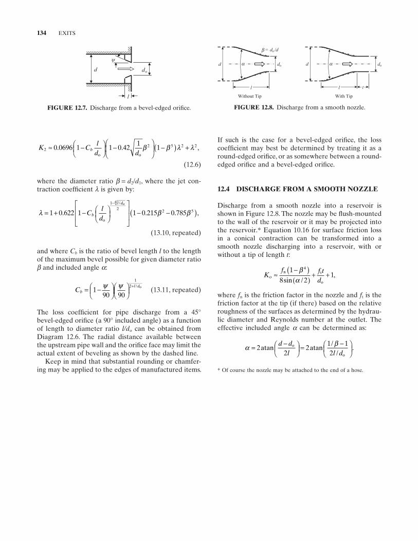
134 EXITS
If such is the case for a bevel - edged orifi ce, the loss coeffi cient may best be determined by treating it as a round - edged orifi ce, or as somewhere between a round - edged orifi ce and a bevel - edged orifi ce.
12.4 DISCHARGE FROM A SMOOTH NOZZLE
Discharge from a smooth nozzle into a reservoir is shown in Figure 12.8 . The nozzle may be fl ush - mounted to the wall of the reservoir or it may be projected into the reservoir. * Equation 10.16 for surface friction loss in a conical contraction can be transformed into a smooth nozzle discharging into a reservoir, with or without a tip of length t :
Kf f t
do
n t
o
≈−( )( )
+ +1
8 21
4βαsin /
,
where f n is the friction factor in the nozzle and f t is the friction factor at the tip (if there) based on the relative roughness of the surfaces as determined by the hydrau-lic diameter and Reynolds number at the outlet. The effective included angle α can be deter mined as:
α β= −⎛⎝⎜
⎞⎠⎟
= −⎛⎝⎜
⎞⎠⎟
22
21 12
atan atan .o
o
d dl l d
//
K C
ld d
b22 5 2 20 0696 1 1 0 42
11≈ −⎛
⎝⎜⎞⎠⎟
−⎛
⎝⎜
⎞
⎠⎟ −( ) +. . ,
o o
β β λ λ
(12.6)
where the diameter ratio β = d 2 / d 1 , where the jet con-traction coeffi cient λ is given by:
λ = + − ⎛⎝⎜
⎞⎠⎟
⎡
⎣
⎢⎢
⎤
⎦
⎥⎥
− −( )−
1 0 622 1 1 0 215 0 785
1
2 5
4
. . .
/
Cl
db
l d
o
2o
,β β
(13.10, repeated)
and where C b is the ratio of bevel length l to the length of the maximum bevel possible for given diameter ratio β and included angle α :
Cbl d
= −⎛⎝⎜
⎞⎠⎟⎛⎝⎜
⎞⎠⎟
+1
90 90
12ψ ψ / o (13.11, repeated)
The loss coeffi cient for pipe discharge from a 45 ° bevel - edged orifi ce (a 90 ° included angle) as a function of length to diameter ratio l/d o can be obtained from Diagram 12.6 . The radial distance available between the upstream pipe wall and the orifi ce face may limit the actual extent of beveling as shown by the dashed line.
Keep in mind that substantial rounding or chamfer-ing may be applied to the edges of manufactured items.
FIGURE 12.8. Discharge from a smooth nozzle.
d do
= do /d
l
do
l
d
t
Without Tip With Tip
a
b
a
* Of course the nozzle may be attached to the end of a hose.
FIGURE 12.7. Discharge from a bevel - edged orifi ce.
d do
ψ
l
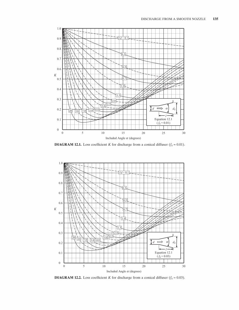
DISCHARGE FROM A SMOOTH NOZZLE 135
DIAGRAM 12.1. Loss coeffi cient K for discharge from a conical diffuser ( f d = 0.01).
K
1.0
0.9
0.8
0.7
0.6
0.5
0.4
0.3
0.2
0.1
0
Included Angle a (degrees)
5 10 15 20 25
1.0
1.5
2.02.5
3.04.05.07.01020
30
0.5
0.7
0
dEd a
lEquation 12.1
( fd = 0.01)
l/d = 0.1
0.3
DIAGRAM 12.2. Loss coeffi cient K for discharge from a conical diffuser ( f d = 0.03).
K
1.0
0.9
0.8
0.7
0.6
0.5
0.4
0.3
0.2
0.1
0
Included Angle a (degrees)
5 10 15 20 25
1.0
1.5
2.02.5
3.04.05.07.01020
30
0.5
0.7
0
dEd
lEquation 12.1
( fd = 0.03)
l/d = 0.1
0.3
a
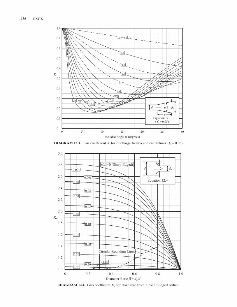
136 EXITS
DIAGRAM 12.3. Loss coeffi cient K for discharge from a conical diffuser ( f d = 0.05).
K
1.0
0.9
0.8
0.7
0.6
0.5
0.4
0.3
0.2
0.1
0
Included Angle a (degrees)
5 10 15 20 25
1.0
1.5
2.02.53.0
4.05.07.01020
30
0.5
0.7
0
dEd a
lEquation 12.1
( fd = 0.05)
l/d = 0.1
0.3
DIAGRAM 12.4. Loss coeffi cient K o for discharge from a round - edged orifi ce.
0.01
0.07
0.15
0.30
0.001
0.03
0.70
1.00
0.20
0.005
0.02
0.10
0.50
0.05
3.0
2.8
2.6
2.4
2.2
2.0
1.8
1.6
1.4
1.2
1.00 0.4 0.6 0.8 1.00.2
Diameter Ratio do/d
Ko
Equation 12.4
d do
r
Circular Rounding Limit
r/do=0 (Sharp-Edged)
b =
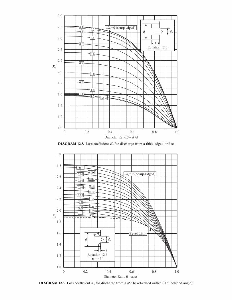
3.0
2.8
2.6
2.4
2.2
2.0
1.8
1.6
1.4
1.2
1.00 0.4 0.6 0.8 1.00.2
Diameter Ratio do/d
Ko
0.3
0.7
0.4
0.8
1.1
0.5
1.2
0.2 0.1
≥1.4
t/do=0 (sharp edged)
Equation 12.5
d do
t
0.9
1.0
0.6
b =
DIAGRAM 12.5. Loss coeffi cient K o for discharge from a thick - edged orifi ce.
1.0
0.10
0.2
0.4 0.5
3.0
2.8
2.6
2.4
2.2
2.0
1.8
1.6
1.4
1.2
1.00 0.4 0.6 0.8 1.0 0.2
Diameter Ratio do/d
Ko
Bevel Limit
l/do=0 (Sharp-Edged)
0.7
0.15
0.3
0.001
0.0050.01
0.02 0.03
0.05 0.07
2.0
Equation 12.6 = 45˚
d do
l
b
y
y
=
DIAGRAM 12.6. Loss coeffi cient K o for discharge from a 45 ° bevel - edged orifi ce (90 ° included angle).
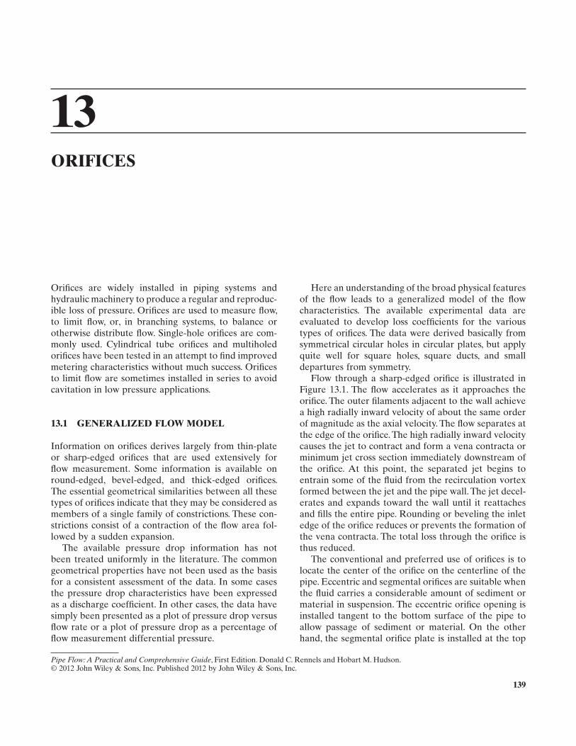
139
13 ORIFICES
Orifi ces are widely installed in piping systems and hydraulic machinery to produce a regular and reproduc-ible loss of pressure. Orifi ces are used to measure fl ow, to limit fl ow, or, in branching systems, to balance or otherwise distribute fl ow. Single - hole orifi ces are com-monly used. Cylindrical tube orifi ces and multiholed orifi ces have been tested in an attempt to fi nd improved metering characteristics without much success. Orifi ces to limit fl ow are sometimes installed in series to avoid cavitation in low pressure applications.
13.1 GENERALIZED FLOW MODEL
Information on orifi ces derives largely from thin - plate or sharp - edged orifi ces that are used extensively for fl ow measurement. Some information is available on round - edged, bevel - edged, and thick - edged orifi ces. The essential geometrical similarities between all these types of orifi ces indicate that they may be considered as members of a single family of constrictions. These con-strictions consist of a contraction of the fl ow area fol-lowed by a sudden expansion.
The available pressure drop information has not been treated uniformly in the literature. The common geometrical properties have not been used as the basis for a consistent assessment of the data. In some cases the pressure drop characteristics have been expressed as a discharge coeffi cient. In other cases, the data have simply been presented as a plot of pressure drop versus fl ow rate or a plot of pressure drop as a percentage of fl ow measurement differential pressure.
Here an understanding of the broad physical features of the fl ow leads to a generalized model of the fl ow characteristics. The available experimental data are evaluated to develop loss coeffi cients for the various types of orifi ces. The data were derived basically from symmetrical circular holes in circular plates, but apply quite well for square holes, square ducts, and small departures from symmetry.
Flow through a sharp - edged orifi ce is illustrated in Figure 13.1 . The fl ow accelerates as it approaches the orifi ce. The outer fi laments adjacent to the wall achieve a high radially inward velocity of about the same order of magnitude as the axial velocity. The fl ow separates at the edge of the orifi ce. The high radially inward velocity causes the jet to contract and form a vena contracta or minimum jet cross section immediately downstream of the orifi ce. At this point, the separated jet begins to entrain some of the fl uid from the recirculation vortex formed between the jet and the pipe wall. The jet decel-erates and expands toward the wall until it reattaches and fi lls the entire pipe. Rounding or beveling the inlet edge of the orifi ce reduces or prevents the formation of the vena contracta. The total loss through the orifi ce is thus reduced.
The conventional and preferred use of orifi ces is to locate the center of the orifi ce on the centerline of the pipe. Eccentric and segmental orifi ces are suitable when the fl uid carries a considerable amount of sediment or material in suspension. The eccentric orifi ce opening is installed tangent to the bottom surface of the pipe to allow passage of sediment or material. On the other hand, the segmental orifi ce plate is installed at the top
Pipe Flow: A Practical and Comprehensive Guide, First Edition. Donald C. Rennels and Hobart M. Hudson.© 2012 John Wiley & Sons, Inc. Published 2012 by John Wiley & Sons, Inc.
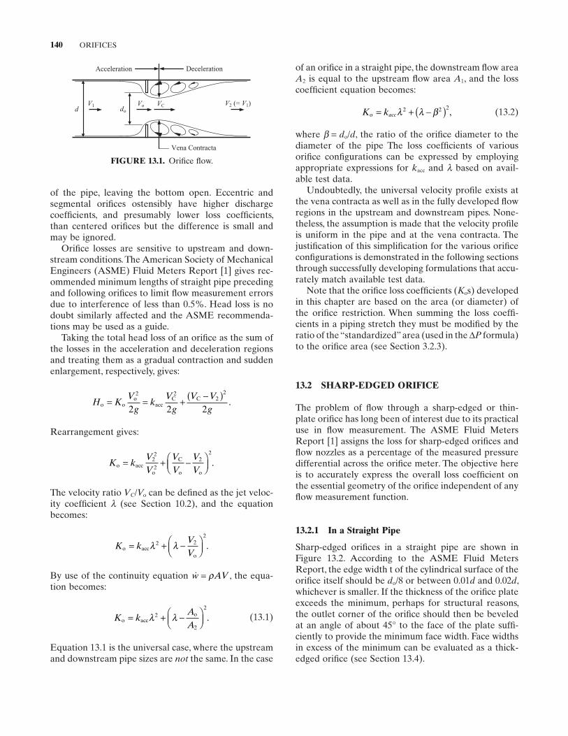
140 ORIFICES
of an orifi ce in a straight pipe, the downstream fl ow area A2 is equal to the upstream fl ow area A1 , and the loss coeffi cient equation becomes:
K kacco = + −( )λ λ β2 2 2, (13.2)
where β = do / d , the ratio of the orifi ce diameter to the diameter of the pipe The loss coeffi cients of various orifi ce confi gurations can be expressed by employing appropriate expressions for kacc and λ based on avail-able test data.
Undoubtedly, the universal velocity profi le exists at the vena contracta as well as in the fully developed fl ow regions in the upstream and downstream pipes. None-theless, the assumption is made that the velocity profi le is uniform in the pipe and at the vena contracta. The justifi cation of this simplifi cation for the various orifi ce confi gurations is demonstrated in the following sections through successfully developing formulations that accu-rately match available test data.
Note that the orifi ce loss coeffi cients ( Ko s) developed in this chapter are based on the area (or diameter) of the orifi ce restriction. When summing the loss coeffi -cients in a piping stretch they must be modifi ed by the ratio of the “ standardized ” area (used in the ΔP formula) to the orifi ce area (see Section 3.2.3 ).
13.2 SHARP - EDGED ORIFICE
The problem of fl ow through a sharp - edged or thin - plate orifi ce has long been of interest due to its practical use in fl ow measurement. The ASME Fluid Meters Report [1] assigns the loss for sharp - edged orifi ces and fl ow nozzles as a percentage of the measured pressure differential across the orifi ce meter. The objective here is to accurately express the overall loss coeffi cient on the essential geometry of the orifi ce independent of any fl ow measurement function.
13.2.1 In a Straight Pipe
Sharp - edged orifi ces in a straight pipe are shown in Figure 13.2 . According to the ASME Fluid Meters Report, the edge width t of the cylindrical surface of the orifi ce itself should be do /8 or between 0.01 d and 0.02 d , whichever is smaller. If the thickness of the orifi ce plate exceeds the minimum, perhaps for structural reasons, the outlet corner of the orifi ce should then be beveled at an angle of about 45 ° to the face of the plate suffi -ciently to provide the minimum face width. Face widths in excess of the minimum can be evaluated as a thick - edged orifi ce (see Section 13.4 ).
of the pipe, leaving the bottom open. Eccentric and segmental orifi ces ostensibly have higher discharge coeffi cients, and presumably lower loss coeffi cients, than centered orifi ces but the difference is small and may be ignored.
Orifi ce losses are sensitive to upstream and down-stream conditions. The American Society of Mechanical Engineers (ASME) Fluid Meters Report [1] gives rec-ommended minimum lengths of straight pipe preceding and following orifi ces to limit fl ow measurement errors due to interference of less than 0.5%. Head loss is no doubt similarly affected and the ASME recommenda-tions may be used as a guide.
Taking the total head loss of an orifi ce as the sum of the losses in the acceleration and deceleration regions and treating them as a gradual contraction and sudden enlargement, respectively, gives:
H KV
gk
Vg
V Vg
o oo
accC C .= = +
−( )2 22
2
2 2 2
Rearrangement gives:
K kVV
VV
VV
o acco
C
o o
2
.= + −
22
22
The velocity ratio VC / Vo can be defi ned as the jet veloc-ity coeffi cient λ (see Section 10.2 ), and the equation becomes:
K kVV
o acco
.= + −
λ λ2 2
2
By use of the continuity equation w AV= ρ , the equa-tion becomes:
K kAA
o acco .= + −
λ λ2
2
2
(13.1)
Equation 13.1 is the universal case, where the upstream and downstream pipe sizes are not the same. In the case
FIGURE 13.1. Orifi ce fl ow.
d
DecelerationAcceleration
Vena Contracta
V2 (= V1)V1 VCdo
Vo
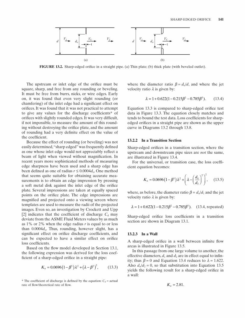
SHARP-EDGED ORIFICE 141
where the diameter ratio β = do / d , and where the jet velocity ratio λ is given by:
λ β β= + − −1 0 622 1 0 215 0 7852 5. ( . . ). (13.4)
Equation 13.3 is compared to sharp - edged orifi ce test data in Figure 13.3 . The equation closely matches and tends to bound the test data. Loss coeffi cients for sharp - edged orifi ces in a straight pipe are shown as the upper curve in Diagrams 13.2 through 13.8 .
13.2.2 In a Transition Section
Sharp - edged orifi ces in a transition section, where the upstream and downstream pipe sizes are not the same, are illustrated in Figure 13.4 .
For the universal, or transition case, the loss coeffi -cient equation becomes:
Kdd
oo= −( ) + −
0 0696 1 5 2
2
2 2
. ,β λ λ (13.5)
where, as before, the diameter ratio β = do / d1 and the jet velocity ratio λ is given by:
λ β β= + − −1 0 622 1 0 215 0 7852 5. ( . . ). (13.4, repeated)
Sharp - edged orifi ce loss coeffi cients in a transition section are shown in Diagram 13.1 .
13.2.3 In a Wall
A sharp - edged orifi ce in a wall between infi nite fl ow areas is illustrated in Figure 13.5 .
In this passage from one large volume to another, the effective diameters, d1 and d2 are in effect equal to infi n-ity; thus β = 0 and Equation 13.4 reduces to λ = 1.622. Also do / d2 = 0, so that substitution into Equation 13.5 yields the following result for a sharp - edged orifi ce in a wall:
Ko = 2 81. .
The upstream or inlet edge of the orifi ce must be square, sharp, and free from any rounding or beveling. It must be free from burrs, nicks, or wire edges. Early on, it was found that even very slight rounding (or chamfering) of the inlet edge had a signifi cant effect on orifi ces. It was found that it was not practical to attempt to give any values for the discharge coeffi cients * of orifi ces with slightly rounded edges. It was very diffi cult, if not impossible, to measure the amount of this round-ing without destroying the orifi ce plate, and the amount of rounding had a very defi nite effect on the value of the coeffi cient.
Because the effect of rounding (or beveling) was not easily determined, “ sharp edged ” was frequently defi ned as one whose inlet edge would not appreciably refl ect a beam of light when viewed without magnifi cation. In recent years more sophisticated methods of measuring edge sharpness have been used and a sharp edge has been defi ned as one of radius r ≤ 0.0004 do . One method that seems quite suitable for obtaining accurate mea-surements is to obtain an edge impression by pressing a soft metal disk against the inlet edge of the orifi ce plate. Several impressions are taken at equally spaced points on the orifi ce plate. The edge impressions are magnifi ed and projected onto a viewing screen where templates are used to measure the radii of the projected images. Even so, an investigation by Crockett and Upp [2] indicates that the coeffi cient of discharge Cd may deviate from the ASME Fluid Meters values by as much as 1% or 2% when the edge radius r is equal to or less than 0.0004 do . Thus, rounding, however slight, has a signifi cant effect on orifi ce discharge coeffi cients, and can be expected to have a similar effect on orifi ce loss coeffi cients.
Based on the fl ow model developed in Section 13.1 , the following expression was derived for the loss coef-fi cient of a sharp - edged orifi ce in a straight pipe:
Ko = −( ) + −( )0 0696 1 5 2 2 2. ,β λ λ β (13.3)
FIGURE 13.2. Sharp - edged orifi ce in a straight pipe. (a) Thin plate; (b) thick plate (with beveled outlet).
(a)
dV2V1 VCdo
t
(b)
dV2V1 VCdo
t
* The coeffi cient of discharge is defi ned by the equation: Cd = actual rate of fl ow/theoretical rate of fl ow.
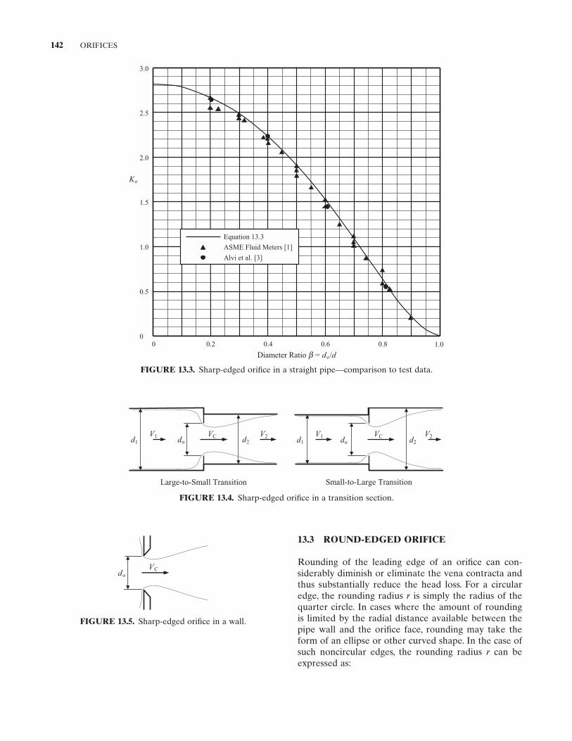
142 ORIFICES
FIGURE 13.3. Sharp - edged orifi ce in a straight pipe — comparison to test data.
3.0
2.5
2.0
1.5
1.0
0.5
0
Ko
Equation 13.3
ASME Fluid Meters [1]
Alvi et al. [3]
Diameter Ratio = do/d
0 0.4 0.6 0.8 1.00.2
b
FIGURE 13.4. Sharp - edged orifi ce in a transition section.
d1V2V1 VCdo d2
Small-to-Large Transition
d1V2V1 VCdo d2
Large-to-Small Transition
13.3 ROUND - EDGED ORIFICE
Rounding of the leading edge of an orifi ce can con-siderably diminish or eliminate the vena contracta and thus substantially reduce the head loss. For a circular edge, the rounding radius r is simply the radius of the quarter circle. In cases where the amount of rounding is limited by the radial distance available between the pipe wall and the orifi ce face, rounding may take the form of an ellipse or other curved shape. In the case of such noncircular edges, the rounding radius r can be expressed as:
FIGURE 13.5. Sharp - edged orifi ce in a wall.
VCdo
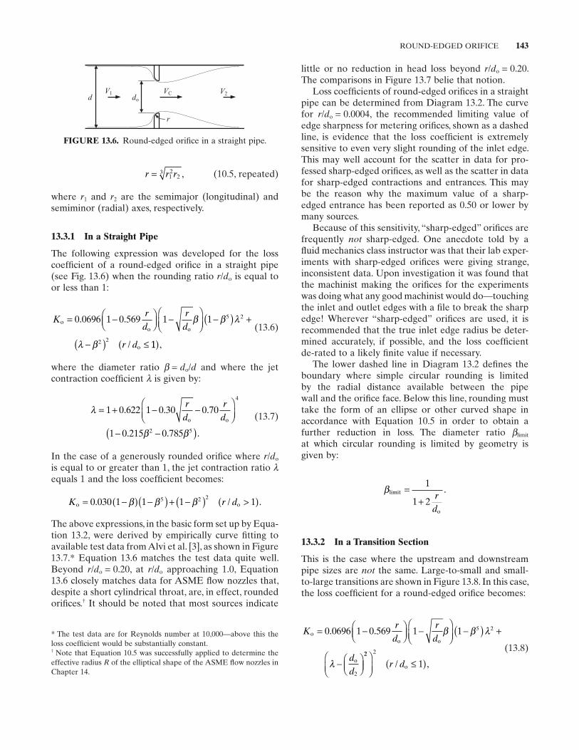
ROUND-EDGED ORIFICE 143
little or no reduction in head loss beyond r / do = 0.20. The comparisons in Figure 13.7 belie that notion.
Loss coeffi cients of round - edged orifi ces in a straight pipe can be determined from Diagram 13.2 . The curve for r / do = 0.0004, the recommended limiting value of edge sharpness for metering orifi ces, shown as a dashed line, is evidence that the loss coeffi cient is extremely sensitive to even very slight rounding of the inlet edge. This may well account for the scatter in data for pro-fessed sharp - edged orifi ces, as well as the scatter in data for sharp - edged contractions and entrances. This may be the reason why the maximum value of a sharp - edged entrance has been reported as 0.50 or lower by many sources.
Because of this sensitivity, “ sharp - edged ” orifi ces are frequently not sharp - edged. One anecdote told by a fl uid mechanics class instructor was that their lab exper-iments with sharp - edged orifi ces were giving strange, inconsistent data. Upon investigation it was found that the machinist making the orifi ces for the experiments was doing what any good machinist would do — touching the inlet and outlet edges with a fi le to break the sharp edge! Wherever “ sharp - edged ” orifi ces are used, it is recommended that the true inlet edge radius be deter-mined accurately, if possible, and the loss coeffi cient de - rated to a likely fi nite value if necessary.
The lower dashed line in Diagram 13.2 defi nes the boundary where simple circular rounding is limited by the radial distance available between the pipe wall and the orifi ce face. Below this line, rounding must take the form of an ellipse or other curved shape in accordance with Equation 10.5 in order to obtain a further reduction in loss. The diameter ratio βlimit
at which circular rounding is limited by geometry is given by:
βlimit
o
.=+
1
1 2r
d
13.3.2 In a Transition Section
This is the case where the upstream and downstream pipe sizes are not the same. Large - to - small and small - to - large transitions are shown in Figure 13.8 . In this case, the loss coeffi cient for a round - edged orifi ce becomes:
Kr
dr
d
dd
oo o
o
= −
−
−( ) +
−
0 0696 1 0 569 1 1 5 2
2
. . β β λ
λ22 2
1
≤( )r d/ ,o
(13.8)
r r r= 12
23 , (10.5, repeated)
where r1 and r2 are the semimajor (longitudinal) and semiminor (radial) axes, respectively.
13.3.1 In a Straight Pipe
The following expression was developed for the loss coeffi cient of a round - edged orifi ce in a straight pipe (see Fig. 13.6 ) when the rounding ratio r / do is equal to or less than 1:
Kr
dr
d
r d
oo o
o
= −
−
−( ) +
−( ) ≤
0 0696 1 0 569 1 1 5 2
2 2
. .
/
β β λ
λ β 11( ),
(13.6)
where the diameter ratio β = do / d and where the jet contraction coeffi cient λ is given by:
λ = + − −
− −( )
1 0 622 1 0 30 0 70
1 0 215 0 785
4
2 5
. . .
. . .
rd
rdo o
β β
(13.7)
In the case of a generously rounded orifi ce where r / do
is equal to or greater than 1, the jet contraction ratio λequals 1 and the loss coeffi cient becomes:
K r do o= −( ) −( ) + −( ) >( )0 030 1 1 1 15 2 2. / .β β β
The above expressions, in the basic form set up by Equa-tion 13.2 , were derived by empirically curve fi tting to available test data from Alvi et al. [3] , as shown in Figure 13.7 . * Equation 13.6 matches the test data quite well. Beyond r / do = 0.20, at r / do approaching 1.0, Equation 13.6 closely matches data for ASME fl ow nozzles that, despite a short cylindrical throat, are, in effect, rounded orifi ces. † It should be noted that most sources indicate
FIGURE 13.6. Round - edged orifi ce in a straight pipe.
dV2V1 VC
do
r
* The test data are for Reynolds number at 10,000 — above this the loss coeffi cient would be substantially constant. † Note that Equation 10.5 was successfully applied to determine the effective radius R of the elliptical shape of the ASME fl ow nozzles in Chapter 14 .
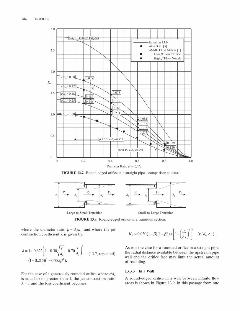
144 ORIFICES
FIGURE 13.7. Round - edged orifi ce in a straight pipe — comparison to data.
3.0
2.5
2.0
1.5
1.0
0.5
00 0.4 0.6 0.8 1.00.2
r/do=0 (Sharp Edged)
Diameter Ratio = do/d1
Ko
0.078r/do=0.08
r/do=0.25
r/do=0.18
r/do=0.125 0.127
0.119
0.128
0.078
0.081
0.079
0.120
0.180
0.183
0.246
0.231
0.255
0.178
0.5 r/do =0.855
0.45 r/do 0.794
r/do=1.00
Equation 13.6
Alvi et al. [3]
ASME Fluid Meters [1]
Low Flow Nozzle
High Flow Nozzle
β
β ≤
≤β ≥
ββ
FIGURE 13.8. Round - edged orifi ce in a transition section.
Large-to-Small Transition Small-to-Large Transition
d1
V2V1 VCdo d2 d1
V2V1 VCdo d2
r r
where the diameter ratio β = do / d1 , and where the jet contraction coeffi cient λ is given by:
λ = + − −
− −( )
1 0 622 1 0 30 0 70
1 0 215 0 785
4
2 5
. . .
. . .
rd
rdo o
β β
(13.7, repeated)
For the case of a generously rounded orifi ce where r / do
is equal to or greater than 1, the jet contraction ratio λ = 1 and the loss coeffi cient becomes:
Kd
r doo
2o
d= −( ) −( ) + −
≥( )0 030 1 1 1 15
2 2
. / .β β
As was the case for a rounded orifi ce in a straight pipe, the radial distance available between the upstream pipe wall and the orifi ce face may limit the actual amount of rounding.
13.3.3 In a Wall
A round - edged orifi ce in a wall between infi nite fl ow areas is shown in Figure 13.9 . In this passage from one
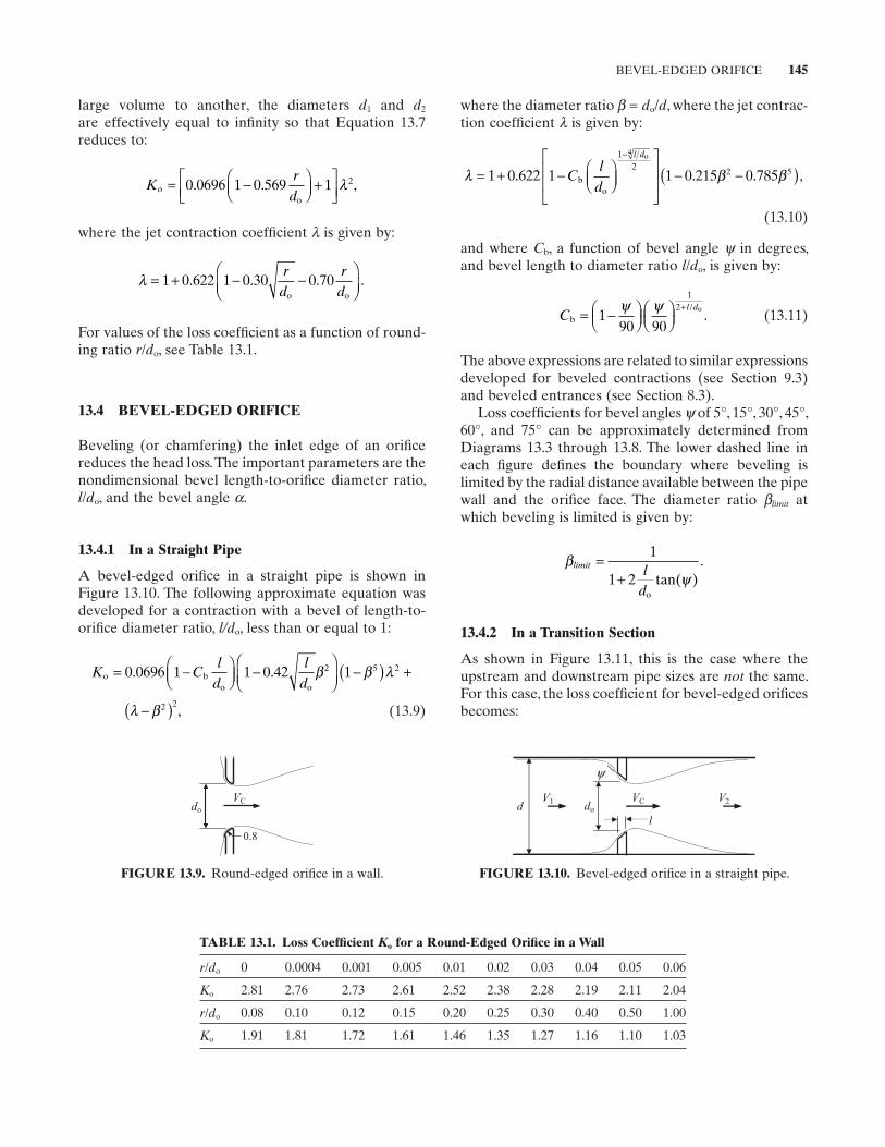
BEVEL-EDGED ORIFICE 145
large volume to another, the diameters d1 and d2
are effectively equal to infi nity so that Equation 13.7 reduces to:
Kr
do
o
,= −
+
0 0696 1 0 569 1 2. . λ
where the jet contraction coeffi cient λ is given by:
λ = + − −
1 0 622 1 0 30 0 70. . . .r
dr
do o
For values of the loss coeffi cient as a function of round-ing ratio r / do , see Table 13.1 .
13.4 BEVEL - EDGED ORIFICE
Beveling (or chamfering) the inlet edge of an orifi ce reduces the head loss. The important parameters are the nondimensional bevel length - to - orifi ce diameter ratio, l / do , and the bevel angle α .
13.4.1 In a Straight Pipe
A bevel - edged orifi ce in a straight pipe is shown in Figure 13.10 . The following approximate equation was developed for a contraction with a bevel of length - to - orifi ce diameter ratio, l/do , less than or equal to 1:
K Cl
dl
do b
o o
= −
−
−( ) +
−( )
0 0696 1 1 0 42 12 5 2
2 2
. .
,
β β λ
λ β (13.9)
where the diameter ratio β = do / d , where the jet contrac-tion coeffi cient λ is given by:
λ β β= + −
− −( )
−
1 0 622 1 1 0 215 0 785
12
2 5
4
. . . ,Cl
d
l d
bo
o
(13.10)
and where Cb , a function of bevel angle ψ in degrees, and bevel length to diameter ratio l / do , is given by:
Cl d
bo= −
+1
90 90
12ψ ψ /
. (13.11)
The above expressions are related to similar expressions developed for beveled contractions (see Section 9.3 ) and beveled entrances (see Section 8.3 ).
Loss coeffi cients for bevel angles ψ of 5 ° , 15 ° , 30 ° , 45 ° , 60 ° , and 75 ° can be approximately determined from Diagrams 13.3 through 13.8 . The lower dashed line in each fi gure defi nes the boundary where beveling is limited by the radial distance available between the pipe wall and the orifi ce face. The diameter ratio βlimit at which beveling is limited is given by:
βψ
limit ld
=+
1
1 2o
tan( ).
13.4.2 In a Transition Section
As shown in Figure 13.11 , this is the case where the upstream and downstream pipe sizes are not the same. For this case, the loss coeffi cient for bevel - edged orifi ces becomes:
FIGURE 13.9. Round - edged orifi ce in a wall.
VCdo
0.8
FIGURE 13.10. Bevel - edged orifi ce in a straight pipe.
dV2V1 VCdo
l
ψ
TABLE 13.1. Loss Coeffi cient Ko for a Round - Edged Orifi ce in a Wall
r / do 0 0.0004 0.001 0.005 0.01 0.02 0.03 0.04 0.05 0.06
Ko 2.81 2.76 2.73 2.61 2.52 2.38 2.28 2.19 2.11 2.04
r / do 0.08 0.10 0.12 0.15 0.20 0.25 0.30 0.40 0.50 1.00
Ko 1.91 1.81 1.72 1.61 1.46 1.35 1.27 1.16 1.10 1.03
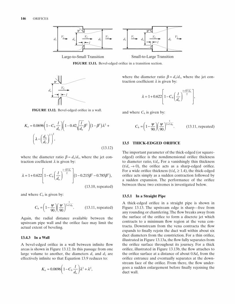
146 ORIFICES
K Cl
dl
d
dd
o bo o
o
≈ −
−
−( ) +
−
0 0696 1 1 0 42 12 5 2
2
. . β β λ
λ
2 2
,
(13.12)
where the diameter ratio β = do / d1 , where the jet con-traction coeffi cient λ is given by:
λ β β= + −
− −( )
−
1 0 622 1 1 0 215 0 785
12
2 5
4
. . . ,Cl
d
l d
bo
o
(13.10, repeated)
and where Cb is given by:
Cl d
bo= −
+1
90 90
12ψ ψ /
. (13.11, repeated)
Again, the radial distance available between the upstream pipe wall and the orifi ce face may limit the actual extent of beveling.
13.4.3 In a Wall
A bevel - edged orifi ce in a wall between infi nite fl ow areas is shown in Figure 13.12 . In this passage from one large volume to another, the diameters d1 and d2 are effectively infi nite so that Equation 13.9 reduces to:
K Cl
do b
o
≈ −
+0 0696 1 2 2. ,λ λ
FIGURE 13.11. Bevel - edged orifi ce in a transition section.
Small-to-Large TransitionLarge-to-Small Transition
VC
ψ
d1
V2V1do d2
l
ψ
d1V2V1 VC
do d2
l
FIGURE 13.12. Bevel - edged orifi ce in a wall.
l
VCdo
ψ where the diameter ratio β = do / d1 , where the jet con-traction coeffi cient λ is given by:
λ = + −
+
1 0 622 1
1 4
. ,
/
Cl
d
l d
bo
2o
and where Cb is given by:
Cl d
bo= −
+1
90 90
12ψ ψ /
. (13.11, repeated)
13.5 THICK - EDGED ORIFICE
The important parameter of the thick - edged (or square - edged) orifi ce is the nondimensional orifi ce thickness to diameter ratio, t/ do . For a vanishingly thin thickness (t/do → 0), the orifi ce acts as a sharp - edged orifi ce. For a wide orifi ce thickness (t/ do ≥ 1.4), the thick - edged orifi ce acts simply as a sudden contraction followed by a sudden expansion. The performance of the orifi ce between these two extremes is investigated below.
13.5.1 In a Straight Pipe
A thick - edged orifi ce in a straight pipe is shown in Figure 13.13 . The upstream edge is sharp — free from any rounding or chamfering. The fl ow breaks away from the surface of the orifi ce to form a discrete jet which contracts to a minimum fl ow region at the vena con-tracta. Downstream from the vena contracta the fl ow expands to fi nally rejoin the duct wall within about six duct diameters from the constriction. For a thin orifi ce, illustrated in Figure 13.13 a, the fl ow fully separates from the orifi ce surface throughout its journey. For a thick orifi ce, illustrated in Figure 13.13 b, the fl ow attaches to the orifi ce surface at a distance of about 0.8 do from the orifi ce entrance and eventually separates at the down-stream face of the orifi ce. From there, the fl ow under-goes a sudden enlargement before fi nally rejoining the duct wall.
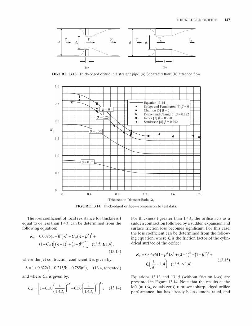
THICK-EDGED ORIFICE 147
FIGURE 13.13. Thick - edged orifi ce in a straight pipe. (a) Separated fl ow; (b) attached fl ow.
t
dV2V1 VC
do
(a) (b)
t
dV2V1 VC
do
The loss coeffi cient of local resistance for thickness t equal to or less than 1.4 do can be determined from the following equation:
K C
C d
th
th
o
ot
= − + −( ) +
−( ) −( ) + −( )
0 0696 1
1 1 1
5 2 2 2
2 2 2
. ( )
/
β λ λ β
λ β ≤≤( )1 4. ,
(13.13)
where the jet contraction coeffi cient λ is given by:
λ β β= + − −( )1 0 622 1 0 215 0 7852 5. . . , (13.4, repeated)
and where Cth is given by:
Cd d
th = −
−
1 0 50
1 40 50
1 4
2 5 3 4 5
..
..
.. .
t t
o o
(13.14)
For thickness t greater than 1.4 do , the orifi ce acts as a sudden contraction followed by a sudden expansion and surface friction loss becomes signifi cant. For this case, the loss coeffi cient can be determined from the follow-ing equation, where fo is the friction factor of the cylin-drical surface of the orifi ce:
K
fd
d
o
oo
ot
t
= −( ) + −( ) + −( ) +
−
>
0 0696 1 1 1
1 4 1 4
5 2 2 2 2.
. ( / . )
β λ λ β
.. (13.15)
Equations 13.13 and 13.15 (without friction loss) are presented in Figure 13.14 . Note that the results at the left (at t /do equals zero) represent sharp - edged orifi ce performance that has already been demonstrated, and
FIGURE 13.14. Thick - edged orifi ce — comparison to test data.
3.0
2.5
2.0
0 0.8 1.2 1.6 2.00.4
Thickness-to-Diameter Ratio t/do
1.5
1.0
0.5
0
Ko
= 0.25
= 0
= 0.50
Equation 13.14 Spikes and Pennington [4] = 0 Charlton [5] = 0 Decker and Chang [6] = 0.122 James [7] = 0.250 Sanderson [8] = 0.252
= 0.75 b
b
bb
bb
b
b
b
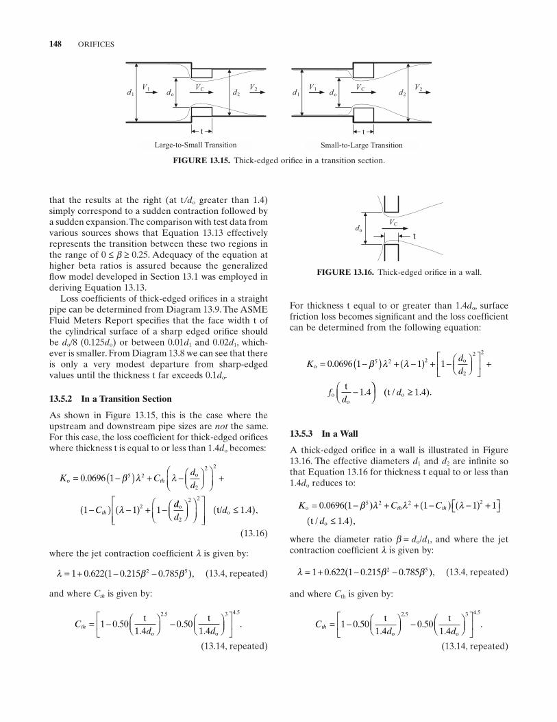
148 ORIFICES
that the results at the right (at t /do greater than 1.4) simply correspond to a sudden contraction followed by a sudden expansion. The comparison with test data from various sources shows that Equation 13.13 effectively represents the transition between these two regions in the range of 0 ≤ β ≥ 0.25. Adequacy of the equation at higher beta ratios is assured because the generalized fl ow model developed in Section 13.1 was employed in deriving Equation 13.13 .
Loss coeffi cients of thick - edged orifi ces in a straight pipe can be determined from Diagram 13.9 . The ASME Fluid Meters Report specifi es that the face width t of the cylindrical surface of a sharp edged orifi ce should be do /8 (0.125 do ) or between 0.01 d1 and 0.02 d1 , which-ever is smaller. From Diagram 13.8 we can see that there is only a very modest departure from sharp - edged values until the thickness t far exceeds 0.1 do .
13.5.2 In a Transition Section
As shown in Figure 13.15 , this is the case where the upstream and downstream pipe sizes are not the same. For this case, the loss coeffi cient for thick - edged orifi ces where thickness t is equal to or less than 1.4 do becomes:
K Cdd
C
th
th
oo= −( ) + −
+
−( ) −( ) + −
0 0696 1
1 1 1
5 2
2
2 2
2
. β λ λ
λ ddd
doot/
2
2 2
1 4
≤( ). ,
(13.16)
where the jet contraction coeffi cient λ is given by:
λ β β= + − −1 0 622 1 0 215 0 7852 5. ( . . ), (13.4, repeated)
and where Cth is given by:
Cd d
th = −
−
1 0 50
1 40 50
1 4
2 5 3 4 5
..
..
.. .
t t
o o
(13.14, repeated)
For thickness t equal to or greater than 1.4 do , surface friction loss becomes signifi cant and the loss coeffi cient can be determined from the following equation:
Kdd
fd
oo
oo
t
= −( ) + −( ) + −
+
−
0 0696 1 1 1
1 4
5 2 2
2
2 2
.
.
β λ λ
≥( / . ).t od 1 4
13.5.3 In a Wall
A thick - edged orifi ce in a wall is illustrated in Figure 13.16 . The effective diameters d1 and d2 are infi nite so that Equation 13.16 for thickness t equal to or less than 1.4do reduces to:
K C C
d
th tho
ot
= − + + −( ) −( ) + ≤( )
0 0696 1 1 1 1
1 4
5 2 2 2. ( )
/ . ,
β λ λ λ
where the diameter ratio β = do / d1 , and where the jet contraction coeffi cient λ is given by:
λ β β= + − −1 0 622 1 0 215 0 7852 5. ( . . ), (13.4, repeated)
and where Cth is given by:
Cd d
th = −
−
1 0 50
1 40 50
1 4
2 5 3 4 5
..
..
.. .
t t
o o
(13.14, repeated)
FIGURE 13.15. Thick - edged orifi ce in a transition section.
VC
t
d1
V2V1do d2
V2VCd1
V1do d2
t
Large-to-Small Transition Small-to-Large Transition
FIGURE 13.16. Thick - edged orifi ce in a wall.
VCdo
t
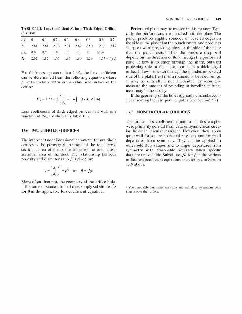
NONCIRCULAR ORIFICES 149
For thickness t greater than 1.4 do , the loss coeffi cient can be determined from the following equation, where fo is the friction factor in the cylindrical surface of the orifi ce:
K fd
do oo
ot
t= + −
≥( )1 57 1 4 1 4. . / . .
Loss coeffi cients of thick - edged orifi ces in a wall as a function of t/ do are shown in Table 13.2 .
13.6 MULTIHOLE ORIFICES
The important nondimensional parameter for multihole orifi ces is the porosity ϕ , the ratio of the total cross - sectional area of the orifi ce holes to the total cross - sectional area of the duct. The relationship between porosity and diameter ratio β is given by:
φ β β φ=
= =
dd
o or1
22 .
More often than not, the geometry of the orifi ce holes is the same or similar. In that case, simply substitute φfor β in the applicable loss coeffi cient equation.
Perforated plate may be treated in this manner. Typi-cally, the perforations are punched into the plate. The punch produces slightly rounded or beveled edges on the side of the plate that the punch enters, and produces sharp, outward projecting edges on the side of the plate that the punch exits. * Thus the pressure drop will depend on the direction of fl ow through the perforated plate. If fl ow is to enter through the sharp, outward projecting side of the plate, treat it as a thick - edged orifi ce. If fl ow is to enter through the rounded or beveled side of the plate, treat it as a rounded or beveled orifi ce. It may be diffi cult, if not impossible; to accurately measure the amount of rounding or beveling so judg-ment may be necessary.
If the geometry of the holes is greatly dissimilar, con-sider treating them as parallel paths (see Section 5.2 ).
13.7 NONCIRCULAR ORIFICES
The orifi ce loss coeffi cient equations in this chapter were primarily derived from data on symmetrical circu-lar holes in circular passages. However, they apply quite well for square holes and passages, and for small departures from symmetry. They can be applied to other odd fl ow shapes and to larger departures from symmetry with reasonable accuracy when specifi c data are unavailable. Substitute φ for β in the various orifi ce loss coeffi cient equations as described in Section 13.6 above.
TABLE 13.2. Loss Coeffi cient Ko for a Thick - Edged Orifi ce in a Wall
t / do 0 0.1 0.2 0.3 0.4 0.5 0.6 0.7
Ko 2.81 2.81 2.78 2.71 2.62 2.50 2.35 2.19
t / do 0.8 0.9 1.0 1.1 1.2 1.3 ≥ 1.4
Ko 2.02 1.87 1.75 1.66 1.60 1.58 1.57 + f( fo ,)
* You can easily determine the entry and exit sides by running your fi ngers over the surface.
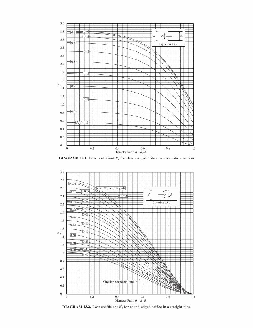
DIAGRAM 13.1. Loss coeffi cient Ko for sharp - edged orifi ce in a transition section.
3.0
2.8
2.6
2.4
2.2
2.0
1.8
1.6
1.4
1.2
1.0
0.8
0.6
0.4
0.2
00 0.4 0.6 0.8 1.0 0.2
Ko
0.2
0.0
0.3
0.4
0.6
do/d2=1.0
0.7
0.8
0.9
0.5
0.1
Equation 13.5
do d2d1
Diameter Ratio = do /dβ
DIAGRAM 13.2. Loss coeffi cient Ko for round - edged orifi ce in a straight pipe.
3.0
2.8
2.6
2.4
2.2
2.0
1.8
1.6
1.4
1.2
1.0
0.8
0.6
0.4
0.2
00 0.4 0.6 0.8 1.0 0.2
Circular Rounding Limit
r/do=0 (Sharp Edged)0.0050.01
0.020.03
0.150.20
0.04
0.06
0.400.50
1.00
0.30 0.25
0.08
0.100.12
0.05
0.001
0.0004
Equation 13.6
r
d do
Diameter Ratio β = do /d
Ko
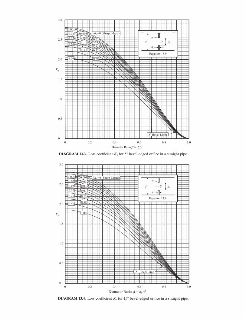
DIAGRAM 13.3. Loss coeffi cient Ko for 5 ° bevel - edged orifi ce in a straight pipe.
0 0.4 0.6 0.8 1.00.2
Diameter Ratio = do /d
3.0
2.5
2.0
1.5
1.0
0.5
0
0.50 1.00
0.10
0.30
0.20
0.15
0.05
0.07
l/do =0 (Sharp Edged)
5˚ Bevel Limit
0.02
0.01
0.005
0.03
0.001
Ko
Equation 13.9
dod
0.
β
α
DIAGRAM 13.4. Loss coeffi cient Ko for 15 ° bevel - edged orifi ce in a straight pipe.
0.50
1.00
0.10
0.30
0.20 0.15
0.05
0.07
l/do =0 (Sharp Edged)
15˚ Bevel Limit
0.02 0.01
0.005
0.03
0.001
0 0.4 0.6 0.8 1.00.2
Diameter Ratio = do /d
Ko
3.0
2.5
2.0
1.5
1.0
0.5
0
Equation 13.9
dod
1
β
α
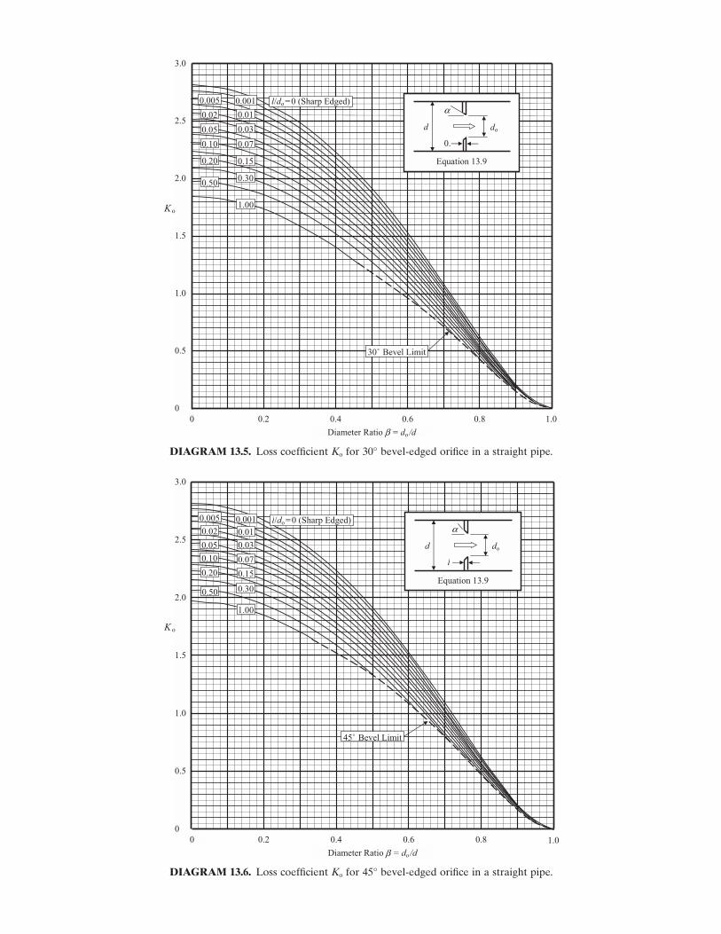
0 0.4 0.6 0.8 1.0 0.2
Diameter Ratio = do /d
3.0
2.5
2.0
1.5
1.0
0.5
0
0.50
1.00
0.10
0.30
0.20 0.15
0.05
0.07
l/do =0 (Sharp Edged)
30˚ Bevel Limit
0.02 0.01
0.005
0.03
0.001
Equation 13.9
dod
l0.
Ko
β
α
DIAGRAM 13.5. Loss coeffi cient Ko for 30 ° bevel - edged orifi ce in a straight pipe.
DIAGRAM 13.6. Loss coeffi cient Ko for 45 ° bevel - edged orifi ce in a straight pipe.
1.00 0.4 0.6 0.80.2
Diameter Ratio = do /d
3.0
2.5
2.0
1.5
1.0
0.5
0
Ko
0.50
1.00
0.10
0.30
0.20 0.15
0.05
0.07
l/do =0 (Sharp Edged)
45˚ Bevel Limit
0.02 0.01
0.005
0.03
0.001
Equation 13.9
dod
l
β
α
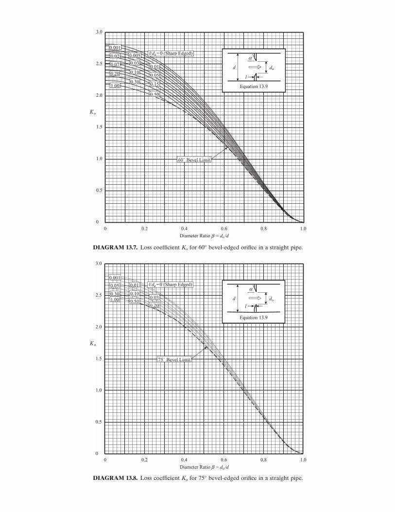
DIAGRAM 13.7. Loss coeffi cient Ko for 60 ° bevel - edged orifi ce in a straight pipe.
0 0.4 0.6 0.8 1.00.2
Diameter Ratio = do /d
3.0
2.5
2.0
1.5
1.0
0.5
0
Ko
0.50
1.00
0.10
0.30
0.20
0.15
0.05
0.07
l/do =0 (Sharp Edged)
60˚ Bevel Limit
0.02
0.01
0.005
0.03
0.001
l
Equation 13.9
dod
l
β
α
DIAGRAM 13.8. Loss coeffi cient Ko for 75 ° bevel - edged orifi ce in a straight pipe.
0.50 1.00 0.10 0.30
0.20
0.05 l/do =0 (Sharp Edged)
75˚ Bevel Limit
0.01
0.03
0.001
0 0.4 0.6 0.8 1.00.2
Diameter Ratio = do /d
3.0
2.5
2.0
1.5
1.0
0.5
0
Ko
Equation 13.9
dod
l
β
α
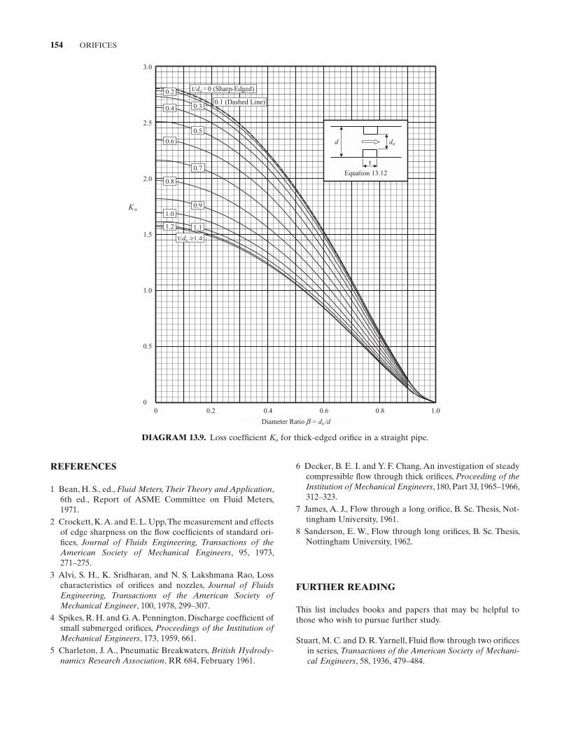
154 ORIFICES
DIAGRAM 13.9. Loss coeffi cient Ko for thick - edged orifi ce in a straight pipe.
0 0.4 0.6 0.8 1.00.2
Diameter Ratio = do /d
K o
t/do =0 (Sharp-Edged)
3.0
2.5
2.0
1.5
1.0
0.5
0
Equation 13.12
d do
t
0.1 (Dashed Line)
0.2
0.30.4
0.5
0.6
0.7
0.8
0.91.0
1.11.2
t/do ≥1.4
β
REFERENCES
1 Bean , H. S. , ed., Fluid Meters, Their Theory and Application , 6th ed., Report of ASME Committee on Fluid Meters, 1971 .
2 Crockett , K. A. and E. L. Upp , The measurement and effects of edge sharpness on the fl ow coeffi cients of standard ori-fi ces , Journal of Fluids Engineering, Transactions of the American Society of Mechanical Engineers , 95 , 1973 , 271 – 275 .
3 Alvi , S. H. , K. Sridharan , and N. S. Lakshmana Rao , Loss characteristics of orifi ces and nozzles , Journal of Fluids Engineering, Transactions of the American Society of Mechanical Engineer , 100 , 1978 , 299 – 307 .
4 Spikes , R. H. and G. A. Pennington , Discharge coeffi cient of small submerged orifi ces , Proceedings of the Institution of Mechanical Engineers , 173 , 1959 , 661 .
5 Charleton , J. A. , Pneumatic Breakwaters , British Hydrody-namics Research Association , RR 684, February 1961 .
6 Decker , B. E. I. and Y. F. Chang , An investigation of steady compressible fl ow through thick orifi ces , Proceeding of the Institution of Mechanical Engineers , 180 , Part 3J, 1965 – 1966 , 312 – 323 .
7 James , A. J. , Flow through a long orifi ce , B. Sc. Thesis, Not-tingham University, 1961 .
8 Sanderson , E. W. , Flow through long orifi ces , B. Sc. Thesis, Nottingham University, 1962 .
FURTHER READING
This list includes books and papers that may be helpful to those who wish to pursue further study.
Stuart , M. C. and D. R. Yarnell , Fluid fl ow through two orifi ces in series , Transactions of the American Society of Mechani-cal Engineers , 58 , 1936 , 479 – 484 .
FURTHER READING 155
Medaugh , F. W. and G. D. Johnson , Investigation of the dis-charge and coeffi cients of small circular orifi ces , Transac-tions of the American Society of Civil Engineers , 10 ( 9 ), 1940 , 422 .
Stuart , M. C. and D. R. Yarnell , Fluid fl ow through two orifi ces in series(II , Transactions of the American Society of Mechanical Engineers , 66 , 1944 , 387 – 397 .
Rouse , H. and A. Abul - Fetouh , Characteristics of the irota-tional fl ow through axially - symmetric orifi ces , Journal of Applied Mechanics, Transactions of the American Society of Mechanical Engineers , 17 ( 4 ), 1950 , 421 – 426 .
Landstra , J. A. , Quarter - circle orifi ces , Transactions of the Insti-tution of Chemical Engineers , 38 , 1960 , 26 – 32 .
Bogema , M. and P. L. Monkmeyer , The quadrant edge orifi ce(a fl uid meter for low Reynolds number , Journal of Basic Engineering, Transactions of the American Society of Mechanical Engineers , 82 , 1960 , 729 – 734 .
Bogema , M. , B. Spring , and M. V. Ramamoorthy , Quadrant edge orifi ce performance - effect of upstream velocity distri-bution , Journal of Basic Engineering, Transactions of the American Society of Mechanical Engineers , 84 , 1962 , 415 – 418 .
Leutheusser , H. J. , Flow nozzles with zero beta ratio , Journal of Basic Engineering, Transactions of the American Society of Mechanical Engineers , 86 , 1964 , 538 – 542 .
Lenkei , A. , Close Clearance Orifi ces , Product Engineering , April 26, 1965 , pp. 57 – 61 .
Ramamoorthy , M. V. and K. Seetharamiah , Quadrant - edge orifi ce and performance at very high Reynolds numbers , Journal of Basic Engineering, Transactions of the American Society of Mechanical Engineers , 88 , 1966 , 9 – 13 .
Ghazi , H. S. , On nonuniform fl ow characteristics at the vena contracta , Journal of Basic Engineering, Transactions of the American Society of Mechanical Engineers , 92 ( 70 - FE - 34 ), 1970 , 1 – 6 .
Miller , D. S. , Internal Guide to Losses in Pipe and Duct Systems , The British Hydromechanics Research Association , 1971 .
Teyssandier , R. G. , Internal separated fl ows — Expansions, nozzles, and orifi ces , PhD dissertation, University of Rhode Island, Kingston, R. I., 1973 .
Miller , R. W. and O. Kneisel , A comparison between orifi ce and fl ow nozzle laboratory data and published coeffi cients , Journal of Fluids Engineering, Transactions of the American Society of Mechanical Engineers , 96 , 1974 , 139 – 149 .
Head , V. P. , Improved expansion factors for nozzles, orifi ces, and variable - area meters , Journal of Fluids Engineering, Transactions of the American Society of Mechanical Engi-neers , 96 , 1974 , 150 – 157 .
Wilson , M. P. Jr. and R. G. Teyssandier , The paradox of the vena contracta , Journal of Fluids Engineering, Transactions
of the American Society of Mechanical Engineers , 97 , 1975 , pp. 366 – 371 .
Nigro , F. E. B. , A. B. Strong , and S. A. Alpay , A numerical study of the laminar viscous incompressible fl ow through a pipe orifi ce , Journal of Fluids Engineering, Transactions of the American Society of Mechanical Engineers , 100 , 1978 , 467 – 472 .
Sparrow , E. M. , J. W. Ramsey , and S. C. Lau , Flow and pressure characteristics downstream of a segmental blockage in a turbulent pipe fl ow , Journal of Fluids Engineering, Transac-tions of the American Society of Mechanical Engineers , 101 , 1979 , 200 – 207 .
Lienhard , J. H. V and J. H. IV Lienhard , Velocity coeffi cients for free jets from sharp - edged orifi ces , Journal of Fluids Engineering, Transactions of the American Society of Mechanical Engineering , 106 , 1984 , 13 .
Grose , R. D. , Orifi ce contraction coeffi cient for invisid incom-pressible fl ow , Journal of Fluids Engineering, Transactions of the American Society of Mechanical Engineers , 107 , 1985 , 36 – 43 .
Bullen , P. R. , D. J. Cheeseman , L. A. Hussain , and A. E. Ruffell , The Determination of pipe contraction pressure loss coef-fi cients for incompressible turbulent fl ow , InternationalJournal of Heat and Fluid Flow , 8 ( 2 ), 1987 , 111 – 118 .
Bullen , P. R. , D. J. Cheeseman , and L. A. Hussain , The effects of inlet sharpness on the pipe contraction loss coeffi cient , International Journal of Heat and Fluid Flow , 9 ( 4 ), 1988 , 431 – 433 .
Andrews , K. A. and R. H. Sabersky , Flow through an orifi ce from a transverse stream , Journal of Fluids Engineering, Transactions of the American Society of Mechanical Engi-neers , 112 , 1990 , 524 – 526 .
Faramarzi , J. and E. Logan , Reattachment length behind a single roughness element in turbulent pipe fl ow , Journal of Fluids Engineering, Transactions of the American Society of Mechanical Engineers , 113 , 1991 , 712 – 714 .
Brundrett , E. , Prediction of pressure drop for incompressible fl ow through screens , Journal of Fluids Engineering, Trans-actions of the American Society of Mechanical Engineers , 115 , 1993 , 239 – 242 .
Brower , W. B. , Jr. , E. Eisler , E. J. Filkorn , J. Gonenc , C. Plati , and J. Stagnitti , On the compressible fl ow through an orifi ce , Journal of Fluids Engineering, Transactions of the American Society of Mechanical Engineers , 115 , 1993 , 660 – 664 .
Agarwal , N. K. , Mean separation and reattachment in turbu-lent pipe fl ow due to an orifi ce plate , Journal of Fluids Engineering, Transactions of the American Society of Mechanical Engineers , 116 , 1994 , 373 – 376 .
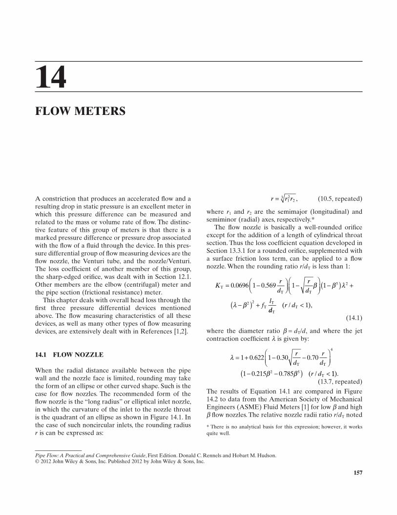
157
14 FLOW METERS
A constriction that produces an accelerated fl ow and a resulting drop in static pressure is an excellent meter in which this pressure difference can be measured and related to the mass or volume rate of fl ow. The distinc-tive feature of this group of meters is that there is a marked pressure difference or pressure drop associated with the fl ow of a fl uid through the device. In this pres-sure differential group of fl ow measuring devices are the fl ow nozzle, the Venturi tube, and the nozzle/Venturi. The loss coeffi cient of another member of this group, the sharp - edged orifi ce, was dealt with in Section 12.1 . Other members are the elbow (centrifugal) meter and the pipe section (frictional resistance) meter.
This chapter deals with overall head loss through the fi rst three pressure differential devices mentioned above. The fl ow measuring characteristics of all these devices, as well as many other types of fl ow measuring devices, are extensively dealt with in References [1,2] .
14.1 FLOW NOZZLE
When the radial distance available between the pipe wall and the nozzle face is limited, rounding may take the form of an ellipse or other curved shape. Such is the case for fl ow nozzles. The recommended form of the fl ow nozzle is the “ long radius ” or elliptical inlet nozzle, in which the curvature of the inlet to the nozzle throat is the quadrant of an ellipse as shown in Figure 14.1 . In the case of such noncircular inlets, the rounding radius r is can be expressed as:
r r r= 12
23 , (10.5, repeated)
where r1 and r2 are the semimajor (longitudinal) and semiminor (radial) axes, respectively. *
The fl ow nozzle is basically a well - rounded orifi ce except for the addition of a length of cylindrical throat section. Thus the loss coeffi cient equation developed in Section 13.3.1 for a rounded orifi ce, supplemented with a surface friction loss term, can be applied to a fl ow nozzle. When the rounding ratio r / dT is less than 1:
Kr
dr
d
fl
TT T
TT
= −
−
−( ) +
−( ) +
0 0696 1 0 569 1 1 5 2
2 2
. . β β λ
λ βdd
r dT
T( / ),< 1
(14.1)
where the diameter ratio β = dT / d , and where the jet contraction coeffi cient λ is given by:
λ
β β
= + − −
− −( ) <
1 0 622 1 0 30 0 70
1 0 215 0 785
4
2 5
. . .
. . ( /
rd
rd
r d
T T
T 11). (13.7, repeated)
The results of Equation 14.1 are compared in Figure 14.2 to data from the American Society of Mechanical Engineers (ASME) Fluid Meters [1] for low β and high β fl ow nozzles. The relative nozzle radii ratio r / dT noted
Pipe Flow: A Practical and Comprehensive Guide, First Edition. Donald C. Rennels and Hobart M. Hudson.© 2012 John Wiley & Sons, Inc. Published 2012 by John Wiley & Sons, Inc.
* There is no analytical basis for this expression; however, it works quite well.
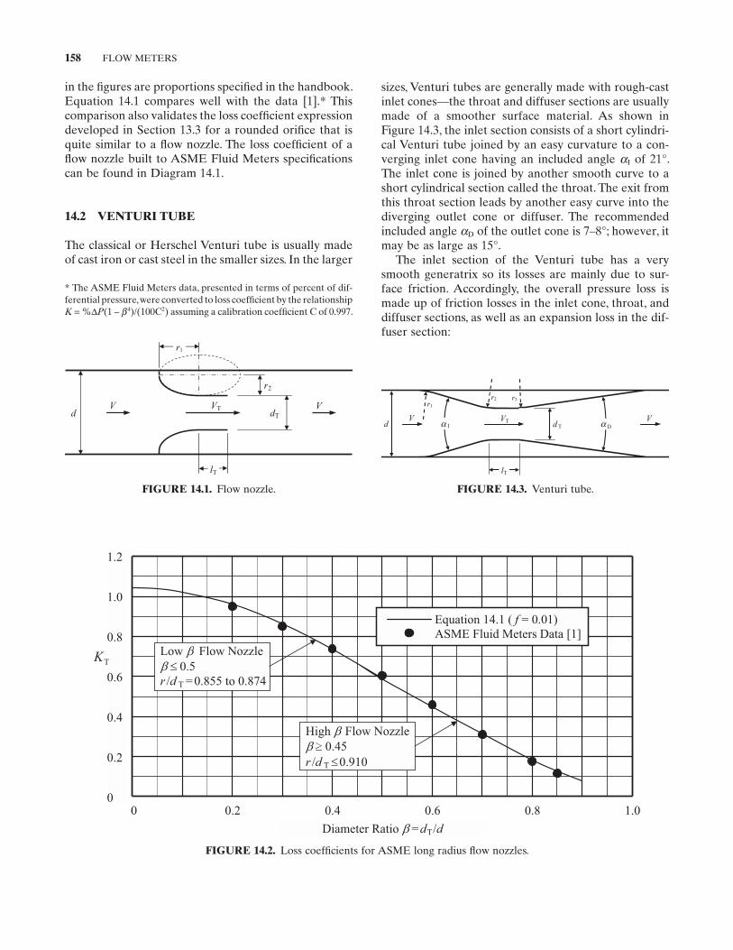
158 FLOW METERS
sizes, Venturi tubes are generally made with rough - cast inlet cones — the throat and diffuser sections are usually made of a smoother surface material. As shown in Figure 14.3 , the inlet section consists of a short cylindri-cal Venturi tube joined by an easy curvature to a con-verging inlet cone having an included angle αI of 21 ° . The inlet cone is joined by another smooth curve to a short cylindrical section called the throat. The exit from this throat section leads by another easy curve into the diverging outlet cone or diffuser. The recommended included angle αD of the outlet cone is 7 – 8 ° ; however, it may be as large as 15 ° .
The inlet section of the Venturi tube has a very smooth generatrix so its losses are mainly due to sur-face friction. Accordingly, the overall pressure loss is made up of friction losses in the inlet cone, throat, and diffuser sections, as well as an expansion loss in the dif-fuser section:
in the fi gures are proportions specifi ed in the handbook. Equation 14.1 compares well with the data [1] . * This comparison also validates the loss coeffi cient expression developed in Section 13.3 for a rounded orifi ce that is quite similar to a fl ow nozzle. The loss coeffi cient of a fl ow nozzle built to ASME Fluid Meters specifi cations can be found in Diagram 14.1 .
14.2 VENTURI TUBE
The classical or Herschel Venturi tube is usually made of cast iron or cast steel in the smaller sizes. In the larger
FIGURE 14.2. Loss coeffi cients for ASME long radius fl ow nozzles.
1.2
1.0
0.8
Equation 14.1 ( f = 0.01)
ASME Fluid Meters Data [1]
Low Flow Nozzle
0 0.2 0.4 0.6 0.8 1.0
Diameter Ratio =dT/d
0.6
0.4
0.2
0
0.5
r /d T =0.855 to 0.874
High Flow Nozzle
0.45
TK
r /d 0.910T
FIGURE 14.1. Flow nozzle.
V
r2
dTdVVT
lT
r1
FIGURE 14.3. Venturi tube.
Vd Td
V VT
lT
DI
r1
r2 r3
aa
* The ASME Fluid Meters data, presented in terms of percent of dif-ferential pressure, were converted to loss coeffi cient by the relationship K = % ΔP (1 – β 4 )/(100C 2 ) assuming a calibration coeffi cient C of 0.997.
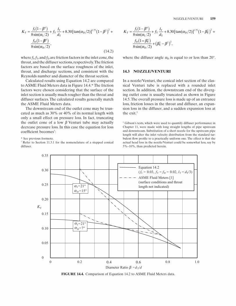
NOZZLE/VENTURI 159
Kf
fld
f
TI
IT
T
TD E
D
=−( )
+ + [ ] −( ) +1
8 28 30 2 1
1
41 75 2 2β
αα β
sin( ). tan( ) .
−−( )+ −( )β
αβ βE
DE
42 2 2
8 2sin( ),
where the diffuser angle αD is equal to or less than 20 ° .
14.3 NOZZLE/VENTURI
In a nozzle/Venturi, the conical inlet section of the clas-sical Venturi tube is replaced with a rounded inlet section. In addition, the downstream end of the diverg-ing outlet cone is usually truncated as shown in Figure 14.5 . The overall pressure loss is made up of an entrance loss, friction losses in the throat and diffuser, an expan-sion loss in the diffuser, and a sudden expansion loss at the exit. ‡
Kf
fld
f
TI
IT
T
TD
D
=−( )
+ + [ ] −( ) +
−
1
8 28 30 2 1
1
41 75 2 2β
αβ
sin( ). tan( ) .α
ββα
4
8 2( )
sin( ),
D
(14.2)
where fI , fT , and fD are friction factors in the inlet cone, the throat, and the diffuser sections, respectively. The friction factors are based on the surface roughness of the inlet, throat, and discharge sections, and consistent with the Reynolds number and diameter of the throat section.
Calculated results using Equation 14.2 are compared to ASME Fluid Meters data in Figure 14.4 . * The friction factors were chosen considering that the surface of the inlet section is usually much rougher than the throat and diffuser surfaces. The calculated results generally match the ASME Fluid Meters data.
The downstream end of the outlet cone may be trun-cated as much as 30% or 40% of its normal length with only a small effect on pressure loss. In fact, truncating the outlet cone of a low β Venturi tube may actually decrease pressure loss. In this case the equation for loss coeffi cient becomes † :
FIGURE 14.4. Comparison of Equation 14.2 to ASME Fluid Meters data.
0 0.2 0.4 0.6 0.8 1.0
Diameter Ratio b =d T/d
KT
0.35
0.30
0.25
0.20
0.15
0.10
0.05
0
I =21°aaD =15°
I =21°
Equation 14.2 ( fI = 0.03, fT = fD = 0.02, lT = dT/3)
ASME Fluid Meters [1] (surface conditions and throat length not indicated)
aD=7°a
† Refer to Section 11.3.1 for the nomenclature of a stepped conical diffuser.
* See previous footnote.
‡ Gibson ’ s tests, which were used to quantify diffuser performance in Chapter 11 , were made with long straight lengths of pipe upstream and downstream. Substitution of a short nozzle for the upstream pipe length will alter the inlet velocity distribution from the standard tur-bulent fl ow profi le to a practically uniform one. The effect is that the actual head loss in the nozzle/Venturi could be somewhat less, say by 5% – 10%, than predicted herein.
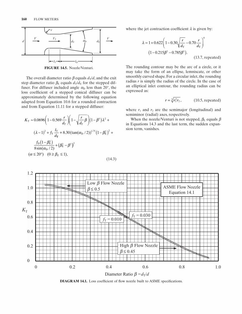
160 FLOW METERS
where the jet contraction coeffi cient λ is given by:
λ
β β
= + − −
− −( )
1 0 622 1 0 30 0 70
1 0 215 0 785
4
2 5
. . .
. . .
rd
rdT T
(13.7, repeated)
The rounding contour may be the arc of a circle, or it may take the form of an ellipse, lemniscate, or other smoothly curved shape. For a circular inlet, the rounding radius r is simply the radius of the circle. In the case of an elliptical inlet contour, the rounding radius can be expressed as:
r r r= 12
23 , (10.5, repeated)
where r1 and r2 are the semimajor (longitudinal) and semiminor (radial) axes, respectively.
When the nozzle/Venturi is not stepped, βE equals βin Equations 14.3 and the last term, the sudden expan-sion term, vanishes.
The overall diameter ratio β equals dT / d , and the exit step diameter ratio βE equals dT / dE for the stepped dif-fuser. For diffuser included angle αD less than 20 ° , the loss coeffi cient of a stepped conical diffuser can be approximately determined by the following equation adapted from Equation 10.6 for a rounded contraction and from Equation 11.11 for a stepped diffuser:
Kr
dr
d
fld
T TT
TT
≈ −
−
−( ) +
−( ) +
0 0696 1 0 569 1 1
1
5 2
2
. . β β λ
λTT
D E
D E
DE
+ ( ) −( ) +
−( )+ −(
8 30 2 1
1
8 2
1 75 2 2
42 2
. tan( / )
sin( / )
.α β
βα
β βf ))
≤ ° ≥ ≤
2
20 0 1( ) ( ),α βE
(14.3)
DIAGRAM 14.1. Loss coeffi cient of fl ow nozzle built to ASME specifi cations.
0 0.2 0.4 0.6 0.8 1.0
Diameter Ratio b =dT/d
1.2
1.0
0.8
0.6
0.4
0.2
0
ASME Flow Nozzle Equation 14.1
Low b Flow Nozzleb ≤ 0.5
High b Flow Nozzleb ≤ 0.45
KT
fT = 0.010fT = 0.030
FIGURE 14.5. Nozzle/Venturi.
dEdTdVV VT
lT
aD
lD
r
FURTHER READING 161
REFERENCES
1. Bean , H. S. , ed., Fluid Meters, Their Theory and Application , 6th ed., Report of ASME Committee on Fluid Meters, 1971 .
2. Spink , L. K. , Principles and Practices of Flow Meter Engi-neering , 9th ed. , The Foxboro Company , Foxboro, MA , 1978 .
FURTHER READING
This list includes books and papers that may be helpful to those who wish to pursue further study.
Warren , J. , A study of head loss in Venturi - meter diffuser sec-tions , Transactions of the American Society of Mechanical Engineers , Paper No. 50 - A - 65, 73 , 1951 , 1 – 4 .
Methods for the Measurement of Fluid Flow , British Standard 1042; Part 1, 1964 .
Leutheusser , H. J. , Flow nozzles with zero beta ratio , Journal of Basic Engineering, Transactions of the American Society of Mechanical Engineers , 86 , 1964 , 538 – 542 .
Replogle , J. A. , L. E. Myers , and K. J. Brust , Evaluation of pipe elbow as fl ow meters , Journal of the Irrigation and Drainage Division, Proceedings of the American Society of Civil Engineers , 92 ( IR3 ), 1966 , 17 – 34 .
Arnberg , B. T. , C. L. Britton , and W. F. Seidl , Discharge coef-fi cient correlations for circular - arc Venturi fl owmeters at critical (sonic) fl ow , Transactions of the American Society of Mechanical Engineers , Paper No. 73 - WA/FM - 8, 96 , 1974 , 1 – 13 .
Miller , R. W. and O. Kneisel , A comparison between orifi ce and fl ow nozzle laboratory data and published coeffi cients , Journal of Fluids Engineering, Transactions of the American Society of Mechanical Engineers , 96 , 1974 , 139 – 149 .
Head , V. P. , Improved expansion factors for nozzles, orifi ces, and variable - area meters , Journal of Fluids Engineering,
Transactions of the American Society of Mechanical Engi-neers , 96 , 1974 , 150 – 157 .
Benedict , R. P. , Loss coeffi cients of fl uid meters , Journal of Fluids Engineering, Transactions of the American Society of Mechanical Engineers , Paper No. 76 - WA/FM - 2, 99 , 1977 , 245 – 248 .
Benedict , R. P. and J. S. Wyler , Analytical and experimental studies of ASME fl ow nozzles , Journal of Fluids Engineer-ing, Transactions of the American Society of Mechanical Engineers , 100 , 1978 , 265 – 275 .
Alvi , S. H. , K. Sridharan , and N. S. Lakshmana Rao , Loss char-acteristics of orifi ces and nozzles , Journal of Fluids Engi-neering, Transactions of the American Society of Mechanical Engineers , 100 , 1978 , 299 – 307 .
Buzzard , W. , Flowmeter Orifi ce Sizing , Handbook No. 10B9000, Fischer and Porter Company , 1978 .
Kopp , J. , Flowmeter selection(Part 1 , in Oil, Gas & Petrochem Equipment , The Petroleum Publishing Company , 1979 .
Kopp , J. , Flowmeter selection(Part 2 , in Oil, Gas & Petrochem Equipment , The Petroleum Publishing Company , 1979 .
ASME Fluid Meters Research Committee , The ISO - ASME Orifi ce Coeffi cient Equation , Mechanical Engineering, July 1981 , pp. 44 – 45 .
Miller , R. W. , Flow Measurement Engineering Handbook , 3rd ed. , McGraw - Hill , 1996 .
Roberson , J. A. and C. T. Crowe , Engineering Fluid Mechanics , 6th ed. , John Wiley & Sons , 1997 (Chapter 13 Flow Measurements).
Baker , R. C. , Flow Measurement Handbook: Industrial Design, Operating Principles, Performance, and Applications , Cam-bridge University Press , 2000 .
Furness , R. , Don ’ t Install That Flowmeter (Until You Read This Article on Installation Claims, Tips(and Reality) , Flow Control, March 2002 , pp. 31 – 47 .
Falcone , G. , Multiphase Flow Metering , Elsevier , 2009 .
163
15 BENDS
This chapter is primarily concerned with the fl ow of an incompressible turbulent fl uid in pipe bends and elbows. Defl ection angle α and bend radius ratio r / d (the ratio of the bend centerline radius to the inside diameter of the pipe) are important geometric parameters. Surface roughness of the wall of the bend, as well as of the con-necting pipe, is also important. Hence, friction factor is important.
The work presented here is for bends where there is no change of fl ow area between the inlet and outlet. It is assumed that roughness of the connecting pipe is similar to roughness of the bend. The work is for circular passages, but can be reasonably applied to square ducts or to rectangular ducts of low aspect ratio.
15.1 ELBOWS AND PIPE BENDS
The pressure loss in pipe bends may be thought of as made up of three components. One component is the pressure loss due to ordinary surface friction that cor-responds to fully developed fl ow in a straight pipe having the same length as the centerline of the bend. A second component is due to a twin - eddy secondary fl owsuperimposed on the main or primary fl ow due to the combined action of centrifugal force and frictional resis-tance of the pipe walls. A third component is due to separation of the main fl ow from the inner and outer radius of the bend and subsequent expansion of the contracted stream. * For bends of small radius of curva-
ture, fl ow separation and secondary fl ow dominate. For bends of large radius of curvature, ordinary surface fric-tion and secondary fl ow prevail. Flow separation and secondary fl ow are illustrated in Figure 15.1 . †
As noted above, the bend radius ratio r / d is defi ned as the ratio of the centerline radius of the bend to the inside diameter of the pipe. In this context, a bend of radius ratio 0.5 represents a bend with a sharp (zero radius) inner corner and an outer bend radius of 1.0. At the extreme is a miter bend in which two pipes are joined together in a sharp angle without any round-ing at the plane of intersection. The rounding of the corner at the inner wall, or simply beveling the corner, greatly attenuates the separation and reduces the pres-sure loss. At the opposite extreme, bend losses, exclud-ing friction losses, are at a minimum when the bend radius ratio is at a maximum.
A bend must always be considered with relation to the straight pipes, or tangents, connected to its ends. This brings about experimental diffi culties. Whatever the velocity distribution may be at the upstream end, the downstream length must be suffi cient for the gradual adjustment of the distribution until it regains a normal velocity profi le. An example of the measured pressure distribution along a bend is shown in Figure 15.2 . In this bend of circular cross section, a marked increase in pressure along the outer wall is accompanied by a corresponding decrease in pressure along the inner wall. The bend loss is found by measuring the pressure dif-ference between static pressure taps located just before
Pipe Flow: A Practical and Comprehensive Guide, First Edition. Donald C. Rennels and Hobart M. Hudson.© 2012 John Wiley & Sons, Inc. Published 2012 by John Wiley & Sons, Inc.
† The fl ow phenomena are shown separately for clarity. In reality, fl ow separation and secondary fl ow occur at the same time in bends of small bend radius ratio.
* At higher bend radius ratios, the fl ow stream may not actually sepa-rate from the walls. However, contraction of fl ow stream and subse-quent redevelopment of the velocity profi le contributes to pressure loss.
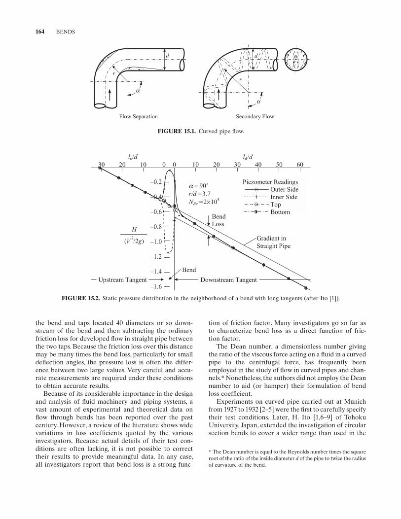
164 BENDS
tion of friction factor. Many investigators go so far as to characterize bend loss as a direct function of fric-tion factor.
The Dean number, a dimensionless number giving the ratio of the viscous force acting on a fl uid in a curved pipe to the centrifugal force, has frequently been employed in the study of fl ow in curved pipes and chan-nels. * Nonetheless, the authors did not employ the Dean number to aid (or hamper) their formulation of bend loss coeffi cient.
Experiments on curved pipe carried out at Munich from 1927 to 1932 [2 – 5] were the fi rst to carefully specify their test conditions. Later, H. Ito [1,6 – 9] of Tohoku University, Japan, extended the investigation of circular section bends to cover a wider range than used in the
the bend and taps located 40 diameters or so down-stream of the bend and then subtracting the ordinary friction loss for developed fl ow in straight pipe between the two taps. Because the friction loss over this distance may be many times the bend loss, particularly for small defl ection angles, the pressure loss is often the differ-ence between two large values. Very careful and accu-rate measurements are required under these conditions to obtain accurate results.
Because of its considerable importance in the design and analysis of fl uid machinery and piping systems, a vast amount of experimental and theoretical data on fl ow through bends has been reported over the past century. However, a review of the literature shows wide variations in loss coeffi cients quoted by the various investigators. Because actual details of their test con-ditions are often lacking, it is not possible to correct their results to provide meaningful data. In any case, all investigators report that bend loss is a strong func-
FIGURE 15.1. Curved pipe fl ow.
d
r
Flow Separation
r
d
Secondary Flow
a
a
FIGURE 15.2. Static pressure distribution in the neighborhood of a bend with long tangents (after Ito [1] ) .
–0.2
–0.4
–0.6
–0.8
–1.0
–1.2
–1.4
–1.6
Piezometer Readings Outer Side Inner Side Top Bottom
Downstream TangentUpstream Tangent
Gradient inStraight Pipe
a = 90˚r/d =3.7NRe =2×10⁵
Bend
lu/d30 20 10 2010 30 40 50 600 0
ld/d
( /2g)2
V
H
Bend Loss
* The Dean number is equal to the Reynolds number times the square root of the ratio of the inside diameter d of the pipe to twice the radius of curvature of the bend.
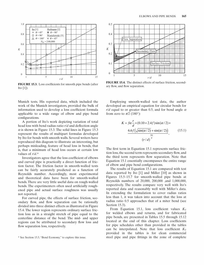
ELBOWS AND PIPE BENDS 165
FIGURE 15.3. Loss coeffi cients for smooth pipe bends (after Ito [1] ) .
1.0
0.8
0.6
0.4
0.2
01 5 10 15
K
r/d
Ito [1] Hofmann [2]
[5]
NRe = 200,000
= 45°qq
q = 90°= 90°
q = 180° q = 45°Wasielewski
Munich tests. His reported data, which included the work of the Munich investigators, provided the bulk of information used to develop a loss coeffi cient formula applicable to a wide range of elbow and pipe bend confi gurations.
A portion of Ito ’ s work depicting variation of total head loss with bend radius ratio r / d and defl ection angle α is shown in Figure 15.3 . The solid lines in Figure 15.3 represent the results of multipart formulas developed by Ito for bends with smooth walls. Several writers have reproduced this diagram to illustrate an interesting, but perhaps misleading, feature of head loss in bends, that is, that a minimum of head loss occurs at certain low values of r / d . *
Investigators agree that the loss coeffi cient of elbows and curved pipe is practically a direct function of fric-tion factor. The friction factor in smooth - walled tests can be fairly accurately predicted as a function of Reynolds number. Accordingly, most experimental and theoretical data have been for smooth - walled bends. There are very little useful data on rough - walled bends. The experimenters often used artifi cially rough-ened pipe and actual surface roughness was usually not reported.
For curved pipe, the effects of surface friction, sec-ondary fl ow, and fl ow separation can be rationally divided into three distinct effects as illustrated in Figure 15.4 . The lower region represents ordinary surface fric-tion loss as in a straight stretch of pipe equal to the centerline distance of the bend. The mid - and upper regions can be attributed to secondary fl ow loss and fl ow separation loss, respectively.
Employing smooth - walled test data, the author developed an empirical equation for circular bends for r / d equal to or greater than 0.5, and for bend angle αfrom zero to π /2 (180 ° ):
K frd
f
f
r d
= + +( ) ( ) +
+( )( )
α 0 10 2 4 2
6 6 2 24
. . sin /
. sin( / ) sin( / )
/
α
α ααπ
.. (15.1)
The fi rst term in Equation 15.1 represents surface fric-tion loss, the second term represents secondary fl ow, and the third term represents fl ow separation. Note that Equation 15.1 essentially encompasses the entire range of elbow and pipe bend confi gurations.
The results of Equation 15.1 are compared with test data reported by Ito [1] and Miller [10] as shown in Figures 15.5 – 15.7 for smooth - walled pipe bends at Reynolds numbers of 20,000, 200,000 ,and 1,000,000, respectively. The results compare very well with Ito ’ s reported data and reasonably well with Miller ’ s data. In extending the formulation to cover radius ratios less than 1, it was taken into account that the loss at radius ratio 0.5 approaches that of a miter bend (see Section 15.3 ).
From Equation 15.1 , loss coeffi cient values KT
for welded elbows and returns, and for fabricated pipe bends, are presented in Tables 15.5 through 15.12 located at the end of this chapter. Loss coeffi cients for pipe schedules other than provided in the tables can be interpolated. Note that loss coeffi cient KT
provided in the tables is for clean commercial steel pipe and pipe fi ttings in the zone of complete
FIGURE 15.4. The distinct effects of surface friction, second-ary fl ow, and fl ow separation.
0.5
0.4
0.3
K
0.2
0.1
01 5 10 15
Surface Friction
Flow Separation
Secondary Flow
r /d
* See Section 15.5 , “ Bend Economy, ” to explore this issue.
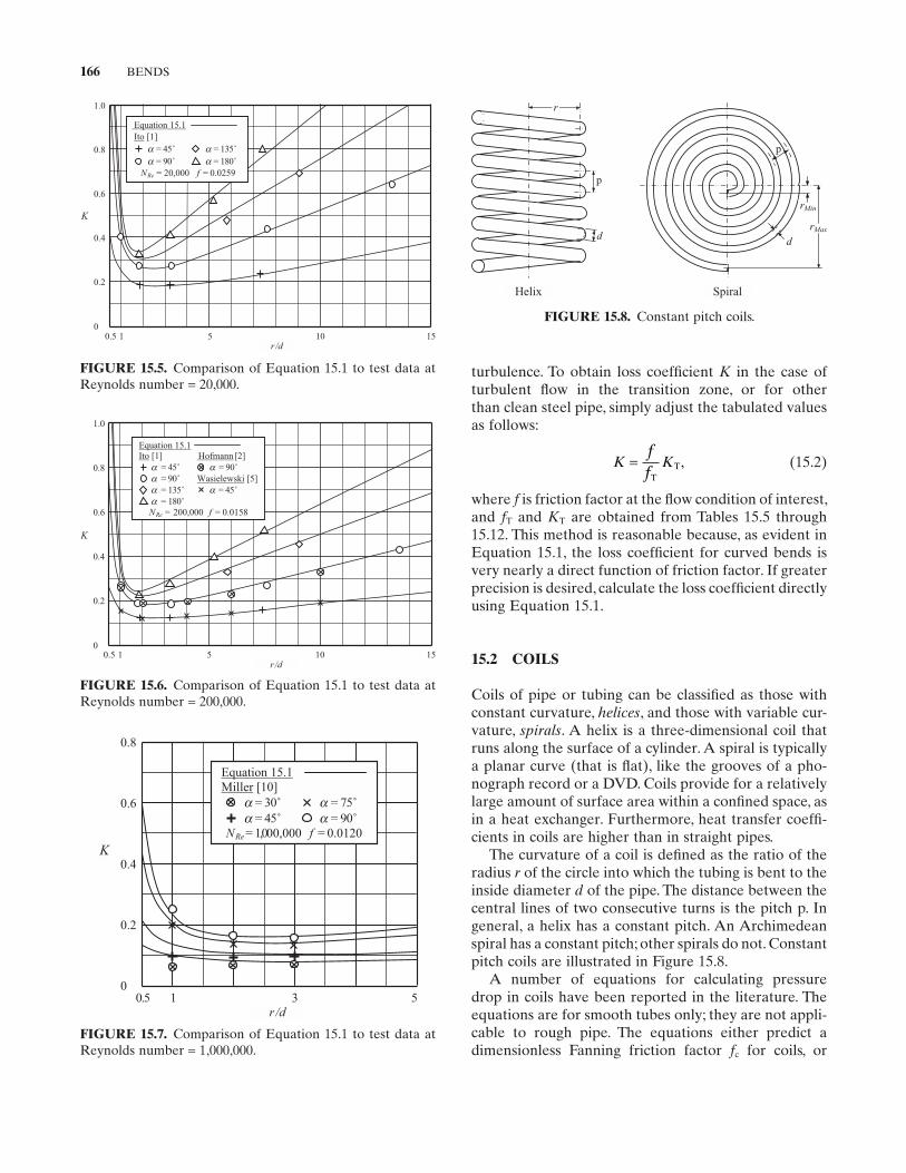
166 BENDS
turbulence. To obtain loss coeffi cient K in the case of turbulent fl ow in the transition zone, or for other than clean steel pipe, simply adjust the tabulated values as follows:
K Kff
=T
T, (15.2)
where f is friction factor at the fl ow condition of interest, and fT and KT are obtained from Tables 15.5 through 15.12 . This method is reasonable because, as evident in Equation 15.1 , the loss coeffi cient for curved bends is very nearly a direct function of friction factor. If greater precision is desired, calculate the loss coeffi cient directly using Equation 15.1 .
15.2 COILS
Coils of pipe or tubing can be classifi ed as those with constant curvature, helices , and those with variable cur-vature, spirals . A helix is a three - dimensional coil that runs along the surface of a cylinder. A spiral is typically a planar curve (that is fl at), like the grooves of a pho-nograph record or a DVD. Coils provide for a relatively large amount of surface area within a confi ned space, as in a heat exchanger. Furthermore, heat transfer coeffi -cients in coils are higher than in straight pipes.
The curvature of a coil is defi ned as the ratio of the radius r of the circle into which the tubing is bent to the inside diameter d of the pipe. The distance between the central lines of two consecutive turns is the pitch p. In general, a helix has a constant pitch. An Archimedean spiral has a constant pitch; other spirals do not. Constant pitch coils are illustrated in Figure 15.8 .
A number of equations for calculating pressure drop in coils have been reported in the literature. The equations are for smooth tubes only; they are not appli-cable to rough pipe. The equations either predict a dimensionless Fanning friction factor fc for coils, or
FIGURE 15.7. Comparison of Equation 15.1 to test data at Reynolds number = 1,000,000.
0.8
0.6
0.4
0.2
0
Equation 15.1
Miller [10]
= 30˚ = 75˚
= 45˚ = 90˚
NRe = 1,000,000 f = 0.0120
K
r/d 0.5 1 3 5
aa
aa
FIGURE 15.5. Comparison of Equation 15.1 to test data at Reynolds number = 20,000.
1.0
0.8
0.6
0.4
0.2
0
Equation 15.1
Ito [1]
= 45˚ = 135˚
= 90˚ = 180˚
N = 20,000 f = 0.0259 Re
K
0.5 1 5 10 15r /d
aa
aa
FIGURE 15.6. Comparison of Equation 15.1 to test data at Reynolds number = 200,000.
1.0
0.5 1 5 10 15r /d
0.8
0.6
0.4
0.2
Equation 15.1
0
K
Ito [1] Hofmann [2]
= 45˚ = 90˚
= 90˚ Wasielewski [5]
= 135˚ = 45˚
= 180˚
N = 200,000 f = 0.0158 Re
aaaa
a
a
FIGURE 15.8. Constant pitch coils.
p
rMin
d
rMax
Spiral
p
d
r
Helix
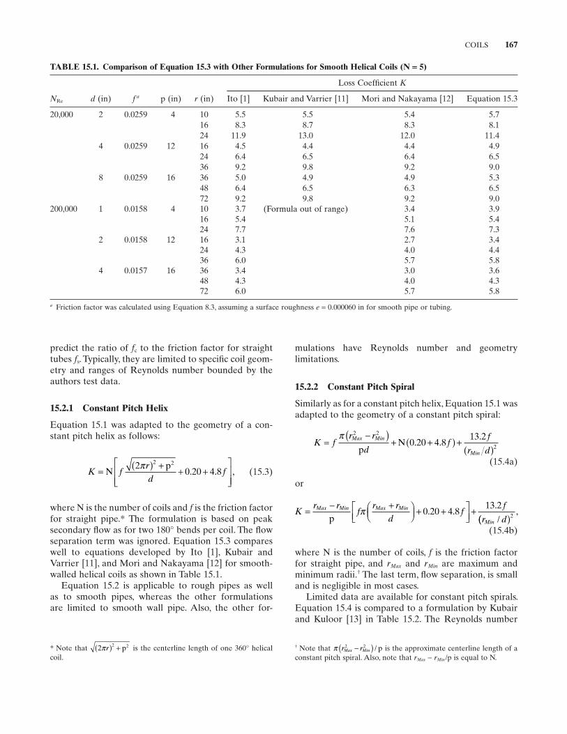
COILS 167
TABLE 15.1. Comparison of Equation 15.3 with Other Formulations for Smooth Helical Coils (N = 5)
NRe d (in) f a p (in) r (in)
Loss Coeffi cient K
Ito [1] Kubair and Varrier [11] Mori and Nakayama [12] Equation 15.3
20,000 2 0.0259 4 10 5.5 5.5 5.4 5.7 16 8.3 8.7 8.3 8.1 24 11.9 13.0 12.0 11.4
4 0.0259 12 16 4.5 4.4 4.4 4.9 24 6.4 6.5 6.4 6.5 36 9.2 9.8 9.2 9.0
8 0.0259 16 36 5.0 4.9 4.9 5.3 48 6.4 6.5 6.3 6.5 72 9.2 9.8 9.2 9.0
200,000 1 0.0158 4 10 3.7 (Formula out of range) 3.4 3.9 16 5.4 5.1 5.4 24 7.7 7.6 7.3
2 0.0158 12 16 3.1 2.7 3.4 24 4.3 4.0 4.4 36 6.0 5.7 5.8
4 0.0157 16 36 3.4 3.0 3.6 48 4.3 4.0 4.3 72 6.0 5.7 5.8
a Friction factor was calculated using Equation 8.3 , assuming a surface roughness e = 0.000060 in for smooth pipe or tubing.
predict the ratio of fc to the friction factor for straight tubes fs . Typically, they are limited to specifi c coil geom-etry and ranges of Reynolds number bounded by the authors test data.
15.2.1 Constant Pitch Helix
Equation 15.1 was adapted to the geometry of a con-stant pitch helix as follows:
K frd
f= ( ) ++ +
Np2
0 20 4 82 2π
. . , (15.3)
where N is the number of coils and f is the friction factor for straight pipe. * The formulation is based on peak secondary fl ow as for two 180 ° bends per coil. The fl ow separation term was ignored. Equation 15.3 compares well to equations developed by Ito [1] , Kubair and Varrier [11] , and Mori and Nakayama [12] for smooth - walled helical coils as shown in Table 15.1 .
Equation 15.2 is applicable to rough pipes as well as to smooth pipes, whereas the other formulations are limited to smooth wall pipe. Also, the other for-
mulations have Reynolds number and geometry limitations.
15.2.2 Constant Pitch Spiral
Similarly as for a constant pitch helix, Equation 15.1 was adapted to the geometry of a constant pitch spiral:
K fr r
df
f
r dMax Min
Min
=−( )
+ +( ) +( )
π 2 2
20 20 4 813 2
pN . .
.
(15.4a)
or
Kr r
fr r
df
f
r dMax Min Max Min
Min
=− +
+ +
+p
π 0 20 4 813 2
. ..
/(( )2 ,
(15.4b)
where N is the number of coils, f is the friction factor for straight pipe, and rMax and rMin are maximum and minimum radii. † The last term, fl ow separation, is small and is negligible in most cases.
Limited data are available for constant pitch spirals. Equation 15.4 is compared to a formulation by Kubair and Kuloor [13] in Table 15.2 . The Reynolds number
* Note that 2 2 2πr( ) + p is the centerline length of one 360 ° helical coil.
† Note that π r rMax Min2 2−( ) / p is the approximate centerline length of a
constant pitch spiral. Also, note that rMax − rMin /p is equal to N.
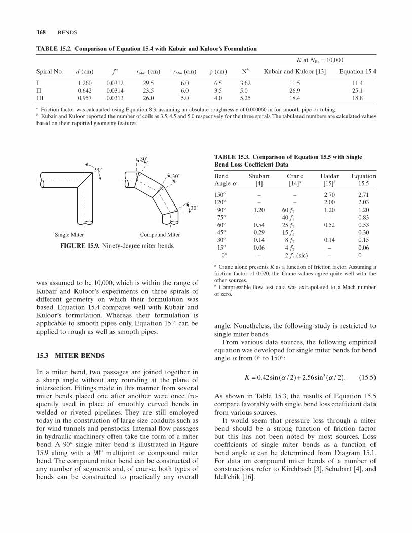
168 BENDS
angle. Nonetheless, the following study is restricted to single miter bends.
From various data sources, the following empirical equation was developed for single miter bends for bend angle α from 0 ° to 150 ° :
K = ( ) + ( )0 42 2 2 56 23. sin / . sin / .α α (15.5)
As shown in Table 15.3 , the results of Equation 15.5 compare favorably with single bend loss coeffi cient data from various sources.
It would seem that pressure loss through a miter bend should be a strong function of friction factor but this has not been noted by most sources. Loss coeffi cients of single miter bends as a function of bend angle α can be determined from Diagram 15.1 . For data on compound miter bends of a number of constructions, refer to Kirchbach [3] , Schubart [4] , and Idel ’ chik [16] .
FIGURE 15.9. Ninety - degree miter bends.
30˚
90˚
30˚
30˚
Compound MiterSingle Miter
TABLE 15.2. Comparison of Equation 15.4 with Kubair and Kuloor ’ s Formulation
Spiral No. d (cm) f a rMax (cm) rMin (cm) p (cm) N b
K at NRe = 10,000
Kubair and Kuloor [13] Equation 15.4
I 1.260 0.0312 29.5 6.0 6.5 3.62 11.5 11.4 II 0.642 0.0314 23.5 6.0 3.5 5.0 26.9 25.1 III 0.957 0.0313 26.0 5.0 4.0 5.25 18.4 18.8
a Friction factor was calculated using Equation 8.3 , assuming an absolute roughness e of 0.000060 in for smooth pipe or tubing. b Kubair and Kuloor reported the number of coils as 3.5, 4.5 and 5.0 respectively for the three spirals. The tabulated numbers are calculated values based on their reported geometry features.
was assumed to be 10,000, which is within the range of Kubair and Kuloor ’ s experiments on three spirals of different geometry on which their formulation was based. Equation 15.4 compares well with Kubair and Kuloor ’ s formulation. Whereas their formulation is applicable to smooth pipes only, Equation 15.4 can be applied to rough as well as smooth pipes.
15.3 MITER BENDS
In a miter bend, two passages are joined together in a sharp angle without any rounding at the plane of intersection. Fittings made in this manner from several miter bends placed one after another were once fre-quently used in place of smoothly curved bends in welded or riveted pipelines. They are still employed today in the construction of large - size conduits such as for wind tunnels and penstocks. Internal fl ow passages in hydraulic machinery often take the form of a miter bend. A 90 ° single miter bend is illustrated in Figure 15.9 along with a 90 ° multijoint or compound miter bend. The compound miter bend can be constructed of any number of segments and, of course, both types of bends can be constructed to practically any overall
TABLE 15.3. Comparison of Equation 15.5 with Single Bend Loss Coeffi cient Data
Bend Angle α
Shubart [4]
Crane [14] a
Haidar [15] b
Equation 15.5
150 ° – – 2.70 2.71 120 ° – – 2.00 2.03 90 ° 1.20 60 fT 1.20 1.20 75 ° – 40 fT – 0.83 60 ° 0.54 25 fT 0.52 0.53 45 ° 0.29 15 fT – 0.30 30 ° 0.14 8 fT 0.14 0.15 15 ° 0.06 4 fT – 0.06
0 ° – 2 fT (sic) – 0
a Crane alone presents K as a function of friction factor. Assuming a friction factor of 0.020, the Crane values agree quite well with the other sources. b Compressible fl ow test data was extrapolated to a Mach number of zero.
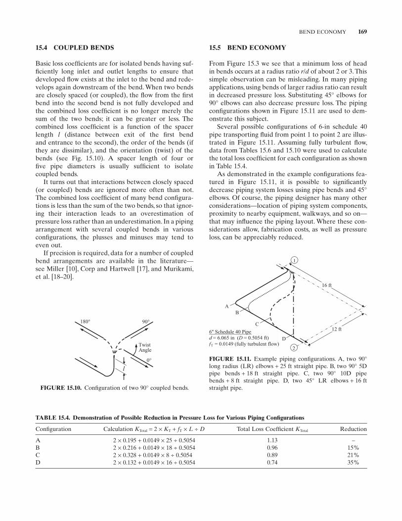
BEND ECONOMY 169
FIGURE 15.10. Confi guration of two 90 ° coupled bends.
0°
90°
l
180°
Twist Angle
FIGURE 15.11. Example piping confi gurations. A, two 90 ° long radius (LR) elbows + 25 ft straight pipe. B, two 90 ° 5D pipe bends + 18 ft straight pipe. C, two 90 ° 10D pipe bends + 8 ft straight pipe. D, two 45 ° LR elbows + 16 ft straight pipe.
6'' Schedule 40 Pipe
d = 6.065 in (D = 0.5054 ft)
fT = 0.0149 (fully turbulent flow)
1
16 ft
12 ft
2
A
B
C
D
15.5 BEND ECONOMY
From Figure 15.3 we see that a minimum loss of head in bends occurs at a radius ratio r / d of about 2 or 3. This simple observation can be misleading. In many piping applications, using bends of larger radius ratio can result in decreased pressure loss. Substituting 45 ° elbows for 90 ° elbows can also decrease pressure loss. The piping confi gurations shown in Figure 15.11 are used to dem-onstrate this subject.
Several possible confi gurations of 6 - in schedule 40 pipe transporting fl uid from point 1 to point 2 are illus-trated in Figure 15.11 . Assuming fully turbulent fl ow, data from Tables 15.6 and 15.10 were used to calculate the total loss coeffi cient for each confi guration as shown in Table 15.4 .
As demonstrated in the example confi gurations fea-tured in Figure 15.11 , it is possible to signifi cantly decrease piping system losses using pipe bends and 45 ° elbows. Of course, the piping designer has many other considerations — location of piping system components, proximity to nearby equipment, walkways, and so on — that may infl uence the piping layout. Where these con-siderations allow, fabrication costs, as well as pressure loss, can be appreciably reduced.
15.4 COUPLED BENDS
Basic loss coeffi cients are for isolated bends having suf-fi ciently long inlet and outlet lengths to ensure that developed fl ow exists at the inlet to the bend and rede-velops again downstream of the bend. When two bends are closely spaced (or coupled), the fl ow from the fi rst bend into the second bend is not fully developed and the combined loss coeffi cient is no longer merely the sum of the two bends; it can be greater or less. The combined loss coeffi cient is a function of the spacer length l (distance between exit of the fi rst bend and entrance to the second), the order of the bends (if they are dissimilar), and the orientation (twist) of the bends (see Fig. 15.10 ). A spacer length of four or fi ve pipe diameters is usually suffi cient to isolate coupled bends.
It turns out that interactions between closely spaced (or coupled) bends are ignored more often than not. The combined loss coeffi cient of many bend confi gura-tions is less than the sum of the two bends, so that ignor-ing their interaction leads to an overestimation of pressure loss rather than an underestimation. In a piping arrangement with several coupled bends in various confi gurations, the plusses and minuses may tend to even out.
If precision is required, data for a number of coupled bend arrangements are available in the literature — see Miller [10] , Corp and Hartwell [17] , and Murikami, et al. [18 – 20] .
TABLE 15.4. Demonstration of Possible Reduction in Pressure Loss for Various Piping Confi gurations
Confi guration Calculation KTotal = 2 × KT + fT × L ÷ D Total Loss Coeffi cient KTotal Reduction
A 2 × 0.195 + 0.0149 × 25 ÷ 0.5054 1.13 – B 2 × 0.216 + 0.0149 × 18 ÷ 0.5054 0.96 15% C 2 × 0.328 + 0.0149 × 8 ÷ 0.5054 0.89 21% D 2 × 0.132 + 0.0149 × 16 ÷ 0.5054 0.74 35%
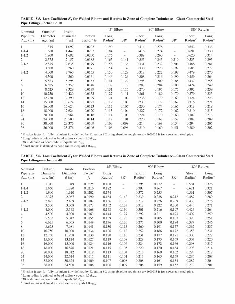
TABLE 15.5. Loss Coeffi cient K T for Welded Elbows and Returns in Zone of Complete Turbulence — Clean Commercial Steel Pipe Fittings — Schedule 10
Nominal Pipe Size d Nom (in)
Outside Diameter d OD (in)
Inside Diameter
d (in) Friction
Factor a f T
45 ° Elbow 90 ° Elbow 180 ° Return
Long Radius b 3R c
Short Radius d
Long Radius b 3R c
Short Radius d
Long Radius b
1 1.315 1.097 0.0222 0.190 – 0.414 0.278 – 0.642 0.333 1 - 1/4 1.660 1.442 0.0207 0.184 – 0.416 0.274 – 0.691 0.330 1 - 1/2 1.900 1.682 0.0200 0.176 – 0.389 0.260 – 0.620 0.314 2 2.375 2.157 0.0188 0.165 0.141 0.353 0.243 0.210 0.535 0.293 2 - 1/2 2.875 2.635 0.0179 0.158 0.136 0.331 0.232 0.204 0.488 0.281 3 3.500 3.260 0.0171 0.154 0.132 0.330 0.228 0.197 0.505 0.277 3 - 1/2 4.000 3.760 0.0165 0.150 0.129 0.318 0.222 0.193 0.479 0.270 4 4.500 4.260 0.0161 0.146 0.126 0.308 0.216 0.190 0.459 0.264 5 5.563 5.295 0.0153 0.141 0.122 0.295 0.209 0.185 0.437 0.255 6 6.625 6.357 0.0148 0.137 0.119 0.287 0.204 0.180 0.424 0.249 8 8.625 8.329 0.0139 0.131 0.115 0.270 0.195 0.175 0.392 0.239 10 10.750 10.420 0.0133 0.127 0.111 0.261 0.189 0.170 0.379 0.233 12 12.750 12.390 0.0129 0.121 0.109 0.238 0.179 0.169 0.324 0.223 14 15.000 13.624 0.0127 0.119 0.108 0.233 0.177 0.167 0.316 0.221 16 16.000 15.624 0.0123 0.117 0.106 0.230 0.174 0.165 0.313 0.218 18 18.000 17.624 0.0120 0.115 0.104 0.227 0.172 0.162 0.310 0.215 20 20.000 19.564 0.0118 0.114 0.103 0.224 0.170 0.160 0.307 0.213 24 24.000 23.500 0.0114 0.112 0.101 0.220 0.167 0.157 0.302 0.209 30 30.000 29.376 0.0109 0.109 0.098 0.214 0.163 0.154 0.294 0.205 36 36.000 35.376 0.0106 0.106 0.096 0.210 0.160 0.151 0.289 0.202
a Friction factor for fully turbulent fl ow defi ned by Equation 8.2 using absolute roughness ε = 0.00015 ft for new/clean steel pipe. b Long radius is defi ned as bend radius r equals 1.5 · d Nom . c 3R is defi ned as bend radius r equals 3.0 d Nom . d Short radius is defi ned as bend radius r equals 1.0 · d Nom .
TABLE 15.6. Loss Coeffi cient K T for Welded Elbows and Returns in Zone of Complete Turbulence — Clean Commercial Steel Pipe Fittings — Schedule 40
Nominal Pipe Size d Nom (in)
Outside Diameter d OD (in)
Inside Diameter
d (in)
Friction Factor a
f T
45 ° Elbow 90 ° Elbow 180 ° Return
Long Radius b 3R c
Short Radius d
Long Radius b 3R c
Short Radius d
Long Radius b
1 1.315 1.049 0.0225 0.188 – 0.395 0.272 – 0.581 0.326 1 - 1/4 1.660 1.380 0.0210 0.182 – 0.397 0.267 – 0.621 0.321 1 - 1/2 1.900 1.610 0.0202 0.174 – 0.372 0.255 – 0.561 0.307 2 2.375 2.067 0.0190 0.164 0.142 0.339 0.238 0.212 0.489 0.289 2 - 1/2 2.875 2.469 0.0182 0.156 0.138 0.312 0.226 0.209 0.430 0.276 3 3.500 3.068 0.0173 0.152 0.133 0.312 0.222 0.200 0.445 0.271 3 - 1/2 4.000 3.548 0.0168 0.148 0.130 0.301 0.216 0.197 0.426 0.264 4 4.500 4.020 0.0163 0.144 0.127 0.292 0.211 0.193 0.409 0.259 5 5.563 5.047 0.0155 0.139 0.123 0.282 0.205 0.187 0.398 0.251 6 6.625 6.065 0.0149 0.136 0.120 0.275 0.200 0.184 0.387 0.246 8 8.625 7.981 0.0141 0.130 0.115 0.260 0.191 0.177 0.362 0.237 10 10.750 10.020 0.0134 0.126 0.112 0.252 0.186 0.172 0.353 0.231 12 12.750 11.938 0.0130 0.120 0.110 0.231 0.177 0.171 0.306 0.222 14 15.000 13.124 0.0127 0.119 0.108 0.228 0.175 0.169 0.303 0.220 16 16.000 15.000 0.0124 0.116 0.106 0.224 0.172 0.166 0.298 0.217 18 18.000 16.876 0.0121 0.115 0.105 0.220 0.170 0.164 0.293 0.214 20 20.000 18.812 0.0119 0.113 0.104 0.218 0.168 0.162 0.29 0.212 24 24.000 22.624 0.0115 0.111 0.101 0.213 0.165 0.159 0.286 0.208 32 32.000 30.624 0.0109 0.107 0.098 0.208 0.161 0.154 0.282 0.20 36 36.000 34.500 0.0106 0.106 0.097 0.206 0.159 0.152 0.279 0.201
a Friction factor for fully turbulent fl ow defi ned by Equation 8.2 using absolute roughness ε = 0.00015 ft for new/clean steel pipe. b Long radius is defi ned as bend radius r equals 1.5 · d Nom . c 3R is defi ned as bend radius r equals 3.0 d Nom . d Short radius is defi ned as bend radius r equals 1.0 · d Nom .
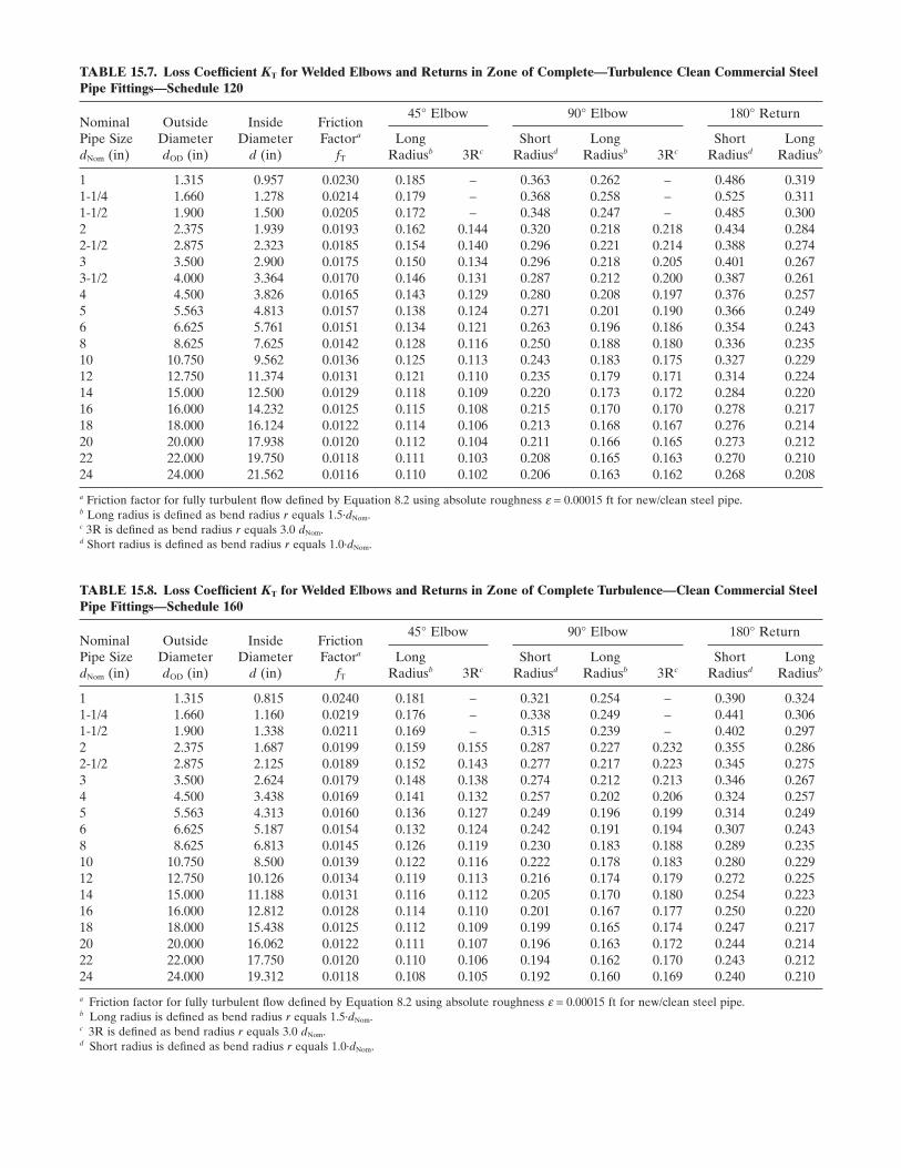
TABLE 15.7. Loss Coeffi cient K T for Welded Elbows and Returns in Zone of Complete — Turbulence Clean Commercial Steel Pipe Fittings — Schedule 120
Nominal Pipe Size d Nom (in)
Outside Diameter d OD (in)
Inside Diameter
d (in)
Friction Factor a
f T
45 ° Elbow 90 ° Elbow 180 ° Return
Long Radius b 3R c
Short Radius d
Long Radius b 3R c
Short Radius d
Long Radius b
1 1.315 0.957 0.0230 0.185 – 0.363 0.262 – 0.486 0.319 1 - 1/4 1.660 1.278 0.0214 0.179 – 0.368 0.258 – 0.525 0.311 1 - 1/2 1.900 1.500 0.0205 0.172 – 0.348 0.247 – 0.485 0.300 2 2.375 1.939 0.0193 0.162 0.144 0.320 0.218 0.218 0.434 0.284 2 - 1/2 2.875 2.323 0.0185 0.154 0.140 0.296 0.221 0.214 0.388 0.274 3 3.500 2.900 0.0175 0.150 0.134 0.296 0.218 0.205 0.401 0.267 3 - 1/2 4.000 3.364 0.0170 0.146 0.131 0.287 0.212 0.200 0.387 0.261 4 4.500 3.826 0.0165 0.143 0.129 0.280 0.208 0.197 0.376 0.257 5 5.563 4.813 0.0157 0.138 0.124 0.271 0.201 0.190 0.366 0.249 6 6.625 5.761 0.0151 0.134 0.121 0.263 0.196 0.186 0.354 0.243 8 8.625 7.625 0.0142 0.128 0.116 0.250 0.188 0.180 0.336 0.235 10 10.750 9.562 0.0136 0.125 0.113 0.243 0.183 0.175 0.327 0.229 12 12.750 11.374 0.0131 0.121 0.110 0.235 0.179 0.171 0.314 0.224 14 15.000 12.500 0.0129 0.118 0.109 0.220 0.173 0.172 0.284 0.220 16 16.000 14.232 0.0125 0.115 0.108 0.215 0.170 0.170 0.278 0.217 18 18.000 16.124 0.0122 0.114 0.106 0.213 0.168 0.167 0.276 0.214 20 20.000 17.938 0.0120 0.112 0.104 0.211 0.166 0.165 0.273 0.212 22 22.000 19.750 0.0118 0.111 0.103 0.208 0.165 0.163 0.270 0.210 24 24.000 21.562 0.0116 0.110 0.102 0.206 0.163 0.162 0.268 0.208
a Friction factor for fully turbulent fl ow defi ned by Equation 8.2 using absolute roughness ε = 0.00015 ft for new/clean steel pipe. b Long radius is defi ned as bend radius r equals 1.5 · d Nom . c 3R is defi ned as bend radius r equals 3.0 d Nom . d Short radius is defi ned as bend radius r equals 1.0 · d Nom .
TABLE 15.8. Loss Coeffi cient K T for Welded Elbows and Returns in Zone of Complete Turbulence — Clean Commercial Steel Pipe Fittings — Schedule 160
Nominal Pipe Size d Nom (in)
Outside Diameter d OD (in)
Inside Diameter
d (in)
Friction Factor a
f T
45 ° Elbow 90 ° Elbow 180 ° Return
Long Radius b 3R c
Short Radius d
Long Radius b 3R c
Short Radius d
Long Radius b
1 1.315 0.815 0.0240 0.181 – 0.321 0.254 – 0.390 0.324 1 - 1/4 1.660 1.160 0.0219 0.176 – 0.338 0.249 – 0.441 0.306 1 - 1/2 1.900 1.338 0.0211 0.169 – 0.315 0.239 – 0.402 0.297 2 2.375 1.687 0.0199 0.159 0.155 0.287 0.227 0.232 0.355 0.286 2 - 1/2 2.875 2.125 0.0189 0.152 0.143 0.277 0.217 0.223 0.345 0.275 3 3.500 2.624 0.0179 0.148 0.138 0.274 0.212 0.213 0.346 0.267 4 4.500 3.438 0.0169 0.141 0.132 0.257 0.202 0.206 0.324 0.257 5 5.563 4.313 0.0160 0.136 0.127 0.249 0.196 0.199 0.314 0.249 6 6.625 5.187 0.0154 0.132 0.124 0.242 0.191 0.194 0.307 0.243 8 8.625 6.813 0.0145 0.126 0.119 0.230 0.183 0.188 0.289 0.235 10 10.750 8.500 0.0139 0.122 0.116 0.222 0.178 0.183 0.280 0.229 12 12.750 10.126 0.0134 0.119 0.113 0.216 0.174 0.179 0.272 0.225 14 15.000 11.188 0.0131 0.116 0.112 0.205 0.170 0.180 0.254 0.223 16 16.000 12.812 0.0128 0.114 0.110 0.201 0.167 0.177 0.250 0.220 18 18.000 15.438 0.0125 0.112 0.109 0.199 0.165 0.174 0.247 0.217 20 20.000 16.062 0.0122 0.111 0.107 0.196 0.163 0.172 0.244 0.214 22 22.000 17.750 0.0120 0.110 0.106 0.194 0.162 0.170 0.243 0.212 24 24.000 19.312 0.0118 0.108 0.105 0.192 0.160 0.169 0.240 0.210
a Friction factor for fully turbulent fl ow defi ned by Equation 8.2 using absolute roughness ε = 0.00015 ft for new/clean steel pipe. b Long radius is defi ned as bend radius r equals 1.5 · d Nom . c 3R is defi ned as bend radius r equals 3.0 d Nom . d Short radius is defi ned as bend radius r equals 1.0 · d Nom .
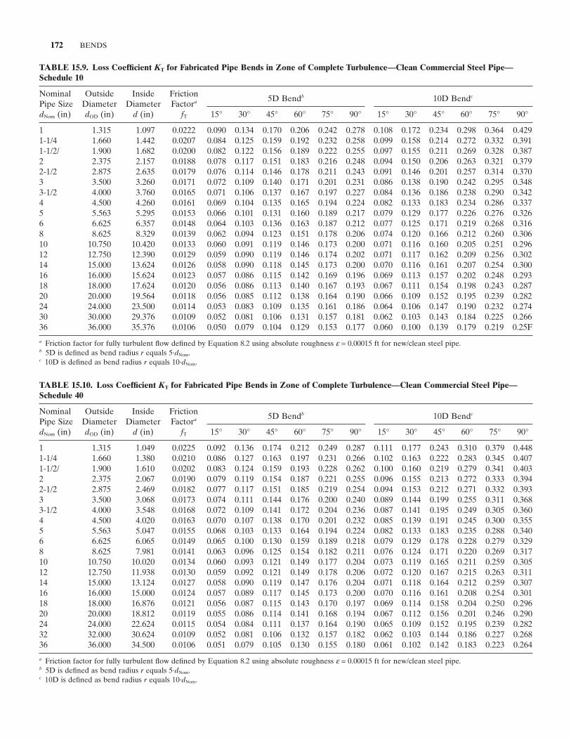
172 BENDS
TABLE 15.9. Loss Coeffi cient K T for Fabricated Pipe Bends in Zone of Complete Turbulence — Clean Commercial Steel Pipe — Schedule 10
Nominal Pipe Size d Nom (in)
Outside Diameter d OD (in)
Inside Diameter
d (in)
Friction Factor a
f T
5D Bend b 10D Bend c
15 ° 30 ° 45 ° 60 ° 75 ° 90 ° 15 ° 30 ° 45 ° 60 ° 75 ° 90 °
1 1.315 1.097 0.0222 0.090 0.134 0.170 0.206 0.242 0.278 0.108 0.172 0.234 0.298 0.364 0.429 1 - 1/4 1.660 1.442 0.0207 0.084 0.125 0.159 0.192 0.232 0.258 0.099 0.158 0.214 0.272 0.332 0.391 1 - 1/2/ 1.900 1.682 0.0200 0.082 0.122 0.156 0.189 0.222 0.255 0.097 0.155 0.211 0.269 0.328 0.387 2 2.375 2.157 0.0188 0.078 0.117 0.151 0.183 0.216 0.248 0.094 0.150 0.206 0.263 0.321 0.379 2 - 1/2 2.875 2.635 0.0179 0.076 0.114 0.146 0.178 0.211 0.243 0.091 0.146 0.201 0.257 0.314 0.370 3 3.500 3.260 0.0171 0.072 0.109 0.140 0.171 0.201 0.231 0.086 0.138 0.190 0.242 0.295 0.348 3 - 1/2 4.000 3.760 0.0165 0.071 0.106 0.137 0.167 0.197 0.227 0.084 0.136 0.186 0.238 0.290 0.342 4 4.500 4.260 0.0161 0.069 0.104 0.135 0.165 0.194 0.224 0.082 0.133 0.183 0.234 0.286 0.337 5 5.563 5.295 0.0153 0.066 0.101 0.131 0.160 0.189 0.217 0.079 0.129 0.177 0.226 0.276 0.326 6 6.625 6.357 0.0148 0.064 0.103 0.136 0.163 0.187 0.212 0.077 0.125 0.171 0.219 0.268 0.316 8 8.625 8.329 0.0139 0.062 0.094 0.123 0.151 0.178 0.206 0.074 0.120 0.166 0.212 0.260 0.306 10 10.750 10.420 0.0133 0.060 0.091 0.119 0.146 0.173 0.200 0.071 0.116 0.160 0.205 0.251 0.296 12 12.750 12.390 0.0129 0.059 0.090 0.119 0.146 0.174 0.202 0.071 0.117 0.162 0.209 0.256 0.302 14 15.000 13.624 0.0126 0.058 0.090 0.118 0.145 0.173 0.200 0.070 0.116 0.161 0.207 0.254 0.300 16 16.000 15.624 0.0123 0.057 0.086 0.115 0.142 0.169 0.196 0.069 0.113 0.157 0.202 0.248 0.293 18 18.000 17.624 0.0120 0.056 0.086 0.113 0.140 0.167 0.193 0.067 0.111 0.154 0.198 0.243 0.287 20 20.000 19.564 0.0118 0.056 0.085 0.112 0.138 0.164 0.190 0.066 0.109 0.152 0.195 0.239 0.282 24 24.000 23.500 0.0114 0.053 0.083 0.109 0.135 0.161 0.186 0.064 0.106 0.147 0.190 0.232 0.274 30 30.000 29.376 0.0109 0.052 0.081 0.106 0.131 0.157 0.181 0.062 0.103 0.143 0.184 0.225 0.266 36 36.000 35.376 0.0106 0.050 0.079 0.104 0.129 0.153 0.177 0.060 0.100 0.139 0.179 0.219 0.25F
a Friction factor for fully turbulent fl ow defi ned by Equation 8.2 using absolute roughness ε = 0.00015 ft for new/clean steel pipe. b 5D is defi ned as bend radius r equals 5 · d Nom . c 10D is defi ned as bend radius r equals 10 · d Nom .
TABLE 15.10. Loss Coeffi cient K T for Fabricated Pipe Bends in Zone of Complete Turbulence — Clean Commercial Steel Pipe — Schedule 40
Nominal Pipe Size d Nom (in)
Outside Diameter d OD (in)
Inside Diameter
d (in)
Friction Factor a
f T
5D Bend b 10D Bend c
15 ° 30 ° 45 ° 60 ° 75 ° 90 ° 15 ° 30 ° 45 ° 60 ° 75 ° 90 °
1 1.315 1.049 0.0225 0.092 0.136 0.174 0.212 0.249 0.287 0.111 0.177 0.243 0.310 0.379 0.448 1 - 1/4 1.660 1.380 0.0210 0.086 0.127 0.163 0.197 0.231 0.266 0.102 0.163 0.222 0.283 0.345 0.407 1 - 1/2/ 1.900 1.610 0.0202 0.083 0.124 0.159 0.193 0.228 0.262 0.100 0.160 0.219 0.279 0.341 0.403 2 2.375 2.067 0.0190 0.079 0.119 0.154 0.187 0.221 0.255 0.096 0.155 0.213 0.272 0.333 0.394 2 - 1/2 2.875 2.469 0.0182 0.077 0.117 0.151 0.185 0.219 0.254 0.094 0.153 0.212 0.271 0.332 0.393 3 3.500 3.068 0.0173 0.074 0.111 0.144 0.176 0.200 0.240 0.089 0.144 0.199 0.255 0.311 0.368 3 - 1/2 4.000 3.548 0.0168 0.072 0.109 0.141 0.172 0.204 0.236 0.087 0.141 0.195 0.249 0.305 0.360 4 4.500 4.020 0.0163 0.070 0.107 0.138 0.170 0.201 0.232 0.085 0.139 0.191 0.245 0.300 0.355 5 5.563 5.047 0.0155 0.068 0.103 0.133 0.164 0.194 0.224 0.082 0.133 0.183 0.235 0.288 0.340 6 6.625 6.065 0.0149 0.065 0.100 0.130 0.159 0.189 0.218 0.079 0.129 0.178 0.228 0.279 0.329 8 8.625 7.981 0.0141 0.063 0.096 0.125 0.154 0.182 0.211 0.076 0.124 0.171 0.220 0.269 0.317 10 10.750 10.020 0.0134 0.060 0.093 0.121 0.149 0.177 0.204 0.073 0.119 0.165 0.211 0.259 0.305 12 12.750 11.938 0.0130 0.059 0.092 0.121 0.149 0.178 0.206 0.072 0.120 0.167 0.215 0.263 0.311 14 15.000 13.124 0.0127 0.058 0.090 0.119 0.147 0.176 0.204 0.071 0.118 0.164 0.212 0.259 0.307 16 16.000 15.000 0.0124 0.057 0.089 0.117 0.145 0.173 0.200 0.070 0.116 0.161 0.208 0.254 0.301 18 18.000 16.876 0.0121 0.056 0.087 0.115 0.143 0.170 0.197 0.069 0.114 0.158 0.204 0.250 0.296 20 20.000 18.812 0.0119 0.055 0.086 0.114 0.141 0.168 0.194 0.067 0.112 0.156 0.201 0.246 0.290 24 24.000 22.624 0.0115 0.054 0.084 0.111 0.137 0.164 0.190 0.065 0.109 0.152 0.195 0.239 0.282 32 32.000 30.624 0.0109 0.052 0.081 0.106 0.132 0.157 0.182 0.062 0.103 0.144 0.186 0.227 0.268 36 36.000 34.500 0.0106 0.051 0.079 0.105 0.130 0.155 0.180 0.061 0.102 0.142 0.183 0.223 0.264
a Friction factor for fully turbulent fl ow defi ned by Equation 8.2 using absolute roughness ε = 0.00015 ft for new/clean steel pipe. b 5D is defi ned as bend radius r equals 5 · d Nom . c 10D is defi ned as bend radius r equals 10 · d Nom .
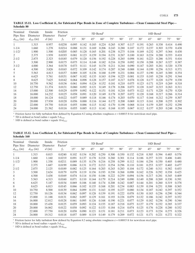
COILS 173
TABLE 15.11. Loss Coeffi cient K T for Fabricated Pipe Bends in Zone of Complete Turbulence — Clean Commercial Steel Pipe — Schedule 80
Nominal Pipe Size d Nom (in)
Outside Diameter d OD (in)
Inside Diameter
d (in)
Friction Factor a
f T
5D Bend b 10D Bend c
15 ° 30 ° 45 ° 60 ° 75 ° 90 ° 15 ° 30 ° 45 ° 60 ° 75 ° 90 °
1 1.315 0.957 0.0230 0.095 0.142 0.183 0.224 0.265 0.307 0.117 0.191 0.263 0.338 0.414 0.490 1 - 1/4 1.660 1.278 0.0214 0.088 0.131 0.169 0.206 0.243 0.280 0.107 0.172 0.237 0.303 0.370 0.438 1 - 1/2/ 1.900 1.500 0.0205 0.085 0.128 0.165 0.201 0.238 0.275 0.104 0.169 0.232 0.297 0.364 0.430 2 2.375 1.939 0.0193 0.081 0.123 0.159 0.194 0.231 0.267 0.100 0.163 0.224 0.288 0.353 0.418 2 - 1/2 2.875 2.323 0.0185 0.079 0.120 0.156 0.192 0.228 0.265 0.098 0.161 0.223 0.286 0.351 0.416 3 3.500 2.900 0.0175 0.075 0.114 0.148 0.182 0.216 0.250 0.092 0.150 0.208 0.267 0.327 0.387 3 - 1/2 4.000 3.364 0.0170 0.073 0.111 0.145 0.178 0.211 0.244 0.090 0.147 0.203 0.261 0.320 0.378 4 4.500 3.826 0.0165 0.072 0.109 0.142 0.174 0.207 0.240 0.088 0.144 0.199 0.256 0.313 0.371 5 5.563 4.813 0.0157 0.069 0.105 0.136 0.168 0.199 0.231 0.084 0.137 0.190 0.245 0.300 0.354 6 6.625 5.761 0.0151 0.067 0.102 0.133 0.163 0.194 0.225 0.081 0.133 0.185 0.238 0.291 0.344 8 8.625 7.625 0.0142 0.064 0.098 0.128 0.157 0.187 0.217 0.078 0.128 0.177 0.228 0.279 0.330 10 10.750 9.562 0.0136 0.061 0.094 0.124 0.152 0.181 0.210 0.075 0.123 0.171 0.219 0.269 0.318 12 12.750 11.374 0.0131 0.060 0.092 0.121 0.149 0.178 0.206 0.073 0.120 0.167 0.215 0.263 0.311 14 15.000 12.500 0.0129 0.059 0.092 0.122 0.151 0.181 0.210 0.073 0.122 0.171 0.220 0.270 0.320 16 16.000 14.232 0.0125 0.058 0.091 0.120 0.149 0.178 0.207 0.072 0.120 0.168 0.217 0.266 0.314 18 18.000 16.124 0.0122 0.057 0.089 0.118 0.146 0.174 0.203 0.070 0.117 0.164 0.212 0.259 0.307 20 20.000 17.938 0.0120 0.056 0.088 0.116 0.144 0.172 0.200 0.069 0.115 0.161 0.208 0.255 0.302 22 22.000 19.750 0.0118 0.055 0.086 0.115 0.142 0.170 0.198 0.068 0.114 0.159 0.205 0.252 0.298 24 24.000 21.562 0.0116 0.055 0.085 0.113 0.141 0.168 0.195 0.067 0.112 0.157 0.203 0.248 0.294
a Friction factor for fully turbulent fl ow defi ned by Equation 8.2 using absolute roughness ε = 0.00015 ft for new/clean steel pipe. b 5D is defi ned as bend radius r equals 5 · d Nom . c 10D is defi ned as bend radius r equals 10 · d Nom .
TABLE 15.12. Loss Coeffi cient K T for Fabricated Pipe Bends in Zone of Complete Turbulence — Clean Commercial Steel Pipe — Schedule 160
Nominal Pipe Size d Nom (in)
Outside Diameter d OD (in)
Inside Diameter
d (in)
Friction Factor a
f T
5D Bend b 10D Bend c
15 ° 30 ° 45 ° 60 ° 75 ° 90 ° 15 ° 30 ° 45 ° 60 ° 75 ° 90 °
1 1.315 0.815 0.0240 0.102 0.154 0.202 0.250 0.300 0.350 0.132 0.218 0.305 0.394 0.485 0.576 1 - 1/4 1.660 1.160 0.0219 0.091 0.137 0.178 0.218 0.260 0.301 0.114 0.186 0.257 0.331 0.406 0.481 1 - 1/2/ 1.900 1.338 0.0211 0.089 0.135 0.176 0.216 0.258 0.299 0.112 0.184 0.256 0.330 0.405 0.480 2 2.375 1.687 0.0199 0.086 0.131 0.172 0.213 0.254 0.296 0.110 0.181 0.253 0.327 0.402 0.477 2 - 1/2 2.875 2.125 0.0189 0.082 0.125 0.164 0.203 0.243 0.283 0.104 0.172 0.240 0.311 0.382 0.453 3 3.500 2.624 0.0179 0.078 0.119 0.156 0.193 0.230 0.268 0.098 0.162 0.226 0.292 0.358 0.425 4 4.500 3.438 0.0169 0.074 0.114 0.150 0.186 0.222 0.259 0.094 0.156 0.217 0.281 0.345 0.409 5 5.563 4.313 0.0160 0.071 0.110 0.144 0.179 0.214 0.249 0.090 0.149 0.208 0.269 0.330 0.391 6 6.625 5.187 0.0154 0.069 0.106 0.140 0.174 0.208 0.242 0.087 0.144 0.201 0.260 0.319 0.378 8 8.625 6.813 0.0145 0.066 0.102 0.135 0.168 0.201 0.234 0.083 0.139 0.194 0.251 0.308 0.365 10 10.750 8.500 0.0139 0.064 0.099 0.131 0.163 0.195 0.227 0.080 0.134 0.187 0.242 0.297 0.352 12 12.750 10.126 0.0134 0.062 0.097 0.128 0.159 0.191 0.222 0.078 0.130 0.183 0.236 0.290 0.344 14 15.000 11.188 0.0131 0.062 0.097 0.129 0.161 0.193 0.226 0.079 0.132 0.186 0.242 0.297 0.352 16 16.000 12.812 0.0128 0.061 0.095 0.126 0.168 0.190 0.221 0.077 0.129 0.182 0.236 0.290 0.344 18 18.000 15.438 0.0125 0.059 0.093 0.124 0.155 0.187 0.218 0.075 0.127 0.179 0.232 0.285 0.337 20 20.000 16.062 0.0122 0.058 0.092 0.122 0.153 0.184 0.214 0.074 0.125 0.176 0.228 0.280 0.332 22 22.000 17.750 0.0120 0.058 0.090 0.121 0.151 0.181 0.211 0.073 0.123 0.173 0.224 0.275 0.326 24 24.000 19.312 0.0118 0.057 0.089 0.119 0.149 0.179 0.209 0.072 0.121 0.171 0.221 0.272 0.322
a Friction factor for fully turbulent fl ow defi ned by Equation 8.2 using absolute roughness ε = 0.00015 ft for new/clean steel pipe. b 5D is defi ned as bend radius r equals 5 · d Nom . c 10D is defi ned as bend radius r equals 10 · d Nom .
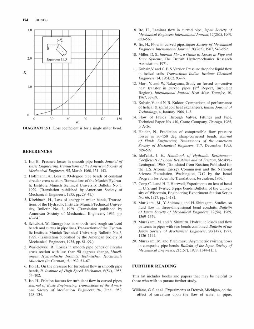
174 BENDS
REFERENCES
1. Ito , H. , Pressure losses in smooth pipe bends , Journal of Basic Engineering, Transactions of the American Society of Mechanical Engineers , 95 , March 1960 , 131 – 143 .
2. Hoffmann , A. , Loss in 90 - degree pipe bends of constant circular cross - section , Transactions of the Munich Hydrau-lic Institute, Munich Technical University, Bulletin No. 3, 1929 . (Translation published by American Society of Mechanical Engineers, 1935, pp. 29 – 41.)
3. Kirchbach , H. , Loss of energy in miter bends , Transac-tions of the Hydraulic Institute, Munich Technical Univer-sity, Bulletin No. 3, 1929 . (Translation published by American Society of Mechanical Engineers, 1935, pp. 43 – 64.)
4. Schubart , W. , Energy loss in smooth - and rough - surfaced bends and curves in pipe lines , Transactions of the Hydrau-lic Institute, Munich Technical University, Bulletin No. 3, 1929 . (Translation published by the American Society of Mechanical Engineers, 1935, pp. 81 – 99.)
5. Wasielewski , R. , Losses in smooth pipe bends of circular cross section with less than 90 degrees change , Mitteil-ungen Hydraulische Instituts, Technischen Hochschule Munchen (in German) , 5 , 1932 , 53 – 67 .
6. Ito , H. , On the pressure for turbulent fl ow in smooth pipe bends , R. Institute of High Speed Mechanics , 6 ( 54 ), 1955 , 54 – 102 .
7. Ito , H. , Friction factors for turbulent fl ow in curved pipes , Journal of Basic Engineering, Transactions of the Ameri-can Society of Mechanical Engineers , 94 , June 1959 , 123 – 134 .
8. Ito , H. , Laminar fl ow in curved pipe , Japan Society of Mechanical Engineers International Journal , 12 ( 262 ), 1969 , 653 – 563 .
9. Ito , H. , Flow in curved pipe , Japan Society of Mechanical Engineers International Journal , 30 ( 262 ), 1987 , 543 – 552 .
10. Miller , D. S. , Internal Flow, a Guide to Losses in Pipe and Duct Systems , The British Hydromechanics Research Association , 1971 .
11. Kubair , V. and C. B. S. Varrier , Pressure drop for liquid fl ow in helical coils , Transactions Indian Institute Chemical Engineers , 14 , 1961/62 , 93 – 97 .
12. Mori , Y. and W. Nakayama , Study on forced convective heat transfer in curved pipes (2 nd Report, Turbulent Region) , International Journal Heat Mass Transfer , 10 , 1967 , 37 – 59 .
13. Kubair , V. and N. R. Kuloor , Comparison of performance of helical & spiral coil heat exchangers , Indian Journal of Technology , 4 , January 1966 , 1 – 3 .
14. Flow of Fluids Through Valves, Fittings and Pipe , Technical Paper No. 410, Crane Company, Chicago, 1985 , p. A - 26 .
15. Haidar , N. , Prediction of compressible fl ow pressure losses in 30 – 150 deg sharp - cornered bends , Journal of Fluids Engineering, Transactions of the American Society of Mechanical Engineers , 117 , December 1995 , 589 – 592 .
16. Idel ’ chik , I. E. , Handbook of Hydraulic Resistance — Coeffi cients of Local Resistance and of Friction , Moskva - Leningrad , 1960 . (Translated from Russian; Published for the U.S. Atomic Energy Commission and the National Science Foundation, Washington, D.C. by the Israel Program for Scientifi c Translations, Jerusalem, 1966.)
17. Corp , C. I. and H. T. Hartwell , Experiments on loss of head in U, S, and Twisted S pipe bends , Bulletin of the Univer-sity of Wisconsin, Engineering Experiment Station Series No. 66, 1927 , pp. 1 – 181 .
18. Murikami , M. , Y. Shimuzu , and H. Shiragami , Studies on fl uid fl ow in three - dimensional bend conduits , Bulletinof Japan Society of Mechanical Engineers , 12 ( 54 ), 1969 , 1369 – 1379 .
19. Murakami , M. and Y. Shimuzu , Hydraulic losses and fl ow patterns in pipes with two bends combined , Bulletin of the Japan Society of Mechanical Engineers , 20 ( 147 ), 1977 , 1136 – 1144 .
20. Murakami , M. and Y. Shimuzu , Asymmetric swirling fl ows in composite pipe bends , Bulletin of the Japan Society of Mechanical Engineers , 21 ( 157 ), 1978 , 1144 – 1151 .
FURTHER READING
This list includes books and papers that may be helpful to those who wish to pursue further study.
Williams , G. S. et al., Experiments at Detroit, Michigan, on the effect of curvature upon the fl ow of water in pipes ,
DIAGRAM 15.1. Loss coeffi cient K for a single miter bend.
0 30 60 90 120 150
3.0
2.0
1.0
0
K
Equation 15.3
a
a
FURTHER READING 175
Transactions of the American Society of Civil Engineers , Paper No. 911, Presented at the Meeting of September 4th, 1901 .
Eustice , J. , Flow of water in curved pipes , Proceedings Royal Society of London, Series A , 84 , 1910 , 107 – 118 .
Eustice , J. , Experiments on stream - line motion in curved pipes , Proceedings Royal Society of London, Series A , 85 , 1911 , 119 – 131 .
White , C. M. , Streamline fl ow through curved pipes , Pro-ceedings of the Royal Society, London , A123 , 1929 , 645 – 663 .
Keulegan , G. H. and K. H. Beij , Pressure loss for fl uid fl ow in curved pipes , Journal of Research of the National Bureau of Standards , 18 , January 1937 , 89 – 115 .
Beij , K. H. , Pressure loss for fl uid fl ow in 90 ° pipe bends , Journal of Research of the National Bureau of Standards , 21 , July 1938 , 1 – 17 .
Freeman , J. R. , Experiments Upon the Flow of Water in Pipes and Pipe Fittings Made At Nashua, New Hampshire, June 28 to October 22, 1892 , The American Society of Mechani-cal Engineers , 1941 .
Vazsonyi , A. and D. Branches , Pressure loss in elbows and duct branches , Transactions of the American Society of Mechani-cal Engineers , 1966 , April 1944 , 177 – 182 .
Kubair , V. and N. R. Kuloor , Flow of Newtonian fl uids in Archimedean spiral tube coils: Correlation of the laminar, transition & turbulent fl ows , Indian Journal of Technology , 4 , January 1966 , 3 – 8 .
Zanker , K. J. and T. E. Brock , A review of the literature on bend fl ow through closed conduit bends , The British Hydromechanics Research Laboratory , TN 901 , July 1967 .
Srinivasan , P. S. , S. S. Nandapurkar , and F. A. Holland , Pressure drop and heat transfer in coils , The Chemical Engineer , ( 218 ), May 1968 , 113 – 119 .
Sprenger , H. , Pressure head loss in 90 ° bends for tubes or ducting of rectangular cross - section , Schweizerische Bau-zeitung , 87 ( 13 ), March 27, 1969 , 233 – 231 (in German).
Srinivasan , P. S. , S. S. Nandapurkar , and F. A. Holland , Friction factor for coils , Transactions of the Institution of Chemical Engineers , 48 , 1970 , 156 – 161 .
Sankaraiah , M. and Y. V. N. Rao , Analysis of steady laminar fl ow of an incompressible Newtonian fl uid through curved pipes of small curvature , Journal of Fluids Engineering, Transactions of the American Society of Mechanical Engi-neers , 95 , March 1973 , 75 – 80 .
Smith , F. T. , Steady motion within a curved pipe , Proceedingsof the Royal Society, London , A347 , 1976 , 345 – 370 .
Singh , R. P. and P. Mishra , Friction factor for Newtonian and non - Newtonian fl uid fl ow in curved pipes , Journal of Chemical Engineering of Japan , 13 ( 4 ), 1980 , 275 – 280 .
Taylor , A. M. K. P. , J. H. Whitelaw , and M. Yianneskis , Curved ducts with strong secondary motion: Velocity measure-ments of developing laminar and turbulent fl ow , Journal of Fluids Engineering, Transactions of the American Society of Mechanical Engineers , 104 , September 1982 , 350 – 359 .
Takami , T. and K. Susou , Flow through curved pipes with elliptic cross section , Bulletin of the Japan Society of Mechanical Engineers , 27 ( 228 ), June 1984 , 1176 – 1181 .
Daskopoulos , P. and A. M. Lenhoff , Flow in curved ducts: Bifurcation structure for stationary ducts , Journal of Fluid Mechanics , 203 , 1989 , 125 – 148 .
Belaidi , A. , M. W. Johnson , and J. A. C. Humphrey , Flow insta-bility in a curved duct of rectangular cross section , Journal of Fluids Engineering, Transactions of the American Society of Mechanical Engineers , 114 , December 1992 , 585 – 592 .
Shimuzu , Y. , Y. Futaki , and S. S. Martin , Secondary fl ow and hydraulic losses within sinuous conduits of rectangular cross section , Journal of Fluids Engineering, Transactions of the American Society of Mechanical Engineers , 114 , December 1992 , 593 – 600 .
Hamakiotes , C. C. and S. A. Berger , Periodic fl ow through curved tubes: The effect of the frequency parameter , Journal of Fluid Mechanics , 210 , 1997 , 353 – 370 .
Graf , E. and S. Neti , Two - phase pressure drop in right angle bends , Journal of Fluids Engineering, Transactions of the American Society of Mechanical Engineers , 122 , December 2000 , 761 – 768 .
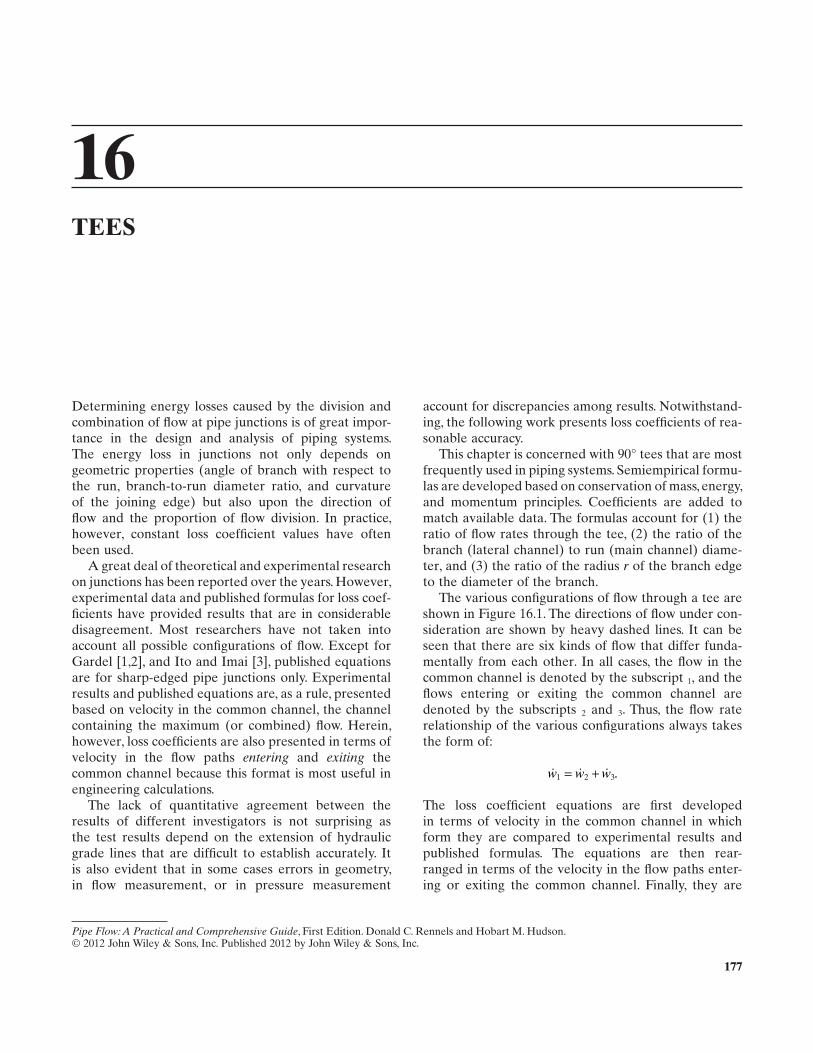
177
16 TEES
Determining energy losses caused by the division and combination of fl ow at pipe junctions is of great impor-tance in the design and analysis of piping systems. The energy loss in junctions not only depends on geometric properties (angle of branch with respect to the run, branch - to - run diameter ratio, and curvature of the joining edge) but also upon the direction of fl ow and the proportion of fl ow division. In practice, however, constant loss coeffi cient values have often been used.
A great deal of theoretical and experimental research on junctions has been reported over the years. However, experimental data and published formulas for loss coef-fi cients have provided results that are in considerable disagreement. Most researchers have not taken into account all possible confi gurations of fl ow. Except for Gardel [1,2] , and Ito and Imai [3] , published equations are for sharp - edged pipe junctions only. Experimental results and published equations are, as a rule, presented based on velocity in the common channel, the channel containing the maximum (or combined) fl ow. Herein, however, loss coeffi cients are also presented in terms of velocity in the fl ow paths entering and exiting the common channel because this format is most useful in engineering calculations.
The lack of quantitative agreement between the results of different investigators is not surprising as the test results depend on the extension of hydraulic grade lines that are diffi cult to establish accurately. It is also evident that in some cases errors in geometry, in fl ow measurement, or in pressure measurement
account for discrepancies among results. Notwithstand-ing, the following work presents loss coeffi cients of rea-sonable accuracy.
This chapter is concerned with 90 ° tees that are most frequently used in piping systems. Semiempirical formu-las are developed based on conservation of mass, energy, and momentum principles. Coeffi cients are added to match available data. The formulas account for (1) the ratio of fl ow rates through the tee, (2) the ratio of the branch (lateral channel) to run (main channel) diame-ter, and (3) the ratio of the radius r of the branch edge to the diameter of the branch.
The various confi gurations of fl ow through a tee are shown in Figure 16.1 . The directions of fl ow under con-sideration are shown by heavy dashed lines. It can be seen that there are six kinds of fl ow that differ funda-mentally from each other. In all cases, the fl ow in the common channel is denoted by the subscript 1 , and the fl ows entering or exiting the common channel are denoted by the subscripts 2 and 3 . Thus, the fl ow rate relationship of the various confi gurations always takes the form of:
w w w1 2 3= + .
The loss coeffi cient equations are fi rst developed in terms of velocity in the common channel in which form they are compared to experimental results and published formulas. The equations are then rear-ranged in terms of the velocity in the fl ow paths enter-ing or exiting the common channel. Finally, they are
Pipe Flow: A Practical and Comprehensive Guide, First Edition. Donald C. Rennels and Hobart M. Hudson.© 2012 John Wiley & Sons, Inc. Published 2012 by John Wiley & Sons, Inc.
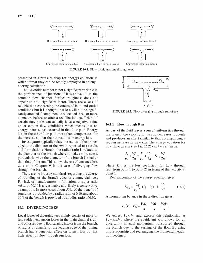
178 TEES
16.1.1 Flow through Run
As part of the fl uid leaves a run of uniform size through the branch, the velocity in the run decreases suddenly and produces an effect similar to that accompanying a sudden increase in pipe size. The energy equation for fl ow through run (see Fig. 16.2 ) can be written as:
P Vg
P Vg
KV
gw w
1 12
2 22
1212
2 2 21ρ ρ+ = + + ,
where K121 is the loss coeffi cient for fl ow through run (from point 1 to point 2) in terms of the velocity at point 1.
Rearrangement of the energy equation gives:
KgV
P PVVw
1212 1 2
22
121
21= −( ) + −
ρ. (16.1)
A momentum balance in the x - direction gives:
A P PV w
gV w
gV w
g1 1 2
2 2 1 1 3−( ) = − + x .
We expect Vx < V1 and express this relationship as Vx = CxDV1 , where the coeffi cient CxD allows for an uncertainty in axial momentum transported through the branch due to the turning of the fl ow. By using this relationship and rearranging, the momentum equa-tion becomes:
presented in a pressure drop (or energy) equation, in which format they can be readily employed in an engi-neering calculation.
The Reynolds number is not a signifi cant variable in the performance of junctions if it is above 10 4 in the common fl ow channel. Surface roughness does not appear to be a signifi cant factor. There are a lack of reliable data concerning the effects of inlet and outlet conditions, but it is thought that loss will not be signifi -cantly affected if components are located three or more diameters before or after a tee. The loss coeffi cient of certain fl ow paths can actually have a negative value under certain fl ow conditions, which means that an energy increase has occurred in that fl ow path. Energy loss in the other fl ow path more than compensates for the increase so that the net result is an energy loss.
Investigators typically relate the radius of the branch edge to the diameter of the run in reported test results and formulations. Herein, the radius ratio is related to the diameter of the branch where it makes more sense, particularly when the diameter of the branch is smaller than that of the run. This allows the use of entrance loss data from Chapter 9 in the case of diverging fl ow through the branch.
There are no industry standards regarding the degree of rounding of the branch edge of commercial tees. For lack of manufacturers ’ information, a radius ratio r / dbranch of 0.10 is a reasonable and, likely, a conserva tive assumption. In most cases about 50% of the benefi t of rounding is provided by a radius ratio of 0.10, and about 90% of the benefi t is provided by a radius ratio of 0.30.
16.1 DIVERGING TEES
Local losses of diverging tees mainly consist of more or less sudden expansion losses in the main channel (run) and of losses due to fl ow turning into or from the branch. A radius or chamfer at the leading edge of the joining branch has a benefi cial effect on branch loss but has little effect on fl ow through run loss.
FIGURE 16.1. Flow confi gurations through tees.
2
3
1 2
1
32
3
1
Converging Flow through Run Converging Flow through Branch Converging Flow into Branch
1
3
2
3
1 2 2
1
3
Diverging Flow through Run Diverging Flow through Branch Diverging Flow from Branch
FIGURE 16.2. Flow diverging through run of tee.
V1 V2
P3 A3
V3
r
d1
P1
A1
P2
A1
d3
Vy3
Vx

DIVERGING TEES 179
FIGURE 16.3. Comparison of Equation 16.5 with data from various investigators for the case of diverging fl ow through run of tee.
0 0.2 0.4 0.6 0.8 1.0
0.4
0.3
0.2
0.1
0
–0.1
K12 1
1
Equation 16.5 Gardel Formula Idel’chik Formula Ito and Imai Formula Kinne Data
w2w
P PgA
V w V w C V w1 21
2 2 1 1 1 31− = − +( ) xD .
By use of the continuity equations w w w3 1 2= − ,w V A w1 1 1= ρ , and w V A w2 2 1= ρ , the momentum equation
becomes:
P PVg
VV
C CVV
w1 2
12
22
12
2
1
1− = − + −
ρxD xD . (16.2)
Substituting Equation 16.2 into Equation 16.1 and letting V w A w1 1 1= ρ and V w A w2 2 1= ρ , the loss coeffi -cient equation becomes:
Kww
C Cww
1222
12
2
11 2 1 2= + −( ) −
xD xD . (16.3)
Experimental results indicate that the loss coeffi cient is fairly insensitive to the diameter ratio d3 / d1 , and to the radius r of the branch inlet. Correlation with available data indicates that CxD is a function of the fl ow rate ratio as follows:
Cww
xD = +0 68 0 19 2
1
. . .
(16.4)
As in the case of converging fl ow through run, a small loss results from the abrupt enlargement and contrac-tion of fl ow area past the branch when w2 approaches w1. This loss was not accounted for in the derivation
of Equation 16.3 . Adding a term to account for this loss, plus substitution of Equation 16.4 into Equation 16.3 , gives:
Kww
ww
ww
122
1
22
12
28
181 0 36 0 98 0 62 0 03= − + +. . . . .
(16.5)
Results from Equation 16.5 are compared with pub-lished formulas by Gardel [2] , Idel ’ chik [4] , and Ito and Imai [3] , as well as with test data by Kinne [5] , in Figure 16.3 . The results compare favorably with Kinne ’ s data and with Ito and Imai ’ s formula; they compare less so with Gardel ’ s and Idel ’ chik ’ s formulas.
Multiplying Equation 16.5 by w w12
22/ produces the
loss coeffi cient for diverging fl ow through run in terms of the velocity at point 2:
Kww
ww
ww
121
2
12
22
26
162 0 62 0 98 0 36 0 03= − + +. . . . .
(16.6)
Loss coeffi cient K122 for diverging fl ow through run can be obtained from Diagram 16.1 . The energy equation in terms of the velocity at point 2 may be written as:
P Pw
g AK
www
1 222
12 12
12
222
12− = + −
ρ
.
By substituting Equation 16.6 into the energy, the pressure drop equation for diverging fl ow through run becomes:
P Pw
g Aww
ww
www
1 222
12
1
2
12
22
26
162
1 62 0 98 0 64 0 03− = − − +
ρ
. . . .
.
(16.7)
16.1.2 Flow through Branch
The change in direction of the fl ow entering the branch causes a detachment that partly depends on the degree
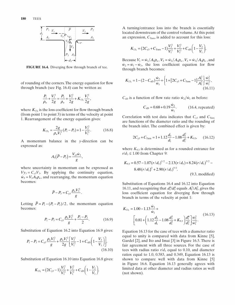
180 TEES
of rounding of the corners. The energy equation for fl ow through branch (see Fig. 16.4 ) can be written as:
P Vg
P Vg
KV
gw w
1 12
3 32
1312
2 2 21ρ ρ+ = + + ,
where K131 is the loss coeffi cient for fl ow through branch (from point 1 to point 3) in terms of the velocity at point 1. Rearrangement of the energy equation gives:
KgV
P PVVw
1312 1 3
32
121
21= −( ) + −
ρ. (16.8)
A momentum balance in the y - direction can be expressed as:
A P PV w
g3 3
3−( ) = y3 ,
where uncertainty in momentum can be expressed as Vy3 = Cy3V3 . By applying the continuity equation, w V A w3 3 3= ρ , and rearranging, the momentum equation
becomes:
P P CVg
w− =332
y3ρ
.
Letting P P P P= − −( )1 1 2 2/ , the momentum equation becomes:
P P CVg
P Pw1 3
32
1 2
2− = + −
y3ρ
. (16.9)
Substitution of Equation 16.2 into Equation 16.9 gives:
P P CVg
Vg
VV
CVV
w w1 3
32
12
22
12
2
121 1− = + − + −
y3 xDρ ρ
.
(16.10)
Substitution of Equation 16.10 into Equation 16.8 gives:
K CVV
VV
CVV
1332
12
22
12
2
11 2 1 1= −( ) + + −
y3 xD .
FIGURE 16.4. Diverging fl ow through branch of tee.
PV1 V2
P3 A3
V3
r
d1
P1
A1
P2
A1
d3
Vy1
Vy3
Vx
A turning/entrance loss into the branch is essentially located downstream of the control volume. At this point an expression, CTurn , is added to account for this loss:
K C CVV
VV
CVV
1332
12
22
12
2
11 2 1 1= + −( ) + + −
y3 Turn xD .
Because V w A w1 1 1= ρ , V w A w2 2 1= ρ , V w A w3 3 1= ρ , and w w w2 1 3= − , the loss coeffi cient equation for fl ow through branch becomes:
K Cww
C CAA
ww
13 xD y3 Turn1 = − −( ) + + + −[ ]
1 2 1 2 13
1
12
32
32
12
,
(16.11)
CxD is a function of fl ow rate ratio w w2 1 as before:
Cww
xD = +0 68 0 19 2
1
. . .
(16.4, repeated)
Correlation with test data indicates that Cy3 and CTurn
are functions of the diameter ratio and the rounding of the branch inlet. The combined effect is given by:
2 1 1 12 1 083
1
33
13
C Cdd
dd
Ky3 Turn 9.3+ = + − +. . , (16.12)
where K9.3 is determined as for a rounded entrance for r / d3 ≤ 1.00 from Chapter 9 :
K r d r d r d
r d
9 3 31 2
3 33 2
3
0 57 1 07 2 13 8 24
8 48
./ /. . / . / . /
. /
= − ( ) − ( ) + ( ) −
( )) + ( )23
5 22 90. / /r d . (9.3, modifi ed)
Substitution of Equations 16.4 and 16.12 into Equation 16.11 , and recognizing that d d1
434/ equals A A1
232/ , gives the
loss coeffi cient equation for diverging fl ow through branch in terms of the velocity at point 1:
Kww
dd
dd
Kd
131 = − +
+ − +
1 00 1 13
0 81 1 12 1 08
3
1
3
1
33
13 9 3
1
. .
. . . .
44
34
32
12d
ww
. (16.13)
Equation 16.13 for the case of tees with a diameter ratio equal to unity is compared with data from Kinne [5] , Gardel [2] , and Ito and Imai [3] in Figure 16.5 . There is fair agreement with all three sources. For the case of tees with radius ratio r / d3 equal to 0.10, and diameter ratios equal to 1.0, 0.583, and 0.349, Equation 16.13 is shown to compare well with data from Kinne [5] in Figure 16.6 . Equation 16.13 generally agrees with limited data at other diameter and radius ratios as well (not shown).
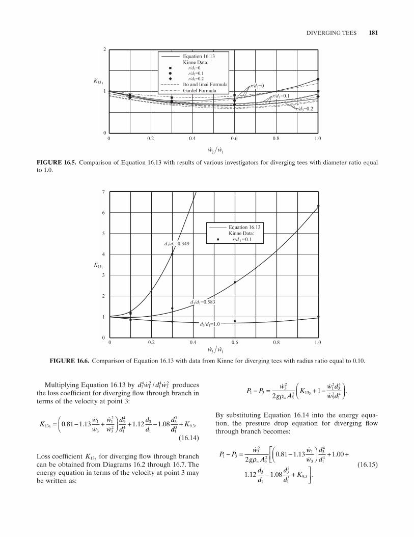
DIVERGING TEES 181
FIGURE 16.5. Comparison of Equation 16.13 with results of various investigators for diverging tees with diameter ratio equal to 1.0.
0 0.2 0.4 0.6 0.8 1.0
2
1
0
K13 1
Equation 16.13 Kinne Data: r/d3=0 r/d3=0.1 r/d3=0.2 Ito and Imai Formula Gardel Formula
r/d3=0
r/d3=0.2
r/d3=0.1
1w2w
FIGURE 16.6. Comparison of Equation 16.13 with data from Kinne for diverging tees with radius ratio equal to 0.10.
0 0.2 0.4 0.6 0.8 1.0
7
6
5
4
3
2
1
0
K131
d3/d1=1.0
d3/d1=0.583
d3/d1=0.349
Equation 16.13 Kinne Data: r/d 3 =0.1
1w3w
Multiplying Equation 16.13 by d w d w34
12
14
32 / produces
the loss coeffi cient for diverging fl ow through branch in terms of the velocity at point 3:
Kww
ww
dd
dd
d13
1
3
12
32
34
14
3
1
33
3 0 81 1 13 1 12 1 08= − +
+ −. . . .
dd
K13 9 3+ . .
(16.14)
Loss coeffi cient K133 for diverging fl ow through branch can be obtained from Diagrams 16.2 through 16.7 . The energy equation in terms of the velocity at point 3 may be written as:
P Pw
g AK
w dw dw
1 332
32 13
12
34
32
142
13− = + −
ρ
.
By substituting Equation 16.14 into the energy equa-tion, the pressure drop equation for diverging fl ow through branch becomes:
P Pw
g Aww
dd
dw
1 332
32
1
3
34
142
0 81 1 13 1 00
1 12
− = −
+ +
ρ. . .
. 33
1
33
13 9 31 08
ddd
K− +
. ..
(16.15)
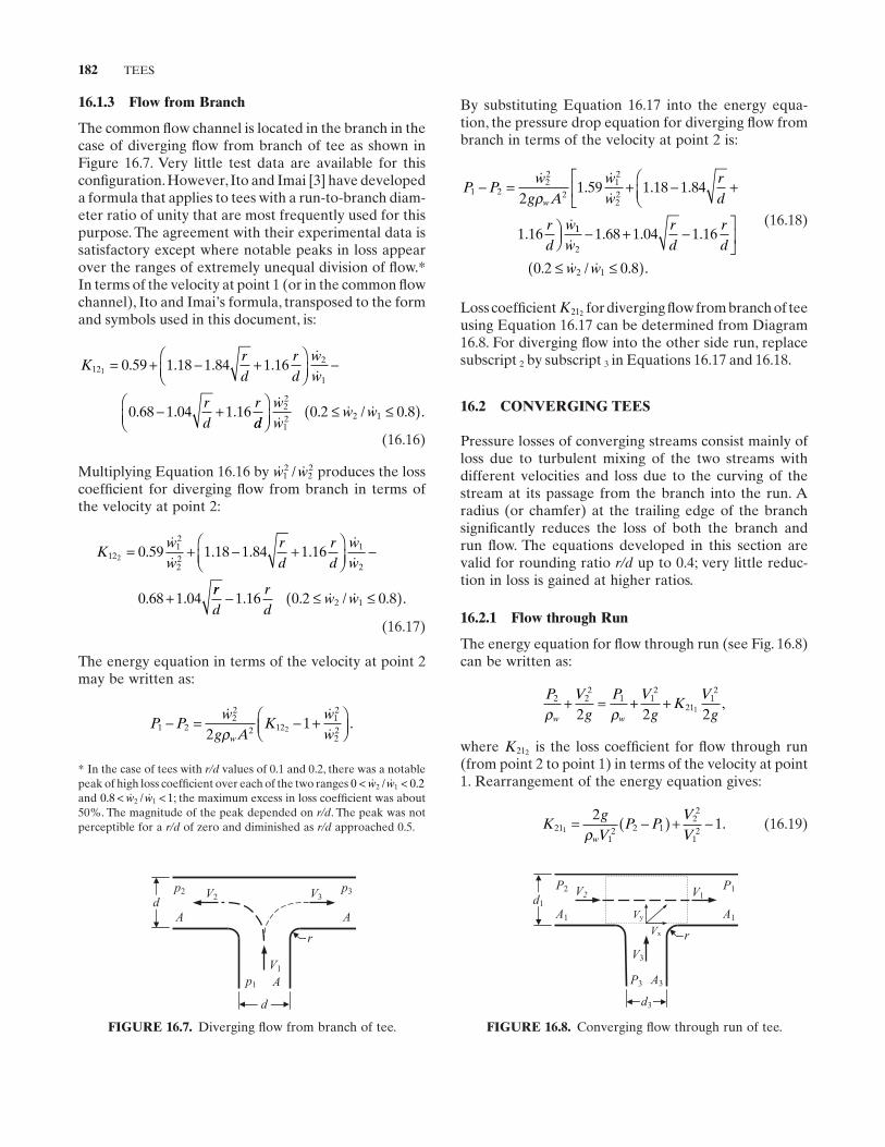
182 TEES
By substituting Equation 16.17 into the energy equa-tion, the pressure drop equation for diverging fl ow from branch in terms of the velocity at point 2 is:
P Pw
g Aww
rd
rd
w
w1 2
22
212
222
1 59 1 18 1 84
1 16
− = + − +
ρ. . .
. 11
2
2 1
1 68 1 04 1 16
0 2 0 8
w
rd
rd
w w
− + −
≤ ≤( )
. . .
. / . .
(16.18)
Loss coeffi cient K212 for diverging fl ow from branch of tee using Equation 16.17 can be determined from Diagram 16.8 . For diverging fl ow into the other side run, replace subscript 2 by subscript 3 in Equations 16.17 and 16.18 .
16.2 CONVERGING TEES
Pressure losses of converging streams consist mainly of loss due to turbulent mixing of the two streams with different velocities and loss due to the curving of the stream at its passage from the branch into the run. A radius (or chamfer) at the trailing edge of the branch signifi cantly reduces the loss of both the branch and run fl ow. The equations developed in this section are valid for rounding ratio r/d up to 0.4; very little reduc-tion in loss is gained at higher ratios.
16.2.1 Flow through Run
The energy equation for fl ow through run (see Fig. 16.8 ) can be written as:
P Vg
P Vg
KV
gw w
2 22
1 12
2112
2 2 21ρ ρ+ = + + ,
where K212 is the loss coeffi cient for fl ow through run (from point 2 to point 1) in terms of the velocity at point 1. Rearrangement of the energy equation gives:
KgV
P PVVw
2112 2 1
22
121
21= −( ) + −
ρ. (16.19)
16.1.3 Flow from Branch
The common fl ow channel is located in the branch in the case of diverging fl ow from branch of tee as shown in Figure 16.7 . Very little test data are available for this confi guration. However, Ito and Imai [3] have developed a formula that applies to tees with a run - to - branch diam-eter ratio of unity that are most frequently used for this purpose. The agreement with their experimental data is satisfactory except where notable peaks in loss appear over the ranges of extremely unequal division of fl ow. *In terms of the velocity at point 1 (or in the common fl ow channel), Ito and Imai ’ s formula, transposed to the form and symbols used in this document, is:
Krd
rd
ww
rd
r
122
11 0 59 1 18 1 84 1 16
0 68 1 04 1 16
= + − +
−
− +
. . . .
. . .
ddww
w w
≤ ≤( )
22
12 2 10 2 0 8. / . .
(16.16)
Multiplying Equation 16.16 by w w12
22/ produces the loss
coeffi cient for diverging fl ow from branch in terms of the velocity at point 2:
Kww
rd
rd
ww
1212
22
1
22 0 59 1 18 1 84 1 16
0 68 1 04
= + − +
−
+
. . . .
. .
rrd
rd
w w− ≤ ≤( )1 16 0 2 0 82 1. . / . .
(16.17)
The energy equation in terms of the velocity at point 2 may be written as:
P Pw
g AK
www
1 222
2 1212
222
12− = − +
ρ
.
FIGURE 16.7. Diverging fl ow from branch of tee.
V3
p1 AV1
r
dV2
p2
A
p3
A
d
FIGURE 16.8. Converging fl ow through run of tee.
P3
Vx
A3
V3
r
d1V1V2
P2
A1
P1
A1Vy
d3
* In the case of tees with r/d values of 0.1 and 0.2, there was a notable peak of high loss coeffi cient over each of the two ranges 0 0 22 1< < w w/ .and 0 8 12 1. /< < w w ; the maximum excess in loss coeffi cient was about 50%. The magnitude of the peak depended on r/d . The peak was not perceptible for a r/d of zero and diminished as r/d approached 0.5.
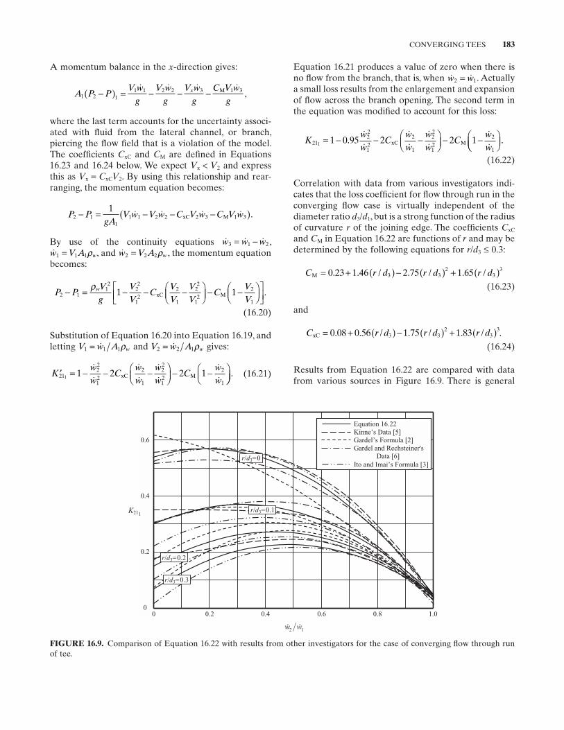
CONVERGING TEES 183
Equation 16.21 produces a value of zero when there is no fl ow from the branch, that is, when w w2 1= . Actually a small loss results from the enlargement and expansion of fl ow across the branch opening. The second term in the equation was modifi ed to account for this loss:
Kww
Cww
ww
Cww
2122
12
2
1
22
12
2
11 1 0 95 2 2 1= − − −
− −.
xC M
.
(16.22)
Correlation with data from various investigators indi-cates that the loss coeffi cient for fl ow through run in the converging fl ow case is virtually independent of the diameter ratio d3 / d1 , but is a strong function of the radius of curvature r of the joining edge. The coeffi cients CxC
and CM in Equation 16.22 are functions of r and may be determined by the following equations for r / d3 ≤ 0.3:
C r d r d r dM = + ( ) − ( ) + ( )0 23 1 46 2 75 1 653 32
33. . / . / . /
(16.23)
and
C r d r d r dxC = + ( ) − ( ) + ( )0 08 0 56 1 75 1 833 32
33. . / . / . / .
(16.24)
Results from Equation 16.22 are compared with data from various sources in Figure 16.9 . There is general
A momentum balance in the x - direction gives:
A P PV w
gV w
gV w
gC V w
gx
1 2 11 1 2 2 3 1 3−( ) = − − − M ,
where the last term accounts for the uncertainty associ-ated with fl uid from the lateral channel, or branch, piercing the fl ow fi eld that is a violation of the model. The coeffi cients CxC and CM are defi ned in Equations 16.23 and 16.24 below. We expect Vx < V2 and express this as Vx = CxCV2 . By using this relationship and rear-ranging, the momentum equation becomes:
P PgA
V w V w C V w C V w2 11
1 1 2 2 2 3 1 31− = − − −( ) xC M .
By use of the continuity equations w w w3 1 2= − ,w V A w1 1 1= ρ , and w V A w2 2 2= ρ , the momentum equation
becomes:
P PVg
VV
CVV
VV
CVV
w2 1
12
22
12
2
1
22
12
2
1
1 1− = − − −
− −
ρxC M
.
(16.20)
Substitution of Equation 16.20 into Equation 16.19 , and letting V w A w1 1 1= ρ and V w A w2 2 1= ρ gives:
′ = − − −
− −
Kww
Cww
ww
Cww
2122
12
2
1
22
12
2
11 1 2 2 1
xC M . (16.21)
FIGURE 16.9. Comparison of Equation 16.22 with results from other investigators for the case of converging fl ow through run of tee.
0 0.2 0.4 0.6 0.8 1.0
0.6
0.4
0.2
0
K211
Equation 16.22 Kinne’s Data [5] Gardel’s Formula [2] Gardel and Rechsteiner's Data [6] Ito and Imai’s Formula [3]
r/d3=0
r/d3=0.2
r/d3=0.1
r/d3=0.3
1w2w
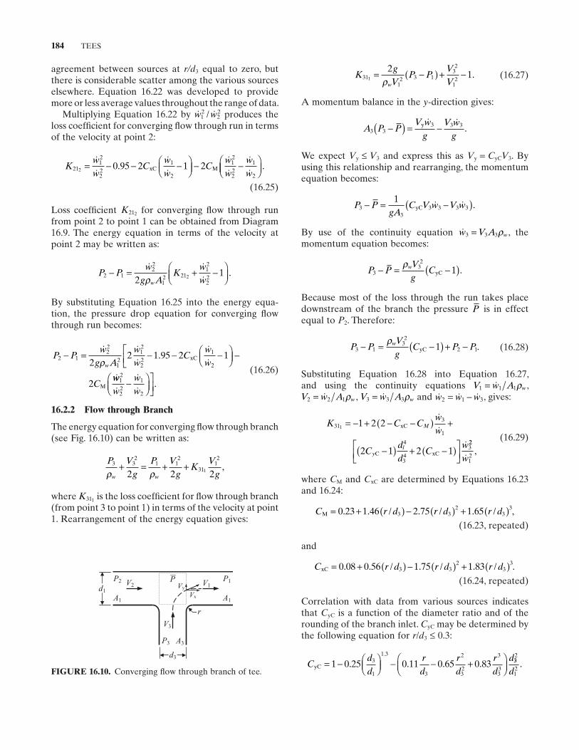
184 TEES
KgV
P PVVw
3112 3 1
32
121
21= −( ) + −
ρ. (16.27)
A momentum balance in the y - direction gives:
A P PV w
gV w
g3 3
3 3 3−( ) = −y .
We expect Vy ≤ V3 and express this as Vy = CyCV3 . By using this relationship and rearranging, the momentum equation becomes:
P PgA
C V w V w33
3 3 3 31− = −( )yC .
By use of the continuity equation w V A w3 3 3= ρ , the momentum equation becomes:
P PVg
Cw3
32
1− = −( )ρyC .
Because most of the loss through the run takes place downstream of the branch the pressure P is in effect equal to P2 . Therefore:
P PVg
C P Pw3 1
32
2 11− = −( ) + −ρyC . (16.28)
Substituting Equation 16.28 into Equation 16.27 , and using the continuity equations V w A w1 1 1= ρ ,V w A w2 2 1= ρ , V w A w3 3 3= ρ and w w w2 1 3= − , gives:
K C Cww
Cdd
Cw
M
yl
313
1
4
34
3
1 1 2 2
2 1 2 1
= − + − −( ) +
−( ) + −( )
xC
C xC
22
12w
, (16.29)
where CM and CxC are determined by Equations 16.23 and 16.24 :
C r d r d r dM = + ( ) − ( ) + ( )0 23 1 46 2 75 1 653 32
33. . / . / . / ,
(16.23, repeated)
and
C r d r d r dxC = + ( ) − ( ) + ( )0 08 0 56 1 75 1 833 32
33. . / . / . / .
(16.24, repeated)
Correlation with data from various sources indicates that CyC is a function of the diameter ratio and of the rounding of the branch inlet. CyC may be determined by the following equation for r / d3 ≤ 0.3:
Cdd
rd
rd
rd
dyC = −
− − +
1 0 25 0 11 0 65 0 833
1
1 3
3
2
32
3
33
. . . ..
332
12d
.
agreement between sources at r/d3 equal to zero, but there is considerable scatter among the various sources elsewhere. Equation 16.22 was developed to provide more or less average values throughout the range of data.
Multiplying Equation 16.22 by w w12
22/ produces the
loss coeffi cient for converging fl ow through run in terms of the velocity at point 2:
Kww
Cww
Cww
ww
2112
22
1
2
12
22
1
22 0 95 2 1 2= − − −
− −
. xC M
.
(16.25)
Loss coeffi cient K212 for converging fl ow through run from point 2 to point 1 can be obtained from Diagram 16.9 . The energy equation in terms of the velocity at point 2 may be written as:
P Pw
g AK
www
2 122
12 21
12
222
12− = + −
ρ
.
By substituting Equation 16.25 into the energy equa-tion, the pressure drop equation for converging fl ow through run becomes:
P Pw
g Aww
Cww
C
w2 1
22
12
12
22
1
222 1 95 2 1
2
− = − − −
−
ρ
. xC
Mwww
ww
12
22
1
2
−
.
(16.26)
16.2.2 Flow through Branch
The energy equation for converging fl ow through branch (see Fig. 16.10 ) can be written as:
P Vg
P Vg
KV
gw w
3 32
1 12
3112
2 2 21ρ ρ+ = + + ,
where K311 is the loss coeffi cient for fl ow through branch (from point 3 to point 1) in terms of the velocity at point 1. Rearrangement of the energy equation gives:
FIGURE 16.10. Converging fl ow through branch of tee.
V2 VyV1
P3
Vx
A3
V3
r
d1
P2
A1
P1
A1
d3
P
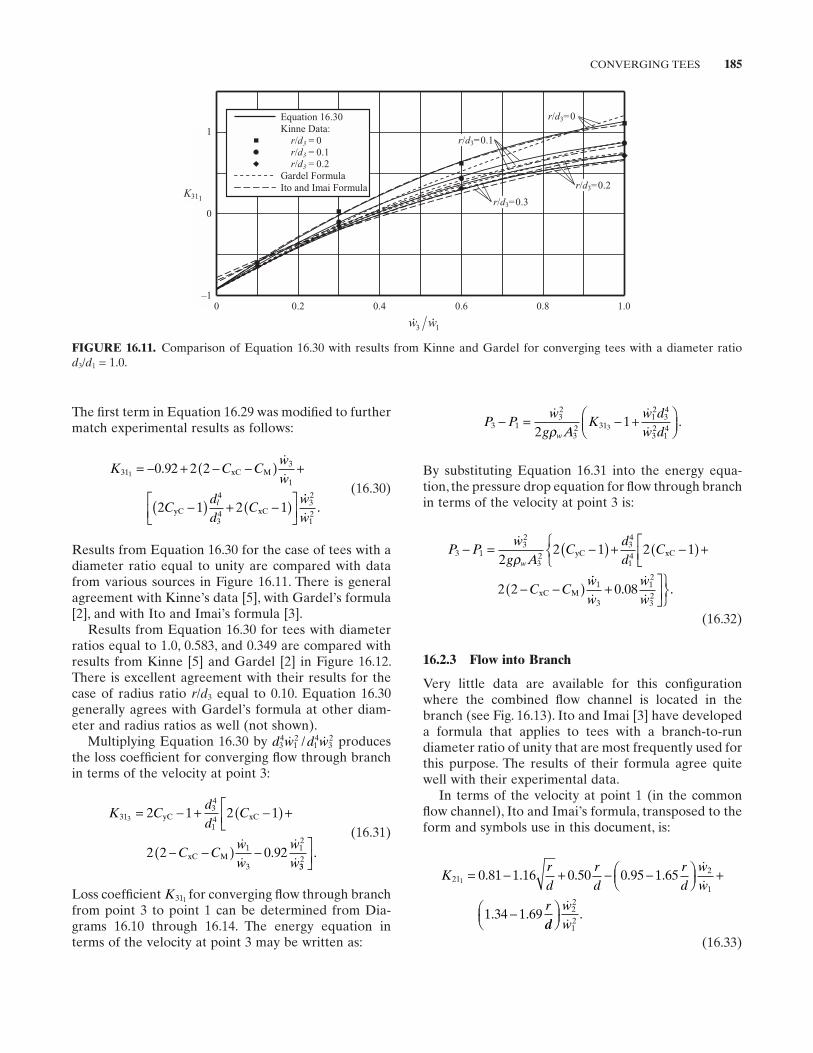
CONVERGING TEES 185
The fi rst term in Equation 16.29 was modifi ed to further match experimental results as follows:
K C Cww
Cdd
Cl
313
1
4
34
1 0 92 2 2
2 1 2 1
= − + − −( ) +
−( ) + −( )
. xC M
yC xC
ww
32
12
. (16.30)
Results from Equation 16.30 for the case of tees with a diameter ratio equal to unity are compared with data from various sources in Figure 16.11 . There is general agreement with Kinne ’ s data [5] , with Gardel ’ s formula [2] , and with Ito and Imai ’ s formula [3] .
Results from Equation 16.30 for tees with diameter ratios equal to 1.0, 0.583, and 0.349 are compared with results from Kinne [5] and Gardel [2] in Figure 16.12 . There is excellent agreement with their results for the case of radius ratio r / d3 equal to 0.10. Equation 16.30 generally agrees with Gardel ’ s formula at other diam-eter and radius ratios as well (not shown).
Multiplying Equation 16.30 by d w d w34
12
14
32 / produces
the loss coeffi cient for converging fl ow through branch in terms of the velocity at point 3:
K Cdd
C
C Cww
ww
3134
14
1
3
12
3 2 1 2 1
2 2 0 92
= − + −( ) +
− −( ) −
yC xC
xC M
.332
.
(16.31)
Loss coeffi cient K311 for converging fl ow through branch from point 3 to point 1 can be determined from Dia-grams 16.10 through 16.14 . The energy equation in terms of the velocity at point 3 may be written as:
FIGURE 16.11. Comparison of Equation 16.30 with results from Kinne and Gardel for converging tees with a diameter ratio d3 / d1 = 1.0.
1
0
–1
r/d3=0
r/d3=0.1
r/d3=0.2
r/d3=0.3K311
Equation 16.30 Kinne Data: r/d3 = 0 r/d3 = 0.1 r/d3 = 0.2 Gardel Formula Ito and Imai Formula
0 0.2 0.4 0.6 0.8 1.0
1w3w
P Pw
g AK
w dw dw
3 132
32 31
12
34
32
142
13− = − +
ρ
.
By substituting Equation 16.31 into the energy equa-tion, the pressure drop equation for fl ow through branch in terms of the velocity at point 3 is:
P Pw
g AC
dd
C
C C
w3 1
32
32
34
142
2 1 2 1
2 2
− = −( ) + −( ) +
− −( )
ρ yC xC
xC M
ww
ww
1
3
12
32
0 08+
. .
(16.32)
16.2.3 Flow into Branch
Very little data are available for this confi guration where the combined fl ow channel is located in the branch (see Fig. 16.13 ). Ito and Imai [3] have developed a formula that applies to tees with a branch - to - run diameter ratio of unity that are most frequently used for this purpose. The results of their formula agree quite well with their experimental data.
In terms of the velocity at point 1 (in the common fl ow channel), Ito and Imai ’ s formula, transposed to the form and symbols use in this document, is:
Krd
rd
rd
ww
r
212
11 0 81 1 16 0 50 0 95 1 65
1 34 1 69
= − + − −
+
−
. . . . .
. .
ddww
22
12
.
(16.33)
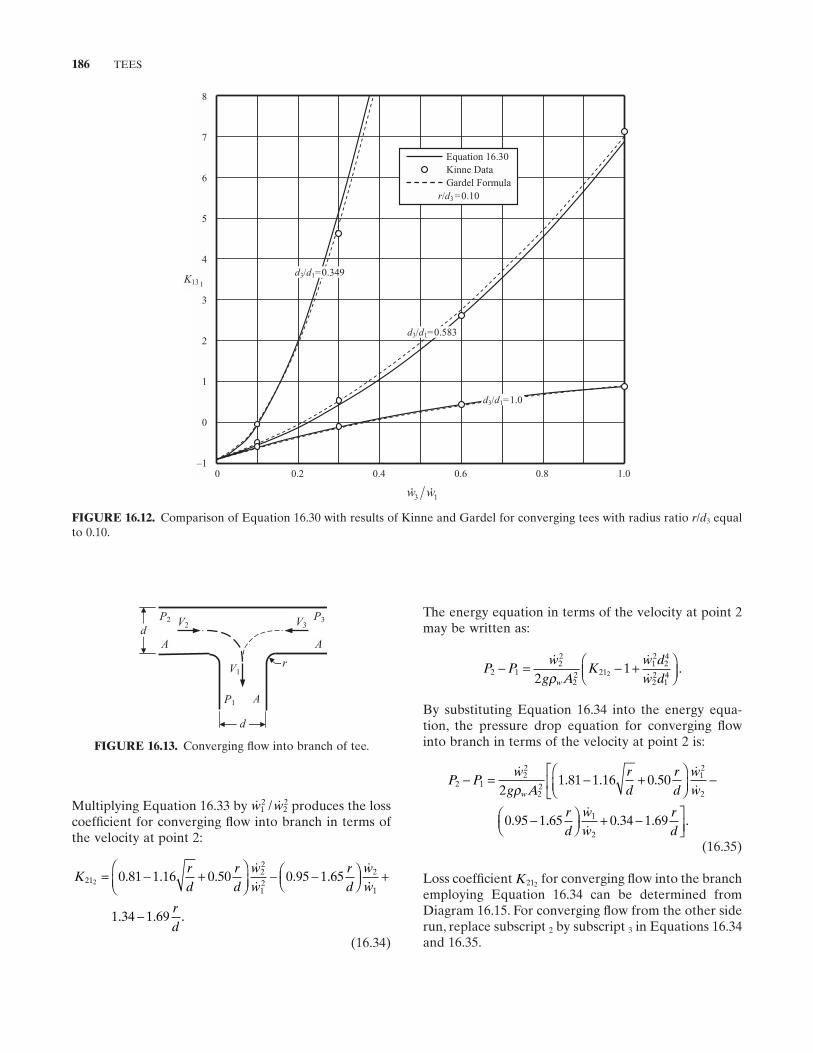
186 TEES
FIGURE 16.12. Comparison of Equation 16.30 with results of Kinne and Gardel for converging tees with radius ratio r / d3 equal to 0.10.
0 0.2 0.4 0.6 0.8 1.0
8
7
6
5
4
3
2
1
0
–1
d3/d1=1.0
Equation 16.30 Kinne Data Gardel Formula
r/d3 =0.10
K13 1
d3/d1=0.349
d3/d1=0.583
1w3w
FIGURE 16.13. Converging fl ow into branch of tee.
V3
P1 A
V1r
dV2
P2
A
P3
A
d
Multiplying Equation 16.33 by w w12
22/ produces the loss
coeffi cient for converging fl ow into branch in terms of the velocity at point 2:
Krd
rd
ww
rd
w21
22
12
22 0 81 1 16 0 50 0 95 1 65= − +
− −
. . . . .
w
rd
1
1 34 1 69
+
−. . .
(16.34)
The energy equation in terms of the velocity at point 2 may be written as:
P Pw
g AK
w dw dw
2 122
22 21
12
24
22
142
12− = − +
ρ
.
By substituting Equation 16.34 into the energy equa-tion, the pressure drop equation for converging fl ow into branch in terms of the velocity at point 2 is:
P Pw
g Ard
rd
www
2 122
22
12
221 81 1 16 0 50
0 95 1
− = − +
−
−
ρ
. . .
. .. . . .65 0 34 1 691
2
rd
ww
rd
+ −
(16.35)
Loss coeffi cient K212 for converging fl ow into the branch employing Equation 16.34 can be determined from Diagram 16.15 . For converging fl ow from the other side run, replace subscript 2 by subscript 3 in Equations 16.34 and 16.35 .
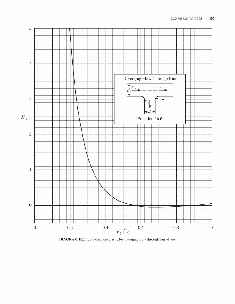
CONVERGING TEES 187
DIAGRAM 16.1. Loss coeffi cient K122 for diverging fl ow through run of tee.
0 0.2 0.4 0.6 0.8 1.0
5
4
3
2
1
0
K12 2
12 ww
Diverging Flow Through Run
1w
2w
3w
Equation 16.6
r
d1
d3
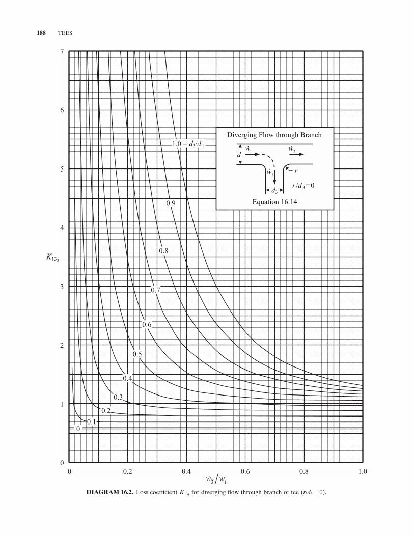
188 TEES
DIAGRAM 16.2. Loss coeffi cient K133 for diverging fl ow through branch of tee ( r / d3 = 0).
7
6
5
4
3
2
1
0
K133
0 0.2 0.4 0.6 0.8 1.013 ww
00.1
0.2
0.3
0.4
0.5
0.6
0.7
1.0 = d3/d 1
0.9
Diverging Flow through Branch
1
w 2
w
3
w
Equation 16.14
r
d1
d3r /d 3 =0
0.8
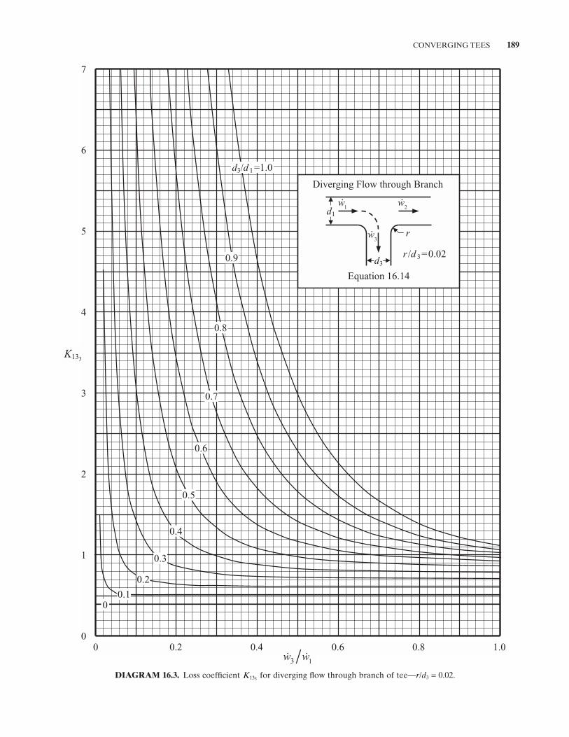
CONVERGING TEES 189
DIAGRAM 16.3. Loss coeffi cient K133 for diverging fl ow through branch of tee — r / d3 = 0.02.
7
6
5
4
3
2
1
0
K133
0 0.2 0.4 0.6 0.8 1.013 ww
d3/d 1 =1.0
0.9
0.8
0.7
0.6
0.5
0.4
0.3
0.2
0.10
Diverging Flow through Branch
1
w 2
w
3
w
Equation 16.14
r
d1
d3r /d 3 =0.02
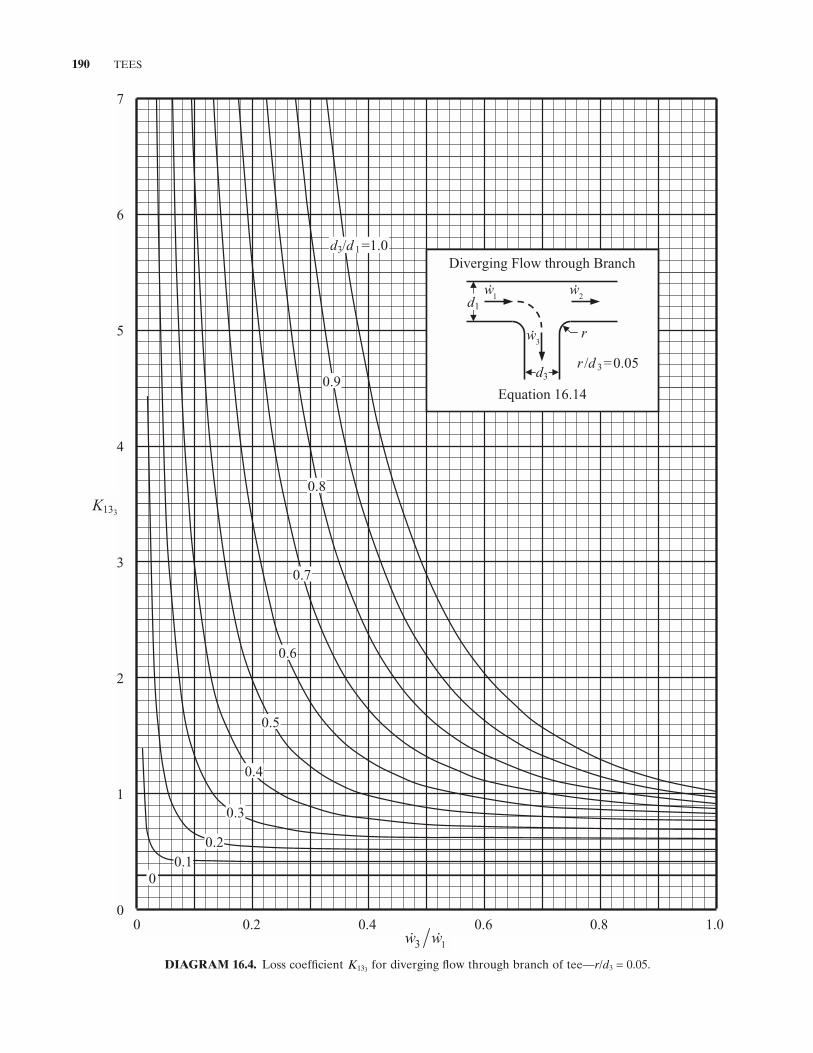
190 TEES
DIAGRAM 16.4. Loss coeffi cient K133 for diverging fl ow through branch of tee — r / d3 = 0.05.
7
6
5
4
3
2
1
0
K133
0 0.2 0.4 0.6 0.8 1.013 ww
d3/d 1 =1.0
0.9
0.8
0.7
0.6
0.5
0.4
0.3
0.20.1
0
Diverging Flow through Branch
1
w 2
w
3
w
Equation 16.14
r
d1
d3r /d 3 =0.05
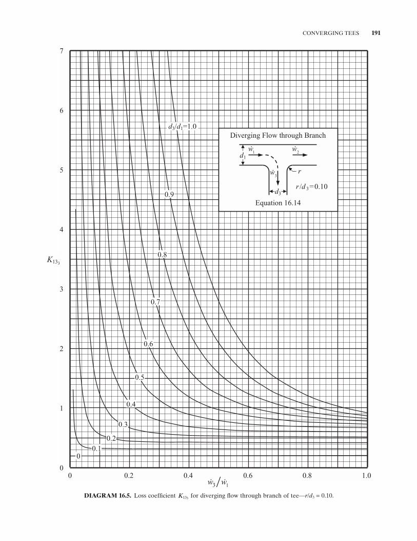
CONVERGING TEES 191
DIAGRAM 16.5. Loss coeffi cient K133 for diverging fl ow through branch of tee — r / d3 = 0.10.
7
6
5
4
3
2
1
0
K133
0 0.2 0.4 0.6 0.8 1.013 ww
d3/d1=1.0
0.9
0.8
0.7
0.6
0.5
0.4
0.3
0.20.1
0
Diverging Flow through Branch
1
w 2
w
3
w
Equation 16.14
r
d1
d3r /d 3 =0.10
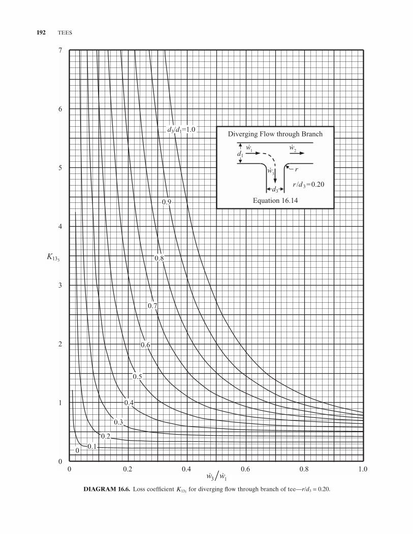
192 TEES
DIAGRAM 16.6. Loss coeffi cient K133 for diverging fl ow through branch of tee — r / d3 = 0.20.
7
6
5
4
3
2
1
0
K133
0 0.2 0.4 0.6 0.8 1.013 ww
0.9
0.8
0.7
0.6
0.5
0.3
0.2
0.1
0.4
0
Diverging Flow through Branch
1
w 2
w
3
w
Equation 16.14
r
d1
d3r /d 3 =0.20
d3/d1=1.0
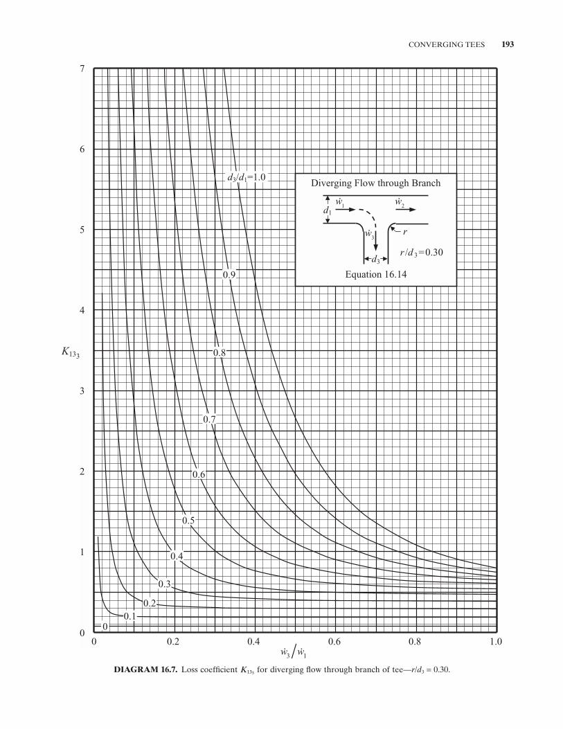
CONVERGING TEES 193
DIAGRAM 16.7. Loss coeffi cient K133 for diverging fl ow through branch of tee — r / d3 = 0.30.
7
6
5
4
3
2
1
0
K133
0 0.2 0.4 0.6 0.8 1.01w
d3/d1=1.0
0.9
0.8
0.7
0.6
0.5
0.4
0.3
0.20.1
0
Diverging Flow through Branch
1
w 2
w
3
w
Equation 16.14
r
d1
d3r /d 3 =0.30
3w
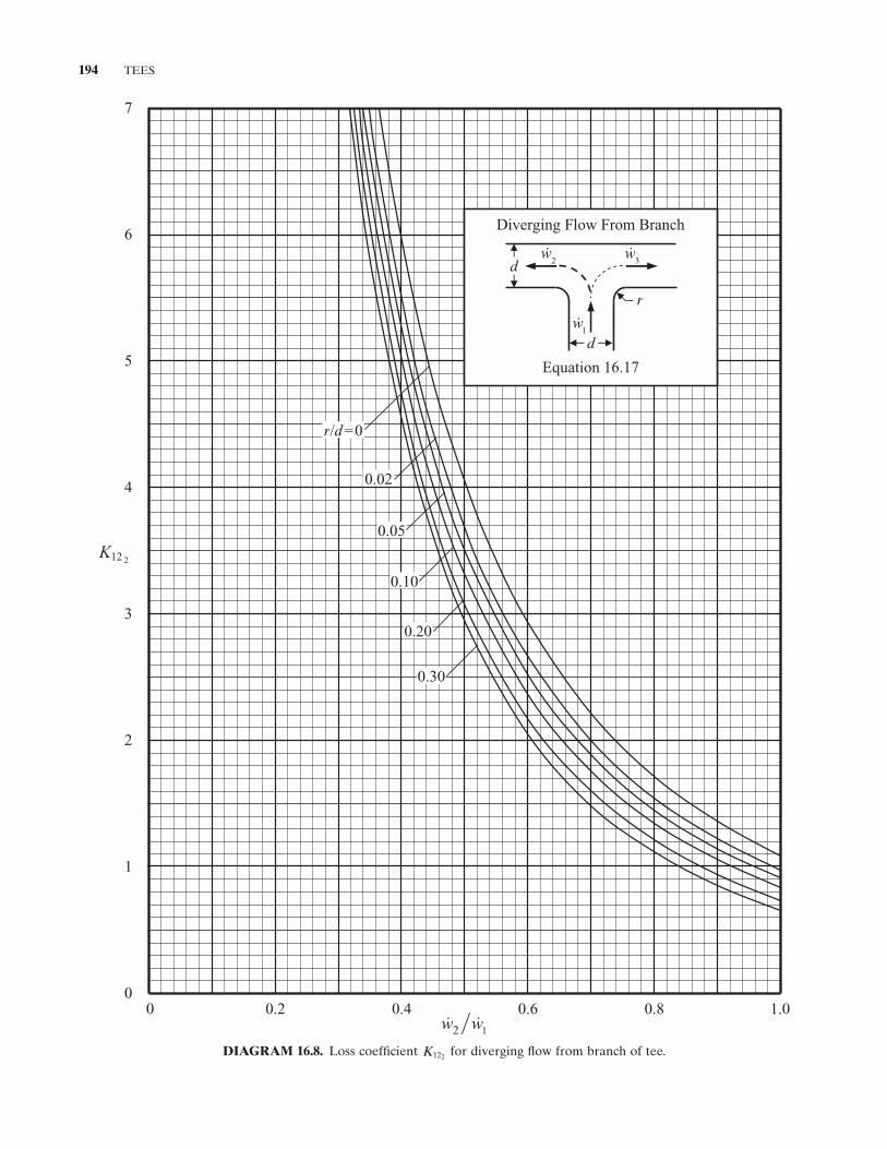
194 TEES
DIAGRAM 16.8. Loss coeffi cient K122 for diverging fl ow from branch of tee.
7
6
5
4
3
2
1
0
K12 2
0 0.2 0.4 0.6 0.8 1.012 ww
0.05
r/d=0
0.02
0.10
0.30
0.20
Diverging Flow From Branch
2w
3w
1w
Equation 16.17
r
d
d
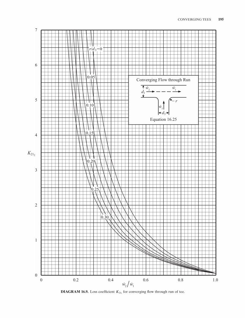
CONVERGING TEES 195
DIAGRAM 16.9. Loss coeffi cient K211 for converging fl ow through run of tee.
7
6
5
4
3
2
1
0
K212
0 0.2 0.4 0.6 0.8 1.01w
0.05
0.10
0.15
0.20
0.25
0.30
r/d 3 =0
Converging Flow through Run
2
w 1
w
3
w
Equation 16.25
r
d1
d3
2w
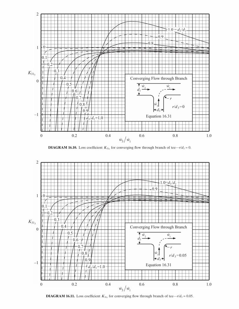
DIAGRAM 16.10. Loss coeffi cient K313 for converging fl ow through branch of tee — r / d3 = 0.
0 0.2 0.4 0.6 0.8 1.0
2
1
0
–1
K313
Converging Flow through Branch
2
w 1
w
3
w
Equation 16.31
r
d1
d3r/d 3 =0
d3 /d1 =1.0
0.9
0.7
0.8
0.5
0.4
0.2
0.6
0.1
0.3
0
1.0 = d3 /d1
0.9
0.8
13 ww
DIAGRAM 16.11. Loss coeffi cient K313 for converging fl ow through branch of tee — r / d3 = 0.05.
0 0.2 0.4 0.6 0.8 1.0
2
1
0
–1
K313
d3 /d1 =1.0
0.9
0.7
0.8
0.5
0.4
0.2
0.6
0.1
0.3
0
1.0=d3 /d1
0.9
Converging Flow through Branch
2
w 1
w
3
w
Equation 16.31
r
d1
d3
r/d 3 =0.05
13 ww
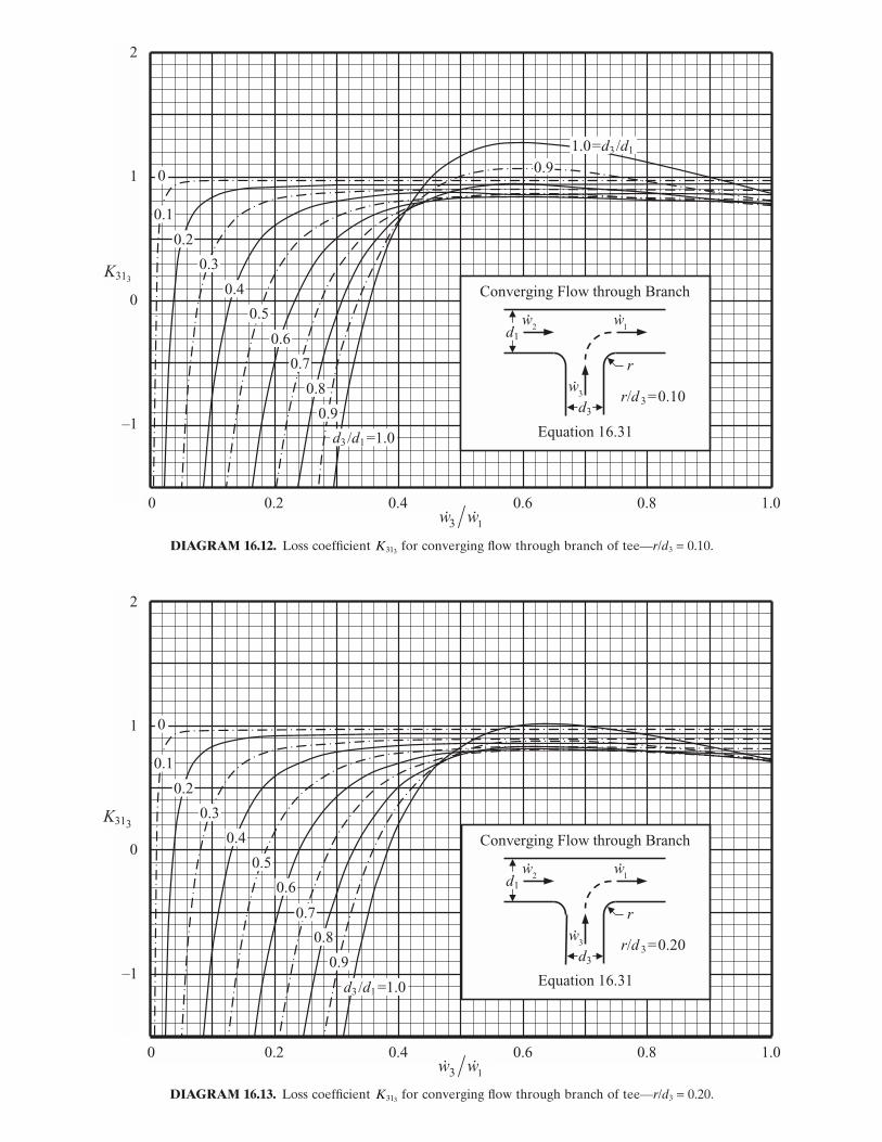
DIAGRAM 16.12. Loss coeffi cient K313 for converging fl ow through branch of tee — r / d3 = 0.10.
2
1
0
–1
K313
d3 /d1 =1.0
0.9
0.7
0.8
0.5
0.4
0.2
0.6
0.1
0.3
0
1.0=d3 /d1
0.9
Converging Flow through Branch
2
w 1
w
3
w
Equation 16.31
r
d1
d3r/d 3 =0.10
0 0.2 0.4 0.6 0.8 1.013 ww
DIAGRAM 16.13. Loss coeffi cient K313 for converging fl ow through branch of tee — r / d3 = 0.20.
2
1
0
–1
K313
d3 /d1 =1.0
0.9
0.7
0.8
0.5
0.4
0.2
0.6
0.1
0.3
0
Converging Flow through Branch
2
w 1
w
3
w
Equation 16.31
r
d1
d3r/d 3 =0.20
0 0.2 0.4 0.6 0.8 1.013 ww
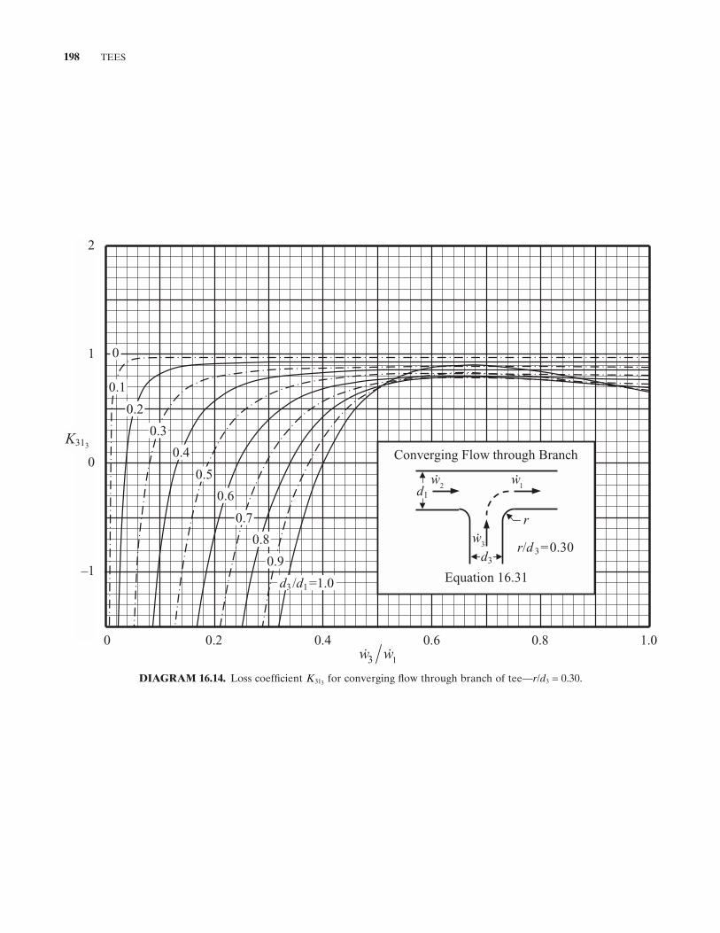
198 TEES
DIAGRAM 16.14. Loss coeffi cient K313 for converging fl ow through branch of tee — r / d3 = 0.30.
0 0.2 0.4 0.6 0.8 1.0
2
1
0
–1
K313
d3 /d1 =1.0
0.9
0.7
0.8
0.5
0.4
0.2
0.6
0.1
0.3
0
Converging Flow through Branch
2
w 1
w
3w
Equation 16.31
r
d1
d3r/d 3 =0.30
13 ww
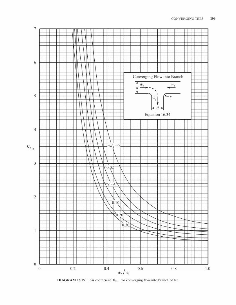
CONVERGING TEES 199
DIAGRAM 16.15. Loss coeffi cient K212 for converging fl ow into branch of tee.
7
6
5
4
3
2
1
0
K212
0 0.2 0.4 0.6 0.8 1.012 ww
0.05
r/d 1 =0
0.10
0.30
0.20
0.02
Converging Flow into Branch
2
w 3
w
1
w
Equation 16.34
r
d
d
200 TEES
Keller , J. D. , The manifold problem , Journal of Applied Mechanics, Transactions of the American Society of Mechan-ical Engineers , 71 , March 1949 , 77 – 85 .
McKnown , J. S. , Mechanics of manifold fl ow , Transactions of the American Society of Civil Engineers , 119 , 1954 , 1103 – 1142 .
Starosolszky , O. , Pressure conditions in pipe branches , V í z ü gyi K ö zlem é nyek , Imprimerie University, Budapest, No. 1958/1, 1958 , pp. 115 – 121 (translated by Language Service Bureau, Washington, D.C.).
Levine , S. , Collision of incompressible - liquid streams in pipe , Leningrad Tech. Inst. No. 8 , 1958 . (Published by Dunod, Paris, 1968).
Zeisser , M. H. , Summary report of single - tube branch and multi - tube branch water fl ow tests conducted by the Uni-versity of Connecticut , Pratt and Whitney Aircraft Divi-sion, United Aircraft Corporation, Report No. PWAC - 231 USAEC Contract AT (11 - 1) - 229. May, 1963 .
Blaisdell , F. W. and P. W. Manson , Loss of energy at sharp - edged pipe junctions in water conveyance systems , U.S. Dept. of Agriculture, Tech. Bulletin No, 1283, 163 pp., 106 fi gs, August, 1963 .
Lakshmana Rao , N. S. , B. C. Syamala Rao , and M. S. Shivas-wamy , Distribution of energy losses at conduit tribufurca-tions , Journal of the Hydraulics Division, Proceedings of the American Society of Civil Engineers , HY6 , November 1968 , 1363 – 1374 .
Ruus , E. , Head losses in wyes and manifolds , Journal of the Hydraulics Division, Proceedings of the American Society of Civil Engineers , HY3 , March 1970 , 593 – 608 .
Bajura , R. A. , A model for fl ow distribution in manifolds , Journal of Engineering for Power, Transactions of the Amer-ican Society of Mechanical Engineers , 93 , January 1971 , 7 – 12 .
Miller , D. S. , Internal Flow, a Guide to Losses in Pipe and Duct Systems , The British Hydromechanics Research Associa-tion , 1971 .
Bajura , R. A. , V. F. LeRose , and L. E. Williams , Fluid distribu-tion in combining, dividing and reverse fl ow manifolds , Journal of Engineering for Power, Transactions of the Amer-ican Society of Mechanical Engineers , Paper No. 73 - Pwr - 1, 1973 , 1 – 11 .
Williamson , J. V. and T. J. Rhone , Dividing fl ow in branches and wyes , Journal of the Hydraulics Division, Proceedings of the American Society of Civil Engineers , HY5 , May 1973 , 747 – 769 .
Bajura , R. A. and E. H. Jones , Flow distribution manifolds , Journal of Fluids Engineering, Transactions of the American Society of Mechanical Engineers , 88 , 1976 , 654 – 666 .
Ito , H. , M. Sato , and K. Oka , Energy losses due to division and combination of fl ow at 90 ° Wyes (in Japanese) , Transac-tions of the Japanese Society of Mechanical Engineers , 50 ( 450 ), 1978 , 342 – 350 .
Shen , P. I. , The effect of friction on fl ow distribution in dividing and combining fl ow manifolds , Journal of Fluids Engineer-ing, Transactions of the American Society of Mechanical Engineers , 114 , March 1992 , 121 – 123 .
REFERENCES
1. Gardel , A. , Chambres d ’ é quilibre , (doctorate thesis in French) É cole Polytechnique de l ’ Universit é de Lausanne, Librairie de l ’ Universite, 1956 .
2. Gardel , A. , Pressure drops in fl ows through T - shaped fi t-tings, (in French) , Bulletin Technique de la Suisse Romande , 83 ( 9 ), April 1957 , pp. 123 – 130 , and (10), May 1957, pp. 143 – 148.
3. Ito , H. and K. Imai , Energy losses at 90 ° pipe junctions , Journal of the Hydraulics Division, Proceedings of the American Society of Civil Engineers , HY9 , September 1973 , 1353 – 1368 .
4. Idel ’ chik , I. E. , Handbook of Hydraulic Resistance — Coeffi cients of Local Resistance and of Friction , Moskva - Leningrad , 1960 , (Translated from Russian. Published for the U.S. Atomic Energy Commission and the National Science Foundation, Washington, D.C. by the Israel Program for Scientifi c Translations, Jerusalem, 1966.)
5. Kinne , E. , Contribution to the knowledge of hydraulic losses in branches , Hydro Institute of Technology Hoschule - Munchen , ( 4 ), 1931 , 70 – 93 . (Translation No. 323 by Bureau of Reclamation, U.S. Dept. of the Interior, Washington, 1955.)
6. Gardel , A. and G. F. Rechsteiner , Les Pertes de Charge dans les Branchments en Te des Conduites de Section Circulaire , (in French), Publication No, 118, Ecole Polytechnique Federale de Lausanne , Lausanne, Switzerland , 1971 .
FURTHER READING
This list includes books and papers that may be helpful to those who wish to pursue further study.
Vogel , G. , Investigation of the loss in right - angled pipe branches , Hydro Institute of Technology Hoschule - Munchen , ( 1 ), 1926 , pp. 75 – 90 , and (2), 1928, pp. 61 – 64.
Corp , C. I. , Experiments on loss of head in U, S, and Twisted S pipe bends , Bulletin of the University of Wisconsin, Engi-neering Experiment Station Series No. 66 , Madison, 1927 .
Petermann , F. , Loss in oblique - angled pipe branches , Hydr. Inst. Tech. Hoschule - Munchen No. 3 , 1929 , pp. 65 – 77 . (Translated by N. H. Eaton and K. H. Beij, American Society of Mechanical Engineer Special Publication, 1935.)
Naramoto , I. and T. Kasai , On the loss of energy at impact of two confi ned streams of water , Kyushu Imperial University College of Engineering Memory , Fukuoka, Japan, 6 ( 3 ), 1931 , 189 – 261 .
Farve , H. , On the laws governing the movement of fl uids in conduits under pressure with lateral fl ow , Univ. des Mines Rev. , Belgium, (ser 8, t. 13) 12: 1937 , pp. 502 – 512 . (Transla-tion supplied by Agr. Res. Serv., St. Anthony Falls Hydr. Lab., Minneapolis.)
Vazsonyi , A. , Pressure loss in elbows and duct branches , Trans-actions of the American Society of Mechanical Engineers , 66 , April 1944 , 177 – 183 .
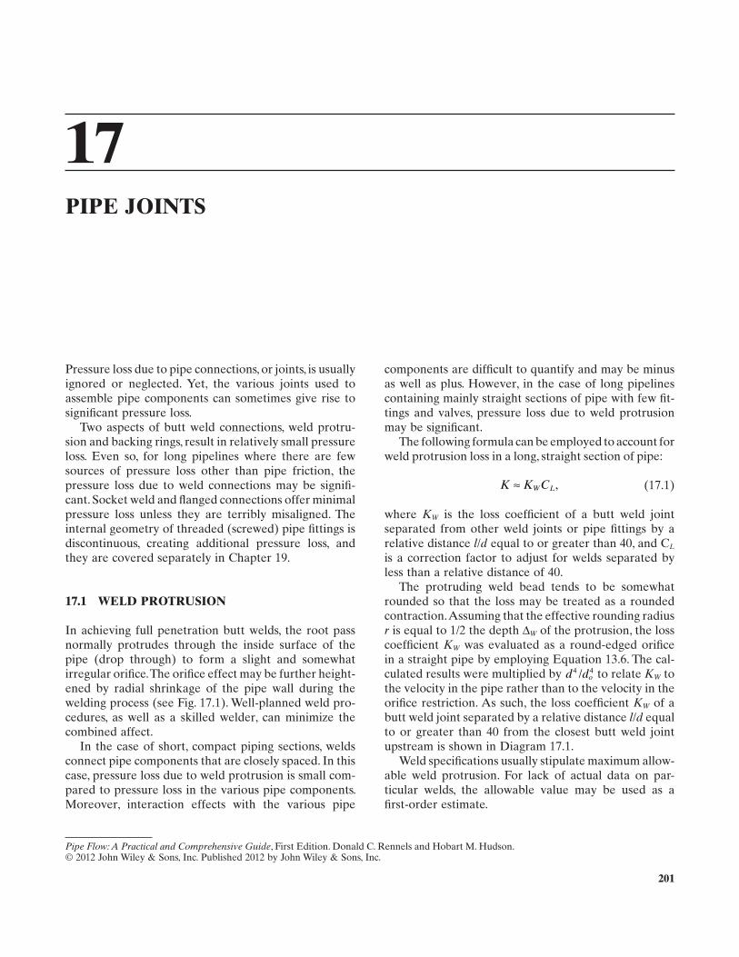
201
17 PIPE JOINTS
Pressure loss due to pipe connections, or joints, is usually ignored or neglected. Yet, the various joints used to assemble pipe components can sometimes give rise to signifi cant pressure loss.
Two aspects of butt weld connections, weld protru-sion and backing rings, result in relatively small pressure loss. Even so, for long pipelines where there are few sources of pressure loss other than pipe friction, the pressure loss due to weld connections may be signifi -cant. Socket weld and fl anged connections offer minimal pressure loss unless they are terribly misaligned. The internal geometry of threaded (screwed) pipe fi ttings is discontinuous, creating additional pressure loss, and they are covered separately in Chapter 19 .
17.1 WELD PROTRUSION
In achieving full penetration butt welds, the root pass normally protrudes through the inside surface of the pipe (drop through) to form a slight and somewhat irregular orifi ce. The orifi ce effect may be further height-ened by radial shrinkage of the pipe wall during the welding process (see Fig. 17.1 ). Well - planned weld pro-cedures, as well as a skilled welder, can minimize the combined affect.
In the case of short, compact piping sections, welds connect pipe components that are closely spaced. In this case, pressure loss due to weld protrusion is small com-pared to pressure loss in the various pipe components. Moreover, interaction effects with the various pipe
components are diffi cult to quantify and may be minus as well as plus. However, in the case of long pipelines containing mainly straight sections of pipe with few fi t-tings and valves, pressure loss due to weld protrusion may be signifi cant.
The following formula can be employed to account for weld protrusion loss in a long, straight section of pipe:
K K CW L≈ , (17.1)
where KW is the loss coeffi cient of a butt weld joint separated from other weld joints or pipe fi ttings by a relative distance l / d equal to or greater than 40, and C Lis a correction factor to adjust for welds separated by less than a relative distance of 40.
The protruding weld bead tends to be somewhat rounded so that the loss may be treated as a rounded contraction. Assuming that the effective rounding radius r is equal to 1/2 the depth ΔW of the protrusion, the loss coeffi cient KW was evaluated as a round - edged orifi ce in a straight pipe by employing Equation 13.6 . The cal-culated results were multiplied by d do
4 4/ to relate KW to the velocity in the pipe rather than to the velocity in the orifi ce restriction. As such, the loss coeffi cient KW of a butt weld joint separated by a relative distance l / d equal to or greater than 40 from the closest butt weld joint upstream is shown in Diagram 17.1 .
Weld specifi cations usually stipulate maximum allow-able weld protrusion. For lack of actual data on par-ticular welds, the allowable value may be used as a fi rst - order estimate.
Pipe Flow: A Practical and Comprehensive Guide, First Edition. Donald C. Rennels and Hobart M. Hudson.© 2012 John Wiley & Sons, Inc. Published 2012 by John Wiley & Sons, Inc.
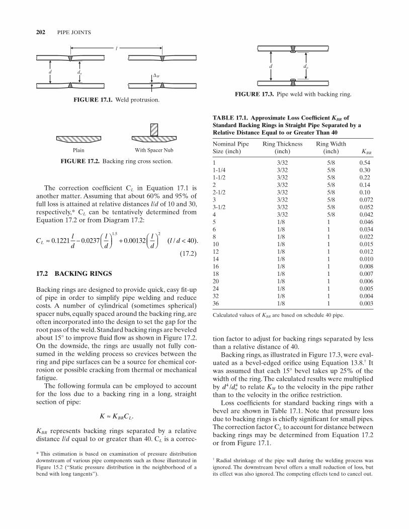
202 PIPE JOINTS
tion factor to adjust for backing rings separated by less than a relative distance of 40.
Backing rings, as illustrated in Figure 17.3 , were eval-uated as a bevel - edged orifi ce using Equation 13.8 . † It was assumed that each 15 ° bevel takes up 25% of the width of the ring. The calculated results were multiplied by d do
4 4/ to relate KW to the velocity in the pipe rather than to the velocity in the orifi ce restriction.
Loss coeffi cients for standard backing rings with a bevel are shown in Table 17.1 . Note that pressure loss due to backing rings is chiefl y signifi cant for small pipes. The correction factor C L to account for distance between backing rings may be determined from Equation 17.2 or from Figure 17.1 .
FIGURE 17.1. Weld protrusion.
l
∆Wdod
FIGURE 17.2. Backing ring cross section.
Plain With Spacer Nub
FIGURE 17.3. Pipe weld with backing ring.
dod
TABLE 17.1. Approximate Loss Coeffi cient KBR of Standard Backing Rings in Straight Pipe Separated by a Relative Distance Equal to or Greater Than 40
Nominal Pipe Size (inch)
Ring Thickness (inch)
Ring Width (inch) KBR
1 3/32 5/8 0.54 1 - 1/4 3/32 5/8 0.30 1 - 1/2 3/32 5/8 0.22 2 3/32 5/8 0.14 2 - 1/2 3/32 5/8 0.10 3 3/32 5/8 0.072 3 - 1/2 3/32 5/8 0.052 4 3/32 5/8 0.042 5 1/8 1 0.046 6 1/8 1 0.034 8 1/8 1 0.022 10 1/8 1 0.015 12 1/8 1 0.012 14 1/8 1 0.010 16 1/8 1 0.008 18 1/8 1 0.007 20 1/8 1 0.006 24 1/8 1 0.005 32 1/8 1 0.004 36 1/8 1 0.003
Calculated values of KBR are based on schedule 40 pipe.
† Radial shrinkage of the pipe wall during the welding process was ignored. The downstream bevel offers a small reduction of loss, but its effect was also ignored. The competing effects tend to cancel out.
* This estimation is based on examination of pressure distribution downstream of various pipe components such as those illustrated in Figure 15.2 ( “ Static pressure distribution in the neighborhood of a bend with long tangents ” ).
The correction coeffi cient C L in Equation 17.1 is another matter. Assuming that about 60% and 95% of full loss is attained at relative distances l / d of 10 and 30, respectively, * C L can be tentatively determined from Equation 17.2 or from Diagram 17.2 :
Cld
ld
ld
l dL ≈ −
+
<0 1221 0 0237 0 00132 40
1 5 2
. . . ( / )..
(17.2)
17.2 BACKING RINGS
Backing rings are designed to provide quick, easy fi t - up of pipe in order to simplify pipe welding and reduce costs. A number of cylindrical (sometimes spherical) spacer nubs, equally spaced around the backing ring, are often incorporated into the design to set the gap for the root pass of the weld. Standard backing rings are beveled about 15 ° to improve fl uid fl ow as shown in Figure 17.2 . On the downside, the rings are usually not fully con-sumed in the welding process so crevices between the ring and pipe surfaces can be a source for chemical cor-rosion or possible cracking from thermal or mechanical fatigue.
The following formula can be employed to account for the loss due to a backing ring in a long, straight section of pipe:
K K CBR L≈ .
KBR represents backing rings separated by a relative distance l / d equal to or greater than 40. C L is a correc-
MISALIGNMENT 203
Open fl ow area Ao was determined as a function of misalignment m in Section 17.3.1 and was presented in Figure 17.5 as a function of m / d . Now we treat the mis-alignment gasket as a sharp - edged orifi ce. The beta ratio can be determined as β = ( Ao / A ) 1/2 . The loss coeffi cient K of the misaligned gasket is determined from Equation 12.6 for a sharp - edged orifi ce. Once again, the calculated results were multiplied by A A2
o/ 2 to relate K to the velocity in the pipe rather than to the velocity in the orifi ce restriction. The approximate loss coeffi cient of a misaligned gasket can be obtained from Diagram 17.4 .
17.3 MISALIGNMENT
Appreciable pressure loss may result when piping com-ponents are misaligned during assembly, or when fl ange gaskets are not properly fi tted.
17.3.1 Misaligned Pipe Joint
Misalignment of a pipe joint is illustrated in Figure 17.4 . It is rational to treat the loss as a sharp - edged contrac-tion in parallel with a sudden expansion. But fi rst, we must determine the geometric relationship between misalignment m and open fl ow area Ao through the pipe joint.
Area Am , and thereby open fl ow area Ao , was deter-mined as a function of misalignment m by integration between the curves formed by the pipe walls. From this, the ratio of fl ow area Ao to fl ow area A of the pipe is presented in Figure 17.5 as a function of misalignment.
Next, the problem was treated as a sudden contrac-tion and sudden expansion in parallel. First, the beta ratio was determined as β = ( Ao / A ) 1/2 . The loss coeffi -cient Kcontr of the sudden contraction fl ow path was determined from Equation 10.5 and the loss coeffi cient Kexp of the sudden expansion fl ow path was determined from Equation 11.8 . Assigning one - half the open fl ow area Ao to each fl ow path, Equation 5.9 was employed to determine the combined loss coeffi cient of the mis-aligned joint. The calculated results were multiplied by A A2
o/ 2 to relate K to the velocity in the pipe rather than to the velocity in the restriction. From this, the loss coef-fi cient of a misaligned pipe joint in terms of the velocity in the pipe can be obtained from Diagram 17.3 .
17.3.2 Misaligned Gasket
A misalignment gasket in a fl anged connection is illus-trated in Figure 17.6 . It is reasonable to treat the loss as a sharp - edged orifi ce in a straight pipe.
FIGURE 17.4. Misaligned pipe joint.
m
Ao
y
x
Am
m/2d
FIGURE 17.5. Open area ratio Ao / A as a function of m / d.
1.0
0.8
0.6
0.4
0.2
00 0.2 0.4 0.6 0.8 1.0
Ao/
A
m/d
FIGURE 17.6. Misaligned fl ange gasket.
Ao
Am
m
d
Ap
Ao = Ap – Am
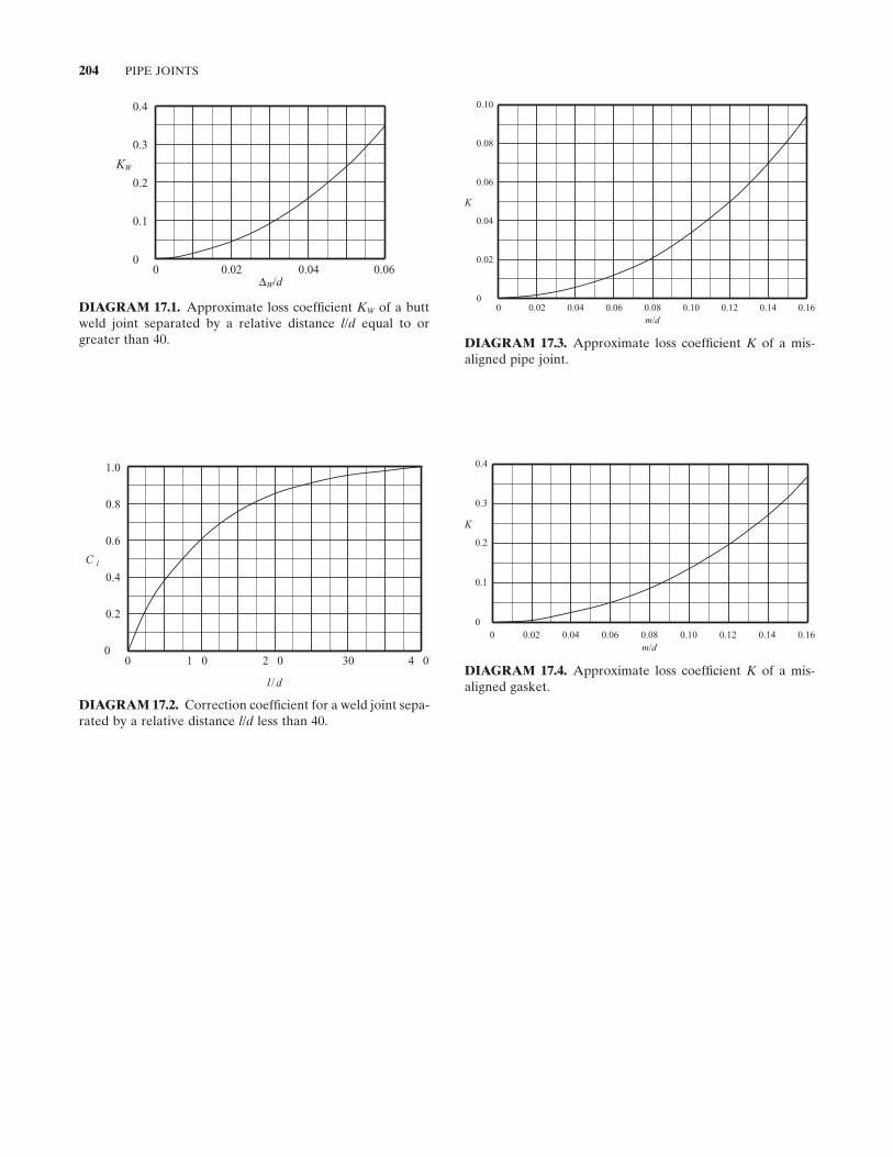
204 PIPE JOINTS
DIAGRAM 17.4. Approximate loss coeffi cient K of a mis-aligned gasket.
0.4
0.3
0.2
0.1
00 0.02 0.04 0.06 0.08 0.10 0.12 0.14 0.16
K
m/d
DIAGRAM 17.1. Approximate loss coeffi cient KW of a butt weld joint separated by a relative distance l / d equal to or greater than 40.
0.4
0.3
0.2
0.1
00 0.02 0.04 0.06
∆W/d
KW
DIAGRAM 17.2. Correction coeffi cient for a weld joint sepa-rated by a relative distance l / d less than 40.
1.0
0.8
0.6
0.4
0.2
00 1 0 2 0 30 4 0
l / d
C l
DIAGRAM 17.3. Approximate loss coeffi cient K of a mis-aligned pipe joint.
0.10
0.08
0.06
0.04
0.02
00 0.02 0.04 0.06 0.08 0.10 0.12 0.14 0.16
K
m/d
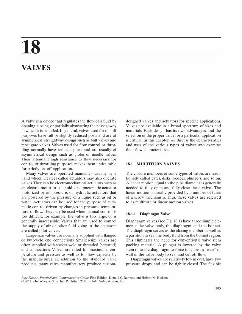
205
18 VALVES
A valve is a device that regulates the fl ow of a fl uid by opening, closing, or partially obstructing the passageway in which it is installed. In general, valves used for on – off purposes have full or slightly reduced ports and are of symmetrical, straightway design such as ball valves and most gate valves. Valves used for fl ow control or throt-tling normally have reduced ports and are usually of asymmetrical design such as globe or needle valves. Their attendant high resistance to fl ow, necessary for control or throttling purposes, makes them undesirable for strictly on – off application.
Many valves are operated manually — usually by a hand wheel. Devices called actuators may also operate valves. They can be electromechanical actuators such as an electric motor or solenoid, or a pneumatic actuator motorized by air pressure; or hydraulic actuators that are powered by the pressure of a liquid such as oil or water. Actuators can be used for the purpose of auto-matic control driven by changes in pressure, tempera-ture, or fl ow. They may be used when manual control is too diffi cult; for example, the valve is too large, or is generally inaccessible. Valves that are used to control the supply of air or other fl uid going to the actuators are called pilot valves.
Large - size valves are normally supplied with fl anged or butt - weld end connections. Smaller - size valves are often supplied with socket - weld or threaded (screwed) end connections. Valves are rated for maximum tem-perature and pressure as well as for fl ow capacity by the manufacturer. In addition to the standard valve products, many valve manufacturers produce custom -
designed valves and actuators for specifi c applications. Valves are available in a broad spectrum of sizes and materials. Each design has its own advantages, and the selection of the proper valve for a particular application is critical. In this chapter, we discuss the characteristics and uses of the various types of valves and examine their fl ow characteristics.
18.1 MULTITURN VALVES
The closure members of some types of valves are tradi-tionally called gates, disks, wedges, plungers, and so on. A linear motion equal to the pipe diameter is generally needed to fully open and fully close these valves. The linear motion is usually provided by a number of turns of a screw mechanism. Thus, these valves are referred to as multiturn or linear motion valves.
18.1.1 Diaphragm Valve
Diaphragm valves (see Fig. 18.1 ) have three simple ele-ments: the valve body, the diaphragm, and the bonnet. The diaphragm serves as the closing member as well as a partition to seal the body fl uid from the bonnet region. This eliminates the need for conventional valve stem packing material. A plunger is lowered by the valve stem onto the diaphragm to force it against a “ weir ” or wall in the valve body to seal and cut off fl ow.
Diaphragm valves are relatively low in cost, have low pressure drops, and can be tightly closed. The fl exible
Pipe Flow: A Practical and Comprehensive Guide, First Edition. Donald C. Rennels and Hobart M. Hudson.© 2012 John Wiley & Sons, Inc. Published 2012 by John Wiley & Sons, Inc.
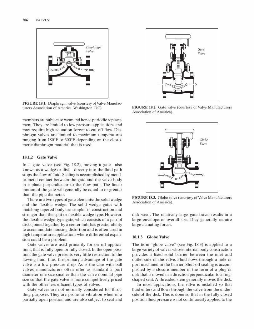
206 VALVES
disk wear. The relatively large gate travel results in a large envelope or overall size. They generally require large actuating forces.
18.1.3 Globe Valve
The term “ globe valve ” (see Fig. 18.3 ) is applied to a large variety of valves whose internal body construction provides a fi xed solid barrier between the inlet and outlet side of the valve. Fluid fl ows through a hole or port machined in the barrier. Shut - off sealing is accom-plished by a closure member in the form of a plug or disk that is moved in a direction perpendicular to a ring - shaped seat. A threaded stem generally moves the disk.
In most applications, the valve is installed so that fl uid enters and fl ows through the valve from the under-side of the disk. This is done so that in the fully closed position fl uid pressure is not continuously applied to the
members are subject to wear and hence periodic replace-ment. They are limited to low pressure applications and may require high actuation forces to cut off fl ow. Dia-phragm valves are limited to maximum temperatures ranging from 180 ° F to 300 ° F depending on the elasto-meric diaphragm material that is used.
18.1.2 Gate Valve
In a gate valve (see Fig. 18.2 ), moving a gate — also known as a wedge or disk — directly into the fl uid path stops the fl ow of fl uid. Sealing is accomplished by metal - to - metal contact between the gate and the valve body in a plane perpendicular to the fl ow path. The linear motion of the gate will generally be equal to or greater than the pipe diameter.
There are two types of gate elements: the solid wedge and the fl exible wedge. The solid wedge gates with matching tapered body are simpler in construction and stronger than the split or fl exible wedge type. However, the fl exible wedge - type gate, which consists of a pair of disks joined together by a center hub, has greater ability to accommodate housing distortion and is often used in high temperature applications where differential expan-sion could be a problem.
Gate valves are used primarily for on – off applica-tions, that is, fully open or fully closed. In the open posi-tion, the gate valve presents very little restriction to the fl owing fl uid; thus, the primary advantage of the gate valve is a low pressure drop. As is the case with ball valves, manufacturers often offer as standard a port diameter one size smaller than the valve nominal pipe size so that the gate valve is more competitively priced with the other less effi cient types of valves.
Gate valves are not normally considered for throt-tling purposes. They are prone to vibration when in a partially open position and are also subject to seat and
FIGURE 18.1. Diaphragm valve (courtesy of Valve Manufac-turers Association of America, Washington, DC).
DiaphragmValve
FIGURE 18.2. Gate valve (courtesy of Valve Manufacturers Association of America).
GateValve
FIGURE 18.3. Globe valve (courtesy of Valve Manufacturers Association of America).
GlobeValve
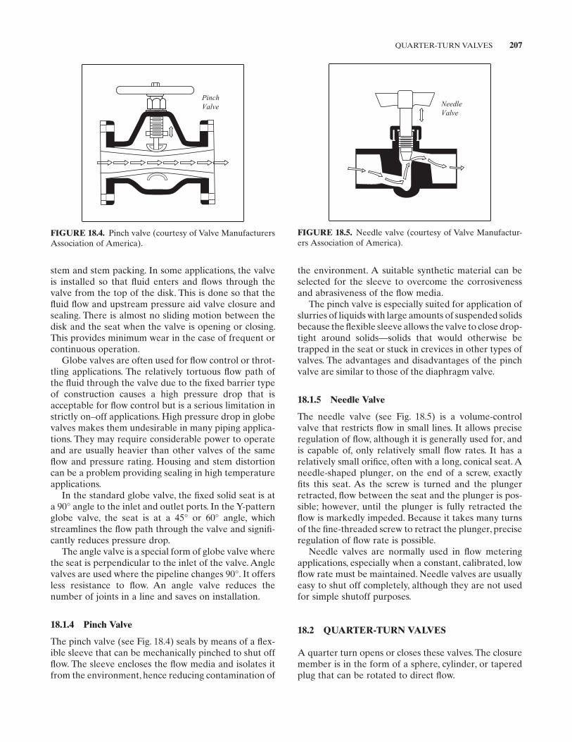
QUARTER-TURN VALVES 207
the environment. A suitable synthetic material can be selected for the sleeve to overcome the corrosiveness and abrasiveness of the fl ow media.
The pinch valve is especially suited for application of slurries of liquids with large amounts of suspended solids because the fl exible sleeve allows the valve to close drop - tight around solids — solids that would otherwise be trapped in the seat or stuck in crevices in other types of valves. The advantages and disadvantages of the pinch valve are similar to those of the diaphragm valve.
18.1.5 Needle Valve
The needle valve (see Fig. 18.5 ) is a volume - control valve that restricts fl ow in small lines. It allows precise regulation of fl ow, although it is generally used for, and is capable of, only relatively small fl ow rates. It has a relatively small orifi ce, often with a long, conical seat. A needle - shaped plunger, on the end of a screw, exactly fi ts this seat. As the screw is turned and the plunger retracted, fl ow between the seat and the plunger is pos-sible; however, until the plunger is fully retracted the fl ow is markedly impeded. Because it takes many turns of the fi ne - threaded screw to retract the plunger, precise regulation of fl ow rate is possible.
Needle valves are normally used in fl ow metering applications, especially when a constant, calibrated, low fl ow rate must be maintained. Needle valves are usually easy to shut off completely, although they are not used for simple shutoff purposes.
18.2 QUARTER - TURN VALVES
A quarter turn opens or closes these valves. The closure member is in the form of a sphere, cylinder, or tapered plug that can be rotated to direct fl ow.
stem and stem packing. In some applications, the valve is installed so that fl uid enters and fl ows through the valve from the top of the disk. This is done so that the fl uid fl ow and upstream pressure aid valve closure and sealing. There is almost no sliding motion between the disk and the seat when the valve is opening or closing. This provides minimum wear in the case of frequent or continuous operation.
Globe valves are often used for fl ow control or throt-tling applications. The relatively tortuous fl ow path of the fl uid through the valve due to the fi xed barrier type of construction causes a high pressure drop that is acceptable for fl ow control but is a serious limitation in strictly on – off applications. High pressure drop in globe valves makes them undesirable in many piping applica-tions. They may require considerable power to operate and are usually heavier than other valves of the same fl ow and pressure rating. Housing and stem distortion can be a problem providing sealing in high temperature applications.
In the standard globe valve, the fi xed solid seat is at a 90 ° angle to the inlet and outlet ports. In the Y - pattern globe valve, the seat is at a 45 ° or 60 ° angle, which streamlines the fl ow path through the valve and signifi -cantly reduces pressure drop.
The angle valve is a special form of globe valve where the seat is perpendicular to the inlet of the valve. Angle valves are used where the pipeline changes 90 ° . It offers less resistance to fl ow. An angle valve reduces the number of joints in a line and saves on installation.
18.1.4 Pinch Valve
The pinch valve (see Fig. 18.4 ) seals by means of a fl ex-ible sleeve that can be mechanically pinched to shut off fl ow. The sleeve encloses the fl ow media and isolates it from the environment, hence reducing contamination of
FIGURE 18.4. Pinch valve (courtesy of Valve Manufacturers Association of America).
PinchValve
FIGURE 18.5. Needle valve (courtesy of Valve Manufactur-ers Association of America).
NeedleValve
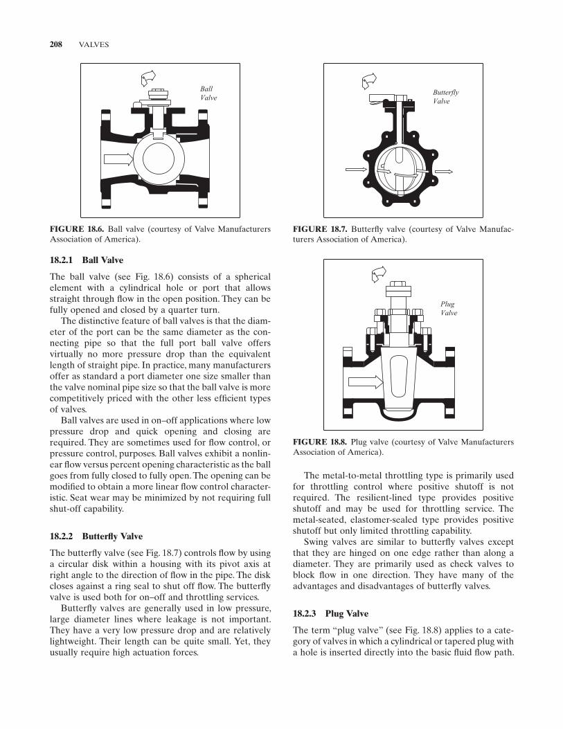
208 VALVES
The metal - to - metal throttling type is primarily used for throttling control where positive shutoff is not required. The resilient - lined type provides positive shutoff and may be used for throttling service. The metal - seated, elastomer - sealed type provides positive shutoff but only limited throttling capability.
Swing valves are similar to butterfl y valves except that they are hinged on one edge rather than along a diameter. They are primarily used as check valves to block fl ow in one direction. They have many of the advantages and disadvantages of butterfl y valves.
18.2.3 Plug Valve
The term “ plug valve ” (see Fig. 18.8 ) applies to a cate-gory of valves in which a cylindrical or tapered plug with a hole is inserted directly into the basic fl uid fl ow path.
FIGURE 18.6. Ball valve (courtesy of Valve Manufacturers Association of America).
BallValve
FIGURE 18.7. Butterfl y valve (courtesy of Valve Manufac-turers Association of America).
ButterflyValve
FIGURE 18.8. Plug valve (courtesy of Valve Manufacturers Association of America).
PlugValve
18.2.1 Ball Valve
The ball valve (see Fig. 18.6 ) consists of a spherical element with a cylindrical hole or port that allows straight through fl ow in the open position. They can be fully opened and closed by a quarter turn.
The distinctive feature of ball valves is that the diam-eter of the port can be the same diameter as the con-necting pipe so that the full port ball valve offers virtually no more pressure drop than the equivalent length of straight pipe. In practice, many manufacturers offer as standard a port diameter one size smaller than the valve nominal pipe size so that the ball valve is more competitively priced with the other less effi cient types of valves.
Ball valves are used in on – off applications where low pressure drop and quick opening and closing are required. They are sometimes used for fl ow control, or pressure control, purposes. Ball valves exhibit a nonlin-ear fl ow versus percent opening characteristic as the ball goes from fully closed to fully open. The opening can be modifi ed to obtain a more linear fl ow control character-istic. Seat wear may be minimized by not requiring full shut - off capability.
18.2.2 Butterfl y Valve
The butterfl y valve (see Fig. 18.7 ) controls fl ow by using a circular disk within a housing with its pivot axis at right angle to the direction of fl ow in the pipe. The disk closes against a ring seal to shut off fl ow. The butterfl y valve is used both for on – off and throttling services.
Butterfl y valves are generally used in low pressure, large diameter lines where leakage is not important. They have a very low pressure drop and are relatively lightweight. Their length can be quite small. Yet, they usually require high actuation forces.
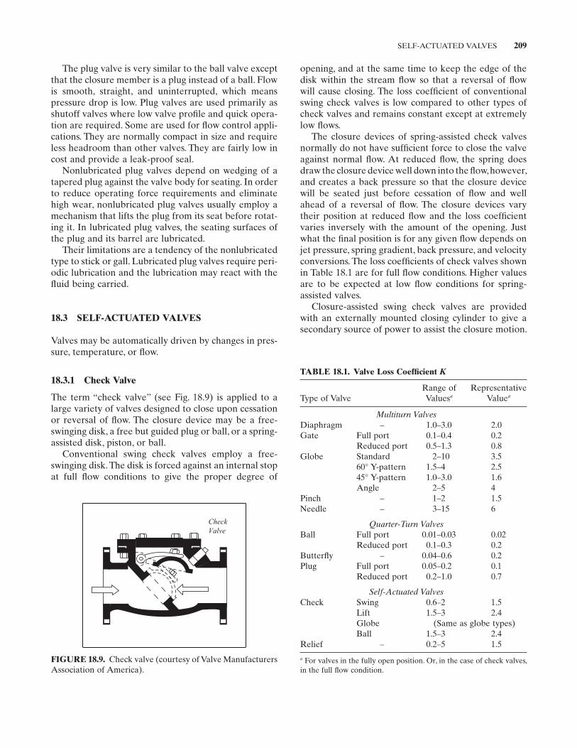
SELF-ACTUATED VALVES 209
opening, and at the same time to keep the edge of the disk within the stream fl ow so that a reversal of fl ow will cause closing. The loss coeffi cient of conventional swing check valves is low compared to other types of check valves and remains constant except at extremely low fl ows.
The closure devices of spring - assisted check valves normally do not have suffi cient force to close the valve against normal fl ow. At reduced fl ow, the spring does draw the closure device well down into the fl ow, however, and creates a back pressure so that the closure device will be seated just before cessation of fl ow and well ahead of a reversal of fl ow. The closure devices vary their position at reduced fl ow and the loss coeffi cient varies inversely with the amount of the opening. Just what the fi nal position is for any given fl ow depends on jet pressure, spring gradient, back pressure, and velocity conversions. The loss coeffi cients of check valves shown in Table 18.1 are for full fl ow conditions. Higher values are to be expected at low fl ow conditions for spring - assisted valves.
Closure - assisted swing check valves are provided with an externally mounted closing cylinder to give a secondary source of power to assist the closure motion.
The plug valve is very similar to the ball valve except that the closure member is a plug instead of a ball. Flow is smooth, straight, and uninterrupted, which means pressure drop is low. Plug valves are used primarily as shutoff valves where low valve profi le and quick opera-tion are required. Some are used for fl ow control appli-cations. They are normally compact in size and require less headroom than other valves. They are fairly low in cost and provide a leak - proof seal.
Nonlubricated plug valves depend on wedging of a tapered plug against the valve body for seating. In order to reduce operating force requirements and eliminate high wear, nonlubricated plug valves usually employ a mechanism that lifts the plug from its seat before rotat-ing it. In lubricated plug valves, the seating surfaces of the plug and its barrel are lubricated.
Their limitations are a tendency of the nonlubricated type to stick or gall. Lubricated plug valves require peri-odic lubrication and the lubrication may react with the fl uid being carried.
18.3 SELF - ACTUATED VALVES
Valves may be automatically driven by changes in pres-sure, temperature, or fl ow.
18.3.1 Check Valve
The term “ check valve ” (see Fig. 18.9 ) is applied to a large variety of valves designed to close upon cessation or reversal of fl ow. The closure device may be a free - swinging disk, a free but guided plug or ball, or a spring - assisted disk, piston, or ball.
Conventional swing check valves employ a free - swinging disk. The disk is forced against an internal stop at full fl ow conditions to give the proper degree of
FIGURE 18.9. Check valve (courtesy of Valve Manufacturers Association of America).
CheckValve
TABLE 18.1. Valve Loss Coeffi cient K
Type of Valve Range of Values a
Representative Value a
Multiturn Valves Diaphragm – 1.0 – 3.0 2.0 Gate Full port 0.1 – 0.4 0.2
Reduced port 0.5 – 1.3 0.8 Globe Standard 2 – 10 3.5
60 ° Y - pattern 1.5 – 4 2.5 45 ° Y - pattern 1.0 – 3.0 1.6 Angle 2 – 5 4
Pinch – 1 – 2 1.5 Needle – 3 – 15 6
Quarter - Turn Valves Ball Full port 0.01 – 0.03 0.02
Reduced port 0.1 – 0.3 0.2 Butterfl y – 0.04 – 0.6 0.2 Plug Full port 0.05 – 0.2 0.1
Reduced port 0.2 – 1.0 0.7
Self - Actuated Valves Check Swing 0.6 – 2 1.5
Lift 1.5 – 3 2.4 Globe (Same as globe types) Ball 1.5 – 3 2.4
Relief – 0.2 – 5 1.5
a For valves in the fully open position. Or, in the case of check valves, in the full fl ow condition.
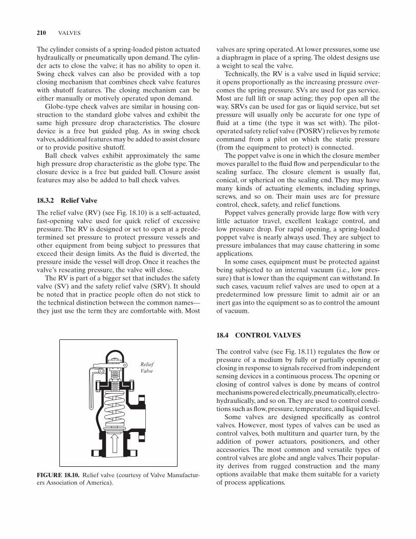
210 VALVES
valves are spring operated. At lower pressures, some use a diaphragm in place of a spring. The oldest designs use a weight to seal the valve.
Technically, the RV is a valve used in liquid service; it opens proportionally as the increasing pressure over-comes the spring pressure. SVs are used for gas service. Most are full lift or snap acting; they pop open all the way. SRVs can be used for gas or liquid service, but set pressure will usually only be accurate for one type of fl uid at a time (the type it was set with). The pilot - operated safety relief valve ( POSRV ) relieves by remote command from a pilot on which the static pressure (from the equipment to protect) is connected.
The poppet valve is one in which the closure member moves parallel to the fl uid fl ow and perpendicular to the sealing surface. The closure element is usually fl at, conical, or spherical on the sealing end. They may have many kinds of actuating elements, including springs, screws, and so on. Their main uses are for pressure control, check, safety, and relief functions.
Poppet valves generally provide large fl ow with very little actuator travel, excellent leakage control, and low pressure drop. For rapid opening, a spring - loaded poppet valve is nearly always used. They are subject to pressure imbalances that may cause chattering in some applications.
In some cases, equipment must be protected against being subjected to an internal vacuum (i.e., low pres-sure) that is lower than the equipment can withstand. In such cases, vacuum relief valves are used to open at a predetermined low pressure limit to admit air or an inert gas into the equipment so as to control the amount of vacuum.
18.4 CONTROL VALVES
The control valve (see Fig. 18.11 ) regulates the fl ow or pressure of a medium by fully or partially opening or closing in response to signals received from independent sensing devices in a continuous process. The opening or closing of control valves is done by means of control mechanisms powered electrically, pneumatically, electro-hydraulically, and so on. They are used to control condi-tions such as fl ow, pressure, temperature, and liquid level.
Some valves are designed specifi cally as control valves. However, most types of valves can be used as control valves, both multiturn and quarter turn, by the addition of power actuators, positioners, and other accessories. The most common and versatile types of control valves are globe and angle valves. Their popular-ity derives from rugged construction and the many options available that make them suitable for a variety of process applications.
The cylinder consists of a spring - loaded piston actuated hydraulically or pneumatically upon demand. The cylin-der acts to close the valve; it has no ability to open it. Swing check valves can also be provided with a top closing mechanism that combines check valve features with shutoff features. The closing mechanism can be either manually or motively operated upon demand.
Globe - type check valves are similar in housing con-struction to the standard globe valves and exhibit the same high pressure drop characteristics. The closure device is a free but guided plug. As in swing check valves, additional features may be added to assist closure or to provide positive shutoff.
Ball check valves exhibit approximately the same high pressure drop characteristic as the globe type. The closure device is a free but guided ball. Closure assist features may also be added to ball check valves.
18.3.2 Relief Valve
The relief valve (RV) (see Fig. 18.10 ) is a self - actuated, fast - opening valve used for quick relief of excessive pressure. The RV is designed or set to open at a prede-termined set pressure to protect pressure vessels and other equipment from being subject to pressures that exceed their design limits. As the fl uid is diverted, the pressure inside the vessel will drop. Once it reaches the valve ’ s reseating pressure, the valve will close.
The RV is part of a bigger set that includes the safety valve (SV) and the safety relief valve ( SRV ). It should be noted that in practice people often do not stick to the technical distinction between the common names — they just use the term they are comfortable with. Most
FIGURE 18.10. Relief valve (courtesy of Valve Manufactur-ers Association of America).
ReliefValve
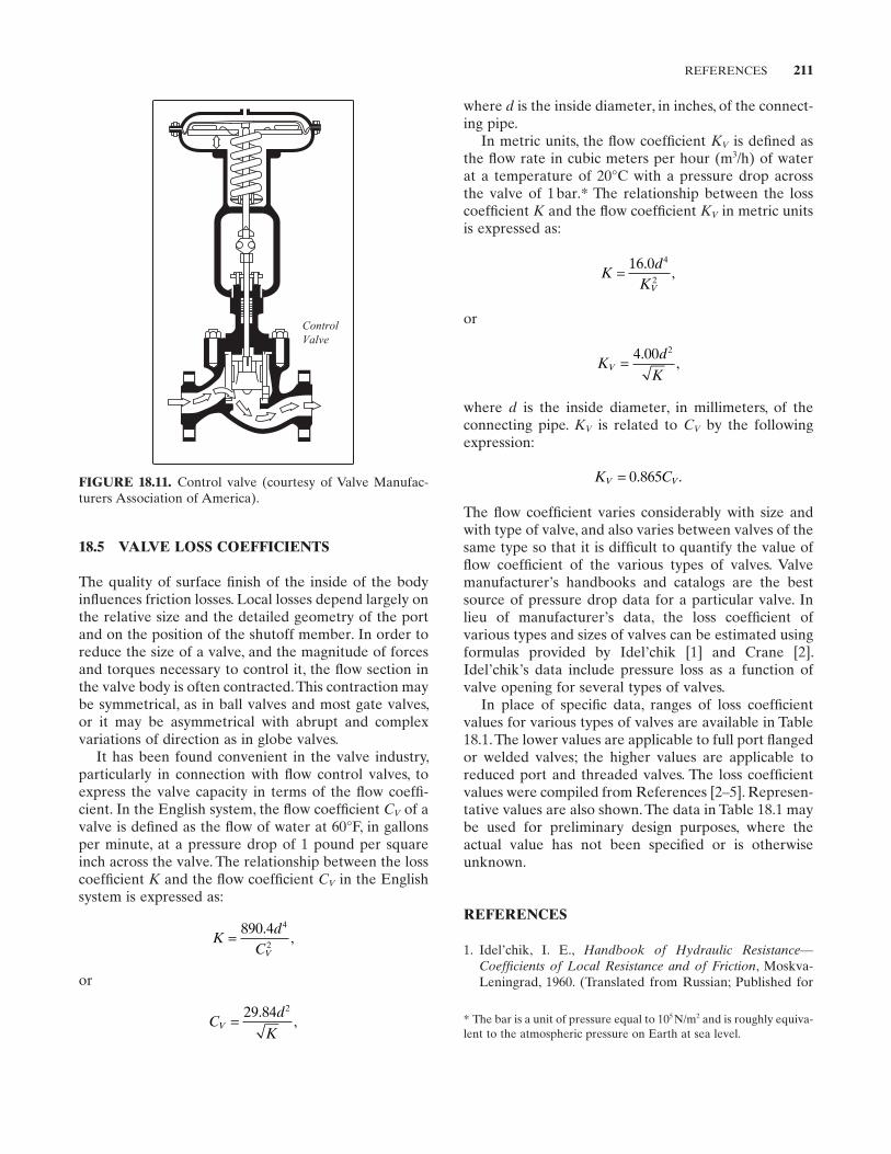
REFERENCES 211
where d is the inside diameter, in inches, of the connect-ing pipe.
In metric units, the fl ow coeffi cient KV is defi ned as the fl ow rate in cubic meters per hour (m 3 /h) of water at a temperature of 20 ° C with a pressure drop across the valve of 1 bar. * The relationship between the loss coeffi cient K and the fl ow coeffi cient KV in metric units is expressed as:
Kd
KV
= 16 0 4
2
.,
or
Kd
KV = 4 00 2.
,
where d is the inside diameter, in millimeters, of the connecting pipe. KV is related to CV by the following expression:
K CV V= 0 865. .
The fl ow coeffi cient varies considerably with size and with type of valve, and also varies between valves of the same type so that it is diffi cult to quantify the value of fl ow coeffi cient of the various types of valves. Valve manufacturer ’ s handbooks and catalogs are the best source of pressure drop data for a particular valve. In lieu of manufacturer ’ s data, the loss coeffi cient of various types and sizes of valves can be estimated using formulas provided by Idel ’ chik [1] and Crane [2] . Idel ’ chik ’ s data include pressure loss as a function of valve opening for several types of valves.
In place of specifi c data, ranges of loss coeffi cient values for various types of valves are available in Table 18.1 . The lower values are applicable to full port fl anged or welded valves; the higher values are applicable to reduced port and threaded valves. The loss coeffi cient values were compiled from References [2 – 5] . Represen-tative values are also shown. The data in Table 18.1 may be used for preliminary design purposes, where the actual value has not been specifi ed or is otherwise unknown.
REFERENCES
1. Idel ’ chik , I. E. , Handbook of Hydraulic Resistance — Coeffi cients of Local Resistance and of Friction , Moskva - Leningrad , 1960 . (Translated from Russian; Published for
18.5 VALVE LOSS COEFFICIENTS
The quality of surface fi nish of the inside of the body infl uences friction losses. Local losses depend largely on the relative size and the detailed geometry of the port and on the position of the shutoff member. In order to reduce the size of a valve, and the magnitude of forces and torques necessary to control it, the fl ow section in the valve body is often contracted. This contraction may be symmetrical, as in ball valves and most gate valves, or it may be asymmetrical with abrupt and complex variations of direction as in globe valves.
It has been found convenient in the valve industry, particularly in connection with fl ow control valves, to express the valve capacity in terms of the fl ow coeffi -cient. In the English system, the fl ow coeffi cient CV of a valve is defi ned as the fl ow of water at 60 ° F, in gallons per minute, at a pressure drop of 1 pound per square inch across the valve. The relationship between the loss coeffi cient K and the fl ow coeffi cient CV in the English system is expressed as:
Kd
CV
= 890 4 4
2
.,
or
Cd
KV = 29 84 2.
,
FIGURE 18.11. Control valve (courtesy of Valve Manufac-turers Association of America).
ControlValve
* The bar is a unit of pressure equal to 10 5 N/m 2 and is roughly equiva-lent to the atmospheric pressure on Earth at sea level.
212 VALVES
Kaisi , M. S. , C. L. Horst , and J. K. Wang , Prediction of valve performance and degradation in nuclear power plant systems , Kaisi Engineering, Inc. , KEI No. 1559, (Prepared for Division of Engineering, Offi ce of Nuclear Regulatory Research, U. S. Nuclear Regulatory Commission, Washing-ton, DC 20666, NRC FIN D2042), 1988 .
Eom , K. , Performance of butterfl y valves as a fl ow controller , Journal of Fluids Engineering, Transactions of the American Society of Mechanical Engineers , 110 , March 1988 , 16 – 19 .
Thorley , A. R. D. , Check valve behavior under transient fl ow conditions: A state - of - the - art review , Journal of Fluids Engineering, Transactions of the American Society of Mechanical Engineers , 111 , June 1989 , 178 – 1893 .
Morris , M. J. and J. C. Dutton , An experimental investigation of butterfl y valve performance downstream of an elbow , Journal of Fluids Engineering, Transactions of the American Society of Mechanical Engineers , 113 , March 1991 , 81 – 85 .
Morris , M. J. and J. C. Dutton , The performance of two but-terfl y valves mounted in series , Journal of Fluids Engineer-ing, Transactions of the American Society of Mechanical Engineers , 113 , September 1991 , 419 – 423 .
Liou , C. P. , Maximum pressure head due to linear valve closure , Journal of Fluids Engineering, Transactions of the American Society of Mechanical Engineers , 113 , December 1991 , 643 – 647 .
Kuehn , S. E. , Valve reliability: Industry challenge for the ‘ 90s , Power Engineering , January 1993 , pp. 20 – 26 .
Lyons , J. L. and C. L. Askland , Lyons ’ Encyclopedia of Valves , Krieger Publishing Company , 1993 .
Stojkov , B. , Valve Primer , Industrial Press , 1997 . Zappe , R. W. , Valve Selection Handbook , 4th ed. , Gulf Publish-
ing , 1998 . Nesbitt , B. , Handbook of Valves and Actuators , Elsevier , 2007 . Skousen , P. L. , Valve Handbook , 3rd ed. , McGraw - Hill , 2011 .
the U.S. Atomic Energy Commission and the National Science Foundation, Washington, D.C. by the Israel Pro-gram for Scientifi c Translations, Jerusalem, 1966.)
2. Crane , Flow of Fluids Through Valves, Fittings and Pipe , Technical Paper No. 410, Crane Company, 1985 .
3. Streeter , V. L. , Fluid fl ow friction factors for pipes, valves and fi ttings , Product Engineering , July 1947 , pp. 89 – 91 .
4. Tube Turns , Flow of fl uids , Bulletin TT 725, 1952 . 5. Fluid Controls , Ball Valve Handbook , 1971 .
FURTHER READING
This list includes books and papers that may be helpful to those who wish to pursue further study.
Stone , J. A. , Discharge coeffi cients and steady - state fl ow forces for hydraulic poppet valves , Journal of Basic Engineering, Transactions of the American Society of Mechanical Engi-neers , 82 , March 1960 , 144 – 154 .
Tullis , J. P. and M. M. Skinner , Reducing cavitation in valves , Journal of the Hydraulics Division, Transactions of the American Society of Civil Engineers , 94 , November 1968 , 1475 – 1488 .
Tullis , J. P. , Cavitation scale effects for valves , Journal of the Hydraulics Division, Proceedings of the American Society of Civil Engineers , 99 , July 1973 , 1109 – 1128 .
Kirik , M. J. and R. J. Gradie , A model for check valve/feedwater system waterhammer analysis , Pressure Vessels & Piping Division, Transactions of the American Society of Mechani-cal Engineers , May 1981 , 1 – 9 .
Goldberg , D. E. and C. L. Karr , Quick stroking: Design of time - optimal valve motions , Journal of Hydraulic Engi-neering, Transactions of the American Society of Mechani-cal Engineers , 109 , June 1987 , 780 – 795 .
Fluid Controls , Piping and valves engineering reference guide , Plant Engineering , March 1987 .
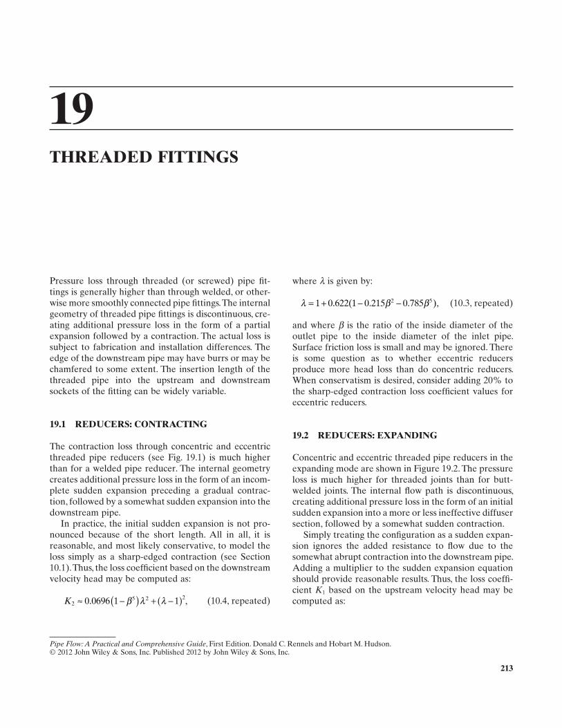
213
19 THREADED FITTINGS
Pressure loss through threaded (or screwed) pipe fi t-tings is generally higher than through welded, or other-wise more smoothly connected pipe fi ttings. The internal geometry of threaded pipe fi ttings is discontinuous, cre-ating additional pressure loss in the form of a partial expansion followed by a contraction. The actual loss is subject to fabrication and installation differences. The edge of the downstream pipe may have burrs or may be chamfered to some extent. The insertion length of the threaded pipe into the upstream and downstream sockets of the fi tting can be widely variable.
19.1 REDUCERS: CONTRACTING
The contraction loss through concentric and eccentric threaded pipe reducers (see Fig. 19.1 ) is much higher than for a welded pipe reducer. The internal geometry creates additional pressure loss in the form of an incom-plete sudden expansion preceding a gradual contrac-tion, followed by a somewhat sudden expansion into the downstream pipe.
In practice, the initial sudden expansion is not pro-nounced because of the short length. All in all, it is reasonable, and most likely conservative, to model the loss simply as a sharp - edged contraction (see Section 10.1 ). Thus, the loss coeffi cient based on the downstream velocity head may be computed as:
K25 2 20 0696 1 1≈ −( ) + −( ). ,β λ λ (10.4, repeated)
where λ is given by:
λ β β= + − −1 0 622 1 0 215 0 7852 5. ( . . ), (10.3, repeated)
and where β is the ratio of the inside diameter of the outlet pipe to the inside diameter of the inlet pipe. Surface friction loss is small and may be ignored. There is some question as to whether eccentric reducers produce more head loss than do concentric reducers. When conservatism is desired, consider adding 20% to the sharp - edged contraction loss coeffi cient values for eccentric reducers.
19.2 REDUCERS: EXPANDING
Concentric and eccentric threaded pipe reducers in the expanding mode are shown in Figure 19.2 . The pressure loss is much higher for threaded joints than for butt - welded joints. The internal fl ow path is discontinuous, creating additional pressure loss in the form of an initial sudden expansion into a more or less ineffective diffuser section, followed by a somewhat sudden contraction.
Simply treating the confi guration as a sudden expan-sion ignores the added resistance to fl ow due to the somewhat abrupt contraction into the downstream pipe. Adding a multiplier to the sudden expansion equation should provide reasonable results. Thus, the loss coeffi -cient K1 based on the upstream velocity head may be computed as:
Pipe Flow: A Practical and Comprehensive Guide, First Edition. Donald C. Rennels and Hobart M. Hudson.© 2012 John Wiley & Sons, Inc. Published 2012 by John Wiley & Sons, Inc.
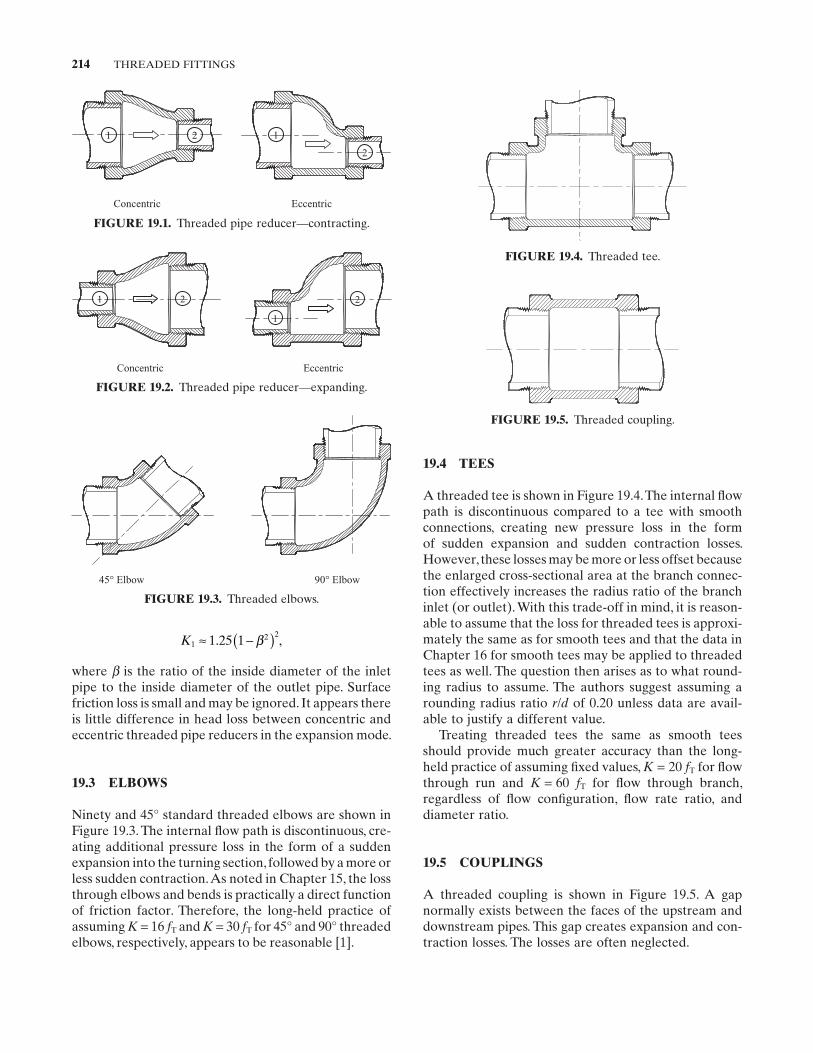
214 THREADED FITTINGS
19.4 TEES
A threaded tee is shown in Figure 19.4 . The internal fl ow path is discontinuous compared to a tee with smooth connections, creating new pressure loss in the form of sudden expansion and sudden contraction losses. However, these losses may be more or less offset because the enlarged cross - sectional area at the branch connec-tion effectively increases the radius ratio of the branch inlet (or outlet). With this trade - off in mind, it is reason-able to assume that the loss for threaded tees is approxi-mately the same as for smooth tees and that the data in Chapter 16 for smooth tees may be applied to threaded tees as well. The question then arises as to what round-ing radius to assume. The authors suggest assuming a rounding radius ratio r / d of 0.20 unless data are avail-able to justify a different value.
Treating threaded tees the same as smooth tees should provide much greater accuracy than the long - held practice of assuming fi xed values, K = 20 fT for fl ow through run and K = 60 fT for fl ow through branch, regardless of fl ow confi guration, fl ow rate ratio, and diameter ratio.
19.5 COUPLINGS
A threaded coupling is shown in Figure 19.5 . A gap normally exists between the faces of the upstream and downstream pipes. This gap creates expansion and con-traction losses. The losses are often neglected.
K12 2
1 25 1≈ −( ). ,β
where β is the ratio of the inside diameter of the inlet pipe to the inside diameter of the outlet pipe. Surface friction loss is small and may be ignored. It appears there is little difference in head loss between concentric and eccentric threaded pipe reducers in the expansion mode.
19.3 ELBOWS
Ninety and 45 ° standard threaded elbows are shown in Figure 19.3 . The internal fl ow path is discontinuous, cre-ating additional pressure loss in the form of a sudden expansion into the turning section, followed by a more or less sudden contraction. As noted in Chapter 15 , the loss through elbows and bends is practically a direct function of friction factor. Therefore, the long - held practice of assuming K = 16 fT and K = 30 fT for 45 ° and 90 ° threaded elbows, respectively, appears to be reasonable [1] .
Concentric
1 12
2
Eccentric
FIGURE 19.1. Threaded pipe reducer — contracting.
1
1
2 2
Concentric Eccentric
FIGURE 19.2. Threaded pipe reducer — expanding.
45° Elbow 90° Elbow
FIGURE 19.3. Threaded elbows.
FIGURE 19.4. Threaded tee.
FIGURE 19.5. Threaded coupling.
REFERENCE 215
19.6 VALVES
The pressure loss through valves with threaded end con-nections is necessarily higher than through valves with smooth connections. In lieu of specifi c data from valve manufacturers, ranges of loss coeffi cient values for various types of valves are presented in Table 18.1 . The higher values are applicable to reduced port and threaded valves; the lower values are applicable to full port, fl anged, or welded valves.
REFERENCE
1. Flow of Fluids Through Valves, Fittings and Pipe , Technical Paper No. 410, Crane Company, Chicago, 1985 , p. A - 26 .
The loss coeffi cient is highly indeterminate. The insertion length of threaded pipe into the upstream and downstream sockets is variable, the expansion loss is relatively incomplete because of the short length of the fi tting, and the degree of “ sharpness ” of the inlet edge of the downstream pipe is unpredictable. None-theless, it is reasonable to model the loss simply as a sudden expansion. Thus, the loss coeffi cient may be computed as:
K ≈ −( )1 2 2β , (19.5)
where β is the ratio of the inside to outside diameter of the pipe (overprediction of the sudden expansion loss may compensate for neglecting the contraction loss). Surface friction loss is small and may be ignored. This is a crude method, but it should provide better results than ignoring the loss entirely.
PART III
FLOW PHENOMENA
A brief categorization of fl ow - induced vibration in piping systems is presented in Chapter 21 . Water hammer and column separation can create signifi cant loads on pipe, its components, and its supports. Ways and means to prevent or mitigate such events are presented.
We learned in Chapter 2 that head loss is a loss of useful energy by conversion of mechanical energy to heat energy, and that in liquid (or incompressible) systems, the heat energy is usually of no consequence. In Chapter 22 , we consider some situations where the heat energy may be of interest in liquid systems.
Whether or not horizontal fl ow passages or openings run full at low fl ow rates may be an important design consideration. This topic is treated in Chapter 23 .
PROLOGUE
There are a number of fl ow phenomena that can affect the performance of piping systems. In Part III , we inves-tigate several interesting phenomena: cavitation, fl ow - induced vibration, temperature rise, and fl ow to run full. The phenomena are related to occurrences in the nuclear power industry. Of course, the information can be applied to fl ow conditions that may exist in any industry.
The phenomenon of cavitation is of great importance in the design and operation of hydraulic equipment. In Chapter 20 , we study its nature and learn how to design and analyze piping systems to avoid its potentially dam-aging effects.
217
Pipe Flow: A Practical and Comprehensive Guide, First Edition. Donald C. Rennels and Hobart M. Hudson.© 2012 John Wiley & Sons, Inc. Published 2012 by John Wiley & Sons, Inc.
219
20 CAVITATION
Understanding the phenomenon of cavitation is of great importance in the design and operation of hydraulic equipment — turbines, pumps, valves, and other piping components. Cavitation may be expected in a fl owing liquid whenever the absolute pressure at a point falls below the vapor pressur e of the liquid. Local vaporiza-tion of the liquid will then result, causing a void or cavity in the fl ow fi eld. The void eventually collapses — oftentimes accompanied by erosion (pitting) of nearby metal surfaces; loss of effi ciency, excessive vibration, fl uctuations of fl ow and pressure, and calculated fl ow rates are inaccurate.
20.1 THE NATURE OF CAVITATION
When the pressure falls below the vapor pressure of the liquid, a cavity of vapor is formed and moves along with the stream. The cavity contains a swirling mass of drop-lets and vapor and, although appearing steady to the naked eye, actually forms and reforms many times a second. The low - pressure cavity is swept downstream into a region of high pressure where it suddenly collapses — the surrounding liquid rushing in to fi ll the void. At the point of disappearance of the cavity, the onrushing liquid comes together, momentarily raising the local pressure within the liquid to a very high value. If the point of collapse of the cavity is in contact with or very near the boundary wall, the wall receives a blow as from a tiny hammer, and its surface may be stressed locally beyond its elastic limit, resulting eventually in
fatigue and destruction of wall material. In the case of rotating machinery, the action predictably takes place in close proximity to the blades or sides of an impeller or draft tube, and particles of the metal may be gradu-ally removed.
The nature of cavitation can be easily observed by study of the fl ow of a liquid through a constriction in a pipe as shown in Figure 20.1 . Under low fl ow conditions, the variation of pressure through the pipe and constric-tion is given by the hydraulic grade line ( HGL ) A, the point of lowest pressure occurring at the minimum area where the velocity is highest. As the downstream pres-sure is reduced (by opening a valve, increasing the speed of a pump, etc.) the fl ow rate will increase to produce HGL B, for which the absolute pressure in the throat of the constriction falls to the vapor pressure of the liquid, causing the inception of cavitation. Further reduction in downstream pressure will then not result in further increase in fl ow rate, but will serve to extend the zone of vapor pressure downstream from the throat of the constriction to produce HGL C. Here the fl ow stream of liquid separates from the boundary walls, producing a cavity in which the mean pressure is the vapor pres-sure of the liquid. The cavity contains a swirling mass of droplets and vapor and, although appearing steady to the naked eye, actually forms and reforms many times a second. *
The sound emitted by the fl ow system changes at the onset of cavitation. At fi rst, it sounds as if sand were
Pipe Flow: A Practical and Comprehensive Guide, First Edition. Donald C. Rennels and Hobart M. Hudson.© 2012 John Wiley & Sons, Inc. Published 2012 by John Wiley & Sons, Inc.
* The nature of cavitation is taken largely from Vennard [1] .
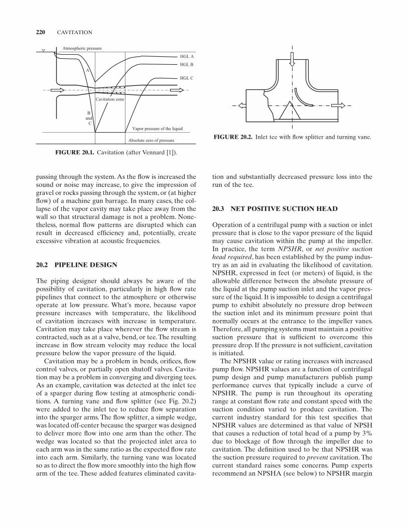
220 CAVITATION
tion and substantially decreased pressure loss into the run of the tee.
20.3 NET POSITIVE SUCTION HEAD
Operation of a centrifugal pump with a suction or inlet pressure that is close to the vapor pressure of the liquid may cause cavitation within the pump at the impeller. In practice, the term NPSHR , or net positive suction head required , has been established by the pump indus-try as an aid in evaluating the likelihood of cavitation. NPSHR, expressed in feet (or meters) of liquid, is the allowable difference between the absolute pressure of the liquid at the pump suction inlet and the vapor pres-sure of the liquid. It is impossible to design a centrifugal pump to exhibit absolutely no pressure drop between the suction inlet and its minimum pressure point that normally occurs at the entrance to the impeller vanes. Therefore, all pumping systems must maintain a positive suction pressure that is suffi cient to overcome this pressure drop. If the pressure is not suffi cient, cavitation is initiated.
The NPSHR value or rating increases with increased pump fl ow. NPSHR values are a function of centrifugal pump design and pump manufacturers publish pump performance curves that typically include a curve of NPSHR. The pump is run throughout its operating range at constant fl ow rate and constant speed with the suction condition varied to produce cavitation. The current industry standard for this test specifi es that NPSHR values are determined as that value of NPSH that causes a reduction of total head of a pump by 3% due to blockage of fl ow through the impeller due to cavitation. The defi nition used to be that NPSHR was the suction pressure required to prevent cavitation. The current standard raises some concerns. Pump experts recommend an NPSHA (see below) to NPSHR margin
passing through the system. As the fl ow is increased the sound or noise may increase, to give the impression of gravel or rocks passing through the system, or (at higher fl ow) of a machine gun barrage. In many cases, the col-lapse of the vapor cavity may take place away from the wall so that structural damage is not a problem. None-theless, normal fl ow patterns are disrupted which can result in decreased effi ciency and, potentially, create excessive vibration at acoustic frequencies.
20.2 PIPELINE DESIGN
The piping designer should always be aware of the possibility of cavitation, particularly in high fl ow rate pipelines that connect to the atmosphere or otherwise operate at low pressure. What ’ s more, because vapor pressure increases with temperature, the likelihood of cavitation increases with increase in temperature. Cavitation may take place wherever the fl ow stream is contracted, such as at a valve, bend, or tee. The resulting increase in fl ow stream velocity may reduce the local pressure below the vapor pressure of the liquid.
Cavitation may be a problem in bends, orifi ces, fl ow control valves, or partially open shutoff valves. Cavita-tion may be a problem in converging and diverging tees. As an example, cavitation was detected at the inlet tee of a sparger during fl ow testing at atmospheric condi-tions. A turning vane and fl ow splitter (see Fig. 20.2 ) were added to the inlet tee to reduce fl ow separation into the sparger arms. The fl ow splitter, a simple wedge, was located off - center because the sparger was designed to deliver more fl ow into one arm than the other. The wedge was located so that the projected inlet area to each arm was in the same ratio as the expected fl ow rate into each arm. Similarly, the turning vane was located so as to direct the fl ow more smoothly into the high fl ow arm of the tee. These added features eliminated cavita-
FIGURE 20.1. Cavitation (after Vennard [1] ).
Cavitation zone
Band
C
A
Vapor pressure of the liquid
HGL A
HGL B
HGL C
Atmospheric pressure
Absolute zero of pressureFIGURE 20.2. Inlet tee with fl ow splitter and turning vane.
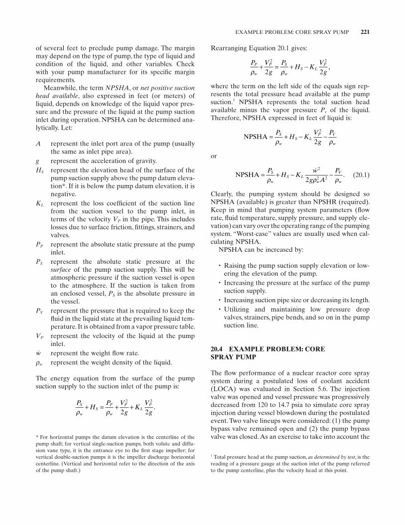
EXAMPLE PROBLEM: CORE SPRAY PUMP 221
Rearranging Equation 20.1 gives:
P Vg
PH K
Vg
P
w
P S
wS L
P
ρ ρ+ = + −
2 2
2 2,
where the term on the left side of the equals sign rep-resents the total pressure head available at the pump suction. † NPSHA represents the total suction head available minus the vapor pressure Pv of the liquid. Therefore, NPSHA expressed in feet of liquid is:
NPSHA = + − −PH K
Vg
PS
wS L
P V
wρ ρ
2
2
or
NPSHA = + − −PH K
wg A
PS
wS L
w
V
wρ ρ ρ 2
2 22. (20.1)
Clearly, the pumping system should be designed so NPSHA (available) is greater than NPSHR (required). Keep in mind that pumping system parameters (fl ow rate, fl uid temperature, supply pressure, and supply ele-vation) can vary over the operating range of the pumping system. “ Worst - case ” values are usually used when cal-culating NPSHA.
NPSHA can be increased by:
• Raising the pump suction supply elevation or low-ering the elevation of the pump.
• Increasing the pressure at the surface of the pump suction supply.
• Increasing suction pipe size or decreasing its length. • Utilizing and maintaining low pressure drop
valves, strainers, pipe bends, and so on in the pump suction line.
20.4 EXAMPLE PROBLEM: CORE SPRAY PUMP
The fl ow performance of a nuclear reactor core spray system during a postulated loss of coolant accident ( LOCA ) was evaluated in Section 5.6 . The injection valve was opened and vessel pressure was progressively decreased from 120 to 14.7 psia to simulate core spray injection during vessel blowdown during the postulated event. Two valve lineups were considered: (1) the pump bypass valve remained open and (2) the pump bypass valve was closed. As an exercise to take into account the
of several feet to preclude pump damage. The margin may depend on the type of pump, the type of liquid and condition of the liquid, and other variables. Check with your pump manufacturer for its specifi c margin requirements.
Meanwhile, the term NPSHA , or net positive suction head available , also expressed in feet (or meters) of liquid, depends on knowledge of the liquid vapor pres-sure and the pressure of the liquid at the pump suction inlet during operation. NPSHA can be determined ana-lytically. Let:
A represent the inlet port area of the pump (usually the same as inlet pipe area).
g represent the acceleration of gravity. HS represent the elevation head of the surface of the
pump suction supply above the pump datum eleva-tion* . If it is below the pump datum elevation, it is negative.
KL represent the loss coeffi cient of the suction line from the suction vessel to the pump inlet, in terms of the velocity VP in the pipe. This includes losses due to surface friction, fi ttings, strainers, and valves.
PP represent the absolute static pressure at the pump inlet.
PS represent the absolute static pressure at the surface of the pump suction supply. This will be atmospheric pressure if the suction vessel is open to the atmosphere. If the suction is taken from an enclosed vessel, PS is the absolute pressure in the vessel.
PV represent the pressure that is required to keep the fl uid in the liquid state at the prevailing liquid tem-perature. It is obtained from a vapor pressure table.
VP represent the velocity of the liquid at the pump inlet.
w represent the weight fl ow rate. ρw represent the weight density of the liquid.
The energy equation from the surface of the pump suction supply to the suction inlet of the pump is:
PH
P Vg
KV
gS
wS
P
w
PL
P
ρ ρ+ = + +
2 2
2 2.
† Total pressure head at the pump suction, as determined by test , is the reading of a pressure gauge at the suction inlet of the pump referred to the pump centerline, plus the velocity head at this point.
* For horizontal pumps the datum elevation is the centerline of the pump shaft; for vertical single - suction pumps, both volute and diffu-sion vane type, it is the entrance eye to the fi rst stage impeller; for vertical double - suction pumps it is the impeller discharge horizontal centerline. (Vertical and horizontal refer to the direction of the axis of the pump shaft.)
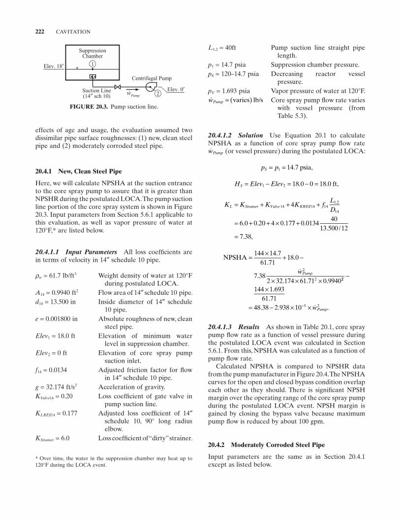
222 CAVITATION
L1,2 = 40ft Pump suction line straight pipe length.
p1 = 14.7 psia Suppression chamber pressure. p8 = 120 – 14.7 psia Decreasing reactor vessel
pressure. pV = 1.693 psia Vapor pressure of water at 120 ° F. wPump = ( )varies lb/s Core spray pump fl ow rate varies
with vessel pressure (from Table 5.3 ).
20.4.1.2 Solution Use Equation 20.1 to calculate NPSHA as a function of core spray pump fl ow rate wPump (or vessel pressure) during the postulated LOCA:
p pS = =1 14 7. ,psia
H Elev ElevS = − = − =1 2 18 0 0 18 0. . ,ft
K K K K fLD
L Strainer Valve KREll= + + +
= + + ×
14 14 141 2
14
4
6 0 0 20 4 0 17
,
. . . 77 0 013440
13 500 127 38
+
=
.. /
. ,
NPSHA = × + −
× × ×
144 14 761 71
18 0
7 382 32 174 61 71 0 9940
2
2
..
.
.. . .
wPump
22
5 2
144 1 69361 71
48 38 2 938 10
−
×
= − × ×−
..
. . .wPump
20.4.1.3 Results As shown in Table 20.1 , core spray pump fl ow rate as a function of vessel pressure during the postulated LOCA event was calculated in Section 5.6.1 . From this, NPSHA was calculated as a function of pump fl ow rate.
Calculated NPSHA is compared to NPSHR data from the pump manufacturer in Figure 20.4 . The NPSHA curves for the open and closed bypass condition overlap each other as they should. There is signifi cant NPSH margin over the operating range of the core spray pump during the postulated LOCA event. NPSH margin is gained by closing the bypass valve because maximum pump fl ow is reduced by about 100 gpm.
20.4.2 Moderately Corroded Steel Pipe
Input parameters are the same as in Section 20.4.1 except as listed below.
effects of age and usage, the evaluation assumed two dissimilar pipe surface roughnesses: (1) new, clean steel pipe and (2) moderately corroded steel pipe.
20.4.1 New, Clean Steel Pipe
Here, we will calculate NPSHA at the suction entrance to the core spray pump to assure that it is greater than NPSHR during the postulated LOCA. The pump suction line portion of the core spray system is shown in Figure 20.3 . Input parameters from Section 5.6.1 applicable to this evaluation, as well as vapor pressure of water at 120 ° F, * are listed below.
20.4.1.1 Input Parameters All loss coeffi cients are in terms of velocity in 14 ″ schedule 10 pipe.
ρw = 61.7 lb/ft 3 Weight density of water at 120 ° F during postulated LOCA.
A14 = 0.9940 ft 2 Flow area of 14 ″ schedule 10 pipe. d14 = 13.500 in Inside diameter of 14 ″ schedule
10 pipe. e = 0.001800 in Absolute roughness of new, clean
steel pipe. Elev1 = 18.0 ft Elevation of minimum water
level in suppression chamber. Elev2 = 0 ft Elevation of core spray pump
suction inlet. f14 = 0.0134 Adjusted friction factor for fl ow
in 14 ″ schedule 10 pipe. g = 32.174 ft/s 2 Acceleration of gravity. KValve14 = 0.20 Loss coeffi cient of gate valve in
pump suction line. KLREll14 = 0.177 Adjusted loss coeffi cient of 14 ″
schedule 10, 90 ° long radius elbow.
KStrainer = 6.0 Loss coeffi cient of “ dirty ” strainer.
FIGURE 20.3. Pump suction line.
Pumpw
Elev. 18′
Elev. 0′Suction Line (14″ sch 10)
Suppression Chamber
2
1
Centrifugal Pump
* Over time, the water in the suppression chamber may heat up to 120 ° F during the LOCA event.
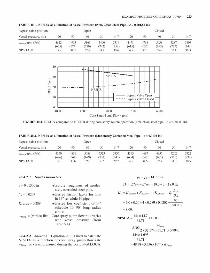
EXAMPLE PROBLEM: CORE SPRAY PUMP 223
TABLE 20.1. NPSHA as a Function of Vessel Pressure (New, Clean Steel Pipe — e = 0.001,80 in)
Bypass valve position Open Closed
Vessel pressure, psia 120 90 60 30 14.7 120 90 60 30 14.7
q Pump , gpm (lb/s) 4622 (635)
4905 (674)
5163 (710)
5400 (742)
5514 (758)
4471 (615)
4768 (656)
5038 (693)
5287 (727)
5407 (744)
NPSHA, ft 35.9 34.3 32.8 31.4 30.6 36.7 35.1 33.6 32.1 31.3
FIGURE 20.4. NPSHA compared to NPSHR during core spray system operation (new, clean steel pipe — e = 0.001,80 in).
40
30
20
10
04000 4500 5000 5500 6000
NP
SH
(fe
et)
Core Spray Pump Flow (gpm)
NPSHR
NPSHA
Bypass Valve Open Bypass Valve Closed
20.4.2.1 Input Parameters
e = 0.01300 in Absolute roughness of moder-ately corroded steel pipe.
f14 = 0.0207 Adjusted friction factor for fl ow in 14 ″ schedule 10 pipe.
KLREll14 = 0.289 Adjusted loss coeffi cient of 14 ″schedule 10, 90 ° long radius elbow.
wPump = (varies) lb/s Core spray pump fl ow rate varies with vessel pressure (from Table 5.4 ).
20.4.2.2 Solution Equation 20.1 is used to calculate NPSHA as a function of core spray pump fl ow rate wPump (or vessel pressure) during the postulated LOCA:
p pS = =1 14 7. ,psia
H Elev ElevS = − = − =1 2 18 0 0 18 0. . ,ft
K K K K fLD
L Strainer Valve KREll= + + +
= + + ×
14 14 141 2
14
4
6 0 0 20 4 0 28
,
. . . 99 0 020740
13 500 128 09
+
=
.. /
. ,
NPSHA = × + −
× × ×
144 14 761 71
18 0
8 092 32 174 61 71 0 9940
2
2
..
.
/. . .
wPump
22
5 2
144 1 69361 71
48 38 3 336 10
−
×
= − × ×−
..
. . .wPump
TABLE 20.2. NPSHA as a Function of Vessel Pressure (Moderately Corroded Steel Pipe — e = 0.0130 in)
Bypass valve position Open Closed
Vessel pressure, psia 120 90 60 30 14.7 120 90 60 30 14.7
q Pump , gpm (lb/s) 4550 (626)
4831 (664)
5088 (699)
5323 (732)
5436 (747)
4393 (604)
4687 (645)
4955 (681)
5202 (715)
5322 (732)
NPSHA, ft 35.3 33.6 32.0 30.5 29.7 36.2 34.5 32.9 31.3 30.5
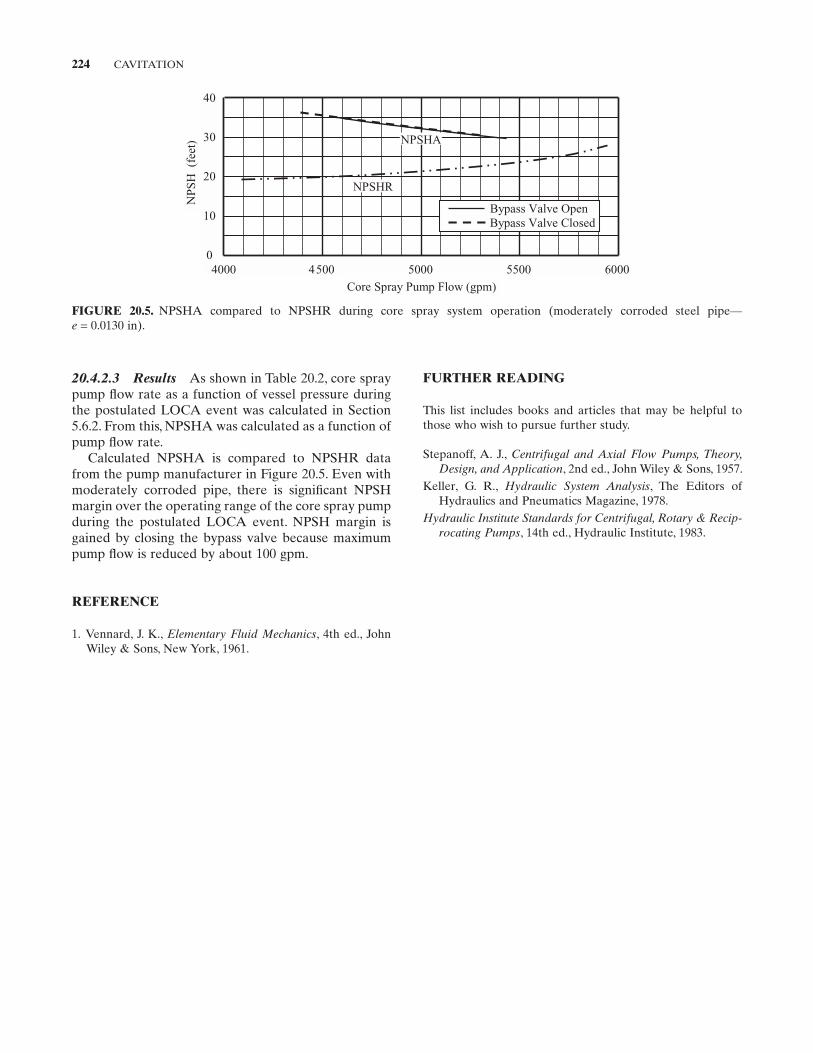
224 CAVITATION
FURTHER READING
This list includes books and articles that may be helpful to those who wish to pursue further study.
Stepanoff , A. J. , Centrifugal and Axial Flow Pumps, Theory, Design, and Application , 2nd ed. , John Wiley & Sons , 1957 .
Keller , G. R. , Hydraulic System Analysis , The Editors of Hydraulics and Pneumatics Magazine, 1978 .
Hydraulic Institute Standards for Centrifugal, Rotary & Recip-rocating Pumps , 14th ed. , Hydraulic Institute , 1983 .
20.4.2.3 Results As shown in Table 20.2 , core spray pump fl ow rate as a function of vessel pressure during the postulated LOCA event was calculated in Section 5.6.2 . From this, NPSHA was calculated as a function of pump fl ow rate.
Calculated NPSHA is compared to NPSHR data from the pump manufacturer in Figure 20.5 . Even with moderately corroded pipe, there is signifi cant NPSH margin over the operating range of the core spray pump during the postulated LOCA event. NPSH margin is gained by closing the bypass valve because maximum pump fl ow is reduced by about 100 gpm.
REFERENCE
1. Vennard , J. K. , Elementary Fluid Mechanics , 4th ed. , John Wiley & Sons , New York , 1961 .
FIGURE 20.5. NPSHA compared to NPSHR during core spray system operation (moderately corroded steel pipe —e = 0.0130 in).
40
30
20
10
04000 4500 5000 5500 6000
NP
SH
(fe
et)
Core Spray Pump Flow (gpm)
NPSHR
NPSHA
Bypass Valve Open Bypass Valve Closed
225
21 FLOW - INDUCED VIBRATION
Flow - induced vibration (FIV) is the structural and mechanical vibration of structures immersed in or conveying fl uid. Many engineering structures are sus-ceptible to the interaction between the fl uid ’ s dy -namic forces and the structures ’ inertial, damping, and elastic forces. Because designers are using materials to their limits, causing structures to become lighter and more fl exible, FIV considerations have become increas-ingly important.
21.1 STEADY INTERNAL FLOW
Steady fl uid fl ow through a pipe can impose pressures on the pipe walls that defl ect the pipe and cause insta-bilities. The pipe may become susceptible to resonance or fatigue failure if its natural frequency falls below certain limits. If the fl uid velocity becomes large enough, the pipe can become unstable. The most familiar form of this instability is the fl ailing about of an unrestricted garden hose.
If a pipe ruptures through its cross section, a fl exible length of unsupported pipe is left spewing out fl uid and is free to whip about and impact on other structures. This occurrence, called pipe whip , was a major consid-eration in the design of nuclear reactor main steam, recirculation, and feed water piping systems, and in the design of other auxiliary piping systems. During the 1970s the nuclear industry responded to the need to evaluate the dynamics of the highly nonlinear pipe whip event and to develop pipe whip restraints.
Criteria were developed for the location of postulated pipe breaks (those points of high relative stress and high relative fatigue). Complying with the criteria resulted in the application of over 100 restraints on the aggregate piping systems inside the typical nuclear reactor containment. * , †
21.2 STEADY EXTERNAL FLOW
Any structure with a suffi ciently bluff trailing edge sheds vortices in a subsonic fl ow; cylindrical structures are particularly susceptible. Periodic forces on the struc-ture are generated as the vortices are alternately shed from side to side of the structure. The large amplitude vibrations that can be induced in elastic structures by vortex shedding are of great practical importance because of their destructive effect on suspension bridges, power transmission lines, television antennas, pipelines, heat exchanger tubes, and nuclear fuel assemblies.
If the frequency of vortex shedding coincides with the natural frequency of the structure, then the forces can induce large amplitude structural vibration normal
Pipe Flow: A Practical and Comprehensive Guide, First Edition. Donald C. Rennels and Hobart M. Hudson.© 2012 John Wiley & Sons, Inc. Published 2012 by John Wiley & Sons, Inc.
* A later industry - wide evaluation, called leak before break , resulted in a signifi cant reduction of the number of pipe restraints. It was proven that fl uid leaking from cracks in the ductile pipe material could be detected, and preventive action taken, long before complete pipe rupture would occur. † See the section “ Further Reading ” at the end of this chapter for further information on this fl ow phenomenon.
226 FLOW-INDUCED VIBRATION
tL
arpipe
=A
.
If the velocity of water or other fl uid in a pipe is sud-denly diminished or stopped, the energy given up by the fl uid will be divided between compressing the liquid itself, stretching the pipe walls, and frictional resistance to wave propagation. Water hammer is manifest as a series of shocks, sounding like hammer blows, which may have suffi cient magnitude to rupture the pipe or damage connected equipment. It may be caused by the nearly instantaneous or too rapid closing of a valve in the line, or by an equivalent stoppage of fl ow that would take place with the sudden failure of electricity supply to a motor - driven pump.
The shock pressure is not concentrated at the valve, and if rupture occurs it may take place near the valve simply because it acts there fi rst. The pressure wave due to water hammer travels back upstream to the inlet of the pipe; there, it reverses and surges back and forth through the pipe. This cycle would continue indefi nitely were it not for viscosity of the fl uid and friction against the pipe walls.
The excess pressure due to water hammer is additive to the normal pressure in the pipe. Complete stoppage of fl ow is not necessary to produce water hammer as any sudden change in velocity will create it to a greater or lesser degree.
Under normal conditions the fl ow through the pipe is steady, having a velocity V past all sections. If the valve is made to close instantaneously, the particles of fl uid in immediate proximity to it will have their velocity at once reduced to zero. If the whole mass of fl uid in the pipe were inelastic (rigid) and contained in pipe walls that were also inelastic, then all the particles of fl uid would likewise be instantaneously brought to rest and the pressure against the valve and all through the pipe would be infi nite. That the pressure does not become infi nite is due to the compressibility of the fl uid and to the elasticity of the pipe wall.
Accounting for compressibility of the fl uid and the elasticity of the pipe wall, it can be shown that the veloc-ity of the pressure wave (or the speed of sound) of the fl uid in the pipe is ‡ :
AB
tw
pipew
gd
=+
144 1
1ρ BE
, (21.1)
where B is the bulk modulus of the fl uid (B is about 300,000 pounds per square inch for fresh water at
to the free stream. If contained in a cavity, sound waves refl ect off the cavity walls. Acoustic resonance has pro-duced intense sound pressure levels in tubular heat exchangers that have damaged heat exchanger shells.
When a tube in a tube array in a cross fl ow is dis-placed from its equilibrium position, a fl uid force, owing to the asymmetry of the fl ow fi eld, may be exerted on the tube and the tube may vibrate with a large ampli-tude. In closely spaced tube arrays often used in heat exchangers, the distinct vortex shedding frequency degenerates into broadband turbulence, which buffets tubes. Such vibrations can be classifi ed as axial fl ow induces of cross fl ow induces, depending on the inci-dent angle of the incoming fl ow with respect to the cylinder ’ s axes.
Damping of structures, avoidance of resonance, and the streamlining of structures are the primary mecha-nisms for limiting FIV. *
21.3 WATER HAMMER †
Pressure changes in a closed conduit produced by changes in fl uid fl ow are called fl uid hammer (or, more generally, water hammer ). The fl uid is usually a liquid, but sometimes can be a gas. The pressure change can create signifi cant loads on pipe, its components, and its supports.
Velocity and pressure changes or disturbances can be expressed as Vd − Vi , and Pd − Pi , where the subscripts iand d designate initial and disturbed values, respectively. If the velocity of a fl uid in a pipe is disturbed, it causes a corresponding disturbance of pressure, related by the classical water hammer relationship:
P PV V
gd i
pipe w d i− =−( )A ρ
,
where A pipe is the speed of sound of the fl uid in the pipe, and ρw is the density of the fl uid.
A fl ow disturbance time can be identifi ed with occur-rences such as full or partial valve opening or closure, pipe rupture, or the period of cyclic pulses caused by hydraulic machinery. If a fl ow disturbance at the system boundary occurs over a time interval of the same order as that required for an acoustic wave to pass through the system, propagation will be important. Most water hammer problems involve a pipe section of arbitrary length L . The pipe acoustic response time t ar , allowing for acoustic propagation throughout its length, is given as
‡ In International System of Units (SI), delete 144 from the equation.
† This section on water hammer is largely taken from Russell [1] and Crocker [2] .
* See previous footnote.
COLUMN SEPARATION 227
value as before. This is because the fi rst small pressure wave, generated as the valve starts to close, will not have had time to make a round trip and return to the valve as a wave lowering the pressure to normal. Equation 21.3 therefore applies for any time of closure up to time trt in Equation 21.4 .
In 1898, N. Joukovsky [3] of Moscow was the fi rst to demonstrate the validity of this equation. Joukovsky experimented with the effects of slow closure time. He concluded that for slow closure times (where closure time tcl is greater than round - trip time trt ) the excess pres-sure is reduced in intensity according to the proportion:
∆∆
PP
tt
Ltmax
rt
cl cl pipe
= = 2A
.
It has been proven since that this relation results in values greater than the actual pressure. Values com-puted from it therefore err on the side of safety.
The simplest method of protecting pipes from water hammer is found to be slowly closing the valve. In the case of long, cross - country pipelines, including gas lines, several minutes closing time may be necessary to allevi-ate water hammer.
In addition, the rise of pressure caused by water hammer may be minimized by the use of pressure relief valves of adequate size. They should be designed to open quickly and close slowly. In the case of liquid systems, air chambers or surge tanks of adequate size connected to the pipe near the valve may prevent pres-sure waves of signifi cant magnitude from passing up the pipe. Such chambers should be kept fi lled with gas, perhaps with the aid of a diaphragm, since the liquid may readily absorb gas under pressure. To obtain great-est effectiveness, these devices should be located as close as possible to the source of the disturbance.
21.4 COLUMN SEPARATION
A water hammer - type event called column separationmay occur in a pipeline fi lled with liquid when a vapor cavity forms and suddenly collapses. This results in a large and nearly instantaneous rise in pressure due to the collision of two liquid columns, or the collision of one liquid column with a closed end. Another related phenomenon, known as steam hammer , might occur in vapor distribution systems. Some vapor may condense into liquid in a section of piping and form a slug. Sub-sequently, the vapor may hurl the slug at high velocity into hydraulic equipment or into pipe fi ttings and cause major problems.
Early on, licensees of operating nuclear reactors in the United States reported a number of column
ordinary conditions), E is the elastic modulus of the pipe material (E is approximately 30,000,000 pounds per square inch for steel), and d and t w are the diameter and wall thickness of the pipe, respectively.
The water hammer pressure ΔPmax , which is the inten-sity of the excess pressure produced by extinguishing the velocity V , can be determined as:
∆PV
gw
pipemax .= ρA (21.2)
If the expression for A pipe , Equation 21.1 , is substi-tuted into Equation 21.2 , the water hammer pressure ΔPmax , is * :
∆P VB
g dmaxw
w
=+
144 1
1
ρBE t
. (21.3)
As an example, the sudden valve closure of 60 ° F water fl owing through a 16 - in schedule 40 steel pipe at a veloc-ity of 20 ft/s results in an excess pressure in the pipe:
V = 20 ft/s ρw = 62.37 lb/ft 3
B = 300,000 lb/in 2
E = 30,000,000 lb/in 2
d = 15.000 in t w = 0.500 in
∆Pmax
= × ×
+ ×20
144 62 37 300 00032 174
1
1300 000
30 000 00015 000
. ,. ,
, ,.
00 500
180 500 11152 2
.
, / ( / )= =lb ft lb in
This example results in a substantial increase above the normal pressure in the pipe. However, it should be noted that the derivation of ΔPmax assumed instanta-neous closure of the valve. This maximum pressure rise at the valve is maintained during the time trt required for the pressure wave to make a round trip of the pipe. For a pipe of length L , this time is:
tL
rtpipe
= 2A
. (21.4)
If the valve is closed gradually, but within this time, the excess pressure at the gate will build up to the maximum
* See previous footnote.
228 FLOW-INDUCED VIBRATION
2. Crocker , S. , Piping Handbook , McGraw - Hill , New York , 1945 .
3. Joukovsky , N. , A translation of Joukovsky ’ s paper on water-hammer experiments , Journal of the American Waterworks Association , 1904 , 335 .
4. NUREG/CR - 2781, Quad - 1 - 82 - 018, EGG - 2203, Evaluation of Waterhammer Events in Light Water Reactor Plants , U.S. Nuclear Regulatory Commission, July 1982 .
FURTHER READING
This list includes works that may be helpful to those who wish to pursue further study.
Parmakian , J. , Waterhammer Analysis , Dover Publications , 1963 .
Thorley , A. R. D. , Pressure transients in hydraulic pipelines , Transactions of the American Society of Mechanical Engi-neers, Journal of Fluids Engineering , 91 , September 1969 , 453 – 461 .
Esswein , G. A. , Development of a Plastic Strain Energy Absorbing Pipe Whip Restraint Design , Special Confer-ence on Structural Design of Nuclear Plant Facilities, American Society of Civil Engineers, December 17 – 18, Volume II, 1973 , pp. 171 – 200 .
Blevins , R. D. , Flow - Induced Vibration , Van Nostrand Rein-hold Co. , New York , 1977 .
Rockwell , D. and E. Naudascher , Self - sustaining oscillations in fl ow past cavities , Transactions of the American Society of Mechanical Engineers, Journal of Fluids Engineering , 104 , June 1982 , 152 – 165 .
GEAP - 24158, COO/4175 - 7, Preliminary Design Handbook for Flow - Induced Vibration of Light Water Reactors , U.S. Department of Energy, November 1978 .
NUREG - 0582, Waterhammer in Nuclear Plants , U.S. Nuclear Regulatory Commission, July 1979 .
Kirik , M. J. and R. J. Gradle , A Model for Check Valve/Feedwater System Waterhammer Analysis , Contributed by the Pressure Vessels & Piping Division of the AmericanSociety of Mechanical Engineers at the Century 2 Pressure Vessels & Piping Conference, San Francisco, Calif., August 12 – 15, 1980 .
Chapman , R. L. , D. D. Christensen , R. E. Dafoe , O. M. Hanner , and M. E. Wells , NUREG/CR - 2059, CAAD - 5629, Compi-lation of Data Concerning Known and Suspected Water-hammer Events in Nuclear Power Plants , EG & G Idaho Inc., April 1982 .
Hatfi eld , F. J. , D. C. Wiggert , and R. S. Otwell , Fluid structure interaction in piping by component synthesis , Transactions of the American Society of Mechanical Engineers, Journal of Fluids Engineering , 111 , September 1982 , 318 – 325 .
Baldwin , R. M. and H. R. Simonns , Flow induced vibrations in safety valves , Transactions of the American Society of Mechanical Engineers, Journal of Pressure Vessel Technol-ogy , 108 , August 1986 , 267 – 272 .
separation events during commercial operation. Many of these events resulted in damage to piping supports and restraints. A few cases involved small cracks or ruptures. None of the events affected the health and safety of the public.
In 1977 the U.S. Nuclear Regulatory Commission ( NRC ) staff initiated a review of reported water hammer events. The most serious and numerous column separa-tion concern was line voiding. This generic cause included: (1) sudden water fl ow into a voided line, (2) steam bubble formation, and (3) steam bubble col-lapse. * Line voiding generally occurred in standby systems such as in emergency core cooling systems that are normally idle. The presence of these voids or steam bubbles was not readily detectable by plant operators. Other major causes of column separation events were steam - water entrainment in the high - pressure coolant injection turbine inlet and outlet lines and in isolation condenser lines.
The U.S. NRC reported the fi ndings and recommen-dations of the industry - wide review in 1982 [4] . Design and operating recommendations for the prevention or mitigation of column separation included:
1. Provide keep - full provisions in standby systems. 2. Provide line void detection and alarm. 3. Train plant operators and maintenance personnel
in the causes and prevention of column separation. 4. Reappraise plant operating and maintenance
procedures. 5. Always account for column separation in the
design of piping, its support system, and other components, such as valves.
These recommendations were incorporated into every operating reactor in the United States and the number of column separation events has signifi cantly declined in the last three decades. The piping designer working in any industry should always consider the above rec-ommendations, particularly when designing systems that are normally idle, or when working with a fl uid system operating at or near saturation pressure and temperature.
REFERENCES
1. Russell , G. E. , Hydraulics , Henry Holt and Company , New York , 1942 .
* Steam bubble formation occurs where a drop in pressure causes hot water to fl ash to steam. Steam bubble collapse occurs due to rapid condensation at steam – water interfaces.
FURTHER READING 229
Fraas , A. P. , Heat Exchanger Design , John Wiley & Sons , 1989 . Bruggeman , J. C. , A. Hirschberg , M. E. H. van Dongen , and A.
P. J. Wijnands , Flow induced pulsations in gas transport systems: Analysis of the infl uence of closed side branches , Transactions of the American Society of Mechanical Engi-neers, Journal of Fluids Engineering , 111 , December 1989 , 484 – 491 .
Moody , F. J. , Introduction to Unsteady Thermofl uid Mechanics , John Wiley & Sons , New York , 1990 .
Liou , C. P. , Maximum pressure head due to linear valve closure , Transactions of the American Society of Mechanical
Engineers, Journal of Fluids Engineering , 113 , December 1991 , 643 – 647 .
Au - Wang , M. K. , Flow - Induced Vibration of Power and Process Plant Components: A Practical Workbook , ASME Books , 2001 .
Sekulic , D. P. and R. K. Shah , Fundamentals of Heat Exchanger Design , John Wiley & Sons , 2003 .
Kaneko , S. , R. Nakamura , F. Inada , M. Kato , and N. W. Mure-ithi , Flow Induced Vibrations, Classifi cations and Lessons from Practical Experiences , Elsevier Ltd. , 2008 .
231
22 TEMPERATURE RISE
We learned in Chapter 2 that head loss is a loss of useful energy by conversion of mechanical energy to heat energy, and that in liquid (or incompressible) systems, the heat energy is usually of no interest. Now we con-sider some situations where the heat energy may be of interest.
Head loss in the English system can be expressed as:
H JU JUEw
LW= − +2 1
,
where EW is the heat energy passing out of the liquid through the walls of the pipe. *
This offers confi rmation that head loss is not a loss of total energy but rather a conversion of mechanical energy into heat energy, part of which may leave the fl uid, the remainder serving to increase its internal energy U . Assuming that all heat generated remains in the liquid (letting heat fl ow EW through the walls of the fl ow system equal zero), the temperature rise ΔT due to head loss can be calculated as:
∆ ∆T
Hc
Pc
L
P w P
= =778 778ρ
.
As an example, calculate the temperature rise of water initially at 200 psia and 120 ° F undergoing a head loss of 100 psid. From Table A.1 , the initial density of the water
is 61.71 lb/ft 3 . The heat capacity cP of water can be taken as 1.0 Btu/lb - ° F:
∆T = ×× ×
= °144 100778 61 71 1 0
0 3. .
. .F
A 0.3 ° F increase in water temperature produces little change in density, viscosity, and vapor pressure and can be neglected in most engineering applications.
In a pump, friction and work of compression increase the temperature of the liquid as it fl ows from suction to discharge. The temperature rise ΔT due to pump opera-tion is † :
∆ ∆T
bhpc W
Ec
Hc
Ec
Pc
EcP
L
P
P
P
L
P
P
P w
L
P
= − = − = −2545778 778η ρ η
,
(22.1)
wherebhp is brake horsepower of the pump; EL is heat loss from the pump through radiation,
bearing, and external seal losses; Hp is pump head; ΔPP is pump differential pressure; cp is heat capacity of the liquid; W is pump fl ow rate; ρw is density of the liquid; and η is pump effi ciency.
Pipe Flow: A Practical and Comprehensive Guide, First Edition. Donald C. Rennels and Hobart M. Hudson.© 2012 John Wiley & Sons, Inc. Published 2012 by John Wiley & Sons, Inc.
† Equation 22.1 was derived from pump temperature rise equations given by Stepanoff [1] and by Karassik et al. [2] .
* If heat energy passes into the liquid, EW will be negative or will appear on the opposite side of the equation.
232 TEMPERATURE RISE
The heat rate is:
HRPump = × ××
=
90 000 46 3 1 00 87 7 48
, . .. .
gal/min lb/ft Btu/lbgal/ft
3
3
6640 000, .Btu/min
Finally, the time required to heat the reactor from 70 ° F to 545 ° F is:
TimeBtu
Btu/minminutes hours≈ ≈ ≈441 000 000
640 000689 11 5
, ,,
. .
The actual time will be longer than 11.5 hours because heat loss from the reactor vessel and adjoining piping, as well as heat loss due to cooling water fl ow to main-tain pump bearing and seal temperature, was ignored in the above calculation. In practice, it normally takes almost 2 days to raise the temperature of the reactor vessel to 545 ° F using heat generated by recirculation pump operation. *
22.3 PUMPING SYSTEM TEMPERATURE
As seen above, friction and the work of compression increase the temperature of the liquid as it fl ows from suction to discharge of a pump. A further temperature increase derives from liquid returned to the pump suction through a minimum - fl ow bypass line that may protect a pump when operating at or near its shutoff head. These temperature increases must be determined in order to specify the design temperature of the pumping system.
Figure 22.1 shows a portion of a control rod drive ( CRD ) system. The high pressure CRD pump continu-ally supplies 80 gpm water to the hydraulic control unit s ( HCU s) during normal plant operation. The minimum fl ow bypass line is designed to maintain a bypass fl ow rate of 61 gpm.
The heat loss term EL is usually small in comparison with the pump power and is most often ignored.
Three example problems follow.
22.1 REACTOR HEAT BALANCE
A reactor system heat balance is prepared during the early design stage of each nuclear power plant. This document provides reactor hydraulic and thermody-namic conditions at rated power for plant design and warranty purposes. The temperature rise, and ensuing entha lpy increase due to recirculation pump operation, is accounted for in the heat balance.
Determine the temperature rise in the recirculation pump loop of a nuclear plant considering that the pump head is 710 ft and the hydraulic effi ciency of the pump is 0.87 at the rated power condition.
From Equation 22.1 (ignoring the heat loss term), the temperature increase is:
∆T =× ×
= °710778 1 0 0 87
1 0. .
. .F
Accordingly, the rated power heat balance for the plant would indicate a 1 ° F increase in temperature across the recirculation pumps and a corresponding 1 Btu/lb increase in enthalpy.
22.2 VESSEL HEAT UP
Preoperational tests are performed at operating pres-sure and temperature conditions prior to loading fuel at nuclear reactors during plant startup. At that time, the reactor recirculation pumps are used to heat and, by way of isolation, pressurize the reactor vessel.
A reactor vessel and adjoining piping contains approximately 150,000 gallons of water. Assuming no heat loss, determine the time required to heat the reactor vessel from 70 ° F to 545 ° F using the recirculation pumps described in Section 22.1 . The combined fl ow rate of the two recirculation pumps is 90,000 gpm, and the density of saturated water at 545 ° F is 46.3 lb/ft 3 .
The amount of heat required to heat the vessel from 70 ° F to 545 ° F is:
∆Heat ≈
× ° − ° ×× °
150 000 545 70
46 3 1 07 48
3
,
. . /.
gal ( F F)
lb/ft Btu (lb F)ggal/ft
Btu
3
441 000 000≈ , , .FIGURE 22.1. High pressure pump with minimum fl ow bypass line.
Pump
From Storage Tank
Bypass Orifice
T1 QCRD
T5 QBypass
T3QBypass
T2 QPump
T4 (=T3)QCRD
T3 QPump
TP
T∆
∆
O
To HydraulicControl Units
* At one nuclear power plant, reactor vessel heat up was attempted before the reactor vessel and adjoining piping were completely insu-lated. Because of excessive heat loss, heat up had to be postponed until insulation efforts were completed.
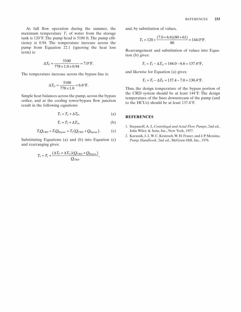
REFERENCES 233
and, by substitution of values,
T5 1207 0 6 6 80 61
80144 0= + +( ) +( ) = °. .
. .F
Rearrangement and substitution of values into Equa-tion (b) gives:
T T T3 5 144 0 6 6 137 4= − = − = °∆ O . . . ,F
and likewise for Equation (a) gives:
T T T2 3 137 4 7 0 130 4= − = − = °∆ P . . . .F
Thus, the design temperature of the bypass portion of the CRD system should be at least 144 ° F. The design temperature of the lines downstream of the pump (and to the HCUs) should be at least 137.4 ° F.
REFERENCES
1. Stepanoff , A. J. , Centrifugal and Axial Flow Pumps , 2nd ed. , John Wiley & Sons, Inc. , New York , 1957 .
2. Karassik , I. J. , W. C. Krutzsch , W. H. Fraser , and J. P. Messina , Pump Handbook , 2nd ed. , McGraw - Hill, Inc. , 1976 .
At full fl ow operation during the summer, the maximum temperature T1 of water from the storage tank is 120 ° F. The pump head is 5100 ft. The pump effi -ciency is 0.94. The temperature increase across the pump from Equation 22.1 (ignoring the heat loss term) is:
∆TP F=× ×
= °5100778 1 0 0 94
7 0. .
. .
The temperature increase across the bypass line is:
∆TO F=×
= °5100778 1 0
6 6.
. .
Simple heat balances across the pump, across the bypass orifi ce, and at the cooling tower/bypass fl ow junction result in the following equations:
T T T3 2= + ∆ P, (a)
T T T5 3= + ∆ O, (b)
T Q T Q T Q Q1 5 2CRD Bypass CRD Bypass .+ = +( ) (c)
Substituting Equations (a) and (b) into Equation (c) and rearranging gives:
T TT T Q Q
Q5 1= +
+( ) +( )∆ ∆P O CRD Bypass
CRD
,
235
23 FLOW TO RUN FULL
Whether or not horizontal fl ow passages run full at low fl ow rates may be an important design consideration. For example, relatively cold fl uid may discharge into a vessel fi lled with a hot fl uid through a horizontal opening. At low fl ow rates, the space above the cold fl uid at the opening may be occupied by hot fl uid because of the difference in density of the two fl uids. * If the fl ow tends to be unsteady, temperature cycling may occur in the discharge openings and cause thermal fatigue of the metal surfaces. A related but different example is strati-fi cation of cold fl uid at the bottom of a horizontal pipe: hot fl uid, or vapor, at the top of the pipe may produce excessive thermal loads on the pipe and its supports.
If the fl ow rate of the fl uid is not suffi cient to fi ll the opening, the condition is called open fl ow . If the fl ow rate is just enough to fi ll the opening, the condition is called full fl ow or fl ow to run full . Submerged fl ow is the condition in which the surface level of the heavy fl uid is above the top of the opening. The governing relation-ships are developed using energy and continuity equa-tions. Inertial and gravitational forces dominate. Shear stresses are considered to exert only a negligible effect on fl ow and thus viscous forces are ignored. Surface tension forces are also ignored. The solutions assume hydrostatic pressure distribution at the opening.
The Froude number, the ratio of inertial and gravi-tational forces (see Section 1.3.5 ), can be used to char-
acterize open fl ow or, in this case, whether or not horizontal openings run full. The Froude number NFr is related to volumetric fl ow rate in cubic feet per second as follows:
Q gR N= π 2 5 2/ ,Fr (23.1)
or in gallons per minute as
q gR N= 448 83 2 5 2. ./π Fr (23.2)
23.1 OPEN FLOW
Figure 23.1 depicts a heavy fl uid discharging into a large space or chamber fi lled with a light fl uid. In this case, the fl ow rate of the heavy fl uid is not suffi cient to fi ll the opening and the condition is called open fl ow .
Using the heavy to light fl uid interface in the opening as the reference elevation and ignoring the approach velocity, the energy equation along a streamline cross-ing the exit of the opening is:
ρ ρ ρheavyheavy
lighthu
gh= +
2
2. (23.3)
Rearranging and letting h = H − y gives:
u g H yheavy light
heavy
=−
−( )2ρ ρ
ρ.
Pipe Flow: A Practical and Comprehensive Guide, First Edition. Donald C. Rennels and Hobart M. Hudson.© 2012 John Wiley & Sons, Inc. Published 2012 by John Wiley & Sons, Inc.
* Of course, the situation would be reversed if hot fl uid were injected into a cold fl uid through horizontal openings. At low fl ow rates, the cold fl uid may occupy the space below the hot fl uid.
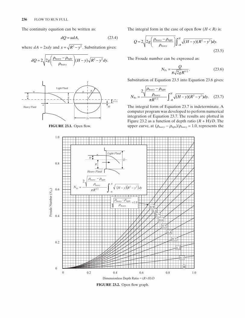
236 FLOW TO RUN FULL
The integral form in the case of open fl ow ( H < R) is:
Q g H y R y dyheavy light
heavy R
H
=−
− −−∫2 2 2 2ρ ρ
ρ( )( ) .
(23.5)
The Froude number can be expressed as:
NQ
gRFr =
π 2 5 2/. (23.6)
Substitution of Equation 23.5 into Equation 23.6 gives:
NR
H y R y dy
heavy light
heavy
R
H
Fr ( )( )=
−
− −−∫
2
5 22 2
ρ ρρ
π /. (23.7)
The integral form of Equation 23.7 is indeterminate. A computer program was developed to perform numerical integration of Equation 23.7 . The results are plotted in Figure 23.2 as a function of depth ratio ( R + H) /D . The upper curve, at ( ρheavy − ρlight )/ ρheavy = 1.0, represents the
The continuity equation can be written as:
dQ udA= , (23.4)
where dA = 2 xdy and x R y= −2 2 . Substitution gives:
dQ g H y R y dyheavy light
heavy
=−
−( ) −2 2 2 2ρ ρρ
.
FIGURE 23.1. Open fl ow.
y (-)
u
Y
dy
R
2x
h
Heavy Fluid
Light Fluid
H
FIGURE 23.2. Open fl ow graph.
1.0
Dimensionless Depth Ratio = (R+H)/D
0.8
0.6
0.4
0.2
0
0.2 0.4 0.6 0.8 1.00
Fro
ude
Num
ber
(N
Fr)
1.0heavy
lightheavy
Hheavy
lightheavy
RNFr
2
Light Fluid
0.8
0.9
0.7
0.6
0.5
0.4
0.3
0.2
0.1
HD
R
Heavy Fluid
0
( )( )∫−
−−
−
−
=
=
R
dyyRyH 2225π
ρρρ
ρρρ
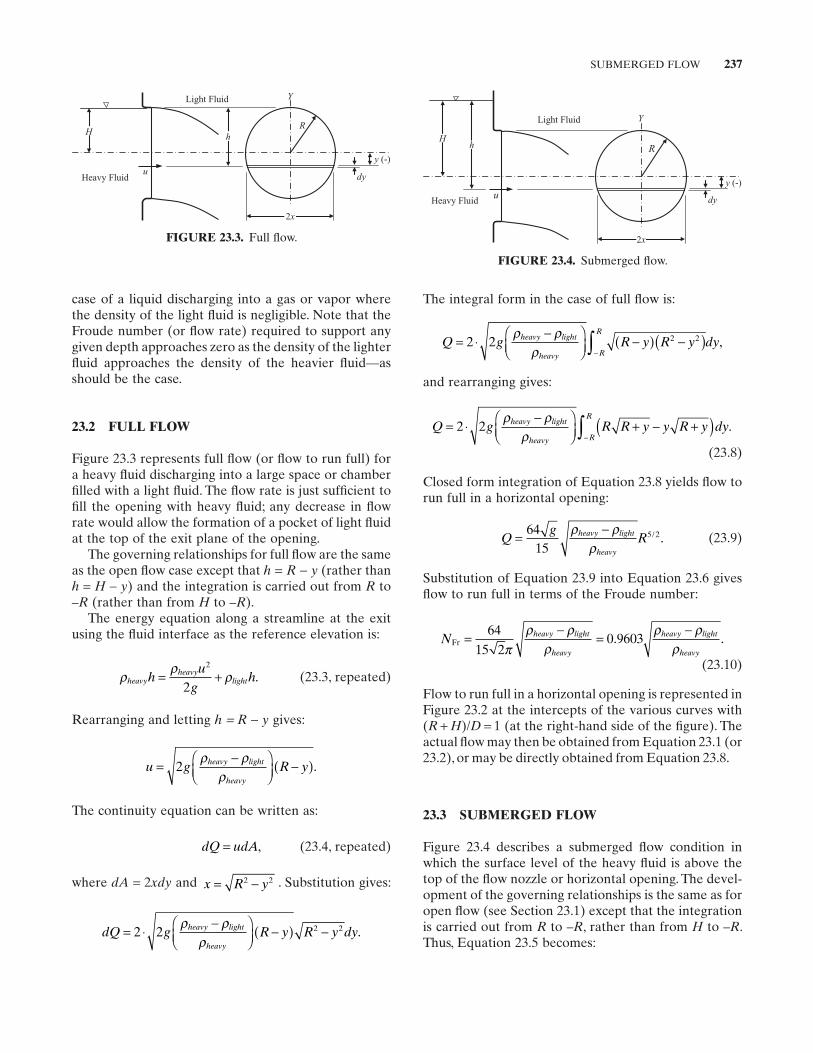
SUBMERGED FLOW 237
The integral form in the case of full fl ow is:
Q g R y R y dyheavy light
heavy R
R
= ⋅−
−( ) −( )−∫2 2 2 2ρ ρ
ρ,
and rearranging gives:
Q g R R y y R y dyheavy light
heavy R
R
= ⋅−
+ − +( )−∫2 2
ρ ρρ
.
(23.8)
Closed form integration of Equation 23.8 yields fl ow to run full in a horizontal opening:
Qg
Rheavy light
heavy
=−64
155 2ρ ρ
ρ/ . (23.9)
Substitution of Equation 23.9 into Equation 23.6 gives fl ow to run full in terms of the Froude number:
N heavy light
heavy
heavy light
heavyFr =
−=
−64
15 20 9603
πρ ρ
ρρ ρ
ρ. .
(23.10)
Flow to run full in a horizontal opening is represented in Figure 23.2 at the intercepts of the various curves with (R + H )/ D = 1 (at the right - hand side of the fi gure). The actual fl ow may then be obtained from Equation 23.1 (or 23.2 ), or may be directly obtained from Equation 23.8 .
23.3 SUBMERGED FLOW
Figure 23.4 describes a submerged fl ow condition in which the surface level of the heavy fl uid is above the top of the fl ow nozzle or horizontal opening. The devel-opment of the governing relationships is the same as for open fl ow (see Section 23.1 ) except that the integration is carried out from R to – R , rather than from H to – R . Thus, Equation 23.5 becomes:
case of a liquid discharging into a gas or vapor where the density of the light fl uid is negligible. Note that the Froude number (or fl ow rate) required to support any given depth approaches zero as the density of the lighter fl uid approaches the density of the heavier fl uid — as should be the case.
23.2 FULL FLOW
Figure 23.3 represents full fl ow (or fl ow to run full) for a heavy fl uid discharging into a large space or chamber fi lled with a light fl uid. The fl ow rate is just suffi cient to fi ll the opening with heavy fl uid; any decrease in fl ow rate would allow the formation of a pocket of light fl uid at the top of the exit plane of the opening.
The governing relationships for full fl ow are the same as the open fl ow case except that h = R − y (rather than h = H − y ) and the integration is carried out from R to – R (rather than from H to – R ).
The energy equation along a streamline at the exit using the fl uid interface as the reference elevation is:
ρ ρ ρheavyheavy
lighthu
gh= +
2
2. (23.3, repeated)
Rearranging and letting h = R − y gives:
u g R yheavy light
heavy
=−
−( )2ρ ρ
ρ.
The continuity equation can be written as:
dQ udA= , (23.4, repeated)
where dA = 2 xdy and x R y= −2 2 . Substitution gives:
dQ g R y R y dyheavy light
heavy
= ⋅−
−( ) −2 2 2 2ρ ρρ
.
FIGURE 23.3. Full fl ow.
u
Y
dy
y (-)
R
2x
h
Heavy Fluid
Light Fluid
H
FIGURE 23.4. Submerged fl ow.
u
Y
dy
y (-)
2x
h
Heavy Fluid
Light Fluid
HR
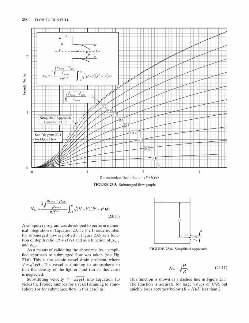
238 FLOW TO RUN FULL
NHR
Fr = . (23.11)
This function is shown as a dashed line in Figure 23.5 . The function is accurate for large values of H / R , but quickly loses accuracy below ( R + H )/ D less than 2.
NR
H Y R y dy
heavy light
heavy
R
R
Fr =
−
− −−∫
2
5 22 2
ρ ρρ
π( )( ) .
(23.11)
A computer program was developed to perform numer-ical integration of Equation 23.11 . The Froude number for submerged fl ow is plotted in Figure 23.5 as a func-tion of depth ratio ( R + H )/ D and as a function of ρheavy
and ρlight . As a means of validating the above results, a simpli-
fi ed approach to submerged fl ow was taken (see Fig. 23.6 ). This is the classic vessel drain problem, where V gH= 2 . The vessel is draining to atmosphere so that the density of the lighter fl uid (air in this case) is neglected.
Substituting velocity V gH= 2 into Equation 1.3 yields the Froude number for a vessel draining to atmo-sphere (or for submerged fl ow in this case) as:
FIGURE 23.5. Submerged fl ow graph.
0 1 2 3
1
2
0
Fro
ude
No.
NF
r
Dimensionless Depth Ratio = (R+H )/D
0
0.1heavy
lightheavy
Simplified Approach Equation 23.12
See Diagram 23.1 for Open Flow
0.90.8
0.4
0.5
0.6
0.2
0.3
0.7
0.1
DR
H
R
R
heavy
lightheavy
Fr dyyyHR
N 2225
2
=−
ρρρ
( )( )∫−−−
−
= Rπ
ρρρ
FIGURE 23.6. Simplifi ed approach.
d
H
V
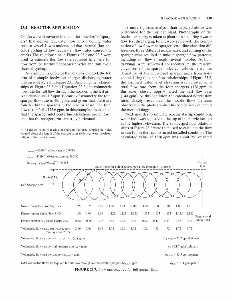
REACTOR APPLICATION 239
A more rigorous analysis than depicted above was performed for the nuclear plant. Photographs of the feedwater spargers, taken at plant startup during a water fl ow test discharging to air, were reviewed. The combi-nation of low fl ow rate, sparger centerline elevation dif-ferences, three different nozzle sizes, and canting of the sparger arms resulted in unique sparger fl ow patterns, including no fl ow through several nozzles. As - built drawings were reviewed to reconstruct the relative elevations of the sparger inlet centerlines as well as departure of the individual sparger arms from hori-zontal. Using the open fl ow relationships of Figure 23.2 , the assumed water level elevation was adjusted until total fl ow rate from the four spargers (138 gpm in this case) closely approximated the test fl ow rate (140 gpm). At this condition, the calculated nozzle fl ow rates closely resembled the nozzle fl ows patterns observed in the photographs. This comparison validated the methodology.
Next, in order to simulate reactor startup conditions, water level was adjusted to the top of the nozzle located at the highest elevation. The submerged fl ow relation-ships of Figure 23.2 were then used to calculate the fl ow to run full in the reconstructed installed condition. The calculated value of 1230 gpm was about 9% of rated
23.4 REACTOR APPLICATION
Cracks were discovered in the outlet “ nozzles ” of sparg-ers* that deliver feedwater fl ow into a boiling water reactor vessel. It was understood that thermal (hot and cold) cycling at low feedwater fl ow rates caused the cracks. The relationships in Figures 23.2 and 23.5 were used to estimate the fl ow rate required to ensure full fl ow from the feedwater sparger nozzles and thus avoid thermal cycling.
As a simple example of the analysis method, the left arm of a simple feedwater sparger discharging water into air is depicted in Figure 23.7 . Applying the relation-ships of Figure 23.2 and Equation 23.2 , the volumetric fl ow rate for full fl ow through the nozzles in the left arm is calculated as 21.7 gpm. Because of symmetry, the total sparger fl ow rate is 43.4 gpm, and given that there are four feedwater spargers in the reactor vessel, the total fl ow to run full is 173.6 gpm. In this example, it is assumed that the sparger inlet centerline elevations are uniform and that the sparger arms are truly horizontal.
FIGURE 23.7. Flow rate required for full sparger fl ow.
H = 0.625 in
heavy = 60 lb/ftr
r
rrr
3 (Feedwater at 200°F)
light = 47 lb/ft3 (Reactor water at 530°F)
[( heavy – light)/ heavy]1/2 = 0.465
Water Level for Full or Submerged Flow through All Nozzles
Left Sparger Arm
Nozzle diameter D (or 2R), inches 1.25 1.25 1.25 1.00 1.00 1.00 1.00 1.00 1.00 1.00 1.00
Dimensionless depth (H + R )/D 1.00 1.00 1.00 1.125 1.125 1.125 1.125 1.125 1.125 1.125 1.125
Froude number NFr (from Figure 23.2) 0.38 0.38 0.38 0.43 0.43 0.43 0.43 0.43 0.43 0.43 0.43
Volumetric flow rate q per nozzle, gpm 2.66 2.66 2.66 1.72 1.72 1.72 1.72 1.72 1.72 1.72 1.72 (from Equation 23.2)
Volumetric flow rate per left sparger arm (qL), gpm Σq = qL = 21.7 gpm/left arm
Volumetric flow rate per right sparger arm (qR), gpm qR = 21.7 gpm/right arm
Volumetric flow rate per sparger (qSparger), gpm qSparger = 43.5 gpm/sparger
Total volumetric flow rate required for full flow through four feedwater spargers, (qTotal), gpm qTotal = 174 gpm/plant
D
Sparger Inlet
Symmetrical About Inlet
* The design of early feedwater spargers featured simple side holes located along the length of the sparger arms to deliver water horizon-tally into the reactor vessel.
240 FLOW TO RUN FULL
FURTHER READING
This list includes books and an article that may be helpful to those who wish to pursue further study.
Chow , V. T. , Open Channel Hydraulics , McGraw - Hill Book Company , 1959 , (the classic text).
Wallis , G. B. , S. J. Crowley , and Y. Hagi , Conditions for a pipe to run full when discharging liquid into a space fi lled with gas , Journal of Fluids Engineering, American Society of Mechanical Engineers , 99 , June 1977 , 405 .
Chandhry , M. H. , Open - Channel Flow , Prentice - Hall , 1993 . Munson , B. R. , D. F. Young , and T. H. Okiishi , Fundamentals
of Fluid Mechanics , 3rd ed. , John Wiley & Sons , 1998 . Jain , S. C. , Open - Channel Flow , John Wiley & Sons , 2000 .
feedwater fl ow assuming water discharging into air. However, during reactor startup the reactor water tem-perature is about 530 ° F ( ρlight = 47 lb/ft 3 ) and the tem-perature of the feedwater is about 200 ° F ( ρheavy = 60 lb/ft3 ). Thus, the above results were adjusted by a factor of:
ρ ρ ρheavy light heavy−( ) = −( ) =/ / . .60 47 60 0 465
This adjustment resulted in a fl ow to run full of 572 gpm (0.465 × 1230 gpm). This turned out to be about 4% of rated feedwater fl ow. A review of plant operating data revealed that feedwater fl ow was maintained at less than 4% rated fl ow for signifi cant periods during plant startup and shutdown. Procedures were established to minimize operating at or below 4% feedwater fl ow.
241
APPENDIX A PHYSICAL PROPERTIES OF WATER AT 1 ATMOSPHERE
These tables present the values of fi ve physical proper-ties of fresh water at various temperatures using units familiar to engineers. In Table A.1 , Fahrenheit tempera-tures are displayed in whole numbers, and properties given in English units are shown unitalicized. Interna-tional System of Units (SI) quantities are given in italics. In Table A.2 , Celsius temperatures are displayed in whole numbers, and properties given in SI units are shown uni-talicized. English quantities are given in italics.
Because the number of Celsius degrees between freezing and boiling is 100, and the number of Fahren-heit degrees in the same span is 180, the ratio between
the two is 5/9, which gives a repeating decimal when converting from ° F to ° C.
The SI unit for absolute viscosity, N - s/m 2 , is exactly 1000 times the derived unit centipoise, which is often used in calculations using the English system. Vapor pressure in SI is given in N/m 2 , a unit sometimes called the pascal.
The specifi c heat is also known as heat capacity. As English and SI units for heat are based on the heat required to raise the temperature of a unit mass of water by a unit degree, the numerical values of the spe-cifi c heat are the same in both systems.
Pipe Flow: A Practical and Comprehensive Guide, First Edition. Donald C. Rennels and Hobart M. Hudson.© 2012 John Wiley & Sons, Inc. Published 2012 by John Wiley & Sons, Inc.
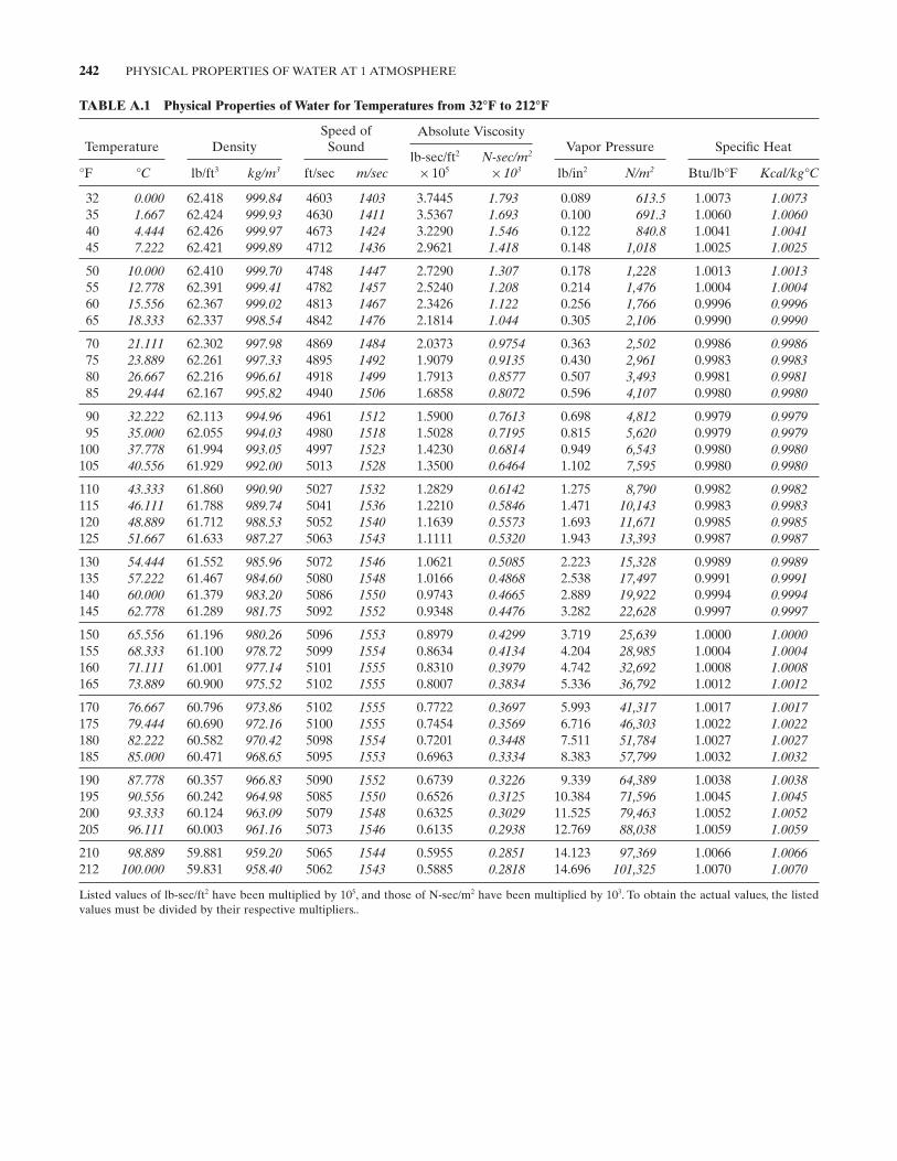
242 PHYSICAL PROPERTIES OF WATER AT 1 ATMOSPHERE
TABLE A.1 Physical Properties of Water for Temperatures from 32 ° F to 212 ° F
Temperature Density Speed of
Sound Absolute Viscosity
Vapor Pressure Specifi c Heat
° F ° C lb/ft 3 kg/m3 ft/sec m/sec lb - sec/ft 2 × 10 5
N - sec/m 2 × 10³ lb/in 2 N/m2 Btu/lb ° F Kcal/kg ° C
32 0.000 62.418 999.84 4603 1403 3.7445 1.793 0.089 613.5 1.0073 1.0073 35 1.667 62.424 999.93 4630 1411 3.5367 1.693 0.100 691.3 1.0060 1.0060 40 4.444 62.426 999.97 4673 1424 3.2290 1.546 0.122 840.8 1.0041 1.0041 45 7.222 62.421 999.89 4712 1436 2.9621 1.418 0.148 1,018 1.0025 1.0025
50 10.000 62.410 999.70 4748 1447 2.7290 1.307 0.178 1,228 1.0013 1.0013 55 12.778 62.391 999.41 4782 1457 2.5240 1.208 0.214 1,476 1.0004 1.0004 60 15.556 62.367 999.02 4813 1467 2.3426 1.122 0.256 1,766 0.9996 0.9996 65 18.333 62.337 998.54 4842 1476 2.1814 1.044 0.305 2,106 0.9990 0.9990
70 21.111 62.302 997.98 4869 1484 2.0373 0.9754 0.363 2,502 0.9986 0.9986 75 23.889 62.261 997.33 4895 1492 1.9079 0.9135 0.430 2,961 0.9983 0.9983 80 26.667 62.216 996.61 4918 1499 1.7913 0.8577 0.507 3,493 0.9981 0.9981 85 29.444 62.167 995.82 4940 1506 1.6858 0.8072 0.596 4,107 0.9980 0.9980
90 32.222 62.113 994.96 4961 1512 1.5900 0.7613 0.698 4,812 0.9979 0.9979 95 35.000 62.055 994.03 4980 1518 1.5028 0.7195 0.815 5,620 0.9979 0.9979
100 37.778 61.994 993.05 4997 1523 1.4230 0.6814 0.949 6,543 0.9980 0.9980 105 40.556 61.929 992.00 5013 1528 1.3500 0.6464 1.102 7,595 0.9980 0.9980
110 43.333 61.860 990.90 5027 1532 1.2829 0.6142 1.275 8,790 0.9982 0.9982 115 46.111 61.788 989.74 5041 1536 1.2210 0.5846 1.471 10,143 0.9983 0.9983 120 48.889 61.712 988.53 5052 1540 1.1639 0.5573 1.693 11,671 0.9985 0.9985 125 51.667 61.633 987.27 5063 1543 1.1111 0.5320 1.943 13,393 0.9987 0.9987
130 54.444 61.552 985.96 5072 1546 1.0621 0.5085 2.223 15,328 0.9989 0.9989 135 57.222 61.467 984.60 5080 1548 1.0166 0.4868 2.538 17,497 0.9991 0.9991 140 60.000 61.379 983.20 5086 1550 0.9743 0.4665 2.889 19,922 0.9994 0.9994 145 62.778 61.289 981.75 5092 1552 0.9348 0.4476 3.282 22,628 0.9997 0.9997
150 65.556 61.196 980.26 5096 1553 0.8979 0.4299 3.719 25,639 1.0000 1.0000 155 68.333 61.100 978.72 5099 1554 0.8634 0.4134 4.204 28,985 1.0004 1.0004 160 71.111 61.001 977.14 5101 1555 0.8310 0.3979 4.742 32,692 1.0008 1.0008 165 73.889 60.900 975.52 5102 1555 0.8007 0.3834 5.336 36,792 1.0012 1.0012
170 76.667 60.796 973.86 5102 1555 0.7722 0.3697 5.993 41,317 1.0017 1.0017 175 79.444 60.690 972.16 5100 1555 0.7454 0.3569 6.716 46,303 1.0022 1.0022 180 82.222 60.582 970.42 5098 1554 0.7201 0.3448 7.511 51,784 1.0027 1.0027 185 85.000 60.471 968.65 5095 1553 0.6963 0.3334 8.383 57,799 1.0032 1.0032
190 87.778 60.357 966.83 5090 1552 0.6739 0.3226 9.339 64,389 1.0038 1.0038 195 90.556 60.242 964.98 5085 1550 0.6526 0.3125 10.384 71,596 1.0045 1.0045 200 93.333 60.124 963.09 5079 1548 0.6325 0.3029 11.525 79,463 1.0052 1.0052 205 96.111 60.003 961.16 5073 1546 0.6135 0.2938 12.769 88,038 1.0059 1.0059
210 98.889 59.881 959.20 5065 1544 0.5955 0.2851 14.123 97,369 1.0066 1.0066 212 100.000 59.831 958.40 5062 1543 0.5885 0.2818 14.696 101,325 1.0070 1.0070
Listed values of lb - sec/ft 2 have been multiplied by 10 5 , and those of N - sec/m 2 have been multiplied by 10 3 . To obtain the actual values, the listed values must be divided by their respective multipliers..
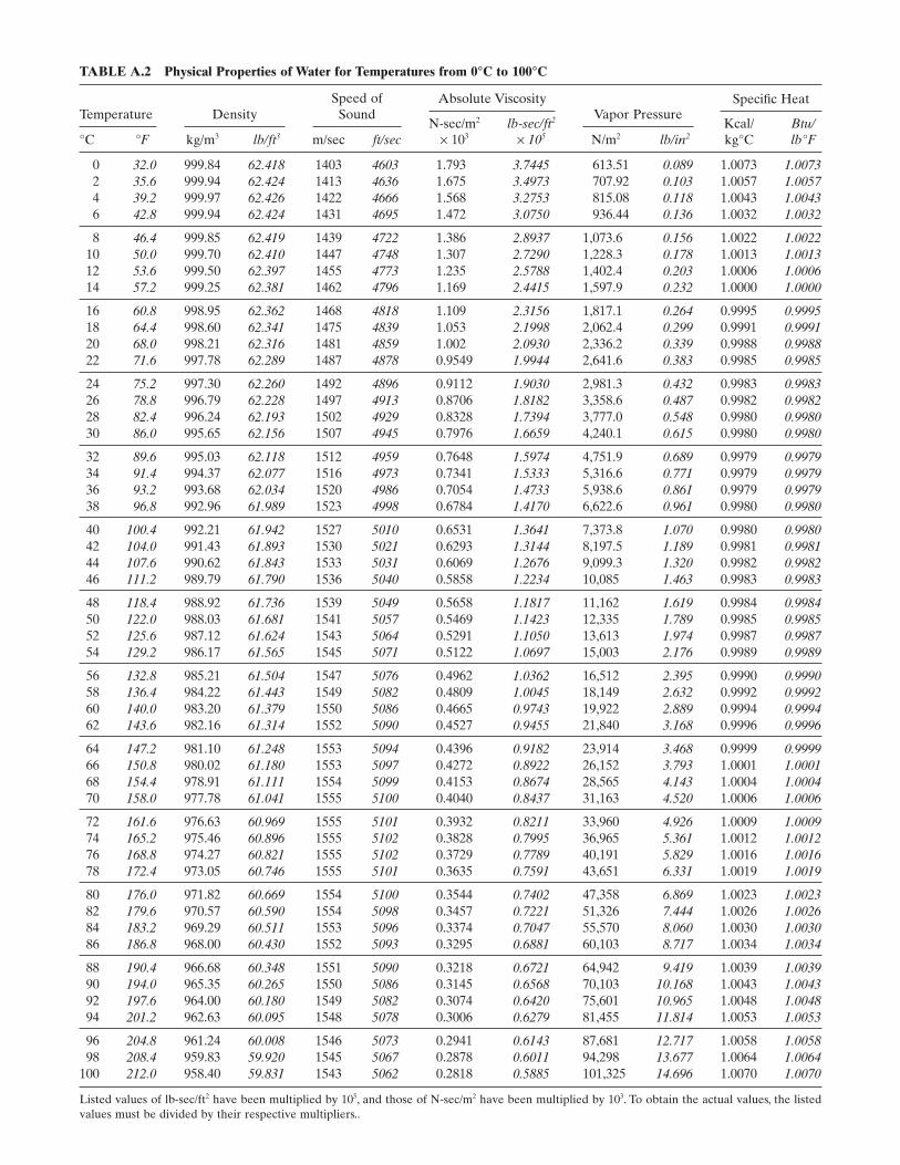
TABLE A.2 Physical Properties of Water for Temperatures from 0 ° C to 100 ° C
Temperature Density Speed of
Sound Absolute Viscosity
Vapor Pressure Specifi c Heat
° C ° F kg/m 3 lb/ft3 m/sec ft/sec N - sec/m 2 × 10 3
lb - sec/ft 2 × 10⁵ N/m 2 lb/in2
Kcal/kg ° C
Btu/lb ° F
0 32.0 999.84 62.418 1403 4603 1.793 3.7445 613.51 0.089 1.0073 1.0073 2 35.6 999.94 62.424 1413 4636 1.675 3.4973 707.92 0.103 1.0057 1.0057 4 39.2 999.97 62.426 1422 4666 1.568 3.2753 815.08 0.118 1.0043 1.0043 6 42.8 999.94 62.424 1431 4695 1.472 3.0750 936.44 0.136 1.0032 1.0032
8 46.4 999.85 62.419 1439 4722 1.386 2.8937 1,073.6 0.156 1.0022 1.0022 10 50.0 999.70 62.410 1447 4748 1.307 2.7290 1,228.3 0.178 1.0013 1.0013 12 53.6 999.50 62.397 1455 4773 1.235 2.5788 1,402.4 0.203 1.0006 1.0006 14 57.2 999.25 62.381 1462 4796 1.169 2.4415 1,597.9 0.232 1.0000 1.0000
16 60.8 998.95 62.362 1468 4818 1.109 2.3156 1,817.1 0.264 0.9995 0.9995 18 64.4 998.60 62.341 1475 4839 1.053 2.1998 2,062.4 0.299 0.9991 0.9991 20 68.0 998.21 62.316 1481 4859 1.002 2.0930 2,336.2 0.339 0.9988 0.9988 22 71.6 997.78 62.289 1487 4878 0.9549 1.9944 2,641.6 0.383 0.9985 0.9985
24 75.2 997.30 62.260 1492 4896 0.9112 1.9030 2,981.3 0.432 0.9983 0.9983 26 78.8 996.79 62.228 1497 4913 0.8706 1.8182 3,358.6 0.487 0.9982 0.9982 28 82.4 996.24 62.193 1502 4929 0.8328 1.7394 3,777.0 0.548 0.9980 0.9980 30 86.0 995.65 62.156 1507 4945 0.7976 1.6659 4,240.1 0.615 0.9980 0.9980
32 89.6 995.03 62.118 1512 4959 0.7648 1.5974 4,751.9 0.689 0.9979 0.9979 34 91.4 994.37 62.077 1516 4973 0.7341 1.5333 5,316.6 0.771 0.9979 0.9979 36 93.2 993.68 62.034 1520 4986 0.7054 1.4733 5,938.6 0.861 0.9979 0.9979 38 96.8 992.96 61.989 1523 4998 0.6784 1.4170 6,622.6 0.961 0.9980 0.9980
40 100.4 992.21 61.942 1527 5010 0.6531 1.3641 7,373.8 1.070 0.9980 0.9980 42 104.0 991.43 61.893 1530 5021 0.6293 1.3144 8,197.5 1.189 0.9981 0.9981 44 107.6 990.62 61.843 1533 5031 0.6069 1.2676 9,099.3 1.320 0.9982 0.9982 46 111.2 989.79 61.790 1536 5040 0.5858 1.2234 10,085 1.463 0.9983 0.9983
48 118.4 988.92 61.736 1539 5049 0.5658 1.1817 11,162 1.619 0.9984 0.9984 50 122.0 988.03 61.681 1541 5057 0.5469 1.1423 12,335 1.789 0.9985 0.9985 52 125.6 987.12 61.624 1543 5064 0.5291 1.1050 13,613 1.974 0.9987 0.9987 54 129.2 986.17 61.565 1545 5071 0.5122 1.0697 15,003 2.176 0.9989 0.9989
56 132.8 985.21 61.504 1547 5076 0.4962 1.0362 16,512 2.395 0.9990 0.9990 58 136.4 984.22 61.443 1549 5082 0.4809 1.0045 18,149 2.632 0.9992 0.9992 60 140.0 983.20 61.379 1550 5086 0.4665 0.9743 19,922 2.889 0.9994 0.9994 62 143.6 982.16 61.314 1552 5090 0.4527 0.9455 21,840 3.168 0.9996 0.9996
64 147.2 981.10 61.248 1553 5094 0.4396 0.9182 23,914 3.468 0.9999 0.9999 66 150.8 980.02 61.180 1553 5097 0.4272 0.8922 26,152 3.793 1.0001 1.0001 68 154.4 978.91 61.111 1554 5099 0.4153 0.8674 28,565 4.143 1.0004 1.0004 70 158.0 977.78 61.041 1555 5100 0.4040 0.8437 31,163 4.520 1.0006 1.0006
72 161.6 976.63 60.969 1555 5101 0.3932 0.8211 33,960 4.926 1.0009 1.0009 74 165.2 975.46 60.896 1555 5102 0.3828 0.7995 36,965 5.361 1.0012 1.0012 76 168.8 974.27 60.821 1555 5102 0.3729 0.7789 40,191 5.829 1.0016 1.0016 78 172.4 973.05 60.746 1555 5101 0.3635 0.7591 43,651 6.331 1.0019 1.0019
80 176.0 971.82 60.669 1554 5100 0.3544 0.7402 47,358 6.869 1.0023 1.0023 82 179.6 970.57 60.590 1554 5098 0.3457 0.7221 51,326 7.444 1.0026 1.0026 84 183.2 969.29 60.511 1553 5096 0.3374 0.7047 55,570 8.060 1.0030 1.0030 86 186.8 968.00 60.430 1552 5093 0.3295 0.6881 60,103 8.717 1.0034 1.0034
88 190.4 966.68 60.348 1551 5090 0.3218 0.6721 64,942 9.419 1.0039 1.0039 90 194.0 965.35 60.265 1550 5086 0.3145 0.6568 70,103 10.168 1.0043 1.0043 92 197.6 964.00 60.180 1549 5082 0.3074 0.6420 75,601 10.965 1.0048 1.0048 94 201.2 962.63 60.095 1548 5078 0.3006 0.6279 81,455 11.814 1.0053 1.0053
96 204.8 961.24 60.008 1546 5073 0.2941 0.6143 87,681 12.717 1.0058 1.0058 98 208.4 959.83 59.920 1545 5067 0.2878 0.6011 94,298 13.677 1.0064 1.0064
100 212.0 958.40 59.831 1543 5062 0.2818 0.5885 101,325 14.696 1.0070 1.0070
Listed values of lb - sec/ft 2 have been multiplied by 10 5 , and those of N - sec/m 2 have been multiplied by 10 3 . To obtain the actual values, the listed values must be divided by their respective multipliers..
245
APPENDIX B PIPE SIZE DATA
Pipe sizes can be confusing because the terminology may relate to historical dimensions that are loosely related to actual dimensions. Early on, pipe was sized by inside diameter. This practice was abandoned to improve compatibility with pipe fi ttings that must usually fi t the outside diameter of the pipe, but it has had a lasting impact on modern standards around the world. Presently, the pipe size designation generally includes two numbers: one that indicates the outside diameter or nominal diameter and another that identi-fi es the wall thickness.
Historically, only a small selection of pipe wall thick-ness was in use: standard weight ( Std ), extra strong ( XS ), and double extra strong ( XXS ), based on the iron pipe size system of the day. In 1927, the American Stan-dards Association created a system of schedule numbers that designated steel pipe wall thickness based on smaller steps between sizes. In the mid - twentieth century, stainless steel pipe — which permitted the use of thinner walls with much less risk of failure due to cor-rosion — came into more common use. Consequently, schedules 5S and 10S were created in 1949, and other “ S ” sizes followed.
Pipe is specifi ed by its nominal inside diameter through 12 in and smaller. In this range, nominal size refers to the approximate inside diameter of a schedule 40 (or standard weight) pipe. Pipe 14 in and larger is
specifi ed by the actual outside diameter. For a given pipe size, the outside diameter is the same for all weights and schedules. In North America, pipe size is specifi ed by Nominal Pipe Size ( NPS ) and is based on inches. The European version is called Diametre Nominal ( DN ) and is based on millimeters. Japan has its own set of standard pipe sizes, called Japanese Industrial Standards (JIS) pipe, that are based on millimeters.
Many different national and international standards exist for pipe sizes, including American Petroleum Insti-tute (API) 5 L, American National Standards Institute (ANSI)/American Society of Mechanical Engineers (ASME) B32.10M and B36.19M in the United States, and British Standard (BS) 1600 and BS European Standard (EN) 10255 in the United Kingdom and Europe. Manufacturing standards commonly require a test of chemical composition and a series of mechanical strength tests for each heat of pipe.
Pipe is made of a wide variety of materials including ceramic, fi berglass, metals, concrete, and plastic. Metallic pipes are commonly made of steel or iron, such as carbon steel, stainless steel, galvanized steel, cast iron, and ductile iron. Inconel, chrome moly, and titanium alloys are used in high temperature and pressure applications. Copper and aluminum pipe are frequently employed.
The following NPS and DN table gives selected data for commercial pipe.
Pipe Flow: A Practical and Comprehensive Guide, First Edition. Donald C. Rennels and Hobart M. Hudson.© 2012 John Wiley & Sons, Inc. Published 2012 by John Wiley & Sons, Inc.
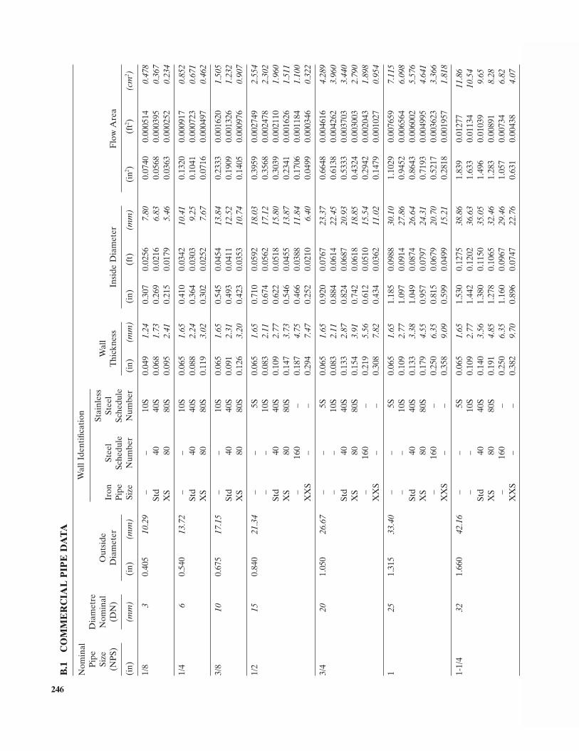
Nom
inal
P
ipe
Dia
met
re W
all I
dent
ifi ca
tion
Nom
inal
P
ipe
Size
(NP
S)
(in)
Dia
met
re
Nom
inal
(DN
)
(mm
)
Out
side
D
iam
eter
Wal
l Ide
ntifi
cati
on
Wal
l T
hick
ness
In
side
Dia
met
er
Flo
w A
rea
(in)
(m
m)
Iron
P
ipe
Size
Stee
l Sc
hedu
leN
umbe
r
Stai
nles
s St
eel
Sche
dule
Num
ber
(in)
(m
m)
(i
n)
(ft)
(m
m)
(i
n 2 ) (f
t 2 )
(c
m2 )
1/8
3 0.
405
10.2
9 –
–
10
S 0.
049
1.24
0.30
7 0.
0256
7.
80 0.
0740
0.
0005
14
0.47
8 St
d 40
40
S 0.
068
1.73
0.26
9 0.
0216
6.
83 0.
0568
0.
0003
95
0.36
7 X
S 80
80
S 0.
095
2.41
0.21
5 0.
0179
5.
46 0.
0363
0.
0002
52
0.23
4
1/4
6 0.
540
13.7
2 –
–
10
S 0.
065
1.65
0.41
0 0.
0342
10
.41
0.13
20
0.00
0917
0.
852
Std
40
40S
0.08
8 2.
24 0.
364
0.03
03
9.25
0.10
41
0.00
0723
0.
671
XS
80
80S
0.11
9 3.
02 0.
302
0.02
52
7.67
0.07
16
0.00
0497
0.
462
3/8
10 0.
675
17.1
5 –
–
10
S 0.
065
1.65
0.54
5 0.
0454
13
.84
0.23
33
0.00
1620
1.
505
Std
40
40S
0.09
1 2.
31 0.
493
0.04
11
12.5
2 0.
1909
0.
0013
26
1.23
2 X
S 80
80
S 0.
126
3.20
0.42
3 0.
0353
10
.74
0.14
05
0.00
0976
0.
907
1/2
15 0.
840
21.3
4 –
–
5S
0.
065
1.65
0.71
0 0.
0592
18
.03
0.39
59
0.00
2749
2.
554
–
–
10S
0.08
3 2.
11 0.
674
0.05
62
17.1
2 0.
3568
0.
0024
78
2.30
2 St
d 40
40
S 0.
109
2.77
0.62
2 0.
0518
15
.80
0.30
39
0.00
2110
1.
960
XS
80
80S
0.14
7 3.
73 0.
546
0.04
55
13.8
7 0.
2341
0.
0016
26
1.51
1 –
16
0 –
0.
187
4.75
0.46
6 0.
0388
11
.84
0.17
06
0.00
1184
1.
100
XX
S –
–
0.
294
7.47
0.25
2 0.
0210
6.
40 0.
0499
0.
0003
46
0.32
2
3/4
20 1.
050
26.6
7 –
–
5S
0.
065
1.65
0.92
0 0.
0767
23
.37
0.66
48
0.00
4616
4.
289
–
–
10S
0.08
3 2.
11 0.
884
0.06
14
22.4
5 0.
6138
0.
0042
62
3.96
0 St
d 40
40
S 0.
133
2.87
0.82
4 0.
0687
20
.93
0.53
33
0.00
3703
3.
440
XS
80
80S
0.15
4 3.
91 0.
742
0.06
18
18.8
5 0.
4324
0.
0030
03
2.79
0 –
16
0 –
0.
219
5.56
0.61
2 0.
0510
15
.54
0.29
42
0.00
2043
1.
898
XX
S –
–
0.
308
7.82
0.43
4 0.
0362
11
.02
0.14
79
0.00
1027
0.
954
1 25
1.31
5 33
.40
–
–
5S
0.06
5 1.
65 1.
185
0.09
88
30.1
0 1.
1029
0.
0076
59
7.11
5 –
–
10
S 0.
109
2.77
1.09
7 0.
0914
27
.86
0.94
52
0.00
6564
6.
098
Std
40
40S
0.13
3 3.
38 1.
049
0.08
74
26.6
4 0.
8643
0.
0060
02
5.57
6 X
S 80
80
S 0.
179
4.55
0.95
7 0.
0797
24
.31
0.71
93
0.00
4995
4.
641
–
160
–
0.25
0 6.
35 0.
815
0.06
79
20.7
0 0.
5217
0.
0036
23
3.36
6 X
XS
–
–
0.35
8 9.
09 0.
599
0.04
99
15.2
1 0.
2818
0.
0019
57
1.81
8
1 - 1/
4 32
1.66
0 42
.16
–
–
5S
0.06
5 1.
65 1.
530
0.12
75
38.8
6 1.
839
0.01
277
11.8
6 –
–
10
S 0.
109
2.77
1.44
2 0.
1202
36
.63
1.63
3 0.
0113
4 10
.54
Std
40
40S
0.14
0 3.
56 1.
380
0.11
50
35.0
5 1.
496
0.01
039
9.65
XS
80
80S
0.19
1 4.
85 1.
278
0.10
65
32.4
6 1.
283
0.00
891
8.28
–
160
–
0.25
0 6.
35 1.
160
0.09
67
29.4
6 1.
057
0.00
734
6.82
XX
S –
–
0.
382
9.70
0.89
6 0.
0747
22
.76
0.63
1 0.
0043
8 4.
07
B.1
C
OM
ME
RC
IAL
PIP
E D
ATA
246
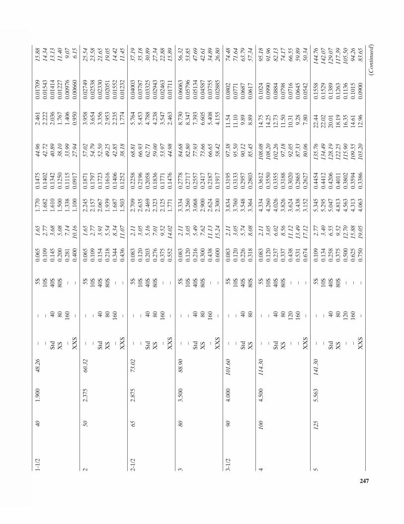
Pip
eSi
ze(N
PS)
(in)
Dia
met
reN
omin
al(D
N)
(mm
)
Out
side
D
iam
eter
Wal
l T
hick
ness
In
side
Dia
met
er
Flo
w A
rea
(in)
(m
m)
Iron
P
ipe
Size
Stee
l Sc
hedu
leN
umbe
r
Stai
nles
s St
eel
Sche
dule
Num
ber
(in)
(m
m)
(i
n)
(ft)
(m
m)
(i
n 2 ) (f
t 2 )
(c
m2 )
1 - 1/
2 40
1.90
0 48
.26
–
–
5S
0.06
5 1.
65 1.
770
0.14
75
44.9
6 2.
461
0.01
709
15.8
8 –
–
10
S 0.
109
2.77
1.68
2 0.
1402
42
.72
2.22
2 0.
0154
3 14
.34
Std
40
40S
0.14
5 3.
68 1.
610
0.13
42
40.8
9 2.
036
0.01
414
13.1
3 X
S 80
80
S 0.
200
5.08
1.50
0 0.
1250
38
.10
1.76
7 0.
0122
7 11
.40
–
160
–
0.28
1 7.
14 1.
338
0.11
15
33.9
9 1.
406
0.00
976
9.07
XX
S –
–
0.
400
10.1
6 1.
100
0.09
17
27.9
4 0.
950
0.00
660
6.15
2 50
2.37
5 60
.32
–
–
5S
0.06
5 1.
65 2.
245
0.18
71
57.0
2 3.
958
0.02
749
25.5
4 –
–
10
S 0.
109
2.77
2.15
7 0.
1797
54
.79
3.65
4 0.
0253
8 23
.58
Std
40
40S
0.15
4 3.
91 2.
067
0.17
23
52.5
0 3.
356
0.02
330
21.6
5 X
S 80
80
S 0.
218
5.54
1.93
9 0.
1616
49
.25
2.95
3 0.
0205
1 19
.05
–
160
–
0.34
4 8.
34 1.
687
0.14
06
42.8
5 2.
235
0.01
552
14.4
2 X
XS
–
–
0.43
6 11
.07
1.50
3 0.
1252
38
.18
1.77
4 0.
0123
2 11
.45
2 - 1/
2 65
2.87
5 73
.02
–
–
5S
0.08
3 2.
11 2.
709
0.22
58
68.8
1 5.
764
0.04
003
37.1
9 –
–
10
S 0.
120
3.05
2.63
5 0.
2196
66
.93
5.45
3 0.
0378
7 35
.18
Std
40
40S
0.20
3 5.
16 2.
469
0.20
58
62.7
1 4.
788
0.03
325
30.8
9 X
S 80
80
S 0.
276
7.01
2.32
3 0.
1836
59
.00
4.23
8 0.
0294
3 27
.34
–
160
–
0.37
5 9.
52 2.
125
0.17
71
53.9
7 3.
547
0.02
463
22.8
8 X
XS
–
–
0.55
2 14
.02
1.77
1 0.
1476
44
.98
2.46
3 0.
0171
1 15
.89
3 80
3.50
0 88
.90
–
–
5S
0.08
3 2.
11 3.
334
0.27
78
84.6
8 8.
730
0.06
063
56.3
2 –
–
10
S 0.
120
3.05
3.26
0 0.
2717
82
.80
8.34
7 0.
0579
6 53
.85
Std
40
40S
0.21
6 5.
49 3.
068
0.25
57
77.9
3 7.
393
0.05
134
47.6
9 X
S 80
80
S 0.
300
7.62
2.90
0 0.
2417
73
.66
6.60
5 0.
0458
7 42
.61
–
160
–
0.43
8 11
.13
2.62
4 0.
2187
66
.65
5.40
8 0.
0375
5 34
.89
XX
S –
–
0.
600
15.2
4 2.
300
0.19
17
58.4
2 4.
155
0.02
885
26.8
0
3 - 1/
2 90
4.00
0 10
1.60
–
–
5S
0.08
3 2.
11 3.
834
0.31
95
97.3
8 11
.54
0.08
02
74.4
8 –
–
10
S 0.
120
3.05
3.76
0 0.
3133
95
.50
11.1
0 0.
0771
71
.64
Std
40
40S
0.22
6 5.
74 3.
548
0.29
57
90.1
2 9.
89
0.06
87
63.7
9 X
S 80
80
S 0.
318
8.08
3.36
4 0.
2803
85
.45
8.89
0.
0617
57
.34
4 10
0 4.
500
114.
30 –
–
5S
0.
083
2.11
4.33
4 0.
3612
10
8.08
14.7
5 0.
1024
95
.18
–
–
10S
0.12
0 3.
05 4.
260
0.35
50
108.
20 14
.25
0.09
90
91.9
6 St
d 40
40
S 0.
237
6.02
4.02
6 0.
3355
10
2.26
12.7
3 0.
0884
82
.13
XS
80
80S
0.33
7 8.
56 3.
826
0.31
88
97.1
8 11
.50
0.07
98
74.1
7 –
12
0 –
0.
438
11.1
2 3.
624
0.30
20
92.0
5 10
.31
0.07
16
66.5
5 –
16
0 –
0.
531
13.4
9 3.
438
0.28
65
87.3
3 9.
28
0.06
45
59.8
9 X
XS
–
–
0.67
4 17
.12
3.15
2 0.
2627
80
.06
7.80
0.
0542
50
.34
5 12
5 5.
563
141.
30 –
–
5S
0.
109
2.77
5.34
5 0.
4454
13
5.76
22.4
4 0.
1558
14
4.76
–
–
10S
0.13
4 3.
40 5.
295
0.44
12
134.
49 22
.02
0.15
29
142.
07 St
d 40
40
S 0.
258
6.55
5.04
7 0.
4206
12
8.19
20.0
1 0.
1389
12
9.07
XS
80
80S
0.37
5 9.
52 4.
813
0.40
11
122.
25 18
.19
0.12
63
117.
39 –
12
0 –
0.
500
12.7
0 4.
563
0.38
02
115.
90 16
.35
0.11
36
105.
50 –
16
0 –
0.
625
15.8
8 4.
313
0.35
94
109.
55 14
.61
0.10
15
94.2
6 X
XS
–
–
0.75
0 19
.05
4.06
3 0.
3386
10
3.20
12.9
6 0.
0900
83
.65
247
(Con
tinue
d)
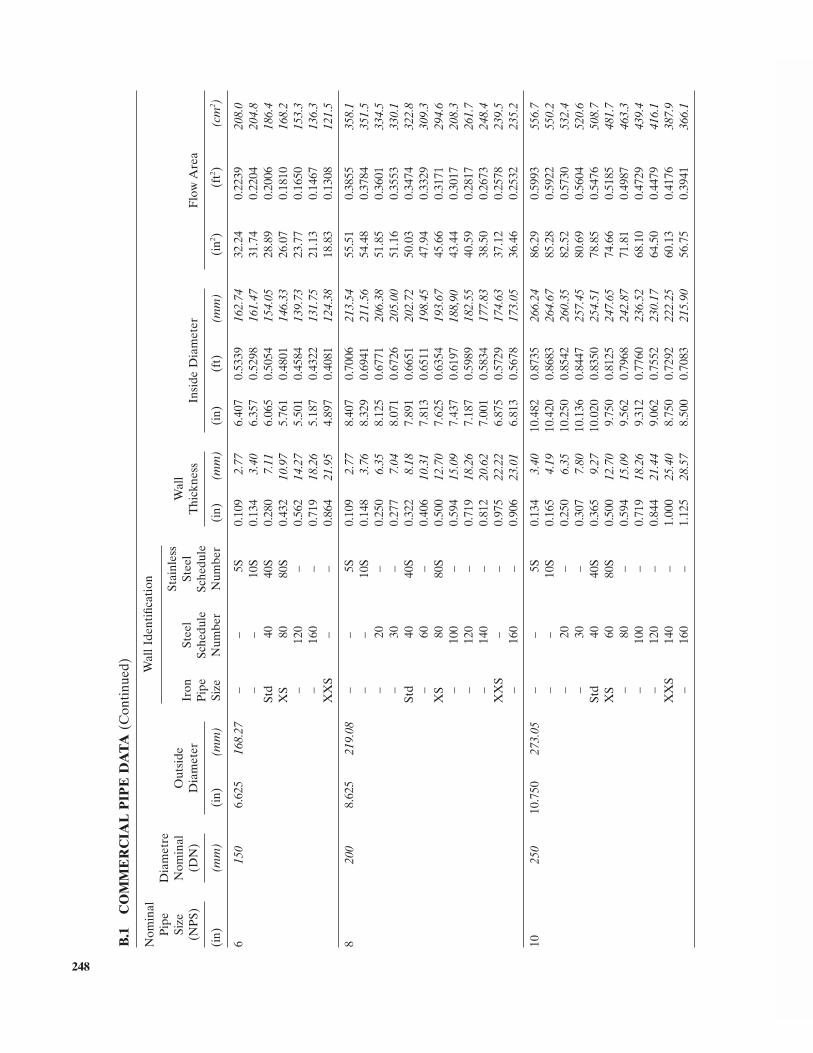
Nom
inal
P
ipe
Size
(NP
S)
(in)
Dia
met
re
Nom
inal
(DN
)
(mm
)
Out
side
D
iam
eter
Wal
l Ide
ntifi
cati
on
Wal
l T
hick
ness
In
side
Dia
met
er
Flo
w A
rea
(in)
(m
m)
Iron
P
ipe
Size
Stee
l Sc
hedu
leN
umbe
r
Stai
nles
s St
eel
Sche
dule
Num
ber
(in)
(m
m)
(i
n)
(ft)
(m
m)
(i
n 2 ) (f
t 2 )
(c
m2 )
6 15
0 6.
625
168.
27 –
–
5S
0.
109
2.77
6.40
7 0.
5339
16
2.74
32.2
4 0.
2239
20
8.0
–
–
10S
0.13
4 3.
40 6.
357
0.52
98
161.
47 31
.74
0.22
04
204.
8 St
d 40
40
S 0.
280
7.11
6.06
5 0.
5054
15
4.05
28.8
9 0.
2006
18
6.4
XS
80
80S
0.43
2 10
.97
5.76
1 0.
4801
14
6.33
26.0
7 0.
1810
16
8.2
–
120
–
0.56
2 14
.27
5.50
1 0.
4584
13
9.73
23.7
7 0.
1650
15
3.3
–
160
–
0.71
9 18
.26
5.18
7 0.
4322
13
1.75
21.1
3 0.
1467
13
6.3
XX
S –
–
0.
864
21.9
5 4.
897
0.40
81
124.
38 18
.83
0.13
08
121.
5
8 20
0 8.
625
219.
08 –
–
5S
0.
109
2.77
8.40
7 0.
7006
21
3.54
55.5
1 0.
3855
35
8.1
–
–
10S
0.14
8 3.
76 8.
329
0.69
41
211.
56 54
.48
0.37
84
351.
5 –
20
–
0.
250
6.35
8.12
5 0.
6771
20
6.38
51.8
5 0.
3601
33
4.5
–
30
–
0.27
7 7.
04 8.
071
0.67
26
205.
00 51
.16
0.35
53
330.
1 St
d 40
40
S 0.
322
8.18
7.89
1 0.
6651
20
2.72
50.0
3 0.
3474
32
2.8
–
60
–
0.40
6 10
.31
7.81
3 0.
6511
19
8.45
47.9
4 0.
3329
30
9.3
XS
80
80S
0.50
0 12
.70
7.62
5 0.
6354
19
3.67
45.6
6 0.
3171
29
4.6
–
100
–
0.59
4 15
.09
7.43
7 0.
6197
18
8,90
43.4
4 0.
3017
20
8.3
–
120
–
0.71
9 18
.26
7.18
7 0.
5989
18
2.55
40.5
9 0.
2817
26
1.7
–
140
–
0.81
2 20
.62
7.00
1 0.
5834
17
7.83
38.5
0 0.
2673
24
8.4
XX
S –
–
0.
975
22.2
2 6.
875
0.57
29
174.
63 37
.12
0.25
78
239.
5 –
16
0 –
0.
906
23.0
1 6.
813
0.56
78
173.
05 36
.46
0.25
32
235.
2
10
250
10.7
50
273.
05 –
–
5S
0.
134
3.40
10.4
82
0.87
35
266.
24 86
.29
0.59
93
556.
7 –
–
10
S 0.
165
4.19
10.4
20
0.86
83
264.
67 85
.28
0.59
22
550.
2 –
20
–
0.
250
6.35
10.2
50
0.85
42
260.
35 82
.52
0.57
30
532.
4 –
30
–
0.
307
7.80
10.1
36
0.84
47
257.
45 80
.69
0.56
04
520.
6 St
d 40
40
S 0.
365
9.27
10.0
20
0.83
50
254.
51 78
.85
0.54
76
508.
7 X
S 60
80
S 0.
500
12.7
0 9.
750
0.81
25
247.
65 74
.66
0.51
85
481.
7 –
80
–
0.
594
15.0
9 9.
562
0.79
68
242.
87 71
.81
0.49
87
463.
3 –
10
0 –
0.
719
18.2
6 9.
312
0.77
60
236.
52 68
.10
0.47
29
439.
4 –
12
0 –
0.
844
21.4
4 9.
062
0.75
52
230.
17 64
.50
0.44
79
416.
1 X
XS
140
–
1.00
0 25
.40
8.75
0 0.
7292
22
2.25
60.1
3 0.
4176
38
7.9
–
160
–
1.12
5 28
.57
8.50
0 0.
7083
21
5.90
56.7
5 0.
3941
36
6.1
248
B.1
C
OM
ME
RC
IAL
PIP
E D
ATA
(C
onti
nued
)
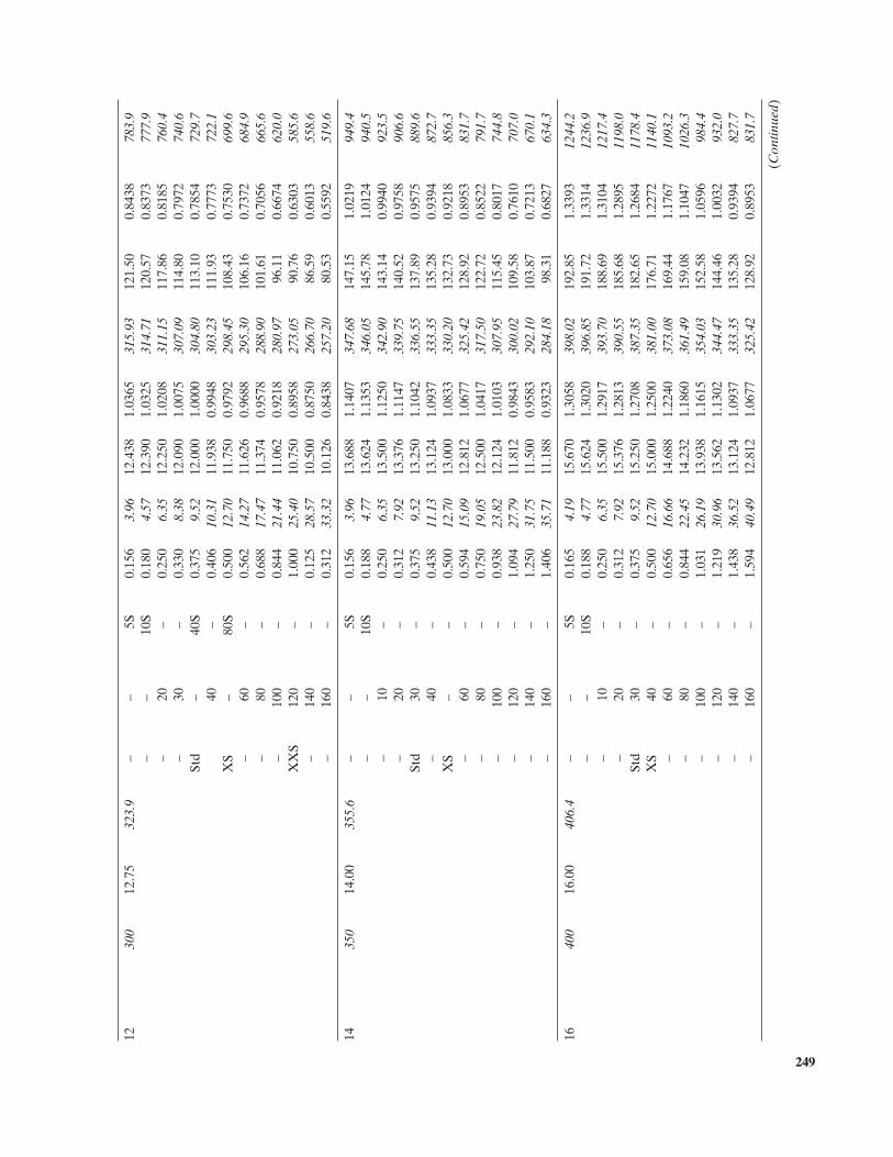
Nom
inal
P
ipe
Size
(NP
S)
(in)
Dia
met
re
Nom
inal
(DN
)
(mm
)
Out
side
D
iam
eter
Wal
l Ide
ntifi
cati
on
Wal
l T
hick
ness
In
side
Dia
met
er
Flo
w A
rea
(in)
(m
m)
Iron
P
ipe
Size
Stee
l Sc
hedu
leN
umbe
r
Stai
nles
s St
eel
Sche
dule
Num
ber
(in)
(m
m)
(i
n)
(ft)
(m
m)
(i
n 2 ) (f
t 2 )
(c
m2 )
12
300
12.7
5 32
3.9
–
–
5S
0.15
6 3.
96 12
.438
1.
0365
31
5.93
121.
50
0.84
38
783.
9 –
–
10
S 0.
180
4.57
12.3
90
1.03
25
314.
71 12
0.57
0.
8373
77
7.9
–
20
–
0.25
0 6.
35 12
.250
1.
0208
31
1.15
117.
86
0.81
85
760.
4 –
30
–
0.
330
8.38
12.0
90
1.00
75
307.
09 11
4.80
0.
7972
74
0.6
Std
–
40S
0.37
5 9.
52 12
.000
1.
0000
30
4.80
113.
10
0.78
54
729.
7
40
–
0.
406
10.3
1 11
.938
0.
9948
30
3.23
111.
93
0.77
73
722.
1 X
S –
80
S 0.
500
12.7
0 11
.750
0.
9792
29
8.45
108.
43
0.75
30
699.
6 –
60
–
0.
562
14.2
7 11
.626
0.
9688
29
5.30
106.
16
0.73
72
684.
9 –
80
–
0.
688
17.4
7 11
.374
0.
9578
28
8.90
101.
61
0.70
56
665.
6 –
10
0 –
0.
844
21.4
4 11
.062
0.
9218
28
0.97
96.1
1 0.
6674
62
0.0
XX
S 12
0 –
1.
000
25.4
0 10
.750
0.
8958
27
3.05
90.7
6 0.
6303
58
5.6
–
140
–
0.12
5 28
.57
10.5
00
0.87
50
266.
70 86
.59
0.60
13
558.
6 –
16
0 –
0.
312
33.3
2 10
.126
0.
8438
25
7.20
80.5
3 0.
5592
51
9.6
14
350
14.0
0 35
5.6
–
–
5S
0.15
6 3.
96 13
.688
1.
1407
34
7.68
147.
15
1.02
19
949.
4 –
–
10
S 0.
188
4.77
13.6
24
1.13
53
346.
05 14
5.78
1.
0124
94
0.5
–
10
–
0.25
0 6.
35 13
.500
1.
1250
34
2.90
143.
14
0.99
40
923.
5 –
20
–
0.
312
7.92
13.3
76
1.11
47
339.
75 14
0.52
0.
9758
90
6.6
Std
30
–
0.37
5 9.
52 13
.250
1.
1042
33
6.55
137.
89
0.95
75
889.
6 –
40
–
0.
438
11.1
3 13
.124
1.
0937
33
3.35
135.
28
0.93
94
872.
7 X
S –
–
0.
500
12.7
0 13
.000
1.
0833
33
0.20
132.
73
0.92
18
856.
3 –
60
–
0.
594
15.0
9 12
.812
1.
0677
32
5.42
128.
92
0.89
53
831.
7 –
80
–
0.
750
19.0
5 12
.500
1.
0417
31
7.50
122.
72
0.85
22
791.
7 –
10
0 –
0.
938
23.8
2 12
.124
1.
0103
30
7.95
115.
45
0.80
17
744.
8 –
12
0 –
1.
094
27.7
9 11
.812
0.
9843
30
0.02
109.
58
0.76
10
707.
0 –
14
0 –
1.
250
31.7
5 11
.500
0.
9583
29
2.10
103.
87
0.72
13
670.
1 –
16
0 –
1.
406
35.7
1 11
.188
0.
9323
28
4.18
98.3
1 0.
6827
63
4.3
16
400
16.0
0 40
6.4
–
–
5S
0.16
5 4.
19 15
.670
1.
3058
39
8.02
192.
85
1.33
93
1244
.2 –
–
10
S 0.
188
4.77
15.6
24
1.30
20
396.
85 19
1.72
1.
3314
12
36.9
–
10
–
0.25
0 6.
35 15
.500
1.
2917
39
3.70
188.
69
1.31
04
1217
.4 –
20
–
0.
312
7.92
15.3
76
1.28
13
390.
55 18
5.68
1.
2895
11
98.0
Std
30
–
0.37
5 9.
52 15
.250
1.
2708
38
7.35
182.
65
1.26
84
1178
.4 X
S 40
–
0.
500
12.7
0 15
.000
1.
2500
38
1.00
176.
71
1.22
72
1140
.1 –
60
–
0.
656
16.6
6 14
.688
1.
2240
37
3.08
169.
44
1.17
67
1093
.2 –
80
–
0.
844
22.4
5 14
.232
1.
1860
36
1.49
159.
08
1.10
47
1026
.3 –
10
0 –
1.
031
26.1
9 13
.938
1.
1615
35
4.03
152.
58
1.05
96
984.
4 –
12
0 –
1.
219
30.9
6 13
.562
1.
1302
34
4.47
144.
46
1.00
32
932.
0 –
14
0 –
1.
438
36.5
2 13
.124
1.
0937
33
3.35
135.
28
0.93
94
827.
7 –
16
0 –
1.
594
40.4
9 12
.812
1.
0677
32
5.42
128.
92
0.89
53
831.
7
249
(Con
tinue
d)
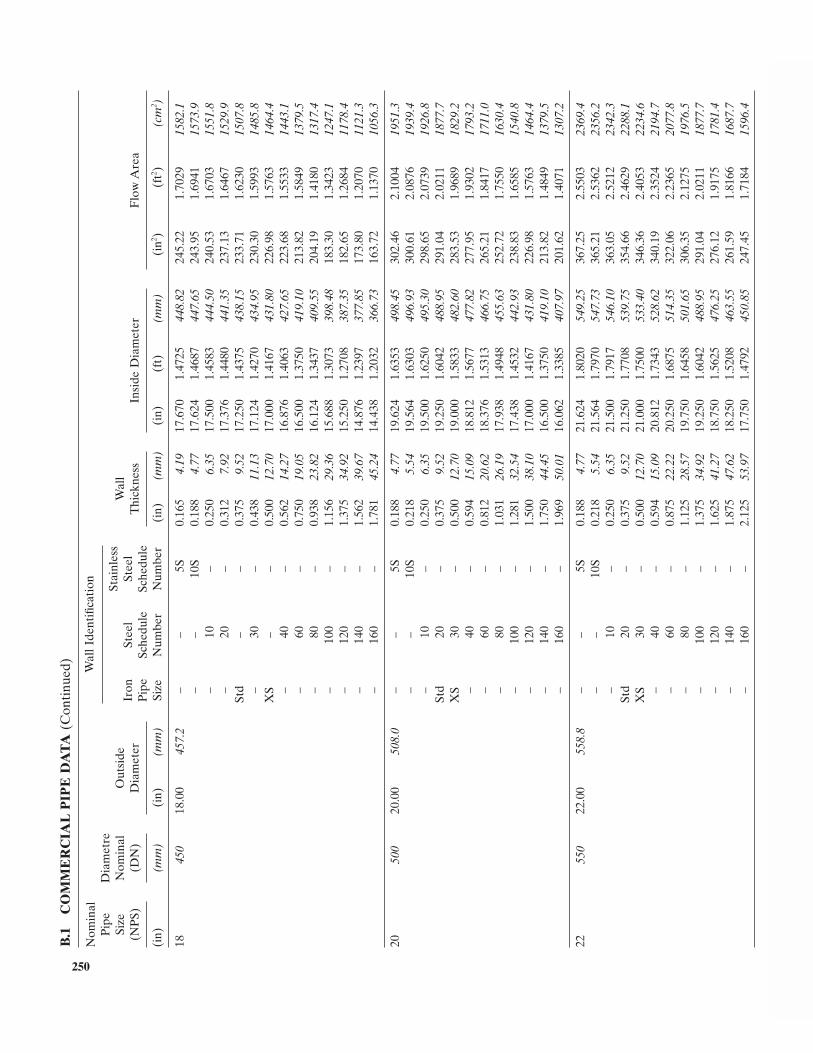
Nom
inal
P
ipe
Si D
iam
etre
N
il
Oid
Wal
l Ide
ntifi
cati
on
Wll
Stai
nles
s
Nom
inal
P
ipe
Size
(NP
S)
(in)
Dia
met
re
Nom
inal
(DN
)
(mm
)
Out
side
D
iam
eter
Wal
l Ide
ntifi
cati
on
Wal
l T
hick
ness
In
side
Dia
met
er
Flo
w A
rea
(in)
(m
m)
Iron
P
ipe
Size
Stee
l Sc
hedu
leN
umbe
r
Stai
nles
s St
eel
Sche
dule
Num
ber
(in)
(m
m)
(i
n)
(ft)
(m
m)
(i
n 2 ) (f
t 2 )
(c
m2 )
18
450
18.0
0 45
7.2
–
–
5S
0.16
5 4.
19 17
.670
1.
4725
44
8.82
245.
22
1.70
29
1582
.1 –
–
10
S 0.
188
4.77
17.6
24
1.46
87
447.
65 24
3.95
1.
6941
15
73.9
–
10
–
0.25
0 6.
35 17
.500
1.
4583
44
4.50
240.
53
1.67
03
1551
.8 –
20
–
0.
312
7.92
17.3
76
1.44
80
441.
35 23
7.13
1.
6467
15
29.9
Std
–
–
0.37
5 9.
52 17
.250
1.
4375
43
8.15
233.
71
1.62
30
1507
.8 –
30
–
0.
438
11.1
3 17
.124
1.
4270
43
4.95
230.
30
1.59
93
1485
.8 X
S –
–
0.
500
12.7
0 17
.000
1.
4167
43
1.80
226.
98
1.57
63
1464
.4 –
40
–
0.
562
14.2
7 16
.876
1.
4063
42
7.65
223.
68
1.55
33
1443
.1 –
60
–
0.
750
19.0
5 16
.500
1.
3750
41
9.10
213.
82
1.58
49
1379
.5 –
80
–
0.
938
23.8
2 16
.124
1.
3437
40
9.55
204.
19
1.41
80
1317
.4 –
10
0 –
1.
156
29.3
6 15
.688
1.
3073
39
8.48
183.
30
1.34
23
1247
.1 –
12
0 –
1.
375
34.9
2 15
.250
1.
2708
38
7.35
182.
65
1.26
84
1178
.4 –
14
0 –
1.
562
39.6
7 14
.876
1.
2397
37
7.85
173.
80
1.20
70
1121
.3 –
16
0 –
1.
781
45.2
4 14
.438
1.
2032
36
6.73
163.
72
1.13
70
1056
.3
20
500
20.0
0 50
8.0
–
–
5S
0.18
8 4.
77 19
.624
1.
6353
49
8.45
302.
46
2.10
04
1951
.3 –
–
10
S 0.
218
5.54
19.5
64
1.63
03
496.
93 30
0.61
2.
0876
19
39.4
–
10
–
0.25
0 6.
35 19
.500
1.
6250
49
5.30
298.
65
2.07
39
1926
.8 St
d 20
–
0.
375
9.52
19.2
50
1.60
42
488.
95 29
1.04
2.
0211
18
77.7
XS
30
–
0.50
0 12
.70
19.0
00
1.58
33
482.
60 28
3.53
1.
9689
18
29.2
–
40
–
0.59
4 15
.09
18.8
12
1.56
77
477.
82 27
7.95
1.
9302
17
93.2
–
60
–
0.81
2 20
.62
18.3
76
1.53
13
466.
75 26
5.21
1.
8417
17
11.0
–
80
–
1.03
1 26
.19
17.9
38
1.49
48
455.
63 25
2.72
1.
7550
16
30.4
–
100
–
1.28
1 32
.54
17.4
38
1.45
32
442.
93 23
8.83
1.
6585
15
40.8
–
120
–
1.50
0 38
.10
17.0
00
1.41
67
431.
80 22
6.98
1.
5763
14
64.4
–
140
–
1.75
0 44
.45
16.5
00
1.37
50
419.
10 21
3.82
1.
4849
13
79.5
–
160
–
1.96
9 50
.01
16.0
62
1.33
85
407.
97 20
1.62
1.
4071
13
07.2
22
550
22.0
0 55
8.8
–
–
5S
0.18
8 4.
77 21
.624
1.
8020
54
9.25
367.
25
2.55
03
2369
.4 –
–
10
S 0.
218
5.54
21.5
64
1.79
70
547.
73 36
5.21
2.
5362
23
56.2
–
10
–
0.25
0 6.
35 21
.500
1.
7917
54
6.10
363.
05
2.52
12
2342
.3 St
d 20
–
0.
375
9.52
21.2
50
1.77
08
539.
75 35
4.66
2.
4629
22
88.1
XS
30
–
0.50
0 12
.70
21.0
00
1.75
00
533.
40 34
6.36
2.
4053
22
34.6
–
40
–
0.59
4 15
.09
20.8
12
1.73
43
528.
62 34
0.19
2.
3524
21
94.7
–
60
–
0.87
5 22
.22
20.2
50
1.68
75
514.
35 32
2.06
2.
2365
20
77.8
–
80
–
1.12
5 28
.57
19.7
50
1.64
58
501.
65 30
6.35
2.
1275
19
76.5
–
100
–
1.37
5 34
.92
19.2
50
1.60
42
488.
95 29
1.04
2.
0211
18
77.7
–
120
–
1.62
5 41
.27
18.7
50
1.56
25
476.
25 27
6.12
1.
9175
17
81.4
–
140
–
1.87
5 47
.62
18.2
50
1.52
08
463.
55 26
1.59
1.
8166
16
87.7
–
160
–
2.12
5 53
.97
17.7
50
1.47
92
450.
85 24
7.45
1.
7184
15
96.4
250
B.1
C
OM
ME
RC
IAL
PIP
E D
ATA
(C
onti
nued
)
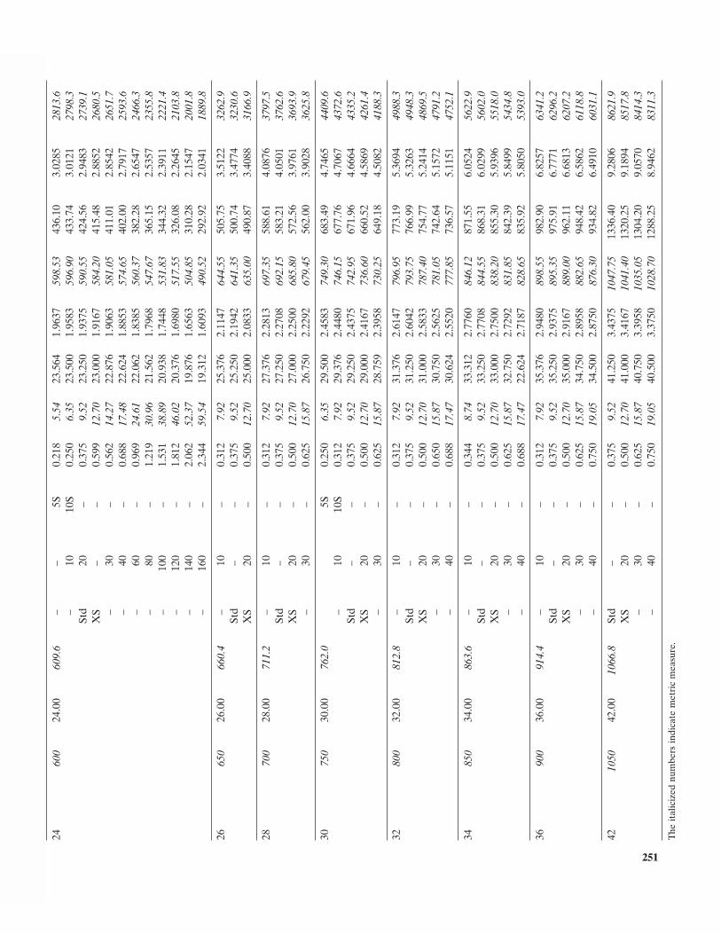
Size
(NP
S)
(in)
Nom
inal
(DN
)
(mm
)
Out
side
Dia
met
erW
all
Thi
ckne
ss
Insi
de D
iam
eter
F
low
Are
a
(in)
(m
m)
Iron
P
ipe
Size
Stee
l Sc
hedu
leN
umbe
r
Stai
nles
sSt
eel
Sche
dule
Num
ber
(in)
(m
m)
(i
n)
(ft)
(m
m)
(i
n 2 ) (f
t 2 )
(c
m2 )
24
600
24.0
0 60
9.6
–
–
5S
0.21
8 5.
54 23
.564
1.
9637
59
8.53
436.
10
3.02
85
2813
.6 –
10
10
S 0.
250
6.35
23.5
00
1.95
83
596.
90 43
3.74
3.
0121
27
98.3
Std
20
–
0.37
5 9.
52 23
.250
1.
9375
59
0.55
424.
56
2.94
83
2739
.1 X
S –
–
0.
599
12.7
0 23
.000
1.
9167
58
4.20
415.
48
2.88
52
2680
.5 –
30
–
0.
562
14.2
7 22
.876
1.
9063
58
1.05
411.
01
2.85
42
2651
.7 –
40
–
0.
688
17.4
8 22
.624
1.
8853
57
4.65
402.
00
2.79
17
2593
.6 –
60
–
0.
969
24.6
1 22
.062
1.
8385
56
0.37
382.
28
2.65
47
2466
.3 –
80
–
1.
219
30.9
6 21
.562
1.
7968
54
7.67
365.
15
2.53
57
2355
.8 –
10
0 –
1.
531
38.8
9 20
.938
1.
7448
53
1.83
344.
32
2.39
11
2221
.4 –
12
0 –
1.
812
46.0
2 20
.376
1.
6980
51
7.55
326.
08
2.26
45
2103
.8 –
14
0 –
2.
062
52.3
7 19
.876
1.
6563
50
4.85
310.
28
2.15
47
2001
.8 –
16
0 –
2.
344
59.5
4 19
.312
1.
6093
49
0.52
292.
92
2.03
41
1889
.8
26
650
26.0
0 66
0.4
–
10
–
0.31
2 7.
92 25
.376
2.
1147
64
4.55
505.
75
3.51
22
3262
.9 St
d –
–
0.
375
9.52
25.2
50
2.19
42
641.
35 50
0.74
3.
4774
32
30.6
XS
20
–
0.50
0 12
.70
25.0
00
2.08
33
635.
00 49
0.87
3.
4088
31
66.9
28
700
28.0
0 71
1.2
–
10
–
0.31
2 7.
92 27
.376
2.
2813
69
7.35
588.
61
4.08
76
3797
.5 St
d –
–
0.
375
9.52
27.2
50
2.27
08
692.
15 58
3.21
4.
0501
37
62.6
XS
20
–
0.50
0 12
.70
27.0
00
2.25
00
685.
80 57
2.56
3.
9761
36
93.9
–
30
–
0.62
5 15
.87
26.7
50
2.22
92
679.
45 56
2.00
3.
9028
36
25.8
30
750
30.0
0 76
2.0
5S
0.25
0 6.
35 29
.500
2.
4583
74
9.30
683.
49
4.74
65
4409
.6 –
10
10
S 0.
312
7.92
29.3
76
2.44
80
746.
15 67
7.76
4.
7067
43
72.6
Std
–
–
0.37
5 9.
52 29
.250
2.
4375
74
2.95
671.
96
4.66
64
4335
.2 X
S 20
–
0.
500
12.7
0 29
.000
2.
4167
73
6.60
660.
52
4.58
69
4261
.4 –
30
–
0.
625
15.8
7 28
.759
2.
3958
73
0.25
649.
18
4.50
82
4188
.3
32
800
32.0
0 81
2.8
–
10
–
0.31
2 7.
92 31
.376
2.
6147
79
6.95
773.
19
5.36
94
4988
.3 St
d –
–
0.
375
9.52
31.2
50
2.60
42
793.
75 76
6.99
5.
3263
49
48.3
XS
20
–
0.50
0 12
.70
31.0
00
2.58
33
787.
40 75
4.77
5.
2414
48
69.5
–
30
–
0.65
0 15
.87
30.7
50
2.56
25
781.
05 74
2.64
5.
1572
47
91.2
–
40
–
0.68
8 17
.47
30.6
24
2.55
20
777.
85 73
6.57
5.
1151
47
52.1
34
850
34.0
0 86
3.6
–
10
–
0.34
4 8.
74 33
.312
2.
7760
84
6.12
871.
55
6.05
24
5622
.9 St
d –
–
0.
375
9.52
33.2
50
2.77
08
844.
55 86
8.31
6.
0299
56
02.0
XS
20
–
0.50
0 12
.70
33.0
00
2.75
00
838.
20 85
5.30
5.
9396
55
18.0
–
30
–
0.62
5 15
.87
32.7
50
2.72
92
831.
85 84
2.39
5.
8499
54
34.8
–
40
–
0.68
8 17
.47
22.6
24
2.71
87
828.
65 83
5.92
5.
8050
53
93.0
36
900
36.0
0 91
4.4
–
10
–
0.31
2 7.
92 35
.376
2.
9480
89
8.55
982.
90
6.82
57
6341
.2 St
d –
–
0.
375
9.52
35.2
50
2.93
75
895.
35 97
5.91
6.
7771
62
96.2
XS
20
–
0.50
0 12
.70
35.0
00
2.91
67
889.
00 96
2.11
6.
6813
62
07.2
–
30
–
0.62
5 15
.87
34.7
50
2.89
58
882.
65 94
8.42
6.
5862
61
18.8
–
40
–
0.75
0 19
.05
34.5
00
2.87
50
876.
30 93
4.82
6.
4910
60
31.1
42
1050
42.0
0 10
66.8
Std
–
–
0.37
5 9.
52 41
.250
3.
4375
10
47.7
5 13
36.4
0 9.
2806
86
21.9
XS
20
–
0.50
0 12
.70
41.0
00
3.41
67
1041
.40
1320
.25
9.18
94
8517
.8 –
30
–
0.
625
15.8
7 40
.750
3.
3958
10
35.0
5 13
04.2
0 9.
0570
84
14.3
–
40
–
0.75
0 19
.05
40.5
00
3.37
50
1028
.70
1288
.25
8.94
62
8311
.3
The
ital
iciz
ed n
umbe
rs in
dica
te m
etri
c m
easu
re.
251
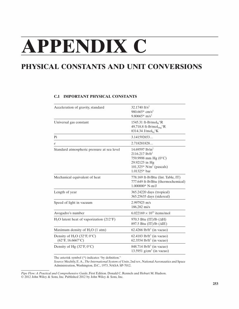
253
APPENDIX C PHYSICAL CONSTANTS AND UNIT CONVERSIONS
C.1 IMPORTANT PHYSICAL CONSTANTS
Acceleration of gravity, standard 32.1740 ft/s 2
980.665 * cm/s 2
9.80665 * m/s 2
Universal gas constant 1545.31 ft - lb/mol lb ° R 49,718.8 ft - lb/mol slug ° R 8314.34 J/mol kg ° K
Pi 3.141592653 …
e 2.718281828 …
Standard atmospheric pressure at sea level 14.69597 lb/in 2
2116.217 lb/ft 2
759.9998 mm Hg (0 ° C) 29.92125 in Hg 101,325 * N/m 2 (pascals) 1.01325 * bar
Mechanical equivalent of heat 778.169 ft - lb/Btu (Int. Table, IT) 777.649 ft - lb/Btu (thermochemical) 1.000000 * N - m/J
Length of year 365.24220 days (tropical) 365.25635 days (sidereal)
Speed of light in vacuum 2.997925 m/s 186,282 mi/s
Avogadro ’ s number 6.022169 × 10 23 items/mol
H 2 O latent heat of vaporization (212 ° F) 970.3 Btu (IT)/lb ( Δ H) 897.5 Btu (IT)/lb ( Δ IE)
Maximum density of H 2 O (1 atm) 62.4266 lb/ft 3 (in vacuo)
Density of H 2 O (32 ° F, 0 ° C) (62 ° F, 16.6667 ° C)
62.4183 lb/ft 3 (in vacuo) 62.3554 lb/ft 3 (in vacuo)
Density of Hg (32 ° F, 0 ° C) 848.714 lb/ft 3 (in vacuo) 13.5951 g/cm 3 (in vacuo)
The asterisk symbol ( * ) indicates “ by defi nition. ” Source : Mechtly, E. A., The International System of Units , 2nd rev., National Aeronautics and Space Administration, Washington, D.C., 1973, NASA SP-7012.
Pipe Flow: A Practical and Comprehensive Guide, First Edition. Donald C. Rennels and Hobart M. Hudson.© 2012 John Wiley & Sons, Inc. Published 2012 by John Wiley & Sons, Inc.
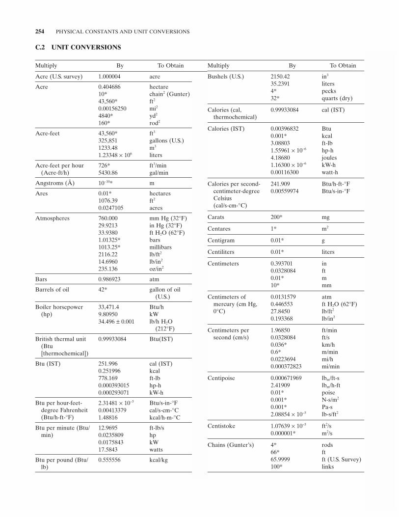
254 PHYSICAL CONSTANTS AND UNIT CONVERSIONS
C.2 UNIT CONVERSIONS
Multiply By To Obtain
Acre (U.S. survey) 1.000004 acre
Acre 0.404686 hectare 10 * chain 2 (Gunter) 43,560 * ft 2
0.00156250 mi 2
4840 * yd 2
160 * rod 2
Acre - feet 43,560 * ft 3
325,851 gallons (U.S.) 1233.48 m 3
1.23348 × 10 6 liters
Acre - feet per hour (Acre- ft/h)
726 * ft 3 /min 5430.86 gal/min
Angstroms ( Å ) 10 − 10 * m
Ares 0.01 * hectares 1076.39 ft 2
0.0247105 acres
Atmospheres 760.000 mm Hg (32 ° F) 29.9213 in Hg (32 ° F) 33.9380 ft H 2 O (62 ° F) 1.01325 * bars 1013.25 * millibars 2116.22 lb/ft 2
14.6960 lb/in 2
235.136 oz/in 2
Bars 0.986923 atm
Barrels of oil 42 * gallon of oil (U.S.)
Boiler horsepower (hp)
33,471.4 Btu/h 9.80950 kW 34.496 ± 0.001 lb/h H 2 O
(212 ° F)
British thermal unit (Btu[thermochemical])
0.99933084 Btu(IST)
Btu (IST) 251.996 cal (IST) 0.251996 kcal 778.169 ft - lb 0.000393015 hp - h 0.000293071 kW - h
Btu per hour - feet - degree Fahrenheit (Btu/h- ft - ° F)
2.31481 × 10 − 5 Btu/s - in - ° F 0.00413379 cal/s - cm - ° C 1.48816 kcal/h - m - ° C
Btu per minute (Btu/min)
12.9695 ft - lb/s 0.0235809 hp 0.0175843 kW 17.5843 watts
Btu per pound (Btu/lb)
0.555556 kcal/kg
Multiply By To Obtain
Bushels (U.S.) 2150.42 in 3
35.2391 liters 4 * pecks 32 * quarts (dry)
Calories (cal, thermochemical)
0.99933084 cal (IST)
Calories (IST) 0.00396832 Btu 0.001 * kcal 3.08803 ft - lb 1.55961 × 10 − 6 hp - h 4.18680 joules 1.16300 × 10 − 6 kW - h 0.00116300 watt - h
Calories per second - centimeter - degree Celsius(cal/s - cm - ° C)
241.909 Btu/h - ft - ° F 0.00559974 Btu/s - in - ° F
Carats 200 * mg
Centares 1 * m 2
Centigram 0.01 * g
Centiliters 0.01 * liters
Centimeters 0.393701 in 0.0328084 ft 0.01 * m 10 * mm
Centimeters of mercury (cm Hg, 0 ° C)
0.0131579 atm 0.446553 ft H 2 O (62 ° F) 27.8450 lb/ft 2
0.193368 lb/in 2
Centimeters per second (cm/s)
1.96850 ft/min 0.0328084 ft/s 0.036 * km/h 0.6 * m/min 0.0223694 mi/h 0.000372823 mi/min
Centipoise 0.000671969 lb m /ft - s 2.41909 lb m /h - ft 0.01 * poise 0.001 * N - s/m 2
0.001 * Pa - s 2.08854 × 10 − 5 lb - s/ft 2
Centistoke 1.07639 × 10 − 5 ft 2 /s 0.000001 * m 2 /s
Chains (Gunter ’ s) 4 * rods 66 * ft 65.9999 ft (U.S. Survey) 100 * links
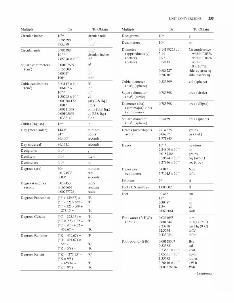
UNIT CONVERSIONS 255
Multiply By To Obtain
Circular inches 10 6 * circular mils 0.785398 in 2
785,398 mils 2
Circular mils 0.785398 mils 2
10 − 6 * circular inches 7.85398 × 10 − 7 in 2
Square centimeters (cm2 )
0.00107639 ft 2
0.155000 in 2
0.0001 * m 2
100 * mm 2
Cubic centimeters (cm3 )
3.53147 × 10 − 5 ft 3
0.0610237 in 3
10 − 6 * m 3
1.30795 × 10 − 6 yd 3
0.000264172 gal (U.S. liq.) 0.001 * liters 0.00211338 pints (U.S. liq.) 0.00105669 qt (U.S. liq.) 0.0338140 fl oz
Cubit (English) 18 * in
Day (mean solar) 1440 * minutes 24 * hours 86,400 * seconds
Day (sidereal) 86,164.1 seconds
Decigrams 0.1 * g
Deciliters 0.1 * liters
Decimeters 0.1 * m
Degrees (arc) 60 * minutes 0.0174533 rad 3600 * seconds
Degrees(arc) per second
0.0174533 rad/s 0.1666667 rev/min 0.00277778 rev/s
Degrees Fahrenheit ( ° F + 459.67) = ° R ( ° F − 32) × 5/9 = ° C ( ° F − 32) × 5/9 +
273.15 = ° K
Degrees Celsius ( ° C + 273.15) = ° K ( ° C × 9/5) + 32 = ° F ( ° C × 9/5) + 32 +
459.67 = ° R
Degrees Rankine ( ° R − 459.67) = ° F ( ° R − 491.67) ×
5/9 = ° C ( ° R × 5/9) = ° K
Degrees Kelvin ( ° K) − 273.15 ° = ° C ( ° K × 9/5)
– 459.67 = ° F ( ° K × 9/5) = ° R
Multiply By To Obtain
Decagrams 10 * g
Decameters 10 * m
Diameter 3.14159265 . . . Circumference (approximately) 3.14 within 0.05% (better) 22/7 within 0.04% (better) 355/113 within
8 × 10 − 6 % 0.886227 side eq area sq 0.707107 side inscrib sq
Cubic diameter (dia3 ) (sphere)
0.523599 vol (sphere)
Square diameter (dia2 ) (circle)
0.785398 area (circle)
Diameter (dia) (semimajor) × dia (semiminor)
0.785398 area (ellipse)
Square diameter (dia2 ) (sphere)
3.14159 area (sphere)
Drams (avoirdupois, avd.)
27.34375 grains 0.0625 * oz (avd.) 1.771845 g f
Dynes 10 − 5 * newtons 2.24809 × 10 − 6 lb f 0.0157366 grains f 3.59694 × 10 − 5 oz f (avoir.) 3.27846 × 10 − 5 oz f (troy)
Dynes per centimeter
0.001 * N/m 5.71015 × 10 − 6 lb/in
Fathoms 6 * ft
Feet (U.S. survey) 1.000002 ft
Feet 30.48 * cm 12 * in 0.3048 * m 1/3 * yd 0.0606061 rods
Foot water (ft H 2 O) (62 ° F)
0.0294655 atm 0.881644 in Hg (32 ° F) 2.23938 cm Hg (0 ° C) 62.3554 lb/ft 2
0.433024 lb/in 2
Foot - pound (ft - lb) 0.00128507 Btu 0.323831 cal 3.23831 × 10 − 4 kcal 5.05051 × 10 − 7 hp - h 1.35582 joules 3.76616 × 10 − 7 kW - h 0.000376616 W - h
(Continued)
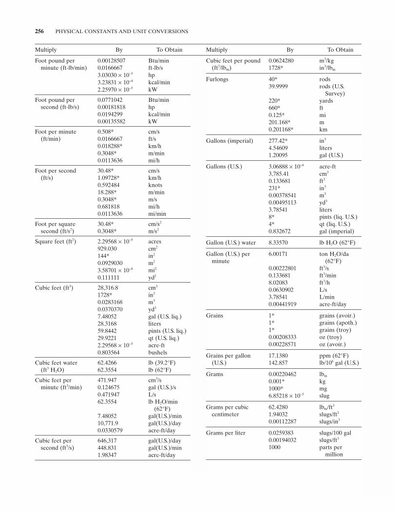
256 PHYSICAL CONSTANTS AND UNIT CONVERSIONS
Multiply By To Obtain
Foot pound per minute (ft - lb/min)
0.00128507 Btu/min 0.0166667 ft - lb/s 3.03030 × 10 − 5 hp 3.23831 × 10 − 4 kcal/min 2.25970 × 10 − 5 kW
Foot pound per second (ft - lb/s)
0.0771042 Btu/min 0.00181818 hp 0.0194299 kcal/min 0.00135582 kW
Foot per minute (ft/min)
0.508 * cm/s 0.0166667 ft/s 0.018288 * km/h 0.3048 * m/min 0.0113636 mi/h
Foot per second (ft/s)
30.48 * cm/s 1.09728 * km/h 0.592484 knots 18.288 * m/min 0.3048 * m/s 0.681818 mi/h 0.0113636 mi/min
Foot per square second (ft/s 2 )
30.48 * cm/s 2
0.3048 * m/s 2
Square feet (ft 2 ) 2.29568 × 10 − 5 acres 929.030 cm 2
144 * in 2
0.0929030 m 2
3.58701 × 10 − 8 mi 2
0.111111 yd 2
Cubic feet (ft 3 ) 28,316.8 cm 3
1728 * in 3
0.0283168 m 3
0.0370370 yd 3
7.48052 gal (U.S. liq.) 28.3168 liters 59.8442 pints (U.S. liq.) 29.9221 qt (U.S. liq.) 2.29568 × 10 − 5 acre - ft 0.803564 bushels
Cubic feet water (ft3 H 2 O)
62.4266 lb (39.2 ° F) 62.3554 lb (62 ° F)
Cubic feet per minute (ft 3 /min)
471.947 cm 3 /s 0.124675 gal (U.S.)/s 0.471947 L/s 62.3554 lb H 2 O/min
(62 ° F) 7.48052 gal(U.S.)/min 10,771.9 gal(U.S.)/day 0.0330579 acre - ft/day
Cubic feet per second (ft 3 /s)
646,317 gal(U.S.)/day 448.831 gal(U.S.)/min 1.98347 acre - ft/day
Multiply By To Obtain
Cubic feet per pound (ft3 /lb m )
0.0624280 m 3 /kg 1728 * in 3 /lb m
Furlongs 40 * rods 39.9999 rods (U.S.
Survey) 220 * yards 660 * ft 0.125 * mi 201.168 * m 0.201168 * km
Gallons (imperial) 277.42 * in 3
4.54609 liters 1.20095 gal (U.S.)
Gallons (U.S.) 3.06888 × 10 − 6 acre - ft 3,785.41 cm 3
0.133681 ft 3
231 * in 3
0.00378541 m 3
0.00495113 yd 3
3.78541 liters 8 * pints (liq. U.S.) 4 * qt (liq. U.S.) 0.832672 gal (imperial)
Gallon (U.S.) water 8.33570 lb H 2 O (62 ° F)
Gallon (U.S.) per minute
6.00171 ton H 2 O/da (62 ° F)
0.00222801 ft 3 /s 0.133681 ft 3 /min 8.02083 ft 3 /h 0.0630902 L/s 3.78541 L/min 0.00441919 acre - ft/day
Grains 1 * grains (avoir.) 1 * grains (apoth.) 1 * grains (troy) 0.00208333 oz (troy) 0.00228571 oz (avoir.)
Grains per gallon (U.S.)
17.1380 ppm (62 ° F) 142.857 lb/10 6 gal (U.S.)
Grams 0.00220462 lb m 0.001 * kg 1000 * mg 6.85218 × 10 − 5 slug
Grams per cubic centimeter
62.4280 lb m /ft 3
1.94032 slugs/ft 3
0.00112287 slugs/in 3
Grams per liter 0.0259383 slugs/100 gal 0.00194032 slugs/ft 3
1000 parts per million

UNIT CONVERSIONS 257
Multiply By To Obtain
Gravity, std. 32.17405 ft/s 2
980.665 * cm/s 2
9.80665 * m/s 2
Hectares 2.47105 acres 107,639 ft 2
100 * acres
Hectograms 100 * g
Hectoliters 100 * Liters
Hectometers 100 * m
Hectowatts 100 * watts
Hex across fl ats 1.154701 Across corners
Hogsheads 63 * gal (U.S.) 238.481 Liters
Horsepower 42.4072 Btu/min 33,000 * ft - lb/min 550 * ft - lb/s 1.01387 metric hp
(cheval - vapeur)
10.6864 kcal/min 0.745700 kW 745.700 watts
Horsepower (boiler) 33,471.4 Btu/h 9.80950 kW 34.496 ± 0.001 lb/h H 2 O
(212 ° F)
Horsepower - hour 2544.43 Btu 6.41186 × 10 5 cal 641.186 kcal 1,980,000 * ft - lb 2.68452 × 10 6 joules 0.745700 kW - h 745.700 watt - h
Inches 2.54 * cm 0.0833333 ft 1000 * mils
Inch of mercury (in Hg, 32 ° F)
0.0334211 atm 70.7262 lb/ft 2
0.491154 lb/in 2
1.13424 ft H 2 O (62 ° F) 13.6109 in H 2 O (62 ° F) 7.85847 oz/in 2
Inch of water (in H2 O, 62 ° F)
0.00245546 atm 0.577365 oz/in 2
5.19628 lb/ft 2
0.0360853 lb/in 2
0.0734703 in Hg (32 ° F)
Square inch (in 2 ) 6.4516 * cm 2
0.00694444 ft 2
645.16 * mm 2
1.27324 circular in 1,273,240 circular mils 1,000,000 * mils 2
Multiply By To Obtain
Cubic inch (in 3 ) 16.3871 cm 3
0.000578704 ft 3
1.63871 × 10 − 5 m 3
2.14335 × 10 − 5 yd 3
0.00432900 gal (U.S.) 0.0163871 liters 0.0346320 pints (liq. U.S.) 0.0173160 qt (liq. U.S.)
Cubic inch per pound (in 3 /lb m )
3.61273 × 10 − 5 m 3 /kg 0.000578704 ft 3 /lb m
Joules 0.000947817 Btu 0.238846 cal 0.000238846 kcal 0.737562 ft - lb 3.72506 × 10 − 7 hp - h 2.77778 × 10 − 7 kW - h 0.000277778 watt - h 1 * watt - s
Kilocalories (kcal) 3.96832 Btu 1000 * cal 3088.03 ft - lb 0.00155961 hp - h 4186.80 joules 0.00116300 kW - h 1.16300 watt - h
Kilocalories per cubic meter (kcal/m3 )
0.112370 Btu/ft 3
Kilocalories per hour - meter - degree Celsius(kcal/h - m - ° C)
0.671969 Btu/h - ft - ° F
Kilocalories per kilogram (kcal/kg)
1.8 * Btu/lb
Kilocalories per minute (kcal/min)
51.4671 ft - lb/s 0.0935766 hp 0.0697800 kW
Kilograms 1000 * g 2.20462 lb m 0.0685218 slugs 0.001 * metric tons
Kilograms per square meter (kg f /m 2 )
0.00142233 lb/in 2
0.204816 lb/ft 2
Kilograms per square centimeter(kgf /cm 2 )
14.2233 lb/in 2
2048.16 lb/ft 2
Kilograms per hour (kg/h)
0.000612395 lb m /s 0.0367437 lb m /min 2.20462 lb m /h
(Continued)
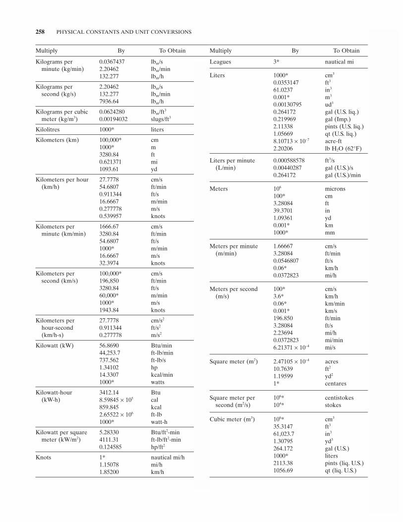
258 PHYSICAL CONSTANTS AND UNIT CONVERSIONS
Multiply By To Obtain
Kilograms per minute (kg/min)
0.0367437 lb m /s 2.20462 lb m /min 132.277 lb m /h
Kilograms per second (kg/s)
2.20462 lb m /s 132.277 lb m /min 7936.64 lb m /h
Kilograms per cubic meter (kg/m 3 )
0.0624280 lb m /ft 3
0.00194032 slugs/ft 3
Kilolitres 1000 * liters
Kilometers (km) 100,000 * cm 1000 * m 3280.84 ft 0.621371 mi 1093.61 yd
Kilometers per hour (km/h)
27.7778 cm/s 54.6807 ft/min 0.911344 ft/s 16.6667 m/min 0.277778 m/s 0.539957 knots
Kilometers per minute (km/min)
1666.67 cm/s 3280.84 ft/min 54.6807 ft/s 1000 * m/min 16.6667 m/s 32.3974 knots
Kilometers per second (km/s)
100,000 * cm/s 196,850 ft/min 3280.84 ft/s 60,000 * m/min 1000 * m/s 1943.84 knots
Kilometers per hour - second (km/h - s)
27.7778 cm/s 2
0.911344 ft/s 2
0.277778 m/s 2
Kilowatt (kW) 56.8690 Btu/min 44,253.7 ft - lb/min 737.562 ft - lb/s 1.34102 hp 14.3307 kcal/min 1000 * watts
Kilowatt - hour (kW - h)
3412.14 Btu 8.59845 × 10 5 cal 859.845 kcal 2.65522 × 10 6 ft - lb 1000 * watt - h
Kilowatt per square meter (kW/m 2 )
5.28330 Btu/ft 2 - min 4111.31 ft - lb/ft 2 - min 0.124585 hp/ft 2
Knots 1 * nautical mi/h 1.15078 mi/h 1.85200 km/h
Multiply By To Obtain
Leagues 3 * nautical mi
Liters 1000 * cm 3
0.0353147 ft 3
61.0237 in 3
0.001 * m 3
0.00130795 ud 3
0.264172 gal (U.S. liq.) 0.219969 gal (Imp.) 2.11338 pints (U.S. liq.) 1.05669 qt (U.S. liq.) 8.10713 × 10 − 7 acre - ft 2.20206 lb H 2 O (62 ° F)
Liters per minute (L/min)
0.000588578 ft 3 /s 0.00440287 gal (U.S.)/s 0.264172 gal (U.S.)/min
Meters 10 6 microns 100 * cm 3.28084 ft 39.3701 in 1.09361 yd 0.001 * km 1000 * mm
Meters per minute (m/min)
1.66667 cm/s 3.28084 ft/min 0.0546807 ft/s 0.06 * km/h 0.0372823 mi/h
Meters per second (m/s)
100 * cm/s 3.6 * km/h 0.06 * km/min 0.001 * km/s 196.850 ft/min 3.28084 ft/s 2.23694 mi/h 0.0372823 mi/min 6.21371 × 10 − 4 mi/s
Square meter (m 2 ) 2.47105 × 10 − 4 acres 10.7639 ft 2
1.19599 yd 2
1 * centares
Square meter per second (m 2 /s)
10 6 * centistokes 10 4 * stokes
Cubic meter (m 3 ) 10 6 * cm 3
35.3147 ft 3
61,023.7 in 3
1.30795 yd 3
264.172 gal (U.S.) 1000 * liters 2113.38 pints (liq. U.S.) 1056.69 qt (liq. U.S.)
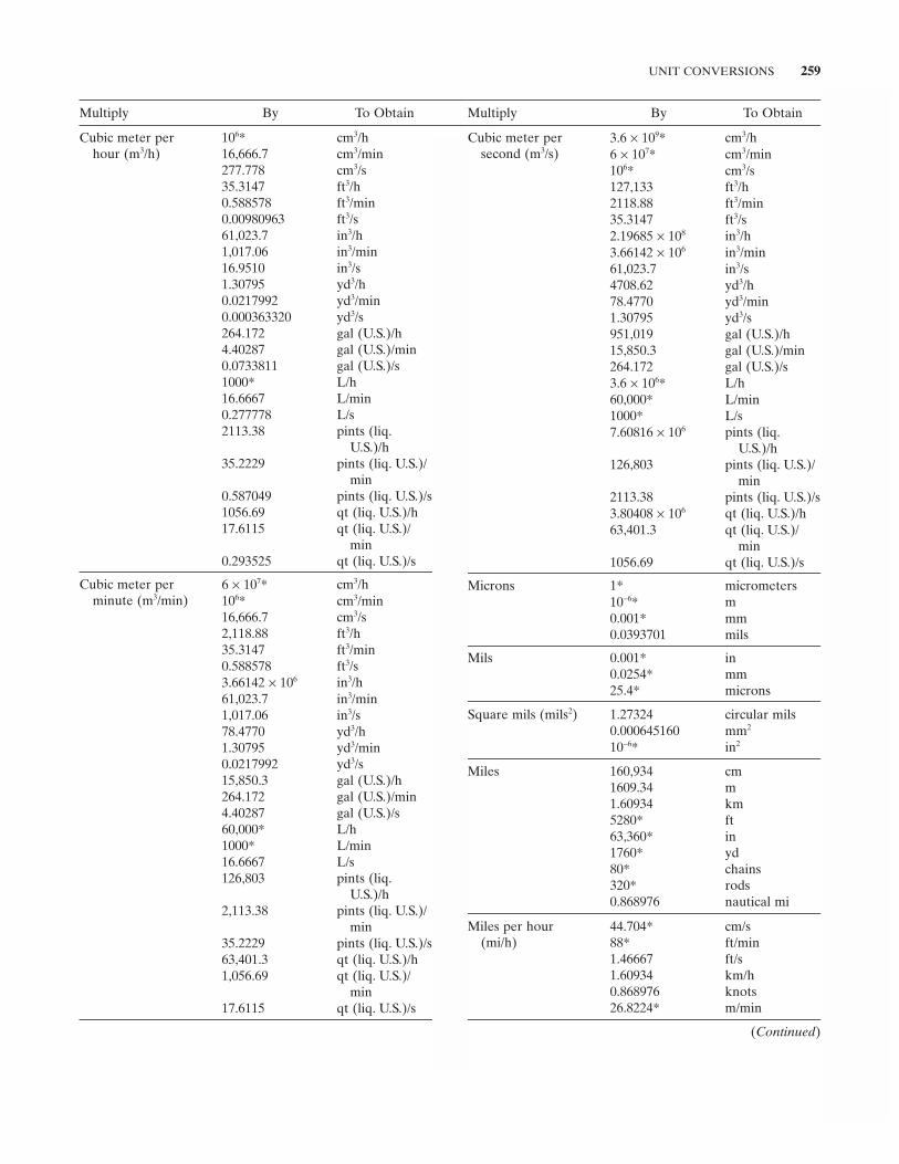
UNIT CONVERSIONS 259
Multiply By To Obtain
Cubic meter per hour (m 3 /h)
10 6 * cm 3 /h 16,666.7 cm 3 /min 277.778 cm 3 /s 35.3147 ft 3 /h 0.588578 ft 3 /min 0.00980963 ft 3 /s 61,023.7 in 3 /h 1,017.06 in 3 /min 16.9510 in 3 /s 1.30795 yd 3 /h 0.0217992 yd 3 /min 0.000363320 yd 3 /s 264.172 gal (U.S.)/h 4.40287 gal (U.S.)/min 0.0733811 gal (U.S.)/s 1000 * L/h 16.6667 L/min 0.277778 L/s 2113.38 pints (liq.
U.S.)/h 35.2229 pints (liq. U.S.)/
min 0.587049 pints (liq. U.S.)/s 1056.69 qt (liq. U.S.)/h 17.6115 qt (liq. U.S.)/
min 0.293525 qt (liq. U.S.)/s
Cubic meter per minute (m 3 /min)
6 × 10 7 * cm 3 /h 10 6 * cm 3 /min 16,666.7 cm 3 /s 2,118.88 ft 3 /h 35.3147 ft 3 /min 0.588578 ft 3 /s 3.66142 × 10 6 in 3 /h 61,023.7 in 3 /min 1,017.06 in 3 /s 78.4770 yd 3 /h 1.30795 yd 3 /min 0.0217992 yd 3 /s 15,850.3 gal (U.S.)/h 264.172 gal (U.S.)/min 4.40287 gal (U.S.)/s 60,000 * L/h 1000 * L/min 16.6667 L/s 126,803 pints (liq.
U.S.)/h 2,113.38 pints (liq. U.S.)/
min 35.2229 pints (liq. U.S.)/s 63,401.3 qt (liq. U.S.)/h 1,056.69 qt (liq. U.S.)/
min 17.6115 qt (liq. U.S.)/s
Multiply By To Obtain
Cubic meter per second (m 3 /s)
3.6 × 10 9 * cm 3 /h 6 × 10 7 * cm 3 /min 10 6 * cm 3 /s 127,133 ft 3 /h 2118.88 ft 3 /min 35.3147 ft 3 /s 2.19685 × 10 8 in 3 /h 3.66142 × 10 6 in 3 /min 61,023.7 in 3 /s 4708.62 yd 3 /h 78.4770 yd 3 /min 1.30795 yd 3 /s 951,019 gal (U.S.)/h 15,850.3 gal (U.S.)/min 264.172 gal (U.S.)/s 3.6 × 10 6 * L/h 60,000 * L/min 1000 * L/s 7.60816 × 10 6 pints (liq.
U.S.)/h 126,803 pints (liq. U.S.)/
min 2113.38 pints (liq. U.S.)/s 3.80408 × 10 6 qt (liq. U.S.)/h 63,401.3 qt (liq. U.S.)/
min 1056.69 qt (liq. U.S.)/s
Microns 1 * micrometers 10 − 6 * m 0.001 * mm 0.0393701 mils
Mils 0.001 * in 0.0254 * mm 25.4 * microns
Square mils (mils 2 ) 1.27324 circular mils 0.000645160 mm 2
10 − 6 * in 2
Miles 160,934 cm 1609.34 m 1.60934 km 5280 * ft 63,360 * in 1760 * yd 80 * chains 320 * rods 0.868976 nautical mi
Miles per hour (mi/h)
44.704 * cm/s 88 * ft/min 1.46667 ft/s 1.60934 km/h 0.868976 knots 26.8224 * m/min
(Continued)
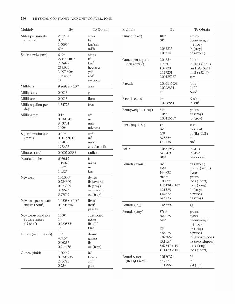
260 PHYSICAL CONSTANTS AND UNIT CONVERSIONS
Multiply By To Obtain
Miles per minute (mi/min)
2682.24 cm/s 88 * ft/s 1.60934 km/min 60 * mi/h
Square mile (mi 2 ) 640 * acres 27,878,400 * ft 2
2.58999 km 2
258.999 hectares 3,097,600 * yd 2
102,400 * rod 2
1 * sections
Millibars 9.86923 × 10 − 4 atm
Milligrams 0.001 * g
Milliliters 0.001 * liters
Million gallon per day
1.54723 ft 3 /s
Millimeters 0.1 * cm 0.0393701 in 39.3701 mils 1000 * microns
Square millimeter (mm2 )
0.01 * cm 2
0.00155000 in 2
1550.00 mils 2
1973.53 circular mils
Minutes (arc) 0.000290888 radians
Nautical miles 6076.12 ft 1.15078 miles 1852 * m 1.852 * km
Newtons 100,000 * dynes 0.224809 lb (avoir.) 0.273205 lb (troy) 3.59694 oz (avoir.) 3.27846 oz (troy)
Newtons per square meter (N/m 2 )
1.45038 × 10 − 4 lb/in 2
0.0208854 lb/ft 2
1 * pascals
Newton - second per square meter (N - s/m 2 )
1000 * centipoise 10 * poise 0.0208854 lb - s/ft 2
1 * Pa - s
Ounce (avoirdupois) 16 * drams 437.5 * grains 0.0625 * lb 0.911458 oz (troy)
Ounce (fl uid) 1.80469 in 3
0.0295735 Liters 29.5735 cm 3
0.25 * gills
Multiply By To Obtain
Ounce (troy) 480 * grains 20 * pennyweight
(troy) 0.083333 lb (troy) 1.09714 oz (avoir.)
Ounce per square inch (oz/in 2 )
0.0625 * lb/in 2
1.73201 in H 2 O (62 ° F) 4.39930 cm H 2 O (62 ° F) 0.127251 in Hg (32 ° F) 0.00425287 atm
Pascals 0.000145038 lb/in 2
0.0208854 lb/ft 2
1 * N/m 2
Pascal - second 1 * N - s/m 2
0.0208854 lb - s/ft 2
Pennyweights (troy) 24 * grains 0.05 * oz (troy) 0.00416667 lb (troy)
Pints (liq. U.S.) 4 * gills 16 * oz (fl uid) 0.5 * qt (liq. U.S.) 28.875 * in 3
473.176 cm 3
Poise 0.0671969 lb m /ft - s 241.909 lb m /ft - h 100 * centipoise
Pounds (avoir.) 16 * oz (avoir.) 256 * drams (avoir.) 444,822 dynes 7000 * grains 0.0005 * tons (short) 4.46429 × 10 − 4 tons (long) 1.21528 lb (troy) 4.44822 newtons 14.5833 oz (troy)
Pounds (lb m ) 0.453592 kg
Pounds (troy) 5760 * grains 366,025 dynes 240 * pennyweight.
(troy) 12 * oz (troy) 3.66025 newtons 0.822857 lb (avoirdupois) 13.1657 oz (avoirdupois) 3.67347 × 10 − 4 tons (long) 4.11429 × 10 − 4 tons (short)
Pound water (lb H 2 O, 62 ° F)
0.0160371 ft 3
27.7121 in 3
0.119966 gal (U.S.)
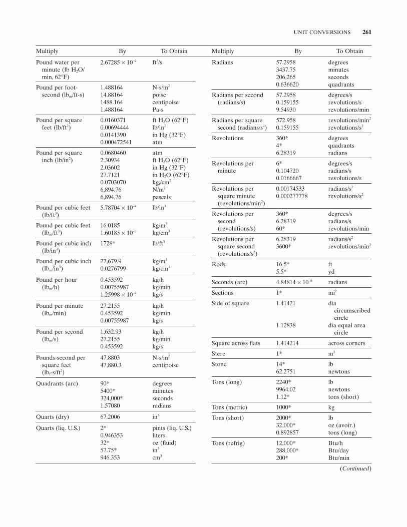
UNIT CONVERSIONS 261
Multiply By To Obtain
Pound water per minute (lb H 2 O/min, 62 ° F)
2.67285 × 10 − 4 ft 3 /s
Pound per foot - second (lb m /ft - s)
1.488164 N - s/m 2
14.88164 poise 1488.164 centipoise 1.488164 Pa - s
Pound per square feet (lb/ft 2 )
0.0160371 ft H 2 O (62 ° F) 0.00694444 lb/in 2
0.0141390 in Hg (32 ° F) 0.000472541 atm
Pound per square inch (lb/in 2 )
0.0680460 atm 2.30934 ft H 2 O (62 ° F) 2.03602 in Hg (32 ° F) 27.7121 in H 2 O (62 ° F) 0.0703070 kg f /cm 2
6,894.76 N/m 2
6,894.76 pascals
Pound per cubic feet (lb/ft3 )
5.78704 × 10 − 4 lb/in 3
Pound per cubic feet (lbm /ft 3 )
16.0185 kg/m 3
1.60185 × 10 − 5 kg/cm 3
Pound per cubic inch (lb/in3 )
1728 * lb/ft 3
Pound per cubic inch (lbm /in 3 )
27,679.9 kg/m 3
0.0276799 kg/cm 3
Pound per hour (lbm /h)
0.453592 kg/h 0.00755987 kg/min 1.25998 × 10 − 4 kg/s
Pound per minute (lbm /min)
27.2155 kg/h 0.453592 kg/min 0.00755987 kg/s
Pound per second (lbm /s)
1,632.93 kg/h 27.2155 kg/min 0.453592 kg/s
Pounds - second per square feet (lbf - s/ft 2 )
47.8803 N - s/m 2
47,880.3 centipoise
Quadrants (arc) 90 * degrees 5400 * minutes 324,000 * seconds 1.57080 radians
Quarts (dry) 67.2006 in 3
Quarts (liq. U.S.) 2 * pints (liq. U.S.) 0.946353 liters 32 * oz (fl uid) 57.75 * in 3
946.353 cm 3
Multiply By To Obtain
Radians 57.2958 degrees 3437.75 minutes 206,265 seconds 0.636620 quadrants
Radians per second (radians/s)
57.2958 degrees/s 0.159155 revolutions/s 9.54930 revolutions/min
Radians per square second (radians/s 2 )
572.958 revolutions/min 2
0.159155 revolutions/s 2
Revolutions 360 * degrees 4 * quadrants 6.28319 radians
Revolutions per minute
6 * degrees/s 0.104720 radians/s 0.0166667 revolutions/s
Revolutions per square minute (revolutions/min2 )
0.00174533 radians/s 2
0.000277778 revolutions/s 2
Revolutions per second(revolutions/s)
360 * degrees/s 6.28319 radians/s 60 * revolutions/min
Revolutions per square second (revolutions/s2 )
6.28319 radians/s 2
3600 * revolutions/min 2
Rods 16.5 * ft 5.5 * yd
Seconds (arc) 4.84814 × 10 − 6 radians
Sections 1 * mi 2
Side of square 1.41421 dia circumscribedcircle
1.12838 dia equal area circle
Square across fl ats 1.414214 across corners
Stere 1 * m 3
Stone 14 * lb 62.2751 newtons
Tons (long) 2240 * lb 9964.02 newtons 1.12 * tons (short)
Tons (metric) 1000 * kg
Tons (short) 2000 * lb 32,000 * oz (avoir.) 0.892857 tons (long)
Tons (refrig) 12,000 * Btu/h 288,000 * Btu/day 200 * Btu/min
(Continued)
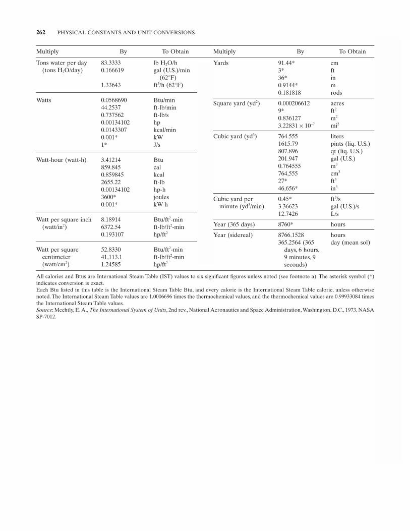
262 PHYSICAL CONSTANTS AND UNIT CONVERSIONS
All calories and Btus are International Steam Table (IST) values to six signifi cant fi gures unless noted (see footnote a). The asterisk symbol ( * ) indicates conversion is exact. Each Btu listed in this table is the International Steam Table Btu, and every calorie is the International Steam Table calorie, unless otherwise noted. The International Steam Table values are 1.0006696 times the thermochemical values, and the thermochemical values are 0.99933084 times the International Steam Table values. Source : Mechtly, E. A., The International System of Units , 2nd rev., National Aeronautics and Space Administration, Washington, D.C., 1973, NASA SP - 7012.
Multiply By To Obtain
Tons water per day (tons H 2 O/day)
83.3333 lb H 2 O/h 0.166619 gal (U.S.)/min
(62 ° F) 1.33643 ft 3 /h (62 ° F)
Watts 0.0568690 Btu/min 44.2537 ft - lb/min 0.737562 ft - lb/s 0.00134102 hp 0.0143307 kcal/min 0.001 * kW 1 * J/s
Watt - hour (watt - h) 3.41214 Btu 859.845 cal 0.859845 kcal 2655.22 ft - lb 0.00134102 hp - h 3600 * joules 0.001 * kW - h
Watt per square inch (watt/in2 )
8.18914 Btu/ft 2 - min 6372.54 ft - lb/ft 2 - min 0.193107 hp/ft 2
Watt per square centimeter(watt/cm2 )
52.8330 Btu/ft 2 - min 41,113.1 ft - lb/ft 2 - min 1.24585 hp/ft 2
Multiply By To Obtain
Yards 91.44 * cm 3 * ft 36 * in 0.9144 * m 0.181818 rods
Square yard (yd 2 ) 0.000206612 acres 9 * ft 2
0.836127 m 2
3.22831 × 10 − 7 mi 2
Cubic yard (yd 3 ) 764.555 liters 1615.79 pints (liq. U.S.) 807.896 qt (liq. U.S.) 201.947 gal (U.S.) 0.764555 m 3
764,555 cm 3
27 * ft 3
46,656 * in 3
Cubic yard per minute (yd 3 /min)
0.45 * ft 3 /s 3.36623 gal (U.S.)/s 12.7426 L/s
Year (365 days) 8760 * hours
Year (sidereal) 8766.1528 hours 365.2564 (365
days, 6 hours, 9 minutes, 9 seconds)
day (mean sol)
263
APPENDIX D COMPRESSIBILITY FACTOR EQUATIONS
D.1 THE REDLICH – KWONG EQUATION
The Redlich - Kwong equation is actually an equation of state. It was formulated by Otto Redlich and Joseph N. S. Kwong in 1949 [ Chemical Review , 44, 1949, 233 - 244]. Their equation is
P = nRT
ba
b TV V V,
−−
+( )
anR T
Pa c
c
= Ω ( ),
.2 2 5
bnRTP
b c
c
= Ω,
where Tc and Pc are the critical temperature and pres-sure of the gas being considered. The constants in the equation are derived as
Ωa = − =−[( )( ) ] . ,/9 2 1 0 427481 3 1
Ωb = − =[( ) ]/ . ./2 1 3 0 086641 3
This equation is quite accurate at the critical tempera-ture for P/Pc = 4 to 40 (error < 2.5%). At higher tem-peratures and at P/Pc above about 5 the equation becomes increasingly inaccurate.
The compressibility factor may be found explicitly from the Redlich - Kwong equation. It is the principal
root of a cubic. Robert C. Reid, John M. Prausnitz, and Thomas K. Sherwood [ The Properties of Gases and Liquids , 3 rd Ed., McGraw - Hill Book Company, 1977] give the cubic as
z z A B B z A B3 2 2 0− + − − − =( ) ,* * * * *
where
AP
TP
Ta r
r
r
r
* = =Ω5 2 5 2
0 42748/ /
. ,
BP
TPT
b r
r
r
r
* . .= =Ω0 086640
In the equations below, Pr is the reduced pressure (that is, the ratio of actual pressure to critical pressure), and Tr is the reduced temperature (that is, the ratio of actual temperature to critical temperature). Let A , B , C , D , and E be constants defi ned by
APT
r
r
= 0 08664. ,
BTr
= 4 93403 2
.,
/
C A A AB= + −2 ,
Pipe Flow: A Practical and Comprehensive Guide, First Edition. Donald C. Rennels and Hobart M. Hudson.© 2012 John Wiley & Sons, Inc. Published 2012 by John Wiley & Sons, Inc.
264 COMPRESSIBILITY FACTOR EQUATIONS
where
B bbT
bT
bTr r r
= − − −12 3
243
,
C ccT
cTr r
= − +12 3
3,
D ddTr
= +12 ,
VV
rc
c
PRT
( )( )
,00
=
and
exp( )
.( )
/( )( )−
= −γ γ
VV
r
e r0 2
0 2
The constants for these equations for a simple fl uid are given in Table D.1 . (The β and γ shown are for the Lee – Kesler equation and should not be confused with those in the Nomenclature.) The equation is solved for Vr
( )0 ,the ideal reduced volume for a simple fl uid, and then the simple fl uid compressibility factor is calculated:
zP
Tr r
r
00
( )( )
= V. (D.2)
Next, using the same reduced pressure and temperature, the equation is solved again for Vr
( )0 , but using the refer-ence fl uid constants from the table; therefore, call this value V R
r( ). Then:
zP
Tr r
r
( )( )
.RRV=
The compressibility factor z for the fl uid of interest is then calculated from the following formula:
z z z z= +
−( )( ) ( ) ( )0 0ωωR
R ,
where ω is Pitzer ’ s acentric factor, and for the reference gas, ωR = 0.3978. The defi nition of the acentric factor is:
ω = − −=log ( ) ..10 0 7 1 000Pvap Tr r ,
DC= − −3
19
,
EC A B= + +6 2
127
2
.
If D3 + E2 ≥ 0, then
z E D E E D E= + + + − + +3 23 3 23 13
.
If D3 + E2 < 0, then
z DE
D= − −
−
+−21
313
1
3cos cos .
Critical constants for selected gases are given in Table D.3 in Section D.3 . Chemical Engineers ’ Handbook (5 th
Ed., McGraw Hill, 1973) indicates that the Redlich - Kwong equation of state fi ts the data for helium and hydrogen only for reduced temperatures of 2.5 and higher when their critical temperatures are increased by 8 ° C, and their critical pressures are increased by 8 atmospheres.
D.2 THE LEE – KESLER EQUATION
Another equation of state that is much more accurate than the Redlich – Kwong equation is the Lee – Kesler equation. This is a generalized Benedict – Webb – Rubin equation developed by B.I. Lee and M.G. Kesler in 1975 from which the compressibility factor may be found. The solution is formidable, but with a computer it can be obtained without much diffi culty using the Newton – Raphson trial - and - error solution technique. Their equa-tion is:
PT
B C D
cT
r r
r r r r
r r r
VV V V
V V
( )
( ) ( ) ( )
( )
( ) ( )
( ) (
0
0 0 2 0 5
43 0 2
1= + + + +
+β γ(( ) ( ))
exp( )
,0 2 0 2
−
γVr
(D.1)
TABLE D.1. Lee – Kesler Constants
Constant Simple Reference Constant Simple Reference
B1 0.1181193 0.2026579 c3 0.0 0.016901 B2 0.265728 0.331511 c4 0.042724 0.041577 B3 0.154790 0.027655 d1 × 10 4 0.155488 0.48736 B4 0.030323 0.203488 d2 × 10 4 0.623689 0.0740366 c1 0.0236744 0.0313385 β 0.65392 1.226 c2 0.0186984 0.0503618 γ 0.060167 0.03754
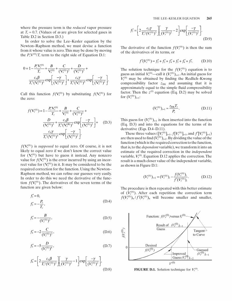
THE LEE–KESLER EQUATION 265
′ =
−
−
fc
T V V Vr r r r7
43 0 5 0 2 0 2
2 2γ γ γ
( ) ( )exp
( )( ) ( ) ( )
.
(D.9)
The derivative of the function f Vr( )( )0 is then the sum of the derivatives of its terms, or
′ = ′ + ′ + ′ + ′ + ′ + ′f V f f f f f fr( ) .( )02 3 4 5 6 7 (D.10)
The solution technique for the f Vr( )( )0 equation is to guess an initial Vr
( )0 — call it ( )( )Vr i0
1= . An initial guess for Vr
( )0 may be obtained by fi nding the Redlich – Kwong compressibility factor zRK and assuming that it is approximately equal to the simple fl uid compressibility factor. Then the z(0) equation (Eq. D.2 ) may be solved for ( )( )Vr i
01= :
( ) .( )Vz T
Pr i
r
r
01= ≈ RK (D.11)
This guess for ( )( )Vr i0
1= is then inserted into the function (Eq. D.3 ) and into the equations for the terms of its derivative (Eqs. D.4 – D.11 ).
These three values ( [ ]( )Vr i0
1= , f Vr i[ ]( )01= , and ′ =f Vr i[ ]( )0
1)are then used to fi nd ( )( )Vr i
02= . By dividing the value of the
function (which is the required correction to the function, that is, to the dependent variable), we transform it into an estimate of the required correction in the independentvariable, Vr
( )0 . Equation D.12 applies the correction. The result is a much closer value of the independent variable, as shown in Figure D.1 :
( ) ( )( )( )
.( ) ( )( )
( )V V
f Vf V
r i r ir i
r i
01
00
0+ = −′
(D.12)
The procedure is then repeated with this better estimate of ( Vr
( )0 ). After each repetition the correction term f V f Vr r( ) / ( )( ) ( )0 0
n n′ will become smaller and smaller,
where the pressure term is the reduced vapor pressure at Tr = 0.7. (Values of ω are given for selected gases in Table D.2 in Section D.3 .)
In order to solve the Lee – Kesler equation by the Newton – Raphson method, we must devise a function from it whose value is zero. This may be done by moving the Pr V (0) / Tr term to the right side of Equation D.1 :
0 10
0 0 2 0 5
43 0 2
= − + + + +PT
B C D
cT
r r
r r r r
r r
VV V V
V
( )
( ) ( ) ( )
( )
( ) ( )
( )exp
β −−
+ −
γ γ γ( ) ( )
exp( )
.( ) ( ) ( )V V Vr r r r
cT0 2
43 0 4 0 2
Call this function f r( )( )V 0 by substituting f r( )( )V 0 for the zero:
fP
TB C
D cT
rr r
r r r
r r r
( )( )
( ) (
( )( )
( ) ( )
( ) (
VV
V V
V V
00
0 0 2
0 54
3
1= − + + +
+ β00 2 0 2
43 0 4 0 2
) ( )
( ) ( )
)exp
( )
( )exp
( )
−
+
−
γ
γ γV
V V
r
r r r
cT
..
(D.3)
f r( )( )V 0 is supposed to equal zero. Of course, it is not likely to equal zero if we don ’ t know the correct value for ( Vr
( )0 ) but have to guess it instead. Any nonzero value for f r( )( )V 0 is the error incurred by using an incor-rect value for ( Vr
( )0 ) in it. It may be considered to be the required correction for the function. Using the Newton – Raphson method, we can refi ne our guesses very easily. In order to do this we need the derivative of the func-tion f r( )( )V 0 . The derivatives of the seven terms of the function are given below:
′ =
′ = −
f
fPT
r
r
1
2
0,
, (D.4)
′ = −fB
Vr3 0 2( )( )
, (D.5)
′ = −fC
Vr4 0 3
2( )( )
, (D.6)
′ = −fD
Vr5 0 6
5( )( )
, (D.7)
′ =
−
−
fc
T V V Vr r r r6
43 0 3 0 2 0 2
2 1β γ γ
( ) ( )exp
( )( ) ( ) ( )
,
(D.8) FIGURE D.1. Solution technique for Vr( )0 .
Function: versus
Tangentto Curve
Result ofGuess
Desired
ImprovedGuess
Guessed
rf(V )
i
(0) V (0)r
(V )(0)r
(0)(V )r i
f(V )(0)r
V (0)
0
)V(f
)0( r
1=
1=
r(V )(0)i 2=
266 COMPRESSIBILITY FACTOR EQUATIONS
acentric factor may be necessary to achieve the best agreement.
D.3 IMPORTANT CONSTANTS FOR SELECTED GASES
Following are two tables of important constants neces-sary to implement the Redlich – Kwong and Lee – Kesler compressibility factor equations. Table D.2 gives the acentric factor ω for selected gases.
Table D.3 gives critical constants for the same gases. Data are included for ammonia, hydrogen, and helium for use in these equations; the data for these gases should be amended as described in Section D.1 for best results in the Redlich – Kwong equation, and as described above in Section D.2 for best results in the Lee – Kesler equation.
Table D.3 includes critical constants from various authorities. It is suggested that consensus values or aver-ages of all the values be used for each constant.
until it becomes small enough — as small a value as desired or allowed by the computational precision of the computer — that the solution may be considered to have been found.
The solution technique described above has one caveat — it works well except in the region of the critical point. There the derivative approaches zero and the procedure usually gets caught in a loop. To circumvent this a different technique must be substituted on the fi rst occurrence of a change in sign of the correction term f V f Vr r( ) / ( )( ) ( )0 0′ . One method is to interpolate between the Vr
( )0 that caused the sign of f Vr( )( )0 to change and the one just previous to it to estimate the Vr
( )0 where the curve crosses the f Vr( )( )0 0= line. The reader will note that Pitzer ’ s acentric factor ω is
used in the solution for the compressibility factor z . Reid et al. ( The Properties of Gases and Liquids , 3rd ed., McGraw - Hill Book Company, New York, 1977) state that application of correlations employing the acentric factor should be limited to normal fl uids; in no case should such correlations be used for H 2 , He, Ne, or for strongly polar and/or hydrogen - bonded fl uids. There-fore, for these nonnormal fl uids it is suggested that the compressibility factor yielded by the Lee – Kesler equa-tion be compared with actual fl uid data compressibility factors on a plot such as Figure 1.3 in Chapter 1 . From this plot it may be seen what shift in critical constants will bring the Lee – Kesler compressibility factor into congruence with the real compressibility factor for the largest region on the chart. Several modifi cations of the
TABLE D.2. Acentric Factor ω for Selected Gases
Acetylene 0.184 CO 2 0.225 Methane 0.008 Air 0.036 Helium – 0.387 Nitrogen 0.040 Ammonia 0.250 n - Hydrogen – 0.22 Oxygen 0.021 Argon – 0.004 p - Hydrogen – 0.219 Propane 0.152
See Table D.3 footnote d for bibliography. Parahydrogen ω is calcu-lated from footnote g data.
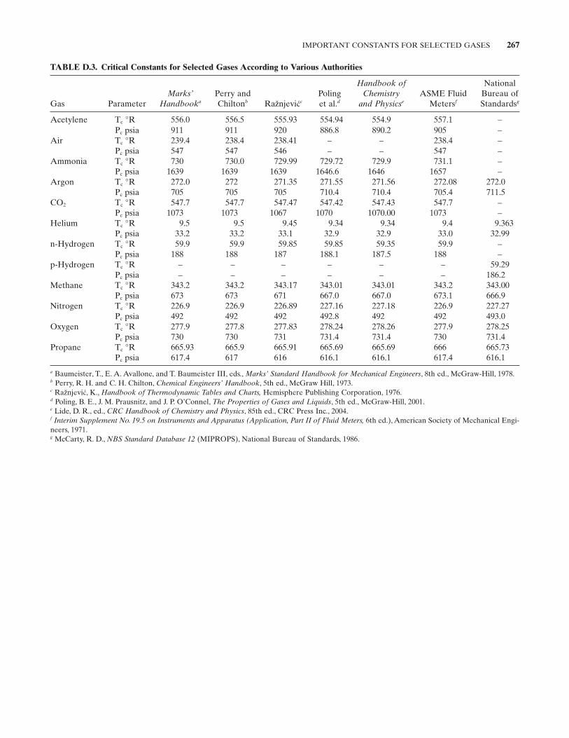
IMPORTANT CONSTANTS FOR SELECTED GASES 267
TABLE D.3. Critical Constants for Selected Gases According to Various Authorities
Gas Parameter Marks ’
Handbooka Perry and Chiltonb Ra ž njevi ćc
Poling et al. d
Handbook of Chemistry
and Physicse ASME Fluid
Metersf
National Bureau of Standardsg
Acetylene T c ° R 556.0 556.5 555.93 554.94 554.9 557.1 – P c psia 911 911 920 886.8 890.2 905 –
Air T c ° R 239.4 238.4 238.41 – – 238.4 – P c psia 547 547 546 – – 547 –
Ammonia T c ° R 730 730.0 729.99 729.72 729.9 731.1 – P c psia 1639 1639 1639 1646.6 1646 1657 –
Argon T c ° R 272.0 272 271.35 271.55 271.56 272.08 272.0 P c psia 705 705 705 710.4 710.4 705.4 711.5
CO 2 T c ° R 547.7 547.7 547.47 547.42 547.43 547.7 – P c psia 1073 1073 1067 1070 1070 .00 1073 –
Helium T c ° R 9.5 9.5 9.45 9.34 9.34 9.4 9.363 P c psia 33.2 33.2 33.1 32.9 32.9 33.0 32.99
n - Hydrogen T c ° R 59.9 59.9 59.85 59.85 59.35 59.9 – P c psia 188 188 187 188.1 187.5 188 –
p - Hydrogen T c ° R – – – – – – 59.29 P c psia – – – – – – 186.2
Methane T c ° R 343.2 343.2 343.17 343.01 343.01 343.2 343.00 P c psia 673 673 671 667.0 667.0 673.1 666.9
Nitrogen T c ° R 226.9 226.9 226.89 227.16 227.18 226.9 227.27 P c psia 492 492 492 492.8 492 492 493.0
Oxygen T c ° R 277.9 277.8 277.83 278.24 278.26 277.9 278.25 P c psia 730 730 731 731.4 731.4 730 731.4
Propane T c ° R 665.93 665.9 665.91 665.69 665.69 666 665.73 P c psia 617.4 617 616 616.1 616.1 617.4 616.1
a Baumeister, T., E. A. Avallone, and T. Baumeister III, eds., Marks ’ Standard Handbook for Mechanical Engineers , 8th ed., McGraw - Hill, 1978. b Perry, R. H. and C. H. Chilton, Chemical Engineers ’ Handbook , 5th ed., McGraw Hill, 1973. c Ra ž njevi ć , K., Handbook of Thermodynamic Tables and Charts, Hemisphere Publishing Corporation, 1976. d Poling, B. E., J. M. Prausnitz, and J. P. O ’ Connel, The Properties of Gases and Liquids , 5th ed., McGraw - Hill, 2001. e Lide, D. R., ed., CRC Handbook of Chemistry and Physics , 85th ed., CRC Press Inc., 2004. f Interim Supplement No. 19.5 on Instruments and Apparatus (Application, Part II of Fluid Meters, 6th ed.), American Society of Mechanical Engi-neers, 1971. g McCarty, R. D., NBS Standard Database 12 (MIPROPS), National Bureau of Standards, 1986.
269
APPENDIX E ADIABATIC COMPRESSIBLE FLOW WITH FRICTION, USING MACH NUMBER AS A PARAMETER
This appendix gives derivations for application equa-tions presented in Chapter 4 .
Street et al. [1] and Shapiro [2] give the following relation for a constant - area duct fl owing a gas with sonic velocity at the exit :
fL
DM
MM
Mave
max ln( )
,= − + + +
+ −
1 12
1
2 11
2
2
2
2
2γγ
γγ
γ
(4.16, repeated)
wherefave = average Darcy friction factor along the duct, Lmax = maximum attainable duct length with M at the
inlet, ft (or m), D = duct diameter, ft (or m), γ = ratio of specifi c heats of fl owing gas, and M = Mach number of the gas fl ow at the duct inlet.
In the development of this equation, f is assumed to be a constant, and fave is taken as a reasonable value for f . In actuality, of course, since fl uid temperature changes continuously along the duct, the fl uid viscosity also changes, and then so does Reynolds Number — resulting in a varying friction factor. But it turns out that the variation is modest enough to be handled by using the average friction factor.
E.1 SOLUTION WHEN STATIC PRESSURE AND STATIC TEMPERATURE ARE KNOWN
Equation 4.16 may be used to fi nd the Lmax of the duct if the essential duct data are available: fl ow rate, inlet static pressure, inlet static temperature, duct diameter, friction factor, and gas ratio of specifi c heats, molecular weight, and compressibility factor. The Mach number of a gas fl owing in a duct (assuming a fl at velocity profi le) is:
Mu V= ≈A A
. (1.4, repeated)
The equation for the acoustic velocity A is:
A mass units or A weight units= =γρ
γρ
P Pg
m w
( ) ( ).
Utilizing the equation of state, Equations 1.6 in Chapter 1 , the acoustic velocity may be expressed as:
A
J mol KKg
= = = =
= °( )
γρ
γ γ γP PP zRT
zRT zRm
T
R
m /
. / ,8314 34
(E.1a)
or
A
ft-lb/mol Rlb
= = = =
= °( )
γρ
γ γ γP PgP zRT
gzRT gzRm
T
R
w /
. .1545 31
(E.1b)
Pipe Flow: A Practical and Comprehensive Guide, First Edition. Donald C. Rennels and Hobart M. Hudson.© 2012 John Wiley & Sons, Inc. Published 2012 by John Wiley & Sons, Inc.
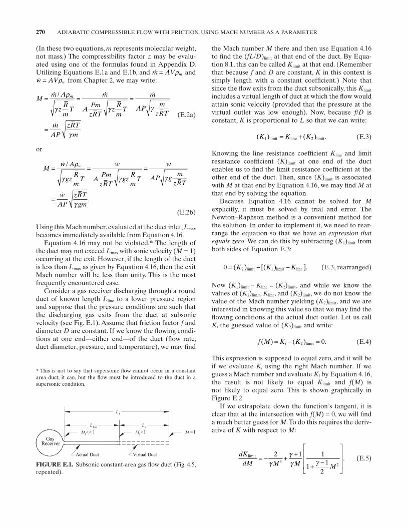
270 ADIABATIC COMPRESSIBLE FLOW WITH FRICTION, USING MACH NUMBER AS A PARAMETER
the Mach number M there and then use Equation 4.16 to fi nd the ( fL / D ) limit at that end of the duct. By Equa-tion 8.1 , this can be called Klimit at that end. (Remember that because f and D are constant, K in this context is simply length with a constant coeffi cient.) Note that since the fl ow exits from the duct subsonically, this Klimit
includes a virtual length of duct at which the fl ow would attain sonic velocity (provided that the pressure at the virtual outlet was low enough). Now, because f / D is constant, K is proportional to L so that we can write:
( ) ( ) .K K K1 2limit line limit= + (E.3)
Knowing the line resistance coeffi cient Kline and limit resistance coeffi cient ( K ) limit at one end of the duct enables us to fi nd the limit resistance coeffi cient at the other end of the duct. Then, since ( K ) limit is associated with M at that end by Equation 4.16 , we may fi nd M at that end by solving the equation.
Because Equation 4.16 cannot be solved for Mexplicitly, it must be solved by trial and error. The Newton – Raphson method is a convenient method for the solution. In order to implement it, we need to rear-range the equation so that we have an expression that equals zero . We can do this by subtracting ( K1 ) limit from both sides of Equation E.3 :
0 2 1= − −[ ]( ) ( ) .K K Klimit limit line (E.3, rearranged)
Now ( K1 ) limit – Kline = ( K2 ) limit , and while we know the values of ( K1 ) limit , Kline , and ( K2 ) limit , we do not know the value of the Mach number yielding ( K2 ) limit , and we are interested in knowing this value so that we may fi nd the fl owing conditions at the actual duct outlet. Let us call Ki the guessed value of ( K2 ) limit and write:
f M K Ki( ) ( ) .= − =2 0limit (E.4)
This expression is supposed to equal zero, and it will be if we evaluate Ki using the right Mach number. If we guess a Mach number and evaluate Ki by Equation 4.16 , the result is not likely to equal Klimit and f ( M ) is not likely to equal zero. This is shown graphically in Figure E.2 .
If we extrapolate down the function ’ s tangent, it is clear that at the intersection with f ( M ) = 0, we will fi nd a much better guess for M . To do this requires the deriv-ative of K with respect to M :
dK
dM M M M
limit = − + +
+ −
2 1 1
11
2
32γ
γγ γ . (E.5)
(In these two equations, m represents molecular weight, not mass.) The compressibility factor z may be evalu-ated using one of the formulas found in Appendix D . Utilizing Equations E.1a and E.1b , and m AV m= ρ and w AV w= ρ from Chapter 2 , we may write:
Mm A
zRm
m
APm
zRTz
Rm
m
APm
zRT
mAP
zRTm
m= = =
=
/ ρ
γ γ γ
γ
Τ Τ (E.2a)
or
Mw A
gzRm
w
APm
zRTgz
Rm
w
AP gm
zRT
wAP
zRTgm
w= = =
=
/
.
ρ
γ γ γ
γ
Τ Τ
(E.2b)
Using this Mach number, evaluated at the duct inlet, Lmax
becomes immediately available from Equation 4.16 . Equation 4.16 may not be violated. * The length of
the duct may not exceed Lmax with sonic velocity ( M = 1) occurring at the exit. However, if the length of the duct is less than Lmax as given by Equation 4.16 , then the exit Mach number will be less than unity. This is the most frequently encountered case.
Consider a gas receiver discharging through a round duct of known length Lline to a lower pressure region and suppose that the pressure conditions are such that the discharging gas exits from the duct at subsonic velocity (see Fig. E.1 ). Assume that friction factor f and diameter D are constant. If we know the fl owing condi-tions at one end — either end — of the duct (fl ow rate, duct diameter, pressure, and temperature), we may fi nd
FIGURE E.1. Subsonic constant - area gas fl ow duct (Fig. 4.5 , repeated).
M <<
L
L L
1
2enil
1 M <21 M =1 1
Actual Duct Virtual Duct
GasReceiver
* This is not to say that supersonic fl ow cannot occur in a constant area duct; it can, but the fl ow must be introduced to the duct in a supersonic condition.
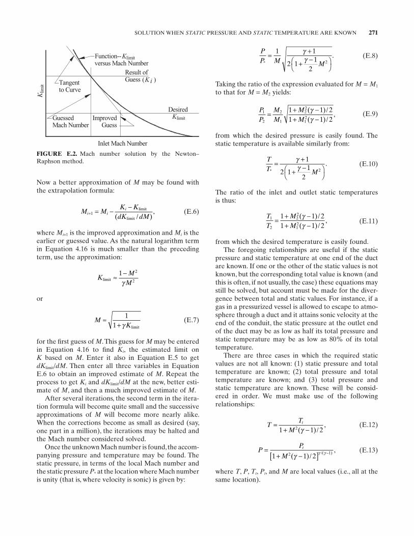
SOLUTION WHEN STATIC PRESSURE AND STATIC TEMPERATURE ARE KNOWN 271
PP M M*
.= +
+ −
1 1
2 11
22
γγ (E.8)
Taking the ratio of the expression evaluated for M = M1
to that for M = M2 yields:
PP
MM
MM
1
2
2
1
22
12
1 1 21 1 2
= + −+ −
( )/( )/
,γγ
(E.9)
from which the desired pressure is easily found. The static temperature is available similarly from:
TT M*
.= +
+ −
γγ
1
2 11
22
(E.10)
The ratio of the inlet and outlet static temperatures is thus:
TT
MM
1
2
22
12
1 1 21 1 2
= + −+ −
( )/( )/
,γγ
(E.11)
from which the desired temperature is easily found. The foregoing relationships are useful if the static
pressure and static temperature at one end of the duct are known. If one or the other of the static values is not known, but the corresponding total value is known (and this is often, if not usually, the case) these equations may still be solved, but account must be made for the diver-gence between total and static values. For instance, if a gas in a pressurized vessel is allowed to escape to atmo-sphere through a duct and it attains sonic velocity at the end of the conduit, the static pressure at the outlet end of the duct may be as low as half its total pressure and static temperature may be as low as 80% of its total temperature.
There are three cases in which the required static values are not all known: (1) static pressure and total temperature are known; (2) total pressure and total temperature are known; and (3) total pressure and static temperature are known. These will be consid-ered in order. We must make use of the following relationships:
TT
Mt=
+ −1 1 22( )/,
γ (E.12)
PP
Mt=
+ −[ ] −1 1 22 1
( )/,/( )γ γ γ (E.13)
where T , P , Tt , Pt , and M are local values (i.e., all at the same location).
Now a better approximation of M may be found with the extrapolation formula:
M MK K
dK dMi i
i+ = − −
1limit
limit( / ), (E.6)
where Mi+ 1 is the improved approximation and Mi is the earlier or guessed value. As the natural logarithm term in Equation 4.16 is much smaller than the preceding term, use the approximation:
KM
Mlimit ≈ −1 2
2γ
or
MK
≈+
11 γ limit
(E.7)
for the fi rst guess of M . This guess for M may be entered in Equation 4.16 to fi nd Ki , the estimated limit on K based on M . Enter it also in Equation E.5 to get dKlimit / dM . Then enter all three variables in Equation E.6 to obtain an improved estimate of M . Repeat the process to get Ki and dKlimit / dM at the new, better esti-mate of M , and then a much improved estimate of M .
After several iterations, the second term in the itera-tion formula will become quite small and the successive approximations of M will become more nearly alike. When the corrections become as small as desired (say, one part in a million), the iterations may be halted and the Mach number considered solved.
Once the unknown Mach number is found, the accom-panying pressure and temperature may be found. The static pressure, in terms of the local Mach number and the static pressure P * at the location where Mach number is unity (that is, where velocity is sonic) is given by:
FIGURE E.2. Mach number solution by the Newton – Raphson method.
Function--versus Mach Number
Tangentto Curve
Result ofGuess
DesiredImproved
GuessGuessedMach Number
Inlet Mach Number
Kti
mil
limitK
( )K i
limitK
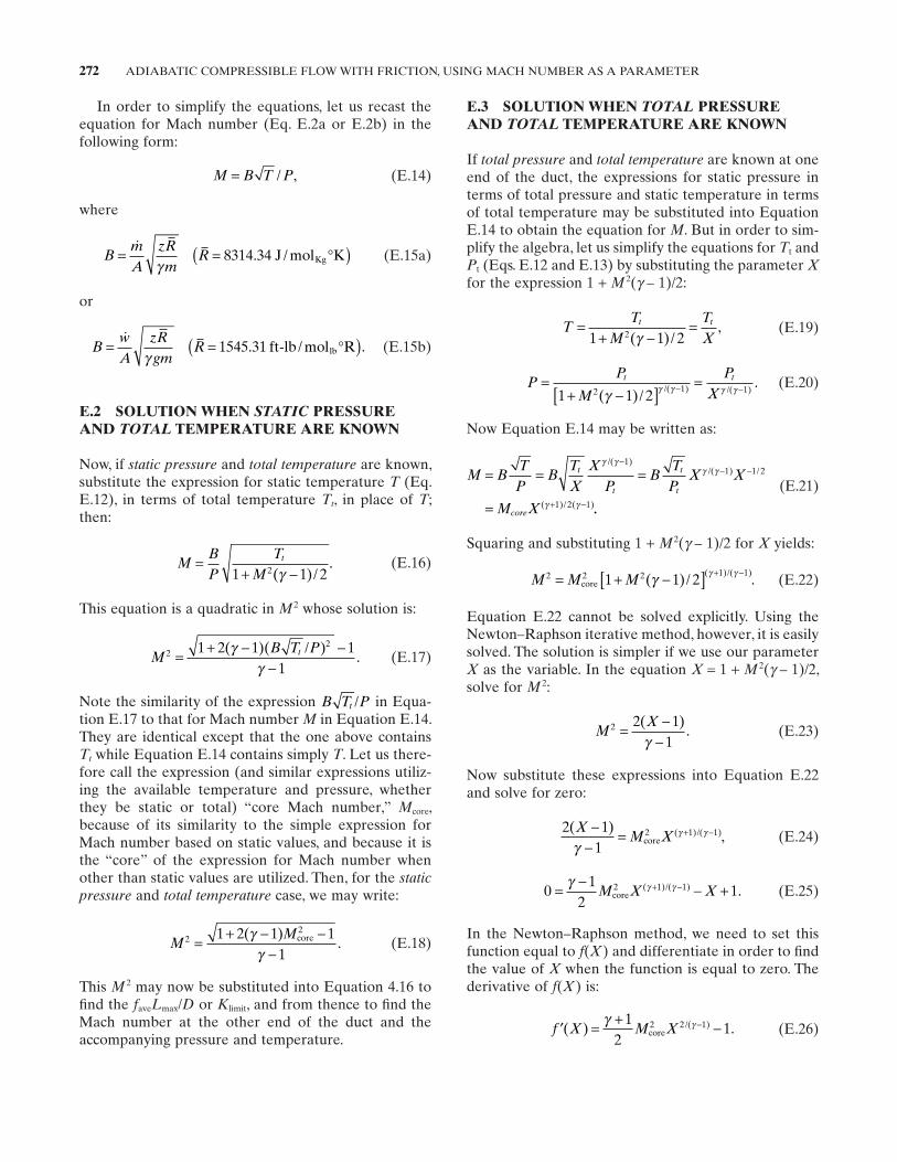
272 ADIABATIC COMPRESSIBLE FLOW WITH FRICTION, USING MACH NUMBER AS A PARAMETER
E.3 SOLUTION WHEN TOTAL PRESSURE AND TOTAL TEMPERATURE ARE KNOWN
If total pressure and total temperature are known at one end of the duct, the expressions for static pressure in terms of total pressure and static temperature in terms of total temperature may be substituted into Equation E.14 to obtain the equation for M . But in order to sim-plify the algebra, let us simplify the equations for Tt and Pt (Eqs. E.12 and E.13 ) by substituting the parameter Xfor the expression 1 + M 2 ( γ – 1)/2:
TT
MTX
t t=+ −
=1 1 22( )/
,γ
(E.19)
PP
M
PX
t t=+ −[ ]
=− −1 1 22 1 1( )/./( ) /( )γ γ γ γ γ (E.20)
Now Equation E.14 may be written as:
M BTP
BTX
XP
BTP
X X
M X
t
t
t
t
core
= = =
=
−− −
+ −
γ γγ γ
γ γ
/( )/( ) /
( )/ ( )
11 1 2
1 2 1 ..
(E.21)
Squaring and substituting 1 + M2 ( γ – 1)/2 for X yields:
M M M2 2 1 11 1 2= + −[ ] + −
core2 ( )/ .
( )/( )γ γ γ (E.22)
Equation E.22 cannot be solved explicitly. Using the Newton – Raphson iterative method, however, it is easily solved. The solution is simpler if we use our parameter X as the variable. In the equation X = 1 + M 2 ( γ – 1)/2, solve for M 2 :
MX2 2 1
1= −
−( )
.γ
(E.23)
Now substitute these expressions into Equation E.22 and solve for zero:
2 1
11 1( )
,( )/( )XM X
−−
= + −
γγ γ
core2 (E.24)
01
211 1= − − ++ −γ γ γM X Xcore
2 ( )/( ) . (E.25)
In the Newton – Raphson method, we need to set this function equal to f ( X ) and differentiate in order to fi nd the value of X when the function is equal to zero. The derivative of f ( X ) is:
′ = + −−f X M X( ) ./( )γ γ12
12 1core2 (E.26)
In order to simplify the equations, let us recast the equation for Mach number (Eq. E.2a or E.2b ) in the following form:
M B T P= / , (E.14)
where
BmA
zRm
R= = °( )γ
8314 34. /J mol KKg (E.15a)
or
BwA
zRgm
R= = °( )γ
1545 31. /ft-lb mol R .lb (E.15b)
E.2 SOLUTION WHEN STATIC PRESSURE AND TOTAL TEMPERATURE ARE KNOWN
Now, if static pressure and total temperature are known, substitute the expression for static temperature T (Eq. E.12 ), in terms of total temperature Tt , in place of T ; then:
MBP
TM
t=+ −1 1 22( )/
.γ
(E.16)
This equation is a quadratic in M2 whose solution is:
MB T Pt2
21 2 1 11
= + − −−
( )( / ).
γγ
(E.17)
Note the similarity of the expression B T Pt / in Equa-tion E.17 to that for Mach number M in Equation E.14 . They are identical except that the one above contains Tt while Equation E.14 contains simply T . Let us there-fore call the expression (and similar expressions utiliz-ing the available temperature and pressure, whether they be static or total) “ core Mach number, ” Mcore , because of its similarity to the simple expression for Mach number based on static values, and because it is the “ core ” of the expression for Mach number when other than static values are utilized. Then, for the staticpressure and total temperature case, we may write:
MM2 1 2 1 1
1= + − −
−( )
.γ
γcore2
(E.18)
This M 2 may now be substituted into Equation 4.16 to fi nd the faveLmax / D or Klimit , and from thence to fi nd the Mach number at the other end of the duct and the accompanying pressure and temperature.
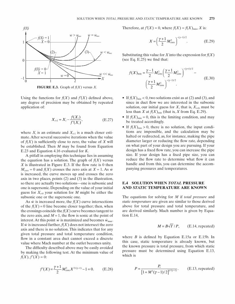
SOLUTION WHEN TOTAL PRESSURE AND STATIC TEMPERATURE ARE KNOWN 273
Therefore, at f′ ( X ) = 0, where f ( X ) = f ( X ) min , X is:
X M= +
− −γ γ12
1 2
core2
( )/
. (E.29)
Substituting this value for X into the expression for f ( X ) (see Eq. E.25 ) we fi nd that:
f X M M
M
( )min
( )/
= − +
−
+
− +γ γ
γ
γ12
12
12
1 2
core2
core2
core2
− −( )/
.γ 1 2
(E.30)
• If f ( X ) min < 0, two solutions exist as at (2) and (3), and since in duct fl ow we are interested in the subsonic solution, our initial guess for X , that is, Xi= 0 , must be less than X at f ( X ) min (that is, X from Eq. E.29 ).
• If f ( X ) min = 0, this is the limiting condition, and may be treated accordingly.
• If f ( X ) min > 0, there is no solution, the input condi-tions are impossible, and the calculation may be halted or redirected, as, for instance, making the pipe diameter larger or reducing the fl ow rate, depending on what part of your design you are pursuing. If your design has a fi xed fl ow rate, you can increase the pipe size. If your design has a fi xed pipe size, you can reduce the fl ow rate to determine what fl ow it can handle and from this, you can determine the accom-panying pressures and temperatures.
E.4 SOLUTION WHEN TOTAL PRESSURE AND STATIC TEMPERATURE ARE KNOWN
The equations for solving for M if total pressure and static temperature are given are similar to those derived above for total pressure and total temperature, and are derived similarly. Mach number is given by Equa-tion E.14 ,
M B T P= / , (E.14, repeated)
where B is defi ned by Equation E.15a or E.15b . In this case, static temperature is already known, but the known pressure is total pressure, from which static pressure must be determined using Equation E.13 , which is
PP
Mt=
+ −[ ] −1 1 22 1
( )/./( )γ γ γ (E.13, repeated)
Using the functions for f ( X ) and f′ ( X ) defi ned above, any degree of precision may be obtained by repeated application of:
X Xf Xf X
i ii
i+ = −
′1( )( )
, (E.27)
where Xi is an estimate and Xi+ 1 is a much closer esti-mate. After several successive iterations when the value of f ( X ) is suffi ciently close to zero, the value of X will be established. Then M may be found from Equation E.23 and Equation 4.16 evaluated for K .
A pitfall in employing this technique lies in assuming the equation has a solution. The graph of f ( X ) versus X is illustrated in Figure E.3 . If the fl ow rate is 0 then Mcore = 0 and f ( X ) crosses the zero axis at X = 1. As wis increased, the curve moves up and crosses the zero axis in two places, points (2) and (3) in the illustration, so there are actually two solutions — one is subsonic and one is supersonic. Depending on the value of your initial guess for Xi= 0 your solution for M might be either the subsonic one or the supersonic one.
As w is increased more, the f ( X ) curve intersections of the f ( X ) = 0 line become closer together; then, when the crossings coincide the f ( X ) curve becomes tangent to the zero axis, and M = 1, the fl ow is sonic at the point of interest. At this point w is maximized and becomes wmax.If w is increased further, f ( X ) does not intersect the zero axis and there is no solution. This indicates that for any given total pressure and total temperature condition, fl ow in a constant area duct cannot exceed a discrete value where Mach number at the outlet becomes unity.
The diffi culty described above may be easily avoided by making the following test. At the minimum value of f ( X ), f ′ ( X ) = 0:
′ = + − =−f X M X( ) ./( )γ γ12
1 02 2 1core (E.28)
FIGURE E.3. Graph of f ( X ) versus X .
f(X) =
(2)
2
f(X)
–11
0
0
1
w <
w < wmax
w = wmaxw > wmax
w = < wmax
X
f(X) =
X =
X =
(3)
0
01
01
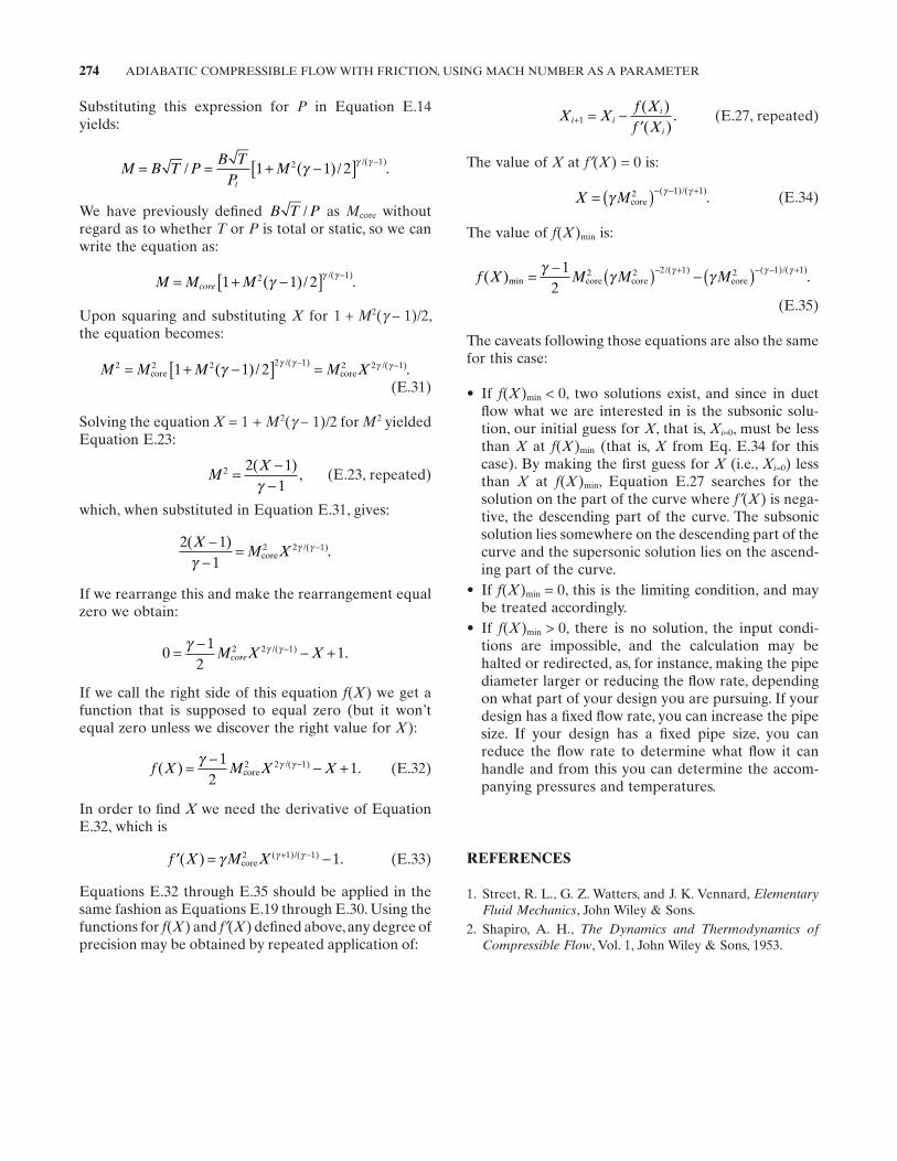
274 ADIABATIC COMPRESSIBLE FLOW WITH FRICTION, USING MACH NUMBER AS A PARAMETER
X Xf Xf X
i ii
i+ = −
′1( )( )
. (E.27, repeated)
The value of X at f′ ( X ) = 0 is:
X M= ( )− − +γ γ γcore2 1 1( )/( )
. (E.34)
The value of f ( X ) min is:
f X M M M( ) .min/( ) ( )/( )= − ( ) − ( )− + − − +γ γ γγ γ γ1
22 2 1 2 1 1
core2
core core
(E.35)
The caveats following those equations are also the same for this case:
• If f ( X ) min < 0, two solutions exist, and since in duct fl ow what we are interested in is the subsonic solu-tion, our initial guess for X , that is, Xi= 0 , must be less than X at f ( X ) min (that is, X from Eq. E.34 for this case). By making the fi rst guess for X (i.e., Xi= 0 ) less than X at f ( X ) min , Equation E.27 searches for the solution on the part of the curve where f′ ( X ) is nega-tive, the descending part of the curve. The subsonic solution lies somewhere on the descending part of the curve and the supersonic solution lies on the ascend-ing part of the curve.
• If f ( X ) min = 0, this is the limiting condition, and may be treated accordingly.
• If f ( X ) min > 0, there is no solution, the input condi-tions are impossible, and the calculation may be halted or redirected, as, for instance, making the pipe diameter larger or reducing the fl ow rate, depending on what part of your design you are pursuing. If your design has a fi xed fl ow rate, you can increase the pipe size. If your design has a fi xed pipe size, you can reduce the fl ow rate to determine what fl ow it can handle and from this you can determine the accom-panying pressures and temperatures.
REFERENCES
1. Street , R. L. , G. Z. Watters , and J. K. Vennard , ElementaryFluid Mechanics , John Wiley & Sons .
2. Shapiro , A. H. , The Dynamics and Thermodynamics of Compressible Flow , Vol. 1 , John Wiley & Sons , 1953 .
Substituting this expression for P in Equation E.14 yields:
M B T PB T
PM
t
= = + −[ ] −/ ( )/ .
/( )1 1 22 1γ γ γ
We have previously defi ned B T P/ as Mcore without regard as to whether T or P is total or static, so we can write the equation as:
M M Mcore= + −[ ] −1 1 22 1
( )/ ./( )γ γ γ
Upon squaring and substituting X for 1 + M2 ( γ – 1)/2, the equation becomes:
M M M M X2 2 2 1 2 11 1 2= + −[ ] =− −core2
core2( )/ .
/( ) /( )γ γ γ γ γ
(E.31)
Solving the equation X = 1 + M2 ( γ – 1)/2 for M2 yielded Equation E.23 :
MX2 2 1
1= −
−( )
,γ
(E.23, repeated)
which, when substituted in Equation E.31 , gives:
2 11
2 2 1( )./( )X
M X−
−= −
γγ γ
core
If we rearrange this and make the rearrangement equal zero we obtain:
01
212 2 1= − − +−γ γ γM X Xcore
/( ) .
If we call the right side of this equation f ( X ) we get a function that is supposed to equal zero (but it won ’ t equal zero unless we discover the right value for X ):
f X M X X( ) ./( )= − − +−γ γ γ12
12 1core2 (E.32)
In order to fi nd X we need the derivative of Equation E.32 , which is
′ = −+ −f X M X( ) .( )/( )γ γ γcore2 1 1 1 (E.33)
Equations E.32 through E.35 should be applied in the same fashion as Equations E.19 through E.30 . Using the functions for f ( X ) and f′ ( X ) defi ned above, any degree of precision may be obtained by repeated application of:
275
APPENDIX F VELOCITY PROFILE EQUATIONS
In this appendix, the derivations of the velocity profi le equations presented in Chapter 2 are shown.
F.1 BENEDICT VELOCITY PROFILE DERIVATION
(Equation numbers in this section are from Benedict [1] .)
In his chapter 5, section 5.4, “ Turbulent Flow in Smooth Pipes, ” Robert P. Benedict gives equation 5.74 (on p. 221 of Reference [1] ) that relates the kinetic energy correction factor to the friction factor in any fl ow situation. It is based in part on equations 5.33 and 5.36 (pp. 201, 203 of Reference [1] ), namely:
u V VRy
c= − 2 5. ln ,* (5.33)
whereu = local fl uid velocity, Vc = fl uid velocity at the center of the pipe, V * = friction velocity, y = distance of u from the wall, and R = radius of pipe;
and
V V Vc= − 3 75. ,* (5.36)
where
V = average velocity of fl uid in the pipe and Vc = velocity of fl uid at the center of the pipe.
The friction velocity is defi ned (on p. 192) as:
Vm
* ,= τρ
0 (5.18)
whereτ0 = fl uid shear stress at the wall and ρm = fl uid mass density.
Then:
V V Vc = + 3 75. .* (5.36 alternate)
Then Benedict writes:
But (5.36) is bound to defi ne an average velocity that is greater than actual, because the log law of (5.33) does not yield a zero velocity gradient at the pipe center (see Figure 5.18).
One of our questions is, “ Does equation 5.36 yield a profi le in which du/dy = 0 at the center? ” The answer is “ no, ” as Hunter Rouse [2] notes, but this is of little practical effect. Benedict expresses equation 5.33 in slightly modifi ed form as:
Pipe Flow: A Practical and Comprehensive Guide, First Edition. Donald C. Rennels and Hobart M. Hudson.© 2012 John Wiley & Sons, Inc. Published 2012 by John Wiley & Sons, Inc.
276 VELOCITY PROFILE EQUATIONS
Then:
uV
f f yR
= + +
1 3 758
2 58
. . ln . (5.36 + 5.38 + 5.40)
Is this for smooth pipes only? Benedict gives for rough pipes:
uyR
VV
+ = + +2 5 3 75. ln .*
. (5.52)
Benedict defi nes u+ as follows:
uu
V+ =
*. (5.19)
Inserting this into Equation 5.52 yields:
uV
yR
VV* *
= + +2 5 3 75. ln .
or
u VyR
V V= + +* *2 5 3 75. ln . .
By dividing by V we get:
uV
VV
yR
VV
= + +* *.2 5 3 75 1. ln .
Then, remembering that V V f* = / 8 (Eq. 5.40, alter-nate ) or V V f*/ /= 8 , we may insert it into the equa-tion above to obtain:
uV
f yR
f= + +
82 5 3 75
81. ln . .
Rearranged, this is:
uV
f f yR
= + +1 3 758
2 58
. . ln .
This is exactly the same as given above as the smooth pipe velocity profi le:
uV
f f yR
= + +
1 3 75
82 5
8. . ln .
So the velocity profi le equation given above is valid (according to Benedict) for both smooth and rough pipes.
The plot of this equation is shown in Figure F.1 .
uV
VV
yRc c
= +
1 2 5. ln*
. (5.38)
Using the Darcy – Weisbach equation,
∆p fLD
Vgc
=
ρ 2
2, (5.39)
with equation 5.2 (p. 182),
τ = ∆prL2
, (5.2)
and with equation 5.18 (equation for friction veloc-ity, V * ),
Vgc* = τ
ρ0 , (5.18)
Benedict obtains:
VV
f VVc c
*,=
8
(5.40)
or
V Vf
* .=8
(5.40 alternate)
We can write equation 5.38 (and Eq. 5.33 ) as:
u V VyR
c= + 2 5. ln* . (5.38 or 5.33 alternate)
Now, if we substitute equations 5.40 alternate and 5.36 alternate into equation 5.38 alternate , we obtain the explicit equation for velocity profi le:
u V VyR
c= + 2 5. ln* . (5.38 alternate)
But
V V Vc = + 3 75. *, (5.36 alternate)
and
V Vf
* .=8
(5.40 alternate)
Therefore,
u V V VyR
V Vf
Vf y
R
Vf
= + +
= +
+
= +
( . *) . * ln
. . ln
.
3 75 2 5
3 758
2 58
1 3 7588
2 58
1 3 758
2 58
+
= + +
. ln
. . ln .
Vf y
R
Vf f y
R
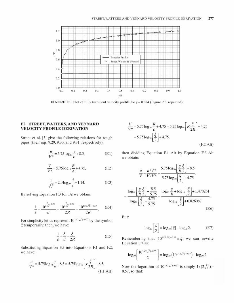
STREET, WATTERS, AND VENNARD VELOCITY PROFILE DERIVATION 277
F.2 STREET, WATTERS, AND VENNARD VELOCITY PROFILE DERIVATION
Street et al. [3] give the following relations for rough pipes (their eqs. 9.29, 9.30, and 9.31, respectively):
u
Vy
*,= +5 75 8 510. log .
ε (F.1)
VV
R*
,= +5 75 4 7510. log .ε
(F.2)
1
2 0 1 1410f
d= +. log .ε
. (F.3)
By solving Equation F.3 for 1/ ε we obtain:
1 10 102
102
1
20 57
1
20 57
1 2 0 57
ε= = =
− −−f f f
d R R
. ./( ) .
. (F.4)
For simplicity let us represent 101 2 0 57/( ) .f − by the symbol ξ temporarily; then, we have:
1
2εξ ξ= =d R
. (F.5)
Substituting Equation F.5 into Equations F.1 and F.2 , we have:
uV
yy
R*= + =
+5 75 8 5 5 752
8 510 10. log . . log . ,ε
ξ
(F.1 Alt)
FIGURE F.1. Plot of fully turbulent velocity profi le for f = 0.024 (Figure 2.3 , repeated).
0.0
0.2
0.4
0.6
0.8
1.0
1.2
0.0 0.1 0.2 0.3 0.4 0.5 0.6 0.7 0.8 0.9 1.0
y/R
u/V
Benedict Profile
Street, Watters & Vennard
VV
RR
R*= + =
+
=
5 75 4 75 5 752
4 75
5 752
10 10
10
. log . . log .
. log
εξ
ξ
+ 4 75. ,
(F.2 Alt)
then dividing Equation F.1 Alt by Equation F.2 Alt we obtain:
uV
u VV V
yR= =
+
+
//
. log .
. log .
**
,5 75
28 5
5 752
4 75
10
10
ξ
ξ
=
+
+=
+log..
log..
log log10
10
102
8 55 75
24 755 75
yR
yR
ξ
ξ
110
10
21 478261
20 826087
ξ
ξ
+
+
.
log ..
(F.6)
But:
log log log10 10 102
2ξ ξ
= [ ] − . (F.7)
Remembering that 101 2 0 57/( ) .f − ≡ ξ , we can rewrite Equation F.7 as:
log log log/( ) .
/( ) .10
1 2 0 57
101 2 0 57
1010
210 2
ff
−−
= ( ) − .
Now the logarithm of 101 2 0 57/( ) .f − is simply 0 57. , so that:
1 2/ ( )f −
278 VELOCITY PROFILE EQUATIONS
Then Equation F.8 may be written as:
uV
yR f
f
=+ +
−
0 434291
20 60723
12
0 044943
. ln .
..
From Figure F.1 , it can be seen that the profi le defi ned by the Street et al. equations falls on the profi le defi ned by Benedict ’ s equations.
REFERENCES
1. Benedict , R. P. , Fundamentals of Pipe Flow , John Wiley & Sons , 1980 .
2. Rouse , H. , ed., Engineering Hydraulics, Proceedings of the Fourth Hydraulics Conference, Iowa Institute of Hydraulic Research, June 12 – 15, 1949 , John Wiley & Sons , 1949 .
3. Street , R. L. , G. Z. Watters , and J. K. Vennard , ElementaryFluid Mechanics , 7th ed. , John Wiley & Sons , 1996 .
log log . .
.
/( .10
1 2 0 571010 2
1
20 57 0 3010300
1
20 871030
f
f
f
−( ) − = − −
= − 00.
Now substitute 1 2 0 8710300/ .f − into equation 2.26 wherever we fi nd log ( / )10 2ξ :
uV
yR f
f
=+ − +
− +
log . .
. .
101
20 8710300 1 478261
1
20 8710300 0 826087
,
uV
yR f
f
=+ +
−
log .
..
101
20 60723
12
0 044943 (F.8)
For convenience in plotting, change the log 10 to ln (i.e., loge ); The log 10 term becomes:
log . ln .10 0 43429448yR
yR
=
279
INDEX
Page references followed by d, f, or t denote diagrams, fi gures, or tables.
American Petroleum Institute (API) pipe standard, 245American Society of Mechanical Engineers (ASME)
Fluid Meters data, 140, 158–159, 159floss coeffi cients for fl ow nozzles, 157–158, 158f
American Standards Association, 245Archimedean spiral, 166Atmospheric pressure, 4, 4fAverage velocity, 5, 13, 15Axial force equations, 14Axisymmetric expansion, sudden, 113Axisymmetric reducing fl ow passage, 14f
Backing rings, 202, 202f, 202tBall valve, 208, 208fBarometric pressure, 4, 4fBarr’s formula for friction factor, 80Bend radius ratio, 163, 165, 165f, 169Bends, 163–173
cavitation in, 220coils, 166–168, 167t
constant pitch helix, 166f, 167constant pitch spiral, 166f, 167–168, 168t
coupled bends, 169, 169felbows and pipe bends, 163–166, 164f–166floss coeffi cient, 164–166, 165f, 168f, 169, 170t–173t, 174dmiter bends, 168, 168f, 168t, 174dpiping confi gurations, losses with differing, 169, 169f,
169t–173tuncertainty values, 70t
Benedict, Robert P., 15, 19Benedict velocity profi le derivation, 275–276, 277fBenedict-Webb-Rubin equation, 264
Pipe Flow: A Practical and Comprehensive Guide, First Edition. Donald C. Rennels and Hobart M. Hudson.© 2012 John Wiley & Sons, Inc. Published 2012 by John Wiley & Sons, Inc.
Absolute pressure, 4Absolute roughness, of pipe walls, 78, 82–84Absolute temperature, 6Absolute viscosity
defi ned, 5of water at different temperatures, 242t–243t
Absolute zero, 6Acceleration, units of, 3Acentric factor, 264, 266, 266tAcoustic resonance, 226Acoustic response time, 226Acoustic velocity, 269Actuators, 205Adiabatic compressible fl ow with friction equation, 37–42
using Mach number as a parameter, 37–41, 269–274change of area and, 40–41when static pressure and static temperature are known,
38–39, 269, 270f, 271fwhen static pressure and total temperature are known,
39–40, 272when total pressure and static temperature are known,
40, 273–274when total pressure and total temperature are known,
40, 272–273, 273fusing static pressure and temperature as parameters,
41–42Air chambers, 227American National Standards Institute (ANSI)/American
Society of Mechanical Engineers (ASME) pipe standard, 245
American National Standards Institute (ANSI) pipe reducers, 107, 121
280 INDEX
Bernoulli, Daniel, 18Bernoulli terms, 18, 23β ratio, 101–102Beveled contraction, 106–107, 106f, 110d–112dBeveled entrance, 91–92, 92f, 95dBevel-edged orifi ce, 145–146
entrances, 93–94, 94f, 96dexits, 133–134, 134f, 137dloss coeffi cient, 145–146, 151d–153din straight pipe, 145, 145f, 151d–153din transition section, 145–146, 146fin a wall, 146, 146f
Borda, Jean-Charles de, 28, 114Borda-Carnot equation, 28, 114, 131Borda’s mouthpiece, 90Borda sudden expansion loss, 28Boyle, Robert, 8Branching fl ow, 51Branching network, 51British Standard (BS) pipe standard, 245Bulk fl ows, 61Butterfl y valve, 208, 208fButt weld
loss coeffi cient, 201, 204dreducers, 107, 121, 123, 123f, 123t
Cavitation, 219–224core spray pump (example problem), 221–224
moderately corroded steel pipe, 222–224, 223t, 224f
new, clean steel pipe, 222, 223f, 223tpump suction line, 222f
nature of, 219–220, 220fnet positive suction head, 220–221pipeline design and, 220sound associated with, 219–220
Celsius, Anders, 6Celsius scale, 6Chamfering
of contractions, 106, 107of tees, 178, 182
Charles, Jacques, 6, 8Check valve, 209–210, 209fChen’s formula for friction factor, 79–80Churchill’s 1973 formula for friction factor, 79Churchill’s 1977 all-regime formula for friction factor,
81–82, 82f–83fCoils, 166–168, 167t
constant pitch helix, 166f, 167constant pitch spiral, 166f, 167–168, 168t
Colebrook, Cyril F., 26Colebrook-White equation, 26, 49, 78Column separation, 227–228Comprehensive average properties, 34, 35fCompressibility chart, 8Compressibility factor, 8, 9f–11fCompressibility factor equations, 263–267
Lee-Kesler equation, 264–266Redlich-Kwong equation, 263–264
Compressible fl ow, fi nding pressure drop in, 31–47adiabatic compressible fl ow with friction equation,
37–42using Mach number as a parameter, 37–41, 269–274using static pressure and temperature as parameters,
41–42approximate compressible fl ow using incompressible fl ow
equations, 32–36using average of inlet or outlet properties, 33, 34f–35fusing expansion factors, 34–36, 36fusing inlet or outlet properties, 32–33
example problem, 43–47isothermal compressible fl ow with friction, 42–43problem solving methods, 31–32
Concentric pipe reducers, 213–214, 214fConical contraction, 104–106, 104f
local loss, 105–106, 106f, 109dsurface friction loss, 105, 105f, 108d
Conical diffuserscomparative effectiveness of diffuser confi gurations,
122tdischarge from, 132, 132f, 135d–136dloss coeffi cients, 115–118, 117f, 119t, 121, 122t,
125d–127dmultistage conical diffuser, 117–120, 118f
stepped conical diffuser, 117–118, 118f, 119t–120ttwo-stage conical diffuser, 118–120, 118f–119f
straight conical diffuser, 114–117, 115f, 117fswirl (tangential rotation of fl ow) in, 115
Conservation equations, 13–21Conservation of energy, 16–18, 51Conservation of mass, 13, 51Conservation of momentum, 13–14Constant pitch helix coil, 166f, 167Constant pitch spiral coil, 166f, 167–168, 168tConstants
critical constants for gases, 267timportant physical, 253tLee-Kesler, 264t
Continuity equation, 13, 140in fl ow through tees, 179–180, 183–184
Continuity principle, 50Contractions
beveled contraction, 106–107, 106f, 110d–112dcavitation in, 220conical contraction, 104–106, 104f
local loss, 105–106, 106f, 109dsurface friction loss, 105, 105f, 108d
entrances (see Entrances)fl ow model for, 101–102loss coeffi cient, 101–107, 108d–112dpipe reducer, 107, 107frounded contraction, 103–104, 104f, 108dsharp-edged contraction, 102–103smooth contraction, 107, 107funcertainty values, 70t
Control valve, 210, 211fConventional head loss, 20, 23, 131Conversions, table of, 254t–262t
INDEX 281
Core spray systemexample problem (fl ow rate), 54–60
moderately corroded steel pipe, 58–60adjusted parameters, 59fl ow during loss of coolant accident, 60ffl ow rate versus vessel pressure, 60fground rules and assumptions, 58input parameters, 58network fl ow equations, 59solution, 59
new, clean steel pipe, 55–58adjusted parameters, 57fl ow during loss of coolant accident, 59ffl ow rate versus vessel pressure, 59fground rules and assumptions, 55–56initial calculations, 57input parameters, 56–57network fl ow equations, 57–58solution, 58
example problem (net positive suction head), 221–224moderately corroded steel pipe, 222–224, 223t, 224fnew, clean steel pipe, 222, 223f, 223tpump suction line, 222f
function of, 54in-vessel piping and spargers, 55fschematic of, 55f
Coupled bends, 169, 169fCoupling effects, 49–50Couplings, threaded, 214–215, 214fCritical pressure, 4, 267tCritical temperature, 6, 267tCritical zone, friction factor and, 77–78Curved wall diffuser, 120–121, 121f, 122t
Darcy, Henry, 24–25Darcy friction factor, 25, 81Darcy-Weisbach equation, 28Dean number, 164De Chézy, Antoine, 24Density
mass density, 5of water at different temperatures, 242t–243tweight density, 5
Diameter ratio, of tees, 180, 181f, 185, 185fDiametre Nominal (DN), 245, 246t–251tDiaphragm valve, 205–206, 206fDiatomic gases, ratio of specifi c heats for, 36Diffuser effi ciency, 115Diffusers
comparative effectiveness of diffuser confi gurations, 122tcurved wall diffuser, 120–121, 121f, 122tdivergence angle, 115–121, 117f, 120t, 125d–127dloss coeffi cients, 115–118, 117f, 119t, 121, 122t, 124d–127dmultistage conical diffuser, 117–120, 118f
stepped conical diffuser, 117–118, 118f, 119t–120ttwo-stage conical diffuser, 118–120, 118f–119f
performance level of, 115purpose of, 113, 115stalled fl ow in, 115
straight conical diffuser, 114–117, 115f, 117fsurface friction loss, 116–117, 124dswirl in, 115
Dimensionless number, Reynolds number as, 25Dimensionless ratios
Froude number, 7loss coeffi cient, 7Mach number, 7reduced pressure, 7reduced temperature, 7relative roughness, 6Reynolds number, 6
Discharge. See ExitsDisturbance time, fl ow, 226Divergence angle, diffuser, 115–121, 117f, 120t, 125d–127dDouble extra strong (XXS) pipe, 245Dynamic head, 113
Eccentric pipe reducers, 213–214, 214fEddies
in bends, 163in expansions, 113
Edge impressions, 141Elastic modulus, 227Elbows
fl ow through, 163–166, 164f–166fthreaded, 214, 214f
Elevation (potential) head, 16Energy
conservation of, 16–18, 51defi ned, 5forms of, 5head loss, 18–19heat, 5, 6, 17kinetic, 5, 17, 113, 115kinetic energy correction factor, 19–20mechanical work, 18potential, 5, 16, 113, 115pressure, 5, 17work, 5
Energy equationdescribed, 16in fl ow through tees, 178, 180–182, 184, 186general, 18for incompressible fl ow, 32simplifi ed, 19, 23
Energy fl uxes, 16fEnergy Grade Line, 20, 21f, 23Energy Line, 20–21EN (European Standard) pipe standard, 245English gravitational system, 3–4Entrances, 89–99
beveled entrance, 91–92, 92f, 95dpressure loss at, 89rounded entrance, 91, 91f, 95dsharp-edged entrance, 89–91
fl ush mounted, 89–90, 90fmounted at a distance, 90, 90f, 94dmounted at an angle, 90–91, 91f
282 INDEX
through an orifi ce, 92–94beveled orifi ce, 93–94, 94f, 96dround-edged orifi ce, 93, 93f, 96dsharp-edged orifi ce, 92–93, 93fthick-edged orifi ce, 93, 93f, 96d
uncertainty values, 70tEquations of state
of gases, 8of liquids, 7
Error. See also Uncertaintysources, 69, 70t
European Standard (EN) pipe standard, 245Exits, 131–137
discharge from an orifi ce, 132–134bevel-edged orifi ce, 133–134, 134f, 137drounded-edged orifi ce, 133, 133f, 136dsharp-edged orifi ce, 132–133, 133fthick-edged orifi ce, 133, 133f, 137d
discharge from conical diffuser, 132, 132f, 135d–136ddischarge from smooth nozzle, 134, 134fdischarge from straight pipe, 131–132, 132fopen discharge, 131, 132fsubmerged discharge, 131, 132funcertainty values, 70t
Expansion factor method, for pressure drop, 34–36, 36fExpansions, 113–123, 124d–127d
comparative effectiveness of diffuser confi gurations, 122t
curved wall diffuser, 120–121, 121f, 122tloss coeffi cients, 115–118, 117f, 119t, 121, 122t, 123, 123t,
124d–127dmultistage conical diffuser, 117–120, 118f
stepped conical diffuser, 117–118, 118f, 119t–120ttwo-stage conical diffuser, 118–120, 118f, 119f
pipe reducer, 121, 123, 123f, 123tstraight conical diffuser, 114–117, 115f, 117f, 119tsudden, 113–114, 114funcertainty values, 70t
Extra strong (XS) pipe, 245
Fahrenheit, Gabriel, 6Fahrenheit scale, 5–6Fanning friction factor, 25, 166Flow
full, 237, 237fgeneralized fl ow model, 139–140open, 235–237, 236fsecondary, 163–165, 164f–165fstalled in a diffuser, 115submerged fl ow, 237–238, 237f–238ftangential rotation (swirl), in conical diffusers, 115
Flow area, by pipe size, 246t–251tFlow-induced vibration, 225–229
column separation, 227–228steady external fl ow, 225–226steady internal fl ow, 225water hammer, 226–227
Flow meters, 157–161fl ow nozzle, 157–159, 158f, 160f, 161dnozzle/Venturi, 159–160, 160funcertainty values, 70tVenturi tube, 107, 158–159, 158f
Flow nozzle, 157–159, 158f, 160f, 161dFlow phenomena, 217–240
cavitation, 219–224fl ow-induced vibration, 225–229fl ow to run full, 235–240temperature rise, 231–233
Flow rate, uncertainty and, 71, 72–73Flow regimes
laminar (streamline), 8, 12fturbulent, 8, 12f
Flow separationin bends, 163–165, 164f, 165fin diffusers, 115
Flow splitter, 220, 220fFlow to run full, 235–240Flow work, 18Fluid hammer. See Water hammerFluid properties
density, 5energy, 5heat, 6pressure, 4–5, 4f–5ftemperature, 5–6velocity, 5viscosity, 5
Fluid velocityassumption of one-dimensionality, 8assumption of uniform, 8average, 13, 15fl at profi le, 13–14
Force, units of, 3–4Fox, J.A., 61Friction. See Surface frictionFriction factor, 16, 16f, 19f, 24–26, 27f, 28
for bends, 165Churchill’s 1977 all-regime formula, 81–82, 82f–83fColebrook-White equation, 26, 78, 80Darcy, 25, 81diffusers and, 116explicit formulations, 79–80
Barr’s formula, 80Chen’s formula, 79–80Churchill’s 1973 formula, 79Colebrook-White equation compared to, 80Haaland’s formulas, 80Manadilli’s formula, 80Moody’s approximate formula, 79Romeo’s formula, 80Shacham’s formula, 80Swamee and Jain formula, 79Wood’s approximate formula, 79
Fanning, 25, 166for helices, 167
Entrances (cont’d)
INDEX 283
laminar fl ow, 25, 77for mitered bends, 168Moody Chart, 27f, 28, 79, 86dNikuradse’s, 25for noncircular passages, 85regions of application
critical zone, 77–78laminar fl ow region, 77turbulent fl ow region, 78
Reynolds number and, 25, 27f, 84, 84tfor spirals, 167surface roughness and, 82, 84, 84tturbulent fl ow, 25, 78
rough pipes, 78smooth pipes, 78
uncertainty values, 70tFriction velocity, 16Froude, William, 7Froude number, 7, 235–238Full fl ow
described, 237, 237freactor application, 239–240, 239f
Gasesacentric factor for, 266tcompressibility factor, 8, 9f–11f, 263–267critical constants, 267tequation of state, 8ratio of specifi c heats, 36
Gasket, misaligned, 203, 203f, 204dGate valve, 206, 206fGauge pressure, 4, 4fGay-Lussac, Joseph, 8General energy equation, 18Generalized fl ow model, 139–140Gibson’s tests, 116–117, 117f, 159Globe valve, 206–207, 206fGrade lines, 20–21, 21f
Haaland’s formulas for friction factor, 80Hagen, Gotthilf, 24Hagen-Poiseuille law, 25Head loss
in bends, 165, 169in conical diffusers, 116of contraction, 101, 103conventional, 20, 23, 131described, 18–19as energy conversion, 231of fl ow meter, 157–160induced turbulence, 28–29in laminar fl ow, 24orifi ce, 140sources, 23–29, 75
induced turbulence, 28–29summing loss coeffi cient, 29surface friction loss, 24–26, 28, 105
in turbulent fl ow, 24–25
Heatdefi ned, 6sensible, 6specifi c, 6units of measurement, 6
Heat energy, 5, 6, 17Heat exchangers, 226Helix, constant pitch, 166f, 167Herschel, Clemens, 24Hydraulic diameter, 85, 105, 116Hydraulic Grade Line, 20, 21f, 219
Incompressible fl ow, 23–29Borda-Carnot equation and, 114energy equation for, 32head loss, 18
conventional, 23sources, 23–29
Incompressible fl ow equations, approximating compressible fl ow using, 32–36
Induced turbulence, as source of pressure loss, 28–29
Inside diameter, pipe, 245, 246t–251tInternational System (SI), 3Isentropic fl ow, 42Isothermal comprehensible fl ow with friction equation,
42–43Ito, H., 164–165
Japanese Industrial Standards (JIS) pipe, 245Jet contraction coeffi cient, 102, 102tJet velocity ratio, 101–104, 102f, 105Joints. See Pipe jointsJoukovsky, N., 227Joule, James Prescott, 17
Kelvin scale, 6Kesler, M.G., 264Kinematic viscosity, 5Kinetic energy, 17
conversion to static pressure, 113, 115defi ned, 5drop in expansions, 113
Kinetic energy correction factor, 19–20Kwong, Joseph N.S., 263
Laminar fl owfriction factor, 25, 77Reynolds number, 77surface friction loss, 24velocity profi le, 16, 20
Laminar fl ow boundary layer, 26Laminar friction factor, 25, 77Leak before break, 225Lee, B.I., 264Lee-Kesler constants, 264tLee-Kesler equation, 8, 264–266Liquids, equation of state for, 7

284 INDEX
Local lossin conical contraction, 105–106, 106f, 109din conical diffuser, 116
Local velocity, 5Loss coeffi cient
of backing rings, 202, 202f, 202tof bends, 164–166, 165f, 168f, 169, 170t–173t,
174dcoupled bends, 169fabricated pipe bends, 172t–173tmiter bends, 174dwelded elbows and returns, 170t–171t
of butt weld, 201, 204dof contractions, 101–107, 108d–112d
beveled contraction, 106–107, 110d–112dconical contraction, 104–106
local loss, 105, 109dsurface friction loss, 105, 108d
pipe reducer, 107rounded contraction, 103–104, 108dsharp-edged contraction, 102–103smooth contraction, 107
defi ned, 7, 28of entrances
beveled orifi ce, 98dfl ush-mounted beveled, 95dfl ush-mounted rounded, 91, 95drounded-edged orifi ce, 93, 96dsharp-edged fl ush-mounted, 89–90sharp-edged mounted at a distance, 90, 94dsharp-edged mounted at an angle, 90, 94dthick-edged orifi ce, 93, 97d
of exitsdischarge from an orifi ce, 132
bevel-edged orifi ce, 133–134, 137drounded-edged orifi ce, 133, 136dsharp-edged orifi ce, 133thick-edged orifi ce, 133, 137d
discharge from conical diffuser, 132, 135d–136ddischarge from smooth nozzle, 134, 134f
of expansions, 114–118, 117f, 121, 122t, 124d–127dcurved wall diffuser, 121, 122tpipe reducer, 121, 123, 123trelationship to diffuser effi ciency, 115stepped conical diffuser, 118, 119tstraight conical diffuser, 114–117, 117f, 119tsudden, 114, 124d
for fl ow nozzle, 157–160, 158f, 160dfor induced turbulence, 28of misaligned gasket, 203, 204dof misaligned pipe joint, 203, 204dof orifi ces, 140–154
bevel-edged orifi ce, 145–146, 151d–153dmultihole, 149noncircular, 149round-edged orifi ce, 143–145, 145t, 150dsharp-edged orifi ce, 141, 150dthick-edged orifi ce, 147–149, 149t, 154d
overview, 75–76
of reducerscontracting, 107, 213expanding, 121, 123, 123t, 213
Reynolds number effect on, 75summing, 29from surface friction, 77, 105, 108dof tees, 177–186, 187d–199d
converging teesfl ow into branch, 186, 199dfl ow through branch, 184–185, 196d–198dfl ow through run, 182–184, 195d
diverging teesfl ow from branch, 182, 194dfl ow through branch, 180–181, 188d–193dfl ow through run, 178–179, 187d
of threaded fi ttingscouplings, 214–215elbows, 214reducers
contracting, 213expanding, 213
tees, 214valves, 215
of valves, 209t, 211, 215of weld protrusion, 201, 204d
Loss of coolant accident, 54, 55, 58–59, 59f–60f, 221–224
Mach, Ernst, 7Mach number
core, 272defi ned, 7as equation parameter in compressible fl ow, 37–40, 269–274
Manadilli’s formula for friction factor, 80Mass, conservation of, 13, 51Mass, units of, 3Mass density, 5Mathcad, 54, 62Mathematica, 54, 62Mechanical work energy, 18Misalignment
gasket, 203, 203f, 204dpipe joint, 203, 203f, 204d
Miter bends, 168, 168f, 168t, 174dMolecular mass, 38Molecular weight, 38Momentum, conservation of, 13–14Momentum equation, in fl ow through tees, 179–180, 183–184Momentum fl ux correction factor, 14–16, 16fMoody, F.J., 61Moody, Lewis F., 28, 79Moody Chart, 27f, 28, 79, 86dMoody’s approximate formula for friction factor, 79Multihole orifi ces, 149Multistage conical diffuser, 117–120, 118f
stepped conical diffuser, 117–118, 118f, 119t–120ttwo-stage conical diffuser, 118–120, 118f–119f
Needle valve, 207, 207fNelson-Obert chart, 38
INDEX 285
Net positive suction headavailable (NPSHA), 221–224, 223f–224f, 223tin core spray pump example problem, 222–224, 223f–224f,
223trequired (NPSHR), 220–222, 223f–224f
Network analysis, 49–60branching fl ow, 51coupling effects, 49–50example problems
core spray system, 54–60, 55fmoderately corroded steel pipe, 58–60new, clean steel pipe, 55–58
ring sparger, 51–54, 52f–53fcalculated fl ow rate, 54tcalculated header pressure, 54tcontinuity equations, 53energy equations, 53–54ground rules and assumptions, 52initial calculations, 53input parameters, 52network equations, 53–54solution, 54
parallel fl ow, 50–51series fl ow, 50
Newton-Raphson method, 264, 265, 270–272, 271fNewton’s second law of motion, 13Nikuradse, Johann, 15, 25, 26f, 35Nodes, of branching network, 51Nominal Pipe Size (NPS), 245, 246t–251tNonaxisymmetric reducing fl ow passage, 14fNoncircular orifi ces, 149
Nozzle/Venturi, 159–160, 160fNuclear reactor
core spray systemheat balance, 232pumping system temperature, 232–233, 232fvessel heat up, 232
Nuclear Regulatory Commission (NRC), 228
Open fl ow, 235–237, 236fOrifi ces, 139–154
bevel-edged orifi ce, 145–146entrances, 93–94, 94f, 96dexits, 133–134, 134f, 137dloss coeffi cient, 145–146, 151d–153din straight pipe, 145, 145f, 151d–153din transition section, 145–146, 146fin a wall, 146, 146f
eccentric, 139–140edge impressions, 141entrances, 92–94
bevel-edged orifi ce, 93–94, 94f, 96dround-edged orifi ce, 93, 93f, 96dsharp-edged orifi ce, 92–93, 93fthick-edged orifi ce, 93, 93f, 96duncertainty values, 70t
exits, 132–134bevel-edged orifi ce, 133–134, 134f, 137dround-edged orifi ce, 133, 133f, 136d
sharp-edged orifi ce, 132–133, 133fthick-edged orifi ce, 133, 133f, 137d
fl ow model, 139–140, 140fhead loss, 140loss coeffi cients, 140–154multihole, 149noncircular, 149round-edged orifi ce, 142–145
entrances, 93, 93f, 96dexits, 133, 133f, 136dloss coeffi cient, 143–145, 145t, 150din straight pipe, 143, 143f–144f, 150din transition section, 143–144, 144fin a wall, 144–145, 145f–145t
segmental, 139–140sharp-edged orifi ce, 140–141
entrances, 92–93, 93fexits, 132–133, 133floss coeffi cient, 141, 150din straight pipe, 140–141, 141f–142fin transition section, 141, 142fin a wall, 141, 142f
thick-edged orifi ce, 146–149entrances, 93, 93f, 96dexits, 133, 133f, 137dloss coeffi cient, 147–149, 149t, 154din straight pipe, 146–148, 147f, 154din transition section, 148, 148fin a wall, 148–149, 148f
uses of, 139Outside diameter, pipe, 245, 246t–251t
Parallel fl ow, 50–51Perfect gas law, 8Perforated plate, 149Physical constants, table of, 253tPiezometric Head Line, 20Pilot-operated safety relief valve, 210Pilot valve, 205Pinch valve, 207, 207fPipe joints
backing rings, 202, 202f, 202tmisalignment, 203, 203f, 204dpressure loss at, 201uncertainty values, 70tweld protrusion, 201–202, 202f, 204d
Pipe reducers. See ReducersPipe size
data table, 246t–251tDiametre Nominal (DN), 245, 246t–251tNominal Pipe Size (NPS), 245, 246t–251tstandards, 245
Pipe whip, 225Pipe whip restraints, 225Piping confi gurations, losses with differing, 169, 169f, 169tPitzer’s acentric factor, 264, 266, 266tPlug valve, 208–209, 208fPoiseuille, Jean, 24Polyatomic gases, ratio of specifi c heats for, 36
286 INDEX
Poppet valve, 210Porosity, of multihole orifi ce, 149Positive displacement pump, transient analysis and, 65–66
heat transfer, 66no heat transfer, 65–66
Potential energydefi ned, 5elevation (potential) head, 16in expansions, 113, 115of pressure, 115
Prandtl, Ludwig, 15, 25Prandtl’s boundary layer theory, 26Prandtl’s equation, 25Prandtl’s smooth pipe formula, 26“Prandtl term,” 28Pressure
absolute, 4atmospheric, 4, 4fbarometric, 4, 4fcritical, 4, 267tdefi ned, 4energy, 17gauge, 4, 4fpotential energy of, 115reduced, 7relationships, 4fstandard atmosphere, 4static, 5, 5ftotal, 5, 5fvapor, 5water hammer, 227
Pressure dropcauses
induced turbulence, 28–29surface friction, 24–25
compressible fl ow, 31–47of fl ow meters, 157laminar fl ow, 24measures of
loss coeffi cient, 7relative roughness, 6Reynolds number, 6
of orifi ces, 139of perforated plate, 149uncertainty, 69–70, 71–72of valves, 205–210
Pressure drop equationfor converging fl ow
in branch of tee, 186through branch of tee, 185through run of tee, 184
for diverging fl owfrom branch of tee, 182through branch of tee, 181through run of tee, 179
Pressure head, 17Pressure loss
in bends, 163–166in contraction, 104at entrances, 89
at pipe joints, 201of piping confi gurations, 169, 169t–173tthreaded fi ttings, 213–215
Pressure relief valves, 227Pressure waves, water hammer and, 226–227Prony, Gaspard Riche de, 24Prony brake, 24Propagation effects, 61
Radius ratio, of tees, 178, 180, 181f, 185, 186fRankine scale, 6Ratio of specifi c heats, 36Reactor heat balance, 232Real gas equations of state, 8Redlich, Otto, 263Redlich-Kwong equation, 8, 263–264Reducers
concentric, 107f, 123, 123fcontracting, 107, 107f, 213, 214feccentric, 107, 107f, 123fexpanding, 121, 123, 123f, 123t, 213–214, 214flosses at, 107, 121, 123threaded, 213–214
contracting, 213, 214fexpanding, 213–214, 214f
welded pipe, 107, 107f, 121, 123, 123fRelative roughness
described, 6friction factor and, 78, 105
Relief valve, 210, 210fResistance coeffi cient, 28Reynolds, Osborne, 6, 25Reynolds number
described, 6, 25friction factors and, 25, 27f, 77–78, 84, 84tHagen-Poiseuille law and, 25laminar fl ow, 77loss coeffi cient, effect on, 75for noncircular passages, 85turbulent fl ow, 25, 78
Ring spargerexample problem, 51–54
calculated fl ow rate, 54tcalculated header pressure, 54tcontinuity equations, 53energy equations, 53–54ground rules and assumptions, 52initial calculations, 53input parameters, 52network equations, 53–54solution, 54
network fl ow diagram, 53fstructure, 51–52, 52f
Romeo’s formula for friction factor, 80Rounded contraction, 103–104
circular rounding, 104felliptical rounding, 104floss coeffi cient, 104, 108drounding radius, 103–104
Rounded entrance, 91, 91f, 95d
INDEX 287
Round-edged orifi ce, 142–145entrances, 93, 93f, 96dexits, 133, 133f, 136dloss coeffi cient, 143–145, 145t, 150din straight pipe, 143, 143f–144f, 150din transition section, 143–144, 144fin a wall, 144–145, 145f, 145t
Rounding radius, 103–104Rouse, Hunter, 15
Secondary fl ow, in bends, 163–165, 164f–165fSeries fl ow, 50Shacham’s formula for friction factor, 80Sharp-edged contraction, 102–103Sharp-edged entrance, 89–91
fl ush mounted, 89–90, 90fmounted at a distance, 90, 90f, 94dmounted at an angle, 90–91, 91f
Sharp-edged orifi ce, 140–141entrances, 92–93, 93fexits, 132–133, 133floss coeffi cient, 141, 150din straight pipe, 140–141, 141f–142fin transition section, 141, 142fin a wall, 141, 142f
Simple average properties, 33–34, 34fSmooth contraction, 107, 107fSmooth nozzle exit, 134, 134fSonic velocity, 269, 270Sparger
core spray system in-vessel piping and spargers, 55freactor feedwater, 239–240, 239fring
example problem, 51–54network fl ow diagram, 53fstructure, 51–52, 52f
Specifi c heatdefi ned, 6of water at different temperatures,
242t–243tSpecifi c volume
average, 33–34defi ned, 5
Specifi c weight, 34–35Speed of sound in water, at different temperatures,
242t–243tSpherical vessel, drain from, 63, 63fSpirals, constant pitch, 166f, 167–178, 168tSquare-edged nozzles, 102Square ring nozzles, 102Stalled fl ow in a diffuser, 115Standard atmospheric pressure, 4Standard weight (Std) pipe, 245Static head, 113Static pressure
defi ned, 5, 5fkinetic energy conversion to, 113, 115
Steam hammer, 227Stepped conical diffuser, 117–118, 118f, 119t–120tStraight conical diffuser, 114–117, 115f, 117f, 119t
Straight pipe exit, 131–132, 132fStreet, Watters, and Vennard velocity profi le derivation,
277–278, 277fSubmerged fl ow, 237–238, 237f–238fSubsonic constant-area gas fl ow duct, 39fSudden expansion
Borda-Carnot equation for, 114, 131loss coeffi cient, 114, 124d
Surface friction, 77–86friction factor (see Friction factor)loss coeffi cient due to, 77, 105, 108d, 116, 124dsurface roughness and, 78, 82–84
Surface friction loss, 24–26, 28in bends, 163–165, 165fin conical contraction, 105, 105f, 108din conical diffusers, 116–117, 124dfriction factors, 25–26, 27f, 28laminar fl ow, 24in pipe reducer, 107, 121, 123Reynolds number and, 25, 77–78turbulent fl ow, 24–25
Surface roughness, of pipe walls, 82–84defi ned, 82friction factor and, 78, 82, 84, 84tinherent margin, 84loss of fl ow area, 84machined surfaces, 84new, clean pipe, 82, 83tturbulent fl ow and, 78
Surge tanks, 227Swamee and Jain formula for friction factor, 79Swing valve, 208–210Swirl (tangential rotation of fl ow), in conical diffusers,
115Système International (SI), 3Systems of units, 3–4
Tangential rotation of fl ow (swirl), in conical diffusers, 115
Tees, 177–199cavitation in, 220confi gurations of fl ow through a tee, 177, 178fconverging tees, 182–186
fl ow into branch, 185–186, 186f, 199dfl ow through branch, 184–185, 184f–185f, 196d–198dfl ow through run, 182–184, 182f–183f, 195d
diverging tees, 178–182fl ow from branch, 182, 182f, 194dfl ow through branch, 179–181, 180f–181f, 188d–193dfl ow through run, 178–179, 178f–179f, 187d
with fl ow splitter, 220, 220floss coeffi cients, 177–186, 187d–199dthreaded, 214, 214fwith turning vane, 220, 220funcertainty values, 70t
Temperatureabsolute, 6critical, 6, 267tdefi nitions, 5–6reduced, 7
288 INDEX
Temperature rise, 231–233calculating, 231in a pump, 231–232pumping system temperature, 232–233,
232freactor heat balance, 232vessel heat up, 232
Thick-edged orifi ce, 146–149entrances, 93, 93f, 96dexits, 133, 133f, 137dloss coeffi cient, 147–149, 149t, 154din straight pipe, 146–148, 147f, 154din transition section, 148, 148fin a wall, 148–149, 148f
Thickness, pipe wall, 245, 246t–251tThreaded fi ttings, 213–215
couplings, 214–215, 214felbows, 214, 214freducers, 213–214
contracting, 213, 214fexpanding, 213–214, 214f
tees, 214, 214funcertainty values, 70tvalves, 215
Time-step integration, transient analysis and, 67–68
direct solution, 67time-step solution, 67–68upright cylindrical vessel drain problem, 67
Total energy infl ow rate, 61Total Head Line, 20Total mass infl ow rate, 61Total pressure, 5, 5fTransient analysis, 61–68
example problemspositive displacement pump, 65–66
heat transfer, 66no heat transfer, 65–66
time-step integration, 67–68direct solution, 67time-step solution, 67–68upright cylindrical vessel drain problem,
67vessel drain times, 62–65
spherical vessel, 63, 63fupright cylindrical vessel, 62–63, 62fupright cylindrical vessel with elliptical heads, 64–65,
64fmethodology, 61–62
Transient fl ow, 61Turbulence, induced, 28–29Turbulent fl ow
described, 8, 12ffriction factor, 25, 78kinetic energy correction factor, 19f, 20Reynolds number, 25, 78surface friction loss, 24–25surface roughness of pipe walls, 78velocity profi le, 15f
Turning vane, 220, 220fTwo-stage conical diffuser, 118–120, 118f–119f
Uncertainty, 69–73defi ned, 69error sources, 69, 70texample problems
fl ow rate, 72–73, 72fpressure drop, 71–72, 71f
fl ow rate, 71–73pressure drop, 69–723-sigma values, 70t
Unit conversions, 254t–262tUnits, systems of, 3–4Unsteady fl ow, 61Upright cylindrical vessel
drain from, 62–65, 62f, 64fwith elliptical heads, drain from, 64–65, 64f
U.S. Customary System (USCS), 3
Vacuum, 4f, 5Valves, 205–212
actuators, 205cavitation in, 220connections, 205control, 210, 211fdefi ned, 205loss coeffi cient, 209t, 211multiturn, 205–207
diaphragm valve, 205–206, 206fgate valve, 206, 206fglobe valve, 206–207, 206fneedle valve, 207, 207fpinch valve, 207, 207f
pilot, 205pilot-operated safety relief valve, 210poppet valve, 210pressure relief, 227quarter-turn, 207–209
ball valve, 208, 208fbutterfl y valve, 208, 208fplug valve, 208–209, 208f
ratings, 205self-actuated, 209–210
check valve, 209–210, 209frelief valve, 210, 210f
swing valve, 208–210threaded connections, 215uncertainty values, 70t
Valve sizing program, 40–41Van der Waals, Johannes, 9Vapor pressure
cavitation and, 219–221defi ned, 5of water at different temperatures, 242t–243t
Velocityacoustic, 269average, 5, 13, 15defi ned, 5
INDEX 289
friction, 16local, 5sonic, 269–270
Velocity head, 17, 28, 77Velocity profi le
with contractions, 20, 20f, 101equations, 15
Benedict velocity profi le derivation, 275–276, 277fderivations of, 275–278Street, Watters, and Vennard velocity profi le derivation,
277–278, 277fwith expansions, 20, 20f, 113fl at, 13, 14parabolic, 16, 20
Vena contractadefi ned, 101orifi ce, 140, 140fsudden contraction, 101, 101f
Venturi tube, 107, 158–159, 158f,Vessel drain times, transient analysis and, 62–65
spherical vessel, 63, 63fupright cylindrical vessel, 62–63, 62fupright cylindrical vessel with elliptical heads, 64–65, 64f
Vibration. See Flow-induced vibration
Viscosityabsolute, 5defi ned, 5kinematic, 5of water at different temperatures, 242t–243t
Von Kármán, Theodor, 15, 25Vortex shedding, 225–226
Water, physical properties of, 241, 242t–243tWater hammer, 226–227Weight density, 5Weisbach, Julius, 24–25Weisbach equation, 28, 90Weld protrusion, 201–202, 202f, 204dWetted perimeter, 85White, Cedric M., 26Wood’s approximate formula for friction factor, 79Work
defi ned, 5fl ow, 18mechanical work energy, 18
Work energydefi ned, 5mechanical, 18
Related Documents