Paul De Grauwe, Yuemei Ji Self-fulfilling crises in the ...eprints.lse.ac.uk/49648/1/__lse.ac.uk_storage_LIBRARY_Secondary... · Paul De Grauwe, Yuemei Ji Self-fulfilling crises in

Paul De Grauwe, Yuemei Ji

Self-fulfilling crises in the Eurozone: an empirical test Article (Published version) (Refereed)

Original citation: de Grauwe, Paul and Ji, Yuemei (2013) Self-fulfilling crises in the Eurozone: an empirical test. Journal of International Money and Finance, 34. pp. 15-36. ISSN 0261-5606 DOI: 10.1016/j.jimonfin.2012.11.003 © 2013 Elsevier Ltd This version available at: http://eprints.lse.ac.uk/49648/ Available in LSE Research Online: December 2014

http://www.lse.ac.uk/researchAndExpertise/Experts/[email protected]

http://www.sciencedirect.com/science/journal/02615606

http://dx.doi.org/10.1016/j.jimonfin.2012.11.003

http://www.elsevier.com/

http://eprints.lse.ac.uk/49648/

Journal of International Money and Finance 34 (2013) 15–36

Contents lists available at SciVerse ScienceDirect

Journal of International Moneyand Finance

journal homepage: www.elsevier .com/locate/ j imf

Self-fulfilling crises in the Eurozone: Anempirical test

Paul De Grauwe a,c,*, Yuemei Ji b,c

a The London School of Economics and Political Science, Houghton Street, London WC2A 2AE, UKb LICOS, University of Leuven, Waaistraat 6, Leuven, BelgiumcCentre for European Policy Studies, 1 Place du Congres, Brussels, Belgium

JEL classifications:E4E5F3G15

Keywords:EurozoneGovernment debtInterest rateSelf-fulfilling crisesMultiple equilibriaPanel dataLender of last resort

* Corresponding author. The London School ofTel.: þ44 (0) 20 7955 6464.

E-mail addresses: [email protected] (P. D

0261-5606http://dx.doi.org/10.1016/j.jimonfin.2012.11.003

� 2013 Elsevier Ltd. Open access under CC

a b s t r a c t

We test the hypothesis that the government bond markets in theEurozone are more fragile and more susceptible to self-fulfillingliquidity crises than in stand-alone countries. We find evidence thata significant part of the surge in the spreads of the peripheral Euro-zone countries during 2010–11 was disconnected from underlyingincreases in the debt to GDP ratios and fiscal space variables, andwasassociated with negative self-fulfilling market sentiments thatbecamevery strong since the endof2010.Weargue that this candrivemember countries of the Eurozone into bad equilibria. We also findevidence that after years of neglecting high government debt, inves-tors became increasingly worried about this in the Eurozone, andreacted by raising the spreads. No such worries developed in stand-alone countries despite the fact that debt to GDP ratios and fiscalspace variables were equally high and increasing in these countries.

� 2013 Elsevier Ltd. Open access under CC BY license.

1. Introduction

The financial crisis that erupted in the industrialized world in 2007 forced governments to savetheir domestic banking systems from collapse and to sustain their economies that experienced theirsharpest postwar recession. As a result, these governments saw their debt levels increase dramatically.Fig. 1 shows this for the US, the UK and the Eurozone.

Fig. 1 is also interesting for another reason. We observe that the increase in the debt to GDP ratiossince 2007 is significantly faster in the US and the UK than in the Eurozone, so much so that at the end

Economics and Political Science, Houghton Street, London WC2A 2AE, UK.

e Grauwe), [email protected] (Y. Ji).

BY license.

mailto:[email protected]

mailto:[email protected]

http://crossmark.dyndns.org/dialog/?doi=10.1016/j.jimonfin.2012.11.003&domain=pdf

www.sciencedirect.com/science/journal/02615606

www.elsevier.com/locate/jimf



http://creativecommons.org/licenses/by/3.0/

http://creativecommons.org/licenses/by/3.0/

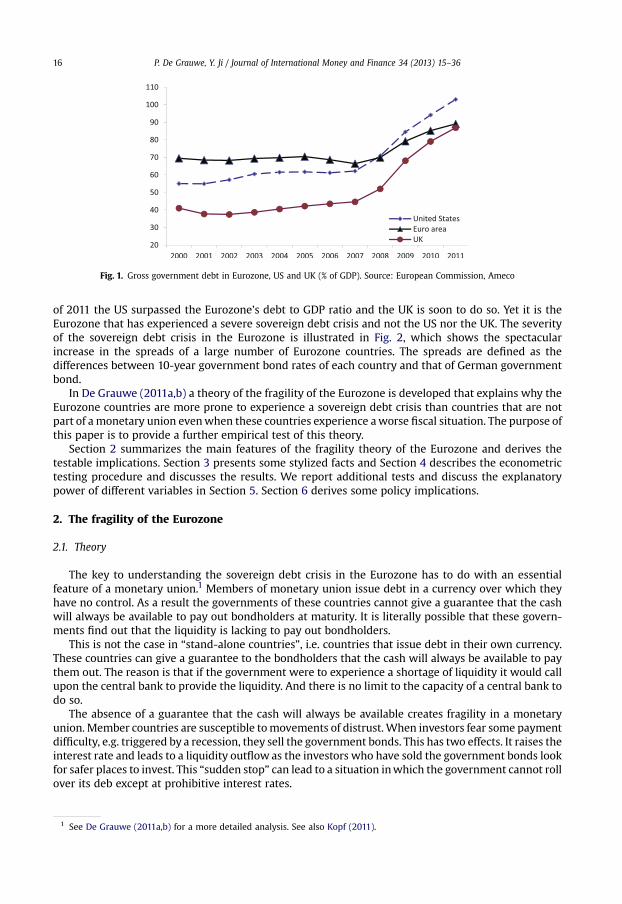
Fig. 1. Gross government debt in Eurozone, US and UK (% of GDP). Source: European Commission, Ameco

P. De Grauwe, Y. Ji / Journal of International Money and Finance 34 (2013) 15–3616

of 2011 the US surpassed the Eurozone’s debt to GDP ratio and the UK is soon to do so. Yet it is theEurozone that has experienced a severe sovereign debt crisis and not the US nor the UK. The severityof the sovereign debt crisis in the Eurozone is illustrated in Fig. 2, which shows the spectacularincrease in the spreads of a large number of Eurozone countries. The spreads are defined as thedifferences between 10-year government bond rates of each country and that of German governmentbond.

In De Grauwe (2011a,b) a theory of the fragility of the Eurozone is developed that explains why theEurozone countries are more prone to experience a sovereign debt crisis than countries that are notpart of a monetary union evenwhen these countries experience aworse fiscal situation. The purpose ofthis paper is to provide a further empirical test of this theory.

Section 2 summarizes the main features of the fragility theory of the Eurozone and derives thetestable implications. Section 3 presents some stylized facts and Section 4 describes the econometrictesting procedure and discusses the results. We report additional tests and discuss the explanatorypower of different variables in Section 5. Section 6 derives some policy implications.

2. The fragility of the Eurozone

2.1. Theory

The key to understanding the sovereign debt crisis in the Eurozone has to do with an essentialfeature of a monetary union.1 Members of monetary union issue debt in a currency over which theyhave no control. As a result the governments of these countries cannot give a guarantee that the cashwill always be available to pay out bondholders at maturity. It is literally possible that these govern-ments find out that the liquidity is lacking to pay out bondholders.

This is not the case in “stand-alone countries”, i.e. countries that issue debt in their own currency.These countries can give a guarantee to the bondholders that the cash will always be available to paythem out. The reason is that if the government were to experience a shortage of liquidity it would callupon the central bank to provide the liquidity. And there is no limit to the capacity of a central bank todo so.

The absence of a guarantee that the cash will always be available creates fragility in a monetaryunion. Member countries are susceptible tomovements of distrust. When investors fear some paymentdifficulty, e.g. triggered by a recession, they sell the government bonds. This has two effects. It raises theinterest rate and leads to a liquidity outflow as the investors who have sold the government bonds lookfor safer places to invest. This “sudden stop” can lead to a situation inwhich the government cannot rollover its deb except at prohibitive interest rates.

1 See De Grauwe (2011a,b) for a more detailed analysis. See also Kopf (2011).

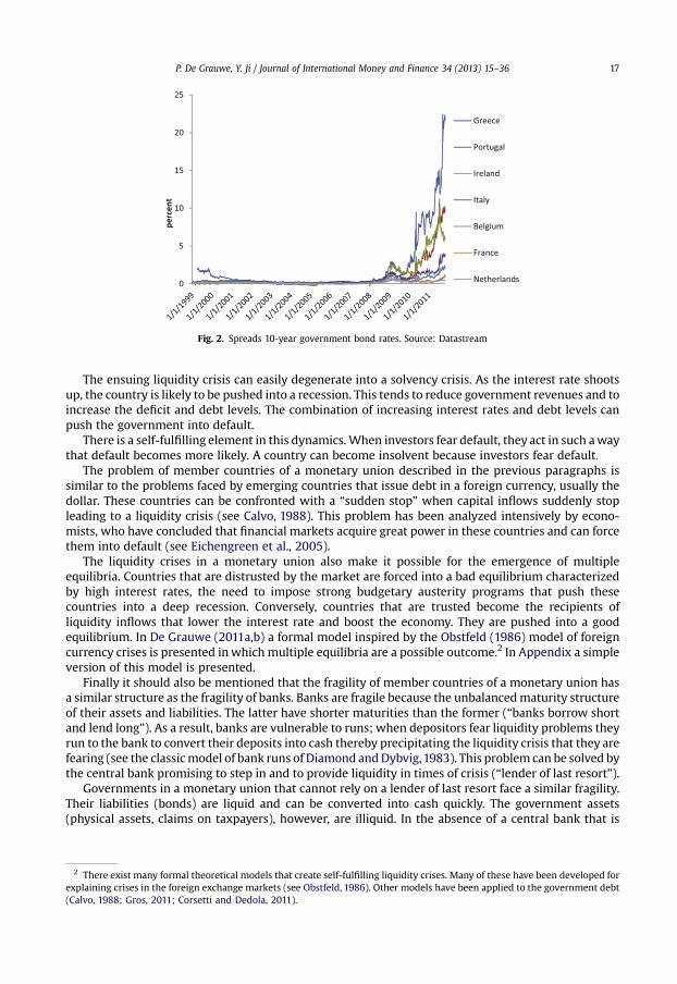
Fig. 2. Spreads 10-year government bond rates. Source: Datastream

P. De Grauwe, Y. Ji / Journal of International Money and Finance 34 (2013) 15–36 17

The ensuing liquidity crisis can easily degenerate into a solvency crisis. As the interest rate shootsup, the country is likely to be pushed into a recession. This tends to reduce government revenues and toincrease the deficit and debt levels. The combination of increasing interest rates and debt levels canpush the government into default.

There is a self-fulfilling element in this dynamics.When investors fear default, they act in such awaythat default becomes more likely. A country can become insolvent because investors fear default.

The problem of member countries of a monetary union described in the previous paragraphs issimilar to the problems faced by emerging countries that issue debt in a foreign currency, usually thedollar. These countries can be confronted with a “sudden stop” when capital inflows suddenly stopleading to a liquidity crisis (see Calvo, 1988). This problem has been analyzed intensively by econo-mists, who have concluded that financial markets acquire great power in these countries and can forcethem into default (see Eichengreen et al., 2005).

The liquidity crises in a monetary union also make it possible for the emergence of multipleequilibria. Countries that are distrusted by the market are forced into a bad equilibrium characterizedby high interest rates, the need to impose strong budgetary austerity programs that push thesecountries into a deep recession. Conversely, countries that are trusted become the recipients ofliquidity inflows that lower the interest rate and boost the economy. They are pushed into a goodequilibrium. In De Grauwe (2011a,b) a formal model inspired by the Obstfeld (1986) model of foreigncurrency crises is presented inwhich multiple equilibria are a possible outcome.2 In Appendix a simpleversion of this model is presented.

Finally it should also be mentioned that the fragility of member countries of a monetary union hasa similar structure as the fragility of banks. Banks are fragile because the unbalancedmaturity structureof their assets and liabilities. The latter have shorter maturities than the former (“banks borrow shortand lend long”). As a result, banks are vulnerable to runs; when depositors fear liquidity problems theyrun to the bank to convert their deposits into cash thereby precipitating the liquidity crisis that they arefearing (see the classicmodel of bank runs of Diamond andDybvig,1983). This problem can be solved bythe central bank promising to step in and to provide liquidity in times of crisis (“lender of last resort”).

Governments in a monetary union that cannot rely on a lender of last resort face a similar fragility.Their liabilities (bonds) are liquid and can be converted into cash quickly. The government assets(physical assets, claims on taxpayers), however, are illiquid. In the absence of a central bank that is

2 There exist many formal theoretical models that create self-fulfilling liquidity crises. Many of these have been developed forexplaining crises in the foreign exchange markets (see Obstfeld, 1986). Other models have been applied to the government debt(Calvo, 1988; Gros, 2011; Corsetti and Dedola, 2011).

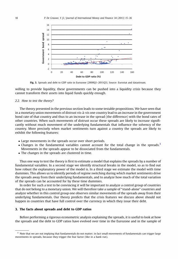
Fig. 3. Spreads and debt to GDP ratio in Eurozone (2000Q1–2011Q3). Source: Eurostat and datastream.


willing to provide liquidity, these governments can be pushed into a liquidity crisis because theycannot transform their assets into liquid funds quickly enough.

2.2. How to test the theory?

The theory presented in the previous section leads to some testable propositions. We have seen thatin amonetary unionmovements of distrust vis-à-vis one country lead to an increase in the governmentbond rate of that country and thus to an increase in the spread (the difference) with the bond rates ofother countries. When such movements of distrust occur these spreads are likely to increase signifi-cantly without much movement of the underlying fundamentals that influence the solvency of thecountry. More precisely when market sentiments turn against a country the spreads are likely toexhibit the following features:

� Large movements in the spreads occur over short periods.� Changes in the fundamental variables cannot account for the total change in the spreads.3

Movements in the spreads appear to be dissociated from the fundamentals.� The changes in the spreads are clustered in time.

Thus one way to test the theory is first to estimate a model that explains the spreads by a number offundamental variables. In a second stage we identify structural breaks in the model, so as to find outhow robust the explanatory power of the model is. In a third stage we estimate the model with timedummies. This allows us to identify periods of regime switching during whichmarket sentiments drivethe spreads away from their underlying fundamentals, and to analyze how much of the total variationof the spreads can be accounted for by these time dummies.

In order for such a test to be convincing it will be important to analyze a control group of countriesthat do not belong to a monetary union.Wewill therefore take a sample of “stand-alone” countries andanalyze whether in this control group one observes similar movements of the spreads away from theirunderlying fundamentals. Our theory predicts that the crisis features we discuss above should nothappen in countries that have full control over the currency in which they issue their debt.

3. The facts about spreads and debt to GDP ratios

Before performing a rigorous econometric analysis explaining the spreads, it is useful to look at howthe spreads and the debt to GDP ratios have evolved over time in the Eurozone and in the sample of

3 Note that we are not implying that fundamentals do not matter; in fact small movements of fundamentals can trigger largemovements in spreads, because they trigger the fear factor (like in a bank run).

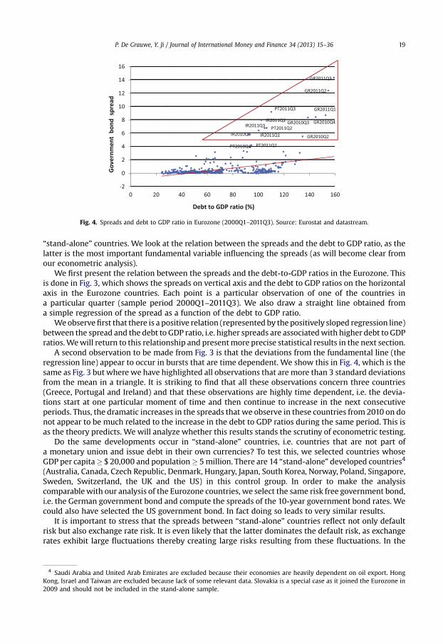
Fig. 4. Spreads and debt to GDP ratio in Eurozone (2000Q1–2011Q3). Source: Eurostat and datastream.


“stand-alone” countries. We look at the relation between the spreads and the debt to GDP ratio, as thelatter is the most important fundamental variable influencing the spreads (as will become clear fromour econometric analysis).

We first present the relation between the spreads and the debt-to-GDP ratios in the Eurozone. Thisis done in Fig. 3, which shows the spreads on vertical axis and the debt to GDP ratios on the horizontalaxis in the Eurozone countries. Each point is a particular observation of one of the countries ina particular quarter (sample period 2000Q1–2011Q3). We also draw a straight line obtained froma simple regression of the spread as a function of the debt to GDP ratio.

We observefirst that there is a positive relation (represented by the positively sloped regression line)between the spread and the debt to GDP ratio, i.e. higher spreads are associatedwith higher debt to GDPratios.Wewill return to this relationship and presentmore precise statistical results in the next section.

A second observation to be made from Fig. 3 is that the deviations from the fundamental line (theregression line) appear to occur in bursts that are time dependent. We show this in Fig. 4, which is thesame as Fig. 3 but where we have highlighted all observations that are more than 3 standard deviationsfrom the mean in a triangle. It is striking to find that all these observations concern three countries(Greece, Portugal and Ireland) and that these observations are highly time dependent, i.e. the devia-tions start at one particular moment of time and then continue to increase in the next consecutiveperiods. Thus, the dramatic increases in the spreads that we observe in these countries from 2010 on donot appear to be much related to the increase in the debt to GDP ratios during the same period. This isas the theory predicts. We will analyze whether this results stands the scrutiny of econometric testing.

Do the same developments occur in “stand-alone” countries, i.e. countries that are not part ofa monetary union and issue debt in their own currencies? To test this, we selected countries whoseGDP per capita� $ 20,000 and population� 5million. There are 14 “stand-alone” developed countries4

(Australia, Canada, Czech Republic, Denmark, Hungary, Japan, South Korea, Norway, Poland, Singapore,Sweden, Switzerland, the UK and the US) in this control group. In order to make the analysiscomparablewith our analysis of the Eurozone countries, we select the same risk free government bond,i.e. the German government bond and compute the spreads of the 10-year government bond rates. Wecould also have selected the US government bond. In fact doing so leads to very similar results.

It is important to stress that the spreads between “stand-alone” countries reflect not only defaultrisk but also exchange rate risk. It is even likely that the latter dominates the default risk, as exchangerates exhibit large fluctuations thereby creating large risks resulting from these fluctuations. In the

4 Saudi Arabia and United Arab Emirates are excluded because their economies are heavily dependent on oil export. HongKong, Israel and Taiwan are excluded because lack of some relevant data. Slovakia is a special case as it joined the Eurozone in2009 and should not be included in the stand-alone sample.

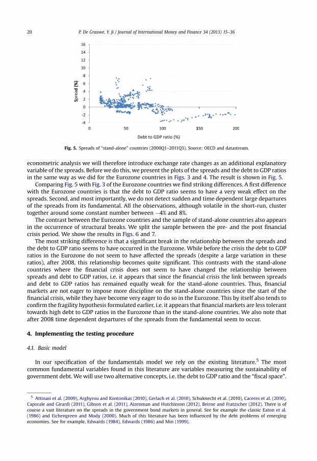
Fig. 5. Spreads of “stand-alone” countries (2000Q1–2011Q3). Source: OECD and datastream.


econometric analysis we will therefore introduce exchange rate changes as an additional explanatoryvariable of the spreads. Beforewe do this, we present the plots of the spreads and the debt to GDP ratiosin the same way as we did for the Eurozone countries in Figs. 3 and 4. The result is shown in Fig. 5.

Comparing Fig. 5 with Fig. 3 of the Eurozone countries we find striking differences. A first differencewith the Eurozone countries is that the debt to GDP ratio seems to have a very weak effect on thespreads. Second, and most importantly, we do not detect sudden and time dependent large departuresof the spreads from its fundamental. All the observations, although volatile in the short-run, clustertogether around some constant number between �4% and 8%.

The contrast between the Eurozone countries and the sample of stand-alone countries also appearsin the occurrence of structural breaks. We split the sample between the pre- and the post financialcrisis period. We show the results in Figs. 6 and 7.

The most striking difference is that a significant break in the relationship between the spreads andthe debt to GDP ratio seems to have occurred in the Eurozone. While before the crisis the debt to GDPratios in the Eurozone do not seem to have affected the spreads (despite a large variation in theseratios), after 2008, this relationship becomes quite significant. This contrasts with the stand-alonecountries where the financial crisis does not seem to have changed the relationship betweenspreads and debt to GDP ratios, i.e. it appears that since the financial crisis the link between spreadsand debt to GDP ratios has remained equally weak for the stand-alone countries. Thus, financialmarkets are not eager to impose more discipline on the stand-alone countries since the start of thefinancial crisis, while they have become very eager to do so in the Eurozone. This by itself also tends toconfirm the fragility hypothesis formulated earlier, i.e. it appears that financial markets are less toleranttowards high debt to GDP ratios in the Eurozone than in the stand-alone countries. We also note thatafter 2008 time dependent departures of the spreads from the fundamental seem to occur.

4. Implementing the testing procedure

4.1. Basic model

In our specification of the fundamentals model we rely on the existing literature.5 The mostcommon fundamental variables found in this literature are variables measuring the sustainability ofgovernment debt. Wewill use two alternative concepts, i.e. the debt to GDP ratio and the “fiscal space”.

5 Attinasi et al. (2009), Arghyrou and Kontonikas (2010), Gerlach et al. (2010), Schuknecht et al. (2010), Caceres et al. (2010),Caporale and Girardi (2011), Gibson et al. (2011), Aizenman and Hutchinson (2012), Beirne and Fratzscher (2012). There is ofcourse a vast literature on the spreads in the government bond markets in general. See for example the classic Eaton et al.(1986) and Eichengreen and Mody (2000). Much of this literature has been influenced by the debt problems of emergingeconomies. See for example, Edwards (1984), Edwards (1986) and Min (1999).

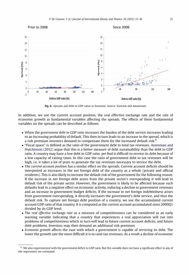
Fig. 6. Spreads and debt to GDP ratios in Eurozone. Source: Eurostat and datastream.


In addition, we use the current account position, the real effective exchange rate and the rate ofeconomic growth as fundamental variables affecting the spreads. The effects of these fundamentalvariables on the spreads can be described as follows.

� When the government debt to GDP ratio increases the burden of the debt service increases leadingto an increasing probability of default. This then in turn leads to an increase in the spread, which isa risk premium investors demand to compensate them for the increased default risk.6

� “Fiscal space” is defined as the ratio of the government debt to total tax revenues. Aizenman andHutchinson (2012) argue that this is a better measure of debt sustainability than the debt to GDPratio. A country may have a low debt to GDP ratio, yet find it difficult to service its debt because ofa low capacity of raising taxes. In this case the ratio of government debt to tax revenues will behigh, i.e. it takes a lot of years to generate the tax revenues necessary to service the debt.

� The current account position has a similar effect on the spreads. Current account deficits should beinterpreted as increases in the net foreign debt of the country as a whole (private and officialresidents). This is also likely to increase the default risk of the government for the following reason.If the increase in net foreign debt arises from the private sector’s overspending it will lead todefault risk of the private sector. However, the government is likely to be affected because suchdefaults lead to a negative effect on economic activity, inducing a decline in government revenuesand an increase in government budget deficits. If the increase in net foreign indebtedness arisesfrom government overspending, it directly increases the government’s debt service, and thus thedefault risk. To capture net foreign debt position of a country, we use the accumulated currentaccount GDP ratio of that country. It is computed as the current account accumulated since 2000Q1divided by its GDP level.

� The real effective exchange rate as a measure of competitiveness can be considered as an earlywarning variable indicating that a country that experiences a real appreciation will run intoproblems of competitiveness which in turn will lead to future current account deficits, and futuredebt problems. Investors may then demand an additional risk premium.

� Economic growth affects the ease with which a government is capable of servicing its debt. Thelower the growth rate the more difficult it is to raise tax revenues. As a result a decline of economic

6 We also experimented with the government deficit to GDP ratio. But this variable does not have a significant effect in any ofthe regressions we estimated.

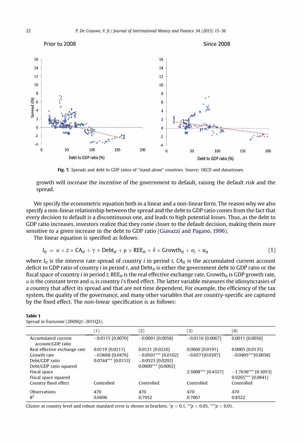
Fig. 7. Spreads and debt to GDP ratios of “stand-alone” countries. Source: OECD and datastream.


growth will increase the incentive of the government to default, raising the default risk and thespread.

We specify the econometric equation both in a linear and a non-linear form. The reasonwhywe alsospecify a non-linear relationship between the spread and the debt to GDP ratio comes from the fact thatevery decision to default is a discontinuous one, and leads to high potential losses. Thus, as the debt toGDP ratio increases, investors realize that they come closer to the default decision, making themmoresensitive to a given increase in the debt to GDP ratio (Giavazzi and Pagano, 1996).

The linear equation is specified as follows:

Iit ¼ aþ z� CAit þ g� Debtit þ m� REEit þ d� Growthit þ ai þ uit (1)

where Iit is the interest rate spread of country i in period t, CAit is the accumulated current accountdeficit to GDP ratio of country i in period t, and Debtit is either the government debt to GDP ratio or thefiscal space of country i in period t, REEit is the real effective exchange rate, Growthit is GDP growth rate,a is the constant term and ai is country i’s fixed effect. The latter variable measures the idiosyncrasies ofa country that affect its spread and that are not time dependent. For example, the efficiency of the taxsystem, the quality of the governance, and many other variables that are country-specific are capturedby the fixed effect. The non-linear specification is as follows:

Table 1Spread in Eurozone (2000Q1–2011Q3).

(1) (2) (3) (4)

Accumulated currentaccount/GDP ratio

�0.0115 [0.0070] �0.0001 [0.0058] �0.0116 [0.0067] 0.0011 [0.0056]

Real effective exchange rate 0.0119 [0.0211] 0.0121 [0.0226] 0.0060 [0.0191] 0.0005 [0.0135]Growth rate �0.0668 [0.0476] �0.0501*** [0.0102] �0.0571[0.0397] �0.0405***[0.0058]Debt/GDP ratio 0.0744*** [0.0133] �0.0523 [0.0292]Debt/GDP ratio squared 0.0009*** [0.0002]Fiscal space 2.5008*** [0.4327] �1.7636*** [0.3053]Fiscal space squared 0.9265*** [0.0841]Country fixed effect Controlled Controlled Controlled Controlled

Observations 470 470 470 470R2 0.6696 0.7952 0.7067 0.8522

Cluster at country level and robust standard error is shown in brackets. *p < 0.1, **p < 0.05, ***p < 0.01.

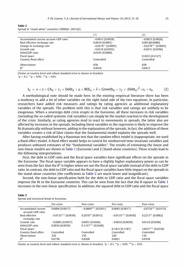
Table 2Spread in “stand-alone” countries (2000Q1–2011Q3).

(1) (2)

Accumulated current account GDP ratio �0.0012 [0.0028] �0.0023 [0.0028]Real effective exchange rate 0.0019 [0.0081] 0.0014[0.0080]Change in exchange rate �0.0274** [0.0095] �0.0278*** [0.0092]Growth rate �0.0216 [0.0295] �0.0231 [0.0296]Debt/GDP ratio 0.0105 [0.0080]Fiscal space 0.2653 [0.2127]Country fixed effect Controlled Controlled

Observations 658 658R2 0.8418 0.8413

Cluster at country level and robust standard error is shown in brackets.*p < 0.1, **p < 0.05, ***p < 0.01.


Iit ¼ aþ z� CAit þ g1 � Debtit þ m� REEit þ d� Growthit þ g2 � ðDebtitÞ2þai þ uit (2)

A methodological note should be made here. In the existing empirical literature there has beena tendency to add a lot of other variables on the right hand side of the two equations. In particular,researchers have added risk measures and ratings by rating agencies as additional explanatoryvariables of the spreads. The problem with this is that risk variables and ratings are unlikely to beexogenous. When a sovereign debt crisis erupts in the Eurozone, all these increases in risk variables(including the so-called systemic risk variables) can simply be the market reaction to the developmentof the crisis. Similarly, as rating agencies tend to react to movements in spreads, the latter also areaffected by increases in the spreads. Including these variables in the regression is likely to improve thefit dramatically without however, adding to the explanation of the spreads. In fact, the addition of thesevariables creates a risk of false claims that the fundamental model explains the spreads well.

After having established by a Hausman test that the random effect model is inappropriate, we useda fixed effect model. A fixed effect model helps to control for unobserved time-invariant variables andproduces unbiased estimates of the “fundamental variables”. The results of estimating the linear andnon-linear models are shown in Table 1 (Eurozone) and 2 (Stand-alone countries). These results lead tothe following interpretations.

First, the debt to GDP ratio and the fiscal space variables have significant effects on the spreads inthe Eurozone. The fiscal space variable appears to have a slightly higher explanatory power as can beseen from the fact that the R2 is higher whenwe use the fiscal space variable instead of the debt to GDPratio. In contrast, the debt to GDP ratio and the fiscal space variables have little impact on the spreads inthe stand-alone countries (the coefficients in Table 2 are much lower and insignificant).

Second, the non-linear specification both for the debt to GDP ratio and the fiscal space variablesimprove the fit in the Eurozone countries. This can be seen from the fact that the R-square in Table 1increases in the non-linear specification. In addition, the squared debt to GDP ratio and the fiscal space

Table 3Spread and structural break in Eurozone.

Pre-crisis Post-crisis Pre-crisis Post-crisis

Accumulated currentaccount GDP ratio

0.0004 [0.0017] �0.0809*** [0.0201] 0.0003 [0.0017] �0.0726*** [0.0153]

Real effectiveexchange rate

�0.0135*** [0.0030] 0.2070** [0.0915] �0.0135*** [0.0030] 0.2213** [0.0882]

Growth rate �0.0005 [0.0037] 0.0053 [0.0266] �0.0010 [0.0039] 0.0124 [0.0208]Debt/GDP ratio 0.0034 [0.0030] 0.1157*** [0.0248]Fiscal space 0.1412 [0.1187] 3.8257*** [0.6538]Country fixed effect Controlled Controlled Controlled ControlledObservations 320 150 320 150R2 0.6758 0.8206 0.6821 0.8358


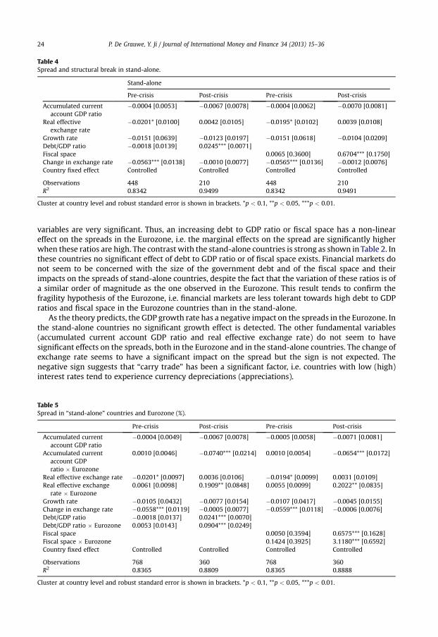
Table 4Spread and structural break in stand-alone.

Stand-alone



�0.0004 [0.0053] �0.0067 [0.0078] �0.0004 [0.0062] �0.0070 [0.0081]


�0.0201* [0.0100] 0.0042 [0.0105] �0.0195* [0.0102] 0.0039 [0.0108]

Growth rate �0.0151 [0.0639] �0.0123 [0.0197] �0.0151 [0.0618] �0.0104 [0.0209]Debt/GDP ratio �0.0018 [0.0139] 0.0245*** [0.0071]Fiscal space 0.0065 [0.3600] 0.6704*** [0.1750]Change in exchange rate �0.0563*** [0.0138] �0.0010 [0.0077] �0.0565*** [0.0136] �0.0012 [0.0076]Country fixed effect Controlled Controlled Controlled Controlled

Observations 448 210 448 210R2 0.8342 0.9499 0.8342 0.9491



variables are very significant. Thus, an increasing debt to GDP ratio or fiscal space has a non-lineareffect on the spreads in the Eurozone, i.e. the marginal effects on the spread are significantly higherwhen these ratios are high. The contrast with the stand-alone countries is strong as shown in Table 2. Inthese countries no significant effect of debt to GDP ratio or of fiscal space exists. Financial markets donot seem to be concerned with the size of the government debt and of the fiscal space and theirimpacts on the spreads of stand-alone countries, despite the fact that the variation of these ratios is ofa similar order of magnitude as the one observed in the Eurozone. This result tends to confirm thefragility hypothesis of the Eurozone, i.e. financial markets are less tolerant towards high debt to GDPratios and fiscal space in the Eurozone countries than in the stand-alone.

As the theory predicts, the GDP growth rate has a negative impact on the spreads in the Eurozone. Inthe stand-alone countries no significant growth effect is detected. The other fundamental variables(accumulated current account GDP ratio and real effective exchange rate) do not seem to havesignificant effects on the spreads, both in the Eurozone and in the stand-alone countries. The change ofexchange rate seems to have a significant impact on the spread but the sign is not expected. Thenegative sign suggests that “carry trade” has been a significant factor, i.e. countries with low (high)interest rates tend to experience currency depreciations (appreciations).

Table 5Spread in “stand-alone” countries and Eurozone (%).



�0.0004 [0.0049] �0.0067 [0.0078] �0.0005 [0.0058] �0.0071 [0.0081]

Accumulated currentaccount GDPratio � Eurozone

0.0010 [0.0046] �0.0740*** [0.0214] 0.0010 [0.0054] �0.0654*** [0.0172]

Real effective exchange rate �0.0201* [0.0097] 0.0036 [0.0106] �0.0194* [0.0099] 0.0031 [0.0109]Real effective exchange

rate � Eurozone0.0061 [0.0098] 0.1909** [0.0848] 0.0055 [0.0099] 0.2022** [0.0835]

Growth rate �0.0105 [0.0432] �0.0077 [0.0154] �0.0107 [0.0417] �0.0045 [0.0155]Change in exchange rate �0.0558*** [0.0119] �0.0005 [0.0077] �0.0559*** [0.0118] �0.0006 [0.0076]Debt/GDP ratio �0.0018 [0.0137] 0.0241*** [0.0070]Debt/GDP ratio � Eurozone 0.0053 [0.0143] 0.0904*** [0.0249]Fiscal space 0.0050 [0.3594] 0.6575*** [0.1628]Fiscal space � Eurozone 0.1424 [0.3925] 3.1180*** [0.6592]Country fixed effect Controlled Controlled Controlled Controlled

Observations 768 360 768 360R2 0.8365 0.8809 0.8365 0.8888


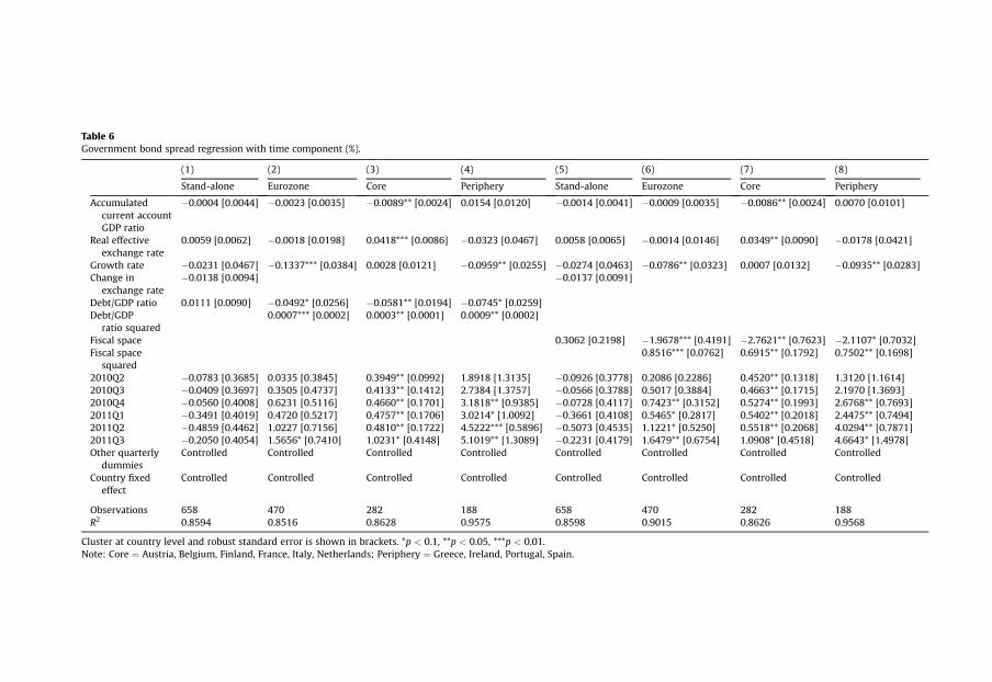
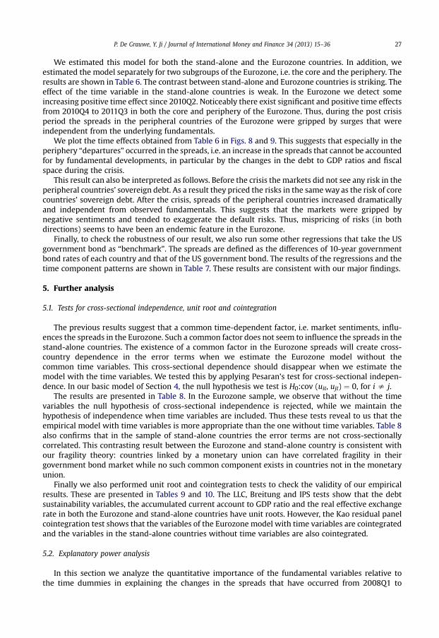
Table 6Government bond spread regression with time component (%).

(1) (2) (3) (4) (5) (6) (7) (8)

Stand-alone Eurozone Core Periphery Stand-alone Eurozone Core Periphery

Accumulatedcurrent accountGDP ratio

�0.0004 [0.0044] �0.0023 [0.0035] �0.0089** [0.0024] 0.0154 [0.0120] �0.0014 [0.0041] �0.0009 [0.0035] �0.0086** [0.0024] 0.0070 [0.0101]


0.0059 [0.0062] �0.0018 [0.0198] 0.0418*** [0.0086] �0.0323 [0.0467] 0.0058 [0.0065] �0.0014 [0.0146] 0.0349** [0.0090] �0.0178 [0.0421]

Growth rate �0.0231 [0.0467] �0.1337*** [0.0384] 0.0028 [0.0121] �0.0959** [0.0255] �0.0274 [0.0463] �0.0786** [0.0323] 0.0007 [0.0132] �0.0935** [0.0283]Change in

exchange rate�0.0138 [0.0094] �0.0137 [0.0091]

Debt/GDP ratio 0.0111 [0.0090] �0.0492* [0.0256] �0.0581** [0.0194] �0.0745* [0.0259]Debt/GDP

ratio squared0.0007*** [0.0002] 0.0003** [0.0001] 0.0009** [0.0002]

Fiscal space 0.3062 [0.2198] �1.9678*** [0.4191] �2.7621** [0.7623] �2.1107* [0.7032]Fiscal space

squared0.8516*** [0.0762] 0.6915** [0.1792] 0.7502** [0.1698]

2010Q2 �0.0783 [0.3685] 0.0335 [0.3845] 0.3949** [0.0992] 1.8918 [1.3135] �0.0926 [0.3778] 0.2086 [0.2286] 0.4520** [0.1318] 1.3120 [1.1614]2010Q3 �0.0409 [0.3697] 0.3505 [0.4737] 0.4133** [0.1412] 2.7384 [1.3757] �0.0566 [0.3788] 0.5017 [0.3884] 0.4663** [0.1715] 2.1970 [1.3693]2010Q4 �0.0560 [0.4008] 0.6231 [0.5116] 0.4660** [0.1701] 3.1818** [0.9385] �0.0728 [0.4117] 0.7423** [0.3152] 0.5274** [0.1993] 2.6768** [0.7693]2011Q1 �0.3491 [0.4019] 0.4720 [0.5217] 0.4757** [0.1706] 3.0214* [1.0092] �0.3661 [0.4108] 0.5465* [0.2817] 0.5402** [0.2018] 2.4475** [0.7494]2011Q2 �0.4859 [0.4462] 1.0227 [0.7156] 0.4810** [0.1722] 4.5222*** [0.5896] �0.5073 [0.4535] 1.1221* [0.5250] 0.5518** [0.2068] 4.0294** [0.7871]2011Q3 �0.2050 [0.4054] 1.5656* [0.7410] 1.0231* [0.4148] 5.1019** [1.3089] �0.2231 [0.4179] 1.6479** [0.6754] 1.0908* [0.4518] 4.6643* [1.4978]Other quarterly

dummiesControlled Controlled Controlled Controlled Controlled Controlled Controlled Controlled

Country fixedeffect

Controlled Controlled Controlled Controlled Controlled Controlled Controlled Controlled

Observations 658 470 282 188 658 470 282 188R2 0.8594 0.8516 0.8628 0.9575 0.8598 0.9015 0.8626 0.9568

Cluster at country level and robust standard error is shown in brackets. *p < 0.1, **p < 0.05, ***p < 0.01.Note: Core ¼ Austria, Belgium, Finland, France, Italy, Netherlands; Periphery ¼ Greece, Ireland, Portugal, Spain.


4.2. Structural break

The graphical analysis of the previous section suggests that a structural break occurs at the time ofthe financial crisis. A Chow test revealed that a structural break occurred in the Eurozone and thestand-alone countries around the year 2008. This allows us to treat the pre- and post-crisis periods asseparate and we show the results in Tables 3 and 4.

In general, the results confirm that since 2008 the markets become more “vigilant” towards somekey economic fundamentals which are associated with higher spreads. To be specific, in both theEurozone and stand-alone countries, the coefficients of the debt to GDP ratio and the fiscal spacevariable are low and insignificant prior to the crisis. In the post-crisis period these coefficients becomelarger and are statistically significant.7 Moreover, the coefficient of the real effective exchange rate isnegative prior to the crisis and this negative effect does not last any more.

However, the contrast in the post-crisis period between the Eurozone and stand-alone countriesare striking. The coefficients of the debt to GDP ratio and the fiscal space in the Eurozone aremuch larger than in the stand-alone countries. Similarly, the coefficient of the real effectiveexchange rate in the Eurozone is significant, while no significant relationship exists in the stand-alonecountries. The negative effect of accumulated current account GDP ratio in the post-crisisbecomes significantly larger in the Eurozone while this effect remains insignificant in the stand-alone countries.

The contrast between the Eurozone and stand-alone countries is also made clear by a pooledregression of the Eurozone and the stand-alone countries. We do this in Table 5. We have addedfour interaction variables “Debt to GDP*Eurozone”, “Fiscal Space*Eurozone”, “Real effective exchangerate*Eurozone” and “Accumulated current account GDP ratio*Eurozone”. These interaction termsmeasure thedegree towhich economic fundamental factors affect the Eurozone spreads differently fromthe stand-alone countries. The results of Table 5 confirm the previous results. The debt sustainabilitymeasures, the real effective exchange rate and the accumulated current account are much stronger andsignificant variables in the Eurozone than in the stand-alone countries especially in the post-crisisperiod. The stand-alone countries seem to be able to “get away with murder” and still not be disci-plined by financial markets.

To summarize, we find a great contrast between the Eurozone and the stand-alone countries. In theformer, we detected a significant increase in the effect of the debt sustainability measures, accumu-lated current account GDP ratio and the real effective exchange rate on the spreads since 2008. Such anincrease is completely absent in the stand-alone countries. This suggests that financial markets appearto punish Eurozone countries more than stand-alone countries for the same imbalances. This by itselftends to support the fragility hypothesis formulated in this paper.

4.3. Introducing time dependency

As will be remembered an important aspect of the fragility hypothesis and of its capacity togenerate self-fulfilling crisis is that it can lead to movements in the spreads that appear to be unrelatedto the fundamental variables of the model. We want to test this hypothesis by measuring the impor-tance of time dependent effects on the spreads that are unrelated to the fundamentals. In order to doso, we introduce time dependency in the basic fixed effect model. In the non-linear specification thisyields:

Iit ¼ aþ z� CAit þ g1 � Debtit þ m� REEit þ d� Growthit þ g2 � ðDebtitÞ2þai þ bt þ 3it (3)

where bt is the time dummy variable. This measures the time effects that are unrelated to thefundamentals of the model or (by definition) to the fixed effects. If significant, it shows that the spreadsmove in time unrelated to the fundamental forces driving the yields.

7 Similar results are obtained by Schuknecht et al. (2010), Arghyrou and Kontonikas (2010), Borgy et al. (2011), Gibson et al.(2011), Beirne and Fratzscher (2012) and Ghosh and Ostry (2012).


We estimated this model for both the stand-alone and the Eurozone countries. In addition, weestimated the model separately for two subgroups of the Eurozone, i.e. the core and the periphery. Theresults are shown in Table 6. The contrast between stand-alone and Eurozone countries is striking. Theeffect of the time variable in the stand-alone countries is weak. In the Eurozone we detect someincreasing positive time effect since 2010Q2. Noticeably there exist significant and positive time effectsfrom 2010Q4 to 2011Q3 in both the core and periphery of the Eurozone. Thus, during the post crisisperiod the spreads in the peripheral countries of the Eurozone were gripped by surges that wereindependent from the underlying fundamentals.

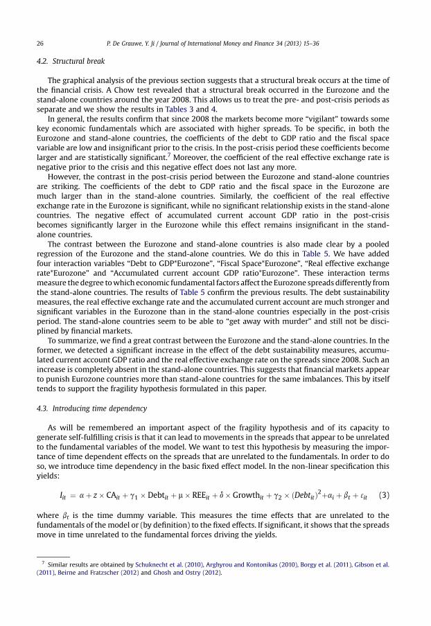
We plot the time effects obtained from Table 6 in Figs. 8 and 9. This suggests that especially in theperiphery “departures” occurred in the spreads, i.e. an increase in the spreads that cannot be accountedfor by fundamental developments, in particular by the changes in the debt to GDP ratios and fiscalspace during the crisis.

This result can also be interpreted as follows. Before the crisis the markets did not see any risk in theperipheral countries’ sovereign debt. As a result they priced the risks in the sameway as the risk of corecountries’ sovereign debt. After the crisis, spreads of the peripheral countries increased dramaticallyand independent from observed fundamentals. This suggests that the markets were gripped bynegative sentiments and tended to exaggerate the default risks. Thus, mispricing of risks (in bothdirections) seems to have been an endemic feature in the Eurozone.

Finally, to check the robustness of our result, we also run some other regressions that take the USgovernment bond as “benchmark”. The spreads are defined as the differences of 10-year governmentbond rates of each country and that of the US government bond. The results of the regressions and thetime component patterns are shown in Table 7. These results are consistent with our major findings.

5. Further analysis

5.1. Tests for cross-sectional independence, unit root and cointegration

The previous results suggest that a common time-dependent factor, i.e. market sentiments, influ-ences the spreads in the Eurozone. Such a common factor does not seem to influence the spreads in thestand-alone countries. The existence of a common factor in the Eurozone spreads will create cross-country dependence in the error terms when we estimate the Eurozone model without thecommon time variables. This cross-sectional dependence should disappear when we estimate themodel with the time variables. We tested this by applying Pesaran’s test for cross-sectional indepen-dence. In our basic model of Section 4, the null hypothesis we test is H0:cov (uit, ujt) ¼ 0, for i s j.

The results are presented in Table 8. In the Eurozone sample, we observe that without the timevariables the null hypothesis of cross-sectional independence is rejected, while we maintain thehypothesis of independence when time variables are included. Thus these tests reveal to us that theempirical model with time variables is more appropriate than the one without time variables. Table 8also confirms that in the sample of stand-alone countries the error terms are not cross-sectionallycorrelated. This contrasting result between the Eurozone and stand-alone country is consistent withour fragility theory: countries linked by a monetary union can have correlated fragility in theirgovernment bond market while no such common component exists in countries not in the monetaryunion.

Finally we also performed unit root and cointegration tests to check the validity of our empiricalresults. These are presented in Tables 9 and 10. The LLC, Breitung and IPS tests show that the debtsustainability variables, the accumulated current account to GDP ratio and the real effective exchangerate in both the Eurozone and stand-alone countries have unit roots. However, the Kao residual panelcointegration test shows that the variables of the Eurozone model with time variables are cointegratedand the variables in the stand-alone countries without time variables are also cointegrated.

5.2. Explanatory power analysis

In this section we analyze the quantitative importance of the fundamental variables relative tothe time dummies in explaining the changes in the spreads that have occurred from 2008Q1 to

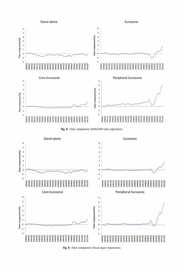
Fig. 9. Time component (Fiscal space regression).

Fig. 8. Time component (Debt/GDP ratio regression).

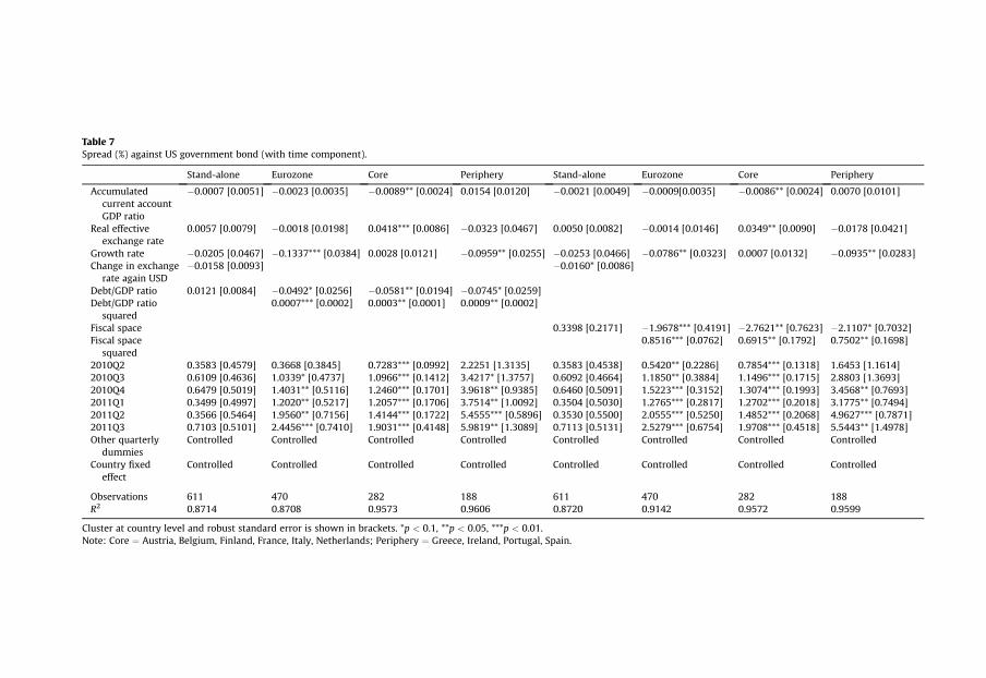
Table 7Spread (%) against US government bond (with time component).

Stand-alone Eurozone Core Periphery Stand-alone Eurozone Core Periphery

Accumulatedcurrent accountGDP ratio

�0.0007 [0.0051] �0.0023 [0.0035] �0.0089** [0.0024] 0.0154 [0.0120] �0.0021 [0.0049] �0.0009[0.0035] �0.0086** [0.0024] 0.0070 [0.0101]


0.0057 [0.0079] �0.0018 [0.0198] 0.0418*** [0.0086] �0.0323 [0.0467] 0.0050 [0.0082] �0.0014 [0.0146] 0.0349** [0.0090] �0.0178 [0.0421]

Growth rate �0.0205 [0.0467] �0.1337*** [0.0384] 0.0028 [0.0121] �0.0959** [0.0255] �0.0253 [0.0466] �0.0786** [0.0323] 0.0007 [0.0132] �0.0935** [0.0283]Change in exchange

rate again USD�0.0158 [0.0093] �0.0160* [0.0086]

Debt/GDP ratio 0.0121 [0.0084] �0.0492* [0.0256] �0.0581** [0.0194] �0.0745* [0.0259]Debt/GDP ratio

squared0.0007*** [0.0002] 0.0003** [0.0001] 0.0009** [0.0002]

Fiscal space 0.3398 [0.2171] �1.9678*** [0.4191] �2.7621** [0.7623] �2.1107* [0.7032]Fiscal space

squared0.8516*** [0.0762] 0.6915** [0.1792] 0.7502** [0.1698]

2010Q2 0.3583 [0.4579] 0.3668 [0.3845] 0.7283*** [0.0992] 2.2251 [1.3135] 0.3583 [0.4538] 0.5420** [0.2286] 0.7854*** [0.1318] 1.6453 [1.1614]2010Q3 0.6109 [0.4636] 1.0339* [0.4737] 1.0966*** [0.1412] 3.4217* [1.3757] 0.6092 [0.4664] 1.1850** [0.3884] 1.1496*** [0.1715] 2.8803 [1.3693]2010Q4 0.6479 [0.5019] 1.4031** [0.5116] 1.2460*** [0.1701] 3.9618** [0.9385] 0.6460 [0.5091] 1.5223*** [0.3152] 1.3074*** [0.1993] 3.4568** [0.7693]2011Q1 0.3499 [0.4997] 1.2020** [0.5217] 1.2057*** [0.1706] 3.7514** [1.0092] 0.3504 [0.5030] 1.2765*** [0.2817] 1.2702*** [0.2018] 3.1775** [0.7494]2011Q2 0.3566 [0.5464] 1.9560** [0.7156] 1.4144*** [0.1722] 5.4555*** [0.5896] 0.3530 [0.5500] 2.0555*** [0.5250] 1.4852*** [0.2068] 4.9627*** [0.7871]2011Q3 0.7103 [0.5101] 2.4456*** [0.7410] 1.9031*** [0.4148] 5.9819** [1.3089] 0.7113 [0.5131] 2.5279*** [0.6754] 1.9708*** [0.4518] 5.5443** [1.4978]Other quarterly

dummiesControlled Controlled Controlled Controlled Controlled Controlled Controlled Controlled

Country fixedeffect

Controlled Controlled Controlled Controlled Controlled Controlled Controlled Controlled

Observations 611 470 282 188 611 470 282 188R2 0.8714 0.8708 0.9573 0.9606 0.8720 0.9142 0.9572 0.9599

Cluster at country level and robust standard error is shown in brackets. *p < 0.1, **p < 0.05, ***p < 0.01.Note: Core ¼ Austria, Belgium, Finland, France, Italy, Netherlands; Periphery ¼ Greece, Ireland, Portugal, Spain.

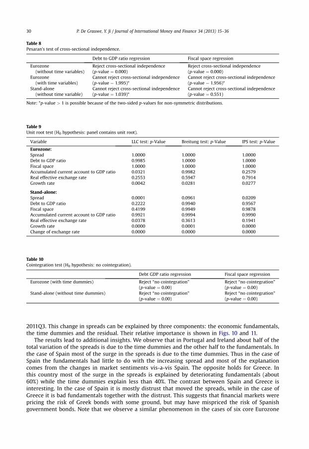
Table 8Pesaran’s test of cross-sectional independence.

Debt to GDP ratio regression Fiscal space regression

Eurozone(without time variables)

Reject cross-sectional independence(p-value ¼ 0.000)

Reject cross-sectional independence(p-value ¼ 0.000)

Eurozone(with time variables)

Cannot reject cross-sectional independence(p-value ¼ 1.995)*


Stand-alone(without time variable)


Cannot reject cross-sectional independence(p-value ¼ 0.551)

Note: *p-value > 1 is possible because of the two-sided p-values for non-symmetric distributions.

Table 9Unit root test (H0 hypothesis: panel contains unit root).

Variable LLC test: p-Value Breitung test: p-Value IPS test: p-Value

Eurozone:Spread 1.0000 1.0000 1.0000Debt to GDP ratio 0.9985 1.0000 1.0000Fiscal space 1.0000 1.0000 1.0000Accumulated current account to GDP ratio 0.0321 0.9982 0.2579Real effective exchange rate 0.2553 0.5947 0.7914Growth rate 0.0042 0.0281 0.0277

Stand-alone:Spread 0.0001 0.0961 0.0209Debt to GDP ratio 0.2222 0.9940 0.9567Fiscal space 0.4199 0.9949 0.9878Accumulated current account to GDP ratio 0.9921 0.9994 0.9990Real effective exchange rate 0.0378 0.3613 0.1941Growth rate 0.0000 0.0001 0.0000Change of exchange rate 0.0000 0.0000 0.0000

Table 10Cointegration test (H0 hypothesis: no cointegration).

Debt GDP ratio regression Fiscal space regression

Eurozone (with time dummies) Reject “no cointegration”(p-value ¼ 0.00)

Reject “no cointegration”(p-value ¼ 0.00)

Stand-alone (without time dummies) Reject “no cointegration”(p-value ¼ 0.00)

Reject “no cointegration”(p-value ¼ 0.00)


2011Q3. This change in spreads can be explained by three components: the economic fundamentals,the time dummies and the residual. Their relative importance is shown in Figs. 10 and 11.

The results lead to additional insights. We observe that in Portugal and Ireland about half of thetotal variation of the spreads is due to the time dummies and the other half to the fundamentals. Inthe case of Spain most of the surge in the spreads is due to the time dummies. Thus in the case ofSpain the fundamentals had little to do with the increasing spread and most of the explanationcomes from the changes in market sentiments vis-a-vis Spain. The opposite holds for Greece. Inthis country most of the surge in the spreads is explained by deteriorating fundamentals (about60%) while the time dummies explain less than 40%. The contrast between Spain and Greece isinteresting. In the case of Spain it is mostly distrust that moved the spreads, while in the case ofGreece it is bad fundamentals together with the distrust. This suggests that financial markets werepricing the risk of Greek bonds with some ground, but may have mispriced the risk of Spanishgovernment bonds. Note that we observe a similar phenomenon in the cases of six core Eurozone

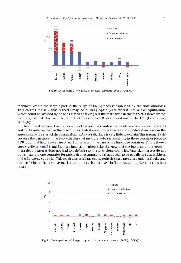
Fig. 10. Decomposition of change in spreads: Eurozone (2008Q1–2011Q3).


members where the largest part in the surge of the spreads is explained by the time dummies.This creates the risk that markets may be pushing Spain (and others) into a bad equilibrium,which could be avoided by policies aimed at taking out the fear factor in the market. Elsewhere wehave argued that this could be done by Lender of Last Resort operations of the ECB (De Grauwe,2011a,b).

The contrast between the Eurozone countries and the stand-alone countries is made clear in Figs.10and 11. As noted earlier, in the case of the stand-alone countries there is no significant increase in thespreads since the start of the financial crisis. As a result, there is very little to explain. This is remarkablebecause the variation in the two variables that measure debt sustainability in these countries (debt toGDP ratios and fiscal space) are at least as large as in the case of the Eurozone countries. This is shownvery vividly in Figs. 12 and 13. Thus financial markets take the view that the build-up of the govern-ment debt measures does not lead to a default risk in stand-alone countries. Financial markets do notpunish stand-alone countries for public debt accumulation that appear to be equally unsustainable asin the Eurozone countries. This result also confirms our hypothesis that a monetary union is fragile andcan easily be hit by negative market sentiments that in a self-fulfilling way can drive countries intodefault.

Fig. 11. Decomposition of change in spreads: Stand-alone countries (2008Q1–2011Q3).

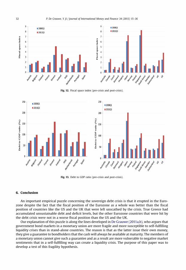
Fig. 13. Debt to GDP ratio (pre-crisis and post-crisis).

Fig. 12. Fiscal space index (pre-crisis and post-crisis).


6. Conclusion

An important empirical puzzle concerning the sovereign debt crisis is that it erupted in the Euro-zone despite the fact that the fiscal position of the Eurozone as a whole was better than the fiscalposition of countries like the US and the UK that were left unscathed by the crisis. True Greece hadaccumulated unsustainable debt and deficit levels, but the other Eurozone countries that were hit bythe debt crisis were not in a worse fiscal position than the US and the UK.

Our explanation of this puzzle is along the lines developed in De Grauwe (2011a,b), who argues thatgovernment bond markets in a monetary union are more fragile and more susceptible to self-fulfillingliquidity crises than in stand-alone countries. The reason is that as the latter issue their own money,they give a guarantee to bondholders that the cashwill always be available atmaturity. Themembers ofa monetary union cannot give such a guarantee and as a result are more vulnerable to negative marketsentiments that in a self-fulfilling way can create a liquidity crisis. The purpose of this paper was todevelop a test of this fragility hypothesis.


On the whole we confirm this hypothesis. We found evidence that a large part of the surge in thespreads of the peripheral Eurozone countries during 2010–11 was disconnected from underlyingincreases in the debt to GDP ratios and fiscal space, and was the result of time dependent negativemarket sentiments that became very strong since the end of 2010. The exception is Greece where wefound that the major increase in the spread was due to deteriorating fundamentals. The stand-alonecountries in our sample have been immune from these liquidity crises and weathered the stormwithout the increases in the spread.

We also found evidence that after years of neglecting high debt to GDP ratios, investors becameincreasingly worried about the high debt to GDP ratios in the Eurozone, and reacted by raising thespreads. No such worries developed in stand-alone countries despite the fact that debt to GDP ratioswere equally high and increasing in these countries. This result can also be said to validate the fragilityhypothesis, i.e. the markets appear to be less tolerant towards large public debt accumulations in theEurozone than towards equally large public debt accumulations in the stand-alone countries.

Thus, the story of the Eurozone is also a story of self-fulfilling debt crises, which in turn lead tomultiple equilibria. Countries that are hit by a liquidity crisis are forced to apply stringent austeritymeasures that force them into a recession, thereby reducing the effectiveness of these austerityprograms. There is a risk that the combination of high interest rates and deep recessions turn theliquidity crisis into a solvency crisis.

In a world where spreads are tightly linked to the underlying fundamentals such as the debt to GDPratio and fiscal space, the only option the policy makers have in reducing the spreads is to improve thefundamentals. This implies measures aimed at reducing the debt burden. If, however, there can bea disconnection between the spreads and the fundamentals, a policy geared exclusively towardsaffecting the fundamentals (i.e. reducing the debt burden) will not be sufficient. In that case policymakers should also try to stop countries from being driven into a bad equilibrium. This can be achievedby more active liquidity policies by the ECB that aim at preventing a liquidity crisis from leading toa self-fulfilling solvency crisis (De Grauwe, 2011a,b).

Acknowledgements

We are grateful to Joshua Aizenman, Geert Dhaene, Daniel Gros, Frank Westermann for insightfulcomments on a previous version of the paper. Financial support of the Belgian National ScienceFoundation (BELSPO) is gratefully acknowledged.

Appendix A. A Model of good and bad equilibriaWe present a very simple model illustrating how multiple equilibria can arise. The starting point is

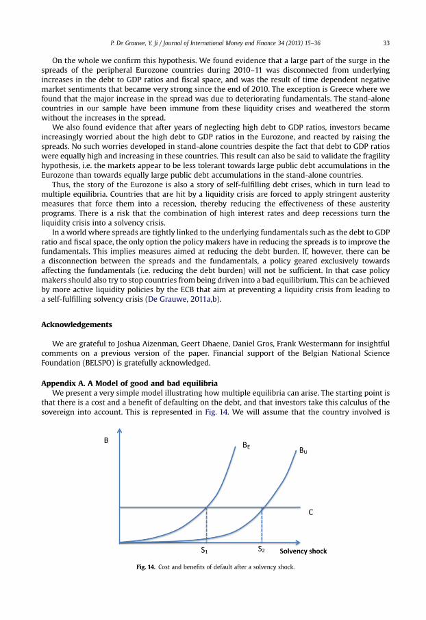
that there is a cost and a benefit of defaulting on the debt, and that investors take this calculus of thesovereign into account. This is represented in Fig. 14. We will assume that the country involved is

Fig. 14. Cost and benefits of default after a solvency shock.


subject to a shock, which takes the form of a decline in government revenues. It may be caused bya recession, or a loss of competitiveness. We call this a solvency shock. The higher this shock the greateris the loss of solvency. We concentrate first on the benefit side. On the horizontal axis we show thesolvency shock. On the vertical axis we represent the benefit of defaulting. There are many ways anddegrees of defaulting. To simplify we assume this takes the form of a haircut of a fixed percentage. Thebenefit of defaulting in this way is that the government can reduce the interest burden on theoutstanding debt. As a result, after the default it will have to apply less austerity, i.e. it will have toreduce spending and/or increase taxes by less than without the default. Since austerity is politicallycostly, the government profits from the default.

A major insight of the model is that the benefit of a default depends on whether this default isexpected or not. We show two curves representing the benefit of a default. BU is the benefit of a defaultthat investors do not expect to happen, while BE is the benefit of a default that investors expect tohappen. Let us first concentrate on the BU curve. It is upward sloping because when the solvency shockincreases, the benefit of a default for the sovereign goes up. The reason is that when the solvencyshock is large, i.e. the decline in tax income is large, the cost of austerity is substantial. Default thenbecomes more attractive for the sovereign. We have drawn this curve to be non-linear, but this is notessential for the argument. We distinguish three factors that affect the position and the steepness ofthe BU curve:

� The initial debt level. The higher is this level, the higher is the benefit of a default. Thus with a higherinitial debt level the BU curve will rotate upwards.

� The efficiency of the tax system. In a country with an inefficient tax system, the government cannoteasily increase taxation. Thus in such a country the option of defaulting becomes more attractive.The BU curve rotates upwards.

� The size of the external debt. When external debt takes a large proportion of total debt there will beless domestic political resistance against default, making the latter more attractive (the BU curverotates upwards).

We now concentrate on the BE curve. This shows the benefit of a default when investors anticipatesuch a default. It is located above the BU curve for the following reason. When investors expecta default, theywill sell government bonds. As a result, the interest rate on government bonds increases.This raises the government budget deficit requiring a more intense austerity program of spending cutsand tax hikes. Thus, default becomes more attractive. For every solvency shock, the benefits of defaultwill be higher than they were when the default was not anticipated.

We now introduce the cost side of the default in Fig.14. The cost of a default arises from the fact that,when defaulting, the government suffers a loss of reputation. This loss of reputation will make itdifficult for the government to borrow in the future.Wewill make the simplifying assumption that thisis a fixed cost (C).

We now have the tools to analyze the equilibrium of the model. We will distinguish between threetypes of solvency shocks, a small one, an intermediate one, and a large one. Take a small solvencyshock: this is a shock S < S1 (this could be the shocks that Germany and the Netherlands experiencedduring the debt crisis). For this small shock the cost of a default is always larger than the benefits (bothof an expected and an unexpected default). Thus the government will not want to default. Whenexpectations are rational investors will not expect a default. As a result, a no-default equilibrium can besustained.

Let us now analyze a large solvency shock. This is one for which S > S2 (this could be the shockexperienced by Greece). For all these large shockswe observe that the cost of a default is always smallerthan the benefits (both of an expected and an unexpected default). The government will want todefault. In a rational expectations framework, investors will anticipate this. As a result, a default isinevitable.

We now turn to the intermediate case: S1 < S < S2 (this could be the shocks that Ireland, Portugaland Spain experienced). For these intermediate shocks we obtain an indeterminacy, i.e. two equilibriaare possible. Which one will prevail depends on what is expected. Suppose the solvency shock is S0 (inFig. 15). In this case there are two potential equilibria, D and N. Take point D, investors expect a default

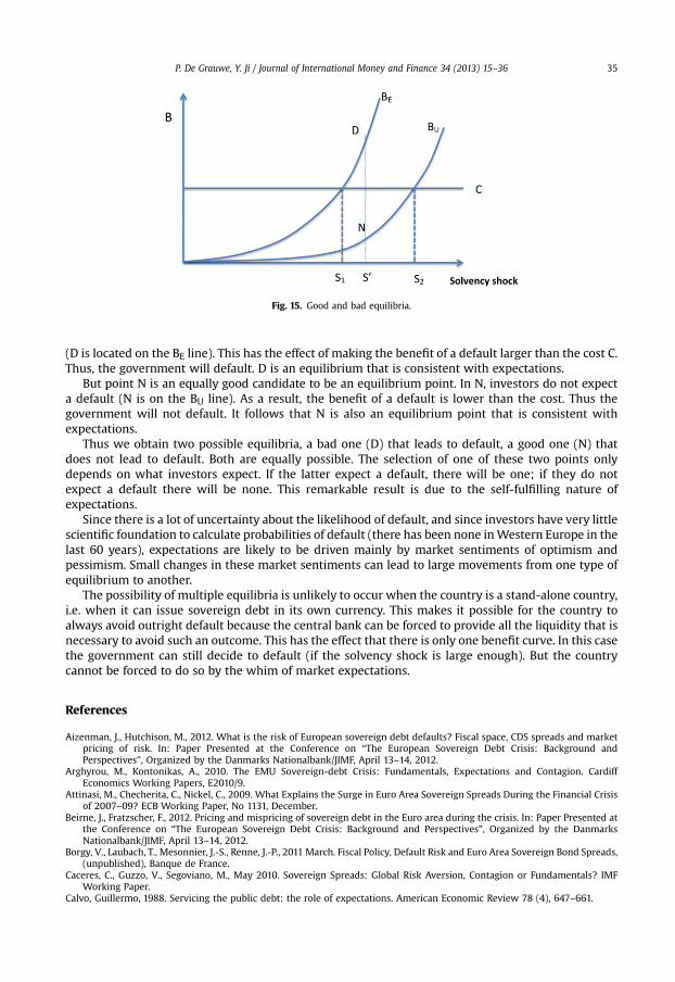
Fig. 15. Good and bad equilibria.


(D is located on the BE line). This has the effect of making the benefit of a default larger than the cost C.Thus, the government will default. D is an equilibrium that is consistent with expectations.

But point N is an equally good candidate to be an equilibrium point. In N, investors do not expecta default (N is on the BU line). As a result, the benefit of a default is lower than the cost. Thus thegovernment will not default. It follows that N is also an equilibrium point that is consistent withexpectations.

Thus we obtain two possible equilibria, a bad one (D) that leads to default, a good one (N) thatdoes not lead to default. Both are equally possible. The selection of one of these two points onlydepends on what investors expect. If the latter expect a default, there will be one; if they do notexpect a default there will be none. This remarkable result is due to the self-fulfilling nature ofexpectations.

Since there is a lot of uncertainty about the likelihood of default, and since investors have very littlescientific foundation to calculate probabilities of default (there has been none inWestern Europe in thelast 60 years), expectations are likely to be driven mainly by market sentiments of optimism andpessimism. Small changes in these market sentiments can lead to large movements from one type ofequilibrium to another.

The possibility of multiple equilibria is unlikely to occur when the country is a stand-alone country,i.e. when it can issue sovereign debt in its own currency. This makes it possible for the country toalways avoid outright default because the central bank can be forced to provide all the liquidity that isnecessary to avoid such an outcome. This has the effect that there is only one benefit curve. In this casethe government can still decide to default (if the solvency shock is large enough). But the countrycannot be forced to do so by the whim of market expectations.

References

Aizenman, J., Hutchison, M., 2012. What is the risk of European sovereign debt defaults? Fiscal space, CDS spreads and marketpricing of risk. In: Paper Presented at the Conference on “The European Sovereign Debt Crisis: Background andPerspectives”, Organized by the Danmarks Nationalbank/JIMF, April 13–14, 2012.

Arghyrou, M., Kontonikas, A., 2010. The EMU Sovereign-debt Crisis: Fundamentals, Expectations and Contagion. CardiffEconomics Working Papers, E2010/9.

Attinasi, M., Checherita, C., Nickel, C., 2009. What Explains the Surge in Euro Area Sovereign Spreads During the Financial Crisisof 2007–09? ECB Working Paper, No 1131, December.

Beirne, J., Fratzscher, F., 2012. Pricing and mispricing of sovereign debt in the Euro area during the crisis. In: Paper Presented atthe Conference on “The European Sovereign Debt Crisis: Background and Perspectives”, Organized by the DanmarksNationalbank/JIMF, April 13–14, 2012.

Borgy, V., Laubach, T., Mesonnier, J.-S., Renne, J.-P., 2011 March. Fiscal Policy, Default Risk and Euro Area Sovereign Bond Spreads,(unpublished), Banque de France.

Caceres, C., Guzzo, V., Segoviano, M., May 2010. Sovereign Spreads: Global Risk Aversion, Contagion or Fundamentals? IMFWorking Paper.

Calvo, Guillermo, 1988. Servicing the public debt: the role of expectations. American Economic Review 78 (4), 647–661.


Caporale, G., Girardi, A., October 2011. Fiscal Spillovers in the Euro Area. Discussion Paper, 1164. DIW, Berlin.Corsetti, G.C., Dedola, L., 2011. Fiscal Crises, Confidence and Default. A Bare-bones model with Lessons for the Euro Area.

Unpublished, Cambridge.De Grauwe, P., 2011a. The governance of a fragile Eurozone, economic policy, CEPS working documents. http://www.ceps.eu/

book/governance-fragile-eurozone.De Grauwe, P., 2011b. The ECB as a Lender of Last Resort. VoxEU. http://www.voxeu.org/index.php?q¼node/6884.Diamond, D.W., Dybvig, P.H., 1983. Bank runs, deposit insurance, and liquidity. Journal of Political Economy 91 (3), 401–419.Eaton, J., Gersovitz, M., Stiglitz, J.E., June 1986. The pure theory of country risk. European Economic Review 30, 481–513.Edwards, S., September 1984. LDC foreign borrowing and default risk: an empirical investigation: 1976–1980. American

Economic Review 74, 726–734.Edwards, S., 1986. The pricing of bonds and bank loans in international markets: an empirical analysis of developing countries’

foreign borrowing. European Economic Review 30, 565–589.Eichengreen, B., Mody, A., 2000. Lending booms, reserves and the sustainability of short- term debt: inferences from the pricing

of syndicated bank loans. Journal of Development Economics 63, 5–44.Eichengreen, B., Hausmann, R., Panizza, U., 2005. the pain of original sin. In: Eichengreen, B., Hausmann, R. (Eds.), Other People’s

Money: Debt Denomination and Financial Instability in Emerging Market Economies. Chicago University Press.Gerlach, S., Schulz, G., Wolff, W., 2010. Banking and Sovereign Risk in the Euro Area. Mimeo, Deutsche Bundesbank.Ghosh, A., Ostry, J., 2012. Fiscal responsibility and public debt limits in a currency union. In: Paper Presented at the Conference

on “the European Sovereign Debt Crisis: Background and Perspectives”, Organized by the Danmarks Nationalbank/JIMF,April 13–14, 2012.

Gibson, H., Hall G., Tavlas, G., 2011 March. The Greek Financial Crisis: Growing Imbalances and Sovereign Spreads. WorkingPaper, Bank of Greece.

Giavazzi, Francesco., Pagano, Marco., 1996. “Non-Keynesian Effects of Fiscal Policy Changes: International Evidence and theSwedish Experience”, Swedish Economic Policy Review, May.

Gros, D., 2011. A Simple Model of Multiple Equilibria and Default. Mimeo, CEPS.Kopf, Christian., 2011. Restoring Financial Stability in the Euro Area, 15 March 2011, In CEPS Policy Briefs.Min, H., 1999. Determinants of Emerging Market Bond Spread: Do Economic Fundamentals Matter? World Bank. http://elibrary.

worldbank.org/content/workingpaper/10.1596/1813-9450-1899.Obstfeld, M., 1986. Rational and self-fulfilling balance-of-payments crises. American Economic Review 76 (1), 72–81.Schuknecht, L., von Hagen, J., Wolswijk, G., 2010. Government Bond Risk Premiums in the EU Revisited the Impact of the

Financial Crisis, ECB Working Paper No 1152, 2010 February.

http://www.ceps.eu/book/governance-fragile-eurozone

http://www.ceps.eu/book/governance-fragile-eurozone

http://www.voxeu.org/index.php%3Fq%3Dnode/6884

http://www.voxeu.org/index.php%3Fq%3Dnode/6884

http://elibrary.worldbank.org/content/workingpaper/10.1596/1813-9450-1899

http://elibrary.worldbank.org/content/workingpaper/10.1596/1813-9450-1899

Paul De Grauwe, Yuemei Ji Self-fulfilling crises in the ...eprints.lse.ac.uk/49648/1/__lse.ac.uk_storage_LIBRARY_Secondary... · Paul De Grauwe, Yuemei Ji Self-fulfilling crises in

Documents