PARTICLE PHYSICS IN THE RANDALL-SUNDRUM FRAMEWORK … · PARTICLE PHYSICS IN THE RANDALL-SUNDRUM ... several aspects of particle physics in the Randall-Sundrum framework are ... Giacomo

PARTICLE PHYSICS IN THE RANDALL-SUNDRUM

FRAMEWORK

A Dissertation

Presented to the Faculty of the Graduate School

of Cornell University

in Partial Fulfillment of the Requirements for the Degree of

Doctor of Philosophy

by

Matthew B. Reece

August 2008

This document is in the public domain.

PARTICLE PHYSICS IN THE RANDALL-SUNDRUM FRAMEWORK

Matthew B. Reece, Ph.D.

Cornell University 2008

In this dissertation, several aspects of particle physics in the Randall-Sundrum

framework are discussed. We view the Randall-Sundum framework as a model

for the dual of a strongly interacting technicolor theory of electroweak symmetry

breaking (EWSB). First, we consider extra dimensional descriptions of models

where there are two separate strongly interacting EWSB sectors (“topcolor” type

models). Such models can help alleviate the tension between the large top quark

mass and the correct value of the Zbb couplings in ordinary Higgsless models. A

necessary consequence is the appearance of additional pseudo-Goldstone bosons

(“top-pions”), which would be strongly coupled to the third generation. Second,

we examine extra-dimensional theories as “AdS/QCD” models of hadrons, pointing

out that the infrared physics can be developed in a more systematic manner by

exploiting backreaction of the nonperturbative condensates. We also show how

asymptotic freedom can be incorporated into the theory, and the substantial effect

it has on the glueball spectrum and gluon condensate of the theory. Finally, we

study the S parameter, considering especially its sign, in models with fermions

localized near the UV brane. We show that for EWSB in the bulk by a Higgs VEV,

S is positive for arbitrary metric and Higgs profile, assuming that the effects from

higher-dimensional operators in the 5D theory are sub-leading and can therefore

be neglected. Our work strongly suggests that S is positive in calculable models

in extra dimensions.

BIOGRAPHICAL SKETCH

Matt Reece was born in Louisville, Kentucky on January 24, 1982, to Beverly

and Kenneth Reece. He grew up in Louisville, where he attended duPont Manual

High School and got his first taste of research in a summer working with electrical

engineers at the University of Louisville. As an undergraduate he attended the

University of Chicago, concentrating in physics and mathematics. While there

he worked on the CDF experiment, which helped to foster his interest in particle

physics but also convinced him that he would be more useful as a theorist than

an experimentalist. His interest in building theoretical models that could be dis-

covered by future experiments led him to Cornell, where he has spent four years

trying to understand what to expect from the upcoming LHC experiments. He

hopes the results will, nonetheless, surprise him.

iii

This dissertation is dedicated to my parents.

iv

ACKNOWLEDGEMENTS

I thank Csaba Csaki for his excellent advice over the past four years. I’ve learned

a great deal of physics from him, but more than that, I’ve learned how to think

like a physicist. Many thanks go to my collaborators on this research: Csaba

Csaki throughout, Christophe Grojean on the material in chapters two and four,

Giacomo Cacciapaglia and John Terning on the material in chapter two, and Kaus-

tubh Agashe on the material in chapter four. Useful discussions and comments on

the material in this thesis came from Gustavo Burdman, Roberto Contino, Cedric

Delaunay, Josh Erlich, Johannes Hirn, Andreas Karch, Ami Katz, Guido Maran-

della, Alex Pomarol, Riccardo Rattazzi, Veronica Sanz, Matthew Schwartz, and

Raman Sundrum. I thank Patrick Meade for collaboration on other research, not

contained in this thesis, and for discussions that have influenced many of my ideas.

I am indebted to others, too numerous to list here yet still important, for sharing

their insights about physics with me. My work has been generously supported by

an Olin Fellowship from Cornell University, an NSF Graduate Research Fellowship,

and a KITP Graduate Fellowship.

v

TABLE OF CONTENTS

Biographical Sketch . . . . . . . . . . . . . . . . . . . . . . . . . . . . . . iiiDedication . . . . . . . . . . . . . . . . . . . . . . . . . . . . . . . . . . . ivAcknowledgements . . . . . . . . . . . . . . . . . . . . . . . . . . . . . . vTable of Contents . . . . . . . . . . . . . . . . . . . . . . . . . . . . . . . viList of Tables . . . . . . . . . . . . . . . . . . . . . . . . . . . . . . . . . viiiList of Figures . . . . . . . . . . . . . . . . . . . . . . . . . . . . . . . . . ix

1 Introduction 11.1 The Standard Model and EWSB . . . . . . . . . . . . . . . . . . . 11.2 Options for the Hierarchy Problem . . . . . . . . . . . . . . . . . . 31.3 Technicolor and Randall-Sundrum . . . . . . . . . . . . . . . . . . . 71.4 Contents . . . . . . . . . . . . . . . . . . . . . . . . . . . . . . . . . 8

2 Top and Bottom: A Brane of Their Own 112.1 Introduction . . . . . . . . . . . . . . . . . . . . . . . . . . . . . . . 112.2 Warmup: Boundary Conditions for a U(1) on an Interval . . . . . . 15

2.2.1 Double AdS case . . . . . . . . . . . . . . . . . . . . . . . . 202.3 The Standard Model in Two Bulks: Gauge Sector . . . . . . . . . . 23

2.3.1 Higgs—top-Higgs . . . . . . . . . . . . . . . . . . . . . . . . 252.3.2 Higgsless—top-Higgs . . . . . . . . . . . . . . . . . . . . . . 262.3.3 Higgsless—higgsless . . . . . . . . . . . . . . . . . . . . . . . 28

2.4 The CFT Interpretation . . . . . . . . . . . . . . . . . . . . . . . . 292.5 Top-pions . . . . . . . . . . . . . . . . . . . . . . . . . . . . . . . . 33

2.5.1 Top-pions from the CFT correspondence . . . . . . . . . . . 332.5.2 Properties of the top-pion from the 5D picture. . . . . . . . 35

2.6 Phenomenology of the Two IR Brane Models . . . . . . . . . . . . . 402.6.1 Overview of the various models . . . . . . . . . . . . . . . . 402.6.2 Phenomenology of the higgsless—top-Higgs model . . . . . . 432.6.3 Phenomenology of the higgsless—higgsless model . . . . . . 52

2.7 Conclusions . . . . . . . . . . . . . . . . . . . . . . . . . . . . . . . 55

3 A Braneless Approach to Holographic QCD 583.1 Introduction . . . . . . . . . . . . . . . . . . . . . . . . . . . . . . . 583.2 AdS/QCD on Randall-Sundrum backgrounds . . . . . . . . . . . . 623.3 Vacuum condensates as IR cutoff . . . . . . . . . . . . . . . . . . . 65

3.3.1 Gluon condensate . . . . . . . . . . . . . . . . . . . . . . . . 673.3.2 The Glueball Spectrum . . . . . . . . . . . . . . . . . . . . . 69

3.4 Incorporating Asymptotic freedom . . . . . . . . . . . . . . . . . . 713.4.1 The Glueball Spectrum . . . . . . . . . . . . . . . . . . . . . 743.4.2 Power Corrections and gluon condensate . . . . . . . . . . . 753.4.3 Relation to Analytic Perturbation Theory . . . . . . . . . . 79

3.5 Effects of the Tr(F 3) condensate . . . . . . . . . . . . . . . . . . . . 81

vi

3.5.1 Gubser’s Criterion: Constraining z1/z0 . . . . . . . . . . . . 833.5.2 Condensates . . . . . . . . . . . . . . . . . . . . . . . . . . . 853.5.3 Glueball spectra . . . . . . . . . . . . . . . . . . . . . . . . . 86

3.6 Linearly confining backgrounds? . . . . . . . . . . . . . . . . . . . . 873.6.1 No linear confinement in the dilaton-graviton system . . . . 883.6.2 Linear confinement from the tachyon-dilaton-graviton system? 90

3.7 Conclusions and Outlook . . . . . . . . . . . . . . . . . . . . . . . . 93

4 The S-parameter in Holographic Technicolor Models 954.1 Introduction . . . . . . . . . . . . . . . . . . . . . . . . . . . . . . . 954.2 A plausibility argument for S > 0 . . . . . . . . . . . . . . . . . . . 984.3 Boundary-effective-action approach to oblique corrections. Simple

cases with boundary breaking . . . . . . . . . . . . . . . . . . . . . 1014.3.1 S > 0 for BC breaking with boundary kinetic mixing . . . . 1054.3.2 S > 0 for BC breaking with arbitrary kinetic functions . . . 105

4.4 S > 0 in models with bulk Higgs . . . . . . . . . . . . . . . . . . . 1074.5 Bulk Higgs and bulk kinetic mixing . . . . . . . . . . . . . . . . . . 111

4.5.1 The general case . . . . . . . . . . . . . . . . . . . . . . . . 1134.5.2 Scan of the parameter space for AdS backgrounds . . . . . . 115

4.6 Conclusions . . . . . . . . . . . . . . . . . . . . . . . . . . . . . . . 119

5 Conclusions 122

Bibliography 125

vii

LIST OF TABLES

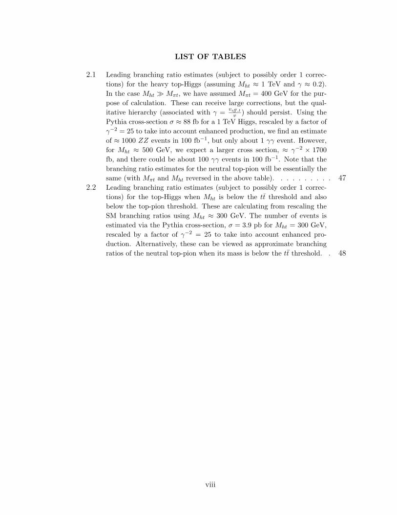
2.1 Leading branching ratio estimates (subject to possibly order 1 correc-tions) for the heavy top-Higgs (assuming Mht ≈ 1 TeV and γ ≈ 0.2).In the case Mht � Mπt, we have assumed Mπt = 400 GeV for the pur-pose of calculation. These can receive large corrections, but the qual-itative hierarchy (associated with γ = veff ,t

v ) should persist. Using thePythia cross-section σ ≈ 88 fb for a 1 TeV Higgs, rescaled by a factor ofγ−2 = 25 to take into account enhanced production, we find an estimateof ≈ 1000 ZZ events in 100 fb−1, but only about 1 γγ event. However,for Mht ≈ 500 GeV, we expect a larger cross section, ≈ γ−2 × 1700fb, and there could be about 100 γγ events in 100 fb−1. Note that thebranching ratio estimates for the neutral top-pion will be essentially thesame (with Mπt and Mht reversed in the above table). . . . . . . . . . 47

2.2 Leading branching ratio estimates (subject to possibly order 1 correc-tions) for the top-Higgs when Mht is below the tt threshold and alsobelow the top-pion threshold. These are calculating from rescaling theSM branching ratios using Mht ≈ 300 GeV. The number of events isestimated via the Pythia cross-section, σ = 3.9 pb for Mht = 300 GeV,rescaled by a factor of γ−2 = 25 to take into account enhanced pro-duction. Alternatively, these can be viewed as approximate branchingratios of the neutral top-pion when its mass is below the tt threshold. . 48

viii

LIST OF FIGURES

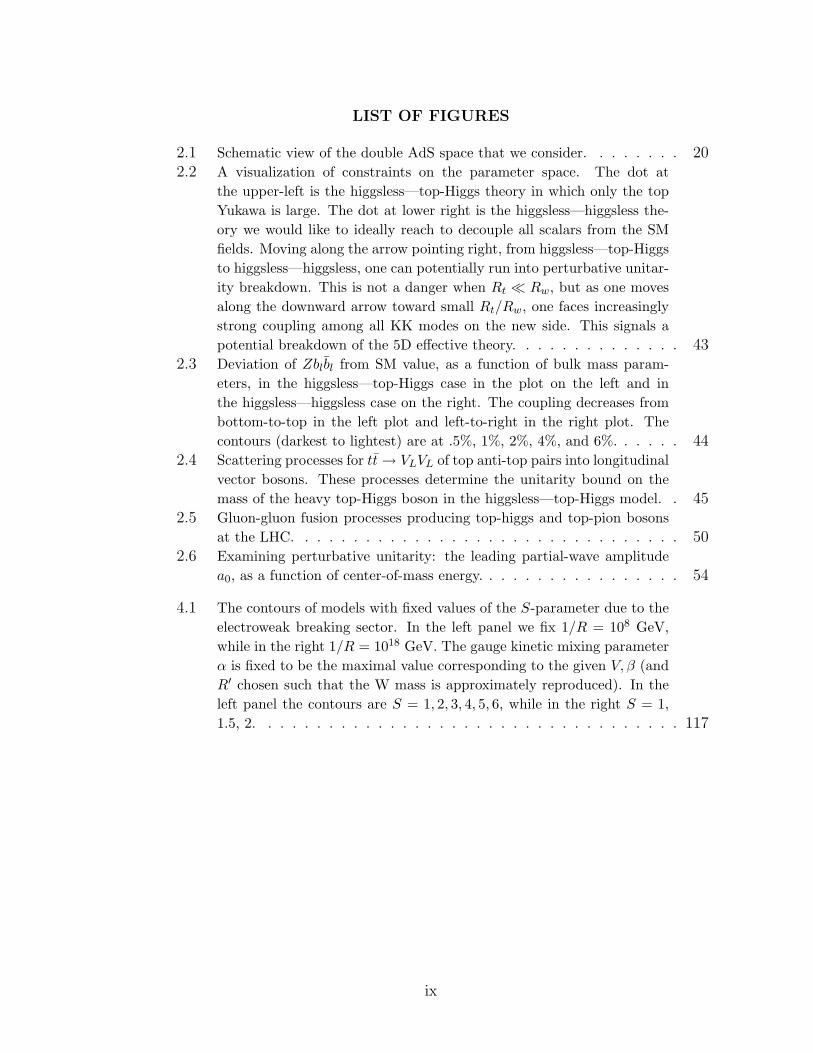
2.1 Schematic view of the double AdS space that we consider. . . . . . . . 202.2 A visualization of constraints on the parameter space. The dot at

the upper-left is the higgsless—top-Higgs theory in which only the topYukawa is large. The dot at lower right is the higgsless—higgsless the-ory we would like to ideally reach to decouple all scalars from the SMfields. Moving along the arrow pointing right, from higgsless—top-Higgsto higgsless—higgsless, one can potentially run into perturbative unitar-ity breakdown. This is not a danger when Rt � Rw, but as one movesalong the downward arrow toward small Rt/Rw, one faces increasinglystrong coupling among all KK modes on the new side. This signals apotential breakdown of the 5D effective theory. . . . . . . . . . . . . . 43

2.3 Deviation of Zblbl from SM value, as a function of bulk mass param-eters, in the higgsless—top-Higgs case in the plot on the left and inthe higgsless—higgsless case on the right. The coupling decreases frombottom-to-top in the left plot and left-to-right in the right plot. Thecontours (darkest to lightest) are at .5%, 1%, 2%, 4%, and 6%. . . . . . 44

2.4 Scattering processes for tt → VLVL of top anti-top pairs into longitudinalvector bosons. These processes determine the unitarity bound on themass of the heavy top-Higgs boson in the higgsless—top-Higgs model. . 45

2.5 Gluon-gluon fusion processes producing top-higgs and top-pion bosonsat the LHC. . . . . . . . . . . . . . . . . . . . . . . . . . . . . . . . 50

2.6 Examining perturbative unitarity: the leading partial-wave amplitudea0, as a function of center-of-mass energy. . . . . . . . . . . . . . . . . 54

4.1 The contours of models with fixed values of the S-parameter due to theelectroweak breaking sector. In the left panel we fix 1/R = 108 GeV,while in the right 1/R = 1018 GeV. The gauge kinetic mixing parameterα is fixed to be the maximal value corresponding to the given V, β (andR′ chosen such that the W mass is approximately reproduced). In theleft panel the contours are S = 1, 2, 3, 4, 5, 6, while in the right S = 1,1.5, 2. . . . . . . . . . . . . . . . . . . . . . . . . . . . . . . . . . . 117

ix

Chapter 1

Introduction

1.1 The Standard Model and EWSB

The Standard Model of particle physics is extraordinarily well-established and well-

tested. It describes all of the known non-gravitational forces and matter through

a gauge group, SU(3) × SU(2)L × U(1)Y , and a set of fermionic matter fields

Q,U,D,L,E with appropriate charges under the gauge group. Despite its success,

there is one subtlety: we know that in the real world SU(2)L × U(1)Y is broken

spontaneously to U(1)EM , the gauge group of electromagnetism. This is known

as “electroweak symmetry breaking” or EWSB for short. The Standard Model

describes this in the simplest way possible: via a scalar doublet Higgs boson H

that gets a vacuum expectation value v ∼ 246 GeV at the minimum of its potential

V (H†H). In the Standard Model a potential is simply added by hand, V (H) =

−µ2H†H + λ(H†H

)2.

The Higgs boson has not yet been discovered; it must be around 115 GeV or

heavier, or the Standard Model must be modified in such a way that it decays in a

manner that could have escaped detection at LEP. Searches are underway at the

Tevatron (and in a narrow mass range near 160 GeV are quite close to excluding a

Standard Model Higgs). The Large Hadron Collider should be turning on within

the next year, and eventually if the Standard Model is correct it will discover the

Higgs.

There are several reasons to think that this is not the whole story. For one, the

real world has gravity, which can be added to the Standard Model as a low-energy

1

effective theory but breaks down at high energies (near the Planck scaleMPl ∼ 1019

GeV). This is outside the scope of this thesis, although it is conceivable that string

theory explains quantum gravity and also gives insight into lower-energy physics.

Another is the observation of neutrino masses, which are suggestive of physics

at higher energy scales, but likely not relevant to the LHC. Yet another is dark

matter, the observed properties of which could be explained by a weakly interacting

massive particle (“WIMP”) with mass at the TeV scale. This is perhaps the most

compelling experimental reason to expect physics beyond the Standard Model to

make its presence known at the LHC.

However, there is a yet more compelling theoretical reason which, in the opinion

of most particle physicists, leads us to expect physics beyond the Standard Model

at the LHC. This is the so-called “hierarchy problem,” and can be viewed as the

question of why the electroweak symmetry breaking scale v is so much smaller

than the fundamental quantum gravity scale MPl. Another way of looking at this

question is: what is the origin of the physics driving the Higgs to get a vacuum ex-

pectation value? While it’s conceivable that there really is a fundamental potential

V (H†H), unexplained by any deeper principle, it’s more appealing to think that

there is other physics determining the potential and the scale v. From a technical

standpoint, the main aspect of the hierarchy is its lack of technical naturalness.

If one begins with a classical mass for the Higgs, quantum effects will produce

“corrections” to the mass of order the cutoff scale of the theory, δm2 ∼ Λ2. This

quadratic divergence implies that there is a fine-tuning in the theory; classical and

quantum masses must nearly balance in order for the final, physical mass to be

much less than the Planck scale. Such considerations lead many to think that

fundamental scalars should not exist in nature, absent some mechanism to protect

them from these severe quantum effects.

2

1.2 Options for the Hierarchy Problem

There are many attitudes one can take toward the hierarchy problem, as it is to

some extent a theorist’s problem, not an experimental one. It is entirely possible

that we just happen to live in a universe with a Higgs with some appropriately

finely-tuned potential. This has led to anthropic arguments for the hierarchy: if the

Higgs vacuum expectation value were too large, physics in our universe would be

very different, and the formation of structure could be altered, for instance. Similar

arguments are currently the only way we have of understanding the smallness of

the cosmological constant Λ (which, together with the Higgs mass, is one of the

only relevant operators in the Standard Model). Since we have at present no way

of addressing the Λ problem other than anthropics, it might not be unreasonable

to appeal to the same thing to explain EWSB. This isn’t very satisfying, from a

theoretical point of view, and from a phenomenological one, it doesn’t tell us what

we should expect from upcoming experiments like the LHC. (Variations on this

theme, like “split supersymmetry”, do make LHC predictions.) While it’s always

worth keeping this in the back of our minds as a possibility we might have to face

if the data don’t show us anything new, for now we will only discuss theoretical

approaches that explain the hierarchy through some physical mechanism.

One theoretical option for addressing the hierarchy problem is to posit TeV-

scale supersymmetry. Supersymmetry is a spacetime symmetry that mixes bosons

with fermions. Fermion masses do not suffer the same severe quadratic divergences

as scalar masses, due to chiral symmetry: the term mψψ in a Lagrangian breaks

the symmetry, so m = 0 is radiatively stable and corrections for finite m are only

logarithmically divergent. Supersymmetry enforces that fermions and scalars have

equal masses. This means that exact supersymmetry cancels quadratic divergences

3

in scalar masses, making them also only logarithmically divergent. The world

around us is not exactly supersymmetric; in fact, we have so far not observed the

supersymmetric partner of any particle in the Standard Model. This implies that

if physics is fundamentally supersymmetric, the extra symmetry is broken at a

scale MSUSY>∼ 1TeV. This scale cuts off the quadratic divergence and resolves the

problem of technical naturalness.

Supersymmetry is the most-studied and, on theoretical grounds, perhaps the

most appealing of options for solving the hierarchy problem. It arises in Calabi-

Yau compactifications of string theory, where it is also naturally broken, frequently

at the string scale. However, it does appear that there are viable models, both

in which supersymmetry is “gravity-mediated” (which, e.g. in IIB strings, could

mean that some Kahler modulus of the Calabi-Yau gets an F term and transmits

the breaking to the Standard Model superpartners) or “gauge-mediated” (in which

case the breaking is at a relatively low scale, and the physics is essentially all low-

energy field theory insensitive to the UV completion). These options each have

their own phenomenological problems, and it is safe to say that there is no existing

model of supersymmetry breaking which is completely problem-free, consistent

with experiment, and theoretically well-motivated. This is one reason to explore

other options. Over the past decade, a number have arisen, including large extra

dimensions [1] and warped extra dimensions [2]. Large extra dimensions transmute

the hierarchy of energy scales into a very large number for the volume of an extra

dimension. It’s not clear that this geometrization of the hierarchy problem succeeds

in really solving it, but it does make exciting and exotic predictions and provides

an intriguing new way of thinking about what the hierarchy means.

Warped extra dimensions, on the other hand, are essentially a much older

4

idea in disguise. Let’s remind ourselves how the hierarchy works in the strong

interactions. For instance, most of the proton mass (of about 1 GeV) arises not

from the fundamental masses of the quarks (which come from EWSB) but from

a “constituent quark mass” supplied by strong dynamics. This scale arises from

chiral symmetry breaking, which is a nonperturbative property of QCD in which

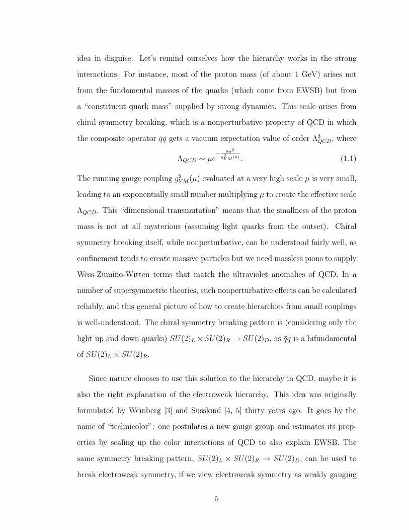
the composite operator qq gets a vacuum expectation value of order Λ3QCD, where

ΛQCD ∼ µe− 8π2

g2Y M

(µ) . (1.1)

The running gauge coupling g2Y M(µ) evaluated at a very high scale µ is very small,

leading to an exponentially small number multiplying µ to create the effective scale

ΛQCD. This “dimensional transmutation” means that the smallness of the proton

mass is not at all mysterious (assuming light quarks from the outset). Chiral

symmetry breaking itself, while nonperturbative, can be understood fairly well, as

confinement tends to create massive particles but we need massless pions to supply

Wess-Zumino-Witten terms that match the ultraviolet anomalies of QCD. In a

number of supersymmetric theories, such nonperturbative effects can be calculated

reliably, and this general picture of how to create hierarchies from small couplings

is well-understood. The chiral symmetry breaking pattern is (considering only the

light up and down quarks) SU(2)L×SU(2)R → SU(2)D, as qq is a bifundamental

of SU(2)L × SU(2)R.

Since nature chooses to use this solution to the hierarchy in QCD, maybe it is

also the right explanation of the electroweak hierarchy. This idea was originally

formulated by Weinberg [3] and Susskind [4, 5] thirty years ago. It goes by the

name of “technicolor”: one postulates a new gauge group and estimates its prop-

erties by scaling up the color interactions of QCD to also explain EWSB. The

same symmetry breaking pattern, SU(2)L × SU(2)R → SU(2)D, can be used to

break electroweak symmetry, if we view electroweak symmetry as weakly gauging

5

a subgroup of the flavor symmetries of the technicolor theory.

This idea sounds very nice, but the experimental data that we have are very

precise and they imply strong constraints on a technicolor scenario. For instance,

one can parametrize the low-energy physics with an electroweak chiral Lagrangian,

similar to the chiral Lagrangian of QCD, for the Goldstone bosons that supply the

longitudinal modes of the Z and W± bosons. Let τ denote Uτ3U† and Vµ =

(DµU)U †. We can construct various gauge-invariant operators from these building

blocks together with the field strengths Wµν and Bµν . The coefficients of these

operators are given names, and constrained by experiment [6]. For example, there

are the famous Peskin-Takeuchi S, T , and U parameters: T relates to the coefficient

of the O(p2) operator (Tr(τVµ))2, while S and U occur at O(p4) and correspond

to the operators BµνTr(τW µν) and (Tr(τWµν))2. The operators T and U violate

custodial symmetry and one can usually avoid constraints simply by constructing

custodially symmetric models, but S is nonzero whenever electroweak symmetry

is broken and it typically imposes severe constraints on technicolor.

Another problem with technicolor is that, while it can quite easily explain elec-

troweak symmetry breaking and the masses of the W± and Z bosons, explaining

fermion masses is more difficult. This is because one needs to generate a Yukawa

coupling, e.g. yHQU , but now H is really a composite operator ψtcψtc of tech-

nicolor fermions ψtc, so this is a nonrenormalizable operator and some model is

needed to explain how it is generated. An alternative is the Georgi-Kaplan mecha-

nism, in which the fermion masses are assumed to originate by a direct coupling of

some elementary fermion to a fermionic operator of the technicolor sector. As we

will see, this is the approach that is at work in the Randall-Sundrum framework.

Once one has a mechanism of generating fermion masses, additional constraints

6

can apply, e.g. bounds on flavor-changing neutral currents. The combination

of constraints from S and constraints from flavor seem to make the prospects for

technicolor fairly bleak, and the model-building difficulties are compounded by the

difficulty of calculating in strongly-coupled field theory. This last point is where

Randall-Sundrum models have changed the nature of the model-building game.

1.3 Technicolor and Randall-Sundrum

The Randall-Sundrum solution to the hierarchy is to imagine that spacetime is

a five-dimensional slice of anti deSitter space (AdS), cut off at two boundaries,

z = zIR and z = zUV � zIR. The natural mass scale for a field localized near zIR

is 1zIR

, but the proper distance between the two boundaries is R log zIR

zUV, with R the

AdS curvature radius. Thus a small five-dimensional distance can easily explain

an exponentially large hierarchy in energy scales. This is, in some sense, a toy

version of the story of dimensional transmutation. The AdS/CFT correspondence

(Reference [7]) suggests that the Randall-Sundrum scenario is dual to a conformal

field theory in which conformal invariance is broken at the ultraviolet end (which

corresponds to a UV cutoff on the field theory, and to coupling the field theory to

dynamical gravity) and at the infrared end [8]. The infrared cutoff is essentially

a simple model of confinement. The separation between zIR and zUV can be

stabilized by the Goldberger-Wise mechanism [9], among others.

If we wish to think of Randall-Sundrum as dual, in the AdS/CFT sense, to

something like a technicolor model, then the Higgs boson should be localized near

zIR (either on the brane, i.e. exactly at zIR, or as a bulk field with a profile that

grows quickly with z). On the other hand, the global symmetries of the CFT

7

become gauge symmetries in AdS, so the technicolor global symmetry becomes a

massless gauge field in the Randall-Sundrum bulk. The symmetries of the Stan-

dard Model, at least, should be weakly gauged, which can be accommodated by

boundary conditions at zUV that allow a zero mode to exist. If the boundary condi-

tions at zIR then give this mode a mass, we can think of it as a “Higgsless” model,

which is still a form of spontaneous breaking of the global symmetry [10, 11].

The major advantage of Randall-Sundrum models over traditional technicolor

scenarios is calculability. A tree-level five-dimensional calculation gives a spec-

trum of narrow resonances, as one expects to find in any large-Nc field theory.

However, in actual four-dimensional field theories, we remain completely unable to

calculate precisely what the masses, decay constants, and couplings of such narrow

resonances are. In Randall-Sundrum models, all this and more is calculable.

1.4 Contents

The second chapter of this thesis, “Top and Bottom: A Brane of Their Own,”

concerns a variation on the Randall-Sundrum scenario in which one considers the

dual of two separate strongly-coupled sectors each coupled to the Standard Model

fields. Here there are two global symmetries containing the electroweak symmetry

group, and the diagonal is weakly gauged. One of the strongly-coupled sectors

communicates with the first two fermion generations while the other communicates

with the third generation, giving some explanation for why the top quark is so much

heavier than the other fermions. This model allows a solution to a problem that

plagued the original Higgsless models, in which it was problematic to have a heavy

enough top mass without distorting the coupling of the left-handed bottom quark

8

to the Z boson. On the other hand, in certain regimes the “brane of their own”

theory becomes difficult to calculate in.

The third chapter of this thesis, “A Braneless Approach to Holographic QCD,”

deals with how well a modification of the Randall-Sundrum scenario can be used to

model the properties of QCD itself. (Such a model would also apply to technicolor

scenarios.) A five-dimensional model is constructed in which the generation of

the QCD scale (dually, of the cutoff zIR) is accomplished by a potential for a

scalar field in the bulk. This potential is engineered to give logarithmic running

of the gauge coupling in the UV, so that the model is essentially a dual of the

story of dimensional transmutation. The properties are found to be very similar

to those of Randall-Sundrum. Some aspects of QCD are modeled well, but the

overall spectrum of massive excitations is very different. The reasons for this are

understandable: AdS/CFT works well for theories at large ’t Hooft coupling, where

almost every operator gets a large anomalous dimension. In the dual gravity theory

this means that almost every field is a heavy string mode and can be ignored. On

the other hand, in an asymptotically free theory like QCD, most operators have

fairly small anomalous dimensions (at least over a wide range of energy scales) and

one would expect that an accurate dual would need to keep fields corresponding

to every operator. Such a theory would rapidly become intractable.

The fourth chapter of this thesis, “The S-parameter in Holographic Technicolor

Models,” focuses on the Peskin-Takeuchi S parameter and in particular its sign.

This is one of the most dangerous constraints on the original technicolor theories

and it should come as no surprise that it is dangerous for Randall-Sundrum scenar-

ios as well. A way of tuning S away by delocalizing fermions is known; it essentially

cancels a significant “pure technicolor” positive S against a negative contribution

9

arising from the details of how the Standard Model fermions couple to fermionic

operators of the technicolor sector. The question arose of whether the “pure tech-

nicolor” contribution, related to a vector minus axial spectral integral, could ever

be negative. We argue that in any calculable Randall-Sundrum-like model, this

contribution to S is strictly positive. Unfortunately a completely general proof of

this for all field theories remains elusive.

In chapter 5 we offer a brief summary of the results and some concluding

remarks about the future prospects of Randall-Sundrum models and open questions

about them.

10

Chapter 2

Top and Bottom: A Brane of Their Own

2.1 Introduction

There has been a tremendous explosion of new models of electroweak symme-

try breaking including large extra dimensions [1], Randall-Sundrum [2], gauge

field Higgs [12], gauge extensions of the minimal supersymmetric standard model

(MSSM) [13], little Higgs [14], and the fat Higgs [15]. All of these new models

share one feature in common: a light Higgs. With the realization that unitarity

can be preserved in an extra-dimensional model by Kaluza-Klein (KK) towers of

gauge fields rather than a scalar [16, 10] a more radical idea has emerged: hig-

gsless models [11, 17, 18, 19]. The most naive implementations of these mod-

els face a number of phenomenological challenges, mostly related to avoiding

strong coupling while satisfying bounds from precision electroweak measurements

[18, 20, 21, 22, 23, 24, 25, 26, 27, 28]. Collider signatures of higgsless models have

been studied in [29, 30], further discussions on unitarity can be found in [31, 32, 33],

while other ideas related to higgsless models can be found in [34, 35, 36]. How-

ever it has gradually emerged that, in a slice of 5 dimensional anti de Sitter space

(AdS5) with a large enough curvature radius and light fermions almost evenly dis-

tributed in the bulk, WW scattering is perturbative because the KK gauge bosons

can be below 1 TeV, and the S parameter and most other experimental constraints

are satisfied because the coupling of the light fermions to the KK gauge bosons is

small [37, 38, 39]. The outstanding problem is how to obtain a large enough top

quark mass without messing up the left-handed top and bottom gauge couplings

or the W and Z gauge boson masses themselves. The tension arises [40, 41] be-

11

cause in order to get a large mass it would seem that the top quark must be close

to the TeV brane where electroweak symmetry is broken by boundary conditions.

However this implies that the top and (hence) the left-handed bottom have large

couplings to the KK gauge bosons, and thus have large corrections to their gauge

couplings. Furthermore this arrangement leads to a large amount of isospin break-

ing in the KK modes of the top and bottom which then feeds into the W and Z

masses through vacuum polarization at one loop [40].

It was previously suggested [37] that a possible solution to this problem

would be for the third generation to live in a separate AdS5. In terms of the

AdS/conformal field theory (CFT) correspondence [7, 42, 8, 44] this means that

the top and bottom (as well as τ and ντ ) would couple to a different (approxi-

mate) CFT sector than the one which provides masses to the W and Z as well

as the light generations. There is a long history of models where the mechanism

of electroweak symmetry breaking is different for the third generation. This is

most often implemented as a Higgs boson that couples preferentially to the third

generation (a.k.a. a “top-Higgs”) but has also appeared in other guises such as

top-color-assisted-technicolor (TC2) where top color [45] produces the top and bot-

tom quark masses and technicolor produces all the other masses. From the point

of view of AdS/CFT, double CFT sectors have been considered for a variety of

reasons. The setup is usually taken to two slices of AdS5 “back-to-back” with a

shared Planck brane. This is intended to approximately describe the situation of

two strongly coupled CFT’s that both couple to the same weakly coupled sector

such as would arise when two conifold singularities are near each other in a higher

dimensional space. The tunneling between the two AdS “wells” was considered in

[46] in order to generate hierarchies. More recently inflationary models [47] have

been based on one or more AdS wells. For other extra dimensional implementation

12

of topcolor-type models see [48, 49].

In this paper we will consider models of electroweak symmetry breaking with

two “back-to-back” AdS5’s in detail. The motivation for these models is to be

able to separate the dynamics responsible for the large top quark mass from that

giving rise to most of electroweak symmetry breaking. Thus we will assume that

the light fermions propagate in an AdS5 sector that is essentially like the higgs-

less model described in [37], while the third generation quarks would propagate in

the new AdS5 bulk. To analyze such theories we first discuss in detail what the

appropriate boundary and matching conditions are in such models. Then we con-

sider the different possibilities for electroweak symmetry breaking on the two IR

branes (Higgs—top-Higgs, higgsless—top-Higgs and higgsless—higgsless) and de-

rive the respective formulae for the gauge boson masses. We then discuss the CFT

interpretation of all of these results. Also from the CFT interpretation we find

that there have to exist uneaten light pseudo-Goldstone bosons (“top-pions”) in

this setup. This is due to the fact that doubling the CFT sectors implies a larger

global symmetry group, while the number of broken gauge symmetries remains

unchanged.

After the general discussion of models with two IR branes we focus on those that

can potentially solve the issues related to the third generation quarks in higgsless

models. A fairly simple way to eliminate these problems is by considering the

higgsless—top-Higgs case, that is when most of electroweak symmetry breaking

originates from the higgsless sector, but the top quark gets its mass from a top-

Higgs on the other TeV brane (which also gives a small contribution to the W

mass ). The only potential issue is that since we assume the top-Higgs vacuum

expectation value (VEV) vt on this brane to be significantly smaller than the

13

Standard Model (SM) Higgs VEV, the top Yukawa coupling needs to be larger

and thus non-perturbative. Also, the coupling of the top-pions to tt and tb will be

of order mt/vt. Ideally, one would like to also eliminate the top-Higgs sector arising

from the new TeV (IR) brane. In this case in order to get a very heavy top one

needs to take the IR cutoff scale on the new side much bigger than on the old side (∼

TeV), while keeping the top and bottom sufficiently far away from the new IR brane

(in order to ensure that the bottom couplings are not much corrected). However,

to make sure that most of the contributions to electroweak symmetry breaking are

still coming from the old side one needs to choose a smaller AdS radius for the side

where the top lives. In this case perturbative unitarity in WW scattering is still

maintained. However, it will also imply that the new side of the 5D gauge theory

is strongly coupled for all energies. Electroweak precision observables are shielded

from these contributions by at least a one-loop electroweak suppression, however

it is not clear that the KK spectrum of particles mostly localized on the new side

would not get order one corrections and thus modify results for third generation

physics significantly.

Finally we analyze some phenomenological aspects of this class of models. An

interesting prediction is the presence of a scalar isotriplet (top-pions), and eventu-

ally a top-Higgs. The top-pions get a mass at loop level from gauge interactions,

and the mass scale is set by the cutoff scale on the new TeV brane so that they

can be quite heavy. The main feature that allows us to distinguish such scalars

from the SM or MSSM Higgses is that they couple strongly with the top (and bot-

tom) quarks, but have sensibly small couplings with the massive gauge bosons and

light quarks. They are expected to be abundantly produced at the Large Hadron

Collider (LHC), via the enhanced gluon or top fusion mechanisms. If heavy, the

main decay channel is in (multi) top pairs, although the golden channel for the

14

discovery is in γγ and ZZ. Thus, a heavy resonance in γγ and l+l−l+l−, together

with an anomalously large rate of multi-top events, would be a striking hint for

this models.

2.2 Warmup: Boundary Conditions for a U(1) on an Inter-

val

As an introduction to the later sections, we will in this section first present a

discussion on how to obtain the boundary conditions (BCs) for a U(1) gauge group

on an interval, broken on both ends by two localized Higgses. The major focus will

be on explaining the effects of the localized Higgs fields on the boundary conditions

for the A5 bulk field, and possible effects of mixings among the scalars, and the

identification of possible uneaten physical scalar fields. We will also be allowing

here a very general gauge kinetic function K(z) in the bulk, which will mimic both

the effect of possible warping, and also the presence of a Planck brane separating

two bulks with different curvatures and gauge couplings. We use a U(1) so that

we keep the discussion as simple as possible, while in the later sections we will use

straightforward generalizations of the results obtained here for more complicated

groups.

We assume that without the Higgs field being turned on the BCs are Neumann

for the Aµ and Dirichlet for the A5, as in the usual orbifold projection. This is

a possible BC allowed by requiring the boundary variations of the action to be

vanishing [10]. With this choice, before the Higgs VEVs are turned on, there

is no zero mode for the A5 and all the massive degrees of freedom are eaten by

the massive vector KK modes. In order to be able to clearly separate the effects

15

of the original boundary conditions from those of the localized fields added on

the boundary, we will add the localized fields a small distance ε away from the

boundary. Of course later on we will be taking the limit ε→ 0.

Thus the Lagrangian we consider is:

L =

∫ L2

L1

dz

{−K(z)

1

4g25

F 2MN + L1δ(z − L1 − ε) + L2δ(z − L2 + ε)

}. (2.1)

As explained above, the generic function K encodes both the eventual warping of

the space and a possible z-dependent kinetic term corresponding to a different g5 on

the two sides of the Planck brane. We also assume that any eventual discontinuity

is regularized such that K is continuous and non-vanishing.

The localized Lagrangians are the usual Lagrangians for the Higgs field in 4D 1

(i = 1, 2):

Li = |Dµφi|2 −λi

2

(|φi|2 −

1

2v2

i

)2

(2.2)

and they will induce non vanishing VEVs vi for the Higgses, around which we

expand:

φi =1√2

(vi + hi) eiπi/vi . (2.3)

The above Lagrangian contains some mixing terms involving Aµ that we want to

cancel out with a generalized Rξ gauge fixing term. Expanding up to bilinear

terms:

L =

∫ L2

L1

dz

{K(z)

g25

(−1

4F 2

µν +1

2(∂zAµ)2 +

1

2(∂µA5)

2 − ∂µA5∂5Aµ

)+

[1

2(∂µh1)

2 − 1

2λ1v

21h

21 +

1

2(∂µπ1 − v1Aµ)2 + ...

]δ(z − L1 − ε)

+

[1

2(∂µh2)

2 − 1

2λ2v

22h

22 +

1

2(∂µπ2 − v2Aµ)2 + ...

]δ(z − L2 + ε)

}. (2.4)

1Note that warp factors are usually added in the localized lagrangians, so that the scale v isnaturally of order 1/R, and λ of order 1. Such factors are not relevant for the discussion at thispoint, so we will neglect them for the moment.

16

The crucial point now is the integration by parts of the mixing term in the

bulk. As a consequence of the displacement of the localized Lagrangians L1,2,

the integral splits into three regions limited by the regularized branes where the

Higgs interactions are localized. The contributions of the edges vanish in the limit

ε → 0, so that the BC on the true boundaries are effectively “screened”, and a

mixing between Aµ and A5 on the branes is generated:(∫ L1+ε

L1

+

∫ L2−ε

L1+ε

+

∫ L2

L2−ε

)dzKA5∂5∂µA

µ =(∫ L1+ε

L1

+

∫ L2

L2−ε

)dz(...)−

∫ L2−ε

L1+ε

dz ∂5 (KA5) ∂µAµ + [KA5∂µA

µ]L2−εL1+ε . (2.5)

Note that the boundary terms would vanish on the true boundaries L1,2, however

they don’t vanish on the branes at L1 + ε and L2− ε, and thus the minimization of

the action will require that A5 has to be non-zero on the branes. In other words,

in the limit ε→ 0 the A5 field will develop a discontinuity on the boundaries.

We can now add a bulk and two brane gauge fixing Lagrangians2:

LGF =

∫ L2

L1

dz

{− 1

g25

1

2ξ(∂µA

µ − ξ∂z (KA5))2 − 1

2ξ1

(∂µA

µ + ξ1

(v1π1 −

Kg25

A5

))2

·

δ(z − L1)−1

2ξ2

(∂µA

µ + ξ2

(v2π2 +

Kg25

A5

))2

δ(z − L2)

}, (2.6)

where the three gauge fixing parameters are completely arbitrary, and the unitary

gauge is realized in the limit where all the ξ’s are sent to infinity.3 This gauge fixing

term is devised such that all the mixing terms between Aµ and A5, π1,2 cancel out.

The full Lagrangian then leads to the following equation of motion for Aµ (in the

2In [50] the authors considered a similar situation, but adding gauge fixing terms in the KKbasis. As it has to be expected, our approach leads to the same results.

3Note that we have chosen a bulk gauge fixing term with a different z dependence than thebulk gauge kinetic term, i.e., we have included a z dependence in the gauge fixing parameter ξ.This allows us to obtain a simple equation of motion for A5, at the price of a non-conventionalform of the gauge propagator that will not be well suited for a warped space loop calculationin general ξ gauge. In the unitary gauge that we will use in this paper, all the ξ dependencevanishes (and thus also the z dependence of ξ will be irrelevant).

17

unitary gauge):

1

K∂z

(K∂zAµ +m2Aµ

)= 0 , (2.7)

while the BCs, fixed by requiring the vanishing of the boundary variation terms in

Eq. (2.4), are:

K(L1,2)

g25

∂zAµ ∓ v21,2Aµ = 0 . (2.8)

The bulk equation of motion for the scalar field A5 will result in:

∂2z (KA5) +

m2

ξA5 = 0 , (2.9)

and the π’s obey the following equations of motion on the branes:(m2

ξ1− v2

1

)π1 + v1

K(L1)

g25

A5|L1= 0 ,(

m2

ξ2− v2

2

)π2 − v2

K(L2)

g25

A5|L2= 0 .

(2.10)

These last equations fix the values of π1,2 in terms of the boundary values of A5.

Finally, requiring that the boundary variations of the full action with respect to

A5 vanish, combined with the above expression (2.10) for the π’s, will give the

desired BCs for A5:∂z (KA5)−

ξ1ξ

K(L1)

g25

m2/ξ1m2/ξ1 − v2

1

A5

∣∣∣∣L1

= 0 ,

∂z (KA5) +ξ2ξ

K(L2)

g25

m2/ξ2m2/ξ2 − v2

2

A5

∣∣∣∣L2

= 0 .(2.11)

From Eq. (2.10) one can see that π is not independent of A5. In the unitary

gauge (ξ →∞) it is also clear from Eq. (2.9) that all the massive modes of A5 are

removed. This is simply expressing the fact that A5 and the π’s are the sources

of the longitudinal components of the massive KK modes, and will be eaten. The

only possible exception for the existence of a physical mode is if there is a massless

state in A5. Without the Higgses on the boundaries this would not be possible

due to the Dirichlet BC. However, we have seen above that the BC for the A5 is

18

significantly changed in the presence of the localized Higgs, and now a massless

state is possible. Physically, this expresses the fact that there are “enough” modes

in A5 to provide all the longitudinal components for the massive KK modes. If we

add some localized Higgs fields, then there may be some massless modes left over

uneaten. We will loosely refer to such modes as pions, to emphasize that these are

physical (pseudo-)Goldstone bosons. In the case of a massless physical pion mode,

the BCs for A5 simplify to:

∂z (KA5)|L1 and L2= 0 . (2.12)

The solution to the equation of motion for the zero mode is of the form:

A5 =g25d

K(z), (2.13)

and using (2.10) we also get that

π1 =d

v1

, π2 = − d

v2

. (2.14)

As expected in the higgsless limit (namely vi → ∞), the π’s vanish. However,

a massless scalar is still left in the spectrum if one chooses to break the gauge

symmetry on both ends of the interval. It is also interesting to note that in the limit

where the function K is discontinuous, the solution A5 develops a discontinuity as

well. But, the function KA5 is still continuous, so that no divergent term appears

in the action for such a solution.

Finally, the spectrum also contains two scalars localized on the branes, corre-

sponding to the physical Higgs fields. As in the usual 4D Higgs mechanism, they

will pick a mass proportional to the quartic coupling, m2h1,2 = λv2

1,2 (and decouple

in the higgsless limits vi →∞).

19

µ

U(1)

AdS5AdS’

5

z = Rtz = R w

z z

g’ , A’ , A’ 5

boundaryIRboundary

IR

boundaryUV

z = R’ z = R’tw

5

g , A , A µ5 5

U(1)

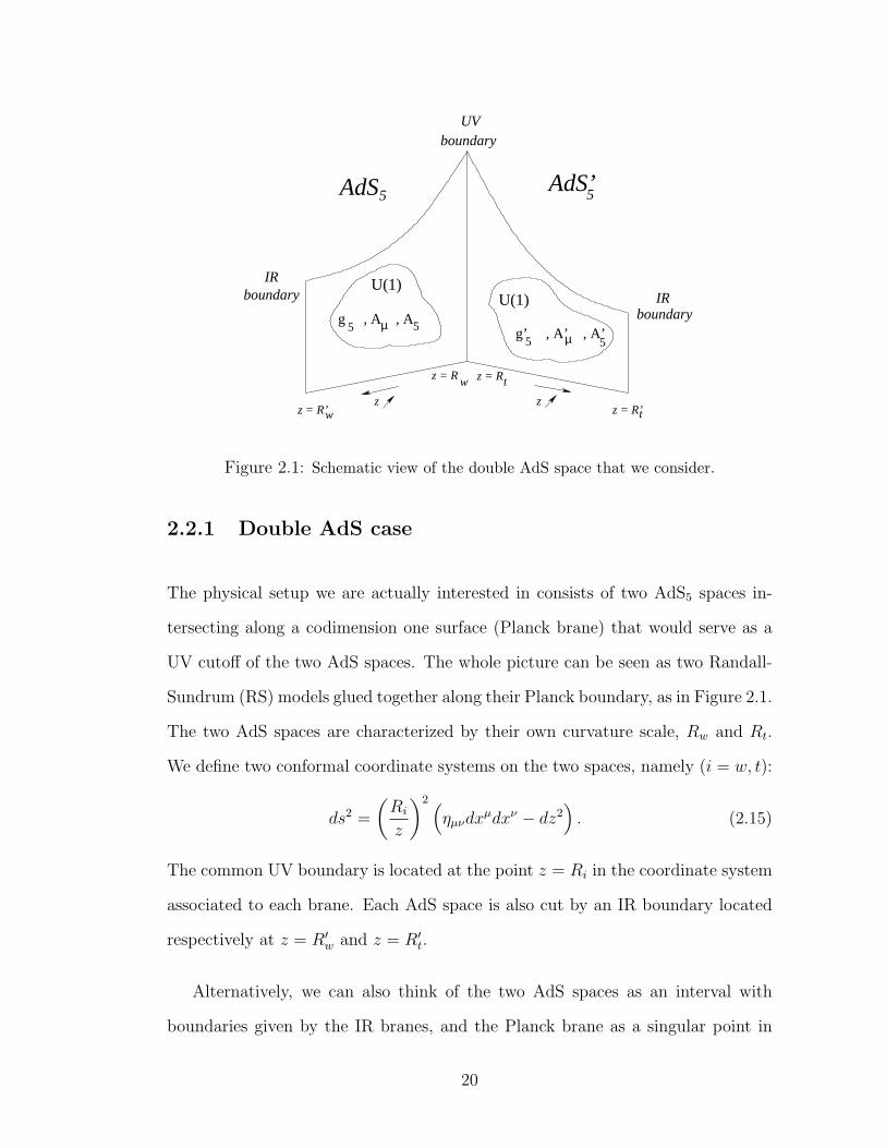
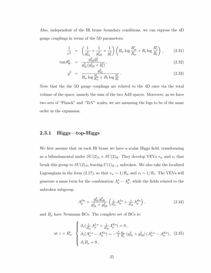
Figure 2.1: Schematic view of the double AdS space that we consider.

2.2.1 Double AdS case

The physical setup we are actually interested in consists of two AdS5 spaces in-

tersecting along a codimension one surface (Planck brane) that would serve as a

UV cutoff of the two AdS spaces. The whole picture can be seen as two Randall-

Sundrum (RS) models glued together along their Planck boundary, as in Figure 2.1.

The two AdS spaces are characterized by their own curvature scale, Rw and Rt.

We define two conformal coordinate systems on the two spaces, namely (i = w, t):

ds2 =

(Ri

z

)2 (ηµνdx

µdxν − dz2). (2.15)

The common UV boundary is located at the point z = Ri in the coordinate system

associated to each brane. Each AdS space is also cut by an IR boundary located

respectively at z = R′w and z = R′t.

Alternatively, we can also think of the two AdS spaces as an interval with

boundaries given by the IR branes, and the Planck brane as a singular point in

20

the bulk. From this point of view we can apply the formalism developed above, in

particular we can define the function K in the two spaces:

K =

Rw

zfor Rw ≤ z ≤ R′w ,

g25

g′52

Rt

z′for Rt ≤ z′ ≤ R′t ,

(2.16)

where we have allowed for a different value of the bulk gauge coupling on the two

sides if g5 6= g′5. In order to maintain the traditional form of the metric in both

sides of the bulk, we have chosen a peculiar coordinate system where z is growing

from the Planck brane towards both the left and the right. This way most formulae

from RS physics will have simple generalizations, however it will also imply some

unexpected extra minus signs. Note that if g5 = g′5, the function K is continuous

on the Planck brane. However, a discontinuity is generated if we define different

gauge couplings on the two sides. As noted before, the only effect of such choice

will be a discontinuity in the wave function of the scalar field A5 on the Planck

brane.

The Lagrangians localized on the two IR branes that cut the two spaces are

(i = w, t):

Li =

(Ri

R′i

)2{|Dµφi|2 −

(Ri

R′i

)2λi

2

(|φi|2 −

1

2v2

i

)2}, (2.17)

where, introducing the above warp factors, all the scales and constants have natural

values, namely λi ∼ 1 and vi ∼ 1/Ri.

For the vectors, Eq. (2.7) reduces to the usual RS equation of motion in the

two bulks, with BCs given by the mass terms on the respective IR branes:

∂zAµ(z)|R′w

+g25

Rw

(vwRw)2

R′wAµ(R′w) = 0 , (2.18)

∂zA′µ(z)

∣∣R′

t+g′5

2

Rt

(vtRt)2

R′tA′µ(R′t) = 0 . (2.19)

21

The equation of motion (2.7) is satisfied on the Planck brane as well, so we can

translate it into matching conditions for the solutions in the two bulks. In particu-

lar, assuming that there are no interactions localized on the Planck brane, Eq. (2.7)

implies that the functions Aµ(z) and K(z)∂zAµ(z) are continuous:

Aµ(Rw) = A′µ(Rt) , (2.20)

1

g25

∂zAµ(z)|Rw= − 1

g′52 ∂zA

′µ(z)

∣∣Rt. (2.21)

The minus sign in the derivative matching Eq. (2.21) comes from the coordinate

systems that we are using. Note that the condition (2.21) would be modified by

localized terms: for instance, if we add a mass term for Aµ, generated by a localized

Higgs, the matching becomes:

1

g25

∂zAµ(z)|Rw+

1

g′52 ∂zA

′µ(z)

∣∣Rt

+ v2PlanckAµ = 0 . (2.22)

In particular, in the large VEV limit, it is equivalent to the vanishing of Aµ (and

of A′µ).

Let us next consider the equations determining possible massless scalar pion

modes. As discussed above, from Eq. (2.9) we can read off that the continuity

condition has to be applied to the functions K(z)A5(z) and ∂z(K(z)A5(z)):

1

g25

A5(Rw) =1

g′52A

′5(Rt) , (2.23)

Rw

g25

∂zA5(z)

z

∣∣∣∣Rw

= −Rt

g′52 ∂z

A′5(z)

z

∣∣∣∣Rt

. (2.24)

The solution then is:

A5(z) = g25d

zRw

,

A′5(z′) = g′5

2d z′

Rt,

πw = −(

R′w

Rw

)2d

vw,

πt = −(

R′t

Rt

)2dvt.

(2.25)

Finally, the two Higgses localized on the IR branes get a mass proportional to

22

the quartic couplings in the potentials:

m2hw

= λw(vwRw)2

R′2w, m2

ht= λt

(vtRt)2

R′2t. (2.26)

Their masses are naturally of order R′−1w or R′−1

t respectively, and have an upper

bound given by the breakdown of perturbative unitarity. Such limits will be much

looser than in the SM, due to the contribution of the gauge boson KK modes, as

we will see in the following sections.

2.3 The Standard Model in Two Bulks: Gauge Sector

We will now use our general formalism developed above to put the Standard Model

in two AdS5 bulks. Our goal will be to separate electroweak symmetry breaking

from the physics of the third generation fermions. In each AdS bulk, we have a

full SU(2)L×SU(2)R×U(1)B−L gauge symmetry, so that a custodial symmetry is

protecting [40] the ρ parameter. We want to specify the boundary and matching

conditions according to the following symmetry breaking pattern: on the common

UV brane only SU(2)L × U(1)Y survives, while on the IR boundaries two Higgses

break the gauge group to the SU(2)D × U(1)B−L subgroup.

The UV brane matching conditions arise from considering an SU(2)R scalar

doublet with a B−L charge 1/2, that acquires a VEV (0, v). As discussed above,

all of the gauge fields ALµ , AR

µ , and Bµ are continuous. The Higgs, in the limit

of large VEV, forces the gauge bosons of the broken generators to vanish on the

Planck brane: AR1,2µ = 0 and Bµ − AR3

µ = 0, thus breaking SU(2)R × U(1)B−L to

U(1)Y . On the other hand, on the unbroken gauge fields ALaµ and (g5L, g5R, g5 are

23

the 5D gauge couplings of SU(2)L, SU(2)R and U(1)B−L)

BYµ =

g25Rg

25

g25R + g2

5

(1

g25R

AR3µ +

1

g25

Bµ

), (2.27)

we need to impose the continuity condition in Eq. (2.21). The complete set of

Planck brane matching conditions then reads

atz = Rw

z′ = Rt

AL aµ = A′L a

µ , AR aµ = A′R a

µ , Bµ = B′µ ,

AR 1,2µ = 0 , Bµ − AR 3

µ = 0 ,

∂zAL aµ + ∂zA

′L aµ = 0 ,

1g25R∂zA

R 3µ + 1

g25R∂zA

′R 3µ + 1

g25∂zBµ + 1

g25∂zB

′µ = 0 .

(2.28)

Here we are assuming equal 5D gauge couplings on the two sides for simplicity.

In case of different g5’s, Eqs. (2.28) will be modified according to the rules given

in the previous section. However, this restricted set of parameters is sufficient for

our purposes, because, as we will comment later, in the gauge sector the effect of

different 5D couplings is equivalent to different AdS curvature scales on the two

sides.

Regarding the IR breaking, we will study three limits: that in which it comes

from a Higgs on both IR branes (“Higgs—top-Higgs”), that in which most elec-

troweak symmetry breaking is from a higgsless breaking while the top gets its

mass from a Higgs (“higgsless—top-Higgs”), and that in which we have higgsless

boundary conditions on both IR branes (“higgsless—higgsless”).

For future convenience, we first recall the expressions for MW in the Randall-

Sundrum scenario with an IR brane Higgs [2, 51] and in the higgsless case [11], in

the limit g5L = g5R at leading log order:

M2W ;Higgs ≈ g2

5

R log R′

R

R2v2

4R′2, (2.29)

M2W ;higgsless ≈ 1

R′2 log R′

R

. (2.30)

24

Also, independent of the IR brane boundary conditions, we can express the 4D

gauge couplings in terms of the 5D parameters:

1

e2=

(1

g25L

+1

g25R

+1

g25

)(Rw log

R′wRw

+Rt logR′tRt

), (2.31)

tan θ2W =

g25Rg

25

g25L(g2

5R + g25), (2.32)

g2 =g25L

Rw log R′w

Rw+Rt log

R′t

Rt

. (2.33)

Note that the the 5D gauge couplings are related to the 4D ones via the total

volume of the space, namely the sum of the two AdS spaces. Moreover, as we have

two sets of “Planck” and “TeV” scales, we are assuming the logs to be of the same

order in the expansion.

2.3.1 Higgs—top-Higgs

We first assume that on each IR brane we have a scalar Higgs field, transforming

as a bifundamental under SU(2)L × SU(2)R. They develop VEVs vw and vt that

break this group to SU(2)D, leaving U(1)B−L unbroken. We also take the localized

Lagrangians in the form (2.17), so that vw ∼ 1/Rw and vt ∼ 1/Rt. The VEVs will

generate a mass term for the combination ALµ −AR

µ , while the fields related to the

unbroken subgroup

ADaµ =

g25Lg

25R

g25L + g2

5R

(1

g25LALa

µ + 1g25RARa

µ

), (2.34)

and Bµ have Neumann BCs. The complete set of BCs is:

at z = R′w

∂z(

1g25LAL a

µ + 1g25RAR a

µ ) = 0 ,

∂z(AL aµ − AR a

µ ) = −v2w

4Rw

R′w

(g25L + g2

5R) (AL aµ − AR a

µ ) ,

∂zBµ = 0 ,

(2.35)

25

and similarly on the other IR brane.

To determine the spectrum in this case, we use the expansion of the Bessel

function for small argument (assuming MAR′ � 1),

ψ(A)(z) ≈ c(A)0 +M2

Az2

(c(A)1 − c

(A)0

2log

z

R

)(2.36)

and solve (much as in [11]). We assume that viRi is small. We find for the W

mass:

M2W ≈ g2

5L

Rw log R′w

Rw+Rt log

R′t

Rt

((Rw

R′w

)2v2

w

4+

(Rt

R′t

)2v2

t

4

)

=g2

4

((Rw

R′w

)2

v2w +

(Rt

R′t

)2

v2t

). (2.37)

This is of the form one would expect for a gauge boson obtaining its mass from

two Higgs bosons. Note that the natural scale of the two contributions is 1R′2

wand

1R′2

trespectively.

We will not discuss this case at any length, as viable Randall-Sundrum models

with Higgs boson exist [40]. We simply note that one can construct a variety

of models analogous to two-Higgs doublet models, in which one has distinct KK

spectra for particles coupling to different Higgs bosons.

2.3.2 Higgsless—top-Higgs

Next we consider a case in which the IR brane at R′w has a higgsless boundary

condition and is responsible for most of the electroweak symmetry breaking, while

a top-Higgs on the brane at R′t makes some smaller contribution to electroweak

26

symmetry breaking. In this case we have distinct BC’s:

at z = R′w

∂z(1

g25LAL a

µ + 1g25RAR a

µ ) = 0 ,

AL aµ − AR a

µ = 0, ∂zBµ = 0 ,(2.38)

while at z = R′t we have the same BCs as in Eq. (2.35).

Solving as above, we find:

M2W ≈ g2

5L

Rw log R′w

Rw+Rt log

R′t

Rt

(Rw

R′2w

2

g25L + g2

5R

+

(Rt

R′t

)2v2

t

4

)

= g2

(2Rw

g25L + g2

5R

1

R′2w+

(Rt

R′t

)2v2

t

4

). (2.39)

This again takes the form of a sum of squares, with one term of the form found

in the usual higgsless models (2.30) and one term in the form of an ordinary

contribution from a Higgs VEV (2.29). Our boundary condition is a limit as

vw →∞ of the previous case, so we expect that for intermediate values of vw, its

contribution will level off smoothly to a constant value.

If we want to disentangle the top mass from the electroweak symmetry breaking

sector, we assume that vtRt � 1 so that the Wmass comes mostly from the

higgsless AdS. In this case the perturbative unitarity in longitudinal W scattering

will be restored by the gauge boson resonances. The physical top-Higgs, arising

from the AdSt, will not contribute much to it and will mostly couple to the top

quark. We will come back to the physics of the third generation in Section 2.6.

27

2.3.3 Higgsless—higgsless

Finally, we consider a case in which both IR branes have higgsless boundary con-

ditions Eq (2.38). In this case, as expected, we find:

M2W ≈ g2

5L

Rw log R′w

Rw+Rt log

R′t

Rt

2

g25L + g2

5R

(Rw

R′2w+Rt

R′2t

)= g2

(2Rw

g25L + g2

5R

1

R′2w+

2Rt

g25L + g2

5R

1

R′2t

), (2.40)

where we have grouped the terms for later convenience in discussing the holographic

interpretation. Note that in the symmetric limit Rw = Rt = R, R′t = R′w = R′,

we recover the usual (one bulk) higgsless result (2.30). Our expression can be

reformulated in another useful way:

M2W =

2g25L

g25L + g2

5R

(1

R′2w+Rt

Rw

1

R′2t

)1

log R′w

Rw+ Rt

Rwlog

R′t

Rt

, (2.41)

In this formulation there is a manifest limit where the contribution of the AdSt is

small, namely if the volume of the new space is smaller that the volume of the old

one: Rt � Rw. In this case the contribution of the top-sector to MW is suppressed.

It is interesting to note that this property is actually related to the relative size

of the 5D gauge coupling and the warping factor. From the matching conditions,

we find that g25 is of order to the total volume of the space. The limit we are

interested in is in fact when the 5D gauge coupling is larger than the warp factor

in the second AdS, namely g25 ≈ Rw � Rt. On the other hand, if we assume that

there also are different gauge couplings on the two spaces, each one of the order of

the local curvature, the decoupling effect disappears. In this sense, at the level of

the gauge bosons, a hierarchy between the curvatures is equivalent to a hierarchy

between the bulk gauge couplings.

It is also interesting to study the spectrum of the resonances: at leading order

in the log-expansion, they decouple into two towers of states proportional to the

28

two IR scales. Namely:

M(n)w′ ≈

µ(n)0,1

R′w, M

(n)t′ ≈

µ(n)0,1

R′t, (2.42)

where the numbers µ(n)0,1 are respectively the zeros of the Bessel functions J0(x) and

J1(x). This is true irrespective of the BC’s on the TeV brane. In the higgsless

case, with Rt � Rw, the tower of states proportional to 1/R′w receives corrections

suppressed by a log:

M(n)(0) ≈ 1

R′w

(µ

(n)0 + π

2

g25R

g25L+g2

5R

Y0(µ(n)0 )

J1(µ(n)0 )

1

logR′

wRw

+O(log−2)

),

M(n)(1) ≈ 1

R′w

(µ

(n)1 + π

2

g25L

g25L+g2

5R

Y1(µ(n)1 )

J2(µ(n)1 )−J0(µ

(n)1 )

1

logR′

wRw

+O(log−2)

).

(2.43)

This is equivalent to the states of a one brane model, up to corrections suppressed

by Rt/Rw. On the other hand, the corrections to the tower proportional to 1/R′t

are always suppressed by Rt/Rw.

Finally, we can compute the oblique observables. Due to the custodial symme-

try, we find T ≈ 0, and for the case when the light fermions are localized close to

the Planck brane the S-parameter is:

S ≈ 6π

g2

2g25L

g25L + g2

5R

Rw +Rt

Rw log R′w

Rw+Rt log

R′t

Rt

. (2.44)

Also in this case, the contribution from the additional AdSt is suppressed by the

ratio Rt/Rw. Just as for the simple higgsless case the contribution to the S-

parameter can be suppressed by moving the light fermions into the bulk and thus

reducing their couplings to the KK gauge bosons [37, 38].

2.4 The CFT Interpretation

We would now like to interpret the formulae in the previous section in the 4D CFT

language. Since we now have two bulks and two IR branes, it is natural to assume

29

that there would be two separate CFT’s corresponding to this system. Each of

these CFT’s has its own set of global symmetries, given by the gauge fields in each

of the bulks. The gauge fields which vanish on the Planck brane correspond to

genuine global symmetries, however the ones that are allowed to propagate through

the UV brane will be weakly gauged. Since there is only one set of light (massless)

modes for these fields, clearly only the diagonal subgroup of the two independent

global symmetries of the two CFT’s will be gauged.

The first test for this interpretation is in the spectrum of the KK modes. Indeed,

in the limit where we remove the Planck brane, the only object that links the two

AdS spaces, we should find two independent towers of states, each one given by the

bound states of the two CFT’s and with masses proportional to the two IR scales.

This is exactly the structure we found in Eq. (2.42). Moreover, the Wboson gets its

mass via a mixing with the tower of KK modes, so that it can be interpreted as a

mixture of the elementary field and the bound states. This mixing also introduces

corrections to the simple spectrum described above, suppressed by the log. In the

limit Rt � Rw the Wmass comes from the AdSw side, so that we expect large

corrections to the states with mass proportional to 1/R′w and small corrections to

the states with mass ∼ 1/R′t. This is confirmed by Eqs. (2.43).

Let us now discuss in detail the interpretation of the electroweak symmetry

breaking mechanisms described in the previous section. We know that the inter-

pretation of a IR brane Higgs field is that the CFT is forming a composite scalar

bound state which then triggers electroweak symmetry breaking, while the inter-

pretation of the higgsless boundary conditions is that the CFT forms a condensate

that gives rise to electroweak symmetry breaking (but no composite scalar). Thus

these latter models can be viewed as extra dimensional duals of technicolor type

30

models. What happens when we have the setup with two IR branes? Each of the

two CFT’s will break its own global SU(2)L×SU(2)R symmetries to the diagonal

subgroup either via the composite Higgs or via the condensate. We can easily

test these conjectures by deriving, just based on this correspondence, the formulae

obtained in the previous section via explicitly solving the 5D equations of motion.

In order to be able to do that we need to find the explicit expression for the pion

decay constant fπ of these CFT’s. This can be most easily found by comparing

the generic expression of the W -mass in higgsless models

M2W =

2g25L

g25L + g2

5R

1

R′2 log R′

R

(2.45)

with the expression for the W -mass in a generic technicolor model with a single

condensate

M2W = g2f 2

π . (2.46)

Using the tree-level relation between g and g5L in RS-type models we find that

f 2π =

2R

g25L + g2

5R

1

R′2. (2.47)

The usual interpretation of this formula [21] in terms of large-N QCD theories is

by comparing it to the relation

fπ ∼√N

4πmρ, (2.48)

where mρ is the characteristic mass of the techni-hadrons, and N is the number of

colors. In our case mρ ∼ 1/R′, so the number of colors would be given by

N ∼ 32π2R

g25L + g2

5R

. (2.49)

Note that one will start deviating from the large N limit once Rg25L+g2

5R� 1.

31

For the case when there is a composite Higgs the effective VEV (as always in

RS-type models) is nothing but the warped-down version of the Higgs VEV

veff = vR

R′. (2.50)

Now we can use this formula to derive expressions for the Wand Z masses

in the general cases with two IR branes. Based on our correspondence both of

the CFT’s break the gauge symmetry, either via a composite Higgs or via the

condensate. Since the gauge group is the diagonal subgroup of the two global

symmetries, we simply need to add up the contribution of the two CFT’s. So for

the Higgs—top-Higgs case we would expect

M2W =

g2

4(v2

eff ,w + v2eff ,t) =

g2

4

((Rw

R′w

)2

v2w +

(Rt

R′t

)2

v2t

), (2.51)

which is in agreement with (2.37). In the mixed higgsless—top-Higgs case we

expect the Wmass to be given by

M2W = g2(f 2

π,w +v2eff ,t

4) = g2

(2Rw

g25L + g2

5R

1

R′2w+

(Rt

R′t

)2v2

t

4

), (2.52)

which is again in agreement with Eq. (2.39). Finally, in the higgsless—higgsless

case we expect the W mass to be given by

M2W = g2(f 2

π,w + f 2π,t) = g2

(2Rw

g25L + g2

5R

1

R′2w+

2Rt

g25L + g2

5R

1

R′2t

), (2.53)

again in agreement with the result of the explicit calculation (2.40).

32

2.5 Top-pions

2.5.1 Top-pions from the CFT correspondence

We can see from the match of the expressions of the W masses above that the

CFT picture is reliable. However, the CFT picture has one additional very

important prediction for this model: the existence of light pseudo-Goldstone

bosons, which are usually referred to as top-pions in the topcolor literature.

The emergence of these can be easily seen from the gauge and global symme-

try breaking structure. We have seen that there are two separate CFT’s, each

of which has its own SU(2)L × SU(2)R global symmetry. Only the diagonal

SU(2)L × U(1)Y is gauged. Both CFT’s will break their respective global sym-

metries as SU(2)L × SU(2)R → SU(2)D. Thus both CFT’s will produce three

Goldstone bosons, while the gauge symmetry breaking pattern is the usual one for

the SM SU(2)L × U(1)Y → U(1)QED, so only three gauge bosons can eat Gold-

stone bosons. Thus we will be left with three uneaten Goldstone modes, which will

manifest themselves as light (compared to the resonances) isotriplet scalars. They

will not be exactly massless, since the fact that only the diagonal SU(2)L×U(1)Y

subgroup is gauged will explicitly break the full set of two SU(2)L×SU(2)R global

symmetries. Thus we expect these top-pions to obtain mass from one-loop elec-

troweak interactions. We can give a rough estimate for the loop-induced size of

the top-pion mass. For this we need to know which linear combination of the two

Goldstone modes arising from the two CFT’s will be eaten. This is dictated by

the Higgs mechanism, and the usual expression for the uneaten Goldstone boson

is

Φtopπ =fπ,tΦw − fπ,wΦt√

f 2π,w + f 2

π,t

, (2.54)

33

where Φw,t are the isotriplet Goldstone modes from the two CFTs, and the fπ’s

should be substituted by fπ,i → 12veff ,i (i = w, t) in case we are not in the higgsless

limit. Since the scale of the resonances in the two CFT’s are given by mρ,i = 1R′

i,

we can estimate the loop corrections to the top pion mass to be of order

m2topπ ∼

g2

16π2(f 2π,w + f 2

π,t)

(f 2

π,w

R′2w+f 2

π,t

R′2t

). (2.55)

Experimentally, these top-pions should be heavier than ∼100 GeV. We will provide

a more detailed expression for their masses when we discuss them in the 5D picture.

We can also estimate the coupling of these top-pions to the top and bottom

quarks, assuming that the top pion lives mostly in the CFT that will give a rather

small contribution to the Wmass, but a large contribution to the top mass. The

usual CFT interpretation of the top and bottom mass is the following [52]: the

left-handed top and bottom are elementary fields living in a doublet of the (tL, bL).

The right handed fields have a different nature: the top is a composite massless

mode contained in a doublet under the local SU(2)R, while the bottom is an

elementary field weakly mixed with the CFT states to justify the lightness of the

bottom. Assuming that a non-linear sigma model is a good description for the

top-pions, we find that the top and bottom masses can be written in the following

SU(2)L × SU(2)R invariant form:

(tR, bR/NbR)U †

R

mt

mt

UL

tL

bL

+ h.c. (2.56)

Here the suppression factor N bR is due to the fact that only a small mixture of

the right handed bottom is actually composite. To obtain the correct masses we

will need N bR ∼ mb/mt. If the top-pion is mostly the Goldstone boson from the

CFTt that gives the top mass then UL = U †R ∼ eiΦaτa/2fπt , which implies that the

34

coupling of the top-pion to the top-bottom quarks will be of the form

mt

2fπ,t

(tLΦ3tR +√

2bLΦ−tR) +mb

2fπ,t

(bLΦ3bR +√

2tLΦ−bR) + h.c. . (2.57)

Thus we can see that the couplings involving tR are proportional to mt/fπ,t, which

will be large in the limit when the CFT does not contribute significantly to the

Wmass. A similar argument can be made in the limit when the electroweak sym-

metry breaking in CFTt appears mostly from the VEV of a composite Higgs. In

this case this Higgs VEV has to produce the top mass, and so we can show that

the couplings of the top pions will be of order mt/veff,t. Thus these couplings will

be unavoidably large both in the higgsless and the higgs limit of the CFTt, and one

has to worry whether these couplings would induce additional shifts in the value

of the top quark mass and the Zbb couplings.

2.5.2 Properties of the top-pion from the 5D picture.

We have shown in Section 2.2 how such massless modes appear in the 5D picture

from the modified BC of the A5 fields. We would like now to study in more

detail their properties, already inferred from the CFT picture. The first check

is to show how the strong coupling with the top and bottom arises in the 5D

picture. Let us recall how the fermion masses are generated through brane localized

interactions [18, 19]. The left- and right-handed fermions are organized in bulk

doublets of SU(2)L and SU(2)R respectively, where specific boundary conditions

are picked in order to leave chiral zero modes, and the localization of the zero

modes is controlled by two bulk masses cL and cR in units of 1/R. The Higgs

localized on the IR brane allows one to write a Yukawa coupling linking the L and

R doublets (in the higgsless limit this corresponds to a Dirac mass term): this gives

35

a common mass to the up- and down- type quarks, due to the unbroken SU(2)D

symmetry. The mass splitting can be then recovered adding a large kinetic term

localized on the Planck brane for the SU(2)R component of the lighter quark [18].

A similar mechanism can be used to generate lepton masses.

In the higgsless—top-Higgs scenario, the localized Yukawa couplings can be

written as: ∫dz

(Rt

R′t

)4

δ(z −R′t)λtopRt (χLφηR + h.c.) , (2.58)

where λtop is a dimensionless quantity, and the 5D fields χL (ηR) are the left-

(right-) handed components that contain the top-bottom zero modes. Expanding

the Higgs around the VEV:

φ =vt√2

(1 +

R′tRt

ht + iπat σ

a

vt

), (2.59)

where the warp factor takes into account the normalization of the scalars, we can

find the trilinear interactions involving the top-pion triplet πat and the top-Higgs

ht. In the following we will assume that the fermion wave functions are given by

the zero modes, basically neglecting the backreaction of the localized terms: this

approximation is valid as long as the top mass is small with respect to the IR brane

scale, namely mtR′t < 1. The wave functions are then

χL =1√Rt

(z

Rt

)2−cL

tl/NtL

bl/NbL

, ηR =1√Rt

(z

Rt

)2+cR

tr/NtR

br/NbR

. (2.60)

The normalizations for the L-fields are given by the bulk integral of the kinetic

term, and are the same for top and bottom N tL = N b

L. On the other hand, for the

br field, the wave function is dominated by the localized kinetic term on the Planck

brane. This is the source for the splitting between the top and bottom mass, so

that

N bR

N tR

=mt

mb

. (2.61)

36

With this in mind, we find that:

mt =λtopvtRt√

2R′t

(R′tRt

)1+cR−cL 1

NLN tR

, (2.62)

and the couplings can be written as

mt

veff ,t

(tr,mb

mt

br

)(ht + iσaπa

t )

tl

bl

. (2.63)

It is clear that the tltr and bltr couplings are enhanced by the ratio mt/veff ,t, while

the couplings involving the r-handed b will be suppressed by the bottom mass.

This will lead to possibly large and incalculable contributions to the top-mass and

the bl coupling with the Z, however it is still plausible to have a heavy top in such

models.

In the higgsless—higgsless limit the situation is more complicated: the top-pion

is a massless mode of the A5 of the broken generators of SU(2)L×SU(2)R (no Higgs

is present in this limit) and its couplings are determined by the gauge interactions

in the bulk, thus involving non trivial integrals of wave functions. However, as

suggested by the CFT interpretation, we will get similar couplings, with veff ,t

replaced by fπ,t, and again the requirement that fπ,t �MW will introduce strong

coupling. This is a generic outcome from the requirement that the symmetry

breaking scale that gives rise to the top mass is smaller than the electroweak scale.

An important, and in some sense related issue is the mass of the top-pion. As

already mentioned, it will pick up a mass at loop level, generated by the interactions

that break the two separate global symmetries. The top only couples to one CFT,

so that its interactions cannot contribute to the top-pion mass. The net effect,

although non-calculable due to strong coupling, is to renormalize the potential for

the Higgs localized on the new IR brane. On the other hand, the only interactions

that break the global symmetries are the gauge interactions that can propagate

37

from one boundary to the other. In the higgsless case, assuming weak coupling,

we expect a contribution of the form:

m2A5

=C(r)

π

g25L + g2

5R

Rt

1

R′2tF (Rt/R

′t), (2.64)

where F (Rt/R′t) is typically order 1 [53]. In the phenomenologically interesting

region, this effect is not calculable, as the gauge KK modes are strongly coupled.

However we still expect the mass scale to be set by 1/R′t. In the case of the top-

Higgs, the gauge KK modes are weakly coupled to the localized Higgses, so a loop

expansion makes sense and Eq. (2.64) is a good estimate of the mass.

Another interesting issue is the sign of the mass squared. Indeed, a negative

mass square for the charged top-pion would signal a breakdown of the electromag-

netic U(1)QED, and would generate a mass for the photon. The gauge contribution

is usually expected to be positive. In other words, we need to make sure that our

symmetry breaking pattern is stable under radiative corrections. A useful way to

think about it is the following: from the effective theory point of view, we have

a two Higgs model. The tree level potential consists of two different and dis-

connected potentials for the two Higgses, so that two different SU(2)L × SU(2)R

global symmetries can be defined. After the Higgses develop VEVs, we can use

a gauge transformation to rotate away the phase of one of them, but a relative

phase could be left. In other words the tree-level potential itself does not guarantee

that the two VEVs are aligned and a U(1) is left unbroken. Once we include the

radiative contribution to the potential, the qualitative discussion does not change:

some mixing terms will be generated by the gauge interactions, lifting the massless

pseudo-Goldstone bosons, but in general a relative phase could be still present.

So, we need to assume that the two VEVs are aligned, maybe by some physics in

the UV. There is an analogous vacuum alignment problem that arises in the SM if

we consider the limit of small u and d masses, where the dominant contribution to

38

the mass of the π± comes from a photon loop. In that case, QCD spectral density

sum rules can be used to show that mπ± > 0 [54]. Thus in the higgsless—higgsless

case it is possible that the dual CFT dynamics can ensure the correct vacuum

alignment, as happens in QCD-like technicolor theories [54].

A possible extension of the model is considering a bulk Higgs instead of brane

localized Higgses, in order to give an explicit mass to the top-pion in analogy with

the QCD case studied in [55]. We imagine that we have a single Higgs stretching

over the two bulks. The generic profile for the Higgs VEV along the AdS space

will be [56]:

v(z) ∼ a( zR

)∆+

+ b( zR

)∆−, (2.65)

where the exponents ∆± = 2 ±√

4 +M2bulkR

2 are determined by the bulk mass

of the scalar. The bulk mass controls the localization of the VEV near the two

IR branes, and in the large mass limit we recover the two Higgses case: all the

resonances become very heavy and decouple, except for one triplet that becomes

light and corresponds to the top-pion. Indeed, its mass will be proportional to the

value of the VEV on the Planck brane, that is breaking the two global symmetries

explicitly. In the CFT picture, the bulk VEV is an operator that connects the

two CFTs and gives a tree level mass to the top-pion. However, the bulk tail will

also contribute to the Wmass: we numerically checked in a simple case that in

any interesting limit, when the bulk Higgs does not contribute to unitarity, the

tree level mass is negligibly small. Nevertheless, this picture solves the photon

mass issue: indeed we have only one Higgs. In other words, the connection on the

Planck brane is forcing the two VEVs on the boundaries to be aligned.

To summarize, the top-pion will certainly get a mass at loop level, whose order

of magnitude can be estimated to be at least one loop factor times 1/R′t. Moreover,

39

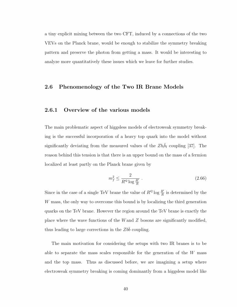
a tiny explicit mixing between the two CFT, induced by a connections of the two

VEVs on the Planck brane, would be enough to stabilize the symmetry breaking

pattern and preserve the photon from getting a mass. It would be interesting to

analyze more quantitatively these issues which we leave for further studies.

2.6 Phenomenology of the Two IR Brane Models

2.6.1 Overview of the various models

The main problematic aspect of higgsless models of electroweak symmetry break-

ing is the successful incorporation of a heavy top quark into the model without

significantly deviating from the measured values of the Zblbl coupling [37]. The

reason behind this tension is that there is an upper bound on the mass of a fermion

localized at least partly on the Planck brane given by

m2f ≤

2

R′2 log R′

R

. (2.66)

Since in the case of a single TeV brane the value of R′2 log R′

Ris determined by the

W mass, the only way to overcome this bound is by localizing the third generation

quarks on the TeV brane. However the region around the TeV brane is exactly the

place where the wave functions of the Wand Z bosons are significantly modified,

thus leading to large corrections in the Zbb coupling.

The main motivation for considering the setups with two IR branes is to be

able to separate the mass scales responsible for the generation of the W mass

and the top mass. Thus as discussed before, we are imagining a setup where

electroweak symmetry breaking is coming dominantly from a higgsless model like

40

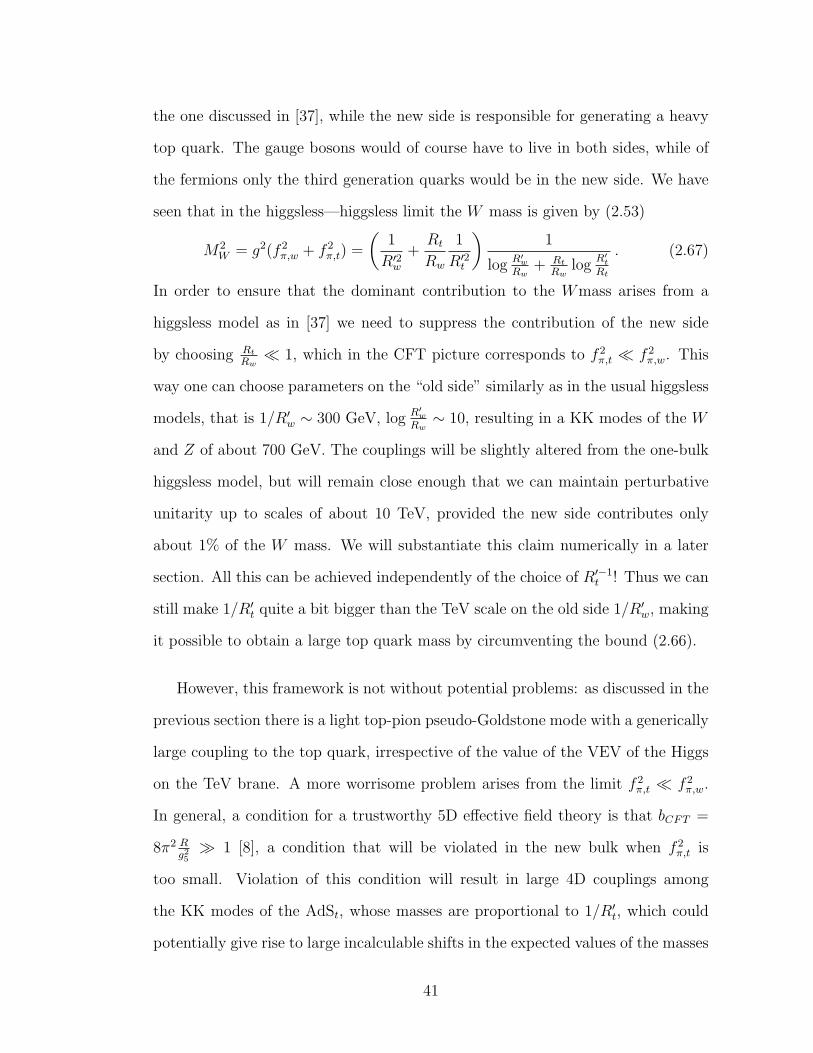
the one discussed in [37], while the new side is responsible for generating a heavy

top quark. The gauge bosons would of course have to live in both sides, while of

the fermions only the third generation quarks would be in the new side. We have

seen that in the higgsless—higgsless limit the W mass is given by (2.53)

M2W = g2(f 2

π,w + f 2π,t) =

(1

R′2w+Rt

Rw

1

R′2t

)1

log R′w

Rw+ Rt

Rwlog

R′t

Rt

. (2.67)

In order to ensure that the dominant contribution to the Wmass arises from a

higgsless model as in [37] we need to suppress the contribution of the new side

by choosing Rt

Rw� 1, which in the CFT picture corresponds to f 2

π,t � f 2π,w. This

way one can choose parameters on the “old side” similarly as in the usual higgsless

models, that is 1/R′w ∼ 300 GeV, log R′w

Rw∼ 10, resulting in a KK modes of the W

and Z of about 700 GeV. The couplings will be slightly altered from the one-bulk

higgsless model, but will remain close enough that we can maintain perturbative

unitarity up to scales of about 10 TeV, provided the new side contributes only

about 1% of the W mass. We will substantiate this claim numerically in a later

section. All this can be achieved independently of the choice of R′−1t ! Thus we can

still make 1/R′t quite a bit bigger than the TeV scale on the old side 1/R′w, making

it possible to obtain a large top quark mass by circumventing the bound (2.66).

However, this framework is not without potential problems: as discussed in the

previous section there is a light top-pion pseudo-Goldstone mode with a generically

large coupling to the top quark, irrespective of the value of the VEV of the Higgs

on the TeV brane. A more worrisome problem arises from the limit f 2π,t � f 2

π,w.

In general, a condition for a trustworthy 5D effective field theory is that bCFT =

8π2 Rg25� 1 [8], a condition that will be violated in the new bulk when f 2

π,t is

too small. Violation of this condition will result in large 4D couplings among

the KK modes of the AdSt, whose masses are proportional to 1/R′t, which could

potentially give rise to large incalculable shifts in the expected values of the masses

41

and couplings of these modes. Note however, that the coupling of the light Wand

Z will never be strong to these KK modes: gauge invariance will make sure that

the couplings of the Wand Z are of the order g to all of these modes. Thus the

expressions for the electroweak precision observables will be shielded by at least

an electroweak loop suppression from the potentially strong couplings of the KK

modes. Moreover, the unitarity in the longitudinal W scattering is still maintained

by the KK modes of the AdSw, which are weakly coupled with the KK modes of

the new AdS. This is again true as long as the Wmass mostly comes from the old

side.

Thus there is a tension in the higgsless—higgsless case between constraints

from perturbative unitarity of WW scattering which will want f 2π,t � f 2

π,w, and

constraints from 5D effective field theory. Of course, we could evade the perturba-

tive unitarity problem by lowering R′−1t to near the scale R′−1

w , but then the new

side would merely be a copy of the old side and one would again start running into

trouble with the third generation physics.

Alternatively, we can consider the higgsless—top-Higgs model, in which we can

take f 2π,w ≈ f 2

π,t but vt small. Then we again find that the new side contributes

little to electroweak symmetry breaking and perturbative unitarity is safe, and we

also have a reasonable 5D effective theory. In this case the only strong coupling

is a large Yukawa coupling for the top quark. Of course, such a model is not

genuinely “higgsless” in the sense that for small vt the Higgs on the new side does

not decouple from the SM fields. However, this surviving Higgs will have small

couplings to the Standard Model gauge bosons and large coupling to the top, so it

can be unusually heavy and will have interesting and distinct properties. We show

a summary of the different constraints on the parameters Rt/Rw and vt (assuming

42

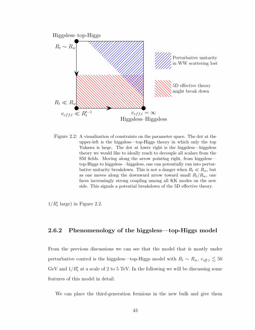
veff,t ≪ R′−1

tveff,t = ∞

Higgsless–Higgsless

Rt ≪ Rw

Rt ∼ Rw

Higgsless–top-Higgs

Perturbative unitarity

in WW scattering lost

5D effective theory

might break down

Figure 2.2: A visualization of constraints on the parameter space. The dot at theupper-left is the higgsless—top-Higgs theory in which only the topYukawa is large. The dot at lower right is the higgsless—higgslesstheory we would like to ideally reach to decouple all scalars from theSM fields. Moving along the arrow pointing right, from higgsless—top-Higgs to higgsless—higgsless, one can potentially run into pertur-bative unitarity breakdown. This is not a danger when Rt � Rw, butas one moves along the downward arrow toward small Rt/Rw, onefaces increasingly strong coupling among all KK modes on the newside. This signals a potential breakdown of the 5D effective theory.

1/R′t large) in Figure 2.2.

2.6.2 Phenomenology of the higgsless—top-Higgs model

From the previous discussions we can see that the model that is mostly under

perturbative control is the higgsless—top-Higgs model with Rt ∼ Rw, veff ,t . 50

GeV and 1/R′t at a scale of 2 to 5 TeV. In the following we will be discussing some

features of this model in detail.

We can place the third-generation fermions in the new bulk and give them

43

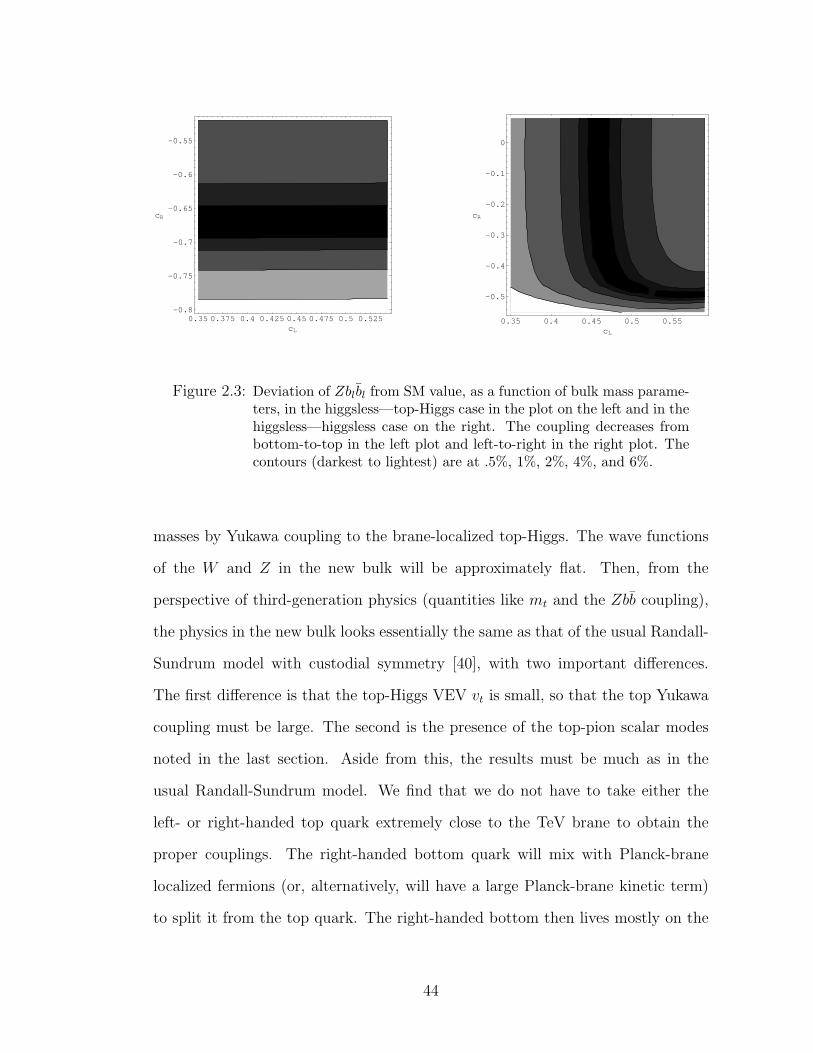
0.35 0.375 0.4 0.425 0.45 0.475 0.5 0.525cL

-0.8

-0.75

-0.7

-0.65

-0.6

-0.55

cR

0.35 0.4 0.45 0.5 0.55cL

-0.5

-0.4

-0.3

-0.2

-0.1

0

cR

Figure 2.3: Deviation of Zblbl from SM value, as a function of bulk mass parame-ters, in the higgsless—top-Higgs case in the plot on the left and in thehiggsless—higgsless case on the right. The coupling decreases frombottom-to-top in the left plot and left-to-right in the right plot. Thecontours (darkest to lightest) are at .5%, 1%, 2%, 4%, and 6%.

masses by Yukawa coupling to the brane-localized top-Higgs. The wave functions

of the W and Z in the new bulk will be approximately flat. Then, from the

perspective of third-generation physics (quantities like mt and the Zbb coupling),

the physics in the new bulk looks essentially the same as that of the usual Randall-

Sundrum model with custodial symmetry [40], with two important differences.

The first difference is that the top-Higgs VEV vt is small, so that the top Yukawa

coupling must be large. The second is the presence of the top-pion scalar modes

noted in the last section. Aside from this, the results must be much as in the

usual Randall-Sundrum model. We find that we do not have to take either the

left- or right-handed top quark extremely close to the TeV brane to obtain the

proper couplings. The right-handed bottom quark will mix with Planck-brane

localized fermions (or, alternatively, will have a large Planck-brane kinetic term)

to split it from the top quark. The right-handed bottom then lives mostly on the

44

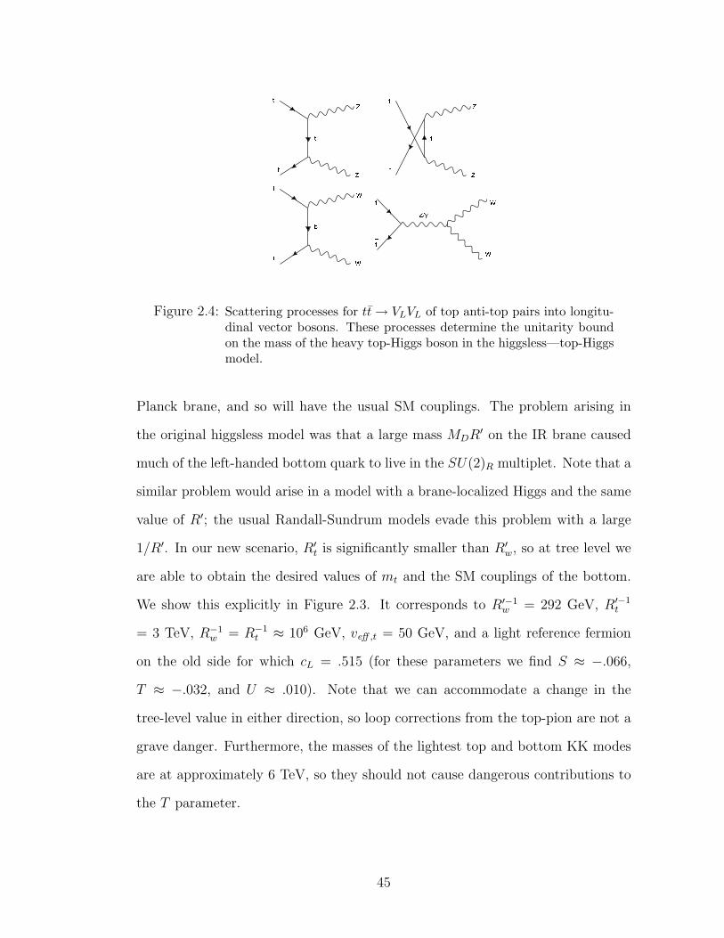
W WW

Z /W

b

Z

Zt t

Z

Z

_ t

_ t_ t

_ t

tt

t t

Figure 2.4: Scattering processes for tt → VLVL of top anti-top pairs into longitu-dinal vector bosons. These processes determine the unitarity boundon the mass of the heavy top-Higgs boson in the higgsless—top-Higgsmodel.

Planck brane, and so will have the usual SM couplings. The problem arising in

the original higgsless model was that a large mass MDR′ on the IR brane caused

much of the left-handed bottom quark to live in the SU(2)R multiplet. Note that a

similar problem would arise in a model with a brane-localized Higgs and the same

value of R′; the usual Randall-Sundrum models evade this problem with a large

1/R′. In our new scenario, R′t is significantly smaller than R′w, so at tree level we

are able to obtain the desired values of mt and the SM couplings of the bottom.

We show this explicitly in Figure 2.3. It corresponds to R′−1w = 292 GeV, R′−1

t

= 3 TeV, R−1w = R−1

t ≈ 106 GeV, veff ,t = 50 GeV, and a light reference fermion

on the old side for which cL = .515 (for these parameters we find S ≈ −.066,

T ≈ −.032, and U ≈ .010). Note that we can accommodate a change in the

tree-level value in either direction, so loop corrections from the top-pion are not a

grave danger. Furthermore, the masses of the lightest top and bottom KK modes

are at approximately 6 TeV, so they should not cause dangerous contributions to

the T parameter.

45

We would like now to investigate the phenomenology of this model in more

detail. A novelty with respect to the usual higgsless models is the presence of light

scalars. The top-Higgs on the AdSt side will couple strongly to tops and give a

small contribution to the Wmass, hence the name top-Higgs. Its tree level mass is

determined by the quartic coupling on the IR brane m2h = λtv

2eff ,t, although large

corrections could arise due to the strong coupling with the top. An important

parameter controlling this model is γ =veff ,t

v, the ratio of the (warped down)

top-Higgs VEV to the usual SM Higgs VEV. If γ � 1, we can have confidence

that perturbative unitarity in WW scattering is restored by the KK modes in the

higgsless bulk, provided they have masses in the 700 GeV range. In this case, the

top-Higgs is not needed for perturbative unitarity in WW scattering, but there is

still a unitarity bound on its mass. This bound arises from considering tt→ VLVL

scattering, where VL denotes a longitudinal W or Z boson. The relevant tree-level

diagrams are shown in Figure 2.4. This bound sets the scale of new physics, ΛNP ,

to be (as in [57])

ΛNP ≤4π√

2

3GFmt

≈ 2.8 TeV. (2.68)

This is computed in an effective theory given by the Standard Model with the Higgs

boson removed and the Yukawa coupling of the top replaced with a Dirac mass.

The resonances that couple to the top in our model are predominantly those on

the new side, which have a mass set by R′−1t , which is large. Thus these resonances

make little contribution to the scattering in question, and we can view ΛNP as a

rough upper bound on the possible mass of the top-Higgs boson in our model. It

is clear anyway that a heavy top-Higgs is allowed. The other set of scalars is an

SU(2) triplet of pseudo-Goldstone bosons that we called top-pions. We estimated

their mass in Eq.2.64. It is set by the scale 1/R′t, so that we expect them to be

quite heavy too, at least heavy enough to avoid direct bounds on charged scalars.

46

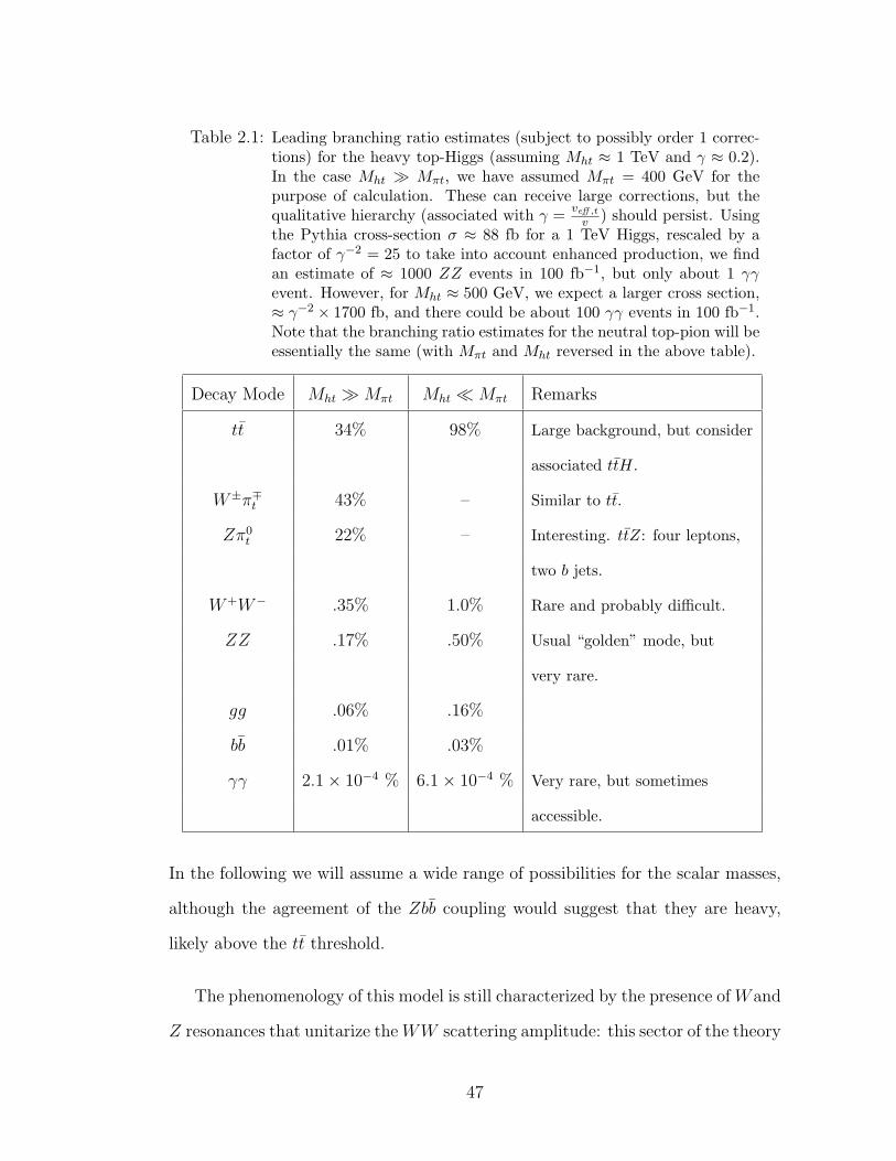
Table 2.1: Leading branching ratio estimates (subject to possibly order 1 correc-tions) for the heavy top-Higgs (assuming Mht ≈ 1 TeV and γ ≈ 0.2).In the case Mht � Mπt, we have assumed Mπt = 400 GeV for thepurpose of calculation. These can receive large corrections, but thequalitative hierarchy (associated with γ = veff ,t

v ) should persist. Usingthe Pythia cross-section σ ≈ 88 fb for a 1 TeV Higgs, rescaled by afactor of γ−2 = 25 to take into account enhanced production, we findan estimate of ≈ 1000 ZZ events in 100 fb−1, but only about 1 γγevent. However, for Mht ≈ 500 GeV, we expect a larger cross section,≈ γ−2 × 1700 fb, and there could be about 100 γγ events in 100 fb−1.Note that the branching ratio estimates for the neutral top-pion will beessentially the same (with Mπt and Mht reversed in the above table).

Decay Mode Mht �Mπt Mht �Mπt Remarks

tt 34% 98% Large background, but consider

associated ttH.

W±π∓t 43% – Similar to tt.

Zπ0t 22% – Interesting. ttZ: four leptons,

two b jets.

W+W− .35% 1.0% Rare and probably difficult.

ZZ .17% .50% Usual “golden” mode, but

very rare.

gg .06% .16%

bb .01% .03%

γγ 2.1× 10−4 % 6.1× 10−4 % Very rare, but sometimes

accessible.

In the following we will assume a wide range of possibilities for the scalar masses,

although the agreement of the Zbb coupling would suggest that they are heavy,

likely above the tt threshold.

The phenomenology of this model is still characterized by the presence of Wand

Z resonances that unitarize theWW scattering amplitude: this sector of the theory

47

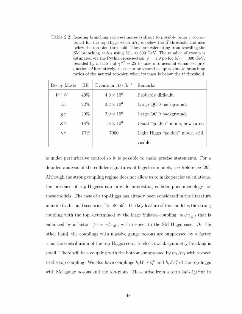
Table 2.2: Leading branching ratio estimates (subject to possibly order 1 correc-tions) for the top-Higgs when Mht is below the tt threshold and alsobelow the top-pion threshold. These are calculating from rescaling theSM branching ratios using Mht ≈ 300 GeV. The number of events isestimated via the Pythia cross-section, σ = 3.9 pb for Mht = 300 GeV,rescaled by a factor of γ−2 = 25 to take into account enhanced pro-duction. Alternatively, these can be viewed as approximate branchingratios of the neutral top-pion when its mass is below the tt threshold.

Decay Mode BR Events in 100 fb−1 Remarks

W+W− 40% 4.0× 106 Probably difficult.

bb 22% 2.2× 106 Large QCD background.

gg 20% 2.0× 106 Large QCD background.

ZZ 18% 1.8× 106 Usual “golden” mode, now rarer.

γγ .07% 7000 Light Higgs “golden” mode, still

visible.

is under perturbative control so it is possible to make precise statements. For a

detailed analysis of the collider signatures of higgsless models, see Reference [29].

Although the strong coupling regime does not allow us to make precise calculations,

the presence of top-Higgses can provide interesting collider phenomenology for

these models. The case of a top-Higgs has already been considered in the literature

in more traditional scenarios [45, 58, 59]. The key feature of this model is the strong

coupling with the top, determined by the large Yukawa coupling mt/veff ,t that is

enhanced by a factor 1/γ = v/veff ,t with respect to the SM Higgs case. On the

other hand, the couplings with massive gauge bosons are suppressed by a factor

γ, as the contribution of the top-Higgs sector to electroweak symmetry breaking is

small. There will be a coupling with the bottom, suppressed bymb/mt with respect

to the top coupling. We also have couplings htW±µπ∓t and htZπ

0t of the top-higgs

with SM gauge bosons and the top-pions. These arise from a term 2ghtAaµ∂

µπat in

48

the Lagrangian.

Let us first discuss the decays of the neutral scalars ht and π0t . If their mass

is above the tt threshold, they will often decay into tops. Notably, if the mass

is large, say 1 TeV, multiple top decays will not be suppressed due to the strong

coupling. However, for Mht � Mπt, the width of the cascade decay ht → W−π+t

is g2

16π

M3h

M2W

, becoming quite large for a very heavy top-Higgs, and even surpassing

the enhanced decay to tops. There is a suppressed tree-level decay to the weak

gauge bosons. Virtual tops will also induce loop decays into gauge bosons, γγ,

W+W−, ZZ, gg, and we generically expect them to be suppressed by a factor

of about(

α3π

)2or(

αs

3π

)2with respect to the tt channel. A simple estimate shows

that the γγ decay is suppressed, but it could still be present in a measurable

number of events at the LHC in decays of the neutral top-pion or even of the top-

Higgs if it is not too heavy. We summarize the various modes in Tables 2.1 and

2.2. The widths are calculated at leading order. That is, the tree-level decays are

calculated by rescaling the tree-level SM widths by appropriate powers of γ, except

for the decays through a top-pion, which are computed directly in our model. (The

decay to bb is computed with the running b quark mass.) Loop-level decays are

calculated by rescaling one-loop SM results by appropriate powers of γ. These

estimates should provide the right qualitative picture, though the large couplings

of the top could induce order one changes. Other interesting channels could open

up if we consider flavor violating decays, like for example tc. It might be relevant or

even dominant in the case of a relatively light scalar (below the tt threshold) [59].

However, these channels are highly model dependent: in this scenario the flavor

physics is generated on the Planck brane via mixings in non-diagonal localized

kinetic terms. For instance, we can choose the parameters so that there is no πttc

coupling at all. So, we will not consider this possibility further. Regarding the

49

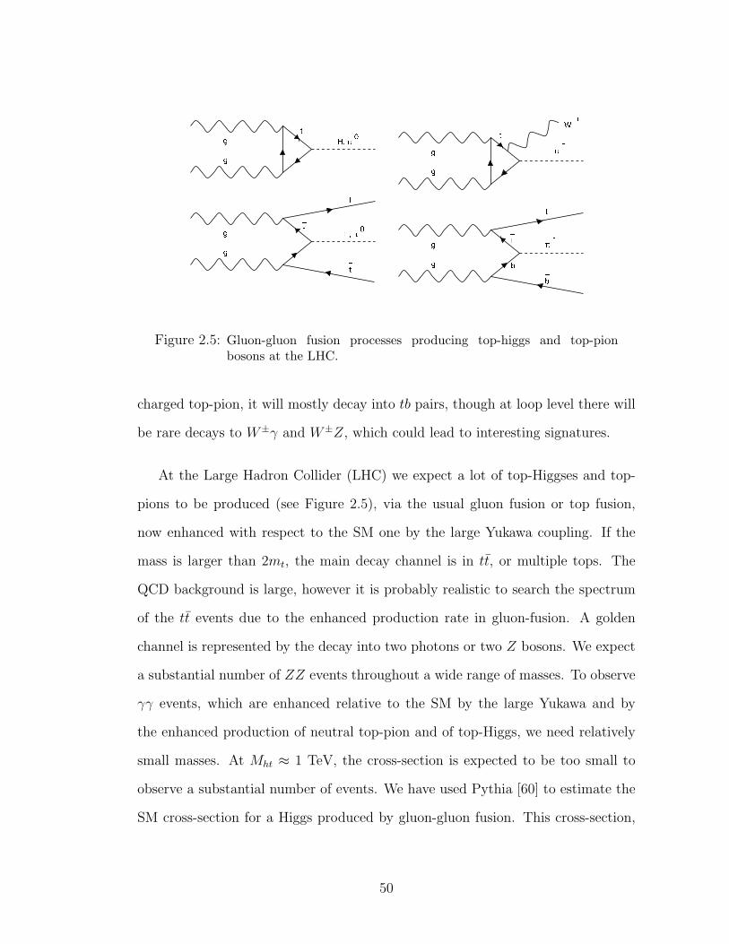
πb_ tgggg

tt �

π � W +

_ bt

_ t

gggg

t

t_ tH , π 0

H , π 0

Figure 2.5: Gluon-gluon fusion processes producing top-higgs and top-pionbosons at the LHC.

charged top-pion, it will mostly decay into tb pairs, though at loop level there will

be rare decays to W±γ and W±Z, which could lead to interesting signatures.

At the Large Hadron Collider (LHC) we expect a lot of top-Higgses and top-

pions to be produced (see Figure 2.5), via the usual gluon fusion or top fusion,

now enhanced with respect to the SM one by the large Yukawa coupling. If the

mass is larger than 2mt, the main decay channel is in tt, or multiple tops. The

QCD background is large, however it is probably realistic to search the spectrum

of the tt events due to the enhanced production rate in gluon-fusion. A golden

channel is represented by the decay into two photons or two Z bosons. We expect

a substantial number of ZZ events throughout a wide range of masses. To observe

γγ events, which are enhanced relative to the SM by the large Yukawa and by

the enhanced production of neutral top-pion and of top-Higgs, we need relatively

small masses. At Mht ≈ 1 TeV, the cross-section is expected to be too small to

observe a substantial number of events. We have used Pythia [60] to estimate the

SM cross-section for a Higgs produced by gluon-gluon fusion. This cross-section,

50

suitably enhanced by the large Yukawa, was used to estimate numbers of LHC

events per 100 fb−1 in Tables 2.1 and 2.2. Of course, strong coupling will modify

our estimates of cross-sections and branching ratios, so the numbers we present

should be taken as order-of-magnitude guides. We expect the neutral top-pion

to have a mass somewhat below the TeV scale, so optimistically one should see

the photon-photon channel from the neutral top-pion irrespective of the top-Higgs

mass. We stress that, for a mass in the 500 GeV region, one can expect roughly

one photon-photon event per fb−1, while the number of ZZ events should be of

order one thousand times larger. At the LHC it will be relatively easy to see peaks

in the two photons or `+`−`+`− channels, due to the reduced background. Thus,

a heavy resonance in γγ, associated with an anomalous production of multi-top

events would be a striking signature of these models. If cascade decays of the

top-Higgs into the top-pion are allowed, we could also observe interesting Ztt(tt)

channels that could lead to striking 6 leptons 4 b events. If the masses are below

the top threshold, the main decay channels will be into b’s and gauge bosons. The

golden channels are again γγ and ZZ. The high rate of bb events even above the

WW threshold could help distinguish a light scalar in our model from a heavy SM

Higgs. Also, if the rate of γγ is not too far below the rate of `+`−`+`− events it

would suggest a large top-loop induced coupling, since in the SM this ratio is fixed

to be roughly(

α3π

)2.

Finally, the charged top-pion would be harder to study: its production is sup-

pressed as we do not have a gluon fusion channel producing solely a top pion. It

will be produced in association with a tb pair or with a W boson. It will then

most likely decay into tb, so that its signal will suffer from a large QCD pollu-

tion. An interesting effect could be an anomalous production of multi b-jet events.

The loop-level decays to Wγ and WZ could produce interesting multi-gauge-boson

51

events, but these have a suppression comparable to the γγ decays of the neutral

top-pion.

2.6.3 Phenomenology of the higgsless—higgsless model

Finally, we summarize the tree-level numerical results for the higgsless—higgsless

limit. Let us first discuss how to fix the values of the parameters corresponding

to a potentially interesting theory. First of all, we would like one of the sides to

be a higgsless model as in [37], with low enough KK masses for the gauge bosons

to ensure perturbative unitarity of the WW scattering amplitudes. This can be

achieved if the first resonance mass is around 600-700 GeV, thus fixing R′−1w ∼ 300

GeV. The value of the W mass will fix the logR′w/Rw ∼ 10, so that a natural

value for R−1w is around 108 GeV. On the new side we need the IR scale to be large

enough to accomodate the top mass, so that R′−1t ∼ 2− 5 TeV � R′−1

w . However,

we want to do it without a low-scale violation of perturbative unitarity. Since the

KK modes on the new side will be very heavy > TeV, this is only possible if the

new side does not contribute a lot to the W mass itself. From (2.67) we can see

that this can be achieved by choosing a smaller curvature radius for the new side

Rt � Rw(R′t/R′w)2. For simplicity we will also assume the 5D gauge couplings

are the same in both bulks, and that g5L = g5R. Then, for any given value of

R′t and of the contribution of the new side to the W mass (that will determine

the perturbative unitarity breakdown scale), we determine the scales Rw,t and R′w,

while g5 is fixed by the Z mass.

We also choose a “reference” bulk fermion in the old bulk as in [37] to fix

the wave-function normalizations. As in the one-bulk case, when this reference

fermion has an approximately flat wave-function (cL ∼ 0.5) the tree-level precision

52

electroweak parameters S, T , and U can all be made small.

To fix the actual numerical values we choose R′−1t = 3 TeV, and we allow the

new bulk to contribute 5% of the W mass, f 2π,t ≈ 0.05(f 2

π,w + f 2π,t). Then for

the values quoted above, we get R′−1w ≈ 276 GeV, and the curvature scales are

R−1w ≈ ×108 GeV and R−1

t ≈ 2 × 1011 GeV. Choosing our reference quark to be

a massless left-handed quark with cL = 0.46, we find at tree-level S ≈ −0.08,

T ≈ −0.04, and U ≈ 0.01.

The first task after fixing the parameters is to verify that the scale of pertur-

bative unitarity violation is indeed pushed above the usual SM scale of 1 TeV. For

this we can study the sum rules [10] that the KK modes masses and couplings have

to satisfy in order for terms in the scattering amplitudes that grow with a powers

of the energy to cancel. We solve numerically for the Kaluza-Klein resonances of

the Z boson. The first one is at M(1)Z ≈ 676 GeV ≈ 2.45R′−1

w , as expected. Sum-

ming the KK modes up to 8 TeV, we find that the E4 sum rule is satisfied to a

precision of 2×10−6 and the E2 sum rule to a precision of 5×10−3. In order to find

the unitarity violation scale we have shown in Figure 2.6 the s-wave partial-wave

amplitude a0 as a function of energy, which is obtained by numerically solving for

all KK mode masses and couplings below 8 TeV, and then approximating the rest

of the tower by an additional heavy mode so the graph does not misbehave at high

energy (note that this approximation has no effect below 8 TeV). We can see that

the unitarity bound from a0 is around 5 TeV, well above the SM scale, and a scale

likely inaccessible to the LHC. As explained in [31], we should only rely on the

low-energy linear behavior of this function, which tells us that the effective theory

is valid up to 5 TeV.

After fixing the parameters in the gauge sector, we are finally ready to consider

53

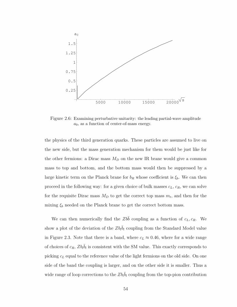
5000 10000 15000 20000�!!!s

0.25

0.5

0.75

1

1.25

1.5

a0

Figure 2.6: Examining perturbative unitarity: the leading partial-wave amplitudea0, as a function of center-of-mass energy.

the physics of the third generation quarks. These particles are assumed to live on

the new side, but the mass generation mechanism for them would be just like for

the other fermions: a Dirac mass MD on the new IR brane would give a common

mass to top and bottom, and the bottom mass would then be suppressed by a

large kinetic term on the Planck brane for bR whose coefficient is ξb. We can then

proceed in the following way: for a given choice of bulk masses cL, cR, we can solve

for the requisite Dirac mass MD to get the correct top mass mt, and then for the

mixing ξb needed on the Planck brane to get the correct bottom mass.

We can then numerically find the Zbb coupling as a function of cL, cR. We

show a plot of the deviation of the Zblbl coupling from the Standard Model value

in Figure 2.3. Note that there is a band, where cL ≈ 0.46, where for a wide range

of choices of cR, Zblbl is consistent with the SM value. This exactly corresponds to

picking cL equal to the reference value of the light fermions on the old side. On one

side of the band the coupling is larger, and on the other side it is smaller. Thus a

wide range of loop corrections to the Zblbl coupling from the top-pion contribution

54

can be accommodated in this model by changing the values of cL,R, and tuning

the sum of the tree-level plus loop corrections to equal the SM value. Thus we

conclude that while in this model there is no a priori reason to expect this coupling

to take on its SM value, parameters can likely be chosen such that the SM value

could be accommodated.

Since we cannot calculate the loop corrections, for concreteness we will examine

a case in which the tree-level value of the Zblbl coupling agrees with the SM. We

take cL = 0.46, cR = −0.1. We then find that we need to take MD ≈ 610 GeV

and ξb ≈ 6000 to obtain mt = 175 GeV and mb = 4.5 GeV. The tree-level Zblbl

coupling then deviates from the SM value by only .03%. We calculate now the

various couplings of the pseudo-Goldstones to the top and bottom. We find that

the couplings involving the right-handed bottom are small: gπ0t blbr

≈ gπ+t tlbr

≈

−0.106. However, as expected, the couplings involving the right-handed top are

large: gπ0t tltr ≈ gπ−t bltr

≈ −4.16. Thus the top-pion coupling is four times larger

than the SM Higgs coupling.

2.7 Conclusions

We have considered extra dimensional descriptions of topcolor-type models. From

the 4D point of view these would correspond to theories where two separate

strongly interacting sectors would contribute to electroweak symmetry breaking.

In the 5D picture these would be two separate AdS bulks with their own IR branes,

and the two bulks intersecting on the common Planck brane. The motivation for

considering such models is the need to separate the dynamics that gives most

of electroweak symmetry breaking from that responsible for the top quark mass

55

(which is the main problematic aspect of higgsless models of electroweak symmetry

breaking).

We have described how to find the appropriate matching and boundary con-

ditions for the fields that propagate in both sides, and gave a description of elec-

troweak symmetry breaking if both IR branes have localized Higgs fields. We have

considered both the cases when the Higgs VEVs are small or large (the higgsless

limit). We discussed the CFT interpretation of all of these limits, and also showed

that a light pseudo-Goldstone boson (“top-pion”) has to emerge in these setups.

Depending on the limit considered, the top-pion could be mostly contained in one

of the brane Higgses or in A5 in the higgsless limit.

Finally, we have used these models to try to resolve the issues surrounding the

third generation quarks in the higgsless theories. In these models one of the bulks

is like a generic higgsless model as in [37] with only the light fermions propagating

there, while the new bulk will contain the top and bottom quark, but will not

be the dominant source of electroweak symmetry breaking. The suppression of

the contribution to the W mass from the new side is either obtained by a small

top-Higgs VEV (higgsless—top-Higgs models) or via a small curvature radius in

the new bulk. A generic issue in all of these cases will be that the top-pions (and

eventually the top-Higgs) are strongly coupled to the top and bottom quarks. In

the higgsless—higgsless case the small curvature radius will also imply that the

KK modes dominantly living on the new side will be strongly coupled among

themselves. In both limits the tree-level top mass and Zbb couplings can be made

to agree with the experimental results, however, due to the coupling of the top-

pion one also needs to worry about large shifts from loop corrections. We have

discussed the basic phenomenological consequences of both limits. The top-pion

56

and top-Higgs are expected to be largely produced at LHC. Their main signature

would be an observable heavy resonance in the γγ channel in association with an

anomalously large rate of multi-top events.

57

Chapter 3

A Braneless Approach to Holographic

QCD

3.1 Introduction

QCD is a perennially problematic theory. Despite its decades of experimental

support, the detailed low-energy physics remains beyond our calculational reach.

The lattice provides a technique for answering nonperturbative questions, but to

date there remain open questions that have not been answered. For instance, the

low-energy scalar spectrum is a puzzle. There are a lot of experimentally observed

states, however their composition (glueball vs. quarkonium) and their mixings

are not well understood. The difficulty for any theory trying to make progress in

this direction is to understand the interaction between the scalar states and the

vacuum condensates of QCD. In this paper we attempt to incorporate the effects of

the vacuum condensates into the holographic model of QCD as a first step toward

understanding the scalar sector in the context of these models.

The SVZ sum rules [61] are a powerful theoretical tool for relating theoretically

solid facts about perturbative QCD with experimental data in the low-energy re-

gion. The basic observation is that the correlator for a current J

Π(q) = i

∫d4x eiqx 〈0 |TJ(x)J(0)| 0〉 (3.1)

may be expanded in a Wilson OPE that is valid up to some power (where in-

stanton corrections begin to invalidate the local expansion), (1/Q2)(dΠ/dQ2) =∑C2d 〈O2d〉, where the O2d are gauge-invariant operators of dimension 2d. In the

58

deep Euclidean domain the coefficients C2d are calculable. On the other hand,

the correlator relates to observable quantities; for instance if J is the vector cur-

rent then ImΠ(s) is directly proportional to the spectral density ρ(s), measurable

from the total cross section σ(e+e− → hadrons). The SVZ sum rules, then, relate

Wilson OPE expansions to measurable quantities. They can become useful for

understanding detailed properties of the first resonances when one takes a Borel

transform that suppresses the effect of higher resonances. As it turns out, keeping

only low orders of perturbation theory in the coefficients C2d, one still obtains rea-

sonable agreement with data, so the assumption that the largest corrections arise

from the condensates is a good one.

Recently another technique for understanding the properties of low-lying

mesons has arisen in the form of AdS/QCD. The phenomenological model con-

structed on this basis [55] takes as its starting points the OPE (much as in the

SVZ sum rules) and the AdS/CFT correspondence [7, 42]. The idea is straight-

forward: rather than attempting to deform the usual Type IIB on AdS5 × S5 to

obtain a theory more like QCD, one starts with QCD and attempts to build a

holographic dual. Of course in detail such a program is bound to eventually run

up against difficulties from α′ corrections, gs corrections, the geometry of the five

compact dimensions (or the proper definition of a noncritical string theory) and

other issues. However, one can set aside these problems, begin with a relatively

small set of fields needed to model the low-lying states in QCD, and see how

well the approximation works. In this phenomenological approach with bulk fields

placed in the Randall-Sundrum background [2], and the AdS space cut off with

a brane at a fixed z = zc in the infrared a surprisingly good agreement with the

physics of the pions, ρ, and a1 mesons has been found [55] (for more recent work

on AdS/QCD see [62, 63]). However, there are several obvious limitations to this

59

model. For example, it does not take into account the power corrections to the

OPE in the UV (the effects of the vacuum condensates), or the corrections coming

from logarithmic running. Also, the theory has a single mass scale (set by the

location of IR cutoff brane) which determines the mass scales in all the different

sectors in QCD.

Here we show how the effect of the vacuum condensates and of asymptotic free-

dom can be simply incorporated into the model. We will limit ourselves to pure

Yang-Mills theory without quarks, though we expect that most of the aspects of

incorporating quarks should be relatively straightforward. For the vacuum con-

densates one has to introduce a dynamical scalar with appropriate mass term and

potential coupled to gravity. There will be a separate field for every gauge invariant

operator of QCD, and a non-zero condensate will lead to a non-trivial profile of the

scalar in the bulk. While the effects of these condensates on the background close

to the UV boundary are small (though not always negligible), they will become the

dominant source in the IR and effectively shut off the space in a singularity (and

without having to cut the space off by hand). This resolves several ambiguities in

choosing the boundary conditions at the IR brane, and the various condensates will

also be able to set different mass scales in the different sectors of QCD. Asymptotic

freedom can be achieved by properly choosing the potential for the scalar corre-

sponding to the Yang-Mills gauge coupling. Incorporating asymptotic freedom will

have an important effect on the glueball sector since a massless Goldstone field will

pick up a mass from the anomalous breaking of scale invariance.

It is natural to ask why we should expect QCD to have any useful holographic

dual. The most well understood examples of holography are in the limit of large

N and g2Y MN � 1, far from the regime of real-world QCD, which apparently

60

would be a completely intractable string theory with a large value of α′. On

the other hand, the large N approximation has frequently been applied in QCD

phenomenology. A major concern in applying holography to QCD is whether the

dual should be local, or whether it can have higher-derivative α′ corrections. The

α′ corrections are associated with the massive stringy excitations in the bulk, which

once integrated out yield complicated Lagrangians for the remaining light fields.

However, we can think of this physics in a different way. Holography is closely

related to the renormalization group [64]; the coordinate z can be identified with

µ−1, where µ is the renormalization group scale. AdS/CFT identifies massive

bulk fields with higher-dimension operators in the field theory. From this point

of view, α′ corrections to the physics of light bulk fields are associated with the

effects of higher-dimension operators coupled to the low-dimension operators in

the RG flow. The OPE tells us that, at large Q2, the effects of these higher-

dimension operators in the field theory are controllably small. From this point of

view, despite the apparently large α′ corrections, it is reasonable to begin with a

local bulk action in terms of fields corresponding to the low dimension operators

of QCD. The example of SVZ gives us hope that this can correctly capture physics

of light mesons. For highly excited mesons, which in QCD look like extended flux

tubes, and thus feel long distances, it is more probable that the strong IR physics

will mix different operators and that our neglect of α′-like corrections will become

more troublesome. It is a general problem, in fact, that physics of highly excited

hadrons is troublesome in these models [65]. Recent proposals for backgrounds

with correct Regge physics [66] offer some hope of addressing this problem. We

will offer some further comments on how a closed-string tachyon might give a

dynamical explanation of such a background, but there is clearly much more to be

done along these lines.

61

The paper is organized as follows. In section 2 we will remind the reader

of the basic formulation of AdS/QCD on Randall-Sundrum backgrounds as in

Reference[55], and discuss some of its shortcomings. In section 3 we will dis-

cuss a class of models that do not incorporate the running of the QCD coupling,

but do incorporate the effects of the lowest vacuum condensate. We will point

out that these backgrounds too have some shortcomings, but improve on the RS

backgrounds, and may provide a useful setting for exploring some questions. We

calculate the gluon condensate and point out that there is a zero mode in the glue-

ball spectrum due to the spontaneous breaking of scale invariance. In section 4 we

discuss the construction of 5D theories with asymptotic freedom. We calculate the

gluon condensate and provide a first estimate of masses for the 0++ glueballs from

these backgrounds. We point out a possible interpretation of the running coupling

where αs remains finite for all energies. In section 5 we show how to systematically

incorporate the effects of the higher condensates. We give a background including

the effect of 〈TrF3〉 and show how it affects the gluon condensate and the glue-

ball spectrum. In section 6 we discuss the difficulties of reproducing the correct

Regge physics, and speculate that closed string tachyon dynamics could perhaps

be responsible for reproducing the necessary IR background. Finally we provide

the conclusions and some outlook in section 7.

3.2 AdS/QCD on Randall-Sundrum backgrounds

We briefly review the AdS/QCD model on Randall-Sundrum backgrounds [55].

One assumes that the metric is exactly AdS in a finite region z = 0 to z = zc, i.e.

ds2 =

(R

z

)2 (dxµdxνηµν − dz2

), 0 ≤ z ≤ zc, (3.2)

62

where zc ∼ Λ−1QCD determines the scale of the mass spectrum. It is assumed that

there is a brane (the “infrared brane”) at z = zc; in practice one assumes a UV

boundary at z = ε and sends ε → 0 at the end of calculations. One puts a field

φO in the bulk for every gauge invariant operator O in the gauge theory. If O is a

p-form of dimension ∆, φ has a 5D mass m25 = (∆ + p)(∆ + p− 4). This operator

has UV boundary conditions dictated by the usual AdS/CFT correspondence. On

the other hand, IR boundary conditions are less clear, and one in principle can

add localized terms on the IR brane.

For instance, in the original papers the treatment involves the rho and a1

mesons and the pions. There are bulk gauge fields, ALM and AR

M (where M is a 5D

Lorentz index) coupling to the operators qLγµtaqL and qRγ

µtaqR. There is also a

bulk scalar Xαβ coupling to the operator qαRq

βL, where α and β are flavor indices.

The scalar Xαβ is assumed to have a profile proportional to δαβ (mαz + 〈qαqα〉 z3),

based on the Klebanov-Witten result [43] that a nonnormalizable term in a scalar

profile corresponds to a perturbation of the Lagrangian by a relevant operator

(in this case, mqq), while a normalizable term corresponds to a spontaneously

generated VEV for the corresponding field theory operator. The profile for X(z)

couples differently to the vector and axial vector mesons and achieves the ρ − a1

mass splitting. Furthermore, the pions arise as pseudo-Nambu-Goldstone modes of

broken chiral symmetry, and the Gell-Mann–Oakes–Renner relationship is satisfied.

Several other constants in the chiral Lagrangian are determined to around 10%

accuracy.

There are several limitations to this model. One is that it does not take into

account the power corrections to the OPE in the UV, or the corrections coming

from logarithmic running. The SVZ sum rules work fairly well with just the lead-

63

ing power correction taken into account [61], and these power corrections can be

incorporated into the form of the metric with a simple ansatz[63]. However, back-

reaction has not been taken into account in such studies, so the Einstein equations

will not be exactly satisfied. Also, in the SVZ sum rule approach, leading correc-

tions to the OPE essentially determine the mass scale of the lightest resonance in

the corresponding channel. In the Randall-Sundrum approach, the leading correc-

tion to the OPE and the IR wall at zc both influence the corresponding mass scale.

This has effects on the spectrum.

For instance, in QCD the mass scales associated with mesons made from quarks

and mesons made from gluons are very different [67]. One can see this in the OPE.

For instance, in the tensor 2++ channel, the leading corrections to the OPE come

from the same operator in the qq case as in the G2 case, but the coefficients are very

different. In the Randall-Sundrum approach, without turning on a background

field VEV the mass scale for both of these channels is set by z−1c . One can turn

on a background VEV and give the fields different couplings to it to reproduce the

difference in the OPEs, but z−1c will continue to play a role in setting their masses.

Another limitation is that these backgrounds lack asymptotic freedom. If one

defines the theory with a cutoff at which αs has some finite value, this might not

appear to be of central importance. On the other hand, we understand that in

real QCD the values of the condensates are determined by the QCD scale at which

the perturbative running coupling blows up, so achieving asymptotic freedom can

allow such a relationship and make the model less ad hoc. Furthermore, we will see

that the lack of proper conformal symmetry breaking can lead to a massless scalar

glueball state (i.e., the model has a “radion problem”), which is most satisfactorily

resolved by incorporating asymptotic freedom.

64

In summary, the AdS/QCD models on hard-wall backgrounds work surprisingly

well for some quantities, but have obvious drawbacks. There are ambiguities in

IR boundary conditions, and the existence of a single IR wall influencing all fields

obscures the relationship between masses of light resonances and power corrections

discovered by Shifman, Vainshtein, and Zakharov. Luckily, there is a simple rem-

edy to these difficulties: we simply remove the IR brane, and allow the growth of

the condensates to dynamically cut the space off in the infrared.

3.3 Vacuum condensates as IR cutoff

To model the pure gauge theory we begin with the action for five-dimensional

gravity coupled to a dilaton (in the Einstein frame):

S =1

2κ2

∫d5x

√g(−R+

12

R2+

1

2gMN∂Mφ∂Nφ). (3.3)

Here κ2 is the 5 dimensional Newton constant and R is the AdS curvature (related

to the the (negative) bulk cosmological constant as R−2 = −κ2

6Λ. Note, that φ is

dimensionless here. The dilaton will couple to the gluon operator GµνGµν . The

fact that there is a non-vanishing gluon condensate in QCD is expressed by the fact

that the dilaton will have a non-trivial background. We can find the most general

such background by solving the coupled system of the dilaton equation of motion

and the Einstein’s equation, under the ansatz that we preserve four-dimensional

Lorentz invariance while the fifth dimension has a warp factor:

ds2 = e−2A(y)ηµνdxµdxν − dy2

φ = φ(y). (3.4)

65

The coupled equations for A(y), φ(y) will then be

4A′2 − A′′ = 4R2

A′2 =φ′2

24+

1

R2

φ′′ = 4A′φ′. (3.5)

A simple way of solving these equations is to use the superpotential method [68, 69],

that is define the function W (φ) such that

A′(y) = W (φ(y))

φ′(y) = 6∂W

∂φ. (3.6)

This is always possible, and the equation determining the superpotential is given

by

V = 18

(∂W

∂φ

)2

− 12W 2 = − 12

R2. (3.7)

To solve for the most general superpotential consistent with our chosen (constant)

potential, it is useful to parameterize it in terms of a “prepotential” w as [69]

W =1

R

(w +

1

w

)W ′ =

√2

3

1

R

(w − 1

w

), (3.8)

which is chosen such that (3.7) is automatically satisfied. The consistency condition

of the two equations in (3.8) implies a simple equation for the prepotential:

w′ =

√2

3w, (3.9)

and thus for the superpotential we find

W (φ) =1

R(Ce

√23φ + C−1e−

√23φ). (3.10)

66

With the superpotential uniquely determined (up to a constant C) we can then go

ahead and integrate the equations in (3.6). The result is

φ(y) =

√3

2log [C tanh 2(y0 − y)/R] ,

A(y) = −1

4log [cosh 2(y0 − y)/R sinh 2(y0 − y)/R] + A0, (3.11)

where y0 and A0 are integration constants. These are the solutions also found

in [69, 70]. In order to have A(y) asymptotically equal to y (for large negative y),

we will fix A0 = y0

R− 1

2log 2. Note, that there is another branch of the solution

where in which tanh is replaced by coth in the solution for φ. In order to have

a form of the solution that is more familiar and useful, we make a coordinate

transformation ey−y0

R = z/zc. This will recast the solution in a form that matches

the usual conformal coordinates xµ, z near z = 0:

ds2 =

(R

z

)2√1−

(z

zc

)8

ηµνdxµdxν − dz2

(3.12)

φ(z) =

√3

2log

1 +(

zzc

)4

1−(

zzc

)4

+ φ0. (3.13)

Here zc is a new parameter determining the IR scale, and we expect zc ∼ Λ−1QCD.

The point z = zc is a naked singularity, which we must imagine is resolved in the

full string theory. Also note that the first correction to the AdS5 metric goes as

z8.

3.3.1 Gluon condensate

We have seen that the metric incorporates power corrections to the pure AdS

solution, which we want to identify with the effects of the gluon condensate. Below

67

we would like to make this statement more precise. According to the general

rules of the AdS/CFT correspondence given some field ϕO on this background

representing an operator O in QCD, the deep-Euclidean correlator of O will have

a Q−8 correction if ϕO has no dilaton coupling, and a Q−4 correction if ϕO couples

to φ. Note that near z = 0, the dilaton behaves φ0 +√

6 z4

z4c. This is in agreement

with the expectation that a field coupling to an operator with dimension ∆ has

two solutions, z∆−d and z∆. In our case ∆ = d = 4, and we expect the constant

piece to correspond to the source for the operator TrG2 and coefficient of the z4

to give the gluon condensate. The precise statement [43] from AdS/CFT is that if

solution to the classical equations of motion Φ has the form near the boundary

Φ(x, z) → zd−∆[Φ0(x) +O(z2)] + z∆[A(x) +O(z2)] (3.14)

then the condensate (one-point function) of the operator O is given by

〈O(x)〉 = (2∆− d)A(x). (3.15)

However, to apply this to the solution in (3.13) we need to make sure that the

appropriate normalization of the fields is used. The expression (3.15) is derived

assuming a scalar field action of the form 1/2∫d4xdz/z3(∂Mφ)2. Comparing this

with the action used here (3.3) we find

〈TrG2〉 = 4√

3

√R3

κ2

1

z4c

. (3.16)

In order to be able to relate this expression for the condensate we need to find

an expression for R3/κ2. This can be done by requiring that the leading term

in the OPE of the gluon operator G2 is correctly reproduced in the holographic

theory. One can simply calculate the leading term in the OPE in QCD [71]∫d4x〈G2(x)G2(0)〉eiqx = −(N2 − 1)

4π2q4 log

q2

µ2+ . . . (3.17)

68

The same quantity can be calculated in the gravity theory by evaluating the action

for the scalar field with a give source φ0(q) in the UV. The general expression for

the action is obtained (after integrating by parts and using the bulk equation of

motion)

S5D =1

2κ2

∫d4x

R3

z3

1

2φ∂zφ|z→0. (3.18)

In order to find the action one can use the bulk equation of motion close to the

UV for the scalar field given by

φ′′ + q2φ− 3

zφ′ = 0. (3.19)

Requiring that the wave function approaches 1 around z = 0 will fix the leading

terms in the wave function:

φ(z) = 1− 1

32q4z4 log q2z2 +

1

4q2z2 + . . . . (3.20)

Taking the second derivative of the action we find∫d4x〈G2(x)G2(0)〉eiqx = − R3

16κ2q4 log q2/µ2 + . . . , (3.21)

from which we get the identification

R3

κ2=

4(N2 − 1)

π2. (3.22)

Using this result we get a prediction for the gluon condensate

〈TrG2〉 =8

πz4c

√3(N2 − 1). (3.23)

3.3.2 The Glueball Spectrum

Now we wish to solve for the scalar glueball spectrum, which is associated with

scalar fluctuations about the dilaton–metric background. The analogous calcula-

tion in the supergravity model has been performed in [72]. We should solve the

69

coupled radion–dilaton equations, as often there is a light mode from the radion.

In other words, we should solve for eigenmodes of the coupled Einstein-scalar sys-

tem. This has been worked out in detail for a generic scalar background in [73]:

the linearized metric and scalar ansatz is given by:

ds2 = e−2A(y)(1− 2F (x, y))dxµdxνηµν − (1 + 4F (x, y))dy2

φ(x, y) = φ0(y) +3

κ2φ0

(F ′(x, y)− 2A′(y)F (x, y)) . (3.24)

This will satisfy the coupled Einstein-scalar equations if F = F (y)eiq·x with q2 =

m2 and F (y) satisfies the differential equation

F ′′ − 2A′F ′ − 4A′′F − 2φ′′0φ′0F ′ + 4A′

φ′′0φ′0F = −e−2Am2F. (3.25)

Using the solutions for A(y) and φ0(y) from Eq. 3.11, and an ansatz F (x, y) =

F (y)eiq·x, with q2 = −m2, this becomes:

F ′′(y) +10

Rcoth

4(y − y0)

RF ′(y) +

16

R2+m2 e2y0/R√

2 sinh 4(y0−y)R

F (y) = 0. (3.26)

Demanding a normalizable solution, we need that (in the z coordinates)∫dz√g|ϕ(z)|2 and

∫dz√gg55|∂zϕ(z)|2 be finite. Thus we need ϕ(z) ∼ z4 at small

z. We need to be somewhat more careful about solving for F : in the z coordinates,

we have that

z → 0 : zdF

dz− 2z

dA

dzF → z

dF

dz− 2F ∼ ϕ(z), (3.27)

so that F (z) ∼ z2 near z = 0 is compatible with our assumptions on the behavior

of ϕ(z). As usual, this equation can be solved using the shooting method: the

differential equation is solved numerically starting from the UV boundary with

arbitrary normalization the BC following from (3.27) (the numerics is very insen-

sitive to the choice of the actual UV BC for the higher modes) for varying values

of m2. For discrete values of m2 the wave function will be normalizable (which

70

numerically is equivalent to requiring a Neumann BC at the location of the singu-

larity). This way we find (in units of z−1c ) glueballs with masses 6.61, 9.84, 12.94,

and 15.98 (and so forth, with regular spacing in mass).

There is also a serious problem: we find a massless mode for the radion (with

the F (z) ∼ z2 UV boundary conditions). This can be understood as follows: in

real QCD, the classical conformal symmetry is broken by the scale anomaly. How-

ever, in our model, it is broken by the z4 profile of the dilaton. AdS/CFT tells

us we should understand turning on such a normalizable background in the UV

as a spontaneous symmetry breaking. In Randall-Sundrum models, one similarly

has a radion problem and needs to invoke (for instance) a Goldberger-Wise stabi-

lization [9] to avoid a massless mode. The radion has not been part of previous

investigations of glueballs on Randall-Sundrum backgrounds [74], so such studies

have essentially assumed that the stabilization mechanism removes a light mode

from the spectrum. However, an added Goldberger-Wise field does not seem to

correspond to an operator of QCD, so it goes against the spirit of the AdS/CFT

correspondence. It is apparent that a palatable solution of the radion problem in

AdS/QCD demands a 5D treatment of scale dependence that mirrors that in 4D.

This motivates us to search for backgrounds incorporating asymptotic freedom,

which also allows us to begin approaching a more detailed matching to perturba-

tive QCD.

3.4 Incorporating Asymptotic freedom

We have shown in the previous section a background that incorporates the lowest

QCD condensate TrF 2 and which automatically provides an IR cutoff via the

71

backreaction of the metric. However, this setup is certainly too simplistic even to

just produce the main features of QCD: for example asymptotic freedom is not

reproduced in that setup. It is the dilaton field that also sets the QCD coupling

constant, and by approaching a constant value the model in the previous section

actually describes a theory that approaches a conformal fixed point in the UV,

rather than QCD. One may think that this is not an important difference for the

IR physics, but this is not quite right. For example as we have seen it introduces

a “radion problem.”

Thus we set out to find a potential for the dilaton that will reproduce the

logarithmic running of the coupling. We assume that similarly to string theory the

gauge coupling is actually given by ebφ(z) (where b is a numerical constant). We

will find a result consistent with expectations from string theory.1

We assume that our action is:

S =1

2κ2

∫d5x

√g(−R− V (φ) +

1

2gMN∂Mφ∂Nφ), (3.28)

where now we will try to determine V (φ) such that we reproduce asymptotic

freedom. If we require that the coupling runs logarithmically, and as usual identify

the energy scale with the inverse of the AdS coordinate z we need to have a solution

of the form

ebφ(z) =1

log z0

z

, (3.29)

where z0 = Λ−1QCD and we do not fix b a priori. Then going to the y coordinates as

usual via the definition ey/R = z/R, we will find

ebφ(y) =R

y0 − y. (3.30)

1Other discussions of backgrounds with logarithmically running coupling can be found in [75,76].

72

If we now assume that this solution follows from a superpotential W then φ′(y) =

6∂W∂φ

= 1b(y0−y)

= 1bRebφ. This implies that W (φ) = 1

6Rb2ebφ + W0. Now that we

have found the form of the superpotential, we can easily solve for the warp factor:

A′(y) = W (φ(y)) = 16b2(y−y0)

+W0, and hence A(y) = A0 +W0y + 16b2

log Ry0−y

. In

z coordinates, this becomes:

A(z) = A0 +W0R log z/R− 1

6b2log log z0/z, (3.31)

and hence e−2A(z) = e−2A0(R/z)2W0R(log z0/z)1/(3b2). From this we conclude that

we should take A0 = 0 and W0 = 1R

to get a solution that looks AdS-like up to

some powers of log z0/z.

The potential corresponding to this superpotential is then given by

V (φ) = 18

(∂W

∂φ

)2

− 12W 2 = − 1

3b2R2

((1

b2− 3

2

)e2bφ + 12ebφ + 36b2

). (3.32)

This is particularly simple in the case that b = ±√

23. In that case we have simply

V (φ) = − 6

R2e±√

23φ − 12

R2(3.33)

W (φ) =1

R

(1

4e±√

23φ + 1

)(3.34)

φ = ∓√

3

2log

y0 − y

R= ∓

√3

2log log

z0

z(3.35)

A =y

R+

1

4log

R

y0 − y= log

z

R− 1

4log log

z0

z, (3.36)

and thus the metric will be

ds2 =

(R

z

)2(√log

z0

zdxµdxνηµν − dz2

)=

e−2 yR

√y0 − y

dxµdxνηµν − dy2. (3.37)

Our dilaton in (3.28) is normalized in an unusual way, nevertheless (3.33) is

recognizable as a potential that commonly occurs in nonsupersymmetric string the-

ory backgrounds: a cosmological constant plus a term exponential in the dilaton.

73

This is quite reasonable from the string theory perspective, where such a term can

arise from dilaton tadpoles in critical backgrounds or from the central charge in

noncritical backgrounds. In fact, the factor√

2/3 arises from string theory consid-

erations in a simple way, which may be an amusing coincidence or may have more

significance. Suppose that there is a noncritical string theory in 5 dimensions. Its

action in string frame has the form [77]

S =1

2κ20

∫d5x(−G)1/2e−2Φ (C +R + 4∂µΦ∂µΦ + · · · ) , (3.38)

where C is proportional to the central charge and is nonvanishing since we are

dealing with a noncritical string. Now we go to Einstein frame:

S =1

2κ2

∫d5x(−G)1/2

(Ce4Φ/3 + R− 4

3∂µΦ∂µΦ + · · ·

), (3.39)

and finally we note that comparing to our normalization above, Φ =√

3/8φ, so

that e4Φ/3 = e√

2/3φ.

3.4.1 The Glueball Spectrum

To calculate the glueball spectrum we can apply Eq. (3.25) for the background in

(3.35-3.36). This equation (transformed to z coordinates) reduces to (in units of

R)

z2F ′′(z)− z

(1 +

5

2 log z0

z

)F ′(z) +

(4

log z0

z

+m2z2√log z0

z

)F (z) = 0. (3.40)

Using the shooting method again we find (in units of z−10 ) glueballs at 2.52, 5.45,

8.16, and 10.81. In particular this background seems to have a light mode from

the radion, but not any zero mode.

Lattice estimates put the first 0++ glueball in pure SU(3) gauge theory at

approximately 1730 MeV, and the second at about 2670 MeV, with uncertainties

74

of order 100 MeV [78]. Thus they put the ratio of the first and second scalar

glueball masses about about 1.54, whereas we find a significantly larger value of

2.16. While the lattice errors are still fairly large, this probably indicates that

we are not so successful at precisely determining properties of the second scalar

glueball resonance. Since we undoubtedly fail to properly describe highly excited

resonances, this is not so surprising. If we set z−10 to match the lattice estimate

for the first glueball mass, we find

z−10 ≈ 680 MeV. (3.41)

One can also calculate the spectrum of spin 2++ glueball masses by solving

the fluctuations of the Einstein equation around the background. The resulting

differential equation we find is

z logz0

zf ′′(z)− (1 + 3 log

z0

z)f ′(z) +m2z

√log

z0

zf(z) = 0. (3.42)

Using the shooting method (and imposing Dirichlet BC on the UV boundary) we

find the lightest modes at 4.03, 6.56, ... in units of 1/z0. It is important to point

out that the lowest spin 2++ glueball is naturally heavier in this setup than the

spin 0++ glueball due to the mixing of the radion with the dilaton. In the usual

supergravity solutions the spin 0++ and 2++ glueballs usually end up degenenerate

(in contradiction to lattice simulations). This is for example the case in the AdS

black hole solution of Witten analyzed in [72] (the additional light scalar modes

identified in [79] do not correspond to QCD modes).

3.4.2 Power Corrections and gluon condensate

We would now like to evaluate the gluon condensate in this theory assuming that

the the IR scale z0 is fixed by the value of the lightest glueball mass. As usual one

75

needs to calculate the 5D action corresponding to a fixed source term turned on

for the QCD coupling and to get the condensate (one -point function) we need to

differentiate the 5D action with respect to the source. Ordinarily, the computation

of the 5D action on a given solution in AdS/QCD reduces to simply a boundary

term. However, in our case it is not so simple: our potential is not just a mass

term, so that the bulk piece V − φ2

∂V∂φ

is not set to zero by the equations of motion.

As a result, the action also has a “bulk” piece.

We evaluate the 5D action as a function of z0, imposing a UV cutoff at ε. The

action is given by:

1

2κ2

∫ z0

z=ε

(R

z

)5

logz0

z

(−R− 1

2z2φ′(z)2 +

12

R2+

6

R2e√

23φ(z)

)dz. (3.43)

This integral can be performed explicitly:

1

2κ2

[1

2z4+

2 log z0

z

z4

]z0

z=ε

(3.44)

We drop the UV divergent terms (the 1/ε4 pieces) assuming that there will be

counter terms absorbing these. Then the explicit expression for the action will be

S(z0) =1

4κ2z40

. (3.45)

Note that this is more easily calculated as

S(z0) =1

2κ2

∫d4x 2

√g4D W (φ), (3.46)

evaluated at the boundary z = z0, where g4D is the induced 4D metric at the

boundary. (This observation has been made before in Reference [80].) To see this,

76

we use the following relations:

−R(y) = −20A′(y)2 + 8A′′(y) = −20W (φ)2 + 48

(∂W

∂φ

)2

(3.47)

−1

2φ′(y)2 = −18

(∂W

∂φ

)2

(3.48)

−V (φ) = −18

(∂W

∂φ

)2

+ 12W 2 (3.49)

to see that√gS5D, evaluated on the solution, is

e−4A(y)

(−8W 2 + 12

(∂W

∂φ

)2)

= 2d

dy

(e−4A(y)W (φ(y))

). (3.50)

This makes it clear that we can use the superpotential as a counterterm on the

UV boundary to cancel the terms diverging as ε→ 0 (which we dropped above.)

It turns out that 1κ2 is almost precisely as in the background without asymptotic

freedom (because, for the fluctuating modes, corrections to the wavefunction near

z = 0 are small αs corrections), so one can still use (3.22) to find the value of

R3/κ2. However, there is a slight subtlety: we found a value for 1κ2 assuming a

source coupled to TrG2. In fact in our case we have fixed the numerical factor in the

correspondence of e√

2/3φ based on its asymptotic behavior. Using the expression

for the coupling in a pure YM theory

αY M(Q) =2π

113Nc log Q

ΛQCD

(3.51)

and identifying ΛQCD = 1z0

and Q = 1z, we have at the cutoff z = ε = 1

Λ:

e√

23φ(ε) =

11Nc

6παY M(Λ) =

11Nc

24π2g2

Y M(Λ). (3.52)

Now, for a fluctuation ϕ(z), we have

e√

2/3(φ(z)+ϕ(z)eiq·x) ≈ e√

2/3φ(z)(1 +√

2/3ϕ(z)eiq·x). (3.53)

77

Now, ϕ(z) near z = 0 behaves like any massless scalar fluctuation on an AdS

background, and thus we have that it shifts the action by an amount

S5D =1

2κ2ϕ(ε)2−1

32q4 log q2/µ2 + · · · . (3.54)

The key now is to understand precisely which field theory correlator corresponds to

taking the second derivative of this expression with respect to ϕ(ε). The field theory

action is− 14g2

Y MF 2; effectively, we are adding a source by taking the coefficient to be

instead − 14g2

Y M(1 + δeiq·x). Comparing this to Eq. 3.53, we see that δ = −

√23ϕ(ε).

Now, we have the two-point correlator for G2 = g−2Y MF

2:∫d4x〈1

4G2(x)

1

4G2(0)〉eiqx = −(N2

c − 1)

64π2q4 log

q2

µ2+ . . . , (3.55)

which should correspond to taking a second derivative with respect to δ of our

above result, and so we find:

R3

κ2=

64

3

N2c − 1

64π2=

(N2c − 1)

3π2. (3.56)

In particular, for Nc = 3, this means that

S5D =2

3π2z40

. (3.57)

In order to find the actual condensate, we have to differentiate the action with

respect to the value of the source on the boundary. In our case the source is just

the QCD coupling itself g−2Y M . Using the expression for the coupling in a pure YM

theory

αY M(Q) =2π

113Nc log Q

ΛQCD

(3.58)

and identifying ΛQCD = 1z0

we find that the derivative with respect to g−2Y M (viewing

gY M as a function of z0) is the same as 24π2

11Ncz0

ddz0

.

Putting all this together, we find that:⟨1

4TrF 2

⟩=

(N2c − 1)

12π2

24π2

11Nc

4z−40 ≈ (1.19z−1

0 )4. (3.59)

78

Using our estimate of z0 from the glueball mass in Eq. 3.41, we obtain:⟨1

4π2TrF 2

⟩=

1

π2(1.19× 680 MeV)4 ≈ 0.043 GeV4. (3.60)

For comparison, an SU(3) lattice calculation found⟨

αs

πG2⟩≈ 0.10 GeV4 [81]. Our

result is of the same order but slightly smaller. Most phenomenological estimates

are smaller, beginning with the SVZ result of⟨

αs

πG2⟩≈ 0.012 GeV4, but for pure

Yang-Mills the value is expected to increase [61].

3.4.3 Relation to Analytic Perturbation Theory

The QCD perturbation series is an asymptotic expansion of some unknown func-

tion, and the divergence at ΛQCD signals only a breakdown of perturbation theory,

not a meaningful infinity. In particular, it has been proposed that the pole of the

logarithm be cancelled by additional terms to produce an “analytic perturbation

theory.” See, for instance, the work of Shirkov and Solovtsov [82] and related lit-

erature (of which there is too much to give an exhaustive account here). It is

interesting that our holographic equations produce a result along these lines, when

interpreted in a particular way.

To see this, note that our identification of the coordinate z with the inverse of

a renormalization group scale µ is only clearly defined in the far UV (near z = 0).

In fact, when we take as a metric ansatz ds2 = exp(−2A(y))dx2 + dy2, it is more

reasonable to interpret A(y) as − log µR, so that the 4D part of the metric goes like

µ2dx2. Our expression for the QCD coupling in terms of the dilaton exp√

2/3φ(y)

is given by Ry0−y

, which blows up at a finite coordinate in exactly the way that

the one-loop QCD beta function tells us αs should blow up at µ = ΛQCD. On the

79

other hand, using the modified identification of the energy scale explained above,

A(y) ↔ − log µR,

that is by identifying the warp factor (instead of y) as the logarithm of the energy

scale, we find that y → y0 corresponds to µ→ 0. Thus we can view exp√

2/3φ(y)

as providing a formula for αs(µ) that is smoothly defined at all µ, which blows up

as a power law in the deep infrared µ→ 0 (instead of µ→ ΛQCD) and reduces to

the perturbative result at large µ.

In particular, one can solve for αs(µ) according to this prescription. The rele-

vant expressions

6π

11Nc

α−1s (µ) = (y0 − y(µ))/R (3.61)

− log µR =y(µ)

R+

1

4log

R

y0 − y(µ)(3.62)

ΛQCD = z−10 =

1

Re−y0/R (3.63)

can be inverted to find

1

αs(µ)=

11Nc

24πW (4µ4/Λ4

QCD), (3.64)

where W (y) is the Lambert W-function [83], that is, the principal value of the

solution to y = x exp(x). In fact, the Lambert W-function appears similarly

in the analytic perturbation theory approach [84], although the form of αs(µ) is

slightly different there. Nonetheless, our results are suggestive of a role for the

backreaction on the metric as enforcing good analytic properties, which deserves

further attention.

80

3.5 Effects of the Tr(F 3) condensate

In pure Yang-Mills, there is an operator of dimension 6, O6 = fabcF aµνF

bνρF

cρµ. This

operator will get a condensate which modifies the OPE at higher orders. We wish

to investigate the size of the corrections on the glueball masses in our approach,

to understand how stable the numerics are. Thus we add a new field χ, and we

wish to modify the superpotential. We should still have in the potential terms Λ

and C exp(bφ), as before. However, now we should also have a mass term for χ,

with m2χ = 6(6 − 4) = 12 by the AdS/CFT correspondence. On the other hand,

our theory is not conformal, and O6 has an anomalous dimension proportional to

αs, suggesting we should also have terms in the potential that couple φ and χ.

For now, we will make no attempt to constrain all the higher-order terms in the

5D action coupling φ and χ. Instead, we seek a superpotential with the properties

discussed above, as a first approximation. Luckily, there is a superpotential which

allows the profiles of the scalars and the warp factor to be found analytically. Our

motivation for this particular choice is that it allows an analytic solution and has

the desired properties. On the other hand, it resembles certain superpotentials

that arise in gauged supergravity [85]:

W (φ, χ) =1

4exp

(√2

3φ

)+ cosh(Bχ). (3.65)

(We will see shortly that B = 1.) The corresponding potential is then:

V (φ, χ) = 18

[(∂W

∂φ

)2

+

(∂W

∂χ

)2]− 12W 2

= −12− 6e√

23φ + (18B4 − 12B2)χ2 − 3B2e

√23φχ2 +O(χ4).(3.66)

We find that φ(y) is as before, whereas χ(y) is given by χ′(y) = 6∂W∂χ

=

6B sinh(Bχ). But this is nearly identical to the equation we solved to find φ(y) in

81

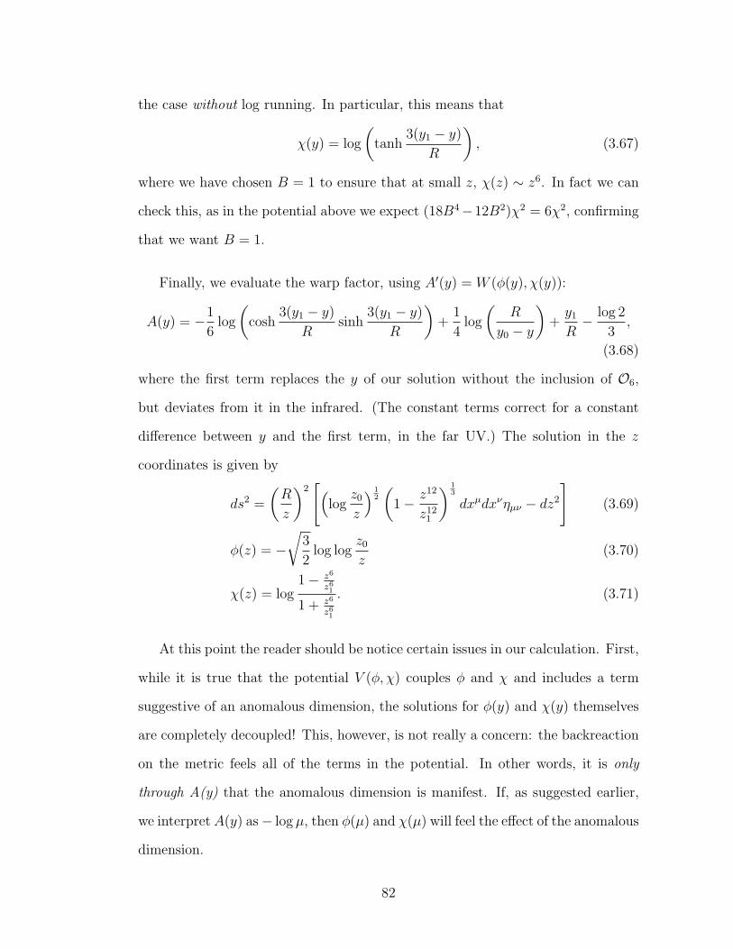
the case without log running. In particular, this means that

χ(y) = log

(tanh

3(y1 − y)

R

), (3.67)

where we have chosen B = 1 to ensure that at small z, χ(z) ∼ z6. In fact we can

check this, as in the potential above we expect (18B4−12B2)χ2 = 6χ2, confirming

that we want B = 1.

Finally, we evaluate the warp factor, using A′(y) = W (φ(y), χ(y)):

A(y) = −1

6log

(cosh

3(y1 − y)

Rsinh

3(y1 − y)

R

)+

1

4log

(R

y0 − y

)+y1

R− log 2

3,

(3.68)

where the first term replaces the y of our solution without the inclusion of O6,

but deviates from it in the infrared. (The constant terms correct for a constant

difference between y and the first term, in the far UV.) The solution in the z

coordinates is given by

ds2 =

(R

z

)2[(

logz0

z

) 12

(1− z12

z121

) 13

dxµdxνηµν − dz2

](3.69)

φ(z) = −√

3

2log log

z0

z(3.70)

χ(z) = log1− z6

z61

1 + z6

z61

. (3.71)

At this point the reader should be notice certain issues in our calculation. First,

while it is true that the potential V (φ, χ) couples φ and χ and includes a term

suggestive of an anomalous dimension, the solutions for φ(y) and χ(y) themselves

are completely decoupled! This, however, is not really a concern: the backreaction

on the metric feels all of the terms in the potential. In other words, it is only

through A(y) that the anomalous dimension is manifest. If, as suggested earlier,

we interpret A(y) as− log µ, then φ(µ) and χ(µ) will feel the effect of the anomalous

dimension.

82

Another issue is that we have sacrificed precise agreement with perturbation

theory for the sake of having a simple, solvable example. We have arranged to

get the logarithmic running of αs, the proper scaling dimension of O6, and an

anomalous dimension term for O6 which is proportional to αs. On the other hand,

we have not been careful to match the coefficient in this anomalous dimension.

Details of the OPE and anomalous dimension for this operator can be found in

Reference [86]; eventually one would want a model that matches them. Of course,

in our discussion of αs(µ) earlier, we also had a second β function coefficient that

did not match. This suggests that our analytically solvable superpotentials, while

useful for a preliminary study, probably need to be replaced by a more detailed nu-

merical study based on a more careful matching of the holographic renormalization

group. Nonetheless, the disagreement appears only at higher orders of perturba-

tion theory, and we can already use our preliminary superpotential W (φ, χ) to get

some sense of the stability of spectra calculated in holographic models.

3.5.1 Gubser’s Criterion: Constraining z1/z0

In our solution, φ(z) blows up at z = z0 while χ(z) blows up at z = z1. The space

will shut off at whichever of these is encountered first. Intuitively it is clear that if

the dimension 6 condensate is to make a relatively small correction to the results

we have already obtained using only the dimension 4 condensate, we should have

z1 > z0, so that χ(z) remains finite over the interval where the solution is defined.

In fact there is a conjecture that will enforce this condition. Namely, Gubser in

Reference [87] has proposed that curvature singularities of the type arising in the

geometries we are considering are allowed only if the scalar potential is bounded

above when evaluated on the solution. By “allowed”, one should understand that

83

in these cases one expects the singularity to be resolved in the full string theory; ge-

ometries violating the criterion are somehow pathological. The conjecture is based

on some nontrivial consistency checks involving considerations of finite tempera-

ture and examples from the Coulomb branch in AdS/CFT, but it is not proven. In

any case we will assume for now that it holds for any geometry that can be properly

thought of as dual to a field theory. It is clear that our original solution involving

only φ satisfies the criterion: in that case we had V (φ) = −12− 6e√

2/3φ < 0.

The case with χ is more subtle. We have

V (φ(z), χ(z)) = −15− 6e√

23φ(z) coshχ(z) + cosh(2χ(z))

= −6

(1−

(zz1

)24)

(1−

(zz1

)12)2

log z0

z

− 121− 4

(zz1

)12

+(

zz1

)24

(1−

(zz1

)12)2 (3.72)

Clearly as z1 → ∞ we recover the previous solution and Gubser’s criterion is

satisfied. On the other hand, as soon as z1 < z0, V begins to attain large positive

values as z → z1. The reason is simple: the function 1− 4x12 + x24 has a zero at

x ≈ 0.9, so the second term above can attain positive values when z ≈ z1, and the

denominator will attain arbitrarily small values provided the singularity at z1 is

reached (i.e. z1 < z0). In fact large positive values of V are attained if and only if

z1 < z0.

In short, Gubser’s criterion limits us to precisely those solutions which can be

viewed in some sense as a perturbation of our existing solution.

84

3.5.2 Condensates

To calculate the condensate we need to again evaluate the classical action for the

solution, which in our case is given by

S =1

2κ2

∫ z0

ε

(R

z

)6

logz0

z

(1− z12

z121

) 23[−1

2(φ′2 + χ′2)

( zR

)2

+12 + 6e√

23φ coshχ+ 6 sinh2 χ−R

]. (3.73)

Again dropping the UV divergent terms we find either using (3.46) or by direct

integration

S =1

2κ2

(z121 − z12

0 )23

2z40z

81

(3.74)

Following the steps for calculating the condensate for the single field case we find

that the modified condensate is given by

⟨1

4TrF 2

⟩=

(N2c − 1)

3π2

24π2

11Nc

z0d

dz0

[(z12

1 − z120 )

23

4z40z

81

]≈ (1.19z−1

0 )41 +

(z0

z1

)12

[1−

(z0

z1

)12] 1

3

.

(3.75)

One can see that for z1 > z0 (as expected from the criterion of Sec. 3.5.1) this

condensate is very insensitive to the actual value of z1. In order to actually fix z1

one would have to calculate the second condensate 〈TrF 3〉 and compare it to the

lattice results. However, there are no reliable lattice estimates for this condensate

available.

It is also plausible that if we account more properly for the anomalous dimension

of TrF 3 and for matching of perturbative corrections to the OPE, we will be able

to select a solution without this ambiguity. However, constructing such a solution

appears to require a numerical study, which we will leave for future work.

85

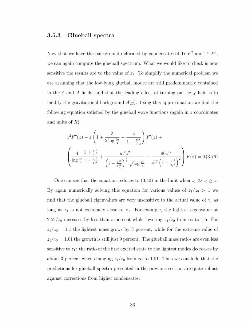
3.5.3 Glueball spectra

Now that we have the background deformed by condensates of Tr F 2 and Tr F 3,

we can again compute the glueball spectrum. What we would like to check is how

sensitive the results are to the value of z1. To simplify the numerical problem we

are assuming that the low-lying glueball modes are still predominantly contained

in the φ and A fields, and that the leading effect of turning on the χ field is to

modify the gravitational background A(y). Using this approximation we find the

following equation satisfied by the glueball wave functions (again in z coordinates

and units of R):

z2F ′′(z)− z

(1 +

5

2 log z0

z

− 4

1− z121

z12

)F ′(z) + 4

log z0

z

1 + z12

z121

1− z12

z121

+m2z2(

1− z12

z121

) 13 √

log z0

z

− 96z12

z121

(1− z12

z121

)2

F (z) = 0.(3.76)

One can see that the equation reduces to (3.40) in the limit when z1 � z0 ≥ z.

By again numerically solving this equation for various values of z1/z0 > 1 we

find that the glueball eigenvalues are very insensitive to the actual value of z1 as

long as z1 is not extremely close to z0. For example, the lightest eigenvalue at

2.52/z0 increases by less than a percent while lowering z1/z0 from ∞ to 1.5. For

z1/z0 = 1.1 the lightest mass grows by 3 percent, while for the extreme value of

z1/z0 = 1.01 the growth is still just 9 percent. The glueball mass ratios are even less

sensitive to z1: the ratio of the first excited state to the lightest modes decreases by

about 3 percent when changing z1/z0 from ∞ to 1.01. Thus we conclude that the

predictions for glueball spectra presented in the previous section are quite robust

against corrections from higher condensates.

86

3.6 Linearly confining backgrounds?

One of the most problematic aspects of holographic QCD is the deep IR physics:

one expects Regge behavior from states of high angular momentum, and a linear

confining potential. The solutions presented in this paper show many qualitative

and quantitative similarities with ordinary QCD. However, they do not properly

describe the highly excited glueball states. Since there is a singularity at a finite

distance, the characteristic mass relation for highly excited glueballs will be that of

ordinary KK theories (in this respect the theory is similar to the models with an IR

brane put in by hand) m2n ∼ n2/z2

0 , instead of the expected Regge-type behavior

m2n ∼ n/z2

0 [65]. Experimental and lattice data suggest that linear confinement

effects persist further into the UV than one might expect, and already the light

resonances observed in QCD seem to fall on Regge trajectories. Regge physics

arises naturally from strings; in our approach, the more massive excitations of the

5D string correspond to high-dimension operators on the field theory side. To

describe linear confinement and Regge physics accurately, then, it is conceivable

that one must take into account the effects of a large number of operators. Thus

we are led to seek alternative, but still well-motivated, approaches to the deep IR

physics. One approach is simply to demand that the 5D fields have IR profiles that

provide the desired behavior, as in Reference[66]. However, one would like to have

a dynamical model of this effect. Here we first check that the backgrounds used in

sections 4-5 do not reproduce such IR profiles. However in [66] it was suggested

suggested that tachyon condensation might provide the appropriate dynamics. We

provide a simple modification of our model possibly substantiating this idea, and

speculate on its relation to known gauge theory effects: namely, UV renormalons

and other 1/Q2 corrections as discussed by Zakharov and others [90].

87

3.6.1 No linear confinement in the dilaton-graviton system

We first try to find other solutions that would not have a singularity at a finite

distance, even for the action (3.28) since until now we have found only a particular

solution for (3.28) using a superpotential. However in general there should be an

infinite family of superpotentials giving the same potential. For the general case

we cannot find the other solutions analytically for all values of the coordinates.

We can, however, attempt to solve the equations of motion analytically close to

the UV boundary. A similar approach has been taken in ref.[88] for a type 0 string

theory containing a tachyon, considered to be dual to non-supersymmetric SU(N)

Yang-Mills with six adjoint scalars. In our case we will not consider a tachyon

for now, as we consider 5D fields to be in one-to-one correspondence with gauge

invariant operators in the 4D dual. There are some orientifold theories in type 0

that have no bulk tachyon, so our approach is not a priori meaningless.

In order to avoid the change of variables needed to achieve an asymptotically

AdS metric (plus power corrections), we solve the equations beginning from the

explicitly conformally flat parametrization of the metric,

ds2 = e−2A(z)(ηµνdx

µdxν − dz2). (3.77)

Then for the Einstein equations and the equation of motion for φ we find (using ′

to denote derivatives with respect to z):

φ′′(z)− 3A′(z)φ′(z)− e−2A(z)∂V (φ)/∂φ = 0, (3.78)

6A′(z)2 − (1/2)φ′(z)2 + e−2A(z)V (φ) = 0, (3.79)

3A′(z)2 − 3A′′(z) + (1/2)φ′(z)2 + e−2A(z)V (φ) = 0. (3.80)

We again use the same potential V (φ) = −6e√

2/3φ(z) − 6 (but no longer assume

the simple expression for the superpotential), and solve the equations in the UV

88

to obtain

φ(z) =

√3

2

(− log log

1

z+

3

4

log log 1z

log 1z

+γ

log 1z

+ · · ·), (3.81)

A(z) = log1

z+

1

2 log 1z

− 3

8

log log 1z(

log 1z

)2 +γ2

+ 3348(

log 1z

)2 + · · · . (3.82)

The omitted terms are those which are smaller as z → 0, i.e. power corrections

in z or higher powers in (− log z)−1. Here γ is a parameter that is undetermined

by the UV equations of motion, just as in the solution of ref.[88]. Further, we find

that if we add small perturbations to exp(√

2/3φ) and to A(z), an O(z4) power

correction to the former is allowed while only constant corrections to the latter

are allowed. It is reassuring that we find a power correction suitable for the gluon

condensate. Ref.[88] found also a correction of order z2 and interpreted it as a UV

renormalon2 (whereas the power correction we have considered may be thought

of as an IR renormalon). The tachyon was crucial to the appearance of the UV

renormalon term, which might have interesting implications.

In order to find a linearly confining solution, we would need to connect these

UV solutions to solutions in the z → ∞ IR region, which would also give linear

confinement. Suppose we then search for a solution that is valid at large z. In

the case that there is no cosmological constant, there is a linear dilaton solution;

this is clear since our equations are those for a noncritical string. The linear

dilaton persists in the presence of a cosmological constant as a solution at large

z; the equations are satisfied up to terms exponentially small at large z by a

linear dilaton on flat 5D space. Such a linear dilaton background does not give a

confining solution. Furthermore, one can check that no other power-law growth in

z is allowed. In particular, the z2 behavior as in Ref. [66] is not a solution to our

equations of motion. Thus we conclude that none of the solutions of the action

2For a review of the physics of the UV renormalon, see Ref. [89].

89

(3.28) will result in a linearly confining background.

3.6.2 Linear confinement from the tachyon-dilaton-

graviton system?

Although we do not understand how to systematically approach the study of UV

renormalon corrections, it is at least superficially plausible that they are associated

with a closed string tachyon. This is a natural scenario to consider, since the UV

renormalon is associated with Q−2 corrections. Ref. [88] found such an association

in a concrete string theory model. The study of such corrections has been discussed

in great detail in the QCD literature, which links the idea of the UV renormalon

to the quadratic corrections associated with the QCD string tension and with a

hypothetical nonperturbative tachyonic gluon mass, as well as with monopoles and

vortices; we can only refer to a small sample of that literature [90]. Holographically,

effects associated with dimension 2 corrections would appear to be associated with

tachyonic physics. Interestingly, it has been proposed that the UV renormalon is

associated with a nonvanishing value of 〈A2〉min where the minimization is over

gauge choices [91]. Such a dimension 2 condensate could plausibly be associated

holographically to a closed string tachyon (one that saturates the Breitenlohner-

Freedman bound [92]), though it does contradict the picture of holographic fields

as being associated to gauge-invariant, local operators in the field theory. The

minimum value of the A2 condensate can be expressed in terms of nonlocal, gauge-

invariant operators, beginning with Fµν(D2)−1F µν [93]. The nonlocality of this

operator is perhaps suggestive of the long-distance, stringy effects of the flux tube

needed to describe excited hadrons.

90

All of these hints of the importance of Q−2 corrections suggest that we take the

idea of a closed string tachyon seriously, despite the lack of a gauge-invariant local

operator for it to match to. Perhaps this indicates that certain 5D corrections can

somehow be “resummed” into the effects of a tachyonic field. The linear confining

potential of QCD has been suggested to relate to an exp cz2 background in 5D [66].

We would like to have a dynamical solution incorporating both asymptotic freedom

in the UV and linear confinement in the IR. We have observed that the cosmological

constant does not destroy the existence of a linear dilaton solution at large z (up to

small corrections). This suggests that if we have a theory with a quadratic tachyon

profile at zero cosmological constant, such a solution may persist in the presence

of a cosmological constant.

The action of the bosonic noncritical string theory including the leading α′ cor-

rections, using a sigma model approach, is (after transforming to Einstein frame),

according to [94]:

1

2κ2

∫d5x√g

[e

43Φ 4

α′(λ− 1)− 2R+

8

3(∂Φ)2 + e−t

(4

α′(1 + t− 1

2λ)e

43Φ +R

−4

3(∂Φ)2 − 4

3∂Φ∂t+ (∂t)2

)]. (3.83)

To this action we are adding a cosmological constant (which we assume could come

from a 5-form flux) and adjust the parameters such that with the t→ 0 substitution

we recover the action considered in the previous section. The resulting action is:

1

2κ2

∫d5x√g

[e

43Φ 12

R2

λ− 1

λ+

12

R2− 2R+

8

3(∂Φ)2 + e−t

(12

R2λ(1 + t− 1

2λ)e

43Φ +R

−4

3(∂Φ)2 − 4

3∂Φ∂t+ (∂t)2

)]. (3.84)

The resulting equations of motion for the metric ansatz ds2 = e2A(z)(dx2 − dz2)

91

are:

4

3e2Ae

43Φ 12

R2λ(λ− 1) +

16

3(3A′Φ′ + Φ′′) + e−t

(e

43Φ+2A 12

R2

1

λ(1 + t− 1

2λ)

4

3+

8

3t′Φ′

−8A′Φ′ − 8

3Φ′′ +

4

3t′2 − 4A′t′

)= 0 (3.85)

12

R2λe

43Φ+2A(

λ

2− t)− 12A′2 − 8A′′ − 4

3Φ′2 − t′2 − 4A′Φ′ − 4

3Φ′′ + 2t′′ + 6A′t′ = 0

(3.86)

−6A′2(2− e−t) +6

R2e2A(1 +

1

λe

43Φ(λ− 1 + e−t(1− λ

2+ t)) + Φ′2(

2

3− 4

3e−t) +

1

2e−t(−4

3Φ′t′ + t′2) = 0. (3.87)

Here λ = (26 − D)/3 = 21/3. One can show that for large z the leading order

solution to these equations is given by

Φ → Φ0, A→ A0, t→ −3

λe2A0+ 4

3Φ0z2 +

1

2(λ− 2). (3.88)

In order to serve our purposes there must be a solution interpolating between

logarithmic running on AdS in the UV and the above confining background (with

flat space and constant dilaton) in the IR. It would be interesting to numerically

study these equations, as well as similar systems in the type 0 string. The IR

solution above has the property that the e−t terms are growing at large z, whereas

the proposed background in Ref. [66] has an exponential shutoff of the metric,

which is not a solution of the above equations. However, the sign does not appear

to affect the existence of Regge physics. Regardless, we intend these remarks not

as a definitive statement, but as a provocative hint that further studies of tachyon

dynamics could be useful for understanding QCD.

92

3.7 Conclusions and Outlook

In this paper we have clarified a number of aspects of AdS/QCD, and sketched

a concrete program for computing in the holographic model and estimating asso-

ciated errors. We have also explained that deep IR physics, associated with high

radial excitations or large angular momentum, is troublesome in this framework.

The underlying reason is that the OPE does not reproduce the quadratic correc-

tions associated with this physics. We have suggested that a closed string tachyon

can reproduce much of the underlying dynamics, but at this point that is a toy

model and it is not clear how to systematically apply the idea to computations.

Our results suggest a number of directions for new work. One obvious task

is to extend these results to theories with flavor. This should be straightforward,

although there are potential numerical difficulties. It would be particularly in-

teresting to see if one can obtain results for mixing of glueballs with qq mesons

without large associated uncertainties.

Another direction is to make more explicit the connection between the renor-

malization group and the holographic dual. The 5D action has an interpretation

as the 4D generating functional W [J ], whereas some numerical attempts involving

truncations of exact RGEs have focused on computing the Legendre transform

of this quantity, Γ[φ]. There are subtle issues of nonperturbative gauge-invariant

regulators that must be considered in such studies, but it is conceivable that such

existing work could be reinterpreted as a computation of background profiles for

various fields, about which we could then compute the spectrum of excitations and

couplings with the usual 5D techniques. We hope to clarify this relationship in a

future paper. It is also interesting in this context to think about how the holo-

graphic renormalization group might relate to the “analytic perturbation theory”

93

framework.

Finally, the intricate story relating 1/q2 corrections, UV renormalons, vortices,

linear confinement, and the closed string tachyon is very interesting and still rather

poorly understood. A better understanding of these quantities and their relation-

ships could elucidate the confining dynamics of QCD, and also shed light on closed

string tachyon condensation in general (with possible applications to cosmology).

94

Chapter 4

The S-parameter in Holographic

Technicolor Models

4.1 Introduction

One of the outstanding problems in particle physics is to understand the mech-

anism of electroweak symmetry breaking. Broadly speaking, models of natural

electroweak symmetry breaking rely either on supersymmetry or on new strong

dynamics at some scale near the electroweak scale. However, it has long been

appreciated that if the new strong dynamics is QCD-like, it is in conflict with

precision tests of electroweak observables [6]. Of particular concern is the S pa-

rameter. It does not violate custodial symmetry; rather, it is directly sensitive to

the breaking of SU(2). As such, it is difficult to construct models that have S

consistent with data, without fine-tuning.

The search for a technicolor model consistent with data, then, must turn to

non-QCD-like dynamics. An example is “walking” [95], that is, approximately

conformal dynamics, which can arise in theories with extra flavors. It has been

argued that such nearly-conformal dynamics can give rise to a suppressed or even

negative contribution to the S parameter [96]. However, lacking nonperturbative

calculational tools, it is difficult to estimate S in a given technicolor theory.

In recent years, a different avenue of studying dynamical EWSB models has

opened up via the realization that extra dimensional models [2] may provide a

weakly coupled dual description to technicolor type theories [8]. The most studied

95

of these higgsless models [10, 11] is based on an AdS5 background in which the

Higgs is localized on the TeV brane and has a very large VEV, effectively decoupling

from the physics. Unitarization is accomplished by gauge KK modes, but this leads

to a tension: these KK modes cannot be too heavy or perturbative unitarity is

lost, but if they are too light then there are difficulties with electroweak precision:

in particular, S is large and positive [18]. In this argument the fermions are

assumed to be elementary in the 4D picture (dual to them being localized on the

Planck brane). A possible way out is to assume that the direct contribution of

the EWSB dynamics to the S-parameter are compensated by contributions to the

fermion-gauge boson vertices [97, 98]. In particular, there exists a scenario where

the fermions are partially composite in which S ≈ 0 [37, 38, 39], corresponding to

almost flat wave functions for the fermions along the extra dimension. The price of

this cancellation is a percent level tuning in the Lagrangian parameter determining

the shape of the fermion wave functions. Aside from the tuning itself, this is also

undesirable because it gives the model-builder very little freedom in addressing

flavor problems: the fermion profiles are almost completely fixed by consistency

with electroweak precision.

While Higgsless models are the closest extra-dimensional models to traditional

technicolor models, models with a light Higgs in the spectrum do not require

light gauge KK modes for unitarization and can be thought of as composite Higgs

models. Particularly appealing are those where the Higgs is a pseudo-Nambu-

Goldstone boson [53, 41, 99, 100]. In these models, the electroweak constraints are

less strong, simply because most of the new particles are heavy. They still have

a positive S, but it can be small enough to be consistent with data. Unlike the

Higgsless models where one is forced to delocalize the fermions, in these models

with a higher scale the fermions can be peaked near the UV brane so that flavor

96

issues can be addressed.

Recently, an interesting alternative direction to eliminating the S-parameter

constraint has been proposed in [101]. There it was argued, that by considering

holographic models of EWSB in more general backgrounds with non-trivial profiles

of a bulk Higgs field one could achieve S < 0. The aim of this paper is to investigate

the feasibility of this proposal. We will focus on the direct contribution of the

strong dynamics to S. In particular, we imagine that the SM fermions can be

almost completely elementary in the 4D dual picture, corresponding to them being

localized near the UV brane. In this case, a negative S would offer appealing new

prospects for model-building since such values of S are less constrained by data

than a positive value [102]. Unfortunately we find that the S > 0 quite generally,

and that backgrounds giving negative S appear to be pathological.

The outline of the paper is as follows. We first present a general plausibility

argument based purely on 4D considerations that one is unlikely to find models

where S < 0. This argument is independent from the rest of the paper, and the

readers interested in the holographic considerations may skip directly to section 4.3.

Here we first review the formalism to calculate the S parameter in quite general

models of EWSB using an extra dimension. We also extend the proof of S > 0

for BC breaking [18] in arbitrary metric to the case of arbitrary kinetic functions

or localized kinetic mixing terms. These proofs quite clearly show that no form of

boundary condition breaking will result in S < 0. However, one may hope that

(as argued in [101]) one can significantly modify this result by using a bulk Higgs

with a profile peaked towards the IR brane to break the electroweak symmetry.

Thus, in the crucial section 4.4, we show that S > 0 for models with bulk breaking

from a scalar VEV as well. Since the gauge boson mass is the lowest dimensional

97

operator sensitive to EWSB one would expect that this is already sufficient to cover

all interesting possibilities. However, since the Higgs VEV can be very strongly

peaked, one may wonder if other (higher dimensional) operators could become

important as well. In particular, the kinetic mixing operator of L,R after Higgs

VEV insertion would be a direct contribution to S. To study the effect of this

operator in section 4.5, it is shown that the bulk mass term for axial field can be

converted to kinetic functions as well, making a unified treatment of the effects of

bulk mass terms and the effects of the kinetic mixing from the higher-dimensional

operator possible. Although we do not have a general proof that S > 0 including

the effects of the bulk kinetic mixing for a general metric and Higgs profile, in

section 4.5.2 we present a detailed scan for AdS metric and for power-law Higgs

vev profile using the technique of the previous section for arbitrary kinetic mixings.

We find S > 0 once we require that the higher-dimensional operator is of NDA

size, and that the theory is ghost-free. We summarize and conclude in section 4.6.

4.2 A plausibility argument for S > 0

In this section we define S and sketch a brief argument for its positivity in a

general technicolor model. The reader mainly interested in the extra-dimensional

constructions can skip this section since it is independent from the rest of the paper.

However, we think it is worthwhile to try to understand why one might expect

S > 0 on simple physical grounds. The only assumptions we will make are that

we have some strongly coupled theory that spontaneously breaks SU(2)L×SU(2)R

down to SU(2)V , and that at high energies the symmetry is restored. With these

assumptions, S > 0 is plausible. S < 0 would require more complicated dynamics,

98

and might well be impossible, though we cannot prove it.1

Consider a strongly-interacting theory with SU(2) vector current V aµ and SU(2)

axial vector current Aaµ. We define (where J represents V or A):

i

∫d4x e−iq·x ⟨Ja

µ(x)J bµ(0)

⟩= δab

(qµqν − gµνq

2)ΠJ(q2). (4.1)

We further define the left-right correlator, denoted simply Π(q2), as ΠV (q2) −

ΠA(q2). In the usual way, ΠV and ΠA are related to positive spectral functions

ρV (s) and ρA(s). Namely, the Π functions are analytic functions of q2 everywhere

in the complex plane except for Minkowskian momenta, where poles and branch

points can appear corresponding to physical particles and multi-particle thresholds.

The discontinuity across the singularities on the q2 > 0 axis is given by a spectral

function. In particular, there is a dispersion relation

ΠV (q2) =1

π

∫ ∞

0

dsρV (s)

s− q2 + iε, (4.2)

with ρV (s) > 0, and similarly for ΠA.

Chiral symmetry breaking establishes that ρA(s) contains a term πf 2πδ(s). This

is the massless particle pole corresponding to the Goldstone of the spontaneously

broken SU(2) axial flavor symmetry. (The corresponding pions, of course, are

eaten once we couple the theory to the Standard Model, becoming the longitudinal

components of theW± and Z bosons. However, for now we consider the technicolor

sector decoupled from the Standard Model.) We define a subtracted correlator by

Π(q2) = Π(q2)+ f2π

q2 and a subtracted spectral function by ρA(s) = ρA(s)−πf 2πδ(s).

Now, the S parameter is given by

S = 4πΠ(0) = 4

∫ ∞

0

ds1

s(ρV (s)− ρA(s)) . (4.3)

1For a related discussion of the calculation of S in strongly coupled theories, see [103].

99

Interestingly, there are multiple well-established nonperturbative facts about ΠV −

ΠA, but none are sufficient to prove that S > 0. There are the famous Weinberg

sum rules [105]

1

π

∫ ∞

0

ds (ρV (s)− ρA(s)) = f 2π , (4.4)

1

π

∫ ∞

0

ds s (ρV (s)− ρA(s)) = 0. (4.5)

Further, Witten proved that Σ(Q2) = −Q2(ΠV (Q2)−ΠA(Q2)) > 0 for all Euclidean

momenta Q2 = −q2 > 0 [106]. However, the positivity of S seems to be more

difficult to prove.

Our plausibility argument is based on the function Σ(Q2). In terms of this

function, S = −4πΣ′(0). (Note that in Σ(Q2) the 1/Q2 pole from ΠA is multiplied

by Q2, yielding a constant that does not contribute when we take the derivative.

Thus when considering Σ we do not need to subtract the pion pole as we did in

Π.) We also know that Σ(0) = f 2π > 0. On the other hand, we know something

else that is very general about theories that spontaneously break chiral symmetry:

at very large Euclidean Q2, we should see symmetry restoration. More specifically,

we expect behavior like

Σ(Q2) → O(

1

Q2k

), (4.6)

where k is associated with the dimension of some operator that serves as an order

parameter for the symmetry breaking. (In some 5D models the decrease of ΠA−ΠV

will actually be faster, e.g. in Higgsless models one has exponential decrease.)

While we are most familiar with this from the OPE of QCD, it should be very

general. If a theory did not have this property and ΠV and ΠA differed significantly

in the UV, we would not view it as a spontaneously broken symmetry, but as an

explicitly broken one. Now, in this context, positivity of S is just the statement

100

that, because Σ(Q2) begins at a positive value and eventually becomes very small,

the smoothest behavior one can imagine is that it simply decreases monotonically,

and in particular, that Σ′(0) < 0 so that S > 0.2 The alternative would be that the

chiral symmetry breaking effects push Σ(Q2) in different directions over different

ranges of Q2. We have not proved that this is impossible in arbitrary theories,

but it seems plausible that the simpler case is true, namely that chiral symmetry

restoration always acts to decrease Σ(Q2) as we move to larger Q2. Indeed, we

will show below that in a wide variety of perturbative holographic theories S is

positive.

4.3 Boundary-effective-action approach to oblique correc-

tions. Simple cases with boundary breaking

In this section we review the existing results and calculational methods for the elec-

troweak precision observables (and in particular the S-parameter) in holographic

models of electroweak symmetry breaking. There are two equivalent formalisms for

calculating these parameters. One is using the on-shell wave function of the W/Z

bosons [51, 22], and the electroweak observables are calculated from integrals over

the extra dimension involving these wave functions. The advantage of this method

is that since it uses the physical wave functions it is easier to find connections to

the Z and the KK mass scales. The alternative formalism proposed by Barbieri,

Pomarol and Rattazzi [18] (and later extended in [24] to include observables off

the Z-pole) uses the method of the boundary effective action [42], and involves

off-shell wave functions of the boundary fields extended into the bulk. This latter

2For a related discussion of the behaviour of Σ(Q2)

in the case of large-Nc QCD, see [104].

101

method leads more directly to a general expression of the electroweak parameters,

so we will be applying this method throughout this paper. Below we will review

the basic expressions from [18].

A theory of electroweak symmetry breaking with custodial symmetry has an

SU(2)L× SU(2)R global symmetry, of which the SU(2)L×U(1)Y subgroup is gauged

(since the S-parameter is unaffected by the extra B −L factor we will ignore it in

our discussion). At low energies, the global symmetry is broken to SU(2)D. In the

holographic picture of [18] the elementary SU(2)×U(1) gauge fields are extended

into the bulk of the extra dimension. The bulk wave functions are determined

by solving the bulk EOM’s as a function of the boundary fields, and the effective

action is just the bulk action in terms of the boundary fields.

In order to first keep the discussion as general as possible, we use an arbitrary

background metric over an extra dimension parametrized by 0 < y < 1, where

y = 0 corresponds to the UV boundary, and y = 1 to the IR boundary. In order

to simplify the bulk equations of motion it is preferential to use the coordinates in

which the metric takes the form 3 [18]

ds2 = e2σdx2 + e4σdy2 . (4.7)

The bulk action for the gauge fields is given by

S = − 1

4g25

∫d5x√−g((FL

MN)2 + (FRMN)2

). (4.8)

The bulk equations of motion are given by

∂2yA

L,Rµ − p2e2σAL,R

µ = 0, (4.9)

or equivalently the same equations for the combinations Vµ, Aµ = (AµL±AµR)/√

2.

3In this paper, we use a (−+ . . .+) signature. 5D bulk indices are denoted by capital Latinindices while we use Greek letters for 4D spacetime indices. 5D indices will be raised and loweredusing the 5D metric while the 4D Minkowski metric is used for 4D indices.

102

We assume that the (light) SM fermions are effectively localized on the Planck

brane and that they carry their usual quantum numbers under SU(2)L × U(1)Y

that remains unbroken on the UV brane. The values of these fields on the UV brane

have therefore a standard couplings to fermion and they are the 4D interpolating

fields we want to compute an effective action for. This dictates the boundary

conditions we want to impose on the UV brane

AL aµ (p2, 0) = AL a

µ (p2), AR 3µ (p2, 0) = AR 3

µ (p2), AR 1,2µ (p2, 0) = 0. (4.10)

A1,2R are vanishing because they correspond to ungauged symmetry generators. The

solutions of the bulk equations of motion satisfying these UV BC’s take the form

Vµ(p2, y) = v(y, p2)Vµ(p2), Aµ(p2, y) = a(y, p2)Aµ(p2). (4.11)

where the interpolating functions v and a satisfy the bulk equations

∂2yf(y, p2)− p2e2σf(y, p2) = 0 (4.12)

and the UV BC’s

v(0, p2) = 1, a(0, p2) = 1. (4.13)

The effective action for the boundary fields reduces to a pure boundary term

since by integrating by parts the bulk action vanishes by the EOM’s:

Seff =1

2g25

∫d4x(Vµ∂yV

µ +Aµ∂yAµ)|y=0 =

1

2g25

∫d4p(V 2

µ ∂yv+ A2µ∂ya)|y=0 (4.14)

And we obtain the non-trivial vacuum polarizations for the boundary vector fields

ΣV (p2) = − 1

g25

∂yv(0, p2), ΣA(p2) = − 1

g25

∂ya(0, p2). (4.15)

The various oblique electroweak parameters are then obtained from the mo-

mentum expansion of the vacuum polarizations in the effective action,

Σ(p2) = Σ(0) + p2Σ′(0) +p4

2Σ′′(0) + . . . (4.16)

103

For example the S-parameter is given by

S = 16πΣ′3B(0) = 8π(Σ′

V (0)− Σ′A(0)). (4.17)

A similar momentum expansion can be performed on the interpolating functions

v and a: v(y, p2) = v(0)(y) + p2v(1)(y) + . . ., and similarly for a. The S-parameter

is then simply expressed as

S = −8π

g25

(∂yv(1) − ∂ya

(1))|y=0. (4.18)

The first general theorem was proved in [18]: for the case of boundary condition

breaking in a general metric, S ≥ 0. The proof uses the explicit calculation of the

functions v(n), a(n), n = 0, 1. First, the bulk equations (4.9) write

∂2yv

(0) = ∂2ya

(0) = 0, ∂2yv

(1) = e2σv(0), ∂2ya

(1) = e2σa(0). (4.19)

And the p2-expanded UV BC’s are

v(0) = a(0) = 1, v(1) = a(1) = 0 at y = 0 (4.20)

Finally, we need to specify the BC’s on the IR brane that correspond to the break-

ing SU(2)L×SU(2)R → SU(2)D

∂yVµ = 0, Aµ = 0, (4.21)

which translates into simple BC’s for the interpolating functions

∂yv(n) = a(n) = 0, n = 0, 1. (4.22)

The solution of these equations are v(0) = 1, a(0) = 1 − y, v(1) =∫ y

0dy′∫ y′

0dy′′e2σ(y′′) − y

∫ 1

0dy′e2σ(y′), a(1) =

∫ y

0dy′∫ y′

0dy′′e2σ(y′′)(1 − y′′) −

y∫ 1

0dy′∫ y′

0dy′′e2σ(y′′)(1− y′′). Consequently

S =8π

g25

(∫ 1

0

dye2σ(y)dy −∫ 1

0

dy

∫ y

0

dy′(1− y′)e2σ(y′)

)(4.23)

which is manifestly positive.

104

4.3.1 S > 0 for BC breaking with boundary kinetic mixing

The first simple generalization of the BC breaking model is to consider the same

model but with an additional localized kinetic mixing operator added on the TeV

brane (the effect of this operator has been studied in flat space in [18] and in AdS

space in [51, 22]). The localized Lagrangian is

− τ

4g25

∫d4x√−gV 2

µν . (4.24)

This contains only the kinetic term for the vector field since the axial gauge field

is set to zero by the BC breaking. In this case the BC at y = 1 for the vector field

is modified to ∂yVµ + τp2Vµ = 0. In terms of the wave functions expanded in small

momenta we get ∂yv(1) + τv(0) = 0. The only change in the solutions will be that

now v(1)′ = −τ −∫ 1

ye2σ(y′)dy′, resulting in

S =8π

g25

(∫ 1

0

e2σ(y)dy −∫ 1

0

dy

∫ y

0

(1− y′)e2σ(y′)dy′ + τ

)(4.25)

Thus as long as the localized kinetic term has the proper sign, the shift in the

S-parameter will be positive. If the sign is negative, there will be an instability in

the theory since fields localized very close to the TeV brane will feel a wrong sign

kinetic term. Thus we conclude that for the physically relevant case S remains

positive.

4.3.2 S > 0 for BC breaking with arbitrary kinetic func-

tions

The next simple extension of the BPR result is to consider the case when there is

an arbitrary y-dependent function in front of the bulk gauge kinetic terms. These

105

could be interpreted as effects of gluon condensates modifying the kinetic terms in

the IR. In this case the action is

S = − 1

4g25

∫d5x√−g(φ2

L(y)(FLMN)2 + φ2

R(y)(FRMN)2

). (4.26)

φL,R(y) are arbitrary profiles for the gauge kinetic terms, which are assumed to

be the consequence of some bulk scalar field coupling to the gauge fields. Note

that this case also covers the situation when the gauge couplings are constant but

g5L 6= g5R. The only assumption we are making is that the gauge kinetic functions

for L,R are strictly positive. Otherwise one could create a wave packet localized

around the region where the kinetic term is negative which would have ghost-like

behavior.

Due to the y-dependent kinetic terms it is not very useful to go into the V,A

basis. Instead we will directly solve the bulk equations in the original basis. The

bulk equations of motion for L,R are given by

∂y(φ2L,R∂yA

L,Rµ )− p2e2σφ2

L,RAL,Rµ = 0 (4.27)

To find the boundary effective action needed to evaluate the S-parameter we per-

form the following decomposition:

ALµ(p2, y) = Lµ(p2)LL(y, p2) + Rµ(p2)LR(y, p2),

ARµ (p2, y) = Lµ(p2)RL(y, p2) + Rµ(p2)RR(y, p2). (4.28)

Here L, R are the boundary fields, and the fact that we have four wave functions

expresses the fact that these fields will be mixing due to the BC’s on the IR

brane. The UV BC’s (4.10) and the IR BC’s (4.21) can be written in terms of the

106

interpolating functions as

(UV) LL(0, p2) = 1, LR(0, p2) = 0, RL(0, p2) = 0, RR(0, p2) = 1. (4.29)

(IR)LL(1, p2) = RL(1, p2), LR(1, p2) = RR(1, p2),

∂y(LL(1, p2) +RL(1, p2)) = 0, ∂y(LR(1, p2) +RR(1, p2)) = 0.

(4.30)

The solution of these equations with the proper boundary conditions and for small

values of p2 is rather lengthy, but straightforward. The end result is that

S = −8π

g25

(φ2

L∂yL(1)R + φ2

R∂yR(1)L

)|y=0 = −8π

g25

(aLR+ aRL

), (4.31)

where the constants aRLare negative as their explicit expressions show. Therefore

S is positive.

4.4 S > 0 in models with bulk Higgs

Having shown than S > 0 for arbitrary metric and EWSB through BC’s, in this

section, we switch to considering breaking of electroweak symmetry by a bulk

scalar (Higgs) vev. We begin by neglecting the effects of kinetic mixing between

SU(2)L and SU(2)R fields coming from higher-dimensional operator in the 5D

theory, expecting that their effect, being suppressed by the 5D cut-off, is sub-

leading. We will return to a consideration of such kinetic mixing effects in the

following sections.

We will again use the metric (4.7) and the bulk action (4.8). Instead of BC

breaking we assume that EWSB is caused by a bulk Higgs which results in a

y-dependent profile for the axial mass term

−∫d5x√−g M

2(y)

2g25

A2M . (4.32)

107

Here M2 is a positive function of y corresponding to the background Higgs VEV.

The bulk equations of motion are:

(∂2y − p2e2σ)Vµ = 0, (∂2

y − p2e2σ −M2e4σ)Aµ = 0. (4.33)

On the IR brane, we want to impose regular Neumann BC’s that preserve the full

SU(2)L× SU(2)R gauge symmetry

(IR) ∂yVµ = 0, ∂yAµ = 0. (4.34)

As in the previous section, the BC’s on the UV brane just define the 4D interpo-

lating fields

(UV ) Vµ(p2, 0) = Vµ(p2), Aµ(p2, 0) = Aµ(p2). (4.35)

The solutions of the bulk equations of motion satisfying these BC’s take the form

Vµ(p2, y) = v(y, p2)Vµ(p2), Aµ(p2, y) = a(y, p2)Aµ(p2), (4.36)

where the interpolating functions v and a satisfy the bulk equations

∂2yv − p2e2σv = 0, ∂2

ya− p2e2σa−M2e4σa = 0. (4.37)

As before, these interpolating functions are expanded in powers of the momentum:

v(y, p2) = v(0)(y) + p2v(1)(y) + . . ., and similarly for a. The S-parameter is again

given by the same expression

S = −8π

g25

(∂yv(1) − ∂ya

(1))|y=0. (4.38)

We will not be able to find general solutions for a(1) and v(1) but we are going to

prove that ∂ya(1) > ∂yv

(1) on the UV brane, which is exactly what is needed to

conclude that S > 0.

First at the zeroth order in p2, the solution for v(0) is simply constant, v(0) = 1,

as before. And a(0) is the solution of

∂2ya

(0) = M2e4σa(0), a(0)|y=0 = 1, ∂ya(0)|y=1 = 0. (4.39)

108

In particular, since a(0) is positive at y = 0, this implies that a(0) remains positive:

if a(0) crosses through zero it must be decreasing, but then this equation shows

that the derivative will continue to decrease and can not become zero to satisfy

the other boundary condition. Now, since a(0) is positive, the equation of motion

shows that it is always concave up, and then the condition that its derivative is

zero at y = 1 shows that it is a decreasing function of y. In particular, we have for

all y

a(0)(y) ≤ v(0)(y), (4.40)

with equality only at y = 0.

Next consider the order p2 terms. What we wish to show is that ∂ya(1) > ∂yv

(1)

at the UV brane. First, let’s examine the behavior of v(1): the boundary conditions

are v(1)|y=0 = 0 and ∂yv(1)∣∣y=1

= 0. The equation of motion is:

∂2yv

(1) = e2σv(0) = e2σ > 0, (4.41)

so the derivative of v(1) must increase to reach zero at y = 1. Thus it is negative

everywhere except y = 1, and v(1) is a monotonically decreasing function of y.

Since v(1)|y=0 = 0, v(1) is strictly negative on (0, 1].

For the moment suppose that a(1) is also strictly negative; we will provide an

argument for this shortly. The equation of motion for a(1) is:

∂2ya

(1) = e2σa(0) +M2e4σa(1). (4.42)

Now, we know that a(0) < v(0), so under our assumption that a(1) < 0, this means

that

∂2ya

(1) ≤ ∂2yv

(1), (4.43)

with equality only at y = 0. But we also know that ∂yv(1)∂ya

(1) at y = 1, since they

both satisfy Neumann boundary conditions there. Since the derivative of ∂ya(1) is

109

strictly smaller over (0, 1], it must start out at a higher value in order to reach the

same boundary condition. Thus we have that

∂ya(1)∣∣y=0

> ∂yv(1)∣∣y=0

. (4.44)

The assumption that we made is that a(1) is strictly negative over the interval

(0, 1]. The reason is the following: suppose that a(1) becomes positive at some

value of y. Then as it passes through zero it is increasing. But then we also have

that ∂2ya

(1) = e2σa(0) +M2e4σa(1), and we have argued above that a(0) > 0. Thus

if a(1) is positive, ∂ya(1) remains positive, because ∂2

ya(1) cannot become negative.

In particular, it becomes impossible to reach the boundary condition ∂ya(1) = 0 at

y = 1. This fills the missing step in our argument and shows that the S parameter

must be positive.

In the rest of this section we show that the above proof for the positivity of

S remains essentially unchanged in the case when the bulk gauge couplings for

the SU(2)L and SU(2)R gauge groups are not equal. In this case (in order to

get diagonal bulk equations of motion) one needs to also introduce the canoni-

cally normalized gauge fields. We start with the generic action (metric factors are

understood when contracting indices)∫d5x√−g(− 1

4g25L

(FLMN)2 − 1

4g25R

(FRMN)2 − h2(z)

2(LM −RM)2

)(4.45)

To get to a canonically normalized diagonal basis we redefine the fields as

A =1√

g25L + g2

5R

(L−R) , V =1√

g25L + g2

5R

(g5R

g5L

L+g5L

g5R

R

). (4.46)

To get the boundary effective action, we write the fields V , A as

A(p2, z) =1√

g25L + g2

5R

(L(p2)− R(p2)

)a(p2, z) , (4.47)

V (p2, z) =1√

g25L + g2

5R

(g5R

g5L

L(p2) +g5L

g5R

R(p2)

)v(p2, z) . (4.48)

110

Here L, R are the boundary effective fields (with non-canonical normalization

exactly as in [18]), while the profiles a, v satisfy the same bulk equations and

boundary conditions as a, v in (4.33)–(4.35) with an appropriate replacement for

M2 = (g25L + g2

5R)h2. In terms of the canonically normalized fields, the boundary

effective action takes its usual form

Seff =1

2

∫d4x

(V ∂yV + A∂yA

)y=0

. (4.49)

And we deduce the vacuum polarization

ΣL3B(p2) = − 1

g25L + g2

5R

(∂yv(0, p2)− ∂ya(0, p

2)) (4.50)

And finally the S-parameter is equal to

S = − 16π

g25L + g2

5R

(∂yv(1) − ∂ya

(1)) (4.51)

Since a(n), v(n), n = 0, 1 satisfy the same equations (4.33)–(4.35) as before, the

proof goes through unchanged and we conclude that S > 0.

4.5 Bulk Higgs and bulk kinetic mixing

Next, we wish to consider the effects of kinetic mixing from higher-dimensional

operator in the bulk involving the Higgs VEV – as mentioned earlier, this kinetic

mixing is suppressed by the 5D cut-off and hence expected to be a sub-leading

effect. The reader might wonder why we neglected it before, but consider it now?

The point is that, although the leading effect on S parameter is positive as shown

above, it can be accidentally suppressed so that the formally sub-leading effects

from the bulk kinetic mixing can be important, in particular, such effects could

change the sign of S. Also, the Higgs VEV can be large, especially when the Higgs

111

profile is “narrow” such that it approximates BC breaking, and thus the large VEV

can (at least partially) compensate the suppression from the 5D cut-off. Of course,

in this limit of BC breaking (δ-function VEV), we know that kinetic mixing gives

S < 0 only if tachyons are present in the spectrum, but we would like to cover the

cases intermediate between BC breaking limit and a broad Higgs profile as well. In

this section, we develop a formalism, valid for arbitrary metric and Higgs profile,

to treat the bulk mass term and kinetic mixing on the same footing and then we

apply this technique to models in AdS space and with power-law profiles for Higgs

VEV in the next section.

We first present a discussion of how a profile for the y-dependent kinetic term

is equivalent to a bulk mass term. This is equivalent to the result [101] that a

bulk mass term can be equivalent to an effective metric. However, we find the

particular formulation that we present here to be more useful when we deal with

the case of a kinetic mixing. Assume we have a Lagrangian for a gauge field that

has a kinetic term

S = − 1

4g25

∫d5x√−gφ2(y)F 2

MN (4.52)

We work in the axial gauge A5 = 0 and again the metric takes the form (4.7). We

redefine the field to absorb the function φ: A(y) = φ(y)A(y). The action in terms

of the new field is then written as

S = − 1

4g25

∫d5x

(e2σF 2

µν + 2(∂yAµ)2 + 2φ′2

φ2A2

µ − 4(∂yAµ)Aµφ′

φ

)(4.53)

To see that the kinetic profile φ is equivalent to a mass term, we integrate by parts

in the second term

S = − 1

4g25

∫d5x√−g(F 2

MN + 2e−4σφ′′

φA2

µ

)+

1

2g25

∫d4x

φ′

φA2

µ

∣∣∣∣10

(4.54)

Thus we find that a bulk kinetic profile is equivalent to a bulk mass plus a boundary

112

mass. The bulk equations of motion for the new variables will then be

∂2yAµ − e2σp2Aµ −

φ′′

φAµ = 0, (4.55)

and the boundary conditions become

∂yAµ =φ′

φAµ. (4.56)

Note, that despite the bulk mass term, there is still a massless mode whose wave-

function is simply φ(z). Now we can reverse the argument and say that a bulk

mass must be equivalent to a profile for the bulk kinetic term plus a boundary

mass term.

4.5.1 The general case

We have seen above how to go between a bulk mass terms and a kinetic function.

We will now use this method to discuss the general case, when there is electroweak

symmetry breaking due to a bulk higgs with a sharply peaked profile toward the

IR brane, and the same Higgs introduces kinetic mixing between L and R fields

corresponding to a higher dimensional operator from the bulk. For now we as-

sume that the Higgs fields that breaks the electroweak symmetry is in a (2,2) of

SU(2)L×SU(2)R, with a VEV 〈H〉 = diag(h(z), h(z))/√

2.4 This Higgs profile h

has dimension 3/2. The 5D action is given by∫d5x√−g[− 1

4g25

[(FL

MN)2 + (FRMN)2

]− (DMH)†(DMH) +

α

Λ2Tr(FL

MNH†HFMN R)

].

(4.57)

Here α is a coefficient of O(1) and Λ is the 5D cutoff scale, given approximately by

Λ ∼ 24π3/g25. The kinetic mixing term just generates a shift in the kinetic terms

4An alternative possibility would be to consider a Higgs in the (3,3) representation ofSU(2)L×SU(2)R.

113

of the vector and axial vector field, and we will write the bulk mass term also as a

shift in the kinetic term for the axial vector field. The exact form of the translation

between the two forms is given by answering the question of how to redefine the

field with an action (note that m2 has a mass dimension 3)

− 1

4g25

∫d5x√−g(wF 2

MN +m22g25AµA

µ)

(4.58)

to a theory with only a modified kinetic term. The appropriate field redefinition

A = ρA will be canceling the mass term if ρ satisfies

∂y(w∂yρ) = m2g25e

4σρ, (4.59)

together with the boundary conditions ρ′|y=1 = 0, ρ|y=0 = 1. The relation between

the new and the old expression for w will be w = ρ2w. The action in this case is

given by

− 1

4g25

∫d5x√−gwF 2

MN +

∫d4x

w(0)

2g25

(∂yρ)A2|y=0 (4.60)

This last boundary term is actually irrelevant for the S-parameter: since it does

not contain a derivative on the field it can not get an explicit p-dependence so

it will not contribute to S, so for practical purposes this boundary term can be

neglected.

With this expression we now can calculate S. For this we need the modified

version of the formula from [101], where the breaking is not by boundary conditions

but by a bulk Higgs. The expression is

S =8π

g25

∫ 1

0

dye2σ(wV − wA). (4.61)

In our case wV = 1− αh2(y)2g25

Λ2 while wA = wAρ2 = (1 +

αh2(y)2g25

Λ2 )ρ2.

This formula also gives another way to see that S > 0 in the absence of kinetic

mixing, without analyzing the functions v(1) and a(1) from Section 4.4 in detail.

114

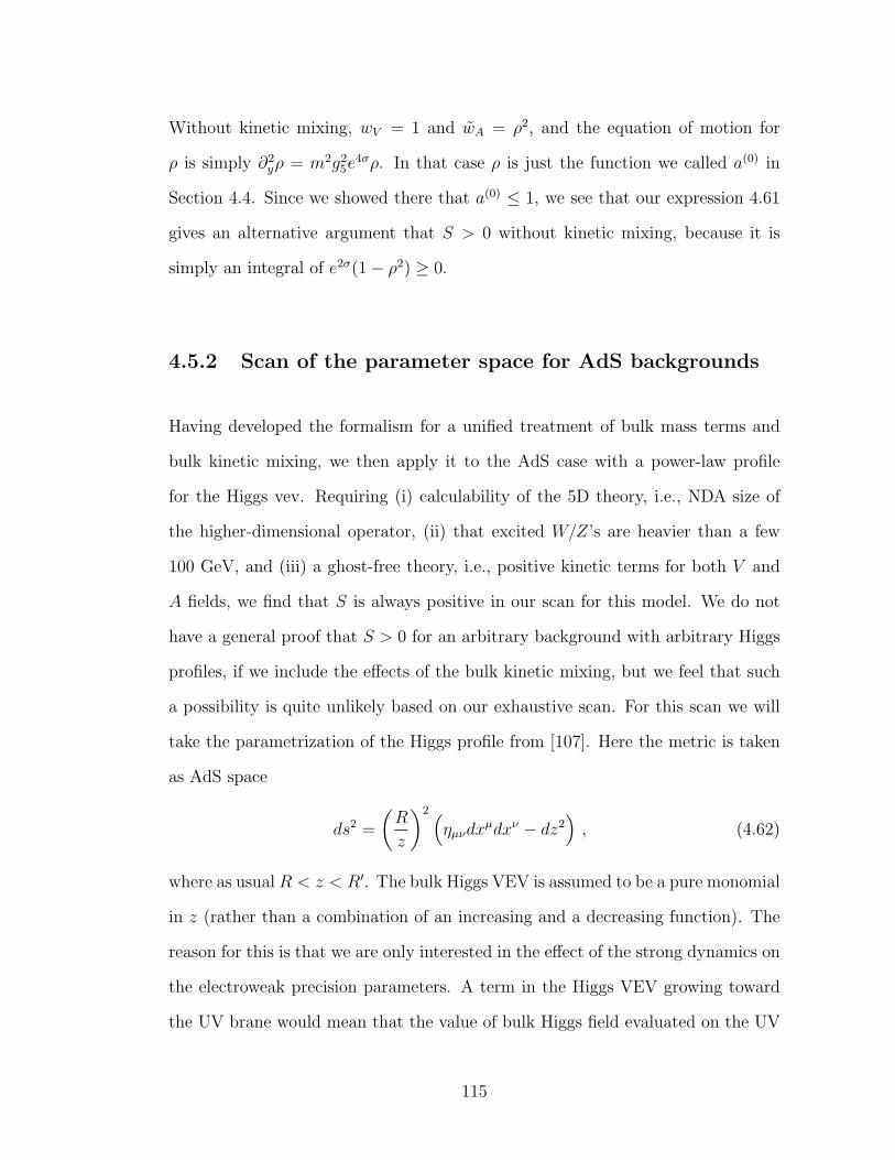
Without kinetic mixing, wV = 1 and wA = ρ2, and the equation of motion for

ρ is simply ∂2yρ = m2g2

5e4σρ. In that case ρ is just the function we called a(0) in

Section 4.4. Since we showed there that a(0) ≤ 1, we see that our expression 4.61

gives an alternative argument that S > 0 without kinetic mixing, because it is

simply an integral of e2σ(1− ρ2) ≥ 0.

4.5.2 Scan of the parameter space for AdS backgrounds

Having developed the formalism for a unified treatment of bulk mass terms and

bulk kinetic mixing, we then apply it to the AdS case with a power-law profile

for the Higgs vev. Requiring (i) calculability of the 5D theory, i.e., NDA size of

the higher-dimensional operator, (ii) that excited W/Z’s are heavier than a few

100 GeV, and (iii) a ghost-free theory, i.e., positive kinetic terms for both V and

A fields, we find that S is always positive in our scan for this model. We do not

have a general proof that S > 0 for an arbitrary background with arbitrary Higgs

profiles, if we include the effects of the bulk kinetic mixing, but we feel that such

a possibility is quite unlikely based on our exhaustive scan. For this scan we will

take the parametrization of the Higgs profile from [107]. Here the metric is taken

as AdS space

ds2 =

(R

z

)2 (ηµνdx

µdxν − dz2), (4.62)

where as usual R < z < R′. The bulk Higgs VEV is assumed to be a pure monomial

in z (rather than a combination of an increasing and a decreasing function). The

reason for this is that we are only interested in the effect of the strong dynamics on

the electroweak precision parameters. A term in the Higgs VEV growing toward

the UV brane would mean that the value of bulk Higgs field evaluated on the UV

115

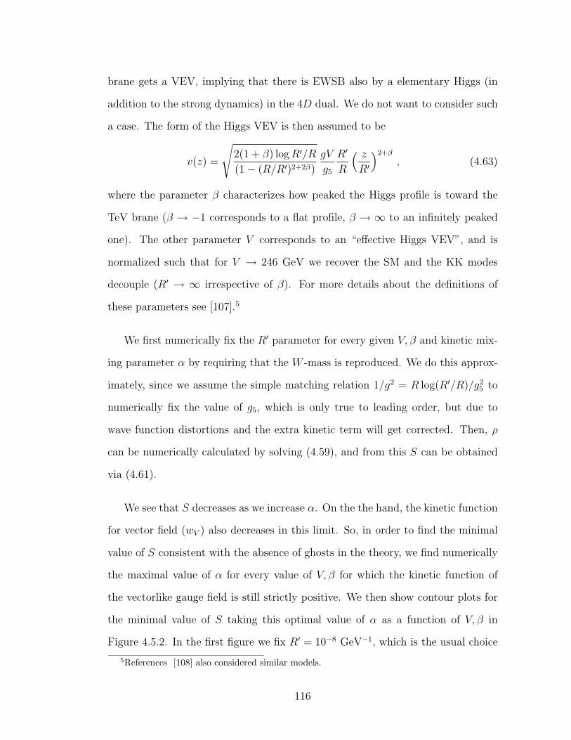
brane gets a VEV, implying that there is EWSB also by a elementary Higgs (in

addition to the strong dynamics) in the 4D dual. We do not want to consider such

a case. The form of the Higgs VEV is then assumed to be

v(z) =

√2(1 + β) logR′/R

(1− (R/R′)2+2β)

gV

g5

R′

R

( zR′

)2+β

, (4.63)

where the parameter β characterizes how peaked the Higgs profile is toward the

TeV brane (β → −1 corresponds to a flat profile, β → ∞ to an infinitely peaked

one). The other parameter V corresponds to an “effective Higgs VEV”, and is

normalized such that for V → 246 GeV we recover the SM and the KK modes

decouple (R′ → ∞ irrespective of β). For more details about the definitions of

these parameters see [107].5

We first numerically fix the R′ parameter for every given V, β and kinetic mix-

ing parameter α by requiring that the W -mass is reproduced. We do this approx-

imately, since we assume the simple matching relation 1/g2 = R log(R′/R)/g25 to

numerically fix the value of g5, which is only true to leading order, but due to

wave function distortions and the extra kinetic term will get corrected. Then, ρ

can be numerically calculated by solving (4.59), and from this S can be obtained

via (4.61).

We see that S decreases as we increase α. On the the hand, the kinetic function

for vector field (wV ) also decreases in this limit. So, in order to find the minimal

value of S consistent with the absence of ghosts in the theory, we find numerically

the maximal value of α for every value of V, β for which the kinetic function of

the vectorlike gauge field is still strictly positive. We then show contour plots for

the minimal value of S taking this optimal value of α as a function of V, β in

Figure 4.5.2. In the first figure we fix R′ = 10−8 GeV−1, which is the usual choice

5References [108] also considered similar models.

116

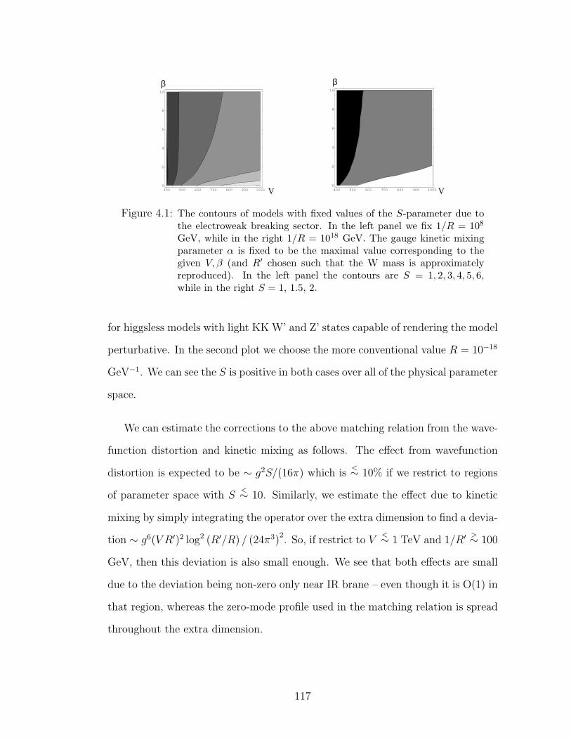
400 500 600 700 800 900 10000

2

4

6

8

10

V

β

400 500 600 700 800 900 10000

2

4

6

8

10

β

V

Figure 4.1: The contours of models with fixed values of the S-parameter due tothe electroweak breaking sector. In the left panel we fix 1/R = 108

GeV, while in the right 1/R = 1018 GeV. The gauge kinetic mixingparameter α is fixed to be the maximal value corresponding to thegiven V, β (and R′ chosen such that the W mass is approximatelyreproduced). In the left panel the contours are S = 1, 2, 3, 4, 5, 6,while in the right S = 1, 1.5, 2.

for higgsless models with light KK W’ and Z’ states capable of rendering the model

perturbative. In the second plot we choose the more conventional value R = 10−18

GeV−1. We can see the S is positive in both cases over all of the physical parameter

space.

We can estimate the corrections to the above matching relation from the wave-

function distortion and kinetic mixing as follows. The effect from wavefunction

distortion is expected to be ∼ g2S/(16π) which is<∼ 10% if we restrict to regions

of parameter space with S<∼ 10. Similarly, we estimate the effect due to kinetic

mixing by simply integrating the operator over the extra dimension to find a devia-

tion ∼ g6(V R′)2 log2 (R′/R) / (24π3)2. So, if restrict to V

<∼ 1 TeV and 1/R′>∼ 100

GeV, then this deviation is also small enough. We see that both effects are small

due to the deviation being non-zero only near IR brane – even though it is O(1) in

that region, whereas the zero-mode profile used in the matching relation is spread

throughout the extra dimension.

117

In order to be able to make a more general statement (and to check that the

neglected additional contributions to the gauge coupling matching from the wave

function distortions and the kinetic mixing indeed do not significantly our results)

we have performed an additional scan over AdS space models where we do not

require the correct physical value of MW to be reproduced. In this scan we then

treat R′ as an independent free parameter. In this case the correct matching

between g and g5 is no longer important for the sign of S, since at every place

where g5 appears it is multiplied by a parameter we are scanning over anyway (V

or α).

We performed the scan again for two values of the AdS curvature, 1/R = 108

and 1018 GeV. For the first case we find that if we restrict α < 10, 1/R′ < 1 TeV

there is no case with S < 0. However, there are some cases with S < 0 for α > 10,

although in these cases the theory is likely not predictive. For 1/R = 1018 GeV we

find that S < 0 only for V ∼ 250 GeV and β ∼ 0, 1/R′ ∼ 1 TeV. In this case α is

of order one (for example α ∼ 5). This case corresponds to the composite Higgs

model of [53, 41, 99] and it is quite plausible that at tree-level S < 0 if a large

kinetic mixing is added in the bulk. However in this case EWSB is mostly due to

a Higgs, albeit a composite particle of the strong dynamics, rather than directly by

the strong dynamics, so it does not contradict the expectation that when EWSB

is triggered directly via strong dynamics, then S is always large and positive.

However, it shows that any general proof for S > 0 purely based on analyzing the

properties of Eqs. (4.59)-(4.61) is doomed to failure, since these equations contain

physical situations where EWSB is not due to the strong dynamics but due to a

light Higgs in the spectrum. Thus any general proof likely needs to include more

physical requirements on the decoupling of the physical Higgs.

118

4.6 Conclusions

In this paper, we have studied the S parameter in holographic technicolor models,

focusing especially on its sign. The motivation for our study was as follows. An

alternative (to SUSY) solution to the Planck-weak hierarchy involves a strongly

interacting 4D sector spontaneously breaking the EW symmetry. One possibil-

ity for such a strong sector is a scaled-up version of QCD as in the traditional

technicolor models. In such models, we can use the QCD data to “calculate” S

finding S ∼ +O(1) which is ruled out by the electroweak precision data. Faced by

this constraint, the idea of a “walking” dynamics was proposed and it can be then

argued that S < 0 is possible which is much less constrained by the data, but the

S parameter cannot be calculated in such models. In short, there is a dearth of

calculable models of (non-supersymmetric) strong dynamics in 4D.

Based on the AdS/CFT duality, the conjecture is that certain kinds of theo-

ries of strong dynamics in 4D are dual to physics of extra dimensions. The idea

then is to construct models of EWSB in an extra dimension. Such constructions

allow more possibilities for model-building, at the same time maintaining calcu-

lability if the 5D strong coupling scale is larger than the compactification scale,

corresponding to large number of technicolors in the 4D dual.

It was already shown that S > 0 for boundary condition breaking for arbitrary

metric (a proof for S > 0 for the case of breaking by a localized Higgs vev was

recently studied in reference [109]). In this paper, we have extended the proof

for boundary condition breaking to the case of arbitrary bulk kinetic functions for

gauge fields or gauge kinetic mixing.

Throughout this paper, we have assumed that the (light) SM fermions are

119

effectively localized near the UV brane so that flavor violation due to higher-

dimensional operators in the 5D theory can be suppressed, at the same time al-

lowing for a solution to the flavor hierarchy. Such a localization of the light SM

fermions in the extra dimension is dual to SM fermions being “elementary”, i.e.,

not mixing with composites from the 4D strong sector. It is known that the S

parameter can be suppressed (or even switch sign) for a flat profile for SM fermions

(or near the TeV brane) – corresponding to mixing of elementary fermions with

composites in the 4D dual, but in such a scenario flavor issues could be a problem.

We also considered the case of bulk breaking of the EW symmetry motivated by

recent arguments that S < 0 is possible with different effective metrics for vector

and axial fields. For arbitrary metric and Higgs profile, we showed that S > 0

at leading order, i.e., neglecting effects from all higher-dimensional operators in

the 5D theory (especially bulk kinetic mixing), which are expected to be sub-

leading effects being suppressed by the cut-off of the 5D theory. We also note that

boundary mass terms can generally be mimicked to arbitrary precision by localized

contributions to the bulk scalar profile, so we do not expect a more general analysis

of boundary plus bulk breaking to find new features. Obtaining S < 0 must

then require either an unphysical Higgs profile or higher-dimensional operators to

contribute effects larger than NDA size, in which case we lose calculability of the

5D theory.

To make our case for S > 0 stronger, we then explored effects of the bulk kinetic

mixing between SU(2)L,R gauge fields due to Higgs vev coming from a higher-

dimensional operator in the 5D theory. Even though, as mentioned above, this

effect is expected to be sub-leading, it can nevertheless be important (especially for

the sign of S) if the leading contribution to S is accidentally suppressed. Also, the

120

large Higgs VEV, allowed for narrow profiles in the extra dimension (approaching

the BC breaking limit), can compensate the suppression due to the cut-off in this

operator. For this analysis, we found it convenient to convert bulk (mass)2 for

gauge fields also to kinetic functions. Although a general proof for S > 0 is lacking

in such a scenario, using the above method of treating the bulk mass for axial

fields, we found that S ∼ +O(1) for AdS5 model with power-law Higgs profile in

the viable (ghost-free) and calculable regions of the parameter space.

In summary, our results combined with the previous literature strongly suggests

that S is positive for calculable models of technicolor in 4D and 5D. We also

presented a plausibility argument for S > 0 which is valid in general, i.e., even for

non-calculable models.

121

Chapter 5

Conclusions

Detailed conclusions have been presented in each chapter, so here we will con-

fine ourselves to a brief summary and some general remarks about the prospects

for the Randall-Sundrum framework to apply to the physics of electroweak sym-

metry breaking. As chapter 2 shows, it is possible to accommodate precision

measurements (Peskin-Takeuchi parameters, the top mass, the Zbb coupling) in

the Randall-Sundrum framework in a way that predicts new light resonances (KK

W and Z bosons unitarizing WW scattering) and other interesting physics (top-

pions). The model is not entirely satisfactory: it isn’t completely free of strong

couplings that render perturbative calculation uncertain, and it requires tuning of

fermion profiles to cancel the large S parameter. The analysis of chapter 4 shows

that such tuning should be generic in any five-dimensional approach to electroweak

symmetry breaking. The strong dynamics seems to be always associated with a

significant positive S. (It is possible that theories exist in which this is not the

case, but such theories should involve large contributions from higher-dimension

operators, suggesting a breakdown of calculability.) Allowing the fermions to mix

strongly with composite fermions as in Reference [37] seems to be necessary to

cancel such effects.

Chapter 3 examined the use of Randall-Sundrum-like frameworks as a model

of QCD. By extension, any asymptotically weakly coupled technicolor-like theory

would have a similar description. Much as in other studies of AdS/QCD (Refer-

ences [55, 62, 65]) the results are mixed. Key qualitative aspects of the physics

come out correct, often to a surprisingly quantitatively accurate degree: confine-

ment and the generation of a gluon condensate are the chief examples in our

122

study. We showed that building a five-dimensional theory that explicitly incor-

porates asymptotic freedom lifts the light radion mode, as expected from general

considerations. However, the mass spectrum remains very different from QCD,

and adding a first example of a higher-dimension operator doesn’t help. Although

we have speculated on models incorporating a tachyon that might generate a more

realistic spectrum, it seems clear that the real problem is that one does not expect

a supergravity-like approximation with few fields to be a good model of the dual

of QCD. AdS/CFT works well when the ’t Hooft coupling is large and most oper-

ators get large anomalous dimensions, so that they are dual to very heavy string

modes that can be integrated out. In QCD, at least over a very wide range of en-

ergies, most operators have small anomalous dimension, so the would-be “stringy”

modes are relatively light. Only when we have full control of stringy physics in

Ramond-Ramond backgrounds should we hope to be able to calculate a true dual

of QCD.

Based on these considerations, we find ourselves in a curious position: we have

interesting five-dimensional effective field theories that we can view as models of

electroweak symmetry breaking. They’re quite good at getting qualitative aspects

of strong-coupling physics right, and we have two ways of thinking about them.

On the one hand, we can view them as toy models of old-fashioned theories of

technicolor based on known field theories. AdS/QCD tells us that they are good

models in some ways, but not in others, and in particular not for the spectrum;

still, the fact that we can do phenomenology with these models suggests that

maybe there are viable technicolor field theories. The alternative point of view is

to view these 5d models as theories in their own right, which are truly dual to some

qualitatively new type of large ’t Hooft coupling technicolor theory. The difficulty

here is that we have only effective theories. Large ’t Hooft coupling theories that

123

break chiral symmetries are known in string theory (e.g. the Klebanov-Strassler

theory [112]), but control of these solutions relies on supersymmetry and it is fair

to say that the details of Randall-Sundrum model building (e.g. the ability to

tune fermion bulk masses) are not guaranteed to be present in string theory. We

also have no direct ability in field theory to construct large ’t Hooft coupling,

confining gauge theories. Thus, the theoretical existence of Randall-Sundrum-like

technicolor theories remains unclear beyond low-energy effective field theory.

The exciting prospect, however, is that experiments could turn out to require

such theories. Apart from the details of the mass spectrum, or the top-pion signals

discussed in chapter 2, we can suggest a few general signs that might point to this.

First is the roughly linear spacing of masses, as discussed in chapter 3. Along with

this comes a lack of high-spin fields, since the stringy modes are parametrically

heavier at large ’t Hooft coupling (unlike in QCD). Yet another is that the contin-

uum production of quarks and gluons (or other, as-yet-unknown partons) in these

theories should look very different from QCD: large ’t Hooft coupling suggests

that we wouldn’t see the characteristic jetty events arising from a parton shower,

but instead more spherical events. (Recently detailed calculations of this sort of

physics have been presented by Hofman and Maldacena [113].) More work remains

to be done to try to sharpen the difference between Randall-Sundrum-like and old-

technicolor-like theories (and to determine whether theories in some intermediate

regime exist). The Large Hadron Collider turns on soon. If it discovers new strong

interactions, these and other questions will become of central importance.

124

BIBLIOGRAPHY

[1] N. Arkani-Hamed, S. Dimopoulos and G. R. Dvali, Phys. Lett. B 429, 263(1998) hep-ph/9803315.

[2] L. Randall and R. Sundrum, Phys. Rev. Lett. 83, 3370 (1999)hep-ph/9905221.

[3] S. Weinberg, Phys. Rev. D 13, 974 (1976).

[4] L. Susskind, Phys. Rev. D 20, 2619 (1979).

[5] S. Dimopoulos and L. Susskind, Nucl. Phys. B 155, 237 (1979).

[6] M. E. Peskin and T. Takeuchi, Phys. Rev. Lett. 65, 964 (1990); B. Holdomand J. Terning, Phys. Lett. B 247, 88 (1990); M. Golden and L. Randall,Nucl. Phys. B 361, 3 (1991); M. E. Peskin and T. Takeuchi, Phys. Rev. D46, 381 (1992).

[7] J. M. Maldacena, Adv. Theor. Math. Phys. 2, 231 (1998) [Int. J. Theor. Phys.38, 1113 (1999)] [arXiv:hep-th/9711200];

[8] N. Arkani-Hamed, M. Porrati, and L. Randall, JHEP 0108, 017 (2001)hep-th/0012148.

[9] W. D. Goldberger and M. B. Wise, Phys. Rev. Lett. 83, 4922 (1999)[arXiv:hep-ph/9907447].

[10] C. Csaki, C. Grojean, H. Murayama, L. Pilo and J. Terning, Phys. Rev. D69, 055006 (2004) hep-ph/0305237.

[11] C. Csaki, C. Grojean, L. Pilo and J. Terning, Phys. Rev. Lett. 92, 101802(2004) hep-ph/0308038.

[12] N. S. Manton, Nucl. Phys. B 158, 141 (1979); I. Antoniadis, K. Benakli andM. Quiros, New J. Phys. 3, 20 (2001) hep-th/0108005; C. Csaki, C. Gro-jean and H. Murayama, Phys. Rev. D 67, 085012 (2003) hep-ph/0210133;C. A. Scrucca, M. Serone and L. Silvestrini, Nucl. Phys. B 669, 128 (2003)hep-ph/0304220; C. A. Scrucca, M. Serone, L. Silvestrini and A. Wulzer,JHEP 0402, 049 (2004) hep-th/0312267; K. Hasegawa, C. S. Lim and

125

N. Maru, Phys. Lett. B 604, 133 (2004) hep-ph/0408028; N. Haba, K. Tak-enaga and T. Yamashita, hep-ph/0411250; Y. Hosotani and M. Mabe,hep-ph/0503020.

[13] M. A. Luty, J. Terning and A. K. Grant, Phys. Rev. D 63, 075001 (2001)hep-ph/0006224. P. Batra, A. Delgado, D. E. Kaplan and T. M. P. Tait,JHEP 0402, 043 (2004) hep-ph/0309149.

[14] N. Arkani-Hamed, A. G. Cohen, E. Katz and A. E. Nelson, JHEP 0207, 034(2002) hep-ph/0206021.

[15] R. Harnik, G. D. Kribs, D. T. Larson and H. Murayama, Phys. Rev. D70, 015002 (2004) hep-ph/0311349; S. Chang, C. Kilic and R. Mahbubani,hep-ph/0405267;

[16] R. S. Chivukula, D. A. Dicus and H. J. He, Phys. Lett. B 525, 175 (2002)hep-ph/0111016; R. S. Chivukula and H. J. He, Phys. Lett. B 532, 121 (2002)hep-ph/0201164; R. S. Chivukula, D. A. Dicus, H. J. He and S. Nandi, Phys.Lett. B 562, 109 (2003) hep-ph/0302263; S. De Curtis, D. Dominici andJ. R. Pelaez, Phys. Lett. B 554, 164 (2003) hep-ph/0211353; Phys. Rev. D 67,076010 (2003) hep-ph/0301059; Y. Abe, N. Haba, Y. Higashide, K. Kobayashiand M. Matsunaga, Prog. Theor. Phys. 109, 831 (2003) hep-th/0302115;H. J. He, hep-ph/0412113.

[17] Y. Nomura, JHEP 0311, 050 (2003) hep-ph/0309189.

[18] R. Barbieri, A. Pomarol and R. Rattazzi, Phys. Lett. B 591 (2004) 141hep-ph/0310285.

[19] C. Csaki, C. Grojean, J. Hubisz, Y. Shirman and J. Terning, Phys. Rev. D70, 015012 (2004) hep-ph/0310355.

[20] H. Davoudiasl, J. L. Hewett, B. Lillie and T. G. Rizzo, Phys. Rev. D 70,015006 (2004) hep-ph/0312193.

[21] G. Burdman and Y. Nomura, Phys. Rev. D 69, 115013 (2004)hep-ph/0312247.

[22] G. Cacciapaglia, C. Csaki, C. Grojean and J. Terning, Phys. Rev. D 70,075014 (2004) hep-ph/0401160.

[23] H. Davoudiasl, J. L. Hewett, B. Lillie and T. G. Rizzo, JHEP 0405, 015

126

(2004) hep-ph/0403300; J. L. Hewett, B. Lillie and T. G. Rizzo, JHEP 0410,014 (2004) hep-ph/0407059.

[24] R. Barbieri, A. Pomarol, R. Rattazzi and A. Strumia, Nucl. Phys. B 703, 127(2004) hep-ph/0405040.

[25] R. Foadi, S. Gopalakrishna and C. Schmidt, JHEP 0403, 042 (2004)hep-ph/0312324; R. Casalbuoni, S. De Curtis and D. Dominici, Phys. Rev.D 70, 055010 (2004) hep-ph/0405188.

[26] R. S. Chivukula, E. H. Simmons, H. J. He, M. Kurachi and M. Tanabashi,Phys. Rev. D 70, 075008 (2004) hep-ph/0406077; R. S. Chivukula, H. J. He,M. Kurachi, E. H. Simmons and M. Tanabashi, Phys. Lett. B 603, 210 (2004)hep-ph/0408262; R. Sekhar Chivukula, E. H. Simmons, H. J. He, M. Kurachiand M. Tanabashi, Phys. Rev. D 71, 035007 (2005) hep-ph/0410154.

[27] H. Georgi, Phys. Rev. D 71, 015016 (2005) hep-ph/0408067.

[28] M. Perelstein, JHEP 0410, 010 (2004) hep-ph/0408072.

[29] A. Birkedal, K. Matchev, and M. Perelstein, Phys. Rev. Lett. 94, 191803(2005) hep-ph/0412278.

[30] C. Schwinn, hep-ph/0504240.

[31] M. Papucci, hep-ph/0408058.

[32] C. Schwinn, Phys. Rev. D 69, 116005 (2004) hep-ph/0402118; D. A. Dicusand H. J. He, hep-ph/0409131;

[33] T. Ohl and C. Schwinn, Phys. Rev. D 70, 045019 (2004) hep-ph/0312263;Y. Abe, N. Haba, K. Hayakawa, Y. Matsumoto, M. Matsunaga and K. Miy-achi, Prog. Theor. Phys. 113, 199 (2005) hep-th/0402146; A. Muck, L. Nilse,A. Pilaftsis and R. Ruckl, Phys. Rev. D 71, 066004 (2005) hep-ph/0411258.

[34] J. Hirn and J. Stern, Eur. Phys. J. C 34, 447 (2004) hep-ph/0401032; JHEP0409, 058 (2004) hep-ph/0403017.

[35] N. Evans and P. Membry, hep-ph/0406285;

[36] S. Gabriel, S. Nandi and G. Seidl, Phys. Lett. B 603, 74 (2004)hep-ph/0406020; T. Nagasawa and M. Sakamoto, Prog. Theor. Phys. 112,

127

629 (2004) hep-ph/0406024; C. D. Carone and J. M. Conroy, Phys. Rev.D 70, 075013 (2004) hep-ph/0407116; S. Chang, S. C. Park and J. Song,hep-ph/0502029; N. K. Tran, hep-th/0502205; J. Hirn and J. Stern,hep-ph/0504277.

[37] G. Cacciapaglia, C. Csaki, C. Grojean and J. Terning, Phys. Rev. D 71,035015 (2005) hep-ph/0409126.

[38] R. Foadi, S. Gopalakrishna and C. Schmidt, Phys. Lett. B 606, 157 (2005)hep-ph/0409266;

[39] R. S. Chivukula, E. H. Simmons, H. J. He, M. Kurachi and M. Tanabashi,hep-ph/0502162; R. Casalbuoni, S. De Curtis, D. Dolce and D. Dominici,hep-ph/0502209; R. S. Chivukula, H. J. He, M. Kurachi, E. H. Simmons andM. Tanabashi, hep-ph/0504114.

[40] K. Agashe, A. Delgado, M. J. May and R. Sundrum, JHEP 0308, 050 (2003)hep-ph/0308036.

[41] K. Agashe, R. Contino and A. Pomarol, hep-ph/0412089.

[42] S. S. Gubser, I. R. Klebanov and A. M. Polyakov, Phys. Lett. B 428, 105(1998) [arXiv:hep-th/9802109]; E. Witten, Adv. Theor. Math. Phys. 2, 253(1998) [arXiv:hep-th/9802150]

[43] I. R. Klebanov and E. Witten, Nucl. Phys. B 556, 89 (1999) [arXiv:hep-th/9905104].

[44] R. Rattazzi and A. Zaffaroni, JHEP 0104, 021 (2001) hep-th/0012248;M. Perez-Victoria, JHEP 0105, 064 (2001) hep-th/0105048.

[45] C. T. Hill, Phys. Lett. B 266, 419 (1991); Phys. Lett. B 345, 483 (1995)hep-ph/9411426; K. D. Lane and E. Eichten, Phys. Lett. B 352, 382 (1995)hep-ph/9503433 for a review see C. T. Hill and E. H. Simmons, Phys. Rept.381, 235 (2003) [Erratum-ibid. 390, 553 (2004)] hep-ph/0203079.

[46] S. Dimopoulos, S. Kachru, N. Kaloper, A. E. Lawrence and E. Silverstein,Phys. Rev. D 64, 121702 (2001) hep-th/0104239.

[47] O. DeWolfe, S. Kachru and H. Verlinde, JHEP 0405, 017 (2004)hep-th/0403123; N. Barnaby, C. P. Burgess and J. M. Cline,hep-th/0412040.

128

[48] N. Arkani-Hamed, H. C. Cheng, B. A. Dobrescu and L. J. Hall, Phys. Rev. D62, 096006 (2000) hep-ph/0006238.

[49] M. Hashimoto and D. K. Hong, Phys. Rev. D 71, 056004 (2005)hep-ph/0409223.

[50] A. Muck, A. Pilaftsis and R. Ruckl, Phys. Rev. D 65, 085037 (2002)hep-ph/0110391.

[51] C. Csaki, J. Erlich, and J. Terning, Phys. Rev. D 66, 064021 (2002)hep-ph/0203034.

[52] R. Contino and A. Pomarol, JHEP 0411, 058 (2004) hep-th/0406257.

[53] R. Contino, Y. Nomura and A. Pomarol, Nucl. Phys. B 671, 148 (2003)hep-ph/0306259.

[54] M. E. Peskin, Nucl. Phys. B 175, 197 (1980); J. Preskill, Nucl. Phys. B 177,21 (1981).

[55] J. Erlich, E. Katz, D. T. Son and M. A. Stephanov, hep-ph/0501128; L. DaRold and A. Pomarol, hep-ph/0501218.

[56] M. A. Luty and T. Okui, hep-ph/0409274.

[57] W. Marciano, G. Valencia, and S. Willenbrock, Phys. Rev. D 40, 1725 (1989);T. Appelquist and M.S. Chanowitz, Phys. Rev. Lett 59, 2405 (1987).

[58] G. Burdman and D. Kominis, Phys. Lett. B 403, 101-107 (1997)hep-ph/9702265; H.-J. He and C.-P. Yuan, Phys. Rev. Lett. 83 28-31 (1999)hep-ph/9810367.

[59] G. Burdman, Phys. Rev. Lett. 83, 2888-2891(1999) hep-ph/9905347.

[60] T. Sjostrand, Comp. Phys. Comm. 67 (1994) 74

[61] M. A. Shifman, A. I. Vainshtein and V. I. Zakharov, Nucl. Phys. B 147, 385(1979).

[62] N. Evans, J. P. Shock and T. Waterson, Phys. Lett. B 622, 165 (2005)[arXiv:hep-th/0505250]; J. Hirn and V. Sanz, JHEP 0512, 030 (2005)

129

[arXiv:hep-ph/0507049]; L. Da Rold and A. Pomarol, JHEP 0601, 157 (2006)[arXiv:hep-ph/0510268]; E. Katz, A. Lewandowski and M. D. Schwartz,arXiv:hep-ph/0510388; J. Erlich, G. D. Kribs and I. Low, arXiv:hep-th/0602110; S. J. Brodsky and G. F. de Teramond, Phys. Rev. Lett. 96,201601 (2006) [arXiv:hep-ph/0602252].

[63] J. Hirn, N. Rius and V. Sanz, Phys. Rev. D 73, 085005 (2006) [arXiv:hep-ph/0512240];

[64] J. de Boer, E. P. Verlinde and H. L. Verlinde, JHEP 0008, 003 (2000)[arXiv:hep-th/9912012]. M. Bianchi, D. Z. Freedman and K. Skenderis, Nucl.Phys. B 631, 159 (2002) [arXiv:hep-th/0112119].

[65] M. Shifman, arXiv:hep-ph/0507246.

[66] A. Karch, E. Katz, D. T. Son and M. A. Stephanov, Phys. Rev. D 74, 015005(2006) [arXiv:hep-ph/0602229]; O. Andreev, Phys. Rev. D 73, 107901 (2006)[arXiv:hep-th/0603170]; O. Cata, arXiv:hep-ph/0605251.

[67] V. A. Novikov, M. A. Shifman, A. I. Vainshtein and V. I. Zakharov, Nucl.Phys. B 191, 301 (1981).

[68] D. Z. Freedman, S. S. Gubser, K. Pilch and N. P. Warner, Adv. Theor. Math.Phys. 3, 363 (1999) [arXiv:hep-th/9904017]; K. Skenderis and P. K. Townsend,Phys. Lett. B 468, 46 (1999) [arXiv:hep-th/9909070]; O. DeWolfe, D. Z. Freed-man, S. S. Gubser and A. Karch, Phys. Rev. D 62, 046008 (2000) [arXiv:hep-th/9909134].

[69] C. Csaki, J. Erlich, C. Grojean and T. J. Hollowood, Nucl. Phys. B 584, 359(2000) [arXiv:hep-th/0004133].

[70] S. S. Gubser, arXiv:hep-th/9902155; A. Kehagias and K. Sfetsos, Phys. Lett.B 454, 270 (1999) [arXiv:hep-th/9902125].

[71] A. L. Kataev, N. V. Krasnikov and A. A. Pivovarov, Nucl. Phys. B 198, 508(1982) [Erratum-ibid. B 490, 505 (1997)] [arXiv:hep-ph/9612326]; S. Narison,Nucl. Phys. B 509, 312 (1998) [arXiv:hep-ph/9612457].

[72] C. Csaki, H. Ooguri, Y. Oz and J. Terning, JHEP 9901, 017 (1999)[arXiv:hep-th/9806021].

130

[73] C. Csaki, M. L. Graesser and G. D. Kribs, Phys. Rev. D 63, 065002 (2001)[arXiv:hep-th/0008151].

[74] H. Boschi-Filho and N. R. F. Braga, Eur. Phys. J. C 32, 529 (2004) [arXiv:hep-th/0209080]; H. Boschi-Filho and N. R. F. Braga, JHEP 0305, 009 (2003)[arXiv:hep-th/0212207].

[75] J. A. Minahan, JHEP 9901, 020 (1999) [arXiv:hep-th/9811156]; I. R. Kle-banov and A. A. Tseytlin, Nucl. Phys. B 547, 143 (1999) [arXiv:hep-th/9812089]; J. A. Minahan, JHEP 9904, 007 (1999) [arXiv:hep-th/9902074].

[76] I. Kirsch and D. Vaman, Phys. Rev. D 72, 026007 (2005) [arXiv:hep-th/0505164].

[77] J. Polchinski, String theory. Vol. 1: An introduction to the bosonic string

[78] C. J. Morningstar and M. J. Peardon, Phys. Rev. D 60, 034509 (1999)[arXiv:hep-lat/9901004]. Y. Chen et al., Phys. Rev. D 73, 014516 (2006)[arXiv:hep-lat/0510074].

[79] R. C. Brower, S. D. Mathur and C. I. Tan, Nucl. Phys. B 587, 249 (2000)[arXiv:hep-th/0003115].

[80] M. Bianchi, D. Z. Freedman and K. Skenderis, JHEP 0108, 041 (2001)[arXiv:hep-th/0105276].

[81] M. Campostrini, A. Di Giacomo and Y. Gunduc, Phys. Lett. B 225, 393(1989).

[82] D. V. Shirkov and I. L. Solovtsov, arXiv:hep-ph/9604363; I. L. Solovtsov andD. V. Shirkov, Theor. Math. Phys. 120, 1220 (1999) [Teor. Mat. Fiz. 120,482 (1999)] [arXiv:hep-ph/9909305].

[83] R.M. Corless, G.H. Gonnet, D.E.G. Hare, D.J. Jeffrey and D.E. Knuth, Adv.Comput. Math, 5, 329 (1996).

[84] E. Gardi, G. Grunberg and M. Karliner, JHEP 9807, 007 (1998) [arXiv:hep-ph/9806462].

[85] L. Girardello, M. Petrini, M. Porrati and A. Zaffaroni, Nucl. Phys. B 569,451 (2000) [arXiv:hep-th/9909047].

131

[86] S. Narison and R. Tarrach, Phys. Lett. B 125, 217 (1983); J. I. Latorre,S. Narison and S. Paban, Phys. Lett. B 191, 437 (1987).

[87] S. S. Gubser, Adv. Theor. Math. Phys. 4, 679 (2002) [arXiv:hep-th/0002160].

[88] R. Grena, S. Lelli, M. Maggiore and A. Rissone, JHEP 0007, 005 (2000)[arXiv:hep-th/0005213].

[89] R. Akhoury and V. I. Zakharov, Nucl. Phys. Proc. Suppl. 64, 350 (1998)[arXiv:hep-ph/9710257].

[90] K. G. Chetyrkin, S. Narison and V. I. Zakharov, Nucl. Phys. B 550, 353 (1999)[arXiv:hep-ph/9811275]; M. N. Chernodub, F. V. Gubarev, M. I. Polikarpovand V. I. Zakharov, Phys. Lett. B 475, 303 (2000) [arXiv:hep-ph/0003006];V. I. Zakharov, arXiv:hep-ph/0309178;

[91] F. V. Gubarev, L. Stodolsky and V. I. Zakharov, Phys. Rev. Lett. 86, 2220(2001) [arXiv:hep-ph/0010057]; F. V. Gubarev and V. I. Zakharov, Phys. Lett.B 501, 28 (2001) [arXiv:hep-ph/0010096]; K. I. Kondo, Phys. Lett. B 514,335 (2001) [arXiv:hep-th/0105299].

[92] P. Breitenlohner and D. Z. Freedman, Phys. Lett. B 115, 197 (1982).

[93] D. Zwanziger, Nucl. Phys. B 345, 461 (1990).

[94] O. Andreev, Nucl. Phys. B 680, 3 (2004) [arXiv:hep-th/0308123].

[95] B. Holdom, Phys. Rev. D 24, 1441 (1981).

[96] R. Sundrum and S. D. H. Hsu, Nucl. Phys. B 391, 127 (1993) [arXiv:hep-ph/9206225]; T. Appelquist and F. Sannino, Phys. Rev. D 59, 067702 (1999)[arXiv:hep-ph/9806409].

[97] C. Grojean, W. Skiba and J. Terning, Phys. Rev. D 73, 075008 (2006)[arXiv:hep-ph/0602154].

[98] G. Cacciapaglia, C. Csaki, G. Marandella and A. Strumia, Phys. Rev. D 74,033011 (2006) [arXiv:hep-ph/0604111].

[99] K. Agashe and R. Contino, Nucl. Phys. B 742, 59 (2006) [arXiv:hep-ph/0510164].

132

[100] G. F. Giudice, C. Grojean, A. Pomarol and R. Rattazzi, arXiv:hep-ph/0703164.

[101] J. Hirn and V. Sanz, Phys. Rev. Lett. 97, 121803 (2006) [arXiv:hep-ph/0606086]; J. Hirn and V. Sanz, arXiv:hep-ph/0612239.

[102] W. M. Yao et al. [Particle Data Group], J. Phys. G 33, 1 (2006).

[103] M. Kurachi and R. Shrock, Phys. Rev. D 74, 056003 (2006) [arXiv:hep-ph/0607231].

[104] S. Friot, D. Greynat and E. de Rafael, JHEP 0410, 043 (2004) [arXiv:hep-ph/0408281].

[105] S. Weinberg, Phys. Rev. Lett. 18, 507 (1967).

[106] E. Witten, Phys. Rev. Lett. 51, 2351 (1983).

[107] G. Cacciapaglia, C. Csaki, G. Marandella and J. Terning, arXiv:hep-ph/0611358.

[108] H. Davoudiasl, B. Lillie and T. G. Rizzo, JHEP 0608, 042 (2006) [arXiv:hep-ph/0508279]; C. D. Carone, J. Erlich and J. A. Tan, Phys. Rev. D 75,075005 (2007) [arXiv:hep-ph/0612242]; M. Piai, arXiv:hep-ph/0609104 andarXiv:hep-ph/0608241.

[109] A. Delgado and A. Falkowski, arXiv:hep-ph/0702234.

[110] T. Kramer and R. Sundrum, private communication.

[111] D. K. Hong and H. U. Yee, Phys. Rev. D 74, 015011 (2006) [arXiv:hep-ph/0602177].

[112] I. R. Klebanov and M. J. Strassler, JHEP 0008, 052 (2000) [arXiv:hep-th/0007191]; M. J. Strassler, arXiv:hep-th/0505153.

[113] D. M. Hofman and J. Maldacena, JHEP 0805, 012 (2008) [arXiv:0803.1467[hep-th]].

133