Part Two Statistical Inference Charles A. Rohde Fall 2001

Welcome message from author
This document is posted to help you gain knowledge. Please leave a comment to let me know what you think about it! Share it to your friends and learn new things together.
Transcript
Part TwoStatistical Inference
Charles A. Rohde
Fall 2001
Contents
6 Statistical Inference: Major Approaches 1
6.1 Introduction . . . . . . . . . . . . . . . . . . . . . . . . . . . . . . . . . . . . 1
6.2 Illustration of the Approaches . . . . . . . . . . . . . . . . . . . . . . . . . . 4
6.2.1 Estimation . . . . . . . . . . . . . . . . . . . . . . . . . . . . . . . . . 5
6.2.2 Interval Estimation . . . . . . . . . . . . . . . . . . . . . . . . . . . . 8
6.2.3 Significance and Hypothesis Testing . . . . . . . . . . . . . . . . . . . 11
6.3 General Comments . . . . . . . . . . . . . . . . . . . . . . . . . . . . . . . . 22
6.3.1 Importance of the Likelihood . . . . . . . . . . . . . . . . . . . . . . 22
6.3.2 Which Approach? . . . . . . . . . . . . . . . . . . . . . . . . . . . . . 22
6.3.3 Reporting Results . . . . . . . . . . . . . . . . . . . . . . . . . . . . . 23
7 Point and Interval Estimation 27
7.1 Point Estimation - Introduction . . . . . . . . . . . . . . . . . . . . . . . . . 27
7.2 Properties of Estimators . . . . . . . . . . . . . . . . . . . . . . . . . . . . . 28
7.2.1 Properties of Estimators . . . . . . . . . . . . . . . . . . . . . . . . . 29
7.2.2 Unbiasedness . . . . . . . . . . . . . . . . . . . . . . . . . . . . . . . 30
7.2.3 Consistency . . . . . . . . . . . . . . . . . . . . . . . . . . . . . . . . 33
7.2.4 Efficiency . . . . . . . . . . . . . . . . . . . . . . . . . . . . . . . . . 35
i
ii CONTENTS
7.3 Estimation Methods . . . . . . . . . . . . . . . . . . . . . . . . . . . . . . . 36
7.3.1 Analog or Substitution Method . . . . . . . . . . . . . . . . . . . . . 37
7.3.2 Maximum Likelihood . . . . . . . . . . . . . . . . . . . . . . . . . . . 39
7.4 Interval Estimation . . . . . . . . . . . . . . . . . . . . . . . . . . . . . . . . 44
7.4.1 Introduction . . . . . . . . . . . . . . . . . . . . . . . . . . . . . . . . 44
7.4.2 Confidence Interval for the Mean-Unknown Variance . . . . . . . . . 47
7.4.3 Confidence Interval for the Binomial . . . . . . . . . . . . . . . . . . 49
7.4.4 Confidence Interval for the Poisson . . . . . . . . . . . . . . . . . . . 49
7.5 Point and Interval Estimation - Several Parameters . . . . . . . . . . . . . . 51
7.5.1 Introduction . . . . . . . . . . . . . . . . . . . . . . . . . . . . . . . . 51
7.5.2 Maximum Likelihood . . . . . . . . . . . . . . . . . . . . . . . . . . . 52
7.5.3 Properties of Maximum Likelihood Estimators . . . . . . . . . . . . . 54
7.5.4 Two Sample Normal . . . . . . . . . . . . . . . . . . . . . . . . . . . 56
7.5.5 Simple Linear Regression Model . . . . . . . . . . . . . . . . . . . . . 59
7.5.6 Matrix Formulation of Simple Linear Regression . . . . . . . . . . . . 62
7.5.7 Two Sample Problem as Simple Linear Regression . . . . . . . . . . . 66
7.5.8 Paired Data . . . . . . . . . . . . . . . . . . . . . . . . . . . . . . . . 69
7.5.9 Two Sample Binomial . . . . . . . . . . . . . . . . . . . . . . . . . . 70
7.5.10 Logistic Regression Formulation of the Two sample Binomial . . . . . 75
8 Hypothesis and Significance Testing 77
8.1 Neyman Pearson Approach . . . . . . . . . . . . . . . . . . . . . . . . . . . . 78
8.1.1 Basic Concepts . . . . . . . . . . . . . . . . . . . . . . . . . . . . . . 78
8.1.2 Summary of Neyman-Pearson Approach . . . . . . . . . . . . . . . . 80
8.1.3 The Neyman Pearson Lemma . . . . . . . . . . . . . . . . . . . . . . 82
CONTENTS iii
8.1.4 Sample Size and Power . . . . . . . . . . . . . . . . . . . . . . . . . . 88
8.2 Generalized Likelihood Ratio Tests . . . . . . . . . . . . . . . . . . . . . . . 93
8.2.1 One Way Analysis of Variance . . . . . . . . . . . . . . . . . . . . . . 98
8.3 Significance Testing and P-Values . . . . . . . . . . . . . . . . . . . . . . . . 103
8.3.1 P Values . . . . . . . . . . . . . . . . . . . . . . . . . . . . . . . . . . 103
8.3.2 Interpretation of P-values . . . . . . . . . . . . . . . . . . . . . . . . 104
8.3.3 Two Sample Tests . . . . . . . . . . . . . . . . . . . . . . . . . . . . 108
8.4 Relationship Between Tests and Confidence Intervals . . . . . . . . . . . . . 111
8.5 General Case . . . . . . . . . . . . . . . . . . . . . . . . . . . . . . . . . . . 112
8.5.1 One Sample Binomial . . . . . . . . . . . . . . . . . . . . . . . . . . . 113
8.6 Comments on Hypothesis Testing and Significance Testing . . . . . . . . . . 117
8.6.1 Stopping Rules . . . . . . . . . . . . . . . . . . . . . . . . . . . . . . 117
8.6.2 Tests and Evidence . . . . . . . . . . . . . . . . . . . . . . . . . . . . 119
8.6.3 Changing Criteria . . . . . . . . . . . . . . . . . . . . . . . . . . . . . 121
8.7 Multinomial Problems and Chi-Square Tests . . . . . . . . . . . . . . . . . . 122
8.7.1 Chi Square Test of Independence . . . . . . . . . . . . . . . . . . . . 128
8.7.2 Chi Square Goodness of Fit . . . . . . . . . . . . . . . . . . . . . . . 131
8.8 PP-plots and QQ-plots . . . . . . . . . . . . . . . . . . . . . . . . . . . . . . 133
8.9 Generalized Likelihood Ratio Tests . . . . . . . . . . . . . . . . . . . . . . . 135
8.9.1 Regression Models . . . . . . . . . . . . . . . . . . . . . . . . . . . . 137
8.9.2 Logistic Regression Models . . . . . . . . . . . . . . . . . . . . . . . . 142
8.9.3 Log Linear Models . . . . . . . . . . . . . . . . . . . . . . . . . . . . 145

iv CONTENTS
Chapter 6
Statistical Inference: MajorApproaches
6.1 Introduction
The problem addressed by “statistical inference” is as follows:
Use a set of sample data to draw inferences (make statements) about someaspect of the population which generated the data. In more precise terms wehave data y which has probability model specified by f(y; θ), a probabilitydensity function, and we want to make statements about the parameters θ.
1
2 CHAPTER 6. STATISTICAL INFERENCE: MAJOR APPROACHES
The three major types of inferences are:
• Estimation: what single value of the parameter is most appropriate.?
• Interval Estimation: what region of parameter values is most consis-tent with the data?
• Hypothesis Testing: which of two values of the parameter is mostconsistent with the data?
Obviously inferences must be judged by criteria as to their usefulness andthere must be methods for selecting inferences.
6.1. INTRODUCTION 3
There are three major approaches to statistical inference:
• Frequentist: which judges inferences based on their performance inrepeated sampling i.e. based on the sampling distribution of the statisticused for making the inference. A variety of ad hoc methods are used toselect the statistics used for inference.
• Bayesian: which assumes that the inference problem is subjective andproceeds by
◦ Elicit a prior distribution for the parameter.
◦ Combine the prior with the density of the data (now assumed to bethe conditonal density of the data given the parameter) to obtainthe joint distribution of the parameter and the data.
◦ Use Bayes Theorem to obtain the posterior distribution of the pa-rameter given the data.
No notion of repeated sampling is needed, all inferences are obtained byexamining properties of the posterior distribution of the parameter.
• Likelihood: which defines the likelihood of the parameter as a functionproportional to the probability density function and states that all in-formation about the parameter can be obtained by examination of thelikelihood function. Neither the notion of repeated sampling or priordistribution is needed.
4 CHAPTER 6. STATISTICAL INFERENCE: MAJOR APPROACHES
6.2 Illustration of the Approaches
In this section we consider a simple inference problem to illustrate the threemajor methods of statistical inference.
Assume that we have data y1, y2, . . . , yn which are a random sample froma normal distribution with parameters µ and σ2, where we assume, for sim-plicity, that the parameter σ2 is known. The probability density function ofthe data is thus
(2πσ2)−n/2 exp
−
1
2σ2
n∑
i=1(yi − µ)2
6.2. ILLUSTRATION OF THE APPROACHES 5
6.2.1 Estimation
The problem is to use the data to determine an estimate of µ.
Frequentist Approach: The frequentist approach uses as estimate y, thesample mean of the data. The sample mean is justified on the basis ofthe facts that its sampling distribution is centered at µ and has sam-pling variance σ2/n. (Recall that the sampling distribution of the samplemean Y of a random sample fron a N(µ, σ2) distribution is N(µ, σ2/n)).Moreover no other estimate has a sampling distribution which is cen-tered at µ with smaller variance. Thus in terms of repeated samplingproperties the use of y ensures that, on average, the estimate is closer toµ than any other estimate. The results of the estimation procedure arereported as:
“The estimate of µ is y with standard error (standard deviation of thesampling distribution) σ/
√n”
6 CHAPTER 6. STATISTICAL INFERENCE: MAJOR APPROACHES
Bayesian: In the Bayesian approach we first select a prior distribution for µ,p(µ). For this problem it can be argued that a normal distribution withparameters µ0 and σµ is appropriate. µ0 is called the prior mean and σ2
µ
is called the prior variance. By Bayes theorem the posterior distributionof µ is given by
p(µ|y) =p(µ)f(y; µ)
f(y)
wherep(µ) = (2πσ2
µ)−1/2 exp
{−12σ2
µ(µ− µ0)
2}
f(y; µ) = (2πσ2)−n/2 exp{ −1
2σ2
∑ni=1(yi − µ)2
}
f(y) =∫ +∞−∞ f(y; µ)p(µ)dµ
It can be shown, with considerable algebra, that the posterior distribu-tion of µ is given by
p(µ|y) = (2πv2)−1/2 exp
{− 1
2v2 (µ− η)2}
i.e. a normal distribution with mean η and variance v. η, is called theposterior mean and v is called the posterior variance where
η =(
1σ2
µ+ n
σ2
)−1 [1σ2
µµ0 + n
σ2y]
v2 =(
1σ2
µ+ n
σ2
)−1
Note that the posterior mean is simply a weighted average of the priormean and the sample mean with weights proportional to their variances.Also note that if the prior distribution is “vague” i.e. σ2
µ is large relativeto σ2 then the posterior mean is nearly equal to the sample mean. Inthe Bayes approach the estimate reported is the posterior mean or theposterior mode which in this case coincide and are equal to η.
6.2. ILLUSTRATION OF THE APPROACHES 7
Likelihood Approach: The likelihood for µ on data y is defined to be pro-portional to the density function of y at µ. To eliminate the proportion-ality constant the likelihood is usually standardized to have maximumvalue 1 by dividing by the density function of y evalued at the valueof µ, µ which maximizes the density function. The result is called thelikelihood function.
In this example, µ, called the maximum likelihood estimate can be shownto be µ = y the sample mean. Thus the likelihood function is
lik (µ;y) =f(y; µ)
f(y; y)
Fairly routine algebra can be used to show that the likelihood in thiscase is given by
lik (µ;y) = exp
−
n(µ− y)2
2σ2
The likelihood approach uses as estimate y which is said to be the valueof µ which is most consistent with the observed data. A graph of thelikelihood function shows the extent to which the likelihood concentratesaround the best supported value.
8 CHAPTER 6. STATISTICAL INFERENCE: MAJOR APPROACHES
6.2.2 Interval Estimation
Here the problem is to determine a set (interval) of parameter values whichare consistent with the data or which are supported by the data.
Frequentist: In the frequentist approach we determine a confidence intervalfor the parameter. That is, a random interval, [θl, θu] is determined suchthat the probability that this interval includes the value of the parameteris 1 − α where 1 − α is the confidence coefficient. (Usually α = .05).Finding the interval uses the sampling distribution of a statistic (exactor approximate) or the bootstrap.
For the example under consideration here we have that the samplingdistribution of Y is normal with mean µ and variance σ2/n so that thefollowing is a valid probability statement
P
−z1−α/2 ≤
√n(Y − µ
σ≤ z1−α/2
= 1− α
and hence
P
Y − z1−α/2
σ√n≤ µ ≤ Y + z1−α/2
σ√n
= 1− α
Thus the random interval defined by
Y ± z1−α/2σ√n
has the property that it will contain µ with probability 1− α.
6.2. ILLUSTRATION OF THE APPROACHES 9
Bayesian: In the Bayesian approach we select an interval of parameter valuesθl, θu such that the posterior probability of the interval is 1 − α. Theinterval is said to be a 1− α credible interval for θ.
In the example here the posterior distribution of µ is normal with meanη and variance v2 so that the interval is obtained from the probabilitystatement
P
(−z1−α/2 ≤
µ− η
v≤ z1−α/2
)= 1− α
Hence the interval isη ± z1−α/2v
or 1
σ2µ
+n
σ2
−1
1
σ2µ
µ0 +n
σ2y
±
1
σ2µ
+n
σ2
−1
We note that if the prior variance σ2µ is large relative to the variance σ2
then the interval is approximately given by
y ± z1−α/2σ√n
Here, however, the statement is a subjective probability statement aboutthe parameter being in the interval not a repeated sampling statementabout the interval containing the parameter.
10 CHAPTER 6. STATISTICAL INFERENCE: MAJOR APPROACHES
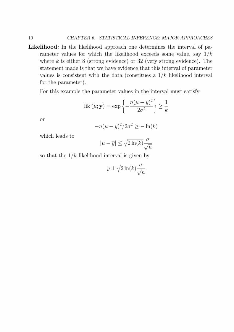
Likelihood: In the likelihood approach one determines the interval of pa-rameter values for which the likelihood exceeds some value, say 1/kwhere k is either 8 (strong evidence) or 32 (very strong evidence). Thestatement made is that we have evidence that this interval of parametervalues is consistent with the data (constitues a 1/k likelihood intervalfor the parameter).
For this example the parameter values in the interval must satisfy
lik (µ;y) = exp
−
n(µ− y)2
2σ2
≥
1
k
or−n(µ− y)2/2σ2 ≥ − ln(k)
which leads to|µ− y| ≤
√2 ln(k)
σ√n
so that the 1/k likelihood interval is given by
y ±√
2 ln(k)σ√n
6.2. ILLUSTRATION OF THE APPROACHES 11
6.2.3 Significance and Hypothesis Testing
The general area of testing is a mess. Two distinct theories dominated the20th century but due to common usage they became mixed up into a setof procedures that can best be described as a muddle. The basic problemis to decide whether a particular set of parameter values (called the nullhypothesis) is more consistent with the data than another set of parametervalues (called the alternative hypothesis).
Frequentist: The frequentist approach has been dominated by two over-lapping procedures developed and advocated by two giants of the field ofstatistics in the 20th century; Fisher and Neyman.
Significance Testing (Fisher): In this approach we have a well definednull hypothesis H0 and a statistic which is chosen so that “extreme values”of the statistic cast doubt upon the null hypothesis in the frequency sense ofprobability.
example: If y1, y2, . . . , yn are observed values of Y1, Y2, . . . , Yn assumed inde-pendent each normally distributed with mean value µ and known variance σ2
suppose that the null hypothesis is that µ = µ0. Suppose also that values of µsmaller than µ0 are not tenable under the scientific theory being investigated.
12 CHAPTER 6. STATISTICAL INFERENCE: MAJOR APPROACHES
It is clear that values of the observed sample mean y larger than µ0 suggestthat H0 is not true. Fisher proposed that the calculation of the p-value beused as a test of significance for H0 : µ = µ0. If the p-value is small wehave evidence that the null hypothesis is not true. The p-value is defined as
p− value = PH0(sample statistic as or more extreme than actually observed)
= PH0(Y ≥ yobs)
= P
Z ≥
√n(yobs − µ0)
σ
Fisher defined three levels of “smallness”, .05, .01 and .001 which lead toa variety of silly conventions such as
∗ − statistically significant∗ − strongly statistically significant
∗ ∗ −very strongly statistically significant
6.2. ILLUSTRATION OF THE APPROACHES 13
Hypothesis Testing (Neyman and Pearson): In this approach a nullhypothesis is selected and an alternative is selected. Neyman and Pearsondeveloped a theory which fixed the probability of rejecting the null hypothesiswhen it is true and maximized the probability of rejecting the null hypothesiswhen it is false. Such tests were designed as rules of “inductive behavior”and were not intended to measure the strength of evidence for or against aparticular hypothesis.
Definition: A rule for choosing between two hypotheses H0 and H1 (basedon observed values of random variables) is called a statistical test of H0 vsH1.
If we represent the test as a function, δ, on the sample space then a testis a statistic of the form
δ(y) =
1 H1 chosen0 H0 chosen
The set of observations which lead to the rejection of H0 is called the criticalregion of the test i.e.
Cδ = {y : δ(y) = 1}
14 CHAPTER 6. STATISTICAL INFERENCE: MAJOR APPROACHES
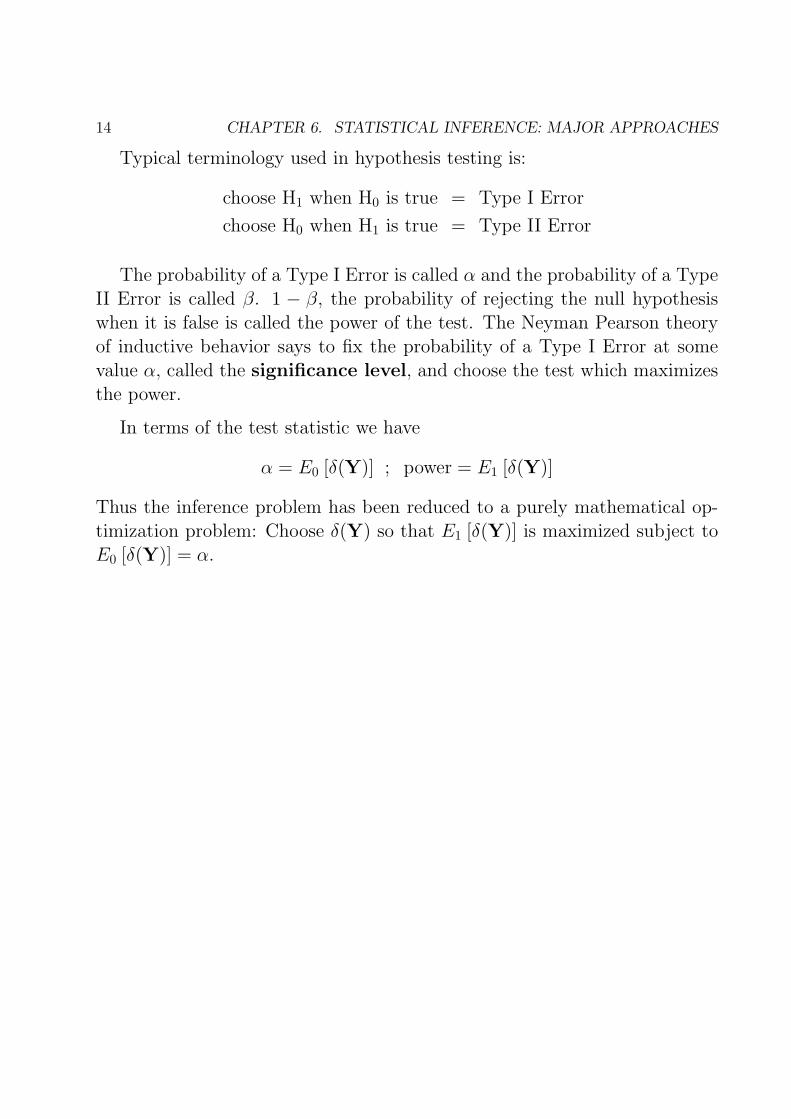
Typical terminology used in hypothesis testing is:
choose H1 when H0 is true = Type I Error
choose H0 when H1 is true = Type II Error
The probability of a Type I Error is called α and the probability of a TypeII Error is called β. 1 − β, the probability of rejecting the null hypothesiswhen it is false is called the power of the test. The Neyman Pearson theoryof inductive behavior says to fix the probability of a Type I Error at somevalue α, called the significance level, and choose the test which maximizesthe power.
In terms of the test statistic we have
α = E0 [δ(Y)] ; power = E1 [δ(Y)]
Thus the inference problem has been reduced to a purely mathematical op-timization problem: Choose δ(Y) so that E1 [δ(Y)] is maximized subject toE0 [δ(Y)] = α.
6.2. ILLUSTRATION OF THE APPROACHES 15
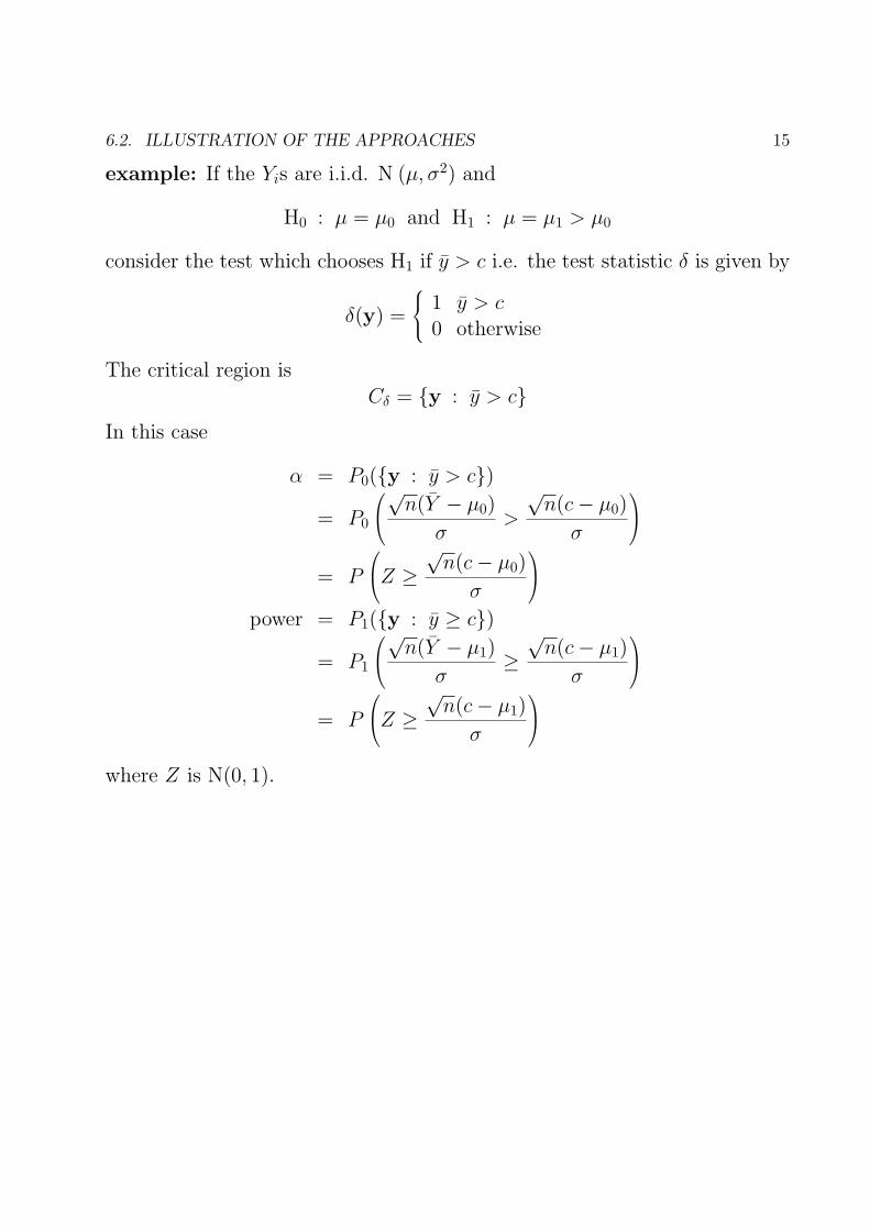
example: If the Yis are i.i.d. N (µ, σ2) and
H0 : µ = µ0 and H1 : µ = µ1 > µ0
consider the test which chooses H1 if y > c i.e. the test statistic δ is given by
δ(y) =
1 y > c
0 otherwise
The critical region isCδ = {y : y > c}
In this case
α = P0({y : y > c})= P0
√
n(Y − µ0)
σ>
√n(c− µ0)
σ
= P
Z ≥
√n(c− µ0)
σ
power = P1({y : y ≥ c})= P1
√
n(Y − µ1)
σ≥√
n(c− µ1)
σ
= P
Z ≥
√n(c− µ1)
σ
where Z is N(0, 1).

16 CHAPTER 6. STATISTICAL INFERENCE: MAJOR APPROACHES
Thus if we want a significance level of .05 we pick c such that
1.645 =
√n(c− µ0
σi.e. c = µ0 + 1.645
σ√n
The power is then
P
Z ≥
√n(c− µ1)
σ
= P
Z ≥ µ0 − µ1
σ+ 1.645
σ√n
Note that α and the power are functions of n and σ and that as α decreasesthe power decreases. Similarly as n increases the power increases and as σ
decreases the power increases.
In general, of two tests with the same α, the Neyman Pearson theorychooses the one with the greater power.
6.2. ILLUSTRATION OF THE APPROACHES 17
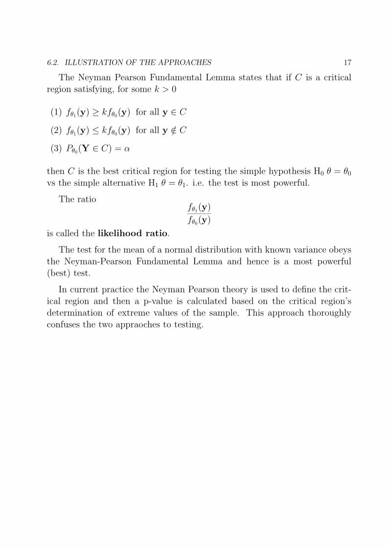
The Neyman Pearson Fundamental Lemma states that if C is a criticalregion satisfying, for some k > 0
(1) fθ1(y) ≥ kfθ0
(y) for all y ∈ C
(2) fθ1(y) ≤ kfθ0
(y) for all y /∈ C
(3) Pθ0(Y ∈ C) = α
then C is the best critical region for testing the simple hypothesis H0 θ = θ0
vs the simple alternative H1 θ = θ1. i.e. the test is most powerful.
The ratiofθ1
(y)
fθ0(y)
is called the likelihood ratio.
The test for the mean of a normal distribution with known variance obeysthe Neyman-Pearson Fundamental Lemma and hence is a most powerful(best) test.
In current practice the Neyman Pearson theory is used to define the crit-ical region and then a p-value is calculated based on the critical region’sdetermination of extreme values of the sample. This approach thoroughlyconfuses the two appraoches to testing.
18 CHAPTER 6. STATISTICAL INFERENCE: MAJOR APPROACHES
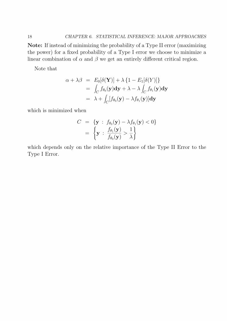
Note: If instead of minimizing the probability of a Type II error (maximizingthe power) for a fixed probability of a Type I error we choose to minimize alinear combination of α and β we get an entirely different critical region.
Note that
α + λβ = E0[δ(Y)] + λ {1− E1[δ(Y )]}=
∫
Cfθ0
(y)dy + λ− λ∫
Cfθ1
(y)dy
= λ +∫
C[fθ0
(y)− λfθ1(y)]dy
which is minimized when
C = {y : fθ0(y)− λfθ1
(y) < 0}=
y :
fθ1(y)
fθ0(y)
>1
λ
which depends only on the relative importance of the Type II Error to theType I Error.
6.2. ILLUSTRATION OF THE APPROACHES 19
Bayesian: In the Bayesian approach to hypothesis testing we assume thatH0 has a prior probability of p0 and that H1 has a prior probability of p1.Then the posterior probability of H0 is given by
fθ0(y)p0
fθ0(y)p0 + fθ1
(y)p1
Similarly the posterior probabilty of H1 is given by
fθ1(y)p1
fθ0(y)p0 + fθ1
(y)p1
It follows that the ratio of the posterior probability of H1 to H0 is given byfθ1
(y)
fθ0(y)
p1
p0
We choose H1 over H0 if this ratio exceeds 1, otherwise we choose H0. Notethat the likelihood ratio again appears, this time as supplying the factorwhich changes the prior odds into the posterior odds. The likelihood ratio inthis situation is an example of a Bayes factor.
For the mean of the normal distribution with known variance the likelihoodratio can be shown to be
exp
(y − µ0 + µ1
2
)n(µ1 − µ0
σ2
so that data increase the posterior odds when the observed sample meanexceeds the value (µ0 + µ1)/2.
20 CHAPTER 6. STATISTICAL INFERENCE: MAJOR APPROACHES
Likelihood: The likelihood approach focuses on the Law of Likelihood.
Law of Likelihood: If
• Hypothesis A specifies that the probability that the random variable X
takes on the value x is pA(x)
• Hypothesis B specifies that the probability that the random variable X
takes on the value x is pB(x)
then
• The observation x is evidence supporting A over B if and only if
pA(x) > pB(x)
• The likelihood ratiopA(x)
pB(x)
measures the strength of that evidence.
The Law of Likelihood measures only the support for one hypotheis rel-ative to another. It does not sanction support for a single hypothesis, norsupport for composite hypotheses.
6.2. ILLUSTRATION OF THE APPROACHES 21
example: Assume that we have a sample y1, y2, . . . , yn which are realizedvalues of Y1, Y2, . . . , Yn where the Yi are iid N (µ, σ2) where σ2 is known. Ofinterest is H0 : µ = µ0 and H1 : µ = µ1 = µ0 + δ where δ > 0.
The likelihood for µ is given by
L(θ;y) =n∏
i=1(2πσ2)−
12 exp
−
(yi − µ)2
2σ2
After some algebraic simplification the likelihood ratio for µ1 vs µ0 is givenby
L1
L0= exp
{(y − µ0 − δ
2
)nδ
σ2
}
It follows thatL1
L0≥ k
if and only if (y − µ0 − δ
2
)nδ
σ2 ≥ ln(k)
i.e.
y ≥ µ0 +δ
2+
σ2 ln(k)
nδor
y ≥ µ0 + µ1
2+
σ2 ln(k)
nδ
Choice of k is usually 8 or 32 (discussed later).
22 CHAPTER 6. STATISTICAL INFERENCE: MAJOR APPROACHES
6.3 General Comments
6.3.1 Importance of the Likelihood
Note that each of the approaches involve the likelihood. For this reasonwe will spend considerable time using the likelihood to determine estimates(point and interval), test hypotheses and also to check the compatability ofresults with the Law of Likelihood.
6.3.2 Which Approach?
Each approach has its advocates, some fanatic, some less so. The impor-tant idea is to use an approach which faithfully conveys the science underinvestigation.
6.3. GENERAL COMMENTS 23
6.3.3 Reporting Results
Results of inferential procedures are reported in a variety of ways dependingon the statistician and the subject matter area. There seems to be no fixedset of rules for reporting the results of estimation, interval estimation andtesting procedures. The following is suggestion by this author on how toreport results.
• Estimation
◦ Frequentist The estimated value of the parameter θ is θ with stan-dard error s.e.(θ). The specific method of estimation might be givenalso.
◦ Bayesian The estimated value of the parameter is θ (the mean ormode) of the posterior distribution of θ. The standard deviation ofthe posterior distribution is s.e.(θ). The prior distribution was g(θ).A graph of the posterior could also be provided.
◦ Likelihood The graph of the likelihood function for θ is as follows.The maximum value (best supported value) is at θ. The shape ofthe likelihood function provides the information on “precision”.

24 CHAPTER 6. STATISTICAL INFERENCE: MAJOR APPROACHES
• Interval Estimation
◦ Frequentist Values of θ between θl and θu are consistent with thedata based on a (1−α) confidence interval. The specific statistic ormethod used to obtain the confidence interval should be mentioned.
◦ Bayesian Values of θ between θl and θu are consistent with the databased on a (1− α) credible interval. The prior distribution used inobtaining the posterior should be mentioned.
◦ Likelihood Values of θ between θl and θu are consistent with thedata based on a 1/k likelihood interval. Presented as a graph isprobably best.

6.3. GENERAL COMMENTS 25
• Testing
◦ Frequentist
◦ Bayesian
◦ Likelihood

26 CHAPTER 6. STATISTICAL INFERENCE: MAJOR APPROACHES

Chapter 7
Point and Interval Estimation
7.1 Point Estimation - Introduction
The statistical inference called point estimation provides the solution to the followingproblem
Given data and a probability model find an estimate for the parameter
There are two important features of estimation procedures:
• Desirable properties of the estimate
• Methods for obtaining the estimate
27

28 CHAPTER 7. POINT AND INTERVAL ESTIMATION
7.2 Properties of Estimators
Since the data in a statistical problem are subject to variability:
• Statistics calculated from the data are also subject to variability.
• The rule by which we calculate an estimate is called the estimator and the actualcomputed value is called the estimate.
◦ An estimator is thus a random variable.
◦ Its realized value is the estimate.
• In the frequentist approach to statistics the sampling distribution of the estimator:
◦ determines the properties of the estimator
◦ determines which of several potential estimators might be best in a given situation.
7.2. PROPERTIES OF ESTIMATORS 29
7.2.1 Properties of Estimators
Desirable properties of an estimator include:
• The estimator should be correct on average i.e. the sampling distribution of the esti-mator should be centered at the parameter being estimated. This property is calledunbiasedness
• In large samples, the estimator should be equal to the parameter being estimated i.e.
P (θ ≈ θ) ≈ 1 for n large
where ≈ means approximately. Equivalently
θp→ θ
This property is called consistency.
• The sampling distribution of the estimator should be concentrated closely around itscenter i.e. the estimator should have small variability. This property is called effi-ciency.
Of these properties most statisticians agree that consistency is the minimum criterionthat an estimator should satisfy.
30 CHAPTER 7. POINT AND INTERVAL ESTIMATION
7.2.2 Unbiasedness
Definition: An estimator θ is an unbiased estimator of a parameter θ if
E(θ) = θ
An unbiased estimator thus has a sampling distribution centered at the value of the parameterwhich is being estimated.
examples:
• To estimate the parameter p in a binomial distribution we use the estimate p = xn
where x is the number of successes in the sample. The corresponding estimator isunbiased since
E(p) = E(
X
n
)=
E(X)
n=
np
n= p
• To estimate the parameter λ in the Poisson distribution we use the estimate λ = xwhere x is the sample mean. The corresponding estimator is unbiased since
E(λ) = E(X) = λ
• To estimate the parameter µ in the normal distribution we use the estimate µ = xwhere x is the sample mean. The corresponding estimator is unbiased since
E(µ) = E(X) = µ
• In fact the sample mean is always an unbiased estimator of the population mean,provided that the sample is a random sample from the population.
7.2. PROPERTIES OF ESTIMATORS 31
Statisticians, when possible, use unbiased estimators.
• The difficulty in finding unbiased estimators in general is that estimators for certainparameters are often complicated functions.
• The resulting expected values cannot be evaluated and hence unbiasedness cannot bechecked.
• Often such estimators are, however, nearly unbiased for large sample sizes; i.e. theyare asymptotically unbiased.
examples:
• The estimator for the log odds in a binomial distribution is
ln
(p
1− p
)
The expected value of this estimate is not defined since there is a positive probabilitythat it is infinite (p = 0 or p = 1)
32 CHAPTER 7. POINT AND INTERVAL ESTIMATION
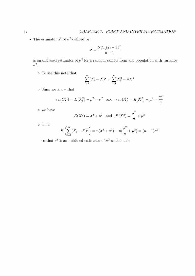
• The estimator s2 of σ2 defined by
s2 =
∑ni=1(xi − x)2
n− 1
is an unbiased estimator of σ2 for a random sample from any population with varianceσ2.
◦ To see this note thatn∑
i=1
(Xi − X)2 =n∑
i=1
X2i − nX2
◦ Since we know that
var (Xi) = E(X2i )− µ2 = σ2 and var (X) = E(X2)− µ2 =
σ2
n
◦ we have
E(X2i ) = σ2 + µ2 and E(X2) =
σ2
n+ µ2
◦ Thus
E
(n∑
i=1
(Xi − X)2
)= n(σ2 + µ2)− n(
σ2
n+ µ2) = (n− 1)σ2
so that s2 is an unbiased estimator of σ2 as claimed.
7.2. PROPERTIES OF ESTIMATORS 33
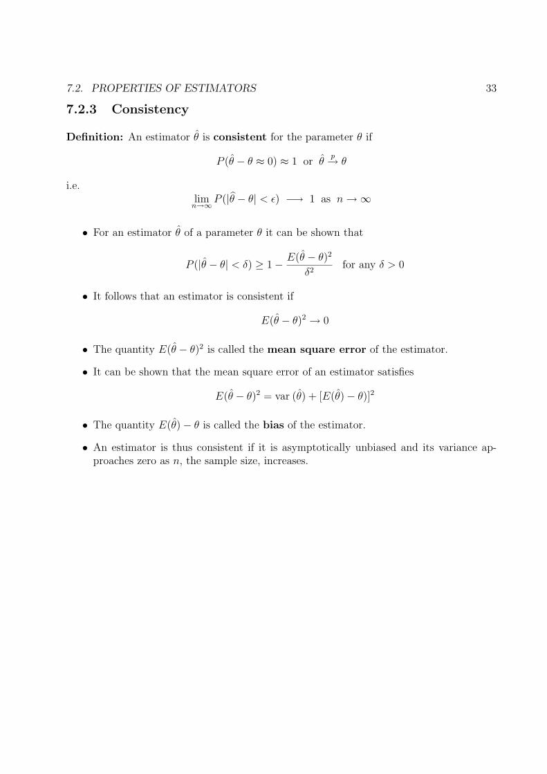
7.2.3 Consistency
Definition: An estimator θ is consistent for the parameter θ if
P (θ − θ ≈ 0) ≈ 1 or θp→ θ
i.e.lim
n→∞P (|θ − θ| < ε) −→ 1 as n →∞
• For an estimator θ of a parameter θ it can be shown that
P (|θ − θ| < δ) ≥ 1− E(θ − θ)2
δ2for any δ > 0
• It follows that an estimator is consistent if
E(θ − θ)2 → 0
• The quantity E(θ − θ)2 is called the mean square error of the estimator.
• It can be shown that the mean square error of an estimator satisfies
E(θ − θ)2 = var (θ) + [E(θ)− θ)]2
• The quantity E(θ)− θ is called the bias of the estimator.
• An estimator is thus consistent if it is asymptotically unbiased and its variance ap-proaches zero as n, the sample size, increases.
34 CHAPTER 7. POINT AND INTERVAL ESTIMATION
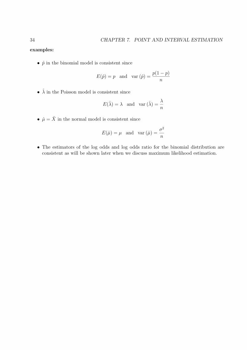
examples:
• p in the binomial model is consistent since
E(p) = p and var (p) =p(1− p)
n
• λ in the Poisson model is consistent since
E(λ) = λ and var (λ) =λ
n
• µ = X in the normal model is consistent since
E(µ) = µ and var (µ) =σ2
n
• The estimators of the log odds and log odds ratio for the binomial distribution areconsistent as will be shown later when we discuss maximum likelihood estimation.
7.2. PROPERTIES OF ESTIMATORS 35
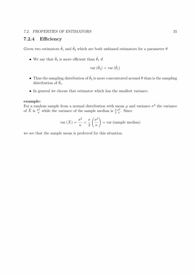
7.2.4 Efficiency
Given two estimators θ1 and θ2 which are both unbiased estimators for a parameter θ
• We say that θ2 is more efficient than θ1 if
var (θ2) < var (θ1)
• Thus the sampling distribution of θ2 is more concentrated around θ than is the samplingdistribution of θ1.
• In general we choose that estimator which has the smallest variance.
example:For a random sample from a normal distribution with mean µ and variance σ2 the varianceof X is σ2
nwhile the variance of the sample median is π
2σ2
n. Since
var (X) =σ2
n<
π
2
(σ2
n
)= var (sample median)
we see that the sample mean is preferred for this situation.

36 CHAPTER 7. POINT AND INTERVAL ESTIMATION
7.3 Estimation Methods
An enormous variety of methods have been proposed for obtaining estimates of parametersin statistical models.
Three methods are of general importance:
• “the analog or substitution method”
• the method of maximum likelihood.
• estimating equations.
7.3. ESTIMATION METHODS 37
7.3.1 Analog or Substitution Method
The analog or substitution method of estimation is based on selecting as the estimate thesample statistic which is the analog to the population parameter being estimated.
examples:
• In the binomial estimate the population proportion p by the sample proportion p = xn.
• In the case of a random sample from the normal distribution estimate the populationmean µ by the sample mean x.
• Estimate the population median by the sample median.
• Estimate the population range by the sample range.
• Estimate the upper quartile of the population by the upper quartile of the sample.
• Estimate the population distribution using the empirical distribution.

38 CHAPTER 7. POINT AND INTERVAL ESTIMATION
While intuitively appealing,
• The analog method does not work in complex situations because there are not sampleanalogs to population parameters.
• There are also few general results regarding desirable properties of estimators obtainedusing the analog method.
7.3. ESTIMATION METHODS 39
7.3.2 Maximum Likelihood
The maximum likelihood method of estimation was introduced in 1921 by Sir Ronald Fisherand chooses that estimate of the parameter which “makes the observed data as likely aspossible”.
Definition: If the sample data is denoted by y, the parameter by θ and the probabilitydensity function by f(y; θ) then the maximum likelihood estimate of θ is that value of θ,θ which maximizes f(y; θ)
• Recall that the likelihood of θ is defined as
lik (θ;y) =f(y; θ)
f(y; θ)
• The likelihood of θ may be used to evaluate the relative importance of different valuesof θ in explaining the observed data i.e. if
lik (θ2;y) > lik (θ1;y)
then θ2 explains the observed data better than θ1.
• As we have seen likelihood is the most important component of the alternative theoriesof statistical inference.
40 CHAPTER 7. POINT AND INTERVAL ESTIMATION
Maximum likelihood estimates are obtained by:
• Maximizing the likelihood using calculus. Most often we have a random sample of sizen from a population with density function f(y; θ). In this case we have that
f(y; θ) =n∏
i=1
f(yi; θ)
Since the maximum of a function occurs at the same value as the maximum of thenatural logarithm of the function it is easier to maximize
n∑
i=1
ln[f(yi; θ)]
with respect to θ. Thus we solve the equations
n∑
i=1
d ln[f(yi; θ)]
dθ= 0
which is called the maximum likelihood or score equation.
• Maximizing the likelihood numerically. Most statistical software programs do this.
• Graphing the likelihood and observing the point at which the maximum value of thelikelihood occurs.

7.3. ESTIMATION METHODS 41
examples:
• In the binomial, p = xn
is the maximum likelihood estimate of p.
• In the Poisson, λ = x is the maximum likelihood estimate of λ.
• In the normal,
◦ µ = x is the maximum likelihood estimate of µ.
◦ s2 is the maximum likelihood estimate of σ2
◦√
s2 = s is the maximum likelihood estimate of σ
42 CHAPTER 7. POINT AND INTERVAL ESTIMATION
In addition to their intuitive appeal and the fact that they are easy to calculate usingappropriate software, maximum likelihood estimates have several important properties.
• Invariance. The maximum likelihood estimate of a function g(θ) is g(θ) where θ is themaximum likelihood estimate of θ.
Assuming that we have a random sample from a distribution with probability densityfunction f(y; θ):
• Maximum likelihood estimates are usually consistent i.e.
θp→ θ0
where θ0 is the true value of θ.
• The distribution of the maximum likelihood estimate in large samples is usually normal,centered at θ, with a variance that can be explicitly calculated. Thus
√n(θ − θ0) ≈ N (0, v(θ0))
where θ0 is the true value of θ and
v(θ0) =1
i(θ0)where i(θ0) = − Eθ0
[d(2) ln(f(Y ); θ0)
dθ(2)0
]
Thus we may obtain probabilities for θ as if it were normal with expected value θ0 andvariance v(θ0). We may also approximate v(θ0) by v(θ).
7.3. ESTIMATION METHODS 43
• If g(θ) is a differentiable function then the approximate distribution of g(θ) satisfies
√n[g(θ)− g(θ0] ≈ N (0, vg(θ0))
wherevg(θ0) = [g(1)(θ0)]
2v(θ0)
vg(θ0) may be approximated by vg(θ)
• Maximum likelihood estimators can be calculated for complex statistical models usingappropriate software.
A major drawback to maximum likelihood estimates is the fact that the estimate, andmore importantly, its variance, depend on the model f(y; θ), and the assumption of largesamples. Using the bootstrap allows us to obtain variance estimates which are robust (donot depend strongly on the validity of the model) and do not depend on large sample sizes.

44 CHAPTER 7. POINT AND INTERVAL ESTIMATION
7.4 Interval Estimation
7.4.1 Introduction
For estimating µ when we have Y1, Y2, . . . , Yn which are i.i.d. N(µ, σ2) where σ2 is known weknow that the maximum likelihood estimate of µ is Y . For a given set of observations weobtain a point estimate of µ, y. However, this does not give us all the information about µthat we would like to have.
In interval estimation we find a set of parameter values which are consistent with thedata.
7.4. INTERVAL ESTIMATION 45
One approach would be to sketch the likelihood function of µ which is given by
L(µ,y) = exp
{−n(µ− y)2
2σ2
}
which shows that the likelihood has the shape of a normal density, centered at y and getsnarrower as n increases.
Another approach is to construct a confidence interval. We use the fact that
µ = Y ∼ N
(µ,
σ2
n
)
i.e. the sampling distribution of Y is normal with mean µ and variance σ2/n. Thus we findthat
P
( |Y − µ|σ/√
n≤ 1.96
)= .95
46 CHAPTER 7. POINT AND INTERVAL ESTIMATION
It follows that
P
(Y − 1.96
σ√n≤ µ ≤ Y + 1.96
σ√n
)= .95
This last statement says that the probability is .95 that the random interval
[Y − 1.96
σ√n
, Y + 1.96σ√n
]
will contain µ.
Notice that for a given realization of Y , say y, the probability that the interval containsthe parameter µ is either 0 or 1 since there is no random variable present at this point.Thus we cannot say that there is a 95% chance that the parameter µ is in a given observedinterval.
Definition: An interval I(Y) ⊂ Θ, the parameter space, is a 100(1 − α)% confidenceinterval for θ if
P (I(Y) ⊃ θ) = 1− α
for all θ ∈ Θ. 1− α is called the confidence level.
Note that we cannot sayP (I(y) ⊃ θ) = 1− α
but we can sayP (I(Y) ⊃ θ) = 1− α
What we can say with regard to the first statement is that we used a procedure whichhas a probability of 1 − α of producing an interval which contains θ. Since the intervalwe observed was constructed according to this procedure we say that we have a set ofparameter values which are consistent with the data at confidence level 1 − α.
7.4. INTERVAL ESTIMATION 47
7.4.2 Confidence Interval for the Mean-Unknown Variance
In the introduction we obtained the confidence interval for µ when the observed data was asample from a normal distribution with mean µ and known variance σ2. If the variance isnot known we use the fact that the distribution of
T =Y − µ
s/√
n
is Student’s t with n− 1 degrees of freedom where
s2 =1
n− 1
n∑
i=1
(Yi − Y )2
is the bias corrected maximum likelihood estimator of σ2.

48 CHAPTER 7. POINT AND INTERVAL ESTIMATION
It follows that
1− α = P
( |Y − µ|s/√
n≤ t1−α/2(n− 1)
)
= P
(|Y − µ| ≤ t1−α/2(n− 1)
s√n
)
= P
(Y − t1−α/2(n− 1)
s√n≤ µ ≤ Y + t1−α/2(n− 1)
s√n
)
Thus the random intervalY ± t1−α/2(n− 1)
s√n
is a 1− α confidence interval for µ. The observed interval
y ± t1−α/2(n− 1)s√n
has the same interpretation as the interval for µ with σ2 known.
7.4. INTERVAL ESTIMATION 49
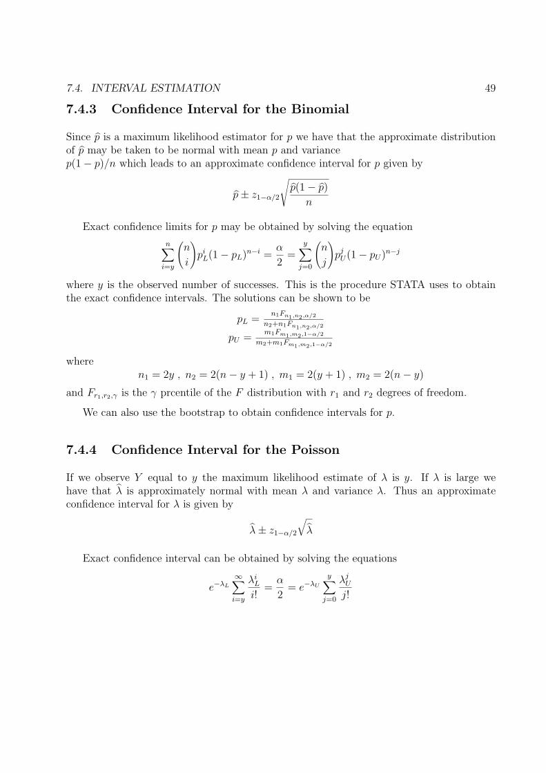
7.4.3 Confidence Interval for the Binomial
Since p is a maximum likelihood estimator for p we have that the approximate distributionof p may be taken to be normal with mean p and variancep(1− p)/n which leads to an approximate confidence interval for p given by
p± z1−α/2
√p(1− p)
n
Exact confidence limits for p may be obtained by solving the equation
n∑
i=y
(n
i
)pi
L(1− pL)n−i =α
2=
y∑
j=0
(n
j
)pj
U(1− pU)n−j
where y is the observed number of successes. This is the procedure STATA uses to obtainthe exact confidence intervals. The solutions can be shown to be
pL =n1Fn1,n2,α/2
n2+n1Fn1,n2,α/2
pU =m1Fm1,m2,1−α/2
m2+m1Fm1,m2,1−α/2
wheren1 = 2y , n2 = 2(n− y + 1) , m1 = 2(y + 1) , m2 = 2(n− y)
and Fr1,r2,γ is the γ prcentile of the F distribution with r1 and r2 degrees of freedom.
We can also use the bootstrap to obtain confidence intervals for p.
7.4.4 Confidence Interval for the Poisson
If we observe Y equal to y the maximum likelihood estimate of λ is y. If λ is large wehave that λ is approximately normal with mean λ and variance λ. Thus an approximateconfidence interval for λ is given by
λ± z1−α/2
√λ
Exact confidence interval can be obtained by solving the equations
e−λL
∞∑
i=y
λiL
i!=
α
2= e−λU
y∑
j=0
λjU
j!

50 CHAPTER 7. POINT AND INTERVAL ESTIMATION
This is the procedure STATA uses to obtain the exact confidence interval. The solutions canbe shown to be
λL = 12χ2
2y,α/2
λU = 12χ2
2(y+1),1−α/2
where χ2r,γ is the γ percentile of the chi-square distribution with r degrees of freedom.
The bootstrap can also be used to obtain confidence intervals for λ.

7.5. POINT AND INTERVAL ESTIMATION - SEVERAL PARAMETERS 51
7.5 Point and Interval Estimation - Several Parameters
7.5.1 Introduction
We now consider the situation where we have a probability model which has several param-eters.
• Often we are interested in only one of the parameters and the other is considered anuisance parameter. Nevertheless we still need to estimate all of the parameters tospecify the probability model.
• We may be interested in a function of all of the parameters e.g. the odds ratio whenwe have two binomial distributions.
• The properties of unbiasedness, consistency and efficiency are still used to evaluate theestimators.
• A variety of methods are used to obtain estimators, the most important of which ismaximum likelihood.
52 CHAPTER 7. POINT AND INTERVAL ESTIMATION
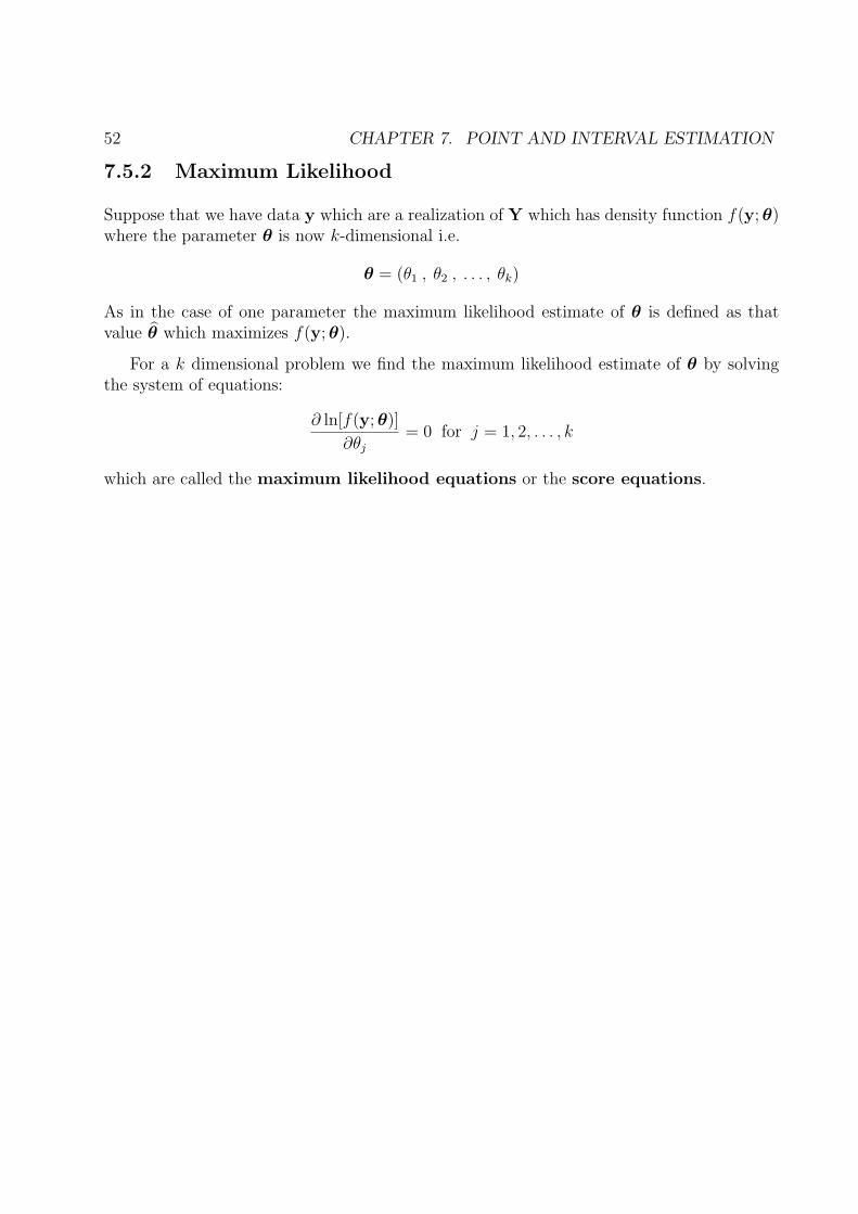
7.5.2 Maximum Likelihood
Suppose that we have data y which are a realization of Y which has density function f(y; θ)where the parameter θ is now k-dimensional i.e.
θ = (θ1 , θ2 , . . . , θk)
As in the case of one parameter the maximum likelihood estimate of θ is defined as thatvalue θ which maximizes f(y; θ).
For a k dimensional problem we find the maximum likelihood estimate of θ by solvingthe system of equations:
∂ ln[f(y; θ)]
∂θj
= 0 for j = 1, 2, . . . , k
which are called the maximum likelihood equations or the score equations.
7.5. POINT AND INTERVAL ESTIMATION - SEVERAL PARAMETERS 53
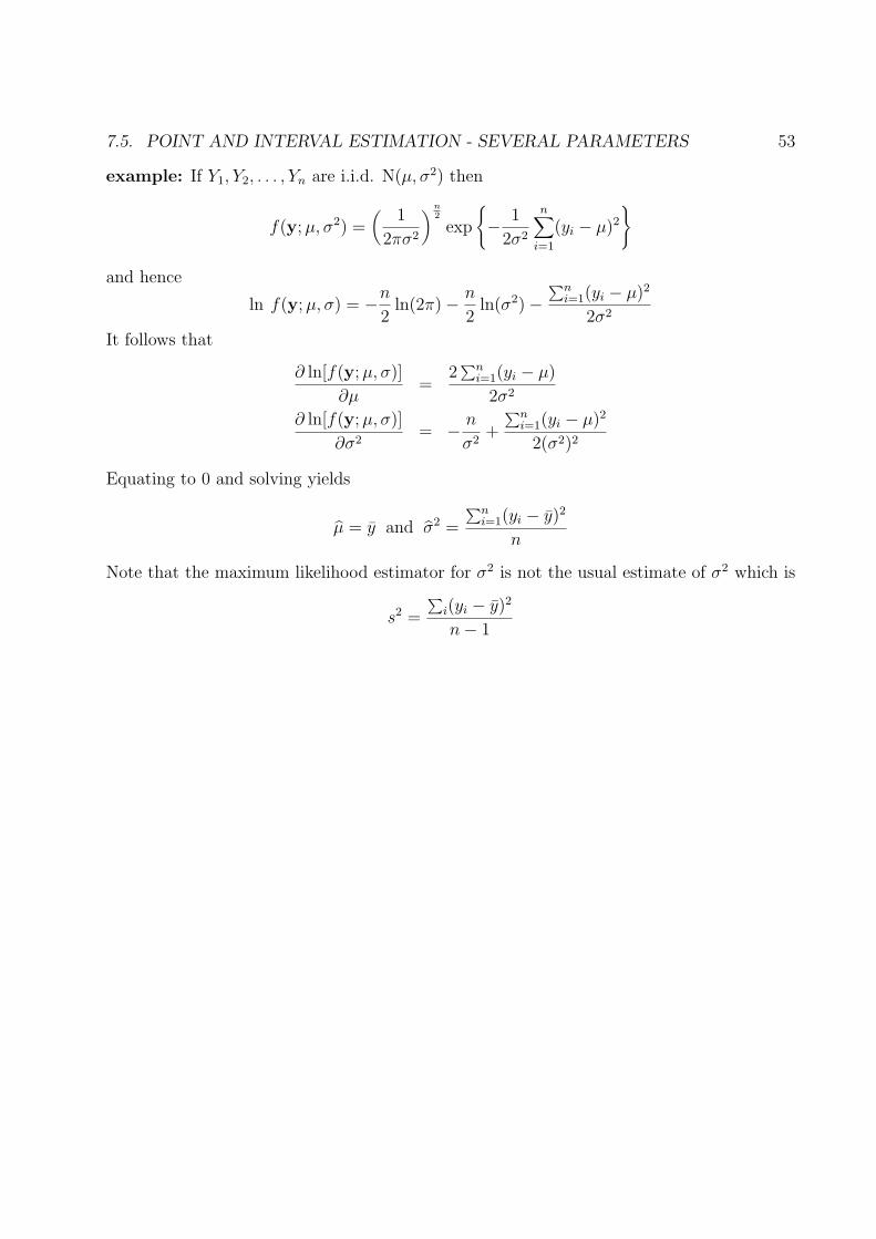
example: If Y1, Y2, . . . , Yn are i.i.d. N(µ, σ2) then
f(y; µ, σ2) =(
1
2πσ2
)n2
exp
{− 1
2σ2
n∑
i=1
(yi − µ)2
}
and hence
ln f(y; µ, σ) = −n
2ln(2π)− n
2ln(σ2)−
∑ni=1(yi − µ)2
2σ2
It follows that
∂ ln[f(y; µ, σ)]
∂µ=
2∑n
i=1(yi − µ)
2σ2
∂ ln[f(y; µ, σ)]
∂σ2= − n
σ2+
∑ni=1(yi − µ)2
2(σ2)2
Equating to 0 and solving yields
µ = y and σ2 =
∑ni=1(yi − y)2
n
Note that the maximum likelihood estimator for σ2 is not the usual estimate of σ2 which is
s2 =
∑i(yi − y)2
n− 1
54 CHAPTER 7. POINT AND INTERVAL ESTIMATION
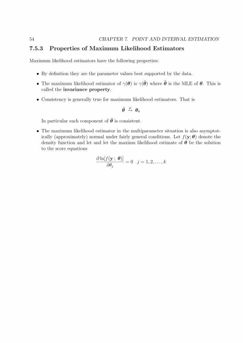
7.5.3 Properties of Maximum Likelihood Estimators
Maximum likelihood estimators have the following properties:
• By definition they are the parameter values best supported by the data.
• The maximum likelihood estimator of γ(θ) is γ(θ) where θ is the MLE of θ. This iscalled the invariance property.
• Consistency is generally true for maximum likelihood estimators. That is
θp→ θ0
In particular each component of θ is consistent.
• The maximum likelihood estimator in the multiparameter situation is also asymptot-ically (approximately) normal under fairly general conditions. Let f(y; θ) denote thedensity function and let and let the maximu likelihood estimate of θ be the solutionto the score equations
∂ ln[f(y ; θ)]
∂θj
= 0 j = 1, 2, . . . , k
7.5. POINT AND INTERVAL ESTIMATION - SEVERAL PARAMETERS 55
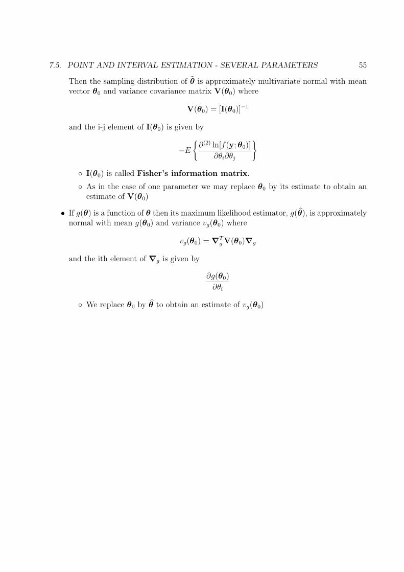
Then the sampling distribution of θ is approximately multivariate normal with meanvector θ0 and variance covariance matrix V(θ0) where
V(θ0) = [I(θ0)]−1
and the i-j element of I(θ0) is given by
−E
{∂(2) ln[f(y; θ0)]
∂θi∂θj
}
◦ I(θ0) is called Fisher’s information matrix.
◦ As in the case of one parameter we may replace θ0 by its estimate to obtain anestimate of V(θ0)
• If g(θ) is a function of θ then its maximum likelihood estimator, g(θ), is approximatelynormal with mean g(θ0) and variance vg(θ0) where
vg(θ0) = ∇Tg V(θ0)∇g
and the ith element of ∇g is given by
∂g(θ0)
∂θi
◦ We replace θ0 by θ to obtain an estimate of vg(θ0)
56 CHAPTER 7. POINT AND INTERVAL ESTIMATION
7.5.4 Two Sample Normal
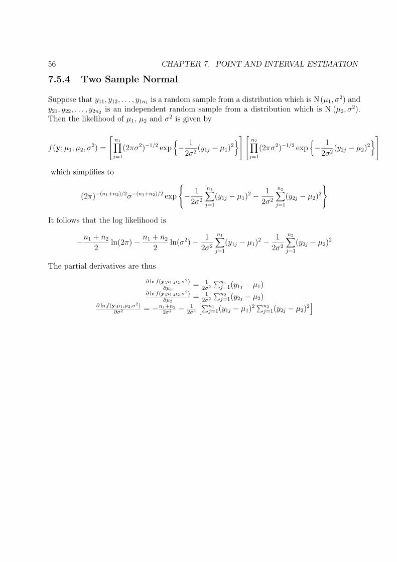
Suppose that y11, y12, . . . , y1n1 is a random sample from a distribution which is N(µ1, σ2) and
y21, y22, . . . , y2n2 is an independent random sample from a distribution which is N (µ2, σ2).
Then the likelihood of µ1, µ2 and σ2 is given by
f(y; µ1, µ2, σ2) =
n1∏
j=1
(2πσ2)−1/2 exp{− 1
2σ2(y1j − µ1)
2}
n2∏
j=1
(2πσ2)−1/2 exp{− 1
2σ2(y2j − µ2)
2}
which simplifies to
(2π)−(n1+n2)/2σ−(n1+n2)/2 exp
−
1
2σ2
n1∑
j=1
(y1j − µ1)2 − 1
2σ2
n2∑
j=1
(y2j − µ2)2
It follows that the log likelihood is
−n1 + n2
2ln(2π)− n1 + n2
2ln(σ2)− 1
2σ2
n1∑
j=1
(y1j − µ1)2 − 1
2σ2
n2∑
j=1
(y2j − µ2)2
The partial derivatives are thus
∂ ln f(y;µ1,µ2,σ2)∂µ1
= 12σ2
∑n1j=1(y1j − µ1)
∂ ln f(y;µ1,µ2,σ2)∂µ2
= 12σ2
∑n2j=1(y2j − µ2)
∂ ln f(y;µ1,µ2,σ2)∂σ2 = −n1+n2
2σ2 − 12σ4
[∑n1j=1(y1j − µ1)
2 ∑n2j=1(y2j − µ2)
2]
7.5. POINT AND INTERVAL ESTIMATION - SEVERAL PARAMETERS 57
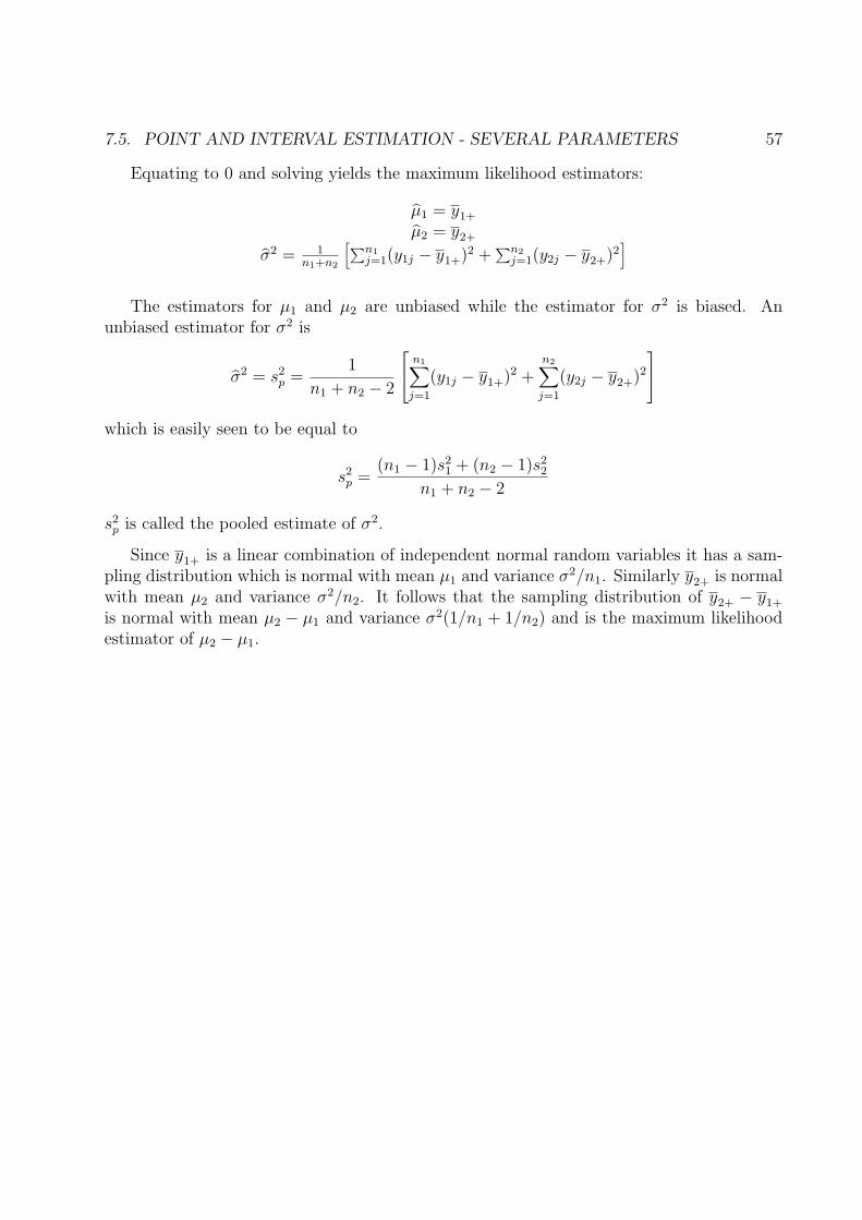
Equating to 0 and solving yields the maximum likelihood estimators:
µ1 = y1+
µ2 = y2+
σ2 = 1n1+n2
[∑n1j=1(y1j − y1+)2 +
∑n2j=1(y2j − y2+)2
]
The estimators for µ1 and µ2 are unbiased while the estimator for σ2 is biased. Anunbiased estimator for σ2 is
σ2 = s2p =
1
n1 + n2 − 2
n1∑
j=1
(y1j − y1+)2 +n2∑
j=1
(y2j − y2+)2
which is easily seen to be equal to
s2p =
(n1 − 1)s21 + (n2 − 1)s2
2
n1 + n2 − 2
s2p is called the pooled estimate of σ2.
Since y1+ is a linear combination of independent normal random variables it has a sam-pling distribution which is normal with mean µ1 and variance σ2/n1. Similarly y2+ is normalwith mean µ2 and variance σ2/n2. It follows that the sampling distribution of y2+ − y1+
is normal with mean µ2 − µ1 and variance σ2(1/n1 + 1/n2) and is the maximum likelihoodestimator of µ2 − µ1.
58 CHAPTER 7. POINT AND INTERVAL ESTIMATION
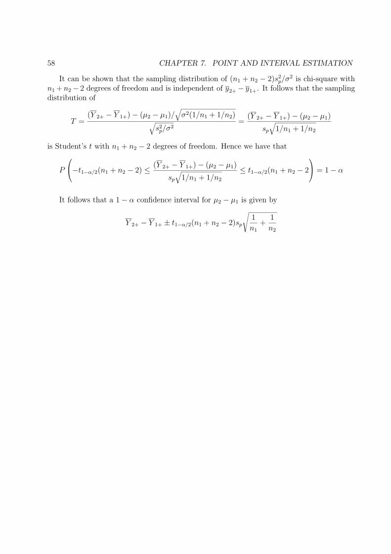
It can be shown that the sampling distribution of (n1 + n2 − 2)s2p/σ
2 is chi-square withn1 + n2− 2 degrees of freedom and is independent of y2+− y1+. It follows that the samplingdistribution of
T =(Y 2+ − Y 1+)− (µ2 − µ1)/
√σ2(1/n1 + 1/n2)√
s2p/σ
2=
(Y 2+ − Y 1+)− (µ2 − µ1)
sp
√1/n1 + 1/n2
is Student’s t with n1 + n2 − 2 degrees of freedom. Hence we have that
P
−t1−α/2(n1 + n2 − 2) ≤ (Y 2+ − Y 1+)− (µ2 − µ1)
sp
√1/n1 + 1/n2
≤ t1−α/2(n1 + n2 − 2
= 1− α
It follows that a 1− α confidence interval for µ2 − µ1 is given by
Y 2+ − Y 1+ ± t1−α/2(n1 + n2 − 2)sp
√1
n1
+1
n2
7.5. POINT AND INTERVAL ESTIMATION - SEVERAL PARAMETERS 59
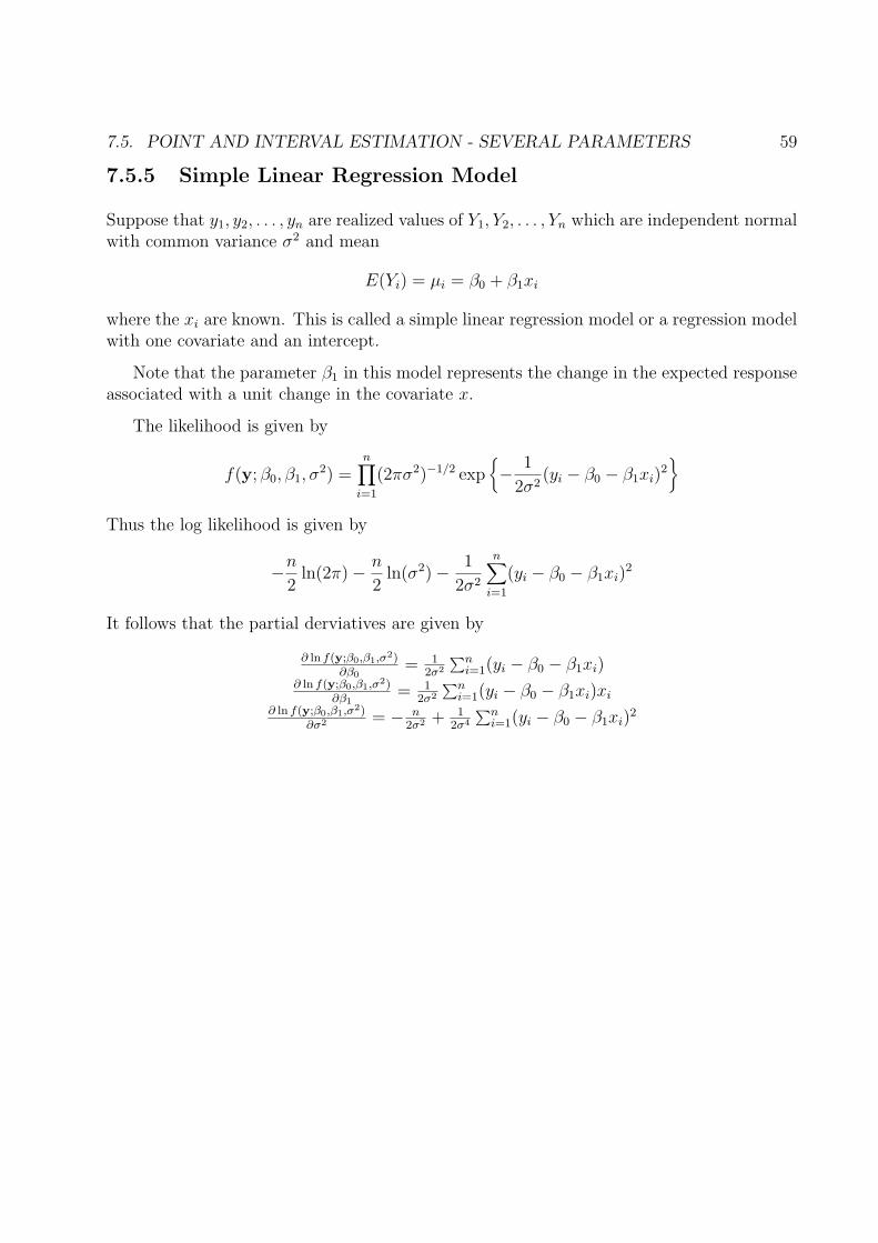
7.5.5 Simple Linear Regression Model
Suppose that y1, y2, . . . , yn are realized values of Y1, Y2, . . . , Yn which are independent normalwith common variance σ2 and mean
E(Yi) = µi = β0 + β1xi
where the xi are known. This is called a simple linear regression model or a regression modelwith one covariate and an intercept.
Note that the parameter β1 in this model represents the change in the expected responseassociated with a unit change in the covariate x.
The likelihood is given by
f(y; β0, β1, σ2) =
n∏
i=1
(2πσ2)−1/2 exp{− 1
2σ2(yi − β0 − β1xi)
2}
Thus the log likelihood is given by
−n
2ln(2π)− n
2ln(σ2)− 1
2σ2
n∑
i=1
(yi − β0 − β1xi)2
It follows that the partial derviatives are given by
∂ ln f(y;β0,β1,σ2)∂β0
= 12σ2
∑ni=1(yi − β0 − β1xi)
∂ ln f(y;β0,β1,σ2)∂β1
= 12σ2
∑ni=1(yi − β0 − β1xi)xi
∂ ln f(y;β0,β1,σ2)∂σ2 = − n
2σ2 + 12σ4
∑ni=1(yi − β0 − β1xi)
2
60 CHAPTER 7. POINT AND INTERVAL ESTIMATION
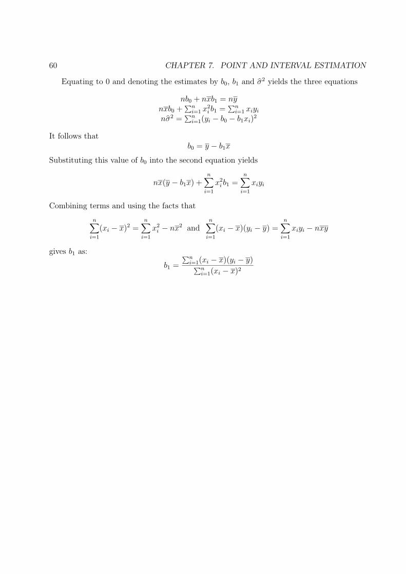
Equating to 0 and denoting the estimates by b0, b1 and σ2 yields the three equations
nb0 + nxb1 = nynxb0 +
∑ni=1 x2
i b1 =∑n
i=1 xiyi
nσ2 =∑n
i=1(yi − b0 − b1xi)2
It follows thatb0 = y − b1x
Substituting this value of b0 into the second equation yields
nx(y − b1x) +n∑
i=1
x2i b1 =
n∑
i=1
xiyi
Combining terms and using the facts that
n∑
i=1
(xi − x)2 =n∑
i=1
x2i − nx2 and
n∑
i=1
(xi − x)(yi − y) =n∑
i=1
xiyi − nxy
gives b1 as:
b1 =
∑ni=1(xi − x)(yi − y)∑n
i=1(xi − x)2
7.5. POINT AND INTERVAL ESTIMATION - SEVERAL PARAMETERS 61
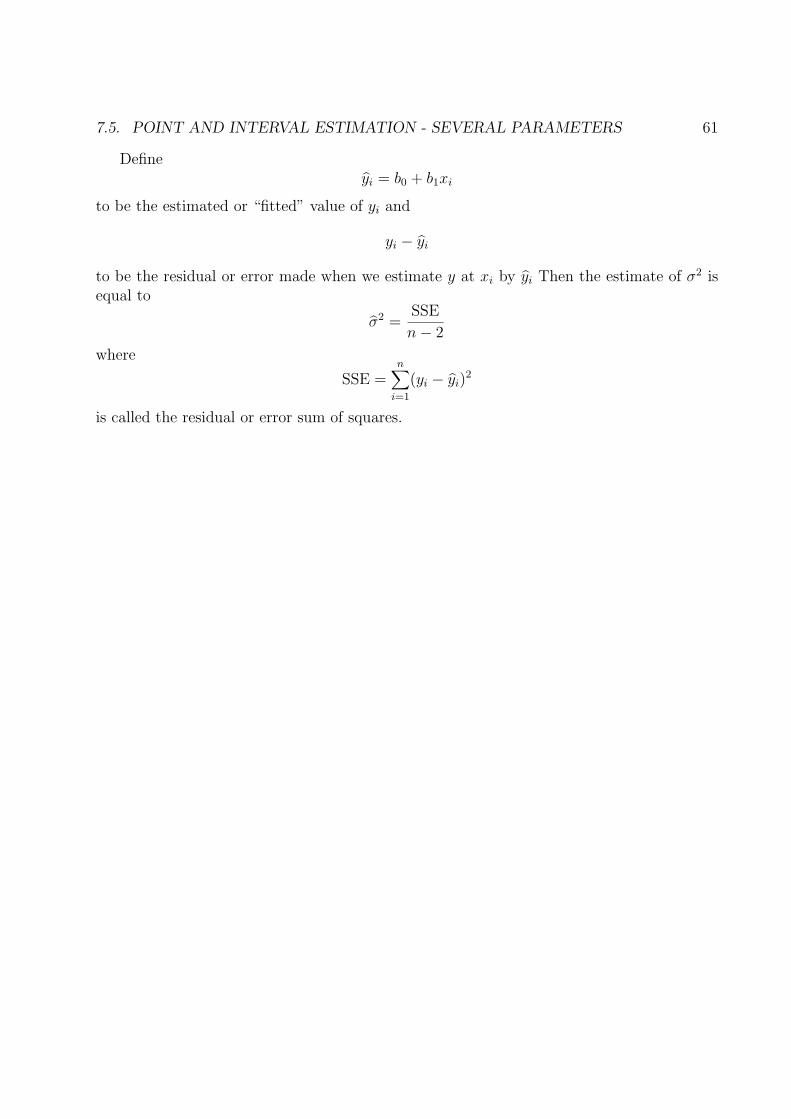
Defineyi = b0 + b1xi
to be the estimated or “fitted” value of yi and
yi − yi
to be the residual or error made when we estimate y at xi by yi Then the estimate of σ2 isequal to
σ2 =SSE
n− 2
where
SSE =n∑
i=1
(yi − yi)2
is called the residual or error sum of squares.

62 CHAPTER 7. POINT AND INTERVAL ESTIMATION
7.5.6 Matrix Formulation of Simple Linear Regression
It is useful to rewrite the simple linear regression model in matrix notation. It turns outthat in this formulation we can add as many covariates as we like and obtain essentially thesame results. Define
y =
y1
y2...
yn
X =
1 x1
1 x2...
...1 xn
β =
[β0
β1
]b =
[b0
b1
]
Then the model may be written as
E(Y) = Xβ var (Y) = Iσ2
7.5. POINT AND INTERVAL ESTIMATION - SEVERAL PARAMETERS 63
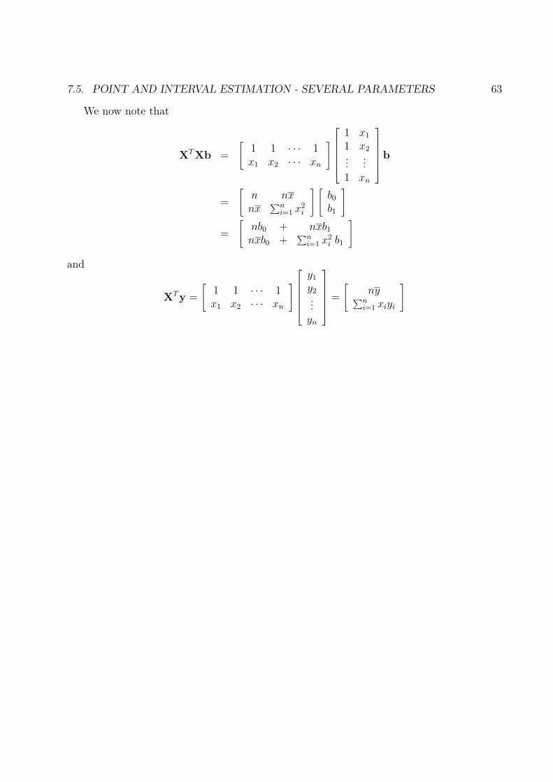
We now note that
XTXb =
[1 1 · · · 1x1 x2 · · · xn
]
1 x1
1 x2...
...1 xn
b
=
[n nxnx
∑ni=1 x2
i
] [b0
b1
]
=
[nb0 + nxb1
nxb0 +∑n
i=1 x2i b1
]
and
XTy =
[1 1 · · · 1x1 x2 · · · xn
]
y1
y2...
yn
=
[ny∑n
i=1 xiyi
]
64 CHAPTER 7. POINT AND INTERVAL ESTIMATION
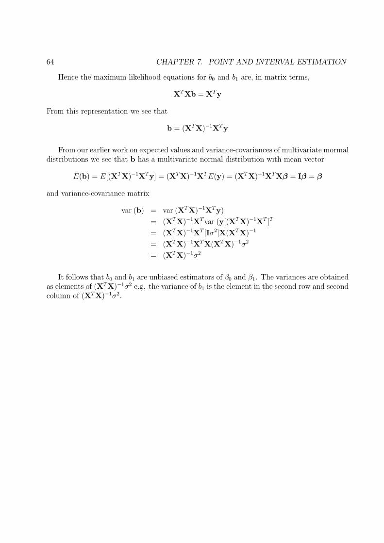
Hence the maximum likelihood equations for b0 and b1 are, in matrix terms,
XTXb = XTy
From this representation we see that
b = (XTX)−1XTy
From our earlier work on expected values and variance-covariances of multivariate mormaldistributions we see that b has a multivariate normal distribution with mean vector
E(b) = E[(XTX)−1XTy] = (XTX)−1XT E(y) = (XTX)−1XTXβ = Iβ = β
and variance-covariance matrix
var (b) = var (XTX)−1XTy)
= (XTX)−1XT var (y[(XTX)−1XT ]T
= (XTX)−1XT [Iσ2]X(XTX)−1
= (XTX)−1XTX(XTX)−1σ2
= (XTX)−1σ2
It follows that b0 and b1 are unbiased estimators of β0 and β1. The variances are obtainedas elements of (XTX)−1σ2 e.g. the variance of b1 is the element in the second row and secondcolumn of (XTX)−1σ2.
7.5. POINT AND INTERVAL ESTIMATION - SEVERAL PARAMETERS 65
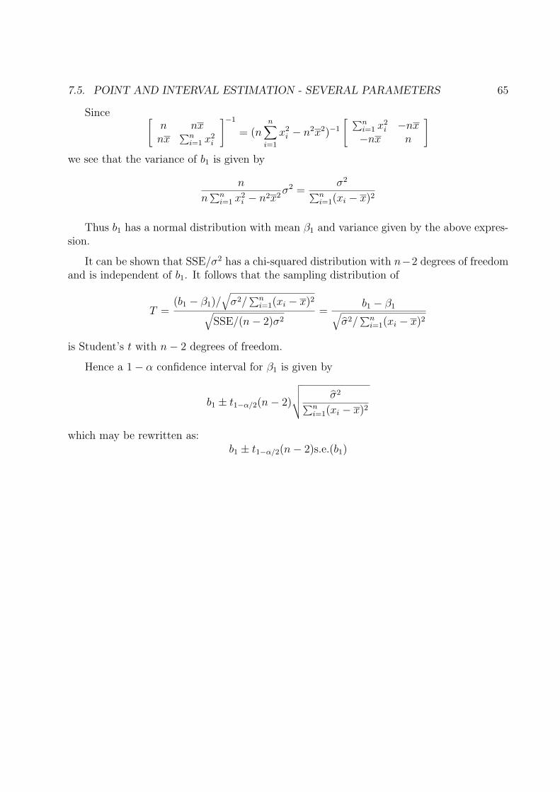
Since [n nxnx
∑ni=1 x2
i
]−1
= (nn∑
i=1
x2i − n2x2)−1
[ ∑ni=1 x2
i −nx−nx n
]
we see that the variance of b1 is given by
n
n∑n
i=1 x2i − n2x2
σ2 =σ2
∑ni=1(xi − x)2
Thus b1 has a normal distribution with mean β1 and variance given by the above expres-sion.
It can be shown that SSE/σ2 has a chi-squared distribution with n−2 degrees of freedomand is independent of b1. It follows that the sampling distribution of
T =(b1 − β1)/
√σ2/
∑ni=1(xi − x)2
√SSE/(n− 2)σ2
=b1 − β1√
σ2/∑n
i=1(xi − x)2
is Student’s t with n− 2 degrees of freedom.
Hence a 1− α confidence interval for β1 is given by
b1 ± t1−α/2(n− 2)
√√√√ σ2
∑ni=1(xi − x)2
which may be rewritten as:b1 ± t1−α/2(n− 2)s.e.(b1)
66 CHAPTER 7. POINT AND INTERVAL ESTIMATION
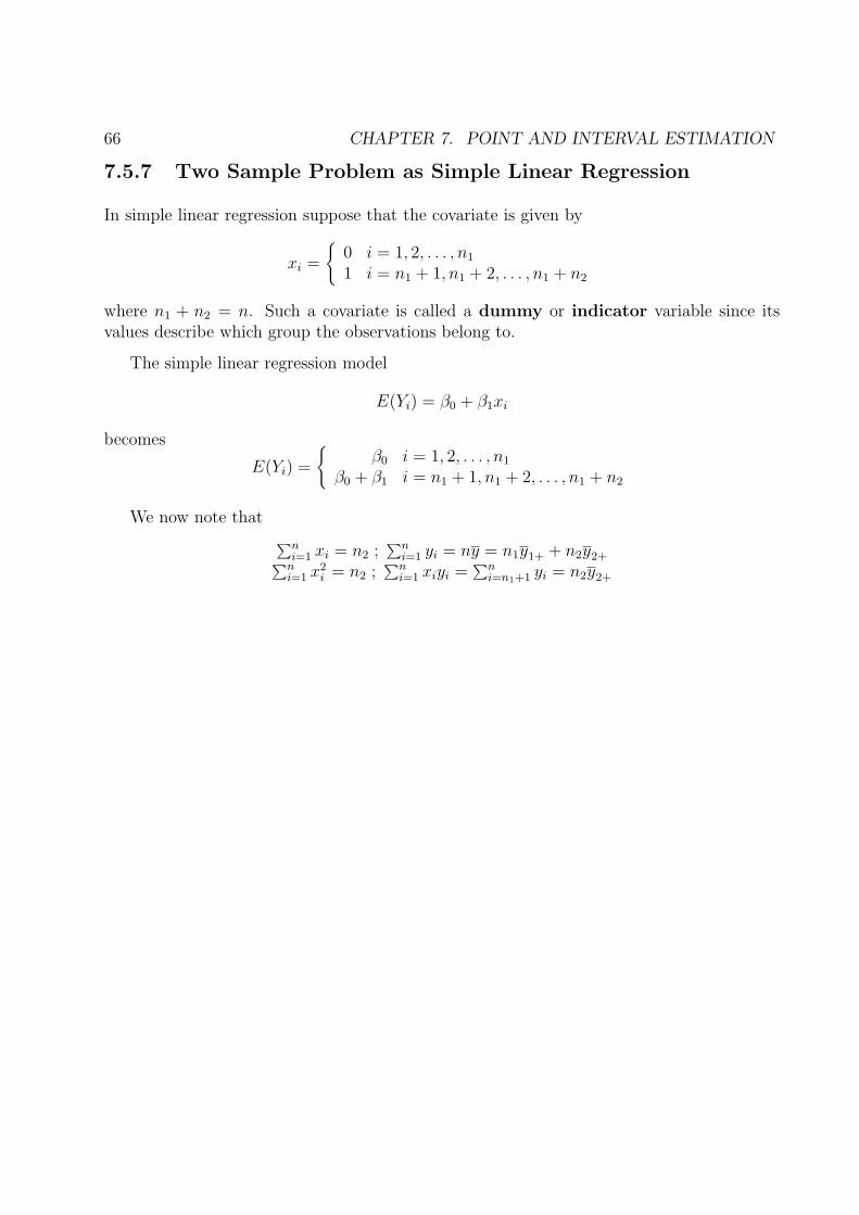
7.5.7 Two Sample Problem as Simple Linear Regression
In simple linear regression suppose that the covariate is given by
xi =
{0 i = 1, 2, . . . , n1
1 i = n1 + 1, n1 + 2, . . . , n1 + n2
where n1 + n2 = n. Such a covariate is called a dummy or indicator variable since itsvalues describe which group the observations belong to.
The simple linear regression model
E(Yi) = β0 + β1xi
becomes
E(Yi) =
{β0 i = 1, 2, . . . , n1
β0 + β1 i = n1 + 1, n1 + 2, . . . , n1 + n2
We now note that
∑ni=1 xi = n2 ;
∑ni=1 yi = ny = n1y1+ + n2y2+∑n
i=1 x2i = n2 ;
∑ni=1 xiyi =
∑ni=n1+1 yi = n2y2+

7.5. POINT AND INTERVAL ESTIMATION - SEVERAL PARAMETERS 67
where we define
Group 1 Group 2y11 = y1 y21 = yn1+1
y12 = y2 y22 = yn1+2
y13 = y3 y23 = yn1+3...
...y1n1 = yn1 y2n2 = yn1+n2
Thus the maximum likelihood equations become
(n1 + n2)b0 + n2b1 = n1y1+ + n2y2+
n2b0 + n2b1 = n2y2+
Subtract the second equation from the first to get
n1b0 = n1y1+ and hence b0 = y1+
It follows thatb1 = y2+ − y1+
68 CHAPTER 7. POINT AND INTERVAL ESTIMATION
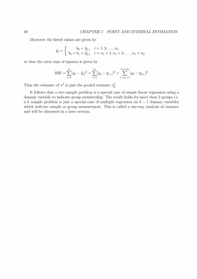
Moreover the fitted values are given by
yi =
{b0 = y1+ i = 1, 2, . . . , n1
b0 + b1 = y2+ i = n1 + 1, n1 + 2, . . . , n1 + n2
so that the error sum of squares is given by
SSE =n∑
i=1
(yi − yi)2 =
n1∑
i=1
(yi − y1+)2 +n1+n2∑
i=n1+1
(yi − y2+)2
Thus the estimate of σ2 is just the pooled estimate s2p.
It follows that a two sample problem is a special case of simple linear regression using adummy variable to indicate group membership. The result holds for more than 2 groups i.e.a k sample problem is just a special case of multiple regression on k − 1 dummy variableswhich indicate sample or group measurement. This is called a one-way analysis of varianceand will be discussed in a later section.

7.5. POINT AND INTERVAL ESTIMATION - SEVERAL PARAMETERS 69
7.5.8 Paired Data
Often we have data in which a response is observed on a collection of individuals at two pointsin time or under two different conditions. Since individuals are most likely independent butobservations on the same individual are probably not independent a two sample procedure isnot appropriate. The simplest approach is to take the difference between the two responses,individual by individual and treat the differences as a one sample problem.
Thus the data are
Subject Response 1 Response 2 Difference1 y11 y21 d1 = y21 − y11
2 y12 y22 d2 = y22 − y12...
......
...n y1n y2n dn = y2n − y1n
The confidence interval for the true mean difference is then based on d with variance s2d/n
exactly as in the case of a one sample problem.
70 CHAPTER 7. POINT AND INTERVAL ESTIMATION
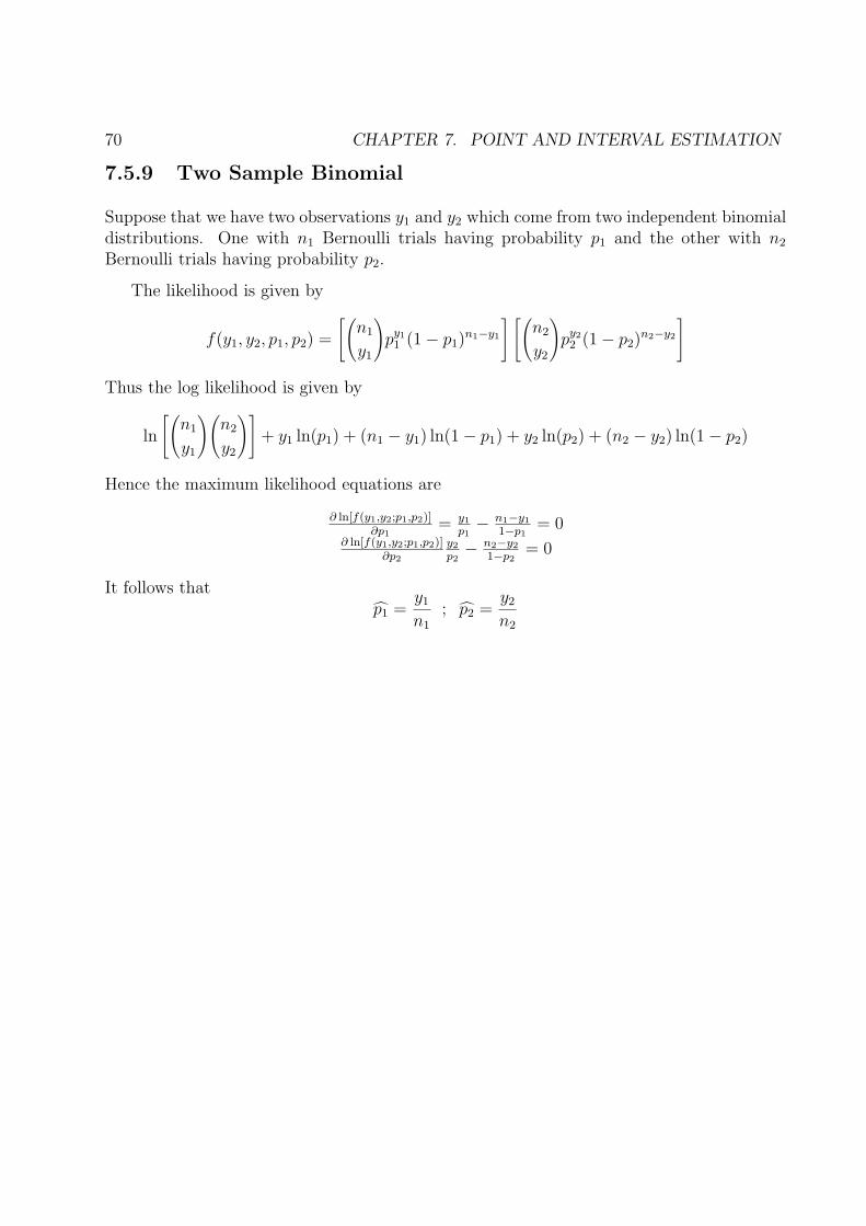
7.5.9 Two Sample Binomial
Suppose that we have two observations y1 and y2 which come from two independent binomialdistributions. One with n1 Bernoulli trials having probability p1 and the other with n2
Bernoulli trials having probability p2.
The likelihood is given by
f(y1, y2, p1, p2) =
[(n1
y1
)py1
1 (1− p1)n1−y1
] [(n2
y2
)py2
2 (1− p2)n2−y2
]
Thus the log likelihood is given by
ln
[(n1
y1
)(n2
y2
)]+ y1 ln(p1) + (n1 − y1) ln(1− p1) + y2 ln(p2) + (n2 − y2) ln(1− p2)
Hence the maximum likelihood equations are
∂ ln[f(y1,y2;p1,p2)]∂p1
= y1
p1− n1−y1
1−p1= 0
∂ ln[f(y1,y2;p1,p2)]∂p2
y2
p2− n2−y2
1−p2= 0
It follows thatp1 =
y1
n1
; p2 =y2
n2
7.5. POINT AND INTERVAL ESTIMATION - SEVERAL PARAMETERS 71
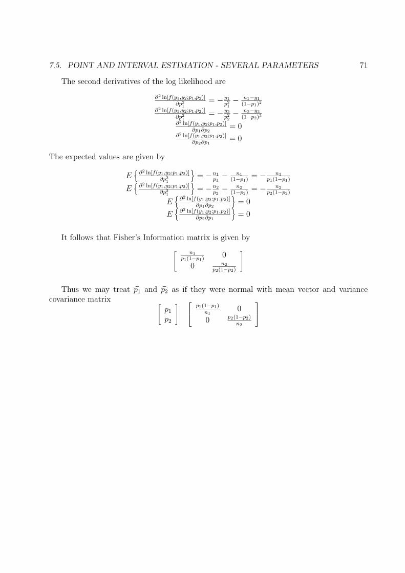
The second derivatives of the log likelihood are
∂2 ln[f(y1,y2;p1,p2)]∂p2
1= −y1
p21− n1−y1
(1−p1)2
∂2 ln[f(y1,y2;p1,p2)]∂p2
1= −y2
p22− n2−y2
(1−p2)2
∂2 ln[f(y1,y2;p1,p2)]∂p1∂p2
= 0∂2 ln[f(y1,y2;p1,p2)]
∂p2∂p1= 0
The expected values are given by
E{
∂2 ln[f(y1,y2;p1,p2)]∂p2
1
}= −n1
p1− n1
(1−p1)= − n1
p1(1−p1)
E{
∂2 ln[f(y1,y2;p1,p2)]∂p2
1
}= −n2
p2− n2
(1−p2)= − n2
p2(1−p2)
E{
∂2 ln[f(y1,y2;p1,p2)]∂p1∂p2
}= 0
E{
∂2 ln[f(y1,y2;p1,p2)]∂p2∂p1
}= 0
It follows that Fisher’s Information matrix is given by
[ n1
p1(1−p1)0
0 n2
p2(1−p2)
]
Thus we may treat p1 and p2 as if they were normal with mean vector and variancecovariance matrix [
p1
p2
]
p1(1−p1)n1
0
0 p2(1−p2)n2
72 CHAPTER 7. POINT AND INTERVAL ESTIMATION
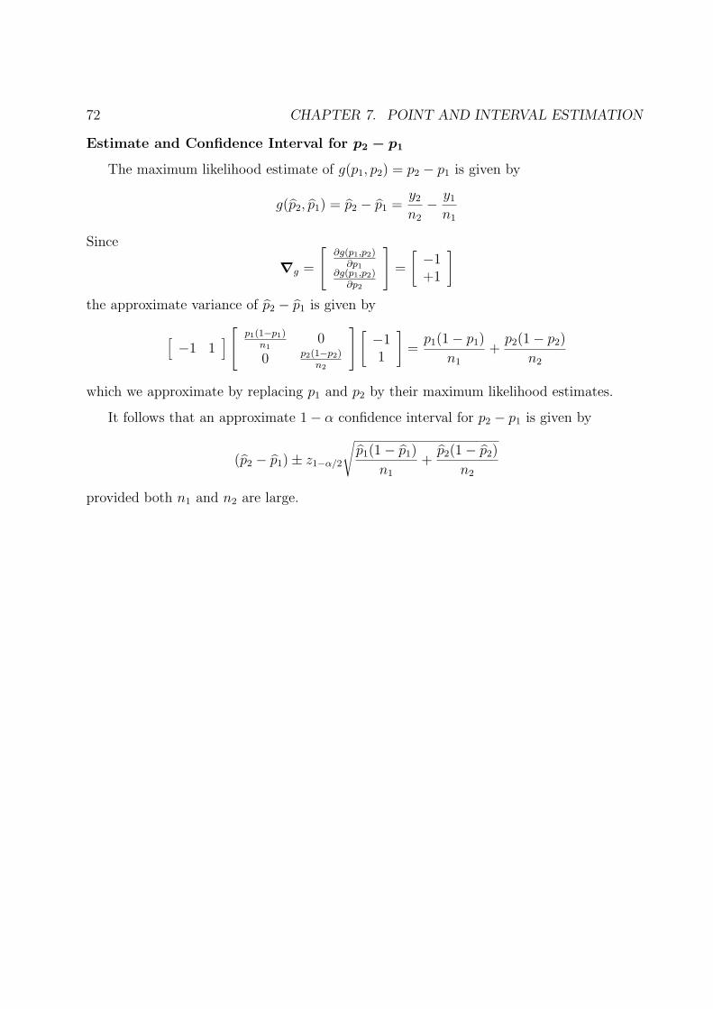
Estimate and Confidence Interval for p2 − p1
The maximum likelihood estimate of g(p1, p2) = p2 − p1 is given by
g(p2, p1) = p2 − p1 =y2
n2
− y1
n1
Since
∇g =
∂g(p1,p2)∂p1
∂g(p1,p2)∂p2
=
[−1+1
]
the approximate variance of p2 − p1 is given by
[−1 1
]
p1(1−p1)n1
0
0 p2(1−p2)n2
[−11
]=
p1(1− p1)
n1
+p2(1− p2)
n2
which we approximate by replacing p1 and p2 by their maximum likelihood estimates.
It follows that an approximate 1− α confidence interval for p2 − p1 is given by
(p2 − p1)± z1−α/2
√p1(1− p1)
n1
+p2(1− p2)
n2
provided both n1 and n2 are large.
7.5. POINT AND INTERVAL ESTIMATION - SEVERAL PARAMETERS 73
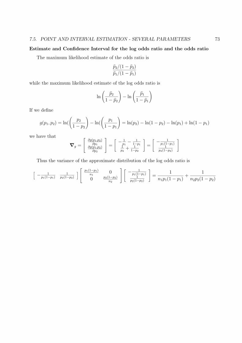
Estimate and Confidence Interval for the log odds ratio and the odds ratio
The maximum likelihood estimate of the odds ratio is
p2/(1− p2)
p1/(1− p1)
while the maximum likelihood estimate of the log odds ratio is
ln
(p2
1− p2
)− ln
(p1
1− p1
)
If we define
g(p1, p2) = ln(
(p2
1− p2
)− ln(
(p1
1− p1
)= ln(p2)− ln(1− p2)− ln(p1) + ln(1− p1)
we have that
∇g =
∂g(p1,p2)∂p1
∂g(p1,p2)∂p2
=
[ − 1p1− 1
1−p11p2
+ 11−p2
]=
[ − 1p1(1−p1)
1p2(1−p2)
]
Thus the variance of the approximate distribution of the log odds ratio is
[− 1
p1(1−p1)1
p2(1−p2)
]
p1(1−p1)n1
0
0 p2(1−p2)n2
[ − 1p1(1−p1)
1p2(1−p2)
]=
1
n1p1(1− p1)+
1
n2p2(1− p2)

74 CHAPTER 7. POINT AND INTERVAL ESTIMATION
We approximate this by
1
n1p1(1− p1)+
1
n2p2(1− p2)=
1
n1p1
+1
n1(1− p1)+
1
n2p2
+1
n2(1− p2)
It follows that a 1− α confidence interval for the log odds ratio is given by
ln
(p2/(1− p2)
p1/(1− p1)
)± z1−α/2
√1
n1p1
+1
n1(1− p1)+
1
n2p2
+1
n2(1− p2)
To obtain a confidence interval for the odds ratio simply exponentiate the endpoints ofthe confidence interval for the log odds ratio.
7.5. POINT AND INTERVAL ESTIMATION - SEVERAL PARAMETERS 75
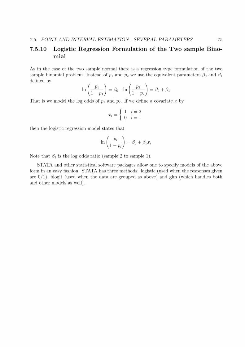
7.5.10 Logistic Regression Formulation of the Two sample Bino-mial
As in the case of the two sample normal there is a regression type formulation of the twosample binomial problem. Instead of p1 and p2 we use the equivalent parameters β0 and β1
defined by
ln
(p1
1− p1
)= β0 ln
(p2
1− p2
)= β0 + β1
That is we model the log odds of p1 and p2. If we define a covariate x by
xi =
{1 i = 20 i = 1
then the logistic regression model states that
ln
(pi
1− pi
)= β0 + β1xi
Note that β1 is the log odds ratio (sample 2 to sample 1).
STATA and other statistical software packages allow one to specify models of the aboveform in an easy fashion. STATA has three methods: logistic (used when the responses givenare 0/1), blogit (used when the data are grouped as above) and glm (which handles bothand other models as well).

76 CHAPTER 7. POINT AND INTERVAL ESTIMATION
Chapter 8
Hypothesis and Significance Testing
The statistical inference called hypothesis or significance testing provides an answer tothe following problem:
Given data and a probability model can we conclude that a parameter θ hasvalue θ0?
• θ0 is a specified value of the parameter θ of particular interest and is called a nullhypothesis.
• In the Neyman Pearson formulation of the hypothesis testing problem the choice isbetween the null hypothesis H0 : θ = θ0 and an alternative hypothesis H1 : θ = θ1.Neyman and Pearson stressed that their approach was based on inductive behavior.
• In the significance testing formulation due mainly to Fisher an alternative hypothe-sis is not explicitly stated. Fisher stressed that his was an approach to inductivereasoning.
• In current practice the two approaches have been combined, the distinctions stressedby their developers has all but disappeared, and we are left with a mess of terms andconcepts which seem to have little to do with advancing science.
77
78 CHAPTER 8. HYPOTHESIS AND SIGNIFICANCE TESTING
8.1 Neyman Pearson Approach
8.1.1 Basic Concepts
A formal approach to the hypothesis testing problem is based on a test of the null hy-pothesis that θ=θ0 versus an alternative hypothesis about θ e.g.
• θ = θ1 ( simple alternative hypothesis).
• θ > θ0 or θ < θ0 (one sided alternative hypotheses)
• θ 6= θ0 (two sided alternative hypothesis).
In a problem in which we have a null hypothesis H0 and an alternative HA there are twotypes of errors that can be made:
• H0 is rejected when it is true.
• H0 is not rejected when it is false.

8.1. NEYMAN PEARSON APPROACH 79
The two types of errors can be summarized in the following table:
“Truth”Conclusion H0 True H0 False
Reject H0 Type I error no errorDo not Reject H0 no error Type II Error
Thus
• Type I Error = reject H0 when H0 is true.
• Type II Error = do not reject H0 when H0 is false.
• Obviously we would prefer not to make either type of error.
• However, in the face of data which is subject to uncertainty we may make errors ofeither type.
• The Neyman-Pearson theory of hypothesis testing is the conventional approach totesting hypotheses.

80 CHAPTER 8. HYPOTHESIS AND SIGNIFICANCE TESTING
8.1.2 Summary of Neyman-Pearson Approach
• Given the data and a probability model, choose a region of possible data values calledthe critical region.
◦ If the observed data falls into the critical region reject the null hypothesis.
◦ The critical region is selected so that it is consistent with departures from H0 infavor of HA.
• The critical region is defined by the values of a test statistic chosen so that:
◦ The probability of obtaining a value of the test statistic in the critical region is≤ α if the null hypothesis is true. i.e. the probability of a Type I error (calledthe size) of the test is required to be ≤ α.
◦ α is called the significance level of the test procedure. Typically α is chosen tobe .05 or .01.
◦ The probability of obtaining a value of the test statistic in the critical region is aslarge as possible if the alternative hypothesis is true. (Equivalently the probabilityof a Type II error is as small as possible).
◦ This probability is called the power of the test.

8.1. NEYMAN PEARSON APPROACH 81
The Neyman-Pearson theory thus tests H0 vs HA so that the probability of aType I error is fixed at level α while the power (ability to detect the alternative)is as large as possible.
Neyman and Pearson justified their approach to the problem from what they called the“inductive behavior” point of view:
“Without hoping to know whether each separate hypothesis is true or falsewe may search for rules to govern our behavior with regard to them, in followingwhich we insure that, in the long run of experience, we shall not be too oftenwrong.”
Thus a test is viewed as a rule of behavior.
82 CHAPTER 8. HYPOTHESIS AND SIGNIFICANCE TESTING
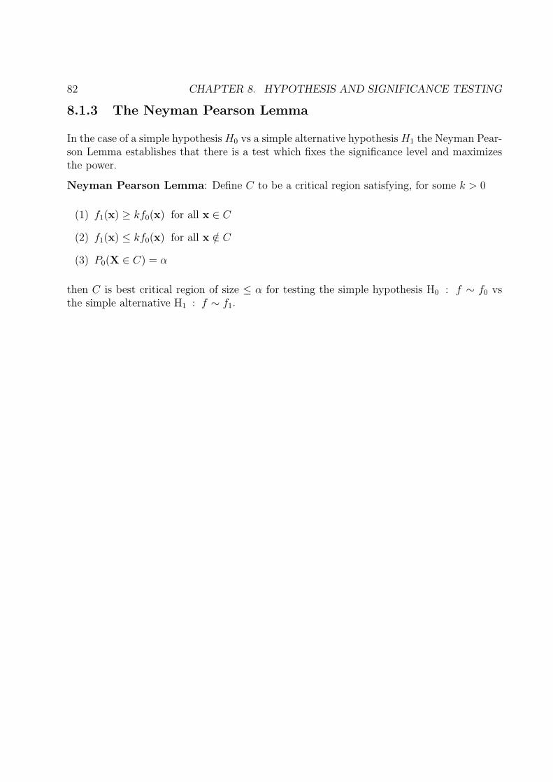
8.1.3 The Neyman Pearson Lemma
In the case of a simple hypothesis H0 vs a simple alternative hypothesis H1 the Neyman Pear-son Lemma establishes that there is a test which fixes the significance level and maximizesthe power.
Neyman Pearson Lemma: Define C to be a critical region satisfying, for some k > 0
(1) f1(x) ≥ kf0(x) for all x ∈ C
(2) f1(x) ≤ kf0(x) for all x /∈ C
(3) P0(X ∈ C) = α
then C is best critical region of size ≤ α for testing the simple hypothesis H0 : f ∼ f0 vsthe simple alternative H1 : f ∼ f1.

8.1. NEYMAN PEARSON APPROACH 83
• All points x for whichf1(x)
f0(x)> k
are in the critical region C
• Points for which the ratio is equal to k can be either in C or in C.
• The ratiof1(x)
f0(x)
is called the likelihood ratio.
• Points are in the critical region according to how strongly they support the alternativehypotheis vis a vis the null hypothesis i.e. according to the magnitude of the likelihoodratio.
◦ That is, points in the critical region have the most value for discriminating betweenthe two hypotheses subject to the restriction that their probability under the nullhypothesis be less than or equal to α.
84 CHAPTER 8. HYPOTHESIS AND SIGNIFICANCE TESTING
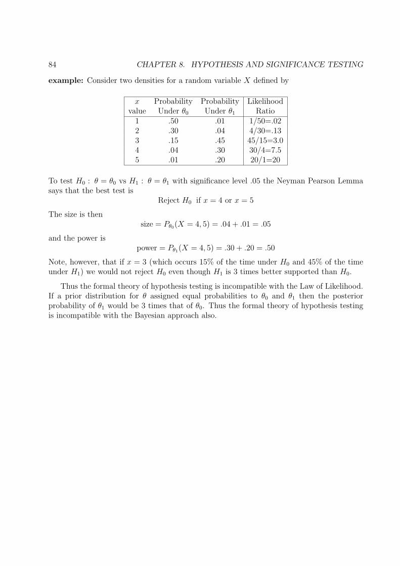
example: Consider two densities for a random variable X defined by
x Probability Probability Likelihoodvalue Under θ0 Under θ1 Ratio
1 .50 .01 1/50=.022 .30 .04 4/30=.133 .15 .45 45/15=3.04 .04 .30 30/4=7.55 .01 .20 20/1=20
To test H0 : θ = θ0 vs H1 : θ = θ1 with significance level .05 the Neyman Pearson Lemmasays that the best test is
Reject H0 if x = 4 or x = 5
The size is thensize = Pθ0(X = 4, 5) = .04 + .01 = .05
and the power ispower = Pθ1(X = 4, 5) = .30 + .20 = .50
Note, however, that if x = 3 (which occurs 15% of the time under H0 and 45% of the timeunder H1) we would not reject H0 even though H1 is 3 times better supported than H0.
Thus the formal theory of hypothesis testing is incompatible with the Law of Likelihood.If a prior distribution for θ assigned equal probabilities to θ0 and θ1 then the posteriorprobability of θ1 would be 3 times that of θ0. Thus the formal theory of hypothesis testingis incompatible with the Bayesian approach also.
8.1. NEYMAN PEARSON APPROACH 85
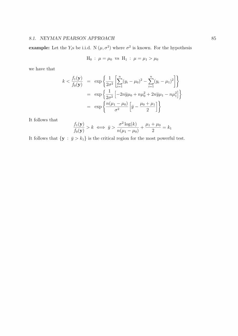
example: Let the Yis be i.i.d. N (µ, σ2) where σ2 is known. For the hypothesis
H0 : µ = µ0 vs H1 : µ = µ1 > µ0
we have that
k <f1(y)
f0(y)= exp
{1
2σ2
[n∑
i=1
(yi − µ0)2 −
n∑
i=1
(yi − µ1)2
]}
= exp{
1
2σ2
[−2nyµ0 + nµ2
0 + 2nyµ1 − nµ21
]}
= exp
{n(µ1 − µ0)
σ2
[y − µ0 + µ1
2
]}
It follows thatf1(y)
f0(y)> k ⇐⇒ y >
σ2 log(k)
n(µ1 − µ0)+
µ1 + µ0
2= k1
It follows that {y : y > k1} is the critical region for the most powerful test.

86 CHAPTER 8. HYPOTHESIS AND SIGNIFICANCE TESTING
If we want the critical region to have size α then we choose k1 so that
P0(Y > k1) = α
i.e.
P0
(√n(Y − µ0)
σ>
√n(k1 − µ0)
σ
)= α
Thusk1 = µ0 + z1−α
σ√n
The test procedure is thus to reject when the observed value of Y exceeds
k1 = µ0 + z1−ασ√n
For this test we have that the power is given by
P1(Y ≥ k1) = P1
(Y ≥ µ0 + z1−α
σ√n
)
= P1
(√n(Y − µ1)
σ≥ −
√n(µ1 − µ0)
σ+ z1−α
)
= P
(Z ≥ −
√n(µ1 − µ0)
σ+ z1−α
)

8.1. NEYMAN PEARSON APPROACH 87
If the alternative hypothesis was that µ = µ1 < µ0 the test would be to reject if
y ≤ µ0 − z1−ασ√n
and the power of this test would be given by
P
(Z ≤
√n(µ0 − µ1)
σ− z1−α
)
There are several important features of the power of this test:
• As the difference between µ1 and µ0 increases the power increases.
• As n increases the power increases.
• As σ2 decreases the power increases.

88 CHAPTER 8. HYPOTHESIS AND SIGNIFICANCE TESTING
8.1.4 Sample Size and Power
application:In a study on the effects of chronic exposure to lead, a group of 34 children living near alead smelter in El Paso, Texas were found to have elevated blood lead levels.
• A variety of tests were performed to measure neurological and psychological function.
• For IQ measurements the following data were recorded:
sample mean = y = 96.44 and standard error = 2.36
where y is the response variable and is the IQ of a subject.
• Assuming the data are normally distributed (IQs often are), the 95% confidence intervalfor µ, defined as the population mean IQ for children with elevated blood lead values,is given by
96.44± (2.035)(2.36) or 91.6 to 101.2
where 2.035 is the .975 Student’s t value with 33 degrees of freedom.
• Thus values of µ between 91.6 and 101.3 are consistent with the data at a 95% confi-dence level.
8.1. NEYMAN PEARSON APPROACH 89
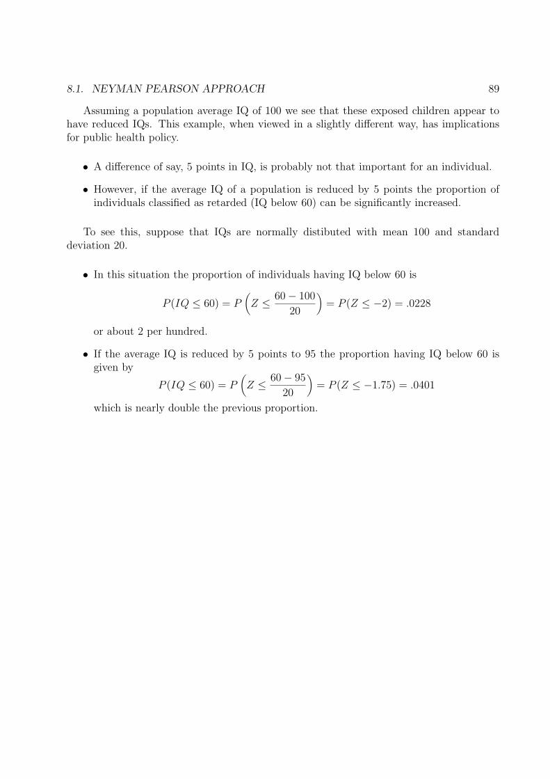
Assuming a population average IQ of 100 we see that these exposed children appear tohave reduced IQs. This example, when viewed in a slightly different way, has implicationsfor public health policy.
• A difference of say, 5 points in IQ, is probably not that important for an individual.
• However, if the average IQ of a population is reduced by 5 points the proportion ofindividuals classified as retarded (IQ below 60) can be significantly increased.
To see this, suppose that IQs are normally distibuted with mean 100 and standarddeviation 20.
• In this situation the proportion of individuals having IQ below 60 is
P (IQ ≤ 60) = P(Z ≤ 60− 100
20
)= P (Z ≤ −2) = .0228
or about 2 per hundred.
• If the average IQ is reduced by 5 points to 95 the proportion having IQ below 60 isgiven by
P (IQ ≤ 60) = P(Z ≤ 60− 95
20
)= P (Z ≤ −1.75) = .0401
which is nearly double the previous proportion.
90 CHAPTER 8. HYPOTHESIS AND SIGNIFICANCE TESTING
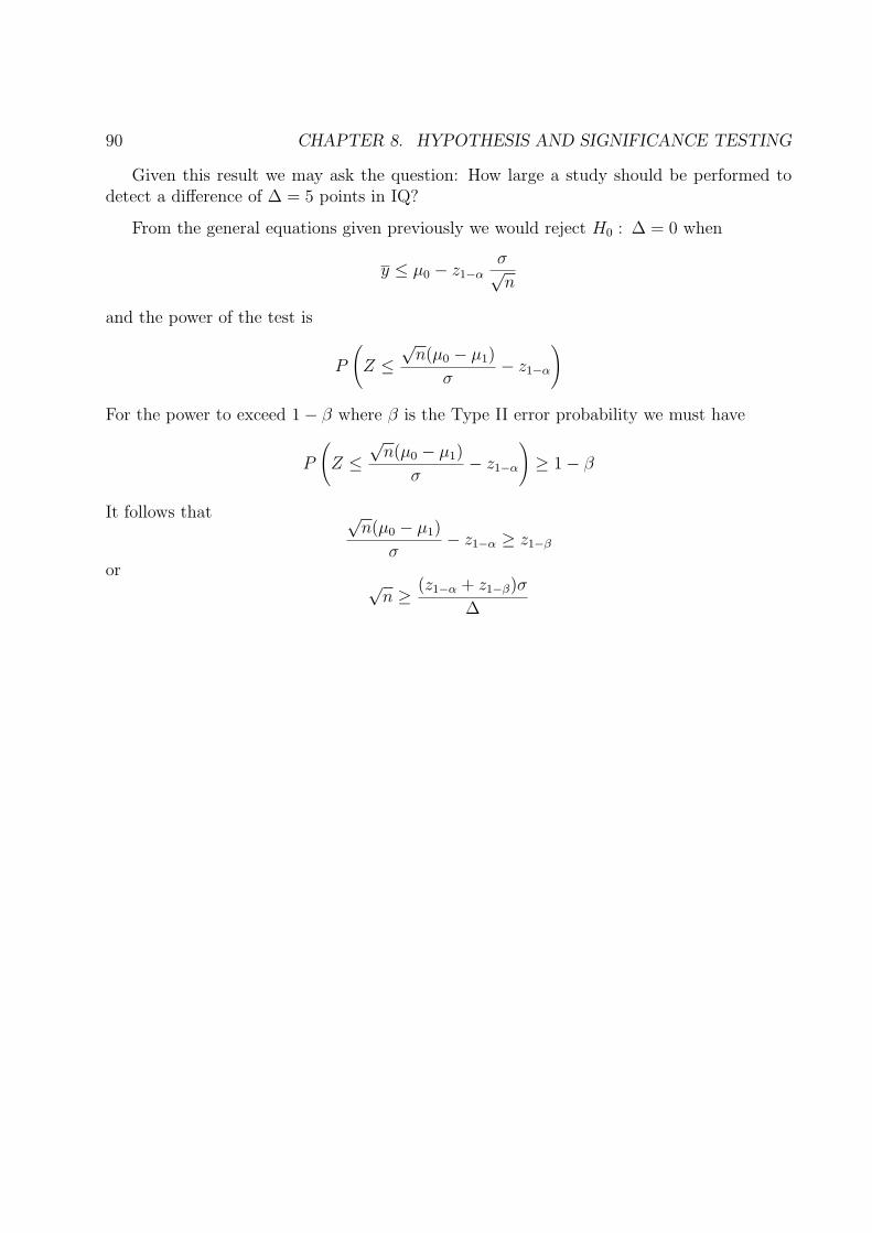
Given this result we may ask the question: How large a study should be performed todetect a difference of ∆ = 5 points in IQ?
From the general equations given previously we would reject H0 : ∆ = 0 when
y ≤ µ0 − z1−ασ√n
and the power of the test is
P
(Z ≤
√n(µ0 − µ1)
σ− z1−α
)
For the power to exceed 1− β where β is the Type II error probability we must have
P
(Z ≤
√n(µ0 − µ1)
σ− z1−α
)≥ 1− β
It follows that √n(µ0 − µ1)
σ− z1−α ≥ z1−β
or √n ≥ (z1−α + z1−β)σ
∆

8.1. NEYMAN PEARSON APPROACH 91
Thus the sample size must satisfy
n ≥ (z1−α + z1−β)2σ2
∆2
For the example with IQ’s we have that
∆ = 5 z1−α = 1.645 z1−β = .84 σ = 20
for a test with size .05 and power .80. Thus we need a sample size of at least
n ≥ (1.645 + .84)2 × 202
52= 98.8
i.e. we need a sample size of at least 99 to detect a difference of 5 IQ points.
92 CHAPTER 8. HYPOTHESIS AND SIGNIFICANCE TESTING
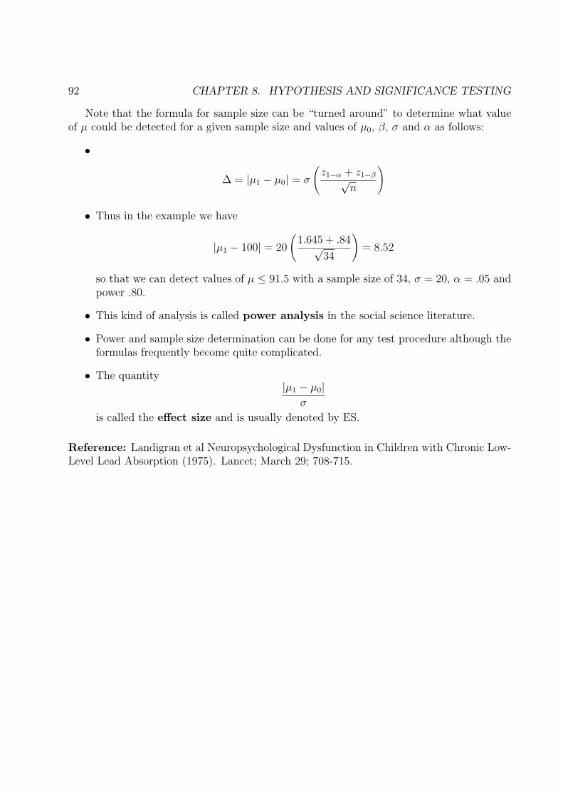
Note that the formula for sample size can be “turned around” to determine what valueof µ could be detected for a given sample size and values of µ0, β, σ and α as follows:
•
∆ = |µ1 − µ0| = σ
(z1−α + z1−β√
n
)
• Thus in the example we have
|µ1 − 100| = 20
(1.645 + .84√
34
)= 8.52
so that we can detect values of µ ≤ 91.5 with a sample size of 34, σ = 20, α = .05 andpower .80.
• This kind of analysis is called power analysis in the social science literature.
• Power and sample size determination can be done for any test procedure although theformulas frequently become quite complicated.
• The quantity|µ1 − µ0|
σ
is called the effect size and is usually denoted by ES.
Reference: Landigran et al Neuropsychological Dysfunction in Children with Chronic Low-Level Lead Absorption (1975). Lancet; March 29; 708-715.
8.2. GENERALIZED LIKELIHOOD RATIO TESTS 93
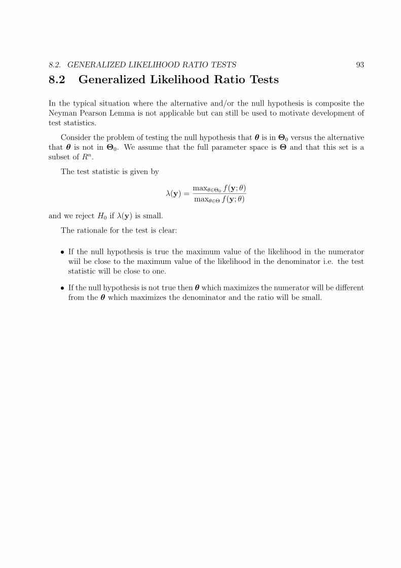
8.2 Generalized Likelihood Ratio Tests
In the typical situation where the alternative and/or the null hypothesis is composite theNeyman Pearson Lemma is not applicable but can still be used to motivate development oftest statistics.
Consider the problem of testing the null hypothesis that θ is in Θ0 versus the alternativethat θ is not in Θ0. We assume that the full parameter space is Θ and that this set is asubset of Rn.
The test statistic is given by
λ(y) =maxθ∈Θ0 f(y; θ)
maxθ∈Θ f(y; θ)
and we reject H0 if λ(y) is small.
The rationale for the test is clear:
• If the null hypothesis is true the maximum value of the likelihood in the numeratorwiil be close to the maximum value of the likelihood in the denominator i.e. the teststatistic will be close to one.
• If the null hypothesis is not true then θ which maximizes the numerator will be differentfrom the θ which maximizes the denominator and the ratio will be small.

94 CHAPTER 8. HYPOTHESIS AND SIGNIFICANCE TESTING
Such tests are called generalized likelihood ratio tests and they have some desirableproperties:
• They reduce to the Neyman Pearson Lemma when the null and the alternative aresimple.
• They usually have desirable large sample properties.
• They usually give tests with useful interpretations.
The procedure for developing generalized likelihood ratio tests is simple:
(1) Find the maximum likelihood estimate of θ under the null hypothesis and calculatef(y; θ) at this value of θ.
(2) Find the maximum likelihood estimate of θ under the full parameter space and calcu-late f(y; θ) at this value of θ.
(3) Form the ratio and simplify to a statistic whose sampling distribution can be foundeither exactly or approximately.
(4) Determine critical values for this statistic, compute the observed value and thus testthe hypothesis.
8.2. GENERALIZED LIKELIHOOD RATIO TESTS 95
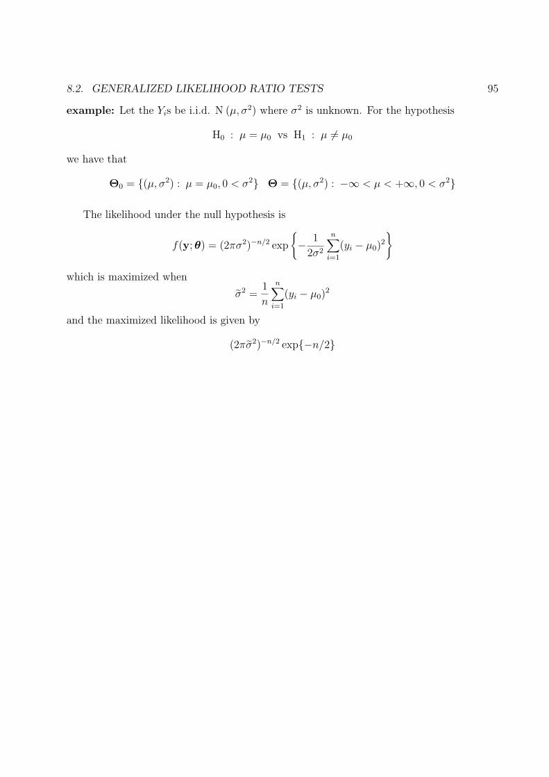
example: Let the Yis be i.i.d. N (µ, σ2) where σ2 is unknown. For the hypothesis
H0 : µ = µ0 vs H1 : µ 6= µ0
we have that
Θ0 = {(µ, σ2) : µ = µ0, 0 < σ2} Θ = {(µ, σ2) : −∞ < µ < +∞, 0 < σ2}
The likelihood under the null hypothesis is
f(y; θ) = (2πσ2)−n/2 exp
{− 1
2σ2
n∑
i=1
(yi − µ0)2
}
which is maximized when
σ2 =1
n
n∑
i=1
(yi − µ0)2
and the maximized likelihood is given by
(2πσ2)−n/2 exp{−n/2}
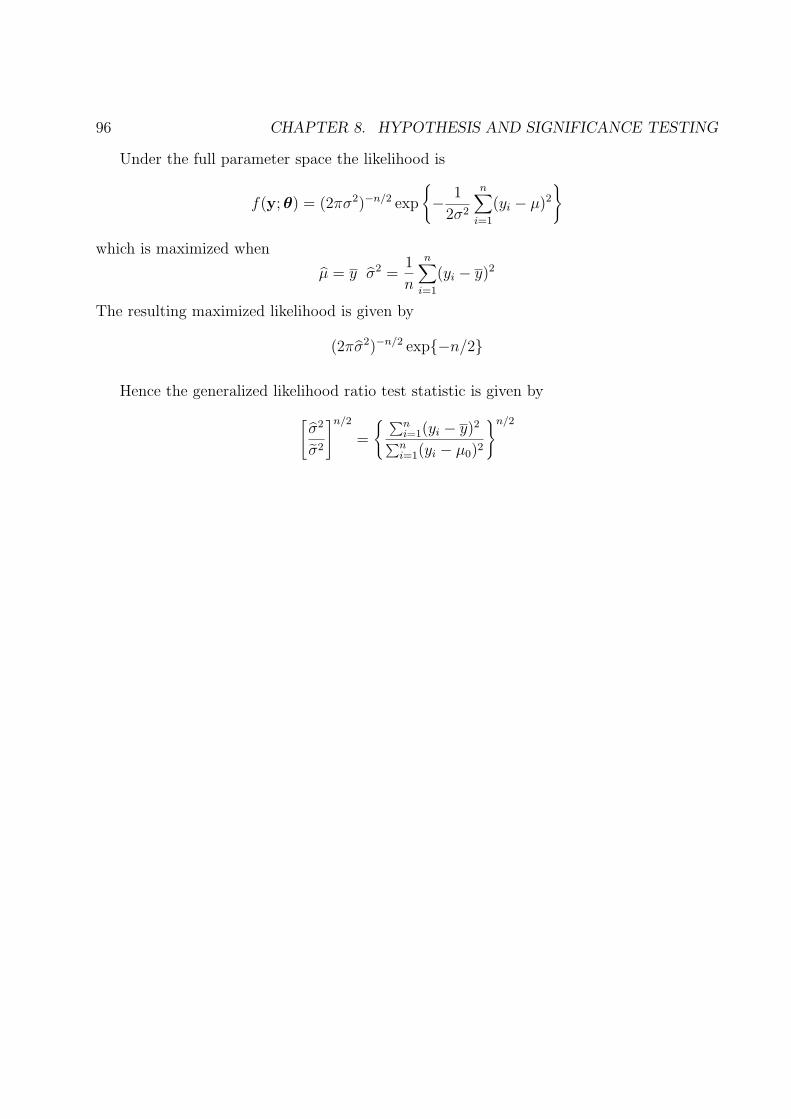
96 CHAPTER 8. HYPOTHESIS AND SIGNIFICANCE TESTING
Under the full parameter space the likelihood is
f(y; θ) = (2πσ2)−n/2 exp
{− 1
2σ2
n∑
i=1
(yi − µ)2
}
which is maximized when
µ = y σ2 =1
n
n∑
i=1
(yi − y)2
The resulting maximized likelihood is given by
(2πσ2)−n/2 exp{−n/2}
Hence the generalized likelihood ratio test statistic is given by
[σ2
σ2
]n/2
=
{ ∑ni=1(yi − y)2
∑ni=1(yi − µ0)2
}n/2
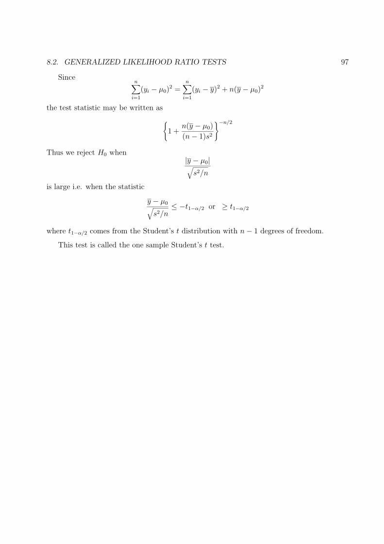
8.2. GENERALIZED LIKELIHOOD RATIO TESTS 97
Sincen∑
i=1
(yi − µ0)2 =
n∑
i=1
(yi − y)2 + n(y − µ0)2
the test statistic may be written as
{1 +
n(y − µ0)
(n− 1)s2
}−n/2
Thus we reject H0 when|y − µ0|√
s2/n
is large i.e. when the statistic
y − µ0√s2/n
≤ −t1−α/2 or ≥ t1−α/2
where t1−α/2 comes from the Student’s t distribution with n− 1 degrees of freedom.
This test is called the one sample Student’s t test.
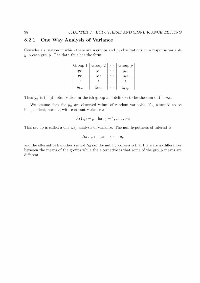
98 CHAPTER 8. HYPOTHESIS AND SIGNIFICANCE TESTING
8.2.1 One Way Analysis of Variance
Consider a situation in which there are p groups and ni observations on a response variabley in each group. The data thus has the form:
Group 1 Group 2 · · · Group py11 y21 · · · yp1
y12 y22 · · · yp2
......
......
y1n1 y2n2 · · · ypnp
Thus yij is the jth observation in the ith group and define n to be the sum of the nis.
We assume that the yij are observed values of random variables, Yij, assumed to beindependent, normal, with constant variance and
E(Yij) = µi for j = 1, 2, . . . , ni
This set up is called a one way analysis of variance. The null hypothesis of interest is
H0 : µ1 = µ2 = · · · = µp
and the alternative hypothesis is not H0 i.e. the null hypothesis is that there are no differencesbetween the means of the groups while the alternative is that some of the group means aredifferent.
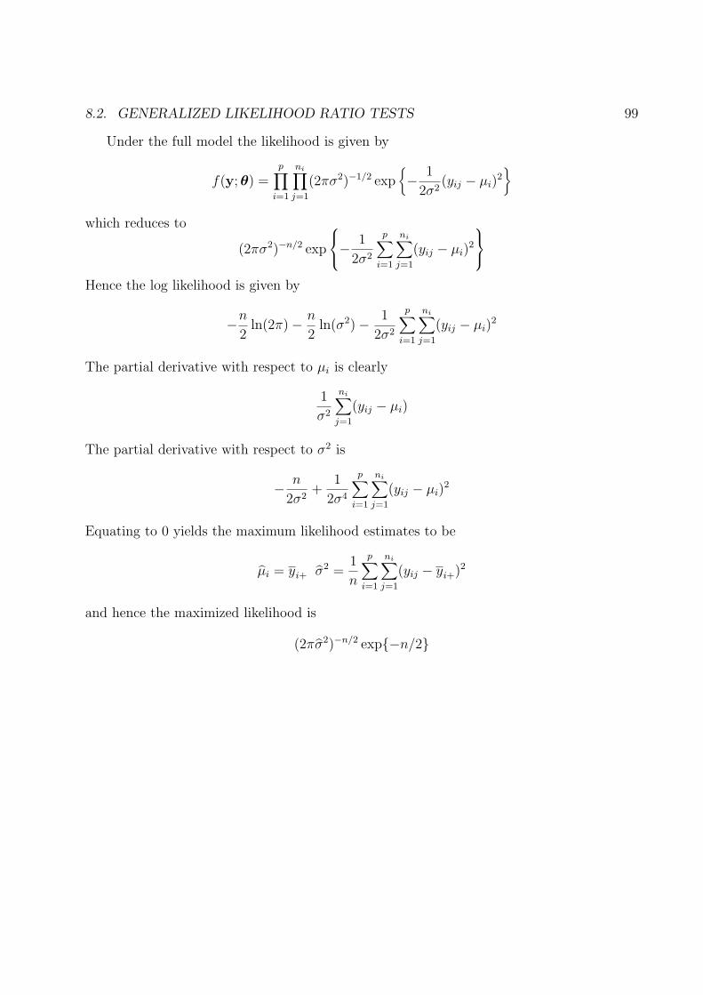
8.2. GENERALIZED LIKELIHOOD RATIO TESTS 99
Under the full model the likelihood is given by
f(y; θ) =p∏
i=1
ni∏
j=1
(2πσ2)−1/2 exp{− 1
2σ2(yij − µi)
2}
which reduces to
(2πσ2)−n/2 exp
−
1
2σ2
p∑
i=1
ni∑
j=1
(yij − µi)2
Hence the log likelihood is given by
−n
2ln(2π)− n
2ln(σ2)− 1
2σ2
p∑
i=1
ni∑
j=1
(yij − µi)2
The partial derivative with respect to µi is clearly
1
σ2
ni∑
j=1
(yij − µi)
The partial derivative with respect to σ2 is
− n
2σ2+
1
2σ4
p∑
i=1
ni∑
j=1
(yij − µi)2
Equating to 0 yields the maximum likelihood estimates to be
µi = yi+ σ2 =1
n
p∑
i=1
ni∑
j=1
(yij − yi+)2
and hence the maximized likelihood is
(2πσ2)−n/2 exp{−n/2}
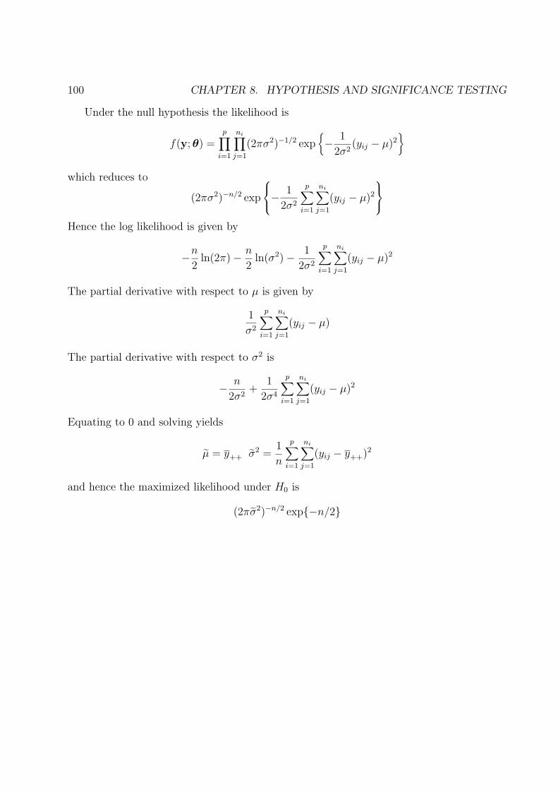
100 CHAPTER 8. HYPOTHESIS AND SIGNIFICANCE TESTING
Under the null hypothesis the likelihood is
f(y; θ) =p∏
i=1
ni∏
j=1
(2πσ2)−1/2 exp{− 1
2σ2(yij − µ)2
}
which reduces to
(2πσ2)−n/2 exp
−
1
2σ2
p∑
i=1
ni∑
j=1
(yij − µ)2
Hence the log likelihood is given by
−n
2ln(2π)− n
2ln(σ2)− 1
2σ2
p∑
i=1
ni∑
j=1
(yij − µ)2
The partial derivative with respect to µ is given by
1
σ2
p∑
i=1
ni∑
j=1
(yij − µ)
The partial derivative with respect to σ2 is
− n
2σ2+
1
2σ4
p∑
i=1
ni∑
j=1
(yij − µ)2
Equating to 0 and solving yields
µ = y++ σ2 =1
n
p∑
i=1
ni∑
j=1
(yij − y++)2
and hence the maximized likelihood under H0 is
(2πσ2)−n/2 exp{−n/2}
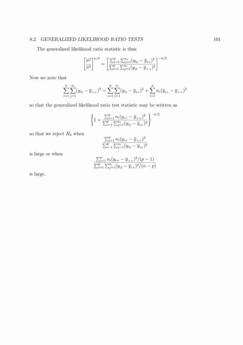
8.2. GENERALIZED LIKELIHOOD RATIO TESTS 101
The generalized likelihood ratio statistic is thus
[σ2
σ2
]n/2
=
[ ∑pi=1
∑nij=1(yij − yi+)2
∑pi=1
∑nij=1(yij − y++)2
]−n/2
Now we note that
p∑
i=1
ni∑
j=1
(yij − y++)2 =p∑
i=1
ni∑
j=1
(yij − yi+)2 +p∑
i=1
ni(yi+ − y++)2
so that the generalized likelihood ratio test statistic may be written as
{1 +
∑pi=1 ni(yi+ − y++)2
∑pi=1
∑nij=1(yij − yi+)2
}−n/2
so that we reject H0 when ∑pi=1 ni(yi+ − y++)2
∑pi=1
∑nij=1(yij − yi+)2
is large or when ∑pi=1 ni(yi+ − y++)2/(p− 1)∑p
i=1
∑nij=1(yij − yi+)2/(n− p)
is large.

102 CHAPTER 8. HYPOTHESIS AND SIGNIFICANCE TESTING
The sampling distribution of this later statistic is F with p − 1 and n − p degrees offreedom.
Thus the generalized likelihood ratio test is to reject H0, all group means equal when thestatistic
Fobs =
∑pi=1 ni(yi+ − y++)2/(p− 1)∑p
i=1
∑nij=1(yij − yi+)2/(n− p)
exceeds the critical value of the F distribution with p− 1 and n− p degrees of freedom.
Preliminary exploration of the data should include calculation of the sample means anda boxplot for each group. These provide rough conclusions about equality of the groups anda quick check on the equality of variability between groups.
8.3. SIGNIFICANCE TESTING AND P-VALUES 103
8.3 Significance Testing and P-Values
Long before the development of the Neyman-Pearson theory significance tests were used toinvestigate hypotheses. These tests were developed on the basis of intuition and were usedto determine whether or a not a given hypothesis was consistent with the observed data.An alternative hypothesis was not explicitly mentioned. Fisher’s thoughts about significancetests were that they are part of a process of “inductive reasoning” from the data to scientificconclusions. After Neyman and Pearson the tests developed by their theories began to beused as significance tests. Thus the two approaches merged and are today considered asbranches of the same theory.
8.3.1 P Values
Definition: The P-value associated with a statistical test is the probability of obtaininga result as or more extreme than that observed.
• Note that the probability is calculated under the assumption that the null hypothesisis true.

104 CHAPTER 8. HYPOTHESIS AND SIGNIFICANCE TESTING
8.3.2 Interpretation of P-values
In this sction we discuss the conventional interpretation of P-values. By definition the P-value gives the chance of observing a result as or more extreme when the null hypothesis istrue under the assumed model.
Thus finding a small P-value in an analysis means either:
• the model is wrong or
• a rare event has occurred or
• the null hypothesis is not true
Given that we assume the model to be true and that it is unlikely that a rare event hasoccurred, a small P-value leads to the conclusion that H0 is not true.
By convention, the P-value for a two-sided test is taken to be the twice the one-sidedP-value.

8.3. SIGNIFICANCE TESTING AND P-VALUES 105
By convention statisticians have chosen the following guidelines for assessing the magni-tude of P values:
• P value greater than .10, not statistically significant.
• P value between .10 and .05, marginally statistically significant (R)
• P value between .05 and .01, statistically significant, (*)
• P value between .01 and .001, statistically significant, (**)
• P value less than .001, statistically significant, (***)
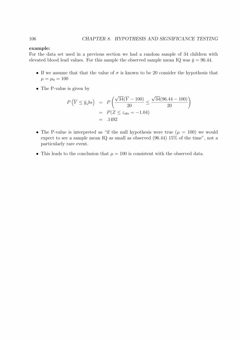
106 CHAPTER 8. HYPOTHESIS AND SIGNIFICANCE TESTING
example:For the data set used in a previous section we had a random sample of 34 children withelevated blood lead values. For this sample the observed sample mean IQ was y = 96.44.
• If we assume that that the value of σ is known to be 20 consider the hypothesis thatµ = µ0 = 100
• The P-value is given by
P(Y ≤ yobs
)= P
(√34(Y − 100)
20≤√
34(96.44− 100)
20
)
= P (Z ≤ zobs = −1.04)
= .1492
• The P-value is interpreted as “if the null hypothesis were true (µ = 100) we wouldexpect to see a sample mean IQ as small as observed (96.44) 15% of the time”, not aparticularly rare event.
• This leads to the conclusion that µ = 100 is consistent with the observed data.
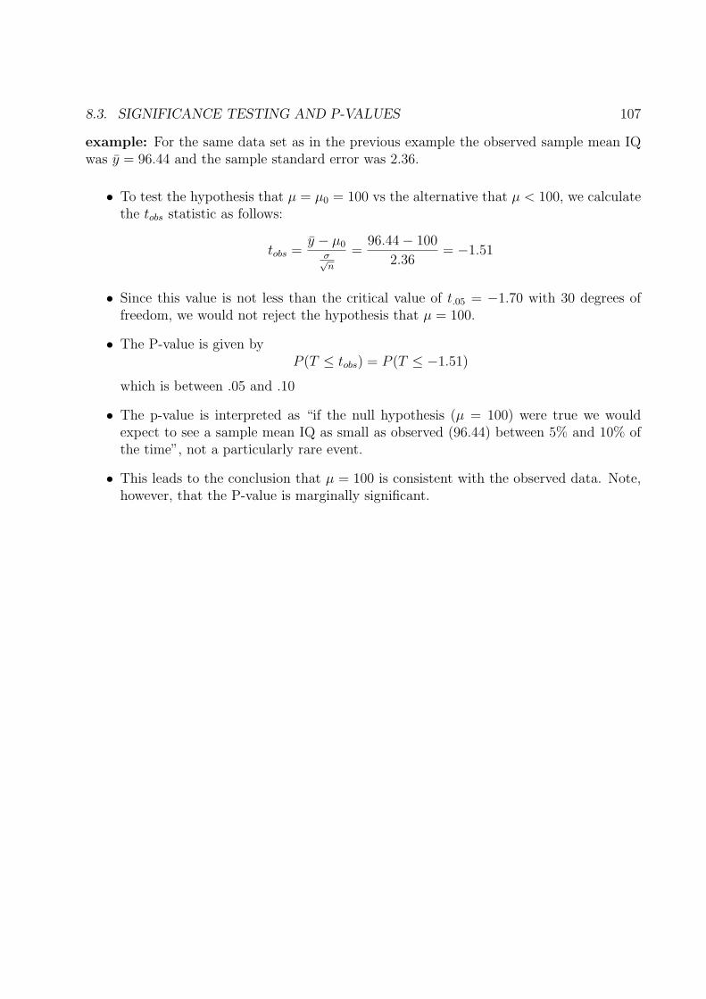
8.3. SIGNIFICANCE TESTING AND P-VALUES 107
example: For the same data set as in the previous example the observed sample mean IQwas y = 96.44 and the sample standard error was 2.36.
• To test the hypothesis that µ = µ0 = 100 vs the alternative that µ < 100, we calculatethe tobs statistic as follows:
tobs =y − µ0
σ√n
=96.44− 100
2.36= −1.51
• Since this value is not less than the critical value of t.05 = −1.70 with 30 degrees offreedom, we would not reject the hypothesis that µ = 100.
• The P-value is given byP (T ≤ tobs) = P (T ≤ −1.51)
which is between .05 and .10
• The p-value is interpreted as “if the null hypothesis (µ = 100) were true we wouldexpect to see a sample mean IQ as small as observed (96.44) between 5% and 10% ofthe time”, not a particularly rare event.
• This leads to the conclusion that µ = 100 is consistent with the observed data. Note,however, that the P-value is marginally significant.
108 CHAPTER 8. HYPOTHESIS AND SIGNIFICANCE TESTING
8.3.3 Two Sample Tests
Suppose we are given two random samples
x1, x2, . . . , xn1 and y1, y2, . . . , yn2
with the x sample coming from a N(µ1, σ2) population and the y sample coming from a
N(µ2, σ2) population. Of interest is the null hypothesis that µ1 = µ2.
• The test statistic in this case is
tobs =y − x√
s2p
(1n1
+ 1n2
)
where
s2p =
(n1 − 1)s21 + (n2 − 1)s2
2
n1 + n2 − 2
is the pooled estimate of σ2. We reject in this case if
– tobs ≥ t1−α if the alternative is µ2 > µ1
– tobs ≤ −t1−α if the alternative is µ2 < µ1
– |tobs| ≥ t1−α/2 if the alternative is µ2 6= µ1
• The P-values for each of the one sided hypotheses is given by
P-value = P (T ≥ |tobs|)
and is twice the above P-value for the two sided hypothesis.
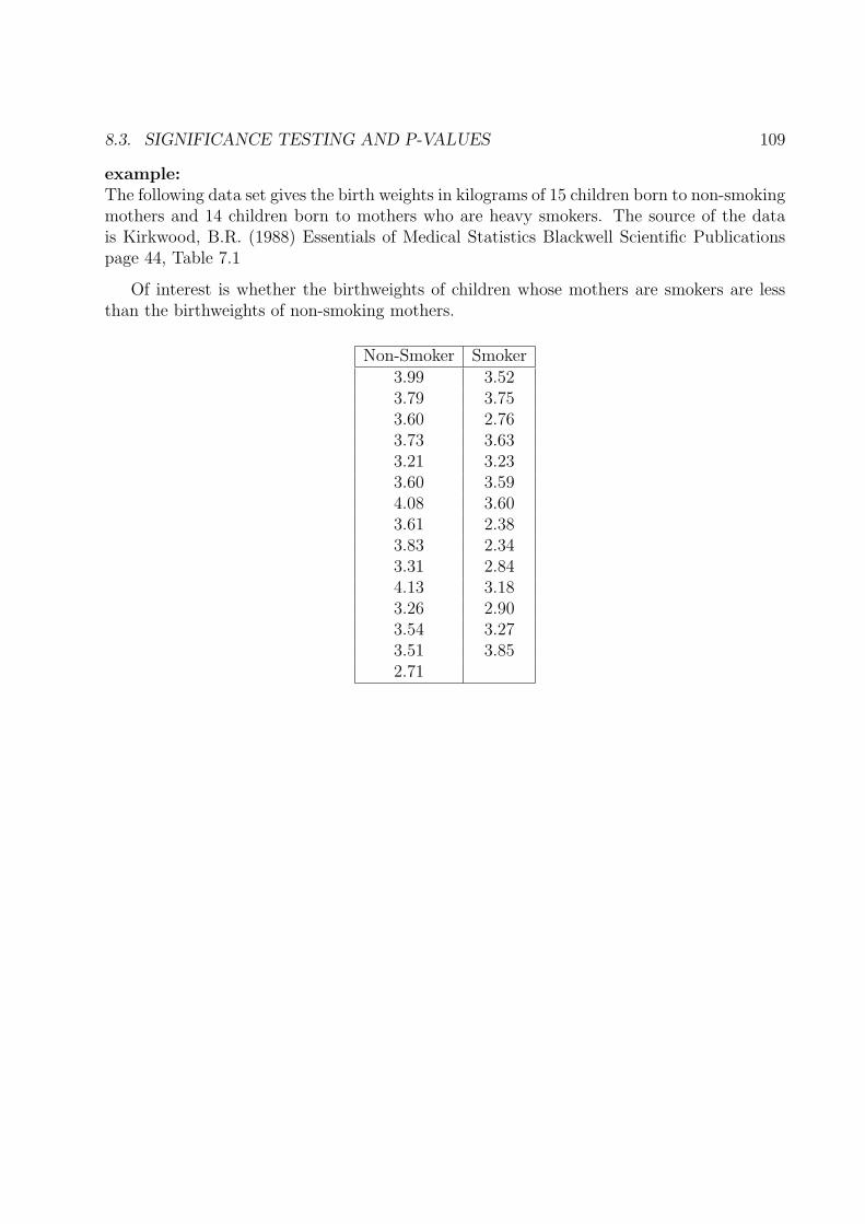
8.3. SIGNIFICANCE TESTING AND P-VALUES 109
example:The following data set gives the birth weights in kilograms of 15 children born to non-smokingmothers and 14 children born to mothers who are heavy smokers. The source of the datais Kirkwood, B.R. (1988) Essentials of Medical Statistics Blackwell Scientific Publicationspage 44, Table 7.1
Of interest is whether the birthweights of children whose mothers are smokers are lessthan the birthweights of non-smoking mothers.
Non-Smoker Smoker3.99 3.523.79 3.753.60 2.763.73 3.633.21 3.233.60 3.594.08 3.603.61 2.383.83 2.343.31 2.844.13 3.183.26 2.903.54 3.273.51 3.852.71
110 CHAPTER 8. HYPOTHESIS AND SIGNIFICANCE TESTING
• For these data we find that
– mean for non-smoking mothers = 3.593, sample variance = 0.1375
– mean for smoking mothers = 3.203, sample variance = 0.2427
• The pooled estimate of σ2 is thus
s2p =
(14× .1375) + (13× .2427)
15 + 14− 2= .1882
• The Student’s t statistic is given by
tobs =3.203− 3.593√.1882( 1
15+ 1
14)
= −2.42
• From the table of the Student’s t distribution with 27 degrees of freedom we find thatthe P-value (one-sided) is .011 so that we reject the hypothesis of equal birthweightsfor smoking and non-smoking mothers and conclude that smoking mothers give birthto children with lower birthweights.
• The 95% confidence interval for the difference in birth weights is given by
(3.203− 3.593)± 2.05
√.1882(
1
15+
1
14) or − .390± .330
– Thus birthweight differences between −.72 and −.06 kilograms are consistent withthe observed data.
– Whether or not such differences are of clinical importance is a matter for deter-mination by clinicians.

8.4. RELATIONSHIP BETWEEN TESTS AND CONFIDENCE INTERVALS 111
8.4 Relationship Between Tests and Confidence Inter-
vals
There is a close connection between confidence intervals and two-sided tests:
If a 100(1−α)% confidence interval is constructed and a hypothesized parametervalue is not in the interval, we reject that value of the parameter at significancelevel α using a two-sided test
• Thus values of a parameter in a confidence interval are consistent with the data in thesense that they would not be rejected if used as a value for the null hypothesis.
• Equivalently, values of the parameter not in the confidence interval are inconsistentwith the data since they would be rejected if used as a value for the null hypothesis.
112 CHAPTER 8. HYPOTHESIS AND SIGNIFICANCE TESTING
8.5 General Case
If the estimate of a parameter θ, θ, has a sampling distribution which is approximatelynormal, centered at θ with estimated standard error s.e.(θ) then an approximate test ofH0 : θ = θ0 may be made using the results for the normal distribution.
• Calculate the test statistic
zobs =θ − θ0
s.e.(θ)
and treat it exactly as for the normal distribution.
• In particular, if the ratio of the estimate to its estimated standard erroris larger than 2, then the hypothesis that the parameter value is zero isinconsistent with the data.
• This fact allows one to assess the significance of results in a variety of complicatedstatistical models.
8.5. GENERAL CASE 113
8.5.1 One Sample Binomial
The observed data consists of the number of successes, x, in n trials, resulting from a binomialdistribution with parameter p representing the probability of success.
The null hypothesis is that p = p0 with alternative hypothesis p > p0 or p < p0 or p 6= p0.It is intuitively clear that:
• If the alternative is that p > p0, large values of x suggest that the alternative hypothesisis true.
• If the alternative is that p < p0, small values of x suggest that the alternative hypothesisis true.
• If the alternative is that p 6= p0, both large and small values of x suggest that thealternative hypothesis is true.
114 CHAPTER 8. HYPOTHESIS AND SIGNIFICANCE TESTING
The principal difference between testing hypothesis for discrete distributions, such as thebinomial, is
• the significance level can not be made exactly equal to α as it can be for the normaldistribution.
• We thus choose the critical region so that the probability of a Type I error is as closeto α as possible without exceeding α.
If the sample size, n, in the binomial is large we use the fact that p is approximatelynormal to calculate a zobs statistic as
zobs =p− p0√p0(1−p0)
n
and use the results for the normal distribution.
8.5. GENERAL CASE 115
example:It is known that the success probability for a standard surgical procedure is .6. A pilot studyof a new surgical procedure results in 10 successes out of 12 patients. Is there evidence thatthe new procedure is an improvement over the standard procedure?
We find the P-value using STATA to be .083 indicating that there is not enough evidencethat the new procedure is superior to the standard.
If we calculate the approximate confidence interval for p we find that the upper confidencelimit is given by
.8333 + 1.96
√.8333× .1667
12= 1.044
while the lower confidence limit is given by
.8333− 1.96
√.8333× .1667
12= .6224
or [.62, 1.0).

116 CHAPTER 8. HYPOTHESIS AND SIGNIFICANCE TESTING
Since the sample size is too small for the large sample result to be valid we calculate theexact upper and lower confidence using STATA. We find that the exact confidence intervalis .515 to .979.
Conclusion: There is insufficient evidence to conclude that the new treatment is superiorto the standard, but, because the study is small there was little power to detect alternativesof importance.
8.6. COMMENTS ON HYPOTHESIS TESTING AND SIGNIFICANCE TESTING 117
8.6 Comments on Hypothesis Testing and Significance
Testing
8.6.1 Stopping Rules
example: A scientist presents the results of 6 Bernoilli trials as (0, 0, 0, 0, 0, 1) and wishesto test
H0 : p =1
2vs H1 : p =
1
3
Under the assumed model the MP test rejects when∑
i Yi = 0 and has α =(
12
)6< .05
Thus with the observed data we do not reject H0 since∑
i Yi = 1.
Suppose, howver, that he informs you that he ran trials until he obtained the first success.Now we note that
P (first success on trial r) = (1− p)r−1p
and to test H0 : p = p0 vs H1 : p = p1 < p0 the likelihood ratio is
(1− p1)r−1p1
(1− p0)r−1p0
=p1
p0
(1− p1
1− p0
)r−1
which is large when r is large since 1− p1 > 1− p0 if p1 < p0
Now note that
P (R ≥ r) =∞∑
y=r
(1− p)y−1p
= p(1− p)r−1∞∑
y=r
(1− p)y−r
= p(1− p)r−1 1
1− (1− p)
= (1− p)r−1
Thus if p = 12
we have that
P (R ≥ 6) =(
1
2
)5
< .05
and we reject H0 since the first success occured on trial number 6.
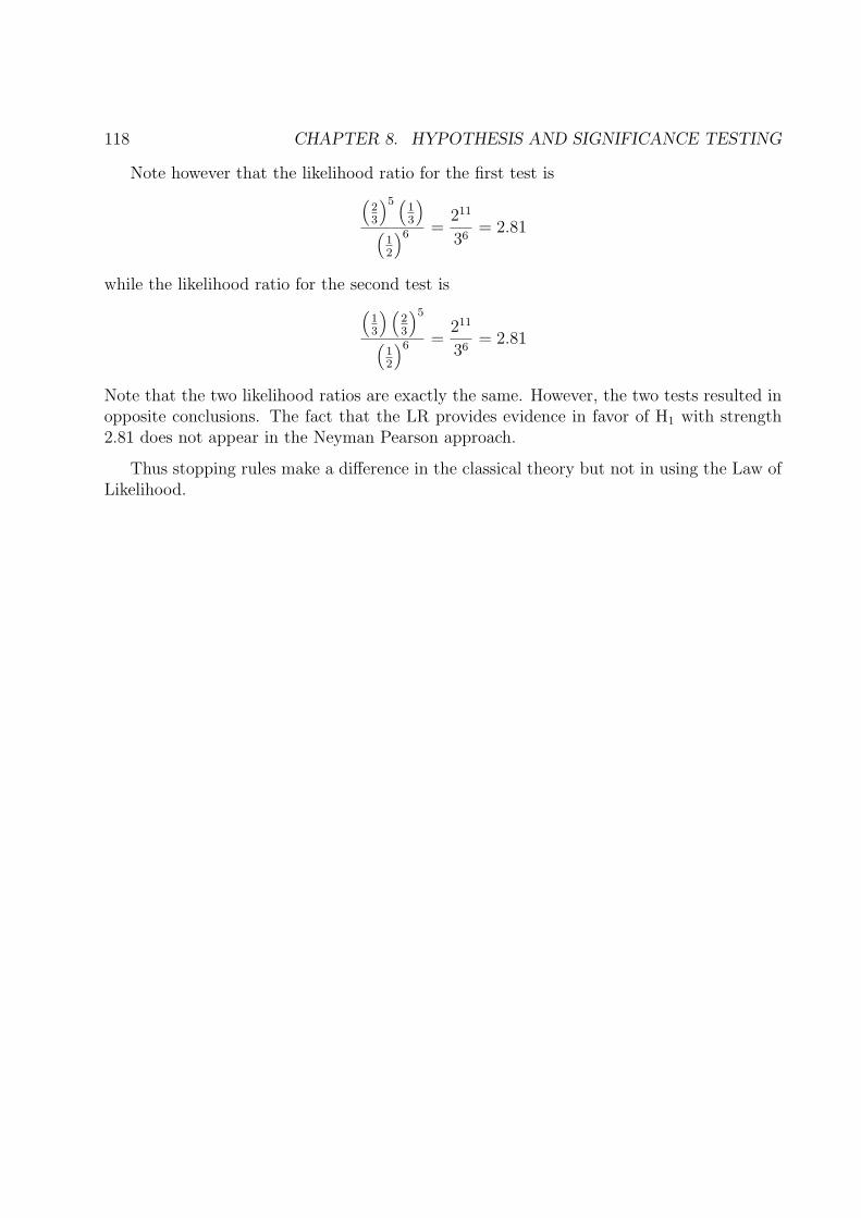
118 CHAPTER 8. HYPOTHESIS AND SIGNIFICANCE TESTING
Note however that the likelihood ratio for the first test is
(23
)5 (13
)
(12
)6 =211
36= 2.81
while the likelihood ratio for the second test is
(13
) (23
)5
(12
)6 =211
36= 2.81
Note that the two likelihood ratios are exactly the same. However, the two tests resulted inopposite conclusions. The fact that the LR provides evidence in favor of H1 with strength2.81 does not appear in the Neyman Pearson approach.
Thus stopping rules make a difference in the classical theory but not in using the Law ofLikelihood.
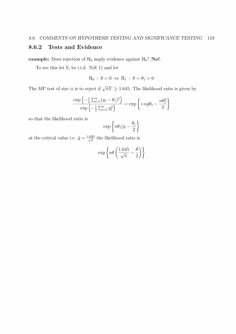
8.6. COMMENTS ON HYPOTHESIS TESTING AND SIGNIFICANCE TESTING 119
8.6.2 Tests and Evidence
example: Does rejection of H0 imply evidence against H0? No!.
To see this let Yi be i.i.d. N(θ, 1) and let
H0 : θ = 0 vs H1 : θ = θ1 > 0
The MP test of size α is to reject if√
nY ≥ 1.645. The likelihood ratio is given by
exp{−1
2
∑ni=1(yi − θ1)
2}
exp{−1
2
∑ni=1 y2
i
} = exp
{+nyθ1 − nθ2
1
2
}
so that the likelihood ratio is
exp
{nθ1(y − θ1
2
}
at the critical value i.e. y = 1.645√n
the likelihood ratio is
exp
{nθ
(1.645√
n− θ
2
)}
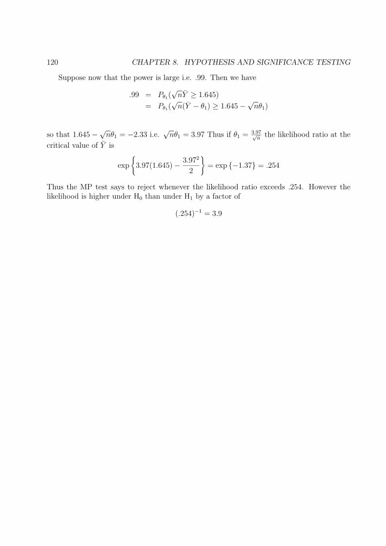
120 CHAPTER 8. HYPOTHESIS AND SIGNIFICANCE TESTING
Suppose now that the power is large i.e. .99. Then we have
.99 = Pθ1(√
nY ≥ 1.645)
= Pθ1(√
n(Y − θ1) ≥ 1.645−√nθ1)
so that 1.645−√nθ1 = −2.33 i.e.√
nθ1 = 3.97 Thus if θ1 = 3.97√n
the likelihood ratio at the
critical value of Y is
exp
{3.97(1.645)− 3.972
2
}= exp {−1.37} = .254
Thus the MP test says to reject whenever the likelihood ratio exceeds .254. However thelikelihood is higher under H0 than under H1 by a factor of
(.254)−1 = 3.9
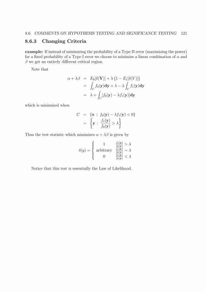
8.6. COMMENTS ON HYPOTHESIS TESTING AND SIGNIFICANCE TESTING 121
8.6.3 Changing Criteria
example: If instead of minimizing the probability of a Type II error (maximizing the power)for a fixed probability of a Type I error we choose to minimize a linear combination of α andβ we get an entirely different critical region.
Note that
α + λβ = E0[δ(Y)] + λ {1− E1[δ(Y )]}=
∫
Cf0(y)dy + λ− λ
∫
Cf1(y)dy
= λ +∫
C[f0(y)− λf1(y)]dy
which is minimized when
C = {x : f0(y)− λf1(y) < 0}=
{y :
f1(y)
f0(y)> λ
}
Thus the test statistic which minimizes α + λβ is given by
δ(y) =
1 f1(y)f0(y)
> λ
arbitrary f1(y)f0(y)
= λ
0 f1(y)f0(y)
< λ
Notice that this test is essentially the Law of Likelihood.
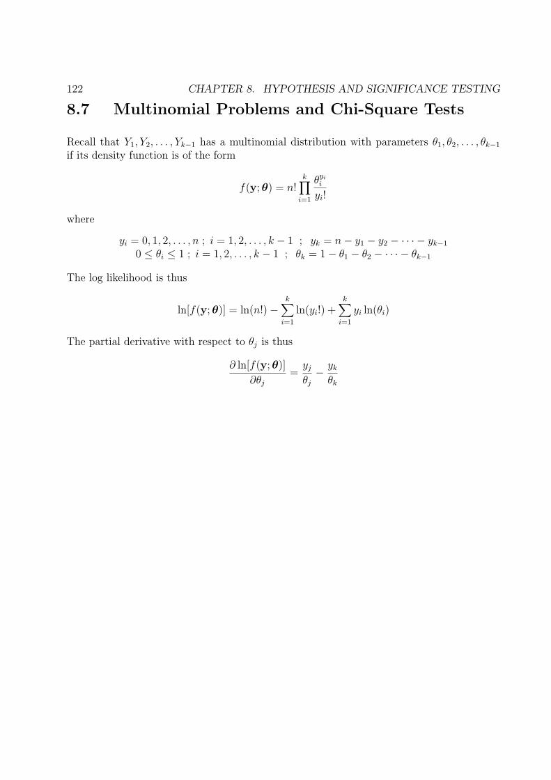
122 CHAPTER 8. HYPOTHESIS AND SIGNIFICANCE TESTING
8.7 Multinomial Problems and Chi-Square Tests
Recall that Y1, Y2, . . . , Yk−1 has a multinomial distribution with parameters θ1, θ2, . . . , θk−1
if its density function is of the form
f(y; θ) = n!k∏
i=1
θyii
yi!
where
yi = 0, 1, 2, . . . , n ; i = 1, 2, . . . , k − 1 ; yk = n− y1 − y2 − · · · − yk−1
0 ≤ θi ≤ 1 ; i = 1, 2, . . . , k − 1 ; θk = 1− θ1 − θ2 − · · · − θk−1
The log likelihood is thus
ln[f(y; θ)] = ln(n!)−k∑
i=1
ln(yi!) +k∑
i=1
yi ln(θi)
The partial derivative with respect to θj is thus
∂ ln[f(y; θ)]
∂θj
=yj
θj
− yk
θk

8.7. MULTINOMIAL PROBLEMS AND CHI-SQUARE TESTS 123
Equating to 0 yieldsyj
θj
=yk
θk
or yj θk = ykθj
Summing from j = 1 to j = k − 1 yields
(n− yk)θk = yk(1− θk) or θk =yk
n
and hence
θj =yj θk
yk
=yj
n; j = 1, 2, . . . , k − 1
The second partial derivatives are given by
∂(2) ln[f(y; θ)]
∂θ(2)j
= −yj
θ2j
− yk
θ2k
∂(2) ln[f(y; θ)]
∂θj∂θj′
= −yk
θ2k
and it follows that Fisher’s Information matrix is given by
I(θ) = {i(θ)}j,j′ =
{ nθj
+ nθk
j = j′
nθk
j′ 6= j
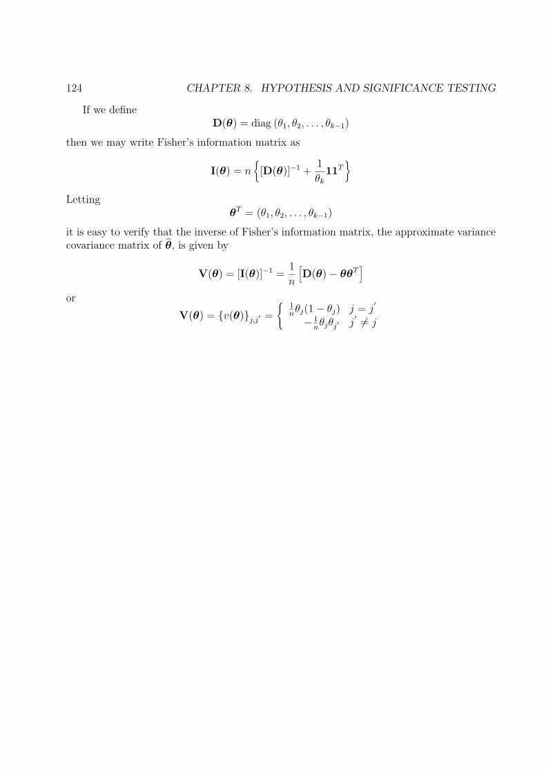
124 CHAPTER 8. HYPOTHESIS AND SIGNIFICANCE TESTING
If we defineD(θ) = diag (θ1, θ2, . . . , θk−1)
then we may write Fisher’s information matrix as
I(θ) = n{[D(θ)]−1 +
1
θk
11T}
LettingθT = (θ1, θ2, . . . , θk−1)
it is easy to verify that the inverse of Fisher’s information matrix, the approximate variancecovariance matrix of θ, is given by
V(θ) = [I(θ)]−1 =1
n
[D(θ)− θθT
]
or
V(θ) = {v(θ)}j,j′ =
{1nθj(1− θj) j = j
′
− 1nθjθj
′ j′ 6= j
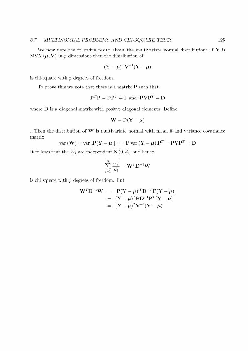
8.7. MULTINOMIAL PROBLEMS AND CHI-SQUARE TESTS 125
We now note the following result about the multivariate normal distribution: If Y isMVN (µ,V) in p dimensions then the distribution of
(Y − µ)TV−1(Y − µ)
is chi-square with p degrees of freedom.
To prove this we note that there is a matrix P such that
PTP = PPT = I and PVPT = D
where D is a diagonal matrix with positve diagonal elements. Define
W = P(Y − µ)
. Then the distribution of W is multivariate normal with mean 0 and variance covariancematrix
var (W) = var [P(Y − µ)] == P var (Y − µ) PT = PVPT = D
It follows that the Wi are independent N (0, di) and hence
p∑
i=1
W 2i
di
= WTD−1W
is chi square with p degrees of freedom. But
WTD−1W = [P(Y − µ)]TD−1[P(Y − µ)]
= (Y − µ)TPD−1PT (Y − µ)
= (Y − µ)TV−1(Y − µ)
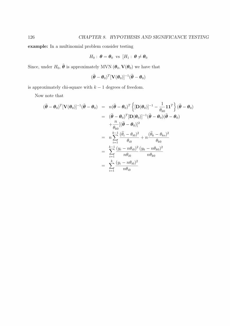
126 CHAPTER 8. HYPOTHESIS AND SIGNIFICANCE TESTING
example: In a multinomial problem consider testing
H0 : θ = θ0 vs [H1 : θ 6= θ0
Since, under H0, θ is approximately MVN (θ0,V(θ0) we have that
(θ − θ0)T [V(θ0)]
−1(θ − θ0)
is approximately chi-square with k − 1 degrees of freedom.
Now note that
(θ − θ0)T [V(θ0)]
−1(θ − θ0) = n(θ − θ0)T
{[D(θ0)]
−1 − 1
θk0
11T}
(θ − θ0)
= (θ − θ0)T [D(θ0)]
−1(θ − θ0)(θ − θ0)
+n
θk0
[(θ − θ0)]2
= nk−1∑
i=1
(θi − θi0)2
θi0
+ n(θk − θko)
2
θk0
=k−1∑
i=1
(yi − nθi0)2
nθi0
(yk − nθk0)2
nθk0
=k∑
i=1
(yi − nθi0)2
nθi0
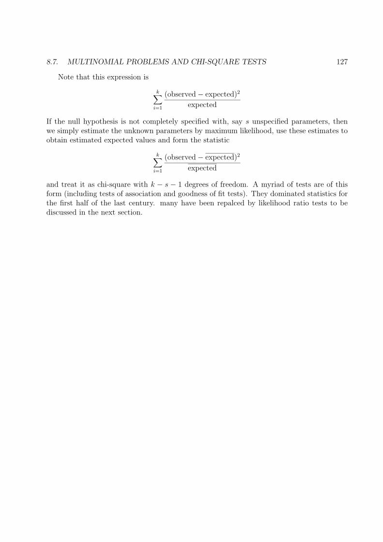
8.7. MULTINOMIAL PROBLEMS AND CHI-SQUARE TESTS 127
Note that this expression is
k∑
i=1
(observed− expected)2
expected
If the null hypothesis is not completely specified with, say s unspecified parameters, thenwe simply estimate the unknown parameters by maximum likelihood, use these estimates toobtain estimated expected values and form the statistic
k∑
i=1
(observed− expected)2
expected
and treat it as chi-square with k − s − 1 degrees of freedom. A myriad of tests are of thisform (including tests of association and goodness of fit tests). They dominated statistics forthe first half of the last century. many have been repalced by likelihood ratio tests to bediscussed in the next section.

128 CHAPTER 8. HYPOTHESIS AND SIGNIFICANCE TESTING
8.7.1 Chi Square Test of Independence
Suppose that we have a random sample of n individuals who are classified according to twocategories R (rows) having r values (levels) and C having c values (levels). We observe nij
individuals who are classified into the cell corresponding to row i and column j. Thus theobserved data are of the form:
Column Category1 2 · · · c Total
1 n11 n12 · · · n1c n1+
Row 2 n21 n22 · · · n2c n2+
Category...
......
......
r nr1 nr2 · · · nrc nr+
Total n+1 n+2 · · · n+c n++ = n
The probabilities are given by
Column Category1 2 · · · c Total
1 p11 p12 · · · p1c p1+
Row 2 p21 p22 · · · p2c n2+
Category...
......
......
r pr1 pr2 · · · prc pr+
Total p+1 p+2 · · · p+c 1
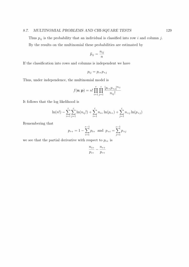
8.7. MULTINOMIAL PROBLEMS AND CHI-SQUARE TESTS 129
Thus pij is the probability that an individual is classified into row i and column j.
By the results on the multinomial these probabilities are estimated by
pij =nij
n
If the classification into rows and columns is independent we have
pij = pi+p+j
Thus, under independence, the multinomial model is
f(n;p) = n!r∏
i=1
c∏
j=1
[pi+p+j]nij
nij!
It follows that the log likelihood is
ln(n!)−r∑
i=1
c∑
j=1
ln(nij!) +r∑
i=1
ni+ ln(pi+) +c∑
j=1
n+j ln(p+j)
Remembering that
pr+ = 1−r−1∑
i=1
pi+ and p+c =c−1∑
j=1
p+j
we see that the partial derivative with respect to pi+ is
ni+
pi+
− nr+
pr+
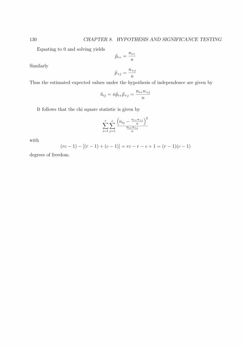
130 CHAPTER 8. HYPOTHESIS AND SIGNIFICANCE TESTING
Equating to 0 and solving yields
pi+ =ni+
n
Similarly
p+j =n+j
n
Thus the estimated expected values under the hypothesis of independence are given by
nij = npi+p+j =ni+n+j
n
It follows that the chi square statistic is given by
r∑
i=1
c∑
j=1
(nij − ni+n+j
n
)2
ni+n+j
n
with(rc− 1)− [(r − 1) + (c− 1)] = rc− r − c + 1 = (r − 1)(c− 1)
degrees of freedom.

8.7. MULTINOMIAL PROBLEMS AND CHI-SQUARE TESTS 131
8.7.2 Chi Square Goodness of Fit
Suppose that we have y1, y2, . . . , yn which are realized values of Y1, Y2, . . . , Yn assumed to beindependent each having the density function f(y; θ) where the values of y are assumed tolie in an interval I. Usually I is (0,∞) or (−∞, +∞).
Divide I into k sub-intervals I1, I2, . . . , Ik defined by
I1 = {y : y ≤ c1}I2 = {y : c1 < y ≤ c2}I3 = {y : c2 < y ≤ c3}
......
...Ik−1 = {y : ck−2 < y ≤ ck−1}
Ik = {y : y > ck−1}
where the ci are cut points and satisfy
c1 < c2 < · · · < ck−1
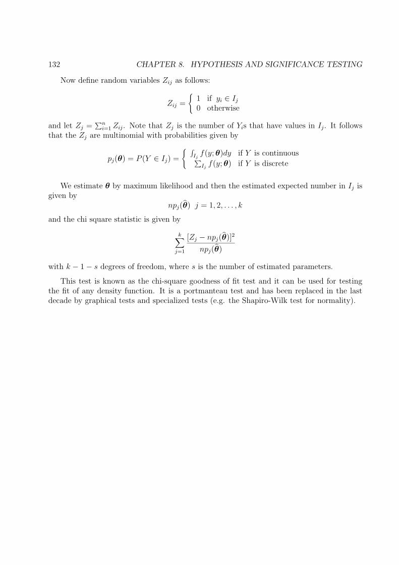
132 CHAPTER 8. HYPOTHESIS AND SIGNIFICANCE TESTING
Now define random variables Zij as follows:
Zij =
{1 if yi ∈ Ij
0 otherwise
and let Zj =∑n
i=1 Zij. Note that Zj is the number of Yis that have values in Ij. It followsthat the Zj are multinomial with probabilities given by
pj(θ) = P (Y ∈ Ij) =
{ ∫Ij
f(y; θ)dy if Y is continuous∑Ij
f(y; θ) if Y is discrete
We estimate θ by maximum likelihood and then the estimated expected number in Ij isgiven by
npj(θ) j = 1, 2, . . . , k
and the chi square statistic is given by
k∑
j=1
[Zj − npj(θ)]2
npj(θ)
with k − 1− s degrees of freedom, where s is the number of estimated parameters.
This test is known as the chi-square goodness of fit test and it can be used for testingthe fit of any density function. It is a portmanteau test and has been replaced in the lastdecade by graphical tests and specialized tests (e.g. the Shapiro-Wilk test for normality).
8.8. PP-PLOTS AND QQ-PLOTS 133
8.8 PP-plots and QQ-plots
To assess whether a given distribution is consistent with an observed sample or whether twosamples can be assumed to have the same distribution therearea variety of graphical methodsavailable. The two most important are the plots known as Q-Q plots and P-P plots. Bothare based on the empirical distribution function defined in the section on exploratory dataanalysis.
Suppose that we have data y1, y2, . . . , yn assumed to be independent with the same dis-tribution F , where
F (y) = P (Y ≤ y)
Recall that the sample distribution function or empirical distribution function isa plot of the proportion of values in the data set less than or equal to y versus y. Moreprecisely, let
zi(y) =
{1 if yi ≤ y0 otherwise
Then the empirical distribution function at y is
Fn(y) =1
n
n∑
i=1
zi(y)
Note that the zi(y) are realized values of random variables which are Bernouilli withprobability
p = E[Zi(y)] = P (Yi ≤ y) = F (y)
so that the empirical distribution function at y is an unbiased estimator of the true distri-bution function i.e.
E[Fn(y)] = F (y)
134 CHAPTER 8. HYPOTHESIS AND SIGNIFICANCE TESTING
Moreover
var [Fn(y)] =p(1− p
n=
F (y)[1− F (y)]
n
so that Fn(y) is a consistent estimator of F (y). It can also be shown that it is the maximumlikelihood estimator of F (y). (If some of the values of Y are censored i.e. we can onlyobserve that Yi ≤ ci then a modification of Fn(y) is called the Kaplan-Meier estimate of thedisribution and forms the basis of survival analysis.)
It follows that a plot of Fn(y) vs F (y) should be a straight line thorough the origin withslope equal to one. Such a plot is called a probability plot or PP-plot since both axes areprobabilities.
It also follows that a plot of F−1n (p), the sample quantiles vs F−1(p) the quantiles of F
should be a straight line through the origin with slope equal to one. Such a plot is called aquantile-quantile or QQ-plot.
Of the two plots QQ-plots are the most widely used. These plots can be convenientlymade using current software but usually involve too much computation to be done by hand.They represent a very valuable technique for comparing observed data sets to theoreticalmodels. STATA and other packages have a variety of programs based on the above simpleideas.
8.9. GENERALIZED LIKELIHOOD RATIO TESTS 135
8.9 Generalized Likelihood Ratio Tests
The generalized likelihood ratio tests which reject when λ(y is small have some useful proper-ties which are fundamental in the analyses used in regression, logistic regression and Poissonregression.
Suppose we have data y1, y2, . . . , yn realized values of Y1, Y2, . . . , Yn which have joint pdf
f(y; θ)
The generalized likelihood ratio test of
H0 : θ ∈ Θ0 vs H1 : θ /∈ Θ0
rejects if
λ(y) =maxθ∈Θ0 f(y; θ)
maxθ∈Θ f(y; θ)
is too small (small being determined by the requirement that the probability of a Type Ierror is less than or equal to the desired significance level).
In particular it can be shown that
−2 log(LR)d−→ χ2(df)
wheredf = dimension(Θ)− dimension(Θ0)
That is, we can determine P-values for the hypothesis that θ ∈ Θ0 using the chi-squaredistribution.
136 CHAPTER 8. HYPOTHESIS AND SIGNIFICANCE TESTING
In a broad class of models, called generalized linear models, the parameter space θ isspecified by linear predictor for the ith observation, ηi defined by
η = β0 +p∑
j=1
xijβj
where the xij are known and β0, β1, . . . , βp are unknown parameters to be estimated from thedata. The βs are called regression coefficients and the xs are called covariates. We note thatif a particular β is 0 then the corresponding covariate is not needed in the linear predictor.
The linear predictor is related to the expected value µi of the ith response variable by alink function g defined so that
g(µi) = ηi = β0 +p∑
j=1
xijβj
Thus examining the βs allows us to determine which of the covariates explain the observedvalues of the response variable and which do not.

8.9. GENERALIZED LIKELIHOOD RATIO TESTS 137
8.9.1 Regression Models
Suppose that the Yis are independent and normally distributed with the same variance σ2,assumed known and that
E(Yi) = µi =p∑
j=0
xijβj = Mi
i.e. the linear predictor is exactly equal to the expected response. The covariate correspond-ing to β0 has each component equal to 1 and is called the intercept term. It is almost alwaysincluded in any linear predictor.
The likelihood is given by
f(y; β, σ2) = (2πσ2)−n/2 exp
{− 1
2σ2
n∑
i=1
(yi −Mi)2
}
From earlier work the estimates are given by
β = b = (XTX)−1XTy
where
b =
b0
b1...bp
=
β0
β1...
βp
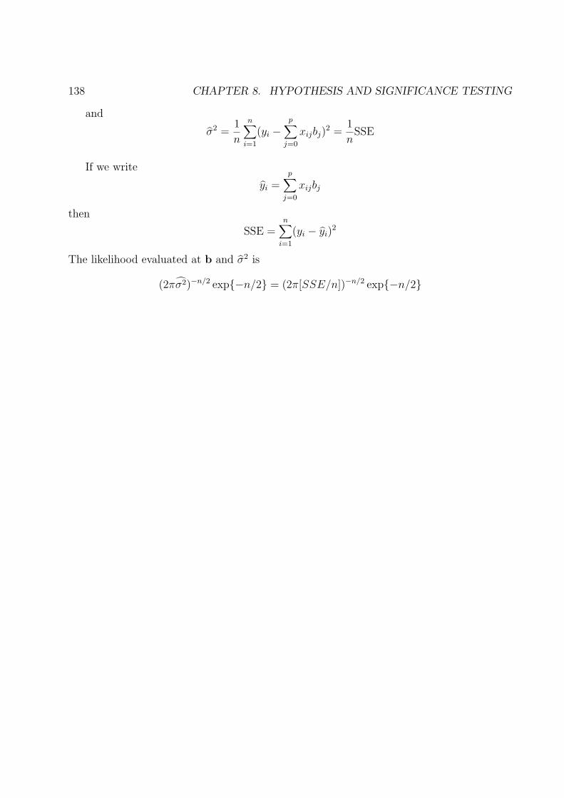
138 CHAPTER 8. HYPOTHESIS AND SIGNIFICANCE TESTING
and
σ2 =1
n
n∑
i=1
(yi −p∑
j=0
xijbj)2 =
1
nSSE
If we write
yi =p∑
j=0
xijbj
then
SSE =n∑
i=1
(yi − yi)2
The likelihood evaluated at b and σ2 is
(2πσ2)−n/2 exp{−n/2} = (2π[SSE/n])−n/2 exp{−n/2}
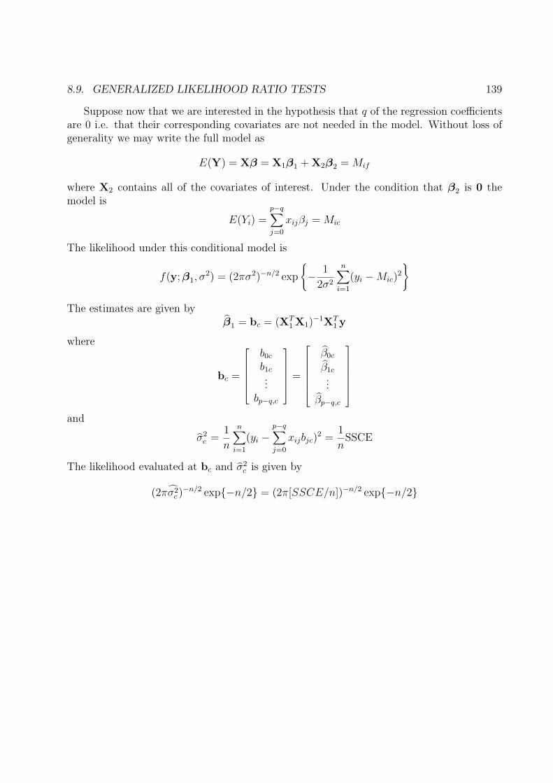
8.9. GENERALIZED LIKELIHOOD RATIO TESTS 139
Suppose now that we are interested in the hypothesis that q of the regression coefficientsare 0 i.e. that their corresponding covariates are not needed in the model. Without loss ofgenerality we may write the full model as
E(Y) = Xβ = X1β1 + X2β2 = Mif
where X2 contains all of the covariates of interest. Under the condition that β2 is 0 themodel is
E(Yi) =p−q∑
j=0
xijβj = Mic
The likelihood under this conditional model is
f(y; β1, σ2) = (2πσ2)−n/2 exp
{− 1
2σ2
n∑
i=1
(yi −Mic)2
}
The estimates are given byβ1 = bc = (XT
1 X1)−1XT
1 y
where
bc =
b0c
b1c...
bp−q,c
=
β0c
β1c...
βp−q,c
and
σ2c =
1
n
n∑
i=1
(yi −p−q∑
j=0
xijbjc)2 =
1
nSSCE
The likelihood evaluated at bc and σ2c is given by
(2πσ2c )−n/2 exp{−n/2} = (2π[SSCE/n])−n/2 exp{−n/2}
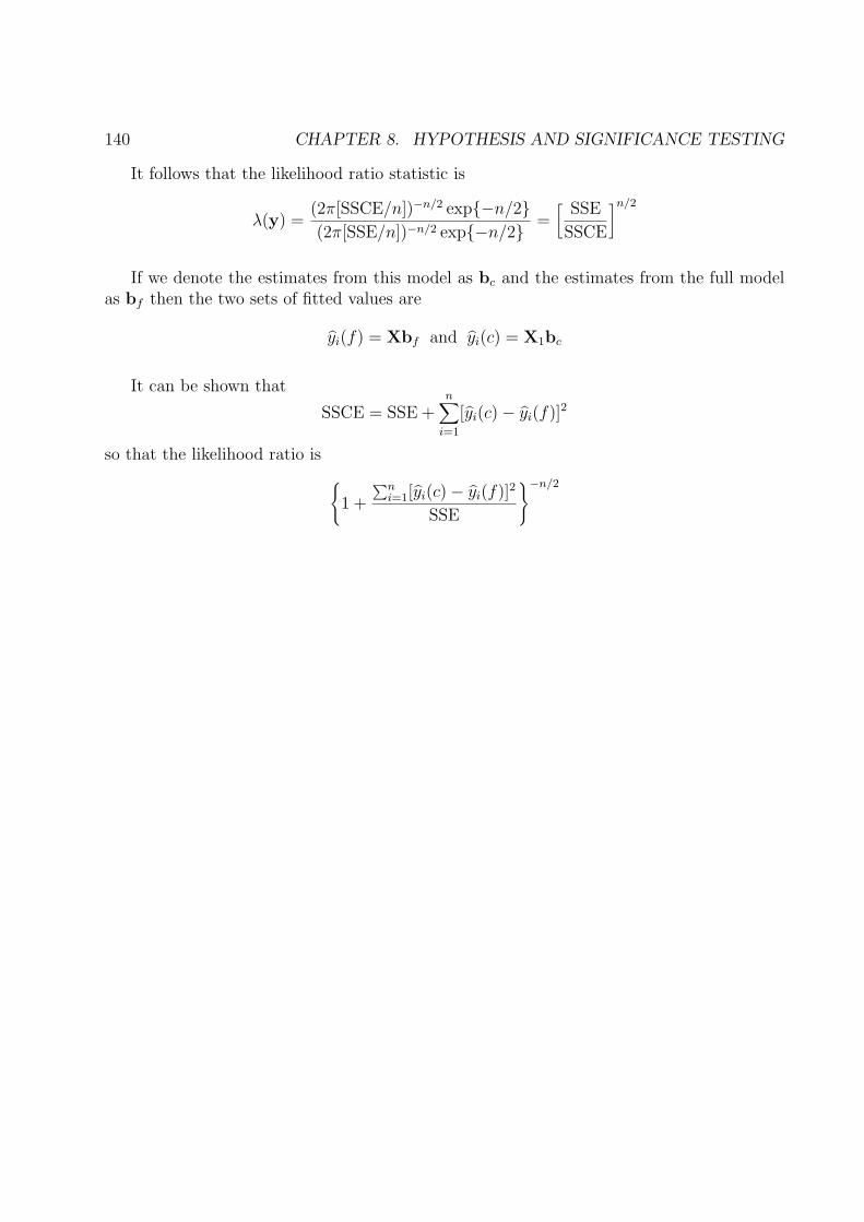
140 CHAPTER 8. HYPOTHESIS AND SIGNIFICANCE TESTING
It follows that the likelihood ratio statistic is
λ(y) =(2π[SSCE/n])−n/2 exp{−n/2}(2π[SSE/n])−n/2 exp{−n/2} =
[SSE
SSCE
]n/2
If we denote the estimates from this model as bc and the estimates from the full modelas bf then the two sets of fitted values are
yi(f) = Xbf and yi(c) = X1bc
It can be shown that
SSCE = SSE +n∑
i=1
[yi(c)− yi(f)]2
so that the likelihood ratio is
{1 +
∑ni=1[yi(c)− yi(f)]2
SSE
}−n/2
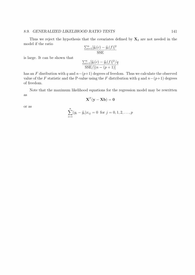
8.9. GENERALIZED LIKELIHOOD RATIO TESTS 141
Thus we reject the hypothesis that the covariates defined by X2 are not needed in themodel if the ratio ∑n
i=1[yi(c)− yi(f)]2
SSE
is large. It can be shown that ∑ni=1[yi(c)− yi(f)]2/q
SSE/[(n− (p + 1)]
has an F disribution with q and n−(p+1) degrees of freedom. Thus we calculate the observedvalue of the F statistic and the P-value using the F distribution with q and n−(p+1) degreesof freedom.
Note that the maximum likelihood equations for the regression model may be rewrittenas
XT (y −Xb) = 0
or asn∑
i=1
(yi − yi)xij = 0 for j = 0, 1, 2, . . . , p
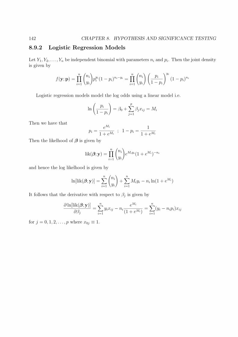
142 CHAPTER 8. HYPOTHESIS AND SIGNIFICANCE TESTING
8.9.2 Logistic Regression Models
Let Y1, Y2, . . . , Yn be independent binomial with parameters ni and pi. Then the joint densityis given by
f(y;p) =n∏
i=1
(ni
yi
)pyi
i (1− pi)ni−yi =
n∏
i=1
(ni
yi
) (pi
1− pi
)yi
(1− pi)ni
Logistic regression models model the log odds using a linear model i.e.
ln
(pi
1− pi
)= β0 +
p∑
j=1
βjxij = Mi
Then we have that
pi =eMi
1 + eMi; 1− pi =
1
1 + eMi
Then the likelhood of β is given by
lik(β;y) =n∏
i=1
(ni
yi
)eMiyi(1 + eMi)−ni
and hence the log likelhood is given by
ln[lik(β;y)] =n∑
i=1
(ni
yi
)+
n∑
i=1
Miyi − ni ln(1 + eMi)
It follows that the derivative with respect to βj is given by
∂ ln[lik(β;y)]
∂βj
=n∑
i=1
yixij − nieMi
(1 + eMi)=
n∑
i=1
(yi − nipi)xij
for j = 0, 1, 2, . . . , p where x0j ≡ 1.
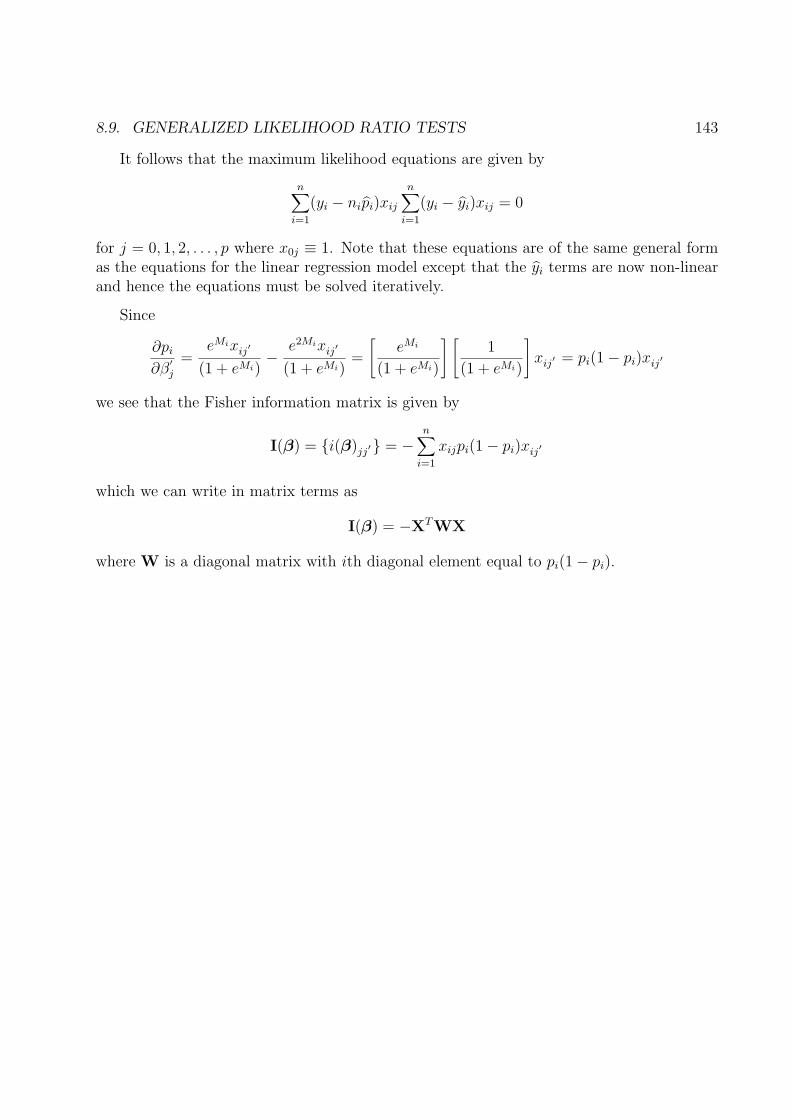
8.9. GENERALIZED LIKELIHOOD RATIO TESTS 143
It follows that the maximum likelihood equations are given by
n∑
i=1
(yi − nipi)xij
n∑
i=1
(yi − yi)xij = 0
for j = 0, 1, 2, . . . , p where x0j ≡ 1. Note that these equations are of the same general formas the equations for the linear regression model except that the yi terms are now non-linearand hence the equations must be solved iteratively.
Since
∂pi
∂β′j
=eMixij′
(1 + eMi)− e2Mixij′
(1 + eMi)=
[eMi
(1 + eMi)
] [1
(1 + eMi)
]xij′ = pi(1− pi)xij′
we see that the Fisher information matrix is given by
I(β) = {i(β)jj′} = −
n∑
i=1
xijpi(1− pi)xij′
which we can write in matrix terms as
I(β) = −XTWX
where W is a diagonal matrix with ith diagonal element equal to pi(1− pi).
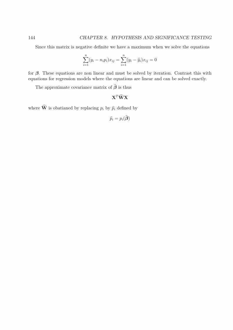
144 CHAPTER 8. HYPOTHESIS AND SIGNIFICANCE TESTING
Since this matrix is negative definite we have a maximum when we solve the equations
n∑
i=1
(yi − nipi)xij =n∑
i=1
(yi − yi)xij = 0
for β. These equations are non linear and must be solved by iteration. Contrast this withequations for regression models where the equations are linear and can be solved exactly.
The approximate covariance matrix of β is thus
XTWX
where W is obatianed by replacing pi by pi defined by
pi = pi(β)
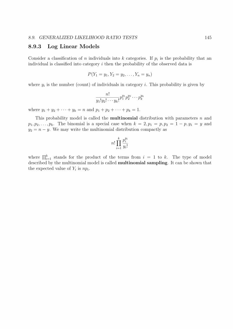
8.9. GENERALIZED LIKELIHOOD RATIO TESTS 145
8.9.3 Log Linear Models
Consider a classification of n individuals into k categories. If pi is the probability that anindividual is classified into category i then the probability of the observed data is
P (Y1 = y1, Y2 = y2, . . . , Yn = yn)
where yi is the number (count) of individuals in category i. This probability is given by
n!
y1!y2! · · · yk!py1
1 py22 · · · pyk
k
where y1 + y2 + · · ·+ yk = n and p1 + p2 + · · ·+ pk = 1.
This probability model is called the multinomial distribution with parameters n andp1, p2, . . . , pk. The binomial is a special case when k = 2, p1 = p, p2 = 1 − p, y1 = y andy2 = n− y. We may write the multinomial distribution compactly as
n!k∏
i=1
pyii
yi!
where∏k
i=1 stands for the product of the terms from i = 1 to k. The type of modeldescribed by the multinomial model is called multinomial sampling. It can be shown thatthe expected value of Yi is npi.
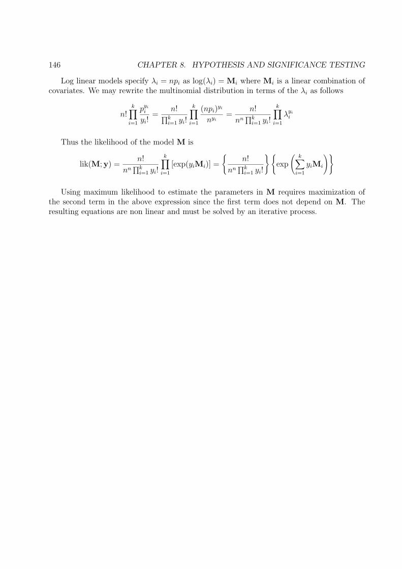
146 CHAPTER 8. HYPOTHESIS AND SIGNIFICANCE TESTING
Log linear models specify λi = npi as log(λi) = Mi where Mi is a linear combination ofcovariates. We may rewrite the multinomial distribution in terms of the λi as follows
n!k∏
i=1
pyii
yi!=
n!∏k
i=1 yi!
k∏
i=1
(npi)yi
nyi=
n!
nn∏k
i=1 yi!
k∏
i=1
λyii
Thus the likelihood of the model M is
lik(M;y) =n!
nn∏k
i=1 yi!
k∏
i=1
[exp(yiMi)] =
{n!
nn∏k
i=1 yi!
} {exp
(k∑
i=1
yiMi
)}
Using maximum likelihood to estimate the parameters in M requires maximization ofthe second term in the above expression since the first term does not depend on M. Theresulting equations are non linear and must be solved by an iterative process.
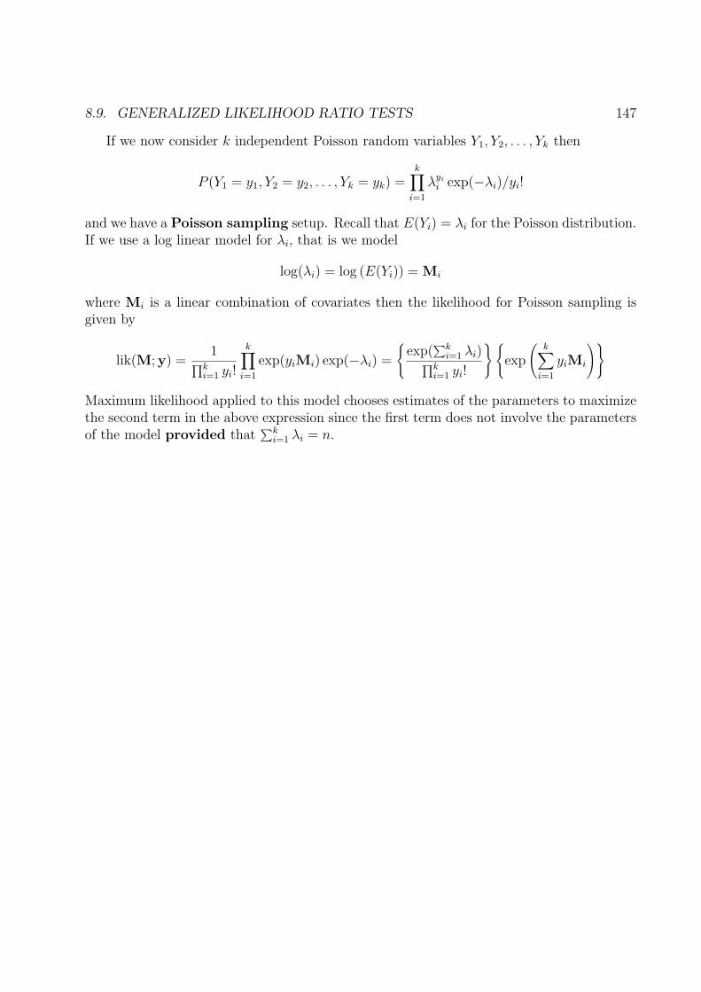
8.9. GENERALIZED LIKELIHOOD RATIO TESTS 147
If we now consider k independent Poisson random variables Y1, Y2, . . . , Yk then
P (Y1 = y1, Y2 = y2, . . . , Yk = yk) =k∏
i=1
λyii exp(−λi)/yi!
and we have a Poisson sampling setup. Recall that E(Yi) = λi for the Poisson distribution.If we use a log linear model for λi, that is we model
log(λi) = log (E(Yi)) = Mi
where Mi is a linear combination of covariates then the likelihood for Poisson sampling isgiven by
lik(M;y) =1
∏ki=1 yi!
k∏
i=1
exp(yiMi) exp(−λi) =
{exp(
∑ki=1 λi)∏k
i=1 yi!
} {exp
(k∑
i=1
yiMi
)}
Maximum likelihood applied to this model chooses estimates of the parameters to maximizethe second term in the above expression since the first term does not involve the parametersof the model provided that
∑ki=1 λi = n.
148 CHAPTER 8. HYPOTHESIS AND SIGNIFICANCE TESTING
Conclusion:If we use the Poisson sampling model and maximize the likelihood under the condition that∑k
i=1 λi = n we will obtain the same estimates, standard errors, etc. as if we had used themultinomial sampling model. The technical reason for this equivalence is that estimatesand standard errors depend only on the expected value of the derivatives of the log of thelikelihood function with respect to the parameters. Since these expected values are the samefor the two likelihoods the assertion follows.
It follows that any program which maximizes Poisson likelihoods can be used for multi-nomial problems. This fact was recognized in the early 1960’s but was not of much use untilappropriate software was developed in the 1970’s and 1980’s.
The same results hold when we have product multinomial sampling i.e. when
group 1 is multinomial (n1, p11, p12, . . . , p1k)
group 2 is multinomial (n2, p21, p22, . . . , p2k)
etc. provided the log linear model using Poisson sampling fixes the group totals i.e.∑k
j=1 λ1j =
n1,∑k
j=1 λ2j = n2, etc. In fitting these models a group term treated as a factor must be in-cluded in the model.

8.9. GENERALIZED LIKELIHOOD RATIO TESTS 149
Summary: Any cross-classified data set involving counts may be modelled by log linearmodels and the Poisson distribution using a log link, provided that any restrictions impliedby the experimental setup are included as terms in the fitting process. This implies that anylogistic regression problem can be considered as a log linear model provided we include inthe fitting process a term for (success, failure), (exposed, non-exposed), etc.
The resulting equations can be shown to be of the form
n∑
i=1
(yi − yi)xij for j = 0, 1, 2, . . . , p
where the fitted values, as in logistic regression are non linear functions of the estimatedregression coefficients so that the equations are non linear and must be solved by iteration.
Related Documents