P. NAVAL POSTGRADUATE SCHOOL

N PS ARCH IV E

1997.12RYAN, P.

NAVAL POSTGRADUATE SCHOOLMonterey, California

THESIS

COMPUTER SIMULATION OF A TWO-PHASECAPILLARY PUMPED LOOP (CPL) USING

SINDA/FLUINT

by

Peter J. Ryan, Jr.

December, 1997

Thesis Advisor: M. D. Kelleher

ThesisR9454

Approved for public release; distribution is unlimited.

DUDLEY KNOX LIBRARYNAVAL POSTGRADUATE SCHOOLMONTEREY CA 93943-5101

REPORT DOCUMENTATION PAGE Form Approved OMB No. 0704-01 88

Public reporting burden for this collection of information is estimated to average 1 hour per response, including the time for reviewing instruction, searching

existing data sources, gathering and maintaining the data needed, and completing and reviewing the collection of information. Send comments regarding this

burden estimate or any other aspect of this collection of information, including suggestions for reducing this burden, to Washington Headquarters Services,

Directorate for Information Operations and Reports, 1215 Jefferson Davis Highway, Suite 1204, Arlington, VA 22202-4302, and to the Office of Management

and Budget, Paperwork Reduction Project (0704-0188) Washington DC 20503.

1 . AGENCY USE ONLY (Leave blank) 2. REPORT DATEDecember 1997

3. REPORT TYPE AND DATES COVEREDMaster's Thesis

4 TITLE AND SUBTITLE COMPUTER SIMULATION OF A TWO-PHASECAPILLARY PUMPED LOOP (CPL) USING SINDA/FLUINT

5. FUNDING NUMBERS

6. AUTHOR(S) Peter J. Ryan, Jr.

7. PERFORMING ORGANIZATION NAME(S) AND ADDRESS(ES)

Naval Postgraduate School

Monterey CA 93943-5000

8. PERFORMINGORGANIZATIONREPORT NUMBER

9. SPONSORING/MONITORING AGENCY NAME(S) AND ADDRESS(ES) 10. SPONSOPJNG/MONITORINGAGENCY REPORT NUMBER

11. supplementary NOTES The views expressed in this thesis are those of the author and do not reflect

the official policy or position of the Department of Defense or the U.S. Government.

12a. DISTRIBUnON/AVAILABILnY STATEMENT

Approved for public release; distribution is unlimited.

12b. DISTRIBUTION CODE

13. ABSTRACT (maximum 200 words)

The heat transfer performance of a prototype capillary pumped loop (CPL) test bed from the U.S. Air Force Phillips Laboratory is

modeled using numerical differencing techniques. A commercial computer code was used to create the model and simulate

performance over a wide range of operating conditions. Steady-state and transient performance were modeled as part of the initial

phase of testing in a program designed to evaluate the effectiveness and reliability of capillary pumped loop technology for use in

spacecraft thermal control. The performance baseline developed in this phase of testing will serve as the foundation for continued

research and development of this technology.

14. subject TERMS: Capillary Pumped Loop (CPL), Evaporator,

Noncondensible Gas (NCG) Trap

15. NUMBER OF

PAGES 136

16. PRICE CODE

17. SECURITY CLASSIFICA-

TION OF REPORT

Unclassified

1 8 . SECURITY CLASSIFI-

CATION OF THIS PAGE

Unclassified

19. SECURITY CLASSIFICA-

TION OF ABSTRACT

Unclassified

20. LIMITATION OFABSTRACT

ULNSN 7540-01-280-5500 Standard Form 298 (Rev. 2-89)

Prescribed by ANSI Std. 239-1 8 298-102

11

Approved for public release; distribution is unlimited

COMPUTER SIMULATION OF A TWO-PHASE CAPILLARY PUMPED LOOP(CPL) USING SINDA/FLUEVT

Peter J. Ryan, Jr.

Lieutenant, United States Navy

B.S., United States Naval Academy, 1991

Submitted in partial fulfillment of the

requirements for the degree of

MASTER OF SCIENCE IN MECHANICAL ENGINEERING

from the

NAVAL POSTGRADUATE SCHOOLDecember, 1997

n?s p

o

DUDLEY KNOX LIBRARY

NAVAL POSTGRADUATE SCHOOLMONTEREY CA 93943-5101

ABSTRACT

The heat transfer performance of a prototype capillary pumped loop (CPL) test

bed from the U.S. Air Force Phillips Laboratory is modeled using numerical differencing

techniques. A commercial computer code was used to create the model and simulate

performance over a wide range of operating conditions. Steady-state and transient

performance were modeled as part of the initial phase of testing in a program designed to

evaluate the effectiveness and reliability of capillary pumped loop technology for use in

spacecraft thermal control. The performance baseline developed in this phase of testing

will serve as the foundation for continued research and development of this technology.

VI

TABLE OF CONTENTS

I. INTRODUCTION 1

A. BACKGROUND 1

B. HEAT PIPES VERSUS CAPILLARY PUMPED LOOPS 3

C. HISTORICAL SUMMARY 7

D. OBJECTIVES 10

II. PHILLIPS LABORATORY CAPILLARY PUMPED LOOP 13

A TEST BED SETUP 13

B. RESERVOIR 17

C. WICK STRUCTURES 18

D.CONDENSER 20

E. NONCONDENSIBLE GAS TRAPS AND OTHER VAPOR BARRIERS 21

F. STARTER PUMP 26

III. CAPILLARY PUMPING THEORY 29

A. THEORY 29

IV. DEVELOPING THE MODEL 33

A. SINDA/FLUINT 33

B. STEADY-STATE MODEL 41

C. TRANSIENT MODEL 61

V. RESULTS 65

A. STEADY STATE 65

B. TRANSIENT MODELING 75

VI. RECOMMENDATIONS 81

APPENDIX A. SINDA/FLUINT NOMENCLATURE 85

APPENDIX B . CPL MODEL COMPONENT NUMBER DESIGNATIONS 87

APPENDIX C. STEADY-STATE PRESSURE PROFILES 89

Vll

APPENDIX D. STEADY-STATE TEMPERATURE COMPARISONS 97

APPENDIX E. TRANSIENT SIMULATION RESULTS 105

APPENDIX F TEMPERATURE-TIME COMPARISONS 119

LIST OF REFERENCES 123

INITIAL DISTRIBUTION LIST 125

vm

ACKNOWLEDGMENT

I would like to acknowledge the support of the U.S. Air Force Phillips Laboratory,

Dr. Don Gluck and Charlotte Gerhart of Nichols Research Corporation, and the staff at

the Power and Thermal Management Division for their technical assistance and hospitality

during my experience tour. I would also like to thank the staff of Cullimore and Ring

Technologies for their fantastic software support during this research. Their timely

assistance and patience were instrumental to this work. In addition, I would like to

express my sincere gratitude and appreciation to Professor Matthew Kelleher for his

advice, support and motivation throughout the thesis process. Lastly, I would like to

thank my wife and family for their love and encouragement.

IX

I. INTRODUCTION

A. BACKGROUND

Most spacecraft thermal control designs use passive measures to control

component temperatures. In these cases, heat dissipation requirements are easily handled

by appropriately sizing an optical solar reflector (OSR) covered radiator to reject the

unwanted heat out into space. These cold-biased designs employ heaters to protect more

sensitive components against the extremely low temperatures encountered during periods

of eclipse. These simple but effective systems have a rich flight history and are still very

useful. [Ref. 1]

In the past five to ten years, the technological explosion in the areas of electronics

and integrated circuitry have had a profound impact on satellite design. Smaller, faster,

more powerful computers have dramatically increased the amount of data which satellites

can collect, store, process, and downlink. The decreased size and weight of electronic

components has allowed more hardware to be placed onboard a particular satellite bus,

thereby increasing the mission capacity of each satellite.

Unfortunately, these same advances have created new challenges for the thermal

control engineer. The powerful, compact electronic components dissipate considerably

more heat over a smaller area. In addition, some of the more highly advanced electronics

and sensors aboard modern spacecraft require cryocoolers to maintain extremely low

operating temperatures. This tasks the thermal control subsystem to handle large amounts

of heat rejection over long periods of time. To date, advances in spacecraft power

generation and thermal control systems have not been nearly as dramatic as those in the

area of integrated circuit technology. The need to reliably dissipate large quantities of

heat while using a minimal amount of power has sparked new interest and research in the

area of satellite thermal control.

In the vacuum of space there is no medium present to accommodate heat transfer

by conduction or convection to or from the spacecraft's environment. The only effective

method of heat transport is by thermal radiation. Some of the more prevalent heat sources

for spacecraft include onboard electronics, the sun, the earth (both by reflecting solar

radiation and its own emission), thrusters, and chemical reactions. [Ref 2]

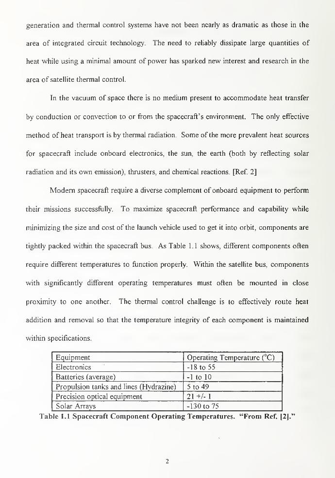
Modern spacecraft require a diverse complement of onboard equipment to perform

their missions successfully. To maximize spacecraft performance and capability while

minimizing the size and cost of the launch vehicle used to get it into orbit, components are

tightly packed within the spacecraft bus. As Table 1 . 1 shows, different components often

require different temperatures to function properly. Within the satellite bus, components

with significantly different operating temperatures must often be mounted in close

proximity to one another. The thermal control challenge is to effectively route heat

addition and removal so that the temperature integrity of each component is maintained

within specifications.

Equipment Operating Temperature (°C)

Electronics -18 to 55

Batteries (average) -1 to 10

Propulsion tanks and lines (Hydrazine) 5 to 49

Precision optical equipment 21 +/- 1

Solar Arrays -130 to 75

Table 1.1 Spacecraft Component Operating Temperatures. "From Ref. [2].'

An emerging technology that has shown considerable promise for spacecraft

thermal control is the capillary pumped loop (CPL). The CPL is a two-phase heat transfer

loop that uses one or more capillary structures (wicks) in concert with heat addition to

generate the pressure gradient which forces the working fluid to circulate from the region

of heat addition to a heat rejection radiator. The heat input alone provides the energy

needed to produce this pressure gradient, and thus ideally no external power input to the

system is required. Although still under development, CPL technology shows significant

potential for use in advanced spacecraft thermal control, where high heat transfer rates

must be sustained over relatively long distances.

The Earth Observing System A.M. (EOS-AM) and the Commercial Experimental

Transporter (COMET) are the first satellites designed to use capillary pumped loops as

their primary thermal control system. The EOS-AM satellite is one of a series of

NASA/NOAA satellites that will be studying the earth's atmosphere. The COMET

satellite was designed to serve as an experimental test platform for a wide variety of space

experiments. The ability of CPLs to maintain a relatively constant temperature over a

wide range of heat inputs makes them especially useful for dissipating heat from

cryocoolers used to cool focal planes on sensors and scientific instruments aboard these

two satellites. [Ref 3]

B. HEAT PIPES VERSUS CAPILLARY PUMPED LOOPS

The concept and design of capillary pumped loops are similar to those of

conventional heat pipes except that in the CPL system the vapor and liquid flows are in the

same direction and are physically separated from each other. [Refs. 1, 2, 3]

Heat pipes are currently used in numerous satellite, aviation, and other mechanical

thermal control systems. They have the ability to receive heat at one end and dissipate it

at the other, and can control the area available for heat exchange. Vapor generated by

heat input at the evaporator end travels through the inner core to the condenser end where

heat is removed. There the liquid reenters the wick and capillary pumping action forces it

back to the evaporator section. Basic heat pipe construction consists of a rigid container,

usually cylindrical, which contains the wick structure and both liquid and vapor phases of

the working fluid. Figure 1.1 shows typical heat pipe layout and operation. [Refs. 4 and

5]

Evaporator

Porous wick

Heat in

Condensate flow

CondenserHeat out

Figure 1.1 Typical Heat Pipe Layout and Operation. "From Ref. [4].'

The advantage of using capillary pumped loop systems instead of conventional

heat pipes stems from the separation of the liquid and vapor phases of the working fluid.

By separating the liquid and vapor portions of the heat exchanger, the heat addition and

removal locations may be separated by relatively large distances. Phase separation also

allows slight superheating of the vapor in the evaporator and subcooling of the liquid in

the condenser, thereby increasing the system AT and the total heat transport capacity.

Capillary pumped loops have been developed which are capable of transporting 25

kilowatts of heat over a ten-meter distance [Ref. 3]. This heat transport is over an order

of magnitude greater than heat transport available with current heat pipe technology.

[Refs. 2, 3, 4 and 6]

Capillary pumped loops also provide flexibility in the path in which heat is

removed. The transport lines connecting the evaporator to the condenser may be routed

around sensitive equipment, reducing the risk of damage or degradation from unwanted

heat transfer. In addition, the CPL design provides the capability to route the condenser

lines to several different radiators. Analogous to current flow in an electrical circuit, more

heat will naturally flow along the path or paths with the greatest potential (temperature)

difference as long as the path resistances are equal. The CPL system will automatically

"select" the most efficient radiators (i.e., the ones with the least incident sunlight and

therefore lowest temperature) to dissipate the acquired heat. The technology exists to

make the transport lines from flexible tubing which may be attached to a deployable

radiator, allowing the radiator to be positioned as required for maximum heat dissipation.

[Ref. 3]

Electrical power is a precious commodity in space. To date, the best electrical

generation systems are only 15-30% efficient. Degradation of these systems due to

radiation effects throughout the life of the satellite reduces their efficiency even further

[Ref 8]. Power is often the life-limiting design parameter, and reducing electrical power

consumption is also a major satellite design goal. What makes capillary pumps attractive

for thermal control is that ideally they do not require external power to force liquid

through the system. The capillary action of the wick material inside the evaporator is

enough to sustain the pressure gradient that forces the working fluid to circulate through

the loop. The pumping process is similar to that of wax being drawn through the wick of

a lighted candle or water being drawn from the roots to the top of a large tree [Ref. 4].

Lubrication, excessive wear and vibration, inertia effects caused by pump rotation, and

life-cycle fatigue are some of the design challenges that can be eliminated since the

capillary pumped loop has no moving parts.

The following description of CPL operation is provided to give the reader a basic

understanding of the heat transport process. When sufficient heat is applied to the

capillary pump (or evaporator), liquid on the outer surface of the wick material

evaporates. As this working fluid changes phase, it absorbs the latent heat of vaporization

and exhibits heat transfer coefficients on the order of 2,500-9,000 W/m2K. The expanding

vapor travels through the loop to the condenser. Upon reaching the condenser, the vapor

begins to condense along the walls of the condenser tubes. Ideally, by the time the

working fluid exits the condenser it is in the form of a subcooled liquid. The liquid exiting

the condenser flows onward to supply the inner annulus of the evaporator, completing the

cycle. By regulating the amount of the condenser "open" for heat rejection, the CPL can

perform as a variable conductance heat transfer device As power input is increased, the

entire condenser will eventually fill with vapor, and the CPL will no longer be able to

increase conductance. This constant conductance mode represents the maximum

theoretical capacity of a particular capillary loop. Figure 1.2 shows a functional schematic

of a capillary pumped loop. [Refs. 3, 6, 7, 9]

HUT SOURCE HUT SINt

SENSOR

hlater

•ISOLATOR LIQUID R~UR."<

Figure 1.2 Capillary Pumped Loop Functional Schematic. "From Ref. [9].

C. HISTORICAL SUMMARY

The first capillary pumped loop was designed and built by F. Stenger of NASA

Lewis Research Center in the early 1960's [Ref 10] Although he published his results in

1966, it was not until the late 1970's that serious development of CPL technology began

in the West, when major aerospace corporations such as TRW, Dornier, Martin Marietta,

and GE Astrospace began researching CPL technology. Universities and research

institutions also began to explore both the terrestrial and space applications of CPL

technology. NASA Goddard Space Flight Center (NGSFC) in Greenbelt, Maryland, has

been the primary researcher in the U.S., producing CPL-1, CPL-2 and the Instrumented

Thermal Test Bed (ITTB). The United States Air Force Wright Patterson Laboratory and

Phillips Laboratory have also made contributions to the study of CPL and loop heat pipe

technology. [Refs 8, 9, 10, 11]

In the mid 1980's, two American CPL flight experiments were conducted. The

first was called (CPL/GAS), and was launched as a "Hitchhiker" experiment on the "Get

Away Special" bridge in the space shuttle cargo bay in 1985. The experiment used two

parallel heat pipes to dissipate 200 watts over a distance of one meter. In 1986, in a

similar experiment, a refurbished CPL/GAS was flown and demonstrated the ability to

transport a heat load of 500 watts. In addition to American flight tests, the Lavochkin

Association of the former Soviet Union conducted a flight test on the Granat mission

using a form of CPL called the Loop Heat Pipe (LHP). The Russian interest in CPL

technology, which began as an effort to cool missile components, has now expanded to

satellite thermal control. The Russian CPL consisted of a single evaporator that used

sintered metal wicks in conjunction with a closely coupled reservoir (compensation

chamber) and a single condenser. The experiment used radiant heating for evaporator

heat input and was reported to be a success. The European Space Agency (ESA) and the

Japanese have also conducted CPL testing. The experiments and flight tests described

above have proven the CPL concept as a viable thermal control device. [Refs. 3, 6, 7, 9,

11,12]

In recent years, two additional flight experiments were conducted by NGSFC

aboard space shuttle missions STS-60 and STS-69. The first flight experiment, CAPL-1,

was conducted in February 1994 using the CPL Engineering Model One (CPL1). Over a

period of eight days, twenty-one attempts were made to start four parallel evaporators.

None of the startup attempts were fully successful, with only ten of the attempts

succeeding in starting at least two evaporators. The experiments showed that the

evaporators had a difficult time initiating nucleate boiling in the liquid-filled vapor

grooves, which eventually led to deprime. [Refs. 3, 6, 9, 12, 13]

After several design changes and further ground testing, NGSFC developed CPL

Engineering Model Two (CPL2), a prototype of the EOS-AM thermal control system.

CPL2 was a three-port single evaporator, usually called a "starter pump". After hardening

the new capillary pumped loop in a thermal vacuum chamber, NGSFC was ready to

conduct another flight test. The CAPL-2 experiment was launched in September 1995

from Cape Canaveral, Florida aboard the Space Shuttle Endeavor. The flight test

incorporated real time control and data acquisition, a major improvement over CAPL-1.

Testing during the 198 hours of system operation included eleven startup tests, power

cycling, reservoir and condenser temperature changes, recovery from three induced

deprimes, and performance under small gravitational acceleration (provided by shuttle

thrusters). The flight test was very successful, and proved that single evaporator, starter

pump configured CPL technology is applicable to operation in a zero gravity environment.

Although these two experiments greatly increased the CPL flight performance database, in

doing so they raised a number of new questions concerning various aspects of CPL

performance. [Refs. 3, 6, 9, 13]

Despite the success of the CAPL-2 experiment, the aerospace industry still views

CPL technology with some skepticism. Before full acceptance of the CPL concept,

industry requires a larger flight test database, especially of multiple evaporator systems.

However, in order to generate that database, CPLs must be flown as "extra" hardware on

board other satellites or the space shuttle. Launching an unnecessary thermal control

system just for testing is expensive, and industry currently seems content to continue using

available systems and technology. Another factor that has affected the acceptance of CPL

technology is that they are currently viewed as large, passive, experimental heat transfer

systems for dissipating very large heat loads. Although CPLs are capable of transporting

kilowatts of heat, they are equally effective at transferring much smaller amounts. Lastly,

there are still a number of CPL performance phenomena that are not fully understood.

Startup anomalies, transient behavior during power cycling, noncondensible gas effects,

and unexplained deprime during steady state are some of the uncertainties in CPL behavior

which drive the need for more ground testing. [Refs. 9, 14]

D. OBJECTIVES

Nichols Research Corporation in association with the United States Air Force

Phillips Laboratory has begun testing a prototype capillary pumped loop test facility at

Kirtland Air Force Base in Albuquerque, New Mexico. The CPL testing is being

conducted by the Thermal Bus Focused Technology Area (FTA) of the Phillips

10

Laboratory VTVS- Structural Systems Branch. The CPL test bed at Phillips Laboratory,

which uses ammonia as the working fluid, was manufactured by Swales & Associates, Inc.

formerly OAO Corporation, under contract from the USAF. [Ref. 9]

The Phillips Laboratory CPL test bed provides the capability to test numerous

component configurations over a wide range of input parameters as well as different

component orientations and elevations. The latter is important in attempting to simulate

the space environment during ground testing. While it is still impractical to ground test

capillary loops in a zero-g environment, adverse orientations may be tested to provide a

"worst case" operational scenario. If the system can continue to perform under the

imposed hostile orientations, then it will most likely survive the gravitational accelerations

during launch and orbit maneuvering, and continue to perform in a gravity free

environment.

The CPL test plan at Phillips Laboratory consists of four phases. Phase 'A' is a

baseline characterization designed to define the basic characteristics of the Swales

capillary pumped loop. This phase, which is currently underway, consists of varying

reservoir and condenser temperatures, power cycling, elevation and tilt changes, and

variations in startup procedure. Phase 'B' will focus on special characterization and

performance improvement. Tests include using nucleation heaters on evaporator pumps

instead of a starter pump, condenser heat load sharing, and reservoir cold shock testing.

Phase 'C will incorporate new components and begin design qualification. In particular,

evaporator pumps of various sizes and materials, advanced wick designs, and smaller

reservoirs with internal baffling are expected to be tested. During this phase, actual

11

equipment may be used instead of heaters to provide thermal mass to the system. Phase

'D' will be devoted to design optimization issues such as weight reduction and decreased

startup time. [Ref. 9]

The purpose of this study is to develop accurate steady-state and transient models

of the Phillips Laboratory capillary pumped loop using a commercial computer code. The

models will increase understanding of the baseline CPL performance, will allow for

augmentation with additional components, and will facilitate evaluation of component and

system modifications during the latter stages of the test plan.

12

II. PHILLIPS LABORATORY CAPILLARY PUMPED LOOP

A. TEST BED SETUP

The CPL test bed at Phillips Laboratory consists of three sections: the evaporator

section, the transport section, and the condenser section. The evaporator section is

currently made up of six capillary pumps (evaporators) with space available for two more.

The transport section contains both the liquid and vapor transport lines, as well as the

reservoir and the mechanical pump. The condenser section contains two parallel

condensers which may be operated together or separately. The CPL test bed layout is

shown in Figure 2.1. [Ref. 9]

The Phillips Laboratory CPL includes a reservoir which is plumbed directly to the

starter pump, isolators, liquid and vapor transport lines whose lengths can be set at 10 feet

(3.048 m), 16 feet (4.877 m), 20 feet (6.096 m), and 26 feet (7.925 m), noncondensible

gas traps, and two condensers. A variable speed micropump is also installed to facilitate

ground testing. The pump, which is capable of providing a flow rate of 0.5 gallons per

minute at 15 psi pressure differential, may be used for repriming the system or reducing

the time required for startup. The pump is only test equipment and is not required for

CPL startup or operation. [Ref. 9]

To facilitate configuration changes and equipment modifications, each section of

the CPL is mounted on rails attached to an aluminum base. The base structure also

contains a jack which can be used to change component elevation of both the evaporator

and condenser sections to + 15 inches (0.381 m) from the normal horizontal layout of the

CPL test bed. In addition, the condenser and evaporator sections may be rotated + 60°

13

and the reservoir may be rotated + 90°. The CPL is contained within a 182 by 44 by 84

inch (4.623 by 1.118 by 2.134 m) envelope and can be operated over a temperature range

of to 50°C. The test bed sits within a Lexan enclosure which is equipped with an

ammonia sensor and two large ventilation fans that are activated automatically in the event

of an ammonia leak. [Ref. 15]

The CPL data acquisition system is made up of a Bernouli drive, a temperature

scanner to manage the thermocouple data input, and two Macintosh computers to run the

Lab View software. There are 1 16 type T thermocouples attached to the various sections

of the capillary pumped loop, with five of them being internally mounted. There is a

Sensotec Model G absolute pressure transducer installed on the reservoir outlet line, and

five Sensotec Model Z differential pressure transducers to measure system pressure losses

in each section. Standard sampling time is three and fifteen seconds for pressure and

temperature data respectively; however these may be reduced to 0.6 and three seconds

respectively during startup or transient events. A schematic of the Phillips Laboratory

CPL is provided in Figure 2.2.

Each evaporator pump is bolted to the bottom of an aluminum plate with a

graphite foil interface to reduce the overall contact resistance and enhance heat transfer.

Electric strip heaters attached to the upper side of the heater plate provide a heat input of

up to 600 watts for each of the 30-inch (0.762 m) evaporators and 300 watts for each of

the 15-inch (0.381 m) evaporators. Due to additional losses in the parallel evaporator

configuration, the total system capacity is less than the sum of the individual evaporator

heat transport ratings. The total system heat transport capability is rated at 2500 watts.

14

Dimensions of the Phillips Laboratory capillary pumped loop components are provided in

Table 2.1.

v> —S OT3 uC v© GO

ue «

2 c« o

fit V

Figure 2.1. Phillips Laboratory CPL Test Bed Layout. "From Ref. [9]".

15

Figure 2.2. Phillips Laboratory CPL Test Bed Schematic. "From Ref. [9].

16

Component Material Length

(cm)

Inner

Diameter

(cm)

Outer

Diameter

(cm)

Reservoir 6063-T6-A1 45.72 9.930 11.43

Reservoir Connect Line 304L SS 200.4 0.216 0.318

Liquid Inlet Header 304L SS 133.5 0.457 0.635

Liquid Transport Line 304L SS 313.2 0.457 0.635

Vapor Exhaust Header 304L SS 169.1 1.021 1.270

Vapor Transport Line 304L SS 311.9 1.021 1.270

Evaporator Tubes (30 in.) 6063-T6 Al 76.20 1.384 1.600

Evaporator Tubes (15 in.) 6063-T6 Al 38.10 1.384 1.600

Evaporator Isolators 304L SS 5.080 1.092 1.270

Condenser Inlet Line 304L SS 1.528 1.021 1.270

Condenser Outlet Line 304L SS 1.750 0.457 0.635

Condenser Inlet Header 6063-T6 Al 38.74 1.422 1.905

Condenser Outlet Header 6063-T6 Al 39.21 1.166 1.905

Condenser Tubes 6063-T6 Al 73.31 0.318 0.633

Table 2.1. Phillips Laboratory CPL Dimensions.

B. RESERVOIR

The function of the reservoir assembly in the capillary pumped loop is to control

the system operating temperature, independent of the surroundings or the heat load

applied. The saturated, two-phase reservoir provides for management and distribution of

the working fluid. It is the relationship between the reservoir and the condenser that

regulates the variable conductance of a capillary loop. Pressure differences caused by

variation in heat load will vary the liquid distribution between the condenser and the

reservoir. The amount of heat dissipation in the condenser depends on the "open" length,

and is controlled by this liquid distribution. "Open" means that the passage is not blocked

by liquid, thereby allowing vapor to enter and condense. Reservoirs are normally-cold

biased, meaning that heat is required to maintain the desired set point temperature. Strip

17

heaters are used at Phillips Laboratory to maintain the reservoir set point temperature to

within + 2 C. [Ref. 9]

Reservoir sizing and system priming are important to CPL performance. At the

cold startup condition, when most of the loop will be hard filled with liquid, there needs to

be some liquid still left in the reservoir. Alternately, at high power and high set point

temperature, the large amount of vapor that is generated will displace liquid from the

condenser and into the reservoir. The reservoir must also be capable of handling this

increase in liquid inventory. The Phillips Laboratory reservoir is designed so that it will be

1 1% full at the C fully flooded (startup) condition and 89% full at the 50 C maximum

temperature operating condition. [Ref. 9]

C. WICK STRUCTURES

Wicks are the most important components in the capillary pumped loop system.

They are found in all evaporators, isolators, and gas traps, as well as the reservoir.

Selecting the wick material is one of the many design decisions that have to be made. The

ideal wick would have an extremely small pore size, good permeability, and low thermal

conductivity. Since pore size and permeability requirements often conflict with each

other, the final selection is more of a compromise between the two.

Metal wicks offer uniformity in construction, durability, and can exhibit adequate

permeability with extremely small pore sizes (down to one micron). They are easy to

install and are capable of performing over a wide temperature range. American firms have

just recently begun production of metal wicks, and they are still relatively expensive.

Plastic wicks also have attractive pore size versus permeability characteristics and offer a

18

much lower thermal conductivity than metal wicks. However, plastic wicks have not been

fabricated below a ten micron pore size and have a relatively low melting point. This

limits their heat transport capability and effective temperature range. Research is currently

being conducted in development of teflon wicks. Although design is still in the early

stages, these wicks have shown a four to five fold increase in capillary pumping limit over

conventional plastic wicks. [Ref 15]

The wicks used throughout the Phillips Laboratory capillary pumped loop consist

of a porous, permeable, ultra high molecular weight (UHMW) polyethylene thermoplastic

foam. Wick pore sizes are 15 microns for all components except for two evaporators

which utilize 10-micron wicks. Two sintered metal wicks with pore sizes of 1.5 microns

have also been purchased, but have not yet been installed. Table 2.2 lists wick properties

for some of the Phillips Laboratory capillary pumped loop components. [Ref. 9]

Wick Material Pore Radius

(m)

Permeability

(m2

)

Capillary

Pumping

Limit (Pa)

Flow

Conductance

Factor

Starter

PumpPolyethylene 1.73 E-05 4.31 E-13 2344.2 2.30 E-12

NCG Trap Polyethylene 3.06 E-05 1.00 E-13 1323.8 7.35 E-13

Isolator Polyethylene 1.86 E-05 1.00 E-13 2433.9 9.67 E-14

Evaporator

#4

Polyethylene 2.04 E-05 1.06 E-13 2268.4 6.76 E-13

Table 2.2. Phillips Laboratory CPL Wick Properties. "From Ref. [15]".

For the NCG trap and the isolator, the capillary pumping limit refers more to the

maximum pressure they can sustain across the liquid-vapor interface to effectively block

vapor transport. These devices are not designed to be "primed" in the sense that during

normal operation they will have liquid on both sides of the wick material.

19

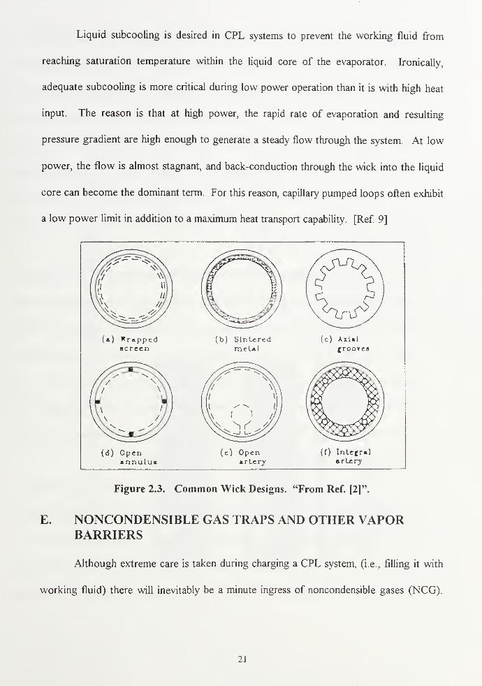
Wicks are typically force-fit within an axially grooved aluminum tube, such that the

wick outer surface and the inside of the tube are contiguous. This creates a passage on

either side of the wick to provide for a liquid-vapor interface within the wick structure.

There are numerous variations in the shape of the wick itself. Some of the more common

designs are shown in Figure 2.3. It is the ability of the liquid-vapor interface within the

wick to withstand a pressure differential that is the key to CPL operation. During normal

operation evaporation occurs on the outer surface of the wick. Near the capillary

pumping limit, the liquid-vapor interface recedes into the wick, reducing the heat transfer

area by as much as 50 percent. [Refs. 3, 16]

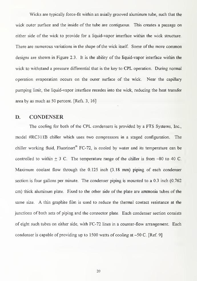
D. CONDENSER

The cooling for both of the CPL condensers is provided by a FTS Systems, Inc.,

model #RC311B chiller which uses two compressors in a staged configuration. The

chiller working fluid, Fluorinert® FC-72, is cooled by water and its temperature can be

controlled to within + 3 C. The temperature range of the chiller is from -80 to 40 C.

Maximum coolant flow through the 0.125 inch (3.18 mm) piping of each condenser

section is four gallons per minute. The condenser piping is mounted to a 0.3 inch (0.762

cm) thick aluminum plate. Fixed to the other side of the plate are ammonia tubes of the

same size. A thin graphite film is used to reduce the thermal contact resistance at the

junctions of both sets of piping and the connector plate. Each condenser section consists

of eight such tubes on either side, with FC-72 lines in a counter-flow arrangement. Each

condenser is capable of providing up to 1500 watts of cooling at -50 C. [Ref 9]

20

Liquid subcooling is desired in CPL systems to prevent the working fluid from

reaching saturation temperature within the liquid core of the evaporator. Ironically,

adequate subcooling is more critical during low power operation than it is with high heat

input. The reason is that at high power, the rapid rate of evaporation and resulting

pressure gradient are high enough to generate a steady flow through the system. At low

power, the flow is almost stagnant, and back-conduction through the wick into the liquid

core can become the dominant term. For this reason, capillary pumped loops often exhibit

a low power limit in addition to a maximum heat transport capability. [Ref. 9]

(a) Wrappedscreen

(b) Sinteredmetal

[c) Axtal

grooves

(d) Openannuluc

(e) Openartery

(f) Integralartery

Figure 2.3. Common Wick Designs. "From Ref. [2]".

E. NONCONDENSIBLE GAS TRAPS AND OTHER VAPORBARRIERS

Although extreme care is taken during charging a CPL system, (i.e., filling it with

working fluid) there will inevitably be a minute ingress of noncondensible gases (NCG).

21

is applied. This heating process or "bake-out" must be carefully done to avoid damage to

wick material. In addition, during normal operation a small fraction of the working fluid

itself may experience chemical breakdown. In the case of ammonia, nitrogen and

hydrogen gases will be produced. Usually, the quantity of such gases is so low that their

effects during normal operation are negligible. They tend to migrate through the system

to the liquid cores of the evaporator pumps, where they are stopped by the wick and begin

to collect. Although these gases do little to affect system performance during normal

operation, their effects during power cycling can be catastrophic. [Refs. 3, 6, 7, 9, 11, 12,

16]

As power is decreased, the system pressure drops, allowing small vapor bubbles at

the end of the liquid core to expand. If they grow large enough, these bubbles can block a

portion of the wick surface. This reduces the area available for evaporation, and thus

reduces the rate at which heat is removed from the evaporator. The associated

temperature rise may expand the bubble further, blocking the entire wick surface. By

destroying the liquid-vapor interface, the bubble takes away the capillary pumping force,

making it impossible for the evaporator to draw liquid into its core. Heat can no longer be

dissipated by this pump. This phenomenon is illustrated in Figure 2.4.

One solution to this problem is to design the evaporator core large enough to

accommodate bubble formation. While this certainly makes the evaporator more robust, it

also adds significant weight and cost to the CPL system. An alternative solution is to

connect the outlet of each condenser to a noncondensible gas trap. The purpose of this

device is to remove noncondensible gases from the liquid and prevent them from being

22

transported to the evaporator headers. Each NCG trap is composed of three concentric

cylinders; an outer ring, a cylinder composed of wick material, and an inner cylinder with

holes at one end. Liquid from the condenser enters between the wick material and the

CO

CO

o

c/5

aD

Ooo

o+->

o

Ohw

uoQ

i

2. o

i§s«O C8

."2 S

2 ss

O "38

2 «= a1-- o00 C

.2 c•3 ra

c SJO v:Q, as

0) u-

H °5 «>

8"g

•5 «

•C

5 oj

2 «=-3

<u " %> E

c/: o< c

s 2

O0c'53

£ 2£ «00-^_ o

•2 ^

O oa. =

S i- oti - °

=3 O C~ — CO

% % aJJ '£ «x> o «ix> a. -=

= 2 -§ 3 =

=: c

CO ,^ CO CO

2--=2 2OJ .3

a.CJT3

Figure 2.4. Effects of Noncondensible Gases.

23

inner cylinder. The wick material allows the liquid to flow through while acting as a

barrier to all gas bubbles larger than its pore size. These larger gas bubbles continue to

travel to the end of the trap where they pass through the holes into the inner storage area.

The NCGs are placed at the subcooled outlet of the condenser because the solubility of

gases in the ammonia is lowest at this point in the system. [Refs. 3, 9]

In addition to blocking the flow of noncondensible gas to the liquid transport

section, NCGs also serve as flow regulators when multiple condensers are connected in

parallel. Since each condenser will likely be connected to a different radiator, it is likely

that each condenser will be dissipating to a different sink temperature. If the temperature

of a sink (or sinks) is too high to completely condense the working fluid within that

condenser, vapor will flow to the NCG, where it will become trapped. The flow

resistance through the wick will force the vapor to be rerouted to another condenser. As

long as other condensers are capable of handling the increased vapor flow, the ineffective

condenser/radiator can be "shut down" until conditions for condensation improve. As the

radiator temperature decreases, flow will gradually return to that condenser. [Ref. 3]

There are currently two basic condenser designs used in most space applications.

The first design is called direct condensation and involves mounting the condenser section

of the capillary pumped loop directly onto the back side of the radiator surface. This

design was incorporated into most of the early ground testing and was used for the first

several flight experiments. Although the design provides a very efficient and inexpensive

way to transfer heat to the radiator for rejection, it is highly susceptible to micro-

meteoroid bombardment. [Ref. 3]

24

There are over 8000 objects larger than 20 centimeters currently orbiting the earth

at altitudes of 300 miles (482.8 km) or less. A ground based observatory using the

Haystack Radar monitors over 140,000 objects one centimeter and larger. The average

velocity of particles in these orbits is near 18,000 miles per hour. The number of these

particles has increased by over a thousand in the past three years alone, and will continue

to rise in the foreseeable future. Satellites, and even the space shuttle itself have had to do

"evasive" maneuvers to avoid impact with orbital debris. [Ref 17]

Some sources of this debris are spent rocket motors, accidentally lost satellite

components, surface erosion, shrapnel from exploding rockets, and intentionally discarded

waste [Ref. 17]. The tremendous velocities of micro-meteoroids and other orbital debris

gives even minute particles enormous momentum. Although the density of these micro-

meteoroids is very low and likelihood of impact even smaller, a single puncture would

result in the complete loss of working fluid inventory and result in total failure of the

thermal control system.

An alternative to direct condensation is the heat pipe heat exchanger (HPHX). In

this design heat is transferred from the condenser to multiple heat pipes through an

interface heat exchanger. This heat exchanger removes heat from the capillary loop

condenser(s) and applies it to the evaporator sections of the heat pipes. These heat pipes

are in turn mounted to a radiator surface, so they can reject the received heat. Although a

micro-meteoroid impact may still disable one of the heat pipes, the system will not suffer

degradation as long as the other heat pipes are capable of handling the increased heat load.

This design is the prototype for the EOS-AM, and has performed well during ground

25

testing, where it demonstrated a heat exchange rate of over 800 watts and heat transfer

coefficients in excess of 6000 W/m2K. [Ref 3]

Wicks are also used as vapor barriers in both the isolators and the reservoir. In the

reservoir, which contains a two-phase mixture and is connected to the evaporator liquid

headers, the wick prevents vapor from flowing to the evaporators. The isolators are

relatively small, with only about 2 inches of active (wicked) length. The isolator wicks are

also designed to prevent the passage of vapor. There is one isolator for each capillary

pump, so that if that pump deprimes, vapor will not flow back through the liquid header

and into the liquid cores of other pumps, thereby causing all pumps on that header to

deprime. [Ref. 9]

F. STARTER PUMP

The starter pump is a short evaporator pump with a relatively large diameter

designed to clear vapor from the evaporator grooves of the other evaporators in the

system. By clearing the vapor grooves, the starter pump creates a liquid-vapor interface in

the other evaporators. With an interface present, surface evaporation rather than nucleate

boiling occurs. If an evaporator is hard filled, i.e., both sides of the wick are filled with

liquid, superheat is required to initiate boiling. [Refs. 3, 6, 7, 9, 16]

Superheat is undesirable for two reasons. First, when fluid in the vapor channel is

superheated just a few degrees, the onset of boiling will be characterized by rapid

formation of a large vapor bubble. This sudden "explosion" of vapor causes a pressure

surge that could exceed the capillary limit of the evaporator pump and blow vapor back

through the wick. In addition, conduction through the wick may allow the vapor channel

26

superheat to raise the evaporator core temperature above the saturation limit, allowing

vapor to form in the interior of the wick. As with noncondensible gases, accumulation of

vapor inside the liquid core reduces the effective heat transfer area and may cause the

evaporator to deprime. [Refs. 3, 6, 7, 9, 11, 12]

Since the starter pump plays such a significant role in reliable start up of the entire

CPL system, it is protected against deprime during its own startup. A device called a

bayonet, which is simple an extension of the reservoir input line, is installed deep within

the starter pump liquid core. With the bayonet positioned deep within the liquid core of

the starter pump, cool liquid flowing into the bayonet tip will help compress, condense, or

flush out any bubbles existing in the evaporator core. Liquid returning from the condenser

to the reservoir must first flow through the starter pump core before flowing through the

bayonet into the reservoir. [Ref. 9]

Vapor exiting the starter pump displaces liquid from the vapor line and the vapor

grooves of other evaporators. To ensure grooves are cleared, a Capillary Vapor Flow

Valve (CVFV) is installed in the vapor line. The CVFV is a screen which prevents the

liquid/vapor interface from traveling to the condenser section until the evaporator grooves

are cleared. The holes in the screen are smaller than the evaporator vapor grooves, so

vapor produced by the starter pump will tend to empty the larger cavities first. [Ref. 9]

27

28

III. CAPILLARY PUMPING THEORY

A. THEORY

By definition, all liquids are in a state of tension. This tensile force comes from

molecular interaction of surface molecules with adjacent ones in the fluid interior. Tensile

stress in solid materials is defined as the force per unit area normal to the direction of the

force. Surface tension is expressed as force per unit length along the surface. This avoids

uncertainty about the actual area over which the force acts. Surface tension is a function

of temperature, almost always decreasing with increasing temperature, and changes

slightly with the type of gas at the liquid-vapor interface. Surface tension is fundamental

to capillary pumping theory. [Refs. 4 and 5]

Another factor that plays an important role in capillary pumping theory is the

cohesion or adhesion between the molecules within a certain liquid and a given surface.

The term "wettability" is used to describe the relationship between the two. A liquid will

"wet" the solid if adhesion dominates over cohesion. Conversely, a liquid will be non-

wetting if cohesive forces between liquid molecules dominate. An accurate measure of

surface wettability is the contact angle observed between a drop of liquid and the surface.

As shown in Figure 3.1, wetting liquids will usually have contact angles less than 90

degrees.

Capillary effects are greatest when a liquid is either highly wetting or highly

nonwetting. For this reason, most heat pipes and capillary pumped loops use liquids that

are highly wetting. Ammonia is a common working fluid, because it exhibits excellent

29

wettability on hard, solid surfaces, is inexpensive, and does not tend to react with standard

CPL and heat pipe materials such as aluminum and stainless steel.

ls<90° 0, s

>90°

WETTING LIQUID NONWETTING LIQUID

Figure 3.1. Contact Angle: Wetting and Nonwetting Fluids. "From Ref. [4]."

Capillarity is a term that describes the ability of a curved liquid surface (meniscus)

to sustain a pressure differential across that surface [Ref. 4.]. This pressure differential is

the driving force behind the CPL system, and determines the maximum heat transport

capability. When the capillary limit of the wick material is reached, further increase in the

heat input cannot be matched with an increase in flow rate. The evaporator will not be

able to draw liquid into its core at the rate with which it is evaporating at the wick surface.

In time the heated part of the wick will dry out, causing the evaporator to deprime.

The capillary limit for a certain wick is defined as

2*q

APc = (r/cos<J) s)

where a is the surface tension of the liquid, r is the bubble radius of curvature, and <j)s is

the contact angle at the interface.

The bubble radius is often difficult to measure directly, and the following alternate

form is usually used.

30

2*CT

APc = rp

where rp

is the effective pore radius of the wick.

Note that the capillary pumping limit is a function of the wick pore radius, surface

tension, and contact angle only. The length and diameter of the evaporator have no effect

on the capillary pumping limit. The polyethylene wick inside Evaporator Pump No. 4 at

Phillips Laboratory has a capillary pumping limit of 2268.4 Pa (0.239 psid). In order for

the evaporator pump to remain operational, the sum of all the pressure losses throughout

the loop must be less than this small amount. System pressure losses are mostly due to

friction within the loop piping and capillary devices such as isolators, NCG traps, etc. If

certain components are at different elevations, there may also be losses (or gains) from

gravity. The following equation summarizes the pressure requirements for a capillary

pumped loop. [Ref 9]

APc > APwick + APf + AP^ + APg

In general, the pressure losses in capillary wicking structures (APWick and APiS0|) are

functions of the liquid viscosity and the wick permeability and can be estimated by the

following equation.

m_* * Do

APwick , APisol — 2 7C A. Kwick Lwick Di

APg, the pressure loss due to gravity, may be calculated from

APg

= p*g*h

APf is the sum of the frictional pressure losses due to pipe flow, and can be

calculated for each pipe section from

31

64*L*V2

APf = Re*D*2

Obviously, pressure losses are a major concern in CPL system design. Pipe sizing

and interior surface finish are selected to minimize flow resistance within the loop. In the

Phillips Laboratory CPL, all transport lines are electro-polished to achieve a surface

roughness of less than 24 micro inches (0.61 \xm) RMS. Fortunately, flow rates are

usually well within the boundaries for laminar flow, and pipe losses are typically small.

The CVFV is designed and positioned so that the wet screen is capable of blocking flow

of vapor during startup without creating a large pressure drop during normal (dry)

operation. Although the wick material in the isolator and the noncondensible gas traps

contribute to the overall pressure drop, the important functions these devices perform

warrant their associated pressure drops. [Ref. 9]

32

IV. DEVELOPING THE MODEL

A. SINDA/FLUINT

Although the operating principles of capillary pumped loops are relatively simple,

the design of a CPL system is quite complicated. The system components are extremely

interdependent and analytical modeling of these systems is almost a necessity. The

Systems Improved Numerical Differencing Analyzer and Fluid Integrator

(SINDA/FLUINT) is a software package which is very useful in system design and

evaluation. It is a general purpose thermal/fluid simulation tool which has evolved from a

thermal analysis program developed by the Chrysler Corporation in the late 1960's.

Martin Marietta expanded the original program to incorporate fluid analysis as well as

convection and radiation effects. [Ref. 1 6]

The current version of the software, SIMDA/FLUINT 3.2, is currently maintained

and distributed by Cullimore and Ring Technologies, Inc. NASA presently uses

SINDA/FLUINT as its standard program for thermal analysis involving single and two-

phase pumped thermal control loops. [Ref. 16]

Throughout this chapter program-specific terminology was used to help simplify

the documentation of the CPL model development. Appendix A contains a list of

SINDA/FLUINT nomenclature and terminology used in this chapter, along with a brief

description of each term. Appendix B is a listing of CPL components and the

corresponding SINDA/FLUINT element number(s) used to model them. The elements in

the submodel diagrams may be referenced back to the exact component which they model.

33

SINDA and FLUINT are really two separate programs which are capable of

functioning independently of one another. It is the capability to mesh the heat transfer

energy balance calculated by SINDA with the one-dimensional fluid flow mass,

momentum, and energy balance calculated by FLUINT that gives SINDA/FLUINT the

capability to completely model complex two-phase systems. [Ref 16]

SINDA/FLUINT is designed as a support tool, and is not very effective without

sound engineering input. If the user fails to input accurate data, connect components

correctly, and select the best available solution routine, the program will either abort or

report a convergence failure. If a system would not work in real life, then it most likely

will not work in SINDA/FLUINT either. There are no "cook book' solutions for any

problem, and the user must make many decisions to come up with a model that effectively

simulates system behavior while producing desired parameter data. It is up to the user to

determine the scope of the model and what outputs are necessary. Not enough data

makes post-processing and analysis difficult, and too much data makes the model hard to

maintain and increases run time. [Ref. 16]

SINDA is a network-style (resistor-capacitor circuit analogy) simulator for heat

transfer problems. Although capable of producing similar results to finite differencing or

finite element programs, SINDA is actually an equation solver. This provides the user

with more flexibility because unlike finite element programs, SINDA is not geometry

based. The user is free to create an arbitrary network of temperature points (nodes)

connected by heat flow paths (conductors) and can easily change the geometry without

having to restructure the entire model. The user can select from one of the available

34

solution methods or write their own customized solution procedure using FORTRAN-

style logic. The longevity and popularity of SINDA/FLUINT can be attributed in part to

the flexibility it provides the user. [Ref. 1 6]

Within SINDA there are four types of nodes available for use in thermal circuit

modeling. These are boundary, diffusion, arithmetic, and heater nodes. Boundary nodes

have infinite thermal capacitance and may not receive an impressed heat source. Their

temperature is time-independent, making them ideal for representing isothermal

boundaries and sinks. Diffusion nodes have finite thermal capacitance, and thus the

amount of thermal energy stored within such nodes changes with time. These are the

most common types of nodes, and are applicable to almost every component or boundary

within a thermal model.

Arithmetic nodes are similar to diffusion nodes, except that they have zero

capacitance. The nodes are instantaneously brought into a steady state energy balance

according to the heat flux supplied and heat exchange with surrounding nodes. The mass

of a component modeled by an arithmetic node must be accounted for by a neighboring

diffusion node. This makes it impossible to build a thermal model consisting solely of

arithmetic nodes. Arithmetic nodes are useful, but their instantaneous changes can result

in system instabilities and oscillations. Heater nodes are used to determine the amount of

heat required (either input or output) to maintain a set temperature.

In SINDA, all thermal nodes must be connected by conductors. There are two

basic types of conductors, linear and radiation. The most common category is linear

conductors. Examples of linear conductors include:

35

1

.

Heat transfer by conduction

k*AG = L

where k is the thermal conductivity, A is the area 1 to heat flow, and L is the length of

heat flow path.

2. Heat transfer by convection

G = h*A

where h is the heat transfer coefficient and A is the heat transfer area.

3

.

Heat transfer by advection (mass transfer)

G = m*Cp

where m is the component mass and Cp

is the specific heat at constant pressure for the

material.

For radiation, the conductance is input in units of energy per unit time per degree

to the fourth power. The user must input the emissivity of the radiating surface, the heat

transfer area, and the appropriate view factor between the control volumes exchanging

energy. The Stefan-Boltzman constant is already incorporated into the program, however

the user must ensure the system of units is accurate.

To facilitate modeling of heat transport by mass flow, conductors may be modeled

as one-way conductors. This permits the "downstream" node to be affected by the

"upstream" node, while the "upstream" node remains thermally isolated from the

"downstream" node. A common type of one-way conductor is a tie, which is used to

connect SINE)A elements to an appropriate FLUINT element. [Ref. 16]

36

FLUINT is intended to provide general analysis and modeling of one-dimensional

internal flow problems. As with SINDA, FLUINT is based on network methods and is

geometry independent. The program is capable of steady-state and transient modeling for

any fluid, and is capable of handling transitions between single and two-phase flows. The

program contains a library with fluid properties for over 300 fluids, 26 of which may be

incorporated into the same model. Library fluids are identified by their ASHRAE

refrigerant number. In addition to the fluids available in the program library, the user has

the option of inputting their own fluid properties. The program also has the capability of

dealing with multiple constituent flows. [Ref. 16]

To build a fluid submodel, FLUINT uses components called lumps to create a

system similar to the nodal network in SINDA. There are three types of lumps available in

FLUINT. Plena are the FLUINT equivalent of boundary nodes. They have infinite

volume and constant thermodynamic state. Tanks are analogous to SINDA diffusion

nodes. They have finite volume and experience mass and heat transfer with resultant

change in thermodynamic state. The user has an option of defining the volume of the tank

in functional form, making it easy to simulate pistons, accumulators, or diastolic pumps.

The fundamental tank equations used in FLUINT are:

1

.

Tank Mass:

dm/dt = I FRi„ - I FRoUt(FR = mass flowrate)

2. Tank Energy:

dU/dt = L (Hdonor * FRm ) - I(Hleff *FRout + QDOT - PL*(dVOL/dt)

3. Tank Volume:

dVOL/dt = VDOT + VOL*COMP*(dPL/dt)

37

Junctions serve the same purpose as arithmetic nodes. They contain no volume

and instantly change to maintain the flow energy balance. They let the user define

important points in the fluid flow path without lengthening solution time. Since junctions

have no volume, the volume of the part of the system which they represent must be

accounted for in an adjacent tank. Again, no fluid model may be constructed by using

junctions for every lump. The basic equations for junctions are:

1. Junction Mass:

ZFRin - iFRout =

2. Junction Energy:

I (Hdonor * FRin ) - 2 (Ffleff* FRoUt) + QDOT =

As in SINDA, the components in FLUTNT must be connected via flow paths.

There are two types of paths, tubes and connectors. Tubes have finite volume and their

flow rates cannot change instantly. They are useful in smoothing out transient solutions,

but offer no real advantage for steady state modeling. The momentum equation for a tube

is:

dFR/dt = (AF/TLEN)*(Plup - Pldown + HC + FC*FR* | FR |

FPOW + AC*FR2

)

The other type of path is the connector. Connectors are time-independent path

through which lumps may exchange energy and mass. Connectors do not model a single

"real" piece of fluid hardware, and may be tailored to model a diverse group of fluid

components. They may be used to represent pumps, valves, bends, orifices, and certain

capillary devices (wicks). The governing equation for the k connector is represented in

FLUTNT by the following:

38

AFRkn+1 = GKk

n(APLj

n+1- APLj

n+I) + HKk

n + EIknAHLj

n+1 + EJknAHLj

n+1 + DK^AFRjT 1

FLUINT also has the ability to model fluid devices. Constant and variable speed

pumps, check valves, control valves, heat exchangers, and evaporators may be modeled

using built-in utilities. The built-in models are more complex than user built devices,

taking into account fluid accelerations, phase changes, and pressure losses. [Ref. 16]

There are four built-in solution routines within SINDA/FLUTNT: STDSTL,

FASTIC, FORWARD, and FWDBCK. Selection of solution method depends on the type

of model to be solved, the desired accuracy, and computation time available. A brief

description of each solution method is outlined below.

1. STDSTL/FASTIC

These subroutines calculate the steady-state solution for both fluid and thermal

networks. A successive point iterative method is used to balance the energy flows

through diffusion and arithmetic nodes. One pass through all nodes is called an iteration.

The heat balance for the I

thnode on the k+l

thiteration is:

i=l

= Qi + I [G,, (T>+1

- T k+1) + G'* {(T^ 1

)

4- (T,

k+1

)

4

}]

N

+ I [Gji (Tjk+1

- T,k+1

) + G'ji {(Tjk+1

)

4- (T

k+1)

4

}]j-i

The superscript (') on the G terms indicates that the conductance is radiative in nature.

This same procedure is also used in the FASTIC, however FASTIC is more tolerant of

inconsistencies in initial conditions. With both routines the user must specify the

maximum number of iterations per time step as well as nodal temperature and fluid

39

property convergence criterion. Relaxing the criterion may help speed up the solution

process. As with all solutions, the necessary benchmark for accuracy is the network

energy balance. [Ref. 16]

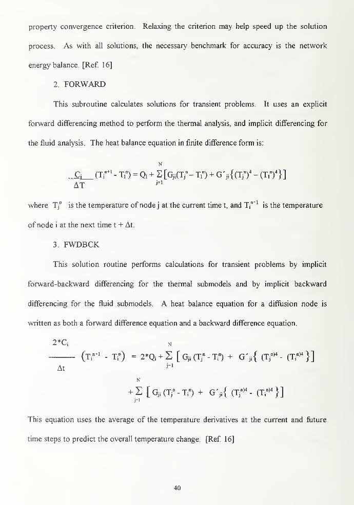
2. FORWARD

This subroutine calculates solutions for transient problems. It uses an explicit

forward differencing method to perform the thermal analysis, and implicit differencing for

the fluid analysis. The heat balance equation in finite difference form is:

N

_Cj (T,n+1

- T,n) = Q, + S [GjiCT/- T,

n) + G'jilCT/)

4 - (T,n

)

4

}]

AT j=1

where T/1

is the temperature of node j at the current time t, and Tin+1

is the temperature

of node i at the next time t + At.

3. FWDBCK

This solution routine performs calculations for transient problems by implicit

forward-backward differencing for the thermal submodels and by implicit backward

differencing for the fluid submodels. A heat balance equation for a diffusion node is

written as both a forward difference equation and a backward difference equation.

2*C, N

(T ;

n+1- Ti

n) = 2*Qj + E [ Gjj (Tj

n- T ;

n) + G'ji{ (T/

04- (T^}]

Atj=1

N

+ 1 [ Gji (Tjn

- Tjn) + G'ji{ (T/

04- (Ti

n)4

}]j=i

This equation uses the average of the temperature derivatives at the current and future

time steps to predict the overall temperature change. [Ref. 16]

40

To facilitate model production, debugging, and interpretation, Cullimore and Ring

Technologies, Inc., has added a graphical user interface. The SINDA Application

Programming System (SINAPS) is an extremely useful program that significantly enhances

modeling capabilities. SINAPS allows the user to build a model graphically using icons to

represent various components. The input blocks for each component are provided in

spreadsheet format to facilitate model creation and maintenance. SINAPS feeds the input

data to SINDA/FLUINT, and after the simulation has been run, reads the output file for

processing. This visualization tool helps accommodate higher-order modeling and

enhances pre- and post-processing operations. With SINAPS, the user can produce X-Y

plots, bar graphs, and data tables of system parameters. There is also an option to color

icons by temperature, quality, pressure, flow rate, heat transfer rate, and conductance.

[Ref 16]

B. STEADY-STATE MODEL

The first step in developing the steady-state model of the Phillips Laboratory

capillary pumped loop was to decide which system components were to be modeled.

First, the model had to accurately reflect steady-state performance over a range of heat

inputs and condenser temperature settings. Second, the model had to be well documented

and well laid out so future updates could easily be made. A CPL schematic, modified to

show only the portion modeled, is provided in Figure 4.1.

The first portion of the overall model to be discussed is the fluid submodel CPL2.

Fluid models tend to be more complex than thermal models in that they require more

input, more complex user logic, and are more likely to contain oscillations during the

41

solution process. For this reason, fluid modeling began with the fewest components

possible, and was only added to if required for the accuracy of the solution. Since small

changes in inputs, or the addition of even one more component can drastically change the

model solution, additions had to be made slowly and the model had to be validated after

each change.

Figure 4.1. Schematic of Modeled Portion of Phillips Laboratory CPL

42

The FLUTNT model contains the components and flow paths required to simulate

CPL operation. For the steady-state model only one evaporator pump (Evaporator pump

No. 4) was selected for modeling. It has proven to be the most robust of the evaporators,

and has undergone the most testing. The pump is 15 (0.381 m) inches long, and is located

at the far end of the inboard evaporator plate. Since the location of this evaporator is at

the end of an evaporator section, it will be relatively easy to add additional pumps at a

later date. The solution procedure chosen assumed that the pump had already successfully

started. This eliminated the need to model the starter pump and avoided the transient

pressure surge which accompanies the clearing of the evaporator vapor grooves and the

displacement of liquid from the vapor section during startup.

The reservoir is a vital component in the CPL system and was therefore included in

the model. To simplify its representation, a plenum was used. Essentially this selection

assumes that the reservoir is capable of perfect system temperature regulation regardless

of heat input or condenser sink temperature. While this may not be true at heat inputs

near maximum, previous modeling of other CPLs has shown that this assumption is valid

throughout most of the CPL operating range [Ref. 16]. The reservoir pressure was set to

match the experimental system operating pressure of 1.1652 MPa, and the temperature

was set at the corresponding saturation temperature of 30 C. All lumps in the system

were initialized to this pressure. An STUBE was used to connect the reservoir to the

liquid transport line, however since there is no flow to or from the reservoir through this

small diameter tube during steady-state operation, the flow rate through this STUBE was

set to zero and the volume of the tube was not incorporated into an adjacent tank.

43

Tanks were used to account for the volume of the liquid transport line from the

condenser, and the liquid header. Tank temperatures were set at 16 C, which accurately

reflects the subcooling provided by the condenser. The qualities of these tanks were

initialized at zero. All tanks were given a compliance of 8.85 E-09 cubic meters per Pa.

The compliance allows for minute changes in tank volume and helps avoid system pressure

spikes which contribute to evaporator pump deprime.

Although this seems like a misrepresentation of reality, it really isn't. Pressure

oscillations during normal operation are inherent to CPL performance. At high power

inputs, some short pressure spikes may reach or exceed the capillary limit of an

evaporator. In testing it has been shown that the extremely short duration of the spikes is

usually not enough to deprime an evaporator. Due to the analytical nature of

SINDA/FLTJTNT however, the program "sees" the pumping limit be exceeded and

deprimes the pump. [Ref 16]

A CAPIL connector was used to connect the liquid inlet header tank with a tank

representing the liquid inside the core of the evaporator pump. The CAPIL device, which

models the evaporator isolator, is similar to an STUBE except the CAPIL adds the

pressure loss and vapor blocking properties of the isolator capillary wick structure. Inputs

to the CAPIL connector are the effective pore radius and the flow conductance factor

(CFC). The CFC is a term which relates the effective flow resistance through a wick

structure to the flow rate and phase of the fluid.

2*7i*Pw*L

CFC = lnOVr;)

In this equation, Pw is the wick permeability (m2), L is the effective wick length (m) and

r ,r; are the wick inner and outer radii.

44

The tank representing the evaporator liquid core was directly connected to the

CAPPMP macro, and was therefore essential in maintaining the primed state. The initial

tank temperature and pressure were identical to those of the liquid inlet header tank. In

order for the CAPPMP to stay primed, the quality of this tank had to remain at zero.

The CAPPMP macro is a powerful built-in component which was used to model

the capillary pump evaporator. The macro consists of a centered junction which is

connected to adjacent fluid lumps via specialized NULL connectors, and to a different

node in a thermal model via a tie. The macro is extremely useful because it takes into

account the pressure drop through the wick, the pressure gradient across the liquid-vapor

meniscus, and the capillary pumping limit of the wick structure. The initial temperature

was set to that of the subcooled liquid and the quality was set to zero. The XVH and

XVL values for the CAPPMP model were also relaxed to help maintain the primed state.

The overall heat transfer conductance of 134.1 W/C was calculated using an average heat

transfer coefficient of 7,000 W/m2C and the outer wick surface area.

UA = h*7i*D *L

D and L are the outer diameter and active wick length in meters. The CAPPMP macro is

directly tied to a diffusion node in the EVP thermal submodel which represents the

evaporator tube wall. The tie is the path through which heat from the heater element

flows to the evaporator.

Although the evaporator wick is made of polyethylene, there will still be a small

amount of conduction through the wick to the evaporator liquid core. If the wick is

sufficiently wet, there will also be conduction through the ammonia itself. Several

45

modifications were made to the steady-state model to account for back-conduction

through the evaporator wick. The first alteration was the addition of an arithmetic node to

the EVP submodel, to which the CAPPMP tie was connected. The purpose of the

arithmetic node was to accurately represent the saturation temperature. To do this, the

normal evaporator UA coefficient was multiplied by 100, making it large enough to

provide minimal temperature difference without affecting problem stability. A conductor

with the old value of UA as its conductance completed modification by connecting the

evaporator wall node to the saturation node. [Ref. 16]

To simulate back-conduction, the tank representing the evaporator liquid core was

thermally tied to the saturation node. The UA coefficient was calculated using

2*7c*kc*L

UA =

ln(ro/ri)

Where kc is the average conductivity and is obtained from

The e in the above equation is the fraction of the wick that is wetted.

In addition to back-conduction through the wick, generated vapor will come in

contact with the evaporator wall during its transit through the evaporator grooves. Since

the evaporator wall temperature is above the saturation temperature, a small degree of

sensible heat will be added to the exiting vapor. In an attempt to model this superheat, a

junction was added to represent the vapor grooves in the evaporator. This junction was

thermally tied to the evaporator wall node to provide a path for the superheat. The UA

coefficient for this tie was derived from the groove are and average film coefficient, both

46

of which were provided by the manufacturer.

To connect this junction to the junction representing the evaporator exhaust

header, an STUBE was used. Since vapor is generated all along the length of the

evaporator, using the entire length would overestimate the true vapor path length. For

this reason, the length of the STUBE was set to the half-length of the evaporator. The

hydraulic diameter and the flow area per groove were obtained from the manufacturer,

and duplication factors of 26 were used on both the upstream and downstream ends to

account for the 26 grooves in the TAG 19 evaporator. [Refs. 9, 16] A diagram of the

thermal resistance network for the CPL model is provided in Figure 4.2.

As in real life, evaporator pumps in the model are temperamental, and it is difficult

to model steady-state without encountering evaporator deprime. Several programming

methods were used to help prevent evaporator deprime. The first method involved the

inputs to the XVH and XVL blocks of the CAPPMP macro. The terms represent the

quality of adjacent lumps necessary to sustain the pump. In essence they are upper and

lower quality limits for the input and output of the capillary device. By relaxing these

conditions slightly, the modeled pump was made more robust without affecting the steady-

state solution.

Another tool which was used to prevent evaporator deprime was the subroutine

SPRJME. SPRJME, short for "stay primed", is able to sense when an evaporator deprime

is imminent and makes adjustments to the pressure and quality of adjacent lumps to ensure

the pump remains primed. Care had to be taken while using this subroutine because

although SPRTME will keep the evaporator from depriming, it may cause the program to

47

produce inaccurate results. There were two ways to ensure that the model was still valid.

First, a program option was used that printed out a message every time SPRIME changed

a value. A continuous stream of messages would indicate that the solution was invalid.

Finally and most important, all submodel energy balances were verified to ensure validity

of the solution.

A junction was used to model the evaporator vapor exhaust. With the assumption

that the vapor line has already been cleared of liquid, the response of the exhaust header

will not have a significant effect on the steady-state solution and selection of a junction is

appropriate. The junction temperature was set at the saturation temperature, and the

initial quality set to 1.0 (i.e., no liquid in vapor grooves during normal operation). If a

transient response of the startup were modeled, a tank might be a better choice because

state properties within a tank cannot change instantly like they can in a junction. A tank

will tend to smooth the transient system response and will help keep the evaporator

primed.

STUBES were used to model the liquid and vapor transport lines. A tank was also

created to account for the volume of each section. The vapor side tubes reflected their

0.01021 meter (0.4 inch) inner diameter and the 4.647 meter (15.33 foot) length between

the evaporator exhaust header and the condenser inlet. Due to the length and small

conductive area of these pipes, axial conduction was orders of magnitude smaller than

heat transfer due to fluid flow and was neglected.

48

— c_ go H u

a ei

c u?

es

Eu

o .=U j r-

Figure 4.2. Thermal Resistance Network for the CPL Model.

49

The condenser portion of the steady-state model was the most difficult to design.

The condenser for the Phillips Laboratory capillary pumped loop is different from most in

that there is not a single path for fluid flow. Each condenser section contains eight parallel

condenser tubes connected to inlet and outlet manifolds. The flow rates in each tube, as

well as the location where condensation occurs is not as easily delineated as in single path

condensers.

The eight parallel lines in the condenser were modeled as eight mini-condensers

using the built-in HX macro. The eight parallel tubes were thermally connected via ties to

the cold plate submodel. Although FLUINT allows for path duplication which might have

simplified modeling somewhat, these factors were not used. Duplication factors assume

that the flow is equally distributed between all tubes. As actual experimentation has

previously shown, that is not the case. Experiments show that a majority of the vapor

travels through the first three tubes, with considerably less vapor flow making it all the

way down the manifold to the last several tubes. In an attempt to model this phenomenon,

the eight "mini" condensers were modeled so that they were completely independent of

each other, allowing for different flow rates in each condenser leg. To conform with the

current test setup, only one of the condensers was modeled.

The HX macro used to model the mini-condensers was designed to model heat

exchangers. Ten discrete points (junctions) were used to model each of the eight

condenser legs. This number was chosen to allow for more accurate determination of

where condensation actually takes place within each leg. By observing the lump quality

during program output, the location of condensation may be estimated to within 10% of

50

the overall condenser length. Finer precision could be achieved by adding more lumps to

each of the mini condensers, but would also increase simulation run time. The condenser

junctions were connected by STUBE connectors, with the end connectors each 0.0912

meters (3.59 inches) long and the four interior connectors each 0.1825 meters (7.18

inches) in length. The segment lengths add up to the total condenser length of 0.733

meters (28.85 inches) per leg. They are less sensitive to flow reversals, and help with

solution stability. Each STUBE reflected the 1/8 inch (0.00318 m) inner diameter of the

Swales and Associates design. [Refs. 9, 16]

Thermal ties were used to connect the junctions for each of the parallel condensers

to separate nodes representing the tube walls in the CLDPLT submodel. As mentioned

before, ties are similar to conductors and are used to link thermal and fluid submodels.

Each tie has a UA coefficient associated with it. The tie parameters may be calculated by

the program itself using one of several correlation methods built into the code, or the user

may define their own equation or subroutine to perform the calculations. The program

calculates the heat transfer coefficient by assuming that for the time step in question, the

lump represents the bulk fluid properties and the node represents the average wall

temperature. Since the step size is usually small, these assumptions are very accurate for

most simulations. The steady-state model incorporated HTNC ties which were

recommended for two-phase flow. Although using these ties shortens the maximum time

step allowed and therefore increases program run time, the ties are capable of handling the

large property variations that accompany phase changes and help maintain stability during

solution. [Ref. 16]

51

The initial layout of the steady-state model did not contain the noncondensible gas

trap at the outlet of the condenser. The effects of noncondensible gases are not yet fully

understood, and modeling them in a one-dimensional SINDA/FLUTNT model would be

extremely difficult. However, after reviewing system performance data, it was noted that

the gas trap did play an important part in the overall system pressure drop and needed to

be modeled if for that reason alone. A CAPEL device was used to model the

noncondensible gas (NCG) trap, using the effective capillary radius and wick permeability

provided by Swales and Associates, Inc. [Ref. 16]

The condenser inlet header was modeled as a junction. The inlet header was

initially set at the saturation temperature and pressure with a quality of 1.0. The outlet

header also was modeled as a junction, however some additional components were added

to it to create the NCG trap. A short STUBE was connected from this junction to a tank

which represented the inlet line to the NCG trap. This was done to provide stability to the

CAPEL connector which connects this STUBE to a similar one representing the liquid

transport line. The tank volume was input as the sum of the volume of the condenser

liquid header and the NCG trap. Tank temperature was set to the subcooled temperature

of 16 C and a quality of zero. These inlet and outlet headers were connected via STUBES

to the eight mini-condensers to completely model the condenser section. The volume of

the inlet header was accounted for in the vapor inlet line tank.

For each STUBE connector mentioned above, loss factors due to pipe bends,

elbows, valves, and tees had to be examined and incorporated into the pressure loss

calculations through each section. Loss data for valves was obtained directly from the

52

manufacturer. Table 4.1 lists the K-factor losses for each applicable STUBE in the CPL2

fluid model. Figure 4.3 shows a diagram of the CPL2 fluid submodel.

The K factors are basically velocity head factors which increase the normal flow

pressure loss through each line. [Ref. 18].

K= APy2pv2

STUBENumber

Flow into

tee branch

(1.9 each)

Flow out of

tee branch

(1.2 each)

90 degree

elbow

(0.74 each)

1 80 degree

elbow

(1.2 each)

Valves

(0.36 each)

Total Kfactor

05 2 2.48*

25 2 10 3 7 18.36

65 1 2 1 3.14

95 1 4 1 2 8.56

Cond.

Tubes

(Inlet)

1 1.90

Cond.

Tubes

(Outlet)

1 1.20

* K factors in parenthesis.

Table 4.1. Pipe Flow K Factors for CPL2 Fluid Submodel.

The steady-state model contains three thermal submodels, one representing the evaporator

section, one representing the condenser, and one representing the liquid and vapor

transport lines. The EVP submodel is made up of six diffusion nodes with their associated

conductors representing the path of heat flow from the heater strips to the evaporator

wall. All conductors are of the linear type. Radiation to the environment was not

included in this thermal submodel because the surfaces of the evaporator section are

covered with insulation, and the differences between ambient and insulation temperature

are small, making heat transfer due to radiation negligible. The heater node is an

53

arithmetic node to provide immediate response to heat input. The thermal capacitance of

each diffusion node was left at the default value since all nodes are treated as arithmetic

during the FASTIC solution method [Ref. 16]. The resistance along the heat transfer path

was dominated by the contact resistance at the junction where plates and/or brackets were

mounted to each other. The contact resistance was calculated using a correlation for

graphite foil in the near-bolt region of the interface. Although graphite foil was used in an

attempt to thermally connect surfaces, its resistance was in some cases two orders of

magnitude greater than the resistance through the highly conductive aluminum. Figure 4.4

shows a diagram of the EVP thermal submodel. [Ref. 2]

The CLDPLT thermal submodel consisted of eight nodes representing the

ammonia side tubing and eight nodes representing the condenser plate. The condenser

itself was modeled as a sink. This was done to simplify the model, and is an accurate

assumption considering the total heat input for the one-evaporator model and the cooling

capability of the condenser. The temperature of the sink could be modified easily to

conform to different radiator temperatures. The ammonia side tubing nodes in the

CLDPLT model were attached to the condenser plate nodes via linear conductors

representing the sum of the conductances through the tube wall, tube mounting bracket,

graphite foil interface, and Vz thickness of the plate. The conductors between the plate and

the sink were identical except for an additional term dealing with the convective

conductance from the coolant flow in the condenser side tubing.

The first step in calculating this additional forced convection conductance term

was to determine the type of flow through the condenser piping. The Reynolds Number

54

(Re), was used to make this determination.

V*DRe = v

where V is the flow velocity, D is the interior pipe diameter, and v is the kinematic

viscosity ofFC-72.

The flow rate of FC-72 through the condenser piping is regulated at 4 gpm, which

equates to a Reynolds number of 3.96 x 104

. This is well above the threshold for laminar

internal pipe flow (-2300), and past the transition region into turbulent flow [Ref. 19].

The Dittus-Boelter equation was used as the correlation for turbulent flow to determine

the convective heat transfer coefficient. Figure 4.5 shows a diagram of the CLDPLT

thermal submodel.

NuD = 0.023 *ReD4/5Pr

-3

To completely define the capillary pumped loop at Phillips Laboratory, another

thermal submodel was needed. Due to the long lengths of liquid and vapor transport lines,

a portion of which have no insulation, there is heat transfer between the lines and the

environment. Neglecting this heat transfer causes only a slight error in flow rates and

pressure drops, but causes discrepancies in vapor and liquid line temperatures.

The vapor-liquid line thermal submodel (VLL) was included to account for heat

transfer to and from the environment. It consists of nodes representing significant

segments of each line. For the vapor side, there are nodes to represent the vapor exhaust

header, the vapor transport line, and the condenser inlet line. For the liquid side, there are

nodes representing the NCG trap outlet line, and the liquid transport line. Each node is

connected via a linear conductor to the environment. The nodes in the VLL submodel are

55

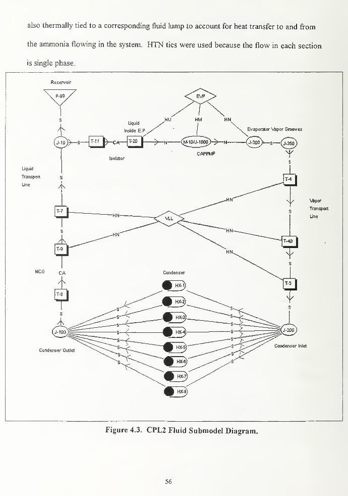
also thermally tied to a corresponding fluid lump to account for heat transfer to and from

the ammonia flowing in the system. HTN ties were used because the flow in each section

is single phase.

Reservoir

Liquid

Transport

Line

EVP

+Liquid

Inside E.P.

.HU HM HN

(Jmo)>-s—|t-h ^-ca—

|

t-2D y—^_N (j£JoIhooo)-^n

Condenser Outlet

Isolator

CAPPMP

Evaporator Vapor Grooves

-(J300)»

—

S (£350)

\J/ Vapor

Transport

Line

Condenser Inlet

Figure 4.3. CPL2 Fluid Submodel Diagram.

56

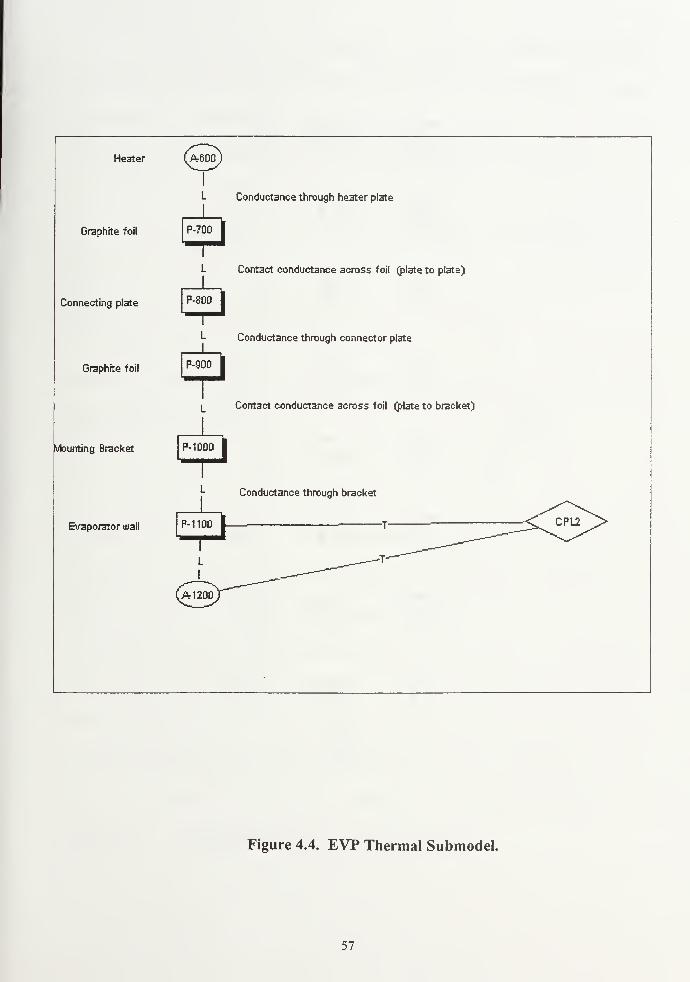
Heater (A:6DD

Graphite foil

Connecting plate

Graphite foil

Evaporator wall

L Conductance through heater plate

P-700 I

L Contact conductance across foil (plate to plate)

F-80.0

L Conductance through connector plate

P-900|

L Contact conductance across foil (plate to bracket)

vtounting Bracket P-1D00

J-Conductance through bracket

Figure 4.4. EVP Thermal Submodel.

57

Figure 4.5. CLDPLT Thermal Submodel.

58

The tube walls experience heat transfer via four methods: axial conduction along

the tubing, natural convection with the surrounding air in the laboratory, forced

convection from fluid within the tube to the tube wall, and radiation to and from the

surroundings. To simplify the model, axial conduction and radiation were neglected. The

conductances for both of these heat transfer paths were small in comparison to natural

convection and internal convection. The axial conductance of the nodes closest to the

reservoir were calculated to be less than 0.001% of that for natural convection, and the

radiative conductance was less than 0.01% of that for natural convection.

The conductance input for each node consisted of two terms. First, the radial

conduction through the tube wall and insulation, if applicable, was calculated. The

equation used is shown below.

2*7i*k*L

C =

ln(ro/ri)

The next conductance which had to be calculated was the conductance due to natural

convection. To determine the natural convection equation to be used, the process itself

had to be examined. The surface of the tubing will either cool or warm a layer of

surrounding air, making it gravitationally unstable with the rest of the air in the room.

There will be a tendency for the cooler, more dense air to flow downward, and the

warmer, lighter air to rise. The fluid motion caused by the density differences causes

convective heat transfer between the tube and this small layer of surrounding air. To

calculate the conductance due to natural convection, the Rayleigh number had to be

determined.

59

g*(3*(Tw - T.)*Lc3

Ra =

va

In this equation, g is the gravitational acceleration, (3 is the expansion coefficient, Lc is the

characteristic length, a is the thermal diffusivity, and v is the kinematic viscosity. In the

above expression, both P, v, and a are properties of the surrounding fluid at the ambient

temperature. With the assumption that air behaves like an ideal gas, P is simply 1/T. The

Lc term is simply the diameter for natural convection over a horizontal cylinder, and is

equal to the surface area divided by the perimeter for the case of natural convection over a

flat plate. For the conductors tied to the bare tubing of the NCG trap outlet line, the

evaporator exhaust line, and the condenser inlet line, the horizontal cylinder correlation

was used. For the insulated transport sections, the following correlation for the average

Nusselt number based on free convection from the upper surface of a heated plate was

used. [Ref. 19]

NuD = 0.54*RaL°-25

As a first approximation, a temperature difference was assumed, the Rayleigh

number calculated, and test runs using 100 and 200 watts were completed. The average

temperature difference along the liquid line was observed for both of these test runs.

These temperature differences were averaged and then substituted into the Rayleigh

number calculations to come up with an "average" Rayleigh number. Figure 4.6 shows a

diagram of the VLL thermal submodel.

Once the model was built, the next step was tailoring the solution procedure using

the model control panels and Fortran-style logic. The most important of these logic

60

control panels is the Operations Data block. In this block Fortran-style code must be

input to command the processor to build the code based on SINAPS inputs. Each

submodel must be correctly built and connected to create the complete capillary pumped

loop model. The solution method must be selected in this field. The FASTIC solution

procedure was selected. The ability of this procedure to smooth initial conditions helps

stabilize the solution, and is the recommended solution procedure when large fluid

submodels are present. The start and end times, step time, and maximum number of

iterations per time step must also be input here.

The other logic blocks deal mostly with tailoring the output of each submodel for

use in post-processing. By instructing the program to output only desired parameters at

desired intervals, the run time and storage requirements may be reduced.

C. TRANSIENT MODEL

Modifications were made to the existing steady-state model to create the model

used in transient solutions. Thermal capacitance was calculated and added for each of the

diffusion nodes in the EVP, VLL, and CLDPLT thermal submodels. A starter pump was

added and connected directly to the reservoir to simulate the bayonet. Although the

starter pump was turned off at the start of each run, it was included in the transient model

to accurately represent the piping between the pump and the reservoir. The tube

connecting the reservoir to the rest of the system could not be disregarded as in the

steady-state model. As conditions change, the reservoir may have to accommodate slight

changes in system inventory until equilibrium is reached.

61

Figure 4.6. VLL Thermal Submodel.

62

The changes in solution procedure were the major alterations implemented for the

transient modeling. A forward differencing technique (FWDBCK) was selected as the

solution method for the transient model. Fortran-style logic was again used to change

input parameters during the solution so system response could be observed. The solution

time had to be modified to provide enough time for the system to steady out after changes

so values could be compared to those produced during steady-state modeling. Figure 4.7

shows the transient CPL2 fluid submodel.

63

EVP

Liquid

Transport

Line

NCG

Liquid

Inside E.P.

,HU HM

(^MOV-S—F^^C^-[^QT > N

HN

n. Evaporator Vapor Grooves

N (j-30oY-s—(jSIsolator

Reservoir

I TS9

Condenser Outlet

Condenser Inlet

Figure 4.7. Transient CPL2 Fluid Submodel.

64

V. RESULTS

A. STEADY-STATE

To verify the accuracy of the steady-state model, the program was run with

different combinations of evaporator power input and condenser set point temperature.

The data produced during each run was compared to actual test data from experiments

conducted at Phillips Laboratory. System temperatures and pressures were used to

compare data to experimental results. The plentiful number of thermocouples positioned

throughout the test setup facilitated overall temperature comparison, however attempts to

compare system pressure drops were more difficult. There are only five differential

pressure transducers in the Phillips Laboratory test setup. Modeling the exact location of

these transducers closely enough to produce an accurate comparison was not practical.

For this reason, only the pressure profile was compared to actual test results. The

pressure profile is a measurement of component pressures at a specific instant in time. To

facilitate presentation, pressure data is plotted for the entire loop. The plots begin with

the evaporator vapor grooves (highest pressure in the system) and continuing along the

loop until reaching the component with the lowest pressure in the system, the evaporator

liquid core. Pressure profiles for 100, 200, and 300 watts (condenser temperature -5 C)

are provided in Figures 5.1 through 5.3.

The profiles displayed in the figures mirror those of actual testing, with the larger

pressure drops occurring across the wicked devices such as the noncondensible gas

(NCG) traps and the isolator. In each case, the pressure rise across the evaporator wick is

65

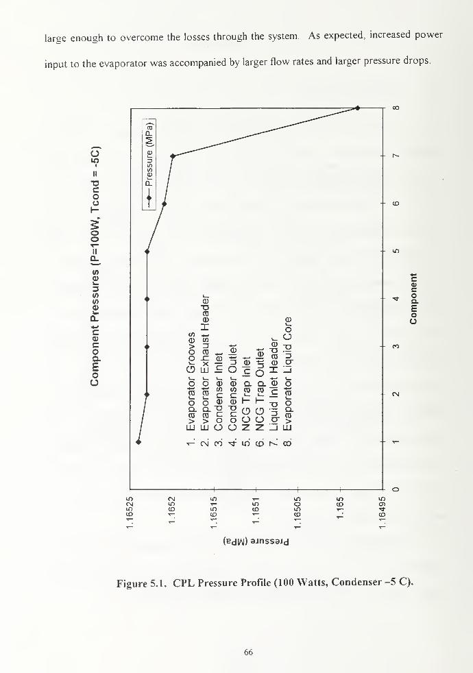
large enough to overcome the losses through the system. As expected, increased power

input to the evaporator was accompanied by larger flow rates and larger pressure drops.

, ^

03

D.

^^^oto 3

i in

ii

CO

TJ oL

C1O 1

o T1-„

£ooT"II i

Q_^^tnou.3(0CO

»-

D.•*•>

Coc >

oa.

Eoo

CD"OCOCD CD

I i_O

coCD w 1— O> -J •4—f CD Tloo

CD jD uCD

'5

I— X _)

c Oa) u

O LU _l_ o X _it t_ 1 I— .*—' t

o O CD CD Q_ Q_ CD oCD

OCD

o

(/)

CCD

COcCD

CD CDi_ i_

h- (-TJ

CDi_o

Q_ Q.CD

Uc

Uc O CD '5 Q.

> > o o O O o >LU LU o O z z _i LU

CN 00 "^ ID CD h- CD

oo

CO

-- m

- *

ca>coa.

Eoo

- CN

m CN m T— m m inCN m T— m o CO a>IT) CD m CD m *tCD T- CD r- CO CO

(BdlAJ) ajnssaJd

Figure 5.1. CPL Pressure Profile (100 Watts, Condenser -5 C).

66

o

ii

DCoU

ooII

CL

</)

Oi_

D(A(/)

O

CocoaEoo

a)

"O05a) CD

X OCO

in l_ o> n ^-* at "Don

03

75

_a>CD

u03

'5

i_ V _j

c Oci> u

O LU j_ O X _jt_ i_ 1 i_ .«—

»

i_o O a> CD Q. Q. CD o03

o03i—O

toc0)

COc

03 03

1- H"O

03

oQ.m

a.03

uc

uc o o '5

> > o o o o u >UJ LU o o z z _i LU

CM CO ^ IO (D S CO

oo

CD

in

- "*

cCD

coa.

Eoa

co

- CN

CO CN T~ m CD CO r-in m m CO <* •<3- •*CD CD CO T— co co CD

(edlAl) ajnssejd

Figure 5.2. CPL Pressure Profile (200 Watts, Condenser -5 C).

67

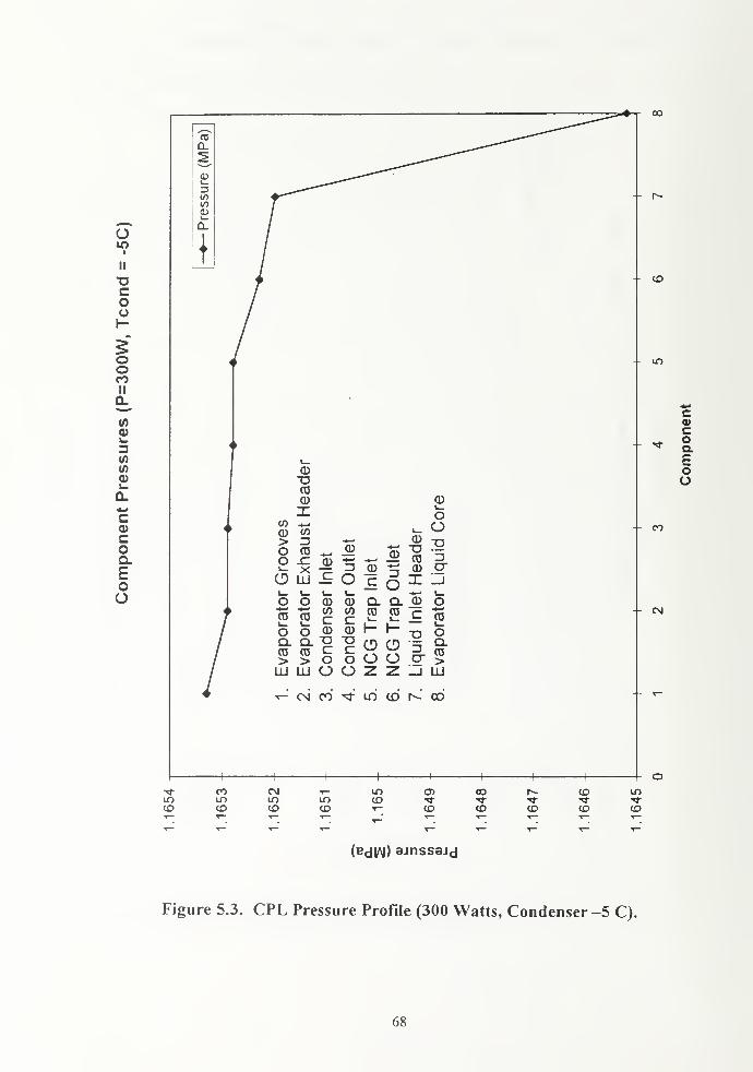
o

II

"DCoU

ooCOII

(A

3W(0V

ccoQ.

Eoo

^aT _^0***^^^

Q_ ^^ ^^^ ^•—^'^

£ ^BlllPl-^--,,,*,,,*,,

Z3 ^^*-'^

CO A^"*"'^co |CD /

u.

0.

1 /

i

t_0)

1"°co0) 0)

x c5

< '

d) CO J-^

O CO _ © "S "S 1£ m - , »i (0 3

OlU-EOcqIIjl_ l_ l_ l_ -»-' l_000)0)0.0.0)0

<

/l_ l_ »— »— i l" "" l_OO0)0)r-l— -no

/ >>ooOOo>/ UJUJOOZZJUJ

T-cNico^iDcbr^co'

1i

1 1 ! 1 1 1

oo

CD

- LT)

0)coQ.

Eoo

CM

* CO CM T— IT) o> CO r^- CD mm m U") m CO -<* •«*• <* "<*- *CD CD CD CO T- co CD CD co CD

(e<j|/\|) ajnssajd

Figure 5.3. CPL Pressure Profile (300 Watts, Condenser -5 C).

68

The pressure profiles of the steady-state model are useful in that they show where

the majority of the system pressure losses occur. As expected, pressure changes in the

liquid and the vapor transport lines, as well as the condenser were small. Appendix C

contains pressure profiles from the other steady-state runs. The pressure losses are driven

for the most part by system flow rates, and profiles for all steady-state runs were similar

since the condenser temperatures modeled (-5, 0, and 5 C) had little effect on system flow

rate. In all runs the pressure losses were within the capillary limit of Evaporator Pump

No. 4.

For temperature data comparison, nine different steady-state runs were completed.

Each run was based on a different power input to evaporator No. 4 and/or a different

condenser set point temperature. To create meaningful plots of temperature data, a

complete "loop" of system temperatures was plotted for each run. The upper left of each

plot shows the evaporator vapor grooves and vapor transport line. The steep slope occurs

as the working fluid enters the condenser, where the plot levels off somewhat before rising

again as the working fluid exits the condenser and proceeds back to the evaporator

section. Figures 5.4 through 5.6 show data comparisons for the 100-Watt steady-state

simulations.

The model indicates the working fluid exits the evaporator as a slightly

superheated vapor which cools rapidly to saturation temperature as it travels through the

uninsulated vapor header. The temperature data remains constant along the vapor

transport line, where the model also predicts condensation to commence. The steep slope

between points 6 and 7 reflects the rapid condensation of the working fluid, which both

69

the model and the experimental data show to occur in the first portion of the condenser.

The differences at point 6 (condenser inlet) are due to differences between the model and

the test setup as to thermocouple placement within the condenser. A relatively small

physical distance can cause large temperature variation in this region where the phase

change is taking place.

10i

IIocoo

ooII

aoISp

a.

Ea>

I-

Ea4->

HCNJ

o oa. a.to m

l|2 gI- no oQ-OTO

qj a) <D« « M rC C C Li]

"D "D "D rna c c y.O O O OO O O Z

p « (O « o\— £ «j

cr o- >

-- CM

Ca>

coa.

Eoo

COo If)

CMOCM

m

(0) 9jniej8dLU9i

Figure 5.4. Temperature Data Comparison (100 W -5C).

70

UJ ,

8 fe

Hoto

IIDCOo

oCMII

o

Ido1-

Q.

Q.

Eo

E

CM

C0)CoQ.

Eo

COoCO

oCM

m m

(3) 9jniBJ3dujai

Figure 5.5. Temperature Data Comparison (200 W -5C).

71

HI ,

o feu UJ

H .. cm

omi

ll

"DCoo3foooII

a

a.

EoI-

Eo•**

(A>»(/)

i,

o n m t ,

o ai c X a>

JJ

o1 r <u 4) c o

8.TO

>oGi-ro

>Coa.mc

"5

c

0)

31- 1-

0)

a>

a>ocas

a>

o</)

c

•o

I

-a

3cr

5?TO H c

a>

0)c0)

10c(1)

inc c

UJ5O \-

>UJ

a.to>UJ

<0

>

73coO

DCoO

coo

DCoOo Oo-z.

a

T3

3cr

Dcr >

LU

*— CM to U") (O f^ CO O) i- *— «- T-

c<u

coQ.

Eoo

- CM

COoCO

mCM

o m

(3) ejn}ej3diu3i

Figure 5.6. Temperature Data Comparison (300 W -5C).

72

At the exit of the condenser, both test data and the model predict a temperature

rise. It is in this portion of the plots, however, that the largest discrepancies exist. The

experimental data shows a marked increase in temperature occurring at the outlet of the

noncondensible gas trap, where the cool liquid coming from the condenser meets the

warmer liquid in the liquid transport line. The model predicts a more gradual temperature

rise, with significant heating occurring in the evaporator liquid core due to back-

conduction through the evaporator wick.

There are several possible causes for the differences in data for the return part of

the capillary loop:

1. The model assumed a reservoir temperature of 30 C, where in experiments this

temperature varied between 3 1 and 35 C.

2. While the model took into account the uninsulated portions of the liquid

transport line, the heat transfer coefficients calculated and the ambient temperature used

were possible sources of error. The model actually predicts condensation to begin along

the uninsulated vapor exhaust header. Figure 5.7 shows the uninsulated portion of the

vapor exhaust header.

3

.

The back-conduction of heat through the evaporator wick may have been

overestimated in the model.

4. As mentioned earlier, thermocouple placement and accuracy also contribute to

temperature differences. The model predicts the temperature of the working fluid,

whereas in most cases the thermocouples are recording the tube wall temperature.

5. The SINDA/FLUTNT model assumes an ideal inventory of working fluid in the

73

capillary pumped loop The inventory of ammonia in the actual test setup is unknown, and

may actually be less than the amount used in the model.

6. Thermophysical properties used in calculating heat transfer coefficients for

conduction and convection were only accurate to + five percent

The overall temperature profiles bear close resemblance in all cases, validating the

accuracy of the steady-state model. The addition of more nodes in the condenser and

liquid transport line submodels may improve the results somewhat, but would also

increase complexity and run time.

Temperature data comparisons for the 200 and 3 00-Watt simulations are provided

in Appendix D

Figure 5.7. Uninsulated Portion of the Vapor Exhaust Header.

74

B. TRANSIENT MODELING

The purpose of the transient modeling was to examine the system response to

changes in power input and condenser set point temperature. Several scenarios were run

and compared to experimental data from Phillips Laboratory. Temperature and mass flow

rates were compared for each run. As shown in Figure 5.8, changes in power input to the

evaporator resulted in corresponding changes in temperatures and mass flow rates within

the loop, which eventually reached steady-state values. The steady-state values reached in

the transient solution were within two degrees of the steady-state solution calculated

earlier for the same condenser set point temperature and power input. Table 5.1

summarizes the transient runs made. For each run, plots of temperature, system mass flow

rate, reservoir mass flow rate, and condenser quality were made. The results are provided

graphically in Appendix E.

Run Number Transient Event Modeled

1 Power change from 300-50 watts, Condenser temperature constant (0 °C)

2 Condenser temperature changes (5 to to -5°C) Power constant 200 W3 Power change 200-300-100 watts, Condenser temperature constant (0 °C)

4 Power change 200- 1 00 watts, Condenser temperature constant (5 °C)

5 Power change 50-300 watts, Condenser temperature constant (15 °C)

Table 5.1. Transient Run Summary.

Of particular interest was flow into or out of the reservoir. When compared to

system flow rates, the flow to or from the reservoir was negligible. Even with evaporator

No. 4 running at its maximum power, condensation still took place at or near the entrance

to the condenser tubing, as shown in Figure 5.9. With the condenser being so efficient at

condensing the vapor, there was little change in the location of the liquid-vapor interface

75

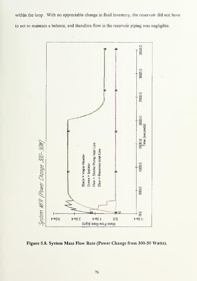
within the loop. With no appreciable change in fluid inventory, the reservoir did not have

to act to maintain a balance, and therefore flow in the reservoir piping was negligible.

I

1

B

»

COcII,

.

a>

03 cw C _l11)

00

a.F

_0j

COJ

X a Q. na OB cu £a.03

>oCO 00

a)

|| IIt/J LT

J* c II II

O a> jt n>00 c =i

CD O Q. OQ

«

to

Jo

*

fr-erj'E t^O'S Wl 00(s/6>i) e;ey mo|j sse^

IS)

s

a

-acoo

a cu

o Es

o8a

asin

ad

17-90"^

Figure 5.8. System Mass Flow Rate (Power Change from 300-50 Watts).

76

CD

CO aPRC CD a— co in

5S J9 a)n

§ ° 1o e o= '» *-3 -O CO

0)

c -" £ oX -c — CDCO ^3 O - a0) »- ^

oco

»- CD Cr_, CO (0

C 4->-C CD CDd "O -rr

u c £ 2 fc

2 S « — CD_J- O _£- _JD CDr* od *- -g« £ 2 o

" Ors

CDCD

" ao

c3 ^ 2 i

i

i » sCDCO

a cd

CD £^1

^̂a?

oCD

" CD^ CD

d * a \ J « *>"-

^*

^ 1

I O- CD

t \ V|

'*.

\

O

<§ \ \ N

$'

i ,_

_v _\ \

^ ^^^^^ ^>v^^^ "^—-^__^

^ ^^* _£^^ -=j

11

*%1 ^"T^-^^ P|o

VV E"0 Z'O I/O

CD

00<3 Aipno

Figure 5.9. Condenser Quality (Power Change from 300-50 Watts).

77

To produce a change in flow rate to or from the reservoir, there had to be a visible

shift in the liquid-vapor interface within the condenser. To model this without increasing

the number of evaporators rejecting heat via the same condenser, the condenser set point

temperature was increased to 15 C. A power change from 50 to 300 watts was imposed

on evaporator No. 4, and the resulting reservoir mass flow rate observed. For this run,

when the power was increased to 300 watts (t = 1000s), there was a corresponding spike

in the reservoir flow rate (see Figure 5.10). The spike, which was an order of magnitude

greater than the steady-state flow rate, lasted approximately one minute before quickly

damping to zero as the system again approached equilibrium. The increase in vapor

generated by the power addition caused a slug of liquid to be displaced from the

condenser and eventually travel into the reservoir. The slight time delay in the spike is

because the liquid must pass through the NCG trap and the starter pump header prior to

reaching the reservoir inlet line.

Comparisons were made between the test data and the model for the power

change of 200-300 watts during model run number three. The time required for

temperatures to change and stabilize to their new values was examined. The small

temperature variation in the vapor portions of the loop made comparison difficult, and

therefore only the liquid portion was analyzed. For four sections of the liquid side of the

loop, temperature-time data for the experiment was plotted along with model data for the

same time period. The time constant for each plot was compared. Figure 5.11 displays a

plot of one of these comparisons. As the plot shows, the response of the modeled NCG

outlet temperature is very similar to the experimental data. The calculated time constants

78

for the model and the experimental data were 257 seconds and 218 seconds respectively.

Similar plots for the other sections of the liquid line are provided in Appendix F.

1

I

I

^

I

Od o

r cdOm

od"SCN

3

OCD

- cdcdCN

1 1500.0

(seconds)

Ei—

ob

- oo

a- CDCDin

1 i i

^ * CD1 1 1 T o

S-90E S-90 Z 9-30 I 00(s/6>|) aiey mo|j ssejAj

9-90 1-

Figure 5.10. Reservoir Mass Flow Rate (Power Change 50-300W, Cond. = 15 C).

79

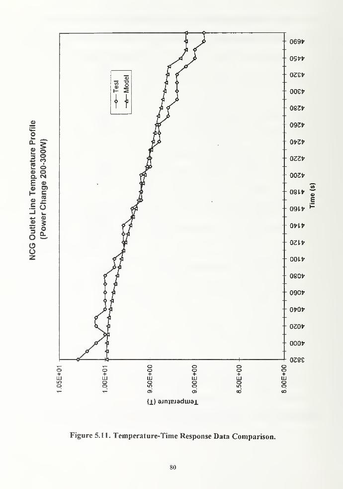
05

* O

ov.

£ I3 2*- CO

o> oE Si

IS-I i-

• £3 °

oo

- 069*

•- os**

- ose*

- ooe*

- 093*

- 093*

- 0*3*

- 033*

-- 003*

- 091* ~.1

-- 091-* p

- 0*1-*

- 031.*

- 001.*

- 090*

- 090*

- 0*0*

- 030*

- 000*

-- 0399

LU

o

O+LUOo

oo+LUomo>

oo+LUOoai

oo+LUomco

oo+LUOOCO

(l) 9JnjBjaduj9i

Figure 5.11. Temperature-Time Response Data Comparison.

80

VI. RECOMMENDATIONS

The models constructed in this research accurately simulate both steady-state and

transient performance of the Phillips Laboratory capillary pumped loop, and are a solid

foundation for continued modeling research. Continued computer-oriented CPL research

should be focused on two principle areas. First, several improvements to the existing

model should be investigated. Second, the addition of the other five evaporators,

isolators, and heaters should be made to produce a complete model of the entire CPL.

The following are some recommendations for improving the model.

1. The model may be simplified wherever possible to shorten computation time

and make the model easier to maintain. Specifically, the EVP submodel may be simplified

by combining nodes and conductances to effectively shorten the path between the heater

strip and the evaporator itself. Calculator registers and default parameters may also be

incorporated to simplify maintenance and compilation time.

2. The VLL submodel conductances and the back-conduction effects through the

wick may be modified to produce a more effective model of liquid line temperatures. The

conductances for natural convection may be modified or possibly combined with radiation

effects to better simulate heat transfer to and from the transport lines. The back-

conduction in the model overestimated the coupling between the saturation node and the

liquid within the evaporator core. The calculations were based on the assumption that the

wick was 50% "wet", and this assumption may be altered to produce more accurate

results. In addition, the test setup itself may be altered to include insulation along the

81

entire vapor and liquid transport lines. This would simplify the models and would help

delay the onset of condensation until the vapor reaches the condenser.

3

.

The condenser section of the CPL2 fluid submodel does not take into account

the manifold effects of the liquid inlet header, and therefore fails to show the flow patterns

of the actual condenser tubes. Future study should attempt to define the pressure

variation along the condenser inlet header to more accurately distribute flow through the

individual condenser tubes.

4. The uncertainty as to the CPL ammonia inventory, although not a major factor

in the one evaporator model, may produce more significant discrepancies when the full

system is modeled. Emptying and recharging the Phillips Laboratory CPL would validate

model assumptions and help with solution accuracy.

It is important that additions to the existing model be made slowly. As stated

earlier, even small modifications to the fluid submodel can drastically alter results and

possibly cause instabilities. Each change should be validated by comparison to existing

test data. In addition to adding the full complement of evaporators, adverse elevation

effects and modifications to the liquid and vapor transport lengths should be made to

increase the performance database.

In conclusion, SINDA/FLUINT computer modeling is an important part of the

overall evaluation of the Phillips Laboratory capillary pumped loop test bed, and could

possibly pay large dividends in the latter phases of the test program. By using a computer

to simulate the effects of adding new hardware or modifying the system configuration,

potential problems may be discovered and dealt with prior to conducting actual

82

experimentation of the system. The savings in both cost and man-hours resulting from

computer modeling could be significant.

83

84

APPENDIX A. SINDA/FLUINT NOMENCLATURE

This appendix provides a list of program-specific terms and abbreviations used in

the description of model development.

AF-CAPEL-CAPPMP -

CLDPLT

-

CFC-COMP-CPL2-DH-DUPI-EVP-FASTIC -

FLUINT -

FORWARD -

FR-FWDBCK -

G-HTNC-HTN-HX-HI-QDOT-RC-SINAPS -

SINDA-SPRIME-STDSTL

-

STUBE

-

TLEN-UA-VLL-VOL-XVH-XVL-

Flow area

Capillary device model

Capillary pump macro

Cold plate thermal submodel

Flow conductance factor

Tank compliance

CPL fluid submodel

Hydraulic diameter

Duplication factor

Evaporator thermal submodel

Fast initial conditions steady-state solution routine

Fluid integrator

Forward differencing solution routine

Flow rate

Forward-backward differencing solution routine

Conductance

Centered-lump convection heat transfer tie

Convection heat transfer tie

Heat exchanger macro

Head loss

Heat transfer rate (W)

Effective 2-D capillary radius

SINDA Application Programming System

Systems Improved Numerical Differencing Analyzer

Stay Primed subroutine to maintain evaporator in the primed state

Steady-state solution routine

Small or short (time independent) tube

Tube length

Heat transfer conductance

Vapor and liquid line thermal submodel

Volume

Quality ofvapor (high)

Quality of vapor (low)

85

86

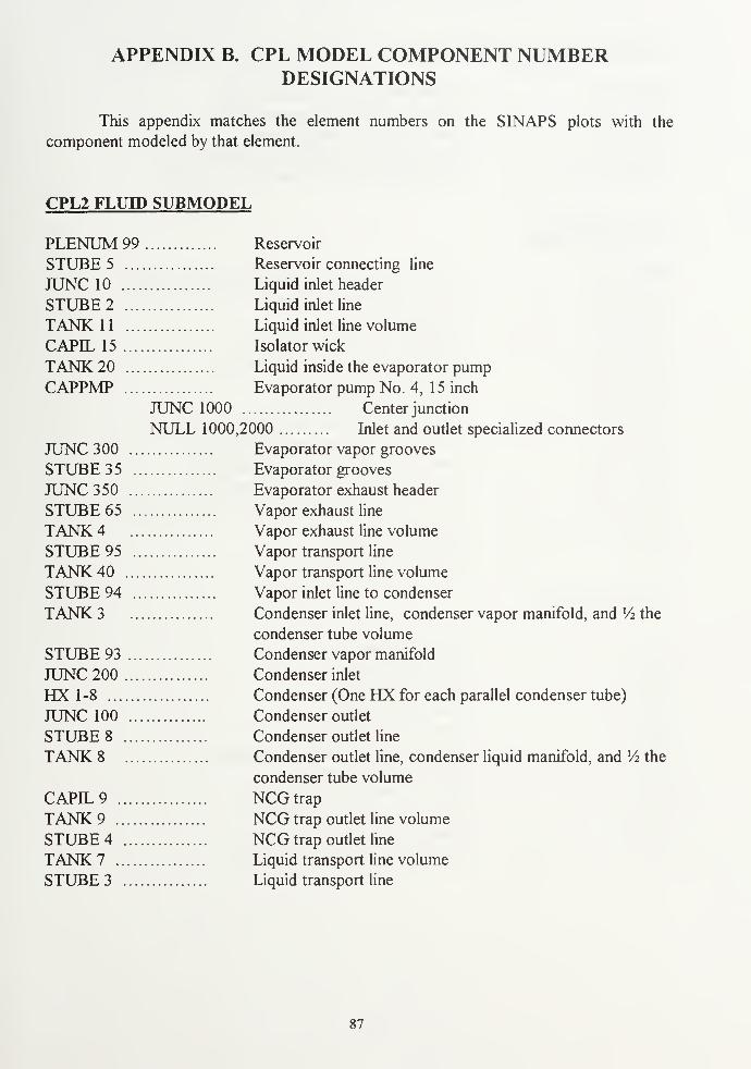
APPENDIX B. CPL MODEL COMPONENT NUMBERDESIGNATIONS

This appendix matches the element numbers on the SINAPS plots with the

component modeled by that element.

CPL2 FLUID SUBMODEL

PLENUM 99 Reservoir

STUBE 5 Reservoir connecting line

JUNC 10 Liquid inlet header

STUBE 2 Liquid inlet line

TANK 11 Liquid inlet line volume

CAPIL 15 Isolator wick

TANK 20 Liquid inside the evaporator pump

CAPPMP Evaporator pump No. 4, 1 5 inch

JUNC 1000 Center junction

NULL 1000,2000 Inlet and outlet specialized connectors

JUNC 300 Evaporator vapor grooves

STUBE 35 Evaporator grooves

JUNC 350 Evaporator exhaust header

STUBE 65 Vapor exhaust line

TANK 4 Vapor exhaust line volume

STUBE 95 Vapor transport line

TANK 40 Vapor transport line volume

STUBE 94 Vapor inlet line to condenser

TANK 3 Condenser inlet line, condenser vapor manifold, and Vi the

condenser tube volume

STUBE 93 Condenser vapor manifold

JUNC 200 Condenser inlet

HX 1-8 Condenser (One HX for each parallel condenser tube)

JUNC 100 Condenser outlet

STUBE 8 Condenser outlet line

TANK 8 Condenser outlet line, condenser liquid manifold, and XA the

condenser tube volume

CAPIL9 NCGtrapTANK 9 NCG trap outlet line volume

STUBE 4 NCG trap outlet line

TANK 7 Liquid transport line volume

STUBE 3 Liquid transport line

87

CLDPLT THERMAL SUBMODEL

NODES 1-8 .

NODES 9-16

NODE 999 ..

COND 17-24

COND 25-32

Condenser piping (Ammonia side)

Condenser section connector plate

Sink (Chiller) (boundary node)

Conductance from plate to fluorinert sink

Conductance from ammonia piping to plate

EVP SUBMODEL

NODE600NODE700NODE800NODE900NODE 1000

NODE 1100

NODE 1200

COND650COND750COND850COND950COND 1050

COND 1250

TEE 1100

TIE 1001

VLL SUBMODEL

NODE 18

NODE 19

NODE22NODE23NODE24NODE 50

COND 17

COND 19

COND 22

COND23COND24

Heater (arithmetic node with variable heat input)

Graphite foil (plate to plate)

Connector plate

Graphite foil (plate to bracket)

Evaporator tube mounting bracket

Evaporator wall

Saturation node (arithmetic)

Conductance through heater plate

Contact conductance across graphite foil

Conductance through connecting plate

Contact conductance across graphite foil

Conductance through bracket to evaporator wall

UAevaporator

Vapor superheat tie

Wick back-conduction tie

NCG outlet line

Liquid transport line

Condenser inlet line

Vapor transport line

Evaporator exhaust line

Ambient temperature (boundary node)

NCG outlet line to ambient

Liquid transport line to ambient

Condenser outlet line to ambient

Vapor transport line to ambient

Evaporator exhaust line to ambient

88

APPENDIX C. STEADY-STATE PRESSURE PROFILES

89

ooii

•DCouh-

3fooII

tooi_

3COCO

o

cocoaEoo

^-~~~~* T

"ciT

Q.

^CDi_13COtod>—D.

<

<

Header

ore

i >

Grooves Exhaust

Inlet

Outlet

Inlet

Outlet

Header

Liquid

C

1_ L_ L_ 1_ *-' L_OOCDCOQ-Q-CDO1

/

22cc22ca3

/ >>0 0(J(JCX>/

LULUOOZZ_JLU4 T-(NC0^lO(DN00

11 1 1

1

-- h-

-- <o

in

- «* oQ.

Eoo

CN

m CN m T- m m mCN m T— in o CO a>m CD m co m •*CO <— CO T— CO CD

(BdlAl) ajnssaJd

90

ooii

•acoo

oocsII

wok-

3V)Uio

cocoQ.

Eoo

^-----**[

c r ^^^~---'Q«;

a> ^-"^L.~

j _-

—

c/»

—

[/> ra> /i-

a

1/

«

»

<

^CD"°CDCD CD

X o4

CD W mO CO _ _0> 0) "S ^o jc a) -t: — — to 2-

©LLI-EOcoXji i »__ i

— w-»- t.

. kOOCDCDQ.Q.CDO

O O ® «Jh h

-o Ococaccxx5-co

I >>ooOOu>I

IJJIJJOOZZJLU4 T-cNoo^mcDsco

1 1 1 1 1

- CD

- "3"

CcucoQ.

Eoo

CO

-- CM

CO CN T— m o> CO r-IT) m in CD * TT "*CD CD CO T— CD CO CD

(BdlAl) 9JnSS9Jd

91

ooII

•acooI-

ooCOII

tL

</>

O

COCO0)

<dcoQ.

Eoo

CD

Q.

-- CO

CD•oCDCD CD

I l_O

coCO CO l_ o> -J •*-* (D "Don

CDc 0)

Q)CD

uCD

"5i— X _) ® 3

c o0) u

O LU _C_ o I -Ji i_ i_ l_ .«_-< k_o O CD Q. Q. oCD

oCD

O

COCQ)

COcCD

CD CD cXJ

CD

oQ. ea-

rn

UC c o o '5 Q.

CD> > o o o o O 1

>LU LU o o z z —I LU

cm ro ^r in cd n co

CO

to

c0>coa.

Eoo

- CM

<* CO CM T— lO o> CO r- CD mm m LO in CO ft -* * "* *<x> CD CO CO T— CO CO CO CD CD

(BdlAj) 3JnSS9Jd

92

o(A

II

oCooI-

ooII

W

3</>

CO0)

cocoaEoO

^^^+P

aTQ.

^̂-^

cui_3c/> WcocuI—

a.

T

<

eader

e

1

1

—

4

r

Grooves

r

Exhaust

H

r

Inlet

r

Outlet

Inlet

Outlet

t

Header

r

Liquid

Cor

H

V

1

/OOQ)<DQ.Q.<DO

/ O O ® 0)1- 1— ^ o

/Q. Q. "O -O CD CD ^ Q.

/>>ooOOo>

4 UJUJOOZZJUJ

11 1 1 1

CD

- *

CCD

CoQ.

Eoo

co

CM

m CN m ^— m m mCN m T— in o CD o>m CD m CO m T- •*tCD r— CD T— CD CD

(edl/\|) ajnssajd

93

ooII

"DCoo

ootNII

(L

(/)

0)i_3y)wo

c<D

CoaEoo

*+[

ar ^Q«=

ai ^—

•

uj r

a> /a> /a> /ua

\/

4

<>

*.CD"°tom a)

<

r

Grooves

r

Exhaust

H

r

Inlet

r

Outlet

Inlet

Outlet

t

Header

r

Liquid

Cor

<

/ 000)0)0.0-0)0

/i_ i_ — *— i_~ i_~ "~~ i_OOO)©!—!- -no

/0_0_"D'0(i)

Cr)

~ CL

>>OOOCJOr >i UJUJOOZZJLU

11 1 1

-- CO

-- m

*

ca>

coa.

Eoo

CO

-- CN

CO CN T— m O)IT) m m CO «i-CO co CO co

CO

CO CD

(ed|/\i) ajnssajd

94

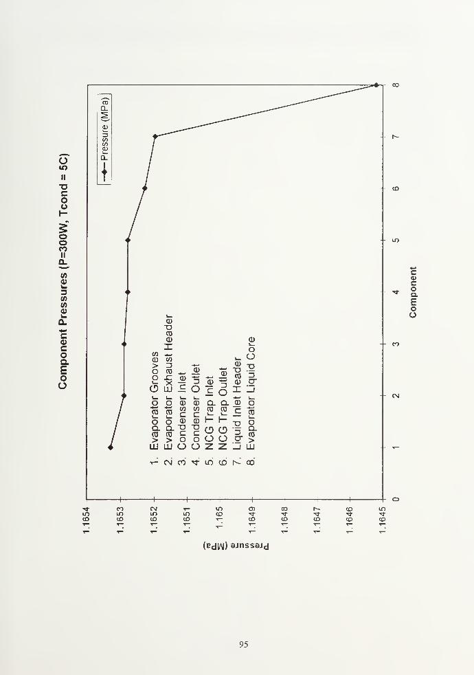
oto

II

TJCouI-

oooII

w0)l_

3(0</)

cocOQ.

Eoo

CO

Q_

o>

toCD

\-- CD

CD

"OCO(D CD

X i_O

(0CO oo l_ o> -J *-• (D "Oon

co

CD

JD CDuCO

'5

i_ V _3

C OCI) u

O LU _t_ o X _it_ t_ i_ l_ -•—1 i_o o CD Q. Q. CD oCO

oCOl_o

00CCD

00cCD

CO CO

TI

CO

oCO-

CO>

Q.CD>

Uco

Uco O O

'5

cr

Q.CO>

LU LU O o z z _i LU

T-c\ico"^-ir)cDr^oo

m

ccoQ.

Eoo

-- CO

CM

Tl- CO CM T— m 05 CO r~ CD inIT) m m m CD "fr -* * •<3- "3-

CD CD CO CD T— CD CD CO CD CD

(edlAJ) sJnssaJd

95

96

APPENDIX D. STEADY-STATE TEMPERATURE COMPARISONS

97

O QJ5 i-

H.. <N

ooii

•acooSfoo17a

o

Q.

E0)

I-

Ea>•**

CO

.. o

-- oo

ca>coaEoa

- <o

<i <>

oco

(A aia> u

01 r§

(TJJO

T- 01

o 0) c X ai OI r 0> 0) c O

oa.

>8.

>

_i

coa.

"5

c

4)

0)

0)o o

Q-

01

T3roai

T

TJ

cr1

"!5 ~to

cTO

<D

ca)

CQJ

c0)

a><nc

ro

cLU

0)

o

ca;

cOro

a.m>UJ

Clro>LU

Oa.

>c:oO

CoO

CoO

-ocoOOO-z.

oo

o

3cr_J

3_l

CM

kro>LU

roCM CO LO <D h- co O)

1 r

o"~

T

u->

eg CM *-

- CM

-+-

O IT)

(0) 8jnjBJ9dujai

98

LU

o1112 I-

Hooii

COo

.. <N

. . O

oII

a

p

Q.

£h-

E

(A

CO

<M| --00

C0)coaEou

- CO

*

- CM2 c u c

listW (0 n X> > m °

mCO

oCO CM

oCN

m in

(0) ajniBjadtuai

99

4*

Ooii

•acoo

o

CM

COII

a

o

aEo>

E

(0

- CO

ccoaEou

<l it

.- (D

- ^t

in

> 0)

§1O £

r?o o"re re

o oa. q.n (0

a. £

s ?-5 o

«22«l 41 i i

0)

o- OIsre 30) crI Zi

re J) o- - CM

l-l-iCT CX >

r o i- cm co

oCO

toCM

OCM

m m

(q) ajnjejadiuai

100

8 fe

H

ou>IIocoo5"ooITa

o

aEl-

Ea>*>»

>.0)

. . CM

. . O

- - CO

ca>

coaEoo

-- tf>

09 <i)a> k_ o

<l> cT) roTO -!- ID

o IV c X ID oJ r m 0) £T O

8.8. c "Si 5 1-

0)D> ro> cl c H K o

c Q. ID

Tcr

i

oTO

o"ro

TO incid

a)tocID

a)coca>

mi/i

c0)

ro

LU

HI

O

Cro "55

coro

Q.ro>LU

Q.ro>LU

OCLro

>

•dcoO

T7CoO

DCoO

coO

(Joo

o

X)

cx3

T3

cr_j

clro>LU

n«- CM CO in to r~- CO CD v *— »—

- -*

- C\J

COoCO

to o(N

m in

(0) djrn&jaduidi

lOl

•"»

UJ .

8 S

Heg

O10II

"DCOo

ooCMII

aoy=o

aE<D

E

(0

<! "I CO

ca>

coaEoo

-- jo

- *

4<

- eg

rsi ei in <b r^

tooCO eg

oeg

m m

(0) 9jniBjaduj8i

102

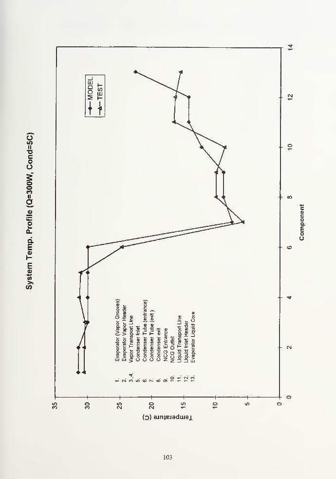
UJ .

H.. CM

o10II

"DCOo

IoCOII

O

o

aE0)

l-

E

>»

- - CO

coaEoo

- CD

«l *>

\

J.

44

- •*</> n>m » oo 0) r

T) mTO T- Q)

O (1) c X ID

J. C a> 0) c: OoQ.

>OQ-

>

_l

coQ.0)c(0

"ai 3I-

<D

1-'x0)

flj

oc

o

<DoTOOJ

T

T33g-

to

o2

<uinc0)

0)</>

ca>

ca>

<1)

in

c0)

cUJ

a)

o

Cro ai

c

a.(D>UJ

Q.TO>UJ

s.ro

>Coo

coO

oo

CoOOo o

o

acr

T33cr_i

oa.

>UJ

1- (N n in <£> t^- 00 05 *— «— *— *-

- CM

mCO

oCO

mCM

oCM

(3) ajrnejadiu3i

103

104

APPENDIX E. TRANSIENT SIMULATION RESULTS

105

Oi TJ U oCD

en

aCDoCDro

I

1

I

I

jj

o>

D

ai

co oT (£>

< )

7D 2:ZJo- II

_J a)D

II

£Zm

CD

CD

oO

V)

> •-»

CO\ .

n TD1. CO(') 0} en

J_ .?";

k_ UJn O

IICO Q.> CD CD

II

> 3II CO

O -* .*:

cc C CO

CD 0_ Q

I I

I I

I,I

-a

'1 o

<ii,

ooinCM

o

aXJcauCDCO

a <d

a' Eo l=

CDaaa

oain

09E 00E 0SZ 00c!

(0) ejniejadiuaj_

OQL

CD

OOl

106

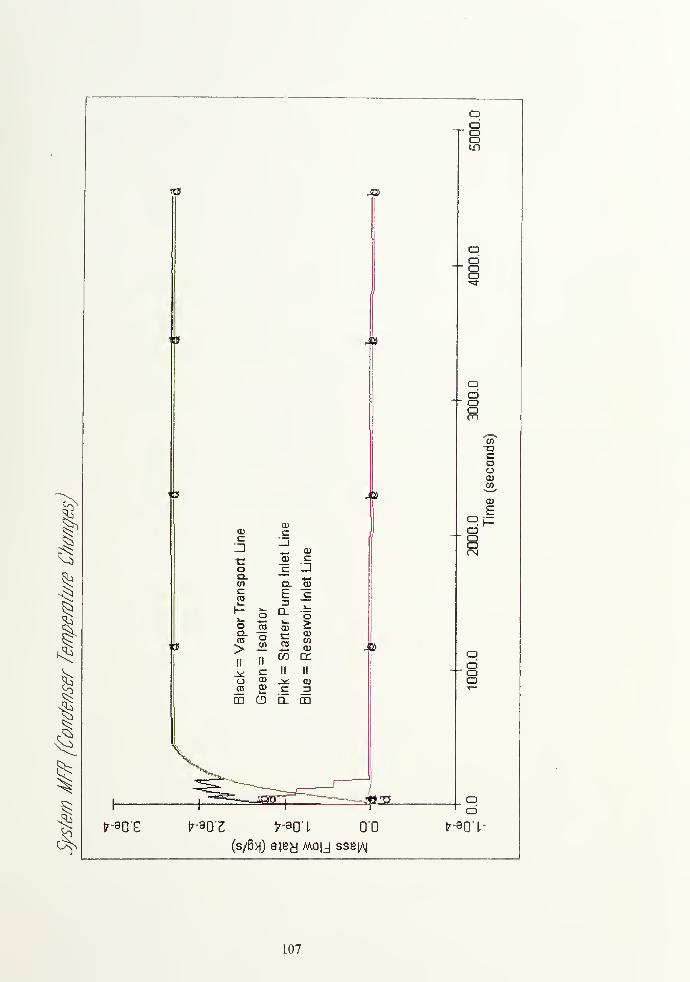
oooID

Itf J®

1

§:

Id^

as

t:oQ.CO

CO

oCO

>II il

uCO

cCD

go

CDc

O) cc I]

E

OL O£QjCOCD

II II

CD

CO

cCD3

gd CD a m

aao

Ja

i

aoamcox>coaCDa^

CD

£a inaaa

a

o

oa

(s/B>0 ajey mo|.j ssbiai

t^-90'l-

107

oooun

I1

|

1

1

I

1

ffl

!)

to

D

co

3o

CDCDO

"O Z3cr II

_1ii

CD

c CDQ>0) -C•_ oCD _l

CD

oOZ3w'3

en k.

CD>

0)

o--•

CO

n ~a ni_ co r>(') CO CO

.1. >o UJQ. o

IICO Q."> CO CD

II

> rj

||m

-2CCJ -*: ^(0 c 05

CD 0_ Q

OOO

aaoon

13 t)

CO

ooCDCO

O L=oooCN

•tt U

ao

\ i

x1

,

-<i^g :jl ¥ oa

0'9£ Q'OE Q'K 0(Z OS I

(0) ajrnej8dwaj_

001 O'S

108

I

1

t

1

COc: 0)— CO

CO oCD

o u -Ccr>

o c oc CD ^..1_J ^Zj CO

(1)

c- C5 CO

CD <- oUJ CJCD ^ r_.O,CD i_ o*— 0) E•

,CO TO£ !

-

A_ 0) CDE3)3 CO o

o CD

CD*"*

m -C O

ja m>

apt.

5= -^ o

OCDOoun

oooo

S»

OaomCO-ocooCDCO

CD

E

oaoCN

at.oCDOo

Z'U

A;||eno

1*0

o00

109

1

I

§:

d̂^

TO JVt

. ^M~* **** M

a

a)>±> cc

l

_J CU

-e au c:

o c _la. *—to Q. CD

CO EZJ

_C

(— o D_ oo CO cu £a.CO

>oto

t:CO c/>

CO

IIII

en ce

.V c: ii II

o a) -2£ toCO <D C 3ID o a CD

,JI

M

aafN

aaaoo

odooGO

to

a T3

r-i oa oa to

CO to

to

£

aao

ooCN

aa

fr-80'E fr-aOZ t^O'l O'O

(s/6>() ajey mo|j sse[Aj

tr9Q'L-

110

1

I

1

h

oj

* V^

flj

oas

-I—*

oa>

T CDOa z:3cr II

'3a>Z3

II

c OQaj

CJ5

CD _J

a)uOO-aZJa-13

>o errator

o £ ok_ TO Q.

(.',) _£ TOH >o x_ LLI

Q.S. "ITO

> TO a)

II

> =II CD

O -* ¥TO

.C TO

OQ Q_ Q

o

p

IJ

•fa IJ

jLqa_ ^L

oCDoaCM

oooa

oooCD

o ocn o

(-i oa 0)CD CO

aj

£

oa

adaoCM

o

O'SE O'OE ok cms Q9i

(q) 3jnjBJ9dLuaj_

001 0'9

111

oao

oaoo

Jit)oaooCO

$110

CO

o oo oa cd

CD CO

CD

CO

c CDCO

CO Oni

1_o U -C— mu c u1_ CD J__) <-i CO

'

CD

£ C1J <0

CD _C ^10 UCU $ r^oHi % "O

CDCO CD

St)

oao

ro oo

112

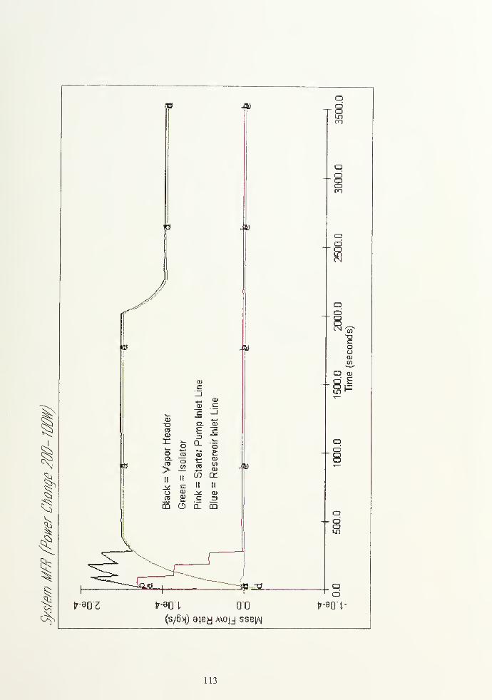
*> JU

1

a?

1

J®

m su>

CD C

B

CD"O05CD

XoCtJ

>

Ez>

Q_

IIII

oCO

CDCD

oa>COa)

en a:

ii ii

1)

CO

CD

GQ O CL CD

I

fr-30'Z

Ik)

¥

asen

aooaCO

CDOCN

aoa-cocjCDCO

O CO

d £

aaa

ao

ad

(s/6 >() ejey mo|-j sse^

fr-90'L-

113

0) fl u _ oo

ooaen

<D

1

I

1

d̂^

U

i0

CDaCO

=3

ocd

T o< )u 2T

_Jcr II

_J 0)3

II

c:CD

cdCD -C

CD

oO-a

ZJ05CU>

cu

oas

o (J oCOcu

a.CO

-L >o i_ UJCl o

IICO u.> <0 cd

II

> =j

II mJ£o .2C ^cCO c CO

CD Q. Q

r i

>i

-i y

a\ 4- aa\

inCM

aooocoaCDCO

a cd

d Ea rzLD ^

aao

USE O'OE 053 OOd

(0) 8jniejadiuaj_

OSL

o001

114

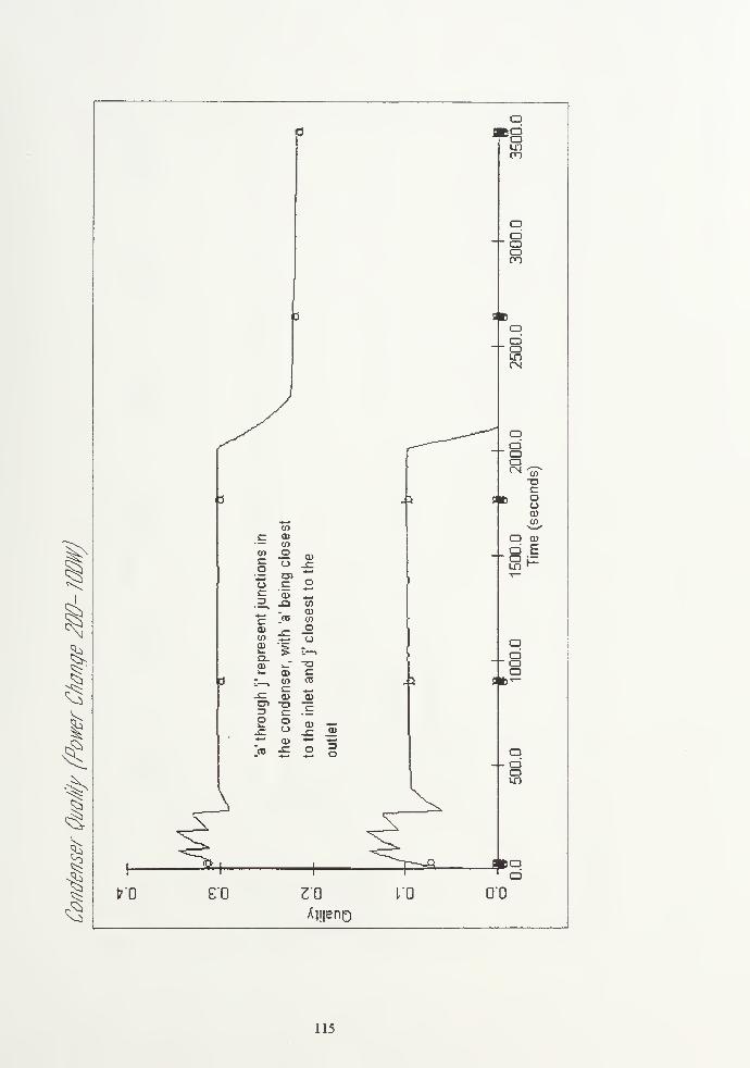
o3 fl a

en

oo

" aom

5 9Bacd

" o

y oJ-T o

oac

a ' i SI

0}++ COto

c a> O a>

t1

'"" CO

o ° =o c: o5 "3> »-

- O LZ

^̂^1

r? - <u

to :£: o oCD

" CDfc- (D C O

J^ d r__ 0) <C i 2 g Hj«-

^ o -a 7:

^3 c -E2 ° a) -

^ r ° r J

^— Q) — *-

> £ 2 o o- CDO

t Vin

I^J ^v

^N^ AiN \^^ s.^ <^_^' ^—>

11 "* 1 1

^7-^Q flirol 1 l

fr'O E'O Z'O

i

] 0"

o

^s Ameno

115

I

3

I

§5

d̂^

TO

;»

iff ;B

CDc_l^_ CD

0) Ck_ c _lIS-a £2.

F_0J

cu ^ ~""~

ooas

Q_

CD

'5

2:Q.cc> CO

UJ

CD

II IICO Lt

-x c II II

o CD -S£ CDcc 0> c Z3

tf -W

CD CD 0-

\'fg

oooorn

ooCN

aoooCM

a acn o

C i uIT) CD*~ <S)

CD

£

oaa

aa

oo

t-90'£ ^07 t^Ol 00(s/6 >)) aiey Moy ssey\|

fr-90't-

116

a> w

li

1

a?

I

1

I

1

a-

a)

oO"'=>

jQ 1)

CD>oo

o4-*

05

O

CDoCOCU

XO

(^03CU

a.ro

CDO•z.o

X £ 7J

a.re

oa II II

> CO cu _j CU

> ZJII

ZJ

.Y 1! m c CD

OCO as

a>a> 05

ww

1 'lw

\\w

*-

ooo

ooaun

CO

a -aC

r-i aQ o55 cu,— co

cu

E

oao

aaun

O'SE O'OE 092 002 OSL

o00L

(q) 3Jn}BJBdLU8J_

117

03

l|

1

I

f

1

O

o

oen

fr*

CO oa>

1-o u -C

enCJ c o1_ CD _^_l O (0_,

CD

c CO CO

CD T oCO (.)

CD 5 r_12-

"O*— CD c

CO CO

c ^_,J_ CD CD

-a co o a)o

7

WO Z£V0 VZZQ 9l£0

aoaunCN

ooo

o-- ao

o80 t'O 00

118

APPENDIX F. TEMPERATURE-TIME COMPARISONS

119

03

<v °

H

2 £°- §£ CO

I?Q) (0

o

o o'5 i.

|- 069fr

09frfr

- ozefr

-- 00£fr

-083fr

-093fr

-OfrZfr

OZZfr

OOZfr

h 08l.fr

091-fr

Ofrl.fr

-02l.fr

-001-fr

-080fr

090fr

OfrOfr

- OZOfr

- OOOfr

038£

0)

E

o+HIoocsi

o+HIOen

o+UJooo

o+HIo

o+UJoCO

o+UJom

o+UJo

o+UJoCO

o+UJoCM

UJo

o+UJoo

(0) ajruejadiuai

120

*=ok.

Q.

0)i_ ^^^

3 £re ok. O© COa.

E1oo

0) CM1- ^^

0)0)

COo co re

•o O3 i_

CT oJ oO (L

rei_

oQ.re>LU

H

- 069*

- 09**

- 028*

- ooe*

- 093*

- 093*

-- 0*2*

-- 032*

- 002*

- 081-*

-- 091.*

- 0*1*

- 021-*

- 001-*

- 080*

- 090*

- 0*0*

020*

- 000*

-- 0288

E

o+inomCM

o+UJocm

o+LUoCO

LUoCM

cm

o+LUo

o+LUoo

o+LUo

o+LUo00

LUo

o+LUoCO

o+LUom

CM CM t-

(0) 8jnjBJ9dU191

121

CD

» O

H2

2 £5 22 «?

8.8E N

5 5? oo

(ACVocoo

OQ_

oo+LUOLO

CD

Oo+LUOocd

oo+111oIT)

oo+LUooin

oo+illom

oo+UJoo

(0) ajniejadiuei

122

LIST OF REFERENCES

1

.

Larson, Wiley J. and Wertz, James R., Space Mission Analysis and Design,Microcosm, Inc., Torrence, CA, 1992.

2. Gilmore, David G., Satellite Thermal Control Handbook, Aerospace Corporation

Press, El Segundo, CA, 1994.

3. Cullimore, Brent A., Capillary PumpedLoop Application Guide, Martin Marietta

Group, Denver, CO, 1993.

4. Silverstein, Calvin C, Design and Technology ofHeat Pipesfor Cooling andHeatExchange, Taylor & Francis, Washington, DC, 1992.

5. Peterson, G. P., An Introduction to Heat Pipes: Modeling, Testing, and Applications,

John Wiley & Sons, Inc., New York, 1994.

6. Maidanik, Y., Fershtater, Y., and K. Goncharov, Capillary Pump Loopfor the System

of Thermal Regulation ofSpacecraft, European Symposium on Space Environmental

and Control Systems, 1991.

7. Kiseev, V. M. Analysis ofMaximum Heat Transfer Capacity of Capillary Loops, Ural

State University, Russia, 1995.

8. Solar Cell Array Design Handbook, Volume 152, NASA/JPL Publication SP 43-38.

9. Test Planfor the Capillary PumpedLoop (CPL) Test Bed, U. S. Air Force Phillips

Laboratory Power and Thermal Management Division (PL/VTPT), Kirtland AFB,Albuquerque, NM. 1995.

10. Stenger, F. J., Experimental Feasibility Study of Water-Filled Capillary PumpedHeat-Transfer Loops, NASA TM-X-13 10, NASA Lewis Research Center, Cleveland,

OH., 1966.

11. Yun, S., Nguyen, T., Kroliczek, E., Chalmers, D., and J. Fredley, Design andAmbientTesting of the Flight Starter Pump Cold Plate, SAE ICES Conference, Monterey,

CA, 1996.

12. Meyer, R., Muller, R., Beckmann, K., Goncharov, K., Kotlarov, E., and Maidanik, Y.,

Investigation of the Heat Transfer Performance ofa Capillary PumpedAmmoniaLoop Under Gravity, SAE ICES Conference, Colorado Springs, CO, 1993.

13. Ku, Jentung, Overview ofCapillary PumpedLoop Technology, NASA Goddard

Space Flight Center, Greenbelt, MD, 1994.

14. Baumann, J., Recommendationsfor Future CPL Development and Risk Reduction,Martin Marietta Astronautics Group, Denver, CO, 1993.

15. Baumann, J., Advances in CPL Technology, CPL Workshop III, Sponsored by NASAGoddard Space Flight Center, Annapolis, MD, 1992.

16. Cullimore, B., et al, SINDA/FLUINT Version 3.2 User's Manual, September 1994.

17. Kuntz, Robert J., "Where is Rachel", Launchspace Magazine, March 1997.

123

18. White, Frank M. FluidMechanics, Third Ed. McGraw-Hill, San Francisco, 1994.

124

INITIAL DISTRIBUTION LIST

Defense Technical Information Center 2

8725 John J. Kingman Road, Ste 0944

Ft. Belvoir, Virginia 22060-6218

Dudley Knox Library 2

Naval Postgraduate School

411 Dyer Road

Monterey, California 93943-5101

Naval/Mechanical Engineering Curricular Officer, Code 34 1

Naval Postgraduate School

Monterey, California 93943-5101

Mechanical Engineering Department Chairman, Code ME 1

Naval Postgraduate School

Monterey, California 93943-5101

Professor Matthew D. Kelleher 3

Mechanical Engineering Department, Code ME/KKNaval Postgraduate School

Monterey, California 93943-5101

Dr. Donald Gluck 3

Phillips Laboratory, VTPT3550 Aberdeen Ave., S.E.

Building 301 17

Kirtland AFB, NM 871 17-5776

LT Peter J. Ryan, Jr., USN..

11338 S.E. 175th Place

Summerfield, Florida 34491

Brent Cullimore

Cullimore and Ring Technologies

9 Red Fox Lane

Littleton, CO 80127

9. Dr. Rudolph Panholzer

Chairman, Space Systems Academic Group

Code SP/PZ

Naval Postgraduate School

Monterey, CA 93943-5002

125

DUDLEY KNOX LIBRARY

NAVAL POSTGRADUATE SCHOOLMONTEREY CA 93943-5101

DUDLEY KNOX LIBRARY

3 2768 00344879 6