Overview of Meta Analysis in Stata

18 Meta-analysis in StataTM

JONATHAN A C STERNE, MICHAEL J BRADBURN,MATTHIAS EGGER

Summary points

• StataTM is a general-purpose, command-line driven, programmablestatistical package.

• A comprehensive set of user-written commands is freely available formeta-analysis.

• Meta-analysis of studies with binary (relative risk, odds ratio, riskdifference) or continuous outcomes (difference in means, standardiseddifference in means) can be performed.

• All the commonly used fixed effect (inverse variance method,Mantel–Haenszel method and Peto’s method) and random effect(DerSimonian and Laird) models are available.

• An influence analysis, in which the meta-analysis estimates are computedomitting one study at a time, can be performed.

• Forest plots, funnel plots and L’Abbé plots can be drawn and statisticaltests for funnel plot asymmetry can be computed.

• Meta-regression models can be used to analyse associations betweentreatment effect and study characteristics.

We reviewed a number of computer software packages that may be used toperform a meta-analysis in Chapter 17. In this chapter we show in detailhow to use the statistical package Stata both to perform a meta-analysis andto examine the data in more detail. This will include looking at theaccumulation of evidence in cumulative meta-analysis, using graphical and statistical techniques to look for evidence of bias, and using meta-regression to investigate possible sources of heterogeneity.

Getting started

Stata is a general-purpose, command-line driven, programmable statisti-cal package in which commands to perform several meta-analytic methods

347

All data sets described in this Chapter are available from the book’s website: <www.systematicreviews.com>.

18 Systematic Reviews-18-cpp 16/2/2001 8:33 am Page 347

SYSTEMATIC REVIEWS IN HEALTH CARE

348

are available. Throughout this chapter, Stata commands appear in boldfont , and are followed by the Stata output that they produce. Usersshould note that the commands documented here do not form part of the“core” Stata package, but are all user-written “add-ons” which are freelyavailable on the internet. In order to perform meta-analyses in Stata, theseroutines need to be installed on your computer by downloading therelevant files from the Stata web site (www.stata.com). See Box 18.1 fordetailed instructions on how to do this.

We do not attempt to provide a full description of the commands:interested readers are referred to help files for the commands, and to therelevant articles in the Stata Technical Bulletin (STB, see reference list). Todisplay the help file, type help followed by the command (for examplehelp metan ) or go into the “Help” menu and click on the “Statacommand…” option. Bound books containing reprints of a year’s Stata

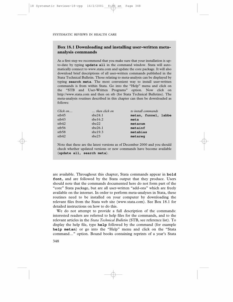
Box 18.1 Downloading and installing user-written meta-analysis commands

As a first step we recommend that you make sure that your installation is up-to-date by typing update all in the command window. Stata will auto-matically connect to www.stata.com and update the core package. It will alsodownload brief descriptions of all user-written commands published in theStata Technical Bulletin. Those relating to meta-analysis can be displayed bytyping search meta . The most convenient way to install user-writtencommands is from within Stata. Go into the “Help” menu and click on the “STB and User-Written Programs” option. Now click onhttp://www.stata.com and then on stb (for Stata Technical Bulletins). Themeta-analysis routines described in this chapter can then be downloaded asfollows:

Click on… … then click on to install commandsstb45 sbe24.1 metan, funnel, labbestb43 sbe16.2 metastb42 sbe22 metacumstb56 sbe26.1 metainfstb58 sbe19.3 metabiasstb42 sbe23 metareg

Note that these are the latest versions as of December 2000 and you shouldcheck whether updated versions or new commands have become available(update all, search meta ).


Technical Bulletin articles are also available and are free to universitylibraries. The articles referred to in this chapter are available in STBreprints volumes 7: (STB 38 to STB 42) and 8 (STB 43 to 48). The Statawebsite gives details of how to obtain these. All the output shown in thischapter was obtained using Stata version 6. Finally, we assume that thedata have already been entered into Stata.

Commands to perform a standard meta-analysis

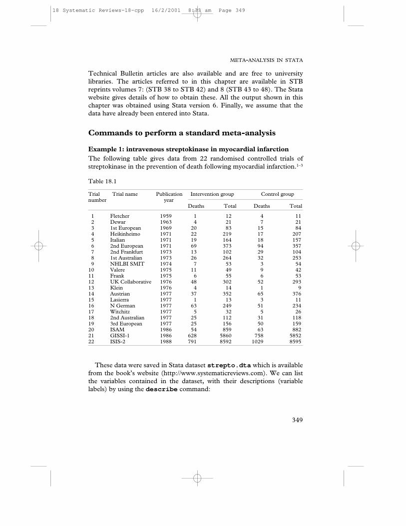
Example 1: intravenous streptokinase in myocardial infarctionThe following table gives data from 22 randomised controlled trials ofstreptokinase in the prevention of death following myocardial infarction.1–3

Table 18.1

Trial Trial name Publication Intervention group Control groupnumber year

Deaths Total Deaths Total

1 Fletcher 1959 1 12 4 112 Dewar 1963 4 21 7 213 1st European 1969 20 83 15 844 Heikinheimo 1971 22 219 17 2075 Italian 1971 19 164 18 1576 2nd European 1971 69 373 94 3577 2nd Frankfurt 1973 13 102 29 1048 1st Australian 1973 26 264 32 2539 NHLBI SMIT 1974 7 53 3 54

10 Valere 1975 11 49 9 4211 Frank 1975 6 55 6 5312 UK Collaborative 1976 48 302 52 29313 Klein 1976 4 14 1 914 Austrian 1977 37 352 65 37615 Lasierra 1977 1 13 3 1116 N German 1977 63 249 51 23417 Witchitz 1977 5 32 5 2618 2nd Australian 1977 25 112 31 11819 3rd European 1977 25 156 50 15920 ISAM 1986 54 859 63 88221 GISSI-1 1986 628 5860 758 585222 ISIS-2 1988 791 8592 1029 8595

These data were saved in Stata dataset strepto.dta which is availablefrom the book’s website (http://www.systematicreviews.com). We can listthe variables contained in the dataset, with their descriptions (variablelabels) by using the describe command:

META-ANALYSIS IN STATA

349


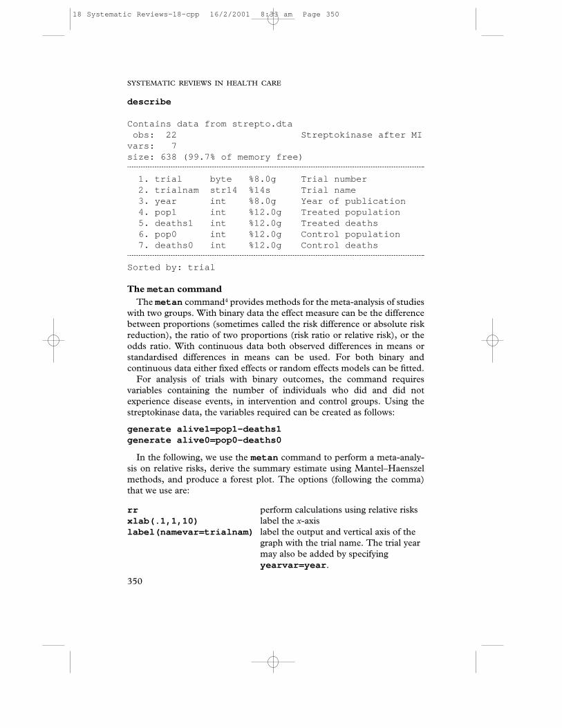
describe

Contains data from strepto.dtaobs: 22 Streptokinase after MI

vars: 7size: 638 (99.7% of memory free)

1. trial byte %8.0g Trial number2. trialnam str14 %14s Trial name3. year int %8.0g Year of publication4. pop1 int %12.0g Treated population5. deaths1 int %12.0g Treated deaths6. pop0 int %12.0g Control population7. deaths0 int %12.0g Control deaths

Sorted by: trial

The metan commandThe metan command4 provides methods for the meta-analysis of studies

with two groups. With binary data the effect measure can be the differencebetween proportions (sometimes called the risk difference or absolute riskreduction), the ratio of two proportions (risk ratio or relative risk), or theodds ratio. With continuous data both observed differences in means orstandardised differences in means can be used. For both binary andcontinuous data either fixed effects or random effects models can be fitted.

For analysis of trials with binary outcomes, the command requiresvariables containing the number of individuals who did and did notexperience disease events, in intervention and control groups. Using thestreptokinase data, the variables required can be created as follows:

generate alive1=pop1-deaths1generate alive0=pop0-deaths0

In the following, we use the metan command to perform a meta-analy-sis on relative risks, derive the summary estimate using Mantel–Haenszelmethods, and produce a forest plot. The options (following the comma)that we use are:

rr perform calculations using relative risksxlab(.1,1,10) label the x-axislabel(namevar=trialnam) label the output and vertical axis of the

graph with the trial name. The trial yearmay also be added by specifying yearvar=year .


350



351

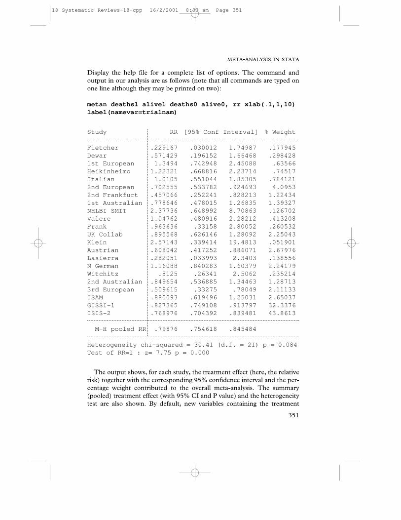
Display the help file for a complete list of options. The command andoutput in our analysis are as follows (note that all commands are typed onone line although they may be printed on two):

metan deaths1 alive1 deaths0 alive0, rr xlab(.1,1,10)label(namevar=trialnam)

Study RR [95% Conf Interval] % Weight

Fletcher .229167 .030012 1.74987 .177945Dewar .571429 .196152 1.66468 .2984281st European 1.3494 .742948 2.45088 .63566Heikinheimo 1.22321 .668816 2.23714 .74517Italian 1.0105 .551044 1.85305 .7841212nd European .702555 .533782 .924693 4.09532nd Frankfurt .457066 .252241 .828213 1.224341st Australian .778646 .478015 1.26835 1.39327NHLBI SMIT 2.37736 .648992 8.70863 .126702Valere 1.04762 .480916 2.28212 .413208Frank .963636 .33158 2.80052 .260532UK Collab .895568 .626146 1.28092 2.25043Klein 2.57143 .339414 19.4813 .051901Austrian .608042 .417252 .886071 2.67976Lasierra .282051 .033993 2.3403 .138556N German 1.16088 .840283 1.60379 2.24179Witchitz .8125 .26341 2.5062 .2352142nd Australian .849654 .536885 1.34463 1.287133rd European .509615 .33275 .78049 2.11133ISAM .880093 .619496 1.25031 2.65037GISSI-1 .827365 .749108 .913797 32.3376ISIS-2 .768976 .704392 .839481 43.8613

M-H pooled RR .79876 .754618 .845484

Heterogeneity chi-squared = 30.41 (d.f. = 21) p = 0.084Test of RR=1 : z= 7.75 p = 0.000

The output shows, for each study, the treatment effect (here, the relativerisk) together with the corresponding 95% confidence interval and the per-centage weight contributed to the overall meta-analysis. The summary(pooled) treatment effect (with 95% CI and P value) and the heterogeneitytest are also shown. By default, new variables containing the treatment


effect size, its standard error, the 95% CI and study weights and samplesizes are added to the dataset.

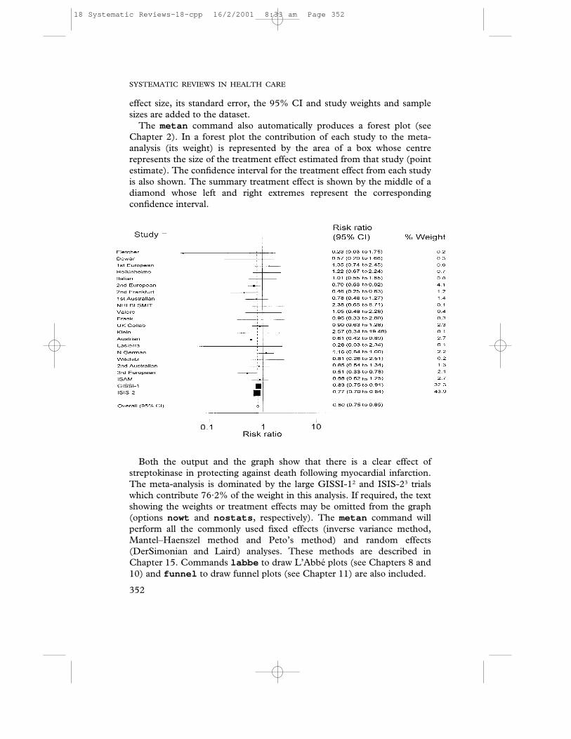
The metan command also automatically produces a forest plot (seeChapter 2). In a forest plot the contribution of each study to the meta-analysis (its weight) is represented by the area of a box whose centrerepresents the size of the treatment effect estimated from that study (pointestimate). The confidence interval for the treatment effect from each studyis also shown. The summary treatment effect is shown by the middle of adiamond whose left and right extremes represent the correspondingconfidence interval.

Both the output and the graph show that there is a clear effect ofstreptokinase in protecting against death following myocardial infarction.The meta-analysis is dominated by the large GISSI-12 and ISIS-23 trialswhich contribute 76·2% of the weight in this analysis. If required, the textshowing the weights or treatment effects may be omitted from the graph(options nowt and nostats , respectively). The metan command willperform all the commonly used fixed effects (inverse variance method,Mantel–Haenszel method and Peto’s method) and random effects(DerSimonian and Laird) analyses. These methods are described inChapter 15. Commands labbe to draw L’Abbé plots (see Chapters 8 and10) and funnel to draw funnel plots (see Chapter 11) are also included.


352


The meta commandThe meta command5–7 uses inverse-variance weighting to calculate fixedand random effects summary estimates, and, optionally, to produce a forestplot. The main difference in using the meta command (compared to themetan command) is that we require variables containing the effectestimate and its corresponding standard error for each study. Commandsmetacum, metainf, metabias and metareg (described later in thischapter) also require these input variables. Here we re-analyse the strep-tokinase data to demonstrate meta , this time considering the outcome onthe odds ratio scale. For odds ratios or risk ratios, the meta commandworks on the log scale. So, to produce a summary odds ratio we need tocalculate the log of the ratio and its corresponding standard error for eachstudy. This is straightforward for the odds ratio. The log odds ratio iscalculated as

generate logor=log((deaths1/alive1)/(deaths0/alive0))

and its standard error, using Woolf’s method, as

generate selogor=sqrt((1/deaths1)+(1/alive1)+(1/deaths0)+(1/alive0))

Chapter 15 gives this formula, together with the standard errors of the riskratio and other commonly used treatment effect estimates. The output canbe converted back to the odds ratio scale using the eform option to expo-nentiate the odds ratios and their confidence intervals. Other options usedin our analysis are:

graph(f) display a forest plot using a fixed-effects summary estimate. Specifying graph(r)changes this to a random-effects estimate

cline draw a broken vertical line at the combined estimate

xlab(.1,1,10) label the x-axis at odds ratios 0·1, 1 and 10xline(1) draw a vertical line at 1id(trialnam) label the vertical axis with the trial name

contained in variable trialnamb2title(Odds ratio) label the x-axis with the text “Odds ratio”.print output the effect estimates, 95% CI and

weights for each study


353



354

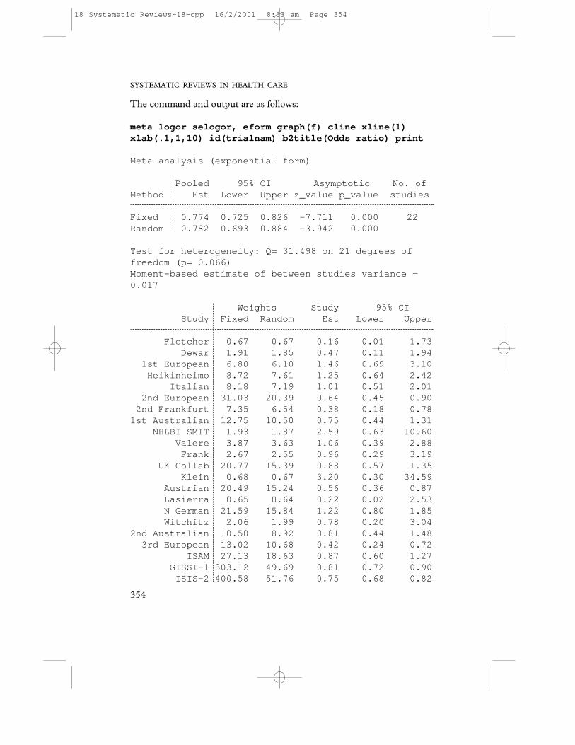
The command and output are as follows:

meta logor selogor, eform graph(f) cline xline(1)xlab(.1,1,10) id(trialnam) b2title(Odds ratio) print

Meta-analysis (exponential form)

Pooled 95% CI Asymptotic No. ofMethod Est Lower Upper z_value p_value studies

Fixed 0.774 0.725 0.826 -7.711 0.000 22Random 0.782 0.693 0.884 -3.942 0.000

Test for heterogeneity: Q= 31.498 on 21 degrees offreedom (p= 0.066)Moment-based estimate of between studies variance =0.017

Weights Study 95% CIStudy Fixed Random Est Lower Upper

Fletcher 0.67 0.67 0.16 0.01 1.73Dewar 1.91 1.85 0.47 0.11 1.94

1st European 6.80 6.10 1.46 0.69 3.10Heikinheimo 8.72 7.61 1.25 0.64 2.42

Italian 8.18 7.19 1.01 0.51 2.012nd European 31.03 20.39 0.64 0.45 0.90

2nd Frankfurt 7.35 6.54 0.38 0.18 0.781st Australian 12.75 10.50 0.75 0.44 1.31

NHLBI SMIT 1.93 1.87 2.59 0.63 10.60Valere 3.87 3.63 1.06 0.39 2.88

Frank 2.67 2.55 0.96 0.29 3.19UK Collab 20.77 15.39 0.88 0.57 1.35

Klein 0.68 0.67 3.20 0.30 34.59Austrian 20.49 15.24 0.56 0.36 0.87Lasierra 0.65 0.64 0.22 0.02 2.53N German 21.59 15.84 1.22 0.80 1.85Witchitz 2.06 1.99 0.78 0.20 3.04

2nd Australian 10.50 8.92 0.81 0.44 1.483rd European 13.02 10.68 0.42 0.24 0.72

ISAM 27.13 18.63 0.87 0.60 1.27GISSI-1 303.12 49.69 0.81 0.72 0.90

ISIS-2 400.58 51.76 0.75 0.68 0.82



355

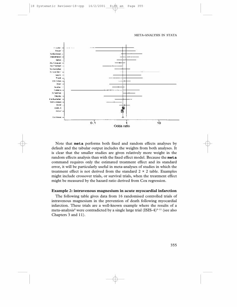
Note that meta performs both fixed and random effects analyses bydefault and the tabular output includes the weights from both analyses. Itis clear that the smaller studies are given relatively more weight in therandom effects analysis than with the fixed effect model. Because the metacommand requires only the estimated treatment effect and its standarderror, it will be particularly useful in meta-analyses of studies in which thetreatment effect is not derived from the standard 2 × 2 table. Examplesmight include crossover trials, or survival trials, when the treatment effectmight be measured by the hazard ratio derived from Cox regression.

Example 2: intravenous magnesium in acute myocardial infarctionThe following table gives data from 16 randomised controlled trials of

intravenous magnesium in the prevention of death following myocardialinfarction. These trials are a well-known example where the results of ameta-analysis8 were contradicted by a single large trial (ISIS-4)9–11 (see alsoChapters 3 and 11).


Table 18.2

Trial Trial name Publication Intervention group Control groupnumber year

Deaths Total Deaths Total

1 Morton 1984 1 40 2 362 Rasmussen 1986 9 135 23 1353 Smith 1986 2 200 7 2004 Abraham 1987 1 48 1 465 Feldstedt 1988 10 150 8 1486 Schechter 1989 1 59 9 567 Ceremuzynski 1989 1 25 3 238 Bertschat 1989 0 22 1 219 Singh 1990 6 76 11 75

10 Pereira 1990 1 27 7 2711 Schechter 1 1991 2 89 12 8012 Golf 1991 5 23 13 3313 Thogersen 1991 4 130 8 12214 LIMIT-2 1992 90 1159 118 115715 Schechter 2 1995 4 107 17 10816 ISIS-4 1995 2216 29 011 2103 29 039

These data were saved in Stata dataset magnes.dta .

describe

Contains data from magnes.dtaobs: 16 Magnesium and CHD

vars: 7

1. trial int %8.0g Trial number2. trialnam str12 %12s Trial name3. year int %8.0g Year of publication4. tot1 long %12.0g Total in magnesium group5. dead1 double %12.0g Deaths in magnesium group6. tot0 long %12.0g Total in control group7. dead0 long %12.0g Deaths in control group

Sorted by: trial

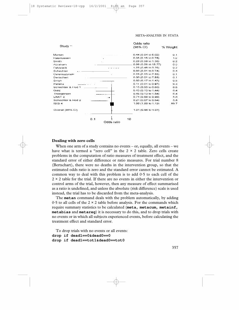
The discrepancy between the results of the ISIS-4 trial and the earliertrials can be seen clearly in the graph produced by the metan command.Note that because the ISIS-4 trial provides 89·7% of the total weight in themeta-analysis, the overall (summary) estimate using fixed-effects analysis isvery similar to the estimate from the ISIS-4 trial alone.


356



357

Dealing with zero cellsWhen one arm of a study contains no events – or, equally, all events – we

have what is termed a “zero cell” in the 2 × 2 table. Zero cells createproblems in the computation of ratio measures of treatment effect, and thestandard error of either difference or ratio measures. For trial number 8(Bertschart), there were no deaths in the intervention group, so that theestimated odds ratio is zero and the standard error cannot be estimated. Acommon way to deal with this problem is to add 0·5 to each cell of the 2 × 2 table for the trial. If there are no events in either the intervention orcontrol arms of the trial, however, then any measure of effect summarisedas a ratio is undefined, and unless the absolute (risk difference) scale is usedinstead, the trial has to be discarded from the meta-analysis.

The metan command deals with the problem automatically, by adding0·5 to all cells of the 2 × 2 table before analysis. For the commands whichrequire summary statistics to be calculated (meta, metacum, metainf,metabias and metareg ) it is necessary to do this, and to drop trials withno events or in which all subjects experienced events, before calculating thetreatment effect and standard error.

To drop trials with no events or all events:drop if dead1==0&dead0==0drop if dead1==tot1&dead0==tot0


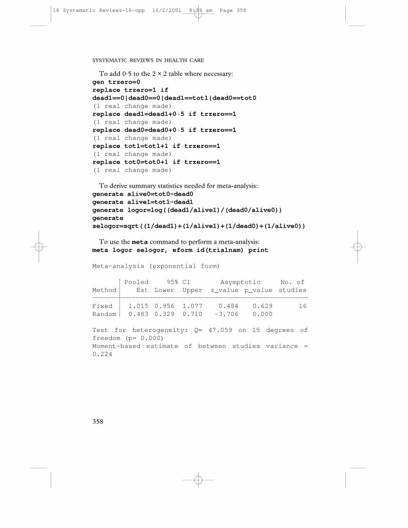
To add 0·5 to the 2 × 2 table where necessary:gen trzero=0replace trzero=1 ifdead1==0|dead0==0|dead1==tot1|dead0==tot0(1 real change made)replace dead1=dead1+0·5 if trzero==1(1 real change made)replace dead0=dead0+0·5 if trzero==1(1 real change made)replace tot1=tot1+1 if trzero==1(1 real change made)replace tot0=tot0+1 if trzero==1(1 real change made)

To derive summary statistics needed for meta-analysis:generate alive0=tot0-dead0generate alive1=tot1-dead1generate logor=log((dead1/alive1)/(dead0/alive0))generateselogor=sqrt((1/dead1)+(1/alive1)+(1/dead0)+(1/alive0))

To use the meta command to perform a meta-analysis:meta logor selogor, eform id(trialnam) print

Meta-analysis (exponential form)


Fixed 1.015 0.956 1.077 0.484 0.629 16Random 0.483 0.329 0.710 -3.706 0.000



358


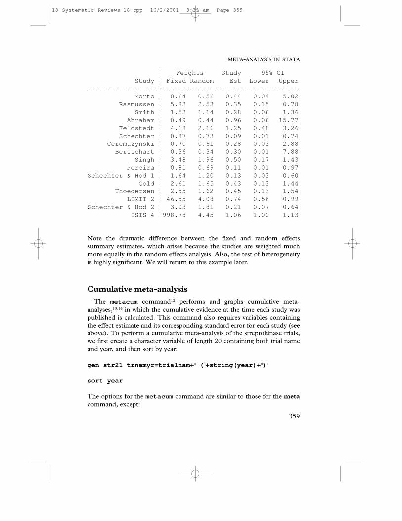
Weights Study 95% CIStudy Fixed Random Est Lower Upper

Morto 0.64 0.56 0.44 0.04 5.02Rasmussen 5.83 2.53 0.35 0.15 0.78

Smith 1.53 1.14 0.28 0.06 1.36Abraham 0.49 0.44 0.96 0.06 15.77

Feldstedt 4.18 2.16 1.25 0.48 3.26Schechter 0.87 0.73 0.09 0.01 0.74

Ceremuzynski 0.70 0.61 0.28 0.03 2.88Bertschart 0.36 0.34 0.30 0.01 7.88

Singh 3.48 1.96 0.50 0.17 1.43Pereira 0.81 0.69 0.11 0.01 0.97

Schechter & Hod 1 1.64 1.20 0.13 0.03 0.60Gold 2.61 1.65 0.43 0.13 1.44

Thoegersen 2.55 1.62 0.45 0.13 1.54LIMIT-2 46.55 4.08 0.74 0.56 0.99

Schechter & Hod 2 3.03 1.81 0.21 0.07 0.64ISIS-4 998.78 4.45 1.06 1.00 1.13

Note the dramatic difference between the fixed and random effectssummary estimates, which arises because the studies are weighted muchmore equally in the random effects analysis. Also, the test of heterogeneityis highly significant. We will return to this example later.

Cumulative meta-analysis

The metacum command12 performs and graphs cumulative meta-analyses,13,14 in which the cumulative evidence at the time each study waspublished is calculated. This command also requires variables containingthe effect estimate and its corresponding standard error for each study (seeabove). To perform a cumulative meta-analysis of the streptokinase trials,we first create a character variable of length 20 containing both trial nameand year, and then sort by year:

gen str21 trnamyr=trialnam+ || ( ||+string(year)+ ||) ||

sort year

The options for the metacum command are similar to those for the metacommand, except:


359


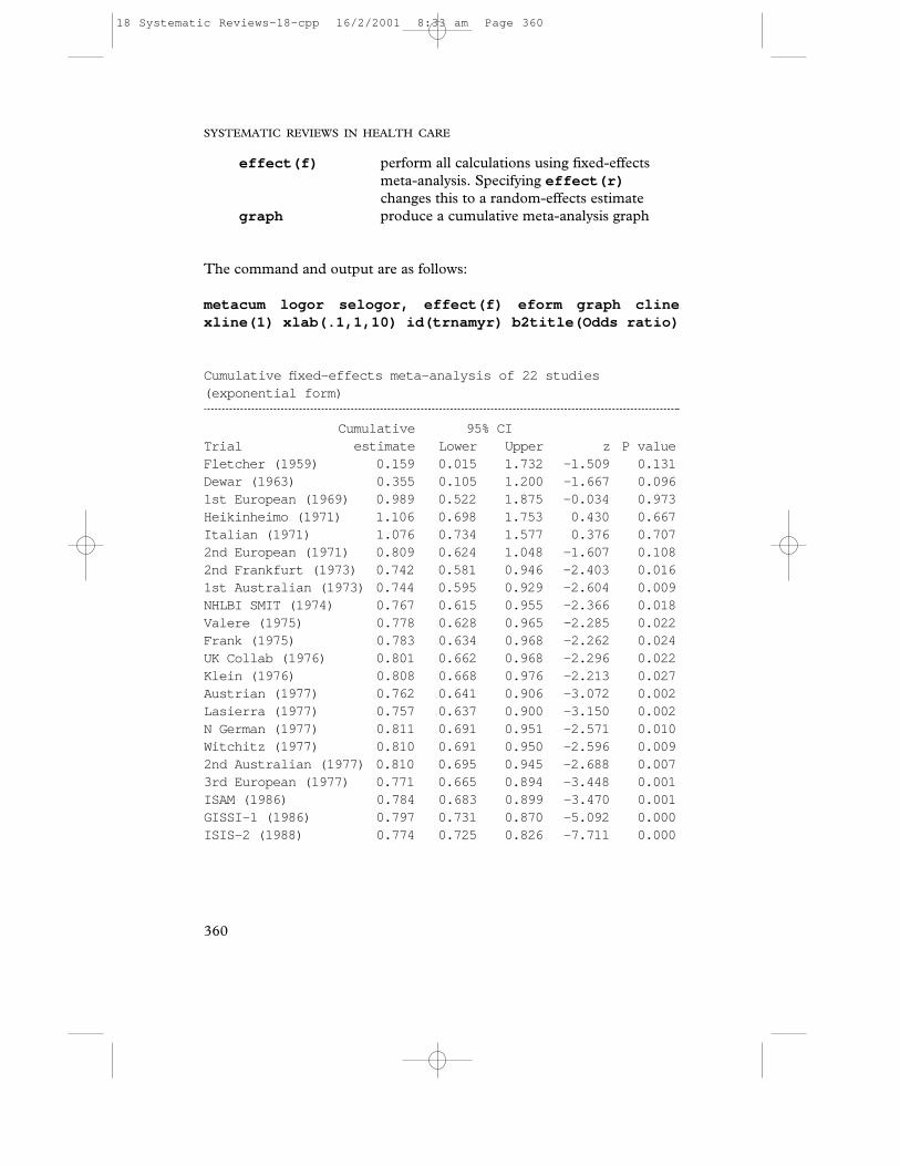
effect(f) perform all calculations using fixed-effects meta-analysis. Specifying effect(r)changes this to a random-effects estimate

graph produce a cumulative meta-analysis graph

The command and output are as follows:

metacum logor selogor, effect(f) eform graph clinexline(1) xlab(.1,1,10) id(trnamyr) b2title(Odds ratio)

Cumulative fixed-effects meta-analysis of 22 studies(exponential form)

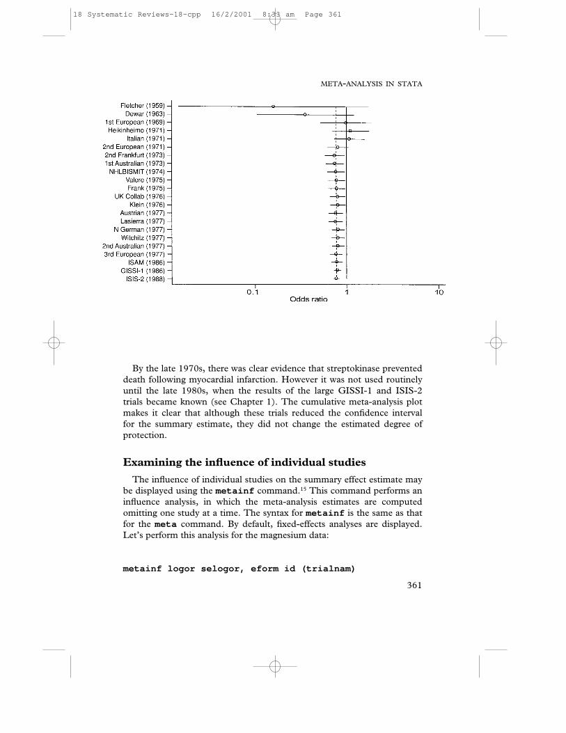
Cumulative 95% CITrial estimate Lower Upper z P valueFletcher (1959) 0.159 0.015 1.732 -1.509 0.131Dewar (1963) 0.355 0.105 1.200 -1.667 0.0961st European (1969) 0.989 0.522 1.875 -0.034 0.973Heikinheimo (1971) 1.106 0.698 1.753 0.430 0.667Italian (1971) 1.076 0.734 1.577 0.376 0.7072nd European (1971) 0.809 0.624 1.048 -1.607 0.1082nd Frankfurt (1973) 0.742 0.581 0.946 -2.403 0.0161st Australian (1973) 0.744 0.595 0.929 -2.604 0.009NHLBI SMIT (1974) 0.767 0.615 0.955 -2.366 0.018Valere (1975) 0.778 0.628 0.965 -2.285 0.022Frank (1975) 0.783 0.634 0.968 -2.262 0.024UK Collab (1976) 0.801 0.662 0.968 -2.296 0.022Klein (1976) 0.808 0.668 0.976 -2.213 0.027Austrian (1977) 0.762 0.641 0.906 -3.072 0.002Lasierra (1977) 0.757 0.637 0.900 -3.150 0.002N German (1977) 0.811 0.691 0.951 -2.571 0.010Witchitz (1977) 0.810 0.691 0.950 -2.596 0.0092nd Australian (1977) 0.810 0.695 0.945 -2.688 0.0073rd European (1977) 0.771 0.665 0.894 -3.448 0.001ISAM (1986) 0.784 0.683 0.899 -3.470 0.001GISSI-1 (1986) 0.797 0.731 0.870 -5.092 0.000ISIS-2 (1988) 0.774 0.725 0.826 -7.711 0.000


360



361

By the late 1970s, there was clear evidence that streptokinase preventeddeath following myocardial infarction. However it was not used routinelyuntil the late 1980s, when the results of the large GISSI-1 and ISIS-2trials became known (see Chapter 1). The cumulative meta-analysis plotmakes it clear that although these trials reduced the confidence intervalfor the summary estimate, they did not change the estimated degree ofprotection.

Examining the influence of individual studies

The influence of individual studies on the summary effect estimate maybe displayed using the metainf command.15 This command performs aninfluence analysis, in which the meta-analysis estimates are computedomitting one study at a time. The syntax for metainf is the same as thatfor the meta command. By default, fixed-effects analyses are displayed.Let’s perform this analysis for the magnesium data:

metainf logor selogor, eform id (trialnam)



362

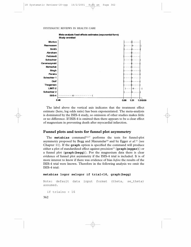
The label above the vertical axis indicates that the treatment effectestimate (here, log odds ratio) has been exponentiated. The meta-analysisis dominated by the ISIS-4 study, so omission of other studies makes littleor no difference. If ISIS-4 is omitted then there appears to be a clear effectof magnesium in preventing death after myocardial infarction.

Funnel plots and tests for funnel plot asymmetry

The metabias command16,17 performs the tests for funnel-plotasymmetry proposed by Begg and Mazumdar18 and by Egger et al.11 (seeChapter 11). If the graph option is specified the command will produceeither a plot of standardized effect against precision11 (graph(egger) ) ora funnel plot (graph(begg) ). For the magnesium data there is clearevidence of funnel plot asymmetry if the ISIS-4 trial is included. It is ofmore interest to know if there was evidence of bias before the results of theISIS-4 trial were known. Therefore in the following analysis we omit theISIS-4 trial:

metabias logor selogor if trial<16, graph(begg)

Note: default data input format (theta, se_theta)assumed.

if trialno < 16


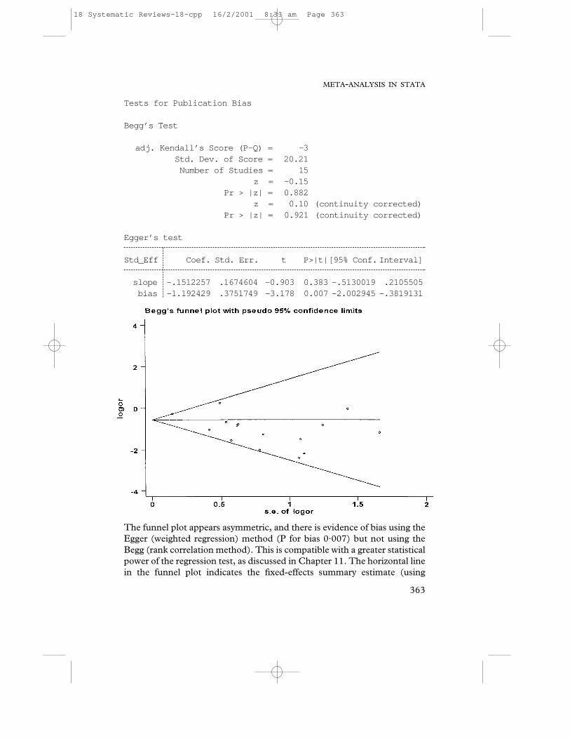
Tests for Publication Bias

Begg’s Test

adj. Kendall’s Score (P-Q) = -3Std. Dev. of Score = 20.21Number of Studies = 15

z = -0.15Pr > |z| = 0.882

z = 0.10 (continuity corrected)Pr > |z| = 0.921 (continuity corrected)

Egger’s test

Std_Eff Coef. Std. Err. t P>|t|[95% Conf. Interval]

slope -.1512257 .1674604 -0.903 0.383 -.5130019 .2105505bias -1.192429 .3751749 -3.178 0.007 -2.002945 -.3819131

The funnel plot appears asymmetric, and there is evidence of bias using theEgger (weighted regression) method (P for bias 0·007) but not using theBegg (rank correlation method). This is compatible with a greater statisticalpower of the regression test, as discussed in Chapter 11. The horizontal linein the funnel plot indicates the fixed-effects summary estimate (using


363


inverse-variance weighting), while the sloping lines indicate the expected95% confidence intervals for a given standard error, assuming no hetero-geneity between studies.

Meta-regression

If evidence is found of heterogeneity in the effect of treatment betweenstudies, then meta-regression can be used to analyse associations betweentreatment effect and study characteristics. Meta-regression can be done inStata by using the metareg command.19

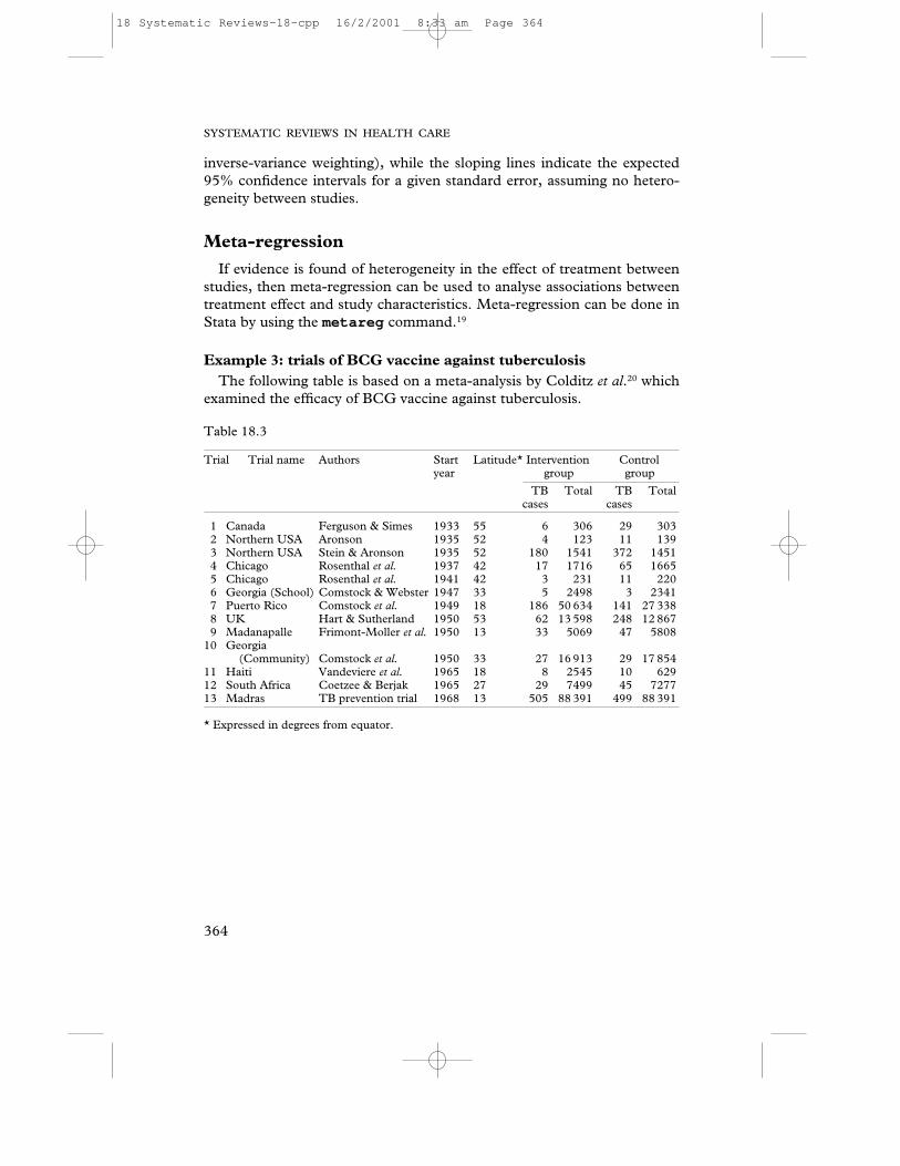
Example 3: trials of BCG vaccine against tuberculosisThe following table is based on a meta-analysis by Colditz et al.20 which

examined the efficacy of BCG vaccine against tuberculosis.

Table 18.3

Trial Trial name Authors Start Latitude* Intervention Controlyear group group

TB Total TB Totalcases cases

1 Canada Ferguson & Simes 1933 55 6 306 29 3032 Northern USA Aronson 1935 52 4 123 11 1393 Northern USA Stein & Aronson 1935 52 180 1541 372 14514 Chicago Rosenthal et al. 1937 42 17 1716 65 16655 Chicago Rosenthal et al. 1941 42 3 231 11 2206 Georgia (School) Comstock & Webster 1947 33 5 2498 3 23417 Puerto Rico Comstock et al. 1949 18 186 50 634 141 27 3388 UK Hart & Sutherland 1950 53 62 13 598 248 12 8679 Madanapalle Frimont-Moller et al. 1950 13 33 5069 47 5808

10 Georgia (Community) Comstock et al. 1950 33 27 16 913 29 17 854

11 Haiti Vandeviere et al. 1965 18 8 2545 10 62912 South Africa Coetzee & Berjak 1965 27 29 7499 45 727713 Madras TB prevention trial 1968 13 505 88 391 499 88 391

* Expressed in degrees from equator.


364


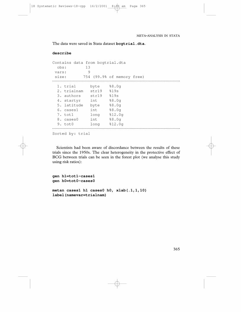
The data were saved in Stata dataset bcgtrial.dta .

describe

Contains data from bcgtrial.dtaobs: 13

vars: 9size: 754 (99.9% of memory free)

1. trial byte %8.0g2. trialnam str19 %19s3. authors str19 %19s4. startyr int %8.0g5. latitude byte %8.0g6. cases1 int %8.0g7. tot1 long %12.0g8. cases0 int %8.0g9. tot0 long %12.0g

Sorted by: trial

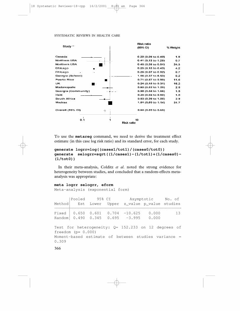
Scientists had been aware of discordance between the results of thesetrials since the 1950s. The clear heterogeneity in the protective effect ofBCG between trials can be seen in the forest plot (we analyse this studyusing risk ratios):

gen h1=tot1-cases1gen h0=tot0-cases0

metan cases1 h1 cases0 h0, xlab(.1,1,10)label(namevar=trialnam)


365



366

To use the metareg command, we need to derive the treatment effectestimate (in this case log risk ratio) and its standard error, for each study.

generate logrr=log((cases1/tot1)/(cases0/tot0))generate selogrr=sqrt((1/cases1)-(1/tot1)+(1/cases0)-(1/tot0))

In their meta-analysis, Colditz et al. noted the strong evidence forheterogeneity between studies, and concluded that a random-effects meta-analysis was appropriate:

meta logrr selogrr, eformMeta-analysis (exponential form)


Fixed 0.650 0.601 0.704 -10.625 0.000 13Random 0.490 0.345 0.695 -3.995 0.000




367

(The different weight of studies under the fixed and random effectsassumption is discussed in Chapter 2).

The authors then examined possible explanations for the cleardifferences in the effect of BCG between studies. The earlier studies mayhave produced different results than later ones. The latitude at which thestudies were conducted may also be associated with the effect of BCG. Asdiscussed by Fine,21 the possibility that BCG might provide greaterprotection at higher latitudes was first recognised by Palmer and Long,22

who suggested that this trend might result from exposure to certainenvironmental mycobacteria, more common in warmer regions, whichimpart protection against tuberculosis.

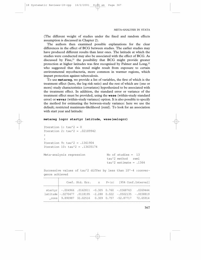
To use metareg , we provide a list of variables, the first of which is thetreatment effect (here, the log risk ratio) and the rest of which are (one ormore) study characteristics (covariates) hypothesized to be associated withthe treatment effect. In addition, the standard error or variance of thetreatment effect must be provided, using the wsse (within-study standarderror) or wsvar (within-study variance) option. It is also possible to specifythe method for estimating the between-study variance: here we use thedefault; restricted maximum-likelihood (reml). To look for an associationwith start year and latitude:

metareg logrr startyr latitude, wsse(selogrr)

Iteration 1: tau^2 = 0Iteration 2: tau^2 = .02189942::Iteration 9: tau^2 = .1361904Iteration 10: tau^2 = .13635174

Meta-analysis regression No of studies = 13tau^2 method remltau^2 estimate = .1364

Successive values of tau^2 differ by less than 10^-4 :conver-gence achieved

Coef. Std. Err. z P>|z| [95% Conf.Interval]

startyr -.004966 .0162811 -0.305 0.760 -.0368763 .0269444

latitude -.0270477 .0118195 -2.288 0.022 -.0502135 -.0038819

_cons 9.890987 32.02516 0.309 0.757 -52.87717 72.65914


The regression coefficients are the estimated increase in the log risk ratioper unit increase in the covariate. So in the example the log risk ratio is esti-mated to decrease by 0·027 per unit increase in the latitude at which thestudy is conducted. The estimated between-study variance has beenreduced from 0·31 (see output from the meta command) to 0·14. Whilethere is strong evidence for an association between latitude and the effect ofBCG, there is no evidence for an association with the year the study started.The estimated treatment effect given particular values of the covariates maybe derived from the regression equation. For example, for a trial beginningin 1950, at latitude 50º, the estimated log risk ratio is given by:

Log risk ratio = 9·891 – 0·00497 × 1950 – 0·0270 × 50 = –1·1505which corresponds to a risk ratio of exp(–1·1505) = 0·316

The use of meta-regression in explaining heterogeneity and identifyingsources of bias in meta-analysis is discussed further in Chapters 8–11.

1 Yusuf S, Collins R, Peto R, et al. Intravenous and intracoronary fibrinolytic therapy inacute myocardial infarction: overview of results on mortality, reinfarction and side-effectsfrom 33 randomized controlled trials. Eur Heart J 1985;6:556–85.

2 Gruppo Italiano per lo Studio della Streptochinasi nell’Infarto Miocardico (GISSI).Effectiveness of intravenous thrombolytic treatment in acute myocardial infarction. Lancet1986;1:397–402.

3 ISIS-2 (Second International Study of Infarct Survival) Collaborative Group. Randomisedtrial of intravenous streptokinase, oral aspirin, both, or neither among 17,187 cases ofsuspected acute myocardial infarction: ISIS-2. Lancet 1988;2:349–60.

4 Bradburn MJ, Deeks JJ, Altman DG. sbe24: metan – an alternative meta-analysiscommand. Stata Tech Bull 1998;44:15.

5 Sharp S, Sterne J. sbe16: Meta-analysis. Stata Tech Bull 1997;38:9–14.6 Sharp S, Sterne J. sbe16.1: New syntax and output for the meta-analysis command. Stata

Tech Bull 1998;42:6–8.7 Sharp S, Sterne J. sbe16.2: Corrections to the meta-analysis command. Stata Tech Bull

1998;43:15.8 Teo KK, Yusuf S, Collins R, Held PH, Peto R. Effects of intravenous magnesium in

suspected acute myocardial infarction: overview of randomised trials. BMJ1991;303:1499–503.

9 ISIS-4 (Fourth International Study of Infarct Survival) Collaborative Group. ISIS-4: arandomised factorial trial assessing early oral captopril, oral mononitrate, and intravenousmagnesium sulphate in 58,050 patients with suspected acute myocardial infarction. Lancet1995;345:669–85.

10 Egger M, Smith GD. Misleading meta-analysis. Lessons from an “effective, safe, simple”intervention that wasn’t. BMJ 1995;310:752–4.

11 Egger M, Smith GD, Schneider M, Minder C. Bias in meta-analysis detected by a simple,graphical test. BMJ 1997;315:629–34.

12 Sterne J. sbe22: Cumulative meta analysis. Stata Tech Bull 1998;42:13–16.13 Lau J, Antman EM, Jimenez-Silva J, Kupelnick B, Mosteller F, Chalmers TC. Cumulative

meta-analysis of therapeutic trials for myocardial infarction. N Engl J Med 1992;327:248–54.14 Antman EM, Lau J, Kupelnick B, Mosteller F, Chalmers TC. A comparison of results of

meta-analyses of randomized control trials and recommendations of clinical experts’Treatments for myocardial infarction. JAMA 1992;268:240–8.

15 Tobias A. sbe26: Assessing the influence of a single study in meta-analysis. Stata Tech Bull1999;47:15–17.


368


16 Steichen T. sbe19: Tests for publication bias in meta-analysis. Stata Tech Bull1998;41:9–15.

17 Steichen T, Egger M, Sterne J. sbe19.1: Tests for publication bias in meta-analysis. StataTech Bull 1998;44:3–4.

18 Begg CB, Mazumdar M. Operating characteristics of a rank correlation test for publicationbias. Biometrics 1994;50:1088–101.

19 Sharp S. sbe23: Meta-analysis regression. Stata Tech Bull 1998;42:16–24.20 Colditz GA, Brewer TF, Berkey CS, et al. Efficacy of BCG vaccine in the prevention of

tuberculosis. Meta-analysis of the published literature. JAMA 1994;271:698–702.21 Fine PEM. Variation in protection by BCG: implications of and for heterologous

immunity. Lancet 1995;346:1339–45.22 Palmer CE, Long MW. Effects of infection with atypical mycobacteria on BCG vaccina-

tion and tuberculosis. Am Rev Respir Dis 1966;94:553–68.


369


Overview of Meta Analysis in Stata

Documents