ORANGE RIVER INTEGRATED WATER RESOURCES …

i

Economic Study of Assurance of Supply Requirements

for Water Resource Management with Reference to Irrigation Agriculture

Volume 2

Procedural Guidelines for the Application of the Assurance of Supply Model in Irrigation

Agriculture

S Barnard1 and R Cloete2

Report to the Water Research Commission

by

1 WRP Consulting Engineers (Pty) Ltd

2 Conningarth Economists

WRC Report No. TT 775/2/18

January 2019

ii

Obtainable from

Water Research Commission Private Bag X03 Gezina, 0031

[email protected] or download from www.wrc.org.za

DISCLAIMER

This report has been reviewed by the Water Research Commission (WRC) and approved for publication. Approval does not signify that the contents necessarily reflect

the views and policies of the WRC, nor does mention of trade names or commercial products constitute endorsement or recommendation for use.

ISBN 978-0-6392-0065-1

Printed in the Republic of South Africa

© WATER RESEARCH COMMISSION

iii

TABLE OF CONTENTS

TABLE OF CONTENTS ........................................................................................................................ III LIST OF FIGURES ................................................................................................................................ IV LIST OF TABLES ................................................................................................................................... V LIST OF ABBREVIATIONS ................................................................................................................... VI 1 INTRODUCTION ............................................................................................................................ 1 1.1 Background ................................................................................................................................... 1 1.2 Purpose ......................................................................................................................................... 1 1.3 Scope ............................................................................................................................................ 2 1.4 Way Forward ................................................................................................................................. 3 2 RELATED LITERATURE ............................................................................................................... 4 2.1 The South African Context ............................................................................................................ 4 2.2 Drought Guidelines ....................................................................................................................... 5 3 PRIORITY TOPICS ........................................................................................................................ 9 3.1 Assurance of Supply ..................................................................................................................... 9 3.2 User Priority and Risk Criteria ..................................................................................................... 10 3.3 Water Resource Planning Model ................................................................................................ 12 3.4 Risk Analysis (Results from WRPM) .......................................................................................... 12 3.5 Water Impact Model .................................................................................................................... 14 3.6 GDP vs. Restriction Relationship ................................................................................................ 14 3.7 Economic Indicators .................................................................................................................... 15 3.8 Present Value of Economic Indicators ........................................................................................ 15 3.9 Expected Value (Mean) of Economic Indicator ........................................................................... 16 4 LIMITATIONS OF THE ASM ....................................................................................................... 17 5 STEP-BY-STEP PROCEDURE FOR APPLYING THE ASM ...................................................... 18 5.1 Concept ....................................................................................................................................... 18 5.2 Configuration of the WRYM and WRPM ..................................................................................... 19 5.3 Execution of WRYM and WRPM and Output Files ..................................................................... 27 5.4 Post-processing of WRYM and WRPM Results ......................................................................... 31 5.5 Configuration of the Water Impact Model ................................................................................... 40 5.6 Incorporating WIM with WRYM and WRPM Results .................................................................. 48 5.7 Execution of ASM ....................................................................................................................... 48 5.8 Interpretation of Results .............................................................................................................. 51 5.9 Economic Indicator Loss vs. Volume Curtailed Relationship ..................................................... 53 5.10 The Farm Production Model ....................................................................................................... 58 5.11 Consideration of Other User Sectors .......................................................................................... 59 6 CONCLUSION AND RECOMMENDATIONS .............................................................................. 60 REFERENCES ...................................................................................................................................... 61

iv

LIST OF FIGURES

Figure 1: Generic decision process for the implementation of water restrictions ................................... 7 Figure 2: Short-term yield reliability – Family of firm yield lines .............................................................. 9 Figure 3: Short-term yield reliability – Family of firm yield lines with demands imposed ...................... 11 Figure 4: Base yield lines of 60% starting storage with demands imposed .......................................... 12 Figure 5: Box-and-whisker plot ............................................................................................................. 13 Figure 6: System curtailment plot ......................................................................................................... 14 Figure 7: GDP loss vs. Volume for indicated restriction levels ............................................................. 15 Figure 8: Analyses matrix in the new model ......................................................................................... 16 Figure 9: Research concept/methodology ............................................................................................ 18 Figure 10: Short-term yield coefficients ................................................................................................ 19 Figure 11: User priority classification and demands in WRPM ............................................................. 20 Figure 12: Short-term yield reliability curves Orange River System ..................................................... 28 Figure 13: Data in plt.out file ............................................................................................................ 28 Figure 14: Data in dam.out file ............................................................................................................ 29 Figure 15: Data in pln.out file as result from WRPM ........................................................................ 30 Figure 16: Example of sys.out file output from WRPM ..................................................................... 31 Figure 17: Combined Gariep and Vanderkloof Dam storage trajectory plot ......................................... 31 Figure 18: Orange River System short-term yield reliability curve with different user priority scenarios including Polihali Dam ........................................................................................................................... 34 Figure 19: Orange River System 40% short-term yield reliability curve with different user priority scenarios including Polihali Dam .......................................................................................................... 35 Figure 20: Steps 1 to 3 of the restriction calculation ............................................................................. 38 Figure 21: Steps 4 to 5 of Restriction calculation ................................................................................. 39 Figure 22: Input to WIM ......................................................................................................................... 40 Figure 23: WIM schematic .................................................................................................................... 44 Figure 24: Procedure using the WRYM ................................................................................................ 48 Figure 25: Procedure using the WRPM ................................................................................................ 48 Figure 26: Modified WIM interface for application with ASM ................................................................ 49 Figure 27: Interface of the ASM ............................................................................................................ 50 Figure 28: WRYM input definition worksheet ........................................................................................ 51 Figure 29: Probability distribution of present values of economic indicators ........................................ 52 Figure 30: Box plots for present value per discount rate ...................................................................... 52 Figure 31: Box plot for annual values over the analysis period ............................................................ 53 Figure 32: Box plot for present value at 0% discount rate for various scenarios .................................. 53 Figure 33: GDP loss – Volume curtailed relationship per annum (Scenario 1) .................................... 54 Figure 34: GDP loss – Volume curtailed relationship per annum (Scenario 1a) .................................. 55 Figure 35: GDP loss – Volume curtailed relationship per annum (Scenario 1b) .................................. 55 Figure 36: Average derived GDP loss – volume curtailed relationship ................................................ 56 Figure 37: Average derived employment loss – volume curtailed relationship ..................................... 57 Figure 38: Average derived household income loss – volume curtailed relationship ........................... 58 Figure 39: Farm production model ........................................................................................................ 58

v

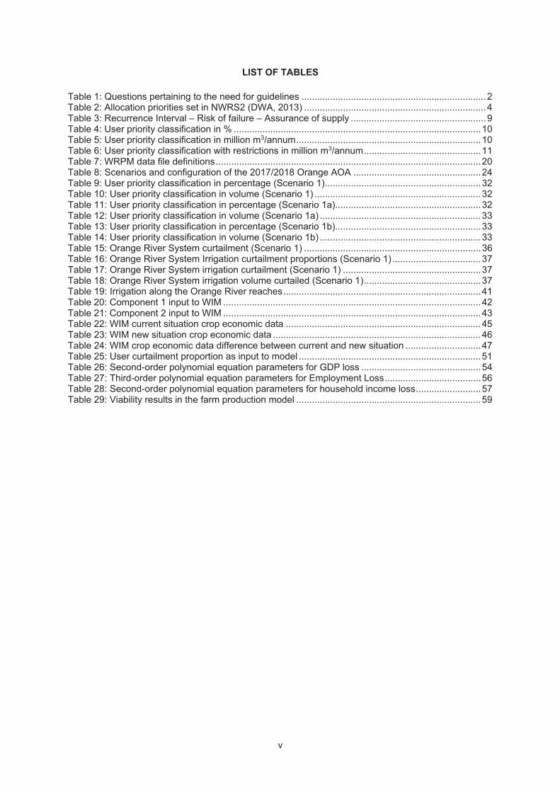
LIST OF TABLES

Table 1: Questions pertaining to the need for guidelines ....................................................................... 2 Table 2: Allocation priorities set in NWRS2 (DWA, 2013) ...................................................................... 4 Table 3: Recurrence Interval – Risk of failure – Assurance of supply .................................................... 9 Table 4: User priority classification in % ............................................................................................... 10 Table 5: User priority classification in million m3/annum ....................................................................... 10 Table 6: User priority classification with restrictions in million m3/annum ............................................. 11 Table 7: WRPM data file definitions ...................................................................................................... 20 Table 8: Scenarios and configuration of the 2017/2018 Orange AOA ................................................. 24 Table 9: User priority classification in percentage (Scenario 1) ............................................................ 32 Table 10: User priority classification in volume (Scenario 1) ................................................................ 32 Table 11: User priority classification in percentage (Scenario 1a)........................................................ 32 Table 12: User priority classification in volume (Scenario 1a) .............................................................. 33 Table 13: User priority classification in percentage (Scenario 1b)........................................................ 33 Table 14: User priority classification in volume (Scenario 1b) .............................................................. 33 Table 15: Orange River System curtailment (Scenario 1) .................................................................... 36 Table 16: Orange River System Irrigation curtailment proportions (Scenario 1) .................................. 37 Table 17: Orange River System irrigation curtailment (Scenario 1) ..................................................... 37 Table 18: Orange River System irrigation volume curtailed (Scenario 1) ............................................. 37 Table 19: Irrigation along the Orange River reaches ............................................................................ 41 Table 20: Component 1 input to WIM ................................................................................................... 42 Table 21: Component 2 input to WIM ................................................................................................... 43 Table 22: WIM current situation crop economic data ........................................................................... 45 Table 23: WIM new situation crop economic data ................................................................................ 46 Table 24: WIM crop economic data difference between current and new situation ............................. 47 Table 25: User curtailment proportion as input to model ...................................................................... 51 Table 26: Second-order polynomial equation parameters for GDP loss .............................................. 54 Table 27: Third-order polynomial equation parameters for Employment Loss ..................................... 56 Table 28: Second-order polynomial equation parameters for household income loss ......................... 57 Table 29: Viability results in the farm production model ....................................................................... 59

vi

LIST OF ABBREVIATIONS

AOA Annual Operating Analysis ASM Assurance of Supply Model CMA Catchment Management Agency DWS Department of Water and Sanitation EWR Environmental Water Requirement GBWSS Greater Bulwer/Donnybrook Bulk Water Supply Scheme GDP Gross Domestic Product HFY Historical Firm Yield HDI Historically Disadvantaged Individual HH Households HHI Household Income IFR Instream Flow Requirements IVRS Integrated Vaal River System IWRP Integrated Water Resource Planning LHWP Lesotho Highlands Water Project LO Lower Orange LOE Lower Orange East LOW Lower Orange West NFI Nett Farm Income NWA National Water Act NWRS National Water Resource Strategy ORP Orange River Project R Rand RSA Republic of South Africa SAM Social Accounting Matrix WC/WDM Water Conservation and Demand Management WIM Water Impact Model WMA Water Management Area WRC Water Resource Commission WRPM Water Resource Planning Model WRYM Water Resource Yield Model

1

1 INTRODUCTION

1.1 Background

During times of drought, the decisions pertaining to drought restriction rules among different water user sectors and the level of assurance at which water should be supplied to them are often disputed. The Department of Water and Sanitation (DWS) is responsible for managing and operating the major water supply systems in South Africa. The DWS undertakes water resource system analysis by using the water resource yield model (WRYM) and the water resource planning model (WRPM). One component of the WRPM is an allocation procedure based on the reservoir yield characteristics derived from the WRYM. The allocation process consists of a user priority classification whereby the water supply from the resource is curtailed according to the assurance of supply at which each user is prioritised. This is referred to as the assurance of supply requirement or risk of curtailment criteria.

There are existing user priority classification tables per water supply system that have been developed by means of a decision process among the stakeholders of the specific water supply system. The decision process can be enhanced by using economic analysis, which is a more scientific and quantitative approach. For the irrigation sector, an existing model referred to as the water impact model (WIM) is used to do economic analysis. With this model, the impact of water restrictions on economic indicators such as gross domestic product (GDP), household income and the number of people employed within a water supply system is determined. The principle is based on the relationship between a reduction in crop production yield and the reduction in water supply to a specific crop.

A decision support tool has been developed to enhance the decision process pertaining to drought restriction rules. The development of this tool is based on a link created between the WRPM and the WIM to enable sensitivity analysis among various scenarios of assurance of supply requirements for the irrigation sector.

Drought restriction analysis and the development of operating rules serve as early warning processes whereby probable water supply curtailments of a specific water resource for a certain planning period are identified. Knowing the possibilities of the water supply system’s potential behaviour in future can assist with improved planning at irrigation scheme level. This may include but is not limited to deciding on the type of crop to be cultivated in the following year by knowing the volume of the normal water supply that will be curtailed and the related economic impact thereof.

This decision support tool is an add-on or enhancement to the post-processing tool that already exists for water resource management undertaken by the DWS. Therefore, the tool should be used in collaboration with the guidelines that already exist for water resource management and the manuals that have been developed for the use of the water resource models.

1.2 Purpose

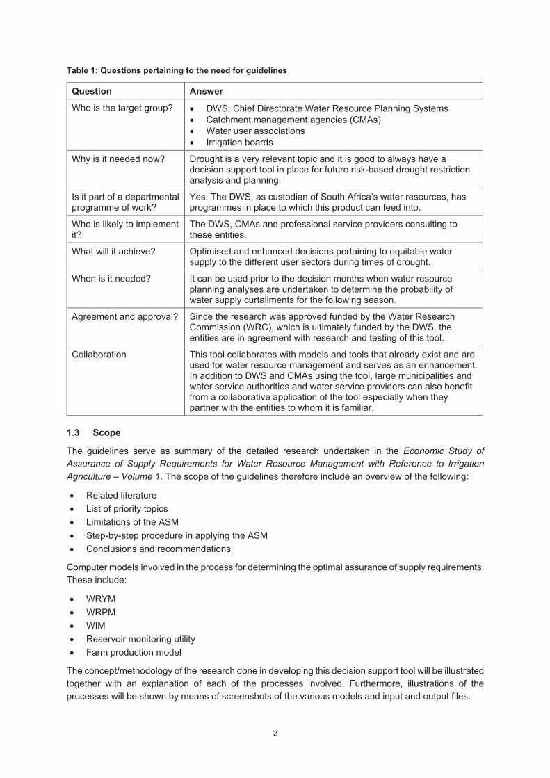
The newly developed decision support tool to determine the assurance supply requirements for water resource management has been tested and is functional. The tool is referred to as the assurance of supply model (ASM). Table 1 addresses a few questions pertaining to the ASM.

The guidelines serve to assist with using this tool and interpreting the results correctly to enhance water supply system operation and management.

2

Table 1: Questions pertaining to the need for guidelines

Question Answer

Who is the target group? DWS: Chief Directorate Water Resource Planning Systems Catchment management agencies (CMAs) Water user associations Irrigation boards

Why is it needed now? Drought is a very relevant topic and it is good to always have a decision support tool in place for future risk-based drought restriction analysis and planning.

Is it part of a departmental programme of work?

Yes. The DWS, as custodian of South Africa’s water resources, has programmes in place to which this product can feed into.

Who is likely to implement it?

The DWS, CMAs and professional service providers consulting to these entities.

What will it achieve? Optimised and enhanced decisions pertaining to equitable water supply to the different user sectors during times of drought.

When is it needed? It can be used prior to the decision months when water resource planning analyses are undertaken to determine the probability of water supply curtailments for the following season.

Agreement and approval? Since the research was approved funded by the Water Research Commission (WRC), which is ultimately funded by the DWS, the entities are in agreement with research and testing of this tool.

Collaboration This tool collaborates with models and tools that already exist and are used for water resource management and serves as an enhancement. In addition to DWS and CMAs using the tool, large municipalities and water service authorities and water service providers can also benefit from a collaborative application of the tool especially when they partner with the entities to whom it is familiar.

1.3 Scope

The guidelines serve as summary of the detailed research undertaken in the Economic Study of Assurance of Supply Requirements for Water Resource Management with Reference to Irrigation Agriculture – Volume 1. The scope of the guidelines therefore include an overview of the following:

Related literature List of priority topics Limitations of the ASM Step-by-step procedure in applying the ASM Conclusions and recommendations

Computer models involved in the process for determining the optimal assurance of supply requirements. These include:

WRYM WRPM WIM Reservoir monitoring utility Farm production model

The concept/methodology of the research done in developing this decision support tool will be illustrated together with an explanation of each of the processes involved. Furthermore, illustrations of the processes will be shown by means of screenshots of the various models and input and output files.

3

The guidelines include a detailed step-by-step procedure as to how the ASM is to be used and operated in collaboration with existing models.

1.4 Way Forward

The guidelines for the ASM will need to be used in collaboration with existing guidelines and user manuals in terms of risk-based drought restrictions rules and analyses.

Although the information used for the analyses undertaken and the testing of the ASM is from different study areas, the guidelines will take on a generic form with reference to different water supply systems analysed.

4

2 RELATED LITERATURE

2.1 The South African Context

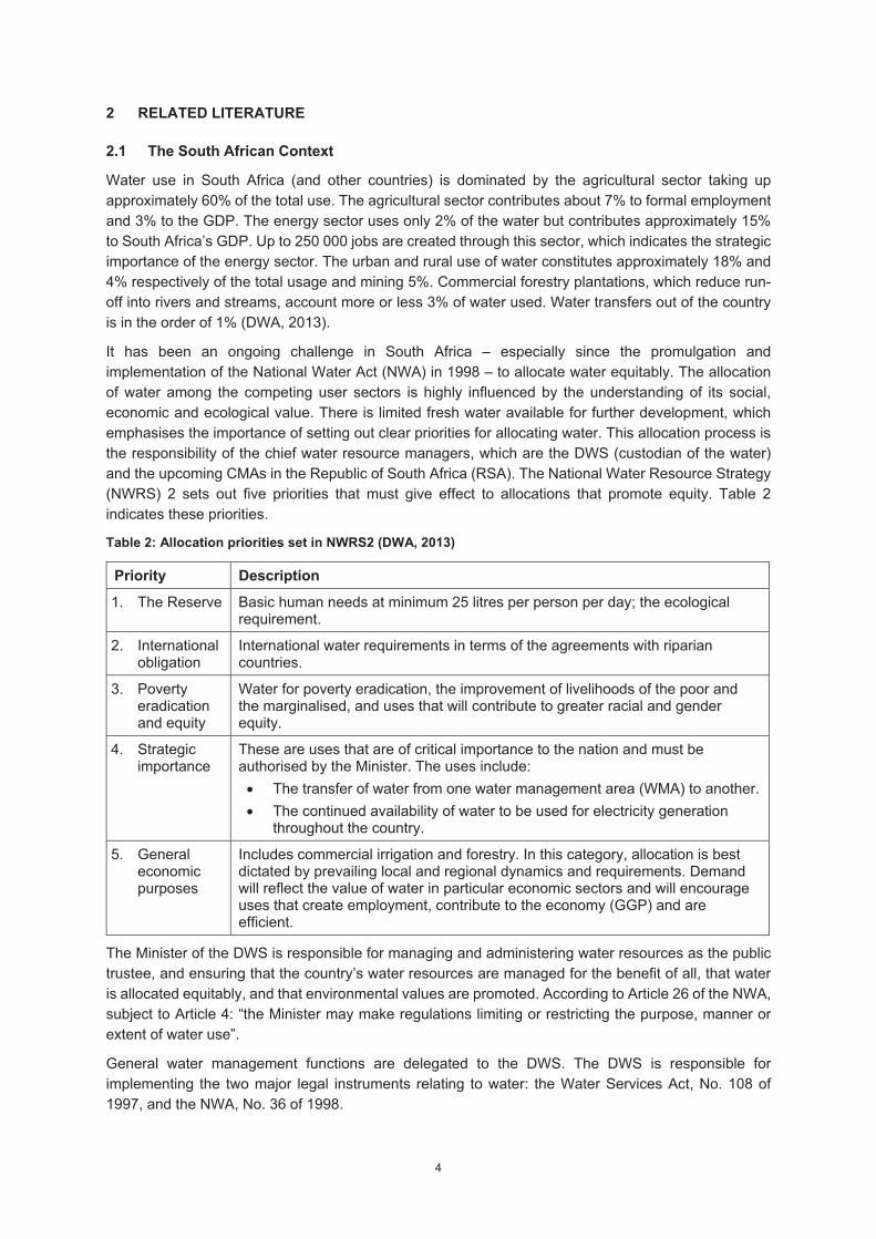
Water use in South Africa (and other countries) is dominated by the agricultural sector taking up approximately 60% of the total use. The agricultural sector contributes about 7% to formal employment and 3% to the GDP. The energy sector uses only 2% of the water but contributes approximately 15% to South Africa’s GDP. Up to 250 000 jobs are created through this sector, which indicates the strategic importance of the energy sector. The urban and rural use of water constitutes approximately 18% and 4% respectively of the total usage and mining 5%. Commercial forestry plantations, which reduce run-off into rivers and streams, account more or less 3% of water used. Water transfers out of the country is in the order of 1% (DWA, 2013).

It has been an ongoing challenge in South Africa – especially since the promulgation and implementation of the National Water Act (NWA) in 1998 – to allocate water equitably. The allocation of water among the competing user sectors is highly influenced by the understanding of its social, economic and ecological value. There is limited fresh water available for further development, which emphasises the importance of setting out clear priorities for allocating water. This allocation process is the responsibility of the chief water resource managers, which are the DWS (custodian of the water) and the upcoming CMAs in the Republic of South Africa (RSA). The National Water Resource Strategy (NWRS) 2 sets out five priorities that must give effect to allocations that promote equity. Table 2 indicates these priorities.

Table 2: Allocation priorities set in NWRS2 (DWA, 2013)

Priority Description

1. The Reserve Basic human needs at minimum 25 litres per person per day; the ecological requirement.

2. International obligation

International water requirements in terms of the agreements with riparian countries.

3. Poverty eradication and equity

Water for poverty eradication, the improvement of livelihoods of the poor and the marginalised, and uses that will contribute to greater racial and gender equity.

4. Strategic importance

These are uses that are of critical importance to the nation and must be authorised by the Minister. The uses include:

The transfer of water from one water management area (WMA) to another. The continued availability of water to be used for electricity generation

throughout the country.

5. General economic purposes

Includes commercial irrigation and forestry. In this category, allocation is best dictated by prevailing local and regional dynamics and requirements. Demand will reflect the value of water in particular economic sectors and will encourage uses that create employment, contribute to the economy (GGP) and are efficient.

The Minister of the DWS is responsible for managing and administering water resources as the public trustee, and ensuring that the country’s water resources are managed for the benefit of all, that water is allocated equitably, and that environmental values are promoted. According to Article 26 of the NWA, subject to Article 4: “the Minister may make regulations limiting or restricting the purpose, manner or extent of water use”.

General water management functions are delegated to the DWS. The DWS is responsible for implementing the two major legal instruments relating to water: the Water Services Act, No. 108 of 1997, and the NWA, No. 36 of 1998.

5

The DWS consists of a number of directorates, all performing different functions. The purpose of the Chief Directorate Integrated Water Resource Planning (IWRP) is to ensure availability of adequate water that is fit for use. This is achieved through holistic planning for the management and development of water resources and systems.

The IWRP function is under the DWS sub-programme of Integrated Planning, which develops comprehensive plans that guide all initiatives and infrastructure development within the water sector; taking the water needs of all users into account and identifying the appropriate mix of interventions. This will ensure a reliable supply of water in the most efficient, sustainable and socially beneficial manner. The purpose is to ensure that the country’s water resources are protected, used, developed, conserved, managed and controlled in a sustainable manner to benefit all people and the environment through effective policies, integrated planning, strategies, knowledge base and procedures.

Four chief directorates reside under IWRP:

National Water Resource Planning develops national strategies and procedures for the reconciliation of water availability and requirements to meet national social and economic development objectives including strategic requirements, resource quality objectives and international obligations.

Options Analysis identifies and evaluates water resource management options/projects to meet future water requirements and for multi-disciplinary project planning to implement these options, including the development of applicable procedures and guidelines.

Water Resource Planning Systems evaluates strategic water resource management challenges, provides expert planning related support and develops planning and management decision support systems with regard to operating rules, water quality, integrated hydrology (including geohydrology) and socio-economic aspects of water resources.

Climate Change contributes to water-related policies and develops appropriate adaptation strategies for the water sector in response to climate change.

In South Africa, a vital component of Integrated Water Resources Management is the progressive devolution of responsibility and authority over water resources to CMAs. The initial scale of operation for the CMAs is that of WMAs (NWA, No. 36 of 1998). In terms of the NWRS, 19 WMAs are delineated in South Africa, with CMAs in various stages of establishment. More recently, a change in approach has seen some CMAs cover more than one WMA, with the intention that nine CMAs will be formed throughout the country.

Section 80 of the NWA describes the initial functions of a CMA:

To investigate and advise interested persons on the protection, use, development, conservation, management and control of the water resources in its WMA.

To develop a catchment management strategy. To coordinate the related activities of water users and of the water management institutions within

its WMA. To promote the coordination of its implementation with the implementation of any applicable

development plan established in terms of the Water Services Act, 1997 (No. 108 of 1997). To promote community participation in the protection, use, development, conservation,

management and control of the water resources in its WMA.

2.2 Drought Guidelines

In 2006 and as a result of drought affecting parts of South Africa, the DWS developed guidelines for the management and operation of water supply systems during normal and drought conditions. The objective was to assist water resource managers and institutions to manage and operate water supply system more effectively and optimally to the benefit of all users dependent on the specific system. The

6

four water supply systems selected as pilot study areas for these guidelines included the Western Cape, Amatole, Vaal and Olifants water supply systems.

These guidelines have assisted with the development of water supply system specific operating rules to discern whether or not the water supply from the resource needs to be curtailed for a given year. The decision on curtailment is mainly influenced by the dam levels at the end of the rainy season. Thus, it is important to establish the severity of the level of curtailment, when it is needed, the timing thereof, and possible relaxation after the drought subsides.

In these guidelines, reference is made to the prioritisation and assurance of supply requirements of the different water user sectors. It indicates that strategic users (such as power stations and major industries) and the urban sector requiring basic human needs will be curtailed to a lesser degree than the irrigation agriculture sector; the levels of curtailment will be different for each system. The curtailment levels are to be reviewed regularly based on the storage levels of the major dams in the water supply system. This is normally done at the end of the rainfall season (wet season) and as indicated by the technical management committee of the system and system operating forums. This decision date will vary from system to system.

In addition, significant emphasis is given to the release of Reserve requirements. The Reserve requirement determination processes are based on the concept that environmental water requirements (EWRs) should reflect the variations in natural flow. This also forms the basis on which possible curtailments of the Reserve are to be determined as opposed to the measure of water availability. The criteria for deciding what levels of curtailments are appropriate and the assurance of supply to various water user sectors during times of curtailments are among the key decisions to be made by the technical management committee and system operating forums.

This section discusses the derivation and implementation of system operating rules of the Guidelines for Water Supply Systems Operations and Management Plans during Normal and Drought Conditions (DWAF, 2006), the methodology for deriving operating rules. These steps include:

Define the system. Define stakeholders. Determine and classify present and future water requirements from the system. Determine water availability from surface water resources in the system. Determine the extent of current groundwater use and potential future use. Determine the details of the existing (or need for new) water resource infrastructure. Determine the (real) extent of the water surplus or deficit. Select the appropriate decision support tools. Develop proposals to match available yield with available water treatment and reticulation

infrastructure. Investigate the factors affecting water quality in the system. Draw up preliminary water quality management objectives. Model alternative water quality scenarios to determine their effects on water quality. Estimate required levels of curtailment during drought conditions. Model the impact on yield under different water quality scenarios. Select the most appropriate water operating scenario. Develop short-term characteristic yield/reliability curves. Derive operating rules for the system. Verify the operating rules. Determine when the next water augmentation scheme may be required.

7

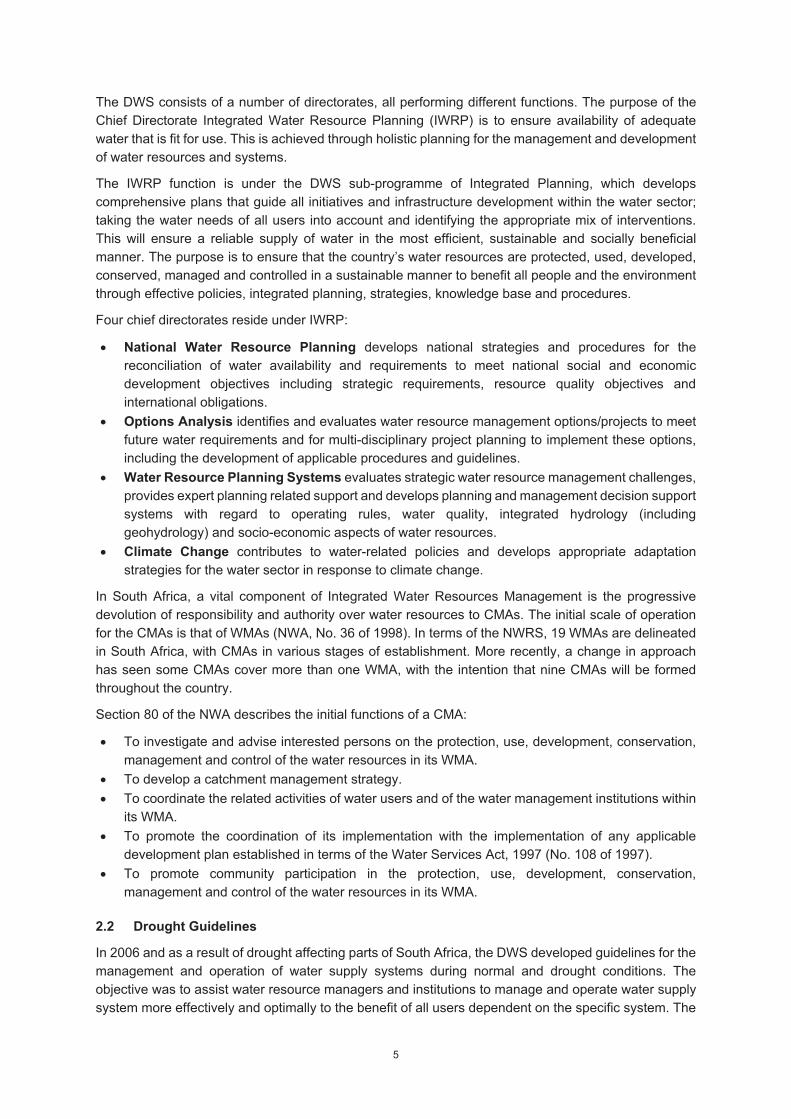
In the summer rainfall regions of South Africa, a decision is made at the end of the rainfall season regarding the need for water restrictions in the season to follow. Such a decision is based on the outcome of stochastic stream flow analysis, which is dictated by the storage in the reservoirs within a water supply system. The process is referred to as the annual operating analysis (AOA) and entails the following:

Activities centred on annual decision dates: 1 May and a review on 1 November of each year. Monitoring implementation of previous years’ rules. Data collation in preparation for analysis. Scenario formulation meeting. System risk analysis of scenarios. System operating forum:

o Present scenario results. o Consult with stakeholders. o Seek consensus on operating ruled for next 12 months.

Document all activities and decision in an AOA report.

Figure 1 shows the typical decision process for implementing or changing water restrictions (the decisions to be taken, the time frame in which they are to be taken, as well as the ongoing monitoring and review process).

Figure 1: Generic decision process for the implementation of water restrictions

Annual Operating Analysis ProcessData collation

preparation for analysis

Scenario formulation and meeting

System risk analysis of scenarios

Annual Decision date

1 May & 1 November

Monitoring implementation of previous year’s rules

Document all activities and decision

annual operating analysis report

System Operating Forum

8

This methodology for deriving operating rules as an existing approach should continue to be applied with the addition of a scientific approach to determine the assurance of supply requirements during drought conditions. Reports, guidelines and manuals that should be used in collaboration with the guidelines for the ASM for application in irrigation agriculture include but are not limited to the following:

Guidelines for Water Supply System Operation and Management Plans during Normal and Drought Conditions (DWAF, 2006).

Maintenance and Updating of Hydrological and System Software – Phase 3 – Procedural Manual for the Water Resources Simulation Model (DWAF, 2008a).

Water Resources Yield Model (WRYM) User Guide – Release 7.5.6.2 (DWAF, 2008b). Water Resources Planning Model (WRPM) – Input Data and File Formats, version 4.4 (DWS,

2013).

9

3 PRIORITY TOPICS

3.1 Assurance of Supply

An already stressed water resource system is likely to become increasingly stressed over time – especially if the system has a finite supply capacity and a growing demand. Therefore, it is important to consider the reliability or assurance at which the demand on a water resource system can be satisfied under various conditions without system failure. A stochastic analysis can be undertaken to determine the assurance of supply, which is illustrated by yield reliability curves. Assurance of supply is expressed as a percentage resulting from the probability of a water resource system failing to supply the demand or target draft thereon at different recurrence intervals of drought periods. For instance, if a system were to fail to supply a demand only once in 200 years, it has a risk of failure of 0.5% and an assurance of supply of 99.5%.

Table 3 lists the most common risk of failures used for stochastic analyses at the corresponding assurance of supply.

Table 3: Recurrence Interval – Risk of failure – Assurance of supply

Recurrence interval Risk of failure (%) Assurance of supply (%)

1:200 years 0.5 99.5

1:100 years 1 99

1:50 years 2 98

1:20 years 5 95

1:10 years 10 90

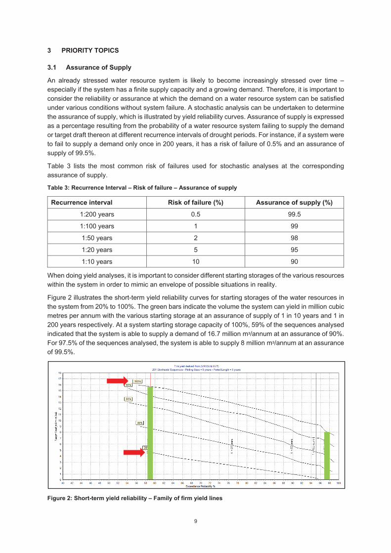
When doing yield analyses, it is important to consider different starting storages of the various resources within the system in order to mimic an envelope of possible situations in reality.

Figure 2 illustrates the short-term yield reliability curves for starting storages of the water resources in the system from 20% to 100%. The green bars indicate the volume the system can yield in million cubic metres per annum with the various starting storage at an assurance of supply of 1 in 10 years and 1 in 200 years respectively. At a system starting storage capacity of 100%, 59% of the sequences analysed indicated that the system is able to supply a demand of 16.7 million urance of 90%. For 97.5% of the sequences analysed, the system is able to supply 8 million of 99.5%.

Figure 2: Short-term yield reliability – Family of firm yield lines

10

3.2 User Priority and Risk Criteria

When a water resource system is challenged with a potential deficit in available supply versus demand – be it infrastructure related, due to a growing population, a drought or combination of all three – it is important to have by-laws in place to protect the water resources in such a system from complete failure. The allocation of water to various users from a water resource system is a challenging exercise –especially in semi-arid regions and in times of drought. However, in a constantly evolving and diverse socio-economic environment, different water users are demanding from a system where there are numerous interdependent variables to consider an optimal water allocation structure.

Different water users have different priorities in terms of the reliability of water supply as well as the risk of non-supply. Higher priority users request water supply at a higher assurance, which means they will settle for a lower volume as long as they are assured of that volume. Lower priority users normally require larger volumes of water and are willing to have it supplied at a lower assurance. Water users with a higher priority typically include users from the domestic sector providing water for basic human need and users from the industrial sector – especially those responsible for power generation.

The environment is considered as a high-priority user; unavoidable losses to the water resource system can be categorised as an imaginary high-priority user. Over and above striving towards an optimal water allocation in terms of water supply from the water resource system, it is vitally important to consider the possible need for water restrictions and the direct and indirect impact thereof on the different user sectors. To aid in the determination of restriction levels, the system and user categories can be tabulated against different levels of assurance of supply known as a user priority classification table.

Table 4 to Table 6 serve as examples to illustrate the process of priority classification for irrigation and domestic users including the determination of the restriction level. This specific allocation is derived from a qualitative approach by a group of decision makers and not based on a scientifically quantifiable approach. In this example, there are three levels of assurance at which the system will supply: low, medium and high priority. The total demand will be allocated at 50%, 30% and 20% for irrigation, and 30%, 20% and 50% for domestic users respectively, as shown in Table 4.

Table 4: User priority classification in %

System and user category

Priority classification (%) Low

(95% assurance) (1:20 year)

Medium (99% assurance)

(1:100 year)

High (99.5% assurance)

(1:200 Year) Irrigation 50 30 20 Domestic 30 20 50 Level of restriction 1 2 3

Table 5 gives the actual volume allocated to the two user sectors at the different priorities of assurance of supply for a total demand of 10 million m /annum.

Table 5: User priority classification in million m3/annum

System and user category

Priority classification (million m3/a)

Low (95% assurance)

(1:20 year)

Medium (99% assurance)

(1:100 year)

High (99.5% assurance)

(1:200 year)

Total

Irrigation 3 1.8 1.2 6 Domestic 1.2 0.8 2.0 4 Total 4.2 2.6 3.2 10 Level of restriction 1 2 3

11

If for argument sake, the system can only supply 8 million m /annum, restrictions of 2 million m /annum are required. Since the total demand at the low priority class is 4.2 million m /annum, it will be sufficient to only curtail 47.6% of this class’s use. This equates to restricting irrigation users by 23.8% (50% × 47.6%) and domestic users by 14.3% (30% × 47.6%).

Table 6 shows the priority classification if restrictions are implemented.

Table 6: User priority classification with restrictions in million m3/annum

System and user category

Priority classification (million m3/a) Low

(95% assurance) (1:20 year)

Medium (99% assurance)

(1:100 year)

High (99.5% assurance)

(1:200 year)

Total

Irrigation 1.57 1.8 1.2 4.57 Domestic 0.63 0.8 2.0 3.43 Total 2.20 2.6 3.2 8 Level of restriction 1 2 3

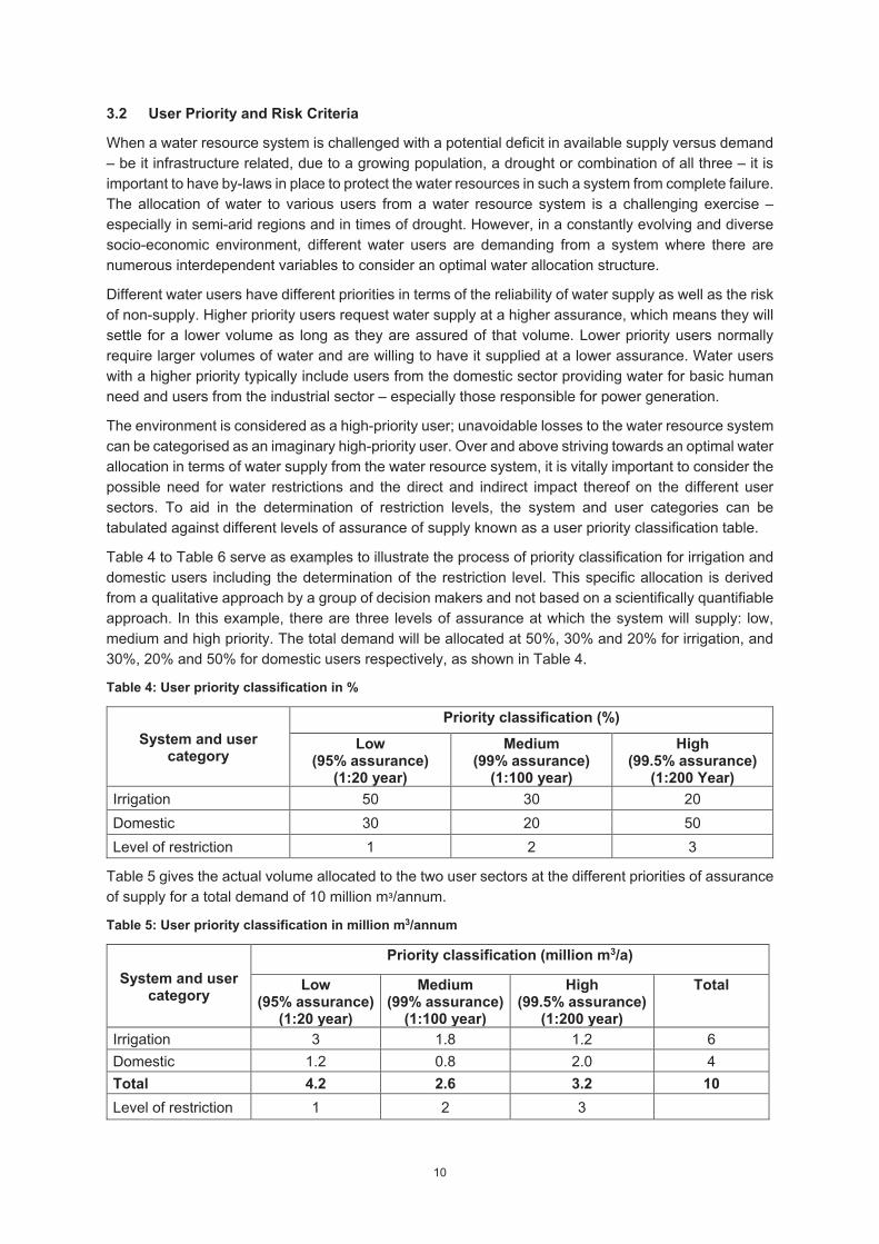
Figure 3 plots the total demand on the system of 10 million m /annum at the different applicable recurrence intervals of risk of non-supply to evaluate if the yield of the system at various starting storages will be sufficient to supply the demand. If the starting storage of the resource is at a lower level at the decision date, an iterative assessment will have to be carried out to determine the required restrictions on the system. Figure 3 shows that the probability of the system running into a deficit is likely if the starting storage is below 80% for the specific user priority definition.

Figure 3: Short-term yield reliability – Family of firm yield lines with demands imposed

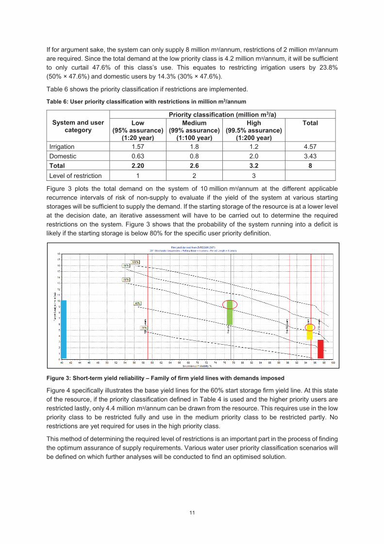
Figure 4 specifically illustrates the base yield lines for the 60% start storage firm yield line. At this state of the resource, if the priority classification defined in Table 4 is used and the higher priority users are restricted lastly, only 4.4 million m /annum can be drawn from the resource. This requires use in the low priority class to be restricted fully and use in the medium priority class to be restricted partly. No restrictions are yet required for uses in the high priority class.

This method of determining the required level of restrictions is an important part in the process of finding the optimum assurance of supply requirements. Various water user priority classification scenarios will be defined on which further analyses will be conducted to find an optimised solution.

12

Figure 4: Base yield lines of 60% starting storage with demands imposed

3.3 Water Resource Planning Model “The WRPM makes use of dynamic stochastic risk of failure analysis over the planning period, taking into account the demand growth, restriction of demands during droughts, phasing in of intervention options over time, the impact of filling times of new storage dams as well as the requirements of water quality related operating rules. The required timing of intervention options can therefore be determined more accurately by the WRPM application, than by simply comparing yield and demand growth over time.” (DWS, 2013)

“The WRPM uses the short-term stochastic yield characteristics to impose restrictions on the water use and or activate transfers to support a particular system or sub-system to protect the resource from running empty during severe drought periods. When intervention options are used, that directly impact on the yield characteristics of a system or sub-system, it will require the development of new sets of short-term stochastic curves.” (DWS, 2013)

Water resource systems are simulated with the WRPM. Drought restrictions are modelled by applying the embedded allocation algorithm. The simulations are carried out for 1000 stochastic sequences that consider both constant development and projections analyses of the configured network systems. The output from the WRPM analyses for use in the further steps is times series of drought restriction levels.

3.4 Risk Analysis (Results from WRPM)

When revising the priority classification for different water users, the risk of non-supply is defined accordingly. High-priority users will typically demand water at an assured supply where the water resource system only fails to supply the demand once in 200 years, which is a high-assurance and a low-risk scenario. Planning analyses results are normally presented in the form of box-and-whisker plots. These plots provide a convenient way of depicting probability distributions, especially if there are a number of probability distributions to be displayed on a particular graph (DWS, 2008). Box plots that illustrate the results of planning analyses can include:

Projected annual water demand versus system supply. Projected annual water resource and system storage volumes. Projected annual system water curtailments.

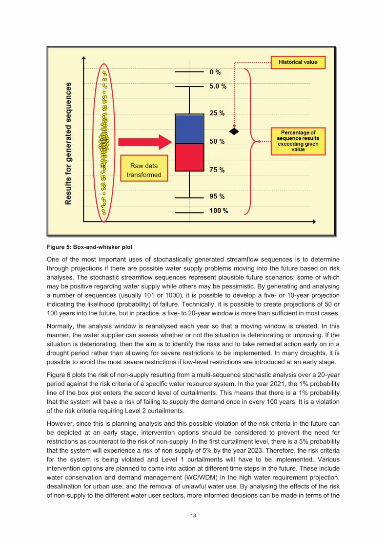
Figure 5 illustrates such a box-and-whisker plot, which indicates a probability distribution as a probability of exceedance of a given value.

13

Figure 5: Box-and-whisker plot

One of the most important uses of stochastically generated streamflow sequences is to determine through projections if there are possible water supply problems moving into the future based on risk analyses. The stochastic streamflow sequences represent plausible future scenarios; some of which may be positive regarding water supply while others may be pessimistic. By generating and analysing a number of sequences (usually 101 or 1000), it is possible to develop a five- or 10-year projection indicating the likelihood (probability) of failure. Technically, it is possible to create projections of 50 or 100 years into the future, but in practice, a five- to 20-year window is more than sufficient in most cases.

Normally, the analysis window is reanalysed each year so that a moving window is created. In this manner, the water supplier can assess whether or not the situation is deteriorating or improving. If the situation is deteriorating, then the aim is to identify the risks and to take remedial action early on in a drought period rather than allowing for severe restrictions to be implemented. In many droughts, it is possible to avoid the most severe restrictions if low-level restrictions are introduced at an early stage.

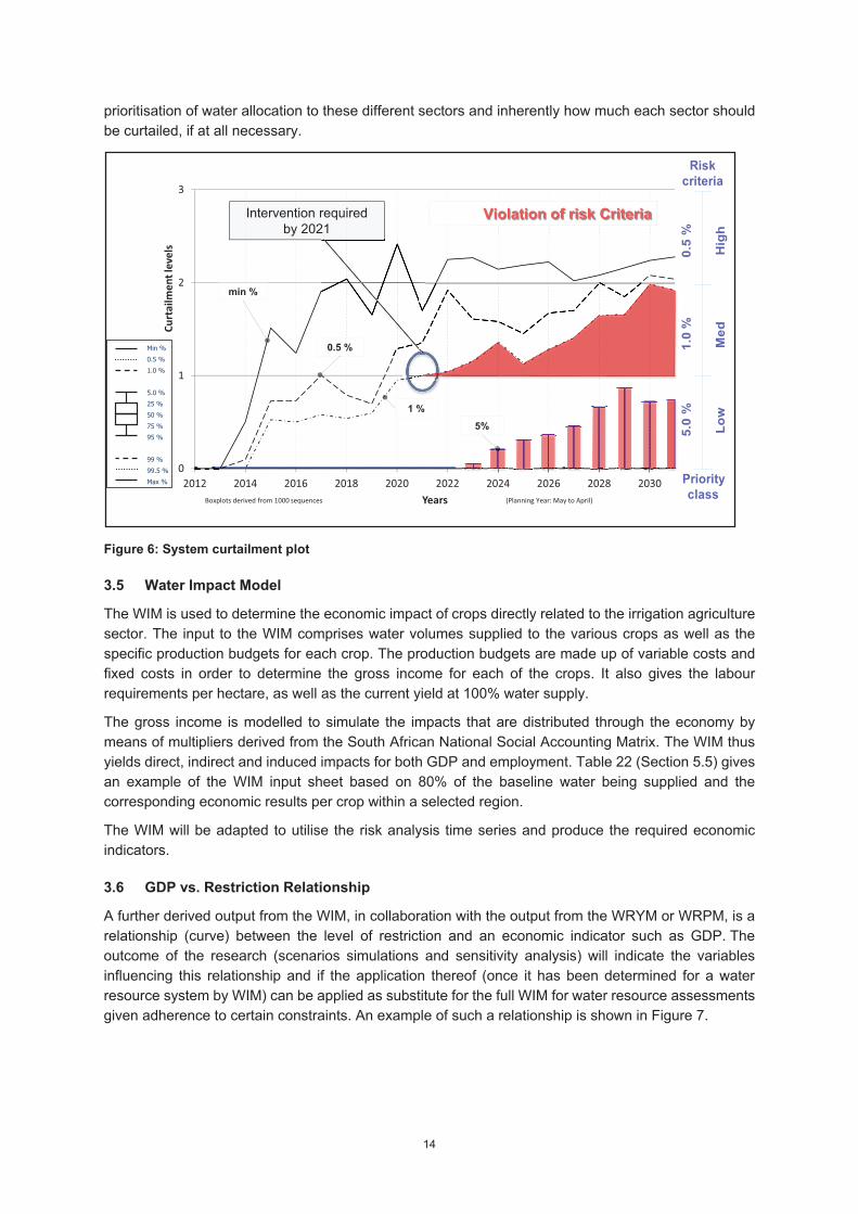
Figure 6 plots the risk of non-supply resulting from a multi-sequence stochastic analysis over a 20-year period against the risk criteria of a specific water resource system. In the year 2021, the 1% probability line of the box plot enters the second level of curtailments. This means that there is a 1% probability that the system will have a risk of failing to supply the demand once in every 100 years. It is a violation of the risk criteria requiring Level 2 curtailments.

However, since this is planning analysis and this possible violation of the risk criteria in the future can be depicted at an early stage, intervention options should be considered to prevent the need for restrictions as counteract to the risk of non-supply. In the first curtailment level, there is a 5% probability that the system will experience a risk of non-supply of 5% by the year 2023. Therefore, the risk criteria for the system is being violated and Level 1 curtailments will have to be implemented. Various intervention options are planned to come into action at different time steps in the future. These include water conservation and demand management (WC/WDM) in the high water requirement projection, desalination for urban use, and the removal of unlawful water use. By analysing the effects of the risk of non-supply to the different water user sectors, more informed decisions can be made in terms of the

Raw data transformed

14

prioritisation of water allocation to these different sectors and inherently how much each sector should be curtailed, if at all necessary.

Figure 6: System curtailment plot

3.5 Water Impact Model

The WIM is used to determine the economic impact of crops directly related to the irrigation agriculture sector. The input to the WIM comprises water volumes supplied to the various crops as well as the specific production budgets for each crop. The production budgets are made up of variable costs and fixed costs in order to determine the gross income for each of the crops. It also gives the labour requirements per hectare, as well as the current yield at 100% water supply.

The gross income is modelled to simulate the impacts that are distributed through the economy by means of multipliers derived from the South African National Social Accounting Matrix. The WIM thus yields direct, indirect and induced impacts for both GDP and employment. Table 22 (Section 5.5) gives an example of the WIM input sheet based on 80% of the baseline water being supplied and the corresponding economic results per crop within a selected region.

The WIM will be adapted to utilise the risk analysis time series and produce the required economic indicators.

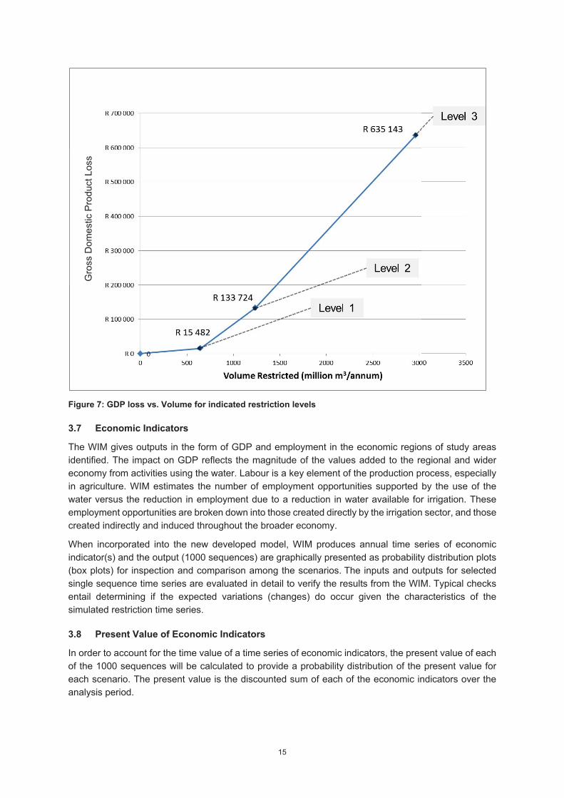
3.6 GDP vs. Restriction Relationship

A further derived output from the WIM, in collaboration with the output from the WRYM or WRPM, is a relationship (curve) between the level of restriction and an economic indicator such as GDP. The outcome of the research (scenarios simulations and sensitivity analysis) will indicate the variables influencing this relationship and if the application thereof (once it has been determined for a water resource system by WIM) can be applied as substitute for the full WIM for water resource assessments given adherence to certain constraints. An example of such a relationship is shown in Figure 7.

0

1

2

3

2012 2014 2016 2018 2020 2022 2024 2026 2028 2030

Curt

ailm

ent l

evel

s

YearsBoxplots derived from 1000 sequences (Planning Year: May to April)

Min %0.5 %1.0 %

5.0 %25 %50 %75 %95 %

99 %99.5 %Max %

5.0

%

1

.0 %

0

.5 %

Low

M

ed

H

igh

Priorityclass

Riskcriteria

Violation of risk CriteriaIntervention required by 2021

High with target WC/WDM Desalination for urban use Unlawful removed

1 %

0.5 %

min %

5%

15

Figure 7: GDP loss vs. Volume for indicated restriction levels

3.7 Economic Indicators

The WIM gives outputs in the form of GDP and employment in the economic regions of study areas identified. The impact on GDP reflects the magnitude of the values added to the regional and wider economy from activities using the water. Labour is a key element of the production process, especially in agriculture. WIM estimates the number of employment opportunities supported by the use of the water versus the reduction in employment due to a reduction in water available for irrigation. These employment opportunities are broken down into those created directly by the irrigation sector, and those created indirectly and induced throughout the broader economy.

When incorporated into the new developed model, WIM produces annual time series of economic indicator(s) and the output (1000 sequences) are graphically presented as probability distribution plots (box plots) for inspection and comparison among the scenarios. The inputs and outputs for selected single sequence time series are evaluated in detail to verify the results from the WIM. Typical checks entail determining if the expected variations (changes) do occur given the characteristics of the simulated restriction time series.

3.8 Present Value of Economic Indicators

In order to account for the time value of a time series of economic indicators, the present value of each of the 1000 sequences will be calculated to provide a probability distribution of the present value for each scenario. The present value is the discounted sum of each of the economic indicators over the analysis period.

Gro

ss D

omes

tic P

rodu

ct L

oss

16

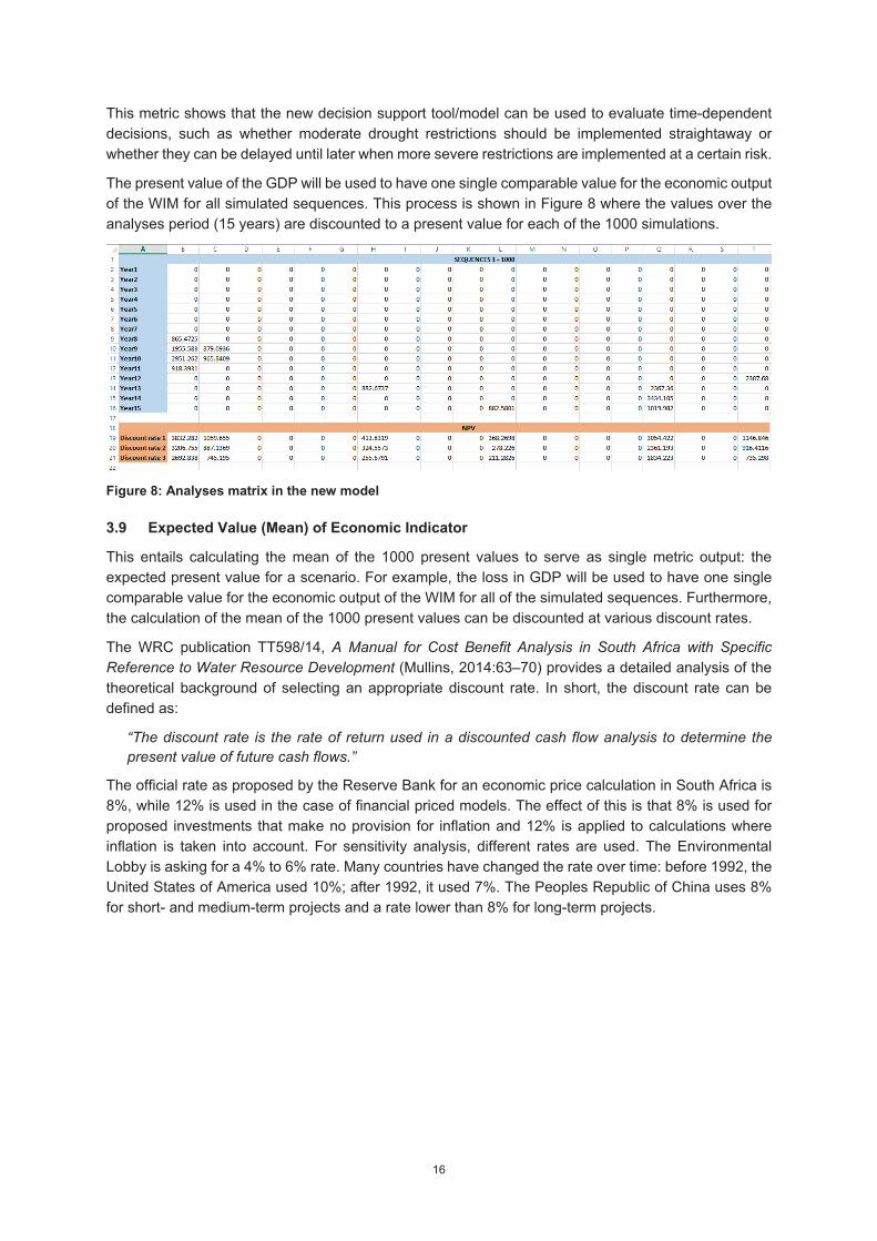
This metric shows that the new decision support tool/model can be used to evaluate time-dependent decisions, such as whether moderate drought restrictions should be implemented straightaway or whether they can be delayed until later when more severe restrictions are implemented at a certain risk.

The present value of the GDP will be used to have one single comparable value for the economic output of the WIM for all simulated sequences. This process is shown in Figure 8 where the values over the analyses period (15 years) are discounted to a present value for each of the 1000 simulations.

Figure 8: Analyses matrix in the new model

3.9 Expected Value (Mean) of Economic Indicator

This entails calculating the mean of the 1000 present values to serve as single metric output: the expected present value for a scenario. For example, the loss in GDP will be used to have one single comparable value for the economic output of the WIM for all of the simulated sequences. Furthermore, the calculation of the mean of the 1000 present values can be discounted at various discount rates.

The WRC publication TT598/14, A Manual for Cost Benefit Analysis in South Africa with Specific Reference to Water Resource Development (Mullins, 2014:63–70) provides a detailed analysis of the theoretical background of selecting an appropriate discount rate. In short, the discount rate can be defined as:

“The discount rate is the rate of return used in a discounted cash flow analysis to determine the present value of future cash flows.”

The official rate as proposed by the Reserve Bank for an economic price calculation in South Africa is 8%, while 12% is used in the case of financial priced models. The effect of this is that 8% is used for proposed investments that make no provision for inflation and 12% is applied to calculations where inflation is taken into account. For sensitivity analysis, different rates are used. The Environmental Lobby is asking for a 4% to 6% rate. Many countries have changed the rate over time: before 1992, the United States of America used 10%; after 1992, it used 7%. The Peoples Republic of China uses 8% for short- and medium-term projects and a rate lower than 8% for long-term projects.

17

4 LIMITATIONS OF THE ASM

Although the ASM has improved the process of determining assurance of supply requirements, final decisions pertaining to this matter still requires expert discretion. The following limitations exist:

The output from the ASM cannot solely be used to advise the user prioritisation, but needs to be interpreted in conjunction with the system yield reliability curves, storage projection plots and other users from the resource. It is important that the Reserve requirements are met at all times and that an optimum user priority option is obtained in order to exempt the Reserve requirements from water supply curtailments.

The model only caters for the irrigation agriculture sector in terms of deriving economic results for decision support and not the other user sectors that also contribute to the specific catchment’s economy. Such an improvement has commenced in other studies [i.e. the Thukela–Vaal Transfer scenario analyses as part of the development of operating rules for the Integrated Vaal River System (IVRS)].

In the results obtained from the analyses, the relationship between the econometric losses and the volume of water curtailed generally has a linear form.

The carry-over effect in terms of the economic impact of consecutive years of drought on the system has not been catered for.

The main limitations to the crop production budgets is that a representative budget structure for each crop and catchment was used. This includes export price analysis that will affect the income of the life cycle of the crop.

.

18

5 STEP-BY-STEP PROCEDURE FOR APPLYING THE ASM

This section gives an informative and step-by-step guide for the processes involved in the ASM as decision support tool. The Orange River System was selected as the water supply system used in the examples provided to explain the process.

The Gariep and Vanderkloof dams are the two largest dams in South Africa, which together form part of the Orange River Project (ORP). Since the decision on system curtailments is based on the storage level of the resource in the water supply system and applicable to all users downstream of the resource, the study area excludes the users upstream of Gariep Dam. It does, however, include users in the Eastern Cape who depend on the water transferred from Gariep Dam via the Ovis tunnel.

5.1 Concept

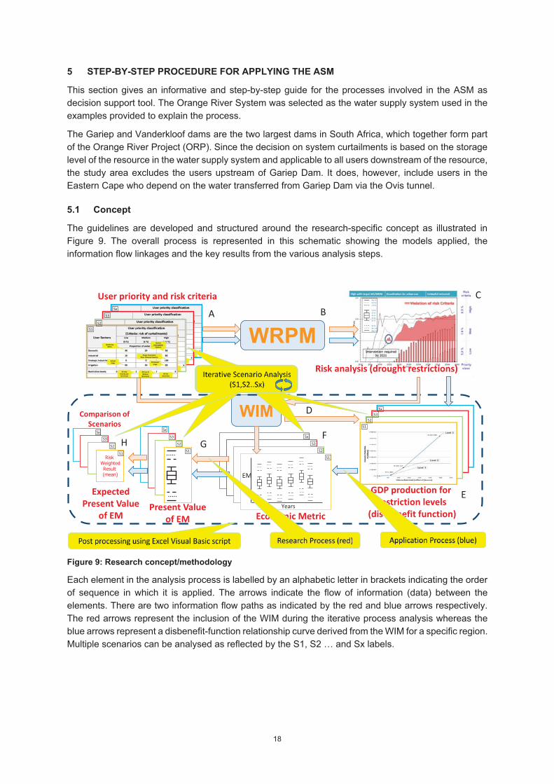
The guidelines are developed and structured around the research-specific concept as illustrated in Figure 9. The overall process is represented in this schematic showing the models applied, the information flow linkages and the key results from the various analysis steps.

Figure 9: Research concept/methodology

Each element in the analysis process is labelled by an alphabetic letter in brackets indicating the order of sequence in which it is applied. The arrows indicate the flow of information (data) between the elements. There are two information flow paths as indicated by the red and blue arrows respectively. The red arrows represent the inclusion of the WIM during the iterative process analysis whereas the blue arrows represent a disbenefit-function relationship curve derived from the WIM for a specific region. Multiple scenarios can be analysed as reflected by the S1, S2 … and Sx labels.

WIM

User priority and risk criteria

Risk analysis (drought restrictions)

GDP production for restriction levels

(dis-benefit function)

EM

Years

Economic Metric

WRPMS2

S1

S3

Sx

S2

S1

S3

Sx

S2S1

S3Sx

S2

S1

S3

Sx

Present Value of EM

Risk WeightedResult (mean)

ExpectedPresent Value

of EM

S2

S1

S3

Sx

Comparison of Scenarios

A B

C

D

E

FGH

19

5.2 Configuration of the WRYM and WRPM

Water resource yield analyses and planning have been done for many water supply systems in South Africa – especially the larger supply systems. These analyses are usually undertaken annually as part of the AOA of a specific system. The DWS is responsible for these analyses. In the case of smaller systems, the DWS has developed drought operating rules for the standalone dams (not directly part of the larger water supply system). This means that data sets for application in the WRYM and WRPM are available, but often need to be updated in terms of water requirements and planned augmentation interventions.

The yield of a water supply system normally remains constant unless the hydrology is updated or there are major changes in water requirements or infrastructure upgrades and addition of transfer schemes. Stochastic short-term yield analyses are undertaken at different starting storage levels of the reservoir/s in the system. Furthermore, a variety of target drafts (demands) are selected to be supplied by the resource to determine at which level of storage the resource can sufficiently supply the demand without failing. These demands are added to the F01 file. Other configuration changes in the WRYM include system demand channels, which can either be specified demands, min-max channels or irrigation blocks. These changes are made in the F03 file. The storage levels of the reservoirs are configured in the F06 data file.

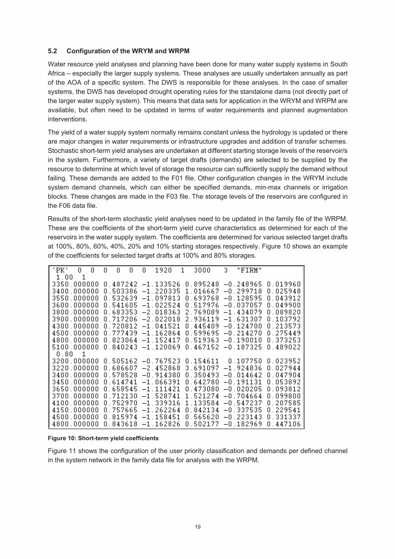
Results of the short-term stochastic yield analyses need to be updated in the family file of the WRPM. These are the coefficients of the short-term yield curve characteristics as determined for each of the reservoirs in the water supply system. The coefficients are determined for various selected target drafts at 100%, 80%, 60%, 40%, 20% and 10% starting storages respectively. Figure 10 shows an example of the coefficients for selected target drafts at 100% and 80% storages.

Figure 10: Short-term yield coefficients

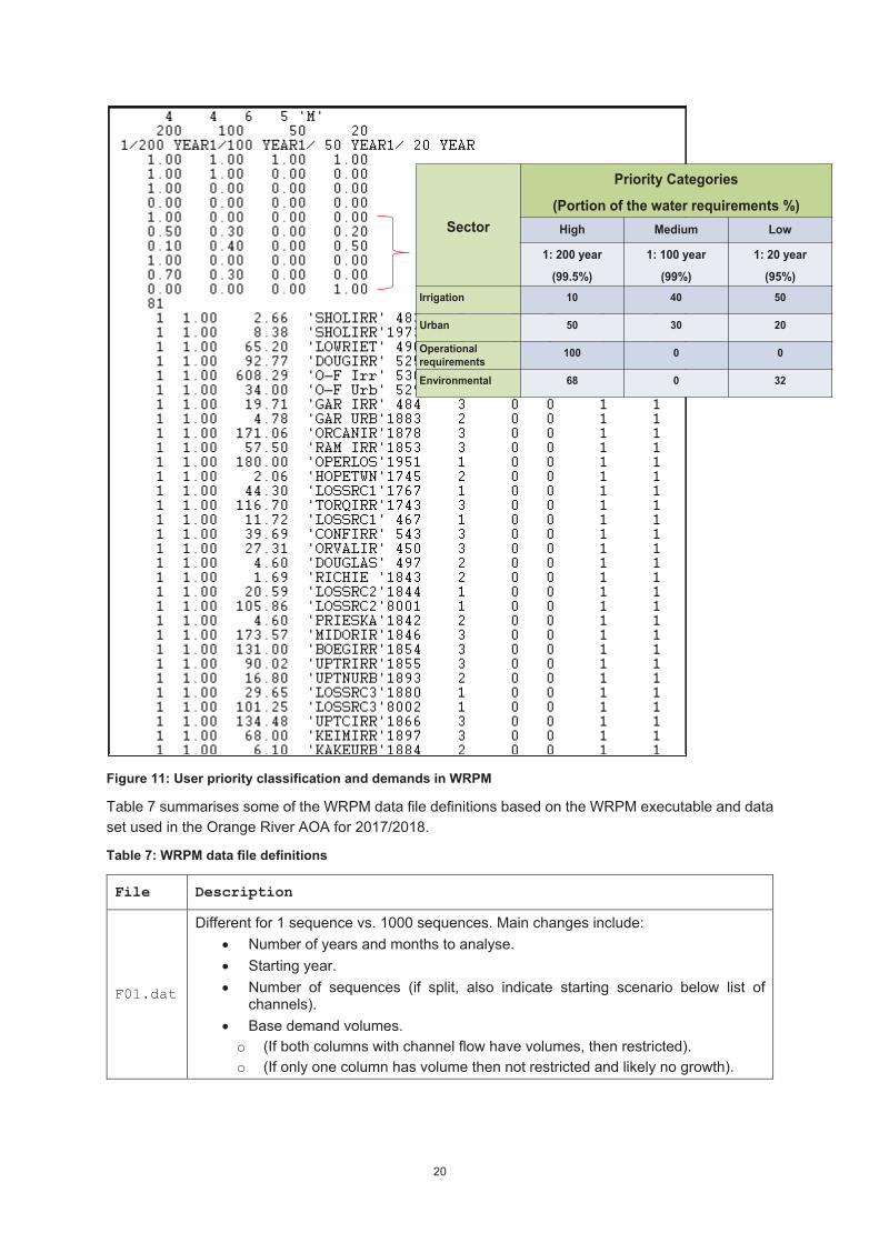
Figure 11 shows the configuration of the user priority classification and demands per defined channel in the system network in the family data file for analysis with the WRPM.

20

Figure 11: User priority classification and demands in WRPM

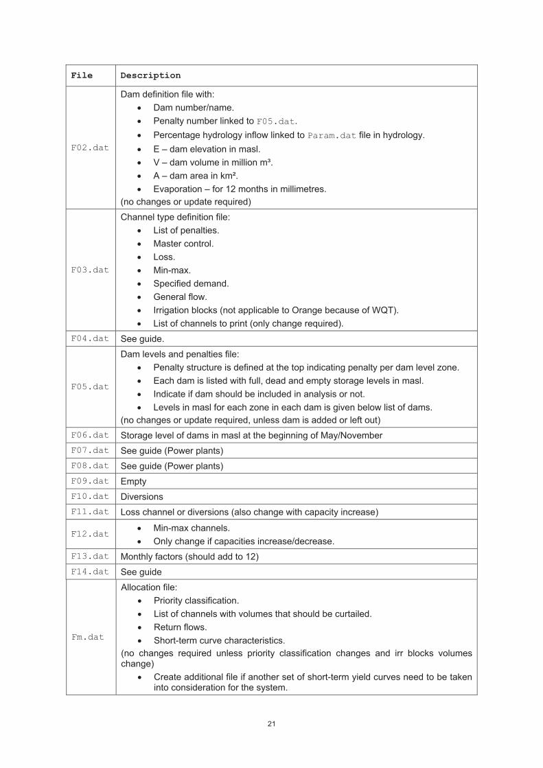
Table 7 summarises some of the WRPM data file definitions based on the WRPM executable and data set used in the Orange River AOA for 2017/2018.

Table 7: WRPM data file definitions

File Description

F01.dat

Different for 1 sequence vs. 1000 sequences. Main changes include: Number of years and months to analyse. Starting year. Number of sequences (if split, also indicate starting scenario below list of

channels). Base demand volumes.

o (If both columns with channel flow have volumes, then restricted). o (If only one column has volume then not restricted and likely no growth).

Sector

Priority Categories

(Portion of the water requirements %)High Medium Low

1: 200 year

(99.5%)

1: 100 year

(99%)

1: 20 year

(95%)Irrigation 10 40 50

Urban 50 30 20

Operationalrequirements

100 0 0

Environmental 68 0 32

21

File Description

F02.dat

Dam definition file with: Dam number/name. Penalty number linked to F05.dat. Percentage hydrology inflow linked to Param.dat file in hydrology. E – dam elevation in masl. V – dam volume in million m³. A – dam area in km². Evaporation – for 12 months in millimetres.

(no changes or update required)

F03.dat

Channel type definition file: List of penalties. Master control. Loss. Min-max. Specified demand. General flow. Irrigation blocks (not applicable to Orange because of WQT). List of channels to print (only change required).

F04.dat See guide.

F05.dat

Dam levels and penalties file: Penalty structure is defined at the top indicating penalty per dam level zone. Each dam is listed with full, dead and empty storage levels in masl. Indicate if dam should be included in analysis or not. Levels in masl for each zone in each dam is given below list of dams.

(no changes or update required, unless dam is added or left out) F06.dat Storage level of dams in masl at the beginning of May/November F07.dat See guide (Power plants) F08.dat See guide (Power plants) F09.dat Empty F10.dat Diversions F11.dat Loss channel or diversions (also change with capacity increase)

F12.dat Min-max channels. Only change if capacities increase/decrease.

F13.dat Monthly factors (should add to 12) F14.dat See guide

Fm.dat

Allocation file: Priority classification. List of channels with volumes that should be curtailed. Return flows. Short-term curve characteristics.

(no changes required unless priority classification changes and irr blocks volumes change)

Create additional file if another set of short-term yield curves need to be taken into consideration for the system.

22

File Description

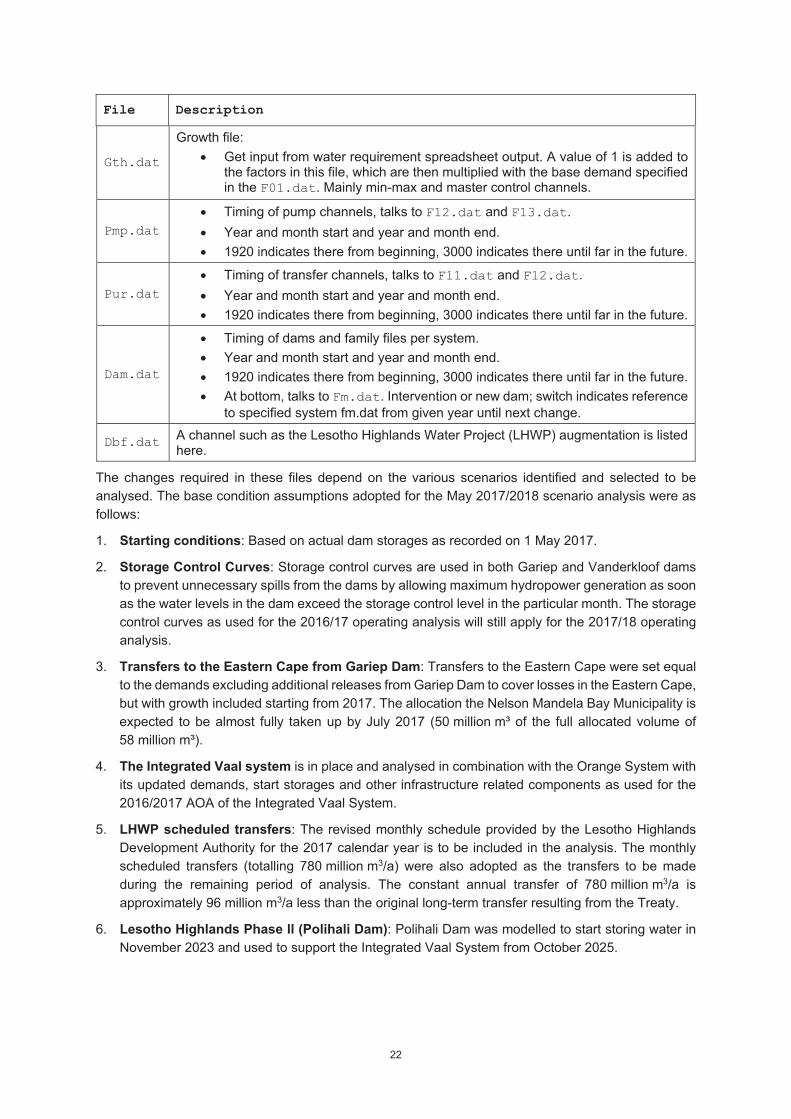
Gth.dat

Growth file: Get input from water requirement spreadsheet output. A value of 1 is added to

the factors in this file, which are then multiplied with the base demand specified in the F01.dat. Mainly min-max and master control channels.

Pmp.dat Timing of pump channels, talks to F12.dat and F13.dat. Year and month start and year and month end. 1920 indicates there from beginning, 3000 indicates there until far in the future.

Pur.dat Timing of transfer channels, talks to F11.dat and F12.dat. Year and month start and year and month end. 1920 indicates there from beginning, 3000 indicates there until far in the future.

Dam.dat

Timing of dams and family files per system. Year and month start and year and month end. 1920 indicates there from beginning, 3000 indicates there until far in the future. At bottom, talks to Fm.dat. Intervention or new dam; switch indicates reference

to specified system fm.dat from given year until next change.

Dbf.dat A channel such as the Lesotho Highlands Water Project (LHWP) augmentation is listed here.

The changes required in these files depend on the various scenarios identified and selected to be analysed. The base condition assumptions adopted for the May 2017/2018 scenario analysis were as follows:

1. Starting conditions: Based on actual dam storages as recorded on 1 May 2017.

2. Storage Control Curves: Storage control curves are used in both Gariep and Vanderkloof dams to prevent unnecessary spills from the dams by allowing maximum hydropower generation as soon as the water levels in the dam exceed the storage control level in the particular month. The storage control curves as used for the 2016/17 operating analysis will still apply for the 2017/18 operating analysis.

3. Transfers to the Eastern Cape from Gariep Dam: Transfers to the Eastern Cape were set equal to the demands excluding additional releases from Gariep Dam to cover losses in the Eastern Cape, but with growth included starting from 2017. The allocation the Nelson Mandela Bay Municipality is expected to be almost fully taken up by July 2017 (50 million m³ of the full allocated volume of 58 million m³).

4. The Integrated Vaal system is in place and analysed in combination with the Orange System with its updated demands, start storages and other infrastructure related components as used for the 2016/2017 AOA of the Integrated Vaal System.

5. LHWP scheduled transfers: The revised monthly schedule provided by the Lesotho Highlands Development Authority for the 2017 calendar year is to be included in the analysis. The monthly scheduled transfers (totalling 780 million m3/a) were also adopted as the transfers to be made during the remaining period of analysis. The constant annual transfer of 780 million m3/a is approximately 96 million m3/a less than the original long-term transfer resulting from the Treaty.

6. Lesotho Highlands Phase ll (Polihali Dam): Polihali Dam was modelled to start storing water in November 2023 and used to support the Integrated Vaal System from October 2025.

23

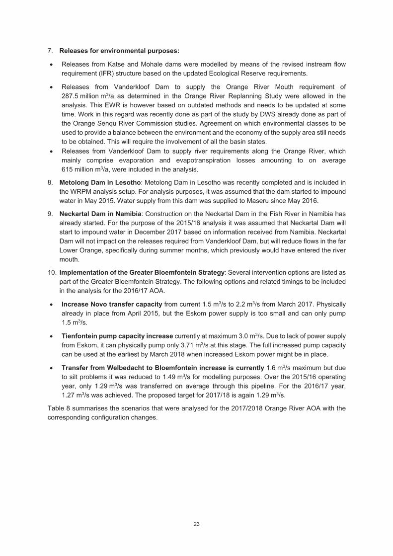
7. Releases for environmental purposes:

Releases from Katse and Mohale dams were modelled by means of the revised instream flow requirement (IFR) structure based on the updated Ecological Reserve requirements.

Releases from Vanderkloof Dam to supply the Orange River Mouth requirement of 287.5 million m3/a as determined in the Orange River Replanning Study were allowed in the analysis. This EWR is however based on outdated methods and needs to be updated at some time. Work in this regard was recently done as part of the study by DWS already done as part of the Orange Senqu River Commission studies. Agreement on which environmental classes to be used to provide a balance between the environment and the economy of the supply area still needs to be obtained. This will require the involvement of all the basin states.

Releases from Vanderkloof Dam to supply river requirements along the Orange River, which mainly comprise evaporation and evapotranspiration losses amounting to on average 615 million m3/a, were included in the analysis.

8. Metolong Dam in Lesotho: Metolong Dam in Lesotho was recently completed and is included in the WRPM analysis setup. For analysis purposes, it was assumed that the dam started to impound water in May 2015. Water supply from this dam was supplied to Maseru since May 2016.

9. Neckartal Dam in Namibia: Construction on the Neckartal Dam in the Fish River in Namibia has already started. For the purpose of the 2015/16 analysis it was assumed that Neckartal Dam will start to impound water in December 2017 based on information received from Namibia. Neckartal Dam will not impact on the releases required from Vanderkloof Dam, but will reduce flows in the far Lower Orange, specifically during summer months, which previously would have entered the river mouth.

10. Implementation of the Greater Bloemfontein Strategy: Several intervention options are listed as part of the Greater Bloemfontein Strategy. The following options and related timings to be included in the analysis for the 2016/17 AOA.

Increase Novo transfer capacity from current 1.5 m3/s to 2.2 m3/s from March 2017. Physically already in place from April 2015, but the Eskom power supply is too small and can only pump 1.5 m3/s.

Tienfontein pump capacity increase currently at maximum 3.0 m3/s. Due to lack of power supply from Eskom, it can physically pump only 3.71 m3/s at this stage. The full increased pump capacity can be used at the earliest by March 2018 when increased Eskom power might be in place.

Transfer from Welbedacht to Bloemfontein increase is currently 1.6 m3/s maximum but due to silt problems it was reduced to 1.49 m3/s for modelling purposes. Over the 2015/16 operating year, only 1.29 m3/s was transferred on average through this pipeline. For the 2016/17 year, 1.27 m3/s was achieved. The proposed target for 2017/18 is again 1.29 m3/s.

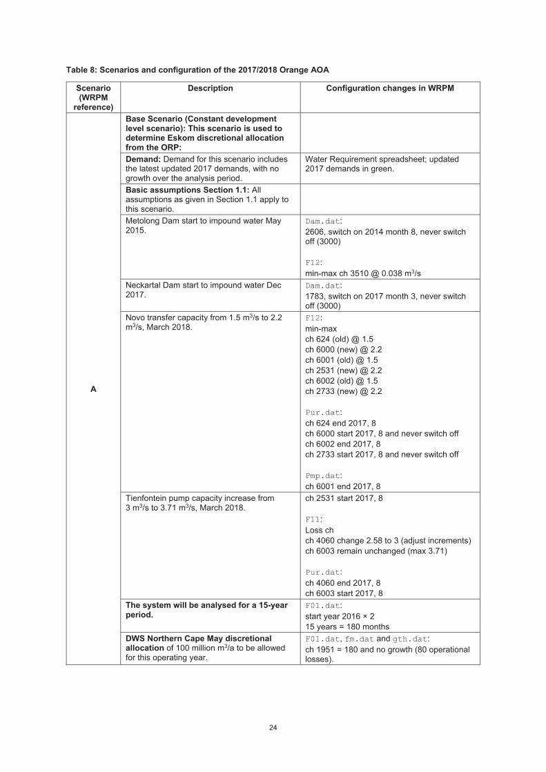
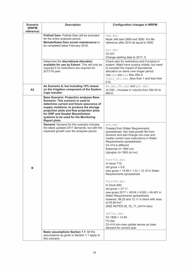
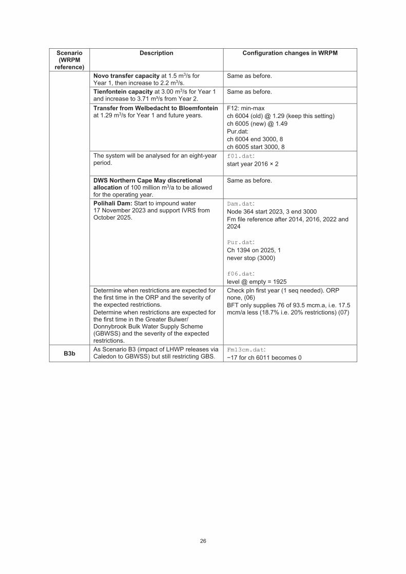
Table 8 summarises the scenarios that were analysed for the 2017/2018 Orange River AOA with the corresponding configuration changes.

24

Table 8: Scenarios and configuration of the 2017/2018 Orange AOA

Scenario (WRPM

reference)

Description Configuration changes in WRPM

A

Base Scenario (Constant development level scenario): This scenario is used to determine Eskom discretional allocation from the ORP:

Demand: Demand for this scenario includes the latest updated 2017 demands, with no growth over the analysis period.

Water Requirement spreadsheet; updated 2017 demands in green.

Basic assumptions Section 1.1: All assumptions as given in Section 1.1 apply to this scenario.

Metolong Dam start to impound water May 2015.

Dam.dat: 2606, switch on 2014 month 8, never switch off (3000) F12: min-max ch 3510 @ 0.038 m3/s

Neckartal Dam start to impound water Dec 2017.

Dam.dat: 1783, switch on 2017 month 3, never switch off (3000)

Novo transfer capacity from 1.5 m3/s to 2.2 m3/s, March 2018.

F12: min-max ch 624 (old) @ 1.5 ch 6000 (new) @ 2.2 ch 6001 (old) @ 1.5 ch 2531 (new) @ 2.2 ch 6002 (old) @ 1.5 ch 2733 (new) @ 2.2 Pur.dat: ch 624 end 2017, 8 ch 6000 start 2017, 8 and never switch off ch 6002 end 2017, 8 ch 2733 start 2017, 8 and never switch off Pmp.dat: ch 6001 end 2017, 8

Tienfontein pump capacity increase from 3 m3/s to 3.71 m3/s, March 2018.

ch 2531 start 2017, 8 F11: Loss ch ch 4060 change 2.58 to 3 (adjust increments) ch 6003 remain unchanged (max 3.71) Pur.dat: ch 4060 end 2017, 8 ch 6003 start 2017, 8

The system will be analysed for a 15-year period.

F01.dat: start year 2016 × 2 15 years = 180 months

DWS Northern Cape May discretional allocation of 100 million m3/a to be allowed for this operating year.

F01.dat, fm.dat and gth.dat: ch 1951 = 180 and no growth (80 operational losses).

25

Scenario (WRPM

reference)

Description Configuration changes in WRPM

Polihali Dam: Polihali Dam will be excluded for the entire analyses period. Mohale/Katse Dam tunnel maintenance to be completed latest February 2018.

Dam.dat: Node 346 start 2900 end 3000. Fm file reference after 2014 all equal to 3000 Pur.dat: Ch 421 Change starting date to 2017, 5

Determine the discretional allocation available for use by Eskom. This will only be required if no restrictions are required for 2017/18 year.

Check plan for restrictions and if surplus in system. Might have surplus initially, but need to consider the impact of discretional allocation on dams over longer period. Use res and sys files (06) in ltplt_v2r.exe. (less than 1 and less than 0.5).

A2 As Scenario A, but including 15% losses on the irrigation component of the Eastern Cape transfer.

Fm.dat, f01.dat and gth.dat: ch 530 – increase irr volume from 594.43 to 683.6.

B

Base Scenario: Projection analyses Base Scenario: This scenario is used to determine current and future assurance of supply violations, to produce the storage projection plots and flow projection plots for ORP and Greater Bloemfontein systems to be used for the Monitoring Report plots:

Demand: Demand for this scenario includes the latest updated 2017 demands, but with the expected growth over the analyses period.

gth.dat: Created from Water Requirements spreadsheet. Get Vaal growth file from Aurecon and add Orange min-max and master control (see instructions in Water Requirements spreadsheet). Ch 414 is different Kakamas ch 1884 incl. Upington ch 1893 (e) incl. Tsrr710.dat: Irr block 710: old gross = 9.9 new gross = 14.65 ( 1.5) = 13.15 in Water Requirements spreadsheet Tsrr692.dat: Irr block 692: old gross = 37.11 new gross 2017 = 49.54 ( 9.06) = 40.481 in Water Requirements spreadsheet; however, 99.25 and 12.11 in block with area of 25.60 km². (SEE NOTES dif_16_17_ch414.xlsx) fm07or.dat: Ch 1859 = 14.65 f12.dat: Ch 414 min-max update serves as base demand for current year.

Basic assumptions Section 1.1: All the assumptions as given in Section 1.1 apply to this scenario.

26

Scenario (WRPM

reference)

Description Configuration changes in WRPM

Novo transfer capacity at 1.5 m3/s for Year 1, then increase to 2.2 m3/s.

Same as before.

Tienfontein capacity at 3.00 m3/s for Year 1 and increase to 3.71 m³/s from Year 2.

Same as before.

Transfer from Welbedacht to Bloemfontein at 1.29 m3/s for Year 1 and future years.

F12: min-max ch 6004 (old) @ 1.29 (keep this setting) ch 6005 (new) @ 1.49 Pur.dat: ch 6004 end 3000, 8 ch 6005 start 3000, 8

The system will be analysed for an eight-year period.

f01.dat: start year 2016 × 2

DWS Northern Cape May discretional allocation of 100 million m3/a to be allowed for the operating year.

Same as before.

Polihali Dam: Start to impound water 17 November 2023 and support IVRS from October 2025.

Dam.dat: Node 364 start 2023, 3 end 3000 Fm file reference after 2014, 2016, 2022 and 2024 Pur.dat: Ch 1394 on 2025, 1 never stop (3000) f06.dat: level @ empty = 1925

Determine when restrictions are expected for the first time in the ORP and the severity of the expected restrictions. Determine when restrictions are expected for the first time in the Greater Bulwer/Donnybrook Bulk Water Supply Scheme (GBWSS) and the severity of the expected restrictions.

Check pln first year (1 seq needed). ORP none, (06) BFT only supplies 76 of 93.5 mcm.a, i.e. 17.5 mcm/a less (18.7% i.e. 20% restrictions) (07)

B3b As Scenario B3 (impact of LHWP releases via Caledon to GBWSS) but still restricting GBS.

Fm13cm.dat: 17 for ch 6011 becomes 0

27

Scenario (WRPM

reference)

Description Configuration changes in WRPM

Dam.dat: Add 2017 at bottom of file when Lesotho support switches off again. Reference to fm14cm Dbf.dat: Ch 6011 start 2016, 8 end 2017, 8 F12.dat: Ch 6012 change 2.58 to 3.0 m3/s Fm13cm.dat: 0 for ch 6011 becomes 17 F01.dat: Volumes for ch 6011 in both = 17 (based on required restrictions for GBS) F13.dat: ch 6011 monthly factor; 4 months @ 3 each Aug 17–Nov 17 Pur.dat: ch 6012 end 2017, 3 ch 6013 start 2017, 3 Pmp.dat: ch 6011 start 2016, 8 end 2017, 8

C

Scenario C: Used to determine the minimum releases from Gariep and Vanderkloof dams.

Eskom discretional allocation: The discretional allocation for this scenario is set to zero.

DWS Northern Cape discretional allocations: The discretional allocation for this scenario is set to zero.

f01.dat, fm.dat: ch 1951 = 180 now set to 80 operational losses

The user of these guidelines is referred to the detailed configuration procedure of the WRYM and WRPM in the following documents:

Water Resources Yield Model (WRYM) User Guide – Release 7.5.6.2 (DWAF, 2008b). Water Resources Planning Model (WRPM) – Input Data and File Formats, version 4.4 (DWS,

2013).

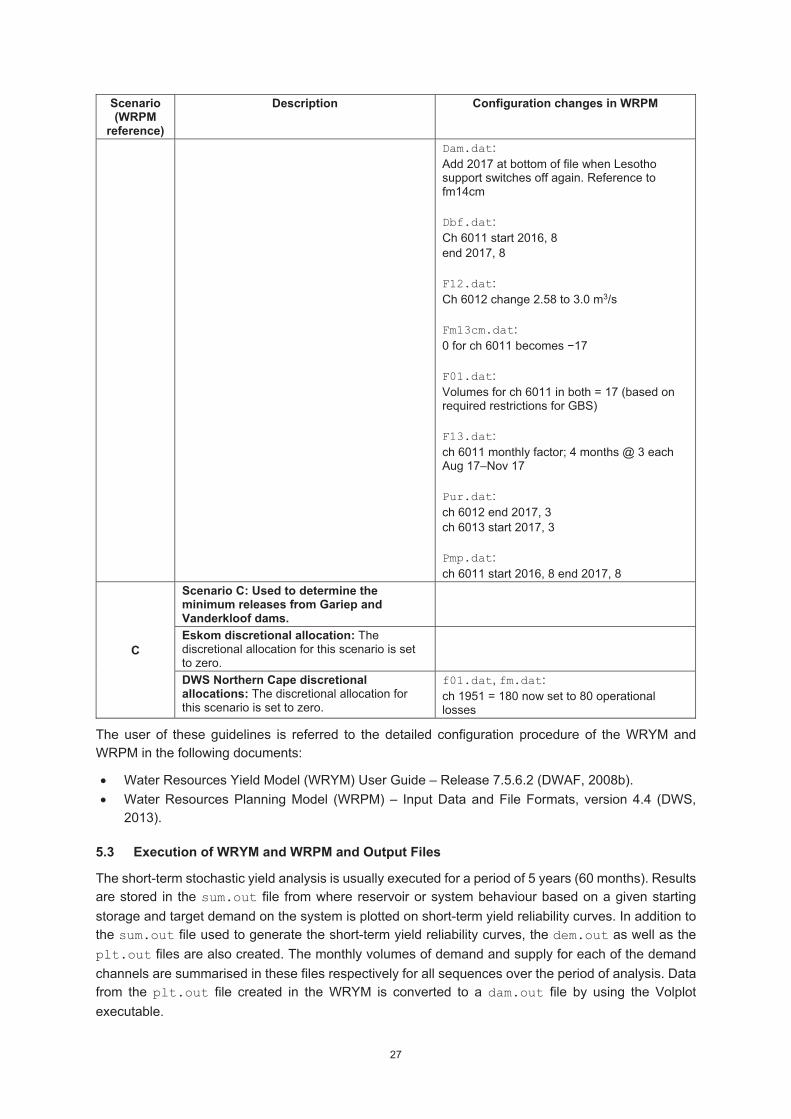
5.3 Execution of WRYM and WRPM and Output Files

The short-term stochastic yield analysis is usually executed for a period of 5 years (60 months). Results are stored in the sum.out file from where reservoir or system behaviour based on a given starting storage and target demand on the system is plotted on short-term yield reliability curves. In addition to the sum.out file used to generate the short-term yield reliability curves, the dem.out as well as the plt.out files are also created. The monthly volumes of demand and supply for each of the demand channels are summarised in these files respectively for all sequences over the period of analysis. Data from the plt.out file created in the WRYM is converted to a dam.out file by using the Volplot executable.

28

Figure 12: Short-term yield reliability curves Orange River System

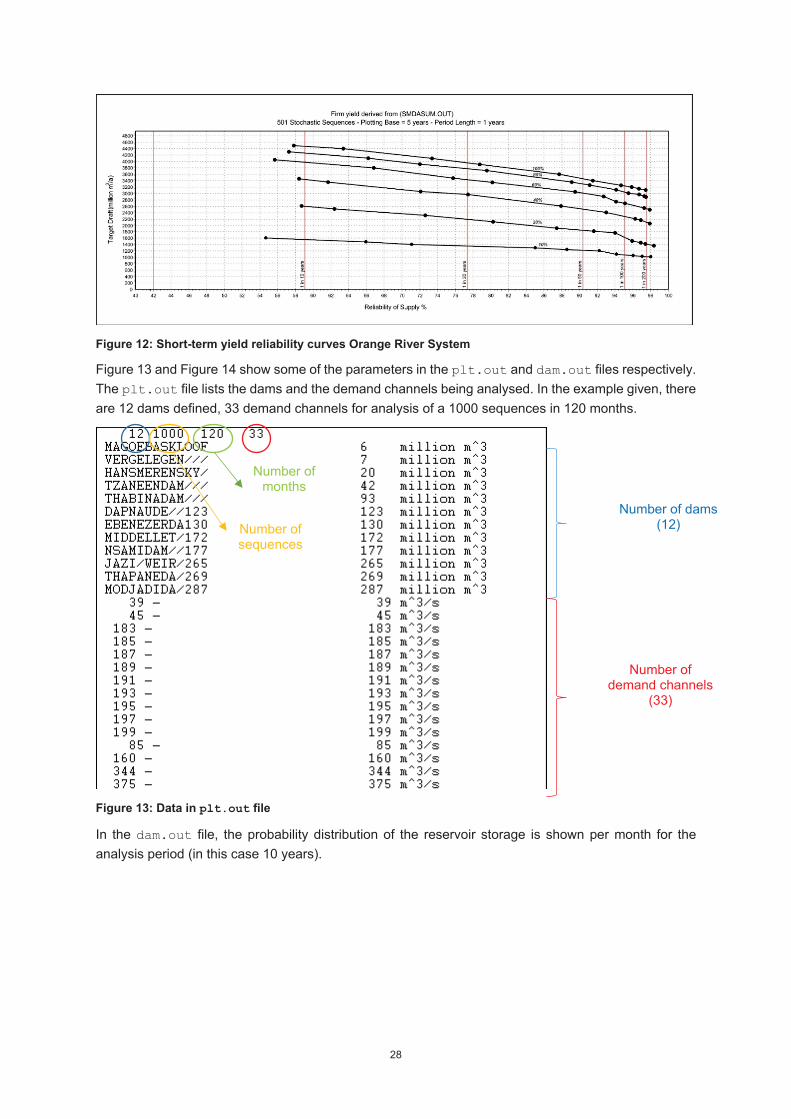
Figure 13 and Figure 14 show some of the parameters in the plt.out and dam.out files respectively. The plt.out file lists the dams and the demand channels being analysed. In the example given, there are 12 dams defined, 33 demand channels for analysis of a 1000 sequences in 120 months.

Figure 13: Data in plt.out file

In the dam.out file, the probability distribution of the reservoir storage is shown per month for the analysis period (in this case 10 years).

Number of dams (12)

Number of demand channels

(33)

Number of sequences

Number of months

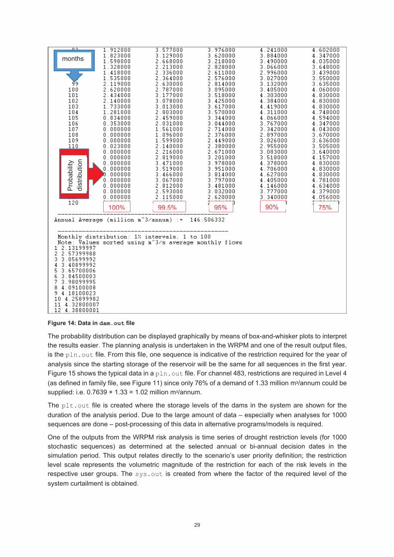
29

Figure 14: Data in dam.out file

The probability distribution can be displayed graphically by means of box-and-whisker plots to interpret the results easier. The planning analysis is undertaken in the WRPM and one of the result output files, is the pln.out file. From this file, one sequence is indicative of the restriction required for the year of analysis since the starting storage of the reservoir will be the same for all sequences in the first year. Figure 15 shows the typical data in a pln.out file. For channel 483, restrictions are required in Level 4 (as defined in family file, see Figure 11) since only 76% of a demand of 1.33 million supplied: i.e. 0.7639 × 1.33 = 1.02 million

The plt.out file is created where the storage levels of the dams in the system are shown for the duration of the analysis period. Due to the large amount of data – especially when analyses for 1000 sequences are done – post-processing of this data in alternative programs/models is required.

One of the outputs from the WRPM risk analysis is time series of drought restriction levels (for 1000 stochastic sequences) as determined at the selected annual or bi-annual decision dates in the simulation period. This output relates directly to the scenario’s user priority definition; the restriction level scale represents the volumetric magnitude of the restriction for each of the risk levels in the respective user groups. The sys.out is created from where the factor of the required level of the system curtailment is obtained.

months Pr

obab

ility

dist

ribut

ion

100% 99.5% 95% 90% 75%

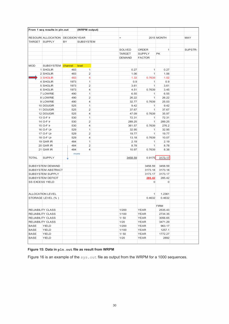
30

From 1 seq results in pln.out (WRPM output)

RESOURCALLOCATION DECISION YEAR = 2015 MONTH MAYTARGET SUPPLY BY SUBSYSTEM

SOLVED ORDER 1 SUPSTR-TARGET SUPPLY PKDEMAND FACTOR

MOD SUBSYSTEM channel level1 SHOLIR 483 1 0.27 1 0.272 SHOLIR 483 2 1.06 1 1.063 SHOLIR 483 4 1.33 0.7639 1.024 SHOLIR 1973 1 0.9 1 0.95 SHOLIR 1973 2 3.61 1 3.616 SHOLIR 1973 4 4.51 0.7639 3.457 LOWRIE 490 1 6.55 1 6.558 LOWRIE 490 2 26.22 1 26.229 LOWRIE 490 4 32.77 0.7639 25.03

10 DOUGIR 525 1 9.42 1 9.4211 DOUGIR 525 2 37.67 1 37.6712 DOUGIR 525 4 47.09 0.7639 35.9713 O-F Ir 530 1 72.31 1 72.3114 O-F Ir 530 2 289.25 1 289.2515 O-F Ir 530 4 361.57 0.7639 276.216 O-F Ur 529 1 32.95 1 32.9517 O-F Ur 529 2 19.77 1 19.7718 O-F Ur 529 4 13.18 0.7639 10.0719 GAR IR 484 1 2.19 1 2.1920 GAR IR 484 2 8.78 1 8.7821 GAR IR 484 4 10.97 0.7639 8.38

TOTAL SUPPLY 3458.59 0.9175 3173.17

SUBSYSTEM DEMAND 3458.59 3458.59SUBSYSTEM ABSTRACT 3173.18 3173.18SUBSYSTEM SUPPLY 3173.17 3173.17SUBSYSTEM DEFICIT 285.42 285.42SS EXCESS YIELD 0 0

ALLOCATION LEVEL 1 1.2361STORAGE LEVEL (% ) 0.4632 0.4632

FIRMRELIABILITY CLASS 1/200 YEAR 2535.43RELIABILITY CLASS 1/100 YEAR 2734.35RELIABILITY CLASS 1/ 50 YEAR 3056.65RELIABILITY CLASS 1/20 YEAR 3471.29BASE YIELD 1/200 YEAR 963.17BASE YIELD 1/100 YEAR 1257.1BASE YIELD 1/ 50 YEAR 1772.27BASE YIELD 1/20 YEAR 2892

more

Figure 15: Data in pln.out file as result from WRPM

Figure 16 is an example of the sys.out file as output from the WRPM for a 1000 sequences.

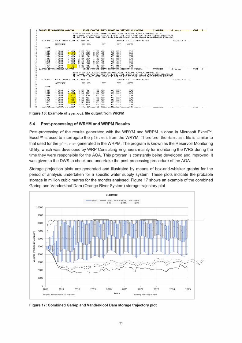
31

Figure 16: Example of sys.out file output from WRPM

5.4 Post-processing of WRYM and WRPM Results

Post-processing of the results generated with the WRYM and WRPM is done in Microsoft Excel™. Excel™ is used to interrogate the plt.out from the WRYM. Therefore, the dam.out file is similar to that used for the plt.out generated in the WRPM. The program is known as the Reservoir Monitoring Utility, which was developed by WRP Consulting Engineers mainly for monitoring the IVRS during the time they were responsible for the AOA. This program is constantly being developed and improved. It was given to the DWS to check and undertake the post-processing procedure of the AOA.

Storage projection plots are generated and illustrated by means of box-and-whisker graphs for the period of analysis undertaken for a specific water supply system. These plots indicate the probable storage in million cubic metres for the months analysed. Figure 17 shows an example of the combined Gariep and Vanderkloof Dam (Orange River System) storage trajectory plot.

Figure 17: Combined Gariep and Vanderkloof Dam storage trajectory plot

0

1000

2000

3000

4000

5000

6000

7000

8000

9000

10000

2016 2017 2018 2019 2020 2021 2022 2023 2024 2025

Volu

me

(mill

ion

m3 /

annu

m)

Years

GARVDK

Boxes 100% 99.5% 99%

Boxplots derived from 1000 sequences (Planning Year: May to April)

& 0% & 0.5% & 1%

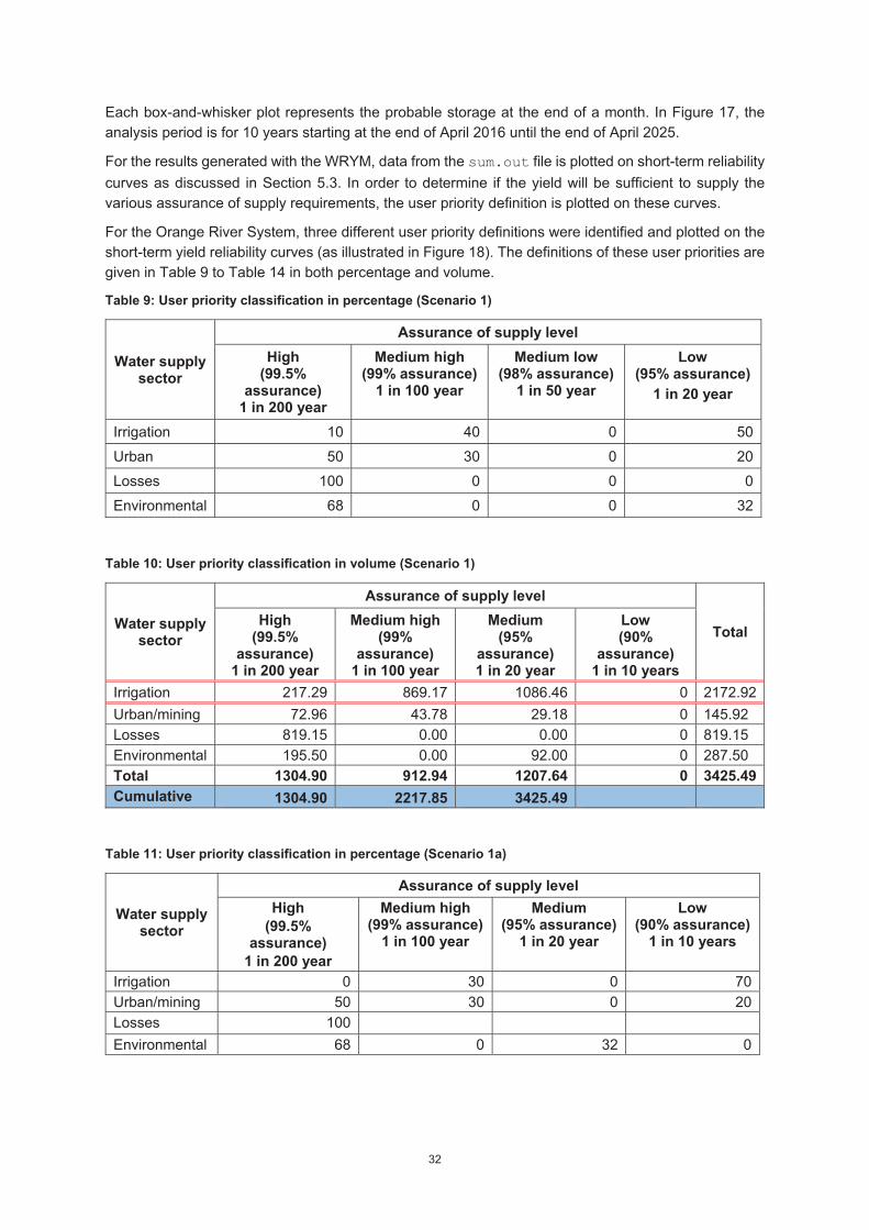
32

Each box-and-whisker plot represents the probable storage at the end of a month. In Figure 17, the analysis period is for 10 years starting at the end of April 2016 until the end of April 2025.

For the results generated with the WRYM, data from the sum.out file is plotted on short-term reliability curves as discussed in Section 5.3. In order to determine if the yield will be sufficient to supply the various assurance of supply requirements, the user priority definition is plotted on these curves.

For the Orange River System, three different user priority definitions were identified and plotted on the short-term yield reliability curves (as illustrated in Figure 18). The definitions of these user priorities are given in Table 9 to Table 14 in both percentage and volume.

Table 9: User priority classification in percentage (Scenario 1)

Water supply sector

Assurance of supply level High

(99.5% assurance)

1 in 200 year

Medium high (99% assurance)

1 in 100 year

Medium low (98% assurance)

1 in 50 year

Low (95% assurance)

1 in 20 year

Irrigation 10 40 0 50 Urban 50 30 0 20 Losses 100 0 0 0 Environmental 68 0 0 32

Table 10: User priority classification in volume (Scenario 1)

Water supply sector

Assurance of supply level

Total High

(99.5% assurance)

1 in 200 year

Medium high (99%

assurance) 1 in 100 year

Medium (95%

assurance) 1 in 20 year

Low (90%

assurance) 1 in 10 years

Irrigation 217.29 869.17 1086.46 0 2172.92 Urban/mining 72.96 43.78 29.18 0 145.92 Losses 819.15 0.00 0.00 0 819.15 Environmental 195.50 0.00 92.00 0 287.50 Total 1304.90 912.94 1207.64 0 3425.49 Cumulative 1304.90 2217.85 3425.49

Table 11: User priority classification in percentage (Scenario 1a)

Water supply sector

Assurance of supply level High

(99.5% assurance)

1 in 200 year

Medium high (99% assurance)

1 in 100 year

Medium (95% assurance)

1 in 20 year

Low (90% assurance)

1 in 10 years

Irrigation 0 30 0 70 Urban/mining 50 30 0 20 Losses 100 Environmental 68 0 32 0

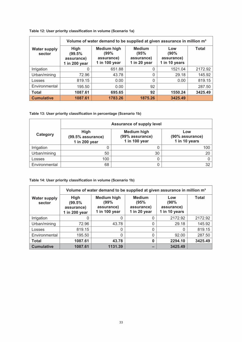
33

Table 12: User priority classification in volume (Scenario 1a)

Water supply sector

Volume of water demand to be supplied at given assurance in million m³

High (99.5%

assurance) 1 in 200 year

Medium high (99%

assurance) 1 in 100 year

Medium (95%

assurance) 1 in 20 year

Low (90%

assurance) 1 in 10 years

Total

Irrigation 0 651.88 0 1521.04 2172.92 Urban/mining 72.96 43.78 0 29.18 145.92 Losses 819.15 0.00 0 0.00 819.15 Environmental 195.50 0.00 92 287.50 Total 1087.61 695.65 92 1550.24 3425.49 Cumulative 1087.61 1783.26 1875.26 3425.49

Table 13: User priority classification in percentage (Scenario 1b)

Category

Assurance of supply level

High (99.5% assurance)

1 in 200 year

Medium high (99% assurance)

1 in 100 year

Low (90% assurance)

1 in 10 years Irrigation 0 0 100 Urban/mining 50 30 20 Losses 100 0 0 Environmental 68 0 32

Table 14: User priority classification in volume (Scenario 1b)

Water supply sector

Volume of water demand to be supplied at given assurance in million m³

High (99.5%

assurance) 1 in 200 year

Medium high (99%

assurance) 1 in 100 year

Medium (95%

assurance) 1 in 20 year

Low (90%

assurance) 1 in 10 years

Total

Irrigation 0 0 0 2172.92 2172.92 Urban/mining 72.96 43.78 0 29.18 145.92 Losses 819.15 0 0 0 819.15 Environmental 195.50 0 0 92.00 287.50 Total 1087.61 43.78 0 2294.10 3425.49 Cumulative 1087.61 1131.39 – 3425.49

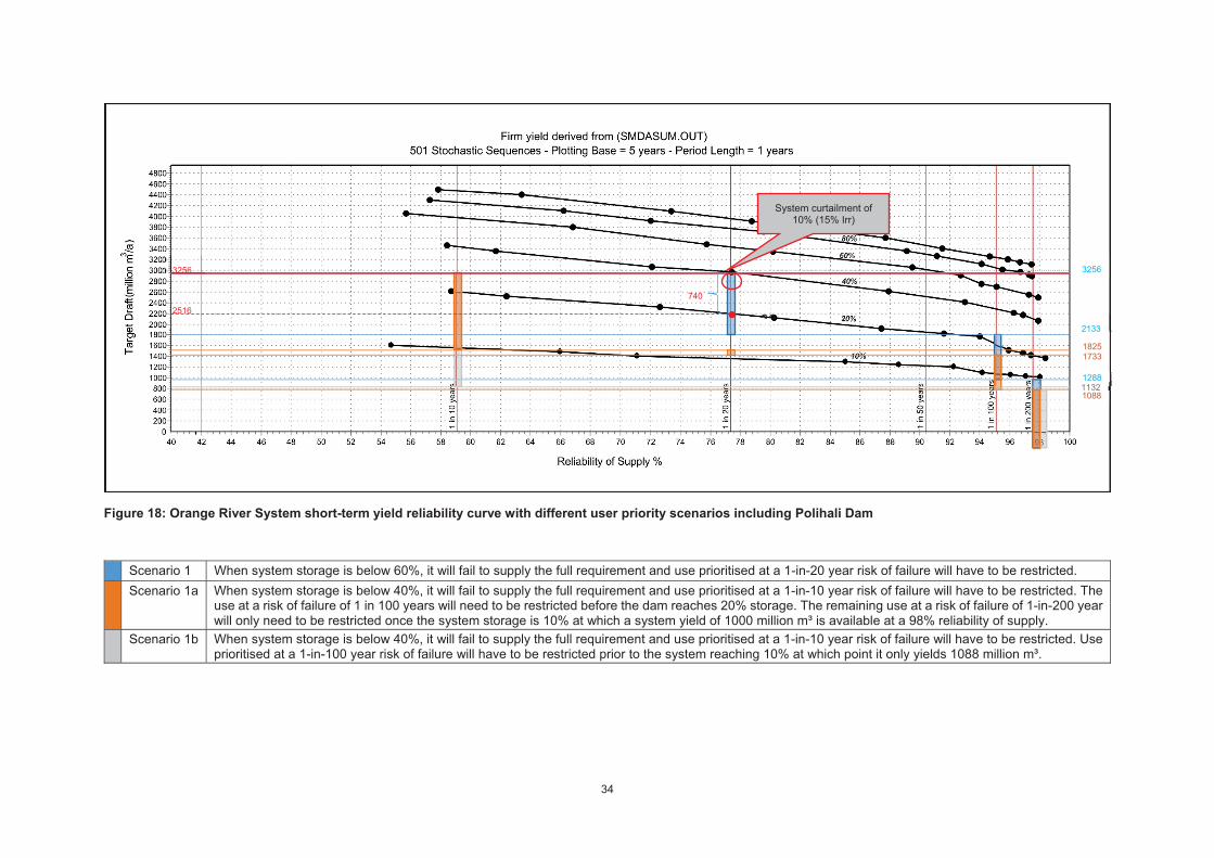
34

Figure 18: Orange River System short-term yield reliability curve with different user priority scenarios including Polihali Dam

Scenario 1 When system storage is below 60%, it will fail to supply the full requirement and use prioritised at a 1-in-20 year risk of failure will have to be restricted. Scenario 1a When system storage is below 40%, it will fail to supply the full requirement and use prioritised at a 1-in-10 year risk of failure will have to be restricted. The

use at a risk of failure of 1 in 100 years will need to be restricted before the dam reaches 20% storage. The remaining use at a risk of failure of 1-in-200 year will only need to be restricted once the system storage is 10% at which a system yield of 1000 million m³ is available at a 98% reliability of supply.

Scenario 1b When system storage is below 40%, it will fail to supply the full requirement and use prioritised at a 1-in-10 year risk of failure will have to be restricted. Use prioritised at a 1-in-100 year risk of failure will have to be restricted prior to the system reaching 10% at which point it only yields 1088 million m³.

1288

2133

3256

12881132 11321088

2133

18251733

System curtailment of 10% (15% Irr)

3256

332516

740

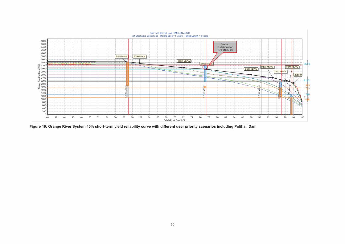
35

Figure 19: Orange River System 40% short-term yield reliability curve with different user priority scenarios including Polihali Dam

Firm yield derived from (SMDASUM.OUT)501 Stochastic Sequences - Plotting Base = 5 years - Period Length = 3 years

Reliability of Supply %100989694929088868482807876747270686664626058565452504846444240

Targ

et D

raft(

milli

on m

3/a)

48004600440042004000380036003400320030002800260024002200200018001600140012001000800600400200

0

2050 Mm

2150 Mm³/a

2200 Mm³/a

2400 Mm³/a2600 Mm³/a

2950 Mm³/a3050 Mm³/a

3350 Mm³/a3450 Mm³/a

1 in

10

year

s

1 in

20

year

s

1 in

50

year

s

1 in

100

yea

rs

1 in

200

yea

rs

1288

arsr

2133

3256

1088

8812881132

y

n 1

n 00

y0ye

aeaayy

32133

1825 1733 ar

sr

in

System curtailment of 10% (15% Irr)

000

3256 net demand including return flows

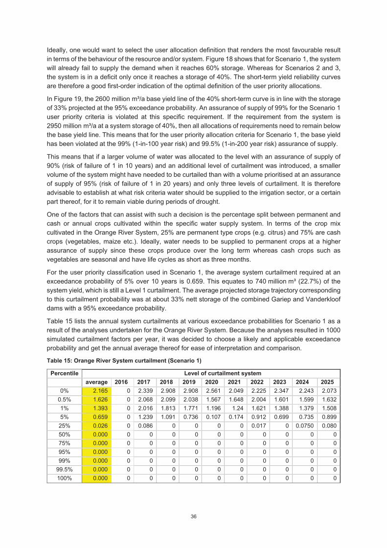
36

Ideally, one would want to select the user allocation definition that renders the most favourable result in terms of the behaviour of the resource and/or system. Figure 18 shows that for Scenario 1, the system will already fail to supply the demand when it reaches 60% storage. Whereas for Scenarios 2 and 3, the system is in a deficit only once it reaches a storage of 40%. The short-term yield reliability curves are therefore a good first-order indication of the optimal definition of the user priority allocations.

In Figure 19, the 2600 million m³/a base yield line of the 40% short-term curve is in line with the storage of 33% projected at the 95% exceedance probability. An assurance of supply of 99% for the Scenario 1 user priority criteria is violated at this specific requirement. If the requirement from the system is 2950 million m³/a at a system storage of 40%, then all allocations of requirements need to remain below the base yield line. This means that for the user priority allocation criteria for Scenario 1, the base yield has been violated at the 99% (1-in-100 year risk) and 99.5% (1-in-200 year risk) assurance of supply.

This means that if a larger volume of water was allocated to the level with an assurance of supply of 90% (risk of failure of 1 in 10 years) and an additional level of curtailment was introduced, a smaller volume of the system might have needed to be curtailed than with a volume prioritised at an assurance of supply of 95% (risk of failure of 1 in 20 years) and only three levels of curtailment. It is therefore advisable to establish at what risk criteria water should be supplied to the irrigation sector, or a certain part thereof, for it to remain viable during periods of drought.

One of the factors that can assist with such a decision is the percentage split between permanent and cash or annual crops cultivated within the specific water supply system. In terms of the crop mix cultivated in the Orange River System, 25% are permanent type crops (e.g. citrus) and 75% are cash crops (vegetables, maize etc.). Ideally, water needs to be supplied to permanent crops at a higher assurance of supply since these crops produce over the long term whereas cash crops such as vegetables are seasonal and have life cycles as short as three months.

For the user priority classification used in Scenario 1, the average system curtailment required at an exceedance probability of 5% over 10 years is 0.659. This equates to 740 million m³ (22.7%) of the system yield, which is still a Level 1 curtailment. The average projected storage trajectory corresponding to this curtailment probability was at about 33% nett storage of the combined Gariep and Vanderkloof dams with a 95% exceedance probability.

Table 15 lists the annual system curtailments at various exceedance probabilities for Scenario 1 as a result of the analyses undertaken for the Orange River System. Because the analyses resulted in 1000 simulated curtailment factors per year, it was decided to choose a likely and applicable exceedance probability and get the annual average thereof for ease of interpretation and comparison.

Table 15: Orange River System curtailment (Scenario 1)

Percentile Level of curtailment system average 2016 2017 2018 2019 2020 2021 2022 2023 2024 2025

0% 2.165 0 2.339 2.908 2.908 2.561 2.049 2.225 2.347 2.243 2.073 0.5% 1.626 0 2.068 2.099 2.038 1.567 1.648 2.004 1.601 1.599 1.632 1% 1.393 0 2.016 1.813 1.771 1.196 1.24 1.621 1.388 1.379 1.508 5% 0.659 0 1.239 1.091 0.736 0.107 0.174 0.912 0.699 0.735 0.899 25% 0.026 0 0.086 0 0 0 0 0.017 0 0.0750 0.080 50% 0.000 0 0 0 0 0 0 0 0 0 0 75% 0.000 0 0 0 0 0 0 0 0 0 0 95% 0.000 0 0 0 0 0 0 0 0 0 0 99% 0.000 0 0 0 0 0 0 0 0 0 0

99.5% 0.000 0 0 0 0 0 0 0 0 0 0 100% 0.000 0 0 0 0 0 0 0 0 0 0

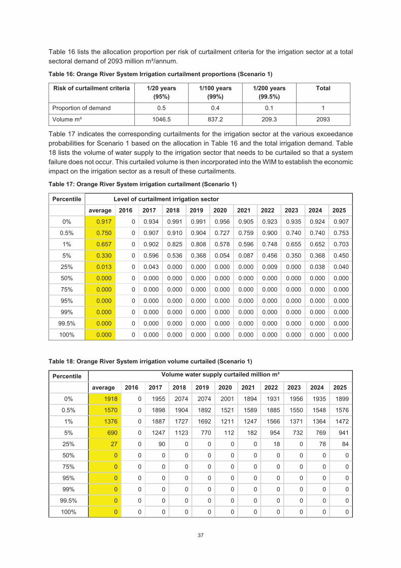
37

Table 16 lists the allocation proportion per risk of curtailment criteria for the irrigation sector at a total sectoral demand of 2093 million m³/annum.

Table 16: Orange River System Irrigation curtailment proportions (Scenario 1)

Risk of curtailment criteria 1/20 years (95%)

1/100 years (99%)

1/200 years (99.5%)

Total

Proportion of demand 0.5 0.4 0.1 1

Volume m³ 1046.5 837.2 209.3 2093

Table 17 indicates the corresponding curtailments for the irrigation sector at the various exceedance probabilities for Scenario 1 based on the allocation in Table 16 and the total irrigation demand. Table 18 lists the volume of water supply to the irrigation sector that needs to be curtailed so that a system failure does not occur. This curtailed volume is then incorporated into the WIM to establish the economic impact on the irrigation sector as a result of these curtailments.

Table 17: Orange River System irrigation curtailment (Scenario 1)

Percentile Level of curtailment irrigation sector

average 2016 2017 2018 2019 2020 2021 2022 2023 2024 2025

0% 0.917 0 0.934 0.991 0.991 0.956 0.905 0.923 0.935 0.924 0.907

0.5% 0.750 0 0.907 0.910 0.904 0.727 0.759 0.900 0.740 0.740 0.753

1% 0.657 0 0.902 0.825 0.808 0.578 0.596 0.748 0.655 0.652 0.703

5% 0.330 0 0.596 0.536 0.368 0.054 0.087 0.456 0.350 0.368 0.450

25% 0.013 0 0.043 0.000 0.000 0.000 0.000 0.009 0.000 0.038 0.040

50% 0.000 0 0.000 0.000 0.000 0.000 0.000 0.000 0.000 0.000 0.000

75% 0.000 0 0.000 0.000 0.000 0.000 0.000 0.000 0.000 0.000 0.000

95% 0.000 0 0.000 0.000 0.000 0.000 0.000 0.000 0.000 0.000 0.000

99% 0.000 0 0.000 0.000 0.000 0.000 0.000 0.000 0.000 0.000 0.000

99.5% 0.000 0 0.000 0.000 0.000 0.000 0.000 0.000 0.000 0.000 0.000

100% 0.000 0 0.000 0.000 0.000 0.000 0.000 0.000 0.000 0.000 0.000

Table 18: Orange River System irrigation volume curtailed (Scenario 1)

Percentile Volume water supply curtailed million m³

average 2016 2017 2018 2019 2020 2021 2022 2023 2024 2025

0% 1918 0 1955 2074 2074 2001 1894 1931 1956 1935 1899

0.5% 1570 0 1898 1904 1892 1521 1589 1885 1550 1548 1576

1% 1376 0 1887 1727 1692 1211 1247 1566 1371 1364 1472

5% 690 0 1247 1123 770 112 182 954 732 769 941

25% 27 0 90 0 0 0 0 18 0 78 84

50% 0 0 0 0 0 0 0 0 0 0 0

75% 0 0 0 0 0 0 0 0 0 0 0

95% 0 0 0 0 0 0 0 0 0 0 0

99% 0 0 0 0 0 0 0 0 0 0 0

99.5% 0 0 0 0 0 0 0 0 0 0 0

100% 0 0 0 0 0 0 0 0 0 0 0

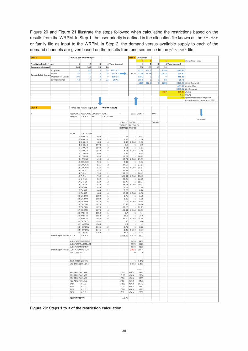
38

Figure 20 and Figure 21 illustrate the steps followed when calculating the restrictions based on the results from the WRPM. In Step 1, the user priority is defined in the allocation file known as the fm.dat or family file as input to the WRPM. In Step 2, the demand versus available supply to each of the demand channels are given based on the results from one sequence in the pln.out file.

STEP 1 Fm7OrS.dat (WRPM input) STEP 3 Calculation3 2 1 Curtailment level

Priority (reliability) class 1 2 3 4 Total demand 1 2 3 4 Total demandReccurence interval 200 100 50 20 200 100 50 20

Irrigation 10 40 0 50 2172.92 217.3 869.2 0 1086 2172.92Urban 50 30 0 20 145.92 3426 72.96 43.78 0 29.18 145.92Operational Losses 100 0 0 0 819.15 819.2 0 0 0 819.15Environmental 68 0 0 32 287.5 195.5 0 0 92 287.5

1305 912.9 0 1208 3425.49 Gross Demand-169.77 Return Flows3255.72 Net Demand

0.27 325.57 deficit0.92 supply10% system restrictions required

(rounded up to the nearest 5%)

STEP 2 From 1 seq results in pln.out (WRPM output)

RESOURCE ALLOCATIO DECISION YEAR = 2015 MONTH MAYTARGET SUPPLY BY SUBSYSTEM

to step 4SOLVED ORDER 1 SUPSTR- 1TARGET SUPPLY PKDEMAND FACTOR

MOD SUBSYSTEM1 SHOLIR 483 1 0.27 1 0.272 SHOLIR 483 2 1.06 1 1.063 SHOLIR 483 4 1.33 0.764 1.024 SHOLIR 1973 1 0.9 1 0.95 SHOLIR 1973 2 3.61 1 3.616 SHOLIR 1973 4 4.51 0.764 3.457 LOWRIE 490 1 6.55 1 6.558 LOWRIE 490 2 26.22 1 26.229 LOWRIE 490 4 32.77 0.764 25.03

10 DOUGIR 525 1 9.42 1 9.4211 DOUGIR 525 2 37.67 1 37.6712 DOUGIR 525 4 47.09 0.764 35.9713 O-F Ir 530 1 72.31 1 72.3114 O-F Ir 530 2 289.25 1 289.315 O-F Ir 530 4 361.57 0.764 276.216 O-F Ur 529 1 32.95 1 32.9517 O-F Ur 529 2 19.77 1 19.7718 O-F Ur 529 4 13.18 0.764 10.0719 GAR IR 484 1 2.19 1 2.1920 GAR IR 484 2 8.78 1 8.7821 GAR IR 484 4 10.97 0.764 8.3822 GAR UR 1883 1 1.75 1 1.7523 GAR UR 1883 2 1.05 1 1.0524 GAR UR 1883 4 0.7 0.764 0.5425 ORCANI 1878 1 20.56 1 20.5626 ORCANI 1878 2 82.25 1 82.2527 ORCANI 1878 4 102.81 0.764 78.5328 RAM IR 1853 1 6.4 1 6.429 RAM IR 1853 2 25.6 1 25.630 RAM IR 1853 4 32.00 0.764 24.4531 OPERLO 1951 1 180 1 18032 HOPETW 1745 1 1.2 1 1.233 HOPETW 1745 2 0.72 1 0.7234 HOPETW 1745 4 0.48 0.764 0.3735 LOSSRC 1767 1 44.3 1 44.3

Including EC losses TOTAL SUPPLY 3458.59 0.918 3173

SUBSYSTEM DEMAND 3459 3459SUBSYSTEM ABSTRACT 3173 3173SUBSYSTEM SUPPLY 3173 3173

Including EC losses SUBSYSTEM DEFICIT 285.4 285.4SS EXCESS YIELD 0 0

ALLOCATION LEVEL 1 1.236STORAGE LEVEL (% ) 0.463 0.463

FIRMRELIABILITY CLASS 1/200 YEAR 2535RELIABILITY CLASS 1/100 YEAR 2734RELIABILITY CLASS 1/ 50 YEAR 3057RELIABILITY CLASS 1/20 YEAR 3471BASE YIELD 1/200 YEAR 963.2BASE YIELD 1/100 YEAR 1257BASE YIELD 1/ 50 YEAR 1772BASE YIELD 1/20 YEAR 2892

RETURN FLOWS -169.77

Demand distribution

Figure 20: Steps 1 to 3 of the restriction calculation

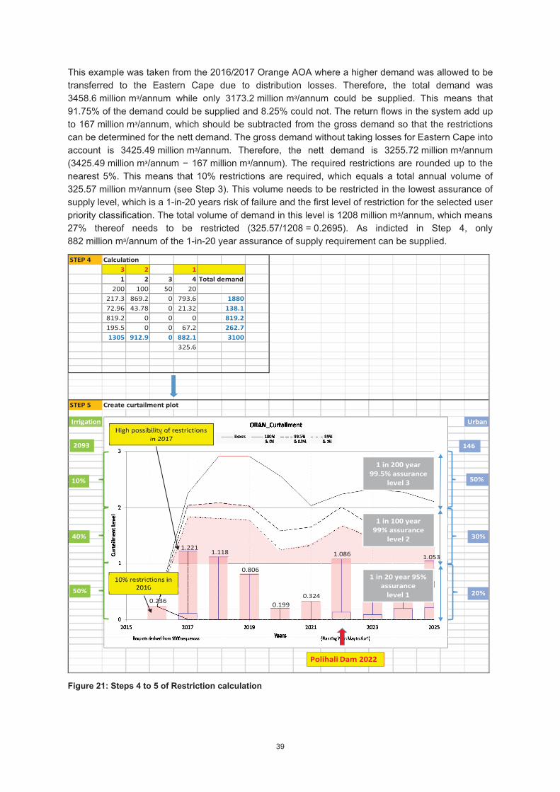
39

This example was taken from the 2016/2017 Orange AOA where a higher demand was allowed to be transferred to the Eastern Cape due to distribution losses. Therefore, the total demand was 3458.6 million m /annum while only 3173.2 million m /annum could be supplied. This means that 91.75% of the demand could be supplied and 8.25% could not. The return flows in the system add up to 167 million m /annum, which should be subtracted from the gross demand so that the restrictions can be determined for the nett demand. The gross demand without taking losses for Eastern Cape into account is 3425.49 million m /annum. Therefore, the nett demand is 3255.72 million m /annum (3425.49 million m /annum 167 million m /annum). The required restrictions are rounded up to the nearest 5%. This means that 10% restrictions are required, which equals a total annual volume of 325.57 million m /annum (see Step 3). This volume needs to be restricted in the lowest assurance of supply level, which is a 1-in-20 years risk of failure and the first level of restriction for the selected user priority classification. The total volume of demand in this level is 1208 million m /annum, which means 27% thereof needs to be restricted (325.57/1208 = 0.2695). As indicted in Step 4, only 882 million m /annum of the 1-in-20 year assurance of supply requirement can be supplied.

STEP 4 Calculation3 2 11 2 3 4 Total demand

200 100 50 20217.3 869.2 0 793.6 1880 188072.96 43.78 0 21.32 138.1 138.1819.2 0 0 0 819.2 819.2195.5 0 0 67.2 262.7 262.71305 912.9 0 882.1 3100 3100

325.6

STEP 5 Create curtailment plot

Irrigation Urban

1 in 20 year 95% assurance

level 1

1 in 100 year 99% assurance

level 2

1 in 200 year 99.5% assurance

level 3

1.221

0.236

1.118

0.806

0.199 0.324

1.086 1.053

10%

40%

50%

2093

Polihali Dam 2022

50%

30%

20%

146

Figure 21: Steps 4 to 5 of Restriction calculation

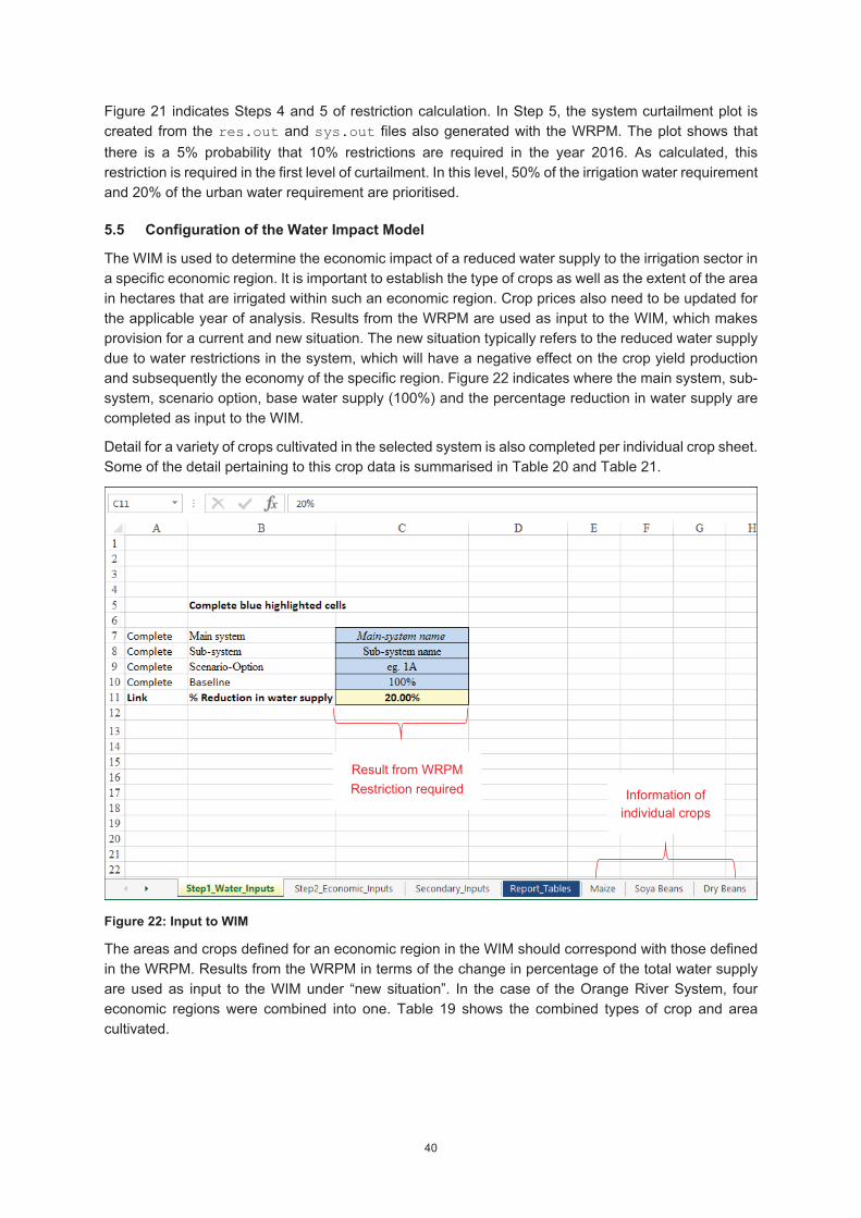
40

Figure 21 indicates Steps 4 and 5 of restriction calculation. In Step 5, the system curtailment plot is created from the res.out and sys.out files also generated with the WRPM. The plot shows that there is a 5% probability that 10% restrictions are required in the year 2016. As calculated, this restriction is required in the first level of curtailment. In this level, 50% of the irrigation water requirement and 20% of the urban water requirement are prioritised.

5.5 Configuration of the Water Impact Model

The WIM is used to determine the economic impact of a reduced water supply to the irrigation sector in a specific economic region. It is important to establish the type of crops as well as the extent of the area in hectares that are irrigated within such an economic region. Crop prices also need to be updated for the applicable year of analysis. Results from the WRPM are used as input to the WIM, which makes provision for a current and new situation. The new situation typically refers to the reduced water supply due to water restrictions in the system, which will have a negative effect on the crop yield production and subsequently the economy of the specific region. Figure 22 indicates where the main system, sub-system, scenario option, base water supply (100%) and the percentage reduction in water supply are completed as input to the WIM.

Detail for a variety of crops cultivated in the selected system is also completed per individual crop sheet. Some of the detail pertaining to this crop data is summarised in Table 20 and Table 21.

Figure 22: Input to WIM

The areas and crops defined for an economic region in the WIM should correspond with those defined in the WRPM. Results from the WRPM in terms of the change in percentage of the total water supply are used as input to the WIM under “new situation”. In the case of the Orange River System, four economic regions were combined into one. Table 19 shows the combined types of crop and area cultivated.

Information of individual crops

Result from WRPM Restriction required

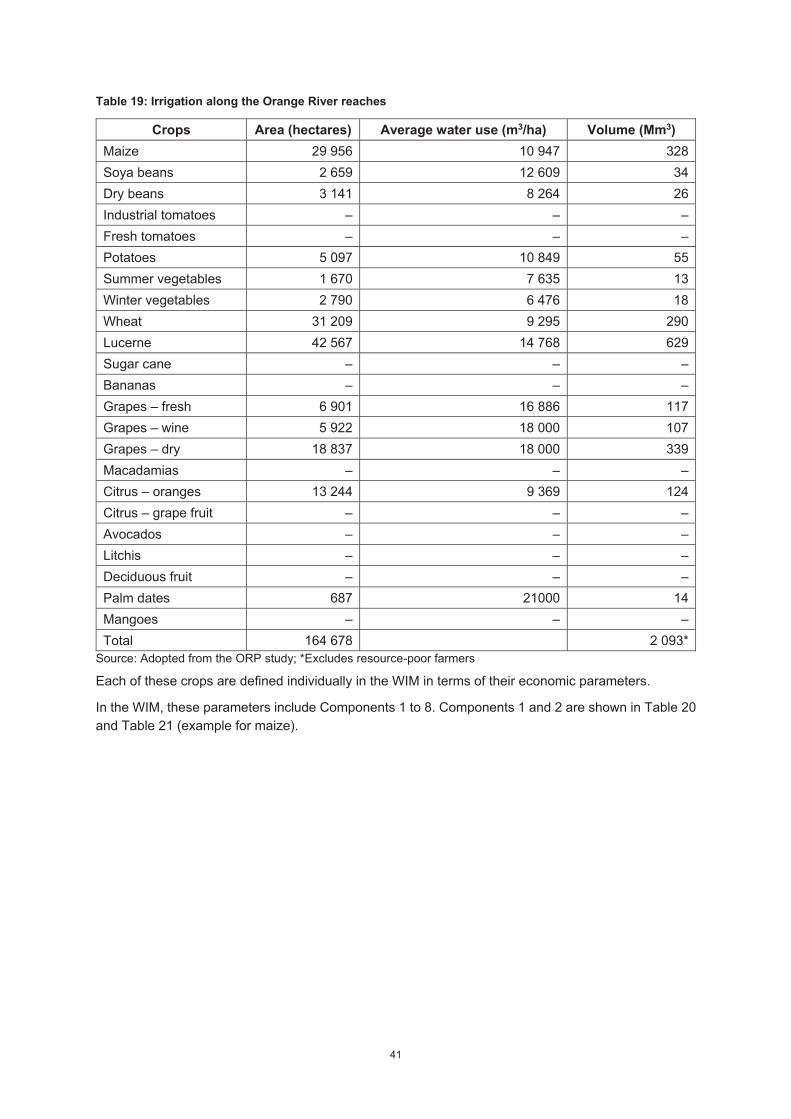
41

Table 19: Irrigation along the Orange River reaches

Crops Area (hectares) Average water use (m3/ha) Volume (Mm3) Maize 29 956 10 947 328 Soya beans 2 659 12 609 34 Dry beans 3 141 8 264 26 Industrial tomatoes – – – Fresh tomatoes – – – Potatoes 5 097 10 849 55 Summer vegetables 1 670 7 635 13 Winter vegetables 2 790 6 476 18 Wheat 31 209 9 295 290 Lucerne 42 567 14 768 629 Sugar cane – – – Bananas – – – Grapes – fresh 6 901 16 886 117 Grapes – wine 5 922 18 000 107 Grapes – dry 18 837 18 000 339 Macadamias – – – Citrus – oranges 13 244 9 369 124 Citrus – grape fruit – – – Avocados – – – Litchis – – – Deciduous fruit – – – Palm dates 687 21000 14 Mangoes – – – Total 164 678 2 093*

Source: Adopted from the ORP study; *Excludes resource-poor farmers

Each of these crops are defined individually in the WIM in terms of their economic parameters.

In the WIM, these parameters include Components 1 to 8. Components 1 and 2 are shown in Table 20 and Table 21 (example for maize).

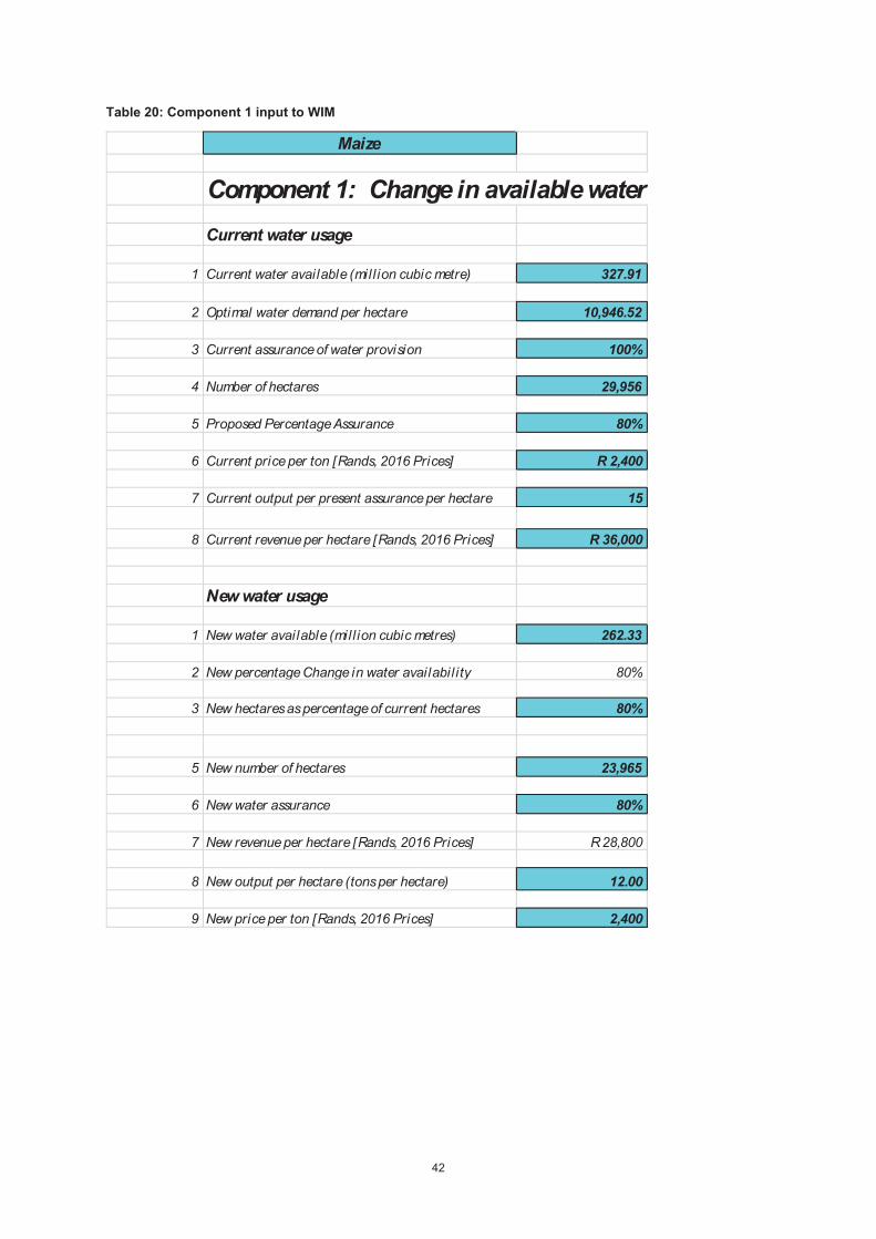
42

Table 20: Component 1 input to WIM

Maize

Component 1: Change in available waterCurrent water usage

1 Current water available (mil l ion cubic metre) 327.91

2 Optimal water demand per hectare 10,946.52

3 Current assurance of water provision 100%

4 Number of hectares 29,956

5 Proposed Percentage Assurance 80%

6 Current price per ton [Rands, 2016 Prices] R 2,400

7 Current output per present assurance per hectare 15

8 Current revenue per hectare [Rands, 2016 Prices] R 36,000

New water usage

1 New water available (mil l ion cubic metres) 262.33

2 New percentage Change in water availabil i ty 80%

3 New hectares as percentage of current hectares 80%

5 New number of hectares 23,965

6 New water assurance 80%

7 New revenue per hectare [Rands, 2016 Prices] R 28,800

8 New output per hectare (tons per hectare) 12.00

9 New price per ton [Rands, 2016 Prices] 2,400

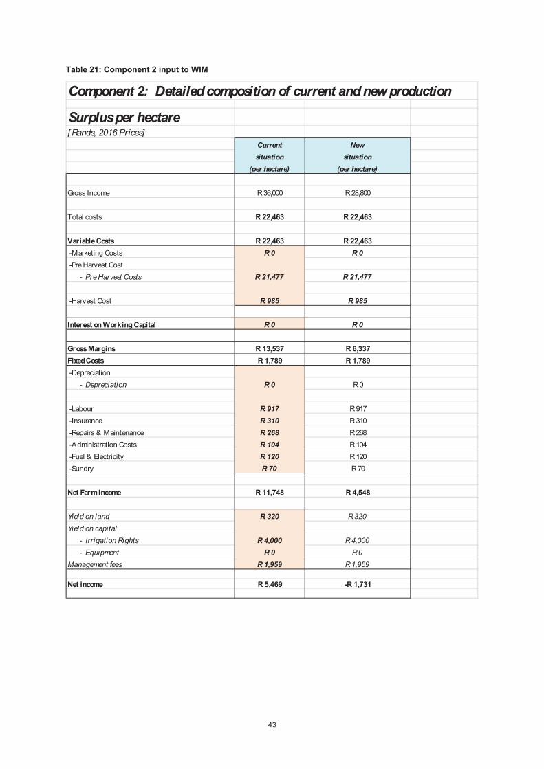
43

Table 21: Component 2 input to WIM

Component 2: Detailed composition of current and new production

Surplus per hectare[ Rands, 2016 Prices]

Current Newsituation situation

(per hectare) (per hectare)

Gross Income R 36,000 R 28,800

Total costs R 22,463 R 22,463

Variable Costs R 22,463 R 22,463 -Marketing Costs R 0 R 0 -Pre Harvest Cost - Pre Harvest Costs R 21,477 R 21,477

-Harvest Cost R 985 R 985

Interest on Working Capital R 0 R 0

Gross Margins R 13,537 R 6,337Fixed Costs R 1,789 R 1,789 -Depreciation - Depreciation R 0 R 0

-Labour R 917 R 917 -Insurance R 310 R 310 -Repairs & Maintenance R 268 R 268 -Administration Costs R 104 R 104 -Fuel & Electricity R 120 R 120 -Sundry R 70 R 70

Net Farm Income R 11,748 R 4,548

Yield on land R 320 R 320Yield on capital - Irrigation Rights R 4,000 R 4,000 - Equipment R 0 R 0Management fees R 1,959 R 1,959

Net income R 5,469 -R 1,731

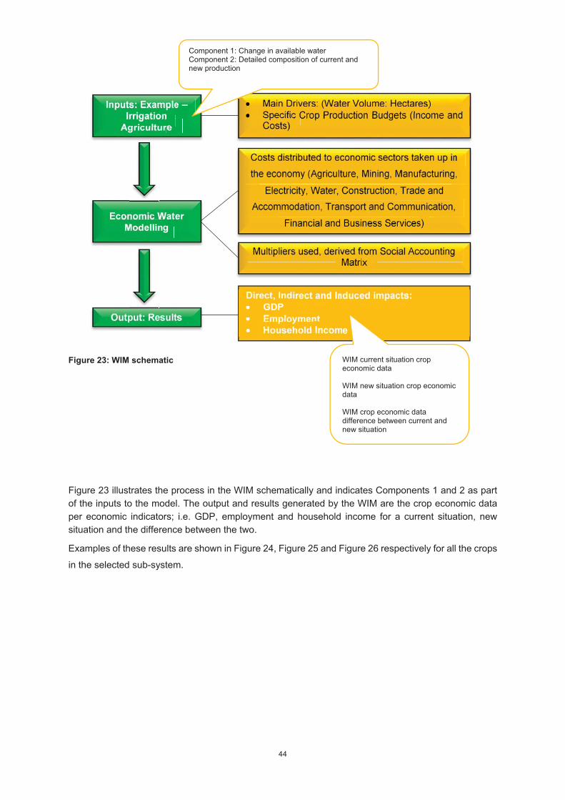
44

Figure 23: WIM schematic

Figure 23 illustrates the process in the WIM schematically and indicates Components 1 and 2 as part of the inputs to the model. The output and results generated by the WIM are the crop economic data per economic indicators; i.e. GDP, employment and household income for a current situation, new situation and the difference between the two.

Examples of these results are shown in Figure 24, Figure 25 and Figure 26 respectively for all the crops

in the selected sub-system.

Component 1: Change in available water Component 2: Detailed composition of current and new production

WIM current situation crop economic data WIM new situation crop economic data WIM crop economic data difference between current and new situation

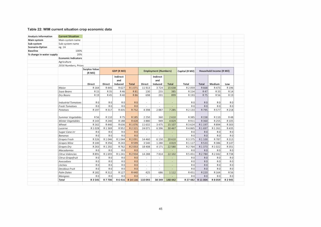
45

Table 22: WIM current situation crop economic data

Analysis Information Current SituationMain system Main-system nameSub-system Sub-system nameScenario-Option eg. 1ABaseline 100%% change in water supply 20%

Economic IndicatorsAgriculture2016 Numbers, Prices

Surplus Value (R Mil)

Capital (R Mil)

Direct Direct

Indirect and

Induced Total Direct

Indirect and

Induced Total Total Total Medium LowMaize R 164 R 445 R 627 R 1 071 11 913 3 724 15 638 R 2 059 R 668 R 473 R 196Soya Beans R 15 R 35 R 46 R 81 130 255 385 R 154 R 47 R 33 R 14Dry Beans R 19 R 45 R 40 R 86 698 201 899 R 193 R 75 R 56 R 19

Industrial Tomatoes R 0 R 0 R 0 R 0 - - - R 0 R 0 R 0 R 0Fresh Tomatoes R 0 R 0 R 0 R 0 - - - R 0 R 0 R 0 R 0Potatoes R 197 R 317 R 435 R 752 4 398 2 887 7 285 R 2 133 R 795 R 577 R 218

Summer Vegetables R 56 R 110 R 75 R 185 2 250 360 2 610 R 385 R 158 R 110 R 48Winter Vegetables R 143 R 240 R 188 R 428 3 880 949 4 829 R 911 R 360 R 255 R 105Wheat R 162 R 440 R 636 R 1 076 11 632 3 475 15 107 R 3 624 R 1 197 R 894 R 303Lucerne R 1 028 R 1 369 R 952 R 2 321 24 071 6 396 30 467 R 4 865 R 1 697 R 1 261 R 435Sugar Cane Irr R 0 R 0 R 0 R 0 - - - R 0 R 0 R 0 R 0Bananas R 0 R 0 R 0 R 0 - - - R 0 R 0 R 0 R 0Grapes Fresh R 326 R 1 046 R 1 044 R 2 091 14 460 6 150 20 610 R 3 375 R 1 100 R 787 R 313Grapes Wine R 100 R 356 R 243 R 599 3 540 1 280 4 819 R 1 117 R 533 R 386 R 147Grapes Dry R 263 R 1 292 R 762 R 2 053 18 408 4 171 22 580 R 2 764 R 1 373 R 1 022 R 351Macadamias R 0 R 0 R 0 R 0 - - - R 0 R 0 R 0 R 0Citrus Valencias R 891 R 1 693 R 1 241 R 2 934 14 288 7 814 22 102 R 5 451 R 2 780 R 2 042 R 738Citrus Grapefruit R 0 R 0 R 0 R 0 - - - R 0 R 0 R 0 R 0Avocadoes R 0 R 0 R 0 R 0 - - - R 0 R 0 R 0 R 0Litchies R 0 R 0 R 0 R 0 - - - R 0 R 0 R 0 R 0Decidous Fruit R 0 R 0 R 0 R 0 - - - R 0 R 0 R 0 R 0Palm Dates R 182 R 312 R 127 R 440 425 686 1 112 R 451 R 220 R 164 R 56Mangoes R 0 R 0 R 0 R 0 - - - R 0 R 0 R 0 R 0Total R 3 545 R 7 700 R 6 416 R 14 116 110 093 38 349 148 442 R 27 482 R 11 004 R 8 059 R 2 945

GDP (R Mil) Employment (Numbers) Household Income (R Mil)

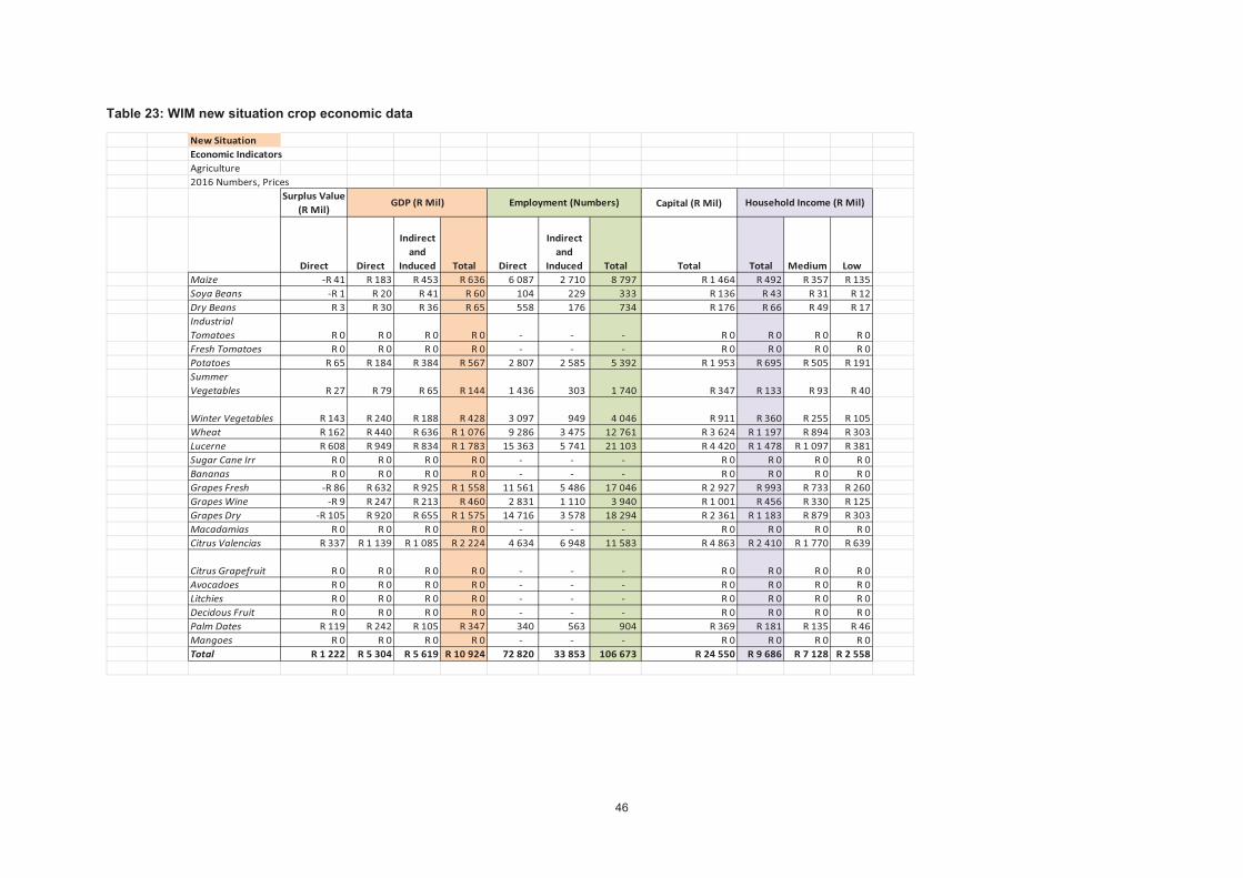
46

Table 23: WIM new situation crop economic data

New SituationEconomic IndicatorsAgriculture2016 Numbers, Prices

Surplus Value (R Mil)

Capital (R Mil)

Direct Direct

Indirect and

Induced Total Direct

Indirect and

Induced Total Total Total Medium LowMaize -R 41 R 183 R 453 R 636 6 087 2 710 8 797 R 1 464 R 492 R 357 R 135Soya Beans -R 1 R 20 R 41 R 60 104 229 333 R 136 R 43 R 31 R 12Dry Beans R 3 R 30 R 36 R 65 558 176 734 R 176 R 66 R 49 R 17Industrial Tomatoes R 0 R 0 R 0 R 0 - - - R 0 R 0 R 0 R 0Fresh Tomatoes R 0 R 0 R 0 R 0 - - - R 0 R 0 R 0 R 0Potatoes R 65 R 184 R 384 R 567 2 807 2 585 5 392 R 1 953 R 695 R 505 R 191Summer Vegetables R 27 R 79 R 65 R 144 1 436 303 1 740 R 347 R 133 R 93 R 40

Winter Vegetables R 143 R 240 R 188 R 428 3 097 949 4 046 R 911 R 360 R 255 R 105Wheat R 162 R 440 R 636 R 1 076 9 286 3 475 12 761 R 3 624 R 1 197 R 894 R 303Lucerne R 608 R 949 R 834 R 1 783 15 363 5 741 21 103 R 4 420 R 1 478 R 1 097 R 381Sugar Cane Irr R 0 R 0 R 0 R 0 - - - R 0 R 0 R 0 R 0Bananas R 0 R 0 R 0 R 0 - - - R 0 R 0 R 0 R 0Grapes Fresh -R 86 R 632 R 925 R 1 558 11 561 5 486 17 046 R 2 927 R 993 R 733 R 260Grapes Wine -R 9 R 247 R 213 R 460 2 831 1 110 3 940 R 1 001 R 456 R 330 R 125Grapes Dry -R 105 R 920 R 655 R 1 575 14 716 3 578 18 294 R 2 361 R 1 183 R 879 R 303Macadamias R 0 R 0 R 0 R 0 - - - R 0 R 0 R 0 R 0Citrus Valencias R 337 R 1 139 R 1 085 R 2 224 4 634 6 948 11 583 R 4 863 R 2 410 R 1 770 R 639

Citrus Grapefruit R 0 R 0 R 0 R 0 - - - R 0 R 0 R 0 R 0Avocadoes R 0 R 0 R 0 R 0 - - - R 0 R 0 R 0 R 0Litchies R 0 R 0 R 0 R 0 - - - R 0 R 0 R 0 R 0Decidous Fruit R 0 R 0 R 0 R 0 - - - R 0 R 0 R 0 R 0Palm Dates R 119 R 242 R 105 R 347 340 563 904 R 369 R 181 R 135 R 46Mangoes R 0 R 0 R 0 R 0 - - - R 0 R 0 R 0 R 0Total R 1 222 R 5 304 R 5 619 R 10 924 72 820 33 853 106 673 R 24 550 R 9 686 R 7 128 R 2 558

GDP (R Mil) Employment (Numbers) Household Income (R Mil)

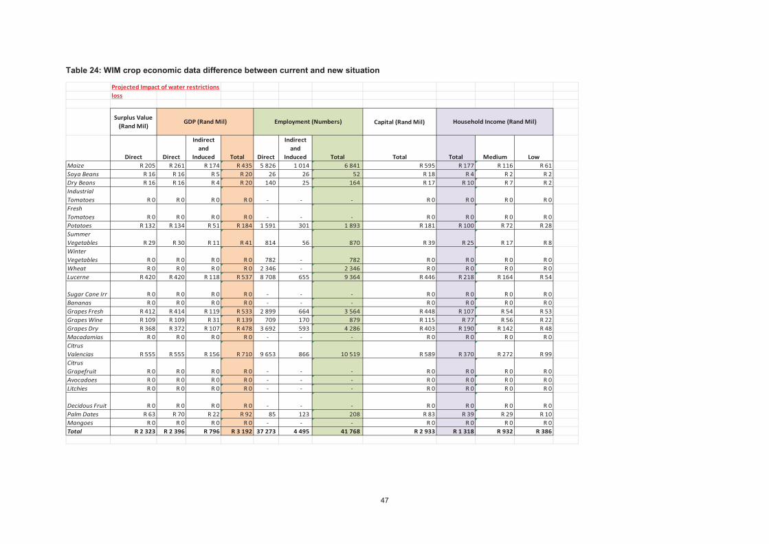
47

Table 24: WIM crop economic data difference between current and new situation

Projected Impact of water restrictionsloss

Surplus Value (Rand Mil)

Capital (Rand Mil)

Direct Direct

Indirect and

Induced Total Direct

Indirect and

Induced Total Total Total Medium LowMaize R 205 R 261 R 174 R 435 5 826 1 014 6 841 R 595 R 177 R 116 R 61Soya Beans R 16 R 16 R 5 R 20 26 26 52 R 18 R 4 R 2 R 2Dry Beans R 16 R 16 R 4 R 20 140 25 164 R 17 R 10 R 7 R 2Industrial Tomatoes R 0 R 0 R 0 R 0 - - - R 0 R 0 R 0 R 0Fresh Tomatoes R 0 R 0 R 0 R 0 - - - R 0 R 0 R 0 R 0Potatoes R 132 R 134 R 51 R 184 1 591 301 1 893 R 181 R 100 R 72 R 28Summer Vegetables R 29 R 30 R 11 R 41 814 56 870 R 39 R 25 R 17 R 8Winter Vegetables R 0 R 0 R 0 R 0 782 - 782 R 0 R 0 R 0 R 0Wheat R 0 R 0 R 0 R 0 2 346 - 2 346 R 0 R 0 R 0 R 0Lucerne R 420 R 420 R 118 R 537 8 708 655 9 364 R 446 R 218 R 164 R 54

Sugar Cane Irr R 0 R 0 R 0 R 0 - - - R 0 R 0 R 0 R 0Bananas R 0 R 0 R 0 R 0 - - - R 0 R 0 R 0 R 0Grapes Fresh R 412 R 414 R 119 R 533 2 899 664 3 564 R 448 R 107 R 54 R 53Grapes Wine R 109 R 109 R 31 R 139 709 170 879 R 115 R 77 R 56 R 22Grapes Dry R 368 R 372 R 107 R 478 3 692 593 4 286 R 403 R 190 R 142 R 48Macadamias R 0 R 0 R 0 R 0 - - - R 0 R 0 R 0 R 0Citrus Valencias R 555 R 555 R 156 R 710 9 653 866 10 519 R 589 R 370 R 272 R 99Citrus Grapefruit R 0 R 0 R 0 R 0 - - - R 0 R 0 R 0 R 0Avocadoes R 0 R 0 R 0 R 0 - - - R 0 R 0 R 0 R 0Litchies R 0 R 0 R 0 R 0 - - - R 0 R 0 R 0 R 0

Decidous Fruit R 0 R 0 R 0 R 0 - - - R 0 R 0 R 0 R 0Palm Dates R 63 R 70 R 22 R 92 85 123 208 R 83 R 39 R 29 R 10Mangoes R 0 R 0 R 0 R 0 - - - R 0 R 0 R 0 R 0Total R 2 323 R 2 396 R 796 R 3 192 37 273 4 495 41 768 R 2 933 R 1 318 R 932 R 386

GDP (Rand Mil) Employment (Numbers) Household Income (Rand Mil)

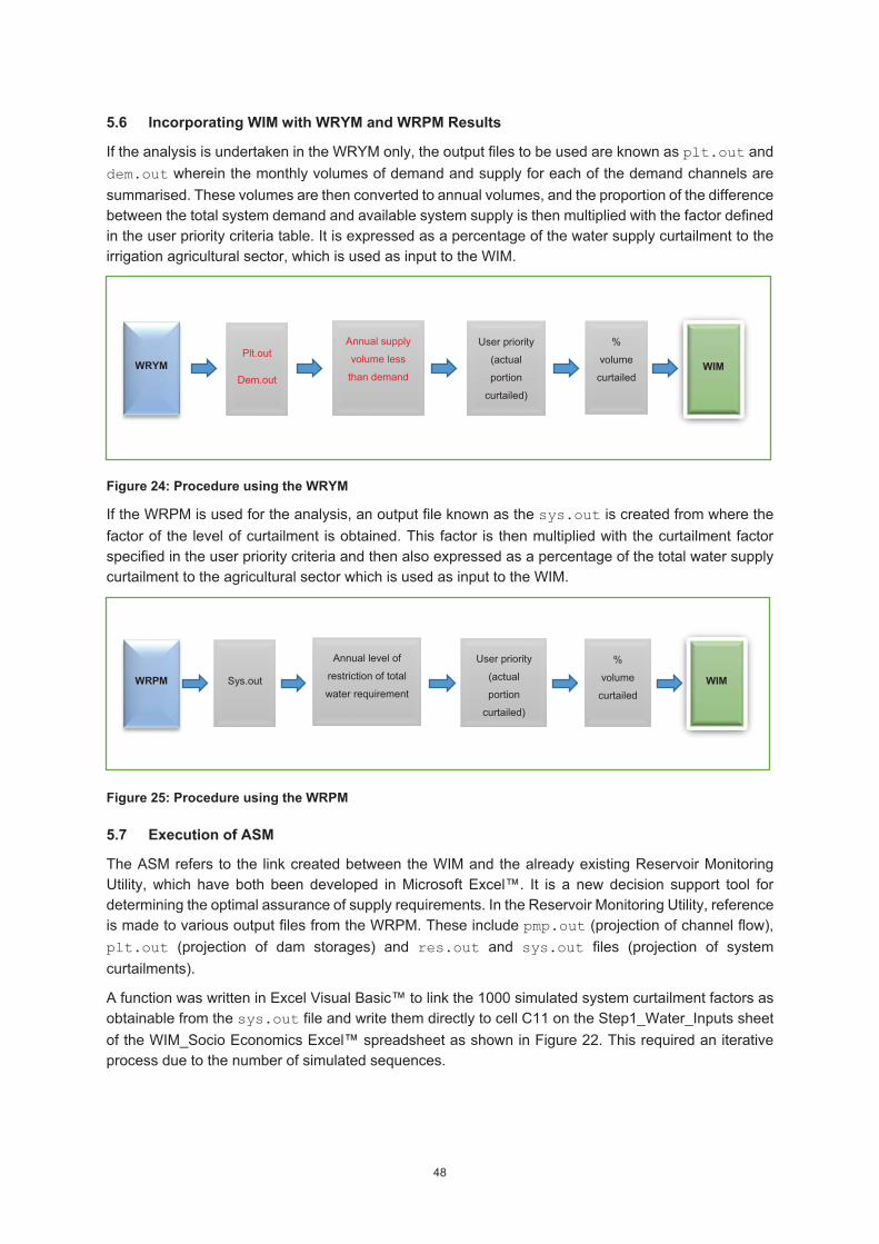
48

5.6 Incorporating WIM with WRYM and WRPM Results

If the analysis is undertaken in the WRYM only, the output files to be used are known as plt.out and dem.out wherein the monthly volumes of demand and supply for each of the demand channels are summarised. These volumes are then converted to annual volumes, and the proportion of the difference between the total system demand and available system supply is then multiplied with the factor defined in the user priority criteria table. It is expressed as a percentage of the water supply curtailment to the irrigation agricultural sector, which is used as input to the WIM.

Figure 24: Procedure using the WRYM

If the WRPM is used for the analysis, an output file known as the sys.out is created from where the factor of the level of curtailment is obtained. This factor is then multiplied with the curtailment factor specified in the user priority criteria and then also expressed as a percentage of the total water supply curtailment to the agricultural sector which is used as input to the WIM.

Figure 25: Procedure using the WRPM

5.7 Execution of ASM

The ASM refers to the link created between the WIM and the already existing Reservoir Monitoring Utility, which have both been developed in Microsoft Excel™. It is a new decision support tool for determining the optimal assurance of supply requirements. In the Reservoir Monitoring Utility, reference is made to various output files from the WRPM. These include pmp.out (projection of channel flow), plt.out (projection of dam storages) and res.out and sys.out files (projection of system curtailments).

A function was written in Excel Visual Basic™ to link the 1000 simulated system curtailment factors as obtainable from the sys.out file and write them directly to cell C11 on the Step1_Water_Inputs sheet of the WIM_Socio Economics Excel™ spreadsheet as shown in Figure 22. This required an iterative process due to the number of simulated sequences.

Plt.out

Dem.out

Annual supply

volume less

than demand

User priority

(actual

portion

curtailed)

%

volume

curtailed WIM WRYM

Sys.out

Annual level of

restriction of total

water requirement

User priority

(actual

portion

curtailed)

%

volume

curtailed

WIM WRPM

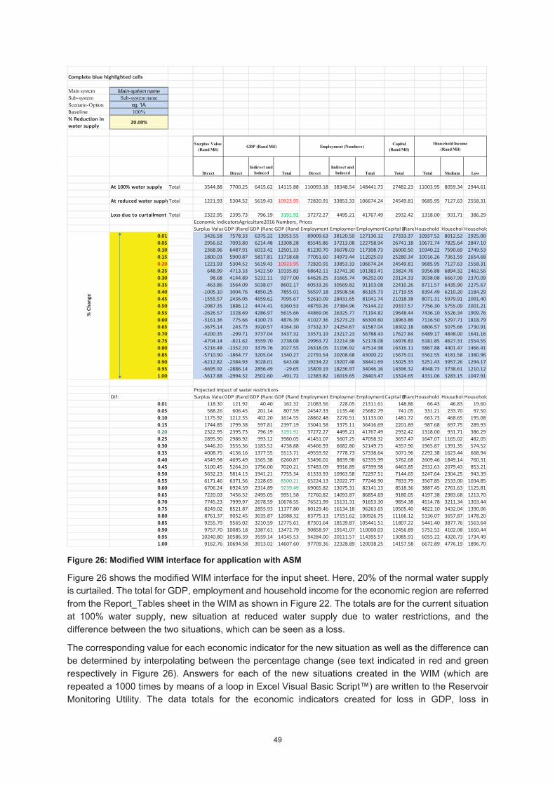
49

Complete blue highlighted cells

Main system Main-system nameSub-system Sub-system name

Scenario-Option eg. 1ABaseline 100%

% Reduction in water supply

20.00%

Surplus Value (Rand Mil)

Capital (Rand Mil)

Direct DirectIndirect and

Induced Total DirectIndirect and

Induced Total Total Total Medium Low

At 100% water supply Total 3544.88 7700.25 6415.62 14115.88 110093.18 38348.54 148441.73 27482.23 11003.95 8059.34 2944.61

At reduced water supplyTotal 1221.93 5304.52 5619.43 10923.95 72820.91 33853.33 106674.24 24549.81 9685.95 7127.63 2558.31

Loss due to curtailment Total 2322.95 2395.73 796.19 3191.92 37272.27 4495.21 41767.49 2932.42 1318.00 931.71 386.29Economic IndicatorsAgriculture2016 Numbers, PricesSurplus ValueGDP (Rand GDP (RandGDP (Rand Employment EmploymenEmployment Household HouseholdHousehold

0.01 3426.58 7578.33 6375.22 13953.55 89009.63 38120.50 127130.12 27333.37 10937.52 8012.52 2925.000.05 2956.62 7093.80 6214.48 13308.28 85545.86 37213.08 122758.94 26741.18 10672.74 7825.64 2847.100.10 2368.96 6487.91 6013.42 12501.33 81230.70 36078.03 117308.73 26000.50 10340.22 7590.69 2749.530.15 1800.03 5900.87 5817.81 11718.68 77051.60 34973.44 112025.03 25280.34 10016.26 7361.59 2654.680.20 1221.93 5304.52 5619.43 10923.95 72820.91 33853.33 106674.24 24549.81 9685.95 7127.63 2558.310.25 648.99 4713.33 5422.50 10135.83 68642.11 32741.30 101383.41 23824.76 9356.88 6894.32 2462.560.30 98.68 4144.89 5232.11 9377.00 64626.25 31665.74 96292.00 23124.33 9038.08 6667.99 2370.090.35 -463.86 3564.09 5038.07 8602.17 60533.26 30569.82 91103.08 22410.26 8711.57 6435.90 2275.670.40 -1005.10 3004.76 4850.25 7855.01 56597.18 29508.56 86105.73 21719.55 8394.49 6210.20 2184.290.45 -1555.57 2436.05 4659.62 7095.67 52610.09 28431.65 81041.74 21018.38 8071.31 5979.91 2091.400.50 -2087.35 1886.12 4474.41 6360.53 48759.26 27384.96 76144.22 20337.57 7756.30 5755.09 2001.210.55 -2626.57 1328.69 4286.97 5615.66 44869.06 26325.77 71194.82 19648.44 7436.10 5526.34 1909.760.60 -3161.36 775.66 4100.73 4876.39 41027.36 25273.23 66300.60 18963.86 7116.50 5297.71 1818.790.65 -3675.14 243.73 3920.57 4164.30 37332.37 24254.67 61587.04 18302.18 6806.57 5075.66 1730.910.70 -4200.35 -299.71 3737.04 3437.32 33571.19 23217.23 56788.43 17627.84 6489.17 4848.00 1641.160.75 -4704.14 -821.62 3559.70 2738.08 29963.72 22214.36 52178.08 16976.83 6181.85 4627.31 1554.550.80 -5216.48 -1352.20 3379.76 2027.55 26318.05 21196.92 47514.98 16316.11 5867.88 4401.47 1466.410.85 -5710.90 -1864.77 3205.04 1340.27 22791.54 20208.68 43000.22 15675.01 5562.55 4181.58 1380.960.90 -6212.82 -2384.93 3028.01 643.08 19234.22 19207.48 38441.69 15025.33 5251.43 3957.26 1294.170.95 -6695.92 -2886.14 2856.49 -29.65 15809.19 18236.97 34046.16 14396.32 4948.73 3738.61 1210.121.00 -5617.88 -2994.32 2502.60 -491.72 12383.82 16019.65 28403.47 13324.65 4331.06 3283.15 1047.91

Projected Impact of water restrictionsDif: Surplus ValueGDP (Rand GDP (RandGDP (Rand Employment EmploymenEmployment Household HouseholdHousehold

0.01 118.30 121.92 40.40 162.32 21083.56 228.05 21311.61 148.86 66.43 46.83 19.600.05 588.26 606.45 201.14 807.59 24547.33 1135.46 25682.79 741.05 331.21 233.70 97.500.10 1175.92 1212.35 402.20 1614.55 28862.48 2270.51 31133.00 1481.72 663.73 468.65 195.080.15 1744.85 1799.38 597.81 2397.19 33041.58 3375.11 36416.69 2201.89 987.68 697.75 289.930.20 2322.95 2395.73 796.19 3191.92 37272.27 4495.21 41767.49 2932.42 1318.00 931.71 386.290.25 2895.90 2986.92 993.12 3980.05 41451.07 5607.25 47058.32 3657.47 1647.07 1165.02 482.050.30 3446.20 3555.36 1183.52 4738.88 45466.93 6682.80 52149.73 4357.90 1965.87 1391.35 574.520.35 4008.75 4136.16 1377.55 5513.71 49559.92 7778.73 57338.64 5071.96 2292.38 1623.44 668.940.40 4549.98 4695.49 1565.38 6260.87 53496.01 8839.98 62335.99 5762.68 2609.46 1849.14 760.310.45 5100.45 5264.20 1756.00 7020.21 57483.09 9916.89 67399.98 6463.85 2932.63 2079.43 853.210.50 5632.23 5814.13 1941.21 7755.34 61333.93 10963.58 72297.51 7144.65 3247.64 2304.25 943.390.55 6171.46 6371.56 2128.65 8500.21 65224.13 12022.77 77246.90 7833.79 3567.85 2533.00 1034.850.60 6706.24 6924.59 2314.89 9239.49 69065.82 13075.31 82141.13 8518.36 3887.45 2761.63 1125.810.65 7220.03 7456.52 2495.05 9951.58 72760.82 14093.87 86854.69 9180.05 4197.38 2983.68 1213.700.70 7745.23 7999.97 2678.59 10678.55 76521.99 15131.31 91653.30 9854.38 4514.78 3211.34 1303.440.75 8249.02 8521.87 2855.93 11377.80 80129.46 16134.18 96263.65 10505.40 4822.10 3432.04 1390.060.80 8761.37 9052.45 3035.87 12088.32 83775.13 17151.62 100926.75 11166.12 5136.07 3657.87 1478.200.85 9255.79 9565.02 3210.59 12775.61 87301.64 18139.87 105441.51 11807.22 5441.40 3877.76 1563.640.90 9757.70 10085.18 3387.61 13472.79 90858.97 19141.07 110000.03 12456.89 5752.52 4102.08 1650.440.95 10240.80 10586.39 3559.14 14145.53 94284.00 20111.57 114395.57 13085.91 6055.22 4320.73 1734.491.00 9162.76 10694.58 3913.02 14607.60 97709.36 22328.89 120038.25 14157.58 6672.89 4776.19 1896.70

GDP (Rand Mil) Employment (Numbers)Household Income

(Rand Mil)

% C

hang

e

Figure 26: Modified WIM interface for application with ASM

Figure 26 shows the modified WIM interface for the input sheet. Here, 20% of the normal water supply is curtailed. The total for GDP, employment and household income for the economic region are referred from the Report_Tables sheet in the WIM as shown in Figure 22. The totals are for the current situation at 100% water supply, new situation at reduced water supply due to water restrictions, and the difference between the two situations, which can be seen as a loss.

The corresponding value for each economic indicator for the new situation as well as the difference can be determined by interpolating between the percentage change (see text indicated in red and green respectively in Figure 26). Answers for each of the new situations created in the WIM (which are repeated a 1000 times by means of a loop in Excel Visual Basic Script™) are written to the Reservoir Monitoring Utility. The data totals for the economic indicators created for loss in GDP, loss in

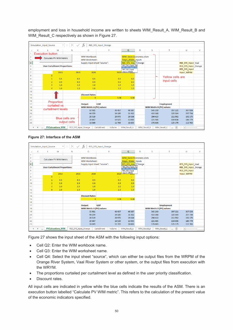
50

employment and loss in household income are written to sheets WIM_Result_A, WIM_Result_B and WIM_Result_C respectively as shown in Figure 27.

Figure 27: Interface of the ASM

Figure 27 shows the input sheet of the ASM with the following input options:

Cell Q2: Enter the WIM workbook name. Cell Q3: Enter the WIM worksheet name. Cell Q4: Select the input sheet “source”, which can either be output files from the WRPM of the

Orange River System, Vaal River System or other system, or the output files from execution with the WRYM.

The proportions curtailed per curtailment level as defined in the user priority classification. Discount rates.

All input cells are indicated in yellow while the blue cells indicate the results of the ASM. There is an execution button labelled “Calculate PV WIM metric”. This refers to the calculation of the present value of the economic indicators specified.

Yellow cells are input cells

Execution button

Proportion curtailed vs

curtailment levels

Blue cells are output cells

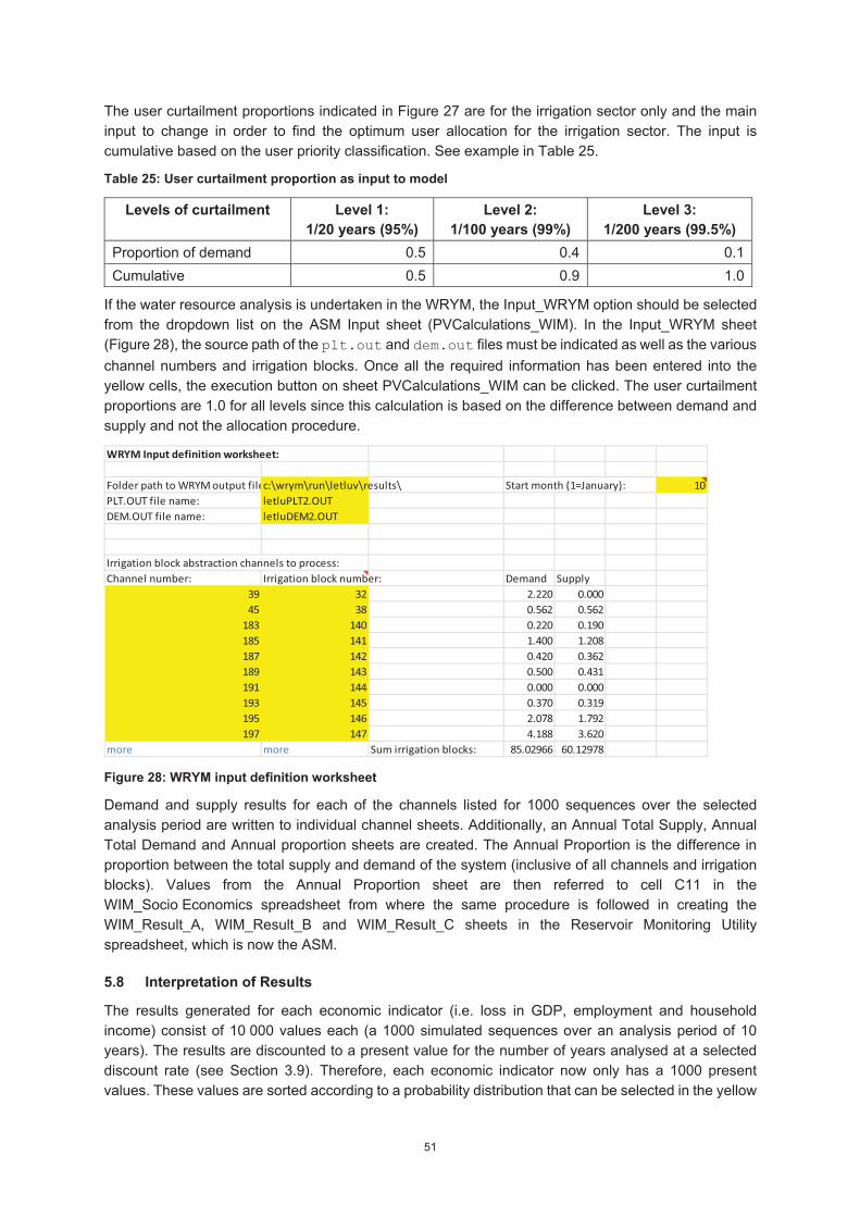
51

The user curtailment proportions indicated in Figure 27 are for the irrigation sector only and the main input to change in order to find the optimum user allocation for the irrigation sector. The input is cumulative based on the user priority classification. See example in Table 25.

Table 25: User curtailment proportion as input to model

Levels of curtailment Level 1: 1/20 years (95%)

Level 2: 1/100 years (99%)

Level 3: 1/200 years (99.5%)

Proportion of demand 0.5 0.4 0.1 Cumulative 0.5 0.9 1.0

If the water resource analysis is undertaken in the WRYM, the Input_WRYM option should be selected from the dropdown list on the ASM Input sheet (PVCalculations_WIM). In the Input_WRYM sheet (Figure 28), the source path of the plt.out and dem.out files must be indicated as well as the various channel numbers and irrigation blocks. Once all the required information has been entered into the yellow cells, the execution button on sheet PVCalculations_WIM can be clicked. The user curtailment proportions are 1.0 for all levels since this calculation is based on the difference between demand and supply and not the allocation procedure.

WRYM Input definition worksheet:

Folder path to WRYM output filec:\wrym\run\letluv\results\ Start month (1=January): 10PLT.OUT file name: letluPLT2.OUTDEM.OUT file name: letluDEM2.OUT

Irrigation block abstraction channels to process:Channel number: Irrigation block number: Demand Supply

39 32 2.220 0.00045 38 0.562 0.562

183 140 0.220 0.190185 141 1.400 1.208187 142 0.420 0.362189 143 0.500 0.431191 144 0.000 0.000193 145 0.370 0.319195 146 2.078 1.792197 147 4.188 3.620

more more Sum irrigation blocks: 85.02966 60.12978

Figure 28: WRYM input definition worksheet

Demand and supply results for each of the channels listed for 1000 sequences over the selected analysis period are written to individual channel sheets. Additionally, an Annual Total Supply, Annual Total Demand and Annual proportion sheets are created. The Annual Proportion is the difference in proportion between the total supply and demand of the system (inclusive of all channels and irrigation blocks). Values from the Annual Proportion sheet are then referred to cell C11 in the WIM_Socio Economics spreadsheet from where the same procedure is followed in creating the WIM_Result_A, WIM_Result_B and WIM_Result_C sheets in the Reservoir Monitoring Utility spreadsheet, which is now the ASM.

5.8 Interpretation of Results

The results generated for each economic indicator (i.e. loss in GDP, employment and household income) consist of 10 000 values each (a 1000 simulated sequences over an analysis period of 10 years). The results are discounted to a present value for the number of years analysed at a selected discount rate (see Section 3.9). Therefore, each economic indicator now only has a 1000 present values. These values are sorted according to a probability distribution that can be selected in the yellow

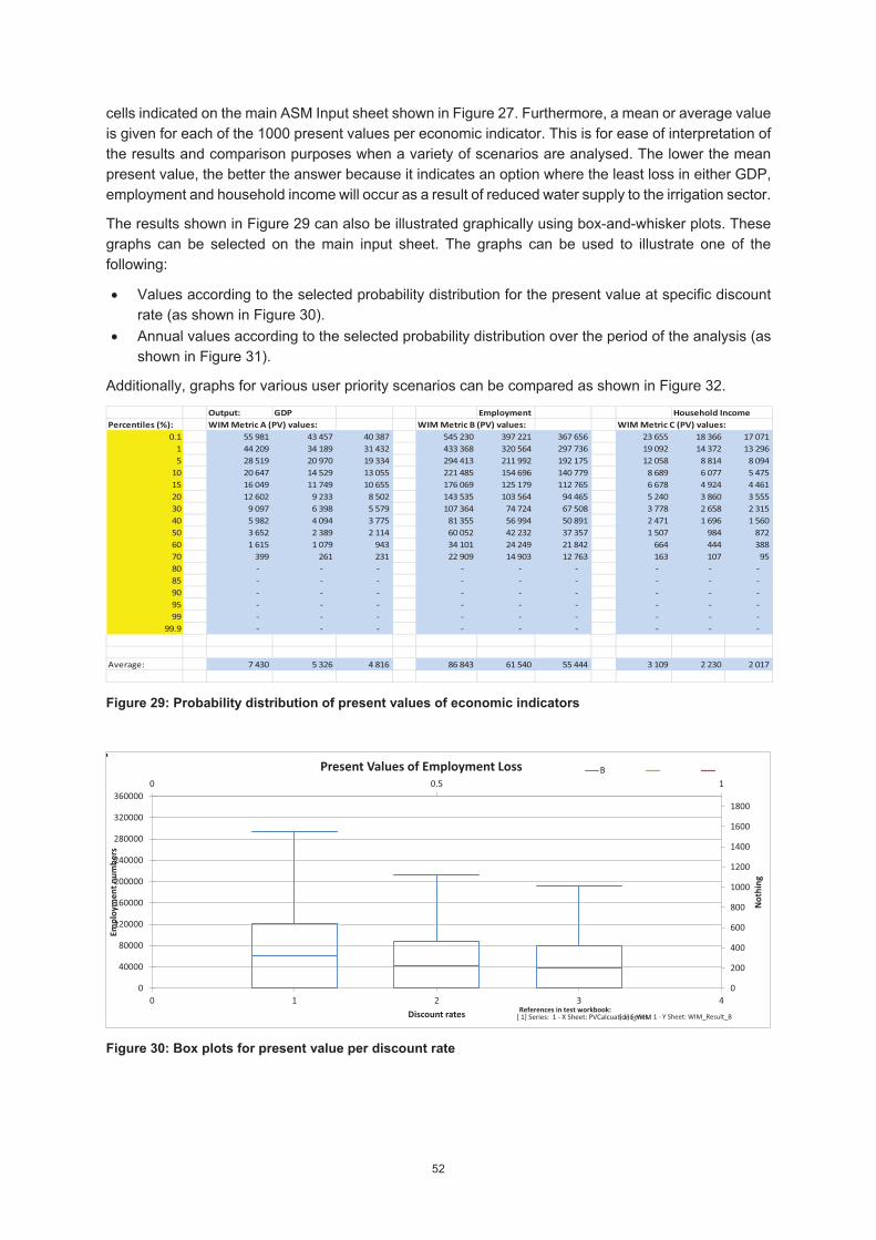
52

cells indicated on the main ASM Input sheet shown in Figure 27. Furthermore, a mean or average value is given for each of the 1000 present values per economic indicator. This is for ease of interpretation of the results and comparison purposes when a variety of scenarios are analysed. The lower the mean present value, the better the answer because it indicates an option where the least loss in either GDP, employment and household income will occur as a result of reduced water supply to the irrigation sector.

The results shown in Figure 29 can also be illustrated graphically using box-and-whisker plots. These graphs can be selected on the main input sheet. The graphs can be used to illustrate one of the following:

Values according to the selected probability distribution for the present value at specific discount rate (as shown in Figure 30).

Annual values according to the selected probability distribution over the period of the analysis (as shown in Figure 31).

Additionally, graphs for various user priority scenarios can be compared as shown in Figure 32. Output: GDP Employment Household Income

Percentiles (%): WIM Metric A (PV) values: WIM Metric B (PV) values: WIM Metric C (PV) values:0.1 55 981 43 457 40 387 545 230 397 221 367 656 23 655 18 366 17 071

1 44 209 34 189 31 432 433 368 320 564 297 736 19 092 14 372 13 296 5 28 519 20 970 19 334 294 413 211 992 192 175 12 058 8 814 8 094

10 20 647 14 529 13 055 221 485 154 696 140 779 8 689 6 077 5 475 15 16 049 11 749 10 655 176 069 125 179 112 765 6 678 4 924 4 461 20 12 602 9 233 8 502 143 535 103 564 94 465 5 240 3 860 3 555 30 9 097 6 398 5 579 107 364 74 724 67 508 3 778 2 658 2 315 40 5 982 4 094 3 775 81 355 56 994 50 891 2 471 1 696 1 560 50 3 652 2 389 2 114 60 052 42 232 37 357 1 507 984 872 60 1 615 1 079 943 34 101 24 249 21 842 664 444 388 70 399 261 231 22 909 14 903 12 763 163 107 95 80 - - - - - - - - - 85 - - - - - - - - - 90 - - - - - - - - - 95 - - - - - - - - - 99 - - - - - - - - -

99.9 - - - - - - - - -

Average: 7 430 5 326 4 816 86 843 61 540 55 444 3 109 2 230 2 017

Figure 29: Probability distribution of present values of economic indicators

Figure 30: Box plots for present value per discount rate

0 0.5 1

0

200

400

600

800

1000

1200

1400

1600

1800

0 1 2 3 40

40000

80000

120000

160000

200000

240000

280000

320000

360000

Not

hing

Discount rates

Empl

oym

ent n

umbe

rs

Present Values of Employment Loss B

[ 1] Series: 1 - Y Sheet: WIM_Result_B

FFF

[ 1] Series: 1 - X Sheet: PVCalcuations_WIM

FFF

References in test workbook:

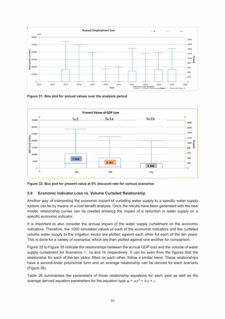
53

Figure 31: Box plot for annual values over the analysis period

Figure 32: Box plot for present value at 0% discount rate for various scenarios

5.9 Economic Indicator Loss vs. Volume Curtailed Relationship

Another way of interpreting the economic impact of curtailing water supply to a specific water supply system can be by means of a cost benefit analysis. Once the results have been generated with the new model, relationship curves can be created showing the impact of a reduction in water supply on a specific economic indicator.

It is important to also consider the annual impact of the water supply curtailment on the economic indicators. Therefore, the 1000 simulated values of each of the economic indicators and the curtailed volume water supply to the irrigation sector are plotted against each other for each of the ten years. This is done for a variety of scenarios, which are then plotted against one another for comparison.

Figure 33 to Figure 35 indicate the relationships between the annual GDP loss and the volume of water supply curtailment for Scenarios 1, 1a and 1b respectively. It can be seen from the figures that the relationship for each of the ten years, fitted on each other, follow a similar trend. These relationships have a second-order polynomial form and an average relationship can be derived for each scenario (Figure 36).

Table 26 summarises the parameters of these relationship equations for each year as well as the average derived equation parameters for the equation type = 2 + + .

-474

0

200

400

600

800

1000

1200

1400

1600

1800

2015 2016 2017 2018 2019 2020 2021 2022 2023 2024 2025 20260

15000

30000

45000

60000

75000

90000

Not

hing

Years

Empl

oym

ent n

umbe

rsAnnual Employment loss B

[ 1] Series: 1 - Y Sheet: WIM_Result_B

FFF

[ 1] Series: 1 - X Sheet: PVCalcuations_WIM

FFF

References in test workbook:

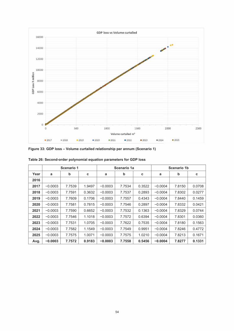
54

Figure 33: GDP loss – Volume curtailed relationship per annum (Scenario 1)

Table 26: Second-order polynomial equation parameters for GDP loss

Scenario 1 Scenario 1a Scenario 1b Year a b c a b c a b c 2016

2017 0.0003 7.7539 1.9497 0.0003 7.7534 0.3522 0.0004 7.8150 0.0708

2018 0.0003 7.7591 0.3632 0.0003 7.7537 0.2893 0.0004 7.8302 0.0277

2019 0.0003 7.7609 0.1706 0.0003 7.7557 0.4343 0.0004 7.8440 0.1459

2020 0.0003 7.7581 0.7815 0.0003 7.7546 0.2897 0.0004 7.8332 0.0421

2021 0.0003 7.7590 0.6652 0.0003 7.7532 0.1363 0.0004 7.8329 0.0744

2022 0.0003 7.7546 1.1018 0.0003 7.7572 0.6394 0.0004 7.8301 0.0360

2023 0.0003 7.7531 1.0705 0.0003 7.7622 0.7535 0.0004 7.8180 0.1563

2024 0.0003 7.7582 1.1549 0.0003 7.7549 0.9951 0.0004 7.8246 0.4772

2025 0.0003 7.7575 1.0071 0.0003 7.7575 1.0210 0.0004 7.8213 0.1671

Avg. 0.0003 7.7572 0.9183 0.0003 7.7558 0.5456 0.0004 7.8277 0.1331

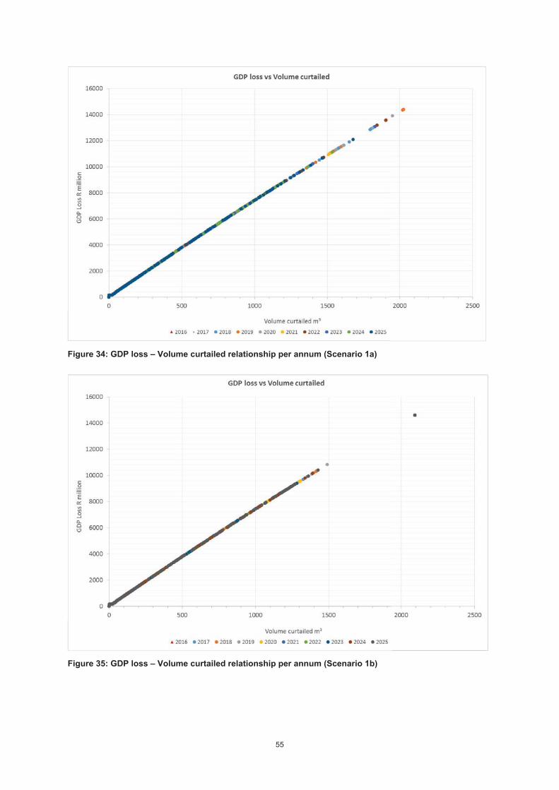
55

Figure 34: GDP loss – Volume curtailed relationship per annum (Scenario 1a)

Figure 35: GDP loss – Volume curtailed relationship per annum (Scenario 1b)

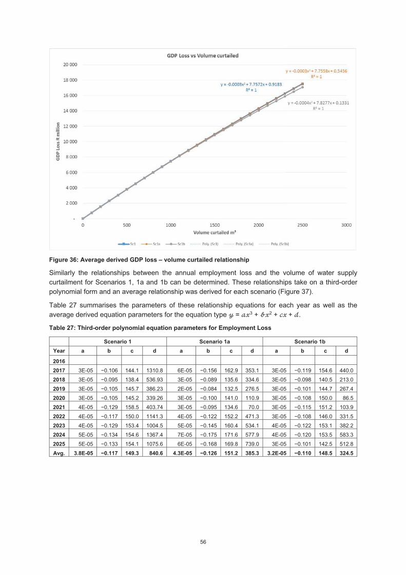
56

Figure 36: Average derived GDP loss – volume curtailed relationship

Similarly the relationships between the annual employment loss and the volume of water supply curtailment for Scenarios 1, 1a and 1b can be determined. These relationships take on a third-order polynomial form and an average relationship was derived for each scenario (Figure 37).

Table 27 summarises the parameters of these relationship equations for each year as well as the average derived equation parameters for the equation type = 3 + 2 + + .

Table 27: Third-order polynomial equation parameters for Employment Loss

Scenario 1 Scenario 1a Scenario 1b Year a b c d a b c d a b c d

2016

2017 3E-05 0.106 144.1 1310.8 6E-05 0.156 162.9 353.1 3E-05 0.119 154.6 440.0 2018 3E-05 0.095 138.4 536.93 3E-05 0.089 135.6 334.6 3E-05 0.098 140.5 213.0 2019 3E-05 0.105 145.7 386.23 2E-05 0.084 132.5 276.5 3E-05 0.101 144.7 267.42020 3E-05 0.105 145.2 339.26 3E-05 0.100 141.0 110.9 3E-05 0.108 150.0 86.5 2021 4E-05 0.129 158.5 403.74 3E-05 0.095 134.6 70.0 3E-05 0.115 151.2 103.9 2022 4E-05 0.117 150.0 1141.3 4E-05 0.122 152.2 471.3 3E-05 0.108 146.0 331.5 2023 4E-05 0.129 153.4 1004.5 5E-05 0.145 160.4 534.1 4E-05 0.122 153.1 382.2 2024 5E-05 0.134 154.6 1367.4 7E-05 0.175 171.6 577.9 4E-05 0.120 153.5 583.3 2025 5E-05 0.133 154.1 1075.6 6E-05 0.168 169.8 739.0 3E-05 0.101 142.5 512.8 Avg. 3.8E-05 0.117 149.3 840.6 4.3E-05 0.126 151.2 385.3 3.2E-05 0.110 148.5 324.5

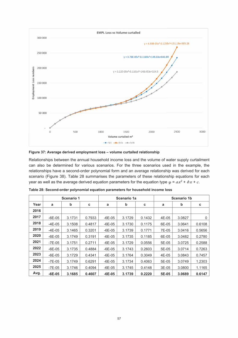
57

Figure 37: Average derived employment loss – volume curtailed relationship

Relationships between the annual household income loss and the volume of water supply curtailment can also be determined for various scenarios. For the three scenarios used in the example, the relationships have a second-order polynomial form and an average relationship was derived for each scenario (Figure 38). Table 28 summarises the parameters of these relationship equations for each year as well as the average derived equation parameters for the equation type = 2 + + .

Table 28: Second-order polynomial equation parameters for household income loss

Scenario 1 Scenario 1a Scenario 1b Year a b c a b c a b c 2016

2017 -6E-05 3.1731 0.7933 -6E-05 3.1729 0.1432 4E-05 3.0827 0 2018 -4E-05 3.1508 0.4817 -6E-05 3.1730 0.1175 6E-05 3.0641 0.6108 2019 -4E-05 3.1465 0.3201 -6E-05 3.1739 0.1771 7E-05 3.0416 0.5656 2020 -6E-05 3.1749 0.3191 -6E-05 3.1735 0.1185 6E-05 3.0482 0.2780 2021 -7E-05 3.1751 0.2711 -6E-05 3.1729 0.0556 5E-05 3.0725 0.2588 2022 -6E-05 3.1735 0.4884 -6E-05 3.1743 0.2603 5E-05 3.0714 0.7263 2023 -6E-05 3.1729 0.4341 -6E-05 3.1764 0.3049 4E-05 3.0843 0.7457 2024 -7E-05 3.1749 0.6291 -6E-05 3.1734 0.4063 5E-05 3.0749 1.2303 2025 -7E-05 3.1746 0.4094 -6E-05 3.1745 0.4148 3E-05 3.0800 1.1165 Avg. -6E-05 3.1685 0.4607 -6E-05 3.1739 0.2220 5E-05 3.0689 0.6147

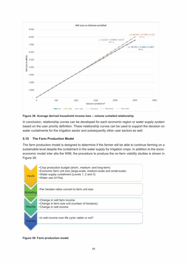
58

Figure 38: Average derived household income loss – volume curtailed relationship

In conclusion, relationship curves can be developed for each economic region or water supply system based on the user priority definition. These relationship curves can be used to support the decision on water curtailments for the irrigation sector and subsequently other user sectors as well.

5.10 The Farm Production Model

The farm production model is designed to determine if the farmer will be able to continue farming on a sustainable level despite the curtailment in the water supply for irrigation crops. In addition to the socio-economic model inter alia the WIM, the procedure to produce the on-farm viability studies is shown in Figure 39.

Figure 39: Farm production model

Inputs

• Crop production budget (short-, medium- and long-term)• Economic farm unit size (large-scale, medium-scale and small-scale)• Water supply curtailment (Levels 1, 2 and 3)• Water use (m3/ha)

Modelling• Per hectare ratios convert to farm unit size

Results

• Change in nett farm income• Change in farm size unit (number of hectares)• Change in nett income

Viability• Is nett income over life cycle viable or not?

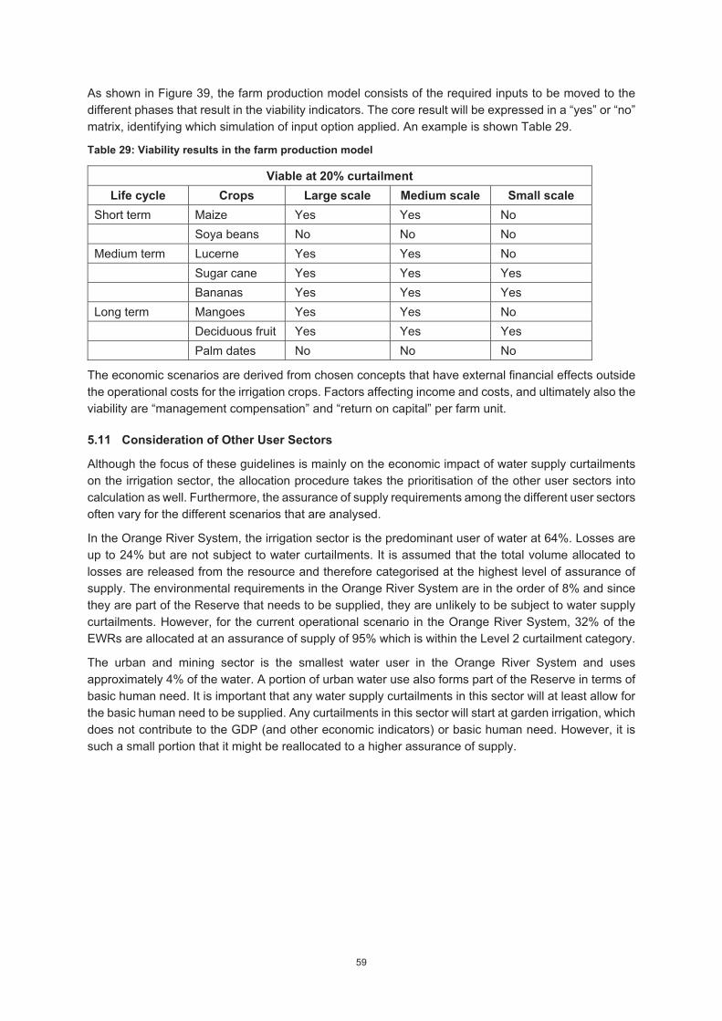
59

As shown in Figure 39, the farm production model consists of the required inputs to be moved to the different phases that result in the viability indicators. The core result will be expressed in a “yes” or “no” matrix, identifying which simulation of input option applied. An example is shown Table 29.

Table 29: Viability results in the farm production model

Viable at 20% curtailment Life cycle Crops Large scale Medium scale Small scale

Short term Maize Yes Yes No Soya beans No No No Medium term Lucerne Yes Yes No Sugar cane Yes Yes Yes Bananas Yes Yes Yes Long term Mangoes Yes Yes No Deciduous fruit Yes Yes Yes Palm dates No No No

The economic scenarios are derived from chosen concepts that have external financial effects outside the operational costs for the irrigation crops. Factors affecting income and costs, and ultimately also the viability are “management compensation” and “return on capital” per farm unit.

5.11 Consideration of Other User Sectors

Although the focus of these guidelines is mainly on the economic impact of water supply curtailments on the irrigation sector, the allocation procedure takes the prioritisation of the other user sectors into calculation as well. Furthermore, the assurance of supply requirements among the different user sectors often vary for the different scenarios that are analysed.

In the Orange River System, the irrigation sector is the predominant user of water at 64%. Losses are up to 24% but are not subject to water curtailments. It is assumed that the total volume allocated to losses are released from the resource and therefore categorised at the highest level of assurance of supply. The environmental requirements in the Orange River System are in the order of 8% and since they are part of the Reserve that needs to be supplied, they are unlikely to be subject to water supply curtailments. However, for the current operational scenario in the Orange River System, 32% of the EWRs are allocated at an assurance of supply of 95% which is within the Level 2 curtailment category.

The urban and mining sector is the smallest water user in the Orange River System and uses approximately 4% of the water. A portion of urban water use also forms part of the Reserve in terms of basic human need. It is important that any water supply curtailments in this sector will at least allow for the basic human need to be supplied. Any curtailments in this sector will start at garden irrigation, which does not contribute to the GDP (and other economic indicators) or basic human need. However, it is such a small portion that it might be reallocated to a higher assurance of supply.

60

6 CONCLUSION AND RECOMMENDATIONS

This study was set out to develop a tool to bridge the water supply curtailment results and the economic results in one large step. This tool is called the ASM. In order to execute this tool, a special interface was pioneered. The advantage of the developed ASM is its ability to process a 1000 simulated values of possible water supply curtailment factors to determine results expressed in a weighted mean present value of economic indicators.

From a technical efficiency point of view, ASM enables water resource engineers to simulate multiple scenarios to determine the optimal water restriction operating rule of a water supply system in a very short time.

Although production work is minimised, which therefore also limits human errors during the activation of the ASM, it is of the utmost importance that the total system with all the different models discussed must be executed by trained and experienced resource economists and water resource engineers.

In both Volume 1 and Volume 2 reports of this study, the applicable limitations of the current modelling system have been identified and discussed to the possible refining and/or expansion of the system. The resource model(s) have initially been designed in the 1970s and imported to South Africa in 1985; the water economic models were initiated during the 1990s. This provides a good platform in confidence for the system as such, although the linking of the two fields is in its initial stages of development.

However, without reliable data and data sources, even the most equipped modelling system cannot provide a reliable outcome. Therefore, the authors strongly recommend that in resource economics, as well as in the spectrum of the water resource engineer, funding, capacity building and continuous research must be provided to make it possible for preserving water for agriculture, industrial, mining and domestic demand without compromising assurance of supply of irrigation agriculture.

The use of this tool should ideally not be limited to the Regulator of water supply but also be introduced to the water user especially in the irrigation sector.

61

REFERENCES

DEPARTMENT OF WATER AFFAIRS (DWA) (2013) National Water Resource Strategy: Water for an Equitable and Sustainable Future (2nd edition). DWA, Pretoria.

DEPARTMENT OF WATER AFFAIRS AND FORESTRY (DWAF) (2006) Guidelines for water supply systems operation and management plans during normal and drought conditions. Ninham Shand (Pty) Ltd in association with Semenya Furumele (Pty) Ltd on behalf of the Directorate: Water Resource Planning Systems. DWAF Report No RSA C000/002305.

DEPARTMENT OF WATER AFFAIRS AND FORESTRY (2008a) Maintenance and updating of hydrological and system software – Phase 3: Procedural manual for the water resources simulation model (WRSM). Hydrosol (Pty) Ltd and WRP Consulting Engineers (Pty) Ltd.

DEPARTMENT OF WATER AFFAIRS AND FORESTRY (2008b) Water resources yield model (WRYM) user guide: Release 7.5.6.2.

DEPARTMENT OF WATER AND SANITATION (DWS) (2013) Water resources planning model (WRPM: Input data and file formats, version 4.4.

MULLINS D (2014) A Manual for Cost Benefit Analysis in South Africa with Specific Reference to Water Resource Development (3rd ed.). Water Research Commission, Pretoria.