Optimal Power Flow with Stability ConstraintsODE23t MATLAB function: using the trapezoidal rule OPF Optimal Power Flow OPFSC Optimal Power Flow with Stability Constraint PQ Power and

SCHOOL OF ENGINEERING AND INFORMATION TECHNOLOGY

ENG470: 2015 ENGINEERING HONOURS THESIS

Optimal Power Flow with Stability Constraints

Author: Youssof Kheder

Academic Supervisor: Dr. Gregory Crebbin

ii

DECLARATION

I certify that the research described in this report has not already been submitted for any

other degree.

I certify that to the best of my knowledge, all sources used and any help received in the

preparation of this dissertation have been acknowledged.

Word count: 12,494

Signed: __________________________________

iii

ABSTRACT

The optimal power flow (OPF) problem aims to control the generation and consumption of

generators and loads. The main objectives are to minimise the generation cost, power losses

while maintaining stability of the generators in the network.

The network used for analysis and testing of OPF with stability constraints is the ‘WSCC 9 bus 3

machine’ [1] network (refer to chapter 5). MATLAB is used to develop algorithms for three

alternative simulations that all encompass the same fault and clearing time in order to compare

the outcomes. The first simulation includes load flow analysis followed by the stability analysis,

leading to an unstable outcome to the network. This is used as the reference point. The second

simulation is of the OPF analysis, followed by a stability analysis and optimisation using the

Nelder-Mead algorithm [2]. The stability constraints were not yet introduced, so the outcome is

also unstable. However, when compared to the load flow (LF) simulation it demonstrates

improved cost effectiveness - real power losses are reduced, power demand is met and the

simulation is efficient. Finally, the optimal power flow with stability constraint (OPFSC) is analysed

and compared with the OPF simulation without stability constraints. This proves to be a stable

network but is more time consuming.

The OPFSC simulation is the final simulation with the stability constraints included and illustrates

the result of a stable network for the three generators. The main determinants for analysis in the

simulation are the power demand, the power losses, network costing and time efficiency. The

simulation time is reduced using various techniques that allow the algorithm to continue solving

iv

the problem without compromising the final result. Time to completion was initially 9.53 seconds.

Following implementation of alternative techniques, this was introduced to 2.96 seconds. This

improvement in time efficiency translates to a reduction in CPU processing requirements and

stability maintenance.

v

TABLE OF CONTENTS DECLARATION ................................................................................................................................ ii

ABSTRACT ......................................................................................................................................iii

TABLE OF CONTENTS ..................................................................................................................... v

ACKNOWLEDGEMENTS ............................................................................................................... viii

LIST OF FIGURES ............................................................................................................................ ix

LIST OF TABLES .............................................................................................................................. xi

LIST OF EQUATIONS ..................................................................................................................... xii

LIST OF ABBRIVIATIONS ............................................................................................................... xiii

1 Introduction .......................................................................................................................... 1

1.1 Literature Review ............................................................................................................... 2

2 Load Flow Analysis ................................................................................................................ 8

2.1 Load Flow: Computation and Techniques .......................................................................... 8

2.2 Comparison of Gauss-Seidel and Newton-Raphson Method ............................................. 9

2.3 Gauss-Seidel Power Flow Solution ................................................................................... 10

3 Optimal Power Flow ............................................................................................................ 12

3.1 Basic Concept and Definitions .......................................................................................... 12

3.2 Optimization Techniques ................................................................................................. 14

3.2.1 Nelder-Mead Algorithm ........................................................................................... 15

3.2.1.1 Nelder-Mead mathematical Example .................................................................. 16

4 Stability ................................................................................................................................ 20

4.1 Power System Stability ..................................................................................................... 20

4.1.1 History on Power System Stability ........................................................................... 21

4.1.2 Classification of Stability .......................................................................................... 22

4.1.3 Angle Stability ........................................................................................................... 23

4.1.4 Voltage Stability ....................................................................................................... 24

4.2 Transient Stability ............................................................................................................. 25

4.2.1 Swing Equation ......................................................................................................... 25

4.2.2 Equal area criterion .................................................................................................. 26

4.2.3 Transient Stability using Numerical Integration ....................................................... 27

4.2.3.1 Trapezoidal Rule ................................................................................................... 28

4.2.4 Stability Margin ........................................................................................................ 29

vi

5 Test System ......................................................................................................................... 31

5.1 WSCC 9 Bus System .......................................................................................................... 31

5.1.1 Generators................................................................................................................ 32

5.1.2 Transformers ............................................................................................................ 33

5.1.3 Transmission Lines ................................................................................................... 33

5.1.4 Loads ........................................................................................................................ 34

6 PowerFactory –Transient Stability Analysis ........................................................................ 35

6.1 Step 1: Load Flow Calculations ......................................................................................... 35

6.2 Step 2 Defining Events...................................................................................................... 35

6.3 Step 3: RMS/EMT Simulation ........................................................................................... 38

7 Results ................................................................................................................................. 40

7.1 Methodology .................................................................................................................... 40

7.1.1 Load Flow Calculations – Gauss-Seidel Method ....................................................... 41

7.1.2 Optimisation Calculations – Nelder-Mead Algorithm .............................................. 42

7.1.3 Stability Analysis Calculations .................................................................................. 44

7.2 LF, OPF and OPFSC Simulations ........................................................................................ 45

7.2.1 LF: MATLAB Code Sequence ..................................................................................... 45

7.2.2 OPF: MATLAB Code Sequence .................................................................................. 46

7.2.3 OPFSC MATLAB Code Sequence ............................................................................... 48

7.3 Simulation Results ............................................................................................................ 50

7.3.1 Simulation 1: Power angle of LF analysis ................................................................. 51

7.3.2 Simulation 2: Power angle of OPF analysis .............................................................. 53

7.3.3 Simulation 3: Power angle for OPFSC analysis ......................................................... 55

7.4 LF, OPF and OPFSC simulation results, overall comparison ............................................. 56

8 Conclusion and Future Work ............................................................................................... 59

8.1 Conclusion ........................................................................................................................ 59

8.2 Future Work ..................................................................................................................... 60

9 Appendices .......................................................................................................................... 63

9.1 Appendix A MATLAB Code ............................................................................................... 63

9.1.1 Runsimulator.m – run file for the overall simulation ............................................... 63

9.1.2 Bloss.m – calculation for network losses ................................................................. 66

9.1.3 costOPF.m – OPF function file .................................................................................. 68

9.1.4 costOPFSC – OPFSC function file .............................................................................. 69

vii

9.1.5 Trstab.m and trstabOPFSC.m – stability analysis file ............................................... 72

9.2 Appendix B Tabulated Simulation Results ....................................................................... 75

9.2.1 Stability reduced matrix data ................................................................................... 75

9.2.2 MATLAB load flow results ........................................................................................ 78

10 References ....................................................................................................................... 80

viii

ACKNOWLEDGEMENTS

I would like to begin by expressing sincere appreciation and gratitude to my academic supervisor

Dr Gregory Crebbin, who has consistently provided constructive advice and direction throughout.

A special thanks also to the academic lecturers from the Engineering Facility, who have given their

support and time throughout my degree.

Finally, I would like to thank my family-namely my brother Nezar, for his support and guidance

and my mother Fatima who has provided endless support and encouragement throughout my

studies and my brother Samir for facilitating the printing of this document!

Finally, I would like to thank my dearest wife Karen for her constant support and advice

throughout my degree, particularly during these last few months. I sincerely appreciate your

dedication and patience putting up with me over the years.

ix

LIST OF FIGURES

Figure 1.1-1 Equivalent circuit of the synchronous generator ........................................................... 5

Figure 1.1-2 Overall procedure for stability constrained OPF [3] ...................................................... 7

Figure 3.2-1 Initiating the algorithm with three values (first iteration, displaying new simplex) ... 16

Figure 3.2-2 Reflection after third iteration ..................................................................................... 17

Figure 3.2-3 Expansion after first iteration ...................................................................................... 17

Figure 3.2-4 Simplex after sixth iterations ....................................................................................... 18

Figure 3.2-5 Expansion after eleventh iteration .............................................................................. 18

Figure 4.1-1 Classification of Power system stability [4] ................................................................. 23

Figure 4.2-1 Phasor-Vector diagram of the rotor angle [5] ............................................................. 26

Figure 4.2-2 Trapezoidal rule with error .......................................................................................... 28

Figure 4.2-3 Trapezoidal rule simulation time increased ................................................................. 29

Figure 4.2-4 Trapezoidal rule with little error and less simulation time .......................................... 29

Figure 5.1-1 WSCC 9 Bus 3 machine system .................................................................................... 32

Figure 6.2-1 Short-Circuit Event, window ........................................................................................ 36

Figure 6.2-2 Making the Short Circuit at line, available ................................................................... 37

Figure 6.2-3 Switch Event, window .................................................................................................. 37

Figure 6.3-1 PowerFactory Simulation: fault clearing time 0.05 seconds ....................................... 39

Figure 7.1-1 Function with maximum iterations of 200 ................................................................... 43

Figure 7.1-2 Function with maximum iteration of 35 ...................................................................... 44

Figure 7.2-1 LF MATLAB code sequence .......................................................................................... 46

Figure 7.2-2 OPF MATLAB code sequence ....................................................................................... 47

Figure 7.2-3 MATLAB code: stability margin .................................................................................... 48

Figure 7.2-4 MATLAB code: Power loss and power demand ........................................................... 49

x

Figure 7.2-5 MATLAB code: Generator limits ................................................................................... 50

Figure 7.3-1 Load Flow simulation, stability analysis ....................................................................... 52

Figure 7.3-2 PowerFactory simulation: using the LF results ............................................................ 52

Figure 7.3-3 OPF simulation, Stability analysis ................................................................................. 54

Figure 7.3-4 PowerFactory simulation: using the OPF results ......................................................... 54

Figure 7.3-5 OPFSC simulation, Stability analysis ............................................................................. 55

Figure 7.3-6 PowerFactory simulation: using the OPFSC results ..................................................... 56

Figure 7.4-1 Simulation results comparing LF, OPF and OPFSC ....................................................... 58

Figure 9.2-1 Reduced bus admittance matrix for LF ........................................................................ 75

Figure 9.2-2 Reduced bus admittance matrix for OPF ..................................................................... 76

Figure 9.2-3 Reduced bus admittance matrix for OPFSC ................................................................. 77

xi

LIST OF TABLES

Table 2.1-1 Iteration count for Gauss-Seidel and Newton-Raphson ................................................. 9

Table 2.2-1 Comparison between Gauss-Seidel and Newton-Raphson Method [16] ..................... 10

Table 2.3-1 Specification system for the known and unknowns for buses within the Network ..... 11

Table 3.1-1 Application for equation (10), (11), (12) and (13) ......................................................... 14

Table 5.1-1 Generator data .............................................................................................................. 33

Table 5.1-2 Transformer data .......................................................................................................... 33

Table 5.1-3 Transmission Line data .................................................................................................. 33

Table 5.1-4 Load data ....................................................................................................................... 34

Table 7.4-1 Overall results for the three simulations ...................................................................... 57

xii

LIST OF EQUATIONS

Equation 1.1-1 Cost Function ............................................................................................................. 4

Equation 1.1-2 Active Power Flow ..................................................................................................... 4

Equation 1.1-3 Reactive Power Flow ................................................................................................. 4

Equation 1.1-4 Generators Real Power Limits ................................................................................... 4

Equation 1.1-5 representing the swing equation as first order equations ........................................ 5

Equation 3.1-1 Generator Cost Function ......................................................................................... 13

Equation 3.1-2 Objective function ................................................................................................... 13

Equation 3.1-3 Non-linear equality constraints ............................................................................... 13

Equation 3.1-4 Non-linear inequality constraints ............................................................................ 13

Equation 4.2-1 Swing Equation ........................................................................................................ 26

Equation 4.2-2 Stability Constraint [3] ............................................................................................. 30

xiii

LIST OF ABBRIVIATIONS

CPU Central Processing Unit

DC Direct Current

G1 Generator 1

G2 Generator 2

G3 Generator 3

GA Genetic Algorithm

H Inertia

IEEE Institution of Electrical and Electronics Engineers

KKT Karush-Kuhn Tucker

LF Load Flow

MATLAB Matrix Laboratory

MVAr Mega Voltage Amps

ODE23t MATLAB function: using the trapezoidal rule

OPF Optimal Power Flow

OPFSC Optimal Power Flow with Stability Constraint

PQ Power and Reactive Power

PSO Particle Swarm Algorithm

PV Power and Voltage

SBSI Step By Step Integration

SLD Single Line Diagram

WSCC Western System Coordinating Council

1

1 Introduction

The optimal power flow [3] (OPF) problem aims to control the generation and consumption of

generators and loads in an electrical distribution network with the main objectives of

optimisation and minimisation of the generation cost, power losses, meeting power demand and

maintaining stability of the generators in the network. This thesis provides an overview of how

the OPF with stability constraint can be achieved. The approach utilised is to begin with a LF

analysis [4] of a network, followed by execution of an OPF algorithm consisting of equality and

inequality constraints and progressing to explain the techniques used for simulation. An overview

of transient stability and steady state stability are introduced to illustrate how the constraints are

utilised. The final section of this report describes the parameters of the test network and the

simulation tools used to perform the analysis and obtain the results.

The first two chapters explain the LF and OPF techniques adapted in the MATLAB simulations and

progress by proposing alternative methods for future works. The Gauss-Seidel [5] and Newton

Raphson [5] are the two LF techniques discussed in Chapter 2, Load Flow Analysis. The Nelder-

Mead algorithm [2], Particle Swarm Optimisation [6] and the Genetic algorithm [7] are the

optimisation techniques discussed in Chapter 3, Optimal Power Flow.

An overview of stability is given in chapter 3 followed by an in-depth explanation of transient

stability. The method proposed for transient stability is by linearisation via numerical integration

with the implementation of the trapezoidal rule. This chapter elaborates further on the method

used to determine stability via the inequality constraint, (Equation 4.2-2 Stability Constraint).

2

This thesis proposes an OPF with Stability Constraints (OPFSC) method, using the Nelder-Mead

algorithm as the optimisation technique and MATLAB as the simulation tool. The MATLAB code

sequence is described in detail through explanation of the data flow sequences for three separate

simulations.

The three simulations performed are: LF, OPF and finally OPFSC. The results are analysed in an

attempt to differentiate all three scenarios. The LF simulation is used to illustrate the network

operating under normal conditions followed by a fault condition with the exclusion of the

optimiser and constraints. The OPF simulation illustrates the effect of optimisation on the

network, along with stability after a network has encountered a fault. The final simulation is the

OPFSC. This follows from the OPF simulation with the incorporation of stability constraints.

1.1 Literature Review

When a power system undergoes transient disturbances and is unable to maintain

synchronisation, the economic burden becomes extremely high [3, 4]. Since the first Optimal

power flow paper published by IEEE in the 1960s there has been an increased interest in the need

to take into account the dynamic security constraints in OPF computations [8, 9]. The

advancements in computational software have aided greatly in resolving stability and optimal

power flow problems, achieving both a solution and improvement to the feasibility. This thesis

provides a review on selected calculation methods being performed and proposed.

The main focus on optimal power flow with constrained stability revolves around the cost of

generation and supply of real and reactive power in power systems. The perfect balance between

3

OPF and stability needs to be analysed so that the feasibility and system security are not

compromised. Utility engineers invest a lot of time into stability studies to avoid running into any

devastating operational problems [3]. The traditional approach used by engineers came from a

trial and error method and by using experience and judgement. The step by step integration

method for solving the swing equation [5] is the current industrial method for transient stability.

Different operation points for power systems means different stability characteristics, which also

means transient stability can be maintained with implementing search methods and defining the

appropriate stability limits. The significant improvements in modern computer technology have

successfully allowed the implementation of online dynamics security assessment programs and

have improved the programs as well as the ability to monitoring stability [3].

When a predetermined stability margin is given, the operating point for a system can be derived.

Over the past two decades, pattern recognition methods have been widely used [3, 9, 10]

although these methods do not explicitly produce a stability margin. However they provide an

effective approach in computing the generation dispatch as well as giving the energy margins and

rotor angles. An OPF problem is treated with voltage and thermal constraints, this can be

compared to the stability problem where the stability can be viewed as a constraint and as an

addition to the OPF constraints. The following references discuss the possibilities of including the

stability constraints to an OPF problem [11], [9] and [12]. The current method for modelling

voltage and thermal constraints is via algebraic equations or inequalities. On the other hand, It is

still debatable how the stability constraints are included due to stability being a dynamic concept

and having differential equations involved [3].

4

The rising growth of competitive power markets has led to a greater understanding and

developing the need of OPF with stability constraints, (see Equation 4.2-2). The traditional

method of trial and error can produce discernment amongst the market players for stressed

power systems. It has been reported that it is unsatisfactory for a deregulated environment to

maintain reliability when operating guidelines are based on off-line stability studies [3]. This is

where online stability analysis becomes a vital component of power distribution systems.

Research from a recent paper (Gan, 2000. [3]), states that there is no general theory in computing

stability limits and has developed an approach as a solution to this problem. The methodology

involves using advanced OPF and step by step integration (SBSI) techniques [3] to transform

differential equations into their equivalent algebraic equations. This method is then applied to

standard nonlinear programming [3] techniques.

In the same paper the method for solving the OPF problem is based on the cost function Equation

1.1-1 which is the objective function. The active and reactive power flow equations are shown in

Equation 1.1-2 and Equation 1.1-3 respectively. Pg is the generator’s active power output with

upper bound Pgmax and the lower bound Pg

min as shown in Equation 1.1-4. The same is true for Qg

which is the reactive power output with the upper bound Qgmax and lower bound Qg

min.

( ) (1) Equation 1.1-1 Cost Function

( ) (2) Equation 1.1-2 Active Power Flow

( ) (3) Equation 1.1-3 Reactive Power Flow

(4) Equation 1.1-4 Generators Real Power Limits

5

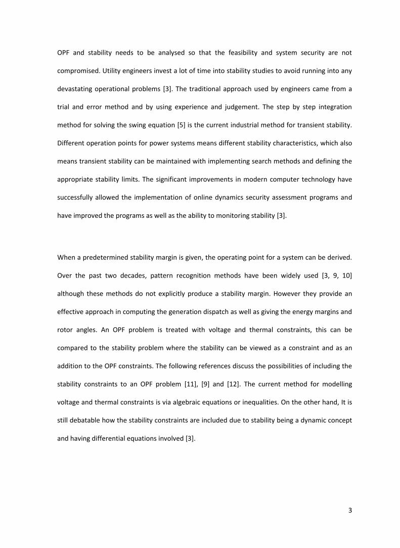
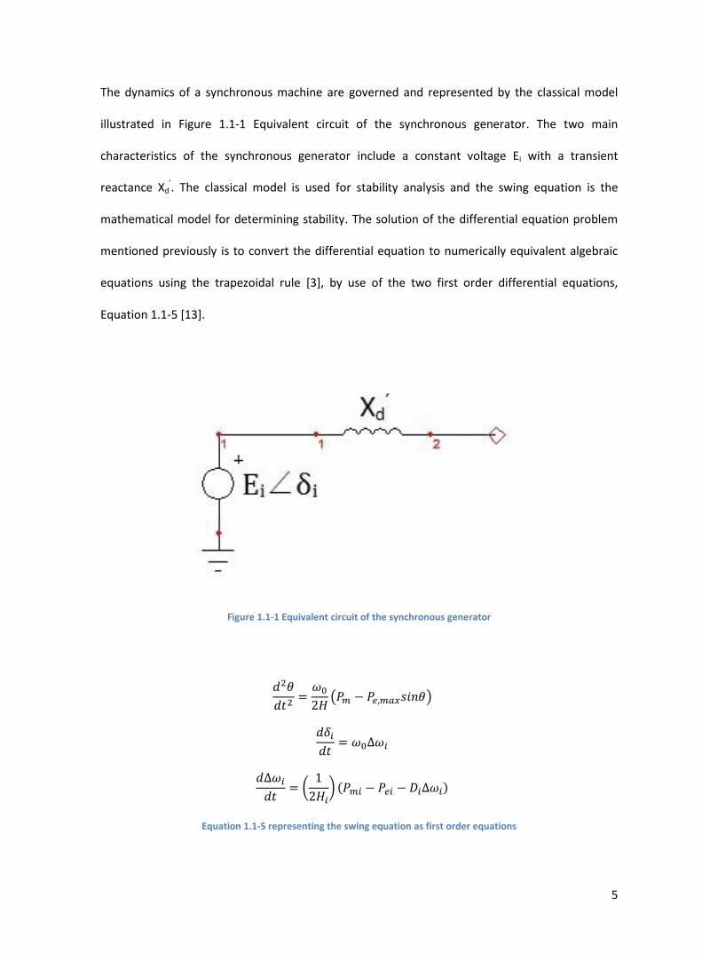
The dynamics of a synchronous machine are governed and represented by the classical model

illustrated in Figure 1.1-1 Equivalent circuit of the synchronous generator. The two main

characteristics of the synchronous generator include a constant voltage Ei with a transient

reactance Xd’. The classical model is used for stability analysis and the swing equation is the

mathematical model for determining stability. The solution of the differential equation problem

mentioned previously is to convert the differential equation to numerically equivalent algebraic

equations using the trapezoidal rule [3], by use of the two first order differential equations,

Equation 1.1-5 [13].

Figure 1.1-1 Equivalent circuit of the synchronous generator

( )

(5)

(6)

(

) ( )

(7)

Equation 1.1-5 representing the swing equation as first order equations

6

Where:

δi = angular position of the rotor with respect to a synchronously rotating reference

Δωi = rotor speed deviation

ω0 = reference frequency

Hi = inertia constant

Pm and Pe = the input and output power respectively

Di = Damping constant

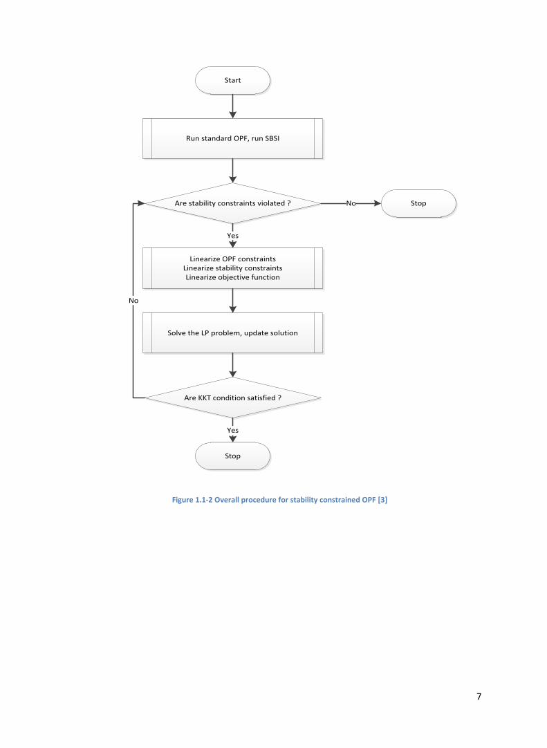
The algorithm for the stability problem is performed using the high level technical computing

language MATLAB [14], which is perfect for algorithm development, data visualisation and

analysis. Figure 1.1-2 illustrates the procedure for OPF analysis with incorporation of the stability

constraints, OPF and function constraints. Techniques for reducing the CPU demand are discussed

in [3] and have been incorporated in the thesis simulation . These are discussed in more detail in

Chapter 3, 4 and 7.

7

Start

Run standard OPF, run SBSI

Linearize OPF constraintsLinearize stability constraintsLinearize objective function

Solve the LP problem, update solution

Are KKT condition satisfied ?

Are stability constraints violated ?

Stop

Stop

Yes

Yes

No

No

Figure 1.1-2 Overall procedure for stability constrained OPF [3]

8

2 Load Flow Analysis

The backbone of any power system is its LF calculations therefore LF computer programs are an

essential tool for an electrical engineer in order to determine whether or not a network is

operational under normal conditions, for planning, to provide economic scheduling, controls for

an existing network and to cater for future expansion [5, 15]. A power system successfully

operates under normal balanced three phase steady-state conditions when:

demands and losses are sufficiently catered for by generation

Bus voltage magnitudes are operating relatively close to the rated values

Generators have specified real and reactive power limits and the network operates within

these conditions.

Transmission lines and transformers within the network are never overloaded.

A power system has known power values, which leads to the computation of power flow

equations. These equations are nonlinear therefore an iterative solution method is implemented.

There are many techniques utilised for solving power flow equations via iteration. The technique

used in this thesis is dependent on the convergence time. It is also important in the setup of the

network parameters in order to perform the optimisation and stability analysis.

2.1 Load Flow: Computation and Techniques

The two conventional iterative techniques being assessed in this thesis with regards to solving a

load flow problem are the Gauss Seidel or Newton Raphson method. The iterative techniques for

calculating load flows are time consuming and difficult to perform by hand therefore

9

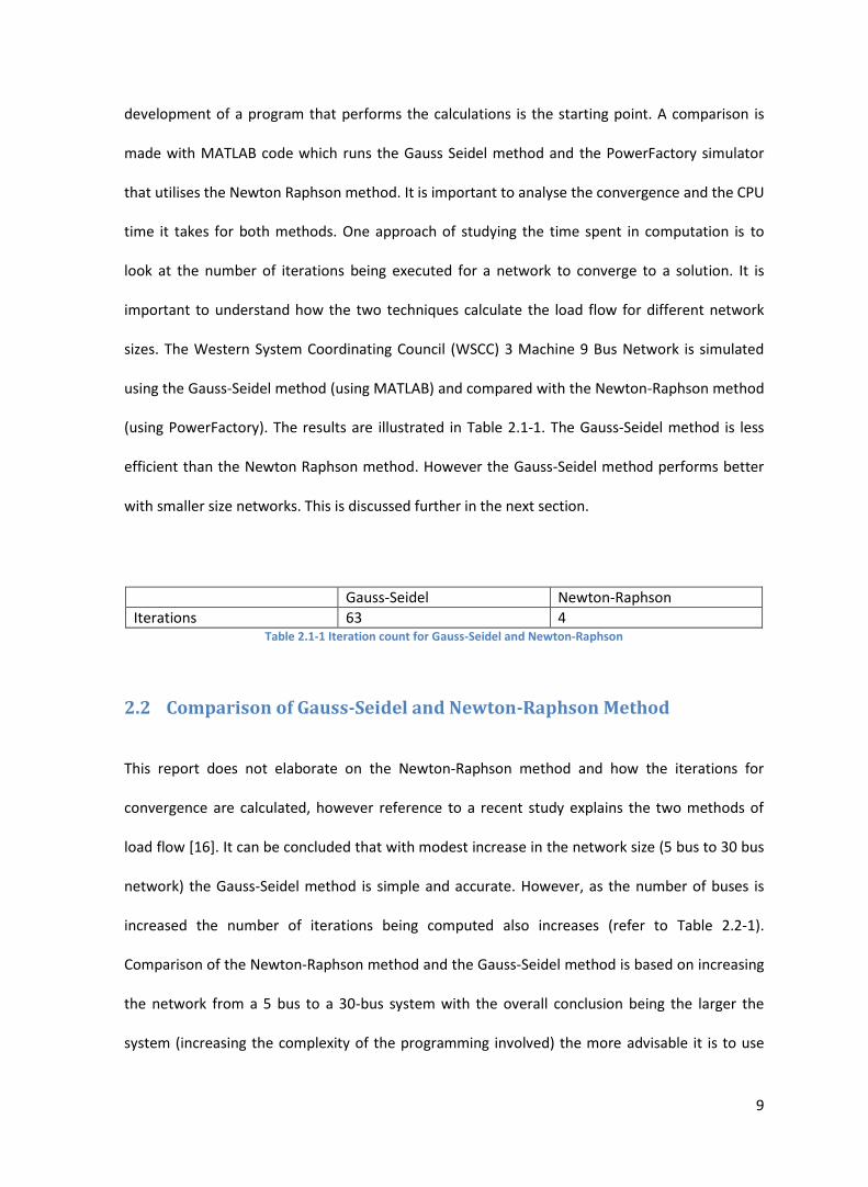
development of a program that performs the calculations is the starting point. A comparison is

made with MATLAB code which runs the Gauss Seidel method and the PowerFactory simulator

that utilises the Newton Raphson method. It is important to analyse the convergence and the CPU

time it takes for both methods. One approach of studying the time spent in computation is to

look at the number of iterations being executed for a network to converge to a solution. It is

important to understand how the two techniques calculate the load flow for different network

sizes. The Western System Coordinating Council (WSCC) 3 Machine 9 Bus Network is simulated

using the Gauss-Seidel method (using MATLAB) and compared with the Newton-Raphson method

(using PowerFactory). The results are illustrated in Table 2.1-1. The Gauss-Seidel method is less

efficient than the Newton Raphson method. However the Gauss-Seidel method performs better

with smaller size networks. This is discussed further in the next section.

Gauss-Seidel Newton-Raphson

Iterations 63 4 Table 2.1-1 Iteration count for Gauss-Seidel and Newton-Raphson

2.2 Comparison of Gauss-Seidel and Newton-Raphson Method

This report does not elaborate on the Newton-Raphson method and how the iterations for

convergence are calculated, however reference to a recent study explains the two methods of

load flow [16]. It can be concluded that with modest increase in the network size (5 bus to 30 bus

network) the Gauss-Seidel method is simple and accurate. However, as the number of buses is

increased the number of iterations being computed also increases (refer to Table 2.2-1).

Comparison of the Newton-Raphson method and the Gauss-Seidel method is based on increasing

the network from a 5 bus to a 30-bus system with the overall conclusion being the larger the

system (increasing the complexity of the programming involved) the more advisable it is to use

10

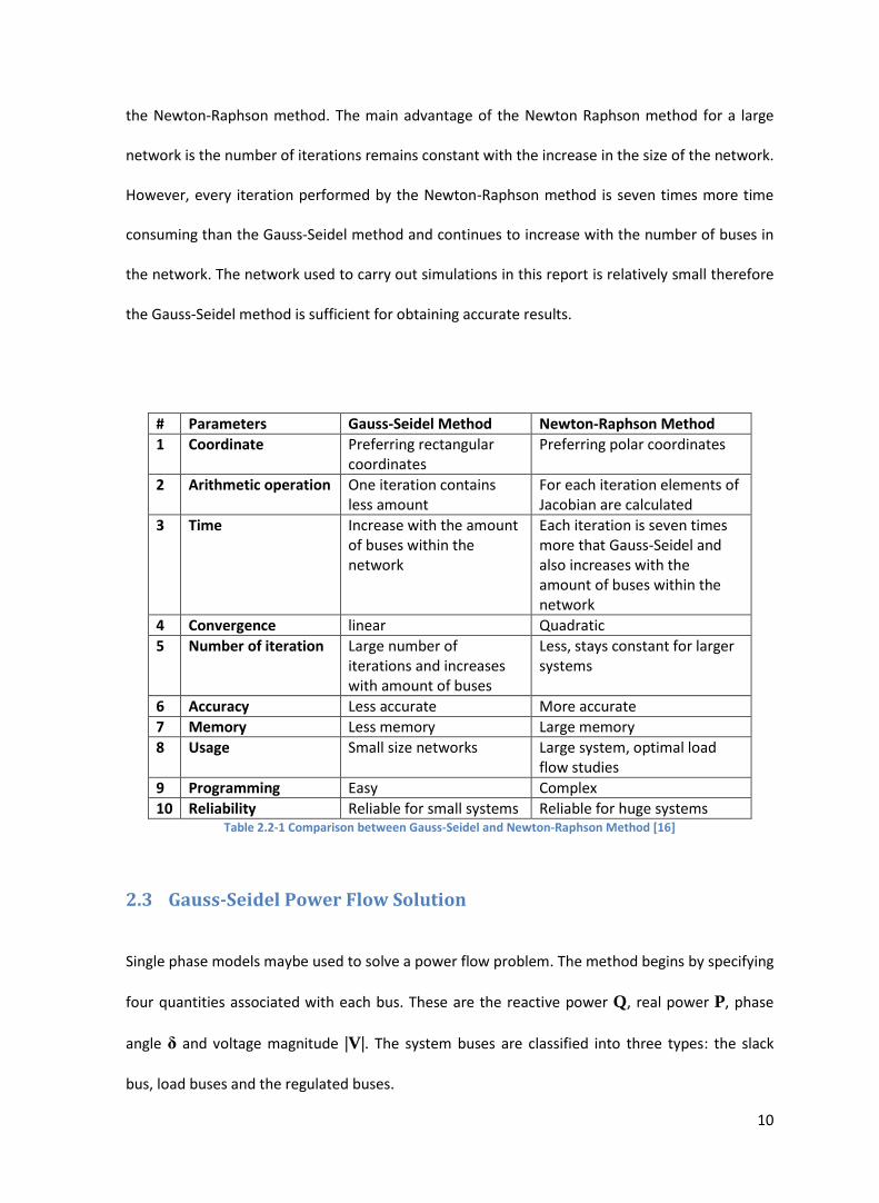
the Newton-Raphson method. The main advantage of the Newton Raphson method for a large

network is the number of iterations remains constant with the increase in the size of the network.

However, every iteration performed by the Newton-Raphson method is seven times more time

consuming than the Gauss-Seidel method and continues to increase with the number of buses in

the network. The network used to carry out simulations in this report is relatively small therefore

the Gauss-Seidel method is sufficient for obtaining accurate results.

# Parameters Gauss-Seidel Method Newton-Raphson Method

1 Coordinate Preferring rectangular coordinates

Preferring polar coordinates

2 Arithmetic operation One iteration contains less amount

For each iteration elements of Jacobian are calculated

3 Time Increase with the amount of buses within the network

Each iteration is seven times more that Gauss-Seidel and also increases with the amount of buses within the network

4 Convergence linear Quadratic

5 Number of iteration Large number of iterations and increases with amount of buses

Less, stays constant for larger systems

6 Accuracy Less accurate More accurate

7 Memory Less memory Large memory

8 Usage Small size networks Large system, optimal load flow studies

9 Programming Easy Complex

10 Reliability Reliable for small systems Reliable for huge systems Table 2.2-1 Comparison between Gauss-Seidel and Newton-Raphson Method [16]

2.3 Gauss-Seidel Power Flow Solution

Single phase models maybe used to solve a power flow problem. The method begins by specifying

four quantities associated with each bus. These are the reactive power Q, real power P, phase

angle δ and voltage magnitude |V|. The system buses are classified into three types: the slack

bus, load buses and the regulated buses.

11

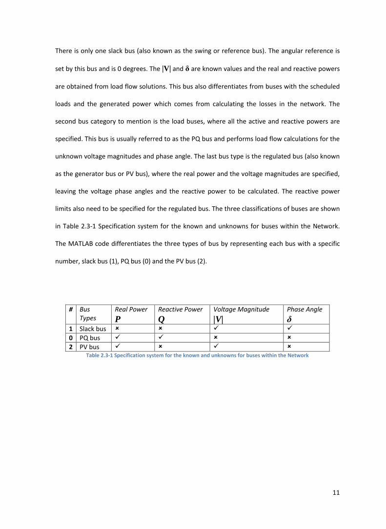
There is only one slack bus (also known as the swing or reference bus). The angular reference is

set by this bus and is 0 degrees. The |V| and δ are known values and the real and reactive powers

are obtained from load flow solutions. This bus also differentiates from buses with the scheduled

loads and the generated power which comes from calculating the losses in the network. The

second bus category to mention is the load buses, where all the active and reactive powers are

specified. This bus is usually referred to as the PQ bus and performs load flow calculations for the

unknown voltage magnitudes and phase angle. The last bus type is the regulated bus (also known

as the generator bus or PV bus), where the real power and the voltage magnitudes are specified,

leaving the voltage phase angles and the reactive power to be calculated. The reactive power

limits also need to be specified for the regulated bus. The three classifications of buses are shown

in Table 2.3-1 Specification system for the known and unknowns for buses within the Network.

The MATLAB code differentiates the three types of bus by representing each bus with a specific

number, slack bus (1), PQ bus (0) and the PV bus (2).

# Bus Types

Real Power

P

Reactive Power

Q

Voltage Magnitude

|V|

Phase Angle

δ

1 Slack bus

0 PQ bus

2 PV bus Table 2.3-1 Specification system for the known and unknowns for buses within the Network

12

3 Optimal Power Flow

The OPF problem was first proposed by Carpentier in 1962 and still remains a fundamental

problem in power systems for today [17]. The main objective of OPF is controlling the generation

and consumption of the network generators and loads while minimizing the generation cost or

power loss in the network. In a practical power system, the networks are highly interconnected

and power plants are not located at the same distance from the various loads. Traditional power

flow analysis does not cater for these conditions. Under normal operating conditions the

generation capacity is more than the total load demand and losses and thus leaves many options

for scheduling generation. The main objective of a power network is to find the real and reactive

power scheduling of each power plant in order to optimise fuel usage and minimise operation

cost. This means having inequality constraints that allow the real and reactive power limits to

abide by the load demand with minimum fuel cost. This is known as an optimal power flow

problem. The cost function, also known as the objective function may include economic cost and

system security or other objectives. Optimal power flow algorithms have been studied by many

researchers using different objective functions and methods [5].

3.1 Basic Concept and Definitions

Generally the production of electric power is a method of harvesting heat energy from a fuel

source and converting it to mechanical energy to produce electricity [18]. A cost function is

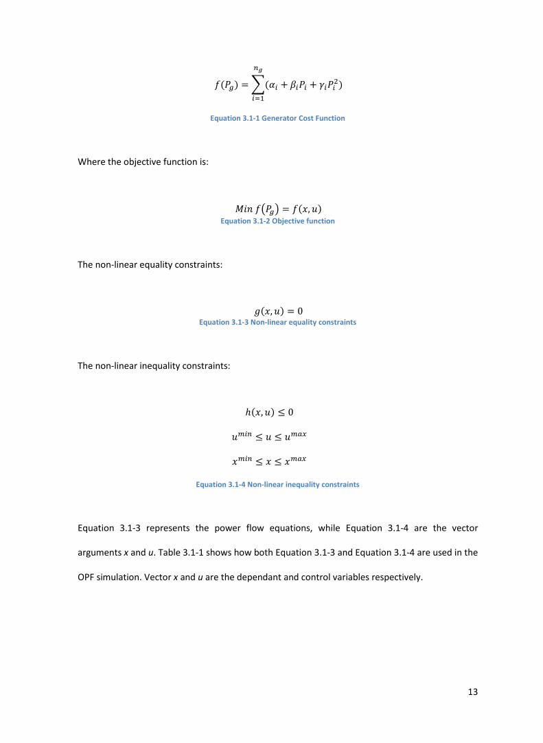
required for each power plant to find the real power generation. The equation for the total

generation cost function is expressed as:

13

( ) ∑(

)

(8)

Equation 3.1-1 Generator Cost Function

Where the objective function is:

( ) ( ) (9) Equation 3.1-2 Objective function

The non-linear equality constraints:

( ) (10) Equation 3.1-3 Non-linear equality constraints

The non-linear inequality constraints:

( )

(11)

(12)

(13)

Equation 3.1-4 Non-linear inequality constraints

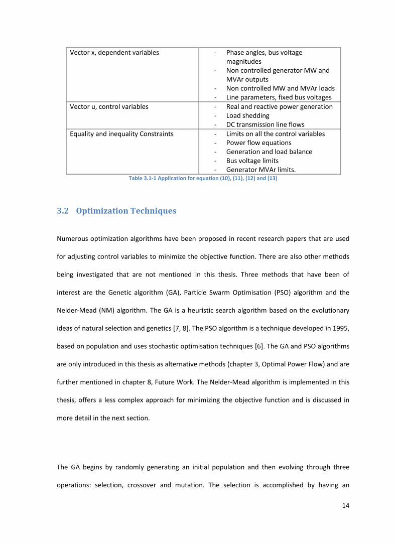
Equation 3.1-3 represents the power flow equations, while Equation 3.1-4 are the vector

arguments x and u. Table 3.1-1 shows how both Equation 3.1-3 and Equation 3.1-4 are used in the

OPF simulation. Vector x and u are the dependant and control variables respectively.

14

Vector x, dependent variables - Phase angles, bus voltage magnitudes

- Non controlled generator MW and MVAr outputs

- Non controlled MW and MVAr loads - Line parameters, fixed bus voltages

Vector u, control variables - Real and reactive power generation - Load shedding - DC transmission line flows

Equality and inequality Constraints - Limits on all the control variables - Power flow equations - Generation and load balance - Bus voltage limits - Generator MVAr limits.

Table 3.1-1 Application for equation (10), (11), (12) and (13)

3.2 Optimization Techniques

Numerous optimization algorithms have been proposed in recent research papers that are used

for adjusting control variables to minimize the objective function. There are also other methods

being investigated that are not mentioned in this thesis. Three methods that have been of

interest are the Genetic algorithm (GA), Particle Swarm Optimisation (PSO) algorithm and the

Nelder-Mead (NM) algorithm. The GA is a heuristic search algorithm based on the evolutionary

ideas of natural selection and genetics [7, 8]. The PSO algorithm is a technique developed in 1995,

based on population and uses stochastic optimisation techniques [6]. The GA and PSO algorithms

are only introduced in this thesis as alternative methods (chapter 3, Optimal Power Flow) and are

further mentioned in chapter 8, Future Work. The Nelder-Mead algorithm is implemented in this

thesis, offers a less complex approach for minimizing the objective function and is discussed in

more detail in the next section.

The GA begins by randomly generating an initial population and then evolving through three

operations: selection, crossover and mutation. The selection is accomplished by having an

15

outcome that results in the survival of the fittest. This gives preference to the stronger individual,

facilitating the carry-over of the genetic material to the next generation. The selection operator

chooses two individuals from the population, where the two genes (represented as eight bits) are

exchanged and from this event an offspring is created and placed into the next generation pool.

During this event a crossover point is selected along the 8 bit string where four bits from each

parent are taken to form the new offspring [7]. Mutation is introduced into the algorithm to

maintain diversity within the population. This is executed by having random bits within the

offspring gene flipped.

The PSO algorithm shares many similarities to the GA. The PSO algorithm begins by generating an

initial population of random solutions and performs a search for an optimal point in the function.

The PSO algorithm differs from the GA due to the absence of any evolution operators such as

crossover and the mutation. The PSO algorithm instead uses particles that fly through the

problem space by following current optimal particles [19]. Comparing PSO with GA, PSO is easier

to implement due to having fewer parameters to adjust.

3.2.1 Nelder-Mead Algorithm

The Nelder-mead algorithm is a heuristic search method that can converge to non-fixed points.

However it is easy to implement compared to GA or PSO and can converge to a broad class of

problems. This technique was proposed first in 1965 by John Nelder and Roger Mead [2]. The

method is based on the concept of a simplex, which is a special polynomial type with N+1 vertices

in N dimensions [20]. Examples of simplexes include:

- Line segment on a line

16

- Triangle on a plane

- Tetrahedron in three dimensional space

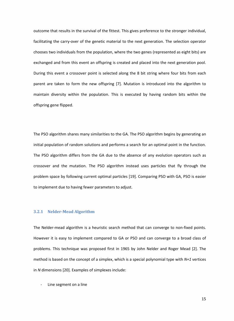
3.2.1.1 Nelder-Mead mathematical Example

A function consisting of two parameters, needs three points to form a triangle and initiate the

calculation involved. The example shown in Figure 3.2-1 uses the vertices (0,1), (0,0) and (1,0).

There are four operations which carry out calculations with the coefficients:

- R =1 (reflection)

- E=2 (expansion)

- K=0.5 (contraction)

- S=0.5 (shrink)

Given n+1 vertices xi, i=1… n+1 and associated function values f(xi).

Figure 3.2-1 Initiating the algorithm with three values (first iteration, displaying new simplex)

- Old simplex refers to the previous calculation values

17

- Sort by function value: Order the vertices to satisfy f(x1) < f2(x2)< … < f(xn+1)

- Calculate xm = Σ xi (averaging all the points leaving out the worst point)

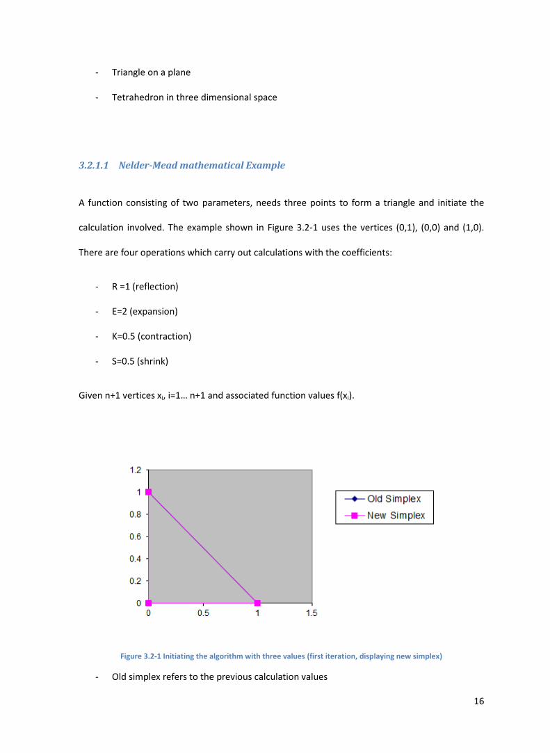
- Reflection. Compute xr = xm + R(xm-xn+1) and evaluate f(xr). If f(x1)< f(xr)< f(xn) accept xr and

terminate the iteration, refer to Figure 3.2-2.

Figure 3.2-2 Reflection after third iteration

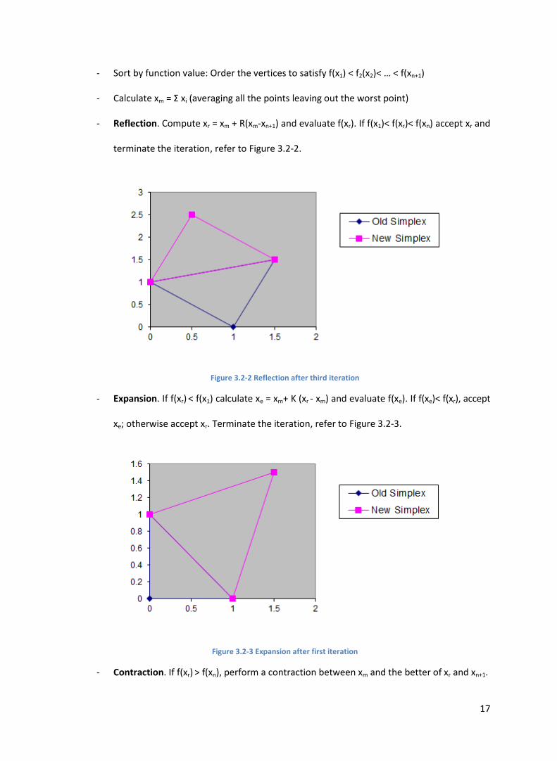
- Expansion. If f(xr) < f(x1) calculate xe = xm+ K (xr - xm) and evaluate f(xe). If f(xe)< f(xr), accept

xe; otherwise accept xr. Terminate the iteration, refer to Figure 3.2-3.

Figure 3.2-3 Expansion after first iteration

- Contraction. If f(xr) > f(xn), perform a contraction between xm and the better of xr and xn+1.

18

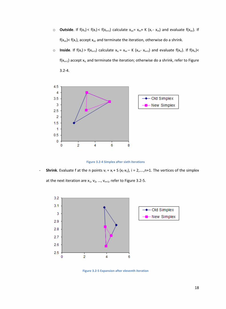
o Outside. If f(xn) < f(xr) < f(xn+1) calculate xoc= xm+ K (xr - xm) and evaluate f(xoc). If

f(xoc)< f(xr), accept xoc and terminate the iteration, otherwise do a shrink.

o Inside. If f(xr) > f(xn+1) calculate xic = xm – K (xm- xn+1) and evaluate f(xic). If f(xic)<

f(xn+1) accept xic and terminate the iteration; otherwise do a shrink, refer to Figure

3.2-4.

Figure 3.2-4 Simplex after sixth iterations

- Shrink. Evaluate f at the n points vi = xi + S (xi-x1), i = 2,….,n+1. The vertices of the simplex

at the next iteration are x1, v2, …, vn+1, refer to Figure 3.2-5.

Figure 3.2-5 Expansion after eleventh iteration

19

An hyphenate illustration of the example shown here is demonstrated in [20]. The table includes

the new values that are calculated for each iteration and the operation that is decided for each

iteration. The graphical representation of the algorithm from the first iteration to the last

iteration when convergence is found, is also shown in figure 6.1a of [20].

20

4 Stability

Power systems have evolved from the central generating stations concept to extremely complex

interconnected systems with technological computing advances. The improvements in digital

computing over the last few decades have drastically altered the techniques used for power

system analysis [21]. This section gives a general description of power system stability including

physical concepts and classification, in addition to analysis of fundamental stability properties.

The emergence of different forms of stability problems and the methods of analysis are broadly

presented.

Before this however, it is useful to consider the following definition:

‘Power-system stability is a term applied to alternating-current electric power systems, denoting

a condition in which the various synchronous machines of the system remain in synchronism, or

“in step,” with each other. Conversely, instability denotes a condition involving loss of

synchronism, or falling “out of step”.’ [22]

4.1 Power System Stability

Power system stability is defined as the property of a power system that permits it to remain in a

state of equilibrium under normal conditions and when subjected to a disturbance has the ability

to swiftly regain that equilibrium [4]. The main focus regarding system stability in this thesis is

influenced by the dynamics of generator rotor angles and power-angle relationships. This has also

been the traditional stability problem concerned with maintaining synchronous operation.

21

Additional cases of instability can also be faced without losing synchronisation. The control of

voltage and stability becomes a concern when there is a collapse of voltage at the load from a

network consisting of an induction motor that is fed by a synchronous generator through a

transmission line [4].

The overall concept of stability can also be described as the way in which a power system behaves

when subjected to a transient disturbance. These transient disturbances can range from small to

large in nature. The collapse of the voltage at the load in a network described as a small

disturbance is generally a common occurrence in a network. A system needs to be capable of

operating under the dynamics of the load changing conditions as well as supply the maximum

amount of power to the load. Secondly a system must also be capable of operating and remain in

synchronised when a severe disturbance is encountered. These include loss of a large generator

or load, loss of a tie between two systems and a short circuit on a transmission line [4].

4.1.1 History on Power System Stability

The issue of stability was first recognised by engineers in 1920’s [3]. This led to laboratory testing

of miniature systems in 1924 followed by field tests on the stability of a practical power systems

in 1925. Theoretical work carried out in the 1930’s was based on networks that consisted of

generators composed of simple voltage sources behind fixed reactance with constant impedances

for loads. These theoretical calculations were a necessity given the computational tools available

during this time period [4].

22

4.1.2 Classification of Stability

As described in the previous section, the instability of a power system can take different forms

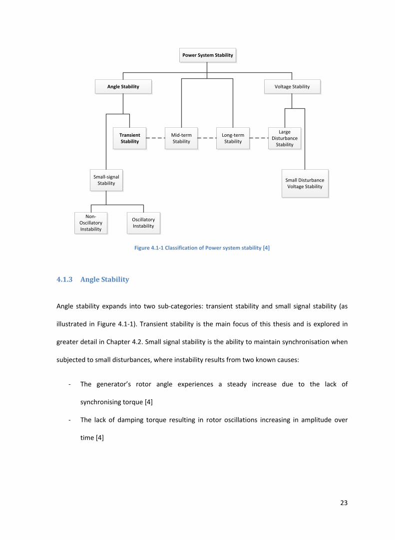
and needs to be broken down into subclasses. Figure 4.1-1 Classification of Power system stability

[4], provides a clear breakdown of power system stability in the form of an axonomical diagram.

This classification illustrates two main classes of stability: angle stability and voltage stability [4].

Angle stability is sub classified into two categories: small-signal (steady state) stability and

transient stability. A steady state power system is one in which the operating condition returns to

steady state (or near the operating point), after being subjected to a small disturbance. The mid-

term stability and long-term stability are newer concepts which have been introduced in more

recent literature. Mid-term stability concentrates on synchronising power oscillations between

different machines [4]. This includes severe upsets: large voltage and frequency excursions, with a

study period of up to several minutes. Long term stability concentrates on large scale system

upsets and as a result sustaining mismatches between generation and consumption of active and

reactive power [4].

23

Power System Stability

Small Disturbance Voltage Stability

Angle Stability Voltage Stability

Transient Stability

Small-signal Stability

Non-Oscillatory Instability

Oscillatory Instability

Mid-term Stability

Long-term Stability

Large Disturbance

Stability

Figure 4.1-1 Classification of Power system stability [4]

4.1.3 Angle Stability

Angle stability expands into two sub-categories: transient stability and small signal stability (as

illustrated in Figure 4.1-1). Transient stability is the main focus of this thesis and is explored in

greater detail in Chapter 4.2. Small signal stability is the ability to maintain synchronisation when

subjected to small disturbances, where instability results from two known causes:

- The generator’s rotor angle experiences a steady increase due to the lack of

synchronising torque [4]

- The lack of damping torque resulting in rotor oscillations increasing in amplitude over

time [4]

24

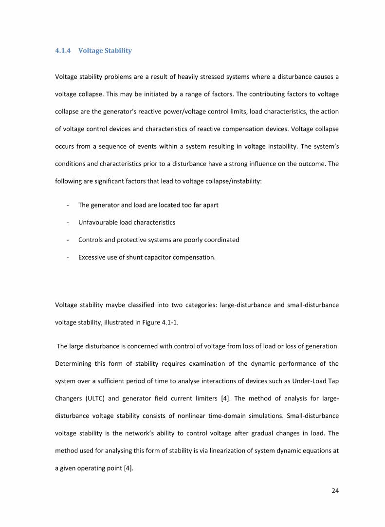
4.1.4 Voltage Stability

Voltage stability problems are a result of heavily stressed systems where a disturbance causes a

voltage collapse. This may be initiated by a range of factors. The contributing factors to voltage

collapse are the generator’s reactive power/voltage control limits, load characteristics, the action

of voltage control devices and characteristics of reactive compensation devices. Voltage collapse

occurs from a sequence of events within a system resulting in voltage instability. The system’s

conditions and characteristics prior to a disturbance have a strong influence on the outcome. The

following are significant factors that lead to voltage collapse/instability:

- The generator and load are located too far apart

- Unfavourable load characteristics

- Controls and protective systems are poorly coordinated

- Excessive use of shunt capacitor compensation.

Voltage stability maybe classified into two categories: large-disturbance and small-disturbance

voltage stability, illustrated in Figure 4.1-1.

The large disturbance is concerned with control of voltage from loss of load or loss of generation.

Determining this form of stability requires examination of the dynamic performance of the

system over a sufficient period of time to analyse interactions of devices such as Under-Load Tap

Changers (ULTC) and generator field current limiters [4]. The method of analysis for large-

disturbance voltage stability consists of nonlinear time-domain simulations. Small-disturbance

voltage stability is the network’s ability to control voltage after gradual changes in load. The

method used for analysing this form of stability is via linearization of system dynamic equations at

a given operating point [4].

25

4.2 Transient Stability

This section details how transient stability is analysed when the network encounters a

disturbance. It begins with a description of the swing equation and includes a mathematical

example (equal area criterion) to illustrate the effects on the rotor of a generator from pre-fault

to during fault and finally to a post fault condition.

The next section explains how the second order swing equation is transformed into two first

order equations using numerical integration. As a result, illustrating how the equation is solved

more efficiently. Finally, the concept of stability margin is introduced, which is very important in

finding suitable power values for the network generators and in maintaining stability.

4.2.1 Swing Equation

The swing equation of a synchronous machine is used to analyse the steady state stability of a

power system. Consider a system operating under normal conditions, where the relative position

of the rotor axis and resultant magnetic field axis are fixed. The angle between these two

positions is known as the power angle. At the time of a disturbance the rotor will either

accelerate or decelerate with respect to the synchronously rotating air gap magneto motive

force, resulting in a relative motion. The equation describing this motion is known as the Swing

Equation [5]. The response of the rotor is the determining factor on whether the system falls back

into a stable state or becomes unstable after a disturbance in the network. The swing equation

includes the inertia H, frequency fo, the mechanical power Pm and the electrical power Pe. One

means of solving this second order equation is using a numerical method (trapezoidal Rule) which

is explained later in this chapter.

26

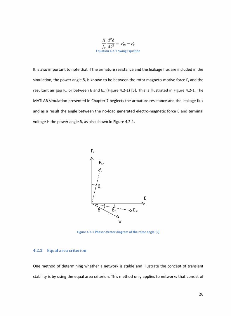
(14)

Equation 4.2-1 Swing Equation

It is also important to note that if the armature resistance and the leakage flux are included in the

simulation, the power angle δr is known to be between the rotor magneto-motive force Fr and the

resultant air gap Fsr or between E and Esr (Figure 4.2-1) [5]. This is illustrated in Figure 4.2-1. The

MATLAB simulation presented in Chapter 7 neglects the armature resistance and the leakage flux

and as a result the angle between the no-load generated electro-magnetic force E and terminal

voltage is the power angle δ, as also shown in Figure 4.2-1.

Figure 4.2-1 Phasor-Vector diagram of the rotor angle [5]

4.2.2 Equal area criterion

One method of determining whether a network is stable and illustrate the concept of transient

stability is by using the equal area criterion. This method only applies to networks that consist of

27

a one machine system connected to an infinite bus or a two machine system [5]. This provides a

graphical interpretation of the energy stored in the rotating mass and gives a quick prediction of

the system’s stability. As the name suggests, two areas are calculated by integrating the swing

equation to determine the state of the network after the disturbance.

The first area A1 is integrated from the equilibrium state δ0 (Pm=Pe) to a sudden change in the

input power (an example can be a fault in the transmission line) which results in having the rotor

angle increased (accelerate) to δ1. The second area A2 is calculated from the δ1 to the δmax (when

the rotor begins to decelerate). The conditions for the network are [5]:

- A1>A2: where the acceleration is larger than the deceleration the system is known as

unstable.

- A1<A2: when the acceleration is smaller than the deceleration, the system is found to

eventually reach the stable state.

- A1=A2: when the acceleration is equal to the deceleration, the condition of the generator

is defined as on the verge of stability.

4.2.3 Transient Stability using Numerical Integration

Integration is the process of measuring the area under a function plotted on a graph, with a

function f(x) being the integrand and having limits ‘a’ and ‘b’ for the lower and upper limits of

integration [23]. The method for calculating the stability is commonly done via integration of the

swing equation, however to include stability constraints into the OPF problem, numerical

integration is used [3].

28

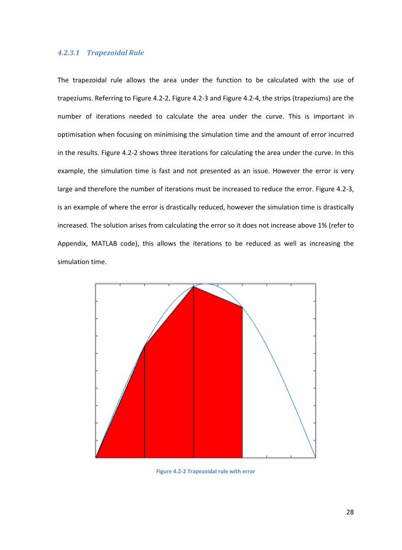
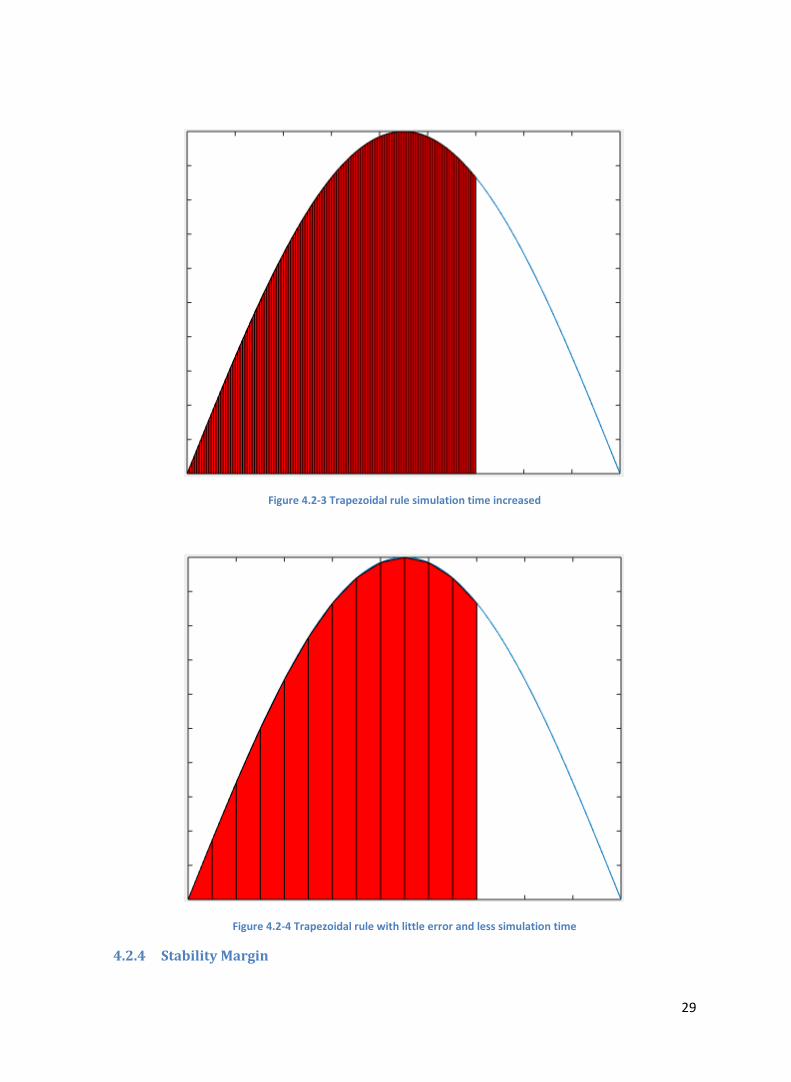
4.2.3.1 Trapezoidal Rule

The trapezoidal rule allows the area under the function to be calculated with the use of

trapeziums. Referring to Figure 4.2-2, Figure 4.2-3 and Figure 4.2-4, the strips (trapeziums) are the

number of iterations needed to calculate the area under the curve. This is important in

optimisation when focusing on minimising the simulation time and the amount of error incurred

in the results. Figure 4.2-2 shows three iterations for calculating the area under the curve. In this

example, the simulation time is fast and not presented as an issue. However the error is very

large and therefore the number of iterations must be increased to reduce the error. Figure 4.2-3,

is an example of where the error is drastically reduced, however the simulation time is drastically

increased. The solution arises from calculating the error so it does not increase above 1% (refer to

Appendix, MATLAB code), this allows the iterations to be reduced as well as increasing the

simulation time.

Figure 4.2-2 Trapezoidal rule with error

29

Figure 4.2-3 Trapezoidal rule simulation time increased

Figure 4.2-4 Trapezoidal rule with little error and less simulation time

4.2.4 Stability Margin

30

A solution for the stability constraint is outlined in “Stability Constraint Optimal Power Flow” [3].

This paper uses the rotor angle to specify whether or not the system is stable. This is found to be

consistent with industry practice by utility engineers. However, there has been no general

method for measuring the stability region of dynamic systems.

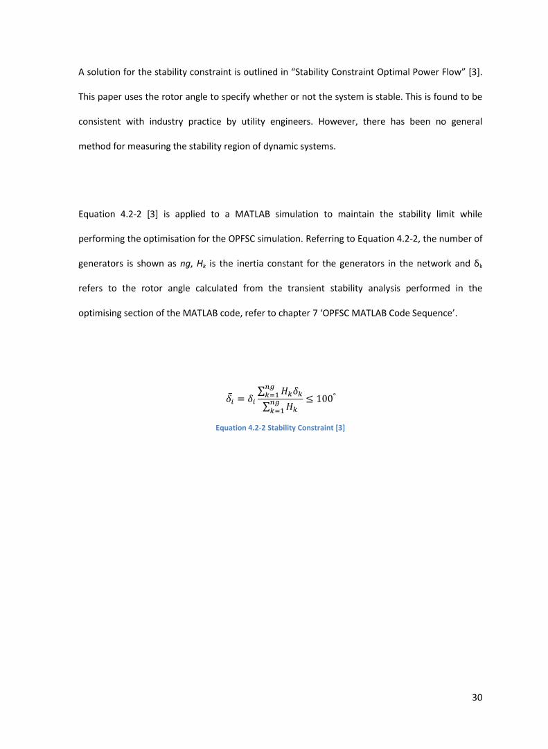
Equation 4.2-2 [3] is applied to a MATLAB simulation to maintain the stability limit while

performing the optimisation for the OPFSC simulation. Referring to Equation 4.2-2, the number of

generators is shown as ng, Hk is the inertia constant for the generators in the network and δk

refers to the rotor angle calculated from the transient stability analysis performed in the

optimising section of the MATLAB code, refer to chapter 7 ‘OPFSC MATLAB Code Sequence’.

∑

∑

(15)

Equation 4.2-2 Stability Constraint [3]

31

5 Test System

The network being analysed is the WSCC 9-bus test case which is a simple approximation of the

Western System Coordinating Council with a comparable system of nine buses and three

generators [24]. PowerFactory has an example of the network readily available for analysing

different simulation scenarios. However, the network is constructed in MATLAB using techniques

taken from [5]. For purposes of this thesis, the network is used in parallel with the MATLAB

simulation to facilitate comparison of results and simulation outcomes.

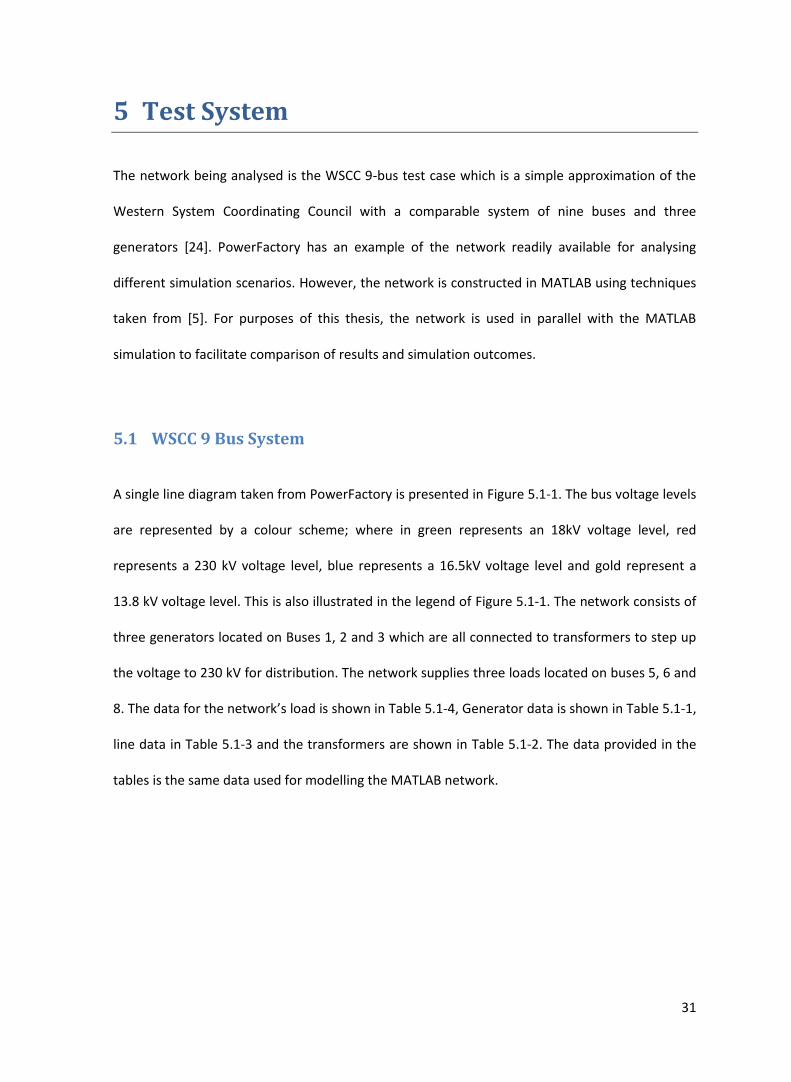
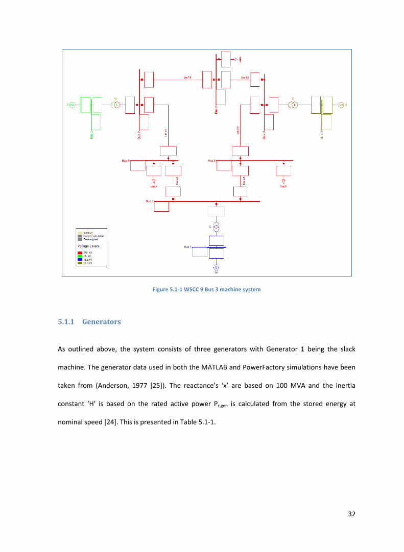
5.1 WSCC 9 Bus System

A single line diagram taken from PowerFactory is presented in Figure 5.1-1. The bus voltage levels

are represented by a colour scheme; where in green represents an 18kV voltage level, red

represents a 230 kV voltage level, blue represents a 16.5kV voltage level and gold represent a

13.8 kV voltage level. This is also illustrated in the legend of Figure 5.1-1. The network consists of

three generators located on Buses 1, 2 and 3 which are all connected to transformers to step up

the voltage to 230 kV for distribution. The network supplies three loads located on buses 5, 6 and

8. The data for the network’s load is shown in Table 5.1-4, Generator data is shown in Table 5.1-1,

line data in Table 5.1-3 and the transformers are shown in Table 5.1-2. The data provided in the

tables is the same data used for modelling the MATLAB network.

32

Figure 5.1-1 WSCC 9 Bus 3 machine system

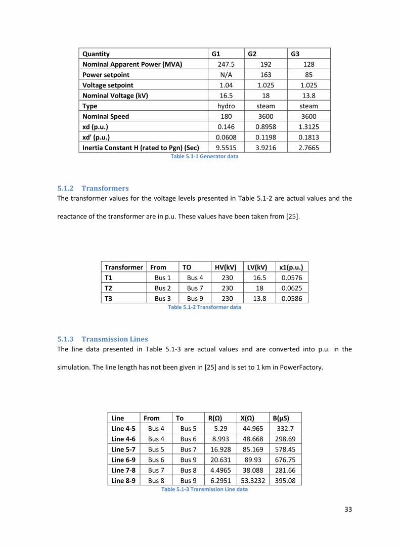
5.1.1 Generators

As outlined above, the system consists of three generators with Generator 1 being the slack

machine. The generator data used in both the MATLAB and PowerFactory simulations have been

taken from (Anderson, 1977 [25]). The reactance’s ‘x’ are based on 100 MVA and the inertia

constant ‘H’ is based on the rated active power Pr,gen is calculated from the stored energy at

nominal speed [24]. This is presented in Table 5.1-1.

33

Quantity G1 G2 G3

Nominal Apparent Power (MVA) 247.5 192 128

Power setpoint N/A 163 85

Voltage setpoint 1.04 1.025 1.025

Nominal Voltage (kV) 16.5 18 13.8

Type hydro steam steam

Nominal Speed 180 3600 3600

xd (p.u.) 0.146 0.8958 1.3125

xd' (p.u.) 0.0608 0.1198 0.1813

Inertia Constant H (rated to Pgn) (Sec) 9.5515 3.9216 2.7665 Table 5.1-1 Generator data

5.1.2 Transformers

The transformer values for the voltage levels presented in Table 5.1-2 are actual values and the

reactance of the transformer are in p.u. These values have been taken from [25].

Transformer From TO HV(kV) LV(kV) x1(p.u.)

T1 Bus 1 Bus 4 230 16.5 0.0576

T2 Bus 2 Bus 7 230 18 0.0625

T3 Bus 3 Bus 9 230 13.8 0.0586 Table 5.1-2 Transformer data

5.1.3 Transmission Lines

The line data presented in Table 5.1-3 are actual values and are converted into p.u. in the

simulation. The line length has not been given in [25] and is set to 1 km in PowerFactory.

Line From To R(Ω) X(Ω) B(μS)

Line 4-5 Bus 4 Bus 5 5.29 44.965 332.7

Line 4-6 Bus 4 Bus 6 8.993 48.668 298.69

Line 5-7 Bus 5 Bus 7 16.928 85.169 578.45

Line 6-9 Bus 6 Bus 9 20.631 89.93 676.75

Line 7-8 Bus 7 Bus 8 4.4965 38.088 281.66

Line 8-9 Bus 8 Bus 9 6.2951 53.3232 395.08 Table 5.1-3 Transmission Line data

34

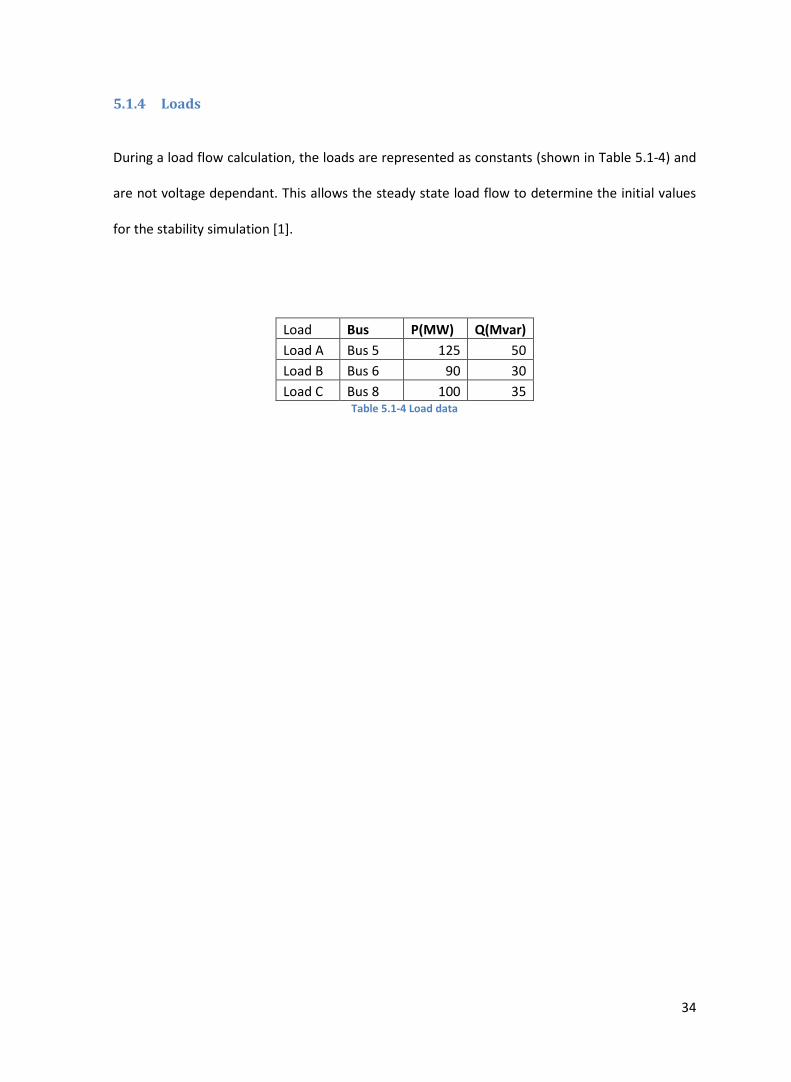
5.1.4 Loads

During a load flow calculation, the loads are represented as constants (shown in Table 5.1-4) and

are not voltage dependant. This allows the steady state load flow to determine the initial values

for the stability simulation [1].

Load Bus P(MW) Q(Mvar)

Load A Bus 5 125 50

Load B Bus 6 90 30

Load C Bus 8 100 35 Table 5.1-4 Load data

35

6 PowerFactory –Transient Stability Analysis

PowerFactory is used to compare the results with the MATLAB simulation. The steps involved in

performing a transient stability simulation are described in this section.

6.1 Step 1: Load Flow Calculations

Upon starting PowerFactory a window called PowerFactory Examples appears and from the tab

option, Examples from Literature, gives access to the 9 Bus System.

The first requirement for the simulation is to perform a LF analysis. This is important because in

order to carry any transient stability analysis, the simulation requires initial conditions. The load

flow can be carried out via the Calculation menu by selecting Load Flow, the shortcut key ctrl+F10

can also be used. In the Load Flow option window, under Calculation Method the AC Load Flow,

balanced, positive sequence must be selected.

6.2 Step 2 Defining Events

The MATLAB simulation for the thesis has used a fault scenario that occurs at bus 5, opening the

line 5-7 (from bus 5 to bus 7) as the post fault scenario. In PowerFactory, this is accomplished by

firstly defining a short-circuit event followed by a switch event. A detailed description is provided

below:

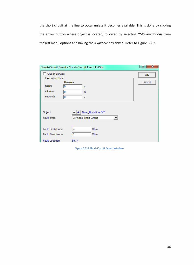
- For the short circuit event Right Click on line 5-7 from the Single Line Diagram, selecting

Define and then selecting Short-Circuit Event. This is shown in Figure 6.2-1, and nothing

for this event requires alteration. It is important to note, that the network will not allow

36

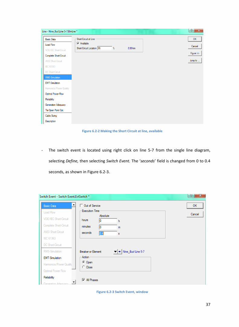
the short circuit at the line to occur unless it becomes available. This is done by clicking

the arrow button where object is located, followed by selecting RMS-Simulations from

the left menu options and having the Available box ticked. Refer to Figure 6.2-2.

Figure 6.2-1 Short-Circuit Event, window

37

Figure 6.2-2 Making the Short Circuit at line, available

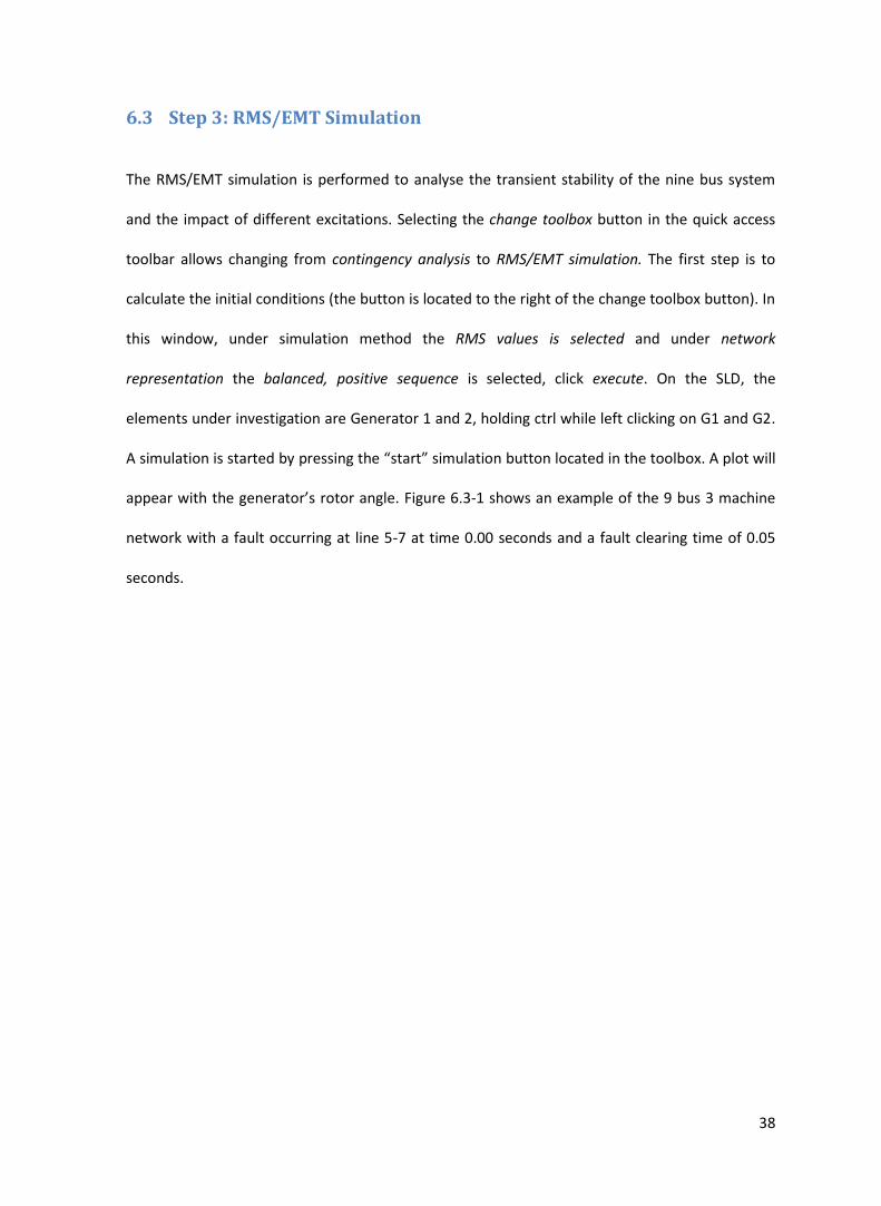
- The switch event is located using right click on line 5-7 from the single line diagram,

selecting Define, then selecting Switch Event. The ‘seconds’ field is changed from 0 to 0.4

seconds, as shown in Figure 6.2-3.

Figure 6.2-3 Switch Event, window

38

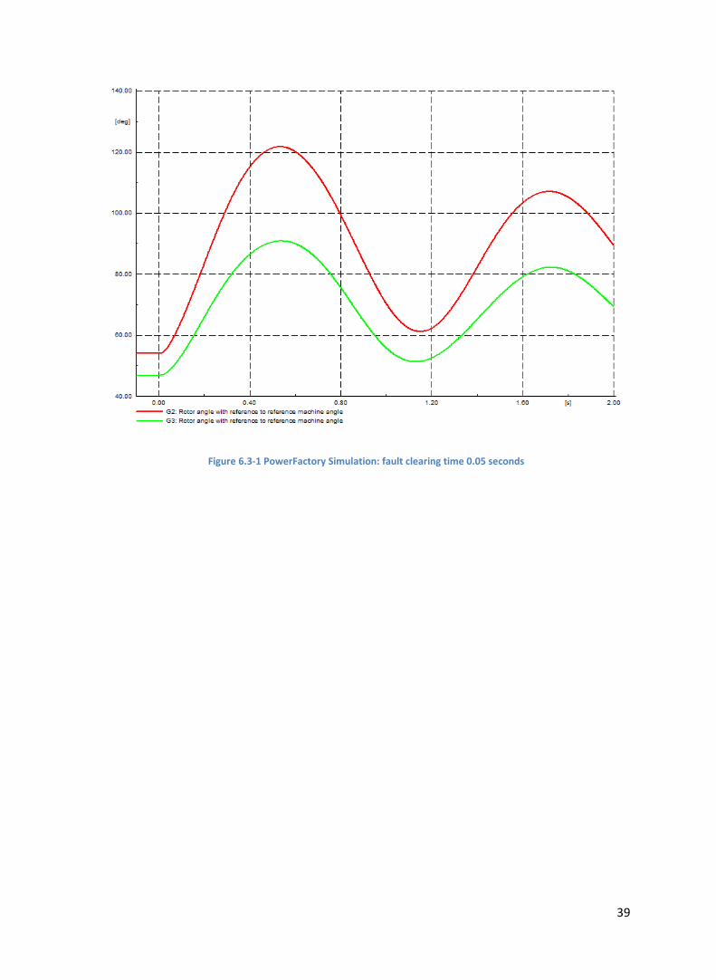
6.3 Step 3: RMS/EMT Simulation

The RMS/EMT simulation is performed to analyse the transient stability of the nine bus system

and the impact of different excitations. Selecting the change toolbox button in the quick access

toolbar allows changing from contingency analysis to RMS/EMT simulation. The first step is to

calculate the initial conditions (the button is located to the right of the change toolbox button). In

this window, under simulation method the RMS values is selected and under network

representation the balanced, positive sequence is selected, click execute. On the SLD, the

elements under investigation are Generator 1 and 2, holding ctrl while left clicking on G1 and G2.

A simulation is started by pressing the “start” simulation button located in the toolbox. A plot will

appear with the generator’s rotor angle. Figure 6.3-1 shows an example of the 9 bus 3 machine

network with a fault occurring at line 5-7 at time 0.00 seconds and a fault clearing time of 0.05

seconds.

39

Figure 6.3-1 PowerFactory Simulation: fault clearing time 0.05 seconds

40

7 Results

This chapter is a summary of the results from the simulations performed. Beginning with an

explanation of the methodology involved using MATLAB simulations followed by detailed

description of the code itself and the three scenarios of interest three scenarios, LF, OPF and

OPFSC. PowerFactory is used to simulation these three scenarios to compare the MATLAB results.

Flow diagrams representing the sequence of the three scenarios are explained culminating in a

result breakdown and analysis.

7.1 Methodology

The code can be divided into three main components beginning with Load flow analysis followed

by optimisation calculations and finally the stability analysis. The first step involves performing a

Load Flow analysis. The main purpose of the load flow analysis being to allow the network

equations to be executed systematically. The method used to solve the network’s power flow

equations is the Gauss-Seidel method. The optimisation is executed using the fminsearch function

provided within MATLAB. This section of the program also includes the inequality and equality

constraints for optimising the cost function described in chapter 3. The final component is the

stability analysis and is located within the optimiser function code. This analysis is based around

the rotor angle calculations, when the system is faced with a disturbance and so pre-fault, fault

and post-fault calculations are needed in order to ensure the stability margin constraint is met.

41

7.1.1 Load Flow Calculations – Gauss-Seidel Method

The Load flow calculations are divided into four main stages, beginning with the input of the

network data, forming the bus admittance matrix followed by Load flow calculations using the

Gauss-Seidel method and concluding with the computation of the line flow and losses.

The first stage involves constructing the network data which is presented as two matrices: bus

data and the line data. This forms the constants that are needed in the next two stages of the

load flow calculations. The bus admittance matrix forms an overall matrix of the network to

perform load flow calculations and is size dependent. For example, a network that consists of 5

buses will form a matrix size of 5x5.

The next stage encompasses executing the Gauss-Seidel calculations using the bus matrix formed

in the previous stage as well as obtaining the necessary network data. As discussed in Chapter 8

Future Work, the Gauss-Seidel method m. file can be replaced with a Newton-Raphson method m.

file if the same format of obtaining network data is followed. Finally, the line flow and losses are

calculated and displayed. A full description and illustration of the sequence can be accessed by

referring to (Saadat, 2010 [5]).

42

7.1.2 Optimisation Calculations – Nelder-Mead Algorithm

The optimisation is obtained using the fminsearch function provided by MATLAB. This uses the

Nelder-Mead simplex (direct search) method. The fminsearch function needs initial values for the

optimisation to begin. These initial values are obtained from the Gauss-Seidel LF solution.

Optimset allows setting the operator to set conditions for the optimisation. The two main

conditions used are to set the maximum allowance of iterations and to plot the cost function per

iteration. This is applied to the two simulations performed, OPF and OPFSC described later in this

chapter. The main purpose of plotting the cost function is to provide feedback on the number of

iterations needed to obtain the generator dispatch values and then to set the maximum iterations

for the simulation. This technique becomes important when trying to minimize the amount of

time needed to optimise a solution. The Optimiser refers to a cost m.file that consists of the cost

function for all three generators within the network and the constraints for the stability (only for

the OPFSC simulation), the generator limits, the calculation of line losses and the network power

demand.

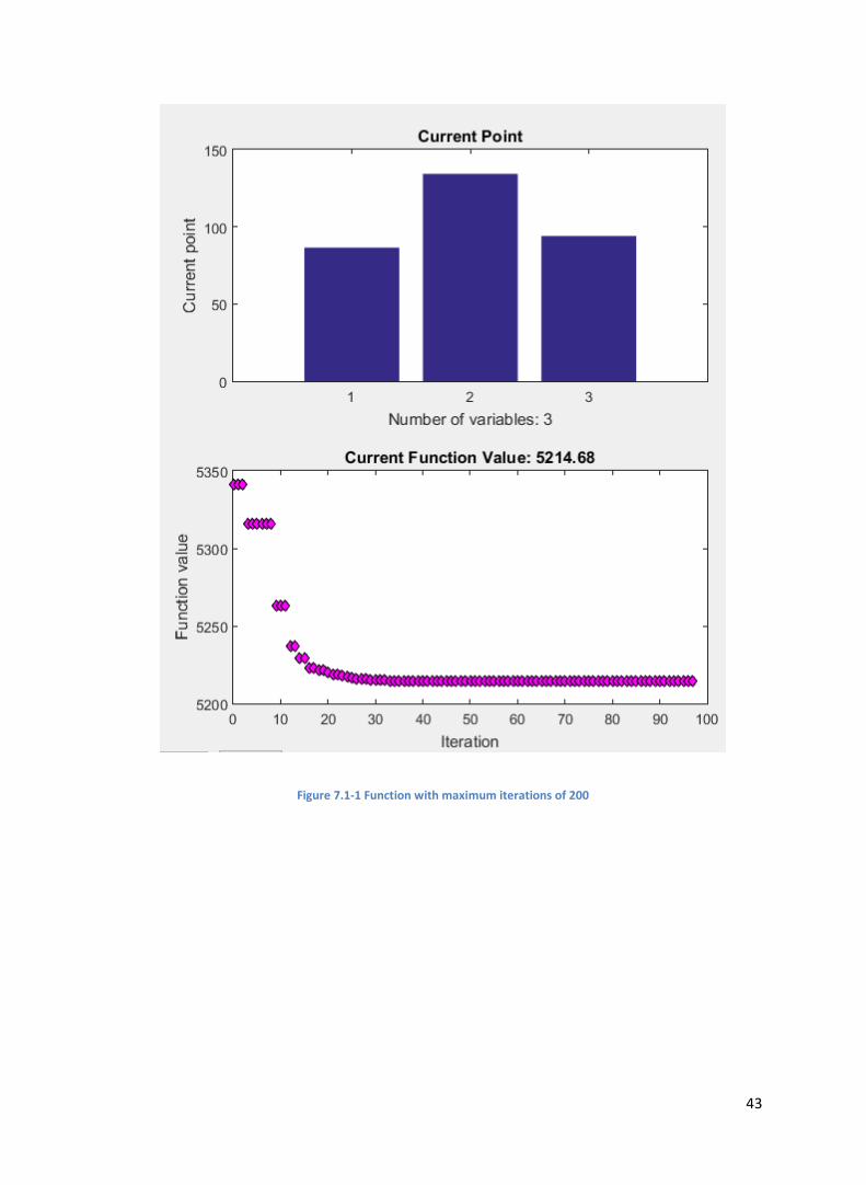
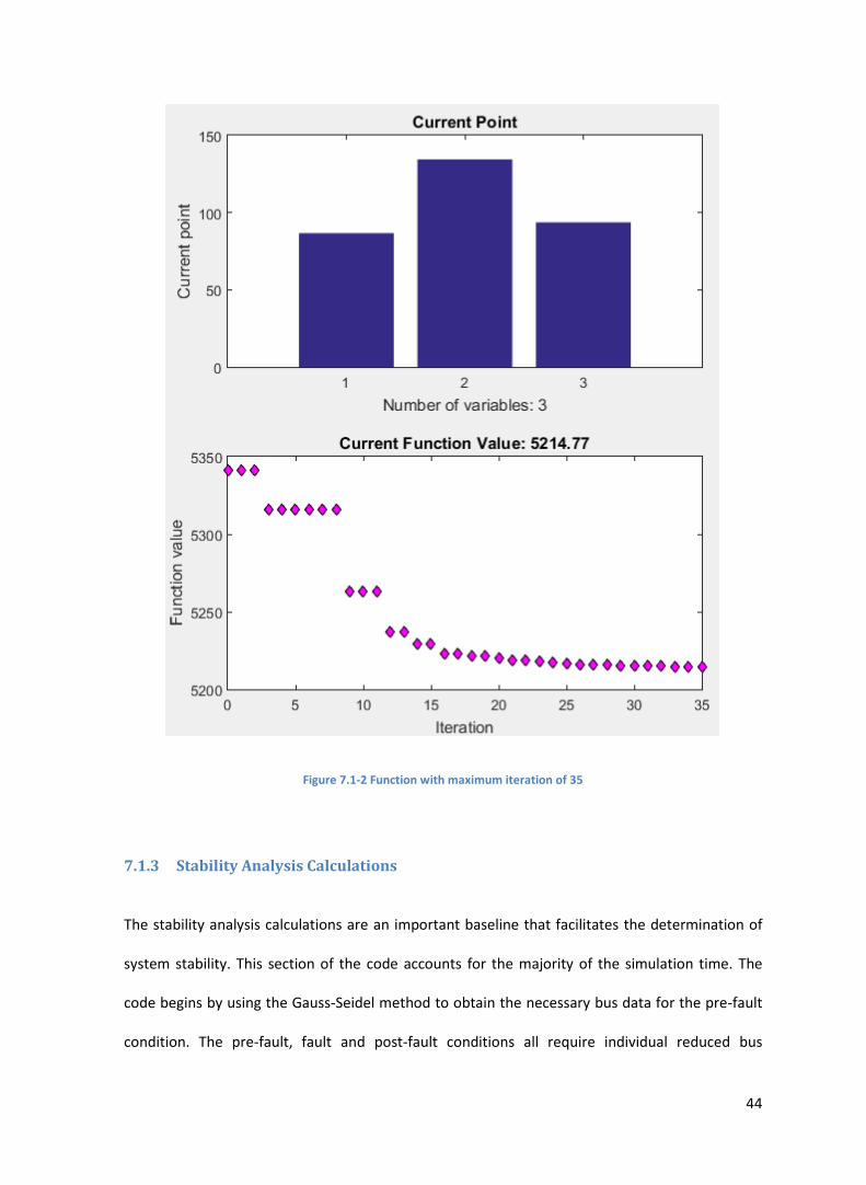
The optimisation function allows the number of iterations to be controlled, leading to improved

time efficiency provided it has converged. Figure 7.1-1 illustrates the iteration set to a maximum

of 200 and the function value at 5214.68 (the ‘current point’ on the y-axis of the bar graph refer

to the magnitude of the real power values for generator 1,2 and 3). In the absence of limiting the

number of iterations, the simulation is very time consuming. However, Figure 7.1-2 illustrates

when the number of iterations is limited to 35 with the function value at 5214.77 the simulation

time is significantly reduced yet the function differences are negligible.

43

Figure 7.1-1 Function with maximum iterations of 200

44

Figure 7.1-2 Function with maximum iteration of 35

7.1.3 Stability Analysis Calculations

The stability analysis calculations are an important baseline that facilitates the determination of

system stability. This section of the code accounts for the majority of the simulation time. The

code begins by using the Gauss-Seidel method to obtain the necessary bus data for the pre-fault

condition. The pre-fault, fault and post-fault conditions all require individual reduced bus

45

matrices to carry out the rotor angle calculations (refer to the Appendix). Prior to the fault

calculations in the code, the bus at where the fault occurs is defined. During the post fault

calculation, the line that is cleared (bus from, bus to) is also defined. The electrical power and

mechanical power for each individual generator are used to calculate the rotor angle using the

ODE23t (this uses the trapezoidal rule) function provided by MATLAB. The total time span for the

calculation of the rotor angle (ODE23t) is reduced to 0.2 seconds after the fault occurs, instead of

the recommended two periods [24]. This reduces the simulation time dramatically. The result of

the time differences is shown in chapter 7.3. The final segment calculates the rotor angle

constraint in order to determine if the system’s real power values needs further optimisation.

7.2 LF, OPF and OPFSC Simulations

There are three different simulations applied in the program, comparing three different scenarios

and results obtained when the network encounters a disturbance. These include Load Flow,

Optimal Power Flow and Optimal Power Flow with Stability constraints. The three simulations are

all adaptations of one another. The LF is the simplest form of code. This forms the base platform

for the OPF code with the addition of the optimising calculations and finally the OPF is elaborated

into the OPFSC code including the additional stability analysis and stability constraints

calculations.

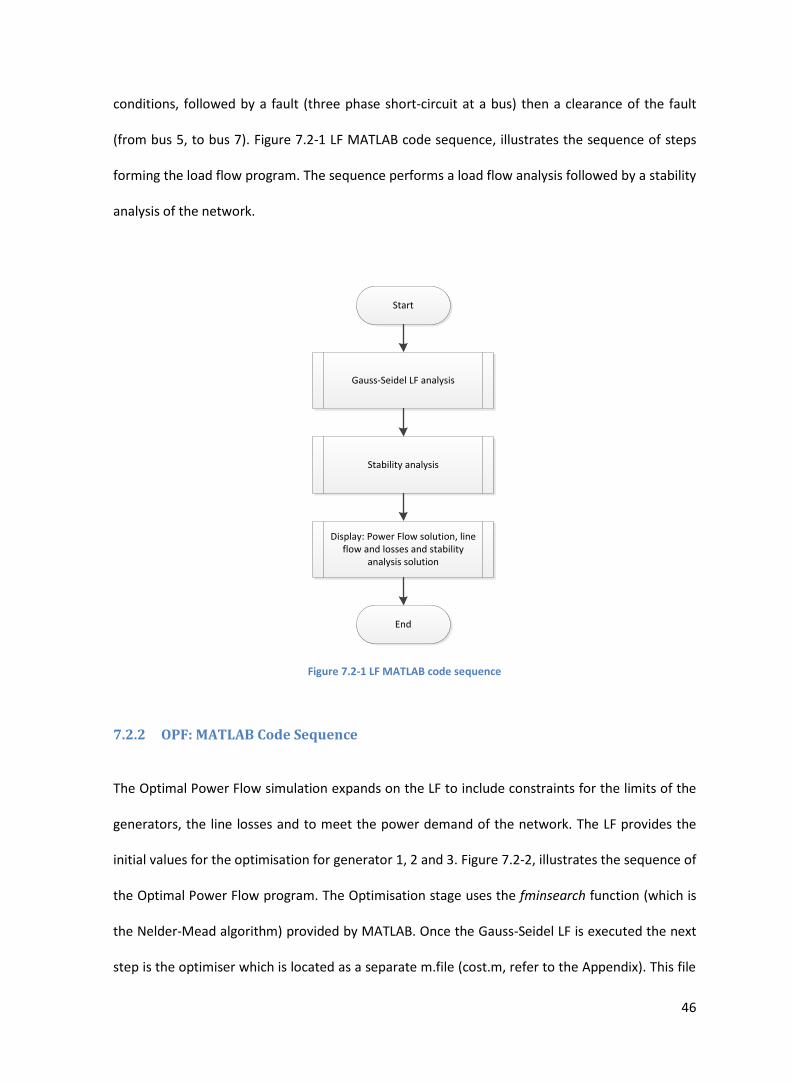
7.2.1 LF: MATLAB Code Sequence

The load flow simulation consists of the calculations of the Gauss-Seidel method, followed by a

stability analysis. This scenario illustrates how the system behaves when operating under normal

46

conditions, followed by a fault (three phase short-circuit at a bus) then a clearance of the fault

(from bus 5, to bus 7). Figure 7.2-1 LF MATLAB code sequence, illustrates the sequence of steps

forming the load flow program. The sequence performs a load flow analysis followed by a stability

analysis of the network.

Start

Gauss-Seidel LF analysis

Stability analysis

Display: Power Flow solution, line flow and losses and stability

analysis solution

End

Figure 7.2-1 LF MATLAB code sequence

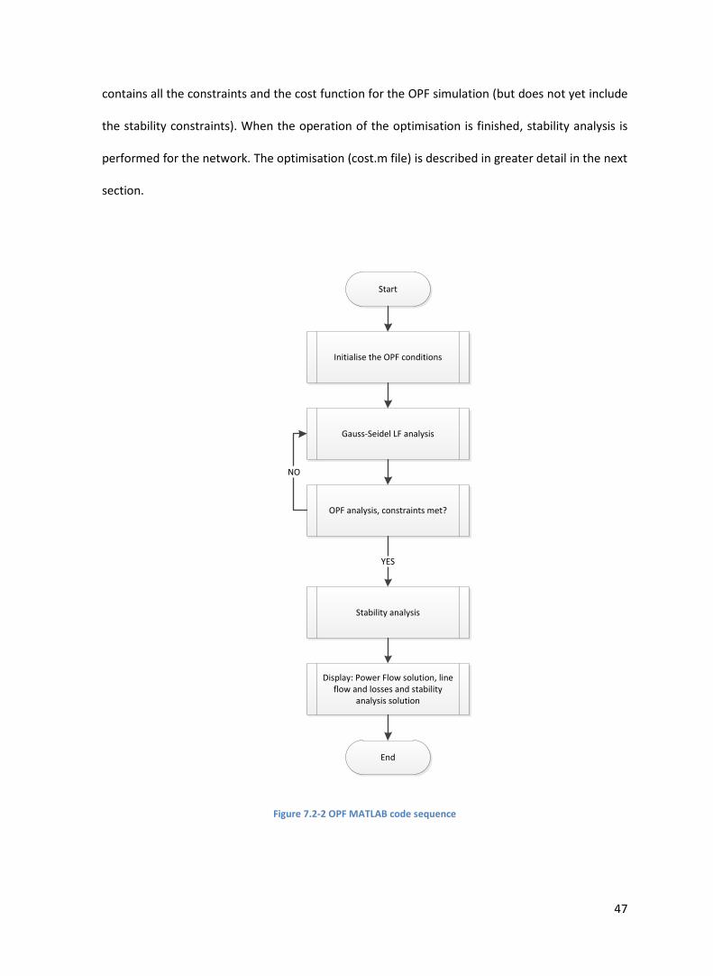
7.2.2 OPF: MATLAB Code Sequence

The Optimal Power Flow simulation expands on the LF to include constraints for the limits of the

generators, the line losses and to meet the power demand of the network. The LF provides the

initial values for the optimisation for generator 1, 2 and 3. Figure 7.2-2, illustrates the sequence of

the Optimal Power Flow program. The Optimisation stage uses the fminsearch function (which is

the Nelder-Mead algorithm) provided by MATLAB. Once the Gauss-Seidel LF is executed the next

step is the optimiser which is located as a separate m.file (cost.m, refer to the Appendix). This file

47

contains all the constraints and the cost function for the OPF simulation (but does not yet include

the stability constraints). When the operation of the optimisation is finished, stability analysis is

performed for the network. The optimisation (cost.m file) is described in greater detail in the next

section.

Start

Gauss-Seidel LF analysis

Initialise the OPF conditions

Display: Power Flow solution, line flow and losses and stability

analysis solution

End

OPF analysis, constraints met?

Stability analysis

YES

NO

Figure 7.2-2 OPF MATLAB code sequence

48

7.2.3 OPFSC MATLAB Code Sequence

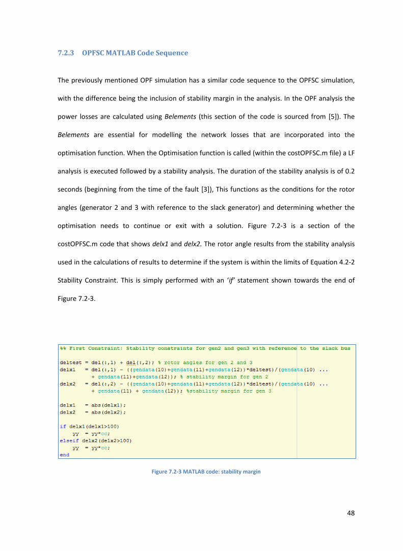
The previously mentioned OPF simulation has a similar code sequence to the OPFSC simulation,

with the difference being the inclusion of stability margin in the analysis. In the OPF analysis the

power losses are calculated using Belements (this section of the code is sourced from [5]). The

Belements are essential for modelling the network losses that are incorporated into the

optimisation function. When the Optimisation function is called (within the costOPFSC.m file) a LF

analysis is executed followed by a stability analysis. The duration of the stability analysis is of 0.2

seconds (beginning from the time of the fault [3]), This functions as the conditions for the rotor

angles (generator 2 and 3 with reference to the slack generator) and determining whether the

optimisation needs to continue or exit with a solution. Figure 7.2-3 is a section of the

costOPFSC.m code that shows delx1 and delx2. The rotor angle results from the stability analysis

used in the calculations of results to determine if the system is within the limits of Equation 4.2-2

Stability Constraint. This is simply performed with an ‘if’ statement shown towards the end of

Figure 7.2-3.

Figure 7.2-3 MATLAB code: stability margin

49

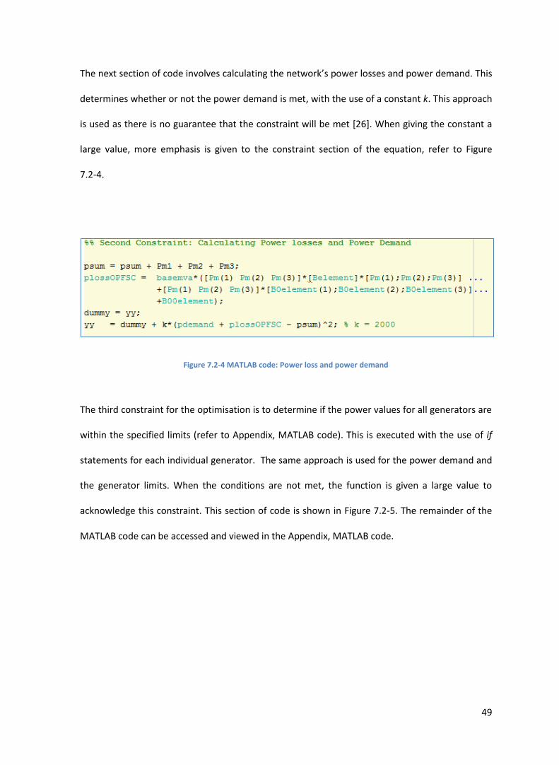
The next section of code involves calculating the network’s power losses and power demand. This

determines whether or not the power demand is met, with the use of a constant k. This approach

is used as there is no guarantee that the constraint will be met [26]. When giving the constant a

large value, more emphasis is given to the constraint section of the equation, refer to Figure

7.2-4.

Figure 7.2-4 MATLAB code: Power loss and power demand

The third constraint for the optimisation is to determine if the power values for all generators are

within the specified limits (refer to Appendix, MATLAB code). This is executed with the use of if

statements for each individual generator. The same approach is used for the power demand and

the generator limits. When the conditions are not met, the function is given a large value to

acknowledge this constraint. This section of code is shown in Figure 7.2-5. The remainder of the

MATLAB code can be accessed and viewed in the Appendix, MATLAB code.

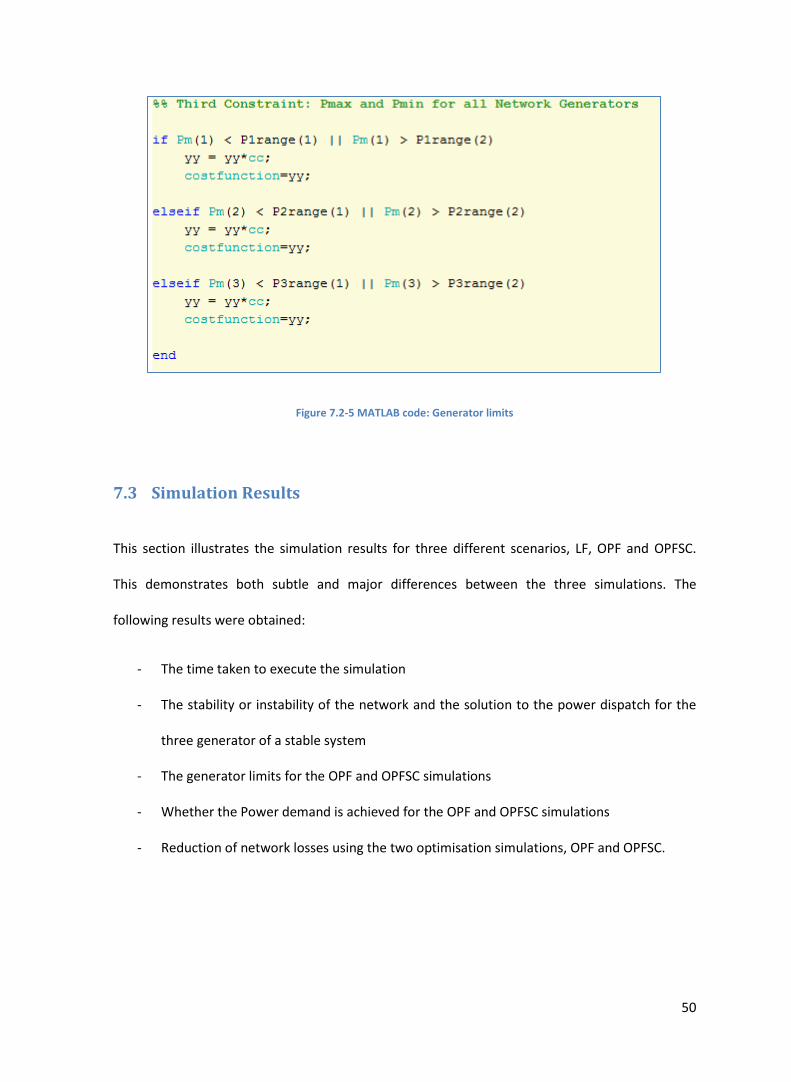
50

Figure 7.2-5 MATLAB code: Generator limits

7.3 Simulation Results

This section illustrates the simulation results for three different scenarios, LF, OPF and OPFSC.

This demonstrates both subtle and major differences between the three simulations. The

following results were obtained:

- The time taken to execute the simulation

- The stability or instability of the network and the solution to the power dispatch for the

three generator of a stable system

- The generator limits for the OPF and OPFSC simulations

- Whether the Power demand is achieved for the OPF and OPFSC simulations

- Reduction of network losses using the two optimisation simulations, OPF and OPFSC.

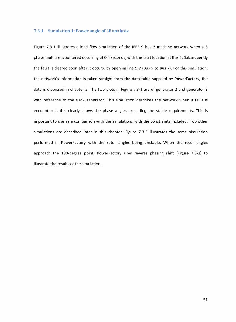
51

7.3.1 Simulation 1: Power angle of LF analysis

Figure 7.3-1 illustrates a load flow simulation of the IEEE 9 bus 3 machine network when a 3

phase fault is encountered occurring at 0.4 seconds, with the fault location at Bus 5. Subsequently

the fault is cleared soon after it occurs, by opening line 5-7 (Bus 5 to Bus 7). For this simulation,

the network’s information is taken straight from the data table supplied by PowerFactory, the

data is discussed in chapter 5. The two plots in Figure 7.3-1 are of generator 2 and generator 3

with reference to the slack generator. This simulation describes the network when a fault is

encountered, this clearly shows the phase angles exceeding the stable requirements. This is

important to use as a comparison with the simulations with the constraints included. Two other

simulations are described later in this chapter. Figure 7.3-2 illustrates the same simulation

performed in PowerFactory with the rotor angles being unstable. When the rotor angles

approach the 180-degree point, PowerFactory uses reverse phasing shift (Figure 7.3-2) to

illustrate the results of the simulation.

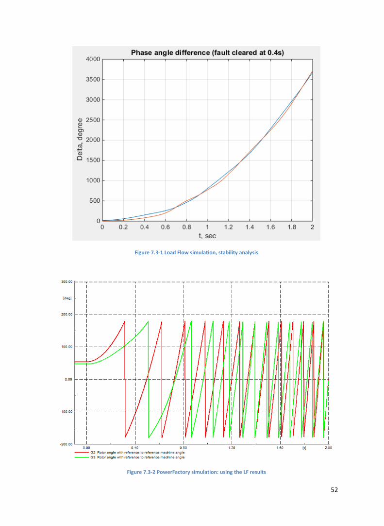
52

Figure 7.3-1 Load Flow simulation, stability analysis

Figure 7.3-2 PowerFactory simulation: using the LF results

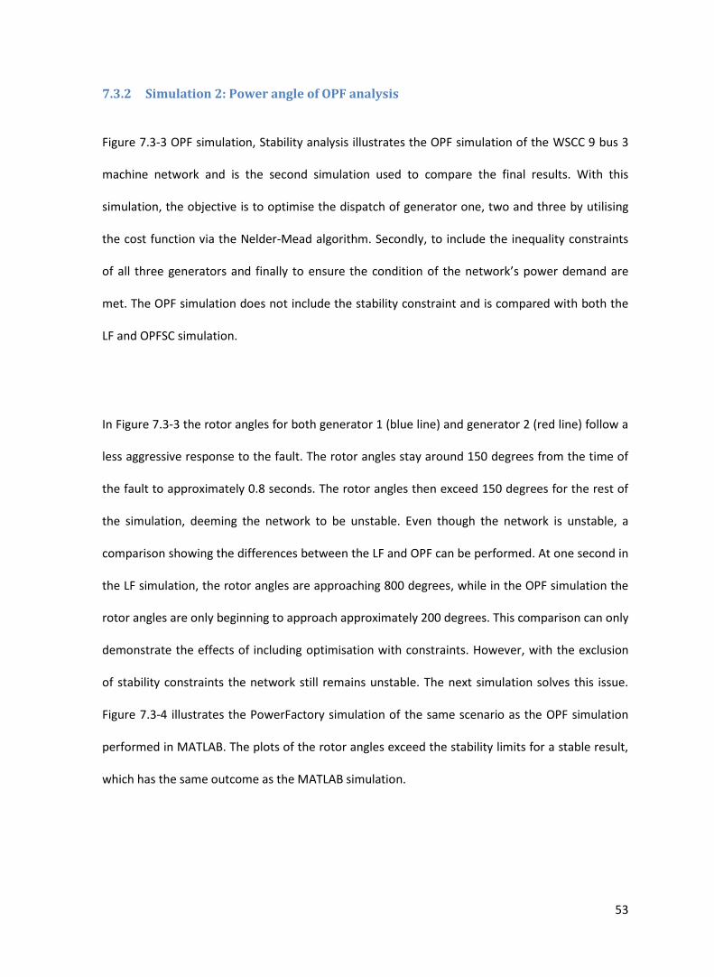
53

7.3.2 Simulation 2: Power angle of OPF analysis

Figure 7.3-3 OPF simulation, Stability analysis illustrates the OPF simulation of the WSCC 9 bus 3

machine network and is the second simulation used to compare the final results. With this

simulation, the objective is to optimise the dispatch of generator one, two and three by utilising

the cost function via the Nelder-Mead algorithm. Secondly, to include the inequality constraints

of all three generators and finally to ensure the condition of the network’s power demand are

met. The OPF simulation does not include the stability constraint and is compared with both the

LF and OPFSC simulation.

In Figure 7.3-3 the rotor angles for both generator 1 (blue line) and generator 2 (red line) follow a

less aggressive response to the fault. The rotor angles stay around 150 degrees from the time of

the fault to approximately 0.8 seconds. The rotor angles then exceed 150 degrees for the rest of

the simulation, deeming the network to be unstable. Even though the network is unstable, a

comparison showing the differences between the LF and OPF can be performed. At one second in

the LF simulation, the rotor angles are approaching 800 degrees, while in the OPF simulation the

rotor angles are only beginning to approach approximately 200 degrees. This comparison can only

demonstrate the effects of including optimisation with constraints. However, with the exclusion

of stability constraints the network still remains unstable. The next simulation solves this issue.

Figure 7.3-4 illustrates the PowerFactory simulation of the same scenario as the OPF simulation

performed in MATLAB. The plots of the rotor angles exceed the stability limits for a stable result,

which has the same outcome as the MATLAB simulation.

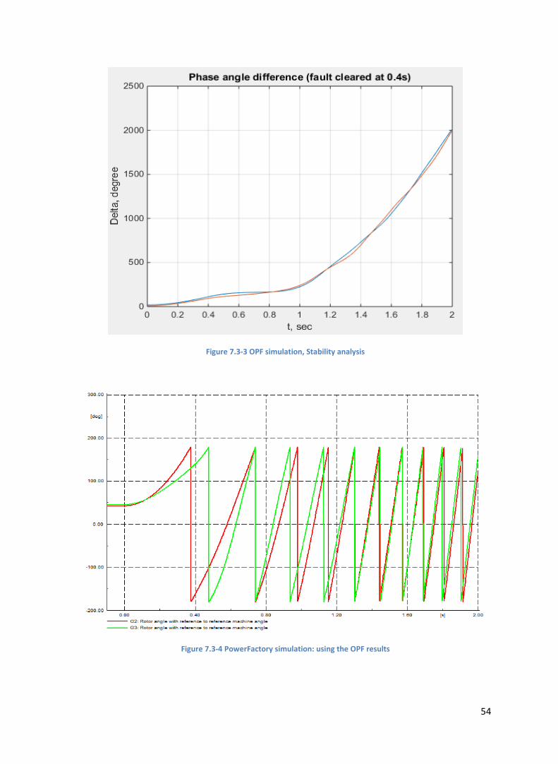
54

Figure 7.3-3 OPF simulation, Stability analysis

Figure 7.3-4 PowerFactory simulation: using the OPF results

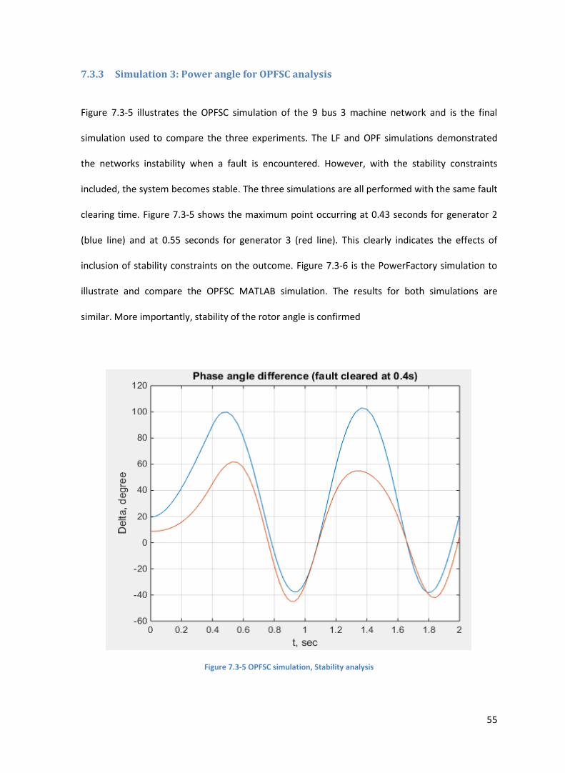
55

7.3.3 Simulation 3: Power angle for OPFSC analysis

Figure 7.3-5 illustrates the OPFSC simulation of the 9 bus 3 machine network and is the final

simulation used to compare the three experiments. The LF and OPF simulations demonstrated

the networks instability when a fault is encountered. However, with the stability constraints

included, the system becomes stable. The three simulations are all performed with the same fault

clearing time. Figure 7.3-5 shows the maximum point occurring at 0.43 seconds for generator 2

(blue line) and at 0.55 seconds for generator 3 (red line). This clearly indicates the effects of

inclusion of stability constraints on the outcome. Figure 7.3-6 is the PowerFactory simulation to

illustrate and compare the OPFSC MATLAB simulation. The results for both simulations are

similar. More importantly, stability of the rotor angle is confirmed

Figure 7.3-5 OPFSC simulation, Stability analysis

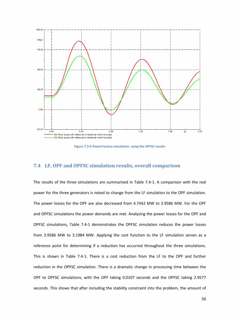
56

Figure 7.3-6 PowerFactory simulation: using the OPFSC results

7.4 LF, OPF and OPFSC simulation results, overall comparison

The results of the three simulations are summarised in Table 7.4-1. A comparison with the real

power for the three generators is noted to change from the LF simulation to the OPF simulation.

The power losses for the OPF are also decreased from 4.7442 MW to 3.9586 MW. For the OPF

and OPFSC simulations the power demands are met. Analysing the power losses for the OPF and

OPFSC simulations, Table 7.4-1 demonstrates the OPFSC simulation reduces the power losses

from 3.9586 MW to 3.1984 MW. Applying the cost function to the LF simulation serves as a

reference point for determining if a reduction has occurred throughout the three simulations.

This is shown in Table 7.4-1. There is a cost reduction from the LF to the OPF and further

reduction in the OPFSC simulation. There is a dramatic change in processing time between the

OPF to OPFSC simulations, with the OPF taking 0.0107 seconds and the OPFSC taking 2.9577

seconds. This shows that after including the stability constraint into the problem, the amount of

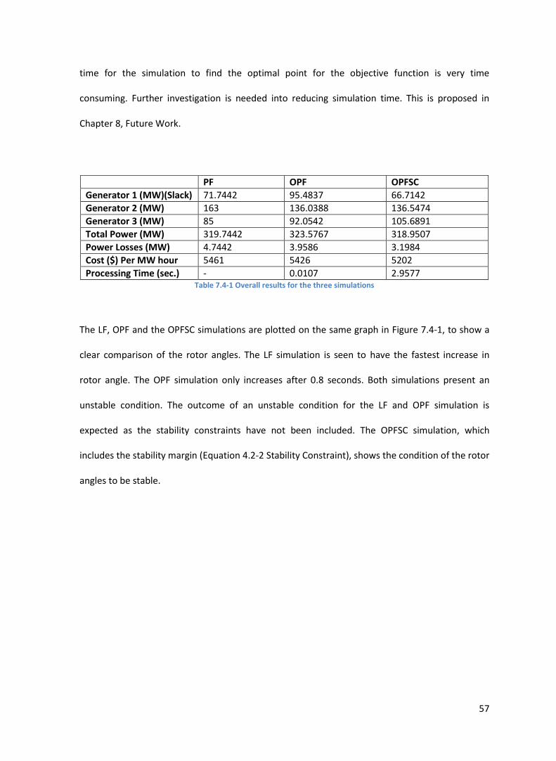
57

time for the simulation to find the optimal point for the objective function is very time

consuming. Further investigation is needed into reducing simulation time. This is proposed in

Chapter 8, Future Work.

PF OPF OPFSC

Generator 1 (MW)(Slack) 71.7442 95.4837 66.7142

Generator 2 (MW) 163 136.0388 136.5474

Generator 3 (MW) 85 92.0542 105.6891

Total Power (MW) 319.7442 323.5767 318.9507

Power Losses (MW) 4.7442 3.9586 3.1984

Cost ($) Per MW hour 5461 5426 5202

Processing Time (sec.) - 0.0107 2.9577 Table 7.4-1 Overall results for the three simulations

The LF, OPF and the OPFSC simulations are plotted on the same graph in Figure 7.4-1, to show a

clear comparison of the rotor angles. The LF simulation is seen to have the fastest increase in

rotor angle. The OPF simulation only increases after 0.8 seconds. Both simulations present an

unstable condition. The outcome of an unstable condition for the LF and OPF simulation is

expected as the stability constraints have not been included. The OPFSC simulation, which

includes the stability margin (Equation 4.2-2 Stability Constraint), shows the condition of the rotor

angles to be stable.

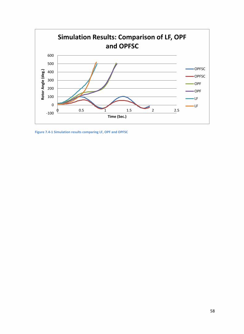
58

Figure 7.4-1 Simulation results comparing LF, OPF and OPFSC

-100

0

100

200

300

400

500

600

0 0.5 1 1.5 2 2.5

Ro

tor

An

gle

(d

eg.

)

Time (Sec.)

Simulation Results: Comparison of LF, OPF and OPFSC

OPFSC

OPFSC

OPF

OPF

LF

LF

59

8 Conclusion and Future Work

8.1 Conclusion

The importance of optimisation and stabilisation of a power system has been highlighted for

many years. The approach used for the methodology and simulating the optimisation problem in

this thesis is based on the methods implemented from research papers [3, 8] cited throughout

this report. However, this thesis uses the Nelder-Mead algorithm for optimisation which is simple

and effective for converging to a solution. Secondly, the method of incorporating the stability

limits using numerical integration facilitates the system’s stability analysis and refinement leading

to reduction in CPU usage during the simulation. This is important when attempting to implement

a real time process.

The three simulations compare results at first without optimisation, secondly with optimisation

and constraints (excluding the stability constraint) and finally optimisation with all constraints,

including the stability constraints. The following was demonstrated:

- Power losses are reduced when implementing the optimisation

- Cost is reduced from the LF simulation to the OPF simulation with a further reduction

with the OPFSC simulation.

- The power demand is always reached for the network throughout the optimisation

simulations.

- Implementing the stability constraint leads to a reduction in power losses, cost and

reaching the power demand while maintaining stability in the network.

60

It is apparent that integration of the stability constraint with the OPFSC led to a reduction in time

efficiency compared to OPF. The method used for time reduction in the OPFSC simulation

involved reducing the stability analysis calculations by 0.2 seconds rather than the full 2 cycles

that is recommended. This method only led to a reduction in the time for the stability analysis

and had no effect on reducing the optimisation algorithm. This illustrates that, after including the

stability constraint, the algorithm for the optimisation was more time consuming leading to more

CPU usage.

Overall, the simulation gives an insight into the effect of optimal power flow when using the

heuristic Nelder-mead algorithm and its ability to include stability constraints into the problem.

This analysis shows that a network can maintain stability while performing optimisation. However

further work needs to be done in order to reduce the CPU demand. A number of methods for

reducing the simulation time are proposed in the next section.

8.2 Future Work

This author has identified four possible simulation adjustments in order to investigate

improvements in optimisation performance and reduction in simulation time. Firstly, LF analysis

could be performed using Newton-Raphson method to replace Gauss-Seidel. Secondly,

optimisation techniques comparing the simulation performance with the genetic algorithm and

the particle swarm algorithm. Thirdly, additional constraints can be included in order to increase

result accuracy. Finally, analysis of an increase in the network size to compare results with data

presented in this thesis.

61

The load flow analysis used in the simulations is the Gauss-Seidel method and has been tested

with the WSCC 9 bus 3 machine network. The number of iterations for the Gauss-Seidel method is

noted in chapter 2 to be 57. DigiSILENT PowerFactory uses the Newton-Raphson method for

performing the load flow analysis and is tested against the WSCC 9 bus 3 machine network. The

amount of iterations recorded is 3. This illustrated the simulation time of the network can be

reduced if the Raphson-Newton method is used. The MATLAB code has been constructed so the

Gauss-Seidel m-file can be replaced by a Newton-Raphson m-file. This is easily achievable if the

same method is followed from ‘Power System Analysis, Hadi Saadat [5].

Optimisation techniques mentioned in chapter 3.-Genetic algorithm and the Particle swarm

algorithm are variant techniques that can be applied to this particular problem. These algorithms

can be used to compare the results with the OPFSC simulation (which uses the Nelder-Mead

algorithm) and to analyse whether this would lead to reduction in processing time. This is

imperative as process time for the simulation in the current Nelder-Mead algorithm increases

dramatically when the stability constraints are introduced. This illustrates that the optimisation is

not sufficiently efficient due to the nature of the Nelder-Mead algorithm. However alternative

algorithms may improve the simulation and would be worth investigating further.

Analysis of the effect of additional constraints leading to increased complexity is another

possibility for future studies with particular focus on time efficiency and system stability. The

majority of the concepts referenced in this thesis are derived from “Optimal Power Flow with

Stability Constraints” research paper [2]. Not all of the inequality constraints that are presented in

this paper have been implemented in the simulation for the thesis.

62

Finally, increasing the network size with application to the OPFSC simulation needs to be

analysed. This can be used to compare the two LF methods (Gauss-Seidel and Raphson-Newton)

in order to determine whether the Newton-Raphson method performs faster with larger

networks, (chapter 2). Secondly, analysing the response in the simulation run time following the

optimisation to decipher if the Nelder-Mead algorithm is a feasible method for larger networks.

Lastly, an overall comparison with the WCSS 9 bus 3 machine network could be undertaken to

determine if the algorithm needs to be altered.

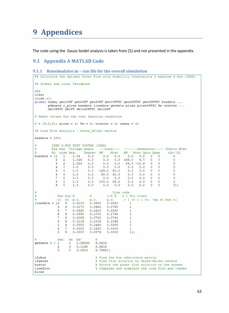
63

9 Appendices

The code using the Gauss-Seidel analysis is taken from [5] and not presented in the appendix.

9.1 Appendix A MATLAB Code

9.1.1 Runsimulator.m – run file for the overall simulation

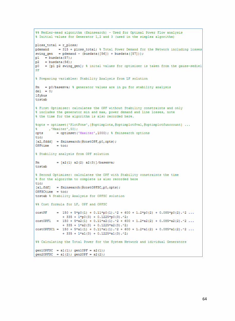
64

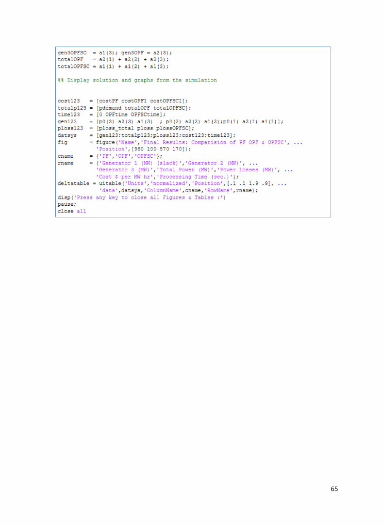
65

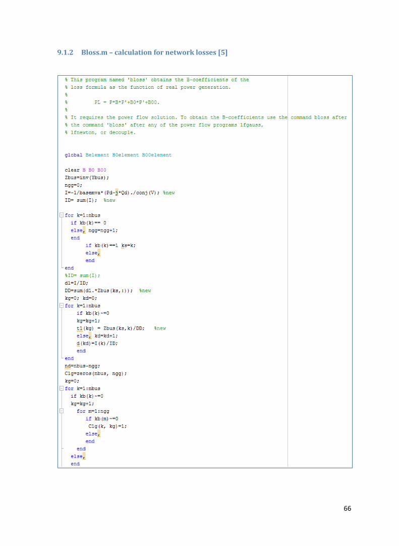
66

9.1.2 Bloss.m – calculation for network losses [5]

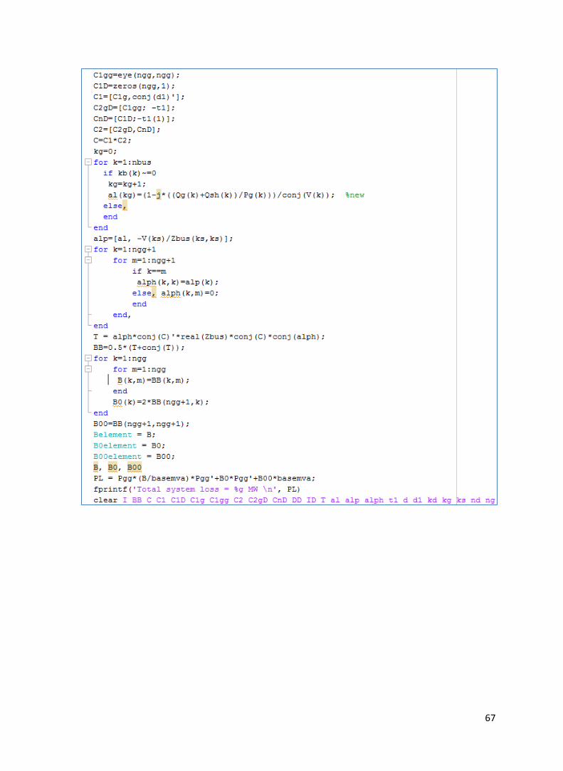
67

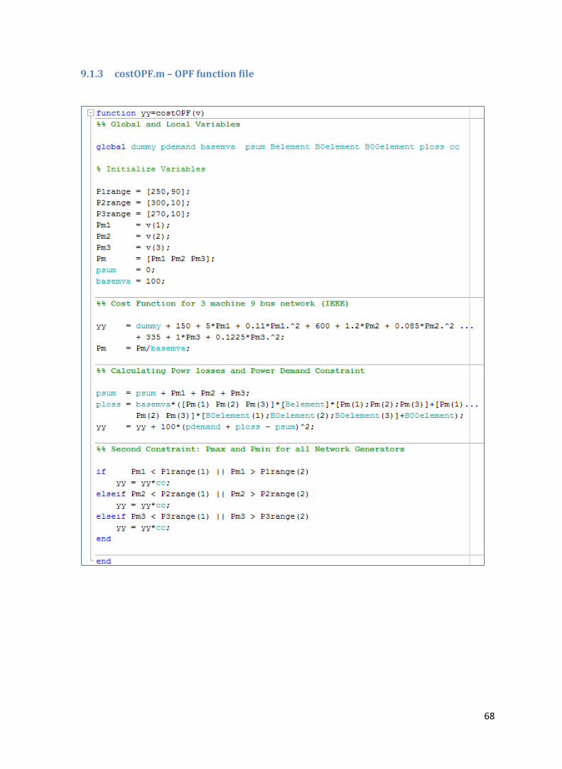
68

9.1.3 costOPF.m – OPF function file

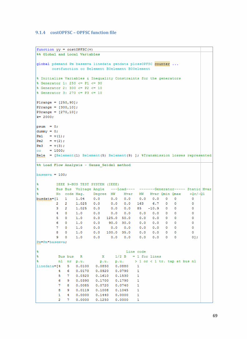
69

9.1.4 costOPFSC – OPFSC function file

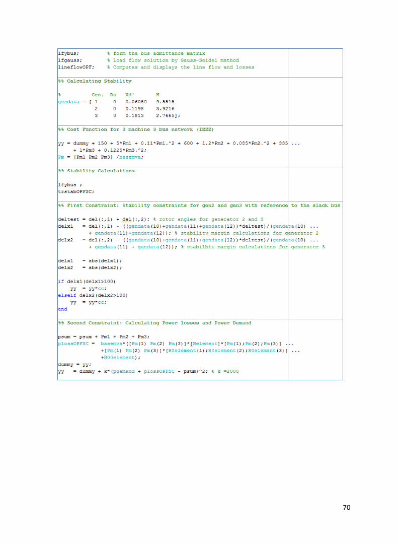
70

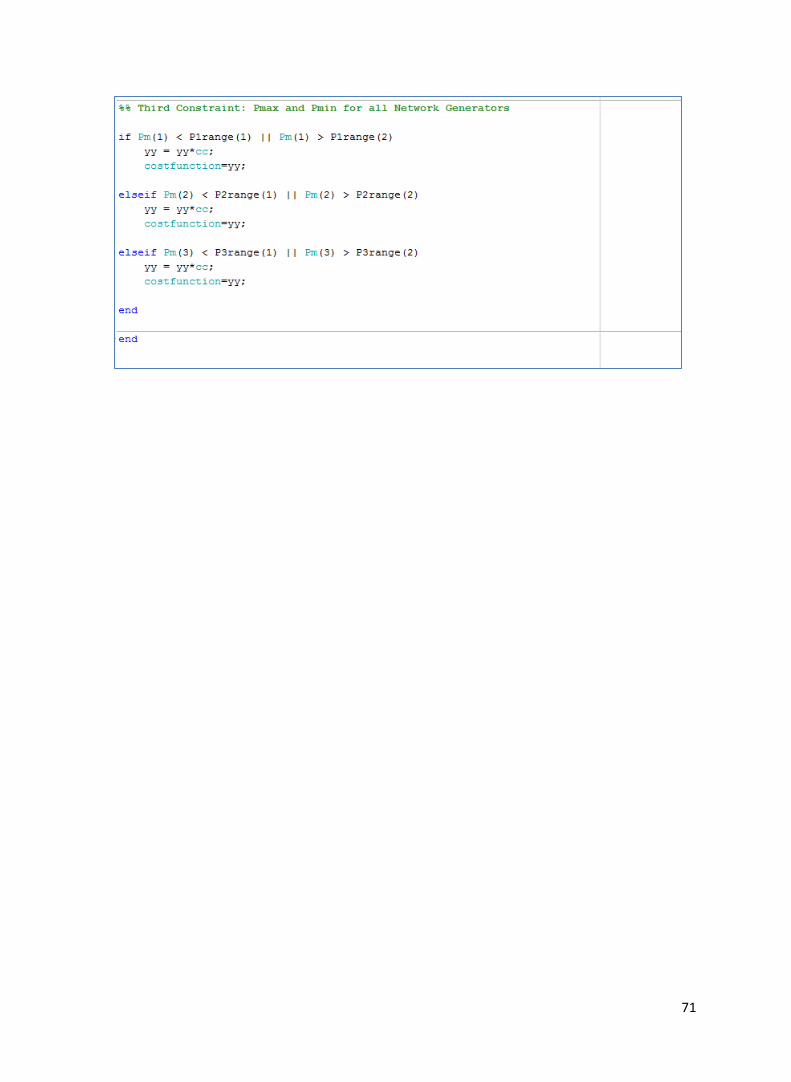
71

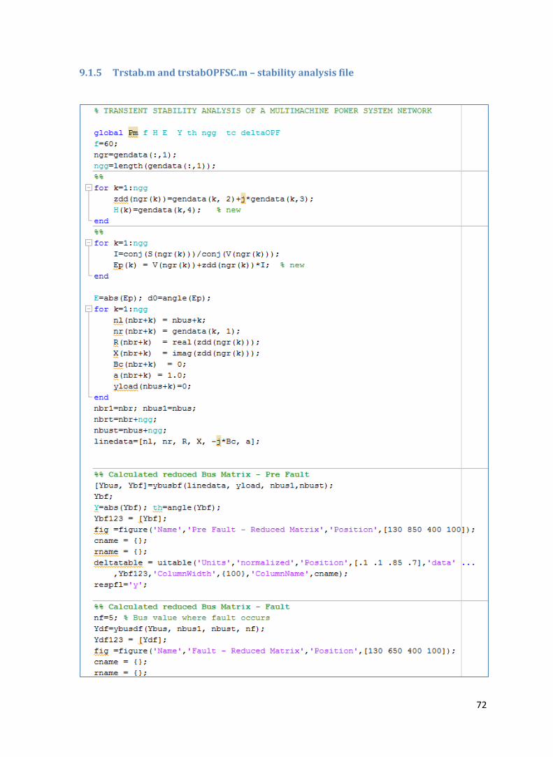
72

9.1.5 Trstab.m and trstabOPFSC.m – stability analysis file

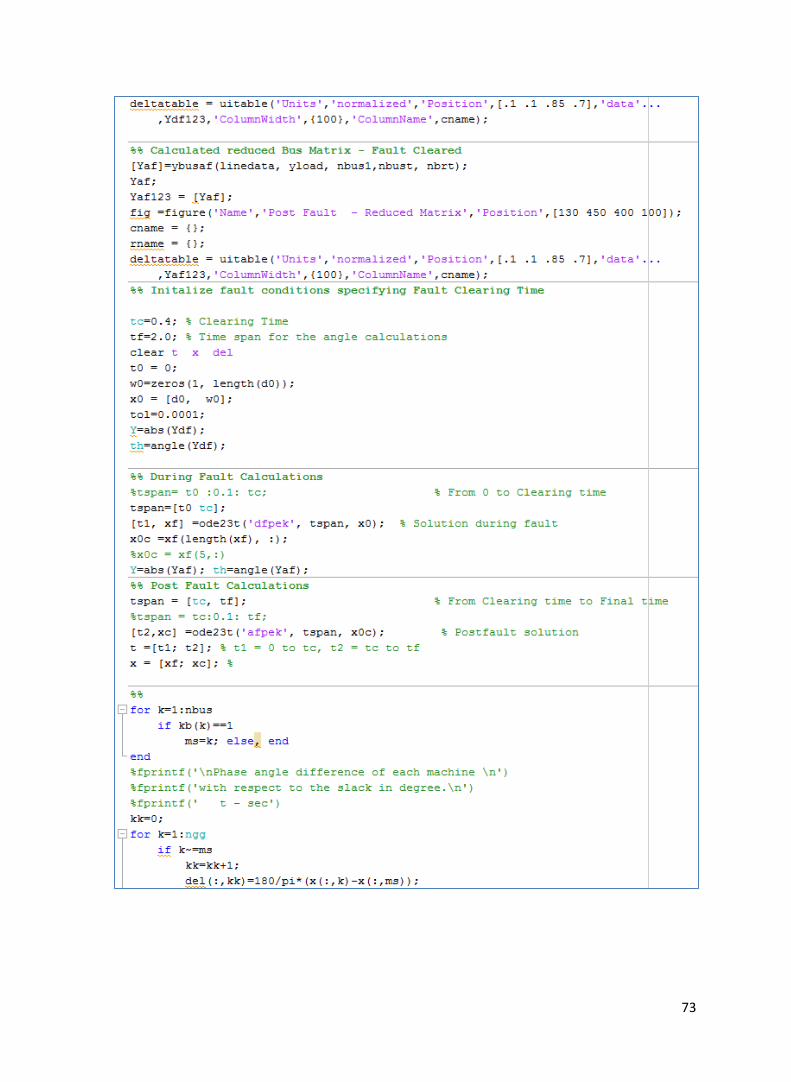
73

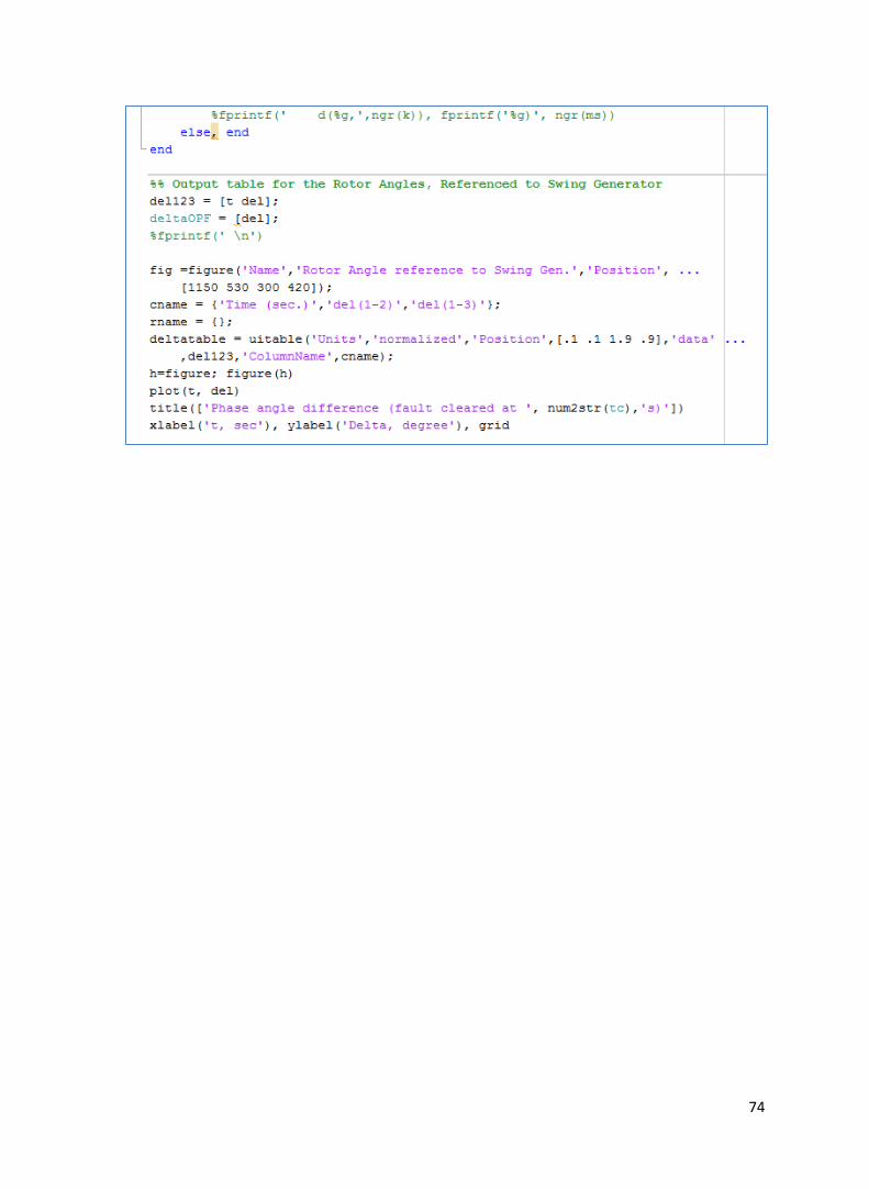
74

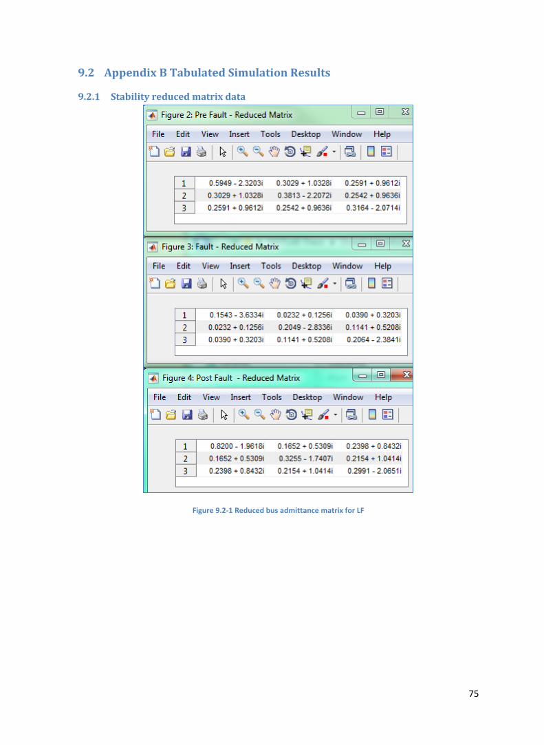
75

9.2 Appendix B Tabulated Simulation Results

9.2.1 Stability reduced matrix data

Figure 9.2-1 Reduced bus admittance matrix for LF

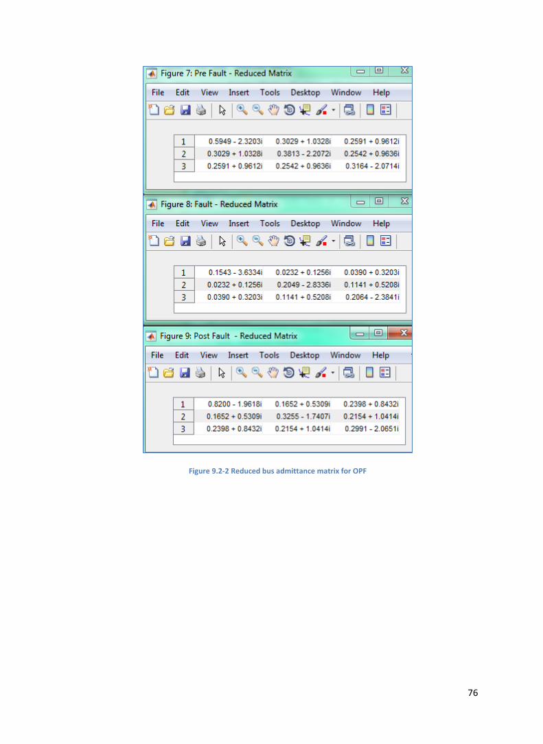
76

Figure 9.2-2 Reduced bus admittance matrix for OPF

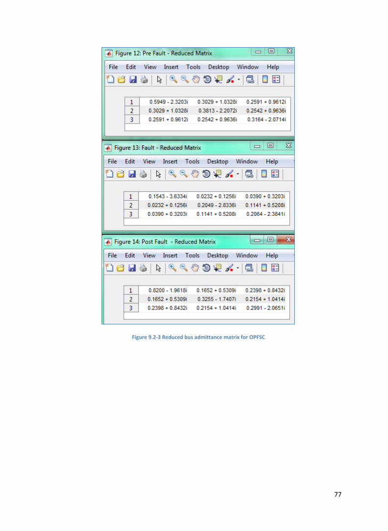
77

Figure 9.2-3 Reduced bus admittance matrix for OPFSC

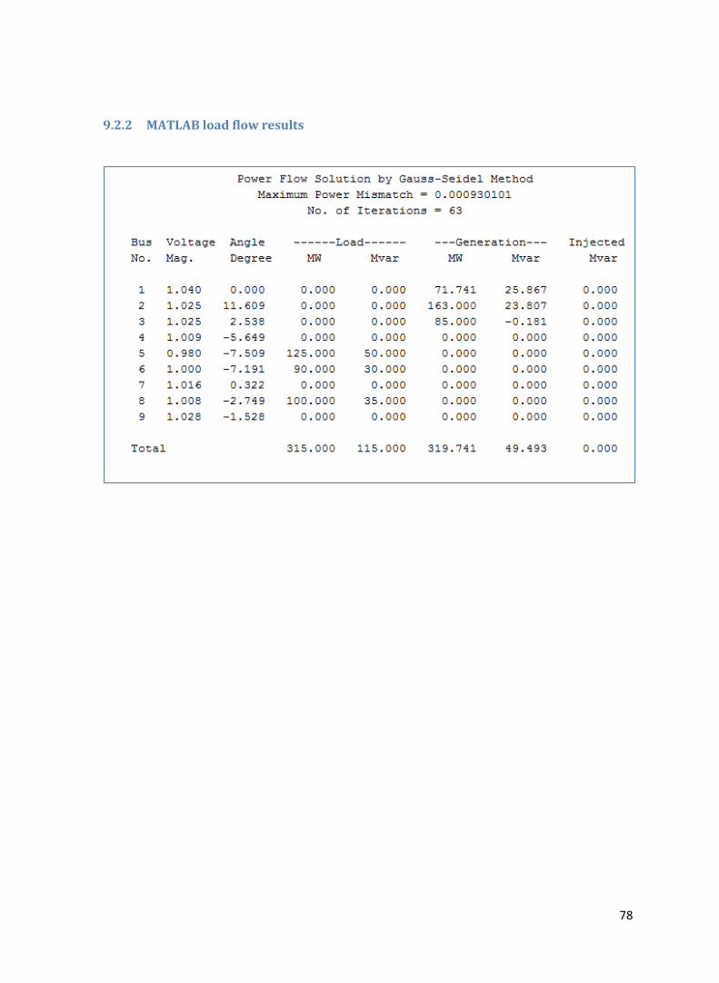
78

9.2.2 MATLAB load flow results

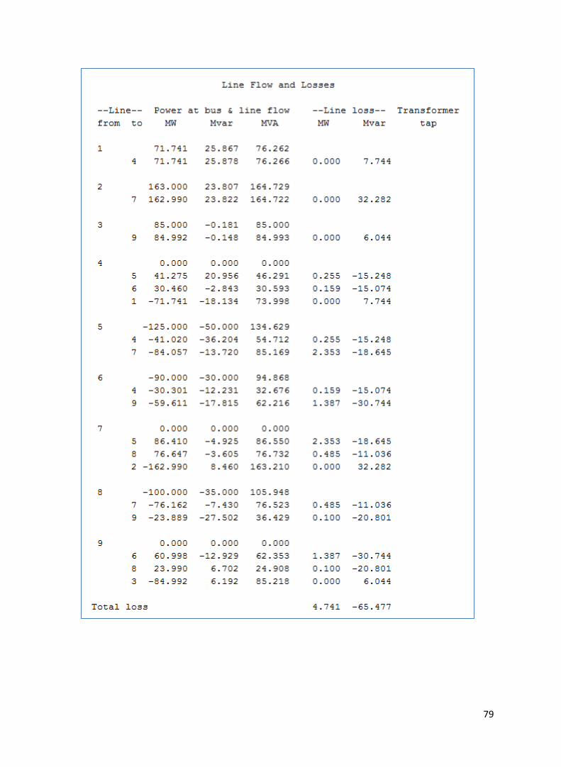
79

80

10 References

[1] "WSCC 9-Bus System," University of Illinois vol. Coordinated Science Laboratory, 2013.

[2] N. J. Singer S, "Nelder-Mead algorithm," Scholarpedia, vol. 4, 2009.

[3] D. Gan, R. J. Thomas, and R. D. Zimmerman, "Stability-constrained optimal power flow,"

Power Systems, IEEE Transactions on, vol. 15, pp. 535-540, 2000.

[4] P. Kundur, Power System Stability and Control. New York: McGraw-Hill Companies, The,

1994.

[5] H. Saadat, Power system analysis, 3rd ed. United States: PSA Pub., 2010.

[6] M. Clerc, Particle swarm optimization. London ; Newport Beach: ISTE, 2006.

[7] G. Winter, Genetic algorithms in engineering and computer science. Chichester ;: New

York : Wiley, 1995.

[8] X. Yan, D. Zhao Yang, M. Ke, Z. Jun Hua, and W. Kit Po, "A Hybrid Method for Transient

Stability-Constrained Optimal Power Flow Computation," Power Systems, IEEE

Transactions on, vol. 27, pp. 1769-1777, 2012.

[9] J. A. Momoh, R. J. Koessler, M. S. Bond, B. Stott, D. Sun, A. Papalexopoulos, et al.,

"Challenges to optimal power flow," Power Systems, IEEE Transactions on, vol. 12, pp.

444-455, 1997.

[10] L. Gan, N. Li, U. Topcu, and S. H. Low, "Optimal power flow in tree networks," in Decision

and Control (CDC), 2013 IEEE 52nd Annual Conference on, 2013, pp. 2313-2318.

[11] J. Carpentier and P. Bornard, "Towards an integrated secure optimal operation of power

systems," in Advances in Power System Control, Operation and Management, 1991.

APSCOM-91., 1991 International Conference on, 1991, pp. 1-16 vol.1.

[12] O. Alsac, J. Bright, M. Prais, and B. Stott, "Further developments in LP-based optimal

power flow," Power Systems, IEEE Transactions on, vol. 5, pp. 697-711, 1990.

81

[13] I. A. Calle, E. D. Castronuovo, and P. Ledesma, "Optimal re-dispatch of an isolated system

considering transient stability constraints," International Journal of Electrical Power &

Energy Systems, vol. 44, pp. 728-735, 1// 2013.

[14] J. H. Mathews and K. D. Fink, Numerical methods using MATLAB, 4th ed. Upper Saddle

River, N.J.: Pearson, 2004.

[15] D. Glover, Power system analysis and design, International student ed. Mason, OH:

Thomson, 2007.

[16] K. A. Kailay and Y. S. Brar, "Identification of Best Load Flow Calculation Method for IEEE-

30 BUS System Using MATLAB," International Journal of Electrical and Electronics

Research, vol. 3, pp. 155-161, July - September 2015.

[17] G. Lingwen, L. Na, T. Ufuk, and L. Steven H, "Optimal Power Flow in Tree Networks,"

Decision and Control, 52nd IEEE Conference on, pp. 2313-2318, 2013.

[18] J. F. Stewart, "Plant Size, Plant Factor, and the Shape of the Average Cost Function in

Electric Power Generation: A Nonhomogeneous Capital Approach," The Bell Journal of

Economics, vol. 10, pp. 549-565, 1979.

[19] A. E. Olsson, Particle swarm optimization : theory, techniques, and applications.

Hauppauge, N.Y.: Nova Science Publishers, 2011.

[20] M. S. Olufsen, "Excel example of Nelder-Mead Algorithm," 2010.

[21] P. W. Sauer and M. A. Pai, Power system dynamics and stability. Upper Saddle River, N.J.:

Prentice Hall, 1998.

[22] E. W. Kimbark, Power system stability. New York: IEEE Press, 1995.

[23] J. Stewart, Calculus : concepts and contexts, 3rd edition. ed. Pacific Grove, Calif.:

Brooks/Cole, 2006.

[24] "Nine Bus System: data information," DigSILENT PowerFactory, 2015.

82

[25] P. M. Anderson and A. A. Fouad, Power system control and stability, 1st ed. Ames: Iowa

State University Press, 1977.

[26] G. Crebbin, "Optimization and Economic Dispatch using Scilab," 19 October 2015.