OBSERVATIONS OF ENERGY AND WATER VAPOR FLUXES ON A …

OBSERVATIONS OF ENERGY AND WATER VAPOR FLUXES ON A LIVING ROOF SURFACE

A Thesis submitted to the faculty of San Francisco State University

In partial fulfillment of the requirements for

the Degree

Master of Arts

In

Geography

by

Siobhan Casey Lavender

San Francisco, California

January 2015

CERTIFICATION OF APPROVAL

I certify that I have read Impacts of living roofs on urban climate in San Francisco

California by Siobhan Casey Lavender, and that in my opinion this work meets the

criteria for approving a thesis submitted in partial fulfillment of the requirement for the

degree Master of Art in Geography at San Francisco State University.

Andrew Oliphant, Ph.D. Professor of Geography

Leonhard Blesius, Ph.D. Associate Professor of Geography

OBSERVATIONS OF ENERGY AND WATER VAPOR FLUXES ON A LIVING ROOF SURFACE

Siobhan Casey Lavender San Francisco, California

2015

The results from this study offer a micrometeorological profile of an extensive/intensive living roof in the Mediterranean climate of San Francisco California, specifically the roof’s impact on the surface radiation budget and surface energy balance. Living roofs have long been touted for their ability to positively impact microclimate by reflecting solar radiation and cooling the atmosphere through the latent heat flux, thereby offsetting adverse effects of the urban heat island effect (UHI). This is the first study using the eddy covariance technique on a living roof, and was achievable due to the roof’s large (one hectare) size and stringent (~50%) data rejection. The annual average albedo of the living roof was 0.20 with a seasonal monthly maximum of .22 and a minimum of 17.39. The annual ensemble average partitioning of energy balance terms indicated that latent and sensible heat fluxes were close to equal with an annual Bowen ratio of 0.96. On a diurnal temporal scale, the sensible heat began to surpass the latent heat in the mid-morning, and on a seasonal timescale, sensible heat dominated the energy balance partitioning in the late summer and early spring, and was overtaken by the latent heat flux in the fall and winter. The latent heat flux produced an annual average cooling rate of 3.19 (MJ m-2 dy-1). Ground heat flux observations indicated that the substrate acted as insulation, with a small average diurnal maximum of 3 (W m-2) of heat energy entering the building below. Energy balance closure as determined by linear regression showed that the turbulent fluxes underestimated available energy by 38% (R2 = 0.92).

I certify that the Abstract is a correct representation of the content of this thesis.

Chair, Thesis Committee Date

iv

PREFACE AND/OR ACKNOWLEGEMENT

This work is due wholly to the tireless dedication and oversight of Professor Andrew

Oliphant who has been the driving force behind my interest and love of this subject

matter. My sincere gratitude to him for guiding me through this project and the

supporting microclimatological theory to which I had not been previously exposed. Also

many thanks to Professor Leonard Blesius who agreed to second this thesis project

despite sitting on numerous other committees this semester; his keen editing skills and

knowledge of physical geography have been a major asset. Thank you to Ryan Thorp

for spearheading the original 2013 deployment of the micrometeorological tower and for

his astute analysis of that deployment’s data, as well as his and Suzanne Maher’s aid in

installing the equipment again in 2014. Thanks to Craig Clements and San Jose State

University for equipment calibration assistance. Lastly without the support of the

California Academy of Sciences and our point-of-contact Kendra Hauser, who gave us

continuous access to the roof and provided ecological and maintenance expertise, this

project would not have been possible.

v

TABLE OF CONTENTS

List of Tables ................................................................................................................. vii

List of Figures ............................................................................................................... viii

1.0 Background and Introduction ..................................................................................... 1

1.1 Urban climates and vegetation cover ............................................................. 1

1.2 UHI and PCI ................................................................................................... 1

1.3 Living roofs .................................................................................................... 3

1.4. The surface energy balance and radiation budget ......................................... 6

2.0 Study Site .................................................................................................................. 8

2.1. Location and background .............................................................................. 8

2.2. Subsurface roof structure ............................................................................ 11

2.3. Ecology and vegetation surveys .................................................................. 12

3.0 Materials and Methods ............................................................................................ 15

3.1. Deployment ................................................................................................. 15

3.2. Project footprint ........................................................................................... 17

3.3. Determining the ground heat flux ................................................................ 19

4.0 Results .................................................................................................................... 21

4.1. Surface radiation budget ............................................................................. 22

4.2. Surface energy balance .............................................................................. 27

4.3. Controls on the surface energy balance ...................................................... 31

4.4. Ground heat flux ......................................................................................... 34

4.5. Annual comparison ..................................................................................... 37

vi

4.6. Energy balance closure ............................................................................... 41

5.0 Discussion ............................................................................................................... 43

5.1. Surface albedo ............................................................................................ 43

5.2. Living roof controls on surface energy balance ........................................... 45

5.3. Ground heat conduction and storage .......................................................... 48

5.4. Controls on energy balance closure and sources of error............................ 49

6.0 For future study: Comparing latent heat flux ............................................................ 51

7.0 Conclusions ............................................................................................................. 52

8.0 References .............................................................................................................. 56

vii

LIST OF TABLES

Table Page

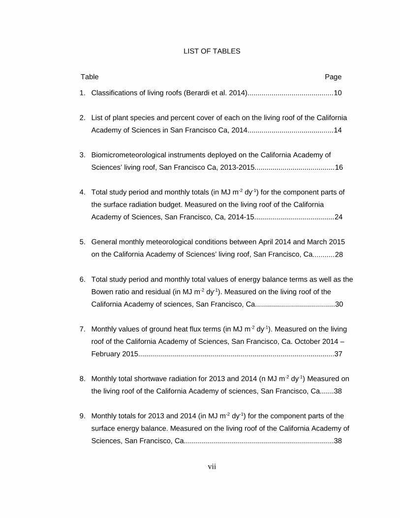
1. Classifications of living roofs (Berardi et al. 2014)...........................................10

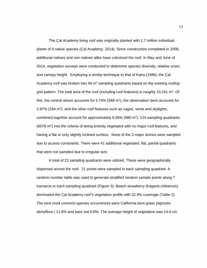
2. List of plant species and percent cover of each on the living roof of the California

Academy of Sciences in San Francisco Ca, 2014...........................................14

3. Biomicrometeorological instruments deployed on the California Academy of

Sciences’ living roof, San Francisco Ca, 2013-2015........................................16

4. Total study period and monthly totals (in MJ m-2 dy-1) for the component parts of

the surface radiation budget. Measured on the living roof of the California

Academy of Sciences, San Francisco, Ca, 2014-15........................................24

5. General monthly meteorological conditions between April 2014 and March 2015

on the California Academy of Sciences’ living roof, San Francisco, Ca...........28

6. Total study period and monthly total values of energy balance terms as well as the

Bowen ratio and residual (in MJ m-2 dy-1). Measured on the living roof of the

California Academy of sciences, San Francisco, Ca........................................30

7. Monthly values of ground heat flux terms (in MJ m-2 dy-1). Measured on the living

roof of the California Academy of Sciences, San Francisco, Ca. October 2014 –

February 2015..................................................................................................37

8. Monthly total shortwave radiation for 2013 and 2014 (n MJ m-2 dy-1) Measured on

the living roof of the California Academy of sciences, San Francisco, Ca.......38

9. Monthly totals for 2013 and 2014 (in MJ m-2 dy-1) for the component parts of the

surface energy balance. Measured on the living roof of the California Academy of

Sciences, San Francisco, Ca...........................................................................38

viii

LIST OF FIGURES

Figures Page

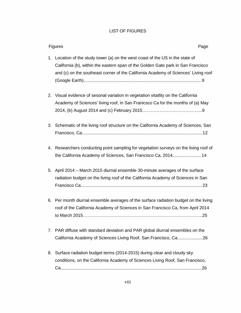
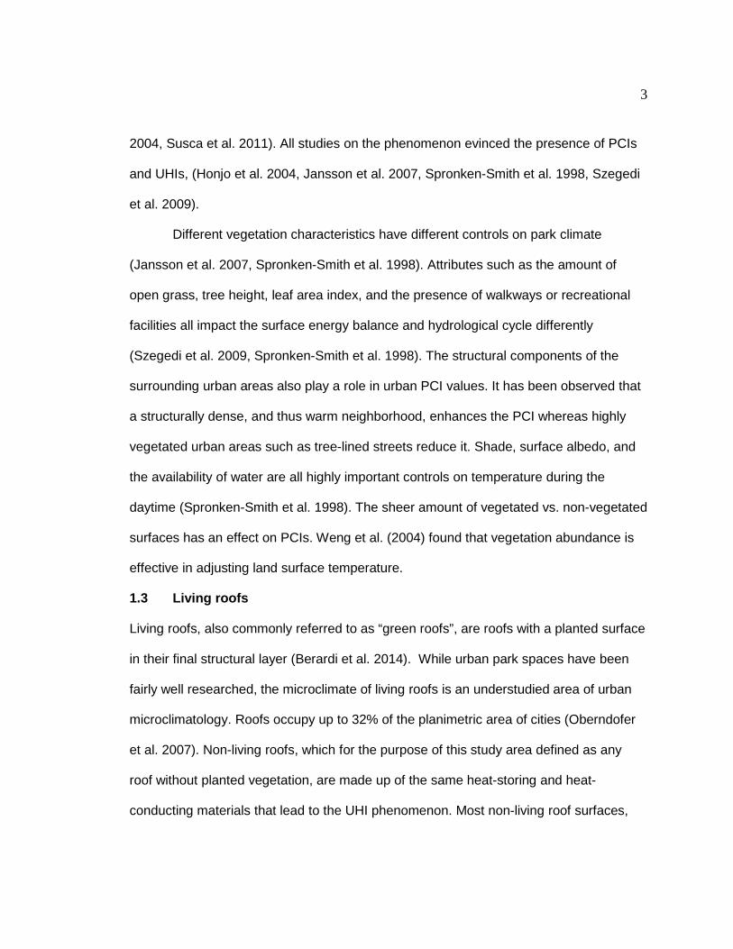
1. Location of the study tower (a) on the west coast of the US in the state of

California (b), within the eastern span of the Golden Gate park in San Francisco

and (c) on the southeast corner of the California Academy of Sciences’ Living roof

(Google Earth)..................................................................................................9

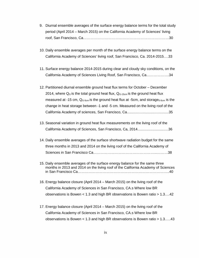
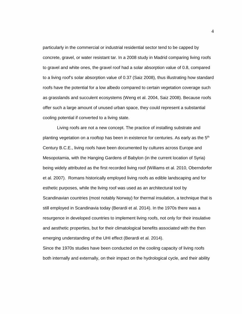
2. Visual evidence of sesonal variation in vegetation vitatlity on the California

Academy of Sciences’ living roof, in San Franicsco Ca for the months of (a) May

2014, (b) August 2014 and (c) February 2015…………………………………...9

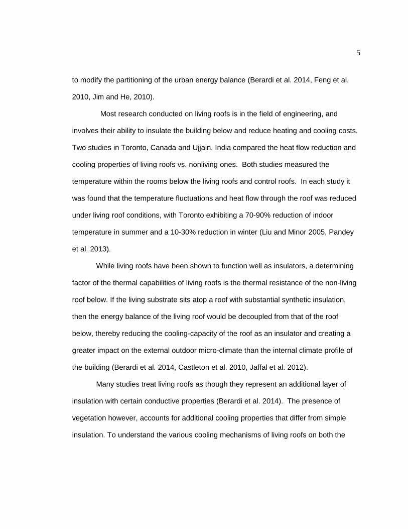
3. Schematic of the living roof structure on the California Academy of Sciences, San

Francisco, Ca....................................................................................................12

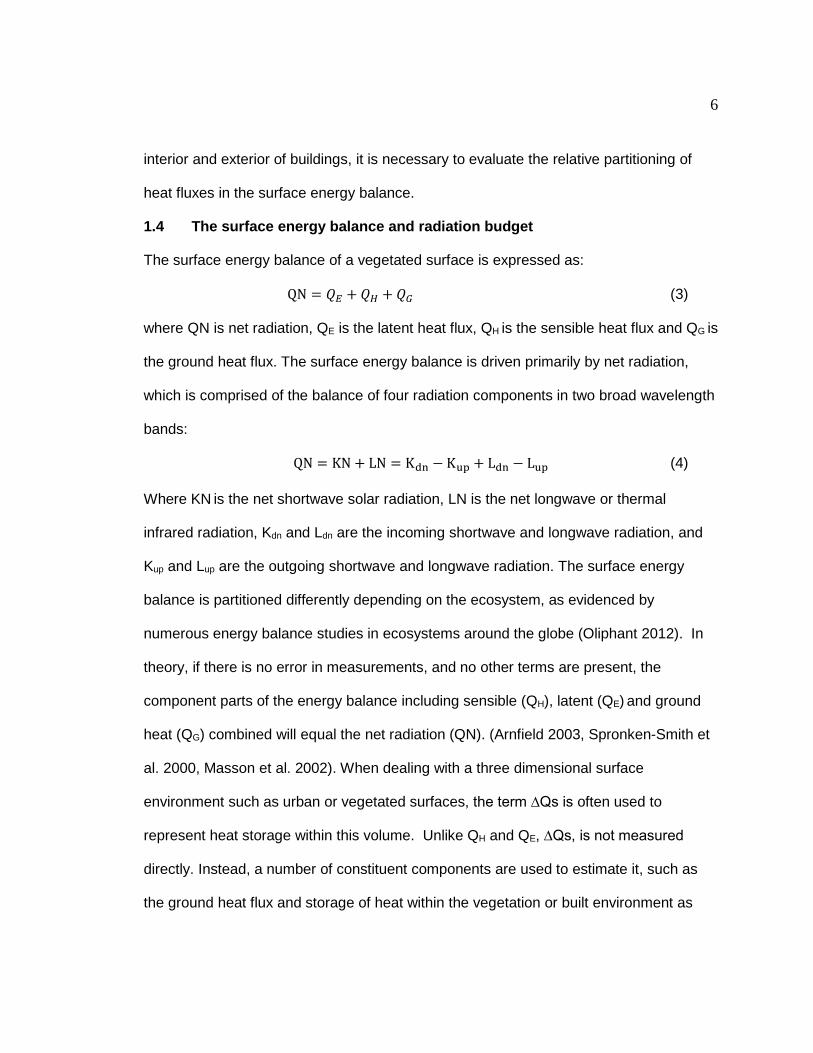
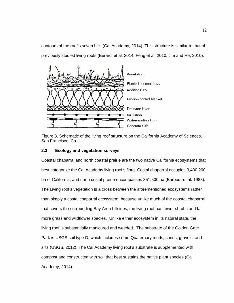
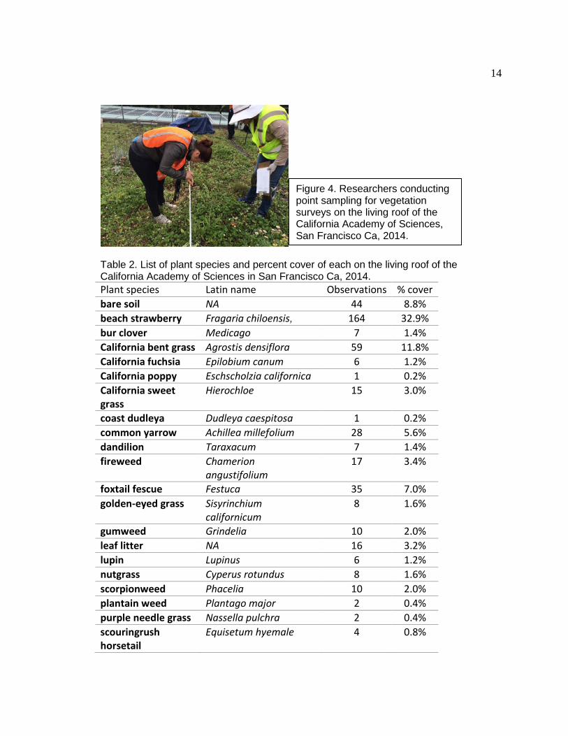
4. Researchers conducting point sampling for vegetation surveys on the living roof of

the California Academy of Sciences, San Francisco Ca, 2014........................14

5. April 2014 – March 2015 diurnal ensemble 30-minute averages of the surface

radiation budget on the living roof of the California Academy of Sciences in San

Francisco Ca.....................................................................................................23

6. Per month diurnal ensemble averages of the surface radiation budget on the living

roof of the California Academy of Sciences in San Francisco Ca, from April 2014

to March 2015………………………………………………………………………..25

7. PAR diffuse with standard deviation and PAR global diurnal ensembles on the

California Academy of Sciences Living Roof, San Francisco, Ca.....................26

8. Surface radiation budget terms (2014-2015) during clear and cloudy sky

conditions, on the California Academy of Sciences Living Roof, San Francisco,

Ca.....................................................................................................................26

ix

9. Diurnal ensemble averages of the surface energy balance terms for the total study

period (April 2014 – March 2015) on the California Academy of Sciences’ living

roof, San Francisco, Ca………………………………………………………………30

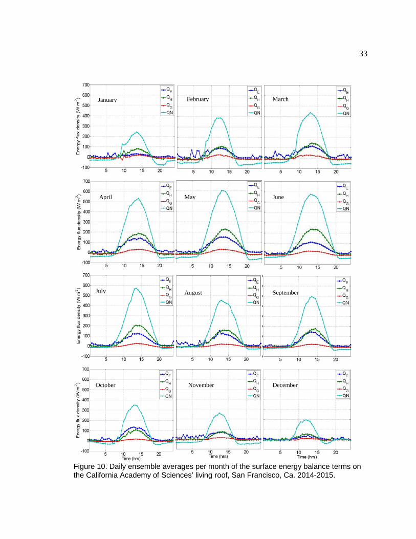
10. Daily ensemble averages per month of the surface energy balance terms on the

California Academy of Sciences’ living roof, San Francisco, Ca. 2014-2015….33

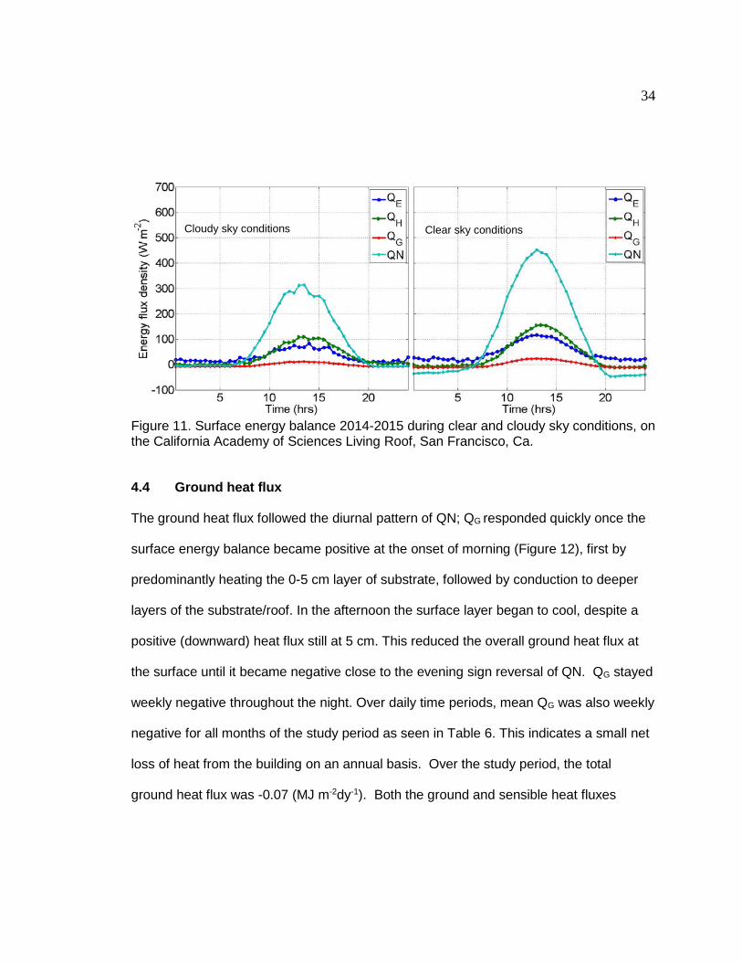
11. Surface energy balance 2014-2015 during clear and cloudy sky conditions, on the

California Academy of Sciences Living Roof, San Francisco, Ca……………….34

12. Partitioned diurnal ensemble ground heat flux terms for October – December

2014, where QG is the total ground heat flux, QG-15cm is the ground heat flux

measured at -15 cm, QG-5cm is the ground heat flux at -5cm, and storage0-5cm is the

change in heat storage between -1 and -5 cm. Measured on the living roof of the

California Academy of sciences, San Francisco, Ca..........................................35

13. Seasonal variation in ground heat flux measurements on the living roof of the

California Academy of Sciences, San Francisco, Ca, 2014...............................36

14. Daily ensemble averages of the surface shortwave radiation budget for the same

three months in 2013 and 2014 on the living roof of the California Academy of

Sciences in San Francisco Ca……………………………………………...………38

15. Daily ensemble averages of the surface energy balance for the same three

months in 2013 and 2014 on the living roof of the California Academy of Sciences in San Francisco Ca…………………………………………………………………..40

16. Energy balance closure (April 2014 – March 2015) on the living roof of the

California Academy of Sciences in San Francisco, CA.s Where low BR

observations is Bowen < 1.3 and high BR observations is Bowen ratio > 1.3….42

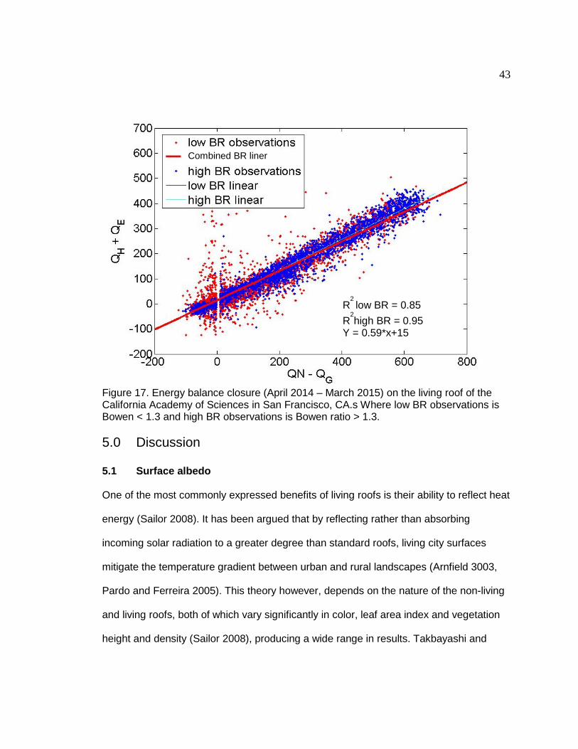
17. Energy balance closure (April 2014 – March 2015) on the living roof of the

California Academy of Sciences in San Francisco, CA.s Where low BR

observations is Bowen < 1.3 and high BR observations is Bowen ratio > 1.3…..43

1

1.0 Background and Introduction

1.1 Urban climates and vegetation cover

Surface composition has a large potential to affect local climates. A number of studies

have shown that vegetation in urban areas impacts the surface energy balance,

hydrological cycle, and carbon budget (Honjo et al. 2003, Santamouris et al. 2007, Xu

and Baldocchi 2004), particularly in urban settings, which are often categorized by

warmer dryer climates when compared to surrounding landscapes. Urban areas tend to

have high aerosol levels, and altered wind flow due to the complex nature of the built

environment. These attributes combined with the material composition of city

landscapes fosters an anthropogenic climate that differs substantially from rural

landscapes. In this setting, vegetation can be an important tool in mitigating city climates

so that they behave more similarly to that of natural ecosystems (Oke 1973). With their

increasing geographic expansion, and growing populations, urban landscapes are

becoming an increasingly dense anthropogenic biome (Alessa and Chapin 2008) with

their own unique climate attributes. In 1990 less than 40% of the global population

resided in urban dwellings, in 2010, over 50% of an even larger global population

occupied city housing. By 2030, it is estimated that 60% of people will reside in cities

(WHO 2013, Arnfield 2003). Therefore there is a need to better understand urban

climates and how urban structure features impact the local climate. This study’s data

was collected between May of 2013 and March of 2015. The objective was to obtain a

micrometeorological profile of living roof, specifically the roof’s impact on the surface

radiation budget and surface energy balance.

1.2 UHI and PCI

2

The first published observational study of urban climate was conducted in London by

Luke Howard (Howard 1833, Oke 1980), who utilized thermometer based observations.

The study demonstrated that London had a higher temperature than the surrounding

countryside. However, it is worth noting that as early as the Roman Empire, scientists

used visual observations of the urban atmosphere to suggest heat differences from

surrounding rural areas, signifying urban climate effects (Grimmond 2006). This

temperature difference is known as the urban heat island (UHI) effect, and can be

expressed as:

UHI = Turban - Trural (1)

where Turban is the temperature within the city space, and Trural is the temperature of the

surrounding rural space. The built urban environment is comprised largely of asphalt,

brick, glass, concrete, and steel. These urban construction materials contribute to

localized high temperatures by their greater ability to store heat (Oke et al. 1991,

Eliasson 2000). Heat storage capacity is particularly significant in cities when observed

on a diurnal scale: often the largest difference in temperatures between urban and rural

landscapes occurs in the early evening (Oke et al. 1991). Just as there is a temperature

gradient between urban and rural spaces, there is similarly a temperature gradient

between cities and urban parks. This phenomenon is known as the park cool island

(PCI) effect, and expressed as:

PCI = Turban – Tpark (2)

Where Tpark is the temperature within the park. PCIs and UHIs have been observed in a

range of climates and locations including in Hungary, Sweden, Japan, Singapore,

Canada and United States (Bottyan et al. 2005, Homer and Eliasson 1999, Honjo et al.

3

2004, Susca et al. 2011). All studies on the phenomenon evinced the presence of PCIs

and UHIs, (Honjo et al. 2004, Jansson et al. 2007, Spronken-Smith et al. 1998, Szegedi

et al. 2009).

Different vegetation characteristics have different controls on park climate

(Jansson et al. 2007, Spronken-Smith et al. 1998). Attributes such as the amount of

open grass, tree height, leaf area index, and the presence of walkways or recreational

facilities all impact the surface energy balance and hydrological cycle differently

(Szegedi et al. 2009, Spronken-Smith et al. 1998). The structural components of the

surrounding urban areas also play a role in urban PCI values. It has been observed that

a structurally dense, and thus warm neighborhood, enhances the PCI whereas highly

vegetated urban areas such as tree-lined streets reduce it. Shade, surface albedo, and

the availability of water are all highly important controls on temperature during the

daytime (Spronken-Smith et al. 1998). The sheer amount of vegetated vs. non-vegetated

surfaces has an effect on PCIs. Weng et al. (2004) found that vegetation abundance is

effective in adjusting land surface temperature.

1.3 Living roofs

Living roofs, also commonly referred to as “green roofs”, are roofs with a planted surface

in their final structural layer (Berardi et al. 2014). While urban park spaces have been

fairly well researched, the microclimate of living roofs is an understudied area of urban

microclimatology. Roofs occupy up to 32% of the planimetric area of cities (Oberndofer

et al. 2007). Non-living roofs, which for the purpose of this study area defined as any

roof without planted vegetation, are made up of the same heat-storing and heat-

conducting materials that lead to the UHI phenomenon. Most non-living roof surfaces,

4

particularly in the commercial or industrial residential sector tend to be capped by

concrete, gravel, or water resistant tar. In a 2008 study in Madrid comparing living roofs

to gravel and white ones, the gravel roof had a solar absorption value of 0.8, compared

to a living roof’s solar absorption value of 0.37 (Saiz 2008), thus illustrating how standard

roofs have the potential for a low albedo compared to certain vegetation coverage such

as grasslands and succulent ecosystems (Weng et al. 2004, Saiz 2008). Because roofs

offer such a large amount of unused urban space, they could represent a substantial

cooling potential if converted to a living state.

Living roofs are not a new concept. The practice of installing substrate and

planting vegetation on a rooftop has been in existence for centuries. As early as the 5th

Century B.C.E., living roofs have been documented by cultures across Europe and

Mesopotamia, with the Hanging Gardens of Babylon (in the current location of Syria)

being widely attributed as the first recorded living roof (Williams et al. 2010, Oberndorfer

et al. 2007). Romans historically employed living roofs as edible landscaping and for

esthetic purposes, while the living roof was used as an architectural tool by

Scandinavian countries (most notably Norway) for thermal insulation, a technique that is

still employed in Scandinavia today (Berardi et al. 2014). In the 1970s there was a

resurgence in developed countries to implement living roofs, not only for their insulative

and aesthetic properties, but for their climatological benefits associated with the then

emerging understanding of the UHI effect (Berardi et al. 2014).

Since the 1970s studies have been conducted on the cooling capacity of living roofs

both internally and externally, on their impact on the hydrological cycle, and their ability

5

to modify the partitioning of the urban energy balance (Berardi et al. 2014, Feng et al.

2010, Jim and He, 2010).

Most research conducted on living roofs is in the field of engineering, and

involves their ability to insulate the building below and reduce heating and cooling costs.

Two studies in Toronto, Canada and Ujjain, India compared the heat flow reduction and

cooling properties of living roofs vs. nonliving ones. Both studies measured the

temperature within the rooms below the living roofs and control roofs. In each study it

was found that the temperature fluctuations and heat flow through the roof was reduced

under living roof conditions, with Toronto exhibiting a 70-90% reduction of indoor

temperature in summer and a 10-30% reduction in winter (Liu and Minor 2005, Pandey

et al. 2013).

While living roofs have been shown to function well as insulators, a determining

factor of the thermal capabilities of living roofs is the thermal resistance of the non-living

roof below. If the living substrate sits atop a roof with substantial synthetic insulation,

then the energy balance of the living roof would be decoupled from that of the roof

below, thereby reducing the cooling-capacity of the roof as an insulator and creating a

greater impact on the external outdoor micro-climate than the internal climate profile of

the building (Berardi et al. 2014, Castleton et al. 2010, Jaffal et al. 2012).

Many studies treat living roofs as though they represent an additional layer of

insulation with certain conductive properties (Berardi et al. 2014). The presence of

vegetation however, accounts for additional cooling properties that differ from simple

insulation. To understand the various cooling mechanisms of living roofs on both the

6

interior and exterior of buildings, it is necessary to evaluate the relative partitioning of

heat fluxes in the surface energy balance.

1.4 The surface energy balance and radiation budget

The surface energy balance of a vegetated surface is expressed as:

QN = 𝑄𝑄𝐸𝐸 + 𝑄𝑄𝐻𝐻 + 𝑄𝑄𝐺𝐺 (3)

where QN is net radiation, QE is the latent heat flux, QH is the sensible heat flux and QG is

the ground heat flux. The surface energy balance is driven primarily by net radiation,

which is comprised of the balance of four radiation components in two broad wavelength

bands:

QN = KN + LN = Kdn − Kup + Ldn − Lup (4)

Where KN is the net shortwave solar radiation, LN is the net longwave or thermal

infrared radiation, Kdn and Ldn are the incoming shortwave and longwave radiation, and

Kup and Lup are the outgoing shortwave and longwave radiation. The surface energy

balance is partitioned differently depending on the ecosystem, as evidenced by

numerous energy balance studies in ecosystems around the globe (Oliphant 2012). In

theory, if there is no error in measurements, and no other terms are present, the

component parts of the energy balance including sensible (QH), latent (QE) and ground

heat (QG) combined will equal the net radiation (QN). (Arnfield 2003, Spronken-Smith et

al. 2000, Masson et al. 2002). When dealing with a three dimensional surface

environment such as urban or vegetated surfaces, the term ∆Qs is often used to

represent heat storage within this volume. Unlike QH and QE, ∆Qs, is not measured

directly. Instead, a number of constituent components are used to estimate it, such as

the ground heat flux and storage of heat within the vegetation or built environment as

7

well as latent and sensible heat storage fluxes within the column of air between the

roughness elements, and the photosynthetic heat component (∆QP) (Oliphant et al.

2004).

In urban areas, an additional term in the surface energy balance is the

anthropogenic heat flux (QF) (Grimmond and Oke 1995). This is the heat that is created

in large part by combustion, heating and cooling, and in small part by human

metabolism. QF is typically substantially smaller when compared to net radiation for any

given location. For example the diurnal maximum QF in a study conducted in Tokyo

Japan was found to average consistently around 200 (W m-2) in the summer compared

with almost 800 (W m-2) (measured at noon) of shortwave radiation (Ichinose et al.

1999).

Controls on the surface energy balance can include atmospheric demand,

turbulent transport, surface resistance, water vapor transport, air temperature, soil water

content (Wilson et al. 2002), available energy, canopy surface and aerodynamic

conductance, atmospheric humidity deficit (Baldocchi et al. 1997), surface albedo,

evapotranspiration, and land disturbance (Liu et al. 2005), building material, presence

and retention of water, vegetation cover, and tree height (Szegedi et al. 2009, Spronken-

Smith et al. 1998).

Latent heat would not be a dominant component of the surface energy balance of

a non-living roof, unless for some reason there was ponding occurring. Therefore it can

be hypothesized that a living roof would have a lower Bowen ratio (β) than a non-living

roof. The Bowen ratio is a common method of evaluating the relative partitioning of the

surface energy balance (Blad and Rosenberg 1973) (Equation 5).

8

𝛽𝛽 = 𝑄𝑄𝐻𝐻/𝑄𝑄𝐸𝐸 (5)

2.0 Study Site

2.1. Location and background

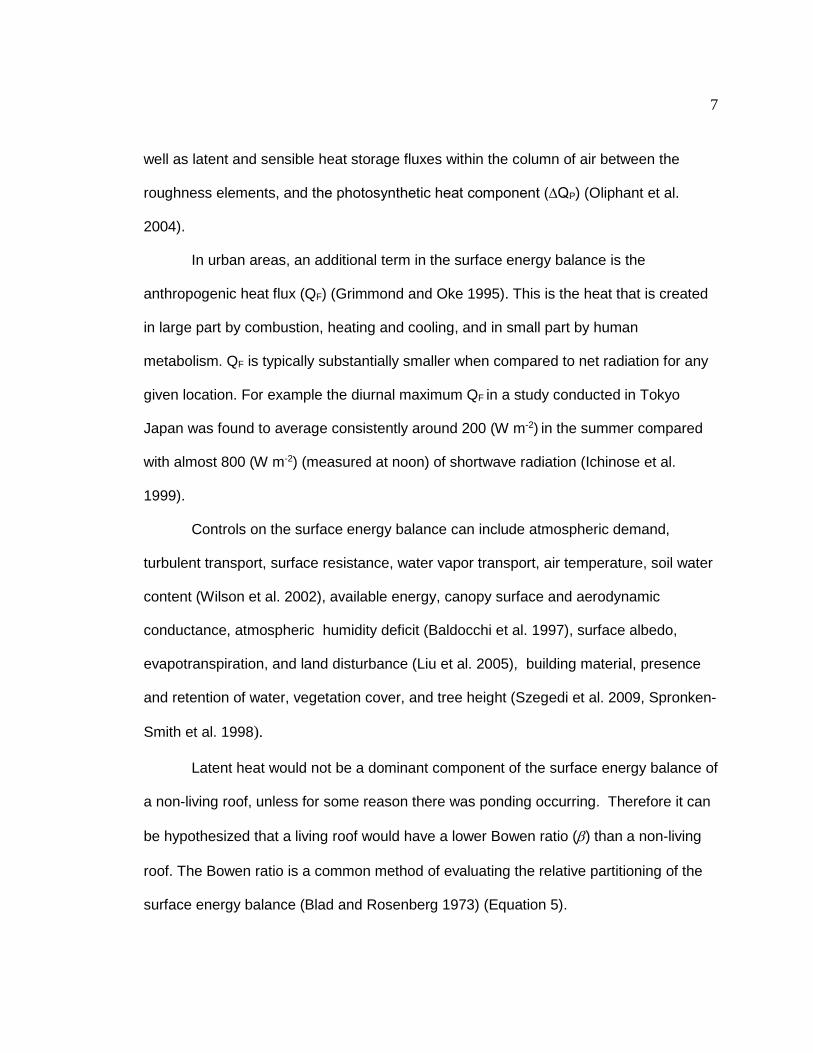
The California Academy of Sciences (Cal Academy) is located within the eastern span of

Golden Gate Park in San Francisco, California (Figure 1) located at 37.77°N, 122.48°W.

San Francisco has a Mediterranean climate with average maximum and minimum

summer temperatures between 15 C° and 21 C° and 10 C°, and 12 C° respectively, and

winter average maximums and minimums between 12 C° and 15 C°, and 7 C° and 10 C°

respectively (Null 1995). Golden Gate Park is a 412 ha mixed-use urban park (SF Parks

and Rec 2014) that is buffered on 3 sides by neighborhoods. The Pacific Ocean

boarders the western edge of the park and prevailing winds are west, northwesterly (Null

1995). San Francisco’s climate is characterized by dry summers, due to the migrating

Pacific high pressure cell which deflects storms to the north, thus limiting summer

precipitation. Conversely, in the winter, the high pressure cell loses intensity and moves

southward, allowing for the intrusion of the moisture-laden low pressure cell, resulting in

cool wet winters (Conomos et al. 1985). There is a frequent advection fog layer typically

present in Golden Gate Park during summer (Oberlander 1956).

During this study period, San Francisco experienced a record-breaking drought.

In 2013 San Francisco received 142 mm rainfall, compared to 647 mm in 2012,

according to the NOOA weather station located in downtown San Francisco, roughly 15

km to the west of the study site. However the living roof was regularly irrigated at night

using a surface sprinkler system. Therefore, the flora on the Cal Academy roof did not

completely experience the climate region’s typical summer dry-out, although there did

9

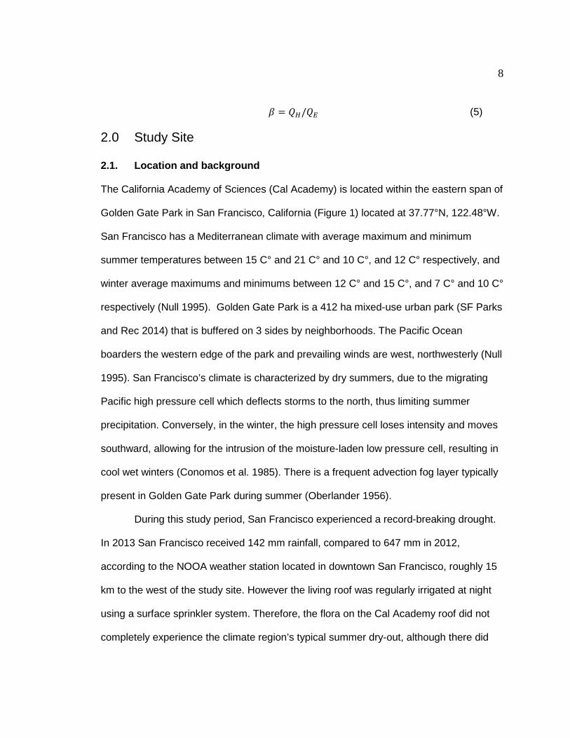
appear to be a visual decline in the vitality of some species during the summer

compared to the onset of the project (Figure 2). According to the Cal Academy’s senior

botanist Frank Alameda, the reason for year-round irrigation of native plants that are

ostensibly climate-tolerant, is to keep the roof in its most vibrant and esthetic state,

thereby encouraging human interest and education (Cal Academy 2014).

(a) (b) (c)

Figure 1. Location of the study tower (a) on the west coast of the US in the state of California (b), within the eastern span of the Golden Gate park in San Francisco and (c) on the southeast corner of the California Academy of Sciences’ Living roof (Google Earth)

(a) (b) (c)

Figure 2. Visual evidence of sesonal variation in vegetation vitatlity on the California Academy of Sciences’ living roof, in San Franicsco Ca for the months of (a) May 2014, (b) August 2014 and (c) February 2015.

The Living roof was designed by architect Renzo Piano in conjunction with

ecological designers Rana Creek, and sits atop a 4 story building located at 55 Music

Concourse Dr., Golden Gate Park San Francisco, California (Figure 1). There are 3

major component roof features: living vegetation and bare soil, the concrete observation

10

deck and walkway, and the glass atrium and skylights (Figure 1c). The roof also has a

number of vents, the most prominent of which are located in the northwest and

southeast corners, as well as atop the smaller southeast dome. The roof has a unique

topography, with 3 large multi meter domes, and 4 smaller domes situated around the

central atrium.

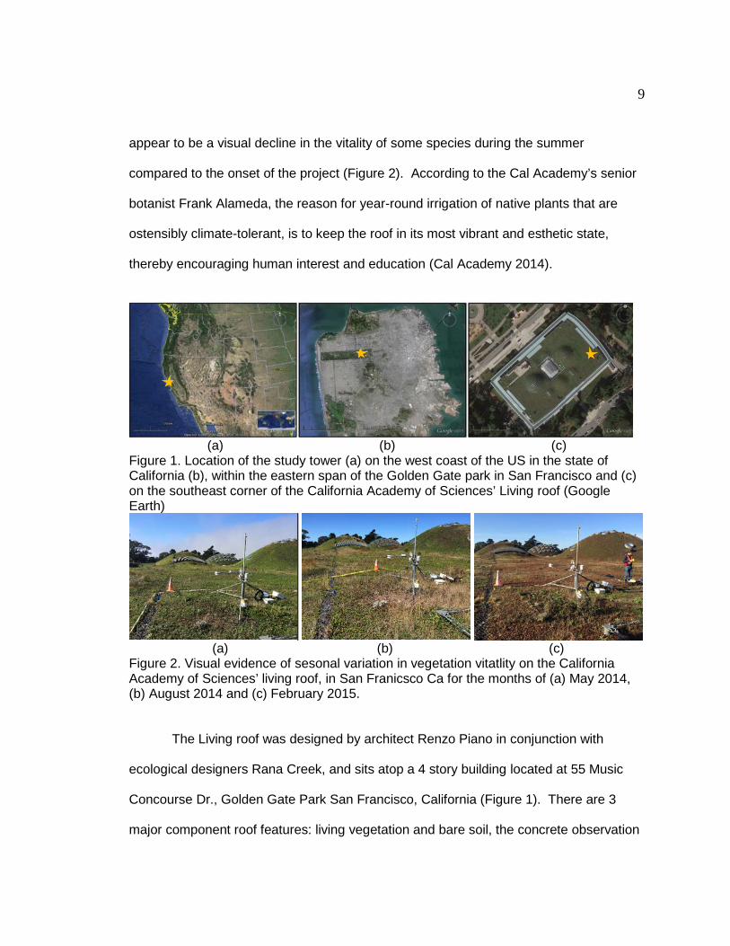
There are 2 major classifications for living roofs: intensive and extensive. Living

roof attributes that define these classifications are shown in Table 1.

Table 1.Classifications of living roofs (Berardi et al. 2014) Attribute Extensive roof Intensive roof

Thickness of growing media

Below 200 mm Above 200 mm

Accessibility Inaccessible Accessible Weight 60-150 kg/m2 Above 300 kg/m2

Diversity of plants Low High Construction Moderate, easy Technical, complex

Irrigation Often not necessary Necessity of drainage and irrigation systems

Maintenance Simple complex

Based on Berardi et al.’s definition, the California Academy of sciences is classified as

an amalgamation of the two categories. As shown in Table 1, one factor in differentiating

the two types of living roof classifications is substrate thickness. Despite being 5 cm

short of the 20 cm substrate thickness that is often the marker of an intensive roof, the

Cal Academy’s roof can be classified as intensive due to its irrigation system, weight,

relatively complex maintenance, accessibility and diversity of flora. On the other hand,

one attribute of the Cal Academy’s living roof that could be classified as extensive, was

the size of the roof itself. Typically intensive roofs are much smaller than extensive

ones. High plant species diversity is particularly utilized in classifying extensive vs

intensive roofs. Species diversity also allowed for comparison between the Cal Academy

11

living roof and other similar ground level environments. A purely extensive roof, by

comparison, such as the one in Wushan, Guangzhou, People’s Republic of China used

as a case study by Feng et al. (2010), had a very shallow substrate (4 cm), and a low

diversity of flora; the only species of note being sedum lineare; making it a worthwhile

comparison to the Cal Academy living roof, but difficult to compare to natural

landscapes. Another study conducted by Theodosiou (2003) used a more intensive roof

in Thessaloniki Greece with a substrate thickness of 12 cm; also comparable to the Cal

Academy living roof.

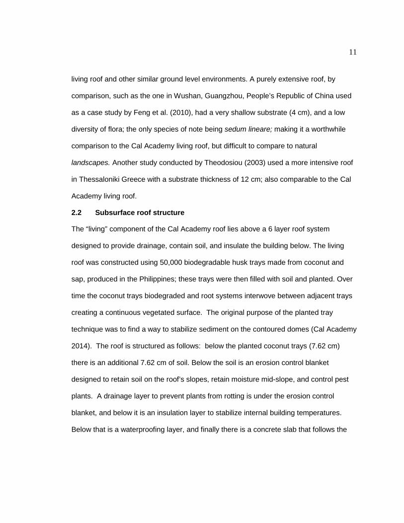
2.2 Subsurface roof structure

The “living” component of the Cal Academy roof lies above a 6 layer roof system

designed to provide drainage, contain soil, and insulate the building below. The living

roof was constructed using 50,000 biodegradable husk trays made from coconut and

sap, produced in the Philippines; these trays were then filled with soil and planted. Over

time the coconut trays biodegraded and root systems interwove between adjacent trays

creating a continuous vegetated surface. The original purpose of the planted tray

technique was to find a way to stabilize sediment on the contoured domes (Cal Academy

2014). The roof is structured as follows: below the planted coconut trays (7.62 cm)

there is an additional 7.62 cm of soil. Below the soil is an erosion control blanket

designed to retain soil on the roof’s slopes, retain moisture mid-slope, and control pest

plants. A drainage layer to prevent plants from rotting is under the erosion control

blanket, and below it is an insulation layer to stabilize internal building temperatures.

Below that is a waterproofing layer, and finally there is a concrete slab that follows the

12

contours of the roof’s seven hills (Cal Academy, 2014). This structure is similar to that of

previously studied living roofs (Berardi et al. 2014, Feng et al. 2010, Jim and He, 2010).

Figure 3. Schematic of the living roof structure on the California Academy of Sciences, San Francisco, Ca. 2.3 Ecology and vegetation surveys

Coastal chaparral and north coastal prairie are the two native California ecosystems that

best categorize the Cal Academy living roof’s flora. Costal chaparral occupies 3,400,200

ha of California, and north costal prairie encompasses 351,500 ha (Barbour et al. 1988).

The Living roof’s vegetation is a cross between the aforementioned ecosystems rather

than simply a costal chaparral ecosystem, because unlike much of the coastal chaparral

that covers the surrounding Bay Area hillsides, the living roof has fewer shrubs and far

more grass and wildflower species. Unlike either ecosystem in its natural state, the

living roof is substantially manicured and weeded. The substrate of the Golden Gate

Park is USGS soil type D, which includes some Quaternary muds, sands, gravels, and

silts (USGS, 2012). The Cal Academy living roof’s substrate is supplemented with

compost and constructed with soil that best sustains the native plant species (Cal

Academy, 2014).

Planted coconut trays

Vegetation

Erosion control blanket

Additional soil

Drainage layer Insulation Waterproofing layer Concrete slab

13

The Cal Academy living roof was originally planted with 1.7 million individual

plants of 9 native species (Cal Academy, 2014). Since construction completed in 2008,

additional natives and non-natives alike have colonized the roof. In May and June of

2014, vegetation surveys were conducted to determine species diversity, relative cover,

and canopy height. Employing a similar technique to that of Kalra (1996), the Cal

Academy roof was broken into 49 m2 sampling quadrants based on the existing rooftop

grid pattern. The total area of the roof (including roof features) is roughly 10,241 m2. Of

this, the central atrium accounts for 5.74% (588 m2), the observation deck accounts for

2.87% (294 m2), and the other roof features such as cages, vents and skylights,

combined together account for approximately 9.56% (980 m2). 124 sampling quadrants

(6076 m2) met the criteria of being entirely vegetated with no major roof features, and

having a flat or only slightly inclined surface. None of the 3 major domes were sampled

due to access constraints. There were 41 additional vegetated, flat, partial quadrants

that were not sampled due to irregular size.

A total of 22 sampling quadrants were utilized. These were geographically

dispersed across the roof. 21 points were sampled in each sampling quadrant. A

random-number table was used to generate stratified random sample points along 7

transects in each sampling quadrant (Figure 3). Beach strawberry (fragaria chiloensis)

dominated the Cal Academy roof’s vegetation profile with 32.9% coverage (Table 2).

The next most common species occurrences were California bent grass (Agrostis

densiflora ) 11.8% and bare soil 8.8%. The average height of vegetation was 14.6 cm.

14

Table 2. List of plant species and percent cover of each on the living roof of the California Academy of Sciences in San Francisco Ca, 2014. Plant species Latin name Observations % cover bare soil NA 44 8.8% beach strawberry Fragaria chiloensis, 164 32.9% bur clover Medicago 7 1.4% California bent grass Agrostis densiflora 59 11.8% California fuchsia Epilobium canum 6 1.2% California poppy Eschscholzia californica 1 0.2% California sweet grass

Hierochloe 15 3.0%

coast dudleya Dudleya caespitosa 1 0.2% common yarrow Achillea millefolium 28 5.6% dandilion Taraxacum 7 1.4% fireweed Chamerion

angustifolium 17 3.4%

foxtail fescue Festuca 35 7.0% golden-eyed grass Sisyrinchium

californicum 8 1.6%

gumweed Grindelia 10 2.0% leaf litter NA 16 3.2% lupin Lupinus 6 1.2% nutgrass Cyperus rotundus 8 1.6% scorpionweed Phacelia 10 2.0% plantain weed Plantago major 2 0.4% purple needle grass Nassella pulchra 2 0.4% scouringrush horsetail

Equisetum hyemale 4 0.8%

Figure 4. Researchers conducting point sampling for vegetation surveys on the living roof of the California Academy of Sciences, San Francisco Ca, 2014.

15

seaside daisy Erigeron glaucus 9 1.8% seep monkeyflower Mimulus 14 2.8% self heal Prunella 15 3.0% sowthistle Sonchus 7 1.4% yellow primrose Primula vulgaris 3 0.6%

3.0 Materials and Methods

3.1 Deployment

In summer 2013 and for the majority of 2014, observations were made of the surface

radiation budget and surface energy balance. All instruments were either mounted on a

tripod tower or buried in the roof’s substrate (Table 3). For above ground measurements,

a CSTAT3 three-dimensional sonic anemometer (Campbell Scientific, Logan Utah) and

a Li-7500 fast response infrared gas analyzer (LI-COR, Lincoln Nebraska) were

stationed at 1 m above the surface. At 1.2 m and 1.1 m respectively, a BF5 sunshine

senor for photosynthetically active radiation (PAR) (Delta-T Devices, Cambridge UK), a

four component net radiometer (Campbell Scientific, Logan Utah), and an HMP45c

thermistor/hygristor (Campbell Scientific, Logan Utah) were mounted. A TE525 rain

gauge (Campbell Scientific, Logan Utah) was mounted just above the surface at 0.4 m.

Within the roof’s substrate, two HFP01 ground heat flux plates (Campbell Scientific,

Logan Utah) were buried at -5 cm in depth, two CS107 thermistors (Campbell Scientific,

Logan Utah) were buried at -15 cm and -3 cm respectively, a CS616 soil moisture probe

(Campbell Scientific, Logan Utah) was inserted to measure the average between the

surface and 15 cm of substrate, and four spatially averaging CS109 thermocouples

(Campbell Scientific, Logan Utah) were inserted between -1 and -5 cm to measure

temperature above the ground heat flux plates. Power for all instruments was supplied

16

by multiple 12 V deep cycle batteries charged by a 75 W solar panel. All data were

collected and stored in a CR3000 data logger in raw 10 Hz samples as well as 30 min

averages. The gas analyzer was periodically calibrated using zero and span gasses for

CO2 and H2O absorption calibration. On September 24th one of the two ground heat flux

plates was moved and reburied at a depth of -15 cm.

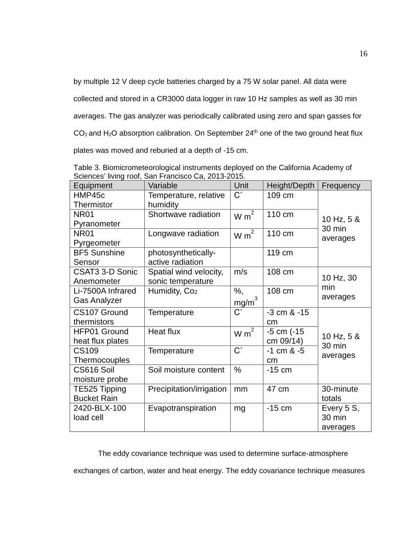
Table 3. Biomicrometeorological instruments deployed on the California Academy of Sciences’ living roof, San Francisco Ca, 2013-2015. Equipment Variable Unit Height/Depth Frequency HMP45c Thermistor

Temperature, relative humidity

C˚ 109 cm

10 Hz, 5 & 30 min averages

NR01 Pyranometer

Shortwave radiation W m2 110 cm

NR01 Pyrgeometer

Longwave radiation W m2 110 cm

BF5 Sunshine Sensor

photosynthetically-active radiation

119 cm

CSAT3 3-D Sonic Anemometer

Spatial wind velocity, sonic temperature

m/s 108 cm 10 Hz, 30 min averages

Li-7500A Infrared Gas Analyzer

Humidity, Co2 %, mg/m3

108 cm

CS107 Ground thermistors

Temperature C˚ -3 cm & -15 cm

10 Hz, 5 & 30 min averages

HFP01 Ground heat flux plates

Heat flux W m2 -5 cm (-15 cm 09/14)

CS109 Thermocouples

Temperature C˚ -1 cm & -5 cm

CS616 Soil moisture probe

Soil moisture content % -15 cm

TE525 Tipping Bucket Rain

Precipitation/irrigation mm 47 cm 30-minute totals

2420-BLX-100 load cell

Evapotranspiration mg -15 cm Every 5 S, 30 min averages

The eddy covariance technique was used to determine surface-atmosphere

exchanges of carbon, water and heat energy. The eddy covariance technique measures

17

rates of vertical transport of atmospheric scalars by turbulent eddies - areas of upward

and downward moving air - that transport the scalar of interest (Baldocchi et al. 2003).

Eddy covariance is an established technique in the micrometeorological community and

has been employed using the same or similar equipment at over 500 sites throughout

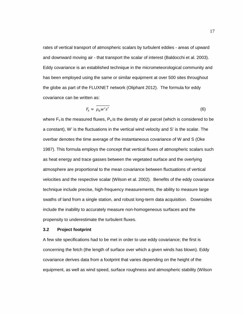
the globe as part of the FLUXNET network (Oliphant 2012). The formula for eddy

covariance can be written as:

𝐹𝐹𝑠𝑠 ≈ 𝜌𝜌𝑎𝑎𝑤𝑤′𝑠𝑠′ ��������� (6)

where Fs is the measured fluxes, Pa is the density of air parcel (which is considered to be

a constant), W’ is the fluctuations in the vertical wind velocity and S’ is the scalar. The

overbar denotes the time average of the instantaneous covariance of W and S (Oke

1987). This formula employs the concept that vertical fluxes of atmospheric scalars such

as heat energy and trace gasses between the vegetated surface and the overlying

atmosphere are proportional to the mean covariance between fluctuations of vertical

velocities and the respective scalar (Wilson et al. 2002). Benefits of the eddy covariance

technique include precise, high-frequency measurements, the ability to measure large

swaths of land from a single station, and robust long-term data acquisition. Downsides

include the inability to accurately measure non-homogeneous surfaces and the

propensity to underestimate the turbulent fluxes.

3.2 Project footprint

A few site specifications had to be met in order to use eddy covariance; the first is

concerning the fetch (the length of surface over which a given winds has blown). Eddy

covariance derives data from a footprint that varies depending on the height of the

equipment, as well as wind speed, surface roughness and atmospheric stability (Wilson

18

et al. 2002, Baldocchi et al. 2003), this makes stationing the instruments at a height

representative of the source area crucial to measuring the desired area and nothing

beyond. The fetch also fluctuates based on whether measurements are being made

during stable or unstable conditions. To maximize usable data, the eddy covariance

tower was installed as low as possible to the Cal Academy’s roof’s surface resulting in

an average 80%ile fetch distance that just passed the roof’s atrium. By comparison,

most eddy covariance towers established in previous studies are placed several meters

high for shorter canopies, and over 10 m high for tall forests (Wilson et al. 2002).

The project footprint model was established from a data set acquired during a

preliminary short-term study performed at the same location in summer 2013. In this

study Hsieh et al.’s (2000) analytical footprint model was employed to estimate the

project footprint for every 30 min interval. All periods when the 80th percentile of the

cumulative flux distance fell outside of the roof area were rejected. The tower was

installed in the southeast corner of the Cal Academy roof in order to obtain the largest

rooftop footprint in the prevailing westerly wind direction. The Cal Academy has the only

living roof in California large enough to utilize this technique, making this the premier

study of living roofs using eddy covariance.

The second specification that had to be met in order to use eddy covariance is

surface homogeneity so that advection (QA) can be discounted (Wofsy et al. 1993;

Moncrieff et al. 1997), as any advection in this case would likely originate from outside

the roof perimeter. The Cal Academy roof is complex. While the plant species and

height distribution across the roof is fairly homogenous, the roof topography may cause

local area flux deviations. The atrium center within the domes is the most significant roof

19

feature within the project footprint; it is typically opened at the end of the day to allow for

cool air to drain down the domes into the plaza for interior cooling (Cal Academy 2014).

The equipment was located roughly 15 m form the leeward edge of the building to avoid

influence of vertical wind motions associated with the building edge. The anthropogenic

heat flux was not independently measured in this study, as the only potential sources –

vents and people on the observation deck – were largely outside the project footprint.

The various surface energy balance terms have unique controls depending on

the environment. Latent heat (QE) and sensible heat (QH) fluxes were measured using

the eddy covariance technique, while conductive ground heat (QG) is measured using

ground heat flux plates. The equation for sensible and latent heat are as follows:

QE = LvW′Pv′ (7.1)

QH = CaW′T′ (7.2)

Where Equation 7.1 is the latent heat flux, where Lv is the latent heat of vaporization, W’

is the fluctuations in vertical velocity and Pv is the vapor density of air, and Equation 7.2

is the sensible heat flux, where Ca is the specific heat of air, W’ is the fluctuations in

vertical velocity, and T’ is the fluctuations in air temperature.

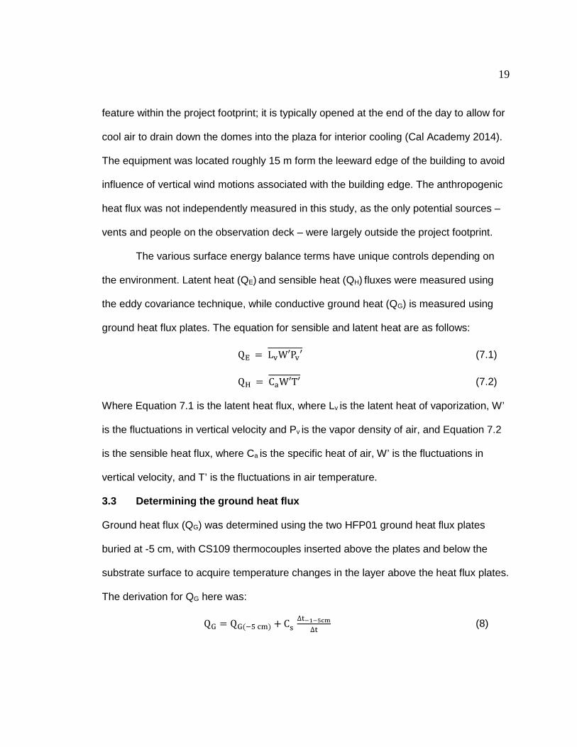
3.3 Determining the ground heat flux

Ground heat flux (QG) was determined using the two HFP01 ground heat flux plates

buried at -5 cm, with CS109 thermocouples inserted above the plates and below the

substrate surface to acquire temperature changes in the layer above the heat flux plates.

The derivation for QG here was:

QG = QG(−5 cm) + Cs ∆t−1−5cm

∆t (8)

20

where Qg(-5 cm) is the measured soil heat flux at depth -5 cm, CS is the soil heat capacity,

and t is time (Oliphant et al. 2011). Heat flux plates were buried to prevent solar radiation

loading. The deeper the plates are buried, the less directly they measure the transfer of

energy from the surface through the ground due to the storage medium between the flux

plates and biosurface (Oke 1987). In order to account for this storage term, T-type

averaging thermocouples were installed between -5 and 0 cm to capture the

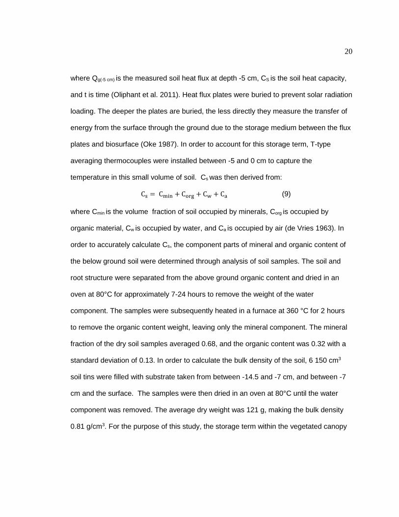
temperature in this small volume of soil. Cs was then derived from:

Cs = Cmin + Corg + Cw + Ca (9)

where Cmin is the volume fraction of soil occupied by minerals, Corg is occupied by

organic material, Cw is occupied by water, and Ca is occupied by air (de Vries 1963). In

order to accurately calculate Cs, the component parts of mineral and organic content of

the below ground soil were determined through analysis of soil samples. The soil and

root structure were separated from the above ground organic content and dried in an

oven at 80°C for approximately 7-24 hours to remove the weight of the water

component. The samples were subsequently heated in a furnace at 360 °C for 2 hours

to remove the organic content weight, leaving only the mineral component. The mineral

fraction of the dry soil samples averaged 0.68, and the organic content was 0.32 with a

standard deviation of 0.13. In order to calculate the bulk density of the soil, 6 150 cm3

soil tins were filled with substrate taken from between -14.5 and -7 cm, and between -7

cm and the surface. The samples were then dried in an oven at 80°C until the water

component was removed. The average dry weight was 121 g, making the bulk density

0.81 g/cm3. For the purpose of this study, the storage term within the vegetated canopy

21

was considered negligible due to the average height of the canopy layer (14.6 cm) and

this term was represented solely by the ground heat flux (QG).

On September 14, 2014, one of the ground heat flux plates buried at -5 cm was

removed and re-buried at -15cm in order to determine the total amount of heat

transferred through the entire substrate into the building roof below. During this period,

the both heat flux plates took measurements at 10 Hz, and data was aggregated into 5 &

30 min averages.

4.0 Results

Data collected between May and July of 2013, and between March of 2014 and March of

2015 was analyzed to determine the characteristics of the surface radiation budget and

the surface energy balance on the California Academy’s living roof. Due to the high rate

of data rejection (~50%) for eddy covariance terms, these characteristics where

consolidated into 30-minute statistics for timeframes ranging from monthly to annual.

These diurnal ensembles were derived using periods when all surface radiation budget

and energy balance terms were available.

A full year of data was collected between 2014 and 2015; showing the annual

variability of the living roof’s microclimate. In addition, the summer deployment in 2013

allowed for inter-annual comparison of summer months between 2013 and 2014.

Seasonal controls on the surface radiation and energy balance terms were examined;

and energy balance closure was assessed on both a total study period and monthly time

scale. The ground heat flux was analyzed at both at the soil-air and soil-roof interfaces to

investigate conductive heat transfer into and out of the building roof.

22

4.1 Surface radiation budget

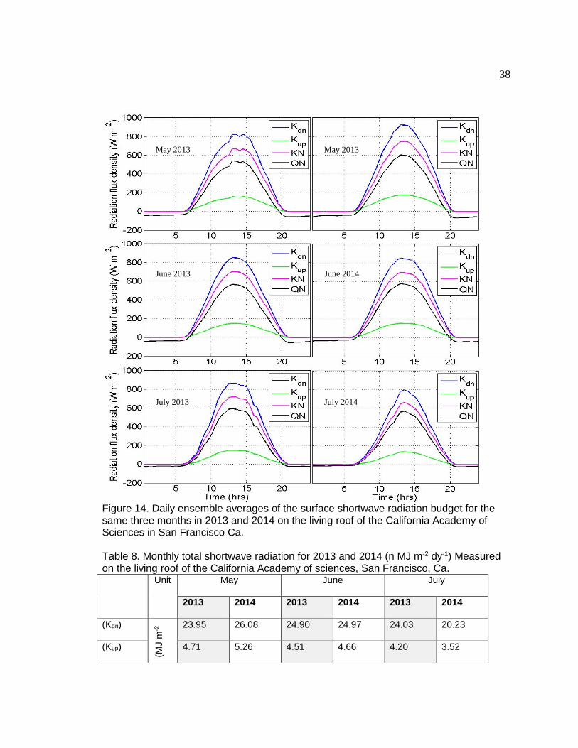
The diurnal ensemble averages for the components of the Surface radiation budget

during the study period are shown in Figure 5. Incoming shortwave radiation (Kdn)

peaked in the afternoon between 12:00 and 14:00 PST. The albedo of the living roof

averaged 20% and was fairly consistent throughout the daylight period. As a result, an

average of 13.18 (MJ m-2 dy-1) was absorbed by the living roof (Table 4). Seasonal

variation in Kdn was primarily driven by solar declination and changes in cloud cover as

evidenced by the low Kdn observations under cloudy conditions and high observations

under clear sky conditions (Figure 8) as well as the corresponding high and low

seasonal Kdn observations shown in Figure 6 during times of high and low solar

declination. Due to the presence of summer advection fog, the peak in Kdn occurred in

May, while July and August showed the most reduction due to cloud cover.

The albedo of the living roof had a seasonal range (4.9%), with highest observations

occurring in the winter and spring, and then decreasing in the summer and early fall.

This corresponds closely to the annual growth cycle of this Mediterranean ecosystem,

with maximum foliage appearing in the wetter growing season over the winter and

spring, and plant species drying out and dying off in the summer despite irrigation

(Figure 2).

Incoming longwave radiation (Ldn) remained relatively constant throughout the diurnal

cycle, reflecting the low diurnal air temperature range (Figure 5). There was also relative

constancy in longwave radiation seasonally across months, indicating a low annual

temperature range. The largest impact on Ldn is due to the presence or absence of

clouds. Outgoing longwave radiation (Lup) was only slightly greater than Ldn, and

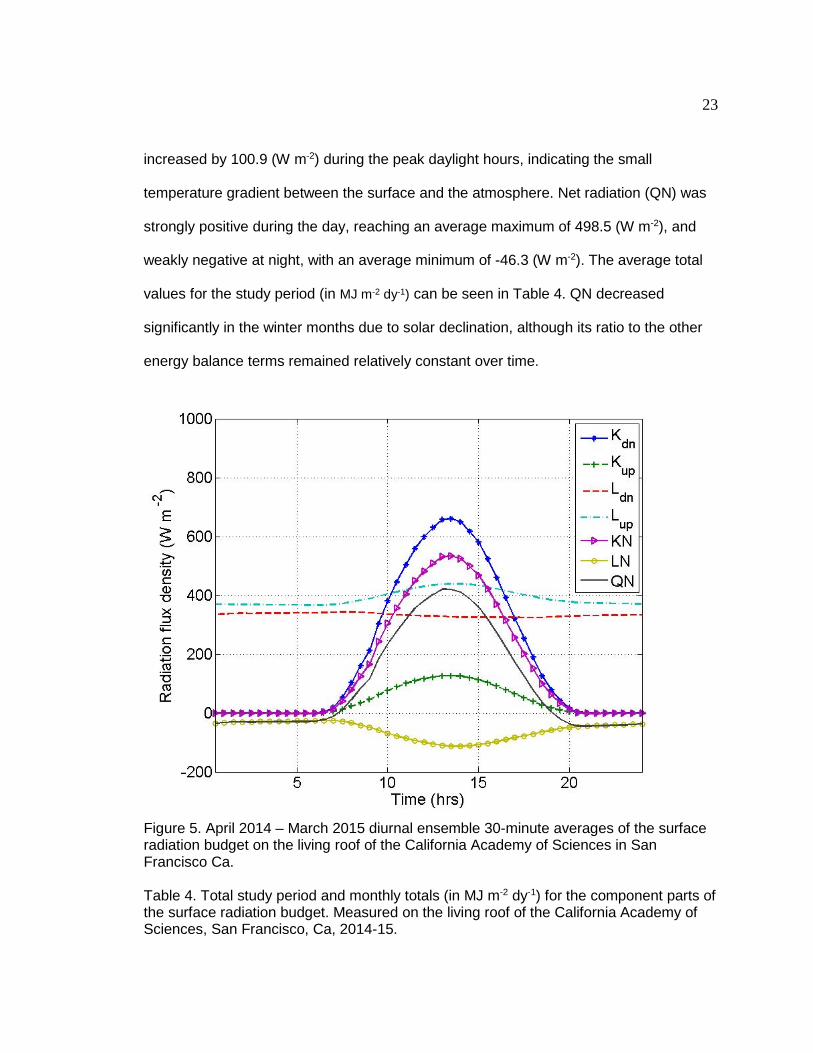
23

increased by 100.9 (W m-2) during the peak daylight hours, indicating the small

temperature gradient between the surface and the atmosphere. Net radiation (QN) was

strongly positive during the day, reaching an average maximum of 498.5 (W m-2), and

weakly negative at night, with an average minimum of -46.3 (W m-2). The average total

values for the study period (in MJ m-2 dy-1) can be seen in Table 4. QN decreased

significantly in the winter months due to solar declination, although its ratio to the other

energy balance terms remained relatively constant over time.

Figure 5. April 2014 – March 2015 diurnal ensemble 30-minute averages of the surface radiation budget on the living roof of the California Academy of Sciences in San Francisco Ca. Table 4. Total study period and monthly totals (in MJ m-2 dy-1) for the component parts of the surface radiation budget. Measured on the living roof of the California Academy of Sciences, San Francisco, Ca, 2014-15.

24

(Kdn) (Kup) (Ldn) (Lup) (KN) (LN) (QN) (α)

(MJ m-2 dy-1) (%)

Total 16.52 3.34 27.97 33.71 13.18 -5.74 8.38 20.43

1_Jan 10.55 2.31 15.43 32.11 8.24 -16.7 2.82 21.90

2_Feb 14.68 3.10 25.99 32.41 11.58 -6.42 5.16 21.12

3_March 16.73 3.75 27.54 32.65 12.98 -5.11 7.87 20.84

4_April 21.70 4.85 27.57 33.19 16.85 -5.62 11.24 22.33

5_May 26.08 5.26 27.37 34.36 20.82 -5.99 13.83 20.16

6_June 24.97 4.66 29.07 34.64 20.31 -5.57 14.74 18.66

7_July 20.23 3.52 31.75 35.01 16.71 -3.26 13.45 17.39

8_Aug 15.23 2.77 32.10 34.45 12.45 -2.35 10.10 18.22

9_Sept 17.49 3.57 30.86 35.04 13.93 -4.18 9.74 20.39

10_Oct 13.95 2.95 29.75 34.54 11.00 -4.79 6.20 21.16

11_Nov 9.10 1.97 28.51 32.91 7.13 -4.4 2.73 21.65

12_Dec 6.62 1.41 30.41 32.70 5.21 -2.29 2.92 21.30

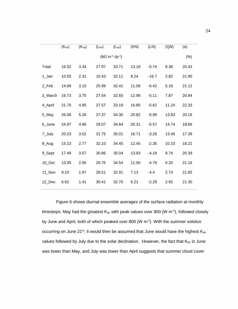
Figure 6 shows diurnal ensemble averages of the surface radiation at monthly

timesteps. May had the greatest Kdn with peak values over 900 (W m-2), followed closely

by June and April, both of which peaked over 800 (W m-2). With the summer solstice

occurring on June 21st, it would then be assumed that June would have the highest Kdn

values followed by July due to the solar declination. However, the fact that Kdn in June

was lower than May, and July was lower than April suggests that summer cloud cover

25

Figure 6. Per month diurnal ensemble averages of the surface radiation budget on the living roof of the California Academy of Sciences in San Francisco Ca, from April 2014 to March 2015.

May April

February

June

July August September

October November December

March January

26

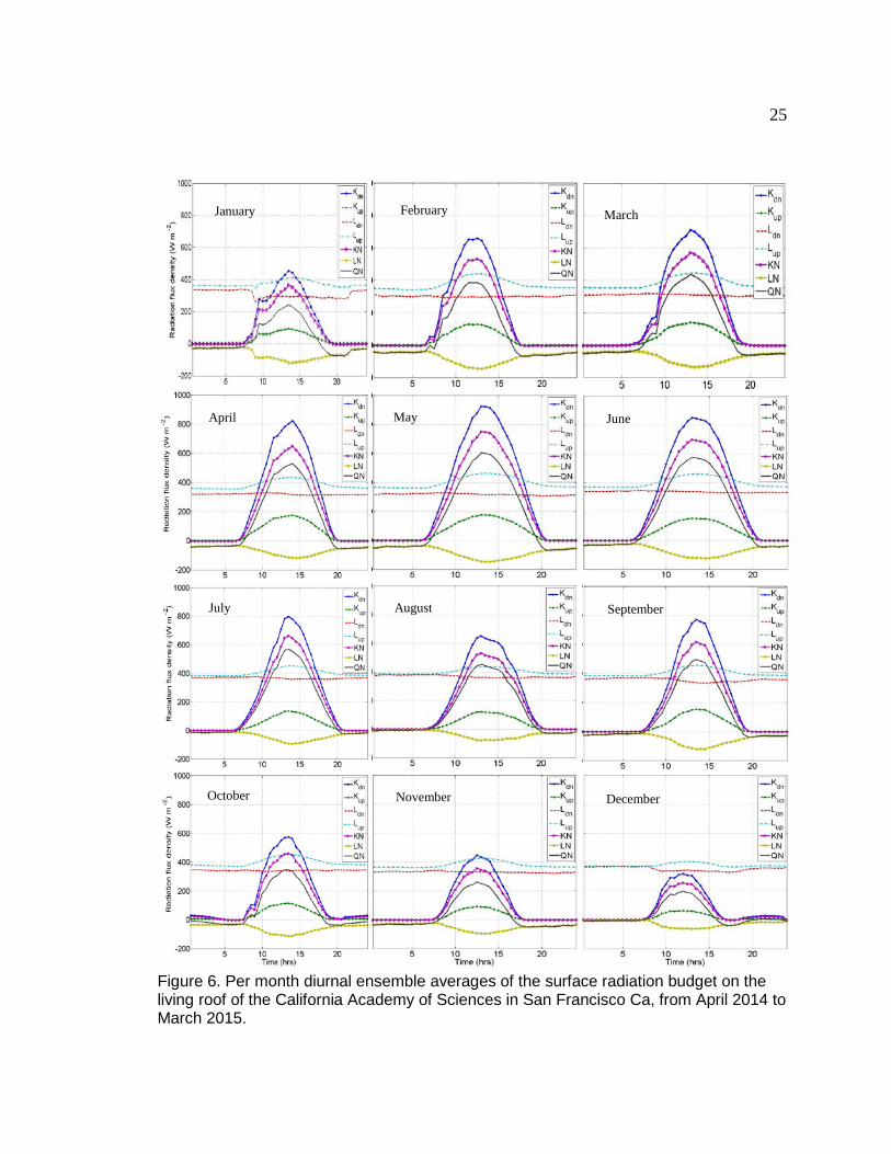
due to advection fog strongly modified the effect of declination. The impact of cloud

cover on the surface radiation budget is also evidenced by the amount of diffuse PAR

occurring on a seasonal basis (Figure 7).

Figure 7. PAR diffuse with standard deviation and PAR global diurnal ensembles on the California Academy of Sciences Living Roof, San Francisco, Ca.

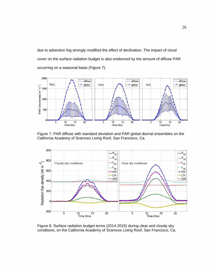
Figure 8. Surface radiation budget terms (2014-2015) during clear and cloudy sky conditions, on the California Academy of Sciences Living Roof, San Francisco, Ca.

May June July

Cloudy sky conditions Clear sky conditions

27

Clear skies were defined as any time when Ldn was less than 370 (W m-2), and cloudy

skies any time when Ldn was greater than 370 (W m-2) (Brant et al. 2008). Clear skies

showed a smaller disparity between incoming and outgoing long wave radiation; both

stayed consistent around 400 (W m-2) with a small increase during the day, whereas

under clear skies, Ldn was noticeably lower than both the corresponding clear skies Lup,

and the Ldn values under cloudy skies. This demonstrates clouds ability to reflect and in

essence “trap” Longwave radiation.

4.2 Surface energy balance

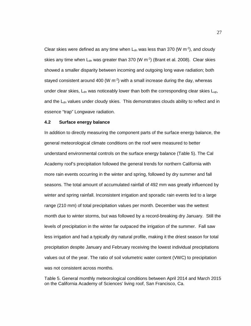
In addition to directly measuring the component parts of the surface energy balance, the

general meteorological climate conditions on the roof were measured to better

understand environmental controls on the surface energy balance (Table 5). The Cal

Academy roof’s precipitation followed the general trends for northern California with

more rain events occurring in the winter and spring, followed by dry summer and fall

seasons. The total amount of accumulated rainfall of 492 mm was greatly influenced by

winter and spring rainfall. Inconsistent irrigation and sporadic rain events led to a large

range (210 mm) of total precipitation values per month. December was the wettest

month due to winter storms, but was followed by a record-breaking dry January. Still the

levels of precipitation in the winter far outpaced the irrigation of the summer. Fall saw

less irrigation and had a typically dry natural profile, making it the driest season for total

precipitation despite January and February receiving the lowest individual precipitations

values out of the year. The ratio of soil volumetric water content (VWC) to precipitation

was not consistent across months.

Table 5. General monthly meteorological conditions between April 2014 and March 2015 on the California Academy of Sciences’ living roof, San Francisco, Ca.

28

Total precipitation/ irrigation (mm)

Mean soil temperature (ºC)

Mean volumetric water content (%)

Mean air temperature (ºC)

Mean wind speed (mph)

Study period

492 15.8 18.3 14.2 1.8

1_Jan 7 11.1 25 14.1 1.2 2_Feb 9 13.5 31 13.4 1.2

3_March 13 14.8 14 12.8 1.4 4_April 47 15.3 13 12.5 1.8 5_May 34 17.4 6 13.9 2.1

6_June 27 17.7 5 13.4 2.4 7_July 40 18.8 11 15.3 2.3 8_Aug 21 18.1 20 15.4 2.3

9_Sept 28 18.7 16 16.0 1.9 10_Oct 16 16.9 23 16.7 1.6 11_Nov 33 13.8 25 14.0 1.0 12_Dec 217 13.4 31 12.9 1.6

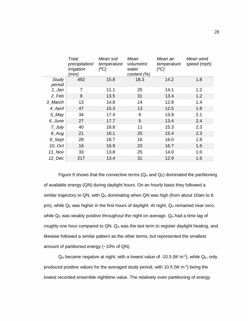
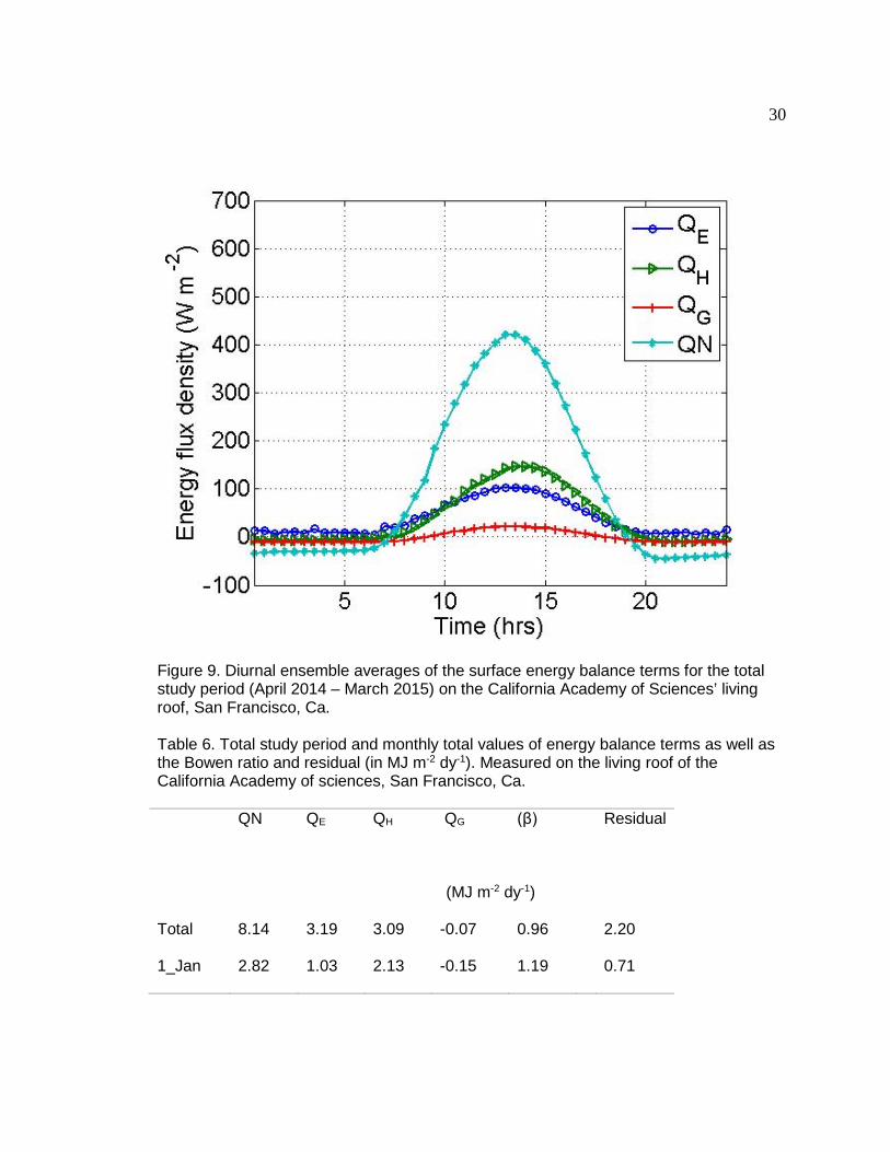
Figure 9 shows that the convective terms (QH and QE) dominated the partitioning

of available energy (QN) during daylight hours. On an hourly basis they followed a

similar trajectory to QN, with QH dominating when QN was high (from about 10am to 6

pm), while QE was higher in the first hours of daylight. At night, QH remained near zero,

while QE was weakly positive throughout the night on average. QH had a time lag of

roughly one hour compared to QN. QG was the last term to register daylight heating, and

likewise followed a similar pattern as the other terms, but represented the smallest

amount of partitioned energy (~10% of QN).

QH became negative at night, with a lowest value of -10.5 (W m-2), while QE, only

produced positive values for the averaged study period, with 10.5 (W m-2) being the

lowest recorded ensemble nighttime value. The relatively even partitioning of energy

29

between the turbulent heat fluxes resulted in a study period Bowen ratio (β) value of 0.96

(Table 6). Seasonally, QG remained consistently negative throughout the year,

indicating that the building under the substrate was conducting heat outwards through

the substrate into the atmosphere. The negative observations show how having a

planted surface above a building differ from natural ecosystems where there would be

no sub-surface heat source.

As Figure 10 shows, the latent heat flux began to surpass the sensible heat flux

in October at the onset of the rainy season. Seasonally both convective fluxes were

highest in summer, began to decline in the fall, and were reduced to less than half their

summer values during the winter when all the energy balance terms were greatly

reduced by the lack of incoming solar radiation. The seasonal variability shows how

strongly the surface energy balance is driven by the magnitudes of the surface radiation

budget, which was likewise dramatically reduced during the winter months.

30

Figure 9. Diurnal ensemble averages of the surface energy balance terms for the total study period (April 2014 – March 2015) on the California Academy of Sciences’ living roof, San Francisco, Ca. Table 6. Total study period and monthly total values of energy balance terms as well as the Bowen ratio and residual (in MJ m-2 dy-1). Measured on the living roof of the California Academy of sciences, San Francisco, Ca. QN QE QH QG (β) Residual

(MJ m-2 dy-1)

Total 8.14 3.19 3.09 -0.07 0.96 2.20

1_Jan 2.82 1.03 2.13 -0.15 1.19 0.71

31

2_Feb 5.21 3.11 1.71 -0.09 0.55 0.47

3_March 7.66 3.75 2.64 -0.05 0.70 1.53

4_April 11.24 4.27 4.14 -0.04 0.97 2.87

5_May 13.83 4.74 5.20 -0.05 1.10 3.94

6_June 14.74 3.54 6.41 -0.01 1.81 4.81

7_July 13.45 3.82 5.19 -0.04 1.36 4.48

8_Aug 10.10 3.88 3.54 -0.03 0.91 2.71

9_Sept 9.75 3.53 3.52 -0.04 1.00 2.73

10_Oct 6.20 3.51 1.86 -0.02 0.53 0.85

11_Nov 2.74 2.31 0.82 -0.12 0.35 -0.27

12_Dec 2.95 0.81 0.81 -0.18 1.00 1.15

4.3 Controls on the surface energy balance

Controls on the surface energy balance were expected to include air and soil

temperature, available energy, precipitation and VWC, and plant transpiration (Wilson et

al. 2002, Liu et al. 2005). For the purpose of this study “precipitation” was defined as any

measureable rainfall or irrigation water as measured by the TE525 tipping bucket rain

gauge. Precipitation observations were only weakly correlated with QE; with July and

August having similar QE observations despite August receiving only half the

precipitation of July (Tables 5 and 6). As previously noted, there was not a strong

relationship between precipitation and VWC. Likewise there was not a strong

relationship between QE and VWC; with QE being highest in April and May, and May

having less than half the mean VWC of April. QH was highest in the summer months

32

(June, July and August) which corresponded to the highest mean wind speeds, although

two of the summer months also had the highest residuals, it is unlikely that high mean

wind speed is responsible for this, because July and August had the same exact mean

wind speed, but vastly different residuals. Also winds speeds were likely driven by macro

seasonal variations in onshore breezes from the western coast of San Francisco.

Available energy was the strongest driver of the turbulent heat fluxes, as clearly

evidenced by Figures 6 and 10.

Clouds also controlled the surface energy balance. Under clear sky conditions

mean QN was 9.78 (MJ m-2 dy-1), and was 7.55 (MJ m-2 dy-1) under cloudy sky

conditions. The Bowen ratio was 0.82 under sunny skies and 1.06 under cloudy

conditions. This implies that there was greater evapotranspiration under clear skies

(Figure 11).

33

Figure 10. Daily ensemble averages per month of the surface energy balance terms on the California Academy of Sciences’ living roof, San Francisco, Ca. 2014-2015.

April May June

July August September

October November December

February January March

34

Figure 11. Surface energy balance 2014-2015 during clear and cloudy sky conditions, on the California Academy of Sciences Living Roof, San Francisco, Ca.

4.4 Ground heat flux

The ground heat flux followed the diurnal pattern of QN; QG responded quickly once the

surface energy balance became positive at the onset of morning (Figure 12), first by

predominantly heating the 0-5 cm layer of substrate, followed by conduction to deeper

layers of the substrate/roof. In the afternoon the surface layer began to cool, despite a

positive (downward) heat flux still at 5 cm. This reduced the overall ground heat flux at

the surface until it became negative close to the evening sign reversal of QN. QG stayed

weekly negative throughout the night. Over daily time periods, mean QG was also weekly

negative for all months of the study period as seen in Table 6. This indicates a small net

loss of heat from the building on an annual basis. Over the study period, the total

ground heat flux was -0.07 (MJ m-2dy-1). Both the ground and sensible heat fluxes

Cloudy sky conditions Clear sky conditions

35

reached their peaks with more similar timing to one another than with the latent heat

which peaked earlier in the day.

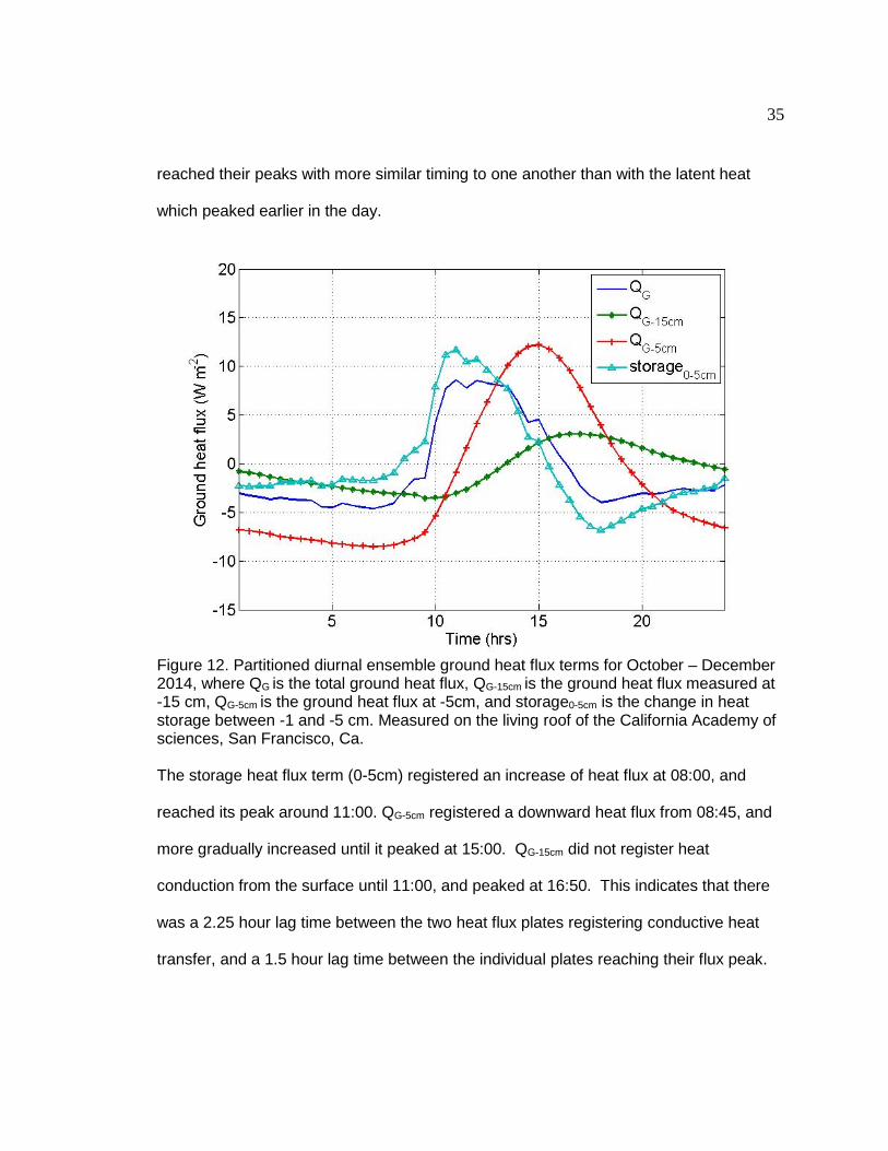
Figure 12. Partitioned diurnal ensemble ground heat flux terms for October – December 2014, where QG is the total ground heat flux, QG-15cm is the ground heat flux measured at -15 cm, QG-5cm is the ground heat flux at -5cm, and storage0-5cm is the change in heat storage between -1 and -5 cm. Measured on the living roof of the California Academy of sciences, San Francisco, Ca. The storage heat flux term (0-5cm) registered an increase of heat flux at 08:00, and

reached its peak around 11:00. QG-5cm registered a downward heat flux from 08:45, and

more gradually increased until it peaked at 15:00. QG-15cm did not register heat

conduction from the surface until 11:00, and peaked at 16:50. This indicates that there

was a 2.25 hour lag time between the two heat flux plates registering conductive heat

transfer, and a 1.5 hour lag time between the individual plates reaching their flux peak.

36

The storage heat flux began to decrease dramatically after 13:50, and decreased to -6.5

(W m-2) by 18:00. QG-5cm began decreasing more steeply at 16:00 and dropped

continuously until -8 (W m-2) . QG-15cm didn’t start decreasing until 18:00, and then

gradually declined throughout the night period with a minimum flux of -3.5 (W m-2).

The magnitude of heat energy (W m-2) also varied greatly between the two

ground heat flux plates. QG-5cm ranged between -10 and 17 (W m-2), while QG-15cm had a

much narrower range of between -3.5 and 5.5. This means that on an average diurnal

basis, only 3 (W m-2) of heat energy was conducted into the building below, and the

remaining QG energy was stored in the substrate and later released in the evening.

Spring Summer

Fall Winter

37

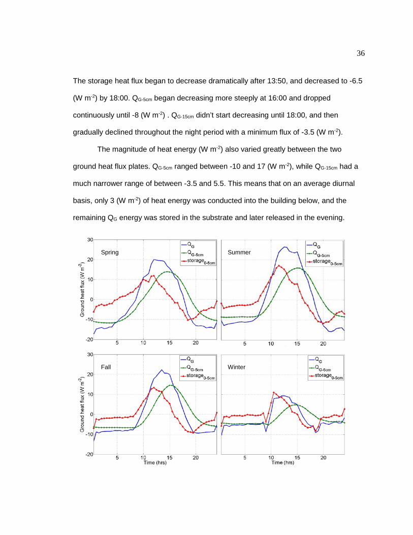
Figure 13. Seasonal variation in ground heat flux measurements on the living roof of the California Academy of Sciences, San Francisco, Ca, 2014.

The time lag is present for all seasons on the living roof. Although as Figure 13 shows,

there is an even greater time lag between QG and QG-5cm in the winter. This is

commensurate with the magnitude of the heat fluxes and indicates the smaller flux

magnitudes correspond to a speed of conduction with depth.

Table 7. Monthly values of ground heat flux terms (in MJ m-2 dy-1). Measured on the living roof of the California Academy of Sciences, San Francisco, Ca. October 2014 – February 2015.

QG-15cm QG-5cm QG

(MJ m-2 dy-1)

10_Oct -0.05 0.05 0.05

11_Nov -0.18 -0.06 -0.07

12_Dec -0.20 -0.14 -0.16

1_Jan 0.81 0.06 0.11

2_Feb -0.15 -0.03 -0.02

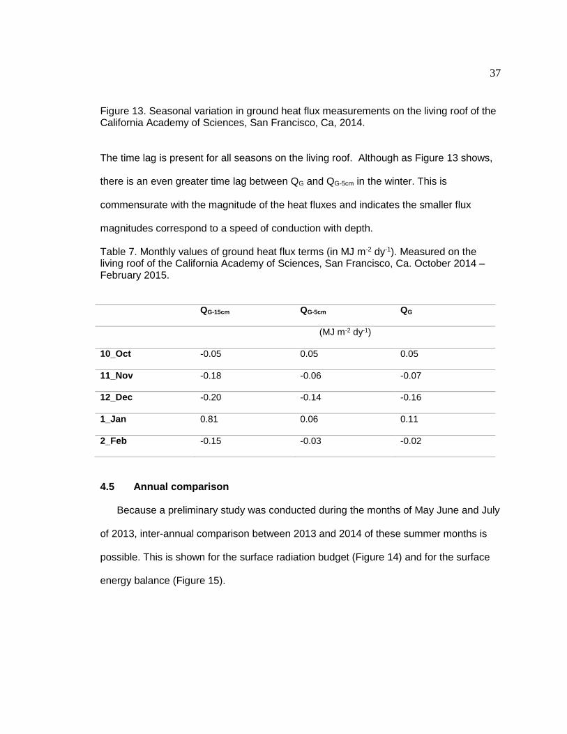
4.5 Annual comparison

Because a preliminary study was conducted during the months of May June and July

of 2013, inter-annual comparison between 2013 and 2014 of these summer months is

possible. This is shown for the surface radiation budget (Figure 14) and for the surface

energy balance (Figure 15).

38

Figure 14. Daily ensemble averages of the surface shortwave radiation budget for the same three months in 2013 and 2014 on the living roof of the California Academy of Sciences in San Francisco Ca. Table 8. Monthly total shortwave radiation for 2013 and 2014 (n MJ m-2 dy-1) Measured on the living roof of the California Academy of sciences, San Francisco, Ca. Unit May June July

2013 2014 2013 2014 2013 2014

(Kdn)

(MJ

m-2

1

23.95 26.08 24.90 24.97 24.03 20.23

(Kup) 4.71 5.26 4.51 4.66 4.20 3.52

May 2013 May 2013

June 2014 June 2013

July 2013 July 2014

39

(KN) 19.24 20.82 20.39 20.31 19.83 16.71

(α) (%) 19.6 20.1 18.1 18.6 17.4 17.3

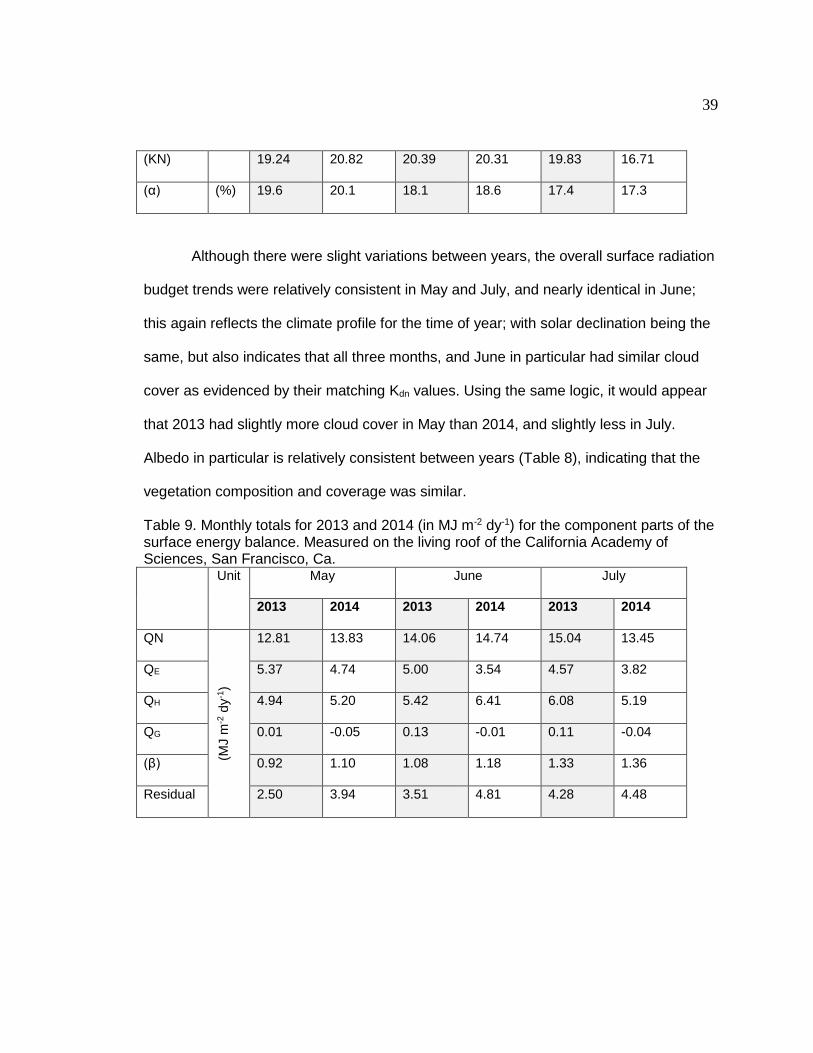
Although there were slight variations between years, the overall surface radiation

budget trends were relatively consistent in May and July, and nearly identical in June;

this again reflects the climate profile for the time of year; with solar declination being the

same, but also indicates that all three months, and June in particular had similar cloud

cover as evidenced by their matching Kdn values. Using the same logic, it would appear

that 2013 had slightly more cloud cover in May than 2014, and slightly less in July.

Albedo in particular is relatively consistent between years (Table 8), indicating that the

vegetation composition and coverage was similar.

Table 9. Monthly totals for 2013 and 2014 (in MJ m-2 dy-1) for the component parts of the surface energy balance. Measured on the living roof of the California Academy of Sciences, San Francisco, Ca. Unit May June July

2013 2014 2013 2014 2013 2014

QN

(MJ

m-2

dy-1

)

12.81 13.83 14.06 14.74 15.04 13.45

QE 5.37 4.74 5.00 3.54 4.57 3.82

QH 4.94 5.20 5.42 6.41 6.08 5.19

QG 0.01 -0.05 0.13 -0.01 0.11 -0.04

(β) 0.92 1.10 1.08 1.18 1.33 1.36

Residual 2.50 3.94 3.51 4.81 4.28 4.48

40

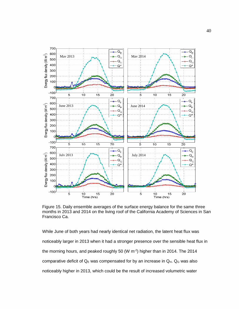
Figure 15. Daily ensemble averages of the surface energy balance for the same three months in 2013 and 2014 on the living roof of the California Academy of Sciences in San Francisco Ca.

While June of both years had nearly identical net radiation, the latent heat flux was

noticeably larger in 2013 when it had a stronger presence over the sensible heat flux in

the morning hours, and peaked roughly 50 (W m-2) higher than in 2014. The 2014

comparative deficit of QE was compensated for by an increase in QH. QG was also

noticeably higher in 2013, which could be the result of increased volumetric water

July 2013 July 2014

June 2014 June 2013

May 2013 May 2014

41

content and thus increased soil heat capacity. Despite the similar patterns between

years, QE was consistently greater in all three 2013 months, as was QG. Although in

both 2014 and 2013 the sensible heat flux dominated the surface energy balance,

leading to a Bowen ratio greater than 1 for both years.

4.6 Energy balance closure

The first law of thermodynamics theoretically requires the energy balance to close

(Oliphant et al. 2004). Energy balance closure is achieved when all the terms on the

right hand side of Equation 1 are equal to the term on the left (QN). Testing for energy

balance closure often results in residual energy; that is, energy that is either being

overestimated or underestimated in some way (Foken 2008, Wilson et al. 2002).

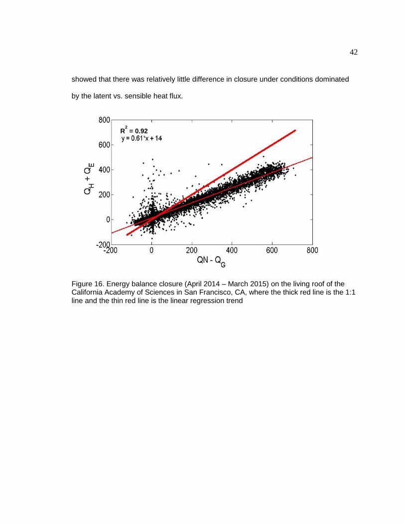
In order to isolate the turbulent fluxes from the remaining surface energy balance terms,

the sum of QE and QH was plotted against QN minus QG for all available 30-minute

periods (Figure 16). If the energy terms were balanced, each period would fall along a

1:1 line. The energy balance closure was assessed for the California Academy of

Sciences’ living roof resulting in turbulent heat fluxes that were 39% lower than available

energy, though with very high consistency (R2=0.92).

Potential reasons for this lack of closure include systematic bias in the

instrumentation, energy sinks that were not considered (such as storage and advection),

and the loss of both low and high frequency contributions to the turbulent fluxes (Wilson

et al. 2002). In order to examine whether the latent or sensible heat fluxes were greater

contributors to the underestimation of turbulent fluxes, observations were separated into

high and low Bowen ratio values where high Bowen ratio was considered any value

above 1.3, and low Bowen ratio was considered any value blow 1.3 (Figure 17). This

42

showed that there was relatively little difference in closure under conditions dominated

by the latent vs. sensible heat flux.

Figure 16. Energy balance closure (April 2014 – March 2015) on the living roof of the California Academy of Sciences in San Francisco, CA, where the thick red line is the 1:1 line and the thin red line is the linear regression trend

R2 = 0.92

43

Figure 17. Energy balance closure (April 2014 – March 2015) on the living roof of the California Academy of Sciences in San Francisco, CA.s Where low BR observations is Bowen < 1.3 and high BR observations is Bowen ratio > 1.3. 5.0 Discussion

5.1 Surface albedo

One of the most commonly expressed benefits of living roofs is their ability to reflect heat

energy (Sailor 2008). It has been argued that by reflecting rather than absorbing

incoming solar radiation to a greater degree than standard roofs, living city surfaces

mitigate the temperature gradient between urban and rural landscapes (Arnfield 3003,

Pardo and Ferreira 2005). This theory however, depends on the nature of the non-living

and living roofs, both of which vary significantly in color, leaf area index and vegetation

height and density (Sailor 2008), producing a wide range in results. Takbayashi and

R2 low BR = 0.85

R2high BR = 0.95

Y = 0.59*x+15

Combined BR liner

44

Moriyama (2007) found the albedo of a living roof (0.15) to be lower than a light gray

concrete roof (0.37) while, Susca et al. (2011) found a living roof to have a greater

albedo (0.20) than a comparative dark non-living roof, which was 0.05. Pardo and

Ferreira (2005) found green colored roofs to be generally at the low end of the albedo

spectrum (0.21) closest to ceramic roofs (0.20). The highest albedo belonged to white

roofs (0.60), and the lowest to dark gray cement roofs (0.13). The annual albedo for the

Cal Academy living roof was 0.20 making it a significant performing roof in terms of its

ability to reflect incoming radiation when compared to standard roofs, and directly

comparable to other living roof studies. The albedo of the Cal Academy roof exemplified

how the surface vegetation mirrored the natural seasonal cycle of phenology and

senescence. KN for the Cal Academy living roof was 13.18 (MJ m-2 dy-1). Using Oke’s

calculation for KN with a known albedo value, were the same amount of solar radiation

to fall on a white roof (α =0.60), KN would be 6.60 (MJ m-2 dy-1), and for a black roof (α

=0.05) KN would be 15.69 (MJ m-2 dy-1). Therefore on an annual basis the Cal Academy

living roof absorbs double the incident radiation as a white roof, but 2.51 (MJ m-2 dy-1)

less than a black roof.

Aside from Phenological changes in vegetation cover, albedo also changes over

time (both daily an annually) depending on solar declination (Oke 1987). Because

standard roofs have no vegetation, seasonal changes in albedo are due only to sun

angle variations, assuming no slope: the lower the sun altitude, the greater the albedo,

therefore on both living and standard roofs in North America, December its adjoining

months would have the lowest solar declination and the highest albedo observations,

while June and its adjoining months would have the greatest declination and therefore

45

lowest albedo observations. However, on the Cal Academy living roof the highest albedo

observations were made in April (0.22) at the height of the Mediterranean ecosystem

growing season and the lowest in July (0.17) and August (0.18), when the vegetation

turned dry and brown. The summer was also the season when the most weeding

occurred to clear out dry dead weeds, leaving noticeable bare earth patches. In April the

general plant color was a light bright green due to the thriving beach strawberry (32.9 %

coverage) and the green California bent grass (11.8 % coverage). In the winter the

beach strawberry changed to a red color while maintaining its same general %

coverage. The colors green and red have been previously shown to have very similar

albedo values (Pardo and Ferreira 2005). The observed surface area on the Cal

Academy roof was horizontal, and did not take into account sun angle variations on the

dome structures, and how the slope and aspect of these structures might impact the

seasonal albedo of the roof.

5.2 Living roof controls on the surface energy balance

The cooling capacity of a living roof is due in part to an enhancement of the latent

heat flux, and associated reduction in sensible heating of the overlying atmosphere

(Rosenzweig et al. 2005, Berardi et al. 2014). This balance is well expressed by the non-

dimensional Bowen ratio (β) which can be compared across urban and natural surfaces.

β varies widely in urban areas depending on the climate and composition of the city

(Grimmond and Oke 1995, Spronken-Smith et al. 1999) and has been found to correlate

strongly and negatively with the fractional area of vegetation (Christen and Vogt 2004).

Since this is generally low in urban areas, β tends to be high; around 5.0 (Oberndoffer et

46

al. (2007). By comparison to natural surfaces, this is equivalent to arid and semi-arid

surfaces (e.g. Oliphant et al. 2011).

On the Cal Academy living roof, annual β was very close to unity (0.96). This is

slightly higher than many natural ecosystems, which can range from 0.48 for wetlands,

to 0.72 for coniferous forests (Eaton et al. 2001). However, studies conducted in similar

Mediterranean climates have found β between 0.5 and 1.6 (Valentini et al. 1991); Other

ecosystems with β close to 1.0 include South African mopane woodlands, Siberian pine

forests (Oberndofer et al. 2007), and continental US grasslands (Kim and Verma 1989)

where the similarity in β observations between studies could partially be explained by

the 18.8% of grass land vegetation cover on the Cal Academy roof; the second largest

plant-type present (Table 2), but is most likely explained by the general climactic

similarities in precipitation and air temperature. The Cal Academy β was also

comparable to a living roof in Hong Kong China, which had a β range between 0.72 for

turf-grass cover and 0.90 for shrub cover (Jim and He 2010). this is surprisingly similar

to the Cal Academy study when considering that Hong Kong is a subtropical humid

climate with far more precipitation than San Francisco, and potentially indicates that the

vegetation components and sub-surface drainage structure provided similar controls on

latent and sensible heat; with Hong Kong having a similar surface layer construction and

perennial peanut (Arachis pintoi) as the predominant herbaceous vegetation cover,

which is similar to beach strawberry in height, coverage and leaf area index. The Bowen

ratio on the Cal Academy living roof fluctuated seasonally, with a standard deviation of

0.36. The highest Bowen ratios occurred in late summer (1.8 in July) with the lowest in

winter and spring, corresponding both to the wet season and observed spring growth.

47

Although there were no adjacent standard roofs with which to compare

observations, the Cal Academy roof, with a β just under 1, would likely produce a PCI

effect if measured against a surrounding urban roof-surface. Perhaps the most

comparable studied park space would be “mixed-use” due to the roofs observation deck,

atrium and skylights. Such urban green spaces can have a PCI value of up to 3.8 (ºC)

(Spronken-Smith et al. 1998). With their lack of water retention for evaporation, and

plants for transpiration, it can be assumed that the entire magnitude of the latent heat

would be added between the sensible and ground heat flux on a theoretical standard

roof adjacent to the Cal Academy. As the annual QH and QG account for 38% and 11%

of QN respectively, this would increase the sensible heat flux to 5.54 (MJ m-2 dy-1), and

ground heat flux to -0.77 (MJ m-2 dy-1).

Although the Cal Academy applies light irrigation in summer, the seasonal plant

functioning tends to follow a Mediterranean seasonal schedule with senescence in the

second half of summer due to water stress and little activity in winter due to low light

levels (Thorp et al. 2014). It is likely that this seasonal pattern in biome vegetation

functioning, accounted for the lower QE observations (relative to QN) in late summer.

The moderate increase in QE from July to August (0.04) cannot be accounted for by the

nearly double increase in VWC, or there would be a likewise more significant jump in QE.

A possible reason for this lack of relationship is that the Cal Academy living roof was too

complex to tease out independent variables without controlling for other environmental

factors that are present in the data. Atmospheric variables included available energy, air

temperature, wind speed and vapor pressure deficit, while surface variables included the

availability of water, plant species and soil porosity. With all of these variables acting at

48

different degrees on both temporal and geographic scales, no single variable other than

QN stood out as a dominant control. Because the soil bulk density was low (0.81 g/cm3),

thus indicating a high volume of pore space, it is likely that water drained rapidly from the

roof’s surface, leaving less water available for VWC observations, and possibly

contributing to the low correlation between QE and VWC. There was however an overall

seasonal trend in increased QE and VWC signifying that while it was not the only or most

dominant variable to control QE, there was a positively correlated relationship between

the two.

5.3 Ground heat conduction and storage

Yet another touted benefit of living roofs is their ability to reduce the energy consumption

of buildings by reducing heat conduction into and out of the building. Buildings account

for roughly 40% of global energy use (Berardi et al. 2014). Ground heat flux was

relatively stable and characteristic of other living roof studies (Tekebayashi et al. 2007,

Feng et al. 2010). Daytime QG was typically around 10% of QN, which is similar to other

vegetated surfaces (Wilson et al. 2002). Heat storage in the urban fabric (∆Qs) is very

hard to measure accurately, and is often calculated as the residual in the energy

balance. However, a review of urban studies show that heat storage accounts for up to

40% of the net radiation, a far larger portion than that of QG on the Cal Academy roof.

These high observations of heat storage within urban structures also lead to high levels

of evening heat emittance and increased UHI values (Oke 1989). Therefore QG on the

living roof is yet another indicator of the roof’s ability to mitigate the UHI effect.

Although no temperature sensors were installed within the Cal Academy’s interior

rooms, a 2007 study on living roof energy performance found a 6-49% reduction in

49

interior building temperature, and a 12-87% reduction in the room temperature directly

below the roof (Santtamouris et al. 2007). In natural ecosystems annual total QG values

are typically near zero, and daily total QG values are typically small and slightly negative

from summer to winter and positive from winter to summer, reflecting the seasonal

change in soil temperature (Oliphant et al. 2004). The seasonally consistent negative

values for daily QG indicate that the building below was, over the long term, conducting

heat toward the substrate surface. This includes conduction through the concrete slab,

waterproofing layer, synthetic insulation, impermeable drainage layer, and erosion

control blanket. The Cal Academy roof is not an outlier in living roofs’ heat conduction

and storage capacity. The equivalent of QG for a study on a living roof in Guangzhou

China had an identical ground heat flux that was likewise negative; indicating that that

roof also emitted heat (Feng et al. 2010). The insulation properties of the substrate were

displayed by the lag time and reduced magnitude between the heat flux observations at

QG-5 and QG-15 which illustrate the living components of the roof act as natural insulation.

This finding is consistent with a study conducted in the Mediterranean climate of Greece

in 2003, where thicker substrate soil likewise exhibited a larger time lag and smaller

variation of the thermal heat flux (Theodosiou 2003). This finding is also consistent with

a 2010 living roof study in Hong Kong which likewise found substantial (2 hour) lag time

in QG energy fluxes (Jim and He, 2010).

5.4 Controls on energy balance closure and sources of error

Controls on energy balance closure can include: Unstable vs. stable conditions, friction

velocity, thermally induced turbulence, time of day, storage effects, and landscape

heterogeneity (Franssen et al. 2010, Barr et al. 2006), horizontal and/or vertical

50

advection of heat, systematic errors associated with the sampling mismatch between

the flux footprint and the sensors measuring other components of the energy balance,

energy sinks that were not accounted for, and low and high frequency loss of turbulent

fluxes (Wilson et al. 2002 B). While advection was systematically avoided by rejecting all

periods when the 80th percentile of the cumulative flux distance fell outside of the roof

area, advection on such a small complex and hilly terrain could lead to error. Although

the instruments were installed with the objective of receiving the turbulent eddies from

across the low-laying flat, eastern portion of the roof, it is possible that the domes

topographically forced turbulence an advection in unaccounted for ways.

Energy balance closure resulted in an annual residual of 2.20 (MJ m-2 dy-1) and

found that the turbulent heat fluxes underestimated the available energy by 39% based

on linear regression. This underestimation was fairly consistent with an annual R2 of

0.92. Lack of energy balance closure indicates that one or more parts of the surface

energy balance equation were incorrectly measured. Either the turbulent heat fluxes

were underestimated, the ground heat flux was underestimated, or the net radiation was

overestimated. An increase of 2.20 (MJ m-2 dy-1) in the ground heat flux would be

improbably large, therefore it is more likely that QN is overestimated, or that QH and QE

are underestimated. Ground heat was likely measured with sufficient accuracy due to

the measurements of soil bulk density (0.81 g/cm3) calculated in spring of 2014. In order

to determine which of the turbulent heat fluxes was being incorrectly measured, 30 min

periods were divided into times of high and low Bowen ratio observations (Figure 17).

The R2 values of 0.85 and 0.95 for low and high observations respectively, indicate that

underestimations of the turbulent heat fluxes were not significantly different when either

51

latent or sensible heat was dominant. This indicates if the eddy covariance technique is

overestimating the turbulent heat fluxes, it is not producing greater errors under wet or

dry conditions. Although the instruments were intentionally installed away from the

leeward edge of the roof, turbulent flows resulting from roof-edge upwelling could have

been measured.

6.0 For future study: Comparing latent heat flux

While the eddy covariance technique was successfully employed on the Cal Academy

roof, it is not a useful study technique for replication because there are so few living

roofs that offer the required footprint to achieve usable observations. In 2014, a

preliminary weighing lysimeter devise was installed adjacent to the eddy covariance

tower to provide independent measurements of evapotranspiration. The function of the

weighing lysimeter method is to measure the mass changes of soil and vegetation over

30 min periods. Over time, estimates of rainfall, irrigation and evapotranspiration are

inferred. In order to determine mass changes, a volume of the desired substrate was

excavated and placed into a container so that the volume of soil and vegetation was

exposed to the atmosphere above, but completely confined within the impermeable

container in all other directions. This become the “inner container”, and was then placed

on top of a modified load cell within an outer container. The modified load cell was

leveled on the bottom of the outer container using leveling screws. A small gap of

approximately 5 mm was left between the walls of the inner and outer containers,

thereby allowing the inner container housing the substrate to stand freely on the

modified load cell, so that the entire force being measured by the load cell was

representative of the inner container without interference form the surrounding substrate.

52

The weighing lysimeter method is independent from the eddy covariance technique, and

thus provides a separate collection of data, from which the two independent values for

evapotranspiration can be compared (Oliphant et al. in press).

𝐹𝐹𝐻𝐻2𝑂𝑂 = ∆𝑊𝑊𝑐𝑐𝐴𝐴𝑐𝑐

∆𝑡𝑡 (10)

where ∆Wc is the change in mass between averaging periods (g), Ac is the cross

sectional area of the volume’s surface and ∆t is the time between averaging periods (0.5

hours). The weighing lysimeter was installed on the Cal Academy roof in September of

2014. Nesting containers were sawed down to the specific height of the Cal Academy’s

living roof substrate (15 cm), with the inner container sawed to a height of 10 cm to

account for the thickness of the modified loadcell (5 cm). The result was a continuous

surface of equal elevation between the lysimiter substrate and that of the surrounding

living roof. The outer container measured 20 cm in diameter. The loadcell was wired into

the data logger, and measurements were originally taken at 10 Hz, but then reduced to 5

S intervals to save space. A key component of the weighing lysimeter technique is to

maintain the biophysical functioning of the substrate within the inner container. Without

living flora, transpiration does not occur; only evaporation is measured. The vegetation

within the inner container was monitored throughout the study and no adverse effects to

plant growth and vitality were observed. This indicates that the field test-study has high

potential for success, and future research could easily be compared with the energy

balance results in this study.

7.0 Conclusions

This study provided over one year of data (2013-2015) on the component parts of the

surface radiation budget and surface energy balance on the Cal Academy living roof.

53

Multiple climate variables such as precipitation and air temperature were measured, and

both the plant and soil composition was assessed. An emphasis was placed on the

partitioning of the surface energy balance between latent, sensible and ground heat

fluxes, seasonality of all components, and controls on both radiative and heat flux

observations. From the cumulative observations, the following conclusions can be

drawn.

The 30-minute diurnal ensemble surface radiation budget components changed

in magnitude over the seasonal time scale with a substantial decrease (range = 15.61

MJ m-2 dy-1) in incoming solar radiation between the summer and winter months due to

the North American latitudinal location and corresponding sun angle. Longwave radiation

changed little over the year compared to shortwave radiation. Net radiation was

controlled by time of year and cloud cover, with diurnal ensembles observed under

cloudy sky conditions resulting in as much as 125 (W m-2) less QN at peak times. The

annual average albedo of 0.20 was directly comparable to other living roofs, higher than

black (0.05) and dark grey (0.15) roofs, and lower only than light gray (0.37) and white

(0.60) roofs, making it an overall significant performer at reflecting heat energy to offset

UHI levels when analyzed on an annual scale. Albedo was seasonally controlled by

phenological changes in plant color and coverage, which slightly superseded the control

of solar declination which followed the anticipated seasonal trend for a northern latitude

location.

The magnitude of the heat flux terms was strongly driven by available energy

derived from the surface energy budget. This strong correlation led to a parallel

decrease in magnitudes of heat fluxes from summer to winter. On an annual average,

54

latent heat surpassed sensible heat by 0.01 (MJ m-2 dy-1) leading to a Bowen ratio of

0.96, indicating that the turbulent heat fluxes were relatively evenly partitioned. β was

governed by seasonal changes in QN and to a lesser degree by phenology and the

availability of water (VWC). β was highest in the late spring and early summer indicating

that biophysical controls impacted QE and QH as evidenced by the switch from QH

dominating the diurnal ensemble observations in the summer to QE dominating in the

winter. Were no vegetation present on the Cal Academy roof, it can be assumed that the

portion of QN occupied by this component would be partitioned into QH and QG, thus the

cooling capacity of the living roof can be measured as the magnitude of QE, thereby

demonstrating that the living roof offset the UHI by 3.19 (MJ m-2 dy-1) on an annual

average scale. The ground heat flux demonstrated the similarities between designed

living roofs and natural substrate. Insulation of the building below was measured as the

amount of heat energy that reached the surface vs. the amount of heat energy that

reached the bottom of the 15 cm substrate; a small average diurnal maximum of 3 (W m-

2) ever reach the building below. Seasonally QG remained negative every month,

indicating that unlike a natural surface, a measurable amount of heat was conducted out

of the building on an annual scale.

The sum of the turbulent heat fluxes (QH +QE) was found to underestimate the

available energy (QN – QG) by 39%. However, no strong correlation was found between

energy balance closure and times of QE or QH dominance, indicating that if they were

incorrectly measured, the turbulent heat fluxes led to equal underestimation under times

of either latent or sensible heat flux dominance. This study confirmed that living roofs do

impact their local microclimates. UHI was offset primarily by the latent heat flux by an

55

average annual magnitude of 3.19 (MJ m-2 dy-1), and by the ground heat flux, which

accounted for around 10% of QN, significantly less than urban structures that can reach

a maximum of 40% of QN. The living roof’s albedo also offset UHI by reflecting the

maximum (over 20%) amount of Kdn during the months with the highest vegetation %

cover and when the plants were in their most vivacious bright green condition. The roof

also impacted the climate of the interior building by only allowing a small annual average

diurnal maximum of 3 (W m-2) to be conducted into the interior building.

56

8.0 References

Alessa, L. and Chapin, F.S. (2008) Anthropogenic biomes: a key contribution to earth-

system science. Trends in Ecology and Evolution. 23, 529-531

Arnfield, A.J. (2003) Two decades of urban climate research: a review of turbulence,

exchanges of energy and water, and the urban heat island. International

Journal of Climatology. 23, 1-26

Baldocchi, D.D. (2003) Assessing the eddy covariance technique for evaluation carbon

dioxide exchange rates of ecosystems: past, present and future. Global

Change Biology. 9, 1-14

Baldocchi, D. D., Vogel, C. A. , Hall, B. (1997), Seasonal variation of energy and water

vapor exchange rates above and below a boreal jack pine forest canopy,

Journal of Geophysical Research: Atmospheres. 102, 28939–28951

Barbour, M.G, William, D. B. (1988) North American Terrestrial Vegetation, Cambridge

University Press, Cambridge

Barr, A., Morgenstern, K., Black, T., McCaughey, J., Nesic, Z. (2006) Surface energy

balance closure by the eddy-covariance method above three boreal forest

57

stands and implications for the measurement of the CO2 flux. Agricultural and

Forest Meteorology. 140, 322–337

Berardi, U., GhaffarianHoseini, A.H., GhaffarianHoseini, A. (2014) State-of-the-are

analysis of the environmental benefits of green roofs. Applied Energy. 115,

411-428

Bladd, B.L., and Rosenberg, N.J. (1973) Lysimetric calibration of the Bowen ratio-energy

balance method for evapotranspiration estimation in the Central Great Plains.

Journal of Applied Meteorology. 13, 227-236

Bottyan, Z., Kircsi, A. Szegedi, S., Unger, J. (2005) The relationship between built-up

areas and the spatial development of the mean maximum urban heat island in

Debrecen, Hungary. International journal of Climatology. 25, 405-418

California Academy of Sciences (2014) Living Roof. Retrieved from:

http://www.calacademy.org/exhibits/living-roof

Castleton, H.F., Stovin, V., Beck, S.B.M., Davison, J.B. (2010) Green roofs; building

energy savings and the potential for retrofit. Energy and Buildings. 42, 1582-

1591

58

Christen, A. and Vogt, R. (2004) Energy and radiation balance of a central European

city. International Journal of Climatology. 24, 1395-1421

Conomos, T.J., Smith, R.E., Gartner, J.W. (1985) Environmental Setting of San

Francisco. Hydrobiologia. 129, 1-12

Eaton, A.K., and Rouse, W.R. (2001) Surface energy balance of the western and central

Canadian subarctic: variations in the energy balance among five major terrain

types. Journal of Climate. 14, 3692-3703

Eliasson, I. (2000) The use of climate knowledge in urban planning. Landscape and

Urban Planning. 48, 31-44

Feng, F., Meng Q., Zhang, Y. (2010) Theoretical and experimental analysis of the

energy balance of extensive green roofs. Energy and Buildings. 42, 959-965

Foken,T. (2008) The Energy Balance Closure Problem: An Overview. Ecological

Applications. 18, 1351-1367

Franssen, H.J., Stöckli, R., Lehner, I., Rotenberg, E., Seneviratne, S.I. (2010) Energy

balance closure of eddy-covariance data: A multisite analysis for European

FLUXNET stations. Agricultural and Forest Meteorology. 150, 1553–1567

59

Grimmond, S. (2006) Applied climatology – urban climate. Progress in Physical

Geography. 30, 270-279

Grimmond, C.S.B., and Oke, T.R. (1995) Comparison Heat Fluxes from Summertime

Observations in the Suburbs of North America. American Meteorological

Society. 38, 922-940

Hsieh, C., Katul, G., Chi, T. (2000) An approximate analytical model for footprint

estimation of scalar fluxes in thermally stratified atmospheric flows. Advances

in Water Resources. 23, 765-72.

Hommer, B., Eliasson, I. (1999) Urban-rural vapor pressure deficit differences and their

role in the development of urban heat islands. International journal of

Climatology. 19, 989-1009

Honjo, T., Narira, K., Sugawara, H., Mikami, T. (2003) Observation of Cool Islan Effect in

Urban parks (Shinjuku Gyoen). Geographical Review of Japan. 6, 403-420

Howard, L. (1833) The climate of London deduced from meteorological observations Vol

1 Harvey and Darton, London

Ichinose, T., Shimodozono, K., Hanaki, K. (1999) Impact of anthropogenic heat on urban

climate in Tokyo. Atmospheric Environment. 33, 3897-3909

60

Jaffal, I., Ouldboukhitine, S.E., Belarbi, R. (2012) A Comprehensive study of the impact

of green roofs on building energy performance. Renewable Energy. 43, 157-

164

Jansson C., Jansson, P.E., Gustafsson, D. (2007) Near surface climate in an urban

vegetated park and its surroundings. Theoretical and Applied Climatology.

89, 185–193

Jim, C.Y., and He, H. (2010) Coupling heat flux dynamics with meteorological conditions

in the green roof ecosystem. Ecological Engineering. 36, 1052-1063

Kalra, Y. P. (1996) Reference Methods for Plant Analysis, CRC Press, Taylor & Francis

Group, LLC

Kim, J., and Verma, S.B. (1989) Components of surface energy balance in a temperate

grassland ecosystem. Boundary-Layer Meteorology. 51, 417-1990

Liu, H., Randerson, J.T., Lindfors, J., Chapin, S. (2005) Changes in the surface energy

budget after fire in boreal ecosystems of interior Alaska: An annual

perspective. Journal of Geographical Research. 110, 1-12

61

Martens, R., Bass, B., Alcazar, S. (2008) Roof–envelope ratio impact on green roof

energy performance. Urban Ecosystems. 4, 399-408

Masson, V., C.S.B. Grimmond, T.R. Oke (2002) Evaluation of the Town Energy Balance

(TEB) Scheme with Direct Measurements from Dry Districts in Two Cities.

Journal of Applied Meteorology. 41, 1011-1026

Moncrieff, J.B., Massheder, J.M., de Burin, H., Elbers, J., Friborg, T., Heusinkveld, B.,

Kabat, P., Scott, S., Soegaard, H. Verhoef, A. (1997) A system to measure

surface fluxes of momentum, sensible heat, water vapor and carbon dioxide.

Journal f Hydrology. 188, 589-611

Oberlander, G.T. (1956) Summer fog precipitation on the San Francisco Peninsula.

Ecology. 37, 851-852

Oke, T.R. (1987) Boundary Layer Climates, Routledge, London

Oberndoffer, E., Lundholm, J., Bass, B., Coffman, R.R., Doshi, H., Dunnett, N., Gaffin,

S., Kohler, M., Liu, K.K.Y., Rowe, B. (2007) Green roofs as urban

ecosystems: ecological structures, functions, and services. BioScence. 57,

823-833

62

Oke, T.R., Johnson, G.T., Steyn, D.G., Watson, I.D. (1991) Simulation of surface urban

heat island under “ideal” conditions at night. Part 2; Diagnostics of causation.

Boundary layer Meteorology. 56, 339-358

Oke, T.R. (1980) The energetic basis of the urban heat island. Quarterly journal of the

Royal meteorology Society. 108, 1-24

Oke, T.R. (1973) City size and the urban heat island. Atmospheric Environment. 7, 769-

779

Oliphant, A.J., Grimmond, C.S.B., Zutter, H.N., Schmid, H.P., Su, H.B., Scott, S.L.,

Offerle, B., Randolph, J.C., Ehman, J. (2004) Heat storage and energy

balance fluxes for a temperate deciduous forest. Agricultural and Forest

Meteorology. 126,185-201

Oliphant, A., Zawar-reza, P., Azizi, G., Dehghanpour, A., Harrison, J. (2011) Surface

energy and water vapor fluxes observed in a desert plantation in central Iran.

Journal of Arid Environments. 75, 926-935

Oliphant, A.J. (2012) Terrestrial Ecosystem-Atmosphere Exchange of CO2, Water and

Energy from FLUXNET; Review and Meta-Analysis of a Global in-situ

Observatory. Geography Compass. 10, 689-705

63

Pandey, S., Hinodliya, D.A., Mod, R. (2013) Experimental investigation on green roofs

over buildings. International Journal of Low-Carbon Technologies. 8, 37-42

Pardo, R.T., and Ferreira, F.L. (2005) Measurement of albedo and analysis of its

influence the surface temperature of building roof materials. Energy and

Buildings. 37, 295-300

Rosenzweig, C., S. Gaffi n, and L. Parshall (Eds.) (2006) Green Roofs in the New York

Metropolitan Region: Research Report. Columbia University Center for Climate

Systems Research and NASA Goddard Institute for Space Studies. New York.

59 pages.

Sailor, D.J. (2008) A green roof model for building energy simulation programs. Energy

and Buildings. 40, 1466-1478

Saiz, S., Kennedy, C., Bass, B., Pressnail, K. (2006) Comparative life cycle assessment

of standard and green roofs. Environmental Science Technology. 40, 4312-4316

Santamouris, M., Pavlou, C., Doukas, P., Mihalakakou, G., Synnefa, A., Hatzibiros, A.,

Patargias, P. (2007) Investigating and analyzing the energy and environmental

performance of an experimental green roof system installed in a nursery school

building in Athens, Greece. Energy. 32, 1781-1788

64

SF Department of Parks and Recreation (2014), Golden Gate Park Guide. Retrieved

from http://sfrecpark.org/

Spronken-Smith, R.A., and Oke, T.R. (1998) The thermal regime of urban parks in two

cities with different summer climates. International Journal of Remote Sensing.

11, 2085-2104

Spronken-Smith, R.A., Oke, T.R., Lowry, W. (2000) Advection and the surface energy

balance across an irrigated urban park. International Journal of Climatology. 20,

1033-1047

Susca T., Gaffin, S.R., Dell’osso, G.R. (2011) positive effects of vegetation: urban heat

island and green roofs. Environmental Pollution. 159, 2119-2126

Szegedi, S., Gyarmati, R. (2009) Impacts of urban green spaces on the spatial structure

of the urban heat island in Debrecen and different sized settlements in its

neighborhood. ACTA Climatologicaet Chorlogica. 43,151-158

Tekebayashi, H. and Moriyama, M. (2007) Surface heat budget on green roof and high

reflection roof for mitigation of urban heat island. Building and Environment. 42,

2971 2979

65

Theodosiou, T.G. (2003) Summer period analysis of the performance of a planted roof

as a passive cooling technique. Energy and Buildings. 35, 909-917

Thorp, R. (2014) Observations of heat, water vapor and carbon dioxide exchanges over

a living roof using eddy covariance. Thesis. San Francisco State University

USGS (2012) Soil types and shaking hazard in the San Francisco Bay Area. Retrieved

from: http://earthquake.usgs.gov/regional/nca/soiltype/

Vallentini, R., De Angelis, P., Matteucci, G., Monaco, R., Dore, S., Scarscia Mugnozza,

G.E. (1996) Seasonal net carbon dioxide exchange of a beech forest with the

Atmosphere. Global Change Biology. 2, 199-207

Weng, Q., Lu, D., Schubring, J. (2004) Estimation of land surface temperature –

vegetation abundance relationship for urban heat island studies. Remote

Sensing of Environment. 89, 467-483

Wilson, K., Baldocchi, D., Aubinet, M., Berbigier, P., Bernhofer, C., Dolman, H., Falge,

E., Field, C., Goldstein, A., Granier, A., Grelle, A., Halldor, T., Hollinger, D.,

Katul, G., Law, B., Lindroth, A., Meyers, T., Moncrieff, J., Monson, R., Oechel,

W., Tenhunen, J., Valentini, R., Verma, S., Vesala, T., Wofsy, S. (2002)

Energy partitioning between latent and sensible heat flux during the warm

season at FLUXNET sites. Water Resources Research. 38, 1294-1318

66

Williams. N.S.G, Rayner, J. P., Raynor, K. (2010) Green roofs for a wide brown land:

opportunities and barriers for rooftop greening in Australia. Urban Forestry &

Urban Greening. 9, 245-251.

Wofsy, S.C., Goulden, M.L., Munger, J.W., Fan, S.M., Bakwin, P.S., Daube, B.C.,

Bassow, F. A., Bazzaz, S.L. (1993) Net exchange of CO2 in a mid-latitude

forest. Science. 260, 1314-1317

Xu, L. Baldocchi, D.D. (2004) Seasonal variation in carbon dioxide exchange over a

Mediterranean annual grassland in California. Agriculture and Forest

meteorology. 1232, 79-96