Numerical Analysis: Trapezoidal and Simpson's RuleNumerical Analysis: Trapezoidal and Simpson’s Rule Natasha S. Sharma, PhD General Trapezoidal Rule T n(f) 1 We saw the trapezoidal

NumericalAnalysis:

Trapezoidaland Simpson’s

Rule

Natasha S.Sharma, PhD

Numerical Analysis: Trapezoidal andSimpson’s Rule

Natasha S. Sharma, PhD

NumericalAnalysis:


Rule


Mathematical question we are interested innumerically answering

How to we evaluate

I =

∫ b

af (x) dx?

Calculus tells us that if F(x) is the antiderivative of afunction f (x) on the interval [a, b], then

I =

∫ b

af (x) dx = F (x)|ba = F (b)− F (a).

Practically, most integrals cannot be evaluated using thisapproach. For example, ∫ 1

0

dx

1 + x5

has a complicated antiderivative and it easier to adopt anumerical method to approximate this integral.

NumericalAnalysis:


Rule


Numerical Integration: A General Framework

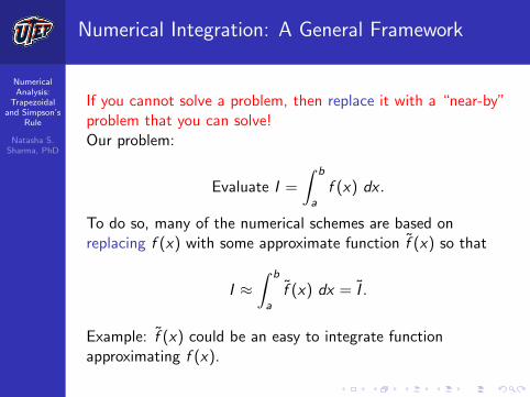
If you cannot solve a problem, then replace it with a “near-by”problem that you can solve!Our problem:

Evaluate I =

∫ b

af (x) dx .

To do so, many of the numerical schemes are based onreplacing f (x) with some approximate function f (x) so that

I ≈∫ b

af (x) dx = I .

Example: f (x) could be an easy to integrate functionapproximating f (x).

NumericalAnalysis:


Rule


Numerical Integration: A General Framework

Then, the approximation error in this case is

E = I − I =

∫ b

a

(f (x)− f (x)

)dx

≤ (b − a) maxa≤x≤b

|f (x)− f (x)|

The inequality above tells us that the approximation error Edepends on:

1 the maximum error in the approximating f (x) that ismaxa≤x≤b |f (x)− f (x)|, and

2 (b − a), the width of the interval.

Next Goal: How to choose f (x)?

NumericalAnalysis:


Rule


Polynomial Approximations to f (x)

Goal Choose an approximation f (x) to f (x) that is easilyintegrable and a good approximation to f (x).Two natural candidates:

1 Taylor polynomials approximating f (x).One caveat: We need f (x) to have derivatives at “a” toexist of a higher order to improve the approximation!

2 Interpolating polynomials approximating f (x).

NumericalAnalysis:


Rule


Example

Example

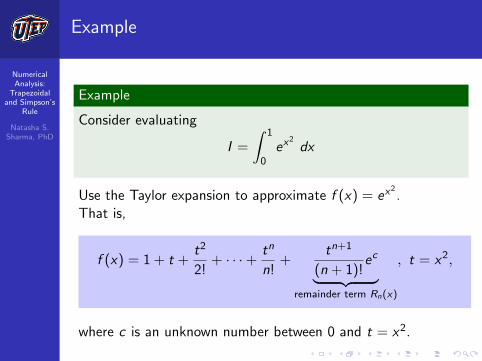
Consider evaluating

I =

∫ 1

0ex

2dx

Use the Taylor expansion to approximate f (x) = ex2.

That is,

f (x) = 1 + t +t2

2!+ · · ·+ tn

n!+

tn+1

(n + 1)!ec︸︷︷︸

remainder term Rn(x)

, t = x2,

where c is an unknown number between 0 and t = x2.

NumericalAnalysis:


Rule


Solution

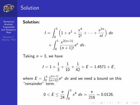
Solution:

I =

∫ 1

0

(1 + x2 +

x4

2!+ · · ·+ x2n

n!

)dx

+

∫ 1

0

x2(n+1)

(n + 1)!ec dx .

Taking n = 3, we have

I = 1 +1

3+

1

10+

1

42+ E = 1.4571 + E ,

where E =∫ 10

x2(n+1)

(n+1)!ec dx and we need a bound on this

“remainder” term.

0 < E ≤ e

24

∫ 1

0x8 dx =

e

216= 0.0126.

NumericalAnalysis:


Rule


Using Interpolating Polynomials

In spite of the simplicity of the above example, it is generallymore difficult to do numerical integration by constructingTaylor polynomial approximations than by constructingpolynomial interpolates.Thus, we construct the function f (x) as the polynomialinterpolating f (x) such that

∫ b

af (x) dx ≈

∫ b

af (x) dx .

Case I: Use linear interpolating polynomial p1(x) approximatingf (x) at two points. We pick a and b.

NumericalAnalysis:


Rule


Using Linear Interpolating Polynomails

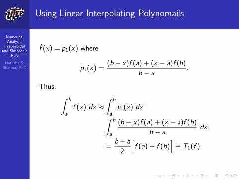
f (x) = p1(x) where

p1(x) =(b − x)f (a) + (x − a)f (b)

b − a.

Thus, ∫ b

af (x) dx ≈

∫ b

ap1(x) dx∫ b

a

(b − x)f (a) + (x − a)f (b)

b − adx

=b − a

2

[f (a) + f (b)

]≡ T1(f )

NumericalAnalysis:


Rule


Trapezoidal Rule

Definition (Trapezoidal Rule)

The integration rule∫ b

af (x) dx ≈ b − a

2

[f (a) + f (b)

]= T1(f )

is called the trapezoidal rule.

NumericalAnalysis:


Rule


Example using Trapezoidal Rule

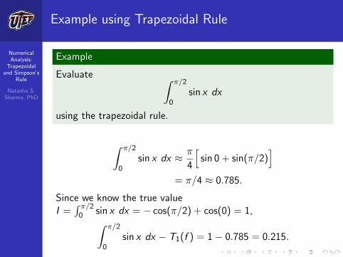
Example

Evaluate ∫ π/2

0sin x dx

using the trapezoidal rule.

∫ π/2

0sin x dx ≈ π

4

[sin 0 + sin(π/2)

]= π/4 ≈ 0.785.

Since we know the true valueI =

∫ π/20 sin x dx = − cos(π/2) + cos(0) = 1,∫ π/2

0sin x dx − T1(f ) = 1− 0.785 = 0.215.

NumericalAnalysis:


Rule


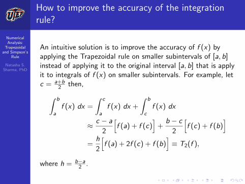
How to improve the accuracy of the integrationrule?

An intuitive solution is to improve the accuracy of f (x) byapplying the Trapezoidal rule on smaller subintervals of [a, b]instead of applying it to the original interval [a, b] that is applyit to integrals of f (x) on smaller subintervals. For example, letc = a+b

2 then,∫ b

af (x) dx =

∫ c

af (x) dx +

∫ b

cf (x) dx

≈ c − a

2

[f (a) + f (c)

]+

b − c

2

[f (c) + f (b)

]=

h

2

[f (a) + 2f (c) + f (b)

]≡ T2(f ),

where h = b−a2 .

NumericalAnalysis:


Rule


Testing on the previous example

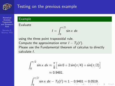
Example

Evaluate

I =

∫ π/2

0sin x dx

using the three point trapezoidal rule.Compute the approximation error I − T2(f ).Please use the Fundamental theorem of calculus to directlycalculate I .

∫ π/2

0sin x dx ≈ π

8

[sin 0 + 2 sin(π/4) + sin(π/2)

]≈ 0.9481.∫ π/2

0sin x dx − T2(f ) ≈ 1− 0.9481 = 0.0519.

NumericalAnalysis:


Rule


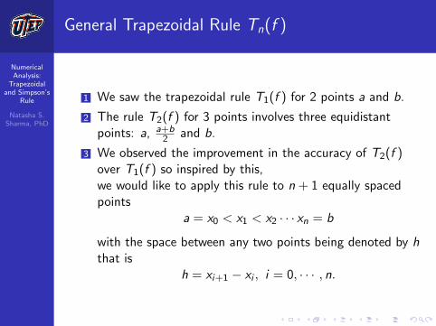
General Trapezoidal Rule Tn(f )

1 We saw the trapezoidal rule T1(f ) for 2 points a and b.

2 The rule T2(f ) for 3 points involves three equidistantpoints: a, a+b

2 and b.

3 We observed the improvement in the accuracy of T2(f )over T1(f ) so inspired by this,we would like to apply this rule to n + 1 equally spacedpoints

a = x0 < x1 < x2 · · · xn = b

with the space between any two points being denoted by hthat is

h = xi+1 − xi , i = 0, · · · , n.

NumericalAnalysis:


Rule


General Trapezoidal Rule Tn(f )

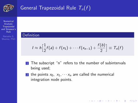
Definition

I ≈ h[1

2f (a) + f (x1) + · · · f (xn−1) +

f (b)

2

]≡ Tn(f )

1 The subscript “n” refers to the number of subintervalsbeing used;

2 the points x0, x1, · · · xn are called the numericalintegration node points.

NumericalAnalysis:


Rule


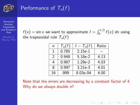
Performance of Tn(f )

f (x) = sin x we want to approximate I =∫ π/20 f (x) dx using

the trapezoidal rule Tn(f )

n Tn(f ) I − Tn(f ) Ratio

1 0.785 2.15e-1 –

2 0.948 5.18e-2 4.13

4 0.987 1.29e-2 4.03

8 0.997 3.21e-3 4.01

16 .999 8.03e-04 4.00

Note that the errors are decreasing by a constant factor of 4.Why do we always double n?

NumericalAnalysis:


Rule


How to improve the accuracy of the integrationrule?

An intuitive solution is to improve the accuracy of f (x) byusing a better interpolating polynomial say a quadraticpolynomial p2(x) instead. Let c = a+b

2 and h = b−a2 then, the

quadratic polynomial is

p2(x) =(x − c)(x − b)

(a− c)(a− b)f (a) +

(x − a)(x − b)

(c − a)(c − b)f (c)

+(x − a)(x − c)

(b − a)(b − c)f (b).

∫ b

af (x) dx ≈

∫ b

ap2(x) dx

=h

3

[f (a) + 4f (c) + f (b)

]≡ S2(f ).

This is called Simpson’s rule.

NumericalAnalysis:


Rule


Simpson’s rule applied to the previous example

Example

Evaluate ∫ π/2

0sin x dx

using the Simpson’s rule.

∫ π/2

0sin x dx ≈ π/2

3

[sin 0 + 4 sin(π/4) + sin(π/2)

]≈ 1.00227∫ π/2

0sin x dx − S2(f ) = −0.00228.

NumericalAnalysis:


Rule


General Simpson’s Rule Sn(f )

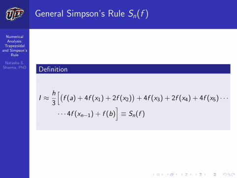
Definition

I ≈ h

3

[(f (a) + 4f (x1) + 2f (x2)

)+ 4f (x3) + 2f (x4) + 4f (x5) · · ·

· · · 4f (xn−1) + f (b)]≡ Sn(f )

NumericalAnalysis:


Rule


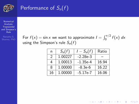
Performance of Sn(f )

For f (x) = sin x we want to approximate I =∫ π/20 f (x) dx

using the Simpson’s rule Sn(f )

n Sn(f ) I − Sn(f ) Ratio

2 1.00227 -2.28e-3 –

4 1.00013 -1.35e-4 16.94

8 1.00000 -8.3e-6 16.22

16 1.00000 -5.17e-7 16.06

NumericalAnalysis:


Rule


Error Formulas: Trapezoidal Rule

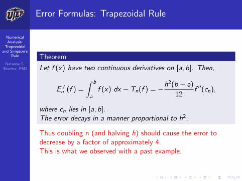
Theorem

Let f (x) have two continuous derivatives on [a, b]. Then,

ETn (f ) =

∫ b

af (x) dx − Tn(f ) = −h2(b − a)

12f ′′(cn),

where cn lies in [a, b].The error decays in a manner proportional to h2.

Thus doubling n (and halving h) should cause the error todecrease by a factor of approximately 4.This is what we observed with a past example.

NumericalAnalysis:


Rule


Example

Example

Consider the task of evaluating

I =

∫ 2

0

dx

1 + x2

using the trapezoidal rule Tn(f ).How large should n be chosen in order to ensure that

|ETn (f )| ≤ 5× 10−6?

NumericalAnalysis:


Rule


Example

Proof.

We begin by calculating the derivatives involved:

f ′(x) =−2x

(1 + x2)2, f ′′(x) =

−2 + 6x2

(1 + x2)3,

it is easy to check that

max0≤x≤2

|f ′′(x)| = 2

thus, |ETn (f )| = |−h

2(b − a)

12f ′′(cn)|

≤ 2h2

12· 2 =

h2

3.

We bound |f ′′(cn)| since we do not know the exact value of cnand hence, we must assume the worst possible value of cn thatmakes the error formula the largest.

NumericalAnalysis:


Rule


Proof

Proof.

When do we have

|ETn (f )| ≤ 5× 10−6?

We need to choose h so small that

h2

3≤ 5× 10−6

which is possible if h ≤ 0.003873 (verify!). This is equivalentto choosing

n =b − a

h=

2− 0

h≥ 516.4.

Thus, n ≥ 517 will make the error smaller than 5× 10−6.

NumericalAnalysis:


Rule


Error Formulas: Simpson’s Rule

Theorem

Let f (x) have four continuous derivatives on [a, b]. Then,

ESn (f ) =

∫ b

af (x) dx − Sn(f ) = −h4(b − a)

180f (4)(cn),

where cn lies in [a, b].The error decays in a manner proportional to h4.

Thus doubling n should cause the error to decrease by a factorof approximately 16.This is what we observed with a past example.

NumericalAnalysis:


Rule


Example

Example

Consider the task of evaluating

I =

∫ 2

0

dx

1 + x2

using the Simpson’s rule Tn(f ).How large should n be chosen in order to ensure that

|ESn (f )| ≤ 5× 10−6?

NumericalAnalysis:


Rule


Proof

Proof.

We compute the fourth derivative

f (4)(x) = 245x4 − 10x2 + 1

(1 + x2)5

max0≤x≤1

|f (4)(x)| = f (4)(0) = 24.

Thus, ESn (f ) = −h4(b − a)

180f (4)(cn)

≤ h4 · 2180

· 24 =4h4

15≤ 5× 10−6

provided h ≤ 0.0658 or n ≥ 30.39,

thus choosing n ≥ 32 will give the desired error bound.

Compare with the trapezoidal rule: n ≥ 517!

NumericalAnalysis:


Rule


One more example

Consider the application of trapezoidal and Simpson’s rule toapproximate ∫ 1

0

√x dx

n ETn (f ) Ratio ES

n (f ) Ratio

2 6.311e-2 – 2.86e-2 –

4 2.338e-2 2.7 1.012e-2 2.82

8 8.536e-3 2.77 3.587e-3 2.83

16 3.085e-3 2.78 1.268e-4 2.83

32 1.108e-3 2.8 4.485e-4 2.83

Observe that the rate of convergence is slower since f (x) =√x

is not sufficiently differentiable on [0, 1]. Both converge at arate proportional to h1.5.

Numerical Analysis: Trapezoidal and Simpson's RuleNumerical Analysis: Trapezoidal and Simpson’s Rule Natasha S. Sharma, PhD General Trapezoidal Rule T n(f) 1 We saw the trapezoidal

Documents