NBER WORKING PAPER SERIES UNBIASED ESTIMATION OF THE HALF ... · Unbiased Estimation of the Half-Life to PPP Convergence in Panel Data Chi-Young Choi, Nelson C. Mark, and Donggyu

NBER WORKING PAPER SERIES

UNBIASED ESTIMATION OF THE HALF-LIFETO PPP CONVERGENCE IN PANEL DATA

Chi-Young ChoiNelson C. Mark

Donggyu Sul

Working Paper 10614http://www.nber.org/papers/w10614

NATIONAL BUREAU OF ECONOMIC RESEARCH1050 Massachusetts Avenue

Cambridge, MA 02138June 2004

The views expressed herein are those of the author(s) and not necessarily those of the National Bureau ofEconomic Research.

©2004 by Chi-Young Choi, Nelson C. Mark, and Donggyu Sul. All rights reserved. Short sections of text,not to exceed two paragraphs, may be quoted without explicit permission provided that full credit, including© notice, is given to the source.

Unbiased Estimation of the Half-Life to PPP Convergence in Panel DataChi-Young Choi, Nelson C. Mark, and Donggyu SulNBER Working Paper No. 10614June 2004JEL No.C32, F31, F47

ABSTRACT

Three potential sources of bias present complications for estimating the half-life of purchasing

power parity deviations from panel data. They are the bias associated with inapproiate aggregation

across heterogeneous coefficients, time aggregation of commodity prices, and downward bias in

estimation of dynamic lag coefficients. Each of these biases have been addressed individually in the

literature. In this paper, we address all three biases in arriving at our estimates. Analyzing an annual

panel data set of real exchange rates for 21 OECD countries from 1948 to 2002, our point estimate

of the half-life is 5.5 years.

Chi-Young ChoiDepartment of EconomicsUniversity of New [email protected]

Nelson MarkDepartment of Economics and EconometricsUniversity of Notre DameNotre Dame, IN 46556and [email protected]

Donggyu SulDepartment of EconomicsUniversity of [email protected]

1 Introduction

The motivation for using panel data to estimate the convergence half-life of purchasingpower parity (PPP) deviations is straightforward. Increasing the number of data pointsby combining the cross-section with the time-series should give more precise estimates.1

Obtaining accurate measurements of the convergence speed to PPP is important becauseof its role in guiding theoretical work on the role of nominal rigidities and the relativeimportance of nominal and real shocks in macro models. Accuracy in estimation isespecially important due to the nonlinearity of the half-life formula as small di¤erencesin the estimated value of dynamic lag coe¢ cients of the real exchange rate can lead tomarkedly di¤erent predictions of the half life.In practice, panel data estimation of the half-life to convergence has been anything

but straightforward. Popular estimators are potentially subject to three sources of bias.Each of these biases have been discussed in the literature and addressed by researcherson an individual basis. In this short paper, we address and control for all three potentialsources of bias to arrive at our �nal estimate of the half life. Using an annual sample of21 OECD country�s CPI-based real exchange rates from 1973 to 2002, when we jointlycontrol for multiple sources of bias, we estimate the half-life to be 5.5 years (95 percentcon�dence interval ranges from 4.3 to 7.3 years). This approximately brings us backto point estimates obtained by the uncorrected least-squares dummy variable method.It is also within Rogo¤�s (1996) consensus estimate of the half life so the PPP puzzleremains in panel data.2

One potential source of bias is inappropriate pooling across cross sectional units. Ifthe real exchange rates of di¤erent countries exhibit heterogenous rates of convergence toPPP then the data should not be pooled because the panel data estimator of a commonautoregressive coe¢ cient can be biased upwards. Imbs et. al. (2004) study how sectoralheterogeneity in convergence rates to the law of one price can result in upward bias ofthe estimated half-life but Chen and Engel (2004) �nd that sectoral heterogeneity is nota quantitatively important source of bias. We do not address sectoral heterogeneity inthis paper but we do examine the potential importance of country-level heterogeneity.A second source of bias is that price indices used to form real exchange rates are

not constructed from point-in-time sampled commodity prices. Instead, source agenciesreport period averages of commodity and service prices. The consequences of this time

1Frankel and Rose (1996) was one of the �rst PPP studies to use panel data. Panel data analysishas been useful in forming a concensus that PPP holds in the long run. While univariate tests on post-1973 data generally cannot reject a unit root in the real exchange rate, panel unit root tests provideconsistent rejections of the unit root hypothesis. See Chiu (2002), Choi (2002), Fleissig and Strauss(2000), Flores et. al. (1999), Lothian (1997), Papell and Theodoridis (1998), and Papell (2004). Thealternative is to obtain long historical time series, as in Lothian and Taylor (1996) but because thosedata span a variety of regimes they pose their own set of complications.

2The PPP puzzle is that real exchange rates exhibit both very long half-lives (three to �ve years)and high short-term volatility.

2

aggregation of the data was �rst discussed by Working (1960). Taylor (2001) extendedthe analysis to the study of PPP by showing that time-aggregation biases results in anupward bias in the estimated half-life.The third source of bias that we consider is the attendant downward small sample

bias that results when a constant is included in the dynamic regression. This bias wasdiscussed in the univariate context by Marriott and Pope (1954) and Kendall (1954),and in the dynamic panel context by Nickell (1981). The source of this downward biascan be seen by noting that using least squares to estimate an autoregression with aconstant is equivalent to running the regression with no constant on observations thatare deviations from the sample mean. The problem then, is that for any observation t,the regression error is correlated with current and future values of the real exchange ratewhich are embedded in the sample mean which in turn is a component of the independentvariable. It is this induced correlation between the regression error and the sample meanthat gives rise to the downward bias. Allowing for �xed e¤ects, the half life based on theleast-squares dummy variable (LSDV) estimator of � will be biased down and will giveestimates of half lives that are too short.3

The remainder of the paper is organized as follows. The next section discusses ourmeasurement of the half-life. Section 3 discusses each of the potential biases. Section4 outlines our bias-adjustment strategies and presents the empirical results. Section 5concludes. An appendix contains derivations for many of the results presented in thetext.

2 Half life measurement

Let the real exchange rate for country i, (i = 1; :::; N) evolve according to a �rst-orderautoregression (AR(1)), qit = �i + �qit�1 + eit; where eit is serially uncorrelated. Thehalf-life H(�); commonly employed as a measure of the speed at which convergence toPPP occurs, is the time required for a unit shock to PPP to dissipate by one half. Inthe AR(1) case, it is t� such that E(qt�) = e1=2 = 1=2; which takes the convenient form

t� = H (�) =ln(0:5)

ln (�)(1)

Due to the nonlinear nature ofH(�); small variations in � lead to disproportionately largevariations in the half life, especially for � in the region near unity.4 Thus if the estimatorof � is biased, failure to provide appropriate adjustments can produce substantiallymisleading estimates of the half life.For more complicated dynamic models that include additional lags or moving average

3The LSDV method is pooled OLS with �xed e¤ects. See Hsiao (2003).4e.g., H(0:93) = 9:56;H(0:95) = 13:5;H(0:97) = 22:8:

3

error terms, eq.(1) would only approximate the true half life. For these models, the exacthalf life can be computed by impulse response analysis. A knotty problem associatedwith general ARMA speci�cations is that the impulse response may not be monotonicso that there may be multiple half lives. We are able to avoid these complications inour empirical analysis by employing annual data for which the AR(1) speci�cation isappropriate.

3 Three possible sources of half-life bias

In this section, we review the three potential sources of bias discussed in the literature.Section 4 discusses our strategy for accounting for these biases.

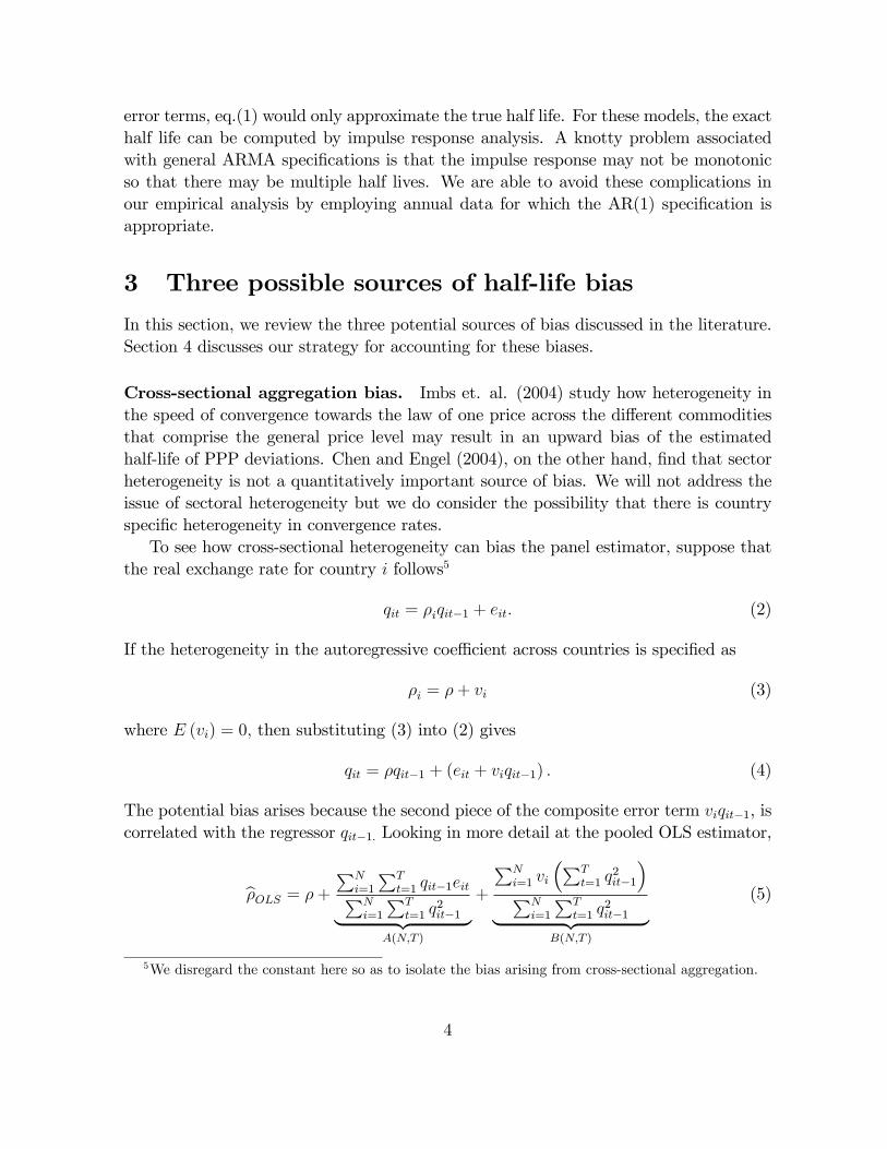
Cross-sectional aggregation bias. Imbs et. al. (2004) study how heterogeneity inthe speed of convergence towards the law of one price across the di¤erent commoditiesthat comprise the general price level may result in an upward bias of the estimatedhalf-life of PPP deviations. Chen and Engel (2004), on the other hand, �nd that sectorheterogeneity is not a quantitatively important source of bias. We will not address theissue of sectoral heterogeneity but we do consider the possibility that there is countryspeci�c heterogeneity in convergence rates.To see how cross-sectional heterogeneity can bias the panel estimator, suppose that

the real exchange rate for country i follows5

qit = �iqit�1 + eit: (2)

If the heterogeneity in the autoregressive coe¢ cient across countries is speci�ed as

�i = �+ vi (3)

where E (vi) = 0; then substituting (3) into (2) gives

qit = �qit�1 + (eit + viqit�1) : (4)

The potential bias arises because the second piece of the composite error term viqit�1, iscorrelated with the regressor qit�1: Looking in more detail at the pooled OLS estimator,

b�OLS = �+

PNi=1

PTt=1 qit�1eitPN

i=1

PTt=1 q

2it�1| {z }

A(N;T )

+

PNi=1 vi

�PTt=1 q

2it�1

�PN

i=1

PTt=1 q

2it�1| {z }

B(N;T )

(5)

5We disregard the constant here so as to isolate the bias arising from cross-sectional aggregation.

4

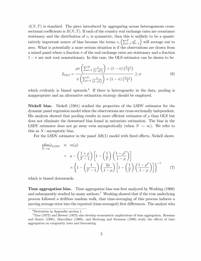
A(N; T ) is standard. The piece introduced by aggregating across heterogeneous cross-sectional coe¢ cients is B(N; T ): If each of the country real exchange rates are covariancestationary and the distribution of vi is symmetric, then this is unlikely to be a quanti-tatively important source of bias because the terms vi

�PTt=1 q

2it�1

�will average out to

zero. What is potentially a more serious situation is if the observations are drawn froma mixed panel where a fraction � of the real exchange rates are stationary and a fraction1� � are unit root nonstationary. In this case, the OLS estimator can be shown to be

b�OLS = ��

�PNi=1

1

(1��2i )

�+ (1� �)

�T+12

��

�PNi=1

1

(1��2i )

�+ (1� �)

�T+12

� � � (6)

which evidently is biased upwards.6 If there is heterogeneity in the data, pooling isinappropriate and an alternative estimation strategy should be employed.

Nickell bias. Nickell (1981) studied the properties of the LSDV estimator for thedynamic panel regression model when the observations are cross-sectionally independent.His analysis showed that pooling results in more e¢ cient estimates of � than OLS butdoes not eliminate the downward bias found in univariate estimation. The bias in theLSDV estimator does not go away even asymptotically (when N ! 1). We refer tothis as N�asymptotic bias.For the LSDV estimator in the panel AR(1) model with �xed e¤ects, Nickell shows

plimN!1

�̂LSDV � m(�)

= ���1 + �

T � 1

��1�

�1

T

��1� �T

1� �

����1�

�1

T � 1

��2�

1� �

��1�

�1

T

��1� �T

1� �

����1(7)

which is biased downwards.

Time aggregation bias. Time aggregation bias was �rst analyzed by Working (1960)and subsequently studied by many authors.7 Working showed that if the true underlyingprocess followed a driftless random walk, that time-averaging of this process induces amoving average error into the reported (time-averaged) �rst di¤erences. The analyst who

6Derivation in Appendix section 1.7Tiao (1972) and Brewer (1973) also develop econometric implications of time aggregation. Rossana

and Seater (1995), Marcellino (1999), and Breitung and Swanson (1999) study the e¤ects of timeaggregation on exogeneity tests and forecasting.

5

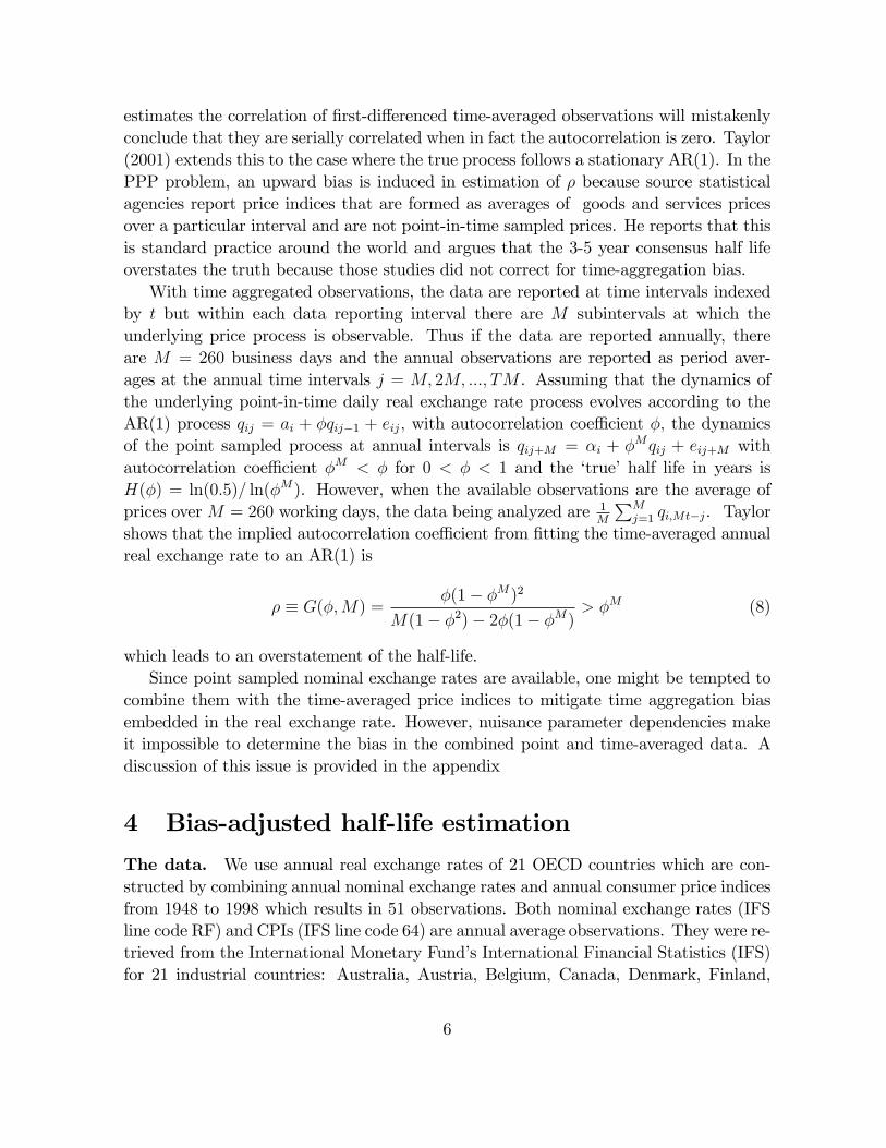
estimates the correlation of �rst-di¤erenced time-averaged observations will mistakenlyconclude that they are serially correlated when in fact the autocorrelation is zero. Taylor(2001) extends this to the case where the true process follows a stationary AR(1). In thePPP problem, an upward bias is induced in estimation of � because source statisticalagencies report price indices that are formed as averages of goods and services pricesover a particular interval and are not point-in-time sampled prices. He reports that thisis standard practice around the world and argues that the 3-5 year consensus half lifeoverstates the truth because those studies did not correct for time-aggregation bias.With time aggregated observations, the data are reported at time intervals indexed

by t but within each data reporting interval there are M subintervals at which theunderlying price process is observable. Thus if the data are reported annually, thereare M = 260 business days and the annual observations are reported as period aver-ages at the annual time intervals j = M; 2M; :::; TM . Assuming that the dynamics ofthe underlying point-in-time daily real exchange rate process evolves according to theAR(1) process qij = ai + �qij�1 + eij; with autocorrelation coe¢ cient �; the dynamicsof the point sampled process at annual intervals is qij+M = �i + �Mqij + eij+M withautocorrelation coe¢ cient �M < � for 0 < � < 1 and the �true�half life in years isH(�) = ln(0:5)= ln(�M). However, when the available observations are the average ofprices over M = 260 working days, the data being analyzed are 1

M

PMj=1 qi;Mt�j. Taylor

shows that the implied autocorrelation coe¢ cient from �tting the time-averaged annualreal exchange rate to an AR(1) is

� � G(�;M) =�(1� �M)2

M(1� �2)� 2�(1� �M)> �M (8)

which leads to an overstatement of the half-life.Since point sampled nominal exchange rates are available, one might be tempted to

combine them with the time-averaged price indices to mitigate time aggregation biasembedded in the real exchange rate. However, nuisance parameter dependencies makeit impossible to determine the bias in the combined point and time-averaged data. Adiscussion of this issue is provided in the appendix

4 Bias-adjusted half-life estimation

The data. We use annual real exchange rates of 21 OECD countries which are con-structed by combining annual nominal exchange rates and annual consumer price indicesfrom 1948 to 1998 which results in 51 observations. Both nominal exchange rates (IFSline code RF) and CPIs (IFS line code 64) are annual average observations. They were re-trieved from the International Monetary Fund�s International Financial Statistics (IFS)for 21 industrial countries: Australia, Austria, Belgium, Canada, Denmark, Finland,

6

France, Germany, Greece, Ireland, Italy, Japan, the Netherlands, New Zealand, Norway,Portugal, Spain, Sweden, Switzerland, the United Kingdom, and the United States.Each country is alternatively considered as the numeraire country.8

In preliminary data analysis, we employed the Phillips and Sul (2003) panel unitroot test which �nds that the real exchange rates de�ned by the alternative numerairesare stationary. We do not devote space for detail reporting of these results since theysimply con�rm the �ndings of earlier research.

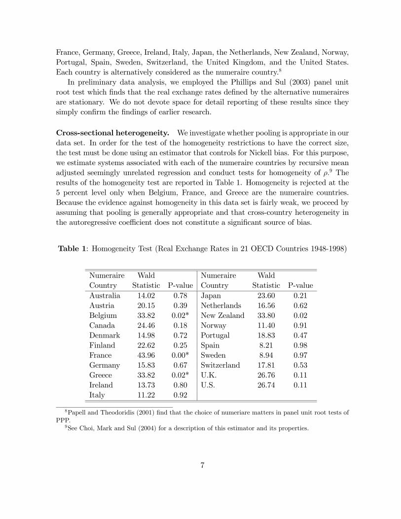
Cross-sectional heterogeneity. We investigate whether pooling is appropriate in ourdata set. In order for the test of the homogeneity restrictions to have the correct size,the test must be done using an estimator that controls for Nickell bias. For this purpose,we estimate systems associated with each of the numeraire countries by recursive meanadjusted seemingly unrelated regression and conduct tests for homogeneity of �:9 Theresults of the homogeneity test are reported in Table 1. Homogeneity is rejected at the5 percent level only when Belgium, France, and Greece are the numeraire countries.Because the evidence against homogeneity in this data set is fairly weak, we proceed byassuming that pooling is generally appropriate and that cross-country heterogeneity inthe autoregressive coe¢ cient does not constitute a signi�cant source of bias.

Table 1: Homogeneity Test (Real Exchange Rates in 21 OECD Countries 1948-1998)

Numeraire Wald Numeraire WaldCountry Statistic P-value Country Statistic P-valueAustralia 14.02 0.78 Japan 23.60 0.21Austria 20.15 0.39 Netherlands 16.56 0.62Belgium 33.82 0.02* New Zealand 33.80 0.02Canada 24.46 0.18 Norway 11.40 0.91Denmark 14.98 0.72 Portugal 18.83 0.47Finland 22.62 0.25 Spain 8.21 0.98France 43.96 0.00* Sweden 8.94 0.97Germany 15.83 0.67 Switzerland 17.81 0.53Greece 33.82 0.02* U.K. 26.76 0.11Ireland 13.73 0.80 U.S. 26.74 0.11Italy 11.22 0.92

8Papell and Theodoridis (2001) �nd that the choice of numeriare matters in panel unit root tests ofPPP.

9See Choi, Mark and Sul (2004) for a description of this estimator and its properties.

7

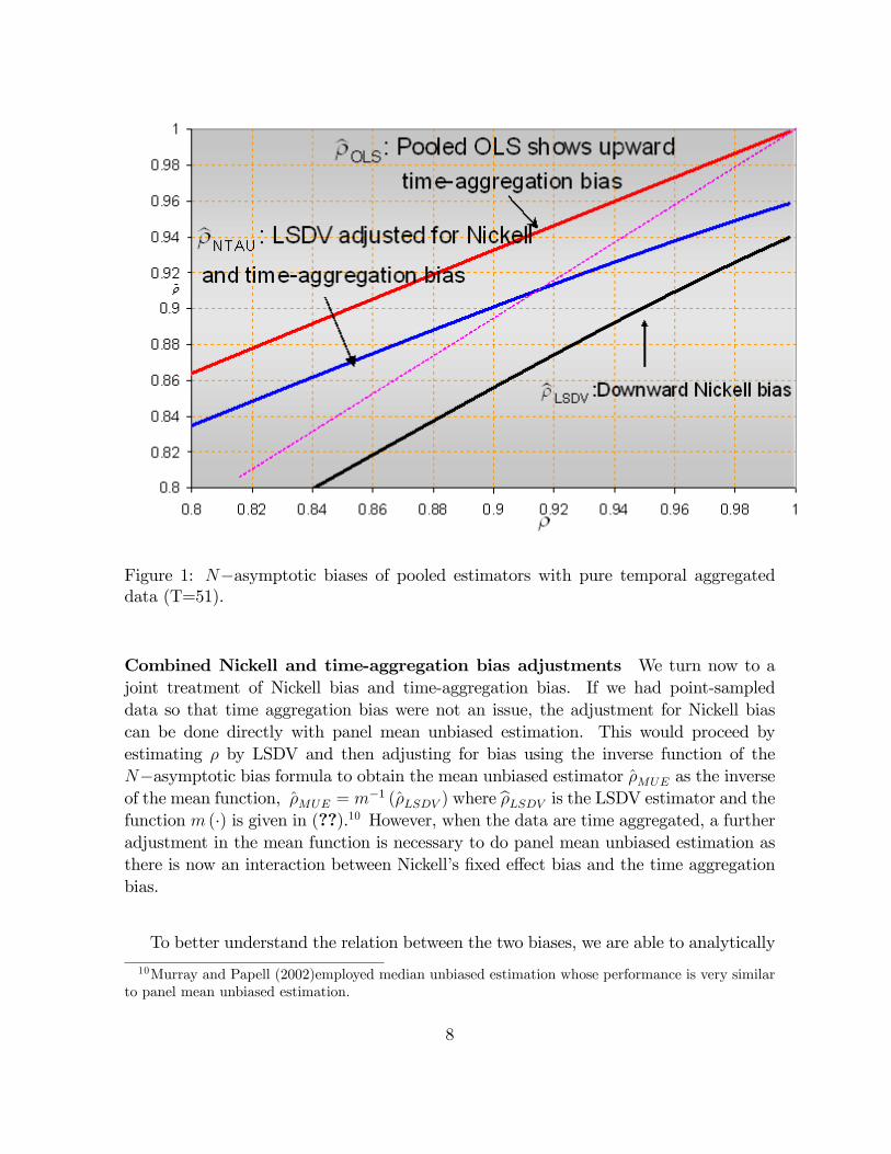
Figure 1: N�asymptotic biases of pooled estimators with pure temporal aggregateddata (T=51).

Combined Nickell and time-aggregation bias adjustments We turn now to ajoint treatment of Nickell bias and time-aggregation bias. If we had point-sampleddata so that time aggregation bias were not an issue, the adjustment for Nickell biascan be done directly with panel mean unbiased estimation. This would proceed byestimating � by LSDV and then adjusting for bias using the inverse function of theN�asymptotic bias formula to obtain the mean unbiased estimator �̂MUE as the inverseof the mean function, �̂MUE = m�1 (�̂LSDV ) where b�LSDV is the LSDV estimator and thefunction m (�) is given in (??).10 However, when the data are time aggregated, a furtheradjustment in the mean function is necessary to do panel mean unbiased estimation asthere is now an interaction between Nickell�s �xed e¤ect bias and the time aggregationbias.

To better understand the relation between the two biases, we are able to analytically

10Murray and Papell (2002)employed median unbiased estimation whose performance is very similarto panel mean unbiased estimation.

8

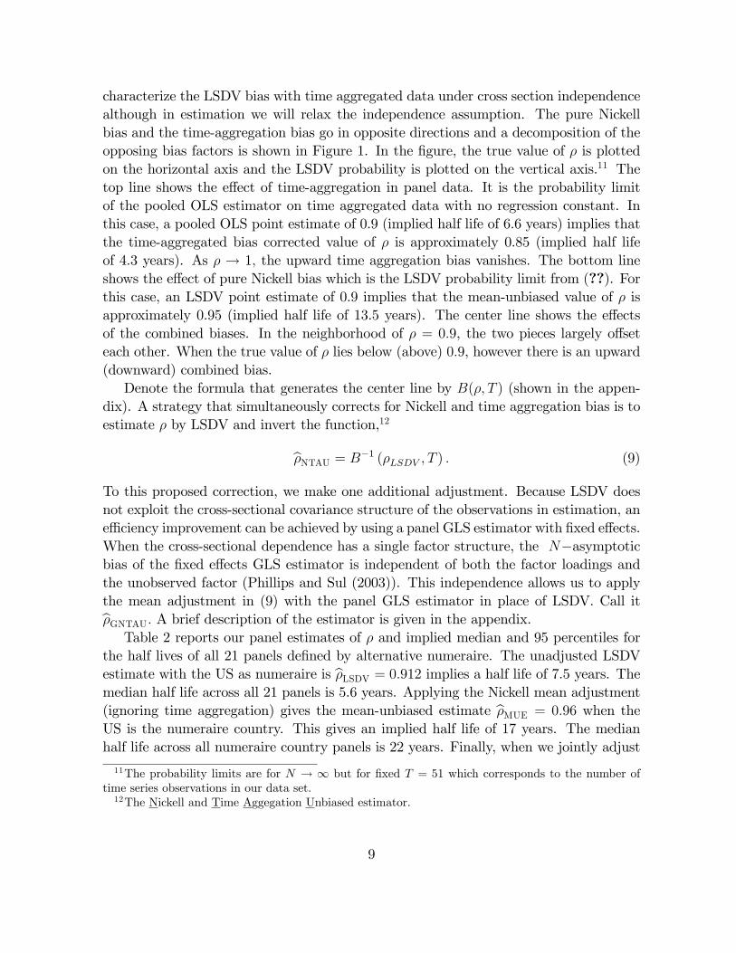
characterize the LSDV bias with time aggregated data under cross section independencealthough in estimation we will relax the independence assumption. The pure Nickellbias and the time-aggregation bias go in opposite directions and a decomposition of theopposing bias factors is shown in Figure 1. In the �gure, the true value of � is plottedon the horizontal axis and the LSDV probability is plotted on the vertical axis.11 Thetop line shows the e¤ect of time-aggregation in panel data. It is the probability limitof the pooled OLS estimator on time aggregated data with no regression constant. Inthis case, a pooled OLS point estimate of 0.9 (implied half life of 6.6 years) implies thatthe time-aggregated bias corrected value of � is approximately 0.85 (implied half lifeof 4.3 years). As � ! 1; the upward time aggregation bias vanishes. The bottom lineshows the e¤ect of pure Nickell bias which is the LSDV probability limit from (??). Forthis case, an LSDV point estimate of 0.9 implies that the mean-unbiased value of � isapproximately 0.95 (implied half life of 13.5 years). The center line shows the e¤ectsof the combined biases. In the neighborhood of � = 0:9, the two pieces largely o¤seteach other. When the true value of � lies below (above) 0:9, however there is an upward(downward) combined bias.Denote the formula that generates the center line by B(�; T ) (shown in the appen-

dix). A strategy that simultaneously corrects for Nickell and time aggregation bias is toestimate � by LSDV and invert the function,12

b�NTAU = B�1 (�LSDV ; T ) : (9)

To this proposed correction, we make one additional adjustment. Because LSDV doesnot exploit the cross-sectional covariance structure of the observations in estimation, ane¢ ciency improvement can be achieved by using a panel GLS estimator with �xed e¤ects.When the cross-sectional dependence has a single factor structure, the N�asymptoticbias of the �xed e¤ects GLS estimator is independent of both the factor loadings andthe unobserved factor (Phillips and Sul (2003)). This independence allows us to applythe mean adjustment in (9) with the panel GLS estimator in place of LSDV. Call itb�GNTAU: A brief description of the estimator is given in the appendix.Table 2 reports our panel estimates of � and implied median and 95 percentiles for

the half lives of all 21 panels de�ned by alternative numeraire. The unadjusted LSDVestimate with the US as numeraire is b�LSDV = 0:912 implies a half life of 7.5 years. Themedian half life across all 21 panels is 5.6 years. Applying the Nickell mean adjustment(ignoring time aggregation) gives the mean-unbiased estimate b�MUE = 0:96 when theUS is the numeraire country. This gives an implied half life of 17 years. The medianhalf life across all numeraire country panels is 22 years. Finally, when we jointly adjust

11The probability limits are for N ! 1 but for �xed T = 51 which corresponds to the number oftime series observations in our data set.12The Nickell and Time Aggegation Unbiased estimator.

9

for Nickell bias and time aggregation bias, estimating the autocorrelation coe¢ cient byGLS and applying the mean adjustment, we obtain an estimate of the autocorrelationcoe¢ cient with the US as numeraire of b�GNTAU = 0:87 which is slightly below the LSDVestimate. The implied half life is 4.8 years (95 percent con�dence interval ranges from 3.7to 6.6 years). The median across all alternative panels is 5.5 years which approximatelyreturns us to the LSDV estimates.

5 Conclusion

PPP research, desperate for larger sample sizes to improve precision and con�dencein empirical estimates, has turned to the analysis of panel data. However, half-lifeestimation from panel data, is subject to two major sources of bias. The �rst source isthe downward bias of the LSDV estimator. The second main source of bias arises fromthe use of time aggregated data. These two opposing biases roughly cancel out. Whenwe simultaneously control for these two opposing biases, the resulting half-life estimatesbring us approximately back to the LSDV estimates.

10

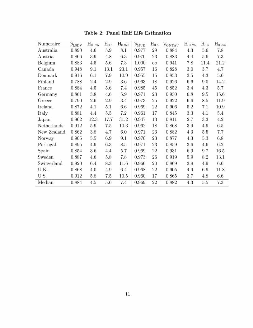
Table 2: Panel Half Life Estimation

Numeraire b�LSDV H0:025 H0:5 H0:975 b�MUE H0:5 b�GNTAU H0:025 H0:5 H0:975Australia 0.890 4.6 5.9 8.1 0.977 29 0.884 4.3 5.6 7.8Austria 0.866 3.9 4.8 6.3 0.970 23 0.883 4.4 5.6 7.3Belgium 0.883 4.5 5.6 7.3 1.000 oo 0.941 7.8 11.4 21.2Canada 0.948 9.1 13.1 23.1 0.957 16 0.828 3.0 3.7 4.7Denmark 0.916 6.1 7.9 10.9 0.955 15 0.853 3.5 4.3 5.6Finland 0.788 2.4 2.9 3.6 0.963 18 0.926 6.6 9.0 14.2France 0.884 4.5 5.6 7.4 0.985 45 0.852 3.4 4.3 5.7Germany 0.861 3.8 4.6 5.9 0.971 23 0.930 6.8 9.5 15.6Greece 0.790 2.6 2.9 3.4 0.973 25 0.922 6.6 8.5 11.9Ireland 0.872 4.1 5.1 6.6 0.969 22 0.906 5.2 7.1 10.9Italy 0.881 4.4 5.5 7.2 0.961 17 0.845 3.3 4.1 5.4Japan 0.962 12.3 17.7 31.2 0.947 13 0.811 2.7 3.3 4.2Netherlands 0.912 5.9 7.5 10.3 0.962 18 0.868 3.9 4.9 6.5New Zealand 0.862 3.8 4.7 6.0 0.971 23 0.882 4.3 5.5 7.7Norway 0.905 5.5 6.9 9.1 0.970 23 0.877 4.3 5.3 6.8Portugal 0.895 4.9 6.3 8.5 0.971 23 0.859 3.6 4.6 6.2Spain 0.854 3.6 4.4 5.7 0.969 22 0.931 6.9 9.7 16.5Sweden 0.887 4.6 5.8 7.8 0.973 26 0.919 5.9 8.2 13.1Switzerland 0.920 6.4 8.3 11.6 0.966 20 0.869 3.9 4.9 6.6U.K. 0.868 4.0 4.9 6.4 0.968 22 0.905 4.9 6.9 11.8U.S. 0.912 5.8 7.5 10.5 0.960 17 0.865 3.7 4.8 6.6Median 0.884 4.5 5.6 7.4 0.969 22 0.882 4.3 5.5 7.3

11

References

[1] Brewer, K.R.W., 1973. �Some Consequences of Temporal Aggregation and Sys-tematic Sampling for ARMA and ARMAX Models,� Journal of Econometrics1, 133-154.

[2] Breitung, Jorg and Norman R. Swanson, 2002. �Temporal Aggregation andSpurious Instantaneous Causality in Multiple Time Series Models,�Journal ofTime Series Analysis, 23, 651-665.

[3] Chiu, Ru-Lin, 2002. �Testing the purchasing power parity in panel data,� Inter-national Review of Economics and Finance, 11, 349�362.

[4] Choi, Chi-Young., 2002. �Searching for Evidence of Long-Run PPP from a PostBretton Woods Panel: Separating the Wheat from the Cha¤,�Journal of Inter-national Money and Finance, forthcoming.

[5] Choi, Chi-Young, Nelson C. Mark and Donggyu Sul, 2004. �Bias Re-duction by Recursive Mean Adjustment in Panel Data,�mimeo, University ofAuckland.

[6] Chen, Shiu-Sheng and Charles Engel, 2004. �Does �Aggregation Bias�Ex-plain the PPP Puzzle?�mimeo, University of Wisconsin.

[7] Fleissig, Adrian R. and Jack Strauss, 2000. �Panel Unit Root Tests of Pur-chasing Power Parity for Price Indices,� Journal of International Money andFinance 19, 489�506.

[8] Flores, Renato, Philippe Jorion, Pierre-Yves Preumont, and ArianeSzafarz, 1999. �Multivariate unit root tests of the PPP hypothesis,�Journalof Empirical Finance, 6, 335�353.

[9] Frankel, Jeffrey A. and Andrew K. Rose, 1996. �A Panel Project on Pur-chasing Power Parity: Mean Reversion within and between Countries,�Journalof International Economics, 40, 209-24.

[10] Hsiao, Cheng., 2003. Analysis of Panel Data, Second Edition. Cambridge Univer-sity Press.

[11] Imbs, J., Mumtaz, H., Ravn, M.O., Rey, H., 2004, �PPP Strikes Back: Aggregationand the Real Exchange Rate,�mimeo, London Business School.

[12] Kendall, M.G., 1954. �Note on Bias in the Estimation of Autocorrelation,�Bio-metrika 41, 403�404.

[13] Lothian, James R. 1997. �Multi-Country Evidence on the Behavior of PurchasingPower Parity under the Current Float,� Journal of International Money andFinance, 16, 19�35.

12

[14] Lothian, James R. and Mark P. Taylor, 1996. �Real Exchange Rate Behav-ior: The Recent Float from the Perspective of the Past Two Centuries,�Journalof Political Economy, 104, 488-509.

[15] Marcellino, Massimiliano, 1999. �Some Consequences of Temporal Aggrega-tion in Empirical Analysis,�Journal of Business and Economic Statistics, 17(1),129�136.

[16] Marriott, F.H.C., Pope, J.A., 1954. �Bias in the Estimation of Autocorrela-tions,�Biometrika, 41, 393-403

[17] Murray, Christian.J., Papell, David.H., 2002. �The Purchasing Power ParityPersistence Paradigm,�Journal of International Economics 56(1), 1�19.

[18] Nickell, S. 1981. �Biases in Dynamic Models with Fixed E¤ects,�Econometrica49, 1417�1426.

[19] Papell, David H., 2004. �The Panel Purchasing Power Parity Puzzle�, mimeo,University of Houston.

[20] Papell, David H., and Hristos Theodoridis, 1998. �Increasing Evidenceof Purchasing Power Parity over the Current Float,� Journal of InternationalMoney and Finance, 17, 41-50.

[21] Papell, David H., and Hristos Theodoridis, 2001. �The Choice of NumeraireCurrency in Panel Tests of Purchasing Power Parity,�Journal of Money, Credit,and Banking, 33, 790-803.

[22] Phillips, P.C.B., Sul, D., 2003. �Bias in Dynamic Panel Estimation with FixedE¤ects, Incidental Trends and Cross Section Dependence,�mimeo, Universityof Auckland.

[23] Rogoff, Kenneth., 1996. �The Purchasing Power Parity Puzzle,� Journal ofEconomic Literature 34(2), 647�668.

[24] Rossana, R.J. and Seater J.J. 1992. �Aggregation, Unit Roots and the Time-Series Structure of Manufacturing Real Wages,�International Economic Review,33(1), 159�179.

[25] Taylor, A.M., 2001. �Potential Pitfalls for the PPP Puzzle? Sampling and Speci-�cation Biases in Mean-Reversion Tests of the Law of One Price.�Econometrica69(2), 473�498.

[26] Tiao, G. C., 1972. �Asymptotic Behavior of Temporal Aggregates of Time Series,�"Biometrika, 59, 525-531.

[27] Working, Holbrook., 1960. �Note on the Correlation of First Di¤erences ofAverages in a Random Chain,�Econometrica 28(4), 916-918.

13

Appendix

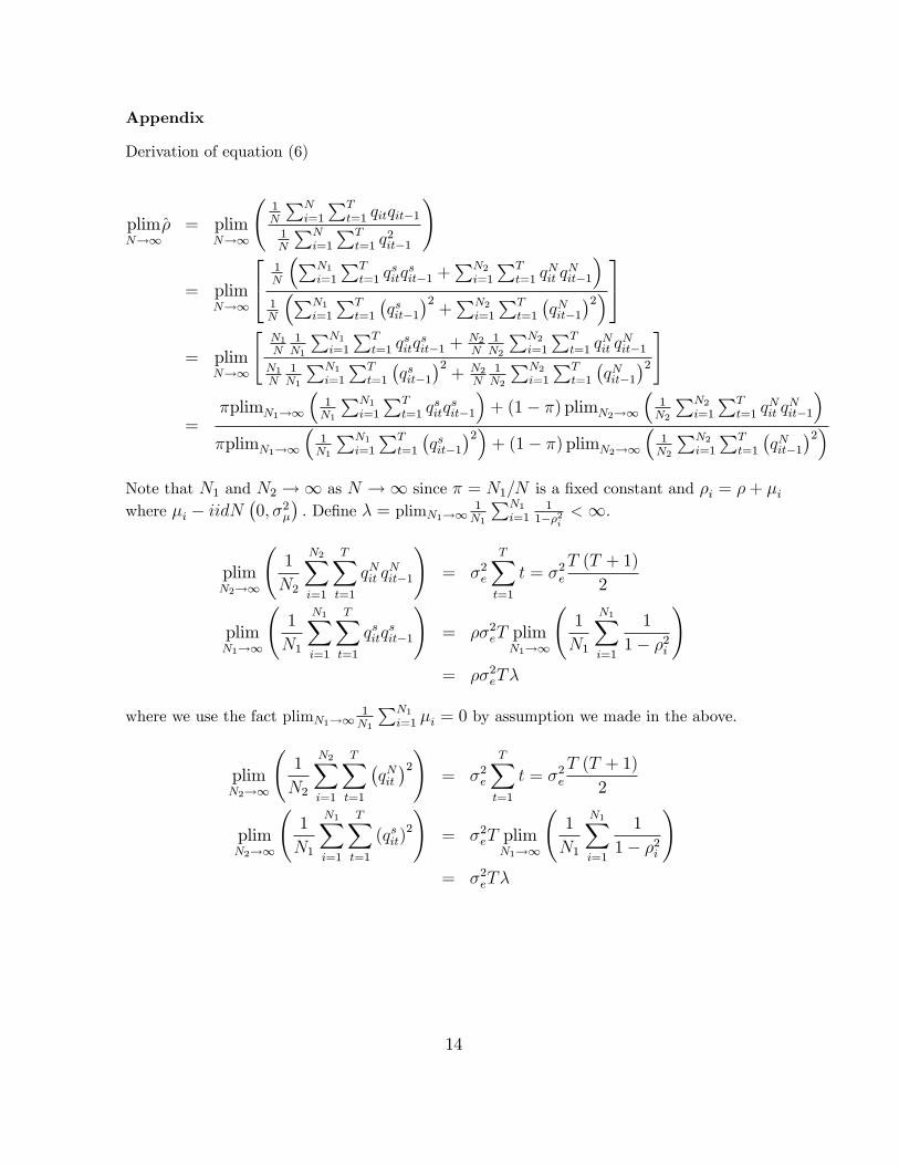
Derivation of equation (6)

plimN!1

�̂ = plimN!1

1N

PNi=1

PTt=1 qitqit�1

1N

PNi=1

PTt=1 q

2it�1

!

= plimN!1

24 1N

�PN1i=1

PTt=1 q

sitq

sit�1 +

PN2i=1

PTt=1 q

Nit q

Nit�1

�1N

�PN1i=1

PTt=1

�qsit�1

�2+PN2

i=1

PTt=1

�qNit�1

�2�35

= plimN!1

"N1N

1N1

PN1i=1

PTt=1 q

sitq

sit�1 +

N2N

1N2

PN2i=1

PTt=1 q

Nit q

Nit�1

N1N

1N1

PN1i=1

PTt=1

�qsit�1

�2+ N2

N1N2

PN2i=1

PTt=1

�qNit�1

�2#

=�plimN1!1

�1N1

PN1i=1

PTt=1 q

sitq

sit�1

�+ (1� �)plimN2!1

�1N2

PN2i=1

PTt=1 q

Nit q

Nit�1

��plimN1!1

�1N1

PN1i=1

PTt=1

�qsit�1

�2�+ (1� �)plimN2!1

�1N2

PN2i=1

PTt=1

�qNit�1

�2�Note that N1 and N2 !1 as N !1 since � = N1=N is a �xed constant and �i = �+ �iwhere �i � iidN

�0; �2�

�: De�ne � = plimN1!1

1N1

PN1i=1

11��2i

< 1:

plimN2!1

1

N2

N2Xi=1

TXt=1

qNit qNit�1

!= �2e

TXt=1

t = �2eT (T + 1)

2

plimN1!1

1

N1

N1Xi=1

TXt=1

qsitqsit�1

!= ��2eT plim

N1!1

1

N1

N1Xi=1

1

1� �2i

!= ��2eT�

where we use the fact plimN1!11N1

PN1i=1 �i = 0 by assumption we made in the above.

plimN2!1

1

N2

N2Xi=1

TXt=1

�qNit�2!

= �2e

TXt=1

t = �2eT (T + 1)

2

plimN2!1

1

N1

N1Xi=1

TXt=1

(qsit)2

!= �2eT plim

N1!1

1

N1

N1Xi=1

1

1� �2i

!= �2eT�

14

Hence we have

plimN!1

�̂ =���2eT�+ (1� �)�2e

T (T+1)2

��2eT�+ (1� �)�2eT (T+1)

2

=���+ (1� �) (T+1)

2

��+ (1� �) (T+1)2

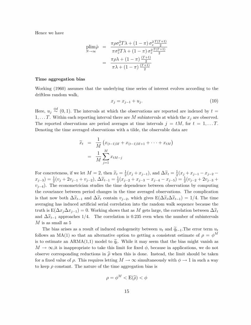
Time aggregation bias

Working (1960) assumes that the underlying time series of interest evolves according to thedriftless random walk,

xj = xj�1 + uj: (10)

Here, ujiid� (0; 1): The intervals at which the observations are reported are indexed by t =

1; : : : T . Within each reporting interval there areM subintervals at which the xj are observed.The reported observations are period averages at time intervals j = tM; for t = 1; : : : T:

Denoting the time averaged observations with a tilde, the observable data are

ext =1

M

�x(t�1)M + x(t�1)M+1 + � � �+ xtM

�=

1

M

MXj=1

xtM�j

For concreteness, if we letM = 2; then ext = 12(xj + xj�1); and �ext = 1

2(xj + xj�1� xj�2�

xj�3) =12(vj + 2vj�1 + vj�2); �ext�1 = 1

2(xj�2 + xj�3 � xj�4 � xj�5) =

12(vj�2 + 2vj�3 +

vj�4). The econometrician studies the time dependence between observations by computingthe covariance between period changes in the time averaged observations. The complicationis that now both �ext�1 and �ext contain vj�2; which gives E(�ext�ext�1) = 1=4: The timeaveraging has induced arti�cial serial correlation into the random walk sequence because thetruth is E(�xj�xj�1) = 0:Working shows that asM gets large, the correlation between �extand �ext�1 approaches 1/4. The correlation is 0.235 even when the number of subintervalsM is as small as 5

The bias arises as a result of induced endogeneity between ut and eqt�1.The error term utfollows an MA(1) so that an alternative option to getting a consistent estimate of � = �M

is to estimate an ARMA(1,1) model to eqt. While it may seem that the bias might vanish asM ! 1;it is inappropriate to take this limit for �xed �, because in applications, we do notobserve corresponding reductions in b� when this is done. Instead, the limit should be takenfor a �xed value of �. This requires lettingM !1 simultaneously with �! 1 in such a wayto keep � constant. The nature of the time aggregation bias is

� = �M < E(b�) < �

15

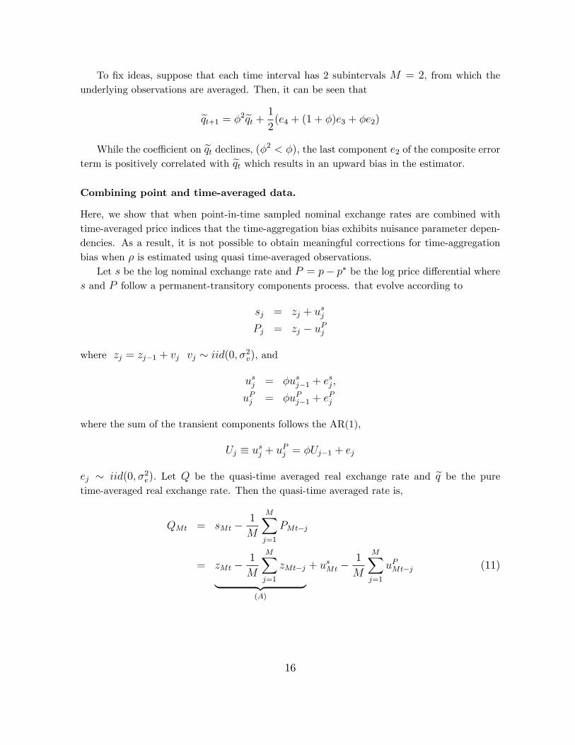
To �x ideas, suppose that each time interval has 2 subintervals M = 2, from which theunderlying observations are averaged. Then, it can be seen that

eqt+1 = �2eqt + 12(e4 + (1 + �)e3 + �e2)

While the coe¢ cient on eqt declines, (�2 < �); the last component e2 of the composite errorterm is positively correlated with eqt which results in an upward bias in the estimator.Combining point and time-averaged data.

Here, we show that when point-in-time sampled nominal exchange rates are combined withtime-averaged price indices that the time-aggregation bias exhibits nuisance parameter depen-dencies. As a result, it is not possible to obtain meaningful corrections for time-aggregationbias when � is estimated using quasi time-averaged observations.

Let s be the log nominal exchange rate and P = p� p� be the log price di¤erential wheres and P follow a permanent-transitory components process. that evolve according to

sj = zj + usj

Pj = zj � uPj

where zj = zj�1 + vj vj � iid(0; �2v); and

usj = �usj�1 + esj ;

uPj = �uPj�1 + ePj

where the sum of the transient components follows the AR(1),

Uj � usj + uPj = �Uj�1 + ej

ej � iid(0; �2e): Let Q be the quasi-time averaged real exchange rate and eq be the puretime-averaged real exchange rate. Then the quasi-time averaged rate is,

QMt = sMt �1

M

MXj=1

PMt�j

= zMt �1

M

MXj=1

zMt�j| {z }(A)

+ usMt �1

M

MXj=1

uPMt�j (11)

16

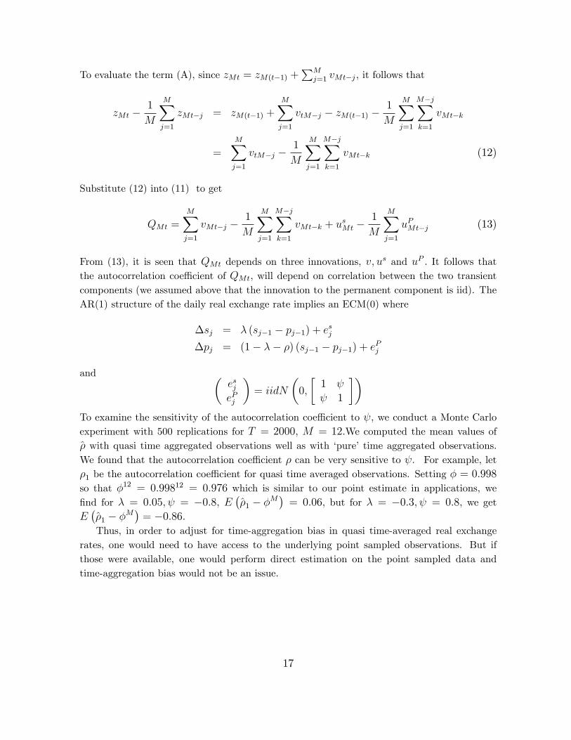
To evaluate the term (A), since zMt = zM(t�1) +PM

j=1 vMt�j; it follows that

zMt �1

M

MXj=1

zMt�j = zM(t�1) +

MXj=1

vtM�j � zM(t�1) �1

M

MXj=1

M�jXk=1

vMt�k

=

MXj=1

vtM�j �1

M

MXj=1

M�jXk=1

vMt�k (12)

Substitute (12) into (11) to get

QMt =MXj=1

vMt�j �1

M

MXj=1

M�jXk=1

vMt�k + usMt �1

M

MXj=1

uPMt�j (13)

From (13), it is seen that QMt depends on three innovations, v; us and uP : It follows thatthe autocorrelation coe¢ cient of QMt; will depend on correlation between the two transientcomponents (we assumed above that the innovation to the permanent component is iid). TheAR(1) structure of the daily real exchange rate implies an ECM(0) where

�sj = � (sj�1 � pj�1) + esj

�pj = (1� �� �) (sj�1 � pj�1) + ePj

and �esjePj

�= iidN

�0;

�1

1

��To examine the sensitivity of the autocorrelation coe¢ cient to ; we conduct a Monte Carloexperiment with 500 replications for T = 2000; M = 12:We computed the mean values of�̂ with quasi time aggregated observations well as with �pure�time aggregated observations.We found that the autocorrelation coe¢ cient � can be very sensitive to . For example, let�1 be the autocorrelation coe¢ cient for quasi time averaged observations. Setting � = 0:998so that �12 = 0:99812 = 0:976 which is similar to our point estimate in applications, we�nd for � = 0:05; = �0:8; E

��̂1 � �M

�= 0:06; but for � = �0:3; = 0:8; we get

E��̂1 � �M

�= �0:86:

Thus, in order to adjust for time-aggregation bias in quasi time-averaged real exchangerates, one would need to have access to the underlying point sampled observations. But ifthose were available, one would perform direct estimation on the point sampled data andtime-aggregation bias would not be an issue.

17

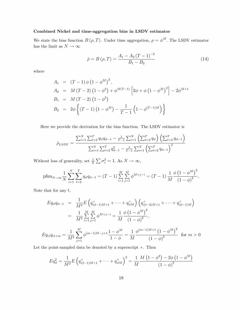
Combined Nickel and time-aggregation bias in LSDV estimator

We state the bias function B (�; T ) : Under time aggregation, � = �M : The LSDV estimatorhas the limit as N !1

�̂ = B (�; T ) =A1 � A2 (T � 1)�2

B1 �B2(14)

where

A1 = (T � 1)��1� �M

�2;

A2 = M (T � 2)�1� �2

�+ �M(T�1)

h2�+ �

�1� �M

�2i� 2�M+1

B1 = M (T � 2)�1� �2

�B2 = 2�

�(T � 1)

�1� �M

�� 1

T � 1

�1� �(T�1)M

��

Here we provide the derivation for the bias function. The LSDV estimator is

�̂LSDV =

PNi=1

PTt=2 qitqit�1 � 1

T�1PN

i=1

�PTt=2 qit

��PTt=2 qit�1

�PN

i=1

PTt=2 q

2it�1 � 1

T�1PN

i=1

�PTt=2 qit�1

�2Without loss of generality, set 1

N

P�2i = 1: As N !1;

plimN!11

N

NXi=1

TXt=2

qitqit�1 = (T � 1)MPi=1

MPj=1

�M+j�i = (T � 1) 1M

��1� �M

�2(1� �)2

;

Note that for any t;

Eqitqit�1 =1

M2E�q+i(t�1)M+1 + � � �+ q+itM

��q+i(t�2)M+1 + � � �+ q+i(t�1)M

�=

1

M2

MPi=1

MPj=1

�M+j�i =1

M

��1� �M

�2(1� �)2

;

Eqi1qi1+m =1

M2

MXj=1

�(m�1)M�j+11� �M

1� �=1

M

�(m�1)M+1�1� �M

�2(1� �)2

for m > 0

Let the point-sampled data be denoted by a superscript +. Then

Eq2it =1

M2E�q+i(t�1)M+1 + � � �+ q+itM

�2=1

M

M�1� �2

�� 2�

�1� �M

�(1� �)2

18

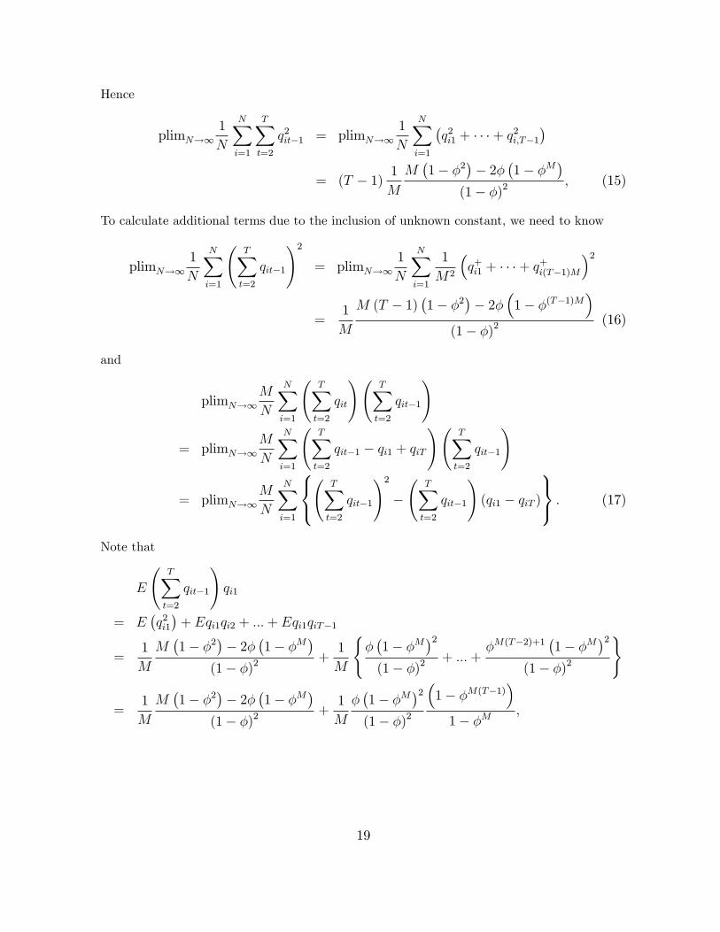
Hence

plimN!11

N

NXi=1

TXt=2

q2it�1 = plimN!11

N

NXi=1

�q2i1 + � � �+ q2i;T�1

�= (T � 1) 1

M

M�1� �2

�� 2�

�1� �M

�(1� �)2

; (15)

To calculate additional terms due to the inclusion of unknown constant, we need to know

plimN!11

N

NXi=1

TXt=2

qit�1

!2= plimN!1

1

N

NXi=1

1

M2

�q+i1 + � � �+ q+i(T�1)M

�2

=1

M

M (T � 1)�1� �2

�� 2�

�1� �(T�1)M

�(1� �)2

(16)

and

plimN!1M

N

NXi=1

TXt=2

qit

! TXt=2

qit�1

!

= plimN!1M

N

NXi=1

TXt=2

qit�1 � qi1 + qiT

! TXt=2

qit�1

!

= plimN!1M

N

NXi=1

8<:

TXt=2

qit�1

!2�

TXt=2

qit�1

!(qi1 � qiT )

9=; : (17)

Note that

E

TXt=2

qit�1

!qi1

= E�q2i1�+ Eqi1qi2 + :::+ Eqi1qiT�1

=1

M

M�1� �2

�� 2�

�1� �M

�(1� �)2

+1

M

(��1� �M

�2(1� �)2

+ :::+�M(T�2)+1 �1� �M

�2(1� �)2

)

=1

M

M�1� �2

�� 2�

�1� �M

�(1� �)2

+1

M

��1� �M

�2(1� �)2

�1� �M(T�1)

�1� �M

;

19

and

E

TXt=2

qit�1

!qiT

= Eqi1qiT + :::+ EqiT�1qiT = Eqi1qi2 + :::+ Eqi1qiT

=1

M

��1� �M

�2(1� �)2

�1� �MT

�1� �M

Hence we have

plimN!11

N

NXi=1

TXt=2

qit�1

!(qi1 � qiT )

=1

M

M�1� �2

�� 2�

�1� �M

�(1� �)2

+1

M

��1� �M

�2(1� �)2

8<:�1� �M(T�1)

�1� �M

��1� �MT

�1� �M

9=;=

1

k

k�1� �2

�� 2�

�1� �k

�(1� �)2

� 1

k

��1� �k

�2(1� �)2

�k(T�1) (18)

Plugging (16), (15) and (18) to (17) yields

plimN!1M

N

NXi=1

TXt=2

qit

! TXt=2

qit�1

!=

1

(1� �)2

nM (T � 2)

�1� �2

�+ �M(T�1)

h2�+ �

�1� �M

�2i� 2�M+1o

Hence the denominator term in (14) is given by

(T � 1)M�1� �2

�� 2�

�1� �M

�(1� �)2

� 1

T � 1M (T � 1)

�1� �2

�� 2�

�1� �(T�1)M

�(1� �)2

= (T � 2)M�1� �2

�� 2�

�(T � 1)

�1� �M

�� 1

T � 1

�1� �(T�1)M

��while the numerator is

(T � 1)��1� �M

�2� 1

T � 1

nM (T � 2)

�1� �2

�+ �M(T�1)

h2�+ �

�1� �M

�2i� 2�M+1o

That is,

�̂ =A1 � A2 (T � 1)�2

B1 �B2

20

Fixed e¤ects GLS

The estimator is fully described in Phillips and Sul (2003). Here, we give only a cursoryaccount. In the absence of time-aggregation, the innovations are governed by the single factormodel,

eit = �i�t + uit

where �i; i = 1; :::N , are the factor loadings and �t is the single driving factor. The uit areserially and mutually independent. Let et = (e1t; :::; eNt); � = (�1; � � � ; �N) ; and ut =(u1t; :::; uNt). Then E (ete0t) = �e = ��0+�u; where �u = E (utu

0t) : The factor loadings can

be estimated by iterative method of moments after imposing a normalization for the varianceof �t. This gives

�̂" = �̂�̂0+ �̂u

where �̂ =��̂1; � � � ; �̂N

�and the diagonal elements of �̂u are

1T

PTt=1 "̂

2it; "̂it = ~qit � �̂m~qit�1

where ~qit = qit � 1T

Pqit, and �̂m is the mean-unbiased estimator of �: Having obtained the

estimated error covariance matrix, one can apply feasible GLS to obtain e¢ cient estimates of�:

When the observations are time aggregated data, the regression error has an MA(1) struc-ture. In this case, we need one further adjustment because feasible GLS should be based onthe long run variance of eit rather than the contemporaneous variance of eit: Since eit followsMA(1), the parametric structure of cross section dependence is now eit = �it + �it�1; where�it = �i�t + uit. The long run covariance matrix for eit becomes

e = E (ete0t) + E

�ete

0t�1�+ E (et�1e

0t)

21