naval postgraduate school - CiteSeerX

NAVAL

POSTGRADUATE

SCHOOL

MONTEREY, CALIFORNIA

THESIS

Approved for public release; distribution is unlimited

A STUDY ON PREDICTIVE ANALYTICS APPLICATION

TO SHIP MACHINERY MAINTENANCE

by

Guan Hock Lee

September 2013

Thesis Advisor: David Olwell

Second Reader: Fotis Papoulias

THIS PAGE INTENTIONALLY LEFT BLANK

i

REPORT DOCUMENTATION PAGE Form Approved OMB No. 0704-0188 Public reporting burden for this collection of information is estimated to average 1 hour per response, including the time for reviewing instruction,

searching existing data sources, gathering and maintaining the data needed, and completing and reviewing the collection of information. Send

comments regarding this burden estimate or any other aspect of this collection of information, including suggestions for reducing this burden, to Washington headquarters Services, Directorate for Information Operations and Reports, 1215 Jefferson Davis Highway, Suite 1204, Arlington, VA

22202-4302, and to the Office of Management and Budget, Paperwork Reduction Project (0704-0188) Washington DC 20503.

1. AGENCY USE ONLY (Leave blank)

2. REPORT DATE September 2013

3. REPORT TYPE AND DATES COVERED Master’s Thesis

4. TITLE AND SUBTITLE

A STUDY ON PREDICTIVE ANALYTICS APPLICATION TO SHIP

MACHINERY MAINTENANCE

5. FUNDING NUMBERS

6. AUTHOR(S) Lee, Guan Hock

7. PERFORMING ORGANIZATION NAME(S) AND ADDRESS(ES)

Naval Postgraduate School

Monterey, CA 93943-5000

8. PERFORMING ORGANIZATION

REPORT NUMBER

9. SPONSORING /MONITORING AGENCY NAME(S) AND ADDRESS(ES)

N/A 10. SPONSORING/MONITORING

AGENCY REPORT NUMBER

11. SUPPLEMENTARY NOTES The views expressed in this thesis are those of the author and do not reflect the official policy

or position of the Department of Defense or the U.S. Government. IRB Protocol number ____N/A____.

12a. DISTRIBUTION / AVAILABILITY STATEMENT Approved for public release; distribution is unlimited

12b. DISTRIBUTION CODE A

13. ABSTRACT (maximum 200 words)

Engine failures on ships are expensive, and affect operational readiness critically due to long turn-around times for

maintenance. Prior to the engine failures, there are signs of engine characteristic changes, for example, exhaust gas

temperature (EGT), to indicate that the engine is acting abnormally. This is used as a precursor towards the modeling

of failures. There is a threshold limit of 520 degree Celsius for the EGT prior to the need for human intervention.

With this knowledge, the use of time series forecasting technique, to predict the crossing over of threshold, is

appropriate to model the EGT as a function of its operating running hours and load. This allows maintenance to be

scheduled “just in time”. When there is a departure of result from the predictive model, Cumulative Sum (CUSUM)

Control charts can then be used to monitor the change early before an actual problem arises. This paper discusses and

demonstrates the proof of principle for one engine and a particular operating profile of a commercial vessel with the

use of predictive analytics. The realization with time series forecasting coupled with CUSUM control chart allows

this approach to be extended to other attributes beyond EGT.

14. SUBJECT TERMS Predictive, Precursor, Machinery Maintenance, Failures 15. NUMBER OF

PAGES 165

16. PRICE CODE

17. SECURITY

CLASSIFICATION OF

REPORT Unclassified

18. SECURITY

CLASSIFICATION OF THIS

PAGE

Unclassified

19. SECURITY

CLASSIFICATION OF

ABSTRACT

Unclassified

20. LIMITATION OF

ABSTRACT

UU

NSN 7540-01-280-5500 Standard Form 298 (Rev. 2-89)

Prescribed by ANSI Std. 239-18

ii

THIS PAGE INTENTIONALLY LEFT BLANK

iii

Approved for public release; distribution is unlimited

A STUDY ON PREDICTIVE ANALYTICS APPLICATION TO SHIP

MACHINERY MAINTENANCE

Guan Hock Lee

Civilian, Singapore Technologies Marine, Ltd.

B.Eng (Electrical & Electronic), Nanyang Technological University, 2006

Submitted in partial fulfillment of the

requirements for the degree of

MASTER OF SCIENCE IN SYSTEMS ENGINEERING

from the

NAVAL POSTGRADUATE SCHOOL

September 2013

Author: Guan Hock Lee

Approved by: David Olwell

Thesis Advisor

Fotis Papoulis

Second Reader

Clifford Whitcomb

Chair, Department of Systems Engineering

iv

THIS PAGE INTENTIONALLY LEFT BLANK

v

ABSTRACT

Engine failures on ships are expensive, and affect operational readiness critically due to

long turn-around times for maintenance. Prior to the engine failures, there are signs of

engine characteristic changes, for example, exhaust gas temperature (EGT), to indicate

that the engine is acting abnormally. This is used as a precursor towards the modeling of

failures. There is a threshold limit of 520 degree Celsius for the EGT prior to the need for

human intervention. With this knowledge, the use of time series forecasting technique, to

predict the crossing over of threshold, is appropriate to model the EGT as a function of its

operating running hours and load. This allows maintenance to be scheduled “just in

time”. When there is a departure of result from the predictive model, Cumulative Sum

(CUSUM) Control charts can then be used to monitor the change early before an actual

problem arises. This paper discusses and demonstrates the proof of principle for one

engine and a particular operating profile of a commercial vessel with the use of predictive

analytics. The realization with time series forecasting coupled with CUSUM control chart

allows this approach to be extended to other attributes beyond EGT.

vi

THIS PAGE INTENTIONALLY LEFT BLANK

vii

TABLE OF CONTENTS

I. INTRODUCTION........................................................................................................1 A. CONDITION-BASED MAINTENANCE ......................................................2 B. ALARM CONTROL AND MONITORING SYSTEM................................4 C. PROBLEM DEFINITION ..............................................................................5

1. Problem Identification .........................................................................5 a. Lack of use of existing data ......................................................5 b. Lack of expertise to analyze data ..............................................6 c. Lack of support for initial high-cost investment ......................6

2. Scope......................................................................................................6 3. Limitations ............................................................................................7

a. Collecting enough engine data for analysis .............................7

b. Analyzing enough engine parameters to construct a

conclusive predictive model ......................................................7

c. Schedule considerations hamper analysis of a working

predictive model.........................................................................8

4. Constraints............................................................................................8 a. To use existing commercial ship engine data ..........................8 b. To use available software resources for modeling ...................8

D. PREVIOUS WORK .........................................................................................8 E. AREA OF RESEARCH AND APPROACH ...............................................10

F. STATISTICAL TOOLS ................................................................................11 G. ORGANIZATION OF STUDY ....................................................................11

II. PREDICTIVE ANALYTICS OVERVIEW ............................................................13 A. HISTORY .......................................................................................................13

B. DEFINITIONS OF THE MAIN COMPONENTS OF THE

READINESS CONCEPT ..............................................................................13 C. PREDICTIVE ANALYTICS TECHNIQUES ............................................14

1. Time series models .............................................................................14 2. Cumulative Sum (CUSUM) Control Chart .....................................16

III. DATA DESCRIPTION AND METHODOLOGY ..................................................25

A. SOURCES OF FAILURES ...........................................................................25

B. DATA COLLECTION ..................................................................................35 C. SELECTION OF VARIABLES ...................................................................35 D. DATA SETS ...................................................................................................37

IV. RESULTS AND DISCUSSION ................................................................................47 A. VALIDATION TECHNIQUE USED FOR THE MODELS .....................47

B. TIME SERIES MODELS .............................................................................47 C. CUMULATIVE SUM (CUSUM) CONTROL CHARTS ...........................58 D. COMPARISONS BETWEEN THE TWO METHODOLOGIES ............65

V. CONCLUSION AND RECOMMENDATIONS .....................................................67

viii

LIST OF REFERENCES ......................................................................................................71

APPENDIX .............................................................................................................................75

INITIAL DISTRIBUTION LIST .......................................................................................145

ix

LIST OF FIGURES

Figure 1. Relationship of CBM to various forms of maintenance (From Williams,

Davis and Drake 1994). .....................................................................................3 Figure 2. ACMS of Roll-On-Roll-Off Passenger Ship Design Mimic (From

Singapore Technologies Marine Limited 2010). ...............................................4 Figure 3. Plot of the CUSUM from column (c) of Table 1 (From Montgomery

2009). ...............................................................................................................21 Figure 4. System block diagram of typical main engine (From American Bureau of

Shipping 2003). ................................................................................................26

Figure 5. Section through typical exhaust valve used on modern two-stroke marine

diesel engines (From Scott 2011). ...................................................................28 Figure 6. Four-stroke engine L 32/44, viewed from the inlet side (From MAN

Diesel 2009). ....................................................................................................36 Figure 7. Parameters to be monitored for condition-monitoring (After American

Bureau of Shipping 2003). ...............................................................................37

Figure 8. Performance data of EGT during FAT (After MAN Diesel 2009). .................38 Figure 9. Graph of cylinder EGT against engine power. ................................................39

Figure 10. Graph of Cylinder outlet mean EGT against engine power. ............................39 Figure 11. EGT binary data from ACMS IO list document (After Singapore

Technologies Marine, Ltd. 2010). ....................................................................40

Figure 12. EGT Analogue data from ACMS IO list document (After Singapore

Technologies Marine, Ltd. 2010). ....................................................................41 Figure 13. Trending data for EGT (After Singapore Technologies Marine, Ltd. 2010). ..42 Figure 14. Graph of engine load against time. ..................................................................43

Figure 15. Graph of Mean EGT against time. ...................................................................43 Figure 16. Plot of EGT against Engine Running hours for ME cylinder 1. ......................44

Figure 17. Plot of EGT against engine running hours at 100% engine load (After

Singapore Technologies Marine, Ltd. 2010). ..................................................45 Figure 18. Correlation coefficient between engine load, units’ EGT and mean EGT. .....46 Figure 19. Graph of Mean EGT and Engine Load against Engine Running Hours. .........48

Figure 20. Graph of Mean EGT against Engine Running Hours using single

predictive model (without using different models for the various load

level). ...............................................................................................................48 Figure 21. Snapshot showing the column for data input. ..................................................51 Figure 22. Snapshot showing portion of sorted data. ........................................................52 Figure 23. Mapping of sorted data to its associated predictive models. ...........................52 Figure 24. Result for Model 25_M1 (25% Engine Load and engine running hours

between 1-2000hours). .....................................................................................53 Figure 25. Final aggregated forecast result of the analyzed data based on the engine

loads of Figure 19. ...........................................................................................54 Figure 26. Results for individual predictive models. ........................................................56 Figure 27. Result of aggregated model, for the operation profile in Figure 19. ................57 Figure 28. Shewhart Xbar chart for the sea-going event. ..................................................58

x

Figure 29. Shewhart Xbar chart for samples between 7500 and 8385. .............................59 Figure 30. Excel setup for the study of DI CUSUM for EGT Cylinder 3.........................60 Figure 31. Anygeth software program for obtaining k and h value. (After Hawkins

and Olwell 1998)..............................................................................................61

Figure 32. DI CUSUM of cylinder three EGT. .................................................................62 Figure 33. DI CUSUM of cylinder three EGT from samples 8350 to 8510. ....................62 Figure 34. DI CUSUM of cylinder three EGT for out-of-control mean of 20. .................63 Figure 35. DI CUSUM of cylinder three EGT from samples 8350 to 8510. ....................64 Figure 36. DI CUSUM of cylinder three EGT from samples 3250-3270. ........................65

xi

LIST OF TABLES

Table 1. Data for the CUSUM Example (From Montgomery 2009). ............................20 Table 2. Common causes for an exhaust gas temperature rise (After Scott 2011). .......32 Table 3. Common exhaust gas temperature errors and troubleshooting guide (After

MAN Diesel 2009). ..........................................................................................35 Table 4. Comparison of R

2 and adjusted R

2 value for curve fitting function. ...............38

Table 5. Alpha and Beta values for the respective models. ...........................................49 Table 6. Summary of results for individual predictive model. ......................................50 Table 7. Results from predictive model program for engine cylinder 3 analysis. .........57

xii

THIS PAGE INTENTIONALLY LEFT BLANK

xiii

LIST OF ACRONYMS AND ABBREVIATIONS

ABS American Bureau of Shipping

ACMS Alarm Control and Monitoring System

ARL Average Run Length

CBM Condition Based Maintenance

CPP Controllable Pitch Propeller

CUSUM Cumulative Sum

DI Decision Interval

DoD Department of Defense

ECR Engine Control Room

EGT Exhaust Gas Temperature

FAT Factory Acceptance Test

GAO Government Accountability Office

HFO Heavy Fuel Oil

IO Input/output

ME Main Engine

MMI Man-Machine Interface

MS Microsoft

MSE Mean Square Error

NPS Naval Postgraduate School

PO Port Office

ROPAX Roll-On-Roll-Off Passenger Ship

RPM Revolution per Minute

SaaS Software as a Service

TCO Total Cost of Ownership

VBA Visual BASIC for Application

WH Wheelhouse

xiv

THIS PAGE INTENTIONALLY LEFT BLANK

xv

EXECUTIVE SUMMARY

This thesis demonstrates the application of predictive analytics to ship machinery

maintenance to aid in the reduction of operational downtime and increase the overall

effectiveness of a ship maintenance program. It also covers predictive analytics tools

available in the market for machinery maintenance and how they can benefit the users to

improve operational availability and system effectiveness.

Condition-based maintenance is a means of applying predictive analytics methods

to manufacturing facilities in a planned maintenance policy where prevention is better

than cure. The main difference between scheduled maintenance and condition-based

maintenance is that the former is scheduled in time whereby the latter mostly has

dynamic or on-request intervals.

A failure is a condition (or state) characterized by the inability of a material,

structure or system to fulfill its intended purpose (task or mission), resulting in its

retirement from usable service (Pau 1981). For this thesis, the failures mentioned will be

associated with the functional failures of the system and studied by observing the

abnormal behavior of the system towards failure limit.

The study of the above was based on the utilization of data obtained from an

Alarm Control and Monitoring System (ACMS) installed onboard a commercial vessel.

The database used for this research was provided by Singapore Technologies Marine Ltd

and collected through ACMS installed onboard a Roll-On-Roll-Off Passenger (ROPAX)

Ship. The period of data collection is 12/19/2010 to 3/18/2011. This set of data enabled

discovery of trends and patterns for the prediction on the functional failure behavior of a

shipboard main engine. With the analysis of the findings, a precursor, symptom or set of

symptoms, can then indicate the need for a maintenance activity to take place before any

critical failures occur.

The focus of the study was on one of the main engine attributes‒main engine

exhaust gas temperature. High exhaust gas temperature reflects potential problems at the

combustion chamber which may or may not cause an overall failure to the Main Engine.

xvi

However, unusually high exhaust gas temperature poises a potential problem to the

overall Main Engine operation and is worthy of study. The study aims to establish that

the use of such methodology is achievable and implementable for the main engine

system. After the verification on the usability of such methodology, it could then be

extended to other system attributes in future.

Two techniques of statistical analysis, mainly time series models and cumulative

sum control charts, are discussed in this thesis. A time series is a set of observations on a

quantitative variable collected over time (Ragsdale 2012). CUSUM Control Charts are

employed to detect a process that has deviated from a specified mean. Visual BASIC for

Application (VBA) of Microsoft (MS) Office Excel was used as the statistical tool

employed for the two techniques of statistical analysis.

Both time series forecasting as well as CUSUM control charts are shown to be

capable of detecting anomalies. Time series models are used for the predicting or

forecasting of the future behavior of variables applied for offline analysis while CUSUM

is better applied for real-time online use. The application of both methodologies,

facilitates “just in time” maintenance, thereby reducing operational downtime and

improves the overall effectiveness of a ship maintenance program.

xvii

ACKNOWLEDGMENTS

The author would like to express his most sincere gratitude to Professor David

Olwell, his thesis supervisor, for guidance, coaching and patience while working on this

thesis throughout the year. His encouragement and advice have helped the author

overcome many challenges along the way for the successful completion of this thesis on

time. His expertise on the topic of preventive maintenance provided insights into this area

of study and allowed the author to build on the methodology for predictive analytics

application to ship machinery maintenance.

The author would like to thank Professor Fotis Papoulis, the second reader for this

thesis, for his advice on the selection of engine parameters for this study. His expertise in

the field of propulsion systems allowed the author to have a deeper understanding of the

propulsion systems and the coupling between the sub-systems.

The author would like to thank Professor Matthew Boensel for offering his

expertise in the time series forecasting area and his patience in explaining and

demonstrating the concepts. Without which, the model would not have been conclusive.

The author would also like to thank Professor Barbara Berlitz for taking time to

proofread the paper despite her busy schedule.

The author would like to thank his former superior, Teo Ching Leong, Mark,

Vice-President (Weapons and Electronics, Automation and System Integration), and

former manager, Tan Chin Guan, for their recommendation and support to attend this

course.

The author would like to thank his current superior, Tan Ching Eng, Senior Vice

President of Engineering Design Center, and Wong Chee Seng, Steve, Director,

Engineering Design Center (Weapons and Electronics and System Integration) for their

support and advice throughout this course. The author also appreciates their provision of

engine data for use in this study.

xviii

The author would like to thank Mr. Lin Zikai, Edwin from American Bureau of

Shipping (ABS) as well as Mr. Alfred Tan from MTU (Tognum Group) for offering

information and their expertise in the area of engines.

The author would like to thank his parents, Lee Peng Choon and Low Lay Bin as

well as his siblings Lee Ling Lay and Lee Guan Seng, for their unwavering care, trust and

support over the years. Their encouragement has kept the author motivated in achieving

his goal.

Lastly, the author would like to thank his wife and daughter, Violet and Hasia,

who have stood unwavering by his side and never doubting in his endeavors.

1

I. INTRODUCTION

Operational readiness is a key issue for military forces, especially in a time of

decreasing resources. Improving system operational availability offers a way to provide a

constant level of force structure while fielding fewer systems. One way to improve

operational availability is to provide preventive maintenance “just in time” to avoid both

the cost and ‘down time’ of corrective maintenance and unnecessary preventive

maintenance. This thesis explores the use of a predictive analytics approach to study the

failures of a commercial main engine (ME) and then suggests how the approach could be

broadened to naval ships.

In today’s environment, resources must be well maintained and ready for use

whenever called upon. This can be achieved by performing less total corrective

(unscheduled) and preventive (scheduled) maintenance as well as by reducing the total

administrative and logistical downtime spent waiting for parts, maintenance personnel, or

transportation during a given period. It is a difficult task to identify a preventive

maintenance period accurately. Overall operational availability of resources can be

improved with the implementation of preventive maintenance, since maintenance is

considered a core component in ensuring that the machinery is functioning efficiently.

According to the United States Department of Defense (DoD) Operation and

Maintenance Overview budget estimate report, the FY2013 budget estimates $33,758.3

million for Navy operating forces as compared to the FY2012 enacted $31,021.5 million.

Ship operations account for approximately $1.5 billion. Out of that, $762 million was for

long-term planned maintenance (U.S. Government Accountability Office 2013). More

recently, maintenance of surface ships was deferred as a result of the mandatory budget

cuts (U.S. Naval Institute News 2013). The United States Navy was reported to have

expended millions of dollars on maintenance actions that are carried out in phased

periods (United States Department of Defense 2012).

Software and hardware may be used to evaluate component health and the

condition of a system based on operational usage. In turn, this information can provide

2

insights on when to schedule maintenance periods, based on statistical and engineering

analyses that predict functional failures of machineries. The determination of a precursor

for maintenance leads to a better, if not equivalent, operational availability at a reduced

cost, because maintenance is done only when needed.

This thesis studied how the application of predictive analytics to ship machinery

maintenance can aid in the reduction of operational downtime and increase the overall

effectiveness of ship maintenance program.

This approach was based on the use of data obtained from an Alarm Control and

Monitoring System (ACMS) installed onboard a commercial vessel. This set of data

enabled discovery of trends and patterns for the prediction of the functional failure

behavior of a shipboard main engine. With the analysis of the findings, a precursor,

symptom or set of symptoms can indicate the need for a maintenance activity to take

place before any critical failures occur.

A. CONDITION-BASED MAINTENANCE

Maintenance is the process of restoring an item to the state whereby it can

perform its required functions. Even a layperson understands that machines fail after a

period of usage and that a certain level of maintenance is required in order to keep the

machine running. However, not many appreciate the philosophy and strategy of

maintenance. Most also know that maintenance can generally be broken down into

scheduled (Preventive) and unscheduled (Corrective) maintenance (Blanchard and

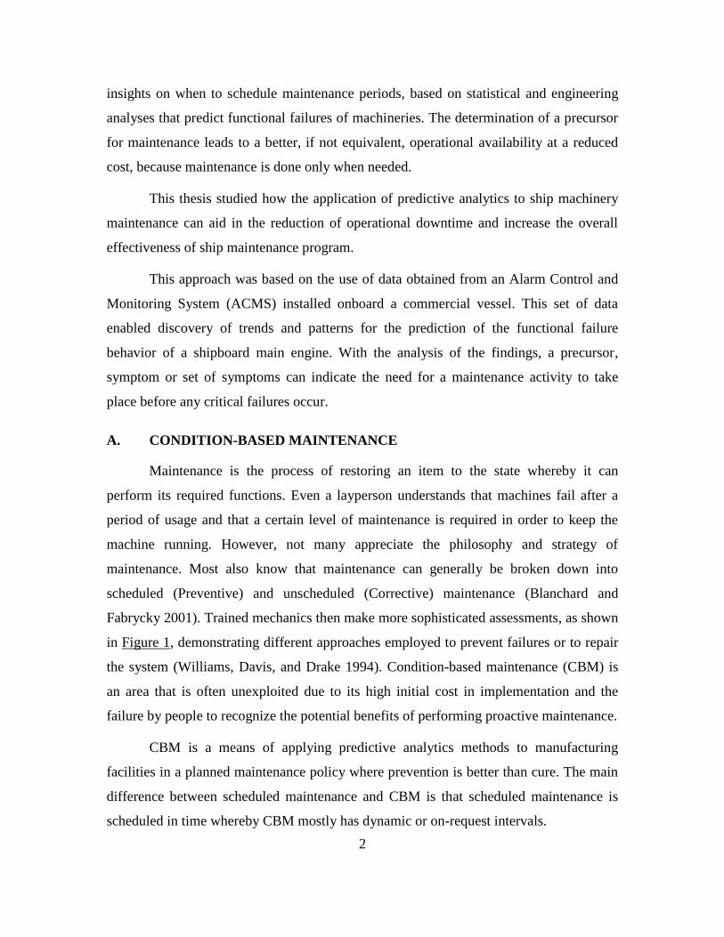
Fabrycky 2001). Trained mechanics then make more sophisticated assessments, as shown

in Figure 1, demonstrating different approaches employed to prevent failures or to repair

the system (Williams, Davis, and Drake 1994). Condition-based maintenance (CBM) is

an area that is often unexploited due to its high initial cost in implementation and the

failure by people to recognize the potential benefits of performing proactive maintenance.

CBM is a means of applying predictive analytics methods to manufacturing

facilities in a planned maintenance policy where prevention is better than cure. The main

difference between scheduled maintenance and CBM is that scheduled maintenance is

scheduled in time whereby CBM mostly has dynamic or on-request intervals.

3

Figure 1. Relationship of CBM to various forms of maintenance (From Williams, Davis

and Drake 1994).

The CBM system involves a number of subsystems and capabilities such as

sensing and data acquisition, signal processing, condition and health estimation,

prognostics and decision assistance. In order to gain access to the system and have visual

monitoring and data information, a Man-Machine Interface (MMI) such as an Alarm

Control and Monitoring System (ACMS) can be utilized. Typically, a CBM system

consists of the integration of various hardware and software, which results in the high

initial implementation cost.

CBM makes use of the information collected on equipment through monitoring

systems such as an ACMS and compares this online data to the machinery’s conditions

with predefined operating thresholds. Data that falls outside of this threshold generates a

maintenance alert to the operator that signifies a probable problem or area of concern.

4

B. ALARM CONTROL AND MONITORING SYSTEM

An ACMS integrates the control and monitoring of the various shipboard systems

into a centralized system and serves to provide real-time data, alarm monitoring, and

control of the ship’s platform systems. It is a proven solution to a ship’s automation

needs, and it has become a trend for commercial ship owners to adopt this system. The

trend for the adoption of automation reduces workload and dependence on engine crews.

It also allows data to be extracted from ACMS for analysis. ACMS allows information to

be visible through the human-machine interface screen pages, also known as mimics, at

prominent or important locations like the Wheelhouse (WH), Engine Control Room

(ECR), and Port Office (PO). These data are processed and displayed via the monitor

through different mimic pages. The information can be displayed in the forms of

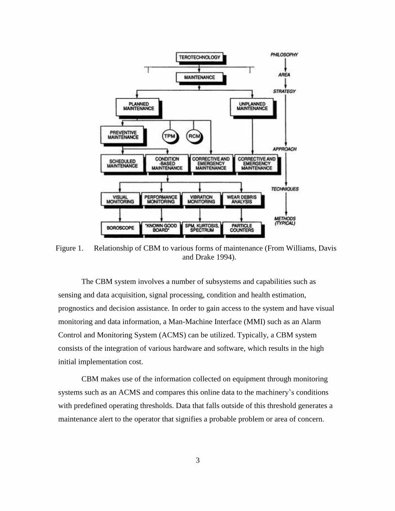
pictorial, text, trends and graphs to facilitate easy comprehension by the operators. An

example of the mimic is as shown in Figure 2 where the system overview is shown.

Figure 2. ACMS of Roll-On-Roll-Off Passenger Ship Design Mimic (From Singapore

Technologies Marine Limited 2010).

5

Ship’s data derived from the ACMS can be used as an extension for predictive

analytics for maintenance of ship machinery. The data can be compared to a predefined

machinery operating threshold and an alert triggered when the data falls outside of the

acceptable area. CBM can be integrated into ACMS, or it can perform as a subsystem on

its own by reading the required data from ACMS.

C. PROBLEM DEFINITION

While the thesis suggests that the application of predictive analytics on ship

machinery maintenance can aid in the reduction of operational downtime and increase the

overall effectiveness of the ship maintenance program, the initial research shows that

there is more that the system needs to achieve. This section will define the problem by

identifying the gaps that need to be filled by the system, as well as the scope, limitations

and constraints of the project.

1. Problem Identification

With the understanding from background and initial research, information

pertaining to the use of predictive analytics is not conclusive. This includes the use of an

appropriate precursor to model and signify machine failures. The selection of an

appropriate precursor is still not concise for a variety of reasons, such as proprietary

concerns, the lack of in-depth information and publication on the methodology for

achieving it, as well as poor utilization of available information that can be used for

analysis. With this understanding, three gaps are identified, and they are as follows:

a. Lack of use of existing data

With the current technology, many ships do have information-gathering

capabilities such as ACMS, but these data are seldom extracted for analysis to contribute

towards preventive maintenance because there is an overwhelming amount of

information available. There is underutilization of the data available.

6

b. Lack of expertise to analyze data

There is a lack of expertise to accurately extract the relevant data from the

vast amount of information available, sort them and analyze them for signs of failure.

Correlation of the various parameters that leads to failures is not well understood by

operators, so there is no means to predict machine failures.

c. Lack of support for initial high-cost investment

Typically, companies are concerned about the high initial cost of

implementing a CBM system. They believe that it is not justifiable for the costs involved.

They also fail to recognize the high maintenance cost incurred throughout the system life

cycle. This idea that regularly scheduled maintenance and corrective maintenance is

cheaper is the traditional approach. Reluctance to invest in the CBM system can also be

attributed to poorly communicated or skewed figures and forecasts during the initial

conceptual phase of a project, projecting minimal costs in the competition for contracts.

These gaps formed the basis for the problem statement addressed by this project.

It can be summarized as follows:

Apply predictive analytics to study and analyze ship machinery failures for a

precursor to ship maintenance indicator that leads to reduced operational downtime and

increased of the overall effectiveness of ship maintenance program.

This study was intended to expand and deepen knowledge of predictive analytics

related to ship maintenance through the conduct of more extensive and thorough research

methodology. Current capabilities of predictive analytics are widely marketed. The

challenge remains to address the issue on the know-how needed and to support a general

application of the methodology across all machinery maintenance.

2. Scope

The main scope of this thesis covers the study of predictive analytics tools

available in the market for machinery maintenance and how predictive analytics can

benefit the users of such applications in operational availability and system effectiveness.

Other issues include:

7

Examination of the existing technology for predictive analytics

application;

Examination of the related functions that have been researched or are in

the process of being researched;

Examination of the system architecture/concepts being employed in the

systems being used;

Investigation of the risk associated with such integration;

Analysis of the data extracted that are relevant to the predictive analytics

analysis;

Obtaining a predictive analytics model for the ship engine machinery

maintenance; and

Investigation of the model to encapsulate enough parameters for sound

analysis.

3. Limitations

There are several limitations to this thesis. These limitations are identified in the

following sections.

a. Collecting enough engine data for analysis

The engine data is collected from an operational commercial vessel. The

storage capacity of the ACMS is limited in size and therefore limits the amount of data

that can be extracted from the system for analysis. There will be occasions when the older

data are overwritten by the more current ones. An estimate of three-months’ worth of

data is available for analysis at any point during data extraction.

b. Analyzing enough engine parameters to construct a conclusive

predictive model

There are many engine attributes as well as other systems’ attributes that

will influence and affect the accuracy of the predictive model. The complexity of the

model for this thesis study is inevitably constrained by the time allocated to this study. As

such, the model may not encompass all the attributes that may constitute a complete

model.

8

c. Schedule considerations hamper analysis of a working predictive

model

Schedule ultimately limited the amount of time available for the

exploration and analysis of the predictive model. This limitation may lead to a less

comprehensive analysis of the predictive model.

4. Constraints

a. To use existing commercial ship engine data

This constraint means that the model is more inclined to the particular

class of vessel from which the data are being extracted. It may not be identical to or

completely appropriate for use on other classes of vessels and adjustments may have to

be made.

b. To use available software resources for modeling

The available software inevitably shapes the presentation of the result

depending on the software functions available.

D. PREVIOUS WORK

Brian P. Murphy, in his 2000 thesis (Murphy, 2000), mentioned the use of

Condition Based Maintenance concepts in which the software diagnostics tools in the

multi-level machinery health assessment could provide machinery monitoring and

prediction of components’ remaining time until a problem occurred. It was highlighted

that this situation awareness of the systems allows the reduction of crew workload

associated with maintenance and operation by virtue of the “just in time” maintenance

concept and eliminates the need for roving watch standers taking handwritten readings of

the machinery status. There were no further details mentioned with respect to the

methodology and success of such a program.

John E. Harding, in his 1994 thesis (Harding, 1994), studied the use of Pseudo

Wigner-Ville Distribution and wavelets analysis as two methods for condition monitoring

of non-stationary and transient shipboard machinery for the detection of fault locations

and their severity level. The motivation for his research paper was to increase the

9

operational capability of naval vessels by establishing some indicator of the health of the

equipment and allows “just in time” maintenance to be performed. His results show a

complete representation of the harmonic nature of the compressor component and that a

change in the mechanical condition of the machine could be established by conducting

Pseudo Wigner-Ville Distribution analysis. The disadvantage of the methodology is that a

complete analysis is time consuming, and it is only applicable to moving components.

In their 1990 research and development report for David Taylor Research Center,

Christopher P. Nemarich, Wayne W. Boblitt, and David W. Harrell (Nemarich et al.

1990) mentioned the development of a demonstration model of a CBM monitoring

system for propulsion and auxiliary systems. The expected benefits of CBM are

improved maintenance procedures and scheduling, increased machinery operational

readiness, and reduced logistics support cost. They make use of sensors and monitoring

systems to gather the data and information for prognostics capability. Prognosis projects

future health based on current and past conditions. It makes use of a probabilistic model

of the high pressure air compressor to provide predictions of future machine health.

Probabilities are assigned to these predictions to give the operators an indication of the

degree of confidence with which the prediction is made. No further details were

mentioned on the degree of success for such a methodology, and there are future plans

mentioned to look into this area of research.

Jose A. Orosa, Angel M. Costa and Rafael Santos from the University of A

Coruña (Orosa et al. 2011), Spain mentioned the use of Visual Basic for Application for

predictive maintenance methodology in their 2011 research. A control chart is being used

to study the exhaust gas temperature in the engine. The control chart is one of the most

important and commonly used among the statistical Quality Control methods for

monitoring process stability and variability. It is a graphical display of a process

parameter plotted against time, with a center line and two control limits (Jennings and

Drake 1997). The exhaust gas temperature sample failure in the main engine is sampled

and, consequently, the p-charts were selected. The p-chart monitors the percent of

samples having the condition, relative to either a fixed or varying sample size, when each

10

sample can either have this condition or not. Any points outside the control limits can

imply a shift in the process and indicates a potential problem.

E. AREA OF RESEARCH AND APPROACH

Predictive analytics have a number of traits that make them a more attractive

approach as compared to the conventional method of the maintenance concept. Predictive

analytics can be used to determine events and outcomes before they occur. They can

provide simulation of a process to determine the risks, as well as facilitate “what if”

scenarios to determine the optimum course of action. Firstly, they are capable of

providing valuable information that can lead to a smarter decision. Secondly, they have

the ability to detect patterns to initiate action. Finally, with the capability to aggregate and

correlate information, they allow suspicious trends to be captured before loss occurs.

These features allow improved collaboration and better control for a better Total Cost of

Ownership (TCO) of a vessel.

Predictive analytics are not without their disadvantages. First, they, like all

models in the market, remain to be tested and verified for inherent inaccuracy. This

inaccuracy may be due to an error in model specification. A model is only as good as it is

defined, and it may include factors that are not significant predictors or factors that may

be significant but unobserved. Another consideration is the inherent error term of the

model. An error term represents the portion of the model that is unexplained. This error

term can be substantial, even in well specified models, and can result in variation

between predictions and actual outcomes.

Second, the initial high cost involved in the implementation of predictive

analytics techniques discourages investment. The high costs are associated with the

hardware and software necessary to facilitate predictive modeling.

Finally, even with the information available, the predictive model is dependent on

how clean and accurate the acquired data is. If there are too many legacy systems with

poor record keeping, the data may be unfit for use.

11

Predictive analytics appear to have the potential to be the upcoming trend for

machinery maintenance to be used as a tool for the next generation. With the increased

use of sensors and data monitoring systems onboard vessels, vast amounts of information

are waiting to be collected, utilized and analyzed to provide better prediction of

machinery failures. The cost effectiveness of such a technique to tap on the existing

infrastructure, determining “just in time” maintenance would theoretically and logically

be attractive. Therefore, this paper aims to justify the application of predictive analytics

on ship machinery maintenance.

F. STATISTICAL TOOLS

The statistical tool selected for this thesis is Visual BASIC for Application (VBA)

of Microsoft (MS) Office Excel. Microsoft owns the VBA, whose code is compiled

(Microsoft 2010; Excel 2010; Jelen and Syrstad 2008; and Roman 2002) in an

intermediate language called the p-code; the latter code is stored by the hosting

application (Access, Excel, Word) as a separate stream in structured storage files

independent from the document streams.

The intermediate code is then executed by a virtual machine. Therefore, the

obtained software resource can only operate in a Windows 98 or above operating system.

Calculus operations and graphics required for the results can be carried out in MS Excel.

The executable program, anygeth, obtained from CUSUM website of the School

of Statistics, University of Minnesota (www.stat.umn.edu) is used for the calculation of

CUSUM reference value and the decision intervals.

G. ORGANIZATION OF STUDY

This thesis first introduces the readers to the concepts of CBM and the available

tools to support it, such as ACMS. A summary of previous work is provided, along with

the author’s area of research and the possible tools used to achieve the objectives of this

research.

12

Chapter II provides an overview of predictive analytics such that sufficient

knowledge of the history, purpose, and methodology can be explained and serves as a

basis for the rest of the chapters.

Chapter III describes the database and procedures that are used to choose the data

for use, and presents the steps of the methodology that leads to the results of this

research.

Chapter IV discusses the results and outputs of the models that were trained in

supporting the goal of this research.

Finally, Chapter V summarizes the conclusions drawn from this research and

provides recommendations for future research opportunities associated with the

predictive analytics technique.

13

II. PREDICTIVE ANALYTICS OVERVIEW

Predictive analytics is essentially an area of statistical analysis that requires the

extraction of information from data and using the information to predict future trends and

behavior patterns (Nyce 2007). Techniques commonly used in predictive analytics are

drawn from a variety of fields such as statistics, modeling, machine learning, and data

mining (Eckerson 2007).

One important distinction of predictive analytics from other business intelligence

tools is that it goes beyond visualizing data and human assumptions; instead it combines

data, theory, and mathematics to make forecasts about the future using current and

historical facts (Grant 2011).

A. HISTORY

Predictive analytics was discovered only a decade ago, and it is the amalgamation

of four various fields: mathematical techniques, data storage capacity, data processing

power, and data creation. The mathematical techniques have existed and improved since

the founding of the Econometric Society in 1930. The data storage capacity has been

around since 1977 with Oracle’s commercialization of the relational database. The

processing power has existed since IBM commercialized business computing with the

IBM 360. Software as a Service (SaaS) and social media provided the final requirement,

data creation (Grant 2011).

Predictive analytics is employed in a variety of industries, which includes

financial services, telecommunications, and healthcare. One of the most well-known

applications is the FICO score, a credit scoring which is widely used in the financial

services (Fair Isaac Corporation 2009).

B. DEFINITIONS OF THE MAIN COMPONENTS OF THE READINESS

CONCEPT

A failure is a condition (or state) characterized by the inability of a material,

structure, or system to fulfill its intended purpose (task or mission), resulting in its

14

retirement from usable service (Pau 1981). For this thesis, the failures mentioned will be

associated with the functional failures of the system and studied by observing the

abnormality behavior of the system in relation to the failure limit.

Degradation is an event that impairs or deteriorates the system’s ability to perform

its specified tasks or mission. This includes improper controls and the effects of the

environment (Pau 1981).

Failure detection is the act of identifying the presence of an unspecified failure

mode in a system, resulting in an unexpected malfunction (Pau 1981). The failure

detection is done through the ACMS for the main engine system under study.

Failure diagnosis is the process of identifying a failure mode (or condition) from

an evaluation of its signs and symptoms (such as performance monitoring measurements)

(Pau 1981). Failure prognosis is the art or act of forecasting a future condition based on

present signs and symptoms observed.

Readiness is the ability of the system to carry out a specified task or mission at a

specified performance level, without catastrophic failure or interruption, when activated

at any given time (Pau 1981).

C. PREDICTIVE ANALYTICS TECHNIQUES

The study of predictive analytics encompasses a variety of techniques ranging

from statistics, modeling, machine learning, and data mining that analyzes past and

current data to make predictions about future events. Two techniques of statistical

analysis, mainly time series models and cumulative sum control chart, will be discussed

in this thesis.

1. Time series models

A time series is a set of observations on a quantitative variable collected over time

(Ragsdale 2012). Time series models are used for the predicting or forecasting of the

future behavior of variables. In many engineering situations, it is nearly impossible to

forecast time series data using a causal regression model since we do not know which

causal independent variables are influencing a particular time series variable. This makes

15

it difficult to build a regression model. Even if we do have some insight as to which

causal variables are affecting a time series, the best regression function estimated from

these data might not accurately reflect so. Finally, even with a well-fit regression function

to data, there is a possibility that we may have to forecast the values of the independent

variable to estimate the future values of the dependent (time series) variable. Forecasting

the causal independent variables might be more difficult than forecasting the original

time series variable.

The possibility of discovering systematic variation in the past behavior of the time

series variable allows the construction of a model of this behavior to help in forecasting

the future behavior. For instance, a fluctuation reflected in data could help to make

estimates about the future, or trends found (whether they are upward or downward), in

the time series, might be expected to continue in the future. Techniques that analyze the

past behavior of a time series variable to predict the future are sometimes referred to as

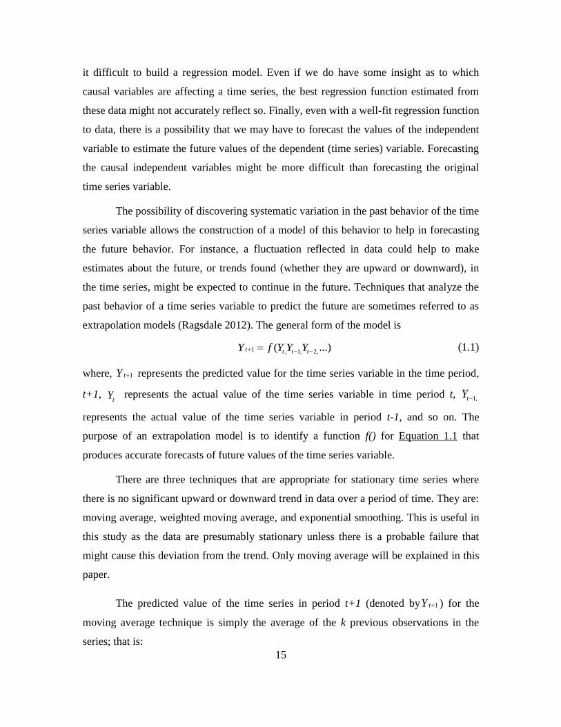
extrapolation models (Ragsdale 2012). The general form of the model is

1 , 1, 2,( ...)t t t tY f Y Y Y (1.1)

where, 1tY represents the predicted value for the time series variable in the time period,

t+1, tY represents the actual value of the time series variable in time period t, 1,tY

represents the actual value of the time series variable in period t-1, and so on. The

purpose of an extrapolation model is to identify a function f() for Equation 1.1 that

produces accurate forecasts of future values of the time series variable.

There are three techniques that are appropriate for stationary time series where

there is no significant upward or downward trend in data over a period of time. They are:

moving average, weighted moving average, and exponential smoothing. This is useful in

this study as the data are presumably stationary unless there is a probable failure that

might cause this deviation from the trend. Only moving average will be explained in this

paper.

The predicted value of the time series in period t+1 (denoted by 1tY ) for the

moving average technique is simply the average of the k previous observations in the

series; that is:

16

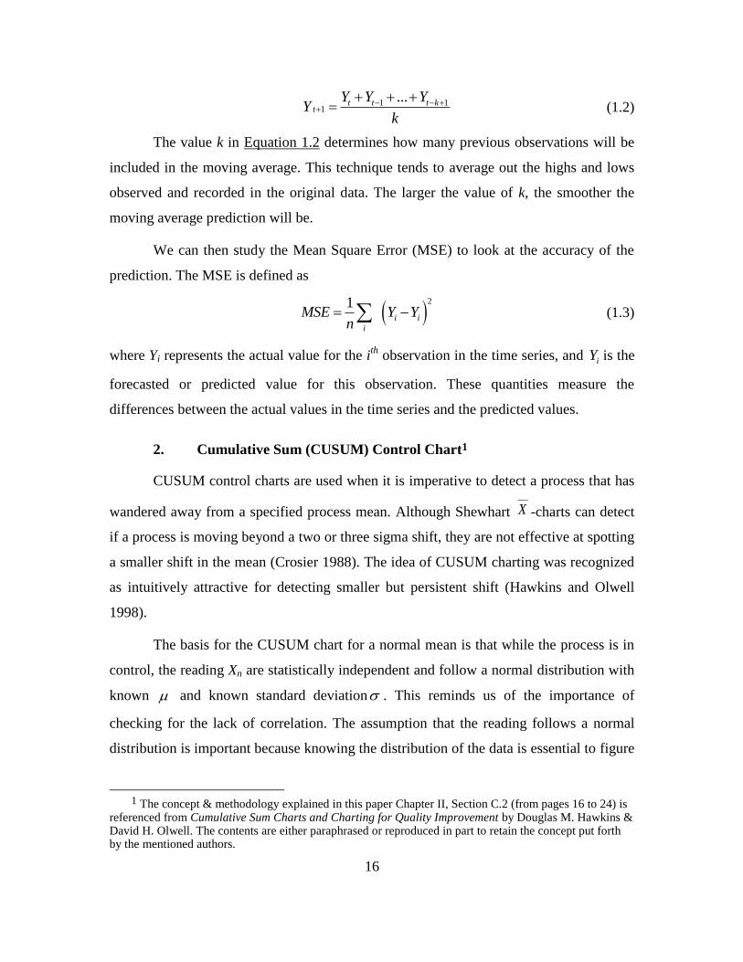
1 11

...t t t kt

Y Y YY

k

(1.2)

The value k in Equation 1.2 determines how many previous observations will be

included in the moving average. This technique tends to average out the highs and lows

observed and recorded in the original data. The larger the value of k, the smoother the

moving average prediction will be.

We can then study the Mean Square Error (MSE) to look at the accuracy of the

prediction. The MSE is defined as

21

i i

i

MSE Y Yn

(1.3)

where Yi represents the actual value for the ith

observation in the time series, and iY is the

forecasted or predicted value for this observation. These quantities measure the

differences between the actual values in the time series and the predicted values.

2. Cumulative Sum (CUSUM) Control Chart1

CUSUM control charts are used when it is imperative to detect a process that has

wandered away from a specified process mean. Although Shewhart X -charts can detect

if a process is moving beyond a two or three sigma shift, they are not effective at spotting

a smaller shift in the mean (Crosier 1988). The idea of CUSUM charting was recognized

as intuitively attractive for detecting smaller but persistent shift (Hawkins and Olwell

1998).

The basis for the CUSUM chart for a normal mean is that while the process is in

control, the reading Xn are statistically independent and follow a normal distribution with

known and known standard deviation . This reminds us of the importance of

checking for the lack of correlation. The assumption that the reading follows a normal

distribution is important because knowing the distribution of the data is essential to figure

1 The concept & methodology explained in this paper Chapter II, Section C.2 (from pages 16 to 24) is

referenced from Cumulative Sum Charts and Charting for Quality Improvement by Douglas M. Hawkins & David H. Olwell. The contents are either paraphrased or reproduced in part to retain the concept put forth by the mentioned authors.

17

out the chart’s false alarm rate and how sensitive it is to actual shift. The last assumptions

that the exact values of the parameters and are known is seldom the case in reality.

However, it can be approximated by measuring the process over a long period while it is

under a state of statistical control. These estimates can be used as true parameter values.

It should be noted that the data sets must be large enough to obtain a reasonably close

estimate of these parameters to be close enough to the true values for practical

application.

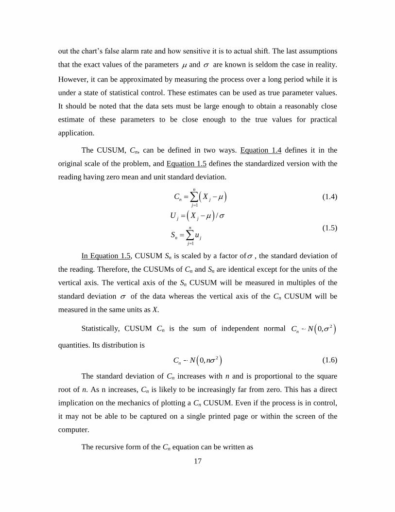
The CUSUM, Cn, can be defined in two ways. Equation 1.4 defines it in the

original scale of the problem, and Equation 1.5 defines the standardized version with the

reading having zero mean and unit standard deviation.

1

n

n j

j

C X

(1.4)

1

/j j

n

n j

j

U X

S u

(1.5)

In Equation 1.5, CUSUM Sn is scaled by a factor of , the standard deviation of

the reading. Therefore, the CUSUMs of Cn and Sn are identical except for the units of the

vertical axis. The vertical axis of the Sn CUSUM will be measured in multiples of the

standard deviation of the data whereas the vertical axis of the Cn CUSUM will be

measured in the same units as X.

Statistically, CUSUM Cn is the sum of independent normal 20,nC N

quantities. Its distribution is

20,nC N n (1.6)

The standard deviation of Cn increases with n and is proportional to the square

root of n. As n increases, Cn is likely to be increasingly far from zero. This has a direct

implication on the mechanics of plotting a Cn CUSUM. Even if the process is in control,

it may not be able to be captured on a single printed page or within the screen of the

computer.

The recursive form of the Cn equation can be written as

18

0

1

0

n n n

C

C C X

(1.7)

The recursive form aids in easy computation of the CUSUM. Each point of the

CUSUM is the previous point plus the offset of the latest point from .

The standardized recursive form of the Cn equation can be written as

0

1

0

n n n

S

S S U

(1.8)

The out-of-control distribution of the CUSUM describes a means to diagnose

shifts in mean. This serves as a pre-warning that there is an anomalies observed in the

process and the possibility of a failure. It triggers the need for further diagnosis or

maintenance actions. Suppose that at some instant m the distribution of Xn changes from

2,N to 2,N . This means that from instant m onwards the mean of Xn

undergoes a persistent shift of size . At any subsequent instant, n, CUSUM can be

written as

1

1 1

n

n i

i

m n

i i

i i m

C X

X X

(1.9)

As the second term of the summation is distributed as 2,N , it will have a

distribution of

2

1

,n

i

i m

X N n m n m

(1.10)

This means that the average value of CUSUM at time n > m is (n-m) . It also

means that starting from the point (m, Cm), the CUSUM on average will trace a path

centered on a line of slope . This serves as the basis for using CUSUM to detect shifts

in mean. While the process remains in control and the reading Xn follows the in-control

2,N distribution, the CUSUM follows a distribution centered on the horizontal axis.

If the mean undergoes a step change, then the CUSUM develops a linear drift, and its

distribution will center instead on a line where slope equals the shift in mean. The

19

diagnosis of the CUSUM therefore consists of distinguishing the no-drift in-control

behavior from the linear drift behavior following a mean shift. What it means here is that

the CUSUM defined in Equation 1.9 is a random walk with mean 0. If the mean shifts

upward to some value n > m, an upward or positive drift will develop in CUSUM.

Conversely, if the mean shifts downward to some value n < m, then a downward or

negative drift will develop in CUSUM.

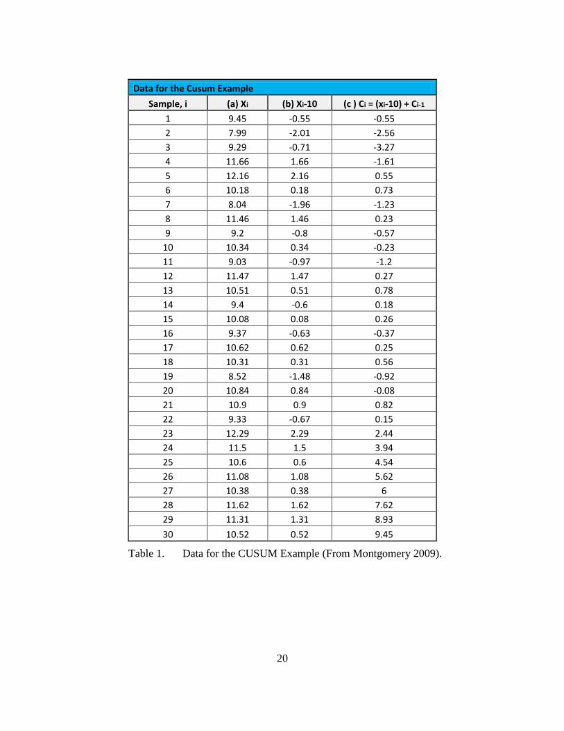
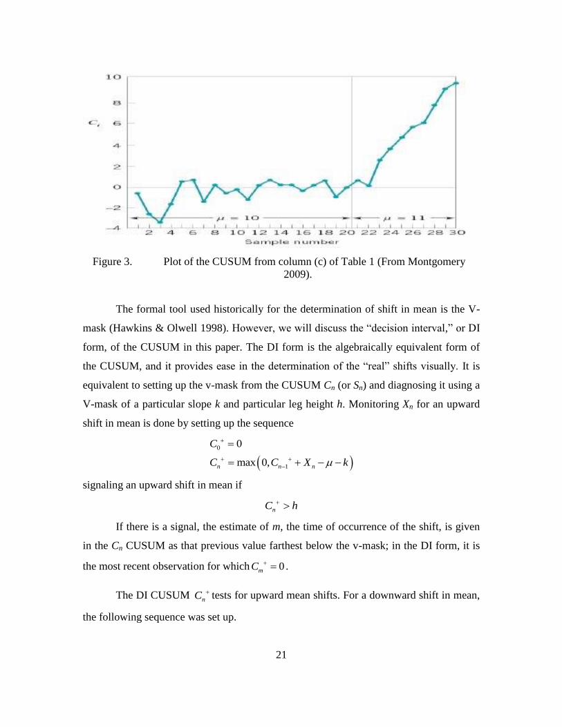
An example on the plot of CUSUM is shown in Figure 3. The process mean

remains at target value of 10 and Equation 1.9 is used for the calculation. The equation

that follows is a manipulation of Equation 1.9 and it describes how the calculations are

done in tabular form, with the data and steps shown in Table 1.

1

10i

i j

j

C x

1

1

10 10i

i j

j

x x

110i ix C

20

Data for the Cusum Example

Sample, i (a) Xi (b) Xi-10 (c ) Ci = (xi-10) + Ci-1

1 9.45 -0.55 -0.55

2 7.99 -2.01 -2.56

3 9.29 -0.71 -3.27

4 11.66 1.66 -1.61

5 12.16 2.16 0.55

6 10.18 0.18 0.73

7 8.04 -1.96 -1.23

8 11.46 1.46 0.23

9 9.2 -0.8 -0.57

10 10.34 0.34 -0.23

11 9.03 -0.97 -1.2

12 11.47 1.47 0.27

13 10.51 0.51 0.78

14 9.4 -0.6 0.18

15 10.08 0.08 0.26

16 9.37 -0.63 -0.37

17 10.62 0.62 0.25

18 10.31 0.31 0.56

19 8.52 -1.48 -0.92

20 10.84 0.84 -0.08

21 10.9 0.9 0.82

22 9.33 -0.67 0.15

23 12.29 2.29 2.44

24 11.5 1.5 3.94

25 10.6 0.6 4.54

26 11.08 1.08 5.62

27 10.38 0.38 6

28 11.62 1.62 7.62

29 11.31 1.31 8.93

30 10.52 0.52 9.45

Table 1. Data for the CUSUM Example (From Montgomery 2009).

21

Figure 3. Plot of the CUSUM from column (c) of Table 1 (From Montgomery

2009).

The formal tool used historically for the determination of shift in mean is the V-

mask (Hawkins & Olwell 1998). However, we will discuss the “decision interval,” or DI

form, of the CUSUM in this paper. The DI form is the algebraically equivalent form of

the CUSUM, and it provides ease in the determination of the “real” shifts visually. It is

equivalent to setting up the v-mask from the CUSUM Cn (or Sn) and diagnosing it using a

V-mask of a particular slope k and particular leg height h. Monitoring Xn for an upward

shift in mean is done by setting up the sequence

0

1

0

max 0,n n n

C

C C X k

signaling an upward shift in mean if

nC h

If there is a signal, the estimate of m, the time of occurrence of the shift, is given

in the Cn CUSUM as that previous value farthest below the v-mask; in the DI form, it is

the most recent observation for which 0mC .

The DI CUSUM nC tests for upward mean shifts. For a downward shift in mean,

the following sequence was set up.

22

0

1

0

min 0,n n n

C

C C X k

with a signal if

nC h

When there is an indication of a downward shift in mean, the last point m for

which 0mC as the estimate of the instant preceding the change in mean.

The CUSUM slope estimator is given by

n mC C

n m

(1.11)

The DI form of the CUSUM can be used to estimate the magnitude of the shift in

mean. The segment of the DI CUSUM leading to the signal starts with some case m for

which 0mC and then is positive up to the point at which it crosses the decision interval

h. The equation 1

n

n m i

i m

C C X k

shows the form in the described segment.

Following the shift in mean from to , the summand has a normal

distribution with mean k . can then be estimated by adding k to the slope of the DI

CUSUM from point m to point n, giving the estimate

n mC Ck

n m

(1.12)

which reduces to nCk

n m

since 0mC .

Similarly, if the downward DI CUSUM signals a shift, then the magnitude of the

shift can be estimated by

nCk

n m

(1.13)

Note that nC and

nC are both necessarily positive and negative, respectively; it

is therefore impossible for the estimate of to lie between –k and k. This also shows that

the estimate of the shift produced by CUSUM is biased away from zero.

23

Similarly, the standardized V-mask-type CUSUM Sn has decision interval

equivalents nS and

nS defined by the recursive equations

0 0S (1.14)

0 0S (1.15)

1max(0, )n n nS S U k

(1.16)

1min(0, )n n nS S U k

(1.17)

The upward CUSUM chart starts out at its initial state0S . After that, it may stay

on the axis or move into positive values. Each set of positive values will end in one of

these two ways: either the CUSUM returns to zero, or it crosses the decision interval.

When the chart crosses the decision interval, this indicates a shift may have happened and

requires attention to diagnose the shift. The CUSUM will generally then be restarted. The

whole sequence going from the starting point to the CUSUM crossing the decision

interval is called a run. The number of observations from the starting point up to the point

at which the decision interval is crossed is called the run length.

When the CUSUM gives a signal although there is no shift occurring, it is known

as a Type 1 error, analogous to the classical hypothesis testing. These false alarms are

undesirable as they caused the unnecessary expenditure of time and effort in search of

nonexistent problems. As such, the runs between inevitable false alarms would be

preferred to be as long as possible.

An error in control charting is analogous to a Type II error in classical hypothesis

testing. This is a chart remaining within its decision interval even though a probable

problem has surfaced. If there has been a shift big enough to have practical implications,

it would be desired to be detected as soon as possible.

The run is a random variable, having a mean, a variance, and a distribution. Its

mean is called the average run length or ARL. The ARL is an imperfect but useful

summary number of the general tendency towards long or short runs. It is less than

perfect since the run length distribution turns out to be highly variable. A high in-control

ARL does not rule out the possibility of a very short run before the CUSUM gives a false

alarm, and a low out-of-control ARL for the CUSUM is no guarantee that there would

24

not be a long run before the CUSUM detected an actual shift. Despite these

imperfections, the ARL is an easily interpreted, well-defined measure for which good

algorithms are available. It is the standard measure of performance of the CUSUM.

Chapter IV Section C will describe further on the h, k and ARL relationship and how it is

calculated from the software program, anygeth.

25

III. DATA DESCRIPTION AND METHODOLOGY

A. SOURCES OF FAILURES

Failure is the inability of a component, machine, or process to function properly

(Scutti and McBrine 2002). Failures can occur in individual parts, the whole machine, or

the entire process itself. The analysis of failure has always been a critical process in

determining the root causes of the problems in engineering. Even so, this logical process

can sometimes be complex. To analyze the failure, many different technical disciplines

can be engaged and employed, coupled with a variety of observation, inspection, and

laboratory techniques. It is imperative to analyze and pinpoint where exactly the failure

lies in order to be able to rectify it effectively.

There are three main categories of failures, and they are described as follows:

Functionality: The simplest form of a failure is a system or component that

operates but does not perform its intended function.

Service life: This is the next level of failure whereby the system or

component performs its function but is rendered unreliable or unsafe.

Inoperability: This is the most severe form of failure whereby a system or

component is totally inoperable.

The most common reasons for failures include the following:

Service or operation conditions (use and misuse);

Improper maintenance (intentional or unintentional);

Improper testing or inspection;

Assembly error;

Fabrication/manufacturing errors; or

Design errors (stress, materials selection, and assumed material condition

or properties).

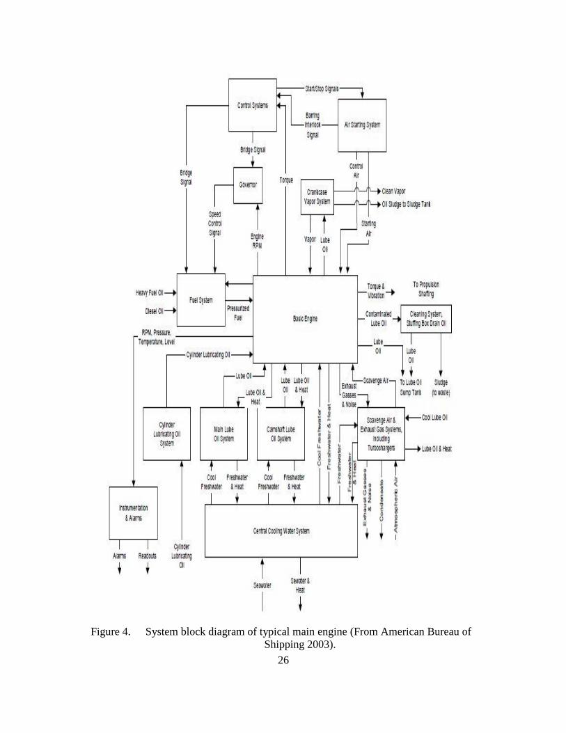
A typical system block diagram of a main engine is as shown in Figure 4.

26

Figure 4. System block diagram of typical main engine (From American Bureau of

Shipping 2003).

27

As seen from the system block diagram above, there are many interfaces and

interactions between systems, subsystems, and components required for proper operation

of a main engine. In this paper, the focus will be exploring the use of predictive analytics

using the CUSUM and time series methodology presented in Chapter II. The focus of the

study will be on one of the main engine attributes‒‒main engine exhaust gas temperature

(EGT). High EGT reflects potential problems at the combustion chamber, which may or

may not cause an overall failure to Main Engine (ME). However, this attribute poised a

potential problem to the overall ME operation and is worthy of study. The study aims to

establish that the use of such a methodology is achievable and implementable for a main

engine system. After the verification of the usability of such a methodology, it could then

be extended to the whole system in future.

The high temperature of diesel exhaust gas is due to the fact that it is a product of

combustion ignition. Despite this, the temperature for diesel exhaust gas still needs to be

controlled within a reasonable range. This is to avoid thermal stressing of other

components. There are many reasons for the temperature of diesel exhaust gas to go

uncharacteristically high in marine diesel engines. Most cases can be attributed to a fuel

system fault which can lead to either a scavenge fire and/or destructive fuel valve. The

occurrence of high EGT may also trigger a series of events‒‒seizure of the exhaust valve,

a burnt turbocharger at the side turbine as well as engine slowdown, a feature of the

safety device associated with the main engine.

The operation of the exhaust valve is described below to provide an overview of

the causes that lead to the temperature rise of exhaust gas. The use of a hydraulically

operated exhaust valve is common nowadays where the spring action is provided by a

pneumatic arrangement instead of a mechanical spring. An overview of the action is as

shown in Figure 5.

28

Figure 5. Section through typical exhaust valve used on modern two-stroke marine

diesel engines (From Scott 2011).

Both the hydraulic action of oil and pneumatic pressure are used for the operation.

In order to open the valve, oil from the lube oil system of the engine is used. The oil is

supplied by a hydraulic pump to a cam on a periodic basis to eject exhaust gases into the

valve, which is followed by combustion.

The exhaust gas not only assists in valve closure, it also provides a spring-

cushioning effect. It is mixed with a minute quantity of lube oil that is used for keeping

the valve guide cool with the use of a bleed-off from this air supply as well as for

lubrication purposes.

The exhaust valve is enclosed in a water cooled cage with fresh water being

circulated through channels cast or machined within the cage. Uniform wear and tear to

the valve head and seat occurs with every rotation of the valve. Valve rotation is

29

achievable with the use of blades welded onto the lower end of the valve spindle. Each

time the exhaust gas exits from the chamber, the valve is rotated by a small amount.

Cast iron is frequently chosen as the material used for the manufacture of the

exhaust valve cage and the valve guides. Cast iron is chosen as these two parts require a

malleable, self-lubricating material due to the continuous action between the guide and

the valve spindle. The valve is renewable and is made from a hard wearing material such

as molybdenum steel, while the spindle itself is made out of Nimonic, a superalloy

comprised of nickel, chromium, titanium, and aluminum. In order to make the valve

sturdy to prevent wear and tear at a fast rate, the seating face of the valve is specially

treated to increase its toughness properties.

The rise of the exhaust gas temperature outside the standard range has a great

impact on the life cycle of the exhaust valve and also on the deterioration of the piston

rings and the cylinder liner. It is therefore vital to be aware of the various symptoms and

causes for an exhaust gas temperature rise to ensure that the temperature stays within the

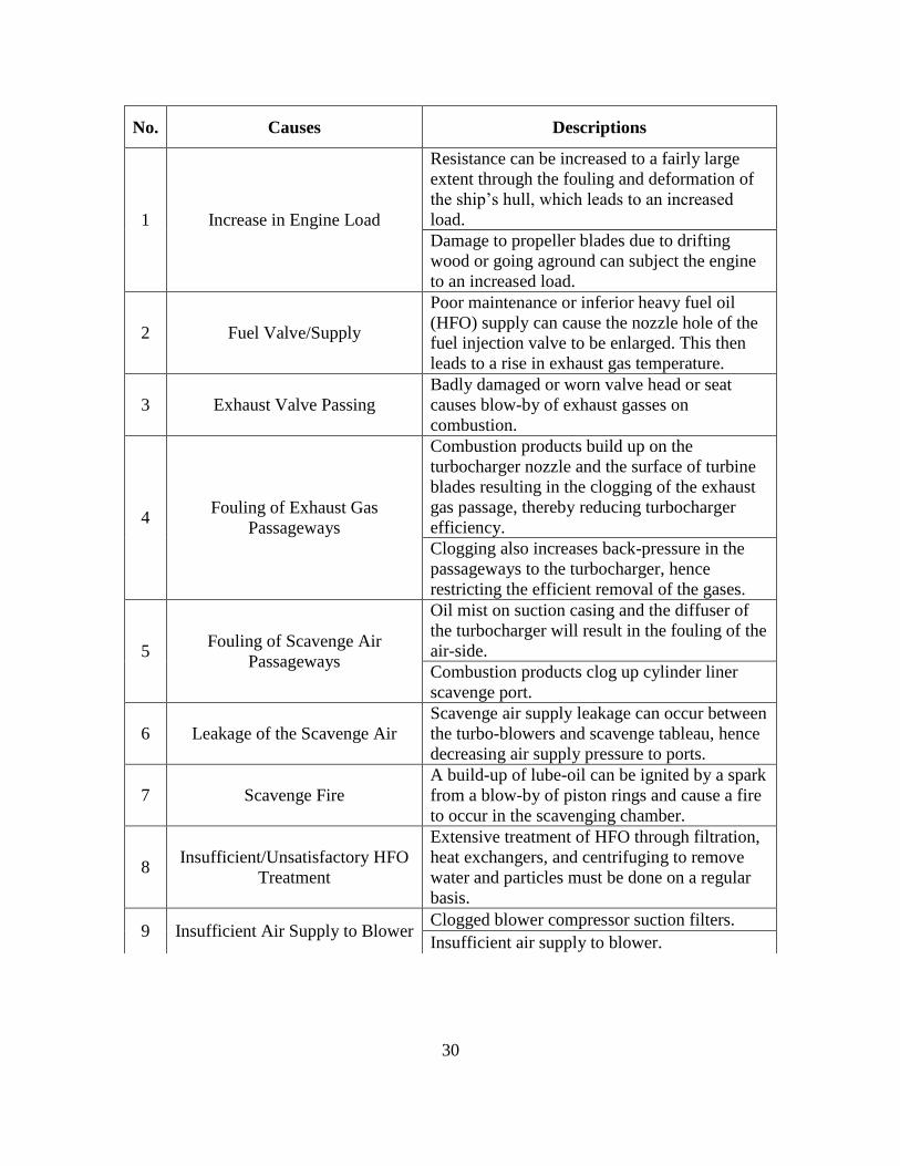
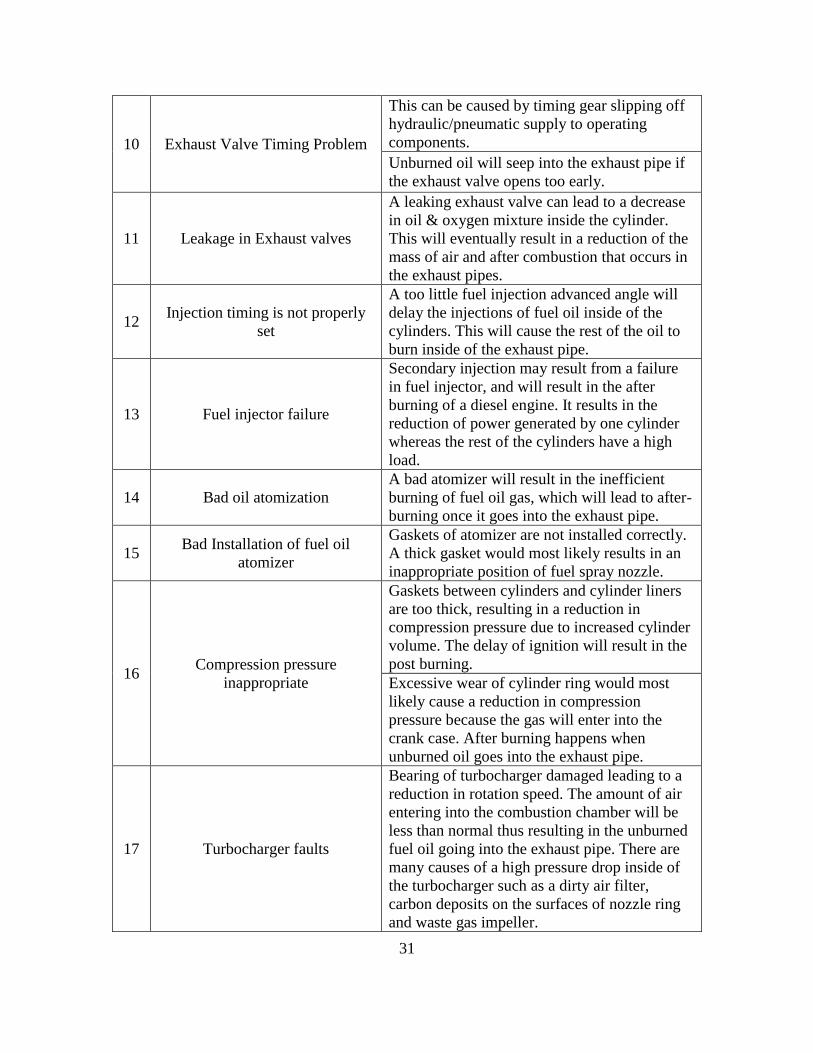
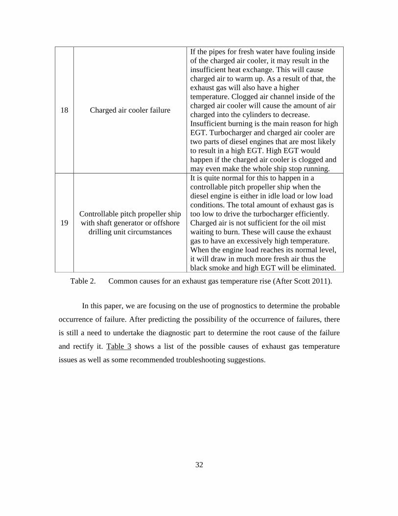
safety zone. Some of the common causes for the rise of EGT are listed in Table 2.

30

No. Causes Descriptions

1 Increase in Engine Load

Resistance can be increased to a fairly large

extent through the fouling and deformation of

the ship’s hull, which leads to an increased

load.

Damage to propeller blades due to drifting

wood or going aground can subject the engine

to an increased load.

2 Fuel Valve/Supply

Poor maintenance or inferior heavy fuel oil

(HFO) supply can cause the nozzle hole of the

fuel injection valve to be enlarged. This then

leads to a rise in exhaust gas temperature.

3 Exhaust Valve Passing

Badly damaged or worn valve head or seat

causes blow-by of exhaust gasses on

combustion.

4 Fouling of Exhaust Gas

Passageways

Combustion products build up on the

turbocharger nozzle and the surface of turbine

blades resulting in the clogging of the exhaust

gas passage, thereby reducing turbocharger

efficiency.

Clogging also increases back-pressure in the

passageways to the turbocharger, hence

restricting the efficient removal of the gases.

5 Fouling of Scavenge Air

Passageways

Oil mist on suction casing and the diffuser of

the turbocharger will result in the fouling of the

air-side.

Combustion products clog up cylinder liner

scavenge port.

6 Leakage of the Scavenge Air

Scavenge air supply leakage can occur between

the turbo-blowers and scavenge tableau, hence

decreasing air supply pressure to ports.

7 Scavenge Fire

A build-up of lube-oil can be ignited by a spark

from a blow-by of piston rings and cause a fire

to occur in the scavenging chamber.

8 Insufficient/Unsatisfactory HFO

Treatment

Extensive treatment of HFO through filtration,

heat exchangers, and centrifuging to remove

water and particles must be done on a regular

basis.

9 Insufficient Air Supply to Blower Clogged blower compressor suction filters.

Insufficient air supply to blower.

31

10 Exhaust Valve Timing Problem

This can be caused by timing gear slipping off

hydraulic/pneumatic supply to operating

components.

Unburned oil will seep into the exhaust pipe if

the exhaust valve opens too early.

11 Leakage in Exhaust valves

A leaking exhaust valve can lead to a decrease

in oil & oxygen mixture inside the cylinder.

This will eventually result in a reduction of the

mass of air and after combustion that occurs in

the exhaust pipes.

12 Injection timing is not properly

set

A too little fuel injection advanced angle will

delay the injections of fuel oil inside of the

cylinders. This will cause the rest of the oil to

burn inside of the exhaust pipe.

13 Fuel injector failure

Secondary injection may result from a failure

in fuel injector, and will result in the after

burning of a diesel engine. It results in the

reduction of power generated by one cylinder

whereas the rest of the cylinders have a high

load.

14 Bad oil atomization

A bad atomizer will result in the inefficient

burning of fuel oil gas, which will lead to after-

burning once it goes into the exhaust pipe.

15 Bad Installation of fuel oil

atomizer

Gaskets of atomizer are not installed correctly.

A thick gasket would most likely results in an

inappropriate position of fuel spray nozzle.

16 Compression pressure

inappropriate

Gaskets between cylinders and cylinder liners

are too thick, resulting in a reduction in

compression pressure due to increased cylinder

volume. The delay of ignition will result in the

post burning.

Excessive wear of cylinder ring would most

likely cause a reduction in compression

pressure because the gas will enter into the

crank case. After burning happens when

unburned oil goes into the exhaust pipe.

17 Turbocharger faults

Bearing of turbocharger damaged leading to a

reduction in rotation speed. The amount of air

entering into the combustion chamber will be

less than normal thus resulting in the unburned

fuel oil going into the exhaust pipe. There are

many causes of a high pressure drop inside of

the turbocharger such as a dirty air filter,

carbon deposits on the surfaces of nozzle ring

and waste gas impeller.

32

Table 2. Common causes for an exhaust gas temperature rise (After Scott 2011).

In this paper, we are focusing on the use of prognostics to determine the probable

occurrence of failure. After predicting the possibility of the occurrence of failures, there

is still a need to undertake the diagnostic part to determine the root cause of the failure

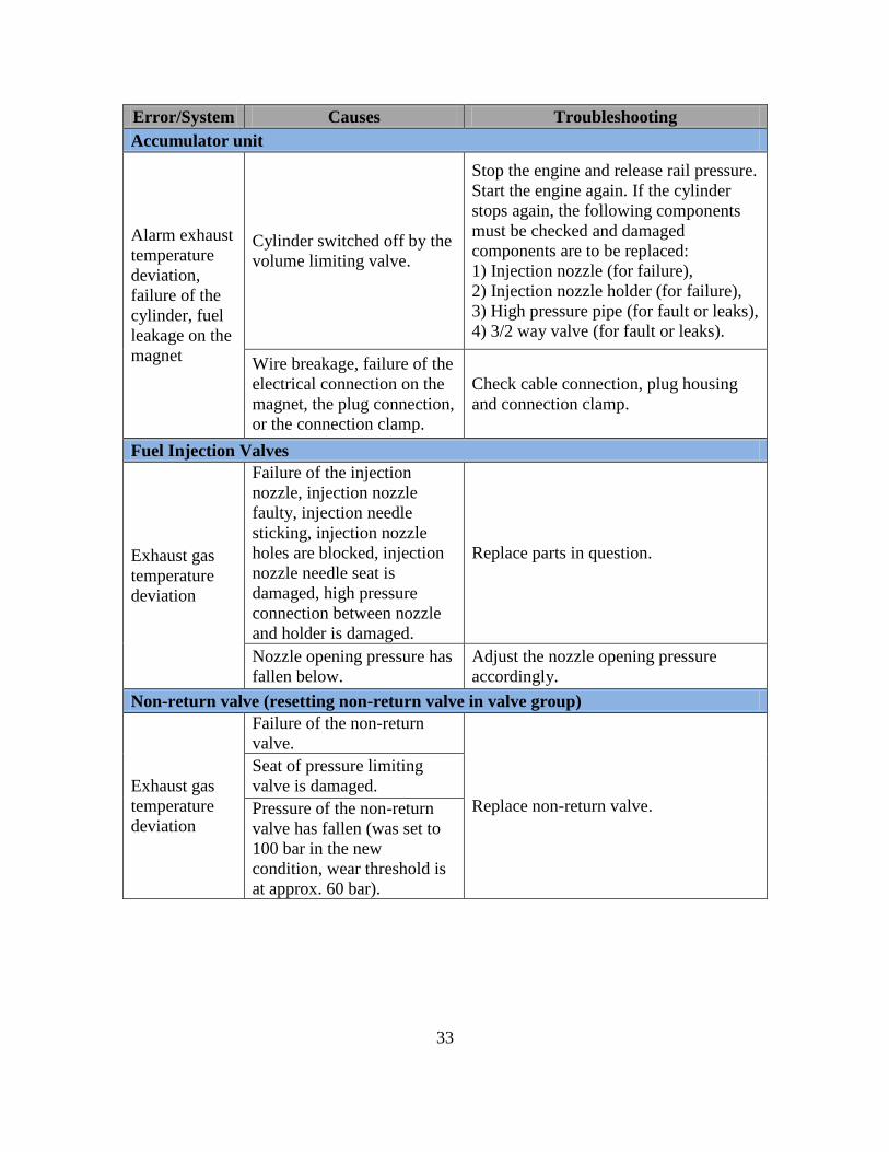
and rectify it. Table 3 shows a list of the possible causes of exhaust gas temperature

issues as well as some recommended troubleshooting suggestions.

18 Charged air cooler failure

If the pipes for fresh water have fouling inside

of the charged air cooler, it may result in the

insufficient heat exchange. This will cause

charged air to warm up. As a result of that, the

exhaust gas will also have a higher

temperature. Clogged air channel inside of the

charged air cooler will cause the amount of air

charged into the cylinders to decrease.

Insufficient burning is the main reason for high

EGT. Turbocharger and charged air cooler are

two parts of diesel engines that are most likely

to result in a high EGT. High EGT would

happen if the charged air cooler is clogged and

may even make the whole ship stop running.

19

Controllable pitch propeller ship

with shaft generator or offshore

drilling unit circumstances

It is quite normal for this to happen in a

controllable pitch propeller ship when the

diesel engine is either in idle load or low load

conditions. The total amount of exhaust gas is

too low to drive the turbocharger efficiently.

Charged air is not sufficient for the oil mist

waiting to burn. These will cause the exhaust

gas to have an excessively high temperature.

When the engine load reaches its normal level,

it will draw in much more fresh air thus the

black smoke and high EGT will be eliminated.

33

Error/System Causes Troubleshooting

Accumulator unit

Alarm exhaust

temperature

deviation,

failure of the

cylinder, fuel

leakage on the

magnet

Cylinder switched off by the

volume limiting valve.

Stop the engine and release rail pressure.

Start the engine again. If the cylinder

stops again, the following components

must be checked and damaged

components are to be replaced:

1) Injection nozzle (for failure),

2) Injection nozzle holder (for failure),

3) High pressure pipe (for fault or leaks),

4) 3/2 way valve (for fault or leaks).

Wire breakage, failure of the

electrical connection on the

magnet, the plug connection,

or the connection clamp.

Check cable connection, plug housing

and connection clamp.

Fuel Injection Valves

Exhaust gas

temperature

deviation

Failure of the injection

nozzle, injection nozzle

faulty, injection needle

sticking, injection nozzle

holes are blocked, injection

nozzle needle seat is

damaged, high pressure

connection between nozzle

and holder is damaged.

Replace parts in question.

Nozzle opening pressure has

fallen below.

Adjust the nozzle opening pressure

accordingly.

Non-return valve (resetting non-return valve in valve group)

Exhaust gas

temperature

deviation

Failure of the non-return

valve.

Replace non-return valve.

Seat of pressure limiting

valve is damaged.

Pressure of the non-return

valve has fallen (was set to

100 bar in the new

condition, wear threshold is

at approx. 60 bar).

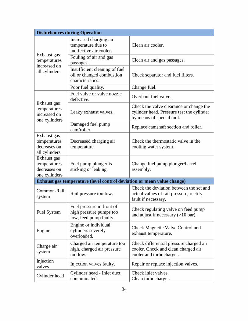
34

Disturbances during Operation

Exhaust gas

temperatures

increased on

all cylinders

Increased charging air

temperature due to

ineffective air cooler.

Clean air cooler.

Fouling of air and gas

passages. Clean air and gas passages.

Insufficient cleaning of fuel

oil or changed combustion

characteristics.

Check separator and fuel filters.

Poor fuel quality. Change fuel.

Exhaust gas

temperatures

increased on

one cylinders

Fuel valve or valve nozzle

defective. Overhaul fuel valve.

Leaky exhaust valves.

Check the valve clearance or change the

cylinder head. Pressure test the cylinder

by means of special tool.

Damaged fuel pump

cam/roller. Replace camshaft section and roller.

Exhaust gas

temperatures

decreases on

all cylinders

Decreased charging air

temperature.

Check the thermostatic valve in the

cooling water system.

Exhaust gas

temperatures

decreases on

one cylinders

Fuel pump plunger is

sticking or leaking.

Change fuel pump plunger/barrel

assembly.

Exhaust gas temperature (level control deviation or mean value change)

Common-Rail

system Rail pressure too low.

Check the deviation between the set and

actual values of rail pressure, rectify

fault if necessary.

Fuel System

Fuel pressure in front of

high pressure pumps too

low, feed pump faulty.

Check regulating valve on feed pump

and adjust if necessary (>10 bar).

Engine

Engine or individual

cylinders severely

overloaded.

Check Magnetic Valve Control and

exhaust temperature.

Charge air

system

Charged air temperature too

high, charged air pressure

too low.

Check differential pressure charged air

cooler. Check and clean charged air

cooler and turbocharger.

Injection

valves Injection valves faulty. Repair or replace injection valves.

Cylinder head Cylinder head - Inlet duct

contaminated.

Check inlet valves.

Clean turbocharger.

35

Inlet and

exhaust valves

Inlet or exhaust valves

sticking, valve springs

broken, valves leaking.

Remove cause.

Replace valve spring.

Control and

monitoring

system

Indicating device or

connection line faulty.

Temperature sensor faulty.

Cabling/Connections

defective/faulty.

Investigate cause and remove.

Replace affected components.

Replace temperature sensor.

Investigate cause and remove.

Replace affected components.

Turbocharger Turbocharger contaminated

or faulty. Repair or clean turbocharger.

Table 3. Common exhaust gas temperature errors and troubleshooting guide

(After MAN Diesel 2009).

B. DATA COLLECTION

The database used for this research was provided by Singapore Technologies

Marine, Ltd. and collected through ACMS installed onboard a Roll-On-Roll-Off

Passenger (ROPAX) Ship. The period of data collection ran from December 19, 2010 to

March 18, 2011. The data was extracted from the ACMS server under the trending

folder. As the data is numerous and big in size, it was reorganized according to various

sea-going events. This makes sense because the main engine is not in operation at harbor,

and data obtained from this point will translate to useless data for the analysis. Currently,

this re-organization is done manually due to a lack of means to classify the data.

C. SELECTION OF VARIABLES

The engines under study have the designation 10L 32/44CR from MAN Diesel as

depicted in Figure 6. It is a non-reversible four stroke in-line engine with a 320mm

cylinder bore and a 440 mm piston stroke. This engine type is equipped with a common

rail injection system and used as marine main drives. The engine has two camshafts‒‒one

for the actuation of the inlet and exhaust valves on the exhaust side and the other for the

actuation of the high pressure pumps on the exhaust counter side. It is also equipped with

MAN Diesel turbochargers from the TC series. The engines are interfaced with

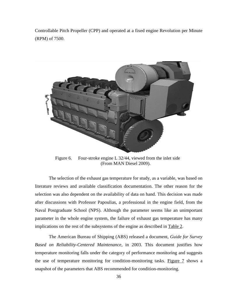
36

Controllable Pitch Propeller (CPP) and operated at a fixed engine Revolution per Minute

(RPM) of 7500.

Figure 6. Four-stroke engine L 32/44, viewed from the inlet side

(From MAN Diesel 2009).

The selection of the exhaust gas temperature for study, as a variable, was based on

literature reviews and available classification documentation. The other reason for the

selection was also dependent on the availability of data on hand. This decision was made

after discussions with Professor Papoulias, a professional in the engine field, from the

Naval Postgraduate School (NPS). Although the parameter seems like an unimportant

parameter in the whole engine system, the failure of exhaust gas temperature has many

implications on the rest of the subsystems of the engine as described in Table 2.

The American Bureau of Shipping (ABS) released a document, Guide for Survey

Based on Reliability-Centered Maintenance, in 2003. This document justifies how

temperature monitoring falls under the category of performance monitoring and suggests

the use of temperature monitoring for condition-monitoring tasks. Figure 7 shows a

snapshot of the parameters that ABS recommended for condition-monitoring.

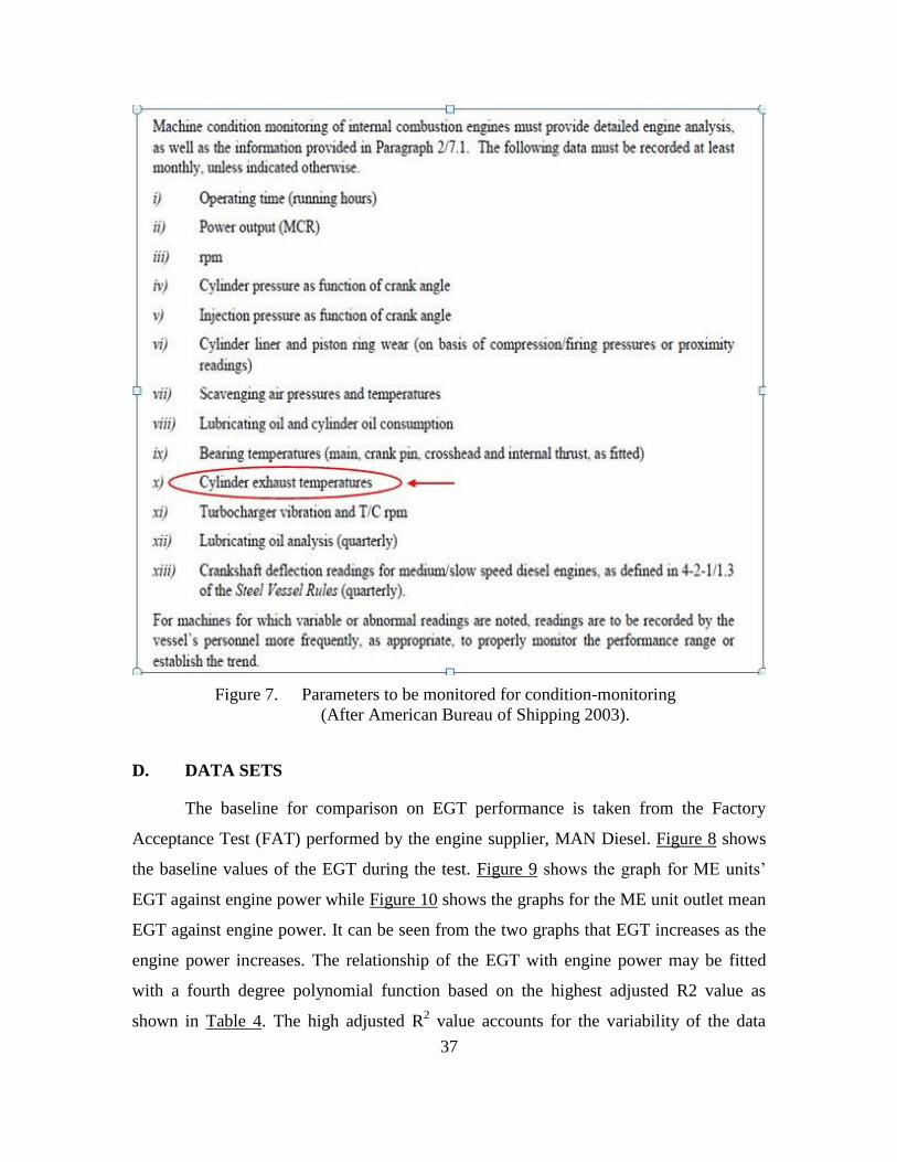
37

Figure 7. Parameters to be monitored for condition-monitoring

(After American Bureau of Shipping 2003).

D. DATA SETS

The baseline for comparison on EGT performance is taken from the Factory

Acceptance Test (FAT) performed by the engine supplier, MAN Diesel. Figure 8 shows

the baseline values of the EGT during the test. Figure 9 shows the graph for ME units’

EGT against engine power while Figure 10 shows the graphs for the ME unit outlet mean

EGT against engine power. It can be seen from the two graphs that EGT increases as the

engine power increases. The relationship of the EGT with engine power may be fitted

with a fourth degree polynomial function based on the highest adjusted R2 value as

shown in Table 4. The high adjusted R2 value accounts for the variability of the data

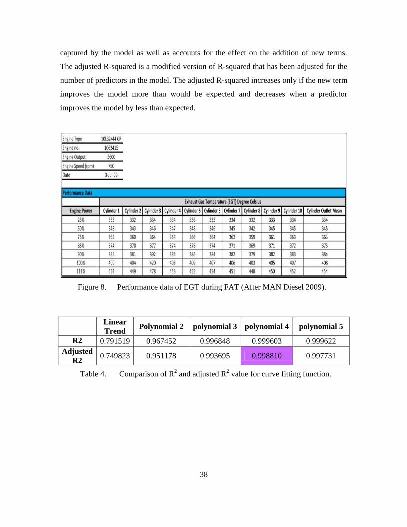
38

captured by the model as well as accounts for the effect on the addition of new terms.

The adjusted R-squared is a modified version of R-squared that has been adjusted for the

number of predictors in the model. The adjusted R-squared increases only if the new term

improves the model more than would be expected and decreases when a predictor

improves the model by less than expected.

Figure 8. Performance data of EGT during FAT (After MAN Diesel 2009).

Linear

Trend Polynomial 2 polynomial 3 polynomial 4 polynomial 5

R2 0.791519 0.967452 0.996848 0.999603 0.999622

Adjusted

R2 0.749823 0.951178 0.993695 0.998810 0.997731

Table 4. Comparison of R2 and adjusted R

2 value for curve fitting function.

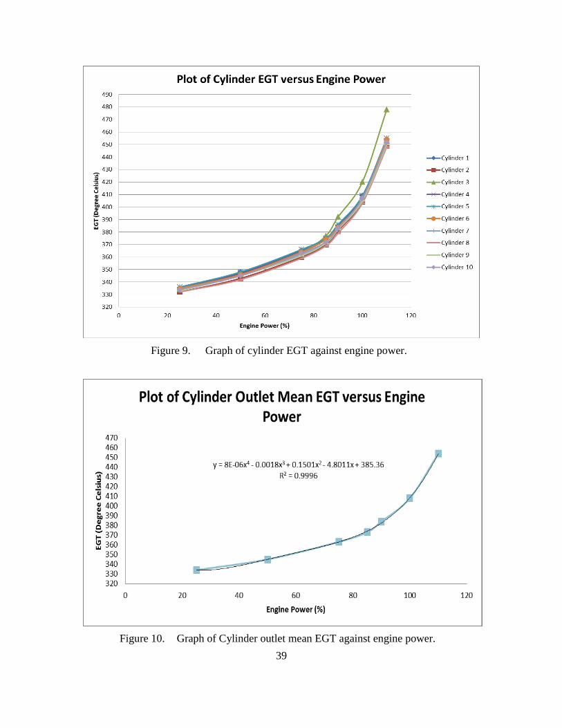
39

Figure 9. Graph of cylinder EGT against engine power.

Figure 10. Graph of Cylinder outlet mean EGT against engine power.

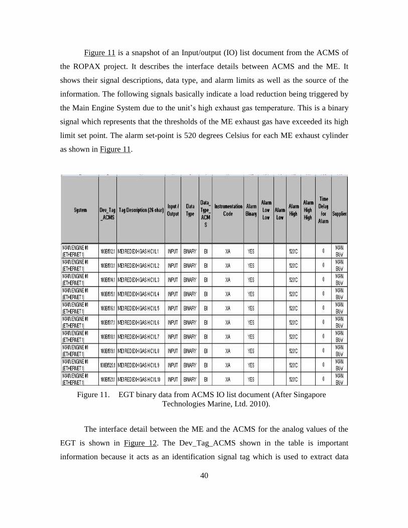
40

Figure 11 is a snapshot of an Input/output (IO) list document from the ACMS of

the ROPAX project. It describes the interface details between ACMS and the ME. It

shows their signal descriptions, data type, and alarm limits as well as the source of the

information. The following signals basically indicate a load reduction being triggered by

the Main Engine System due to the unit’s high exhaust gas temperature. This is a binary

signal which represents that the thresholds of the ME exhaust gas have exceeded its high

limit set point. The alarm set-point is 520 degrees Celsius for each ME exhaust cylinder

as shown in Figure 11.

Figure 11. EGT binary data from ACMS IO list document (After Singapore

Technologies Marine, Ltd. 2010).

The interface detail between the ME and the ACMS for the analog values of the

EGT is shown in Figure 12. The Dev_Tag_ACMS shown in the table is important

information because it acts as an identification signal tag which is used to extract data

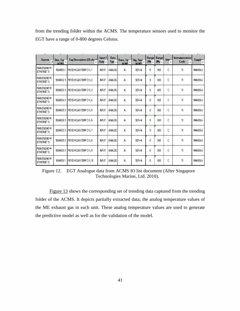
41

from the trending folder within the ACMS. The temperature sensors used to monitor the

EGT have a range of 0-800 degrees Celsius.

Figure 12. EGT Analogue data from ACMS IO list document (After Singapore

Technologies Marine, Ltd. 2010).

Figure 13 shows the corresponding set of trending data captured from the trending

folder of the ACMS. It depicts partially extracted data; the analog temperature values of

the ME exhaust gas in each unit. These analog temperature values are used to generate

the predictive model as well as for the validation of the model.

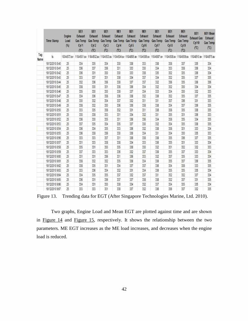
42

Figure 13. Trending data for EGT (After Singapore Technologies Marine, Ltd. 2010).

Two graphs, Engine Load and Mean EGT are plotted against time and are shown

in Figure 14 and Figure 15, respectively. It shows the relationship between the two

parameters. ME EGT increases as the ME load increases, and decreases when the engine

load is reduced.

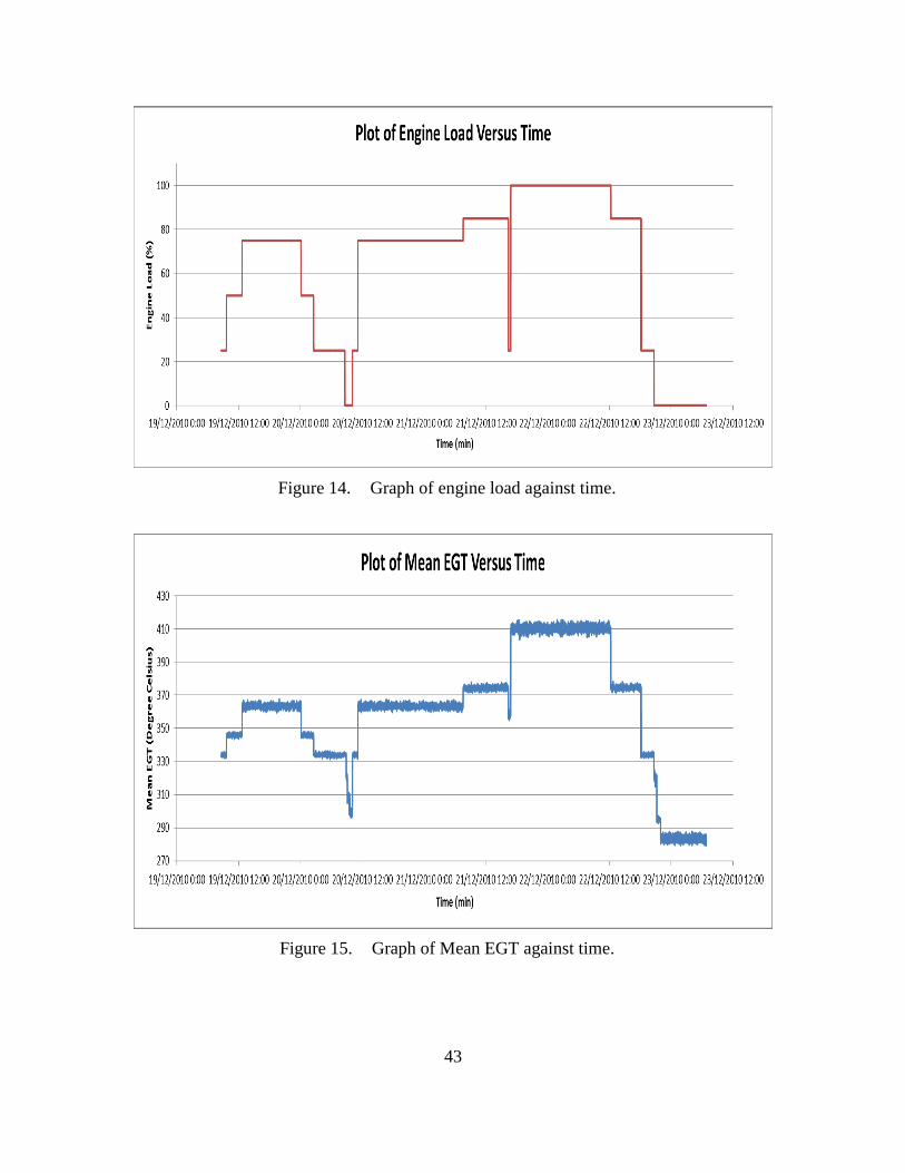
43

Figure 14. Graph of engine load against time.

Figure 15. Graph of Mean EGT against time.

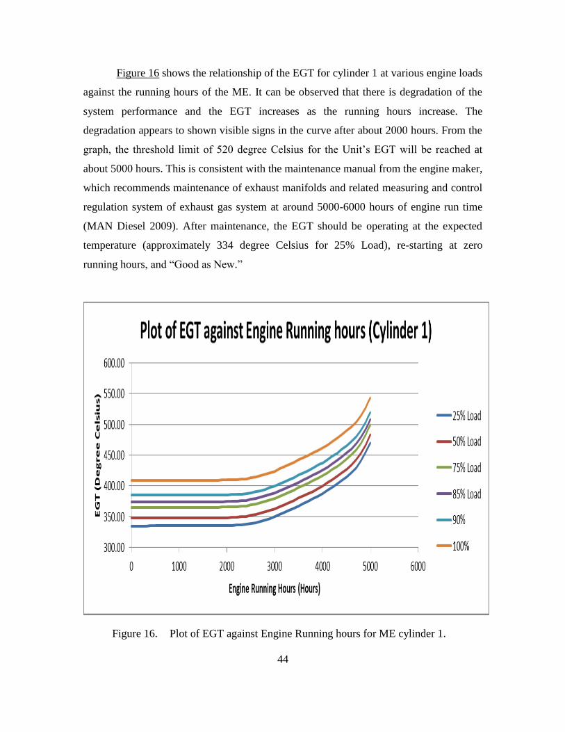
44

Figure 16 shows the relationship of the EGT for cylinder 1 at various engine loads

against the running hours of the ME. It can be observed that there is degradation of the

system performance and the EGT increases as the running hours increase. The

degradation appears to shown visible signs in the curve after about 2000 hours. From the

graph, the threshold limit of 520 degree Celsius for the Unit’s EGT will be reached at

about 5000 hours. This is consistent with the maintenance manual from the engine maker,

which recommends maintenance of exhaust manifolds and related measuring and control

regulation system of exhaust gas system at around 5000-6000 hours of engine run time

(MAN Diesel 2009). After maintenance, the EGT should be operating at the expected

temperature (approximately 334 degree Celsius for 25% Load), re-starting at zero

running hours, and “Good as New.”

Figure 16. Plot of EGT against Engine Running hours for ME cylinder 1.

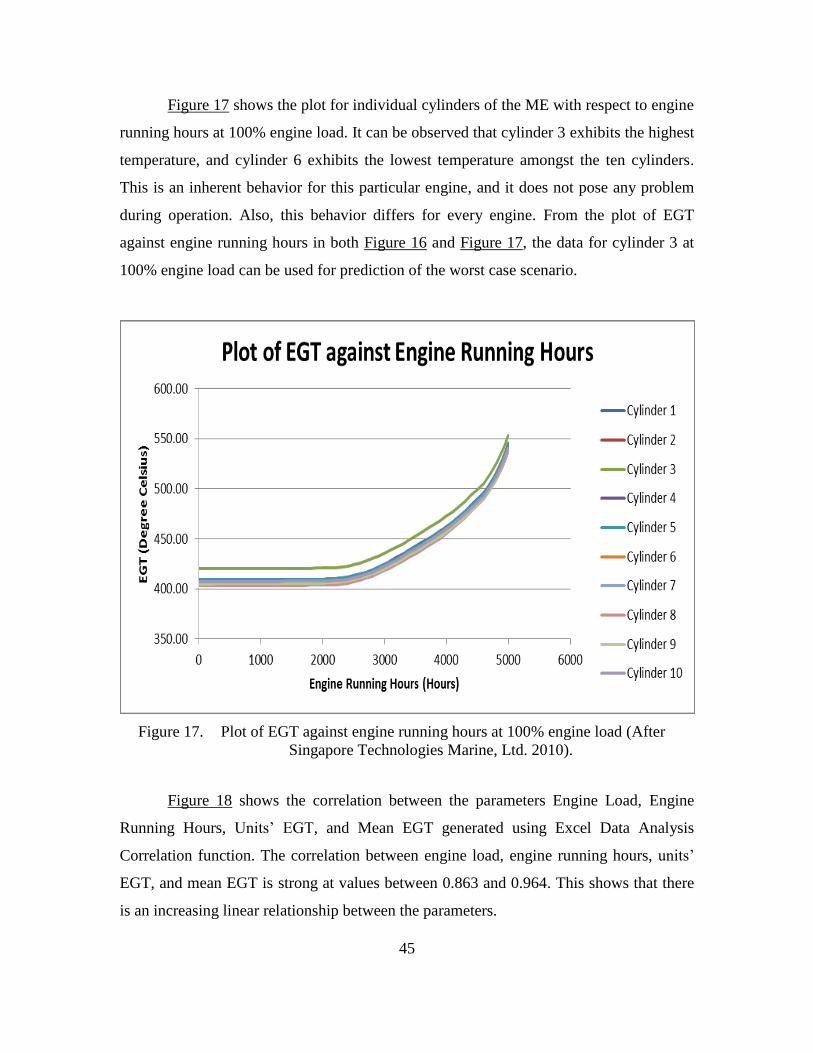
45

Figure 17 shows the plot for individual cylinders of the ME with respect to engine

running hours at 100% engine load. It can be observed that cylinder 3 exhibits the highest

temperature, and cylinder 6 exhibits the lowest temperature amongst the ten cylinders.

This is an inherent behavior for this particular engine, and it does not pose any problem

during operation. Also, this behavior differs for every engine. From the plot of EGT

against engine running hours in both Figure 16 and Figure 17, the data for cylinder 3 at

100% engine load can be used for prediction of the worst case scenario.

Figure 17. Plot of EGT against engine running hours at 100% engine load (After

Singapore Technologies Marine, Ltd. 2010).

Figure 18 shows the correlation between the parameters Engine Load, Engine

Running Hours, Units’ EGT, and Mean EGT generated using Excel Data Analysis

Correlation function. The correlation between engine load, engine running hours, units’

EGT, and mean EGT is strong at values between 0.863 and 0.964. This shows that there

is an increasing linear relationship between the parameters.

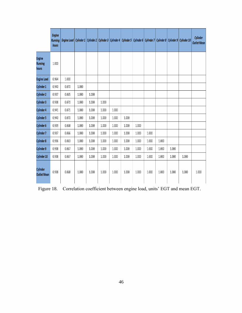
46

Figure 18. Correlation coefficient between engine load, units’ EGT and mean EGT.

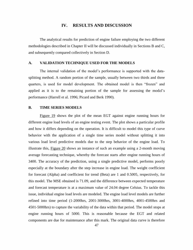
47

IV. RESULTS AND DISCUSSION

The analytical results for prediction of engine failure employing the two different

methodologies described in Chapter II will be discussed individually in Sections B and C,

and subsequently compared collectively in Section D.

A. VALIDATION TECHNIQUE USED FOR THE MODELS

The internal validation of the model’s performance is supported with the data-

splitting method. A random portion of the sample, usually between two thirds and three

quarters, is used for model development. The obtained model is then “frozen” and

applied as it is to the remaining portion of the sample for assessing the model’s

performance (Harrell et al. 1996; Picard and Berk 1990).

B. TIME SERIES MODELS

Figure 19 shows the plot of the mean EGT against engine running hours for

different engine load levels of an engine testing event. The plot shows a particular profile

and how it differs depending on the operation. It is difficult to model this type of curve

behavior with the application of a single time series model without splitting it into

various load level predictive models due to the step behavior of the engine load. To

illustrate this, Figure 20 shows an instance of such an example using a 2-month moving

average forecasting technique, whereby the forecast starts after engine running hours of

3400. The accuracy of the prediction, using a single predictive model, performs poorly

especially at the boundary after the step increase in engine load. The weight coefficient

for forecast (Alpha) and coefficient for trend (Beta) are 1 and 0.5005, respectively, for

this model. The MSE obtained is 71.09, and the difference between expected temperature

and forecast temperature is at a maximum value of 24.04 degree Celsius. To tackle this

issue, individual engine load levels are modeled. The engine load level models are further

refined into time period (1-2000hrs, 2001-3000hrs, 3001-4000hrs, 4001-4500hrs and

4501-5000hrs) to capture the variability of the data within that period. The model stops at

engine running hours of 5000. This is reasonable because the EGT and related

components are due for maintenance after this mark. The original data curve is therefore

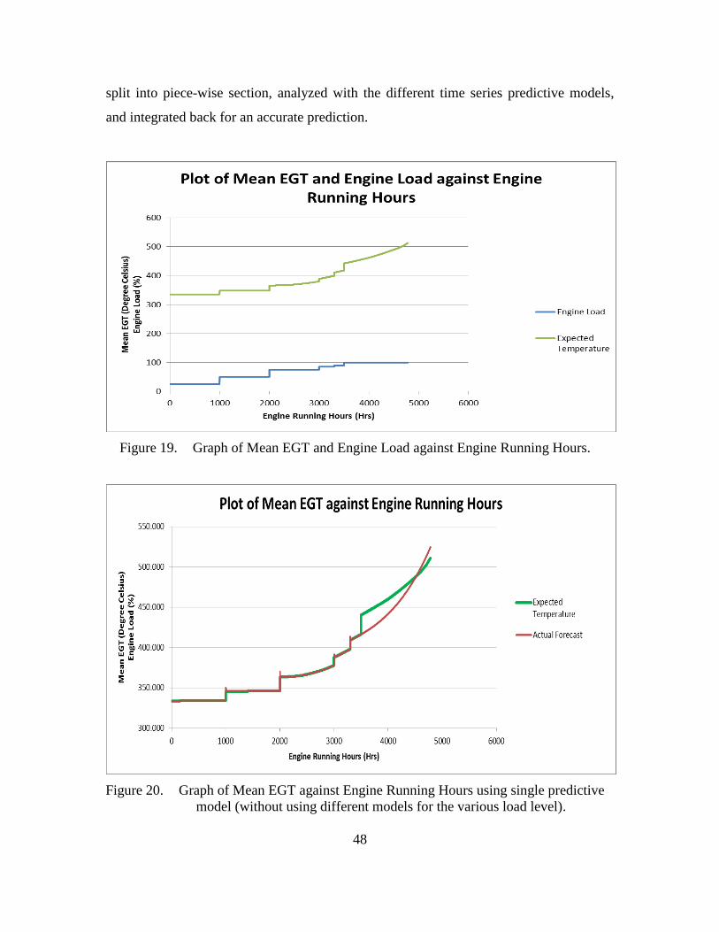
48

split into piece-wise section, analyzed with the different time series predictive models,

and integrated back for an accurate prediction.

Figure 19. Graph of Mean EGT and Engine Load against Engine Running Hours.

Figure 20. Graph of Mean EGT against Engine Running Hours using single predictive

model (without using different models for the various load level).

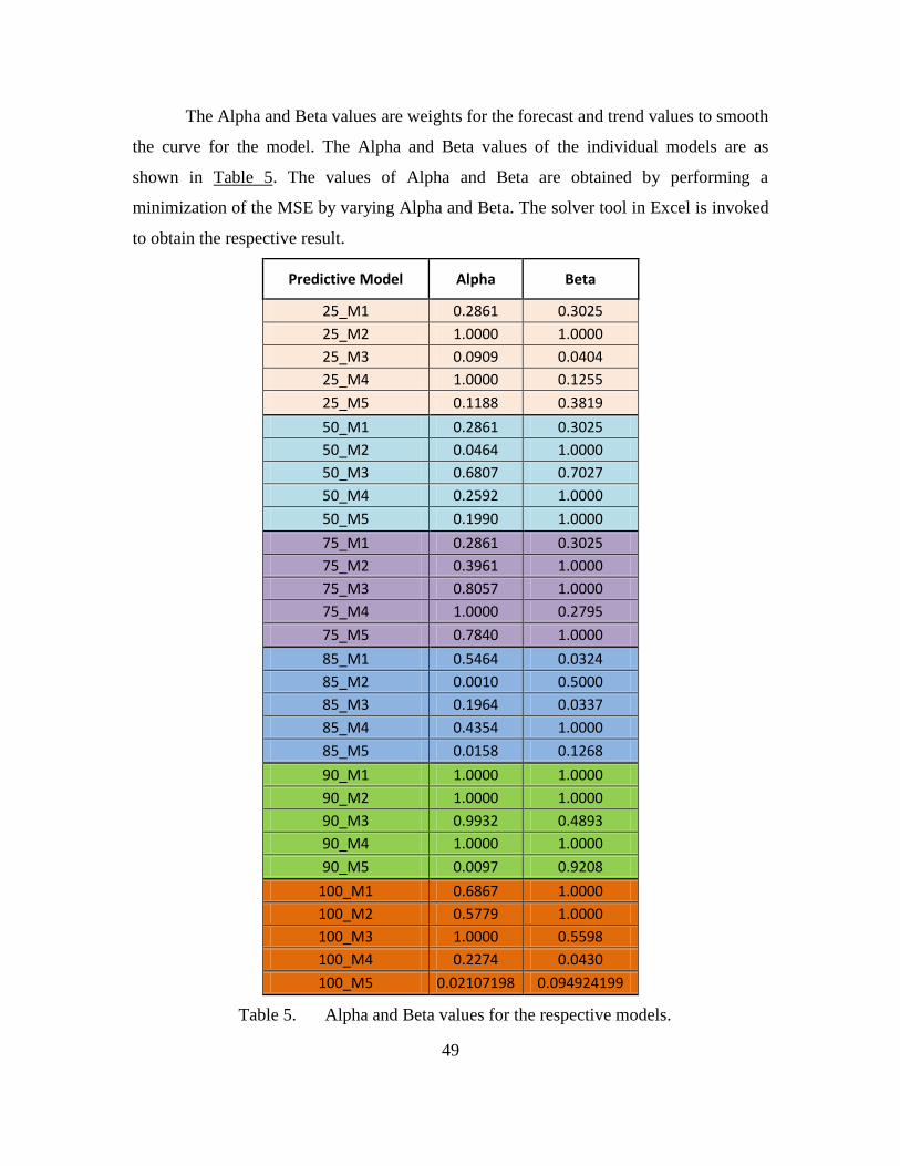
49

The Alpha and Beta values are weights for the forecast and trend values to smooth

the curve for the model. The Alpha and Beta values of the individual models are as

shown in Table 5. The values of Alpha and Beta are obtained by performing a

minimization of the MSE by varying Alpha and Beta. The solver tool in Excel is invoked

to obtain the respective result.

Predictive Model Alpha Beta

25_M1 0.2861 0.3025

25_M2 1.0000 1.0000

25_M3 0.0909 0.0404

25_M4 1.0000 0.1255

25_M5 0.1188 0.3819

50_M1 0.2861 0.3025

50_M2 0.0464 1.0000

50_M3 0.6807 0.7027

50_M4 0.2592 1.0000

50_M5 0.1990 1.0000

75_M1 0.2861 0.3025

75_M2 0.3961 1.0000

75_M3 0.8057 1.0000

75_M4 1.0000 0.2795

75_M5 0.7840 1.0000

85_M1 0.5464 0.0324

85_M2 0.0010 0.5000

85_M3 0.1964 0.0337

85_M4 0.4354 1.0000

85_M5 0.0158 0.1268

90_M1 1.0000 1.0000

90_M2 1.0000 1.0000

90_M3 0.9932 0.4893

90_M4 1.0000 1.0000

90_M5 0.0097 0.9208

100_M1 0.6867 1.0000

100_M2 0.5779 1.0000

100_M3 1.0000 0.5598

100_M4 0.2274 0.0430

100_M5 0.02107198 0.094924199

Table 5. Alpha and Beta values for the respective models.

50

The results for the individual predictive models using Mean EGT as a baseline

model are summarized as shown in Table 6.

Load (%)

Engine Running

Hours (Hours)

Predictive Model

Difference Between Actual Data and forecasted Data (Error)

Mean Standard

Error Standard Deviation

Min Max Mean

Square Error

25

1-2000 25_M1 -3.208E-05 4.203E-06 1.879E-04 -1.408E-03 6.419E-04 3.634E-08

2001-3000 25_M2 3.729E-02 3.673E-03 1.161E-01 -1.000E-02 6.305E-01 1.487E-02

3001-4000 25_M3 4.166E-02 2.814E-03 8.899E-02 -2.368E-02 4.248E-01 9.648E-03

4001-4500 25_M4 1.848E-03 4.065E-04 9.089E-03 -1.838E-02 5.039E-02 8.587E-05

4501-5000 25_M5 -4.936E-03 4.144E-03 9.248E-02 -3.286E-01 3.726E-01 8.559E-03

50

1-2000 50_M1 -1.660E-04 1.304E-05 5.830E-04 -3.466E-03 6.212E-04 3.673E-07

2001-3000 50_M2 3.192E-02 3.233E-03 1.022E-01 -2.646E-02 5.526E-01 1.146E-02

3001-4000 50_M3 -1.107E-03 4.649E-04 1.470E-02 -5.478E-02 1.041E-01 2.172E-04

4001-4500 50_M4 4.919E-02 4.971E-03 1.112E-01 -3.542E-02 3.995E-01 1.475E-02

4501-5000 50_M5 1.854E-01 6.267E-03 1.398E-01 2.966E-02 9.030E-01 5.391E-02

75

1-2000 75_M1 4.252E-06 1.616E-06 7.225E-05 -3.246E-04 6.276E-04 5.236E-09

2001-3000 75_M2 4.917E-02 4.306E-03 1.362E-01 -8.023E-03 7.079E-01 2.094E-02

3001-4000 75_M3 -1.971E-03 6.599E-04 2.087E-02 -6.974E-02 1.071E-01 4.389E-04

4001-4500 75_M4 -1.214E-04 3.992E-04 8.927E-03 -2.990E-02 4.667E-02 7.954E-05

4501-5000 75_M5 2.187E-01 8.566E-03 1.912E-01 6.507E-02 1.135E+00 8.428E-02

85

1-2000 85_M1 -9.666E-06 2.410E-06 1.078E-04 -6.207E-04 5.426E-04 1.170E-08

2001-3000 85_M2 6.169E-02 3.385E-03 1.070E-01 -1.242E-01 3.722E-01 1.525E-02

3001-4000 85_M3 3.526E-02 2.775E-03 8.775E-02 -1.978E-02 4.862E-01 8.935E-03

4001-4500 85_M4 6.683E-03 7.636E-04 1.707E-02 -2.134E-02 7.382E-02 3.356E-04

4501-5000 85_M5 3.271E-01 1.617E-02 3.610E-01 -4.627E-01 1.195E+00 2.370E-01

90

1-2000 90_M1 1.125E-05 2.340E-06 1.047E-04 -4.400E-04 5.400E-04 1.107E-08

2001-3000 90_M2 1.120E-01 8.962E-03 2.834E-01 -7.500E-03 1.329E+00 9.277E-02

3001-4000 90_M3 -2.823E-03 4.981E-04 1.575E-02 -5.493E-02 6.179E-02 2.558E-04

4001-4500 90_M4 3.715E-02 3.418E-03 7.644E-02 -2.414E-02 3.494E-01 7.211E-03

4501-5000 90_M5 8.015E-02 1.572E-02 3.507E-01 -5.378E-01 9.072E-01 1.292E-01

100

1-2000 100_M1 -7.086E-04 3.808E-05 1.703E-03 -7.271E-03 3.200E-04 3.400E-06

2001-3000 100_M2 8.459E-03 1.953E-03 6.177E-02 -1.068E-01 3.480E-01 3.883E-03

3001-4000 100_M3 -3.287E-03 6.370E-04 2.014E-02 -6.579E-02 1.044E-01 4.161E-04

4001-4500 100_M4 4.216E-02 3.168E-03 7.084E-02 -2.327E-02 2.495E-01 6.786E-03

4501-5000 100_M5 3.287E-01 1.531E-02 3.417E-01 -3.972E-01 1.179E+00 2.246E-01

Table 6. Summary of results for individual predictive model.

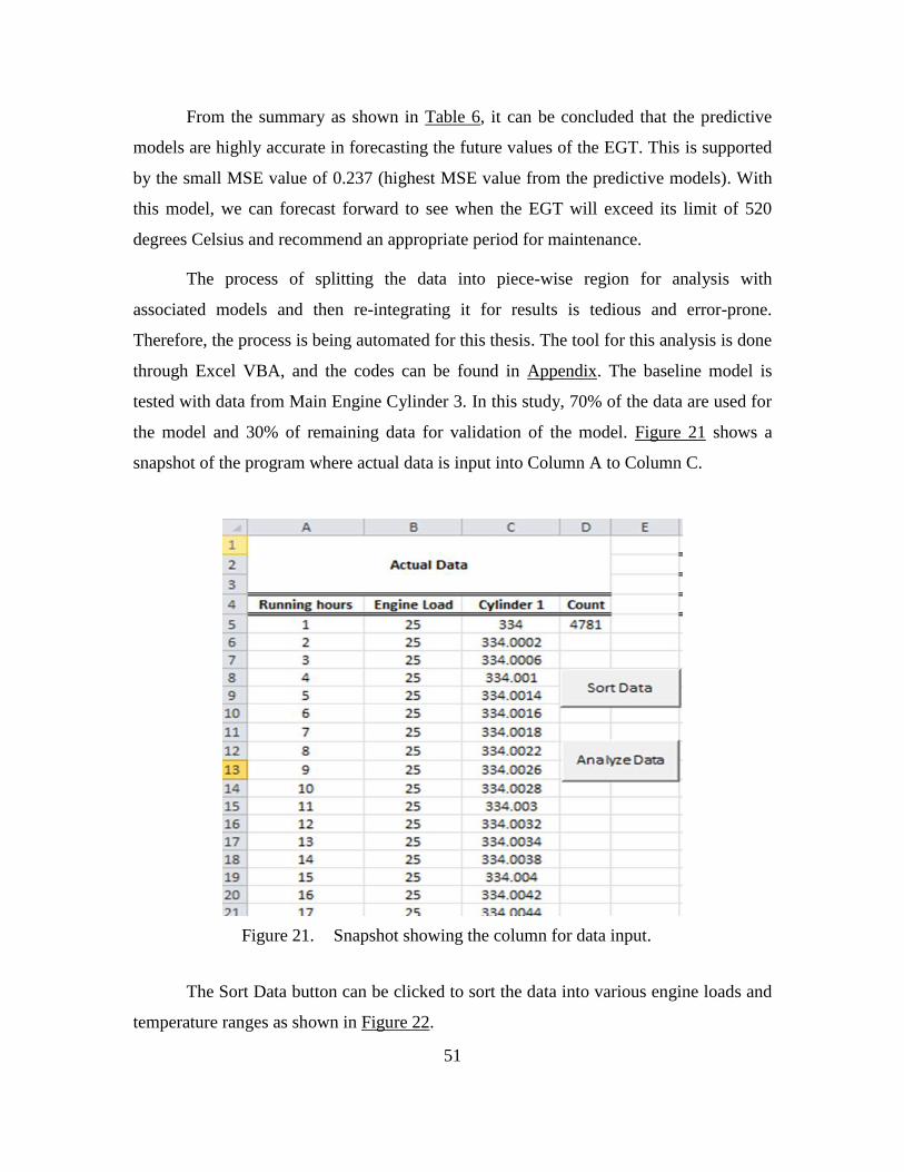
51

From the summary as shown in Table 6, it can be concluded that the predictive

models are highly accurate in forecasting the future values of the EGT. This is supported

by the small MSE value of 0.237 (highest MSE value from the predictive models). With

this model, we can forecast forward to see when the EGT will exceed its limit of 520

degrees Celsius and recommend an appropriate period for maintenance.

The process of splitting the data into piece-wise region for analysis with

associated models and then re-integrating it for results is tedious and error-prone.

Therefore, the process is being automated for this thesis. The tool for this analysis is done

through Excel VBA, and the codes can be found in Appendix. The baseline model is

tested with data from Main Engine Cylinder 3. In this study, 70% of the data are used for

the model and 30% of remaining data for validation of the model. Figure 21 shows a

snapshot of the program where actual data is input into Column A to Column C.

Figure 21. Snapshot showing the column for data input.

The Sort Data button can be clicked to sort the data into various engine loads and

temperature ranges as shown in Figure 22.

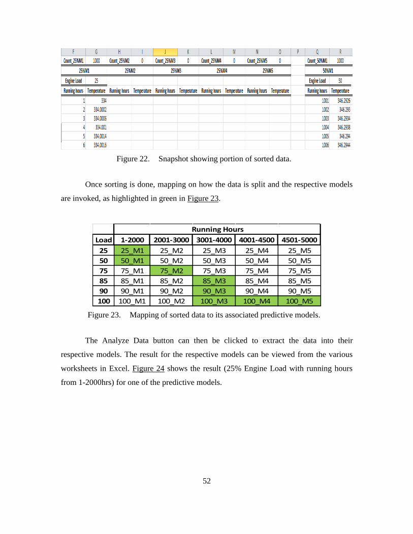
52

Figure 22. Snapshot showing portion of sorted data.

Once sorting is done, mapping on how the data is split and the respective models

are invoked, as highlighted in green in Figure 23.

Figure 23. Mapping of sorted data to its associated predictive models.

The Analyze Data button can then be clicked to extract the data into their

respective models. The result for the respective models can be viewed from the various

worksheets in Excel. Figure 24 shows the result (25% Engine Load with running hours

from 1-2000hrs) for one of the predictive models.

Load 1-2000 2001-3000 3001-4000 4001-4500 4501-5000

25 25_M1 25_M2 25_M3 25_M4 25_M5

50 50_M1 50_M2 50_M3 50_M4 50_M5

75 75_M1 75_M2 75_M3 75_M4 75_M5

85 85_M1 85_M2 85_M3 85_M4 85_M5

90 90_M1 90_M2 90_M3 90_M4 90_M5

100 100_M1 100_M2 100_M3 100_M4 100_M5

Running Hours

53

Figure 24. Result for Model 25_M1 (25% Engine Load and engine running hours

between 1-2000hours).

These individual models’ results will automatically be aggregated back to the

original format and displayed in “Result for test” worksheet as shown in Figure 25.

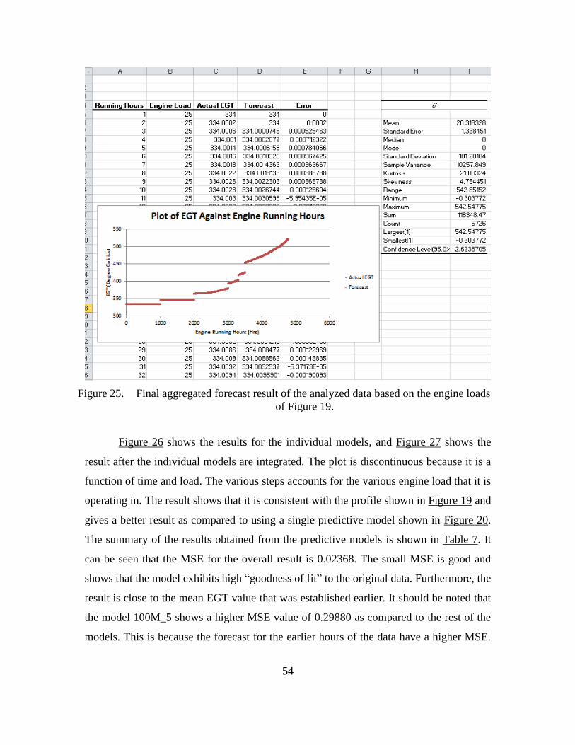
54

Figure 25. Final aggregated forecast result of the analyzed data based on the engine loads

of Figure 19.

Figure 26 shows the results for the individual models, and Figure 27 shows the

result after the individual models are integrated. The plot is discontinuous because it is a

function of time and load. The various steps accounts for the various engine load that it is

operating in. The result shows that it is consistent with the profile shown in Figure 19 and

gives a better result as compared to using a single predictive model shown in Figure 20.

The summary of the results obtained from the predictive models is shown in Table 7. It

can be seen that the MSE for the overall result is 0.02368. The small MSE is good and

shows that the model exhibits high “goodness of fit” to the original data. Furthermore, the

result is close to the mean EGT value that was established earlier. It should be noted that

the model 100M_5 shows a higher MSE value of 0.29880 as compared to the rest of the

models. This is because the forecast for the earlier hours of the data have a higher MSE.

55

It can also mean that the data exhibits greater variation as compared to the baseline

model.

It is imperative to know at this point that although MSE is used as a measure for

accuracy, it is sometimes wise to compute the MSE using the most recent values. This is

because the lowest MSE may result from fitting older values very well, but it fits recent

values poorly. Therefore, care should be taken when comparing the MSE.

With this model, the user can observe the trend from the graph when the predicted

temperature will exceed the threshold temperature of 520 degree Celsius based on their

expected operating scenario. The user can then plan their maintenance activities

accordingly, for example, allocation of manpower, booking of facilities and ordering of

parts when the predicted temperature reaches 500 degree Celsius.

The result from the forecast model can also serves as a warning to user if the

predicted temperature deviates too much from the expected temperature. In that situation,

the user can look at the CUSUM control chart, which will be discuss in Chapter IV

Section C, and confirms if there are any anomalies.

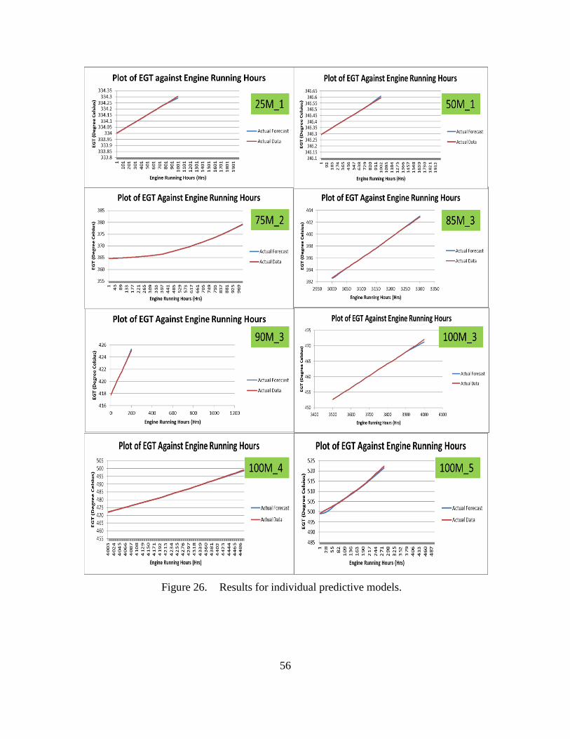
56

Figure 26. Results for individual predictive models.

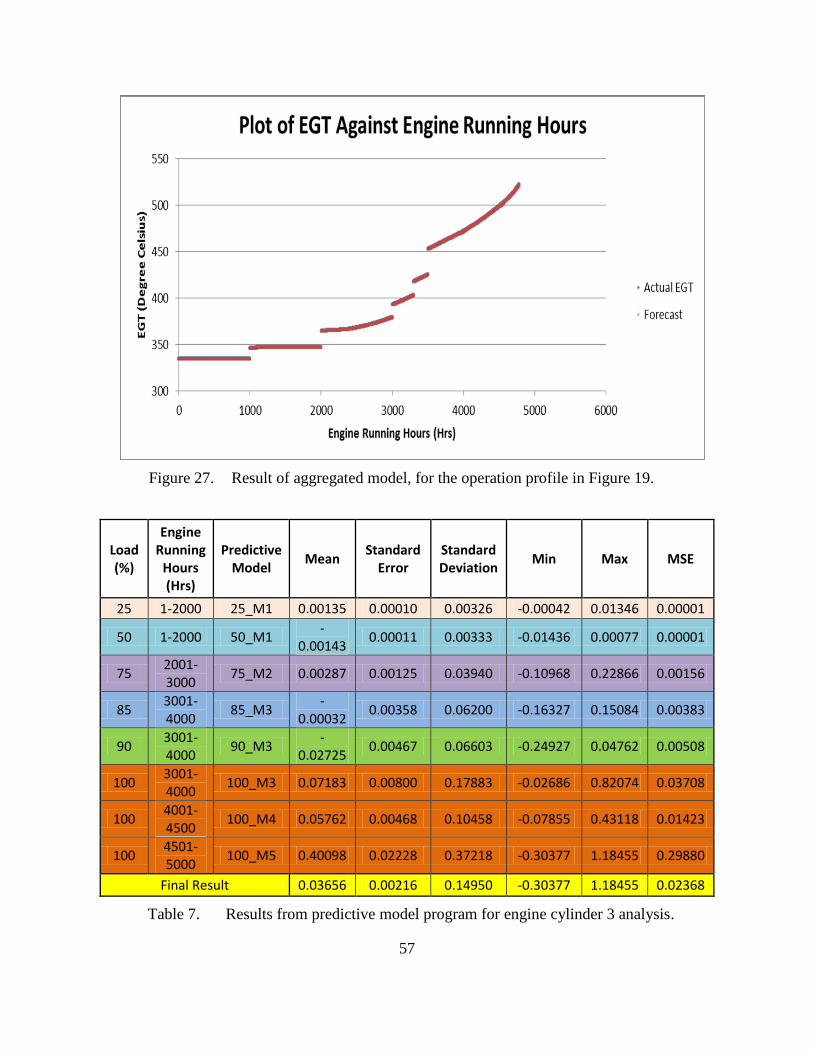
57

Figure 27. Result of aggregated model, for the operation profile in Figure 19.

Load (%)

Engine Running

Hours (Hrs)

Predictive Model

Mean Standard

Error Standard Deviation

Min Max MSE

25 1-2000 25_M1 0.00135 0.00010 0.00326 -0.00042 0.01346 0.00001

50 1-2000 50_M1 -

0.00143 0.00011 0.00333 -0.01436 0.00077 0.00001

75 2001-3000

75_M2 0.00287 0.00125 0.03940 -0.10968 0.22866 0.00156

85 3001-4000

85_M3 -

0.00032 0.00358 0.06200 -0.16327 0.15084 0.00383

90 3001-4000

90_M3 -

0.02725 0.00467 0.06603 -0.24927 0.04762 0.00508

100 3001-4000

100_M3 0.07183 0.00800 0.17883 -0.02686 0.82074 0.03708

100 4001-4500

100_M4 0.05762 0.00468 0.10458 -0.07855 0.43118 0.01423

100 4501-5000

100_M5 0.40098 0.02228 0.37218 -0.30377 1.18455 0.29880

Final Result 0.03656 0.00216 0.14950 -0.30377 1.18455 0.02368

Table 7. Results from predictive model program for engine cylinder 3 analysis.

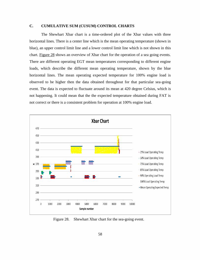
58

C. CUMULATIVE SUM (CUSUM) CONTROL CHARTS

The Shewhart Xbar chart is a time-ordered plot of the Xbar values with three

horizontal lines. There is a center line which is the mean operating temperature (shown in

blue), an upper control limit line and a lower control limit line which is not shown in this

chart. Figure 28 shows an overview of Xbar chart for the operation of a sea going events.

There are different operating EGT mean temperatures corresponding to different engine

loads, which describe the different mean operating temperature, shown by the blue

horizontal lines. The mean operating expected temperature for 100% engine load is

observed to be higher then the data obtained throughout for that particular sea-going

event. The data is expected to fluctuate around its mean at 420 degree Celsius, which is

not happening. It could mean that the the expected temperature obtained during FAT is

not correct or there is a consistent problem for operation at 100% engine load.

Figure 28. Shewhart Xbar chart for the sea-going event.

59

Figure 29 shows a zoom-in version of the event between samples 7500 to 8385.

The control limits are located three standard deviation of the mean, above and below the

center line. The standard deviation is 7.55 degree Celsius. The limits are determined to be

at 397 and 443 degree Celsius. When the points are within the two limits, it means that

the process is in control and should be left to run as it is. When the points are out of the

control limit, it means that the process is out of control. It signifies a problem and a need

to look at the problem seriously. The problem with using Xbar chart for this particular

application is that it grows increasingly confusing with the different load levels, its

corresponding mean operating temperatures (center lines), and their associated lower and

upper control limit lines.

Figure 29. Shewhart Xbar chart for samples between 7500 and 8385.

The DI CUSUM chart is used in this study instead as it accounts for the different

load level mean operating temperatures, simply by monitoring if the points stays within

the decision intervals, h+ and h

- . The exhaust gas temperature for cylinder three is

studied with the use of Excel. A sample of the setup is as shown in Figure 30. The data

analysis tool from Excel is used to generate the descriptive statistics for the difference

between Xi and the mean operating temperature, U0. The in-control standard deviation is

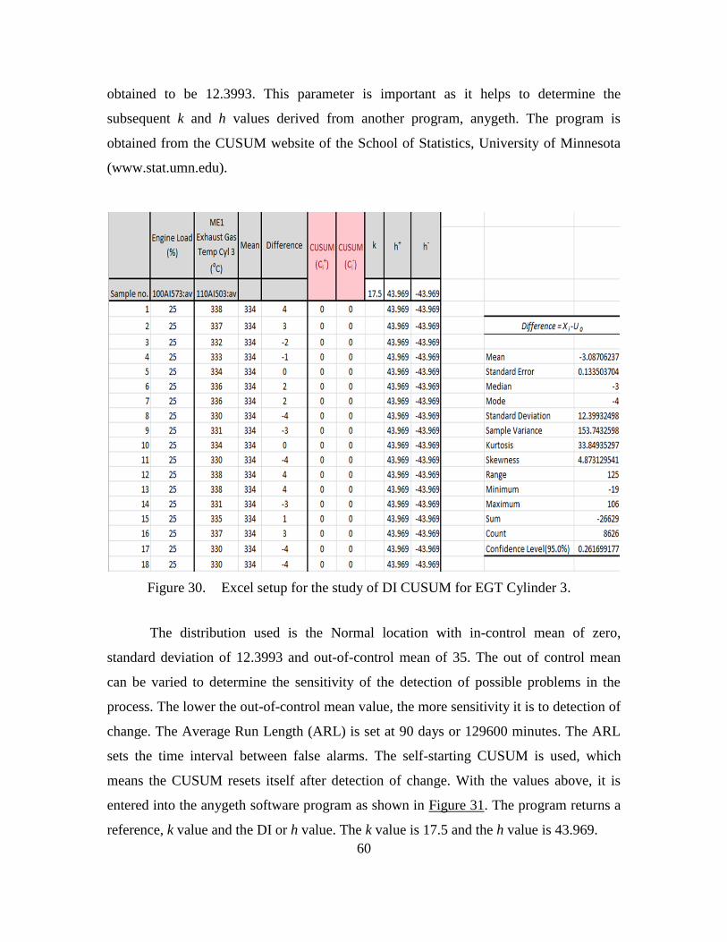
60

obtained to be 12.3993. This parameter is important as it helps to determine the

subsequent k and h values derived from another program, anygeth. The program is

obtained from the CUSUM website of the School of Statistics, University of Minnesota

(www.stat.umn.edu).

Figure 30. Excel setup for the study of DI CUSUM for EGT Cylinder 3.

The distribution used is the Normal location with in-control mean of zero,

standard deviation of 12.3993 and out-of-control mean of 35. The out of control mean

can be varied to determine the sensitivity of the detection of possible problems in the

process. The lower the out-of-control mean value, the more sensitivity it is to detection of

change. The Average Run Length (ARL) is set at 90 days or 129600 minutes. The ARL

sets the time interval between false alarms. The self-starting CUSUM is used, which

means the CUSUM resets itself after detection of change. With the values above, it is

entered into the anygeth software program as shown in Figure 31. The program returns a

reference, k value and the DI or h value. The k value is 17.5 and the h value is 43.969.

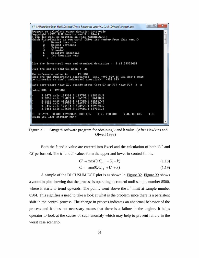
61

Figure 31. Anygeth software program for obtaining k and h value. (After Hawkins and

Olwell 1998)

Both the k and h value are entered into Excel and the calculation of both Ci+ and

Ci- performed. The h

+ and h

- values form the upper and lower in-control limits.

1max(0, )i i iC C U k

(1.18)

1min(0, )i i iC C U k

(1.19)

A sample of the DI CUSUM EGT plot is as shown in Figure 32. Figure 33 shows

a zoom in plot showing that the process is operating in-control until sample number 8500,

where it starts to trend upwards. The points went above the h+ limit at sample number

8504. This signifies a need to take a look at what is the problem since there is a persistent

shift in the control process. The change in process indicates an abnormal behavior of the

process and it does not necessary means that there is a failure in the engine. It helps

operator to look at the causes of such anomaly which may help to prevent failure in the

worst case scenario.

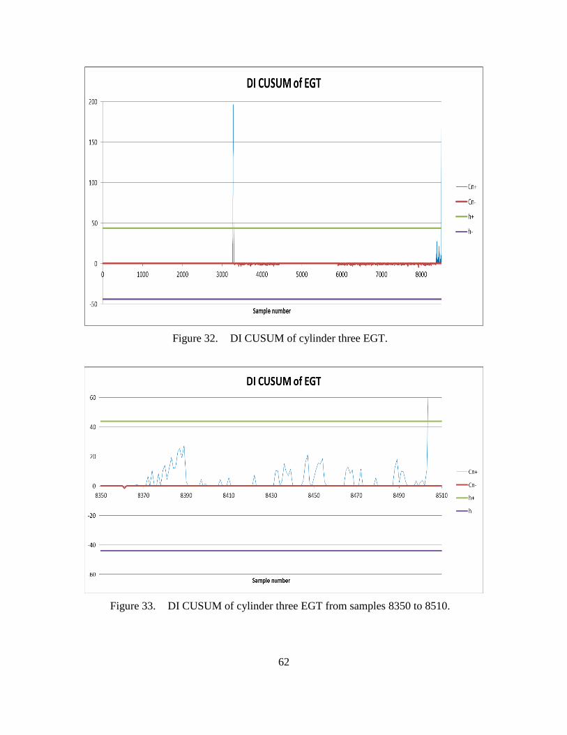
62

Figure 32. DI CUSUM of cylinder three EGT.

Figure 33. DI CUSUM of cylinder three EGT from samples 8350 to 8510.

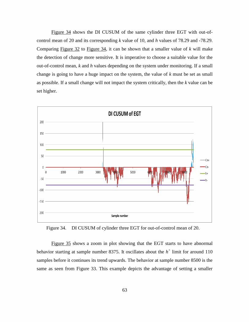
63

Figure 34 shows the DI CUSUM of the same cylinder three EGT with out-of-

control mean of 20 and its corresponding k value of 10, and h values of 78.29 and -78.29.

Comparing Figure 32 to Figure 34, it can be shown that a smaller value of k will make

the detection of change more sensitive. It is imperative to choose a suitable value for the

out-of-control mean, k and h values depending on the system under monitoring. If a small

change is going to have a huge impact on the system, the value of k must be set as small

as possible. If a small change will not impact the system critically, then the k value can be

set higher.

Figure 34. DI CUSUM of cylinder three EGT for out-of-control mean of 20.

Figure 35 shows a zoom in plot showing that the EGT starts to have abnormal

behavior starting at sample number 8375. It oscillates about the h+ limit for around 110

samples before it continues its trend upwards. The behavior at sample number 8500 is the

same as seen from Figure 33. This example depicts the advantage of setting a smaller

64

value of k because it captures the anomaly as early as in sample 8375. Due to its

sensitivity, it captures small persistent change very quickly.

Figure 35. DI CUSUM of cylinder three EGT from samples 8350 to 8510.

Figure 36 shows another instance where the process starts to trend upwards above

the h+ limit after sample number 3258. This is consistent with the result when the out-of-

control mean is set at 35 as shown in Figure 32. It is also interesting to observe that when

we set the out-of-control mean to be 20, Cn- actually trends downwards below the h

- limit

as shown in Figure 34. This means that at some point of time, the EGT is actually

running colder than it should have been. This may be attributed by poor combustion or

cooler ambient temperature from the surrounding.

From the results, it can be seen that by setting an appropriate out-of-control mean,

and getting the corresponding h and k values, CUSUM control chart is highly sensitive to

small changes in process. CUSUM proves to be capable of detecting anomalies, which

serves to warn user that it is time they check on the system before possible failures arises.

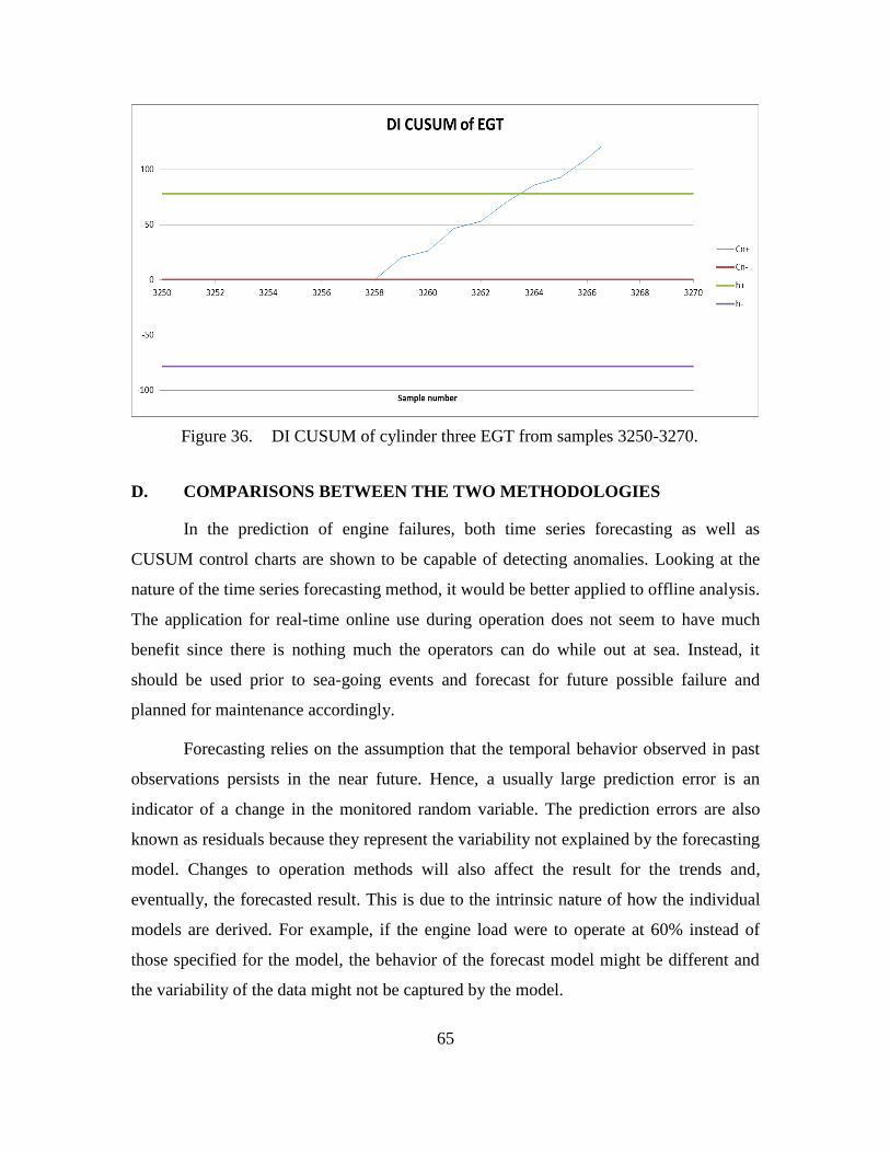
65

Figure 36. DI CUSUM of cylinder three EGT from samples 3250-3270.

D. COMPARISONS BETWEEN THE TWO METHODOLOGIES

In the prediction of engine failures, both time series forecasting as well as

CUSUM control charts are shown to be capable of detecting anomalies. Looking at the

nature of the time series forecasting method, it would be better applied to offline analysis.

The application for real-time online use during operation does not seem to have much

benefit since there is nothing much the operators can do while out at sea. Instead, it

should be used prior to sea-going events and forecast for future possible failure and

planned for maintenance accordingly.

Forecasting relies on the assumption that the temporal behavior observed in past

observations persists in the near future. Hence, a usually large prediction error is an

indicator of a change in the monitored random variable. The prediction errors are also

known as residuals because they represent the variability not explained by the forecasting

model. Changes to operation methods will also affect the result for the trends and,

eventually, the forecasted result. This is due to the intrinsic nature of how the individual

models are derived. For example, if the engine load were to operate at 60% instead of

those specified for the model, the behavior of the forecast model might be different and

the variability of the data might not be captured by the model.

66

Generally, the more a priori knowledge is available, the easier it is to detect any

changes with a high accuracy. Parametric methods typically have more power than non-

parametric methods, which means that they allow for the detection of more true

anomalies at the same false alarm level (probability of an alarm in absence of any

significant change). However, if the assumption is incorrect, parametric methods lose

their decisive power and may lead to wrong decisions. In the case of EGT anomaly

detection, it is not totally correct to assume that the monitored variable follows a specific

distribution; thus the detection should be non-parametric or at least robust enough against

non-normality. Furthermore, changes should be detected very swiftly while online

without requiring any prior knowledge about their magnitude. This is due to the lack of

readily available information for different operation scenarios.

CUSUM control chart, in this case, is a practical solution to statistical online

change detection. In a control chart, the mean and variability of a monitored variable are

characterized by a centerline (CL), an upper control limit (UCL), and a lower control

limit (LCL). A change is detected if the measured value exceeds one of the control limits.

CUSUM control charts can therefore be used as online tools to look at anomalies and can

serve as a form of warning to the operator for possible failures.

The comparison between these two methods is pretty distinct although both allow

prediction on the detection of failure. Time series forecasting tends toward prediction

used for future planning for maintenance (offline mode) while the CUSUM control chart

serves as an online monitoring and control tool, observing the anomaly of the process for

an operation.

67

V. CONCLUSION AND RECOMMENDATIONS

The study of the predictive methodology, both time series forecasting and

CUSUM, displays potential means on how it can be applied to ship machinery

maintenance. Both methodologies display accuracy in predicting machinery failures, and

this can be used to the advantage of the users. Time series forecasting can be used as an

offline analysis tool while CUSUM can be used as a real-time monitoring tool. A

combination of both methods allows greater capability to predict ship machinery failures

and allows “just in time” maintenance as compared to the traditional maintenance

strategy that is considered both preventive and corrective.

With prior knowledge of possible future failure, administrators responsible for the

purchase of parts, delivery of components, docking of vessel, if required, and other

logistical work can plan well ahead. It reduces the risk of corrective maintenance, the

shortage of parts, and last minute purchases. It could also allow lower quantities of spares

to be purchased since inventory can be planned ahead of time based on prediction. This in

turn reduces the need for storage space as well as for resources to maintain the huge

inventory. Overall, this will increase the turn-around time for maintenance, reduce the

operational downtime, and improve the overall effectiveness of the ship maintenance

program.

The results from the modeling done in this paper display the potential means on

how both predictive methodologies can be applied to ship machinery maintenance. Both

methodologies display accuracy in predicting failures in machinery, and this can be used

to the advantage of the users.

In the time series results, the relationship between the two parameters, ME EGT

and ME load was established: ME EGT increases as the ME load increases and decreases

when the engine load is reduced. From this relationship, a mean EGT value was derived,

and the results for the mean EGT produced were close. MSE was used as a measure for

accuracy in this modeling. The small MSE derived shows that the time series model

exhibits high “goodness of fit” to the original data. However, one should exercise caution

68

when computing the MSE as lowest MSE may result from fitting older values very well,

but it fits recent values poorly.

The time series forecast model allows the user to observe the trend of the

predicted temperature and plan for their maintenance activity before it exceeds the high

temperature limit of 520 degree Celsius.

For the CUSUM results, the control limits are established for the parameters. In

this paper, DI CUSUM was used instead as it accounts for the different load level mean

operating temperatures, simply by monitoring if the points stays within the decision

intervals, h+ and h

-. The results shows that a smaller value of k will make the detection of

change more sensitive, and hence it is imperative to choose a suitable value for the out-

of-control mean, k and h values depending on the system under monitoring.

The CUSUM results also shows that there were two instances of abnormal

behaviors (most likely failure), that occurs around the same point (sample number 3258

and 8500) for both k values of 17.5 and 10. This confirmed that the control chart is

capable of detecting anomalies accurately. Furthermore, there were more symptoms

displayed prior to the upward departure of the data around its mean of zero at sample

number 8500, when a k value of 10 was used. This shows that a smaller k value is more

sensitive to chnge and can detect the anomalies earlier.

The study of predictive analytics for commercial vessel main engines exhaust gas

temperature shows the possibility of and reasonable accuracy in predicting failures. As

such, this methodology possesses qualities that can be adopted and extended for a more

effective ship maintenance program for naval vessels.

The study has confirmed that the predictive methodology is feasible in its limited

parameters analysis. Some recommendations for future work may include the following

for a more conclusive model.

i. The study of turbocharger pressure and temperature in relation to the

failure of the main engine.

69

ii. The study of turbocharger vibration and RPM in relation to the failure of

the main engine.

iii. The study of air flow that affects the combustion process and the operation

of the main engine.

iv. The study of bearing temperature in relation to the failure of the main

engine.

v. An enhanced version of the automated time series forecasting method with

graphical user interface, allowing more parameters to be selected and

analyzed. It can also incorporate auto calculation of predicted time to

failure which offers greater ease of comprehension.

vi. An enhanced version of the automated time series forecasting with various

forecasting techniques templates, allowing operators the flexibility to

select and fit the best model for the application.

vii. The architecture for an integrated, real-time, online CUSUM process

control monitoring and alarm system.

viii. An automated CUSUM program with graphical user interface for the

operator to varies the input parameters and plot a graph. It should be

flexible enough to incorporate other types of distributions.

ix. The exploration of multivariate quality control using Shewhart charting –

Hotelling’s T2. This is to account for increased sensitivity to departures

from the in-control. The study could measure how the different EGT

cylinders may affect the overall behavior of the system.

A combination of both methods allows greater capability to predict ship

machinery failures and allows “just in time” maintenance as compared to the traditional

maintenance strategy that is considered both preventive and corrective.

70

THIS PAGE INTENTIONALLY LEFT BLANK

71

LIST OF REFERENCES

American Bureau of Shipping. Guide for Survey Based on Reliability-Centered

Maintenance (December 2003). ABS. Last modified July 17, 2013.

http://www.eagle.org/eagleExternalPortalWEB/appmanager/absEagle/absEagleDe

sktop?_nfpb=true&_pageLabel=abs_eagle_portal_rules_guides_download_page

&pub_id=121.

Blanchard, Benjamin S. and Walter J. Fabrycky. 2001. Systems Engineering and Analysis

(Third Edition). Upper Saddle River, NJ: Prentice Hall.

Clark, Jason. All About .NET (May 12, 2001). “Microsoft P-Code Technology.” Last

Modified July 11, 2013 http://www.codeproject.com/Articles/1107/All-About-

NET.

Crosier, Ronald B. 1988. Multivariate Generalization of Cumulative Sum Quality-

Control Schemes. Technometrics, vol. 30, no.3. 291–303

Eckerson, Wayne. Extending the Value of your Data Warehousing Investment (May 10,

2007). The Data Warehouse Institute. Last modified May 27, 2013.

http://tdwi.org/articles/2007/05/10/predictive-analytics.aspx?sc_lang=en.

Fair Isaac Corporation. FICO, Your Guide to the Science That Makes Customer Decision

Smarter. Last modified May 27, 2013.

http://www.fico.com/en/FIResourcesLibrary/Predictive_Analytics_2025BR.pdf.

Grant, Stanley. Why Predictive Analytics is Important and More (June 13, 2011),

Contemporary Analysis Work Smart. Last Accessed May 27, 2013.

http://blog.canworksmart.com/predictive-analytics/why-predictive-analytics/.

Hawkins, Douglas M. and Olwell, David H. 1998. Cumulative Sum Charts and Charting

for Quality Improvement. New York: Springer.

Harrell, F. E, Lee, K. L., Mark, D. B. 1996. “Multivariable Prognostic Models: Issues in

Developing Models, Evaluating Assumptions and Adequacy, and Measuring and

Reducing Errors. Statistics,” Medicine 15: 361–87.

Harding, John E. 1994. “Time-Frequency Domain Distribution and Its Application to

Reciprocating Machinery Analysis.” Master’s thesis, Naval Postgraduate School.

Jelen, B. and Syrstad, T. 2007. Visual Basic for Application (VBA) and Macros for

Microsoft Office Excel 2007 (business solutions) (Second Edition). Indianapolis,

Indiana: pp. 42–52.

72

Jenning, A. D. and Drake, P. R. 1997. “Machine Tool Condition Monitoring Using

Statistical Quality Control Charts.” International Journal of Machine Tools

Manufacture 37, no. 9: 1243–49.

MAN Diesel. 2009. “Operative Management III – Operating faults.” MAN Diesel.

MAN Diesel. 2009. “Shop Test Protocol.” MAN Diesel.

MAN Diesel. 2009. “Technical Documentation Engine Operating Instructions.” MAN

Diesel.

MAN Diesel. 2009. “Troubleshooting.” MAN Diesel.

Montgomery, Douglas C. 2009. Introduction to Statistical Quality Control (Sixth

Edition). New York: John Wiley & Sons, Inc.

Murphy, Brian P. 2000. “Machinery Monitoring Technology Design Methodology for

Determining the Information and Sensors Required for Reduced Manning of

Ships.” Master’s thesis, Massachusetts Institute of Technology.

Nemarich, Christopher P., Boblitt, Wayne W. and Harrell, David W. 1990. A Condition

Based Maintenance Monitoring System for Naval Shipboard Machinery.

Bethesda, MD: David Taylor Research Center.

http://www.stormingmedia.us/29/2985/A298522.html.

Nyce, Charles. 2007. Predictive Analytics White Paper. American Institute for Chartered

Property Casualty Underwriters/Insurance Institute of America, P1. Last Modified

May 27, 2013.

http://www.theinstitutes.org/doc/predictivemodelingwhitepaper.pdf.

Orosa, José. A, Angel M. Costa and Rafael Santos. 2011. “Research about New

Predictive-Maintenance Methodology using VBA for Marine Engineering

Applications,” Applications and Experiences of Quality Control, Prof. Ognyan

Ivanov (Ed.), InTech. Last modified July 17, 2013.

http://www.intechopen.com/books/applications-and-experiences-of-quality-

control/research-about-newpredictive- maintenance-methodology-using-vba-for-

marine-engineering-applications.

Pau, L.F. Failure Diagnosis and Performance Monitoring. 1981. New York: Marcel

Dekker, Inc.

Picard, R. R, and K. N. Berk. 1990. “Data Splitting.” American Statistician 44: 140–147.

Ragsdale, Cliff T. 2012. Spreadsheet Modeling and Decision Analysis (6th

Edition).

Belmont, CA: Cengage Learning.

Roman, S. 2002. Writing Excel Macros with VBA. Sebastopol, CA: O’Reilly.

73

Scott, Willie. 2011. “Diagnosing Cause of High EGT in Marine Engines.” Bright Hub

Engineering. Last modified July 17, 2013.

http://www.brighthubengineering.com/marine-engines-machinery/50147-

diagnosing-causes-of-high-egt-in-marine-engines/.

Scutti, J .J. and W. J. McBrine. 2002 “Introduction to Failure Analysis and Prevention,

Failure Analysis and Prevention,” in ASM Handbook (Vol. 11).

Cleveland, OH: ASM International. Last Modified July 17, 2013.

http://products.asminternational.org/hbk/index.jsp.

Singapore Technologies Marine, Ltd. 2010. “ACMS IO List Document of Roll-On-Roll-

Off Passenger Ship Design Mimic.” Singapore Technologies Marine, Ltd.

Singapore Technologies Marine, Ltd. 2010. “ACMS of Roll-On-Roll-Off Passenger Ship

Design Mimic.” Singapore Technologies Marine, Ltd.

Singapore Technologies Marine, Ltd. 2010. “ACMS Trending Data of Roll-On-Roll-Off

Passenger Ship Design Mimic.” Singapore Technologies Marine, Ltd.

U. S. Department of Defense. 2012. Operation and Maintenance Overview Fiscal Year

2013 Budget Estimates. Office of the Under Secretary of Defense

(Controller)/Chief Financial Officer. Last modified May 27, 2013.

http://comptroller.defense.gov/defbudget/fy2013/fy2013_OM_Overview.pdf.

U. S. Government Accountability Office (GAO). 1992. Navy Maintenance: Overseas

Ship Repairs and Associated Costs. NSIAS-93-61. Last modified April 10, 2013.

http://www.gao.gov/products/NSIAD-93-61.

U. S. Naval Institute News.2013. Congressional Group Urges Navy to Maintain Ships.

USNI News Editor. Last modified April 10, 2013.

http://news.usni.org/2013/03/29/congressional-group-urges-navy-to-maintain-

ships.

Williams, John H., Alan Davis, and Paul R. Drake. 1994. Condition-Based Maintenance

and Machine Diagnostics. UK: Chapman & Hall.

Last modified May 28, 2013.

http://books.google.com/books?hl=en&lr=&id=BQt1btdo-

tAC&oi=fnd&pg=PT14&dq=condition+based+maintenance+theory&ots=xs2F3h

072v&sig=RWD5QKhWAQuGOvhr6jjikAoMw28.

74

THIS PAGE INTENTIONALLY LEFT BLANK

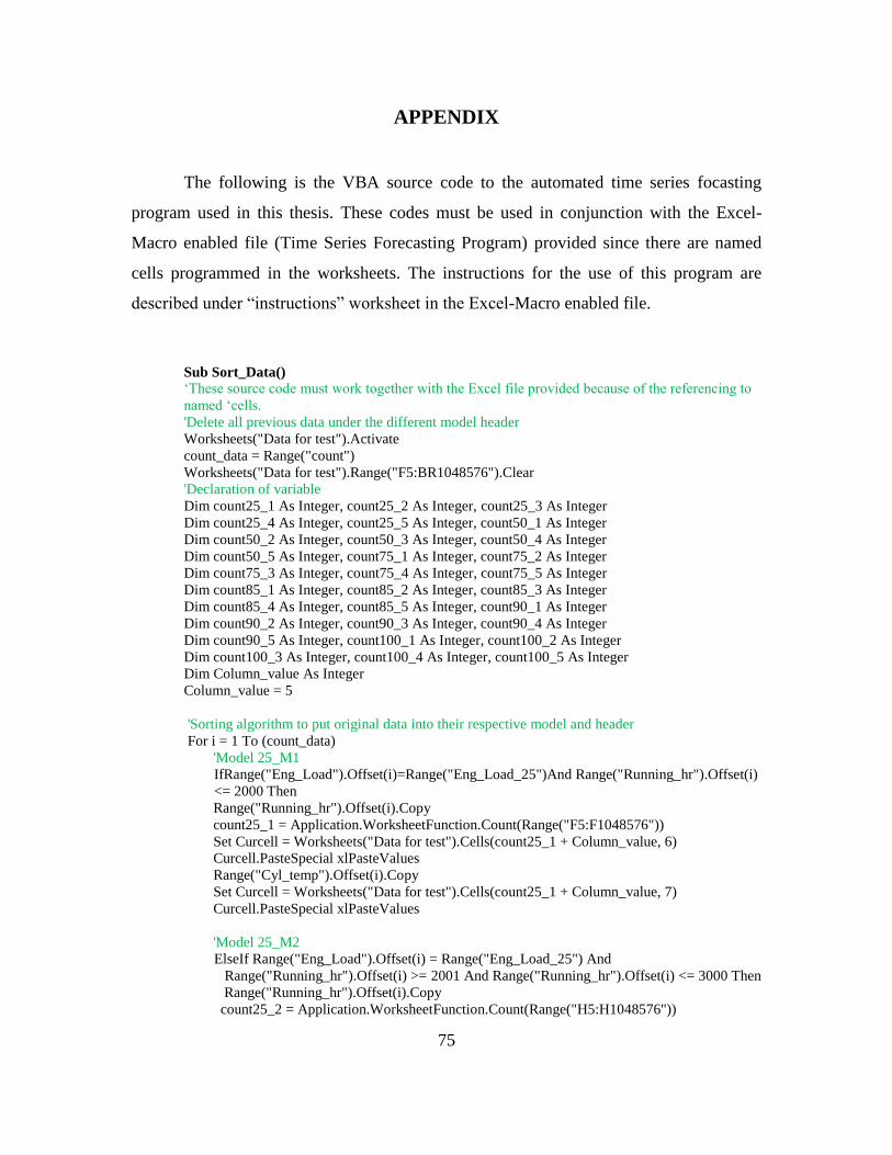
75

APPENDIX

The following is the VBA source code to the automated time series focasting

program used in this thesis. These codes must be used in conjunction with the Excel-

Macro enabled file (Time Series Forecasting Program) provided since there are named

cells programmed in the worksheets. The instructions for the use of this program are

described under “instructions” worksheet in the Excel-Macro enabled file.

Sub Sort_Data()

‘These source code must work together with the Excel file provided because of the referencing to

named ‘cells.

'Delete all previous data under the different model header

Worksheets("Data for test").Activate

count_data = Range("count")

Worksheets("Data for test").Range("F5:BR1048576").Clear

'Declaration of variable

Dim count25_1 As Integer, count25_2 As Integer, count25_3 As Integer

Dim count25_4 As Integer, count25_5 As Integer, count50_1 As Integer

Dim count50_2 As Integer, count50_3 As Integer, count50_4 As Integer

Dim count50_5 As Integer, count75_1 As Integer, count75_2 As Integer

Dim count75_3 As Integer, count75_4 As Integer, count75_5 As Integer

Dim count85_1 As Integer, count85_2 As Integer, count85_3 As Integer

Dim count85_4 As Integer, count85_5 As Integer, count90_1 As Integer

Dim count90_2 As Integer, count90_3 As Integer, count90_4 As Integer

Dim count90_5 As Integer, count100_1 As Integer, count100_2 As Integer

Dim count100_3 As Integer, count100_4 As Integer, count100_5 As Integer

Dim Column_value As Integer

Column_value = 5

'Sorting algorithm to put original data into their respective model and header

For i = 1 To (count_data)

'Model 25_M1

IfRange("Eng_Load").Offset(i)=Range("Eng_Load_25")And Range("Running_hr").Offset(i)

<= 2000 Then

Range("Running_hr").Offset(i).Copy

count25_1 = Application.WorksheetFunction.Count(Range("F5:F1048576"))

Set Curcell = Worksheets("Data for test").Cells(count25_1 + Column_value, 6)

Curcell.PasteSpecial xlPasteValues

Range("Cyl_temp").Offset(i).Copy

Set Curcell = Worksheets("Data for test").Cells(count25_1 + Column_value, 7)

Curcell.PasteSpecial xlPasteValues

'Model 25_M2

ElseIf Range("Eng_Load").Offset(i) = Range("Eng_Load_25") And

Range("Running_hr").Offset(i) >= 2001 And Range("Running_hr").Offset(i) <= 3000 Then

Range("Running_hr").Offset(i).Copy

count25_2 = Application.WorksheetFunction.Count(Range("H5:H1048576"))

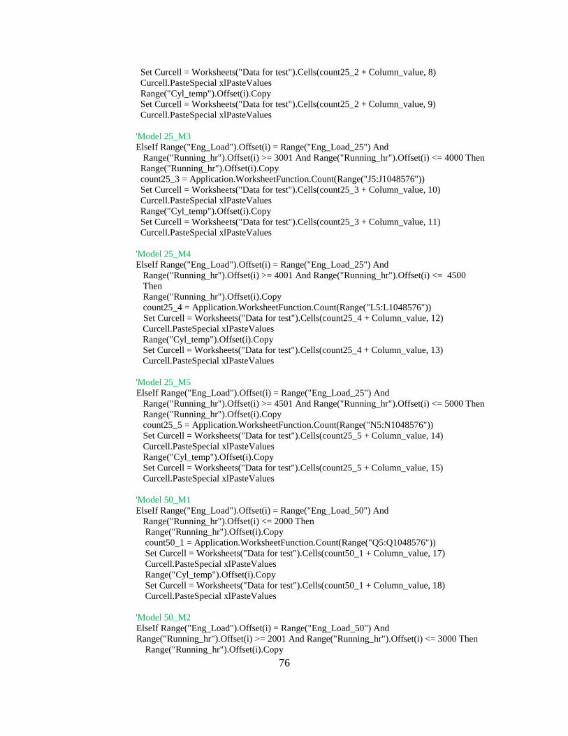
76

Set Curcell = Worksheets("Data for test").Cells(count25_2 + Column_value, 8)

Curcell.PasteSpecial xlPasteValues

Range("Cyl_temp").Offset(i).Copy

Set Curcell = Worksheets("Data for test").Cells(count25_2 + Column_value, 9)

Curcell.PasteSpecial xlPasteValues

'Model 25_M3

ElseIf Range("Eng_Load").Offset(i) = Range("Eng_Load_25") And

Range("Running_hr").Offset(i) >= 3001 And Range("Running_hr").Offset(i) <= 4000 Then

Range("Running_hr").Offset(i).Copy

count25_3 = Application.WorksheetFunction.Count(Range("J5:J1048576"))

Set Curcell = Worksheets("Data for test").Cells(count25_3 + Column_value, 10)

Curcell.PasteSpecial xlPasteValues

Range("Cyl_temp").Offset(i).Copy

Set Curcell = Worksheets("Data for test").Cells(count25_3 + Column_value, 11)

Curcell.PasteSpecial xlPasteValues

'Model 25_M4

ElseIf Range("Eng_Load").Offset(i) = Range("Eng_Load_25") And

Range("Running_hr").Offset(i) >= 4001 And Range("Running_hr").Offset(i) <= 4500

Then

Range("Running_hr").Offset(i).Copy

count25_4 = Application.WorksheetFunction.Count(Range("L5:L1048576"))

Set Curcell = Worksheets("Data for test").Cells(count25_4 + Column_value, 12)

Curcell.PasteSpecial xlPasteValues

Range("Cyl_temp").Offset(i).Copy

Set Curcell = Worksheets("Data for test").Cells(count25_4 + Column_value, 13)

Curcell.PasteSpecial xlPasteValues

'Model 25_M5

ElseIf Range("Eng_Load").Offset(i) = Range("Eng_Load_25") And

Range("Running_hr").Offset(i) >= 4501 And Range("Running_hr").Offset(i) <= 5000 Then

Range("Running_hr").Offset(i).Copy

count25_5 = Application.WorksheetFunction.Count(Range("N5:N1048576"))

Set Curcell = Worksheets("Data for test").Cells(count25_5 + Column_value, 14)

Curcell.PasteSpecial xlPasteValues

Range("Cyl_temp").Offset(i).Copy

Set Curcell = Worksheets("Data for test").Cells(count25_5 + Column_value, 15)

Curcell.PasteSpecial xlPasteValues

'Model 50_M1

ElseIf Range("Eng_Load").Offset(i) = Range("Eng_Load_50") And

Range("Running_hr").Offset(i) <= 2000 Then

Range("Running_hr").Offset(i).Copy

count50_1 = Application.WorksheetFunction.Count(Range("Q5:Q1048576"))

Set Curcell = Worksheets("Data for test").Cells(count50_1 + Column_value, 17)

Curcell.PasteSpecial xlPasteValues

Range("Cyl_temp").Offset(i).Copy

Set Curcell = Worksheets("Data for test").Cells(count50_1 + Column_value, 18)

Curcell.PasteSpecial xlPasteValues

'Model 50_M2

ElseIf Range("Eng_Load").Offset(i) = Range("Eng_Load_50") And

Range("Running_hr").Offset(i) >= 2001 And Range("Running_hr").Offset(i) <= 3000 Then

Range("Running_hr").Offset(i).Copy

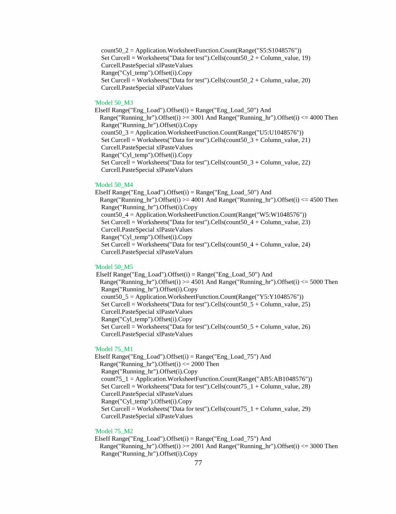
77

count50_2 = Application.WorksheetFunction.Count(Range("S5:S1048576"))

Set Curcell = Worksheets("Data for test").Cells(count50_2 + Column_value, 19)

Curcell.PasteSpecial xlPasteValues

Range("Cyl_temp").Offset(i).Copy

Set Curcell = Worksheets("Data for test").Cells(count50_2 + Column_value, 20)

Curcell.PasteSpecial xlPasteValues

'Model 50_M3

ElseIf Range("Eng_Load").Offset(i) = Range("Eng_Load_50") And

Range("Running_hr").Offset(i) >= 3001 And Range("Running_hr").Offset(i) <= 4000 Then

Range("Running_hr").Offset(i).Copy

count50_3 = Application.WorksheetFunction.Count(Range("U5:U1048576"))

Set Curcell = Worksheets("Data for test").Cells(count50_3 + Column_value, 21)

Curcell.PasteSpecial xlPasteValues

Range("Cyl_temp").Offset(i).Copy

Set Curcell = Worksheets("Data for test").Cells(count50_3 + Column_value, 22)

Curcell.PasteSpecial xlPasteValues

'Model 50_M4

ElseIf Range("Eng_Load").Offset(i) = Range("Eng_Load_50") And

Range("Running_hr").Offset(i) >= 4001 And Range("Running_hr").Offset(i) <= 4500 Then

Range("Running_hr").Offset(i).Copy

count50_4 = Application.WorksheetFunction.Count(Range("W5:W1048576"))

Set Curcell = Worksheets("Data for test").Cells(count50_4 + Column_value, 23)

Curcell.PasteSpecial xlPasteValues

Range("Cyl_temp").Offset(i).Copy

Set Curcell = Worksheets("Data for test").Cells(count50_4 + Column_value, 24)

Curcell.PasteSpecial xlPasteValues

'Model 50_M5

ElseIf Range("Eng_Load").Offset(i) = Range("Eng_Load_50") And

Range("Running_hr").Offset(i) >= 4501 And Range("Running_hr").Offset(i) <= 5000 Then

Range("Running_hr").Offset(i).Copy

count50_5 = Application.WorksheetFunction.Count(Range("Y5:Y1048576"))

Set Curcell = Worksheets("Data for test").Cells(count50_5 + Column_value, 25)

Curcell.PasteSpecial xlPasteValues

Range("Cyl_temp").Offset(i).Copy

Set Curcell = Worksheets("Data for test").Cells(count50_5 + Column_value, 26)

Curcell.PasteSpecial xlPasteValues

'Model 75_M1

ElseIf Range("Eng_Load").Offset(i) = Range("Eng_Load_75") And

Range("Running_hr").Offset(i) <= 2000 Then

Range("Running_hr").Offset(i).Copy

count75_1 = Application.WorksheetFunction.Count(Range("AB5:AB1048576"))

Set Curcell = Worksheets("Data for test").Cells(count75_1 + Column_value, 28)

Curcell.PasteSpecial xlPasteValues

Range("Cyl_temp").Offset(i).Copy

Set Curcell = Worksheets("Data for test").Cells(count75_1 + Column_value, 29)

Curcell.PasteSpecial xlPasteValues

'Model 75_M2

ElseIf Range("Eng_Load").Offset(i) = Range("Eng_Load_75") And

Range("Running_hr").Offset(i) >= 2001 And Range("Running_hr").Offset(i) <= 3000 Then

Range("Running_hr").Offset(i).Copy

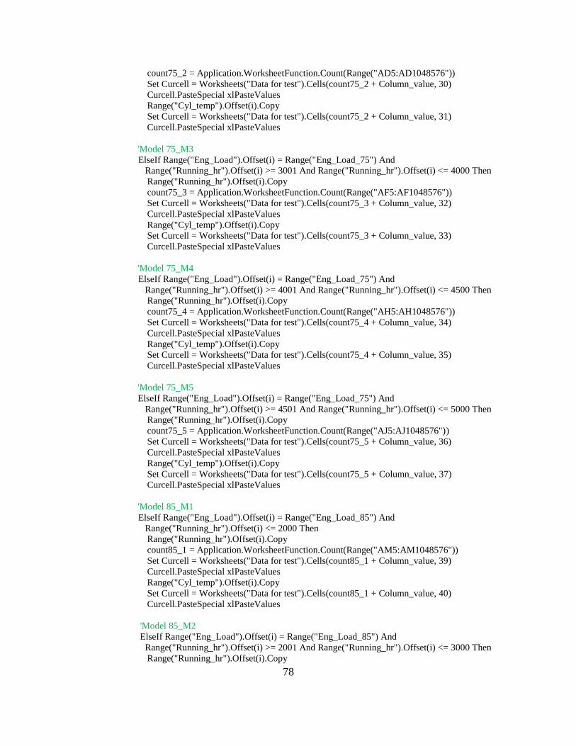
78

count75_2 = Application.WorksheetFunction.Count(Range("AD5:AD1048576"))

Set Curcell = Worksheets("Data for test").Cells(count75_2 + Column_value, 30)

Curcell.PasteSpecial xlPasteValues

Range("Cyl_temp").Offset(i).Copy

Set Curcell = Worksheets("Data for test").Cells(count75_2 + Column_value, 31)

Curcell.PasteSpecial xlPasteValues

'Model 75_M3

ElseIf Range("Eng_Load").Offset(i) = Range("Eng_Load_75") And

Range("Running_hr").Offset(i) >= 3001 And Range("Running_hr").Offset(i) <= 4000 Then

Range("Running_hr").Offset(i).Copy

count75_3 = Application.WorksheetFunction.Count(Range("AF5:AF1048576"))

Set Curcell = Worksheets("Data for test").Cells(count75_3 + Column_value, 32)

Curcell.PasteSpecial xlPasteValues

Range("Cyl_temp").Offset(i).Copy

Set Curcell = Worksheets("Data for test").Cells(count75_3 + Column_value, 33)

Curcell.PasteSpecial xlPasteValues

'Model 75_M4

ElseIf Range("Eng_Load").Offset(i) = Range("Eng_Load_75") And

Range("Running_hr").Offset(i) >= 4001 And Range("Running_hr").Offset(i) <= 4500 Then

Range("Running_hr").Offset(i).Copy

count75_4 = Application.WorksheetFunction.Count(Range("AH5:AH1048576"))

Set Curcell = Worksheets("Data for test").Cells(count75_4 + Column_value, 34)

Curcell.PasteSpecial xlPasteValues

Range("Cyl_temp").Offset(i).Copy

Set Curcell = Worksheets("Data for test").Cells(count75_4 + Column_value, 35)

Curcell.PasteSpecial xlPasteValues

'Model 75_M5

ElseIf Range("Eng_Load").Offset(i) = Range("Eng_Load_75") And

Range("Running_hr").Offset(i) >= 4501 And Range("Running_hr").Offset(i) <= 5000 Then

Range("Running_hr").Offset(i).Copy

count75_5 = Application.WorksheetFunction.Count(Range("AJ5:AJ1048576"))

Set Curcell = Worksheets("Data for test").Cells(count75_5 + Column_value, 36)

Curcell.PasteSpecial xlPasteValues

Range("Cyl_temp").Offset(i).Copy

Set Curcell = Worksheets("Data for test").Cells(count75_5 + Column_value, 37)

Curcell.PasteSpecial xlPasteValues

'Model 85_M1

ElseIf Range("Eng_Load").Offset(i) = Range("Eng_Load_85") And

Range("Running_hr").Offset(i) <= 2000 Then

Range("Running_hr").Offset(i).Copy

count85_1 = Application.WorksheetFunction.Count(Range("AM5:AM1048576"))

Set Curcell = Worksheets("Data for test").Cells(count85_1 + Column_value, 39)

Curcell.PasteSpecial xlPasteValues

Range("Cyl_temp").Offset(i).Copy

Set Curcell = Worksheets("Data for test").Cells(count85_1 + Column_value, 40)

Curcell.PasteSpecial xlPasteValues

'Model 85_M2

ElseIf Range("Eng_Load").Offset(i) = Range("Eng_Load_85") And

Range("Running_hr").Offset(i) >= 2001 And Range("Running_hr").Offset(i) <= 3000 Then

Range("Running_hr").Offset(i).Copy

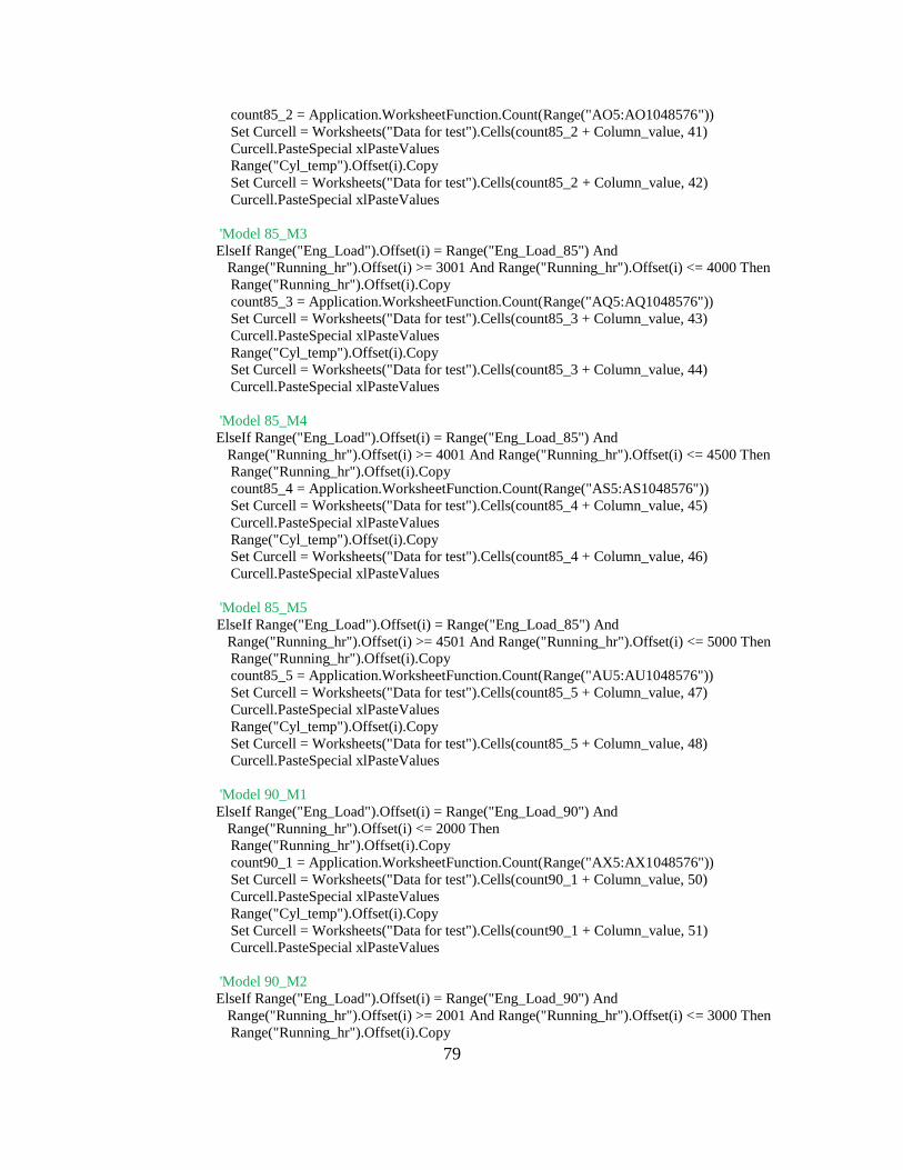
79

count85_2 = Application.WorksheetFunction.Count(Range("AO5:AO1048576"))

Set Curcell = Worksheets("Data for test").Cells(count85_2 + Column_value, 41)

Curcell.PasteSpecial xlPasteValues

Range("Cyl_temp").Offset(i).Copy

Set Curcell = Worksheets("Data for test").Cells(count85_2 + Column_value, 42)

Curcell.PasteSpecial xlPasteValues

'Model 85_M3

ElseIf Range("Eng_Load").Offset(i) = Range("Eng_Load_85") And

Range("Running_hr").Offset(i) >= 3001 And Range("Running_hr").Offset(i) <= 4000 Then

Range("Running_hr").Offset(i).Copy

count85_3 = Application.WorksheetFunction.Count(Range("AQ5:AQ1048576"))

Set Curcell = Worksheets("Data for test").Cells(count85_3 + Column_value, 43)

Curcell.PasteSpecial xlPasteValues

Range("Cyl_temp").Offset(i).Copy

Set Curcell = Worksheets("Data for test").Cells(count85_3 + Column_value, 44)

Curcell.PasteSpecial xlPasteValues

'Model 85_M4

ElseIf Range("Eng_Load").Offset(i) = Range("Eng_Load_85") And

Range("Running_hr").Offset(i) >= 4001 And Range("Running_hr").Offset(i) <= 4500 Then

Range("Running_hr").Offset(i).Copy

count85_4 = Application.WorksheetFunction.Count(Range("AS5:AS1048576"))

Set Curcell = Worksheets("Data for test").Cells(count85_4 + Column_value, 45)

Curcell.PasteSpecial xlPasteValues

Range("Cyl_temp").Offset(i).Copy

Set Curcell = Worksheets("Data for test").Cells(count85_4 + Column_value, 46)

Curcell.PasteSpecial xlPasteValues

'Model 85_M5

ElseIf Range("Eng_Load").Offset(i) = Range("Eng_Load_85") And

Range("Running_hr").Offset(i) >= 4501 And Range("Running_hr").Offset(i) <= 5000 Then

Range("Running_hr").Offset(i).Copy

count85_5 = Application.WorksheetFunction.Count(Range("AU5:AU1048576"))

Set Curcell = Worksheets("Data for test").Cells(count85_5 + Column_value, 47)

Curcell.PasteSpecial xlPasteValues

Range("Cyl_temp").Offset(i).Copy

Set Curcell = Worksheets("Data for test").Cells(count85_5 + Column_value, 48)

Curcell.PasteSpecial xlPasteValues

'Model 90_M1

ElseIf Range("Eng_Load").Offset(i) = Range("Eng_Load_90") And

Range("Running_hr").Offset(i) <= 2000 Then

Range("Running_hr").Offset(i).Copy

count90_1 = Application.WorksheetFunction.Count(Range("AX5:AX1048576"))

Set Curcell = Worksheets("Data for test").Cells(count90_1 + Column_value, 50)

Curcell.PasteSpecial xlPasteValues

Range("Cyl_temp").Offset(i).Copy

Set Curcell = Worksheets("Data for test").Cells(count90_1 + Column_value, 51)

Curcell.PasteSpecial xlPasteValues

'Model 90_M2

ElseIf Range("Eng_Load").Offset(i) = Range("Eng_Load_90") And

Range("Running_hr").Offset(i) >= 2001 And Range("Running_hr").Offset(i) <= 3000 Then

Range("Running_hr").Offset(i).Copy

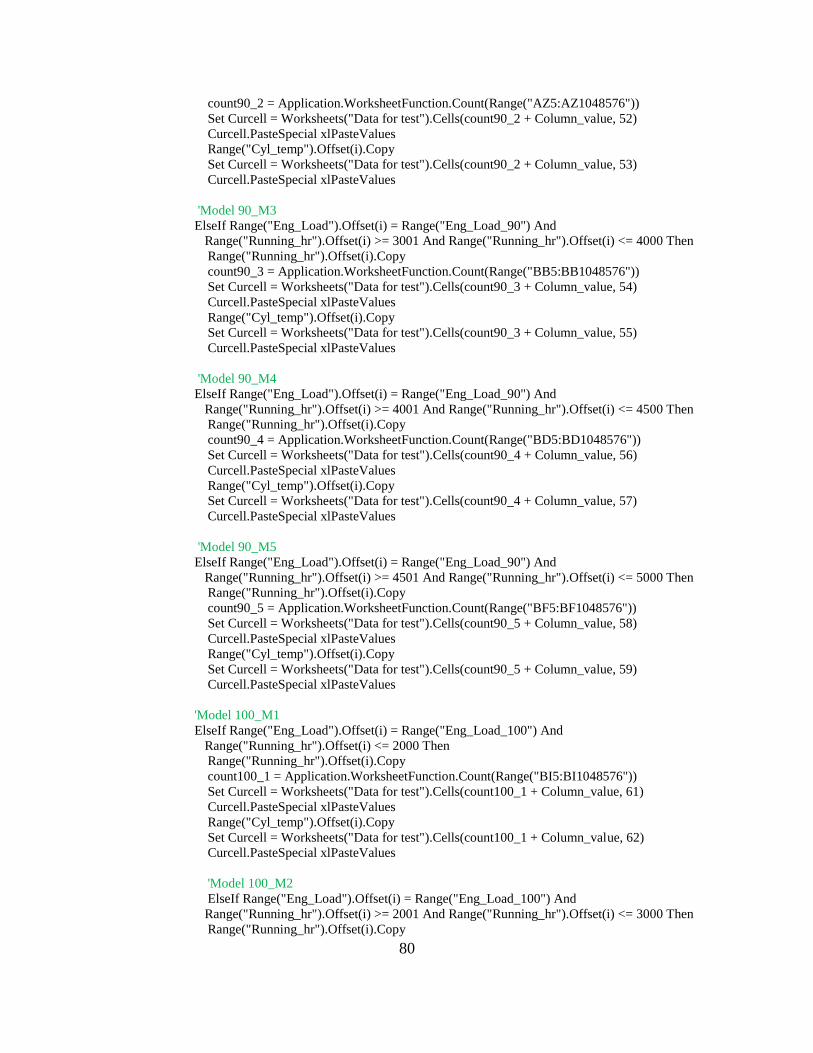
80

count90_2 = Application.WorksheetFunction.Count(Range("AZ5:AZ1048576"))

Set Curcell = Worksheets("Data for test").Cells(count90_2 + Column_value, 52)

Curcell.PasteSpecial xlPasteValues

Range("Cyl_temp").Offset(i).Copy

Set Curcell = Worksheets("Data for test").Cells(count90_2 + Column_value, 53)

Curcell.PasteSpecial xlPasteValues

'Model 90_M3

ElseIf Range("Eng_Load").Offset(i) = Range("Eng_Load_90") And

Range("Running_hr").Offset(i) >= 3001 And Range("Running_hr").Offset(i) <= 4000 Then

Range("Running_hr").Offset(i).Copy

count90_3 = Application.WorksheetFunction.Count(Range("BB5:BB1048576"))

Set Curcell = Worksheets("Data for test").Cells(count90_3 + Column_value, 54)

Curcell.PasteSpecial xlPasteValues

Range("Cyl_temp").Offset(i).Copy

Set Curcell = Worksheets("Data for test").Cells(count90_3 + Column_value, 55)

Curcell.PasteSpecial xlPasteValues

'Model 90_M4

ElseIf Range("Eng_Load").Offset(i) = Range("Eng_Load_90") And

Range("Running_hr").Offset(i) >= 4001 And Range("Running_hr").Offset(i) <= 4500 Then

Range("Running_hr").Offset(i).Copy

count90_4 = Application.WorksheetFunction.Count(Range("BD5:BD1048576"))

Set Curcell = Worksheets("Data for test").Cells(count90_4 + Column_value, 56)

Curcell.PasteSpecial xlPasteValues

Range("Cyl_temp").Offset(i).Copy

Set Curcell = Worksheets("Data for test").Cells(count90_4 + Column_value, 57)

Curcell.PasteSpecial xlPasteValues

'Model 90_M5

ElseIf Range("Eng_Load").Offset(i) = Range("Eng_Load_90") And

Range("Running_hr").Offset(i) >= 4501 And Range("Running_hr").Offset(i) <= 5000 Then

Range("Running_hr").Offset(i).Copy

count90_5 = Application.WorksheetFunction.Count(Range("BF5:BF1048576"))

Set Curcell = Worksheets("Data for test").Cells(count90_5 + Column_value, 58)

Curcell.PasteSpecial xlPasteValues

Range("Cyl_temp").Offset(i).Copy

Set Curcell = Worksheets("Data for test").Cells(count90_5 + Column_value, 59)

Curcell.PasteSpecial xlPasteValues

'Model 100_M1

ElseIf Range("Eng_Load").Offset(i) = Range("Eng_Load_100") And

Range("Running_hr").Offset(i) <= 2000 Then

Range("Running_hr").Offset(i).Copy

count100_1 = Application.WorksheetFunction.Count(Range("BI5:BI1048576"))

Set Curcell = Worksheets("Data for test").Cells(count100_1 + Column_value, 61)

Curcell.PasteSpecial xlPasteValues

Range("Cyl_temp").Offset(i).Copy

Set Curcell = Worksheets("Data for test").Cells(count100_1 + Column_value, 62)

Curcell.PasteSpecial xlPasteValues

'Model 100_M2

ElseIf Range("Eng_Load").Offset(i) = Range("Eng_Load_100") And

Range("Running_hr").Offset(i) >= 2001 And Range("Running_hr").Offset(i) <= 3000 Then

Range("Running_hr").Offset(i).Copy

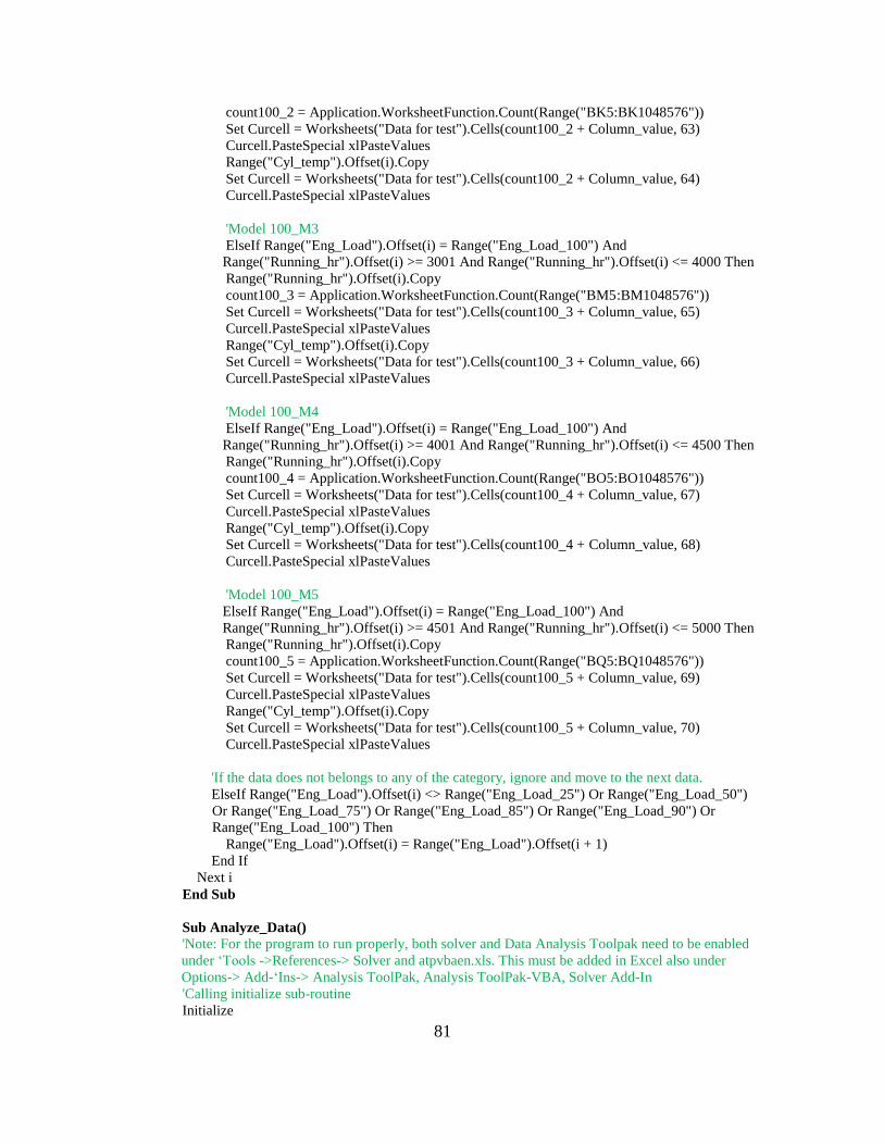
81

count100_2 = Application.WorksheetFunction.Count(Range("BK5:BK1048576"))

Set Curcell = Worksheets("Data for test").Cells(count100_2 + Column_value, 63)

Curcell.PasteSpecial xlPasteValues

Range("Cyl_temp").Offset(i).Copy

Set Curcell = Worksheets("Data for test").Cells(count100_2 + Column_value, 64)

Curcell.PasteSpecial xlPasteValues

'Model 100_M3

ElseIf Range("Eng_Load").Offset(i) = Range("Eng_Load_100") And

Range("Running_hr").Offset(i) >= 3001 And Range("Running_hr").Offset(i) <= 4000 Then

Range("Running_hr").Offset(i).Copy

count100_3 = Application.WorksheetFunction.Count(Range("BM5:BM1048576"))

Set Curcell = Worksheets("Data for test").Cells(count100_3 + Column_value, 65)

Curcell.PasteSpecial xlPasteValues

Range("Cyl_temp").Offset(i).Copy

Set Curcell = Worksheets("Data for test").Cells(count100_3 + Column_value, 66)

Curcell.PasteSpecial xlPasteValues

'Model 100_M4

ElseIf Range("Eng_Load").Offset(i) = Range("Eng_Load_100") And

Range("Running_hr").Offset(i) >= 4001 And Range("Running_hr").Offset(i) <= 4500 Then

Range("Running_hr").Offset(i).Copy

count100_4 = Application.WorksheetFunction.Count(Range("BO5:BO1048576"))

Set Curcell = Worksheets("Data for test").Cells(count100_4 + Column_value, 67)

Curcell.PasteSpecial xlPasteValues

Range("Cyl_temp").Offset(i).Copy

Set Curcell = Worksheets("Data for test").Cells(count100_4 + Column_value, 68)

Curcell.PasteSpecial xlPasteValues

'Model 100_M5

ElseIf Range("Eng_Load").Offset(i) = Range("Eng_Load_100") And

Range("Running_hr").Offset(i) >= 4501 And Range("Running_hr").Offset(i) <= 5000 Then

Range("Running_hr").Offset(i).Copy

count100_5 = Application.WorksheetFunction.Count(Range("BQ5:BQ1048576"))

Set Curcell = Worksheets("Data for test").Cells(count100_5 + Column_value, 69)

Curcell.PasteSpecial xlPasteValues

Range("Cyl_temp").Offset(i).Copy

Set Curcell = Worksheets("Data for test").Cells(count100_5 + Column_value, 70)

Curcell.PasteSpecial xlPasteValues

'If the data does not belongs to any of the category, ignore and move to the next data.

ElseIf Range("Eng_Load").Offset(i) <> Range("Eng_Load_25") Or Range("Eng_Load_50")

Or Range("Eng_Load_75") Or Range("Eng_Load_85") Or Range("Eng_Load_90") Or

Range("Eng_Load_100") Then

Range("Eng_Load").Offset(i) = Range("Eng_Load").Offset(i + 1)

End If

Next i

End Sub

Sub Analyze_Data()

'Note: For the program to run properly, both solver and Data Analysis Toolpak need to be enabled

under ‘Tools ->References-> Solver and atpvbaen.xls. This must be added in Excel also under

Options-> Add-‘Ins-> Analysis ToolPak, Analysis ToolPak-VBA, Solver Add-In

'Calling initialize sub-routine

Initialize

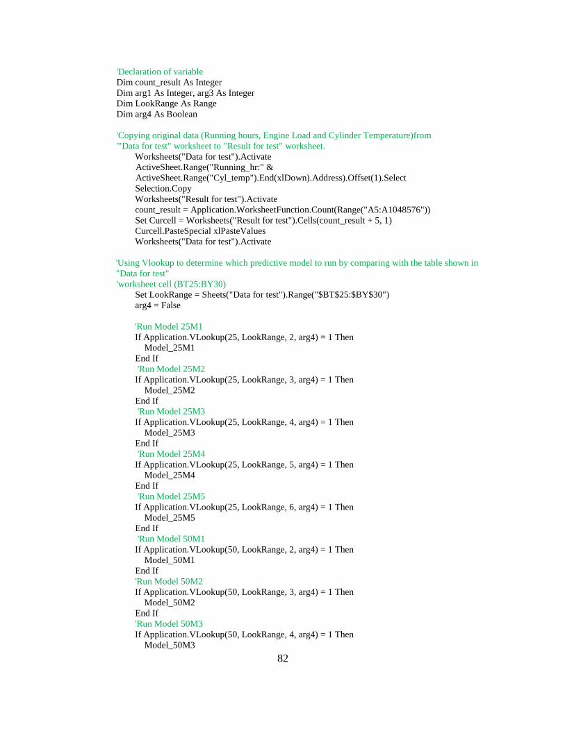
82

'Declaration of variable

Dim count_result As Integer

Dim arg1 As Integer, arg3 As Integer

Dim LookRange As Range

Dim arg4 As Boolean

'Copying original data (Running hours, Engine Load and Cylinder Temperature)from

'"Data for test" worksheet to "Result for test" worksheet.

Worksheets("Data for test").Activate

ActiveSheet.Range("Running_hr:" &

ActiveSheet.Range("Cyl_temp").End(xlDown).Address).Offset(1).Select

Selection.Copy

Worksheets("Result for test").Activate

count_result = Application.WorksheetFunction.Count(Range("A5:A1048576"))

Set Curcell = Worksheets("Result for test").Cells(count_result + 5, 1)

Curcell.PasteSpecial xlPasteValues

Worksheets("Data for test").Activate

'Using Vlookup to determine which predictive model to run by comparing with the table shown in

"Data for test"

'worksheet cell (BT25:BY30)

Set LookRange = Sheets("Data for test").Range("$BT$25:$BY$30")

arg4 = False

'Run Model 25M1

If Application.VLookup(25, LookRange, 2, arg4) = 1 Then

Model_25M1

End If

'Run Model 25M2

If Application.VLookup(25, LookRange, 3, arg4) = 1 Then

Model_25M2

End If

'Run Model 25M3

If Application.VLookup(25, LookRange, 4, arg4) = 1 Then

Model_25M3

End If

'Run Model 25M4

If Application.VLookup(25, LookRange, 5, arg4) = 1 Then

Model_25M4

End If

'Run Model 25M5

If Application.VLookup(25, LookRange, 6, arg4) = 1 Then

Model_25M5

End If

'Run Model 50M1

If Application.VLookup(50, LookRange, 2, arg4) = 1 Then

Model_50M1

End If

'Run Model 50M2

If Application.VLookup(50, LookRange, 3, arg4) = 1 Then

Model_50M2

End If

'Run Model 50M3

If Application.VLookup(50, LookRange, 4, arg4) = 1 Then

Model_50M3

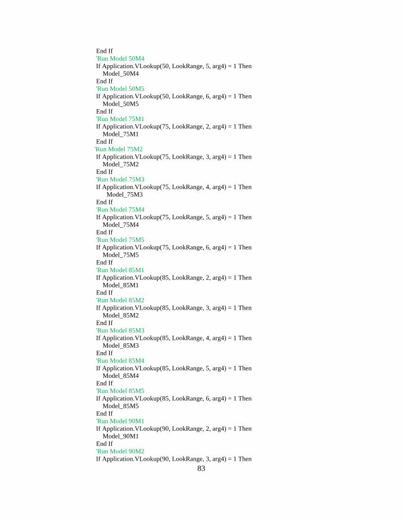
83

End If

'Run Model 50M4

If Application.VLookup(50, LookRange, 5, arg4) = 1 Then

Model_50M4

End If

'Run Model 50M5

If Application.VLookup(50, LookRange, 6, arg4) = 1 Then

Model_50M5

End If

'Run Model 75M1

If Application.VLookup(75, LookRange, 2, arg4) = 1 Then

Model_75M1

End If

'Run Model 75M2

If Application.VLookup(75, LookRange, 3, arg4) = 1 Then

Model_75M2

End If

'Run Model 75M3

If Application.VLookup(75, LookRange, 4, arg4) = 1 Then

Model_75M3

End If

'Run Model 75M4

If Application.VLookup(75, LookRange, 5, arg4) = 1 Then

Model_75M4

End If

'Run Model 75M5

If Application.VLookup(75, LookRange, 6, arg4) = 1 Then

Model_75M5

End If

'Run Model 85M1

If Application.VLookup(85, LookRange, 2, arg4) = 1 Then

Model_85M1

End If

'Run Model 85M2

If Application.VLookup(85, LookRange, 3, arg4) = 1 Then

Model_85M2

End If

'Run Model 85M3

If Application.VLookup(85, LookRange, 4, arg4) = 1 Then

Model_85M3

End If

'Run Model 85M4

If Application.VLookup(85, LookRange, 5, arg4) = 1 Then

Model_85M4

End If

'Run Model 85M5

If Application.VLookup(85, LookRange, 6, arg4) = 1 Then

Model_85M5

End If

'Run Model 90M1

If Application.VLookup(90, LookRange, 2, arg4) = 1 Then

Model_90M1

End If

'Run Model 90M2

If Application.VLookup(90, LookRange, 3, arg4) = 1 Then

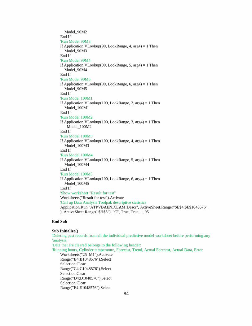
84

Model_90M2

End If

'Run Model 90M3

If Application.VLookup(90, LookRange, 4, arg4) = 1 Then

Model_90M3

End If

'Run Model 90M4

If Application.VLookup(90, LookRange, 5, arg4) = 1 Then

Model_90M4

End If

'Run Model 90M5

If Application.VLookup(90, LookRange, 6, arg4) = 1 Then

Model_90M5

End If

'Run Model 100M1

If Application.VLookup(100, LookRange, 2, arg4) = 1 Then

Model_100M1

End If

'Run Model 100M2

If Application.VLookup(100, LookRange, 3, arg4) = 1 Then

Model_100M2

End If

'Run Model 100M3

If Application.VLookup(100, LookRange, 4, arg4) = 1 Then

Model_100M3

End If

'Run Model 100M4

If Application.VLookup(100, LookRange, 5, arg4) = 1 Then

Model_100M4

End If

'Run Model 100M5

If Application.VLookup(100, LookRange, 6, arg4) = 1 Then

Model_100M5

End If

'Show worksheet "Result for test"

Worksheets("Result for test").Activate

'Call up Data Analysis Toolpak descriptive statistics

Application.Run "ATPVBAEN.XLAM!Descr", ActiveSheet.Range("$E$4:$E$1048576" _

), ActiveSheet.Range("$H$5"), "C", True, True, , , 95

End Sub

Sub Initialize()

'Deleting past records from all the individual predictive model worksheet before performing any

‘analysis.

'Data that are cleared belongs to the following header:

'Running hours, Cylinder temperature, Forecast, Trend, Actual Forecast, Actual Data, Error

Worksheets("25_M1").Activate

Range("B4:B1048576").Select

Selection.Clear

Range("C4:C1048576").Select

Selection.Clear

Range("D4:D1048576").Select

Selection.Clear

Range("E4:E1048576").Select

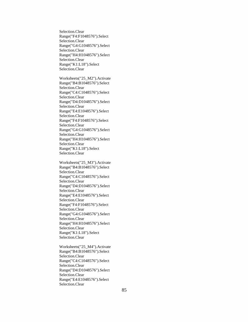
85

Selection.Clear

Range("F4:F1048576").Select

Selection.Clear

Range("G4:G1048576").Select

Selection.Clear

Range("H4:H1048576").Select

Selection.Clear

Range("K1:L18").Select

Selection.Clear

Worksheets("25_M2").Activate

Range("B4:B1048576").Select

Selection.Clear

Range("C4:C1048576").Select

Selection.Clear

Range("D4:D1048576").Select

Selection.Clear

Range("E4:E1048576").Select

Selection.Clear

Range("F4:F1048576").Select

Selection.Clear

Range("G4:G1048576").Select

Selection.Clear

Range("H4:H1048576").Select

Selection.Clear

Range("K1:L18").Select

Selection.Clear

Worksheets("25_M3").Activate

Range("B4:B1048576").Select

Selection.Clear

Range("C4:C1048576").Select

Selection.Clear

Range("D4:D1048576").Select

Selection.Clear

Range("E4:E1048576").Select

Selection.Clear

Range("F4:F1048576").Select

Selection.Clear

Range("G4:G1048576").Select

Selection.Clear

Range("H4:H1048576").Select

Selection.Clear

Range("K1:L18").Select

Selection.Clear

Worksheets("25_M4").Activate

Range("B4:B1048576").Select

Selection.Clear

Range("C4:C1048576").Select

Selection.Clear

Range("D4:D1048576").Select

Selection.Clear

Range("E4:E1048576").Select

Selection.Clear

86

Range("F4:F1048576").Select

Selection.Clear

Range("G4:G1048576").Select

Selection.Clear

Range("H4:H1048576").Select

Selection.Clear

Range("K1:L18").Select

Selection.Clear

Worksheets("25_M5").Activate

Range("B4:B1048576").Select

Selection.Clear

Range("C4:C1048576").Select

Selection.Clear

Range("D4:D1048576").Select

Selection.Clear

Range("E4:E1048576").Select

Selection.Clear

Range("F4:F1048576").Select

Selection.Clear

Range("G4:G1048576").Select

Selection.Clear

Range("H4:G1048576").Select

Selection.Clear

Range("I4:H1048576").Select

Selection.Clear

Range("K1:L18").Select

Selection.Clear

Worksheets("50_M1").Activate

Range("B4:B1048576").Select

Selection.Clear

Range("C4:C1048576").Select

Selection.Clear

Range("D4:D1048576").Select

Selection.Clear

Range("E4:E1048576").Select

Selection.Clear

Range("F4:F1048576").Select

Selection.Clear

Range("G4:G1048576").Select

Selection.Clear

Range("H4:H1048576").Select

Selection.Clear

Range("K1:L18").Select

Selection.Clear

Worksheets("50_M2").Activate

Range("B4:B1048576").Select

Selection.Clear

Range("C4:C1048576").Select

Selection.Clear

Range("D4:D1048576").Select

Selection.Clear

Range("E4:E1048576").Select

87

Selection.Clear

Range("F4:F1048576").Select

Selection.Clear

Range("G4:G1048576").Select

Selection.Clear

Range("H4:H1048576").Select

Selection.Clear

Range("K1:L18").Select

Selection.Clear

Worksheets("50_M3").Activate

Range("B4:B1048576").Select

Selection.Clear

Range("C4:C1048576").Select

Selection.Clear

Range("D4:D1048576").Select

Selection.Clear

Range("E4:E1048576").Select

Selection.Clear

Range("F4:F1048576").Select

Selection.Clear

Range("G4:G1048576").Select

Selection.Clear

Range("H4:H1048576").Select

Selection.Clear

Range("K1:L18").Select

Selection.Clear

Worksheets("50_M4").Activate

Range("B4:B1048576").Select

Selection.Clear

Range("C4:C1048576").Select

Selection.Clear

Range("D4:D1048576").Select

Selection.Clear

Range("E4:E1048576").Select

Selection.Clear

Range("F4:F1048576").Select

Selection.Clear

Range("G4:G1048576").Select

Selection.Clear

Range("H4:H1048576").Select

Selection.Clear

Range("K1:L18").Select

Selection.Clear

Worksheets("50_M5").Activate

Range("B4:B1048576").Select

Selection.Clear

Range("C4:C1048576").Select

Selection.Clear

Range("D4:D1048576").Select

Selection.Clear

Range("E4:E1048576").Select

Selection.Clear

Range("F4:F1048576").Select

88

Selection.Clear

Range("G4:G1048576").Select

Selection.Clear

Range("H4:G1048576").Select

Selection.Clear

Range("I4:H1048576").Select

Selection.Clear

Range("K1:L18").Select

Selection.Clear

Worksheets("75_M1").Activate

Range("B4:B1048576").Select

Selection.Clear

Range("C4:C1048576").Select

Selection.Clear

Range("D4:D1048576").Select

Selection.Clear

Range("E4:E1048576").Select

Selection.Clear

Range("F4:F1048576").Select

Selection.Clear

Range("G4:G1048576").Select

Selection.Clear

Range("H4:H1048576").Select

Selection.Clear

Range("K1:L18").Select

Selection.Clear

Worksheets("75_M2").Activate

Range("B4:B1048576").Select

Selection.Clear

Range("C4:C1048576").Select

Selection.Clear

Range("D4:D1048576").Select

Selection.Clear

Range("E4:E1048576").Select

Selection.Clear

Range("F4:F1048576").Select

Selection.Clear

Range("G4:G1048576").Select

Selection.Clear

Range("H4:H1048576").Select

Selection.Clear

Range("K1:L18").Select

Selection.Clear

Worksheets("75_M3").Activate

Range("B4:B1048576").Select

Selection.Clear

Range("C4:C1048576").Select

Selection.Clear

Range("D4:D1048576").Select

Selection.Clear

Range("E4:E1048576").Select

Selection.Clear

89

Range("F4:F1048576").Select

Selection.Clear

Range("G4:G1048576").Select

Selection.Clear

Range("H4:H1048576").Select

Selection.Clear

Range("K1:L18").Select

Selection.Clear

Worksheets("75_M4").Activate

Range("B4:B1048576").Select

Selection.Clear

Range("C4:C1048576").Select

Selection.Clear

Range("D4:D1048576").Select

Selection.Clear

Range("E4:E1048576").Select

Selection.Clear

Range("F4:F1048576").Select

Selection.Clear

Range("G4:G1048576").Select

Selection.Clear

Range("H4:H1048576").Select

Selection.Clear

Range("K1:L18").Select

Selection.Clear

Worksheets("75_M5").Activate

Range("B4:B1048576").Select

Selection.Clear

Range("C4:C1048576").Select

Selection.Clear

Range("D4:D1048576").Select

Selection.Clear

Range("E4:E1048576").Select

Selection.Clear

Range("F4:F1048576").Select

Selection.Clear

Range("G4:G1048576").Select

Selection.Clear

Range("H4:G1048576").Select

Selection.Clear

Range("I4:H1048576").Select

Selection.Clear

Range("K1:L18").Select

Selection.Clear

Worksheets("85_M1").Activate

Range("B4:B1048576").Select

Selection.Clear

Range("C4:C1048576").Select

Selection.Clear

Range("D4:D1048576").Select

Selection.Clear

Range("E4:E1048576").Select

90

Selection.Clear

Range("F4:F1048576").Select

Selection.Clear

Range("G4:G1048576").Select

Selection.Clear

Range("H4:H1048576").Select

Selection.Clear

Range("K1:L18").Select

Selection.Clear

Worksheets("85_M2").Activate

Range("B4:B1048576").Select

Selection.Clear

Range("C4:C1048576").Select

Selection.Clear

Range("D4:D1048576").Select

Selection.Clear

Range("E4:E1048576").Select

Selection.Clear

Range("F4:F1048576").Select

Selection.Clear

Range("G4:G1048576").Select

Selection.Clear

Range("H4:H1048576").Select

Selection.Clear

Range("K1:L18").Select

Selection.Clear

Worksheets("85_M3").Activate

Range("B4:B1048576").Select

Selection.Clear

Range("C4:C1048576").Select

Selection.Clear

Range("D4:D1048576").Select

Selection.Clear

Range("E4:E1048576").Select

Selection.Clear

Range("F4:F1048576").Select

Selection.Clear

Range("G4:G1048576").Select

Selection.Clear

Range("H4:H1048576").Select

Selection.Clear

Range("K1:L18").Select

Selection.Clear

Worksheets("85_M4").Activate

Range("B4:B1048576").Select

Selection.Clear

Range("C4:C1048576").Select

Selection.Clear

Range("D4:D1048576").Select

Selection.Clear

Range("E4:E1048576").Select

Selection.Clear

91

Range("F4:F1048576").Select

Selection.Clear

Range("G4:G1048576").Select

Selection.Clear

Range("H4:H1048576").Select

Selection.Clear

Range("K1:L18").Select

Selection.Clear

Worksheets("85_M5").Activate

Range("B4:B1048576").Select

Selection.Clear

Range("C4:C1048576").Select

Selection.Clear

Range("D4:D1048576").Select

Selection.Clear

Range("E4:E1048576").Select

Selection.Clear

Range("F4:F1048576").Select

Selection.Clear

Range("G4:G1048576").Select

Selection.Clear

Range("H4:G1048576").Select

Selection.Clear

Range("I4:H1048576").Select

Selection.Clear

Range("K1:L18").Select

Selection.Clear

Worksheets("90_M1").Activate

Range("B4:B1048576").Select

Selection.Clear

Range("C4:C1048576").Select

Selection.Clear

Range("D4:D1048576").Select

Selection.Clear

Range("E4:E1048576").Select

Selection.Clear

Range("F4:F1048576").Select

Selection.Clear

Range("G4:G1048576").Select

Selection.Clear

Range("H4:H1048576").Select

Selection.Clear

Range("K1:L18").Select

Selection.Clear

Worksheets("90_M2").Activate

Range("B4:B1048576").Select

Selection.Clear

Range("C4:C1048576").Select

Selection.Clear

Range("D4:D1048576").Select

Selection.Clear

Range("E4:E1048576").Select

92

Selection.Clear

Range("F4:F1048576").Select

Selection.Clear

Range("G4:G1048576").Select

Selection.Clear

Range("H4:H1048576").Select

Selection.Clear

Range("K1:L18").Select

Selection.Clear

Worksheets("90_M3").Activate

Range("B4:B1048576").Select

Selection.Clear

Range("C4:C1048576").Select

Selection.Clear

Range("D4:D1048576").Select

Selection.Clear

Range("E4:E1048576").Select

Selection.Clear

Range("F4:F1048576").Select

Selection.Clear

Range("G4:G1048576").Select

Selection.Clear

Range("H4:H1048576").Select

Selection.Clear

Range("K1:L18").Select

Selection.Clear

Worksheets("90_M4").Activate

Range("B4:B1048576").Select

Selection.Clear

Range("C4:C1048576").Select

Selection.Clear

Range("D4:D1048576").Select

Selection.Clear

Range("E4:E1048576").Select

Selection.Clear

Range("F4:F1048576").Select

Selection.Clear

Range("G4:G1048576").Select

Selection.Clear

Range("H4:H1048576").Select

Selection.Clear

Range("K1:L18").Select

Selection.Clear

Worksheets("90_M5").Activate

Range("B4:B1048576").Select

Selection.Clear

Range("C4:C1048576").Select

Selection.Clear

Range("D4:D1048576").Select

Selection.Clear

Range("E4:E1048576").Select

Selection.Clear

93

Range("F4:F1048576").Select

Selection.Clear

Range("G4:G1048576").Select

Selection.Clear

Range("H4:G1048576").Select

Selection.Clear

Range("I4:H1048576").Select

Selection.Clear

Range("K1:L18").Select

Selection.Clear

Worksheets("100_M1").Activate

Range("B4:B1048576").Select

Selection.Clear

Range("C4:C1048576").Select

Selection.Clear

Range("D4:D1048576").Select

Selection.Clear

Range("E4:E1048576").Select

Selection.Clear

Range("F4:F1048576").Select

Selection.Clear

Range("G4:G1048576").Select

Selection.Clear

Range("H4:H1048576").Select

Selection.Clear

Range("K1:L18").Select

Selection.Clear

Worksheets("100_M2").Activate

Range("B4:B1048576").Select

Selection.Clear

Range("C4:C1048576").Select

Selection.Clear

Range("D4:D1048576").Select

Selection.Clear

Range("E4:E1048576").Select

Selection.Clear

Range("F4:F1048576").Select

Selection.Clear

Range("G4:G1048576").Select

Selection.Clear

Range("H4:H1048576").Select

Selection.Clear

Range("K1:L18").Select

Selection.Clear

Worksheets("100_M3").Activate

Range("B4:B1048576").Select

Selection.Clear

Range("C4:C1048576").Select

Selection.Clear

Range("D4:D1048576").Select

Selection.Clear

Range("E4:E1048576").Select

94

Selection.Clear

Range("F4:F1048576").Select

Selection.Clear

Range("G4:G1048576").Select

Selection.Clear

Range("H4:H1048576").Select

Selection.Clear

Range("K1:L18").Select

Selection.Clear

Worksheets("100_M4").Activate

Range("B4:B1048576").Select

Selection.Clear

Range("C4:C1048576").Select

Selection.Clear

Range("D4:D1048576").Select

Selection.Clear

Range("E4:E1048576").Select

Selection.Clear

Range("F4:F1048576").Select

Selection.Clear

Range("G4:G1048576").Select

Selection.Clear

Range("H4:H1048576").Select

Selection.Clear

Range("K1:L18").Select

Selection.Clear

Worksheets("100_M5").Activate

Range("B4:B1048576").Select

Selection.Clear

Range("C4:C1048576").Select

Selection.Clear

Range("D4:D1048576").Select

Selection.Clear

Range("E4:E1048576").Select

Selection.Clear

Range("F4:F1048576").Select

Selection.Clear

Range("G4:G1048576").Select

Selection.Clear

Range("H4:G1048576").Select

Selection.Clear

Range("I4:H1048576").Select

Selection.Clear

Range("K1:L18").Select

Selection.Clear

'Deleting past records from the Result for test worksheet before performing any analysis.

'Data that are cleared belongs to the following header:

'Running hours, Engine Load, Actual EGT, Actual Forecast, Error

Worksheets("Result for test").Activate

Range("A5:A1048576").Select

Selection.Clear

Worksheets("Result for test").Activate

95

Range("B5:B1048576").Select

Selection.Clear

Worksheets("Result for test").Activate

Range("C5:C1048576").Select

Selection.Clear

Worksheets("Result for test").Activate

Range("D5:D1048576").Select

Selection.Clear

Worksheets("Result for test").Activate

Range("H1:I21").Select

Selection.Clear

End Sub

Sub Model_25M1()

'Model_25M1 is the predictive model for 25% Main Engine Load with running hours from 1-

‘2000.

'Declaration of variables

Dim count25_M1 As Integer

Dim count_result As Integer

Dim Column_value As Integer

Dim count_pos As Integer

Dim arg1 As Integer, arg3 As Integer

Dim LookRange As Range

Dim arg4 As Boolean

'Column value is used to control cell position for data to be input or extract

Column_value = 4

'Copy original data from "Data for test" worksheet to "25_M1" worksheet for model analysis.

Worksheets("Data for test").Activate

ActiveSheet.Range("Run_25M1:" &

ActiveSheet.Range("Temp_25M1").End(xlDown).Address).Offset(1).Select

Selection.Copy

Worksheets("25_M1").Activate

count25_M1 = Application.WorksheetFunction.Count(Range("B4:B1048576"))

Set Curcell = Worksheets("25_M1").Cells(count25_M1 + Column_value, 2)

Curcell.PasteSpecial xlPasteValues

'Set the first forecast value to be the same as the first cylinder temperature value.

Range("Forecast").Offset(1).Formula = "=C4"

'Set the trend to be zero since there is no previous data for trend.

Range("Trend").Offset(1) = 0

'The Actual Forecast will be the sum of Forecast and Trend.

Range("AF").Offset(1).Formula = "=D4+E4"

'The Actual Data will be copied over from the data in cylinder temperature cell.

Range("AD").Offset(1).Formula = "=C4"

'The error is the difference between Actual Data and Actual Forecast.

Range("Error").Offset(1).Formula = "=G4-F4"

'count_data1 is used to control cell position for data to be input or extract

count_data1 = Range("count25M1_80").Value - 1

'The Forecast is the result of Alpha*past cylinder temp + (1-Alpha)*Actual Forecast

Range("Forecast").Offset(2).Formula = "= $I$1 * C4 + (1 -$I$1 ) * F4"

'The trend is the result of Beta * Difference of past forecast + (1-Beta)*Previous Trend

Range("Trend").Offset(2).Formula = "=$I$2 * (D5-D4)+ (1 - $I$2) * E4"

96

'The Actual Forecast will be the sum of Forecast and Trend.

Range("AF").Offset(2).Formula = "= D5 + E5"

'The Actual Data will be copied over from the data in cylinder temperature cell.

Range("AD").Offset(2).Formula = "=C5"

'The error is the difference between Actual Data and Actual Forecast.

Range("Error").Offset(2).Formula = "= G5 -F5"

'Counting the position of the last data cell

LR = Range("count25M1").Value + 3

'Copy the formula from 2nd row of the cells which contains data to end of the data.

Range("D5:H5").AutoFill Destination:=Range("D5:H" & LR)

'This set of data is used for validation purpose. It will highlight the cell in yellow.

'It copy the previous Actual Forcast value to the new forecast cell. This will repeat till end of

‘data and

'then used to validate the goodness of fit for the model.

Range("Forecast").Offset(count_data1 + 2).Value = "=F" & (count_data1 + 4)

Range("Forecast").Offset(count_data1 + 2).Interior.Color = RGB(255, 255, 51)

Range("Forecast").Offset(count_data1 + 2).Select

ActiveCell.AutoFill Destination:=Range(ActiveCell.Offset(0, -1), ActiveCell.Offset(0, -

1).End(xlDown)).Offset(0, 1)

'Call up Solver tool to obtain minumum value of MSE, and set the Alpha and Beta Values.

solversolve userfinish:=True

'Call up Data Analysis Toolpak descriptive statistics

Application.Run "ATPVBAEN.XLAM!Descr", ActiveSheet.Range("$H$3:$H$1048576" _

), ActiveSheet.Range("$K$1"), "C", True, True, , , 95

'Copying the Actual Forcast result from the model to the "Result for test" worksheet

Worksheets("Result for test").Activate

count_result = Application.WorksheetFunction.Count(Range("A5:A1048576"))

count_pos = Application.WorksheetFunction.Count(Range("D5:D1048576"))

For i = 1 To (count_result - count_pos)

Set LookRange = Sheets("25_M1").Range("B4:F1048576")

arg4 = False

x = ActiveSheet.Range("Result_Running_hr").Offset(count_pos + i).Value

Range("Result_Forecast").Offset(count_pos + i) = Application.VLookup(x, LookRange, 5,

arg4)

Next i

Worksheets("Data for test").Activate

End Sub

Sub Model_25M2()

'Model_25M2 is the predictive model for 25% Main Engine Load with running hours from 2001-

‘3000.

'Declaration of variables

Dim count25_M2 As Integer

Dim count_result As Integer

Dim Column_value As Integer

Dim count_pos As Integer

Dim arg1 As Integer, arg3 As Integer

Dim LookRange As Range

Dim arg4 As Boolean

'Column value is used to control cell position for data to be input or extract

97

Column_value = 4

'Copy original data from "Data for test" worksheet to "25_M2" worksheet for model analysis.

Worksheets("Data for test").Activate

ActiveSheet.Range("Run_25M2:" &

ActiveSheet.Range("Temp_25M2").End(xlDown).Address).Offset(1).Select

Selection.Copy

Worksheets("25_M2").Activate

count25_M2 = Application.WorksheetFunction.Count(Range("B4:B1048576"))

Set Curcell = Worksheets("25_M2").Cells(count25_M2 + Column_value, 2)

Curcell.PasteSpecial xlPasteValues

'Set the first forecast value to be the same as the first cylinder temperature value.

Range("Forecast_25M2").Offset(1).Formula = "=C4"

'Set the trend to be zero since there is no previous data for trend.

Range("Trend_25M2").Offset(1) = 0

'The Actual Forecast will be the sum of Forecast and Trend.

Range("AF_25M2").Offset(1).Formula = "=D4+E4"

'The Actual Data will be copied over from the data in cylinder temperature cell.

Range("AD_25M2").Offset(1).Formula = "=C4"

'The error is the difference between Actual Data and Actual Forecast.

Range("Error_25M2").Offset(1).Formula = "=G4-F4"

'count_data1 is used to control cell position for data to be input or extract

count_data1 = Range("count25M2_80").Value - 1

'The Forecast is the result of Alpha*past cylinder temp + (1-Alpha)*Actual Forecast

Range("Forecast_25M2").Offset(2).Formula = "= $I$1 * C4 + (1 -$I$1 ) * F4"

'The trend is the result of Beta * Difference of past forecast + (1-Beta)*Previous Trend

Range("Trend_25M2").Offset(2).Formula = "=$I$2 * (D5-D4)+ (1 - $I$2) * E4"

'The Actual Forecast will be the sum of Forecast and Trend.

Range("AF_25M2").Offset(2).Formula = "= D5 + E5"

'The Actual Data will be copied over from the data in cylinder temperature cell.

Range("AD_25M2").Offset(2).Formula = "=C5"

'The error is the difference between Actual Data and Actual Forecast.

Range("Error_25M2").Offset(2).Formula = "= G5 -F5"

'Counting the position of the last data cell

LR = Range("count25M2").Value + 3

'Copy the formula from 2nd row of the cells which contains data to end of the data.

Range("D5:H5").AutoFill Destination:=Range("D5:H" & LR)

'This set of data is used for validation purpose. It will highlight the cell in yellow.

'It copy the previous Actual Forcast value to the new forecast cell. This will repeat till end of

‘data and

'then used to validate the goodness of fit for the model.

Range("Forecast_25M2").Offset(count_data1 + 2).Value = "=F" & (count_data1 + 4)

Range("Forecast_25M2").Offset(count_data1 + 2).Interior.Color = RGB(255, 255, 51)

Range("Forecast_25M2").Offset(count_data1 + 2).Select

ActiveCell.AutoFill Destination:=Range(ActiveCell.Offset(0, -1), ActiveCell.Offset(0, -

1).End(xlDown)).Offset(0, 1)

'Call up Solver tool to obtain minumum value of MSE, and set the Alpha and Beta Values.

solversolve userfinish:=True

'Call up Data Analysis Toolpak descriptive statistics

Application.Run "ATPVBAEN.XLAM!Descr", ActiveSheet.Range("$H$3:$H$1048576" _

98

), ActiveSheet.Range("$K$1"), "C", True, True, , , 95

'Copying the Actual Forcast result from the model to the "Result for test" worksheet

Worksheets("Result for test").Activate

count_result = Application.WorksheetFunction.Count(Range("A5:A1048576"))

count_pos = Application.WorksheetFunction.Count(Range("D5:D1048576"))

For i = 1 To (count_result - count_pos)

Set LookRange = Sheets("25_M2").Range("B4:F1048576")

arg4 = False

x = ActiveSheet.Range("Result_Running_hr").Offset(count_pos + i).Value

Range("Result_Forecast").Offset(count_pos + i) = Application.VLookup(x, LookRange, 5,

arg4)

Next i

Worksheets("Data for test").Activate

End Sub

Sub Model_25M3()

'Model_25M3 is the predictive model for 25% Main Engine Load with running hours from 3001-

‘4000.

'Declaration of variables

Dim count25_M3 As Integer

Dim count_result As Integer

Dim Column_value As Integer

Dim count_pos As Integer

Dim arg1 As Integer, arg3 As Integer

Dim LookRange As Range

Dim arg4 As Boolean

'Column value is used to control cell position for data to be input or extract

Column_value = 4

'Copy original data from "Data for test" worksheet to "25_M3" worksheet for model analysis.

Worksheets("Data for test").Activate

ActiveSheet.Range("Run_25M3:" &

ActiveSheet.Range("Temp_25M3").End(xlDown).Address).Offset(1).Select

Selection.Copy

Worksheets("25_M3").Activate

count25_M3 = Application.WorksheetFunction.Count(Range("B4:B1048576"))

Set Curcell = Worksheets("25_M3").Cells(count25_M3 + Column_value, 2)

Curcell.PasteSpecial xlPasteValues

'Set the first forecast value to be the same as the first cylinder temperature value.

Range("Forecast_25M3").Offset(1).Formula = "=C4"

'Set the trend to be zero since there is no previous data for trend.

Range("Trend_25M3").Offset(1) = 0

'The Actual Forecast will be the sum of Forecast and Trend.

Range("AF_25M3").Offset(1).Formula = "=D4+E4"

'The Actual Data will be copied over from the data in cylinder temperature cell.

Range("AD_25M3").Offset(1).Formula = "=C4"

'The error is the difference between Actual Data and Actual Forecast.

Range("Error_25M3").Offset(1).Formula = "=G4-F4"

'count_data1 is used to control cell position for data to be input or extract

count_data1 = Range("count25M3_80").Value - 1

99

'The Forecast is the result of Alpha*past cylinder temp + (1-Alpha)*Actual Forecast

Range("Forecast_25M3").Offset(2).Formula = "= $I$1 * C4 + (1 -$I$1 ) * F4"

'The trend is the result of Beta * Difference of past forecast + (1-Beta)*Previous Trend

Range("Trend_25M3").Offset(2).Formula = "=$I$2 * (D5-D4)+ (1 - $I$2) * E4"

'The Actual Forecast will be the sum of Forecast and Trend.

Range("AF_25M3").Offset(2).Formula = "= D5 + E5"

'The Actual Data will be copied over from the data in cylinder temperature cell.

Range("AD_25M3").Offset(2).Formula = "=C5"

'The error is the difference between Actual Data and Actual Forecast.

Range("Error_25M3").Offset(2).Formula = "= G5 -F5"

'Counting the position of the last data cell

LR = Range("count25M3").Value + 3

'Copy the formula from 2nd row of the cells which contains data to end of the data.

Range("D5:H5").AutoFill Destination:=Range("D5:H" & LR)

'This set of data is used for validation purpose. It will highlight the cell in yellow.

'It copy the previous Actual Forcast value to the new forecast cell. This will repeat till end of

‘data and

'then used to validate the goodness of fit for the model.

Range("Forecast_25M3").Offset(count_data1 + 2).Value = "=F" & (count_data1 + 4)

Range("Forecast_25M3").Offset(count_data1 + 2).Interior.Color = RGB(255, 255, 51)

Range("Forecast_25M3").Offset(count_data1 + 2).Select

ActiveCell.AutoFill Destination:=Range(ActiveCell.Offset(0, -1), ActiveCell.Offset(0, -

1).End(xlDown)).Offset(0, 1)

'Call up Solver tool to obtain minumum value of MSE, and set the Alpha and Beta Values.

solversolve userfinish:=True

'Call up Data Analysis Toolpak descriptive statistics

Application.Run "ATPVBAEN.XLAM!Descr", ActiveSheet.Range("$H$3:$H$1048576" _

), ActiveSheet.Range("$K$1"), "C", True, True, , , 95

'Copying the Actual Forcast result from the model to the "Result for test" worksheet

Worksheets("Result for test").Activate

count_result = Application.WorksheetFunction.Count(Range("A5:A1048576"))

count_pos = Application.WorksheetFunction.Count(Range("D5:D1048576"))

For i = 1 To (count_result - count_pos)

Set LookRange = Sheets("25_M3").Range("B4:F1048576")

arg4 = False

x = ActiveSheet.Range("Result_Running_hr").Offset(count_pos + i).Value

Range("Result_Forecast").Offset(count_pos + i) = Application.VLookup(x, LookRange, 5,

arg4)

Next i

Worksheets("Data for test").Activate

End Sub

Sub Model_25M4()

'Model_25M4 is the predictive model for 25% Main Engine Load with running hours from 4001-

‘4500.

'Declaration of variables

Dim count25_M4 As Integer

Dim count_result As Integer

Dim Column_value As Integer

100

Dim count_pos As Integer

Dim arg1 As Integer, arg3 As Integer

Dim LookRange As Range

Dim arg4 As Boolean

'Column value is used to control cell position for data to be input or extract

Column_value = 4

'Copy original data from "Data for test" worksheet to "25_M4" worksheet for model analysis.

Worksheets("Data for test").Activate

ActiveSheet.Range("Run_25M4:" &

ActiveSheet.Range("Temp_25M4").End(xlDown).Address).Offset(1).Select

Selection.Copy

Worksheets("25_M4").Activate

count25_M4 = Application.WorksheetFunction.Count(Range("B4:B1048576"))

Set Curcell = Worksheets("25_M4").Cells(count25_M4 + Column_value, 2)

Curcell.PasteSpecial xlPasteValues

'Set the first forecast value to be the same as the first cylinder temperature value.

Range("Forecast_25M4").Offset(1).Formula = "=C4"

'Set the trend to be zero since there is no previous data for trend.

Range("Trend_25M4").Offset(1) = 0

'The Actual Forecast will be the sum of Forecast and Trend.

Range("AF_25M4").Offset(1).Formula = "=D4+E4"

'The Actual Data will be copied over from the data in cylinder temperature cell.

Range("AD_25M4").Offset(1).Formula = "=C4"

'The error is the difference between Actual Data and Actual Forecast.

Range("Error_25M4").Offset(1).Formula = "=G4-F4"

'count_data1 is used to control cell position for data to be input or extract

count_data1 = Range("count25M4_80").Value - 1

'The Forecast is the result of Alpha*past cylinder temp + (1-Alpha)*Actual Forecast

Range("Forecast_25M4").Offset(2).Formula = "= $I$1 * C4 + (1 -$I$1 ) * F4"

'The trend is the result of Beta * Difference of past forecast + (1-Beta)*Previous Trend

Range("Trend_25M4").Offset(2).Formula = "=$I$2 * (D5-D4)+ (1 - $I$2) * E4"

'The Actual Forecast will be the sum of Forecast and Trend.

Range("AF_25M4").Offset(2).Formula = "= D5 + E5"

'The Actual Data will be copied over from the data in cylinder temperature cell.

Range("AD_25M4").Offset(2).Formula = "=C5"

'The error is the difference between Actual Data and Actual Forecast.

Range("Error_25M4").Offset(2).Formula = "= G5 -F5"

'Counting the position of the last data cell

LR = Range("count25M4").Value + 3

'Copy the formula from 2nd row of the cells which contains data to end of the data.

Range("D5:H5").AutoFill Destination:=Range("D5:H" & LR)

'This set of data is used for validation purpose. It will highlight the cell in yellow.

'It copy the previous Actual Forcast value to the new forecast cell. This will repeat till end of

‘data and

'then used to validate the goodness of fit for the model.

Range("Forecast_25M4").Offset(count_data1 + 2).Value = "=F" & (count_data1 + 4)

Range("Forecast_25M4").Offset(count_data1 + 2).Interior.Color = RGB(255, 255, 51)

Range("Forecast_25M4").Offset(count_data1 + 2).Select

ActiveCell.AutoFill Destination:=Range(ActiveCell.Offset(0, -1), ActiveCell.Offset(0, -

1).End(xlDown)).Offset(0, 1)

101

'Call up Solver tool to obtain minumum value of MSE, and set the Alpha and Beta Values.

solversolve userfinish:=True

'Call up Data Analysis Toolpak descriptive statistics

Application.Run "ATPVBAEN.XLAM!Descr", ActiveSheet.Range("$H$3:$H$1048576" _

), ActiveSheet.Range("$K$1"), "C", True, True, , , 95

'Copying the Actual Forcast result from the model to the "Result for test" worksheet

Worksheets("Result for test").Activate

count_result = Application.WorksheetFunction.Count(Range("A5:A1048576"))

count_pos = Application.WorksheetFunction.Count(Range("D5:D1048576"))

For i = 1 To (count_result - count_pos)

Set LookRange = Sheets("25_M4").Range("B4:F1048576")

arg4 = False

x = ActiveSheet.Range("Result_Running_hr").Offset(count_pos + i).Value

Range("Result_Forecast").Offset(count_pos + i) = Application.VLookup(x, LookRange, 5,

arg4)

Next i

Worksheets("Data for test").Activate

End Sub

Sub Model_25M5()

'Model_25M5 is the predictive model for 25% Main Engine Load with running hours from 4501-

‘5000.

'Declaration of variables

Dim count25_M5 As Integer

Dim count_result As Integer

Dim Column_value As Integer

Dim count_pos As Integer

Dim arg1 As Integer, arg3 As Integer

Dim LookRange As Range

Dim arg4 As Boolean

'Column value is used to control cell position for data to be input or extract

Column_value = 4

'Copy original data from "Data for test" worksheet to "25_M5" worksheet for model analysis.

Worksheets("Data for test").Activate

ActiveSheet.Range("Run_25M5:" &

ActiveSheet.Range("Temp_25M5").End(xlDown).Address).Offset(1).Select

Selection.Copy

Worksheets("25_M5").Activate

count25_M5 = Application.WorksheetFunction.Count(Range("B4:B1048576"))

Set Curcell = Worksheets("25_M5").Cells(count25_M5 + Column_value, 2)

Curcell.PasteSpecial xlPasteValues

'Getting the average of the previous two values

Range("MA_25").Offset(3).Formula = "=Average(C4:C5)"

'Finding the position for the last data

LR = Range("count25M5").Value + 3

'Copy the formula to the end of the data.

Range("D6").AutoFill Destination:=Range("D6:D" & LR)

102

'Set the first forecast value to be the same as the first moving average temperature value.

Range("Forecast_25M5").Offset(1).Formula = "=D4"

Range("Forecast_25M5").Offset(2).Formula = "=D5"

Range("Forecast_25M5").Offset(3).Formula = "=D6"

'Set the trend to be zero since there is no previous data for trend.

Range("Trend_25M5").Offset(1) = 0

Range("Trend_25M5").Offset(2) = 0

Range("Trend_25M5").Offset(3) = 0

'The Actual Forecast will be the sum of Forecast and Trend.

Range("AF_25M5").Offset(1).Formula = "=E6+F6"

Range("AF_25M5").Offset(2).Formula = "=E6+F6"

Range("AF_25M5").Offset(3).Formula = "=E6+F6"

'The Actual Data will be copied over from the data in cylinder temperature cell.

Range("AD_25M5").Offset(1).Formula = "=C6"

Range("AD_25M5").Offset(2).Formula = "=C6"

Range("AD_25M5").Offset(3).Formula = "=C6"

'The error is the difference between Actual Data and Actual Forecast.

Range("Error_25M5").Offset(1).Formula = "=H6-G6"

Range("Error_25M5").Offset(2).Formula = "=H6-G6"

Range("Error_25M5").Offset(3).Formula = "=H6-G6"

'count_data1 is used to control cell position for data to be input or extract

count_data1 = Range("count25M5_80").Value - 1

'The Forecast is the result of Alpha*past MA cylinder temp + (1-Alpha)*Actual Forecast

Range("Forecast_25M5").Offset(4).Formula = "= $J$1 * D6 + (1 -$J$1 ) * G6"

'The trend is the result of Beta * Difference of past forecast + (1-Beta)*Previous Trend

Range("Trend_25M5").Offset(4).Formula = "=$J$2 * (E7-E6)+ (1 - $J$2) * E6"

'The Actual Forecast will be the sum of Forecast and Trend.

Range("AF_25M5").Offset(4).Formula = "= E7 + F7"

'The Actual Data will be copied over from the data in cylinder temperature cell.

Range("AD_25M5").Offset(4).Formula = "=C7"

'The error is the difference between Actual Data and Actual Forecast.

Range("Error_25M5").Offset(4).Formula = "= H7 -G7"

'Counting the position of the last data cell

LR = Range("count25M5").Value + 3

'Copy the formula from 2nd row of the cells which contains data to end of the data.

Range("E7:I7").AutoFill Destination:=Range("E7:I" & LR)

'This set of data is used for validation purpose. It will highlight the cell in yellow.

'It copy the previous Actual Forcast value to the new forecast cell. This will repeat till end of

‘data and

'then used to validate the goodness of fit for the model.

Range("Forecast_25M5").Offset(count_data1 + 2).Value = "=G" & (count_data1 + 4)

Range("Forecast_25M5").Offset(count_data1 + 2).Interior.Color = RGB(255, 255, 51)

Range("Forecast_25M5").Offset(count_data1 + 2).Select

ActiveCell.AutoFill Destination:=Range(ActiveCell.Offset(0, -1), ActiveCell.Offset(0, -

1).End(xlDown)).Offset(0, 1)

'Call up Solver tool to obtain minumum value of MSE, and set the Alpha and Beta Values.

solversolve userfinish:=True

'Call up Data Analysis Toolpak descriptive statistics

Application.Run "ATPVBAEN.XLAM!Descr", ActiveSheet.Range("$I$3:$I$1048576" _

), ActiveSheet.Range("$K$1"), "C", True, True, , , 95

103

'Copying the Actual Forcast result from the model to the "Result for test" worksheet

Worksheets("Result for test").Activate

count_result = Application.WorksheetFunction.Count(Range("A5:A1048576"))

count_pos = Application.WorksheetFunction.Count(Range("D5:D1048576"))

For i = 1 To (count_result - count_pos)

Set LookRange = Sheets("25_M5").Range("B4:G1048576")

arg4 = False

x = ActiveSheet.Range("Result_Running_hr").Offset(count_pos + i).Value

Range("Result_Forecast").Offset(count_pos + i) = Application.VLookup(x, LookRange, 6,

arg4)

Next i

Worksheets("Data for test").Activate

End Sub

Sub Model_50M1()

'Model_50M1 is the predictive model for 50% Main Engine Load with running hours from 1-

‘2000.

'Declaration of variables

Dim count50_M1 As Integer

Dim count_result As Integer

Dim Column_value As Integer

Dim count_pos As Integer

Dim arg1 As Integer, arg3 As Integer

Dim LookRange As Range

Dim arg4 As Boolean

'Column value is used to control cell position for data to be input or extract

Column_value = 4

'Copy original data from "Data for test" worksheet to "50_M1" worksheet for model analysis.

Worksheets("Data for test").Activate

ActiveSheet.Range("Run_50M1:" &

ActiveSheet.Range("Temp_50M1").End(xlDown).Address).Offset(1).Select

Selection.Copy

Worksheets("50_M1").Activate

count50_M1 = Application.WorksheetFunction.Count(Range("B4:B1048576"))

Set Curcell = Worksheets("50_M1").Cells(count50_M1 + Column_value, 2)

Curcell.PasteSpecial xlPasteValues

'Set the first forecast value to be the same as the first cylinder temperature value.

Range("Forecast_50M1").Offset(1).Formula = "=C4"

'Set the trend to be zero since there is no previous data for trend.

Range("Trend_50M1").Offset(1) = 0

'The Actual Forecast will be the sum of Forecast and Trend.

Range("AF_50M1").Offset(1).Formula = "=D4+E4"

'The Actual Data will be copied over from the data in cylinder temperature cell.

Range("AD_50M1").Offset(1).Formula = "=C4"

'The error is the difference between Actual Data and Actual Forecast.

Range("Error_50M1").Offset(1).Formula = "=G4-F4"

'count_data1 is used to control cell position for data to be input or extract

count_data1 = Range("count50M1_80").Value - 1

'The Forecast is the result of Alpha*past cylinder temp + (1-Alpha)*Actual Forecast

Range("Forecast_50M1").Offset(2).Formula = "= $I$1 * C4 + (1 -$I$1 ) * F4"

'The trend is the result of Beta * Difference of past forecast + (1-Beta)*Previous Trend

104

Range("Trend_50M1").Offset(2).Formula = "=$I$2 * (D5-D4)+ (1 - $I$2) * E4"

'The Actual Forecast will be the sum of Forecast and Trend.

Range("AF_50M1").Offset(2).Formula = "= D5 + E5"

'The Actual Data will be copied over from the data in cylinder temperature cell.

Range("AD_50M1").Offset(2).Formula = "=C5"

'The error is the difference between Actual Data and Actual Forecast.

Range("Error_50M1").Offset(2).Formula = "= G5 -F5"

'Counting the position of the last data cell

LR = Range("count50M1").Value + 3

'Copy the formula from 2nd row of the cells which contains data to end of the data.

Range("D5:H5").AutoFill Destination:=Range("D5:H" & LR)

'This set of data is used for validation purpose. It will highlight the cell in yellow.

'It copy the previous Actual Forcast value to the new forecast cell. This will repeat till end of

‘data and

'then used to validate the goodness of fit for the model.

Range("Forecast_50M1").Offset(count_data1 + 2).Value = "=F" & (count_data1 + 4)

Range("Forecast_50M1").Offset(count_data1 + 2).Interior.Color = RGB(255, 255, 51)

Range("Forecast_50M1").Offset(count_data1 + 2).Select

ActiveCell.AutoFill Destination:=Range(ActiveCell.Offset(0, -1), ActiveCell.Offset(0, -

1).End(xlDown)).Offset(0, 1)

'Call up Solver tool to obtain minumum value of MSE, and set the Alpha and Beta Values.

solversolve userfinish:=True

'Call up Data Analysis Toolpak descriptive statistics

Application.Run "ATPVBAEN.XLAM!Descr", ActiveSheet.Range("$H$3:$H$1048576" _

), ActiveSheet.Range("$K$1"), "C", True, True, , , 95

'Copying the Actual Forcast result from the model to the "Result for test" worksheet

Worksheets("Result for test").Activate

count_result = Application.WorksheetFunction.Count(Range("A5:A1048576"))

count_pos = Application.WorksheetFunction.Count(Range("D5:D1048576"))

For i = 1 To (count_result - count_pos)

Set LookRange = Sheets("50_M1").Range("B4:F1048576")

arg4 = False

x = ActiveSheet.Range("Result_Running_hr").Offset(count_pos + i).Value

Range("Result_Forecast").Offset(count_pos + i) = Application.VLookup(x, LookRange, 5,

arg4)

Next i

Worksheets("Data for test").Activate

End Sub

Sub Model_50M2()

'Model_50M2 is the predictive model for 50% Main Engine Load with running hours from 2001-

‘3000.

'Declaration of variables

Dim count50_M2 As Integer

Dim count_result As Integer

Dim Column_value As Integer

Dim count_pos As Integer

Dim arg1 As Integer, arg3 As Integer

Dim LookRange As Range

Dim arg4 As Boolean

105

'Column value is used to control cell position for data to be input or extract

Column_value = 4

'Copy original data from "Data for test" worksheet to "50_M2" worksheet for model analysis.

Worksheets("Data for test").Activate

ActiveSheet.Range("Run_50M2:" &

ActiveSheet.Range("Temp_50M2").End(xlDown).Address).Offset(1).Select

Selection.Copy

Worksheets("50_M2").Activate

count50_M2 = Application.WorksheetFunction.Count(Range("B4:B1048576"))

Set Curcell = Worksheets("50_M2").Cells(count50_M2 + Column_value, 2)

Curcell.PasteSpecial xlPasteValues

'Set the first forecast value to be the same as the first cylinder temperature value.

Range("Forecast_50M2").Offset(1).Formula = "=C4"

'Set the trend to be zero since there is no previous data for trend.

Range("Trend_50M2").Offset(1) = 0

'The Actual Forecast will be the sum of Forecast and Trend.

Range("AF_50M2").Offset(1).Formula = "=D4+E4"

'The Actual Data will be copied over from the data in cylinder temperature cell.

Range("AD_50M2").Offset(1).Formula = "=C4"

'The error is the difference between Actual Data and Actual Forecast.

Range("Error_50M2").Offset(1).Formula = "=G4-F4"

'count_data1 is used to control cell position for data to be input or extract

count_data1 = Range("count50M2_80").Value - 1

'The Forecast is the result of Alpha*past cylinder temp + (1-Alpha)*Actual Forecast

Range("Forecast_50M2").Offset(2).Formula = "= $I$1 * C4 + (1 -$I$1 ) * F4"

'The trend is the result of Beta * Difference of past forecast + (1-Beta)*Previous Trend

Range("Trend_50M2").Offset(2).Formula = "=$I$2 * (D5-D4)+ (1 - $I$2) * E4"

'The Actual Forecast will be the sum of Forecast and Trend.

Range("AF_50M2").Offset(2).Formula = "= D5 + E5"

'The Actual Data will be copied over from the data in cylinder temperature cell.

Range("AD_50M2").Offset(2).Formula = "=C5"

'The error is the difference between Actual Data and Actual Forecast.

Range("Error_50M2").Offset(2).Formula = "= G5 -F5"

'Counting the position of the last data cell

LR = Range("count50M2").Value + 3

'Copy the formula from 2nd row of the cells which contains data to end of the data.

Range("D5:H5").AutoFill Destination:=Range("D5:H" & LR)

'This set of data is used for validation purpose. It will highlight the cell in yellow.

'It copy the previous Actual Forcast value to the new forecast cell. This will repeat till end of

‘data and

'then used to validate the goodness of fit for the model.

Range("Forecast_50M2").Offset(count_data1 + 2).Value = "=F" & (count_data1 + 4)

Range("Forecast_50M2").Offset(count_data1 + 2).Interior.Color = RGB(255, 255, 51)

Range("Forecast_50M2").Offset(count_data1 + 2).Select

ActiveCell.AutoFill Destination:=Range(ActiveCell.Offset(0, -1), ActiveCell.Offset(0, -

1).End(xlDown)).Offset(0, 1)

'Call up Solver tool to obtain minumum value of MSE, and set the Alpha and Beta Values.

solversolve userfinish:=True

'Call up Data Analysis Toolpak descriptive statistics

106

Application.Run "ATPVBAEN.XLAM!Descr", ActiveSheet.Range("$H$3:$H$1048576" _

), ActiveSheet.Range("$K$1"), "C", True, True, , , 95

'Copying the Actual Forcast result from the model to the "Result for test" worksheet

Worksheets("Result for test").Activate

count_result = Application.WorksheetFunction.Count(Range("A5:A1048576"))

count_pos = Application.WorksheetFunction.Count(Range("D5:D1048576"))

For i = 1 To (count_result - count_pos)

Set LookRange = Sheets("50_M2").Range("B4:F1048576")

arg4 = False

x = ActiveSheet.Range("Result_Running_hr").Offset(count_pos + i).Value

Range("Result_Forecast").Offset(count_pos + i) = Application.VLookup(x, LookRange, 5,

arg4)

Next i

Worksheets("Data for test").Activate

End Sub

Sub Model_50M3()

'Model_50M3 is the predictive model for 50% Main Engine Load with running hours from 3001-

‘4000.

'Declaration of variables

Dim count50_M3 As Integer

Dim count_result As Integer

Dim Column_value As Integer

Dim count_pos As Integer

Dim arg1 As Integer, arg3 As Integer

Dim LookRange As Range

Dim arg4 As Boolean

'Column value is used to control cell position for data to be input or extract

Column_value = 4

'Copy original data from "Data for test" worksheet to "50_M3" worksheet for model analysis.

Worksheets("Data for test").Activate

ActiveSheet.Range("Run_50M3:" &

ActiveSheet.Range("Temp_50M3").End(xlDown).Address).Offset(1).Select

Selection.Copy

Worksheets("50_M3").Activate

count50_M3 = Application.WorksheetFunction.Count(Range("B4:B1048576"))

Set Curcell = Worksheets("50_M3").Cells(count50_M3 + Column_value, 2)

Curcell.PasteSpecial xlPasteValues

'Set the first forecast value to be the same as the first cylinder temperature value.

Range("Forecast_50M3").Offset(1).Formula = "=C4"

'Set the trend to be zero since there is no previous data for trend.

Range("Trend_50M3").Offset(1) = 0

'The Actual Forecast will be the sum of Forecast and Trend.

Range("AF_50M3").Offset(1).Formula = "=D4+E4"

'The Actual Data will be copied over from the data in cylinder temperature cell.

Range("AD_50M3").Offset(1).Formula = "=C4"

'The error is the difference between Actual Data and Actual Forecast.

Range("Error_50M3").Offset(1).Formula = "=G4-F4"

'count_data1 is used to control cell position for data to be input or extract

107

count_data1 = Range("count50M3_80").Value - 1

'The Forecast is the result of Alpha*past cylinder temp + (1-Alpha)*Actual Forecast

Range("Forecast_50M3").Offset(2).Formula = "= $I$1 * C4 + (1 -$I$1 ) * F4"

'The trend is the result of Beta * Difference of past forecast + (1-Beta)*Previous Trend

Range("Trend_50M3").Offset(2).Formula = "=$I$2 * (D5-D4)+ (1 - $I$2) * E4"

'The Actual Forecast will be the sum of Forecast and Trend.

Range("AF_50M3").Offset(2).Formula = "= D5 + E5"

'The Actual Data will be copied over from the data in cylinder temperature cell.

Range("AD_50M3").Offset(2).Formula = "=C5"

'The error is the difference between Actual Data and Actual Forecast.

Range("Error_50M3").Offset(2).Formula = "= G5 -F5"

'Counting the position of the last data cell

LR = Range("count50M3").Value + 3

'Copy the formula from 2nd row of the cells which contains data to end of the data.

Range("D5:H5").AutoFill Destination:=Range("D5:H" & LR)

'This set of data is used for validation purpose. It will highlight the cell in yellow.

'It copy the previous Actual Forcast value to the new forecast cell. This will repeat till end of

‘data and

'then used to validate the goodness of fit for the model.

Range("Forecast_50M3").Offset(count_data1 + 2).Value = "=F" & (count_data1 + 4)

Range("Forecast_50M3").Offset(count_data1 + 2).Interior.Color = RGB(255, 255, 51)

Range("Forecast_50M3").Offset(count_data1 + 2).Select

ActiveCell.AutoFill Destination:=Range(ActiveCell.Offset(0, -1), ActiveCell.Offset(0, -

1).End(xlDown)).Offset(0, 1)

'Call up Solver tool to obtain minumum value of MSE, and set the Alpha and Beta Values.

solversolve userfinish:=True

'Call up Data Analysis Toolpak descriptive statistics

Application.Run "ATPVBAEN.XLAM!Descr", ActiveSheet.Range("$H$3:$H$1048576" _

), ActiveSheet.Range("$K$1"), "C", True, True, , , 95

'Copying the Actual Forcast result from the model to the "Result for test" worksheet

Worksheets("Result for test").Activate

count_result = Application.WorksheetFunction.Count(Range("A5:A1048576"))

count_pos = Application.WorksheetFunction.Count(Range("D5:D1048576"))

For i = 1 To (count_result - count_pos)

Set LookRange = Sheets("50_M3").Range("B4:F1048576")

arg4 = False

x = ActiveSheet.Range("Result_Running_hr").Offset(count_pos + i).Value

Range("Result_Forecast").Offset(count_pos + i) = Application.VLookup(x, LookRange, 5,

arg4)

Next i

Worksheets("Data for test").Activate

End Sub

Sub Model_50M4()

'Model_50M4 is the predictive model for 50% Main Engine Load with running hours from 4001-

‘4500.

'Declaration of variables

Dim count50_M4 As Integer

Dim count_result As Integer

108

Dim Column_value As Integer

Dim count_pos As Integer

Dim arg1 As Integer, arg3 As Integer

Dim LookRange As Range

Dim arg4 As Boolean

'Column value is used to control cell position for data to be input or extract

Column_value = 4

'Copy original data from "Data for test" worksheet to "50_M4" worksheet for model analysis.

Worksheets("Data for test").Activate

ActiveSheet.Range("Run_50M4:" &

ActiveSheet.Range("Temp_50M4").End(xlDown).Address).Offset(1).Select

Selection.Copy

Worksheets("50_M4").Activate

count50_M4 = Application.WorksheetFunction.Count(Range("B4:B1048576"))

Set Curcell = Worksheets("50_M4").Cells(count50_M4 + Column_value, 2)

Curcell.PasteSpecial xlPasteValues

'Set the first forecast value to be the same as the first cylinder temperature value.

Range("Forecast_50M4").Offset(1).Formula = "=C4"

'Set the trend to be zero since there is no previous data for trend.

Range("Trend_50M4").Offset(1) = 0

'The Actual Forecast will be the sum of Forecast and Trend.

Range("AF_50M4").Offset(1).Formula = "=D4+E4"

'The Actual Data will be copied over from the data in cylinder temperature cell.

Range("AD_50M4").Offset(1).Formula = "=C4"

'The error is the difference between Actual Data and Actual Forecast.

Range("Error_50M4").Offset(1).Formula = "=G4-F4"

'count_data1 is used to control cell position for data to be input or extract

count_data1 = Range("count50M4_80").Value - 1

'The Forecast is the result of Alpha*past cylinder temp + (1-Alpha)*Actual Forecast

Range("Forecast_50M4").Offset(2).Formula = "= $I$1 * C4 + (1 -$I$1 ) * F4"

'The trend is the result of Beta * Difference of past forecast + (1-Beta)*Previous Trend

Range("Trend_50M4").Offset(2).Formula = "=$I$2 * (D5-D4)+ (1 - $I$2) * E4"

'The Actual Forecast will be the sum of Forecast and Trend.

Range("AF_50M4").Offset(2).Formula = "= D5 + E5"

'The Actual Data will be copied over from the data in cylinder temperature cell.

Range("AD_50M4").Offset(2).Formula = "=C5"

'The error is the difference between Actual Data and Actual Forecast.

Range("Error_50M4").Offset(2).Formula = "= G5 -F5"

'Counting the position of the last data cell

LR = Range("count50M4").Value + 3

'Copy the formula from 2nd row of the cells which contains data to end of the data.

Range("D5:H5").AutoFill Destination:=Range("D5:H" & LR)

'This set of data is used for validation purpose. It will highlight the cell in yellow.

'It copy the previous Actual Forcast value to the new forecast cell. This will repeat till end of

‘data and

'then used to validate the goodness of fit for the model.

Range("Forecast_50M4").Offset(count_data1 + 2).Value = "=F" & (count_data1 + 4)

Range("Forecast_50M4").Offset(count_data1 + 2).Interior.Color = RGB(255, 255, 51)

Range("Forecast_50M4").Offset(count_data1 + 2).Select

ActiveCell.AutoFill Destination:=Range(ActiveCell.Offset(0, -1), ActiveCell.Offset(0, -

1).End(xlDown)).Offset(0, 1)

109

'Call up Solver tool to obtain minumum value of MSE, and set the Alpha and Beta Values.

solversolve userfinish:=True

'Call up Data Analysis Toolpak descriptive statistics

Application.Run "ATPVBAEN.XLAM!Descr", ActiveSheet.Range("$H$3:$H$1048576" _

), ActiveSheet.Range("$K$1"), "C", True, True, , , 95

'Copying the Actual Forcast result from the model to the "Result for test" worksheet

Worksheets("Result for test").Activate

count_result = Application.WorksheetFunction.Count(Range("A5:A1048576"))

count_pos = Application.WorksheetFunction.Count(Range("D5:D1048576"))

For i = 1 To (count_result - count_pos)

Set LookRange = Sheets("50_M4").Range("B4:F1048576")

arg4 = False

x = ActiveSheet.Range("Result_Running_hr").Offset(count_pos + i).Value

Range("Result_Forecast").Offset(count_pos + i) = Application.VLookup(x, LookRange, 5,

arg4)

Next i

Worksheets("Data for test").Activate

End Sub

Sub Model_50M5()

'Model_50M5 is the predictive model for 50% Main Engine Load with running hours from 4501-

‘5000.

'Declaration of variables

Dim count50_M5 As Integer

Dim count_result As Integer

Dim Column_value As Integer

Dim count_pos As Integer

Dim arg1 As Integer, arg3 As Integer

Dim LookRange As Range

Dim arg4 As Boolean

'Column value is used to control cell position for data to be input or extract

Column_value = 4

'Copy original data from "Data for test" worksheet to "50_M5" worksheet for model analysis.

Worksheets("Data for test").Activate

ActiveSheet.Range("Run_50M5:" &

ActiveSheet.Range("Temp_50M5").End(xlDown).Address).Offset(1).Select

Selection.Copy

Worksheets("50_M5").Activate

count50_M5 = Application.WorksheetFunction.Count(Range("B4:B1048576"))

Set Curcell = Worksheets("50_M5").Cells(count50_M5 + Column_value, 2)

Curcell.PasteSpecial xlPasteValues

'Getting the average of the previous two values

Range("MA_50").Offset(3).Formula = "=Average(C4:C5)"

'Finding the position for the last data

LR = Range("count50M5").Value + 3

'Copy the formula to the end of the data.

Range("D6").AutoFill Destination:=Range("D6:D" & LR)

110

'Set the first forecast value to be the same as the first moving average temperature value.

Range("Forecast_50M5").Offset(1).Formula = "=D4"

Range("Forecast_50M5").Offset(2).Formula = "=D5"

Range("Forecast_50M5").Offset(3).Formula = "=D6"

'Set the trend to be zero since there is no previous data for trend.

Range("Trend_50M5").Offset(1) = 0

Range("Trend_50M5").Offset(2) = 0

Range("Trend_50M5").Offset(3) = 0

'The Actual Forecast will be the sum of Forecast and Trend.

Range("AF_50M5").Offset(1).Formula = "=E6+F6"

Range("AF_50M5").Offset(2).Formula = "=E6+F6"

Range("AF_50M5").Offset(3).Formula = "=E6+F6"

'The Actual Data will be copied over from the data in cylinder temperature cell.

Range("AD_50M5").Offset(1).Formula = "=C6"

Range("AD_50M5").Offset(2).Formula = "=C6"

Range("AD_50M5").Offset(3).Formula = "=C6"

'The error is the difference between Actual Data and Actual Forecast.

Range("Error_50M5").Offset(1).Formula = "=H6-G6"

Range("Error_50M5").Offset(2).Formula = "=H6-G6"

Range("Error_50M5").Offset(3).Formula = "=H6-G6"

'count_data1 is used to control cell position for data to be input or extract

count_data1 = Range("count50M5_80").Value - 1

'The Forecast is the result of Alpha*past MA cylinder temp + (1-Alpha)*Actual Forecast

Range("Forecast_50M5").Offset(4).Formula = "= $J$1 * D6 + (1 -$J$1 ) * G6"

'The trend is the result of Beta * Difference of past forecast + (1-Beta)*Previous Trend

Range("Trend_50M5").Offset(4).Formula = "=$J$2 * (E7-E6)+ (1 - $J$2) * E6"

'The Actual Forecast will be the sum of Forecast and Trend.

Range("AF_50M5").Offset(4).Formula = "= E7 + F7"

'The Actual Data will be copied over from the data in cylinder temperature cell.

Range("AD_50M5").Offset(4).Formula = "=C7"

'The error is the difference between Actual Data and Actual Forecast.

Range("Error_50M5").Offset(4).Formula = "= H7 -G7"

'Counting the position of the last data cell

LR = Range("count50M5").Value + 3

'Copy the formula from 2nd row of the cells which contains data to end of the data.

Range("E7:I7").AutoFill Destination:=Range("E7:I" & LR)

'This set of data is used for validation purpose. It will highlight the cell in yellow.

'It copy the previous Actual Forcast value to the new forecast cell. This will repeat till end of

‘data and

'then used to validate the goodness of fit for the model.

Range("Forecast_50M5").Offset(count_data1 + 2).Value = "=G" & (count_data1 + 4)

Range("Forecast_50M5").Offset(count_data1 + 2).Interior.Color = RGB(255, 255, 51)

Range("Forecast_50M5").Offset(count_data1 + 2).Select

ActiveCell.AutoFill Destination:=Range(ActiveCell.Offset(0, -1), ActiveCell.Offset(0, -

1).End(xlDown)).Offset(0, 1)

'Call up Solver tool to obtain minumum value of MSE, and set the Alpha and Beta Values.

solversolve userfinish:=True

'Call up Data Analysis Toolpak descriptive statistics

Application.Run "ATPVBAEN.XLAM!Descr", ActiveSheet.Range("$I$3:$I$1048576" _

), ActiveSheet.Range("$K$1"), "C", True, True, , , 95

111

'Copying the Actual Forcast result from the model to the "Result for test" worksheet

Worksheets("Result for test").Activate

count_result = Application.WorksheetFunction.Count(Range("A5:A1048576"))

count_pos = Application.WorksheetFunction.Count(Range("D5:D1048576"))

For i = 1 To (count_result - count_pos)

Set LookRange = Sheets("50_M5").Range("B4:G1048576")

arg4 = False

x = ActiveSheet.Range("Result_Running_hr").Offset(count_pos + i).Value

Range("Result_Forecast").Offset(count_pos + i) = Application.VLookup(x, LookRange, 6,

arg4)

Next i

Worksheets("Data for test").Activate

End Sub

Sub Model_75M1()

'Model_75M1 is the predictive model for 75% Main Engine Load with running hours from 1-

‘2000.

'Declaration of variables

Dim count75_M1 As Integer

Dim count_result As Integer

Dim Column_value As Integer

Dim count_pos As Integer

Dim arg1 As Integer, arg3 As Integer

Dim LookRange As Range

Dim arg4 As Boolean

'Column value is used to control cell position for data to be input or extract

Column_value = 4

'Copy original data from "Data for test" worksheet to "75_M1" worksheet for model analysis.

Worksheets("Data for test").Activate

ActiveSheet.Range("Run_75M1:" &

ActiveSheet.Range("Temp_75M1").End(xlDown).Address).Offset(1).Select

Selection.Copy

Worksheets("75_M1").Activate

count75_M1 = Application.WorksheetFunction.Count(Range("B4:B1048576"))

Set Curcell = Worksheets("75_M1").Cells(count75_M1 + Column_value, 2)

Curcell.PasteSpecial xlPasteValues

'Set the first forecast value to be the same as the first cylinder temperature value.

Range("Forecast_75M1").Offset(1).Formula = "=C4"

'Set the trend to be zero since there is no previous data for trend.

Range("Trend_75M1").Offset(1) = 0

'The Actual Forecast will be the sum of Forecast and Trend.

Range("AF_75M1").Offset(1).Formula = "=D4+E4"

'The Actual Data will be copied over from the data in cylinder temperature cell.

Range("AD_75M1").Offset(1).Formula = "=C4"

'The error is the difference between Actual Data and Actual Forecast.

Range("Error_75M1").Offset(1).Formula = "=G4-F4"

'count_data1 is used to control cell position for data to be input or extract

count_data1 = Range("count75M1_80").Value - 1

'The Forecast is the result of Alpha*past cylinder temp + (1-Alpha)*Actual Forecast

Range("Forecast_75M1").Offset(2).Formula = "= $I$1 * C4 + (1 -$I$1 ) * F4"

'The trend is the result of Beta * Difference of past forecast + (1-Beta)*Previous Trend

112

Range("Trend_75M1").Offset(2).Formula = "=$I$2 * (D5-D4)+ (1 - $I$2) * E4"

'The Actual Forecast will be the sum of Forecast and Trend.

Range("AF_75M1").Offset(2).Formula = "= D5 + E5"

'The Actual Data will be copied over from the data in cylinder temperature cell.

Range("AD_75M1").Offset(2).Formula = "=C5"

'The error is the difference between Actual Data and Actual Forecast.

Range("Error_75M1").Offset(2).Formula = "= G5 -F5"

'Counting the position of the last data cell

LR = Range("count75M1").Value + 3

'Copy the formula from 2nd row of the cells which contains data to end of the data.

Range("D5:H5").AutoFill Destination:=Range("D5:H" & LR)

'This set of data is used for validation purpose. It will highlight the cell in yellow.

'It copy the previous Actual Forcast value to the new forecast cell. This will repeat till end of

‘data and

'then used to validate the goodness of fit for the model.

Range("Forecast_75M1").Offset(count_data1 + 2).Value = "=F" & (count_data1 + 4)

Range("Forecast_75M1").Offset(count_data1 + 2).Interior.Color = RGB(255, 255, 51)

Range("Forecast_75M1").Offset(count_data1 + 2).Select

ActiveCell.AutoFill Destination:=Range(ActiveCell.Offset(0, -1), ActiveCell.Offset(0, -

1).End(xlDown)).Offset(0, 1)

'Call up Solver tool to obtain minumum value of MSE, and set the Alpha and Beta Values.

solversolve userfinish:=True

'Call up Data Analysis Toolpak descriptive statistics

Application.Run "ATPVBAEN.XLAM!Descr", ActiveSheet.Range("$H$3:$H$1048576" _

), ActiveSheet.Range("$K$1"), "C", True, True, , , 95

'Copying the Actual Forcast result from the model to the "Result for test" worksheet

Worksheets("Result for test").Activate

count_result = Application.WorksheetFunction.Count(Range("A5:A1048576"))

count_pos = Application.WorksheetFunction.Count(Range("D5:D1048576"))

For i = 1 To (count_result - count_pos)

Set LookRange = Sheets("75_M1").Range("B4:F1048576")

arg4 = False

x = ActiveSheet.Range("Result_Running_hr").Offset(count_pos + i).Value

Range("Result_Forecast").Offset(count_pos + i) = Application.VLookup(x, LookRange, 5,

arg4)

Next i

Worksheets("Data for test").Activate

End Sub

Sub Model_75M2()

'Model_75M2 is the predictive model for 75% Main Engine Load with running hours from 2001-

‘3000.

'Declaration of variables

Dim count75_M2 As Integer

Dim count_result As Integer

Dim Column_value As Integer

Dim count_pos As Integer

Dim arg1 As Integer, arg3 As Integer

Dim LookRange As Range

Dim arg4 As Boolean

113

'Column value is used to control cell position for data to be input or extract

Column_value = 4

'Copy original data from "Data for test" worksheet to "75_M2" worksheet for model analysis.

Worksheets("Data for test").Activate

ActiveSheet.Range("Run_75M2:" &

ActiveSheet.Range("Temp_75M2").End(xlDown).Address).Offset(1).Select

Selection.Copy

Worksheets("75_M2").Activate

count75_M2 = Application.WorksheetFunction.Count(Range("B4:B1048576"))

Set Curcell = Worksheets("75_M2").Cells(count75_M2 + Column_value, 2)

Curcell.PasteSpecial xlPasteValues

'Set the first forecast value to be the same as the first cylinder temperature value.

Range("Forecast_75M2").Offset(1).Formula = "=C4"

'Set the trend to be zero since there is no previous data for trend.

Range("Trend_75M2").Offset(1) = 0

'The Actual Forecast will be the sum of Forecast and Trend.

Range("AF_75M2").Offset(1).Formula = "=D4+E4"

'The Actual Data will be copied over from the data in cylinder temperature cell.

Range("AD_75M2").Offset(1).Formula = "=C4"

'The error is the difference between Actual Data and Actual Forecast.

Range("Error_75M2").Offset(1).Formula = "=G4-F4"

'count_data1 is used to control cell position for data to be input or extract

count_data1 = Range("count75M2_80").Value - 1

'The Forecast is the result of Alpha*past cylinder temp + (1-Alpha)*Actual Forecast

Range("Forecast_75M2").Offset(2).Formula = "= $I$1 * C4 + (1 -$I$1 ) * F4"

'The trend is the result of Beta * Difference of past forecast + (1-Beta)*Previous Trend

Range("Trend_75M2").Offset(2).Formula = "=$I$2 * (D5-D4)+ (1 - $I$2) * E4"

'The Actual Forecast will be the sum of Forecast and Trend.

Range("AF_75M2").Offset(2).Formula = "= D5 + E5"

'The Actual Data will be copied over from the data in cylinder temperature cell.

Range("AD_75M2").Offset(2).Formula = "=C5"

'The error is the difference between Actual Data and Actual Forecast.

Range("Error_75M2").Offset(2).Formula = "= G5 -F5"

'Counting the position of the last data cell

LR = Range("count75M2").Value + 3

'Copy the formula from 2nd row of the cells which contains data to end of the data.

Range("D5:H5").AutoFill Destination:=Range("D5:H" & LR)

'This set of data is used for validation purpose. It will highlight the cell in yellow.

'It copy the previous Actual Forcast value to the new forecast cell. This will repeat till end of

‘data and

'then used to validate the goodness of fit for the model.

Range("Forecast_75M2").Offset(count_data1 + 2).Value = "=F" & (count_data1 + 4)

Range("Forecast_75M2").Offset(count_data1 + 2).Interior.Color = RGB(255, 255, 51)

Range("Forecast_75M2").Offset(count_data1 + 2).Select

ActiveCell.AutoFill Destination:=Range(ActiveCell.Offset(0, -1), ActiveCell.Offset(0, -

1).End(xlDown)).Offset(0, 1)

'Call up Solver tool to obtain minumum value of MSE, and set the Alpha and Beta Values.

solversolve userfinish:=True

'Call up Data Analysis Toolpak descriptive statistics

114

Application.Run "ATPVBAEN.XLAM!Descr", ActiveSheet.Range("$H$3:$H$1048576" _

), ActiveSheet.Range("$K$1"), "C", True, True, , , 95

'Copying the Actual Forcast result from the model to the "Result for test" worksheet

Worksheets("Result for test").Activate

count_result = Application.WorksheetFunction.Count(Range("A5:A1048576"))

count_pos = Application.WorksheetFunction.Count(Range("D5:D1048576"))

For i = 1 To (count_result - count_pos)

Set LookRange = Sheets("75_M2").Range("B4:F1048576")

arg4 = False

x = ActiveSheet.Range("Result_Running_hr").Offset(count_pos + i).Value

Range("Result_Forecast").Offset(count_pos + i) = Application.VLookup(x, LookRange, 5,

arg4)

Next i

Worksheets("Data for test").Activate

End Sub

Sub Model_75M3()

'Model_75M3 is the predictive model for 75% Main Engine Load with running hours from 3001-

‘4000.

'Declaration of variables

Dim count75_M3 As Integer

Dim count_result As Integer

Dim Column_value As Integer

Dim count_pos As Integer

Dim arg1 As Integer, arg3 As Integer

Dim LookRange As Range

Dim arg4 As Boolean

'Column value is used to control cell position for data to be input or extract

Column_value = 4

'Copy original data from "Data for test" worksheet to "75_M3" worksheet for model analysis.

Worksheets("Data for test").Activate

ActiveSheet.Range("Run_75M3:" &

ActiveSheet.Range("Temp_75M3").End(xlDown).Address).Offset(1).Select

Selection.Copy

Worksheets("75_M3").Activate

count75_M3 = Application.WorksheetFunction.Count(Range("B4:B1048576"))

Set Curcell = Worksheets("75_M3").Cells(count75_M3 + Column_value, 2)

Curcell.PasteSpecial xlPasteValues

'Set the first forecast value to be the same as the first cylinder temperature value.

Range("Forecast_75M3").Offset(1).Formula = "=C4"

'Set the trend to be zero since there is no previous data for trend.

Range("Trend_75M3").Offset(1) = 0

'The Actual Forecast will be the sum of Forecast and Trend.

Range("AF_75M3").Offset(1).Formula = "=D4+E4"

'The Actual Data will be copied over from the data in cylinder temperature cell.

Range("AD_75M3").Offset(1).Formula = "=C4"

'The error is the difference between Actual Data and Actual Forecast.

Range("Error_75M3").Offset(1).Formula = "=G4-F4"

'count_data1 is used to control cell position for data to be input or extract

115

count_data1 = Range("count75M3_80").Value - 1

'The Forecast is the result of Alpha*past cylinder temp + (1-Alpha)*Actual Forecast

Range("Forecast_75M3").Offset(2).Formula = "= $I$1 * C4 + (1 -$I$1 ) * F4"

'The trend is the result of Beta * Difference of past forecast + (1-Beta)*Previous Trend

Range("Trend_75M3").Offset(2).Formula = "=$I$2 * (D5-D4)+ (1 - $I$2) * E4"

'The Actual Forecast will be the sum of Forecast and Trend.

Range("AF_75M3").Offset(2).Formula = "= D5 + E5"

'The Actual Data will be copied over from the data in cylinder temperature cell.

Range("AD_75M3").Offset(2).Formula = "=C5"

'The error is the difference between Actual Data and Actual Forecast.

Range("Error_75M3").Offset(2).Formula = "= G5 -F5"

'Counting the position of the last data cell

LR = Range("count75M3").Value + 3

'Copy the formula from 2nd row of the cells which contains data to end of the data.

Range("D5:H5").AutoFill Destination:=Range("D5:H" & LR)

'This set of data is used for validation purpose. It will highlight the cell in yellow.

'It copy the previous Actual Forcast value to the new forecast cell. This will repeat till end of

‘data and

'then used to validate the goodness of fit for the model.

Range("Forecast_75M3").Offset(count_data1 + 2).Value = "=F" & (count_data1 + 4)

Range("Forecast_75M3").Offset(count_data1 + 2).Interior.Color = RGB(255, 255, 51)

Range("Forecast_75M3").Offset(count_data1 + 2).Select

ActiveCell.AutoFill Destination:=Range(ActiveCell.Offset(0, -1), ActiveCell.Offset(0, -

1).End(xlDown)).Offset(0, 1)

'Call up Solver tool to obtain minumum value of MSE, and set the Alpha and Beta Values.

solversolve userfinish:=True

'Call up Data Analysis Toolpak descriptive statistics

Application.Run "ATPVBAEN.XLAM!Descr", ActiveSheet.Range("$H$3:$H$1048576" _

), ActiveSheet.Range("$K$1"), "C", True, True, , , 95

'Copying the Actual Forcast result from the model to the "Result for test" worksheet

Worksheets("Result for test").Activate

count_result = Application.WorksheetFunction.Count(Range("A5:A1048576"))

count_pos = Application.WorksheetFunction.Count(Range("D5:D1048576"))

For i = 1 To (count_result - count_pos)

Set LookRange = Sheets("75_M3").Range("B4:F1048576")

arg4 = False

x = ActiveSheet.Range("Result_Running_hr").Offset(count_pos + i).Value

Range("Result_Forecast").Offset(count_pos + i) = Application.VLookup(x, LookRange, 5,

arg4)

Next i

Worksheets("Data for test").Activate

End Sub

Sub Model_75M4()

'Model_75M4 is the predictive model for 75% Main Engine Load with running hours from 4001-

‘4500.

'Declaration of variables

Dim count75_M4 As Integer

Dim count_result As Integer

116

Dim Column_value As Integer

Dim count_pos As Integer

Dim arg1 As Integer, arg3 As Integer

Dim LookRange As Range

Dim arg4 As Boolean

'Column value is used to control cell position for data to be input or extract

Column_value = 4

'Copy original data from "Data for test" worksheet to "75_M4" worksheet for model analysis.

Worksheets("Data for test").Activate

ActiveSheet.Range("Run_75M4:" &

ActiveSheet.Range("Temp_75M4").End(xlDown).Address).Offset(1).Select

Selection.Copy

Worksheets("75_M4").Activate

count75_M4 = Application.WorksheetFunction.Count(Range("B4:B1048576"))

Set Curcell = Worksheets("75_M4").Cells(count75_M4 + Column_value, 2)

Curcell.PasteSpecial xlPasteValues

'Set the first forecast value to be the same as the first cylinder temperature value.

Range("Forecast_75M4").Offset(1).Formula = "=C4"

'Set the trend to be zero since there is no previous data for trend.

Range("Trend_75M4").Offset(1) = 0

'The Actual Forecast will be the sum of Forecast and Trend.

Range("AF_75M4").Offset(1).Formula = "=D4+E4"

'The Actual Data will be copied over from the data in cylinder temperature cell.

Range("AD_75M4").Offset(1).Formula = "=C4"

'The error is the difference between Actual Data and Actual Forecast.

Range("Error_75M4").Offset(1).Formula = "=G4-F4"

'count_data1 is used to control cell position for data to be input or extract

count_data1 = Range("count75M4_80").Value - 1

'The Forecast is the result of Alpha*past cylinder temp + (1-Alpha)*Actual Forecast

Range("Forecast_75M4").Offset(2).Formula = "= $I$1 * C4 + (1 -$I$1 ) * F4"

'The trend is the result of Beta * Difference of past forecast + (1-Beta)*Previous Trend

Range("Trend_75M4").Offset(2).Formula = "=$I$2 * (D5-D4)+ (1 - $I$2) * E4"

'The Actual Forecast will be the sum of Forecast and Trend.

Range("AF_75M4").Offset(2).Formula = "= D5 + E5"

'The Actual Data will be copied over from the data in cylinder temperature cell.

Range("AD_75M4").Offset(2).Formula = "=C5"

'The error is the difference between Actual Data and Actual Forecast.

Range("Error_75M4").Offset(2).Formula = "= G5 -F5"

'Counting the position of the last data cell

LR = Range("count75M4").Value + 3

'Copy the formula from 2nd row of the cells which contains data to end of the data.

Range("D5:H5").AutoFill Destination:=Range("D5:H" & LR)

'This set of data is used for validation purpose. It will highlight the cell in yellow.

'It copy the previous Actual Forcast value to the new forecast cell. This will repeat till end of

‘data and

'then used to validate the goodness of fit for the model.

Range("Forecast_75M4").Offset(count_data1 + 2).Value = "=F" & (count_data1 + 4)

Range("Forecast_75M4").Offset(count_data1 + 2).Interior.Color = RGB(255, 255, 51)

Range("Forecast_75M4").Offset(count_data1 + 2).Select

ActiveCell.AutoFill Destination:=Range(ActiveCell.Offset(0, -1), ActiveCell.Offset(0, -

1).End(xlDown)).Offset(0, 1)

117

'Call up Solver tool to obtain minumum value of MSE, and set the Alpha and Beta Values.

solversolve userfinish:=True

'Call up Data Analysis Toolpak descriptive statistics

Application.Run "ATPVBAEN.XLAM!Descr", ActiveSheet.Range("$H$3:$H$1048576" _

), ActiveSheet.Range("$K$1"), "C", True, True, , , 95

'Copying the Actual Forcast result from the model to the "Result for test" worksheet

Worksheets("Result for test").Activate

count_result = Application.WorksheetFunction.Count(Range("A5:A1048576"))

count_pos = Application.WorksheetFunction.Count(Range("D5:D1048576"))

For i = 1 To (count_result - count_pos)

Set LookRange = Sheets("75_M4").Range("B4:F1048576")

arg4 = False

x = ActiveSheet.Range("Result_Running_hr").Offset(count_pos + i).Value

Range("Result_Forecast").Offset(count_pos + i) = Application.VLookup(x, LookRange, 5,

arg4)

Next i

Worksheets("Data for test").Activate

End Sub

Sub Model_75M5()

'Model_75M5 is the predictive model for 75% Main Engine Load with running hours from 4501-

‘5000.

'Declaration of variables

Dim count75_M5 As Integer

Dim count_result As Integer

Dim Column_value As Integer

Dim count_pos As Integer

Dim arg1 As Integer, arg3 As Integer

Dim LookRange As Range

Dim arg4 As Boolean

'Column value is used to control cell position for data to be input or extract

Column_value = 4

'Copy original data from "Data for test" worksheet to "75_M5" worksheet for model analysis.

Worksheets("Data for test").Activate

ActiveSheet.Range("Run_75M5:" &

ActiveSheet.Range("Temp_75M5").End(xlDown).Address).Offset(1).Select

Selection.Copy

Worksheets("75_M5").Activate

count75_M5 = Application.WorksheetFunction.Count(Range("B4:B1048576"))

Set Curcell = Worksheets("75_M5").Cells(count75_M5 + Column_value, 2)

Curcell.PasteSpecial xlPasteValues

'Getting the average of the previous two values

Range("MA_75").Offset(3).Formula = "=Average(C4:C5)"

'Finding the position for the last data

LR = Range("count75M5").Value + 3

'Copy the formula to the end of the data.

Range("D6").AutoFill Destination:=Range("D6:D" & LR)

118

'Set the first forecast value to be the same as the first moving average temperature value.

Range("Forecast_75M5").Offset(1).Formula = "=D4"

Range("Forecast_75M5").Offset(2).Formula = "=D5"

Range("Forecast_75M5").Offset(3).Formula = "=D6"

'Set the trend to be zero since there is no previous data for trend.

Range("Trend_75M5").Offset(1) = 0

Range("Trend_75M5").Offset(2) = 0

Range("Trend_75M5").Offset(3) = 0

'The Actual Forecast will be the sum of Forecast and Trend.

Range("AF_75M5").Offset(1).Formula = "=E6+F6"

Range("AF_75M5").Offset(2).Formula = "=E6+F6"

Range("AF_75M5").Offset(3).Formula = "=E6+F6"

'The Actual Data will be copied over from the data in cylinder temperature cell.

Range("AD_75M5").Offset(1).Formula = "=C6"

Range("AD_75M5").Offset(2).Formula = "=C6"

Range("AD_75M5").Offset(3).Formula = "=C6"

'The error is the difference between Actual Data and Actual Forecast.

Range("Error_75M5").Offset(1).Formula = "=H6-G6"

Range("Error_75M5").Offset(2).Formula = "=H6-G6"

Range("Error_75M5").Offset(3).Formula = "=H6-G6"

'count_data1 is used to control cell position for data to be input or extract

count_data1 = Range("count75M5_80").Value - 1

'The Forecast is the result of Alpha*past MA cylinder temp + (1-Alpha)*Actual Forecast

Range("Forecast_75M5").Offset(4).Formula = "= $J$1 * D6 + (1 -$J$1 ) * G6"

'The trend is the result of Beta * Difference of past forecast + (1-Beta)*Previous Trend

Range("Trend_75M5").Offset(4).Formula = "=$J$2 * (E7-E6)+ (1 - $J$2) * E6"

'The Actual Forecast will be the sum of Forecast and Trend.

Range("AF_75M5").Offset(4).Formula = "= E7 + F7"

'The Actual Data will be copied over from the data in cylinder temperature cell.

Range("AD_75M5").Offset(4).Formula = "=C7"

'The error is the difference between Actual Data and Actual Forecast.

Range("Error_75M5").Offset(4).Formula = "= H7 -G7"

'Counting the position of the last data cell

LR = Range("count75M5").Value + 3

'Copy the formula from 2nd row of the cells which contains data to end of the data.

Range("E7:I7").AutoFill Destination:=Range("E7:I" & LR)

'This set of data is used for validation purpose. It will highlight the cell in yellow.

'It copy the previous Actual Forcast value to the new forecast cell. This will repeat till end of

‘data and

'then used to validate the goodness of fit for the model.

Range("Forecast_75M5").Offset(count_data1 + 2).Value = "=G" & (count_data1 + 4)

Range("Forecast_75M5").Offset(count_data1 + 2).Interior.Color = RGB(255, 255, 51)

Range("Forecast_75M5").Offset(count_data1 + 2).Select

ActiveCell.AutoFill Destination:=Range(ActiveCell.Offset(0, -1), ActiveCell.Offset(0, -

1).End(xlDown)).Offset(0, 1)

'Call up Solver tool to obtain minumum value of MSE, and set the Alpha and Beta Values.

solversolve userfinish:=True

'Call up Data Analysis Toolpak descriptive statistics

Application.Run "ATPVBAEN.XLAM!Descr", ActiveSheet.Range("$I$3:$I$1048576" _

), ActiveSheet.Range("$K$1"), "C", True, True, , , 95

119

'Copying the Actual Forcast result from the model to the "Result for test" worksheet

Worksheets("Result for test").Activate

count_result = Application.WorksheetFunction.Count(Range("A5:A1048576"))

count_pos = Application.WorksheetFunction.Count(Range("D5:D1048576"))

For i = 1 To (count_result - count_pos)

Set LookRange = Sheets("75_M5").Range("B4:G1048576")

arg4 = False

x = ActiveSheet.Range("Result_Running_hr").Offset(count_pos + i).Value

Range("Result_Forecast").Offset(count_pos + i) = Application.VLookup(x, LookRange, 6,

arg4)

Next i

Worksheets("Data for test").Activate

End Sub

Sub Model_85M1()

'Model_85M1 is the predictive model for 85% Main Engine Load with running hours from 1-

‘2000.

'Declaration of variables

Dim count85_M1 As Integer

Dim count_result As Integer

Dim Column_value As Integer

Dim count_pos As Integer

Dim arg1 As Integer, arg3 As Integer

Dim LookRange As Range

Dim arg4 As Boolean

'Column value is used to control cell position for data to be input or extract

Column_value = 4

'Copy original data from "Data for test" worksheet to "85_M1" worksheet for model analysis.

Worksheets("Data for test").Activate

ActiveSheet.Range("Run_85M1:" &

ActiveSheet.Range("Temp_85M1").End(xlDown).Address).Offset(1).Select

Selection.Copy

Worksheets("85_M1").Activate

count85_M1 = Application.WorksheetFunction.Count(Range("B4:B1048576"))

Set Curcell = Worksheets("85_M1").Cells(count85_M1 + Column_value, 2)

Curcell.PasteSpecial xlPasteValues

'Set the first forecast value to be the same as the first cylinder temperature value.

Range("Forecast_85M1").Offset(1).Formula = "=C4"

'Set the trend to be zero since there is no previous data for trend.

Range("Trend_85M1").Offset(1) = 0

'The Actual Forecast will be the sum of Forecast and Trend.

Range("AF_85M1").Offset(1).Formula = "=D4+E4"

'The Actual Data will be copied over from the data in cylinder temperature cell.

Range("AD_85M1").Offset(1).Formula = "=C4"

'The error is the difference between Actual Data and Actual Forecast.

Range("Error_85M1").Offset(1).Formula = "=G4-F4"

'count_data1 is used to control cell position for data to be input or extract

count_data1 = Range("count85M1_80").Value - 1

'The Forecast is the result of Alpha*past cylinder temp + (1-Alpha)*Actual Forecast

Range("Forecast_85M1").Offset(2).Formula = "= $I$1 * C4 + (1 -$I$1 ) * F4"

'The trend is the result of Beta * Difference of past forecast + (1-Beta)*Previous Trend

Range("Trend_85M1").Offset(2).Formula = "=$I$2 * (D5-D4)+ (1 - $I$2) * E4"

120

'The Actual Forecast will be the sum of Forecast and Trend.

Range("AF_85M1").Offset(2).Formula = "= D5 + E5"

'The Actual Data will be copied over from the data in cylinder temperature cell.

Range("AD_85M1").Offset(2).Formula = "=C5"

'The error is the difference between Actual Data and Actual Forecast.

Range("Error_85M1").Offset(2).Formula = "= G5 -F5"

'Counting the position of the last data cell

LR = Range("count85M1").Value + 3

'Copy the formula from 2nd row of the cells which contains data to end of the data.

Range("D5:H5").AutoFill Destination:=Range("D5:H" & LR)

'This set of data is used for validation purpose. It will highlight the cell in yellow.

'It copy the previous Actual Forcast value to the new forecast cell. This will repeat till end of

‘data and

'then used to validate the goodness of fit for the model.

Range("Forecast_85M1").Offset(count_data1 + 2).Value = "=F" & (count_data1 + 4)

Range("Forecast_85M1").Offset(count_data1 + 2).Interior.Color = RGB(255, 255, 51)

Range("Forecast_85M1").Offset(count_data1 + 2).Select

ActiveCell.AutoFill Destination:=Range(ActiveCell.Offset(0, -1), ActiveCell.Offset(0, -

1).End(xlDown)).Offset(0, 1)

'Call up Solver tool to obtain minumum value of MSE, and set the Alpha and Beta Values.

solversolve userfinish:=True

'Call up Data Analysis Toolpak descriptive statistics

Application.Run "ATPVBAEN.XLAM!Descr", ActiveSheet.Range("$H$3:$H$1048576" _

), ActiveSheet.Range("$K$1"), "C", True, True, , , 95

'Copying the Actual Forcast result from the model to the "Result for test" worksheet

Worksheets("Result for test").Activate

count_result = Application.WorksheetFunction.Count(Range("A5:A1048576"))

count_pos = Application.WorksheetFunction.Count(Range("D5:D1048576"))

For i = 1 To (count_result - count_pos)

Set LookRange = Sheets("85_M1").Range("B4:F1048576")

arg4 = False

x = ActiveSheet.Range("Result_Running_hr").Offset(count_pos + i).Value

Range("Result_Forecast").Offset(count_pos + i) = Application.VLookup(x, LookRange, 5,

arg4)

Next i

Worksheets("Data for test").Activate

End Sub

Sub Model_85M2()

'Model_85M2 is the predictive model for 85% Main Engine Load with running hours from 2001-

‘3000.

'Declaration of variables

Dim count85_M2 As Integer

Dim count_result As Integer

Dim count_pos As Integer

Dim Column_value As Integer

Dim arg1 As Integer, arg3 As Integer

Dim LookRange As Range

Dim arg4 As Boolean

'Column value is used to control cell position for data to be input or extract

121

Column_value = 4

'Copy original data from "Data for test" worksheet to "85_M2" worksheet for model analysis.

Worksheets("Data for test").Activate

ActiveSheet.Range("Run_85M2:" &

ActiveSheet.Range("Temp_85M2").End(xlDown).Address).Offset(1).Select

Selection.Copy

Worksheets("85_M2").Activate

count85_M2 = Application.WorksheetFunction.Count(Range("B4:B1048576"))

Set Curcell = Worksheets("85_M2").Cells(count85_M2 + Column_value, 2)

Curcell.PasteSpecial xlPasteValues

'Set the first forecast value to be the same as the first cylinder temperature value.

Range("Forecast_85M2").Offset(1).Formula = "=C4"

'Set the trend to be zero since there is no previous data for trend.

Range("Trend_85M2").Offset(1) = 0

'The Actual Forecast will be the sum of Forecast and Trend.

Range("AF_85M2").Offset(1).Formula = "=D4+E4"

'The Actual Data will be copied over from the data in cylinder temperature cell.

Range("AD_85M2").Offset(1).Formula = "=C4"

'The error is the difference between Actual Data and Actual Forecast.

Range("Error_85M2").Offset(1).Formula = "=G4-F4"

'count_data1 is used to control cell position for data to be input or extract

count_data1 = Range("count85M2_80").Value - 1

'The Forecast is the result of Alpha*past cylinder temp + (1-Alpha)*Actual Forecast

Range("Forecast_85M2").Offset(2).Formula = "= $I$1 * C4 + (1 -$I$1 ) * F4"

'The trend is the result of Beta * Difference of past forecast + (1-Beta)*Previous Trend

Range("Trend_85M2").Offset(2).Formula = "=$I$2 * (D5-D4)+ (1 - $I$2) * E4"

'The Actual Forecast will be the sum of Forecast and Trend.

Range("AF_85M2").Offset(2).Formula = "= D5 + E5"

'The Actual Data will be copied over from the data in cylinder temperature cell.

Range("AD_85M2").Offset(2).Formula = "=C5"

'The error is the difference between Actual Data and Actual Forecast.

Range("Error_85M2").Offset(2).Formula = "= G5 -F5"

'Counting the position of the last data cell

LR = Range("count85M2").Value + 3

'Copy the formula from 2nd row of the cells which contains data to end of the data.

Range("D5:H5").AutoFill Destination:=Range("D5:H" & LR)

'This set of data is used for validation purpose. It will highlight the cell in yellow.

'It copy the previous Actual Forcast value to the new forecast cell. This will repeat till end of

‘data and

'then used to validate the goodness of fit for the model.

Range("Forecast_85M2").Offset(count_data1 + 2).Value = "=F" & (count_data1 + 4)

Range("Forecast_85M2").Offset(count_data1 + 2).Interior.Color = RGB(255, 255, 51)

Range("Forecast_85M2").Offset(count_data1 + 2).Select

ActiveCell.AutoFill Destination:=Range(ActiveCell.Offset(0, -1), ActiveCell.Offset(0, -

1).End(xlDown)).Offset(0, 1)

'Call up Solver tool to obtain minumum value of MSE, and set the Alpha and Beta Values.

solversolve userfinish:=True

'Call up Data Analysis Toolpak descriptive statistics

Application.Run "ATPVBAEN.XLAM!Descr", ActiveSheet.Range("$H$3:$H$1048576" _

122

), ActiveSheet.Range("$K$1"), "C", True, True, , , 95

'Copying the Actual Forcast result from the model to the "Result for test" worksheet

Worksheets("Result for test").Activate

count_result = Application.WorksheetFunction.Count(Range("A5:A1048576"))

count_pos = Application.WorksheetFunction.Count(Range("D5:D1048576"))

For i = 1 To (count_result - count_pos)

Set LookRange = Sheets("85_M2").Range("B4:F1048576")

arg4 = False

x = ActiveSheet.Range("Result_Running_hr").Offset(count_pos + i).Value

Range("Result_Forecast").Offset(count_pos + i) = Application.VLookup(x, LookRange, 5,

arg4)

Next i

Worksheets("Data for test").Activate

End Sub

Sub Model_85M3()

'Model_85M3 is the predictive model for 85% Main Engine Load with running hours from 3001-

‘4000.

'Declaration of variables

Dim count85_M3 As Integer

Dim count_result As Integer

Dim Column_value As Integer

Dim count_pos As Integer

Dim arg1 As Integer, arg3 As Integer

Dim LookRange As Range

Dim arg4 As Boolean

'Column value is used to control cell position for data to be input or extract

Column_value = 4

'Copy original data from "Data for test" worksheet to "85_M3" worksheet for model analysis.

Worksheets("Data for test").Activate

ActiveSheet.Range("Run_85M3:" &

ActiveSheet.Range("Temp_85M3").End(xlDown).Address).Offset(1).Select

Selection.Copy

Worksheets("85_M3").Activate

count85_M3 = Application.WorksheetFunction.Count(Range("B4:B1048576"))

Set Curcell = Worksheets("85_M3").Cells(count85_M3 + Column_value, 2)

Curcell.PasteSpecial xlPasteValues

'Set the first forecast value to be the same as the first cylinder temperature value.

Range("Forecast_85M3").Offset(1).Formula = "=C4"

'Set the trend to be zero since there is no previous data for trend.

Range("Trend_85M3").Offset(1) = 0

'The Actual Forecast will be the sum of Forecast and Trend.

Range("AF_85M3").Offset(1).Formula = "=D4+E4"

'The Actual Data will be copied over from the data in cylinder temperature cell.

Range("AD_85M3").Offset(1).Formula = "=C4"

'The error is the difference between Actual Data and Actual Forecast.

Range("Error_85M3").Offset(1).Formula = "=G4-F4"

'count_data1 is used to control cell position for data to be input or extract

count_data1 = Range("count85M3_80").Value - 1

123

'The Forecast is the result of Alpha*past cylinder temp + (1-Alpha)*Actual Forecast

Range("Forecast_85M3").Offset(2).Formula = "= $I$1 * C4 + (1 -$I$1 ) * F4"

'The trend is the result of Beta * Difference of past forecast + (1-Beta)*Previous Trend

Range("Trend_85M3").Offset(2).Formula = "=$I$2 * (D5-D4)+ (1 - $I$2) * E4"

'The Actual Forecast will be the sum of Forecast and Trend.

Range("AF_85M3").Offset(2).Formula = "= D5 + E5"

'The Actual Data will be copied over from the data in cylinder temperature cell.

Range("AD_85M3").Offset(2).Formula = "=C5"

'The error is the difference between Actual Data and Actual Forecast.

Range("Error_85M3").Offset(2).Formula = "= G5 -F5"

'Counting the position of the last data cell

LR = Range("count85M3").Value + 3

'Copy the formula from 2nd row of the cells which contains data to end of the data.

Range("D5:H5").AutoFill Destination:=Range("D5:H" & LR)

'This set of data is used for validation purpose. It will highlight the cell in yellow.

'It copy the previous Actual Forcast value to the new forecast cell. This will repeat till end of

‘data and

'then used to validate the goodness of fit for the model.

Range("Forecast_85M3").Offset(count_data1 + 2).Value = "=F" & (count_data1 + 4)

Range("Forecast_85M3").Offset(count_data1 + 2).Interior.Color = RGB(255, 255, 51)

Range("Forecast_85M3").Offset(count_data1 + 2).Select

ActiveCell.AutoFill Destination:=Range(ActiveCell.Offset(0, -1), ActiveCell.Offset(0, -

1).End(xlDown)).Offset(0, 1)

'Call up Solver tool to obtain minumum value of MSE, and set the Alpha and Beta Values.

solversolve userfinish:=True

'Call up Data Analysis Toolpak descriptive statistics

Application.Run "ATPVBAEN.XLAM!Descr", ActiveSheet.Range("$H$3:$H$1048576" _

), ActiveSheet.Range("$K$1"), "C", True, True, , , 95

'Copying the Actual Forcast result from the model to the "Result for test" worksheet

Worksheets("Result for test").Activate

count_result = Application.WorksheetFunction.Count(Range("A5:A1048576"))

count_pos = Application.WorksheetFunction.Count(Range("D5:D1048576"))

For i = 1 To (count_result - count_pos)

Set LookRange = Sheets("85_M3").Range("B4:F1048576")

arg4 = False

x = ActiveSheet.Range("Result_Running_hr").Offset(count_pos + i).Value

Range("Result_Forecast").Offset(count_pos + i) = Application.VLookup(x, LookRange, 5,

arg4)

Next i

Worksheets("Data for test").Activate

End Sub

Sub Model_85M4()

'Model_85M4 is the predictive model for 85% Main Engine Load with running hours from 4001-

‘4500.

'Declaration of variables

Dim count85_M4 As Integer

Dim count_result As Integer

Dim Column_value As Integer

124

Dim count_pos As Integer

Dim arg1 As Integer, arg3 As Integer

Dim LookRange As Range

Dim arg4 As Boolean

'Column value is used to control cell position for data to be input or extract

Column_value = 4

'Copy original data from "Data for test" worksheet to "85_M4" worksheet for model analysis.

Worksheets("Data for test").Activate

ActiveSheet.Range("Run_85M4:" &

ActiveSheet.Range("Temp_85M4").End(xlDown).Address).Offset(1).Select

Selection.Copy

Worksheets("85_M4").Activate

count85_M4 = Application.WorksheetFunction.Count(Range("B4:B1048576"))

Set Curcell = Worksheets("85_M4").Cells(count85_M4 + Column_value, 2)

Curcell.PasteSpecial xlPasteValues

'Set the first forecast value to be the same as the first cylinder temperature value.

Range("Forecast_85M4").Offset(1).Formula = "=C4"

'Set the trend to be zero since there is no previous data for trend.

Range("Trend_85M4").Offset(1) = 0

'The Actual Forecast will be the sum of Forecast and Trend.

Range("AF_85M4").Offset(1).Formula = "=D4+E4"

'The Actual Data will be copied over from the data in cylinder temperature cell.

Range("AD_85M4").Offset(1).Formula = "=C4"

'The error is the difference between Actual Data and Actual Forecast.

Range("Error_85M4").Offset(1).Formula = "=G4-F4"

'count_data1 is used to control cell position for data to be input or extract

count_data1 = Range("count85M4_80").Value - 1

'The Forecast is the result of Alpha*past cylinder temp + (1-Alpha)*Actual Forecast

Range("Forecast_85M4").Offset(2).Formula = "= $I$1 * C4 + (1 -$I$1 ) * F4"

'The trend is the result of Beta * Difference of past forecast + (1-Beta)*Previous Trend

Range("Trend_85M4").Offset(2).Formula = "=$I$2 * (D5-D4)+ (1 - $I$2) * E4"

'The Actual Forecast will be the sum of Forecast and Trend.

Range("AF_85M4").Offset(2).Formula = "= D5 + E5"

'The Actual Data will be copied over from the data in cylinder temperature cell.

Range("AD_85M4").Offset(2).Formula = "=C5"

'The error is the difference between Actual Data and Actual Forecast.

Range("Error_85M4").Offset(2).Formula = "= G5 -F5"

'Counting the position of the last data cell

LR = Range("count85M4").Value + 3

'Copy the formula from 2nd row of the cells which contains data to end of the data.

Range("D5:H5").AutoFill Destination:=Range("D5:H" & LR)

'This set of data is used for validation purpose. It will highlight the cell in yellow.

'It copy the previous Actual Forcast value to the new forecast cell. This will repeat till end of

‘data and

'then used to validate the goodness of fit for the model.

Range("Forecast_85M4").Offset(count_data1 + 2).Value = "=F" & (count_data1 + 4)

Range("Forecast_85M4").Offset(count_data1 + 2).Interior.Color = RGB(255, 255, 51)

Range("Forecast_85M4").Offset(count_data1 + 2).Select

ActiveCell.AutoFill Destination:=Range(ActiveCell.Offset(0, -1), ActiveCell.Offset(0, -

1).End(xlDown)).Offset(0, 1)

125

'Call up Solver tool to obtain minumum value of MSE, and set the Alpha and Beta Values.

solversolve userfinish:=True

'Call up Data Analysis Toolpak descriptive statistics

Application.Run "ATPVBAEN.XLAM!Descr", ActiveSheet.Range("$H$3:$H$1048576" _

), ActiveSheet.Range("$K$1"), "C", True, True, , , 95

'Copying the Actual Forcast result from the model to the "Result for test" worksheet

Worksheets("Result for test").Activate

count_result = Application.WorksheetFunction.Count(Range("A5:A1048576"))

count_pos = Application.WorksheetFunction.Count(Range("D5:D1048576"))

For i = 1 To (count_result - count_pos)

Set LookRange = Sheets("85_M4").Range("B4:F1048576")

arg4 = False

x = ActiveSheet.Range("Result_Running_hr").Offset(count_pos + i).Value

Range("Result_Forecast").Offset(count_pos + i) = Application.VLookup(x, LookRange, 5,

arg4)

Next i

Worksheets("Data for test").Activate

End Sub

Sub Model_85M5()

'Model_85M5 is the predictive model for 85% Main Engine Load with running hours from 4501-

‘5000.

'Declaration of variables

Dim count85_M5 As Integer

Dim count_result As Integer

Dim Column_value As Integer

Dim count_pos As Integer

Dim arg1 As Integer, arg3 As Integer

Dim LookRange As Range

Dim arg4 As Boolean

'Column value is used to control cell position for data to be input or extract

Column_value = 4

'Copy original data from "Data for test" worksheet to "85_M5" worksheet for model analysis.

Worksheets("Data for test").Activate

ActiveSheet.Range("Run_85M5:" &

ActiveSheet.Range("Temp_85M5").End(xlDown).Address).Offset(1).Select

Selection.Copy

Worksheets("85_M5").Activate

count85_M5 = Application.WorksheetFunction.Count(Range("B4:B1048576"))

Set Curcell = Worksheets("85_M5").Cells(count85_M5 + Column_value, 2)

Curcell.PasteSpecial xlPasteValues

'Getting the average of the previous two values

Range("MA_85").Offset(3).Formula = "=Average(C4:C5)"

'Finding the position for the last data

LR = Range("count85M5").Value + 3

'Copy the formula to the end of the data.

Range("D6").AutoFill Destination:=Range("D6:D" & LR)

'Set the first forecast value to be the same as the first moving average temperature value.

126

Range("Forecast_85M5").Offset(1).Formula = "=D4"

Range("Forecast_85M5").Offset(2).Formula = "=D5"

Range("Forecast_85M5").Offset(3).Formula = "=D6"

'Set the trend to be zero since there is no previous data for trend.

Range("Trend_85M5").Offset(1) = 0

Range("Trend_85M5").Offset(2) = 0

Range("Trend_85M5").Offset(3) = 0

'The Actual Forecast will be the sum of Forecast and Trend.

Range("AF_85M5").Offset(1).Formula = "=E6+F6"

Range("AF_85M5").Offset(2).Formula = "=E6+F6"

Range("AF_85M5").Offset(3).Formula = "=E6+F6"

'The Actual Data will be copied over from the data in cylinder temperature cell.

Range("AD_85M5").Offset(1).Formula = "=C6"

Range("AD_85M5").Offset(2).Formula = "=C6"

Range("AD_85M5").Offset(3).Formula = "=C6"

'The error is the difference between Actual Data and Actual Forecast.

Range("Error_85M5").Offset(1).Formula = "=H6-G6"

Range("Error_85M5").Offset(2).Formula = "=H6-G6"

Range("Error_85M5").Offset(3).Formula = "=H6-G6"

'count_data1 is used to control cell position for data to be input or extract

count_data1 = Range("count85M5_80").Value - 1

'The Forecast is the result of Alpha*past MA cylinder temp + (1-Alpha)*Actual Forecast

Range("Forecast_85M5").Offset(4).Formula = "= $J$1 * D6 + (1 -$J$1 ) * G6"

'The trend is the result of Beta * Difference of past forecast + (1-Beta)*Previous Trend

Range("Trend_85M5").Offset(4).Formula = "=$J$2 * (E7-E6)+ (1 - $J$2) * E6"

'The Actual Forecast will be the sum of Forecast and Trend.

Range("AF_85M5").Offset(4).Formula = "= E7 + F7"

'The Actual Data will be copied over from the data in cylinder temperature cell.

Range("AD_85M5").Offset(4).Formula = "=C7"

'The error is the difference between Actual Data and Actual Forecast.

Range("Error_85M5").Offset(4).Formula = "= H7 -G7"

'Counting the position of the last data cell

LR = Range("count85M5").Value + 3

'Copy the formula from 2nd row of the cells which contains data to end of the data.

Range("E7:I7").AutoFill Destination:=Range("E7:I" & LR)

'This set of data is used for validation purpose. It will highlight the cell in yellow.

'It copy the previous Actual Forcast value to the new forecast cell. This will repeat till end of

‘data and

'then used to validate the goodness of fit for the model.

Range("Forecast_85M5").Offset(count_data1 + 2).Value = "=G" & (count_data1 + 4)

Range("Forecast_85M5").Offset(count_data1 + 2).Interior.Color = RGB(255, 255, 51)

Range("Forecast_85M5").Offset(count_data1 + 2).Select

ActiveCell.AutoFill Destination:=Range(ActiveCell.Offset(0, -1), ActiveCell.Offset(0, -

1).End(xlDown)).Offset(0, 1)

'Call up Solver tool to obtain minumum value of MSE, and set the Alpha and Beta Values.

solversolve userfinish:=True

'Call up Data Analysis Toolpak descriptive statistics

Application.Run "ATPVBAEN.XLAM!Descr", ActiveSheet.Range("$I$3:$I$1048576" _

), ActiveSheet.Range("$K$1"), "C", True, True, , , 95

'Copying the Actual Forcast result from the model to the "Result for test" worksheet

127

Worksheets("Result for test").Activate

count_result = Application.WorksheetFunction.Count(Range("A5:A1048576"))

count_pos = Application.WorksheetFunction.Count(Range("D5:D1048576"))

For i = 1 To (count_result - count_pos)

Set LookRange = Sheets("85_M5").Range("B4:G1048576")

arg4 = False

x = ActiveSheet.Range("Result_Running_hr").Offset(count_pos + i).Value

Range("Result_Forecast").Offset(count_pos + i) = Application.VLookup(x, LookRange, 6,

arg4)

Next i

Worksheets("Data for test").Activate

End Sub

Sub Model_90M1()

'Model_90M1 is the predictive model for 90% Main Engine Load with running hours from 1-

‘2000.

'Declaration of variables

Dim count90_M1 As Integer

Dim count_result As Integer

Dim Column_value As Integer

Dim count_pos As Integer

Dim arg1 As Integer, arg3 As Integer

Dim LookRange As Range

Dim arg4 As Boolean

'Column value is used to control cell position for data to be input or extract

Column_value = 4

'Copy original data from "Data for test" worksheet to "90_M1" worksheet for model analysis.

Worksheets("Data for test").Activate

ActiveSheet.Range("Run_90M1:" &

ActiveSheet.Range("Temp_90M1").End(xlDown).Address).Offset(1).Select

Selection.Copy

Worksheets("90_M1").Activate

count90_M1 = Application.WorksheetFunction.Count(Range("B4:B1048576"))

Set Curcell = Worksheets("90_M1").Cells(count90_M1 + Column_value, 2)

Curcell.PasteSpecial xlPasteValues

'Set the first forecast value to be the same as the first cylinder temperature value.

Range("Forecast_90M1").Offset(1).Formula = "=C4"

'Set the trend to be zero since there is no previous data for trend.

Range("Trend_90M1").Offset(1) = 0

'The Actual Forecast will be the sum of Forecast and Trend.

Range("AF_90M1").Offset(1).Formula = "=D4+E4"

'The Actual Data will be copied over from the data in cylinder temperature cell.

Range("AD_90M1").Offset(1).Formula = "=C4"

'The error is the difference between Actual Data and Actual Forecast.

Range("Error_90M1").Offset(1).Formula = "=G4-F4"

'count_data1 is used to control cell position for data to be input or extract

count_data1 = Range("count90M1_80").Value - 1

'The Forecast is the result of Alpha*past cylinder temp + (1-Alpha)*Actual Forecast

Range("Forecast_90M1").Offset(2).Formula = "= $I$1 * C4 + (1 -$I$1 ) * F4"

'The trend is the result of Beta * Difference of past forecast + (1-Beta)*Previous Trend

Range("Trend_90M1").Offset(2).Formula = "=$I$2 * (D5-D4)+ (1 - $I$2) * E4"

128

'The Actual Forecast will be the sum of Forecast and Trend.

Range("AF_90M1").Offset(2).Formula = "= D5 + E5"

'The Actual Data will be copied over from the data in cylinder temperature cell.

Range("AD_90M1").Offset(2).Formula = "=C5"

'The error is the difference between Actual Data and Actual Forecast.

Range("Error_90M1").Offset(2).Formula = "= G5 -F5"

'Counting the position of the last data cell

LR = Range("count90M1").Value + 3

'Copy the formula from 2nd row of the cells which contains data to end of the data.

Range("D5:H5").AutoFill Destination:=Range("D5:H" & LR)

'This set of data is used for validation purpose. It will highlight the cell in yellow.

'It copy the previous Actual Forcast value to the new forecast cell. This will repeat till end of

‘data and

'then used to validate the goodness of fit for the model.

Range("Forecast_90M1").Offset(count_data1 + 2).Value = "=F" & (count_data1 + 4)

Range("Forecast_90M1").Offset(count_data1 + 2).Interior.Color = RGB(255, 255, 51)

Range("Forecast_90M1").Offset(count_data1 + 2).Select

ActiveCell.AutoFill Destination:=Range(ActiveCell.Offset(0, -1), ActiveCell.Offset(0, -

1).End(xlDown)).Offset(0, 1)

'Call up Solver tool to obtain minumum value of MSE, and set the Alpha and Beta Values.

solversolve userfinish:=True

'Call up Data Analysis Toolpak descriptive statistics

Application.Run "ATPVBAEN.XLAM!Descr", ActiveSheet.Range("$H$3:$H$1048576" _

), ActiveSheet.Range("$K$1"), "C", True, True, , , 95

'Copying the Actual Forcast result from the model to the "Result for test" worksheet

Worksheets("Result for test").Activate

count_result = Application.WorksheetFunction.Count(Range("A5:A1048576"))

count_pos = Application.WorksheetFunction.Count(Range("D5:D1048576"))

For i = 1 To (count_result - count_pos)

Set LookRange = Sheets("90_M1").Range("B4:F1048576")

arg4 = False

x = ActiveSheet.Range("Result_Running_hr").Offset(count_pos + i).Value

Range("Result_Forecast").Offset(count_pos + i) = Application.VLookup(x, LookRange, 5,

arg4)

Next i

Worksheets("Data for test").Activate

End Sub

Sub Model_90M2()

'Model_90M2 is the predictive model for 90% Main Engine Load with running hours from 2001-

‘3000.

'Declaration of variables

Dim count90_M2 As Integer

Dim count_result As Integer

Dim Column_value As Integer

Dim count_pos As Integer

Dim arg1 As Integer, arg3 As Integer

Dim LookRange As Range

Dim arg4 As Boolean

'Column value is used to control cell position for data to be input or extract

129

Column_value = 4

'Copy original data from "Data for test" worksheet to "90_M2" worksheet for model analysis.

Worksheets("Data for test").Activate

ActiveSheet.Range("Run_90M2:" &

ActiveSheet.Range("Temp_90M2").End(xlDown).Address).Offset(1).Select

Selection.Copy

Worksheets("90_M2").Activate

count90_M2 = Application.WorksheetFunction.Count(Range("B4:B1048576"))

Set Curcell = Worksheets("90_M2").Cells(count90_M2 + Column_value, 2)

Curcell.PasteSpecial xlPasteValues

'Set the first forecast value to be the same as the first cylinder temperature value.

Range("Forecast_90M2").Offset(1).Formula = "=C4"

'Set the trend to be zero since there is no previous data for trend.

Range("Trend_90M2").Offset(1) = 0

'The Actual Forecast will be the sum of Forecast and Trend.

Range("AF_90M2").Offset(1).Formula = "=D4+E4"

'The Actual Data will be copied over from the data in cylinder temperature cell.

Range("AD_90M2").Offset(1).Formula = "=C4"

'The error is the difference between Actual Data and Actual Forecast.

Range("Error_90M2").Offset(1).Formula = "=G4-F4"

'count_data1 is used to control cell position for data to be input or extract

count_data1 = Range("count90M2_80").Value - 1

'The Forecast is the result of Alpha*past cylinder temp + (1-Alpha)*Actual Forecast

Range("Forecast_90M2").Offset(2).Formula = "= $I$1 * C4 + (1 -$I$1 ) * F4"

'The trend is the result of Beta * Difference of past forecast + (1-Beta)*Previous Trend

Range("Trend_90M2").Offset(2).Formula = "=$I$2 * (D5-D4)+ (1 - $I$2) * E4"

'The Actual Forecast will be the sum of Forecast and Trend.

Range("AF_90M2").Offset(2).Formula = "= D5 + E5"

'The Actual Data will be copied over from the data in cylinder temperature cell.

Range("AD_90M2").Offset(2).Formula = "=C5"

'The error is the difference between Actual Data and Actual Forecast.

Range("Error_90M2").Offset(2).Formula = "= G5 -F5"

'Counting the position of the last data cell

LR = Range("count90M2").Value + 3

'Copy the formula from 2nd row of the cells which contains data to end of the data.

Range("D5:H5").AutoFill Destination:=Range("D5:H" & LR)

'This set of data is used for validation purpose. It will highlight the cell in yellow.

'It copy the previous Actual Forcast value to the new forecast cell. This will repeat till end of

‘data and

'then used to validate the goodness of fit for the model.

Range("Forecast_90M2").Offset(count_data1 + 2).Value = "=F" & (count_data1 + 4)

Range("Forecast_90M2").Offset(count_data1 + 2).Interior.Color = RGB(255, 255, 51)

Range("Forecast_90M2").Offset(count_data1 + 2).Select

ActiveCell.AutoFill Destination:=Range(ActiveCell.Offset(0, -1), ActiveCell.Offset(0, -

1).End(xlDown)).Offset(0, 1)

'Call up Solver tool to obtain minumum value of MSE, and set the Alpha and Beta Values.

solversolve userfinish:=True

'Call up Data Analysis Toolpak descriptive statistics

Application.Run "ATPVBAEN.XLAM!Descr", ActiveSheet.Range("$H$3:$H$1048576" _

130

), ActiveSheet.Range("$K$1"), "C", True, True, , , 95

'Copying the Actual Forcast result from the model to the "Result for test" worksheet

Worksheets("Result for test").Activate

count_result = Application.WorksheetFunction.Count(Range("A5:A1048576"))

count_pos = Application.WorksheetFunction.Count(Range("D5:D1048576"))

For i = 1 To (count_result - count_pos)

Set LookRange = Sheets("90_M2").Range("B4:F1048576")

arg4 = False

x = ActiveSheet.Range("Result_Running_hr").Offset(count_pos + i).Value

Range("Result_Forecast").Offset(count_pos + i) = Application.VLookup(x, LookRange, 5,

arg4)

Next i

Worksheets("Data for test").Activate

End Sub

Sub Model_90M3()

'Model_90M3 is the predictive model for 90% Main Engine Load with running hours from 3001-

‘4000.

'Declaration of variables

Dim count90_M3 As Integer

Dim count_result As Integer

Dim Column_value As Integer

Dim count_pos As Integer

Dim arg1 As Integer, arg3 As Integer

Dim LookRange As Range

Dim arg4 As Boolean

'Column value is used to control cell position for data to be input or extract

Column_value = 4

'Copy original data from "Data for test" worksheet to "90_M3" worksheet for model analysis.

Worksheets("Data for test").Activate

ActiveSheet.Range("Run_90M3:" &

ActiveSheet.Range("Temp_90M3").End(xlDown).Address).Offset(1).Select

Selection.Copy

Worksheets("90_M3").Activate

count90_M3 = Application.WorksheetFunction.Count(Range("B4:B1048576"))

Set Curcell = Worksheets("90_M3").Cells(count90_M3 + Column_value, 2)

Curcell.PasteSpecial xlPasteValues

'Set the first forecast value to be the same as the first cylinder temperature value.

Range("Forecast_90M3").Offset(1).Formula = "=C4"

'Set the trend to be zero since there is no previous data for trend.

Range("Trend_90M3").Offset(1) = 0

'The Actual Forecast will be the sum of Forecast and Trend.

Range("AF_90M3").Offset(1).Formula = "=D4+E4"

'The Actual Data will be copied over from the data in cylinder temperature cell.

Range("AD_90M3").Offset(1).Formula = "=C4"

'The error is the difference between Actual Data and Actual Forecast.

Range("Error_90M3").Offset(1).Formula = "=G4-F4"

'count_data1 is used to control cell position for data to be input or extract

count_data1 = Range("count90M3_80").Value - 1

131

'The Forecast is the result of Alpha*past cylinder temp + (1-Alpha)*Actual Forecast

Range("Forecast_90M3").Offset(2).Formula = "= $I$1 * C4 + (1 -$I$1 ) * F4"

'The trend is the result of Beta * Difference of past forecast + (1-Beta)*Previous Trend

Range("Trend_90M3").Offset(2).Formula = "=$I$2 * (D5-D4)+ (1 - $I$2) * E4"

'The Actual Forecast will be the sum of Forecast and Trend.

Range("AF_90M3").Offset(2).Formula = "= D5 + E5"

'The Actual Data will be copied over from the data in cylinder temperature cell.

Range("AD_90M3").Offset(2).Formula = "=C5"

'The error is the difference between Actual Data and Actual Forecast.

Range("Error_90M3").Offset(2).Formula = "= G5 -F5"

'Counting the position of the last data cell

LR = Range("count90M3").Value + 3

'Copy the formula from 2nd row of the cells which contains data to end of the data.

Range("D5:H5").AutoFill Destination:=Range("D5:H" & LR)

'This set of data is used for validation purpose. It will highlight the cell in yellow.

'It copy the previous Actual Forcast value to the new forecast cell. This will repeat till end of

‘data and

'then used to validate the goodness of fit for the model.

Range("Forecast_90M3").Offset(count_data1 + 2).Value = "=F" & (count_data1 + 4)

Range("Forecast_90M3").Offset(count_data1 + 2).Interior.Color = RGB(255, 255, 51)

Range("Forecast_90M3").Offset(count_data1 + 2).Select

ActiveCell.AutoFill Destination:=Range(ActiveCell.Offset(0, -1), ActiveCell.Offset(0, -

1).End(xlDown)).Offset(0, 1)

'Call up Solver tool to obtain minumum value of MSE, and set the Alpha and Beta Values.

solversolve userfinish:=True

'Call up Data Analysis Toolpak descriptive statistics

Application.Run "ATPVBAEN.XLAM!Descr", ActiveSheet.Range("$H$3:$H$1048576" _

), ActiveSheet.Range("$K$1"), "C", True, True, , , 95

'Copying the Actual Forcast result from the model to the "Result for test" worksheet

Worksheets("Result for test").Activate

count_result = Application.WorksheetFunction.Count(Range("A5:A1048576"))

count_pos = Application.WorksheetFunction.Count(Range("D5:D1048576"))

For i = 1 To (count_result - count_pos)

Set LookRange = Sheets("90_M3").Range("B4:F1048576")

arg4 = False

x = ActiveSheet.Range("Result_Running_hr").Offset(count_pos + i).Value

Range("Result_Forecast").Offset(count_pos + i) = Application.VLookup(x, LookRange, 5,

arg4)

Next i

Worksheets("Data for test").Activate

End Sub

Sub Model_90M4()

'Model_90M4 is the predictive model for 90% Main Engine Load with running hours from 4001-

‘4500.

'Declaration of variables

Dim count90_M4 As Integer

Dim count_result As Integer

Dim Column_value As Integer

132

Dim count_pos As Integer

Dim arg1 As Integer, arg3 As Integer

Dim LookRange As Range

Dim arg4 As Boolean

'Column value is used to control cell position for data to be input or extract

Column_value = 4

'Copy original data from "Data for test" worksheet to "90_M4" worksheet for model analysis.

Worksheets("Data for test").Activate

ActiveSheet.Range("Run_90M4:" &

ActiveSheet.Range("Temp_90M4").End(xlDown).Address).Offset(1).Select

Selection.Copy

Worksheets("90_M4").Activate

count90_M4 = Application.WorksheetFunction.Count(Range("B4:B1048576"))

Set Curcell = Worksheets("90_M4").Cells(count90_M4 + Column_value, 2)

Curcell.PasteSpecial xlPasteValues

'Set the first forecast value to be the same as the first cylinder temperature value.

Range("Forecast_90M4").Offset(1).Formula = "=C4"

'Set the trend to be zero since there is no previous data for trend.

Range("Trend_90M4").Offset(1) = 0

'The Actual Forecast will be the sum of Forecast and Trend.

Range("AF_90M4").Offset(1).Formula = "=D4+E4"

'The Actual Data will be copied over from the data in cylinder temperature cell.

Range("AD_90M4").Offset(1).Formula = "=C4"

'The error is the difference between Actual Data and Actual Forecast.

Range("Error_90M4").Offset(1).Formula = "=G4-F4"

'count_data1 is used to control cell position for data to be input or extract

count_data1 = Range("count90M4_80").Value - 1

'The Forecast is the result of Alpha*past cylinder temp + (1-Alpha)*Actual Forecast

Range("Forecast_90M4").Offset(2).Formula = "= $I$1 * C4 + (1 -$I$1 ) * F4"

'The trend is the result of Beta * Difference of past forecast + (1-Beta)*Previous Trend

Range("Trend_90M4").Offset(2).Formula = "=$I$2 * (D5-D4)+ (1 - $I$2) * E4"

'The Actual Forecast will be the sum of Forecast and Trend.

Range("AF_90M4").Offset(2).Formula = "= D5 + E5"

'The Actual Data will be copied over from the data in cylinder temperature cell.

Range("AD_90M4").Offset(2).Formula = "=C5"

'The error is the difference between Actual Data and Actual Forecast.

Range("Error_90M4").Offset(2).Formula = "= G5 -F5"

'Counting the position of the last data cell

LR = Range("count90M4").Value + 3

'Copy the formula from 2nd row of the cells which contains data to end of the data.

Range("D5:H5").AutoFill Destination:=Range("D5:H" & LR)

'This set of data is used for validation purpose. It will highlight the cell in yellow.

'It copy the previous Actual Forcast value to the new forecast cell. This will repeat till end of

‘data and

'then used to validate the goodness of fit for the model.

Range("Forecast_90M4").Offset(count_data1 + 2).Value = "=F" & (count_data1 + 4)

Range("Forecast_90M4").Offset(count_data1 + 2).Interior.Color = RGB(255, 255, 51)

Range("Forecast_90M4").Offset(count_data1 + 2).Select

ActiveCell.AutoFill Destination:=Range(ActiveCell.Offset(0, -1), ActiveCell.Offset(0, -

1).End(xlDown)).Offset(0, 1)

133

'Call up Solver tool to obtain minumum value of MSE, and set the Alpha and Beta Values.

solversolve userfinish:=True

'Call up Data Analysis Toolpak descriptive statistics

Application.Run "ATPVBAEN.XLAM!Descr", ActiveSheet.Range("$H$3:$H$1048576" _

), ActiveSheet.Range("$K$1"), "C", True, True, , , 95

'Copying the Actual Forcast result from the model to the "Result for test" worksheet

Worksheets("Result for test").Activate

count_result = Application.WorksheetFunction.Count(Range("A5:A1048576"))

count_pos = Application.WorksheetFunction.Count(Range("D5:D1048576"))

For i = 1 To (count_result - count_pos)

Set LookRange = Sheets("90_M4").Range("B4:F1048576")

arg4 = False

x = ActiveSheet.Range("Result_Running_hr").Offset(count_pos + i).Value

Range("Result_Forecast").Offset(count_pos + i) = Application.VLookup(x, LookRange, 5,

arg4)

Next i

Worksheets("Data for test").Activate

End Sub

Sub Model_90M5()

'Model_90M5 is the predictive model for 90% Main Engine Load with running hours from 4501-

‘5000.

'Declaration of variables

Dim count90_M5 As Integer

Dim count_result As Integer

Dim Column_value As Integer

Dim count_pos As Integer

Dim arg1 As Integer, arg3 As Integer

Dim LookRange As Range

Dim arg4 As Boolean

'Column value is used to control cell position for data to be input or extract

Column_value = 4

'Copy original data from "Data for test" worksheet to "90_M5" worksheet for model analysis.

Worksheets("Data for test").Activate

ActiveSheet.Range("Run_90M5:" &

ActiveSheet.Range("Temp_90M5").End(xlDown).Address).Offset(1).Select

Selection.Copy

Worksheets("90_M5").Activate

count90_M5 = Application.WorksheetFunction.Count(Range("B4:B1048576"))

Set Curcell = Worksheets("90_M5").Cells(count90_M5 + Column_value, 2)

Curcell.PasteSpecial xlPasteValues

'Getting the average of the previous two values

Range("MA_90").Offset(3).Formula = "=Average(C4:C5)"

'Finding the position for the last data

LR = Range("count90M5").Value + 3

'Copy the formula to the end of the data.

Range("D6").AutoFill Destination:=Range("D6:D" & LR)

134

'Set the first forecast value to be the same as the first moving average temperature value.

Range("Forecast_90M5").Offset(1).Formula = "=D4"

Range("Forecast_90M5").Offset(2).Formula = "=D5"

Range("Forecast_90M5").Offset(3).Formula = "=D6"

'Set the trend to be zero since there is no previous data for trend.

Range("Trend_90M5").Offset(1) = 0

Range("Trend_90M5").Offset(2) = 0

Range("Trend_90M5").Offset(3) = 0

'The Actual Forecast will be the sum of Forecast and Trend.

Range("AF_90M5").Offset(1).Formula = "=E6+F6"

Range("AF_90M5").Offset(2).Formula = "=E6+F6"

Range("AF_90M5").Offset(3).Formula = "=E6+F6"

'The Actual Data will be copied over from the data in cylinder temperature cell.

Range("AD_90M5").Offset(1).Formula = "=C6"

Range("AD_90M5").Offset(2).Formula = "=C6"

Range("AD_90M5").Offset(3).Formula = "=C6"

'The error is the difference between Actual Data and Actual Forecast.

Range("Error_90M5").Offset(1).Formula = "=H6-G6"

Range("Error_90M5").Offset(2).Formula = "=H6-G6"

Range("Error_90M5").Offset(3).Formula = "=H6-G6"

'count_data1 is used to control cell position for data to be input or extract

count_data1 = Range("count90M5_80").Value - 1

'The Forecast is the result of Alpha*past MA cylinder temp + (1-Alpha)*Actual Forecast

Range("Forecast_90M5").Offset(4).Formula = "= $J$1 * D6 + (1 -$J$1 ) * G6"

'The trend is the result of Beta * Difference of past forecast + (1-Beta)*Previous Trend

Range("Trend_90M5").Offset(4).Formula = "=$J$2 * (E7-E6)+ (1 - $J$2) * E6"

'The Actual Forecast will be the sum of Forecast and Trend.

Range("AF_90M5").Offset(4).Formula = "= E7 + F7"

'The Actual Data will be copied over from the data in cylinder temperature cell.

Range("AD_90M5").Offset(4).Formula = "=C7"

'The error is the difference between Actual Data and Actual Forecast.

Range("Error_90M5").Offset(4).Formula = "= H7 -G7"

'Counting the position of the last data cell

LR = Range("count90M5").Value + 3

'Copy the formula from 2nd row of the cells which contains data to end of the data.

Range("E7:I7").AutoFill Destination:=Range("E7:I" & LR)

'This set of data is used for validation purpose. It will highlight the cell in yellow.

'It copy the previous Actual Forcast value to the new forecast cell. This will repeat till end of

‘data and

'then used to validate the goodness of fit for the model.

Range("Forecast_90M5").Offset(count_data1 + 2).Value = "=G" & (count_data1 + 4)

Range("Forecast_90M5").Offset(count_data1 + 2).Interior.Color = RGB(255, 255, 51)

Range("Forecast_90M5").Offset(count_data1 + 2).Select

ActiveCell.AutoFill Destination:=Range(ActiveCell.Offset(0, -1), ActiveCell.Offset(0, -

1).End(xlDown)).Offset(0, 1)

'Call up Solver tool to obtain minumum value of MSE, and set the Alpha and Beta Values.

solversolve userfinish:=True

'Call up Data Analysis Toolpak descriptive statistics

Application.Run "ATPVBAEN.XLAM!Descr", ActiveSheet.Range("$I$3:$I$1048576" _

), ActiveSheet.Range("$K$1"), "C", True, True, , , 95

135

'Copying the Actual Forcast result from the model to the "Result for test" worksheet

Worksheets("Result for test").Activate

count_result = Application.WorksheetFunction.Count(Range("A5:A1048576"))

count_pos = Application.WorksheetFunction.Count(Range("D5:D1048576"))

For i = 1 To (count_result - count_pos)

Set LookRange = Sheets("90_M5").Range("B4:G1048576")

arg4 = False

x = ActiveSheet.Range("Result_Running_hr").Offset(count_pos + i).Value

Range("Result_Forecast").Offset(count_pos + i) = Application.VLookup(x, LookRange, 6,

arg4)

Next i

Worksheets("Data for test").Activate

End Sub

Sub Model_100M1()

'Model_100M1 is the predictive model for 100% Main Engine Load with running hours from 1-

‘2000.

'Declaration of variables

Dim count100_M1 As Integer

Dim count_result As Integer

Dim Column_value As Integer

Dim count_pos As Integer

Dim arg1 As Integer, arg3 As Integer

Dim LookRange As Range

Dim arg4 As Boolean

'Column value is used to control cell position for data to be input or extract

Column_value = 4

'Copy original data from "Data for test" worksheet to "100_M1" worksheet for model

‘analysis.

Worksheets("Data for test").Activate

ActiveSheet.Range("Run_100M1:" &

ActiveSheet.Range("Temp_100M1").End(xlDown).Address).Offset(1).Select

Selection.Copy

Worksheets("100_M1").Activate

count100_M1 = Application.WorksheetFunction.Count(Range("B4:B1048576"))

Set Curcell = Worksheets("100_M1").Cells(count100_M1 + Column_value, 2)

Curcell.PasteSpecial xlPasteValues

'Set the first forecast value to be the same as the first cylinder temperature value.

Range("Forecast_100M1").Offset(1).Formula = "=C4"

'Set the trend to be zero since there is no previous data for trend.

Range("Trend_100M1").Offset(1) = 0

'The Actual Forecast will be the sum of Forecast and Trend.

Range("AF_100M1").Offset(1).Formula = "=D4+E4"

'The Actual Data will be copied over from the data in cylinder temperature cell.

Range("AD_100M1").Offset(1).Formula = "=C4"

'The error is the difference between Actual Data and Actual Forecast.

Range("Error_100M1").Offset(1).Formula = "=G4-F4"

'count_data1 is used to control cell position for data to be input or extract

count_data1 = Range("count100M1_80").Value - 1

'The Forecast is the result of Alpha*past cylinder temp + (1-Alpha)*Actual Forecast

Range("Forecast_100M1").Offset(2).Formula = "= $I$1 * C4 + (1 -$I$1 ) * F4"

136

'The trend is the result of Beta * Difference of past forecast + (1-Beta)*Previous Trend

Range("Trend_100M1").Offset(2).Formula = "=$I$2 * (D5-D4)+ (1 - $I$2) * E4"

'The Actual Forecast will be the sum of Forecast and Trend.

Range("AF_100M1").Offset(2).Formula = "= D5 + E5"

'The Actual Data will be copied over from the data in cylinder temperature cell.

Range("AD_100M1").Offset(2).Formula = "=C5"

'The error is the difference between Actual Data and Actual Forecast.

Range("Error_100M1").Offset(2).Formula = "= G5 -F5"

'Counting the position of the last data cell

LR = Range("count100M1").Value + 3

'Copy the formula from 2nd row of the cells which contains data to end of the data.

Range("D5:H5").AutoFill Destination:=Range("D5:H" & LR)

'This set of data is used for validation purpose. It will highlight the cell in yellow.

'It copy the previous Actual Forcast value to the new forecast cell. This will repeat till end of

‘data and

'then used to validate the goodness of fit for the model.

Range("Forecast_100M1").Offset(count_data1 + 2).Value = "=F" & (count_data1 + 4)

Range("Forecast_100M1").Offset(count_data1 + 2).Interior.Color = RGB(255, 255, 51)

Range("Forecast_100M1").Offset(count_data1 + 2).Select

ActiveCell.AutoFill Destination:=Range(ActiveCell.Offset(0, -1), ActiveCell.Offset(0, -

1).End(xlDown)).Offset(0, 1)

'Call up Solver tool to obtain minumum value of MSE, and set the Alpha and Beta Values.

solversolve userfinish:=True

'Call up Data Analysis Toolpak descriptive statistics

Application.Run "ATPVBAEN.XLAM!Descr", ActiveSheet.Range("$H$3:$H$1048576" _

), ActiveSheet.Range("$K$1"), "C", True, True, , , 95

'Copying the Actual Forcast result from the model to the "Result for test" worksheet

Worksheets("Result for test").Activate

count_result = Application.WorksheetFunction.Count(Range("A5:A1048576"))

count_pos = Application.WorksheetFunction.Count(Range("D5:D1048576"))

For i = 1 To (count_result - count_pos)

Set LookRange = Sheets("100_M1").Range("B4:F1048576")

arg4 = False

x = ActiveSheet.Range("Result_Running_hr").Offset(count_pos + i).Value

Range("Result_Forecast").Offset(count_pos + i) = Application.VLookup(x, LookRange, 5,

arg4)

Next i

Worksheets("Data for test").Activate

End Sub

Sub Model_100M2()

'Model_100M2 is the predictive model for 100% Main Engine Load with running hours from

‘2001-3000.

'Declaration of variables

Dim count100_M2 As Integer

Dim count_result As Integer

Dim Column_value As Integer

Dim count_pos As Integer

Dim arg1 As Integer, arg3 As Integer

Dim LookRange As Range

Dim arg4 As Boolean

137

'Column value is used to control cell position for data to be input or extract

Column_value = 4

'Copy original data from "Data for test" worksheet to "100_M2" worksheet for model

‘analysis.

Worksheets("Data for test").Activate

ActiveSheet.Range("Run_100M2:" &

ActiveSheet.Range("Temp_100M2").End(xlDown).Address).Offset(1).Select

Selection.Copy

Worksheets("100_M2").Activate

count100_M2 = Application.WorksheetFunction.Count(Range("B4:B1048576"))

Set Curcell = Worksheets("100_M2").Cells(count100_M2 + Column_value, 2)

Curcell.PasteSpecial xlPasteValues

'Set the first forecast value to be the same as the first cylinder temperature value.

Range("Forecast_100M2").Offset(1).Formula = "=C4"

'Set the trend to be zero since there is no previous data for trend.

Range("Trend_100M2").Offset(1) = 0

'The Actual Forecast will be the sum of Forecast and Trend.

Range("AF_100M2").Offset(1).Formula = "=D4+E4"

'The Actual Data will be copied over from the data in cylinder temperature cell.

Range("AD_100M2").Offset(1).Formula = "=C4"

'The error is the difference between Actual Data and Actual Forecast.

Range("Error_100M2").Offset(1).Formula = "=G4-F4"

'count_data1 is used to control cell position for data to be input or extract

count_data1 = Range("count100M2_80").Value - 1

'The Forecast is the result of Alpha*past cylinder temp + (1-Alpha)*Actual Forecast

Range("Forecast_100M2").Offset(2).Formula = "= $I$1 * C4 + (1 -$I$1 ) * F4"

'The trend is the result of Beta * Difference of past forecast + (1-Beta)*Previous Trend

Range("Trend_100M2").Offset(2).Formula = "=$I$2 * (D5-D4)+ (1 - $I$2) * E4"

'The Actual Forecast will be the sum of Forecast and Trend.

Range("AF_100M2").Offset(2).Formula = "= D5 + E5"

'The Actual Data will be copied over from the data in cylinder temperature cell.

Range("AD_100M2").Offset(2).Formula = "=C5"

'The error is the difference between Actual Data and Actual Forecast.

Range("Error_100M2").Offset(2).Formula = "= G5 -F5"

'Counting the position of the last data cell

LR = Range("count100M2").Value + 3

'Copy the formula from 2nd row of the cells which contains data to end of the data.

Range("D5:H5").AutoFill Destination:=Range("D5:H" & LR)

'This set of data is used for validation purpose. It will highlight the cell in yellow.

'It copy the previous Actual Forcast value to the new forecast cell. This will repeat till end of

‘data and

'then used to validate the goodness of fit for the model.

Range("Forecast_100M2").Offset(count_data1 + 2).Value = "=F" & (count_data1 + 4)

Range("Forecast_100M2").Offset(count_data1 + 2).Interior.Color = RGB(255, 255, 51)

Range("Forecast_100M2").Offset(count_data1 + 2).Select

ActiveCell.AutoFill Destination:=Range(ActiveCell.Offset(0, -1), ActiveCell.Offset(0, -

1).End(xlDown)).Offset(0, 1)

'Call up Solver tool to obtain minumum value of MSE, and set the Alpha and Beta Values.

solversolve userfinish:=True

138

'Call up Data Analysis Toolpak descriptive statistics

Application.Run "ATPVBAEN.XLAM!Descr", ActiveSheet.Range("$H$3:$H$1048576" _

), ActiveSheet.Range("$K$1"), "C", True, True, , , 95

'Copying the Actual Forcast result from the model to the "Result for test" worksheet

Worksheets("Result for test").Activate

count_result = Application.WorksheetFunction.Count(Range("A5:A1048576"))

count_pos = Application.WorksheetFunction.Count(Range("D5:D1048576"))

For i = 1 To (count_result - count_pos)

Set LookRange = Sheets("100_M2").Range("B4:F1048576")

arg4 = False

x = ActiveSheet.Range("Result_Running_hr").Offset(count_pos + i).Value

Range("Result_Forecast").Offset(count_pos + i) = Application.VLookup(x, LookRange, 5,

arg4)

Next i

Worksheets("Data for test").Activate

End Sub

Sub Model_100M3()

'Model_100M3 is the predictive model for 100% Main Engine Load with running hours from

‘3001-4000.

'Declaration of variables

Dim count100_M3 As Integer

Dim count_result As Integer

Dim Column_value As Integer

Dim count_pos As Integer

Dim arg1 As Integer, arg3 As Integer

Dim LookRange As Range

Dim arg4 As Boolean

'Column value is used to control cell position for data to be input or extract

Column_value = 4

'Copy original data from "Data for test" worksheet to "100_M3" worksheet for model

‘analysis.

Worksheets("Data for test").Activate

ActiveSheet.Range("Run_100M3:" &

ActiveSheet.Range("Temp_100M3").End(xlDown).Address).Offset(1).Select

Selection.Copy

Worksheets("100_M3").Activate

count100_M3 = Application.WorksheetFunction.Count(Range("B4:B1048576"))

Set Curcell = Worksheets("100_M3").Cells(count100_M3 + Column_value, 2)

Curcell.PasteSpecial xlPasteValues

'Set the first forecast value to be the same as the first cylinder temperature value.

Range("Forecast_100M3").Offset(1).Formula = "=C4"

'Set the trend to be zero since there is no previous data for trend.

Range("Trend_100M3").Offset(1) = 0

'The Actual Forecast will be the sum of Forecast and Trend.

Range("AF_100M3").Offset(1).Formula = "=D4+E4"

'The Actual Data will be copied over from the data in cylinder temperature cell.

Range("AD_100M3").Offset(1).Formula = "=C4"

'The error is the difference between Actual Data and Actual Forecast.

Range("Error_100M3").Offset(1).Formula = "=G4-F4"

139

'count_data1 is used to control cell position for data to be input or extract

count_data1 = Range("count100M3_80").Value - 1

'The Forecast is the result of Alpha*past cylinder temp + (1-Alpha)*Actual Forecast

Range("Forecast_100M3").Offset(2).Formula = "= $I$1 * C4 + (1 -$I$1 ) * F4"

'The trend is the result of Beta * Difference of past forecast + (1-Beta)*Previous Trend

Range("Trend_100M3").Offset(2).Formula = "=$I$2 * (D5-D4)+ (1 - $I$2) * E4"

'The Actual Forecast will be the sum of Forecast and Trend.

Range("AF_100M3").Offset(2).Formula = "= D5 + E5"

'The Actual Data will be copied over from the data in cylinder temperature cell.

Range("AD_100M3").Offset(2).Formula = "=C5"

'The error is the difference between Actual Data and Actual Forecast.

Range("Error_100M3").Offset(2).Formula = "= G5 -F5"

'Counting the position of the last data cell

LR = Range("count100M3").Value + 3

'Copy the formula from 2nd row of the cells which contains data to end of the data.

Range("D5:H5").AutoFill Destination:=Range("D5:H" & LR)

'This set of data is used for validation purpose. It will highlight the cell in yellow.

'It copy the previous Actual Forcast value to the new forecast cell. This will repeat till end of

‘data and

'then used to validate the goodness of fit for the model.

Range("Forecast_100M3").Offset(count_data1 + 2).Value = "=F" & (count_data1 + 4)

Range("Forecast_100M3").Offset(count_data1 + 2).Interior.Color = RGB(255, 255, 51)

Range("Forecast_100M3").Offset(count_data1 + 2).Select

ActiveCell.AutoFill Destination:=Range(ActiveCell.Offset(0, -1), ActiveCell.Offset(0, -

1).End(xlDown)).Offset(0, 1)

'Call up Solver tool to obtain minumum value of MSE, and set the Alpha and Beta Values.

solversolve userfinish:=True

'Call up Data Analysis Toolpak descriptive statistics

Application.Run "ATPVBAEN.XLAM!Descr", ActiveSheet.Range("$H$3:$H$1048576" _

), ActiveSheet.Range("$K$1"), "C", True, True, , , 95

'Copying the Actual Forcast result from the model to the "Result for test" worksheet

Worksheets("Result for test").Activate

count_result = Application.WorksheetFunction.Count(Range("A5:A1048576"))

count_pos = Application.WorksheetFunction.Count(Range("D5:D1048576"))

For i = 1 To (count_result - count_pos)

Set LookRange = Sheets("100_M3").Range("B4:F1048576")

arg4 = False

x = ActiveSheet.Range("Result_Running_hr").Offset(count_pos + i).Value

Range("Result_Forecast").Offset(count_pos + i) = Application.VLookup(x, LookRange, 5,

arg4)

Next i

Worksheets("Data for test").Activate

End Sub

Sub Model_100M4()

'Model_100M4 is the predictive model for 100% Main Engine Load with running hours from

‘4001-4500.

'Declaration of variables

Dim count100_M4 As Integer

140

Dim count_result As Integer

Dim Column_value As Integer

Dim count_pos As Integer

Dim arg1 As Integer, arg3 As Integer

Dim LookRange As Range

Dim arg4 As Boolean

'Column value is used to control cell position for data to be input or extract

Column_value = 4

'Copy original data from "Data for test" worksheet to "100_M4" worksheet for model

‘analysis.

Worksheets("Data for test").Activate

ActiveSheet.Range("Run_100M4:" &

ActiveSheet.Range("Temp_100M4").End(xlDown).Address).Offset(1).Select

Selection.Copy

Worksheets("100_M4").Activate

count100_M4 = Application.WorksheetFunction.Count(Range("B4:B1048576"))

Set Curcell = Worksheets("100_M4").Cells(count100_M4 + Column_value, 2)

Curcell.PasteSpecial xlPasteValues

'Set the first forecast value to be the same as the first cylinder temperature value.

Range("Forecast_100M4").Offset(1).Formula = "=C4"

'Set the trend to be zero since there is no previous data for trend.

Range("Trend_100M4").Offset(1) = 0

'The Actual Forecast will be the sum of Forecast and Trend.

Range("AF_100M4").Offset(1).Formula = "=D4+E4"

'The Actual Data will be copied over from the data in cylinder temperature cell.

Range("AD_100M4").Offset(1).Formula = "=C4"

'The error is the difference between Actual Data and Actual Forecast.

Range("Error_100M4").Offset(1).Formula = "=G4-F4"

'count_data1 is used to control cell position for data to be input or extract

count_data1 = Range("count100M4_80").Value - 1

'The Forecast is the result of Alpha*past cylinder temp + (1-Alpha)*Actual Forecast

Range("Forecast_100M4").Offset(2).Formula = "= $I$1 * C4 + (1 -$I$1 ) * F4"

'The trend is the result of Beta * Difference of past forecast + (1-Beta)*Previous Trend

Range("Trend_100M4").Offset(2).Formula = "=$I$2 * (D5-D4)+ (1 - $I$2) * E4"

'The Actual Forecast will be the sum of Forecast and Trend.

Range("AF_100M4").Offset(2).Formula = "= D5 + E5"

'The Actual Data will be copied over from the data in cylinder temperature cell.

Range("AD_100M4").Offset(2).Formula = "=C5"

'The error is the difference between Actual Data and Actual Forecast.

Range("Error_100M4").Offset(2).Formula = "= G5 -F5"

'Counting the position of the last data cell

LR = Range("count100M4").Value + 3

'Copy the formula from 2nd row of the cells which contains data to end of the data.

Range("D5:H5").AutoFill Destination:=Range("D5:H" & LR)

'This set of data is used for validation purpose. It will highlight the cell in yellow.

'It copy the previous Actual Forcast value to the new forecast cell. This will repeat till end of

‘data and

'then used to validate the goodness of fit for the model.

Range("Forecast_100M4").Offset(count_data1 + 2).Value = "=F" & (count_data1 + 4)

Range("Forecast_100M4").Offset(count_data1 + 2).Interior.Color = RGB(255, 255, 51)

Range("Forecast_100M4").Offset(count_data1 + 2).Select

141

ActiveCell.AutoFill Destination:=Range(ActiveCell.Offset(0, -1), ActiveCell.Offset(0, -

1).End(xlDown)).Offset(0, 1)

'Call up Solver tool to obtain minumum value of MSE, and set the Alpha and Beta Values.

solversolve userfinish:=True

'Call up Data Analysis Toolpak descriptive statistics

Application.Run "ATPVBAEN.XLAM!Descr", ActiveSheet.Range("$H$3:$H$1048576" _

), ActiveSheet.Range("$K$1"), "C", True, True, , , 95

'Copying the Actual Forcast result from the model to the "Result for test" worksheet

Worksheets("Result for test").Activate

count_result = Application.WorksheetFunction.Count(Range("A5:A1048576"))

count_pos = Application.WorksheetFunction.Count(Range("D5:D1048576"))

For i = 1 To (count_result - count_pos)

Set LookRange = Sheets("100_M4").Range("B4:F1048576")

arg4 = False

x = ActiveSheet.Range("Result_Running_hr").Offset(count_pos + i).Value

Range("Result_Forecast").Offset(count_pos + i) = Application.VLookup(x, LookRange, 5,

arg4)

Next i

Worksheets("Data for test").Activate

End Sub

Sub Model_100M5()

'Model_100M5 is the predictive model for 100% Main Engine Load with running hours from

‘4501-5000.

'Declaration of variables

Dim count100_M5 As Integer

Dim count_result As Integer

Dim Column_value As Integer

Dim count_pos As Integer

Dim arg1 As Integer, arg3 As Integer

Dim LookRange As Range

Dim arg4 As Boolean

'Column value is used to control cell position for data to be input or extract

Column_value = 4

'Copy original data from "Data for test" worksheet to "100_M5" worksheet for model

‘analysis.

Worksheets("Data for test").Activate

ActiveSheet.Range("Run_100M5:" &

ActiveSheet.Range("Temp_100M5").End(xlDown).Address).Offset(1).Select

Selection.Copy

Worksheets("100_M5").Activate

count100_M5 = Application.WorksheetFunction.Count(Range("B4:B1048576"))

Set Curcell = Worksheets("100_M5").Cells(count100_M5 + Column_value, 2)

Curcell.PasteSpecial xlPasteValues

'Getting the average of the previous two values

Range("MA_100").Offset(3).Formula = "=Average(C4:C5)"

'Finding the position for the last data

LR = Range("count100M5").Value + 3

142

'Copy the formula to the end of the data.

Range("D6").AutoFill Destination:=Range("D6:D" & LR)

'Set the first forecast value to be the same as the first moving average temperature value.

Range("Forecast_100M5").Offset(1).Formula = "=D4"

Range("Forecast_100M5").Offset(2).Formula = "=D5"

Range("Forecast_100M5").Offset(3).Formula = "=D6"

'Set the trend to be zero since there is no previous data for trend.

Range("Trend_100M5").Offset(1) = 0

Range("Trend_100M5").Offset(2) = 0

Range("Trend_100M5").Offset(3) = 0

'The Actual Forecast will be the sum of Forecast and Trend.

Range("AF_100M5").Offset(1).Formula = "=E6+F6"

Range("AF_100M5").Offset(2).Formula = "=E6+F6"

Range("AF_100M5").Offset(3).Formula = "=E6+F6"

'The Actual Data will be copied over from the data in cylinder temperature cell.

Range("AD_100M5").Offset(1).Formula = "=C6"

Range("AD_100M5").Offset(2).Formula = "=C6"

Range("AD_100M5").Offset(3).Formula = "=C6"

'The error is the difference between Actual Data and Actual Forecast.

Range("Error_100M5").Offset(1).Formula = "=H6-G6"

Range("Error_100M5").Offset(2).Formula = "=H6-G6"

Range("Error_100M5").Offset(3).Formula = "=H6-G6"

'count_data1 is used to control cell position for data to be input or extract

count_data1 = Range("count100M5_80").Value - 1

'The Forecast is the result of Alpha*past MA cylinder temp + (1-Alpha)*Actual Forecast

Range("Forecast_100M5").Offset(4).Formula = "= $J$1 * D6 + (1 -$J$1 ) * G6"

'The trend is the result of Beta * Difference of past forecast + (1-Beta)*Previous Trend

Range("Trend_100M5").Offset(4).Formula = "=$J$2 * (E7-E6)+ (1 - $J$2) * E6"

'The Actual Forecast will be the sum of Forecast and Trend.

Range("AF_100M5").Offset(4).Formula = "= E7 + F7"

'The Actual Data will be copied over from the data in cylinder temperature cell.

Range("AD_100M5").Offset(4).Formula = "=C7"

'The error is the difference between Actual Data and Actual Forecast.

Range("Error_100M5").Offset(4).Formula = "= H7 -G7"

'Counting the position of the last data cell

LR = Range("count100M5").Value + 3

'Copy the formula from 2nd row of the cells which contains data to end of the data.

Range("E7:I7").AutoFill Destination:=Range("E7:I" & LR)

'This set of data is used for validation purpose. It will highlight the cell in yellow.

'It copy the previous Actual Forcast value to the new forecast cell. This will repeat till end of

‘data and

'then used to validate the goodness of fit for the model.

Range("Forecast_100M5").Offset(count_data1 + 2).Value = "=G" & (count_data1 + 4)

Range("Forecast_100M5").Offset(count_data1 + 2).Interior.Color = RGB(255, 255, 51)

Range("Forecast_100M5").Offset(count_data1 + 2).Select

ActiveCell.AutoFill Destination:=Range(ActiveCell.Offset(0, -1), ActiveCell.Offset(0, -

1).End(xlDown)).Offset(0, 1)

'Call up Solver tool to obtain minumum value of MSE, and set the Alpha and Beta Values.

solversolve userfinish:=True

'Call up Data Analysis Toolpak descriptive statistics

143

Application.Run "ATPVBAEN.XLAM!Descr", ActiveSheet.Range("$I$3:$I$1048576" _

), ActiveSheet.Range("$K$1"), "C", True, True, , , 95

'Copying the Actual Forcast result from the model to the "Result for test" worksheet

Worksheets("Result for test").Activate

count_result = Application.WorksheetFunction.Count(Range("A5:A1048576"))

count_pos = Application.WorksheetFunction.Count(Range("D5:D1048576"))

For i = 1 To (count_result - count_pos)

Set LookRange = Sheets("100_M5").Range("B4:G1048576")

arg4 = False

x = ActiveSheet.Range("Result_Running_hr").Offset(count_pos + i).Value

Range("Result_Forecast").Offset(count_pos + i) = Application.VLookup(x, LookRange, 6,

arg4)

Next i

Worksheets("Data for test").Activate

End Sub

144

THIS PAGE INTENTIONALLY LEFT BLANK

145

INITIAL DISTRIBUTION LIST

1. Defense Technical Information Center

Ft. Belvoir, Virginia

2. Dudley Knox Library

Naval Postgraduate School

Monterey, California