Nav Cad 2007 Demo Guide

NavCadDemo

NavCad is a tool for and propulsion analy

HydroCo13 Jenkins CDurham, NH

Tel (603Fax (603

[email protected]

No part of this manual, nor the software described herein, mby obtaining written permission from HydroComp, Inc.

CopCopyright © 2007 HydroC

TradeNavCad is a tradema

™ 2007

Guide

resistance prediction sis of marine vehicles

mp, Inc.

ourt, Suite 200 03824 USA )868-3344 )868-3366 compinc.com compinc.com

ay be used, copied, modified, or transferred in any way, except

yright omp, Inc. All rights reserved. marks

rk of HydroComp, Inc.

What Can I Do With This Demo? 1

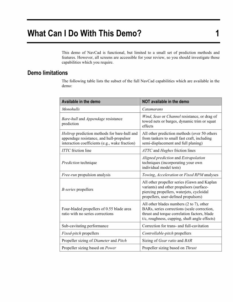
This demo of NavCad is functional, but limited to a small set of prediction methods and features. However, all screens are accessible for your review, so you should investigate those capabilities which you require.

Demo limitations The following table lists the subset of the full NavCad capabilities which are available in the demo:

Available in the demo NOT available in the demo Monohulls Catamarans

Bare-hull and Appendage resistance prediction

Wind, Seas or Channel resistance, or drag of towed nets or barges, dynamic trim or squat effects

Holtrop prediction methods for bare-hull and appendage resistance, and hull-propulsor interaction coefficients (e.g., wake fraction)

All other prediction methods (over 50 others from tankers to small fast craft, including semi-displacement and full planing)

ITTC friction line ATTC and Hughes friction lines

Prediction technique Aligned prediction and Extrapolation techniques (incorporating your own individual model tests)

Free-run propulsion analysis Towing, Acceleration or Fixed RPM analyses

B-series propellers

All other propeller series (Gawn and Kaplan variants) and other propulsors (surface-piercing propellers, waterjets, cycloidal propellers, user-defined propulsors)

Four-bladed propellers of 0.55 blade area ratio with no series corrections

All other blades numbers (2 to 7), other BARs, series corrections (scale correction, thrust and torque correlation factors, blade t/c, roughness, cupping, shaft angle effects)

Sub-cavitating performance Correction for trans- and full-cavitation

Fixed-pitch propellers Controllable-pitch propellers

Propeller sizing of Diameter and Pitch Sizing of Gear ratio and BAR

Propeller sizing based on Power Propeller sizing based on Thrust

Demonstration Guide To NavCad Operation 2 This chapter is an 18-step introduction to the operation of NavCad. It is intended to allow you to investigate the entire interface, calculation procedures, and output.

The Demonstration uses data for a 50 m fast monohull vessel.

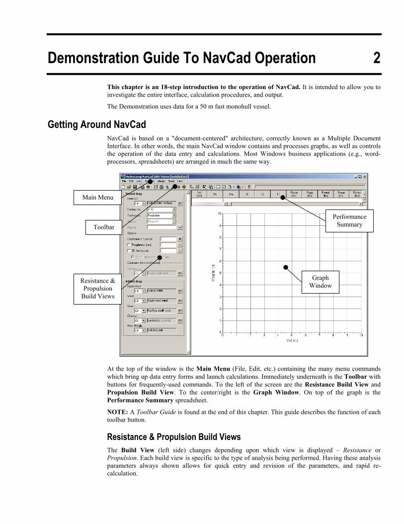
Getting Around NavCad NavCad is based on a "document-centered" architecture, correctly known as a Multiple Document Interface. In other words, the main NavCad window contains and processes graphs, as well as controls the operation of the data entry and calculations. Most Windows business applications (e.g., word-processors, spreadsheets) are arranged in much the same way.

Main Menu

Performance Summary Toolbar

Graph Window

Resistance & Propulsion

Build Views

At the top of the window is the Main Menu (File, Edit, etc.) containing the many menu commands which bring up data entry forms and launch calculations. Immediately underneath is the Toolbar with buttons for frequently-used commands. To the left of the screen are the Resistance Build View and Propulsion Build View. To the center/right is the Graph Window. On top of the graph is the Performance Summary spreadsheet.

NOTE: A Toolbar Guide is found at the end of this chapter. This guide describes the function of each toolbar button.

Resistance & Propulsion Build Views The Build View (left side) changes depending upon which view is displayed – Resistance or Propulsion. Each build view is specific to the type of analysis being performed. Having these analysis parameters always shown allows for quick entry and revision of the parameters, and rapid re-calculation.

Demonstration Guide To NavCad Operation 2–2

Graph Window A graph of the current job results is always displayed. A different graph is shown depending upon the type of calculation being performed (e.g., for Resistance calculations, the graph might show Rbare (bare-hull resistance), for Propulsion it might be PBtotal (total brake power). The currently displayed graph will be updated after a calculation.

Performance Summary A performance summary spreadsheet is shown above the graph which holds the active performance results. The values shown in the summary are different for resistance and propulsion results, and all of the results are updated on every calculation. This insures that all data and results are properly related to their equilibrium resistance-propulsion relationships.

Getting Help Within NavCad NavCad contains a context-sensitive help system that is attached to the various windows and fields. It contains program guides and technical information useful for the successful operation of the program. Pressing F1 or the Help button at any time will display the help screen.

Within the Help menu are particular Help items that may be of general interest. These items describe the interface commands and menu selections.

Starting the Demonstration After you have installed the NavCad 2007 Demo, run it like you would any other program. Instructions are shown below for the 18 illustrated steps.

Step 1 - Beginning a new project

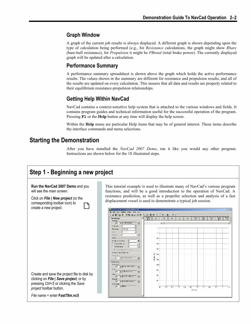
Run the NavCad 2007 Demo and you will see the main screen.

Click on File | New project (or the corresponding toolbar icon) to create a new project.

Create and save the project file to disk by clicking on File | Save project, or by pressing Ctrl+S or clicking the Save project toolbar button.

File name = enter Fast78m.nc5

This tutorial example is used to illustrate many of NavCad’s various program functions, and will be a good introduction to the operation of NavCad. A resistance prediction, as well as a propeller selection and analysis of a fast displacement vessel is used to demonstrate a typical job session.


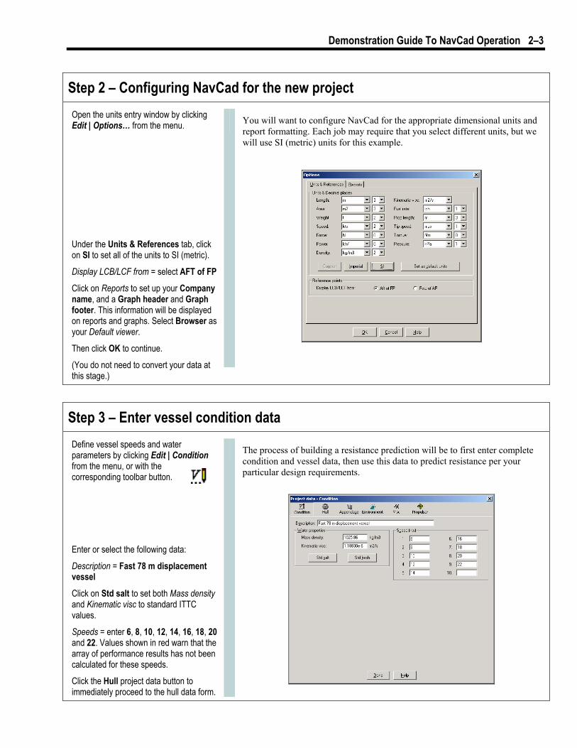
Step 2 – Configuring NavCad for the new project Open the units entry window by clicking Edit | Options… from the menu.

Under the Units & References tab, click on SI to set all of the units to SI (metric).

Display LCB/LCF from = select AFT of FP Click on Reports to set up your Company name, and a Graph header and Graph footer. This information will be displayed on reports and graphs. Select Browser as your Default viewer.

Then click OK to continue.

(You do not need to convert your data at this stage.)

You will want to configure NavCad for the appropriate dimensional units and report formatting. Each job may require that you select different units, but we will use SI (metric) units for this example.

Step 3 – Enter vessel condition data Define vessel speeds and water parameters by clicking Edit | Condition from the menu, or with the corresponding toolbar button.

Enter or select the following data:

Description = Fast 78 m displacement vessel Click on Std salt to set both Mass density and Kinematic visc to standard ITTC values.

Speeds = enter 6, 8, 10, 12, 14, 16, 18, 20 and 22. Values shown in red warn that the array of performance results has not been calculated for these speeds.

Click the Hull project data button to immediately proceed to the hull data form.

The process of building a resistance prediction will be to first enter complete condition and vessel data, then use this data to predict resistance per your particular design requirements.


Step 4 – Enter hull data

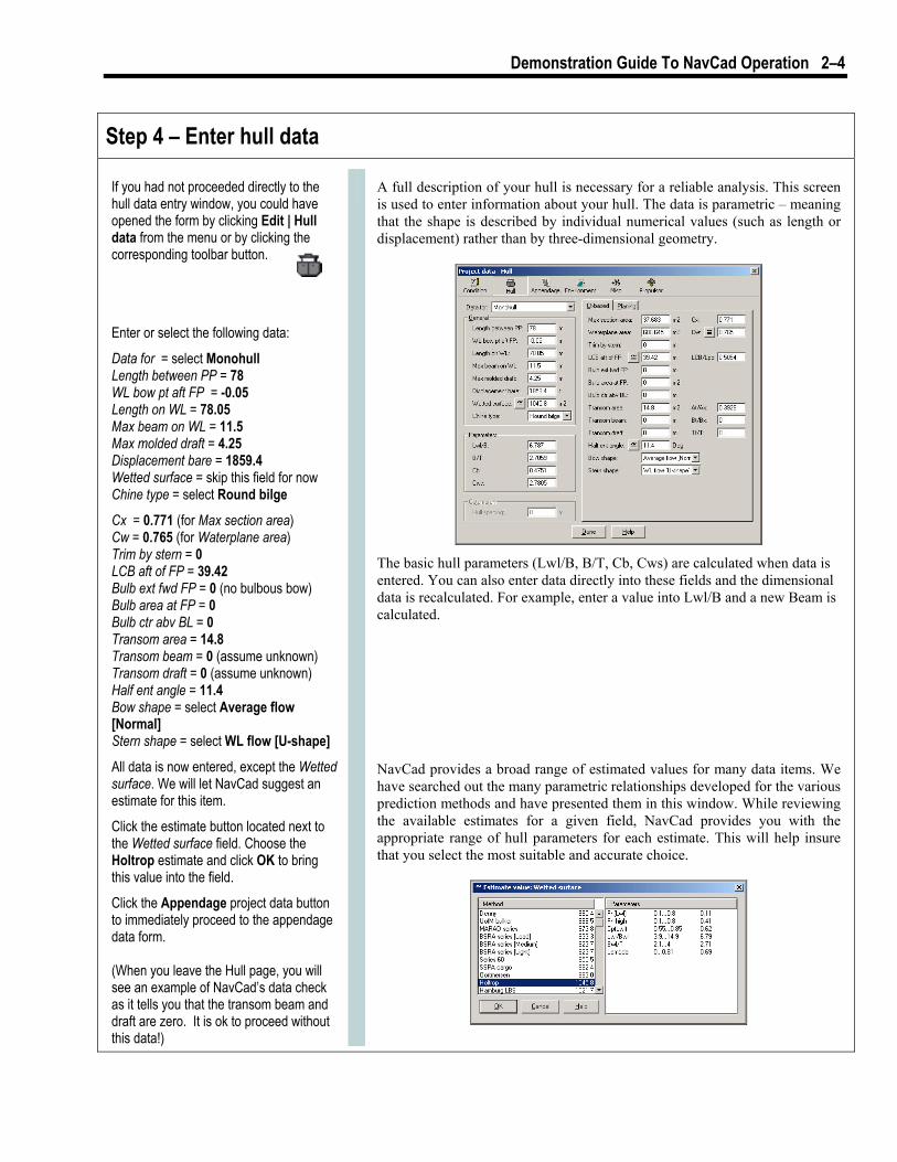
If you had not proceeded directly to the hull data entry window, you could have opened the form by clicking Edit | Hull data from the menu or by clicking the corresponding toolbar button.


Data for = select Monohull Length between PP = 78 WL bow pt aft FP = -0.05 Length on WL = 78.05 Max beam on WL = 11.5 Max molded draft = 4.25 Displacement bare = 1859.4 Wetted surface = skip this field for now Chine type = select Round bilge

Cx = 0.771 (for Max section area) Cw = 0.765 (for Waterplane area) Trim by stern = 0 LCB aft of FP = 39.42 Bulb ext fwd FP = 0 (no bulbous bow) Bulb area at FP = 0 Bulb ctr abv BL = 0 Transom area = 14.8 Transom beam = 0 (assume unknown) Transom draft = 0 (assume unknown) Half ent angle = 11.4 Bow shape = select Average flow [Normal] Stern shape = select WL flow [U-shape] All data is now entered, except the Wetted surface. We will let NavCad suggest an estimate for this item.

Click the estimate button located next to the Wetted surface field. Choose the Holtrop estimate and click OK to bring this value into the field.

Click the Appendage project data button to immediately proceed to the appendage data form. (When you leave the Hull page, you will see an example of NavCad’s data check as it tells you that the transom beam and draft are zero. It is ok to proceed without this data!)

A full description of your hull is necessary for a reliable analysis. This screen is used to enter information about your hull. The data is parametric – meaning that the shape is described by individual numerical values (such as length or displacement) rather than by three-dimensional geometry.

The basic hull parameters (Lwl/B, B/T, Cb, Cws) are calculated when data is entered. You can also enter data directly into these fields and the dimensional data is recalculated. For example, enter a value into Lwl/B and a new Beam is calculated. NavCad provides a broad range of estimated values for many data items. We have searched out the many parametric relationships developed for the various prediction methods and have presented them in this window. While reviewing the available estimates for a given field, NavCad provides you with the appropriate range of hull parameters for each estimate. This will help insure that you select the most suitable and accurate choice.


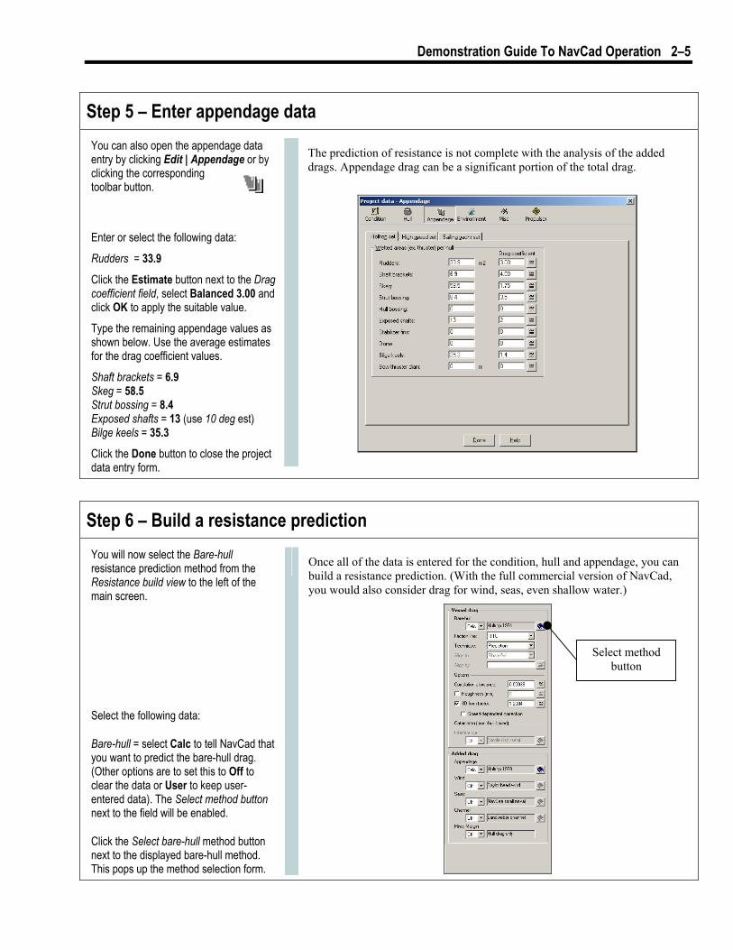
Step 5 – Enter appendage data You can also open the appendage data entry by clicking Edit | Appendage or by clicking the corresponding toolbar button.


Rudders = 33.9

Click the Estimate button next to the Drag coefficient field, select Balanced 3.00 and click OK to apply the suitable value.

Type the remaining appendage values as shown below. Use the average estimates for the drag coefficient values.

Shaft brackets = 6.9 Skeg = 58.5 Strut bossing = 8.4 Exposed shafts = 13 (use 10 deg est) Bilge keels = 35.3

Click the Done button to close the project data entry form.

The prediction of resistance is not complete with the analysis of the added drags. Appendage drag can be a significant portion of the total drag.

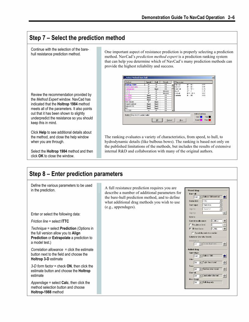
Step 6 – Build a resistance prediction You will now select the Bare-hull resistance prediction method from the Resistance build view to the left of the main screen.

Select the following data:

Bare-hull = select Calc to tell NavCad that you want to predict the bare-hull drag. (Other options are to set this to Off to clear the data or User to keep user-entered data). The Select method button next to the field will be enabled.

Click the Select bare-hull method button next to the displayed bare-hull method. This pops up the method selection form.

Once all of the data is entered for the condition, hull and appendage, you can build a resistance prediction. (With the full commercial version of NavCad, you would also consider drag for wind, seas, even shallow water.)

Select method button


Step 7 – Select the prediction method Continue with the selection of the bare-hull resistance prediction method.

Review the recommendation provided by the Method Expert window. NavCad has indicated that the Holtrop 1984 method meets all of the parameters. It also points out that it has been shown to slightly underpredict the resistance so you should keep this in mind.

Click Help to see additional details about the method, and close the help window when you are through.

Select the Holtrop 1984 method and then click OK to close the window.

One important aspect of resistance prediction is properly selecting a prediction method. NavCad’s prediction method expert is a prediction ranking system that can help you determine which of NavCad’s many prediction methods can provide the highest reliability and success.

The ranking evaluates a variety of characteristics, from speed, to hull, to hydrodynamic details (like bulbous bows). The ranking is based not only on the published limitations of the methods, but includes the results of extensive internal R&D and collaboration with many of the original authors.

Step 8 – Enter prediction parameters Define the various parameters to be used in the prediction.


Friction line = select ITTC

Technique = select Prediction (Options in the full version allow you to Align Prediction or Extrapolate a prediction to a model test.)

Correlation allowance = click the estimate button next to the field and choose the Holtrop 3-D estimate

3-D form factor = check ON, then click the estimate button and choose the Holtrop estimate

Appendage = select Calc, then click the method selection button and choose Holtrop-1988 method

A full resistance prediction requires you are describe a number of additional parameters for the bare-hull prediction method, and to define what additional drag methods you wish to use (e.g., appendages).


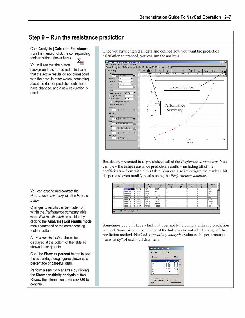
Step 9 – Run the resistance prediction Click Analysis | Calculate Resistance from the menu or click the corresponding toolbar button (shown here).

You will see that the button background has turned red to indicate that the active results do not correspond with the data. In other words, something about the data or prediction definitions have changed, and a new calculation is needed.

You can expand and contract the Performance summary with the Expand button.

Changes to results can be made from within the Performance summary table when Edit results mode is enabled by clicking the Analysis | Edit results mode menu command or the corresponding toolbar button.

An Edit results toolbar should be displayed at the bottom of the table as shown in the graphic.

Click the Show as percent button to see the appendage drag figures shown as a percentage of bare-hull drag.

Perform a sensitivity analysis by clicking the Show sensitivity analysis button. Review the information, then click OK to continue.

Once you have entered all data and defined how you want the prediction calculation to proceed, you can run the analysis.

Results are presented in a spreadsheet called the Performance summary. You can view the entire resistance prediction results – including all of the coefficients – from within this table. You can also investigate the results a bit deeper, and even modify results using the Performance summary.

Sometimes you will have a hull that does not fully comply with any prediction method. Some piece or parameter of the hull may be outside the range of the prediction method. NavCad’s sensitivity analysis evaluates the performance “sensitivity” of each hull data item.

Expand button

Performance Summary


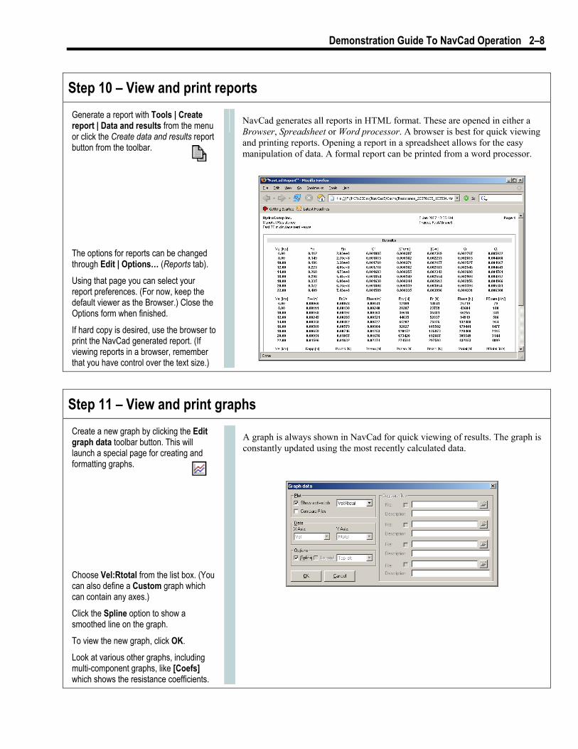
Step 10 – View and print reports Generate a report with Tools | Create report | Data and results from the menu or click the Create data and results report button from the toolbar.

The options for reports can be changed through Edit | Options… (Reports tab).

Using that page you can select your report preferences. (For now, keep the default viewer as the Browser.) Close the Options form when finished.

If hard copy is desired, use the browser to print the NavCad generated report. (If viewing reports in a browser, remember that you have control over the text size.)

NavCad generates all reports in HTML format. These are opened in either a Browser, Spreadsheet or Word processor. A browser is best for quick viewing and printing reports. Opening a report in a spreadsheet allows for the easy manipulation of data. A formal report can be printed from a word processor.

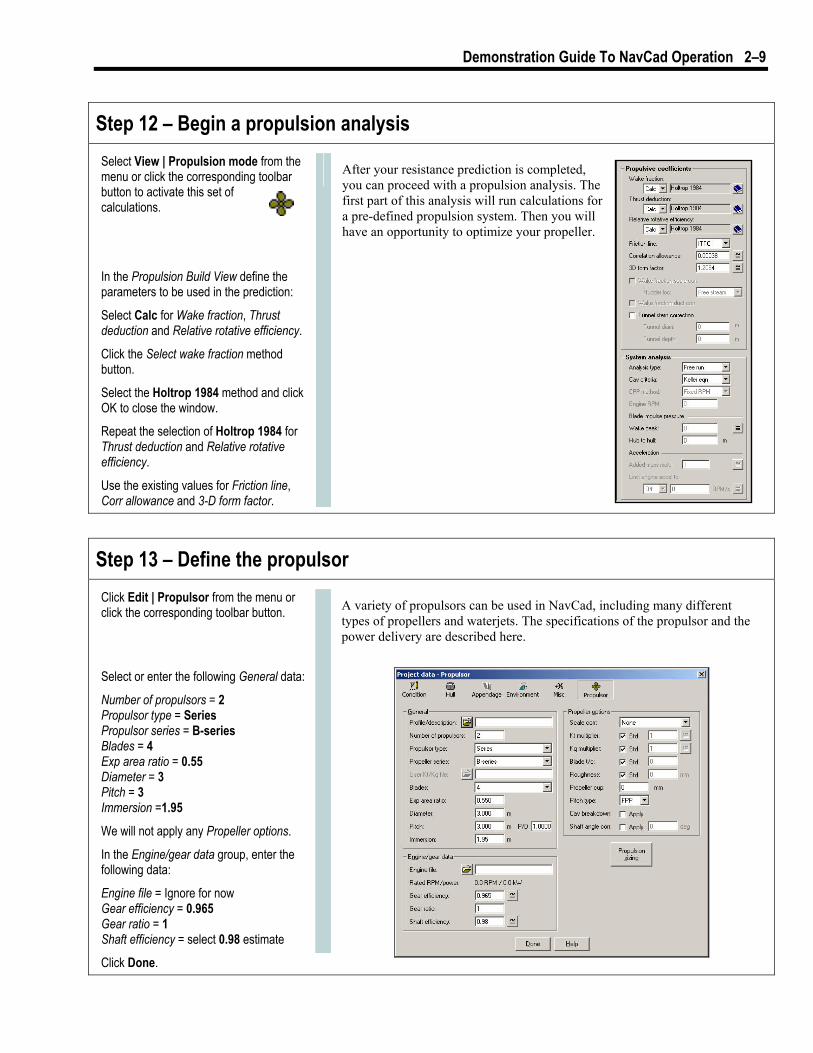
Step 11 – View and print graphs Create a new graph by clicking the Edit graph data toolbar button. This will launch a special page for creating and formatting graphs.

Choose Vel:Rtotal from the list box. (You can also define a Custom graph which can contain any axes.)

Click the Spline option to show a smoothed line on the graph.

To view the new graph, click OK.

Look at various other graphs, including multi-component graphs, like [Coefs] which shows the resistance coefficients.

A graph is always shown in NavCad for quick viewing of results. The graph is constantly updated using the most recently calculated data.


Step 12 – Begin a propulsion analysis Select View | Propulsion mode from the menu or click the corresponding toolbar button to activate this set of calculations.

In the Propulsion Build View define the parameters to be used in the prediction:

Select Calc for Wake fraction, Thrust deduction and Relative rotative efficiency.

Click the Select wake fraction method button.

Select the Holtrop 1984 method and click OK to close the window.

Repeat the selection of Holtrop 1984 for Thrust deduction and Relative rotative efficiency.

Use the existing values for Friction line, Corr allowance and 3-D form factor.

After your resistance prediction is completed, you can proceed with a propulsion analysis. The first part of this analysis will run calculations for a pre-defined propulsion system. Then you will have an opportunity to optimize your propeller.

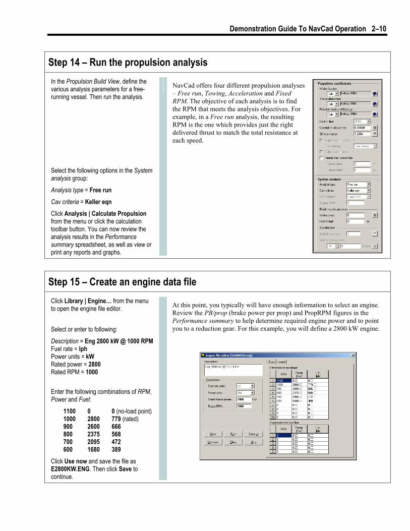
Step 13 – Define the propulsor Click Edit | Propulsor from the menu or click the corresponding toolbar button.

Select or enter the following General data:

Number of propulsors = 2 Propulsor type = Series Propulsor series = B-series Blades = 4 Exp area ratio = 0.55 Diameter = 3 Pitch = 3 Immersion =1.95

We will not apply any Propeller options.

In the Engine/gear data group, enter the following data:

Engine file = Ignore for now Gear efficiency = 0.965 Gear ratio = 1 Shaft efficiency = select 0.98 estimate

Click Done.

A variety of propulsors can be used in NavCad, including many different types of propellers and waterjets. The specifications of the propulsor and the power delivery are described here.


Step 14 – Run the propulsion analysis In the Propulsion Build View, define the various analysis parameters for a free-running vessel. Then run the analysis.

Select the following options in the System analysis group:

Analysis type = Free run

Cav criteria = Keller eqn

Click Analysis | Calculate Propulsion from the menu or click the calculation toolbar button. You can now review the analysis results in the Performance summary spreadsheet, as well as view or print any reports and graphs.

NavCad offers four different propulsion analyses – Free run, Towing, Acceleration and Fixed RPM. The objective of each analysis is to find the RPM that meets the analysis objectives. For example, in a Free run analysis, the resulting RPM is the one which provides just the right delivered thrust to match the total resistance at each speed.

Step 15 – Create an engine data file Click Library | Engine… from the menu to open the engine file editor.

Select or enter to following:

Description = Eng 2800 kW @ 1000 RPM Fuel rate = lph Power units = kW Rated power = 2800 Rated RPM = 1000

Enter the following combinations of RPM, Power and Fuel:

1100 0 0 (no-load point) 1000 2800 779 (rated) 900 2600 666 800 2375 568 700 2095 472 600 1680 389 Click Use now and save the file as E2800KW.ENG. Then click Save to continue.

At this point, you typically will have enough information to select an engine. Review the PB/prop (brake power per prop) and PropRPM figures in the Performance summary to help determine required engine power and to point you to a reduction gear. For this example, you will define a 2800 kW engine.


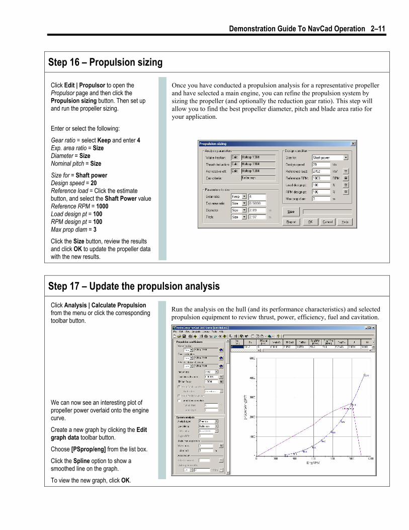
Step 17 – Update the propulsion analysis Click Analysis | Calculate Propulsion from the menu or click the corresponding toolbar button.

We can now see an interesting plot of propeller power overlaid onto the engine curve.

Create a new graph by clicking the Edit graph data toolbar button.

Choose [PSprop/eng] from the list box.

Click the Spline option to show a smoothed line on the graph.

To view the new graph, click OK.

Run the analysis on the hull (and its performance characteristics) and selected propulsion equipment to review thrust, power, efficiency, fuel and cavitation.

Step 16 – Propulsion sizing

Click Edit | Propulsor to open the Propulsor page and then click the Propulsion sizing button. Then set up and run the propeller sizing.

Enter or select the following:

Gear ratio = select Keep and enter 4 Exp. area ratio = Size Diameter = Size Nominal pitch = Size

Size for = Shaft power Design speed = 20 Reference load = Click the estimate button, and select the Shaft Power value Reference RPM = 1000 Load design pt = 100 RPM design pt = 100 Max prop diam = 3

Click the Size button, review the results and click OK to update the propeller data with the new results.

Once you have conducted a propulsion analysis for a representative propeller and have selected a main engine, you can refine the propulsion system by sizing the propeller (and optionally the reduction gear ratio). This step will allow you to find the best propeller diameter, pitch and blade area ratio for your application.


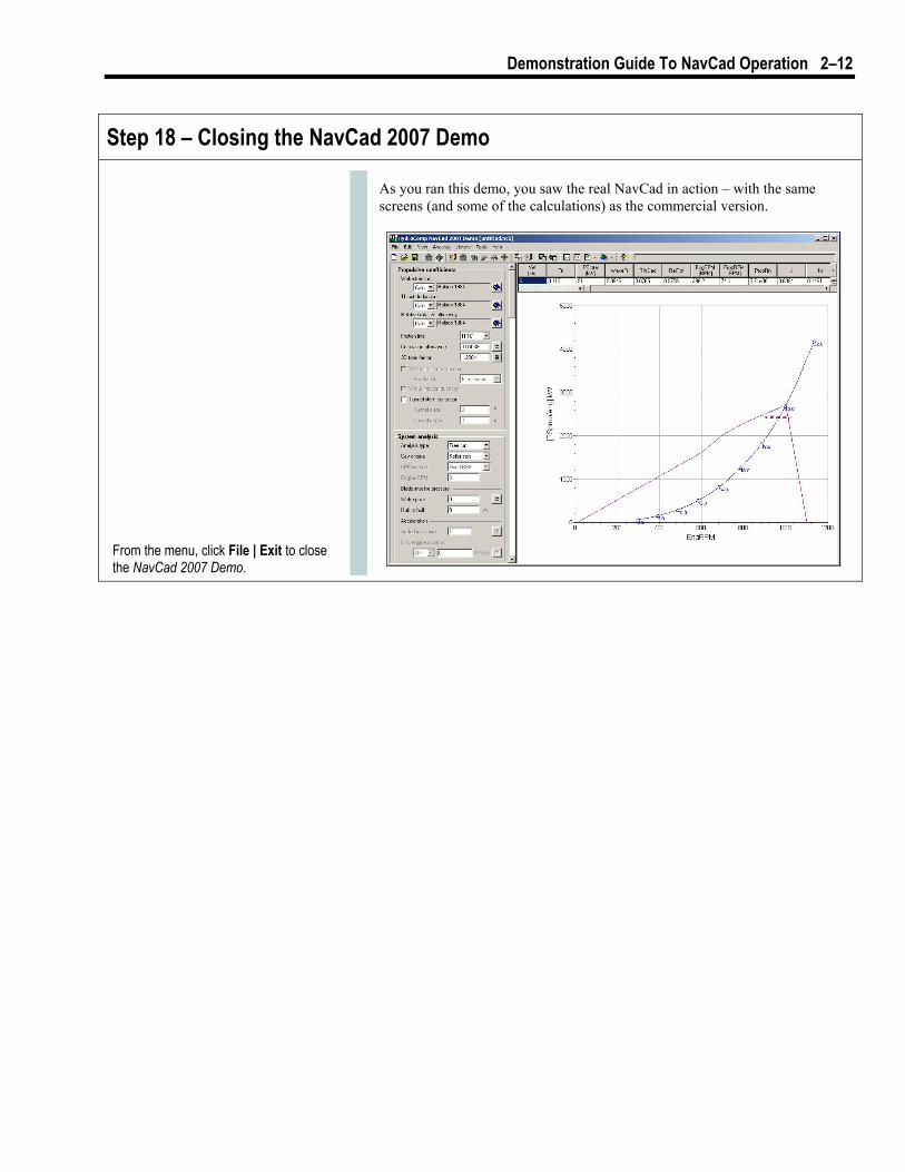
Step 18 – Closing the NavCad 2007 Demo

From the menu, click File | Exit to close the NavCad 2007 Demo.

As you ran this demo, you saw the real NavCad in action – with the same screens (and some of the calculations) as the commercial version.


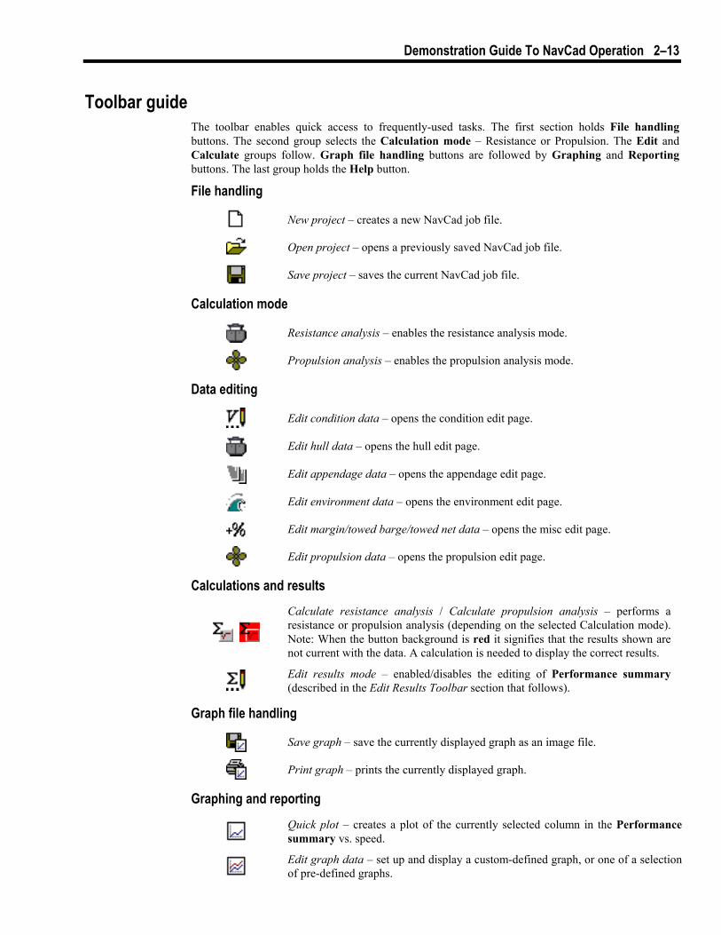
Toolbar guide The toolbar enables quick access to frequently-used tasks. The first section holds File handling buttons. The second group selects the Calculation mode – Resistance or Propulsion. The Edit and Calculate groups follow. Graph file handling buttons are followed by Graphing and Reporting buttons. The last group holds the Help button.

File handling

New project – creates a new NavCad job file.

Open project – opens a previously saved NavCad job file.

Save project – saves the current NavCad job file.

Calculation mode

Resistance analysis – enables the resistance analysis mode.

Propulsion analysis – enables the propulsion analysis mode.

Data editing

Edit condition data – opens the condition edit page.

Edit hull data – opens the hull edit page.

Edit appendage data – opens the appendage edit page.

Edit environment data – opens the environment edit page.

Edit margin/towed barge/towed net data – opens the misc edit page.

Edit propulsion data – opens the propulsion edit page.

Calculations and results

Calculate resistance analysis / Calculate propulsion analysis – performs a resistance or propulsion analysis (depending on the selected Calculation mode). Note: When the button background is red it signifies that the results shown are not current with the data. A calculation is needed to display the correct results.

Edit results mode – enabled/disables the editing of Performance summary (described in the Edit Results Toolbar section that follows).

Graph file handling

Save graph – save the currently displayed graph as an image file.

Print graph – prints the currently displayed graph.

Graphing and reporting

Quick plot – creates a plot of the currently selected column in the Performance summary vs. speed.

Edit graph data – set up and display a custom-defined graph, or one of a selection of pre-defined graphs.


Create results report / Create data and results report – generates a results only report or a data and results report.

View report with Browser / …with Spreadsheet / …with Word processor – selects the type of report viewer type (web browser, spreadsheet or word processor).

Help

Help – opens the NavCad help file.

Calculation progress bar During a calculation this displays the progress of the calculation.

Edit Results Toolbar When NavCad is in Edit results mode an Edit Results Toolbar is shown between the graph and the Performance Summary. This toolbar holds buttons that affect the results in the Performance Summary. Each of the two views – Resistance and Propulsion – has its own Edit Results Toolbar.

Resistance

Select data to recalc from – Select the item to be the basis for the re-calculation.

Show as percent – Shows the added drag resistances as percentages.

Show sensitivity analysis– Performs and displays the results of a sensitivity analysis.

Fill selected column – Fills the selected column with the currently selected cell value.

Zero selected column – Fills the selected column with zeros.

Clear all results – Clears all results in the Performance summary.

Propulsion

Select data to recalc from – Select the item to be the basis for the re-calculation.

Fill selected column – Fills the selected column with the currently selected cell value.

Zero selected column – Fills the selected column with zeros.

The NavCad User’s Guide 3

The NavCad User’s Guide is a very thorough instruction manual for NavCad operation. It is also a comprehensive resource on various hydrodynamic topics.

The chapters have been arranged to provide an extensive Tutorial of NavCad functions, followed by the technical background for the calculations. A number of appendices offer detailed insight into individual prediction methods.

User’s Guide contents A brief outline of each chapter is described below.

Chapter 1 – Introduction & Getting Started • Installation and setup • Additional setup for network licensing

Chapter 2 – A Quick Tutorial • Getting Around NavCad • A General Example

• • • • • • • • • • • • • • • • • •

• • • • •

Beginning a new project Configuring NavCad for the new project Enter vessel condition data Enter hull data Enter appendage data Build a resistance prediction Select the prediction method Enter prediction parameters Run the resistance prediction View and print reports View and print graphs Begin a propulsion analysis Define the propulsor Run the propulsion analysis Create an engine data file Propulsion sizing Update the propulsion analysis Closing NavCad

• Toolbar Guide

Chapter 3 – Program Examples

• Starting a New Project • Creating a project data file • Configuring NavCad for a new project

• Entering Data For a Resistance Prediction Enter vessel condition data Enter hull data Enter appendage data Enter environment data Enter a design margin

• Running a Resistance Prediction

The NavCad User’s Guide 3-2

• • • •

• •

• •

• • • • • • •

• • • •

• • •

• •

• •

Select the prediction method The "Method Expert” Enter prediction parameters Run the prediction calculation

• Evaluating a Resistance Prediction Reviewing and modifying results Sensitivity analysis

• View, Edit and Print Reports Tabular reports of results and data Graphical reports of results

• Blade Scan Analysis Propeller data Scan data Parameters Data plot Buttons Example Improve accuracy of Mean pitch with more data

Chapter 4 - Resistance Prediction • Numerical Bare-hull Prediction • Geosim Coefficient (CT-based) Method

• Overview • Viscous Resistance

• Form • Residuary and Wave-making Resistance

• Three-dimensional system • Resistance/Weight Ratios • Equilibrium Planing Case • Catamaran Interference

Nature of interference CT-based interference prediction Planing interference prediction Catamaran "whole-system" methods

• Model-Ship Correlation • Modifying Existing Prediction Methods • Hydrodynamic Dimensions

Length Longitudinal center of buoyancy Data at “midship”

• About Bare-Hull Prediction Methods • Correlating Bare-hull Prediction to Known Performance • Aligned Prediction

Ct-based hulls Planing hulls

• Expansion Ct-based analysis Planing analysis

• Using Full-scale Trials Like Model Data • Appendages • Wind and Seas • Restrictive Channel Effects • Towed Nets and Barges


Chapter 5 – Propulsion Analysis • Principal Analysis Formula

• Effective Power • Delivered (Developed) Power • Shaft Power • Brake Power • Quasi-Propulsive Coefficient (QPC) • Overall Propulsive Coefficient (OPC)

• Propulsive Efficiency • Hull influences (propulsive coefficients)

• Wake fraction • Thrust deduction • Relative-rotative Efficiency • Tunnel Stern Correction • Shaft Efficiency • Gear Efficiency

• System Analysis • • • •

• • • • • •

• • •

• • • • • •

• •

Free-run Towing Fixed RPM Acceleration

• Evaluating Acceptable Performance Engine RPM Cavitation Tip Cavitation Face Cavitation Back Cavitation Blade Impulse Pressure

• Calculation of Propulsor Performance Thrust and Torque Coefficients Propeller Open-water Efficiency Series Types

• Series Corrections Thrust and Power Factors (KT/KQ multipliers) Geometric Corrections Cupped propellers Scale Correction Cavitation Correction Shaft Angle Correction (Oblique Flow)

• User-defined KT/KQ • Comments on the Nature of Propellers

Pitch, Speed and RPM Diameter and RPM

• Controllable Pitch Propellers • Waterjet Performance

• Waterjet Data • Thrust and Torque Coefficients

• Oblique Flow • Cosine Effects • Inflow Pitch Angle Effects • Net Thrust and Torque • Calculation Technique

• Finding Optimum Propeller Performance


• Propeller Series • • • • • •

• • • •

•

• • • • • •

Diameter Pitch Blade Area Number of Blades Skew Revolution

• Choosing Conditions for Sizing Design Speed Load Identity and Design Point Engine Considerations Numerical Propeller Selection Procedures

• Engine Performance Fuel Rate

Chapter 6 – Supplemental Calculations • Dynamic Trim

• Ct-based Hulls • Planing Hulls

• Vessel Squat • Ct-based Hulls

• Blade Scan Analysis Propeller data Scan data Parameters Data plot Buttons Example

• Improve accuracy of Mean pitch with more data • Barge Train Resistance

• Prediction Methods

Appendix A - References • References • Symbols

Appendix B - Errors and Warnings • Calculation Errors • General Errors • Project Errors • Procedural Errors • IDF File Errors.

Appendix C - Data Descriptions • Data field descriptions

Appendix D - Symbols and Values • Symbols and Values

Appendix E – Importing and Exporting Data • NavCad Project File (.NC5) • SwiftCraft Project File (.HCF) • Model/parent Library File (.MDL)


• Propeller Library File (.PRP) • User-defined Kt/Kq Library File (.KTQ) • Waterjet Library File (.JET) • Engine Library File (.ENG) • IMSA Transfer Definition File (.IDF)

Appendix F – External Programs • Run time data transfer • Running user programs

Appendix G - Reference Standards • Water Characteristics • Miscellaneous Standards

Appendix H - Resistance Prediction Methods • Bare-hull – Monohull, Catamaran, Interference Methods • Added resistance – Appendage , Wind, Seas, Channel, Miscellaneous margin • Towed Nets and Towed Barges

Appendix I - Propulsive Coefficient Prediction Methods • Description of Methods

Appendix J - Open Water Propeller Series • Propeller Series

Nav Cad 2007 Demo Guide

Documents

relative rotative

selected column

navcad users

edit results

propulsion

resistance

performance

edit results